Power transmission systems for offshore wind farms
121
Power transmission systems for offshore wind farms: Technical-economic analysis 1 Abstract Several studies claim that wind power will play a major role in the energy supply of the European Union, forecasting 70 GW of new installed capacity in the next five years. Given the accelerated growth that offshore wind power is experiencing, many challenges are to be addressed in the next few years and substantial improvements are to be expected. Offshore wind farms (OWF) are expected to increase in rated power and in distance from shore, thus increasing the relevance of the transmission system. Therefore, a detailed technical-economic analysis is necessary to estimate which is the optimal transmission system to transmit the power generated at the OWF. This thesis presents a technical-economic analysis of power transmission systems for OWF. The aim of this work is to determine the most suitable power transmission technology for a given set of OWF characteristics. Costs and losses of different proposed technologies are investigated: high-voltage alternating current (HVAC), high-voltage direct current (HVDC) based on voltage-source converters (VSC), and low-frequency alternating current (LFAC). For the technical part of the analysis, the strengths and weaknesses of each technology are exposed, as well as the role of the main components investigated. Regarding the economic side of the thesis, the costs of the major components of each transmission system are associated to cost functions, and their losses modelled. Availability of the components is also considered, as well as the variability of the self-made cost functions. The self-made cost functions, being contributions of this work, are provided for public use. The costs of the whole transmission system including losses are obtained as a function of a range of variables (transmission length, rated power, voltage level, etc.). Additionally, the employed cost functions and loss calculations are summarized in a spreadsheet, which is openly available upon request. Besides giving the cost functions, the technical-economic analysis is applied to a set of case studies to draw a comparison between a range of proposed transmission systems. The obtained results indicate that the break-even point between HVAC and HVDC is to be found in the 50-100 km range, approaching 50 km in the case of large OWF (e.g. 1000 MW). Additionally, the studied cases also reveal that LFAC could result the most suitable option in the 50-70 km range.
-
Upload
khangminh22 -
Category
Documents
-
view
1 -
download
0
Transcript of Power transmission systems for offshore wind farms

Power transmission systems for offshore wind farms: Technical-economic analysis 1
Abstract
Several studies claim that wind power will play a major role in the energy supply of
the European Union, forecasting 70 GW of new installed capacity in the next five years. Given
the accelerated growth that offshore wind power is experiencing, many challenges are to be
addressed in the next few years and substantial improvements are to be expected. Offshore
wind farms (OWF) are expected to increase in rated power and in distance from shore, thus
increasing the relevance of the transmission system. Therefore, a detailed technical-economic
analysis is necessary to estimate which is the optimal transmission system to transmit the
power generated at the OWF.
This thesis presents a technical-economic analysis of power transmission systems for OWF.
The aim of this work is to determine the most suitable power transmission technology for a
given set of OWF characteristics. Costs and losses of different proposed technologies are
investigated: high-voltage alternating current (HVAC), high-voltage direct current (HVDC)
based on voltage-source converters (VSC), and low-frequency alternating current (LFAC). For
the technical part of the analysis, the strengths and weaknesses of each technology are
exposed, as well as the role of the main components investigated. Regarding the economic side
of the thesis, the costs of the major components of each transmission system are associated to
cost functions, and their losses modelled. Availability of the components is also considered, as
well as the variability of the self-made cost functions. The self-made cost functions, being
contributions of this work, are provided for public use. The costs of the whole transmission
system including losses are obtained as a function of a range of variables (transmission length,
rated power, voltage level, etc.). Additionally, the employed cost functions and loss
calculations are summarized in a spreadsheet, which is openly available upon request.
Besides giving the cost functions, the technical-economic analysis is applied to a set of case
studies to draw a comparison between a range of proposed transmission systems. The
obtained results indicate that the break-even point between HVAC and HVDC is to be found
in the 50-100 km range, approaching 50 km in the case of large OWF (e.g. 1000 MW).
Additionally, the studied cases also reveal that LFAC could result the most suitable option in
the 50-70 km range.

2
Acknowledgements
Few bachelor thesis lead to the writing of an academic paper. It is said that those who do,
either work on a leading-edge technology or benefit from a very good supervisor. For this case,
it is unquestionable that without the help and dedication of Rodrigo Teixeira Pinto, this would
have never been possible. His help and has driven myself to discover such an interesting
academic field such as power transmission, and I am infinitely thankful for that. I would have
never worked so hard and achieved this work without him. Many thanks, Rodrigo; and
congratulations on the birth of your child, Vito.
I would also like to particularly thank Oriol Gomis for his attitude, for giving me the
opportunity to work with Rodrigo, and for giving me the chance to be involved in such a great
team at the CITCEA. Thanks to Muhammad Raza for his powerful advices, and for his infinite
patience resolving my doubts.
I would also like to mention Professor Josep A. Sànchez for his help and advice on the statistics
part of the modelling equations, strengthening this present work.
Thanks to my family for their support, and especially to Sofía, as you have dealt with my
frustrations, angers, and joy when building this work. Your support and love is beyond what
I could ask for.

Power transmission systems for offshore wind farms: Technical-economic analysis 3
Summary
ABSTRACT ________________________________________________________ 1
ACKNOWLEDGEMENTS __________________________________________ 2
SUMMARY ________________________________________________________ 3
LIST OF ACRONYMS ______________________________________________ 6
PREFACE __________________________________________________________ 7
1. INTRODUCTION _____________________________________________ 8
1.1. Offshore wind energy ............................................................................................... 8
1.2. Problem description ................................................................................................ 10
1.3. Problematic overview ............................................................................................. 12
1.4. Objectives .................................................................................................................. 15
1.5. Scope .......................................................................................................................... 16
2. TECHNICAL BACKGROUND _________________________________ 18
2.1. HVAC ........................................................................................................................ 18
2.1.1. General Description ..................................................................................................... 18
2.1.2. HVAC transmission losses ......................................................................................... 19
2.1.3. Subsea cables ................................................................................................................. 23
2.1.4. Power Transformer ...................................................................................................... 25
2.1.5. GIS Switchgear ............................................................................................................. 26
2.1.6. Reactive power control ................................................................................................ 26
2.2. MVAC ........................................................................................................................ 29
2.3. HVDC VSC ............................................................................................................... 30
2.3.1. Why DC? ....................................................................................................................... 30
2.3.2. General functioning ..................................................................................................... 31
2.3.3. Converter station technologies .................................................................................. 31
2.3.4. HVDC VSC cables ........................................................................................................ 34
2.3.5. Further implications of HVDC: MTDC networks .................................................. 35

4
2.4. LFAC .......................................................................................................................... 36
2.4.1. LFAC principle .............................................................................................................. 36
2.4.2. Low frequency Transformers ..................................................................................... 39
2.4.3. LFAC power converter ................................................................................................ 40
3. COST MODELLING __________________________________________ 43
3.1. Tool description ....................................................................................................... 43
3.2. OWF variables .......................................................................................................... 44
3.3. Loss cost calculation methodology ....................................................................... 45
3.4. HVAC cost ................................................................................................................ 46
3.4.1. HVAC common variables ........................................................................................... 46
3.4.2. Base cost ......................................................................................................................... 48
3.4.3. Distance dependent costs ............................................................................................ 51
3.4.4. HVAC Losses and reactive power ............................................................................. 54
3.4.5. MVAC costs ................................................................................................................... 65
3.5. HVDC cost ................................................................................................................ 66
3.5.1. Base variables ................................................................................................................ 66
3.5.2. Base cost ......................................................................................................................... 67
3.5.3. Distance dependent costs ............................................................................................ 69
3.5.4. HVDC transmission system losses ............................................................................ 71
3.6. LFAC Costs ............................................................................................................... 73
3.6.1. LFAC base variables ..................................................................................................... 73
3.6.2. Low frequency Transformers ..................................................................................... 75
3.6.3. Offshore substation structure ..................................................................................... 76
3.6.4. Power converters: CCV and B2B-VSC ...................................................................... 76
3.7. Determination of the break-even distance and area .......................................... 78
3.7.1. HVAC cost variability .................................................................................................. 79
3.7.2. HVDC cost variability .................................................................................................. 80
3.8. Availability ............................................................................................................... 81
3.9. Guide for choosing adequate inputs – transmission system constraints ....... 82
4. CASE STUDY ________________________________________________ 85

Power transmission systems for offshore wind farms: Technical-economic analysis 5
4.1. Results ........................................................................................................................ 87
4.1.1. First case: HVAC, HVDC, LFAC comparison ......................................................... 87
4.1.2. Second case: Suitability of HVDC taking into consideration the power outages
experienced in Bard 1 .................................................................................................. 96
4.1.3. Additional case study: optimal power transmission system for a 1000 MW wind
farm ................................................................................................................................ 97
CONCLUSIONS _________________________________________________ 100
REFERENCES ____________________________________________________ 102
APPENDIX 1 : BUDGET __________________________________________ 112
APPENDIX 2: DESIGNED TOOL __________________________________ 115
APPENDIX 3: STATISTICAL DATA OF THE SELF-MADE COST
FUNCTIONS ________________________________________________ 120

6
List of Acronyms
CCV Cycloconverter
GIS Gas-insulated switchgear
HVAC High-voltage alternating current
HVDC High-voltage direct current
LCC Line-commutated converter
LFAC Low-frequency alternating current
MVAC Medium-voltage alternating current
NPV Net present value
OWF Offshore wind farm
VSC Voltage-source converter

Power transmission systems for offshore wind farms: Technical-economic analysis 7
Preface
The thesis contributions are:
analysis of the economic feasibility of offshore wind farms (OWFs) connected with
low-frequency ac (LFAC) transmission systems as an alternative power transmission
technology;
providing the scientific community with new cost functions for voltage-source
converters, HVDC cables and GIS switchgears;
adapted cost functions for HVDC-VSC offshore platforms and LFAC offshore
platforms;
providing a tool that calculates the capital costs and losses of a subsea power
transmission system, as a function of the offshore wind farm characteristics, with
variable configuration and different technologies, including the system availability.
The newly developed cost functions have been included in this tool, in addition to cost
functions available in the literacy, resulting in a powerful cost-estimator;
exposing a detailed methodology on general loss calculation of the considered
components.

8
1. Introduction
1.1. Offshore wind energy
Wind energy is nowadays a growing trend. As it can be seen in Figure 1, the wind
industry has experienced a sustained growth over the last decade. Wind energy provides a
reliable, clean, safe and competitive alternative in comparison with other energy sources, such
as fossil fuels. Most countries have plans for increasing the production of electricity related to
renewable energy, by means of wind power: only in Europe, forecasts predict 70 GW of new
wind power plants for the next five years [1] [2].
Figure 1 Cumulative capacity installed in EU (GW) (data source: [3]).
In 2012, the EU reached the 100 GW milestone of installed capacity, confirming the fast growth
that wind energy is experiencing in the last decade. In fact, it is estimated that wind energy
will supply alone 25.7% of EU’s electricity demand by 2030, according to the European Wind
Energy Association (EWEA) [4].
12,917,3
23,128,5
34,440,8
48
56,7
65,1
75,3
85,1
94,5
106,2
117,3
128,8
0
20
40
60
80
100
120
140
2000 2001 2002 2003 2004 2005 2006 2007 2008 2009 2010 2011 2012 2013 2014

Power transmission systems for offshore wind farms: Technical-economic analysis 9
However, wind farms occupy a large amount of space compared to conventional power
plants, produce noticeable undesired noise and have a considerable visual impact. Therefore,
placing wind farms offshore is a convenient alternative, even offering significant advantages
over land based wind systems, since with higher annual mean wind speeds, a higher energy
yield is obtained. Countries such as Germany, Denmark, Sweden, the Netherlands, and China
are currently operating offshore wind farms (OWFs) and many others have wind farms in
development [1].
The first offshore wind farm was inaugurated in 1991, 2.5 km off of the Danish coast, featuring
eleven 450 kW turbines for a total capacity of 4.95 MW [5]. Until 2001, the development of
offshore wind was unstable and irregular, dependent of small near-shore projects in Danish
and Dutch waters, with capacities of less than 1 MW. In 2001, with 20 turbines and a total
capacity of 40 MW, the first “utility-scale” wind farm was built in Danish waters, the
Middlegrunden project [6]. Figure 3.1-2 shows that offshore wind is experiencing substantial
growth; after the first years of initial developments, and that nowadays large-scale offshore
wind farms, e.g. 630 MW (London Array wind farm, 2013), are currently operating.
Figure 2 Cumulative and annual offshore wind installations (MW) (data source: [2]).
Offshore wind developments are also being considered outside of the EU. For instance, the
Chinese government has set ambitious targets of 5 GW of installed offshore wind capacity by
2015 and 30 GW by 2020, which could make China the country with the highest installed
1993 1994 1995 1996 1997 1998 1999 2000 2001 2002 2003 2004 2005 2006 2007 2008 2009 2010 2011 2012 2013 2014
Annual 0 2 5 16,8 0 2,8 0 4 50,5 170 278,2 88,7 90 92,5 318,4 373,48 576,9 882,7 873,55 1165,5 1587 1483,3
Cumulative 5 7 12 29 29 32 32 36 88 258 532 622 712 804 1123 1496 2073 2956 3829 4995 6582 8065
0
1000
2000
3000
4000
5000
6000
7000
8000
9000
0
200
400
600
800
1000
1200
1400
1600
1800
Cu
mu
lati
ve I
nst
alle
d C
apac
ity
(MW
)
An
nu
al Installed
capacity (M
W)

10
capacity offshore.
Given the strong growth that offshore wind power is experiencing, many challenges are to be
addressed in the next few years and substantial improvements are to be expected, some of
which related with cost reduction measures and resource optimization [7] . Offshore wind
levelized cost of energy (LCoE1) is nowadays around 140 €/MWh, but is expected to diminish
to 90 €/MWh around 2030 [4], making it a tough competitor to fossil fuels [8].
1.2. Problem description
Offshore wind farms consist of arrays of turbines linked together in a given layout. The
energy generated by the turbines is directed through distribution cables to a collection point,
and then transmitted to the grid. This last step represents the challenge that will be analyzed
in this thesis (coloured in red in the following figure).
Figure 3 Schema of an offshore wind farm [9].
In the beginning of the offshore wind industry development, as the distances to shore were
considerably small and the amount of energy to be transmitted was relatively low, the
transmission of this energy was not as challenging, and usually ac transmission systems at
1 LCoE – Levelized Cost of Electricity incorporates all the costs incurred during the life of a power
station, including for example CAPEX, O&M (operations and maintenance), fuel and
decommissioning costs, and divides the discounted sum of those costs by the discounted lifetime
output from the power station, resulting in a lifetime average (levelized) cost per unit of electricity.

Power transmission systems for offshore wind farms: Technical-economic analysis 11
medium voltage were involved.
However, as it can be seen in Figure 4, the rated power of offshore wind farms has largely
grown in the last few years, and it is expected to increase more in the next decades [2] [4].
Furthermore, offshore wind farms are built nowadays at an appreciable distance from
coastline – e.g. 121 km in the case of Bard 1 OWF – and this trend is expected to continue over
the next decades [10]. Those two factors consequently increase the importance of the power
transmission, thus making the transmission technology a crucial decision factor.
Figure 4 Average installed capacity of offshore wind farms (Data source: [10])
In fact, an increase on capacity corresponds with an increase in transmitted energy, which
necessarily implies cables with higher voltage and power ratings. The number of cables,
voltage level, and the technology used, are all factors that influence the cost and losses of the
connection, and therefore have a significant influence on the wind farm profit.
In addition, as the distance to shore increases, those factors have greater importance as costs
and losses can be much higher with long shore connections. Table 1 shows a cost breakdown
0
100
200
300
400
500
600
19
91
19
92
19
93
19
94
19
95
19
96
19
97
19
98
19
99
20
00
20
01
20
02
20
03
20
04
20
05
20
06
20
07
20
08
20
09
20
10
20
11
20
12
20
13
20
14
Un
der
Co
nst
.
Co
nse
nte
d
Pla
nn
ed
(MW
)
Table 1 Cost breakdown of an offshore wind farm. Source: [11]
Capital investment cost 2,4 - 3,6 M€/MW
Wind turbine cost share 30 - 50%
Power transmission cost share 15 - 30%
Construction cost share 15 - 25%
Other capital cost share 8 - 30%

12
of an OWF, estimating power transmission costs between 15% and 30% of the total cost, the
latter applying for more isolated OWF.
It has been stated so far that OWF are expected to increase in rated power and in distance from
shore, thus increasing the relevance of the transmission system. Therefore, a detailed technical-
economic analysis is necessary to estimate which is the optimal transmission system to
transmit the power generated at the OWF. Consequently, the research question driving the
present work is presented as:
Which would be the most suitable transmission system for a particular offshore wind farm, in terms of
costs, loss reduction, and technical feasibility?
1.3. Problematic overview
The query in the research question is the suitability of high-voltage alternating current
(HVAC) transmission systems. As the overwhelming majority of power transmission systems
are HVAC, what are the reasons behind considering other technologies? In fact, the main issue
with HVAC, setting aside other matters, is that the transmission capability of HVAC subsea
cables is limited. The presence of reactive power compromises the transmission of active
power, particularly in long transmissions and higher voltages. This issue is further developed
in Section 2.1.2 .
On the other hand, high-voltage direct-current (HVDC) overcomes most of the HVAC
transmission system flaws (see Section 2.3.1), but comes at a higher base cost (ac-dc converters
mainly). Furthermore, distance-dependent costs are lower for HVDC than for their HVAC
counterpart, which leads to a break-even point where HVDC transmission system costs
become lower. Figure 5 illustrates this fact.

Power transmission systems for offshore wind farms: Technical-economic analysis 13
Figure 5 Qualitative chart of HVAC and HVDC transmission systems costs
As the distance rises, costs and losses of HVAC subsea transmission systems overcome the
costs of the HVDC alternative. The distance at which the break-even point occurs depends on
many factors (e.g. rated power of the OWF or the voltage level of both transmission systems),
but generally falls in the 50-100 km range, depending on considered configurations [11] [12],
with recent reports favouring 50 km [13] [14]. Determining the break-even distance as a
function of the transmission characteristics is one of the main goals of this work, and it is
considered that it will be helpful to the scientific community working on power transmission
or on OWF concepts.
Table 2 shows data of recently commissioned OWF. None of both transmission technologies
is clearly dominant in recently commissioned OWF, although remotely located OWF transmit
their power by means of HVDC systems (e.g. Bard 1, Borkum West 2, Nordsee Ost and
Meerwind Süd), whereas the ones nearer to the grid employ HVAC systems (Anholt, Greater
Gabbard and London Array 1).
Table 2 Recently-commissioned OWF
Offshore wind farm Transmission
length [km]
Rated power
[MW]
Transmission
type
Commissioning
year
Anholt (Denmark) 25 400 HVAC 2013
Bard 1 (Germany) 121 400 HVDC 2013
Borkum West 2 (Ger.) 75 400 HVDC 2013
Greater Gabbard (UK) 46 506 HVAC 2012
Co
st
Distance
HVAC
HVDC
Break-even point

14
London Array 1 (UK) 55 630 HVAC 2013
Nordsee Ost (Ger.) 85 295 HVDC 2013
Meerwind Süd (Ger.) 85 288 HVDC2 2013
Additionally, another technology is suggested amongst the reviewed literature: low-
frequency alternating current (LFAC) [15]. It can be understood as a compromise between
HVAC and HVDC [16]. The conversion from low frequency to 50 Hz is supposed to be less
expensive than from ac to dc, as well as distance-dependent costs should be lower than for
HVAC, suggesting that LFAC would be competitive in the 30-150 km range [17] [18]. That
would translate in a cost pattern similar to the one shown in Figure 6. Nevertheless, the
technical feasibility of LFAC for OWF power transmission is still being discussed as specialists
do not agree on various aspects, such as the conversion topology, and hitherto3, no OWF
power transmission has employed the LFAC technology.
Figure 6 Expected cost function of LFAC
2 Nordsee Ost and Meerwind Süd share the same HVDC 576 MW offshore hub
3 June 2015.
Co
st
Distance
HVAC
HVDC
LFAC
Break-even point

Power transmission systems for offshore wind farms: Technical-economic analysis 15
1.4. Objectives
This thesis is conceived as a technical-economic analysis of the different technologies for
power transmission in offshore wind farms. The purpose of this work is then to determine the
optimum transmission technology for a given offshore wind project. The main objectives
underlying this matter are the following:
present technical considerations, as well as advantages and disadvantages of the
considered technologies;
achieve an accurate economic analysis for HVAC and HVDC transmission systems,
treating the OWF characteristics as well as the transmission characteristics as variables;
analyse the economic feasibility of LFAC, by estimating its costs and comparing them
to HVAC and HVDC.
The thesis main chapters are consequently the following:
Chapter 2 presents the technical background of HVAC, MVAC, HVDC and LFAC
transmission systems, though a literature review. The general performance of each
technology is analysed, highlighting their strengths and weaknesses. Moreover, the
role of the main components in each technology is described. MVAC is included as it
was used for some OWF, but will not be given the same level of attention (see section
2.2)
Chapter 3 draws the technical-economic analysis, by building cost functions of every
component as well as modelling the system losses, whilst considering technical
decisions over the system configuration. A deeper look at HVAC and HVDC is made
in Section 0, including the cost functions variability, which should enhance the validity
of the results;
Chapter 4 applies the technical-economic model to a real case, discussing the obtained
results against real data;
The utilized cost functions are included in a spreadsheet, which calculates the cost of
the considered transmission technologies for any data introduced by the user. A cost
sensitivity analysis is included, as well as the possibility to modify technical decisions,
or inputs. This spreadsheet is intended to make accessible the results of this present
work.

16
Regarding the methodology, a thorough literature review has been made to back up its
technical background, as well as to support the modelling decisions made in the thesis. For
the economic analysis, the procedure has been to build self-made cost functions when the
collected data allowed. In other cases, not enough data has been obtained to determine the
costs patterns, and cost functions used by other researchers have been employed. If none of
the previous was possible, justified assumptions have been made.
1.5. Scope
This thesis focuses on the transmission system of offshore wind farms, from the
offshore substation to the onshore substation: power cables, transformers and power
converters are the main studied components. Furthermore, losses and cost patterns of those
devices are very relevant to this work. More precisely, this thesis analyses technical
considerations of different technologies regarding power transmission. Once the technical
considerations are analysed, the economic analysis will take place. For emerging technologies,
such as LFAC, some elements whose technical feasibility is not proven will still be considered.
Everything outside the transmission system is outside the scope of this work. That implies that
the wind farm turbines, infield collection cables (i.e. anything related to the inner workings of
the wind farm) is out of the scope of this project. Additionally, it will be assumed that no grid
reinforcements or grid modifications due to the injection of bulk power will are necessary at
the point of common coupling onshore.
A study on the economic viability of an offshore wind farm, analysing the profitability (net
present value, internal return rate, etc.) of the investment will not be considered, because to do
that the costs of the wind turbines, collection system, wind availability, would have to be
accurately studied, and that would not necessarily affect the obtained results for the
transmission system technology.
Regarding the economic analysis, this project focuses on building the cost functions and
establishing costs patterns of the power transmission system, thus determining the costs of the
components and evaluating their losses. This type of economic analyse will be more useful to
other researchers than analysing the economic viability of an OWF, as the cost functions

Power transmission systems for offshore wind farms: Technical-economic analysis 17
obtained can be adapted to other studies, e.g. to estimate the cost of other subsea power
transmission systems.

18
2. Technical Background
In this Chapter, technical information of the considered power transmission technologies is
presented. The functioning of each technology is described, and the role of the main necessary
components is analysed. The described components are relevant for the technical-economic
analysis, performed in Chapter 3, and are included in the cost models.
2.1. HVAC
Nowadays, HVAC is the most common method used for power transmission [19]. Until recent
years, it was the only technology employed regarding offshore wind farms, along with MVAC
[20].
Since the development of transformers, which allow for high power and insulation levels, have
overall lower loses, and relatively simple operation and maintenance, HVAC has been the
dominant technology for electricity transmission all over the world. Regarding offshore wind
farms, it was indeed the main technology in the early years of development, when wind parks
had a small rated capacity and were built close to shore. Nevertheless, nowadays, the offshore
wind farm characteristics determine whether HVAC is the optimal option.
In the following sections, HVAC offshore transmission systems will be described, their basic
functioning and disadvantages will be presented, and the role of the main components will be
analysed.
2.1.1. General Description
The basic functioning of an HVAC transmission is the following: the power produced by the
wind farm at medium-voltage alternating-current4 (MVAC) is sent to an offshore substation,
which contains a power transformer, which steps up the voltage to values typically between
110kV and 275kV. The power is transmitted at this voltage through subsea cables, generally
buried until it finally reaches the onshore substation, where the connection to the grid is made.
Other components, such as switchgears and reactive power compensation systems are
necessary to guarantee the power transmission.
4 Typically 30-36 kV.

Power transmission systems for offshore wind farms: Technical-economic analysis 19
Figure 7 illustrates a basic scheme of an HVAC offshore transmission system (note that
although ac systems generally have three phases, only one phase is represented).
Figure 7 General Scheme of an HVAC transmission, per phase. A: Offshore wind farm, infield power is transmitted at medium
voltage to the offshore substation (B). B: Offshore substation, containing various electrical devices, notably the step-up power
transformer and switchgear, as well as reactive power compensation systems. C: HVAC three-phase subsea line, which carries
power from the offshore substation (B) to the onshore substation (D), at high voltage. D: Onshore substation, the connection
with the grid is produced. Reactive compensation systems and switchgears may also be present, as well as a power transformer
if the grid voltage level differs from the HVAC voltage level (C).
2.1.2. HVAC transmission losses
This section aims to give an overview about the losses (and reactive power generation) of
HVAC transmission systems, to understand its limitations. Detailed loss evaluation for HVAC
is developed in Section 3.4.4.
Most losses, up to 60% (see Chapter 4), regarding the transmission system of an OWF are in
fact located at the submarine cables. There are two types of losses, depending on the nature of
the involved power: reactive losses5 (capacitive and inductive) and active losses (ohmic and
dielectric losses).
5 Although called reactive “losses”, it does not configure a loss of energy, but a form of energy which is
generated in ac systems and that cannot be utilized.

20
In fact, the reason behind stepping up the transmission voltage is to substantially reduce ohmic
losses, which are proportional to the square of the current amplitude (see (1)). At a given
power, doubling the voltage halves the current, hence reducing ohmic losses by a quarter.
With this in mind, in theory, the more the voltage is raised, the more the ohmic losses are
decreased.
𝑃𝑙𝑜𝑠𝑠𝑒𝑠 = 3 · 𝐼𝑐𝑎𝑏𝑙𝑒2 · 𝑟 · 𝑑 𝑄𝐿 = 3 · 𝐼𝑐𝑎𝑏𝑙𝑒
2 · 2𝜋 · 𝑓 · 𝐿 · 𝑑
(1)
where;
𝑃𝑙𝑜𝑠𝑠𝑒𝑠: Ohmic losses in the cables [W];
𝑄𝐿: Reactive power produced by inductive effects [VAr];
𝐼𝑐𝑎𝑏𝑙𝑒: Cable current intensity [A];
𝑓 : Electric frequency [Hz];
r: Line resistance [Ohm/km];
L: Line inductance [H/km];
d: Line length [km].
The formulae for inductive and ohmic losses are shown above. Ohmic losses in ac are due to
the conductor resistivity, the skin effect and the proximity effect (refer to Section 3.4.4.1 for
further details on the ac resistance, and on proximity and skin effect); whereas inductive losses
are due to the displacement between voltage and current, which can happen in ac systems. On
the other hand, subsea cables have a lower inductance than overhead lines due to the lower
spacing between conductor and the earth. Both inductive and ohmic losses are current-square
dependent. Bearing that in mind, to lower the losses, the highest possible voltage should be
established.
However, regarding offshore transmission, other types of losses are also significant and may
considerably reduce the transmitted power, thus plundering the efficiency of the whole
transmission. Ohmic and inductive losses are both dependent of the square of the current, and
are tackled by rising the voltage level. On the other hand, cables generate capacitive power

Power transmission systems for offshore wind farms: Technical-economic analysis 21
(capacitive “losses”) proportionally to the voltage squared, as shown in (2). It can be noticed
that these capacitive “losses” are not load-dependent, as they are a function of the voltage
level, and not dependent on the transmitted current.
𝑄𝑐 = 3 · (
𝑈𝑅𝑀𝑆
√3)2
· 2𝜋 · 𝑓 · 𝐶 · 𝑑 (2)
where;
𝑄𝑐: Reactive power produced by capacitor effects [VAr];
𝑈𝑅𝑀𝑆: Phase to phase voltage level [V];
𝑓 : Electric frequency [Hz];
C: Line capacitance [F/km];
d: Line distance [km].
Usually, the capacitive “losses” are of lesser importance in overhead HVAC transmission
lines, except for very long transmission distances, as the capacitance of those lines is smaller
than in HVAC underground or submarine cables. However, in subsea transmission lines, due
to proximity between conductors and the sheath, the capacitance is much higher. In fact, while
for overhead lines the capacitance lies in the 9-14 nF range, subsea cable capacitance falls in
the 200-300 nF range, i.e. 20 times higher [21]. On the contrary, inductive reactive power is
lower in subsea cables than in overhead lines, typically the inductance of subsea cables is the
half of the overhead lines inductance [21].
Thus, the more the voltage is risen to reduce ohmic and inductive losses (mainly ohmic losses),
the more the capacitive “losses” increase. In reality, as those “losses” are voltage-square
dependent, they become an overwhelming problem, particularly in long subsea cables. In fact,
as the reactive power produced by the cable capacitance rises, the real power which could be
transmitted decreases. In fact, the cable apparent power can be calculated as:
𝑆 = √(𝑃𝑡𝑟𝑎𝑛𝑠𝑚𝑖𝑡𝑡𝑒𝑑 + 𝑃𝑙𝑜𝑠𝑠𝑒𝑠)
2 + 𝑄𝑡𝑜𝑡2 , 𝑤ℎ𝑒𝑟𝑒 𝑄𝑡𝑜𝑡 = 𝑄𝐿 − 𝑄𝑐 , (3)
where;
𝑃𝑡𝑟𝑎𝑛𝑠𝑚𝑖𝑡𝑡𝑒𝑑 : Power transmitted and delivered to the grid [W];
𝑄𝑡𝑜𝑡: Total reactive power produced by inductive and capacitive effects [VAr];

22
𝑆: Apparent power [VA].
For a given voltage level and a given current intensity, the apparent power S remains more or
less constant throughout the cables. Consequently, an increase in reactive power implies a
decrease in active power, thus plundering the efficiency of the whole transmission. This
concept is illustrated in Figure 8. It shows the transmittable active power of an 800 mm2 three-
core cable with respect to distance, for different voltage levels. The higher the voltage level,
the higher the generated reactive power per kilometre of cable. Hence, for high voltage levels,
the reduction of the active power transmission capability is steeper.
Figure 8 Active power transmission capability of subsea 800mm2 three-core cables at different voltage levels, with compensation
at both ends of the cable
Note that this fact indicates that the ac cables must be rated higher than the active power they
are supposed to transmit. For example, the 275 kV cable is only able to carry 50% of its rated
power as active power for a transmission length of approximately 120 km, the rest being
reactive power. Consequently, for a 275 kV 120 km transmission system, the cables should be
rated the double of the power they must transmit, resulting in higher costs. This is a very
deterrent fact for HVAC subsea transmission.
The same concept can be understood by analysing the current behaviour throughout the
cables. Figure 9 illustrates the model of a short transmission line [22].
0
0,2
0,4
0,6
0,8
1
0 50 100 150 200 250 300 350
Act
ive
po
wer
[p
u]
Distance [km]
275 kV-50 Hz
220 kV-50 Hz
150 kV-50 Hz
110 kV-50 Hz

Power transmission systems for offshore wind farms: Technical-economic analysis 23
Figure 9 : Transmission Line model for short distances [22].
As shown in Figure 9, the current in the transmission system can be split on its active
component, responsible for the transmission of active power, and its reactive component,
which is related to the inductive and capacitive elements of the transmission systems.
Finally, it can be observed that there is a parallel conductance G that has not been mentioned
yet. This conductance models the dielectric losses, which are active losses that are voltage-
square dependent (see Section 3.4.4.3), being proportional to the capacitive reactive power as
shown in (4):
𝑃𝑑𝑖𝑒𝑙𝑒𝑐𝑡𝑟𝑖𝑐 = 𝑄𝑐 · tan 𝛿 (4)
where tan(δ) is a material-dependent factor, typically around 0,004 [23].
In conclusion, it could be said that ac systems present some challenges that can compromise
its power transmission capability. Furthermore, the voltage level decision must take into
account two facts: a higher voltage level will require more reactive power compensation and
may compromise the power transmission performance; nevertheless lowering voltage level
implies increasing ohmic losses, hence reducing transmission performance.
Next, through Sections 2.1.3 to 2.1.6, the main components of an HVAC offshore transmission
system will be analysed.
2.1.3. Subsea cables
Subsea cables must carry the power between the offshore substation and the onshore
substation. They are a critical component of the transmission, that determines most of the
losses and reactive power, as the entire power generated reaches the grid through them.

24
The first choice to be made regards the number of cores. Either one three-core cable or three
single-core cables can be employed for three-phase systems, where the latter option is
preferred for bulk power transmission. Considering that three single-core cables need less
cross-section than three-core cables, a lesser amount of copper is needed, reducing the costs
[24].
However, to lay three cables symmetrically is costlier than laying one single cable.
Additionally, to keep the system symmetrical, transposition of the cables is needed at certain
intervals. With transposition is meant that the single-phase cables have to change in relative
position to keep the system balanced. According to [24], this operation has to be done
approximatively every 50 km. The screens of the cables have to be cross-bonded as well to
eliminate sheath-circulating currents. The cost of transposition is high, especially at sea where
it is a real technical challenge and increases the cables installation cost. Therefore, the preferred
option for offshore ac transmission is to employ three-core cables.
The other critical choice to be made is the insulation material. In fact, cables are classified by
their insulation material, which strongly influence the cable electrical performance and
behaviour [22]. For offshore transmission systems, cross-linked polyethylene (XLPE) insulated
cables are recommended by manufacturers [25]. Cross-linked polyethylene has been used for
submarine cables since 1973 and for underground land cables even before [25]. XLPE is made
by cross-linking chains of low-density polyethylene to form three dimensional networks. The
XLPE material has excellent insulating properties and a high level of performance. Moreover,
its dielectric loss factor is notably low compared to other insulation materials (five times less
than other materials, such as paper oil or polyethylene rubber [26]).
Regarding the conductor, either copper or aluminium are possible. Copper is usually
preferred, as it has a high conductivity (lower ohmic losses) and can carry a larger amount of
power for a given section. In fact, to achieve the same conductivity, aluminium cables need a
cross section 50% higher [27]. Alternatively, aluminium cables cost less but are more difficult
to install [27]. Therefore, aluminium becomes a more interesting option when copper prices
rise.

Power transmission systems for offshore wind farms: Technical-economic analysis 25
Figure 10 72kV three-core power cable [28]
2.1.4. Power Transformer
A transformer is a basic device in power distribution and power transmission. The role of
a power transformer is to vary levels of voltage between two circuits by means of
electromagnetic induction. Basic characteristics of a transformer are its nominal power, which
indicates the maximum power it can operate in steady state; and its turn ratio, which indicates
the voltage transformation ratio. There is the need of transformers whenever voltage levels
have to be varied. In addition, more than one transformer is needed at the same point when
carrying large amounts of power, as generally individual transformers cannot withstand loads
bigger than 1000 MVA [29],as well as various transformers operating at the same point
increase reliability.
Figure 11 Large Power Transformer (Source: Siemens)

26
In OWF, the collection systems are usually in medium voltage (33kV) and, for HVAC
transmission purposes, the voltage must be increased to higher voltage values, usually
between 110kV and 275 kV [28]. Along with other equipment, the group of offshore
transformers is mounted on an offshore substation near the wind farm. At the end of the
transmission, the other group of transformers varies the voltage level to meet the grid voltage.
This latter group of transformers is not necessary in case the transmission voltage matches the
grid connection voltage.
Large power transformers have overall very high efficiency, being reported as high as 99,85%
[30]. Its losses come from copper windings (load-dependent ohmic losses), and from the iron
core (non-load dependent). Transformer loss calculations are furtherly developed in Section
3.4.4.7.
2.1.5. GIS Switchgear
A switchgear is a main protective element of a transmission system. Adapted to high
voltages and high current; it helps connecting and disconnecting in case of a fault or short-
circuit, and one of its main components is a circuit breaker [25]. Whenever there is a fault, the
circuit breaker helps in disconnecting the circuit and quenching the fault current. On the other
hand, the switchgear also contains measuring instrumental systems to monitor the transmitted
power.
As for offshore applications, gas insulated switchgears are mostly employed [25]. Moreover,
gas-insulated switchgear are more compact and have smaller dimensions than conventional
switchgears, thus making them more suitable to be mounted on an offshore substation, where
space is critical. This component will be included in the cost models.
2.1.6. Reactive power control
As discussed in Section 2.1.2, electrical systems, notably buried cables, produce reactive
power. Reactive power must be compensated to prevent a decrease in active power.
Furthermore, TSO have strict requirements on power factor values, which must be respected
to inject power into the grid [31]. There are different strategies and different devices used for
reactive compensation. Note that as the reactive power produced in subsea cables is mostly

Power transmission systems for offshore wind farms: Technical-economic analysis 27
capacitive, reactive compensators must produce inductive power.
As for strategies, the most common is to split power compensation between onshore and
offshore substations [13]. Nevertheless, compensating reactive power offshore implies a
bigger substation, thus increasing the offshore foundation costs. Other strategies are possible,
such as installing all the compensators onshore to reduce costs. Figure 12 illustrates this
concept. As shows in the figure, even at low distances such as 50 km other strategies than 50/50
splitting imply a noticeable reduction of the transmitted power.
Figure 12 Transmitted power as a function of distance, for different voltage levels and different reactive compensating strategies.
Source: [13]
Regarding reactive power compensation devices, there are two generally options: fixed-value
compensators, and variable compensators. On one side, fixed-value compensators, such as
shunt reactors, are cheaper and occupy less space, but they cannot adjust their VAr ratings to
match power fluctuations. On the other side, variable compensators such as STATCOMs
(Static Synchronous Compensator) are more expensive, but trough power electronics they can
aim to compensate the exact value desired at each moment.
Due to the nature of wind, current generated by the OWF is variable; hence, the reactive power
produced also fluctuates. Nevertheless, the current only affects the inductive reactive power,
which was found to be generally two orders of magnitudes smaller than the capacitive reactive
power. Therefore, variations in the reactive power generated by the transmission system are

28
of less than 1% . Consequently, variable compensators are only needed when there are very
strict requirements at the grid coupling point, i.e. when it is required complete reactive power
compensation6.
For this work, shunt reactors will be considered at the offshore wind farm, and a STATCOM
will be considered onshore whenever they are necessary to meet the grid code requirements.
6 If a power factor of 1 is required (i.e. no reactive power at the grid point of common coupling), it must
be ensured that full compensation is made. For this purpose, STATCOMS are more suitable as they
can adjust its value to exactly compensate all the reactive power.

Power transmission systems for offshore wind farms: Technical-economic analysis 29
2.2. MVAC
In functioning aspects, medium voltage alternative current (MVAC) is very similar to
HVAC, but operates at a lower voltage. In fact, in MVAC, the voltage is not stepped up at the
sending point, hence the produced power is transmitted at the same voltage level as the infield
wind farm voltage level.
Consequently, transmission transformers are not needed and initial costs are reduced.
Moreover, the offshore substation can be spared, as there is no need of adapting the voltage
level. On the other hand, operating with a lower voltage implies a greater current. As very
large ampacities tend to be avoided, numerous three-phase systems are needed to transmit
notable amounts of power. In fact, ohmic losses can be potentially much higher than in HVAC,
as ohmic losses are dependent on the current squared.
Therefore, MVAC is suitable if those losses can be constrained, i.e. with small wind farms or
very short distances to shore. It is suggested that MVAC would be suitable for OWF rated less
than 200MW, and less than 20 km far from the grid coupling point [22]. However, even that is
questionable: e.g., the Nysted 1 wind farm, rating 165,6 MW and with a transmission length
of 10,75 km , employs HVAC at 132 kV for the transmission system, most likely to reduce the
transmission losses.

30
2.3. HVDC VSC
2.3.1. Why DC?
Since transformers made ac systems won the war of currents in early 20th century, ac has
been the preferred method for power transmission. Direct current has been mostly relegated
for years to other fields, such as electronics and some chemical industrial processes.
However, starting from the 1970’s, dc started to be considered an interested method for bulk
power transmission. It has been shown in Section 2.1.2 that ac systems present some
disadvantages, related to reactive capacitive power and its consequences on power
transmission capability, particularly when transmitting larges amount of power through
subsea cables.
DC systems, on the other hand, do not present any sort of reactive power. In fact, capacitive
and inductive effects are a consequence of the sinusoidal variations of voltage and current, as
reactive power is a function of the frequency, as can be seen in (1) and (2). If voltage and current
do not oscillate (i.e. the frequency is null), line inductance and line capacitance effects are null
in steady state. Therefore, dc systems are only limited by ohmic losses, as inductive and
capacitive effects are not present. Consequently, there is no need to compensate the reactive
power produced by the cables, lowering the transmission system cost. On the other hand, the
absence of reactive power increases system stability, virtually permitting power to be
transmitted with a dc connection for very long distances [12].
Moreover, as skin and proximity effect are inherent to ac systems, they do not affect dc
systems. Therefore, for two equivalent systems, the ac line resistance is higher than the dc one;
hence, active (ohmic) losses in dc lines are lower. In fact, it is equivalent to say that the
equivalent cross section between ac and dc is lower in the latter, which decreases cable costs.
Besides that, direct current allows for different ac grids to be linked asynchronously.
Therefore, it can help system stability and prevent cascading failures, by stopping faults or
overloads from propagating. Changes in load that would cause portions of an ac network to
become unsynchronized and to separate, would not similarly affect a dc link, and the power

Power transmission systems for offshore wind farms: Technical-economic analysis 31
flow through the dc link can be used to stabilize the ac network [12].
2.3.2. General functioning
Figure 13 : General scheme of an HDVC transmission line A: Offshore wind farm, infield power is transmitted at medium
voltage to the offshore substation (B). B: Offshore substation, containing various electrical devices, notably the step-up power
transformer and the converter. C: HVDC line, which carries power from the offshore substation (B) to the onshore substation
(C), at high voltage. D: Onshore substation, where the connection with the grid is made and the energy is converted back to ac,
contains mainly the other converter station, and may contain a group of transformers, to meet the grid voltage level. Other
electrical equipment are also present. E: Overhead line from the ac grid.
The power collected at the inner distribution cables at medium voltage ac is driven to the
offshore substation, where the voltage level is stepped up to a value suitable for the converter
station. Then, the converter station, allocated in the offshore substation, converts voltages and
currents from ac to dc. The power is transferred by dc cables to the onshore substation, where
the power is converted inversely from dc to ac. The voltage level is then adapted to the grid
voltage by another transformer, and the connection with the grid is produced. Note than for
large power transmission, various converters and transformers may be necessary at the same
spot.
2.3.3. Converter station technologies
Converting the power from ac to dc efficiently has been historically an overwhelming
challenge. Although ac/dc converters have been used in electronics and other low voltage
applications, converting bulk power (higher than hundreds of MW) from ac to dc was not
feasible until recent decades. There are currently two dominant technologies in use in these
high-power converters: line-commutated converters (LCC) and voltage-source converters

32
(VSC).
2.3.3.1. Line-commutated converter
Most of HDVC converters in operation are LCC [32]. Modern LCC are based on controllable
switching devices, employing thyristor valves to perform the commutation. In a LCC, the dc
current does not change its direction; it flows through a large inductance and can be
considered almost constant. On the ac side, the converter behaves approximately as a current
source, injecting both grid-frequency and harmonic currents into the ac network. For this
reason, LCC for HVDC is also known as a current-source converter. Because the direction of
current cannot be varied, reversal of the direction of power flow (when required) is achieved
by reversing the polarity of dc voltage at both stations [32].
LCCs rely on a strong ac system to function. In fact, an ac voltage is necessary to allow the
commutation from one switching device to another. Consequently, LCCs depend upon a
synchronous ac grid to ensure the electricity conversion. Moreover, a line-commutated
converter in steady-state operation at 1 p.u. (rated) active power will consume 0.6 p.u. of
reactive power [33], which has to be compensated with capacitor banks, thus implying a larger
substation size. Nevertheless, LCCs have lower losses than their counterpart – VSC converters
– does; LCC losses are indeed reported as 0.7% of the converted power [34].
Despite the lower losses, an HVDC LCC substation needs much more space. Compared to a
VSC-HVDC station, a complete LCC ones needs double the space [35]. This is mainly due to
the need of capacitor banks as mentioned, and filter banks to cope with the harmonics. LCC
converters generate harmonics, which are to be filtered [36]; hence implying that there is need
to accommodate filters in the substations. According to [33], an LCC substation in the
hundred-MW range would need between 1600 and 5000 m2 only for the filter banks.
Even though LCC converters are an interesting option for bulk power transmission, they are
not suitable for offshore applications7. Taking in consideration that the cost of an offshore
platform is highly dependent on its size (the more the needed space, the bigger the offshore
structure), installing an LCC converter would translate in a strong increase in the offshore
7 However, it has been stated that some of the LCC issues for offshore wind (such as the space needed
for filter banks) could be resolved with alternative control strategies [65].

Power transmission systems for offshore wind farms: Technical-economic analysis 33
substation cost. Additionally, LCC need a strong ac grid to properly commutate the current
between the thyristor valves and it is not capable to provide black start capability to the
offshore wind farms [9]. Therefore, there is not a single offshore wind farm operating with an
LCC converter. Consequently, LCC converters will not be considered as an option in the
present work.
2.3.3.2. Voltage-source converter
Alternatively, VSCs overcome most of the LCC challenges regarding offshore
transmission, and offer other significant advantages. It is an incipient technology; the first VSC
converted being installed onshore in 1997. The use of those converters in offshore transmission
is relatively new, as the first VSC converter was installed offshore in 2005. Back then they used
two-level topologies, whereas nowadays, VSC employ modular multi-level converter (MMC)
concepts.
VSC are based on IGBT transistors, which are fully controllable – they can be turned both on
and off – on contrary to the thyristors used in LCC converters. Furthermore, in VSCs the active
and the reactive power can be controlled independently, so there is no need for reactive power
compensation [37]. Additionally, in VSC converters reversal of the power flow is done by
reversal of the current – again on the contrary to LCC converters, where the voltage polarity
is inverted – thus making them more suitable for dc grid applications [38]. Moreover, as their
ac voltage has a low harmonic content, the need for filters is greatly reduced or even eliminated
[39].
Another factor which makes VSC converters more interesting for offshore applications is their
black start capability. In case of a blackout, VSC converters can lead the grid restoration
(provided its capacitors are charged and can function as a voltage source) as they are not
dependent on an ac grid to function, nor require an external power supply. According to [40],
VSC converters make restoration of the system more reliable and less complicated, by
providing a stable frequency and voltage during the recovery process.
On the other hand, one of the main drawback of VSC converters is their losses. Initially, losses
on the first VSC converter were reported as 3% of the converted power for the first designs
[41]. Nowadays, modern modular multi-level converters achieve less than 1% losses per
converter [42].

34
In conclusion, MMC VSC converters have been proved to be more suitable for offshore wind
power-conversion than LCC converters. Notably their reactive power control and lower need
for space makes them the preferred option for offshore HVDC power transmission
technology. Table 3 compares the main features of both LCC and VSC technologies.
Regarding the converter configuration, different topologies are possible (e.g. bipolar topology,
or homopolar topology) with various configurations of converters and cabling systems [12].
Regarding the converters, to diminish the transmission system costs, this thesis will consider
a configuration with only one single converter per converter station, i.e. one converter offshore
and one converter onshore.
Table 3 Comparison between LCC and VSC converter technologies
LCC-HVDC VSC-HVDC
Maximum rated values per
converter 2000MW ± 800 kV (onshore) 1800MW ± 500 kV [43]
Transistors Partially controllable, thyristors Fully controllable, IGBT
Losses 0.7% 1%
Volume V0 0.5·V0
Black start capability No Yes
Power reversal Invert voltage polarity Invert current flow
Control of reactive power Uncontrolled. Approximatively
rated as 60% of the active
transferred power
Control of the reactive power
produced
2.3.4. HVDC VSC cables
Compared to ac subsea cable, dc cables can carry a notably higher active power. As there
is no capacitive or inductive effects (see Sections 2.1.2 and 2.3.1), there is no reactive power
produced in steady state. Moreover, as stated in Section 2.3.1, since proximity and skin effect
are inexistent in dc conductors, the dc line resistance is lower for a given cross section,
compared to ac cables, thus giving lower cable losses.
Furthermore, as dc systems are not affected by reactive power (refer to Section 2.3.1), or the
dielectric as losses calculated in (4), the choosing of the voltage level is not theoretically
constrained; being only limited by the cable technology at and 500kV [43]. Therefore, with
lesser losses and higher voltage levels, each dc cable is able to transmit higher power than ac

Power transmission systems for offshore wind farms: Technical-economic analysis 35
cables [13] [9].
When a monopolar topology is desired (i.e. single converter on each side), either one single
cable or two cables can be used [12]. The use of a single cable implies that the return path is
made by means of a ground return. Alternatively, two cables at opposite polarity can be
employed [9]. This latter case, which consists in single converters with two cables at opposite
polarity, is called a symmetric monopole. When employing two cables, both are laid in the
same trench and, consequently, the two magnetic fields at opposite polarity will nearly cancel
each other. In contrast, single-cable dc systems are not allowed in some countries due to the
high electromagnetic field that is generated [9]. Therefore, symmetric systems are preferred
and will be considered for the technical-economic analysis performed in this thesis.
As for any power cable, copper is preferred in general as the conductor material for its
excellent conductivity compared to other materials, as exposed in Section 2.1.3. Nevertheless,
aluminium cables may be employed, particularly in onshore applications [9]. Regarding the
cable insulation, extruded XLPE is the preferred option [44].
2.3.5. Further implications of HVDC: MTDC networks
Multi-Terminal dc networks (MTDC) has been the subject of intense research lately [45] [46]
[47]. The inherent capabilities of HVDC for bulk power transmission imply that in the long
term, with a constant growing of energy demand, large dc grids will be necessary [48]. VSC-
HVDC systems are much more suitable for multi-terminal dc networks than LCC-HVDC [45].
Therefore, employing HVDC-VSC power transmission systems for offshore wind farms,
besides any economic advantage or loss reduction, would prepare offshore wind for future dc
grid integration.

36
2.4. LFAC
Low-frequency alternating current (LFAC) is supposed to offer the possibility to combine
the best of HVDC and HVAC, while eliminating most of their technical disadvantages [49].
Hitherto, LFAC transmission systems have not been applied to OWF, but they are the subject
of intense research [15] [17] [18] and [49] to [50]. This Section highlights the main benefits and
drawbacks of LFAC.
2.4.1. LFAC principle
The main drawback of HVAC cables, their reduction of the power transmission capability as
the cable length grows, is partially mitigated with LFAC. While HVDC eliminates any reactive
current, LFAC maintains them, but at a lesser degree than HVAC. By employing a lower
electric frequency, the reactive power is proportionally reduced. This fact drives two
consequences: firstly, less costs associated with the reactive power compensation. Secondly,
any reduction of the transmittable active power happens at higher distances.
Figure 14 shows the power transmission capability of three LFAC and HVAC cables, with
LFAC employing 50/3 Hz as the electric frequency. While the 150 kV cable has its power
transmission capability reduced to a 60% at approximatively 200 km, this occurs at 600 km for
the low frequency cables. Consequently, the cables must not be overrated as much as the
HVAC cables to guarantee a certain power transmission capability.
It should also be noted that with lower capacitive reactive power, higher voltages could be
applied to LFAC cables without being concerned with the reduction of the transmittable active
power.
Additionally, as the ac resistance increase due to the proximity and skin effects is proportional
to the frequency, the effective resistance of LFAC cables is lower than their HVAC equivalent,
thus presenting also lower ohmic losses. Furthermore, as the reactive power is lower in LFAC
cables, its dielectric losses would also be lower.

Power transmission systems for offshore wind farms: Technical-economic analysis 37
Figure 14 Power transmission capability of HVAC and LFAC cables [51]
To lower the harmonic content, it has been stated that the frequency should be set lower than
a third of the standard frequency [17]. In fact, all the consulted articles consider 50/3 Hz (20 Hz
on 60 Hz systems) as the standard LFAC frequency [50] [52] [17] [18]. Therefore, this present
work is also considering 50/3 (and 20 Hz) for LFAC.
For obtaining a transmission system with a lower frequency, two different general
configurations are available. The first configuration considers that the power is generated at
standard frequency (50 or 60 Hz), and then converted to low frequency at the offshore
substation, and back to the standard frequency at the onshore substation.
On the other hand, the second configuration proposes that the power is already generated by
the turbines at low frequency. The latter implies that both the infield power collection and the
power transmission is made at 50/3 Hz, thus eliminating the need of a frequency conversion
in the offshore substation [50]. However, producing the power at low frequency would mean
a redesign of the turbine transformers, although that has been considered feasible [50].
For this work, the latter option will be considered. It is thought that the first configuration (ac-
ac conversion at the onshore and offshore substation) will most probably result more
expensive than performing a single conversion operation. Furthermore, two conversion
operations imply two converter devices, but it also implies that the offshore substation must
accommodate those converters, which translates into higher costs. Regarding the transmission
0
0,2
0,4
0,6
0,8
1
1,2
0 100 200 300 400 500 600
Act
ive
po
wer
(p
.u.)
Distance [km]
Active power transmission capability of ac subsea cables
275 kV-50 Hz
220 kV-50 Hz
150 kV-50 Hz
110 kV-50 Hz
275 kV-16,7 Hz
220 kV-16,7 Hz
150 kV-16,7 Hz
110 kV-16,7 Hz

38
costs, generating the power at low frequency should be more cost-effective8.
Figure 15 illustrates the considered LFAC configuration, with both the transmission and the
power generation at low frequency.
Figure 15 General scheme of the considered LFAC transmission line A: OWF, infield power is transmitted at medium voltage
and low frequency to the offshore substation (B). B: Offshore substation, containing various electrical devices, notably the step-
up low-frequency power transformer. C: LFAC line, which carries power from the offshore substation (B) to the onshore
substation (C), at high voltage and low frequency. D: Onshore substation, where the connection with the grid is made and the
energy is converted to standard grid frequency. Contains mainly the ac/ac converter station, and may contain a group of
transformers, to meet the grid voltage level. Other electrical equipment is also present. E: Overhead line from the AC grid.
As for any transmission system, the voltage is stepped up for transmission purposes. This is
done at the offshore substation by means of low-frequency-adapted transformers. The power
is then transmitted at high voltage up to the onshore substation, where the voltage is stepped
down and the frequency is changed to the standard grid frequency. This latter conversion
operation can be done in numerous ways, and the different options will be analysed in Section
3.6.4.
The following sections analyse how the conversion operation can be made, and which are the
differences between a low-frequency transformer and a standard step-up transformer.
Additionally, the literacy indicates that ac XLPE cables can also be employed for LFAC [49].
8 Nevertheless, the cost of redesigning the turbine transformers may surpass the benefits of a single
converting operation. However, this is out of the scope of this present work, which focuses on the
power transmission.

Power transmission systems for offshore wind farms: Technical-economic analysis 39
Regarding LFAC reactive compensation devices, no dedicated studies have been found,
although it is suggested that no reactive compensation may be necessary below 25 Hz [53]. On
the other hand, [54] states that the physical size of the reactive power compensation systems
are independent of the frequency, which means the same cost for each MVAr of reactive
compensation.
2.4.2. Low frequency Transformers
The role of those transformers is the of their HVAC counterpart: they must step up the
voltage level from the collection system medium voltage to the transmission high voltage at
the offshore substation, and change it to the grid voltage level at the onshore substation.
However, as they operate at a lower frequency, they present some differences compared to
standard step-up transformers.
Their main difference is size related. For the same rated power, a lower frequency requires a
larger transformer size and weight [50], which necessarily means a bigger offshore structure
and consequently higher costs for both the transformers and the offshore structure [54] [55].
Table 4 shows a comparison between a 200 MVA three-phase transformer at standard and low
frequency [18]. Size and weight of the 16,67 Hz transformer is around the triple of the 50 Hz
transformer, and costs behave similarly, although they will be studied in more detailed in
Section 3.6.2.
Table 4 Data for 200 MVA three-phase 16,67 and 50 Hz transformers
frequency Weight Volume Approximate cost
50 Hz 125 t 52,52 m3 5 M€
16,67 Hz 374,26 t 157,24 m3 15 M€
On the other hand, the transformer core losses, which are frequency-dependent, are decreased
compared to standard frequency transformers. The core losses can be reduced to a half of their
value at 50 Hz, and consequently the total transformer losses (windings and core losses) are
also decreased, e.g. by 10% [18].
40
2.4.3. LFAC power converter
There are different proposed devices to convert the 16,67 Hz transmitted power into
standard frequency. Predominantly cycloconverters and back-to-back VSC (B2B-VSC) are
suggested to perform the conversion. Note that this matter remains the most discussed issue
about LFAC as researchers do not agree which method is the most suitable for converting the
frequency [18] [50] [52]. This section analyses both options, drawing a comparison of their
advantages and disadvantages.
Cycloconverters (CCV) are thyristor-based ac-ac converters, which rely on the ac grid to effect
the commutation. However, they generate a high harmonic content, thus large filtering is
required and the power quality is compromised (see Figure 16).
Moreover, cycloconverters stations require a large footprint to accommodate the filters,
although that is not a great downside as space is not as critical in the onshore substation as in
the offshore substation. Additionally, CCVs do not have an independent control of the reactive
power, needing reactive compensation devices as they always generate inductive reactive
power [50]. It should be also considered that CCVs are, just as the HVDC LCC converters,
vulnerable to grid faults, as they require an ac grid to perform the commutation [17].
Nevertheless, the advantages of employing a CCV are its reduced cost and losses [18],
compared to a B2B-VSC, as well as increased reliability since CCV is a mature technology.
On the other hand, a B2B-VSC scheme imply an independent control of active and reactive
power, black start capability, as well as no filtering, but comes with higher losses and costs

Power transmission systems for offshore wind farms: Technical-economic analysis 41
(Section 2.3.3.2 has covered the VSC in detail). Table 5 summarizes the main differences
between CCVs and BtB-VSC as power converters.
Table 5 Comparison between CCV and BtB-VSC as power converters for LFAC
CCV B2B-VSC
Transistors Partially controllable, thyristors Fully controllable, IGBT
Substation footprint Large space needed for filters Low space needed
Black start capability No, poor fault ride-through capability Yes
Cost lower higher
Losses lower higher
Control of reactive
power
Uncontrolled. Approximatively rated
as 60% of the active transferred power
Control of the reactive power
produced
It is unclear in the related literature which of the two options should be considered. Contrarily
Figure 16 Voltage and current waveforms at the grid side of a CCV [46].

42
to LCC-HVDC transmission systems, the CCV would be installed only onshore, hence, in
principle the impact of the larger space is not as critical. Although the CCV has lower costs
and losses, it does not have black start capability and provided a lower power quality. Due to
the latter reason, some researchers do not even consider CCV as a feasible option [49],
although others state that their lower cost would make LFAC competitive. As there is no clear
preferred option in literature, both options will be considered for this work. Nevertheless, if
voltage-source converters continue to benefit from reduced losses and costs reductions, over
the next years they will probably be the preferred option.

Power transmission systems for offshore wind farms: Technical-economic analysis 43
3. Cost modelling
The main purpose of this work is to provide a tool, based on a technical-economic
analysis, which determines the electrical transmission costs from the OWF collection point to
the grid coupling point, and calculates the break-even distance between HVDC and HVAC
transmission technologies. This chapter gives firstly a general description on how the model
functions. Secondly, for HVAC9, HVDC and LFAC, it explains how the cost models have been
achieved, and the technical considerations employed. Note that losses and costs are treated
separately for each component (i.e. the cable losses are treated in a different Chapter than the
cable costs), as their calculation takes a different approach. All the cost functions are
summarized in a spreadsheet, to make the cost and loss calculations of the entire power
transmission system.
3.1. Tool description
The tool works the following way: first, the user introduces the main data regarding
the offshore wind farm (see Section 3.2). Second, to calculate the cost for each transmission
technology, the user introduces additional inputs for each. The tool then determines the costs
(including losses) for each technology, returning them as a function of the transmission
distance. Note that the main aim of these models is to calculate the break-even point between
different technologies, and to estimate the capital costs of the power transmission from the
OWF collecting point to the grid. Other associated costs, such as grid reinforcements or
insurance costs, are out of the scope of this work.
An approach to minimize the number of inputs has been utilized, whenever it has been
possible. In fact, the user is not expected to know deeply about specific variables, and the
intention is to perform the calculations with the minimum number of variables introduced by
the user. Moreover, due to the reduced number of data available to establish the cost functions,
linear functions are mostly employed. Detailed statistical data of every cost function can be
found in the Appendix 3.
To start, the user has to introduce the main inputs, common to all technologies (see Section
9 MVAC costs are treated in a sub-section of HVAC (see Sub-section 3.4.5).

44
3.2), which describe the OWF. Then, for each considered technology (HVAC, MVAC, HVDC
and LFAC), the user must decide on some additional inputs (e.g. the voltage level) to perform
the calculations that determine the break-even point. For HVAC, LFAC, and HVDC, the user
is provided with values which indicate the suitability of the introduced parameters regarding
the transmission capability (see Section 3.9)
For every technology, costs are divided in two categories: the costs that are independent of the
line length, the base costs; and the costs that are proportional to the line length, the distance-
dependent costs. Additionally, the models are implemented in a spreadsheet, thus making
modifications in the inputs an accessible task.
3.2. OWF variables
Regarding the cost calculations, the main inputs are related with the OWF parameters. To
achieve the model, the variables shown in Table 6 are taken as principal and commune to all
models.
Table 6 Model basic variables
Base variables Description Units
POWF Nominal active power produced by all the turbines,
at full load i.e. the offshore wind park rated power MW
cOWF Capacity factor (p.u.)
Cenergy Energy selling price (feed-in tariff) €/MWh
tOWF OWF expected lifespan years
i Discount rate %
Although any value can be chosen for those variables, some recommendations are made. This
technical-economic analysis is aimed for large OWFs, thus POWF should be in the hundreds of
MW range. The capacity factor, which is indeed the utilization rate, is reported in the 40-50%
range (0.4 to 0.5 p.u.), according to [56]. Therefore, it is set by default at 0,4. The energy selling
price considered is by default as 50 €/MWh, but higher prices can be encountered if subsides

Power transmission systems for offshore wind farms: Technical-economic analysis 45
are taken into account10 (e.g. the feed-in price for an OWF in Germany is at 190€/MWh [57]).
Finally, regarding the expected lifespan, industry predictions are in the 20-25 years range and,
consequently, tOWF is taken as 20 years by default.
3.3. Loss cost calculation methodology
The losses cost is calculated as the cost of non-sold energy. Firstly, for each electrical device,
the power losses are estimated. Each technology contains its own section detailing the power
loss calculation. Secondly, the yearly cost of these losses is calculated with the energy selling
price as given in (5). Thirdly, the net present value of those losses throughout the OWF
operational time is calculated for a given discount rate, show in (6).
𝐶𝑜𝑠𝑡𝑦𝑒𝑎𝑟𝑙𝑦𝑗= 𝑃𝑙𝑜𝑠𝑠𝑒𝑠𝑗
· 8765,81 · 𝐶𝑒𝑛𝑒𝑟𝑔𝑦 (5)
where,
𝑃𝑙𝑜𝑠𝑠𝑒𝑠𝑗: generated losses of the device “j” [MW].
The average number of hours in a year is taken as 8765,81.
𝑁𝑃𝑉𝑙𝑜𝑠𝑠𝑒𝑠𝑗= 𝐶𝑜𝑠𝑡𝑦𝑒𝑎𝑟𝑙𝑦𝑗
· 1 − (
11 + 𝑖)
𝑡𝑂𝑊𝐹+1
1 − (1
1 + 𝑖)
(6)
With 𝑁𝑃𝑉𝑙𝑜𝑠𝑠𝑒𝑠𝑗 in € and 𝑡𝑂𝑊𝐹 in years.
The loss factor cost is therefore, for convenience, defined in €/W by (7). This factor will be used
for loss cost calculation throughout the entire thesis.
𝐹𝑙𝑜𝑠𝑠 = 8765,81 · 𝐶𝑒𝑛𝑒𝑟𝑔𝑦 · 10−6 · 1 − (
11 + 𝑖)
𝑡𝑂𝑊𝐹+1
1 − (1
1 + 𝑖) (7)
10 Energy selling price for OWF often benefits from subsidies, i.e. the energy selling price is guaranteed
at a certain level. For example, a recent round (2015) in the UK guarantees selling price in the range of
80-120 £/MWh for newly commissioned OWF (approx. 111-166 €/MWh) [64].

46
3.4. HVAC cost
3.4.1. HVAC common variables
To effect the calculations, the user must decide the following variables:
Table 7 HVAC main inputs
Variables Description Units
URMS,HVAC Phase to phase voltage level of the
transmission cables V
SHVAC Cable cross section mm2
f Electric line frequency Hz
ncables,HVAC Number of three-core cables -
The electric line frequency is chosen by default as 50 Hz, but it is modifiable as it could be
interesting to introduce other values, such as 60 Hz, which is the frequency in North America
and in parts of South America and Asia. The voltage level should be chosen between 110 kV
and 275 kV, as the cost equations have been modelled in this range only.
In fact, no data has been found for OWF regarding subsea HVAC transmission systems
operating at higher voltage levels, most probably due to increased reduction of active power
transmission capability (see Section 2.1.2). The standardized voltage levels for subsea
transmission are 110 kV, 132 kV, 150 kV, 220 kV and 275 kV. For the cable cross section, the
user must choose from a list of standardized values.
Once the conductor cross-section has been chosen, the three-core cable ampacity (i.e. the
maximum intensity that each cable core can withstand) is deduced from values given by
suppliers [28], reported in Table 8.
In case the user wishes to choose a non-standardized cross-section, the ampacity 𝐼𝑚𝑎𝑥,𝐻𝑉𝐴𝐶 is
estimated from the values given by suppliers. Finally, the number of three-core cables should
be chosen.

Power transmission systems for offshore wind farms: Technical-economic analysis 47
Table 8 Ampacity of three-core cables
Cross section [mm2] Ampacity [A/core]
300 530
400 590
500 655
630 715
800 775
1000 825
With those values introduced, the mean active current per cable core and the cable power
rating is deduced as:
𝐼𝑚𝑒𝑎𝑛,𝐻𝑉𝐴𝐶 =𝑐𝑂𝑊𝐹·𝑃𝑂𝑊𝐹
𝑛𝑐𝑎𝑏𝑙𝑒𝑠,𝐻𝑉𝐴𝐶·√3·𝑈𝑅𝑀𝑆 ; 𝑆𝑐𝑎𝑏𝑙𝑒,𝐻𝑉𝐴𝐶 = √3 · 𝑈𝑅𝑀𝑆 · 𝐼𝑚𝑎𝑥,𝐻𝑉𝐴𝐶 (8)
where,
Im,HVAC: mean current in each cable core [A];
POWF: OWF rated power [W];
URMS: phase-to-phase voltage level [V];
Im,HVAC: mean value of the active electric current taking in account the capacity factor cOWF, i.e.
the active current that each cable must carry in normal operation [A];
𝑆𝑐𝑎𝑏𝑙𝑒,𝐻𝑉𝐴𝐶: rated power of each cable, i.e. the maximum power the each cable can withstand
in steady-state [W].
The inputs choice determines the transmission system performance, and should be chosen
wisely. Note that the value of the mean active current is independent of the cable rated
ampacity, as the first one is calculated with the introduced parameters, whereas the second
one is given by suppliers. That could lead to unrealistic situations, where the cable rated
ampacity is lower than the mean current value. The same problem will appear with LFAC and
HVDC models. To prevent those situations and give indications to choose an adequate cable,
a guide is available within the program that should help the user, and prevent unrealistic
situations. How this guide has been made is treated in Section 3.9.

48
3.4.2. Base cost
The costs of transformers, switchgears, and the costs of the offshore structure are treated in
this section.
3.4.2.1. Transformers
To model the transformer cost, data has been gathered from [58] and [59]. These data has been
plotted to establish a relationship between costs and the rated transformer power, which is
displayed in Figure 17.
Figure 17 Transformer cost as a function of its rated power
It is observed that there is a strong correlation (R² = 0.986) between the cost and the rated power
of a transformer. The fitted curve obtained from the data in Figure 17 is given by:
where,
CTR,HVAC: cost of a single transformer [M€];
y = 0,0321x0,7592
R² = 0,9859
0
1
2
3
4
5
6
0 100 200 300 400 500 600 700 800 900
Co
st [
M€]
S [MVA]
𝐶𝑇𝑅,𝐻𝑉𝐴𝐶 = 0,0418 · 𝑆𝑇𝑅,𝐻𝑉𝐴𝐶0,7592 (9)

Power transmission systems for offshore wind farms: Technical-economic analysis 49
STR,HVAC: rated power of the transformer [MW].
In this particular case, another equation modelling transformers costs has been found in [60],
thus making it possible to contrast and verify (9). Figure 18 shows that the two curves fit well
and since there is no appreciable difference, (9) can be considered validated.
Figure 18 Transformer cost as determined by own model (red) and referred model (black)
Concerning the number of transformers employed, there will be two separate groups needed,
one for each substation (cf. Section 2.1.4). Each group must be rated to the OWF full power. In
[61], different transformer offshore topologies are studied, and it is concluded that the
optimum topology depends on economic considerations, such as the discount rate. On the
most unfavourable scenario, the optimum topology is determined as two transformers per
substation, each rated at 60% of the OWF maximum power [61]. This is the configuration
adopted in this work as it balances reliability and cost: in case of a transformer fault, there is
still one unit with 60% capacity. Additionally, overrating transformers decreases their losses,
as their load index is decreased (transformer losses are detailed in Section 3.4.4.7).
Therefore, there will be four transformers in total (two per substation), each rated at 0,6·POWF.
However, it has not been found information and costs for transformers larger than 800 MVA;
thus it is not advisable to extend the cost analysis for OWFs bigger than 1600 MW. Therefore,
to correctly model OWFs with installed capacities higher than 1600 MW, more than two
transformers per substation may be necessary.
0
1
2
3
4
5
6
7
8
60 160 260 360 460 560 660 760

50
3.4.2.2. HV Switchgears
Regarding HV switchgears, interesting data is available in [58], and has been plotted in Figure
19.
Figure 19 Cost of HV switchgear. Data source: [58]
Based on the presented data, the cost of a HV GIS can be obtained via a linear model, which
yields:
𝐶𝐺𝐼𝑆 = 0,0117 · 𝑈𝑅𝑀𝑆 + 0,0231 (10)
Contrary to most of the cost models, the GIS costs were found to be voltage-dependent and
not power-dependent.
As a switchgear purpose is fundamentally protection and it is needed between critical
components. As the wind farm infield collection system and the grid integration point are out
of the scope of this work, the switchgear is needed at the sending and arriving point of the
offshore and onshore substation. Consequently, the number of necessary HV switchgears will
y = 0,0117x + 0,0231R² = 0,9771
0
0,5
1
1,5
2
2,5
3
3,5
4
4,5
5
0 50 100 150 200 250 300 350 400 450
Swit
chge
ar c
ost
[M€
]
Rated Voltage [kV]

Power transmission systems for offshore wind farms: Technical-economic analysis 51
be two per cable, one allocated at the offshore substation and another at the onshore
substation.
3.4.2.3. Offshore substation structure
The cost of an offshore structure depends on its size. According to [60] and [62], the cost of a
sophisticated offshore substation structure, i.e. with enough space for the electrical necessary
equipment, living space for workers and additional services such as an heliport is modelled
by the following equation:
𝐶𝑆𝑆,𝐻𝑉𝐴𝐶 = 2,534 + 0,0887 · 𝑃𝑂𝑊𝐹 (11)
where,
CSS,HVAC: cost of the offshore substation foundation [M€];
POWF: OWF rated power [MW].
It would be interesting to relate cost of the offshore platform directly with its volume. Some
volume and weight data is available in [58] for a 300-MW and a 500-MW HVAC platform.
Estimating the offshore platform cost with (11), the cost per cubic meter and per ton can be
calculated (see Table 9). It can be observed that as the platform cost increases, the marginal
cost for its size decreases, whereas the cost per ton increases. Nevertheless, those behaviours
cannot be extrapolated with only two data points.
Table 9 HVAC platform cost data
Rated Power [MW] Volume[m3] Weight [t] Cost[M€] Cost [€/m3] Cost [€/t]
300 9001 2000 29,1 3238 14572
500 21600 2500 46,9 2171 18754
3.4.3. Distance dependent costs
3.4.3.1. Cable cost
Cable cost modelling was found to be very challenging, as there is few data available and the
models found in literature where mostly for MV cables. The study performed in [58] reports
cost of three-core HVAC cable, shown in Table 10. In [13], cost of a 250-MVA three-core cable
is reported as being 0.6 M€/km, whereas [63] reports a mean cost of 0.75 M€/km for a three-

52
core cable.
Table 10 HVAC three-core cable cost. Data from [58]
V(kV) S(MVA) Cost(M€/km)
132 200 0.518 - 0.805
220 300 0.575 - 0.863
245 400 0.748 - 1.150
These data would be enough to estimate values for specific cases. However, to incorporate the
cable costs to the technical-economic analysis, a modelling function should be achieved. From
[62], an interesting model has been found, which is also employed in [60]. Lundberg states that
the cost of three core cables can be modelled through an exponential equation with an offset
constant, as in (12):
𝐶𝑐𝑎𝑏𝑙𝑒𝑠,𝐻𝑉𝐴𝐶 = 𝐴 + 𝐵 · 𝑒
𝐶·𝑆𝑐𝑎𝑏𝑙𝑒,𝐻𝑉𝐴𝐶102⁄
(12)
where,
A, B and C: constants that depend on the voltage level;
Ccables,HVAC: cost of the HVAC three-core cables [M€/km];
Scable,HVAC: rated power of a single cable [MVA].
The following table is reported regarding values of the constants in (12) [64]11.
Table 11 Values of constants for modelling HVAC cable costs. Data from [62]
V [kV] A [M€] B [M€] C [MVA-1]
22 0,031 0,063 6,15
33 0,044 0,064 4,10
45 0,056 0,066 3,00
66 0,074 0,068 2,05
11 Those costs where reported in Swedish Krona, converted to euro using the 2003 exchange rate, and
updated with the mean Eurozone inflation rate of 2%/year.

Power transmission systems for offshore wind farms: Technical-economic analysis 53
132 0,213 0,023 1,66
220 0,344 0,012 1,16
The approach taken to use (12) to calculate the HVAC cable costs is the following one: the three
constants (A, B and C) have to be modelled for every voltage level. With this latter operation,
(13), (14) and (15) were obtained12:
𝐴𝐻𝑉𝐴𝐶 = 0,001631 · 𝑈𝑅𝑀𝑆 − 0,0142 (13)
𝐵𝐻𝑉𝐴𝐶 = 0,9805 · (𝑈𝑅𝑀𝑆)−0,765 (14)
𝐶𝐻𝑉𝐴𝐶 = 45,713 · (𝑈𝑅𝑀𝑆)−0,693 (15)
Combining (13), (14) and (15) with (12), the cost of HVAC three-core cables can be obtained.
Note that based on the data displayed in Table 11, the model cannot be deemed reliable for
URMS values beyond 220 kV.
3.4.3.2. Cable laying cost
The cable laying costs data found were varied. In fact, cable laying costs depends on many
factors, such as weather conditions – that can delay the laying process – and vessel
availability13.
The study done by Lancheros assumes a cost of 0,3 M€/km for each three-core cable [13],
whereas Van Eeckhout considers 0,170 M€/km per three-core cable [63]. Additionally,
additiofnal data is obtained from [9] and reported in Table 12.
Table 12 Data for HVAC cable laying cost. Source: [9]
Laying cost [M€/km] Cross-section [mm2] Voltage level [kV]
0,254 500 132
0,268 800 132
12 With the best-fitting curves
13 A complete review of cable installation challenges can be found in [63] , which covers vessel
availability among various matters.

54
0,285 800 132
0,238 800 150
0,282 500 220
0,310 800 220
The costs in Table 12 are not suitable for a cost function, as they do not show a clear pattern.
The reason is that there are factors which strongly affect the costs (i.e. vessel availability and
weather conditions), from which no data has been found. Instead of achieving a poor model
(linear multiple regression explains less than 50% of the cost variance), a more cautious
assumption has been made. For this work, a constant cost of 0,273 M€/km will be assumed for
each cable, which is the mean cost of the available data.
3.4.4. HVAC Losses and reactive power
To calculate the cable losses, the cable parameters (i.e. its resistance, capacitance and
inductance) must be determined. Moreover, to model the losses of the cables as a function of
the transmission line length, the parameters must be calculated themselves as a function of the
transmission line length.
3.4.4.1. Cable Resistance
The ac cable resistance is calculated following the standards from the IEC 60287, provided in
[65] and [66]. In fact, the equivalent ac resistance of a cable is the dc resistance increased by
factor dependent on proximity and skin effect, as it can be seen in (16):
𝑅𝑎𝑐 = 𝑅𝑑𝑐 · (1 + 𝑦𝑠 + 𝑦𝑝) (16)
where,
Rac: ac resistance of the conductor [Ω/km];
Rdc: dc resistance of the conductor [Ω/km];
ys and yp: unitless factors representing respectively the skin and the proximity effects.

Power transmission systems for offshore wind farms: Technical-economic analysis 55
The dc resistance of the conductors is calculated as follows:
𝑅𝑑𝑐 =
1,02 · 109 · 𝜌20
𝑆· (1 + 𝛼20 · (𝜃 − 20)) (17)
where,
ρ20: thermal resistivity of the conductor material at 20ºC [Ω·m];
α20: thermal coefficient of the conductor material at 20ºC [K-1];
S: cross-sectional area of the conductor material [mm2];
𝜃: conductor material operating temperature [ºC].
As the conductor material is copper (refer to Section 2.1.3 for the conductor material decision),
the thermal values employed are 1,7241·10-8 and 3,93·10-3 for, respectively, the thermal
resistivity and the thermal coefficient. Regarding the conductor temperature, it is set at 90ºC,
which is the maximal operational temperature for XLPE cables [26].
The determination of the skin effect factor is made through the following equation:
𝑦𝑠 =(8 · 𝜋 · 𝑓 · 10−7 · 𝑘𝑠
𝑅𝑑𝑐⁄ )
2
192 + (8 · 𝜋 · 𝑓 · 10−7 · 𝑘𝑠
𝑅𝑑𝑐⁄ )
2 (18)
where 𝑓 is the electric frequency [Hz].
The factor ks is dependent on the conductor geometry, and equal to 1 when conductors are
round and stranded [66], which is the case.
Additionally, the proximity effect, for three-core cables, is calculated the following (19) and
(20):
𝑦𝑝 =𝑥𝑝
4
192 + 0,8 · 𝑥𝑝4· (
𝑑𝑐
𝑠𝑐) ·
[
0,312 · (𝑑𝑐
𝑠𝑐)2
+1,18
𝑥𝑝4
192 + 0,8 · 𝑥𝑝4 + 0,27
]
(19)
𝑥𝑝
4 = (8 · 𝜋 · 𝑓 · 10−7 · 𝑘𝑠
𝑅𝑑𝑐⁄ )
2
(20)
where,

56
dc: conductor diameter [mm];
𝑠𝑐: Spacing between conductor axes [mm];
The factor kp is equal to 1 for round and stranded conductors [66].
The conductor diameter can be calculated easily from the conductor cross section, but the
spacing between conductors cannot be easily estimated14. As it is not desired to treat 𝑠𝑐 as a
new input, it has been necessary to estimate spacing between conductors as a function of the
known variables. A relationship that explained more than 95% of the variability was achieved
by linear regression, treating 𝑠𝑐 as a function of the voltage level and the conductor diameter:
𝑠𝑐 = 20,491 + 0,15155 · 𝑈𝑅𝑀𝑆 + 0,78141 · 𝑑𝑐 (21)
where 𝑈𝑅𝑀𝑆 is the phase to phase voltage level [kV].
Combining (21) with (19) and (20), the ac resistance of the subsea cable can be calculated
without the need for new inputs.
3.4.4.2. Cable inductance and cable capacitance
Determining the cable capacitance and inductance has been challenging. The formulae found
in literature to calculate cable capacitance or inductance require knowing extensive geometry
data from the cable, such as its sheath and insulation thickness or the laying distance between
conductors. Most of these geometry data, such as laying distance between conductors, was
14 Between the conductors inside a three-core cable the insulation is to be found, whose thickness
depends on the voltage level. Consequently, the distance between conductor axes is not simply two
times its radius.

Power transmission systems for offshore wind farms: Technical-economic analysis 57
found to be inaccessible or case dependent.
Figure 20 Sheath thickness as a function of the cable ampacity.
However, an attempt was made to model those geometry data as a function of some already
considered variables, such as the cross section, voltage level and cable ampacities. Minor
correlations were found, and inaccuracies were revealed when contrasting the established
correlations with additional data. Figure 20 shows an example of those poor correlations, with
data obtained from [67]. A modelling function that explains 49,9% of the variability has been
deemed unfit for this work.
In fact, accurate determination or estimation of such geometry data would require an extensive
analysis of XLPE power cables geometry, and would only be valid in case-specific analyses.
Additionally, this technical-economic analysis aims to requiring a minimum number of inputs,
and should be usable without the need of very specific cable geometry knowledge. Therefore,
using formulae that requires extensive geometry data was not considered.
Nevertheless, capacitance and inductance of the cable must be determined somehow to
calculate the reactive power. Another approach was taken, imitating procedures usually made
in other fields. To reveal some correlations, data available in [67] of cable capacitance and cable
inductance were sequentially plotted as a function of the entire input variables considered.
Although no direct correlations were found, one interesting relationship was revealed;
between cable capacitance (and cable inductance) and two of the inputs, the voltage level and
R² = 0,4989
0
0,5
1
1,5
2
2,5
3
3,5
0,00 100,00 200,00 300,00 400,00 500,00 600,00 700,00 800,00 900,00
Sh
eath
th
ick
nes
s [m
m]
Ampacity [A]

58
the conductor diameter (which can be deduced from the cross section).
Figure 21 Cable capacitance as a function of voltage level and conductor diameter. Data from [67].
Figure 22 Cable inductance as a function of voltage level and conductor diameter. Data from [67].
Figure 21 and Figure 22 show the relationship between cable reactance, voltage level, and the
conductor diameter. It can be seen that the relationship is not linear, thus it is not suitable to
0
0,05
0,1
0,15
0,2
0,25
0,3
0 50 100 150 200 250 300
Cab
le c
apac
itan
ce (
uF/
km)
Voltage level (kV)
15.8 mm
18.1 mm
20.4 mm
23.2 mm
26.2 mm
29.8 mm
33.7 mm
37.9 mm
0,25
0,3
0,35
0,4
0,45
0,5
0 50 100 150 200 250 300
Cab
le in
du
ctan
ce (
mH
/km
)
Voltage level (kV)
15.8 mm
18.1 mm
20.4 mm
23.2 mm
26.2 mm
29.8 mm
33.7 mm
37.9 mm

Power transmission systems for offshore wind farms: Technical-economic analysis 59
model them by a linear regression, e.g. as done in (21).
Taking in account the relationship previously found, an alternative strategy was taken.
Looking at Figure 22 and Figure 21, it is clear that both capacitance and inductance could be
estimated by means of two-variable interpolations: interpolating from the conductor diameter
and the voltage level. As double interpolation is not implemented within Excel, the function
was programmed, with code found in [68] and some minimal modifications. Then finally, a
method was found to correctly estimate cable capacitance and inductance, without the need
for new inputs.
3.4.4.3. Dielectric loss factor
Several studies of dielectric behaviour of XLPE cables are available, albeit most of them analyse
medium voltage cables [69] [70]. The main dependencies that those studies outline are an
increase of the dielectric loss factor with temperature and aging, up to values of 0,0200. It is
mentioned in [71] that the IEC standard is 0,004. On the other hand, suppliers claim a value of
0,0004 (10 times less than the standard), which may be achievable with their technology [26].
Anyway, a more conservative default value of 0,004 (which is modifiable), is considered for
this work according to the IEC standard.
3.4.4.4. Cable reactive power
Calculation of the reactive power generated can be done once the line inductance and line
capacitance has been found. As exposed in Section 2.1.2, reactive power is generated by
inductive and capacitive effects, as show in (22) and (23):
𝑞𝑐 = 𝑛𝑐𝑎𝑏𝑙𝑒𝑠 · 3 · (
𝑈𝑅𝑀𝑆
√3)2
· 2𝜋 · 𝑓 · 𝐶 (22)
𝑞𝑙 = 𝑛𝑐𝑎𝑏𝑙𝑒𝑠 · 3 · 𝐼𝑚2 · 2𝜋 · 𝑓 · 𝐿 (23)
where,
qc: capacitive power generated per kilometre of power transmission line [VAr/km];
ql: inductive power generated per kilometre of power transmission line [VAr/km];
ncables: number of cables;
URMS: phase-to-phase value of the voltage level [V];

60
f: electric frequency [Hz];
C: line capacitance [F/km];
L: line inductance [H/km];
Im: mean value of the current [A].
In fact, as the inductive reactive power generated is current-dependent (i.e. load-dependent),
the mean value of the current is employed for the calculation:
𝑞𝑡𝑜𝑡 = 𝑞𝑙 − 𝑞𝑐 (24)
Finally, the total reactive power per kilometre of line qtot [VAr/km] is calculated through (24).
Capacitive power generated is bigger than the inductive power, hence the compensation must
be made with inductive reactive power through shunt reactors (see Section 2.1.6). As stated in
Section 2.1.6 a STATCOM unit will be also considered, to meet the grid requirements.
The cost of reactors is set at 0,01 M€/MVAr, as stated by Van Eeckhout [63]. Alternatively,
Lundberg considers the cost of a shunt reactor as 2/3 of that of a transformer with the same
MVA rating [62] [11]. Nevertheless, this latter approach is not considered, as it implies that the
distance could not be considered as a variable.
For a 100-MVAr and a 200-MVAr STATCOM, the reported costs are, respectively, in the range
of 5,75 to 11,5 M€ and 11,5 to 23 M€ [58], giving an approximate cost of 0,086 M€/MVAr. As
stated in Section 2.1.6, little reactive power variation is to be expected. Consequently, for this
work a single STATCOM rated at 10% of the produced reactive power will be considered (this
ratio is modifiable by the user). The following equation is then obtained:
𝐶𝑐𝑜𝑚𝑝𝑒𝑛𝑠𝑎𝑡𝑖𝑜𝑛 = 0,01 · |𝑞𝑡𝑜𝑡| + 0,086 · 0,1 · |𝑞𝑡𝑜𝑡| (25)
where,
𝑞𝑡𝑜𝑡: total reactive power generated by the cables [MVAr];
𝐶𝑐𝑜𝑚𝑝𝑒𝑛𝑠𝑎𝑡𝑖𝑜𝑛: cost of compensating the reactive power generated [M€].
Additionally, it must be taken in account that compensation systems also present their own
losses. Shunt reactors are built similarly to transformers, although they lack the secondary

Power transmission systems for offshore wind farms: Technical-economic analysis 61
windings. Their losses are reported as 0,2% of the transmitted power [72], which is consistent
as they are similar to the transformer losses (see Section 3.4.4.7). Consequently, the shunt
reactor losses and its cost can be calculated as in (26) and (27):
𝑃𝑙𝑜𝑠𝑠𝑒𝑠,𝑟𝑒𝑎𝑐𝑡𝑜𝑟 = 0,002 · |𝑞𝑡𝑜𝑡| (26)
𝐶𝑟𝑒𝑎𝑐𝑡𝑜𝑟𝑙𝑜𝑠𝑠𝑒𝑠 = 𝑃𝑙𝑜𝑠𝑠𝑒𝑠,𝑟𝑒𝑎𝑐𝑡𝑜𝑟 · 𝐹𝑙𝑜𝑠𝑠 (27)
Where,
𝑃𝑙𝑜𝑠𝑠𝑒𝑠,𝑟𝑒𝑎𝑐𝑡𝑜𝑟: losses in the reactors [W/km];
𝐶𝑟𝑒𝑎𝑐𝑡𝑜𝑟𝑙𝑜𝑠𝑠𝑒𝑠 : cost of losses in reactors [€/km];
qtot: total reactive power generated by the cables [VAr] (it is here in VAr to match the units).
On the other hand, the STATCOM losses will not be accounted for, because it is not possible
to known when the STATCOM will be necessary. Even if the grid coupling requirements are
very strict, the STATCOM will not be operating continuously, only when there is an
unpredicted imbalance in the reactive power; i.e. if there is a failure in a shunt reactor, or if the
current in the transmission cables reaches its maximum value. Hence, as it is not possible to
predict how long the STATCOM will be operating and at which ratings it will need to operate.
3.4.4.5. Cable active losses
Once the line parameters are calculated, the cable ohmic and dielectric losses can be deduced
through (28) and (29):
𝑃𝑜ℎ𝑚𝑖𝑐,𝐻𝑉𝐴𝐶𝑎𝑐𝑡𝑖𝑣𝑒 = 𝑛𝑐𝑎𝑏𝑙𝑒𝑠 · 3 · (𝐼𝑚,𝐻𝑉𝐴𝐶)2 · 𝑅𝑎𝑐 (28)
𝑃𝑑𝑖𝑒𝑙𝑒𝑐𝑡𝑟𝑖𝑐 = 𝑞𝑐 · tan(𝛿) · (29)
where;
𝑃𝑜ℎ𝑚𝑖𝑐,𝐻𝑉𝐴𝐶𝑎𝑐𝑡𝑖𝑣𝑒 : losses caused lost by the active part of the current, per kilometre of line [W/km];
ncables: number of cables;
Im: mean value of the current [A];
Rac: conductor resistance per km [Ω/km];

62
Pdielectric: power loss by dielectric effects per kilometre of line [W/km];
qc: capacitive power per km of line [VAr/km];
tan(δ): dielectric loss factor.
And their cost is calculated with (30):
𝐶𝐻𝑉𝐴𝐶 𝑐𝑎𝑏𝑙𝑒𝑎𝑐𝑡𝑖𝑣𝑒 𝑙𝑜𝑠𝑠𝑒𝑠 = (𝑃𝑜ℎ𝑚𝑖𝑐,𝐻𝑉𝐴𝐶
𝑎𝑐𝑡𝑖𝑣𝑒 + 𝑃𝑑𝑖𝑒𝑙𝑒𝑐𝑡𝑟𝑖𝑐) · 𝐹𝑙𝑜𝑠𝑠 (30)
where 𝐶𝐻𝑉𝐴𝐶 𝑐𝑎𝑏𝑙𝑒𝑙𝑜𝑠𝑠𝑒𝑠 is the cost of the losses in each HVAC cable [€/km].
3.4.4.6. Charging current
The cable current is split in its active and reactive component, where the reactive component
corresponds to the charging current. As said in Section 2.1.2, the charging current increases
along the distance due to the capacitive and inductive elements of the cable, and is calculated
using (31):
𝑖𝑐 =𝑞𝑡𝑜𝑡
√3 · 𝑈𝑅𝑀𝑆 · 𝑛𝑐𝑎𝑏𝑙𝑒𝑠
(31)
where the charging current is obtained in A/km. The cable current will therefore increase along
the cables, increasing its ohmic losses. However, the compensation at both ends reduces its
value, and the compensated charging current becomes half of its original value [49].
𝑖𝑐,𝑐𝑜𝑚𝑝𝑒𝑛𝑠𝑎𝑡𝑒𝑑 =𝑖𝑐
2⁄ (32)
So for a given distance l,
𝑖𝑐𝑎𝑏𝑙𝑒(𝑙) = 𝐼𝑚,𝐻𝑉𝐴𝐶 +𝑖𝑐2
· 𝑙 (33)
The ohmic losses are calculated by (34), in W/km:
𝑃𝑜ℎ𝑚𝑖𝑐,𝐻𝑉𝐴𝐶 = 𝑛𝑐𝑎𝑏𝑙𝑒𝑠 · 3 · [𝑖𝑐𝑎𝑏𝑙𝑒(𝑙)]2 · 𝑅𝑎𝑐 (34)
where 𝑅𝑎𝑐 is the ac resistance [Ω/km].
Moreover, as the active current and the reactive one are lagging 90º, the following applies

Power transmission systems for offshore wind farms: Technical-economic analysis 63
(Pythagoras theorem):
𝑃𝑜ℎ𝑚𝑖𝑐,𝐻𝑉𝐴𝐶(𝑙) = 𝑛𝑐𝑎𝑏𝑙𝑒𝑠 · 3 · (𝐼𝑚,𝐻𝑉𝐴𝐶
2 +𝑖𝑐
2
4· 𝑙2) · 𝑅𝑎𝑐 (35)
Therefore, the ohmic losses can be split in its active current component, and its charging
current component. The active current component is treated in section 3.4.4.5, whereas the
ohmic losses caused by the charging current are calculated separately with (36):
𝑃𝑜ℎ𝑚𝑖𝑐,𝐻𝑉𝐴𝐶
𝑐ℎ𝑎𝑟𝑔𝑖𝑛𝑔(𝑙) = 𝑛𝑐𝑎𝑏𝑙𝑒𝑠 · 3 · 𝑙2 ·
𝑖𝑐2
4· 𝑅𝑎𝑐 (36)
To obtain the charging ohmic losses for the total transmission length, (36) must be integrated15:
𝑃𝑜ℎ𝑚𝑖𝑐,𝐻𝑉𝐴𝐶
𝑐ℎ𝑎𝑟𝑔𝑖𝑛𝑔
𝒕𝒐𝒕𝒂𝒍= ∫ 𝑛𝑐𝑎𝑏𝑙𝑒𝑠 · 3𝑙2
𝑖𝑐2
4𝑅𝑎𝑐
𝑑𝑡𝑜𝑡
0
· 𝑑𝑙 =3 · 𝑛𝑐𝑎𝑏𝑙𝑒𝑠 · 𝑅𝑎𝑐 · 𝑖𝑐
2
12· 𝑑𝑡𝑜𝑡
3 (37)
Equation (37) indicates that the total ohmic losses due to charging current can be expressed as
a coefficient multiplied by the third power of the total transmission length.
This distinction between charging and active ohmic losses is made because it is implemented
in the spreadsheet tool, which needs to treat separately fixed costs, linear distance-dependent
costs, and this cubic distance-dependent cost. Consequently, the cost factor derived from the
charging current ohmic losses is calculated as:
𝐶𝐻𝑉𝐴𝐶 𝑐𝑎𝑏𝑙𝑒
𝑐ℎ𝑎𝑟𝑔𝑖𝑛𝑔 𝑙𝑜𝑠𝑠𝑒𝑠= 𝑛𝑐𝑎𝑏𝑙𝑒𝑠 · 3 ·
𝑖𝑐2
12· 𝑅𝑎𝑐 · 𝐹𝑙𝑜𝑠𝑠 (38)
where 𝐶𝐻𝑉𝐴𝐶 𝑐𝑎𝑏𝑙𝑒𝑐ℎ𝑎𝑟𝑔𝑖𝑛𝑔 𝑙𝑜𝑠𝑠𝑒𝑠
is in fact in €/km3.
3.4.4.7. Transformer losses
Regarding the transformer losses, it was intended first to achieve the loss calculation by means
of the transformer parameters. Figure 23 shows the equivalent per unit (p.u.) circuit of a
15 Multiplying (36) by distance, in lieu of integrating it, would mean considering a constant charging
current (a constant value that depends on the maximum length), which is wrong and would
overestimate the value of the charging current losses.

64
transformer (per phase). Rc and Xm stand for the iron losses (non-load dependent) and Req and
Xeq model the copper losses (load dependent). No direct values of the copper and iron
resistances were found, but some losses indexes were available.16
Figure 23 Transformer equivalent circuit (p.u.)
Most data available regarding large power transformer losses are global efficiencies. ABB
claims efficiencies up to 99,85% for their offshore power transformers [30]. Moreover, a general
equation for power transformer efficiency is provided in [29]:
𝑒𝑓𝑓𝑇𝑅 = 0,00082377 · ln(𝑆𝑇𝑅,𝐻𝑉𝐴𝐶) + 0,99365 (39)
where STR,HVAC is the rated power of the transformer [MVA] and effTR is the efficiency in p.u.
Additionally, data is exposed in [73], at rated power the reported non-load losses are 0,033%
and the load-related losses are 0,30%, for a total of 99,67% efficiency. It is also stated in [73]
that for transformers rating from 400 MVA to 1000 MVA, an efficiency of 99,6% could be
assumed (0,2% of non-load losses and 0,2% load-losses at maximum load). If the values of non-
load losses and load-losses are known, the losses of the transformer at any load can be
calculated as:
16 The losses indexes are in fact the values or copper and iron parameters, in p.u.
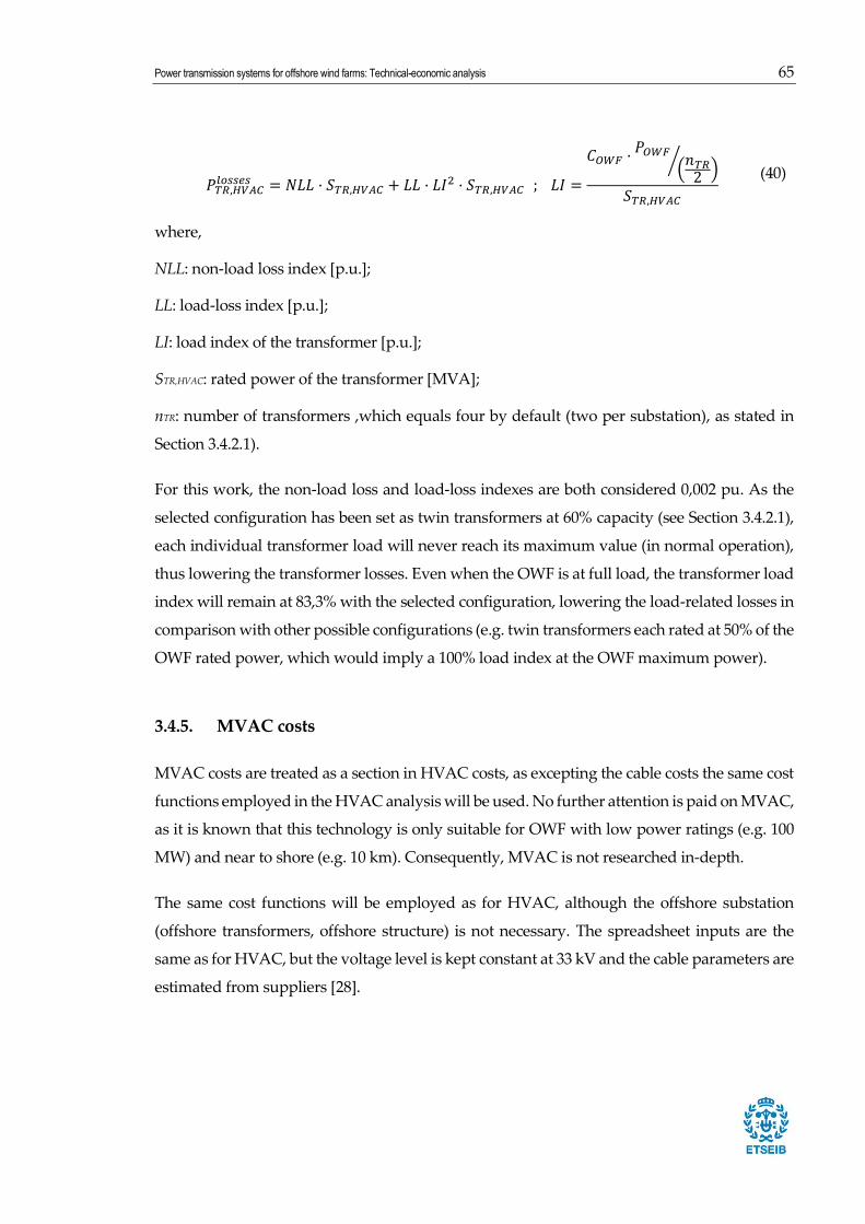
Power transmission systems for offshore wind farms: Technical-economic analysis 65
𝑃𝑇𝑅,𝐻𝑉𝐴𝐶𝑙𝑜𝑠𝑠𝑒𝑠 = 𝑁𝐿𝐿 · 𝑆𝑇𝑅,𝐻𝑉𝐴𝐶 + 𝐿𝐿 · 𝐿𝐼2 · 𝑆𝑇𝑅,𝐻𝑉𝐴𝐶 ; 𝐿𝐼 =
𝐶𝑂𝑊𝐹 ·𝑃𝑂𝑊𝐹
(𝑛𝑇𝑅2
)⁄
𝑆𝑇𝑅,𝐻𝑉𝐴𝐶
(40)
where,
NLL: non-load loss index [p.u.];
LL: load-loss index [p.u.];
LI: load index of the transformer [p.u.];
STR,HVAC: rated power of the transformer [MVA];
nTR: number of transformers ,which equals four by default (two per substation), as stated in
Section 3.4.2.1).
For this work, the non-load loss and load-loss indexes are both considered 0,002 pu. As the
selected configuration has been set as twin transformers at 60% capacity (see Section 3.4.2.1),
each individual transformer load will never reach its maximum value (in normal operation),
thus lowering the transformer losses. Even when the OWF is at full load, the transformer load
index will remain at 83,3% with the selected configuration, lowering the load-related losses in
comparison with other possible configurations (e.g. twin transformers each rated at 50% of the
OWF rated power, which would imply a 100% load index at the OWF maximum power).
3.4.5. MVAC costs
MVAC costs are treated as a section in HVAC costs, as excepting the cable costs the same cost
functions employed in the HVAC analysis will be used. No further attention is paid on MVAC,
as it is known that this technology is only suitable for OWF with low power ratings (e.g. 100
MW) and near to shore (e.g. 10 km). Consequently, MVAC is not researched in-depth.
The same cost functions will be employed as for HVAC, although the offshore substation
(offshore transformers, offshore structure) is not necessary. The spreadsheet inputs are the
same as for HVAC, but the voltage level is kept constant at 33 kV and the cable parameters are
estimated from suppliers [28].

66
3.5. HVDC cost
3.5.1. Base variables
In the same way as explained in Section 3.4.1, to obtain the costs for an HVDC transmission
system, the user most introduce a set of variables (see Table 13) which are the base of the cost
modelling.
Table 13 HVDC main inputs
Variables Description Units
UHVDC Phase to phase voltage level of the transmission cables kV
SHVDC Cable cross section mm2
ncables,HVDC Number of cable pairs -
The number of cables pairs ncables,HVDC is by default limited to 1 being the system bipolar (see
section 2.3.4), although it can be increased. On the other hand, each cable rated ampacity
𝐼𝑟𝑎𝑡𝑒𝑑,𝐻𝑉𝐷𝐶 is estimated from the values given by suppliers (see Table 14), and the mean current
and the rated power of each cable pair are calculated through (41).
𝑃𝑟𝑎𝑡𝑒𝑑,𝑐𝑎𝑏.𝑝𝑎𝑖𝑟 = 2 · 𝐼𝑟𝑎𝑡𝑒𝑑,𝐻𝑉𝐷𝐶 · 𝑈𝐻𝑉𝐷𝐶 𝐼𝑚,𝐻𝑉𝐷𝐶 =𝑐𝑂𝑊𝐹·𝑃𝑂𝑊𝐹
2·𝑛𝑐𝑎𝑏𝑙𝑒𝑠,𝐻𝑉𝐷𝐶·𝑈𝐻𝑉𝐷𝐶
(41)
where,
Table 14 Rated ampacities of HVDC cables
Cross section
[mm2]
Ampacity
[A/core]
Cross section
[mm2]
Ampacity
[A/core]
95 343 1200 1458
120 392 1400 1594
150 441 1600 1720
185 500 1800 1830
240 583 2000 1953
300 662 2200 2062
400 765 2400 2170
500 883 2600 2275
630 1023 2800 2373
800 1175 3000 2473
1000 1335

Power transmission systems for offshore wind farms: Technical-economic analysis 67
𝑃𝑟𝑎𝑡𝑒𝑑,𝑐𝑎𝑏.𝑝𝑎𝑖𝑟: rated power of each cable pair [W];
𝐼𝑟𝑎𝑡𝑒𝑑,𝐻𝑉𝐷𝐶 : rated current of each cable [A];
𝐼𝑚,𝐻𝑉𝐷𝐶: mean current of each cable [A];
cOWF: OWF capacity factor;
𝑃𝑂𝑊𝐹 : OWF rated power [MW].
3.5.2. Base cost
3.5.2.1. Transformers cost
As mentioned in Section 2.3.2, HVDC systems also need transformers to step up the voltage.
The cost function shown in (9) is employed; and the same configuration with two transformers
is assumed, as it constitutes the optimum relationship between reliability and cost [61].
3.5.2.2. VSC converter cost
It is known that the cost of VSC converters can be higher than 100 M€. Lancheros [13] states
120M€ for a 1000MW converter (2013), whereas Lazaridis [74] and Lundberg [62] agree on a
cost of 0,11M€/MW (2005 and 2003). Schoenmakers [9] assumes a cost of 0,085 M€/MW for a
±150 kV converter and 0,093M€/MW for a ±300 kV converter (2008). The ENTSOE [58] reported
costs (2011) are given in Table 3.5-3.
Table 15 VSC converter cost data [58]
Rated Power [MW] Cost range [M€] Mean Cost [M€/MW]
500 75 - 92 0,167
850 98 - 105 0,119
1250 121 - 150 0,108
2000 144 - 196 0,085
Being an incipient technology, VSC converters costs have decreased as the technology
improved. For this reason, costs reported in recent sources are considered more reliable.
Moreover, as it can be seen in Table 15, assuming a constant cost per MW would be a vague
assumption, as the costs decreases with the converter rated power. Furthermore, as costs from
[58] are stated to come from suppliers, they are considered particularly relevant. Therefore,
those data are used to achieve a cost function, shown in Figure 24.

68
Figure 24 VSC converter cost as a function of its rated power
𝐶𝑉𝑆𝐶 = 0,0589 · 𝑆𝑉𝑆𝐶 + 54,985 (42)
where,
CVSC: cost of a single converter [M€];
SVSC: converter rated power [MW].
As discussed in Sections 2.3.3.2 and 2.3.4, there will be two converters, one for each conversion
operation: a rectifier at the offshore substation and an inverter at the onshore one.
3.5.2.3. HVDC Offshore substation structure
It is known that a VSC-HVDC offshore structure needs more size than its equivalent HVAC
structure. Consequently, its costs will be higher. From data in [58], it can be estimated that a
VSC platform costs are from 57,9% to 115,4% higher than an HVAC platform for the same
rated power. Furthermore, it is stated that a VSC platform is 85% bigger than an equivalent
HVAC platform [63]. As 85% falls in the middle of the cost increase range, it is a prudent value
to consider. Consequently, the cost of an offshore substation structure is modelled as:
y = 0,0589x + 54,895R² = 0,9843
0
20
40
60
80
100
120
140
160
180
200
0 500 1000 1500 2000 2500
Co
st [
M€
]
Rated Power [MW]

Power transmission systems for offshore wind farms: Technical-economic analysis 69
𝐶𝑆𝑆,𝐻𝑉𝐷𝐶 = 1,85 · (2,534 + 0,0887 · 𝑃𝑂𝑊𝐹) (43)
where,
𝐶𝑆𝑆,𝐻𝑉𝐷𝐶 : cost of the offshore HVDC substation platform [M€];
𝑃𝑂𝑊𝐹 : OWF rated power [MW].
3.5.3. Distance dependent costs
3.5.3.1. Cable cost
To achieve a function that estimates the cost of dc cables, data has been gathered from
literature. Two different approaches have been revealed: authors either assume a fixed cost
[63] [13], or they consider a cost function, as achieved by Lundberg in 2003 [62] [74]. However,
dc cables technology (extruded XLPE) has made significate advances since 2003 [75], thus
Lundberg cost function could be outdated. Consequently, it has been intended to build a new
cost function. For this purpose, data from [58] has been plotted to reveal any correlation
(Figure 25).
Figure 25 HVDC VSC cable cost as a function of its rated power and voltage level. Data source: [58]
It is observed that the cost of the cable is suitable for a multiple regression, with the rated
power and the voltage level as variables:
𝐶𝑐𝑎𝑏𝑙𝑒 𝑝𝑎𝑖𝑟,𝐻𝑉𝐷𝐶 = 0,652 + 0,00098 · Prated,cab.pair − 0,002363 · 𝑈𝐻𝑉𝐷𝐶 (44)
where;
𝐶𝑐𝑎𝑏𝑙𝑒 𝑝𝑎𝑖𝑟,𝐻𝑉𝐷𝐶 : cost of each cable pair [M€/km];
0
0,2
0,4
0,6
0,8
1
1,2
0 200 400 600 800 1000 1200 1400
Co
st p
er p
air
[M€
/km
]
Rated Power [MW]
±150 kV
±320 kV

70
𝑃𝑟𝑎𝑡𝑒𝑑,𝑐𝑎𝑏.𝑝𝑎𝑖𝑟 : rated power of the cable pair [MW];
𝑈𝐻𝑉𝐷𝐶: HVDC voltage level [kV].
Nevertheless, the model obtained should not be used for voltages and power rates outside the
data ranges shown in Figure 25.
Note that the number of cables must be even, to match the chosen topology (symmetric
monopolar). Additionally, it must be accounted that a pair of cables laid in the same trench
cannot handle more than 1400MW [76]. Consequently, for OWF rated less than 1400MW a
single cable pair will be enough, and their rated power will match the OWF rated power
(POWF). However, for larger ratings, the number of cable pairs should be increased, and the
OWF rated power should be equally distributed amongst each cable pair.
3.5.3.2. Cable laying cost
Each cable pair must be laid in the same trench to minimize the generated magnetic fields
(Section 2.3.4). As for ac cable laying, there is not enough reliable data to achieve a cost
function. A compromise is then made using the available information reported in Table 16.
Table 16 HVDC cable laying cost data.
Reported cost [M€/km] (per cable pair) Reference
0,575 - 1,035 [58]
0,176 [62]
0,600 [13]
0,200 [74]
0,215 [63]
A compromise cost is therefore set at 0.4 M€/km for each cable pair. The cost data for this
particular case is considered unreliable at some degree: as all the costs come from different
sources, it is not known what is included. It could be supposed that the lower cost corresponds
simply to installing the cables and digging the trenches, while maybe the higher one includes
route survey among other services.

Power transmission systems for offshore wind farms: Technical-economic analysis 71
3.5.4. HVDC transmission system losses
3.5.4.1. DC cables losses
For dc cables, losses are much simpler to calculate than for HVAC cables, as there is no reactive
power, and no proximity and skin effects (compare with Section 2.3.1). The dc resistance is
calculated with (17) with the previously selected cross-section SHVDC. The losses are calculated
as:
𝑃𝑜ℎ𝑚𝑖𝑐,𝐻𝑉𝐷𝐶 = 2 · 𝑛𝑐𝑎𝑏𝑙𝑒𝑠,𝐻𝑉𝐷𝐶 · 𝐼𝑚,𝐻𝑉𝐷𝐶2 · 𝑅𝑑𝑐 (45)
where;
Im,HVDC: mean current [A];
Rdc: cable resistance [Ω/km];
Pohmic,HVDC: ohmic losses in the cables [W/km].
By default the number of cables ncables,HVDC is two.
As done for HVAC, the losses cost is calculated as the cost of the non-produced energy, taking
in account the OWF lifespan:
𝐶𝐻𝑉𝐷𝐶 𝑐𝑎𝑏𝑙𝑒𝑙𝑜𝑠𝑠𝑒𝑠 = 𝑃𝑜ℎ𝑚𝑖𝑐,𝐻𝑉𝐷𝐶 · 𝐹𝑙𝑜𝑠𝑠 (46)
where;
𝐶𝐻𝑉𝐷𝐶 𝑐𝑎𝑏𝑙𝑒𝑙𝑜𝑠𝑠𝑒𝑠 : cost of the losses in the HVDC cables [€/km];
Pohmic,HVDC: power of the losses in the HVDC cables [W/km].
3.5.4.2. Converter losses
As discussed in Section 2.3.3.2, reported VSC converter losses have gradually decreased from
3% down to 1% with newer technology generation [42]. For this work, it is assumed that the
VSC losses are 1% of the converted power, obtaining the following equation:
𝑃𝑙𝑜𝑠𝑠𝑒𝑠,𝑉𝑆𝐶 = 0,01 · 𝐶𝑂𝑊𝐹 · 𝑃𝑂𝑊𝐹 (47)
where,
Plosses,VSC: losses power of a single converter [W];

72
cOWF: OWF capacity factor;
POWF: OWF rated power [W].
The cost of these losses is evaluated in (48). Notice that the VSC losses cost could actually be
very high. As an example, for a 500 MW OWF, assuming the cost of energy (Cenergy) at 50
€/MWh and a lifespan of 15 years, VSC losses cost amount to 26.3 M€.
𝐶𝑉𝑆𝐶𝑙𝑜𝑠𝑠𝑒𝑠 = 𝑃𝑙𝑜𝑠𝑠𝑒𝑠,𝑉𝑆𝐶 · 𝐹𝑙𝑜𝑠𝑠 (48)
where,
𝐶𝑉𝑆𝐶𝑙𝑜𝑠𝑠𝑒𝑠 : Cost of the losses in both VSC converters [€]
Plosses,VSC: Losses power of both VSC converters [W].

Power transmission systems for offshore wind farms: Technical-economic analysis 73
3.6. LFAC Costs
As LFAC transmission systems are still in figuring as a theoretical proposal for OWFs, the
related power transmission costs have not been extensively investigated by researchers as in
comparison to HVDC or HVAC solutions. A cost comparison between VSC-HVDC and LFAC
was performed in [18], whereas the cost of some components at non-standard frequencies is
estimated in [55].
For this work, the same cost functions as HVAC will be considered, except for transformers
and transformer losses, whose cost patterns will be established by analysing its differences
with standard step-up transformers. Offshore structure costs for LFAC will also be particularly
studied.
The costs of the necessary ac-ac converters (CCV and B2B-VSC) will also be analysed. For the
rest of the devices, the same cost patterns as the ones established for HVAC will be utilized.
Note that it is not an unreasonable approximation as, for example, it is known that standard
HVAC cables can be employed for LFAC [49]. Even though the same cost functions are
applied, the results will be different since, for instance, operating at a lower frequency will
cause reactive power compensation to be much lower. Additionally, a lower frequency allows
employing transmission cables with higher voltages than for standard HVAC without strong
reductions on the power transmission capability.
3.6.1. LFAC base variables
To perform the calculations, the user must provide the following variables:
Table 17 HVAC main inputs
Variables Description Units
URMS,LFAC Phase to phase voltage level of the transmission cables V
SHVAC Cable cross section mm2
f Electric line frequency Hz
ncables,LFAC Number of three-core cables -
The electric line frequency is set by default at 16,67 Hz (50/3), but the user can choose to employ
20 Hz , which would be the standard for 60 Hz grids. As for HVAC, the voltage level should
be between 110 kV and 275 kV, as the modelling equations have been made with some

74
limitations (estimation of cable capacitance and inductance). For the cable cross section, the
user must choose from a list of standardized values, which are the same as for the HVAC
subsea cables.
Once the conductor cross-section has been chosen, the three-core cable ampacity (i.e. the
maximum intensity that each cable core can withstand) is deduced from values given by
suppliers [28], reported in Table 18 . The same values for ampacity are employed than for
HVAC. In case the user wishes to choose a non-standardized cross-section, the ampacity
𝐼𝑟𝑎𝑡𝑒𝑑,𝐿𝐹𝐴𝐶 is estimated from the values given by the suppliers. Finally, the number of three-
core cables should be chosen.
Table 18 Ampacity of three-core cables
Cross section
[mm2]
Ampacity
[A/core]
300 530
400 590
500 655
630 715
800 775
1000 825
With those values introduced, the mean active current per cable core and the cable power
rating are deduced:
𝐼𝑚𝑒𝑎𝑛,𝐿𝐹𝐴𝐶 =𝑐𝑂𝑊𝐹·𝑃𝑂𝑊𝐹
𝑛𝑐𝑎𝑏𝑙𝑒𝑠,𝐿𝐹𝐴𝐶·√3·𝑈𝑅𝑀𝑆,𝐿𝐹𝐴𝐶 ; 𝑆𝑐𝑎𝑏𝑙𝑒,𝐿𝐹𝐴𝐶 = √3 · 𝑈𝑅𝑀𝑆,𝐿𝐹𝐴𝐶 · 𝐼𝑚𝑎𝑥,𝐿𝐹𝐴𝐶 (49)
Where, Im,LFAC is calculated in Amperes per core, with POWF in Watts and URMS in Volts. Im,HVLF
corresponds to the mean value of the active electric current taking in account the capacity
factor cOWF, i.e. the active current that each cable must carry in normal operation. 𝑆𝑐𝑎𝑏𝑙𝑒,𝐿𝐹𝐴𝐶
corresponds to the rated power of each cable, i.e. the maximum power the each cable can
withstand in steady-state.
As for HVDC and HVAC, the user is shown some parameters which should assure that a
suitable transmission system is selected (see Section 3.9 for further explanations).
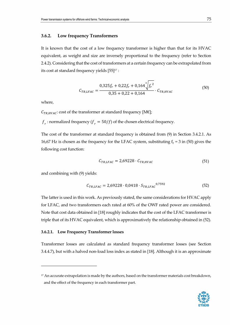
Power transmission systems for offshore wind farms: Technical-economic analysis 75
3.6.2. Low frequency Transformers
It is known that the cost of a low frequency transformer is higher than that for its HVAC
equivalent, as weight and size are inversely proportional to the frequency (refer to Section
2.4.2). Considering that the cost of transformers at a certain frequency can be extrapolated from
its cost at standard frequency yields [55]17 :
𝐶𝑇𝑅,𝐿𝐹𝐴𝐶 =0,325𝑓𝑟 + 0,22𝑓𝑟 + 0,164√𝑓𝑟
23
0,35 + 0,22 + 0,164· 𝐶𝑇𝑅,𝐻𝑉𝐴𝐶
(50)
where,
𝐶𝑇𝑅,𝐻𝑉𝐴𝐶: cost of the transformer at standard frequency [M€];
𝑓𝑟 : normalized frequency (𝑓
𝑟= 50/𝑓) of the chosen electrical frequency.
The cost of the transformer at standard frequency is obtained from (9) in Section 3.4.2.1. As
16,67 Hz is chosen as the frequency for the LFAC system, substituting fr = 3 in (50) gives the
following cost function:
𝐶𝑇𝑅,𝐿𝐹𝐴𝐶 = 2,69228 · 𝐶𝑇𝑅,𝐻𝑉𝐴𝐶 (51)
and combining with (9) yields:
𝐶𝑇𝑅,𝐿𝐹𝐴𝐶 = 2,69228 · 0,0418 · 𝑆𝑇𝑅,𝐿𝐹𝐴𝐶0,7592 (52)
The latter is used in this work. As previously stated, the same considerations for HVAC apply
for LFAC, and two transformers each rated at 60% of the OWF rated power are considered.
Note that cost data obtained in [18] roughly indicates that the cost of the LFAC transformer is
triple that of its HVAC equivalent, which is approximatively the relationship obtained in (52).
3.6.2.1. Low Frequency Transformer losses
Transformer losses are calculated as standard frequency transformer losses (see Section
3.4.4.7), but with a halved non-load loss index as stated in [18]. Although it is an approximate
17 An accurate extrapolation is made by the authors, based on the transformer materials cost breakdown,
and the effect of the frequency in each transformer part.

76
statement, it serves to illustrate that low-frequency transformers present lower iron losses.
3.6.3. Offshore substation structure
As done for the HVDC technology in Section 3.5.2.3, the goal is to establish a relationship
between the costs of the LFAC and the HVAC offshore structure. The cost of an LFAC offshore
structure, able to accommodate the offshore LFAC substation, should be lower than the HVDC
offshore structure cost, as the size of the latter is known to be higher [18], but higher than the
HVAC offshore structure cost, as the low frequency transformers have increased size and
weight.
Combining data from [18] and [58], one can estimate that for an HVAC offshore structure, the
transformers account for 10% of the total weight18: the weight of a 300 MW HVAC structure
is reported as 2000 t, whereas the weight of two 50-Hz 180-MVA three-phase transformers is
estimated from [18] at 200 metric tons. In addition, as the weight of the low frequency
transformers is triple that of standard transformers (see Section 2.4.2), one can estimate that
the size, and thus the cost, of a LFAC offshore structure is 20% higher than the cost of an
equivalent HVAC offshore structure assuming that all the other equipment remain
unchanged. The previous statement, combined with (11), results in a cost function for the cost
of the LFAC offshore structure:
𝐶𝑆𝑆,𝐿𝐹𝐴𝐶 = 1,2 · (2,534 + 0,0887 · 𝑃𝑂𝑊𝐹) (53)
3.6.4. Power converters: CCV and B2B-VSC
The cost of a back-to-back (B2B) VSC converter can be estimated proportional to the costs of a
VSC converter (section 3.5.2.2). For cycloconverters (CCVs), no cost data have been found. In
fact, no information has been found for CCVs in the MW power range. Nevertheless, as CCV
technology is based on thyristors, its cost could be extrapolated from the costs of line-
commutated converters, which are also thyristor based and which have cost data available
from [58] (see Table 19).
Indications are that three-phase/three-phase cycloconverters for LFAC should need 36
18 Same configuration as for HVAC and HVDC : two twin Transformers per substation, each one rated
at 60% of the rated power of the OWF

Power transmission systems for offshore wind farms: Technical-economic analysis 77
thyristor valves (12 valves per phase) [17], whereas LCC employs only 12 thyristor valves [77].
Assuming that most of the costs are due to the thyristor valves, it could be estimated that the
power-dependent cost of a CCV corresponds to the triple of the cost of a LCC with the same
rated power.
Table 19 Reported cost data of LCC [58]
Rated Power [MW] Cost range [M€] Mean Cost
1000 81 - 104 92,5
2000 150 - 184 167,0
3000 196 - 230 213,0
Table 19 can be used to establish a cost function for the CCVs as:
𝐶𝐶𝐶𝑉 = 3 · 0,0603 · 𝑆𝑟𝑎𝑡𝑒𝑑 + 37 (54)
For the B2B-VSC costs, it must be accounted that two VSC are necessary. Nevertheless, as the
two converters are assembled together, one may assume that the cost of the whole B2B system
is not the equal the sum of the cost of two converters, but has a lower value as some
components can be spared, and space can be saved by employing lower voltages and higher
currents, since a transmission system between both VSCs is not needed. Consequently, the
cost of a B2B-VSC is assumed as 1,5 times the cost of a single VSC converter19:
𝐶𝐵𝑡𝐵−𝑉𝑆𝐶 = 1,5 · (0,0589 · 𝑆𝑉𝑆𝐶 + 54,985) (55)
However, as it is difficult to estimate the actual relationship between the costs of B2B-VSC
systems and normal VSC-HVDC ones, the multiplication factor is left open for the user as an
additional input that can be modified.
Regarding the converter losses, it is assumed that the B2B-VSC behaves as a VSC converter
(losses equal to 1% of the transmitted power), and the reported losses of the LCC are
considered for the CCV (0.7% of the transmitted power as stated in Section 2.3.3.1).
19 As it is difficult to estimate the actual relationship between the costs of B2B-VSC systems and normal
VSC-HVDC ones, the multiplication factor is left open for the user as an additional input which can
be modified.

78
3.7. Determination of the break-even distance and area
The break-even distance corresponds to the point where the costs of a HVDC transmission
system become lower than their HVAC counterpart. Even if the economic analysis is
accurately done, variability is inherent to any cost function. Even though the break-even point
is a useful value to determinate the optimum transmission system, accounting for the
variability in cost functions translates into a more accurate estimation. If the upper and lower
predictions of each model are considered, the upper and lower cost predictions can be
obtained, resulting in a break-even area rather than a break-even point (see Figure 26). For
every self-made cost function, its variability will be considered by calculating prediction
intervals, i.e. intervals which the values are expected to lie within with a certain probability.
Figure 26 Break-even area when cost functions variability is considered. Distance-dependent costs variability is not considered
here. Red=HVAC Blue=HVDC
Figure 26 should be similar to the obtained results. Note that as the distance-dependent costs
are also subject to variability, the slope of the upper and lower limits will also be different, not
only their intercept value.
As a general value, it is assumed for the statistical models that a prediction interval of 95% is
accurate enough. The prediction interval for the cost functions is written as follows:

Power transmission systems for offshore wind farms: Technical-economic analysis 79
[�̂� − 1,96 · 𝜎𝑒𝑠𝑡 ; �̂� + 1,96 · 𝜎𝑒𝑠𝑡] (56)
where �̂� is the value predicted by the model, and 𝜎𝑒𝑠𝑡 is the standard deviation of the model.
On the other hand, whenever a mean value has been assumed in lieu of building a cost
function (e.g. cable laying costs), the following interval was considered:
[𝑦 − 1,96 · 𝜎 ; 𝑦 + 1,96 · 𝜎] (57)
where 𝑦 is the mean value of the considered data and 𝜎 is the standard deviation of the cost
data.
Statistical results of each model can be found in the annexes. For every achieved cost function,
the lower and upper 95% limits are considered, following (56) and (59). In the spreadsheet tool
built, the upper and lower cost analyses are displayed to the user, along with the break-even
area. For referenced cost functions, variability cannot be considered, as the original data is not
known and the functions statistical parameters are not reported.
Note that the purpose of this lower and upper cost estimation is to give an idea of the break-
even point variability, and not to perform an in-depth statistical study. This is why the
considered prediction intervals described in (56) and (58) obviate some mathematical
considerations and make some statistical assumptions, such as assuming normally distributed
and uncorrelated residuals, or considering that the residual standard deviation provides a
good estimate of the forecast standard deviation.
3.7.1. HVAC cost variability
For HVAC technology cost functions, the following standard deviations are obtained:
Transformer cost function : σTR = 0,154 M€;
GIS cost function: σGIS = 0,339 M€.
For cable laying costs, where a mean value has been assumed (see Section 3.4.3.2), the data
are considered reliable enough to consider its variability (all data come from the same
source), obtaining, hence, σcable laying, HVAC = 0,025 M€/km.

80
3.7.2. HVDC cost variability
For the HVDC technology cost functions, the following standard deviations are obtained:
Transformer cost function: σTR = 0,154 M€ (same as for HVAC);
VSC cost function: σVSC = 5,86 M€;
HVDC cable cost function: σcable pair,HVDC = 0,0475 M€/km.
As said in Section 3.5.3.2, HVDC cable laying cost data are not reliable enough. Their
unreliability as well as having only five data points makes any consideration of variability
futile (considering the variability of this cost would translate in negative cost for the lower 95%
range limit, which has no meaning).
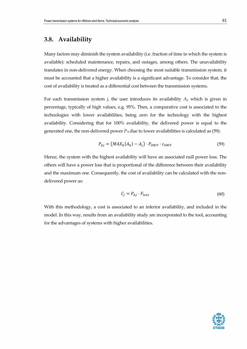
Power transmission systems for offshore wind farms: Technical-economic analysis 81
3.8. Availability
Many factors may diminish the system availability (i.e. fraction of time in which the system is
available): scheduled maintenance, repairs, and outages, among others. The unavailability
translates in non-delivered energy. When choosing the most suitable transmission system, it
must be accounted that a higher availability is a significant advantage. To consider that, the
cost of availability is treated as a differential cost between the transmission systems.
For each transmission system j, the user introduces its availability Aj, which is given in
percentage, typically of high values, e.g. 95%. Then, a comparative cost is associated to the
technologies with lower availabilities, being zero for the technology with the highest
availability. Considering that for 100% availability, the delivered power is equal to the
generated one, the non-delivered power PAj due to lower availabilities is calculated as (59):
𝑃𝐴𝑗 = (𝑀𝐴𝑋𝑘{𝐴𝑘} − 𝐴𝑗) · 𝑃𝑂𝑊𝐹 · 𝑐𝑂𝑊𝐹 (59)
Hence, the system with the highest availability will have an associated null power loss. The
others will have a power loss that is proportional of the difference between their availability
and the maximum one. Consequently, the cost of availability can be calculated with the non-
delivered power as:
𝐶𝑗 = 𝑃𝐴𝑗 · 𝐹𝑙𝑜𝑠𝑠 (60)
With this methodology, a cost is associated to an inferior availability, and included in the
model. In this way, results from an availability study are incorporated to the tool, accounting
for the advantages of systems with higher availabilities.

82
3.9. Guide for choosing adequate inputs – transmission system
constraints
As previously discussed, choosing the cable cross-section, voltage level, and the number of
cables must be done carefully. Due to the tool functioning, the user could theoretically
introduce inputs that could make the cables exceed their ratings, making the whole economic
analysis useless. Consequently, some resources are given to the user to analyse the suitability
of the introduced transmission characteristics. The resources have been designed to fulfil the
following criteria:
1. The transmission system (the cables) must be able to transmit full OWF rated power (i.e.
the transmission systems is able to operate when the OWF produces its maximum power);
2. The transmission capability must not be reduced due to the presence of reactive power
beyond the OWF rated power, within a considered distance to shore (applies to HVAC,
LFAC and MVAC).
The first criterion is easy to introduce. As the user introduces the transmission parameters
(voltage level, cross section, number of cables), the transmission system maximum load ratio
is displayed, calculated as follows:
𝑀𝑎𝑥𝑖𝑚𝑢𝑚 𝑢𝑡𝑖𝑙𝑖𝑧𝑎𝑡𝑖𝑜𝑛 𝑟𝑎𝑡𝑖𝑜 =
𝑃𝑂𝑊𝐹
𝑛𝑐𝑎𝑏𝑙𝑒𝑠 · 𝑆𝑐𝑎𝑏𝑙𝑒 (61)
where 𝑆𝑐𝑎𝑏𝑙𝑒 is the rated power of each cable [MVA] , 𝑛𝑐𝑎𝑏𝑙𝑒𝑠 corresponds to the number of
cables and 𝑃𝑂𝑊𝐹 corresponds to the OWF rated power.
The maximum utilization ratio should be inferior to 100%, to transmit the maximum rated
power. Along with this ratio, a large “YES” or a large “NO” is shown respectively if the
utilization ratio is lower or higher than 100%.20
The second criterion is more challenging to implement. As mentioned in Section 2.1.2, the
20 However, there are ongoing discussions that it would actually be more economically benefitial to
implement OWFs with transmission systems rated at lower capacities than the farm itself. The reason is
that since the OWFs only produce at full load hours for a small amount of time, most of the time the
cable full capacity is not used.

Power transmission systems for offshore wind farms: Technical-economic analysis 83
generation of reactive power in the subsea cables gradually reduces the power transmission
capability over the distance. As MVAC systems are only suitable for low distances, the
reduction of transmission capability has not been considered for this technology, being the
latter not noticeable for short distances (10-15 km). Thus, for HVAC and LFAC, the following
approach has been taken: the transmission capability is calculated as a function of the distance,
and some key values are displayed to the user.
The total reactive power generated qtot has been calculated for each technology in MVAr/km.
Hence, as the reactive power can be expressed as a function of the distance, the active power
transmission capability is also a function of the distance:
𝑆2 = 𝑃2 + (𝑞𝑡𝑜𝑡 · 𝑑)2 ⟹ 𝑃(𝑑) = √𝑆2 − (𝑞𝑡𝑜𝑡 · 𝑑)2 (62)
Where P(d) [MW] represents the transmittable power at the distance “d” [km] , and S
corresponds to the maximum transmittable power of the transmission system, calculated as
the power rating of each cable multiplied by the number of cables.
Nevertheless, the latter expression corresponds to uncompensated reactive power, and it has
been stated that full compensation is made. For 50/50 compensation in offshore/onshore
substations, the reactive power is evenly distributed at both ends of the cable; hence the
charging current is reduced to the half of the charging current without compensation [9] [78].
Therefore, the transmittable power with 50/50 compensation is calculated as:
𝑃(𝑑)𝑐𝑜𝑚𝑝𝑒𝑛𝑠𝑎𝑡𝑖𝑜𝑛 = √𝑆2 − (𝑞𝑡𝑜𝑡
2· 𝑑)
2
(63)
Figure 27 shows the active power transmission capability of a 400MW OWF with a capacity
factor of 0,4 ,employing two 1000 mm2 three-core cables at 150 kV and 50 Hz. The horizontal
lines correspond respectively to the maximum and the mean power generation of the OWF. It
can be seen that approximatively beyond approximatively 70 km, this transmission system
(with compensation) will not be able to transmit the OWF rated power, resulting in a loss of
power whenever the OWF is at 100% capacity.
It is understood that the cables must be rated higher than the OWF to avoid any power
limitation occurring throughout the transmission system. As a general value, if the distance to
shore is not known, it could be established that the transmission system should be chosen to
avoid any power limitation before 120 km, as OWF tend to be built at most 120 km far from

84
shore.
To help the user, the limiting distance (the distance at which the transmission system cannot
handle 100% of the OWF generated power) will be displayed for the chosen transmission
characteristics. This distance can be derived from (63), and is calculated as:
𝑑𝑙𝑖𝑚𝑖𝑡 = √(𝑆2 − 𝑃𝑂𝑊𝐹
2) ·4
𝑞𝑡𝑜𝑡2 (64)
Once the user chooses the transmission system characteristics, this value is displayed along
with the maximum utilization ratio. Note that if the maximum utilization ration is higher than
100%, the limit distance is 0 km, thus fulfilling the second criteria guarantees fulfilling the first
one.
Figure 27 Power transmission capability of a 400 MW OWF employing 2·3·1000mm2 HVAC cables at 150 kV (50 Hz)
0,0
50,0
100,0
150,0
200,0
250,0
300,0
350,0
400,0
450,0
0 50 100 150 200 250 300 350
P [
MW
]
distance [km]
Without compensation With compensation 50/50 OWF rated power OWF mean power

Power transmission systems for offshore wind farms: Technical-economic analysis 85
4. Case study
The studied case corresponds to the Bard 1 wind farm, which is the remotest offshore wind
farm to date. Table 20 shows reported data over Bard1. It is situated in the North Sea (in
German waters), approximatively 110 km far from shore. The power transmission is made
through HVDC and this case is particularly interesting because it has suffered a series of
power outages at the transmission system, translated in several months without feeding
power. This leads to the following question: Do the costs derived from the power outages
compensate for using an HVDC power transmission system, instead of an HVAC one? The following
cases will be analysed:
1st case: a technical-economic analysis of HVAC, LFAC and HVDC power transmission
systems for Bard1 will be performed, employing the designed spreadsheet tool, which
incorporates the cost functions and the technical considerations presented in Chapters
2 and 3.
2nd case: a comparison of the actually employed HVDC power transmission system,
with a chosen HVAC power transmission system and the cost of the aforementioned
outages.
3rd case: a study of a 1000 MW OWF, taken as a general case.
Table 20 Bard 1 offshore wind farm general data [79] [80] [81]
Characteristic Value Comments
Rated power 400 MW Capacity factor estimated at 0,4
Turbines 80 turbines Each rated at 5 MW with a lifetime of 20 years
Distance to shore 112 km Computed from the centre of the wind farm
Transmission length 194,6 km 121 km subsea and 73,6 km underground cable
Power transmission HVDC +/-150 kV 2x1200 mm2 Cu (Symmetric Monopolar)
The data about Bard 1 shown in Table 20 are used for the cost modelling (400MW as the OWF
rated power, 20 years for the lifespan). Regarding the capacity factor and the discount rate,
general values of respectively 0,4 and 6% are employed. Additionally, the energy selling price
is considered 190 €/MWh, as it is stated as the Germany feed-in tariff [57]. It is also stated that
the HVDC power transmission system consists in 2x1200 mm2 copper cables (symmetric
monopolar) [81]. Those data have been introduced in the model. To perform a comparison,

86
two alternative HVAC and one LFAC power transmission systems have been proposed. The
different power transmission system data are shown in Table 20Table 21.
Table 21 Chosen power transmission system data
Characteristic HVDC* HVAC-1 HVAC-2 HVAC-3 LFAC**
Voltage level [kV] ±150 110 132 150 275
Electric frequency [Hz] - 50 50 50 16,67 (50/3)
Number of cables 2
(1 pair)
3
(3-core)
3
(3-core)
3
(3-core)
2
(3-core)
Conductor cross-section [mm²] 1200 3x1000 3x630 3x500 3x300
* Real data employed for the transmission
** CCV is employed for the conversion.
The analysis considers 121 km as the transmission length, which corresponds to the subsea
section of the power transmission of Bard 1. Apart from the real case employed HVDC system,
four alternative transmission systems are proposed. Considering that the transmission length
is 121 km , no higher HVAC voltages (e.g. 220 kV) can be considered due to the
aforementioned restrictions on the power transmission capability (see Section 3.9).
Consequently, the chosen ac voltages are 110 kV and 150 kV, and the number of cables and
the cross-section are selected to guarantee the power transmission capability: for lower voltage
levels, a higher cross-section and number of cables is necessary. Finally, the proposed LFAC
transmission system employs a cycloconverter for the frequency conversion, as it is cheaper
than a B2B HVDC converter, and the goal of the analysis is to make LFAC as competitive as
possible.

Power transmission systems for offshore wind farms: Technical-economic analysis 87
4.1. Results
4.1.1. First case: HVAC, HVDC, LFAC comparison
Considering a transmission distane of 121 km, the totals costs for each transmission system
are presented in Table 22, whereas Figure 28 displays a general breakdown of the total costs.
Table 22 Transmission system costs at 121 km
Trans. System HVDC HVAC-1 HVAC-2 HVAC-3 LFAC
Subst. costs 238,14 56,60 58,14 59,41 158,52
Cables costs 136,41 373,48 328,87 315,74 237,93
Losses cost 138,35 157,21 161,72 171,27 129,82
Total cost [M€] 512,90 587,29 548,73 546,42 526,27
Figure 28 Costs breakdown of each transmission system. Losses cost includes all losses, cables costs include installation and
supplying costs, and substation costs includes transformers, converters, switchgears and the offshore structure costs.
For the considered distance, the most economical option is the HVDC transmission system,
which is indeed the actually technology chosen for the real OWF. Among the HVAC options,
the transmission system at 150 kV is the most suitable. As stated in the previous sections,
results confirm that substation costs are much higher in HVDC than in HVAC, whereas cables
0
100
200
300
400
500
600
700
HVDC HVAC-1 HVAC-2 HVAC-3 LFAC
Co
st [
M€]
Losses costs
Cables costs
Substationscosts

88
costs remained lower. Regarding the losses, at this distance they are quite similar, due to the
fact that HVDC has important losses in its converters that compensate the benefits of lower
ohmic losses in the cables. On the other hand, LFAC costs are more evenly distributed between
cables and substations. However, its losses remain similar to the HVAC and HVDC losses
again because the converter losses compensate for lower cable losses. It should be noted that,
excluding HVDC, the LFAC system was found to be cheaper than the three HVAC
alternatives.
The following sections will make a more detailed analysis of the results. The first section
deepens the cost breakdown, whereas the second one analyses the losses.
4.1.1.1. Costs breakdown of each proposed option
This section details the results, showing the costs of each element in the proposed transmission
systems. The following tables show the costs breakdown, whereas the subsequent figures help
to highlight the main cost differences between each transmission system.
Table 23 Costs breakdown of the HVDC proposed system
HVDC
Characteristic Unitary cost Units Total Comments
Converters 78,55 2 157,09 One per substation
Transformers 2,68 4 10,72 Two per substation
Offshore structure 70,33 1 70,33
Total substations costs 238,14
Cable pair 0,73 121 88,01 Unitary costs in M€/km
Installation 0,40 121 48,40
Total cables costs 136,41
Cable losses 0,23 121 27,59 In M€/km
Transformer losses 44,31 - 44,31 Total transformer losses
Converter losses 66,46 - 66,46 Total converter losses
Total losses costs 138,35
Total costs 512,90

Power transmission systems for offshore wind farms: Technical-economic analysis 89
Table 24 Costs breakdown of the HVAC-1 proposed system
HVAC-1
Concept Unitary cost Units Total Comments
Switchgears 1,31 6 7,86 Two per cable (one in each side)
Transformers 2,68 4 10,72 Two per substation
Offshore structure 38,01 1 38,01
Total substations costs 56,60
Cable pair 0,76 3x121 274,38 Unitary costs in M€/km·cable, three
cables employed Installation 0,27 3x121 99,10
Total cables costs 373,48
Cable losses 0,81 121 106,00 In M€/km, includes ohmic, dielectric
and compensation losses
Transformer losses 44,31 - 44,31 Total transformer losses
Reactive power costs 0,06 121 6,90 In M€/km
Total losses costs 157,21
Total costs 587,28
Table 25 Costs breakdown of the HVAC-2 proposed system
HVAC-2
Concept Unitary cost Units Total Comments
Switchgears 1,57 6 9,41 Two per cable (one in each side)
Transformers 2,68 4 10,72 Two per substation
Offshore structure 38,01 1 38,01
Total substations costs 58,14
Cable pair 0,63 3x121 229,77 Unitary costs in M€/km·cable, three
cables employed Installation 0,27 3x121 99,10
Total cables costs 328,87
Cable losses 0,83 121 109,91 In M€/km, includes ohmic, dielectric
and compensation losses
Transformer losses 44,31 - 44,31 Total transformer losses
Reactive power costs 0,06 121 7,50 In M€/km
Total losses costs 161,72
Total costs 548,73

90
Table 26 Costs breakdown of the HVAC-3 proposed system
HVAC-3
Concept Unitary cost Units Total Comments
Switchgears 1,78 6 10,67 Two per cable (one in each side)
Transformers 2,68 4 10,72 Two per substation
Offshore structure 38,01 1 38,01
Total substations costs 59,41
Cable pair 0,60 3x121 216,64 Unitary costs in M€/km·cable, three
cables employed Installation 0,27 3x121 99,10
Total cables costs 315,74
Cable losses 0,88 121 118,1 In M€/km, includes ohmic, dielectric
and compensation losses
Transformer losses 44,31 - 44,31 Total transformer losses
Reactive power costs 0,07 121 8,86 In M€/km
Total losses costs 171,27
Total costs 546,41
Table 27 Costs breakdown of the LFAC proposed system
LFAC
Concept Unitary cost Units Total Comments
Converter 71,37 1 71,37 One cycloconverter at the offshore
substation
Switchgears 3,24 4 12,96 Two per cable (one in each side)
Transformers 7,22 4 28,87 Two per substation
Offshore structure 45,62 1 45,62
Total substations costs 158,82
Cable pair 0,71 2x121 171,87 Unitary costs in M€/km·cable, two
cables employed Installation 0,27 2x121 66,07
Total cables costs 237,93
Cable losses 0,60 121 76,33 In M€/km, includes ohmic, dielectric
and compensation losses Transformer losses 24,33 - 24,33 Total transformer losses

Power transmission systems for offshore wind farms: Technical-economic analysis 91
Converter losses 23,29 - 23,29 Total converter losses
Reactive power costs 0,05 121 5,86 In M€/km
Total losses costs 129,82
Total costs 526,56
Figure 29 Costs breakdown of each proposed system
Figure 30 Costs breakdown of the HVAC-1 proposed system, in p.u.
0,00
100,00
200,00
300,00
400,00
500,00
600,00
HVDC HVAC-1 HVAC-2 HVAC-3 LFAC
Co
st [
M€]
Cable losses
Compensation
Cable installation
Cable supply
Switchgear costs
Transformer losses
Transformers
Converter losses
Converters
Offshore struct.
0%
10%
20%
30%
40%
50%
60%
70%
80%
90%
100%
HVDC HVAC-1 HVAC-2 HVAC-3 LFAC
Cable losses
Compensation
Cable installation
Cable supply
Switchgear costs
Transformer
lossesTransformers
Converter losses
Converters

92
Figure 31 Costs breakdown of the HVAC-1 proposed system, comparing individuals costs
The previous figures highlight that the main costs are to be found in the cable systems
(encompassing cable supply, cable installation, cable losses and reactive power compensation
costs) for HVAC, which accounts for more than 80% of the total cost. The cost of the cable
supply (i.e. the cost of the cables themselves) particularly stands out, representing 40-50% of
the total cost. With higher voltages, a soft reduction of those costs is observed, thanks to the
fact the lower cross-section can be used, which indeed translates in lower cable supply costs.
On the other hand, the converters account for more than 50% of the total cost in a HVDC
transmission system. The expected cost reductions and loss reductions in the converters would
definitively reduce the HVDC system costs. As the other costs are substantially lower than for
HVAC, it is obvious that the further costs and losses reduction would make HVDC
competitive at even shorter distances. For example, if VSC costs and VSC losses are reduced
to a half, the breakeven point is to be found around 60 km, instead of around 105 km, which
0,00
50,00
100,00
150,00
200,00
250,00
300,00
HVDC HVAC-1 HVAC-2 HVAC-3 LFAC
Co
st [
M€]
Offshore
struct.
Converters
Converter
losses
Transformers
Transformer
losses
Switchgear
costs
Cable supply
Cable
installation
Compensation
Cable losses

Power transmission systems for offshore wind farms: Technical-economic analysis 93
is the case with the current costs.
Alternatively, the costs of LFAC are more distributed, again showing this cost behaviour in
the middle between HVAC and HVDC. The cable costs also rise higher than the others do, but
it could be due to the fact that no dedicated cost-function has been built for LFAC cables,
employing as stated the HVAC cables cost function. It may be possible that further
investigation leads to a different cost trend, more similar to those associated to HVDC.
4.1.1.2. Losses in the proposed options
Table 28 offers a detailed view of the losses in each proposed transmission system.
Approximately each MW of losses equals to 20,8 M€ in costs through the OWF lifetime
(considering a selling price of 190€/MWh).
Table 28 Losses breakdown for each transmission system, in MW
Losses [MW] HVDC HVAC-1 HVAC-2 HVAC-3 LFAC
Converter losses 3,20 - - - 1,12
Transformer losses 2,10 2,10 2,10 2,10 1,70
Ohmic losses 1,33 2,86 2,83 2,80 1,75
Dielectric losses - 1,51 1,66 1,92 1,26
Compensation losses - 0,74 0,81 0,96 0,63
Total losses [MW] 6,63 7,21 7,40 7,78 6,47
Converter losses compromise the performance of the HVDC system, accounting for almost
the half of the losses. Nevertheless, with a higher cross-section and lower electric resistance,
the cable ohmic losses are lower in dc. Additionally, accounting that it has no dielectric losses
and no compensation is needed (thus no losses in the reactive compensation systems), HVDC
presents lower losses than the HVAC systems. For higher distances, this is even more
exaggerated, as ohmic losses continue to grow over the distance, whereas the converter losses
remain the same.
On the other hand, the LFAC proposed system present the overall lowest losses. Although it
suffers from every type of losses, each individual loss component is lower than for the other
systems: higher voltage and lower frequency result in lower ohmic losses, a lower reactive
power generation translates in decreased dielectric and compensation losses, and finally a
lower frequency implies a reduction in the transformer losses. Additionally, it has less
converter losses than a VSC-HVDC, as it employs a single converter, whose losses are

94
considered lower.
Regarding HVAC systems, it is noticed that the higher losses are in the 150-kV system. A
higher voltage level implies higher reactive power, thus more dielectric and compensation
losses. One could expect to observe a substantial decrease in the ohmic losses as the voltage
level goes up, but in fact, the ohmic losses are more or less the same for each voltage level.
That is because a lower cross-section is employed for higher voltages, to reduce the cable costs.
The reduction on the current is compensated by the reduction on the cross-section, which
increases the electric resistance.
Figure 32 and Figure 33 display interesting additional charts to enhance the comprehension of
the losses patterns.
Figure 32 Losses breakdown for each transmission system, in MW
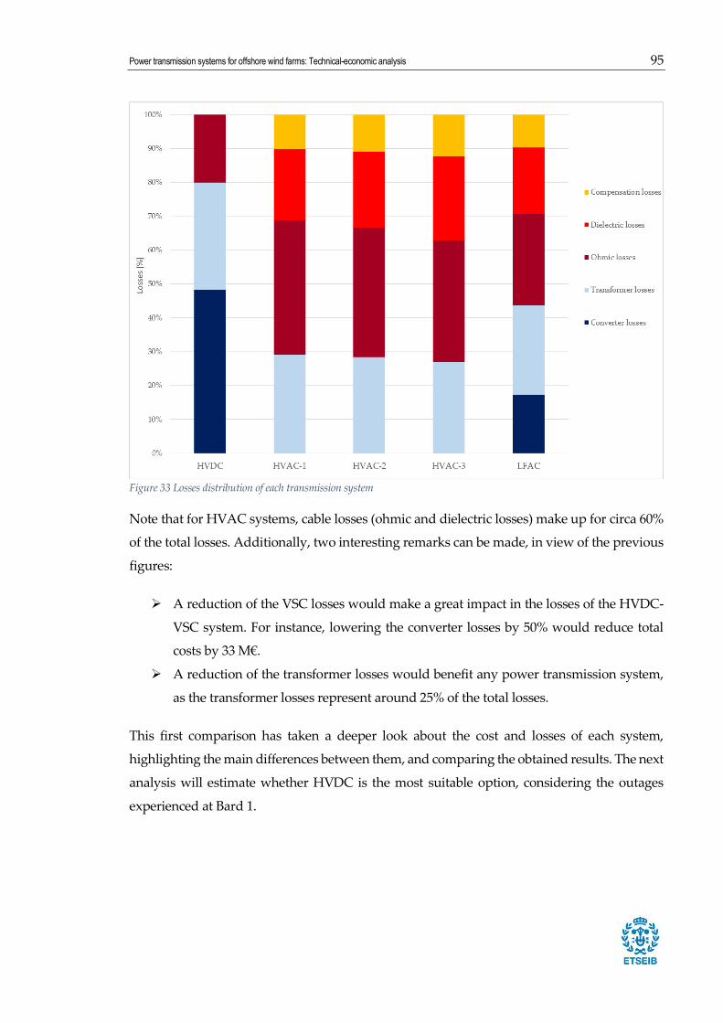
Power transmission systems for offshore wind farms: Technical-economic analysis 95
Figure 33 Losses distribution of each transmission system
Note that for HVAC systems, cable losses (ohmic and dielectric losses) make up for circa 60%
of the total losses. Additionally, two interesting remarks can be made, in view of the previous
figures:
A reduction of the VSC losses would make a great impact in the losses of the HVDC-
VSC system. For instance, lowering the converter losses by 50% would reduce total
costs by 33 M€.
A reduction of the transformer losses would benefit any power transmission system,
as the transformer losses represent around 25% of the total losses.
This first comparison has taken a deeper look about the cost and losses of each system,
highlighting the main differences between them, and comparing the obtained results. The next
analysis will estimate whether HVDC is the most suitable option, considering the outages
experienced at Bard 1.

96
4.1.2. Second case: Suitability of HVDC taking into consideration the power
outages experienced in Bard 1
For this section, a comparison is drawn between the actual employed HVDC system and a
proposed HVAC system. Taking into account the results obtained in Section 4.1.1, the HVAC-
3 transmission system will be considered for this comparison. For the considered Bard 1
characteristics, the HVDC has a cost advantage of 33,5 M€ over HVAC-3, but the cost of the
outages could surpass this cost difference.
At first, a deeper look on the experienced outages should be done. No official source from Bard
1 owner details all the power outages, although many scientific newspapers report the
different and repeated transmission problems [82] [83] [84] [85] [86]. No clear information has
been found about the specifics of the transmission problems, although the following facts are
repeatedly reported:
The project was three years out of schedule;
The transmission problems are located at the offshore converter substation (named
BorWin 1). A smouldering fire took place in March 2014, in the converter platform.
The wind farm owner, instead of relying in an experienced supplier (ABB, Siemens,
Alstom wind), manufactured the converter within its own company.
It seems clear that the source of problems is in the offshore substation, more precisely in the
converter, which was not manufactured by any reputed supplier. Regarding the duration of
outages, different power outages of variable duration are reported in the referenced sources:
3 months outage from October 2013 to January 2014;
57 days outage from 23 March 2014 to May 2014, extending to July 2014;
Several short-duration outages. For example, 17 days of cumulated outages in January
and February 2015.
The exact cumulated duration of all the power outages is not clear. However, based on the
reports, it is at the very least 74 days without any power deliver, and it is probably more than
160 days.

Power transmission systems for offshore wind farms: Technical-economic analysis 97
The cost of these outages is estimated as the cost of non-delivered energy. Assuming a capacity
factor of 0,4, and taking into account the German feed-in tariff of 190 €/MWh; each outage day
translates into 729,6 k€ of non-delivered energy. Figure 34 shows the cost of those outages
being included in the total costs of the HVDC system.
Figure 34 Costs of the HVDC transmission system for Bard 1, compared to the costs of the proposed HVAC-3 transmission
system; including the cost of outages.
After 46 days of total outage, the HVDC system results more expensive than the proposed
HVAC-3 transmission system. Considering that on the most optimistic point of view, there are
at least 74 days without any power delivery, it is clear that an HVAC system would have been
a much better option for Bard offshore 1: assuming 74 days without operation, the HVDC total
costs exceeds the HVAC considered one by 21 M€. At 160 days of cumulated outage, the cost
difference rises up to 83 M€.
4.1.3. Additional case study: optimal power transmission system for a 1000 MW
wind farm
It has already been stated that the future of offshore wind leads to larger and more isolated
wind farms [87]. For this reason, it is interesting to study the power transmission system for a
500
520
540
560
580
600
620
640
660
680
700
0 20 40 60 80 100 120 140 160 180 200
Co
st[M
€]
Days of outage
HVAC-3 transmission cost HVDC cost including days of outage

98
remote 1 GW offshore wind farm. Apart from a power rating of 1 GW, a capacity factor of
40%, lifespan of 20 years, discount rate of 8%, and an energy price of 100 €/MWh are
considered. Table 29 shows the characteristics of proposed transmission systems for this wind
farm, whereas Figure 35 shows the cost of those transmission systems.
Table 29 Proposed transmission systems for a 1000 MW wind farm
Characteristic HVDC HVAC LFAC*
Voltage level ±300 kV 132 kV 275 kV
Electric frequency - 50 Hz 16,67 Hz (50/3)
Number of cables 2 (one pair) 6 (three-core) 3 (three-core)
Conductor cross-section 1600 mm2 3x1000 mm2 3x1000 mm2
* B2B-VSC is employed for the conversion
Figure 35 Costs of the proposed power transmission systems, as a function of the distance
It was expected that LFAC costs would be the lowest ones in the 50-80 km range, but LFAC is
not predominant at any distance. However, the costs of the LFAC converter could have been
estimated too high. In fact, if the ac-ac converter costs are halved, the LFAC transmission
system becomes the optimal option in the 50-70 km range. Regarding LFAC, further
0,00
200,00
400,00
600,00
800,00
1000,00
1200,00
0 20 40 60 80 100 120 140
To
tal
cost
[M
€]
Distance [km]
HVAC
HVDC
LFAC

Power transmission systems for offshore wind farms: Technical-economic analysis 99
investigation is needed, particularly regarding the converter costs, but its economic feasibility
is absolutely not discarded.
Excluding LFAC, the break-even point between HVAC and HVDC costs stands at 59 km.
Accounting the variability, the break-even point falls in the 52-70 km range (see Figure 36).
Figure 36 Break-even area for the proposed HVAC and HVDC transmission systems
Looking at the previous figure, it seems that the statement made by researchers could be
confirmed for large and isolated wind farms: it is often claimed that HVDC is the most
economic option for distances to shore around 50 km. This work has found that this statement
remains true for large OWF, with a rated power close to 1 GW, provided that the HVDC
transmission system can achieve a high availability.
0,00
200,00
400,00
600,00
800,00
1000,00
1200,00
1400,00
0 20 40 60 80 100 120 140
To
tal
cost
[M
€]
Distance [km]

100
Conclusions
As discussed in the introduction, the development of large and remote offshore wind
farms is a reality. In the coming years, we will see offshore wind power becoming a major
element of the European energy resources, thus increasing the relevance of the power
transmission system. In this thesis a technical-economic analysis tool to select the power
transmission systems for offshore wind farms was successfully developed.
For the technical part, the different available technologies – HVAC, HVDC, … – have been
carefully examined, focusing on its main strengths and weaknesses; as well as exposing the
role of the main components. The economic analysis has established cost patterns that were
hitherto not available, and has combined these into a model giving the total costs of a power
transmission, given an OWF design and a set of transmission parameters. The latter has been
implemented in an open-access spreadsheet, that includes all the cost functions, as well as the
loss calculations and availability costs. The spreadsheet includes detailed instructions for the
user on how to introduce the variables, and display the necessary results, accounting the cost
functions variability. Upon request, a non-protected version of the spreadsheet can be
provided, in order to introduce alternative cost functions or to improve the models.
The studied cases have successfully test the economic model, providing interesting
results:
From the first case study, it can be concluded that reliability issues can completely
modify the transmission costs. Because of that, reliability was included as a factor in
the economic analysis and in the spreadsheet.
The break-even point between HVAC and HVDC generally falls in the 50-100 km
range. It strongly depends on the OWF characteristics and the different transmission
parameters (e.g. voltage level, cable cross-section), although as a general statement it
can be said it is close to 50 km for large offshore wind farms (e.g. 1000 MW) and around
100 km for lower power ratings (e.g. 400 MW).
The feasibility of LFAC is not discarded, and is found to be very dependent on its
substations costs, particularly on the cost of the low-frequency converters. Depending

Power transmission systems for offshore wind farms: Technical-economic analysis 101
on the latter, LFAC would be the most suitable technology in the medium distance
range, e.g. 50-70 km.
Although it is true that, for the studied cases, the losses in the HVDC systems are
lower, the main loss-related difference between HVAC and HVDC is in the
distribution of the losses. For HVAC, they are mostly situated in the cables, whereas
for HVDC the biggest share of the losses is in the converters. This is particularly
important because the losses in the HVDC converters are expected to further decrease
(they have decreased from 3% down to 1% in the last decade), whereas not much
improvement is to be expected in the HVAC cable losses (at least until
superconducting cables do not appear to reduce the resistivity of copper).
Finally yet importantly, this work has provided some cost functions that were previously not
found in the literature, and are encouraged to be used. The aim of this thesis is considered to
be completely fulfilled, having provided a tool which determines the costs of a power
transmission system for OWF, as well as having carefully studied the position of the break-
even point.
On the other hand, this works leaves room for future work, which could expand the usefulness
of the technical-economic analysis:
A deeper study on the costs of ac-ac frequency converters;
Expanding and refining the cost functions with extensive cost data provided by
suppliers;
Converting the tool into an iterative program, that accounts the power changes along
the transmission (e.g., taking into account the voltage drop along the cable);
The next step would be to achieve an optimization model, which could directly return
the optimal power transmission system for a given OWF. Note that the equations
provided in this work could be absolutely employed for this purpose.

102
References
[1] GWEC, "Global Wind Report," 2014.
[2] EWEA, "Wind Energy Scenarios for 2020," July 2014.
[3] EWEA. (2014) Annual Statistics. [Online].
http://www.ewea.org/fileadmin/files/library/publications/statistics/EWEA-Annual-
Statistics-2014.pdf
[4] EY (Ernst & Young associates), "Offshore wind in Europe," March 2015.
[5] 4Coffshore. [Online]. http://www.4coffshore.com/windfarms/ravnsborg-denmark-
dk06.html
[6] LORC. Middlegrunden data. [Online]. http://www.lorc.dk/offshore-wind-farms-
map/middelgrunden
[7] The Crown Estate, "Offshore wind cost reduction : Pathways study," May 2012.
[8] EWEA. (March 2015) [Online]. http://www.ewea.org/press-
releases/detail/2015/03/10/offshore-wind-industry-can-compete-with-gas-and-coal-
within-a-decade/
[9] Dirk Schoenmakers, "Optimization of the coupled grid connection of offshore wind
farms," 2008.
[10] EWEA. (2014) European Offshore Statistics. [Online].
http://www.ewea.org/fileadmin/files/library/publications/statistics/EWEA-European-
Offshore-Statistics-2014.pdf
[11] N. Barberis Negra, J. Todorovic, L. Lazaridis T. Ackermann, Evaluation of Electrical

Power transmission systems for offshore wind farms: Technical-economic analysis 103
Transmission Concepts for Large Offshore Wind Farms, 2007.
[12] R. Teixeira Pinto, "MULTI-TERMINAL DC NETWORKS - System Integration, Dynamics
and Control," 2014.
[13] Camilo Lancheros, "Transmission systems for offshore wind farms: a technical,
environmental and economical assesment," 2013.
[14] Shanshan Wang, Guangfu Tang, and Zhiyuan He, "Comprehensive evaluation of VSC-
HVDC transmission based on improved analytic hierarchy process," in Electric Utility
Deregulation and Restructuring and Power Technologies, 2008. DRPT 2008. Third International
Conference on, Nanjuing, 2008, pp. 2207-2211.
[15] Tsuyoahi Funaki and Kenji Matsuura, "Feasibility of the Low Frequency AC
transmission," 2000.
[16] Xifan Wang and Xiuli Wang, "Feasibility Study of Fractional Frequency Transmission
System," IEEE transactions on power systems, vol. 11, no. 2, pp. 962-697, May 1996.
[17] Shi You, Zhao Xu and Vladislav Akhmatov Nan Qin, "Offshore wind farm connection
with low frequency AC technology".
[18] Dr. Ronan Meere and Dr. Terence O’Donnell Mr. Jonathan Ruddy, "Comparison of VSC-
HVDC with Low Frequency AC for Offshore Wind Farm Design and Interconnection,"
in EERA Deepwind, 2015.
[19] K. Meah and S. Ula, "Comparative evaluation of HVDC and HVAC transmission
systems," in IEEE Power Engineering Society – General Meeting, June 2007.
[20] J. Todorovic and T. Ackermann N. Barberis Negra, Loss Evaluation of HVAC and HVDC
Transmission Solutions for Large Offshore Wind Farms, 2006.
[21] Golder Associates, "Study on the comparative merits of overhead electricity transmission
lines versus underground cables," May 2008.
[22] Markel Zubiaga, "Power AC Transmission Lines, Energy Transmission and Grid

104
Integration of AC Offshore Wind Farms, MSc Markel Zubiaga," INTECH, 2012. [Online].
http://www.intechopen.com/books/energy-transmission-and-grid-integration-of-ac-
offshore-wind-farms/power-ac-transmission-lines
[23] Vinay Mehrotra, Ajith Varghese, Hali Moleski, Richard Marek, Bill Henning, Hasse
Nordman, Jim Thompson H. Jin Sim, Comparison of Standards – ANSI / IEEE and IEC ,
Comparison of standards.
[24] Lars Liljestrand, Flemming Krogh, Johan Karlstrand, and Jutta Hanson Stefan G.
Johansson, "AC cable solutions for offshore wind energy,". [Online].
http://wind.nrel.gov/public/SeaCon/Proceedings/Copenhagen.Offshore.Wind.2005/doc
uments/papers/Poster/S.G.Johansson_ACCablesolutionsforOffshoreWindEnergy.pdf
[25] Sthitadhee Sarkar, "Power Transmission Options for Offshore Windfarms in Scotland,"
Department of Mechanical and Aerospace Engineering, University of Strathclyde., 2012.
[26] Nexans. (2003) Nexans Submarine Power Cables. [Online].
http://www.nexans.com/Germany/group/doc/en/NEX_Submarine_neu.pdf
[27] Rick Schlobohm and Bill Brownell Larry Pryor. http://apps.geindustrial.com/. [Online].
http://apps.geindustrial.com/publibrary/checkout/Alum-
Copper?TNR=White%20Papers%7CAlum-Copper%7Cgeneric
[28] ABB. ABB power cables. [Online].
http://www.abb.com/cawp/seitp202/9121cb7988318aecc1257b200039da24.aspx
[29] Angelo Baggini, "The updated EU energy efficiency standardisation of HV and MV
transformers," in INTERNATIONAL ENERGY EFFICIENT TRANSFORMERS
WORKSHOP 2013, 42ND MEETING OF THE APEC EGEE&C, Bangkok, November 2013.
[30] ABB. (2011) ABB power transformers. [Online].
https://library.e.abb.com/public/a2492a9e17a69c1a83257984002ada63/Global_low%20re
s.pdf?filename=Global_low%20res.pdf

Power transmission systems for offshore wind farms: Technical-economic analysis 105
[31] Constantinos Sourkounis and Pavlos Tourou, "Grid Code Requirements for Wind Power
Integration in Europe," in Power Options for the Eastern Mediterranean Region, Limassol,
Cyprus, 2012.
[32] Overview of line-commutated based HVDC, Document available on CIGRE website.
[33] N. Aparicio, S. Añó-Villalba, and S. Bernal-Perez R. Blasco-Gimenez, "LCC-HVDC
Connection of Offshore Wind," IEEE Transactions on industrial electronics, vol. 60, no. 6,
pp. 2372-2380, June 2013.
[34] S. Norrga, "VSC HVDC - Past , Present and Future," in 14th European Conference on Power
Electronics and Applications, Birmingham, 2011.
[35] Alstom Grid. (2011, June) alstom.com. [Online].
http://www.alstom.com/Global/CleanGrid/Resources/Documents/HVDC-
VSC%20transmission%20technology%20of%20the%20future%20-%20Think%20Grid%
20n%C2%B08%20.pdf
[36] J. Leon, R. Portillo, L. Franquelo, and M. Aguirre J. Napoles, "Selective harmonic
mitigation technique for high-power converters," IEEE Transactions on industrial
electronics, vol. 57, no. 7, pp. 2315-2323, July 2010.
[37] K. Friedrich, "Modern HVDC PLUS Application of VSC in Modular Multilevel
Converter Topology," in IEEE International Symposium on Industrial Electronics, 2010.
[38] R. Belmans S. Cole, "Transmission of Bulk Power: The History and Applications of
Voltage-Source Converter High-Voltage," IEEE Ind. Electron. Magazine, no. 6, 2009.
[39] L.A. Gregoire, J. Bélanger W. Li, "Control and Performance of a Modular Multilevel
Converter System," in Conference on Power Systems , Halifax, September 2011.
[40] H. Duchen, M. Karlsson, L. Ronstrom and B. Abrahamsson Y. Jiang-Hafner, "HVDC
with Voltage Source Converters - A powerful black start capability," in IEEE PES
Conference, Chicago, April 2008.

106
[41] M. Barnes and A. Beddard, "Voltage Source Converter HVDC Links - The state of the art
and issues going forward," Energy procedia, no. 24, pp. 108-122, January 2012.
[42] P.S. Alstom Grid, Stafford, UK Jones and C.C Davidson, "Calculation of power losses for
MMC-based VSC HVDC stations," in 15th European conference on Power Electronics and
Applications, Lille, 2-6 September 2013.
[43] ABB. [Online]. http://new.abb.com/systems/hvdc/hvdc-light
[44] Kazutoshi ABE, Makoto SUIZU, Shoji MASHIO, Osamu MATSUNAGA, Shinya ASAI
and Shoshi KATAKAI , J-Power Systems Corporation Yoshinao MURATA, "HVDC
XLPE CABLE SYSTEMS APPLICABLE FOR HIGHER TEMPERATURE AND
POLARITY REVERSAL OPERATION ," in 8th International Conference on Insulated Power
Cables, Versailles, June 2011.
[45] R. Teixeira Pinto, "Multi-Terminal DC Networks : System Integration, Dynamics and
Control," TU Delft, Doctoral Thesis March 2014.
[46] A. Raza, Xu Dianguo, Su Sunwen, and Li Wiexing, "Modeling and control of multi
terminal VSC HVDC transmission system for integrating large offshore wind farms," in
Multi-Topic Conference (INMIC), 2014 IEEE 17th International, Karachi, December 2014, pp.
467-472.
[47] Silvio Rodrigues, R. Teixeira Pinto, P. Bauer, and J. Pierik, "Optimization of social welfare
and transmission losses in offshore MTDC networks through multi-objective genetic
algorithm," in Power Electronics and Motion Control Conference (IPEMC), 2012 7th
International , Harbin, China, June 2012, pp. 1287-1294.
[48] S. Rodrigues, R.T. Pinto, P. Bauer, and J. Pierik, "Optimal Power Flow Control of VSC-
Based Multiterminal DC Network for Offshore Wind Integration in the North Sea,"
Emerging and Selected Topics in Power Electronics, IEEE , vol. 1, pp. 260-268, September
2013.

Power transmission systems for offshore wind farms: Technical-economic analysis 107
[49] Urban Axelsson, Andre Canelhas Espen Olsen, "Low Frequency AC Transmission on
large scale Offshore Wind Power Plants," in 13th wind integration workshop, Berlin,
November 2014, pp. 559-564.
[50] Y. Tang, L. Ran, T. Yang, J. Yu P. B. Wyllie, "Low Frequency AC Transmission - Elements
of a Design for Wind Farm Connection," 2013.
[51] Truls Normann, Ultra-long Subsea Power Transmission Using Frequency Step-up
Equipment, April 2014, Presentation from MCE deepwater development.
[52] Michael H. Johnson and Dionysios C. Aliprantis Hao Chen, "Low-Frequency AC
Transmission for Offshore wind power," IEEE transactions on power delivery, vol. 28, no.
4, pp. 2236-2244, October 2013.
[53] K. Rudion, A. Orths, P. B. Eriksen, H. Abildgaard and Z. A. Styczynski C. Nguyen Mau,
Grid Connection of Offshore Wind Farm based DFIG with Low Frequency AC
Transmission System, 2010.
[54] Daniel J. Rogers, Carlos E. Ugalde-Loo, Jun Liang ,Oriol Gomis-Bellmunt José Luis
Domínguez-García, "Effect of non-standard operating frequencies on the economic cost
of offshore AC," Renewable energy : an international journal, no. 44, pp. 267-280, 2012.
[55] M. De Prada-Gil, O. Gomis-Bellmunt, A. Sumper J.L Domínguez García, "Technical and
economic assessment of offshore ac hubs operating at non-standard frequencies," in 13th
Wind Integration Workshop, Berlin, November 2014, pp. 565-570.
[56] Navigant consulting, Inc. (2013, October) U.S. Office of Energy Efficiency and Renewable
Energy (EERE). [Online].
http://www1.eere.energy.gov/wind/pdfs/offshore_wind_market_and_economic_analy
sis_10_2013.pdf
[57] offshore-windenergie.net, http://www.offshore-windenergie.net/en/politics/eeg-
remuneration, Germany feed-in tariffs.
[58] ENTSOE. (2011, November) Offshore transmission technology. [Online].

108
https://www.entsoe.eu/fileadmin/user_upload/_library/publications/entsoe/SDC/Europ
ean_offshore_grid_-_Offshore_Technology_-_FINALversion.pdf
[59] Ragnar Ulsund, "Offshore Power Transmission: Submarine high voltage transmission
alternatives," June 2009.
[60] G. Forte, M. Pisani and M. Trovato M. Dicorato, "Guidelines for assessment of
investment cost for offshore wind generation," Renewable Energy, no. 36, pp. 2043-2051,
2011.
[61] Lyndon Greedy, Fabio Spinato, Colin A Morgan Andrew R Henderson, "Optimising
Redundancy of Offshore Electrical Infrastructure Assets by Assessment of Overall
Economic Cost ," in European Offshore Wind Energy Conference, Stockholm, September
2009.
[62] Stefan Lundberg, "Performance comparison of wind park configurations," Göteborg,
2003.
[63] Bram Van Eeckhout, "The economic value of VSC HVDC compared to HVAC for
offshore wind farms," 2007-2008.
[64] Eurostat, http://ec.europa.eu/eurostat/inflation-dashboard/, Eurozone statisitcal
economic data.
[65] Open electrical. http://www.openelectrical.org. [Online].
http://www.openelectrical.org/wiki/index.php?title=Cable_Impedance_Calculations
[66] General Cable. http://www.generalcable.co.nz. [Online].
http://www.generalcable.co.nz/getattachment/a4c607a4-d112-40dd-9306-
e1c2af3ed7d3/AC-Resistance,-Skin-Proximity-Effects.aspx
[67] ABB. (2010, April) https://library.e.abb.com. [Online].
https://library.e.abb.com/public/2fb0094306e48975c125777c00334767/XLPE%20Submari

Power transmission systems for offshore wind farms: Technical-economic analysis 109
ne%20Cable%20Systems%202GM5007%20rev%205.pdf
[68] Tushar Mehta. (2012, December) [Online]. http://www.tushar-
mehta.com/excel/newsgroups/interpolation/#Two%5Fdimensional%5Finterpolation%5
F
[69] Nor Akmal Mohd. Jamail, Nor Anija Jalaludi Asmarashid Ponniran, "Tan Delta and
Capacitance Characteristics of Underground XLPE Cables ," in Malaysian Technical
Universities Conference on Engineering and Technology, Kuantan, June 2009.
[70] Anuchit Aurairatch, "A PRELIMINARY STUDY OF LOSS FACTOR IN DIELECTRIC
OF CABLE PRODUCED IN THAILAND," 2006.
[71] Asmarashid Ponniran and Muhammad Saufi Kamarudin, "Study on the Performance of
Underground XLPE Cables in Service Based on Tan Delta and Capacitance
Measurements," in 2nd IEEE International Conference on Power and Energy, Johor Baharu,
December 2008, pp. 39-43.
[72] A. Cancino and R.Malewski, "TESTING AND LOSS MEASUREMENT OF HV SHELL-
TYPE SHUNT-REACTORS AT VERY LOW POWER FACTOR," 2004.
[73] Stefan Fassbinder, "EFFICIENCY AND LOSS EVALUATION OF LARGE POWER
TRANSFORMERS," ECI Publication No Cu0144, May 2013.
[74] Lazaros P. Lazaridis, "Economic Comparison of HVAC and HVDC Solutions for Large
Offshore Wind Farms under Special Consideration of Reliability," Stockholm, 2005.
[75] Masatoshi SAKAMAKI, Kazutoshi ABE, Yoshiyuki INOUE, Shoji MASHIO, Seiji
KASHIYAMA, Osamu MATSUNAGA, Tsuyoshi IGI, Masaru WATANABE, Shinya
ASAI and Shoshi KATAKAI Yoshinao MURATA*, "Development of High Voltage DC-
XLPE Cable System," April 2013. [Online]. http://global-
sei.com/technology/tr/bn76/pdf/76-09.pdf
[76] ABB, HVDC light power cables, 2006.
[77] Lie Xu, Brendan Fox Sarah Foster, "Control of an LCC HVDC System for Connecting

110
Large Offshore Wind Farms with Special Consideration of Grid Fault," in Power and
Energy Society General Meeting - Conversion and Delivery of Electrical Energy in the 21st
Century, Pittsburgh, July 2008, pp. 1-8.
[78] Maja Harfman T. , Song Chi, Satish K. Gunturi, Rajib Datta Joseph Song-Manguelle,
"Power Transfer Capability of HVAC Cables for Subsea Transmission and Distribution
Systems".
[79] http://www.4coffshore.com/windfarms/bard-offshore-1-germany-
de23.html%3EBARD%20Offshore%201, Detailed data about Bard 1 offshore wind farm.
[80] http://www.lorc.dk/offshore-wind-farms-map/bard-offshore-1, Detailed data about
Bard 1 offshore wind farm (2).
[81] http://www.4coffshore.com/windfarms/hvdc-converter-borwin1-converter-cid1.html,
Information about the Bard1 power transmission system.
[82] Sara Knight, "Politics block German offshore wind link," Wind Power Monthly, May 2015.
[83] "'Dirty electricity' probe at BorWin1," Renews, June 2014.
[84] Sara Knight, "Bard 1 transmission problems continue," Wind Power Offshore, June 2014.
[85] Pierre L. Gosselin, Spiegel: Germany’s Large-Scale Offshore Windpark Dream Morphs
Into An Engineering And Cost Nightmare, June 2014, Science Blog.
[86] Pierre L. Gosselin, Giant 400 MW BARD I Offshore Windpark Shut-Down Extended Yet
Again! Delay Is Now More Than 1 Year !, June 2014, Science Blog.
[87] C. Restrepo, E. Kontos, R. Teixeira Pinto, P. Bauer S. Rodrigues, "Trends of offshore wind
projects," Renewable and Sustainable Energy Reviews, vol. 49, pp. 1114-1135, September
2015.
[88] Global Marine Energy, Lessons Learned: Offshore cable installation, 2010.

Power transmission systems for offshore wind farms: Technical-economic analysis 111
[89] UK government, "Contracts for Difference (CFD) Allocation Round One Outcome ,"
February 2015.
[90] Navigant, "Offshore Wind Market and Economic Analysis," October 2013. [Online].
http://www1.eere.energy.gov/wind/pdfs/offshore_wind_market_and_economic_analy
sis_10_2013.pdf
[91] IRENA, "RENEWABLE ENERGY TECHNOLOGIES - Cost analysis series : Wind
Power," June 2012.

112
Appendix 1 : Budget
The budget of this thesis accounts for research and development of this present work, as well
as involved office equipment and software.
Office equipment
A laptop is necessary in order to conduct the research and develop the cost functions, as well
as to write the thesis.
Table 30 Office equipment budget
Concept Unitary price Units Total
Mountain workstation 950 €
1 950 €
TOTAL 950 €
Development tools and software
In order to access to most of the information, purchase of various IEEE articles is required, as
well as MS Excel and Minitab to develop and analyse cost patterns.
Table 31 Development tools and software budget
Concept Unitary price Units Total
IEEE article subscription 27,85 € (per article)
90 2506,5 €
MS Excel 60 € (Excel Home)
1 60 €
Minitab software 30 € (six months license)
1 30 €
TOTAL 2596,5 €

Power transmission systems for offshore wind farms: Technical-economic analysis 113
Labour
Labour costs are divided respectively in research hours, development hours and writing
hours, assuming the salary of a junior researcher at 40€/h.
Table 32 Labour budget
Concept Unitary price Units Total
Research 40 €/h
200 8000 €
Development 40 €/h
150 6000 €
Writing 40 €/h
200 8000 €
TOTAL 22000 €
Total budget
Table 33 Total budget
Concept Total
Office equipment 950 €
Development tools and software 2596,5 €
Labour 22000 €
TOTAL (without taxes) 25456,5 €
TOTAL (21% tax) 30802,37 €
The budget of this work is therefore set at 30802,37 €.

114

Power transmission systems for offshore wind farms: Technical-economic analysis 115
Appendix 2: Designed tool
The tool consists in a MS Excel spreadsheet organized in five different sheets. The first one
gives the necessary instructions to correctly utilize the program, and where to find general
information.
Figure 37 First sheet of the technical-economic analysis developed tool.

116
The second sheet is reserved for internal calculations, it is where the important parameters are
calculated (e.g. cable resistance, cable reactance, elaborated cost functions, internal results of
the model, etc.). Note that this sheet is not supposed to be available to the standard user, and,
therefore, its design is not as important as the sheets that are available.
Figure 38 second sheet of the technical-economic analysis developed tool.
Figure 39 Closer look on the second sheet of the technical-economic analysis developed tool.

Power transmission systems for offshore wind farms: Technical-economic analysis 117
The third sheet is where the inputs are introduced by the user and it is the main page of this
tool.
Figure 40 third sheet of the technical-economic analysis developed tool.

118
The fourth and fifth sheets present the results. The fourth sheets displays two charts (one
including all technologies and one excluding (MVAC), along with a table that gives the costs
as a function for every transmission length. The fifth sheet excludes LFAC, and is centred on
the break-even point concept. It also shows the break-even range and displays a chart showing
the cost variability.
Figure 41 Fourth sheet of the technical-economic analysis developed tool.

Power transmission systems for offshore wind farms: Technical-economic analysis 119
Figure 42 Fifth sheet of the technical-economic analysis developed tool.

120
Appendix 3: Statistical data of the self-made cost
functions
This appendix contains statistical data of the self-made cost functions. Note that for the
transfromers (Figure 43), the cost function is potential; hence the model is made with the
natural logarithm of the variables.
Figure 43 Statistical data of the transformer cost function
Figure 44 Statistical data of the GIS cost function
Estadísticas de la regresión
Coeficiente de correlación múltiple 0,9929336
Coeficiente de determinación R^2 0,98591713
R^2 ajustado 0,98435237
Error típico 0,05476021
Observaciones 11
ANÁLISIS DE VARIANZA
Grados de libertadSuma de cuadradosPromedio de los cuadrados F Valor crítico de F
Regresión 1 1,88939159 1,88939159 630,0743114 1,21453E-09
Residuos 9 0,02698813 0,00299868
Total 10 1,91637972
Coeficientes Error típico Estadístico t Probabilidad Inferior 95% Superior 95% Inferior 95,0% Superior 95,0%
Intercepción -3,17598025 0,17519898 -18,1278465 2,15646E-08 -3,572307875 -2,779652615 -3,572307875 -2,779652615
LN(STr) 0,75915713 0,03024376 25,1012811 1,21453E-09 0,690740989 0,827573267 0,690740989 0,827573267
Estadísticas de la regresión
Coeficiente de correlación múltiple 0,98847561
Coeficiente de determinación R^2 0,97708404
R^2 ajustado 0,95416808
Error típico 0,33904826
Observaciones 3
ANÁLISIS DE VARIANZA
Grados de libertadSuma de cuadradosPromedio de los cuadrados F Valor crítico de F
Regresión 1 4,90136294 4,90136294 42,63770478 0,096743546
Residuos 1 0,11495372 0,11495372
Total 2 5,01631667
Coeficientes Error típico Estadístico t Probabilidad Inferior 95% Superior 95% Inferior 95,0% Superior 95,0%
Intercepción 0,02308032 0,51922684 0,04445132 0,97172003 -6,574322273 6,620482906 -6,574322273 6,620482906
Voltage level [kV] 0,0116738 0,00178779 6,52975534 0,096743546 -0,011042168 0,034389774 -0,011042168 0,034389774

Power transmission systems for offshore wind farms: Technical-economic analysis 121
Figure 45 Statistical data of the dc cables cost function
Figure 46 Statistical data of the VSC cost function
Estadísticas de la regresión
Coeficiente de correlación múltiple 0,93759961
Coeficiente de determinación R^2 0,87909304
R^2 ajustado 0,83073025
Error típico 0,04753681
Observaciones 8
ANÁLISIS DE VARIANZA
Grados de libertadSuma de cuadradosPromedio de los cuadrados F Valor crítico de F
Regresión 2 0,08215113 0,04107557 18,17705546 0,005083096
Residuos 5 0,01129874 0,00225975
Total 7 0,09344988
Coeficientes Error típico Estadístico t Probabilidad Inferior 95% Superior 95% Inferior 95,0% Superior 95,0%
Intercepción 0,65199257 0,05075301 12,8463816 5,08873E-05 0,521527794 0,782457338 0,521527794 0,782457338
Prated cable-pair [MW] 0,00098002 0,00019087 5,13445972 0,003662332 0,000489371 0,001470671 0,000489371 0,001470671
Voltage level [kV] -0,00236262 0,00061455 -3,84445103 0,012068962 -0,003942383 -0,000782861 -0,003942383 -0,000782861
Estadísticas de la regresión
Coeficiente de correlación múltiple 0,99214306
Coeficiente de determinación R^2 0,98434785
R^2 ajustado 0,97652177
Error típico 5,85956166
Observaciones 4
ANÁLISIS DE VARIANZA
Grados de libertadSuma de cuadradosPromedio de los cuadrados F Valor crítico de F
Regresión 1 4318,51857 4318,51857 125,7779565 0,007856942
Residuos 2 68,6689257 34,3344629
Total 3 4387,1875
Coeficientes Error típico Estadístico t Probabilidad Inferior 95% Superior 95% Inferior 95,0% Superior 95,0%
Intercepción 54,8950803 6,71232928 8,17824603 0,014624154 26,01425841 83,77590223 26,01425841 83,77590223
P[MW] 0,05889558 0,00525146 11,2150772 0,007856942 0,036300353 0,081490811 0,036300353 0,081490811