A&A 554, A69 (2013)DOI: 10.1051/0004-6361/201321042c© ESO 2013

Astronomy&

Astrophysics

3D climate modeling of close-in land planets:Circulation patterns, climate moist bistability, and habitability

J. Leconte1, F. Forget1, B. Charnay1, R. Wordsworth2, F. Selsis3,4,E. Millour1, and A. Spiga1

1 LMD, Institut Pierre-Simon Laplace, Université P. et M. Curie, BP99, 75005 Paris, Francee-mail: jeremy.leconte@lmd.jussieu.fr

2 Department of Geological Sciences, University of Chicago, 5734 S Ellis Avenue, Chicago, IL 60622, USA3 Université de Bordeaux, Observatoire Aquitain des Sciences de l’Univers, BP 89, 33271 Floirac Cedex, France4 CNRS, UMR 5804, Laboratoire d’Astrophysique de Bordeaux, BP 89, 33271 Floirac Cedex, France

Received 4 January 2013 / Accepted 27 March 2013

ABSTRACT

The inner edge of the classical habitable zone is often defined by the critical flux needed to trigger the runaway greenhouse instability.This 1D notion of a critical flux, however, may not be all that relevant for inhomogeneously irradiated planets, or when the watercontent is limited (land planets). Based on results from our 3D global climate model, we present general features of the climate andlarge-scale circulation on close-in terrestrial planets. We find that the circulation pattern can shift from super-rotation to stellar/antistellar circulation when the equatorial Rossby deformation radius significantly exceeds the planetary radius, changing the redistribu-tion properties of the atmosphere. Using analytical and numerical arguments, we also demonstrate the presence of systematic biasesamong mean surface temperatures and among temperature profiles predicted from either 1D or 3D simulations. After including acomplete modeling of the water cycle, we further demonstrate that two stable climate regimes can exist for land planets closer thanthe inner edge of the classical habitable zone. One is the classical runaway state where all the water is vaporized, and the other isa collapsed state where water is captured in permanent cold traps. We identify this “moist” bistability as the result of a competitionbetween the greenhouse effect of water vapor and its condensation on the night side or near the poles, highlighting the dynamicalnature of the runaway greenhouse effect. We also present synthetic spectra showing the observable signature of these two states.Taking the example of two prototype planets in this regime, namely Gl 581 c and HD 85512 b, we argue that depending on the rate ofwater delivery and atmospheric escape during the life of these planets, they could accumulate a significant amount of water ice at theirsurface. If such a thick ice cap is present, various physical mechanisms observed on Earth (e.g., gravity driven ice flows, geothermalflux) should come into play to produce long-lived liquid water at the edge and/or bottom of the ice cap. Consequently, the habitabilityof planets at smaller orbital distance than the inner edge of the classical habitable zone cannot be ruled out. Transiting planets in thisregime represent promising targets for upcoming exoplanet characterization observatories, such as EChO and JWST.

Key words. planets and satellites: general – planets and satellites: atmospheres – planets and satellites: physical evolution –planet-star interactions

1. Beyond the runaway greenhouse limit

Because of the bias of planet characterization observatoriestoward strongly irradiated objects on short orbits, planets identi-fied as near the inner edge of the habitable zone represent valu-able targets. This does, however, raise numerous questions con-cerning our understanding of the processes delimiting this inneredge.

For a planet like the Earth, which from the point of view ofclimate can be considered as an aqua planet1, a key constraintis provided by the positive feedback of water vapor on climate.When the insolation of the planet is increased, more water vaporis released in the atmosphere by the hotter surface, increasing thegreenhouse effect. If on Earth today this effect is balanced byother processes, in particular the increase in infrared emissionby the surface with temperature, it has been shown that abovea critical absorbed stellar flux, the planet cannot reach radiative

1 i.e. a planet whose surface is largely covered by connected oceansthat have a planet-wide impact on the climate. Not to be confused withan ocean planet for which, in addition, water must represent a significantfraction of the bulk mass (Léger et al. 2004).

equilibrium balance and is heated until the surface can radiateat optical wavelength around a temperature of 1400 K (Kastinget al. 1984; Kasting 1988). All the water at the surface is va-porized. The planet is in a runaway greenhouse state. Roughlyspeaking, this radiation limit stems from the fact that the surfacemust increase its temperature to radiate more, but the amount ofwater vapor in the troposphere, hence the opacity of the latter,increases exponentially with this surface temperature (becauseof the Clausius-Clapeyron relation). Then the thermal emissionof the opaque atmosphere is emitted at the level at which the op-tical depth is close to unity, a level whose temperature reaches anasymptotic value, hence the limited flux2 (Nakajima et al. 1992;Pierrehumbert 2010).

While large uncertainties remain regarding the radiative ef-fect of water vapor continuum and the nonlinear, 3D effect ofdynamics and clouds, the critical value of the average absorbed

2 A similar but slightly subtler limit stems from considering the radia-tive/thermodynamic equilibrium of the stratosphere (Kombayashi 1967;Ingersoll 1969; Nakajima et al. 1992), but it is less constraining in thecase considered.

Article published by EDP Sciences A69, page 1 of 17

A&A 554, A69 (2013)

stellar radiation, (1 − A)F?/4 (where F? is the stellar flux at thesubstellar point and A is the planetary bond albedo), should con-servatively range between 240 W/m2 (the mean absorbed stellarradiation on Earth) and 350 W/m2 (Abe et al. 2011). Terrestrialplanets emitting such (low) IR fluxes will be difficult to charac-terize in the near future.

Fortunately, the runaway greenhouse limit discussed aboveis not as fundamental as it may appear. Indeed, the theory out-lined above assumes that a sufficient3 reservoir of liquid water isavailable everywhere on the surface (Selsis et al. 2007). Whileit would seem from 1D modeling that liquid water would disap-pear at a lower surface temperature for a planet with a limitedwater inventory, it goes the opposite way in 3D. Global climatemodels show that such “land planets” can have a wider habitablezone (Abe et al. 2011). Near the inner edge, this property stemsfrom the fact that atmospheric transport of water from warm tocold regions of the planets is not counteracted by large-scale sur-face runoff (Abe et al. 2005). Heavily irradiated regions are thendrier and can emit more IR flux than the limit found for a satu-rated atmosphere.

In principle, it is thus possible to find planets that absorb andre-emit more flux than the runaway greenhouse threshold andfor which liquid or solid water can be thermodynamically stableat the surface, provided that they have accreted limited watersupplies (or lost most of them). As shown hereafter, this couldbe the case for Gl 581 c (Udry et al. 2007; Mayor et al. 2009;Forveille et al. 2011) and HD 85512 b (Pepe et al. 2011), theonly two confirmed planets having masses that are compatiblewith a terrestrial planet (M p <∼ 7−8 M⊕; although defining sucha mass limit is questionable) and that lie beyond the inner edgeof the classical habitable zone but receive a moderate stellar flux,F?/4 < 1000 W/m2. These planets lie even closer to the star thatthe inner edge of the limits set by Abe et al. (2011) for landplanets.

However, for those close-in planets whose rotation stateshave been strongly affected by tidal dissipation and which areeither in a state of synchronous, pseudo-synchronous4, or reso-nant rotation with near zero obliquity (Goldreich & Peale 1966;Heller et al. 2011; Makarov et al. 2012), efficient and permanentcold traps present on the dark hemisphere or at the poles could ir-reversibly capture all the available water in a permanent ice cap.To tackle this issue, we performed several sets of global climatemodel simulations for prototype land planets with the charac-teristic masses and (strong) incoming stellar fluxes of Gl 581 cand HD 85512 b. Three-dimensional climate models are neededto assess the habitability of land planets in such scenarios be-cause horizontal inhomogeneities in impinging flux and waterdistribution are the key features governing the climate. This mayexplain why this scenario has received little attention so far.

One of the difficulties lies in the lack, as will be extensivelydiscussed here, of a precise flux limit above which a runawaygreenhouse state is inevitable. Instead, for a wide range of pa-rameters, two stable equilibrium climate regimes exist becauseof the very strong positive feedback of water vapor. The actualregime is determined not only by the incoming stellar flux andspectrum, or by the planet’s atmosphere, but also by the amountof water available and its initial distribution. Consequently, in-stead of trying to cover the whole parameter space, here we

3 Meaning that, if fully vaporized, the water reservoir must produce asurface pressure that is higher than the pressure of the critical point ofwater (220bars).4 The stability of the pseudo-synchronous rotation state is still beingdebated for terrestrial planets (Makarov & Efroimsky 2013).

have performed simulations for two already detected planets.We show that qualitatively robust features appear in our simu-lations and argue that the processes governing the climate dis-cussed here are quite general.

In Sect. 2 we introduce the various components of our nu-merical climate model and present the basic climatology of ourmodel in a completely dry case (Sect. 3). We show that the at-mospheric circulation can settle into two different regimes –namely, super-rotation or stellar/anti-stellar circulation – andthat the transition of one regime to the next occurs when theequatorial Rossby deformation radius significantly exceeds theplanetary radius. We also show that strong discrepancies can oc-cur between 1D and globally averaged 3D results. Then we showthat when water is present, the climate regime reached dependson the initial conditions and can exhibit a bistability (Sect. 4).We argue that this bistability is a dynamical manifestation of theinterplay between the runaway greenhouse instability on the hothemisphere and the cold trapping arising either on the dark sideor near the poles. In Sect. 5, we discuss the long-term stability ofthe different regimes found here and show that, if atmosphericescape is efficient, it could provide a stabilizing feedback forthe climate. In Sect. 6, we suggest that if the planet has beenable to accumulate a large amount of ice in its cold traps suchthat ice draining by glaciers is significant, liquid water could bepresent at the edge of the ice cap where glaciers melt. We alsodiscuss the possible presence of subsurface water under a thickice cap. Finally, in Sect. 7 we present synthetic spectra and dis-cuss the observable signatures of the two climate regimes dis-cussed above.

2. Method

Our simulations were performed with an upgraded version ofthe LMD generic global climate model (GCM) specifically de-veloped for the study of extrasolar planets (Wordsworth et al.2010, 2011; Selsis et al. 2011) and paleoclimates (Wordsworthet al. 2013; Forget et al. 2013). The model uses the 3D dynam-ical core of the LMDZ 3 GCM (Hourdin et al. 2006), based ona finite-difference formulation of the primitive equations of geo-physical fluid dynamics. A spatial resolution of 64 × 48 × 20 inlongitude, latitude, and altitude is used for the simulations.

2.1. Radiative transfer

The method used to produce our radiative transfer model issimilar to Wordsworth et al. (2011). For a given mixture ofatmospheric gases, here N2 with 376 ppmv of CO2 and avariable amount of water vapor, we computed high-resolutionspectra over a range of temperatures and pressures using theHITRAN 2008 database (Rothman et al. 2009). Because theCO2 concentration depends on the efficiency of complex weath-ering processes, it is mostly unconstrained for hot synchronousland planets. The choice of an Earth-like concentration is thus ar-bitrary, but our prototype atmosphere should be representative ofa background atmosphere with a low greenhouse effect. For thisstudy we used temperature and pressure grids with values T =110, 170, ..., 710K, p = 10−3, 10−2, ..., 105mbar. The H2Ovolume mixing ratio could vary in the range 10−7, 10−6, ..., 1.The H2O lines were truncated at 25 cm−1, while the water vaporcontinuum was included using the CKD model (Clough et al.1989). We also account for opacity due to N2−N2 collision-induced absorption (Borysow & Frommhold 1986; Richard et al.2011).

A69, page 2 of 17

J. Leconte et al.: 3D climate modeling of close-in land planets

The correlated-k method was then used to produce a smallerdatabase of coefficients suitable for fast calculation in a GCM.Thanks to the linearity of the Schwarzschild equation of radia-tive transfer, the contribution of the thermal emission and down-welling stellar radiation can be treated separately, even in thesame spectral channel. We therefore do not assume any spec-tral separation between the stellar and planetary emission wave-lengths. For thermal emission, the model uses 19 spectral bands,and the two-stream equations are solved using the hemisphericmean approximation (Toon et al. 1989). Infrared scattering byclouds is also taken into account. Absorption and scattering ofthe downwelling stellar radiation is treated with the δ-Eddingtonapproximation within 18 bands. Sixteen points are used for theg-space integration, where g is the cumulated distribution func-tion of the absorption data for each band.

As in Wordsworth et al. (2010), the emission spectrum ofour M dwarf, Gl 581, was modeled using the Virtual PlanetLaboratory AD Leo data (Segura et al. 2005). For the K starHD 85512, we used the synthetic spectrum of a K dwarf with aneffective temperature of 4700 K, g = 102.5 m s−2 and [M/H] =−0.5 dex from the database of Allard et al. (2000).

2.2. Water cycle

In the atmosphere, we follow the evolution of water in its va-por and condensed phases. These tracers are advected by thedynamical core, mixed by turbulence and dry and moist con-vection. Much care has been devoted to develop a robust andnumerically stable water cycle scheme that is accurate both inthe trace gas (water vapor mass mixing ratio qv 1) and dom-inant gas (qv ∼ 1) limit. In particular, the atmospheric massand surface pressure variation (and the related vertical trans-port of tracers through pressure levels) due to any evapora-tion/sublimation/condensation of water vapor is taken into ac-count with a scheme similar to the one developed by Forget et al.(2006) for CO2 atmospheres.

Cloud formation is treated using the prognostic equations ofLe Treut & Li (1991). For each column and level, this schemeprovides the cloud fraction fc and the mass mixing ratio of con-densed water ql, which are both functions of qv and the satura-tion vapor mass mixing ratio qs. In addition, when part of a col-umn reaches both 100% saturation and a super-moist-adiabaticlapse rate, moist convective adjustment is performed followingManabe & Wetherald (1967), and the cloud fraction is set tounity. In the cloudy part of the sky, the condensed water is as-sumed to form a number Nc of cloud particles per unit massof moist air. This quantity, which represents the number den-sity per unit mass of activated cloud condensation nuclei, is as-sumed to be uniform throughout the atmosphere (Forget et al.2013). Then, the effective radius of the cloud particles is givenby reff =

(3 ql/4 π ρc Nc

)1/3, where ρc is the density of condensed

water (103 kg/m3 for liquid and 920 kg/m3 for ice). Precipitationis computed with the scheme of Boucher et al. (1995). Since thisscheme explicitly considers the dependence on gravity, cloudparticle radii, and background air density, it should remain validfor a wide range of situations. Finally, the total cloud fraction ofthe column is assumed to be the cloud fraction of the level withthe thickest cloud, and radiative transfer is computed both in thecloudy and clear sky regions. Fluxes are then linearly weightedbetween the two regions.

On the surface, ice can also have a radiative effect by lin-early increasing the albedo of the ground to Aice (see Table 1;in the present version of the code, both surface and ice albedos

Table 1. Standard parameters used in the climate simulations.

Planet name Gl 581 c HD 85512 bStellar luminosity L? [L] 0.0135 0.126Stellar mass M? [M] 0.31 0.69Orbital semi-major axis a [AU] 0.073 0.26Orbital rotation rate Ωorb [s−1] 5.59 × 10−6 1.25 × 10−6

Orbital eccentricity e 0–0.05 0–0.11Obliquity ε p 0 –Tidal resonance n 1, 3:2 –atmospheric pressure ps [bar] 0.1–10 –Mass† M p [M⊕] 6.25 4.15Radius‡ R p [R⊕] 1.85 1.60Surface gravity g [m s−2] 18.4 15.8Surface albedo As 0.3 –Ice albedo Aice 0.3–0.55 –Surface roughness z0 [m] 1 × 10−2 –Specific heat capacity cp [J K−1kg−1] 1003.16 –Condensation nuclei Nc [kg−1] 1 × 105 –

Notes. (†) This is the mass used in simulations. It is inferred from theM p sin i measured by radial velocity by assuming i = 60. This incli-nation seems favored by recent observations of a disk around Gl 581.(‡) Inferred from the mass assuming Earth density.

are independent of the wavelength) until the ice surface den-sity exceeds a certain threshold (here 30 kg m−2). In the generalcase, the values taken for both of these parameters can have asignificant impact on the mean radiative balance of a planet.In addition, providing an accurate ice mean albedo can provedifficult, because it depends on the ice cover, light incidence,state of the ice/snow, but also on the stellar spectrum (ice ab-sorbing more efficiently infrared light; Joshi & Haberle 2012).However, in our case of a strongly irradiated, spin synchronizedland planet where water is in limited supply, most of the dayside is above 0C, and ice can form only in regions receiving lit-tle or no visible flux. As a result, and as confirmed by our tests,the value chosen for Aice has a negligible impact on the resultspresented hereafter.

3. Climate on synchronous planets: what 1D cannottell you

So far, most studies concerned with the determination of the lim-its of the habitable zone have used 1D calculations. While thesesingle-column models can provide reasonable answers for plan-ets with (very) dense atmospheres and/or a rapid rotation thatlimits large-scale temperature contrasts, we show here that onlya 3D model can treat the case of synchronized or slowly rotatingexoplanets properly. To that purpose we quantify the discrepan-cies that can arise between 1D and 3D models both analyticallyand numerically.

3.1. Equilibrium temperatures vs physical temperatures

When considering the energetic balance of an object, one of thefirst quantities coming to mind is the equilibrium temperature,i.e. the temperature that a blackbody would need to have to radi-ate the absorbed flux. If one assumes local thermal equilibriumfor each atmospheric column, one can define the local equilib-rium temperature

Teq,µ? ≡

((1 − A) F? µ?

σ

)1/4

, (1)

A69, page 3 of 17

A&A 554, A69 (2013)

where F? is the stellar flux at the substellar point at the timeconsidered, A the local bond albedo, µ? the cosine of the stellarzenith angle (assumed equal to zero when the star is below thehorizon), and σ the Stefan-Boltzmann constant.

Relaxing the local equilibrium condition but still assumingglobal thermal equilibrium of the planet, one can define the ef-fective equilibrium temperature

Teq ≡

(1

S σ

∫(1 − A) F? µ?dS

)1/4

≡

((1 − A) F?

4σ

)1/4

, (2)

where S is the planet’s surface area and A the effective, planetarybond albedo.

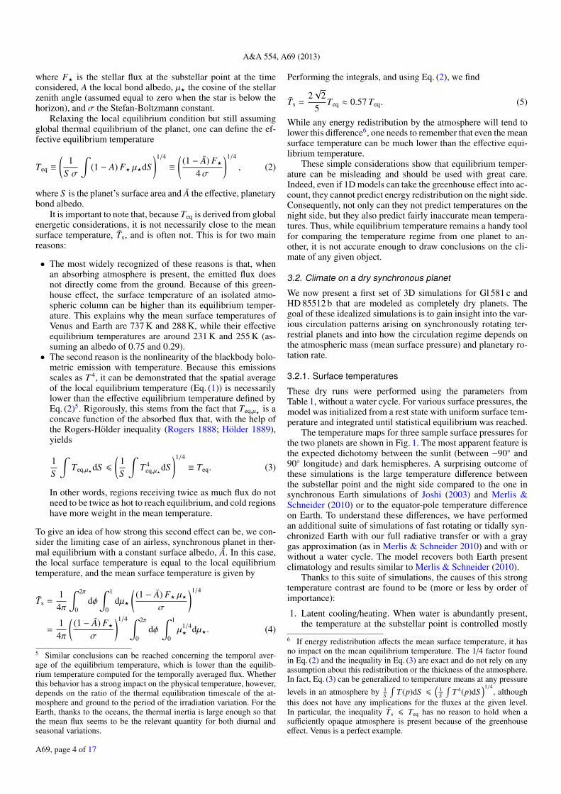
It is important to note that, because Teq is derived from globalenergetic considerations, it is not necessarily close to the meansurface temperature, Ts, and is often not. This is for two mainreasons:

• The most widely recognized of these reasons is that, whenan absorbing atmosphere is present, the emitted flux doesnot directly come from the ground. Because of this green-house effect, the surface temperature of an isolated atmo-spheric column can be higher than its equilibrium temper-ature. This explains why the mean surface temperatures ofVenus and Earth are 737 K and 288 K, while their effectiveequilibrium temperatures are around 231 K and 255 K (as-suming an albedo of 0.75 and 0.29).

• The second reason is the nonlinearity of the blackbody bolo-metric emission with temperature. Because this emissionsscales as T 4, it can be demonstrated that the spatial averageof the local equilibrium temperature (Eq. (1)) is necessarilylower than the effective equilibrium temperature defined byEq. (2)5. Rigorously, this stems from the fact that Teq,µ? is aconcave function of the absorbed flux that, with the help ofthe Rogers-Hölder inequality (Rogers 1888; Hölder 1889),yields

1S

∫Teq,µ?dS 6

(1S

∫T 4

eq,µ?dS)1/4

≡ Teq. (3)

In other words, regions receiving twice as much flux do notneed to be twice as hot to reach equilibrium, and cold regionshave more weight in the mean temperature.

To give an idea of how strong this second effect can be, we con-sider the limiting case of an airless, synchronous planet in ther-mal equilibrium with a constant surface albedo, A. In this case,the local surface temperature is equal to the local equilibriumtemperature, and the mean surface temperature is given by

Ts =1

4π

∫ 2π

0dφ

∫ 1

0dµ?

((1 − A) F? µ?

σ

)1/4

=1

4π

((1 − A) F?

σ

)1/4 ∫ 2π

0dφ

∫ 1

0µ1/4? dµ?. (4)

5 Similar conclusions can be reached concerning the temporal aver-age of the equilibrium temperature, which is lower than the equilib-rium temperature computed for the temporally averaged flux. Whetherthis behavior has a strong impact on the physical temperature, however,depends on the ratio of the thermal equilibration timescale of the at-mosphere and ground to the period of the irradiation variation. For theEarth, thanks to the oceans, the thermal inertia is large enough so thatthe mean flux seems to be the relevant quantity for both diurnal andseasonal variations.

Performing the integrals, and using Eq. (2), we find

Ts =2√

25

Teq ≈ 0.57 Teq. (5)

While any energy redistribution by the atmosphere will tend tolower this difference6, one needs to remember that even the meansurface temperature can be much lower than the effective equi-librium temperature.

These simple considerations show that equilibrium temper-ature can be misleading and should be used with great care.Indeed, even if 1D models can take the greenhouse effect into ac-count, they cannot predict energy redistribution on the night side.Consequently, not only can they not predict temperatures on thenight side, but they also predict fairly inaccurate mean tempera-tures. Thus, while equilibrium temperature remains a handy toolfor comparing the temperature regime from one planet to an-other, it is not accurate enough to draw conclusions on the cli-mate of any given object.

3.2. Climate on a dry synchronous planet

We now present a first set of 3D simulations for Gl 581 c andHD 85512 b that are modeled as completely dry planets. Thegoal of these idealized simulations is to gain insight into the var-ious circulation patterns arising on synchronously rotating ter-restrial planets and into how the circulation regime depends onthe atmospheric mass (mean surface pressure) and planetary ro-tation rate.

3.2.1. Surface temperatures

These dry runs were performed using the parameters fromTable 1, without a water cycle. For various surface pressures, themodel was initialized from a rest state with uniform surface tem-perature and integrated until statistical equilibrium was reached.

The temperature maps for three sample surface pressures forthe two planets are shown in Fig. 1. The most apparent feature isthe expected dichotomy between the sunlit (between −90 and90 longitude) and dark hemispheres. A surprising outcome ofthese simulations is the large temperature difference betweenthe substellar point and the night side compared to the one insynchronous Earth simulations of Joshi (2003) and Merlis &Schneider (2010) or to the equator-pole temperature differenceon Earth. To understand these differences, we have performedan additional suite of simulations of fast rotating or tidally syn-chronized Earth with our full radiative transfer or with a graygas approximation (as in Merlis & Schneider 2010) and with orwithout a water cycle. The model recovers both Earth presentclimatology and results similar to Merlis & Schneider (2010).

Thanks to this suite of simulations, the causes of this strongtemperature contrast are found to be (more or less by order ofimportance):

1. Latent cooling/heating. When water is abundantly present,the temperature at the substellar point is controlled mostly

6 If energy redistribution affects the mean surface temperature, it hasno impact on the mean equilibrium temperature. The 1/4 factor foundin Eq. (2) and the inequality in Eq. (3) are exact and do not rely on anyassumption about this redistribution or the thickness of the atmosphere.In fact, Eq. (3) can be generalized to temperature means at any pressurelevels in an atmosphere by 1

S

∫T (p)dS 6

(1S

∫T 4(p)dS

)1/4, although

this does not have any implications for the fluxes at the given level.In particular, the inequality Ts 6 Teq has no reason to hold when asufficiently opaque atmosphere is present because of the greenhouseeffect. Venus is a perfect example.

A69, page 4 of 17

J. Leconte et al.: 3D climate modeling of close-in land planets

Fig. 1. Surface temperature maps (in C) for the dry Gl 581 c (top row) and HD 85512 b (bottom row) runs for a total pressure (ps) of 0.1, 1 and10 bars (from left to right). Longitude 0 corresponds to substellar point.

thermodynamically and is much lower than in the dry case.Latent energy transported by the atmosphere to the night sidealso contributes significantly to the warming of the latter.

2. Non-gray opacities. In our case dry case, greenhouse issolely due to the 15 µm band of CO2 (especially on thenight side). Thus, using a gray opacity of the backgroundatmosphere with an optical depth near unity, as done inMerlis & Schneider (2010), considerably underestimates thecooling of the surface and thus overestimates the night sidetemperature.

3. A different planet. When its bulk density is constant, boththe size and the surface gravity increase with the planet’ssize. Apart from the dynamical effect due to the variation inRossby number (extensively discussed below), for a givensurface pressure (ps), both the mass of the atmosphere andits radiative timescale (τrad) decrease with gravity (and withincoming flux for the latter) and that the advective timescale(τadv) increases with the radius. For a given surface pressure,the energy transport, thought to scale with the atmosphericmass and τrad/τadv, thus tends to be less efficient on a moremassive and more irradiated object.

Indeed, as expected, the temperature difference decreases withincreasing total pressure, because the strength of the advectionof sensible heat to the night side increases with atmosphericmass. Both because of this more efficient redistribution and ofthe greenhouse effect of the atmosphere, the globally averagedmean surface temperature increases with surface pressure, asshown in Fig. 2.

For comparison, we also computed the surface temperatureyielded by the 1D version of our model. In this case, the atmo-spheric column is illuminated with a constant flux equal to theglobally averaged impinging flux (1/4 of the substellar value)and with a stellar zenith angle of 60. Apart from this prescrip-tion for the flux and the fact that large-scale dynamics is turnedoff, our 1D code is exactly the same as our 3D one. As can beseen in Fig. 2, even with a 10 bar atmosphere, the 1D model isstill 30 K hotter than the globally averaged 3D temperature. Thisdifference increases up to 70 K for the 100 mb case because re-distribution is less efficient (see Sect. 3.1). A surface albedo of0.3 is assumed here, similar to that in desert regions on Earth.

0.1 0.2 0.5 1.0 2.0 5.0 10.0100

150

200

250

300

350

ps bar

Tem

per

atu

reK

1D

Mean

Min

Fig. 2. Globally averaged (solid, filled) and minimum (dashed, empty)temperatures as a function of surface pressure for Gl 581 c (black cir-cles) and HD 85512 b (gray squares). For comparison, the surface tem-perature of the 1D model for Gl 581 c is also shown (dotted curve). Theerror bars on the 200 mbar case show the temperatures reached by vary-ing the surface albedo between 0.1 and 0.5.

The sensitivity of the surface temperature when albedo is variedbetween 0.1 and 0.5 is shown in Fig. 2.

A troubling and quite counterintuitive outcome of these sim-ulations is that, as shown in Fig. 2, although Gl 581 c receivesmore flux and has a higher mean surface temperature thanHD 85512 b, its minimum temperatures are always lower. As canbe seen in Fig. 1, the models for Gl 581 c present very cold re-gions located at mid latitudes and west of the western termina-tor (also called morning limb), whereas the HD 85512 b modelshave a rather uniform (and higher in average) temperature overthe whole night side.

3.2.2. Circulation regime

Further investigations have shown that this difference is a signa-ture of the distinct circulation regimes arising on the two planets.

A69, page 5 of 17

A&A 554, A69 (2013)

Fig. 3. Wind maps (arrows) at the 200 mb pressure level (top panel) and near the surface (900 mb pressure level; bottom panel) for Gl 581 c,Gl 581 c with a slower rotation (see text), and HD 85512 b (from left to right, respectively). The mean surface pressure is 1 b for all the models.Color scale (same for all panels) and numbers show the wind speed in m/s. Air is converging toward the substellar point at low altitudes in allmodels. However, whereas the standard Gl 581 c case clearly exhibits eastward jets (super-rotation) at higher altitudes, both slowly rotating casestend to have stellar/anti stellar winds at the same level.

Indeed, as shown in Fig. 3, our simulations of the atmosphere ofGl 581 c develop eastward jets (super-rotation) as found in manyGCM of tidally locked exoplanets (Showman et al. 2008, 2011,2013; Thrastarson & Cho 2010; Heng & Vogt 2011; Heng et al.2011; Showman & Polvani 2011). Conversely, the atmosphere ofHD 85512 b seems to settle predominantly into a regime of stel-lar/anti stellar circulation where high-altitude winds blow fromthe day side to night side in a symmetric pattern with respectto the substellar point (upper right panel of Fig. 3; similar to theslowly rotating case of Merlis & Schneider 2010).

To understand these distinct circulation regimes, one needsto understand the mechanism responsible for the onset of super-rotation on tidally locked exoplanets. Showman & Polvani(2011) show that the strong longitudinal variations in radiativeheating causes the formation of standing, planetary-scale equa-torial Rossby and Kelvin waves. By their interaction with themean flow, these waves transport eastward momentum from themid latitudes toward the equator, creating and maintaining anequatorial jet. As a result, they predict that the strength of thejet increases with the day/night temperature difference and thatthe latitudinal width of this jet scales as the equatorial Rossbydeformation radius

LRo ≡

√N Hβ, (6)

where N is the Brunt-Väisälä frequency, H the pressure scaleheight of the atmosphere (N H being the typical speed of gravitywaves), and β ≡ ∂ f /∂y the latitudinal derivative of the Coriolisparameter, f ≡ 2 Ω sin θ, with Ω the planet rotation rate and θthe latitude (β = 2 Ω/R p at the equator). Roughly, the equato-rial Rossby deformation radius is the typical length scale overwhich an internal (gravity) wave created at the equator is signif-icantly affected by the Coriolis force. This allows us to define adimensionless equatorial Rossby deformation length

L ≡LRo

R p=

√N H

2 Ω R p· (7)

This latter prediction is directly relevant to our case. Indeed, al-though they have rather similar sizes and gravity, Gl 581 c rotatesaround its star in ∼13 Earth days (d) whereas HD 85512 b, whichorbits a brighter K star, has a ∼58 d orbital period. If spin orbitsynchronization has occurred, the Coriolis force is thus expectedto have a much weaker effect on the circulation of HD 85512 b.To quantify this, we evaluate L in our case. In a dry stably strat-ified atmosphere with a lapse rate dT/dz, the Brunt-Väisälä fre-quency is given by

N2 =g

T

(g

cp+

dTdz

), (8)

cp being the heat capacity of the gas at constant pressure. Thepressure scale height is given by

H ≡k BTma g

, (9)

where k B is the Boltzmann constant and ma the mean molecularweight (in kg) of the air. Assuming an isothermal atmosphere,this yields

L =

√k B

ma c1/2p

T 1/2

2 Ω R p· (10)

Assuming an N2-dominated atmosphere, using the equilibriumtemperature as a proxy for T and disregarding the latitude fac-tor, one finds L = 1.1 for Gl 581 c and 2.5 for HD 85512 b. Inour slowly rotating case, the planet is thus too small to containa planetary Rossby wave, and the mechanism described above istoo weak to maintain super-rotation. This also explains why thejet is planet-wide in the more rapidly rotating case of Gl 581 c.To confirm this analysis, we ran a simulation of Gl 581 c wherewe, everything else being equal, reduced the rotation rate bya factor of five so that the L is the same as for HD 85512 b(Ω = Ωorb/5 case; middle column of Fig. 3). As expected from

A69, page 6 of 17

J. Leconte et al.: 3D climate modeling of close-in land planets

Fig. 4. Zonally averaged zonal winds (in m/s) for the dry Gl 581 c runs for a total surface pressure of 0.1, 1 and 10 bars (from left to right).

the dimensional analysis, in this slowly rotating case, no jets ap-pear, and we recover a stellar/antistellar circulation. Another ar-gument in favor of this analysis is that the location and shapeof the cold regions and wind vortices present in the Gl 581 ccase (see Figs. 1 and 3) are strongly reminiscent of Rossby-wavegyres seen in the Matsuno-Gill standing wave pattern (Matsuno1966; Gill 1980; Showman & Polvani 2011).

Another way to look at this is to consider a multiway forcebalance (Showman et al. 2013). One way to tilt eddy velocitiesnorthwest-southeast in the northern hemisphere and southwest-northeast in the southern hemisphere, driving super-rotation,is to have a force balance between pressure-gradient (∇pΦ ≡k B∆T∆ ln p/(maR p), where ∆T is the horizontal day-night tem-perature difference and ∆ ln p is logarithmic pressure range overwhich this temperature difference is maintained), Coriolis (≈ f uwhere u is the wind speed), and advection (≈u2/R p) accelera-tion (see Showman et al. (2013) for a discussion on the effect ofdrag). In this case one should have

∇pΦ ∼ f u ∼u2

R p, (11)

which leads to u ∼ f R p and eventually f ∼√∇pΦ/R p.

If f √∇pΦ/R p this three-way force balance should

reduce to a two-way force balance between advection andpressure-gradient accelerations, which in turn leads to symmet-ric day-night flow. A numerical estimate with the same parame-ters as above with ∆T = 100 K and ∆ ln p = 1 yields a criticalrotation period of about 10 d, close to Gl 581 c rotation period,but much smaller than the one of HD 85512 b. This confirms thatHD 85512 b should have a much more pronounced day-night cir-culation pattern than Gl 581 c, but it also tells us that the Coriolisforce is already quite weak in the force balance of Gl 581 c, ex-plaining the significant meridional wind speeds seen in Fig. 3.

There are a few general differences with previous close-in gi-ant planet 3D simulations, however. First, in all our simulations,low-altitude winds converge toward the substellar point. This re-sults from the strong depression caused there by a net mass fluxhorizontal divergence high in the atmosphere driving a large-scale upward motion. Second, even at levels where eastwardwinds are the strongest (in the simulations with super-rotation),the wind speeds exhibit a minimum (possibly negative) along theequator, westward from the substellar point. At a fixed altitude,this results from a pressure maximum occurring there because of

æ

æ

æ

æ

ææ

æ

æ

æ

à

à

à

à

à

à

à

øø

0.1 0.2 0.5 1.0 2.0 5.0 10.00.0

0.1

0.2

0.3

0.4

0.5

0.6

ps HbarL

Red

istr

ibu

tio

nef

fici

encyHΗL

Gl581c

HD85512b

Fig. 5. Redistribution efficiency η (ratio of night to day side outgoingthermal emission) as a function of atmospheric total pressure (ps) forGl 581 c (black circles) and HD 85512 b (gray squares). η = 0 impliesno energy redistribution at all, whereas an homogeneous thermal emis-sion would yield η = 1. The star symbol shows the redistribution effi-ciency of the Ω = Ωorb/5 Gl 581 c case.

the higher temperature, and consequently higher pressure scaleheight.

Another feature visible in Fig. 4 is the dependence of thestrength of the zonal jet on the atmospheric mean surface pres-sure (lower pressure causing faster winds). A detailed analysis isbeyond the scope of this study. Nevertheless, these simulationsseem to confirm that zonal wind speeds increase with forcingamplitude (Showman & Polvani 2011). Indeed, an increasingpressure entails a decreasing thermal contrast between the twohemispheres and a smaller forcing, hence the lower wind speeds.

Surprisingly, the presence of a strong equatorial jet lowersthe heat redistribution efficiency by the atmosphere. By focus-ing the flow around the equator, the Coriolis force prevents anefficient redistribution to the midlatitudes on the night side. Toquantify this redistribution in a simple way, we computed theratio η of the mean outgoing thermal flux that is emitted by thenight side over the mean outgoing thermal flux from the dayside (see Fig. 5). With this definition, no redistribution shouldyield η = 0, whereas a very homogeneous emission would pro-duce η = 1. As expected, the redistribution increases with total

A69, page 7 of 17

A&A 554, A69 (2013)

150 200 250 300 350 400 4500

2

4

6

8

10

Temperature HKL

Alt

itu

deHk

mL

Gl581c, ps=1b

1D

3D Fig. 6. Temperature profilesof the 1 bar case for Gl 581 c(Gray curves). The solidblack curve stands for thespatially averaged profile ofthe 3D simulation. For com-parison, the dashed curverepresents the temperatureprofile obtained with theglobal 1D model.

pressure. At constant pressure, redistribution seems to be con-trolled by the equatorial Rossby number and is more important inthe slowly rotating cases (HD 85512 b and Ω = Ωorb/5 Gl 581 ccase).

Further idealized simulations are needed to fully understandthe mechanisms controlling both the circulation pattern and theenergy redistribution on slowly rotating, synchronous terrestrialplanets.

3.2.3. Thermal profile

Finally, in Fig. 6, we present typical temperature profiles ob-tained from our simulations (here in the 1 bar case, but pro-files obtained for different pressures are qualitatively similar).For comparison, Fig. 6 also shows the profile obtained from thecorresponding global 1D simulation, and the spatially averagedprofile from our 3D run.

One can directly see that, in the lower troposphere, temper-ature decreases with altitude on the day side following an adi-abatic profile and increases on the night side. This temperatureinversion on the night side is caused by the redistribution of heat,which is most efficient near 2−4 km above the surface wherewinds are not damped by the turbulent boundary layer. The re-sulting mean temperature profile cannot be reproduced by the1D model, which is too hot near the surface and too cold bymore than 50 K in the upper troposphere. The discrepancy tendsto decrease in the upper stratosphere.

4. Bistable climate: runaway vs cold trapping

As inferred from 1D models (e.g. Kasting et al. 1993; Selsiset al. 2007) and confirmed by our 3D simulations (not shown), ifwater were present in sufficient amount everywhere on the sur-face (aquaplanet case), both our prototype planets (Gl 581 c andHD 85512 b) would enter a runaway greenhouse state (Kastinget al. 1984). The large flux that they receive thus prevents theexistence of a deep global ocean on their surfaces.

However, as is visible in Fig. 1, because of the rather ineffi-cient redistribution, a large fraction of the surface present mod-erate temperatures for which either liquid water or ice wouldbe thermodynamically stable at the surface. In the 10b case,the whole night side exhibits mean temperatures that are simi-lar to the annual mean in Alaska. It is thus very tempting to de-clare these planets habitable because there is always a fraction of

the surface where liquid water could flow. While tempting, oneshould not jump to this conclusion because of the two followingpoints.

• Even if water is thermodynamically stable, it is always evap-orating. Consequently, the water vapor is transported bythe atmosphere until it condenses and precipitates (rains orsnows) onto the ground in cold regions. This mechanismtends to dry warmer regions and to accumulate condensedwater in cold traps. If these cold traps are permanent, or ifno mechanism is physically removing the water from them– e.g. ice flow due to the gravitational flattening of an icecap, equilibration of sea level (see Sect. 6) – this transport isirreversible.

• Because it is a strong greenhouse gas, water vapor has animportant positive feedback. The presence of a small amountof water can dramatically increase surface temperatures andeven trigger the runaway greenhouse instability.

Therefore, even if useful, “dry” simulations cannot be used toassess the climate of a planet where water is potentially present,and the distribution of the latter7. In this section we present a setof simulations that take the full water cycle into account but witha limited water inventory.

We show that, as already suggested by Abe et al. (2011), cli-mate regimes on heavily irradiated land planets result from thecompetition of the two aforementioned processes that enablesthe existence of two stable equilibrium states: a “collapsed” statewhere almost all the water is trapped in permanent ice caps onthe night side or near the poles, and a runaway greenhouse statewhere all the water is in the atmosphere. Furthermore, we showthat the collapsed state can exist at much higher fluxes than in-ferred by Abe et al. (2011) and that there is no precise flux limit,because it can depend on both the atmosphere mass and wateramount.

4.1. Synchronous case

Our numerical experiment is as follows. For our two planets andfor various pressures, we start from the equilibrium state of thecorresponding “dry” run described in Sect. 3.2 to which a givenamount of water vapor is added. To do so, a constant mass mix-ing ratio of water vapor, qv, is prescribed everywhere in the at-mosphere, and surface pressure is properly rescaled to take theadditional mass into account. Two typical examples of the tem-poral evolution of the surface temperature and water vapor con-tent in these runs is presented in Fig. 7.

While idealized, this numerical experiment has the advan-tage of not introducing additional parameters to characterize theinitial distribution of water. It also provides us with an upperlimit on the impact of a sudden water vapor release as vapor ispresent in the upper atmosphere where its greenhouse effect ismaximum. From another point of view, this experiment roughlymimics a planet-wide release of water by accretion of a large as-teroid or planetesimal and can give us insight into the evolutionof the water inventory after a sudden impact.

Because of the sudden addition of water vapor, the atmo-sphere is disturbed out of radiative balance. Water vapor sig-nificantly reduces the planetary albedo by absorbing a signif-icant fraction of the stellar incoming radiation, and it also re-duces the outgoing thermal flux. The temperature thus rapidly

7 At low stellar incoming fluxes, the presence of water also entailspositive feedback through the ice albedo feedback so that this argumentstill holds (see e.g. Pierrehumbert 2010).

A69, page 8 of 17

J. Leconte et al.: 3D climate modeling of close-in land planets

1 5 10 50 100 50010000.0

0.2

0.4

0.6

0.8

1.0

Time d

Vap

or

frac

tio

n

ps200mb

1 5 10 50 100 5001000

300320340360380400

Time d

TsK

Fig. 7. Time evolution of the fraction of water vapor in the atmosphereover the total water amount and of the mean surface temperature forGl 581 c with a 200 mbar background atmosphere. The black solid curverepresents a model initialized with a water vapor column of 150 kg/m2

and the gray dashed one with 250 kg/m2. After a short transitional pe-riod, either the water collapses on the ground in a few hundred days(solid curve) or the atmosphere reaches a runaway greenhouse state(dashed curve).

increases until a quasi-static thermal equilibrium that is consis-tent with the amount of water vapor is reached in a few tensof days (see Fig. 7). At the same time, water vapor condenses,forms clouds, and precipitates onto the ground near the cold-est regions of the surface. As temperature increases, the amountof precipitation can decrease because the re-evaporation of thefalling water droplets or ice grains becomes more efficient. Theevaporation of surface water also becomes more efficient.

Then, the system can follow two different paths. If the initialamount of water vapor and the associated greenhouse effect arelarge enough, evaporation will overcome precipitation, and theatmosphere will stay in a stable hot equilibrium state where allthe water is vaporized (with the exception of a few clouds; Fig. 7and top panel in Fig. 8). Because this state is maintained by thegreenhouse effect of water vapor and any amount of water addedat the surface is eventually vaporized, this state is the usual run-away greenhouse state (Nakajima et al. 1992). In contrast, forlower water-vapor concentrations, the temperature increase isnot large enough, and the water vapor collapses in the cold traps(Fig. 7 and bottom panel in Fig. 8). The amount of water vapordecreases and the surface slowly cools down again until most ofthe water is present in ice caps in the colder regions of the sur-face. An example of the ice surface density of a collapsed stateat the end of the simulation is presented in Fig. 9. Because subli-mation/condensation processes are constantly occurring, this icesurface density may continue to evolve, but on a much longertime scale that is difficult to model (see Wordsworth et al. 2013for a discussion). Then, water vapor is fairly well mixed withinall the atmosphere, and its mixing ratio is mainly controlled bythe saturation mass mixing ratio just above the warmest regionof the ice caps. Depending on the simulations, this mass mixingratio varies between 10−4 and 10−5.

To investigate the factor determining the selection of one ofthese two regimes, we ran a large grid of simulations, varyingboth the total surface pressure and the initial amount of watervapor. Since the main effect of water vapor is its impact on the

Fig. 8. Surface temperature map (in C) reached at equilibrium for thetwo cases depicted in Fig. 7 (parameters of Gl 581 c with a 200 mbarbackground atmosphere). The model shown in the top panel was initial-ized with a water vapor column of 250 kg/m2 and is in runaway green-house state. The bottom panel shows a collapsed state initialized withonly 150 kg/m2 of water vapor.

Fig. 9. Ice surface density of the collapsed state of the 200 mb casefor Gl 581 c presented in Fig. 8. The average ice surface density is150 kg/m2. Most of the ice has collapsed in the cold traps.

radiative budget, the quantity of interest is the total water vaporcolumn mass (also called water vapor path)

m?v ≡

∫ ∞

z=0qv ρ dz =

∫ ps

p=0qv

dpg, (12)

which is linked to the spectral optical depth of water vapor (τνv)by the relation dτνv = κνvqvρdz = κνvdm?

v .Results for the case of Gl 581 c are summarized in Fig. 10. At

a given pressure, a small initial amount of water vapor results ina collapsed case. However, there is always a critical, initial wa-ter vapor path, which is a function of the background pressure,

A69, page 9 of 17

A&A 554, A69 (2013)

0 200 400 600 800 100020

50

100

200

500

mvk

gm

2

Collapse

Runaway

Fig. 10. Climate regime reached as function of the initial surface pres-sure and water vapor column mass (m?

v ) for Gl 581 c runs. Red filleddisks represent simulations that reached runaway greenhouse states, andblue empty circles stand for simulation where water collapsed. The blueshaded region roughly depicts the region where collapse is observed.The gray dashed line represents the demarcation between runaway andcollapse states for HD 85512 b. At higher surface pressure, redistribu-tion is large and cold traps are less efficient. Less water vapor is thusneeded to trigger the runaway greenhouse instability.

above which the runaway greenhouse instability is triggered anddevelops. Because redistribution efficiency increases with atmo-spheric mass, cold trapping becomes weaker and the critical ini-tial water vapor path decreases with background atmosphere sur-face pressure.

We also carried out simulations with a large amount of wa-ter (more than the critical water vapor path discussed above),but distributed only at the surface in the cold traps. For a back-ground atmosphere less massive than ∼1−5 bar, these simula-tions are found to be stable against runaway. This demonstratesthat, for a given total amount of water larger than the criti-cal water vapor path, a “moist” bistability exists in the system.Owing to the inhomogeneous insolation, the 1D notion of criticalflux above which runaway greenhouse becomes inevitable is nolonger valid, highlighting the dynamical nature of the runawaygreenhouse that needs a large enough initial amount of watervapor to be triggered.

When the insolation is decreased, a higher amount of watervapor is needed to trigger the runaway greenhouse instability,and this at every background pressure. As would be expected,planets receiving less flux are more prone to fall into a collapsestate. However, unexpectedly, results for HD 85512 b do not fol-low this trend. At every background pressure, a lower amountof water vapor is needed to trigger the runaway greenhouse in-stability, as shown in Fig. 10. This is due to the peculiar factthat, because of the higher redistribution efficiency caused bythe lower rotation rate of the planet, cold traps are warmer (seeSect. 3.2 and Fig. 2 for details). Since evaporation is mainly con-trolled by the saturation pressure of water above the cold traps,it is more efficient, destabilizing the climate.

In addition to the work of Abe et al. (2011), which showsthat runaway could be deferred to higher incoming fluxes on landplanets, our simulations demonstrate that, even for a given flux,such heavily irradiated land planets can exhibit two stable cli-mates in equilibrium. Furthermore, we have shown that the statereached by the atmosphere depends not only on the impingingflux, but also on the mass of the atmosphere, on the initial waterdistribution, and on the circulation regime (controlled by the

forcing, the size of the planet, and its rotation rate). This bista-bility is due to the dynamical competition between cold trappingand greenhouse effect. An important consequence of this bista-bility is that the climate present on planets beyond the inner edgeof the habitable zone will not only depend on their backgroundatmosphere’s mass and composition, but also on the history ofthe water delivery and escape, as discussed below.

4.2. The 3:2 resonance

Because of the strong tidal interaction with their host star and ofthe small angular momentum contained in the planetary spin,rocky planets within or closer than the habitable zone of Mand K stars are thought to be rapidly synchronized. Indeed, thestandard theory of equilibrium tides (Darwin 1880; Hut 1981;Leconte et al. 2010) predicts that a planet should synchronize ona timescale equal to

τsyn =13

r2g

M p a6

GM2?R3

pk 2,p ∆t p, (13)

where rg is the dimensionless gyration radius (r2g = 2/5 for a

homogeneous interior; Leconte et al. 2011), G is the univer-sal gravitational constant, k 2,p the tidal Love number of de-gree 2, and ∆t p a time lag that characterizes the efficiency ofthe tidal dissipation into the planet’s interior (the higher ∆t p, thehigher the dissipation). Other variables are defined in Table 1.While the magnitude of the tidal dissipation in massive terrestrialplanets remains largely unconstrained (Hansen 2010; Bolmontet al. 2011), one can have a rough idea of the orders of mag-nitude involved by using the time lag derived for the Earth,k 2,p ∆t p = 0.305 × 629 s (Neron de Surgy & Laskar 1997). Thisyields a synchronization timescale of 25 000 yr for Gl 581 c and10 Myr for HD 85512 b, preventing these planets from maintain-ing an initial obliquity and fast rotation rate (Heller et al. 2011).

As demonstrated by Makarov et al. (2012) in the caseGl 581 d, which is more eccentric and farther away from itsparent star than Gl 581 c, tidal synchronization is not the onlypossible spin state attainable by the planet. As for Mercury, ifthe planet started from an initially rapidly rotating state, it couldhave been trapped in multiple spin orbit resonances during itsquick tidal spin down because of its eccentric orbit. BecauseGl 581 c also has a non-negligible eccentricity of 0.07 ± 0.06(Forveille et al. 2011), it has almost a 50% probability of be-ing captured in 3:2 resonance (depending on parameter used)before reaching the synchronization (Makarov & Efroimsky,priv. comm., 2012). Higher order resonances are too weak.

To assess the impact of an asynchronous rotation, we per-formed the analysis described above in the 3:2 resonance case.The rotation rate of the planet is thus three halfs of the orbitalmean motion and the solar day lasts two orbital periods. As ex-pected, depending on the thermal inertia of the ground and onthe length of the day, the night side is hotter than in the synchro-nized case. More importantly, there is no permanent cold trap atlow latitudes. However, as for Mercury (Lawrence et al. 2013),because of the low obliquity, a small area near the poles remainscold enough to play this role, and ice can be deposited there.As the magnitude of the large-scale transport of water vapor islower towards the pole compared to the night side (zonal windsare stronger than meridional ones), the trapping is less efficient.As a result, the transition towards the runaway greenhouse statediscussed in the previous section is triggered by a lower initialwater vapor path. The timescale needed to condense all the watervapor near the poles is also much longer.

A69, page 10 of 17

J. Leconte et al.: 3D climate modeling of close-in land planets

0.1 0.2 0.5 1.0 2.0 5.010.0

0.01

0.05

0.10

0.50

1.00

5.00

10.00 0.3

1

3

10

30

100

300

Time HGyrL

Esc

ape

flu

xH1

0-11

kgm

2sL

Oce

anL

ifet

imeHG

yrL

Fig. 11. Energy-limited escape flux as a function of stellar age (ε =0.15; solid curve) for Gl 581 c (black) and HD 85512 b (gray). The dot-ted curve is the diffusion limit in the runaway state ( fstr(H2) = 0.1 andTstr = 300 K), and the dashed curve is an upper limit to the escape inthe collapse state ( fstr(H2) = 10−4 and Tstr = 220 K). The time neededto evaporate an Earth ocean of water (≈1.4×1021 kg) is indicated on theright scale.

5. Evolution of the water inventory

How stable are the two equilibrium states described above in thelong term? It is possible that the climate regime exhibited by anirradiated land planet changes during its life depending on therate of water delivery and escape of the atmosphere and/or wa-ter: triggering runaway when water delivery (or water ice subli-mation by impacts) is too large and collapsing water when eitherthe background atmosphere or the water vapor mass decreasesbelow a certain threshold. We now briefly put some limits on thefluxes involved.

5.1. Atmospheric escape

When water vapor is present in the upper atmosphere, XUV radi-ations can photo dissociate it and the light hydrogen atoms canescape8. An upper limit on this escape flux is provided by theenergy limited flux (Watson et al. 1981) approximated by

Fel = εR pFXUV

GM p(kg m−2 s−1), (14)

where FXUV is the energetic flux received by the planet and ε theheating efficiency. The problem then lies in estimating the flux ofenergetic photons, which varies with time (see Selsis et al. 2007for a discussion). Estimates of Fel are shown in Fig. 11 wherethe XUV flux parametrization of Sanz-Forcada et al. (2010) anda heating efficiency of ε = 0.15 have been used9. In some cases,this formula can also be used to estimate the escape of the back-ground atmosphere itself.

8 Of course, the energy available to photodissociate water moleculesthemselves can also limit escape. Very simple calculations seem to sug-gest that this constraint is less stringent in our case, but this conclusionstrongly depends on the assumed stellar spectral energy density in theXUV.9 To give an idea of the impact on the water inventory, in Fig. 11 weestimated the lifetime of an Earth ocean by τocean = Mocean/(4πR2

p Fel),where Mocean = 1.4× 1021 kg. This instantaneous estimate does not takethe flux variation during the period considered into account.

In atmospheres where the amount of water vapor in the up-per atmosphere is limited, the escape flux can be limited by thediffusion of water vapor in air. Following Abe et al. (2011), thediffusion-limited escape flux is written as

Fdl = fstr(H2) bia(ma − mi) g

k BTstr, (15)

where fstr(H2) is the mixing ratio of hydrogen in all forms inthe stratosphere, Tstr is the temperature there, and ma and mi arethe particle mass of air and the species considered, and bia isthe binary diffusion coefficient of i in air (for H2 in air bia =1.9 × 1021(T/300 K)0.75 m−1s−1).

In the collapsed state, the longitudinal and vertical cold trapsare efficient. Temperature and water-vapor mixing ratios are thuslow in the stratosphere (Tstr ≈ 220 K and fstr(H2) < 10−4; seeFig. 11). In the runaway state, the stratosphere temperature ismuch higher (≈300 K), and water is rather well mixed in theatmosphere. The mixing ratio can be directly calculated fromthe total water amount. To show an example, we plotted the caseof fstr(H2) ≈ 10−1 in Fig. 11.

Of course, to have a comprehensive view of the problem, hy-drodynamic and nonthermal (due to stellar winds) escape shouldalso be accounted for. However, some conclusions can be made.First, it seems that escape of the background atmosphere couldbe efficient during the first few hundred million years to onebillion year. This supports the possibility of a thin atmosphere.Second, as expected, escape of water vapor is always greater inthe runaway state because of the higher temperature and humid-ity in the higher atmosphere (Kasting et al. 1984). Third, in thecollapse state, cold traps limit the humidity of the upper atmo-sphere, so escape is most likely diffusion-limited to a rather lowvalue.

Interestingly enough, the sudden increase of water loss whenrunaway is triggered can provide a strong negative feedbackon the water content of land planets beyond the classical inneredge of the habitable zone. Indeed, at least at early times wherethe XUV flux is strong enough, if a significant fraction of wa-ter is accreted suddenly and triggers the runaway, water escapewill act to lower the water vapor amount until collapse ensues.This should happen when the atmospheric water vapor contentis within order of magnitude of, although lower than, the criti-cal water column amount shown in Fig. 1010. Then, cold-trappedwater has a much longer lifetime. This could particularly playa role during the early phases of accretion, where a runawaystate is probable considering the strong energy and water va-por flux due to the accretion of large planetesimals (Raymondet al. 2007), a possibly denser atmosphere, and a faster rotation.If the planet receives a moderate water amount, the water couldbe lost in a few tens to a hundred million years, leaving time tothe planet to cool down and accrete a significant amount of icethrough accretion of comets and asteroids later on, either pro-gressively or during a “late heavy bombardment” type of eventfor example (Gomes et al. 2005). The possibility a such a sce-nario is supported by the debris disk has been recently imagedin the Gl 581 system (Lestrade et al. 2012).

10 In the numerical experiment shown in Fig. 10, the critical water col-umn amount is defined as the minimum water vapor amount to add toa cold initial state to force its transition into a hot runaway state. Thislimit would probably be lower if we started with higher temperatures,because cold trapping would be less efficient. We thus expect that thetransition from runaway to collapse state occurs at smaller amounts ofatmospheric water vapor.

A69, page 11 of 17

A&A 554, A69 (2013)

0 200 400 600 800 1000

0.005

0.010

0.050

0.100

0.500

1.000

1

3

10

30

100

300

psmbar

Tra

pp

ing

ratek

gd

1m

2

Tra

pp

ing

rateM

oce

anM

yr

Fig. 12. Maximum trapping rate per unit surface (m?v ) reached in our

simulations as a function of the background surface pressure. The leftscale shows the total trapping rate on the planetary scale in Earth’soceans (≈1.4 × 1021 kg) per Myr.

5.2. Cold trapping rate

A constraint on the accumulation of ice from such a late wa-ter delivery is that the delivery rate must be low enough to allowtrapping to take place without triggering the runaway. To first or-der, our simulations presented in Sect. 4 can be used to quantifythis cold trapping rate.

We consider a case where the water vapor collapses. As seenin Fig. 7, except for the very early times of the simulations, thewater vapor content of the atmosphere exponentially tends to-wards its (low) equilibrium value. We can thus define an effec-tive trapping rate m?

v = m?v /(2 τc) (in kg s−1m−2), where m?

v isthe initial water-vapor column mass and τc the time taken bythe atmosphere to decrease the water vapor amount by a factorof two. This is basically a rough estimate of the critical rate ofwater delivery above which runaway greenhouse would ensue.

The maximum trapping rate obtained in our simulations asa function of the background atmosphere surface pressure isgiven in Fig. 12. As expected, trapping is less efficient whenthe atmospheric mass is higher because cold traps are warmer.The exponential decrease can be understood considering that re-evaporation efficiency linearly decreases with saturation pres-sure that exponentially decreases with temperature followingClausius-Clapeyron law. Then, the maximum amount of ice thatcan be accumulated really depends on the duration of the phaseduring which water is delivered to the planet, but the quite hightrapping rate found in our simulations suggest that if water accre-tion occurs steadily, the final water inventory may not be limitedby the trapping efficiency but by the rate of water delivery afterthe planet formation11.

6. On the possibility of liquid water

Our simulations show that, if the atmosphere is not too thickand the rate of water delivery high enough (while still avoidingrunaway), a large amount of water can accumulate in the cold

11 This estimation is relevant only for a synchronized planet without athick primordial atmosphere releasing a negligible geothermal flux. Allof these assumptions may be far from valid during the first few thousandto million years of the planet’s life, when the planet was still releasingthe energy due to its accretion and losing a possibly thick primary atmo-sphere of hydrogen and helium. In addition, the synchronization occurson comparable timescales (see Sect. 4.2).

NorthPole

Ice cap

Liquid water

Dry ground

CloudsIce Flows

vapor

Fig. 13. Schematic view of the eyeball planet scenario with a dry dayside and a thick ice cap on the night side.

traps. However, the low temperatures present there prevent liquidwater stability. Are these land planets possibly habitable? Canliquid water flow on their surface for an extended period of time?

A possibility is that both volcanism and meteoritic impactscould be present on the night side, creating liquid water, as hasbeen recently proposed to explain the evidence of flowing liq-uid water during the early Martian climate (Segura et al. 2002;Halevy et al. 2007; Wordsworth et al. 2013). Liquid water pro-duced that way is, however, only episodic.

In this section, we briefly explain various mechanismsthat could produce long-lived liquid water (as summarized inFig. 13). In particular, we argue that, considering the thickness ofthe ice cap that could be present, gravity-driven ice flows sim-ilar to those taking place on Earth could transport ice towardwarm regions where it would melt. Liquid water could thus beconstantly present near the edge of the ice cap. We also discussthe possibility of having subsurface liquid water produced bythe high pressures reached at the bottom of an ice cap combinedwith a significant geothermal flux.

We also explored the quasi-snowball scenario proposed bySelsis et al. (2007) for Gl 581 c where a low equilibrium temper-ature is provided by a very high ice albedo (>0.9) and tempera-ture slightly exceeds 0C at the substellar point. Notwithstandingthe difficulty of having such high albedo ices around such a redstar (Joshi & Haberle 2012), our simulations tend to show thatthis scenario can be discarded. Indeed, the very strong positivefeedback of both water vapor and ice albedo render this solutionvery unstable and no equilibrium state was found.

6.1. Ice flows

As described in Sect. 4, if water accumulates on the surface, theatmosphere continuously acts to transport it towards the coldestregions where it is the most stable (more precipitations and lessevaporation). As this accumulation seems possible mostly forlow background atmospheric pressures, locations always existon the surface where temperature is below freezing (see Figs. 1and 2) and only ice is stable.

If atmospheric transport were the only transport mechanismof water on Earth, the water would also accumulate onto thepoles, and liquid water would only be present when the Sunmelted the top of the ice cap during summer. However, other pro-cesses come into play to limit the thickness of the polar ice caps.Most importantly, because ice is not completely rigid, gravity

A69, page 12 of 17

J. Leconte et al.: 3D climate modeling of close-in land planets

Fig. 14. Ice distribution for different surface pressures for Gl 581 c (ps = 100 mb, 400 mb and 1 b from left to right). Dry regions are in dark gray,ice caps are shown in white, and liquid water is in blue. For background surface pressures above 300 mb, the greenhouse effect of water vapor issufficient to melt water even on the night side.

tends to drain ice from the upper regions (or regions where theice cap is thicker) towards lower regions creating ice flows, asseen in Greenland and Antarctica, among other places. Theseice flows physically remove ice from the cold traps to transportit towards regions where it can potentially melt, at the edge ofglaciers, for example.

Assuming that enough water has been able to accumulate onthe surface without triggering the runaway greenhouse instabil-ity, such ice flows should eventually occur. Thus, liquid waterproduced by melting should be present when the ice is drainedto the day side where temperatures are above 0C. Quantifyingthe amount of ice necessary and the average amount of liquidwater is, however, much more uncertain, and maybe not relevantconsidering our present (lack of) knowledge concerning extraso-lar planets surface properties and topography. It should be saidthat in Greenland, an ice sheet of around 2 km is sufficient totransport ice over distances of about 500−1000 km and createice displacements up to 2−3 km per year near glaciers (Rignotet al. 2011; Rignot & Mouginot 2012). Since gravity (which isthe main driver) and typical horizontal length scales both scalelinearly with radius if density is kept constant, this order of mag-nitude should remain valid for more massive land planets.

As discussed in Sect. 5, ice thicknesses of a few tens of kilo-meters could possibly be reached. It is thus possible to imaginea stationary climate state where i) a thick enough ice cap pro-duces ice flows and liquid water at the edge of warmer regions;ii) this liquid water evaporates; and iii) the resulting water vaporis transported back near the coldest regions where it precipitates.A question that remains is whether the additional amount of wa-ter vapor that will be released in the atmosphere can be largeenough to trigger the runaway greenhouse instability that wouldcause the melting and evaporation of the whole ice cap.

To assess the possibility of this scenario, we ran another setof simulations with a thick ice cap. Because we did not wantto add any free parameter (such as the total amount of ice) andwe want a worst-case scenario (the most favorable to triggeringthe runaway), we modified our base model so that the surfacecould act as an infinite reservoir of water whose property (liquidor solid) depends solely on the ground temperature (above orbelow 0 C). In particular, we did not consider the latent heatneeded to melt water that would have a stabilizing effect on theclimate by lowering the water-vapor evaporation rate.

Another problem comes from the fact that freezing regionschange as the amount of water vapor increases in the atmo-sphere. In our numerical experiment, we thus updated the sur-face properties at each time step as follows. A dry surface gridcell becomes wet (a reservoir of water) if it has a neighbor withice on its surface: the ice cap extends. Since we want to model

a case where only the edge of the ice cap melts, if a wet surfacegrid cell has no neighbor where water ice is present, it is dried.Then the model is initialized from the dry state from Sect. 3.2where a seed of ice has been implanted in the cold trap, and ranuntil either a stationary equilibrium state is reached or the sur-face is completely dried by the runaway greenhouse effect. Testsimulations show that the final state reached does not depend onthe initial distribution of ice.

For Gl 581 c, our simulations show that above five bars, run-away is inevitable. Below one bar, a stationary state is alwaysfound where ice and liquid water are both present on the surfaceat the same time (see Fig. 14). Depending on the topography nearthe ice cap edge, this could correspond to a situation where lakesare constantly replenished by the melting water or where rivuletsmoisten a more extended region. Interestingly, as shown in themiddle and left hand panels of Fig. 14, ice does not necessarilycover all the night side because of the radiative effect of watervapor which tends to warm the surface (see Fig. 15), and the in-homogeneous redistribution of energy discussed in Sect. 3.2. Inparticular, melting first occurs eastward from the day side nearthe equator where the surface is heated by the hot air comingfrom the day side through the jet, as seen in the 400 mbar caseof Fig. 14.

For HD 85512 b, again, we find that runaway occurs at lowerbackground surface pressures. The transition occurs between400 and 500 mb. Also, because of the more homogeneous tem-perature distribution of the night side, the transition is not asprogressive as shown in Fig. 14 for Gl 581 c. If the 400 mb casereaches a steady state with a full ice coverage of the night side,the 500mb case is almost dry.

These simulations demonstrate that, even in our most strin-gent case, the scenario of a thick ice cap, vigorous ice flows anda significant amount of liquid water could be present withouttriggering the runaway greenhouse effect. Indeed, in these sim-ulations, most of the grid cells next to the ice cap are coveredby liquid water (see Fig. 14), and the climate remains stable.Given our resolution, this corresponds to a wet region with awidth of about 1000 km, which is probably an overestimationof the horizontal extension of the region where melting will oc-cur. Interestingly, when there is liquid water on the surface inour model, part of the wet surface is always receiving some sun-light, because a state with liquid water only on the night sideis not stable. In this case, water vapor condenses and the waterfreezes. One must bear in mind that, without further informa-tion, we did not include any runoff of liquid water at the surface,assuming that the small amount of flowing water would be evap-orated before crossing these 1000 km. A more complete model

A69, page 13 of 17

A&A 554, A69 (2013)

Fig. 15. Surface temperature map (in C) in the 100 mb case in the pres-ence of a thick ice cap and liquid water near the terminator (see text).Day side temperatures are up to 50 K higher than in the dry case (upperleft panel of Fig. 1).

of the ice sheet, ice flows and runoff would be necessary to com-pletely settle this matter.

6.2. Subsurface liquid water?

As for icy moons such as Europa and Enceladus (Sotin et al.1998; Pappalardo et al. 1999) and subsurface lakes such as theVostok lake on Earth (Oswald & Robin 1973), if a thick ice capexists, the possible presence of a significant amount of subsur-face liquid water at the bottom of the ice layer is also worth con-sidering. Indeed, because of the decrease in ice melting temper-ature with pressure and the increase in temperature with depthcaused by any geothermal flux, it is easier, in a way, to melt wa-ter below a thick ice sheet than on the surface.

To assess this possibility, we estimated the ice thicknessneeded to melt water beneath it as function of the geothermalflux. Considering that vertical energy transport in the subsurfaceis mainly performed by thermal conduction, and that quasi-staticequilibrium is reached, the temperature gradient is given by

dTdz

= −φg

Kth, (16)

where φg is the (positive) geothermal flux and Kth is the ther-mal conductivity of water ice that ranges between 2.22 W/m/Kat 0C and 3.48 W/m/K at −100 C. Thanks to hydrostatic equi-librium, and assuming a constant density and conductivity forice (here 920 kg/m3 and 0.3 W/m/K respectively), the tempera-ture pressure profile is given by

T (p) = Ts +φg

ρicegKth(p − ps) , (17)

where Ts and ps are the local surface temperature and pressureand ρice the mass density of ice. Following Wagner et al. (1994),we parametrize the melting curve of water ice by

pmelt(T ) = p0

[1 − 0.626 × 106

1 − (TT0

)−3+ 0.197135 × 106

1 − (TT0

)21.2 ], (18)

E

Fig. 16. Ice-cap minimal thickness (in m) needed to reach melting tem-perature at the bottom of the ice sheet as a function of the temperatureat its surface and internal heat flux. The white area represents the regionwhere conditions are too cold for liquid water to exist, even at highpressure. This internal flux could be caused by release of primordialheat content, radioactive decay, and tidal heating. The top scale showsthe eccentricity needed to provide the given flux for Gl 581 c assumingEarth tidal response (see text).

æ

æ

æ

æ

æ

æ

æ

æ

æ

æ

ç

çç

ç

ç

ç

ç

ç

ç

à

0 50 100 150 200 250

0.10

0.15

0.20

0.25

0.30

mvapHkgm2L

Bo

nd

Alb

edo

700 mb

200 mb

Fig. 17. Bond albedo as a func-tion of water vapor columnamount for Gl 581 c runs withps = 200 mb (gray dashedcurve) and ps = 700 mb (blacksolid curve). The surface albedoof 0.3 is shown as the longdashed horizontal line.

where T0 = 273.16 K and p0 = 611.657 Pa are the temperatureand pressure of the triple point of water. This parametrization isvalid only between 251.165 and 273.16 K because liquid wateris not stable below this temperature at any pressure.

Then, for a given geothermal flux and surface temperature,subsurface liquid water can exist if the curves parametrized byEqs. (17) and (18) intersect each other. By solving this implicitequation, we can find the pressure at which melting occurs anddefine the minimal ice cap thickness needed to reach this pres-sure, lice = (p − ps)/(ρiceg) (for the atmosphere considered,ps can safely be neglected in the above equations). Numericalestimates of this thickness as a function of surface temperatureand geothermal flux are shown in Fig. 16 for a typical gravityof 18 m/s2.

One can see that even if no geothermal flux is present,subsurface liquid water could exist for warm enough regions.The thickness needed would be rather large (∼3−10 km), whichseems unlikely. Depending on the amount of internal flux,

A69, page 14 of 17

J. Leconte et al.: 3D climate modeling of close-in land planets

1.000.50 2.000.30 3.001.500.700

2

4

6

8

Wavelength HΜmL

FΛH1

0-19

Wm

2Μ

mL

CollapseRunaway

5 10 20 500

1

2

3

4

5

Wavelength HΜmL

FΛH1

0-19

Wm

2Μ

mL

CollapseRunaway

510K

410K

320K

Fig. 18. Synthetic spectrum in reflection (left) and thermal emission (right) during secondary transit of a Gl 581 c like planet with a 200 mbatmosphere at 10 parsecs. The black solid and the gray dashed lines respectively stand for the dry collapsed and runaway case presented in Fig. 8.Thin dashed lines in the emission part correspond to blackbody spectra at the temperatures indicated. In the runaway case, water is abundant in theatmosphere and H2O absorption bands are noticeable throughout the spectrum (between 5 and 9 µm in the emission spectrum and above 0.7 µm inreflection). The shift in the thermal emission toward shorter wavelengths due to the much hotter surface is also striking.

however, the minimal thickness can be much lower. On Earth,radioactive decay and release of primordial heat generate anoverall averaged geothermal flux of 92 mW/m2 (Davies &Davies 2010). If we assume that the rate of volumetric heatingis constant, this mean flux should scale linearly with the planet’sradius, and our more massive planet should produce between 1.6and 1.8 times this flux. With such a flux, the thickness needed de-creases below 1.5 km in the coldest regions but could be as lowas 300 m.

Finally, another important source of internal flux for close-in planets is the friction created by the bodily tides raised bythe host star. An estimate of this tidal dissipation in the syn-chronous case is given by Eq. (14) of Leconte et al. (2010) (seealso Hut 1981). This heating is a function of the orbital eccen-tricity of the planet and of the efficiency of the tidal dissipa-tion into the planet’s interior (the imaginary part of the Lovenumber, k 2,p ∆t p; see Sect. 4.2). For an Earth-like dissipationand eccentricities shown in Table 1, the flux can be estimatedto be ∼600 mW/m2 for Gl 581 c and would contribute in largepart to the interior energy budget12. As shown in Fig. 16, thethickness needed to produce liquid water would be much lower(<300 m). Because the measured eccentricity is highly uncer-tain, we computed the eccentricity needed to produce the inter-nal fluxes shown in Fig. 16 (top scale of the figure). However,one must bear in mind that the dissipation constant is also highlyuncertain, and the tidal flux computed here could easily changeby an order of magnitude. For HD 85512 b the tidal flux is muchlower (0.1 mW/m2) because the planet is much farther awayfrom its parent K star.

Extended reservoirs of subsurface water can thus not be ruledout. The ice thickness needed, if realistic internal fluxes arepresent, is much lower than the one that could potentially beaccumulated as discussed in Sect. 5.

7. Observable signature

Can observation allow us to distinguish between the differentclimate regimes presented here? To start answering this ques-tion, we consider various possible observables. If a given target’s

12 This estimation differs from the one of Selsis et al. (2007) becausethey used an eccentricity of 0.16 as initially found by Udry et al. (2007).

flux is too small to use spectroscopy, broad band photometry (asdone for Kepler-10 b (Batalha et al. 2011) and CoRoT-7 b (Légeret al. 2009)) can already provide constraints. Indeed, as shown inFig. 17, the presence of water vapor in the atmosphere of a planetorbiting an M dwarf strongly decreases its Bond albedo becausemany water spectral bands peak at the same wavelengths as thestellar spectrum. However, while this method can hint at thepresence of a strong absorber in the atmosphere of the planetobserved – hinting at the presence of an atmosphere itself – astrong degeneracy exists between the various possible gases, sospectroscopy is needed. This signature will, of course, decreasefor more massive, bluer stars.

To go further, we computed synthetic spectra of variousmodels depicted above. We used the tool developed by Selsiset al. (2011) that can model the spectral phase curve of a planetin an arbitrary geometrical configuration directly from the outputof the GCM code. Here we focus only on the spectrum that couldbe observed during the secondary transit of a transiting analog ofGl 581 c at 10 parsecs. An example of the spectra computed forthe 200 mb runaway and collapse cases presented in Figs. 7 and 8are shown in Fig. 18.

Although the intensity of the bolometric signal is weak, onecan see that spectral differences between a runaway and a col-lapse case are striking. First, one can easily spot the absorptionbands of water vapor in the reflection spectrum in the runawaycase, which are not present in the dry collapse case. Indeed,when water vapor becomes a significant constituent of the at-mosphere, the latter becomes thick in the H2O molecular bandseven in the near infrared. A large fraction of the incoming stellarradiation is thus absorbed in those bands before being reflectedby the surface or Rayleigh scattering. Second, in the emissionspectrum, one can see that the planet in runaway can only ra-diate trough the H2O window regions around 4 and 10 µm. Thesurface that is heated by the strong resulting greenhouse effectthus radiates at shorter wavelengths.

If sufficient accuracy is met (see Selsis et al. 2011 for a moredetailed discussion), further observation may thus provide strongconstraints on the climate regime reached on such strongly ir-radiated land planets, since the presence of strong H2O spectralfeatures should be correlated with the shape of the thermal emis-sion.

A69, page 15 of 17

A&A 554, A69 (2013)

8. What’s next?

As for Gl 581 c or HD 85512 b, the habitability of planets receiv-ing more flux than the classical runaway greenhouse has oftenbeen discarded on the basis of 1D models that predict that anocean cannot be stable under these conditions.

Here, we have demonstrated that because of the inhomo-geneity of the impinging flux and of the natural ability of theatmosphere to transport condensable species toward colder re-gions where it can be captured, the presence of surface watercannot be ruled out on the sole basis of the mean absorbed stel-lar flux. In fact, because of the strong positive feedbacks of wa-ter vapor, two stable equilibrium climate regimes exist for theatmosphere: a runaway greenhouse state and a state where allthe water is trapped on the surface in cold regions. A key find-ing of this study is that the state in which the atmosphere settlesdepends not only on the incoming flux, but also on many otherfactors: atmospheric mass, water content and initial distribution,spin state, and circulation regime.

If it is not easy to set clear limits on the domain of exis-tence of this bistable regime, however a few trends do emerge.First, the mechanism described above strongly relies on the ex-istence of an efficient permanent (or slowly evolving) cold trap.The trapping in a spin orbit resonance or a very low obliquitythus seem to strongly favor the onset of the bistability. Second,except for changes in the circulation pattern, the domain of ex-istence of the collapse state narrows down in the pressure/initialwater vapor amount parameter space when the incoming fluxincreases. These two arguments suggest that the domain of thebistability should become smaller when the star becomes moremassive because regions where tidal interactions causing reso-nances to occur and damping obliquity move at higher fluxes.Again, it is difficult to set a clear limit in terms of a spectral typeabove which this bistability cannot occur. Let us just say thatour simulations support the existence of a bistability around Mand K dwarfs, and that, if not for its thick atmosphere, Venus’climate would be very close to the one of HD 85512 b, extend-ing this statement to G dwarfs. The presence of ice on the polesof Mercury (Lawrence et al. 2013) also gives observational sup-port to this scenario, at least within the limit of a vanishing at-mosphere. The validity of our results thus seems to extend to abroad range of situations.

Interestingly, because all the parameters affecting the occur-rence of a bistable state change during the life of the planet, thepresent climate of a given object may depend on the evolution-ary path that it followed. In particular, the history of the waterdelivery and of the atmospheric escape may play a crucial rolein determining whether these objects are dry rocks surroundedby a hot steam atmosphere or else harbor vast ice deposits on thenight side and near the poles.

Another finding is that the atmospheric circulation presenton synchronous extrasolar planets does not necessary settle intoa state of super-rotation. Since the super-rotation seems to bepowered by planetary-scale Rossby and Kelvin waves, we findthat it weakens when the wavelength of these waves, i.e. theequatorial Rossby deformation radius, significantly exceeds theplanetary radius. For small and/or very slowly rotating planets(synchronously rotating on a wide orbit, for example) the cir-culation seems to be dominated by a symmetrical stellar to antistellar circulation at high altitudes.

To move further ahead, observational data are needed.Fortunately, exoplanet-characterizing observatories, such asEChO (Tinetti et al. 2012) and JWST, should soon be avail-able. And even if the characterization of Earth analogs around

M dwarfs proves to be very challenging, we will learn a lotfrom the observation of planets beyond the runaway greenhouselimit, such as transiting versions of the ones described here andeven hotter. Combining spectral observations of the primary andsecondary transits (and possibly phase curves) of a number ofstrongly irradiated terrestrial exoplanets should indeed help usunravel the variety of atmospheric masses, compositions, andhistories, which are, at the present time, the most poorly con-strained parameters used in exoplanetary atmosphere modeling.

Acknowledgements. J.L. thanks V. Makarov and M. Efroimsky for providingcalculations on the spin state of Gl 581 c and O. Grasset for an inspiring dis-cussion concerning icy moons and subsurface oceans. We thank our referee,A. Showman, for his insightful comments. J.L. received funding from the DIMACAV. F.S. acknowledges support from the European Research Council (ERCGrant 209622: E3ARTHs).

ReferencesAbe, Y., Numaguti, A., Komatsu, G., & Kobayashi, Y. 2005, Icarus, 178, 27Abe, Y., Abe-Ouchi, A., Sleep, N. H., & Zahnle, K. J. 2011, Astrobiology, 11,

443Allard, F., Hauschildt, P. H., & Schweitzer, A. 2000, ApJ, 539, 366Batalha, N. M., Borucki, W. J., Bryson, S. T., et al. 2011, ApJ, 729, 27Bolmont, E., Raymond, S. N., & Leconte, J. 2011, A&A, 535, A94Borysow, A., & Frommhold, L. 1986, ApJ, 311, 1043Boucher, O., Le Treut, H., & Baker, M. B. 1995, J. Geophys. Res., 100, 16395Clough, S., Kneizys, F., & Davies, R. 1989, Atmosph. Res., 23, 229Darwin, G. H. 1880, Roy. Soc. London Philos. Trans. Ser. I, 171, 713Davies, J. H., & Davies, D. R. 2010, Solid Earth, 1, 5Forget, F., Montabone, L., & Lebonnois, S. 2006, in Mars Atmosphere

Modelling and Observations, eds. F. Forget, M. A. Lopez-Valverde, M. C.Desjean, et al., 422

Forget, F., Wordsworth, R., Millour, E., et al. 2013, Icarus, 222, 81Forveille, T., Bonfils, X., Delfosse, X., et al. 2011, A&A, submitted

[arXiv:1109.2505]Gill, A. E. 1980, Quart. J. Roy. Meteor. Soc., 106, 447Goldreich, P., & Peale, S. 1966, AJ, 71, 425Gomes, R., Levison, H. F., Tsiganis, K., & Morbidelli, A. 2005, Nature, 435, 466Halevy, I., Zuber, M. T., & Schrag, D. P. 2007, Science, 318, 1903Hansen, B. M. S. 2010, ApJ, 723, 285Heller, R., Leconte, J., & Barnes, R. 2011, A&A, 528, A27Heng, K., & Vogt, S. S. 2011, MNRAS, 415, 2145Heng, K., Frierson, D. M. W., & Phillipps, P. J. 2011, MNRAS, 418, 2669Hölder, O. 1889, Nachrichten von der Königl. Gesellschaft der Wissenschaften

und der Georg-Augusts-Universität zu GöttingenHourdin, F., Musat, I., Bony, S., et al. 2006, Climate Dynamics, 27, 787Hut, P. 1981, A&A, 99, 126Ingersoll, A. P. 1969, J. Atmos. Sci., 26, 1191Joshi, M. 2003, Astrobiology, 3, 415Joshi, M. M., & Haberle, R. M. 2012, Astrobiology, 12, 3Kasting, J. F. 1988, Icarus, 74, 472Kasting, J. F., Pollack, J. B., & Ackerman, T. P. 1984, Icarus, 57, 335Kasting, J. F., Whitmire, D. P., & Reynolds, R. T. 1993, Icarus, 101, 108Kombayashi, M. 1967, J. Meteor. Soc. Japan, 45, 137Lawrence, D. J., Feldman, W. C., Goldsten, J. O., et al. 2013, Science, 339,

292Le Treut, H., & Li, Z.-X. 1991, Climate Dynamics, 5, 175Leconte, J., Chabrier, G., Baraffe, I., & Levrard, B. 2010, A&A, 516, A64Leconte, J., Lai, D., & Chabrier, G. 2011, A&A, 528, A41Léger, A., Selsis, F., Sotin, C., et al. 2004, Icarus, 169, 499Léger, A., Rouan, D., Schneider, J., et al. 2009, A&A, 506, 287Lestrade, J.-F., Matthews, B. C., Sibthorpe, B., et al. 2012, A&A, 548, A86Makarov, V. V., & Efroimsky, M. 2013, ApJ, 764, 27Makarov, V. V., Berghea, C., & Efroimsky, M. 2012, ApJ, 761, 83Manabe, S., & Wetherald, R. T. 1967, J. Atmos. Sci., 24, 241Matsuno, T. 1966, J. Meteorol. Soc. Japan, 44, 25Mayor, M., Bonfils, X., Forveille, T., et al. 2009, A&A, 507, 487Merlis, T. M., & Schneider, T. 2010, J. Adv. Mod. Earth Sys., 2, 13Nakajima, S., Hayashi, Y.-Y., & Abe, Y. 1992, J. Atmos. Sci., 49, 2256Neron de Surgy, O., & Laskar, J. 1997, A&A, 318, 975Oswald, G. K. A., & Robin, G. D. Q. 1973, Nature, 245, 251

A69, page 16 of 17

J. Leconte et al.: 3D climate modeling of close-in land planets

Pappalardo, R. T., Belton, M. J. S., Breneman, H. H., et al. 1999, J. Geophys.Res., 104, 24015

Pepe, F., Lovis, C., Ségransan, D., et al. 2011, A&A, 534, A58Pierrehumbert, R. T. 2010, Principles of Planetary Climate (CUP)Raymond, S. N., Quinn, T., & Lunine, J. I. 2007, Astrobiology, 7, 66Richard, C., Gordon, I., Rothman, L., et al. 2011, J. Quant. Spec. Rad. Trans.,Rignot, E., & Mouginot, J. 2012, Geophys. Res. Lett., 39, 11501Rignot, E., Mouginot, J., & Scheuchl, B. 2011, Science, 333, 1427Rogers, L. J. 1888, Messenger of MathematicsRothman, L. S., Gordon, I. E., Barbe, A., et al. 2009, J. Quant. Spec. Rad. Trans.,

110, 533Sanz-Forcada, J., Ribas, I., Micela, G., et al. 2010, A&A, 511, L8Segura, T. L., Toon, O. B., Colaprete, A., & Zahnle, K. 2002, Science, 298, 1977Segura, A., Kasting, J. F., Meadows, V., et al. 2005, Astrobiology, 5, 706Selsis, F., Kasting, J. F., Levrard, B., et al. 2007, A&A, 476, 1373Selsis, F., Wordsworth, R. D., & Forget, F. 2011, A&A, 532, A1Showman, A. P., & Polvani, L. M. 2011, ApJ, 738, 71

Showman, A. P., Menou, K., & Cho, J. Y.-K. 2008, in ASP Conf. Ser. 398,eds. D. Fischer, F. A. Rasio, S. E. Thorsett, & A. Wolszczan, 419

Showman, A. P., Cho, J. Y.-K., & Menou, K. 2011, in Atmospheric Circulationof Exoplanets, ed. S. Seager, 471

Showman, A. P., Fortney, J. J., Lewis, N. K., & Shabram, M. 2013, ApJ, 762, 24Sotin, C., Grasset, O., & Beauchesne, S. 1998, in Solar System Ices, eds.

B. Schmitt, C. de Bergh, & M. Festou, Astrophys. Space Sci. Lib., 227, 79Thrastarson, H. T., & Cho, J. Y. 2010, ApJ, 716, 144Tinetti, G., Beaulieu, J. P., Henning, T., et al. 2012, Exp. Astron., 34, 311Toon, O. B., McKay, C. P., Ackerman, T. P., & Santhanam, K. 1989, J. Geophys.

Res., 94, 16287Udry, S., Bonfils, X., Delfosse, X., et al. 2007, A&A, 469, L43Wagner, W., Saul, A., & Pruss, A. 1994, J. Phys. Chem. Ref. Data, 23, 515Watson, A. J., Donahue, T. M., & Walker, J. C. G. 1981, Icarus, 48, 150Wordsworth, R. D., Forget, F., Selsis, F., et al. 2010, A&A, 522, A22Wordsworth, R. D., Forget, F., Selsis, F., et al. 2011, ApJ, 733, L48Wordsworth, R., Forget, F., Millour, E., et al. 2013, Icarus, 222, 1

A69, page 17 of 17