WAKE OF HORIZONTAL AXIS TIDAL-CURRENT

TURBINE AND ITS EFFECTS ON SCOUR

CHEN LONG

THESIS SUBMITTED IN FULFILLMENTS

OF THE REQUIREMENTS

FOR THE DEGREE OF DOCTOR OF PHILOSOPHY

FACULTY OF ENGINEERING

UNIVERSITY OF MALAYA

KUALA LUMPUR

2017

ii

UNIVERSITY OF MALAYA

ORIGINAL LITERARY WORK DECLARATION

Name of Candidate : Chen Long (Passport No: G24016475/E81427840)

Registration / Matric No : KHA130150

Name of Degree : DOCTOR OF PHILOSOPHY

Title of Thesis (“this Work”):

WAKE OF HORIZONTAL AXIS TIDAL-CURRENT TURBINE AND ITS

EFFECTS ON SCOUR

Field of Study: Water Resource Engineering

I do solemnly and sincerely declare that:

1) I am the sole author/ writer of this Work;

2) This work is original;

3) Any use of any work in which copyright exists was done by way of fair dealing

and permitted purposes and any excerpt or extract from, or reference to or

reproduction of any copyright work has been disclosed exxpressly and suffciently

and the title of the Work and its authorship have been acknowledge in this Work;

4) I do not have any actual knowledge nor do I ought resonable to know that the the

making of this work consititutes an infringement of any copoyright work;

5) I hereby assign all and every rights in the copyright of this Work to the University

of Malaya (“UM”), who henceforth shall be owner of the copyright in this Work

and that any reprodcution or use in any form or by ant means whatsoever is

prohibited without the written consent of UM having been first had and obtained;

6) I am fully aware that if in the course of making this Work I have infringed any

copyright whether intentionally or otherwise, I may be subject to legal action or

any other action as may be determined by UM.

Candidate’s Signature Date

----------------------------

Subscribed and solemnly declare before,

Witness’s Signature Date

--------------------------

Name:

Designation:

iii

ABSTRACT

Many large scale tidal current turbines (TCTs) have been tested and deployed around

the world. It is foreseeable that tidal current will be a vital natural resource in future

energy supplies. The wake generated from the TCT amplifies the scour process around

the support structure. It causes sediment transport at the seabed and it may result in

severe environmental impacts. The study aims to investigate the generated wake and its

effects on the scour process around the support structure of the TCT. An analytical

wake model is proposed to predict the initial velocity and its lateral distribution

downstream of the TCT. The analytical wake model consists of several equations

derived from the theoretical works of ship propeller jets. Axial momentum theory is

used to predict the minimum velocity at the immediate plane of the wake and followed

by recovery equation to determine the minimum velocity at lateral sections along the

downstream of the wake. Gaussian distribution is applied to predict the lateral

velocity distribution in a wake. The proposed model is also able to predict wake

structure under various ambient turbulence conditions (TI= 3%, 5%, 8% and 15%).

The proposed wake model is validated by comparing the results with well-accepted

experimental measurements. Goodness-of-fit analysis has been conducted by using the

estimator of R-square (R2) and Mean Square Error (MSE). The R2 and MSE are in the

range of 0.1684 – 0.9305 and 0.004 – 0.0331, respectively. A TCT model was

incorporated in OpenFOAM to simulate the flow between rotor and seabed due to the

fact that the flow is responsible for the sediment transport. The axial component of

velocity is the dominating velocity of the flow below the TCT. The maximum axial

velocity under the turbine blades is around 1.07 times of the initial incoming flow. The

iv

maximum radial and tangential velocity components of the investigated layer are

approximately 4.12% and 0.22% of the maximum axial velocity. The acceleration of

flow under the rotor changes seabed boundary layer profile. The geometry of the

turbine also affects the flow condition. Results showed that the velocity increases with

the number of blades. Both the axial and radial velocities were significantly influenced

by the number of blades, the tangential velocity was found to be insignificant. A

physical model of TCT is placed in a hydraulic flume for scour test. The scour rate of

the fabricated model was investigated. The decrease of tip clearance increases the

scour depth. The shortest tip clearance results in the fastest and most sediment

transport. The maximum scour depth reached approximately 18.5% of rotor diameter.

Experimental results indicated that regions susceptible to scour typically persist up to

1.0Dt downstream and up to 0.5Dt to either side of the turbine support centre. The

majority of the scour occurred in the first 3.5 hr. The maximum scour depth reaches

equilibrium after 24 hr test. The study correlated scour depth of the TCT with the tip

clearance. An empirical formula has been proposed to predict the time-dependent scour

depth of the pile-supported TCT.

v

ABSTRAK

Turbin semasa pasang surut (TCT) yang berskala besar telah banyak diuji dan

digunakan seluruh dunia. Boleh diramalkan bahawa tenaga berpunca daripada pasang

surut laut akan menjadi satu sumber semula jadi yang penting bagi bekalan tenaga

pada masa yang akan datang. Ekoran air yang dihasilkan oleh TCT menggandakan

proses kerokan di sekeliling struktur sokongan. Ini menyebabkan pengangkutan

sedimen pada dasar laut dan boleh menyebabkan impak alam sekitar yang teruk. Satu

model analitikal telah dihasilkan untuk menjangka halaju permulaan dan pengedaran

hala di hiliran TCT. Model analitikal ini terdiri daripada beberapa formula yang

diperolehi daripada teori jet kincir kapal. Teori momentum digunakan untuk

manjangka halaju minima di satah segera lee wake dan diikuti dengan persamaan

pemulihan untuk menentukan halaju minima di seksyen sisian sepanjang hiliran ekoran

air. Pengedaran Gaussian digunakan untuk menjangka halaju sisian dalam satu wake.

Model yang dihasilkan berupaya untuk menjangka struktur ekoran air bagi pelbagai

keadaan turbulen (TI= 3%, 5%, 8% dan 15%). Model yang dihasilkan telah divalidasi

dengan membanding keputusan yang diperoleh dengan eksperimen. Alanisa

Goodness-of-fit telah dibuat dengan menggunakan jangkaan Kuasa Dua R (R2) dan

Ralat Min Kuasa Dua (MSE). R2 dan MSE adalah dalam julat 0.1684-0.9305 dan

0.004-0.0331. Satu model TCT telah dimasukkan dalam OpenFOAM untuk

mensimulasikan aliran di antara pemutar dan dasar laut kerana aliran merupakan factor

yang mempengaruhi pengakutan sedimen. Halaju komponen paksi-x merupakan halaju

dominan di bawah turbin arus laut. Halaju paksi-x maxima di bawah bilah turbine

adalah serata 1.07 kali aliran permulaan. Komponen had laju jejarian dan halaju tangen

vi

maxima bagi lapisan yang dikaji adalah lebih kurang 4.12% dan 0.22% had laju

paksi-x maxima. Aliran berubah secara berkadar langsung dengan halaju aliran

permulaan. Pecutan aliran di bawah pemutar mengubahkan profil lapisan sempadan

dasar laut. Geometri turbin juga mempengaruhi keadaan aliran. Keputusan

menunjukkan bahawa halaju meningkat dengan bilangan bilah. Kedua-dua halaju

paksi-x dan jejarian dipengaruhi dengan ketara oleh bilangan bilah, dan halaju tangen

pula didapati tidak akan dipengaruhi secara ketara. Satu model TCT fisikal telah

diletakkan dalam satu flum untuk menguji kerokan. Kadar kerokan bagi model ini

telah dikaji dalam flum tersebut. Pengurangan kelegaan hujung meningkatkan

kedalaman kerokan. Kelegaan hujung yang paling kecil menyebabkan pengangkutan

sedimen yang paling banyak dan cepat. Kedalaman kerokan maxima mencapai 18.5%

diameter pemutar. Keputusan ini menunjukkan kawasan yang terdedah kepada kerokan

adalah berkadar langsung dengan diameter turbin, dan biasanya berterusan sehingga

1.0Dt di hilir dan 0.5Dt di sebelah pusat sokongan turbin. Kebanyakan kerokan wujud

dalam 3.5 jam pertama. Kedalaman kerokan mencapai keseimbangan selepas 24 jam

ujian. Kajian ini adalah untuk mengaitkan kedalaman kerokan TCT dengan kelegaan

hujung. Satu formula empirikal untuk menjangka kedalaman kerokan bergantung

kepada masa bagi TCT yang disokong oleh cerucuk telah dicadangkan.

vii

ACKNOWLEDGEMENTS

First and foremost, I would like to deliver my sincere gratitude and appreciation to my

thesis supervisors Prof. Ir. Dato' Dr. Roslan Hashim, Associate Prof. Dr. Faridah

Othman and Prof. Dr. Lam Wei Haur of their kindness in giving me a golden

opportunity to carry out research for PhD study. The thanks also goes to Dr. Pezhman,

who also offered great assistance in my research and thesis writing. Their continuous

guidance, support and advice throughout finishing this project are highly appreciated.

Besides, I want express my grateful thanks to Mr. Termizi who offered significant

assistance in helping me to set-up the experiments. In addition, my deepest gratitude

goes to Ministry of Higher Education Malaysia for the financial support under

UM.C/HIR/MOHE/ENG/34 and UM.C/HIR/MOHE/ENG/47. This thesis would not

have been possible unless Ministry of Education is willing to provide research grant.

Meanwhile, I am indebted to many of my teammates in the marine renewable energy

group to support and encourage me in this thesis project.

Last but not least, I would like to deliver my special thanks to my parents. Their

sacrifices to raise me in today’s challenging environment are unimaginable. The

supports from them both financially and spiritually throughout my study are highly

appreciated. I love my parents.

viii

TABLE OF CONTENTS

Declaration by the Candidate ································································· ii

Abstract ·························································································· iii

Abstrak ··························································································· v

Acknowledgements ··········································································· vii

Table of Contents ········································································· viii-xi

List of Figures ············································································ xii-xiii

List of Tables ·················································································· xiv

List of Symbols and Abbreviations ···················································· xv-xvii

CHAPTER 1: INTRODUCTION

1.1 Background of Study ······································································ 1

1.2 Problem Statement ········································································ 2

1.3 Research Objectives········································································ 4

1.4 Scope of Research ·········································································· 5

1.5 Significance of Study ······································································ 6

1.6 Outline of Thesis ··········································································· 7

CHAPTER 2: LITERATURE REVIEW

2.1 Overview ···················································································· 8

2.2 Background of Tidal Current Energy ···················································· 8

2.3Potential Tidal Stream Energy in Malaysia ············································· 11

2.4Wake of TCT ················································································ 12

2.4.1 Wake Characteristics and Its Recovery ········································ 12

2.4.2 Wake Modelling ································································· 16

2.5Flow Condition between Rotor and Seabed ············································ 19

2.6Ship Propeller Jets and Its Induced Scour ·············································· 20

2.6.1 Nature of Ship Propeller Jets ····················································· 20

2.6.2 Ship’s Propeller Jets Induced Scour ············································· 24

2.7 Seabed Scour for Different Type of Support Structures ····························· 26

2.7.1 Support Structures of TCT ······················································· 26

ix

2.7.2 Scour Behaviour of Different Types Support Structure ······················· 27

2.8 Scour Nature of TCT ······································································ 29

2.9 Scour Prediction of TCT ································································· 30

2.9.1 Empirical Equations for Scour Prediction of Pier/Pile ························ 30

2.9.2 Applicability of Existing Models for Prediction Scour of TCT ·············· 36

2.9.3 Development of Scour Prediction Models ······································ 39

CHAPTER 3: METHODOLOGY

3.1Overview ···················································································· 43

3.2Derivation of Analytical Wake Model ·················································· 45

3.2.1 Efflux Velocity ······································································ 45

3.2.2 Wake Velocity Distribution ························································ 48

3.2.3 Position of Efflux Velocity ························································ 50

3.2.4 Recovery of Minimum Axial Velocity ··········································· 51

3.2.4.1 Influence of Turbulence Intensity ········································ 52

3.3 Numerical Simulation ···································································· 55

3.3.1 OpenFOAM ········································································· 55

3.3.2 Governing Equations ······························································· 55

3.3.3 Geometry Creation ································································· 57

3.3.4 Boundary and Initial Conditions ················································· 59

3.3.5 Meshing ·············································································· 61

3.4 Experiment Setup for Scour Test ······················································· 62

CHAPTER 4: RESULTS AND DISCUSSION

4.1Overview ···················································································· 67

4.2Wake Prediction ············································································ 67

4.2.1 Position of Efflux Velocity ························································ 67

4.2.2 Comparison with Previous Model and Experimental Data ··················· 68

4.2.3 Influence of Turbulence Intensity ················································ 74

4.2.3.1 Turbulence Intensity (TI=3% and 5%) ································ 74

4.2.3.2 High Turbulence Intensity (TI=15%) ·································· 79

x

4.2.4 Proposed Schematic Diagram of Turbine Wake································ 84

4.2.5 Goodness of Fit ····································································· 86

4.3 Flow Condition between Rotor and Seabed ··········································· 89

4.3.1 Influence of Rotor Tip Clearance ················································ 90

4.3.1.1 Axial Velocity ····························································· 90

4.3.1.2 Radial Velocity ···························································· 97

4.3.1.3 Tangential Velocity ····················································· 102

4.3.2 Influence of Blade Numbers ···················································· 106

4.3.2.1 Axial Velocity ··························································· 106

4.3.2.2 Radial Velocity ·························································· 112

4.3.2.3 Tangential Velocity ····················································· 117

4.3.3 Boundary Layer Development ·················································· 120

4.3.4 Validation of Numerical Models and Mesh Independence Study ········· 122

4.4 Scour Nature of TCT ···································································· 125

4.4.1 Spatial Scour Profile ························································· 125

4.4.2 Temporal Evolution ·························································· 128

4.4.2.1 Temporal Variation of Scour Profiles ··························· 128

4.4.2.2 Temporal Variation of Maximum Scour Depth ················ 139

4.4.2.3 Proposed Scour Prediction Model ······························· 141

4.4.3 Comparison with Conventional Bridge/Pile Scour ······················ 144

CHAPTER 5: CONCLUSIONS AND RECOMMENDATIONS

5.1 Conclusions ·············································································· 146

5.1.1 Analytical Wake Model ·························································· 146

5.1.2 Flow between Rotor and Bed ··················································· 147

5.1.3 Tip Clearance on the Scour Depth of Pile-Supported TCT ················· 148

5.1.4 Temporal Scour Profiles of Pile-Supported TCT ···························· 148

5.1.5 Correlation of the Tip Clearance with Time-Dependent Maximum

Scour Depth······································································· 149

5.2 Recommendations for Future Works ················································· 150

xi

REFERENCES·············································································· 151

LIST OF PUBLICATIONS AND PAPERS PRESENTED

APPENDIX

xii

LIST OF FIGURES

Figure 2.1: The tidal turbine SeaGen rated 1.2MW in Strangford Lough

(Image courtesy of MCT Ltd) 10

Figure 2.2: Atlantis Resource Corp, AR1000 1MW, prior to installation

(Image courtesy of Atlantis Resource Corp) 10

Figure 2.3: Energy density profile of tidal current across Malaysia

(Lim and Koh, 2011) 11

Figure 2.4: Centre plane velocity deficit for varying disk submersion depth;

Disk centre at 0.75d (top), 0.06d (centre) and 0.33d (bottom) 13

Figure 2.5: Wake characteristics of horizontal axis

tidal-current turbine 14

Figure 2.6: Schematic view of propeller jet (Hamill, 1987) 22

Figure 2.7: Comparison of velocity profile between a ship propeller jet and

turbine wake 24

Figure 2.8: Different types of support structures with horizontal

marine current turbines 26

Figure 2.9: The comparison of predicted scour depth with measured

scour depth 38

Figure 3.1: Flowchart of the research 44

Figure 3.2: A tidal-current turbine actuator disc model 46

Figure 3.3: Dimensionless minimum axial velocity recovery of turbine

wake (TI=8%) 51

Figure 3.4: Dimensionless minimum axial velocity recovery of turbine

wake (TI=3%) 53

Figure 3.5: Dimensionless minimum axial velocity recovery of turbine

wake (TI=15%) 54

Figure 3.6: The geometry of turbines with different

blade numbers 58

Figure 3.7: The computational domain 60

Figure 3.8: Slice section of the mesh domain along the X-axis direction 61

Figure 3.9: Tilting flume in Hydraulic Laboratory, University of Malaya

62

Figure 3.10: mini LDV measurement system 64

Figure 3.11: Schematic view of scour experiment 66

Figure 3.12: Photo of turbine model (Dt = 0.2 m) and flume 66

Figure 4.1: Validation of the proposed analytical wake model:

(a) x/Dt=1.0; (b) x/Dt=2.0; (c) x/Dt=3.0; (d) x/Dt=5.0;

(e) x/Dt=7.0 and (f) x/Dt=9.0 69

Figure 4.2: Comparison of the wake shape between experimental

(TI=3%) and predicted values: (a) x/Dt=1.2; (b) x/Dt=2.0;

(c) x/Dt=3.0; (d) x/Dt=4.0; (e) x/Dt=5.0; (f) x/Dt=6.0;

(g) x/Dt=7.0 and (h) x/Dt=8.0 75

xiii

Figure 4.3: Comparison of the wake shape between experimental

(TI=15%) and predicted values: (a) x/Dt=1.2; (b) x/Dt=2.0;

(c) x/Dt=3.0; (d) x/Dt=4.0; (e) x/Dt=5.0; (f) x/Dt=6.0;

(g) x/Dt=7.0 and (h) x/Dt=8.0 80

Figure 4.4: Schematic view of turbine wake (proposed) 84

Figure 4.5: Schematic view of three velocity components 89

Figure 4.6: Dimensionless axial component velocity at different layers

with various tip clearances from seabed:

a. 1.0Dt; b. 0.8Dt; c. 0.6Dt; d. 0.4Dt 93

Figure 4.7: Dimensionless pressure of fluids at different layers near

seabed (height of tip clearance=1.0Dt) 95

Figure 4.8: Schematic diagram of flow between seabed and TCT 96

Figure 4.9: Dimensionless radial component velocity at different layers

with various heights of tip clearances from seabed:

a. 1.0Dt; b. 0.8Dt; c. 0.6Dt; d. 0.4Dt 99

Figure 4.10: Dimensionless tangential velocities at various tip clearances:

a. 1.0Dt; b. 0.8Dt; c. 0.6Dt; d. 0.4Dt 104

Figure 4.11: Dimensionless axial component velocity at different layers:

a. 0.05C; b. 0.50C 108

Figure 4.12: Axial velocity contour of turbine with different blade number:

a. 2-blade; b. 3-blade; c. 4-blade; d. 5-blade 110

Figure 4.13: Dimensionless radial component velocity at different layers:

a. 0.05C; b. 0.50C 113

Figure 4.14: Radial velocity contour of turbine with different blade numbers:

a. 2-blade; b. 3-blade; c. 4-blade d. 5-blade 115

Figure 4.15: Tangential velocity contour of turbine with different

blade numbers: a. 2-blade; b. 3-blade; c. 4-blade; d. 5-blade 118

Figure 4.16: The development of boundary layer behind

turbine rotors 122

Figure 4.17: Axial velocity profiles behind turbine blades (x=1.2Dt) 123

Figure 4.18: Mesh independence study 124

Figure 4.19: 3D surface map of 24-hr scour by SURFER 126

Figure 4.20: Temporal dimensionless scour holes profile at different times

(Tip clearance=5 cm); a. y/Dt = 0; b. y/Dt= -0.1; c. y/Dt = 0.1.

e. y/Dt= -0.2; f. y/Dt= 0.2 130

Figure 4.21: Temporal dimensionless scour holes profile at different times

(Tip clearance=10 cm); a. y/Dt= 0; b. y/Dt= -0.1; c. y/Dt= 0.1.

e. y/Dt = -0.2; f. y/Dt= 0.2 133

Figure 4.22: Temporal dimensionless scour holes profile at different times

(Tip clearance=15 cm); a. y/Dt= 0; b. y/Dt= -0.1; c. y/Dt= 0.1.

e. y/Dt= -0.2; f. y/Dt= 0.2 136

Figure 4.23: Time-dependent maximum scour depth 139

Figure 4.24: Comparison of temporal scour depth 141

Figure 4.25: Comparison between measured and predicted

time-dependent scour depth 143

xiv

LIST OF TABLES

Table 2.1: Equations for efflux velocity 21

Table 2.2: Scour Depth Predictions 25

Table 2.3: Summary of equations for predicting scour around

piles/piers 31

Table 3.1: General blades geometry description for IFREMER-LOMC

configuration 58

Table 3.2: Boundary condition of domain 60

Table 3.3: Turbine, flow flume and sediment parameter used during

the experiment 65

Table 4.1: General geometric properties of turbine 68

Table 4.2: Position of efflux velocity 68

Table 4.3: Goodness-of-fit analysis 87

Table 4.4: Analytical wake model 88

Table 4.5: Maximum velocity component at each

investigated layer 91

Table 4.6: Maximum radial component of velocity 98

Table 4.7: Maximum tangential component of velocity 103

Table 4.8: Maximum velocity component at each

investigated layer 106

xv

LIST OF SYMBOLS AND ABBREVIATIONS

A Area of actuator disc

a Pier width/diameter

b Flume width

c Wake growth factor

C Tip clearance

CT Thrust coefficient

D Width/diameter of pile/pier

Dt Diameter of the turbine disc

Dp Diameter of the propeller

𝐸𝑜 Hashimi efflux coefficient

Fr Froude number of incoming flow

Fo Densimetric Froude number

I Turbulence intensity

U1 Axial velocity in at location 1

U2 Axial velocity in at location 2

U3 Axial velocity in at location 3

U4 Axial velocity in at location 4

Va Axial velocity

Vo Efflux velocity

V∞ Free stream velocity

Vmax Maximum lateral distribution velocity

Vmin Minimum axial velocity

Vx,r Lateral distribution velocity

Va Axial velocity

Vr Radial velocity

Vt Tangential velocity

x Longitudinal /downstream distance

y Lateral (spanwise) distance

n Rotational speed in rev/s

P1 Pressure in Pa at location 1

P2 Pressure in Pa at location 2

P3 Pressure in Pa at location 3

P4 Pressure in Pa at location 4

r Radial distance in metres

Rt Radius of turbine rotor

Rp Radius of propeller

ReD Reynolds number

Rmo Location of efflux velocity from rotational axis

S Scour Depth

St Scour depth at time t

T Thrust in Newton

Tw Wave period of incoming flow in seconds

Ks Correction factor of pier shape

xvi

K Correction factor of flow angle

Kb Correction factor of bed condition

Kd Correction factor for size of bed material

Ky Correction factor for flow depth

Kσ Correction factor for sediment grading

K Correction factor for pier alignment

KI Correction factor for flow intensity

KG Correction factor for channel geometry

Kw Correction factor for pier with/ pile diameter

Kv Correction factor accounting for wave action

Kh Correction factor accounting for piles that do not extend over the

entire water column

uf Approach shear velocity

ucr Critical shear velocity

Ucr Threshold depth averaged current velocity

Uc Depth averaged current velocity

Uuc Undisturbed current velocity

Um Maximum value of the undisturbed orbital velocity at the sea bottom

Rb Bulk Reynold number

RT Turbine rotor Reynolds number

𝑅𝑒𝐷 Pile Reynold number

𝑅𝑒𝛿 Boundary layer Reynolds number

Qw Flow discharge

U Velocity at the edge of the bed boundary layer

𝑣 Kinematic viscosity of water

Angle of attack

L Pier length

h Flow depth

hp Pile height

Ix x-component of turbulence intensity

Iy y-component of turbulence intensity

Iz z-component of turbulence intensity

I Turbulence intensity

u’ x-components of turbulence

v’ y-components of turbulence

w’ z-components of turbulence

Vref Reference mean velocity

𝜉 Stewart efflux coefficient

휀𝑚 Maximum depth of scour

𝛿 Blockage ratio

d16 Sediment size is 16% finer by weight

d50 Median sediment grain size

d84 Sediment size is 84% finer by weight

g Acceleration due to gravity

𝜎𝑔 Geometric standard deviation of sediment particles

∆𝜌 Difference between the mass density of the sediment and the fluid

xvii

𝜌 Density of fluid

𝜌𝑤 Density of water

𝜌𝑠 Density of sand

𝜇𝑡 Turbulent viscosity

𝐶𝜇 Empirical constant

fi Predicted value

yav Mean of measured value

yi Measured value

wi Weighting applied to each data point

m Total numbers of measured value

AMI Arbitrary Mesh Interface

BAR Blade area ratio

CFD Computational fluid dynamics

EIA Environmental impact assessment

KC Keulegan-Carpenter number

LDA Laser Doppler Anemometer

MCT Marine Current Turbine Ltd

MSE Mean square error

RANS Reynolds-averaged Navier–Stokes

SSE Sum of squares due to errors

TTS Total sum of squares

TI Turbulence intensity

TSR Tip speed ratio

TCT Tidal current turbine

ZFE Zone of flow establishment

ZEF Zone of established flow

1

CHAPTER 1: INTRODUCTION

1.1 Background of Study

The energy crisis is one of the major problems that humans have to deal with as people

rely heavily on electricity (Rocks and Runyon, 1972). The world population has an

average growth rate of 0.9% per year. It was estimated it will reach 8.7 billion in 2035.

The energy demands will remarkably increase when more people move to urban areas

(EIA, 2013). There are many untapped natural resources in the ocean. These resources

are potential to be harnessed and make a contribution to future energy supplies. Marine

current power is one of the possible resources to generate electricity. It has some

advantages over other renewable energy sources as it is easier to be predicted and

quantified (Watchorn et al., 2000). Many studies of the tidal or marine current energy

have been carried out in the past decade. It is foreseeable that marine current will be a

vital natural resource in future energy supplies (Rourke et al., 2010). Many of

large-scale tidal/marine current turbines have been tested and deployed around the

world (OES-IA Annual Report, 2011, 2012, 2013, 2014).

Malaysia is a tropical country that has a long coastline. The country has high

potential to develop marine renewable energy. The support of the research and

development in the renewable energies from Malaysian government is rather strong. In

the year 2011, Renewable Energy Act and Sustainable Energy Development Authority

Act have been enacted. The acts are the catalyst for the industry of renewable energy in

Malaysia (Chong and Lam, 2013). Tidal energy extraction in a few locations in

Malaysia can generate electricity up to 14.5 GW h annually (Lim and Koh, 2010). Tidal

2

energy is a promising ocean resource available in Malaysia for future energy supplies

(Hashim and Ho, 2011).

The interaction between tidal turbines with ambient environment is interest to many

researchers. Installation of a TCT accelerates the vicinity flow leading to the change of

surrounding environment (Xia et al., 2010; Shields et al., 2011). Collision risk, acoustic

emission, sediment dynamics and morphodynamics of such device have long been

identified (Neill et al., 2012). Continuous assessment of environmental impacts of such

device is acting a barrier to obtaining permission from relevant authorities. (Hill et al.,

2014). Marine Current Turbine Ltd. (MCT) and Verdant Power have had cost a

multi-million dollar to monitor environment impacts (Neill et al., 2009). Environmental

impact assessments (EIAs) have to be conducted before the application of this

technology. The interaction between tidal turbines with ambient environment is unclear

at present. Affordable and environmental friendly tidal energy could strengthen the

confidence of interested parties to install tidal turbines in potential sites.

1.2 Problem Statement

The presence of tidal stream device could accelerate the flow in its vicinity and lead to

local scour around the TCT (Xia et al., 2010; Shields et al., 2011). Scour around marine

structures have been well recognized as an engineering issue which causes structural

instability (Hoffmans and Verheij, 1997). It is crucial to ensure the structural safety of

the TCT during the operation phase to avoid disturbance of energy transmission. Scour

related foundation and scour protection is costly, it takes account 30% of the total cost

in wind turbine industry (Sumer, 2007). Repair of coastal structure failure due to

3

scouring is considerably high, where USD 2-10 million is the cost per failure (Lillycrop

and Hughes, 1993). The change of the seabed topology may worsen the flow speed and

direction. The change of the environment after installation of the TCT should not affect

the performance of the turbine.

Scour at bridge piers have been studied extensively in the past (Breusers and

Raudkivi, 1991; Melville and Coleman, 2000). Scour around the foundation of offshore

wind turbine also attracts researcher attention. Researchers proposed effective scour

protection techniques to mitigate the impact of scouring on the stability and dynamic

behavior of the offshore wind turbine (De Vos et al. 2011). The scour behavior of TCT

has not been well understood (Vybulkova, 2013). Also, it has been reported that the

sediment transport in the energy extraction region may have adverse environmental

impacts (Shields et al., 2011). Scour leads to the change of sea floor topography which

may result in negative consequences for the indigenous marine flora and fauna. If

vegetation present at the seabed, the plants are exposed to high shear stress. The

survivability of the vegetation is being affected as well as the food-supply of marine

fauna. (Vybulkova, 2013). The nature of the interactions between flow generated from

the rotor and seabed is not clear at present.

Some knowledge gaps have also been identified, such as the wake and scour

prediction. No model is available to predict the wake structure under various turbulence

conditions. The flow between turbine rotor and seabed is responsible for the sediment

transport and the information of the flow is limited. The time-dependent scour profile

4

around the support of tidal current turbine is not studied, while no model is available to

predict the maximum scour depth around the support of TCT.

1.3 Research Objectives

The study aims to quantify the effect of the flow generated by the rotor on the scour

behaviour of the TCT. The generated wake may affect the velocity near seabed. The

sediment at seabed could be severely eroded. Comprehensive understanding the wake

structure and scour nature of TCT enables engineers to offer a cost-effective design for

the foundation and scour protection. Documentation of the flow near the turbine and

seabed also gives profound insights on the environmental monitoring. The research

objectives are listed as follows:

a) To develop an analytical wake model of TCT

b) To apply a TCT model for the characterization of the flow between rotor and

seabed

c) To identify the effects of rotor tip clearance on the scour depth of the TCT

d) To examine the temporal variation of the scour profiles of the TCT

e) To correlate the rotor tip clearance with the time-dependent maximum scour

depth

The results, analytical and numerical models are presented as engineering tools to

predict, design and mitigate the wake and its associated effects of TCT in the future.

5

1.4 Scope of Research

The first objective is to propose an analytical model to predict the initial velocity and its

lateral distribution downstream of TCT. The analytical wake model consists of several

equations derived from the research works of ship propeller jets assuming a Gaussian

distribution for the lateral velocity distribution in a wake. The prediction of wake

velocity requires the efflux velocity as an initial input. The recovery of the minimum

velocity equation is based on empirical results. The model also aims to predict the wake

structure under various ambient turbulence of TI=3%, 5%, 8% and 15% when incoming

flow is uniform. The applicability of the proposed model to predict the velocity

distribution of turbine wake in the condition of non-uniform incoming flow is not

testified in the study.

The study simulates the three-dimensional flow, namely the axial, radial and

tangential velocity components below turbine blades with different tip clearances. The

tip clearances for simulation are 1.0Dt, 0.8Dt, 0.6Dt and 0.4Dt. The turbine rotor is

duplicated based on the NACA 63418 hydrofoil profile. Design of turbine rotor is out of

the scope of the thesis. The effects of support structure on the flow between rotor and

bed are not discussed in the study. The study also investigates the influence of the

number of blades on the flow between rotor and seabed. Besides, it also intends to

examine the boundary layer development around TCT.

The third, fourth and fifth objectives are to investigate the scour pattern around the

support structure of the TCT. The physical model TCT is placed in a hydraulic flume for

scouring test. The scour rate of the physical model under the clear water condition has

6

been investigated. The scour rate of scour profile of the TCT is investigated. The effects

of rotor tip clearance on the scour profile are identified. The study correlates the scour

depth of the TCT with the tip clearance. The relation of the scour depth with tip

clearance is only valid for horizontal axis TCT with pile-supported structure.

1.5 Significance of Study

Prediction of the wake is important to understand the flow condition behind a TCT. The

proposed model offers a simple, rapid and cost-effective manner to predict the velocity

profile of the wake at lateral sections of downstream. The velocity of the wake is a vital

factor to decide the spacing among each turbine at a tidal farm. The proposed model

also provides an initial input for the scour prediction around the support of TCTs. The

numerical model applied to characterize the flow below rotor can be an engineering tool

for future flow simulation. The flow conditions help engineers to understand the flow

that may affect the sediment transport around the tidal turbine. The scour prediction

model enables the monitoring of temporal maximum scour depth. The scour pattern of

the TCT can be instructions for the engineers to mitigate severe sediment transport at

energy extraction site. All the research outcomes could help with the design of more

affordable and environmentally friendly tidal current energy.

7

1.6 Outline of Thesis

The thesis consists of five chapters. Chapter 1 presents a brief introduction to the

concepts of TCT and its importance for human beings to overcome the energy crisis.

Chapter 1 also summarizes the objectives and states the overview of this thesis. Chapter

2 documents the backgrounds of tidal current energy and available source in Malaysia.

It also covers the state-of-art research of tidal energy in the aspects of the wake and

environmental impacts. Chapter 3 presents the methods employed in the study. Chapter

4 documents the findings of the study. Chapter 5 presents the conclusions and

contribution, with the recommendation for future work. List of publications have been

included after the reference section. Appendix presents the photos of the instruments

used in the experimental tests.

8

CHAPTER 2: LITERATURE REVIEW

2.1 Overview

This section summarizes the relevant research works up to date. Section 2.2 briefly

introduces tidal current energy and its advantages over other renewable resources.

Section 2.3 identifies the potential sites of tidal stream energy in Malaysia. Sections 2.4,

2.5 and 2.6 document the characteristics of wake and ship propeller jets. These three

sections also realize the similarities among these two fluids. Section 2.7 introduces the

types of support structures of TCT. It also includes the general seabed response of each

support structure. Section 2.8 presents the scour pattern around the support of TCT.

Section 2.9 summarizes the equations of scouring prediction for pier/pile and discusses

the applicability of existing empirical equations for scour prediction of TCT.

2.2 Background of Tidal Current Energy

Tidal current energy comes from the relative motions of the Earth-Moon system. The

tidal movements are cyclic variations in the level of the seas and oceans (Williams,

2000). Tidal current energy is principally harnessing the kinetic energy of moving water

to power turbines. It is in a similar manner to wind turbines that use moving air (Hassan

et al., 2012). TCTs are usually installed in high-velocity areas where the water flows are

concentrated. The potential places for tidal turbine installation are such as entrances to

bays and rivers or between land masses (Fraenkel, 2002).

9

The horizontal axis TCT is a type of hydrofoil-shaped blades applied in tidal

current energy devices (Bryden et al., 1998). The horizontal axis tidal turbines rotate

about a horizontal axis which is parallel to the current stream (Camporeale and Magi,

2000; Bahaj et al., 2007). The companies actively engaged in TCT development are

Aquamarine Power Ltd. (UK), Atlantis Resource Corporation PTE Ltd.(Singapore),

Blue Energy Ltd.(Canada), Hammerfest Storm AS(Norway), Lunar Energy Ltd.(UK),

Marine Current Turbines Ltd.(UK), Ocean Flow Energy Ltd. (UK), Open-Hydro

Ltd.(Ireland), Pulse Generation Ltd.(UK), SMD Hydrovision Ltd. (UK), Tidal Energy

Ltd.(UK) and Verdant Power Ltd.(USA). These companies designed various types of

tidal current energy device. The tidal turbines in detail which including their dimensions,

features and status of development can be found in the work of Rourke et al. (2010) and

Bahaj (2011).

Figure 2.1 shows a horizontal axis tidal turbine deployed by Marine Current

Turbine Ltd. It is a second generation device consisting of a piled twin rotor two-bladed

horizontal axis turbine converter of an installed capacity 1.2 MW. The tidal turbine is

the world’s first commercial-scale tidal turbine prototype to generate electricity onto the

grid (Bahaj, 2011). Atlantis Resource Corp designed a commercial-scale horizontal axis

turbine AR1000 for open ocean deployment, as shown in Figure 2.2. The first AR1000

was successfully and commissioned at the Europe Marine Energy Center (EMEC)

facility during summer of 2011 (Atlantis Resource, 2015).

10

Figure 2.1: The tidal turbine SeaGen rated 1.2MW in Strangford Lough (Image

courtesy of MCT Ltd)

Figure 2.2: Atlantis Resource Corp, AR1000 1MW before installation (Image courtesy

of Atlantis Resource Corp).

11

2.3 Potential Tidal Stream Energy in Malaysia

Lim and Koh (2011) conducted an analytical study coupled POM to determine the tidal

energy density profile of Malaysia (see Figure 2.3). It was concluded that Pontian,

Kapar, Tanjung, Alor Star, Karang, Semporna, Kota Blud, Kuching and Sibu were the

locations with high potential for tidal energy extraction. The amount of tidal energy that

can be extracted at these places is mainly dependent on the features of the designed

turbine. Lim and Koh (2011) assumed twin rotor horizontal axis turbines employed. The

factors that influence the energy supplied by the turbine are the cut-in speed of turbines,

the swept area of turbines and the power efficiency. Lim and Koh (2011) eventually

identified that Sibu, Pulau Jambongan and Kota Belud are the locations with great

potential for tidal energy extraction with the prior assumptions. The total amount of

electricity that can be generated by tidal turbines at those places is about 14.5 G

Wh/year.

Figure 2.3: Energy density profile of tidal current across Malaysia (Lim and Koh, 2011)

12

In addition, researchers (Chong and Lam, 2012; Sakmani et al, 2013) claimed the

Straits of Malacca is a potential site for the development of tidal energy. It is the longest

Straits in the world and it has a constant minimum flow of 0.5m/s with maximum up to

4m/s in particular regions (Chong and Lam, 2012). Sakmani et al. (2013) used the data

from acoustic Doppler current profiler (ADCP) and with the considerations of

environmental issue and cost-effectiveness. They proposed Pulau Pangkor as the

potential site for tidal stream energy development. The efforts from Lim and Koh (2011),

Chong and Lam (2012) and Sakmani et al. (2013) offer insight for Malaysia to realize

the potential of tidal energy for future energy supplies.

2.4 Wake of TCT

2.4.1 Wake Characteristics and Its Recovery

Mayers and Bahaj (2010) stated that the fluids passing through the rotor plane region

experience velocity reduction and form an expanding wake. The velocity deficit

influences the performance of the turbines in tandem and thus affects the overall

efficiency of tidal-current turbines in arrays. Myers and Bahaj (2012) reported that

proper spacing of TCTs in the upstream may enhance the available kinetic energy of the

downstream up to 22%. It is therefore of significant importance to study the wake

characteristics as it will ultimately affect the output of tidal array farms.

The first attempt to study wake is Myers and Bahaj (2007) performed wake studies

of a 0.4 m diameter horizontal axis marine current turbine in a circulating channel. The

measurements indicated that the variations of water surface elevation and flow velocity

could occur. Sun et al. (2008) applied the absorption disc representing the TCT to

13

investigate the near wake of the tidal turbine. It was focused on the effects of wake on

the free-surface and flow velocity close to the disc. Sun et al. (2008) claimed that fluid

reaches the disc it accelerates as it passes through. The speed then reduced directly

behind the disc. Their findings also showed that a drop in the free-surface behind the

disc occurred. The study of Myers and Bahaj (2010) performed experimental analysis of

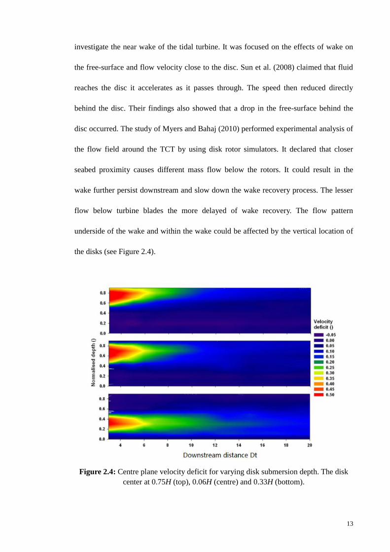
the flow field around the TCT by using disk rotor simulators. It declared that closer

seabed proximity causes different mass flow below the rotors. It could result in the

wake further persist downstream and slow down the wake recovery process. The lesser

flow below turbine blades the more delayed of wake recovery. The flow pattern

underside of the wake and within the wake could be affected by the vertical location of

the disks (see Figure 2.4).

Figure 2.4: Centre plane velocity deficit for varying disk submersion depth. The disk

center at 0.75H (top), 0.06H (centre) and 0.33H (bottom).

14

Pinon et al. (2012) conducted wake study of three-bladed TCT in uniform free

upstream current. The axial velocity profiles at different locations behind the turbine

have been illustrated in Figure 2.5, where r is the radial distance, Rt is the radius of the

turbine, Dt is the diameter of the turbine, Va is the axial velocity, V is the free stream

velocity. The wake has approximately 50% velocity deficit in near wake region

(x/Dt=1.2). The maximum velocity deficit occurs at near centre of the rotation axis. The

velocity deficit decreases at a slow rate along the downstream. It is in line with

observation reported by Myers et al. (2008) and Myers and Bahaj (2010). The wake

(Figure 2.5) is not fully covered even at 8.0Dt downstream. It has approximately 35%

velocity deficit. The recovery of wake velocity to free stream velocity can be further

downstream. Results from Batten et al. (2013) showed that up to 22Dt downstream the

wake velocity has not been fully recovered to the upstream velocity.

Figure 2.5: Wake characteristics of horizontal axis tidal-current turbine.

-3.0

-2.0

-1.0

0.0

1.0

2.0

3.0

0.4 0.5 0.6 0.7 0.8 0.9 1.0 1.1

r/R

t

Va/V

x/Dt=1.2

x/Dt=6.0

x/Dt=8.0

15

According to Pantan (Lam et al., 2012c), turbulence intensity can be defined for

each velocity component as the root mean square (RMS) referenced to a mean flow

velocity (Vref), as Equation (2.1).

I𝑥 =√𝑢′

𝑉𝑟𝑒𝑓, I𝑦 =

√𝑣′

𝑉𝑟𝑒𝑓 , I𝑧 =

√𝑤′

𝑉𝑟𝑒𝑓 (2.1)

where Ix, Iy, Iz are the x-component, y-component and z-component of turbulence

intensity, respectively. The overall turbulence intensity is defined by Equation (2.2).

I =√

1

3(𝑢′+𝑣′+𝑤‘)

𝑉𝑟𝑒𝑓 (2.2)

where I is the overall turbulence intensity, u’,v’,w’are the x-,y-,z-components of

turbulence and Vref is the reference mean velocity.

Ambient turbulence intensity has a crucial role on the wake shape behind the TCT.

The studies of Maganga et al. (2010), Myers and Bahaj (2010), and Mycek et al. (2014)

highlighted that the ambient turbulence intensity influences the wake structure. The

detail experimental work from Mycek et al. (2014) pointed out the significant role of

ambient turbulence on the behaviour of a three-blade turbine. Their results showed that

the wake shape, length, and strength largely depended on the upstream turbulence

conditions. The wake remained pronounced ten diameters downstream of the turbine

with almost 20% velocity deficit when I=3%. On the other hand, the wake recovers

much faster with a higher turbulence intensity I=15%. The upstream conditions

including velocity, turbulence and shear stress are almost fully recovered six diameters

16

downstream. However, high turbulence condition may cause more force fluctuations

and thus decrease the lifespan of the blade.

2.4.2 Wake Modelling

Extensive efforts of analytical, numerical and experimental studies have been done in

the past to understand the nature of wake. Perforated disks can provide appropriate

physical knowledge to understand turbines behavior. It also has been widely applied in

turbine simulations in wind turbine experiments (Builtjes 1978; Sforza et al., 1981;

Vermeulen and Builtjes, 1982). Sun et al. (2008) firstly applied the absorption disc

representing the turbine to study the near wake. Sun et al. (2008) believed that thrust

force on the turbine is of principal importance in the wake development. A series of

thrust forces on a real turbine can be simulated by perforated disk with a range of

porosities.

Myers and Bahaj (2010) also highlighted that investigations of such technology at

medium or large scale at basic research level is infeasible. The work of wake

investigation needs to focus on small scale testing, which is able to conduct at

laboratory. Myers and Bahaj (2010) also doubted the modelling of horizontal axis rotors

at very small scale. They believed that the channel flow properties cannot scale down

precisely while maintaining rotor thrust, power, and tip speed without remarkably

changing aspects of the downstream flow field. Accurate tip speed scaling of a 100 mm

diameter rotor would require the rotor to have a rotational speed up to 1500 rpm if the

rotor needs to maintain a typical full-scale tip speed of 10 m/s. It is the main reason that

17

Myers and Bahaj (2010) employed a mesh disk to identify the governing parameters

affecting the wake.

Harrison et al. (2010) conducted CFD simulations using an actuator disc and

compared to the experimental results of Myers and Bahaj (2010). It discovered that the

trend of wake recovery and turbulence levels is qualitatively similar in the CFD and

experimental results. There are significant computational benefits in approximating the

turbine as a disc rather than modelling its geometry in full in a RANS simulation. A full

model of the rotor requires mesh resolution at the blade surface to be sufficient to

capture the boundary layer and separation. This requires a very large number of mesh

elements and computational efforts. Furthermore, modelling a rotating turbine requires

that the model be unsteady and the blades change position with every time step.

The actual representation of the flow generated by rotor turbine is still achievable,

many numerical and experimental efforts to study the tidal turbine wakes by using real

turbine rotor have been also carried out (Maganga et al., 2010; Mycek et al. 2011, 2014;

Pinon et al., 2012; Stallard et al., 2011, 2013; Batten et al., 2013;Tedds et al., 2014). The

size of the turbines incorporated in all these studies ranges from 0.27 to 0.8 m. Pinon et

al. (2012) developed a particle method to model unsteady three-dimensional wake flows

of tidal turbine other than actuator disc. The velocity of the wake of the turbine has

good agreement with experiments up to ten diameters downstream of the turbine. The

one from Tedds et al. (2014) challenged those researches used disks modelled turbine

and claimed that their approaches may not predict the turbulent kinetic energy decay

rate of HATT wakes precisely.

18

Although numerical and experimental techniques have become sophisticated and

accurate in recent years, a simple analytical model is still useful to predict the wake

profile of tidal current turbines as its simplicity and cost-effective. Many analytical

investigations have been conducted on wind turbine wakes. One of the pioneering

analytical wake models is proposed by Jensen (1983).The most recent one is from

Bastankhah and Porté-Agel (2014) proposed a new analytical model for wind turbine

wakes by applying conservation of mass and momentum. They assumed a Gaussian

distribution of the velocity deficit in the wake. The tidal turbine and wind turbine

operate in the different ambient environment. The flow direction and turbulence in river

and marine currents are far more consistent and predictable compared to wind in the

atmospheric boundary layer. The analytical tools may be more suitable to be applied in

tidal turbine wake.

The pioneering model in predicting lateral velocity behind tidal turbine is proposed

previously by Lam and Chen (2014). They also assumed a Gaussian distribution for the

wake velocity and validated the proposed equation by comparing to experimental data

of Maganga et al. (2010). The predicted mean stream wise velocity agrees well with the

experimental data when the I=8%. Better understanding of the wake characterization is

also critical to quantify the potential effects on the sediments transport capacity. The

sediment transport in the energy extraction region has negative environmental impacts

(Shields et al., 2011). The analytical model for tidal turbine wake prediction could help

the engineers rapidly to calculate the wake velocity and identify the transport capacity

of the water column along the downstream of turbine wake.

19

2.5 Flow Condition between Rotor and Seabed

As presented in Section 2.4, a velocity deficit occurs behind a turbine and gradually the

velocity increases along the downstream of the wake. The formation of wake will affect

the flow close to the seabed. However, to date, little work has been done to present the

flow behaviour under a rotor. Myers and Bahaj (2007) reported wake studies of a 1/30th

scale horizontal axis tidal turbine and found that the blockage-type effects took place.

The measured velocity is greater than the incoming flow around the sides of the rotor.

Sun (2008) simulated turbine by using actuator mesh disk and claimed that localised

flow acceleration occurs during the energy extraction of the turbine. Chamorro et al.

(2013) performed velocity measurements in the near wake of a 3-bladed turbine. It was

found that tangential component was to be remarkably insignificant at the turbine tip

radius and higher radial velocity was observed near the turbine tip.

No information was found on the flow pattern further closer to the seabed. The flow

between rotor and seabed are responsible for the sediment transport. The flow is also of

importance when determining TST effects on ecosystem health and morphodynamics.

The nature mechanism of the turbine may also impose tangential and radial velocity

components in the water flow. All these factors may have environmental impacts on the

region of energy extraction. The flow below the rotor is responsible for the scour and

sediment transport as some sediment may lift up. Better understanding of the flow

pattern below rotor could offer critical insights into the influence of rotor on the scour

mechanism and sediment transport in the near flow field of the TCT.

20

2.6 Ship Propeller Jets and its Induced Scour

2.6.1 Nature of Ship Propeller Jets

The well-established knowledge of ship propeller jets could be a benchmark for

investigation of the wake development and scour nature of the TCT. This section aims

to review the fundamental knowledge of ship propeller jets and to figure out the

similarities between ship propeller jets and turbine wake. Ship propeller has a reverse

mechanism as TCT. A TCT harnesses kinetic energy from the current flow (He et al.,

2011). A ship propeller converts the torque of a shaft to produce axial thrust for

propulsion (Lam et al., 2010; He et al., 2011). Tidal-current turbine produces the wake

and the ship propeller produces the jets during operations, respectively. Lam et al. (2010)

conducted Laser Doppler Anemometry (LDA) measurements and stated that the axial

component of velocity is the primary contributor to the velocity magnitude at the initial

plane of a ship’s propeller jet. The tangential and radial components are the second and

third-largest contributors to the velocity magnitude.

Lam et al. (2011) reviewed the equations used to predict the velocity distribution

within a ship’s propeller jet. The study found that the rotational and radial components

of velocity are still poorly understood compared to the axial component of velocity. The

accuracy of the entire jet relies on the initial prediction of efflux velocity (Stewart, 1992;

Lam et al. 2011). Efflux velocity is defined as the maximum velocity taken from a

time-averaged velocity distribution along the initial propeller plane (Ryan, 2002).

Equations for predicting efflux velocity have been proposed Hamill (1987), Stewart

(1992) and Hashimi (1993), as shown in Table 2.1. These studies have found that the

21

efflux velocity of propeller jets was associated with thrust coefficient (Ct), speed of

rotation of propeller in revolutions per second (n) and propeller diameter (Dp). Stewart

(1996) reported that the coefficient used in the equation to predict efflux velocity was

not a constant. This coefficient depends on the propeller characteristics.

Table 2.1: Equations for efflux velocity

Proposed Equation Notation

Hamill (1987)

𝑉𝑜 = 1.33𝑛𝐷𝑝√𝐶𝑡 𝑉𝑜 is efflux velocity, n is speed of

rotation of propeller in

revolutions per second, Dp is

propeller diameter and 𝐶𝑡 is

thrust coefficient.

Stewart (1992)

𝑉𝑜 = 𝜉𝑛𝐷𝑝√𝐶𝑡

𝜉 = 𝐷𝑝−0.0686 (𝑃

𝐷𝑝⁄ )

1.519

𝐵𝐴𝑅−0.323

𝜉 is Stewart’s efflux coefficient,

P/Dp is the pitch ratio of the

propeller, BAR is the blade area

ratio (ratio of projected area of all

blades to the total area of the

propeller disc).

Hashimi (1993)

𝑉𝑜 = 𝐸𝑜𝑛𝐷𝑝√𝐶𝑡

𝐸𝑜 = (𝐷𝑝

𝐷ℎ⁄ )

−0.403

𝐶𝑡−1.79𝐵𝐴𝑅0.744

𝐸𝑜 is Hashimi’s efflux

coefficient, Dh is the diameter of

propeller hub.

Many researchers claimed that that the velocity magnitude of a ship’s propeller jet

tends to decay along the longitudinal axis from the initial plane immediately

downstream of the propeller jet (efflux plane)， (Blaauw and van de Kaa, 1978; Hamill,

1987; Stewart, 1992; McGarvey, 1996). The fluid in this region has high viscous shear

and it causes the fluid mix with surrounding water. The fluid within the propeller jet

gradually decelerates with longitudinal distance from the propeller face. The still

ambient fluid slowly accelerates at the same time (Brewster, 1997). A ship propeller jet

consists of two zones, namely the zone of flow establishment (ZFE) and the zone of

22

established flow (ZEF). Figure 2.6 depicts the schematic diagram of these two regions.

The jet forms the zone of flow establishment initially while the propeller is rotating.

Because the hub is at the center of the propeller, the propeller jet forms a low velocity

core along the axis of rotation within the zone of flow establishment. The velocity

profiles of propeller jets within the zone of flow establishment have two peak ridges.

The influence of the hub disappears gradually along longitudinal axis due to the mixing

of fluid in high velocity and fluid in low velocity central core (Hamill, 1987). The fluid

is mixing with the surrounding water both inwardly and outwardly along the axis of

rotation at the beginning (McGarvey, 1996; Lam et al., 2011). The flow will only be

mixed outwardly at a certain distance downstream. It is the region called the zone of

established flow. There is only one maximum velocity peak located at the axis of

rotation in this region (McGarvey, 1996; Lam et al. 2011).

Figure 2.6: Schematic view of propeller jet (Hamill, 1987)

23

Lam et al. (2012a) presented fluids flow in the zone of flow establishment from a

ship propeller. The measurements at two locations in the zone of flow establishment

have been selected and demonstrated in Figure 2.7, where Rp is radius of propeller, Dp is

diameter of propeller, Vo is efflux velocity for ship propeller jets and free stream

velocity for turbine wake. The axial velocity at x/Dp=0.79 and x/Dp=1.05 have little

differences. It shows two-peaked ridges velocity profile with a low velocity core at the

centre. The axial velocity distribution of turbine wake (1.2Dt) presented in Figure 2.7

shows reverse velocity distribution as ship propeller jets. It has two dips of velocity

deficit and a high core velocity near the centre. The axial velocity of turbine wake

further downstream shows one dip only. The propeller and the turbine both have three

blades. The diameter of the propeller (76 mm) is much smaller that of turbine (700 mm).

The experiment conducted by Lam et al. (2012) is in “bollard pull” condition (zero

advance speed). The velocity outside the jets is zero which is different with the flow

field outside the turbine wake. The velocity distribution of turbine wake (x/Dt=1.2) has

been inverted in order to compare with that of ship propeller jets. The inverted axial

velocity profile of turbine wake has a similar pattern as the velocity distribution of ship

propeller jets (see Figure 2.7). It is foreseeable the velocity profile of ship propeller jets

and inverted wake will be more identical if the propeller and turbine have similar

geometrical characteristics.

24

Figure 2.7: Comparison of velocity profile between a ship propeller jet and turbine

wake

2.6.2 Ship’s Propeller Jets Induced Scour

The velocity investigation of ship’s propeller jets has been discussed in the preceding

section. Sumer and Fredsøe (2002), Whitehouse (1998) and Gaythwaite (2004) claimed

that the velocity prediction within a ship’s propeller jet is the initial step to investigate

the seabed scouring. Blaauw and van de Kaa (1978), Verhey (1983), and Aberle and

Soehngen (2008) focused on the prediction of the maximum scour depth in the absence

of berthing structure. Hamill (1987) carried out an extensive study to investigate seabed

scour due to the propeller jet by using both the fine and coarse sands. The temporal

development of maximum depth of scour was examined and it can be written in a

dimensional consideration, as shown in Table 2.2. Hamill (1987) suggested that the

-2.0

-1.5

-1.0

-0.5

0.0

0.5

1.0

1.5

2.0

0.0 0.2 0.4 0.6 0.8 1.0

r/R

t or

r/R

p

Va/V

Shi propeller jet, x/Dp=0.79, Lam et al. (2012)

Shi propeller jet, x/Dp=1.05, Lam et al. (2012)

Turbine wake, x/Dt=1.20, Pinon et al. (2012)

25

scour depth relates to the densimetric Froude number, size of sediment and the

clearance between the propeller and seabed. The maximum velocity and its distribution

of a jet mainly depend on the characteristics of a turbine. Hamill et al. (1999) extended

their earlier studies by including the effect of propeller jets on quay walls. They showed

that the densimetric Froude number (Fo) plays the most important role in affecting scour

depth through dimensional analysis. Hong et al. (2013) studied the development of a

scour hole with non-cohesive sediments due to the jet induced by a rotating propeller,

which focused on the influences of various parameters on the time-dependent maximum

scour depth.

Table 2.2: Scour Depth Predictions

Proposed Equation Notation

Hamill (1987)

휀𝑚

𝐷𝑝= 𝑓 [𝐹𝑜 ,

𝐷𝑝

𝑑50,

𝐶

𝑑50]

𝐹𝑜 =𝑉𝑜

√𝑔𝑑50∆𝜌𝜌

휀𝑚 is maximum depth of scour,

𝐹𝑜 is densimetric Froude number,

𝑑50 is median sediment grain

size, C is clearance between the

propeller tip and the seabed, 𝑔 is

acceleration due to gravity, ∆𝜌

is difference between the mass

density of the sediment and the

fluid, and 𝜌 is density of fluid.

Hong et al. (2013)

𝑆𝑡

𝐷𝑝= 𝑘1[𝑙𝑜𝑔10(

𝑉0𝑡

𝐷𝑝) − 𝑘2]𝑘3

Where

𝑘1 = 0.014𝐹01.120 (

𝐶

𝐷𝑝)

−1.740

(𝐶

𝑑50)

−0.170

𝑘2 = 1.882𝐹0−0.009 (

𝐶

𝐷𝑝)

2.302

(𝐶

𝑑50)

−0.441

𝑘3 = 2.477𝐹0−0.073 (

𝐶

𝐷𝑝)

0.53

(𝐶

𝑑50)

−0.045

𝑆𝑡 is the scour depth at time t, 𝐷𝑝

is the diameter of propeller. The

equation is valid only for

0.5<𝐶

𝐷𝑝<2.87 and 5.55< 𝐹0<11.1.

26

2.7 Seabed Scour for Different Type of Support Structures

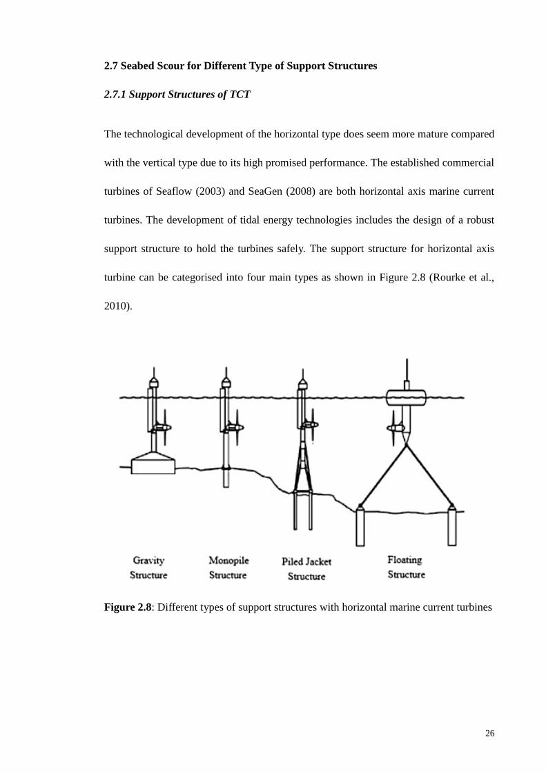
2.7.1 Support Structures of TCT

The technological development of the horizontal type does seem more mature compared

with the vertical type due to its high promised performance. The established commercial

turbines of Seaflow (2003) and SeaGen (2008) are both horizontal axis marine current

turbines. The development of tidal energy technologies includes the design of a robust

support structure to hold the turbines safely. The support structure for horizontal axis

turbine can be categorised into four main types as shown in Figure 2.8 (Rourke et al.,

2010).

Figure 2.8: Different types of support structures with horizontal marine current turbines

27

(1) Gravity structure: The gravity structure is a concrete or steel structure to hold the

turbine by its self-weight to resist overturning.

(2) Monopile structure: The monopile structure is a large steel beam with a hollow

section penetrating to a depth of seabed between 20 and 30 m for a soft seabed. The

processes of predrilling, positioning and grouting are required for the seabed condition

of hard rock.

(3) Tripod/Piled Jacket structure: The tripod Jacket structure anchors each corner of the

basement to the seabed by using steel piles. These steel piles are driven in between 10

and 20 m into the seabed to hold the structure firmly. Tripod Jacket structure is a

well-established technology in the application of oil and gas industry.

(4) Floating structure: Floating structure is suitable for the application of deep water.

The floating device appears at the surface of the water to hold the submerged turbine

structure in the water. The submerged structure is locked to the mounting device at the

seabed by using chains, wire or synthetic rope.

2.7.2. Scour Behaviour of Different Types of Support Structures

Rambabu et al. (2003) stated the fluid flow, geometry of foundation and seabed

conditions are the governing factors for the seabed scouring. The characteristics of fluid

flow include the current velocity, Reynolds number of model and Froude number of the

flow. The abovementioned four types of foundations have different areas of contact with

the seabed. The selection of support structures leads to different flow patterns occurring

at the foundation of with different formation of flow-induced vortices in the vicinity of

support structures. Different foundation geometries cause different scouring patterns.

28

The gravity structure is most susceptible to seabed scouring due to its large contact

area with the seabed compared to the other three types of foundation. The determination

of geometry size and seabed preparation is required to implement the gravity structure

as the foundation of horizontal axis TCT. The monopile is less susceptible to scour

compared to gravity structure due to its small contact area with the seabed (Rourke et al.,

2010). McDougal and Sulisz (1989) stated the floating structure gives lowest impact on

the seabed scour due to the low area of contact between the structure base and seabed.

However, it may have less advantage on the positioning of the turbine in harsh marine

environment.The scour of piled jacket structure is more complicated than the other

structures due to its footing shape (Rudolph et al., 2009).

The seabed preparation is time-consuming and the construction process of the

foundation is costly. The potential sites for marine current energy have fast flowing

fluid, which may be dangerous for divers. Gravity structure may be suitable for the sites

without excessive seabed preparation. Monopile structure can be used to replace the

gravity structure as no seabed preparation is required prior to the installation (Rourke et

al., 2010). The piled Jacket and floating structures are both alternatives without seabed

preparation. The floating structure needs stable points at the seafloor, fixing the

structure to the seabed through chains.

The scour development around monopile structures has been studied extensively for

the foundation of offshore wind turbine in the past few decades (Sumer, 2007; Rudolph

et al., 2009). The application of monopile structures in TCT is suggested for both the

cost and structural stability (Fraenkel, 2002). The first tidal turbine in the world (300kW

29

Seaflow) is supported by a monopile, which generated electricity successfully (Fraenkel,

2007). The monopile structure is analogous to the bridge piers and piles which have

been studied for more than a hundred years. The knowledge pool of the bridge piers and

piles study is the references to the monopile structures of TCT.

2.8 Scour Nature of TCT

Neill et al. (2009) developed large grid cell (km-scale) simulations to explore the

impacts of array turbine farm on sediment dynamics. It claimed that small amount of

energy extracted from a site might affect the erosion and deposition pattern over a long

distance from the point of energy extraction. The effects may up to 50 km in the case of

the Bristol Channel. Vybulkova (2013) modified vorticity transport model to simulate

wake and its interactions with local sediment. The results show that the flows

downstream of the rotor affect the marine environment over scales of a few centimetres.

Hill et al. (2014) conducted a study on the scour of an axil-flow hydrokinetic turbine

under clear water and live-bed conditions. Results indicate that the rotor of turbine

increases the local shear stress of sediment around the turbine. The velocity deficit in

the wake region leads to the flow acceleration below the rotor. The local scour of the

turbine is accelerated and expanded when compared to bridge scour. Results indicate

that regions susceptible to scour typically persist up to 2 times turbine diameters

downstream and up to 1.5 times turbine diameter to either side of the turbine centre

location. Within the regions, results showed scour depths approaching 12-15% of

turbine diameter from small scale experiment and 30-35% of turbine diameter from the

large-scale experiments. Future work is required to investigate the temporal evolution of

30

tidal turbine scour process. It is also recommended to identify the effects of tip

clearance on the scour rate of TCT.

2.9 Scour Prediction of TCT

2.9.1 Empirical Equations for Scour Prediction of Pile/Pier

Numerous equations and relations have been proposed to estimate the scour depth of a

pier or pile in the previous studies, as shown in Table 2.3. Neill (1973) proposed a

simple equation in 1973 to relate the depth of scour to the diameter of penetrated

structure to be a constant (Ks). Ks is the correction factor for pier shape, which is a

constant depending on the shape of the penetrated structure. Neill (1973) proposed the

correction factor Ks=1.5 for round-nose pier or circular pier and Ks =2.0 for rectangular

pier. The study of Neill has been the foundation for the works of Richardson et al. (1975)

at Colorado State University (CSU), Breusers et al. (1977) , Breusers and Raudkivi

(1991), Ansari and Qadar (1994) and Richardson and Davis (2001). These researchers

included more parameters to consider the incoming flow, water depth, bed condition and

size of sediment to enhance the Neill’s equation.

31

Table 2.3: Summary of equations for predicting scour around piles/piers

Existing Equations Notation

Neill 1973 𝑆

𝐷= 𝐾𝑠

S is the vertical distance between the

maximum depth in scour hole in

equilibrium situation and the

surrounding undisturbed bed, D is

pile diameter, and 𝐾𝑠 is the

correction factor of pier shape.

Richardson et al. 1975 CSU

𝑆

𝐷= 2.0𝐾𝑠𝐾𝜃(

ℎ

𝐷)0.35𝐹𝑟

0.43

𝐾𝜃=(cos 𝜃 +𝐿

𝑎sin 𝜃)0.65

𝐹𝑟 =𝑈𝑐

(𝑔ℎ)0.5

𝐾𝜃 is the correction factor for flow

angle of attack, h is water depth, Fr

is the Froude number of incoming

flow, 𝜃 is angle of flow attack, L

is pier length, a is pier

width/diameter, Uc is depth-averaged

current velocity and g is

gravitational acceleration.

Breusers et al. 1977

𝑆

𝐷 = 1.5𝐾𝑠𝐾𝜃𝐾𝑏𝐾𝑑 tanh(

ℎ

𝐷)

𝐾𝑏 = 0 , 𝑖𝑓 𝑈𝑐

𝑈𝑐𝑟< 0.5

𝐾𝑏 = 2 (𝑈𝑐

𝑈𝑐𝑟) − 1, 𝑖𝑓 0.5 ≪

𝑈𝑐

𝑈𝑐𝑟< 1

𝐾𝑏 = 1, 𝑖𝑓 𝑈𝑐

𝑈𝑐𝑟≫ 1

𝐾𝑏 is the correction factor for bed

condition, 𝐾𝑑 is the correction factor

for size of bed material (Uc is the

depth-averaged current speed and Ucr

is the threshold depth-averaged

current speed.

Breusers and Raudkivi 1991 𝑆

𝐷= 2.3𝐾𝑦𝐾𝑠𝐾𝑑𝐾𝜎𝐾𝛽

𝐾𝑦 is the correction factor of flow

depth, 𝐾𝑑 is the correction factor of

pier and sediment size, 𝐾𝜎 is the

correction factor of sediment grading

and 𝐾𝛽 is the correction factor of

pier alignment.

Sumer et al.1992 𝑆

𝐷= 1.3{1 − exp(−𝑚(𝐾𝐶 − 6))}

KC =𝑈𝑚𝑇𝑤

𝐷

m is an empirical factor determined

from experiments as a constant of

0.03, KC is Keulegan-Carpenter

number (drag force / inertia force of

flow), Um is amplitude of the wave

velocity variations near the bed in

absence of pile (statistic parameter), T stands for wave period of

incoming flow in second.

Ansari and Qadar 1994 𝑆

𝐷= 0.86𝐷2 , 𝑤ℎ𝑒𝑟𝑒 𝐷 < 2.2𝑚

𝑆

𝐷= 3.06𝐷−0.6 , 𝑤ℎ𝑒𝑟𝑒 𝐷 > 2.2𝑚

D is projected width of pier.

32

Table 2.3, continued, Summary of equations for predicting scour around piles/piers

Melville 1997 𝑆

𝐷= 𝐾𝑦𝐾𝑠𝐾𝑑𝐾𝐼𝐾𝛽𝐾𝐺

𝐾𝐼 is the correction factor of flow

intensity, 𝐾𝐺 is the correction

factor of channel geometry

Richardson and Davis 2001

𝑆

𝐷= 2.0𝐾𝑠𝐾𝜃𝐾𝑏𝐾𝑑𝐾𝑤(

ℎ

𝐷)0.35𝐹𝑟

0.43

𝐾𝑤 is the enhance correction factor

for pier width/pile diameter.

Sumer and Fredsøe 2002 𝑆

𝐷= 1.3{1 − 𝑒𝑥𝑝(−𝐴(𝐾𝐶 − 𝐵))}

𝑓𝑜𝑟 𝐾𝐶 ≥ 𝐵

𝐴 = 0.03 + 3

4𝑈𝑐𝑤

2.6

𝐵 = 6𝑒𝑥𝑝 (−4.7𝑈𝑐𝑤)

𝑈𝑐𝑤 =𝑈𝑢𝑐

𝑈𝑢𝑐 + 𝑈𝑚

Uuc is the undisturbed current

velocity, and Um is the maximum

value of the undisturbed orbital

velocity at the sea bottom (statistic

parameter).

Raaijmakers and Rudolph 2008 𝑆

𝐷= 1.5𝐾𝑣𝐾ℎ 𝑡𝑎𝑛ℎ(

ℎ

𝐷)

𝐾ℎ = (ℎ𝑝

ℎ)0.67

𝐾𝑣 = 1 − 𝑒𝑥𝑝(−𝐴)

𝐴 = 0.012𝐾𝐶 + 0.57𝐾𝐶1.77𝑈𝑐

3.67

𝐾𝑣 is correction factor accounting

for wave action, 𝐾ℎ is correction

factor accounting for piles that do

not extend over the entire water

column, ℎ𝑝 is pile height and not

over h.

Richardson et al. (1975) at Colorado State University (CSU) improved Neill’s

equation by considering the water depth and incoming flow. The angle attack of the

incoming flow and the water depth are both being considered in Richardson’s equation.

Richardson’s equation proposed that the ratio of the depth of scour to the diameter of

the pier is two times of the multiplication of four dimensionless terms. These

dimensionless terms are term of pier geometry, term of angle attack, term of water depth

over diameter ratio and term of Froude number of flow.

33

Breusers et al. (1977) improved the empirical equation for predicting the scour depth

based on experimental observations with consideration of tidal flow in 1977. The bed

conditions, size of bed sediment and water depth were included in Breusers’s equation.

The inclusion of the bed condifreplacetions and size of sediment is important to relate

the source of scour (incoming flow) to the area being scoured (seabed). Breusers and

Raudkivi (1991) included the consideration of the water depth (Ky) as Richardson’s

equation (1975) and the group of pier alignment (K). The correction factor of bed

conditions proposed by Breusers et al. (1977) was replaced by an analogous correction

factor, namely sediment grading (K). The correction factor of grading considers the

seabed with various layers, which is vulnerable to be scoured, rather than only the top

layer of bed. The consideration of sediment grading is essential at the seabed with

non-uniform sediments. Melville (1997) proposed another analogous scour estimator

with extra factors such as flow intensity (KI) and channel geometry (KG).

Sumer et al. (1992) carried out the experimental investigation into scour around

piles exposed to waves. His research suggested that the effects of particlelee wake and

horseshoe vortex are the two crucial components related to scour process. The

horseshoe vortex contributes to the scour in front of the structure, whereas the lee wake

forms the vortex shedding contributing the scour at the back of the structure. The

conditions of horseshoe vortex and lee wake depend on the Keulegan-Carpenter (KC)

number (Sumer et al., 1992). Sumer et al. (1992) also proposed KC number can be used

to relate to the equilibrium scour depth on live beds. KC number is a ratio of the

amplitude of wave velocity variations and the wave period of the incoming flow to the

diameter of a pile, as shown in Table 2.3.

34

Ansari and Qadar (1994) estimated the ultimate depth of local scour at bridge piers

based on his empirical study of field measurements. The equation is developed based on

the curves of the envelope from the field data with the consideration of a wide range of

parameters. The scour depth is related to solely one parameter, which is the diameter of

pier. The development of the equation may be transferable to produce the scour equation

to tidal current energy. However, the sufficient scour data of TCT may be required for

the development by using the approach of Ansari and Qadar (1994).

Richardson and Davis (2001) proposed an enhanced equation to determine the

ultimate scour depth for both live-bed and clear-water scours in 2001. The equation

considers the large particle as the sediment at the seabed and the wide pier in the scour

process. The large particle may reduce the scour depth at seabed compared with the

small particle as sediment. For the consideration of wide piers, Richardson and Davis

(2001) conducted the flume studies to investigate the scour depth by using wide piers in

shallow water. The results from experimental study are compared to the field

measurement of the scour depth at bascule piers (a type of wide pier). The enhanced

correction factor of pier width (Kw) is proposed in addition to the correction factor of

pier shape (Ks) in 1975 to consider the impact of wide piers to the scour depth. The Kw

can be applied when the following conditions are matched: (1) the ratio of flow depth

(H) to pier width/pile diameter (D) is less than 0.8; (2) the ratio of pier width to median

diameter of bed material (d50) is greater than 50; (3) the Froude number of flow is

subcritical.

Sumer and Fredsøe (2001) carried out the investigation to include the influences of

current to the ocean wave induced-scour proposed in 1992. The equation is derived

from the experiments in the range of KC in between 5 to 30 for the live-bed condition.

The tidal current changes with time in a day and therefore the orbital velocity (velocity

of particles due to wave motion) is used for the equation derivation. The time-averaged

35

velocity has been used to consider the current speed in the equation. Sumer and Fredsøe

(2001) also suggested that the depth of time-averaged current-induced scour is 1.3 times

the diameter of the pile (S/D=1.3) with a standard deviation of 0.7. Other than that, den

Boon et al. (2004) proposed that the maximum depth of scour around a monopile with

sole consideration of current is 1.75D when no protective unit is used at the seabed.

The prediction of scour depth for full water depth piles is well developed. All the

aforementioned predictors apply to full water depth piles. However, if the pile

height-to-diameter ratio is smaller than a critical value, the size of the horseshoe vortex

in front of the pile will decrease with a decrease in pile height (Sumer, 2002). Therefore,

the scour depth in front the cylinder will reduce with decrease in pile height. The

decrease of pile height also weakens the vortex shedding behind the cylinder, which

results in the reduction of scour depth behind the structure. More and more attention has

been drawn to quantify the effect of pile height to scour depth. Raaijmakers and

Rudolph (2008) proposed an equilibrium scour depth equation with considerations of

wave action and pile height lower than the water level. The equation is applicable to

anyone of following conditions: 1) the KC number is small; 2) the height of pier is

lower than the water depth; 3) the pile is relatively wide compared to the water depth.

More recently, Simons et al. (2009) presented experimental works on scour

development around truncated cylindrical structures. Their results show that depth and

extent of scour are largely reduced for the cylinder height less than one cylinder

diameter compared to tests with a full water depth cylinder. Besides, their study

demonstrated the scour depth concerning tidal flow condition. The tests indicate that

scour is remarkably reduced with bi-directional tidal condition compared the equivalent

unidirectional current. The flow condition at potential sites plays a crucial role for the

scour around the support structure of TCT.

36

The previous studies demonstrated that the depth of scour for piers or piles is

significantly influenced by the geometry of the structure, condition of incoming flow,

seabed condition, seabed material, and water depth. These parameters will give the

analogous impacts to the seabed scour for the TCT. The rotating rotor of the TCT

influences the scour mechanism around the support structures, especially when the rotor

is close to the seafloor. The rotor of the TCT becomes an additional factor for the scour

process. The well-established knowledge on the turbine wake and ship propeller jets

could offer a critical insight on the hydrodynamics of flow disturbed by the rotor.

2.9.2 Applicability of Existing Models for Predicting Scour of TCT

This section aims to identify the appropriateness of existing approaches for predicting

scour depth around pile-supported TCT. Many empirical methods are available as

presented in section 2.9.2. Rudolph et al. (2004) conducted a comparison between the

existing empirical equations and the results of field study and concluded that the

empirical equation from Breusers (1977) can be used to predict the scour depth

effectively.

Breusers’s equation does not include a Froude number in his expression. The

inclusion of a Froude number is important as a determination of the nature of flow

(Harris et al., 2010). Richardson and Davis (2001) adopted Froude number in his

expression. Potential TCT sites have deep water. For an instance, the, the water depth of

potential location for tidal energy extraction in Malaysia can up to 93 m (Kota Belud).

The Froude number is quite small unlike in river. In the case of deep water, the Froude

number may not need to be taken into consideration when comes to the prediction of

scour depth. However, the free surface in proximity to rotor allows the water depth to

37

vary and the consideration of gravity cannot be ignored. The extraction of energy from a

flow results in channel head drop. The head drop for a single turbine unit in a large

channel is quite small. The effects could be aggravated in array TCT farm. A row of

TCTs cause a significant change of water depth in the downstream as well as the

increase of flow speed. It subsequently results in pronounced variation in Froude

number (Bahaj et al., 2007).

Breusers’s (1977) and Richardson and Davis’s (2001) equations have been selected

as two of the proposed equations to develop an engineering model named scour time

evolution predictor (STEP) to predict the development of scour evolution of offshore

structures. In STEP, the comparison of these two empirical equations against

experimental measurement has been made (Harris et al., 2010), as shown in Figure 2.9.

In Figure 2.9, the variation between the empirical equations and the experimental

measurements can be found. Harris et al. (2010) stated that the empirical scour depth

predictors have a reasonable agreement with the experimental measurements. These

empirical equations are a reasonable starting-point to develop a time-varying model,

which includes the scour depth due to tide, wave and their combination. This scour time

evolution model has been applied in the offshore wind turbine studies.

38

Figure 2.9: The comparison of predicted scour depth with measured scour depth.

Annandale (2006) proposed an approach to estimate the potential erosion of

complex soils by relating the stream power (river) to the soil resistance of scour. Harris

et al. (2010) applied Annandale’s approach to the marine environment with

modifications. Harris et al. (2010) called this modified method as Earth Materials

approach, which can be used to assess the scour in complex marine soils. Harris’s

approach requires information of soil properties. The seabed is a formation of soil with

different layers, which the depth of each layer needs to be used as an input. The depth of

each layers need to be obtained through site investigation. Richardson and Davis’s

(2001) equation has been adopted to calculate the maximum depth of scour in the Earth

Materials approach.

Equations from Breusers (1977) and Richardson and Davis (2001) have been

widely used in the prediction of scour depth. If the clearance between the rotor and

0

0.05

0.1

0.15

0.2

0.25

0 0.05 0.1 0.15 0.2 0.25

Eq

uil

ibri

um

sco

ur

dep

th -

Pre

dic

ted

: m

Equilibrium scour depth - measured:m

Richardson and Davis (2001)

Breusers et al. (1977)

39

seabed is relatively high, the flow suppression at seabed may become insignificant. The

consideration of rotor on the seabed scouring is therefore negligible. The equations from

Breusers (1977), Richardson and Davis (2001) are still the best equations to date as it

has been widely applied in offshore engineering. However, the scour process around the

support of TCT is relatively complicated. The development of scour not only depends

on a range of tidal, seasonal and long terms variations in currents, wave action and

water depth at the site but also the rotating of rotor. No empirical equation to date was

found to quantify the influence of rotors to TCT induced scour. It is suggested to include

the effect of the rotor in the scour prediction of TCT.

2.9.3 Computational Fluid Dynamic Software and Scour Prediction

Despite many empirical methods for prediction of scour depth are available,

Computational Fluid Dynamic (CFD) is getting popular due to its reduction of the cost

and time in the simulation process. CFD can also be used to simulate a full-scale

structure virtually without consideration of the scaling effect (Zhao et al. 2010). Olsen

and Melaaen (1993) was the earliest simulated a three-dimensional scour hole

development around the base of a circular pier. Roulund et al. (2005) also numerically

simulated local scour around a vertical pile. They suggested that the

boundary-layer-thickness-to-pile diameter ratio and the Reynolds number affected the

horseshoe vortex and the bed shear stress. However, numerical models for scour require

using empirical equations for sediment transport rates which are obtained from

experiments.

40

Deltares, Wallingford and DHI developed many scour models in operation. These

models took into account the constantly changing hydrodynamics. Nielsen and Hansen

(2007) from DHI Water & Environment developed an engineering model named WiTuS

(Wind Turbine Scour). Their model took into account both the constantly changing

hydrodynamics and seabed material properties. The simulation results showed that the

scour depth will be approximately 0.3 times of pile diameter for the condition of a larger

wave period in the North Sea. It is significantly smaller than 1.3 times of pile diameter,

which is the industry standard. It demonstrated that larger wave period decreases the

scour depth considerably in a combined wave-current condition. Nielsen’s colleagues

Dixen et al. (2012) developed tables of scour rate to predict long time span of scour

around the foundation of the offshore wind farm. Dixen’s method can be used to predict

the scour development at different stages. The tables of scour rate were developed based

on the results from 3D simulations. The development of scour hole with times can be

predicted as the flow characteristics at different times are known. The predicted results

are in good agreement with the experimental data. The new method can also be used to

estimate the backfilling of a scour hole for any given structure (Dixen et al., 2012;

Sumer et al., 2012).

Deltares implemented the software “OSCAR” for scour assessment in the tender

phase. This software is based on the empirical-mathematical relations. On the other

hand, Deltares developed a flexible integrated modelling feature called Delft3D. This

modelling feature has a non-hydrostatic option linked to a Z-model approach. It has

been successfully implemented in the process of sediment transport. Delft3D-FLOW is

now applicable to a wide range of scour problems around the offshore structures

41

(Deltares). Zhang et al. (2015) developed a numerical model based on commercial CFD

package FLOW-3D to simulate the current induced scour around the support of tidal

turbine. The model is validated by comparing the numerical results with Zhao et al.

(2010). The experiment conducted by Zhao et al. (2010) is a test of seabed scour around

a monopile foundation. The comparison does not approve that the numerical model is

applicable to investigate the scour induced by tidal turbine. The simulation also only

lasts for 30 min. The scour depth does not reach equilibrium state. Investigate the scour

depth until it is equilibrium through numerical methods usually take long time.

OpenFOAM as an open source CFD software has been widely applied in today’s

research and engineering work. Higuera et al. (2013) demonstrated that the OpenFOAM

can be successfully simulating some costal engineering cases. Mulualem et al. (2013)

developed an Immersed Body Force model via OpenFOAM to examine the

performance of a tidal turbine. The greatest advantage of OpenFOAM is that the users

are able to modify the source code to satisfy their respective simulation objectives. Liu

(2008) also proposed a numerical model FOAMSCOUR through OpenFOAM. It is a

numerical model for local scour of pile with the free surface and automatic mesh

deformation. The free surface is modelled by VOF method while the scour process is

modelled by moving mesh method. Liu (2008) stated that coupled simulations of flow

with sediment transport usually take long time. Besides, Harrison et al. (2010) also

claimed that a full model of the rotor requires mesh resolution at the blade surface to be

sufficient to capture the boundary layer and separation. This requires a very large

number of mesh elements and computational efforts. Modelling a rotating turbine also

requires that the model be unsteady and the blades change position with every time step.

42

The incorporation of the rotor into scour model further increases the computational

power. The scour mechanism of TCT is more complex than those conventional

bridge/pile scour. A combination of physical scale model and CFD model may be

alternative to solve the scour issue of tidal turbine in terms of time and

cost-effectiveness at the current stage.

43

CHAPTER 3: METHODOLOGY

3.1 Overview

The main methodologies employed in the study are analytical approach, numerical

simulation and physical modelling. The analytical approach is based on the established

knowledge from ship propeller jets proposing equations for predicting lateral velocity

distribution of the wake (Section 3.2). The numerical simulation focuses on the

simulation of the flow field below turbine blades (Section 3.3). The experimental work

intends to investigate the scour nature of the TCT (Section 3.4 and Section 3.5). Figure

3.1 shows the flowchart of the overall methodology of the study.

44

Figure 3.1: Flowchart of the research

Methodology

Axial momentum theory,

equations of Hamill

(1987), empirical

experimental results of

wake recovery

Efflux velocity, wake

recovery rate, lateral

wake equations

Analytical wake model

for various ambience

turbulence (TI=3%, 5%,

8%, 15%).

Validated by comparing

with experimental data

Numerical simulation

OpenFOAM:

flow condition between

rotor and bed.

Geometry creation by

Salome, k-e turbulence

model with modified

pimpleDyMFoam solver

Different tip clearances,

different number of blades

Validated by comparing

with experimental data&

mesh independence

study

Axial, tangential and

radial component of

velocity, boundary layer

de

IFREMER-LOMC

turbine with

Dt=0.2m, support

structure D=0.02m

Flume in hydraulic lab of

University of Malaya (1m

wide, 1 m high, 16m long)

Correlated

time-dependent scour

depth with tip clearance

Different tip clearances;

Time dependent scour

profile (3.5, 7.0 and 24

hr); Maximum scour

depth

Experiment: scour

evolution of

pile-supported tidal

current turbine

Wake model by

analytical derivation

45

3.2 Derivation of Analytical Wake Model

3.2.1 Efflux Velocity

The Axial momentum theory is used to derive the efflux velocity equation. Figure 3.2

shows the TCT actuator disc model with the change of current flow pattern in one

direction. Due to the assumption that neither the upstream nor the downstream region

consist of any work done, the Bernoulli function is applied to the two control volumes

on each side of the turbine rotor to produce Equations (3.1) and (3.2). Equation (3.1)

shows the relationship between the pressures and velocities upstream of the disc.

𝑃1 +1

2𝜌𝑈1

2 = 𝑃2 +1

2𝜌𝑈2

2 (3.1)

Equation (3.2) shows the relationship between the pressures and velocities downstream

of the turbine disc.

𝑃3 +1

2𝜌𝑈3

2 = 𝑃4 +1

2𝜌𝑈4

2 (3.2)

where ρ is the density of the fluid in kg/m3, P1, P2, P3 and P4 are the pressures in Pa,

and U1, U2, U3 and U4 are the axial velocities in m/s at the respective locations shown in

Figure 3.2.

46

Figure 3.2: A tidal-current turbine actuator disc model.

The thrust is then expressed as the net sum of the forces on each side of the actuator disc

as shown in Equation (3.3).

𝑇 = 𝐴(𝑃2 − 𝑃3) (3.3)

where T is the thrust, A is the area of the actuator disc, and P2 and P3 are the respective

pressures located at the two side of the turbine disc. It is assumed that the far upstream

and far downstream pressures are equal P1 = P4 and that the velocity across the disc

remains the same, U2 = U3. Equation (4) is obtained by solving P2 – P3 using Equations

(3.1), (3.2) and (3.3).

𝑇 =1

2𝜌𝐴(𝑈1

2 − 𝑈42) (3.4)

Lam and Chen (2014) assumed that the dimensional analysis of thrust on the turbine

disc, giving consideration to density, rotational speed and diameter, is similar to the

dimensional analysis of thrust on the propeller disc. As a result, the deduced thrust

coefficient equation is as shown in Equation (3.5).

47

𝐶𝑡 =𝑇

𝜌𝑛2𝐷𝑡4 (3.5)

where Ct is the thrust coefficient, ρ is the density of fluid in kg/m3, Dt is the diameter of

the turbine disc in metres, n is the rotational speed in rev/s, and T is the thrust in

Newtons. Equation (3.6) is obtained by equating the thrust equations, Equations (3.4)

and (3.5), with the substitution of A by the equation of the area of a circle, (πDt2) /4.

𝐶𝑡𝜌𝑛2𝐷𝑡4 =

1

2𝜌 (

1

4𝜋𝐷𝑡

2) (𝑈12 − 𝑈4

2) (3.6)

However, the assumption of simulating the area of the rotor disc as a circle is not

satisfactory. The real cross section area of a tidal turbine is rather smaller than the circle.

The tidal turbines operate at lower speed compare to ship propellers. In order to

eliminate the flaws of the term “A” and rotational speed “n” in the derivation, the

authors applied the thrust coefficient of the turbine as Equation (3.7):

𝐶𝑡 =𝑇

1

2𝜌𝐴𝑈2

(3.7)

Equation (3.8) is obtained by equating the thrust equations, Equations (3.4) and (3.7),

with the substitution of U by the upstream velocity U1.

1

2𝐶𝑡𝜌𝐴𝑈1

2 =1

2𝜌𝐴(𝑈1

2 − 𝑈42) (3.8)

Equation (3.8) is rearranged to obtain Equation (3.9).

𝑈4 = √𝑈12 − 𝑈1

2𝐶𝑡 (3.9)

Taking the efflux velocity as V0 and the free stream velocity as V∞, substituting into

Equation (3.9) produces Equation (3.10).

𝑉0 = 𝑉∞√1 − 𝐶𝑡 (3.10)

48

3.2.2 Wake velocity distribution

The Albertson et al. (1950) applied the axial momentum theory and used a plain water

jet to study the velocity distribution within the jet. According to the Gaussian

probability distribution and the research work conducted by Albertson et al. (1950),

Lam and Chen (2014) proposed Equation (3.11) which could be applied to predict the

wake velocity distribution behind the TCT.

𝑉𝑥,𝑟 = 𝑉∞ − (𝑉∞ − 𝑉𝑚𝑖𝑛)𝑒[−((𝑟+0.081𝑥−(𝐷𝑡/2))

2/(2(0.081𝑥)2))]

(3.11)

Berger et al. (1981) highlighted the presence of hub so that the flow pattern along the

ration axis of a ship propeller jet is different from a plain water jet. Hamill (1987)

realised the assumption of the plain water jet that the maximum axial velocity at any

lateral section occurs at the rotation axis cannot be right. He refined Albertson’s (1950)

work and suggested two equations (Equations 3.12 and 3.13) to estimate the lateral

distribution at cross sections within the zone of flow establishment.

𝑉𝑥,𝑟

𝑉𝑚𝑎𝑥= 𝑒[−(1 2⁄ )((𝑟−𝑅𝑚𝑜)/(𝑅𝑚𝑜 2⁄ ))2] (3.12)

Equation (3.12) was applicable to distances up to 0.5Dt downstream of the propeller.

The distribution of axial velocity for the remainder in the zone of flow establishment

can be determined using Equation (3.13).

𝑉𝑥,𝑟

𝑉𝑚𝑎𝑥= 𝑒[−(1 2⁄ )((𝑟−𝑅𝑚𝑜)/((𝑅𝑚𝑜 2⁄ )+0.075(𝑥−𝑅𝑡)))2] (3.13)

The turbine wake’s lateral velocity distribution equation was derived by referring to the

research work carried out by Hamill et al. (1987). For the turbine disc, the velocity

deficit occurred behind the turbine. The minimum axial velocity, Vmin, was considered

and was included in Equations (3.12) and (3.13) to form Equations (3.14).

49

𝑉𝑥,𝑟 = 𝑉∞ − (𝑉∞ − 𝑉𝑚𝑖𝑛)𝑒𝐴 (3.14)

when x ≤ 0.5𝐷𝑡

A = [−0.5((𝑟 − 𝑅𝑚𝑜) (𝑅𝑚𝑜

2))2]⁄ (3.15)

when x > 0.5𝐷𝑡

A = [−0.5((𝑟 − 𝑅𝑚𝑜) ((𝑅𝑚𝑜

2) + 0.075(𝑥 − 𝑅𝑡)))2]⁄ (3.16)

where V∞ is the free stream velocity, Vmin is the minimum velocity, Rt is the radius of the

turbine disc, Dt is the diameter of the turbine disc, x is axial distance, r is the radial

distance. Rmo is defined as the location of efflux velocity from the rotational axis.

Lam and Chen (2014) described that the efflux velocity of a turbine is the minimum

velocity taken from a time-averaged velocity distribution along the initial turbine face.

Equation (3.13) was used to predict the velocity distribution of a ship’s propeller jet

within the zone of flow establishment. The equation may be invalid for the prediction of

wake profile at the region further downstream. The experimental results from Maganga

et al. (2010) showed that the minimum velocity will locate at the rotational axis at

region x/Dt>3.0. Equation (3.6) is initially rearranged as Equations (3.17):

when 0.5𝐷𝑡 < x ≤ 3.0𝐷𝑡

A = [−0.5((𝑟 − 𝑅𝑚𝑜) ((𝑅𝑚𝑜

2⁄ ) + 0.075(𝑥 − 𝑅𝑡)))2]⁄ (3.17)

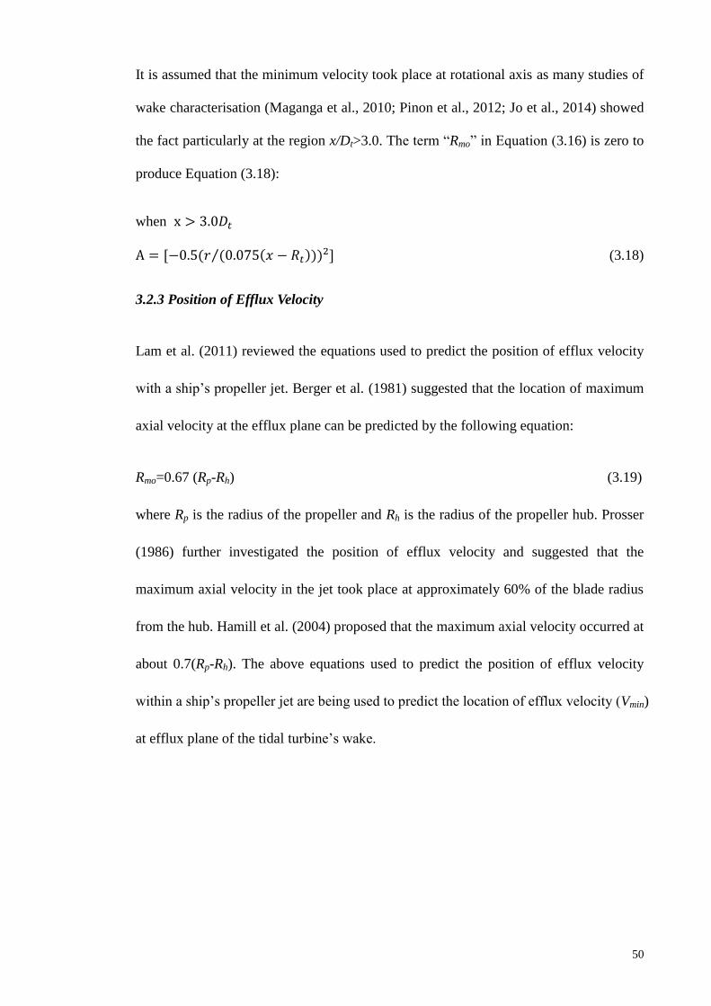
50

It is assumed that the minimum velocity took place at rotational axis as many studies of

wake characterisation (Maganga et al., 2010; Pinon et al., 2012; Jo et al., 2014) showed

the fact particularly at the region x/Dt>3.0. The term “Rmo” in Equation (3.16) is zero to

produce Equation (3.18):

when x > 3.0𝐷𝑡

A = [−0.5(𝑟 (0.075(𝑥 − 𝑅𝑡)))2]⁄ (3.18)

3.2.3 Position of Efflux Velocity

Lam et al. (2011) reviewed the equations used to predict the position of efflux velocity

with a ship’s propeller jet. Berger et al. (1981) suggested that the location of maximum

axial velocity at the efflux plane can be predicted by the following equation:

Rmo=0.67 (Rp-Rh) (3.19)

where Rp is the radius of the propeller and Rh is the radius of the propeller hub. Prosser

(1986) further investigated the position of efflux velocity and suggested that the

maximum axial velocity in the jet took place at approximately 60% of the blade radius

from the hub. Hamill et al. (2004) proposed that the maximum axial velocity occurred at

about 0.7(Rp-Rh). The above equations used to predict the position of efflux velocity

within a ship’s propeller jet are being used to predict the location of efflux velocity (Vmin)

at efflux plane of the tidal turbine’s wake.

51

3.2.4 Recovery of Minimum Axial Velocity

The prediction of lateral velocity behind tidal turbines is based on predicting the

minimum velocity at various sections. Once the minimum velocity at a certain

cross-section is attained, the lateral distribution at the plane can be approximated using

the developed equations. The minimum velocity at various sections is not constant. It

changes along the downstream as the water in the wake region mixes with ambient

fluids. An empirical equation is derived from the experimental data of Maganga et al.

(2010) to provide a useful method to predict the recovery rate of minimum velocity at

downstream of the turbine wake. The recovery of minimum velocity at downstream of

the turbine wake from Maganga et al. (2010) is shown in Figure 3.3

Figure 3.3: Dimensionless minimum axial velocity recovery of turbine wake (TI=8%).

y = 0.0927x + 0.993

R² = 0.993

0.0

0.5

1.0

1.5

2.0

2.5

0 1 2 3 4 5 6 7 8 9 10

Vm

in/V

o

x/Dt

TI=8%

52

A linear relationship between Vmin/Vo and x/Dt with correlation coefficient

R2=0.993 is proposed to predict minimum velocity from efflux plane x/Dt=0.

𝑉𝑚𝑖𝑛𝑉𝑜

⁄ = 0.0927 (𝑥𝐷𝑡

⁄ ) + 0.993 (3.20)

Equation (3.20) can be used to predict the minimum velocity along the downstream

of turbine wake when the ambient turbulence intensity is approximately 8%. The

obtained minimum velocity at each lateral section is an initial input to estimate the

lateral velocity distribution.

3.2.4.1 Influence of Turbulence Intensity

The turbulence intensity (TI) is not a globe constant, or even a geographical site

constant. According to Mac Enri et al. (2013) presented that the turbulence intensity

varies from 3.2% to 7.1% depending on the mean velocity, edd and flood or neap and

spring tides. Therefore, the analytical wake model aims to predict wake velocity under

various ambient turbulent intensity (TI=3%, 5%, 8% and15%). The turbulence intensity

is commonly occurred in the real site. Figure 3.4 presented the dimensionless minimum

axial velocity recovery under low turbulence condition (TI=3%). The recovery rate is

rather slow in the near wake region (x/Dt<4). The recovery of minimum axial velocity is

getting faster in the region x/Dt>4. It may be due to lack of mixing under the low

turbulence intensity. Empirical equations are proposed to predict the minimum axial

velocity at each lateral section under low turbulence conditions (TI=3%).

53

Figure 3.4: Dimensionless minimum axial velocity recovery of turbine wake

(TI=3%)

0 < 𝑥𝐷𝑡

⁄ ≤ 4

𝑉𝑚𝑖𝑛𝑉𝑜

⁄ = 0.0106 (𝑥𝐷𝑡

⁄ ) + 1.0351 (3.21)

𝑥𝐷𝑡

⁄ > 4

𝑉𝑚𝑖𝑛𝑉𝑜

⁄ = 0.1123 (𝑥𝐷𝑡

⁄ ) + 0.5826 (3.22)

Figure 3.5 illustrated the dimensionless minimum axial velocity recovery under

ambient turbulence intensity TI=15%. The ambient turbulence is high so that the water

in the wake region has strong mixing with ambient fluids. The recovery rate in the near

wake region is much faster than that of the previous two conditions. Empirical

equations are proposed to predict the decay of minimum axial velocity as follows:

y = 0.0106x + 1.0351

R² = 0.1772

y = 0.1123x + 0.5826

R² = 0.9919

0.0

0.5

1.0

1.5

2.0

2.5

0 1 2 3 4 5 6 7 8 9 10

Vm

in/V

o

x/Dt

TSR=3.67, TI=3%

54

0 < 𝑥𝐷𝑡

⁄ ≤ 4

𝑉𝑚𝑖𝑛𝑉𝑜

⁄ = 0.1505 (𝑥𝐷𝑡

⁄ ) + 0.8597 (3.23)

𝑥𝐷𝑡

⁄ > 4

𝑉𝑚𝑖𝑛𝑉𝑜

⁄ = 0.0372 (𝑥𝐷𝑡

⁄ ) + 1.4085 (3.24)

Figure 3.5: Dimensionless minimum axial velocity recovery of turbine wake

(TI=15%)

y = 0.1505x + 0.8597

R² = 0.7988 y = 0.0372x + 1.4085

R² = 0.87

0.0

0.5

1.0

1.5

2.0

2.5

0 1 2 3 4 5 6 7 8 9 10

Vm

in/V

o

x/Dt

TSR=3.67, TI=15%

55

3.3 Numerical Simulation

3.3.1 OpenFOAM

The OpenFOAM toolbox is a free, open source CFD software package produced by

OpenCFD Ltd (OpenFOAM, 2015). The CFD package should be able to provide a

reliable prediction of the velocity field around the rotor discs of tidal turbines and able

to recreate the turbine geometry similar to the prototype. The OpenFOAM users are able

to modify the source code to satisfy their respective simulation objectives. It is a great

advantage which makes many challenging simulations of engineering issues achievable.

The solver employed in the current study is so called pimpleDyMFoam. It is a transient

solver for incompressible, flow of Newtonian fluids on a moving mesh. The solving

algorithm is PIMPLE, as it is a new algorithm merged from PISO (pressure implicit

with a splitting of operators) and SIMPLE (semi-implicit method for pressure linked

equations) algorithms (Higuera et al., 2013). The “DyM” in pimpleDyMFoam stands

for dynamic meshes. Hence, it is capable of simulating the rotating movement of turbine

rotors. It also can simulate the dynamic mesh refinement along the surface of the turbine

blades.

3.3.2 Governing Equations

The governing equations for the fluid are the RANS equations. The details of the

equations can be found in the OpenFOAM source code. The equations are solved in

ensemble-averaged form, including appropriate models for the effect of turbulence

(OpenFOAM, 2015). The turbulence in the fluid is estimated by the standard 𝑘 − 휀

turbulence model (Launder and Spalding, 1972). It is a well-established turbulence

56

model. The two equations allow the turbulent velocity and length scales to be

independently determined. This model is semi-empirical and solved flows based on the

assumption that the rate of production and dissipation of turbulent flows are in

near-balance in energy transfer. The dissipation of the energy, ε can be expressed as

Eq. (3.25):

ε =𝑘3/2

𝑙 (3.25)

where k represents the kinetic energy of the flow and l is the length scale involved. This

is related to the turbulent viscosity, 𝜇𝑡 based on the Prandtl Mixing length model as

Equation. (3.26).

𝜇𝑡 = 𝜌𝐶𝜇𝑘2

(3.26)

where 𝐶𝜇 is an empirical constant and 𝜌 is the density of the flow. The standard

k − ε model uses the following transport equations for 𝑘 and 휀 (Equations (3.27) and

(3.28)).

𝜕(𝜌𝑘)

𝜕𝑡 + div (𝜌𝑘𝒖)= div[

𝜇𝑡

𝜎𝑘𝑔𝑟𝑎𝑑(𝑘)]+2𝜇𝑡𝐸𝑖𝑗𝐸𝑖𝑗 − 𝜌휀 (3.27)

and the 휀 equation as

𝜕(𝜌𝑘)

𝜕𝑡 + div (𝜌휀𝒖)= div[

𝜇𝑡

𝜎𝑔𝑟𝑎𝑑(휀)]+ 𝐶1 𝑘

2𝜇𝑡𝐸𝑖𝑗𝐸𝑖𝑗 − 𝐶2 𝜌2

𝑘 (3.28)

where 𝐸𝑖𝑗 is the mean rate of deformation of a fluid element in a turbulent flow

(Versteeg and Malalasekera, 1995).

Transient term Convection term Diffusion term Production term Destruction term

57

The 𝑘 and 휀 equations are developed by inserting them into the transport

equations. The transport equation has the transient term, convection term, diffusion term,

production term and destruction term. The production term in the k equation is to

transfer the energy from the mean flow to the turbulence whereas the destructive term is

responsible for the dissipation of energy, into heat due to the viscous nature of the flow.

The constants in the equations have been given after a wide range of examinations for

turbulent flows, where 𝐶𝜇=0.09; 𝐶1 = 1.44;𝐶2 = 1.92 𝜎𝑘 = 1.00; 𝜎 =1.30.

3.3.3 Geometry Creation

The blade geometry of turbine was generated based on the IFREMER-LOMC

configuration as shown in Pinon et al. (2012). The origins of the turbine blade were

from Tidal Generation Limited. Table 3.1 shows the IFREMER-LOMC configuration

of the turbine blade. The turbine blades were designed according to a NACA 63418

profile which has been widely used. The duplication of the turbine blade was done by

using the open source software SALOME. The turbine geometry was created in stereo

lithography (STL) format and imported to OpenFOAM. Figure 3.6 shows the turbine

geometries with different number of blades.

58

Table 3.1: General blades geometry description for IFREMER-LOMC configuration

Description IFREMER-LOMC

Rotor radius (Rt) 350mm

Hub radius 46mm

Hub length 720mm

Pitch (set angle) 0o

TSR (Tip Speed Ratio) 3.67

Sense of rotation Anti-clockwise

Reynolds number ≈280,000

Figure 3.6: The geometry of turbines with different blade numbers.

59

3.3.4 Boundary and Initial Conditions

Parameters have to be determined before the setting of the boundary and initial

conditions. The Tip Speed Ratio (TSR) is one of the parameters and defined as:

𝑇𝑆𝑅 =Ф𝑅𝑡

𝑉∞ (3.29)

where Rt is the turbine radius in meter, Ф is the rotational speed in radian per second

and V∞ is the upstream current velocity in meter per second. The TSR for

IFREMER-LOMC case equals to 3.67. According to the radius of the turbine and inlet

flow velocity 0.8 m/s, it is known that the turbine rotates at a constant speed of 480

deg/s.

A seabed was virtually created and was modelled using the no-slip boundary

condition. The no-slip seabed condition allows the viscous effects of seabed faces and

lead to the formation of a boundary layer. The setting of no-slip condition at the bottom

wall is due to such a fact that a boundary layer occurs at the seabed in real world case.

In addition, the free surface interface between the water and air was not included in the

numerical model in order to reduce the computational time. The sliding mesh modelling

technique was used in the simulation case. The Arbitrary Mesh Interface (AMI) was

applied between the rotor and stator sub-domains. AMI is a technique that allows the

numerical simulation across disconnected mesh domains in adjacent region. The

domains can be stationary or move relative to one another (OpenFOAM, 2015). The

external boundary conditions are tabulated in Table 3.2. The dimensions of the

computational domain are 2.86Dt and 2.86Dt, 3.00Dt in the x-, y- and z-directions,

respectively (see Figure 3.7). The flow direction is from –x to x.

60

Table 3.2: Boundary condition of domain

Designation Description Boundary condition

AA1BB1 Inlet fixedValue

AA1DD1 Side wall No slip (fixed wall)

DD1EE1 Outlet inletOutlet

BB1EE1 Side wall No slip (fixed wall)

ABDE Top wall No slip (fixed wall)

A1B1D1E1 Bottom wall No slip (fixed wall)

G Turbine AMI

Figure 3.7: The computational domain.

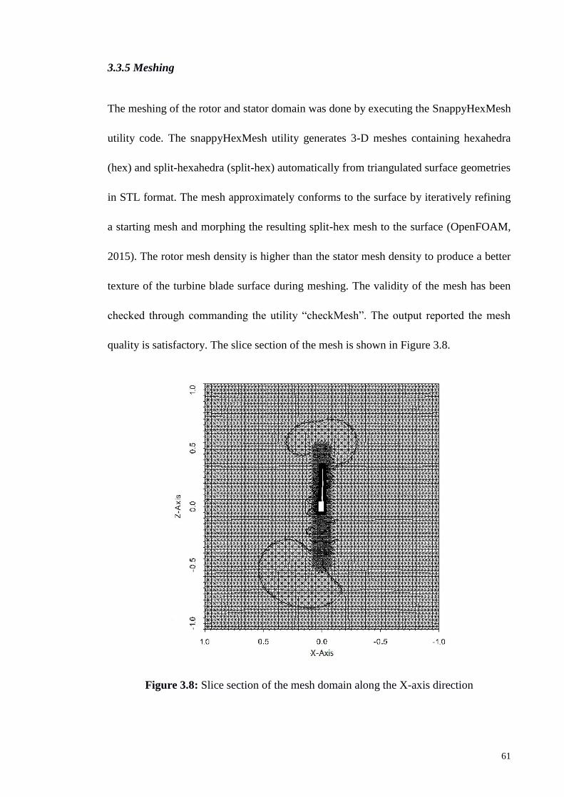
61

3.3.5 Meshing

The meshing of the rotor and stator domain was done by executing the SnappyHexMesh

utility code. The snappyHexMesh utility generates 3-D meshes containing hexahedra

(hex) and split-hexahedra (split-hex) automatically from triangulated surface geometries

in STL format. The mesh approximately conforms to the surface by iteratively refining

a starting mesh and morphing the resulting split-hex mesh to the surface (OpenFOAM,

2015). The rotor mesh density is higher than the stator mesh density to produce a better

texture of the turbine blade surface during meshing. The validity of the mesh has been

checked through commanding the utility “checkMesh”. The output reported the mesh

quality is satisfactory. The slice section of the mesh is shown in Figure 3.8.

Figure 3.8: Slice section of the mesh domain along the X-axis direction

62

3.4 Experiment Set-up for Scour Test

A series of clear water scour tests have been performed in the Hydraulic Laboratory of

University of Malaya, Malaysia. The flume is 16 m long and 1 m wide, built with

transparent glass wall for flow visualization (See Figure 3.9). The turbine positioned 5

m downstream of the channel origin (x=0 m). The incoming flow was conditioned using

a porous mattress to break the turbulence structures created from the pump and supply

pipes, therefore offering uniform flow for the test section. The turbine support tower and

nacelle were made from PVC pipe. The turbine rotor was fabricated by rapid

prototyping using ABS material. The turbine was outfitted with a miniature DC motor

for voltage measurements. Reasonable tip speed ratios were maintained by the internal

resistance of the device. The flow depth was maintained by the tailgate, while the water

was supplied by three pumps.

Figure 3.9: Tilting flume in Hydraulic Laboratory, University of Malaya

63

The turbine model used during the experimental testes was a three bladed axis flow

turbine with rotor diameter Dt = 0.2 m. The diameter of the turbine support tower was

0.02 m. The flow depth 0.45 m was maintained by adjusting the tailgate at the end of

flume. The approaching velocity 0.23 m/s was also maintained constantly during the

experiments. The velocity of the incoming flow is monitored by the 2D mini LDV

system (See Figure 3.10). At 1:70th

geometric scaling the experiments in the scour

investigation represents a 14 m diameter turbine in water depth of 31.5 m and applying

Froude similitude, a mean velocity of 1.92 m/s. The experimental scaling issue of tidal

turbine has been highlighted by Harrison et al. (2010) and Myers and Bahaj (2010).

High Froude numbers often take place in laboratory that may lead to alteration of water

surface. Froude similarity is normally maintained between model system and prototype.

Myers and Bahaj (2010) also stated that discrepancy in Reynolds numbers between

prototype and model is acceptable for the scaling of hydraulic channels under the

following two conditions: 1) Froude similarity is maintained; 2) both full-scale and

model Reynolds numbers are within the same turbulent region.

A sediment recess 0.1 m deep, 5.0 m long and 1.0 m wide was constructed inside

the flume. Before commencement of each experiment, the sediment was first levelled

using a sand leveller. The turbine position and test section were selected to be within an

area where the flow and the underlying bed topography were sufficiently far from inlet

and outlet of the flume. During the tests, the TCT was embedded in the middle of the

bed sediment recess. The flume was slowly filled with water from both upstream and

downstream pipes at a low rate. It prevents the disturbance of the levelled sand bed.

Once the predetermined water depth was reached, the pump will be on and the

experimental run was started by adjusting the flow rate at the inlet.

64

The water was carefully drained off from the flume at the end of each test to

prohibit the disturbance to the scour profiles. The scour profiles around the

pile-supported TCT are measured by a laser distance meter with an accuracy of 0.1 mm.

The laser distance meter measured the bed elevation for each 1 cm in length and 1 cm in

width. The detailed parameters of the experiments are presented in Table 3.3.

Figure 3.10: mini LDV measurement system

The geometric standard deviation was calculated from 𝜎𝑔= (d84/d16)0.5

= 1.3 which

is smaller than 1.4. It is indicating that the sand was uniformly graded (Barkdoll et al.

2007). The flow depth was also set to ensure approach section the incoming flow

velocity at the approach section (uf) was below the critical incipient velocity (ucr)

(uf<ucr=0.032 m/s, for the sand bed-material of d50=1.0 mm) based on the Shield curve

(Wu and Wang, 1999). Figure 3.11 presents a schematic diagram of the test section,

turbine and instrumentation used during the experimental tests. Figure 3.12 illustrates

the photo of turbine model and flume.

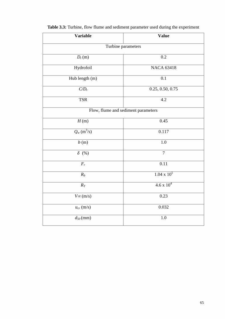
65

Table 3.3: Turbine, flow flume and sediment parameter used during the experiment

Variable Value

Turbine parameters

Dt (m) 0.2

Hydrofoil NACA 63418

Hub length (m) 0.1

C/Dt 0.25, 0.50, 0.75

TSR 4.2

Flow, flume and sediment parameters

H (m) 0.45

Qw (m3/s) 0.117

b (m) 1.0

𝛿 (%) 7

Fr 0.11

Rb 1.04 x 105

RT 4.6 x 104

V (m/s) 0.23

ucr (m/s) 0.032

d50 (mm) 1.0

66

Figure 3.11: Schematic view of scour experiment

Figure 3.12: Photo of turbine model (Dt = 0.2 m) and flume

67

CHAPTER 4: RESULTS AND DISCUSSION

4.1 Overview

This chapter documents the results and relevant discussion of the study. Section 4.2

shows the validation of the proposed model. Despite the direct comparison of predicted

velocity with experimental data, a goodness of fit test is also conducted to testify the

level of accuracy of the proposed model. Section 4.3 documents the characterization of

the flow below turbine rotor. Axial, radial and tangential component of velocity below

the turbine rotor are illustrated. Section 4.4 presents the scour evolution and profile

around the support structure of tidal current turbine.

4.2 Wake Prediction

4.2.1 Position of Efflux Velocity

The experimental results from Maganga et al. (2010), Pinon et al. (2012) and Mycek et

al. (2014) are used for the validation of the proposed wake model. The turbine

incorporated in their experiments is based on NACA 63418 and the general geometrical

properties of the turbine are shown in Table 4.1. The calculated locations of minimum

velocities (Rmo) in the turbine wake are tabulated in Table 4.2. The Rmo was initially

assumed to be 0.2.

68

Table 4.1: General geometric properties of turbine

Rotor diameter 350 mm

Radius of hub 46 mm

Number of blades 3

Position of rotor relative to flume tank Upstream

Pitch angle (degree) 0

Table 4.2: Position of efflux velocity

Equation Rmo

Berger et al. (1987), Rmo=0.67 (R-Rh) 0.20

Prosser (1986), Rmo=0.6R 0.21

Hamill et al. (2004), Rmo=0.7 (R-Rh) 0.21

4.2.2 Comparison of Results with Previous Model and Experimental Data

The study conducted by Maganga et al. (2010) has been chosen to further testify the

validity of the proposed wake model. The previous proposed analytical equation by the

Lam and Chen (2014) has also been incorporated in the comparison. Figure 4.1 (a-f)

illustrates the comparison of experimental measurements and the theoretical predictions

by the authors. The experimental work conducted by Maganga et al. (2010) suggested

the wake profiles have two dips at x/Dt=1.0 and x/Dt=2.0.

69

a. x/Dt=1.0

b. x/Dt=2.0

Figure 4.1: Validation of the proposed analytical wake model: (a) x/Dt=1.0; (b) x/Dt=2.0;

(c) x/Dt=3.0; (d) x/Dt=5.0; (e) x/Dt=7.0 and (f) x/Dt=9.0

-3.0

-2.0

-1.0

0.0

1.0

2.0

3.0

0.0 0.2 0.4 0.6 0.8 1.0 1.2

r/R

t

Va/V

Exp. Data

Proposed Eq.

Lam and Chen (2014）

-3.0

-2.0

-1.0

0.0

1.0

2.0

3.0

0.0 0.2 0.4 0.6 0.8 1.0 1.2

r/R

t

Va/V

Exp. Data

Proposed Eq.

Lam and Chen (2014）

70

c. x/Dt=3.0

d. x/Dt=5.0

Figure 4.1, continued.

-3.0

-2.0

-1.0

0.0

1.0

2.0

3.0

0.0 0.2 0.4 0.6 0.8 1.0 1.2

r/R

t

Va/V

Exp. Data

Proposed Eq.

Lam and Chen (2014）

-3.0

-2.0

-1.0

0.0

1.0

2.0

3.0

0.0 0.2 0.4 0.6 0.8 1.0 1.2

r/R

t

Va/V

Exp. Data

Proposed Eq.

Lam and Chen (2014）

71

e. x/Dt=7.0

f. x/Dt=9.0

Figure 4.1, continued.

-3.0

-2.0

-1.0

0.0

1.0

2.0

3.0

0.0 0.2 0.4 0.6 0.8 1.0 1.2

r/R

t

Va/V

Exp. Data

Proposed Eq.

Lam and Chen (2014）

-3.0

-2.0

-1.0

0.0

1.0

2.0

3.0

0.0 0.2 0.4 0.6 0.8 1.0 1.2

r/R

t

Va/V

Exp. Data

Proposed Eq.

Lam and Chen (2014）

72

Lam and Chen (2014) discussed this issue based on the experience of ship propeller

jets. The influence of the hub disappears gradually along the longitudinal axis due to

penetration of high velocity fluid into low velocity central core. The fluids in the ship

propeller jet are mixing with the surrounding water both inwardly and outwardly along

the rotational axis (Lam et al., 2011). The fluids only mix outwardly at a certain

distance downstream where the ship propeller jet is fully expanded. There is only one

maximum velocity peak located at the axis of rotation in the zone of established flow

(Lam et al., 2011). The dips in the turbine wake also disappear gradually along the

longitudinal axis. There is only one minimum velocity located at the rotational axis at

further downstream of wake region.

It was noticed that the new theoretical predicted curve at x/Dt=1.0, x/Dt=2.0 and

x/Dt=3.0 fits the measured curve principally. The region of r/Rt=1.2 to 3.0 and -1.2 to

-3.0 showed some discrepancies between the new theoretical and experimental values of

mean streamwise velocity. The largest variation of the theoretical mean streamwise

velocity of this region was approximately 8% compared with experimental results. The

variation in percentage is calculated by applying the formula shown in Equation (4.1).

𝑉𝑎𝑟𝑖𝑎𝑡𝑖𝑜𝑛 (%) = 𝐸𝑥𝑝𝑒𝑟𝑖𝑚𝑒𝑛𝑡𝑎𝑙 𝑚𝑒𝑎𝑠𝑢𝑟𝑒𝑚𝑒𝑛𝑡−𝑇ℎ𝑒𝑜𝑟𝑒𝑡𝑖𝑐𝑎𝑙 𝑝𝑟𝑒𝑑𝑖𝑐𝑡𝑖𝑜𝑛

𝐸𝑥𝑝𝑒𝑟𝑖𝑚𝑒𝑛𝑡𝑎𝑙 𝑚𝑒𝑎𝑠𝑢𝑟𝑒𝑚𝑒𝑛𝑡× 100% (4.1)

This discrepancy might be due to the effect of the free surface. The water surface in

the experimental flume may have fluctuation. The support structure of the turbine may

be another contributor to the variation. The comparison of experimental results and

theoretical predictions at the rotational axis also showed inconformity. The

disagreement at the rotational axis at x/Dt=1.0 is high, which is approximately 25%. The

high discrepancy at this region might be due to the hub. The length of the hub is

equivalent to one diameter of the turbine. The predictions of the new analytical equation

73

and experimental data have a good agreement at the rotational axis at x/Dt=2.0 and

x/Dt=3.0.

The newly proposed Equation (3.14) has an advantage over the equation suggested

by Lam and Chen (2014). The derivation of the equation from Lam and Chen (2014) is

based on the axial momentum theory and plain water jet. In reality, the velocity

characteristic of a ship’s propeller jet is more complicated than a plain water jet. The

dips appearing in the figures were therefore not able to be predicted by the equation

proposed by Lam and Chen (2014). The minimum velocities uniformed the velocities in

the region from r/Rt=-0.8 to 0.8 in Figures 4.1(a)-4.1(c). The new analytical wake model

is a refinement of the previous equations. It is able to predict the lateral velocity

distribution behind tidal current turbine with the appearance of dips in the near wake

region.

Figure 4.1(e)-4.1(f) illustrate the properties of the lateral velocity distribution at 5.0

Dt, 7.0 Dt and 9.0 Dt downstream, respectively. The wakes are fully expanded and there

is only one minimum velocity located at the axis of rotation. The experimental

measurements of the wake profiles at downstream distances of 5 Dt, 7.0 Dt and 9.0 Dt

produce a classical Gaussian distribution shape. The new wake model is also able to

predict the velocity distribution at these locations. The new theoretically predicted curve

at the lateral distance x/Dt =5.0 fits the experimental measurement curve well. It has

better predictions compared to the previous equations proposed by Lam and Chen

(2014). The prediction at the region from r/Rt=0 to r/Rt=-1.0 nearly overlaps with

experimental data. The largest variation in mean stream wise velocity between the

experimental results and the theoretical predictions is approximately 7%, which is 2%

less than the equation proposed by Lam and Chen (2014). The prediction of lateral

velocity distribution at x/Dt =7.0 and x/Dt =9.0 has equal performance as the previously

74

proposed equation. No evident deviation is observed among the two theoretical

predictions.

4.2.3 Influence of Turbulence Intensity

4.2.3.1 Turbulence Intensity (TI=3%and 5%)

The experimental results from Mycek et al. (2014) have been chosen to testify the

applicability of the proposed equation under ambient turbulence intensity (TI=3%).

Wake growth rate c was introduced and is replacing the constant 0.075 in Equation

(3.16). Figure 4.2 demonstrates the comparison of predicted wake profile with

experimental results under turbulence intensity of 3%. The wake growth rate c=0.065 is

suggested to fit the experimental data. The experimental conducted by Pinon et al.

(2012) which with 5% ambient turbulence intensity also incorporated in the comparison.

The wake shape of the experimental results under TI=3% and TI=5% have similar

manner. The variation of these two turbulence levels is not significant. Another possible

explanation for this phenomenon is that the ratio of the ambient turbulence intensity to

the turbulence added by the tidal turbine itself is small. It is, therefore, the incoming

turbulence does not result in many differences in the mixing process. The predicted

lateral velocity distributions are in acceptable agreement with experimental results. The

major discrepancy occurred at the rotational axis at x/Dt =1.2, x/Dt =2.0 and x/Dt =3.0. It

might be due to the flow disturbance caused by the hub.

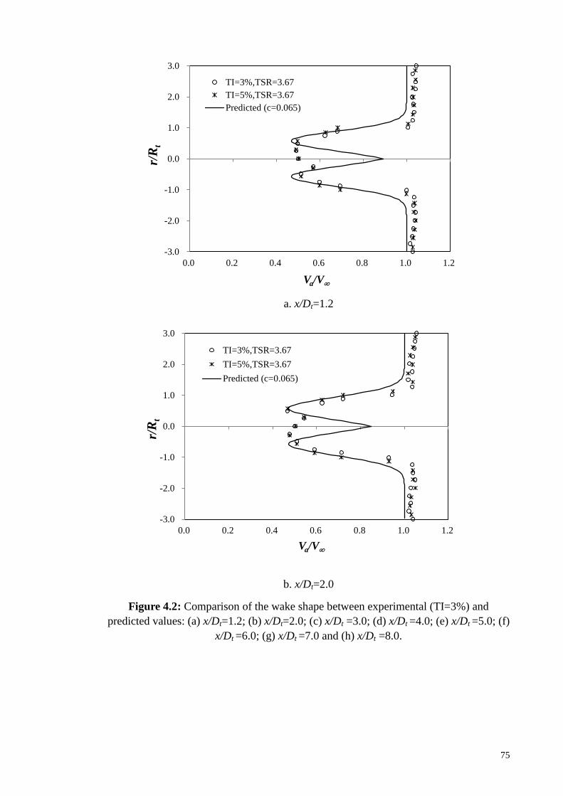
75

a. x/Dt=1.2

b. x/Dt=2.0

Figure 4.2: Comparison of the wake shape between experimental (TI=3%) and

predicted values: (a) x/Dt=1.2; (b) x/Dt=2.0; (c) x/Dt =3.0; (d) x/Dt =4.0; (e) x/Dt =5.0; (f)

x/Dt =6.0; (g) x/Dt =7.0 and (h) x/Dt =8.0.

-3.0

-2.0

-1.0

0.0

1.0

2.0

3.0

0.0 0.2 0.4 0.6 0.8 1.0 1.2

r/R

t

Va/V

TI=3%,TSR=3.67

TI=5%,TSR=3.67

Predicted (c=0.065)

-3.0

-2.0

-1.0

0.0

1.0

2.0

3.0

0.0 0.2 0.4 0.6 0.8 1.0 1.2

r/R

t

Va/V

TI=3%,TSR=3.67

TI=5%,TSR=3.67

Predicted (c=0.065)

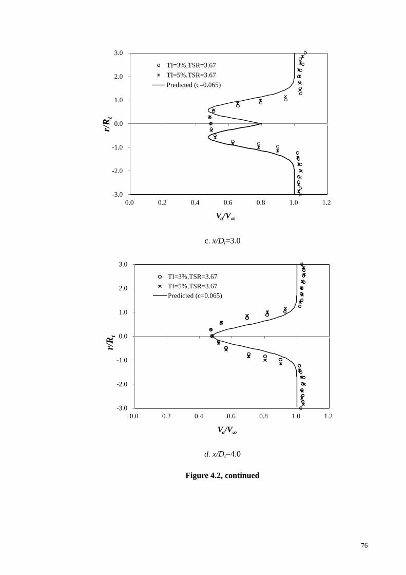
76

c. x/Dt=3.0

d. x/Dt=4.0

Figure 4.2, continued

-3.0

-2.0

-1.0

0.0

1.0

2.0

3.0

0.0 0.2 0.4 0.6 0.8 1.0 1.2

r/R

t

Va/V

TI=3%,TSR=3.67

TI=5%,TSR=3.67

Predicted (c=0.065)

-3.0

-2.0

-1.0

0.0

1.0

2.0

3.0

0.0 0.2 0.4 0.6 0.8 1.0 1.2

r/R

t

Va/V

TI=3%,TSR=3.67

TI=5%,TSR=3.67

Predicted (c=0.065)

77

e. x/Dt=5.0

f. x/Dt=6.0

Figure 4.2, continued.

-3.0

-2.0

-1.0

0.0

1.0

2.0

3.0

0.0 0.2 0.4 0.6 0.8 1.0 1.2

r/R

t

Va/V

TI=3%,TSR=3.67

TI=5%,TSR=3.67

Predicted (c=0.065)

-3.0

-2.0

-1.0

0.0

1.0

2.0

3.0

0.0 0.2 0.4 0.6 0.8 1.0 1.2

r/R

t

Va/V

TI=3%,TSR=3.67

TI=5%,TSR=3.67

Predicted (c=0.065)

78

g. x/Dt=7.0

h. x/Dt=8.0

Figure 4.2, continued.

-3.0

-2.0

-1.0

0.0

1.0

2.0

3.0

0.0 0.2 0.4 0.6 0.8 1.0 1.2

r/R

t

Va/V

TI=3%,TSR=3.67

TI=5%,TSR=3.67

Predicted (c=0.065)

-3.0

-2.0

-1.0

0.0

1.0

2.0

3.0

0.0 0.2 0.4 0.6 0.8 1.0 1.2

r/R

t

Va/V

TI=3%,TSR=3.67

TI=5%,TSR=3.67

Predicted (c=0.065)

79

4.2.3.2 High Turbulence Intensity (TI=15%)

Figure 4.3 demonstrates the comparison of predicted wake profile with high ambient

turbulence intensity (TI=15%). The experimental data of velocity distribution at these

locations have not shown the appearance of two dips. The two dips merged as one dip at

the region near to the rotational axis. The strong mixing of the wake with ambient fluids

results in the earlier disappearance of two dips. Equation (3.14) and (3.18) are used to

predict the wake profile at high turbulence level. The proposed curve shows

discrepancies at x/Dt=1.2, x/Dt=2.0 and x/Dt=3.0. It overestimates the velocity from

r/Rt=0 to r/Rt=1.0. The water in the wake region has strong mixing with ambient fluids.

The water is highly turbulent and the properties are not feasible to be measured.

Numerical technique is recommended to capture the disappearance of two dips at high

ambient turbulence intensity. However, the predicted wake shapes are in line with the

velocity distribution at far wake region under TI=15% (x/Dt =4.0, 5.0, 6.0, 7.0 and 8.0).

The wake recovers rapidly at this turbulence level and the mixing in the far wake region

tends to be weaker.

80

a. x/Dt =1.2

b. x/Dt =2.0

Figure 4.3: Comparison of the wake shape between experimental (TI=15%) and

predicted values: (a) x/Dt =1.2; (b) x/Dt =2.0; (c) x/Dt =3.0; (d) x/Dt =4.0; (e) x/Dt =5.0;

(f) x/Dt =6.0; (g) x/Dt =7.0 and (h) x/Dt =8.0

-3.0

-2.0

-1.0

0.0

1.0

2.0

3.0

0.0 0.2 0.4 0.6 0.8 1.0 1.2

r/R

t

Va/V

TI=15%,TSR=3.67

Predicted (c=0.095)

-3.0

-2.0

-1.0

0.0

1.0

2.0

3.0

0.0 0.2 0.4 0.6 0.8 1.0 1.2

r/R

t

Va/V

TI=15%,TSR=3.67

Predicted (c=0.095)

81

c. x/Dt =3.0

d. x/Dt =4.0

Figure 4.3, continued.

-3.0

-2.0

-1.0

0.0

1.0

2.0

3.0

0.0 0.2 0.4 0.6 0.8 1.0 1.2

r/R

t

Va/V

TI=15%,TSR=3.67

Predicted (c=0.095)

-3.0

-2.0

-1.0

0.0

1.0

2.0

3.0

0.0 0.2 0.4 0.6 0.8 1.0 1.2

r/R

t

Va/V

TI=15%,TSR=3.67

Predicted (c=0.095)

82

e. x/Dt =5.0

f. x/Dt =6.0

Figure 4.3, continued.

-3.0

-2.0

-1.0

0.0

1.0

2.0

3.0

0.0 0.2 0.4 0.6 0.8 1.0 1.2

r/R

t

Va/V

TI=15%,TSR=3.67

Predicted (c=0.095)

-3.0

-2.0

-1.0

0.0

1.0

2.0

3.0

0.0 0.2 0.4 0.6 0.8 1.0 1.2

r/R

t

Va/V

TI=15%,TSR=3.67

Predicted (c=0.095)

83

g. x/Dt =7.0

h. x/Dt =8.0

Figure 4.3, continued.

-3.0

-2.0

-1.0

0.0

1.0

2.0

3.0

0.0 0.2 0.4 0.6 0.8 1.0 1.2

r/R

t

Va/V

TI=15%,TSR=3.67

Predicted (c=0.095)

-3.0

-2.0

-1.0

0.0

1.0

2.0

3.0

0.0 0.2 0.4 0.6 0.8 1.0 1.2

r/R

t

Va/V

TI=15%,TSR=3.67

Predicted (c=0.095)

84

4.2.4 Proposed Schematic Diagram of Turbine Wake

Hamill (1987) proposed a schematic diagram of a ship propeller jet as shown in Chapter

2 (See Figure 2.6). The preceding discussion indicated that the flow behaviour of

turbine wake has similarities with ship propeller jets. The study depicts a schematic

view of tidal turbine wake. The regions with a turbine wake can also be categorized into

the same zones as a ship propeller jet (See Figure 4.4). The zone of flow establishment

lies close to the turbine face and velocity within the zone has two-dip ridges. The

presence of hub at the centre of turbine results in the wake has a high-velocity core

along the axis of rotation within the zone of flow establishment. At first, the fluid is

mixing with the surrounding water both inwardly and outwardly along the axis of

rotation. The length of the zone of flow establishment depends on the ambient

turbulence intensity. The zone of established flow is following the zone of flow

establishment. In this region, the flow only mix outwardly and it has only one minimum

velocity dip located at the rotational axis.

Figure 4.4: Schematic view of turbine wake (proposed)

85

The proposed wake model has an acceptable agreement with the experimental

results at various ambient turbulence intensities. The new wake model also predicts the

wake shape with appearance of two dips at near wake region. The experimental results

from Maganga et al. (2010), Pinon et al. (2012) and Mycek et al. (2014) also showed

the appearance of two dips in the wake. The experimental results of wake properties at

high ambient turbulence level (15%) do not indicate the appearance of two dips (see

Figure 4.3). The higher turbulence intensity results in the earlier merging of two dips.

The wake deficit behind turbine rotor may cause suspended sediment in the water

to fall down. The concentration of suspended sediment between rotor and seabed may

increase. Consequently, it may affect the bed load and the scour process around the

support of TCT will be affected. The velocity deficit in the wake region also leads to the

flow acceleration below the rotor. Hill et al. (2014) believed that the transition point

between the scour hole and the deposited sand dune may suggest a relationship between

the wake of the tidal turbine and the sand bed surface. The wake velocity at lateral

sections along downstream shows its sediment transport capacity in the water column.

The proposed analytical wake model may serve as an initial input for the scour

prediction. The wake also affects the velocity near seabed and the flow conditions

between rotor and seabed are discussed in Section 4.3.

86

4.2.5 Goodness-of-Fit

The above figures are providing justification for the quality of the fit provided by the

given wake model. The study provides quantitative goodness-of-fit estimator R-square

(R2). This statistic measures how successful the fit is in explaining the variation of the

data. R-square is the square of the correlation between the response values and the

predicted values. R-square is defined as:

R-square=1-[Sum(i=1 to m){wi (yi - fi)2}] /[Sum(i=1 to m){wi (yi - yav)

2}] = 1 - SSE/SST (4.2)

Here fi is the predicted value from the proposed model; yav is the mean of the

experimental data; yi is the experimental data value; m is the number of experimental

data points. wi is the weighting applied to each data point, usually wi=1 (Goodness of fit

Statistics). SSE is the sum of squares due to error and SST is the total sum of squares.

The authors also provide the goodness-of-fit estimator Mean Square Error (MSE).The

MSE is defined as:

MSE=SSE/m (4.3)

MSE value closer to 0 indicates the model is more useful for prediction. The results

of the estimators are tabulated in Table 4.3. The R2 and MSE are in range of

0.1684-0.9305 (close to 1 better) and 0.0004-0.0331 (close to 0 better) respectively. The

R2 are relative low at certain locations. However, the MSE are close to 0 for all the

lateral sections. The results of the MSE provide justifications for the correlations

proposed in the wake model. The prediction of the wake profile usually at x/Dt>3.0 is

better than that of near wake region. The flow in the near wake region is with high shear

87

and turbulent. The wake pattern is rather complicated. More experimental results of near

wake are required for future investigation. The proposed analytical wake model is

indicated in Table 4.4.

Table 4.3: Goodness-of-fit analysis

x/Dt I=3% I=8% I=15%

R2 MSE R2 MSE R2 MSE

1.0 N/A N/A 0.3455 0.0331 N/A N/A

1.2 0.3188 0.0327 N/A N/A 0.7073 0.0111

2.0 0.3473 0.0320 0.4411 0.0290 0.7813 0.0056

3.0 0.3766 0.0289 0.5478 0.0186 0.8064 0.0006

4.0 0.8491 0.0064 N/A N/A 0.5502 0.0021

5.0 0.9305 0.0017 0.9098 0.0023 0.6009 0.0011

6.0 0.9172 0.0024 N/A N/A 0.2823 0.0008

7.0 0.8071 0.0042 0.7507 0.0036 0.1684 0.0006

8.0 0.7999 0.0035 N/A N/A 0.5381 0.0004

9.0 N/A N/A 0.6112 0.0037 N/A N/A

*N/A: experimental results not available

88

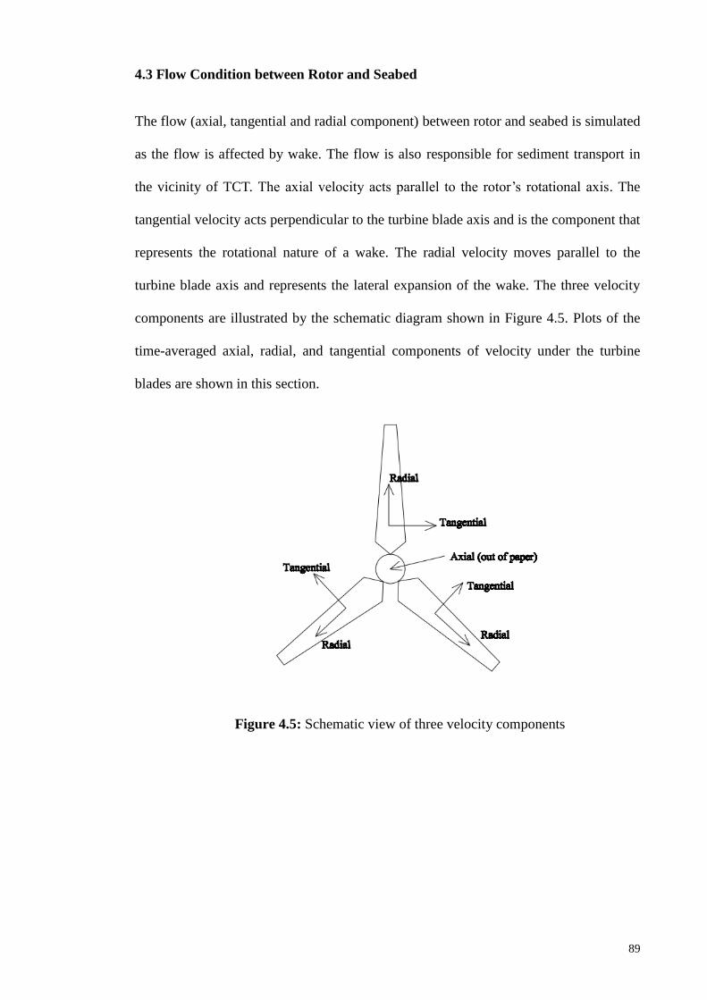
89

4.3 Flow Condition between Rotor and Seabed

The flow (axial, tangential and radial component) between rotor and seabed is simulated

as the flow is affected by wake. The flow is also responsible for sediment transport in

the vicinity of TCT. The axial velocity acts parallel to the rotor’s rotational axis. The

tangential velocity acts perpendicular to the turbine blade axis and is the component that

represents the rotational nature of a wake. The radial velocity moves parallel to the

turbine blade axis and represents the lateral expansion of the wake. The three velocity

components are illustrated by the schematic diagram shown in Figure 4.5. Plots of the

time-averaged axial, radial, and tangential components of velocity under the turbine

blades are shown in this section.

Figure 4.5: Schematic view of three velocity components

90

4.3.1 Influence of Rotor Tip Clearance

4.3.1.1 Axial Velocity

Ship propeller jet-induced scour has been studied for many years. Earlier researchers

focused solely on the axial velocity field within the ship’s propeller jets, due to the large

contribution made by the axial velocity to seabed scouring. Lam et al. (2011) conducted

Laser Doppler Anemometry measurement and claimed that the axial component of

velocity is the main contributor to the velocity magnitude of the initial plane of a ship’s

propeller jet. Liu (2010) compared the downstream velocity profile of a propeller and a

tidal turbine. It found that the direction of the downstream velocities of a propeller

against that a turbine is opposing. This phenomenon indicates the different function of a

tidal turbine and a propeller. The propeller is trying to transfer energy into the fluids

which result in the acceleration of inflow. The tidal turbine aims to harness the kinetic

energy from fluids and ends up slowing down the inflow.

Table 4.5 tabulates each maximum component velocity of the flow between the

TCT and the seabed. It indicates that axial velocity is the biggest contributor to the

velocity magnitude, in the same manner as ship’s propeller jets. The maximum axial

component of velocity in the investigated layers occurred in 0.5C (C=0.4Dt), x/Dt=0.4.

The maximum value of axial velocity has approximately 1.07 times greater than the

initial velocity. The maximum local acceleration of velocity around the current

extraction device in the study of Sun (2008) study is approximately 1.2 times of its

initial velocity. The maximum velocity locates at x/Dt=1 and 0.3Dt away from the tip of

the turbine blade. The flow acceleration in Sun’s work is more significant than the

91

current simulation. The experimental instrument applied in her study is actuator disk. It

suggests that the turbine characteristic influences the extent of flow acceleration.

Furthermore, Sun took the free surface effect of numerical modelling into consideration.

The interaction between air and water might increase the velocity around the turbine.

Table 4.5: Maximum velocity component at each investigated layer

Height of

tip

clearance

Layer Axial velocity Radial velocity Tangential

velocity

(Va/V)% (Vr/Va)% (Vt/Va)%

1.00Dt 0.50C 105.15 2.05 0.03

0.25C 104.66 0.73 <0.01

0.05C 100.00 0.27 <0.01

0.80Dt 0.50C 105.53 2.48 0.05

0.25C 104.93 0.93 0.02

0.05C 100.07 0.30 0.01

0.60Dt 0.50C 106.00 3.12 0.08

0.25C 105.19 1.27 0.04

0.05C 84.39 0.31 0.04

0.40Dt 0.50C 106.69 4.12 0.22

0.25C 105.30 1.80 0.11

0.05C 60.00 0.70 0.08

Figure 4.6 shows that the axial velocity of different layers between the TCT and the

seabed under different heights of tip clearance. The axial component of velocity in the

upper two investigated layers (0.25C and 0.50C above seabed) has a moderate increase.

The increment of velocity is approximately 5% of the initial incoming flow in average.

The axial velocity near seabed (0.05C above seabed) at each tip clearance case is lesser

than the initial velocity due to the boundary layer effect. However, the fluids at each

layer below and behind the turbine have slight higher axial velocity than that at the

same level before turbine. This behaviour is different with the fluids passed through the

rotor plane. The fluids passed through the rotor plane region experienced velocity

92

reduction and formed an expanding wake. The faster moving stream (below rotors)

serves to re-energise the wake, breaking it up and increasing the velocity (Myers and

Bahaj, 2010).

Moreover, the contraction of the TCT increases flow velocity. Based on the

Bernoulli equation, the increase of velocity will be balanced by the decrease in pressure.

As shown in Figure 4.7, the pressure of the fluids behind the turbine blades decreased at

each investigated layer. The pressure has been non-dimensionalised by the atmospheric

pressure (101.325 kPa). The difference of pressures on the two sides of turbine blades

results in a suction phenomenon. The fluids at the high pressure side will be sucked to

the low pressure side. This suction effect further accelerates the fluids below turbine

blades on the back side. These reasons mentioned above contributed to the velocity

acceleration of the fluids in each investigated layer. Figure 4.8 presents a schematic

diagram to describe the flow under rotors of the TCT. A low pressure zone is formed

below the boundary of the wake.

93

Figure 4.6: Dimensionless axial component velocity at different layers with various tip

clearances from seabed: a. 1.0Dt; b. 0.8Dt; c. 0.6Dt; d. 0.4Dt.

0.5

0.6

0.7

0.8

0.9

1.0

1.1

-1.5 -1.0 -0.5 0.0 0.5 1.0 1.5

Va/V

0

x/Dt

a.

0.50C

0.25C

0.05C

0.5

0.6

0.7

0.8

0.9

1.0

1.1

-1.5 -1.0 -0.5 0.0 0.5 1.0 1.5

Va/V

0

x/Dt

b.

0.50C

0.25C

0.05C

94

Figure 4.6, continued.

0.5

0.6

0.7

0.8

0.9

1.0

1.1

-1.5 -1.0 -0.5 0.0 0.5 1.0 1.5

Va/V

0

x/Dt

c.

0.50C

0.25C

0.05C

0.5

0.6

0.7

0.8

0.9

1.0

1.1

-1.5 -1.0 -0.5 0.0 0.5 1.0 1.5

Va/V

0

x/Dt

d.

0.50C

0.25C

0.05C

95

Figure 4.7: Dimensionless pressure of fluids at different layers near seabed (height of

tip clearance=1.0Dt)

0.00000

0.00005

0.00010

0.00015

0.00020

0.00025

0.00030

0.00035

0.00040

-1.5 -1.0 -0.5 0.0 0.5 1.0 1.5

P/P

a

x/Dt

0.50C

0.25C

0.05C

96

Figure 4.8 Schematic diagram of flow between the seabed and the TCT

The distribution of axial component velocity has a similar pattern despite different

confinements. The influence of seabed proximity in the current study is not evident. It

suggests the wake does not expand remarkably and it approaches the seabed. The fluids

beneath the rotor disk are enough to re-energise the wake. Moreover, the solidity of

turbine blade is low. The fluids pass through the turbine smoothly as the blockage effect

is not significant. The flow suppression under the turbine is not pronounced. A turbine

with high blade area ratio may have different velocity pattern when the confinement

below turbine varies. The flow acceleration below the turbine blades is expected to

develop along the downstream of the wake. The flow acceleration will probably affect

the scour process and amplify the sediment transport at seabed.

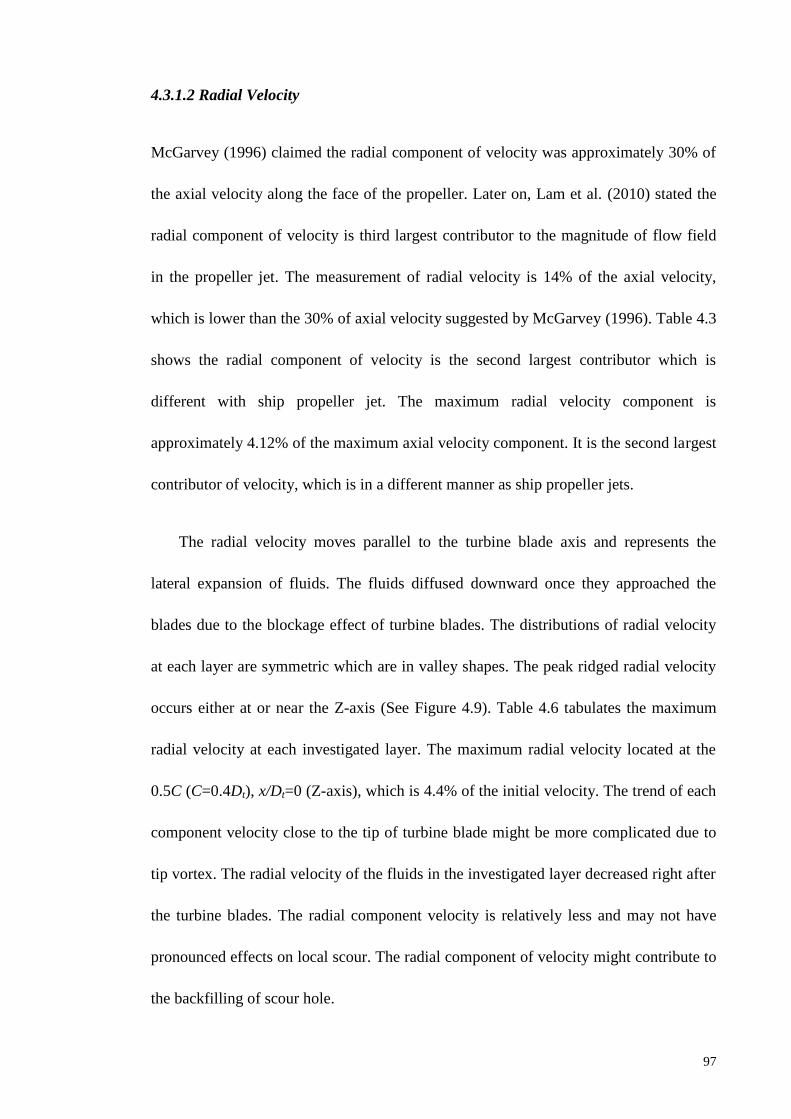
97

4.3.1.2 Radial Velocity

McGarvey (1996) claimed the radial component of velocity was approximately 30% of

the axial velocity along the face of the propeller. Later on, Lam et al. (2010) stated the

radial component of velocity is third largest contributor to the magnitude of flow field

in the propeller jet. The measurement of radial velocity is 14% of the axial velocity,

which is lower than the 30% of axial velocity suggested by McGarvey (1996). Table 4.3

shows the radial component of velocity is the second largest contributor which is

different with ship propeller jet. The maximum radial velocity component is

approximately 4.12% of the maximum axial velocity component. It is the second largest

contributor of velocity, which is in a different manner as ship propeller jets.

The radial velocity moves parallel to the turbine blade axis and represents the

lateral expansion of fluids. The fluids diffused downward once they approached the

blades due to the blockage effect of turbine blades. The distributions of radial velocity

at each layer are symmetric which are in valley shapes. The peak ridged radial velocity

occurs either at or near the Z-axis (See Figure 4.9). Table 4.6 tabulates the maximum

radial velocity at each investigated layer. The maximum radial velocity located at the

0.5C (C=0.4Dt), x/Dt=0 (Z-axis), which is 4.4% of the initial velocity. The trend of each

component velocity close to the tip of turbine blade might be more complicated due to

tip vortex. The radial velocity of the fluids in the investigated layer decreased right after

the turbine blades. The radial component velocity is relatively less and may not have

pronounced effects on local scour. The radial component of velocity might contribute to

the backfilling of scour hole.

98

Table 4.6: Maximum radial component of velocity

Height of tip

clearance

Layer Position Radial velocity

(x/Dt) (Vr/Vo)%

1.00Dt 0.50C 0.00 2.16

0.25C 0.04 0.76

0.05C -1.37 0.27

0.80Dt 0.50C 0.00 2.62

0.25C 0.02 0.98

0.05C -1.34 0.30

0.60Dt 0.50C 0.00 3.31

0.25C 0.00 1.34

0.05C -1.37 0.26

0.40Dt 0.50C 0.00 4.40

0.25C 0.03 1.90

0.05C 1.40 0.42

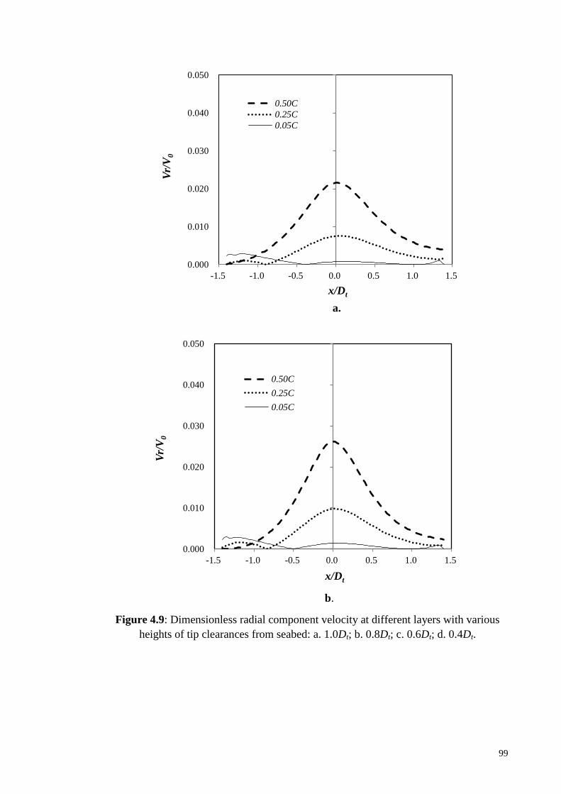
99

Figure 4.9: Dimensionless radial component velocity at different layers with various

heights of tip clearances from seabed: a. 1.0Dt; b. 0.8Dt; c. 0.6Dt; d. 0.4Dt.

0.000

0.010

0.020

0.030

0.040

0.050

-1.5 -1.0 -0.5 0.0 0.5 1.0 1.5

Vr/

V0

x/Dt

a.

0.50C

0.25C

0.05C

0.000

0.010

0.020

0.030

0.040

0.050

-1.5 -1.0 -0.5 0.0 0.5 1.0 1.5

Vr/

V0

x/Dt

b.

0.50C

0.25C

0.05C

100

0.00

0.01

0.02

0.03

0.04

0.05

-1.5 -1.0 -0.5 0.0 0.5 1.0 1.5

Vr/

V0

x/Dt

c.

0.50C

0.25C

0.05C

0.00

0.01

0.02

0.03

0.04

0.05

-1.5 -1.0 -0.5 0.0 0.5 1.0 1.5

Vr/

V0

x/Dt

c.

0.50C

0.25C

0.05C

101

Figure 4.9, continued.

0.00

0.01

0.02

0.03

0.04

0.05

-1.5 -1.0 -0.5 0.0 0.5 1.0 1.5

Vr/

V0

x/Dt

c.

0.50C

0.25C

0.05C

0.00

0.01

0.02

0.03

0.04

0.05

-1.5 -1.0 -0.5 0.0 0.5 1.0 1.5

Vr/

V0

x/Dt

d.

0.50C

0.25C

0.05C

102

4.3.1.3 Tangential Velocity

Many researches approved that the tangential component of velocity is the second

largest contributor to the resultant field in the ship’s propeller jet. Prosser (1986)

estimated the magnitude of maximum tangential velocity is approximately 30% of the

maximum axial velocity. The results have been contradicted by Lam et al. (2010),

they reported that the maximum tangential component of velocity within a ship

propeller jet is 82% of the maximum axial velocity. The tangential velocity acts

perpendicular to the turbine blade rotating axis. The tangential component results from

the rotating nature of turbine blades and it contributes to the rotation of fluids. The

fluids below and behind the turbine should not have significant tangential component as

the fluids are away from the blades.

Figure 4.10 shows the distribution of tangential velocity. The distribution of

tangential velocity is more complicated compared to the radial velocity. The distribution

of tangential velocity varies with height of tip clearance and it is remarkably small.

However, Figure 4.10d is more predictable and shows seasonal rise and falls of

tangential velocity at the layer 0.5C when tip clearance is 0.4Dt. This might be the

cyclic decay of tangential component. Table 4.7 shows the maximum tangential velocity

at each investigated layer. The highest tangential velocity occurred at x/Dt=0.09

(C=0.4Dt), which is 0.24% of initial incoming flow. It shows the rotational of fluids is

higher in the region near turbine blade.

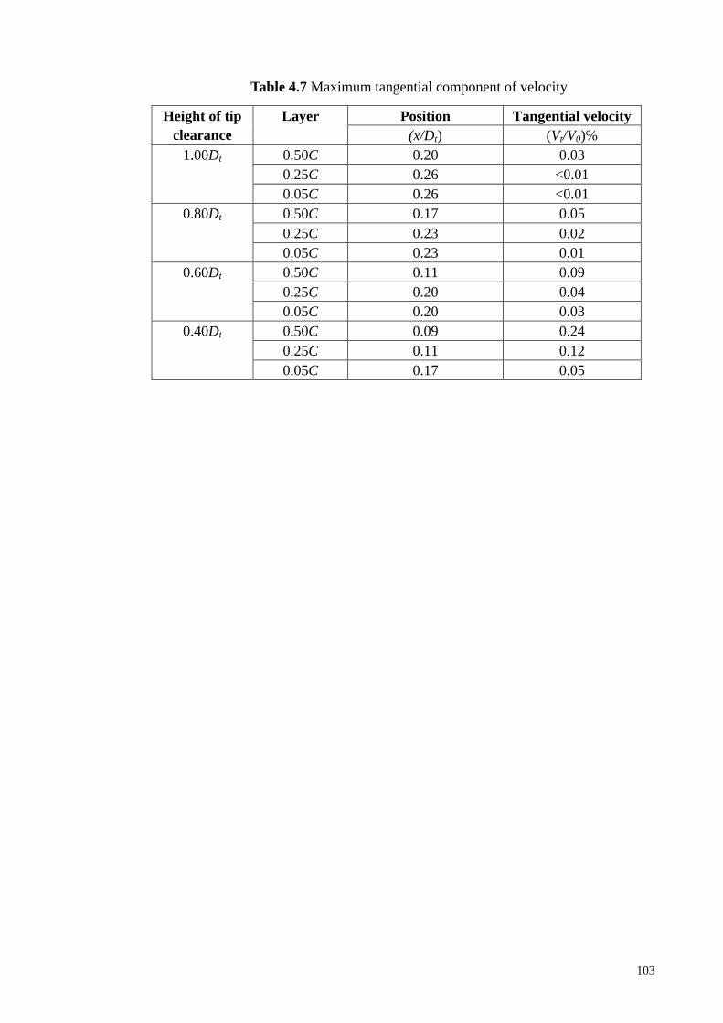
103

Table 4.7 Maximum tangential component of velocity

Height of tip

clearance

Layer Position Tangential velocity

(x/Dt) (Vt/V0)%

1.00Dt 0.50C 0.20 0.03

0.25C 0.26 <0.01

0.05C 0.26 <0.01

0.80Dt 0.50C 0.17 0.05

0.25C 0.23 0.02

0.05C 0.23 0.01

0.60Dt 0.50C 0.11 0.09

0.25C 0.20 0.04

0.05C 0.20 0.03

0.40Dt 0.50C 0.09 0.24

0.25C 0.11 0.12

0.05C 0.17 0.05

104

Figure 4.10: Dimensionless tangential velocities at various tip clearances: a. 1.0Dt; b.

0.8Dt; c. 0.6Dt; d. 0.4Dt.

0.0000

0.0005

0.0010

0.0015

0.0020

0.0025

-1.5 -1.0 -0.5 0.0 0.5 1.0 1.5

Vt/V

x/Dt

a.

0.50C

0.25C

0.05C

0.0000

0.0005

0.0010

0.0015

0.0020

0.0025

-1.5 -1.0 -0.5 0.0 0.5 1.0 1.5

Vt/V

x/Dt

b.

0.50C

0.25C

0.05C

105

Figure 4.10, continued.

0.0000

0.0005

0.0010

0.0015

0.0020

0.0025

-1.5 -1.0 -0.5 0.0 0.5 1.0 1.5

Vt/V

x/Dt

c.

0.50C

0.25C

0.05C

0.0000

0.0005

0.0010

0.0015

0.0020

0.0025

-1.5 -1.0 -0.5 0.0 0.5 1.0 1.5

Vt/V

x/Dt

d.

0.50C

0.25C

0.05C

106

4.3.2 Influence of Blade Numbers

4.3.2.1 Axial Velocity

Liu (2010) presented a study and showed that the number of blades has a significant

importance for the efficiency of turbine performance. This section presents the effect of

the number of blades on the flow between the TCT and the seabed. Table 4.8 tabulates

the maximum velocity component at each investigated layer. The axial velocity is the

dominant component of fluids under the turbine blades in all computational cases. The

radial component of velocity is the second largest contributor to the magnitude of

velocity instead of the tangential component.

Table 4.8: Maximum velocity component at each investigated layer

Number

of Blades

Layer Axial

velocity

Radial

velocity

Tangential

velocity

(Va/V)% (Vr/Va)% (Vt/Va)%

2-blade 0.05C 100.07 0.29 <0.010

0.50C 103.63 1.35 0.019

3-blade 0.05C 100.08 0.28 <0.010

0.50C 105.14 2.16 0.026

4-blade 0.05C 100.90 0.30 <0.010

0.50C 106.88 3.07 0.011

5-blade 0.05C 103.25 0.27 <0.010

0.50C 109.12 4.18 0.014

Figure 4.11 shows the axial velocity of the flow near the seabed. The fluids at each

layer below and behind the turbine have a higher axial velocity than that at the same

level before the turbine. The fluids behind the turbine in the two layers did experience

acceleration, particularly in the layer of 0.5Dt. The two-blade turbine has the least flow

change, which is approximately 3.6% acceleration. The maximum acceleration is

approximately 9% from the five-bladed turbine (see Figure 4.11b). The fluids near the

107

seabed (0.05Dt) have less acceleration than the other layers. The lower change of axial

velocity at that layer is due to the viscous effect of the seabed. The five-bladed turbine

also causes the largest acceleration in the region near the seabed. The blade area ratio is

a key parameter of the flow under the rotors. A turbine with a higher solidity results in

greater velocity reduction right behind the rotors. The water around the rotors will move

faster to recover the velocity deficit in the cone-shaped wake region.

108

Figure 4.11: Dimensionless axial component velocity at different layers: a. 0.05C; b.

0.50C.

0.96

0.98

1.00

1.02

1.04

1.06

1.08

1.10

-1.5 -1.0 -0.5 0.0 0.5 1.0 1.5

Va/V

x/Dt

a.

2blades

3blades

4blades

5blades

0.96

0.98

1.00

1.02

1.04

1.06

1.08

1.10

-1.5 -1.0 -0.5 0.0 0.5 1.0 1.5

Va/V

x/Dt

b.

2 blades

3 blades

4 blades

5 blades

109

Figure 4.12 shows the contour plot of axial velocity around the turbines. The

behaviour of flow acceleration for the fluids around the turbine blades differs from the

fluids passing through the rotor plane. The flow outside the wake region will re-energise

the wake. It was observed that the fluids outside the wake region in Figure 4.12 tend to

have a higher velocity than the free stream. The acceleration around the turbine blades

in the current study is in line with Sun (2008) and Hill et al. (2014). This further

suggests that the turbine characteristics influence the extent of flow acceleration.

Therefore, the geometry of TCT may also affect the scour process.

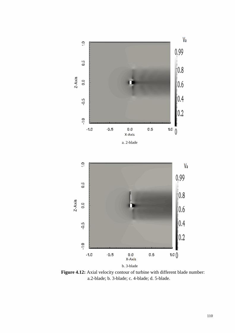
110

a. 2-blade

b. 3-blade

Figure 4.12: Axial velocity contour of turbine with different blade number:

a.2-blade; b. 3-blade; c. 4-blade; d. 5-blade.

111

c. 4-blade

d. 5-blade

Figure 4.12, continued.

112

4.3.2.2 Radial velocity

The increase of blade numbers does not change the velocity components of ships’

propeller jets. The radial component of velocity of the flow below (0.05C and 0.50C

from seabed) the turbine blades is the second largest contributor to the magnitude of

velocity instead of the tangential component. Figure 4.13 illustrates the radial

component of the flow field between the TST and the seabed. The distribution of radial

velocity at the 0.50C layer is relatively predictable. The distributions of radial velocity

at the 0.50C layer are axisymmetric. The highest radial velocity component is

approximately 0.042V and occurs near the Z-axis when the turbine has 5 blades. The

fluids near the seabed (0.05C) have minor radial component. However, the flow near the

seabed shows the same trend as the water flows in the 0.50C layer. The greater number

of blades results in a higher radial velocity of fluids. The radial velocity starts to

decrease at the back of the turbine in all computational cases. Table 4.7 also shows that

the number of blades has a significant effect on the maximum radial velocity below the

turbine blades. The radial velocity under the five-bladed turbine is approximately two

times the radial velocity below the two-bladed turbine.

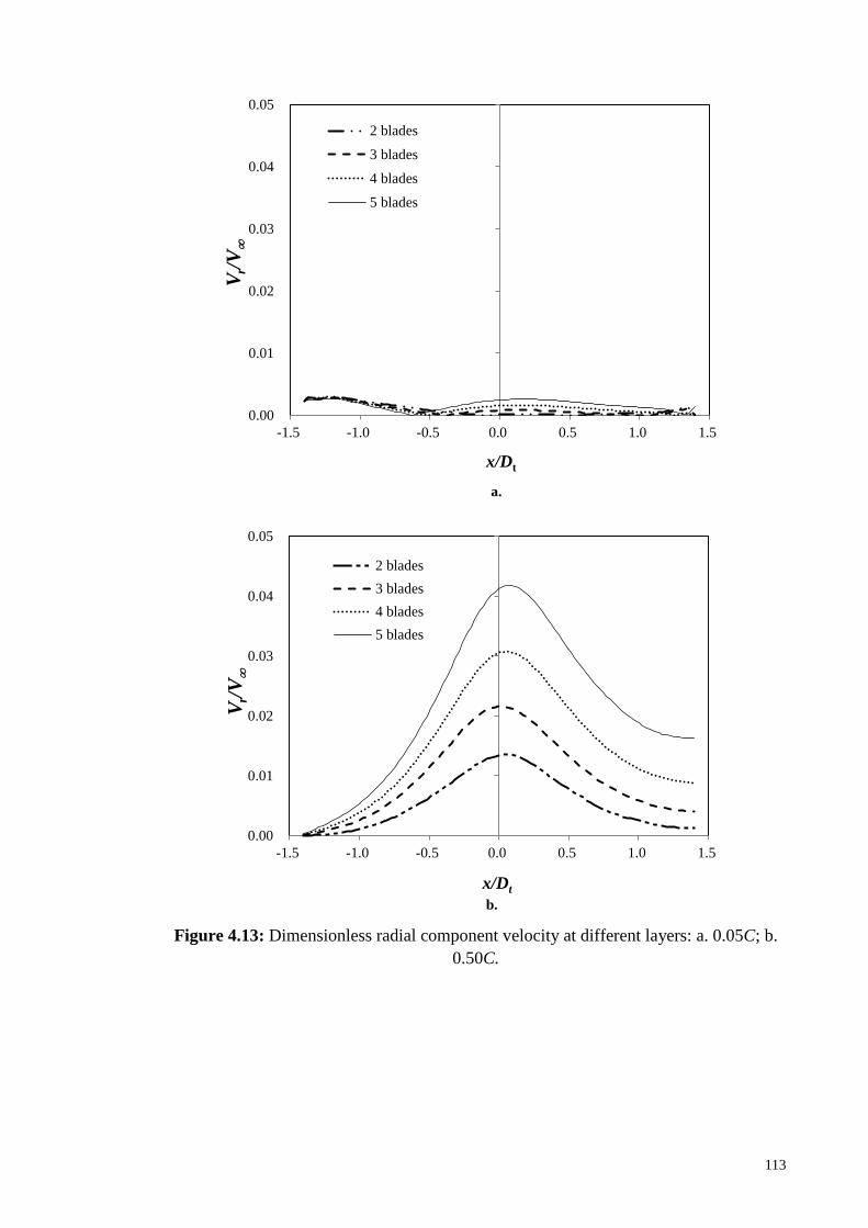
113

Figure 4.13: Dimensionless radial component velocity at different layers: a. 0.05C; b.

0.50C.

0.00

0.01

0.02

0.03

0.04

0.05

-1.5 -1.0 -0.5 0.0 0.5 1.0 1.5

Vr/

V

x/Dt

a.

2 blades

3 blades

4 blades

5 blades

0.00

0.01

0.02

0.03

0.04

0.05

-1.5 -1.0 -0.5 0.0 0.5 1.0 1.5

Vr/

V

x/Dt

b.

2 blades

3 blades

4 blades

5 blades

114

The fluids are diffused downward once they approached the blades as radial

velocity represents the lateral expansion of fluids. More fluids will be diffused away if

the turbine has a higher blade area ratio. Figure 4.14 presents a contour plot of radial

velocity around the turbines. It demonstrates that more radial components exist in the

region closer to the turbine blades. It further demonstrates that a higher blade area ratio

could cause higher radial velocity in fluids at the downstream (see Fig. 4.14d). Higher

radial velocity was also observed near turbine tip compares to other regions. It is in line

with the study of Chamorro et al. (2013). They also observed higher radial velocity near

the turbine tip. Figure 4.14 shows that the fluids below the rotational axis have negative

radial velocity. It indicates that as the fluids below the rotational axis approach the

turbine blades while the fluids diffuse downward. The radial velocity may cause the

sediment diffuse downward as well.

115

a. 2-blade

b. 3-blade

Figure 4.14: Radial velocity contour of turbine with different blade numbers: a. 2-blade;

b. 3-blade; c. 4-blade d. 5-blade.

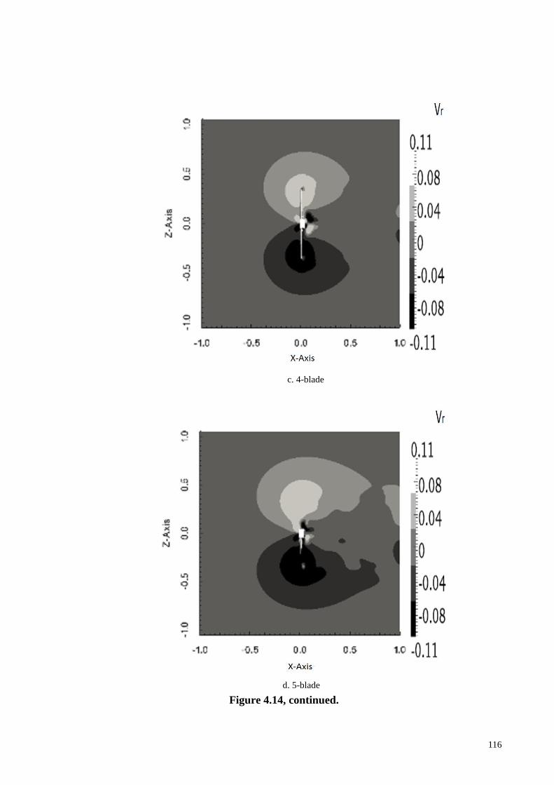
116

c. 4-blade

d. 5-blade

Figure 4.14, continued.

117

4.3.2.3 Tangential velocity

The tangential velocity acts perpendicular to the rotating axis of the turbine blade. The

tangential component results from the rotating nature of the turbine blades and it

contributes to the rotation of fluids. The tangential component is the second largest

contributor to the velocity magnitude of the jets produced by a three-bladed and a

six-bladed propeller (Lam et al., 2012b). However, the flow field under the turbine

blades has a small tangential component. Figure 4.15 shows the tangential velocity

around the turbines (2, 3, 4 and 5 blades).

118

a. 2-blade

b. 3-blade

Figure 4.15: Tangential velocity contour of turbine with different blade numbers: a.

2-blade; b. 3-blade; c. 4-blade; d. 5-blade.

119

c. 4-blade

d. 5-blade

Figure 4.15, continued.

120

A ship’s propeller imposes rotational force to produce the swirling velocity field. A

high tangential velocity component is expected in the flow field of ship propeller jets.

However, a TCT extracts energy through the rotation. The induced tangential velocity in

the flow field generated by the turbine can reasonably be less compared to the jet

produced by a ship propeller. The tangential component of velocity is even less

significant under the turbine blades. The tangential velocity below rotor may not affect

the scour process around the support of TCT. The tangential component is pronounced

in the wake. It is identical with the study of Chamorro et al. (2013), which they detected

a high tangential velocity near the wake core. It may contribute to the interaction

between the suspended particles and wake.

4.3.3 Development of Boundary Layer

The mechanism of horseshoe vortex is of significant importance in the process of scour.

The rotation of the incoming flow results in the horseshoe vortex. The boundary layer

experiences a three-dimensional separation under the influence of the adverse pressure

gradient induced by the presence of the support structure. The separated boundary layer

accordingly rolls up to from a spiral vortex around the support structure (Sumer and

Fredsøe, 2002).

The incoming boundary layer and pressure gradient induced by the support

structure are the two necessary preconditions to generate a horseshoe vortex. Baker

(1979a; 1979b) claimed that the non-dimensional quantities describing the horseshoe

vortex in the case of steady current mainly depends on the following parameters:

121

𝛿

𝐷, 𝑅𝑒𝐷

(or alternatively 𝑅𝑒𝛿), and pile geometry

in which 𝛿/𝐷= the ratio of bed boundary layer thickness to the pile diameter, 𝑅𝑒𝐷= the

pile Reynolds number (Equation (4.4)):

𝑅𝑒𝐷=

𝑈𝐷𝑝

𝑣 (4.4)

and 𝑅𝑒𝛿= the bed-boundary-layer Reynolds number (Equation (4.5)):

𝑅𝑒𝛿=

𝑈𝛿

𝑣 (4.5)

where U is the velocity at the edge of the bed boundary layer, 𝑣 is the kinetic viscosity.

Figure 4.16 shows the current boundary layer profile with rotor in operation in

conjunction with measured data from Chilworth flume, University of Southampton

(Myers et al., 2008). The measured boundary layer profiles are without presence of

energy extraction devices. The seabed condition incorporated in the current numerical

simulation is without roughness. The numerical results indicate that the flow near

seabed is increasing and the velocity gradient is reduced compared with the

experimental data without rotor in operation. The flow acceleration increases the shear

stress on seabed and causes more sediment to transport. The five-bladed turbine results

in highest acceleration. The difference of the flow acceleration under different turbines

is not significant. Minor difference of velocity near seabed in long term could cause

evident differences on the capacity of sediment transport. More logarithmic velocity

distribution exists in real marine environment. The presence of rotor significantly

interferes with the boundary layer. The changes of flow near seabed possibly affect the

bed load and suspended load of sediment. The increase of number of blades results in

greater acceleration of flow under the TCT. The turbine with higher blade area ratio

may need higher shaft height to avoid severe triggering of sediment transport.

122

Figure 4.16: The development of boundary layer behind turbine rotors

4.3.4 Validation of Numerical Results and Mesh Independence Study

Experimental results and numerical simulation by Pinon et al. (2010) for investigating

wake of TCT were used in the study to validate the numerical model. The velocity

profile at the location 1.2Dt behind the turbine was presented and compared with results

obtained by Pinon et al. (See Figure 4.17). There is some variability in the region near

the rotational axis. The cause of this disagreement might be the length of the hub. The

computational results agree well with the experimental results of Pinon et al. (2010).

Figure 4.17 also shows that the axial velocity under turbine blades experienced a slight

increase.

0.0

0.1

0.2

0.3

0.4

0.5

0.6

0.7

0.8

0.9

1.0

0.0 0.1 0.2 0.3 0.4 0.5 0.6 0.7 0.8 0.9 1.0 1.1

No

rma

lise

d D

epth

Normalised Velocity

1/7th Power Law

Smooth bed (Myers et al.2008)

OpenFOAM 2 blades

OpenFOAM 3 blades

OpenFOAM 4 blades

OpenFOAM 5 blades

123

Figure 4.17: Axial velocity profiles behind turbine blades (x=1.2Dt)

The number of cells in CFD can influence the results due to the approximations and

time-averaging method used in RANS equations (Daly et al., 2013). A greater number

of cells may result in a more accurate solution for the problem with a specified

numerical setting. The increase in mesh density also requires more computational power.

The mesh independence study attempts to investigate the velocity field accurately with

less processing time.

The computational case with a three-bladed turbine was selected and the mesh

independence study incorporated the turbine in the numerical simulation with finer

meshes. The cell numbers were increased to 545757 and 655908 cells. The mesh

independence was tested by selecting axial velocity at the layer 0.5C from the bed

(C=350mm). The results obtained by using a finer mesh give no discernible changes in

-1.5

-1.0

-0.5

0.0

0.5

1.0

1.5

0 0.2 0.4 0.6 0.8 1 1.2

r/D

t

Va/V

OpenFOAM

Experiment

124

the predicted flow field (see Figure 4.18). The results of velocity magnitude are in good

agreement for both fine and coarse meshes. A mesh density of 451039 cells is used for

the investigation, which has the advantage of less processing time.

Figure 4.18: Mesh independence study

0.98

0.99

1.00

1.01

1.02

1.03

1.04

1.05

1.06

1.07

1.08

-1.5 -1.0 -0.5 0.0 0.5 1.0 1.5

Va/V

x/Dt

451039 Cells

545757 Cells

655908 Cells

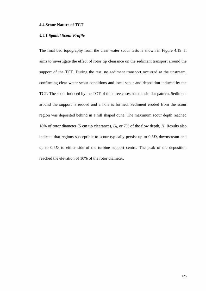
125

4.4 Scour Nature of TCT

4.4.1 Spatial Scour Profile

The final bed topography from the clear water scour tests is shown in Figure 4.19. It

aims to investigate the effect of rotor tip clearance on the sediment transport around the

support of the TCT. During the test, no sediment transport occurred at the upstream,

confirming clear water scour conditions and local scour and deposition induced by the

TCT. The scour induced by the TCT of the three cases has the similar pattern. Sediment

around the support is eroded and a hole is formed. Sediment eroded from the scour

region was deposited behind in a hill shaped dune. The maximum scour depth reached

18% of rotor diameter (5 cm tip clearance), Dt, or 7% of the flow depth, H. Results also

indicate that regions susceptible to scour typically persist up to 0.5Dt downstream and

up to 0.5Dt to either side of the turbine support centre. The peak of the deposition

reached the elevation of 10% of the rotor diameter.

126

a. 5 cm tip clearance

b. 10 cm tip clearance

Figure 4.19: 3D surface map of 24-hr scour by SURFER

127

c. 15 cm tip clearance

Figure 4.19, continued.

As discovered in Section 4.3, the obstruction induced by the spinning rotor

resulting acceleration of the flow between the bottom rotor tip and bed surface. This

acceleration increases the local shear stress and it amplifies the scour mechanism. It is

therefore the short tip clearance (5 cm) can cause severe sediment transport around the

support of the TCT. The extent of scour hole increases with the decrease of tip clearance.

The highest tip clearance 15 cm results in the least eroded sand from the bed. The scour

holes and deposited sand are asymmetric particularly in the case of 5 cm tip clearance. It

is due to asymmetric shear stress impacted at the bed. It conforms to the study

conducted by Zhang et al. (2015).

128

4.4.2 Temporal Evolution

4.4.2.1 Temporal Variation of Scour Profiles

Figures 4.20, 4.21 and 4.22 present the temporal dimensionless scour holes profile at

3.5, 7.0 and 24 hr. The turbine rotor places 5cm, 10cm and 15 cm from bed, respectively.

The investigated cases are in the same manner in terms of scour development. Looking

closely at the measured developments of scour profile at various lateral positions, it can

be observed that a scour hole is formed around the support tower. The majority of scour

occurred at the initial 3.5 hr. The size of scour holes increase with time. The scour depth

slightly increases after 3.5 hr scour. A deposition mound is also observed downstream at

initial stage. The depositional wedge also moves further downstream as the test in

progress. A secondary sand dune is formed right behind the primary dune after 24 hr

test.

At the case of 5 cm tip clearance, maximum scour occurred at approximately x/Dt=

-0.1, y/Dt= -0.1, reached the depth of S/Dt=0.185. The highest depositional wedge

reached elevations of approximately 10% of the Dt at location x/Dt=1.0, y/Dt=0.1. The

highest secondary sand dune is only 3.5% of Dt at location x/Dt=1.8, y/Dt= 0.2. It is has

been observed that there is no secondary sand dune at the first 7 hr scour test. It is

probably due to the primary deposition wedge reached a certain height and it becomes

susceptible to the flow below turbine rotor. The accelerated flow below rotor turbine

eroded the deposited sand dune.

129

In the case of 10 cm tip clearance, maximum scour depth is approximately 16% of

Dt and took place at x/Dt= -0.05, y/Dt=0 and x/Dt=-0.05, y/Dt= -0.1. The highest primary

sand dune has an elevation of 0.075Dt and it happened after 7 hr scour test other than 24

hr. It may due to the primary scour dune deposition is less than its erosion in the

subsequent test. The highest primary deposition located at the region of x/Dt=0.6-0.7,

y/Dt=0.0-0.1. Secondary dune is also formed but with lower elevation. The highest

secondary sand dune is only 3% of Dt at x/Dt=1.5, y/Dt=0.0.

For the investigated case of 15 cm tip clearance, maximum scour depth occurred at

x/Dt= -0.05, y/Dt=0 and x/Dt=-0.05, y/Dt= -0.1 which is same as the case of 10 cm tip

clearance. The maximum scour depth is approximate 0.145Dt. The highest primary

deposition is 8.5% of Dt located at x/Dt= 0.7, y/Dt=0 and x/Dt=0.7, y/Dt= -0.1. The

secondary sand dune is getting lower and lower as the rotor of turbine rotor moves up.

The highest secondary sand dune is only 2% of turbine diameter at locations x/Dt= 1.2,

y/Dt=0 and x/Dt=1.2, y/Dt= -0.1.

As seen from all the investigated cases, it has been observed that the maximum

scour depth increase as the decrease of tip clearance. The maximum scour depth

occurred in front of the support pile. It is generally at the region x/Dt=-0.05 – -0.1 and

y/Dt=0.0 – -0.1. The height of primary and secondary deposited sand dunes also

increases as the decreases in tip clearance. The location of peak sand dune is a bit

complicated due to the influence of the flow between turbine rotor and bed. Furthermore,

the transition point between net erosion and net deposition moves downstream as the

test ongoing. Hill et al. (2014) suggested that the transition point may reveal a

130

relationship between turbine wake and the bed surface. The transition points of Hill et al.

(2014) are between x/Dt=1.0 to x/Dt =2.0. This region has been noted by Chamorro et al.

(2013) and they claimed that the turbine wake coherence starts to break down in this

region where the most rapid velocity deficit recovery begins. However, the furthest

transition point of the current study located at x/Dt=0.5 in all the cases after 24 hr scour

test. The difference of the locations of the transition point may be due to the difference

of turbine geometry and flow velocity.

a.

Figure 4.20: Temporal dimensionless scour holes profile at different times (Tip

clearance=5 cm); a. y/Dt = 0; b. y/Dt= -0.1; c. y/Dt = 0.1. e. y/Dt= -0.2; f. y/Dt = 0.2.

-0.20

-0.15

-0.10

-0.05

0.00

0.05

0.10

-1.0 -0.5 0.0 0.5 1.0 1.5 2.0 2.5

S/D

t

x/Dt

3.5hr

7.0hr

24hr

131

b.

c.

Figure 4.20, continued.

-0.20

-0.15

-0.10

-0.05

0.00

0.05

0.10

-1.0 -0.5 0.0 0.5 1.0 1.5 2.0 2.5

S/D

t

x/Dt

3.5hr

7.0hr

24hr

-0.20

-0.15

-0.10

-0.05

0.00

0.05

0.10

-1.0 -0.5 0.0 0.5 1.0 1.5 2.0 2.5

S/D

t

x/Dt

3.5hr

7.0hr

24hr

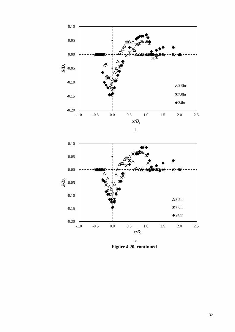
132

d.

e.

Figure 4.20, continued.

-0.20

-0.15

-0.10

-0.05

0.00

0.05

0.10

-1.0 -0.5 0.0 0.5 1.0 1.5 2.0 2.5

S/D

t

x/Dt

3.5hr

7.0hr

24hr

-0.20

-0.15

-0.10

-0.05

0.00

0.05

0.10

-1.0 -0.5 0.0 0.5 1.0 1.5 2.0 2.5

S/D

t

x/Dt

3.5hr

7.0hr

24hr

133

a.

b.

Figure 4.21: Temporal dimensionless scour holes profile at different times (Tip

clearance=10 cm); a. y/Dt = 0; b. y/Dt = -0.1; c. y/Dt = 0.1. e. y/Dt = -0.2; f. y/Dt = 0.2.

-0.20

-0.15

-0.10

-0.05

0.00

0.05

0.10

-1.0 -0.5 0.0 0.5 1.0 1.5 2.0 2.5

S/D

t

x/Dt

3.5hr

7.0hr

24hr

-0.20

-0.15

-0.10

-0.05

0.00

0.05

0.10

-1.0 -0.5 0.0 0.5 1.0 1.5 2.0 2.5

S/D

t

x/Dt

3.5hr

7.0hr

24hr

134

c.

d.

Figure 4.21, continued.

-0.20

-0.15

-0.10

-0.05

0.00

0.05

0.10

-1.0 -0.5 0.0 0.5 1.0 1.5 2.0 2.5

S/D

t

x/Dt

3.5hr

7.0hr

24hr

-0.20

-0.15

-0.10

-0.05

0.00

0.05

0.10

-1.0 -0.5 0.0 0.5 1.0 1.5 2.0 2.5

S/D

t

x/Dt

3.5 hr

7.0 hr

24 hr

135

e.

Figure 4.21, continued.

-0.20

-0.15

-0.10

-0.05

0.00

0.05

0.10

-1.0 -0.5 0.0 0.5 1.0 1.5 2.0 2.5

S/D

t

x/Dt

3.5 hr

7.0hr

24 hr

136

a.

b.

Figure 4.22: Temporal dimensionless scour holes profile at different times (Tip

clearance=15cm); a. y/Dt = 0; b. y/Dt = -0.1; c. y/Dt = 0.1. e. y/Dt= -0.2; f. y/Dt = 0.2.

-0.20

-0.15

-0.10

-0.05

0.00

0.05

0.10

-1.0 -0.5 0.0 0.5 1.0 1.5 2.0 2.5

S/D

t

x/Dt

3.5hr

7.0hr

24hr

-0.20

-0.15

-0.10

-0.05

0.00

0.05

0.10

-1.0 -0.5 0.0 0.5 1.0 1.5 2.0 2.5

S/D

t

x/Dt

3.5hr

7.0hr

24hr

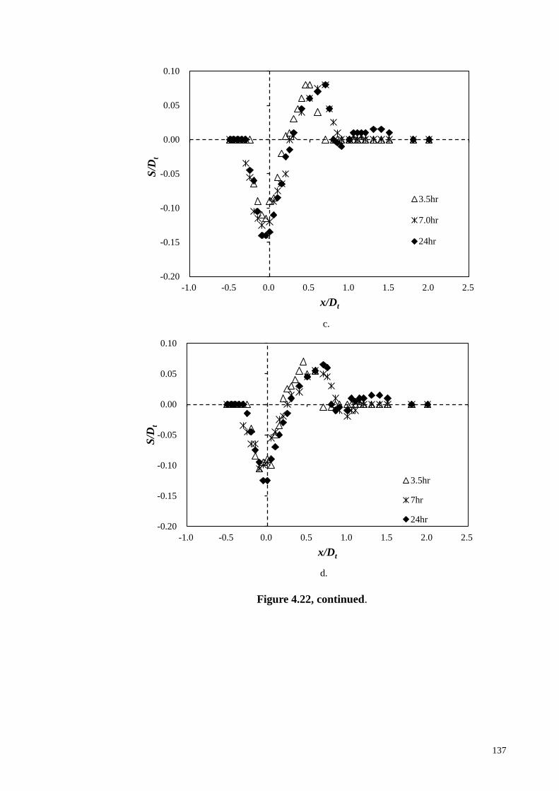
137

c.

d.

Figure 4.22, continued.

-0.20

-0.15

-0.10

-0.05

0.00

0.05

0.10

-1.0 -0.5 0.0 0.5 1.0 1.5 2.0 2.5

S/D

t

x/Dt

3.5hr

7.0hr

24hr

-0.20

-0.15

-0.10

-0.05

0.00

0.05

0.10

-1.0 -0.5 0.0 0.5 1.0 1.5 2.0 2.5

S/D

t

x/Dt

3.5hr

7hr

24hr

138

e.

Figure 4.22, continued.

-0.20

-0.15

-0.10

-0.05

0.00

0.05

0.10

-1.0 -0.5 0.0 0.5 1.0 1.5 2.0 2.5

S/D

t

x/Dt

3.5hr

7hr

24 hr

139

4.4.2.2 Temporal Variation of Maximum Scour Depth

Figure 4.23 illustrates the temporal scour depth under different tip clearances. The

𝑆𝑡/𝐷𝑡 is a logarithmic function of time (t). It observed that the majority of the scour of

all the investigated cases occurred in the first 3.5 hours. After 7 hr of scour test, all three

cases reach near-equilibrium conditions. The depth of scour increased more quickly in

the case with 5 cm tip clearance. The slowest scour occurred in the case of 15 cm tip

clearance. The maximum scour also occurred in the case of 5cm tip clearance, which is

approximately 18.5% of the rotor diameter Dt (8% of flow depth). The least scour

happened in the case of 15 cm tip clearance, which is approximately 14% of the rotor

diameter Dt (6% of flow depth).

Figure 4.23: Time-dependent maximum scour depth

0.00

0.02

0.04

0.06

0.08

0.10

0.12

0.14

0.16

0.18

0.20

0 200 400 600 800 1000 1200 1400 1600

St/

Dt

t (mins)

Clearance 5 cm

Clearance 10cm

Clearance 15cm

140

A comparison between the experimental results of the current study and Hill et al.

(2014) of temporal scour depth is presented in Figure. 4.24. The time has been

normalized by the respective velocity at hub height. It shows that the large-scale

experiment did not approach equilibrium stage. The small-scale experiments approach

the near-equilibrium. Hill et al. (2014) also indicated that the sour hole evolves faster

when the rotor is on the upstream side of the support tower. The temporal evolution of

scour depth of small-scale experiments indicated similar pattern with the author’s

results (C=5 cm), particularly the case of rotor upstream. The authors’ experiments are

conducted with rotor upstream. The results of Hill et al. (2014) in Fig.10 are taken from

x/Dt=0.66 and y/Dt=0 for all cases. The results of current study are taken from x/Dt=-0.1

and y/Dt=-01. These locations are on the downstream side of the rotors. With the rotor

on the downstream of the support tower, the flow acceleration between rotor and seabed

may take place later. The scour amplification occurs potentially further downstream

from the support tower. The location of rotor plays an important role for the scour

mechanism of tidal turbine. The development of wake of the turbine affects the scour

mechanism. The prediction of wake profile is able to provide insightful inputs for the

scour prediction around the support of TCT.

The temporal evolution of scour hole for large-scale experiment is relatively faster

compare to small-scale experiments. However, it should be noted that the velocity at

hub height is 0.66 m/s. This indicated the incoming flow velocity plays a significant role

on the temporal evolution of scour hole. The size of the rotor may also cause the faster

evolution of scour hole as the large-scale experiment with a 0.5 m diameter rotor.

141

Figure 4.24: Comparison of temporal scour depth

4.4.2.3 Proposed Scour Prediction Model

Research to provide methods for predicting scour depth around the pile-supported

structure of tidal turbine is limited. The maximum scour depth at any time t, St, is

assumed to be a function of 10 independent variables as follows:

𝑆𝑡 = 𝑓1(𝑉0, 𝐷𝑡 , 𝑑50, 𝐶, 𝜌, 𝜌𝑠, 𝑔, 𝐻, 𝑣, 𝑡) (4.6)

In the works of ship propeller jet induced scour (Rajaratnam, 1981; Hamill, 1999;

Hong et al., 2013), the fluid viscosity could be neglected as the Reynolds number of the

jet is greater than 10,000. The Reynolds number of the wake induced by the physical

model of the turbine is around 29,100. The viscosity term is ignored in the following

analysis. The water depth of the study is reasonable high, the Froude number is

0.00

0.05

0.10

0.15

0.20

0.25

0.30

0.35

0.0 0.5 1.0 1.5 2.0 2.5 3.0

St/

Dt

tVhub/Dt

Small scale: rotor downstream (Hill et al., 2014)

Small scale: rotor upstream (Hill et al., 2014)

Large scale: rotor downstream (Hill et al., 2014)

C=5.0cm

C=10cm

C=15cm

x104

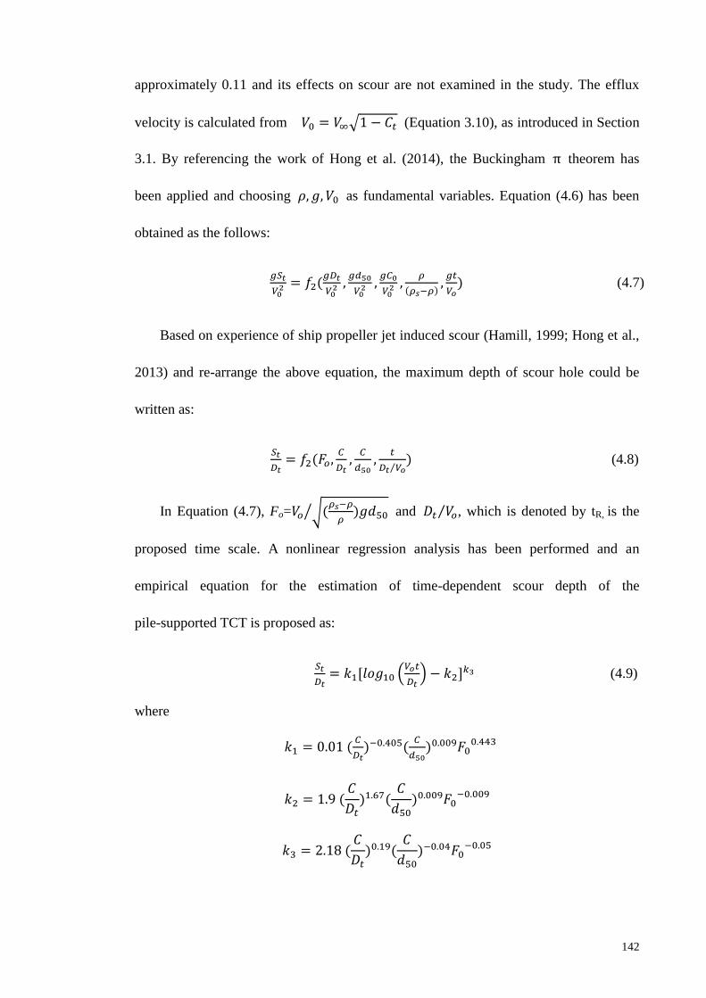
142

approximately 0.11 and its effects on scour are not examined in the study. The efflux

velocity is calculated from 𝑉0 = 𝑉∞√1 − 𝐶𝑡 (Equation 3.10), as introduced in Section

3.1. By referencing the work of Hong et al. (2014), the Buckingham π theorem has

been applied and choosing 𝜌, 𝑔, 𝑉0 as fundamental variables. Equation (4.6) has been

obtained as the follows:

𝑔𝑆𝑡

𝑉02 = 𝑓2(

𝑔𝐷𝑡

𝑉02 ,

𝑔𝑑50

𝑉02 ,

𝑔𝐶0

𝑉02 ,

𝜌

(𝜌𝑠−𝜌),

𝑔𝑡

𝑉𝑜) (4.7)

Based on experience of ship propeller jet induced scour (Hamill, 1999; Hong et al.,

2013) and re-arrange the above equation, the maximum depth of scour hole could be

written as:

𝑆𝑡

𝐷𝑡= 𝑓2(𝐹𝑜 ,

𝐶

𝐷𝑡,

𝐶

𝑑50,

𝑡

𝐷𝑡 𝑉𝑜⁄) (4.8)

In Equation (4.7), Fo=𝑉𝑜 √(𝜌𝑠−𝜌

𝜌)𝑔𝑑50⁄ and 𝐷𝑡 𝑉𝑜⁄ , which is denoted by tR, is the

proposed time scale. A nonlinear regression analysis has been performed and an

empirical equation for the estimation of time-dependent scour depth of the

pile-supported TCT is proposed as:

𝑆𝑡

𝐷𝑡= 𝑘1[𝑙𝑜𝑔10 (

𝑉𝑜𝑡

𝐷𝑡) − 𝑘2]𝑘3 (4.9)

where

𝑘1 = 0.01 (𝐶

𝐷𝑡)−0.405(

𝐶

𝑑50)0.009𝐹0

0.443

𝑘2 = 1.9 (𝐶

𝐷𝑡)1.67(

𝐶

𝑑50)0.009𝐹0

−0.009

𝑘3 = 2.18 (𝐶

𝐷𝑡)0.19(

𝐶

𝑑50)−0.04𝐹0

−0.05

143

Figure 4.25 presents the overall comparison between the computed and observed

temporal maximum scour depth. The R-squared value ranges from 0.7747 to 0.9737.

The best fitting of the experimental data with predicted value is in the case C=10 cm.

The lowest R-squared value in the case of C=15 cm is 0.7747 which is still consider

very good based on Henriksen et al. (2003). Equation 4.9 has good agreement with

present experimental data under the conditions of 0.25 ≤ 𝐶 𝐷𝑡⁄ ≤ 0.75 ,

50 ≤ 𝐶 𝑑50⁄ ≤ 150 and 𝐹0 = 1.8965 . More experimental results are necessary to

enlarge the applicable range of the proposed model.

Figure 4.25: Comparison between measured and predicted time-dependent scour depth

0.00

0.05

0.10

0.15

0.20

0.00 0.05 0.10 0.15 0.20

Pre

dic

ted

St/

Dt

Measured St/Dt

C=5cm, R2=0.9692

C=10cm, R2=0.9737

C=15cm, R2=0.7747

144

4.4.3 Comparison with Conventional Bridge/Pile Scour

The presence of rotor adds complexity to the scour induced by the pile-supported TCT.

The scour mechanism of the TCT is different from the conventional bridge/pile scour.

The main differences come from the generated wake and the flow below the wake. The

flow below wake tends to move faster than the free stream and may act to amplify the

scour process which results in the increase of the scour rate. The study showed that the

tip clearance (vertical location) of rotor affects the scour depth around the support of the

TCT which is line with Zhang et al. (2015). Figure 4.24 also indicated that the lateral

location of the rotor affects the scour profile of tidal turbine. The proposed efflux

velocity is employed for the prediction of time-dependent scour depth. The prediction of

wake profiles provides initial input for the scour profile prediction.

The turbine geometry may also affect the scour process. This is because of the

geometry affects the flow between rotor and seabed. As presented in section 4.3.2, the

number of blades affects the axial and radial component of velocity. The study of Hill et

al. (2014) also stated that the scour process of TCT depends on geometrical properties

of turbine rotor. They also highlighted that the device performance may affect the scour

mechanism.

The flow characteristic of a river stream is significantly different from tidal

variations. River flow is unidirectional and it may have strong stochastic variation on

daily to seasonal base (Khan et al., 2009). The tides undergo fluctuations of dominant

periodic nature. The tide is either diurnal or semidiurnal. Many sites are relatively

bi-directional. The flow reversal can be 20o or more away from 180

o (Myers and Bahaj,

145

2005; Blunden and Bahaj, 2006; Haydar et al., 2012). The scour test performed in the

study is under the case of unidirectional flow. The study of Escarameia and May (1999)

and McGovern (2014) reported that the equilibrium scour depth is smaller than the case

under unidirectional flows due to backfilling of scour hole during reversing flow. In the

site of relatively bi-directional flow, the predicted scour rate and depth by using

proposed scour model is probably larger than the real case. The conservative feature of

the proposed model safeguards the stability of the support of TCTs. The proposed model

is based on the reference guide of ship propeller jets induced scour. The scour process of

TCTs is complicated due to the presence of the rotor. The attempts by referencing ship

propeller jet induced scour predictor is promising and the proposed model (Equation 4.9)

can be used as a starting point for future model development.

146

CHAPTER 5: CONCLUSIONS AND RECOMMENDATIONS

5.1 Conclusions

The main purposes of the thesis were to study the flow nature of turbine wake and to

explore the impacts of turbine wake on the seabed. The conclusions of the research

objectives listed in Section 1.3 are addressed in the following:

5.1.1 Analytical Wake Model

The validity of the analytical wake model is demonstrated. It is able to predict the

two-dipped wake structure. Two-dipped wake model is able to predict the two

axisymmetric minimum velocities within the zone of flow establishment compared to

the equations of Lam and Chen (2014). The two minimum velocities merged to be one

minimum velocity in the zone of established flow. The proposed model is also able to

predict the wake model under various ambient turbulence conditions (TI=3%, 5%, 8%

and 15%). The analytical wake model is documented in Table 4.2.

The procedure to predict the wake structure is summarised. Prediction of the wake

structure is started by predicting the efflux velocity. Efflux velocity is able to be

predicted using the enhanced equation Vo (Equation 3.10) to predict the minimum

velocities at various positions from the turbine depending on the turbulence intensity.

Goodness-of-fit analysis has been conducted by comparing with published experimental

data. The estimator of R-square (R2) and Mean Square Error (MSE) indicated that the

predicted wake stricture has acceptable agreement with the published experimental

results.

147

5.1.2 Flow between Rotor and Bed

OpenFOAM is able to predict the velocity profile under the rotor of the TCT. The axial

component is the largest contributor to the magnitude of the velocity. The radial

component of the velocity is the second largest contributor to the magnitude of the

velocity. The tangential component is insignificant so that it suggests the tangential

component of velocity has no impact on the scour and deposition process. The

confinement has no effect on the velocity pattern of each velocity component when the

tip clearance is large enough.

The blockage ratio of TCT is directly proportional to the extent of flow acceleration.

The presence of rotor changes the boundary layer profile subsequently results in the

altering of horseshoe vortex formation. A schematic diagram to describe the flow profile

between seabed and TCT has been proposed (Figure 4.8). The blockage ratio of a TCT

is directly proportional to the extent of flow acceleration. A higher blade area ratio of

turbine cause more velocity deficit right behind the turbine plane. A higher blade area

ratio causes higher velocity acceleration around the turbine rotors. A larger blade area

ratio also results in higher radial velocity in the near-field of the turbine. The change of

tangential velocity was found to be insignificant due to change of blade area ratio.

The characterization of the flow conditions offers the preliminary insight into the

interaction between the turbine and the ambient environment. The geometry of the

turbine is of importance to the flow. The study demonstrates the possibility of

OpenFOAM as a promising method to investigate TCT related issue. The height of tip

clearances and turbine geometry are the two critical parameters in scour design of TCT.

148

5.1.3 Tip Clearance on the Scour Depth of Pile-Supported TCT

The presence of rotor amplifies the scour process around the support of the TCT. The

decrease of tip clearance increases the scour depth. The maximum scour depth reached

18.5% of the rotor diameter. Results indicate that regions susceptible to scour typically

persist up to 1.0Dt downstream and up to 0.5Dt to either side of the turbine support

centre.

The tip clearance plays the most important role in affecting the scour depth and

scour rate. The case of 5 cm tip clearance results in the fastest scour and most sediment

transport, while the case of 15 cm tip clearance has the slowest and least sediment

transport.

5.1.4 Temporal Scour Profiles of Pile-Supported TCT

Majority of the scour occurred in the first 3.5 hr in all the cases. The scour depths of all

the cases reach near-equilibrium state after 7 hr test. A “V” shape scour hole is formed

around the support tower. A deposition mound is also observed downstream at initial

stage. The primary deposition mound moves further downstream with time. A secondary

dune is formed right behind the primary dune after 24 hr of scour test.

149

5.1.5 Correlation of the Tip Clearance with Time-Dependent Maximum Scour Depth

Using the experimental data, the 𝑆𝑡/𝐷𝑡 is a logarithmic function of time. An empirical

formula (Equation 4.9) to estimate the time-dependent maximum scour depth is

proposed as the following:

𝑆𝑡

𝐷𝑡= 𝑘1[𝑙𝑜𝑔10 (

𝑉𝑜𝑡

𝐷𝑡) − 𝑘2]𝑘3

where

𝑘1 = 0.01 (𝐶

𝐷𝑡)−0.405(

𝐶

𝑑50)0.009𝐹0

0.443

𝑘2 = 1.9 (𝐶

𝐷𝑡)1.67(

𝐶

𝑑50)0.009𝐹0

−0.009

𝑘3 = 2.18 (𝐶

𝐷𝑡)0.19(

𝐶

𝑑50)−0.04𝐹0

−0.05

Equation 3.10 (Efflux velocity) is an initial input for the proposed scour prediction. The

predicted results indicate acceptable agreement with the present experimental data.

150

5.2 Recommendations for Future Works

Though large amount of works has been done to understand the wake and scour of TCT,

the scope of this work is limited. Recommendations for future research are listed as

follows:

I. The wave may affeect the turbine performance and wake structure. The effect of

wave on the wake would need to be studied

II. Field measurements of turbine wake profile can be done.

III. The applicability of the porposed turbine wake model can be testified when the

incoming flow is non-uniform.

IV. Higher resolution of numerical model can be conducted to capture the detail flow

near turbine rotor.

V. Further research can be carried out to cover a wider range of densimetric Froude

number for the scour prediction around the support of TCT. For instance, different

incoming velocity and various sediment sizes.

VI. More attention should be drawn to the scour nature of TCT under live-bed

condition.

VII. The effect of the wave on the scour depth of TCT can be investigated.

VIII. The scour rate of TCT under bi-directional flow condition can be examined.

IX. The investigation on scour profile of TCT under tide and wave combined condition

needs be carried out.

X. The interations of turbines may affect the scour mechanisms. The investigation of

scour of TCT in arrays needs to be investigated.

151

REFERENCES

Aberle, J., & Söhngen, B. (2008). Analysis of propeller jet induced scours. In

International Conference on Fluvial Hydraulics River Flow (pp. 3-5).

Albertson, M. L., Dai, Y. B., Jensen, R. A., & Rouse, H. (1950). Diffusion of

submerged jets. Transactions of the American Society of Civil Engineers,

115(1), 639-664.

Annandale, G. (2005). Scour technology: mechanics and engineering practice.

McGraw Hill Professional.

Ansari, S. A., & Qadar, A. (1994). Ultimate depth of scour around bridge piers. In

Hydraulic Engineering (1994) (pp. 51-55). ASCE.

Atlantis Resource. 16th, Jan, 2015, from

http://atlantisresourcesltd.com/turbines/ar-series/ar1000.html

Bahaj, A. S. (2011). Generating electricity from the oceans. Renewable and

Sustainable Energy Reviews, 15(7), 3399-3416.

Bahaj, A.S., Batten, W.M.J., & McCann, G. (2007). Experimental verification of

numerical predictions for the hydrodynamic performance of horizontal axis

marine current turbines. Renewable Energy, 32 (15), 2479-2490.

Bahaj, A. S., Myers, L. E., Thomson, M. D., & Jorge, N. (2007, September).

Characterising the wake of horizontal axis marine current turbines. In

Proceedings of the 7th European wave and tidal energy conference (p. 9).

Baker, C. J. (1979a). The laminar horseshoe vortex. Journal of fluid mechanics, 95(02),

347-367.

Baker, C. J. (1979b). Vortex flow around the bases of obstacles (Doctoral dissertation,

University of Cambridge). Retrieved from

https://www.repository.cam.ac.uk/handle/1810/244806

Barkdoll, B. D., Ettema, R., & Melville, B. W. (2007). Countermeasures to protect

bridge abutments from scour (Vol. 587). Transportation Research Board.

Bastankhah, M., & Porté-Agel, F. (2014). A new analytical model for wind-turbine

wakes. Renewable Energy, 70, 116-123.

Batten, W. M., Harrison, M. E., & Bahaj, A. S. (2013). Accuracy of the actuator

disc-RANS approach for predicting the performance and wake of tidal turbines.

Philosophical Transactions of the Royal Society of London A: Mathematical,

Physical and Engineering Sciences, 371(1985), 20120293.

152

Berger, W., FelKel, K., Hager, M., Oebius, H., & Schale, E. (1981, June). Courant

provoque par les bateaux protection des berges et solution pour eviter l’erosion

du lit du haut rhin. In PIANC, 25th Congress, Section I-1. Edinburgh.

Blaauw, H. G., & Van de Kaa, E. J. (1978). Erosion of bottom and sloping banks

caused by the screw race of manoevring ships (pp. 1-12). Delft Hydraulics.

Blunden, L. S., & Bahaj, A. S. (2006). Initial evaluation of tidal stream energy

resources at Portland Bill, UK. Renewable Energy, 31(2), 121-132.

Breusers, H.N.C., Raudkivi, A.J. (1991). Scouring. Balkema, Rotterdam.

Bryden, I.G., Naik, S., Fraenkel, P., Bullen, C.R. (1998). Matching tidal current plants

to local flow conditions. Energy, 23 (9), 699-709.

Brewster, P.M. (1997). Modelling the wash from a ship’s propeller. (Unpublished

doctoral dissertation). University of Queen’s Belfast, Northern Ireland.

Breusers, H. N. C., Nicollet, G., & Shen, H. W. (1977). Local scour around cylindrical

piers. Journal of Hydraulic Research, 15(3), 211-252.

Breusers, H. N. C., & Raudkivi, A. J. (1991). Scouring, hydraulic structures design

manual. IAHR, AA Balkema, Rotterdam, 143.

Builtjes, P. J. H. (1978). The interaction of windmill wakes. In 2nd international

symposium on wind energy systems (Vol. 1, p. 5).

Camporeale, S.M., & Magi, V. (2000). Stream tube model for analysis of vertical axis

variable pitch turbine for marine currents energy conversion. Energy

Conversion and Management, 41(16), 1811-1827.

Chamorro, L. P., Hill, C., Morton, S., Ellis, C., Arndt, R. E. A., & Sotiropoulos, F.

(2013). On the interaction between a turbulent open channel flow and an

axial-flow turbine. Journal of Fluid Mechanics, 716, 658-670.

Chamorro, L. P., Troolin, D. R., Lee, S. J., Arndt, R. E. A., & Sotiropoulos, F. (2013).

Three-dimensional flow visualization in the wake of a miniature axial-flow

hydrokinetic turbine. Experiments in fluids, 54(2), 1-12.

Chong, H., & Lam, W. (2013). Ocean renewable energy in Malaysia: The potential of

the straits of Malacca. Renewable and Sustainable Energy Reviews, 23,

169-178.

Copping, A., Battey, H., Brown-Saracino, J., Massaua, M., & Smith, C. (2014). An

international assessment of the environmental effects of marine energy

development. Ocean & Coastal Management, 99, 3-13.

153

Daly, T., Myers, L. E., & Bahaj, A. S. (2013). Modelling of the flow field surrounding

tidal turbine arrays for varying positions in a channel. Philosophical

Transactions of the Royal Society of London A: Mathematical, Physical and

Engineering Sciences, 371(1985), 20120246.

Den Boon, J. H., Sutherland, J., Whitehouse, R., Soulsby, R., Stam, C. J. M.,

Verhoeven, K. Verhoeven, M. Høgedal., & Hald, T. (2004, November). Scour

behaviour and scour protection for monopile foundations of offshore wind

turbines. In Proceedings of the European Wind Energy Conference (Vol. 14).

De Vos, L., De Rouck, R., Troch, P., & Frigaard, P. (2011). Empirical design of scour

protections around monopile foundations Part 1: Static approach. Coastal

Engineering, 58, 540-533.

Dixen, M., Lohmann, I. P., & Christensen, E. D. (2012). Method to predict long time

span of scour around offshore wind turbine foundations. Coastal Engineering

Proceedings, 1(33), 88.

Escarameia, M., & May, R. W. P. (1999). Scour around structures in tidal flows.

Retrieved from:

http://eprints.hrwallingford.co.uk/706/2/SR521-Scour-structures-tidal-flows-HRW

allingford.pdf

Fraenkel, P. L. (2002). Power from marine currents. Proceedings of the Institution of

Mechanical Engineers, Part A: Journal of Power and Energy, 216(1), 1-14.

Fraenkel, P. L. (2007). Marine current turbines: pioneering the development of marine

kinetic energy converters. Proceedings of the Institution of Mechanical

Engineers, Part A: Journal of Power and Energy, 221(2), 159-169.

Gaythwaite, J. W. (2004). Design of marine facilities for the berthing, mooring, and

repair of vessels (No. 2nd Edition).

Gebreslassie, M. G., Tabor, G. R., & Belmont, M. R. (2013). Numerical simulation of a

new type of cross flow tidal turbine using OpenFOAM–Part I: Calibration of

energy extraction. Renewable Energy, 50, 994-1004.

Goodness-of-fit Statistics. Retrieved 9th

Oct, 2014. Retrieved from

http://web.maths.unsw.edu.au/~adelle/Garvan/Assays/GoodnessOfFit.html

Hamill, G.A. (1987). Characteristics of the screw wash of a maneuvering ship and

resulting bed scour. (Unpublished doctoral dissertation). Queen’s University of

Belfast, Northern Ireland.

Hamill, G. A., Johnston, H. T., & Stewart, D. P. (1999). Propeller wash scour near

quay walls. Journal of waterway, port, coastal, and ocean engineering, 125(4),

170-175.

154

Hamill, G. A., McGarvey, J. A., & Hughes, D. A. B. (2004). Determination of the

efflux velocity from a ship's propeller. Proceedings of the ICE-Maritime

Engineering, 157(2), 83-91.

Hamill, G. A., McGarvey, J. A., & Hughes, D. A. B. (2004, June). Determination of the

efflux velocity from a ship's propeller. In Proceedings of the Institution of Civil

Engineers-Maritime Engineering (Vol. 157, No. 2, pp. 83-91). Thomas Telford

Ltd.

Hashim, H., & Ho, W.S. (2011). Renewable energy policies and initiatives for a

sustainable energy future in Malaysia. Renewable and Sustainable Energy

Reviews, 15, 4870-4887.

Hashimi, H.N. (1993). Erosion of a granular bed at a quay wall by a ship’s screw

wash. (Unpublished doctoral dissertation). Queen’s University of Belfast,

Northern Ireland.

Harris, J., Whitehouse, R. J. S., & Benson, T. (2010). The time evolution of scour

around offshore structures. ICE-Maritime Engineering, 163(1), 3-17.

Harrison, M. E., Batten, W. M. J., Myers, L. E., & Bahaj, A. S. (2010). Comparison

between CFD simulations and experiments for predicting the far wake of

horizontal axis tidal turbines. IET Renewable Power Generation, 4(6),

613-627.

Hassan, U. (1993). A wind tunnel investigation of the wake structure within small wind

turbine farms. Harwell Laboratory, Energy Technology Support Unit.

Hassan, H.F., El-Shafie, A., & Karim. O.A. (2012). Tidal current turbines glance at the

past and look into future prospects in Malaysia. Renewable and Sustainable

Energy Reviews, 16, 5707-5717.

He, L., Kinnas, S. A., & Xu, W. (2011, January). Numerical methods for the prediction

of unsteady performance of marine propellers and current turbines. In The

Twenty-first International Offshore and Polar Engineering Conference.

International Society of Offshore and Polar Engineers.

Henriksen, H. J., Troldborg, L., Nyegaard, P., Sonnenborg, T. O., Refsgaard, J. C., &

Madsen, B. (2003). Methodology for construction, calibration and validation of

a national hydrological model for Denmark. Journal of Hydrology, 280(1),

52-71.

Higuera, P., Lara, J. L., & Losada, I. J. (2013). Simulating coastal engineering

processes with OpenFOAM®. Coastal Engineering, 71, 119-134.

Hill, C., Musa, M., Chamorro, L. P., Ellis, C., & Guala, M. (2014). Local scour around

a model hydrokinetic turbine in an erodible channel. Journal of Hydraulic

Engineering, 140(8), 04014037.

155

Hoffmans, G.J.C.M., & Verheij, H.J. (1997). Scour Manual. Balkema, Rotterdam.

Hong, J. H., Chiew, Y. M., & Cheng, N. S. (2013). Scour caused by a propeller jet.

Journal of Hydraulic Engineering, 139(9), 1003-1012.

International Energy Agency (IEA). (2013). World Energy Outlook. London.

Jensen, N. O. (1983). A note on wind turbine interaction. Risoe National Laboratory,

Roskilde, Denmark, Technical Report No. M-2411.

Jo, C. H., Lee, J. H., Rho, Y. H., & Lee, K. H. (2014). Performance analysis of a HAT

tidal current turbine and wake flow characteristics. Renewable Energy, 65,

175-182.

Julien, P. Y., Ruff, J. F., & Ji, U. (2006). Alternative designs of pier-scour protection

for the Gupo and Subway Bridge on the Lower Nakdong River.

Kang, S., Borazjani, I., Colby, J. A., & Sotiropoulos, F. (2012). Numerical simulation

of 3D flow past a real-life marine hydrokinetic turbine. Advances in water

resources, 39, 33-43.

Khan, M. J., Bhuyan, G., Iqbal, M. T., & Quaicoe, J. E. (2009). Hydrokinetic energy

conversion systems and assessment of horizontal and vertical axis turbines for

river and tidal applications: A technology status review. Applied Energy, 86(10),

1823-1835.

Lam, W.H., & Chen, L. (2014). Equations used to predict velocity distribution within a

wake from a horizontal axis tidal current turbine. Ocean Engineering, 79,

35-42.

Lam, W. H., Hamill, G.A., Robinson, D., & Raghunathan, S. (2010). Observations of

the initial 3D flow from a ship's propeller. Ocean Engineering, 37(14),

1380-1388.

Lam, W. H., Hamill, G.A., Robinson, D., Raghunathan, S., & Song, Y. (2012a).

Analysis of the 3D zone of flow establishment from a ship’s propeller. KSCE

Journal of Civil Engineering, 16(4), 465-477.

Lam, W.H., Hamill, G.A., Song, Y.C., Robinson, D.J., & Raghunathan, S. (2011). A

review of the equations used to predict the velocity distribution within a ship’s

propeller jet. Ocean Engineering, 38, 1–10.

Lam, W. H., Robinson, D. J., Hamill, G. A., Zhao, J. F., & Jia, M. (2012b).

Time-averaged velocity and turbulence intensity at the initial downstream flow

from a six-bladed ship propeller. Ocean Engineering, 51, 85-93.

Lam, W. H., Robinson, D. J., Hamill, G. A., & Johnston, H. T. (2012c). An effective

method for comparing the turbulence intensity from LDA measurements and

CFD predictions within a ship propeller jet. Ocean Engineering, 52, 105-124.

156

Launder, B. E., & Spalding, D. B. (1972). Lectures in mathematical models of

turbulence.

Liu, P. (2010). A computational hydrodynamics method for horizontal axis turbine–

Panel method modeling migration from propulsion to turbine energy. Energy,

35(7), 2843-2851.

Lillycrop, W.J. & Hughes, S.A. (1993). Scour Hole Problems Experienced by the

Corps of Engineers: Data presentation and Summary, Vicksburg: CERC-93-2,

US Army Engineer Waterways Experiment Station. Coastal Engineering

Research Centre.

Lim, Y. S., & Koh, S. L. (2010). Analytical assessments on the potential of harnessing

tidal currents for electricity generation in Malaysia. Renewable Energy, 35(5),

1024-1032.

Liu, X.F. (2008). Numerical models for scour and liquefaction around object under

currents and waves. (Doctoral Thesis, University of Illinois at

Urbana-Champaign).Retrieved from

http://water.engr.psu.edu/liu/publications.html

MacEnri, J., Reed, M., & Thiringer, T. (2013). Influence of tidal parameters on SeaGen

flicker performance. Philosophical Transactions of the Royal Society of

London A: Mathematical, Physical and Engineering Sciences, 371(1985),

20120247.

Maganga, F., Germain, G., King, J., Pinon, G., & Rivoalen, E. (2010). Experimental

characterisation of flow effects on marine current turbine behaviour and on its

wake properties. IET Renewable Power Generation, 4(6), 498-509.

McDougal, W. G., & Sulisz, W. (1989). Seabed stability near floating structures.

Journal of waterway, port, coastal, and ocean engineering, 115(6), 727-739.

McGarvey, J.A. (1996). The influence of the rudder on the hydrodynamics and the

resulting bed scour, of a ship’s screw wash. (Doctoral Dissertation, University

of Queen’s Belfast).

McGovern, D. J., Ilic, S., Folkard, A. M., McLelland, S. J., & Murphy, B. J. (2014).

Time development of scour around a cylinder in simulated tidal currents.

Journal of Hydraulic Engineering, 140(6), 04014014.

Melville, B. W. (1997). Pier and abutment scour: integrated approach. Journal of

Hydraulic Engineering, 123(2), 125-136.

Melville, B.W., & Coleman, S.E. (2000). Bridge Scour. Water Resource Publication.

CO, USA.

157

Mycek, P., Gaurier, B., Germain, G., Pinon, G., & Rivoalen, E. (2013). Numerical and

experimental study of the interaction between two marine current turbines.

International Journal of Marine Energy, 1, 70-83.

Mycek, P., Gaurier, B., Germain, G., Pinon, G., & Rivolen, E. (2014). Experimental

study of the turbulence intensity effects on marine current turbines behaviour.

Part I: One single turbine. Renewable Energy, 66, 729-746.

Myers, L., & Bahaj, A. S. (2005). Simulated electrical power potential harnessed by

marine current turbine arrays in the Alderney Race. Renewable Energy, 30(11),

1713-1731.

Myers, L., & Bahaj, A. S. (2007). Wake studies of a 1/30th scale horizontal axis marine

current turbine. Ocean Engineering, 34(5), 758-762.

Myers, L.E., & Bahaj, A.S. (2010). Experimental analysis of the flow field around

horizontal axis tidal turbines by use of mesh disk rotor simulators. Renewable

Energy, 37, 218-227.

Myers, L.E., & Bahaj, A.S. (2012). An experimental investigation simulating flow

effects in first generation marine current energy converter arrays. Renewable

Energy, 37, 26-36.

Myers, L., Bahaj, A. S., Germain, G., & Giles, J. (2008, January). Flow boundary

interaction effects for marine current energy conversion devices. In World

Renewable Energy Congress X, Glasgow, Juillet 2008.

Neill, C. R. (1973). Guide to bridge hydraulics. Roads & Transportation Association of

Canada.

Neill, S. P., Jordan, J. R., & Couch, S. J. (2012). Impact of tidal energy converter (TEC)

arrays on the dynamics of headland sand banks. Renewable Energy, 37(1),

387-397.

Neill, S. P., Litt, E. J., Couch, S. J., & Davies, A. G. (2009). The impact of tidal stream

turbines on large-scale sediment dynamics. Renewable Energy, 34(12),

2803-2812.

OES-IA Annual Report 2010 (2011). Implementing Agreement on Ocean Energy

Systems. Lisbon, Portugal.

OES-IA Annual Report 2011 (2012). Implementing Agreement on Ocean Energy

System. Lisbon, Portugal.

OES-IA Annual Report 2012 (2013). Implementing Agreement on Ocean Energy

System. Lisbon, Portugal.

158

Olsen, N. R., & Melaaen, M. C. (1993). Three-dimensional calculation of scour around

cylinders. Journal of Hydraulic Engineering, 119(9), 1048-1054.

OpenFOAM. 16th

Jan, 2015. Retrieved from http://www.openfoam.com/

Pinon, G., Mycek, P., Germain, G., & Rivoalen, E. (2012). Numerical simulation of the

wake of marine current turbines with a particle method. Renewable Energy, 46,

111-126.

Prosser, M. J. (1986). Propeller induced scour. BHRA, Fluid Engineering Centre.

Raaijmakers, T., & Rudolph, D. (2008, November). Time-dependent scour

development under combined currents and waves conditions-laboratory

experiments with online monitoring technique. In Proc. 4th Int. Conf. Scour

Erosion, ICSE, Tokyo (pp. 152-161).

Rajaratnam, N. (1981). Erosion by plane turbulent jets. Journal of hydraulic Research,

19(4), 339-358.

Rambabu, M., Rao, S. N., & Sundar, V. (2003). Current-induced scour around a

vertical pile in cohesive soil. Ocean Engineering, 30(7), 893-920.

Richardson, E.V., & Davis, S.R. (2001). Evaluating scour at bridges (4th ed.).

Washington, D.C.: Hydraulic Engineering Circular No.18 (HEC-18), Federal

Highway Administration.

Rocks, L., & Runyon, R.P. (1972). The Energy Crisis. New York: Crown Publishers.

Roulund, A., Sumer, B. M., Fredsøe, J., & Michelsen, J. (2005). Numerical and

experimental investigation of flow and scour around a circular pile. Journal of

Fluid Mechanics, 534, 351-401.

Rourke, F. O., Boyle, F., & Reynolds, A. (2010). Marine current energy devices:

current status and possible future applications in Ireland. Renewable and

Sustainable Energy Reviews, 14(3), 1026-1036.

Rudolph, D., Bos, K. J., Luijendijk, A. P., Rietema, K., & Out, J. M. M. (2004,

November). Scour around offshore structures–analysis of field measurements.

In Proceedings 2nd International Conference on Scour and Erosion (pp.

14-17).

Rudolph, D., Raaijmakers, T. C., & De Sonneville, B. (2009, September). Challenges

and recent advances in offshore scour modelling. In 12th International

Conference The Jack-Up Platform–Design, Construction and Operations,

London (pp. 15-16).

159

Sakmani, A. S., Lam, W. H., Hashim, R., & Chong, H. Y. (2013). Site selection for

tidal turbine installation in the Strait of Malacca. Renewable and Sustainable

Energy Reviews, 21, 590-602.

Sforza, P. M., Stasi, W., Smorto, M., & Sheerin, P. (1979, January). Wind turbine

generator wakes. In AIAA, Aerospace Sciences Meeting (Vol. 1).

Shields, M.A., Woolf, D.K., Grist, E.P.M., Kerr, S.A., Jackson, A.C., Harris R.E., …

Jonathan, S. (2011). Marine renewable energy: the ecological implications of

altering the hydrodynamics of the marine environment. Ocean and Coastal

Management, 54, 2-9.

Simons, R., Weller, J., & Whitehouse, R. J. S. (2009). Scour development around

truncated cylindrical structures. In Proceedings of the 5th Coastal Structures

Conference, CSt07 (Vol. 2, pp. 1881-1890). World Scientific Publishing.

Stallard, T., Collings, R., Feng, T., & Whelan, J. I. (2011, September). Interactions

between tidal turbine wakes: experimental study of a group of 3-bladed rotors.

In Proceedings of 9th European Wave and Tidal Energy Conference

(EWTEC2011) (pp. on-CD).

Stallard, T., Collings, R., Feng, T., & Whelan, J. (2013). Interactions between tidal

turbine wakes: experimental study of a group of three-bladed rotors.

Philosophical Transactions of the Royal Society of London A: Mathematical,

Physical and Engineering Sciences, 371(1985), 20120159.

Stewart, D.P.J. (1992). Characteristics of a ships screw wash and the influence of

Quay wall proximity. (Doctoral dissertation, Queen’s University of Belfast).

Sumer, B.M. (2007) Mathematical modelling of scour: A review. Journal of Hydraulic

Research, 45(6), 723-735.

Sumer, B. M., & Fredsøe, J. (2001). Scour around pile in combined waves and current.

Journal of Hydraulic Engineering, 127(5), 403-411.

Sumer, B. M., & Fredsøe, J. (2002). The mechanics of scour in the marine environment.

World Scientific.

Sumer, B. M., Fredsøe, J., & Christiansen, N. (1992). Scour around vertical pile in

waves. Journal of waterway, port, coastal, and ocean engineering.

Sumer, B. M., Petersen, T. U., Locatelli, L., Fredsøe, J., Musumeci, R. E., & Foti, E.

(2012). Backfilling of a scour hole around a pile in waves and current. Journal

of Waterway, Port, Coastal, and Ocean Engineering, 139(1), 9-23.

Sun, X. (2008). Numerical and experimental investigation of tidal current energy

extraction. (Doctoral dissertation, The University of Edinburg). Retrieved from

https://www.era.lib.ed.ac.uk/handle/1842/2756

Tedds, S. C., Owen, I., & Poole, R. J. (2014). Near-wake characteristics of a model

horizontal axis tidal stream turbine. Renewable Energy, 63, 222-235.

160

Transportation Association of Canada. (2004). Guide to bridge hydraulics. Thomas

Telford.

Verhey, H. (1900, January). The stability of bottom and banks subjected to the

velocities in the propeller jet behind ships. In 8th International Harbour

Congress.

Versteeg, H. K., & Malalasekera, W. (2007). An introduction to computational fluid

dynamics: the finite volume method. Pearson Education.

Vermeulen, P. E. J., & Builtjes, P. J. H. (1982). Turbulence Measurements in

Simulated Wind-Turbine Clusters. Hoofdgroep Maatschappelijke Technologie

TNO.

Vybulkova, L. (2013). A study of the wake of an isolated tidal turbine with application

to its effects on local sediment transport (Doctoral dissertation, University of

Glasgow). Retrieved from http://theses.gla.ac.uk/4997/

Wang, D., Atlar, M., & Sampson, R. (2007). An experimental investigation on

cavitation, noise, and slipstream characteristics of ocean stream turbines.

Proceedings of the Institution of Mechanical Engineers, Part A: Journal of

Power and Energy, 221(2), 219-231.

Watchorn, M., Trapp, T., Sayigh, A.A.M. (2000). Tidal stream renewable offshore

power generation. World Renewable Energy Congress VI. Oxford: Pergamon.

2664-667.

Whitehouse, R. J. S. (2006). Scour at coastal structures. In: Third International

Conference on Scour and Erosion, 1-3 November, Amsterdam, The Netherlands.

Whitehouse, R. (1998). Scour at marine structures: A manual for practical

applications. Thomas Telford.

Williams, G.E. (2000). Geological constraints on the Precambrian history of Earth’s

rotation and the Moon’s orbit. Reviews of Geophysics, 38, 37-59.

Wu, W., & Wang, S. S. (1999). Movable bed roughness in alluvial rivers. Journal of

Hydraulic Engineering, 125(12), 1309-1312.

Xia, J.Q., Falconer, R.A., & Lin, B. (2010). Impact of different tidal renewable energy

projects on the hydrodynamic processes in the Severn Estuary, UK. Ocean

Modelling, 32, 86-104.

Zanke, U. C., Hsu, T. W., Roland, A., Link, O., & Diab, R. (2011). Equilibrium scour

depths around piles in noncohesive sediments under currents and waves.

Coastal Engineering, 58(10), 986-991.

161

Zhang, J., Gao, P., Zheng, J., Wu, X., Peng, Y., & Zhang, T. (2015). Current-induced

seabed scour around a pile-supported horizontal-axis tidal stream turbine.

Journal of Marine Science and Technology, 23(6), 929-936.

Zhao, M., Cheng, L., & Zang, Z. (2010). Experimental and numerical investigation of

local scour around a submerged vertical circular cylinder in steady currents.

Coastal Engineering, 57(8), 709-721.

162

LIST OF PUBLICATIONS AND PAPERS PRESENTED

Publications:

Chen, L., & Lam, W.H., (2014). Slipstream between marine current turbine and seabed,

Energy, 68, 801-810. (ISI-Cited)

Lam, W.H., & Chen, L., (2014). Equations used to predict the velocity distribution

within a wake from horizontal axis tidal current turbine, Ocean Engineering,

79, 35-42. (ISI-Cited)

Chen, L., & Lam, W.H., (2014). Methods for predicting seabed scour around marine

current turbine. Renewable and Sustainable Energy Reviews, 29, 683-692.

(ISI-Cited)

Lam, WH., Chen, L. & Hashim, R. (2015). Analytical wake model of tidal current

turbine, Energy, 79, 512-521. (ISI-Cited)

Chen, L., & Lam, W.H. (2015). A review of survivability and remedial actions of tidal

current turbine. Renewable and Sustainable Energy Reviews, 43, 891-900.

(ISI-Cited)

Papers Presented:

Chen, L., Lam, W.H., & Shamsuddin, A.H. (2013). Potential scour of marine current

turbine based on experience of offshore wind turbine. IOP Conference Series:

Earth and Environmental Science 16. (Scopus-Cited)

Chen, L., & Lam, W.H. (2014). Scour prediction of tidal-current turbine: inclusion of

flow field generated by rotor. 2nd

Asian Wave and Tidal Energy Conference,

28-31, July, Tokyo.

163

164

165

166

167

168

Appendix: Photos of Experiments/Instruments

Figure A1: Control panel of pump

Figure A2: Water Pump

169

Figure A3: Laser distance metre

Figure A4: Hydraulic flume

170

Figure A5 Tailgate of the flume

Figure A6: Plastic Mattress to break the flow from pump

171

Figure A7: General scour profile of pile-supported TCT