High-Order Compact Scheme for the Steady Stream-Function Vorticity Equations

High�Order Compact Scheme for the Steady

Stream�Function Vorticity Equations�

W� F� Spotz and G� F� Carey

CFD Laboratory� Department of Aerospace Engineering andEngineering Mechanics� The University of Texas at Austin� Austin�

TX �� U�S�A�

Abstract

A higher�order compact scheme that is O�h�� on the nine�point stencilis formulated for the steady stream�function vorticity form of the Navier�Stokes equations� The resulting stencil coe�cients are presented andhence this new scheme can be easily incorporated into existing industrialsoftware� Special treatment of the wall boundary conditions is required�The method is tested on representative model problems and comparesvery favorably with other schemes in the literature�

� Introduction

A compact di�erence scheme is one that is restricted to the patch of cells imme�diately surrounding any given node and does not extend further� Most standarddi�erence schemes�such as the central di�erence scheme �CDS� for second or�der elliptic PDEs�are compact� For time�dependent PDE�s explicit high�orderupwind schemes are not compact �see for example Leonard � � � althoughsome high�order compact semi�implicit and implicit schemes have been devel�oped �see Noye � � �� These schemes are generally less convenient especiallynear boundaries and lead to sparse systems with much greater bandwidth� Thehigh�order compact �HOC� methods considered here are di�erent in that thegoverning di�erential equation is used to approximate the leading truncationerror terms in the more standard central schemes �see � � �� These meth�ods exploit local superconvergence properties so that the solution may achievesuperior accuracy at the nodes�

The schemes are di�cult to develop due to the need for extensive algebraicmanipulation especially for variable coe�cients or nonlinear problems such asthe Navier�Stokes system considered here� However once developed the stencilsare now available and can be incorporated easily in existing software� The

�International Journal for Numerical Methods in Engineering� vol� �� c�� by John Wiley � Sons� Ltd�

��

HOC method for the convection�di�usion equation was developed previouslyand veri�ed to be O�h�� accurate � � Moreover it has also been shown to reducenumerical oscillations an important property which has also been proven forthe one�dimensional case� �It should also be noted that HOC methods may beachieved via other mechanisms ��

The outline of the paper is as follows� in Section � we present the HOCscheme for a class of linear elliptic PDEs in �D with variable coe�cients� Thenthis is extended to the stream�function vorticity system in Section �� A high�order compact treatment of wall boundary conditions is also presented here�Convergence studies verifying O�h�� accuracy for a model Stokes problem aregiven in Section � as well as driven cavity results on a coarse grid comparedwith �ne grid results at increasing Reynolds number�

� HOC Convection Di�usion

In order to develop the the HOC scheme for the stream�function vorticity for�mulation in section � we need to be able to treat transport equations with non�constant convection coe�cients� Accordingly let us �rst construct a schemefor a steady form of the convection di�usion equation with variable convectivecoe�cients� Consider the steady convection di�usion equation

�

��

�x��

�y�

�� c�x� y�

��

�x� d�x� y�

��

�y� f�x� y��

for transport variable � on some domain � where in general c d and f areassumed su�ciently smooth functions of position and appropriate boundaryconditions hold on �� We remark that this is a simpli�ed form of the equationmodeled in � with di�usion coe�cients a � b � �� Moreover to simplify theformulation for �� let � be a union of rectangular shapes discretized as auniform mesh of square cells of size h� �The extension to graded structuredgrids is still under development ��

Let �ij denote ��xi� yj� etc� and introduce �nx�ij n � �� as the standardO�h�� central di�erence approximation to �n�

�xnat point ij� Central di�erence

approximations to cross derivatives will be denoted similarly by �nx�my �ij � Sub�

stituting these central di�erence operators into equation �� yields��x � ��y � cij�x � dij�y

��ij � �ij � fij � ��

where the truncation error is

�ij �h�

��

��

�c��

�x�� d

��

�y�

��

��

�x��

�y�

��ij

� O�h��

If �ij is dropped from equation �� we obtain a standard compact O�h�� centraldi�erence approximation with truncation error given by equation ��

To obtain a high�order compact formulation for �� we simply approximatethe leading term of �ij in �� to an appropriate order� This implies that each of

��

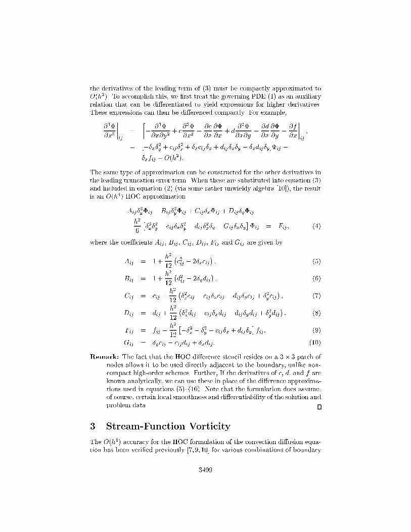
the derivatives of the leading term of �� must be compactly approximated toO�h�� To accomplish this we �rst treat the governing PDE �� as an auxiliaryrelation that can be di�erentiated to yield expressions for higher derivatives�These expressions can then be di�erenced compactly� For example

��

�x�

��ij

�

��

��

�x�y�� c

��

�x��

�c

�x

��

�x� d

��

�x�y��d

�x

��

�y��f

�x

��ij

�

� ��x��y � cij�

�x � �xcij�x � dij�x�y � �xdij�y �ij �

�xfij � O�h��

The same type of approximation can be constructed for the other derivatives inthe leading truncation error term� When these are substituted into equation ��and included in equation �� via some rather unwieldy algebra �� the resultis an O�h�� HOC approximation

�Aij��x�ij �Bij�

�y�ij � Cij�x�ij � Dij�y�ij�

h�

�

��x�

�y � cij�x�

�y � dij�

�x�y �Gij�x�y

��ij � Fij � ��

where the coe�cients Aij Bij Cij Dij Fij and Gij are given by

Aij � � �h�

��

�c�ij � ��xcij

� ��

Bij � � �h�

��

�d�ij � ��ydij

� ��

Cij � cij �h�

��

��xcij � cij�xcij � dij�ycij � ��ycij

� ��

Dij � dij �h�

��

��xdij � cij�xdij � dij�ydij � ��ydij

� ��

Fij � fij �h�

��

��x � ��y � cij�x � dij�y

�fij � ��

Gij � �ycij � cijdij � �xdij � ��

Remark� The fact that the HOC di�erence stencil resides on a �� patch ofnodes allows it to be used directly adjacent to the boundary unlike non�compact high�order schemes� Further If the derivatives of c d and f areknown analytically we can use these in place of the di�erence approxima�tions used in equations �� Note that the formulation does assumeof course certain local smoothness and di�erentiability of the solution andproblem data�

� Stream�Function Vorticity

The O�h�� accuracy for the HOC formulation of the convection di�usion equa�tion has been veri�ed previously � � �� for various combinations of boundary

��

conditions convection coe�cients and forcing functions� The present treat�ment explores the use of this method for the decoupled iterative form of the�D steady�state stream�function vorticity equations for viscous incompress�ible �ow�

For a nondimensionalized velocity �eld V � u�� v�� where �� and �� areunit vectors in the �dimensionless� x and y directions respectively the streamfunction � may be de�ned to within an arbitrary constant by

u ��

�y� ��

v � ��

�x� ��

The de�nition of � implies that the incompressible continuity condition is sat�is�ed� The �D scalar vorticity is de�ned as the signed magnitude of the curl ofthe velocity � � �v

�x�

�u�y

and implies from �� and ��

�r��

Taking the curl of the �D vector momentum equation we obtain the scalarvorticity transport equation

�r�� ReV � r� � f� ��

where f is a nondimensional forcing function and Re � UL�

is the Reynoldsnumber with U a characteristic velocity L a characteristic length scale and the kinematic viscosity of the �uid�

For the purposes of this study we will consider wall boundary conditions asthese present some di�culty in maintaining high�order accuracy� The de�nitionof the stream function �� and �� can be used to relate any velocity bound�ary conditions to the stream function� For a wall boundary moving tangent toits surface with a constant velocity Vw the no�slip no�penetration conditionbecomes

��

�n� �Vw� ��

��

�s� ��

where n is the direction normal to the wall and s is tangent to the wall� Thelatter equation implies � is constant on the boundary� Transport equations ��and �� together with velocity relations �� and �� plus boundary condi�tions �� and �� complete the mathematical description of the fully coupledstream�function vorticity problem�

�� HOC Stream�Function Vorticity Formulation

The HOC formulation for the stream�function equation �� follows by substi�tuting � for � � for f and setting c � d � � in equation �� to obtain

�

��x � ��y �

h�

��x�

�y

��ij �

��

h�

��

��x � ��y

��ij � ��

��

Similarly the HOC approximation to the vorticity equation �� is obtainedby substituting � for � and setting c � Re u and d � Re v in equation ��However u and v are derived from � by �� and �� and therefore theseequations should also be represented to su�cient order� For example

uij ��

�y

��ij

�

� �y�ij �h�

�

��

�y�

��ij

� O�h��

and using ��

uij � �y�ij �h�

�

��

�y�

��

�x��y

�ij

� O�h��

� �y�ij �h�

�

��y�ij � ��x�y�ij

� O�h��

Likewise for the y component of the velocity ��

vij � ��x�ij �h�

�

��x�ij � �x�

�y�ij

� O�h��

Neglecting the O�h�� terms in equations �� and �� we obtain the high�ordercompact approximations for the velocity components uij and vij to be used inthe vorticity transport equation�

�� HOC Wall Boundary Conditions

We seek now to construct compact high�order formulas for the wall boundaryconditions� Let us �rst consider boundary condition �� applied for conve�nience at a vertical wall x � � so that the normal direction is simply the x�direction� For an arbitrary node �x�� yj� along this boundary the given velocityis

v�j � ��

�x

��j

�

� ��x ��j �h

�

��

�x�

��j

�h�

�

��

�x�

��j

�h�

��

��

�x�

��j

� O�h��

where ��x represents the forward di�erence operator in the x direction� Us�

ing �� x�

in �� can be written as

��

�x�

��j

� ��j ��

�y�

��j

� ��

� ��j �

��

where we have used the fact that ��y�

� � on a vertical wall� Furthermore

di�erentiating ��

��

�x�

��j

� ��

�x

��j

��

�x�y�

��j

�

� ��

�x

��j

��v

�y�

��j

�

� ��

�x

��j

�

where we have used �� to relate � and v and the fact that ��v�y�

is also zero ona vertical wall� Finally

��

�x�

��j

� ��

�x�

��j

��v

�x�y�

��j

�

Substituting these expressions into �� yields

v�j � ��x ��j �h

��j �

h�

�

��

�x

��j

�h�

��

��

�x�

��j

�h�

��

��v

�x�y�

��j

� O�h��

A second�order compact approximation can be easily obtained by simplyneglecting the third fourth and �fth terms on the right of �� That is

v�j � ��x ��j �h

��j � O�h��

and setting v�j � Vw � However this scheme will locally pollute the accuracy ofthe HOC solution near the boundary�

A third�order compact approximation can be obtained by utilizing a one�sided di�erence approximation for ��

�xin �� so that

v�j � ��x ��j �h

��j �

h�

��x ��j � O�h��

To obtain fourth�order accuracy in �� we need three approximations at

the wall� �� an O�h�� approximation to d�dx

�� an O�h� approximation to d��dx�

and �� an O�h� approximation to ��v�x�y�

� The third requirement is the easiestsimply

��v

�x�y�

��j

� ��x ��yv�j � O�h��

Examining the terms involving ��x

and ��x�

h�

�

��

�x

��j

�h�

��

��

�x�

��j

�h�

�

��x ��j �

h

�

��

�x�

��j

� O�h��

��h�

��

��

�x�

��j

�

�h�

��x ��j �

h�

��

��

�x�

��j

� O�h��

��

and using �� we can write

��

�x�

��j

� Re

�u�j

��

�x

��j

� v�j��

�y

��j

�

��

�y�

��j

� f�j �

��Re v�j�y � ��y

��j � f�j � O�h��

where we have used the fact that u�j � �� Applying �� in �� thecomplete fourth�order compact approximation to the boundary condition istherefore

v�j �h�

��

��x �

�yv�j � f�j

�

��x ��j �

�h

��h�

��x �

h�

��

�Re v�j�y � ��y

��j � O�h��

Similar conditions can be easily derived for the remaining three walls of a rect�angular cavity�

Boundary conditions at the corners are handled in a similar manner� Therestricted geometry at the corners prevents the derivation of a fourth�ordercompact formula but a third�order approximation is possible� For example atthe upper left corner �x�� yM � we can approximate �� in both the horizontaland vertical directions� Summing these results and replacing high�order termswith appropriate di�erence expressions we obtain

h

��M �

h�

�

��x � ��y

��M � �

��x � ��y

��M�

u�M � v�M �h�

�

��x �

�

y u�M � ��x ��

y v�M�

� O�h��

where M is the index of nodes along y � ��A second�order corner formula the lowest�order approximation of �� which

still involves the vorticity can be obtained by dropping the O�h�� terms from ��

h

��M � �

��x � ��y

��M � u�M � v�M � O�h��

Note that when � � � on the boundary this reduces to

h

��M � �u�M � v�M � O�h��

which reduces even further to ��M � � when the wall velocities are zero� Laterin the driven cavity problem we encounter the additional di�culty of a badcorner singularity in the vorticity� This loss of regularity is seen to degrade thescheme near the singular points�

�� Coupled and Decoupled Forms

Solution to the nonlinear problem proceeds by iteration� Let us consider a typi�cal iterative step� The current iterates are given by the solution at the previous

��

step� Using these current iterates in a successive approximation scheme wecan compute higher�order compact approximations to the velocities from ��and �� Using this result in �� with c � Re u d � Re v to approximatethe vorticity transport equation �� we obtain the HOC approximation at theinterior nodes�

!C�n�� !F

�n��

where !C�n�

represents the HOC matrix for �� and !F�n�

is the current HOC

forcing vector� Note that !C�n�

is not a square matrix it has only as many rowsas there are interior grid points� The remaining HOC equations at the boundarynodes follow from our choice of �� or �� Similarly let L and !L bethe non�square CDS and HOC Laplace matrices corresponding to the interiornodes� The HOC matrix representation of �� at the interior nodes is therefore

!L� �

�I �

h�

��L

��

Finally the boundary conditions �� and �� may be expressed

N� �B� � !U�n�

� ��

�B � ��

where N is the "normal derivative# matrix B is the vorticity boundary matrix!U�n�

is the current HOC velocity term and the subscript B refers to boundarypoints only� �Similarly the subscript I will refer to interior points in the blockmatrix notation��

In the coupled algorithm the current values of � and � are computed si�multaneously� For conceptual clarity let us split � and � into two parts onecontaining only interior data one containing only boundary data� The valuesat successive approximate iterate �n � �� are thus computed by solving�

��!LII !LIB I � h�

��LIIh�

��LIBO I O O

O O !C�n�

II!C�n�

IB

N II N IB BIB BBB

��I

�B

�I�B

��n��

�

��

�

�

!F!U

��n�

� ��

where !L L !C N and B have been partitioned into sub�matrices correspond�ing to interior and boundary components� We emphasize that the last rowrepresents �� the normal derivative boundary condition on �� For the caseRe � � �Stokes �ow� the problem is linear and the system �� is solved onlyonce�

The decoupled algorithm is simply a block iterate form of the coupled algo�rithm� We solve for the stream function and vorticity separately by lagging the

��

appropriate terms�

�!LII !LIBO I

� ��I

�B

��n��

�I � h�

��LIIh�

��LIBO O

��I�B

��n��

!C�n�

II!C�n�

IB

BIB BBB

� ��I�B

��n��

�O O

N II N IB

� ��I

�B

��n��

�!F!U

��n��

Note that we have not changed the equations which model the system but onlythe procedure by which the successive approximations are de�ned� The bottomrow in the second matrix problem looks like a vorticity boundary condition butin reality it is not� It is a stream�function boundary condition in which thevorticity only serves to model higher�order terms�

All of the numerical experiments in the section that follows are computedusing the decoupled algorithm with the added provision that successive iteratesmay be under�relaxed� That is to say if �� is the stream function computedfrom the �rst half of the decoupled algorithm then �n�� is given by

��n�� n��

where is the relaxation factor�

� Stream�Function Vorticity Results

Tests of the HOC formulation of the stream�function vorticity algorithm werelimited to two types� a model problem with known solution to verify convergencerates and the driven cavity problem whose exact solution is not known butfor which there are �ne�grid comparison results in the literature�

�� Convergence Test

To construct a test problem with known solution we specify the stream�function

� � ��x� x��y � y��

on the unit square� The corresponding vorticity function derived from equa�tion �� is

� � ��x� � �x � ��y � y�� x� x��y� � �y � ��

and the velocities derived from �� and �� are

u � ��x� x��y � y�� y��

v � ��x� x�� x��y � y��

This problem was designed such that the no�slip no�penetration conditionholds for the velocities u and v on the boundary� The problem is driven by the

��

1e-07

1e-06

1e-05

1e-04

1e-03

1e-02

1e-01

1e+00

0.01 0.10 1.00

Abs

(Bou

ndar

y E

rror

)

h, Mesh Size

HOC Vorticity Boundary Error

SECONDm = 1.94THIRD

m = 2.92FOURTHm = 3.99

1e-08

1e-07

1e-06

1e-05

1e-04

1e-03

1e-02

1e-01

1e+00

0.01 0.10 1.00

Abs

(Mid

poin

t Err

or)

h, Mesh Size

HOC Vorticity Midpoint Error

SECONDm = 2.08THIRD

m = 2.94FOURTHm = 3.75

SPEC m = 4.03

Figure �� HOC vorticity error convergence plots on the boundary and at themidpoint for the model problem with Re � ��

forcing function f which is constructed by substituting the above functions �u and v in �� In the following numerical test we solve the linear Stokes �owproblem Re � � to better isolate the e�ect of the choice of boundary conditions�The fourth�order scheme is applied in the interior and each of the boundarytreatments is compared� In Figure � the vorticity error at a representativeboundary point �x � �� y � �� and at the midpoint �x � y � �� are graphedfor a succession of meshes and for each of the implementations of the boundaryconditions discussed� O�h�� boundary conditions are labelled "SECOND# in theplots O�h�� boundary conditions are labelled "THIRD# and O�h�� boundaryconditions are labelled "FOURTH�# Results for the case where we use ourknowledge of � to provide speci�ed boundary conditions �labelled "SPEC#�are also included for the vorticity error at the midpoint� The experimentalasymptotic convergence rate m of the error E at the stated points is computedby using the results for the meshes h � �� h � �� and included in the plot�

Figures � and � are surface and contour plots of the HOC stream functionand vorticity on a �� grid� They are visually indistinguishable from theexact surface and contour plots�

The boundary error plot indicates that the rates of convergence are as pre�dicted by the boundary condition formulas� This veri�es our interpretation of

��

0.0

0.5

1.0 0.0

0.5

1.0

-0.03

-0.02

-0.01

0.00

x

y

Psi

Figure �� Surface and contour plot of the HOC stream function solution for theanalytic model problem�

the boundary condition we use as that of the stream function� These rates ofconvergence are maintained on the interior� It is interesting to note that theO�h�� boundary conditions result in smaller errors at the midpoint than dospeci�ed exact boundary conditions using the known vorticity function�

�� Driven Cavity

The lid�driven cavity �ow is a standard test case for steady Navier�Stokes com�putations and there are numerous published results that can be used for com�parison purposes� However this problem is complicated by the presence of twocorner singularities �� We consider the unit cavity � � �� withhorizontal lid velocity u � �� v � �� On the remaining sides u � v � ��

Table � is a short description of the results for HOC driven cavity runsfor selected combinations of Re grid size side boundary condition accuracyand corner boundary condition accuracy� For Stokes �ow �Re � �� the mostaccurate combination of boundary conditions produces good results at a grid ascoarse as ��

However for convection�dominated cases we see that this combination ofboundary conditions results in oscillations on coarse grids� When the cornerboundary condition accuracy is reduced from O�h�� to O�h�� the magnitude

��

0.0

0.5

1.0 0.0

0.5

1.0

-1.0

-0.5

0.0

0.5

1.0

x

y

Zeta

Figure �� Surface and contour plot of the HOC vorticity solution for the analyticmodel problem�

of oscillations drop indicating that the singularities are better represented bylow�order approximations� Nevertheless oscillations persist for this combina�tion of boundary conditions probably due to the convective component of thefourth�order side boundary condition� When we reduce the accuracy of the sideboundary conditions from O�h�� to O�h�� these oscillations disappear even oncoarse grids� However this pollutes the accuracy of the solution on the interiorslightly�

Returning to Stokes �ow contours for � and � obtained from the HOCsolution on a uniform �� grid are shown in Figure �� Next in Figures �and � for Re � �� the horizontal velocity u along the vertical centerline andthe vertical velocity v along the horizontal centerline are compared with the�ne grid results of Ghia et al �� who solved the driven cavity with an upwind�nite di�erence method and deferred correction term for an overall second�order approximation� These HOC results are again for a �� grid and arecomparable to the results from a �� ne grid in �� Our results also agreeclosely with the HOC primitive variable results in MacKinnon and Johnson � at this Reynolds number and grid size�

Figure � shows the HOC vorticity along the four borders of the cavity atRe � �� grid O�h�� side boundary conditions and O�h�� cornerboundary conditions� Note that the vorticity oscillates along the moving walls

��

Table �� Qualitative HOC driven cavity results for selected Re grid size andboundary conditions�

Re Grid Side Corner CommentsBCs BCs

� �� O�h�� O�h�� Very coarse but no oscillations� �� O�h�� O�h�� Better resolution of �ow features

�� O�h�� O�h�� Large oscillations in � on moving wall�� O�h�� O�h�� Smaller oscillations in � on moving wall�� O�h�� O�h�� No oscillations but corner separation bubble is

not resolved�� O�h�� O�h�� No oscillations accurate solutions corner bubble

appears�� O�h�� O�h�� Large oscillations in � on moving wall�� O�h�� O�h�� Very slight oscillations in � on moving wall�� O�h�� O�h�� No oscillations both corner separation bubbles re�

solved�� O�h�� O�h�� Slight oscillations in � on moving wall �more than

�� O�h�� O�h�� Iterations stagnate�� O�h�� O�h�� Iterations stagnate�� O�h�� O�h�� Oscillations in � on moving wall�� O�h�� O�h�� No oscillations good accuracy

but not along the stationary walls indicating that the oscillations are probablydue to convection terms in the fourth�order boundary condition� Interestinglythese oscillations do not propagate into the interior�

We see from Figure � that decreasing the side boundary condition accuracyfrom O�h�� to O�h�� eliminates the oscillations and still results in a reasonablyaccurate approximation� The comparison to UDS is even more striking for thevelocity components along the cavity centerlines shown in Figures � and ��

� Concluding Remarks

A HOC scheme with high�order boundary treatment was developed and ap�plied successfully to the stream�function vorticity equations for Navier�Stokesproblems� The derivation of the �nal equations required extensive algebraic ma�nipulation but can now be programmed by others for applications and industrialuse� These resulting equations are not available elsewhere in the literature� Weremark that symbolic manipulators may eventually prove useful for these typesof schemes but were not found useful here�

To verify that high�order convergence was being achieved a model Stokes

��

0.0 0.2 0.4 0.6 0.8 1.00.0

0.2

0.4

0.6

0.8

1.0

x

y

-1e-5

-1e-4

-0.01

-0.03

-0.05

-0.07

-0.09

-0.1

0.0 0.2 0.4 0.6 0.8 1.0

0.0

0.2

0.4

0.6

0.8

1.0

x

y

-5

-4

-3

-2

-1

-0.5

0

0 0

0.5 0.5

0.5

1 1

2 2

3 3

�a� Stream Function�b� Vorticity

Figure �� HOC driven cavity contours of the stream function and vorticity forRe � � on a �� grid�

problem was constructed with a known analytic solution� The method wasthen applied to the driven cavity problem despite the presence of two cornersingularities in the vorticity� Nevertheless it compared favorably with resultson much �ner grids using more standard methods�

Acknowledgements

The authors wish to express their appreciation to Bob MacKinnon for his com�ments and assistance� This research has been supported by the Texas AdvancedTechnology Program a grant from ARPA and by the industrial associates ofthe CEOGRR�

References

� B�P� Leonard� A stable and accurate convective modeling procedure basedon quadratic upstream interpolation� Computer Methods in Applied Me�

chanics and Engineering ��

��

0.0

0.2

0.4

0.6

0.8

1.0

-0.4 -0.2 0.0 0.2 0.4 0.6 0.8 1.0

y

u

Re = 400

HOC (31x31)UDS (31x31)CDS (31x31)

Ghia (129x129)

Figure �� Driven cavity results for the horizontal velocity component along thevertical centerline Re � �� Note� results utilizes O�h�� boundary conditions�

-0.5

-0.4

-0.3

-0.2

-0.1

0.0

0.1

0.2

0.3

0.4

0.0 0.2 0.4 0.6 0.8 1.0

v

x

Re = 400

HOC (31x31)UDS (31x31)CDS (31x31)

Ghia (129x129)

Figure �� Driven cavity results for the vertical velocity component along thehorizontal centerline Re � �� Note� results utilizes O�h�� side boundaryconditions and O�h�� corner boundary conditions�

��

-80

-60

-40

-20

0

20

40

60

80

100

120

140

0.0 0.2 0.4 0.6 0.8 1.0

Vor

tici

ty

x or y

HOC Driven Cavity, 4th-Order BCs, Re=1000, 41x41 grid

y = 1y = 0x = 1x = 0

Figure �� Vorticity on the four boundaries of the driven cavity problem forRe � �� and O�h�� boundary conditions�

-120

-100

-80

-60

-40

-20

0

0.0 0.1 0.2 0.3 0.4 0.5 0.6 0.7 0.8 0.9 1.0

Vor

tici

ty

x

Re = 1000

HOC (41x41)UDS (41x41)

Ghia (129x129)

Figure �� Driven cavity results for the vorticity along the moving wall Re �� Note� results utilize O�h�� side boundary conditions and O�h�� cornerboundary conditions�

��

0.0

0.2

0.4

0.6

0.8

1.0

-0.4 -0.2 0.0 0.2 0.4 0.6 0.8 1.0

y

u

Re = 1000

HOC (41x41)UDS (41x41)

Ghia (129x129)

Figure �� Driven cavity results for the horizontal velocity component alongthe vertical centerline Re � �� Note� results utilizes O�h�� side boundaryconditions and O�h�� corner boundary conditions�

-0.6

-0.5

-0.4

-0.3

-0.2

-0.1

0.0

0.1

0.2

0.3

0.4

0.0 0.2 0.4 0.6 0.8 1.0

v

x

Re = 1000

HOC (41x41)UDS (41x41)

Ghia (129x129)

Figure �� Driven cavity results for the vertical velocity component along thehorizontal centerline Re � �� Note� results utilize O�h�� side boundaryconditions and O�h�� corner boundary conditions�

��

� B�P� Leonard and S� Mokhtari� Beyond �rst�order upwinding� The ultra�sharp alternative for non�oscillatory steady�state simulation of convection�International Journal for Numerical Methods in Engineering ��

� B�J� Noye and H�H� Tan� A third�order semi�implicit �nite di�erencemethod for solving the one�dimensional convection�di�usion equation� In�ternational Journal for Numerical Methods in Engineering �� July ��

� B�J� Noye� New third�order �nite�di�erence method for transient one�dimensional advection�di�usion� Communications in Applied Numerical

Methods �� May ��

� R�J� MacKinnon and G�F� Carey� Analysis of material interface disconti�nuities and superconvergent �uxes in �nite di�erence theory� Journal of

Computational Physics ��

� R�J� MacKinnon and G�F� Carey� Superconvergent derivatives� A Taylorseries analysis� International Journal for Numerical Methods in Engineer�

ing ��

� R�J� MacKinnon and G�F� Carey� Nodal superconvergence and solution en�hancement for a class of �nite element and �nite di�erence methods� SIAMJournal on Scienti�c and Statistical Computing �� March��

� R�J� MacKinnon G�F� Carey and P� Murray� A procedure for calculat�ing vorticity boundary conditions in the streamfunction�vorticity method�Communications in Applied Numerical Methods ��

� R�J� MacKinnon and R�W� Johnson� Di�erential equation based represen�tation of truncation errors for accurate numerical simulation� InternationalJournal for Numerical Methods in Fluids ��

�� W�F� Spotz� Superconvergent �nite di�erence methods with applicationsto viscous �ow� Master�s thesis University of Texas at Austin ��

�� R�W� Johnson and R�J� MacKinnon� An auxiliary equation method ob�taining superconvergent �nite element approximations� Communications

in Applied Numerical Methods ��

�� R�W� Johnson and R�J� MacKinnon� Equivalent versions of the QUICKscheme for �nite�di�erence and �nite volume numerical methods� Commu�nications in Applied Numerical Methods ��

�� J�K� Dukowitz and J�D� Ramshaw� Tensor viscosity method for convectionin numerical �uid dynamics� Journal of Computational Physics ��

��

�� P�W� Hemker� Mixed defect correction iteration for the accurate solutionof the convection di�usion equation� In W� Hackbusch and U� Trottenbergeditors Multigrid Methods� Proceedings of Conference Held in K�oln�Porz�

November �� pages �� Berlin �� Springer�Verlag�

�� M�M� Gupta and et� al� Single�cell high order di�erence method for steadystate advection�di�usion equation� In Proceedings of the Symposium�

International Association for Hydraulic Research pages ��

�� M�M� Gupta R�P� Manohar and J�W� Stephenson� A single cell high or�der scheme for the convection�di�usion equation with variable coe�cients�International Journal for Numerical Methods in Fluids ��

�� S�C�R� Dennis and J�D� Hudson� Compact h� �nite di�erence approxima�tions to operators of Navier�Stokes type� Journal of Computational Physics��

�� S� Abarbanel and A� Kumar� Compact higher�order schemes for the Eulerequations� Journal of Scienti�c Computing ��

�� W�F� Spotz and G�F� Carey� High�order compact schemes for nonuniformgrids� IMA Journal of Numerical Analysis Submitted May ��

�� P� Grisvard editor� Singularities and Constructive Methods for Their Treat�

ment Proceedings of the Conference held in Oberwolfach� West Germany�Springer�Verlag New York ��

�� U� Ghia K�N� Ghia and C�T� Shin� High Re solutions for incompressible�ow using Navier�Stokes equations and a multi�grid method� Journal of

Computational Physics pages ��

��

High-Order Compact Scheme for the Steady Stream-Function Vorticity Equations

Documents

Transcript of High-Order Compact Scheme for the Steady Stream-Function Vorticity Equations