Interacting vorticity waves as an instability mechanism for magnetohydrodynamic shear instabilities

Under consideration for publication in J. Fluid Mech. 1

Interacting vorticity waves as an instabilitymechanism for MHD shear instabilities

E. Heifetz1,2, J. Mak1†, J. Nycander2 and O. M. Umurhan3,4

1Department of Geophysics & Planetary Sciences, Tel Aviv University, Tel Aviv, 69978, Israel2Department of Meteorology, Stockholm University, Stockholm, Sweden

3NASA Ames Research, Space Sciences Division, Mail Stop N-245-3, Moffett Field, CA 940434SETI Institute, 189 Bernardo Ave., Suite 100, Mountain View, CA 94043

(Received DATE UPDATED)

The interacting vorticity wave formalism for shear flow instabilities is extended hereto the magnetohydrodynamic (MHD) setting, to provide a mechanistic description forthe stabilising and destabilising of shear instabilities by the presence of a backgroundmagnetic field. The interpretation relies on local vorticity anomalies inducing a non-localvelocity field, resulting in action-at-a-distance. It is shown here that the waves supportedby the system are able to propagate vorticity via the Lorentz force, and waves may inter-act; existence of instability then rests upon whether the choice of basic state allows forphase-locking and constructive interference of the vorticity waves via mutual interaction.To substantiate this claim, we solve the instability problem of two representative basicstates, one where a background magnetic field stabilises an unstable flow and the otherwhere the field destabilises a stable flow, and perform relevant analyses to show how thismechanism operates in MHD.

Key Words: ***do this on submission website***

1. Introduction

Shear flows are ubiquitous in fluid systems, and shear flow instability, nonlinear de-velopment and its transition into turbulence remains an active area of research to thepresent day. We focus here on magnetohydrodynamic (MHD) shear instabilities, relevantto astrophysical systems such as, for example, the solar tachocline, the magnetopause,and atmospheres of hot exoplanets. In particular, we are interested in the physical mech-anisms leading to ideal parallel shear instabilities in MHD.The argument generally is that, in the presence of a background magnetic field that

has a component parallel to the background flow, fluid instabilities have to do work tobend field lines, thus the presence of a background magnetic field should be stabilising.This is generally found to be true in planar geometry when the background magnetic fieldis uniform (e.g., Chandrasekhar 1981; Biskamp 2003). However, this argument does notaccount for the observed destabilisation of hydrodynamically stable flows in the presenceof spatially varying background magnetic fields (e.g., Stern 1963; Kent 1966, 1968; Chen &Morrison 1991; Tatsuno & Dorland 2006; Lecoanet et al. 2010), or the fact that a uniformfield can destabilise some wavenumbers that are hydrodynamically stable (e.g., Kent

† Email address for correspondence: [email protected]; present address: Schoolof Mathematics, University of Edinburgh, James Clerk Maxwell Building, The King’s Buildings,Edinburgh, EH9 3FD, UK

2 E. Heifetz, J. Mak, J. Nycander and O. M. Umurhan

+q+q −q−q

+q −q−q

U(y)

∆Q < 0

∆Q > 0

0

π/2

−π/2

π

hinderin

ghelping

growing

decaying

Figure 1. A pictorial representation of the wave interaction mechanism for the case of twoRossby waves. Here, q ∼ −∆Qη, where q is vorticity, η is displacement, and ∆Q is the magnitudeof the vorticity jump of the background flow profile. Taking into account the sign of ∆Q at eachjump, the q anomalies resulting from the η distribution are labelled accordingly. The top wavehas a self-induced propagation to the left relative to the mean flow, and vice versa for the bottomwave, and both waves propagating counter to the mean flow. The waves interact with the othervia the non-local velocity field induced by local vorticity anomalies, and the induced velocitiesdecay with distance from vorticity anomalies, represented here by the length of the arrows. Thewaves may be held steady owing to counter-propagation relative to the mean flow, together withthe mutual interaction between the waves, resulting in a phase-locked configuration. The wavescan then constructively interfere and lead to instability. A phase difference regime diagramis given on the left, where the phase-difference is defined as ∆ǫ = ǫ2 − ǫ1, the lower wavedisplacement relative to the upper wave; the configuration here has ∆ǫ = −π/2.

1966, 1968; Ray & Ershkovich 1983). Further, in two-dimensional spherical geometry (noradial motion), a flow close to the observed solar differential rotation is hydrodynamicallystable, but is destabilised by the presence of an azimuthal background magnetic fieldvarying in latitude (e.g., Gilman & Fox 1997; Gilman & Cally 2007). To reconcile thesecontrasting effects, the negative-energy wave interpretation (e.g., Cairns 1979), based onwave resonance and energetic arguments, is sometimes invoked (e.g., Ruderman & Belov2010). The aim here is to provide an intuitive mechanistic interpretation that reconcilesthe contrasting influences of the magnetic field on MHD shear instabilities.We present here an interpretation of shear instabilities in terms of interacting vorticity

waves. This interpretation includes as a special case the Counter-propagating RossbyWaves (CRW) mechanism (e.g., Bretherton 1966; Hoskins et al. 1985), a mechanismwell-known in geophysical fluid dynamics, and has been argued by Baines & Mitsudera(1994) to be an equivalent approach to the negative-energy wave explanation for shearinstability. A basic schematic of the mechanism is recalled here for the Rossby wave casein figure 1, with a description of the mechanism given in the caption.

The main ingredients required for instability in this interpretation are phase-lockingand constructive interference, achieved via counter-propagation of waves relative to themean flow, action-at-a-distance by the non-local velocity field induced by local vorticityanomalies, and an appropriate phase-shift between the two waves. Normal mode instabil-ity may also occur whenever the waves are phase-locked with relative phase-difference (de-fined here in terms of wave displacement) satisfying ∆ǫ ∈ (−π, 0). If the self-propagationspeed of each wave is large compared to its local mean flow, the action-at-a-distance inter-action should hinder the waves’ propagation speed to maintain phase-locking; this occurswhen ∆ǫ ∈ (−π/2, 0), and generally characterises long wavelength dynamics. By contrast,the self-propagation speed of short wavelength waves counter to the mean flow is gener-ally weak, hence instability is obtained when the waves help each other’s propagation to

Instability mechanism for MHD shear instabilities 3

overcome the background flow while growing, and this occurs when ∆ǫ ∈ (−π,−π/2).Essentially, the mechanism may be summarised as “the induced velocity field of each

Rossby wave keeps the other in step, and makes the other grow” (Hoskins et al. 1985).For more details, we refer the reader to the recent review of Carpenter et al. (2013) andreferences within.

In the case of figure 1, we have illustrated the fundamental mechanism using Rossbywaves, but this is not the only possibility. As long as we have wave modes that counter-propagate against the mean flow and they propagate vorticity, it is perfectly possiblefor a configuration displayed in figure 1 to occur. Harnik et al. (2008), Rabinovich et al.

(2011) and Guha & Lawrence (2013) have shown that, in the context of shear instabilitiesin stratified fluids, displacement of an interface leads to an induced buoyancy field, thatin turn induces an appropriate vorticity field via baroclinic torque, thus Rossby–gravitywaves may also propagate vorticity. When two vorticity and/or density interfaces arepresent, the interaction of the relevant wave modes leads to instability of the Kelvin–Helmholtz type (two vorticity interfaces; e.g, Drazin & Reid 1981, Baines & Mitsudera1994), Holmboe type (essentially one vorticity and one density interface; Holmboe 1962,Baines & Mitsudera 1994), and the Taylor–Caulfield type (two density interfaces; Taylor1931, Caulfield 1994). For recent reviews and studies of shear instabilities in stratifiedfluids and their interpretation in terms of wave interactions, see Balmforth et al. (2012),Carpenter et al. (2010, 2013) and Guha & Lawrence (2013).

We show here that a similar interpretation holds in MHD. Wave displacement changesthe magnetic field configuration, and since the Lorentz force is generally rotational; thisin turn generates vorticity anomalies, so Alfven waves may propagate vorticity. We canthus use the vorticity wave interaction framework as an interpretation for MHD shearinstabilities. Furthermore, this dynamical framework explains why we have stabilisationor destabilisation by the magnetic field: the choice of basic state and parameter valuesaffects the properties of the wave modes, and the presence of instability depends onwhether supported wave modes can phase-lock and achieve mutual amplification.Previous works on this topic have, for elucidation purposes, mainly considered piecewise-

linear basic states with interfacial wave solutions of the form q(x, y, t) = qδ(y−L)eik(x−ct),where y = L is the location of ‘jump’ in the profile. If one can show that the vorticitygeneration is non-zero only at these jumps, then interfacial wave solutions are exact solu-tions. A small number of jumps in the basic state results in a dispersion relation that is alow order algebraic equation with closed form solutions. Further analysis of the solutionsmay be carried out in a relatively straight-forward manner (e.g., Rabinovich et al. 2011).One notable exception to this exactness in the hydrodynamic setting is the Charneyproblem (e.g., Heifetz et al. 2004b), where the presence of differential rotation β resultsin non-localised vorticity generation. A similar phenomenon occurs for the MHD case.Although this does not pose a problem for the numerical computation of the eigenvaluesand eigenfunctions, extra care is required when interpreting the results and the physicalmechanism. This subtlety is explained in detail here, and the regimes where the inter-facial wave assumption is a reasonable approximation to the full solution are exploredaccordingly for the instability problems we consider.

The layout of this article is follows. We provide the mathematical set up in §2, andexplain how even simple Alfven waves propagate vorticity via the Lorentz force. Ad-ditionally, we demonstrate the non-local nature of vorticity generation. For conceptualunderstanding of how waves in the system propagate vorticity, we consider the dynamicsof interfacial waves in §3. To demonstrate the instability mechanism, we solve the insta-bility problem for two piecewise-linear basic states, for comparison with previous workemploying the interacting vorticity wave formalism, and to test the performance of the in-


terfacial wave assumption. In §4, we consider the case where a background magnetic fieldstabilises the flow, taking the background flow to be the Rayleigh profile demonstratedin figure 1, together with a uniform background magnetic field. We first give details forthe numerical method we employ, then analyse in some detail the full solution, providingplots of eigenfunctions and showing how the schematic in figure 1 is modified by MHDeffects. Analytic solutions resulting from the interface assumption are derived, comparedwith the full solutions, and analysed accordingly. We give a similar account in §5 for thecase where a linear shear flow is destabilised by a spatially varying background magneticfield. We conclude and discuss our results in §6.

2. Mathematical formulation

The crux of the mechanism displayed in figure 1 is that waves supported by the systemand choice of basic state propagate vorticity, and their interaction leads to instability.In this section, we provide the general mathematical formulation, and explain how evensimple Alfven waves, supported when the background flow and field are uniform, maypropagate vorticity via the Lorentz force. We consider the dynamics of waves when theflow and field are sheared in the next section.

2.1. Two-dimensional MHD and action of Lorentz force

We are interested here in ideal MHD instabilities. The homogeneous, incompressibleMHD equations are

∂u

∂t+ u · ∇u = − 1

ρ0∇p+ 1

µ0ρ0j∗ ×B∗, (2.1a)

∂B∗

∂t+ u · ∇B∗ = B∗ · ∇u, (2.1b)

∇ · u = 0, ∇ ·B∗ = 0. (2.1c)

Here, j∗ = ∇ × B∗ is the current. In Cartesian co-ordinates, an analogue of Squire’stheorem holds (see e.g., Hughes & Tobias 2001, and discussion within), thus we mayformulate the problem in two-dimensions. The domain is taken to be the (x, y)-plane, withperiodicity in x, and as yet unspecified in y. The incompressibility condition allows us towrite the velocity u and magnetic field B = B∗/

√µ0ρ0 (where µ0 is the permeability of

free-space and ρ0 is the constant density) in terms of a streamfunction ψ and magneticpotential A, defined here as u = ez × ∇ψ and B = ez × ∇A. From this, the vorticityq = ez · ∇ × u and current j = ez · ∇ ×B satisfy the relations q = ∇2ψ and j = ∇2A,and equations (2.1) take the equivalent form

Dq

Dt= ∇ · (jB),

DA

Dt= 0. (2.2)

To see how the Lorentz force ∇ · (jB) results in rotational motion, we suppose wehave, for argument sake, B0ex with B0 = const > 0, and

j(x0, y0)ez = j0ez, j(x1, y1)ez = j1ez, (2.3)

where j1 > j0, x1 > x0, y1 = y0; this is a scenario where ∂(jbx)/∂x > 0, and note herethat j and bx are ‘full’ quantities as we have not yet linearised about a basic state. Ingeneral, the Lorentz term is F = j ×B, and, with the right-hand-screw convention, thecurrent distribution above produces

F (x0, y0) = F0ey, F (x1, y1) = F1ey, (2.4)


j0 j1

F0 F1

bx = B0 > 0

+q

∂

∂x(jbx) > 0

Figure 2. A pictorial representation of how the vorticity is generated by the Lorentz termj ×B = ∇ · (jB) in two-dimensional incompressible MHD; see text for details.

with F1 > F0 > 0. A material line connecting (x0, y0) and (x1, y1) is rotated anti-clockwise, i.e., this gives us a positive vorticity anomaly, and is consistent with positiveforcing in equation (2.2); this is shown pictorially in figure 2. An analogous interpretationexplains how ∂(jby)/∂y > 0 results also in positive vorticity (e.g., rotate figure 2 anti-clockwise by π/2).

2.2. Linearisation and Alfven wave dynamics

We now linearise (2.2) about a general basic state U(y)ex and B(y)ex (and thus Q =−∂U/∂y and J = −∂B/∂y), which results in the system of equations

(

∂

∂t+ U

∂

∂x

)

q =− ∂Q

∂y

∂ψ

∂x+B

∂j

∂x+∂J

∂y

∂A

∂x, (2.5a)

(

∂

∂t+ U

∂

∂x

)

A =B∂ψ

∂x, (2.5b)

where all quantities with no overbars are perturbation quantities. We note that B(∂j/∂x)and (∂J/∂y)(∂A/∂x) are the linearised forms of ∂(jbx)/∂x and ∂(jby)/∂y respectively,so they result in vortical motion as in figure 2. The cross-stream displacement η is givenby

v =∂ψ

∂x=

(

∂

∂t+ U

∂

∂x

)

η, (2.6)

and, substituting this into (2.5b) and integrating results in the relation

A = Bη +A0(y); (2.7)

we will take the non-advective contribution A0 associated with non-conservative effectsto be zero for the rest of this work.

For simple Alfven waves (e.g., Biskamp 2003), we take the case U = 0, and B =constant > 0 without loss of generality. With this, the governing equations become∂q/∂t = B(∂j/∂x) and ∂η/∂t = ∂ψ/∂x. We observe that η ∼ A from relation (2.7),i.e., a positive displacement is correlated with a positive A anomaly. Furthermore, since∇2A = j and the Laplacian is a negative definite operator, this implies the relationη ∼ −j.

One main difference between Alfven waves and Rossby waves is that the former aregoverned by a second rather than first order differential equation, thus two initial condi-tions need to be specified, in this case on q and η. In figure 3 we consider the cases wherethe initial conditions (in black) are in phase and in anti-phase. Focussing on figure 3awhere η ∼ q, since η ∼ −j, we have the appropriate B(∂j/∂x) at the wave nodes, andthus results in the appropriate ∂q/∂t tendencies for the q configuration in the lower panel


(a) (b)

+q+q+q −q−q−q

+q+q+q −q−q−q

(+η,−j)(+η,−j)(+η,−j)(+η,−j)

(−η,+j)(−η,+j)(−η,+j)(−η,+j)

B∂j

∂x> 0B

∂j

∂x> 0B

∂j

∂x> 0B

∂j

∂x> 0 B

∂j

∂x< 0B

∂j

∂x< 0

∂q

∂t> 0

∂q

∂t> 0

∂q

∂t> 0

∂q

∂t> 0

∂q

∂t< 0

∂q

∂t< 0

qq

ηη

Figure 3. Pictorial representation for wave dynamics associated with B(∂j/∂x), with B > 0without loss of generality. The top and bottom panels are the η and q initial conditions, where(a) η ∼ q, and (b) η ∼ −q. Black colours are tendencies associated with the chosen initialcondition, blue is the influence of the η profile on q, and red is the influence of the q profile onη. See text for description.

(in blue); this moves the q profile to the right. At the same time, the q initial conditiontogether with the relation ψ ∼ −q implies a velocity field that moves the η profile also tothe right (see also the waves in figure 1), and thus the whole wave propagates in concertto the right. An analogous argument for figure 3b where the initial condition has η ∼ −qshows the wave propagating instead to the left. A superposition of these equal amplituderight and left going waves results in a standing wave configuration (see, e.g., appendixB of Harnik et al. 2008). It may be seen from the resulting linearised equations that, ifwe consider modal solutions of the form eik(x−ct) (we take the y-wavenumber to be zerofor simplicity), ca = ±B for Alfven waves, and c > 0 implies we have η ∼ −j ∼ q, whilstc < 0 implies that η ∼ −j ∼ −q; these relations are consistent with the schematic pre-sented in figure 3a, b respectively. More generally, as long as the η and q initial conditionsare not in quadrature with each other, we obtain travelling wave solutions associated withthe B(∂j/∂x) term.

2.3. Green’s function formulation

Wave interaction via action-at-a-distance may be represented mathematically by a Green’sfunction formalism, employed by previous authors (e.g., Harnik et al. 2008). Noting thatj = ∇2A and ψ = ∇2q, and taking the domain to be x-periodic, a Fourier transformleads to

j =

(

−k2 + ∂2

∂y2

)

A, q =

(

−k2 + ∂2

∂y2

)

ψ, (2.8)

where k denotes the x-wavenumber. (2.8) may be formally inverted to give(

A(y)ψ(y)

)

=

∫

G(y, y′)

(

j(y′)q(y′)

)

dy′, (2.9)

where G(y, y′) is a Green’s function chosen to satisfy the boundary conditions. Then,with the governing equations (2.5a), (2.6), and substituting for the appropriate terms


using relations (2.7) and (2.9), the problem is completely specified in terms of q and η,and all intermediate effects from changes in A and j are implicit.

For the piecewise-linear profiles we consider in the subsequent sections, we note thisapproach of using Green’s functions guarantees the continuity of the total pressure anddisplacement everywhere. The kinematic condition for the continuity of the interface isalready invoked in (2.6). From the y-component of the linearised momentum equation,we observe that the inverted v and by from q and j are guaranteed to be continuous byproperties of the Green’s function, so the total pressure p is also continuous since U andB are continuous.

2.4. Generation of vorticity away from interfaces

If the background profiles are piecewise-linear, and, without loss of generality, a ‘jump’ islocated at y = L, then q ∼ qδ(y−L) is exact if it can be shown that vorticity generation isnon-zero only at that location. One notable exception, however, is the Charney problem,(e.g., Heifetz et al. 2004b) where vorticity generation is non-local, and we demonstratehere this occurs in the MHD case also. To show this, we take the Laplacian of (2.5b),and the resulting linearised equation for j is given by

(

∂

∂t+ U

∂

∂x

)

j =

(

∂Q

∂y+ 2Q

∂

∂y

)

∂A

∂x+B

∂q

∂x−(

∂J

∂y+ 2J

∂

∂y

)

∂ψ

∂x. (2.10)

Then, even if (∂Q/∂y, ∂J/∂y) = (∆Q,∆J)δ(y−L), with (j, q) ∼ (j, q)δ(y−L) at t = 0, ifQ and J are non-zero at y 6= L, this generates non-zero j away from y = L, which in turnresults in non-zero q away from y = L from the vorticity equation. So δ-function solutionsare generically not self-consistent solutions (one example where δ-function solutions areexact solutions is when B is zero everywhere except at isolated locations, e.g., currentsheet profiles), thus interfacial wave solutions fail to capture all the dynamics, since weare setting to zero contributions away from the interfaces and we do not know a priori

whether the neglected contributions are significant to the dynamics. Further, non-localgeneration of vorticity implies that critical layers will play a role in the dynamics (e.g.,Rabinovich et al. 2011).

Although we will choose q and η as the fundamental variables for the bulk of the dis-cussion, this is not the only possibility. It turns out there are some numerical advantagesin utilising q and j as the variables when computing for the full numerical solutions.The two choices are of course equivalent as far as the full solution is concerned. A briefdiscussion of the (q, j) equations is given in appendix B shows how they differ wheninterfacial wave dynamics are the focus.

3. Interfacial wave dynamics

In this section, we assume solutions in q an j take the form of δ-functions to elucidatehow we may expect waves to propagate vorticity. We do this primarily for conceptualprogress, to provide links between the wave eigenstructure and the underlying physics.

We consider an unbounded y-domain; the Green’s function for this setting is given by

G(y, y′) = − 1

2ke−k|y−y′|. (3.1)

We take piecewise-linear U and B (thus piecewise-constant Q and J), with

∂Q

∂y= ∆Qδ(y − L),

∂J

∂y= ∆Jδ(y − L). (3.2)


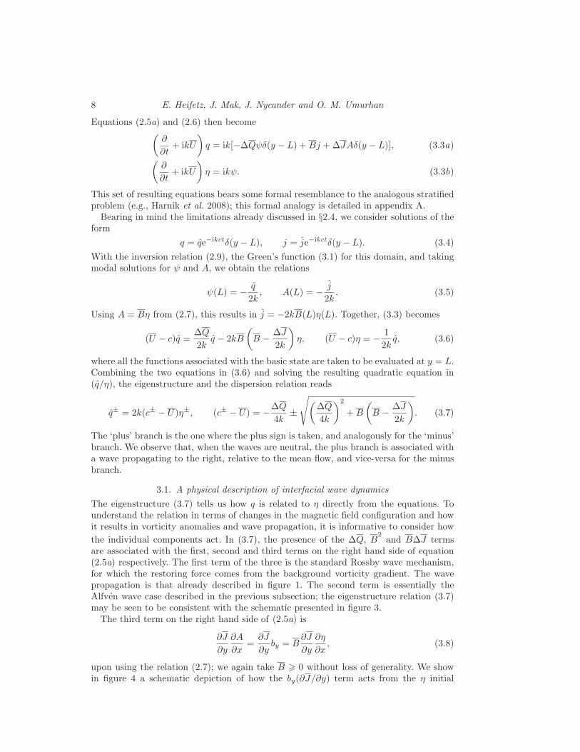
Equations (2.5a) and (2.6) then become(

∂

∂t+ ikU

)

q = ik[−∆Qψδ(y − L) +Bj +∆JAδ(y − L)], (3.3a)

(

∂

∂t+ ikU

)

η = ikψ. (3.3b)

This set of resulting equations bears some formal resemblance to the analogous stratifiedproblem (e.g., Harnik et al. 2008); this formal analogy is detailed in appendix A.

Bearing in mind the limitations already discussed in §2.4, we consider solutions of theform

q = qe−ikctδ(y − L), j = je−ikctδ(y − L). (3.4)

With the inversion relation (2.9), the Green’s function (3.1) for this domain, and takingmodal solutions for ψ and A, we obtain the relations

ψ(L) = − q

2k, A(L) = − j

2k. (3.5)

Using A = Bη from (2.7), this results in j = −2kB(L)η(L). Together, (3.3) becomes

(U − c)q =∆Q

2kq − 2kB

(

B − ∆J

2k

)

η, (U − c)η = − 1

2kq, (3.6)

where all the functions associated with the basic state are taken to be evaluated at y = L.Combining the two equations in (3.6) and solving the resulting quadratic equation in(q/η), the eigenstructure and the dispersion relation reads

q± = 2k(c± − U)η±, (c± − U) = −∆Q

4k±

√

(

∆Q

4k

)2

+B

(

B − ∆J

2k

)

. (3.7)

The ‘plus’ branch is the one where the plus sign is taken, and analogously for the ‘minus’branch. We observe that, when the waves are neutral, the plus branch is associated witha wave propagating to the right, relative to the mean flow, and vice-versa for the minusbranch.

3.1. A physical description of interfacial wave dynamics

The eigenstructure (3.7) tells us how q is related to η directly from the equations. Tounderstand the relation in terms of changes in the magnetic field configuration and howit results in vorticity anomalies and wave propagation, it is informative to consider how

the individual components act. In (3.7), the presence of the ∆Q, B2and B∆J terms

are associated with the first, second and third terms on the right hand side of equation(2.5a) respectively. The first term of the three is the standard Rossby wave mechanism,for which the restoring force comes from the background vorticity gradient. The wavepropagation is that already described in figure 1. The second term is essentially theAlfven wave case described in the previous subsection; the eigenstructure relation (3.7)may be seen to be consistent with the schematic presented in figure 3.

The third term on the right hand side of (2.5a) is

∂J

∂y

∂A

∂x=∂J

∂yby = B

∂J

∂y

∂η

∂x, (3.8)

upon using the relation (2.7); we again take B > 0 without loss of generality. We showin figure 4 a schematic depiction of how the by(∂J/∂y) term acts from the η initial


(+η,−j)(+η,−j)

(+η,−j)(+η,−j)

(−η,+j)(−η,+j)

(−η,+j)(−η,+j)

by < 0by < 0

by < 0by < 0

by > 0

by > 0

∆J < 0

∆J > 0

by∂J

∂y> 0

by∂J

∂y> 0by

∂J

∂y> 0

by∂J

∂y< 0by

∂J

∂y< 0

by∂J

∂y< 0

∂q

∂t> 0

∂q

∂t> 0

∂q

∂t> 0

∂q

∂t< 0

∂q

∂t< 0

∂q

∂t< 0

B(y)

B(y) = 0

(a)

(b)

Figure 4. Pictorial representation for wave dynamics associated with by(∂J/∂y), the third term

on the right hand side of (2.5a), with (a) B∆J < 0 and (b) B∆J > 0; without loss of generality,

B > 0. The initial conditions are given in black, and the resulting tendencies arising from thechoice of initial conditions are given in blue. See text for more details.

condition. In figure 4a, we have a case where B∆J < 0. We still have η ∼ −j (seeparagraph just after equation 2.7), and the distribution of by at the nodes of the wave(in black) then follows from the relation by = B(∂η/∂x). With this, the initial conditionresults in a by(∂J/∂y) distribution which in turn implies ∂q/∂t tendency at the nodes (inblue). This configuration is exactly like the one in figure 3, and thus we have travellingwave solutions. If instead we have B∆J > 0 as in figure 4b, the ∂q/∂t tendencies at thenodes are reversed. Similar arguments used in figure 3 then show that the η and q initialconditions propagate in opposite directions to each other unless they are in quadrature,for which no travelling wave configuration is possible.

When the η and q initial conditions are in quadrature, this implies that we have agrowing/decaying standing wave configuration. For the hydrodynamic stratified setting,the schematic presented in figure 4b is formally similar to an interpretation of Rayleigh–Taylor instability (e.g., Harnik et al. 2008). Although this suggests a local instabilityeven in the absence of a background flow (this is not impossible, since magneto-staticprofiles can suffer ideal MHD instabilities, e.g., Ch. 19 of Goldston & Rutherford 1995), atheorem due to Lundquist states that, in the case where the background magnetic field inmagneto-hydrostatic equilibrium has straight field lines, the perturbation energy cannotgrow, and the background state is stable (Lundquist 1951, paragraph of equation 29). Thisstability condition is satisfied in planar geometry by B(y). The prediction of instabilityat the local level when the state is globally stable presumably stems from the fact that weare considering isolated δ-function solutions for the purposes of elucidating the physicslinking vorticity anomalies with wave displacement. The neglected contributions and theresulting mutual interactions will presumably suppress this apparent instability.

In the presence of a background shear flow, however, instability is possible. As high-lighted in Stern (1963), taking a profile with B∆J < 0 everywhere in the domain resultsin instability when the background flow is stable in the hydrodynamic setting. Simi-


lar investigations in planar geometry of the destabilising nature of the magnetic fieldhave mainly considered profiles where B∆J < 0 in the domain, so here, for one of theexamples, we also take a basic state that satisfies this condition.

4. Unstable profile stabilised by uniform magnetic field

Having demonstrated how we expect waves to propagate vorticity anomalies, we nowconsider two instability problems to demonstrate the instability mechanism, one wherethe field stabilises an unstable flow, and the other where the field destabilises a stable flow.Both basic states are chosen so that there is only one non-dimensional parameter, givenby M = B/U , where the tildes denotes the relevant Alfven speed and velocity scales. Wenote that, from linear analysis, there is a stability theorem which states that |B| > |U |pointwise everywhere guarantees the absence of exponentially growing instabilities (e.g.,Hughes & Tobias 2001); the basic states are tailored so that the caseM > 1 is equivalentto the aforementioned condition, with M = 1 the case where we have equality.

We first provide details to the numerical method we employ to obtain our full solu-tions, then analyse these solutions and explain how the instability mechanism detailed infigure 1 is modified by MHD effects. To test the validity of taking only a small numberof interfaces, we consider the approximated problem where only two interfaces are taken;closed form solutions may be obtained from the resulting low order algebraic system, andthese are compared with the full solutions accordingly.

4.1. Numerical method

The governing equations depend on the choice of variables we employ for the numericalscheme. If we describe the dynamics in terms of q and η, the governing equations are(2.5a) and (2.6). Upon using j = ∇2A = ∇2(Bη), where we have used the identity (2.7),and with ψ =

∫

q(y′)G(y, y′) dy′, the resulting system of equations (2.5a) and (2.6) maybe written in discretised form as

∂

∂t

(

qη

)

= −ik

(

U+ Q′G −B

2(−k2I+ D2) + 2BJD1

−G U

)

(

qη

)

, (4.1)

where, for example U = U(yi)× I, a prime denotes a y-derivative, and D1,2 are the appro-priate discretised differential operators for y-derivatives. Taking uniform grid spacing ∆y,we take for example ∂Q/∂y = ∆Q/∆y at the yj entry when ∂Q/∂y = ∆Qδ(y− yj). If aquantity J is discontinuous at yj , we take J(yj) = [J(yj−1)+J(yj+1)]/2. The discretisedGreen’s function is given by (Harnik et al. 2008)

Gm,n = −∆y

2ke−k|ym−yn|; (4.2)

this is a dense matrix. The system may be advanced in time accordingly if one considersan initial value problem in the context of non-modal instabilities (e.g., Constantinou& Ioannou 2011). For (q, η) = (q, η)e−ik(x−ct), the eigenvalues and eigenvectors of thesystem (4.1) are the normal mode solutions.

It turns out it is numerically more stable to solve the problem in (q, j) variables, thuswe couple equation (2.5a) with (2.10) instead of (2.6). A similar manipulation usingA =

∫

j(y′)G(y, y′) dy′ results in

∂

∂t

(

qj

)

= −ik

(

U+ Q′G −B− J

′G

−B+ J′G+ 2JG′ U− Q

′G− 2QG′

)

(

qj

)

, (4.3)


where, in this case, G′ is the derivative of the Green’s function, with discretised formdefined to be

G′m,n =

+(∆y/2)e−k(ym−yn), ym > yn,

−(∆y/2)e+k(ym−yn), ym < yn,

0, ym = yn.

(4.4)

The value of 0 is taken at ym = yn because the wave supported on ym does not induce anyu or bx at ym. The lack of derivative operators in this latter matrix (4.3) results in a lowercondition number when compared to the (q, η) formulation in the test examples we haveconsidered. The two formulations are of course equivalent, and the relevant eigenfunctionsmay be obtained from both formulations; here, the numerical results presented wereobtained by solving (4.3).

Results presented here have been subjected to domain size and resolution tests. Adomain size of y ∈ [−5, 5] was employed. A resolution of ∆y = 10−2 (in non-dimensionalunits) was found to be sufficient for modes away from marginality, while for modesclose to marginality, a resolution of ∆y = 5 × 10−3 was employed instead to avoid theappearance of spurious instabilities. The linear algebra problem was solved using theeig(A) command in MATLAB, and we pick out the mode with the largest imaginarypart. Sample tests shows the most unstable eigenvalues obtained are well separated fromthe rest of the spectrum and, further, occur in conjugate pairs (a more general resultfor ideal instabilities which may be shown via consideration of the adjoint form of thegoverning equation; see, e.g., Drazin & Reid 1981).

4.2. Basic state and full numerical solution

We consider first the Rayleigh profile as the background flow, with a uniform backgroundmagnetic field. In dimensional form, we take

U(y) =

ΛL, y > L,

Λy, |y| < L,

−ΛL, y < −L,B(y) = B0. (4.5)

For this problem, J = 0 and ∂J/∂y = 0. Scaling by

B = B0, T =1

Λ, L = L, U = ΛL, (4.6)

the resulting non-dimensional parameter is M = B/U , a ratio of the typical Alfvenvelocity and the shear velocity, effectively a measure of the field strength, and B → Mand j → Mj in (4.3) (as well as 4.1) upon rescaling. M > 1 corresponds to the regimewhere there are no linear, normal mode instabilities. The linear stability properties of thisbasic state has been studied by Ray & Ershkovich (1983), who focused on computation ofthe growth rates of the instabilities via a shooting method, however not on the structureof the eigenfunctions.

We show in figure 5 the growth rates of the full solution (kci)full over parameter space;we note that cr = 0 for all unstable modes here, a result arising from the symmetriespossessed by the basic state. The calculated growth rates are in agreement with the resultsdocumented in Ray & Ershkovich (1983) after taking into account the different scalingsused. The explanation for the shape of the instability region is that, at M = 0, thereis no phase-locking for short waves since they are too slow to overcome the backgroundadvection. At moderate M , these short waves are now sufficiently fast (from the non-dimensional version of 3.7) to overcome the background advection, become phase-locked,


000

0.5

0.5

1

10.25 0.75

0.1

0.2M

k

Figure 5. Growth rates (kci)full of the full numerical solution associated with the basic state(4.5), with the thick red curve denoting the stability boundary. Here, cr = 0 for all unstablemodes. The red cross and circle correspond to the parameter location associated with the eigen-function displayed in figure 6a, b respectively. The resonance condition is plotted as the dashedblue line.

and constructively interfere. At large enough M , all waves become too fast, and phase-locking is not possible.

Sometimes it is informative in such investigations to plot the so called resonance condi-tions (e.g., Carpenter et al. 2013). These are the locations where the counter-propagatinginterfacial waves have matching phase speeds, taking into account advection by the back-ground flow. In this setting, these are the values of k where

c−1 (M,k) = 1 + c−ra(M,k), c+2 (M,k) = −1− c−

ra(M,k) (4.7)

are equal for some given M , with c−ra= −(1/4k)−

√

(1/4k)2 +M2 the non-dimensionalphase-speed of the counter-propagating waves; the signs in (4.7) take into account thefact that c−

rais negative. The idea is that, if interacting interfacial counter-propagating

waves are the only things contributing to the dynamics, then the location where theresonance condition is satisfied should be near to the location of optimal growth; if thisis not the case, it shows other dynamics (e.g., critical layers, pro-propagating modes)are important. It also gives an indication of where in parameter space the interactionrequired for instability can be expected, especially at large k. We overlay the locationwhere the resonance condition is satisfied in figure 5, and we see that the agreement withthe location of optimal growth is only reasonable for small M , so we expect dynamicsaway from the interface to not be negligible at larger M and also at larger k. This isconfirmed by plots of the eigenfunctions; we show in figure 6 two eigenfunctions, oneconfiguration that is generic for parameter values away from the stability boundary, andone at the same wavenumber, but at increased M , and is a sample configuration for acase close to marginality; the parameter choices are given by the red cross and circle infigure 5 respectively.

In figure 6a, the eigenfunction configuration is generic in that the dominant contribu-tions to vorticity comes from the two interfaces at y = ±1, and the contributions in the|y| 6= 1 region are comparatively small (note the colour axis scales of the correspondingsub-panels). The outer two vorticity contributions have a phase-shift that is close to π/2(0.25 in the normalised units used in the diagram), and the middle tilted structure has


0

0

0

0

0

0

00

0

00

0

00

0

0

0

0

0

0

0

0

0.25

0.25

0.25

0.25

0.5

0.5

0.5

0.5

0.75

0.750.75

0.75

1.05

0.95

-0.25-0.25

-0.5-0.5

-0.75

-0.75

-0.95

-1

-1

-1

-1-1-1

-1.05

×10-3

-2

2

-0.002

-0.002

-0.002

-0.002

-0.002

-0.002

0.002

0.002

0.002

0.002

0.002

0.002

-0.004

-0.004

-0.004

0.004

0.004

y

kx/(2π)

(a)1

1

1

1

1

11

1

0.9

0.8

-0.8

-0.9

0.1

-0.1

-0.001

-0.001

0.001

0.001

-0.003 0.003

0.003

(b)

Figure 6. Representative eigenfunctions (normalised by the maximum absolute value of q) ofthe profile given in (4.5), both for k = 0.4, but with (a) M = 0.5, and (b) M = 0.9. The red andblue shading are for positive and negative q respectively, and η is plotted as labelled contours;note the difference in the colour scales used between the sub-panels. The y-scale is continuousbetween the panels (note the displacement contours are continuous in magnitude) but is notlinear for display purposes.

vorticity contributions that have opposite signs in between two like-signed vorticity con-tributions from the interface. The vorticity eigenfunction is, going from top to bottom,in anti-phase, in quadrature and in phase with displacement, i.e., q ∼ (−η,−iη,+η) re-spectively. The outer two waves are really counter-propagating vorticity waves, and theinner wave resembles a standing wave. We have further carried out a decomposition ofthe vorticity eigenfunction into its constituents using equation (2.5a); in this case, thenon-zero terms are −(∂ψ/∂x)(∂Q/∂y) and B(∂j/∂x), divided by U − c. At the interfacelocations, the vorticity contribution comes from both terms, with the −(∂ψ/∂x)(∂Q/∂y)term being the dominant contribution; the effect of the B(∂j/∂x) contribution is to alterthe magnitude and the phase-difference between the two waves.

Figure 6a is represented schematically in figure 7. With the configuration depicted, wesee that the presence of the middle standing wave counteracts the effects of the vorticityanomalies associated with the outer counter-propagating waves. If we were to make theinterface assumption, we would neglect the contributions away from the interfaces andremove this centre contribution, and we would expect to over-estimate (i), the growthrates, and (ii), the propagation speed, the region where phase-locking is possible andthus the size of the instability region. We would expect the over-estimation to be mostsignificant when the field strength is large, and for short waves; this is because the inter-action decreases exponentially with wavenumber, so the overall constructive interferencebetween the counter-propagating waves is weaker for short waves than long waves, andit is short waves that are too slow to overcome the background advection.

The phase relation for the middle contribution q ∼ −iη may be obtained from consid-


+q+q−q −q

+q −q−q

+q+q −q−q

q ∼ −η

q ∼ −iη

q ∼ +η

Figure 7. Schematic of how the critical layer contribution plays a role in the dynamics. Withoutthe centre contribution denoted by the green parts, the dynamics of the two waves (q ∼ −η andq ∼ +η) are as in figure 1. The centre wave acts as a standing wave with q ∼ −iη, with a resultingvorticity configuration as depicted in the figure. Then it is seen that the extra contributions actsagainst the vorticity anomalies associated with the counter-propagating waves, and is thus astabilising effect.

ering the vorticity equation (2.5a). Away from y = ±1, we have, for this problem,

q =M2j

(U − cr)− ici. (4.8)

We may suppose that q is likely to be maximised at the location where U −cr = 0, whichis y = 0 here since cr = 0, resulting in the relation q ∼ iM2j/ci. From relation (2.7),we have j ∼ ∇2η, and so q ∼ −iM2η/ci, as required. This is analogous to what wasfound in the stratified setting for Rabinovich et al. (2011). The effect of the critical levelis expected to be more pronounced when we are near marginality.

As we approach marginality via increasing k and/or increasing M , the tilting of themiddle structure increases, becomes thinner in the cross-stream extent, and eventuallysplits into three tilted structures. A sample case for which we approach marginality byincreasing M is shown in figure 6b. The first thing to note is that vorticity generationis significant at the location where U(y) − cr = 0, but also at around y = ±M . Themechanistic interpretation for instability and stabilisation however is not significantlyaltered. There is perhaps some cancellation of the contributions due to the tilted struc-tures, but, schematically, we still have two counter-propagating waves, with a standingwave in between that counteracts the vorticity contributions associated with the counter-propagating waves, again as in figure 7.

The structures at y = ±M are perhaps not too surprising once we note that Alfvenwaves are non-dispersive and have non-dimensional phase speed ca = ±M in our setting,regardless of the wave number. Thus, from a physical point of view, we have forced,short wavelength standing Alfven waves since U(y) − ca = 0 at these locations. From amathematical point of view, we recall that, equivalently, the modal problem with generalbasic state in two-dimensional incompressible MHD in non-dimensional form is governed


by the second-order differential equation (e.g., Hughes & Tobias 2001)

d

dy

(

S2(y)dη

dy

)

− k2S2(y)η = 0, S2(y) = (U(y)− c)2 −M2B2(y). (4.9)

If we take the view that critical levels are where the governing eigenvalue differentialequations break down, the critical levels can occur when U(y) − c = 0 and also whereU(y) − c = ±MB(y), with the latter associated with Alfven waves. The appearance ofmultiple critical levels is not an isolated feature in MHD, and appears for example inshear flow problems on the f -plane (e.g., appendix B of Lott 2003).The second point to note for figure 6b is the change in the phase-shift of the counter-

propagating components compared to figure 6a, even though the same wavenumber waschosen. The stabilisation does not come solely from increasing the strength of the centrecontribution, unlike in one of the examples considered by Rabinovich et al. (2011). Bychanging the field strength, we change both the strength of the critical layer contributionand the wave properties at the interfaces. Although the critical layer contribution is nowstronger, the phase-shift between the vorticity contributions of the outer waves are alsoapproaching an anti-phase configuration, so both effects contribute to the reduction ingrowth rate. It is also interesting to recall that, when the two outer vorticity contributionsare in anti-phase, this implies that the corresponding displacement is in phase (e.g.,Heifetz et al. 2004a), as seen in the η eigenfunction. In other words, the whole region isundulating as one; this is physically consistent in that, as we increase the field strength,the magnetic field imparts more ‘stiffness’ to the fluid, and the fluid is forced to undulateas a whole.

As a final point, figure 6b is generic for eigenfunctions near marginal stability in thesense that, as ci goes to zero, the tilted structures become thinner and the configura-tion goes to one where there is no longer constructive interference due to the vorticityassociated with the counter-propagating modes being in phase or in anti-phase. We haveshown here the case where vorticity becomes increasingly out of phase, but of coursethey may also become increasingly in phase, depending on where we are on the stabilityboundary. There is an intermediate region where the stabilisation is solely due to thestrengthening of the centre contribution, but this is a somewhat special case and, gener-ically, both the changes to phase-shift and strengthening of the critical layer contributeto the neutralisation of the instability.

4.3. Interfacial wave dynamics

From figure 6a, we observe that the contribution in the centre can be small, so we maysuppose that taking solutions of the form

q = q1δ(y − 1) + q2δ(y + 1), j = j1δ(y − 1) + j2δ(y + 1) (4.10)

has the potential to be a reasonable approximation to the full solution, at least awayfrom marginality. Since this neglects the standing wave contribution that counteractsthe two counter-propagating waves, we expect the resulting solutions have, compared tothe solutions presented in figure 5, larger growth rates and a larger region of instability.

We start from the (q, η) formulation with equation (2.5a) and (2.6). From the inversionrelation (2.9), we have, in non-dimensional form,

A1,2 = − 1

2k(j1,2 + j2,1e

−2k), ψ1,2 = − 1

2k(q1,2 + q2,1e

−2k). (4.11)

Our vorticity equation (2.5a) will have j involved so we also need expressions for j1,2.


Using A = Bη from (2.7), we obtain from equation (4.11)

j1,2 = − 2k

1− e−4k(η1,2 − η2,1e

−2k). (4.12)

Substituting accordingly, the governing equations (2.5a) and (2.6) becomes(

∂

∂t± ik

)

q1,2 = ± i

2(q1,2 + q2,1e

−2k)− 2kM2

1− e−4k(η1,2 − η2,1e

−2k), (4.13a)

(

∂

∂t± ik

)

η1,2 = − i

2(q1,2 + q2,1e

−2k). (4.13b)

In writing equations (4.13), the fundamental assumption is that the other interface exists,which results in the appearance of exponential factors (1−e−4k)−1 multiplying some of theη terms. This is unlike the stratified case considered in Rabinovich et al. (2011). Althoughthe displacement is related to the perturbation magnetic potential and buoyancy for therespective cases, in the MHD case the current also appears in the vorticity equation;there is no analogue of this in the stratified case.

Considering modal solutions, the system (4.13) has closed form solutions given by

c = ±

√

√

√

√

1− 1

2k+

1− e−4k

8k2+M2 ±

√

1

4k2

(

1− 1− e−4k

4k

)2

+ 2M2ξ, (4.14)

where

ξ = 1− 1

k+

1− e−4k

8k2+

1 + e−4k

1− e−4k. (4.15)

WhenM = 0, (4.14) reduces to the hydrodynamic solutions c = ±√

(1− 2k)2 − e−4k/2k(e.g., Drazin & Reid 1981). For k ≪ 1, a straight forward asymptotic analysis of (4.14)yields c = i

√1−M2, which is the vortex sheet result in incompressible MHD (e.g.,

Chandrasekhar 1981).Figure 8a shows the growth rates (kci)int of the unstable branch of (4.14). Like the

full solution, the unstable modes here have cr = 0. In figure 8b we show contours of theweighted error E = 1− (kci)full/(kci)int; when E = 0, the approximated solution (4.14)agrees completely with the full solution, whilst E = 1 shows the approximated solutionpredicts instability when it is otherwise absent in the full solution. In agreement withthe hypotheses, we over-estimate growth rates as well as regions of instability, with theover-estimation being most significant in the short wave regime and near the stabilityboundary. In this instance, the resonance condition from equation (4.7) shows betterqualitative agreement with the location of optimal growth, which is to be expected sincewe have artificially removed the contributions away from the interfaces.Previous authors analysing the stratified problem (Harnik et al. 2008; Rabinovich et al.

2011) have observed that, since there are two wave branches, the modal solutions willhave a pro- and counter-propagating component. The existence of the two componentsare due to the fact that there is an intermediate step linking displacement with vorticity.In our schematic presented above in figure 7, the instability results from the interactionof counter-propagating modes, so it is informative to investigate the role of the pro-propagating mode. A similar analysis to Rabinovich et al. (2011) may be carried outhere, by taking into account the asymmetric non-dimensional eigenstructure given by

q±1 = 2kc±raη±1 , q±2 = −2kc∓

raη±2 , c±

ra= − 1

4k±

√

(

1

4k

)2

+M2. (4.16)


0 000

00 0.250.25

0.50.5

0.5

0.5

0.5 0.750.75

11

1

1

1

0.1

0.2

M

k

(a) (b)

Figure 8. Results from taking only two interfaces, for the profile given in (4.5). (a) shows thegrowth rates (kci)int of the approximated solution from (4.14). (b) shows the weighted errorE = 1− (kci)full/(kci)int. The thick red line here is the stability boundary of the full solution infigure 5, while the resonance condition from equation (4.7) is shown as the blue dashed curve.

We may transform the system of equations (4.13) into a system of equations in terms of(η±1 , η

±2 ) via a direct substitution, a self-similarity transform (e.g., Harnik et al. 2008),

or otherwise. We come to essentially the same conclusions as Rabinovich et al. (2011),where, when there is an instability, the pro-propagating mode should satisfy the relation(η+1 , η

−2 ) = −χ(η+2 , η−1 ), where χ ∈ [0, 1], i.e., the pro-propagating mode on one flank

is smaller by a factor of χ and in anti-phase with the counter-propagating mode onthe other flank. The existence of the pro-propagating mode provides extra hinderingto the counter-propagating modes, with its effect being most significant in the k ≪ 1regime. One could consider taking χ = 0 approximation that artificially removes thepro-propagating mode; the resulting analytical solution is

c = ±

√

(

1 + c−ra +M2e−4k

(1− e−4k)(c+ra − c−ra)

)2

−(

c−ra −2kM2

1− e−4k

)2(e−2k

c+ra − c−ra

)2

. (4.17)

We show in figure 9 several line plots of the analytical solution (4.14) and the χ = 0solution (4.17). The differences between the solutions in this case are so slight that theyare only distinguishable at high values of M . This points to the scenario that, althoughthe pro-propagating mode must exist as part of the physics, its effect on the instabilityfor this profile is almost negligible compared to the counter-propagating mode. One mayobtain the numerical values of χ by computing the eigenfunctions (which are just complexnumbers in this case), and taking χ = |η+1 |/|η+2 | = |η−2 |/|η−1 |; although not shown here,we have χ . 0.1 over most of the region where there is instability.

5. Stable profile destabilised by a spatially varying magnetic field

We now carry out a similar investigation for the case where a stable flow is destabilisedby a spatially varying magnetic field. We consider the dimensional basic state

U(y) = Λy, B(y) =

+Γy, y > L,

+ΓL, |y| < L,

−Γy, y < −L,(5.1)


000

0

0

0

0

0

0 111 222

0.20.20.2

-0.2-0.2-0.20.30.30.3

-0.3-0.3-0.3

kc i

c r

k

(a) (b) (c)

Figure 9. Line plots of the growth rate kci (top row) and the phase speed cr (bottom row)associated with the growing and decaying solutions of the full solution (4.14), denoted by solidlines, and the χ = 0 solutions (4.17), denoted by dashed lines. These are evaluated at fixed M ,with (a) M = 0.5, (b) M = 0.75, and (c) M = 0.9. The χ = 0 solution is, for the most part,indistinguishable from the analytical solution.

and ∂Q/∂y = 0 here. Scaling by

B = ΓL, T =1

Λ, L = L U = ΛL, (5.2)

the non-dimensional parameter is again M = B/U , and (B, J, j) → M(B, J, j) afterrescaling. This piecewise-linear magnetic field profile (resembling a wake) is chosen sothat it satisfies B∆J < 0. This profile choice is inspired partly by the parabolic magneticfield profiles B ∼ y2 considered by Chen & Morrison (1991) and Tatsuno & Dorland(2006) and the single interface profile considered by Stern (1963). One notable differencehowever is that this profile has a well-defined region of maximum |∂J/∂y|, whilst theprofiles considered previously generally have ∂J/∂y = const throughout the domain, sothis profile is not intended to be directly comparable to those previous studies. This casealso has some similarities to the problem where there is a linear shear with two densityjumps (the Taylor–Caulfield type instability), considered previously by, for example,Rabinovich et al. (2011); we have here instead two jumps in the current profile. Again,M = 1 is the cutoff for linear, normal mode instability.

Figure 10 shows contours of (kci)full for this instability problem, and, again, cr = 0 forthe unstable modes because of the symmetries possessed by the basic state. The shape ofthe instability region in parameter space may again be appropriately justified. At smallM , waves are too slow to overcome the background advection except at k ≪ 1. As Mincreases, waves become sufficiently fast, overcome the background advection and achievephase-locking. For large enough M , all waves are too fast to phase-lock. The resonancecondition in this case are the locations where

c−1 (M,k) = 1− cA(M,k), c+2 (M,k) = −1 + cA(M,k), cA =M

√

1 +1

2k(5.3)

are equal to each other. The conclusion is similar to the previous problem shown infigure 5, where we expect dynamics away from the interfaces to be significant.In figure 11 we show two eigenfunctions, one that is representative of a growing mode

away from the stability boundary, and one for a case close to marginality; again, the


0.5 00

0.5

1

0.25 0.75

0.03

0.06M

k

Figure 10. Growth rates (kci)full of the full numerical solution associated with the basic state(5.1). Here, cr = 0 for all unstable modes. The red cross and circle correspond to the parameterlocation associated with the eigenfunction displayed in figure 11a, b respectively. The thick redline is the stability boundary, and the blue dashed curve is the resonance condition given in(5.3); numerical noise is present at small k partly due to the form of the phase speed cA.

parameter locations are given respectively by the red cross and circle in figure 10. Forboth cases, we notice that the same contour levels are used for all three sections, unlikethe previous instability problem displayed in figure 6. This immediately reinforces thesuggestion that considering interfacial wave solutions only at y = ±1 as in (4.10) is goingto be an overly drastic approximation, since we will be neglecting contributions that arecomparable in size to those at the interface.

Like the previous case, we have significant structures appearing at y = ±M , thelocations where we have forced, stationary Alfven waves with ca = ±M (note this is notcA given in equation 5.3). What is different in this case is that the schematic presentedin figure 7 applies for the inner tilted structures, and so it is Alfven waves at y =±M rather than the waves supported by the interfaces that drive the instability. Thereare several extra interactions between the structures (affecting wave propagation andinteraction) that lead to the overall instability eigenfunction in figure 11. Comparingbetween figure 11a, b, we observe again that it is a mix of changes to the overall phase-shiftbetween the structures that lead to the neutralisation of the instability. Notice also that,since we are approaching marginality by increasing M in figure 11b, the displacementcontours become increasingly in phase, as in the previous example in figure 6b.We should stress here that the instability in figure 11 really does require the presence

of two current jumps to operate, while the B(∂j/∂x) term acts to modify the resultinginteraction. To support this claim, we have carried out calculations for which we onlyhave one jump. In this setting there is no instability, since the contributions on the otherinterface, its adjacent tilted structure so the standing wave in the centre are absent.The resulting vorticity eigenfunction has the interface and adjacent tilted structure inanti-phase, and there is no constructive interference there. Removing both the jumps(i.e., linear shear flow with a uniform background magnetic field) also does not resultin instability. For the profile (5.1) we consider here, the strength of the current gradientand background magnetic field are simultaneously controlled by M . We considered amodified problem where the two parameters may be varied independently; we also arriveat similar conclusions to the one presented here.


0.02

0.02

0.02 0.

02

0.02

0.02

0.04

0.04

0.04

0.04

0.04

0.04

0.06

0.06

0.06

0.06

0.06

0.06

0.08

0.08

0.08

0.08

0.08

0.08

0.1

0.1

0.1

0.1

0.1

0.1

0.12

0.12

0.12

0.12

0.12

0.12

0.14

0.14

0.14

0.14

0.14

0.14

0.16

0.16

0.16

0.16

0.16

0.18

0.18

0.18

0.18

0.22

0.05

0.05

0.05

0.05

0.05

0.05

0.1

0.1

0.1

0.1

0.1

0.1

0.15

0.15

0.15

0.15

0.15

0.15

00

0

0

0

0

0

0

0

0

0

0

00

0.2

0.2

0.2

0.2

0.2

0.2

0.2

0.2

0.4

0.6

0.8

11

1

1

1

1

-0.2

-0.4

-0.6

-0.8

-1-1

-1

-1

0.25

0.25

0.25

0.25

0.25

0.25

0.25

0.5 0.5

0.5

0.75 0.75

0.75

0.95

-0.25

-0.25

-0.25

-0.5

-0.75

-0.95

0.125

0.125

0.125

0.125

0.125

0.125

-0.125

-0.125

-0.125

-0.125

-0.125

-0.125

0.03

0.03

0.03

0.03

-0.03

-0.03

0.015

0.015

0.015

0.015

-0.015

-0.015

y

kx/(2π)

(a) (b)

Figure 11. Representative eigenfunctions (normalised by the maximum absolute value of thevorticity) of the profile given in (5.1), both for k = 0.25, but with (a) M = 0.8, and (b)M = 0.98. The red and blue shading are for positive and negative vorticity respectively, andthe displacement is plotted as labelled contours. In (b), the y-scale is continuous between thepanels (note the displacement contours are continuous in magnitude) but is not linear for displaypurposes.

We may take a similar approach to the work detailed in §4.3, by neglecting contribu-tions away from the interfaces, which results in analytical solutions that may be analysedaccordingly. However, we do not expect this to provide an accurate approximation forthis particular choice of basic state, since we are neglecting contributions that are of thesame order of magnitude as the ones at the interface. A comparison of the full numericalsolutions with the resulting analytical solution shows that the analytical solution grosslyover-estimates growth rates and the region of instability. In light of the poor comparisonof the analytical result with the correct full numerical solution, we omit here the resultsthat are counterparts to those presented in §4.3.

6. Conclusion and discussion

We have extended the interacting vorticity wave formalism to the MHD setting toprovide a physical interpretation of the instability mechanism for MHD shear instabilities.In this framework, the existence of instability depends on whether the choice of basic stateallows vorticity waves to resonate; whether the field stabilises or destabilises is dependenton how the resulting configuration affects wave properties. We have demonstrated thatvorticity generation occurs at the locations where the background magnetic field and thebackground shear are both non-zero so, unlike certain hydrodynamic cases, critical layersmust play a role in the dynamics even for piecewise-linear basic states.To demonstrate the modifications to the underlying instability mechanism by MHD


effects, and to compare with previous results and to evaluate the limitations of the in-terfacial wave assumption, we considered the instability characteristics of two piecewise-linear basic states, one where the field stabilises the unstable flow, and the other wherethe field destabilises the stable flow. The first example considered is the Rayleigh profile.The growth rate contours of the full solution agrees with the previous results of Ray& Ershkovich (1983); our contribution here is to rationalise the shape of the instabilityregion via the properties of the phase-speeds of the wave propagation. The resonancecondition and its lack of agreement with the locations of optimal growth suggests thatdynamics away from the interfaces are important; this is confirmed by plots of the eigen-functions, which shows that we effectively have a standing wave structure at U(y)−c = 0in between two counter-propagating modes, schematically represented by figure 7. Ad-ditionally, we are able to predict the phase relations of this standing wave contributionfrom the equations. As we approach marginality, one interesting feature is that we haveadditional structures appearing at the levels where U(y)− c = ±MB(y); these are crit-ical levels that correspond to locations where we have forced, stationary Alfven waves.Changing the field strength affects both the strength of the critical layer and phase-shiftsof the waves. Although there will be special cases where marginality is achieved whenthe critical layer contribution overwhelms the other contributions, generically speaking,it is a combination of the two effects that leads to neutralisation of the instability. In thisexample, we argued that the dynamics of two interfacial waves can serve as a reasonableapproximation to the full problem. We predicted and found that such an approximationover-estimates the growth rate and the region of instability. Appropriate analyses in themanner of Rabinovich et al. (2011) were performed to explore the instability character-istics under the interfacial wave assumption.

The second example we considered is a linear shear flow destabilised by a spatially vary-ing background magnetic field. The magnetic field profile was inspired by the parabolicprofile B(y) ∼ y2 considered by both Chen & Morrison (1991) and Tatsuno & Dorland(2006), although we stress that the results are not entirely comparable since ∂J/∂y is con-stant throughout the domain for the parabolic profiles. With regards to the eigenfunction,a robust feature is that, like the previous example, tilted structures with significant contri-butions of vorticity exists at the critical levels. The schematic in figure 7 however appliesinstead to the forced, stationary Alfven waves located at U(y) − c = ±MB(y) counter-acted by the standing wave contribution associated with the critical level U(y)− c = 0.The principal interactions driving the instability are from these stationary Alfven wavesaway from the interfaces, rather than from interfacial waves.

Part of the reason for employing piecewise-linear profiles is to obtain a simplified prob-lem for understanding the dynamics leading to instability, as well as for comparison withprevious works on a similar topic. One important point we highlighted is that one needsto be careful when making the interfacial wave assumption, since vorticity generationis generally not localised in the MHD case. The non-local generation of vorticity occursmore generally when considering the instability problem for smooth basic states (arguablymore realistic for modelling purposes), and the resulting eigenstructure generically has aspatial dependence on the cross-stream coordinate. Although waves are then not as well-defined, one may wonder whether the same mechanistic interpretation summarised byfigure 7 here is schematically correct. One study that supports this was reported in one ofthe authors’ PhD thesis (Mak 2013). For calculations of the profile U(y) = tanh(y) and auniform background magnetic field, plots of the eigenfunction showing structures similarto figure 6a here were found. We expect analogous structures to appear in eigenfunctionsfrom calculations with other smooth basic states, demonstrating that shear instabilitiesmay be interpreted as the mutual interaction of vorticity regions. One other possible sce-


nario for smooth profiles is that the overall eigenfunction could look schematically likefigure 4b, occurring for example when the basic state gradients are weak/non-existent,although this has not been found for the examples considered here.

Beyond incompressible MHD, this wave interaction framework, together with the previ-ous works on for the stratified case (Harnik et al. 2008; Rabinovich et al. 2011; Carpenteret al. 2010, 2013; Guha & Lawrence 2013) may perhaps explain the observations madein the previous work of Lecoanet et al. (2010), where they consider the shear instabilityproblem in a stratified fluid, with a background magnetic field. The field in that casecan stabilise or destabilise; we suspect this is most likely due to whether the vorticitywave modes supported by the choice of the basic state can interact accordingly, leadingto instability; we suspect this is why the Richardson number or Miles–Howard criterion(e.g., Miles 1961) is not necessarily applicable to stratified MHD shear flows.

Although we have focussed on modal instabilities here, the formulation is kept in the∂η/∂t = Aη form (where η denotes the state vector and A denotes the appropriateoperator) so that it may also be used to investigate non-normal mode instabilities andtransient growth (e.g., Constantinou & Ioannou 2011; Guha & Lawrence 2013). Further,our profiles were chosen so that, when M > 1, |B| > |U | pointwise everywhere, anda stability theorem forbids normal mode instabilities. Profiles violating this conditionlocally do suffer instabilities, and, in particular, have been found for studies in bothtwo-dimensional, spherical, incompressible and shallow water MHD (see the recent re-view by Gilman & Cally 2007). Although this particular scenario is not one we haveaddressed here, a extension of our interpretation to spherical MHD appears possible (ahydrodynamic extension in spherical co-ordinates was given by Methven et al. 2005).These instabilities may be explained by energetic arguments, and an extension of ourmechanistic interpretation will serve to complement the existing explanation. Further,shallow water MHD simulations on a rotating spherical planet show the emergence ofstable compact monopolar vortex structures of nested patches of opposite signed vorticitywhose stability is maintained by a strong vertical current (Cho 2008); this is noteworthysince the same monopolar vortex structure in the absence of the aforementioned confiningmagnetic effects are otherwise unstable (e.g., van Heijst & Clercx 2009). It is conjecturedhere the instability chracteristics of such structures may also be attributed to interact-ing vorticity waves. A formulation of the problem in spherical MHD allows for a moreappropriate comparison to the existing results, and this is currently under investigationby the authors.

This work was initiated whilst JM and EH were visiting MISU, with EH supported bythe Rossby visiting fellowship of the International Meteorological Institute of Sweden.EH is grateful to Michael Mond for fruitful discussion and to his teacher AlexanderErshkovich for his insight and wisdom. JM thanks Toby Wood, Andrew Gilbert, DavidHughes and Stephen Griffiths for comments and pointing out some references. OMUthanks James Cho, Peter Read and Paul Dellar for enlightening conversations on thematter of magnetic vortex generation. Constructive comments from the three anonymousreferees are gratefully acknowledged. The order of authorship is alphabetical.

Appendix A. Some formal analogies with the stratified problem

Using (2.7) to rewrite (2.5a), the linearised vorticity equation in MHD is given by

(

∂

∂t+ U

∂

∂x

)

q = −∂Q∂y

∂ψ

∂x+B

∂j

∂x+

(

B∂J

∂y

)

∂η

∂x, (A 1)


coupled accordingly by the kinematic condition; η and ψ here are, respectively, thehorizontal displacement and streamfunction in the xy-plane. For the analogous prob-lem in the Bousinessq system, using the fact that (∂/∂t + U∂/∂x)b = −wN2(z) and(∂/∂t+U∂/∂x)ζ = w, integrating yields the relation that b = −ηN2(z), where N2(z) isthe background buoyancy frequency. The resulting vorticity equation reads

(

∂

∂t+ U

∂

∂x

)

q = −∂Q∂z

∂φ

∂x−N2 ∂ζ

∂x. (A 2)

Here, ζ and φ are respectively the vertical displacement and streamfunction in the xz-plane. Then the formal similarity is that −B(∂J/∂y) ↔ N2. The analogy is not entirelycomplete here because of the B(∂j/∂x) term. Further, one may use the identity j =∇2A = ∇2(Bη) in (A 1) and observe that the final term disappears, and instead we have∇2η terms (see also equation 4.1). This does not invalidate the physical interpretationpresented in §3 since we are merely looking at different forms of the same terms describingthe physics. Indeed, if there was no cancellation, then one may suppose there is someregion where |B(∂j/∂x)| ≪ |(∂A/∂x)(∂J/∂y)|, and then the analogy with the stratifiedproblem holds, although the physics of the two systems are fundamentally different.

We note that, in the stratified problem, without assuming interfacial waves, the evo-lution equation for the perturbation energy is given by

1

2

∂

∂t

⟨

(u2 + w2) +N2ζ2⟩

= −⟨

uw∂U

∂z

⟩

(A 3)

where the angle bracket denotes a domain integral. So if N2 < 0, it is still possible forthe perturbation kinetic energy to grow even in the absence of a background flow. In theMHD case, a similar manipulation leads first to

∂u

∂t+ U

∂u

∂x= −v ∂U

∂y− ∂

∂x(· · · ), ∂v

∂t+ U

∂v

∂x= B

(

∂J

∂yη + j

)

− ∂

∂y(· · · ), (A 4)

where the terms in (· · · ) between the two equations are the same. Again, it is the ap-pearance of the perturbation current that makes the analogy incomplete. If we howeverassume that ∂J/∂y = ∆Jδ(y −L) and j = jeikxδ(y −L), then it may be shown that, aty = L,

1

2

∂

∂t

⟨

(u2 + v2) +B(2kB −∆J)η2⟩

= −⟨

uv∂U

∂y

⟩

, (A 5)

and, in the absence of a background flow, if B∆J > 0, it is still possible for the pertur-bation kinetic energy to grow at the expense of magnetic energy, resulting in instability.

With regards to the non-dimensional units, we recall that, in the stratified case, thegoverning non-dimensional parameter is Ri = N2/(∂U/∂z)2. In MHD, the governingnon-dimensional number is

M2 =B2

0

U20

∼ B(L2B)

L2U2 ∼ −B(∂J/∂y)

(∂U/∂y)2, (A 6)

and so M2 has a formal analogy with Ri. We should stress that this is only a formalanalogy, since it does not take into account of the B(∂j/∂x) term, which results in wavemodes that are fundamentally different from the gravity wave modes. We note that, ina similar vein, Stern (1963) defines what he calls the magnetic Richardson number as(translated into our notation) Rim = (∂B/∂y)2/(∂U/∂y)2.


Appendix B. Formulation in terms of q and j variables

One alternative approach is to use q and j as the fundamental variable over q andη when considering interface solutions. One immediate issue is that, from the currentperturbation equation (2.10), Q and J are not-well defined at the interface locations. Afurther approximation that one might make is that the terms with the coefficient Q andJ are small compared to ∂Q/∂y and ∂J/∂y; this may be appropriate if we have reasonto believe that interfacial waves are the most important aspect to the dynamics, perhapswhen the basic state gradients are strong. With this assumption, we obtain the systemof equations

(

∂

∂t+ U

∂

∂x

)

q =− ∂Q

∂y

∂ψ

∂x+B

∂j

∂x+∂J

∂y

∂A

∂x, (B 1a)

(

∂

∂t+ U

∂

∂x

)

j =+∂Q

∂y

∂A

∂x+B

∂q

∂x− ∂J

∂y

∂ψ

∂x. (B 1b)

With this, we notice that, if we define a generalised streamfunction and vorticity asφ± = (ψ ±A)/2 and Q± = (q ± j)/2, then we have ∇2φ± = Q± and that

[

∂

∂t+ (U ∓B)

∂

∂x

]

Q± = −(

∂Q

∂y± ∂J

∂y

)

∂φ∓

∂x. (B 2)

This has some formal similarities to employing Elsasser variables (e.g., Biskamp 2003) inwriting the MHD equations, although this is of course different since we have made anapproximation by dropping certain terms in the j equation.

REFERENCES

Baines, P. G. & Mitsudera, H. 1994 On the mechanism of shear instabilities. J. Fluid Mech.276, 327–342.

Balmforth, N. J., Roy, A. & Caulfield, C. P. 2012 Dynamics of vorticity defects in strat-ified shear flow. J. Fluid Mech. 694, 292–331.

Biskamp, D. 2003 Magnetohydrodynamic turbulence. Cambridge University Press.Bretherton, F. P. 1966 Baroclinic instability and the short wavelength cut-off in terms of

potential vorticity. Q. J. Roy. Met. Soc. 92, 335–345.Cairns, R. A. 1979 The role of negative energy waves in some instabilities of parallel flows. J.

Fluid Mech. 92, 1–14.Carpenter, J. R., Balmforth, N. J. & Lawrence, G. A. 2010 Identifying unstable modes

in stratified shear layers. Phys. Fluids 22, 054104.Carpenter, J. R., Tedford, E. W., Heifetz, E. & Lawrence, G. A. 2013 Instability in

stratified shear flow: Review of a physical interpretation based on interacting waves. Appl.Mech. Rev. 64, 061001.

Caulfield, C. P. 1994 Multiple linear instability of layered stratified shear flow. J. Fluid Mech258, 255285.

Chandrasekhar, S. 1981 Hydrodynamic and hydromagnetic stability , dover edn. Dover Publi-cations Inc.

Chen, X. L. & Morrison, P. J. 1991 A sufficient condition for the ideal instability of shearflow with parallel magnetic field. Phys. Fluids B 3, 863865.

Cho, J. Y.-K. 2008 Atmospheric dynamics of tidally synchronized extrasolar planets. Phil.Trans. R. Soc. A 366, 4477–448.

Constantinou, N. C. & Ioannou, P. J. 2011 Optimal excitation of two-dimensional Holmboeinstabilities. Phys. Fluids 23,074102.

Drazin, P. G. & Reid, W. H. 1981 Hydrodynamic stability , 2nd edn. Cambridge UniversityPress.


Gilman, P. A. & Cally, P. S. 2007 Global MHD instabilities of the tachocline. In The SolarTachocline (ed. D. W. Hughes, R. Rosner & N. O. Weiss). Cambridge University Press.

Gilman, P. A. & Fox, P. A. 1997 Joint instability of latitudinal differential rotation andtoroidal magnetic fields below the solar convection zone. Astrophys. J. 484, 439–454.

Goldston, R. J. & Rutherford, P. H. 1995 Introduction to plasma physics, pap/dskt edn.Taylor & Francis.

Guha, A. & Lawrence, G. A. 2013 A wave interaction approach to studying non-modalhomogeneous and stratified shear instabilities. J. Fluid Mech. 755, 336–364.

Harnik, N., Heifetz, E., Umurhan, O. M. & Lott, F. 2008 A buoyancy-vorticity waveinteraction approach to stratified shear flow. J. Atmos. Sci. 65, 2615–2630.

Heifetz, E., Bishop, C. H., Hoskins, B. J. & Methven, J. 2004a The counter-propagatingRossby-wave perspective on baroclinic instability. I: Mathematical basis. Q. J. Roy. Met.Soc. 130, 211–231.

Heifetz, E., Methven, J., Hoskins, B. J. & Bishop, C. H. 2004b The counter-propagatingRossby-wave perspective on baroclinic instability. II: Application to the Charney model.Q. J. Roy. Met. Soc. 130, 233–258.

Holmboe, J. 1962 On the behaviour of symmetric waves in stratified shear layers. Geophys.Publ. 24, 67–113.

Hoskins, B. J., McIntyre, M. E. & Robertson, A. W. 1985 On the use and significance ofisentropic potential vorticity maps. Q. J. Roy. Met. Soc. 111, 877–946.

Hughes, D. W. & Tobias, S. M. 2001 On the instability of magnetohydrodynamic shear flows.Proc. R. Soc. Lond. A 457, 1365–1384.

Kent, A. 1966 Instability of laminar flow of a perfect magnetofluid. Phys. Fluids 9, 1286.Kent, A. 1968 Stability of laminar magnetofluid flow along a parallel magnetic field. J. Plasma

Phys. 2, 543–556.Lecoanet, D., Zweibel, E. G., Townsend, R. H. D. & Huang, Y.-M. 2010 Violation of

Richardson’s criterion via introduction of a magnetic field. Astrophys. J. 712, 1116–1128.Lott, F. 2003 Large-scale flow response to short gravity waves breaking in a rotating shear

flow. J. Atmos. Sci. 1704, 1691–4862.Lundquist, S. 1951 On the stability of magneto-hydrostatic fields. Phys. Rev. 83, 307–311.Mak, J. 2013 Shear instabilities in shallow-water magnetohydrodynamics. PhD thesis, Univer-

sity of Leeds.Methven, J., Heifetz, E., Hoskins, B. J. & Bishop, C. H. 2005 The counter-propagating

Rossby-wave perspective on baroclinic instability. III: Primitive-equation disturbances onthe sphere. Q. J. Roy. Met. Soc. 131, 1393–1424.

Miles, J. W. 1961 On the stability of heterogeneous shear flows. J. Fluid Mech. 10, 496–508.Rabinovich, A., Umurhan, O. M., Harnik, N., Lott, F. & Heifetz, E. 2011 Vorticity

inversion and action-at-a-distance instability in stably stratified shear flow. J. Fluid Mech.670, 301–325.

Ray, T. P. & Ershkovich, A. I. 1983 Kelvin–Helmholtz instabilities in a sheared compressibleplasma. Mon. Not. R. Astron. Soc. 204, 821–831.

Ruderman, M. S & Belov, N. A 2010 Stability of MHD shear flows: Application to spacephysics. J. Phys.: Conf. Ser. 216, 012016.

Stern, M. E. 1963 Joint instability of hydromagnetic fields which are separately stable. Phys.Fluids 6, 636–642.

Tatsuno, T. & Dorland, W. 2006 Magneto-flow instability in symmetric field profiles. Phys.Plasmas 13, 092107.

Taylor, G. I. 1931 Effect of variation in density on the stability of superposed streams of fluid.Proc. R. Soc. Lond. A 132, 499–523.

van Heijst, G. J. F. & Clercx, H. J. H. 2009 Laboratory modeling of geophysical vortices.Ann. Rev. Fluid Mech. 41, 143–164.

Interacting vorticity waves as an instability mechanism for magnetohydrodynamic shear instabilities

Documents

Transcript of Interacting vorticity waves as an instability mechanism for magnetohydrodynamic shear instabilities