Atmospheric Sciences:

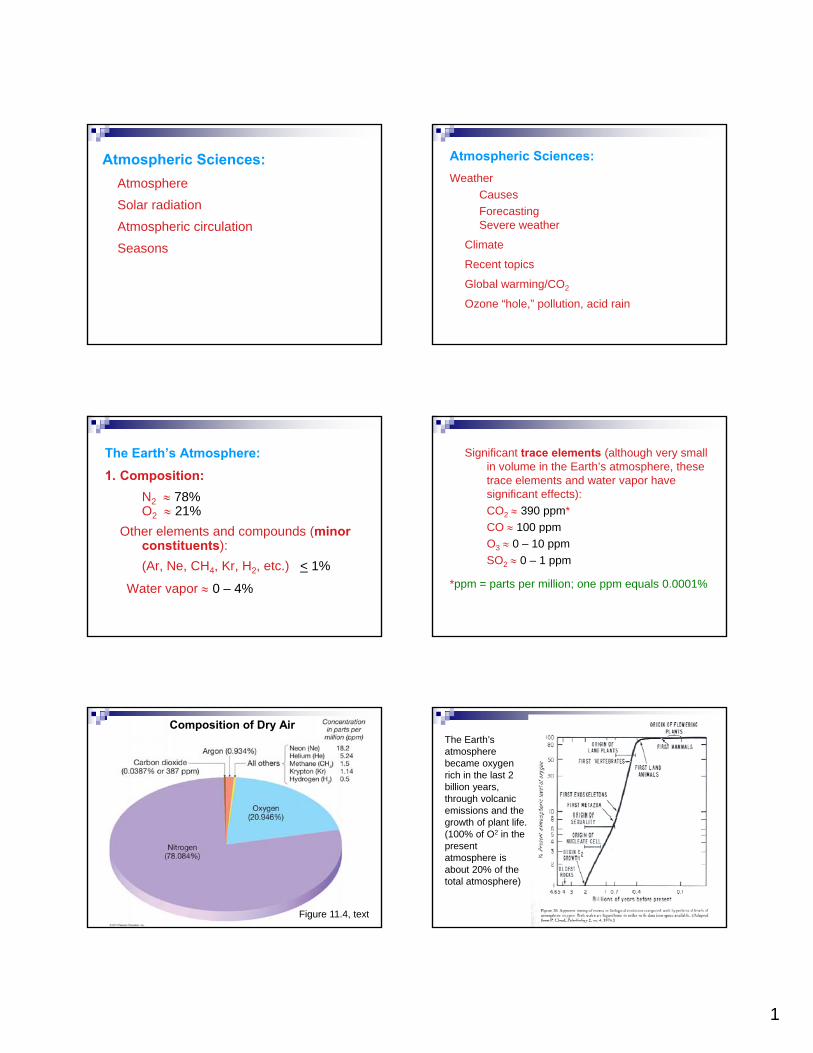
1

Atmospheric Sciences:

Atmosphere

Solar radiation

Atmospheric circulation

Seasons

Atmospheric Sciences:

Weather

Causes

ForecastingSevere weather

Climate

Recent topics

Global warming/CO2

Ozone “hole,” pollution, acid rain

The Earth’s Atmosphere:

1. Composition:

N2 78%O2 21%

O (Other elements and compounds (minor constituents):

(Ar, Ne, CH4, Kr, H2, etc.) < 1%

Water vapor 0 – 4%

Significant trace elements (although very small in volume in the Earth’s atmosphere, these trace elements and water vapor have significant effects):

CO2 390 ppm*

CO 100 ppmCO 100 ppm

O3 0 – 10 ppm

SO2 0 – 1 ppm

*ppm = parts per million; one ppm equals 0.0001%

Composition of Dry Air

Figure 11.4, text

The Earth’s atmosphere became oxygen rich in the last 2 billion years, through volcanic emissions and the growth of plant life.(100% of O2 in the present atmosphere is about 20% of the total atmosphere)

2

2. The atmosphere is layered by: Temperature (in lowest layer, temperature

decreases with altitude)

Pressure (pressure decreases with elevation)

Moisture content (generally decreases

with elevation; why?) – cold air (higher altitude) holds less moisture; source of most water is Earth’s surface (oceans, lakes rivers, land surface)

Air Pressure

Decreases with

Altit dAltitude

Figure 11.7, text

D = 0.00009 (more than 10 times lower density than at sea level)

Felix Baumgartner skydive Oct. 14, 2012, almost 39 km above sea level

Air Pressure Decreases with Altitude – Because as altitude increases, there is less air above, and, the density of air decreases rapidly with altitude, the pressure

Figure 11.7, text

D = Density of air (in g/cm3) – note that density of the atmosphere also decreases with altitude D = 0.00126

D = 0.00071

D = 0.00040

versus altitude relationship is a curve

Because it is a gas, the layer of atmosphere is not homogeneous, as a layer of water would be. So, there are more molecules of air per cubic meter (because of the

The difference between the number of molecules per unit volume of air

at the top and bottom of the atmosphere is much greater

than illustrated in this diagram.

Figure 13.1, text

(because of the weight of the overlying atmosphere) at lower levels of the atmosphere. This causes the curved pressure vs. altitude relationship seen in the previous slide.


If the “atmosphere” was water, the altitude vs. pressure relationship would be a straight line!


Figure 11.7, text


D = 0.00071

D = 0.00040


Graph for plotting Pressure and Wind Speed versus Time –Hurricane Hugo, wind speed (triangles) and pressure (dots) Sept. 11-22, 1989 – HW 4

3

Map for plotting Hurricane Hugo Track (note sample data near bottom of map; due to the map projection, the lines of longitude [meridians] show the North direction [as illustrated by heavy black arrows])

Homework #4 – Hurricanes Hugo and KatrinaSatellite photo of Hurricane Hugo (Time is UTC or GMT =

EST + 5 hours), 2031 hours, 21 Sept. 1989

http://web.ics.purdue.edu/~braile/eas100/hwk4SatelliteImage.pdf

Earth’s Atmosphere – a thin layer

Figure I.8, text

“Atmospheric gases scatter blue wavelengths of visible light more than other wavelengths, giving the Earth’s visible edge a blue halo. At higher and higher altitudes, the atmosphere becomes so thin that it essentially ceases to exist. Gradually, the atmospheric halo fades into the blackness of space. This astronaut photograph captured on July 20, 2006, shows a nearly translucent moon emerging from behind the halo.” http://earthobservatory.nasa.gov/IOTD/view.php?id=7373

http://earthsky.org/space/view-from-space-layers-of-atmosphere-on-the-horizon


“The Earth's atmosphere is an extremely thin sheet of air extending from the surface of the Earth to the edge of space. The Earth is a sphere with a roughly 13,000 km diameter; the thickness of the atmosphere is about 100 km. In this picture, taken from a spacecraft orbiting at 300 km above the surface, we can see the atmosphere as the thin blue band between the surface and the blackness of space. If the Earth were the size of a basketball, the thickness of the atmosphere could be modeled by a thin sheet of plastic wrapped around the ball. At any given location, the air properties also vary with the di t f th f f th E th Th h t th

http://www.grc.nasa.gov/WWW/K-12/airplane/atmosphere.html

distance from the surface of the Earth. The sun heats the surface of the Earth, and some of this heat goes into warming the air near the surface. The heated air rises and spreads up through the atmosphere. So the air temperature is highest near the surface and decreases as altitude increases. The pressure of the air can be related to the weight of the air over a given location. As we increase altitude through the atmosphere, there is some air below us and some air above us. But there is always less air above us than was present at a lower altitude. Therefore, air pressure decreases as we increase altitude.”

4


http://www.nasa.gov/mission_pages/station/multimedia/gallery/iss030e031275.html The Moon and Earth's atmosphere“ISS030-E-031275 (8 Jan. 2012) --- One of a series of photos of the moon and Earth's atmosphere as seen from the International Space Station over a period of time that covered a number of orbits by the orbital outpost.”

“THE THIN BLUE LINE: Earth’s thin atmosphere is all that stands between life on Earth and the cold, dark void of space. Our planet's atmosphere has no clearly defined upper boundary but gradually thins out into space. The layers of the atmosphere have different characteristics, such as protective ozone in the stratosphere, and weather in the lowermost layer. The setting Sun is also featured in this image from ISS, 2008.” http://fettss.arc.nasa.gov/collection/details/earth-atmosphere/

Notice the very thin,

illuminated atmosphere

http://www.nasa.gov/mission_pages/shuttle/shuttlemissions/sts135/multimedia/fd14/Image_Gallery_Collection_archive_8.html

Space Shuttle Atlantis leaving the International Space Station on the last NASA Space Shuttle Mission (STS 135) July 21, 2011.

Temperature variation with altitude (we will focus on the lowermost layer, the troposphere

Figure 11.9, text

troposphere, where most weather phenomena occur)

Temperature variation with elevation(lowest layer of the atmosphere, the troposphere,

where most weather phenomena occur)

e (k

m)

Figure 11.9, text

Alti

tude



e (k

m)

Vertical movements of air produce cooling for upward movement and heating for downward movement

Figure 11.9, text

Alti

tude

heating for downward movement because of change in pressure (adiabatic cooling or heating - thermodynamics)

5

Because temperature decreases rapidly with altitude, water vapor % also decreases with altitude (remember very dry air on cold

Water vapor % in air is lower at low temperatures.

http://en.wikipedia.org/wiki/Water_vapor

winter days!.) (Atmospheric pressure also decreases with altitude and has an effect on water vapor %, but the temperature effect is more important.)

~ temp. at 10 km altitude

~ temp. at sea level


Felix Baumgartner skydive Oct. 14, 2012, almost 39 km above sea level


Figure 11.7, text


D = 0.00071

D = 0.00040




e (k

m)

Vertical movements of air produce cooling for upward movement and heating for downward movement

Figure 11.9, text

Alti

tude

heating for downward movement because of change in pressure (adiabatic cooling or heating - thermodynamics)

3. Atmospheric circulation occurs on multiple scales of distance and time:

Global pattern (large scale, changes

over seasons as well as hundreds of years)

Regional weather patterns (changes

over days to weeks)

Severe weather (local, and changes

over hours to days)

(We will discuss atmospheric circulation at various time scales later.)

Solar Radiation:

Electromagnetic radiation/energy

Energy source for atmosphericcirculation and weather

Solar Energy: 1 part in 109 strikes Earth in 1 minute, solar energy that strikes

Earth is more than humans use in 1 year Solar emissions are mostly in visible,

ultraviolet, and infrared parts of EM spectrum Energy is reflected, absorbed, transmitted

through atmosphere Most energy eventually radiated back into

space by Earth and atmosphere as infrared energy (so atmosphere is approximately in equilibrium)

6

Electromagnetic Spectrum

Figure 11.19, text

Energy Transfer in the Atmosphere:

-- Radiation

-- Conduction

-- Convection (mass transport; wind and other atmospheric circulation)

Figure 11.17, text

Temperature Changes:

Heating near equator cooling in polar regions (variations with seasons, weather systems, length of day)

Adiabatic heating and cooling (a g g (thermodynamic effect)

- volume of air which moves to lower pressure expands and cools;

- volume of air which moves to higher pressure compresses and warms

Temperature Changes:

Warm air rises (less dense) and cools

Similarly, cool air sinks (more dense) and warms

The Reason for Seasons:

Tilt of the Earth (results in less energy from the Sun per unit area hitting the Earth’s surface in winter and more in

)summer)

The tilt also causes significantly different length of day (hours with sunlight and therefore heating) during seasons

Time-lapse (about one hour) photograph from Earth (northern hemisphere) showing position of Polaris (“the North star”) and other

stars that appear to circle Polaris (actually due to Earth’s rotation)

Polaris

http://www.flickr.com/photos/juniorvelo/312672130/

7

Time-lapse (several hours) photograph from Earth (northern hemisphere) showing position of Polaris (“the North star”) and other stars that appear to circle Polaris (actually due to Earth’s rotation)

Polaris

http://www.wainscoat.com/astronomy/

http://en.wikipedia.org/wiki/Circumpolar_star

Time-lapse animation from Earth (northern hemisphere) showing position of Polaris (“the North star”) and other stars that appear to circle Polaris (actually due to Earth’s rotation) (http://en.wikipedia.org/wiki/Circumpolar_star)

Polaris


Polaris


The geometry of the Earth’s tilt and the rotational axis pointing to Polaris

Earth’s axis with its 23 degree tilt (relative to the plane of the ecliptic), the North directed axis points towards Polaris (the North Star in the constellation Ursa Minor), and angle relationships for a location at 40o North latitude and nighttime (~midnight) in the northern hemisphere summer solstice (June 21).

What would be the angle of Polaris aboveangle of Polaris above the horizon if you were standing at the Equator? At the North Pole? In Australia?

Earth-Sun Relationships

To Polaris

Figure 11.14, text

Area Covered by Different Sun Angles

Tropics Mid-latitude Polar

Figure 11.12, text

8

Sun Angle vs. Depth Rays Must Travel through Atmosphere to Reach Earth’s Surface

Figure depicts winter in the northern hemisphere. Note low angle of Sun in polarof Sun in polar regions and distance that rays travel through the atmosphere (atmospheric thickness greatly exaggerated).

Figure 11.13, text

“Reasons for Seasons” – Earth and Sun orbit, tilt and Sun angle animations (Please view

these animations and watch carefully; they will help you fully understand the “reasons for seasons”):

http://www.classzone.com/books/earth_science/terc/content/visualizations/es0408/es0408page01.cfm?chapter no=04

44

visualizations/es0408/es0408page01.cfm?chapter_no 04

http://www.mathsisfun.com/earth-orbit.html

Earth Orbit: https://www.youtube.com/watch?v=R2lP146KA5A

Reasons for Seasons - Summary

So, … ~23 degree tilt of the Earth causes:1. Variable heating over the seasons; heating is also dependent on

latitude (more heating near equator than near poles) because of angle of the Sun’s rays hitting Earth.

2. Changes in length of day (versus night; winter versus summer).3. More absorption of solar energy by the atmosphere in the polar

regions because of the low angle of the Sun’s rays.

World Distribution ofMean Temperature - January

Figure 11.37, text

Note highest temperatures are south of the equator. Also note “moderation” of low temperatures in the N. Pacific and N. Atlantic areas due to exchange of heat from ocean.

World Distribution ofMean Temperature - July

Note highest temperatures are north of the equator. Also note very cold temperatures in south polar region.

Figure 11.38, text

Effect of Seasons on Average Temperatures by Latitude

9

Effect of Seasons on Length of Day by Latitude Global Atmospheric Circulation Primarily the result of heating at the equator and cooling (less heating) at the poles.

Also, the Coriolis effect causes deflection, and therefore a modification of the expected circulation pattern.

Global Circulation on a Non-rotating EarthCirculation (convection) pattern expected from heating near the equator and cooling near the poles.

Note that becauseNote that, because warm air rises near the equator, the surface winds would be expected to be from pole to equator.

Figure 13.16, text

Idealized Global Circulation

Global circulation breaks into cells due to Coriolis effect and fact that it is too far from equator to pole (10,000 km) for air(10,000 km) for air to retain temperature deviation. Note that the resulting surface winds are the “Trade Winds” (prevailing winds).

Figure 13.17, text

Idealized Global Circulation (close-up, 3-D)Global circulation breaks into cells due to Coriolis effect and fact that it is too far from equator to pole (10,000 km) for air to retain

Thickness of the atmosphere greatly exaggerated

Sailing ship to Europe

to retain temperature deviations. Note that the resulting surface winds are the “Trade Winds” (prevailing winds).

Figure 13.17, text

Note that most of the U.S. (30-60 degrees N) has westerly trade winds so weather systems mostly go from west to east

Sailing ship from Europe

Idealized Global Circulation (close-up, 3-D View)Global circulation breaks into cells due to Coriolis effect and fact that it is too far from equator to pole (10,000 km) for air to retain

Note descending dry air (~30o N) –lost moisture near equator, and cool air holds less moisture

to retain temperature deviation. The resulting surface winds are the “Trade Winds” (prevailing winds).

Note rising moist air in tropical area – air loses moisture by precipitation as it rises and cools (Figure 13.17, text)

10

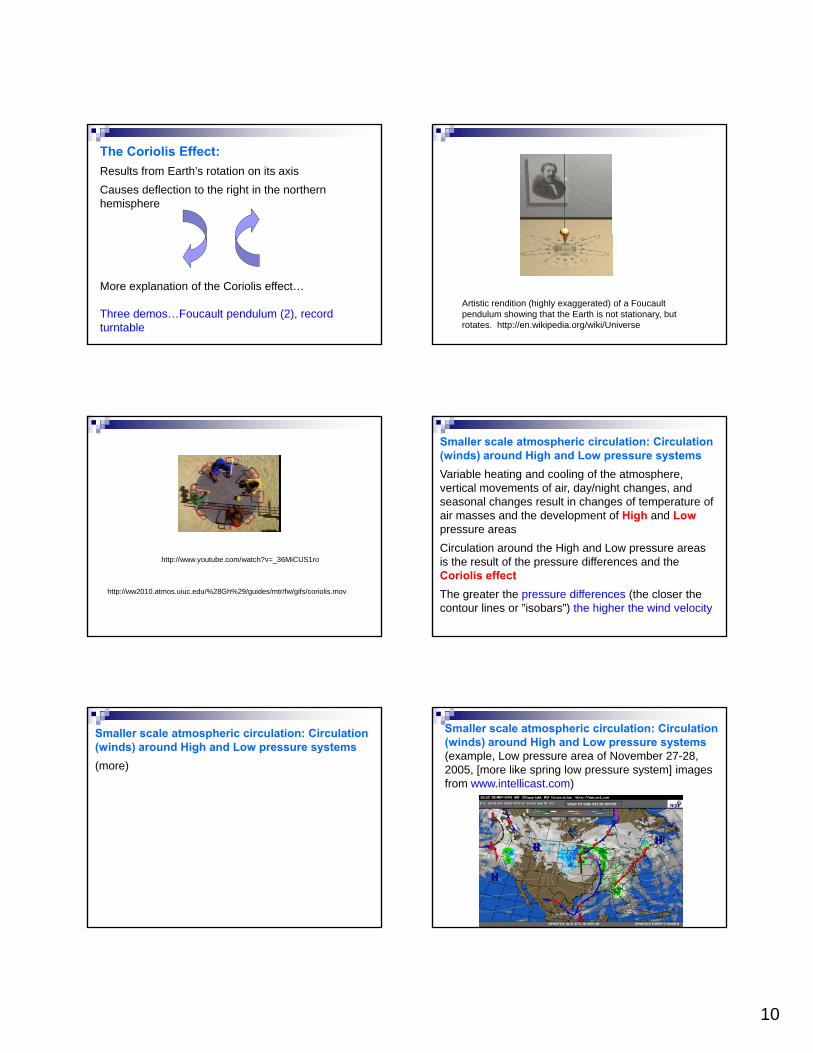
The Coriolis Effect:

Results from Earth’s rotation on its axis

Causes deflection to the right in the northern hemisphere

More explanation of the Coriolis effect…

Three demos…Foucault pendulum (2), record turntable

Artistic rendition (highly exaggerated) of a Foucault pendulum showing that the Earth is not stationary, but rotates. http://en.wikipedia.org/wiki/Universe

http://www.youtube.com/watch?v=_36MiCUS1ro

http://ww2010.atmos.uiuc.edu/%28Gh%29/guides/mtr/fw/gifs/coriolis.mov

Smaller scale atmospheric circulation: Circulation (winds) around High and Low pressure systems

Variable heating and cooling of the atmosphere, vertical movements of air, day/night changes, and seasonal changes result in changes of temperature of air masses and the development of High and Lowpressure areas

Circulation around the High and Low pressure areas is the result of the pressure differences and the Coriolis effect

The greater the pressure differences (the closer the contour lines or ”isobars”) the higher the wind velocity

Smaller scale atmospheric circulation: Circulation (winds) around High and Low pressure systems

(more)

Smaller scale atmospheric circulation: Circulation (winds) around High and Low pressure systems(example, Low pressure area of November 27-28, 2005, [more like spring low pressure system] images from www.intellicast.com)

11

Rain RainSnow Snow

Eastward moving front

Rain

Eastward moving front

Rain

Radar Loop 1400 – 1645 GMT 28 November 2005

Radar/Surface Loop 1930 11/27 – 1615 11/28 GMT

The Coriolis Effect:

Results from Earth’s rotation on its axis

Causes deflection to the right in the northern hemisphere

More explanation of the Coriolis effect…

Three demos…Foucault pendulum (2), record turntable

Infrared satellite loop over the Pacific ocean showing counter-clockwise circulation around a low pressure area south of the Aleutian Islands (04:00 – 08:00 GMT, Feb. 1, 2015).


12

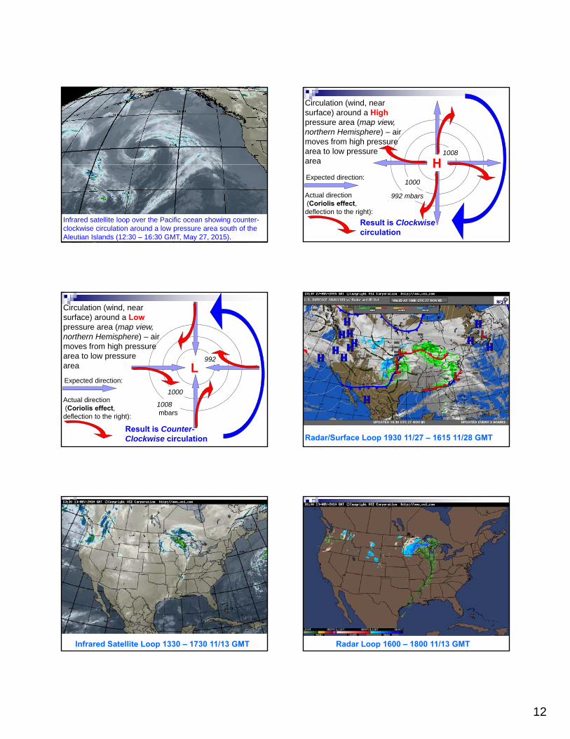
Infrared satellite loop over the Pacific ocean showing counter-clockwise circulation around a low pressure area south of the Aleutian Islands (12:30 – 16:30 GMT, May 27, 2015).

H1008

Circulation (wind, near surface) around a Highpressure area (map view, northern Hemisphere) – airmoves from high pressurearea to low pressurearea H

992 mbars

1000

Result is Clockwise circulation

Expected direction:

Actual direction(Coriolis effect, deflection to the right):

L992

Circulation (wind, near surface) around a Lowpressure area (map view, northern Hemisphere) – airmoves from high pressurearea to low pressurearea L

1000

1008mbars

Result is Counter-Clockwise circulation

Expected direction:

Actual direction(Coriolis effect, deflection to the right):

Radar/Surface Loop 1930 11/27 – 1615 11/28 GMT

Infrared Satellite Loop 1330 – 1730 11/13 GMT Radar Loop 1600 – 1800 11/13 GMT

13

Radar Loop 1600 – 1800 11/13 GMT

Prominent Low pressure area with counterclockwise circulation. Also note generally west to east movement for this mostly mid-latitude region – Pacific infrared satellite image loop 1500 – 1900 GMT Feb. 28, 2014

Circulation (wind, near surface) around a Highpressure area (cross section view to show 3rd dimension of circulation)

Cool (from high elev.), Dry, (from high elev.), Descending (more dense) air.

Earth’s surface

H

Ele

vatio

n

Air warms as it descends (adiabatic heating). Result is “good” weather (clear, dry)

Circulation (wind, near surface) around a Lowpressure area (cross section view to show 3rd dimension of circulation)

Warm (from low elev.), Moist, (from low elev.), Rising (less dense) air.Clouds and

Earth’s surface

LEle

vatio

n

Air cools as it rises (adiabatic cooling). Result is “bad” weather (cloudy, precipitation)

precipitation from cooled moist air

Typical atmospheric pressure pattern; note High and Low pressure air masses.

Figure 13.7, text


14


3-D view of circulation around High and Low pressure areas.

Figure 14.14, text

Circulation around Low pressure area often results in formation of a cold front. Collision of dry, cold air with warm, moist air results in precipitation and, possibly, thunderstorms and tornadoes.

Cold front moves from west to east due to trade winds(westerlies, in mid-l tit d 30 60

Figure 14.12, text

Warm, moist airfrom south and gulf of Mexico

latitudes, 30o-60o

N) and counter-clockwise circulationaround the Low

Cold, dry air (fromnorth)

Clouds associated with a Low pressure area and cold front

Figure 14.13, text Warm, moist air

Cold, dry air

Cold air (moving east) is more dense so it stays near the Earth’s surface and causes the adjacent warm moist air to rise along the front producing clouds, precipitation and storms.

Figure 14.8, text

Warm, moist air

Cold, dry air

Photo and caption by Santiago Borja. “A colossal Cumulonimbus flashes over the Pacific Ocean as we circle around it at 37000 feet [~11.3 km] en route to South America.” http://photography.nationalgeographic.com/nature-photographer-of-the-year-2016/gallery/week-1-landscape/6

Rising warm moist air expands and cools as it rises (adiabatic cooling) and flows outward at the top of the Troposphere (~12 km altitude) as there is warmer air (due to ozone content) above in the Stratosphere.

15

Review of Ocean Bathymetry Exercise – Bathymetric Profile (Hwk #3) – and the concept of vertical exaggeration in figures.

Bathymetric profile (ocean depth) across the Atlantic Ocean, Figure 9.15, text.

VE ~ 22

Review of Ocean Bathymetry Exercise – Bathymetric Profile (Hwk #3) – and the concept of vertical exaggeration (VE) in figures.

VE – slope is actually very, very small!

Bathymetric profile (ocean depth) across the Atlantic Ocean, zoomed in, Figure 9.15, text.

VE ~ 22

A. The bathymetry profile from homework #3; the ocean topography is vertically exaggerated (VE) about 200 times so that we can see details. B. The same figure at 1-to-1 (no VE) or true scale. Note that we cannot see any details of the bathymetry because the horizontal distance is so large compared to the depth. C. Same as B except including the curvature of the Earth. VE – slope is actually very, very small!

D. Detailed bathymetry (VE = 35) for profile D (see map E). No VE

No VE, but with true curvature of the Earth

VE example: Elevation profiles for Mt. St. Helens (before & after 1980 eruption) and Mauna Loa volcanoes at true scale (top) and 2x VE (bottom).

0 0.5 1 1.5 2 2.5 3 3.5 4

x 104

0

2000

4000

Distance (m)

Ele

vatio

n (

m)

Elevation Profiles, Mauna Loa and Mt. St. Helens (No Vertical Exaggeration)

Elevation Profiles Mauna Loa and Mt St Helens (2X Vertical Exaggeration)

0 0.5 1 1.5 2 2.5 3 3.5 4

x 104

0

2000

4000

Distance (m)

Ele

vatio

n (

m)

Elevation Profiles, Mauna Loa and Mt. St. Helens (2X Vertical Exaggeration)

Seeing Volcanoesin 3-D – Mt. St. Helens, before andafter the 1980eruption

Styrofoam topography models –each layer representsa contour line of

elevation

What is Vertical Exaggeration?

True scale, or 1 to 1, or no vertical exaggeration

3X vertical exaggeration (VE)

Horizontal scale same

Vertical scale times 3

16

Mt. Hood, OR

Google Earth perspective view (as if you were viewing from an airplane) of Mt. St. Helens volcano with no vertical exaggeration (1-to-1 scale), view looking ~South.

Mt. Hood, OR

Google Earth perspective view of Mt. St. Helens volcano with 2x vertical exaggeration (VE).

Radar/Surface Loop 1930 11/27 – 1615 11/28 GMT, note front and counter-clockwise circulation around Low

Example of global circulation/climate effect: Deserts

Namib Desert, USGS

Death Valley, CA, NPS

http://www.earthscienceworld.org/imagebank/




Figure 13.17, text


Example of global circulation/climate effect: Deserts(areas of very low precipitation, shaded yellow) occur at about 30 degrees from the equator (Hadley cells).

Saharadesert

W. Australiandesert

SW U.S.desert

SE Asiarain forest

Middle Eastdesert

Amazon rain forest

Central Africa rain forest

Kalaharidesert

desert

Patagoniadesert

Yellow areas <10 inches (25 cm) annual rainfall

Note: rain forests mostly near equator

17

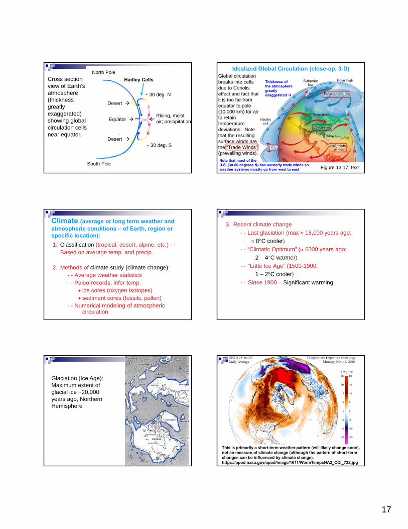
Cross section view of Earth’s atmosphere (thickness greatly exaggerated)

Desert

~ 30 deg. N

E t Rising, moist

North Pole

Hadley Cells

showing global circulation cells near equator.

Desert ~ 30 deg. S

Equator g,

air; precipitation

South Pole




Figure 13.17, text


Climate (average or long term weather and atmospheric conditions – of Earth, region or specific location):

1. Classification (tropical, desert, alpine, etc.) - -Based on average temp. and precip.

2. Methods of climate study (climate change):- - Average weather statistics- - Paleo-records, infer temp.

ice cores (oxygen isotopes) sediment cores (fossils, pollen)

- - Numerical modeling of atmospheric circulation

3. Recent climate change

- - Last glaciation (max 18,000 years ago;

8C cooler)

- - “Climatic Optimum” ( 6000 years ago;

2 – 4C warmer)

“Littl I A ” (1500 1900- - “Little Ice Age” (1500-1900;

1 – 2C cooler)

- - Since 1900 – Significant warming

Glaciation (Ice Age): Maximum extent of glacial ice ~20,000 years ago, Northern Hemisphere

This is primarily a short-term weather pattern (will likely change soon), not an measure of climate change (although the pattern of short-term changes can be influenced by climate change). https://apod.nasa.gov/apod/image/1611/WarmTempsNA2_CCI_722.jpg

18

https://apod.nasa.gov/apod/image/1611/WarmTempsNA2_CCI_722.jpg

Explanation: Why is it so warm in northern North America? Usually during this time of year -- mid-November -- temperatures average as much as 30 degrees colder. Europe is not seeing a similar warming. One factor appears to be an unusually large and stable high pressure region that has formed over Canada, keeping normally colder arctic air away. Although the fundamental cause of any weather pattern is typically complex, speculation holds that this persistent Canadian anticyclonic region is related to warmer than average sea surface temperatures in the mid-Pacific -- an El Niño -- operating last winter. North Americans should enjoy it while it lasts, though. In the next week or two, cooler-than-average temperatures now being recorded in the mid-Pacific -- a La Niña --might well begin to affect North American wind and temperature patterns.

Causes of Climate Change:

1. Astronomical effects (Milankovitch Cycles)- -Long-term changes in Earth’s orbit produce small changes in solar heating at any location on Earth. (A natural phenomenon.)o a ( a u a p e o e o )

2. Plate tectonics (continental drift - - very long-term changes) (A natural phenomenon.)

3. Changes in solar constant (the “solar constant” is not really a constant but a measure of energy output)? The total amount of solar energy (the solar constant) may change over long time periods or may vary periodically over shorter time periods. (A natural phenomenon.)

4 Periods of intense volcanism (ash and SO in the4. Periods of intense volcanism (ash and SO2 in the atmosphere can reduce average temperature from the ash or increase the average temperature from the SO2 – a greenhouse gas). (A natural phenomenon.)

5. CO2 (and other greenhouse gases) increases and greenhouse effect. There has been a rapid increase in greenhouse gases in the past century due to burning of fossil fuels and other industrial processes. (Primarily a human-caused phenomenon.) http://en.wikipedia.org/wiki/Carbon_dioxide

~ 405 in 2017

Milankovitch Cycles(astronomical effects on climate): Eccentricity(stretch in orbit), Obliquity (change in tilt

l ) P i

Milankovitch Cycles

1. Eccentricity (stretch of orbit) Period ~ 100,000 yrs

2. Changes in obliquity (tilt of

angle), Precession(change of direction of axis [precession] and major axis of elliptical orbit)

axis) Period ~ 41,000 yrs

3. Precession (of axis direction and major axis of elliptical orbit) Periods ~ 26,000 and 23,000 yrs

Simplified diagram of Milankovitch Cycles(perspective view of orbit)

Eccentricity

Obliquity(23 +/- 1.5 degrees tilt)

Precession

http://www.global-greenhouse-warming.com/Milankovitch-cycles.html

19

http://www.globalwarmingart.com/wiki/Wikipedia:Milankovitch_cycles

Circular orbit of a planet

Elliptical orbit of a planet

Obliquity (change in tilt angle)



Axial Precession

Precession of the major axis of the elliptical orbit (ellipticity exaggerated)

Time-lapse (about one hour) photograph from Earth (northern hemisphere) showing position of Polaris (“the North star”) and other

stars that appear to circle Polaris (actually due to Earth’s rotation)

Polaris

http://www.flickr.com/photos/juniorvelo/312672130/


Polaris


http://en.wikipedia.org/wiki/Circumpolar_star

Each of the three Milankovitch (orbital) cycles predicts a temperature change on Earth that looks like:

Sum of the three cycles looks like:

The cooling periods predicted by the Milankovitch cycles correlate well with times of ice ages.

20

Past and future Milankovitch cycles. Prediction of past and future orbital parameters with great accuracy. ε is obliquity (axial tilt). e is eccentricity. ϖ is longitude of perihelion. esin(ϖ) is the precession index, which together with obliquity, controls the seasonal cycle of insolation. Q is the calculated daily-averaged

Obliquity

Eccentricity

Orbit Precession

Precession Index

I l ti (H ti )y g

insolation at the top of the atmosphere, on the day of the summer solstice at 65 N latitude. Benthic forams and Vostok ice core show two distinct proxies for past global sealevel and temperature, from ocean sediment and Antarctic ice respectively. Vertical gray line is current conditions, at 2 ky A.D.Time

Insolation (Heating)

Benthic Forams

Vostok Ice Core

CO2 (ppm)

Inferred Temp (oC)

CH ( )

Time Present

CH4 (ppv)

Oxygen Isotopes (Temp. Proxy)

Insolation (Milankovitch effect)

From ice core data (http://en.wikipedia.org/wiki/Global_warming)

Global CO2 (ppm) – past 800,000 Years

Data from Ice Cores; Mauna Loa Observations from 1958, Figure 11.26, text

Also note that the recent increase is much more rapid than the increases from natural variations

Time

2016 (~405)The very rapid increase since 1900, the amplitude of the 2014 CO2

concentration (highest since at least 800,000 years ago), and the lack of any apparent periodicities or other natural causes that could explain the recent increase, is strong evidence that the cause is fossil fuel consumption.

Last 800,000 years of CO2 levels in the atmosphere (Scripps,http://keelingcurve.ucsd.edu/)

Time

U.S. Energy Consumption – 2008, 84% Fossil Fuels (CO2 Emissions)

World Energy Consumption ~95% Fossil Fuels. Also see Figure 11.24, text

U.S. Energy Consumption, sources of energy – 2011, 83% (81% in 2014) Fossil Fuels

World Energy Consumption ~95% Fossil Fuels. Also see Figure 11.24, text

21

U.S. Greenhouse gases and emissions by source, 2013 (USAToday, February 20, 2014)

https://www.epa.gov/ghgemissions/overview-greenhouse-gases

Also water vapor and very small % of Ozone

U.S. CO2 Production –mostly from burning of Fossil Fuels (CO2

Emissions), U.S. contributes nearly 25% of the world’s greenhouse gas emissions!

Important: SeeImportant: See Worksheet (no class 11/20) and AtmsNotes.pdf material to understand the greenhouse effect (also acid rain, ozone)

U.S. annual per capita CO2

production (Figure 11.27, L&T, 2014)

Two millennia of mean surface temperatures according to different reconstructions, each smoothed on a decadal scale. The unsmoothed, annual value for 2004 is also plotted for reference.

http://en.wikipedia.org/wiki/Global_warming

Year

Time

Recent Global Temperature Change


http://svs.gsfc.nasa.gov/Gallery/ArcticSeaIceResources.html

Also, a 2012 report shows that N. Hemisphere snow cover in June has decreased by about 18% per decade since 1979 (http://www.arctic.noaa.gov/report12/snow.html)


22

Arctic Sea Ice Extent

2012

Median of previous years

http://nsidc.org/arcticseaicenews/ http://www.nasa.gov/topics/earth/features/warming_antarctica.html

50-year (2009) Temperature Change (Degrees C)

http://www.nasa.gov/topics/earth/features/warming_antarctica.html

Ocean climate change indicators, 1900-2013 (http://nca2014.globalchange.gov/highlights/report-findings/oceans)

Climate video (example of Sahara desert [dry winds] in northern Africa and rain forest in central, equatorial Africa)in central, equatorial Africa) illustrates global circulation pattern (Hadley cells).

One inch (2.54 cm) per decade increase


Climate Change: The local view – Indiana Precipitation data, 1970 – 2013 (Lafayette Journal and Courier, September 28, 2014)

One half oF (0.28 oC) per decade increase


Climate Change: The local view – Indiana Temperature data, 1970 – 2013 (Lafayette Journal and Courier, September 28, 2014)

23

1997 – last large El Nino

2016, through 11/25


Climate Change: The local view – San Francisco, CA rainfall data. Note, no significant long term trend until at least the year 2000. Also, the drought (beginning in 2011-12) appears to be unusual, and may not last very long, if it is similar to previous low rainfall periods. (http://www2.ucar.edu/atmosnews/perspective/10879/california-dryin)

Climate Change Video from NASA - Six Decades of a Warming Earthhttp://www.nasa.gov/content/goddard/nasa-finds-2013-sustained-long-term-climate-warming-trend/#.UumGjRC2Lob

http://www.youtube.com/watch?v=gaJJtS_WDmI

Mean surface temperature change for the period 1999 to 2008 relative to the average temperatures from 1940 to 1980


Global CO2 (ppm) – past 800,000 Years

Data from Ice Cores; Mauna Loa Observations from 1958, Figure 11.26, text

Also note that the recent increase is much more rapid than the increases from natural variations

Time

2016 (~405)The very rapid increase since 1900, the amplitude of the 2014 CO2

concentration (highest since at least 800,000 years ago), and the lack of any apparent periodicities or other natural causes that could explain the recent increase, is strong evidence that the cause is fossil fuel consumption.

Last 800,000 years of CO2 levels in the atmosphere (Scripps,http://keelingcurve.ucsd.edu/)

Time

24

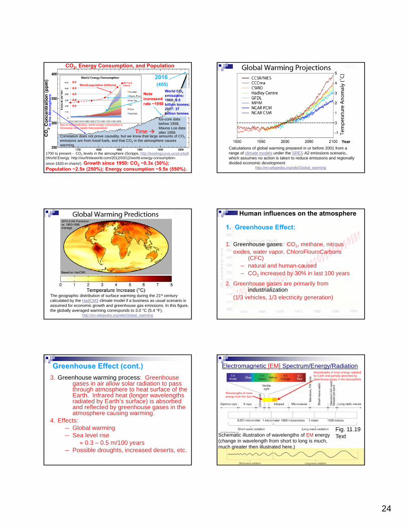
2016(405)

Note increased rate ~1950

8.0

6.0

4.0

2.0

0.0

2017 (7.6 billion)World population (billions)

CO2, Energy Consumption, and Population

World CO2

emissions: 1960: 9.5 billion tonnes; 2017: 37 billion tonnes

e A

tmo

sph

ere

1700 to present - CO2 levels in the atmosphere (Scripps, http://keelingcurve.ucsd.edu/) (World Energy: http://ourfiniteworld.com/2012/03/12/world-energy-consumption-

since-1820-in-charts/). Growth since 1950: CO2 ~0.3x (30%); Population ~2.5x (250%); Energy consumption ~5.5x (550%).

Correlation does not prove causality, but we know that large amounts of CO2

emissions are from fossil fuels, and that CO2 in the atmosphere causes warming.

Due to industrialization, world energy consumption is increasing more rapidly than population!

Time

Ice-core data before 1958, Mauna Loa data after 1958.

In t

he

Calculations of global warming prepared in or before 2001 from a range of climate models under the SRES A2 emissions scenario,. which assumes no action is taken to reduce emissions and regionally divided economic development


Year

The geographic distribution of surface warming during the 21st century calculated by the HadCM3 climate model if a business as usual scenario is assumed for economic growth and greenhouse gas emissions. In this figure, the globally averaged warming corresponds to 3.0 °C (5.4 °F).


1. Greenhouse Effect:

1. Greenhouse gases: CO2, methane, nitrousoxides, water vapor, ChloroFlouroCarbons

(CFC)t l d h d

Human influences on the atmosphere

-- natural and human-caused-- CO2 increased by 30% in last 100 years

2. Greenhouse gases are primarily from industrialization

(1/3 vehicles, 1/3 electricity generation)

Greenhouse Effect (cont.)

3. Greenhouse warming process: Greenhouse gases in air allow solar radiation to pass through atmosphere to heat surface of the Earth. Infrared heat (longer wavelengths radiated by Earth’s surface) is absorbed and reflected by greenhouse gases in the y g gatmosphere causing warming.

4. Effects:-- Global warming-- Sea level rise

0.3 – 0.5 m/100 years-- Possible droughts, increased deserts, etc.

Electromagnetic [EM] Spectrum/Energy/Radiation

Wavelengths of most energy from the Sun

Wavelengths of most energy radiated by Earth and partially absorbed by greenhouse gases in the atmosphere

Fig. 11.19 TextSchematic illustration of wavelengths of EM energy

(change in wavelength from short to long is much, much greater then illustrated here.)

25

Greenhouse Effect (cont.)

5. “Complications:”-- How much CO2 storage in oceans?-- Human vs. natural causes?-- Political -- industrialized vs. developing

countriescountries-- Deforestation compounds the problem

by removing CO2 -consuming and O2-producing plants, and adding CO2 toatmosphere by burning.

See pages 371-381 in Text.

It’s now about 405

Figure 11.5, text

Recent atmospheric carbon dioxide (CO2) increases. Monthly CO2 measurements display seasonal oscillations in overall yearly uptrend; each year's maximum occurs during the Northern Hemisphere's late spring, and declines during its growing season as plants remove some atmospheric CO2. http://en.wikipedia.org/wiki/Global_warming

Growth in Atmospheric Methane (data from Greenland ice cores, note logarithmic time scale and

rapid increase in last 100 years)en

trat

ion

,

lli

on

Years before present

Met

han

e co

nce

par

ts p

er

bil

So, CO2 in Atmosphere is “good” – Earth’s atmosphere would be ~ 30C colderwithout the greenhouse effect!

But, CO2 is increasing in atmosphere ( l b l i ) C t CO i i(global warming); Current CO2 emissions:

US 5 tons/year/person

World < 1 ton/year/person

Correlation of emissions and global average temperatures

(+) Global emissions of SO2

(x106 tons)

CO2

Temp.

370

350

330

310

200

160

120

80

Correlation of global average temperature, industrial SO2

emissions and CO2 concentration in the atmosphere, 1880-2000.

(o) CO2 concentration (ppm) Year

SO2

290

270

250

40

0

370 3702000

26

http://www.exxonmobil.com/Corporate/Files/news_pub_eo2012.pdf

http://vulcan.project.asu.edu/pdf/Gurney.EST.2009.pdf

2012 CO2

emissions

USA Today, August 20, 2013

2012 CO2 emissions, re-visited…

Population (millions, and % of world population):

China 1360 19%USA 316 4.5%%India 1210 17%Russia 143 2.0%Japan 128 1.8%

Normalized by Population

http://en.wikipedia.org/wiki/World_population

USA Today, August 20, 2013

6.2%

15%

1.9%

11% 10%

World CO2

emissions from Energy

USA Today, September 22, 2014

Europe CO2 emissions, 2000 to 2013

USA Today, September 23, 2014

27

November, 2009 Icebergs near South Island ofNew Zealand (some >200 m long) that broke off (total of >30 km2 area of ice sheet) on the Antarctic ice sheet due to warming


Also, a 2012 report shows that N. Hemisphere snow cover in June has decreased by about 18% per decade since 1979 (http://www.arctic.noaa.gov/report12/snow.html)


2. Ozone “Layer”:

1. Ozone = O3

-- Only 3 ppm in atmosphere

-- Most Ozone is in stratosphere (10-50 km


Most Ozone is in stratosphere (10 50 km

above Earth)

-- CFCs in upper atmosphere rapidly destroys Ozone

See pages 357-360 in Text.

Two Chlorine reactions (“chain reactions”) which take place in the upper atmosphere (stratosphere, ~ 10-50 km elevation):

Cl + O3 ClO + O2 (1)90% of Ozone 90% f

50

15

km

ClO + O3 Cl + 2 O2 (2)

(ClO reacts with another ozone)

Because Cl is very reactive, these conversions are rapid (1 s to 1 min)

Note that after the second reaction, O3 is gone and Cl is still present (and can react with and destroy another O3 molecule – chain reaction!).

90% of Air

Elevation (km)0

15

The result of this chain reaction is:

1. 2 O3 O2 + 2 O2 [loss of Ozone]

2. Cl Cl [Chlorine remains, perpetuating the

chain reaction]

28

Ozone “Layer” (cont.)

2. Effects:

-- Ozone is highly corrosive; damages crops, contributes to smog, and is a health hazard (lung damage) in thehealth hazard (lung damage) in the lower atmosphere

-- In the upper atmosphere (stratosphere) , Ozone blocks harmful UV radiation

So, Ozone in the upper atmosphere is “Good” (but is being depleted by CFCs);

Ozone in the lower atmosphere is “Bad” (pollution).

Ozone Hole

Figure 11.17, text

Ozone Hole

Figure 11.17, text

Ozone Hole

Figure 11.17, text

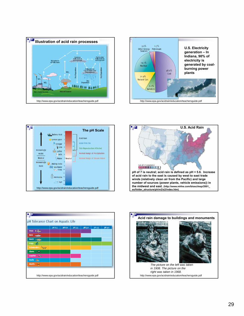
3. Acid Rain

- SO2, NOx sulfuric and nitric acids inatmosphere and in precipitation

- Produced by burning fossil fuels


- Destroys wildlife in lakes forests building stone, concrete

29

Illustration of acid rain processes

http://www.epa.gov/acidrain/education/teachersguide.pdf

U.S. Electricity generation – In Indiana, 90% of electricity is generated by coal-burning power g pplants


The pH Scale


U.S. Acid Rain

pH of 7 is neutral; acid rain is defined as pH < 5.6. Increase of acid rain to the east is caused by west to east trade winds (relatively clean air from the Pacific) and large number of sources (power plants, vehicle emissions)) in the midwest and east. (http://www.mhhe.com/biosci/esp/2001_es/folder_structure/ph/m2/s2/index.htm)


Acid rain damage to buildings and monuments

The picture on the left was takenin 1908. The picture on theright was taken in 1968.


30

4. Other pollutants (example, Mercury in the environment)


Mercury comes from batteries placed in landfills and from burning of coal Graphs show

Hg accumulation

of coal. Graphs show accumulation of Hg in MN and WI lake sediments with time from 1700 to 1980.

Yea

r

Note ~ exponential increase

Hurricanes:

1. Form in Tropical marine areas ( 5 - 20 latitude;not right at the equator because of small CoriolisEffect)

2. Energy for storm (Energy for one day of ahurricane Electricity produced in US in one year)y p y )

Solar radiation -- Heated air rises forming low pressure region, also provides moisture in atmosphere by evaporationfrom ocean

(Note: some Hurricane examples and discussion were presented in class earlier in the semester and are included in the IntroNotes.pdf and EarthNotes.pdf files)

Hurricanes (cont.) Exchange of heat from warm (> 28C)

ocean to atmosphere; therefore, storms form in late summer in oceanic areas

Latent heat of condensation further drives storm by heating air when moisture in air y gcondenses to form rain (heating 1 cm3 = 1 g of water to evaporation takes 1 calorie [adding energy to the water to make it water vapor], so when the water vapor condenses [precipitation], it releases this energy).

Hurricanes (cont.)

3. Circulation

Hurricanes move according to the trade

winds ( 10 – 50 km/hr)

Circulation in hurricane is around low ( l k i i Npressure (counter-clockwise in N.

Hemisphere); higher velocity near center because of conservation of angular momentum (like spinning figure skater)

Hurricanes (cont.)

4. Damage from hurricane

High winds (> 122 km/hr [75 mph])g ( [ p ])

Torrential rains (up to 25 cm in a few hours)

Salt water flooding of fresh water region Table 14.2 L&T, 2017

31

CSU Atlantic Hurricanes forecasts for 2012 and 2013 seasons (USA Today, April 11, 2013)

2013 actual = 2 hurricanes, 14 named storms

Name Dates activeStorm category at

peak intensityMax 1-min wind

mph (km/h)Min.press.

(mbar)Arlene April 19 – 21 Tropical storm 50 (85) 990Bret June 19 – 20 Tropical storm 45 (75) 1007

Cindy June 20 – 23 Tropical storm 60 (95) 992

Four July 6 – 7Tropical

depression30 (45) 1008

Don July 17 – 19 Tropical storm 50 (85) 1007Emily July 31 – August 2 Tropical storm 45 (75) 1005FranklinAugust 7 – 10 Cat. 1 hurricane 85 (140) 981G t A t 13 17 C t 2 h i 105 (165) 967Gert August 13 – 17 Cat. 2 hurricane 105 (165) 967Harvey Aug. 17 – Sept. 1 Cat. 4 hurricane 130 (215) 938Irma Aug. 30 – Present Cat. 5 hurricane 185 (295) 914Jose Sept. 5 – Present Cat. 4 hurricane 155 (250) 938Katia Sept. 5 – Present Cat. 2 hurricane 105 (165) 972Maria Sept. 16 – 20 Cat. 5 hurricane 175 (280) 908

Also (after Maria): Nate (H), Ophelia (H), Philippe (TS), Rina (TS)2017 Atlantic hurricane season (June 1-November 30) (https://en.wikipedia.org/wiki/2017_Atlantic_hurricane_season)

https://upload.wikimedia.org/wikipedia/commons/c/c6/2017_Atlantic_hurricane_season_summary_map.png 2017 Atlantic Hurricanes

https://weather.com/storms/hurricane/news/2016-hurricane-season-forecast-noaa-the-weather-company-csu Aug. 31, 2016

Hurricanes (cont.)

Storm surge (up to 7 m of local, temporarysea level rise; most significant cause of damage and loss of life)

-- Low pressure (as low as 900mbproduces 1 m of surge)p g )

-- Storm buildup (especially for “bay-like” coastlines, “focusing”)

-- Wave action-- High tides can compound the storm

surge

32

Calculated storm surge, Katrina, 29 August, 2005, SLOSH model, www.noaa.gov

~5 – 6 m~6 – 8 m>~8 m

~2 – 4 m~4 – 5 m

5 – 6 m

Storm surge

Hurricanes (cont.)5. Names for Hurricanes (“just for interest”):

Atlantic Ocean: Hurricanes

W. Pacific Ocean: Typhoons

Indian Ocean: Cyclones

Australia: Willy Willys Australia: Willy-Willys

In Sept. 1995, there were 5 hurricanes in the Atlantic at one time

Hurricane Andrew, 1992, infrared satellite image taken every 12 hours from 23 -26 Aug.

Note intensification and weakening of storm with time

Hurricane Andrew, 1992 in Gulf of Mexico

33

Track of Hurricane Andrew, 1992 (orange and red dots indicate Hurricane strength winds)

Hurricane Andrew, 1992


Figure 14.23, text

Strongest winds in NEQuadrant of Hurricane

Figure 14.25, text


34

Hurricane Andrew, 1992 Hurricane Andrew, 1992

Hurricane Camille, 1969, Richelieu Apartments, Pass Christian, Mississippi

Hurricane Camille, 1969

Hurricane Frances, Sept. 2004 Hurricane Frances, Sept. 2004

35

Hurricane Dean, Aug. 2, 2007 Hurricane Katrina, Aug. 25-30, 2005

Hurricane Season – June 8 to August 29, 2005:6/8-6/13 TS Arlene7/3-7/7 Hurr. Cindy7/7-7/10 Hurr. Dennis7/14-7/20 Hurr. Emily7/21-7/29 TS Franklin8/3-8/8 TS Harvey8/7-8/18 Hurr. Irene8/25 8/30 H K t i

Exploring Planet Earth

http://www.nasa.gov/vision/earth/lookingatearth/h2005_katrina.htmlhttp://svs.gsfc.nasa.gov/vis/a000000/a003200/a003279/index.html

8/25-8/30 Hurr. Katrina……

9/18-9/24 Hurr. Rita…

Total of 21 storms in 2005

Hurricane Season, Katrina, Aug. 27, 2005

Exploring Planet Earth

http://www.nasa.gov/vision/earth/lookingatearth/h2005_katrina.html

Hurricane Katrina, Aug. 28-29, 2005 Hurricane Katrina, 2005

36

Hurricane Katrina,August 28, 2005,Category 5

Hurricane Katrina,August 28, 2005,Category 5

Hurricane Katrina, 2005 Hurricane Katrina, 2005

37

Hurricane Track Site: http://hurricane.csc.noaa.gov/hurricanes/viewer.html Legend (hurricanes

are red and dark red)

Base map

150 Years of Hurricanes

Atlantic HurricanesPacific Hurricanes

150 Years of Hurricanes Note that many Atlantic hurricanes form off the west coast of Africa (and track west [trade winds])

Note that the entire east and gulf coasts of the US have been impacted by hurricanes


Tropical Storms and Hurricanes 1842-2013



Tropical Storms and Hurricanes 1842-2013


38

From USA Today, Aug. 22, 2012

Most intense landfalling U.S. hurricanes Intensity is measured solely by central pressure

Rank Hurricane Year Landfall pressure

1 "Labor Day" 1935 892 mbar (hPa)2 Camille 1969 909 mbar (hPa)3 Katrina 2005 918 mbar (hPa)4 Andrew 1992 922 mbar (hPa)( )5 Indianola 1886 925 mbar (hPa)6 "Florida Keys" 1919 927 mbar (hPa)7 "Okeechobee" 1928 929 mbar (hPa)8 Donna 1960 930 mbar (hPa)9 "New Orleans" 1915 931 mbar (hPa)10 Carla 1961 931 mbar (hPa)

Source: U.S. National Hurricane Center

Costliest U.S. Atlantic hurricanes Cost refers to total estimated property damage.

Rank Hurricane Year Cost (2004 USD)

1 Katrina 2005 $80 billion (2005 USD)

2 Andrew 1992 $43.672 billion$

3 Charley 2004 $15 billion

4 Wilma 2005 $14.4 billion (2005 USD)

5 Ivan 2004 $14.2 billion

Main article: List of costliest U.S. Atlantic hurricanes

Costliest Atlantic Hurricanes, 1851-2007 (Katrina, 2005, not shown) http://csc-s-maps-q.csc.noaa.gov/hurricanes/

http://www1.ncdc.noaa.gov/pub/data/images/2011-Landfalling-Hurricanes-32x34.pdfhttp://www.ncdc.noaa.gov/oa/climate/severeweather/hurricanes.html

39

Today: Tornadoes

Day of Lafayette area and Kokomo Tornadoes (01:00 GMT)

24-hr Radar Loop 00:00 – 23:00 GMT Nov. 17, 2013



Surface Conditions – Nov. 17-18, 2013

40

Illinois and Indiana tornadoes, Nov. 17, 2013 (J&C, 11/18/2013)Tornado Damage, Washington, IL, Nov. 17, 2013 (news.yahoo.com)

Tornado Damage, Washington, IL, Nov. 17, 2013 (USAToday, 11/19/2013) Tornado Damage, Washington, IL, Nov. 17, 2013 (USAToday, 11/19/2013)

Tornado Damage, Washington, IL, Nov. 17, 2013 (news.yahoo.com) Tornado Damage, Washington, IL, Nov. 17, 2013 (news.yahoo.com)

41

Tornado Damage, Washington, IL, Nov. 17, 2013 (news.yahoo.com) Tornado Damage, Washington, IL, Nov. 17, 2013 (news.yahoo.com)

Tornado near Lebanon, IN, Nov. 17, 2013 (J&C, 11/18/2013)Tornado Damage, Kokomo, IN, Nov. 17, 2013 (news.yahoo.com)

Tornado Damage, Lafayette, IN, Nov. 17, 2013 (J&C, 11/19/2013)Tornado Damage, Southwestern Middle School, Lafayette, IN, Nov. 17, 2013 (J&C, 11/18/2013)

42

Tornado Damage, Southwestern Middle School, Lafayette, IN, Nov. 17, 2013 (J&C, 11/18/2013) Tornado near Lebanon, IN, Nov. 17, 2013 (J&C, 11/18/2013)

Tornadoes in SE US – April 27-28, 2011: At least 160 tornadoes in “outbreak”, at least 291 deaths, 10 states.

249

http://www.youtube.com/watch?v=vz8xiHpBGNM&feature=related

http://www.youtube.com/watch?v=6U1asLiDYB0&feature=related

http://www.nytimes.com/2011/04/29/us/29tornadoes.html

Tornadoes in SE US – April 27-28, 2011: At least 160 tornadoes in “outbreak”, at least 215 deaths.

250


http://www.youtube.com/watch?v=6U1asLiDYB0&feature=related

Tornadoes in SE US – April 27-28, 2011: At least 160 tornadoes in “outbreak”, at least 215 deaths.

251


http://www.youtube.com/watch?v=6U1asLiDYB0&feature=related 252

43

Before and After

253

255

April 27-28 Tornado Outbreak, 2011 900+

256

April 27-28 Tornado Outbreak, 2011 900+

257

Recent update on tornadoes per year, USA Today, August 21, 2013

L

258

L

44

259

342+

Front

260USA Today, April 29, 2011

Tornadoes EF1 or greater 2014: Through April 21, 2014 – only 20 tornadoes and no tornado deaths

2014

261USA Today, April 23, 2014 (total: 401 (EF1+) with 45 deaths in 2014)

Tornadoes EF1 or greater 2014: Through April 21, 2014 – only 20 tornadoes and no tornado deaths

http://www.ncdc.noaa.gov/sotc/tornadoes/

2011

1974

Data from NOAA - http://stevengoddard.wordpress.com/2014/04/28/us-tornado-deaths-in-sharp-decline-since-the-1920s/

Vilonia, AR, EF-3 (NWS) tornado April 27, 2014

This House

At least 26 tornadodeaths

Tree

Tree

BushBush

264

Note that damage is very localized (USA Today, April 29, 2014)

From Google Earth

This House

deathsin SE U.S., April 27-28, 2014

45

265(USA Today, April 29, 2014)

Tornadoes:1. Form in intense thunderstorms caused by collision of cold air and warm, moist air along a Front.

266

Elkhart, Indiana, 1965 April 11; note “twin funnels”.

Near Howard, South Dakota, 1884 August 28 (oldest known photo of a tornado), note funnel clouds that have or are descending from very dark “wall cloud”. Also note debris around funnel cloud.

267

Tornado and flying debris,Chapter14 , text

268

Tornadoes (cont.)

2. Midwest US is most prominent location (“tornado alley”)

-- moisture from Gulf of Mexico

-- Cold air from Canada moving south and

east and “guided” by Rocky Mtns. and

269

g y y

Appalachians

3. Mostly in Spring due to climatic conditions of warm air in Gulf of Mexico and SE U.S and occasional cold air and front moving south and east from cold Canadian air mass.

Tornadoes (cont.)4. Conditions for formation:

-- unstable air -- cold air over-riding warm (warm air below then rises due to lower density, cold air above descends due to higher density leading to strong vertical

)

270

movements)

-- rising, warm, moist air

-- precipitation, evaporation (and cooling)

cause down-drafts when warm air contacts cold air along the front

-- Tornado occurs in updraft region

46

Circulation around Low pressure area often results in formation of a cold front. Collision of dry, cold air with warm, moist air results in precipitation and, possibly, thunderstorms and tornadoes.

Cold front moves from west to east due to trade winds(westerlies) and

t l k i

Figure 14.8, text

Warm, moist air

Cold, dry air

counter-clockwise circulation around the Low

Clouds associated with a Low pressure area and cold front

Figure 14.9, text Warm, moist air

Cold, dry air

Cold air is more dense so it stays near the Earth’s surface and cause the adjacent warm moist air to rise along the front (shows cross section view equivalent to profile E to C of Figure 14.8, text)

West East

Figure 14.6, text

Warm, moist air

Cold, dry air

274Supercell Thunderstorm

275Lightning from Thunderstorm, Figure 14.12, text Figure 14.13, text

47

Severe storms areas by month (USA Today, April 8, 2013)

Tornadoes (cont.)5. Characteristics:

-- Weak F0 to F1 (winds <180 km/hr)-- Strong F2 to F3 (winds 181- 332 km/hr)-- Violent F4 to F5 (winds >333 km/hr)

(about 20/yr violent; peak in April; most deaths and damage result from the small

278

deaths and damage result from the small number of violent [F4 to F5] tornadoes each year)

-- Intensity of tornado is ~ proportional to the amount of water vapor in air

279Table 14.1, text, L&T, 2008

Table 14.1, text, L&T, 2014

280

http://www.tornadoproject.com/cellar/fscale.htm

Lafayette, IN

282

Tracks of tornadoes from the April 3, 1974 tornado outbreak, one of the most significant tornado days in history. There were 148 tornadoes and 330 people were killed.

48

http://uxblog.idvsolutions.com/2012/05/tornado-tracks.html

Watch the YouTube video to see the tornado tracks (1950-2011) by year: http://www.youtube.com/watch?v=1d8OVf829kw

http://www.youtube.com/watch?v=1d8OVf829kw

On next slide, watch for 1974 and 2011

http://www.youtube.com/watch?v=1d8OVf829kw

Damage in Spencer, South Dakota from May 30, 1998 tornado

286

Most tornadoes are 100 to 1000 m wide so most damage is limited to a narrow track.

Tornado damage and track, F3 Moore, OK, May 8, 2003, NASA Earth Observatory image

287

Tornado damage, F5 Moore, OK, May 3, 1999.

288

49

Tornado damage, Moore, OK, May 3, 1999. Maximum wind speed measured at over 500 km/hr (~300 mi/hr)

289

Tornado damage, Moore, OK, May 3, 1999.

290

291April 28, 2011 photo shows tornado damage in Pleasant Grove, Ala. Jconline Mar. 20, 2013.

Multiple-Vortex Tornado

Figure 14.22, text

Figure 14.21, text

Average number of tornadoes, tornado days, and annual tornado incidence each month in the U.S. (Figure 14.23, text)

293 294USAToday April 11, 2012

50

295 296

297

U.S. Weather related disasters 1980-1995: 46 disasters (at least $1 billion in damages, March 2012 dollars).

Total losses = $339 billion.(National Geographic, Sept., 2012)

298

Disaster Type:

Population increased by ~ 37 million

U.S. Weather related disasters 1996-2011: 87disasters (at least $1 billion in damages, March 2012 dollars).

Total losses = $541 billion.(National Geographic, Sept., 2012)

299

Disaster Type:

Population increased by ~ 45 million

Note increased number of events and large-loss events

Atmospheric Sciences:

Documents

Transcript of Atmospheric Sciences: