A Phase-Offset Estimation Method for InSAR DEM ... - MDPI

Remote Sens. 2012, 4, 745-761; doi:10.3390/rs4030745

Remote Sensing ISSN 2072-4292

www.mdpi.com/journal/remotesensing Article

A Phase-Offset Estimation Method for InSAR DEM Generation Based on Phase-Offset Functions

José Claudio Mura 1,*, Muriel Pinheiro 2, Rafael Rosa 2 and João Roberto Moreira 2

1 National Institute for Space Research (INPE), São José dos Campos, 12227-010 SP, Brazil 2 Orbisat da Amazônia S. A (ORBISAT), São José dos Campos, 12244-000 SP, Brazil;

E-Mails: [email protected] (M.P.); [email protected] (R.R.);

[email protected] (J.R.M.)

* Author to whom correspondence should be addressed; E-Mail: [email protected].

Received: 9 January 2012; in revised form: 5 March 2012 / Accepted: 6 March 2012 /

Published: 20 March 2012

Abstract. This paper presents a novel method for estimating the absolute phase offset in

interferometric synthetic aperture radar (SAR) measurements for digital elevation model

(DEM) generation. The method is based on “phase-offset functions (POF),” relating phase

offset to topographic height, and are computed for two different overlapping interferometric

data acquisitions performed with considerably different incidence angles over the same

area of interest. For the purpose of extended mapping, opposite viewing directions are

preferred. The two “phase-offset functions” are then linearly combined, yielding a

“combined phase-offset function (CPOF)”. The intersection point of several straight lines

(CPOFs), corresponding to different points in the overlap area allows for solving the phase

offset for both acquisitions. Aiming at increasing performance and stability, this

intersection point is found by means of averaging many points and applying principal

component analysis. The method is validated against traditional phase offset estimation

with corner reflectors (CR) using real OrbiSAR-1 data in X- and P-band.

Keywords: SAR Interferometry; phase offset estimation; absolute phase; DEM

1. Introduction

SAR interferometry is a well-known technique used to generate a Digital Elevation Model (DEM),

which converts the absolute interferometric phase data into height data [1–4]. The absolute

OPEN ACCESS

Remote Sens. 2012, 4

746

interferometric phase data can be obtained by removing the ambiguity of 2π from the measured

interferometric phase using a phase-unwrapping algorithm [5–8]. For InSAR data there is a residual

phase–offset value in the interferogram after phase unwrapping, which is a constant value for the

whole scene, and which must be estimated. This phase component comes mainly from the phase

induced by the interferometric SAR processing strategy, a not well-determined internal delay, and

from the ratio between the range resolution and the wavelength used.

The absolute interferometric phase estimation is often solved by using ground control points

(GCPs) within the scene or through the use of an already calibrated area. Automatic methods have also

been proposed, based on spectral diversity [9–11] and on a maximum likelihood estimator [12]. By

using GCPs, one can estimate the phase-offset values with great accuracy, making the generation of

high accuracy DEMs possible. However, in certain regions of dense forest or in fluvial regions, it can

be difficult to have access to appropriate areas to deploy the corner reflectors (GCPs). Dispensing the

GCPs can lead not only to lower implementation cost, but also to a decrease in environmental impact

associated with corner deployment.

This paper describes a method to estimate the phase-offset value automatically using a pair of

unwrapped interferometric phases, whose data have been acquired in opposite flight directions and

with an overlap area between the tracks. For a selected point in the overlapped area, a function relating

phase-offset value to height value, called here phase-offset function (POF), can be built for each

acquisition within a known height interval. The POFs of both acquisitions can be combined through a

linear combination to remove its dependency on height, creating a combined phase-offset function

(CPOF), whose slope is range dependent. The same procedure can be extended to a set of points

spread over the overlapped area, creating a set of CPOFs whose intersections provide the estimate of

the phase-offset values for both acquisitions. The performance of this method has been evaluated using

data from the OrbiSAR-1 System in X and P bands; the results are compared with those obtained by

using ground control points. This method has also been tested with OrbiSAR-1 data from an Amazon

forest area without the use of GCPs to evaluate its performance in this environment for topographic

mapping.

2. Proposed Method

SAR Interferometry is based on the measurement of the phase difference from the complex-valued

resolution elements of two co-registrated images, acquired by two separated antennas (baseline B) as

shown in Figure 1. The measured interferometric phase is wrapped in 2π, represented by m in Figure 1.

The grid of the wrapped phase values is transformed into a grid of unwrapped phase values by using a

phase-unwrapping algorithm that adds to each measured phase value a constant integer multiple of 2π,

represented by unw in Figure 1.

The phase-offset value, represented by off in Figure 1, is a constant phase component for the whole

scene that must be estimated and added to the unwrapped phase in order to obtain the absolute

interferometric phase abs, from which a digital elevation model (DEM) can be generated. The

phase-offset value can be positive or negative, and is sometimes greater than 2π, depending on the

interferometric SAR processing strategy used.


747

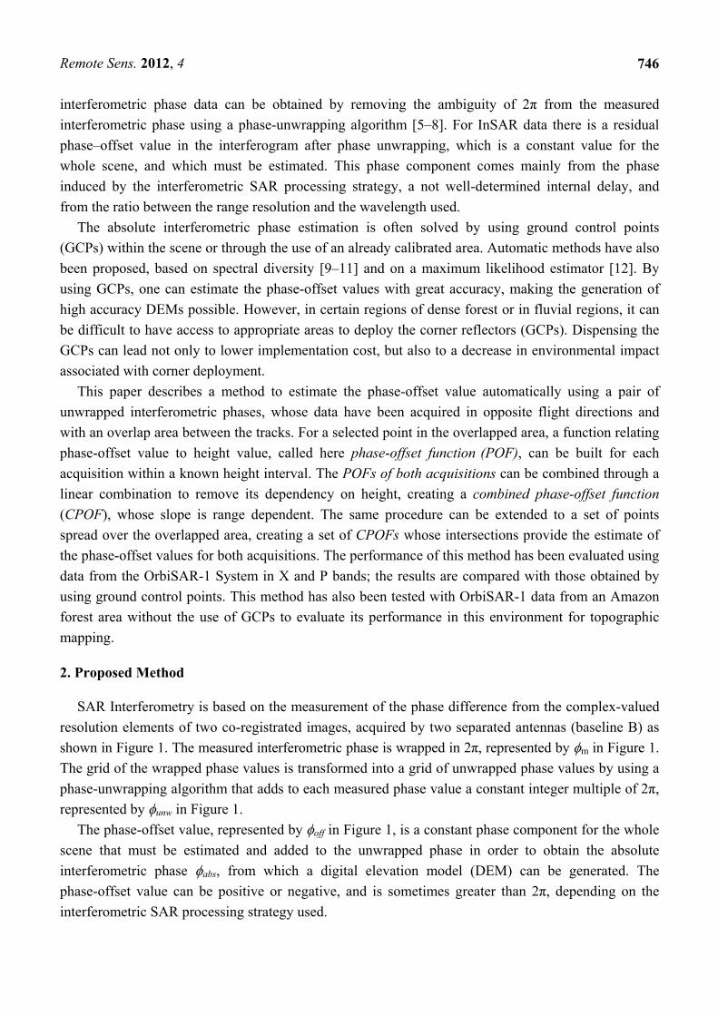
Figure 1. Representation of the interferometric phase components.

The proposed method to estimate the phase-offset value for an InSAR airborne system is based on the

following assumptions: the interferometric SAR images are generated in zero-Doppler geometry [13],

and the atmospheric effects are negligible. Considering the previous assumptions and taking antenna

A1 as the reference (Figure 1), the following equations can be written

offunwabs , (1)

abs

pr

4

, (2)

abs

prrrr

2221 , (3)

with p = 1 for monostatic acquisitions and p = 2 for bistatic acquisitions schemes.

Assuming a flat-earth geometry, for sake of simplicity, the terrain height can be represented by:

cos1rHh (4)

From the Equations (2) and (3), the Equation (4) can be rewritten as

cos

22

abs

prHh , (5)

where h is the terrain height, H is the platform altitude and the look-angle for the antenna A1.

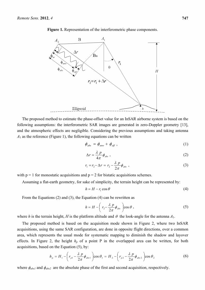
The proposed method is based on the acquisition mode shown in Figure 2, where two InSAR

acquisitions, using the same SAR configuration, are done in opposite flight directions, over a common

area, which represents the usual mode for systematic mapping to diminish the shadow and layover

effects. In Figure 2, the height hp of a point P in the overlapped area can be written, for both

acquisitions, based on the Equation (5), by:

22221111 cos2

cos2

abspabspp

prH

prHh (6)

where abs1 and abs2 are the absolute phase of the first and second acquisition, respectively.


748

Equation (6) can be rewritten as

2222211111 cos2

)cos(cos2

)cos(

abspabsp

prH

prH , (7)

2211 cos2

cos2

abspabsp

ph

ph , (8)

2211 coscos absasb (9)

Equation (9) shows that the absolute phases of both acquisitions, for a point P with height hp, are

only related by their incident angles. From this equation, the phase-offset off 1 can be related as a

function of off 2, as follows:

2221112211 cos)(cos)(coscos offunwoffunwabsasb , (10)

22221111 coscoscoscos offunwoffunw , (11)

11221221 )cos(cos)cos(cos unwunwoffoff , (12)

phoffoff RK 21 , (13)

with

12 coscos K and 12 unwunwph KR (14)

Considering that Kθ and Rph are constant values at the position P with the height hp, the phase-offset value off 1 can be seen as a linear combination of off 2, depending on the relation of the incident angle and the unwrapped phase difference between the two acquisitions.

Figure 2. Acquisition mode of airborne InSAR system for systematic mapping.

In order to build up the phase-offset function, we first consider the absolute phase value of a generic

point Pi selected, based on its geographic coordinate, with a Cartesian coordinate of (xp, yp, zp) and


749

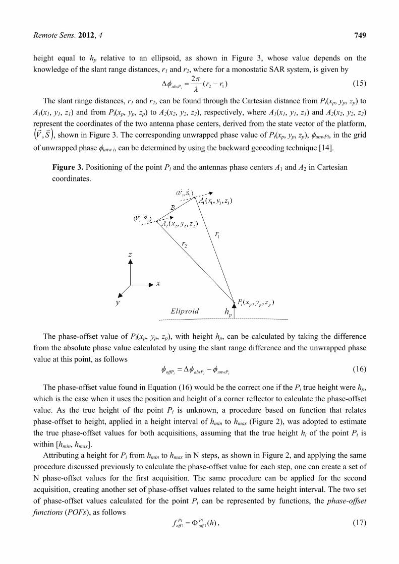
height equal to hp relative to an ellipsoid, as shown in Figure 3, whose value depends on the

knowledge of the slant range distances, r1 and r2, where for a monostatic SAR system, is given by

)(2

12 rriabsP

(15)

The slant range distances, r1 and r2, can be found through the Cartesian distance from Pi(xp, yp, zp) to

A1(x1, y1, z1) and from Pi(xp, yp, zp) to A2(x2, y2, z2), respectively, where A1(x1, y1, z1) and A2(x2, y2, z2)

represent the coordinates of the two antenna phase centers, derived from the state vector of the platform,

SV

, , shown in Figure 3. The corresponding unwrapped phase value of Pi(xp, yp, zp), unwPi, in the grid

of unwrapped phase unw i, can be determined by using the backward geocoding technique [14].

Figure 3. Positioning of the point Pi and the antennas phase centers A1 and A2 in Cartesian

coordinates.

The phase-offset value of Pi(xp, yp, zp), with height hp, can be calculated by taking the difference

from the absolute phase value calculated by using the slant range difference and the unwrapped phase

value at this point, as follows

iii unwPabsPoffP (16)

The phase-offset value found in Equation (16) would be the correct one if the Pi true height were hp,

which is the case when it uses the position and height of a corner reflector to calculate the phase-offset

value. As the true height of the point Pi is unknown, a procedure based on function that relates

phase-offset to height, applied in a height interval of hmin to hmax (Figure 2), was adopted to estimate

the true phase-offset values for both acquisitions, assuming that the true height hi of the point Pi is

within [hmin, hmax]. Attributing a height for Pi from hmin to hmax in N steps, as shown in Figure 2, and applying the same

procedure discussed previously to calculate the phase-offset value for each step, one can create a set of

N phase-offset values for the first acquisition. The same procedure can be applied for the second

acquisition, creating another set of phase-offset values related to the same height interval. The two set

of phase-offset values calculated for the point Pi can be represented by functions, the phase-offset

functions (POFs), as follows )(11 hf Pi

offPi

off , (17)


750

)(22 hf Pioff

Pioff , (18)

where h varies from hmin to hmax in N height steps.

Considering that the true height ht of the point Pi is unknown, the phase-offset values cannot be

determined from the POFs Pif1 and Pif2 . In order to overcome this problem, the following procedure

was used to estimate the phase-offset values of both acquisitions:

- Firstly, as the POFs represented by the Equations (17) and (18) are generated within the same

height interval, [hmin, hmax], one can combine them creating a new function gi, the combined

phase-offset function (CPOF), which relates the phase-offset values in the space off 1 × off 2

for the point Pi. A CPOF can be represented by a function that relates the phase-offset values of

both acquisitions, for each height step, through the relation based on the Equation (13),

as follows

)()(21 .)()(hphhoffoff RKhh , (19)

with

)(1)(2)( coscos hhhK and 1)(2)( unwhunwhph KR (20)

The terms Kθ and Rph of the Equation (19) can be considered quite constant when computed in a

short height interval for the same point Pi. Based on that, one can suppose without loss of

generality, that Equation (19) represents a linear function of ioff 1 with respect to i

off 2, where

the term Kθ represents the angular coefficient and the term Rph represents the constant value of

this linear function. The coefficients Kθ and Rph change according to the range position selected

for a point in the overlapped area.

- Secondly, considering another point Pk in the overlapped area, with a different range position

from Pi, another two POFs, one for each acquisition, can be created for the point Pk. These two

new functions can be combined, creating another CPOF, the gk, that relates the phase-offset

values of both acquisition in the space off 1 × off 2 for the point Pk.

- Finally, as the CPOFs gi and gk are generated using the same height interval in different range

positions, represented in the space off 1 × off 2, they have different angular coefficients,

ensuring an intersection point between them, from where the phase-offset values for both

acquisitions can be estimated, as illustrated in Figure 4. The coordinates of the intersection point

in off 1 × off 2, shown in Figure 4(c), represent the estimate values of the phase-offset for the

first acquisition, off 1, and for the second acquisition, off 2.

In order to get an accurate estimation of the phase-offset values, instead of two points, a set of

points in the overlapped area, with different range positions, can be used to produce a set of CPOFs in

the space off 1 × off, with a common intersection point. Due to noise presence in the interferometric

unwrapped phase, or to abrupt variation of the phase, the common point of the intersection is not

unique but has a cluster of points, very close together, from where the phase-offset values can be

estimated.


751

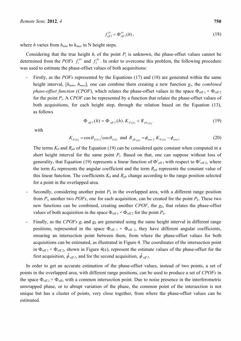
Figure 4. (a) The illustration of the POF (relating phase-offset to height) for the first

acquisition in two points, Pi and Pk, where hi and hk represent the true height of these points

respectively. (b) The illustration of the POF for the second acquisition for the same points.

(c) The CPOFs gi and gk in the space off 1 × off 2 are used to estimate the phase-offset

values off 1 and off 2 through the intersection point of gi and gk.

3. Processing Sequence

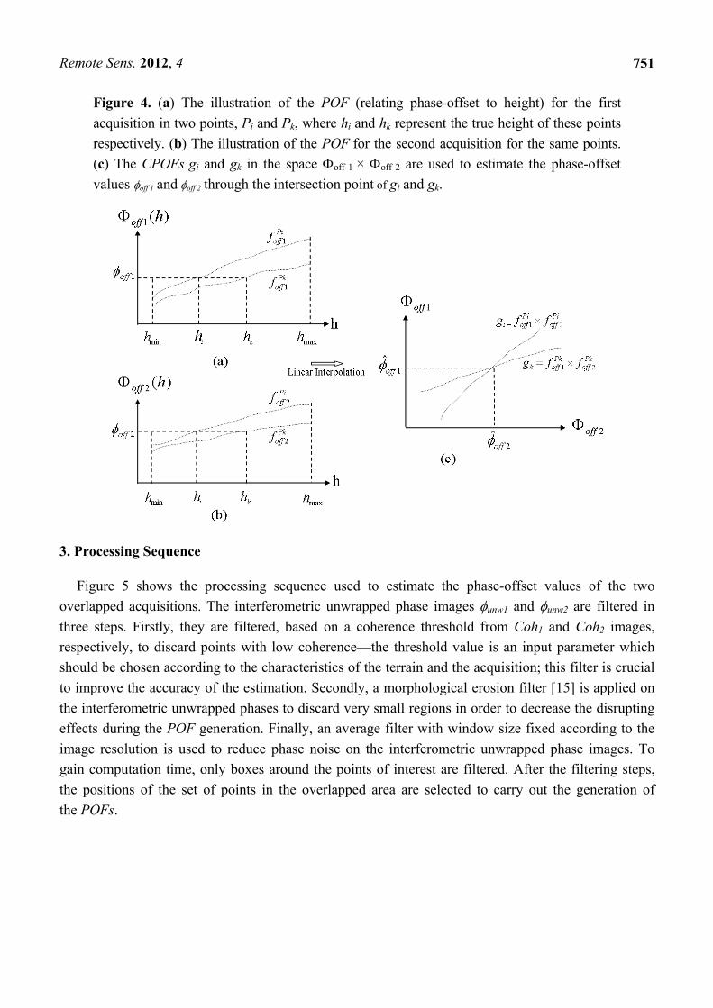
Figure 5 shows the processing sequence used to estimate the phase-offset values of the two

overlapped acquisitions. The interferometric unwrapped phase images unw1 and unw2 are filtered in

three steps. Firstly, they are filtered, based on a coherence threshold from Coh1 and Coh2 images,

respectively, to discard points with low coherence—the threshold value is an input parameter which

should be chosen according to the characteristics of the terrain and the acquisition; this filter is crucial

to improve the accuracy of the estimation. Secondly, a morphological erosion filter [15] is applied on

the interferometric unwrapped phases to discard very small regions in order to decrease the disrupting

effects during the POF generation. Finally, an average filter with window size fixed according to the

image resolution is used to reduce phase noise on the interferometric unwrapped phase images. To

gain computation time, only boxes around the points of interest are filtered. After the filtering steps,

the positions of the set of points in the overlapped area are selected to carry out the generation of

the POFs.


752

Figure 5. Processing sequence for phase-offset estimation.

)(

)(

22

11

hf

hf

off

off

2121 ),( offoffLinearcomb inffCombg

minh

1off

2off

11 Cohunw 22 Cohunw

Coordinate rotation using Principal Component Transformation

Phase offset estimation, DEM difference calculation and Parameters updating

21maxminˆˆoffoffh hh

h

12DEM

maxh

Coherence threshold filter Coherence threshold filter

Erosion filter

Spatial filter Spatial filter

Erosion filter

Linearity check of

Phase-offset functions

combg

Combined phase-offset function

To illustrate the processing step that generates the POFs shown in Figure 5, a processing sequence

was performed in a pair of the InSAR data gathered by the OrbiSAR-1 X-band system shown in

Figure 6. The generation of the POFs f1 and f2 for a selected point in the overlapped area, shown in

Figure 5, is based on the approach previously described and represented by Equations (17) and (18); in

the next step of the processing chain, the POFs are combined through a linear combination, creating a

CPOF gcomb in the space off 1 × off 2.

Carrying out the same operations for a set of points in the overlapped area, a set of functions gcomb

can be created from where the intersection point can be estimated. Figure 7 shows the set of CPOF for

100 points scanned in the overlapped area in a height interval [hmax − hmin] equal to 200 m, based on the

knowledge of the terrain topography from the SRTM DEM data, and a height step δh equal to 2 m.


753

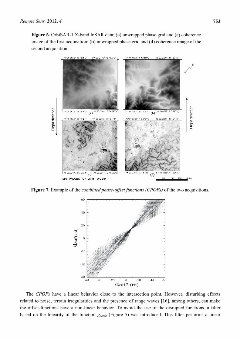
Figure 6. OrbiSAR-1 X-band InSAR data; (a) unwrapped phase grid and (c) coherence

image of the first acquisition; (b) unwrapped phase grid and (d) coherence image of the

second acquisition.

Figure 7. Example of the combined phase-offset functions (CPOFs) of the two acquisitions.

The CPOFs have a linear behavior close to the intersection point. However, disturbing effects

related to noise, terrain irregularities and the presence of range waves [16], among others, can make

the offset-functions have a non-linear behavior. To avoid the use of the disrupted functions, a filter

based on the linearity of the function gcomb (Figure 5) was introduced. This filter performs a linear


754

approximation of the curves and uses the chi-square goodness of fit statistics [17] to decide which ones

will be used for the estimation and which ones will be discarded.

In order to make it easier to determine the intersection point of the CPOFs, the CPOFs are rotated

using the Principal Components Analysis (PCA) [18], which is a mathematical procedure that uses an

orthogonal transformation to convert a set of observations of possibly correlated variables, in this case

the set of CPOFs gcomb, into a set of values of uncorrelated variables called Principal Components.

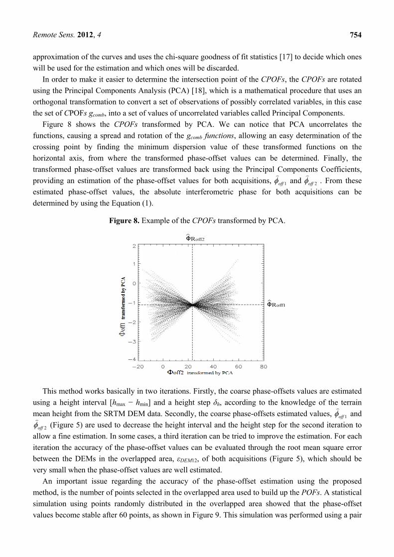
Figure 8 shows the CPOFs transformed by PCA. We can notice that PCA uncorrelates the

functions, causing a spread and rotation of the gcomb functions, allowing an easy determination of the

crossing point by finding the minimum dispersion value of these transformed functions on the

horizontal axis, from where the transformed phase-offset values can be determined. Finally, the

transformed phase-offset values are transformed back using the Principal Components Coefficients,

providing an estimation of the phase-offset values for both acquisitions, 1off

and 2off

. From these

estimated phase-offset values, the absolute interferometric phase for both acquisitions can be

determined by using the Equation (1).

Figure 8. Example of the CPOFs transformed by PCA.

This method works basically in two iterations. Firstly, the coarse phase-offsets values are estimated

using a height interval [hmax − hmin] and a height step δh, according to the knowledge of the terrain

mean height from the SRTM DEM data. Secondly, the coarse phase-offsets estimated values, 1off

and

2off

(Figure 5) are used to decrease the height interval and the height step for the second iteration to

allow a fine estimation. In some cases, a third iteration can be tried to improve the estimation. For each

iteration the accuracy of the phase-offset values can be evaluated through the root mean square error

between the DEMs in the overlapped area, εDEM12, of both acquisitions (Figure 5), which should be

very small when the phase-offset values are well estimated.

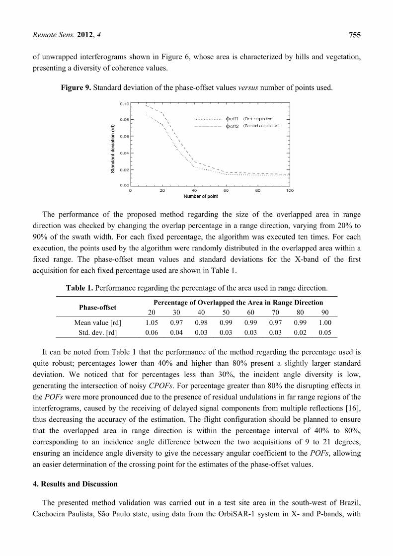
An important issue regarding the accuracy of the phase-offset estimation using the proposed

method, is the number of points selected in the overlapped area used to build up the POFs. A statistical

simulation using points randomly distributed in the overlapped area showed that the phase-offset

values become stable after 60 points, as shown in Figure 9. This simulation was performed using a pair


755

of unwrapped interferograms shown in Figure 6, whose area is characterized by hills and vegetation,

presenting a diversity of coherence values.

Figure 9. Standard deviation of the phase-offset values versus number of points used.

The performance of the proposed method regarding the size of the overlapped area in range

direction was checked by changing the overlap percentage in a range direction, varying from 20% to

90% of the swath width. For each fixed percentage, the algorithm was executed ten times. For each

execution, the points used by the algorithm were randomly distributed in the overlapped area within a

fixed range. The phase-offset mean values and standard deviations for the X-band of the first

acquisition for each fixed percentage used are shown in Table 1.

Table 1. Performance regarding the percentage of the area used in range direction.

Phase-offset Percentage of Overlapped the Area in Range Direction

20 30 40 50 60 70 80 90

Mean value [rd] 1.05 0.97 0.98 0.99 0.99 0.97 0.99 1.00 Std. dev. [rd] 0.06 0.04 0.03 0.03 0.03 0.03 0.02 0.05

It can be noted from Table 1 that the performance of the method regarding the percentage used is

quite robust; percentages lower than 40% and higher than 80% present a slightly larger standard

deviation. We noticed that for percentages less than 30%, the incident angle diversity is low,

generating the intersection of noisy CPOFs. For percentage greater than 80% the disrupting effects in

the POFs were more pronounced due to the presence of residual undulations in far range regions of the

interferograms, caused by the receiving of delayed signal components from multiple reflections [16],

thus decreasing the accuracy of the estimation. The flight configuration should be planned to ensure

that the overlapped area in range direction is within the percentage interval of 40% to 80%,

corresponding to an incidence angle difference between the two acquisitions of 9 to 21 degrees,

ensuring an incidence angle diversity to give the necessary angular coefficient to the POFs, allowing

an easier determination of the crossing point for the estimates of the phase-offset values.

4. Results and Discussion

The presented method validation was carried out in a test site area in the south-west of Brazil,

Cachoeira Paulista, São Paulo state, using data from the OrbiSAR-1 system in X- and P-bands, with


756

the parameters shown in Table 2. Four corner reflectors were deployed to the test site area to provide

an accurate phase-offset estimation, which was used as a reference.

Table 2. OrbiSAR-1 System-flight parameters.

Parameter Band

X P

Wavelength (λ) [m] 0.031228 0.713791

Flight altitude (H) [Km] 5.6 5.6

Incident angle (θ)—mid swath [deg] 50 50

Normal Baseline (Bn)—mid swath [m] 2.16 35.3

Swath width [Km] 7.0 7.0

Chirp bandwidth [MHz] 200 50

DEM spatial resolution [m] 2.0 2.0

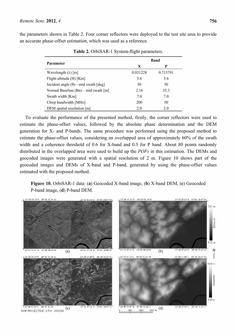
To evaluate the performance of the presented method, firstly, the corner reflectors were used to

estimate the phase-offset values, followed by the absolute phase determination and the DEM

generation for X- and P-bands. The same procedure was performed using the proposed method to

estimate the phase-offset values, considering an overlapped area of approximately 60% of the swath

width and a coherence threshold of 0.6 for X-band and 0.5 for P band. About 80 points randomly

distributed in the overlapped area were used to build up the POFs in this estimation. The DEMs and

geocoded images were generated with a spatial resolution of 2 m. Figure 10 shows part of the

geocoded images and DEMs of X-band and P-band, generated by using the phase-offset values

estimated with the proposed method.

Figure 10. OrbiSAR-1 data: (a) Geocoded X-band image, (b) X-band DEM, (c) Geocoded

P-band image, (d) P-band DEM.


757

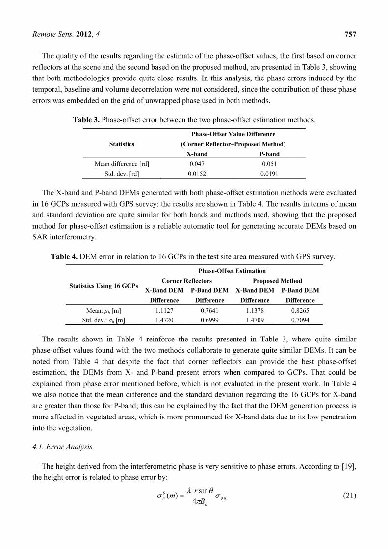
The quality of the results regarding the estimate of the phase-offset values, the first based on corner

reflectors at the scene and the second based on the proposed method, are presented in Table 3, showing

that both methodologies provide quite close results. In this analysis, the phase errors induced by the

temporal, baseline and volume decorrelation were not considered, since the contribution of these phase

errors was embedded on the grid of unwrapped phase used in both methods.

Table 3. Phase-offset error between the two phase-offset estimation methods.

Statistics

Phase-Offset Value Difference

(Corner Reflector–Proposed Method)

X-band P-band

Mean difference [rd] 0.047 0.051

Std. dev. [rd] 0.0152 0.0191

The X-band and P-band DEMs generated with both phase-offset estimation methods were evaluated

in 16 GCPs measured with GPS survey: the results are shown in Table 4. The results in terms of mean

and standard deviation are quite similar for both bands and methods used, showing that the proposed

method for phase-offset estimation is a reliable automatic tool for generating accurate DEMs based on

SAR interferometry.

Table 4. DEM error in relation to 16 GCPs in the test site area measured with GPS survey.

Statistics Using 16 GCPs

Phase-Offset Estimation

Corner Reflectors Proposed Method

X-Band DEM

Difference

P-Band DEM

Difference

X-Band DEM

Difference

P-Band DEM

Difference

Mean: μh [m] 1.1127 0.7641 1.1378 0.8265

Std. dev.: σh [m] 1.4720 0.6999 1.4709 0.7094

The results shown in Table 4 reinforce the results presented in Table 3, where quite similar

phase-offset values found with the two methods collaborate to generate quite similar DEMs. It can be

noted from Table 4 that despite the fact that corner reflectors can provide the best phase-offset

estimation, the DEMs from X- and P-band present errors when compared to GCPs. That could be

explained from phase error mentioned before, which is not evaluated in the present work. In Table 4

we also notice that the mean difference and the standard deviation regarding the 16 GCPs for X-band

are greater than those for P-band; this can be explained by the fact that the DEM generation process is

more affected in vegetated areas, which is more pronounced for X-band data due to its low penetration

into the vegetation.

4.1. Error Analysis

The height derived from the interferometric phase is very sensitive to phase errors. According to [19],

the height error is related to phase error by:

un

h B

rm

4

sin)( (21)


758

where u is the phase uncertainty, Bn is the normal baseline, θ the incident angle, r the slant range

distance and λ the wavelength.

The standard phase error and the phase uncertainty with 95% of confidence level, according to [17],

are given respectively by:

Nrde )( (22)

and

eu rd 0.2)( (23)

where is the standard deviation of the interferometric phase, N is the number of measurement and

is the mean phase error.

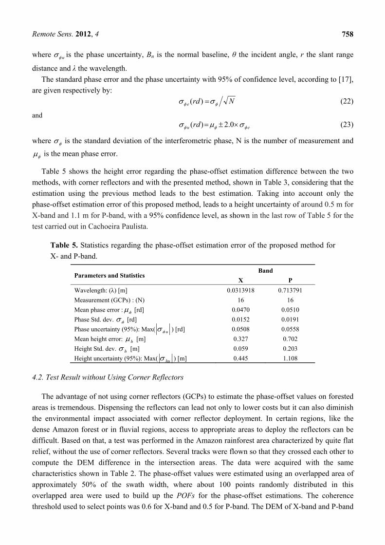
Table 5 shows the height error regarding the phase-offset estimation difference between the two

methods, with corner reflectors and with the presented method, shown in Table 3, considering that the

estimation using the previous method leads to the best estimation. Taking into account only the

phase-offset estimation error of this proposed method, leads to a height uncertainty of around 0.5 m for

X-band and 1.1 m for P-band, with a 95% confidence level, as shown in the last row of Table 5 for the

test carried out in Cachoeira Paulista.

Table 5. Statistics regarding the phase-offset estimation error of the proposed method for

X- and P-band.

Parameters and Statistics Band

X P

Wavelength: (λ) [m] 0.0313918 0.713791

Measurement (GCPs) : (N) 16 16

Mean phase error : [rd] 0.0470 0.0510

Phase Std. dev. [rd] 0.0152 0.0191

Phase uncertainty (95%): Max( u ) [rd] 0.0508 0.0558

Mean height error: h [m] 0.327 0.702

Height Std. dev. h [m] 0.059 0.203

Height uncertainty (95%): Max( hu ) [m] 0.445 1.108

4.2. Test Result without Using Corner Reflectors

The advantage of not using corner reflectors (GCPs) to estimate the phase-offset values on forested

areas is tremendous. Dispensing the reflectors can lead not only to lower costs but it can also diminish

the environmental impact associated with corner reflector deployment. In certain regions, like the

dense Amazon forest or in fluvial regions, access to appropriate areas to deploy the reflectors can be

difficult. Based on that, a test was performed in the Amazon rainforest area characterized by quite flat

relief, without the use of corner reflectors. Several tracks were flown so that they crossed each other to

compute the DEM difference in the intersection areas. The data were acquired with the same

characteristics shown in Table 2. The phase-offset values were estimated using an overlapped area of

approximately 50% of the swath width, where about 100 points randomly distributed in this

overlapped area were used to build up the POFs for the phase-offset estimations. The coherence

threshold used to select points was 0.6 for X-band and 0.5 for P-band. The DEM of X-band and P-band


759

were generated with a spatial resolution of 2.5 m. The goal of this test was to verify if the phase-offset

values would be well estimated for each track, enabling the generation of quite similar DEMs on the

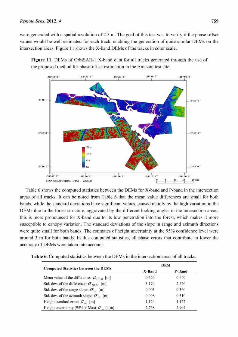
intersection areas. Figure 11 shows the X-band DEMs of the tracks in color scale.

Figure 11. DEMs of OrbiSAR-1 X-band data for all tracks generated through the use of

the proposed method for phase-offset estimation in the Amazon test site.

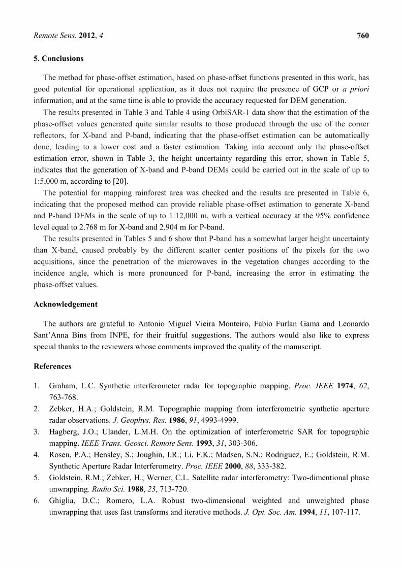
Table 6 shows the computed statistics between the DEMs for X-band and P-band in the intersection

areas of all tracks. It can be noted from Table 6 that the mean value differences are small for both

bands, while the standard deviations have significant values, caused mainly by the high variation in the

DEMs due to the forest structure, aggravated by the different looking angles in the intersection areas;

this is more pronounced for X-band due to its low penetration into the forest, which makes it more

susceptible to canopy variation. The standard deviations of the slope in range and azimuth directions

were quite small for both bands. The estimates of height uncertainty at the 95% confidence level were

around 3 m for both bands. In this computed statistics, all phase errors that contribute to lower the

accuracy of DEMs were taken into account.

Table 6. Computed statistics between the DEMs in the intersection areas of all tracks.

Computed Statistics between the DEMs DEM

X-Band P-Band

Mean value of the difference: DEM [m] 0.520 0.640

Std. dev. of the difference: DEM [m] 3.170 2.520

Std. dev. of the range slope: rg [m] 0.003 0.360

Std. dev. of the azimuth slope: az [m] 0.008 0.310

Height standard error: he [m] 1.124 1.127

Height uncertainty (95% ): Max(| hu |) [m] 2.768 2.904


760

5. Conclusions

The method for phase-offset estimation, based on phase-offset functions presented in this work, has

good potential for operational application, as it does not require the presence of GCP or a priori

information, and at the same time is able to provide the accuracy requested for DEM generation.

The results presented in Table 3 and Table 4 using OrbiSAR-1 data show that the estimation of the

phase-offset values generated quite similar results to those produced through the use of the corner

reflectors, for X-band and P-band, indicating that the phase-offset estimation can be automatically

done, leading to a lower cost and a faster estimation. Taking into account only the phase-offset

estimation error, shown in Table 3, the height uncertainty regarding this error, shown in Table 5,

indicates that the generation of X-band and P-band DEMs could be carried out in the scale of up to

1:5,000 m, according to [20].

The potential for mapping rainforest area was checked and the results are presented in Table 6,

indicating that the proposed method can provide reliable phase-offset estimation to generate X-band

and P-band DEMs in the scale of up to 1:12,000 m, with a vertical accuracy at the 95% confidence

level equal to 2.768 m for X-band and 2.904 m for P-band.

The results presented in Tables 5 and 6 show that P-band has a somewhat larger height uncertainty

than X-band, caused probably by the different scatter center positions of the pixels for the two

acquisitions, since the penetration of the microwaves in the vegetation changes according to the

incidence angle, which is more pronounced for P-band, increasing the error in estimating the

phase-offset values.

Acknowledgement

The authors are grateful to Antonio Miguel Vieira Monteiro, Fabio Furlan Gama and Leonardo

Sant’Anna Bins from INPE, for their fruitful suggestions. The authors would also like to express

special thanks to the reviewers whose comments improved the quality of the manuscript.

References

1. Graham, L.C. Synthetic interferometer radar for topographic mapping. Proc. IEEE 1974, 62,

763-768.

2. Zebker, H.A.; Goldstein, R.M. Topographic mapping from interferometric synthetic aperture

radar observations. J. Geophys. Res. 1986, 91, 4993-4999.

3. Hagberg, J.O.; Ulander, L.M.H. On the optimization of interferometric SAR for topographic

mapping. IEEE Trans. Geosci. Remote Sens. 1993, 31, 303-306.

4. Rosen, P.A.; Hensley, S.; Joughin, I.R.; Li, F.K.; Madsen, S.N.; Rodriguez, E.; Goldstein, R.M.

Synthetic Aperture Radar Interferometry. Proc. IEEE 2000, 88, 333-382.

5. Goldstein, R.M.; Zebker, H.; Werner, C.L. Satellite radar interferometry: Two-dimentional phase

unwrapping. Radio Sci. 1988, 23, 713-720.

6. Ghiglia, D.C.; Romero, L.A. Robust two-dimensional weighted and unweighted phase

unwrapping that uses fast transforms and iterative methods. J. Opt. Soc. Am. 1994, 11, 107-117.


761

7. Fornaro, G.; Franceschetti, G.; Lanari, R. Interferometric SAR phase unwrapping using Green’s

formulation. IEEE Trans. Geosci. Remote Sens. 1996, 34, 720-727.

8. Pritt, M.D. Phase unwrapping by means of multigrid techniques for interferometric SAR. IEEE

Trans. Geosci. Remote Sens. 1996, 34, 728-738.

9. Madsen, S.N. Absolute phase determination techniques in SAR interferometry. Proc. SPIE 1995,

2487, 393-401.

10. Scheiber, R.; Fischer, J. Absolute Phase Offset in SAR Interferometry: Estimation by Spectral

Diversity and Integration into Processing. In Proceedings of EUSAR, Ulm, Germany, 25–27 May

2004.

11. Brcic, R.; Eineder, M.; Bamler, R. Absolute Phase Estimation from TerraSAR-X Acquisitions

using Wideband Interferometry. In Proceedings of IEEE Radar Conference, Pasadena, CA, USA,

4–8 May 2009.

12. Eineder, M.; Adam, N. A maximum likelihood estimator to simultaneously unwrap, geocode and

fuse SAR interferograms from different viewing geometries into one digital elevation model.

IEEE Trans. Geosci. Remote Sens. 2005, 43, 24-36.

13. Fornaro, G.; Sansosti, E.; Lanari, R.; Tesauro, M. Role of processing geometry in SAR raw data

focusing.IEEE Trans. Aerosp. Electron. Syst. 2002, 38, 441-454.

14. Schreier, G. Standard Geocoded Ellipsoid Corrected Images. In SAR Geocoding: Data and

Systems; Chapter 6; Wichmann Verlag: Kalsruhe, Germany, 1993; pp. 159-163.

15. Maragos, P. Morphological Filtering for Image Enhancement and Feature Detection. In Handbook

of Image and Video Processing, 2nd ed.; Bovik, A.C., Ed.; Academic Press: New York, NY,

USA, 2005; pp. 135-156.

16. Pinheiro, M.; Rosa, R.; Moreira, J.R. Multi-Path Correction Model for Multi-Channel Airborne

SAR. In Proceedings of 2009 IEEE International Geoscience & Remote Sensing Symposium

(IGARSS’09), Cape Town, South Africa, 12–19 June 2009; Volume 3, pp. 729-732.

17. Taylor, J.R. An Introduction to Error Analysis: The Study of Uncertainties in Physical

Measurements, 2nd ed.; University Science Books: Sausalito, CA, USA, 1997.

18. Richards, J.A.; Jia, X.P. Multispectral Transformation of Image Data. In Remote Sensing Digital

Image Analysis, 2nd ed.; Springer-Verlag: Berlin, Germany, 1993; pp.137-163.

19. Rodriguez, E.; Martin, J.M. Theory and design of interferometric synthetic aperture radar. IEE

Proc.-F 1992, 139, 147-159.

20. Greenwalt, C.R.; Schultz, M.E. Principles and Error Theory and Cartographic Applications;

ACIC Thechnical Report No 96; Aeronautical Chart and Information Center: St. Louis, MO,

USA, 1968.

© 2012 by the authors; licensee MDPI, Basel, Switzerland. This article is an open access article

distributed under the terms and conditions of the Creative Commons Attribution license

(http://creativecommons.org/licenses/by/3.0/).

A Phase-Offset Estimation Method for InSAR DEM ... - MDPI

Documents

Transcript of A Phase-Offset Estimation Method for InSAR DEM ... - MDPI