University of Denver University of Denver

Digital Commons @ DU Digital Commons @ DU

Electronic Theses and Dissertations Graduate Studies

1-1-2013

Study the Carrier Frequency Offset (CFO) for Wireless OFDM Study the Carrier Frequency Offset (CFO) for Wireless OFDM

Saeed Mohseni University of Denver

Follow this and additional works at: https://digitalcommons.du.edu/etd

Part of the Electrical and Electronics Commons

Recommended Citation Recommended Citation Mohseni, Saeed, "Study the Carrier Frequency Offset (CFO) for Wireless OFDM" (2013). Electronic Theses and Dissertations. 438. https://digitalcommons.du.edu/etd/438

This Dissertation is brought to you for free and open access by the Graduate Studies at Digital Commons @ DU. It has been accepted for inclusion in Electronic Theses and Dissertations by an authorized administrator of Digital Commons @ DU. For more information, please contact jennifer.cox@du.edu,dig-commons@du.edu.

STUDY THE CARRIER FREQUENCY OFFSET (CFO) FOR WIRELESS

OFDM

__________

A Dissertation

Presented to

the Faculty of Engineering and Computer Science

University of Denver

__________

In Partial Fulfillment

of the Requirements for the Degree

Doctor of Philosophy

__________

by

Saeed Mohseni

June 2013

Advisor: Dr. Mohammad A. Matin

©Copyright by Saeed Mohseni 2013

All Rights Reserved

ii

Author: Saeed Mohseni

Title: STUDY THE CARRIER FREQUENCY OFFSET (CFO) FOR WIRELESS OFDM

Advisor: Dr. Mohammad A. Matin

Degree Date: June 2013

Abstract

Due to high proficiency with high bandwidth efficiency, orthogonal frequency

division multiplexing (OFDM) has been selected for broadband wireless communication

systems. Since OFDM can provide large data rates with sufficient robustness to radio

channel impairments, and due to its robustness against the multipath delay spread, OFDM

has always been a designated technique for broadband wireless communication mobile

systems. Nevertheless, OFDM suffers from Carrier Frequency Offset (CFO). CFO has

been recognized as a major disadvantage of OFDM. CFO can lead to the frequency

mismatch in transmitter and receiver oscillator. Lack of the synchronization of the local

oscillator signal, for down conversion in the receiver with the carrier signal contained in

the received signal, can cause the performance of OFDM to degrade. In other words, the

orthogonality of the OFDM relies on the condition that the transmitter and receiver

operate with exactly the same frequency reference. If this is not the case, the perfect

orthogonality of the subcarrier will be lost, which can result in CFO. In this research, the

source of creating CFO and the major CFO estimation algorithms have been reviewed

and discussed in literature. We then proposed some algorithms and techniques for

estimating and compensating for the effect of CFO. We showed that our proposed

methods have a better performance with low complexity.

Although this research focuses on CFO, high Peak-to-Average Power Ratio

(PAPR) has been named as the other main drawback of the OFDM modulation format.

iii

The chapter 4 is dedicated to PAPR. In this chapter after investigating PAPR, we

proposed a technique that leads to the reduction of PAPR. On the other hand, in wireless

communication path loss is the main power loss that occurs between the transmitter and

the receiver antenna. Therefore, chapter 5 is dedicated to investigate indoor and outdoor

path loss. We then proposed an extended model that can be used to cover the outdoor and

indoor environment for predicting the path loss. Chapter 6 contains the results and

conclusion.

iv

Acknowledgements

I am most grateful to my advisor, Dr. Mohammad A. Matin, for his consistence

support, encouragement, expertise, and exquisite guidance throughout my PhD study. I

also appreciate the members of my committee, Dr. Jun Jason Zhang, Dr. George Edwards

and Dr. Davor Balzar for their guidance and support.

I would like to express my deepest gratitude to my mother and my brother,

Mansour for their willing encouragement and support during my study over the years.

Special thanks go to my beloved wife, Sima, for her consistence love and support, and to

my lovely children, Sarina and Daniel, for bringing me all the joy and happiness in the

world.

I send my blessings to my late father for all he had done for his children,

especially for the love of learning that he planted in his children’s hearts. Even though he

is not alive, I am sure his soul gets happy when he sees that his children are successful. I

also wish to express my appreciation to all those who have cared for me.

v

Table of contents

Abstract ............................................................................................................................... ii

Acknowledgements ............................................................................................................ iv

Table of contents ................................................................................................................. v

List of figures ................................................................................................................... viii

List of tables ...................................................................................................................... xii

List of abbreviations ........................................................................................................ xiii

Chapter 1 ............................................................................................................................. 1 Introduction ......................................................................................................................... 1

1.1 Background ....................................................................................................... 1 1.2 Problem statement ............................................................................................. 2

1.3 Objective ........................................................................................................... 2 1.4 Scope of research work ..................................................................................... 3 1.5 Methodology ..................................................................................................... 3

1.6 Contribution and publications ........................................................................... 3 1.7 Chapter organization ......................................................................................... 5

Chapter 2 ............................................................................................................................. 7 Concept of OFDM .............................................................................................................. 7

2.1 Introduction ....................................................................................................... 7 2.2 The history of OFDM ....................................................................................... 7

2.3 OFDM ............................................................................................................... 8 2.4 Concept of overlapping modulation.................................................................. 9 2.5 The methods of organizing the subcarriers in OFDM .................................... 11

2.6 The role of cyclic prefix .................................................................................. 12 2.7 The effect of subcarriers and Guard Band on system performance ................ 14 2.8 Modulation ...................................................................................................... 14

2.8.1 Coherent Modulation for OFDM systems ....................................... 15 2.8.2 M-ary Amplitude Shift Keying (MASK/M-ary ASK)..................... 15 2.8.3 M-ary Phase Shift Keying (MPSK/M-ary PSK) .............................. 15 2.8.4 M-ary Quadrature Amplitude Modulation (MQAM/M-ary QAM) . 16

2.9 The advantages and disadvantages of OFDM ................................................ 16 2.10 Challenges in the OFDM wireless systems .................................................. 17 2.11 Path losses and fading in OFDM systems .................................................... 18

2.12 Choice of OFDM parameters ........................................................................ 21 2.18 A typical schematic of an OFDM transceiver ............................................... 24 2.19 Proprietary OFDM Flavors ........................................................................... 25

vi

Chapter 3 ........................................................................................................................... 26

Carrier Frequency Offset (CFO) ....................................................................................... 26 3.1 Introduction ..................................................................................................... 26 3.2 Effects of frequency offset on OFDM signals ................................................ 27

3.3 Carrier Frequency Offset (CFO) ..................................................................... 28 3.4 Sources of frequency offset ............................................................................ 34 3.5 Doppler Effect ................................................................................................. 34 3.6 The effect of integer and fractional part of CFO ............................................ 35 3.7 Effect of CFO on phase shift .......................................................................... 37

3.8 Effect of CFO on degradation of OFDM systems .......................................... 39 3.9 The effect of CFO, phase noise, and Rayleigh fading .................................... 41 3.10 The relation between frequency offset and SNR .......................................... 43 3.11 Frequency synchronization ........................................................................... 44

3.12 Sampling clock mismatch ............................................................................. 45 3.13 The effect of STO on OFDM Synchronization ............................................. 46

3.14 The effect of ISI on OFDM systems ............................................................. 47 3.15 Effect of CFO on creating ICI ...................................................................... 49

3.16 The effect of Symbol and Sample Timing Offset ......................................... 49 3.17 The effect of using DCR on CFO ................................................................. 51 3.18 The effect of increasing the range of CFO estimation .................................. 53

3.19 Using Time domain equalizer (TDE) to combat the effect of ICI and ISI ... 54 3.20 Synchronization using the cyclic extension .................................................. 57

3.21 CFO estimation algorithm and Techniques .................................................. 57 3.22 Training based algorithm .............................................................................. 58 3.23 Blind and Semi-blind algorithms .................................................................. 58

3.24 Study of the training based and blind algorithms ......................................... 59

3.25 Reviewing the Pilot based and Non-pilot base estimation............................ 63 3.26 Model for CFO .............................................................................................. 64 3.27 Pilot based and Non-pilot base estimation .................................................... 65

3.28 Blind CFO estimation technique using SPRIT-Like Algorithm ................... 66 3.29 Blind CFO estimation technique using MUSIC Algorithm .......................... 69

3.30 Study of the CFO estimation using periodic preambles ............................... 70 3.31 Investigating of the estimation Technique using Cyclic Prefix (CP) ........... 74

3.32 Proposed Algorithm ...................................................................................... 77

Chapter 4 ........................................................................................................................... 84 Peak to Average Power Ratio ........................................................................................... 84

4.1 Introduction ..................................................................................................... 84 4.2 Peak to Average Power Ratio (PAPR)............................................................ 84

4.3 Techniques for reduction PAPR ..................................................................... 85 4.4 Selecting Mapping (SLM) .............................................................................. 85

4.5 Partial Transmission Sequence (PTS) ............................................................. 86 4.6 Clipping and Filtering (CAF).......................................................................... 87 4.7 Types of Clipping Techniques ........................................................................ 89 4.8 Coding techniques ........................................................................................... 93 4.9 Proposed algorithm for reducing PAPR ......................................................... 95

vii

Chapter 5 ........................................................................................................................... 99

Path Loss ........................................................................................................................... 99 5.1 Introduction ..................................................................................................... 99 5.2 Path loss models ............................................................................................ 102

5.3 Free–Space model ......................................................................................... 102 5.4 Plane-Earth Model ........................................................................................ 104 5.5 Multipath Fading ........................................................................................... 105 5.6 Delay spread.................................................................................................. 107 5.7 Okumura-Hata (OH) Model .......................................................................... 108

5.8 COST-231 Model.......................................................................................... 113 5.9 Dual Slope Model ......................................................................................... 113 5.10 Multi-Slope/Extended Hata model for urban zone ..................................... 114 5.11 The other Models ........................................................................................ 116

5.12 Indoor path loss ........................................................................................... 116 5.13 Indoors Propagation .................................................................................... 117

5.14 Building propagation .................................................................................. 117 5.15 Wall Penetration.......................................................................................... 118

5.16 Window Penetration.................................................................................... 118 5.17 Indoors Propagations .................................................................................. 119 5.18 Indoor model ............................................................................................... 119

5.19 Proposed algorithm ..................................................................................... 123

Chapter 6 ......................................................................................................................... 126

Results, Conclusion and future Work ............................................................................. 126 6.1 Preface........................................................................................................... 126 6.2 Summary ....................................................................................................... 127

6.3 Carrier Frequency Offset (CFO) ................................................................... 128

6.4 Peak to Average Power Ratio ....................................................................... 145 6.5 Path Loss ....................................................................................................... 151 6.4 Future work ................................................................................................... 158

Bibloiography ................................................................................................................. 159

Appendix ......................................................................................................................... 168 List of publications ............................................................................................. 168

viii

List of figures

Figure 2.1-a Concept of OFDM signal in conventional multicarrier technique ................. 9

Figure 2.1-b Concept of OFDM signal in orthogonal multicarrier modulation ............... 10

Figure 2.2-a Spectra of an OFDM sub-channel ................................................................ 10

Figure 2.2-b Spectra of an OFDM signal.......................................................................... 10

Figure 2.3 Illustration of the orthogonality relationship between signals ........................ 11

Figure 2.4-a Spectral setting ............................................................................................. 12

Figure 2.4-b OFDM transmission BW.............................................................................. 12

Figure 2.5 Cyclic Prefix (CP) ........................................................................................... 13

Figure 2.6-a OFDM signal ................................................................................................ 19

Figure 2.6-b Transmitted data ........................................................................................... 20

Figure 2.6-c Received data ............................................................................................... 20

Figure 2.7 Data rates comparison ..................................................................................... 24

Figure 2.8 A typical schematic diagram of an OFDM transceiver system ....................... 25

Figure 3.1 Illustration of frequency offset (δf) ................................................................. 27

Figure 3.2 Frequency offset ....................................................................................... 28

Figure 3.3 Block diagram of the OFDM transceiver system ............................................ 29

Figure 3.4 Structure of an OFDM system with the required units for estimating and

compensating CFO.................................................................................... 31

Figure 3.5 Block diagram of the OFDM wireless transceiver system .............................. 31

Figure 3.6 OFDM receiver with frequency synchronization ............................................ 33

Figure 3.7 Effect of CFO when ........................................................................... 36

ix

Figure 3.8 Effect of CFO when ......................................................................... 37

Figure 3.9 Effect of CFO (ξ) on phase in the time domain............................................... 38

Figure 3.10 Effect of CFO (ξ) on phase difference .......................................................... 38

Figure 3.11 SNR degradation as a function of the frequency offset ................................. 40

Figures 3.12 Signal-to-Interference-plus-Noise-Ratio (SINR) ......................................... 42

Figures 3.13 Signal-to-Interference-plus-Noise-Ratio (SINR) ......................................... 43

Figure 3.14 SNR degradation versus sampling offset ...................................................... 42

Figure 3.15 The overall ICI created by frequency offset .................................................. 49

Figure 3.16 Block diagram of the DCR with I/Q and CFO compensation ....................... 52

Figure 3.17 MSE versus D ................................................................................................ 54

Figure 3.18 Block diagram of a TDE for a typical OFDM system................................... 55

Figure 3.19 Cyclic prefix for synchronization .................................................................. 57

Figure 3.20 Example of the timing metric for the AWGN channel (SNR = 10dB) ......... 61

Figure 3.21 A typical block diagram for wireless OFDM system .................................... 65

Figure 3.22 Multi-user MIMO-OFDM systems diagram ................................................. 78

Figure 3.23 CFO estimation .............................................................................................. 80

Figure 3.24 BER VS Eb/N0 .............................................................................................. 83

Figure 4.1 Block diagram of the SLM technique ............................................................. 86

Figure 4.2 Block diagram of partial transmission sequence (PTS) approach ................... 86

Figure 4.3 Time domain OFDM signal............................................................................. 88

Figure 4.4 OFDM transmitter using clipping and filtering ............................................... 88

x

Figure 4.5 Functions-based clipping for PAPR reduction for .......................................... 90

(a) Classical-clipping (b) Heavy side-clipping

(c) Deep clipping (d) Smooth-clipping

Figure 4.6-a Average power performance ........................................................................ 91

Figure 4.6-b BER performance ......................................................................................... 91

Figure 4.7 PAPR reduction performance .......................................................................... 92

Figure 4.8 Space between subcarriers (1/Ts) .................................................................... 95

Figure 4.9 Illustration for Eq. (4.10) ................................................................................. 97

Figure 4.10 Reduction of PAPR is about 0.2 dB .............................................................. 98

Figure 5.1 Types of various fading channel .................................................................... 100

Figure 5.2 LOS, multipath channel environment ............................................................ 102

Figure 5.3 Free space model ........................................................................................... 103

Figure 5.4 No LOS channel ............................................................................................ 106

Figure 5.5 Two multipath components ........................................................................... 108

Figure 5.6 OH model versus free space path loss ........................................................... 111

Figure 5.7 Path loss in urban zone versus open zone ..................................................... 112

Figure 5.8 Mean path loss as the function of the distance between the transmitter and

receiver antenna ...................................................................................... 116

Figure 5.9 Passage of wave through the window ........................................................... 119

Figure 5.10 Wall attenuation for two different wall structures ....................................... 121

Figure 6.1 Doppler frequency respect to the angle of incident ....................................... 131

Figure 6.2 Illustration of moving component in wireless vehicle communication......... 132

Figure 6.3 Normalized Doppler frequency ..................................................................... 133

xi

Figure 6.4 BER versus SNR for three different values for angles of incident................ 134

Figure 6.5 Performance of BER versus SNR considering the different values of beam-

width and frequency alignment ............................................................... 136

Figure 6.6 Effect of frequency offset on ICI loss ........................................................... 137

Figure 6.7 SNR degradation versus relative frequency offset ........................................ 139

Figure 6.8 Effect of CFO on phase in the time domain .................................................. 140

Figure 6.9 MSE versus D ................................................................................................ 141

Figure 6.10 CFO estimation ............................................................................................ 142

Figure 6.11 Schematic diagram of proposed method ..................................................... 143

Figure 6.12 MSE versus SNR ......................................................................................... 144

Figure 6.13 CCDF OF OFDM ........................................................................................ 150

Figure 6.14 CDF Plot of PAPR....................................................................................... 150

Figure 6.15 BER versus SNR ......................................................................................... 151

Figure 6.16 IEEE model for path loss with initial d0 ...................................................... 153

Figure 6.17 Path loss model with initial d00 .................................................................... 155

Figure 6.18 Proposed method versus common model .................................................... 157

xii

List of tables

Table 2.1 Path loss exponent ............................................................................................ 21

Table 2.2 Timing related parameters for the OFDM systems .......................................... 22

Table 2.3 Rate dependent parameters for the OFDM systems ......................................... 23

Table 3.1 Effect of the CFO on transmitted signal ........................................................... 34

Table 4.1 PAPR reduction comparison ............................................................................. 94

Table 4.2 Comparison for reduction techniques ............................................................... 95

Table 5.1 Classification of the channel environments .................................................... 101

Table 5.2 Average floor attenuation for two different buildings .................................... 122

xiii

List of abbreviations

3GPP 3rd Generation Partnership Project

ADSL Asynchronous Digital Subscriber Line

A/D Analog-to-Digital

AOI Angle of Incident

ASK Amplitude Shift Keying

AWGN Additive White Gaussian Noise

BER Bit Error Rate

BP Break Point

BW Bandwidth

CAF Clipping and Filtering

CAZAC Constant Amplitude Zero Autocorrelation

CBC Complement Block Coding

CC Classical-Clipping

CCDF Complementary Cumulative Distribution Function

CDMA Code Division Multiple Access

CE Cyclic Extension

CFO Carrier Frequency Offset

CP Cyclic Prefix

DAB Digital Audio Broadcasting

dB Decibel

DC Deep-Clipping

xiv

DCR Direct Conversion Receivers

DE Doppler Effect

DFT Discrete Fourier Transform

DMB Digital Mobile Broadcasting

DPSD Doppler Power Spectrum Density

DSBW Directional Scattering Bandwidth

DVB Digital Video Broadcasting

ESPRIT Estimation of Signal Parameter via Rotational

Invariance Techniques

EVD Eigenvalue Decomposition

FAF Floor Attenuation Factor

FFT Fast Fourier Transform

FSP Free Space Propagation

GB Guard Band

HC Heavy side-Clipping

HPA High Power Amplifier

HST High Speed Transportation

ICI Inter-Carrier Interference

ISI Inter Symbol Interference

IEEE Institute of Electrical and Electronics Engineers

IFFT Inverse Fast Fourier Transform

IDFT Inverse Discrete Fourier Transform

I/Q In-phase and Quadrature

xv

ISI Inter Symbol Interference

LOS Line Of Sight

LOSC Local Oscillator Signal

LSF Large Scale Fading

SSF Small Scale Fading

MASK/M-ary ASK M-ary Amplitude Shift Keying

MC-CDMA Multi Carrier Code Division Multiple Access

MLE Maximum Likelihood Estimate

MPSK/M-ary PSK M-ary Phase Shift Keying

MQAM/M-ary QAM M-ary Quadrature Amplitude Modulation

MSE Mean Square Error

MUSIC MUltiple SIgnal Classifier

NLOS No Line Of Sight

OFDM Orthogonal Frequency Division Multiplexing

OSC Oscillator

PA Power Amplifier

PAPR Peak to Average Power Ratio

PCS Personal Communication System

PL Path Loss

PSD Power Spectrum Density

PSK Phase Shift Keying

PTS Partial Transmission Sequence

QAM Quadrature Amplitude Modulation

xvi

QPSK Quadrature Phase-Shift Keying

RF Radio Frequency

SBCC Sub-Block Complement Coding

SC Smooth-Clipping

SCD Sampling Clock Drift

SCs Sub-Carriers

ScFO Sampling clock Frequency Offset

SINR Signal-to-Interference-plus-Noise-Ratio

SISO Single-Input Single-Output

SLM Selective Mapping

SMOPT Selective Mapping of Partial Tones

SNR Signal-to-Noise Ratio

SSF Small Scale Fading

STO Symbol Time Offset

SVD Spectral Value Decomposition

TDE Time Domain Equalizer

TDR Transmission Data Rate

TI Tone Injection

TR Tone Reservation

VTD Vehicle Travel Direction

WAF Wall Attenuation Factor

UTD Uniform Theory of Diffraction

1

Chapter 1

Introduction

1.1 Background

The Orthogonal Frequency Division Multiplexing (OFDM) system was suggested

for the first time during the Second World War and gradually was studied for use as a

high speed modem and for digital mobile communication. Approximately 55 years ago,

Doelz et al. [1] published the idea of dividing the transmitting data into the number of

interleaved bit streams and modulate numerous carriers. Then Chang [2], in the middle of

the 1960’s, presented the basic idea of multicarrier modulation. But it was Weinstein and

Ebert [3] that brought it to fruition. They showed how to apply the Discrete Fourier

Transform (DFT) to perform the baseband modulation and demodulation. They showed

how, by using the DFT, we can increase and improve the efficiency of the modulation

and demodulation.

However, due to the high proficiency with high bandwidth and its ability to

provide large data rates and its robustness against the multipath delay spread, OFDM has

been selected for the broadband wireless systems. But in order to efficiently modulate

and demodulate the OFDM signals, and preventing the degradation of the OFDM

wireless systems, a few pre and post tasks must be done. The most important in an

2

OFDM transceiver are estimating and compensating the Carrier Frequency Offset (CFO),

frequency synchronization, and Peak-to-Average Power Reduction (PAPR).

1.2 Problem statement

Although OFDM has many advantages, OFDM systems are very sensitive to the

CFO. CFO is one of the most important drawbacks of the OFDM wireless

communication system. CFO destroys the orthogonality relationship between the

subcarrier and creates Inter-Carrier Interference (ICI). ICI can create frequency mismatch

between the transmitter and receiver. This frequency mismatch can lead to the severe

performance degradation issue for OFDM wireless systems. Therefore, for a reliable

receiver, the effect of the CFO must be estimated and compensated. In short, no matter

which method to be used, the carrier frequency offset should be estimated and

compensated to keep the orthogonality in OFDM systems.

1.3 Objective

The main focus of this research is on CFO. In this research we have investigated

the reasons of creating CFO and we have analyzed its effects on the performance of the

OFDM systems. We have reviewed and discussed the major CFO estimation algorithms

and techniques in literature and have evaluated their performance and efficiency. Then

we have proposed some algorithms and techniques for estimating and compensating for

the effect of CFO. Our goal is to propose the algorithm and method that can compensate

for the effect of CFO and gain better performance with lower complexity.

3

1.4 Scope of research work

In this research the main focus is on exploring and using advanced mathematical

tools to overview the available algorithms and techniques and then to propose an

algorithm for reducing the complexity and computational process for CFO estimation in

wireless OFDM systems. As we mentioned since PAPR and path loss are the other issues

that degrade the OFDM performance, in Chapter 4, after briefly investigating them, we

have proposed a method with lower complexity for PAPR and then we have presented an

analytical model for optimizing indoor and outdoor radio propagation prediction for path

loss in wireless OFDM communication systems.

1.5 Methodology

To achieve our objectives we use different mathematical approaches and Matlab

software version R2011-a.

- Mathematical tools are used for investigating the available algorithms, techniques

and methods and obtaining an analytical algorithm or method for improving the

existence methods.

- MATLAB is used for simulation and comparing the proposed algorithm with the

algorithms and techniques that were suggested by the others.

1.6 Contribution and publications

This research is on the study of the effects of carrier frequency offset (CFO) for

wireless orthogonal frequency-division multiplexing (OFDM) systems. Most of the

research and contributions have already published in various peer review journals

4

(publications list is in page 168). Following paragraph will concise in respect to each of

the publications.

One of the major drawbacks for OFDM system is Carrier frequency offset (CFO).

A training based technique for estimating and compensation for the bigger range of CFO

has been presented. A method for CFO estimation which is based on cost function and

uses the structure of the subcarrier has been suggested. Then the research continued by

investigating the effect of carrier frequency offset and frequency synchronization on

different parameters on OFDM systems. The research showed the dependency of the

SNR to the frequency offset and a better approach by using the repetitive pattern to

increase the range of estimation has been showed.

In addition to CFO research my initial research was in Peak-to-Average Power

Ratio (PAPR) and path loss which were published in peer review journal as stated below.

A method has been presented which in compare with the conventional OFDM, the

separation of subcarriers (SCs) is forth. Thus, in each OFDM symbol, only the first

⁄ samples will be sent while the rest will be ignored, which leads to decrease the

maximum of PAPR. In this case, the rest of the samples by using the partial symmetry of

Fourier transform can be constructed.

An approach for the path loss propagation model for indoor/outdoor path loss has

proposed which is on the base of calculating a new initial value plus the field

measurements.

5

1.7 Chapter organization

The dissertation is divided into five chapters. The layouts for these chapters are as

follows:

Chapter 1 includes background, the problem statement, the objective, the scope

of the research work, methodology, and the chapter organization.

Chapter 2 provides a brief history and background of OFDM system in wireless

communication, and its applications; and a study of the principles of OFDM system in

detail, including the concept of OFDM systems, OFDM theory, OFDM modulation and

demodulation techniques, key components of OFDM transmission (OFDM related

issues), advantages and disadvantages of using OFDM for communication systems, and

OFDM transceiver architecture.

Chapter 3 includes: the study of Carrier Frequency Offset (CFO), sources of

frequency offset, effects of frequency synchronization errors in OFDM systems,

challenges in CFO estimation, the effect of CFO on degradation of OFDM systems and

phase shift, the relation between frequency offset and SNR, a blind and semi-blind CFO

estimation for OFDM systems, a training based algorithm, CAZAC sequences for joint

CFO. A review of the pilot based and non-pilot based estimation are studied in detail, and

our proposed our algorithms for estimating CFO are then presented.

Chapter 4 covers the High Peak to Average Power Ratio (PAPR). In this chapter

we briefly study the High Peak to Average Power Ratio (PAPR) and the techniques that

have been used for reduction PAPR such as Selecting Mapping (SLM), Partial

Transmission Sequence (PTS), Clipping and Filtering (CAF) and then we have proposed

an algorithm for reducing the PAPR with lower complexity.

6

Chapter 5 has dedicated to the study of the outdoor and indoor path loss for

mobile wireless channel and then we proposed a method that can be used for estimating

indoor and outdoor path loss for wireless OFDM systems.

Chapter 6 includes: summary, conclusions and Future works. This chapter is

followed by the list of our publications, bibliography, and published journal and

conference papers.

7

Chapter 2

Concept of OFDM

2.1 Introduction

One generation ago, we would have been astonished if we could see today’s

wireless technology growth. The growth of wireless communication has depended upon

many factors such as communication technology, consumers’ and business professionals’

needs, multimedia communication desires, computer technology and finally

price/expenses for providing the wireless communication services. Today, the people

want to be able to have access to the applications and services that they had with a fixed

wire-line connection through the wireless communication at any moment, any place and

any condition (mobile or stationary).

2.2 The history of OFDM

We have recently witnessed a dramatic flow of interest in orthogonal frequency

division multiplexing (OFDM). The evidence is in the numerous publications and the

number of stunning experimental demos that have been accomplished in OFDM area [4].

Although the concept of OFDM is not new and dates back to the decade of 1950’s, then

its usage was not common or popular due to the limitations in practical implementation.

8

In 1971, Weinstein and Ebert [5] suggested using Discrete Fourier Transform (DFT) to

implement OFDM. This good idea decreased the complexity of implementation. The

passing of time and the introduction of the Fast Fourier Transform (FFT) and then using

it for implementation of OFDM began a new era where OFDM became popular and

common.

OFDM can be used in different schema; it can be used both as a modulation

scheme and as a multiple access scheme. Multi Carrier Code Division Multiple Access

(MC-CDMA) is the combination of the OFDM with Code Division Multiple Access

(CDMA). In the first step of this technique, the signal spreads with a spreading code in

frequency domain and is then sent over the subcarriers. In short, the concept of

Orthogonal Frequency Division Multiplexing (OFDM) has been considered for many

decades and it took a long time for OFDM to evolve to where it is today, and to be

utilized by various standards, such as 802.11 a/g and 802.16 [6][7]. However it is good to

mention that using and expanding the OFDM system is determined by three

requirements:

1. Available bandwidth;

2. Tolerable delay spread;

3. Doppler account.

2.3 OFDM

OFDM is a multiplexing technique that divides the bandwidth into multiple

frequency sub-carriers. The multiple sub-carriers are closely spaced to each other without

9

causing interference. Due to the high flexibility that Orthogonal Frequency Division

offers and the efficiency of OFDM in using the bandwidth (BW) and its high tolerance

for induced distortion, the OFDM has been considered as the modulation process for

diverse applications in wireless communication systems.

Some of these applications are: Multiple Input Multiple Output (MIMO);

Asynchronous Digital Subscriber Line (ADSL); Digital Audio Broadcasting (DAB);

Digital Video Broadcasting (DVB); Local Area Network (LAN); Mobile Broad Band

Wireless Access (MBWA); and 3rd

Generation Partnership Project (3GPP) Long Term

Evolution (LTE) [8].

2.4 Concept of overlapping modulation

The figures 2.1-a, and 2.1-b illustrate the concept of using overlapping

multicarrier modulation techniques compared with non-overlapping multicarrier

techniques. As seen in figure 2.1 [9], applying this technique can save fifty percent of the

bandwidth (BW). But for reducing the cross talk between subcarriers (SCs) and

preventing adjacent carrier interference, the carrier must be mathematically orthogonal.

Figure 2.1-a Concept of OFDM signal in conventional multicarrier technique

10

Figure 2.1-b Concept of OFDM signal in orthogonal multicarrier modulation technique

Figure 2.2 is an example of the OFDM spectrum. Figure 2.2 (a) shows the

spectrum of the individual data of the sub-channel. The OFDM signal, multiplexed in the

individual spectra with frequency spacing equal to the transmission speed of each SC, is

shown in Figure 2.2 (b).

Figure 2.2 Spectra of (a) an OFDM sub-channel (b) an OFDM signal

Orthogonality between two signals allows the multiple information signals to be

transmitted and detected without problem and interference. As illustrated in figure 2.3

[10], carrier centers are in orthogonal frequencies and there is an orthogonality

relationship between signals. In figure 2.3 the peak of every single signal coincides with

11

the lowest part of the other signals (trough), and there is ⁄ space between the

subcarriers (SCs).

Figure 2.3 Illustration of the orthogonality relationship between signals

2.5 The methods of organizing the subcarriers in OFDM

The OFDM organizes the subcarriers (SCs) in the frequency domain by assigning

the information signal onto the different subcarriers. Assigning the subcarriers (SCs) can

be done by two methods. Consider a set of subcarriers that are assigned to an OFDM

frame. The methods are as follows:

Method 1: In this method, first, OFDM reads the bits/symbol and then allocates

one subcarrier to it. In the second step, it reads another group of bits per symbols and

then allocates the subcarrier which is orthogonal to the subcarrier in step one. This

procedure is then repeated.

Method 2: In this method, first OFDM reads the bits/word of the entire OFDM

frame and then constructs a matrix that each element of this matrix represents one word.

12

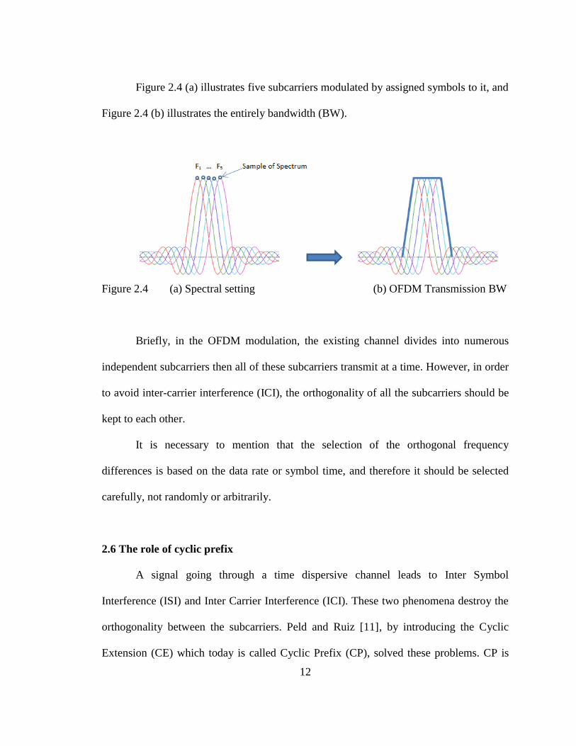
Figure 2.4 (a) illustrates five subcarriers modulated by assigned symbols to it, and

Figure 2.4 (b) illustrates the entirely bandwidth (BW).

Figure 2.4 (a) Spectral setting (b) OFDM Transmission BW

Briefly, in the OFDM modulation, the existing channel divides into numerous

independent subcarriers then all of these subcarriers transmit at a time. However, in order

to avoid inter-carrier interference (ICI), the orthogonality of all the subcarriers should be

kept to each other.

It is necessary to mention that the selection of the orthogonal frequency

differences is based on the data rate or symbol time, and therefore it should be selected

carefully, not randomly or arbitrarily.

2.6 The role of cyclic prefix

A signal going through a time dispersive channel leads to Inter Symbol

Interference (ISI) and Inter Carrier Interference (ICI). These two phenomena destroy the

orthogonality between the subcarriers. Peld and Ruiz [11], by introducing the Cyclic

Extension (CE) which today is called Cyclic Prefix (CP), solved these problems. CP is

13

actually a copy of the last samples from IFFT, which is placed in front of the symbol.

Figure 2.5 shows the use of CP. In Figure 2.5 is the length of the cyclic prefix and

is the length of the OFDM symbol and .

Figure 2.5 Cyclic Prefix (CP)

To escape Inter-Symbol Interference (ISI) and Inter Carrier Interference (ICI), the

length of the CP must be as long as the noteworthy part of the impulse response. If the

Cyclic Prefix is shorter than the impulse response, the convolution is not going to be

circular. This leads to the creation of ISI. On the other hand, since CP does not carry any

useful data, the transmission rate will be reduced by increasing the number of samples in

CP.

It is important to note that the transmitted energy will be amplified with the length

of the CP. However, the insertion of the Cyclic Prefix causes the loss of Signal to Noise

Ratio (SNR) which is stated as follows:

(

) (2.1)

14

On the other hand, inserting the CP leads to the decrease of the number of

symbols which are transmitted per second. Therefore, the length of the CP should not be

longer than necessary.

2.7 The effect of subcarriers and Guard Band on system performance

The result of increasing the number of Subcarriers (SCs) and Guard Band (GB)

can be pointed out as follows:

- Increasing the number of SCs can lead to the increase of the power efficiency

but it can make the system be more sensitive to the Doppler spread.

- Increasing the number of SCs and increasing the bandwidth can lead to the

reduction of the Inter Symbol Interference (ISI) but at the cost of reducing the bandwidth

(BW) efficiency and power efficiency.

2.8 Modulation

Modulation can be accomplished by changing the amplitude, frequency and phase

of the sinusoidal carrier. In general there are two different modulation methods: coherent

and non-coherent modulation. The coherent modulation techniques use the reference

phase between the transmitter and receiver which results in a precise demodulation on the

receiver side. The non-coherent modulation is used in low data rate systems like Digital

Audio Broadcasting (DAB). Generally in case of the lack of knowledge of the carrier

phase, the non-coherent is more useful. Since it does not need carrier or phase tracking

and channel estimation, the structure of the receiver will be simpler.

15

2.8.1 Coherent Modulation for OFDM systems

The suitable coherent modulation methods for OFDM systems are: Amplitude

Shift Keying (ASK), Phase Shift Keying (PSK), and Quadrature Amplitude Modulation

(QAM). Since each of these methods can be represented as an M-ary modulation

schemas, we have M-ary ASK, M-ary PSK and M-ary QAM.

2.8.2 M-ary Amplitude Shift Keying (MASK/M-ary ASK)

In this modulation the information will be carried in amplitude. So if we assume a

set of { }, the signal can be stated as:

(2.2)

The 2-ASK which is called BPSK is one of the common modulation schemas that

has been generally used. The constellation points are located in √ ⁄ and √ ⁄ (E

is signal energy per symbol.)

2.8.3 M-ary Phase Shift Keying (MPSK/M-ary PSK)

In this modulation the phase is shifted for different constellation. In this case there

is M possible signals which have ⁄ where each signal is given as:

√

(

) (2.3)

It is necessary to mention that 2-PSK is the same BPSK.

16

2.8.4 M-ary Quadrature Amplitude Modulation (MQAM/M-ary QAM)

This modulation is a combination of amplitude and phase modulation. The M

signals can be given as follows:

√

√

(2.4)

Where { } is the element of an matrix, this matrix can be stated as [12]:

[

] (2.5)

For , it is as 4-PSK, which is called Quadrature PSK (QPSK).

2.9 The advantages and disadvantages of OFDM

OFDM has become one of the most exciting developments in the area of modern

broadband wireless networks. During recent years, the applications of OFDM, principally

in digital communication systems such as Digital Audio Broadcasting (DAB), Digital

Video Broadcasting (DVB) and Digital Mobile Broadcasting (DMB) have highlighted

some of the important and key advantages of OFDM.

These advantages can be summarized as follows:

17

Since narrowband interference hits only a small portion of the Subcarriers (SCs),

it is considered to be robust against narrowband;

For dealing with multipath, OFDM is the best and more efficient method;

OFDM makes the single frequency network possible;

Using OFDM leads to the deletion of the need of the high complexity receiver,

making it possible to use the low complexity receiver;

OFDM has a high resistance against selective fading and interference.

Some of the disadvantages of OFDM are:

Sensitivity to frequency offset and phase noise;

Having high Peak to Average Power Ratio (PAPR).

2.10 Challenges in the OFDM wireless systems

The OFDM systems are very sensitive to the frequency offset because it can cause

the Inter Carrier Interference (ICI). This can lead to the frequency mismatched in

transmitter and receiver oscillator. Timing and frequency offsets are the origin of the

interference of sub-channels with each other. Since OFDM wireless systems are very

sensitive to the CFO, it can severely degrade the performance of the OFDM wireless

systems. Therefore it has been recognized as one of the most major drawbacks in OFDM

wireless systems. On the other hand, OFDM consists of multiple sinusoids summed

together which it can create a huge Peak-to-Average Power Ratio (PAPR). High PAPR

has been named as the other drawback of the OFDM modulation format. In RF systems,

the major problem resides in the power amplifiers (PA) at the transmitter end, where the

18

amplifier gain will saturate at high input power. High PAPR is not a trivial issue for

OFDM systems because it decreases the efficiency of the power amplifier (PA). Low

efficiency of the power amplifier is a problem, especially in small mobile devices on the

uplink [13].

In short, two important issues for OFDM challenges are:

1. Carrier Frequency Offset (CFO);

2. Peak-to-Average Power Ratio (PAPR).

2.11 Path losses and fading in OFDM systems

The first obvious difference between the wired and wireless channel is the amount

of transmitted power that actually reaches the receiver. Path loss can be caused by many

different effects, such as free space loss, refraction, diffraction, environment, weather

condition, and the distance between transmitter and receiver.

In wireless communication, due to the mobility of the user, the transmission

medium can vary with time. At times, the variation of the transmission medium can be

huge. On the other hand, the signal that the receiver gets from the transmitter can come

via a number of different propagation paths. This phenomenon can cause fading.

The model for predicting the signal strength that a receiver receives is usually

based on the Free Space Propagation (FSP) model. In this model, there is no attenuation

between the signal that the transmitter sends and the signal that the receiver receives, and

there in no obstacle between them. This means the sending and receiving is based on the

Line Of Sight (LOS).

19

In a real environment, the Radio Frequency waves (RF) are basically affected by

three different phenomena: reflection, scattering and diffraction. Fading is another

phenomenon that causes the change of the amplitude of the signal over time and

frequency. There are two kinds of Fading: shadow fading and multipath induced fading.

Shadow fading is produced by an obstacle that affects the propagation of the RF wave

and the multipath induced fading. As is obvious from its name, it is created by the

multipath propagation. Fading phenomena, unlike the additive noise, is considered as a

non-additive degradation. The following figures 2.6 (a), 2.6 (b) and 2.6 (c) illustrate the

transmission and receiving of the OFDM signal without considering the effect of noise,

path loss and fading.

Figure 2.6 (a) OFDM Signal

20

Figure 2.6 (b) Transmitted Data

Figure 2.6 (c) Received Data

21

The table 2.1 shows the path loss exponent.

Environment Path loss exponent

Free space 2 2

Urban area cellular radio 2.7–3.5

Shadowed urban cellular radio 3–5

In building line-of-sight 1.6–1.8

Obstructed in building 4–6

Obstructed in factories 2–3

Table 2.1 Path Loss Exponent [14]

So many factors can have effect on the total received power. These factors can

assign the allowable transmit power. In this part we will study these factors in details, and

we will show how these factors should be modeled simply based on the path loss and the

distance between the transmitter and receiver.

2.12 Choice of OFDM parameters

The most important parameters that should be considered in any OFDM design

are guard time, symbol duration, the number of the subcarriers, subcarrier spacing, and

type of the modulation. However, what dictates and assigns the selection of the

parameters are the system requirements. Some of the common system requirements are

desired bit rate, available bandwidth (BW), Doppler values and acceptable delay spread.

It is necessary to mention that some of these requirements can conflict with each other.

For example, if we want to have a good delay spread tolerance, we should select a huge

22

number of the subcarrier with the slight subcarrier spacing. But for a good tolerance

against the phase noise, the opposite is true. Therefore, there are different parameters for

OFDM systems, and selecting always leads to a tradeoff between them. Basically the

three main ones that should be considered are bit rate, bandwidth (BW), and delay

spread. Since the guard time must be two to four times the Root Mean Squared of the

Delay Spread (RMSDS) among the mentioned parameters, the delay spread is the one

that assigns the guard time. This value is related to the type of coding and modulation. It

is noteworthy that the higher order of the QAM (i.e. 64-QAM) compared with QPSK has

a higher degree of sensitivity to the ICI and ISI. The other prerequisite which has a direct

impact on the selection of the parameters is the desired integer number of samples within

the FFT/IFFT interval and the symbol interval. The accepted OFDM time related and rate

related parameters in IEEE 802.11 are respectively listed in tables 2.2 and 2.3.

Parameters Values

Number of data sub-carriers 48

Number of pilot sub-carriers 4

Total number of sub-carriers 52

Sub-carrier frequency spacing 0.3125 MHz

IFFT/FFT period 3.2μs (1/ΔF)

Preamble duration 16μs

Signal duration BPSK-OFDM symbol 4μs (TGI+TFFT)

Guard Interval (GI) duration 0.8μs (TFFT/4)

Training symbol GI duration 1.6μs (TFFT/2)

Symbol interval 4μs (TGI+TFFT)

Short training sequence duration 8μs (10TFFT/4)

Long training sequence duration 8μs (TGI+TFFT)

Table 2.2: The timing related parameters for the OFDM systems [15]

23

Modulation Coding

rate

(R)

Coded

bits per

subcarrie

r (NBPSC)

Coded bits

per OFDM

symbol

(NCBPS)

Data

bits per

OFDM

symbol

(NDBPS)

Data rate

(Mb/s)

(20 MHz

channel

spacing)

Data rate

(Mb/s)

(10 MHz

channel

spacing)

Data rate

(Mb/s)

(5 MHz

channel

spacing

BPSK 1/2 1 48 24 6 3 1.5

BPSK 3/4 1 48 36 9 4.5 2.25

QPSK 1/2 2 96 48 12 6 3

QPSK 3/4 2 96 72 18 9 4.5

16-QAM 1/2 4 192 96 24 12 6

16-QAM 3/4 4 192 144 36 18 9

64-QAM 1/2 6 288 192 48 24 12

64-QAM 3/4 6 288 216 54 27 13.5

Table 2.3: The rate dependent parameters for the OFDM systems [15]

As you see in table 2.3 the data rate has different values. These values vary

according to the type of the modulation. For OFDM-AWGN (OFDM-Additive White

Gaussian Noise), the performance of the data rate comparison for the different schemes in

IEEE 802.11 is illustrated in figure 2.7. The theoretical values can be calculated as

follows:

(2.6)

√ ⁄ (2.7)

Here is signal bandwidth. (BW), is symbol length, is data rate and is

guard interval length. The data rate varies according to the type of the modulation and has

a different value for BPSK, QPSK, 16QAM, and 64QAM.

24

Figure 2.7 Data rates comparison

2.18 A typical schematic of an OFDM transceiver

Figure 2.8 shows a typical schematic diagram of an OFDM transceiver system.

The IFFT unit modulates a block of input values to a number of subcarriers. On the

receiver side, these subcarriers will be demodulated by the FFT unit which actually is the

reverse operation of what is done in IFFT unit. Since these two operations are practically

identical, the IFFT can be created by conjugating the input and output of an FFT and then

dividing the output by the FFT size.

25

Figure 2.8 A typical schematic diagram of an OFDM transceiver system

2.19 Proprietary OFDM Flavors

At the end of this brief discussion about OFDM, it is worth mentioning that there

are four variants of OFDM. These four variants are:

1. Vector OFDM (VOFDM)

2. Wideband OFDM (WOFDM)

3. Adaptive OFDM (AOFDM)

4. Flash OFDM

It is necessary to be mentioned that with regard to the simulation requirements

and the comparison of the different algorithms or methods and suggested algorithm

and method, the components of each block might be changed or modified related to

the discussed model in the related section.

26

Chapter 3

Carrier Frequency Offset (CFO)

3.1 Introduction

The orthogonality of the OFDM relies on the condition that the transmitter and

receiver operate with exactly the same frequency reference. If this is not the case, the

perfect orthogonality of the subcarrier will be lost, which can result to subcarrier leakage.

This phenomenon is also known as the Inter Carrier Interference (ICI) [16]. In other

words, the OFDM systems are sensitive to the frequency synchronization errors in the

form of CFO. CFO can lead to the Inter Carrier Interference (ICI). Therefore, CFO plays

a key role in frequency synchronization. Basically to get a good performance of OFDM,

the CFO should be estimated and compensated.

Lack of the synchronization of the local oscillator signal (L.OSC), for down

conversion in the receiver with the carrier signal contained in the received signal, causes

Carrier Frequency Offset (CFO) which can create the following factors:

(i) Frequency mismatched in the transmitter and the receiver oscillator;

(ii) Inter Carrier Interference (ICI);

(iii) Doppler Effect (DE).

27

3.2 Effects of frequency offset on OFDM signals

When CFO happens, it causes the receiver signal to be shifted in frequency (δf).

This is illustrated in the figure 3.1. If the frequency error is an integer multiple of

subcarrier spacing δf, then the received frequency domain subcarriers are shifted by

[17].

Figure 3.1 Illustration of frequency offset (δf)

On the other hand, as we know the subcarriers (SCs) will sample at their peak,

and this can only occur when there is no frequency offset. However, if there is any

frequency offset, the sampling will be done at the offset point which is not the peak point.

This causes a reduction of the amplitude of the anticipated subcarriers, which can result

in the rise of the Inter Carrier Interference (ICI) from the adjacent subcarriers (SCs).

Figure 3.2 [18] shows the impact of carrier frequency offset (CFO). It is necessary to

mention that although it is true that the frequency errors typically arise from a mismatch

between the reference frequencies of the transmitter and the receiver local oscillators, this

difference is avoidable due to the tolerance that electronics elements have.

28

Figure 3.2 Frequency offset

Therefore, there is always a difference between the carrier frequencies that is

generated in the receiver with the one that is generated in transmitter; this difference is

called frequency offset and is:

(3.1)

where is the carrier frequency in the transmitter and is the carrier frequency in

receiver.

3.3 Carrier Frequency Offset (CFO)

The OFDM systems are very sensitive to the carrier frequency offset (CFO) and

timing. Therefore, before demodulating the OFDM signals at the receiver side, the

receiver must be synchronized to the time frame and to the carrier frequency which has

been transmitted. In order to help the synchronization, the signals that are transmitted

29

have the references parameters that are used in the receiver for synchronization.

However, in order for the receiver to be synchronized with the transmitter, it needs to

know two important factors:

(i) prior to the FFT process, where it should start sampling the incoming

OFDM symbol from;

(ii) how to estimate and correct any carrier frequency offset (CFO).

After estimating the symbol boundaries in the receiver and detecting if the symbol

is present, the next step is to estimate the frequency offset.

The block diagram of the OFDM transceiver system, including the modulation,

digital-to-analog (D/A) converter, channel and noise, the analog-to-digital (A/D)

converter, and the demodulation, is illustrated in figure 3.3 [19].

Figure 3.3 Block diagram of the OFDM transceiver system

30

A received signal without carrier frequency offset can be considered as follows:

[ ] [ ] [ ] (3.2)

Eq. 3.2 can be considered if and only if the effect of CFO is ignored. In the

presence of the CFO the received signal can be stated as [20]:

[ ] [ ]

(3.3)

∑ [ ] [ ]

[ ]

]

[ ]

In Eq. 3.3, is the normalized frequency offset. Part two in Eq. 3.3 is the result of

the effect of ICI due to the presence of the frequency offset. As can be observed from Eq.

3.3, the CFO causes the amplitude of the signal to be degraded by the following factor:

(3.4)

According to Eq. 3.3, the shift that the received signal experiences is equal to:

⁄ (3.5)

As we know, the normalized (ɛ) CFO has two parts: integer part ( ), and

fractional par ( ). Therefore, it can be stated as:

(3.6)

The integer part leads to the cyclic shift in the received signal, but the fractional

part has the effect of phase distortion and amplitude of the received signal. Figure 3.4

31

[19] illustrates a typical block diagram of the OFDM system with the fractional

frequency offset estimation, and integer frequency offset estimation for estimating and

compensating for the effect of CFO in the receiver.

Figure 3.4 Structure of an OFDM system with the required units for estimating and

compensating CFO

Figure 3.5 [18], shows the block diagram of the OFDM wireless transceiver

system, and the output of the FFT at the receiver. In figure 3.5, [ ] is as follows [21]:

Figure 3.5 Block diagram of the OFDM wireless transceiver system

32

[ ]

∑ [ ] [ ]

( )

(

)

( (

) ) (3.7)

(3.8)

[ ]

[ ] [ ]

(

(

⁄ ))

(

)

∑ [ ] [ ]

[

(

) ( (

)

)]

For simplicity, set equal to:

[

(

) ( (

) )]

[

(

) ( (

) )] (3.9)

Therefore

[ ]

[ ] [ ] (

(

⁄ )) (

)

∑ [ ] [ ]

(3.10)

33

The result in Eq. 3.10 indicates, in the case of the existence of any frequency

offset, the estimation of the output symbol depends on the input values.

On the other hand, if there is no frequency offset, i.e. , then the received

signal is:

[ ]

[ ] [ ] (3.11)

Due to the frequency mismatch, the performance of an OFDM system can be

reduced. This loss of performance can be compensated by estimating the frequency offset

on the receiver side. Figure 3.6 [18] shows an OFDM Receiver with frequency

synchronization.

Figure 3.6 OFDM receiver with frequency synchronization

Table 3.1 [18] is a cliff notes for the effect of CFO on a transmitted signal in time

domain and frequency domain.

34

Received signal Effect of CFO on received signal

Time domain [ ] [ ]

Frequency domain [ ] [ ]

Table 3.1 Effect of the CFO on transmitted signal

3.4 Sources of frequency offset

A few sources can cause frequency offset, such as frequency drifts in transmitter

and receiver oscillators, Doppler shift, radio propagation, and the tolerance that

electronics elements have in local oscillators in the transmitter and the receiver. When

there is a relative motion between transmitter and receiver, the Doppler can happen [22].

It is worth mentioning that the radio propagation talks about the behavior of radio waves

when they are broadcasted from transmitter to receiver. In terms of propagation, the radio

waves are generally affected by three phenomena which are diffraction, scattering and

reflection.

3.5 Doppler Effect

The Doppler Effect (DE) is defined as follows:

(3.12)

Here fd is Doppler Frequency, c is the speed of light, and v is the velocity of the

moving receiver. The normalized CFO can be stated as:

(3.13)

35

Where is the subcarrier spacing, ɛ has two parts, one integer ( ) and one

fractional ( ). So we have:

(3.14)

where ⌊ ⌋

3.6 The effect of integer and fractional part of CFO

As previously mentioned, the normalized CFO has made of two parts: integer part

, and fractional part . The integer part causes the received signal to the receiver to

experience a cyclic shift. The effect of the fractional part is as follows. The received

signal in time domain can be considered [23]:

[ ] ∑ [ ] ⁄

[ ] [ ] [ ] (3.15)

Here, [ ], [ ], [ ]and [ ] represent the received symbol, channel frequency

response, transmitted symbol, and the noise in the frequency domain for the kth

subcarrier.

{ [ ]} [ ]

∑ [ ] [ ]

⁄ [ ] (3.16)

Here, [ ] { [ ]}.

To see the effect of the CFO, we discard the phase noise and merely consider the

CFO [24]. Therefore, Eq. 3.16 can be written as:

36

[ ]

∑ [ ] [ ]

⁄ [ ] (3.17)

The FFT of Eq. 3.17 yields [23]:

[ ] { } (3.18)

[ ]

( ⁄ ) ⁄ [ ] [ ] [ ] [ ] (3.19)

The first part of Eq. 3.19 shows the effect of the fractional part of the CFO.

Figures 3.7 and 3.8 [25] show its effect. However, as expected, by growing the fractional

part of the CFO, the effect increases on phase distortion and amplitude. This can be seen

in figures 3.7 and 3.8. In these figures the effect of noise and Symbol Time Offset (STO)

are not reflected at all.

Figure 3.7 Effect of CFO when

37

Figure 3.8 Effect of CFO when

3.7 Effect of CFO on phase shift

To see the effect of CFO on phase shift, we consider there is no phase noise.

Therefore, the time domain received signal considering Eq. 3.17 can be considered as

follows:

[ ]

∑ [ ] [ ]

⁄ [ ] (3.20)

Figure 3.9 [25] illustrates the effect of CFO on the phase in the time domain and

Figure 3.10 [25] presents the phase change between them. Here we consider that the

system is not exposed to any noise. The solid line in Figure 3.9 shows when there is no

CFO (i.e. perfect case), and dash lines show when the amount of the CFO in the system is

equal to 1.4.

38

Figure 3.9 Effect of CFO (ξ) on phase in the time domain

Figure 3.10 Effect of CFO (ξ) on phase difference

39

3.8 Effect of CFO on degradation of OFDM systems

The complex transmitted OFDM signal in a period T at the frequency m/T can be

stated as [26]:

(∑

) (3.21)

in which is data symbol and the term represents the time varying phase due to

the carrier frequency offset between the transmitter and receiver.

With a reasonable approximation, the degradation in terms of dB is defined as

[26]:

((

)

) (3.22)

in which the signal to noise ratio (SNR) is: ⁄ , is the variance for others noises,

and is the power of the component.

In case of the presence of frequency offset between the transmitter and

receiver, the in Eq. 3.21 is defined as:

(3.23)

Therefore, the degradation (D) for OFDM is defined as [26]:

(

)

(3.24)

From Eq. (7) it can be observed that the degradation for an OFDM is proportional

with the square root of the frequency offset and it is also proportional with ⁄ . In

40

other words, OFDM is very sensitive to frequency offset and frequency offset can cause

severe degradation in OFDM systems.

Figure 3.11 [19] illustrates the SNR degradation as a function of the frequency

offset to the subcarrier spacing. For this illustration, the values for ⁄ will be 18 and

16 db. However, the maximum acceptable frequency offset can only happen when the

frequency offset is less than one percent of the subcarrier space. As a result, for

overcoming the mentioned problem, the frequency synchronization must be used before

the FFT.

Figure 3.11 SNR degradation as a function of the frequency offset

0 0.05 0.1 0.15 0.2 0.25 0.3 0.35 0.4 0.45 0.510

-15

10-14

10-13

10-12

10-11

10-10

10-9

10-8

Frequency Offset (%)

Deg

rad

ati

on

of

SN

R (

dB

)

18 db

16 db

41

3.9 The effect of CFO, phase noise, and Rayleigh fading

As previously mentioned, two key parameters that should be considered in

designing any OFDM communication system are CFO and phase noise. In this part we

show the effect of CFO, phase noise, and Rayleigh fading on the performance of the

OFDM wireless systems.

The effect of CFO with the phase noise, Rayleigh fading and time jitter on the

performance of the OFDM wireless systems can be stated as follows [27,28]:

(3.25)

{ }

[ {

∑

( )

}]

| | | |

where:

Normalized CFO

Input SNR (Signal-to-Noise-Ratio)

Time jitter

Variance of the noise phase

Rayleigh fading

Number of subcarriers

In the case of the absence of time jitter and assuming a nonfading environment

(i.e. α=1), Eq. 3.25 will be as follows:

42

{ }

[ {

∑

}]

| | (3.26)

Figures 3.25 and 3.13 illustrate the effect of SINR VS the CFO, considering the

different values of the SNR.

In figures 3.12 and 3.13 the variance of phase noise is respectively equal to 0.018

and 1.25. As can be seen in figures 3.12 and 3.13, by increasing the value of the variance

of phase noise, the amount of SINR reduces. Figures 3.12 and 3.13 also display that the

value of SINR will also be decreased by growing the SNR.

Figure 3.12 Signal-to-Interference-plus-Noise-Ratio (SINR)

43

Figure 3.13 Signal-to-Interference-plus-Noise-Ratio (SINR)

3.10 The relation between frequency offset and SNR

The effect of CFO on Signal-to-Noise Ratio (SNR) in OFDM systems was studied

by Pollet et al. [29]. The impact of the CFO on the degradation in terms of dB is given by

[30]:

(3.27)

are frequency offset, symbol duration, energy per bit (for

OFDM signal), and one sided noise power spectrum density (PSD).

The effect of frequency offset is similar to the effect of noise and it may cause

degradation of the Signal-to-Noise Ratio (SNR) where SNR is:

(3.28)

44

Figure 3.14 [19] illustrates the impact of the sampling offset on the degradation of

SNR. As Figure 3.14 shows, by increasing the number of subcarriers, the degradation of

OFDM increases.

Figure 3.14 SNR degradation versus sampling offset

3.11 Frequency synchronization

The frequency synchronization for OFDM systems can be classified by two

methods: data aided and non-data aided. While the data aided uses the pilot symbols for

estimation, the non-data aided uses a Cyclic Prefix (CP) correction.

In wireless OFDM systems, synchronization is the most important issue. In order

for the receiver to regenerate the signal that the transmitter sends, it must be synchronized

in frequency, time, and phase with the transmitter. Since the mobile OFDM systems work

45

in a dynamic environment, this is not an easy case. However, in the OFDM wireless

systems, two reasons that lead to frequency offset between the receiver and the

transmitter are:

(i) sampling clock mismatch

(ii) misalignment

3.12 Sampling clock mismatch

The Analog-to-Digital (A/D) on the receiver side is responsible for determining

the sampling time. A/D does not have always the exact sampling clock. This can cause a

relative drift between the receiver’s sampling in respect to the transmitter. This drift,

called Sampling Clock Drift (SCD) (or sampling clock error), reduces the OFDM system

performance. The SCE produces the rotation of subcarriers which leads to ICI and finally

destroys the orthogonality between the subcarriers. Many researchers have discussed and

evaluated the effect of SCD on OFDM wireless systems [31]. The normalized sampling

error can be stated as follows:

(3.29)

where, is the received sampling period and is the transmit sampling period. The

total effect can be shown as [32]:

[

]

(3.30)

Here is the received subcarrier, are OFDM symbol index and

subcarrier index, is Additive White Gaussian Noise (AWGN), is total symbol

duration, is useful sample duration, and is additional interference because of the

46

sampling frequency offset. The degradation of OFDM systems, due to this effect, can be

given by [33]:

[

] (3.31)

As it can be seen from Eq. 3.31, the degradation performance of OFDM wireless

systems increase by the square power of the frequency offset.

3.13 The effect of STO on OFDM Synchronization

The effect of the STO depends to the estimated starting point of the OFDM

symbol. Three main possibilities can be considered as follows: the estimated starting

point of the OFDM symbols can occur at the exact timing point, before the exact timing

point, and after the exact timing point. In the first situation, the OFDM symbols will be

recovered and there will be no type of the interference. In the second situation, the

orthogonality among the subcarrier will be well-preserved but a phase offset will be

introduced which will be proportional to the STO. In the third situation, the signal will

contain a portion of the current and a portion of the next OFDM symbol. Therefore, the

received signal contains the ISI which is caused by the next symbol, and the

orthogonality between the subcarriers will be destroyed. By taking the FFT of the signal

which is the combination of the current and the next OFDM symbol we have:

∑ ⁄ ∑

⁄

(3.32)

where and are the normalized STO and CFO.

47

After extending and simplifying Eq. 3.32, the following terms appears in it, which

relates to the presence of the ICI and indicate the lack of orthogonality:

∑ ⁄ ∑

(3.33)

When the extreme delay of the multipath channel is longer than the length of the

Cyclic Prefix (CP), the end portion of the OFDM symbol will affect the head portion of

the following symbol. This effect appears as the Inter-Symbol Interference (ISI). The

other factor that has effect on creating the ISI and ICI is the timing of the FFT window

start point, even though the length of the CP will be enough long. Note that when the FFT

window start point is later than the start of the symbol, both ISI and ICI will be occur.

3.14 The effect of ISI on OFDM systems

The signals that arrive to the receiver come from the different paths. Therefore,

there is a time delay between the signals which can cause inter-symbol interference (ISI).

ISI causes the degradation of performance in the reception of the receiver. Consider the

output of the modulator unit in the transmitter as:

∑ [∑ ]

(3.34)

Respectively are: symbol duration, data symbol and block size, and

is kth subcarrier frequency where

and

{ [ ]

(3.35)

48

Eq. 3.34 can be stated as follows:

∑ (3.36)

The transmitted signal can be stated as:

∑[∑ ] (3.37)

L is the data symbol length.

The received OFDM signal considering the AWGN and multipath condition can

be presented as follows [34]:

∑ ∑

(3.38)

If we consider Q=L-N and the length of the multipath channel ( ) to be as long

as the guard interval, Eq. 3.38 can be separated and stated in two time intervals as

follows:

(3.39)

{

∑

∑

∑

As it can be seen, the first interval has the ISI from the previous symbol and

desired symbol, but the next interval merely has the wanted data symbol. However, the

advantage of the OFDM wireless systems is their robustness against the multipath delay

spread. Decreasing the effect of ISI can be accomplished by using the long symbol

period.

49

3.15 Effect of CFO on creating ICI

As previously noted, the lack of orthogonality in the received signal to the OFDM

receiver creates carrier frequency offset. CFO introduces the ICI in the system. However,

Figure 3.15 [19] illustrates the ICI due to the frequency offset. Figure 3.15 was created

for different values of frequency offset. As it can be seen from figure 3.15, increasing the

frequency offsets the ICI increases.

Figure 3.15 The overall ICI created by frequency offset

3.16 The effect of Symbol and Sample Timing Offset

When the data blocks in the input of the FFT in receiver are exactly matched with

the ones from the transmitted IFFT block in transmitter, we can claim that we have

achieved a perfect synchronization. There is two kind of synchronization: late

synchronization, and early synchronization. If the synchronization tick comes after the

50

perfect synchronization point, it is called the late synchronization. This can destroy the

orthogonality of the subcarrier and cause ICI. By getting the Cyclic Prefix (CP) enough

long, we can eliminate the major effects of the early synchronization. It is worth

mentioning that we must avoid the late synchronization in all the cases. However, the late

synchronization can also cause a chunk of the channel response to fall out of the channel

estimation window, which can create an additional noise. Therefore, consider an Additive

White Gaussian Noise (AWGN) channel which the vector received signal can presented

as:

[ ] (3.40)

After the demodulation via FFT unit, it is [35]:

(3.41)

(

)

∑ ⁄

∑ ⁄

⁄

⁄

∑ ⁄

∑ ⁄

⁄

⁄

As it is obvious from Eq. 3.41, the symbol timing offset can create three effects:

ISI, ICI and phase rotation.

Carrier Frequency Offset (CFO) and Sampling clock Frequency Offset

(ScFO) cause the phase rotation in the received signals which can be stated as:

(

) (3.42)

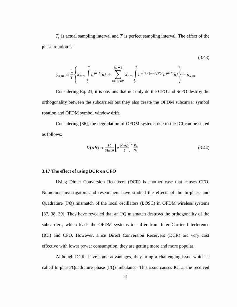
51

is actual sampling interval and is perfect sampling interval. The effect of the

phase rotation is:

(3.43)

{ ∫

∑

∫ ⁄

}

Considering Eq. 21, it is obvious that not only do the CFO and ScFO destroy the

orthogonality between the subcarriers but they also create the OFDM subcarrier symbol

rotation and OFDM symbol window drift.

Considering [36], the degradation of OFDM systems due to the ICI can be stated

as follows:

[

]

(3.44)

3.17 The effect of using DCR on CFO

Using Direct Conversion Receivers (DCR) is another case that causes CFO.

Numerous investigators and researchers have studied the effects of the In-phase and

Quadrature (I/Q) mismatch of the local oscillators (LOSC) in OFDM wireless systems

[37, 38, 39]. They have revealed that an I/Q mismatch destroys the orthogonality of the

subcarriers, which leads the OFDM systems to suffer from Inter Carrier Interference

(ICI) and CFO. However, since Direct Conversion Receivers (DCR) are very cost

effective with lower power consumption, they are getting more and more popular.

Although DCRs have some advantages, they bring a challenging issue which is

called In-phase/Quadrature phase (I/Q) imbalance. This issue causes ICI at the received

52

signals to lead to CFO. It is well known that OFDM systems are sensitive to CFO, and

many CFO and I/Q imbalance estimation and compensation methods and techniques have

been proposed. Some of these techniques assume a perfect timing synchronization, which

makes it very difficult to accomplish in practice. To show the impact of I/Q imbalance on

the received signal, consider Figure 3.16 [19] which shows the block diagram of the DCR

with I/Q and CFO compensation configuration.

Figure 3.16 Block diagram of the DCR with I/Q and CFO compensation configuration

The received RF signals to the DCR receiver antenna can be stated as [40]:

{[ ] } (3.45)

where , and in order are: baseband equivalent channel, baseband transmitted

signal, and carrier frequency. According to the [40], [41] and [42], the down converted

signal at the receiver side can be presented as:

53

{ [ ] { [ ]}

} (3.46)

In Eq. 3.46, you can see the presence of the frequency offset ( ) in the down

converted signal at the receiver side, which needs to be estimated and compensated.

3.18 The effect of increasing the range of CFO estimation

The algorithms that use CP for estimating CFO can only estimate the CFO in a

limited range. This limited range is:

(3.47)

To increase this limit, the distance between two blocks of samples for correction

need to be decreased by using a training symbol. To increase the CFO estimation within a

bigger range we can use Eq. 3.47 [43, 44].

{∑

[ ] [ ]⁄ ⁄ } (3.48)

where ⁄ is an integer. Here the range is:

(3.49)

The CFO estimation range by using Eq. 3.48 will be increased to | | .

However this increase costs in the degradation of the MSE performance. Figure 3.17 [25]

shows the effect of increasing the estimation range of CFO versus the MSE performance

for D=1 (red graph) and D=4 (black graph).

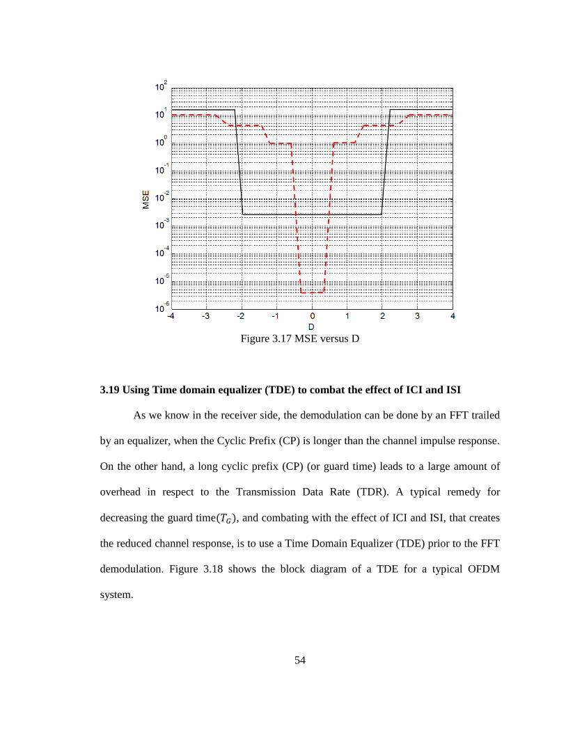
54

Figure 3.17 MSE versus D

3.19 Using Time domain equalizer (TDE) to combat the effect of ICI and ISI

As we know in the receiver side, the demodulation can be done by an FFT trailed

by an equalizer, when the Cyclic Prefix (CP) is longer than the channel impulse response.

On the other hand, a long cyclic prefix (CP) (or guard time) leads to a large amount of

overhead in respect to the Transmission Data Rate (TDR). A typical remedy for

decreasing the guard time , and combating with the effect of ICI and ISI, that creates

the reduced channel response, is to use a Time Domain Equalizer (TDE) prior to the FFT

demodulation. Figure 3.18 shows the block diagram of a TDE for a typical OFDM

system.

55

Figure 3.18 Block diagram of a TDE for a typical OFDM system

The matrix form for the figure 3.18 can be given as:

(3.50)

where W (which is a FFT Matrix ), X and h are as follows:

56

[

(

)

(

)

(

)

(

)

(

)

(

)

(

)

(

)

]

(3.51)

[

[ ] [ ] [ ] [ ]

[ ] [ ]

[ ] [ ] [ ]

]

(3.52)

{ [ ] [ ] [ ] [ ]} (3.53)

is the length of the cyclic prefix and S is the length of a symbol plus the cyclic prefix

and is:

(3.54)

The output of FFT is:

{ [ ] [ ] [ ] [ ]} (3.55)

57

3.20 Synchronization using the cyclic extension

One of the properties of the Cyclic Prefix/Cyclic Extension (CP/CE) is that the

first portion of every OFDM symbol is identical to the last part. This property can help us

to use the cyclic extension for synchronization issue not only for time synchronization

but also for frequency synchronization [45, 46]. Figure 3.19 illustrates the usage of the

cyclic prefix (CP) for synchronization.

∫

(3.56)

Figure 3.19 Cyclic prefix for synchronization

3.21 CFO estimation algorithm and Techniques

CFO can produce Inter Carrier Interference (ICI) which can be much worse than

the effect of noise on OFDM systems. That is why various CFO estimation and

compensation algorithms have been proposed.

58

Its importance is evidenced by the researchers who have proposed numerous and

various CFO estimation and compensation techniques and algorithms. These methods can

generally be categorized into two major branches:

1. Training based algorithm;

2. Blind algorithm and Semi-blind algorithm.

3.22 Training based algorithm

The training sequence can be designed in a way that can limit the number of

computations at the receiver side. Generally, these algorithms have a low computational

complexity. However, the negative point of the training based algorithm is that the

training sequences must be transmitted from the transmitter during its transmission. This

can cause a reduction of the effectiveness of the data throughput.

3.23 Blind and Semi-blind algorithms

Another algorithm that has been used is called the Blind CFO estimation

algorithm. In this algorithm, by using the statistical properties of the received signal, the

CFO will be estimated. Since the receiver does not have any knowledge of the signal that

the transmitter has been sending, the blind algorithm is considered to have a high

computational complexity. The high computational complexity is the disadvantage of

these algorithms. Compared with training based algorithm, blind algorithms have no need

to transmit the training sequences and, therefore, there is no training overhead for these

algorithms.

59

3.24 Study of the training based and blind algorithms

In this part, a few proposed training and Blind algorithms are discussed. For the

CFO estimation, Paul H. Moose [47] in his paper “The technique for OFMD frequency

offset correction” suggested a training based CFO estimation algorithm. His paper is

divided into two major sections. In the first section, he showed the effect of offset errors

on the signal to noise (SN). In the second part, he presented an algorithm to estimate the

offset, and use it to remove it prior to the demodulation. He presented the algorithm for

maximum likelihood estimate (MLE) of frequency offset using the values of a repeated

data symbol. In this algorithm, two repetitive OFDM symbols are sent. This algorithm

works on the base of knowing the start point of the OFDM symbol. In this paper, the

maximum likelihood estimate (MLE) of CFO is defined as follows [47]:

{ ∑ [

] ∑ [

]} (3.57)

where: is the maximum likelihood estimate (MLE) for CFO, is the imaginary part,

Re is the real part and * means the complex conjugate. In this estimation the mean square

error is:

[ ]

(3.58)

where is the ratio of the signal to noise for the received signals, and N is the number of

subcarriers (SCs).

60

According to the paper, the limit of accurate estimation (for acquisition range) for

this algorithm is | | ⇒ . Therefore, the

acquisition range for subcarrier spacing is between -0.5 and 0.5, which is smaller than the

value that is in the IEEE 802.11a. When the acquisition range goes towards the 0.5,

may jump to -0.5 due to the noise and the discontinuity of the arctangent. When this

occurs, the estimate is no longer unbiased and, in practice, it becomes useless. This

estimation for the small values of CFO is conditionally unbiased. However, the big

weakness of the suggested algorithm in Moose’s paper is its dependency to the starting

point. Therefore, the algorithm needs to know the start point of the OFDM symbol.

For the CFO estimation, and in order to overcome the weakness in Moose’s

algorithm, Timothy M. Schmidl and Donald C. Cox, in their paper “Robust Frequency

and Timing Synchronization for OFDM [48]” suggest the time domain OFDM system

based on the two identical halves in order to solve the problem of determining the starting

point of the OFDM symbol,. In this method, finding the symbol timing for OFDM means

finding an estimate of where the symbol starts. Figure 3.20, shows an example of the

timing metric as a window slides past coincidence for the Additive White Gaussian Noise

(AWGN) channel for an OFDM signal with 1000 subcarriers, a carrier frequency offset

of 12.4 subcarrier spacing, and an signal-to-noise ratio (SNR) of 10 dB Here the SNR is

the total signal (of all the subcarriers) to noise power ratio.

61

Figure 3.20 Example of the timing metric for the AWGN channel

(SNR = 10dB) [48]

As it is shown, the timing metric reaches a plateau. Since there is no Inter Symbol

Interference (ISI) within this plateau to distort the signal, the starting point of OFDM can

be chosen at any spot on this plateau. The timing metric is defined as follows [48]:

| |

(3.59)

where

∑

(3.60)

and

∑ | | (3.61)

62

As you see, the is an auto correlation function and is a normalized

constant. In this estimation, the mean square error is:

[ ]

(3.62)

The Mean Square Errors (MSE) in both methods (Moose and Timothy) are near

and similar to each other.

By comparing the Moose’s method and Timothy’s method, we can tell that the

advantage of Timothy’s method is its simplicity. Plus it is not dependent upon the starting

point. In Moose’ method, the frequency synchronization is done in frequency domain.

But in the Timothy’s method, the frequency synchronization is achieved in time domain

in which the complexity of Fast Fourier Transform (FFT) in time domain is much less

than in frequency domain. It should be noted that both of these methods use the periodic

training sequence; one in frequency domain and the other in time domain. It is necessary

to mention that the time domain periodic training sequences are the ones that have been

accepted in various wireless standards. However, there are some limitations for CFO

estimation in these methods for SISO-OFDM.

A semi-blind method was proposed for simultaneously estimating the carrier

frequency offsets (CFOs) and channels of an uplink for MIMO-OFDM system by

Yonghong Zeng, A. Rahim Leyman, and Tung-Sang Ng [49]. In this method, a pilot

OFDM block for each user is exploited for resolving the CFOs and the ambiguity matrix.

Two dedicated pilot designs, periodical and consecutive, had been discussed. Based on

63

each pilot design and the estimated shaped channels, two methods were proposed to

estimate the CFOs. The algorithm that is used in this method can be summarized as

follows [49]:

1. Computing

2. Finding orthogonal eigenvectors of matrix

3. Finding the eigenvalue decomposition (EVD)

After finding the CFOs, the ambiguity matrix obtains. In this method, when the

CFOs have been estimated at the base station, recovery of the signal is still a problem

[49]. However the complex steps that follow them in semi-blind algorithms make its

implementation difficult. Basically, the computational complexity of this algorithm is too

high for practical implementation.

Other groups of algorithms, which are called Semi-blind algorithms, are proposed

to estimate multiple CFO values. These algorithms have pros and cons. However, most of

the proposed algorithms have computational a complexity which make their

implementation difficult and their complexity grows nonlinearly. On the other hand, by

using the MIMO instead of SISO, the other requirements, both in transmitter side and

receiver side, such as multiple clock signals (distributed or centralized clock signal) come

into the boarding table.

3.25 Reviewing the Pilot based and Non-pilot base estimation

Generally speaking, CFO estimation and compensation approaches can be divided

into two main approaches: Pilot Based Estimation (PBE) and Non-Pilot Based Estimation

64

(NPBE); NPBE is also called blind estimation. Although many good blind estimation

algorithms have been proposed, but it is worth mentioning that the main advantage of the

PBE method over NPBE is its accuracy and reliability.

3.26 Model for CFO

Figure 3.21 illustrates the block diagram of the OFDM wireless transceiver

system. Consider this figure with N subcarriers with the sampling rate ⁄ . Therefore,

we have:

(3.63)

[ ] (3.64)

(3.65)

where

[

] (3.66)

After DFT unit, we have:

[ ]

(3.67)

(3.68)

( ) (3.69)

where is carrier offset matrix, is a matrix, is data, is channel

response, and L is length of cyclic prefix.

65

(3.70)

Here the CFO and need to be estimated and applied.

Figure 3.21 A typical block diagram for wireless OFDM system

3.27 Pilot based and Non-pilot base estimation

In pilot based estimation which involves at least one pilot symbol, the receiver

signal can be stated as:

(3.71)

The Maximum Likelihood Estimate (MLE) for and is as follows:

( ) ‖ ‖ (3.72)

66

Considering the fact that most of the time during the tracking ICI the residual

carrier offset is small. So we can assume that the ICI can be considered as an additional

Gaussian noise. Therefore, Eq. 3.68 can approximately be stated as:

( ) (3.73)

where , consider not only the ICI but also noise. Add , which corresponds to pilot

locations, so we can state:

⁄

⁄

(3.74)

where

The non-pilot methodology does not use reference symbols to estimating CFO. In

this method, on the base of the structure and statistical data of the received signals, the

Frequency Offset (FO) will be estimated.

3.28 Blind CFO estimation technique using SPRIT-Like Algorithm

This algorithm uses the shift invariant structure available in the signal subspace of

the cissoids to estimate the desired parameters for generalizing the eigenvalues

calculation [50]. The kth

block of a sample received signal block minus the prefix is

stated as:

[ ] (3.75)

Considering Eq. 3.75, the consecutive samples in forward and backward

directions can be expressed as:

67

[ ]

(3.76)

[ ] (3.77)

where

The operate H in [ ] means the conjugate is transposed. Considering that, the N-

point received signal can be stated as:

(3.78)

As the definition, , therefore and

( ) (3.79)

it can be shown that:

(3.80)

where

( ) (3.81)

the diagonal matrix is:

(3.82)

In the same way, backward vector can be stated as follows:

68

[

] (3.83)

[

]

(3.84)

The operate H in [ ] means the complex conjugate. By assuming

, the covariance matrix can be given as follows:

∑ ∑ [

]

(3.85)

[ ]

Now by using the Spectral Value Decomposition (SVD), the eigenvectors of

can be found and the eigenvalues of the diagonal matrix can be presented as

follows:

( ) (3.86)

However the Carrier Frequency Offset in this algorithm can be found from:

∑

⁄ (3.87)

where the CFO can be computed as follows:

(

∑

) (3.88)

69

Although this algorithm is considered as having a good performance, the selection

of has a key role for having the eigenvectors of . However, comparing

MUSIC-like searching method, this method is better.

3.29 Blind CFO estimation technique using MUSIC Algorithm

This algorithm uses the known structure of the subspace of the OFDM signals. In

brief, the MUSIC algorithm, by using the receiver outputs, constructs polynomial costs

function as follows [51]:

∑ ∑ ‖ ‖

∑ ∑

(3.89)

Here . But, if there are several virtual carriers, we can select

in order to decrease the computational complexity. On the other hand, if , then

will be equal to zero. This gives us the opportunity to find Carrier Offset by

calculating the along the unit circle.

It also estimates the CFO as the null of . It should be noted that since this

algorithm uses the intrinsic orthogonality among the OFDM sub-channels, , it still has an

algebraic structure that is the function of carrier offset when that which receives to the

receiver is getting severely modified.

This property is that which the MUSIC algorithm uses to formulate the cost

function and it is why the MUSIC search algorithm is highly accurate.

70

3.30 Study of the CFO estimation using periodic preambles

In this section, the overview of the CFO estimation techniques and comparison

with each other is in aspect of computational complexity. As mentioned, CFO has two

parts, fractional and integer. Some researchers proposed the algorithms that estimate the

integer part and some proposed the methods that estimate the fractional part. Huang and

Letaief [52] suggested a method that took care of both parts in CFO. P. Moose [53]

suggested the maximum likelihood CFO estimator which worked on the base of a

preamble with two identical pilot symbols. This method will not be optimal when the

number of periods is more than two. To advance the performance, Morelli et al. [54]

proposed a good algorithm using preambles when the periodic is bigger than two. Minn

et al. [55] showed that by using the Linear Unbiased Estimation (LUE), the Morelli

proposed algorithm can be improved. Yu and et al. [56] suggested the ML CFO Estimator

for mentioned proposed algorithm. It is apparent that the problem with these entire

algorithms is that they have high computational complexity. To improve and lower the

complexity, Yu and et al. [57] proposed a method for CFO estimation. Their algorithm

contains few steps which are: constructing the correlation matrix, calculating required

coefficient for correlation matrix, finding non-zero roots, and finally finding the CFO. In

the following part, we go through the algorithm that Yu and et al. proposed. The received

preamble to the receiver can be expressed as:

(3.90)

is considered as Additive White Gaussian Noise (AWGN), and ε is CFO.

(3.91)

71

is preamble signal with period N and length , where ,

is channel response, and is the output signal from transmitter. However, ,

and can be defined as follows:

[ ] (3.92)

[ ] (3.93)

[ ] (3.94)

and

[ ] (3.95)

[

] (3.96)

[ ] (3.97)

[

] (3.98)

Eq. 3.90 can be stated as:

(3.99)

Based on the approach of Yu and et al. [57], X should be estimated by the LS

method, and then CFO would be estimated by using ML function. With this technique,

the estimation of CFO is achieved by the following steps:

By having , the LS estimate of X is:

72

⁄ (3.100)

means Hermitian Operation. However by plugging into Eq. 3.99, we

have:

∑ ‖ ‖ (3.101)

is the identity matrix and

[ ] (3.102)

Considering [58], the pth and qth entry of is as follows:

⁄ ∑

[ ] (3.103)

However, in this technique, the equation for CFO estimation is as follows:

{ ( )} { }

(3.104)

where is the vector that includes the diagonal elements of A, and is [59]:

∑ (3.105)

For getting the optimal of the CFO estimation, we need to take the derivative of

Eq. 3.105 respect to ε and set it equal to zero, so we will have:

∑ ∑

(3.106)

∑ (3.107)

The role of the operator is isolating the imaginary part of the scalar value.

Consider as follows:

(3.108)

The CFO estimation based on Yu and et al. [57] can be obtained as:

73

(3.109)

is as:

{ ( )} | | (3.110)

As is obvious from Eq. 3.107, it needs the root finding procedure. Although this

method has good performance, since it needs to go through the root finding procedure, it

has computational complexity.

To solve the problem in the Yu and et al. method, Hung-Tao Hsieh and et al. [60]

proposed an approximation method for finding ε as follows:

∑ ∑ | |

∑ ∑ | | | |

(3.111)

where:

(3.112)

∑| |

∑

∑ ∑

∑

(3.113)

(3.114)

74

However according to Eq. 3.113, the accuracy of CFO estimation in this

technique depends on the level of the signal-to-noise ratio, and the result can be good if

| |. Generally, we can say the estimation range in this method is:

| |

(3.115)

3.31 Investigating of the estimation Technique using Cyclic Prefix (CP)

This technique uses the length of Cyclic Prefix (CP) to compensate the effect

CFO [61]. Consider the signal of the transmitter as follows:

√ ∑

(3.116)

where

N is the Inverse Fast Fourier Transform (IFFT) block length and is length of

Cyclic Prefix (CP).

The signal received by receiver can be stated as:

∑

(3.117)

where is propagation delay and is initial phase, is CFO and is Additive

White Gaussian Noise (AWGN).

In receiver side, the OFDM demodulator removes the CP and considers the

sample vector as:

∑ (3.118)

where is a symbol vector, is CFO matrix, and is the channel matrix.

By switching the column of , we can state Eq. 3.118 as:

75

∑ (3.119)

Here the goal is to exploit the redundancy of Cyclic Prefix (CP) on Eq. 3.119. An

equation similar to Eq. 3.119 can be stated as follows:

∑ (3.120)

is:

[ | |

{ | }

{ | }

| | ] (3.121)

Considering Equations 3.119 and 3.120, we can construct the following equation:

[

] ∑

[

] [

] (3.122)

For the sake of simplicity, Eq. 3.122 can be stated as follows:

∑ (3.123)

The goal is to design a CFO mitigation matrix as follows:

(3.124)

76

In Eq. 3.121, consider . Therefore, this

equation can be defined as follows:

[ ] { |

(3.125)

Since all does not have to be used, we select vector among them, where:

(3.126)

For , the CFO matrices are ( ). In this case,

Eq. 4.25 will be altered to search for a CFO mitigation matrix as follows:

[

] (3.127)

where

In this technique, first by using Eq. 3.126, you choose appropriate parameters,

and, by using of and Eq. 3.124, you calculate , and then finally by using Eq. 3.122,

you can get a sample vector for the OFDM block. By using these results you can

compensate the effect of the CFO. This method is efficient and a linear complexity, since

and, for the whole OFDM block, we only need to determine one time.

Therefore, the computational complexity of this method is linear which makes it an

77

effective technique. But the CFO estimation technique using CP is only good

when .

3.32 Proposed Algorithm

Due to the weakness of the CFO estimation using CP, and to improve it for the

amounts of which are greater than the mentioned values, we offer using training

symbols. Before we start, first a signal model needs to be selected. Thus the first step in

our algorithm is selecting a signal model. The general models that have been used for the

received signal can be considered as follows:

(3.128)

where is Gaussian noise and is Carrier Frequency Offset (CFO), can be

defined as follows:

∑ (3.129)

Consider an OFDM-MIMO system, like figure 3.22 with ni transmitter and nr

receiver antennas as follows:

78

Figure 3.22 Multi-user MIMO-OFDM systems diagram

Here the channel is matrix.

[

] [

] [

] [

] (3.130)

The received signal vector form can be written as follows:

[ ] (3.131)

This is a vector containing samples. The symbol [ ] means vector

transpose and the training symbols are with the condition:

(3.132)

Eq. 3.129 can be written as:

(3.133)

However, this is the general model that they usually consider for investigating.

For simplicity, in our algorithm consider one transmit antenna for each user, which in

general denotes it by nt , and consider the number of antenna for the Base Station by nr

79

with this condition that always is bigger or equal to . With this

assumption, the received signal at any receiver antenna can be stated as:

∑ ∑

(3.134)

where:

Channel impulse response

Transmitted signal from mth

user

Additive white Gaussian noise (AWGN)

As Eq. 3.134 states, the CFO should be calculated for each of the . After

removing the CP in receiver, Eq. 3.134 can be presented in matrix form as follows:

∑ (3.135)

So we consider our signal model as Eq. 3.135. The second step in algorithm is

using the training symbols. Consider that the transmitter is sending the training symbols

with a repetitive pattern that is being called D. It is worth mentioning that these training

symbols can be generated by taking the IFFT of the signal in frequency domain.

Therefore:

[ ] {

(3.136)

Here is an M-array symbol. The receiver, by using the following Eq., can

estimate the CFO:

{∑

[ ] [ ]⁄ ⁄ } (3.137)

80

where ⁄ is an integer. Here the range is:

(3.138)

By considering the average, Eq. 4.39 can be stated as:

{∑ ∑

[ ⁄ ] [ ]⁄ ⁄

} (3.139)

As it is obvious from Eq. 3.139; by increasing the repetitive pattern (D), the range

for increases. Figure 3.23 illustrates the result of the simulation of the suggested

algorithm.

Figure 3.23 CFO Estimation

0 5 10 15 20 25 30 35 4010

-8

10-7

10-6

10-5

10-4

10-3

SNR in terms of (dB)

Mean

Sq

uare

Err

or

(MS

E)

CFO Estimation

81

Another suggested frequency offset estimation works on the base of using training

sequences. As we know the training symbols are positioned at the start of each frame as a

preamble which is used for finding out the timing metric in the receiver.

This method includes the following units: Data Timing Detector (DTD), Timing

Estimator (TE), and Fine Frequency Finder (FFF) (the schematic diagram for this method

can be found in Chapter 6, Section 6.3).

The output of the FFT unit in this schematic is as follows:

∑ ⁄ (3.140)

where , An and rn in order are the conjugate of the training sequence and

useful portion of the received training symbols.

is defined as follows:

(3.141)

is sample interval

Eq. 3.140 give us the exact frequency, only when the biggest amount of

| | is at the center. But since this is most of the time, an offset due to the noise

and Doppler Effects effects the output of the Eq. (16) and it is not going to be correct.

Below shows the offset in the right and left side of the center as follows:

| |

| |

82

To fix the output of the Eq. (16), define as follows:

{ | | | |

| | | | (3.142)

Therefore we can state:

(3.143)

⁄ (3.144)

(

⁄ ) (3.145)

The schematic diagram of this method and result can be found in Chapter 6,

Section 6.3.

Figure 3.25 shows the BER VS Eb/N0 for QPSK modulation for theoretical and

simulated.

83

Figure 3.24 BER VS Eb/N0

0 5 10 15 20

10-4

10-3

10-2

10-1

100

Eb/N0

BE

R

Simulated

Theoretical-QPSK

84

Chapter 4

Peak to Average Power Ratio

4.1 Introduction

In this section, the various PAPR reduction techniques are reviewed and studied

and then our algorithm for PAPR reduction is proposed. The comparison of different

PAPR reduction algorithms is based on their performance, bandwidth (BW) expansion,

and computational complexity. This chapter ends with Path loss, which after

investigating the indoor and outdoor path, our proposed algorithm for predicting the

indoor and outdoor path loss is presented.

4.2 Peak to Average Power Ratio (PAPR)

High Peak to Average Power Ratio (PAPR) for OFDM system is still a

demanding area and difficult issue. The radio transmitter stations have to use a High

Power Amplifier (HPA) to get enough transmission power for coverage in their desired

areas. On the other hand, in order the HPA have the most output power efficiency, it must

be designed to work close to the saturation region. Therefore, due to the high PAPR of

input signals, a factor which is called memory-less nonlinear distortion will come into the

communication channels. We know the OFDM receiver’s efficiency is sensitive to the

85

HPA. If the high power amplifier does not work in a linear region it can cause the out-of-

band power to be kept under the specified limits. This condition can cause inefficient

amplification and expensive transmitters. Thus, it is necessary to investigate PAPR

reduction techniques for the OFDM system.

4.3 Techniques for reduction PAPR

In order to reduce the PAPR of a transmitted signal, various techniques have

already been explored and investigated. The most approaches which have been used to

reduce PAPR are: clipping [62,63], Selective Mapping (SLM) [64,66], coding schemes

[65,67], nonlinear compounding transforms [68,69], Partial Transmission Sequence

(PTS), Tone Reservation (TR), and Tone Injection (TI) [70,71]. These techniques can be

divided into three main categories:

1. Selecting mapping and Partial Transmission Sequence (PTS)

2. Clipping and Filtering (CAF)

3. Coding techniques

4.4 Selecting Mapping (SLM)

In the Selecting Mapping (SLM) technique, the multiple transmit signals that are

generated by the multiplication of the different phase vectors with OFDM symbols, are

taken and the one that produces the least PAPR will be selected. Naturally, when the

receiver receives these signals and wants to recover the phase information, it needs to

know which phase vector has been used in transmitter. That is why, in this technique for

86

letting the receiver know which phase vector has been selected, sending a separate

control signal is necessary. Figure 4.1, shows the block diagram of the SLM technique.

Figure 4.1 Block diagram of the SLM technique [72]

4.5 Partial Transmission Sequence (PTS)

In the Partial Transmission Sequence technique, the data block to be transmitted

is partitioned into disjoint sub-blocks and the sub-blocks are combined using phase

factors to minimize PAPR [73].

Figure 4.2 Block diagram of partial transmission sequence (PTS) approach [74]

87

Figure 4.2 shows the block diagram of the partial transmission sequence (PTS)

approach. As can be seen from figure 4.2, PTS requires M IFFT operations for each data

block, and the number of the required side information bits is ⌊ ⌋ where ⌊ ⌋denotes

the smallest integer that does not exceed. Considering the method that PTS technique

uses to reduce the PAPR reduction, two important issues come to the table. First consider

the high computational complexity for searching the optimal phase factors, and then

sending the information that the receiver must have in order to be able to do the correct

decoding of the bit sequence that is transmitted. Obviously complexity will be the main

point of view. In short, PTS in comparison with SLM has less computational complexity

and has a better PAPR reduction. But SLM needs less bits of side information.

4.6 Clipping and Filtering (CAF)

This technique, by assigning a set point level, clips the time domain signal to the

pre-assigned set point level. (See figure 4.3) Among the techniques that have been used

for reducing PAPR, the most common and easiest technique is clipping and filtering

(CAF). In this technique, the part of the signal that is not in the permitted region will be

clipped. Clipping and filtering happens on the transmitter side, but in order for the

receiver will be able to compensate, it needs to know two parameters, size of the clipping

and its location.

88

Figure 4.3 Time domain OFDM signal

It was shown that the CAF of amplitude would lead to the expense of in-band

distortion and out-of-band radiation [62], which causes degradation of the system’s

performance. One way of reducing the out-of-band radiation is to apply filtering after

clipping. Since the out-of-band can interfere with the communications in an adjacent

frequency band, out-of-band is more critical. Among the methods, the clipping and

filtering-based method is very powerful from the viewpoint of the tradeoff between the

PAPR reduction and error rate. Figure 4.4 illustrates the OFDM transmitter using

clipping scheme.

Figure 4.4 OFDM transmitter using clipping and filtering

89

4.7 Types of Clipping Techniques

There are four clipping techniques for PAPR reduction. These four techniques can

be compared with each other regarding their PARA reduction, average power variation

and total degradation. These techniques are:

1. Classical-Clipping (CC)

2. Heavy side-Clipping (HC)

3. Deep- Clipping (DC)

4. Smooth-Clipping (SC).

The clipped signal is expressed as [75]:

(4.1)

where the is the clipping function. The clipping functions for CC, HC, DC, and SC

clipping techniques in order are defined as follows [75]:

{

(4.2)

(4.3)

{

(4.4)

{

(4.5)

90

Where in these functions, the clipping level is A, the clipping depth factor is ,

and

. Figure 4.5 shows the clipping on base of the mentioned clipping function.

Figure 4.5 Functions-based clipping for PAPR reduction for

(a) Classical-Clipping (b) Heavy side-Clipping

(c) Deep Clipping (d) Smooth-Clipping [75]

Figures 4.6 and 4.7 shows side by side simulation results for the average power

performance, BER performance, and PAPR reduction for the mentioned techniques.

91

Figure 4.6 (a) Average Power Performance [75]

Figure 4.6 (b) BER Performance [75]

92

Figure 4.7 PAPR Reduction Performance [75]

Figure 4.6 is the simulation results for the average power performance, BER

performance and PAPR reduction. Consider the results for CC, HC, DC, and SC clipping

technique. HC is the worst technique among the four. The others are almost the same, so

it is very hard to say which of these three one is the best.

However, even though the clipping is the simplest method, clipping can produce

some peak re-growth., This peak re-growth shows itself after the clipping and filtering

and can cause the signals to exceed from the set point of clipping in some spots. The

offered solution for this problem in some papers is to repeat the clipping and filtering.

Although this solution fixes the re-growth problem, it will increase the cost of

computational complexity.

93

4.8 Coding techniques

Coding techniques work on the base of finding the code words among a set of

code words that produce the lowest PAPR and then using them for mapping the input

data. In this technique, if the number of subcarriers (N) is small, the lookup table has to

be considered to be used.

A.E. Jones [67] in his paper “Block coding scheme for reduction of peak to mean

envelope power ratio of multicarrier transmission schemes” offered the idea of mapping

three bits data into 4 bit code word. The added bit is the odd parity code which is added

to the last bit across the channel. The big drawback of this method is that it is only good

for reducing the PAPR for a 4 bit code word. Later, in the publication “Multicarrier

transmission peak-to-average power reduction using simple block code”. S. Fragiacomo,

C. Matrakidis and J.J. O'Reilly suggested a very simple but efficient block code for

reducing PAPR. In their technique, a simple added bit code applies across the channels of

a multicarrier system for reducing the PAPR [76]. Even though this reduction achieves

the minimum increase in complexity, but it is done at the expense of reducing bandwidth.

If the frame size gets large, the proposed technique will not be effective. However, Tao

Jiang and Guangzi Zhu [77] proposed a new coding scheme as Complement Block

coding (CBC) for deleting the frame size problem in Fragiacomo’s method. They

claimed it would reduce the PAPR with no restriction for frame size. The proposed

method has a lower complexity than the other scheme even when the frame size is large.

The flexibility in coding rate choice and low complexity of this technique with large

frame sizes and high coding rates can make it a good candidate for an OFDM system.

94

Table 4.1 is shows the PAPR reduction for different coding techniques. In this table,

CBC stands for Complement Block coding, SBC stands for Simple Block Coding, MSBC

stands for Modified SBC, SOPC stands for simple odd parity code, and CC stands for

Cyclic Coding.

Table 4.1 PAPR reduction comparison [78]

T. Jiang and G. X. Zhu [79], proposed a new block coding scheme with low

complexity called Sub-Block Complement Coding (SBCC). This is similar to the

Fragiacomo’s method, with almost the same advantages. At the end of coding techniques,

we can conclude that simplicity and the abilities of this technique make it a good

candidate for use in OFDM systems. The only disadvantage that can be mentioned is

getting a worthy performance of PAPR reduction is at the price of coding rate loss. Table

4.2 illustrates the comparison for the three discussed major reduction techniques.

95

Table 4.2 Comparison for reduction technique

4.9 Proposed algorithm for reducing PAPR

OFDM is a multiplexing technique that divides the bandwidth into multiple

frequency sub-carriers. It uses multiple sub-carriers which are closely spaced to each

other without causing interference. As illustrated in figure 4.8, carrier centers are in

orthogonal frequencies and there is an orthogonality relationship between signals. In this

figure, the peak of each signal coincides with the trough of the other signals, and, since

there is ⁄ space between the subcarriers (SCs), the subcarriers are orthogonal.

Orthogonality between two signals lets the multiple information signals be transmitted

and detected without a glitch and interference.

Figure 4.8 Space between subcarriers (1/Ts)

96

For designing an OFDM system, it is very useful to be able to apply a

mathematical expression for calculating PAPR distribution. On the other hand, by having

PAPR distribution, we can use it to calculate Bit Error Rate (BER). Depending on the

type of model and technique used, we have a different expression for PAPR. However,

PAPR is calculated from the peak-amplitude of the waveform divided by the average

value of the waveform

{| [ ]| }

{| [ ]| } (4.6)

The amplitude of x[n] has a Rayleigh distribution, while the power has a central

chi-square distribution with two degrees of freedom. The distribution of PAPR, in terms

of a Complementary Cumulative Distribution Function (CCDF), can be given as follows

[80]:

(| [ ]|

{| [ ]| } ) (4.7)

The probability that PAPR will be above a certain threshold point (PAPR0) is [80]:

(4.8)

The decibel form for Eq. (3.8) is as follows:

(4.9)

As has been mentioned previously, there is ⁄ space between the subcarriers

and OFDM uses multiple sinusoidal, which can be defined as follows:

∑

∑ (4.10)

97

Figure 4.9 Illustration for Eq. (4.10)

where

√

(4.11)

where [

By substituting Eq. (4.11) for Eq. (4-10) we get:

√ ∑

(4.12)

where the is information signal and is corresponding carrier signal.

The simulation in figure 4.10 shows the reduction of PAPR of about 0.2 dB

therefore the performance of reducing PAPR. This is the advantage of this method.

98

Figure 4.10 Reduction of PAPR is about 0.2 dB

99

Chapter 5

Path Loss

5.1 Introduction

In wireless communication, the radio propagation investigates the behavior of

radio waves when they are transmitted from one point to another point. Radio

propagation can be affected by numerous factors and understanding them has several

practical benefits. When propagation is considered in an outdoor environment, one is

primarily interested in three types of areas: urban, suburban, and rural areas. Of course,

the presence of trees, buildings, moving cars, and other obstacles need to be considered

also. The presence of objects in a channel can cause the channel to lose its free space

classification. When this happens, various methods of propagation occur. These can be

classified into four main propagation mechanisms: direct propagation, reflection,

diffraction, and scattering. Generally speaking, radio waves can usually be affected by

reflection, diffraction, and scattering whose intensity depends on the environment. Direct

propagation is the Line Of Sight (LOS) signal component. Therefore, it can be considered

as the free space propagation. The phenomena of reflection and scattering are functions

of the wavelength and object dimensions. If the wave length is smaller than the

dimension of the object, the phenomenon of reflection takes place. If the dimensions of

100

the object are smaller than the wavelength, the phenomenon of scattering happens.

Reflection and scattering are the source of multipath in a channel which can change the

signal amplitudes, signal phases, and times of arrival signals at the receiver antenna.

Other terms that describe the multipath characteristics of a channel are delay spread,

angle spread, and power delay. The change of signal amplitude over the time and

frequency is called fading. Signal fading can be produced by various signal components

(LOS and/or multipath propagation) or it can be caused by shadowing from an obstacle.

In the former it is called multipath fading, and in the latter it is called shadow fading.

Basically, fading can be categorized into two major kinds, Small Scale Fading (SSF) and

Large Scale Fading (LSF). Small Scale Fading (SSF) happens when there is a rapid

change in the signal levels. In a short distance, these changes in the signal level occur

while the mobile station is in motion. In this case, the interference of the multiple signal

paths is the factor that causes the rapid variation in the signal level. On the other hand,

the Large Scale Fading (LSF) refers to average path loss and shadowing. Figure 5.1 is a

brief graphic illustration of the different types of fading channel and table 5.1 shows the

channel environment classification.

Figure 5.1 Types of various fading channel

101

Table 5.1 Classification of the channel environments

The radio channel is known by the amount of the Inter Symbol Interference (ISI).

The movement of the transmitter and receiver, the presence and the type of the objects,

and changing the weather conditions can cause the channel to vary over the time. All of

the above mentioned issues and some other issues are factors that are considered in

wireless system design and development. Figure 5.2 illustrates the LOS and multipath

channel environment.

What makes the exact analysis of the wireless channel difficult is the dynamic

environment between the transmitter antenna and receiver antenna. Optimization of the

wireless communication systems is getting more and more critical due to the growth of

the broad band mobile communication. Propagation models are usually used to predict

the received signal strength at a certain distance from the transmitter. Propagation models

are very useful for estimating the coverage area of the transmitter. This can help a radio

service provider plan efficient radio coverage. Moreover propagation models are useful

for predicting signal attenuation or path loss [82].

102

Figure 5.2 LOS, Multipath channel environment

5.2 Path loss models

There are different empirical and statistical models that can be used for outdoor

and indoor environments. In the following section, we investigate some of the outdoor

and indoor models which can be used as propagation models.

5.3 Free–Space model

This model is an analytical model in which the electromagnetic signals that

radiate from transmitter antenna is a function of the inverse square of the

distance ⁄ . This model is generally good for the satellite communication where

the signals actually travel through the free space. This model is not an adequate model for

precisely predicting the path loss for mobile communication systems where there are

additional losses such as terrestrial obstacles, reflections, etc., Therefore, to construct a

103

more generalized model we need to consider the parameter in actual environments. The

Friis equation [83] is the equation that is used for a free-space propagation model. This

model is applicable for predicting the strength of the received signal where there is no

obstacle between the transmitter antenna and receiver antenna, and the transmitter and

receiver antenna are in line-of-sight (LOS). Figure 5.3 illustrates the free space model.

Figure 5.3 Free space model

The Friis equation is as follows:

(5.1)

where is received power, is transmitted power, is transmitted gain, is received

gain, is wavelength of the radiation, is distance, and is hardware system loss

factor. Eq. (5.1) shows that the received power has an exponential relationship with the

distance which it means it exponentially decreases by increasing the distance and it

increases by increasing the antenna gains. The free space path loss, , in dB can be

stated as:

(

) (5.2)

104

(

) (5.3)

Since the actual environment has a direct effect on the received signal, to

construct a more generalized model for path loss we need to consider it. The Log distance

path loss model is:

(

)

(5.4)

(

) (5.5)

where is the reference distance and its value depends to the propagation environments,

is called path loss exponent and its value also depends toon the propagation

environment (for free space ). Since the surrounding environment depends on the

location of the receiver and can vary, every path can have different path loss. To consider

such a condition, a model called log normal shadowing is used. This model allows the

receiver to have different path loss at the same distance from the receiver. This model is

stated as follows:

(5.6)

(

)

(5.7)

Here is a Gaussian random variable with standard deviation of .

5.4 Plane-Earth Model

In this model the path loss is more than the free space. The received signals to the

receiver antenna are a combination of the signals that come from the direct path and the

105

indirect path. The direct path is considered as the Line of Sight (LOS) signal and the

signal that comes from the reflection form objects are considered as No Line of Sight

(NLOS). This model is called the Plane-Earth model since it considers the reflection from

the ground that is flat, not curved. The equation that is used for this analytical model is:

(5.8)

or

(5.9)

where is called correction factor and its value depends on the carrier frequency. and

are the height of the receiver antenna and transmitter antenna, and is the distance

between transmitter antenna and receiver antenna, with this assumption that

.

5.5 Multipath Fading

There are short periods where there is no line of sight signal (NLOS) path

between the transmitter antenna and receiver antenna. In this instance, the received signal

in the receiver comes from the reflections from the different objects (see figure 5.4).

Therefore, these reflected received signals have different amplitude, different phase and,

to some extent, different times. These occurrences can cause the received power to the

receiver to go up and down. This effect, which occurs over a short distances, is called fast

fading. Since the Rayleigh distribution refers to the variations on the received power in

106

the absence of the existence of the line of sight (LOS) between the transmitter antenna

and receiver antenna, the fast fading is also called Rayleigh fading. This is verified both

experimentally and theoretically that it is a Rayleigh distributed [84]. The received signal

envelope in a complex form can be stated as Eq. 5.10.

Figure 5.4 No LOS channel

∑

(5.10)

Here is the phase and is the amplitude and

where the amplitude is:

√

(5.11)

107

It is necessary to mention that the term Fast Fading does not always refer to the

movement for the transmitter, the receiver, or both of them. It only implies that the

distance between continuous fades are to some extent small. Undeniably, it is obvious

that if the transmitter, the receiver, or both of them are in motion, the chance of

successive fades occurring will increase at that time.

5.6 Delay spread

In multipath there are different path lengths from the transmitter antenna to the

receiver antenna. Therefore, different signals from different paths hit the receiver antenna

at different times. Comparing with symbol period, when the maximum time difference

between the first arriving signal and last one is big enough, the receiver

experiences the Inter Symbol Interference (ISI). In time domain, delay spread is directly

related to coherence bandwidth in frequency domain. The relation between delay

spread and coherence bandwidth is [85]:

(5.12)

If , then the channel is considered as frequency selective and if

then the channel is considered as frequency flat [86, 87]. To show that the

channel is not flat, consider figure 5.5 with two signal paths and with the equal amplitude

A. One of them hits the receiver antenna with delay.

In this model, the received signal can be written as:

(5.13)

Take the Fourier transform

108

(5.14)

[ ] (5.15)

where the transfers function and its magnitude | | can be stated as follows:

(

) [ (

)] (5.16)

| | [ (

)] (5.17)

Figure 5.5 Two multipath components

5.7 Okumura-Hata (OH) Model

The Okumura-Hata model [88] is a usual propagation model that can be used for

an urban area, a suburban area and an open area. Okumura/Hata is the most common

model that is applied for path loss. The Okumura model is the model that has been gained

after doing numerous experiments [89]. It is one kind of model that is used for predicting

109

the path loss in urban areas for mobile communication systems [90]. For determining the

path loss, the OH model uses empirical data. According to the OH model, the path loss

(LOH), in terms of dB for different environments, is as follows [88]:

(5.18)

where is the path loss for Okumura-Hata model and d is the distance of the Base

Transceiver Station to Mobile Station in terms of meters which sometimes is shown as

. A. B depends on the antenna height and frequency and is defined as follows:

(5.19)

(5.20)

Where is the frequency in terms of MHz, is called the correction factor

for the Mobile Station antenna (MS-antenna) with the height in terms of meters, and

is the BTS-MS distance in terms of meters.

is the environmental correction factor and has a different value for urban,

suburban and open areas as follows:

CA for open areas is:

(5.21)

110

CA for suburban areas is:

⁄ (5.22)

CA in dB for urban areas which can be considered as:

For a large city:

(5.23)

For a medium to small city:

(5.24)

The environmental correction factor for an urban area that is considered small can

be considered as zero (CA=0). Figure 5.6 show the free space propagation path loss

versus the Okumura Hata (OH) model for an open area, an urban area and a suburban

area. In figure 5.6, the values of the parameters are as follows: ,

and .

111

Figure 5.6 OH model VS free space path loss

Figure 5.7 shows the path loss in an urban zone versus a plain zone for this model.

As expected, due to the obstructions that can be found in an urban zone, the path loss is

much larger than in the open zone.

112

Figure 5.7 Path loss in urban zone versus open zone

The Okumura-Hata (OH) model has some limitations. Since the signal level can

be severely affected by both Line Of Sight (LOS) and Non-Line Of Sight (NLOS) signal

paths in the distances less than one kilometer [91], Okumura-Hata is not suitable for the

personal communication systems that are under a circular area with a one kilometer

radius. There is also a limitation for the range of the , and as follows:

100

101

102

103

50

60

70

80

90

100

110

fc=1000 (MHz)

Distance (in Meter)

Path

lo

ss

(d

B)

Urban Zone

Open zone

113

5.8 COST-231 Model

This model is the extension of thr Okumura-Hata model. The COST-231 model

gives us more freedom in frequency range by extending the frequency bound to 2 GHz.

The frequency range in this model is:

The path loss for COST-231 is given as follows [92, 93]:

(5.25)

(5.26)

[ ]

Since this is the extended model for the Okumura-Hata model, the is the

same as mentioned in Equations (5.22), (5.23), and (5.24). The values of

depends to the dimensions of the city. For instance, for small to medium cities it can be

considered zero and for big cities it can be considered

.

5.9 Dual Slope Model

As previously mentioned, another weakness of the Okumura-Hata model is that it

is not suitable for the zones which are under a circular area with less than a one kilometer

radius. The Dual Slope model can be used for extending the Okumura-Hata model to

cover less than one kilometer as follows:

[ ] (5.27)

114

, and respectively is: break point distance which is 1 kilometer, path

loss slope for near area and BTS-MS distance in Kilometers. The is given as

follows [91]:

(5.28)

Here and which is called free space path loss is as follows:

(5.29)

where and respectively are frequency in Mega Hertz and BTS-MS distance in meters.

5.10 Multi-Slope/Extended Hata model for urban zone

This model, which is actually an extended Hata model for urban areas, is an

approach for path loss where the distance is from 0.1 kilometer to 20 kilometers

[94]. This model divided the distance into three categories. For

each category it proposes an equation. The equations for this model are [94]:

[ ⁄ ] (5.30)

[ ] (5.31)

115

⁄ { }

{ } (5.32)

where

{ }

{ { ⁄ } } (5.33)

{ { ⁄ } } (5.34)

Here are the distance between the transmitter and the receiver in terms of

km. The carrier frequency in terms of MHz, is the maximum height of the transmitter

antenna and the receiver antenna in terms of km antenna. is the minimum height of

the transmitter antenna and the receiver antenna in terms of km. When the height of the

antenna is very low for the following equation should be used:

{ }

{ { ⁄ } } (5.35)

Figure 5.8 [94] shows the mean path loss versus the distance between the

transmitter antenna and the receiver antenna at 2.6 GHz for different distances.

116

Figure 5.8 Mean path loss as the function of the distance between the transmitter

and receiver antenna [94]

5.11 The other Models

There are different models [95, 96] that have recently been developed and used.

Most of them come from the measurement for different situations and different cases and

most of them also use different parameters for different conditions and cases.

5.12 Indoor path loss

Due to the increasing usage of the Personal Communication Systems (PCS), there

is heightened interest in characterizing radio propagation inside buildings. Because of the

refractions, reflections, and diffraction by the objects inside the malls or buildings, the

signals that reach the receiver comes from a different path. Generally, the indoor

117

propagation is influenced by the layout of the building. Path loss between the transmitter

and the receiver is the amount of average attenuation that the Radio Frequency (RF)

experiences. This amount depends on whatever is between the transmitter antenna and

the receiver antenna. This path loss in dB is defined by [97]:

(5.36)

where is received power and is transmitted power.

5.13 Indoors Propagation

Considering the growth of the OFDM mobile communication system, the size of a

cell is getting smaller and smaller; from Macro-cell to the Pico-cell. Therefore, the

services should include both indoor and outdoor environments.

The differences of the indoor mobile channel to the outdoor mobile channel can

be summarized as follows:

i. The distance covered in an indoor environment is considerably smaller;

ii. The indoor environment has more variability;

iii. Due to the nature of the structures of the buildings, or malls, and the materials that

have been used to construct them, the indoor propagation inside the malls and

buildings has a more complex multipath structure.

5.14 Building propagation

The propagation of waves inside the malls and buildings has a complex

mechanism which governs by some detailed parameters. These parameters depend on the

118

following criteria: building layout, structure of the building, type of the walls and

windows (which specifies the wave penetration), and propagation inside the building and

between the interior walls and roofs.

5.15 Wall Penetration

The amount of path loss during the penetration of the waves inside the buildings

depends on:

(i) the wall dielectric coefficient;

(ii) the thickness of the wall;

(iii) the direction of the wave incident;

(iv) the polarization of the waves.

There is another loss for the waves that passes through the walls. This loss is

called Ohmic loss. The amount of Ohmic loss depends on the type of the material that is

used for building the walls and its moisture content.

5.16 Window Penetration

The windows of the building are considered as receiving apertures. All the plane

waves that hit the windows can penetrate through the windows without any attenuation to

the depth of

. Figure 5.9 illustrates the passage of wave through the window. Any

diffusion inside the building can happen when the wave is diffracted by the objects and

bounced from the interior walls. The other diffraction that can be considered is that from

119

the windows’ edges. These diffractions can affect the plane wave that goes through the

window.

Figure 5.9 Passage of wave through the window

5.17 Indoors Propagations

Indoor propagations include floor propagation and interior propagation. Since the

floor is usually built with reinforced steel grid, the usual loss can be considered from 10

to 20 dB/F (dB per floor). The interior of the building varies from big open spaces (such

as spaces in the malls) to dense spaces (such as crowded offices).

5.18 Indoor model

Because of the increased usage of mobile systems inside malls, buildings,

airports, and train stations [98], the indoor propagation prediction is getting increasingly

more important for OFDM mobile systems. There are different approaches to model

120

indoor propagation. A good approach can be based on the empirical propagation model

combined with an electromagnetic theory such as Uniform Theory of Diffraction (UTD).

As previously discussed, for indoor path loss walls and floors need to be considered.

Depending on the type of the walls and floors, each has an attenuation factor [99, 97].

Wall attenuation is a function of the angle of incident. Wave incident to the wall partially

reflects and partially penetrates.

Considering Snell’s law of refraction (Eq. 5.37), the reflection and transmission

between two media depends on the dielectric constant of the media and the incident angle

of the wave.

√

(5.37)

where , are dielectric constant, are angle of incident and reflation.

Figure 5.10 illustrates the wall attenuation for two different wall structures [100]. Floor

attenuation also depends on floor structure.

121

Figure 5.10 Wall attenuation for two different wall structures [100]

122

Table 5.2 shows the floor attenuation for two different buildings [101].

Office Building #1

Location FAF (dB) PL (dB)

Through 1 floor 12.9 7

Through 2 floor 18.7 2.8

Through 3 floor 24.4 1.7

Through 4 floor 27 1.5

Office Building #2

Location FAF (dB) PL (dB)

Through 1 floor 16.2 2.9

Through 2 floor 27.5 5.4

Through 3 floor 31.6 7.2

Table 5.2 The average floor attenuation for two different building [101]

On the other hand, the distance of the building from the transmitter antenna is an

important factor. The distance inside the buildings or malls where considerable

attenuation starts to occur is called Break Point (BP) [102]. This break point depends on

the location, the structure of the buildings, and their distance from the transmitter

antenna. The distance of break point can be calculated by using the size of first

Fresnel zone [22]. The model for indoor path loss can be considered as [99, 97]:

(

)

[ (

)

(

)

]

∑ ∑

(5.38)

where WAF is wall attenuation factor, FAF is floor attenuation factor, P and Q are the

number of walls and floors, and are path loss components, and is a

123

step function, when the value of step function is 0, and when the value of

step function is 1.

When electromagnetic radiation is incident on a wall or a floor in an oblique

fashion, less power will be transmitted through the wall than would happen at the normal

incidence. In this case, the term changes to and the

term changes to [103] where and are the angles of incidence of

the signal on the walls and floors. Note that inside malls and buildings, the received

signals to the mobile unit are the summation of the infinite number of the scatters. It is

also worth mentioning that the indoor propagation, like outdoor propagation, can be

subject to LOS or NLOS. The only difference is that the LOS environment follows

Rician distribution while the NLOS environment follows Rayleigh distribution.

5.19 Proposed algorithm

The objective of channel characterization is its evaluation, at any point within the

region and at any time, in terms of its effect on the performance of the wireless

communications system.

In order for a channel model to be reliable for designing and system research of

OFDM based systems, it should consider the following criteria:

i) it should be as close as it possible to the physical propagation phenomena for the

desired environment;

ii) it should be as simple as it can be for simulation;

124

iii) it should be a comprehensive model for different case scenarios, not for a

particular condition.

Considering [105-108], the IEEE is using the Eq. (5.39) to model the path loss.

This model considers for :

(

) (5.39)

where is 100 meters. , which is related to the receiver antenna, is called the

correlation coefficient for receiver antenna. , and are defined as:

(

) (5.40)

(5.41)

Here is the height of the transmitter antenna. Depending on the model, the

parameters a, b, and c can get different values. The following values are the range of

values that are considered in IEEE for different path loss models. Depending on the

models, these values are: , , and

For this model, , which is considered as the initial or reference distance, causes

a discontinuity at meters. To fix this problem, a different reference distance,

which is called , should be defined [106, 107]. To find , Eq. (5.3) is used as a

reference. The proposed equation is as follows:

| (5.42)

125

In Eq. (5.42); | is the path loss with the new initial reference (i.e. d00),

is break point path loss, and is the attenuation impact factor. The result of

proposed method has been discussed in Chapter 6, Section 6.5.

126

Chapter 6

Results, Conclusion and future Work

6.1 Preface

The goal of this dissertation was to focus on the study of the effects of Carrier

Frequency Offset (CFO) and frequency synchronization on OFDM wireless systems.

Although we have targeted on the effect of CFO on OFDM wireless systems and have

completely achieved this objective in Chapter 3, we have presented two independent

pieces of work on PAPR and path loss for OFDM Wireless systems.

Since the high PAPR is another major drawback in OFDM wireless systems, we

have decided to dedicate Chapter 4 to investigate PAPR. Since the path loss is the main

reason for losing power between the transmitter and the receiver antenna in any wireless

communication system, we have devoted Chapter 5 to investigating the indoor and

outdoor path loss for OFDM wireless systems.

Please note that part of the work that has been presented in Chapters 3, 4, 5, and 6

of this dissertation have been published by us in journals (see the list of our publications

in page 133).

127

6.2 Summary

In Chapter 1 of this dissertation, we have talked about five main elements that

have been followed for our research. These five elements are: background, problem

statement, objective, scope of research, and methodology. This chapter is followed by the

chapter organizations section. This section includes the main titles that have been studied

and reviewed in each of the individual chapters.

In Chapter 2 we have presented a short review on the history of OFDM and the

concept of OFDM systems. We have talked about the advantages and disadvantages of

OFDM wireless systems and we have gone through the pros, the cons, and the challenges

that are inherent in OFDM wireless systems. We have also talked about modulation, path

losses, and fading related to OFDM wireless systems. Finally, we have had a short

discussion on the choice of the OFDM parameters and which is the most important of

these to be considered. In short, this chapter has provided a brief but a good knowledge

base on OFDM wireless systems.

In Chapter 3, which is the main chapter, the focus is on Carrier Frequency Offset

(CFO). In this chapter, CFO has been discussed in detail. After discussing the sources of

creating CFO, the effect of CFO and frequency synchronization on different parameters

that are problematic in OFDM wireless systems have been reviewed and investigated

from different aspects and in detail.

This chapter has also included a detailed discussion on CFO, frequency error, and

frequency synchronization. The most important CFO estimation techniques and

algorithms, such as blind and semi-blind algorithm, training based algorithm, periodic

128

preambles and cyclic preambles, have been studied, compared and covered in this

chapter. Finally, we have proposed an algorithm for CFO estimation techniques which

has lower computation complexity.

In Chapter 4, after explaining and reviewing the Peak to Average Power Ratio

(PAPR), the causes of creating PAPR have been investigated. We have discussed the

effect of PAPR on OFDM wireless systems in detail. We have also included a detailed

discussion on PAPR reduction techniques and algorithms such as Selecting Mapping

(SLM), Partial Transmission Sequence (PTS) and clipping and filtering techniques.

Finally, we have presented our proposed technique for PAPR reduction.

In Chapter 5, we have presented a short investigation and overview of the

behavior of the radio waves propagation. After a detailed discussion on the path loss

models, we investigated the factors that cause indoor path loss and outdoor path loss. We

also studied the indoor and outdoor propagation in detail. Finally, we have proposed a

comprehensive algorithm that can be used to predict the path loss for indoors/outdoors in

the usual urban area.

6.3 Carrier Frequency Offset (CFO)

In Chapter 3, we discussed the CFO and presented comprehensive literature for

CFO and frequency synchronization. We analyzed the effects of CFO on different

parameters on an OFDM wireless system.

As previously mentioned, CFO is called the most significant drawback in

Orthogonal Division Multiplexing wireless systems. In this dissertation, we have

129

investigated and overviewed the frequency synchronization algorithms and methods that

can be used to estimate the CFO for wireless communication OFDM systems. Our main

goal was to find a technique that can set a fair balance between the computational

complexity and good performance. During the investigation of the different CFO

estimation techniques, we found out when CFO is very large, we will experience

performance degradation. This degradation of performance is due to the approximation

error.

In Chapter 3 we presented a comprehensive and detailed analysis of the effect of

CFO on OFDM wireless systems. We studied the effect of CFO on different factors on

OFDM wireless systems. As mentioned, one of the causes that creates CFO is the

Doppler Effect (DE).

Doppler Effect, which is also called dynamic CFO, is the result of moving the

receiver, the transmitter, or both.

Considering the tolerances that the electronic components have, there is always a

difference between the carrier frequencies that the local oscillator creates in the receiver

and the one that is created in the transmitter. Therefore:

(6.1)

where fr and fc are respectively carrier frequency in the receiver and carrier frequency on

the transmitter side, and fdif is the difference between them.

The equation for the Doppler Effect is as follows:

(6.2)

130

Here fd is Doppler Frequency, c is the speed of light, and v is the velocity of the

moving receiver.

The maximum Doppler Frequency is defined as:

(6.3)

Relative speed between receiver and transmitter

Carrier wavelength

On the other hand, the amount of frequency offset depends to the angle of

incident (AOI). Therefore, we have:

(6.4)

According to the [110] the probability of the distribution of the AOI can be

expressed as:

] (6.5)

Angle between mobile and scattering

Zero order Bessel function

Directional scattering bandwidth (DSBW)

Figure 6.1 illustrates the relative location of the Base Station (BS) and a moving

vehicle. This figure shows the Doppler frequency respect to angle of incident. What

131

reaches the receiver antenna is: [ ] and

[ ] where is the antenna beam width.

Figure 6.1 Doppler frequency respect to the angle of incident

As is obvious from the above discussion, the vehicle speed, the angle of the

incident of the transmitted signal, and the direction of moving vehicle have serious effect

on frequency offset. It is good to mention that the Vehicle Travel Direction (VTD) can

vary from 0 to 2π. Figure 6.2 is an illustration of the moving component in wireless

vehicle communication.

132

Figure 6.2 Illustration of moving component in wireless vehicle communication

Therefore, we can consider the following equation:

(6.6)

where θ is the angle between two vectors, i.e. electromagnetic wave and velocity. The

normalized Doppler frequency is defined as [111]:

(6.7)

As figure 6.3 [111] shows, by growing velocity, the normalized Doppler

Frequency will be increased. On the other hand, the angle θ is the one that assigns its

sign.

133

Figure 6.3 Normalized Doppler Frequency [111]

The figure 6.4 shows the BER for different values for SNR, considering the angle

of arrival signal due to the Doppler Effect. As the figure 6.3 shows for the angle bigger

than 90 degrees, the Doppler Effect is negative, but for the angle that is less than 90

degrees, the Doppler Effect is positive.

134

Figure 6.4 BER VS SNR for three different values for angles of incident [111]

As the investigation shows, the optimal frequency offsets for the lowest ICI is

predicted by considering the Doppler power spectrum Density (D-PSD).

D-PSD refers to the power distribution of the signal frequency (in the wireless

communication) by considering the Doppler Effects.

In OFDM mobile systems, the Doppler Effects give a certain span of the

frequency offsets which are assigned with the Doppler PSD.

135

It is good to mention that there are two methods for getting the D-PSD. The first

method is based on analytical predictions and the second method is based on

experimental methods. However, the D-PSD for the direction scattering channel can be

stated as [110]:

{

( √ (

)

)

√ (

)

| |

(6.8)

is the angle of mobile direction with LOS

is called k-factor which is the ratio of LOS/NLOS

In OFDM mobile wireless systems used in High Speed Transportation (HST), the

effect of Doppler spread can be respectively large. This can cause degradation of

frequency alignment for Inter-Carrier-Interference (ICI) reduction.

In Quick Time-Varying OFDM (QTV-OFDM) wireless mobile systems, applying

the suitable frequency alignment in the Receiver’s Local Oscillator (R-LOSC) and using

the directional antenna is a good solution for decreasing ICI. Therefore, to reduce Inter-

Carrier Interference, we need to apply different rules for frequency alignments and

beams-widths as the directional antenna. Figure 6.5 illustrates the results of applying

these rules in the performance of BER, for different values of frequency alignment and

beam-widths versus SNR.

136

Figure 6.5 Performance of BER versus SNR considering the different values of

beam-width and frequency alignment

As figure 6.5 illustrates, using the frequency alignment with using a direction

antenna has a big impact on reducing the ICI.

As discussed in Chapter 3, the lack of orthogonality in the received signal to the

OFDM receiver creates carrier frequency offset. CFO introduces the ICI in the system.

As figure 6.6 illustrates, by increasing the frequency ICI increases are offset.

137

Figure 6.6 Effect of frequency offset on ICI loss

The other important CFO impact on OFDM wireless systems is the dependency of

the SNR on the frequency offset.

Eq. 6.9 [112] shows the dependency of the SNR on the frequency offset.

( )

(6.9)

The total average power of the channel response

Power of desired signal

Power of noise

Frequency offset

138

where is defined as follows:

⁄ (6.10)

As is obvious from Eq. 6.1, the effect of frequency offset is to decrease the signal

power by . Since depends on N, the SNR also depends on the number of N.

By increasing N, we can write:

⁄ (6.11)

Therefore we have:

(6.12)

By plugging this into Eq. 6.1 we have:

( )

(6.13)

So the SNR degradation due to the frequency offset can be stated as:

(6.14)

(6.15)

139

Figure 6.7 illustrates the SNR degradation versus relative frequency offset for

selected values (i.e. 5 dB, 10 dB, 15 dB, and 20 dB).

Figure 6.7 SNR degradation versus relative frequency offset [112]

In figure 6.7, the nominal SNR (i.e.

) is selected from 5 dB to 20 dB. As

figure 6.7 shows, by increasing the frequency offset the SNR degradation grows.

140

On the other hand, CFO has an effect on phase shift. Figure 6.8 shows the effect

of CFO on phase shift in time domain. For more details and discussion on the effect of

frequency offset see Chapter 3.

Figure 6.8 Effect of CFO on phase in time domain

As we have also discussed in Chapter 3, the algorithms that use Cyclic Prefix for

estimating and compensating CFO only estimate the CFO in the limited ranges between -

0.5 and 05 (i.e.

). To remove this limitation, the equation for estimating CFO

141

had to be modified. Eq. 3.139, brought in Chapter 3, give us more freedom in CFO

estimation range. Considering Eq. 3.139 in Chapter 3, the range of CFO can be any

integer number (i.e. ).

Although the result of the simulation confirms the gain in performance and we

would be able to increase the range of CFO estimation, it costs in the degradation of the

MSE performance. This can be seen in figure 6.9. However, figure 6.10 shows the

comparisons between suggested and training base method.

Figure 6.9 MSE versus D

142

Figure 6.10 CFO Estimation

Figure 6.11 illustrates the block diagram of the other method that can be used for

CFO estimation. DTD, TE and FFF in the diagram stand for Data Timing Detector

(DTD), Timing Estimator (TE), and Fine Frequency Finder (FFF).

143

Figure 6.11 Schematic diagram of proposed method

The are as follows:

(6.16)

⁄ (6.17)

(

⁄ ) (6.18)

Figure 6.12 illustrates the comparison of this method with Schmidle method.

More discussion can be found in Chapter 3, Section 3.32.

144

Figure 6.12 MSE versus SNR

As a result, we have shown that CFO has serious effect on different factors of

OFDM wireless systems. Therefore, estimating and compensating for it has a high degree

of importance. But it is good to mention that, in the real world, the frequency offset

cannot perfectly be estimated for the OFDM wireless systems and it always impacts the

performance of the OFDM systems. Nonetheless, we have an acceptable range of the

carrier frequency offset (CFO). In that range, we can reach to our desired performance for

the OFDM wireless system.

145

6.4 Peak to Average Power Ratio

In Chapter 4, we have studied the PAPR and techniques for reducing it. However,

reducing PAPR is meant to decrease the distortion that is presented by nonlinearity.

Therefore, as a result, PAPR reduction leads to a reduction of both out-of-band radiation

and the BER degradation. In this dissertation, some of the important approaches, by

focusing on PAPR reduction, have been discussed and a simple and effective method,

combining clipping, filtering, and reducing the number of OFDM symbol, has been

proposed.

Please note that PAPR is not unsolvable. The key is the complexity and the cost

associated with the proposed schemes. Considering this, we came up with a solution that

satisfies the above.

As we know, the average power ratio is defined as:

[

] (6.19)

If we consider our signal tone as

{| |} (6.20)

∫

(6.21)

We know

. Therefore:

{

∫ ⁄

} (6.22)

Since: ∫ ⁄

(6.23)

the PAR will be:

146

[

] [

⁄] (6.24)

Now, consider a signal as:

(6.25)

To find its PAPR, first find its peak and its average.

Its peak can be found by raising it to the 2nd

power, taking its derivative, and

setting it equal to zero.

(6.26)

(6.27)

[

] (6.28)

The Pavg of Eq.1 will be as follows:

∫ [ ]

⁄

(6.29)

Therefore:

[

] [

] (6.30)

Consider two scenarios. First, the amplitude of A is equal to the amplitude of B

and second, the amplitude of A is much bigger than B.

If then:

147

[

] [

] (6.31)

If then:

[

] (6.32)

To summarize of the above discussion:

1. the PAPR for the signal that is made of M signal with the same amplitude and

the same phase is:

(6.33)

2. the amount of PAPR is ruled by the amplitude of the signal.

Now consider the signal as a complex sinusoidal signal with the period T, as

follows:

(6.34)

The PAPR is:

[ ]

∫

(6.35)

Therefore, a complex sinusoidal tone has a PAPR equal to one.

148

Since the OFDM signal is the summation of multiple sinusoidal with the

frequency separation equal to ⁄ , each of them is modulated with independent . The

mathematical form of such a signal can be stated as:

∑

(6.36)

For simplicity, consider so, in this case, the maximum expected PAPR for

an OFDM signal with N subcarrier can be stated as follows:

[ ]

[ ]

(6.37)

The Eq. 2 is the max value of PAPR for an OFDM with N subcarrier if, and only

if, all the subcarriers align in phase and are modulated similarly and equally.

In our suggested method comparing with conventional OFDM, the separation of

subcarriers (SCs) will be fourth.

Thus, in each OFDM symbol, only the first ⁄ samples will be sent while

the rest will be ignored. As we know, in order for the receiver to be synchronized, the rest

of the samples by using the partial symmetry of Fourier transform and using Eq.

4.11(Chapter 4), will be constructed.

√ ∑

(6.38)

149

As Eq. 6.38 shows, each of the information signals multiplied by the related

sinusoidal (which its frequency is K/T) and then summed will be sent out as .

However, the OFDM signal can be represented as follows [81]:

∑ ∑

(6.39)

{

√

[ ]

[ ] (6.40)

where T is the period of each subcarrier, and 1/T is the space between the subcarriers. In

our method for each OFDM symbol, only the first 1+N/4 sample will be sent. Therefore,

the mathematical representation for our proposed scheme is as follows:

∑ ∑

(6.41)

{

√ (

) [ ]

[ ] (6.42)

By using Eq. 6.42 and clipping and filtering techniques, we get a better

performance comparing to [62] and [75]. Here, the complete relation between PAPR,

CCDF and BER are used to determine the performance of the proposed method. The

simulation results in figures 6.13, 6.14 and 6.15 show the reduction of PAPR.

150

Figure 6.13 CCDF OF OFDM

Figure 6.14 CDF Plot of PAPR

4 5 6 7 8 9 100

0.1

0.2

0.3

0.4

0.5

0.6

0.7

0.8

0.9

1

papr, x (dB)

Pro

babili

ty,

X <

=x

Proposed Mehtod

CC Technique

151

Figure 6.15 BER VS SNR

As figure 6.1 in Chapter 4 shows, compared with the clipping technique, our

proposed method can obtain a better reduction of PAPR. For a detailed discussion, refer

to Chapter 4 of this dissertation.

6.5 Path Loss

In Chapter 5, we presented a short overview of propagation channel characteristic

and modeling. We also talked about different types of models for wireless channel

systems. Distance dimension is one of the causes of path loss. Shadowing and multipath

152

fading is the cause of delay spread. We also talked about indoor environments and

finally, proposed an equation for modeling outdoor and indoor environments.

AN indoor environment, due to the presence of different type of obstacles such as

walls, furniture and etc., causes the radio wave to experience multiple reflections.

Therefore, the waves that hit the receiver antenna come from different paths which lead

to fading phenomena.

In a practical wireless communication system, the indoor propagation is more

complex than the outdoor propagation. Objects that are in indoor environments can

strictly affect the propagation characteristics of any wireless radio channel. The

performance of indoor OFDM wireless systems can be limited by propagation

characteristics. Therefore, it is very significant to know how the surrounding objects can

impact the propagation. In another words, indoor propagation is complicated. Each

indoor environment can be different. Eq. A large number of measurements are required

for getting the coefficients for any equation that is offered for any model. These

measurements can obtain statistical results that lead to the realistic values for different

environments and can provide good estimates for both large scale and small scale indoor

environments. With more measurements, it is likely that the models can be refined and

accurately predict the path loss in many more different environments. However, the

method, results, and conclusion are as follows.

As we mentioned in Chapter 5, , which is considered as the initial or reference

distance, causes a discontinuity at meters. This can be seen in figure 6.16.

153

Figure 6.16 IEEE model for path loss with initial d0

To fix this problem, a different reference distance called is needed. For

finding d00, in Eq. (5.3), consider and L=1. Therefore, Eq. (5.3) can be

written as:

(

) (

)

(6.43)

(

) (6.44)

154

By putting for in Eq. (5.39) and Eq. (6.44) and then set it equal to each

other we have:

(

) (

) (6.45)

On the other hand, for finding , we put d in Eq. (6.44), so we have:

(

) (6.46)

Put this value for in Eq. (6.45), and:

(

) (

) (

) (6.47)

Solving the Eq. (6.47) for gives:

(

) (6.48)

(

)

(6.49)

(6.50)

So the new equations are:

| (

) (

) (6.51)

| (

) (6.52)

This is shown in figure 6.17. As can be seen in figure 6.17, there is no

discontinuity at meters.

155

Figure 6.17 Path loss model with initial d00

Now, recall Eq. (5.38) and consider the effect of the angles of incidence of the

signal on the walls and floors [98, 104, 109] to get:

(

)

[ (

)

(

)

] ∑ (

)

∑ (

)

(6.53)

By contributing the indoor path loss Eq. (6.53) with Eq. (6.51), the total path loss

will be the sum of the outdoor plus the indoor path loss.

156

| (6.54)

If therefore then the total path loss is

| (6.55)

Since the surrounding objects, medium and different electromagnetic fields from

different sources in a desired area, have an attenuation impact on the received signal to

the receiver, we add (in term of dB) to Eq. (6.54) which is for the impact of these

factors. This attenuation impact factor varies with different environments and can only be

found by taking a large number of onsite measurements.

| (6.56)

Figure 6.18 shows the result of path loss for a typical urban area with normal

density of the obstacles by using the suggested method and a common urban method.

Since the method considers all the mentioned factors for predicting the path loss, it looks

more comprehensive and more close to the real area that can be considered.

157

Figure 6.18 Proposed method VS common model

At the end of this discussion it is necessary to mention that any model has its own

limitation for the prediction of path loss such as accuracy. The model’s accuracy

compared to the field measurements varies. That is why they do the custom calculations

for their models in industry by taking the field measurements and using the results. It is

worth mentioning that, despite the huge efforts to date, much work remains in

understanding and predicting the exact characteristics of mobile communications

channels.

100

101

102

103

104

40

60

80

100

120

140

160

Distance (in terms of meter)

Path

lo

ss

(in

term

s o

f d

B)

Common used method in Urban Area

Proposed method in Urban Area

158

6.4 Future work

In OFDM wireless communication systems, the pilots that are used for channel

estimation are also used for synchronization. On the other hand, the cyclic prefix is used

by the synchronizer for synchronization. Therefore, for creating the better performance

for OFDM systems and avoid redundancy, future work can be done on the basis of

combing these two factors. On the other hand, future work can be beyond the current idea

of the CFO estimation algorithms. The future CFO estimation algorithm can work on the

basis of the Q-learning algorithm. Of course, such an algorithm needs to have a low and

tolerable penalty for its weak estimations.

Considering what we have covered in Chapter 5 and Chapter 6 for PAPR and path

loss, future work for them can be stated as follows.

All the algorithms and techniques that are used for reducing PAPR are applied

after detecting the high PAPR signals. Future work can be done on the basis of predicting

and preventing the creation of PAPR.

By increasing the velocity of the mobiles and transportation systems, we will

experience more time varying effects on the received signals to the OFDM wireless

systems. Therefore, future work for prediction the path loss should give more attention to

this fact.

159

Bibloiography

[1] Lee, Doelz, M.L.; Heald, E.T; Matin, D.L.; “Binary Data Transmission

Techniques for Linear Systems” Proceeding of the IRE, Volume 45, pages 656-

661; May 1957.

[2] R.W. Chang; “Orthogonal Frequency Division Multiplexing”, U.S. Patent

3,488,455, filed 1960’s issued Jan, 1970.

[3] Weinstein, S. B., and P. M. Ebert, “Data Transmission of Frequency Division

Multiplexing Using the Discrete Frequency Transform” IEE Transaction on

Communications, Volume 19, No. 5, pp 628-634 (in Ch. 1), October 1971.

[4] William Shieh, Ivan Djordjevic; “OFDM for Optical Communications” Academic

press, Elsevier, 2010.

[5] Weinstein, S., Ebert, P.,“Data Transmission by Frequency-Division Multiplexing

Using the Discrete Fourier transform,” IEEE Transactions on Communications,

vol. 19, no. 5, pp. 628–633, October 1971.

[6] Nick LaSorte, W. Justin Barnes, Hazem H. Refai, “The History of Orthogonal

Frequency Division Multiplexing” IEEE, 2008.

[7] The history of orthogonal frequency-division multiplexing [History of

Communications], IEEE Communications Magazine, 2009.

[8] 3GPP TR 25.814 V7.1.0, 3rd Generation Partnership Project; Technical

Specification Group Radio Access Network; Physical layer aspects for evolved

Universal Terrestrial Radio Access September 2006.

[9] Nick LaSorte, W. Justin Barnes, Hazem H. Refai, Member, IEEE; “The History

of Orthogonal Frequency Division Multiplexing” 2008.

[10] Figure 2.3, comes from “OFDM” Presentation by Dennis Harding, 2009.

[11] A. Peled and A. Ruiz, “Frequency domain data transmission using reduced

computational complexity algorithms”, Processing of the IEEE International

Conference Acoustics, Speech and Signal Processing, Denver Colorado, pp 946-

968, 1980.

[12] Haykin S., “Communication Systems”, Published by John Wiley & Sons, Printed:

1994.

[13] Samuel C Yang; “OFDMA System Analysis and Design” mobile communication

series, Artech house, 2010.

160

[14] Rappaport, Theodore S., “Wireless Communications: Principles and Practice”,

2nd Edition, page 76, 2002.

[15] IEEE Standards Association; http://standards.ieee.org/about/get/802/802.11.html,

http://standards.ieee.org/getieee802/download/802.11-2012.pdf (Access January,

2012).

[16] “LTE the UMTS Long Term Evolution from Theory to Practice”, Edited by:

Stefania Sesia, Issam Tujik, Matthew Baker, 2009.

[17] T. Keller and L. Hanzo, “Adaptive multi-carrier modulation: A convenient

framework for time-frequency processing in wireless communications,” vol. 88,

no. 5, pp. 611–640, May 2000.

[18] Mohseni S. and Matin M. A., “Study of the estimation techniques for the Carrier

Frequency Offset (CFO) in OFDM systems”, International Journal of Computer

Science and Network Security, Vol. 12 No. 6, pp 73-80, 2012.

[19] Mohseni S. and Matin M. A., “Investigating the effect of the Carrier Frequency

Offset (CFO) and Frequency synchronization on the performance of the OFDM

Wireless systems”, International Journal of Computer Science and Network

Security, Vol. 12 No. 12, pp: 85-92, 2012.

[20] P. H. Moose, “A technique for orthogonal frequency division multiplexing

frequency offset correction”, IEEE Transaction on Communications, volume 42,

issue 10, pp 2908-2914, 1994.

[21] J. G. Proakis, Digital communications, 4th ed. McGraw-Hill, 2001

[22] Patrick Robertson, Stefan Kaiser “the Effects of Doppler Spreads in OFDM (A)

Mobile Radio Systems” Institute for Communications Technology, German

aerospace Center (DLR), 2010.

[23] Muschallik, C “Influence of RF oscillator on an OFDM signal” IEEE Transaction,

volume 41, issue 3, pp: 592–603, 1995.

[24] Minn, H., Zeng M., and Bhargava V. K., “On Timing Offset Estimation for

OFDM Systems”, IEEE Transaction Communication Volume 4, No. 7, 2000.

[25] Mohseni S. and Matin M. A., “Study of the Sensitivity of the OFDM wireless

systems to the Carrier Frequency OFFSET (CFO)”, International Journal of

Distributed and Parallel Systems (IJDPS) Vol. 4, No. 1, pp 73-80, 2013.

[26] POLLET, T., Van Blade, M., and Moeneclaey, “BER sensitivity of OFDM

systems to Carrier Frequency Offset and Wiener phase noise” IEEE Transaction

on Communication, VOL. 43, NO. 2/3/4, Feb/Mar/April 1995.

161

[27] IEEE PES Technical Committee Meeting, Montreal 2006.

[28] Mathecken, P. Riihonen, T. Werner, and S. Wichman, “Performance Analysis of

OFDM with Wiener Phase Noise and Frequency Selective Fading Channel” IEEE

Transaction Communication, volume 59, Pages: 1321-1331, 2011.

[29] Pollet, T., Spruyt, P., and Moeneclaey, M. “The BER performance of OFDM

systems using non-synchronized sampling,” IEEE, Conference Publications,

Volume 1, pp 253-257, 1994.

[30] Richard Van Nee and Ramjee Prasad, OFDM for Wireless Multimedia

Communica-tions, The Artech House Universal Personal Communications,

Norwood, MA, 2000.

[31] Sang Hyun Do ; Hong Bae Cho ; Hyung Jin Chol ; Ki Bum Kim “ A new joint

algorithm of symbol timing recovery and sampling clock adjustment for OFDM

Systems“ IEEE Volume: 44 Issue: 3, pp 1142-1149, 1998.

[32] Speth M., Dacke D., and H. Meyr, “Minimum overhead burst synchronization for

OFDM broadband transmission” Global Telecommunications Conference, IEEE,

Volume 5, pp 2777-2782, 1998.

[33] Pollet, T., Spruyt, P., and Moeneclaey, M. “The BER performance of OFDM

systems using non-synchronized sampling,” IEEE, Conference Publications,

Volume 1, pp 253-257, 1994.

[34] S. Halford, and K. Halford, “implementing OFDM in Wireless” Intersil

corporation, www.intersil.com, 2001 (Access January 2011).

[35] Michael Speth, Student Member, IEEE, Stefan A. Fechtel, Member, IEEE,

Gunnar Fock, and Heinrich Meyr, Fellow, “Optimum Receiver Design for

Wireless Broad-Band Systems Using OFDM” part I, IEEE transactions on

communications, VOL. 47, NO. 11, November 1999.

[36] Pollet, T., Van Bladel, M., Moeneclaey, M. “BER sensitivity of OFDM systems

to carrier frequency offset and Wiener phase noise” IEEE transactions on

communications, VOL. 43, NO. 12, November 1995.

[37] A. Tarighat and A. H. Sayed, “Joint compensation of transmitter and receiver

impairments in OFDM systems,” IEEE Transaction,. Wireless Communication

2007.

[38] D. Tandur and M. Moonen, “Joint adaptive compensation of transmitter and

receiver IQ imbalance under carrier frequency offset in OFDM based systems,”

IEEE Trans. Signal Processing, vol. 55, pp. 5246-5252, Nov. 2007.

162

[39] J. Tubbax, B. Come, L. V. der Perre, S. Donnay, M. Moonen, and H. D. Man,

“Compensation of transmitter IQ imbalance for OFDM systems,” in Proc. IEEE

Intl. Conf. Acoustics, Speech and Signal Process., May 2004.

[40] H. Lin and K. Yamashita, “Subcarrier allocation based compensation for carrier

frequency offset and I/Q imbalances in OFDM systems,” IEEE Trans. Wireless

Commun., vol. 8, no. 1, pp. 18–23, Jan. 2009.

[41] G. Xing, M. Shen, and H. Liu, “Frequency offset and I/Q imbalance

compensation for direct-conversion receivers,” IEEE Trans. Wireless Commun.,

vol. 4, no. 2, pp. 673–680, Mar. 2005.

[42] H. Minn, M. Zeng, and V. K. Bhargava, “On timing offset estimation for OFDM

systems,” IEEE Commun. Lett., vol. 4, no. 7, pp. 242–244, Jul. 2000.

[43] Schmidl, T.M., Cox, D.C. “Low-overhead, low-complexity [burst]

synchronization for OFDM”, IEEE, Communications, ICC '96, Conference

Record, Converging Technologies for Tomorrow's Applications, 1996 volume 3,

pp 1301-1306, 1996.

[44] Schmidl, T.M. and Cox, D.C. (1997) “Robust frequency and timing

synchronization for OFDM” IEEE Transaction on Communication, vol. 45, pp

1613–1621, 1997.

[45] Van de beek, J. , M. Sandell, M. Isaksson, and P. O. Borjesson, “Low-Complex

Frame Synchronization in OFDM Systems”, Proceedings of International

Conference on Universal Personal Communications ICUPC, 95, 1995.

[46] Sandell M., J. van de beek, and P. Borjesson, “Timing and Frequency

Synchronization in OFDM systems Using the Cyclic Prefix”, Proceedings of

International symposium On Synchronization, Germany, 1995, pp 16-19,

December 14-15, 1995.

[47] P. H. Moose, “A technique for orthogonal frequency division multiplexing

frequency offset correction” IEEE Transactions on Communications, vol. 42, no.

10, pages: 2908–2914, 1994.

[48] T. Schmidl and D. Cox, “Robust frequency and timing synchronization for

OFDM," IEEE Trans. Commun., vol. 45, no. 12, pp. 1613{1621, 1997.

[49] Yonghong Zeng, A. Rahim Leyman, and Tung-sang Ng,“Joint Semi-blind

Frequency Offset and Channel estimation for Multiuser MIMO-OFDM Uplink”

IEEE Transaction on Communications, Vol. 55, No. 12, 2007.

[50] Ufuk Tureli, Hui Liu, and Michael D. Zoltowski, “OFDM Blind Carrier Offset

Estimation: ESPRIT”, IEEE Transactions on communications, Volume 48, 2000.

163

[51] Hui Liu, and Ufuk Tureli, “A High-Efficiency Carrier Estimator for OFDM

Communications”, IEEE communications Letters, Volume 2, No. 4, 1998.

[52] D. Huang and K. Letaef, “Carrier frequency offset estimation for OFDM systems

using null subcarriers,” IEEE Transaction Communication, Volume 54, No. 5, pp

813–823, 2006.

[53] P. Moose, “A technique of orthogonal frequency division multiplexing frequency

offset correlation”, IEEE Transaction Communication, Volume 42, pp 2908-2914,

1994.

[54] M. Morelli, and U. Mengali, “An improved frequency offset estimator for OFDM

applications” IEEE Communication Letter, Volume 3, pp 75–77, 1999.

[55] H. Minn, P. Tarasak, and V Bhargava, “OFDM frequency offset

estimationmethods based on BLUE principle” IEEE Vehicle Technology

Conference, Vancouver, Canada, pp 1230–1234, 2002.

[56] J. Li, G. Liu, and G. Giannakis, “Carrier frequency offset estimation for OFDM-

based WLANs” IEEE Signal Processing Letter, Volume 8, pp 80–82, 2001.

[57] J. H. Yu and Y. T. Su, “Pilot-assisted maximum-likelihood frequency offset

estimation for OFDM systems,” IEEE Transaction Communication, volume 52,

No. 11, pp 1997–2007, 2004.

[58] S. Tretter, “Estimating the frequency of a noisy sinusoid by linear regression”,

IEEE Transaction Information Theory, Volume IT-31, Pp 832–835, 1985.

[59] P. Stoica and A. Nehorai, “MUSIC, maximum likelihood, and Cramer–Rao

bound,” IEEE Transaction Acoustic, Speech, and Signal Processing, Volume 37,

pp 720–741, 1989.

[60] Hung-Tao Hsieh, anWen-Rong Wud, “Maximum Likelihood Timing and Carrier

Frequency Offset Estimation for OFDM Systems with Periodic Preambles”, IEEE

Transactions on Vehicular Technology, Volume 58, 2009.

[61] Xiaohua (Edward) Li and Fan Ng, “Carrier Frequency Offset Mitigation in

Asynchronous Cooperative OFDM Transmissions” IEEE Transactions on Signal

processing, VOL. 56, No. 2, 2008.

[62] R. O’Neill and L. B. Lopes; “Envelope Variations and Spectral Splatter in

Clipped Multicarrier Signals”, University of Leeds, United Kingdom. IEEE

Conference, 1995.

164

[63] G. Ren, H. Zhang, and Y. L. Chang, “A complementary clipping transform

technique for the reduction of peak-to-average power ratio of OFDM system,”

IEEE, 2003.

[64] S.H. Muller and J.B. Huber, “OFDM with reduced peak-to-average power ratio

by optimum combination of partial transmit sequences,” IEEE Conference, 1997.

[65] S. B. Slimane, “Reducing the peak-to-average power ratio of OFDM signals

through precoding,” IEEE vol. 56, 2007.

[66] R. W. Bauml, R. F. H. Fisher, and J. B. Huber, “Reducing the Peak-to- Average

Power Ratio of Multicarrier Modulation by Selected mapping,” IEE Electronics

Letters, vol. 32, no. 22, pp. 2056–2057, 1996.

[67] A. E. Jones, T. A.Wilkinson, & S. K. Barton, “Block coding scheme for reduction

of peak-to-average envelope power ratio of multicarrier transmission systems,”

IEE Electronics Letters, vol. 30. 1994.

[68] Xianbin Wang, T. T. Tjhung, and C. S. Ng, “Reduction of Peak-to-Average

Power Ratio of OFDM System Using A Companding Technique,” IEEE Trans.

Broadcasting, vol. 45, no. 3, pp. 303–307, 1999.

[69] T. G. Pratt, N. Jones, L. Smee, and M. Torrey, “OFDM link performance with

companding for PAPR reduction in the presence of nonlinear amplification,”

IEEE Conference, 2006.

[70] J. Tellado, “Peak to Average Power Ratio Reduction for Multicarrier

Modulation”, University of Stanford, 1999.

[71] S. Yoo, S. Yoon, S. Y. Kim, and I. Song, “A Novel PAPR Reduction scheme for

OFDM systems: Selective Mapping of Partial Tones (SMOPT),” IEEE Trans.

Consumer Electronics, vol. 52, 2006.

[72] S. H. Müller and J. B. Huber, “A Comparison of Peak Power Reduction Schemes

for OFDM,” IEEE Conference, 1997.

[73] S. H. Han and J. H. Lee, “PAPR Reduction of OFDM Signals Using a Reduced

Complexity PTS technique,” IEEE Signal Processing Letters, vol. 11, no. 11,

2004.

[74] Tao Jiang, Weidong Xiang, Paul C. Richardson, Jinhua Guo, and Guangxi Zhu,

“PAPR Reduction of OFDM Signals Using Partial Transmit Sequences With Low

Computational Complexity,” IEEE Trans. Broadcasting, vol. 53, no. 3, pp. 719–

724, 2007.

165

[75] Désiré GUEL and Jacques Palicot “Analysis and Comparison of Clipping

Techniques for OFDM Peak-To-Average Power Ration reduction”, IEEE Trans.

Broadcasting, Vol 53, no. 3, pp 719-724, 2007.

[76] S. Fragicomo, C. Matrakidis, and J. J. OReilly, “Multicarrier transmission peak-

to-average power reduction using simple block code,” IEE Electronics Letters,

vol. 34, no. 14, 1998.

[77] Tao Jiang and Guangxi Zhu, Huazhong University of Science and Technology,

“Complement Block Coding for Reduction in Peak-to-Average Power Ratio of

OFDM Signals,” IEEE Communications Magazine, 2005.

[78] Seung Hee Han, Stanford University, Jae Hong Lee, Seoul National University,

Peak to Average Power Ration Reduction techniques for Multicarrier

Transmission., IEEE Communication Magazine, 2005.

[79] Tao. Jiang and Guangxi Zhu, “OFDM Peak-to-Average Power Ratio Reduction

by Complement Block Coding Scheme and Its Modified Version,” IEEE

Vehicular Technology Conference 2004.

[80] “LTE the UMTS Long Term Evolution from Theory to Practice”, Edited by:

Stefania Sesia, Issam Tujik, Matthew Baker, 2009.

[81] D. Karampatsis, M.R.D. Rodrigues and I. Darwazeh, "Implications of linear phase

dispersion on OFDM and Fast-OFDM systems," London Communications

Symposium UCL, pp 117-120, London, UK, 2002.

[82] Jalel Chebil, Ali K. Lwas, Md. Rafiqul Islam and Al-Hareth Zyoud “Comparison

of Empirical Propagation Path Loss Models for Mobile Communications in the

Suburban Area of Kuala Lumpur” 4th International Conference on Mechatronics

(ICOM), 17-19 May 2011, Kuala Lumpur, Malaysia, 2011.

[83] Friis, H.T. “A note on a simple transmission formula”. Proc. IRE, 34(5), 254–256,

1946.

[84] Jakes, W.C. “Microwave Mobile Communication” Wiley, IEEE Press, 1994.

[85] Rappaport, T.S., “Wireless Communications: Principles and Practice”, Upper

Saddle River, NJ: Prentice-Hall, 2002.

[86] Paularaj, A.J., et al., “an Overview of MIMO Communications, A Key to Gigabit

Wireless,” Proceedings of the IEEE, vol. 92, No. 2, pp. 198-218, 2004.

[87] Goldsmith, A. “Wireless Communications, Cambridge”, U.K.: Cambridge

University Press, 2005.

166

[88] HATA, M., “Empirical formula for propagation loss in land mobile radio

services”, IEEE Transaction on Vehicular Technology, vol. 29, No. 3, pp 317 –

325, 1980.

[89] Okumura, Y., Ohmori, E., Kawano, T., and Fukuda, K., “Field strength and its

variability in VHF and UHF land mobile radio service”. Rev. Elec.

Communication. Lab., 16, 825–873, 1968.

[90] Hata, M. “Empirical formula for propagation loss in land mobile radio services”.

IEEE Trans. Veh. Technol., 29(3), 317–325, 1980.

[91] Rahnema, M. UMTS Network Planning, and interoperation with GSM Wiley and

Sons Ltd. 2009.

[92] Goldsmith Andrea, “Wireless Communications” Cambridge University Press,

2005.

[93] V.S. Abhayawardhana, I.J. Wassel, D. Crosby, M.P. Sellars, M.G. Brown

“Comparison of empirical propagation path loss models for fixed wireless access

systems” Proceedings of the 61st IEEE Vehicular Technology Conference,

Ipswich, UK, Volume 1, pp 73-77, 2005.

[94] Electronic Communication Committee (ECC) within the European Conference of

Postal and Communications Administration (CEPT), “Derivation of a block edge

mask (BEM) for terminal stations in the 2.6 GHz frequency band (2500-2690

MHz)”, ECC report 131, Dublin, 2009.

[95] S. Ichitsubo, T. Furuno, T. Taga, and R. Kawasaki, “Multipath Propagation

Model for Line-of-Sight Street Microcells in Urban Area” IEEE Transactions on

Vehicular Technology, pp 422-427, 2000.

[96] D. Har, H. H. Xia, and H. L. Bertoni, “Path-Loss Prediction Model for

Microcells” IEEE Transactions on Vehicular Technology, pp. 1453-1463, 1999.

[97] J. M. Keenan and A. J. Motley, “Radio Coverage in buildings”, British Telecom

Technology Journal, 8(1): 19-24, 1990.

[98] H. Hashemi, “The indoor radio propagation channel”, Proceedings IEEE, 81(7):

943-968, July, 1993.

[99] S. Y. Seidel and T. S. Rappaport, “914 MHz path loss Prediction models for

Indoor Wireless Communications in Multifloored Buildings”, IEEE Transactions

on Antennas and Propagation, 40(2): 207-217, 1992.

167

[100] K. W. Cheung, J. H. M. Sau and R. D. Murch, “A New Empirical Model for

Indoor Propagation Prediction” IEEE Transactions on Vehicular Technology,

1997.

[101] Tapan K. Sarkar, Zhong Ji., Kyungjung Kim, Abdellatif Medour, and Magdalena

Salazar-Palma “A Survey of Various Propagation Models for Mobile

Communication” IEEE Antennas and Propagation Magazine ISSN 1045-9243,

Vol. 45, Issue 3, pp. 51 – 82, 2003.

[102] R. Green, “Radio Link design for microcellular systems”, British Telecom

Technology Journal, 8(1): 85-96, 1990.

[103] W. Honcharenko, H. L. Bertoni, J. L. Dailing, J, Qian and H. D. Yee,

“Mechanisms goverining UHF propagation on single floors in modern office

buildings”, IEEE Transactions on Vehicular Technologh, 41(4): 496-504, 1992.

[104] K. W. Cheung, J. H. M. Sau, and R. D. Murch, “A New empirical Model for

Indoor Propagation Prediction,” IEEE Transactions on Vehicular Technology,

VT-47, 3, pp. 996-1001, 1998.

[105] Erceg, V., Greenstein, L.J., Tjandra, S.Y. et al. “An empirically based path loss

model for wireless channels in suburban environments” IEEE J. Select. Areas

Communication, 17(7), pp 1205–1211, 1999.

[106] IEEE 802.16j-06/013r3, “Multi-Hop Relay System Evaluation Methodology

(Channel Model and Performance Metric)” , 2007.

[107] IEEE 802.16.3c-01/29r4,“Channel Models for Fixed Wireless Apps”, 2001.

[108] IST (2004) 4-027756. WINNER II, D1.1.1 WINNER II Interim Channel Models

[109] H. L. Bertoni, “Radio Propagation for Modern Wireless Systems”, Upper Saddle

River, NJ, Prentice Hall PTR, pp. 90-92, 2000.

[110] C. Tepedelenlioglu, A. Abdi, G. Giannakis, and M. Kaveh, “Estimation of

Doppler spread and signal strength in mobile communications with applications to

handoff and adaptive transmission” Wireless Communication Mobile Computer,

volume 1, pp 221-242, 2001.

[111] M. Tayebi, M. Bouziani, “Performance analysis of OFDM systems in the

presence of Doppler Effect” Journal of Electrical and Electronics Engineering

(IOSR-JEEE) Vol. 4, pp 2278-1676, 2013.

[112] J. Won Lee, Hui-Ling Lou, d. Toumpakaris and J. Cioffi, “Effect of Carrier

Frequency Offset on OFDM Systems for Multipath Fading Channels” Department

of Electrical Engineering, Stanford University, IEEE 2004.

168

Appendix

List of publications

Journals:

[1] Mohseni S. and Matin M. A., “Study of the Sensitivity of the OFDM wireless

systems to the Carrier Frequency OFFSET (CFO)”, International Journal of

Distributed and Parallel Systems (IJDPS) Vol. 4, No. 1, pp 73-80, 2013.

[2] Mohseni S. and Matin M. A., “Investigating the effect of the Carrier Frequency

Offset (CFO) and Frequency synchronization on the performance of the OFDM

Wireless systems”, International Journal of Computer Science and Network

Security, Vol. 12, No. 12, pp 85-92, 2012.

[3] Mohseni S. and Matin M. A., “Study of the estimation techniques for the Carrier

Frequency Offset (CFO) in OFDM systems”, International Journal of Computer

Science and Network Security, Vol. 12 No. 6, pp 73-80, 2012.

[4] Mohseni S. and Matin M. A., “Investigating the Reducing Techniques for the Peak to

Average Power Ratio (PAPR) in OFDM Systems”, International Journal of

Computer Science and Network Security, Vol. 12, No. 4, pp 1-8, 2012.

[5] Mohseni S. and Matin M. A., “Study of propagation path loss for OFDM mobile

systems”, International Journal of Computer Science and Network Security, Vol.

12, No. 9 pp 15-23, 2012.

[6] Mohseni S. and Matin M. A., “The Effects of Carrier frequency Offset in Wireless

OFDM System”, Journal of Optical Communication and Networking, 2013

(Submitted).

Proceedings:

[7] Bloul A., Mohseni S., Alhason B., Ayad M., Matin M. A.: “Simulation of OFDM

technique for wireless communication systems”, Proc. SPIE, Vol. 7797, 77971B,

2010.

[8] Mohseni S., Bader Alhasson, Matin M. A.: “Characterizations of Multi-segment DFB

Laser”, Proc. SPIE, Vol. 7072, 70720C, 2008.