100 IEEE TRANSACTIONS ON VISUALIZATION AND COMPUTER GRAPHICS, VOL. 2, NO, 2> JUNE 1996

Construc

S h y h - K u a n g U e n g , Christopher Sikorski, and Kwan-Liu Ma, Member, /E€€

Abstract-Streamline construction is one of the most fundamental techniques for visualizing steady flow fields. Streamribbons and streamtubes are extensions for visualizing the rotation and the expansion of the flow. This paper presents efficient algorithms for constructing streamlines, streamribbons, and streamtubes on unstructured grids. A specialized Runge-Kutta method is developed to speed up the tracing of streamlines. Explicit solutions are derived for calculating the angular rotation rates of streamribbons and the radii of streamtubes. In order to simplify mathematical formulations and reduce computational costs, all calculations are carried out in the canonical coordinate system instead of the physical coordinate system. The resulting speed-up in overall performance helps explore large flow fields.

1 INTRODUCTION TREAMLINES are paths of massless particles which are released in a steady flow. Plotting of the particle paths

produces a streamline picture which allows engineers to visualize fluid motion and to locate the regions of high and low velocity and, from these, the zones of high and low pressure. Additional information about the flow field, such as local flow rotation and expansion, can be shown in the form of a streamribbon and a streamtube.

Given a steady flow with velocity field ii(?(t)), a stream- line can be calculated by solving the following ordinary differential equation:

where t is the integration variable and is not to be confused with time [l].

The path swept by a deformable line segment becomes a streamribbon. Thus a streamribbon can reveal the transla- tion, the angular rotation, and the rate of shear deformation of the flow. Volpe 121 creates a streamribbon by tracing a large number of adjacent streamlines. However, the num- ber of streamlines needed to form smooth ribbon surfaces could be tremendous and the corresponding computational cost would be high. Therefore, in practice, the construction is simplified, though some information such as shear de- formation would be lost.

In [31, a stream-surface, which is similar to a streamribbon, is generated by computing only a few streamlines and creat- ing polygons between adjacent streamlines to form the sur-

* S . -K Ueng and C. Sikorski are with the Department of Computer Science, University of Utah, Salt Lake City, UT 84112. E-mail: iskueng, sikorski@cs.utah.edu.

Engineeriug (ICASE), Mail S t o p 132C, NASA Langley Research Center, Hampton, V A 23681. E-mail: kma@icase.edu.

e K.-L. Ma is with the Institutefor Computer Applications in Science and

For information on obtaining reprints of this article, please send e-mail to. transvcg@computer.org, and reference IEEECS Log Number 1196016.

face of the stream-surface. This method requires complicated algorithms to deal with convergence, divergence and split- ting of a stream-surface. Darmofal and Haimes [41, Ma and Smith [5], and Pagendarm [6] use one streamline and vectors normal to the local velocity to form a streamribbon. In this way, the resulting ribbons only represent the translation and the angular rotation of the flow. We adopt their algorithms by using two parallel edges to form a streamribbon.

Formally, a streamtube is defined as the surface formed by all streamlines passing through a given closed curve in the flow [l]. Streamtubes are used to visualize expansion, contraction and deformation of the flow. In [41, a stream- tube is created by connecting the circular crossflow sections along a streamline. The radius of a cross flow section is de- termined by the local cross flow expansion rate. The streamtube constructed in this manner only reveals the flow expansion rate along the streamline. Since this tech- nique is more computationally feasible, we adopt it in this work. In order not to be confused with the formal definition of the streamtube concept, hereafter, we use the name iconic stucamtube.

In [5], to visualize both flow convection and diffusion, statistical dispersion of the fluid elements about a stream- line is computed by using added scalar information about the mean square root value of the vector field and its La- grangian time scale. The result defines the radius of the cross flow section and also forms a tube-like surface. In [7], Schroeder et al. describe a technique called stream polygon for visualizing local deformation and strain of the flow. In their work, local flow field information is represented by using a regular polygon which is perpendicular to the local vector field. A streamtube can be generated by sweeping the polygon along a streamline. The radius of the stream- tube varies with the velocity magnitude, such that the mass flow is a constant along the streamtube.

In this paper, we describe new computational methods for fast streamline, streamribbon and iconic streamtube

1077-2626/96$05 00 01996 IEEE

UENG ET AL.: EFFICIENT STREAMLINE, STREAMRIBBON, AND STREAMTUBE CONSTRUCTIONS ON UNSTRUCTURED GRIDS 101

construction on unstiructured grids. We assume that all in- put data cells are linear tetrahedra, which allows us to sim- plify some of the formulations. Data cells of other types must be decomposed into tetrahedra in a preprocessing step. After the decomposition, the original vector field is considered to be a piecewise linear vector field in the re- sulting mesh. A method is illustrated in [8] to subdivide hexahedral cells into tetrahedral cells.

In the finite element analysis, to achieve better computa- tional efficiency, calculations are often done in the canoni- cal coordinate system rather than in the physical coordinate system. As further explained in the next section, cells in the canonical coordinate system can be handled straightfor- wardly since they are normalized and transformed to the origin. In this work, we take the same approach. Test re- sults show saving in both computational cost and memory requirements when compared to results from our previous research [9] which takes the the opposite approach. How- ever, the results reported by Sadarjoen et al. [lo] show oth- erwise. The main reason is that their test data are hexahe- dron cells instead of tetrahedron cells. For deformed hexa- hedra, the coefficients of the coordinate transformation function cannot be accurately calculated by using simple differencing methods;. In order to improve accuracy, more sophisticated methods, thus more computationally expen- sive, must be used.

Our algorithms consist of the following steps: choose an initial point in the physical coordinate system. find the cell containing the initial point. transform the point to the canonical coordinate system. while the streamline construction is not completed, do: * compute the next point along the particle path.

for the streamribbon or the iconic streamtube con- struction, additional calculations are carried out.

* calculate ancl store the physical coordinates of the new results.

* locate the cell containing the point calculated in this step.

For generating particle paths, a specialized version of the fourth-order Runge-Kutta method (SRK4) is developed which requires only one matrix-vector multiplication and one vector-vector addition to calculate a new streamline point. The angular rotation rate of streamribbons and the radius of iconic streamtubes are governed by ordinary differential equations which were solved numerically in the past. Explicit solutions of these equations are now derived to speed up the construction of streamribbons and iconic streamtubes. Test results show our algorithms result in significant improve- ment in performance over traditional algorithms.

2 COORDINATE TRANSFORMATION We assume that the edges of the cells are straight line seg- ments. Therefore, a cell is a linear tetrahedron in both coor- dinate systems, and each canonical coordinate is regarded as a linear polynomial of the physical coordinates. The co- ordinate transformation function can be formulated as:

< = T * Z + k ,

a00 a01 a02 = [;;: ;;J,

(2)

where 5? is a physical coordinate vector and 5 = [<, 17, cl' is the canonical coordinate vector of I. As depicted in Fig. 1, after the coordinate transformation, the first vertex of the cell is located at the origin, and the other three vertices are located one unit away along the three axes, 5, ?,7, and & of the canonical coordinate system.

T = [ko k, k 2 ] I

s Transformation -lp( I

0 1 5 X

Physical Coordinates Canonical Coordinates

Fig. 1. Coordinate system transformation.

On the other hand, the physical coordinates can be rep- resented as linear functions of the canonical coordinates, too. Without loss of generality, we assume that the vertices of the original cell are ordered as those of the unit cell in Fig. 2. The inverse coordinate transformation function can be expressed as:

Z = ( 1 - < - 7 7 - i ) * 5 ? , + < * 5 ? * + 7 7 * Z . 2 + i * ~ 3 , (3)

where (, 7, and are the canonical coordinates and Zi , i = 0, ..., 3 are the physical coordinates of the four vertices.

vertex 1 5 vertex0

Fig. 2. Unit tetrahedral cell in canonical coordinate system.

3 VECTOR FIELD INTERPOLATION When calculating streamlines in the canonical coordinate system, the velocity field might be transformed from the physical coordinate system to the canonical coordinate system before the calculation is taken place [lll. However, in our work, the velocity field is not transformed. Instead, a

102 IEEE TRANSACTIONS ON VISUALIZATION AND COMPUTER GRAPHICS, VOL. 2, NO. 2, JUNE 1996

new governing equation of streamlines is deduced in the next section to accommodate the change of coordinate sys- tem. Therefore, the three components of the original vector field are treated as three linear functions of the canonical coordinates directly. Referring to the unit cell shown in Fig. 2, the interpolation function of the velocity field can be for- mulated as:

G * ( E ) = ( l - < - q - < ) * G o + ( * G,+q i U * + < i 2 3

where 5, 7, and care the canonical coordinates, and ii,, i = 0, ..., 3 are the velocity field values at the vertices. The interpolation function can be expanded as:

2 = [Uo U" (4)

The elements of the matrix B can be computed directly since the vector field values are stored at all vertices.

4 STREAMLINE CONSTRUCTION Since the velocity field is not transformed from the physical coordinate system to the canonical coordinate system, the original governing equation of streamlines defined in the physical coordinate system needs to be modified. By differ- entiating both sides of (2) and applying (11, we have:

From (2), the above equation can be rewritten as:

= T * ii * (t)) where ii * is the vector field in the canonical coordinate system, which is defined in (4). Therefore the governing equation of streamlines can be written as:

= c * z + z . (5 )

To solve (5), the fourth-order Runge-Kutta method is usually applied. After obtaining a new point on the stream- line, the cell containing this point needs to be located for further calculation. A cell-searching method is described in the next section. In addition, the physical coordinates of the new point are computed by using (3). The physical coordi-

nates are used for constructing a graphical representation of the streamline. After identifying the cell, the calculation of the streamline can be continued. This procedure is repeated until the streamline reaches a physical boundary or the number of time steps exceeds a pre-defined limit.

4.1 Cell Searching It is not a straight forward task to identify the cell contain- ing a given streamline point. We use an algorithm pre- sented in [12] to solve this cell searching problem. After a new streamline point is calculated in the canonical coordi- nate system, the cell containing this point can be located based on the following rules:

If all the canonical coordinates belong to the interval [0,1], and their sum ( 5 + 7 + 0 is less than or equal to 1, the point is resident in the current cell and the cell searching is completed. If any one of the canonical coordinates is less than 0, the searching continues in the neighboring cell which is in the half space where the canonical coordinate is negative. Otherwise, the neighboring cell with coordinate sum greater than 1 is selected to replace the current cell and the searching continues.

two-dimensional example is shown in Fig. 3.

Fig. 3. Cell searching in 2D canonical coordinate system

4.2 Step Size In order to integrate a streamline, we need to select a proper discretization step size. In [13], Buning proposed a method to calculate the step size for streamline construction. In his method, the step size is determined by the cell size and the inverse of the velocity vector magnitude. We adopt a similar method to compute the step size in the canonical coordinate system. In our algorithm, we make the distance between two consecutive streamline points in the canonical coordinate system be less than 1, which is the shortest edge of the unit cell in Fig. 2. Assume that the step size is h, the flow velocity values at the four vertices are li,, li1, l i2, and l i3. Based on (5), the step size is determined by:

< 1,

UENG ET AL.: EFFICIENT STREAMLINE, STREAMRIBBON, AND STREAMTUBE CONSTRUCTIONS ON UNSTRUCTURED GRIDS 103

where 11 . [I2 is the 2-norm of the vector field. In order to sat- isfy this inequality, we select:

1 k = min-

OG<3 T * e. II 1112

The step size h can be computed and stored for each cell based on the local velocity field. In our implementation, a global step size, which is equal to the minimum value of h over all cells, is used for the streamline construction.

5 STREAMRIBBON AND ICONIC STREAMTUBE CONSTRUCTION

A streamribbon has two edges. The first edge of a stream- ribbon is the calculated streamline, and the second edge is generated by connecting the end points of the normal vec- tors of the streamline. The normal vectors are calculated by rotating a constant length vector about the streamline at each point of the streamline. The constant length vector can be any vector which is orthogonal to the streamline at the initial point in the physical coordinate system. Since the streamline construction is performed in the canonical coor- dinate system, the constant normal vector is transformed into the canonical coordinate system and rotated there. Af- ter being rotated, the normal vector is transformed back to the physical coordinate system.

The surface of the streamribbon is formed by connecting the end points of the normal vectors and their corresponding points on the streamline. An example is depicted in Fig. 4. The angle of rotating the constant length vector is governed by:

d 0 1 2

- dt = -(w .S),

(6)

where B is the rotation angle. Equations (6) and ( 5 ) are solved stepwise when constructing a streamribbon.

Normal Veclor

Streamline X(1-11 XU)

Fig. 4. Example of streamribbon construction.

An iconic streamtube is created by generating a stream- line and by connecting the circular crossflow sections along the streamline. The radius of an iconic streamtube, Y, is governed by the following ordinary differential equation:

1 dr 1 r d t 2 _ _ = -v, . * ' (7)

where V r . fined as:

* is the local cross flow divergence and is de-

along the streamline. This ordinary differential equation says that the change rate of the local flow volume is equivalent to the local flow divergence. Equations (5) and (7) are solved stepwise when constructing an iconic streamtube. Equation (5) is used to calculate the center of the tube, while (7) is used to calculate the tube radius. Fig. 5 contains an example of constructing an iconic streamtube.

Circular Crossflow Section

Fig. 5. Example of iconic streamtube construction.

5.1 The Curl and Divergence of the Vector Field In the canonical coordinate system, the partial derivative d f

of a linear function f in a unit cell can be calculated by using the following equation:

_ - af h-fo a< -m

= fl - f0 l

where fo and fi are the function values at vertices 0 and 1 of the cell, respectively, and to and t, are the 5 coordinates of these two vertices. By applying the same deduction steps, we have:

where f2 and f3 are the function values at vertices 2 and 3. Assume ii* = [u*,v*,w*JT is the vector field defined in the canonical coordinate system. Equation (4) implies:

in which represents the change of velocity magnitude

104 IEEE TRANSACTIONS ON VISUALIZATION AND COMPUTER GRAPHICS, VOL. 2, NO. 2, JUNE 1996

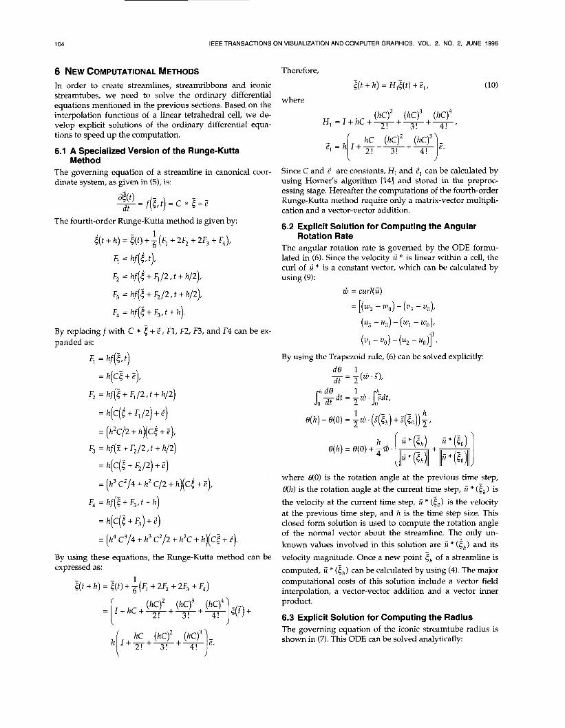
6 NEW COMPUTATIONAL METHODS Therefore,

In order to create streamlines, streamribbons and iconic streamtubes, we need to solve the ordinary differential equations mentioned in the previous sections. Based on the interpolation functions of a linear tetrahedral cell, we de- velop explicit solutions of the ordinary differential equa- tions to speed up the computation.

6.1 A Specialized Version of the Runge-Kutta

The governing equation of a streamline in canonical coor- dinate system, as given in (5), is:

Method

- = f ( < , t ) = c * t + z dt

The fourth-order Runge-Kutta method is given by: 1

F, = k f ( t , t ) ,

t ( t + k ) = t ( t ) + Z(F, + 2F2 + 2F3 + F4),

F2 = kf(< + F1/2 , t + k /2) ,

F3 = k f ( t + F2/2 , t + h/2) ,

F4 = k f ( t + F3, t + k).

By replacing f with C * 5 + Z, F1, F2, F3, and F4 can be ex- panded as:

t(t + k ) = H,t ( t ) + Z,, (10)

where

(kc)' (kC)3 ( / z C ) ~ H, = I + k C + T + - + - 3 ! 4! '

e, = k I+-+- - [ 2 ! 3 !

Since C and Z are constants, HI and Z1 can be calculated by using Horner's algorithm 1141 and stored in the preproc- essing stage. Hereafter the computations of the fourth-order Runge-Kutta method require only a matrix-vector multipli- cation and a vector-vector addition.

6.2 Explicit Solution for Computing the Angular Rotation Rate

The angular rotation rate is governed by the ODE formu- lated in (6). Since the velocity ii * is linear within a cell, the curl of ii * is a constant vector, which can be calculated by using (9):

F1 = k f (<, t ) By using the Trapezoid rule, (6) can be solved explicitly:

= h( C< + Z), F2 = h f ( t + F1/2, t + k /2 )

= k(C(< + F1/2) + Z) = (h2C/2 + h) (C t + z),

F3 = kf(? + F 2 / 2 , t + k / 2 )

= k(C(< + F,/2) + Z)

= (h3 C 2 / 4 + h2 C / 2 + k)(CE + 2). where go) is the rotation angle at the previous time step, f l k ) is the rotation angle at the current time step, ii * (<,I is

F4 = hf( t + F3, t + h)

= k(C@ + F3) + 2)

= ( k4 C3/4 + k 3 C 2 / 2 + k2C + k)(C< + 2).

the velocity at the current time step, ii * (Z0) is the velocity at the previous time step, and k is the time step size. This closed form solution is used to compute the rotation angle of the normal vector about the streamline. The only un- known values involved in this solution are ii * (th) and its velocity magnitude. Once a new point th of a streamline is computed, ii * ( E h ) can be calculated by using (4). The major computational costs of this solution include a vector field interpolation, a vector-vector addition and a vector inner

By using these equations, the Runge-Kutta method can be expressed as:

1 t ( t + k ) = <(t) + z(F, + 2F2 + 2F3 + F4)

product.

6.3 Explicit Solution for Computing the Radius \ /

The governing equation of the iconic streamtube radius is shown in (7). This ODE can be solved analytically:

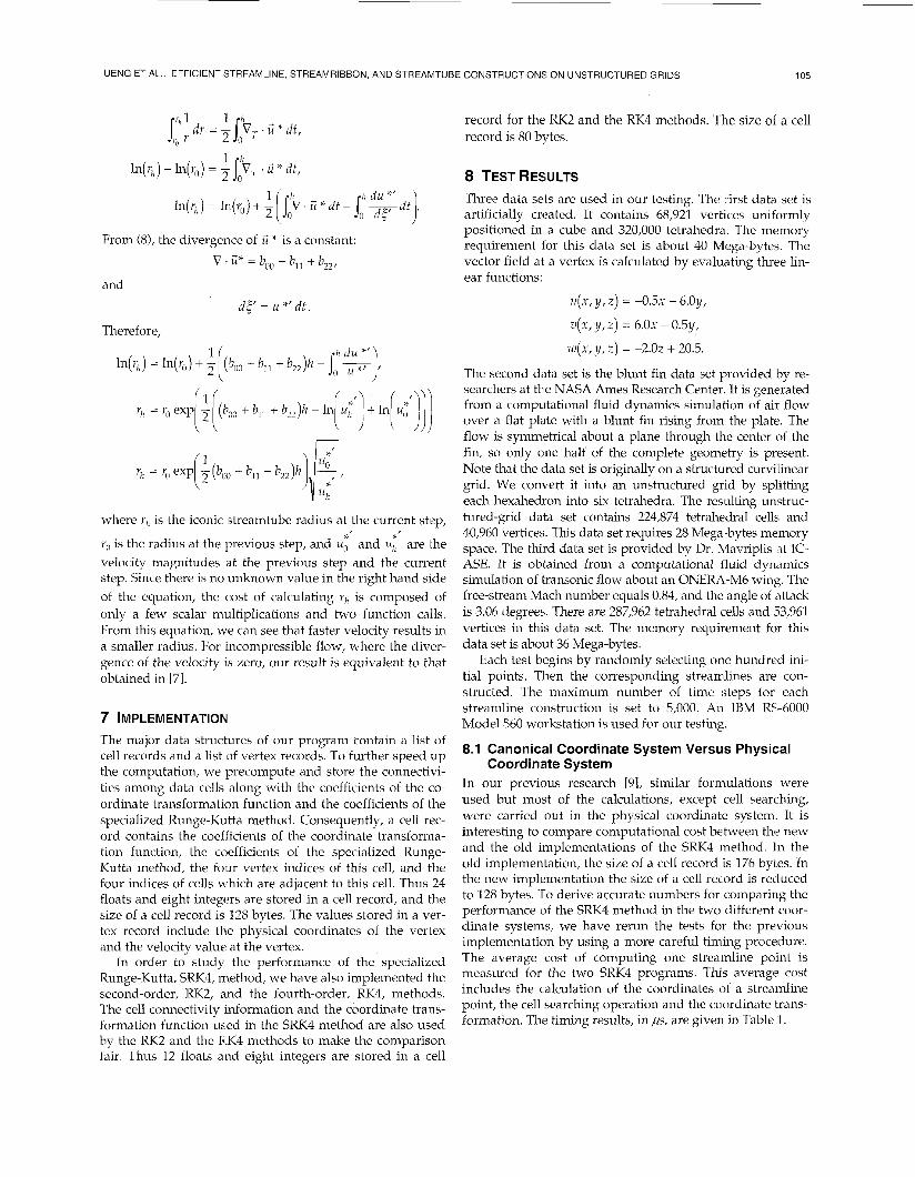
UENG ET AL.: EFFICIENT STREAMLINE, STREAMRIBBON, AND STREAMTUBE CONSTRUCTIONS ON UNSTRUCTURED GRIDS

From (8), the divergence of 2 * is a constant: V . U" = bo, + b,, + b,,,

and

d5' = U " ' d t .

Therefore,

where rll is the iconic streamtube radius at the current step,

yo is the radius at the previous step, and u0 and uh are the velocity magnitudes at the previous step and the current step. Since there is no unknown value in the right hand side of the equation, the cost of calculating yh is composed of only a few scalar multiplications and two function calls. From this equation, we can see that faster velocity results in a smaller radius. For incompressible flow, where the diver- gence of the velocity is zero, our result is equivalent to that obtained in 171.

*' *'

7 IMPLEMENTATIONI The major data structures of our program contain a list of cell records and a list of vertex records. To further speed up the computation, we precompute and store the connectwi- ties among data cells along with the coefficients of the co- ordinate transformation function and the coefficients of the specialized Runge-Ku tta method. Consequently, a cell rec- ord contains the coefficients of the coordinate transforma- tion function, the coefficients of the specialized Runge- Kutta method, the four vertex indices of this cell, and the four indices of cells which are adjacent to this cell. Thus 24 floats and eight integers are stored in a cell record, and the size of a cell record is 128 bytes. The values stored in a ver- tex record include thLe physical coordinates of the vertex and the velocity value at the vertex.

In order to study the performance of the specialized Runge-Kutta, SRK4, method, we have also implemented the second-order, RK2, and the fourth-order, RK4, methods. The cell connectivity information and the coordinate trans- formation function used in the SRK4 method are also used by the RK2 and the R.K4 methods to make the comparison fair. Thus 12 floats and eight integers are stored in a cell

105

record for the RK2 and the RK4 methods. ThLe size of a cell record is 80 bytes.

8 TEST RESULTS Three data sets are used in our testing. The first data set is artificially created. It contains 68,921 vertices uniformly positioned in a cube and 320,000 tetrahedra. The memory requirement for this data set is about 40 MI-ga-bytes. The vector field at a vertex is calculated by evaluating three lin- ear functions:

U(X, y, 2) = -0 .5~ - 6.0y, V(X, y, 2) = 6 . 0 ~ - 0.5y,

W ( X , y, Z ) = -2.02 + 20.5.

The second data set is the blunt fin data set provided by re- searchers at the NASA Ames Research Center. It is generated from a computational fluid dynamics simulation of air flow over a flat plate with a blunt fin rising from the plate. The flow is symmetrical about a plane through the center of the fin, so only one half of the complete geometry is present. Note that the data set is originally on a structured curvilinear grid. We convert it into an unstructured grid by splitting each hexahedron into six tetrahedra. The resulting un:jtruc- tured-grid data set contains 224,874 tetrahedral cells and 40,960 vertices. This data set requires 28 Mega-bytes memory space. The third data set is provided by Dr. Mavriplis ,at IC- ASE. It is obtained from a computational fluid dynamics simulation of transonic flow about an ONERA.-M6 wing. The free-stream Mach number equals 0.84, and the angle of attack is 3.06 degree:;. There are 287,962 tetrahedral cells and 53,961 vertices in this data set. The memory requirement for this data set is about 36 Mega-bytes.

Each test begins by randomly selecting one hundred ini- tial points. Then the corresponding streamllines are con- structed. The maximum number of time :steps for each streamline construction is set to 5,000. An IBM RS-6000 Model 560 workstation is used for our testing,.

8.1 Canonical Coordinate System Versus Physical

In our previous research [9], similar formulations were used but most of the calculations, except cell searching, were carried out in the physical coordinat'e system. It is interesting to compare computational cost between the new and the old implementations of the SRK4 method. In the old implementation, the size of a cell record is 176 bytes. In the new implementation the size of a cell record is reduced to 128 bytes. To derive accurate numbers for comparing the performance of the SRK4 method in the two different coor- dinate systems, we have rerun the tests for the previous implementation by using a more careful timing procedure. The average cost of computing one strea:mline point is measured for the two SRK4 programs. This average cost includes the calculation of the coordinates of a streamline point, the cell searching operation and the co'ordinate trans- formation. TFie timing results, in ,LE, are giver1 in Table 1.

Coordinate System

106 IEEE TRANSACTIONS ON VISUALIZATION AND COMPUTER GRAPHICS, VOL. 2, NO. 2, JUNE 1996

time @Is) data set 1 data set 2 data set 3

Canonical Coord. Physical Coord. 11.53 22.16 10.46 17.49 13.28 17.43

The new SRK4 program is always faster than the old SRK4 program. We find that the cell searching operation makes the old program slower. About 60% more searching is done by the old SRK4 implementation. In the new im- plementation, streamline points are calculated in the ca- nonical coordinate system. Based on the canonical coordi- nates of a streamline point, it is easier to verify whether a new cell should be searched. Therefore unnecessary cell searching calculation is avoided.

8.2 SRK4 Method Versus RK4 and RK2 Methods The execution times, in seconds, of constructing from 1 to 100 streamlines by using the SRK4, the RK4, and the RK2 methods are plotted in Figs. 6, 7, and 8. The execution time includes the cost of streamline point calculation, cell searching and coordinate transformation. To make the comparison fair, the RK2 and the RK4 programs are im- plemented based on the framework of the SRK4 program. That is, all information used by the SRK4 program is also used in the RK2 and the RK4 programs. Some effort is un- dertaken to optimize the RK2 and RK4 implementation; for example, if the computations at the current step and the previous step occur in the same cell, all interpolation func- tion coefficients calculated for the previous step are reused in the computation of the current step.

15

10

- U

m I

2 .ri

5

I I I I I

RK4 + RK2 L

RK4 +

0 2 0 4 0 60 80 1 o c Number of Streamlines

Fig. 6. Timing of constructing streamlines on data set 1.

1 5 r - - - - - - S R K 4 +

0 2 0 4 0 E O 80 100 Number of Streamlines

Fig. 7. Timing of constructing streamlines on data set 2

I I I I I

RK4 RK2 L

:RK4 +

0 2 0 4 0 E 0 80 100 Number of Streamlines

Fig. 8. Timing of constructing streamlines on data set 3.

Since the major function evaluations of all three methods are of the same kind, i.e., matrix-vector multiplication, we can predict their performance by counting the number of function evaluations used in each method. For calculating a new point in a streamline, only one function evaluation is needed for the SRK4 method, while four function evalua- tions are needed for the RK4 method and two function evaluations are needed for the RK2 method. Therefore, the SRK4 method is supposed to be faster than the RK2 method by a factor of 2.0, and faster than the RK4 method by a fac- tor of 4.0. Since the costs of cell searching and coordinate transformation are included in the cost, and the RK2 and

UENG ET AL.: EFFICIENT STREAMLINE, STREAMRIBBON, AND STREAMTUBE CONSTRUCTIONS ON UNSTRUCTURED GRIDS

~

107

the RK4 programs are optimized to avoid unnecessary cal- culation, the performance of the SRK4 method depicted in the figures is not that much better. However, it is still at least 1.7 times faster than the RK2 method and 2.5 times faster than the RK4 method. The average cost of computing a streamline point is presented in Table 2.

TABLE 2 EXECUTION TIME OF A SINGLE TIME STEP OF SRK4 AND RK2 AND RK4 METHODS

We also implemented the RK2 and the RK4 methods without optimization, i.e. all interpolation function coeffi- cients are re-calculated at each step. Test results of these two methods are compared with those of the SRK4 method and shown in Fig. 9 for the first data set. According to the results, the SRK4 prop,ram is now much faster than the RK2 and the RK4 programs. Specifically, the SRK4 method is at least 4 times faster than RK2 method and 5 times faster than RK4 method. Table 3 shows the average cost of a single slep computation. The purpose of this test is to reveal the supe- riority of the SRK4 inethod over the RK2 and the RK4 methods in an extreme situation, in which no two consecu- tive points of a streamline locate at the same cell.

35

3 0

2 5

U 20 1

U1 I

2 E 15 -4

10

5

I I I I I

P RK4 + RK2 L RK4 + RK4 + RK2 L RK4 +

0 20 40 60 80 100 N u m b e r of Streamlines

Fig. 9. Testing results by using data set 1 with nonoptimized codes.

TABLE 3 EXECUTION TIME OF A SINGLE STEP OF THE SRK4,

(NONOPTIMIZED) RK2 AND (NONOPTIMIZED) RK4 METHODS

data set 1 11.53 49.44 55.44 data set 2 10.46 48.49 54.73 data set 3 10.48 49.41 55.69

time @.SI)

8.3 Visualization Results Some visualization results generated by our programs are displayed in the two color plates. The upper left image in Plate 1 shows, a streamribbon visualization od the first data set. In this image, the streamribbons spiral toward a ciritical point which is a saddle point in the vector field. The streamribbons are colored according to velocity magni- tudes. The upper right image shows an iconic streamtube visualization of the same data set. This image reveals not only the rotation of the flow but also the expansion and contraction of the flow. The streamribbon and iconic streamtube visualization of the blunt fin data set are shown in the lower half of Plate 1. Some irregular flow movements have been revealed near the vertical boundary of the physi- cal domain.

The pair of the images in the upper half of Plate 2 dis- play the streamribbon and iconic streamtube visualimtion of the ONERA-M6 wing data set. We can see that the flow rotates around the wing tip while it moves smoothly klefore and after pas:sing of the wing tip. Finally, the bottom two images in Plate 2 show the streamribbon and the iconic streamtube images of a fourth data set provided by re- searchers at the NASA Langley Research Ce:nter. This data set is generated from a computational fluid dynamics simulation of flow about a wing with a trailing-edge flap in a wind tunnel. There are about two million cells in this, data set. Fifty Streamlines are constructed by using fifty initial points which are randomly selected in the physical domain. From this image, we can see that the flow pattern is changed when the flow passes above the deflected trailing- edge flap. A secondary flow that takes place through the gap between the wing and the flap is showrl in this image too. For a large data set containing several millions of cells, a large number of streamlines can be traced and stored in a batch mode or by using a parallel computer. Researchers then examine the stored streamlines using an interactive viewer.

9 CONCLUSIONS The plotting of streamlines is an effective way of visualiz- ing fluid motion in steady flow. We derive a new computa- tional method which greatly simplifies the conventional fourth-order Runge-Kutta method. Explicit solutions are derived for computing the angular rotation rate of flow and the flow expinsion rate to speed up the construction of streamribbons and iconic streamtubes, respectively. In or- der to simplify mathematical formulations, reduce memory usage and further improve the performance of our special- ized RK4 method, the computation is performed in the ca- nonical coordinate system instead of the physical coordi- nate system. These new computational methods and their implementation are evaluated by using three data sets. Test results show that the SRK4 method is indeed superior to the more conventional methods. Moreover, the explicit so- lutions derived also significantly reduce the overall execu- tion time.

While we have improved particle tracing calculations, the computational and memory requirements of tracing in a large data set are high. For example, when using our algo-

108 IEEE TRANSACTIONS ON VISUALIZATION AND COMPUTER GRAPHICS, VOL. 2, NO. 2, JUNE 1996

rithm, a data set of three million cells would take over 350 megabytes of memory. For such a data set which do not fit into the main memory of an average workstation, we have developed an out-of-core tracing strategy with which all data are stored on disk and only a subset of the data is loaded into the main memory upon demand. A prototype implementation of the out-of-core approach demonstrates interactive particle tracing in very large data sets on a 64- megabyte workstation. On the other hand, if a parallel computer is available, both data and tracing can be distrib- uted to multiple processors.

ACKNOWLEDGMENTS This work has been supported in part by the Advanced Combustion Engineering Research Center and the National Aeronautics and Space Administration under NASA con- tract NAS1-19480. Thanks go to the anonymous reviewers who provided many useful suggestions on ways to im- prove the manuscript.

REFERENCES 111

PI

131

[41

151

161

171

181

191

1101

1111

1121

1131

t141

J.K. Vennard and R.L. Street, Elementary Fluid Mechanics. John Wiley & Sons, 1975. G. Volpe, ”Streamlines and Streamribbons in Aerodynamics,” P m c . AIAA 27th Aerospace Science Meeting, Reno, Nev., Jan. 1989. J. Hultquist, ”Interactive Numerical Flow Visualization Using Stream Surfaces,” PhD thesis, Univ. of North Carolina, Chapel Hill, Technical Report TR95-014,1995. D. Darmofal and R. Haimes, “Visualization of 3-D Vector Fields: Variations on a Stream,” PYOC. A I A A 30th Aerospace Science Meeting and Exhibit, Reno, Nev., Jan. 1992. K.-L. Ma and P.J. Smith, ”Cloud Tracing in Convection-Diffusion Systems,” Proc. Visualization ’93 Coni., pp. 253-260. IEEE CS Press, 1993. H.-6. Pagendarm and B. Walter, ”Feature Detection from Vector Quantities in a Numerically Simulated Hypersonic Flow Field in Combination with Experimental Flow Visualization,” Proc. Visu- alization ’94 Conf., pp. 117-123. IEEE CS Press, 1994. W.J. Schroeder, C.R. Volpe, and W.E. Lorensen, “The Stream Polygon: A Technique for 3D Vector Field Visualization,” Proc. Visualization ’91 Coizf., pp. 126-132. IEEE CS Press, 1991. M.P. Garrity, “Raytracing Irregular Volume Data,” PYOC. Sniz Diego Wor/tshop Volume Visiialization, pp. 35-40, San Diego, Dec. 1990. S.K. Ueng, K. Sikorski, and K.-L. Ma, ”Fast Algorithms for Visu- alizing Fluid Motion in Steady Flow on Unstructured Grids,” Proc. Visualization ’95 Col$., pp. 313-320. IEEE CS Press, 1995. A. Sadarjoen, T. van Walsum, A.J.S. Hin, and F.H. Post, ”Particle Tracing Algorithms for Curvilinear Grids,” Proc. F i f t h Eurogvaphics Workshop Visualization in Scientific Computing, Rostock, Germany, May 1994. B. Hamann, D. Wu, and R. Moorhead, ”Flow Visualization with Surface Particles,” I E E E T ~ a n s . Visualization and Computev Gmphics, vol. 1, no. 3, pp. 210-217, Sept. 1995. R. Lohner and J. Ambrosiano, “A Vectorized Particle Tracer for Unstructured Grids,” ]. Computational Physics, vol. 91, pp. 22-31, 1990. P. Buning, “Sources of Error in the Graphical Analysis of cfd Re- sults,” ]. Scientific Computing, vol. 3, no. 2, pp. 149-164, 1988. G.H. Golub and C.F. van Loan, Matrix Computations. Johns Hop- kins Univ. Press, 1989.

Shyh-Kuang Ueng received his BS from Soochow University, Taipei, Taiwan, in 1985, and his MS in computer science from National Taiwan Uni- versity, Taipei, Taiwan, in 1988. He is currently a PhD student in computer science at the Uni- versity of Utah. His research interests include scientific computing, scientific visualization, and algorithms.

Christopher Sikorski holds the PhD degree from the University of Utah in scientific compu- tation with a special emphasis on computational complexity and algorithm design. He is an asso- ciate professor of computer science at the Uni- versity of Utah. His research interests concen- trate on parallel scientific computation, compu- tational complexity for continuous problems, 3D visualization algorithms, and applications in computational fluid dynamics, combustion engi- neering, and geophysics modeling.

Dr. Sikorski is the author or coauthor of two research monographs, one lecture notes, numerous journal articles, and several papers in conference proceedings. His graduate students are or were holding positions at Columbia University, the University of Utah, Lehigh Uni- versity, National Taiwan University, National Korean University, and NASA Langley Research Center.

Kwan-Liu Ma received his BS, MS, and PhD degrees in computer science from the University

of Utah. He is a staff scientist at the Institute of Computer Applications for Science and Engi-

neering (CASE) and an adjunct assistant pro- fessor of computer science at Old Dominion

University, where he teaches scientific visuali- zation. His research interests include computer

graphics, scientific visualization, and parallel and distributed computing. Dr. Ma is a member

of the IEEE, ACM, and Phi Kappa Phi.

UENG ET AL.: EFFICIENT S,TREAMLINE, STREAMRIBBON, AND STREAMTUBE CONSTRUCTIONS ON UNSTRUCTURED GRIDS

PLATE 1

109