Electromagnetic Particle-in-Cell Algorithms on Unstructured ...

Electromagnetic Particle-in-Cell Algorithms on Unstructured

Meshes for Kinetic Plasma Simulations

Dissertation

Presented in Partial Fulfillment of the Requirements for the Degree Doctor ofPhilosophy in the Graduate School of The Ohio State University

By

Dong-Yeop Na, M.S.

Graduate Program in Electrical and Computer Engineering

The Ohio State University

2018

Dissertation Committee:

Prof. Fernando L. Teixeira, Advisor

Prof. Kubilay Sertel

Prof. Robert Lee

c© Copyright by

Dong-Yeop Na

2018

Abstract

Plasma is a significantly ionized gas composed of a large number of charged parti-

cles such as electrons and ions. A distinct feature of plasmas is the collective interac-

tion among charged particles. In general, the optimal approach used for modeling a

plasma system depends on its characteristic (temporal and spatial) scales. Among var-

ious kinds of plasmas, collisionsless plasmas correspond to those where the collisional

frequency is much smaller than the frequency of interests (e.g. plasma frequency) and

the mean free path is much longer than the characteristic length scales (e.g. Debye

length).

Collisionless plasmas consisting of kinetic space charge particles interacting with

electromagnetic fields are well-described by Maxwell-Vlasov equations. Electromag-

netic particle-in-cell (EM-PIC) algorithms solve Maxwell-Vlasov systems on a com-

putational mesh by employing coarse-grained superparticle. The concept of super-

particle, which may represent millions of physical charged particles (coarse-graining

of the phase space), facilitates the realization of computer simulations for under-

scaled kinetic plasma systems mimicking the physics of real kinetic plasma systems.

In this dissertation, we present an EM-PIC algorithm on general (irregular) meshes

based on discrete exterior calculus (DEC) and Whitney forms. DEC and Whitney

forms are utilized for consistent discretization of Maxwells equation on general ir-

regular meshes. The proposed EM-PIC algorithm employs a mixed finite-element

ii

time-domain (FETD) field solver which yields a symplectic integrator satisfying en-

ergy conservation. Importantly, we employ Whitney-forms-based gather and scatter

schemes to obtain exact charge conservation from first principles, which had been a

long-standing challenge for PIC algorithms on irregular meshes.

Several further contributions are made in this dissertation: (i) We develop a local

and explicit EM-PIC on unstructured grids using sparse approximate inverse (SPAI)

strategy and study macro- and microscopic residual errors in motions of charged par-

ticles affected by the approximate inverse errors. (ii) We extend the present EM-PIC

algorithm to the relativistic regime with several relativistic particle-pushers and com-

pare their performance. (iii) We implement a secondary electron emission (SEE)

processor based on probabilistic Furman-Pivi model and numerically investigate mul-

tipactor effects that are resonant electron discharges from conducting surfaces by

external RF fields. (iv) We diagnose numerical Cherenkov radiation, which is a detri-

mental effect frequently found in EM-PIC simulations involving relativistic plasma

beams, for the present EM-PIC algorithm on general meshes. (v) We extend the

FETD field solver for the solution of Maxwell’s equations in circularly symmetric

or body-of-revolution (BOR) geometries. (vi) Lastly, we combine the EM-PIC algo-

rithm with the BOR-FETD field solver for the efficient analysis of vacuum electronic

devices (VED).

iii

Dedicated to my beloved wife Da-Young and my family

iv

Acknowledgments

First and foremost, I would like to express my sincere gratitude to my advisor,

Prof. Fernando L. Teixeira, for the support, encouragement, and guidance during the

years of my graduate study. It has been a great honor and privilege to work with him.

His passion and immense knowledge in electromagnetics, mathematics, and physics,

and kindness and commitment to his students will always inspire me.

Besides, I would like to thank Dr. Yuri A. Omelchenko and Prof. Ben-Hur V.

Borges for their helpful discussions and suggestions.

My special appreciation also goes to the members of my doctoral committee, Prof.

Kubilay Sertel and Prof. Robert Lee, for insightful comments.

I would like to thank to many of ESL colleagues, past and present, Haksu Moon,

WoonGi Yeo, Jungwhan Park, Carlos A. Viteri, Cagdas Gunes, Daniel O. Acero, and

Julio L. Nicolini, and my friends, Yun-Shik Hahn, Chunghyun Lee, Jongchan Choi,

Kyoung-Ho Jeong, and Huyngjun Kim.

I wish to thank my family for their constant support and unconditional love.

Last but not least, I would like to share this accomplishment with my beloved

wife, Da-Young, and sincerely appreciate her her encouragement, support, and love.

v

Financial support from National Science Foundation grant ECCS-1305838, De-

fense Threat Reduction Agency grant HDTRA1-18-1-0050, Ohio Supercomputer Cen-

ter grants PAS-0061 and PAS-0110, and The Ohio State University Presidential Fel-

lowship Program are gratefully acknowledged.

vi

Vita

March 30, 1987 . . . . . . . . . . . . . . . . . . . . . . . . . . . . . Born - Seoul, Korea

Feburary, 2012 . . . . . . . . . . . . . . . . . . . . . . . . . . . . . B.S. in Electrical and Computer Eng.,Ajou University, Suwon, Korea

July, 2014 . . . . . . . . . . . . . . . . . . . . . . . . . . . . . . . . . . M.S. in Electrical and Computer Eng.,Ajou University, Suwon, Korea

August, 2014-May, 2017 . . . . . . . . . . . . . . . . . . . . Graduate Research Associate,ElectroScience Laboratory,The Ohio State University, USA

May, 2017-May, 2018 . . . . . . . . . . . . . . . . . . . . . . . Presidential Fellowship Program,The Ohio State University, USA

May, 2018-August, 2018 . . . . . . . . . . . . . . . . . . . . Graduate Research Associate,ElectroScience Laboratory,The Ohio State University, USA

August, 2018-present . . . . . . . . . . . . . . . . . . . . . . . Graduate Teaching Associate,Electrical and Computer Eng.,The Ohio State University, USA

Publications

Jounral Publications

Dong-Yeop Na, Haksu Moon, Yuri A. Omelchenko, Fernando L. Teixeira, “Local,explicit, and charge-conserving electromagnetic particle-in-cell algorithm on unstruc-tured grids,” IEEE Trans. Plasma Sci., 44 (2016) 1353–1362.

Dong-Yeop Na, Yuri A. Omelchenko, Haksu Moon, Ben-Hur V. Borges, FernandoL. Teixeira, “Axisymmetric charge-conservative electromagnetic particle simulationalgorithm on unstructured grids: Application to microwave vacuum electronic De-vices,” J. Comput. Phys., 346 (2017) 295–317.

vii

Dong-Yeop Na, Haksu Moon, Yuri A. Omelchenko, Fernando L. Teixeira, “Rel-ativistic extension of a charge-conservative finite element solver for time-dependentMaxwell-Vlasov equations,” Phys. Plasmas, 25 (2018) 013109.

Dong-Yeop Na, Ben-Hur V. Borges, Fernando L. Teixeira, “Finite element time-domain body-of-revolution Maxwell solver based on discrete exterior calculus,” J.Comput. Phys., 376 (2017) 249–275.

Conference publications

Dong-Yeop Na, Fernando L. Teixeira, Yuri A. Omelchenko, “Charge-conservingrelativistic PIC algorithm on unstructured grids,” 2016 USNC-URSI National RadioScience Meeting, Boulder, CO, Jan. 6-9, 2016.

Dong-Yeop Na, Fernando L. Teixeira, H. Moon, Yuri A. Omelchenko, “Full-waveFETD-based PIC algorithm with local explicit update,” 2016 IEEE InternationalSymposium on Antennas and Propagation and USNC-URSI Radio Science Meeting,Fajardo, PR, June 26-July 1, 2016.

Dong-Yeop Na, Fernando L. Teixeira, Yuri A. Omelchenko, “Unstructured-gridand conservative electromagnetic particle-in-cell: application to micromachined slow-wave structures,” 2016 IEEE International Symposium on Antennas and Propagationand USNC-URSI Radio Science Meeting, Fajardo, PR, June 26-July 1, 2016.

Dong-Yeop Na, Yuri A. Omelchenko, Fernando L. Teixeira, “An efficient algorithmfor simulation of plasma beam high-power microwave sources,” 2017 IEEE MTT-SInternational Microwave Symposium, Honolulu, HI, June 4-9, 2017.

Dong-Yeop Na, Fernando L. Teixeira, Ben-Hur V. Borges, “Finite-element time-domain solver for axisymmetric devices based on discrete exterior calculus and trans-formation optics,” 2017 SBMO/IEEE MTT-S International Microwave and Opto-electronics Conference, Aguas de Lindoia, Brazil, Aug. 27-30, 2017.

Dong-Yeop Na, Yuri A. Omelchenko, Fernando L. Teixeira, “Irregular-grid-basedparticle-in-cell simulations of resonant electron discharges with probabilistic secondaryelectron emission model,” 2017 XXXIInd General Assembly and Scientific Sympo-sium of the International Union of Radio Science, Montreal, QC, Canada, August19-26, 2017.

viii

Dong-Yeop Na, Yuri A. Omelchenko, Fernando L. Teixeira, “Discretization ofMaxwell-vlasov equations based on discrete exterior calculus,” 2017 XXXIInd GeneralAssembly and Scientific Symposium of the International Union of Radio Science,Montreal, QC, Canada, August 19-26, 2017.

Dong-Yeop Na, Julio L. Nicolini, Robert Lee, Ben-Hur V. Borges, Yuri A. Omelchenko,Fernando L. Teixeira, “Diagnosis of Numerical Cherenkov Instability in Plasma Simu-lations on General Mesh,” Computational Aspects of Time Dependent ElectromagneticWave Problems in Complex Materials, The Institute of Computational and Experi-mental Research in Mathematics (ICERM), Providence, RI, June 24-29, 2018.

Dong-Yeop Na, Fernando L. Teixeira, Yuri A. Omelchenko, “Dispersion Analy-sis of Electron Bernstein Waves in Magnetized Warm Plasmas by Finite ElementParticle-in-Cell Modeling,” 2018 IEEE International Symposium on Antennas andPropagation and USNC-URSI Radio Science Meeting, Boston, MA, July 8-13, 2018.

Dong-Yeop Na, Fernando L. Teixeira, Yuri A. Omelchenko, “Numerical CherenkovRadiation Effects from Grid Dispersion in Finite Element Particle-in-Cell Simulationsof Relativistic Electron Beams,” 2018 IEEE International Symposium on Antennasand Propagation and USNC-URSI Radio Science Meeting, Boston, MA, July 8-13,2018.

Fields of Study

Major Field: Electrical and Computer Engineering

Studies in:

Electromagnetic theoryComputational electromagneticsAntennasMathematics

ix

Table of Contents

Page

Abstract . . . . . . . . . . . . . . . . . . . . . . . . . . . . . . . . . . . . . . . ii

Dedication . . . . . . . . . . . . . . . . . . . . . . . . . . . . . . . . . . . . . . iv

Acknowledgments . . . . . . . . . . . . . . . . . . . . . . . . . . . . . . . . . . v

Vita . . . . . . . . . . . . . . . . . . . . . . . . . . . . . . . . . . . . . . . . . vii

List of Tables . . . . . . . . . . . . . . . . . . . . . . . . . . . . . . . . . . . . xiv

List of Figures . . . . . . . . . . . . . . . . . . . . . . . . . . . . . . . . . . . xvi

1. Introduction . . . . . . . . . . . . . . . . . . . . . . . . . . . . . . . . . . 1

1.1 Background and motivation . . . . . . . . . . . . . . . . . . . . . . 11.2 Contribution of this dissertation . . . . . . . . . . . . . . . . . . . 61.3 Organization of this dissertation . . . . . . . . . . . . . . . . . . . 7

2. Local, Explicit, and Charge-conserving EM-PIC on Unstructured Mesh . 11

2.1 Explicit FETD-PIC Algorithm . . . . . . . . . . . . . . . . . . . . 132.1.1 Mixed E − B FETD scheme . . . . . . . . . . . . . . . . . . 142.1.2 Gather-scatter and particle pusher steps . . . . . . . . . . . 162.1.3 Discrete continuity equation . . . . . . . . . . . . . . . . . . 17

2.2 Sparse Approximate Inverse (SPAI) strategy . . . . . . . . . . . . . 192.2.1 Discrete Gauss’ law . . . . . . . . . . . . . . . . . . . . . . 20

2.3 Numerical Results . . . . . . . . . . . . . . . . . . . . . . . . . . . 212.3.1 Single-particle trajectories . . . . . . . . . . . . . . . . . . . 212.3.2 Plasma ball expansion . . . . . . . . . . . . . . . . . . . . . 272.3.3 Electron beam in a vacuum diode . . . . . . . . . . . . . . . 302.3.4 Electron Bernstein waves . . . . . . . . . . . . . . . . . . . 33

x

2.4 Conclusion . . . . . . . . . . . . . . . . . . . . . . . . . . . . . . . 35

3. Relativitic Extension of Particle-Pusher . . . . . . . . . . . . . . . . . . . 36

3.1 Particle-pushers in the relativistic regime . . . . . . . . . . . . . . . 373.1.1 Relativistic Boris pusher . . . . . . . . . . . . . . . . . . . . 383.1.2 Vay pusher . . . . . . . . . . . . . . . . . . . . . . . . . . . 403.1.3 Higuera-Cary pusher . . . . . . . . . . . . . . . . . . . . . . 41

3.2 Numerical results . . . . . . . . . . . . . . . . . . . . . . . . . . . . 413.2.1 Synchrocyclotron . . . . . . . . . . . . . . . . . . . . . . . . 413.2.2 Harmonic oscillations in Lorentz-boosted frame . . . . . . . 443.2.3 Relativistic Bernstein Modes in Magnetized Pair-Plasma . . 47

3.3 Conclusion . . . . . . . . . . . . . . . . . . . . . . . . . . . . . . . 55

4. Multipactor . . . . . . . . . . . . . . . . . . . . . . . . . . . . . . . . . . 57

4.1 Irregular-Grid EM-PIC Algorithm integrated with Furman-Pivi model 604.2 Charge-conserving scatter near conducting surface . . . . . . . . . 614.3 Furman-Pivi SEE model implementation . . . . . . . . . . . . . . . 624.4 Numerical Results and Discussion . . . . . . . . . . . . . . . . . . . 63

4.4.1 Verification of SEE model in EM-PIC simulations . . . . . . 634.4.2 Multipactor on copper versus stainless steel surfaces . . . . 664.4.3 Surface treatment effects . . . . . . . . . . . . . . . . . . . . 684.4.4 Multipactor susceptibility to RF voltage amplitude . . . . . 704.4.5 Multipactor saturation effects . . . . . . . . . . . . . . . . . 72

4.5 Conclusion . . . . . . . . . . . . . . . . . . . . . . . . . . . . . . . 75

5. Numerical Cherenkov Radiation and Grid Dispersion Effects . . . . . . . 79

5.1 Numerical Cherenkov Radiation in the FDTD-based EM-PIC Algo-rithm . . . . . . . . . . . . . . . . . . . . . . . . . . . . . . . . . . 81

5.2 Numerical Cherenkov Radiation in finite-element-based EM-PIC Al-gorithms . . . . . . . . . . . . . . . . . . . . . . . . . . . . . . . . . 855.2.1 SQ Mesh . . . . . . . . . . . . . . . . . . . . . . . . . . . . 885.2.2 Triangular-element-based FE meshes . . . . . . . . . . . . . 92

5.3 Numerical Experiments . . . . . . . . . . . . . . . . . . . . . . . . 1005.4 Conclusion . . . . . . . . . . . . . . . . . . . . . . . . . . . . . . . 109

6. Finite-Element Time-Domain Body-of-Revolution Maxwell-Solver . . . . 111

6.1 Formulation . . . . . . . . . . . . . . . . . . . . . . . . . . . . . . . 1136.1.1 Exploration of transformation optics (TO) concepts . . . . . 1136.1.2 Field decomposition . . . . . . . . . . . . . . . . . . . . . . 115

xi

6.1.3 Mixed FE time-domain BOR solver . . . . . . . . . . . . . . 1166.1.4 Symmetry axis singularity treatment . . . . . . . . . . . . . 123

6.2 Numerical Examples . . . . . . . . . . . . . . . . . . . . . . . . . . 1256.2.1 Cylindrical cavity . . . . . . . . . . . . . . . . . . . . . . . . 1266.2.2 Logging-while-drilling sensor simulation . . . . . . . . . . . 129

6.3 Conclusion . . . . . . . . . . . . . . . . . . . . . . . . . . . . . . . 137

7. Axisymmetric Electromagnetic Particle-in-Cell Algorithm: Application toMicrowave Vacuum Electronic Devices . . . . . . . . . . . . . . . . . . . 140

7.1 Spatial dimensionality reduction . . . . . . . . . . . . . . . . . . . 1457.1.1 Exterior calculus representation of Maxwell’s equations . . . 1457.1.2 Cylindrical axisymmetry constraints . . . . . . . . . . . . . 1467.1.3 Modified Hodge star operator . . . . . . . . . . . . . . . . . 147

7.2 Validation . . . . . . . . . . . . . . . . . . . . . . . . . . . . . . . . 1507.2.1 Metallic hollow cylindrical cavity . . . . . . . . . . . . . . . 1507.2.2 Space-charge-limited (SCL) cylindrical diode . . . . . . . . 152

7.3 Numerical examples . . . . . . . . . . . . . . . . . . . . . . . . . . 1567.3.1 Relativistic backward-wave oscillator (BWO) . . . . . . . . 158

7.4 Conclusion . . . . . . . . . . . . . . . . . . . . . . . . . . . . . . . 166

Appendices 168

A. Basics of Plasmas . . . . . . . . . . . . . . . . . . . . . . . . . . . . . . . 168

A.1 Fundamental parameters . . . . . . . . . . . . . . . . . . . . . . . . 168A.2 Quasi-neutrality in plasma . . . . . . . . . . . . . . . . . . . . . . . 170A.3 Plasma oscillation . . . . . . . . . . . . . . . . . . . . . . . . . . . 171A.4 Collisions in plasmas . . . . . . . . . . . . . . . . . . . . . . . . . . 172

B. Kinetic Plasma Description . . . . . . . . . . . . . . . . . . . . . . . . . 174

B.1 Plasma kinetic equation . . . . . . . . . . . . . . . . . . . . . . . . 174B.2 Vlasov equation for collisionless plasmas . . . . . . . . . . . . . . . 178B.3 Superparticle: Coarse-grained f (x,v, t) . . . . . . . . . . . . . . . 179B.4 Maxwell-Vlasov or Poisson-Vlasov systems . . . . . . . . . . . . . . 181

C. Discrete Exterior Caclulus (DEC) . . . . . . . . . . . . . . . . . . . . . . 183

C.1 Whitney forms . . . . . . . . . . . . . . . . . . . . . . . . . . . . . 183C.2 Pairing operation . . . . . . . . . . . . . . . . . . . . . . . . . . . . 184C.3 Generalized Stokes’ theorem . . . . . . . . . . . . . . . . . . . . . . 184

xii

C.4 Discretization of Maxwell’s equation . . . . . . . . . . . . . . . . . 184C.4.1 Cartesian coordinates case . . . . . . . . . . . . . . . . . . . 184C.4.2 Body-of-revolution case . . . . . . . . . . . . . . . . . . . . 185

C.5 Incidence Matrices . . . . . . . . . . . . . . . . . . . . . . . . . . . 187C.6 Discrete Hodge matrix . . . . . . . . . . . . . . . . . . . . . . . . . 189C.7 Barycentric dual lattice relations . . . . . . . . . . . . . . . . . . . 193

D. Cartesian-like PML implementation . . . . . . . . . . . . . . . . . . . . . 195

E. Stability Conditions . . . . . . . . . . . . . . . . . . . . . . . . . . . . . 201

Bibliography . . . . . . . . . . . . . . . . . . . . . . . . . . . . . . . . . . . . 203

xiii

List of Tables

Table Page

2.1 Number of elements in Meshes 1, 2, and 3 . . . . . . . . . . . . . . . . . 22

2.2 Convention used for particle trajectory visualization. . . . . . . . . . . . 24

3.1 Verification of discrete Gauss’ law for the non-relativistic case (Fig.3.2a). . . . . . . . . . . . . . . . . . . . . . . . . . . . . . . . . . . . . 45

3.2 Verification of discrete Gauss’ law for the relativistic case without syn-chronization (Fig. 3.2b). . . . . . . . . . . . . . . . . . . . . . . . . . 46

3.3 Verification of discrete Gauss’ law for the relativistic case with syn-chronization (Fig. 3.2c). . . . . . . . . . . . . . . . . . . . . . . . . . 46

4.1 Multipactor simulation parameters for the parallel waveguide in Fig. 4.7a. 69

4.2 Triangularly-grooved surface parameters. . . . . . . . . . . . . . . . . 70

4.3 Mesh parameters. . . . . . . . . . . . . . . . . . . . . . . . . . . . . . 70

4.4 Spectral amplitude of output voltage signals for high-order harmonics. 73

5.1 Basic meshes properties. . . . . . . . . . . . . . . . . . . . . . . . . . 102

6.1 Maximum time-step intervals for various cases in the simulation ofcylindrical metallic cavity. . . . . . . . . . . . . . . . . . . . . . . . . 127

6.2 Eigenfrequencies for the cylindrical cavity and normalized errors be-tween numerical and analytic results. . . . . . . . . . . . . . . . . . . 132

7.1 Estimation of the run time of EM-PIC simulations based on FETDand FDTD at each time-update. . . . . . . . . . . . . . . . . . . . . . 149

xiv

7.2 Resonant frequencies for axisymmetric cavity modes and normalizederrors between numerical and analytic works. . . . . . . . . . . . . . . 153

7.3 Mesh information for different SCSWS cases . . . . . . . . . . . . . . 163

xv

List of Figures

Figure Page

2.1 Basic steps in a EM-PIC algorithm. On unstructured meshes, conven-tional field solvers are implicit, requiring the solution of a (large) linearsystem at each time step. . . . . . . . . . . . . . . . . . . . . . . . . . 14

2.2 Charge-conserving gather and scatter steps [1]. (a) Interpolation of Eand B at the position of the particle by edge-based (left) and face-based degrees of freedom contributions (right) (weighted by the Whit-ney functions) in the gather step. (b) Exact charge-conserving scatterscheme. The sum of the two colored areas in the left, representing themagnitude of the edge currents, is equal to the blue area in the left,representing the charge variation at node 1 during one time step. . . 16

2.3 Relative position difference (RPD) of the various test particles w.r.t.the standard particle placed at the origin, in a polar diagram wherethe radial distance is represented in logarithmic scale. . . . . . . . . . 23

2.4 Results for a circular particle trajectory on 3 different meshes. (a) (b)(c) Particle trajectory histories. (d) (e) (f) RPDs versus time for thefour test particles. (g) (h) (i) Normalized RPD bands for the four testparticles. . . . . . . . . . . . . . . . . . . . . . . . . . . . . . . . . . . 25

2.5 Results for a trajectory with drift. (a) (b) (c) Particle trajectory his-tory. (d) (e) (f) RPDs versus time for the four test particles. (g) (h)(i) Normalized RPD bands for the four test particles. . . . . . . . . . 27

2.6 Radial current versus radius coordinate for the expanding plasma attime step n = 9× 104 using the LU-based implicit fields solver and theSPAI-based explicit field solver with k = 2, 4, and 6. . . . . . . . . . 28

xvi

2.7 (a) Normalized residuals of the discrete continuity equation for theplasma ball expansion example using different field solvers, at t =2×104∆t. (b) Similar results for the discrete Gauss’ law. (c) Averagednormalized residuals for the discrete Gauss’ law versus time step index. 29

2.8 Results for the accelerated electron beam at t = 6×104∆t. (a) (b) Par-ticle distribution snapshot from charge-conserving EM-PIC algorithmsusing an LU-based implicit solver and a SPAI-based (k = 2) explicitsolver, respectively . (c) Particle distribution snapshot from a con-ventional (non-charge conserving on the unstructured grid) EM-PICalgorithm with an LU-based implicit solver. (d) (e) (f) Correspondingelectric-field profile distributions. . . . . . . . . . . . . . . . . . . . . 31

2.9 Number density and average velocity of particles across a transversalsection of the electron beam at t = 3 × 103∆t, after steady-state hasbeen reached. . . . . . . . . . . . . . . . . . . . . . . . . . . . . . . . 32

2.10 Simulated ω × k dispersion diagram for the X mode propagation andfor electron Bernstein waves in a magnetized warm plasma. Here ωpe isthe plasma frequency and ∆x is the grid spacing, chosen uniform. Theanalytical results are indicated by the red dots in the diagram. Notethat the use of a charge-conserving scatter step in PIC algorithm asdescribed in [1] reduces the numerical noise and yields cleaner spectralbands in the numerically generated band diagrams. In addition, acharge-conserving scatter step mitigates the spurious DC field causeby spurious charge accumulation on the grid nodes, as observed atthe bottom of the zoomed plots. Overall, a very good agreement isobserved between the numerical and the analytical results. . . . . . . 34

3.1 (a) Cyclotron configuration. (b) Computational domain, where theblue vertical strip indicates the region where an external longitudinalRF electric field is applied. The DC magnetic field is applied in thewhole computational region except for the RF acceleration gap (red). 42

3.2 Electron trajectories on a cyclotron: (a) Non-relativistic, (b) Relativis-tic, unsynchronized, and (c) Relativistic, synchronized. . . . . . . . . 43

3.3 Orbital frequency and relativistic factor for the case shown in Fig. 3.2c. 44

3.4 Comparison of electron velocity magnitudes of the three cases shownin Fig. 3.2. . . . . . . . . . . . . . . . . . . . . . . . . . . . . . . . . . 45

xvii

3.5 Motion of harmonic oscillator of a single positron inverse-Lorentz-transformed into Laboratory frame. . . . . . . . . . . . . . . . . . . . 47

3.6 Dispersion relations for classical (non-relativistic) electron Bernsteinmodes of PIC results (Parula colormap) and analytic predictions [2](dashed red line). . . . . . . . . . . . . . . . . . . . . . . . . . . . . . 48

3.7 An isotropic 2D Maxwell-Boltzmann-Juttner velocity distribution, f0 (p)for η = 1/20: (a) Speed distribution and (b) relativistic velocity dis-tribution. . . . . . . . . . . . . . . . . . . . . . . . . . . . . . . . . . 51

3.8 Dispersion relations for plasma waves propagating in magnetized rel-ativistic pair-plasma for η = 1/20: Comparison of PIC results andanalytic prediction. . . . . . . . . . . . . . . . . . . . . . . . . . . . . 52

3.9 Normalized residuals versus nodal index for (a) discrete continuityequation (DCE) and (b) discrete Gauss law (DGL). . . . . . . . . . . 53

4.1 Schematic illustration of a typical SEE process in an irregular-grid-based

EM-PIC simulation. Note that electric current densities by the primary or

secondaries are deposited on red- or blue-highlighted edges, respectively. . 58

4.2 Comparison of simulation and experimental results for SEE on copper [(a)

and (b)] and stainless steel [(c) and (d))] surfaces. Figures (a) and (c)

illustrate SEY δ versus the primary incident energy. Figures (b) and (d)

show the emitted-energy spectrum dδ/dE. . . . . . . . . . . . . . . . . . 59

4.3 Geometrical illustration of exact charge conservation on irregular grids for

a primary impact (also applicable for secondary electrons emitted on the

opposite way) at PEC surfaces during ∆t. Plot (a) depicts the charge vari-

ation rate at jth node. Plot (b) depicts the divergence of current on jth

node, which is equal to the sum of ith and kth currents. . . . . . . . . . . 61

4.4 Angular dependence of δ on a copper surface. . . . . . . . . . . . . . . . 65

xviii

4.5 PIC results for probabilistic SEE model. (a) Superparticle population versus

time (RF voltage periods). (b) and (c) Snapshots of particle’s trajectories

for copper and stainless steel cases, respectively. These trajectory snapshots

are taken during four successive half-periods of the RF signal, i.e.: t/TRF ∈(0, 0.5), t/TRF ∈ (0.5, 1), t/TRF ∈ (1, 1.5), and t/TRF ∈ (1.5, 2), where

TRF = 1/fRF = 0.96 [ns]. . . . . . . . . . . . . . . . . . . . . . . . . . . 65

4.6 Particle trajectory snapshots on the phase space. The coordinate axes rep-

resent x/10 [m], y [m], and the normalized speed of the particles (|vp| /20c).

Each plot corresponds to a half-period of the RF signal, as in Fig. 4.5. . . 66

4.7 Multipactor in parallel plate waveguides. (a) Schematics of the problem ge-

ometry. (b) Flat surface waveguide meshing. (c) Triangular-grooved waveg-

uide meshing. . . . . . . . . . . . . . . . . . . . . . . . . . . . . . . . . 68

4.8 RF voltage amplitude susceptibility at fRFDpp = 4 [GHz·mm] for flat and

grooved copper surfaces. . . . . . . . . . . . . . . . . . . . . . . . . . . 71

4.9 RF voltage cycle versus population amplification, An for both surfaces at

V aRF = 1, 143.16 V. . . . . . . . . . . . . . . . . . . . . . . . . . . . . . 72

4.10 Output signals for both surfaces (a) in time-domain and (b) frequency domain. 74

4.11 Particle position snapshots taken over a half RF period during the saturation

regime. The RF voltage period is 0.5 ns. Plots (a)-(f) are for the flat surface

and plots (g)-(l) are for the grooved surfaces. . . . . . . . . . . . . . . . 76

4.12 External-field and self-field snapshots taken over a half period during the

saturation regime. The RF voltage period is 0.5 ns. Plots (a)-(f) are for the

flat surface and plots (g)-(l) are for the grooved surfaces. . . . . . . . . . 77

4.13 Snapshots of vy [m/s] versus y [m] taken over a half RF period during the



4.14 Snapshots of vx [m/s] versus y [m] taken over a half RF period during the



xix

5.1 Numerical grid dispersion of the 2-D Yee’s FDTD scheme on a struc-tured mesh. (a) The red color surface represents the dispersion diagramof the normalized frequency ω∆t/π versus the normalized numericalwavenumber κh in radians. The olive color surface represents the lightcone. The contour levels at the bottom represent the normalized phaseerrors (with respect to the color bar). (b) Wavenumber magnitude ver-sus frequency for different wave propagation angles with respect to thex axis, φp ∈ [0o, 45o]. . . . . . . . . . . . . . . . . . . . . . . . . . . . 82

5.2 Analytic NCR predictions on a structured FDTD grid for a bulk beamvelocity vb = 0.9c. (a) 3-D numerical dispersion diagrams (in red)and beam planes (fundamental plane in green and aliased beams intransparent yellow). (b) Trajectories of NCR solutions projected ontothe 2-D κ-space. . . . . . . . . . . . . . . . . . . . . . . . . . . . . . 84

5.3 Schematic illustration of the four types of mesh considered in thisstudy. (a) Square regular (SQ) elements in both FDTD and FETD,(b) right-angle triangular (RAT) elements in FETD, (c) isosceles tri-angular (ISOT) elements in FETD, and (d) highly-irregular triangular(HIGT) elements in FETD. . . . . . . . . . . . . . . . . . . . . . . . 86

5.4 Schematic of SQ mesh. There are two characteristic edges (A and B)directed along the y and x and colored in red and blue, respectively. . 88

5.5 Numerical grid dispersion for the FETD scheme on the SQ mesh. (a)The red color surface represents the dispersion diagram of the normal-ized frequency ω∆t/π versus the normalized numerical wavenumberκh in radians. The olive color surface represents the light cone. Thecontour levels at the bottom represent the normalized phase errors(with respect to the color bar). Note that the normalized phase erroris always negative in this case because of a slightly faster-than-lightnumerical phase velocity. (b) Projected dispersion curves for differentwave propagation angles with respect to the x axis φp ∈ [0o, 45o]. . . . 91

5.6 Analytic prediction of NCR for the FETD algorithm on the SQ meshwhen vb = 0.9c. (a) 3-D dispersion diagram. (b) NCR solution con-tours projected onto the first Brillouin zone in the κ-space. . . . . . . 92

xx

5.7 A periodically-arranged triangular grid. It has three characteristicedges denoted by A, B, and C. Labels inside circles denote globalfacet indexes and labels inside rectangles and pentagons denote localedge and node indexes, respectively. . . . . . . . . . . . . . . . . . . . 93

5.8 Numerical grid dispersion for the FETD scheme on the RAT mesh withthe CFL number equal to one. Unlike the FDTD or FETD-SQ cases,this diagram exhibits an additional (upper) dispersion band. (a) Thered (lower band) and blue (upper band) color surfaces represent thedispersion diagram of the normalized frequency ω∆t/π versus the nor-malized numerical wavenumber κh in radians. The olive color surfacerepresents the light cone. The contour levels at the bottom repre-sent the normalized phase errors (with respect to the color bar). (b)Projected dispersion curves for different wave propagation angles withrespect to the x axis φp ∈ [−45o, 45o]. . . . . . . . . . . . . . . . . . . 96

5.9 (a) The vector proxy of a Whitney 1-form associated with the edge−→AB on a triangular mesh. (b) Tangential component along edge. (c)Normal component to the edge direction. . . . . . . . . . . . . . . . 97

5.10 Analytic prediction of NCR for the FETD-based EM-PIC scheme onthe RAT mesh assuming a plasma beam with bulk velocity vb = 0.9c.(a) Dispersion diagram. (b) NCR solution contours projected onto thefirst Brillouin zone in the κ-space. . . . . . . . . . . . . . . . . . . . . 98

5.11 Numerical grid dispersion for the FETD scheme on the ISOT meshwith CFL number equal to one. Unlike the FDTD or FETD-SQ cases,this diagram exhibits an additional (upper) dispersion band. (a) Thered (lower band) and blue (upper band) color surfaces represent thedispersion diagram of the normalized frequency ω∆t/π versus the nor-malized numerical wavenumber κh in radians. The olive color surfacerepresents the light cone. The contour levels at the bottom and toprepresent the normalized phase errors (with respect to the color bar).(b) Projected dispersion curves for different wave propagation angleswith respect to the x axis φp ∈ [26.57o, 90o]. . . . . . . . . . . . . . . 98

5.12 Analytic prediction of NCR for the FETD-based EM-PIC scheme onthe ISOT mesh assuming a plasma beam with bulk velocity vb = 0.9c.(a) Dispersion diagram. (b) NCR solution contours projected onto thefirst Brillouin zone in the κ-space. . . . . . . . . . . . . . . . . . . . . 99

xxi

5.13 Initial velocity distributions for a relativistic pair plasma beam withbulk velocity vb = 0.9c (γb ≈ 2.3). (a) Phase space in the beam restframe. (b) Velocity distribution in the beam rest frame. (c) Phasespace in the laboratory frame. (d) Velocity distribution in the labora-tory frame. . . . . . . . . . . . . . . . . . . . . . . . . . . . . . . . . 101

5.14 (a) HIGT mesh. (b) Histogram of the edge lengths. (c) Histogram ofthe triangular element angles. . . . . . . . . . . . . . . . . . . . . . . 102

5.15 B field amplitude distribution (log scale) over the first Brillouin zone inthe κ-space as measured from EM-PIC simulation snapshots at 47 µs.(a) and (c) plots correspond to FDTD- and FETD-based EM-PIC sim-ulations on the SQ mesh, respectively. In (b) and (d), the analyticalpredictions are superimposed to the numerical results. . . . . . . . . . 104

5.16 B field amplitude distribution (log scale) over the first Brillouin zone inthe κ-space as measured from EM-PIC simulation snapshots at 47 µs.(a) and (c) plots correspond to FETD-based EM-PIC simulations onthe RAT and ISOT meshes, respectively. In (b) and (d), the analyticalpredictions are superimposed to the numerical results. . . . . . . . . . 105

5.17 B field amplitude distribution (log scale) over the first Brillouin zone inthe κ-space as measured from FETD-based EM-PIC simulation snap-shots at 47 µs on the HIGT mesh. . . . . . . . . . . . . . . . . . . . . 107

5.18 The qualitative comparison of the B field amplitude distribution (logscale) on the κ-space between FDTD and FETD-HIGT cases. (a)shows the spectral amplitude of B versus κyh at some fixed values ofκyh and vice-versa in (b). . . . . . . . . . . . . . . . . . . . . . . . . 107

5.19 Evolution of the magnetic energy Wm due to NCR on various meshes. 108

5.20 Snaphots of the magnetic field distribution resulting from EM-PICsimulations of a single electron-positron pair moving relativistically.The snapshots are taken at 75.2 ns, 112.8 ns, and 150.4 ns, as indicated.The results correspond to: (a-c) FDTD-based EM-PIC simulation onSQ mesh , (d-f) FETD-based EM-PIC simulation on SQ mesh, (g-i) FETD-based EM-PIC simulation on the RAT mesh, (j-l) FETD-based EM-PIC simulation on ISOT mesh, (m-o) FETD-based EM-PICsimulation on HIGT mesh. . . . . . . . . . . . . . . . . . . . . . . . . 110

xxii

6.1 Depiction of an axisymmetric structure. . . . . . . . . . . . . . . . . . 113

6.2 (2+1) setup for fields on (a) primal and (b) dual meshes at the meridianplane. The vertical axis is ρ and the horizontal axis is z. . . . . . . . 116

6.3 Vector proxies of various degrees of Whitney forms on the mesh: (a)

W(1)j , (b) W

(2)k , (c) W

(0)i , and (d) W

(RWG)j . Note that tj is a unit

vector tangential to j−th edge and parallel to its direction and nk is aunit vector normal to k−th face. . . . . . . . . . . . . . . . . . . . . . 119

6.4 Field boundary conditions on the primal mesh for the TEφ field with (a)perfect magnetic conductor (m = 0) and (b) perfect electric conductor(m 6= 0) and for the TMφ field with (c) perfect magnetic conductor(m 6= 0) and (d) perfect electric conductor (m = 0). Dashed linesindicate Dirichlet boundary condition, for example edges on the z axisrepresenting a perfect electric conductor boundary for TEφ field in(b), or nodes on the z axis representing a perfect electric conductorboundary for the TMφ field in (d). . . . . . . . . . . . . . . . . . . . 124

6.5 Schematic view of the simulated cylindrical cavity with perfect electricconductor (PEC) walls. The cavity dimensions are a = 0.5 m andh = 1 m. . . . . . . . . . . . . . . . . . . . . . . . . . . . . . . . . . . 127

6.6 Normalized spectral amplitude for E, showing the eigenfrequencies ofthe cavity. Black solid lines correspond to the present FETD-BORresult. Red solid and blue dashed lines are analytic predictions for theTEmnp and TMmnp eigenfrequencies, respectively. . . . . . . . . . . . 129

6.7 Transient snapshots for Ez inside the cylindrical cavity at (a) 1.0024 [µs],(b) 1.0028 [µs], (c) 1.0032 [µs], and (d) 1.0036 [µs]. . . . . . . . . . . 130

6.8 Transient snapshots forBz inside the cylindrical cavity at (a) 1.0024 [µs],(b) 1.0028 [µs], (c) 1.0032 [µs], and (d) 1.0036 [µs]. . . . . . . . . . . 131

6.9 Logging-while-drilling sensor problem geometry (from inner to outerfeatures): metallic mandrel, transmit (Tx) and receive (Rx) coil an-tennas, mud-filled borehole, and adjacent geological formation. . . . . 133

xxiii

6.10 Logging-while-drilling sensor responses. (a) First scenario: the con-ductivity of the adjacent geological formation is varied. (b) Secondscenario: the sensor moves downward through a borehole surroundedby a geological formation with three horizontal layers. . . . . . . . . . 135

6.11 Computed (a) AR and (b) PD (in deg.) by a logging-while-drillingsensor surrounded by homogeneous geological formations with differentconductivities. This corresponds to the first scenario in Fig. 6.10. Theresults from the present algorithm are compared against FDTD andNMM results [3] (see more details in the main text). . . . . . . . . . . 136

6.12 Computed PD (deg.) between the two receivers of the logging-while-drilling sensor versus the z position of the transmitter coil antenna.This corresponds to the second scenario in Fig. 6.10. The resultsfrom the present algorithm are compared against FDTD and NMMresults [3] (see more details in the main text). . . . . . . . . . . . . . 137

6.13 Electric field distribution during the half period for zTx = (a) −50 inch,(b) −25 inch, (c) 5 inch, (d) 25 inch, (e) 50, and (f) 70 inch. Note thatzTx = 0 at the interface between first (5 S/m) and second (0.0005 S/m)formations. . . . . . . . . . . . . . . . . . . . . . . . . . . . . . . . . 138

7.1 Schematics of two examples of axisymmetric vacuum electronic devices.(a) Backward-wave oscillator producing bunching effects on an electronbeam. Wall ripples are designed to support slow-wave modes in thedevice. (b) Space-charge-limited cylindrical vacuum diode. . . . . . . 142

7.2 A charged ring travels inside an axisymmetric object bounded by PEC:(a) a 3D view, (b) the meridian plane. . . . . . . . . . . . . . . . . . 146

7.3 The original problem shown in Fig. 7.2 is replaced by an equivalent2D problem in the meridian plane as depicted above, which considersTEφ-polarized EM fields on Cartesian space with an artificial inhomo-geneous medium. The variable coloring serves to stress the dependencyof the artificial medium parameters on ρ. . . . . . . . . . . . . . . . . 149

7.4 Snapshots for electric field distribution at 2 µs. Note that RGB colorsand white arrows indicate magnitudes and vectors of the electric fields,respectively. . . . . . . . . . . . . . . . . . . . . . . . . . . . . . . . . 151

7.5 Spectrum for resonant cavity modes from 1 MHz to 1 GHz. . . . . . . 152

xxiv

7.6 Schematics for divergent and convergent flows in the cylindrical diode. 154

7.7 Space-charge-limited current density for various Lz/ρo and comparisonbetween present EM-PIC simulations and KARAT by [4]. . . . . . . . . 155

7.8 Electric field intensity of self- and external fields at the instant of vir-tual cathode formation. . . . . . . . . . . . . . . . . . . . . . . . . . . 156

7.9 Shematics of backward-wave oscillator with an instant particle distri-bution snapshots at t = 21.50 ns. . . . . . . . . . . . . . . . . . . . . 157

7.10 Electric potential distribution (contour plots) and corresponding elec-tric fields (vector plots) between the cathode and the anode. . . . . . 157

7.11 A zoomed-in region of four rightmost corrugations of Fig. 7.9 withRGB color scales reflecting particle velocities. . . . . . . . . . . . . . 159

7.12 Phase-space plot at 24.00 ns. . . . . . . . . . . . . . . . . . . . . . . . 160

7.13 A snapshot of steady-state self-fields (76.00 ns). . . . . . . . . . . . . 160

7.14 Output signal analysis in (a) time and (b) frequency domains. . . . . 161

7.15 Verification of charge conservation at nodes along time (at time-stepsof 7.5 × 104, 9 × 104, 12 × 104) by testing NR levels of (a) DCE and(b) DGL. . . . . . . . . . . . . . . . . . . . . . . . . . . . . . . . . . 162

7.16 3D velocity plots for an electron beam with the BFS magnetic field of0.5 T. . . . . . . . . . . . . . . . . . . . . . . . . . . . . . . . . . . . 162

7.17 SCSWS boundary profiles for all cases. . . . . . . . . . . . . . . . . . 163

7.18 Field signal at the output port in (a) SCSWS and (b) staircased SC-SWS in the time domain. . . . . . . . . . . . . . . . . . . . . . . . . 164

7.19 Normalized spectral amplitude at the output port in SCSWS and stair-cased SCSWS. . . . . . . . . . . . . . . . . . . . . . . . . . . . . . . 165

7.20 Dispersion relations from “cold tests”. . . . . . . . . . . . . . . . . . 166

xxv

C.1 Example (primal) unstructured mesh. . . . . . . . . . . . . . . . . . . 187

C.2 Incidence matrices for (a) curl [Dcurl] and (b) gradient [Dgrad] operatorsfor the mesh in Fig. C.1. . . . . . . . . . . . . . . . . . . . . . . . . . 188

C.3 Sparsity patterns for discrete Hodge matrices corresponding to the toymesh depicted in Fig. C.1: (a) [?ε]

0→0, (b) [?ε]1→1, (c)

[?−1µ

]1→1, and

(d) [?µ−1 ]2→2. . . . . . . . . . . . . . . . . . . . . . . . . . . . . . . . 192

xxvi

Chapter 1: Introduction

1.1 Background and motivation

Plasma is a significantly ionized gas, known as the fourth state of matter, com-

posed of a large number of charged particles such as electrons and ions [5]. A distinct

feature in characterizing most plasmas originates from collective interactions among

all charged particles through the long-range behavior of Coulomb forces [6] rather than

binary interactions or hard collisions (between every two particles) which dominate

molecular dynamics of neutral gases [7]. At low densities, plasmas behave classically

and its underlying dynamics includes particle kinematics and electromagnetism.

In general, the approach used for modeling a plasma system depends on its char-

acteristic (temporal and spatial) scales [8]. The simplest one is magnetohydrodynam-

ics (MHD), which is computationally efficient, based on the assumption of plasmas

behaving like fluids [5], but only captures large-scale phenomena, and some of the

physics such waves and instabilities are not described. The most accurate model is

of course to microscopically account for the dynamics of all charged particles. This is

impractical though since, as noted, usual plasmas consist of large numbers of charged

particles.

1

Among various kinds of plasmas, collisionsless plasmas correspond to those where

the strong binary Coulomb collisions are almost negligible for their description [6,

9, 10]. This occurs if the collisional frequency is much smaller than the frequency

of interest (e.g. plasma frequency) and the mean free path is much longer than the

characteristic length scale (e.g. Debye length). The main focus of this dissertation

will be on the study of collisionless plasmas.

The behavior of collisionless plasmas is governed by Vlasov equation which de-

scribes nonlinear evolution of the phase space distribution function, viz. the num-

ber density over the 6-dimensional phase space (position and momentum) [9]. The

Maxwell-Vlasov system is the combination of the Vlasov equation with Maxwell’s

equations in a multi-physical system involving (1) Maxwell’s equation, (2) Newton’s

law of motions, and (3) Lorentz force acting on each particle [10]. In this system

each particle will be tracked in 3-dimensional Euclidean space in response to Lorentz

forces. In modeling collisionless plasmas, a coarse-graining of the phase distribu-

tion function (relatively macroscopic treatment) is employed to make the number

of simulated particles not too large. In this case, superparticles are employed, each

representing typically several millions of actual charged particles [11–13].

Electromagnetic particle-in-cell (EM-PIC) algorithm is a numerical approach to

solve the Maxwell-Vlasov system by temporally tracking all superparticles over the

Euclidean space [11–13]. From their kinetic movement, the algorithm calculates their

equivalent currents with the (direct or Galerkin) projection onto a grid (cell complex)

which reconstructs the original problem domain. Subsequently, EM fields driven by

the currents are to be solved by applying conventional computational electromagnetic

(CEM) techniques, specifically, discrete counterparts of EM fields are updated on the

2

grid. Then, the updated discrete fields are interpolated at the superparticles’ posi-

tions so as to evaluate Lorentz forces acting on superparticles. Finally superparticles

are accelerated and pushed to the new positions by solving Lorentz force equation

and Newton’s law of motion. The above describes a fundamental cycle that EM-PIC

algorithm conducts at each time step and this is repeated through the desired simula-

tion time window. The four steps in each cycle are called scatter, field-solver, gather,

and particle-pushers, respectively [11–13].

Most previous EM-PIC algorithms have employed a structured grid with the use

of the finite-difference time-domain (FDTD) algorithm [11–14] or the pseudo-spectral

time-domain (PSTD) algorithm [15] and here demonstrated successful performances

on various practical applications. Apart from the historical origin, the main reasons

to use the structured grids are that (1) its formulation and implementation is rather

simple but robust enough, (2) it is relatively straightforward to introduce finite size

superparticles (shape factors) onto the grid that can alleviate some numerical arti-

facts [12], (3) discrete charge conservation can be achieved for arbitrary orders of

shape factors [16–18], and (4) superparticles can be easily tracked along the grid.

Nevertheless, structured grids present two fundamental drawbacks: (1) staircasing

errors and (2) poor numerical dispersion properties [19, 20]. The former severely de-

grades the geometric fidelity while modeling realistic devices that may include curved

and slanted boundaries. In addition, local mesh refinement (to capture locally find

features) is hampered. Furthermore, it becomes difficult to accurately model sec-

ondary electron emission process from curved surfaces. As a result, structured grids

necessitate the use of special treatments such as ad-hoc cut cell methods or conformal

finite-difference approaches [21] that may violate energy and charge conservation.

3

A natural alternative is to use unstructured grids based on the finite-element

method (FEM). Such grids are devoid from staircasing errors and provide better per-

formance w.r.t. numerical grid dispersions [22]. Moreover, unstructured grids enable

a greater degree of space adaptivity using mesh refinement techniques. Conventional

FEM to solve for electromagnetic fields [23] are mostly based on vector wave equation

in the frequency domain and implemented using either a weighted residual method or

variational principle. In this dissertation, we shall utilize FEM applied for transient

plasma problems on the time-domain. In this case, the time-varying Maxwell’s curl

equations are discretized based on compatible discretization principles, yielding the

so called mixed E−B finite-element time-domain (FETD) scheme [24–26]. In order to

do that, the discrete exterior calculus of differential forms shall be utilized, shedding

light on clearer geometrical meaning for all Maxwell dynamic variables hidden behind

vector calculus [27–36].

A long-standing challenge for EM-PIC simulations on unstructured grids has been

violation of charge conservation which requires a posterior corrections based on costly

Poisson’s solvers. Based on compatible discretization principles, a novel EM-PIC

method on unstructured grids has been proposed in [1] which makes use of Whitney

forms for the scatter and gather algorithms, guaranteeing exact charge conservation

from first principles.

Nevertheless, there are still important challenges when using unstructured grids

such as: (1) the resulting Maxwell field solver is implicit on the time domain, requiring

a sequential linear solver at each time step and (2) A full analysis of the grid numerical

dispersion remains necessary to evaluate grid-heating-effects and numerical Cherenkov

instabilities in unstructured grids.

4

In this dissertation, we first develop a local and explicit EM-PIC on unstructured

grids using a sparse approximate inverse (SPAI) strategy. We study the perturba-

tions in the motion of charged particles induced by the approximate inverse error. In

addition, we extend the EM-PIC algorithm on unstructured grids to the relativistic

regime using several types of relativistic particle-pushers (Boris, Vay, and Higuera-

Cary pushers [37–39]). Their performance is compared analytically and numerically.

We implement realistic particle boundary conditions for secondary electron emission

(SEE) based on the probabilistic Furman-Pivi model [40] and study multipactor ef-

fects associated to avalanched electrons resonant with external RF voltages frequently

observed in high power microwave applications. In addition, we investigate numerical

Cherenkov radiation (NCR) or instability, which is a detrimental effect frequently

found in EM-PIC simulations involving relativistic plasma beams.

Another motivation of this dissertations is in the development of the EM-PIC

solvers in circularly symmetric or body-of-revolution (BOR) geometries, which is

important a plethora of applications involving analysis and design of high power mi-

crowave devices, directed energy devices and other applications. In the cylindrical

coordinate system, azimuthal field variations can be described by eigenmodal ex-

pansions, where the modal field solutions is reduced a 2-dimensional problem in the

meridian ρz-plane. In this dissertation, we shall explore transformation optics (TO)

principles [26, 41–45] to map the original 3-D BOR problem to a 2-D equivalent one

in the meridian ρz-plane based on a Cartesian coordinate system where cylindrical

metric is fully embedded into the constitutive properties of an effective inhomoge-

neous and anisotropic medium that fills the domain. On the meridian plane, the

fields are decomposed into TEφ and TMφ polarizations. In this way, a Cartesian

5

2-D FETD code can be easily retrofitted to this problem with no modifications nec-

essary except to accommodate the presence of the artificial medium. We validate

the algorithm against analytic solutions for resonant fields in cylindrical cavities and

pseudo-analytical solutions for the radiated fields by cylindrically symmetric antennas

in layered media.

We combine the EM-PIC algorithm with the BOR-FETD scheme into an axisym-

metric EM-PIC algorithm optimized for the analysis of vacuum electronic devices

(VED) [46–50]. These typically employ corrugated cylindrical or coaxial waveguides,

called slow-wave structure (SWS), that interact with an energetic electron beam to

produce high power microwaves. We use the algorithm to investigate the physical

performance of VEDs designed to harness particle bunching effects arising from the

coherent (resonance) Cherenkov electron beam interactions within micro-machined

SWSs.

1.2 Contribution of this dissertation

Main contributions of this dissertation are:

• Integration of a local and explicit FETD scheme with the sparse approximate in-

verse (SPAI) strategy with the previous charge conservative EM-PIC algorithm

on unstructured grids and investigation of the approximate inversion error in-

fluencing on the motion of charged particles.

• Extension of the algorithm to the relativistic regime with Boris, Vay, and

Higuera-Cary particle-pushers and comparison of their relative performance.

6

• Numerical analysis of parallel-plate multipactor effects based on probabilistic

Furman-Pivi model for the estimation of secondary electron emission process.

• Evaluation of numerical Cherenkov radiations (or instabilities) present in rela-

tivistic EM-PIC simulations with a generalized grid dispersion analysis account-

ing for different mesh element shapes.

• Development of a new FETD Maxwell solver for the general analysis of body-

of-revolution (BOR) geometries based on transformation optics concepts.

• Development of the EM-PIC algorithm optimized for the analysis of axisymmet-

ric vacuum electronic devices such as cylindrical vacuum diodes and backward-

wave oscillators.

More details for each contribution are presented in the next subsection.

1.3 Organization of this dissertation

This dissertation is organized as follows.

In Chapter 2, we present a charge-conserving EM-PIC algorithm on unstructured

grids based on a FETD methodology with explicit field update, i.e., requiring no linear

solver [51]. The proposed explicit EM-PIC algorithm attains charge conservation from

first principles by representing fields, currents, and charges by differential forms of

various degrees, following the methodology put forth in [1]. The need for a linear

solver is obviated by constructing a SPAI for the FE system matrix, which also

preserves the locality (sparsity) of the algorithm. We analyze in detail the residual

error caused by SPAI on the motions of charged particles and beam trajectories and

7

show that this error is several order of magnitude smaller than the inherent error

caused by the spatial and temporal discretizations.

Accurate modeling of relativistic particle motions is essential for physical predic-

tions in many problems involving vacuum electronic devices, particle accelerators, and

relativistic plasmas. In Chapter 3, we extend the local, explicit, and charge-conserving

FETD-PIC algorithm to the relativistic regime by implementing and comparing three

relativistic particle-pushers: (relativistic) Boris, Vay, and Higuera-Cary [52]. We illus-

trate the application of the proposed relativistic FETD-PIC algorithm for the analysis

of particle cyclotron motion at relativistic speeds, harmonic particle oscillation in the

Lorentz-boosted frame, and relativistic Bernstein modes in magnetized charge-neutral

(pair) plasmas.

In Chapter 4, we combine a novel FE-based EM-PIC algorithm for the solution

of Maxwell-Vlasov equations on unstructured grids together with the Furman-Pivi

probabilistic model governing the secondary electron emission (SEE) process [53].

The Furman-Pivi probabilistic model [40] is based on a broad phenomenological fit

to experiment data to obtain accurate simulations of SEE process (rather than a

conventional monoenergetic one). The algorithm is suited for the analysis of reso-

nant electron discharging phenomena (multipactor effects) in high-power RF devices

since the use of unstructured grids enables local mesh refinement and simulation of

complex geometries with minimal geometrical defeaturing. We apply the algorithm

to model multipactor effects on waveguides with flat or corrugated walls and contrast

the evolution of the electron population in various cases and investigate the respective

saturation process arising from self-field counterbalance effects.

8

In Chapter 5, we investigate numerical Cherenkov radiation (NCR) or instabil-

ity which is a detrimental effect frequently found in EM-PIC simulations involv-

ing relativistic plasma beams [54]. NCR is caused by spurious coupling between

electromagnetic-field modes and multiple beam resonances. This coupling may result

from the slowdown of poorly-resolved waves due to numerical (grid) dispersion and

from aliasing mechanisms. NCR has been studied in the past for finite-difference-

based EM-PIC algorithms on regular (structured) meshes with rectangular elements.

In this chapter, we extend the analysis of NCR to finite-element-based EM-PIC al-

gorithms implemented on unstructured meshes. The influence of different mesh ele-

ment shapes and mesh layouts on NCR is studied. Analytic predictions are compared

against results from FE-based EM-PIC simulations of relativistic plasma beams on

various mesh types.

In Chapter 6, we present a FETD Maxwell solver for the analysis of BOR ge-

ometries based on discrete exterior calculus (DEC) of differential forms and TO con-

cepts [55]. We explore TO principles to map the original 3-D BOR problem to a

2-D one in the meridian ρz-plane based on a Cartesian coordinate system where

the cylindrical metric is fully embedded into the constitutive properties of an effec-

tive inhomogeneous and anisotropic medium that fills the domain. The proposed

solver uses a (TEφ,TMφ) field decomposition and an appropriate set of DEC-based

basis functions on an irregular grid discretizing the meridian plane. A symplectic

time discretization based on a leap-frog scheme is applied to obtain the full-discrete

marching-on-time algorithm. We validate the algorithm by comparing the numeri-

cal results against analytical solutions for resonant fields in cylindrical cavities and

9

against pseudo-analytical solutions for fields radiated by cylindrically symmetric an-

tennas in layered media.

In Chapter 7, we present a charge-conservative EM-PIC algorithm optimized for

the analysis of cylindrically-shaped VEDs, which typically employ corrugated cylin-

drical or coaxial waveguides, called slow-wave structure (SWS), with an energetic

electron plasma beam to produce high power microwaves [56]. Present Maxwell field

solver is a specific version of the BOR-FETD scheme, viz. only accounting for only the

zeroth azimuthal eigenmode, combined with the Cartesian EM-PIC algorithm. The

previous advances including charge conservation, local and explicit field update, rela-

tivistic extension of particle-pusher, and the BOR-FETD scheme, have made possible

this work, which is motivated by the demand to accurately capture realistic physics

of beam-SWS interactions in complex geometry devices. The algorithm is validated

considering cylindrical cavity and space-charge-limited cylindrical diode problems.

We use the algorithm to investigate the physical performance of VEDs designed to

harness particle bunching effects arising from the coherent (resonance) Cherenkov

electron beam interactions within micro-machined slow wave structures.

10

Chapter 2: Local, Explicit, and Charge-conserving EM-PIC

on Unstructured Mesh

In the past few decades, electromagnetic particle-in-cell (EM-PIC) algorithms

coupled to time-dependent Maxwell’s equations [11, 13, 57] have been applied to a

variety of problems involving charged particles and beam-wave interaction, including

plasma-based accelerators [58–61], inertial confinement fusion [62], and vacuum elec-

tronic devices [46,63]. Historically, EM-PIC codes have been using regular grids and

finite-difference approaches [14], such as the celebrated Yee’s finite-difference time-

domain (FDTD) algorithm [64]. However, complex geometries involving curved (such

as conformal cathodes and curved waveguide sections) or very fine geometrical fea-

tures cannot be accurately modeled by regular grids because of ensuing ‘staircase’

(step-cell) effects [65]. Although many studies have been done to ameliorate staircase

errors in finite-differences, including the use of conformal finite-differences [21, 66],

heterogeneous grids [67], and subgridding [68, 69], the most general solution to this

problem is to employ irregular, unstructured grids (meshes). The finite-element (FE)

method is a better option in this case because it is naturally suited for such type of

grids. In addition, FE also enables a greater degree of space-adaptivity (using mesh

refinement techniques) in a systematic fashion and can also be applied for transient

problems using FE time-domain (FETD) algorithms [27,70].

11

However, existing FE-based EM-PIC codes based on unstructured grids have three

important drawbacks. First, FE-based EM-PIC algorithms tend to numerically vio-

late charge conservation due to the fact that the continuity equation leaves residuals

at the discrete level on unstructured grids. Past efforts to enforce charge conserva-

tion have included adding a posterior correction steps by Poisson’s solvers [14] or

pseudo-currents [71]. However, the former approach requires a time-consuming linear

solver at each time step and the latter introduces a diffusion parameter that may alter

the physics. A recent charge-conserving PIC algorithm based on second-order vector

wave equation for the electric field that does not require introduction of correction

terms is described in [72,73]. However, the solution space of the second-order vector

wave equation in the time-domain includes spurious solutions with secular growth

of the form t∇φ, which are not physical admissible solutions to Maxwell’s equations

and can pollute the numerical results [1,74,75]. More recently, a novel gather-scatter

algorithm with exact charge conservation on unstructured grids was described in [1],

based on concepts borrowed from differential geometry [30,35] and discrete differential

forms [28, 76]. Charge-conserving PIC algorithms were also developed under similar

tenets in [77,78]. A second challenge for unstructured-grid EM-PIC algorithms is that

the field solver is implicit, i.e., it requires the repeated solution of a linear system of

equations sequentially at each time step [27,79]. Finally, a third challenge (shared by

FDTD-based algorithms as well) is that their performance is hindered by the global

Courant stability bounds on time steps used to advance fields and particles.

In order to overcome the second challenge noted above, a sparse inverse approx-

imation (SPAI) strategy for unstructured meshes [26, 33] is incorporated here into

an explicit FETD-based EM-PIC algorithm with exact charge-conserving properties

12

developed in [1]. For a given mesh, the resulting SPAI explicit solver obtains an

approximation for the inverse of the FE system matrix based on (powers of) the

sparsity pattern of the original FE system matrix. This is done once-and-for-all for

any given mesh i.e., independently from any field excitation and particle distribution,

and decoupled from the field update. The SPAI explicit solver is easily parallelizable

and produces exponential convergence of the approximate inverse matrix to the ex-

act inverse matrix as the density (sparsity) of the former is increased (reduced) [33].

Importantly, since sparsity is retained, the algorithm remains local [26]. The explicit

and sparse nature of the resulting EM-PIC algorithm enable integration with asyn-

chronous time stepping techniques [80–82] designed to overcome the third challenge

indicated above. We investigate in detail here the effect of the approximate inverse

on the particle dynamics by comparing particle trajectories computed with the new

proposed algorithm against analytical solutions (when available) and a conventional

implicit EM-PIC algorithm employing a direct LU-solver. We show that the error

caused by the SPAI approximation is several order of magnitude smaller than inherent

space and time discretization errors.

2.1 Explicit FETD-PIC Algorithm

A typical EM-PIC algorithm consists of four basic steps [1]: (1) field solver (con-

sisting of electric and/or magnetic field updates from Maxwell’s equations), (2) gather

step (fields interpolation at each particle position), (3) scatter (assigning currents to

grid edges and charges to grid nodes from the particle positions and velocities), and

(4) particle acceleration and push (governed by Lorentz force and Newton’s law of

13

B update( Faraday’s law )

Gather

Particle Acceleration & Push(Lorentz force / Newton’s law of motion)

Scatter

E update ( Ampere’s law )

Implicit

Figure 2.1: Basic steps in a EM-PIC algorithm. On unstructured meshes, conven-tional field solvers are implicit, requiring the solution of a (large) linear system ateach time step.

motion). These four steps are sequentially performed at each time step, as illustrated

in Fig. 2.1.

2.1.1 Mixed E − B FETD scheme

In the language of differential forms for the electromagnetic field [83], the electric

field E and the (Hodge dual of the) current density ?J are represented as 1-forms, and

the magnetic flux density B is represented as a 2-form [24]. On a mesh, 1-forms and

2-forms are associated to mesh edges and facets, respectively [30, 35]. Accordingly,

14

in order to discretize Maxwell’s equations, the FETD algorithm expands E and ?J

in terms of Whitney 1-forms associated with edges of the mesh, and B in terms of

Whitney 2 forms associated with faces of the mesh [1, 24].

Next, using the generalized Stoke’s theorem to obtain semi-discrete equations fol-

lowed by a leap-frog discretization in time (second-order symplectic time integration),

the following full-discrete FETD scheme is obtained [1, 33]:

[B]n+ 12 = [B]n−

12 −∆t [Dcurl] · [E]n (2.1)

[?ε] · [E]n+1 = [?ε] · [E]n + ∆t(

[Dcurl]T · [?µ−1 ] · [B]n+ 1

2 − [J]n+ 12

). (2.2)

where ∆t is the time step increment, the superscript n denotes the time step index,

and [B], [E], and [J] are column vectors representing B on each face, and E and ?J

on each edge, respectively. In addition, [Dcurl] is the incidence matrix representing

the discrete exterior derivative (or, equivalently, the discrete curl operator distilled

from the metric, that is, with elements in the set −1, 0, 1) on the mesh [30,33], and

[?ε] and [?µ−1 ] are discrete Hodge (mass) matrices whose elements are given by the

volume integrals [33,76]

[?ε]J,j = ε

∫Ω

W(1)J ·W

(1)j dΩ (2.3)

[?µ−1 ]K,k

= µ−1

∫Ω

W(2)K ·W

(2)k dΩ (2.4)

where W(1)j , j = 1, . . . , N1 and W

(2)k , k = 1, . . . , N2 are the vector proxies of Whitney

1- and 2-forms [30] that span the set ofN1 edges andN2 faces of the mesh, respectively.

It can be shown that [Dcurl]T =

[Dcurl

], the incidence matrix on the dual mesh [1,30,

35,84]. Eqs. (1) and (2) constitute an implicit field solver because [?ε] is nondiagonal:

in order to update the electric field from eq. (2) it is necessary to solve a large linear

15

𝔼𝔼 1𝑛𝑛𝑊𝑊1

(1) 𝑟𝑟𝑝𝑝𝑛𝑛





edge1

edge2 edge3

𝑟𝑟𝑝𝑝𝑛𝑛

𝔹𝔹 𝑖𝑖𝑛𝑛+12 + 𝔹𝔹 𝑖𝑖

𝑛𝑛−12

2𝑊𝑊𝑖𝑖


face𝑖𝑖𝑟𝑟𝑝𝑝𝑛𝑛

(a)

edge1

edge2 edge3

node2

node1

node3𝕁𝕁 2𝑛𝑛+12

𝕁𝕁 1𝑛𝑛+12


𝑟𝑟𝑝𝑝𝑛𝑛+1


𝑟𝑟𝑝𝑝𝑛𝑛+1ℚ 1

𝑛𝑛+1 − ℚ 1𝑛𝑛

(b)

Figure 2.2: Charge-conserving gather and scatter steps [1]. (a) Interpolation of Eand B at the position of the particle by edge-based (left) and face-based degrees offreedom contributions (right) (weighted by the Whitney functions) in the gather step.(b) Exact charge-conserving scatter scheme. The sum of the two colored areas in theleft, representing the magnitude of the edge currents, is equal to the blue area in theleft, representing the charge variation at node 1 during one time step.

system of equations at every time step. The explicit scheme proposed here is detailed

in Chapter 2.2 below.

2.1.2 Gather-scatter and particle pusher steps

In the gather step, Whitney forms are used to determine the electric and magnetic

field values at the position of each particle, as depicted schematically in Fig. 2.2a.

Specifically, from the values of [E]n on edges and [B]n+ 12 and [B]n−

12 on faces, vector

16

proxies of Whitney forms are used to interpolate En(x) and Bn(x) at any ambient

point x, and in particular at the charged particles’ locations, by

E (x, n∆t) ≡ En(x) =

N1∑j=1

EnjW(1)j (x) (2.5)

B (x, n∆t) ≡ Bn(x) =

N2∑k=1

1

2

(Bn+ 1

2k + Bn−

12

k

)W

(2)k (x) (2.6)

where Enj denotes the j-th element of the column vector [E]n and likewise for Bn+ 12

k

and Bn−12

k . This is illustrated schematically in Fig. 2.2a. In the scatter step, we

compute the particle current densities mapped to the edges of the mesh, i.e. to the

mesh-based quantity [J]n+ 12 , for incorporation back into the field solver. We adopt

here the charge-conserving scatter for unstructured grids recently proposed in [1]. By

referring to Fig. 4.3, given the initial xnp and final xn+1p locations of a particle p with

charge qp during a time step ∆t, the associated current flowing along edge 1 is written

as

Jn1 =qp∆t

∫ xn+1p

xnp

W(1)1 (x) · dl =

qp∆t

[λ1(xnp )λ2(xn+1

p )− λ1(xn+1p )λ2(xnp )

](2.7)

where λ1(x) and λ2(x) are the barycentric coordinates of point x w.r.t vertices 1 and 2

respectively (the boundary points of edge 1 in consideration). Analogous assignments

follow for the other edges of the mesh.

2.1.3 Discrete continuity equation

As demonstrated in [1], the above scatter algorithm yields exact charge conserva-

tion at the discrete level because the variation of the charge at any node of the mesh

exactly matches the total current flowing in or out of that particular node. In other

17

words, the discrete continuity equation (DCE) below holds

[Ddiv

]· [J]n+ 1

2 +[Q]n+1 − [Q]n

∆t= 0 (2.8)

where[Ddiv

]is the incidence matrix associated to the discrete divergence operator

in the dual mesh, which is also equal to [Dgrad]T [1, 30, 35, 84], and [Q]n denotes the

column vector with the charge associated to each node of the mesh1. Note that the

nodal charge at any node i us obtained from the sum of the nearby particle charges

weighted by their corresponding barycentric coordinates w.r.t. at that particular

node, that is

Qni =

∑p

qpλi(xnp ). (2.9)

Barycentric coordinates can be identified as Whitney 0-forms associated to a par-

ticular node i, i.e. W(0)i (xnp ) = λi(x

np ) [30, 35]. We provide a geometrical illus-

tration of (2.8) in Fig. 4.3. From eq. (2.9), the charge variation at node 1 due

to a charged particle movement during ∆t is proportional to λ1(xn+1p ) − λ1(xnp ).

This quantity is represented by the blue-colored area in Fig. 4.3. At the same

time, from eq. (2.7), the current flowing along edge 1 is associated with the factor

λ1(xnp )λ2(xn+1p ) − λ1(xn+1

p )λ2(xnp ), which is equal to the red-colored area in Fig. 4.3.

A similar factor is present for edge 2 which is indicated by the green-colored area.

From the area equivalences, it is clear that the sum of the current flow out of node 1

along edges 1 and 2 is equal to the charge variation on node 1.

The particle push step computes the Lorentz force acting on each charged parti-

cle given the (interpolated) electric and magnetic fields at the particle location and

1The equivalence between[Ddiv

]and [Dgrad]

T, and similarly between

[Dcurl

]and [Dcurl]

Tis up

to a sign, depending on the relative orientation chosen for the primal and dual meshes [30].

18

its velocity, and applies Newton’s force law to accelerate the particle. This step is

implemented here by extending the particle push described in [1] to the relativistic

regime based on the methodology put forth in [38].

2.2 Sparse Approximate Inverse (SPAI) strategy

As noted above, a linear solve (implicit time-update) is required in (2.2) due to

the presence of [?ε] multiplying the unknown [E]n+1 on the l.h.s. Naively, this linear

solve could be avoided by pre-multiplying both sides of (2.2) by [?ε]−1, leading to

[E]n+1 = [E]n + ∆t [?ε]−1 ·

([Dcurl

]· [?µ−1 ] · [B]n+ 1

2 − [J]n+ 12

). (2.10)

This multiplication is, of course, wholly impractical for large problems because [?ε]−1

is dense and such a direct inversion is computationally very costly and scales poorly

with size. Even for relatively small problems, the fact that [?ε]−1 is dense makes

the algorithm non-local and unsuited for asynchronous time-update algorithms [80].

Instead, to obtain an explicit and local field update algorithm, we explore the fact

that, in the continuum, not only ?ε but also ?−1ε is a strictly local operator [26,

76, 85]. This indicates that, although dense, [?ε]−1 should be well approximated

by a sparse approximate inverse (SPAI), which we denote [?ε]−1a . Each column of

[?ε]−1a can be obtained independently (and in parallel fashion) once a suitable sparsity

pattern for [?ε]−1a is chosen. Since the sparsity pattern of [?ε] encodes nearest-neighbor

edge adjacency, good candidates for the sparsity pattern of [?ε]−1a are [?ε]

k for k =

1, 2, . . ., which would encode k-nearest neighbor adjacency among edges (with larger

k providing better accuracy but denser matrices). A parallel algorithm for computing

[?ε]−1a along these lines is detailed in [33], where it is also shown that the Frobenius

19

norm of the difference matrix ‖ [?ε]−1a − [?ε]

−1 ‖F has exponential convergence to zero

for increasing k.

Once [?ε]−1a is precomputed, the explicit and local SPAI-based field update simply

writes

[E]n+1 = [E]n + ∆t [?ε]−1a ·

([Dcurl

]· [?µ−1 ] · [B]n+ 1

2 − [J]n+ 12

). (2.11)

2.2.1 Discrete Gauss’ law

By premultiplying both sides of (2.11) by[Ddiv

]·[?ε]a, where

[Ddiv

]is the incidence

matrix representing the discrete divergence operator on the dual grid, and using the

identity[Ddiv

]· [D∗curl] = 0 [30,35,84], we obtain

[Ddiv

]· [?ε]a · [E]n+1 =

[Ddiv

]· [?ε]a · [E]n + ∆t

[Ddiv

]· [J]n+ 1

2 . (2.12)

This last equation can be rearranged as

[Ddiv

]· [?ε]a ·

([E]n+1 − [E]n

∆t

)= −

[Ddiv

]· [J]n+ 1

2 , (2.13)

which, using (2.8), can be rewritten as

[Ddiv

]· [?ε]a ·

([E]n+1 − [E]n

∆t

)=

[Q]n+1 − [Q]n

∆t. (2.14)

Eq. (2.14) implies that residuals of the discrete Gauss’ law (DGL) at any two succes-

sive time steps remain the same, in other words

[Ddiv

]· [?ε]a · [E]n+1 − [Q]n+1 =

[Ddiv

]· [?ε]a · [E]n − [Q]n , (2.15)

and by induction,

[Ddiv

]· [?ε]a · [E]n − [Q]n︸︷︷︸

resn

=[Ddiv

]· [?ε]a · [E]0 − [Q]0︸︷︷︸

res0

(2.16)

20

for all n, so that if initial conditions have[Ddiv

]· [?ε]a · [E]0 = [Q]0, then the DGL is

verified for all time steps.

In the next Section, we analyze the error incurred by the above SPAI approx-

imation to obtain an explicit field solver for EM-PIC simulations on unstructured

grids.

2.3 Numerical Results

In order to investigate the error caused by the SPAI-based explicit solver in EM-

PIC simulations, we consider in this Section examples involving single charged particle

trajectories, a plasma ball expansion, and an accelerated electron beam.

2.3.1 Single-particle trajectories

Typical PIC simulations comprise an ensemble of superparticles effecting a coarse-

graining of the phase-space. As such, instantaneous errors in individual particle trajec-

tories may not always be relevant when computing grid-averaged physical quantities.

Nevertheless, it is of interest to examine the secular trends on the particle trajectory

discrepancies.

We investigate the motion of a single charged particle initially positioned at the

origin in the presence of an external magnetic field Bextz and electric field Eext

y . In

this case, the exact solution can be written as [86]

x (t) =vy,0ωc

cosωct+

(vx,0ωc

+qpE

exty

mpω2c

)sinωct−

(qpE

exty

mpω2c

t+vy,0ωc

)(2.17)

y (t) =vy,0ωc

sinωct−(vx,0ωc

+qpE

exty

mpω2c

)cosωct+

(qpE

exty

mpω2c

+vy,0ωc

)(2.18)

where vx,0 and vy,0 are the initial velocity components.

21

Table 2.1: Number of elements in Meshes 1, 2, and 3

Mesh 1 Mesh 2 Mesh 3Edge # 951 2168 6036Face # 610 1408 3960Node # 342 761 2077∆lav [m] 0.1160 0.0590 0.0300

We examine two types of single-particle trajectories. The first corresponds a pure

cyclotron motion (Bz 6= 0 and Ey = 0) and the second includes a drift motion as well

(Bz 6= 0 and Ey 6= 0). We assume a superparticle with qp = −1.6×10−15 [C] and mass

mp = 9.1×10−27 [kg]. In both cases, the initial velocity is set equal to 2×108 [m/s]. We

consider three unstructured meshes labeled, from coarsest to finest, as 1, 2, and 3, all

of which discretize the domain Ω = (x, y) ∈ [0, 1]2. Table 2.1 provides information

about the number of elements and other properties of the meshes considered. The

parameter ∆lav indicates the average edge length, which roughly halves for each mesh

index increment.

The boundaries of the solution domain are truncated using a perfectly matched

layer (PML) [74, 75]. The time increment is chosen as ∆t as 10, 5, and 2.5 [ps] for

meshes 1, 2, and 3, respectively, and the simulation is terminated at t = 150 [ns].

An implicit solver based on LU decomposition is used as reference. Charged

particle trajectories calculated by using such LU solver are referred to standard tra-

jectories. On the other hand, particle trajectories obtained by the SPAI-based explicit

field solver are designated as test trajectories. The effect of the inverse approximation

error can be quantified by examining the discrepancy between standard and test tra-

jectories. This discrepancy can be further compared to the discrepancy in particles’

22

𝐑𝐑𝐑𝐑𝐑𝐑𝐭𝐭𝐭𝐭𝐭𝐭𝐭𝐭𝟏𝟏𝒏𝒏

𝐑𝐑𝐑𝐑𝐑𝐑𝐭𝐭𝐭𝐭𝐭𝐭𝐭𝐭𝟐𝟐𝒏𝒏

𝐑𝐑𝐑𝐑𝐑𝐑𝐭𝐭𝐭𝐭𝐭𝐭𝐭𝐭𝟑𝟑𝒏𝒏

𝐑𝐑𝐑𝐑𝐑𝐑𝐭𝐭𝐭𝐭𝐭𝐭𝐭𝐭𝟒𝟒𝒏𝒏

(a)

Figure 2.3: Relative position difference (RPD) of the various test particles w.r.t. thestandard particle placed at the origin, in a polar diagram where the radial distanceis represented in logarithmic scale.

trajectories between that result from the LU-based solver and the analytic solution,

which measures the inherent numerical (space and time) discretization error.

To quantify the error, we define the relative position difference (RPD), which is

the ratio of the magnitude of the difference between the standard and test position

vectors at certain time step n to the total travel length of the standard particle up

to time step n, i.e.,

RPDntestj

=

∣∣∣xnp,testj− xnp,std

∣∣∣∑n

i=1

∣∣xip,std − xi−1p,std

∣∣ =|dntestj

|Lstd

(2.19)

where RPDntestj

is the RPD for the j-th test particle at time instant n, and xip,std and

xip,testjare the standard and test particle position, respectively, at time step i.

23

Table 2.2: Convention used for particle trajectory visualization.

solver test particle number symbol usedanalytical sol. 1 ©

SPAI k = 2 2 +SPAI k = 4 3 ×SPAI k = 6 4

For visualization purposes, we plot the RPD in a polar graph as shown in Fig. 2.3,

with the radial coordinate represented in a logarithmic scale. The standard trajectory

points computed by the implicit LU-based solver are indicated by 4 and placed at

the origin of the RPD for all times. The symbols ©, +, ×, and represent, in turn,

the relative position of test particles’ 1, 2, 3, and 4 w.r.t. to standard trajectory

points, as given by the vector dntestj/Lstd. As summarized in Table 2.2, these four

sets of points correspond, respectively, to the exact trajectory points obtained via an

analytic solution and to the trajectory points obtained using the SPAI-based explicit

field solver with k = 2, 4, and 6.

24

(a) (b) (c)

2 4 6 8 10 12 14x 10-8

10-20

10-16

10-12

10-8

10-4

time [sec]

RPD

[a.u

.]

AnalyticSPAI w/ k=2SPAI w/ k=4SPAI w/ k=6

space and time discretization error

inverseapprox.error

(d)

2 4 6 8 10 12 14x 10-8

10-20

10-16

10-12

10-8

10-4

time [sec]

RPD

[a.u

.]


(e)

2 4 6 8 10 12 14x 10-8

10-20

10-16

10-12

10-8

10-4

time [sec]R

PD [a

.u.]


(f)


(g)


(h)


(i)

Figure 2.4: Results for a circular particle trajectory on 3 different meshes. (a) (b) (c)Particle trajectory histories. (d) (e) (f) RPDs versus time for the four test particles.(g) (h) (i) Normalized RPD bands for the four test particles.

25

Oscillatory motion

In this case Bextz = 5.085 × 10−3 [Wb/m2] and Eext

y = 0 [V/m] so that a pure

cyclotron motion with angular frequency ωc = 6.05 × 102 [rad/s] results. Fig. 2.4

illustrates the result of the SCP test for the circular trajectory. Figs. 2.4a, 2.4b,

and 2.4c illustrate the trajectory of the SCP for Meshes 1, 2, and 3, respectively.

Figs. 2.4d, 2.4e, and 2.4f show the RPDs for four test particles on each mesh. It is

seen that RPDs for the analytic test particle is very large (several orders of magnitude)

compared to the RPDs of the EM-PIC simulation with SPAI-based explicit field solver

for k = 2, 4, and 6. We note again that the RPD for the analytic test particle arises

from space and time discretization errors, whereas the other RPDs are due solely

to the inverse approximation error. Therefore, these results indicate that inverse

approximation error is negligible compared to the other inherent numerical errors.

We also note, as expected, that the RPD due to the discretization error decreases as

the mesh is progressively refined (curve with © in Figs. 2.4d, 2.4e, and 2.4f). On the

other hand, the RPD due to the inverse approximation error remains fairly constant

across the different meshes

(curves with +, ×, and in Figs. 2.4d, 2.4e, and 2.4f). Examining these figures,

it is also observed that the error decreases as the parameter k increases.

Fig. 2.4g, 2.4h, and 2.4i show the RPD bands normalized by the analytic test par-

ticle’s RPD (i.e. setting the RPD of the analytical result to unity radius in the plot).

In all cases, the normalized RPD bands rotate around the origin (LU-decomposition

implicit solution) around nearly circular orbits. Such normalized RPD bands for

test particles 2, 3, and 4 become larger as mesh is refined since the space and time

discretization errors decrease, as noted above.

26

(a)

0 1 2 3x 10-7

10-18

10-14

10-10

10-6

10-2

time [sec]

RPD

[a.u

.]


(b)


(c)

Figure 2.5: Results for a trajectory with drift. (a) (b) (c) Particle trajectory history.(d) (e) (f) RPDs versus time for the four test particles. (g) (h) (i) Normalized RPDbands for the four test particles.

E×B drift motion

In this case, we set Bextz = 5.085×10−3 [Wb/m2] and Eext

y = −5×103 [V/m]. This

add a drift motion to the trajectory of the particle, as seen in Fig. 2.5a. We consider

mesh 3 result only, for brevity. The RPD data is shown in Fig. 2.5b and Fig. 2.5c.

Similar to the pure circular trajectory case, the RPDs for different k are very small

compared to analytic RPD. It is again seen that the bands converge to the center of

the circle, which stands for the position of the standard particle, as k increases.

2.3.2 Plasma ball expansion

In the next example, we consider the simulation of an expanding plasma ball.

We consider 5 × 104 superparticles, each representing 200 electrons, initially placed

uniformly within a circle of 0.5 [m] radius centered at the origin. At t = 0 positive

and negative charged particles overlap, with net zero charge everywhere. Negative

particles are initialized with Maxwellian distribution with thermal velocity |vth| =

0.1×c [m/s]. Positive charged are assumed with zero velocity at all times. The initial

27

0 1 2 3 4 5

-1.2

-1

-0.8

-0.6

-0.4

-0.2

0

radius [m]

radi

al c

urre

nt d

ensi

ty [ µ

A/m

]

SPAI-PIC w/ k=2SPAI-PIC w/ k=4SPAI-PIC w/ k=6LUD-PIC

𝑡𝑡 = 9,000∆𝑡𝑡

radi

alcu

rren

tden

sity

[µA/

m2 ]

radius [m]

Figure 2.6: Radial current versus radius coordinate for the expanding plasma at timestep n = 9×104 using the LU-based implicit fields solver and the SPAI-based explicitfield solver with k = 2, 4, and 6.

density of particles is n ≈ 6.37× 104 [m−3] and the Debye length is λD ≈ 0.663 [m],

resulting on a plasma parameter Λ = 4πnλd ≈ 2.34 × 105. The unstructured mesh

used in this simulation has 1880 faces, 2884 edges, and 1005 nodes. A PML is used

to truncate the solution domain. A time step increment ∆t = 5 [ps] is used, and the

simulation is terminated at 10 [ns].

Fig. 2.6 shows the radial current density from the plasma expansion at t = 9 ×

103∆t as a function of the radial coordinate computed by implicit LU-based and

explicit SPAI-based field solvers with k = 2, 4, and 6. The picture in the inset of

Fig. 2.6 shows a snapshot of the particle distribution at t = 9 × 103∆t. There is

no discernible difference in the current density profile among the results shown in

Fig. 2.6.

28

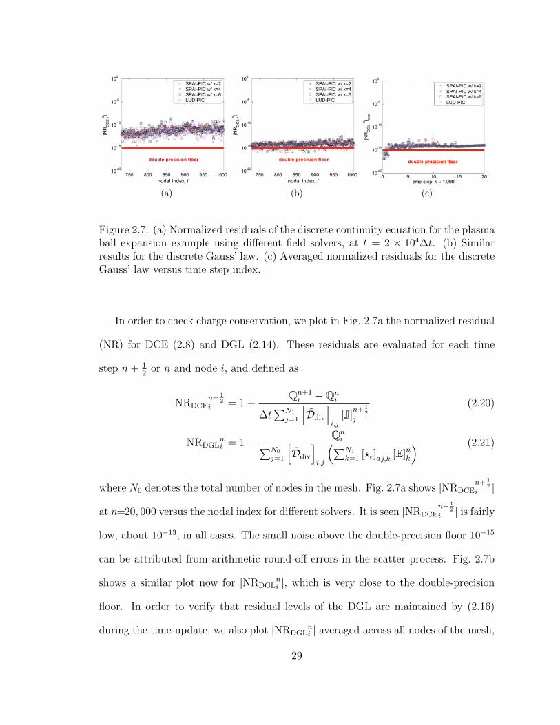
nodal index, i

(a)

nodal index, i

(b) (c)

Figure 2.7: (a) Normalized residuals of the discrete continuity equation for the plasmaball expansion example using different field solvers, at t = 2 × 104∆t. (b) Similarresults for the discrete Gauss’ law. (c) Averaged normalized residuals for the discreteGauss’ law versus time step index.

In order to check charge conservation, we plot in Fig. 2.7a the normalized residual

(NR) for DCE (2.8) and DGL (2.14). These residuals are evaluated for each time

step n+ 12

or n and node i, and defined as

NRDCEn+ 1

2i = 1 +

Qn+1i −Qn

i

∆t∑N1

j=1

[Ddiv

]i,j

[J]n+ 1

2j

(2.20)

NRDGLni = 1− Qn

i∑N0

j=1

[Ddiv

]i,j

(∑N1

k=1 [?ε]aj,k [E]nk

) (2.21)

where N0 denotes the total number of nodes in the mesh. Fig. 2.7a shows |NRDCEn+ 1

2i |

at n=20, 000 versus the nodal index for different solvers. It is seen |NRDCEn+ 1

2i | is fairly

low, about 10−13, in all cases. The small noise above the double-precision floor 10−15

can be attributed from arithmetic round-off errors in the scatter process. Fig. 2.7b

shows a similar plot now for |NRDGLni |, which is very close to the double-precision

floor. In order to verify that residual levels of the DGL are maintained by (2.16)

during the time-update, we also plot |NRDGLni | averaged across all nodes of the mesh,

29

i.e. |NRnDGL|ave =

∑N0

i=1 NRDGLni /N0 as a function of the time step n in Fig. 2.7c. As

seen, |NRnDGL|ave has nearly constant values close to the double-precision floor, with

only a very small increase due to cumulative round-off error.

2.3.3 Electron beam in a vacuum diode

In order to further verify charge conservation and stability for long-time simula-

tions, we simulate next an electron beam accelerated by a vacuum diode. The domain

Ω = (x, y) ∈ [0, 1]2 has lateral walls representing anode and cathode surfaces with

potential difference set as 1.5×105 [V]. The top and bottom boundaries of the domain

are truncated by a PML. The unstructured mesh has 2301 faces, 3524 edges, and 1224

nodes. The time step interval is set to ∆t = 270 [ps], and the simulation is run up to

16.2 [µs]. Each superparticle used in the simulation represents 50×106 electrons. For

the thermionic emission of electrons from the cathode at the left boundary, a slow ini-

tial mean velocity of 104 [m/s] is assumed for the electrons. Fig. 2.8 presents snapshots

of the particle distribution and the self-field (electric) profile. Fig. 2.8a and Fig. 2.8d

show the field and particle distribution for the charge-conserving EM-PIC algorithm

with LU-based implicit field solver. Fig. 2.8b and Fig. 2.8e show the field and particle

distribution for the charge-conserving EM-PIC algorithm with SPAI-based (k = 2)

explicit field solver. Finally, Fig. 2.8c and Fig. 2.8f show the field and particle dis-

tribution for an EM-PIC with LU-based implicit field solver and conventional gather

step (non-charge-conserving on an unstructured grid) where edge currents are ob-

tained from the straightforward projection of the instantaneous product qv, summed

over all particles, onto the edge element W(1)j , i.e.

30

(a) (b) (c)

(d) (e) (f)

Figure 2.8: Results for the accelerated electron beam at t = 6 × 104∆t. (a) (b)Particle distribution snapshot from charge-conserving EM-PIC algorithms using anLU-based implicit solver and a SPAI-based (k = 2) explicit solver, respectively .(c) Particle distribution snapshot from a conventional (non-charge conserving on theunstructured grid) EM-PIC algorithm with an LU-based implicit solver. (d) (e) (f)Corresponding electric-field profile distributions.

Jn+ 12

j =∑p

qpvn+ 1

2p ·W(1)

j

(xn+ 1

2p

)(2.22)

where xn+ 1

2p = (xn+1

p + xnp )/2. In the latter case, violation of the continuity equation

produced spurious bunching of the charges into strips of higher density. In addition,

the self field is highly asymmetric and randomly oriented near the beam center. These

31

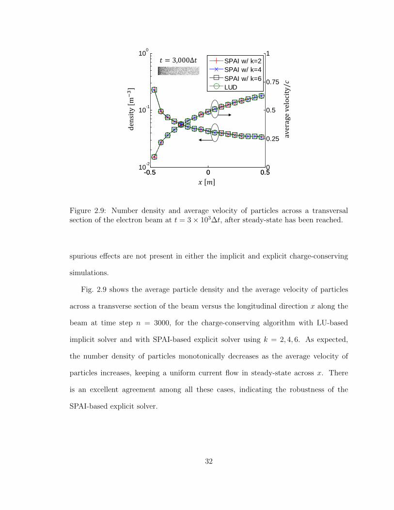
-0.5 0 0.510-2

10-1

100

-0.5 0 0.50

0.25

0.5

0.75

1SPAI w/ k=2SPAI w/ k=4SPAI w/ k=6LUD

dens

itym−3

𝑥𝑥 𝑚𝑚

aver

age

velo

city

/𝑐𝑐

𝑡𝑡 = 3,000∆𝑡𝑡

Figure 2.9: Number density and average velocity of particles across a transversalsection of the electron beam at t = 3× 103∆t, after steady-state has been reached.

spurious effects are not present in either the implicit and explicit charge-conserving

simulations.

Fig. 2.9 shows the average particle density and the average velocity of particles

across a transverse section of the beam versus the longitudinal direction x along the

beam at time step n = 3000, for the charge-conserving algorithm with LU-based

implicit solver and with SPAI-based explicit solver using k = 2, 4, 6. As expected,

the number density of particles monotonically decreases as the average velocity of

particles increases, keeping a uniform current flow in steady-state across x. There

is an excellent agreement among all these cases, indicating the robustness of the

SPAI-based explicit solver.

32

2.3.4 Electron Bernstein waves

Electron Bernstein waves are instrumental for many applications such as plasma

heating, driving plasma currents, and temperature measurement diagnostics [2]. Such

waves are present in over-dense plasmas otherwise inaccessible to electromagnetic

(EM) electron cyclotron waves. Because electron Bernstein wave propagation is only

possible inside the magnetized warm plasma, mode conversion from EM waves in-

cluding ordinary (O) or extraordinary (X) modes [2] should be performed.

Here, we analyze dispersion characteristics of electron Bernstein waves propagat-

ing in the magnetized warm plasma by using the proposed FETD-PIC algorithm on

irregular grids. It is shown that the use of non-charge-conserving scatter algorithms in

FETD-PIC simulations induces a spurious static (self-)field due to charge deposition

on the grid and, as a result, produces more noisy spectral bands. In contrast, the

proposed charge-conserving FETD-PIC solver [1,51,56] is shown to produce sharper

spectral bands with less noise.

Magnetized warm plasmas can support two types of waves both propagating and

polarized in a direction perpendicular to the stationary magnetic field: (i) X mode

and (ii) electron Bernstein waves. In what follows, we compare the dispersion relations

for the X mode and electron Bernstein waves obtained analytically and numerically

by means of FETD-PIC simulations.

We assume a z-directed stationary magnetic field and electron Bernstein wave

propagation along x, with the same conditions as used in [87]. Consider a magne-

tized warm plasma with electron density ne = 2.4 × 1020 [m−3] and static applied

magnetic field ~B = 5.13z [T]. The electrons have initial random distribution over

[0.0005, 0.012] × [0, 0.000025] and Maxwellian distribution for the thermal velocity

33

Figure 2.10: Simulated ω × k dispersion diagram for the X mode propagation andfor electron Bernstein waves in a magnetized warm plasma. Here ωpe is the plasmafrequency and ∆x is the grid spacing, chosen uniform. The analytical results areindicated by the red dots in the diagram. Note that the use of a charge-conservingscatter step in PIC algorithm as described in [1] reduces the numerical noise and yieldscleaner spectral bands in the numerically generated band diagrams. In addition,a charge-conserving scatter step mitigates the spurious DC field cause by spuriouscharge accumulation on the grid nodes, as observed at the bottom of the zoomedplots. Overall, a very good agreement is observed between the numerical and theanalytical results.

with |~vth| = 0.07c. We set the total number of (macro-)particles in the simulation

equal to 13,800, corresponding to a scaling factor of 5× 109. The motion of ions (of

mass mi) is neglected since mi/me ≈ 1, 838, where me is the electron mass. Also, we

have ωpe = 8.7 × 1011 [rad/s] and ωce = 9.0 × 1011 [rad/s], where ωpe is the plasma

frequency [rad/s] and ωce is the gyrofrequency [rad/s]. Using the FETD-PIC simula-

tion data, we perform a Fourier analysis of electric field sampled in space and time

to obtain the dispersion relation ω(kx) for the X mode and for the electron Bernstein

wave.

Fig. 2.10 shows the dispersion relations computed analytically and numerically.

The reference analytical result for this problem is obtained from [2]. It can be seen

34

that the X mode is dominant for small kx, but as kx increases the electron Bern-

stein wave becomes dominant. The two close-in views compare results from charge-

conserving and non charge-conserving EM-PIC simulations. In the latter case, a

strong spurious static (self-)field is produced, which perturbs the particle trajectories

and is evidenced by the noisy spectral bands. The absolute spectral resolution is

affected by the time step increments employed in the EM-PIC simulation. With this

in mind, we have chosen identical increments for both simulations.

2.4 Conclusion

We have developed a EM-PIC algorithm suited for unstructured grids that com-

bines a local explicit field solver with a charge-conserving scatter-gather scheme. A

sparse approximate inverse is pre-computed to obviate the need for a linear solver at

each time step and to retain the local nature of the algorithm. Excellent agreement

was verified between EM-PIC simulations utilizing the proposed field solver and a con-

ventional (implicit) field solver based on a LU-solver. The explicit and local nature of

the proposed EM-PIC algorithm makes it suitable for integration with asynchronous

time stepping techniques as well.

35

Chapter 3: Relativitic Extension of Particle-Pusher

Particle-in-cell (PIC) algorithms [11–13, 88, 89] have been a very successful tool

in many scientific and engineering applications such as electron accelerators [59, 60,

90], laser-plasma interactions [88, 91–94], astrophysics [95, 96], vacuum electronic de-

vices [56, 97, 98] and semiconductor devices [99–102]. In many cases, the particles

of interest are often in the relativistic regime and the relevant physical phenomena

need to be described by taking into account fully relativistic effects. Relativistic PIC

algorithms can be found in a variety of references [90–94,99,103–106].

In this chapter, the previously developed charge conserving FETD PIC algorithm

developed in [1, 51] for time-dependent Maxwell-Vlasov equations is extended to the

relativistic regime. In particular, we integrate Boris [107], Vay [38], and Higuera-

Cary [108] relativistic pushers in the conservative PIC-FETD algorithm for solving

time-dependent Maxwell-Vlasov equations and provide a brief comparison among

them. Several examples such as particle cyclotron motion, harmonic particle oscil-

lation in the Lorentz-boosted frame, and relativistic Bernstein modes in magnetized

charge-neutral (pair) plasmas are presented for validation. We adopt MKS units

throughout this work.

36

3.1 Particle-pushers in the relativistic regime

In the particle update step, the particle mass is modified to account for relativistic

effects such that

drpdt

=upγp, (3.1)

dupdt

=q

m0

[E (rp, t) + vp ×B (rp, t)] , (3.2)

where up = γpvp, vp is the velocity of the p-th particle, and γp is its relativistic factor

defined as γ−2p = 1− |vp|2/c2. Using the central-differences to approximate the time

derivatives, Eqs. (3.1) and (3.2) are discretized as

rn+1p − rnp

∆t=

un+ 1

2p

γn+ 1

2p

, (3.3)

un+ 1

2p − u

n− 12

p

∆t=

q

m0

[Enp + vp ×Bn

p

]=

q

m0

(Enp +

upγp×Bn

p

), (3.4)

where vp is the mean particle velocity between the n± 12

time steps, which can also

be approximated as up/γp with up = γpvp.

In the non-relativistic case, γp → 1, vp can be chosen based on the midpoint rule,

viz. vnp = vnp =(vn+ 1

2p + v

n− 12

p

)/2, to obtain updated phase coordinates explicitly.

In this case, the (non-relativistic) Boris algorithm is typically used not only due to its

computationally-efficient velocity update obtained by separating irrotational (electric)

and rotational (magnetic) forces but also because of its long-term numerical stability.

The latter property essentially means that, in spite of not being symplectic, the non-

relativistic Boris algorithm preserves phase-space volume such that it provides energy

conservation bounded within a finite interval. Note that every symplectic integrator

guarantees phase-space volume-preservation but not vice-versa. In contrast, in the

37

relativistic regime vp should be carefully determined to accurately model the kinetics

of high-energy particles. Next, we examine in detail three different relativistic pushers

proposed by Boris, Vay, and Higuera-Cary.

3.1.1 Relativistic Boris pusher

The main tenet of the relativistic Boris pusher is basically similar to the non-

relativistic-Boris-pusher, viz. separation of irrotational and rotational forces [89].

Importantly, it averages vp as

vp,B =v(un+ 1

2p − εnp

)+ v

(un− 1

2p + εnp

)2

(3.5)

where v (u) = u/√

1 + |u|2 /c2, εnp = αEnp , and α = q∆t/2m0. The particle velocity

update in the relativistic Boris pusher follows the procedure below [89]

u−B = un− 1

2p + εnp , (3.6)

u′

B = u−B + u−B × tB, (3.7)

u+B = u−B + u

′

B × sB, (3.8)

un+ 1

2p = u+

B + εnp , (3.9)

where u−B,u′B, and u+

B are auxiliary vectors and the subscript B refers to the Boris

algorithm. In addition, tB = βnp /γp,B, sB = 2tB/ (1 + |tB|2), and βnp = αBnp . The

factor γp,B is computed as

γp,B =√

1 + |u−B|2/c2 =√

1 + |u+B|2/c2, (3.10)

and to obtain Bnp , we set:

Bnp =

1

2

(Bn+ 1

2p + B

n− 12

p

). (3.11)

38

Note that the relativistic Boris pusher has two variants: with and without correc-

tion. The relativistic Boris pusher without correction uses tB as defined above. The

relativistic Boris pusher with correction uses tB = (βp/|βp|) tan(∣∣βnp ∣∣/γp,B) instead.

The separation of two different forces can be easily observed by substituting Eqs.

(3.6) and (3.9) into Eq. (3.4), which results in

u+B − u−B = α

(u+B + u−Bγp,B

×Bnp

). (3.12)

In Eq. (3.12), the effect of Enp is completely removed, so that only magnetic rotation

is effected.

The relativistic Boris pusher preserves volumes in the phase-space because the

determinant of Jacobian for time-update map, ψnB :(rnp ,u

n− 12

p

)→(rn+1p ,u

n+ 12

p

)equals to one [107, 108]. To verify that, we express determinant of the Jacobian for

ψnB as ∣∣∣∣∣∣ ∂ψnB

∂(rnp ,u

n− 12

p

)∣∣∣∣∣∣ =

∣∣∣∣∣ ∂rn+1p /∂rnp ∂rn+1

p /∂un− 1

2p

∂un+ 1

2p /∂rnp ∂u

n+ 12

p /∂un− 1

2p

∣∣∣∣∣ , (3.13)

where from (3.3) we have that ∂rn+1p /∂rnp = ¯I + ∂u

n+ 12

p /∂xnp , with ¯I being the 3 × 3

identity matrix. If we assume that electromagnetic fields to be uniform along the

particle trajectory during one time step, ∂un+ 1

2p /∂xnp = 0. In addition, it is clear that

∂xn+1p /∂xnp = ¯I. Substituting u

n+ 12

p from (3.4) into (3.3) and taking a derivative w.r.t.

∂un− 1

2p of the resulting equation, we obtain ∂xn+1

p /∂un− 1

2p = ∆t

(∂u

n+ 12

p /∂un− 1

2p

). As

a result, the determinant in (3.13) simply takes the form of∣∣∣∂u

n+ 12

p /∂un− 1

2p

∣∣∣. This

derivative can be computed by splitting one time-update into two half-time-updates

and evaluating each serially as follows∣∣∣∂un+ 1

2p /∂u

n− 12

p

∣∣∣ =

∣∣∣∣∣∂un+ 1

2p /∂up

∂un− 1

2p /∂up

∣∣∣∣∣ =

∣∣∣∂un+ 1

2p /∂up

∣∣∣∣∣∣∂un− 1

2p /∂up

∣∣∣ . (3.14)

39

But since [108]∣∣∣∂un+ 1

2p /∂up,B

∣∣∣ =∣∣∣∂u

n− 12

p /∂up,B

∣∣∣ = 1 +

∣∣βnp ∣∣2 +(βnp · up,B

)2

γ4p,B

, (3.15)

it follows that∣∣∣∂u

n+ 12

p /∂un− 1

2p

∣∣∣ = 1 and therefore the relativistic-Boris-pusher is phase-

space volume-preserving. This means that energy conservation is attained for long

time simulations down to machine precision accuracy (with residual error stemming

from round-off errors). However, the main disadvantage of the relativistic-Boris-

pusher is that it cannot accurately capture correct the particle acceleration by electric

forces. This is because magnetic rotation fails to consider the varying relativistic

factor due to electric field effects during the magnetic rotation.

3.1.2 Vay pusher

The Vay pusher corrects trajectories of relativistic particles experiencing electric

fields by averaging vp as

vp,V =v(un+ 1

2p

)+ v

(un− 1

2p

)2

. (3.16)

The particle velocity update follows the procedure below [38]

unp = un− 1

2p + εnp + v

n− 12

p × βnp , (3.17)

u′

V = unp + εnp , (3.18)

un+ 1

2p = |sV |

[u′

B +(u′

V · tV)

tV + u′

V × tV

], (3.19)

γn+ 1

2p =

√0.5σ + 0.5

√σ2 + 4×

(∣∣βnp ∣∣2 + u∗2V

), (3.20)

σ = γ′2V −

∣∣βnp ∣∣2 , (3.21)

where tV = βnp /γn+ 1

2p , sV = 2tV / (1 + |tV |2), u∗V = u

′V ·βnp /c, and γ

′V =

√1 +

∣∣u′V ∣∣′2 /c2.

The Vay pusher correctly models energetic particle motion under electric forces with

40

Lorentz (relativistic) invariance. In other words, the relation between the particle’s

trajectory observed in a (relativistic) moving and laboratory frames satisfy Lorentz

transformation.

3.1.3 Higuera-Cary pusher

The Higuera-Cary pusher provides an accurate treatment of electric forces by

approximating the average velocity as [108]

vp,H = v

(un+ 1

2p + u

n− 12

p

2

). (3.22)

The particle velocity update is basically similar to Boris algorithm except for the

relativistic factor as

γp,H =1

2

[γ2p,B −

∣∣βnp ∣∣2 +√(γp,B −

∣∣βnp ∣∣)2+ 4

(∣∣βnp ∣∣2 +∣∣βnp · u−B∣∣2)

]. (3.23)

Therefore, the Higuera-Cary pusher is also phase-space volume-preserving.

3.2 Numerical results

3.2.1 Synchrocyclotron

To validate the relativistic PIC formulation, we first examine a synchrocyclotron

example. As electrons usually have velocities near to the speed of light in this case,

progressively more energy needs to be delivered to accelerate them due to relativistic

effects. The relativistic mass increase results in a lower orbital (cyclotron) frequency.

Therefore, the driving RF electric field should have variable frequencies matching this

relativistic cyclotron frequency. Fig. 3.1b illustrates the computational mesh used for

the simulation where centripetal force from external magnets is present in the red

41

(a) (b)

Figure 3.1: (a) Cyclotron configuration. (b) Computational domain, where the bluevertical strip indicates the region where an external longitudinal RF electric field isapplied. The DC magnetic field is applied in the whole computational region exceptfor the RF acceleration gap (red).

region leading to a circular motion of electrons and a longitudinal RF electric field is

present in the vertical blue strip leading to a periodic electron acceleration.

Fig. 3.2a shows the electron cyclotron motion in a non-relativistic regime, where

the relativistic factor is assumed to be one. An electron is injected at (x, y) =

(0.52, 0.5) m with an initial velocity of |v0| = v0 = 1× 107 m/s. The static magnetic

force is determined to be Bz = m0v0/qr = 2.84281 × 10−3 T for an initial orbital

radius r of 0.02 m and the RF electric force is set to be Ex = 2 × 105 V/m. The

thickness of the vertical strip in which the longitudinal electric field is present is 0.02

m. As can be seen, the spacing of two adjacent orbits becomes successively smaller

due to the increasing velocity. Fig. 3.2b shows the trajectory of the electron with

42

6/29/2015 7

Settings

# of time steps : 5000Time increment (Δt) : 4e-11 sec.Initial velocity (v0) : 1e7 m/sInitial position : (0.52, 0.5)Initial radius of circular trajectory : 0.02 mGap between dees : 0.02 m

Magnetic force (Bz) = mv/(rq) = 2.84281e-3 Wb/m2

Electric force (Ex) = 2e5 V/m

Non-relativistic caseRegion of acceleration

(a)

6/29/2015 8

relativistic case, unsynched relativistic case, synched

(b)

6/29/2015 8

relativistic case, unsynched relativistic case, synched

(c)

Figure 3.2: Electron trajectories on a cyclotron: (a) Non-relativistic, (b) Relativistic,unsynchronized, and (c) Relativistic, synchronized.

same initial conditions. For this example, we use the PIC formulation with the rel-

ativistic Boris pusher with correction discussed in the previous section. In this case,

the frequency of the RF electric force is set to be constant (79.6 MHz), which results

in an unsynchronized phase between particle velocity and electric force and a mixed

trajectory. In Fig. 3.2c, the frequency of the RF electric field is matched to the orbital

frequency of the electron, the synchrocyclotron frequency given by f = qB/2πγm0.

This frequency is shown, together with the relativistic factor, as a function of the

number of time steps of the simulation, in Fig. 3.3. Therefore, the in-phase accelera-

tion is maintained at all times and a circular trajectory is observed at higher energies.

Note that the total distance over which an electron moves in this case is shorter than

that for the non-relativistic case because of its smaller speed caused by the relativis-

tic mass. Fig. 3.4 shows the electron velocity magnitudes in the three cases. It is

clearly observed that the deceleration occurs near 4000 time steps for the second case.

43

Figure 3.3: Orbital frequency and relativistic factor for the case shown in Fig. 3.2c.

Also, the third case shows slightly smaller magnitudes than the first one due to the

relativistic mass.

Tables 3.1, 3.2, and 3.3 provide a verification of Gauss’ law. The amount of

charge on arbitrarily selected mesh nodes is recorded at different time steps. As

the rightmost columns in these tables show, the normalized residual associated to

the discrete version of Gauss’ law is very small and near the double precision floor

(< 10−15).

3.2.2 Harmonic oscillations in Lorentz-boosted frame

In order to compare how accurately the three different kinds of relativistic particle

pushers capture relativistic E ×B drift motions, we consider a harmonic oscillatory

motion of a positron in the Lorentz-boosted frame with γf = 2 such as in [38]. Initial

parameters of the harmonic motion are transformed via the Lorentz transformation

into the moving frame along y and PIC simulations are performed in the moving

frame. At the end of simulations, we re-transform the phase coordinates from the

44

0 1000 2000 3000 4000 5000106

107

108

109

time steps

|v|

non-relativisticrelativistic, unsynchedrelativistic, synched

Velocity comparison

3x108

Figure 3.4: Comparison of electron velocity magnitudes of the three cases shown inFig. 3.2.

Table 3.1: Verification of discrete Gauss’ law for the non-relativistic case (Fig. 3.2a).

n Nodal Index qn S · [?ε] · en∣∣∣ S·[?ε]·en−qnqn

∣∣∣1000 89 -7.62302 ×10−20 -7.62302 ×10−20 1.15269 ×10−14

2000 26 -1.29865 ×10−20 -1.29865 ×10−20 4.95884 ×10−13

3000 110 -3.39127 ×10−20 -3.39127 ×10−20 3.19447 ×10−15

4000 233 -1.10205 ×10−19 -1.10205 ×10−19 1.26699 ×10−14

5000 259 -1.98727 ×10−20 -1.98727 ×10−20 2.24868 ×10−13

45

Table 3.2: Verification of discrete Gauss’ law for the relativistic case without syn-chronization (Fig. 3.2b).


∣∣∣1000 235 -7.20396 ×10−20 -7.20396 ×10−20 7.10129 ×10−14

2000 247 -3.70748 ×10−20 -3.70748 ×10−20 5.20444 ×10−13

3000 83 -5.30434 ×10−20 -5.30434 ×10−20 1.44212 ×10−13

4000 39 -8.31747 ×10−20 -8.31747 ×10−20 2.76415 ×10−14

5000 143 -8.17890 ×10−20 -8.17890 ×10−20 1.83523 ×10−13

Table 3.3: Verification of discrete Gauss’ law for the relativistic case with synchro-nization (Fig. 3.2c).


∣∣∣1000 235 -9.02849 ×10−20 -9.02849 ×10−20 9.86590 ×10−15

2000 179 -4.05879 ×10−20 -4.05879 ×10−20 1.68005 ×10−13

3000 196 -1.75078 ×10−20 -1.75078 ×10−20 4.06155 ×10−13

4000 116 -7.70014 ×10−21 -7.70014 ×10−21 2.83334 ×10−14

5000 332 -8.90351 ×10−20 -8.90351 ×10−20 2.06847 ×10−14

46

Figure 3.5: Motion of harmonic oscillator of a single positron inverse-Lorentz-transformed into Laboratory frame.

moving frame into the laboratory frame by using the inverse Lorentz transformation.

We compare the resultant trajectories of the harmonic oscillators obtained with three

different particle-pushers and analytic predictions in Fig. 3.5. As we discussed in Sec.

C, the relativistic Boris pusher (without or with correction) cannot capture correct

relativistic E × B drift motion; on the other hand, results obtained with the Vay

pusher and Higuera-Cary pusher accurately match the analytic prediction.

3.2.3 Relativistic Bernstein Modes in Magnetized Pair-Plasma

The non-relativistic electron Bernstein mode [2, 109], which is a purely electro-

static plasma wave perpendicularly propagating to a stationary magnetic field, has

47

Figure 3.6: Dispersion relations for classical (non-relativistic) electron Bernsteinmodes of PIC results (Parula colormap) and analytic predictions [2] (dashed redline).

been mainly explored in magnetic plasma confinement fusion as a promising alter-

native to conventional electron cyclotron electromagnetic waves such as the ordinary

(O) or extraordinary (X) modes which have frequency cutoffs associated with plasma

density [110]. The Bernstein mode is free from the density cut-off, and as a re-

sult, it is able to reach the core of over-dense plasmas in Tokamak devices and heat

the plasma electrons effectively. It is well known that conventional non-relativistic

Bernstein waves are present at harmonics of electron cyclotron resonances [2], as

shown in Fig. 3.6, which illustrates dispersion relations, in terms of the normalized

frequency ω = ω/ωc and normalized transverse wavenumber is k⊥ = kxc/ωc, of non-

relativistic electron Bernstein and X modes based on PIC simulations (colormap) and

compare the simulation results with analytic predictions (dashed red line). In this

case, ωc = 9.0 × 1011 rad/s, B0 = 5.13z T, ωp = 8.7 × 1011, n0 = 2.4 × 1020 m−3,

and the initial isotropic speed distribution (equilibrium state) obeys a Maxwellian

48

distribution with vth = 0.07c. The simulation parameters are chosen similar to [87].

Runaway electrons can cause plasma discharge disruptions in fusion devices. The

interaction of runaway electron beams with plasma turbulence requires full electro-

magnetic treatment in relativistic regimes. Relativistic plasma waves propagating

in energetic electron-positron pair-plasmas have also been of interest in astrophysics

(pulsar atmospheres). Therefore, it is desirable to extend the investigation of Bern-

stein modes to the relativistic regime. Recently, analytic works have been done to

characterize the behaviors of Bernstein modes in relativistic pair-plasmas [111–114].

There are several features distinguishing the classical Bernstein wave from the rel-

ativistic one: (1) The classical Maxwellian distribution (equilibrium state) is modi-

fied to the Maxwell-Boltzmann-Juttner distribution (relativistic Maxwellian), (2) the

mobility of positively-charged particles is identical to that of negatively-charged par-

ticles, and (3) the conventional dispersion relations are significantly transformed to

undamped or damped closed curve shapes. In this example, we use the developed

FETD PIC algorithm to perform simulations of Bernstein modes propagating in rel-

ativistic magnetized pair-plasmas and compare the results with analytic predictions.

Analytic prediction

To derive analytic dispersion relations of magnetized plasma waves [2, 111–114],

we should obtain a complex permittivity tensor, ¯ε associated with plasma currents.

First of all, we consider a small perturbation imposed on equilibrium magnetized

49

pair-plasmas with parameters of

fs (r,p, t) = f0,s (p) + f1,s (r,p, t) , (3.24)

B = B0 + B1ei(k·r−ωt), (3.25)

E = E1ei(k·r−ωt), (3.26)

where fs is a distribution function represented in the phase space for the species s,

E is electric field intensity, B is magnetic flux density, and subscriptions of 0 and

1 denote equilibrium and perturbed quantities, respectively. Note that perturbed

electromagnetic fields are proportional to ei(k·r−ωt). Equilibrium relativistic electron-

positron pair-plasmas are typically described by Maxwell-Boltzmann-Juttner (rela-

tivistic Maxwellian) distribution which is given by

fMBJ0 (p) =

(1

4πm02c3

)η

K2 (η)e−ηγ (3.27)

where η = m0ckBT

, kB is the Boltzmann constant, T is the kinetic temperature, K2 (·)

is the modified Bessel function of the second kind, and γ = (1 + p2

c2)−1/2

. The evolu-

tion of the distribution function is governed by the Vlasov equation. Its first-order

approximation takes the form of

df1,s (r,p, t)

dt= −qs (E1 + v ×B1) ei(k·r−ωt) · ∂f0,s (p)

∂p. (3.28)

Substituting Eq. (3.27) into Eq. (3.28) and integrating Eq. (3.28) over time, solutions

for the perturbed distribution function, f1,s can be obtained. Then, plasma currents

are calculated based on f1,s as

J =∑s

qsms

∫pf1,s (r,p, t) d3p =

∑s

¯σs · E1 (3.29)

50

(a) (b)

Figure 3.7: An isotropic 2D Maxwell-Boltzmann-Juttner velocity distribution, f0 (p)for η = 1/20: (a) Speed distribution and (b) relativistic velocity distribution.

where ¯σ is a conductivity tensor from which we obtain the complex permittivity

associated with plasma currents as

¯ε = ε0

(¯I −

¯σ

iωε0

). (3.30)

We are interested in longitudinal electrostatic plasma waves propagating in the x-

direction. Thus, (ω, kx) curves yielding zeros of εxx form the dispersion relations for

Bernstein modes in a magnetized relativistic pair-plasma. The expression for εxx can

be written as [111]

εxxε0

= 1−2ω2

pη

k

2

x

η

K2 (η)

∫ ∞0

p2e−ηγ × 2F3

(1

2, 1;

3

2, 1− γω, 1 + γω;−β2

)dp− 1

,

(3.31)

where 2F3

(12, 1; 3

2, 1− a, 1 + a;−b2

)is a hypergeometric function, which is defined as

2F3

(1

2, 1;

3

2, 1− a, 1 + a;−b2

)=

1

2

∫ ∞0

πa

sin (πa)sin θJa (b sin θ) J−a (b sin θ) dθ,

(3.32)

51

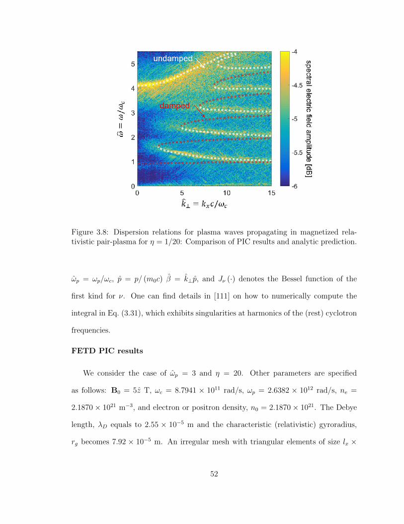
Figure 3.8: Dispersion relations for plasma waves propagating in magnetized rela-tivistic pair-plasma for η = 1/20: Comparison of PIC results and analytic prediction.

ωp = ωp/ωc, p = p/ (m0c) β = k⊥p, and Jν (·) denotes the Bessel function of the

first kind for ν. One can find details in [111] on how to numerically compute the

integral in Eq. (3.31), which exhibits singularities at harmonics of the (rest) cyclotron

frequencies.

FETD PIC results

We consider the case of ωp = 3 and η = 20. Other parameters are specified

as follows: B0 = 5z T, ωc = 8.7941 × 1011 rad/s, ωp = 2.6382 × 1012 rad/s, ne =

2.1870× 1021 m−3, and electron or positron density, n0 = 2.1870× 1021. The Debye

length, λD equals to 2.55 × 10−5 m and the characteristic (relativistic) gyroradius,

rg becomes 7.92 × 10−5 m. An irregular mesh with triangular elements of size lx ×

52

(a) (b)

Figure 3.9: Normalized residuals versus nodal index for (a) discrete continuity equa-tion (DCE) and (b) discrete Gauss law (DGL).

ly is constructed with ly = rg and lx = 1000 × rg and average mesh element size

comparable to λD. The number of nodes, edges, and faces in the mesh are 7252,

18123, 10872, respectively. The left and right boundaries of the mesh are terminated

by perfectly matched layers (PML) [74, 115] to mimic open boundaries. Periodic

boundary conditions (PBC) are applied at the top and bottom boundaries. In order

to obtain the dispersion relation in (kx, ω) for Bernstein waves propagating along

x, we spatially sample the electric field along the x direction at each time-step and

perform a Fourier transform on the resulting data set in (x, t). The PML treatment

of the left and right boundaries not only reduces unwanted reflections but also avoids

aliasing effects in the dispersion relation caused by PBC with low sampling rates and

the presence of image sources. Whenever particles meet a PBC boundary wall, they

are removed and reassigned the same relative position on the other PBC boundary

wall and same momentum. The total number of superparticles for e and p species

representing 1.7222×1010 electrons and positrons, respectively, is set to Nsp,e+Nsp,p =

4 × 105. Note that Nsp,e and Nsp,p are identical, and our simulation is initialized

53

so that the average number of superparticles per grid element is around 40. This

number attempts to provide a good trade-off between simulation speed and the rate

of plasma self-heating. Initially, superparticles are uniformly distributed on the mesh

in a pairwise fashion. i.e. with each species-e superparticle collocated with another

species-p superparticle. This arrangement produces zero initial electric field. Based

on an Maxwell-Boltzmann-Juttner distribution for the initial speed as depicted in Fig.

3.7a), superparticles for species e are then launched in random 2D directions. The

corresponding p superparticles are simultaneously launched with same speed in the

opposite direction. Consequently, both species of superparticles follow an isotropic

Maxwell-Boltzmann-Juttner velocity distribution, see Fig. 3.7b. Fig. 3.7a compares

the Maxwell-Boltzmann-Juttner distribution and classical Maxwellian distribution.

It can be seen that the classical Maxwellian velocity distribution starts to gradually

deviate from the relativistic one above the most probable velocity, which is about

v/c = 0.21. We simulate up to 100, 000 of time-steps and employ ∆t = 0.01 ps chosen

with Courant factor of 0.2. Then, we perform space and time Fourier transforms of

sampled data to obtain the dispersion relations.

Fig. 3.8 illustrates the dispersion relations for relativistic Bernstein waves with

η = 1/20, compared to analytic predictions. It is observed in Fig. 3.8 that there

are solutions of curved shape between every two neighboring harmonics of the (rest)

cyclotron frequency. Our PIC simulations capture this feature quite well, which dis-

tinguishes the relativistic Bernstein wave from the classical one as predicted by theory.

It is also interesting to note that every upper curve of each solution is considerably

weaker since, as pointed out in [113], the damping coefficient for the upper curve is

larger than that for the lower curve. In addition, there are two kinds of stationary

54

modes at around ω = 0.9 and ω = 4.1. As shown in [111], these stationary modes are

nearly dependent on ωp and the gap and location frequency between two stationary

modes becomes smaller as η decreases (ultra-relativistic). It should be noted that

even though PIC simulations are somewhat noisy, some physical damping should be

certainly present (especially in warm plasmas and for high kx). Introducing a spec-

tral filtering scheme to reduce the noise may lead to heating and artifacts. It is

highly desirable to compare numerical results with analytical predictions here since

although there are many PIC codes available, there is little understanding of how

well PIC codes describe classical plasma effects, like Bernstein modes. It is expected

that the most efficient way to reduce the numerical noise is to use high-order particle

gather/scatter procedures. We leave these issues to a future work.

In order to check charge conservation, Fig. 3.9 illustrates normalized residuals

for the discrete continuity equation (DCE) (Fig. 7.15a) and the discrete Gauss law

(DGL) (Fig. 7.15b) across all mesh nodes at three different time-steps, n = 10, 000,

20, 000, and 30, 000. It is observed in Fig. 7.15a and Fig. 7.15b that the normalized

residuals are fairly low, near the double precision floor, which again indicates that no

spurious charges are deposited at the nodes.

3.3 Conclusion

A finite element time-domain particle-in-cell algorithm is presented to simulate the

relativistic Maxwell-Vlasov equation. The key feature of the algorithm is to combine

a new charge-conserving scatter/gather scheme for irregular meshes with relativistic

particle pushers for efficient plasma simulations. Three different relativistic particle

55

pushers are considered and briefly compared. Several numerical examples are provided

for illustration purposes.

56

Chapter 4: Multipactor

Resonant electron discharges from metallic or dielectric surface, also known as

multipactor effects, are often observed in high-power radio frequency (RF) devices

such as accelerators, vacuum tubes, and satellite payloads. This effect generally

degrades and limits device performance [116,117]. On the other hand, discharge effects

can be harnessed by various technologies including electron guns, plasma displays, and

for energy dissipation to protect highly sensitive receivers [118]. As a bridge between

the theoretical and experimental analysis, computer simulations have been employed

in recent years to analyze multipactor effects via electromagnetic particle-in-cell (EM-

PIC) algorithms [11, 119, 120], which basically solve Maxwell-Vlasov equations for

tracking the non-linear evolution of coarse-grained distribution of charged particles

(tenuous plasma) and its interaction with the RF field.

In this chapter, we numerically investigate multipactor effects using the novel

EM-PIC algorithm based on the finite-element time-domain (FETD) method im-

plemented on unstructured (irregular) grids [1, 51]. The use of unstructured grids

enables local mesh refinement and simulation of complex geometries with minimal

geometrical defeaturing, see Fig. 4.7 below. The present algorithm attains energy

and charge conservation [51], a feature that has eluded previous EM-PIC algorithm

implementations on irregular grids. In addition, the present algorithm implements

57

Figure 4.1: Schematic illustration of a typical SEE process in an irregular-grid-based EM-PIC simulation. Note that electric current densities by the primary or secondaries aredeposited on red- or blue-highlighted edges, respectively.

the Furman-Pivi probabilistic model [40], based on a broad phenomenological fit to

experiment data, to obtain accurate simulations of secondary electron emission (SEE)

process (rather than a conventional monoenergetic one). We illustrate the proposed

algorithm by examining multipactor effects taking place on waveguides with flat or

corrugated (triangularly-grooved) walls. We contrast the evolution of the electron

population in various cases and investigate the respective saturation process arising

from self-field counterbalance effects.

We illustrate the proposed algorithm by examining multipactor effects taking place

on waveguides with flat or corrugated (triangularly-grooved) walls. We contrast the

evolution of the electron population in various cases and investigate the respective

saturation process arising from self-field counterbalance effects.

58

(a) (b)

(c) (d)

Figure 4.2: Comparison of simulation and experimental results for SEE on copper [(a) and(b)] and stainless steel [(c) and (d))] surfaces. Figures (a) and (c) illustrate SEY δ versusthe primary incident energy. Figures (b) and (d) show the emitted-energy spectrum dδ/dE.

59

4.1 Irregular-Grid EM-PIC Algorithm integrated with Furman-Pivi model

We integrate the probabilistic Furman-Pivi SEE model into the EM-PIC algo-

rithm. In this model [40], three types of (macroscopic) mechanisms producing sec-

ondary electrons are incorporated: (1) backscattered (BS) or almost elastic, (2) re-

diffused (RD) or partially elastic, and (3) true-secondary (TS) or inelastic. A typical

scenario for the SEE process during one time step ∆t (i.,e. from time-step n to n+1) in

the EM-PIC algorithm is illustrated in Fig. 4.1. When the primary electron (red solid

line) trajectory intersects a metallic surface, the SEE algorithm launches secondaries

(BS, RD, or TS, indicated by blue solid lines) via a stochastic process governed by

the primary electron kinetic energy and incidence angle. Once all trajectories of the

secondary electrons are obtained, the scatter step in the EM-PIC algorithm converts

the electron trajectories into equivalent electric currents along edges of the irregu-

lar grid. In this process, the trajectory of the primary inside the metal (red dashed

line) is discarded and the primary becomes dummy. As noted, the use of irregular

grids enables a more accurate description of complex geometries, including curved

and textured-surface treatments employed to suppress the multipactor effects [121]

or found in electron gun technologies. In the present EM-PIC algorithm, implemen-

tation of electron emission process from curved boundaries is more natural than in

regular-grid-based EM-PIC algorithms. This is because the latter necessitates the use

of ad hoc cut-cell methods or conformal finite-difference approaches [21]. For the pur-

pose of implementing the field boundary conditions, the metallic surfaces are assumed

as perfect electric conductors (PEC) at RF frequencies. A summary description and

a pseudocode implementing the SEE process are provided in Appendix II.

60

(a) (b)

Figure 4.3: Geometrical illustration of exact charge conservation on irregular grids for aprimary impact (also applicable for secondary electrons emitted on the opposite way) atPEC surfaces during ∆t. Plot (a) depicts the charge variation rate at jth node. Plot (b)depicts the divergence of current on jth node, which is equal to the sum of ith and kth

currents.

4.2 Charge-conserving scatter near conducting surface

Given a particle trajectory (motion) during one unit time interval ∆t, the scatter

step of a PIC algorithm assigns the consequent current onto the edges of the grid

around the metallic boundary. From Maxwell’s equations, the tangential electric and

magnetic field components at a PEC surface are zero. As such, the present field solver

enforces zero tangential fields at the metallic surfaces. A charged particle next to a

metallic surface will induce a surface charge distribution on the surface that can be

obtained from image theory assuming a charged particle sufficiently close to a locally

planar surface. As the charged particle approaches the surface from the grid domain,

the fields due to the charged particle and its image will cancel each other. When

the particle hits the surface, the associated field becomes zero and the charge is then

61

absorbed (discarded) by the EM-PIC algorithm. On the grid, charge conservation is

obtained by a proper balance between the variation of the node-based charges and

the edge-based currents that touch a given node. This is illustrated in Fig. 4.3: when

a single charged particle inside the kth face (triangle) crossed the metallic (PEC)

surfaces and leaves the problem domain (dashed black line), there is an associated

non-zero grid charge at the ith node (green square) and associated currents at the jth1

(red) and jth2 (blue) edges. From a geometrical viewpoint, the grid charge variation

rate on ith node, which from the Whitney 0-form expansion is associated to the green-

colored area divided by ∆t, is equal to the sum of the grid currents flowing in/out

of the ith node, which is the sum of two grid currents at jth1 and jth2 edges. Form

the Whitney 1-form expansion of the currents, the latter is equivalent to the sum of

two areas colored in red and blue. A mathematical derivation of these results can be

found in [1, 51].

4.3 Furman-Pivi SEE model implementation

The basic steps implementing the probabilistic Furman-Pivi SEE model are sum-

marized in the EM-PIC code are summarized in Algorithm 1. Initially, a vacant 1-D

workspace of size Np,max × 1 is set for either dummy or effective macroparticles. At

each time-step, a for loop is performed with respect to the index p that checks whether

or not the p-th particle is dummy by Dummy Effective Checker, yielding the integer

a: 1 (effective) or 0 (dummy). If a = 1, Particle Acceleration and Particle Push

accelerate and push the p-th particle during one time-step, respectively, and yield

its updated velocity vn+ 1

2p and position xn+1

p . Afterwards, Impact Checker tests the

occurrence of the impact of p-th particle on metal surfaces, producing the integer b:

62

1 (impact) or 0 (no impact). If b = 0, scatter uses xnp and xn+1p to compute grid

electric currents, jn+ 12 . If b = 1, the SEE algorithm determines the impact position,

energy, and angle via Impact Position, Energy, and Angle, respectively. After

the primary’s trajectory between xnp to impact position ximpp is converted to an grid

electric current, the primary particle is discarded (absorbed). In accordance with

the impact information obtained above, the number of the secondaries NSEY is com-

puted by Compute SEY based on the Furman-Pivi probabilistic SEE model. Another

for loop is performed to compute the launching energy and angle for the secondaries.

This information is are saved in vacant bins found by Min Dummy Finder. Finally, the

new secondaries are launched and their current transferred to the grid in the scatter

step.

4.4 Numerical Results and Discussion

4.4.1 Verification of SEE model in EM-PIC simulations

In order to validate the probabilistic SEE process for embedding in present EM-

PIC algorithm, we carried out impact simulations on copper and stainless steel sur-

faces without external fields. We obtained statistical averages of two important pa-

rameters: the secondary electron yield (SEY) δ and the emitted-energy spectrum

dδ/dE. We compare the simulation results against experimental data from [122].

Fig. 4.2a and Fig. 4.2c plot δ versus the incident electron energy [eV] for normal

incidence when the superparticle number Np is set equal to 5 × 105, for copper and

stainless steel surfaces, respectively. Fig. 4.2b and Fig. 4.2d show dδ/dE versus the

secondary electron energy assuming primary impact energy E0 = 295 [eV] and E0 =

300 [eV], respectively, and normal incidence. The superparticle number Np in these

63

Algorithm 1: Basic steps for implementation of SEE in the EM-PIC algorithm.

for p ∈ [1, 2, ..., Np,max] doa← Dummy Effective Checker(p);if a == 1 then

vn+ 1

2p ← Particle Acceleration(p);

xn+1p ← Particle Push(p);

b← Impact Checker(p);if b == 1 then

ximpp ← Impact Position(p);d← Impact Energy(p);e← Impact Angle(p);

jn+ 12 ← Scatter

(xnp ,x

impp

);

Delete Primary(p);NSEY ← Compute SEY(d,e);for q ∈ [1, 2, ..., NSEY ] do

r ← Min Dummy Finder();Compute Launch Energy(r);Compute Launch Angle(r);xn+1r ← Particle Push(r);

jn+ 12 ← Scatter

(ximpp ,xn+1

r

);

end

else

jn+ 12 ← Scatter

(xnp ,x

n+1p

);

end

end

end

simulations is 1 × 106. Overall, there is very good agreement between the present

simulation results and the experimental data. We also tested the angular dependence

of the SEE process for various primary incident angles. This is shown in Fig. 4.4,

where it can be seen that grazing incidence generates more secondaries than the

normal incidence, as expected. Note that present algorithm assumes the same angular

distribution function (cosine-like) as introduced in [40].

64

Figure 4.4: Angular dependence of δ on a copper surface.

(a) (b) (c)

Figure 4.5: PIC results for probabilistic SEE model. (a) Superparticle population versustime (RF voltage periods). (b) and (c) Snapshots of particle’s trajectories for copper andstainless steel cases, respectively. These trajectory snapshots are taken during four succes-sive half-periods of the RF signal, i.e.: t/TRF ∈ (0, 0.5), t/TRF ∈ (0.5, 1), t/TRF ∈ (1, 1.5),and t/TRF ∈ (1.5, 2), where TRF = 1/fRF = 0.96 [ns].

65

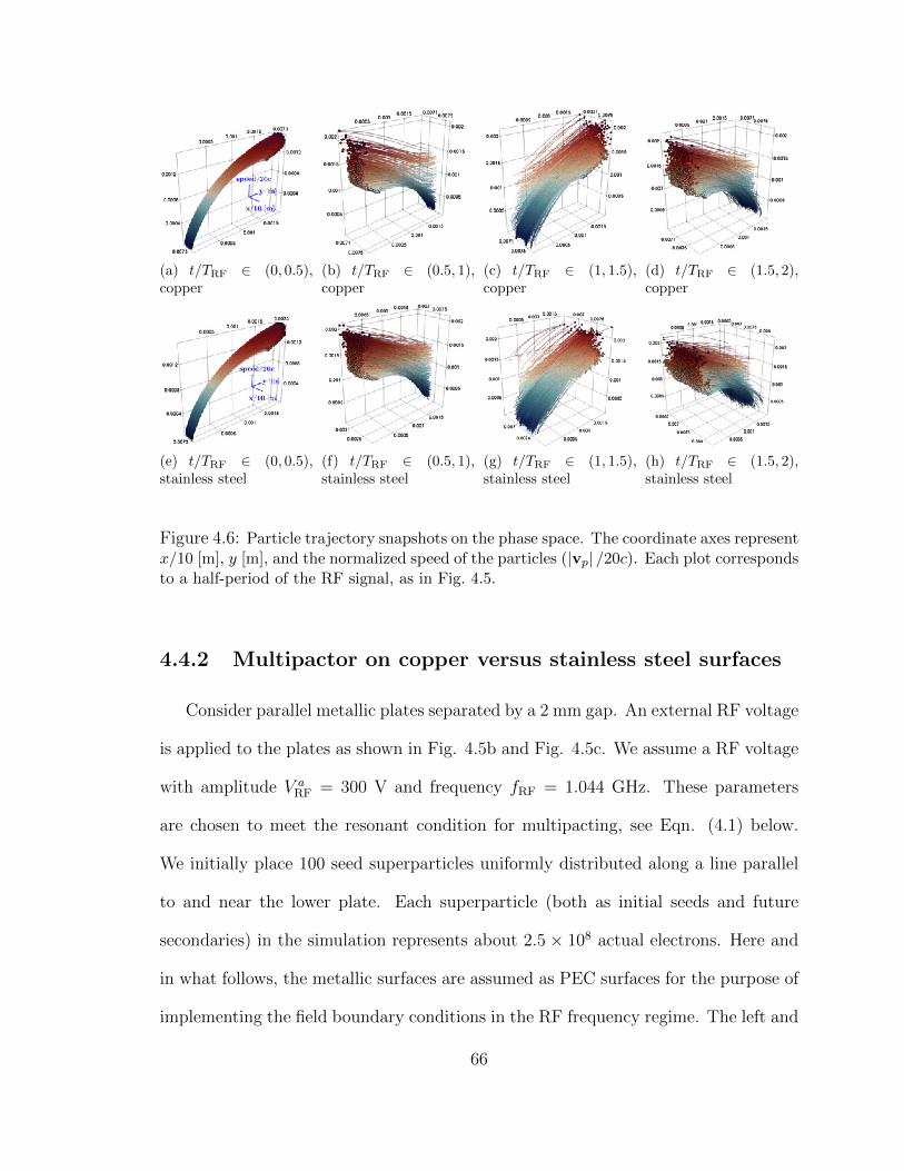
(a) t/TRF ∈ (0, 0.5),copper

(b) t/TRF ∈ (0.5, 1),copper

(c) t/TRF ∈ (1, 1.5),copper

(d) t/TRF ∈ (1.5, 2),copper

(e) t/TRF ∈ (0, 0.5),stainless steel

(f) t/TRF ∈ (0.5, 1),stainless steel

(g) t/TRF ∈ (1, 1.5),stainless steel

(h) t/TRF ∈ (1.5, 2),stainless steel

Figure 4.6: Particle trajectory snapshots on the phase space. The coordinate axes representx/10 [m], y [m], and the normalized speed of the particles (|vp| /20c). Each plot correspondsto a half-period of the RF signal, as in Fig. 4.5.

4.4.2 Multipactor on copper versus stainless steel surfaces

Consider parallel metallic plates separated by a 2 mm gap. An external RF voltage

is applied to the plates as shown in Fig. 4.5b and Fig. 4.5c. We assume a RF voltage

with amplitude V aRF = 300 V and frequency fRF = 1.044 GHz. These parameters

are chosen to meet the resonant condition for multipacting, see Eqn. (4.1) below.

We initially place 100 seed superparticles uniformly distributed along a line parallel

to and near the lower plate. Each superparticle (both as initial seeds and future

secondaries) in the simulation represents about 2.5× 108 actual electrons. Here and

in what follows, the metallic surfaces are assumed as PEC surfaces for the purpose of

implementing the field boundary conditions in the RF frequency regime. The left and

66

right ends of the grid are terminated by a perfectly matched layer (PML) [41]. Copper

and stainless steel have different δ profiles, cf. Fig. 4.2a and Fig. 4.2c in [40]. Except

for primary impacts with very low incident energy, electron avalanches can occur since

δ is overall larger than unity. It is worth noting that in the copper plates most of

the secondaries tend to be true-secondary. On the other hand, both backscattered

and true-secondary electrons are prevalent in the stainless steel plates. Fig. 4.5

shows some EM-PIC simulation results that capture the distinct features in copper

and stainless steel. In Fig. 4.5a, we compare the temporal growth of superparticle

population between the plates over first two periods of the RF voltage. A nearly

stepwise increase of the population can be observed in the copper plate whenever

primary electrons hit the walls since the most of SEE is produced by TS emission and

they are regular accelerated along the retarding RF voltage. On the other hand, in the

stainless steel plate the net superparticle population increases rather more gradually

due to the balance between almost elastic and inelastic secondary emissions. This

implies that roughly half of electrons, which are of TS and BS, feel a accelerating

force (in-phase) from the RF field while the remaining electrons are not in phase;

however, this is enough for them to hit the wall so that net electron avalanches also

occur. This is evidenced in Fig. 4.6, which illustrates the particles’ trajectory in the

phase space for successive half cycles of the RF signal. In these plots, the particle

trajectories are colored with respect to their speed (faster by red lines, slower by blue

lines). The axes represent the spatial coordinates, x/10 m and y m, versus normalized

speed of the particles |vp| /20c for each half of the RF voltage period, as indicated.

It can be observed that for the second half-period the stainless steel surface creates

more energetic electrons at the moment of the emission than the copper surface. As a

67

(a)

(b) (c)

Figure 4.7: Multipactor in parallel plate waveguides. (a) Schematics of the problem geom-etry. (b) Flat surface waveguide meshing. (c) Triangular-grooved waveguide meshing.

result, they produce more primary impacts that are out of phase with the RF field (in

addition to the regularly accelerated ones). This causes the total electron population

to increase gradually in the stainless steel case rather than the stepwise sense as in

the copper case, see also Fig. 4.5a.

4.4.3 Surface treatment effects

Consider a waveguide with copper plates separated by a gap size Dpp m and longi-

tudinal length Lpp, as depicted in Fig. 4.7a. In this case, a transverse electromagnetic

(TEM) wave is injected from the input (left) port by exciting a line current source

between the plates. The output voltage is measured at the right-end port. We denote

68

Table 4.1: Multipactor simulation parameters for the parallel waveguide in Fig. 4.7a.

Dpp [mm] fRF [GHz] V aRF [V] Lpp [mm] Lmp [mm]

2 2 1,143 150 30

fRF and VRF as the frequency and RF voltage amplitude of the input signal. Ini-

tially, we place 1, 000 superparticle seeds uniformly distributed near the lower plate

and launch them with zero velocities (the electron cloud region in Fig. 4.7a). Each

superparticle represents 2× 107 actual electrons. In order to prevent stray electrons

spreading much laterally during multipacting, it is assumed that only the central

section of length Lmp (blue-glowed-solid lines in Fig. 4.7a) are constituted by copper

yielding the secondaries. The other surfaces are assumed as collectors that absorb

electrons. The resonant condition for multipacting is given by

fRF =1

2√πDpp

√V a

RF

qeme

[Hz] (4.1)

where qe and me charge and mass for an electron. All parameters are chosen to

meet the resonant condition and represented in Table 4.4. We consider two types

of surfaces: flat and triangularly-grooved surfaces, as illustrated in Fig. 4.7b and

Fig. 4.7c, respectively. The width, depth, angle, and number of grooves are denoted

as wg, hg, αg, and Ng, respectively, and their values are given in Table 4.2. Note

that a triangularly-grooved surface might reduce δ depending on αg, as discussed

in [121]. The domain is discretized using an unstructured mesh. Table 5.1 lists

some of the mesh parameters: N0, N1, and N2 are the number of nodes, edges, and

faces, respectively. In addition, ∆tmax denotes the maximum time-step interval for

stable simulations according to the Courant-Friedrichs-Lewy (CFL) criterion. Both

69

Table 4.2: Triangularly-grooved surface parameters.

wg [mm] hg [mm] αg [deg.] Ng

0.2 0.5495 40 150

Table 4.3: Mesh parameters.

N0 N1 N2 ∆tmax [fs]

flat surface 2,913 7,823 4,911 135grooved surface 11,394 31,476 20,083 75

simulations adopt ∆t = 50 [fs]. In order to accurately capture the behaviors of fields

around the grooved surface, we apply a local mesh refinement near the tips, as shown

in Fig. 4.7c.

4.4.4 Multipactor susceptibility to RF voltage amplitude

In order to examine the multipactor susceptibility to the RF voltage amplitude,

we observed the electron population multiplication during the first five RF voltage

periods (initial build-up) and for different RF voltage amplitudes. Reference [123]

noted that the rate of change in the number of stray electrons over time to provide a

measure of multipactor susceptibility. Here, we introduce a gain factor g as

g =(Nnfp,eff/N

nsp,eff

)1/[2fRF(nf−ns)∆t] (4.2)

where Nnp,eff denotes the number of superparticle flying between plates at the nth

time-step, and the exponent represents the inverse of the total number of primary

hits during the considered time interval (nf − ns)∆t. As noted, we choose nf = 2.5

70

Figure 4.8: RF voltage amplitude susceptibility at fRFDpp = 4 [GHz·mm] for flat andgrooved copper surfaces.

ns and ns = 0 here. Multipactor occurs when g > 1 and becomes stronger for larger

g, akin to the conventional δ.

Fig. 4.8 illustrates RF voltage amplitude versus g for flat and grooved copper

surfaces with fRF ·Dpp = 4 GHz·mm. On the flat case, the simulations indicated that

multipactor is triggered for RF voltage amplitudes VRF in the range from about 200

V to 1, 600 V. These simulation results are in good agreement with range estimates

from the Hatch-Williams model [122], represented by the red and blue shaded regions

in Fig. 4.8. The peaks observed in the low (at about 0.35 kV) and high (at about 0.85

kV) voltage regimes result from third-order and first-order multipactor, respectively.

In contrast to these results, the susceptibility band in the grooved case becomes

wider and moves toward higher voltages as seen in Fig. 4.8. This can be explained

by the fact that the effective gap size of the grooved waveguide is larger than the

71

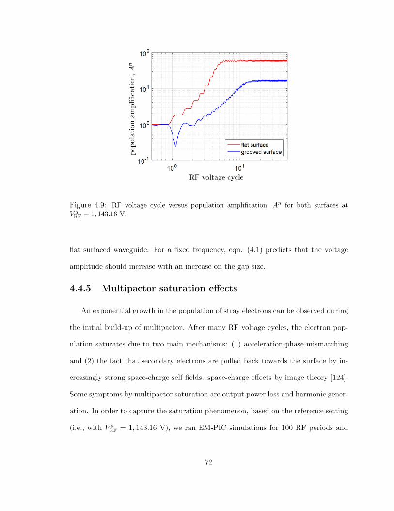
Figure 4.9: RF voltage cycle versus population amplification, An for both surfaces atV a

RF = 1, 143.16 V.

flat surfaced waveguide. For a fixed frequency, eqn. (4.1) predicts that the voltage

amplitude should increase with an increase on the gap size.

4.4.5 Multipactor saturation effects

An exponential growth in the population of stray electrons can be observed during

the initial build-up of multipactor. After many RF voltage cycles, the electron pop-

ulation saturates due to two main mechanisms: (1) acceleration-phase-mismatching

and (2) the fact that secondary electrons are pulled back towards the surface by in-

creasingly strong space-charge self fields. space-charge effects by image theory [124].

Some symptoms by multipactor saturation are output power loss and harmonic gener-

ation. In order to capture the saturation phenomenon, based on the reference setting

(i.e., with V aRF = 1, 143.16 V), we ran EM-PIC simulations for 100 RF periods and

72

Table 4.4: Spectral amplitude of output voltage signals for high-order harmonics.

flat surface grooved surface

fRF = 2 [GHz] 9.6620× 102 1.0803× 103

2nd harmonic 1.8682× 10−1 -3rd harmonic 4.7680× 100 3.8502× 100

4th harmonic 1.9876× 10−1 -5th harmonic 1.3681× 10−1 4.1402× 10−1




for both types of surfaces. Fig. 4.9 shows the log-scale plot of the electron popula-

tion amplification factor An = Nnp /N

0p , where Np is total number of superparticles

flying between two metallic plates at time step n, vesus the RF voltage cycle. The

number density increases at an exponential rate up to an intermediate stage close to

about six RF cycles, beyond which saturation is reached due to strong space-charge

self fields. During the intermediate stage, the amplitude of RF fields prevail over the

space-charge self field, and most secondaries successfully escape from the emission

surface.

Fig. 4.10a shows the instantaneous RF voltage at the output port over time. As

expected, the output voltage amplitudes in both cases are smaller than the input volt-

age amplitude (green-dashed line, 1, 143.16 V). Their spectra are shown in Fig. 4.10b

where it can be clearly seen that, in addition to the original 2 GHz signal, many

frequency harmonics are generated in both cases.

73

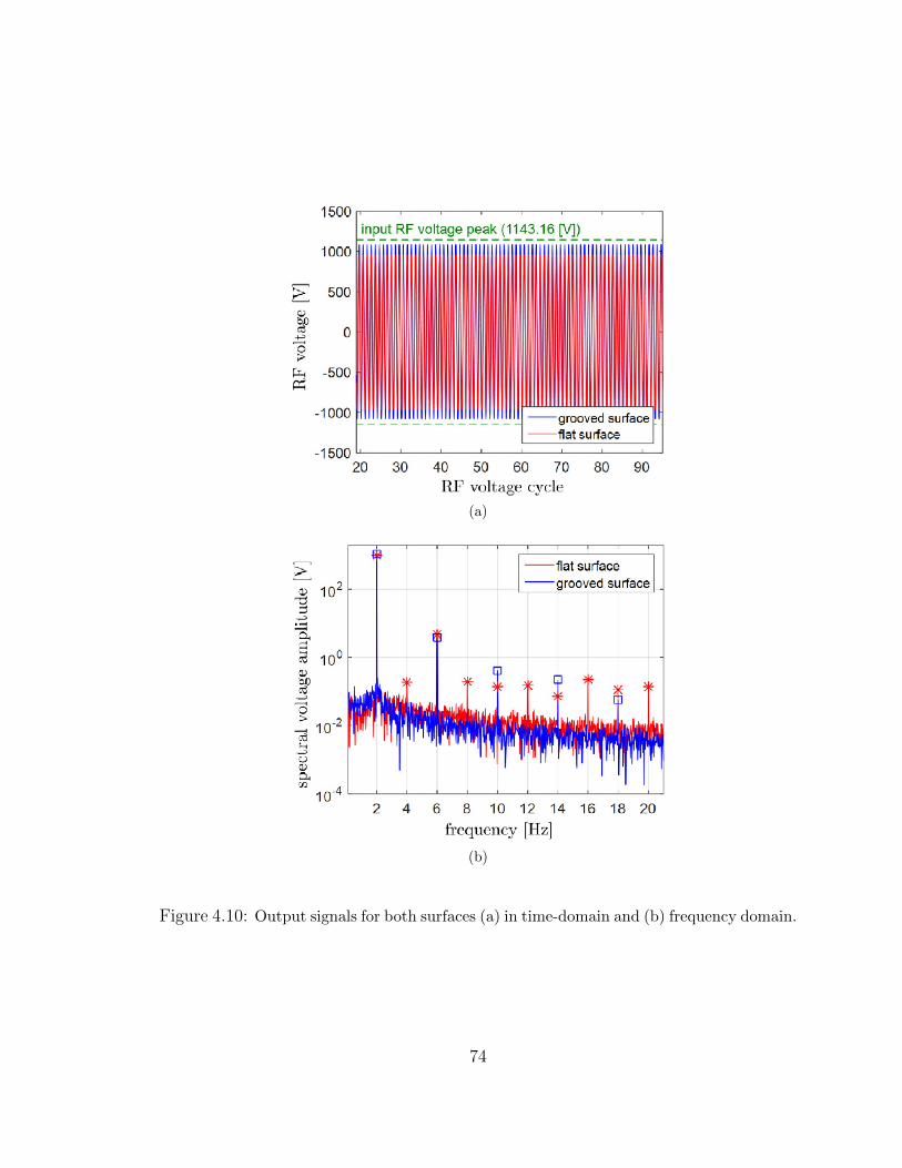
(a)

(b)

Figure 4.10: Output signals for both surfaces (a) in time-domain and (b) frequency domain.

74

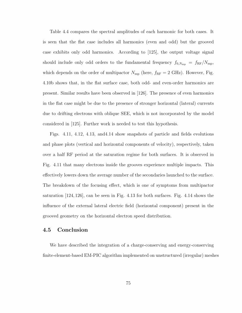
Table 4.4 compares the spectral amplitudes of each harmonic for both cases. It

is seen that the flat case includes all harmonics (even and odd) but the grooved

case exhibits only odd harmonics. According to [125], the output voltage signal

should include only odd orders to the fundamental frequency f0,Nmp = fRF/Nmp,

which depends on the order of multipactor Nmp (here, fRF = 2 GHz). However, Fig.

4.10b shows that, in the flat surface case, both odd- and even-order harmonics are

present. Similar results have been observed in [126]. The presence of even harmonics

in the flat case might be due to the presence of stronger horizontal (lateral) currents

due to drifting electrons with oblique SEE, which is not incorporated by the model

considered in [125]. Further work is needed to test this hypothesis.

Figs. 4.11, 4.12, 4.13, and4.14 show snapshots of particle and fields evolutions

and phase plots (vertical and horizontal components of velocity), respectively, taken

over a half RF period at the saturation regime for both surfaces. It is observed in

Fig. 4.11 that many electrons inside the grooves experience multiple impacts. This

effectively lowers down the average number of the secondaries launched to the surface.

The breakdown of the focusing effect, which is one of symptoms from multipactor

saturation [124, 126], can be seen in Fig. 4.13 for both surfaces. Fig. 4.14 shows the

influence of the external lateral electric field (horizontal component) present in the

grooved geometry on the horizontal electron speed distribution.

4.5 Conclusion

We have described the integration of a charge-conserving and energy-conserving

finite-element-based EM-PIC algorithm implemented on unstructured (irregular) meshes

75

(a) t = 24.50 [ns] (b) t = 24.55 [ns] (c) t = 24.60 [ns]

(d) t = 24.65 [ns] (e) t = 24.70 [ns] (f) t = 24.75 [ns]

(g) t = 24.50 [ns] (h) t = 24.55 [ns] (i) t = 24.60 [ns]

(j) t = 24.65 [ns] (k) t = 24.70 [ns] (l) t = 24.75 [ns]

Figure 4.11: Particle position snapshots taken over a half RF period during the saturationregime. The RF voltage period is 0.5 ns. Plots (a)-(f) are for the flat surface and plots(g)-(l) are for the grooved surfaces.

with the Furman-Pivi probabilistic model describing SEE processes on metallic sur-

faces. The proposed SEE/EM-PIC algorithm enables mesh refinement and is better

suited to model to complex geometries. The algorithm was validated by comparing

simulation results with available prior data.The algorithm was applied to evaluate

and compare multipactor effects on copper and stainless steel parallel plates. In addi-

tion, the algorithm was employed to compare multipactor on copper waveguides with

flat or corrugated (triangularly-grooved) walls. The multipactor saturation process

was examined by quantifying the output power loss and harmonic generation arising

from acceleration phase mismatching and self-field counterbalance effects.

76

(a) t = 24.50 [ns] (b) t = 24.55 [ns] (c) t = 24.60 [ns]

(d) t = 24.65 [ns] (e) t = 24.70 [ns] (f) t = 24.75 [ns]

(g) t = 24.50 [ns] (h) t = 24.55 [ns] (i) t = 24.60 [ns]

(j) t = 24.65 [ns] (k) t = 24.70 [ns] (l) t = 24.75 [ns]

Figure 4.12: External-field and self-field snapshots taken over a half period during thesaturation regime. The RF voltage period is 0.5 ns. Plots (a)-(f) are for the flat surfaceand plots (g)-(l) are for the grooved surfaces.

(a) t = 24.50[ns]

(b) t = 24.55[ns]

(c) t = 24.60[ns]

(d) t = 24.65[ns]

(e) t = 24.70[ns]

(f) t = 24.75[ns]

(g) t = 24.50[ns]

(h) t = 24.55[ns]

(i) t = 24.60[ns]

(j) t = 24.65[ns]

(k) t = 24.70[ns]

(l) t = 24.75[ns]

Figure 4.13: Snapshots of vy [m/s] versus y [m] taken over a half RF period during thesaturation regime. The RF voltage period is 0.5 ns. Plots (a)-(f) are for the flat surfaceand plots (g)-(l) are for the grooved surfaces.

77

(a) t = 24.50[ns]

(b) t = 24.55[ns]

(c) t = 24.60[ns]

(d) t = 24.65[ns]

(e) t = 24.70[ns]

(f) t = 24.75[ns]

(g) t = 24.50[ns]

(h) t = 24.55[ns]

(i) t = 24.60[ns]

(j) t = 24.65[ns]

(k) t = 24.70[ns]

(l) t = 24.75[ns]

Figure 4.14: Snapshots of vx [m/s] versus y [m] taken over a half RF period during thesaturation regime. The RF voltage period is 0.5 ns. Plots (a)-(f) are for the flat surfaceand plots (g)-(l) are for the grooved surfaces.

78

Chapter 5: Numerical Cherenkov Radiation and Grid

Dispersion Effects

Electromagnetic particle-in-cell (EM-PIC) simulations have become an important

tool for the study of a wide variety of problems associated with collisionless plasmas,

including high power vacuum electronic devices [46, 47, 56], laser-wakefield acceler-

ation [127], and astrophysical phenomena [128], to name just a few. Despite their

success, there exist a number of outstanding challenges that limit the accuracy and

robustness of EM-PIC simulations. Among them, the numerical Cherenkov radia-

tion (NCR) instability, first observed by Godfrey [129], has been recognized as an

important detrimental factor in EM-PIC simulations involving high-energy (relativis-

tic) charged particles (including Lorentz-boosted frames) [130, 131] and collisionless

shocks [132]. On regular periodic meshes such as used by the finite-difference time-

domain (FDTD) method, NCR results from the coupling between numerical electro-

magnetic modes and plasma beam resonances. This coupling may result from the

slow down of poorly-resolved waves due to numerical (grid) dispersion [133, 134] or

from aliasing mechanisms [135,136].

The study of the causes and behavior of NCR is of critical importance for devel-

oping mitigation strategies [15, 20, 135–138]. NCR has been extensively studied for

FDTD-based and spectral-based EM-PIC algorithms based on regular meshes [20,

79

129–132, 135, 136]. For problems involving complex geometries however, it is often

advantageous to employ more general meshes which can better conform to curved

and/or irregular boundaries as well as support adaptive mesh refinement capabilities.

In this chapter, we analyze NCR effects in EM-PIC simulations based on more

general meshes. The finite element time-domain (FETD)-based EM-PIC algorithm

discussed in [1, 51, 52] is employed for this purpose. This explicit algorithm includes

a charge-conserving scatter algorithm [1] and the Higuera-Cary particle-pusher to

fully take into account relativistic effects and yield an overall energy-conserving al-

gorithm [39, 52] . The reason for adopting this FETD-based EM-PIC algorithm in

this study is twofold: (1) Contrary to most past FE-based EM-PIC algorithms imple-

mented on general meshes 2, the present algorithm attains both charge and energy-

conservation from first principles. (2) The standard FDTD algorithm can be retrieved

as a special version of this mixed FETD scheme implemented on a regular mesh with

square elements, in which low-order quadrature rules are employed in the evaluation

of the mass (Hodge) matrices elements to yield diagonal matrices and a fully ex-

plicit field update [140]. This facilitates a direct comparison of NCR effects arising in

FETD-based EM-PIC simulations with those in FDTD-based EM-PIC simulations.

As noted, NCR is closely related to numerical dispersion. Most past numerical

dispersion studies in FE-based Maxwell field solvers have been carried out in the

frequency domain (or equivalently, with no time discretization errors included) [22,

141,142] and only a few in the time domain [143]. Key conclusions from these studies

are as follows: (1) a good quality mesh (i.e. one having near equilateral elements) is

best for minimizing local phase errors per wavelength and (2) the cumulative phase

2Some notable exceptions are the compatible FE-based formulations described in Refs. [77,78,139]

80

error can be smaller on highly unstructured grids due to cancellation effects. The

numerical dispersion analysis carried out in these works have focused on well-resolved

waves, which is the practical regime of interest to provide sufficiently accurate results

for pure EM simulations. However, in order to analyze NCR in EM-PIC simulations,

a complete numerical dispersion map over the first Brillouin zone (the periodic layout

of the mesh elements) must be determined because, among other reasons, electric

currents, mapped from moving charged particles to the mesh during the scatter step

of EM-PIC algorithm, are not explicitly bandlimited in contrast to the typical sources

present in particle-free EM simulations. In this work, complete dispersion diagrams

over the first Brillouin zone are obtained for meshes with different element shapes

and layouts and analytical predictions for NCR are compared with numerical results

from EM-PIC simulations.

5.1 Numerical Cherenkov Radiation in the FDTD-based EM-PIC Algorithm

Owing to its flexibility and robustness, the FDTD algorithm is arguably the most

popular field solver for time-domain Maxwell’s equations [19]. As such, FDTD-based

(Yee) EM-PIC simulations are widely employed in plasma physics applications. The

FDTD uses central-difference approximations for both space and time derivatives ap-

plied on a structured regular mesh. The numerical dispersion for the FDTD algorithm

in 2-D takes the form [19,144][1

hsin

(κxh

2

)]2

+

[1

hsin

(κyh

2

)]2

=

[1

c∆tsin

(ω∆t

2

)]2

, (5.1)

where c is the speed of light in vacuum, ∆t is the time step interval, h is the edge

length of a square unit cell in the structured mesh, and κ = κxx + κyy is the 2-D

81

(a) (b)

Figure 5.1: Numerical grid dispersion of the 2-D Yee’s FDTD scheme on a structuredmesh. (a) The red color surface represents the dispersion diagram of the normalizedfrequency ω∆t/π versus the normalized numerical wavenumber κh in radians. Theolive color surface represents the light cone. The contour levels at the bottom rep-resent the normalized phase errors (with respect to the color bar). (b) Wavenumbermagnitude versus frequency for different wave propagation angles with respect to thex axis, φp ∈ [0o, 45o].

wavenumber for plane waves propagating on the mesh. We use the tilde to indicate

numerical wavenumber κ (as modified by numerical dispersion) as opposed to exact

wavenumber κ. Throughout this work, the time convention ejωt is adopted.

The dispersion diagram (ω, κ) can be plotted by solving (5.1) [?]. Consider an

example with h = 1 m and ∆t = h/(√

2c)≈ 2.35 ns, which corresponds to the max-

imum time step allowed by the Courant-Friedrichs-Lewy (CFL) stability condition.

In Fig. 5.1a, the numerical grid dispersion diagram ωGD (κ) is displayed by a red

surface, and the light cone is shown in the olive green color. Contour levels at the

bottom of the figure represent the normalized phase differences (errors) between the

light cone and the numerical grid dispersion, [c|κ| − ωGD (κ)] ∆t/π, indicative of how

much faster or slower numerical waves propagate compared to the speed of light. The

82

normalized wave frequencies are plotted versus the normalized κ for various prop-

agation directions φp ∈ [0o, 45o] along the grid3 in Fig. 5.1b. These results show

that the numerical phase velocity has an anisotropic behavior on the FDTD mesh

and is always slower than the speed of light in vacuum [145]. Suppose that a cold

plasma beam is relativistically drifting along the x-axis with a bulk beam velocity of

vb = 0.9c. Its space-charge mode (or entropy mode) can be characterized in the dis-

persion diagram by a plane with inclination given by the beam velocity (beam plane).

NCR is emitted from the coupling region where the numerical grid dispersion surface

and the beam plane intersect in the first Brillouin zone. Furthermore, because of spa-

tial and temporal aliasing effects, NCR can also be produced by resonances in other

beam planes originated from higher-order Brillouin zones as well [135, 136], called

aliased beams. The dispersion relation for space-charge modes, including spatial and

temporal aliasing effects, on a structured mesh is given by

ω − 2π

∆tv = vb

(κx −

2π

hu

)(5.2)

where u and v are integers and the fundamental resonance mode has u = v = 0.

Since the spatial aliasing effect directly depends on the shape factors used for current

deposition (scatter step) onto the FDTD grid, NCR can be mitigated to some extent

by increasing the spline order of the shape factors [146].

Fig. 5.2 illustrates the fundamental and aliased beam planes in the green and

transparent yellow colors respectively, and the numerical dispersion in red within the

first Brillouin zone, in which κ ∈ [−π/h, π/h]× [−π/h, π/h] and ω ∈ [−π/∆t, π/∆t].

As seen in Fig. 5.2a, the NCR, caused by the fundamental beam resonance, is present

3Here, φp = 0o corresponds to a direction along the grid axis and φp = 45o corresponds to adirection along the grid diagonals. Due to the FDTD symmetry, the behavior in the φp ∈ [0o, 45o]repeats periodically along the other directions.

83

(a) (b)

Figure 5.2: Analytic NCR predictions on a structured FDTD grid for a bulk beamvelocity vb = 0.9c. (a) 3-D numerical dispersion diagrams (in red) and beam planes(fundamental plane in green and aliased beams in transparent yellow). (b) Trajecto-ries of NCR solutions projected onto the 2-D κ-space.

over a relatively narrow spectrum of wavenumbers due to the slower phase velocity of

poorly-resolved waves for wavenumbers close to the grid cut-off. On the other hand,

NCR produced by aliased beam resonances are spread out throughout the κ-space and

may occur regardless of whether numerical dispersion is corrected or not. The loci for

NCR solutions can be found by using root-find-solvers. These solutions are visualized

more clearly in the κ-space as depicted in Fig. 5.2b with u, v ∈ −3,−2, ..., 2, 3.

Again, the fundamental beam resonance is shown in green and aliased ones are shown

in yellow.

84

5.2 Numerical Cherenkov Radiation in finite-element-basedEM-PIC Algorithms

To analyze NCR on more general meshes, an EM-PIC algorithm [1, 51, 52] based

on a mixed FETD field solver [33, 76] is adopted here for the reasons listed in the

Introduction. The present FETD field solver is based on an expansion of electro-

magnetic fields as a linear combination of discrete differential forms (Whitney forms)

defined over mesh elements and an explicit (leap-frog) discretization in time. The

most essential aspects of the field solver are outlined in Chapter 1.

We first consider four periodic meshes, each with different element shapes and lay-

outs as depicted in Fig. 5.3. They are denoted as square (SQ), right-angle triangular

(RAT), isosceles triangular (ISOT), and highly-irregular triangular (HIGT). This sec-

tion provides an analytical study of numerical dispersion and consequent NCR on SQ,

RAT, and ISOT meshes. These three meshes have periodic arrangements of elements

and hence are amenable to such analysis. Analytical predictions of this Section are

compared against EM-PIC simulation results in the next Section. NCR effects in

FETD-based EM-PIC simulations on HIGT meshes are also presented in the next

Section. The FETD-based EM-PIC algorithm is implemented on all four meshes,

whereas the FDTD-based EM-PIC algorithm is implemented exclusively on the SQ

mesh.

In order to analyze the numerical dispersion in the FETD algorithm implemented

on SQ, RAT, and ISOT meshes, we consider a numerical plane wave expressed as

E0ej(ωn∆t−κ·r). In the FETD algorithm, the discrete degrees of freedom (DoF) of

the electric field are associated with the edges of the mesh. Suppose that tj is the

tangential unit vector along the jth edge of the mesh. The plane wave solutions can

85

(a) (b)

(c) (d)

Figure 5.3: Schematic illustration of the four types of mesh considered in this study.(a) Square regular (SQ) elements in both FDTD and FETD, (b) right-angle triangular(RAT) elements in FETD, (c) isosceles triangular (ISOT) elements in FETD, and (d)highly-irregular triangular (HIGT) elements in FETD.

86

be projected onto the edges as (E0 · tj)ej(ωn∆t−κ·r) and the factor E0 · tj can be taken

as the DoF associated with the jthedge. In addition, by using the superscript n to

represent the nth time step, we may denote the discrete DoFs as enj . For a plane wave

propagating on a periodic mesh, it is possible to express the field value on an arbitrary

edge using only the field values on a few number of so-called characteristic edges

through multiplication of a spatial offset factor of the form e−jκ·−−→AA′ , where

−−→AA′ is the

relative position vector between the non-characteristic edge A′ and its corresponding

characteristic edge A. Because of this, the number of DoFs can be restricted to

the number of the characteristic edges and the size of the matrices involved can be

greatly reduced, see also [22]. Note that the SQ mesh has only two characteristic

edges whereas the RAT and ISOT meshes have three characteristic edges.

The full-discrete vector wave equation for the electric field can be written as [33,79]

[?ε] · en+1 =(2 [?ε]−∆t2CT · [?µ−1 ] ·C

)· en − [?ε] · en−1. (5.3)

For a discrete plane wave with harmonic evolution of the form ejωn∆t, it is clear that

en±1 = ene±jω∆t so that (5.3) becomes

X · en =

2 [cos (ω∆t)− 1] M + ∆t2S· en = 0, (5.4)

where M = [?ε] (mass matrix) and S = CT · [?µ−1 ] ·C (stiffness matrix). Non-trivial

solutions can be obtained by solving det (X) = 0 which determines the numerical

dispersion relation (ω, κ) on the mesh. In what follows, NCR analysis is presented

for SQ, RAT, and ISOT meshes. The numerical dispersion analysis is similar to [22]

except that time-discretization is also included.

87

Figure 5.4: Schematic of SQ mesh. There are two characteristic edges (A and B)directed along the y and x and colored in red and blue, respectively.

5.2.1 SQ Mesh

The SQ mesh has two characteristic edges, y- and x-directed. Let these two edges

be denoted as A and B, colored in red and blue, respectively, in Fig. 5.4. Local

matrices for the three facets spanned by the support of the edge elements A and B

are first computed. Then, the global mass and stiffness matrices can be constructed as

a sum of three local matrices attributed to each facet. The dashed red (for y-directed

edges) and dashed blue (for x-directed edges) lines in Fig. 5.4 depict the relative

position vectors between characteristic and non-characteristic edges. As detailed in

Chapter 1, in the mixed FETD algorithm, the electric field is represented as a linear

88

combination of Whitney 1-forms associated 1:1 with mesh element edges and the

magnetic flux density by a linear combination of Whitney 2-forms associated 1:1 with

mesh element faces (note that Whitney 1- and 2-forms are also known as edge and

face elements in the finite element literature). The vector proxies of Whitney 1- and

2-forms for the jth edge and kth face are written as [23]

W(1)j (r) = αΠ

(α− α(1)

j

h/2

)Λ

(β − β(1)

j

h

), (5.5)

W(2)k (r) =

z

h2Π

(x− x(2)

k

h/2

)Π

(y − y(2)

k

h/2

), (5.6)

where j and k are edge and face indices, α and β stand for Cartesian coordinates x and

y or vice-versa depending on the direction of the jth edge, and the point(x

(p)q , y

(p)q

)is the center of the qth p-cell (p = 1: edge, p = 2: face). In addition, Π (·) and Λ (·)

are scalar pulse and roof-top functions defined as

Π (ζ) =

1, |ζ| ≤ 10, |ζ| > 1

, (5.7)

Λ (ζ) =

1− |ζ| , |ζ| ≤ 10, |ζ| > 1

. (5.8)

The global mass and stiffness matrices for DoFs on the characteristic edges, namely

[enA, enB]T , can then be written as

M = M1 + M2 + M3, (5.9)

S = S1 + S2 + S3, (5.10)

89

with

M1 = ε0∆

[1/3 + e−jκ·

−→AA1,r/6 0

0 1/3 + e−jκ·−−→BB1,u/6

],

M2 = ε0∆

[1/3 + e−jκ·

−→AA2,l∆/6 0

0 0

],

M3 = ε0∆

[0 0

0 1/3 + e−jκ·−−→BB3,d/6

], (5.11)

S1 =1

µ0∆

[1− e−jκ·

−→AA1,r −1 + e−jκ·

−−→BB1,u

−1 + e−jκ·−→AA1,r 1− e−jκ·

−−→BB1,u

],

S2 =1

µ0∆

[1− e−jκ·

−→AA2,l e−jκ·

−−→BB2,d − e−jκ·

−−→BB2,u

0 0

],

S3 =1

µ0∆

[0 0

e−jκ·−→AA3,l − e−jκ·

−→AA3,r , 1− e−jκ·

−−→BB3,d

], (5.12)

where ∆ is the area of the SQ mesh unit cell and the relative position vectors are given

by−→AA1,r = (h, 0),

−→AA2,l = (−h, 0),

−→AA3,l = (0,−h),

−→AA3,r = (h,−h),

−−→BB1,u = (0, h),

−−→BB2,d = (−h, 0),

−−→BB2,u = (−h, h), and

−−→BB3,d = (0,−h). As noted before, the

numerical grid dispersion can then be found by solving det (X) = 0 for different ω

and obtaining κ on the first Brillouin zone.

Fig. 5.5 illustrates the numerical grid dispersion of the FETD algorithm on the

SQ mesh with h = 1 [m] and ∆t = 1.35 [ns], which is the maximum time step for

the stable field-update according the CFL limit4. Unlike the FDTD case, it is clear

from Fig. 5.5a that numerical plane waves propagate slightly faster than light in

this case, regardless of the propagation direction, over the entire first Brillouin zone.

Fig. 5.5b projects the numerical dispersion on the normalized wavenumber/frequency

plane, with different propagation directions illustrated by different colors in the φp ∈

[0o, 45o] range. As noted before, the standard FDTD algorithm can be recognized as

4The maximum time step in the FETD scheme can be obtained through an eigenvalue analysison M−1 · S [33].

90

(a) (b)

Figure 5.5: Numerical grid dispersion for the FETD scheme on the SQ mesh. (a) Thered color surface represents the dispersion diagram of the normalized frequency ω∆t/πversus the normalized numerical wavenumber κh in radians. The olive color surfacerepresents the light cone. The contour levels at the bottom represent the normalizedphase errors (with respect to the color bar). Note that the normalized phase erroris always negative in this case because of a slightly faster-than-light numerical phasevelocity. (b) Projected dispersion curves for different wave propagation angles withrespect to the x axis φp ∈ [0o, 45o].

a special version of the FETD on the SQ mesh in which low-order quadrature rules

are employed in evaluating the mass (Hodge) matrices elements to yield diagonal

matrices [140]. Conversely, the FETD algorithm on the SQ mesh can be regarded as a

modified FDTD scheme in which non-diagonal coupling, present in the mass matrices,

mimics an extended finite-difference stencil approximating spatial derivatives. As

discussed in [20], the extended stencil makes numerical waves propagate faster than

the speed of light. The latter effect can also be understood from the fact that the

extended spatial stencil results in a stronger coupling of various degrees of freedom

on the mesh. Because of faster numerical wave speeds, the maximum time step for a

stable update in the FETD algorithm on a SQ mesh is smaller than the FDTD limit

on the same mesh by a factor of 0.58, which agrees with [20].

91

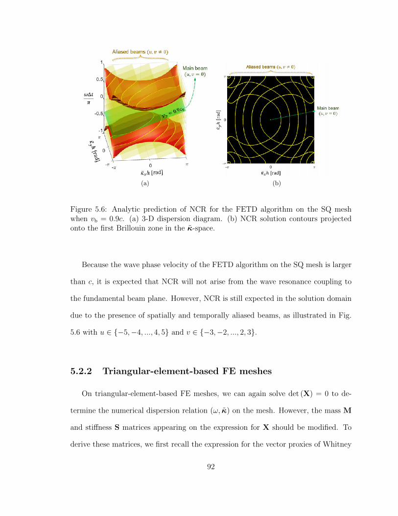
(a) (b)

Figure 5.6: Analytic prediction of NCR for the FETD algorithm on the SQ meshwhen vb = 0.9c. (a) 3-D dispersion diagram. (b) NCR solution contours projectedonto the first Brillouin zone in the κ-space.

Because the wave phase velocity of the FETD algorithm on the SQ mesh is larger

than c, it is expected that NCR will not arise from the wave resonance coupling to

the fundamental beam plane. However, NCR is still expected in the solution domain

due to the presence of spatially and temporally aliased beams, as illustrated in Fig.

5.6 with u ∈ −5,−4, ..., 4, 5 and v ∈ −3,−2, ..., 2, 3.

5.2.2 Triangular-element-based FE meshes

On triangular-element-based FE meshes, we can again solve det (X) = 0 to de-

termine the numerical dispersion relation (ω, κ) on the mesh. However, the mass M

and stiffness S matrices appearing on the expression for X should be modified. To

derive these matrices, we first recall the expression for the vector proxies of Whitney

92

Figure 5.7: A periodically-arranged triangular grid. It has three characteristic edgesdenoted by A, B, and C. Labels inside circles denote global facet indexes and labelsinside rectangles and pentagons denote local edge and node indexes, respectively.

1- and 2-forms on triangular meshes [147–149]

W(1)j (r) = λ[1]j

∇λ[2]j− λ[2]j

∇λ[1]j(5.13)

W(2)k (r) = 2∇λ1k ×∇λ2k(on 2-dimensional meshes). (5.14)

at each jth edge and kth facet on the mesh, where [j]i and ji denote the jth local

node index for ith edge and the jth local node index for ith facet, respectively. In

addition, in what follows (j)i denotes the jth local edge index for ith facet. For an

arbitrary point (x, y) inside a kth facet, the relationship between local nodal and

barycentric coordinates is given byx1k x2k x3ky1k y2k y3k

1 1 1

·λ1kλ2kλ3k

=

xy1

. (5.15)

93

Consider a periodically-arranged triangular grid, as shown in Fig. 5.7. The local

mass matrix for the kth facet can be obtained by [23,150]

Mlock =

Mloc(1,1)k

M loc(1,2)k

M loc(1,3)k

M loc(2,1)k

M loc(2,2)k

M loc(2,3)k

M loc(3,1)k

M loc(3,2)k

M loc(3,3)k

, (5.16)

where

M loc(i,j)k

= 2Ak[αi,j βi,j γi,j

]·

∇λ1k ·∇λ1k∇λ1k ·∇λ2k∇λ2k ·∇λ2k

, (5.17)

α =1

12

1 1 11 3 11 3 1

,β =1

12

−1 −1 1−1 3 31 3 3

,γ =1

12

1 −1 −1−1 1 1−1 1 3

. (5.18)

and Ak is the area of the kth facet. Each element index in the expression of the

local mass matrix above also denotes the local edge index of the kth facet. The local

stiffness matrix Slock =

(Clock

)T · [?µ−1 ]lock·Cloc

k is given by

Slockth =

Sloc(1,1)k

Sloc(1,2)k

Sloc(1,3)k

Sloc(2,1)k

Sloc(2,2)k

Sloc(2,3)k

Sloc(3,1)k

Sloc(3,2)k

Sloc(3,3)k

, (5.19)

where Sloc(i,j)k

= (−1)i+j/Ak. We define a function F (jk , k) that yields one of

the characteristic edges of the kth facet according to the local edge index jk, i.e.,

F (jk , k) = gk(= A, B, or C). Likewise, the inverse function F−1 = H yields the

jth local edge index of the kth facet, jk, i.e. H (F (jk , k)) = jk.

Projecting plane wave solutions into DoFs on edges, the relationship between the

DoFs for similar edges in different facets kth and Kth can be written as

egK = egke−jκ·−−−→gkgK = eF(jk,k)

e−jϕ[gk→gK ] (5.20)

where −−→gkgK is the relative position vector from the center of the edge gk to gK and

ϕ[gk→gK ] is the corresponding phase delay. For e = [eA, eB, eC ]T , the global mass and

94

stiffness matrices can be assembled by

MG1,g1 =4∑p=1

M loc

(H(Gp),H(gp))p, for Gp = gp

M loc(H(Gp),H(gp))p

e−jϕ[g1→gp] , for Gp 6= gp, (5.21)

SG1,g1 =4∑p=1

Sloc

(H(Gp),H(gp))p, for Gp = gp

Sloc(H(Gp),H(gp))p

e−jϕ[g1→gp] , for Gp 6= gp, (5.22)

where Gp and gp are outputs of the F function for local edges in p facets (see Fig. 5.7).

As noted before, the numerical grid dispersion of the FETD schemes on periodically-

arranged triangular grids can then be obtained by substituting the above mass and

stiffness matrices into (5.4) and solving the characteristic equation det (X) = 0. We

will examine next triangular meshes composed of RAT and ISOT elements.

Right-angle triangular-element (RAT) mesh

The unit cell of the RAT mesh corresponds to setting a = 0 and b = 1 (see

Fig. 5.7). The numerical dispersion diagram of the FETD-RAT scheme over the

first spatial Brillouin zone is illustrated in Fig. 5.8. The first spatial Brillouin zone

of the RAT mesh in the κ-space is shaped as an inclined hexagon. As depicted in

Fig. 5.8a, red and blue surfaces correspond to the lower and upper grid dispersion

of the mesh. The normalized phase errors are shown by means of contour maps

at the bottom and top planes along the (vertical) frequency axis. Fig. 5.8b shows

the numerical dispersion curves for different propagation directions φp ∈ [−45o, 45o].

Dirac points denote the points where the lower and upper dispersion bands meet5.

It is observed that the numerical dispersion in the lower band is highly anisotropic.

5This nomenclature is borrowed from solid state physics, where it is used to describe attachmentof valence and conduction energy bands.

95

(a) (b)

Figure 5.8: Numerical grid dispersion for the FETD scheme on the RAT mesh with theCFL number equal to one. Unlike the FDTD or FETD-SQ cases, this diagram exhibitsan additional (upper) dispersion band. (a) The red (lower band) and blue (upperband) color surfaces represent the dispersion diagram of the normalized frequencyω∆t/π versus the normalized numerical wavenumber κh in radians. The olive colorsurface represents the light cone. The contour levels at the bottom represent thenormalized phase errors (with respect to the color bar). (b) Projected dispersioncurves for different wave propagation angles with respect to the x axis φp ∈ [−45o, 45o].

Although in the upper band wave propagation is faster than light due to its inverse-

like shape compared to the lower band, NCR may still be produced by intersection

with aliased beams. The existence of an upper dispersion band on meshes based

on RAT elements can be understood from the fact that the normal component of

the (vector proxy of) Whitney 1-forms used to expand the electric field on the mesh

exhibit discontinuities at the edges of triangular meshes. Fig. 5.9 illustrates the

normal discontinuity of Whitney 1-forms. This is in contrast to meshes based on SQ

elements where Whitney 1-forms exhibit both tangential and normal continuity (due

to zero normal components). Strictly speaking, Whitney 1-forms on triangular grids

are only tangentially continuous [147, 149]. Indeed, the numerical grid dispersion

behavior on meshes with periodically-arranged triangular elements is reminiscent of

96

(a) (b) (c)

Figure 5.9: (a) The vector proxy of a Whitney 1-form associated with the edge−→AB

on a triangular mesh. (b) Tangential component along edge. (c) Normal componentto the edge direction.

that of photonic band gap structures in which the discontinuity of the normal field

component is caused by periodic material interfaces [151,152].

Fig. 5.10 shows the analytic prediction of NCR for the FETD-based EM-PIC

scheme on the RAT mesh assuming a plasma beam with bulk velocity vb = 0.9c. Fig.

5.10a depicts the numerical dispersion diagram over the first Brillouin zone superim-

posed to the fundamental and aliased beams. Set of NCR solutions in the κ-space

are shown in Fig. 5.10b with u ∈ −5,−4, ..., 4, 5 and v ∈ −3,−2, ..., 2, 3.

Isosceles triangular-element (ISOT) mesh

The unit cell for the ISOT mesh corresponds to a = 0.5 and b = 1. Similar to the

RAT case, the numerical dispersion diagram exhibits both lower and upper dispersion

bands as shown in Fig. 5.11. Fig. 5.12 shows the NCR prediction for a beam bulk

97

(a) (b)

Figure 5.10: Analytic prediction of NCR for the FETD-based EM-PIC scheme onthe RAT mesh assuming a plasma beam with bulk velocity vb = 0.9c. (a) Dispersiondiagram. (b) NCR solution contours projected onto the first Brillouin zone in theκ-space.

(a) (b)

Figure 5.11: Numerical grid dispersion for the FETD scheme on the ISOT meshwith CFL number equal to one. Unlike the FDTD or FETD-SQ cases, this dia-gram exhibits an additional (upper) dispersion band. (a) The red (lower band) andblue (upper band) color surfaces represent the dispersion diagram of the normalizedfrequency ω∆t/π versus the normalized numerical wavenumber κh in radians. Theolive color surface represents the light cone. The contour levels at the bottom and toprepresent the normalized phase errors (with respect to the color bar). (b) Projecteddispersion curves for different wave propagation angles with respect to the x axisφp ∈ [26.57o, 90o].

98

(a) (b)

Figure 5.12: Analytic prediction of NCR for the FETD-based EM-PIC scheme on theISOT mesh assuming a plasma beam with bulk velocity vb = 0.9c. (a) Dispersiondiagram. (b) NCR solution contours projected onto the first Brillouin zone in theκ-space.

velocity vb = 0.9c. There is no NCR caused by the fundamental beam resonances in

this case; however, NCR is still excited by waves coupling to aliased beam resonances

as illustrated in Fig. 5.12b, where u ∈ −5,−4, ..., 4, 5 and v ∈ −3,−2, ..., 2, 3.

Highly-irregular triangular-element (HIGT) mesh

In contrast to the SQ, RAT, and ISOT meshes considered above, the HIGT mesh

does not have a periodic layout of elements. The aperiodic layout of the elements

in the HIGT mesh precludes a similar type of analytical study of NCR as made

before for the other meshes. As a result, NCR effects in HIGT are investigated

exclusively by means of numerical simulations in the next Section. Note that the phase

errors due to numerical dispersion on the meshes with periodic triangular elements,

as seen in Figs. 5.8 and 5.11, can be positive or negative (i.e. with dispersion

curves above or below the light line) depending on angle of propagation relative

99

to the (local) element orientation. Therefore, it is expected that for an unstructured

(aperiodic) mesh composed of triangular elements of different shapes and orientations,

the cummulative phase error may be reduced due to some cancellation effects. This

result has been numerically observed before in [22].

5.3 Numerical Experiments

In this Section, EM-PIC simulations are conducted to verify the analytic predic-

tions made in the previous Section. In addition, FETD-based EM-PIC simulations

on the HIGT mesh (for which no analytical prediction is available) are also included

for comparison. Two basic scenarios are considered here: a relativistically-drifting

(electron-positron) pair-plasma and a single electron-positron pair moving in the rel-

ativistic regime.

First, consider a relativistic pair-plasma drifting along the x-axis with the ve-

locity vb = 0.9c (equivalent to a Lorentz factor of γb ≈ 2.3). The electron plasma

frequency is set to ωpe ≈ 4× 105 rad/s and the electron density to ne = 1× 108 m−2

(same for positrons). Superparticles representing 2.5× 106 charged particles are used

for each species (electrons and positrons). The average number of superparticle per

cell is set to 40 for the SQ mesh and 20 for the RAT, ISOT, HIGT meshes 6. In

all cases the problem domain Ω =

(x, y) ∈ [0, 128]2

m2 is terminated by periodic

boundary conditions for both fields and particles. Initially, all superparticles are uni-

formly distributed over the entire simulation domain and each pair of superparticles

is placed at the same position to produce zero net initial fields. The initial velocity

distribution in the beam rest frame vbf for both electrons and positrons is Maxwellian

6Note that for similar edge sizes, SQ mesh elements are about twice the size of the triangularmesh elements

100

(a) (b) (c) (d)

Figure 5.13: Initial velocity distributions for a relativistic pair plasma beam with bulkvelocity vb = 0.9c (γb ≈ 2.3). (a) Phase space in the beam rest frame. (b) Velocitydistribution in the beam rest frame. (c) Phase space in the laboratory frame. (d)Velocity distribution in the laboratory frame.

with thermal velocity vth = 0.005c (see Fig. 5.13a and 5.13b). The resulting Debye

length equals to λbfD =

√ε0v2

thme/ (neq2e) ≈ 2.657 m. The initial velocity distribution

in the laboratory frame vlf is shown in Fig. 5.13c and Fig. 5.13d. The relation-

ship between vlfx and vbf

x can be obtained by applying the Lorentz velocity transfor-

mation vlfx =

(vbfx + vb

)/(1 + vbv

bfx /c

2)

and vlfy = vbf

y

√1− (vb/c)

2/(1 + vbv

bfx /c

2).

Due to length contraction, the Debye length in the laboratory frame reduces to

λlfD = λbf

D/γb ≈ 1.158 m.

EM-PIC simulations are performed based on the following setups: (1-a) FDTD-

based solver on the SQ mesh, (1-b) FETD-based solver on the SQ mesh, (2) FETD-

based solver on the RAT mesh, (3) FETD-based solver on the ISOT mesh, and (4)

FETD-based solver on the HIGT mesh. The HIGT mesh is shown in Fig. 5.14. Note

again that the SQ, RAT, and ISOT meshes have periodic layouts of elements, whereas

HIGT has an aperiodic layout. To ensure a good mesh quality in the latter case, the

angles of triangular elements are enforced to be no less by 30o. The average angle

is near 60o. The angle distribution (histogram) is shown in Fig. 5.14. All meshes

101

(a) (b) (c)

Figure 5.14: (a) HIGT mesh. (b) Histogram of the edge lengths. (c) Histogram ofthe triangular element angles.

are designed so that the average edge length lavg is comparable to λlfD to mitigate

self-heating effects. Table 5.1 lists the basic properties of the four types of mesh.

Table 5.1: Basic meshes properties.

parameters simulation type: (1-a) (1-b) (2) (3) (4)

h [m] 1.00 1.00 1.00 1.00 -lavg [m] 1.00 1.00 1.14 1.08 1.24N0 (# nodes) 16,641 16,641 16,641 16,641 13,239N1 (# edges) 33,024 33,024 49,408 49,408 39,202N2 (# faces) 16,384 16,384 32,768 32,768 25,964∆tmax [ns] 2.35 1.35 1.11 1.03 1.02

In the deep relativistic regime (i.e. very large γb) for 2-D FDTD-based EM-PIC

simulations, the optimal time step ∆tmag for the lowest rate of NCR production

has been determined [135, 136] to be ∆topt ≈ 0.9192∆tmax,2D = 0.9192h/√

2c where

∆tmax,2D is the maximum time step for stability, as dictated by the CFL condition.

On the other hand, the NCR growth rate in the mildly relativistic regime has been

102

observed to monotonically decrease as ∆t increases, that is ∆topt → ∆tmax,2D. In

either case, ∆topt does not differ substantially from ∆tmax,2D. The present FDTD-

based EM-PIC simulations adopt ∆tmax,2D as a reference for comparison.

To obtain NCR dispersion maps in the κ-space representation, the z component of

the B field is measured across the mesh at the end of the simulation (t = 47 µs). A 2-

D fast Fourier transform (FFT) is then performed on the sampled data to obtain B in

the κ-space representation. Fig. 5.15 shows contour plots of the amplitude of B in log

scale over the first Brillouin zone in the κ-space from FDTD-based and FETD-based

EM-PIC simulations on the SQ meshe (cases (1-a) and (1-b)). Fig. 5.16 illustrates

the same for FETD-based EM-PIC simulations on the RAT and ISOT meshes (cases

(2) and (3)). Analytic prediction curves are superimposed on the simulation results in

Figs. 5.15b, 5.15d, 5.16b and 5.16d. The black and gray colors denote fundamental

and aliased beams, respectively. A very good agreement is observed between the

numerical results and the analytic predictions in all cases.

It is observed that on periodic triangular grids, NCR can be purely transverse and

longitudinal unlike the SQ case (FDTD or FETD) as discussed in [136]. On the other

hand, propagation along certain directions (‘characteristics edges’) is prohibited. It

is evident also that the NCR distribution in the κ-space is strongly dependent on

the mesh element shapes. The existence of the upper grid dispersion bands is also

confirmed from their contributions to the NCR solutions in the κ-space. Compared

to the FDTD-based simulation and to the FETD-based simulations on the RAT and

ISOT meshes, the NCR observed in FETD-based EM-PIC simulation on the SQ

mesh exhibits weaker amplitudes. Also of note is that even though there is no NCR

103

(a) (b)

(c) (d)

Figure 5.15: B field amplitude distribution (log scale) over the first Brillouin zonein the κ-space as measured from EM-PIC simulation snapshots at 47 µs. (a) and(c) plots correspond to FDTD- and FETD-based EM-PIC simulations on the SQmesh, respectively. In (b) and (d), the analytical predictions are superimposed to thenumerical results.

104

(a) (b)

(c) (d)

Figure 5.16: B field amplitude distribution (log scale) over the first Brillouin zonein the κ-space as measured from EM-PIC simulation snapshots at 47 µs. (a) and(c) plots correspond to FETD-based EM-PIC simulations on the RAT and ISOTmeshes, respectively. In (b) and (d), the analytical predictions are superimposed tothe numerical results.

105

produced by the fundamental beam in FETD-ISOT case (3), the NCR caused by

from aliasing beams shows up stronger than those in FETD-SQ case (1-b).

The NCR amplitude distribution in the κ-space for the FETD-based EM-PIC

simulation on the HIGT mesh is shown in Fig. 5.17. Unlike the previous cases,

the aperiodic layout of mesh elements of the HIGT mesh precludes spatial coherency.

Instead, a diffusive-like (spatially incoherent) pattern in the κ-space is present instead.

Fig. 5.18 shows a quantitative comparison of the B field amplitude distribution in

the κ-space between the FDTD and FETD-HIGT cases. Fig. 5.18a depicts the

amplitude of B versus κyh at some fixed values of κxh and vice-versa in Fig. 5.18b.

This corresponds to vertical and horizontal cuts, respectively, on Figs. 5.15a and

5.17. It can be seen that the peak spectral amplitude in the FDTD case is about

two orders of magnitude larger than that in the FETD-HIGT case. The peaks in the

FDTD result correspond to spatially coherent NCR modes. In the FETD-HIGT case,

on the other hand, NCR is more evenly spread in the κ-space.

As also observed in [146,153], these results above confirm that the observed mag-

netic field originates from NCR. Similar to the analysis done in [146, 153] we next

compare the growth rate of the NCR-induced magnetic field by evaluating the total

magnetic field energy on the mesh given by [34]:

Wn+ 1

2m =

1

2bn+ 1

2 · [?µ−1 ] · bn+ 12 . (5.23)

The above expression is computed as a function of time for the various types of mesh

considered above. These results are shown in Fig. 5.19. Among all cases, the FETD-

based EM-PIC simulation on the SQ mesh exhibits the smallest growth rate at earlier

times. More importantly, the magnetic energy produced by NCR in the SQ, RAT,

and ISOT meshes (periodic layouts) reach saturation levels which are at least one

106

Figure 5.17: B field amplitude distribution (log scale) over the first Brillouin zone inthe κ-space as measured from FETD-based EM-PIC simulation snapshots at 47 µson the HIGT mesh.

(a) (b)

Figure 5.18: The qualitative comparison of the B field amplitude distribution (logscale) on the κ-space between FDTD and FETD-HIGT cases. (a) shows the spectralamplitude of B versus κyh at some fixed values of κyh and vice-versa in (b).

107

Figure 5.19: Evolution of the magnetic energy Wm due to NCR on various meshes.

order of magnitude above that in the HIGT mesh (aperiodic layout). This could be

attributed to the fact that, as noted above, the latter type of mesh does not support

spatially coherent NCR modes. These features could be explored to devise possible

strategies for NCR mitigation such as for example, use of hybrid meshes composed

of SQ and HIGT elements in different subdomains.

In order to further illustrate the distinct NCR behavior across various meshes, we

consider the simulation of a single electron-positron pair moving at relativistic veloc-

ity. Although strictly speaking an EM-PIC simulation of a single particle pair may

not describe very precisely the underlying physics due to the finite mesh resolution,

it is nevertheless useful for unveiling NCR patterns. We assume an electron (e) and

a positron (p) are launched with ve,p = vbx ± 1.7 × 105y m/s, respectively, where

vb = 0.9c m/s. We observe the resulting magnetic field on the very same meshes as

considered before. Fig. 5.20 shows snapshots of magnetic field on each mesh at three

108

time instants, as indicated. It can be seen that in the case of meshes with periodic

layouts, NCR have preferential directions of propagation according to the intersection

points in the first Brillouin zone. In contrast, the NCR pattern on the HIGT mesh

has a diffusive-like shape originating from the particle trail.

5.4 Conclusion

We analyzed numerical Cherenkov radiation (NCR) effects arising in finite-element-

based EM-PIC algorithms on different types of mesh. Complete dispersion diagrams

over the first Brillouin zone were derived for periodic meshes with different element

shapes and layouts. Analytical NCR predictions were compared against numerical

results from EM-PIC simulations. Considering a relativistic plasma beam simula-

tion, it was observed that the mesh element shape and mesh layout have a marked

influence on the ensuing NCR properties. In particular, it was also observed that

EM-PIC simulations on an unstructured mesh (with irregular triangular elements)

does not support spatially coherent NCR modes due to the aperiodic nature of the

mesh layout. In this case, a diffusive-like behavior is observed for the NCR in the

spatial domain. Importantly, it was observed that the spurious energy produced by

NCR on the unstructured mesh reaches saturation levels that are considerably lower

than those on meshes based on periodic layout of (rectangular or triangular) elements.

For simplicity, the analysis was carried out here in 2-D but is is expected that similar

conclusions apply to 3-D as well.

109

(a) (b) (c)

(d) (e) (f)

(g) (h) (i)

(j) (k) (l)

(m) (n) (o)

Figure 5.20: Snaphots of the magnetic field distribution resulting from EM-PIC sim-ulations of a single electron-positron pair moving relativistically. The snapshots aretaken at 75.2 ns, 112.8 ns, and 150.4 ns, as indicated. The results correspond to:(a-c) FDTD-based EM-PIC simulation on SQ mesh , (d-f) FETD-based EM-PICsimulation on SQ mesh, (g-i) FETD-based EM-PIC simulation on the RAT mesh,(j-l) FETD-based EM-PIC simulation on ISOT mesh, (m-o) FETD-based EM-PICsimulation on HIGT mesh.

110

Chapter 6: Finite-Element Time-Domain

Body-of-Revolution Maxwell-Solver

The solution of Maxwell’s equations in circularly symmetric or body-of-revolution

(BOR) geometries is important for a plethora of applications involving analysis and

design of microwave devices (e.g. cavity resonators, coaxial cables, waveguides, an-

tennas, high-power amplifiers, etc.) [23,56,154–160], electromagnetic scattering [161–

164], metamaterials [165], and exploration geophysics [3, 166–171], to name a few.

Azimuthal field variations in BOR problems can be described by Fourier modal de-

composition, with the modal field solutions reduced to a two-dimensional (2-D) prob-

lem in the meridian ρz-plane. Frequency-domain finite element (FE) Maxwell solvers

for BOR problems have been developed in the past by discretizing the second-order

vector wave equation using edge elements for either the electric or the magnetic field

[158,159,163,165,172] which avoids some of the pitfalls encountered when using scalar

elements [161].

It is highly desirable to develop BOR FE solvers in the time domain as well. Time-

domain FE solvers are better suited for simulating broadband problems, for capturing

transient processes such as those involved in beam-wave interactions [1, 27, 51], and

for handling non-linear problems. However, the use of the second-order vector wave

111

equation as a starting point for a time-domain FE formulation, as done in frequency-

domain Maxwell FE solvers, is inadequate. As mentioned in Chapter 2, this is because

the vector wave equation admits solutions of the form t∇φ, which are not original

solutions of Maxwell’s equations and, even if not excited by (properly set) initial

conditions, may emerge in the course of the simulation due to round-off errors and

pollute the results for long integration times [173]. To avoid this problem, a mixed

(basis) FE solver based directly on the first-order should be adopted in the time

domain [25,28,74,75].

In this chapter, we present a mixed FE BOR solver for time-domain Maxwell’s

curl equations based on transformation optics (TO) [26, 41–45] and discretization

principles based on the discrete exterior calculus (DEC) of differential forms [27–

36]. We explore TO principles to map the original three-dimensional (3-D) BOR

problem to an equivalent problem on the 2-D meridian plane where the resulting

metric is not the cylindrical one but instead the Cartesian one (i.e., with no radial

factors present). The cylindrical metric becomes fully embedded into the constitutive

properties of an effective (artificial) inhomogeneous anisotropic medium that fills the

entire domain. In this way, a Cartesian 2-D FE code can be retrofitted to this problem

with no modifications necessary except to accommodate the presence of anisotropic

media. Similar ideas have been explored in the past but restricted to the frequency-

domain finite-difference (FD) context and to structured grids only [174]. In the FE

context considered here, DEC principles are used to discretize Maxwell’s equations

on unstructured (irregular) grids using discrete differential (Whitney) forms [24, 26,

29, 32, 76]. Unstructured grids permits a more flexible representation of irregular

geometries and reduce the need for geometrical defeaturing. In addition to the above

112

Figure 6.1: Depiction of an axisymmetric structure.

advantages, the proposed formalism facilitates treatment of the coordinate singularity

on the axis of symmetry (z axis) because it does not require any modification of the

basis functions for ρ = 0 (otherwise necessary in prior BOR FE solvers [158,163,172]).

As detailed in the Appendix, the DEC formalism also facilitates implementation of

perfectly matched layers (PML) to truncate the outer boundaries. We validate the

algorithm against analytical solutions for resonant fields in cylindrical cavities and

against pseudo-analytical solutions for the radiated fields by cylindrically symmetric

antennas in layered media.

6.1 Formulation

6.1.1 Exploration of transformation optics (TO) concepts

Consider a BOR object with symmetry axis along z, such as the waveguide struc-

ture depicted in Fig. 6.1. It is well known that the vector operators (gradient, curl,

and divergence) in cylindrical coordinates have additional metric scaling factors not

present in Cartesian coordinates. However, by exploiting TO concepts [30,41,42], we

113

can map the cylindrical-system Maxwell’s curl equations to a Cartesian-like equations

where the metric factors are embedded into artificial constitutive tensors. For conve-

nience we denote these calculations under the generic banner of TO but some of these

ideas actually predate TO per se. They can be traced to earlier applications involv-

ing Maxwell’s equations in BOR geometries and to Weitzenbock identities involving

differential forms of different degrees [175] in cylindrical (polar) coordinates.

Starting from Maxwell’s equations in cylindrical coordinates, and considering ar-

tificial anisotropic permittivity and permeability tensors ¯ε′ and ¯µ′ of the form

¯ε′ = ¯ε · ¯Rε = ¯ε ·

ρ 0 00 ρ−1 00 0 ρ

, (6.1)

¯µ′ = ¯µ · ¯Rµ = ¯µ ·

ρ−1 0 00 ρ 00 0 ρ−1

, (6.2)

where the constitutive parameters of the original medium are given by

¯ε =

ερ 0 00 εφ 00 0 εz

, ¯µ =

µρ 0 00 µφ 00 0 µz

.and using the following rescaling for the fields

E′ = ¯RE · E =

1 0 00 ρ 00 0 1

· E, (6.3)

D′ = ¯RD ·D =

ρ 0 00 1 00 0 ρ

·D, (6.4)

B′ = ¯RB ·B =

ρ 0 00 1 00 0 ρ

·B, (6.5)

H′ = ¯RH ·H =

1 0 00 ρ 00 0 1

·H, (6.6)

114

we can rewrite the resulting Maxwell’s curl equations as

∇′ × E′ = −∂B′

∂t, (6.7)

∇′ ×H′ =∂D′

∂t, (6.8)

D′ = ¯ε′ · E′, (6.9)

B′ = ¯µ′ ·H′, (6.10)

with

∇′ ×A′ =

∣∣∣∣∣∣ρ φ z∂∂ρ

∂∂φ

∂∂z

A′ρ A′φ A′z

∣∣∣∣∣∣ . (6.11)

The modified curl operator in the equivalent (primed) system seen in (6.11) is devoid

of any radial scaling and thus locally isomorphic to the Cartesian curl operator.

6.1.2 Field decomposition

We decompose the fields into two sets: TEφ- and TMφ-polarized fields, corre-

sponding to E ′ρ, E ′z, B′φ and E ′φ, B′ρ, B′z, respectively. In what follows, we use

superscripts ‖ or ⊥ to denote fields transverse or normal to the 2-D meridian plane.

The TEφ field components can be expressed as E′‖ and B′⊥ and the TMφ as E′⊥ and

B′‖. In the DEC context, the electric field intensity, the magnetic flux density, the

electric flux density, and the magnetic field intensity are likewise represented as 1-, 2-,

2-, and 1-forms7 on the 3-D Euclidean space, respectively [30]. For present analysis

based on the meridian plane (a 2-D manifold), E‖ is transverse to the plane and still

is represented as a 1-form. On the other hand, E⊥ should be represented as a 0-form

since it is a point-based quantity on this manifold. Likewise, although B⊥ is a 2-form

in 3-D, B‖ is represented as a 1-form on the 2-D meridian plane.

71- and 2-forms correspond to physical quantities naturally associated to line and surface integrals,respectively.

115

(a) (b)

Figure 6.2: (2+1) setup for fields on (a) primal and (b) dual meshes at the meridianplane. The vertical axis is ρ and the horizontal axis is z.

6.1.3 Mixed FE time-domain BOR solver

We factor the transverse (i.e. ρ and z) and normal (i.e. φ) variations of the

polarization-decomposed Maxwell fields on the 2-D meridian plane as

E′ (ρ, φ, z, t) =

Mφ∑m=−Mφ

E′‖m (ρ, z, t) Φm (φ) +

Mφ∑m=−Mφ

E′⊥m (ρ, z, t) Ψm (φ) , (6.12)

B′ (ρ, φ, z, t) =

Mφ∑m=−Mφ

B′⊥m (ρ, z, t) Φm (φ) +

Mφ∑m=−Mφ

B′‖m (ρ, z, t) Ψm (φ) , (6.13)

where Mφ is the maximum order of the Fourier harmonics considered and

Φm (φ) =

cos (mφ) , for m < 01, for m = 0sin (mφ) , for m > 0

, (6.14)

Ψm (φ) =

sin (mφ) , for m < 01, for m = 0cos (mφ) , for m > 0

. (6.15)

116

Substituting (6.12) and (6.13) into (6.7), by using the orthogonality between modes,

i.e. ∫ 2π

0

Φm (φ) Φn (φ) dφ = Cmδmn, (6.16)∫ 2π

0

Ψm (φ) Ψn (φ) dφ = Cmδmn, (6.17)

where Cm = π for m 6= 0 and C0 = 2π, we obtain the modal Faraday’s law as

∇′‖ × E′‖m (ρ, z, t) = −∂B′⊥m (ρ, z, t)

∂t, (6.18)

∇′‖ × E′⊥m (ρ, z, t) = −∂B′‖m (ρ, z, t)

∂t+ |m|E′‖m (ρ, z, t)× φ, (6.19)

for m = −Mφ, ...,Mφ, where ∇′‖ = ρ∂/∂ρ+ z∂/∂z.

We discretize (6.18) and (6.19) on the meridian plane using an unstructured mesh

based on simplicial (triangular) cells and by expanding the fields in a mixed basis as

scalar or vector proxies of discrete differential forms (Whitney forms) [28, 30, 35]. In

particular, the TEφ field is expanded as

E′‖m (ρ, z, t) =

N1∑j=1

E‖j,m (t) W(1)j (ρ, z) , (6.20)

B′⊥m (ρ, z, t) =

N2∑k=1

B⊥k,m (t) W(2)k (ρ, z) , (6.21)

where W(p)q is the vector proxy of a Whitney p-form w

(p)q [1] associated with the q-th

p-cell (p = 0, 1, 2 for nodes, edges, and facets, respectively) on the grid, and Np is the

total number of p-cells on the grid. The expressions for the Whitney forms and their

proxies are provided in Appendix C. Likewise, the TMφ field is represented as

E′⊥m (ρ, z, t) =

N0∑i=1

E⊥i,m (t) φ W(0)i (ρ, z) , (6.22)

B′‖m (ρ, z, t) =

N1∑j=1

B‖j,m (t) W(RWG)j (ρ, z) . (6.23)

117

In what follows, we denote W(1)j × φ = W

(RWG)j , since this expression recovers the

so-called Rao-Wilton-Glisson (RWG) functions [176,177]8. Note that we use dummy

index subscripts i, j, and k to indicate the i-th node, j-th edge, and k-th face,

respectively. The various basis functions above are depicted in Fig. 6.3, see also [147,

178].

By substituting (6.20) and (6.21) into (6.18), and (6.22) and (6.23) into (6.19),

we obtain the following equations

N1∑j=1

E‖j,m (t)(∇′‖ ×W

(1)j

)= − ∂

∂t

N2∑k=1

B⊥k,m (t) W(2)k (6.24)

N0∑i=1

E⊥i,m (t)∇′‖W(0)i = − ∂

∂t

N1∑j=1

B‖j,m (t) W(1)j + |m|

N1∑j=1

E‖j,m (t) W(1)j , (6.25)

for m = −Mφ, ...,Mφ and where we have used the fact that ∇′‖ ×(φW

(0)i

)=(

∇′‖W(0)i

)× φ. The equations above can be recast using the exterior calculus of

differential forms as

N1∑j=1

E‖j,m (t)(d′‖w

(1)j

)= − ∂

∂t

N2∑k=1

B⊥k,m (t)w(2)k , (6.26)

N0∑i=1

E⊥i,m (t)(d′‖w

(0)i

)= − ∂

∂t

N1∑j=1

B‖j,m (t)w(1)j + |m|

N1∑j=1

E‖j,m (t)w(1)j , (6.27)

where d′‖ = dρ ∂/∂ρ+ dz ∂/∂z is the exterior derivative on the meridian plane.

Applying DEC principles, (6.26) can be paired to the 2-cells of the mesh and (6.27)

to the 1-cells of the mesh (see Appendix C) so that, by invoking the generalized Stokes’

theorem [28, 30, 32, 35, 36] (see Appendix C), the exterior derivative can be replaced

by incidence operators on the mesh (see also Appendix C). Next, by discretizing

the time derivatives using central-differences in a staggered manner (leap-frog time

8In other words, W(RWG)j is the Hodge dual of W

(1)j in 2-D [32,35,85].

118

(a) (b)

(c) (d)

Figure 6.3: Vector proxies of various degrees of Whitney forms on the mesh: (a) W(1)j ,

(b) W(2)k , (c) W

(0)i , and (d) W

(RWG)j . Note that tj is a unit vector tangential to j−th

edge and parallel to its direction and nk is a unit vector normal to k−th face.

119

discretization) we obtain the following update equations for Faraday’s law

[B⊥m]n+ 1

2 =[B⊥m]n− 1

2 −∆t [Dcurl] ·[E‖m]n, (6.28)[

B‖m]n+ 1

2 =[B‖m]n− 1

2 −∆t(

[Dgrad] ·[E⊥m]n − |m| [E‖m]n) , (6.29)

where ∆t is a time step increment and the superscript n indicates the time-step

index. [Dcurl] and [Dgrad] are N2 × N1 and N1 × N0 incidence matrices, respectively,

that encode the curl and the gradient operators on the FE mesh with elements in the

set −1, 0, 1 (see C.5). The field unknowns are represented by the column vectors[B⊥m]

=[B⊥m,1, ...,B⊥m,N2

]T,[E‖m]

=[E‖m,1, ...,E

‖m,N1

]T,[B‖m]

=[B‖m,1, ...,B

‖m,N1

]T,

and[E⊥m]

=[E⊥m,1, ...,E⊥m,N0

]T.

We proceed along similar lines for Ampere’s law by expressing the D′ and H′ fields

as

D′ (ρ, φ, z, t) =

Mφ∑m=0

D′‖m (ρ, z, t) Φm (φ) +

Mφ∑m=0

D′⊥m (ρ, z, t) Ψm (φ) , (6.30)

H′ (ρ, φ, z, t) =

Mφ∑m=0

H′⊥m (ρ, z, t) Φm (φ) +

Mφ∑m=0

H′‖m (ρ, z, t) Ψm (φ) . (6.31)

After substituting (6.30) and (6.31) to (6.8), applying trigonometric orthogonality to

the resulting equations, and matching the field components, we arrive at

∇′‖ ×H′‖m (ρ, z, t) =

∂D′⊥m (ρ, z, t)

∂t, (6.32)

∇′‖ ×H′⊥m (ρ, z, t) =

∂D′‖m (ρ, z, t)

∂t− |m|H′‖m (ρ, z, t)× φ. (6.33)

As before, we discretize (6.32) and (6.33) on the 2-D meridian plane, the important

difference being that the discretization for D′ and H′ is on the dual mesh [26,30,35,85],

120

as opposed to the FE (primal) mesh as done for E′ and B′. In this way, we obtain

D′‖m (ρ, z, t) =

N1∑j=1

D‖j,m (t) W(RWG)j (ρ, z) , (6.34)

H′⊥m (ρ, z, t) =

N0∑i=1

H⊥i,m (t) φW(0)

i (ρ, z) , (6.35)

D′⊥m (ρ, z, t) =

N2∑k=1

D⊥k,m (t) W(2)k (ρ, z) , (6.36)

H′‖m (ρ, z, t) =

N1∑j=1

H‖j,m (t) W(1)j (ρ, z) . (6.37)

where we use the tilde˜to denote quantities associated with the dual mesh. Similar to

the discrete counterparts of Faraday’s law, by substituting (6.34) and (6.35) into (6.32)

and (6.36) and (6.37) into (6.33) and by applying DEC principles and a leap-frog

time discretization to the resulting equations, we obtain the discrete representations

of Ampere’s law as

[D⊥m]n+1

=[D⊥m]n

+ ∆t[Dcurl

]·[H‖m]n+ 1

2 , (6.38)[D‖m]n+1

=[D‖m]n

+ ∆t([Dgrad

]·[H⊥m]n+ 1

2 − |m|[H‖m]n+ 1

2

), (6.39)

where[Dcurl

]and

[Dgrad

]are incidence matrices on the dual mesh, with sizes N2×N1

and N1×N0, respectively. As before,[H⊥m],[D‖m],[H‖m], and

[D⊥m]

are column vectors

containing the degrees of freedom of the modal fields.

121

We use the (discrete) Hodge star operator [26, 30, 35, 85] to convert the discrete

Ampere’s law from the dual mesh to the primal mesh. In this way,

[?ε]0→0 ·

[E⊥m]n+1

= [?ε]0→0 ·

[E⊥m]n

+ ∆t(

[Dgrad]T · [?µ−1 ]1→1 ·[B‖m]n+ 1

2

), (6.40)

[?ε]1→1 ·

[E‖m]n+1

= [?ε]1→1 ·

[E‖m]n

+ ∆t(

[Dcurl]T · [?µ−1 ]2→2 ·

[B⊥m]n+ 1

2 − |m| [?µ−1 ]1→1 ·[B‖m]n+ 1

2

), (6.41)

where[Dcurl

]= [Dgrad]T ,

[Dgrad

]= [Dcurl]

T and the discrete Hodge matrix elements

are given by [30,35,76]

[?ε]1→1J,j =

∫Ω

(ε0ρ)w(1)J ∧ ?

(w

(1)j

)=

∫Ω

(ε0ρ) W(1)J ·W

(1)j dV︸︷︷︸

vector proxy representation

, (6.42)

[?µ−1 ]2→2K,k

=

∫Ω

(µ−1

0 ρ)w

(2)K ∧ ?

(w

(2)k

)=

∫Ω

(µ−1

0 ρ)W

(2)K ·W

(2)k dV︸︷︷︸

vector proxy rep.

, (6.43)

[?ε]0→0I,i =

∫Ω

(ε0ρ−1)w

(0)I ∧ ?

(w

(0)i

)=

∫Ω

(ε0ρ−1) [

W(0)I φ]·[W

(0)i φ]dV︸︷︷︸

vector proxy rep.

, (6.44)

[?µ−1 ]1→1J,j

=

∫Ω

(µ0ρ)−1w(RWG)J ∧ ?

(w

(RWG)j

)=

∫Ω

(µ0ρ)−1[W

(1)J × φ

]·[W

(1)j × φ

]dV︸︷︷︸

vector proxy rep.

, (6.45)

where Ω is the (compact) spatial support of the Whitney forms, and the ρ, ρ−1

factors result from the use of the TO in the mapping, as discussed before, where

they enter as modifiers of constitutive properties rather than differential operator

factors. The discrete Hodge matrices defined in (6.42), (6.43), (6.44), and (6.45)

are instantiations of the (discrete) Galerkin-Hodge operator. It should be emphasized

that the Galerkin-Hodge operator is not a natural consequence of DEC. The Galerkin-

Hodge operator was originally proposed in [179] and it satisfies a number of built-in

122

properties for stability in arbitrary simplicial meshes as discussed in, for example:

[35], [180], [181], [182].

The field updates in (6.40) and (6.41) call for sparse linear solvers due to the

presence of the matrices [?ε]0→0 and [?ε]

1→1. From (6.42) and (6.44), it is seen that

[?ε]0→0 and [?ε]

1→1 are diagonally dominant and symmetric positive definite matrices;

consequently, the linear solve can be performed very quickly. Nevertheless, this needs

to be repeated at every time step. The linear solve can be obviated by computing

a sparse approximate inverse (SPAI) of [?ε]0→0 and [?ε]

1→1 prior to the start of the

time updating procedure. This strategy is discussed in [51] and [33]. The present

algorithm is explicit and hence conditionally stable. The stability conditions are

discussed in E.

6.1.4 Symmetry axis singularity treatment

For BOR problems where the line ρ = 0 (symmetry axis) is part of the solution

domain (for example, in hollow waveguides), it becomes necessary to treat the field

behavior there by means of appropriate boundary conditions. The boundary condi-

tions at ρ = 0 are mode-dependent and should account for the cylindrical coordinate

system singularity and the related degeneracy of the ρ and φ unit vectors there. When

m = 0, there is no field variation along azimuth and, in the absence of charges at

ρ = 0, both azimuthal and radial field components are zero at ρ = 0. On the other

hand, the axial field component should be zero for m 6= 0 [183] since the axial di-

rection is invariant with respect to φ and a field dependency of the form cos (mφ) or

sin (mφ) with m 6= 0 would imply a multivalued result at ρ = 0 due to the coordinate

degeneracy there. As a result, when m = 0, the boundary ρ = 0 can be represented

123

(a)

(b)

(c)

(d)

Figure 6.4: Field boundary conditions on the primal mesh for the TEφ field with (a)perfect magnetic conductor (m = 0) and (b) perfect electric conductor (m 6= 0) andfor the TMφ field with (c) perfect magnetic conductor (m 6= 0) and (d) perfect electricconductor (m = 0). Dashed lines indicate Dirichlet boundary condition, for exampleedges on the z axis representing a perfect electric conductor boundary for TEφ fieldin (b), or nodes on the z axis representing a perfect electric conductor boundary forthe TMφ field in (d).

124

as a perfect electric conductor for the TEφ field and as a perfect magnetic conductor

for the TMφ field. Conversely, when m 6= 0, the ρ = 0 boundary can be represented

as a perfect magnetic conductor for the TEφ field and as a perfect electric conductor

for the TMφ field. A homogeneous Neumann boundary condition for the electric field

can be used to represent the perfect magnetic conductor case and a homogeneous

Dirichlet boundary condition for the perfect electric conductor case. Implementation

of such boundary conditions on the primal mesh is illustrated in Fig. 6.4. Dashed

lines in Fig. 6.4b and 6.4d denote the Dirichlet boundary implementation: along the

z axis, the perfect electric conductor condition is enforced on grid edges for the TEφ

case and on grid nodes for the TMφ case. Likewise, Fig. 6.4a and 6.4c illustrate ap-

plication of the Neumann boundary condition: along the z axis, the perfect magnetic

conductor condition is enforced on grid edges for the TEφ case and on grid nodes for

the TMφ case.

Using the boundary conditions described above, the present FETD-BOR Maxwell

solver does not require any modifications in the basis functions on the grid cells

adjacent to the z axis, unlike prior FE-BOR Maxwell solvers.

6.2 Numerical Examples

In order to validate present FETD-BOR Maxwell solver, we first consider a cylin-

drical cavity and compare the resonance frequency results to the analytical predic-

tions. Then, we illustrate two practical examples of devices based on BOR geome-

tries: logging-while-drilling sensors used for Earth formation resistivity profiling in

geophysical exploration and relativistic BWO for high-power microwave applications.

125

6.2.1 Cylindrical cavity

We simulate the eigenfrequencies of a hollow cylindrical cavity with metallic walls

using the present FETD-BOR Maxwell solver, and compare the results to analytic

predictions. The cavity has radius a = 0.5 m and height h = 1 m, as depicted in

Fig. 6.5. Magnetic and electric dipole current sources M (r, t) and J (r, t) oriented

along φ and excited by broadband Gaussian-modulated pulses are placed at arbitrary

locations inside the cavity rs = (ρs, φs, zs), so that

M (r, t) , J (r, t) = φ G(t) δ (r− rs) =

= φ G(t) δ(r‖ − r‖s

)π + 2π

Mφ∑m=1

cos [m (φ− φs)]

(6.46)

where G(t) = e−[(t−tg)/(2σg)]2 sin [2πfg (t− tg)] with tg = 20 ns, σg = 1.9 ns, and

fg = 300 MHz, and r‖ = ρρ + zz. We use Fourier series expansion to describe

δ (φ− φs) in (6.46) in order to match the modal field expansion used before. A total

of four dipole sources (electric and magnetic currents) are used to excite a rich gamut

of eigenmodes, as illustrated in Fig. 6.5. The meridian plane of the cylindrical cavity

is discretized by an unstructured grid with 4, 045 nodes, 11, 939 edges, and 7, 895 faces

(seen as the ρz plane for φ = 180o in Fig. 6.8). The metallic boundaries are treated as

perfect electric conductors. In this case, the maximum azimuthal modal order Mφ was

set equal to 4 to investigate the field solution up to this order. Higher order modes can

be included by simply increasing Mφ. This is straightforward since azimuthal modal

fields with different orders are orthogonal to each other. From the stability analysis

in E, the maximum time-step intervals for various cases are presented in Table 6.1.

Here we chose ∆t = 1 ps for the simulations and used a total of 1 × 107 time steps

to provide sufficiently narrow resonance peaks. By recording the time history of the

126

Figure 6.5: Schematic view of the simulated cylindrical cavity with perfect electricconductor (PEC) walls. The cavity dimensions are a = 0.5 m and h = 1 m.

Table 6.1: Maximum time-step intervals for various cases in the simulation of cylin-drical metallic cavity.

m = 0 m 6= 0

TEφ-pol. TMφ-pol. m = 1 m = 2 m = 3 m = 4

∆tmax [ps] 10.009 10.249 10.009 6.4792 4.5545 3.4843

127

electric field values at arbitrary locations inside the cavity and performing a Fourier

transform, we obtain the eigenfrequencies as peaks in the Fourier spectrum. Fig. 6.6

shows the normalized spectral amplitude as a function of frequency. The black solid

line is the result obtained by using present FETD-BOR Maxwell solver. The red

dashed and blue solid lines indicate analytic predictions for the eigenfrequencies of

the TEmnp and TMmnp modes in this cavity, respectively. The analytic expressions

for the eigenfrequencies are given by

fTEmnp =2c

π

√χ′2mn +

(pπh

)2

,

for m = 0, 1, ..., n = 1, 2, ..., p = 1, 2, ... , (6.47)

fTMmnp =2c

π

√χ2mn +

(pπh

)2

,

for m = 0, 1, ..., n = 1, 2, ..., p = 0, 1, ... , (6.48)

where c is speed of light, χmn and χ′mn are the roots of the equations Jm (aχmn) = 0

and J ′m (aχ′mn) = 0, respectively, with Jm (·) being the Bessel function of first kind

and J ′m (·) its derivative with respect to the argument. It is clear from Fig. 6.6 that

there is a great agreement between the simulated and analytic eigenfrequencies. Table

7.2 shows the relative error between the simulated fs and analytical fa frequencies.

The relative error is below 0.03 % in all cases, indicating the accuracy of the proposed

field solver.

To illustrate the field behavior, Fig. 6.8 shows snapshots for electric field intensity

and magnetic flux density distribution inside the cavity on four ρz planes with φ = 0o,

φ = 90o, 180o, 270o and two ρφ planes with z = 0.2 m and 0.8 m, at two time instants:

1.0024 µs, 1.0028 µs, 1.0032 µs, and 1.0036 µs. Due to the location of the dipole

sources, the transient fields produced include many eigenmodes, and are basically

128

Figure 6.6: Normalized spectral amplitude for E, showing the eigenfrequencies of thecavity. Black solid lines correspond to the present FETD-BOR result. Red solid andblue dashed lines are analytic predictions for the TEmnp and TMmnp eigenfrequencies,respectively.

asymmetric. It can be seen that the (tangential or normal) boundary conditions on

the outer perfect electric conductor walls for electric field intensity and magnetic flux

density are well satisfied. Moreover, the correct field distribution along the symmetry

axis is well reproduced by the chosen boundary conditions at ρ = 0, without any

spurious artifacts.

6.2.2 Logging-while-drilling sensor simulation

Logging-while-drilling sensors have BOR geometries and are routinely used for

hydrocarbon exploration [3,167–171]. As the drilling process is performed, these sen-

sors record logs obtained by the measurements of fields produced by loop (multi-coil)

antennas present in the sensor and reflected from the surrounding geological forma-

tion. Logging-while-drilling sensors are typically equipped with a series of transmitter

129

(a) (b)

(c) (d)

Figure 6.7: Transient snapshots for Ez inside the cylindrical cavity at (a) 1.0024 [µs],(b) 1.0028 [µs], (c) 1.0032 [µs], and (d) 1.0036 [µs].

130

(a) (b)

(c) (d)

Figure 6.8: Transient snapshots for Bz inside the cylindrical cavity at (a) 1.0024 [µs],(b) 1.0028 [µs], (c) 1.0032 [µs], and (d) 1.0036 [µs].

131

Table 6.2: Eigenfrequencies for the cylindrical cavity and normalized errors betweennumerical and analytic results.

Resonant modes fa [MHz] |fa − fs| /fa × 100 [%]

TM010 229.6369 1.1854× 10−2

TE111 231.1104 8.0278× 10−4

TM011 274.2865 2.4558× 10−2

TE211 327.9619 1.0503× 10−2

TE112 347.7241 1.7614× 10−2

TM110 365.8931 2.8110× 10−2

TM012 377.8003 7.0851× 10−3

TE011, TM111 395.4463 1.5709× 10−3

TE212 418.4005 9.3816× 10−3

TE311 428.3025 6.0946× 10−3

TE012, TM112 473.1572 1.2629× 10−2

TE113 483.1273 4.4680× 10−3

TM210 490.4134 5.2154× 10−3

TE312 500.9421 1.0443× 10−2

TM013 505.2060 2.0998× 10−3

TM211 512.8404 8.3352× 10−3

TM020 527.1202 2.3910× 10−2

TE411 529.4750 6.8899× 10−3

TE121 530.7481 2.5411× 10−2

TE213 536.2453 5.4133× 10−3

TM021 548.0472 2.9989× 10−2

and receiver loop antennas that are wrapped around the outer diameter of a metal-

lic mandrel attached to the bit drill [184–189]. Fields produced by the transmitter

coil(s) interact with the adjacent well-bore environment and are detected by a pair (or

more) of receiver coils along the logging-while-drilling sensor at same axial distance

from the transmitter(s). Two types of measurements are typically used to determine

the resistivity profiles of the adjacent formation. The first is the amplitude ratio

(AR) between the electromotive force (e.m.f.) excited at the two receiver coils and

132

Figure 6.9: Logging-while-drilling sensor problem geometry (from inner to outer fea-tures): metallic mandrel, transmit (Tx) and receive (Rx) coil antennas, mud-filledborehole, and adjacent geological formation.

the second is their phase difference (PD). In this section, we consider a prototypical

concentric logging-while-drilling sensor generating a TMφ field distribution in the for-

mation with m = 09. The logging-while-drilling sensor depicted in Fig. 6.9 consists

of a metallic cylindrical mandrel modeled as a perfect electric conductor inside a con-

centric cylindrical borehole. Three loop antennas are used: one as transmitter and

two as receivers. The borehole created by the drilling process is filled with a lubricant

fluid (mud). The three coil antennas are moving downward in tandem as the drilling

process occur.

We consider two scenarios for the adjacent Earth formation, as shown in Fig.

6.10. In the first scenario, the borehole is filled with a low conductive (oil-based)

9Not only the geometry but also the field excitation is axisymmetric in this case.

133

fluid (mud) having σ = 0.0005 S/m and surrounded by geological formations with

different conductivities. We compute the AR and PD as a function of the formation

conductivity. In the second scenario, the borehole is filled with a high conductive

(water-based) fluid having σ = 2 S/m, and the formation has three horizontal layers

with different conductivities as shown. We compute the AR and PD as the set of

coil antennas (sensor) moves downward. In both cases, the relative permittivity and

permeability are assumed equal to one everywhere, and the transmitter coil radiates

a 2 MHz signal. In the time domain, this is implemented through a current signal

along the transmitter coil given by ITx(t) = r(t) sin (ωt), where

r(t) =

0, t < 0

0.5

[1− cos

(ωt

2α

)], 0 6 t < αT

1, t > αT,

(6.49)

is a raised-cosine ramp function, T = 2π/ω is the signal period, and α is the number

of sine wave cycles during the ramp duration αT . The use of ramp function mitigates

high frequency components otherwise produced by an abrupt turn-on at t = 0, and

yields faster convergence of AR and PD (after approximately one time period T ) [3].

We choose α = 0.5 to yield a continuous first-order derivative and no DC (zero-

frequency) component for the signal. From the time-domain signals computed at the

two receivers, we extract the corresponding phases θ and amplitudes A using

θ = tan−1

(q2 sin (ωt1)− q1 sin (ωt2)

q1 cos (ωt2)− q2 cos (ωt1)

), (6.50)

A =

∣∣∣∣ q1

sin (ωt1 + θ)

∣∣∣∣ , (6.51)

134

(a) (b)

Figure 6.10: Logging-while-drilling sensor responses. (a) First scenario: the conduc-tivity of the adjacent geological formation is varied. (b) Second scenario: the sensormoves downward through a borehole surrounded by a geological formation with threehorizontal layers.

where q1 and q2 are signals computed at times t1 and t2, respectively [3]. Next, the

AR and PD are calculated as

AR = ARx2/ARx1 , (6.52)

PD = θRx2 − θRx1 . (6.53)

The azimuthal electric current along the transmitter coil is modeled as a nodal

current density on the meridian plane and the metallic mandrel is regarded as perfect

electric conductor. The FE domain is truncated by a PML to mimic an open domain.

We use 8 layers for the PML to yield a reflectance below −50 dB [74].

135

(a) (b)

Figure 6.11: Computed (a) AR and (b) PD (in deg.) by a logging-while-drilling sensorsurrounded by homogeneous geological formations with different conductivities. Thiscorresponds to the first scenario in Fig. 6.10. The results from the present algorithmare compared against FDTD and NMM results [3] (see more details in the main text).

Fig. 6.11 shows results for the behavior of AR and PD versus the conductivity

on a homogeneous formation. The results are compared against previous results ob-

tained by the finite-difference time-domain (FDTD) and the numerical mode matching

(NMM) methods [3]. There is excellent agreement between the results. Results for

the second scenario are shown in Fig. 6.12, where PD is plotted as a function of the

z position of the transmitter, zTx, and compared against previous results obtained by

the FDTD and NMM methods [3]. Again, an excellent agreement is obtained. As

expected, the PD is higher when the coil antennas are within high attenuation (high

conductivity) layer and vice versa. The conductance profile and the corresponding

axial extension of each formation is shown in green color in Fig. 6.12. Fig. 6.13a−Fig.

6.13f show snapshots of the electric field distributions for different zTx to illustrate

the field behavior.

136

Figure 6.12: Computed PD (deg.) between the two receivers of the logging-while-drilling sensor versus the z position of the transmitter coil antenna. This correspondsto the second scenario in Fig. 6.10. The results from the present algorithm arecompared against FDTD and NMM results [3] (see more details in the main text).

6.3 Conclusion

We presented a new finite-element time-domain (FETD) Maxwell solver for the

analysis of body-of-revolution (BOR) geometries. The proposed solver is based on

discrete exterior calculus (DEC) and transformation optics (TO) concepts. We ex-

plored TO principles to map the original 3-D problem from a cylindrical coordinate

system to an equivalent problem on a 2-D (Cartesian-like) meridian ρz plane, where

the cylindrical metric is factored out from the differential operators and embedded on

an effective (artificial) inhomogeneous and anisotropic medium that fills the domain.

This enables the use of Cartesian 2-D FE code with no modifications necessary except

to accommodate the presence of anisotropic media. The spatial discretization is done

on an unstructured mesh on the 2-D meridian plane and effected by decomposing the

137

(a) (b)

(c) (d)

(e) (f)

Figure 6.13: Electric field distribution during the half period for zTx = (a) −50 inch,(b) −25 inch, (c) 5 inch, (d) 25 inch, (e) 50, and (f) 70 inch. Note that zTx = 0 atthe interface between first (5 S/m) and second (0.0005 S/m) formations.

138

fields into their TEφ and TMφ components and expanding each eigenmode into an

appropriate set of (vector or scalar) basis functions (Whitney forms) based on DEC

principles. A leap-frog (symplectic) time-integrator is applied to the semi-discrete

Maxwell curl equations and used to obtain a fully discrete, marching-on-time evo-

lution algorithm. Unlike prior solvers, the present FETD-BOR Maxwell solver does

not require any modifications on the basis functions adjacent to the symmetry axis.

Rather, the field behavior on the symmetry axis can be simply implemented through

properly selected homogeneous Dirichlet and Neumann applied to the eigenmodal

expansion.

139

Chapter 7: Axisymmetric Electromagnetic Particle-in-Cell

Algorithm: Application to Microwave Vacuum Electronic

Devices

Historically the need for high-power electromagnetic (EM) radiation sources in

the gigahertz and terahertz frequency ranges has triggered significant technical ad-

vances in vacuum electronic devices (VED) [46–50], such as the gyrotron, free electron

Laser, and traveling wave tube (TWT). These devices serve as a basis for a variety

of applications in radar and communications systems, plasma heating for fusion, and

radio-frequency (RF) accelerators [63,190].

Amplification of RF signals is usually obtained by exploiting resonance Cerenkov

interactions between an electron beam and the modal field supported by a slow-wave

structure (SWS) [47,191–194]. SWSs are often made by imposing periodic ripples on

the conducting wall of cylindrically symmetric waveguides, as illustrated in Fig. 7.1a,

so that the phase velocity of the modal field becomes slower than the speed of light

in vacuum due to the Bragg scattering [195].

According to the dispersion relations associated with the geometry of SWSs, re-

sultant Cerenkov interactions can amplify forward or backward waves10. Similarly

10Along the direction of the group velocity w. r. t. the beam velocity.

140

to plasma instabilities, the evolution of forward and backward waves can be charac-

terized by convective instabilities that grow over time while traveling away from the

location of initial disturbance and absolute instabilities that propagate a local initial

disturbance throughout the whole device volume [47]. Traveling-wave tube amplifiers

(TWTA) and backward-wave oscillators (BWO) are two practical examples utilizing

convective and absolute instabilities, respectively.

Recent studies have shown that a particular SWS geometry may significantly en-

hance the system performance of TWTs. For example, nonuniform (locally periodic)

ripples used in BWOs may improve mode conversion efficiency [196,197], and tapering

ripples may reduce reflections at the output of TWTA and prevent internal oscilla-

tions [191,198]. More importantly, smooth device edges are preferred for high-output

power applications in order to mitigate pulse shortening, which is a major bottleneck

for increasing output powers beyond the gigawatts range [199, 200]. This is because

extremely strong field singularities, which accumulate on the sharp edges, may create

interfering plasmas that terminate the output signal at an earlier time. Sinusoidally

corrugated slow wave structures (SCSWS) have been increasingly adopted in many

modern high-power BWO systems to combat this problem [?]. In addition, a vari-

ety of micro-machining fabrication techniques have been developed to enable better

device performances by using much tighter tolerances. These technological advances

have allowed the production of devices operating at higher frequencies, including the

THz regime.

Computational experiments for VEDs employ electromagnetic particle-in-cell (EM-

PIC) algorithms [11, 13, 57, 201], which numerically solve the Maxwell-Vlasov equa-

tions describing weakly coupled (collision-less) systems, where the collective behavior

141

xy

z

(a) (b)

Figure 7.1: Schematics of two examples of axisymmetric vacuum electronic devices.(a) Backward-wave oscillator producing bunching effects on an electron beam. Wallripples are designed to support slow-wave modes in the device. (b) Space-charge-limited cylindrical vacuum diode.

of charged particles prevails over their binary collisions [11–13]. A typical PIC al-

gorithm tracks the temporal evolution of macro-particles seeded in a coarse-grained

six-dimensional (6D) phase space11. A typical PIC algorithm consists of four ba-

sic steps, viz. the field solver, the field gather, the particle push, and the particle

charge/current scatter, which are repeated at every time iteration. This provides a

self-consistent update of particles and field states in time.

As a field solver, most EM-PIC simulations employ the celebrated Yee’s finite-

difference time-domain (FDTD) method for regular grids, due to its simplicity. There

is a plethora of FDTD-based EM-PIC codes such as UNIPIC, MAGIC, TWOQUICK, KARAT,

VORPAL, and others [97, 202, 203]. However, the relatively poor grid-dispersion prop-

erties of this algorithm [19] causes spurious numerical Cerenkov radiation [20]. More-

over, in complex geometries such as those of modern VEDs, “staircase” (step-cell)

11That is, a finite-size ensemble of physical particles with positions and momenta.

142

effects present a critical challenge. Using FDTD for an accurate analysis of geomet-

rically complex devices, which typically have curved boundaries or very fine geomet-

rical features, may require excessive mesh refinement and therefore result in a waste

of computational resources. Many studies have been done to mitigate the staircasing

errors in finite-difference (FD) methods, in particular through using conformal FD

discretizations [21,98].

On the other hand, the finite-element time-domain (FETD) method [27, 70] fun-

damentally eliminates the undesired staircase effects since it is naturally based on

unstructured (irregular) grids, which can more easily be made conformal to complex

geometries and can be augmented by powerful mesh refinement algorithms. Unfor-

tunately, conventional FETD-based PIC algorithms have historically faced numerical

challenges that result from a lack of exact charge conservation on unstructured grids.

This gives rise to the accumulation of spurious charges which must be removed by ap-

plying costly a posteriori corrections [14,71]. In addition, implicit time updates used

in conventional FETD require repeated linear solves at each time-step [27]. Recently, a

novel charge-conserving scatter scheme for unstructured grids, inspired by differential-

geometric ideas and the exterior calculus of differential forms [26,30,35,178,204,205],

has been proposed in [1]. Other charge-conservative EM-PIC algorithms for unstruc-

tured grids were also developed under similar tenets in [77, 78, 206]. In addition, an

charge-conserving EM-PIC algorithm with explicit time-update that is both local (i.e.

preserves sparsity) and obviates the need for linear solvers at each time step has been

described in [25,33,51] based on the sparse approximate inverse (SPAI) of the discrete

Hodge operator (the finite-element “mass” matrix).

143

These recent advances have made possible the present work, which is motivated

by the demand to accurately capture realistic physics of beam-SWS interactions in

complex geometry devices. In this chapter, we present a charge-conservative EM-PIC

algorithm based on unstructured grids and optimized for the analysis and design of

axisymmetric VEDs. Since conventional SWSs are cylindrically axisymmetric (in-

variant along φ), SWS studies can be best done with algorithms that explore this

symmetry, so that significant computational resources can be saved and the algo-

rithm may be feasibly implemented as a forward engine in a design loop [98]. We

show that under the assumption of cylindrical symmetry of fields and sources one

can reduce the original 3D geometry to a 2.5D setup by introducing an artificial in-

homogeneous medium12, considering TEφ-polarized fields in the meridian (ρz) plane.

Note that this is a special version of the BOR-FETD scheme, viz. only accounting

for only the zeroth azimuthal eigenmode, combined with the Cartesian EM-PIC al-

gorithm. We validate our algorithm using analytical results for a cylindrical cavity

and previously obtained results for a space-charge-limited (SCL) vacuum diode (see

Fig. 7.1b). We include a micro-machined SWS-based BWO example, designed to

harness particle bunching effects from coherent Cerenkov beam-wave interaction, to

demonstrate the advantages of utilizing unstructured grids without staircasing error

to predict the device performance.

12In a manner akin to the “transformation optics” technique [30,41,42,207].

144

7.1 Spatial dimensionality reduction

In this section we describe a numerical model for 3D VEDs with cylindrical ax-

isymmetry based on an equivalent 2D model discretized on an unstructured (irregular)

grid in the meridian plane.

7.1.1 Exterior calculus representation of Maxwell’s equations

We represent Maxwell’s equations using the exterior calculus of differential forms [35,

77,178,205,208] as

dE =−∂B∂t, (7.1)

dH=∂D∂t

+ J , (7.2)

dD=Q, (7.3)

dB= 0, (7.4)

where E and H are 1-forms for the electric and magnetic field intensity, D and B are

2-forms for the electric and magnetic flux density, J is 2-form for the electric current

density, Q is 3-form for the electric charge density, and operator d is the exterior

derivative encompassing conventional curl and divergence operators [34,147,209,210].

These 1-, 2-, and 3-forms can be expressed using a set of non-orthonormal-basis in

a cylindrical coordinate system (dρ, dφ, dz) [41, 209]. For instance, E (1-form) is

expressed as E = Eρdρ+Eφdφ+Ezdz; then, its vector proxy can be written as ~E =

Eρρ+Eφρφ+Ez z. Similarly, B (2-form) is given by B = Bρdφ∧dz+Bφdz∧dρ+Bzdρ∧dφ

(where ∧ is the exterior or wedge product [204, 205, 210]) and its vector proxy takes

the form of ~B = Bρρρ+Bφφ+ Bz

ρz [209].

145

(a)

(b)

Figure 7.2: A charged ring travels inside an axisymmetric object bounded by PEC:(a) a 3D view, (b) the meridian plane.

7.1.2 Cylindrical axisymmetry constraints

Consider a charged ring with constant density along azimuth that travels inside

of a cylindrically axisymmetric tube bounded by a perfect electric conductor (PEC)

with a radial boundary profile of ∂Ω = R (z) where Ω is the computational domain

and R is the wall radius which only depends on z, as shown in Fig. 7.2a. Cylindrical

axisymmetry, used here, implies that there is no variation along φ (∂/∂φ = 0) in the

device geometry, fields, and sources. It should be noted that axisymmetric sources in

the meridian plane are represented as charge rings (see Fig. 7.2b). There exist two

146

useful constraints that simplify the original 3D problem: (i) elimination of the dφ ∂∂φ

term in the exterior derivative d, viz. d = dρ ∂∂ρ

+ dz ∂∂z

and (ii) retainment of only

transverse magnetic (TM) eigenmodes with m = 013. The first constraint enables the

same calculus in the meridian plane as in the 2D Cartesian coordinate system with

the cylindrical metric factor embedded into the constitutive relations, as discussed

below. The second constraint simplifies expressions for fields and sources as

E =Eρdρ+ Ezdz, (7.5)

B=Bφdz ∧ dρ, (7.6)

D=Dρdφ ∧ dz +Dzdρ ∧ dφ, (7.7)

H=Hφdφ. (7.8)

From equations of (7.5), (7.6), (7.7), (7.8), it is straightfoward to show that a 3D

problem with cylindrical axisymmetry can be represented by a 2D problem describing

TEφ-polarized fields on the meridian plane (see also Fig. 7.3).

7.1.3 Modified Hodge star operator

The Hodge star operator ? map p-forms into (n− p)-forms in n-dimensional

space14 [26, 34,35,85,209,211]. In our case, we have

H=µ−10 ? B, (7.9)

D= ε0 ? E . (7.10)

13The index m is used here to denote azimuthal harmonics.

14The Hodge star operator can be understood geometrically as yielding the orthogonal complementof a given differential form to the volume form in n-space. In the 3D case for example, ?(dx) =dy ∧ dz, ?(dz ∧ dρ) = ρdφ, ?(1) = dx∧ dy ∧ dz = ρ dρ∧ dφ∧ dz and so forth [209]. For an arbitraryp-form A in n-space, we have A∧ (?A) = |A|2dV , where is dV is the volume element in n-space. Assuch, A ∧ (?A) provide the L2 ( or“energy”) element norm of A.

147

The Hodge operators incorporate the metrical properties of the system, which in the

cylindrical case are expressed by a metric tensor diag(1, ρ2, 1). For the magnetic field

and flux density, substituting (7.8) into the left-hand side term of (7.9) gives

H = Hφdφ, (7.11)

and substituting (7.6) into the right-hand side term of (7.9) yields

µ−10 ? B=µ−1

0 ? (Bφdz ∧ dρ) = µ−10 Bφ ? (dz ∧ dρ)

=µ−10 Bφρdφ =

(µ−1

0 ρ)Bφdφ = µ−1 (ρ)Bφdφ. (7.12)

Note that ? only acts on the differentials such as dz, dρ, and dφ. By comparing (7.11)

and (7.12) and introducing an artificial magnetic permeability, µ (ρ) = µ0ρ−1, we can

extract the radial factor ρ from the Hodge star operator. As a result, we can reuse

simple Cartesian space calculus with metric tensor diag(1, 1, 1) and a Hodge operator

devoid of additional metric factors. For the electric field and flux density, substituting

(7.7) into the left-hand side term of (7.10) yields

D = Dρdφ ∧ dz+Dzdρ ∧ dφ, (7.13)

and substituting (7.5) into the right-hand side term of (7.10) gives

ε0 ? E = ε0 ? (Eρdρ+ Ezdz) = ε0 (Eρ ? dρ+ Ez ? dz)

= ε0 (Eρρdφ ∧ dz + Ezdρ ∧ ρdφ) = (ε0ρ) (Eρdφ ∧ dz + Ezdρ ∧ dφ)

= ε (ρ) (Eρdφ ∧ dz + Ezdρ ∧ dφ) . (7.14)

In a similar fashion, an artificial electrical permittivity takes the form of ε (ρ) = ε0ρ.

Essentially, an original 3D problem with cylindrical axisymmetry is replaced by an

equivalent 2D problem with TEφ-polarized fields immersed in Cartesian space with an

148

Figure 7.3: The original problem shown in Fig. 7.2 is replaced by an equivalent 2Dproblem in the meridian plane as depicted above, which considers TEφ-polarized EMfields on Cartesian space with an artificial inhomogeneous medium. The variablecoloring serves to stress the dependency of the artificial medium parameters on ρ.

Table 7.1: Estimation of the run time of EM-PIC simulations based on FETD andFDTD at each time-update.

Each time-update Field-solver Gather Particle-push Scatter

FETD (T1) 5N1 3Np Np 3Np

FDTD (T2) 4N1 4Np Np 4Np

inhomogeneous medium with artificial permittivity and permeability, as illustrated

schematically in Fig. 7.3. As a result, present field-solver borrowing the concept

of TO are free from the axial issues associated with the ρ factor present in ~∇× in

cylindrical coordinate systems.

We can estimate the run time of FETD and FDTD at each time-update. Each

step will be proportional to some factors, as follows: where N1 is the number of

edges, and Np is the number of superparticles, and T1 and T2 are the run time of

149

FETD and FDTD during one time-update. Then, T1 ≈ 5N1 + 3Np + Np + 3Np and

T2 ≈ 4N1 + 4Np +Np + 4Np. In addition, we need to consider the time to track which

element the particle is and FDTD can track particles much easier than FETD due

to the use of structured grids. However, for the curved boundary, FDTD may need

more edges to accurately model the boundary. Then, the total time of FETD will be

nT1 + SPAI solver time and FDTDs is nT2 with n is the total number of time-steps

for a PIC simulation. As a results, the run time is comparable to each other.

7.2 Validation

In this section, we provide validation examples. First, we consider a metallic

cylindrical cavity and compare the resonant frequencies of the TM0np cavity modes

obtained by the present field solver with the exact (analytic) results. Second, we

model a space-charge-limited cylindrical diode with a finite-length emitter and com-

pare the maximum injection currents for divergent and convergent electron beam

flows against previously published results.

7.2.1 Metallic hollow cylindrical cavity

Assume a hollow cylindrical cavity with metallic walls, radius a = 0.5 m and

height h = 1 m (see Fig. 7.4). Two magnetic point sources M1 (ρ, z, t) and M2 (ρ, z, t)

excited by Gaussian-modulated pulses of broadband spectrum are placed at arbitrary

positions given as

M1 (ρ = 0.37, z = 0.2, t) =0.7e−(t−tg/22σg

)2cos [ωg (t− tg/2)] (7.15)

M2 (ρ = 0.08, z = 0.7, t) =0.5e−(t−tg2σg

)2cos [ωg (t− tg)] (7.16)

150

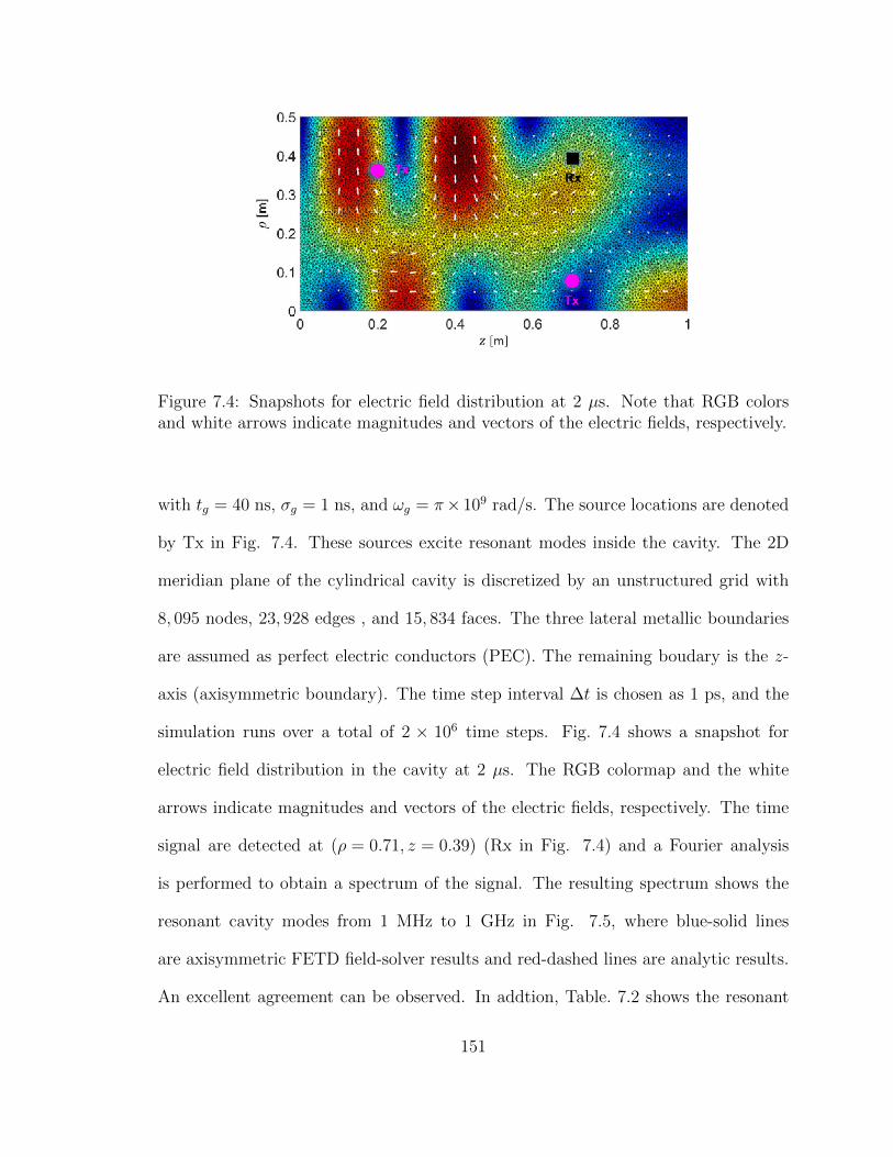
Figure 7.4: Snapshots for electric field distribution at 2 µs. Note that RGB colorsand white arrows indicate magnitudes and vectors of the electric fields, respectively.

with tg = 40 ns, σg = 1 ns, and ωg = π× 109 rad/s. The source locations are denoted

by Tx in Fig. 7.4. These sources excite resonant modes inside the cavity. The 2D

meridian plane of the cylindrical cavity is discretized by an unstructured grid with

8, 095 nodes, 23, 928 edges , and 15, 834 faces. The three lateral metallic boundaries

are assumed as perfect electric conductors (PEC). The remaining boudary is the z-

axis (axisymmetric boundary). The time step interval ∆t is chosen as 1 ps, and the

simulation runs over a total of 2 × 106 time steps. Fig. 7.4 shows a snapshot for

electric field distribution in the cavity at 2 µs. The RGB colormap and the white

arrows indicate magnitudes and vectors of the electric fields, respectively. The time

signal are detected at (ρ = 0.71, z = 0.39) (Rx in Fig. 7.4) and a Fourier analysis

is performed to obtain a spectrum of the signal. The resulting spectrum shows the

resonant cavity modes from 1 MHz to 1 GHz in Fig. 7.5, where blue-solid lines

are axisymmetric FETD field-solver results and red-dashed lines are analytic results.

An excellent agreement can be observed. In addtion, Table. 7.2 shows the resonant

151

Figure 7.5: Spectrum for resonant cavity modes from 1 MHz to 1 GHz.

frequencies for TMmnp cavity modes15 and the normalized error defined as |fs−fa|fa

where fs and fa are numerical and analytic resonant frequencies, respectively. It is

seen that all resonant cavity modes are axisymmetric (m = 0) and the normalized

errors are fairly low.

7.2.2 Space-charge-limited (SCL) cylindrical diode

As a second validation example, we test the accuracy of present EM-PIC algorithm

by modeling a SCL cylindrical diode with finite-length emitter. By applying an

external voltage to the cathode, a fast rise in the number of electrons emitted from

the cathode initially occurs; however, in the steady-state the injection current density

eventually becomes saturated due to space charge effects. For an infinitely long

cylindrical diode and electrodes, Langmuir-Blodgett’s law describes the SCL current

15m, n, and p are associated with eigenmode orders along azimuthal (φ), radial (ρ), and longitu-dinal directions (z), respectively.

152

Table 7.2: Resonant frequencies for axisymmetric cavity modes and normalized errorsbetween numerical and analytic works.

(m,n, p) fa [GHz]|fa−fs|fa

× 100 [%] (m,n, p) fa [GHz]|fa−fs|fa

× 100 [%]

(0, 1, 0) 0.230 0.083 (0, 1, 5) 0.784 0.0035(0, 1, 1) 0.274 0.040 (0, 2, 4) 0.799 0.0048(0, 1, 2) 0.378 0.040 (0, 3, 0) 0.826 0.0014(0, 1, 3) 0.505 0.047 (0, 3, 1) 0.840 0.019(0, 2, 0) 0.527 0.042 (0, 3, 1) 0.879 0.017(0, 2, 1) 0.548 0.031 (0, 3, 1) 0.917 0.027(0, 2, 2) 0.607 0.0030 (0, 2, 5) 0.929 0.027(0, 1, 4) 0.642 0.023 (0, 3, 3) 0.941 0.016(0, 2, 3) 0.693 0.034 − − −

per unit length J1D,LB as

J1D,LB ≡8πε0

9

√2e

m

V 3/2

ρβ(7.17)

where V is the external voltage, e and m are charge and mass of electrons, ρ is a

radial coordinate, and

β = µ− 2µ2

5+

11µ3

120− 47µ4

3300+ ..., (7.18)

with µ = ln (ρ/ρc) and where ρc denotes the radius of the cathode. Here, we assume

the emitting electrode with axial length Le. The finite element solution domain is

given by Ω = (ρ, z) ∈ [ρi, ρo]× [0, Lz] with ρi = 5 mm, ρo = 15 mm, and Lz = 100

mm. The domain has the horizontal wall segments representing electrode surfaces

(cathode or anode), as shown in Fig. 7.6. If the inner conductor is chosen as a

cathode, the electron flow becomes divergent, on the other hand, it is convergent.

The left and right boundaries of the domain are truncated by a perfectly matched

layer (PML) [115, 212]. The unstructured mesh has 7, 313 nodes, 21, 334 edges, and

14, 022 faces. We choose ∆t = 0.15 ps and the simulation runs up to a total 30, 000

time-steps.

153

(a)

(b)

Figure 7.6: Schematics for divergent and convergent flows in the cylindrical diode.

Fig. 7.6 illustrates snapshots for electron beam distribution with Le = 10 mm and

V = 1 kV. In order to determine J2D,max injection, we first fix the superparticle scaling

factor Csp, indicating the number of electrons for each superparticle, and gradually

increase the superparticle injection rate until the virtual cathode starts to form. We

simulate a total pf 8 cases, including Le/ρo = 0.4, 1, 2.425, and 4 for each divergent

and convergent electron flow, and compare the maximum injection current density

without formation of a virtual cathode, J2D,max injection to the previous results ob-

tained by [4] with KARAT, which is a FDTD-based EM-PIC algorithm. Fig. 7.7 shows

J2D,max injection versus Lz/ρo for divergent and convergent electron flows. Red-solid

(divergent) and -dashed (convergent) lines are KARAT results and blue-markers with

upper ranges are obtained from present EM-PIC simulations. The upper ranges on

the blue markers stand for an interval where an exact solutions for the current density

154

Figure 7.7: Space-charge-limited current density for various Lz/ρo and comparisonbetween present EM-PIC simulations and KARAT by [4].

may exist. The marker indicates maximum current density without the virtual cath-

ode formation and upper horizontal line is minimum injection current density with

virtual cathode formation. Two markers are used because of the stepwise increases

in the current density by the assumed superparticle number in our EM-PIC model.

Decreasing superparticle scaling factor or increasing superparticle injection rate can

yield higher resolution. Fig. 7.7 shows very good agreement between the results of

the present EM-PIC algorithm and those of KARAT, for both divergent and convergent

flows. In addition, it is seen that, as Le/ρo increases, the current density converges

to the limit of Langmuir-Blodgett’s law as expected.

Fig. 7.8 shows the magnitude of the electrical self-field and external field at the

instant of virtual cathode formation. Since the external field is stronger as ρ decreases,

a divergent flow produces more charges on the cathode surface so that their self-field

155

(a)

(b)

Figure 7.8: Electric field intensity of self- and external fields at the instant of virtualcathode formation.

may cancel the external field. As a result, the current density of divergent flows is

larger than that of convergent flow.

7.3 Numerical examples

In this section, we present simulations of a relativistic BWO device operating at

π-point by using the proposed EM-PIC algorithm. First we consider a SWS with

sinusoidal ripples on a cylindrical waveguide section and determine its characteristics

by performing a “cold” test (i.e. without the presence of an electron beam). Then,

we perform “hot” tests (with electron beams) of BWO to check the reliability and

validity of our axisymmetric EM-PIC algorithm. In particular, we are interested

in investigating effects of staircasing errors on the predicted behavior of the BWO

system.

156

Figure 7.9: Shematics of backward-wave oscillator with an instant particle distribu-tion snapshots at t = 21.50 ns.

Figure 7.10: Electric potential distribution (contour plots) and corresponding electricfields (vector plots) between the cathode and the anode.

157

7.3.1 Relativistic backward-wave oscillator (BWO)

Consider a BWO system composed of the cathode-anode, the SCSWS region,

the beam collector, the output port, and the beam focusing system. In order to

produce the relativistic electron beam, we apply an external voltage difference V0

between cathode and anode. We choose −550 kV which produces the electron beam

with mean axial velocity vbeam = 0.877c with the width of 2 mm. Fig. 7.10 illustrates

electric potential distribution (contour plots) and corresponding electric fields (vector

plots) by solving Poisson equations.

Each super-particle represents 1.495 × 107 electrons so that the total injection

current is around 1.5 kA. On average, 102 macro-particles are assigned to each grid

cell. The Debye length λD in our simulations is 10.7258 mm and much larger than

the average grid (edge) length, lav = 1.1123 mm. This avoids artificial heating of

the electron beam. The electron beam is emitted from the cathode and eventually

absorbed at the collector. We consider a SCSWS with radial profile R(z) = 12(A+B)+

12(A − B) cos

(2πCz), where A and B are maximum and minimum radii, respectively,

and C is the corrugation period. The total number of corrugations along the structure

is denoted as Ncrg. Based on a eigenmode analysis 16 (see the double-refined case

in Fig. 7.20), the SCSWS was designed to have A = 17.1 mm, B = 12.9 mm,

C = 7.5 mm, and Ncrg = 14.5 for Ku-band operation. We terminate the output ports

of the BWO system by inserting a PML. All left vertical walls except for the cathode

are truncated by PML to avoid spurious reflections. By using a PML with thickness

equals to 0.2λ0 where λ0 is wavelength of the center frequency, the PML reflection

coefficient, defined in [74], is as low as −92 dB. In the beam focusing system, a static

16Corresponding to the absence of an electron beam or a so-called ‘cold test’.

158

Figure 7.11: A zoomed-in region of four rightmost corrugations of Fig. 7.9 with RGBcolor scales reflecting particle velocities.

axial magnetic field is applied over the SWS region. We enforce axisymmetric fields

at the z-axis, by applying a perfect magnetic conductor (PMC) boundary condition

there (note that only the Ez component is present on axis). For the particles incident

on the axis we use a perfectly reflecting boundary condition.

System performance

Fig. 7.9 illustrates a snapshot of the electron beam at t = 21.50 ns. In Fig. 7.11

we plot a zoomed-in beam picture that shows the four rightmost corrugations, where

RGB colors indicate variations in normalized particle velocities vb/c. The periodic

particle beam bunching is a result of particles being accelerated or decelerated, which

means that the beam electrons synchronously lose and recover their kinetic energy.

The net energy is transferred from the beam to the waves as seen in Fig. 7.12, which

illustrates a phase space distribution of the particle beam at 24.00 ns. The particles

decelerated from the initial velocity (0.877c m/s) dominate the accelerated particles,

so that a net loss of the beam kinetic energy leads to amplification of the TM01

mode. Fig. 7.13 presents a vector plot of self-fields generated by the electron beam at

t = 76.00 ns (in steady state). Coherent Cerenkov beam-wave interactions give rise

159

Figure 7.12: Phase-space plot at 24.00 ns.

Figure 7.13: A snapshot of steady-state self-fields (76.00 ns).

to a strong TM01 mode that may be observed within the SWS region. The self-fields

at the output port were analyzed in time and frequency domains, as shown in Fig.

7.14a and Fig. 7.14b, respectively. It can be seen in Fig. 7.14a that although initially

there are no oscillations, the output signal starts to oscillate simultaneously with

the onset of beam bunching. This signal keeps evolving and eventually approaches

a steady state at about 35 ns. By performing the Fourier analysis of steady-state

output signals, we show that their spectrum shows a good degree of single-mode

160

purity at fosc = 15.575 GHz, as shown in Fig. 7.14b. In order to verify charge

(a) (b)

Figure 7.14: Output signal analysis in (a) time and (b) frequency domains.

conservation, we plot the normalized residuals (NR) versus the nodal indices for the

discrete continuity equation (DCE) and discrete Gauss law (DGL) [51] in Figs. 7.15a

and Fig. 7.15b, respectively. Fig. 7.15a shows that NR levels for DCE remain fairly

low at all nodes and very close to the double precision floor (below 10−15). Sparsely

observed peaks are due to the fact that the electron-beam edges, where electrons

occasionally travel through extremely small cell fractions, generate numerical noise

during the scatter step. However, these errors still remain well below 10−10. NR

levels for DGL are also distributed around the double precision floor as shown in Fig.

7.15b, which means that charge conservation is maintained within round-off errors.

The transverse dynamics of an electron beam in the cross-section plane are sensitive

to gyroradius value ρg which depends on the BFS magnetic field strength. Fig. 7.16

shows 3D electron velocity plots for a weaker BFS magnetic field reduced from 5 T

161

(a) (b)

Figure 7.15: Verification of charge conservation at nodes along time (at time-steps of7.5× 104, 9× 104, 12× 104) by testing NR levels of (a) DCE and (b) DGL.

𝑣p×108

[m/s]

2.52

2.55

2.49

2.46

2.43

2.40

Figure 7.16: 3D velocity plots for an electron beam with the BFS magnetic field of0.5 T.

to 0.5 T. RGB colors again indicate particle velocity magnitudes. The weaker axial

magnetic field yields a relatively larger ρg in the polar (ρφ) plane, which makes the

electron beam to gradually expand radially.

Staircasing error analysis

We now examine staircasing errors resulting from a discrete approximation of the

SCSWS boundary. We consider eight cases comprising the same BWO geometry

modeled by: (i) a coarse mesh, (ii) a double-refined mesh, (iii) a quadruple-refined

162

Figure 7.17: SCSWS boundary profiles for all cases.

Table 7.3: Mesh information for different SCSWS cases

Case N0 N1 N2 ave(ledge

)[mm]

coarse 4,564 12,978 8,415 2.50double-refined 5,801 16,545 10,745 1.67

quadruple-refined 8,771 25,236 16,466 1.11octuple-refined 15,333 44,542 29,210 0.74

coarse staircased 4,593 13,005 8,413 2.50double-refined staircased 5,909 16,766 10,858 1.67

quadruple-refined staircased 8,939 25,547 16,610 1.11octuple-refined staircased 15,543 44,904 29,362 0.74

mesh, (iv) a octuple-refined mesh, (v) a coarse mesh with staircased boundary, (vi)

a double-refined mesh with staircased boundary, (vii) a quadruple-refined mesh with

staircased boundary, and (viii) a octuple-refined mesh with staircased boundary.

Fig. 7.17 depicts one period of the SCSWS boundary as rendered by the different

meshes. All cases employ unstructured meshes. Although unstructured meshes do not

necessitate staircased boundaries, the latter are enforced to reproduce the staircasing

that would be present on structured meshes. At the same time, this setup allows for

a detailed study that effectively isolates staircasing error from grid-dispersion errors.

The mesh information for all cases is shown in Table 7.3. We have performed hot tests

for all cases, keeping the number of superparticle per each cell by 106 on average.

163

(a) (b)

Figure 7.18: Field signal at the output port in (a) SCSWS and (b) staircased SCSWSin the time domain.

Field output signals in time and oscillation frequencies are displayed in Fig. 7.18

and Fig. 7.19. The results based on meshes devoid of staricasing error presented in

Fig. 7.18a converge much faster that those of meshes with staircased boundaries in

Fig. 7.18b The oscillation frequency values in Fig. 7.19 also shows the fast convergent

rate of present EM-PIC simulations. In paricular, it is interesting to see that the

results from the BWO with a staircased SCSWS are unable to capture mcuh RF

oscillation at all in the case of coarse and double-refined meshes (case (v) and (vi)).

The RF oscillation is more visible on quadruple- or octuple-refined meshes (case (vii)

and (viii)). This is because underestimation of the π-point frequency17 in the modal

dispersion causes a slow-charge mode driven by the electron beam [213] to falls into

the forward wave region and, as a result, the system does not act as an oscillator

17π-point denotes the solution of the modal field which have maximum frequency in the passband.

164

Figure 7.19: Normalized spectral amplitude at the output port in SCSWS and stair-cased SCSWS.

anymore. Note that the BWO system here is designed to operate at π-point of the

modal fields. The underestimation of the π-point frequency in the staircased boundary

is shown by Fig. 7.20, which depicts the dispersion diagrams for the TM01 mode of

each SWS. The analytic dispersion relation for the TM01 mode is obtained based on

Floquet’s theory by considering harmonics up to 6th order [214]. It is clearly seen

that the π-point frequency decreases as the staircasing error become significant. On

the other hand, the cases without staircasing errors rapidly converge to the analytic

prediction.

165

Figure 7.20: Dispersion relations from “cold tests”.

7.4 Conclusion

We introduced a new axisymmetric charge-conservative EM-PIC algorithm on

unstructured grids for the analysis and design of micromachined VEDs with cylin-

drical axisymmetry. We demonstrated that cylindrical symmetry in device geometry,

fields, and sources enables reduction of the 3D problem to a 2D one through intro-

ducing an artificial inhomogeneous medium, considering TEφ-polarized fields in the

meridian (ρz) plane. As a result, computational resources are significantly reduced.

The unstructured-grid spatial discretization is achieved by using Whitney forms in

the meridian plane. Using leapfrog time integration, we obtained space- and time-

discretized Maxwell’s equations which form a so-called mixed E − B FETD scheme.

A local explicit time update is made possible by employing the SPAI approach [51].

166

Interpolation pf the field values to the particles’ positions is also performed by Whit-

ney forms and next used for solving the Newton-Lorentz equations of motion of each

particle. Relativistic particles are accelerated and pushed in space with a corrected

Boris algorithm. In the particle scatter step, we utilized a Cartesian charge-conserving

scatter scheme for unstructured grids [1]. The algorithm was validated considering

cylindrical cavity and space-charge-limited (SCL) cylindrical diode problems. We also

illustrated the advantages of the present algorithm in the analysis of a BWO system

including a slow-wave waveguide structure with complex geometry.

167

Appendix A: Basics of Plasmas

In this chapter, the basics of plasmas are covered including fundamental param-

eters, its distinct feature (quasi-neutrality and collective interaction), and motion of

a single charged particle under electromagnetic fields.

A.1 Fundamental parameters

Charge is denoted as q measured in Coulomb [C], for example, qe = −1.60217662×

10−1 [C] (negatively charged) is of a single electron with a subscription e. Note that,

in what follows, subscriptions i, p, and n are for ion (proton), positron, and neutron,

respectively. qi = qp = 1.60217662× 10−1 [C] (positively charged).

Mass (at rest) are measured in kilogram [kg] denoted as m, then, me = mp =

9.10938356×10−31 [kg] whereas mi = 1.672623×10−27 [kg] and mn = 1.674929×10−27

[kg]. Since ion is much heavier than electron, some of our simulations later will assume

that ions are stationary while electrons moving.

Number density, n is how many (charged) particles are present in unit volume,

typically measured in [cm−3 or m−3]. Usually it refers to the electron density ne,

for example, 107 [m3] in the solar wind (1AU), 1020 [m3] in Tokamak for magnetic

confinement fusion, 1012 [m3] in the ionosphere etc.

168

Temperature is a quantity measured with thermometer, but here, it is to be related

to the molecular kinetic energy to characterize thermal or random motions in gases.

Consider a gas composed of many molecules, then, the ideal gas law18 has states that

PV = NkBT (A.1)

where P [Pa or N/m2] is a pressure exerted by the gas, V [m−3] is the volume it

occupies, N is the number of the molecules, T [K] is its absolute temperature, and kB

is the Boltzmann constant given by kB = 1.3810×10−23 [J/K]. It can be equivalently

associated with kinetic parameters by examining momentum changes in the impaction

of a molecule to a rigid wall, as follows

PV =1

3Nm

⟨v2⟩

(A.2)

where v [m/s] is the speed of the molecules and 〈·〉 is the average operator. Note that

1/3 factor ahead of Eqn. (A.2) comes from the space dimensionality of 3. Since PV

in Eqn. (A.2) canceled (divided) by N and 2/3 equals to the average kinetic energy of

the gas, a new relationship between temperature and kinetic energy can be obtained

as

〈KE〉 =1

2m⟨v2⟩

=3

2kBT. (A.3)

Rearranging the above equation in terms of velocity results in

vth ≡√〈v2〉 =

√3kBT

m, (A.4)

so called thermal velocity. As expected, the hotter gas, the higher thermal velocity.

It basically describes thermal (or random) motion of particles in the gas (at its rest)

18The relationship was deduced from experimental measurements of Charles’ law and Boyle’s law.It describes the behaviors of real gases under most conditions.

169

and a measure of the temperature. Another choice for thermal velocity could be the

root-mean-sqaure (rms) of the magnitude of the velocity in any one dimension as

vth =

√kBT

m. (A.5)

Note that the kinetic temperature

T ≡ 1

3m⟨v2⟩

(A.6)

is measured through typically electron-volts [eV] unit and 1 [eV] is equivalent to

1.60217662 × 10−19 [J] (same as a single electron charge) or 1 [J] is equivalent to

6.24150913× 1018 [eV].

Maxwell-Boltzmann distribution naturally models the thermal equilibrium state

of gases. There are two speeds to characterize the Maxwell-Boltzmann distribution

which are most probable velocity at the maximum probability and rms velocity same

to the thermal velocity.

A.2 Quasi-neutrality in plasma

Consider a plasma composed of an equal number of electrons and ions freely

moving, i.e. n ≡ ne ≈ ni. Although the plasma is almost neutral in a macroscopic

scale, the charge neutrality breaks down in shorter scales, hence, plasma is usually

called quasi-neutral. If we place a test positively-charged point particle into the quasi-

neutral plasma, its electric potential will create forces attracting electrons nearby,

forming a cloud around the test charge to neutralize it. As a consequence, the modified

potential with the consideration of both the test charge and the electron clouds will

170

take the form of19

φ (x) =qT

4πε0rexp

(−√

2r

λD

)(A.7)

where r is a radial distance from the test charge and

λ2D = ε0

kBT∑s n0,sq2

s

= ε0∑s

v2th,sms

n0,sq2s

. (A.8)

As seen in Eqn. (A.7), the potential is exponentially decreasing, therefore, negligible

enough since other particles feel it far away from the test charge. in other words,

electrostatic fields the test charge is screened out and we usually this screening effect

is effective beyond λD, called Debye length. Total number of charged particles per

Debye shpere is the measure of plasma parameter denoted as

Λ =4

3πnλ3

D. (A.9)

Usually, in collisionless plasmas, the plasmas parameter greater than 1.

A.3 Plasma oscillation

Here, we investigate dynamic response of a quasi-neutral plasma to a small per-

turbation, viz. a restoring force. When some electrons are slightly displaced, electric

fields will be immediately created between the separated gap and it tends to remain

light electrons back to original position. Due to their inertia, electrons will overshoot

and then vice versa again based on total energy conservation (from electrostatic to ki-

netic energy or oppositely) as of a pendulum motion. Such a oscillation will continue

around the equilibrium position with a specific frequency depending on the property

19The original electric potential by the test charge is inversely proportional to r2.

171

of the plasma. This frequency is referred as plasma frequency given by

ωp,s =

√nsq2

s

ε0ms

(A.10)

for s species where ε0 is permittivity in a vacuum. This is the most fundamental

timescale to characterize plasmas and usually the electrons’ is of interest in plasma

physics.

A.4 Collisions in plasmas

One of distinct features in plasmas against neutral gases is the collective inter-

action among charged particles through long-range Coulomb force instead of direct

binary collisions of which individual even causes a large deflection in the trajectory

of the particle. A collision between two molecules in a neutral gas is basically rigid

body collisions (billiard) resulting in large angle of deflection. This can be thought

as direct, binary, and strong interaction each other. On the other hand, collisions in

a plama are predominantly by Coulomb force which is long-range, so that individual

particle will interact all nearby particles. Moreover, Coulomb force becomes rapidly

week, most of charged particles will have minor deflections. Plasma can be divided

into collisional and collisionless type. Collisional plasmas further can be decomposed

into (i) fully ionized and (ii) partially or weakly ionized. In the latter, dominant

collisions occur between charged particles and neutral atoms or molecules. For such

a collision, we can introduce a key quantity cross sectional area σc to estimate how

often collisions occur. For binary collisions, simply

σc ≡ πd20 (A.11)

172

where d0 denotes the radius of the particle. collision frequency is given by

νn ≡ nnσc 〈v〉 (A.12)

Then, the average mean free path which is

lmpf ≡〈v〉νn

=1

nnσc(A.13)

As expected, the more direct binary collisions happen by increase of velocity, number

density, and large cross-section area.

On contrary, Coulomb collisions between charged particles are not straightforward.

This is because deflection by Coulomb collisions are not significant compared to the

direct binary collisions. Alternatively, for Coulomb collisions, we define the collision

frequency and mean free path is the measure of the particle trajectory is deflected by

90o angle by successive Coulomb interactions.

Being collisionless does not mean that charged particles never have any interac-

tions but interactions dominates their behaviors. In collisionless plasmas, we take

into account their collective behaviors, i.e. it is sufficient to consider the effect of the

average EM fields on the particles instead of individual collision.

173

Appendix B: Kinetic Plasma Description

B.1 Plasma kinetic equation

In a vacuum, consider a fully ionized plasma composed of a huge number (denoted

as N) of charged particles such as electrons and ions. When individual charged

particle can be modeled as a point-like particle in 3-dimensional space moving with

a specific velocity, the plasma can be described by summing up all contributions

of which each would be a product between spatial and velocity delta distribution

function as

fm (x,v, t) =N∑i=1

δ (x− xi (t)) δ (v − vi (t)) (B.1)

where fm is called the microscopic phase space distribution function and the sub-

scription m stands for its microscopic quantity. In other words, fm is the number

of the charged particles over an infinitesimal volume in 6-dimensional phase space,

i.e. number density, therefore, its unit becomes [#/m6s−3]. It is straightforward to

check that, based on conservation of the number of particles (i.e. in the Hamiltonian

dynamical system), ∫R3v

fm (x,v, t) dv = nm (x, t) , (B.2)∫R3x

∫R3v

fm (x,v, t) dvdx = N, (B.3)

174

where R3x and R3

v are 3-dimensional position and velocity spaces, respectively, and

nm (x, t) denotes the microscopic number density. Then, trajectories of all charged

paticles can be tracked from a set of

midvidt

= qi [Em (xi, t) + vi ×Bm (xi, t)] , for i = 1, 2, ..., N, (B.4)

where for the ith particle, Em (xi, t) Bm (xi, t) are instantaneous electric field intensity

and magnetic flux density, respectively, and mi and qi are mass and charge, respec-

tively. These microscopic electromagnetic fields, which are very jumpy, are governed

by Maxwell’s equation writing

∇× Em = −∂Bm

∂t, (B.5)

∇×Bm =1

c20

∂Em

∂t+ µ0J

m, (B.6)

∇ · Em = −ρm/ε0, (B.7)

∇ ·Bm = 0, (B.8)

where ρm and Jm are electric charge and current densities, respectively, c0 is the speed

of light in a vacuum, and ε0 and µ0 are permittivity and permeanbility, respectively.

The microscopic charge density and current densities can be obtained through zeroth

and first moments for fm over the velocity space, respectively, as follows

ρm (x, t) ≡N∑i=1

qi

∫R3v

fm (x,v, t) dv =N∑i

qiδ (x− xi (t)) , (B.9)

Jm (x, t) ≡N∑i=1

qi

∫R3v

vfm (x,v, t) dv =N∑i

qivi (t) δ (x− xi (t)) . (B.10)

Note that solutions of the microscopic Maxwell’s equations driven by above sources

are directly associated with Coulomb forces between two charged particles. Althgouh

a system of such microscopic equations yields a complete and exact description of the

175

plasma evolution, it is impossible to solve it due to the (almost) infinite number of

charged particles in usual plasmas (ranging from 1016 to 1024) beyond current high

performance computing capabilities. Alternatively, we can relax the complexity by

using an average procedure to macroscopically model the plasma but still staying

in the kinetic description. In order to develop the average procedure, let us first

introduce a single evolution equation embedding the N number of equations of motion

by evaluating the total derivative of fm with respect to time such as

dfm

dt≡ ∂fm

∂t+dx

dt· ∂f

m

∂x+dv

dt· ∂f

m

∂v

=∂fm

∂t+ v · ∂f

m

∂x+

q

m[Em + v ×Bm]

∂fm

∂v= 0. (B.11)

This equation is called Klimontovich equation and the reason for which the total time

derivative equals to zero can be deduced from dfm/dt plugged with (B.1) as

dfm

dt=

N∑i=1

[∂

∂t+dxidt· ∂∂x

+dvidt· ∂∂v

]δ (x− xi (t)) δ (v − vi (t)) , (B.12)

with the following equalities

(∂/∂t) δ (x− xi) = − (dxi/dt) · (∂/∂x) δ (x− xi) , (B.13)

(∂/∂t) δ (v − vi) = − (dvi/dt) · (∂/∂v) δ (v − vi) . (B.14)

As a first step to average the Klimontovich equation, consider a small volume in

the phase space, sized by ∆V = ∆Vx∆Vv where ∆Vx = ∆x∆y∆z and ∆Vv =

∆vx∆vy∆vz, containing N∆V number of charged particles. A carfule selection for

the size of the volume is required, satisfying a following condition as

n−1/3 < ∆x < λD (B.15)

where n is the number density and λD is Debye length. This simply means that the

average process should have the effective relaxation to the complexity (for the smaller

176

statistical flucuation) as well as capture the fundamental properties of the plasma.

As a consequence, one can find the collective behaviors of the plasma present in the

order of the Debye length scale guarantieeng N∆V (nλ3D)

2 1.

Let us decompose the microscopic distribution function in terms of the ensem-

ble averaged one and an error term. Taking the ensemble average operator to the

distribution function, denoted as 〈fm〉, yields the macroscopic number density with

respect to the small volume ∆V given by

〈fm (x,v, t)〉 ≡ limn−1/3<∆x<λD

N∆V

∆V. (B.16)

and the error term can be written as

δfm ≡ fm − 〈fm〉 (B.17)

with a zero ensemble average, namely, 〈δfm〉 = 0. Specifically, 〈fm〉 represents the

smoothened properties of the plasma in a scale larger than ∆x while δfm implies the

discrete particle (very jumpy and spiky) effects of individual charged particles hidden

under the scale (smaller than ∆x). The ensemble average operator should be taken

also to the Maxwell dynamic variables, for the example of electric field intensity,

Em = 〈Em〉+ δEm. (B.18)

In terms of the macroscopic quantities, we can rewrite Klimontovich equation as

∂ 〈fm〉∂t

+ v · ∂ 〈fm〉

∂x+

q

m[〈Em〉+ v × 〈Bm〉] ∂ 〈f

m〉∂v

=q

m[δEm + v × δBm]

∂δfm

∂v. (B.19)

Terms in the left hand side are in relation to the smoothened response of the plasma

whereas the right represents binary Coulomb collisions within the Debye length scale.

177

It is important to note that there are many terminologies referring these two distinct

properties

Not only for its convenience but also due to the fact that the averaged proper-

ties are only of our main interest, we cancel the notations (1) bracket 〈·〉 and (2)

superscript m from all the ensemble averaged microscopic quantities, for example,

f (x,v, t) instead of 〈fm (x,v, t)〉, such that

∂f

∂t+ v · ∂f

∂x+

q

m[E + v ×B]

∂f

∂v= C (f) (B.20)

where C (f) refers a (binary) Coulomb collisional operator again coming from discrete-

ness effects (strong correlations between two charged particles via Coulomb force).

This is the fundamental set of equations decomposed into collisionless and colli-

sional effects and provides the complete kinetic description of a plasma. It should

be mentioned that it does not mean the Coulomb collisional operator can collectively

take into account all collisional effects but in some cases such as magnetized plas-

mas the discreteness effect will be reaching and significant beyond the Debye length

scale. Nevertheless, this discussion is still useful and intuitive enough at least for this

manuscript intensively discussing about particle-in-cell algorithm later on.

B.2 Vlasov equation for collisionless plasmas

There are plasmas where contributions of the Coulomb collisional operator may

be negligible, called collisionless plasmas, i.e. C (f) = 0, such that

∂f

∂t+ v · ∂f

∂x+

q

m[E + v ×B]

∂f

∂v= 0, (B.21)

which is called Vlasov equation. Following two conditions are typically used to ex-

amine whether or not plasmas are collisionless as (1) ωinterest νc and (2) λD lmfp

178

where ωinterest is a (angular) frequency of our interest, usually chosen as the plasma

frequency ωp that is characteristic time scale of plasma, νc is the collisional frequency

illustrating how often collisions occur, and lmfp denotes the mean free path that is

a average distance for charged particles to be deflected up to 90o. Here, much de-

tails about parameters related to collisional effects are not covered. In a word, in

collisionless plasmas its characteristic time and distance scales are too short for col-

lisions to take place in. Consequently, in addition to the conservation of the number

of particles f becomes incompressible, meaning that their velocity cannot be drifted

nor diffused20. Such incompressibility allows us to coarse-grain the phase space dis-

tribution function, identically known as superparticle, so as to model the collisionless

plasmas more efficiently. This is an underlying feature on which particle-in-cell algo-

rithm is based and enjoys for its realization.

B.3 Superparticle: Coarse-grained f (x,v, t)

Once and for all our main focus will be on finding the smoothened properties in

the plasmas without any consideration of collisional effects. Let us first decompose

the phase distribution function f (x,v, t) for a collisionless plasma with respect to

species s as

f (x,v, t) =

e,i∑s=1

fs (x,v, t) . (B.22)

Then, each species function can be represented by the superposition of its coarse-

grained (segmentized) versions with an index p (Np in total), centered on the specific

20Coulomb collisions may lead to velocity drift or diffusion such that the phase space distributionfunction may have compression or expansion.

179

phase space coordinates (xp,vp) as

fs (x,v, t) ≈Np∑p=1

fp (x,v, t) =

Np∑p=1

Sx (x− xp)Sv (v − vp) (B.23)

where fp is called superparticle (also called macroparticle or computational particle

by one’s preference) used in particle-in-cell algorithms and S function is a shape

function macroscopically describing the number density of actual charged particles at

once instead of adding up many delta particles. Note that xp and vp are representing

the center phase space coordinates of the superparticle. Each superparticle usually

represent millions of actual charged particles that results in the huge reduction the

computational costs for plasma kinetic simulations. The shape function is represented

by a tensor product

Sζ (ζ − ζp) =3∏i=1

Sζi(ζi − ζip

)(B.24)

where ζi denotes one of components in a generalized coordinate system, ζ = (ζ1, ζ3, ζ3)

representing vectors in either Euclidean or velocity spaces. It should have following

conditions:

(1) Compact support21

(2) Normalization ∫R1ζi

Sζi(ζi − ζip

)dζi = 1 (B.25)

(3) Symmetry

Sζi(ζi − ζip

)= S

(ζip − ζi

)(B.26)

In particular, for the velocity coarse-graining, a delta function is usually preferred so

as to avoid the dispersion of spatial shape function over the 3-dimensional Euclidean

21Each superparticle taking a small portion of the phase space is supposed not to share its supportwith others’. For example, exponential functions are not allowable.

180

space, marching on time, where our analysis is mainly done. For the spatial coarse-

graining, here two popular choices are introduced: one is again using a delta function

and the other one is with b-spline. We are going to discuss pros and cons of these

later more in detail.

B.4 Maxwell-Vlasov or Poisson-Vlasov systems

It is still difficult to explicitly find solutions of Vlasov equation due to its large

domain dimensionality (i.e. 6-dimensional phase space). Alternatively, equivalent

solutions for the evolution of collisionless plasmas can be obtained through the relax-

ation of Vlasov system which are either Poisson-Vlasov or Maxwell-Vlasov systems.

Plugging the superparticle expression (B.23) to the Vlasov equation (B.21) and eval-

uating zeroth and first (with position and velocity vectors) orders of moments for the

resultant equation for all superparticles of s species turn out to be

dNp

dt= 0, (B.27)

dxpdt

= vp, (B.28)

dvpdt

=qsms

[Ep + vp ×Bp] , (B.29)

for p = 1, 2, ..., Np where all quantities with subscription p are for pth superparticle.

Note that electric and magnetic forces, associated with Ep and Bp in the above, are

forces directly acting on pth superparticle and can be obtained through mediating

(averaging) electromagnetic fields by the spatial shape function as

Ep ≡ E (xp, t) =

∫∫∫R3x

E (x, t)Sx (x− xp) dx, (B.30)

Bp ≡ B (xp, t) =

∫∫∫R3x

B (x, t)Sx (x− xp) dx. (B.31)

181

For the example of the delta shape function, it is going to be direct evaluation of

electromagnetic fields at the location of superparticles.

Equation (B.27) is about conservation of the number of superparticle, meaning

that describes that any superparticle should not be disappeared nor created and

Newton’s law of motion and Lorentz force can be found in (B.28) and (B.29). Above

equations coupled with Maxwell’s (curl) equations is called Maxwell-Vlasov system

(multiphysical) while dealing with full electromagnetic effects.

In the electrostatic limit, one may be able to neglect the magnetic flux density

term in the Lorentz force such that

dvpdt≈ qsms

Ep. (B.32)

In this case, Poisson equation is to be associated with (B.28) and (B.32) instead of

Faraday’s and Ampere’s law, referred as Poisson-Vlasov system. Most earlier versions

of plasma kinetic simulations were solving Poisson-Vlasov system, on the other hand,

this manuscript will focus on the Maxwell-Vlasov system including the solution space

of Poisson-Vlasov system.

182

Appendix C: Discrete Exterior Caclulus (DEC)

C.1 Whitney forms

Whitney p-forms are canonical interpolants of discrete differential p-forms [215].

As explained below, Whitney p-forms are naturally paired to the p-cells of the mesh,

where p refers to the dimensionality, i.e. p = 0 refers to nodes, p = 1 to edges, p = 1

to facets and so on [30]. On simplices (e.g. on triangular cells in 2-D or tetrahedral

cells in 3-D), Whitney 0-, 1-, and 2-forms are expressed as [30,147,215]

w(0)i = λi, (C.1)

w(1)i = λiadλib − λibdλia , (C.2)

w(2)i = 2 (λiadλib ∧ dλic + λibdλic ∧ dλia + λicdλia ∧ dλib) , (C.3)

where d is the exterior derivative, ∧ is the exterior product, ia, ib, and ic denote the

grid nodes belonging to the i-th p-cell for p = 1 or 2, and λ denotes the barycentric

coordinate associated to a given node.

The corresponding vector proxies for Whitney 0-, 1-, and 2-forms write as [1, 30]

W(0)i = λi, (C.4)

W(1)i = λia∇λib − λib∇λia , (C.5)

W(2)i = 2 (λia∇λib ×∇λic + λib∇λic ×∇λia + λic∇λia ×∇λib) . (C.6)

183

C.2 Pairing operation

One of the key properties of Whitney p-forms is that they admit a natural “pair-

ing” with the p-cells of the mesh [30]. Computationally, the pairing operation between

an i-th p-cell of the grid σi(p) and a Whitney form w(p)j associated with the j-th p-cell

is effected by the integral below and yields [30,35]⟨σi(p), w

(p)j

⟩=

∫σi(p)

w(p)j = δi,j, (C.7)

where δi,j is the Kronecker delta, for p = 0, . . . , 3 in 3-D space.

C.3 Generalized Stokes’ theorem

The generalized Stokes’ theorem recovers Stokes’ and Gauss’ theorems of vector

calculus for p = 1, 2, respectively, and the fundamental theorem of calculus for p = 0.

The generalized Stokes’ theorem of exterior calculus for a Whitney p-form [30,32,35,

216,217] states ⟨σ(p+1), dw

(p)j

⟩=⟨(∂σ(p+1)

)(p), w

(p)j

⟩(C.8)

where ∂ is the boundary operator that maps an (oriented) p-cell on the grid to the

set of (oriented) (p − 1)-cells comprising its boundary. Note that ∂2 = 0 and hence

d2 = 0 from (C.8). This latter identity is the exterior calculus counterpart of the

vector calculus identities ∇×∇ = 0 and ∇ ·∇× = 0.

C.4 Discretization of Maxwell’s equation

C.4.1 Cartesian coordinates case

Using the pairing operation and generalized Stokes’ theorem, we can obtain dis-

crete Maxwell’s equation on a irregular lattice (unstructured grid). For example,

184

applying pairing for the K-th 2-cell into Faraday’s law on the primal mesh gives

⟨σK(2), dE

⟩=

⟨σK(2),

∂B∂t

⟩, (C.9)

and applying generalized Stokes’ theorem into the left-hand side term of (C.17) yields

⟨∂σK(2), E

⟩=

∂

∂t

⟨σK(2),B

⟩. (C.10)

Substituting (7.5) and (7.6) into (C.18) and using

∂σK(2) =

N1∑j=1

CK,jσj(1) (C.11)

where CK,j is an element in an incidence matrix which takes a value in the set of

−1, 0, 1 [30, 35,218,219], we obtain⟨N1∑j=1

CK,jσj(1),

N1∑j=1

Ej (t)w(1)j

⟩=

∂

∂t

⟨σK(2),

N2∑k=1

Bj (t)w(2)k

⟩. (C.12)

By using (C.7), (C.19) can be rewritten as

N1∑j=1

CK,jEj (t) =∂

∂tBK (t) , (C.13)

for K = 1, ..., N2. (C.13) represents the discrete representation of Faraday’s law as

written in (2.1). Discrete Ampere’s law can be obtained by a similar procedure on

the dual mesh.

C.4.2 Body-of-revolution case

By pairing Faraday’s law for the TEφ field with the m-th azimuthal eigenmode

set in (6.26) with K-th 2-cell σk(2) of the FE grid (primal mesh) and applying the

generalized Stokes’ theorem, we obtain⟨σK(2),

N1∑j=1

E‖j,m (t)[d′‖w

(1)j

]⟩= −

⟨σK(2),

∂

∂t

N2∑k=1

B⊥k,m (t)w(2)k

⟩, (C.14)

185

⟨σK(2),

N1∑j=1

E‖j,m (t)w(1)j

⟩= −

⟨σK(2),

∂

∂t

N2∑k=1

B⊥k,m (t)w(2)k

⟩. (C.15)

Using ∂σK(2) =∑N1

j=1CK,jσj(1), where CK,j is the incidence matrix associated to the

exterior derivative applied to 1-forms (curl operator on the mesh), see (C.5), we

obtain [30,35,218,219]

N1∑j=1

CK,jE‖j,m (t) = − ∂

∂tB⊥K,m (t) , (C.16)

for m = −Mφ, ...,Mφ. The elements of the incidence matrix take values in the set of

−1, 0, 1,

Likewise, pairing (6.27) with J-th 1-cells σJ(1) of the primal mesh gives⟨σJ(1),

N0∑i=1

E⊥i,m (t)[d′‖w

(0)i

]⟩−

⟨σJ(1), |m|

N1∑j=1

E‖j,m (t)w(1)j

⟩

= −

⟨σJ(1),

∂

∂t

N1∑j=1

B‖j,m (t)w(1)j

⟩, (C.17)

and applying generalized Stokes’ theorem to the left-hand side of (C.17) yields⟨∂σJ(1),

N0∑i=1

E⊥i,m (t)w(0)i

⟩−

⟨σJ(1), |m|

N1∑j=1

E‖j,m (t)w(1)j

⟩

= −

⟨σJ(1),

∂

∂t

N1∑j=1

B‖j,m (t)w(1)j

⟩, (C.18)

Similarly to before, we can write ∂σJ(1) =∑N0

i=1GJ,iσi(1), where GJ,i is the incidence

matrix associated to the exterior derivative applied to 0-forms (gradient operator on

the mesh), and obtain

N0∑i=1

GJ,iE⊥i,m (t)− |m|E‖J,m (t) = − ∂

∂tB‖J,m (t) , (C.19)

for J = 1, ..., N1. An analogous procedure can be used to obtain the discrete rendering

of Ampere’s law for on the dual mesh.

186

Figure C.1: Example (primal) unstructured mesh.

C.5 Incidence Matrices

Frequently used in graph theory, in mathematics an incidence matrix is a matrix

providing oriented connectivity information between two classes of objects, for exam-

ple between nodes and edges, in the incident context. Incidence matrices can be used

to represent on a mesh the discrete exterior derivative or, equivalently, the grad, curl,

and div operators distilled from their metric structure [30,35,217]. Since, from (C.8),

the discrete exterior derivative can be seen as the dual of the boundary operator,

incidence matrices encode the relationship between each oriented p-cell of the mesh

and its boundary oriented (p−1)-cells (say, between an edge and its boundary nodes,

a face element and its boundary edges, and so on). To provide a concrete example,

we consider a small mesh with perfect magnetic conductor (or free edges) boundaries

187

(a)

(b)

Figure C.2: Incidence matrices for (a) curl [Dcurl] and (b) gradient [Dgrad] operatorsfor the mesh in Fig. C.1.

188

as depicted in Fig. C.1. Red-colored numbers denote the nodal indices, black-colored

numbers the edge indices, and blue-colored numbers the face indices. Intrinsic edge

orientation is defined by ascending index order of the two nodes associated with any

given edge. For example, if we consider [Dcurl], of size N2×N1, there are three edges

wrapping face number 6: edges 8, 9, and 20. As a result, [Dcurl]6,8 = 1, [Dcurl]6,9 = −1,

and [Dcurl]6,9 = 1. The sign is determined by comparing the intrinsic orientation of

each edge with the curl in Fig. C.1: if they are opposite, the element is −1, otherwise

it is +1. Furthermore, [Dcurl]6,j = 0 for all other j−th edges. This is represented in

Fig. C.2a, which shows the entire [Dcurl] for this mesh. A curl orientation on each

face is supposed to follow the intrinsic orientation of the first local edge (i.e. an edge

with the smallest index among three edges for the face). Likewise, if we consider

[Dgrad], of size N1 × N0, there are two nodes connected to edge 10: nodes 4 and 5.

The corresponding elements are [Dgrad]10,4 = −1 and [Dgrad]10,5 = 1. The element for

the diverging node with the gradient (the intrinsic edge orientation) in Fig. C.1 is

−1, otherwise it is +1.

C.6 Discrete Hodge matrix

A (discrete) Hodge star operator encodes all the metric information and is used to

transfer information between the primal and dual meshes [30,32,76,85,180]. Here, we

use a Galerkin-Hodge construction [32,33,179,180], which leads to symmetric positive

definite matrices and enables energy-conserving discretizations in arbitrary simplicial

meshes [35]. As noted before in Section 2, the Galerkin-Hodge operator is not a natu-

ral consequence of DEC [182]. The Hodge operator also incorporates the constitutive

properties (permittivity and permeability) of the background medium [74].

189

Inhomogeneous and anisotropic media can be easily dealt with by incorporating

piecewise constant permittivity and permeability over each cell, for example. In the

present FETD-BOR solver, the elements of the Hodge matrices including the radial

scaling factor from the cylindrical metric are assembled by adding the contributions

from all cells as:

[?ε]1→1J,j =

N2∑k=1

∫Ωk

(εkρk) W(1)J ·W

(1)j dV, (C.20)

[?µ−1 ]2→2K,k

=

N2∑k=1

∫Ωk

(µ−1k ρk

)W

(2)K ·W

(2)k dV, (C.21)

[?ε]0→0I,i =

N2∑k=1

∫Ωk

(εkρ−1k

) [W

(0)I φ]·[W

(0)i φ]dV, (C.22)

[?µ−1 ]1→1J,j

=

N2∑k=1

∫Ωk

(µ−1k ρ−1

k

) [W

(1)J × φ

]·[W

(1)j × φ

]dV, (C.23)

where Ωk is the area of the k−th cell, and ρk =∑3

i=1 ρki/3 where ρki is ρ coordinate

of i−th node touching k−th face and for simplicity we have assumed isotropic me-

dia assuming permittivity and permeability values εk and µk, resp., on cell k. Since

Whitney forms have compact support, we can express the global discrete Hodge ma-

trix as a sum of local matrices (excluding element-wise permittivity and permeability

information) for the K-th face as

[T ]0→0K = ∆K

1/6 1/12 1/121/12 1/6 1/121/12 1/12 1/6

, (C.24)

[T ]1→1K = ∆K

T 1→111 T 1→1

12 T 1→113

T 1→121 T 1→1

22 T 1→123

T 1→131 T 1→1

32 T 1→133

, (C.25)

[T ]2→2K = 4∆K (∇λ1 ×∇λ2) · φ, (C.26)

190

where ∆K is the area of K-th face and

T 1→11,1 =

∇λ1 ·∇λ1

6+

∇λ2 ·∇λ2

6− ∇λ1 ·∇λ2

6, (C.27)

T 1→11,2 =

∇λ1 ·∇λ1

6− ∇λ2 ·∇λ2

6− ∇λ1 ·∇λ2

6, (C.28)

T 1→11,3 =

∇λ1 ·∇λ1

6− ∇λ2 ·∇λ2

6+

∇λ1 ·∇λ2

6, (C.29)

T 1→12,1 = T 1→1

12 , (C.30)

T 1→12,2 =

∇λ1 ·∇λ1

2+

∇λ2 ·∇λ2

6+

∇λ1 ·∇λ2

2, (C.31)

T 1→12,3 =

∇λ1 ·∇λ1

6+

∇λ2 ·∇λ2

6+

∇λ1 ·∇λ2

2, (C.32)

T 1→13,1 = T 1→1

13 , (C.33)

T 1→13,2 = T 1→1

23 , (C.34)

T 1→13,3 =

∇λ1 ·∇λ1

6+

∇λ2 ·∇λ2

2+

∇λ1 ·∇λ2

2. (C.35)

Due to the local support of the Whitney forms, the above Hodge matrices are very

sparse (and diagonally dominant). Their sparsity patterns for the mesh in Fig. C.1

are provided in Fig. C.3. The number of non-zero elements per row (or column)

in these Hodge matrices is invariant with respect to the mesh size, so the sparsity

increases for larger meshes.

For the axisymmetric EM-PIC code, its discrete Hodge matrices are identical to

[?ε]1→1 and

[?−1µ

]2→2, respectively. In this case, it can be also analytically evaluated

[56] rather than using the elementwise ρk.

In the Cartesian coordinate system, its discrete Hodge matrices are also identical

to [?ε]1→1 and

[?−1µ

]2→2, respectively, with ρk = 1.

191

(a) (b)

(c) (d)

Figure C.3: Sparsity patterns for discrete Hodge matrices corresponding to the toy

mesh depicted in Fig. C.1: (a) [?ε]0→0, (b) [?ε]

1→1, (c)[?−1µ

]1→1, and (d) [?µ−1 ]2→2.

192

C.7 Barycentric dual lattice relations

The barycentric dual lattice [35,210] has a similar contraction identity to (C.7) in

n-dimensional space, given by⟨σi(n−p), ?w

(p)j

⟩=

∫σi(n−p)

?w(p)j = δi,j. (C.36)

Note that p is the (primal) grid element dimension and a quantity with a tilde is of

the dual mesh. Since we consider Hodge duals of electric current and charge densities

in the primal mesh, we need to express them in dual formulation to be used in discrete

Ampere’s law. The electric current density can be expressed by

J = ? (J?) = ?

(N1∑j=1

J?,jw(1)j

)=

N1∑j=1

J?,j ?(w

(1)j

). (C.37)

In order to obtain the discrete representation for Ampere’s law, we combine the

pairing, i.e.⟨σ

(K)2 , (·)

⟩(at a K-th face in the dual mesh) with Ampere’s law. The

electric current density term become⟨σ

(K)2 ,

N1∑j=1

J?,j ? w(1)j

⟩=

N1∑j=1

J?,j⟨σ

(K)1 , ?w

(1)j

⟩=

N1∑j=1

δK,j J?,j. (C.38)

Therefore, we can write above in matrix form as

[J] = [I] · [J?] (C.39)

where [J] is a column vector with all Dofs for J expanded in terms of Whitney 1-

forms on the dual mesh, and [I] is the identity matrix. A similar procedure can be

done for the electric charge density in Gauss’ law:

[Q] = [I] · [Q?] (C.40)

where [Q] is a column vector with all Dofs forQ expanded in terms of Whitney 2-forms

on the dual mesh. It is worth mentioning that our charge conserving scatter scheme

193

is a natural result of Galerkin projection of (ambient) current and charge densities,

which are basically to be associated with dual grids, via (known) Whitney forms in

the primal grids. Strictly speaking, the results of the Galerkin projection for the

sources are DoFs (J and Q) on the dual mesh likewise parameters in the constitutive

relations D and H. However, since discrete Hodge matrices for the sources are a tricky

identity matrix as the above, such that we do not need to explicitly distinguish them.

194

Appendix D: Cartesian-like PML implementation

A perfectly matched layer (PML) is used to absorb outgoing waves in FE simula-

tions, enabling analysis of open-domain problems [220, 221]. As described before, in

the present FETD-BOR the spatial discretization is performed in the meridian plane

mapped onto a Cartesian domain with the cylindrical metric factor transferred to the

constitutive relations. The resulting constitutive relations correspond to a medium

that is inhomogeneous and doubly anisotropic. As such, a Cartesian PML imple-

mentation extended to such media can be used. Such formulation exists [212] and is

adapted here to the FETD-BOR case as follows.

In the 2-D Cartesian plane, the PML can be effected as an analytic continuation on

the spatial variables to complex space [212,221], given by u→ u =∫ u

0su (u′) du′ where

su (u′) is a complex stretching variable and u stands for ρ or z. This transformation

can also be expressed as

r′‖ → r

′‖ = ¯Γ · r′‖, (D.1)

where ¯Γ = ρρ (ρ/ρ)+zz (z/z). As before, the apostrophe ′ in r′‖ denotes the transverse

coordinates on the 2-D meridian plane. The modified nabla operator (posterior to

the TO-based transformation and hence devoid of the 1/ρ factor in the φ derivative)

195

following such analytical continuation is given by

∇′ → ∇′ = ρ1

sρ

∂

∂ρ+ φ

∂

∂φ+ z

1

sz

∂

∂z, (D.2)

or simply

∇′ = ¯S · ∇′, (D.3)

where ¯S = ρρ (1/sρ) + φφ (1) + zz (1/sz). Following [212], since su (u) and ∂/∂u′

commute when u 6= u′ and ¯S is a diagonal tensor, the following identity holds for any

vector a in the Cartesian-like 2-D meridian plane:

∇′ ×(

¯S−1 · a)

=(

det¯S)−1 ¯S ·

(¯S · ∇′

)× a. (D.4)

Applying this analytic continuation to (6.18), (6.19), (6.32), and (6.33) in the

Fourier domain (with time convention of ejωt) yields the modified Maxwell’s equations

for each mode m as

∇′‖ × E′‖cm

(r′‖)

= −jωB′⊥cm

(r′‖), (D.5)

∇′‖ × E′⊥cm

(r′‖)

= −jωB′‖cm

(r′‖)

+ |m|E′‖cm(r′‖)× φ, (D.6)

∇′‖ ×H′‖cm

(r′‖)

= jωD′⊥cm

(r′‖), (D.7)

∇′‖ ×H′⊥cm

(r′‖)

= jωD′‖cm

(r′‖)− |m|H′‖cm

(r′‖)× φ, (D.8)

with constitutive relations in analytic-continued complex space as

D′cm

(r′‖)

= ¯ε′ (ω) · E′cm(r′‖), (D.9)

B′cm

(r′‖)

= ¯µ′ (ω) ·H′cm(r′‖), (D.10)

where the superscript c denotes non-Maxwellian (complex space) fields and ¯ε′ and

¯µ′ indicates constitutive parameters of the original medium incorporating the radial

196

scaling factors from the TO mapping. Next, using (D.1) and (D.3), we can revert

(D.5)−(D.8) back to a real-valued spatial domain by writing

(¯S · ∇′‖

)× E′

‖cm

(¯Γ · r′‖

)= −jωB′

⊥cm

(¯Γ · r′‖

), (D.11)(

¯S · ∇′‖)× E′

⊥cm

(¯Γ · r′‖

)= −jωB′

‖cm

(¯Γ · r′‖

)− |m| φ× E′

‖cm

(¯Γ · r′‖

), (D.12)(

¯S · ∇′‖)×H′

‖cm

(¯Γ · r′‖

)= jωD′

⊥cm

(¯Γ · r′‖

), (D.13)(

¯S · ∇′‖)×H′

⊥cm

(¯Γ · r′‖

)= jωD′

‖cm

(¯Γ · r′‖

)+ |m| φ×H′

‖cm

(¯Γ · r′‖

). (D.14)

Using the identity (D.4), we can rewrite (D.11)−(D.14) as

∇′‖ ×[¯S−1 · E′‖cm

(¯Γ · r′‖

)]= −jω

[(det¯S

)−1 ¯S ·B′⊥cm(

¯Γ · r′‖)]

, (D.15)

∇′‖ ×[¯S−1 · E′⊥cm

(¯Γ · r′‖

)]= −jω

[(det¯S

)−1 ¯S ·B′‖cm(

¯Γ · r′‖)]

− |m|[(

det¯S)−1 ¯S ·

φ× E′

‖cm

(¯Γ · r′‖

)], (D.16)

∇′‖ ×[¯S−1 ·H′‖cm

(¯Γ · r′‖

)]= jω

[(det¯S

)−1 ¯S ·D′⊥cm(

¯Γ · r′‖)]

, (D.17)

∇′‖ ×[¯S−1 ·H′⊥cm

(¯Γ · r′‖

)]= jω

[(det¯S

)−1 ¯S ·D′‖cm(

¯Γ · r′‖)]

+ |m|[(

det¯S)−1 ¯S ·

φ×H′

‖cm

(¯Γ · r′‖

)]. (D.18)

We can further verify the identity below

(det¯S

)−1 ¯S ·φ× E′

‖cm

(¯Γ · r′‖

)= φ×

[¯S−1 · E′‖cm

(¯Γ · r′‖

)], (D.19)(

det¯S)−1 ¯S ·

φ×H′

‖cm

(¯Γ · r′‖

)= φ×

[¯S−1 ·H′⊥cm

(¯Γ · r′‖

)]. (D.20)

197

and introduce a new set of fields defined as

E′am

(r′‖)

= ¯S−1 · E′cm(

¯Γ · r′‖), (D.21)

H′am

(r′‖)

= ¯S−1 ·H′cm(

¯Γ · r′‖), (D.22)

D′am

(r′‖)

=(

det¯S)−1 ¯S ·D′cm

(¯Γ · r′‖

), (D.23)

B′am

(r′‖)

=(

det¯S)−1 ¯S ·B′cm

(¯Γ · r′‖

), (D.24)

so that, by substituting (D.21)−(D.24) back into (D.15)−(D.18), and utilizing the

identities (D.19) and (D.20), we finally obtain

∇′‖ × E′‖am

(r′‖)

= −jωB′⊥am

(r′‖), (D.25)

∇′‖ × E′⊥am

(r′‖)

= −jωB′‖am

(r′‖)

+ |m|E′‖am(r′‖)× φ, (D.26)

∇′‖ ×H′‖am

(r′‖)

= jωD′⊥am

(r′‖), (D.27)

∇′‖ ×H′⊥am

(r′‖)

= jωD′‖am

(r′‖)− |m|H′‖am

(r′‖)× φ. (D.28)

with

D′am

(r′‖)

=

[(det¯S

)−1 ¯S · ¯ε′ (ω) · ¯S]· E′am

(r′‖), (D.29)

B′am

(r′‖)

=

[(det¯S

)−1 ¯S · ¯µ′ (ω) · ¯S]·H′am

(r′‖). (D.30)

The above expressions show that E′am, H′am, D′am, and B′am obey Maxwell’s equations

in an equivalent PML medium with constitutive parameters given by

¯εPML =

[(det¯S

)−1 ¯S · ¯ε′ (ω) · ¯S]

, (D.31)

¯µPML =

[(det¯S

)−1 ¯S · ¯µ′ (ω) · ¯S]

. (D.32)

198

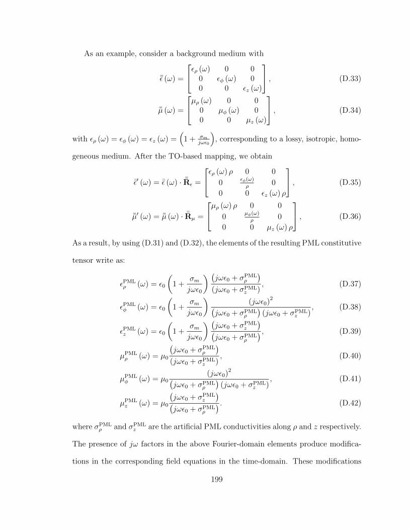
As an example, consider a background medium with

¯ε (ω) =

ερ (ω) 0 00 εφ (ω) 00 0 εz (ω)

, (D.33)

¯µ (ω) =

µρ (ω) 0 00 µφ (ω) 00 0 µz (ω)

, (D.34)

with ερ (ω) = εφ (ω) = εz (ω) =(

1 + σmjωε0

), corresponding to a lossy, isotropic, homo-

geneous medium. After the TO-based mapping, we obtain

¯ε′ (ω) = ¯ε (ω) · ¯Rε =

ερ (ω) ρ 0 0

0εφ(ω)

ρ0

0 0 εz (ω) ρ

, (D.35)

¯µ′ (ω) = ¯µ (ω) · ¯Rµ =

µρ (ω) ρ 0 0

0µφ(ω)

ρ0

0 0 µz (ω) ρ

, (D.36)

As a result, by using (D.31) and (D.32), the elements of the resulting PML constitutive

tensor write as:

εPMLρ (ω) = ε0

(1 +

σmjωε0

) (jωε0 + σPML

ρ

)(jωε0 + σPML

z ), (D.37)

εPMLφ (ω) = ε0

(1 +

σmjωε0

)(jωε0)2(

jωε0 + σPMLρ

)(jωε0 + σPML

z ), (D.38)

εPMLz (ω) = ε0

(1 +

σmjωε0

) (jωε0 + σPML

z

)(jωε0 + σPML

ρ

) , (D.39)

µPMLρ (ω) = µ0

(jωε0 + σPML

ρ

)(jωε0 + σPML

z ), (D.40)

µPMLφ (ω) = µ0

(jωε0)2(jωε0 + σPML

ρ

)(jωε0 + σPML

z ), (D.41)

µPMLz (ω) = µ0

(jωε0 + σPML

z

)(jωε0 + σPML

ρ

) . (D.42)

where σPMLρ and σPML

z are the artificial PML conductivities along ρ and z respectively.

The presence of jω factors in the above Fourier-domain elements produce modifica-

tions in the corresponding field equations in the time-domain. These modifications

199

are implemented using an auxiliary differential equation (ADE) approach as described

in, e.g., [74, 75].

200

Appendix E: Stability Conditions

To determine the stability conditions, we express the field update in matrix form

as

wn+1 = ¯G · wn =(

¯I + ¯T)· wn (E.1)

with

wn =

[B⊥m]n− 1

2[B‖m]n− 1

2[E⊥m]n[

E‖m]n

, wn+1 =

[B⊥m]n+ 1

2[B‖m]n+ 1

2[E⊥m]n+1[

E‖m]n+1

, (E.2)

and

¯T =

¯0N2×N2 ,

¯0N2×N1 ,¯0N2×N0 , −∆t [Dcurl]

¯0N1×N2 ,¯0N1×N1 , −∆t [Dgrad] , ∆t |m| ¯IN1×N1

¯0N0×N2 , ∆t ¯XTMφ , −∆t2 ¯XTMφ · [Dgrad], ∆t2 |m| ¯XTMφ

∆t ¯XTEφ , −∆t |m| ¯A, −∆t2 |m| ¯A · [Dgrad] , −∆t2 ¯XTEφ · [Dcurl]−∆t2 |m|2 ¯A

,

(E.3)

where

¯XTMφ =([?ε]

0→0)−1 · [Dgrad]T ·[?−1µ

]1→1, (E.4)

¯XTEφ =([?ε]

1→1)−1 · [Dcurl]T ·[?−1µ

]2→2, (E.5)

¯A =([?ε]

1→1)−1 ·[?−1µ

]1→1. (E.6)

201

A necessary condition for stability is |λ ¯G| ≤ 1 for all eigenvalues λ ¯G of ¯G [222].

When m = 0, the field update equation becomes decoupled into two independent

numerical integrators for TEφ and TMφ fields. In this case, following [33], we can

easily obtain the stability criteria for both polarizations in closed form as

∆tTEφ,m=0 ≤2√

max(λX

TEφ·[Dcurl]

) , (E.7)

∆tTMφ,m=0 ≤2√

max(λX

TMφ·[Dgrad]

) , (E.8)

where λXTEφ·[Dcurl] and λX

TMφ·[Dgrad] denote the eigenvalues of XTEφ · [Dcurl] and XTMφ ·

[Dgrad] respectively.

When m 6= 0, we can simply represent ¯G using 2× 2 block matrices ¯X and [D] as

¯G =

[¯I(N2+N1)×(N2+N1), −∆t [D]

∆t ¯X, ¯I(N0+N1)×(N0+N1) −∆t2 ¯X · [D]

](E.9)

where

¯X =

[¯0N0×N2 ,¯XTMφ

¯XTEφ , − |m| ¯A

], (E.10)

and

[D] =

[¯0N2×N0 , [Dcurl]

[Dgrad] − |m| ¯IN1×N1

]. (E.11)

Therefore, the stability condition is similarly obtained as

∆tm6=0 ≤2√

max(λ ¯X·[D]

) (E.12)

where λ ¯X·[D] are the eigenvalues of ¯X · [D]. Note that in this case the maximum time

step depends on the modal index magnitude |m|.

202

Bibliography

[1] H. Moon, F. L. Teixeira, and Y. A. Omelchenko, “Exact charge-conservingscattergather algorithm for particle-in-cell simulations on unstructured grids:A geometric perspective,” Comput. Phys. Commun., vol. 194, pp. 43–53, 2015.

[2] T. H. Stix, Waves in Plasmas. New York: AIP-press, 1992.

[3] Y.-K. Hue, F. L. Teixeira, L. S. Martin, and M. S. Bittar, “Three-dimensionalsimulation of eccentric LWD tool response in boreholes through dipping forma-tions,” IEEE Trans. Geosci. Remote Sens., vol. 43, no. 2, pp. 257–268, 2005.

[4] K. G. Kostov and J. J. Barroso, “Space-charge-limited current in cylindricaldiodes with finite-length emitter,” Phys. Plasmas, vol. 9, pp. 1039–1042, 2002.

[5] K. P. Thorne and R. D. Blanford, Modern Classical Physics. Princeton, NJ:Princeton University Press, 2017.

[6] R. Fitzpatrick, Plasma Physics: An Introduction. New York: CRC Press, 2016.

[7] R. M. Hanson and S. Green, Introduction to Molecular Thermodynamics. Hern-don, VA: University Science Books, 2008.

[8] S. A. Ledvina, Y.-J. Ma, and E. Kallio, “Modeling and simulating flowing plas-mas and related phenomena,” Space Science Reviews, vol. 139, pp. 1–4, 2008.

[9] J. D. Callen, Fundamentals of Plasma Physics, 2006.

[10] G. Colonna and A. DAngola, Plasma Modeling: Methods and Applications.Philadelphia, PA: IOP Publishing, 2016.

[11] R. W. Hockney and J. W. Eastwood, Computer Simulation Using Particles.New York: CRC Press, 1988.

[12] J. M. Dawson, “Particle simulation of plasmas,” Rev. Mod. Phys., vol. 55,pp. 403–447, 1983.

[13] C. K. Birdsall and A. B. Langdon, Plasma Physics via Computer Simulation.New York: CRC Press, 2004.

203

[14] J. W. Eastwood, “The virtual particle electromagnetic particle-mesh method,”Comput. Phys. Commun., vol. 64, pp. 252–266, 1991.

[15] B. B. Godfrey and J.-L. Vay, “Improved numerical Cherenkov instability sup-pression in the generalized PSTD PIC algorithm,” Comput. Phys. Commun.,vol. 196, pp. 221 – 225, 2015.

[16] J. Villasenor and O. Buneman, “Rigorous charge conservation for local electro-magnetic field solvers,” Comput. Phys. Commun., vol. 69, no. 2, pp. 306 – 316,1992.

[17] T. Z. Esirkepov, “Exact charge conservation scheme for particle-in-cell simula-tion with an arbitrary form-factor,” Comput. Phys. Commun., vol. 135, no. 2,pp. 144 – 153, 2001.

[18] T. Umeda, Y. Omura, T. Tominaga, and H. Matsumoto, “A new charge conser-vation method in electromagnetic particle-in-cell simulations,” Comput. Phys.Commun., vol. 156, no. 1, pp. 73 – 85, 2003.

[19] A. Taflove and S. C. Hagness, Computational Electrodynamics: The Finite-Difference Time-Domain Method. Norwood: Artech House, third ed., 2005.

[20] A. D. Greenwood, K. L. Cartwright, J. W. Luginsland, and E. A. Baca, “On theelimination of numerical Cerenkov radiation in PIC simulations,” J. Comput.Phys., vol. 201, pp. 665–684, 2004.

[21] C. S. Meierbachtol, A. D. Greenwood, J. P. Verboncoeur, and B. Shanker,“Conformal electromagnetic particle in cell: A review,” IEEE Trans. PlasmaSci., vol. 43, pp. 3778–3793, 2015.

[22] J.-Y. Wu and R. Lee, “The advantages of triangular and tetrahedral edge el-ements for electromagnetic modeling with the finite-element method,” IEEETrans. Antennas Propag., vol. 45, pp. 1431–1437, Sep 1997.

[23] J.-M. Jin, The finite element method in electromagnetics. New Jersey: JohnWiley & Sons, 2015.

[24] B. He and F. L. Teixeira, “Mixed E-B finite elements for solving 1-D, 2-D,and 3-D time-harmonic Maxwell curl equations,” IEEE Microw. Compon. Lett.,vol. 17, no. 5, pp. 313–315, 2007.

[25] B. He and F. L. Teixeira, “Sparse and explicit FETD via approximate inverseHodge (mass) matrix,” IEEE Microw. Wireless Compon. Lett., vol. 16, pp. 348–350, 2006.

204

[26] B. He and F. L. Teixeira, “Differential forms, Galerkin duality, and sparseinverse approximations in finite element solutions of Maxwell equations,” IEEETrans. Antennas Propag., vol. 55, pp. 1359–1368, 2007.

[27] F. L. Teixeira, “Time-domain finite-difference and finite-element methods forMaxwell equations in complex media,” IEEE Trans. Antennas Propag., vol. 56,pp. 2150–2166, 2008.

[28] B. He and F. L. Teixeira, “On the degrees of freedom of lattice electrodynamics,”Phys. Lett. A, vol. 336, pp. 1–7, 2005.

[29] L. Kettunen, K. Forsman, and A. Bossavit, “Discrete spaces for div and curl-freefields,” IEEE Trans. Magn., vol. 34, no. 5, pp. 2551–2554, 1998.

[30] F. L. Teixeira and W. C. Chew, “Lattice electromagnetic theory from a topo-logical viewpoint,” J. Math. Phys., vol. 40, pp. 169–187, 1999.

[31] D. N. Arnold, R. S. Falk, and R. Winther, “Finite element exterior calculus,homological techniques, and applications,” Acta Numerica, vol. 15, pp. 1–155,2006.

[32] J. Kangas, T. Tarhasaari, and L. Kettunen, “Reading Whitney and finite el-ements with hindsight,” IEEE Trans. Magn., vol. 43, no. 4, pp. 1157–1160,2007.

[33] J. Kim and F. L. Teixeira, “Parallel and explicit finite-element time-domainmethod for Maxwell’s equations,” IEEE Trans. Antennas Propag., vol. 59,pp. 2350–2356, 2011.

[34] F. L. Teixeira, “Differential forms in lattice field theories: An overview,” ISRNMath. Phys., vol. 2013, p. 16, 2013.

[35] F. L. Teixeira, “Lattice Maxwell’s equations,” Prog. Electromagn. Res., vol. 148,pp. 113–128, 2014.

[36] S. C. Chen and W. C. Chew, “Numerical electromagnetic frequency domainanalysis with discrete exterior calculus,” J. Comput. Phys., vol. 350, pp. 668 –689, 2017.

[37] J. P. Boris, “Relativistic plasma simulation-Optimization of a hybrid code,”in in Proc. the Fourth Conference on Numerical Simulation of Plasmas 1970,(Navl Research Laboratory, Washington, DC, 1970).

[38] J.-L. Vay, “Simulation of beams or plasmas crossing at relativistic velocity,”Phys. Plasmas, vol. 15, p. 056701, 2008.

205

[39] A. V. Higuera and J. R. Cary, “Structure-preserving second-order integration ofrelativistic charged particle trajectories in electromagnetic fields,” Phys. Plas-mas, vol. 24, no. 5, p. 052104, 2017.

[40] M. A. Furman and M. T. F. Pivi, “Probabilistic model for the simulation ofsecondary electron emission,” Phys. Rev. ST Accel. Beams, vol. 5, p. 124404,Dec 2002.

[41] F. L. Teixeira and W. C. Chew, “Differential forms, metrics, and the reflec-tionless absorption of electromagnetic waves,” J. Electromagn. Waves Appl.,vol. 13, pp. 665–686, 1999.

[42] J. B. Pendry, D. Schurig, and D. R. Smith, “Controlling electromagnetic fields,”Science, vol. 312, pp. 1780–1782, 2006.

[43] J. A. Silva-Macedo, M. A. Romero, and B.-H. V. Borges, “An extended FDTDmethod for the analysis of electromagnetic field rotations and cloaking devices,”PIER, vol. 87, pp. 183–196, 2008.

[44] O. Ozgun and M. Kuzuoglu, “Software metamaterials: Transformation mediabased multiscale techniques for computational electromagnetics,” J. Comput.Phys., vol. 236, pp. 203–219, 2013.

[45] O. Ozgun and M. Kuzuoglu, “Cartesian grid mapper: Transformation mediafor modeling arbitrary curved boundaries with cartesian grids,” IEEE AntennasWireless Propag. Lett., vol. 13, pp. 1771–1774, 2014.

[46] S. H. Gold and G. S. Nusinovich, “Review of high-power microwave sourceresearch,” Rev. Sci. Instrum., vol. 68, pp. 3945–3974, 1997.

[47] R. A. Cairns and A. D. R. Phelps, Generation and Application of High PowerMicrowaves. New York: CRC Press, 1997.

[48] J. H. Booske, R. J. Dobbs, C. D. Joye, C. L. Kory, G. R. Neil, G.-S. Park,J. Park, and R. J. Temkin, “Vacuum electronic high power terahertz sources,”IEEE Trans. THz Sci. Technol., vol. 1, pp. 54–75, 2011.

[49] J. H. Booske, “Plasma physics and related challenges of millimeter-wave-to-terahertz and high power microwave generation,” Phys. Plasmas, vol. 15,p. 055502, 2008.

[50] X. Li, J. Wang, J. Sun, Z. Song, H. Ye, Y. Zhang, L. Zhang, and L. Zhang,“Experimental study on a high-power subterahertz source generated by an over-moded surface wave oscillator with fast startup,” IEEE Trans. Electron Devices,vol. 60, pp. 2931–2935, 2013.

206

[51] D.-Y. Na, H. Moon, Y. A. Omelchenko, and F. L. Teixeira, “Local, explicit,and charge-conserving electromagnetic particle-in-cell algorithm on unstruc-tured grids,” IEEE Trans. Plasma Sci., vol. 44, pp. 1353–1362, 2016.

[52] D.-Y. Na, H. Moon, Y. A. Omelchenko, and F. L. Teixeira, “Relativistic exten-sion of a charge-conservative finite element solver for time-dependent Maxwell-Vlasov equations,” Phys. Plasmas, vol. 25, no. 1, p. 013109, 2018.

[53] D.-Y. Na and F. L. Teixeira, “Analysis of multipactor effects by particle-in-cell algorithm integrated with secondary electron emission model on irregulargrids,” IEEE Trans. Plasma Sci., vol. under review.

[54] D.-Y. Na, J. L. Nicolini, R. Lee, B.-H. V. Borges, Y. A. Omelchenko, and F. L.Teixeira, “Diagnosing numerical Cherenkov instabilities in relativistic plasmasimulations on general meshes,” J. Comput. Phys., vol. under review.

[55] D.-Y. Na, B.-H. V. Borges, and F. L. Teixeira, “Finite element time-domainbody-of-revolution Maxwell solver based on discrete exterior calculus,” J. Com-put. Phys., vol. 376, pp. 249 – 275, 2019.

[56] D.-Y. Na, Y. A. Omelchenko, H. Moon, B.-H. V. Borges, and F. L. Teixeira,“Axisymmetric charge-conservative electromagnetic particle simulation algo-rithm on unstructured grids: Application to microwave vacuum electronic de-vices,” J. Comput. Phys., vol. 346, pp. 295 – 317, 2017.

[57] Y. N. Grigoryev, V. A. Vshivkov, and M. P. Fedoruk, Numerical “Particle-In-Cell” Methods: Theory and Applications. Boston: Walter de Gruyter, 2002.

[58] E. Esarey, P. Sprangle, J. Krall, and A. Ting, “Overview of plasma-based ac-celerator concepts,” IEEE Trans. Plasma Sci., vol. 24, pp. 252–288, April 1996.

[59] D. L. Bruhwiler, R. E. Giacone, J. R. Cary, J. P. Verboncoeur, P. Mardahl,E. Esarey, W. P. Leemans, and B. A. Shadwick, “Particle-in-cell simulationsof plasma accelerators and electron-neutral collisions,” Phys. Rev. ST Accel.Beams, vol. 4, p. 101302, Oct 2001.

[60] C. Huang, V. K. Decyk, C. Ren, M. Zhou, W. Lu, W. B. Mori, J. H. Cooley,T. M. A. Jr., and T. Katsouleas, “QUICKPIC: A highly efficient particle-in-cell code for modeling wakefield acceleration in plasmas,” J. Comput. Phys.,vol. 217, no. 2, pp. 658 – 679, 2006.

[61] S. F. Martins, R. A. Fonseca, W. Lu, W. B. Mori, and L. O. Silva, “Explor-ing laser-wakefield-accelerator regimes for near-term lasers using particle-in-cellsimulation in lorentz-boosted frames,” Nature Phys., vol. 6, pp. 311–316, 2010.

207

[62] D. J. Strozzi, M. Tabak, D. J. Larson, L. Divol, A. J. Kemp, C. Bellei, M. M.Marinak, and M. H. Key, “Fast-ignition transport studies: Realistic electronsource, integrated particle-in-cell and hydrodynamic modeling, imposed mag-netic fields,” Phys. Plasmas, vol. 19, no. 7, p. 072711, 2012.

[63] E. Schamiloglu, “High power microwave sources and applications,” in2004 IEEE MTT-S International Microwave Symposium Digest (IEEE Cat.No.04CH37535), vol. 2, pp. 1001–1004, 2004.

[64] F. L. Teixeira, “A summary review on 25 years of progress and future challengesin FDTD and FETD techniques,” Aces J., vol. 25, pp. 1–14, 2010.

[65] Y. Srisukh, J. Nehrbass, F. L. Teixeira, J. . Lee, and R. Lee, “An approach forautomatic grid generation in three-dimensional FDTD simulations of complexgeometries,” IEEE Antennas Prop. Mag., vol. 44, pp. 75–80, Aug 2002.

[66] H. O. Lee and F. L. Teixeira, “Locally-conformal FDTD for anisotropic con-ductive interfaces,” IEEE Trans. Antennas Prop., vol. 58, pp. 3658–3665, Nov2010.

[67] B. Donderici and F. L. Teixeira, “Accurate interfacing of heterogeneous struc-tured FDTD grid components,” IEEE Trans. Antennas Prop., vol. 54, pp. 1826–1835, June 2006.

[68] B. Donderici and F. L. Teixeira, “Improved FDTD subgridding algorithms viadigital filtering and domain overriding,” IEEE Trans. Antennas Prop., vol. 53,pp. 2938–2951, Sept 2005.

[69] B. Donderici and F. L. Teixeira, “Domain-overriding and digital filtering for 3-DFDTD subgridded simulations,” IEEE Microwave Wireless Components Lett.,vol. 16, pp. 10–12, Jan 2006.

[70] J.-F. Lee, R. Lee, and A. Cangellaris, “Time-domain finite-element methods,”IEEE Trans. Antennas Propag., vol. 45, pp. 430–442, 1997.

[71] B. Marder, “A method for incorporating Gauss’ law into electromagnetic PICcodes,” J. Comput. Phys., vol. 68, pp. 48–55, 1987.

[72] A. Candel, A. Kabel, L. Lee, Z. Li, C. Limborg, C. Ng, E. Prudencio, G. Schuss-man, R. Uplenchwar, and K. Ko, “Parallel finite element particle-in-cell codefor simulations of space-charge dominated beam-cavity interactions,” in in Proc.IEEE Particle Accelerator Conference’07, (Albuquerque, NM, 2007), pp. 908–210.

208

[73] A. Candel, A. Kabel, L. Lee, Z. Li, C. Limborg, E. P. C. Ng, G. Schussman,R. Uplenchwar, and K. Ko, “Parallel higher-order finite element method foraccurate field computations in wakefield and PIC simulations,” in in Proc. ICAP2006, (SLAC, Menlo Park, CA, 2009).

[74] B. Donderici and F. L. Teixeira, “Mixed finite-element time-domain method fortransient Maxwell equations in doubly dispersive media,” IEEE Trans. Microw.Theory Techn., vol. 56, pp. 113–120, 2008.

[75] B. Donderici and F. L. Teixeira, “Conformal perfectly matched layer for themixed finite-element time-domain method,” IEEE Trans. Antennas Propag.,vol. 56, no. 4, pp. 1017–1026, 2008.

[76] B. He and F. L. Teixeira, “Geometric finite element discretization of Maxwellequations in primal and dual spaces,” Phys. Lett. A, vol. 349, pp. 1–14, 2006.

[77] J. Squire, H. Qin, and W. M. Tang, “Geometric integration of the Vlasov-Maxwell system with a variational particle-in-cell scheme,” Phys. Plasmas,vol. 19, p. 084501, 2012.

[78] M. C. Pinto, S. Jund, S. Salmon, and E. Sonnendrucker, “Charge-conservingFEM-PIC schemes on general grids,” C. R. Mec., vol. 342, pp. 570–582, 2014.

[79] H. Moon, F. L. Teixeira, J. Kim, and Y. A. Omelchenko, “Trade-offs for un-conditional stability in the finite-element time-domain method,” IEEE Microw.Wireless Compon. Lett., vol. 24, pp. 361–363, June 2014.

[80] Y. A. Omelchenko and H. Karimabadi, “Self-adaptive time integration of flux-conservative equations with sources,” J. Comput. Phys., vol. 216, no. 1, pp. 179– 194, 2006.

[81] H. Karimabadi, J. Driscoll, Y. Omelchenko, and N. Omidi, “A new asyn-chronous methodology for modeling of physical systems: Breaking the curseof courant condition,” J. Comput. Phys., vol. 205, no. 2, pp. 755 – 775, 2005.

[82] Y. A. Omelchenko and H. Karimabadi, “Event-driven, hybrid particle-in-cellsimulation: A new paradigm for multi-scale plasma modeling,” J. Comput.Phys., vol. 216, no. 1, pp. 153 – 178, 2006.

[83] C. W. Misner, K. S. Thorne, and J. A. Wheeler, Gravitation. San Francisco:Freeman, 1973.

[84] M. Clemens and T. Weiland, “Discrete electromagnetics: Maxwell’s equationstailored to numerical simulations,” Prog. Electromagn. Res., vol. 32, p. 65, 2001.

209

[85] A. Gillette and C. Bajaj, “Dual formulations of mixed finite element methodswith applications,” Comput. Aided Des., vol. 43, pp. 1213–1221, 2011.

[86] M. Moisan and J. Pelletier., Individual Motion of a Charged Particle in Electricand Magnetic Fields. Dordrecht, The Netherlands: Springer, 2012.

[87] J. Xiao, H. Qin, J. Liu, Y. He, R. Zhang, and Y. Sun, “Explicit high-order non-canonical symplectic particle-in-cell algorithms for Vlasov-Maxwell systems,”Phys. Plasmas, vol. 22, no. 11, p. 112504, 2015.

[88] C. Nieter and J. R. Cary, “VORPAL: A versatile plasma simulation code,” J.Comput. Phys., vol. 196, no. 2, pp. 448 – 473, 2004.

[89] J. P. Verboncoeur, “Particle simulation of plasmas: Review and advances,”Plasma Phys. and Contr. F., vol. 47, pp. A231–A260, 2005.

[90] R. A. Fonseca, L. O. Silva, F. S. Tsung, V. K. Decyk, W. Lu, C. Ren, W. B.Mori, S. Deng, S. Lee, Katsouleas, T., and J. C. Adam, Computational Sci-ence — ICCS 2002: International Conference Amsterdam, The Netherlands,April 21–24, 2002 Proceedings, Part III. Heidelberg, Germany: Springer BerlinHeidelberg, 2002.

[91] A. Pukhov and J. M. ter Vehn, “Relativistic laser-plasma interaction by multi-dimensional particle-in-cell simulations,” Phys. Plasmas, vol. 5, no. 5, pp. 1880–1886, 1998.

[92] A. Pukhov, “Three-dimensional electromagnetic relativistic particle-in-cell codeVLPL (Virtual Laser Plasma Lab),” J. Plasma Phys., vol. 61, p. 425, 1999.

[93] M. Honda, J. M. ter Vehn, and A. Pukhov, “Two-dimensional particle-in-cell simulation for magnetized transport of ultra-high relativistic currents inplasma,” Phys. Plasmas, vol. 7, p. 1302, 2000.

[94] A. F. Lifschitz, X. Davoine, E. Lefebvre, J. Faure, C. Rechatin, and V. Malka,“Particle-in-cell modelling of laserplasma interaction using fourier decomposi-tion,” J. Comput. Phys., vol. 228, p. 1803, 2009.

[95] D. Tsiklauri, J.-I. Sakai, and S. Saito, “Particle-in-cell simulations of circularlypolarised Alfvn wave phase mixing: A new mechanism for electron accelerationin collisionless plasmas,” Astron. Astrophy., vol. 435, p. 1105, 2005.

[96] L. Sironi and A. Spitkovsky, “Synthetic spectra from particle-in-cell simulationsof relativistic collisionless shocks,” Astrophys. J., vol. 707, p. L92, 2009.

210

[97] J. Wang, D. Zhang, C. Liu, Y. Li, Y. Wang, H. Wang, H. Qiao, and X. Li,“UNIPIC code for simulations of high power microwave devices,” Phys. Plas-mas, vol. 16, p. 033108, 2009.

[98] Y. Wang, J. Wang, Z. Chen, G. Cheng, and P. Wang, “Three-dimensionalsimple conformal symplectic particle-in-cell methods for simulations of highpower microwave devices,” Comput. Phys. Comm., vol. 205, pp. 1 – 12, 2016.

[99] C. K. Birdsall, “Particle-in-cell charged-particle simulations, plus Monte Carlocollisions with neutral atoms, PIC-MCC,” IEEE Trans. Plasma Sci., vol. 19,p. 65, 1991.

[100] S. J. Choi and M. J. Kushner, “A particle-in-cell simulation of dust charging andshielding in low pressure glow discharges,” IEEE Trans. Plasma Sci., vol. 22,p. 138, 1994.

[101] H.-Y. Wang, W. Jiang, and Y. N. Wang, “Implicit and electrostatic particle-in-cell/Monte Carlo model in two-dimensional and axisymmetric geometry: I.Analysis of numerical techniques,” Plasma Sources Sci. Technol., vol. 19, 2010.

[102] J. S. Kim, M. Y. Hur, I. C. Song, H.-J. Lee, and H. J. Lee, “Simulation of low-pressure capacitively coupled plasmas combining a parallelized particle-in-cellsimulation and direct simulation of Monte Carlo,” IEEE Trans. Plasma Sci.,vol. 42, p. 3819, 2014.

[103] J. T. Donohue and J. Gardelle, “Simulation of Smith-Purcell terahertz radiationusing a particle-in-cell code,” Phys. Rev. Spec. Top. Accel. Beam, vol. 9, 2006.

[104] Y. Sentoku, K. Mima, Z. M. Sheng, K. N. P. Kaw, and K. Nishikawa, “Three-dimensional particle-in-cell simulations of energetic electron generation andtransport with relativistic laser pulses in overdense plasmas,” Phys. Rev. E,vol. 65, 2002.

[105] H. Burau, R. Widera, W. Honig, G. Juckeland, A. Debus, T. Kluge,U. Schramm, T. E. Cowan, R. Sauerbrey, and M. Bussmann, “PIConGPU: Afully relativistic particle-in-cell code for a GPU cluster,” IEEE Trans. PlasmaSci., vol. 38, p. 2831, 2010.

[106] J.-L. Vay and B. B. Godfrey, “Modeling of relativistic plasmas with the particle-in-cell method,” C. R. Mec., vol. 342, 2014.

[107] H. Qin, S. Zhang, J. Xiao, J. Liu, Y. Sun, and W. M. Tang, “Why is borisalgorithm so good?,” Phys. Plasmas, vol. 20, no. 8, p. 084503, 2013.

211

[108] A. V. Higuera and J. R. Cary, “Structure-preserving second-order integration ofrelativistic charged particle trajectories in electromagnetic fields,” Phys. Plas-mas, vol. 24, no. 5, p. 052104, 2017.

[109] I. B. Bernstein, “Waves in a plasma in a magnetic field,” Phys. Rev., vol. 109,pp. 10–21, 1958.

[110] H. P. Laqua, “Electron Bernstein wave heating and diagnostic,” Plasma Phys.Control. Fusion, vol. 49, no. 4, p. R1, 2007.

[111] R. Gill and J. S. Heyl, “Dispersion relations for Bernstein waves in a relativisticpair plasma,” Phys. Rev. E, vol. 80, p. 036407, Sep 2009.

[112] D. A. Keston, E. W. Laing, and D. A. Diver, “Bernstein modes in a weaklyrelativistic electron-positron plasma,” Phys. Rev. E, vol. 67, p. 036403, Mar2003.

[113] E. W. Laing and D. A. Diver, “Damped Bernstein modes in a weakly relativisticpair plasma,” Phys. Rev. E, vol. 72, p. 036409, Sep 2005.

[114] E. W. Laing and D. A. Diver, “Ultra-relativistic electrostatic Bernstein waves,”Plasma Phys. Control. Fusion, vol. 55, no. 6, p. 065006, 2013.

[115] F. L. Teixeira and W. C. Chew, “Unified analysis of perfectly matched layersusing differential forms,” Microw. Opt. Techn. Lett., vol. 20, pp. 124–126, 1999.

[116] J. R. M. Vaughan, “Multipactor,” IEEE Trans. Electron Devices, vol. 35,pp. 1172–1180, July 1988.

[117] R. F. Parodi, “Multipacting,” p. 12 p, Dec 2011. Comments: presented at theCERN Accelerator School CAS 2010: RF for accelerators, Ebeltoft, 8-17 June2010.

[118] R. A. Kishek and Y. Y. Lau, “Multipactor discharge on a dielectric,” Phys.Rev. Lett., vol. 80, pp. 193–196, Jan 1998.

[119] J. W. You, H. G. Wang, J. F. Zhang, S. R. Tan, and T. J. Cui, “Accuratenumerical method for multipactor analysis in microwave devices,” IEEE Trans.Electron Devices, vol. 61, pp. 1546–1552, May 2014.

[120] J. W. You, H. G. Wang, J. F. Zhang, S. R. Tan, and T. J. Cui, “Accurate nu-merical analysis of nonlinearities caused by Multipactor in microwave devices,”IEEE Microw. Wireless Compon. Lett., vol. 24, pp. 730–732, Nov 2014.

[121] M. Pivi, F. K. King, R. E. Kirby, T. O. Raubenheimer, G. Stupakov, andF. Le Pimpec, “Sharp reduction of the secondary electron emission yield fromgrooved surfaces,” J. Appl. Phys., vol. 104, no. 10, p. 104904, 2008.

212

[122] A. J. Hatch and H. B. Williams, “Multipacting modes of high-frequency gaseousbreakdown,” Phys. Rev., vol. 112, pp. 681–685, Nov 1958.

[123] J. de Lara, F. Perez, M. Alfonseca, L. Galan, I. Montero, E. Roman, and D. R.Garcia-Baquero, “Multipactor prediction for on-board spacecraft RF equipmentwith the MEST software tool,” IEEE Trans. Plasma Sci., vol. 34, pp. 476–484,April 2006.

[124] S. Riyopoulos, “Multipactor saturation due to space-charge-induced debunch-ing,” Phys. Plasmas, vol. 4, no. 5, pp. 1448–1462, 1997.

[125] E. Sorolla, S. Anza, B. Gimeno, A. M. Perez, C. Vicente, J. Gil, F. J. Perez-Soler, F. D. Quesada, A. lvarezAlvarez, and V. E. Boria, “An analytical modelto evaluate the radiated power spectrum of a multipactor discharge in a parallel-plate region,” IEEE Trans. Electron Devices, vol. 55, pp. 2252–2258, Aug 2008.

[126] Y. Li, W. Qiang, S. Lin, and H. Wang, “Particle-in-cell simulation of satura-tion process of multipactor in parallel-plate transmission lines,” in 2015 IEEEInternational Vacuum Electronics Conference (IVEC), pp. 1–2, April 2015.

[127] E. Esarey, C. B. Schroeder, and W. P. Leemans, “Physics of laser-driven plasma-based electron accelerators,” Rev. Mod. Phys., vol. 81, pp. 1229–1285, Aug 2009.

[128] Y. Matsumoto, T. Amano, and M. Hoshino, “Electron acceleration in a nonrel-ativistic shock with very high Alfven Mach number,” Phys. Rev. Lett., vol. 111,p. 215003, Nov 2013.

[129] B. B. Godfrey, “Numerical Cherenkov instabilities in electromagnetic particlecodes,” J. Comput. Phys., vol. 15, no. 4, pp. 504 – 521, 1974.

[130] J.-L. Vay, C. Geddes, E. Cormier-Michel, and D. Grote, “Numerical methodsfor instability mitigation in the modeling of laser wakefield accelerators in aLorentz-boosted frame,” J. Comput. Phys., vol. 230, no. 15, pp. 5908 – 5929,2011.

[131] R. Lehe, A. Lifschitz, C. Thaury, V. Malka, and X. Davoine, “Numerical growthof emittance in simulations of laser-wakefield acceleration,” Phys. Rev. ST Accel.Beams, vol. 16, p. 021301, Feb 2013.

[132] A. Bret, A. Stockem, F. Fiuza, C. Ruyer, L. Gremillet, R. Narayan, and L. O.Silva, “Collisionless shock formation, spontaneous electromagnetic fluctuations,and streaming instabilities,” Phys. Plasmas, vol. 20, no. 4, p. 042102, 2013.

[133] S. Wang and F. L. Teixeira, “Dispersion-relation-preserving FDTD algorithmsfor large-scale three-dimensional problems,” IEEE Trans. Antennas Prop.,vol. 51, pp. 1818–1828, Aug 2003.

213

[134] S. Wang and F. L. Teixeira, “Grid-dispersion error reduction for broadbandFDTD electromagnetic simulations,” IEEE Trans. Magn., vol. 40, pp. 1440–1443, March 2004.

[135] B. B. Godfrey and J.-L. Vay, “Numerical stability of relativistic beam multi-dimensional PIC simulations employing the Esirkepov algorithm,” J. Comput.Phys., vol. 248, pp. 33 – 46, 2013.

[136] X. Xu, P. Yu, S. F. Martins, F. S. Tsung, V. K. Decyk, J. Vieira, R. A. Fonseca,W. Lu, L. O. Silva, and W. B. Mori, “Numerical instability due to relativisticplasma drift in EM-PIC simulations,” Comput. Phys. Comm., vol. 184, no. 11,pp. 2503 – 2514, 2013.

[137] B. B. Godfrey, J.-L. Vay, and I. Haber, “Numerical stability analysis of thepseudo-spectral analytical time-domain PIC algorithm,” J. Comput. Phys.,vol. 258, pp. 689 – 704, 2014.

[138] J.-L. Vay, I. Haber, and B. B. Godfrey, “A domain decomposition methodfor pseudo-spectral electromagnetic simulations of plasmas,” J. Comput. Phys.,vol. 243, pp. 260 – 268, 2013.

[139] M. Kraus, K. Kormann, P. J. Morrison, and E. Sonnendrcker, “GEMPIC: Geo-metric electromagnetic particle-in-cell methods,” J. Plasma Phys., vol. 83, no. 4,p. 905830401, 2017.

[140] R. Lee, “A note on mass lumping in the finite element time domain method,”IEEE Trans. Antennas Propag., vol. 54, pp. 760–762, Feb 2006.

[141] R. Lee and A. C. Cangellaris, “A study of discretization error in the finite ele-ment approximation of wave solutions,” IEEE Trans. Antennas Propag., vol. 40,pp. 542–549, May 1992.

[142] G. S. Warren and W. R. Scott, “An investigation of numerical dispersion inthe vector finite element method using quadrilateral elements,” IEEE Trans.Antennas Propag., vol. 42, pp. 1502–1508, Nov 1994.

[143] A. Monorchio, E. Martini, G. Manara, and G. Pelosi, “A dispersion analysisfor the finite-element method in time domain with triangular edge elements,”IEEE Microw. Wireless Compon. Lett., vol. 1, pp. 207–210, 2002.

[144] S. Wang and F. L. Teixeira, “A finite-difference time-domain algorithm opti-mized for arbitrary propagation angles,” IEEE Trans. Antennas Prop., vol. 51,pp. 2456–2463, Sept 2003.

214

[145] S. Wang and F. L. Teixeira, “A three-dimensional angle-optimized finite-difference time-domain algorithm,” IEEE Trans. Microwave Theory Tech.,vol. 51, pp. 811–817, March 2003.

[146] N. Ikeya and Y. Matsumoto, “Stability property of numerical Cherenkov radi-ation and its application to relativistic shock simulations,” Publications of theAstronomical Society of Japan, vol. 67, no. 4, p. 64, 2015.

[147] A. Bossavit, “Whitney forms: A class of finite elements for three-dimensionalcomputations in electromagnetism,” IEE Proc., Part A: Phys. Sci., Meas. In-strum., Manage. Educ., vol. 135, pp. 493–500, 1988.

[148] R. N. Rieben, G. H. Rodrigue, and D. A. White, “A high order mixed vectorfinite element method for solving the time dependent Maxwell equations onunstructured grids,” J. Comput. Phys., vol. 204, no. 2, pp. 490 – 519, 2005.

[149] F. Rapetti and A. Bossavit, “Whitney forms of higher degree,” SIAM J. Numer.Anal., vol. 47, no. 3, pp. 2369–2386, 2009.

[150] G. Strang and G. Fix, An Analysis of the Finite Element Method. Wellesley-Cambridge Press, 2008.

[151] K.-Y. Jung and F. L. Teixeira, “Numerical study of photonic crystals with asplit band edge: Polarization dependence and sensitivity analysis,” Phys. Rev.A, vol. 78, p. 043826, Oct 2008.

[152] K.-Y. Jung and F. L. Teixeira, “Photonic crystals with a degenerate bandedge: Field enhancement effects and sensitivity analysis,” Phys. Rev. B, vol. 77,p. 125108, Mar 2008.

[153] R. Nuter and V. Tikhonchuk, “Suppressing the numerical Cherenkov radiationin the Yee numerical scheme,” J. Comput. Phys., vol. 305, pp. 664 – 676, 2016.

[154] J.-F. Lee, G. M. Wilkins, and R. Mitra, “Finite-element analysis of axisym-metric cavity resonator using a hybrid edge element technique,” IEEE Trans.Microw. Theory Techn., vol. 41, no. 11, pp. 1981–1987, 1993.

[155] F. L. Teixeira and J. R. Bergmann, “Moment-method analysis of circularlysymmetric reflectors using bandlimited basis functions,” IEEE Proc. - Microw.Antennas Propapag., vol. 144, pp. 179–183, Jun 1997.

[156] F. L. Teixeira and J. R. Bergmann, “B-spline basis functions for moment-method analysis of axisymmetric reflector antennas,” Microw. Opt. Tech. Lett.,vol. 14, no. 3, pp. 188–191, 1997.

215

[157] G. M. Wilkins, J. F. Lee, and R. Mittra, “Numerical modeling of axisymmet-ric coaxial waveguide discontinuities,” IEEE Trans. Microw. Theory Techn.,vol. 39, no. 8, pp. 1323–1328, 1991.

[158] A. D. Greenwood and J.-M. Jin, “Finite-element analysis of complex axisym-metric radiating structures,” IEEE Trans. Antennas Propag., vol. 47, no. 8,pp. 1260–1266, 1999.

[159] X. Rui, J. Hu, and Q. H. Liu, “Higher order finite element method for inhomo-geneous axisymmetric resonators,” PIER B, vol. 21, pp. 189–201, 2010.

[160] W. Tierens and D. D. Zutter, “BOR-FDTD subgridding based on finite elementprinciples,” J. Comput. Phys., vol. 230, no. 12, pp. 4519 – 4535, 2011.

[161] A. Khebir, J. D’Angelo, and J. Joseph, “A new finite element formulation for RFscattering by complex bodies of revolution,” IEEE Trans. Antennas Propag.,vol. 41, pp. 534–541, May 1993.

[162] L. Medgyesi-Mitschang and J. Putnam, “Electromagnetic scattering from ax-ially inhomogeneous bodies of revolution,” IEEE Trans. Antennas Propag.,vol. 32, pp. 797–806, Aug 1984.

[163] A. D. Greenwood and J.-M. Jin, “A novel efficient algorithm for scattering froma complex BOR using mixed finite elements and cylindrical PML,” IEEE Trans.Antennas Propagat., vol. 47, no. 4, pp. 620–629, 1999.

[164] A. N. O’Donnell and R. J. Burkholder, “High-frequency asymptotic solution forthe electromagnetic scattering from a small groove around a conical or cylin-drical surface,” IEEE Trans. Antennas Propag., vol. 61, pp. 1003–1008, Feb2013.

[165] Y. B. Zhai, X. W. Ping, W. X. Jiang, and T. J. Cui, “Finite-element analysisof three-dimensional axisymmetric invisibility cloaks and other metamaterialdevices,” Commun. Comput. Phys., vol. 8, no. 4, pp. 823–834, 2010.

[166] D. Pardo, L. Demkowicz, C. Torres-Verdın, and M. Paszynski, “Simulationof resistivity logging-while-drilling (LWD) measurements using a self-adaptivegoal-oriented hp finite element method,” SIAM J. Appl. Math, vol. 66, no. 6,pp. 2085–2106, 2006.

[167] M. S. Novo, L. C. da Silva, and F. L. Teixeira, “Comparison of coupled-potentials and field-based finite-volume techniques for modeling of boreholeem tools,” IEEE Geosci. Remote Sens. Lett., vol. 5, no. 2, pp. 209–211, 2008.

216

[168] M. S. Novo, L. C. da Silva, and F. L. Teixeira, “Three-dimensional finite-volumeanalysis of directional resistivity logging sensors,” IEEE Trans. Geosci. RemoteSens., vol. 48, no. 2, pp. 1151–1158, 2010.

[169] D. Hong, W. F. Huang, H. Chen, and Q. H. Liu, “Novel and stable formulationsfor the response of horizontal-coil eccentric antennas in a cylindrically multilay-ered medium,” IEEE Trans. Antennas Propag., vol. 65, pp. 1967–1977, April2017.

[170] S. Yang, D. Hong, W. F. Huang, and Q. H. Liu, “A stable analytic modelfor tilted-coil antennas in a concentrically cylindrical multilayered anisotropicmedium,” IEEE Geosci. Remote Sens. Lett., vol. 14, pp. 480–483, April 2017.

[171] Y. Fang, Z. Y. J. Dai, J. Zhou, and Q. H. Liu, “Through-casing hydraulicfracture evaluation by induction logging i: An efficient EM solver for fracturedetection,” IEEE Trans. Geosci. Remote Sens., vol. 55, no. 2, pp. 1179–1188,2017.

[172] M. F. Wong, M. Prak, and V. F. Hanna, “Axisymmetric edge-based finite ele-ment formulation for bodies of revolution: Application to dielectric resonators,”IEEE MTT-S Digest, pp. 285–288, 1995.

[173] R. A. Chilton and R. Lee, “The discrete origin of FETD-Newmark late timeinstability, and a correction scheme,” J. Comput. Phys., vol. 224, pp. 1293–1306,2007.

[174] D. M. Shyroki, “Efficient cartesian-grid-based modeling of rotationally symmet-ric bodies,” IEEE Trans. Microw. Theory Techn., vol. 55, no. 6, pp. 1132–1138,2007.

[175] P. R. Kotiuga, “Weitzenbock identities and variational formulations in nanopho-tonics and micromagnetics,” IEEE Trans. Magn., vol. 43, no. 4, pp. 1669–1672,2007.

[176] S. Rao, D. Wilton, and A. Glisson, “Electromagnetic scattering by surfaces ofarbitrary shape,” IEEE Trans. Antennas Propag., vol. 30, pp. 409–418, May1982.

[177] K. F. Warnick, Numerical Analysis for Electromagnetic Integral Equations.Boston: Artech House, 2008.

[178] P. W. Gross and P. R. Kotiuga, Electromagnetic Theory and Computation: ATopological Approach. Cambridge: Cambridge University Press, 2004.

[179] J. Dodziuk, “Finite-difference approach to the Hodge theory of harmonicforms,” Am. J. Math., vol. 98, no. 1, pp. 79–104, 1976.

217

[180] T. Tarhasaari, L. Kettunen, and A. Bossavit, “Some realizations of a discreteHodge operator: A reinterpretation of finite element techniques [for em fieldanalysis],” IEEE Trans. Magn., vol. 35, no. 3, pp. 1494–1497, 1999.

[181] A. Bossavit, “Computational electromagnetism and geometry (5): The GalerkinHodge,” J. Japan Soc. Appl. Electromagn. Mech., vol. 8, no. 2, pp. 203–209,2000.

[182] P. R. Kotiuga, “Theoretical limitations of discrete exterior calculus in the con-text of computational electromagnetics,” IEEE Trans. Magn., vol. 44, no. 6,pp. 1162–1165, 2008.

[183] J. E. Lebaric and D. Kajfez, “Analysis of dielectric resonator cavities usingthe finite integration technique,” IEEE Trans. Microw. Theory Techn., vol. 37,no. 11, pp. 1740–1748, 1989.

[184] H. Li and H. Wang, “Investigation of eccentricity effects and depth of investi-gation of azimuthal resistivity LWD tools using 3d finite difference method,” J.Petroleum Sci. Eng., vol. 143, pp. 211–225, 2016.

[185] Z. Q. Zhang and Q. H. Liu, “Simulation of induction-logging response usingconjugate gradient method with nonuniform fast Fourier and fast Hankel trans-forms,” Radio Sci., vol. 36, no. 4, pp. 599–608, 2001.

[186] M. S. Novo, L. C. da Silva, and F. L. Teixeira, “A comparative analysis of krylovsolvers for three-dimensional simulations of borehole sensors,” IEEE Geosci.Remote Sens. Lett., vol. 8, pp. 98–102, Jan 2011.

[187] H. O. Lee, F. L. Teixeira, L. E. S. Martin, and M. S. Bittar, “Numerical model-ing of eccentered LWD borehole sensors in dipping and fully anisotropic earthformations,” IEEE Trans. Geosci. Remote Sens., vol. 50, no. 3, pp. 727–735,2012.

[188] G. S. Liu, F. L. Teixeira, and G. J. Zhang, “Analysis of directional logging toolsin anisotropic and multieccentric cylindrically-layered earth formations,” IEEETrans. Antennas Propag., vol. 60, no. 1, pp. 318–327, 2012.

[189] G. S. Rosa, J. R. Bergmann, and F. L. Teixeira, “A robust mode-matchingalgorithm for the analysis of triaxial well-logging tools in anisotropic geophysicalformations,” IEEE Trans. Geosci. Remote Sens., vol. 55, pp. 2534–2545, May2017.

[190] A. V. Gaponov-Grekhov and V. L. Granatstein, Applications of High-PowerMicrowaves. Norwood: Artech House, 1994.

218

[191] D. Shiffler, J. A. N., and G. S. Kerslick, “A high-power, traveling wave tubeamplifier,” IEEE Trans. Plasma Sci., vol. 18, pp. 546–552, 1990.

[192] H. R. Johnson, “Backward-wave oscillators,” Proc. IRE, vol. 43, pp. 684–697,1955.

[193] A. V. Gunin, A. I. Klimov, S. D. Korovin, I. K. Kurkan, I. V. Pegel, S. D.Polevin, A. M. Roitman, V. V. Rostov, A. S. Stepchenko, and E. M. Tot-meninov, “Relativistic X-band BWO with 3-GW output power,” IEEE Trans.Plasma Sci., vol. 26, pp. 326–331, 1998.

[194] W. B. Case, R. D. Kaplan, J. E. Golub, and J. E. Walsh, “Space-charge-Cerenkov and cyclotron-Cerenkov instabilities in an electron-beam dielectricsystem,” J. Appl. Phys., vol. 55, pp. 2651–2658, 1984.

[195] W. C. Chew, Waves and Fields in Inhomogeneous Media. New York: IEEEpress, 1995.

[196] L. D. Moreland, E. Schamiloglu, W. Lemke, S. D. Korovin, V. V. Rostov, A. M.Roitman, K. J. Hendricks, and T. A. Spencer, “Efficiency enhancement of highpower vacuum BWO’s using nonuniform slow wave structures,” IEEE Trans.Plasma Sci., vol. 22, pp. 554–565, 1994.

[197] U. Chipengo, M. Zuboraj, N. K. Nahar, and J. L. Volakis, “A novel slow-wavestructure for high-power-band backward wave oscillators with mode control,”IEEE Trans. Plasma Sci., vol. 43, pp. 1879–1886, 2015.

[198] D. Shiffler, J. A. Nation, L. Schachter, J. D. Ivers, and G. S. Kerslick, “Ahigh-power two stage traveling-wave tube amplifier,” J. Appl. Phys., vol. 70,pp. 106–113, 1991.

[199] F. J. Agee, “Evolution of pulse shortening research in narrow band, high powermicrowave sources,” IEEE Trans. Plasma Sci., vol. 26, pp. 235–245, 1998.

[200] S. D. Korovin, G. A. Mesyats, I. V. Pegel, S. D. Polevin, and V. P. Tarakanov,“Pulsewidth limitation in the relativistic backward wave oscillator,” IEEETrans. Plasma Sci., vol. 28, no. 3, pp. 485–495, 2000.

[201] A. Candel, A. Kabel, L. Lee, Z. Li, C. Ng, G. Schussman, K. Ko, I. Ben-Zvi, andJ. Kewisch, “Parallel 3d finite element particle-in-cell simulations with Pic3P,”in No. SLAC-PUB-13671, vol. 2, p. FR5PFP069, 2009.

[202] J. Wang, Z. Chen, Y. Wang, D. Zhang, C. Liu, Y. Li, H. Wang, H. Qiao, M. Fu,and Y. Yuan, “Three-dimensional parallel UNIPIC-3D code for simulations ofhigh-power microwave devices,” Phys. Plasmas, vol. 17, p. 073107, 2010.

219

[203] C. Nieter, J. R. Cary, G. R. Werner, D. N. Smithe, and P. H. Stoltz, “Ap-plication of Dey-Mittra conformal boundary algorithm to 3d electromagneticmodeling,” J. Comput. Phys., vol. 228, pp. 7902 – 7916, 2009.

[204] W. L. Burke, Applied Differential Geometry. Cambridge: Cambridge UniversityPress, 1985.

[205] H. Flanders, Differential Forms with Applications to the Physical Sciences. NewYork: Dover, 1989.

[206] M. C. Pinto, M. Mounier, and E. Sonnendrucker, “Handling the divergenceconstraints in Maxwell and Vlasov-Maxwell simulations,” Appl. Math. Comp.,vol. 272, pp. 403–419, 2016.

[207] H. Chen, C. T. Chan, and P. Sheng, “Transformation optics and metamateri-als,” Nature Mater., vol. 9, pp. 387–396, 2010.

[208] P. Castillo, R. N. Rieben, and D. A. White, “FEMSTER: An object-orientedclass library of high-order discrete differential forms,” ACM Trans. Math. Soft-ware, vol. 31, no. 4, pp. 425 – 457, 2005.

[209] K. F. Warnick, R. H. Selfridge, and D. V. Arnold, “Teaching electromagneticfield theory using differential forms,” IEEE Trans. Edu., vol. 40, pp. 53–68,1997.

[210] S. Sen, S. Sen, J. C. Sexton, and D. H. Adams, “Geometric discretizationscheme applied to the abelian Chern-Simons theory,” Phys. Rev. E, vol. 61,pp. 3174–3185, 2000.

[211] T. Tarhasaari, L. Kettunen, and A. Bossavit, “Some realizations of a discreteHodge operator: A reinterpretation of finite element techniques [for EM fieldanalysis],” IEEE Trans. Magn., vol. 35, pp. 1494–1497, 1999.

[212] F. L. Teixeira and W. C. Chew, “General closed-form PML constitutive tensorsto match arbitrary bianisotropic and dispersive linear media,” IEEE Microw.Guided Wave Lett., vol. 8, pp. 223–225, 1998.

[213] J. Benford, J. A. Swegle, and E. Schamiloglu, High Power Microwaves. NewYork: CRC Press, 2015.

[214] J. J. Barroso, J. P. L. Neto, and K. G. Kostov, “Cylindrical waveguide with ax-ially rippled wall,” J. Microw. Optoelectron. Electromagn. Appl., vol. 2, pp. 75–89, 2002.

[215] H. Whitney, Geometric Integration Theory. New York: Dover, 2005.

220

[216] S. S. Cairns, “The generalized theorem of Stokes,” Trans. Amer. Math. Soc.,vol. 40, pp. 167–174, 1936.

[217] L. Kettunen, K. Forsman, and A. Bossavit, “Gauging in Whitney spaces,” IEEETrans. Magn., vol. 35, no. 3, pp. 1466–1469, 1999.

[218] T. J. R. Hughes, W. K. Liu, and T. K. Zimmermann, “Lagrangian-Eulerianfinite element formulation for incompressible viscous flows,” Comput. MethodAppl. M., vol. 29, pp. 329–349, 1981.

[219] A. H. Guth, “Existence proof of a nonconfining phase in four-dimensional U(1)lattice gauge theory,” Phys. Rev. D, vol. 21, pp. 2291–2307, 1980.

[220] J.-P. Berenger, “A perfectly matched layer for the absorption of electromagneticwaves,” J. Comput. Phys., vol. 114, no. 2, pp. 185 – 200, 1994.

[221] F. L. Teixeira and W. C. Chew, “Complex space approach to perfectly matchedlayers: A review and some new developments,” International Journal of Nu-merical Modelling: Electronic Networks, Devices and Fields, vol. 13, no. 5,pp. 441–455, 2000.

[222] S. Wang and F. L. Teixeira, “Some remarks on the stability of time-domainelectromagnetic simulations,” IEEE Trans. Antennas Propag., vol. 52, no. 3,pp. 895–898, 2004.

221

Electromagnetic Particle-in-Cell Algorithms on Unstructured ...

Documents

Transcript of Electromagnetic Particle-in-Cell Algorithms on Unstructured ...