Noname manuscript No.

(will be inserted by the editor)

An Experimental Illustration of 3D Facial Shape Analysis

under Facial Expressions

Boulbaba Ben Amor · Hassen Drira ·

Lahoucine Ballihi · Anuj Srivastava ·

Mohamed Daoudi.

Received: date / Accepted: date

Abstract The main goal of this paper is to illustrate a geometric analysis of 3D facial

shapes in presence of varying facial expressions. This approach consists of the following

two main steps: (i) Each facial surface is automatically denoised and preprocessed to

result in an indexed collection of facial curves. During this step one detects the tip of

the nose and defines a surface distance function with that tip as the reference point.

The level curves of this distance function are the desired facial curves. (ii) Comparisons

between faces are based on optimal deformations from one to another. This, in turn, is

based on optimal deformations of the corresponding facial curves across surfaces under

an elastic metric. The experimental results, generated using a subset of FRGC (Face

Recognition Grand Challenge) v2 dataset, demonstrate the success of the proposed

framework in recognizing people under different facial expressions. The recognition

rates obtained here exceed those for a baseline ICP algorithm on the same dataset.

Keywords Facial shape analysis · 3D Face recognition · automatic preprocessing

Boulbaba Ben AmorInstitut Telecom ; Telecom Lille1 ; LIFL CNRS France.Tel.: +33 (0) 3 20 43 64 18Fax: +33 (0) 3 20 33 55 99E-mail: boulbaba.benamor@telecom-lille1.eu

Hassen DriraInstitut Telecom ; Telecom Lille1 ; LIFL CNRS, France.

Lahoucine BallihiGSCM/LRIT, Faculte des Sciences, Rabat, Morocco ; LIFL CNRS, France.

Anuj SrivastavaDepartement of Statistics, Florida State University, Tallahassee, FL 32306, USA.

Mohamed DaoudiInstitut Telecom ; Telecom Lille1, LIFL CNRS, France.

2

1 Introduction

Automatic face recognition has actively been researched in recent years, and various

techniques using ideas from 2D image analysis have been presented. Although a sig-

nificant progress has been made, the task of automated, robust face recognition is still

a distant goal. 2D Image-based methods are inherently limited by variability in imag-

ing factors such as illumination and pose. An emerging solution is to use 3D imaging

sensors for capturing surfaces of human faces, and use these data in performing face

recognition. Such observations are relatively invariant to illumination and pose, al-

though they do vary with facial expressions. As the technology for acquiring 3D facial

surfaces becomes simpler and cheaper, the use of 3D facial scans will be increasingly

prominent. Trying to use 3D information has become an emerging research direction

in order to make face recognition more accurate and robust.

One approach is to use classical 2D images analysis techniques by forming range

(depth) images from the 3D data. Hesher et al. [5] presented an efficient technique to

compare certain aspects of facial shapes using ideas from image analysis: a search for

optimal subspace based on stochastic gradient algorithm on a Grassman manifold was

proposed. The second approach is to represent facial surfaces by certain geometrical

features sets, such as the convex parts, areas with high curvatures, saddle points, etc

[12]. For surface matching, the authors used classical 3D surface alignment algorithms,

typically ICP (Iterative Closest Point), that compute the residual error between the

probe surface and the 3D images in the gallery [1]. ICP is a procedure which iteratively

minimizes the distance between two sets of points. Only a rigid transformation is taken

into account in this type of algorithms. Although such feature definitions are intuitively

meaningful, the computation of curvatures involves numerical approximation of second

derivatives, and thus is very susceptible to observation noise. All these approaches treat

the face as a rigid object and do not perform well in the presence of expression variation.

However, an important requirement of a face analysis system is to handle the non-rigid

of points across faces. Bronstein et al. [2] use a geodesic distance function to define level

curves that are invariant to rigid motions and also to facial expressions to some extent.

They consider the facial surface (only a frontal view) as an isometric surface (length

preserving). Using a global transformation based on geodesics, they obtain invariant

forms to facial expressions. After the transformation, they perform one classical rigid

surface matching and PCA for sub-space building and face matching. The results shown

were obtained on a small dataset containing 220 faces of 30 subjects - 3 artificial and

27 human. Chang et al. [3], explore an approach that matches multiple, overlapping

surface patches around the nose area and then combines the results from these matches

to achieve greater accuracy. This work seeks to explore what can be achieved by using

a subset of the face surface that is approximately rigid across expression variation.

Kakadiaris et al. [9] utilize an annotated face model to study geometrical variability

across faces.

Our approach is to represent facial surfaces as indexed collections of closed curves

in R3 on faces, termed facial curves, and to apply tools from shape analysis of curves.

Facial curves are level curves of a surface distance function defined to be the length of

the shortest path between that point and a fixed reference point (taken to be the tip

of the nose) along the facial surface. This function is stable with respect to changes in

facial expressions [6]. In this paper we analyze the shape of facial surfaces by analyzing

the shape of facial curves. We propose an algorithm for computing geodesic paths

3

between two facial surfaces and a new tool for computing geodesic distance between

to finding an optimal deformations between faces.

The rest of this paper is organized as follows. In section 2, we briefly describe the

FRGC dataset and the automatic data preprocessing. Section 3 describes our frame-

work for shape analysis for facial curves and facial surfaces. In section 4, we present

experiments of our framework on a subset of FRGC dataset for face recognition and

authentication. Section 5 contains the concluding remarks.

2 FRGC database description and preprocessing

In order to assess the recognition performance of the proposed framework, we use a sub-

set of FRGC v2 dataset. This benchmark database [15] includes 4007 3D frontal scans

for 466 subjects and is considered as a challenging database as it contains sessions with

both neutral and non-neutral expressions. Moreover, the laser-based 3D scanner used

in the acquisition process introduces noise in the data. In fact, some of 3D face scans

suffer from missing data (holes), spikes, artifacts specially in teeth region, occlusions

caused by the hair, etc.

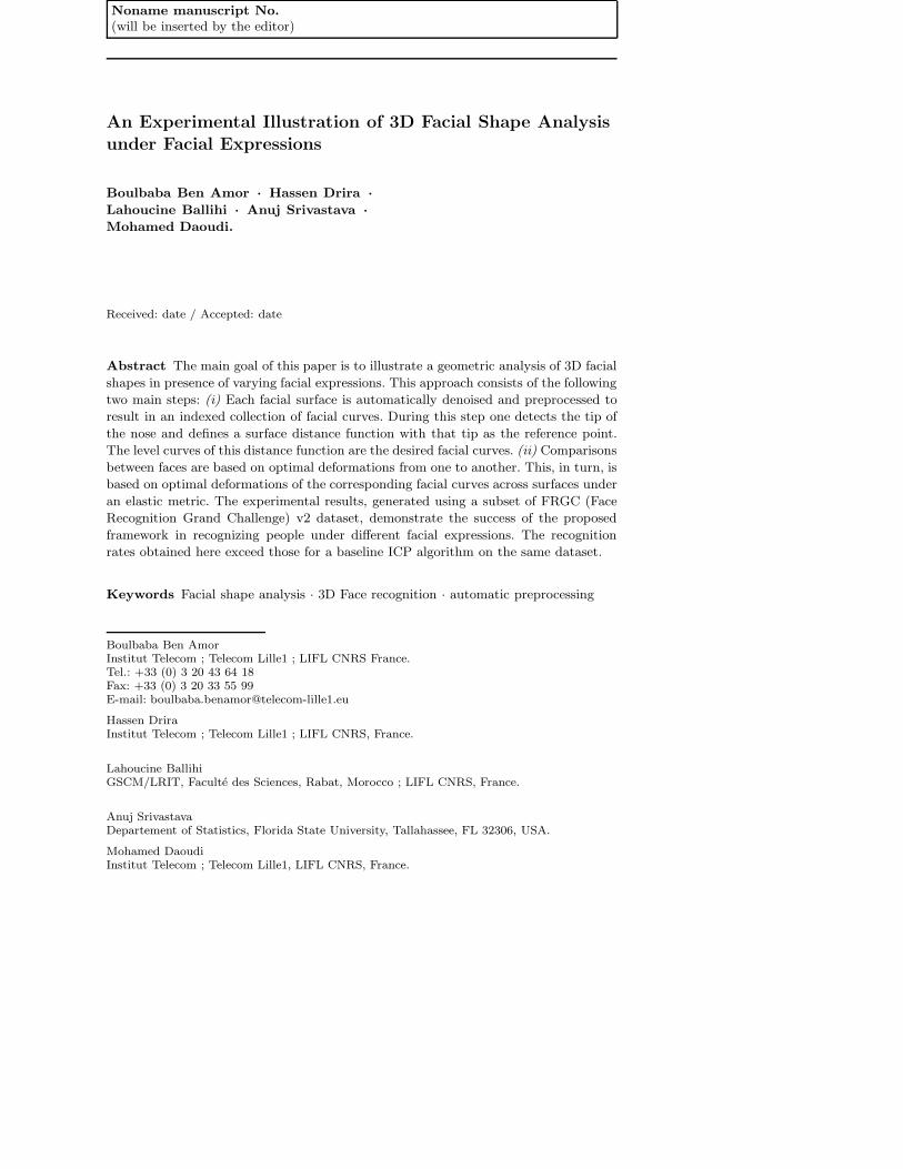
We focus in this work on designing a complete solution for 3D face analysis and

recognition. For that purpose, it is crucial to begin by denoising the data by removing

spikes, filling holes and extract only the useful part of face from depth image. Figure 1

shows different steps of our preprocessing solution to overcome these problems. Starting

from an original range image of a face, we firstly apply a 2D median filter in order to

remove spikes while preserving edges. Secondly, using a smooth interpolation, we fill

holes by adding points in parts where the laser has been completely absorbed (e.g.

eyes or eyebrows). Next, we use the Delaunay triangulation to generate a triangulated

mesh from the point cloud. On this high quality mesh, we apply the procedure shown

in Figure 2 to localize the nose tip, necessary for cropping the useful region of the face.

For this purpose, a sphere function having center the nose tip and radius R = 100mm is

constructed and the part outside the sphere is cropped. Finally, a collection of geodesic

level curves are extracted by locating iso-geodesic points from the reference (nose tip)

using the Dijkastra algorithm [4]:

– Nose tip detection : Through the center of the mass of the face, a first transverse

plane (parallel to x-z plane) slices the facial surface. The intersection of the plane

and the surface results in a horizontal profile of the face. A second sagittal plane

(parallel to y-z plane) passing through the maximum of the obtained horizontal

profile, cuts the face on a vertical profile. The nose tip is located at the maximum

of the middle part of this 2D curve as illustrated in Figure 2. This step is very

important in our general framework as it is necessary to correctly crop faces and

extract geodesic circles from the surface.

– Level curves extraction : Our facial shape analysis algorithm operates using 3D

curves extracted by computing geodesic length function along the face. This choice

is motivated by the robustness of this function to facial deformations as described in

[2]. In addition to its intrinsic invariance to rigid transformations such as rotations

and translations, this distance better preserves the separations of facial features as

compared to the Euclidian distance in R3.

4

Removing spikes

(Median filter)

Filling holes

(Interpolation)

Mesh generation

(Delaunay)

Nose tip detection

Face cropping

Face smoothing

Geodesic level

curves extraction

Original range image

FileID = 02463d546

Final 3D face model

Number of cells: 40194

Number of points: 20669

Memory: 1.04 MB

Geodesic curves

Fig. 1 Automatic FRGC data preprocessing and facial curves extraction

Let S be a facial surface denoting a scanned face. Although in practice S is a

triangulated mesh, start the discussion by assuming that it is a continous surface.

Let D : S −→ R+ be a continous geodesic map on S. Let cλ denote the level set

of D, also called a facial curve, for the value λ ∈ D(S), i.e. cλ = {p ∈ S|D(P ) =

GD(r, p) = λ} ⊂ S where r denotes the reference point (in our case the nose tip)

and GD(r, p) is the length of the shortest path from r to p on the mesh. We can

reconstruct S from these level curves according to S = ∪λcλ.

The preprocessing is one of the main issues in this such problems, so we have com-

bined the preprocessing steps described above to develop an automatic algorithm.

This algorithm has successfully processed 3971 faces in FRGC v2, which means a

success rate of 99.1% as described in the Table 1. This automatic preprocessing

procedure failed for 16 faces taken in Fall 2003 and 20 faces taken in Spring 2004.

Actually, it is the nose detection step that fails more than other steps. Figure 3

presents some examples of these faces. The main cause is the additive information

which moves the mass center far from the face and the profiles extracted do no

more match with the face profiles. For these faces, we have fixed manually the nose

tip and so we have cleaned all the FRGC v2 faces, 99.1% automatically and 0.9%

manually.

From the perspective of shape analysis, the preprocessing step is performed off-line

and the timing of each preprocessing step is given in Table 2.

5

Transverse

slicing

Triangulated 3D modelSagittal

slicing

Nose tip

extraction

Nose tip

Horizontal profile

Vertical profile

Fig. 2 Automatic nose tip detection procedure

File ID = 04339d301 File ID = 04730d129 File ID = 04816d71

File ID = 04339d300 File ID = 04730d128 File ID = 04816d70

3D

sh

ap

e o

f fa

ce

2D

co

lor

imag

e

Fig. 3 Examples of face for which preprocessing is failed

3 A Geometric Framework for shape analysis

As indicated earlier, our goal is to analyze shapes of facial surfaces using shapes

of facial curves. In other words, we divide each surface into an indexed collection

of simple, closed curves in R3 and the geometry of a surface is then studied using

the geometries of the associated curves. Since these curves, previouslly called facial

6

Table 1 Results of preprocessing procedure on FRGC dataset

Original files Success prepro-cessing

failed prepro-cessing

Success Rates(%)

Fall 2003 1893 1877 16 99.15Spring 2004 2114 1994 20 98.99FRGC v2 4007 3971 36 99.1

Table 2 Time consuming of proprocessing steps

Proprocessing step time consuming (s)Median filtering 0.091333

Filling holes 3.091428Delaunay triangulation 2.578

Nose tipe detection 0.093Face smoothing 1.235

Fig. 4 Examples of face with extracted curves

curves, have been defined as level curves of an intrinsic distance function on the

surface, their geometries in turn are invariant to the rigid transformation (rotation

and translation) of the original surface. At least theoretically, these curves jointly

contain all the information about the surface and one can go back-and-forth be-

tween the surface and the curves without any ambiguity. In practice, however, some

information is lost when one works with a finite subset of these curves rather than

the full set. Later, through experiments on real data, we will demonstrate that the

choice of facial curves for studying shapes of facial surfaces is both natural and

convenient.

In the following section, we will describe a differential-geometric approach for ana-

lyzing shapes of simple, closed curves in R3. In recent years, there have been several

papers for studying shapes of continuous curves. The earlier papers, including [18,

11,13,14], were mainly concerned with curves in R2, while the curves in higher

dimensions were studied later. In this paper, we will follow the theory laid out

by Joshi et al. [7,8] for elastic shape analysis of continuous, closed curves in Rn

and particularize it for facial curves in R3. The mathematical framework for using

elastic shape analysis of facial curves was first presented in [17].

3.1 Facial curves

We start by considering a closed curve β in R3. Since it is a closed curve, it is natural

to parametrize it using β : S1 → R

3. We will assume that the parameterization is

7

non-singular, i.e. ‖β(t)‖ 6= 0 for all t. The norm used here is the Euclidean norm

in R3. Note that the parameterization is not assumed to be arc-length; we allow a

larger class of parameterizations for improved analysis. To analyze the shape of β,

we shall represent it mathematically using a square-root velocity function (SRVF),

denoted by q(t), according to:

q(t).=

β(t)√

‖β(t)‖. (1)

q(t) is a special function that captures the shape of β and is particularly convenient

for shape analysis, as we describe next. Firstly, the squared L2-norm of q, given by:

‖q‖2 =

∫

S1

〈q(t), q(t)〉 dt =

∫

S1

‖β(t)‖dt ,

which is the length of β. Therefore, the L2-norm is convenient to analyze curves of

specific lengths. Secondly, as shown in [7], the classical elastic metric for comparing

shapes of curves becomes the L2-metric under the SRVF representation. This point

is very important as it simplifies the calculus of elastic metric to the well-known

calculus of functional analysis under the L2-metric.

In order to restrict our shape analysis to closed curves, we define the set:

C = {q : S1 → R

3|

∫

S1

q(t)‖q(t)‖dt = 0} ⊂ L2(S1, R3) . (2)

Here L2(S1, R

3) denotes the set of all functions from S1 to R

3 that are square

integrable. The quantity∫

S1 q(t)‖q(t)‖dt denotes the total displacement in R3 as

one traverses along the curve from start to end. Setting it equal to zero is equivalent

to having a closed curve. Therefore, C is the set of all closed curves in R3, each

represented by its SRVF. Notice that the elements of C are allowed to have different

lengths. Due to a nonlinear (closure) constraint on its elements, C is a nonlinear

manifold. We can make it a Riemannian manifold by using the metric: for any

u, v ∈ Tq(C), we define:

〈u, v〉 =

∫

S1

〈u(t), v(t)〉 dt . (3)

We have used the same notation for the Riemannian metric on C and the Euclidean

metric in R3 hoping that the difference is made clear by the context. For instance,

the metric on the left side is in C while the metric inside the integral on the right

side is in R3. For any q ∈ C, the tangent space:

Tq(C) = {v : S1 → R

3| 〈v, w〉 = 0, w ∈ Nq(C)} ,

where Nq(C), the space of normals at q is given by:

Nq(C) = span{q1(t)

‖q(t)‖q(t)+‖q(t)‖e1,

q2(t)

‖q(t)‖q(t)+‖q(t)‖e2,

q3(t)

‖q(t)‖q(t)+‖q(t)‖e3} ,

and where {e1, e2, e3} form an orthonormal basis of R3.

So far we have described a set of closed curves and have endowed it with a Rie-

mannian structure. Next we consider the issue of representing the shapes of these

curves. It is easy to see that several elements of C can represent curves with the

8

same shape. For example, if we rotate a curve in R3, we get a different SRVF but

its shape remains unchanged. Another similar situation arises when a curve is re-

parameterized; a re-parameterization changes the SRVF of curve but not its shape.

In order to handle this variability, we define orbits of the rotation group SO(3) and

the re-parameterization group Γ as the equivalence classes in C. Here, Γ is the set

of all orientation-preserving diffeomorphisms of S1 (to itself) and the elements of Γ

are viewed as re-parameterization functions. For example, for a curve β : S1 → R

3

and a function γ : S1 → S

1, γ ∈ Γ , the curve β(γ) is a re-parameterization of β.

The corresponding SRVF changes according to q(t) 7→√

γ(t)q(γ(t)). We set the

elements of the set:

[q] = {√

γ(t)Oq(γ(t))|O ∈ SO(3), γ ∈ Γ} ,

to be equivalent from the perspective of shape analysis. The set of such equiva-

lence classes, denoted by S.= C/(SO(3) × Γ ) is called the shape space of closed

curves in R3. S inherits a Riemannian metric from the larger space C and is thus

a Riemannian manifold itself.

The main ingredient in comparing and analyzing shapes of curves is the construc-

tion of a geodesic between any two elements of S , under the Riemannian metric

given in Eqn. 3. Given any two curves β1 and β2, represented by their SVRFs q1and q2, we want to compute a geodesic path between the orbits [q1] and [q2] in the

shape space S . This task is accomplished using a path straightening approach which

was introduced in [10]. The basic idea here is to connect the two points [q1] and [q2]

by an arbitrary initial path α and to iteratively update this path using the negative

gradient of an energy function E[α] = 12

∫

s〈α(s), α(s)〉 ds. The interesting part is

that the gradient of E has been derived analytically and can be used directly for

updating α. As shown in [10], the critical points of E are actually geodesic paths

in S . Thus, this gradient-based update leads to a critical point of E which, in turn,

is a geodesic path between the given points.

Figure 5 shows some illustrations of this idea. The top row two facial surfaces and

five level curves extracted from each of these surfaces. The remaining five rows

display geodesic paths between the corresponding level curves of the two faces,

obtained using the path-straightening approach. In each case, the first and the last

curves are the ones extracted from the two surfaces, and the intermediate curves

denote equally-spaced points on the corresponding geodesic α. These curves have

been scaled to the same length to improve display of geodesics. We will use the

notation d(β1, β2) to denote the geodesic distance, or the length of the geodesic in

S , between the two curves β1 and β2.

Why do we expect that shapes of facial curves are central to analyzing the shapes of

facial surfaces? There is plenty of psychological evidence that certain facial curves,

especially those around nose, lips and other prominent parts, can capture the es-

sential features of a face. Our experiments support this idea in a mathematical way.

We have computed geodesic distances between corresponding facial curves of differ-

ent faces – same people different facial expressions and different people altogether.

We have found that the distances are typically smaller for faces of the same people,

despite different expressions, when compared to the distances between facial curves

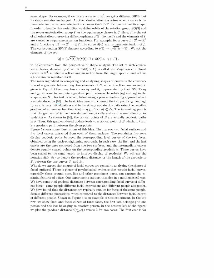
of different people. Shown in Figure 6 is an example of this experiment. In the top

row, we show faces and facial curves of three faces, the first two belonging to one

person and the last belonging to another person. In the bottom left of the figure,

we plot the geodesic distance d(c1λ, c2λ) versus λ for two cases: The first case is for

9

Fig. 5 Examples of geodesic between curves

facial curves from the first two faces, i.e. same person, and the distance is shown

using a broken line. The second case is for facial curves from different people (first

and the last face in the first row) and the distance is shown using the solid line.

As this experiment suggest, the differences in shapes of facial curves is generally

smaller for the same person and larger for different persons. Therefore, shapes of

facial curves can play a central role in analyzing shapes of facial surfaces.

3.2 Facial surfaces

Now we extend ideas developed in the previous section for analyzing shapes of

facial curves to the shapes of full facial surfaces. As mentioned earlier, we are going

to represent a facial surface S with an indexed collection of the level curves of the

D function. That is,

S ↔ {cλ, λ ∈ [0, L]} ,

where cλ is the level set associated with D = λ. Through this relation, each facial

surface has been represented as an element of the set C[0,L]. In our framework,

the shapes of any two faces are compared by comparing their corresponding facial

curves. Given any two surfaces S1 and S2, and their facial curves {c1λ, λ ∈ [0, L]}

10

2 4 6 8 10 12 14 16 18 20 22 24250.05

0.1

0.15

0.2

0.25

0.3

Fig. 6 Top rows shows facial curves extracted from three example facial surfaces – the firsttwo belong to the same person and the last belongs to another person. The bottom left showsthe plot of the mean of distances for each level d(c1

λ, c2

λ) for two cases – for 125 genuine accesses

(broken line) and for 125 impostor accesses (solid line). The bottom right highlights the tworegions – one around the nose profile and the other containing eyes and mouth – that havehigher values in the distance plot.

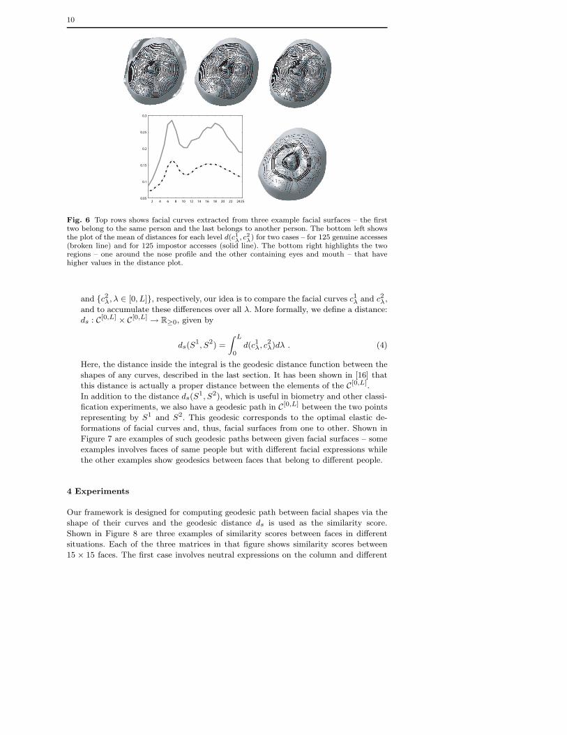
and {c2λ, λ ∈ [0, L]}, respectively, our idea is to compare the facial curves c1λ and c2λ,

and to accumulate these differences over all λ. More formally, we define a distance:

ds : C[0,L] × C[0,L] → R≥0, given by

ds(S1, S2) =

∫ L

0d(c1λ, c2λ)dλ . (4)

Here, the distance inside the integral is the geodesic distance function between the

shapes of any curves, described in the last section. It has been shown in [16] that

this distance is actually a proper distance between the elements of the C[0,L].

In addition to the distance ds(S1, S2), which is useful in biometry and other classi-

fication experiments, we also have a geodesic path in C[0,L] between the two points

representing by S1 and S2. This geodesic corresponds to the optimal elastic de-

formations of facial curves and, thus, facial surfaces from one to other. Shown in

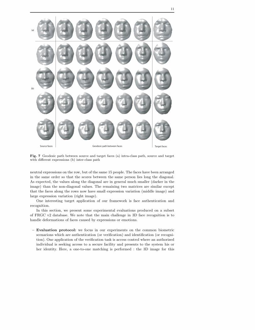
Figure 7 are examples of such geodesic paths between given facial surfaces – some

examples involves faces of same people but with different facial expressions while

the other examples show geodesics between faces that belong to different people.

4 Experiments

Our framework is designed for computing geodesic path between facial shapes via the

shape of their curves and the geodesic distance ds is used as the similarity score.

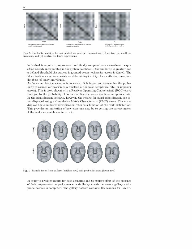
Shown in Figure 8 are three examples of similarity scores between faces in different

situations. Each of the three matrices in that figure shows similarity scores between

15 × 15 faces. The first case involves neutral expressions on the column and different

11

Source faces Target facesGeodesic path between faces

(a)

(b)

Fig. 7 Geodesic path between source and target faces (a) intra-class path, source and targetwith different expressions (b) inter-class path

neutral expressions on the row, but of the same 15 people. The faces have been arranged

in the same order so that the scores between the same person lies long the diagonal.

As expected, the values along the diagonal are in general much smaller (darker in the

image) than the non-diagonal values. The remaining two matrices are similar except

that the faces along the rows now have small expression variation (middle image) and

large expression variation (right image).

One interesting target application of our framework is face authentication and

recognition.

In this section, we present some experimental evaluations produced on a subset

of FRGC v2 database. We note that the main challenge in 3D face recognition is to

handle deformations of faces caused by expressions or emotions.

– Evaluation protocol: we focus in our experiments on the common biometric

scenarions which are authentication (or verification) and identification (or recogni-

tion). One application of the verification task is access control where an authorized

individual is seeking access to a secure facility and presents to the system his or

her identity. Here, a one-to-one matching is performed : the 3D image for this

12

Probes

Ga

lle

ry

(c) Neutral vs. large expressions

similarity matrix (inter-sessions)

Probes

Ga

lle

ry

(b) Neutral vs. small expressions similarity

matrix (inter-sessions)

Probes

Ga

lle

ry

(a) Neutral vs. neutral expressions similarity

matrix (inter-sessions)

Fig. 8 Similarity matrices for (a) neutral vs. neutral comparsions, (b) neutral vs. small ex-pressions, and (c) neutral vs. large expressions

individual is acquired, preprocessed and finally compared to an enrollment acqui-

sition already incorporated in the system database. If the similarity is greater than

a defined threshold the subject is granted access, otherwise access is denied. The

identification scenarion consists on determining identity of an authorized user in a

database of many individuals.

As far as verification scenario is concerned, it is important to examine the proba-

bility of correct verification as a function of the false acceptance rate (or imposter

access). This is often shown with a Receiver Operating Characteristic (ROC) curve

that graphs the probability of correct verification versus the false acceptance rate.

In the identification scenario, however, the results for facial identification are of-

ten displayed using a Cumulative Match Characteristic (CMC) curve. This curve

displays the cumulative identification rates as a function of the rank distribution.

This provides an indication of how close one may be to getting the correct match

if the rank-one match was incorrect.

Pro

be

Ga

lle

ry

Fig. 9 Sample faces from gallery (heigher row) and probe datasets (lower row)

In order to produce results for both scenarios and to explore effect of the presence

of facial expressions on performance, a similarity matrix between a gallery and a

probe dataset is computed. The gallery dataset contains 125 sessions for 125 dif-

13

ferent subjects acquired with neutral expressions selected from FRGC v2 dataset.

The probe dataset includes completely different sessions of these subjects under

non-neutral facial expressions, as shown in Figure 9. Due to sensitivity of our al-

gorithm to opened mouth, expressions in probe dataset include only scans with

closed mouths.

In this matrix, the diagonal terms represent match scores (or Genuine Access)

contrary to non-diagonal terms which represent Non-match scores (or Imposter

Access). These scores allow us to produce the ROC and the CMC curves for this

scenario.

– Preliminary results : We compare results of our algorithm with a standard

implementation of ICP which is considered as a baseline in 3D face recognition. The

same protocol was followed to compute similarity matrices for both the algorithms

on the same preprocessed data.

As shown in Figure 10 the ROC curve of our approach is always above the ICP

one which means that our verification rate at each false accept rate is greater than

ICP verification rate. In addition, the Equal Error Rate which is the error rate for

false accept rate equal to false reject rate, is lower in our case (8%) than the ICP

case (15%).

10−2

10−1

100

101

50

60

70

80

90

100

False Accept Rate (%)

Ver

ifica

tion

Rat

e (%

)

ICP (baseline)Proposed appraoch

Fig. 10 Receiver operating characteristic curves for our approach and ICP (baseline)

These results are confirmed with the CMC curves for the two algorithms (Figure

11). In fact, rank-one recognition rate given by our algorithm is about 88.8% com-

pared to 78.5% given by the ICP algorithm. Moreover, at the fourth rank, our

14

algorithm is already able to recognize 97.8% of the subjects in contrast with ICP

which recognition rate at this rank is still under 89%.

1 5 9 13 17 21 25 29 33 37 41 45 49 5375

77

79

81

83

85

87

89

91

93

95

97

99

100

Rank

Rec

og

nit

ion

Rat

e (%

)

ICP (baseline)Proposed Approach

Fig. 11 Cumulative Match Characteristic curves for our approach and ICP (baseline)

5 Conclusions

In this paper, we have illustrated a geometric analysis of 3D facial shapes in presence

of both netural and non-neutral facial expressions. In this analysis, the preprocessing

is completely automated - the algorithm processes the face scan data, detects the tip

of the nose and extracts a set of facial curves. The main tool presented in this paper

is the construction of geodesic paths between arbitrary two facial surfaces. The length

of a geodesic between any two facial surfaces is computed as the geodesic length be-

tween a set of their facial curves. This length quantifies differences in their shapes ;

it also provides an optimal deformation from one to the other. In order to validate

our approach in presence of facial expressions, a similarity matrix between 125 probe

images with facial expressions and 125 gallery images with the neutral expression is

computed. Authentication and recognition scores are produced and compared with a

standard implementation of ICP as a baseline. The results of our algorithm outper-

form the baseline ICP algorithm which prove robustness of the proposed framework to

deformations caused by facial expressions.

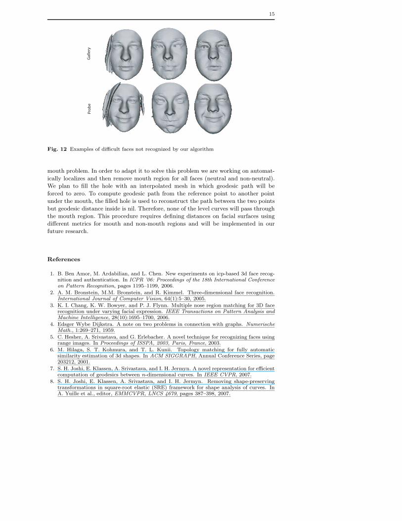
Our approach extract closed curves from the face using geodesic distance and one

reference point (the nose tip). Curve extraction procedure is not adapted to the opened

15

Ga

lle

ryP

rob

e

Fig. 12 Examples of difficult faces not recognized by our algorithm

mouth problem. In order to adapt it to solve this problem we are working on automat-

ically localizes and then remove mouth region for all faces (neutral and non-neutral).

We plan to fill the hole with an interpolated mesh in which geodesic path will be

forced to zero. To compute geodesic path from the reference point to another point

under the mouth, the filled hole is used to reconstruct the path between the two points

but geodesic distance inside is nil. Therefore, none of the level curves will pass through

the mouth region. This procedure requires defining distances on facial surfaces using

different metrics for mouth and non-mouth regions and will be implemented in our

future research.

References

1. B. Ben Amor, M. Ardabilian, and L. Chen. New experiments on icp-based 3d face recog-nition and authentication. In ICPR ’06: Proceedings of the 18th International Conferenceon Pattern Recognition, pages 1195–1199, 2006.

2. A. M. Bronstein, M.M. Bronstein, and R. Kimmel. Three-dimensional face recognition.International Journal of Computer Vision, 64(1):5–30, 2005.

3. K. I. Chang, K. W. Bowyer, and P. J. Flynn. Multiple nose region matching for 3D facerecognition under varying facial expression. IEEE Transactions on Pattern Analysis andMachine Intelligence, 28(10):1695–1700, 2006.

4. Edsger Wybe Dijkstra. A note on two problems in connection with graphs. NumerischeMath., 1:269–271, 1959.

5. C. Hesher, A. Srivastava, and G. Erlebacher. A novel technique for recognizing faces usingrange images. In Proceedings of ISSPA, 2003, Paris, France, 2003.

6. M. Hilaga, S. T. Kohmura, and T. L. Kunii. Topology matching for fully automaticsimilarity estimation of 3d shapes. In ACM SIGGRAPH, Annual Conference Series, page203212, 2001.

7. S. H. Joshi, E. Klassen, A. Srivastava, and I. H. Jermyn. A novel representation for efficientcomputation of geodesics between n-dimensional curves. In IEEE CVPR, 2007.

8. S. H. Joshi, E. Klassen, A. Srivastava, and I. H. Jermyn. Removing shape-preservingtransformations in square-root elastic (SRE) framework for shape analysis of curves. InA. Yuille et al., editor, EMMCVPR, LNCS 4679, pages 387–398, 2007.

16

9. I. A. Kakadiaris, G. Passalis, G. Toderici, M. N. Murtuza, N. Karampatziakis, and T. Theo-haris. Three-dimensional face recognition in the presence of facial expressions: An anno-tated deformable model approach. IEEE Transactions on Pattern Analysis and MachineIntelligence, 29(4):1–10, 2007.

10. E. Klassen and A. Srivastava. Geodesics between 3D closed curves using path-straightening. In Proceedings of ECCV, Lecture Notes in Computer Science, pages I:95–106, 2006.

11. E. Klassen, A. Srivastava, W. Mio, and S. Joshi. Analysis of planar shapes using geodesicpaths on shape spaces. IEEE Pattern Analysis and Machine Intelligence, 26(3):372–383,March, 2004.

12. X. Lu, A. K. Jain, and D. Colbry. Matching 2.5d face scans to 3d models. IEEE Trans-actions on Pattern Analysis and Machine Intelligence, 28(1):31–43, Jan. 2006.

13. P. W. Michor and D. Mumford. Riemannian geometries on spaces of plane curves. Journalof the European Mathematical Society, 8:1–48, 2006.

14. W. Mio, A. Srivastava, and S. Joshi. On shape of plane elastic curves. InternationalJournal of Computer Vision, 73(3):307–324, 2007.

15. P. Jonathon Phillips, Patrick J. Flynn, Todd Scruggs, Kevin W. Bowyer, Jin Chang,Kevin Hoffman, Joe Marques, Jaesik Min, and William Worek. Overview of the facerecognition grand challenge. In CVPR ’05: Proceedings of the 2005 IEEE ComputerSociety Conference on Computer Vision and Pattern Recognition (CVPR’05) - Volume1, pages 947–954, Washington, DC, USA, 2005. IEEE Computer Society.

16. C. Samir, A. Srivastava, M. Daoudi, and E. Klassen.17. A. Srivastava, C. Samir, S. Joshi, and M. Daoudi. Elastic shape models for face analysis

using curvilinear coordinates. Journal of Mathematical Imaging and Vision, accepted forpublication, 2008.

18. L. Younes. Computable elastic distance between shapes. SIAM Journal of Applied Math-ematics, 58:565–586, 1998.