Facial nerve electrodiagnostics for patients with facial palsy
Upload
khangminh22Category
view
3download
0
FACULDADE DE ENGENHARIA DA UNIVERSIDADE DO PORTO
Study on recognition of facialexpressions of affect
Beatriz Peneda Coelho
FINAL VERSION
MSC DISSERTATION
Supervisor: Hélder Filipe Pinto de Oliveira
Second Supervisor: João Pedro Silva Monteiro
January 21, 2019

c© Beatriz Peneda Coelho, 2019

Resumo
O reconhecimento de expressões faciais é uma área particularmente interessante em visão com-putacional, pois traz inúmeros benefícios para a nossa sociedade. Benefícios esses que podem sertraduzidos num grande número de aplicações no âmbito da neurociência, psicologia e segurança.A relevância do tema reflete-se na vasta literatura já produzida que descreve sinais notáveis deprogresso. No entanto, o desenvolvimento e avanço de novas abordagens ainda enfrenta váriosdesafios. Esses desafios compreendem variações na posição da cabeça, variações na iluminação,oclusões e erros de registro. Um dos focos desta área é alcançar resultados semelhantes quando sepassa de um ambiente controlado para um cenário mais próximo da realidade.
Embora o reconhecimento de expressões faciais tenha sido abordado em projetos considerav-elmente diferentes, é exequível dar enfâse à necessidade de chamar à atenção para o design de umainterface que simula o envolvimento do paciente nos cuidados de saúde como uma aplicação fu-tura. Uma tendência crescente tem sido observada, no entanto, ainda há algumas questões abertasque precisam de obter resposta para causar um impacto significativo no âmbito da saúde.
O objetivo deste trabalho é estudar qual seria uma boa abordagem para o reconhecimento deexpressões faciais. Adicionalmente, estaria enquadrado com uma aplicação futura que permitiriaser usada no contexto da reabilitação com recurso a jogos sérios. Em outras palavras, seria umaabordagem baseada em jogos interativos que iria inferir a satisfação dos pacientes durante o jogo.Na revisão bibliográfica, serão fornecidas bases teóricas para compreender na íntegra este trabalho,bem como propostas de algoritmos anteriores para reconhecimento de expressões faciais. Alémdisso, esta tarefa de reconhecimento como um sistema automático será descrita passo a passo.A metodologia segue a ordem em que as etapas foram executadas. O passo inicial foi localizaros rostos nas imagens. Posteriormente, a extração de características recorrendo a dois métodosreconhecidos: Histograma de Gradientes Orientados e Padrões Binários Locais. Os resultados sãoapresentados para duas bases de dados, CK+ e AffectNet.
Finalmente, foi possível obter uma precisão de 96,55% para a base de dados CK+. Parauma base de dados em que os participantes estão a posar os algoritmos considerados tendema ter bom desempenho, enquanto que uma base de dados espontânea (AffectNet) resulta numdesempenho inferior. Contudo, com resultados ainda satisfatórios, uma vez que as imagens estãoa ser classificadas considerando 7 expressões possíveis, mais a expressão neutra e estão a serusadas bases de dados com um desequilíbrio no número de imagens por expressão.
i

ii

Abstract
Facial expression recognition is a particularly interesting field of computer vision since it bringsinnumerable benefits to our society. Benefits that can be translated into a large number of ap-plications in subjects such as, neuroscience, psychology and security. The relevance of the topicis reflected in the vast literature already produced describing notable signs of progress. How-ever, the development and the advancement of new approaches is still facing multiple challenges.Challenges include head-pose variations, illumination variations, identity bias, occlusions, andregistration errors. One of the focus in this field is to achieve similar results when moving from acontrolled environment to a more naturalistic scenario.
Though facial expression recognition has been addressed in considerable different projects, itis feasible to emphasize the call for attention to the design of an interface that simulates addressingpatient engagement in healthcare, as a future application. A rising tendency has been noticed,however, there are still some open questions need to be answered to make a significant impact onhealth care.
The goal of this work is to study what would be a good approach to perform facial expressionrecognition. Additionally, a framework for future application that would enable dealing with arehabilitation context using serious games. In other words, it would be an interactive game basedapproach to infer the patients contentment while playing. In the literature review, theoretical basisneeded to fully comprehend this work will be provided as well as the previous algorithm proposalsfor facial expression recognition. Furthermore, facial expression recognition as an automatic sys-tem will be described step by step. The methodology follows the order in which these steps wereperformed. The initial step was to locate the faces in the images. Subsequently, the extraction offeatures by two acknowledged methods, the Histogram of Oriented Gradients and the Local Bi-nary Patterns. Latterly, the classification was performed using Random Forest and Support VectorMachines. The results were presented for two datasets, the CK+ and the AffectNet dataset.
Finally, it was possible to obtain 96.55% as the accuracy value for the CK+ dataset. For aposed dataset the considered algorithms tend to perform well whereas for an in-the-wild dataset(AffectNet) the outcome is a lower performance. However, the results are still satisfactory sincethe face images are being classified into 7 possible expressions, plus the neutral and it is been usedimbalanced datasets.
iii

iv

Acknowledgments
I gratefully thank my supervisor Hélder Filipe Pinto de Oliveira and second supervisor João PedroSilva Monteiro for their time, patience and knowledge. I gratefully thank my parents, sister,and grandmother as they were always there for me, giving me unconditional love and support. Igratefully thank my boyfriend that even far made himself present and supported me at all times. Igratefully thank my friends, the old ones and the new ones that I met along the way. This wouldnot be possible to accomplish without the encouragement given by these people in my life.
Beatriz Coelho
v

vi

“True worth is as inevitably discoveredby the facial expression, as its oppositeis sure to be clearly represented there.The human face is nature’s tablet, the
truth is certainly written thereon.”
Johann Kaspar Lavater
vii

viii

Contents
1 Introduction 11.1 Context . . . . . . . . . . . . . . . . . . . . . . . . . . . . . . . . . . . . . . . 11.2 Motivation and Objectives . . . . . . . . . . . . . . . . . . . . . . . . . . . . . 21.3 Contributions . . . . . . . . . . . . . . . . . . . . . . . . . . . . . . . . . . . . 21.4 Document Structure . . . . . . . . . . . . . . . . . . . . . . . . . . . . . . . . . 2
2 Literature Review 52.1 Facial Expressions . . . . . . . . . . . . . . . . . . . . . . . . . . . . . . . . . 52.2 Facial Expressions: Methods for Assessing . . . . . . . . . . . . . . . . . . . . 6
2.2.1 Electromyography . . . . . . . . . . . . . . . . . . . . . . . . . . . . . 62.2.2 Facial Action Coding System . . . . . . . . . . . . . . . . . . . . . . . 7
2.3 Automatic Facial Expression Recognition . . . . . . . . . . . . . . . . . . . . . 92.3.1 Face Detection . . . . . . . . . . . . . . . . . . . . . . . . . . . . . . . 102.3.2 Dimensionality Reduction . . . . . . . . . . . . . . . . . . . . . . . . . 112.3.3 Feature Extraction . . . . . . . . . . . . . . . . . . . . . . . . . . . . . 112.3.4 Feature Selection . . . . . . . . . . . . . . . . . . . . . . . . . . . . . . 122.3.5 Expression Classification . . . . . . . . . . . . . . . . . . . . . . . . . . 132.3.6 Challenges . . . . . . . . . . . . . . . . . . . . . . . . . . . . . . . . . 142.3.7 Algorithms Analysis of Facial Expression Approaches . . . . . . . . . . 142.3.8 Competitions . . . . . . . . . . . . . . . . . . . . . . . . . . . . . . . . 15
2.4 Feature Methods . . . . . . . . . . . . . . . . . . . . . . . . . . . . . . . . . . 162.4.1 Histogram of Oriented Gradients (HOG) . . . . . . . . . . . . . . . . . 162.4.2 Local Binary Patterns (LBP) . . . . . . . . . . . . . . . . . . . . . . . . 162.4.3 Scale-Invariant Feature Transform (SIFT) . . . . . . . . . . . . . . . . . 182.4.4 Principal Component Analysis (PCA) . . . . . . . . . . . . . . . . . . . 18
2.5 Feature Selection Techniques . . . . . . . . . . . . . . . . . . . . . . . . . . . . 192.5.1 Sequential Forward Selection (SFS) . . . . . . . . . . . . . . . . . . . . 192.5.2 Sequential Backward Selection (SBS) . . . . . . . . . . . . . . . . . . . 192.5.3 Mutual Information (MI) . . . . . . . . . . . . . . . . . . . . . . . . . . 192.5.4 Lasso Regularization . . . . . . . . . . . . . . . . . . . . . . . . . . . . 19
2.6 Machine Learning Algorithms . . . . . . . . . . . . . . . . . . . . . . . . . . . 202.6.1 Viola-Jones . . . . . . . . . . . . . . . . . . . . . . . . . . . . . . . . . 202.6.2 Support Vector Machines (SVM) . . . . . . . . . . . . . . . . . . . . . . 212.6.3 Decision Trees (DT) . . . . . . . . . . . . . . . . . . . . . . . . . . . . 212.6.4 Random Forest (RF) . . . . . . . . . . . . . . . . . . . . . . . . . . . . 22
2.7 Facial Expression Databases . . . . . . . . . . . . . . . . . . . . . . . . . . . . 242.8 Final Considerations . . . . . . . . . . . . . . . . . . . . . . . . . . . . . . . . 26
ix

x CONTENTS
3 Methodology 273.1 Face Localization and Crop . . . . . . . . . . . . . . . . . . . . . . . . . . . . . 283.2 Facial Features . . . . . . . . . . . . . . . . . . . . . . . . . . . . . . . . . . . 29
3.2.1 HOG . . . . . . . . . . . . . . . . . . . . . . . . . . . . . . . . . . . . 293.2.2 LBP . . . . . . . . . . . . . . . . . . . . . . . . . . . . . . . . . . . . . 293.2.3 PCA . . . . . . . . . . . . . . . . . . . . . . . . . . . . . . . . . . . . . 29
3.3 Feature Selection . . . . . . . . . . . . . . . . . . . . . . . . . . . . . . . . . . 323.3.1 MI Based Approach . . . . . . . . . . . . . . . . . . . . . . . . . . . . 32
3.4 Classification . . . . . . . . . . . . . . . . . . . . . . . . . . . . . . . . . . . . 333.4.1 SVM . . . . . . . . . . . . . . . . . . . . . . . . . . . . . . . . . . . . 333.4.2 RF . . . . . . . . . . . . . . . . . . . . . . . . . . . . . . . . . . . . . . 33
3.5 Final Considerations . . . . . . . . . . . . . . . . . . . . . . . . . . . . . . . . 34
4 Results and Discussion 354.1 Dataset . . . . . . . . . . . . . . . . . . . . . . . . . . . . . . . . . . . . . . . 35
4.1.1 The Extended Cohn – Kanade (CK+) . . . . . . . . . . . . . . . . . . . 354.1.2 AffectNet . . . . . . . . . . . . . . . . . . . . . . . . . . . . . . . . . . 364.1.3 AffectNet Adapted . . . . . . . . . . . . . . . . . . . . . . . . . . . . . 404.1.4 Splitting Method: Train and Test Set . . . . . . . . . . . . . . . . . . . . 42
4.2 Face Detector Validation . . . . . . . . . . . . . . . . . . . . . . . . . . . . . . 424.2.1 Face Detector Validation Approach Results . . . . . . . . . . . . . . . . 44
4.3 Classifier Results . . . . . . . . . . . . . . . . . . . . . . . . . . . . . . . . . . 464.3.1 SVM Classifier Results . . . . . . . . . . . . . . . . . . . . . . . . . . . 464.3.2 RF Classifier Resuls . . . . . . . . . . . . . . . . . . . . . . . . . . . . 494.3.3 Feature Selection Based on MI Results . . . . . . . . . . . . . . . . . . 524.3.4 Discussion . . . . . . . . . . . . . . . . . . . . . . . . . . . . . . . . . 53
5 Conclusions and Future Work 575.1 Conclusions . . . . . . . . . . . . . . . . . . . . . . . . . . . . . . . . . . . . . 575.2 Future Work . . . . . . . . . . . . . . . . . . . . . . . . . . . . . . . . . . . . . 58
A Detailed Results 59A.1 Results in the form of graphs obtained from the use of the SVM and RF Classifiers. 59
References 75

List of Figures
2.1 Facial Muscles. From [1] . . . . . . . . . . . . . . . . . . . . . . . . . . . . . . 62.2 Upper and Lower AU examples. From [2]. . . . . . . . . . . . . . . . . . . . . 82.3 Examples of combined AU. Adapted from [3]. . . . . . . . . . . . . . . . . . . 82.4 Categorization of Automatic Facial Expression Recognition Systems. Adapted
from [4]. . . . . . . . . . . . . . . . . . . . . . . . . . . . . . . . . . . . . . . . 102.5 HOG of the face. From [5]. . . . . . . . . . . . . . . . . . . . . . . . . . . . . 172.6 Image sequence of the process described above: an input image, LBP image, and
the correspondent histogram. From [6]. . . . . . . . . . . . . . . . . . . . . . . 172.7 Example of the eigenfaces showing that as well as encoding the facial features, it
also encodes the illumination in the face images. From [7]. . . . . . . . . . . . . 182.8 On the left, feature examples are shown. On the right it is presented the AdaBoost
two first selected features. Adapted from [8]. . . . . . . . . . . . . . . . . . . . 202.9 On the left and center it is demonstrated how to calculate the integral image. On
the right, it is shown D which can be calculated through the integral image. From [9]. 212.10 The Attentional Cascade. . . . . . . . . . . . . . . . . . . . . . . . . . . . . . . 212.11 On the left it is shown the original feature space whereas on the right, it is the
non-linear separation of those features. . . . . . . . . . . . . . . . . . . . . . . . 222.12 Example of Decision Tree, which aim is to sort the variables a, b, and c. Adapted
from [10] . . . . . . . . . . . . . . . . . . . . . . . . . . . . . . . . . . . . . . 222.13 Example of a simple RF. . . . . . . . . . . . . . . . . . . . . . . . . . . . . . . 23
3.1 Automatic Facial Expression Recognition System. . . . . . . . . . . . . . . . . . 273.2 Representation of the performed steps to obtain a face image on the CK+ dataset. 283.3 Example of the HOG implementation on the CK+ and AffectNet dataset, on the
upper and lower images respectively. Starting from the left it shows the originalimage, followed by the HOG image and the respective histogram. . . . . . . . . 30
3.4 Example of the LBP implementation on the CK+ and AffectNet dataset, on theupper and lower images respectively. Starting from the left it shows the originalimage, followed by the LBP image and the respective histogram. . . . . . . . . . 31
3.5 ’Mean’ face computed by the PCA. . . . . . . . . . . . . . . . . . . . . . . . . 313.6 Representation of the first principal components on the CK+ dataset. . . . . . . . 323.7 Representation of the first principal components on the AffectNet dataset. . . . . 32
4.1 Examples of the CK+ dataset. In the upper part, there are some images originallyfrom the CK dataset and those below are the data included in the new version.Adapted from [11]. . . . . . . . . . . . . . . . . . . . . . . . . . . . . . . . . . 36
4.2 Images sequence obtained from a subject when the labelled emotion is “Surprise”.From [12]. . . . . . . . . . . . . . . . . . . . . . . . . . . . . . . . . . . . . . . 36
xi

xii LIST OF FIGURES
4.3 Software application used by the annotators to label into the categorical and di-mensional models of affect. An image has only one face annotated (for instance,the one in the green box). From [13]. . . . . . . . . . . . . . . . . . . . . . . . . 38
4.4 Images distributed in the Valence and Arousal dimensions of the circumplex model.From [13]. . . . . . . . . . . . . . . . . . . . . . . . . . . . . . . . . . . . . . . 40
4.5 Percentages of the agreement between the two annotators for the different expres-sions. From [13]. . . . . . . . . . . . . . . . . . . . . . . . . . . . . . . . . . . 41
4.6 On the right, an example of the overlapping area between two objects. On the left,an example of the area of union of those objects. . . . . . . . . . . . . . . . . . . 43
4.7 Some samples with both the representation of the ground truth and the predictedbounding boxes. . . . . . . . . . . . . . . . . . . . . . . . . . . . . . . . . . . . 43
4.8 Some samples in which a face could not be detected in the image. . . . . . . . . 44
A.1 Graph representing the HOG features from the CK+ dataset classified using theSVM classifier with a rbf kernel. . . . . . . . . . . . . . . . . . . . . . . . . . . 59
A.2 Graph representing the HOG features from the CK+ dataset classified using theSVM classifier with a polynomial kernel (degree equal to 1). . . . . . . . . . . . 60
A.3 Graph representing the HOG features from the CK+ dataset classified using theSVM classifier with a polynomial kernel (degree equal to 2). . . . . . . . . . . . 60
A.4 Graph representing the HOG features from the CK+ dataset classified using theSVM classifier with a polynomial kernel (degree equal to 3). . . . . . . . . . . . 61
A.5 Graph representing the HOG features from the AffectNet dataset classified usingthe SVM classifier with a rbf kernel. . . . . . . . . . . . . . . . . . . . . . . . . 61
A.6 Graph representing the HOG features from the AffectNet dataset classified usingthe SVM classifier with a polynomial kernel (degree equal to 1). . . . . . . . . . 62
A.7 Graph representing the HOG features from the AffectNet dataset classified usingthe SVM classifier with a polynomial kernel (degree equal to 2). . . . . . . . . . 62
A.8 Graph representing the HOG features from the AffectNet dataset classified usingthe SVM classifier with a polynomial kernel (degree equal to 3). . . . . . . . . . 63
A.9 Graph representing the LBP features from the CK+ dataset classified using theSVM classifier with a rbf kernel. . . . . . . . . . . . . . . . . . . . . . . . . . . 63
A.10 Graph representing the LBP features from the CK+ dataset classified using theSVM classifier with a polynomial kernel (degree equal to 1). . . . . . . . . . . . 64
A.11 Graph representing the LBP features from the CK+ dataset classified using theSVM classifier with a polynomial kernel (degree equal to 2). . . . . . . . . . . . 64
A.12 Graph representing the LBP features from the CK+ dataset classified using theSVM classifier with a polynomial kernel (degree equal to 3). . . . . . . . . . . . 65
A.13 Graph representing the LBP features from the AffectNet dataset classified usingthe SVM classifier with a rbf kernel. . . . . . . . . . . . . . . . . . . . . . . . . 65
A.14 Graph representing the LBP features from the AffectNet dataset classified usingthe SVM classifier with a polynomial kernel (degree equal to 1). . . . . . . . . . 66
A.15 Graph representing the LBP features from the AffectNet dataset classified usingthe SVM classifier with a polynomial kernel (degree equal to 2). . . . . . . . . . 66
A.16 Graph representing the LBP features from the AffectNet dataset classified usingthe SVM classifier with a polynomial kernel (degree equal to 3). . . . . . . . . . 67
A.17 Graph representing the PCA obtained from the CK+ dataset classified using theSVM classifier with a rbf kernel. . . . . . . . . . . . . . . . . . . . . . . . . . . 67
A.18 Graph representing the PCA obtained from the CK+ dataset classified using theSVM classifier with a polynomial kernel (degree equal to 1). . . . . . . . . . . . 68

LIST OF FIGURES xiii
A.19 Graph representing the PCA obtained from the CK+ dataset classified using theSVM classifier with a polynomial kernel (degree equal to 2). . . . . . . . . . . . 68
A.20 Graph representing the PCA obtained from the CK+ dataset classified using theSVM classifier with a polynomial kernel (degree equal to 3). . . . . . . . . . . . 69
A.21 Graph representing the PCA obtained from the AffectNet dataset classified usingthe SVM classifier with a rbf kernel. . . . . . . . . . . . . . . . . . . . . . . . . 69
A.22 Graph representing the PCA obtained from the AffectNet dataset classified usingthe SVM classifier with a polynomial kernel (degree equal to 1). . . . . . . . . . 70
A.23 Graph representing the PCA obtained from the AffectNet dataset classified usingthe SVM classifier with a polynomial kernel (degree equal to 2). . . . . . . . . . 70
A.24 Graph representing the PCA obtained from the AffectNet classified using the SVMclassifier with a polynomial kernel (degree equal to 3). . . . . . . . . . . . . . . 71
A.25 Graph representing the HOG features from the CK+ dataset classified using theRF classifier. . . . . . . . . . . . . . . . . . . . . . . . . . . . . . . . . . . . . 71
A.26 Graph representing the HOG features from the AffectNet dataset classified usingthe RF classifier. . . . . . . . . . . . . . . . . . . . . . . . . . . . . . . . . . . . 72
A.27 Graph representing the LBP features from the CK+ dataset classified using the RFclassifier. . . . . . . . . . . . . . . . . . . . . . . . . . . . . . . . . . . . . . . 72
A.28 Graph representing the LBP features from the AffectNet dataset classified usingthe RF classifier. . . . . . . . . . . . . . . . . . . . . . . . . . . . . . . . . . . . 73
A.29 Graph representing the PCA obtained from the CK+ dataset classified using theRF classifier. . . . . . . . . . . . . . . . . . . . . . . . . . . . . . . . . . . . . 73
A.30 Graph representing the PCA obtained from the AffectNet dataset classified usingthe RF classifier. . . . . . . . . . . . . . . . . . . . . . . . . . . . . . . . . . . . 74

xiv LIST OF FIGURES
List of Tables
2.1 Number of the AU and correspondent description. Adapted from [11]. . . . . . . 72.2 Criteria to define emotions in facial action units. Adapted from [11]. . . . . . . . 82.3 Main challenges in automatic expression recognition. . . . . . . . . . . . . . . . 142.4 RGB Dataset. . . . . . . . . . . . . . . . . . . . . . . . . . . . . . . . . . . . . 252.5 3D Dataset. . . . . . . . . . . . . . . . . . . . . . . . . . . . . . . . . . . . . . 252.6 Thermal Dataset. . . . . . . . . . . . . . . . . . . . . . . . . . . . . . . . . . . 26
4.1 Frequency of each expression represented in the peak frames on the CK+ database. 374.2 Frequency of each annotated image in each category. . . . . . . . . . . . . . . . 394.3 Number of images and the correspondent percentage of each Expression on the
Manually Annotated set. . . . . . . . . . . . . . . . . . . . . . . . . . . . . . . 414.4 Percentage of the occlusions present in the AffectNet dataset. . . . . . . . . . . . 414.5 Percentage of other elements present in the images of AffectNet dataset. . . . . . 424.6 Results of the IoU evaluation metric. . . . . . . . . . . . . . . . . . . . . . . . . 454.7 Results for the 50:50 split using the SVM classifier. . . . . . . . . . . . . . . . . 474.8 Results for the 60:40 split using the SVM classifier. . . . . . . . . . . . . . . . . 474.9 Results for the 70:30 split using the SVM classifier. . . . . . . . . . . . . . . . . 474.10 Results for the 80:20 split using the SVM classifier. . . . . . . . . . . . . . . . . 474.11 Results for the 90:10 split using the SVM classifier. . . . . . . . . . . . . . . . . 484.12 Results for the 50:50 split using the RF classifier. . . . . . . . . . . . . . . . . . 504.13 Results for the 60:40 split using the RF classifier. . . . . . . . . . . . . . . . . . 504.14 Results for the 70:30 split using the RF classifier. . . . . . . . . . . . . . . . . . 504.15 Results for the 80:20 split using the RF classifier. . . . . . . . . . . . . . . . . . 514.16 Results for the 90:10 split using the RF classifier. . . . . . . . . . . . . . . . . . 514.17 Summary of the best achieved results on the CK+ dataset. . . . . . . . . . . . . . 544.18 Summary of the best achieved results on the AffectNet dataset. . . . . . . . . . . 55
xv

xvi LIST OF TABLES

Abbreviations
AdaBoost Adaptive BoostingAU Action UnitsBNC Bayesan Network ClassifiersCNN Convolutional Neural NetworksCVPR Conference on Computer Vision and Pattern RecognitionDNN Deep Neural NetworksDT Decision TreesFACS Facial Coding SystemsFER Facial Expression RecognitionHCI Human–computer interactionHMM Hidden Markov ModelsHOG Histogram of Oriented GradientsIJCV International Journal of Computer VisionIoU Intersection Over UnionJAFFE Japanese Female Facial Expression DatabaseLASSO Least Absolute Shrinkage and Selection OperatorLDA Linear Discriminant AnalysisMI Mutual InformationRBF Radial Basis FunctionRF Random ForestRFD Radboud Faces DatabaseRGB Red, Green, BlueSBS Sequential Backward SelectionSFS Sequential Forward SelectionSVM Support Vector Machines
xvii


Chapter 1
Introduction
The development in the field of facial expression recognition is already bringing and is expected
to bring even more benefits to our society due to its significant growth in the last years. A consid-
erable amount of applications is present in subjects as neuroscience, psychology and security [14].
Notable progress has been made in the field, however, despite the development and the advance-
ment in new approaches, there are still barriers that are not easily overcome. Moreover, it is not
yet possible to draw irrefutable conclusions in the expression recognition when performed in an
uncontrolled environment.
1.1 Context
In the framework of a future application to create serious games in a rehabilitation context ad-
dressing patient engagement in healthcare, this thesis emerged as the initial study of approaches to
perform FER. The target of this ultimate application would be the interaction between the medical
staff and the patients that had suffered from breast cancer and would be then going through the
rehabilitation process.
Breast cancer has shown to be the most common malignant tumor in women. In Western
Europe, its incidence is approximately 90 new cases per 100,000 inhabitants [15]. Despite these
figures, mortality in most countries is considerably low. This means that the number of survivors
who need to learn how to live with the undesirable side effects of breast cancer treatment is in-
creasing year after year. There are 4 physical restraints that can be a consequence of the treatments
performed to save or extend the lives of those affected. These include impaired mobility, strength,
and stiffness of the upper limb, the onset of pain, among other effects that can be identified.
Regarding physical recovery, as previously mentioned it is recommended that the patient should
attend some rehabilitation sessions. However, during these sessions restrictions on mobility are
often not visible or easily quantifiable. This is because before the person starts showing a decrease
in mobility, such as failing to raise the arm to the head and at a certain point only being able to raise
it up to shoulder height, that person will probably begin to express some difficulty in performing
this movement. In this context, it will be considered the problem of facial expression recognition
1
2 Introduction
that in a future application will be able to quantify the patient’s expression according to a specific
model using computer vision.
1.2 Motivation and Objectives
As it was shown in the example above, in a clinical environment, recognition of facial expressions
performs a significant role since it defines if the patient is comfortable with the movements that
he or she is executing [16]. Accordingly, the great difficulty in this recognition is the fact that it
would be considered an uncontrolled environment. This means the patient being evaluated would
not be necessarily cooperating, also the acquisition system to use would be low-cost, so it would
not be the most appropriate for that purpose. Other problems, now concerning the methods used
should be equally taken into consideration. These methods are not guaranteed to be robust to
certain characteristics of the chosen data, such as possible variations in head position, variations
in illumination or facial occlusions caused by glasses or facial hair.
Data from the rehabilitation sessions was not possible to access and use due to the time con-
straint to obtain authorizations as well as to the raise of ethical concerns. Therefore, what is
intended with this dissertation, is to be able to automatically recognize facial expressions in a
chosen set of visual data. The validation will happen in a future application enabling to draw
conclusions about the patient’s state regarding the complications resulting from the treatment of
breast cancer that the patient tries to revert in the rehabilitation sessions. Thereby, initially an
existent methodology or group of methodologies for the recognition of facial expressions should
be chosen, then they should be studied and, in the future, validated.
1.3 Contributions
The major contributions of this thesis to the scientific community are the following :
• The implementation of a framework for facial expression recognition using conventional
techniques achieving accuracy rates close to some state-of-the-art algorithms.
• A comparative study of algorithms used to perform the recognition task is presented in this
dissertation. The relevance of this study encompasses the fact that it describes the process
of becoming acquainted with different approaches for the task at hand. This might be useful
as a starting point if one has little knowledge on the subject and intends to study and explore
it more deeply.
1.4 Document Structure
Apart from the introduction, this document contains four more chapters. In chapter 2, it is de-
scribed the background information and state of the art on recognition of facial expression classi-
fication and the existing methods. Chapter 3 addresses the methodology including the approaches

1.4 Document Structure 3
and methods that have been found to be the most feasible and adequate to perform facial expres-
sion recognition. In chapter 4, the results are presented and discussed. Chapter 5 refers to the
conclusions and the potential future work for the dissertation.

4 Introduction

Chapter 2
Literature Review
This chapter will explain the theoretical basis needed to fully comprehend this thesis and study the
current state of Facial Expression Recognition as well as to understand how an automatic facial
expression recognition system works.
2.1 Facial Expressions
By the time Charles Darwin wrote "The Expression of Emotion in Man and Animals", in the 19th
century, the willingness to study and perceive Facial Expressions was notably encouraged [4]. This
increasing interest also mirrors the notoriety that has been given to nonverbal communication [17]
since the subsequent models highlight their employment as a communicative tool.
Facial Expressions are voluntarily or involuntarily employed as a powerful nonverbal clue by
people when interacting with each other [18]. They can provide meaningful information when it
comes to communication, by giving feedback about our level of interest, the level of understanding
of the transmitted message or simply a way of showing our desire to be the next ones to have the
opportunity to talk. Thus, it enables people to communicate more efficiently. Since others can be
acknowledged of an individual’s emotional state, motivations or intention to deliberately engage in
a behaviour. Therefore, the question that arises now is through which mechanisms are the human
vision system endowed with the ability to perceive facial expressions. To do that, the focus should
be the understanding of the three types of facial perception [19]:
• Holistic;
• Componential;
• Configural.
Regarding the holistic perception models, the human face is perceived as a gestalt (a whole), fea-
tures are not seen as isolated components of the face. Componential perception, on the other hand,
considers that in the human vision system there are determined features separately processed. Fi-
nally, in configural processing the spatial relations of two parts of a face (e.g. distance between
5

6 Literature Review
mouth and nose) can be variant or invariant depending on the kind of performed movement or the
person’s facial viewpoint [20].
2.2 Facial Expressions: Methods for Assessing
In the present section, two methods for measuring facial expressions are addressed. Additionally,
the advantages and disadvantages of each method.
2.2.1 Electromyography
The first method to be considered is the electromyography (EMG). This technique is for assessing
the electrical activity created by the muscles was applied to identify the activation of some facial
muscles. Over a long period of time owing to some technical issues just two different facial mus-
cles M. zygomaticus major (smiling), M. corrugator supercilii (frowning) could be studied. Only
recently, the performance of this technique has reached satisfactory results due to the augmented
sensitivity [21]. The development of this procedure allowed the identification and record of the
activity of slightly visible face muscles. Along with the muscles mentioned before, M. levator
labii superioris (disgust) is also one of the muscles that provides useful information when trying
to assess facial expression.
Figure 2.1: Facial Muscles. From [1]

2.2 Facial Expressions: Methods for Assessing 7
The advantage of the facial electromyography is the fact that it is a precise method, able to
perceive the subtle visible facial muscle activity that could not be detectable to the naked eye [22].
It is even capable of registering the response when the participants were taught to suppress their
facial expressions. Concerning the disadvantages, this is an intrusive method [23] which means
that is highly complex to perform and implies a lot of constraints to the experimental context.
This makes it really difficult to use the EMG method really difficult to use the EMG method on
participants in a real environment [21].
2.2.2 Facial Action Coding System
The second method, Facial Action Coding System (FACS) was first mentioned by Carl-Herman
Hjortsjö, a Swedish anatomist, in the book "Man’s face and mimic language" [24]. Afterwards,
Paul Ekman and Wallace Friesen in 1978 adapted the anatomist previous work and published [25].
Finally, in 2002, a minor revision was carried out with the contribution of Joseph Hager leading to
the following publication [26].
FACS is a system that implies the analysis of changes in the expressions of a person’s face, the
identification of certain facial movements, and the posterior categorization into emotional expres-
sions [22]. Thus, is used to describe facial behaviour [23]. To be performed, the human face is
divided into individual components defined by the muscle movements [23]. These individual com-
ponents are the basic units of measurement in FACS called Action Units (AU). The contraction of
certain facial muscles is what defines an AU, it can be individual (see Figure 2.2) or combined (see
Figure 2.3 ) [27] and produces a unique defined image feature. One example is the contraction of
the M. frontalis (pars medialis). When it occurs, the rising of the inner part of the eyebrows can
be observed, this consists in the AU 1 [28].
Table 2.1: Number of the AU and correspondent description. Adapted from [11].
AU Description AU Description AU Description1 Inner Brow Raiser 13 Cheek Puller 25 Lips Part2 Outer Brow Raiser 14 Dimpler 26 Jaw Drop4 Brow Lowerer 15 Lip Corner Depressor 27 Mouth Stretch5 Upper Lip Raiser 16 Lower Lip Depressor 28 Lip Suck6 Cheek Raiser 17 Chin Raiser 29 Jaw Thrust7 Lid Tightener 18 Lip Puckerer 31 Jaw Clencher9 Nose Wrinkler 20 Lip Stretcher 34 Cheek Puff10 Upper Lip Raiser 21 Neck Tightener 38 Nostril Dilator11 Nasolabial Deepener 23 Lip Tightener 39 Nostril Compressor12 Lip Corner Puller 24 Lip Pressor 43 Eyes Closed

8 Literature Review
Figure 2.2: Upper and Lower AU examples. From [2].
Figure 2.3: Examples of combined AU. Adapted from [3].
Table 2.2: Criteria to define emotions in facial action units. Adapted from [11].
Emotion Facial Action UnitsAnger AU combination should include AU23 and AU24Contempt AU14Disgust AU9 or AU10Fear AU combination of 1+2+4Happiness AU12Sadness AU combination of 1+4+15 or AU11Surprise AU combination of 1+2 or AU5
The advantage of FACS when compared to the EMG method is that the first one is non-
intrusive which means it can be easily undertaken in any environment. The performance of FACS
can also vary depending on whether it is executed manually or automatically. Automatic FACS
allow the attainment of more precise results since the subjects can be studied without biases by the
researcher [21]. So, it provides an objective and reliable analysis of expressions [29]. Also, it does
not only measure the emotion-relevant movements but all facial movements [22]. On the other
hand, the disadvantage when executed manually is its subjectivity as well as the time required to
perform this method as it is severely labour-intensive [23].
Of the two methods described above, the observational coding scheme Facial Action Systems
is the most notable and used for facial measurement [30].

2.3 Automatic Facial Expression Recognition 9
2.3 Automatic Facial Expression Recognition
Automatic Facial Expression Recognition has been an intensely developed field of research due
to the interest that has been given to its large number of applications. As it allows to create adap-
tive human-computer interfaces, which detect and interpret the human expressions and adapt the
interface accordingly [31]. Corneanu et al. [4] provided a summary of some of those applications.
Where reference is made to “Robovie”, a robot designed to communicate with humans [32], as
well as to a pain detection system that monitors the patient’s progress [33, 34]. Further exam-
ples include the improvement of e-learning scenarios by identifying frustration in students, the
improvement of gaming experience, for instance, by adjusting the level of difficulty and, at last,
the detection of drowsy driving [35].
Samal et al., Pantic et al. and Fasel et al. [36, 37, 38] are extensive surveys of the past achieve-
ments that refer to the end of the 20th century, the beginning of the 21st century. In these, the
early works in the field describing the issues that researchers were dealing with at the time can
be found. Overcoming variations in the face appearance, for instance, in pose or size [39]. Since
these early works addressed barely a single part of the question. After all, they were the result of
the first attempts to automatically analyze facial expressions [36, 40]. Afterwards, it is described
the performance of facial expression recognition systems in samples generated exclusively from
controlled scenarios. In such scenarios, the face is in frontal view due to the camera positioning.
Moreover, it is known beforehand that a face is in the image [37].
Zeng et al. [41] and Corneanu et al. [4], on the other hand, gather the literature more recently
produced. Their focus was the methods and specifications required to perform the recognition [42].
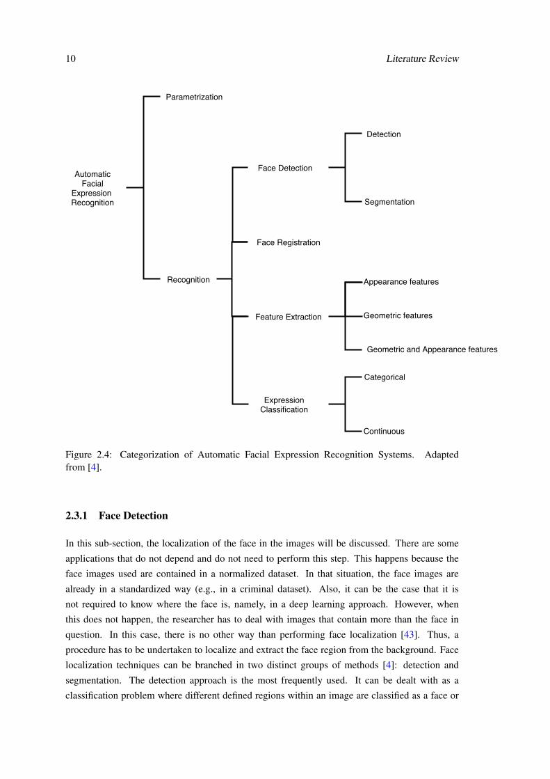
In [4], Corneanu et al. proposed a way of categorizing these techniques (see Figure 2.4), splitting
into two major components, namely, parametrization and recognition of facial expression. The
first branch, parametrization is the method that assigns facial expressions to a coding scheme;
FACS, for example. Concerning the automatic facial expression recognition, the general approach
is detailed in four key steps [4]. These will be described in more detail in the next sub-section.
• Face Detection — The purpose of the first step is to find out if the image contains a face
and where.
• Feature Extraction — Then, the extraction of the features on the obtained samples will be
performed, which results in a feature vector.
• Feature Selection — This step consists of selecting the most relevant features from a
dataset, generating a new subset of features.
• Expression Classification — At last, extracted features of the second step are used as an
input into the classifier and finally the classifier generates an output with the recognized
expression.
10 Literature Review
AutomaticFacial
Expression Recognition
Parametrization
Recognition
Face Detection
Feature Extraction
Face Registration
ExpressionClassification
Detection
Segmentation
Appearance features
Categorical
Continuous
Geometric features
Geometric and Appearance features
Figure 2.4: Categorization of Automatic Facial Expression Recognition Systems. Adaptedfrom [4].
2.3.1 Face Detection
In this sub-section, the localization of the face in the images will be discussed. There are some
applications that do not depend and do not need to perform this step. This happens because the
face images used are contained in a normalized dataset. In that situation, the face images are
already in a standardized way (e.g., in a criminal dataset). Also, it can be the case that it is
not required to know where the face is, namely, in a deep learning approach. However, when
this does not happen, the researcher has to deal with images that contain more than the face in
question. In this case, there is no other way than performing face localization [43]. Thus, a
procedure has to be undertaken to localize and extract the face region from the background. Face
localization techniques can be branched in two distinct groups of methods [4]: detection and
segmentation. The detection approach is the most frequently used. It can be dealt with as a
classification problem where different defined regions within an image are classified as a face or

2.3 Automatic Facial Expression Recognition 11
non-face. While segmentation, on the other hand, is the technique in which the aim is to link a label
to each pixel of the image. Thereby, the image is divided into a few segments each one assigned
to a label, in which some share the label, that means these segments have identical characteristics.
This results in a simpler representation of the image which provides clearer analysis.
Besides that, it should also be taken into consideration the fact that for a distinct types of
images, there should be different ways of proceeding. For instance, in the case of RGB1 images,
the Viola-Jones algorithm [8] is the most used and accepted. It is available in the OpenCV2
library. Furthermore, this algorithm main principle is based on a cascade of weak classifiers. It is
considered to be fast since it rapidly eliminates the parts that visibly do not contain face images [8].
However, it has some limitations caused by the different pose variations and when dealing with
large occlusions. In order to overcome these limitations methods with multiple pose detectors or
probabilistic approaches should be considered. Also, more specific methods such as CNN or SVM
should be taken into consideration. For 3D images, the way of proceeding provides the possibility
of obtaining better results and a more detailed feature base. So, the aim is to recognize any face
regardless of the pose orientation of the input image. To do that, curvature features are used to
find high curvature components of the face (e.g., the nose tip).
2.3.2 Dimensionality Reduction
Dimensionality reduction of high dimensional data is an essential step when it is intended to use
this data as the input of a machine learning algorithm. In the present case, the handled data are
images and to avoid a problem referred to as the curse of dimensionality [44] it has to be performed
a transformation into a low dimensional representation of the data. Moreover, a great number of
features can affect negatively the learning algorithms as it increases the risk of overfitting, it is
more computationally costly, decreases its performance, and requires more memory availability.
From [45], dimensionality reduction is branched out into feature extraction and feature se-
lection. Feature extraction is a transformative method in which the data is projected into a low
dimensional feature space. On the other hand, feature selection consists of selecting the most rel-
evant features from the initial dataset, as if it was a filter, creating a new subset of features. These
two branches will be studied below.
2.3.3 Feature Extraction
The next step in this system is feature extraction, it can be described as the procedure that allows
the extraction of relevant data from a face.
Relevant data such as face regions, measures, and angles are intended to be obtained [43]. To
do that, there are two different types of approaches that should be considered: geometric-feature
based methods and appearance-feature based methods. Geometric features give information about
shape and distances of facial components. These features are well-succeeded when the goal is
1System of colors that represents the three primary colors red, green and blue, which combined allow to produce awide chromatic spectrum.
2Open Source Computer Vision.

12 Literature Review
to describe facial expressions, however, they are not able to detect some attributes that are not
so prominent as the wrinkles, for instance. In this approach, the first thing to do is localize and
collect a considerable number of facial components so a feature vector can be created representing
the face geometry [46]. Geometric-based methods can be more expensive in terms of computing.
Nevertheless, they are more robust to changes in, among others, size and head pose. Appearance
features, on the other side, are steadier and are not influenced by noise, which allows the detection
of a more complex and complete group of facial expressions. Regarding the appearance-based
methods, image filters can be tested in both the whole face or certain regions of a face in order to
obtain a feature vector.
2.3.4 Feature Selection
In the previous sub-section, a representation of the face was obtained in the form of a vector of
features. However, not all those features contribute in the same way to the recognition task. Some
of them have little or no significant contribution. In addition, the reduction of the data results in a
better performance if the right subset is chosen, less computing time, and a clearer comprehension
of the features [47].
Multiple methods for feature selection are accessible in the literature. It should be noted
that methods as the Principal Component Analysis, explained in the sub-section 2.4.4, must not
be confused with feature selection methods. This is because, although it performs dimensional
reduction it does not only select and remove the features from the original set but changes them
generating new features. Feature selection methods are usually grouped into Embedded, Filter and
Wrapper methods [47]. These 3 groups will be described below.
• Wrapper Methods- In this method, the performance of the classifier is taken into account
as the method’s principle. From the original dataset, a subset of features will be selected and
tested. A score will be associated with each subset [48]. In the end, the subset that achieved
the highest score will be chosen. Wrapper methods can be seen as a "brute force" technique
which requires a substantial computational effort [49].
Two of the most commonly explored methods are Forward Selection and Backward Elimi-
nation.
• Filter Methods- Considered as a preprocessing task, this method, through procedures to
rank the features orders them and selects the features positioned at the top of the rank,
discarding the ones in the lower positions [47]. Its implementation is independent and per-
formed before classification. In addition, it is considered to be faster than the previous
method [49].
Examples of ranking procedures from [50, 47] are the following: Chi-Squared, the Correla-
tion and Mutual Information Criteria.

2.3 Automatic Facial Expression Recognition 13
In the literature, Filter Methods have been presented such as, ReliefF [51], Fisher Score [52]
and the Information Gain based on the Mutual Information Criterion [53].
• Embedded Methods- At last, contrary to the wrapper methods, the embedded focus on the
reduction of the time to compute the classification of each subset. The selection of features,
in this case, is carried out in the process of training. These methods are specifically used for
certain algorithms [49].
The Embedded Methods based on regularization achieve successful results and because of
that a significant attention has been drawn to them [54]. This branch of the Embedded
Methods includes methods as the Lasso [55], and Elastic net regularization [56],
2.3.5 Expression Classification
At last, the final step in which the expression is classified. In this phase, two models that describe
how people perceive and identify which facial expression are they observing will be considered:
• Categorical
• Continuous
The first one consists of a determined set of emotions, grouped in emotion categories. Among
a certain number of possible strategies, usually, for each of these emotion categories, a classifier
is trained. Usually, the six basic emotions, namely anger, disgust, fear, happiness, surprise, and
sadness are the categories chosen. However, there are some cases in which other categories are
included, for instance, expressions of pain, empathy, or others that indicate the existence of men-
tal disorders. The term categorical means that while a person is changing from a surprise to a sad
emotion it can only be identified one of these two emotions [57]. There is no emotion in between.
In contrast, the continuous shows that emotion is not a binary variable but can have different inten-
sities, in other words, emotions can be a combination of basic emotions (e.g., happily surprised).
This is a more exhaustive model, but it has the advantage of being able to define expressions with-
out any supervision applying clustering. Methods for expression recognition can also be divided
into two other group models:
• Static
• Dynamic
The static models evaluate every single frame independently, the techniques that they use for clas-
sification can be NN [58], RF, SVM. In early works, Neural Network was the most used classifier,
however, in the latest approaches the chosen techniques were the SVM and the BNC. The SVM
[18] provides robustness in the process of classification, this can be observed by the high classi-
fication accuracy when compared to the other methods. It performed well even in situations that
was expected not to, due to the presence of noise caused by illumination variations or head pose

14 Literature Review
variation [18]. Dynamic models, on the contrary, use features that are separately extracted from
each frame, so the evolution of the expression in the course of time can be modelled. The classifier
used is Hidden Markov Models (HMM) [59], it provides a method for modelling variable-length
expression series. This method was studied before being applied to facial expression classifica-
tion, however, because the results achieved by other methods had higher levels of accuracy it was
seldom used.
It is easier to train and implement a static classifier, as in the case of a dynamic classifier it
is necessary to have more training samples and learning parameters. Furthermore, when there are
differences among expressions they are robustly modelled by dynamic transitions that occur in the
distinct phases of an expression. This is relevant as, while communicating, people only express
subtle and sometimes almost invisible facial expressions. Those facial expressions are hard to
identify in a single image, but likely noticeable when shown in a video sequence.
2.3.6 Challenges
Although there is a lot of interest in this area and much progress was made, there is still plenty
of difficulties to overcome. The complexity of the process and the changeability of the facial ex-
pressions [60] do not help to improve the accuracy when performing facial expression recognition.
The main challenges in this recognition can be found in the table 2.3 [14, 60, 61]:
Table 2.3: Main challenges in automatic expression recognition.
Challenge DescriptionHead-pose variations Head-pose variations occur when considering uncontrolled con-
ditions since the participants can move, or the angle of the cameracan change. The ideal scenario would be the employment of onlyfrontal images which it is not likely to happen.
Illumination variations In the situations where the environment is not controlled, and sopictures can be taken in different lights. Also, even in environ-ments of constant light, some body movements can cause shad-ows or differences in the intensity of the illumination.
Registration Errors Registration techniques commonly lead to registration error, sothe researcher should be prepared to deal with that to guaranteethe accuracy of the results.
Occlusions It can occur due to head movements, as in the case of the illumi-nation variations, but it can also be the presence of glasses, beardor scarves.
Identity bias To deal with it, it is required to be able to tell identity-relatedshape and texture hints for subject-independent recognition.
2.3.7 Algorithms Analysis of Facial Expression Approaches
• Happy et al. [62], 2015 — In this thesis, a framework is described consisting, at first, on
the localization of the face using the Viola-Jones algorithm. Secondly, facial landmark

2.3 Automatic Facial Expression Recognition 15
detection was performed followed by extraction of the features using the LBP technique.
The posterior application of the PCA allowed the feature vector’s dimensionality reduction.
At last, the SVM was used as the multi-class classifier to translate the feature vectors in
expressions. It presented an accuracy of 94.09% for 329 samples of the CK+ dataset and
92.22% for 183 images in the JAFFE dataset.
• Matsugu et al. [39], 2003 — This work claimed to be the first FER model. In addition, it
claimed to be independent of the participant as well as robustly invariant to its appearance
and positioning. A CNN model was implemented using the disparities of the local features
between a neutral and a face enacting an expression. It followed an approach of one unique
CNN structure achieving an accuracy of 97.6% for 5600 images of ten participants.
• Carcagnì et al. [63], 2015- The paper contributes with a study of the HOG implementation
to perform facial expression recognition since the goal is to give emphasis to its use in this
context. The pipeline includes a first stage which focus is the face detection and registration.
The face detection uses the Viola-Jones algorithm. Then, it develops a HOG representation
of the images comparing it to other frequently used approaches. In a second stage, tests were
carried out in some of the publicly available datasets. The SVM approach was used to clas-
sify the images from datasets, such as CK+ and the RFD. The accuracy values were 98.8%,
98.5%, 98.5%, 98.2% for the CK+ 6 expressions, CK+ 7 expressions, RFD 7 expressions
and RFD 8 expressions, respectively.
• Shan et al. [64], 2009 — This work provides an empirical analysis of the use of the LBP fea-
tures in the problem of FER. The classification was performed by means of the application
of algorithms on datasets, such as the Cohn-kanade, the JAFFE, and the MMI databases.
The algorithms used to classify the expressions were the Template matching, SVM, LDA,
and Linear programming. Furthermore, the performance is inspected on different image
resolutions and in situations close to the real-world setting. Regarding the CK database,
the achieved accuracy was 88.9%, 79.1% and 73.4% for the SVM, Template matching and
LDA, respectively, when considering 7 expressions.
• Jia et al. [65], 2016 — The present work proposes a methodology that uses the PCA as a
feature extractor applied on a RF classifier. The tested dataset was the Japanese Female
Database in which, at first it was performed the preprocessing of the images (i.e. face
detection, crop and resize and noise removal), followed by the classification. This last step
used SVM and RF whose recognition rate was 73.3% and 77.5%, respectively.
2.3.8 Competitions
• Valstar et al. [66], 2011 — This paper presents the first challenge in automatic FER, the
FERA2011. This challenge had 2 variants, one detected Action Units whereas the other fo-
cused on discrete expressions. The challenge selected the GEMEP database [67], however,
16 Literature Review
only a part of this dataset was used. A baseline is described using the LBP, PCA, and SVM
for the 2 variants of the challenge.
• Valstar et al. [68], 2015 — The second FER challenge addressed the detection of the AU
occurrence and the estimation of its intensity for previously segmented data as well as a fully
automated version. The BP4DSpontaneous [69] and the SEMAINE dataset [70] composed
the data used in this challenge. To perform the extraction of the appearance features a
local LGBP descriptor[71], and the Cascaded Regression facial point detector[72] for the
geometric features were used. At last, a linear SVM performed the detection of the AU
occurrence, and a linear SVR was used for the intensity.
• Valstar et al. [73], 2017 — Lastly, the third challenge adds to the previous one the difficulty
of dealing with data generated when varying the positioning and the camera angle. The
sub-challenges are, as previously stated, the AU detection and the estimation of its intensity.
In this case, the geometric features were obtained by the Cascaded Continuous Regression
facial point detector[74]. In contrast to the previous challenges, for the FERA2015 the tem-
poral dynamics was modeled by using the learning method Conditional Random Field[75]
(AU occurrence) and Conditional Ordinal Random Field[76] (AU intensity).
2.4 Feature Methods
2.4.1 Histogram of Oriented Gradients (HOG)
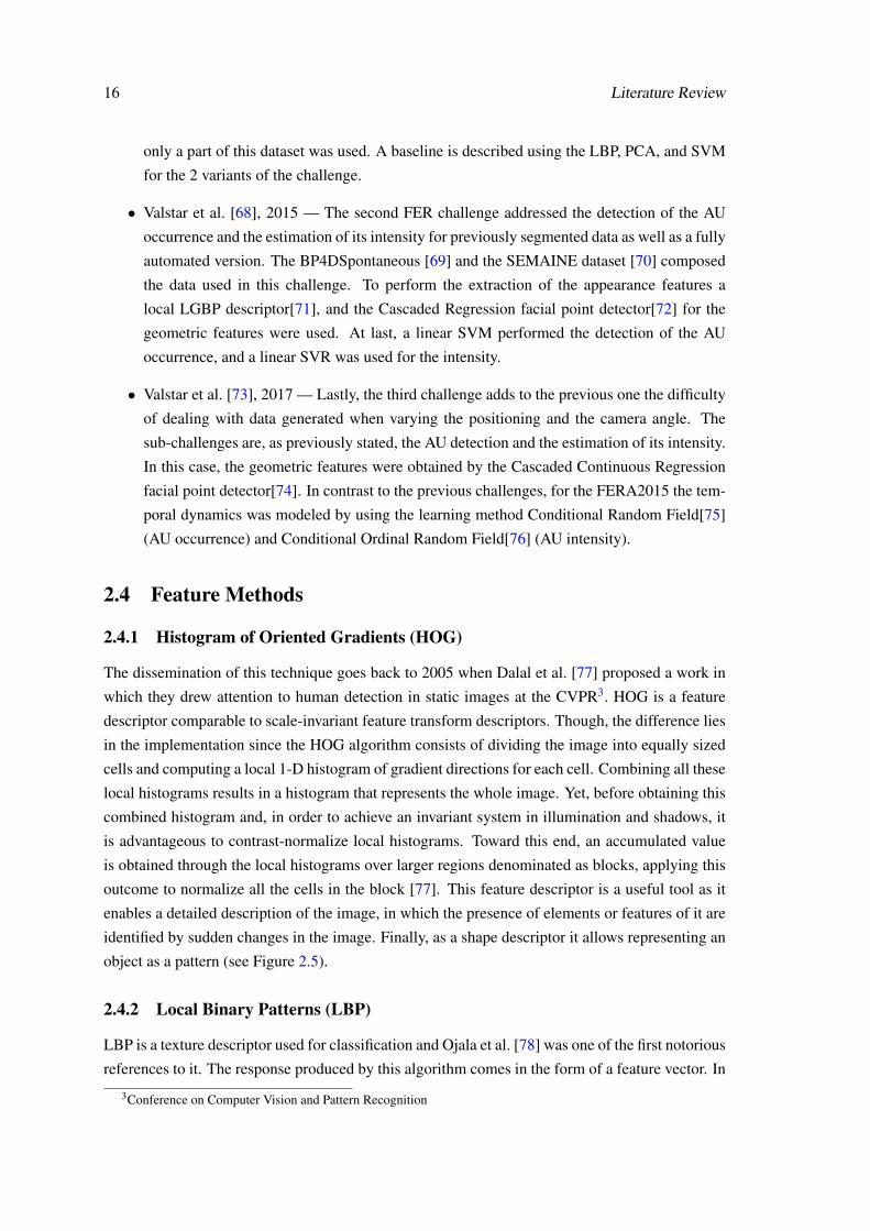
The dissemination of this technique goes back to 2005 when Dalal et al. [77] proposed a work in
which they drew attention to human detection in static images at the CVPR3. HOG is a feature
descriptor comparable to scale-invariant feature transform descriptors. Though, the difference lies
in the implementation since the HOG algorithm consists of dividing the image into equally sized
cells and computing a local 1-D histogram of gradient directions for each cell. Combining all these
local histograms results in a histogram that represents the whole image. Yet, before obtaining this
combined histogram and, in order to achieve an invariant system in illumination and shadows, it
is advantageous to contrast-normalize local histograms. Toward this end, an accumulated value
is obtained through the local histograms over larger regions denominated as blocks, applying this
outcome to normalize all the cells in the block [77]. This feature descriptor is a useful tool as it
enables a detailed description of the image, in which the presence of elements or features of it are
identified by sudden changes in the image. Finally, as a shape descriptor it allows representing an
object as a pattern (see Figure 2.5).
2.4.2 Local Binary Patterns (LBP)
LBP is a texture descriptor used for classification and Ojala et al. [78] was one of the first notorious
references to it. The response produced by this algorithm comes in the form of a feature vector. In
3Conference on Computer Vision and Pattern Recognition

2.4 Feature Methods 17
Figure 2.5: HOG of the face. From [5].
practice, to obtain this LBP feature vector a window of determined dimensions is taken, supposed
that a 3x3 pixel block is chosen . Moving this window through the image, the value of the pixel
at the center of the block is used to threshold its surrounding pixels [6]. This means that the pixel
values of each of the 8 neighbours will be compared to the center pixel and so, in the case of
the neighbour pixel having an intensity value greater than the center, it will be replaced by “0” if
not, becomes a “1”. The next step involves reading the modified values in the 3x3 window in the
clockwise direction leading to an 8 digits binary pattern that is converted to decimal afterwards.
After carrying out this process in the whole image a histogram can be generated giving information
about the frequency of the pattern occurrence. At last, the final step implies concatenating the
results to obtain the feature vector [78].
Figure 2.6: Image sequence of the process described above: an input image, LBP image, and thecorrespondent histogram. From [6].

18 Literature Review
2.4.3 Scale-Invariant Feature Transform (SIFT)
David Lowe presented this method to generate image features in [79, 80]. The scale-invariant
feature transform has been applied to several topics as motion tracking, object and gesture recog-
nition. As the name suggests, this algorithm is used to extract and describe invariant features.
That is to say it extracts and describes features that are invariant to image scale, variations in the
illumination, translation, and rotation of the element in issue. This approach consists of a great
collection of key points descriptors possessing extremely distinctive characteristics. Such charac-
teristics enable this algorithm to find an accurate match in a large set of features [80], which means
the same object has a high chance of being detected in another image.
2.4.4 Principal Component Analysis (PCA)
PCA is a statistical method invented by Karl Pearson in 1901 [81]. The method concerned identi-
fies the maximum variance and after that reduces their dimensionality [82]. In fact, it can reduce a
large dataset into a smaller dataset preserving most of the information existing in the large dataset.
It is used to give emphasis to variation and highlight patterns by converting the initially considered
data into principal components [83]. Since these components are ordered by their ability to ex-
plain the variability of the data, the first principal component is the one that can account for most
of the variability. Thus, the subsequent components can explain the remaining variability, and so
on. Eigenfaces [84] consist in the Principal Component Analysis when performed in a dataset of
face images. The focus in this method are the significant features which are the areas of maximum
change in a face (e.g. the significant variation visible from the eyes to nose). However, those sig-
nificant features are not necessarily translated in a region of the face as the eyes or the nose [85].
The intention here is to capture the relevant variations among faces so it is possible to differentiate
them.
Figure 2.7: Example of the eigenfaces showing that as well as encoding the facial features, it alsoencodes the illumination in the face images. From [7].

2.5 Feature Selection Techniques 19
2.5 Feature Selection Techniques
2.5.1 Sequential Forward Selection (SFS)
SFS is an algorithm used to perform feature selection. The process of selection is initialized
testing an empty vector of features. Then, one feature is added to the vector at a time and each new
generated vector of features is tested. The fact that a feature allows achieving the best performance
in the classification is what defines if it is kept or discarded of the vector of features. In the end,
the selected set of features is returned.
2.5.2 Sequential Backward Selection (SBS)
Contrary to the previous algorithm, the Sequential Backward Selection starts considering all the
features and excludes one at a time. In this case, it is excluded the features that reflect the least
reduction of the classifier’s performance.
2.5.3 Mutual Information (MI)
The principle of MI consists of calculating the dependency measure between two variables [86].
In machine learning it is used as a feature selection criterion which defines the relevance or redun-
dancy of the features. Therefore, a score is calculated indicating how well descriptive a feature (x)
is of the labels (y). In the end, a predefined number of features (k) corresponding to the highest
scores is chosen. This score is presented as the mutual information, MI(xi,y) below:
MI(xi,y) = ∑xi∈{0,1}
∑y∈{0,1}
p(xi,y) logp(xi,y)
p(xi)p(y)(2.1)
MI will be equal to 0 in the case of x and y be independents and superior if there is a depen-
dency [47].
2.5.4 Lasso Regularization
Lasso, proposed by Robert Tibshirani in 1996 [55] is an effective technique that performs both
regularization and feature selection [87]. It formulates that the model specifications are restricted,
the sum of its absolute values is upper limited by defined value. To this end, one of the steps
performs a shrinking (regularization). The coefficients of the features are penalized being shrunk
to 0. The selected features are the ones whose coefficient is other than zero. This process aims to
reduce the error in the prediction [87].

20 Literature Review
2.6 Machine Learning Algorithms
2.6.1 Viola-Jones
Viola-Jones is an extensively used real-time object detection approach published in 2001 in [8, 88].
It is known for its ability to perform rapid image processing with high detection rates. The target of
this framework, as well as one of its motivations, was the definition of the face detection problem.
The fact that a fast face detector was created made it suitable for a wide range of applications,
such as user interfaces and image datasets [8]. There are three main aspects of this system that
are worth highlighting. Its robustness, which means there is a high True-Positive rate and a low
False-Positive consistently, its capability to process images in real time and, finally, its exclusive
use to detect faces in images and not recognition as it can be mistaken. Furthermore, according
to this work, to build such a face detection system 3 steps need to be accomplished [89]. These
steps are the folowing: obtaining the Integral Image, the implementation of AdaBoost and, at last
classification using an Attentional Aascade.
Figure 2.8: On the left, feature examples are shown. On the right it is presented the AdaBoost twofirst selected features. Adapted from [8].
2.6.1.1 Integral Image
An Integral Image is an image representation that was first presented by the name Summed-Area
Table, which is used as a fast way of computing Haar-like features at various scales [8]. In practice,
it efficiently calculates the sum of intensities over manifold overlapping rectangle regions of an
image [9]. See Figure 2.9.
2.6.1.2 AdaBoost
AdaBoost is a learning algorithm which acts in both the selection of a limited number of signif-
icant features as well as in the training of classifiers [90]. In this regard, it occurs a boost in the
performance due to the combination of weighted “weak” classifiers that yields to this “strong”
boosted classifier [88].
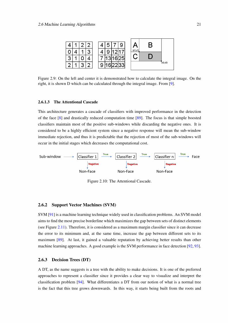
2.6 Machine Learning Algorithms 21
Figure 2.9: On the left and center it is demonstrated how to calculate the integral image. On theright, it is shown D which can be calculated through the integral image. From [9].
2.6.1.3 The Attentional Cascade
This architecture generates a cascade of classifiers with improved performance in the detection
of the face [8] and drastically reduced computation time [89]. The focus is that simple boosted
classifiers maintain most of the positive sub-windows while discarding the negative ones. It is
considered to be a highly efficient system since a negative response will mean the sub-window
immediate rejection, and thus it is predictable that the rejection of most of the sub-windows will
occur in the initial stages which decreases the computational cost.
Figure 2.10: The Attentional Cascade.
2.6.2 Support Vector Machines (SVM)
SVM [91] is a machine learning technique widely used in classification problems. An SVM model
aims to find the most precise borderline which maximizes the gap between sets of distinct elements
(see Figure 2.11). Therefore, it is considered as a maximum margin classifier since it can decrease
the error to its minimum and, at the same time, increase the gap between different sets to its
maximum [89]. At last, it gained a valuable reputation by achieving better results than other
machine learning approaches. A good example is the SVM performance in face detection [92, 93].
2.6.3 Decision Trees (DT)
A DT, as the name suggests is a tree with the ability to make decisions. It is one of the preferred
approaches to represent a classifier since it provides a clear way to visualize and interpret the
classification problem [94]. What differentiates a DT from our notion of what is a normal tree
is the fact that this tree grows downwards. In this way, it starts being built from the roots and

22 Literature Review
Figure 2.11: On the left it is shown the original feature space whereas on the right, it is the non-linear separation of those features.
goes down to the leaves [95]. It is essentially a binary tree, in which the leaves correspond to
the different target class labels. A test node, on the other hand, represents a feature and it is
where the decision occurs. The outcome that results from the decision defines which one of the
branches to follow, and so on until a leaf is reached, which means the class has been predicted (see
Figure 2.12).
Figure 2.12: Example of Decision Tree, which aim is to sort the variables a, b, and c. Adaptedfrom [10]
2.6.4 Random Forest (RF)
RF [96] is an acknowledged statistical method in a wide variety of subjects [97]. The classifier
consists of using multiple Decision Trees 4 combined, whose training process applies the bagging
method proposed by Leo Breiman in [98]. As previously mentioned, when a DT is fully-grown a
4Quinlan et al. in [95]

2.6 Machine Learning Algorithms 23
prediction is reached. However, in the case of RF, it is the combination of all the interim predic-
tions that yield to a final prediction, achieving notorious improvements in the accuracy values [99].
This way of proceeding corresponds to the aforementioned bagging method. In addition, the fact
that it is used sub-set of randomly selected features from the training set as the input for each tree
leads to favourable error rates comparable to the AdaBoost algorithm [97] 5.
Figure 2.13: Example of a simple RF.
5Freund et al. in [90]

24 Literature Review
2.7 Facial Expression Databases
When benchmarking techniques, it is highly important to use the most appropriate dataset. There-
fore, it is extremely important to take into consideration the final goal of the task. In this work,
since it is aimed to recognize facial expressions it is likely to use databases, such as the following:
• Japanese Female Facial Expressions (JAFFE) — This database consists in the record of
10 Japanese female models enacting 7 expressions making a total of 213 images (Lyons et
al. [100], 1998).
• Cohn-Kanade AU-Coded Expression Database (CK) — The CMU-Pittsburgh AU-Coded
Face Expression Image Database contains 2105 image sequences, in which were included
182 participants from diverse ethnic group obtaining a description in facial expression labels
(e.g. happiness) and FACS basic units (AU) (Kanade et al. [101], 2000)
• MMI Facial Expression Database (MMI) — This database consists of 1500 samples divided
in static and image sequences. The faces are positioned in a frontal angle enacting different
expressions measured in AUs from the Facial Action Coding System (FACS) (Pantic et
al. [102], 2005)
• Taiwanese Facial Expression Image Database (TFEID) — TFEID contains 7200 images
from 40 particIpants, half are women. Eight expressions are represented, with some pose
variations (Chen et al. [103], 2007)
• Extended Cohn–Kanade (CK+) — The CK+ represents an increase of 22% in the number of
sequences and 27% in the case of the participants when compared to the first release of the
CK. Also, in this extended version, it was added spontaneous sequences and their respective
description in FACS and expression labels (Lucey et al. [11], 2010).
• Multimedia Understanding Group (MUG) — Mug is organized in two groups, the first one
contains data from 86 models performing the six main expressions (anger, disgust, fear,
happiness, sadness, surprise) defined in FACS, whereas the second one contains induced
expressions performed in lab environment by the same group of participants (Aifanti et
al. [104], 2010).
• Facial Expressions In The Wild Project (AFEW/SFEW) — Acted Facial Expressions in the
Wild (AFEW) is a dynamic temporal database in which the samples were collected from
movies. The selection of 700 frames from the AFEW database originated a static subset
labelled for 6 expressions called Static Facial Expressions in the Wild (SFEW) (Dhall et
al. [105], 2012).
• Facial Expression Recognition 2013 (FER2013) — FER2013 was first made public for the
Kaggle competition. The dataset contains 35887 grayscale face images labelled for 7 ex-
pressions (Goodfellow et al. [106], 2013)

2.7 Facial Expression Databases 25
• AffectNet — This database contains roughly 1,000,000 face images in the wild setting ob-
tained from the Internet, half of these were manually annotated for 7 emotions and the
intensity of valence and arousal. The remaining were automatically annotated training the
ResNext Neural Network on the manually annotated set. (Mollahosseini et al. [13], 2017)
The properties of a database can be organized in three main categories, this organization is
based on the content, in the capture modality and in the participants [4]. Content includes infor-
mation as the type of labels, which expressions are present, whether the samples were taken with
an intention or not (posed or spontaneous), and, at last, if it contains images (static) or video se-
quences (dynamic). On the other hand, the capture modality describes if the data was captured in
laboratory conditions or not, changes in perspective, illumination and finally occlusions. Lastly, it
is the compilation of the data in statistical terms, such as age, gender and ethnic group [4].
Table 2.4: RGB Dataset.
Dataset Description Intention Gray/ColorCK The first dataset to be made public. This first
version is considerably small.Posed pri-mary facialexpressions
Mostly gray
CK+ Extended version of CK with an increasednumber of samples both posed and sponta-neous.
Spontaneousimagesadded plusthe previousposed ones
Mostly gray
MMI Marked an improvement by adding profileviews of primary expressions and almost allexisting AUs of the FACS.
Spontaneousand Posed
Color
JAFFE A dataset of static images captured in a labenvironment. It contains 213 samples with 7expressions acted by 10 Japanese women
Posed Gray
AFEW It is a dynamic dataset, carefully describingthe age, gender, and pose of the images, oneof the 6 primary expressions
Posed Color
Table 2.5: 3D Dataset.
Dataset Description Intention Gray/ColorBU-3DFE [107] 6 expressions out of 100 distinct subjects,
taken under 4 different intensity levels.Posed Color
Bosphorus [108] Low ethnic diversity, however, it containsmany expressions, head poses, and occlu-sions.
Posed Color tex-ture images
BU-4DFE(video) [109]
High-resolution 3D dynamic facial expres-sion dataset.
Posed Color tex-ture video

26 Literature Review
Table 2.6: Thermal Dataset.
Dataset Description Intention Gray/ColorIRIS [110] Images from 30 subjects. It includes a set of
images labelled with 3 posed primary emo-tions capture on different illuminations.
Posed Gray
NIST [111] Consists of 1573 images, of which 78 arefrom women and the rest from men.
Posed Gray
NVIE [112] The 215 subjects enact six expressions. In theposed setting it is included also some occlu-sions and illumination from different angles.
Spontaneousand Posed
Gray
KTFE [113] As the NVIE, this database contains the 6 ex-pressions. Includes samples from 26 subjectsfrom Vietnam, Japan, and Thailand
Spontaneousand Posed
-
2.8 Final Considerations
In this chapter, the topic of study Facial Expressions was introduced, as well as the structure of an
Automatic Facial Expression Recognition System, depicting each one of the steps and how they
were performed in other similar works. Moreover, the most appropriate datasets to deal with the
problem of expression recognition are presented.
Gathering all this information was a fundamental milestone to be able to decide which of those
methods and algorithms would be implemented hereafter. Also, it was taken into consideration
the computational cost of some techniques and the public availability of the datasets. With this in
mind, the chosen techniques were the following:
• Viola-Jones approach to perform face detection as it is still widely used in current works
due to its effectiveness in the localization of the faces;
• HOG, LBP and PCA to obtain the facial features, the first because of its ability to detect
abrupt changes, the second for being a robust texture descriptor that can deal with illumi-
nation variations, and the last one which is able to create a representation that explains the
variance of the images and discard the redundant features making it faster to run;
• MI to select the features due to its ability to deal with inconsistent relations between the
features and the target variables, also it is not computationally intensive;
• SVM and RF to perform classification, as the first is one of the most used algorithms able
to achieve high accuracy values, and the second one, a classifier known for its great per-
formance due to the combination of predictions that allows achieving a more reliable final
prediction.
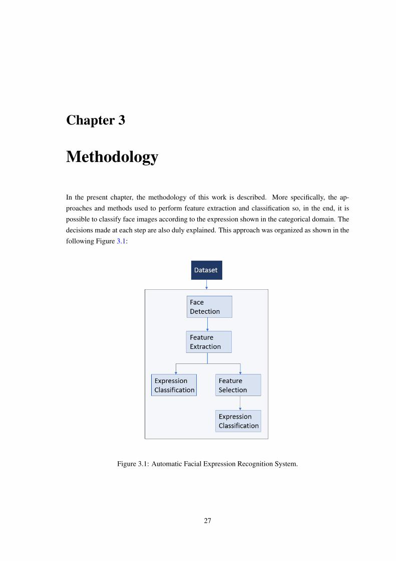
Chapter 3
Methodology
In the present chapter, the methodology of this work is described. More specifically, the ap-
proaches and methods used to perform feature extraction and classification so, in the end, it is
possible to classify face images according to the expression shown in the categorical domain. The
decisions made at each step are also duly explained. This approach was organized as shown in the
following Figure 3.1:
Figure 3.1: Automatic Facial Expression Recognition System.
27

28 Methodology
3.1 Face Localization and Crop
The aim of this stage is to detect and crop the faces present in the images. Nevertheless, there
was a slight difference in the pre-processing of these two datasets. The CK+ had no annotations
for the location of the face in the image, which meant that a face detection technique would have
to be applied. Toward this end, the OpenCV library seemed to be a reasonable option, since it
is acknowledged by their Object Detection approach with a few of pre-trained classifiers for the
face and, moreover, some more specific regions of the face as the eyes or the mouth (smile).
This detector uses a Haar Feature-based Cascade Classifier originally proposed by Paul Viola and
Michael Jones [8] (see Section 2.6.1) which continues to be one of the most frequently used [114]
methods. On the contrary, the AffectNet Database provided already the location of the faces in the
images (see Figure 4.3). In this case, a bounding box for each face has been previously found by
using the OpenCV face detector. The provided coordinates represent that bounding box expanded
in fifteen percent.
Hereupon, regardless the way the location of the faces in the images was obtained, we ended
up with 4 values (x,y,w,h) which are the required information to crop the images, and so our
final image would only have the desired region of interest, the face. Finally, and because the
preprocessing step is to produce an image that can be used with a certain efficiency and straight
by the feature extractor, the images from both datasets were converted to grayscale and resized to
a fixed size, in this case, 256x256 pixels [13].
Figure 3.2: Representation of the performed steps to obtain a face image on the CK+ dataset.

3.2 Facial Features 29
3.2 Facial Features
Objects are effortlessly recognized by the human eye due to the ability of our brain to associate
them with some specific characteristics. The mastery of this skill is the result of its development
since the day we were born by observing the world around us. The aim of Computer Vision is,
precisely, to imitate the human eye. For this purpose, information from an image is acquired using
feature extraction techniques. In chapter 2, a few of these techniques were reviewed and some of
them implemented so it would be possible to draw conclusions on how well they would be able
to describe the image faces. In this experiment, the chosen feature extraction techniques consider
the image as a whole [115]: HOG, LBP, and PCA.
3.2.1 HOG
Different facial expressions trigger different changes in the face, as can be observed in Figure 4.1.
The distinct characteristics among different facial expressions are easily identified, for instance,
surprise is represented by arching the eyebrows, and keeping the eyes and mouth wide open. On
the contrary, to lower the eyebrows and press the lips together defines another facial expression,
anger. These are the features that are intended to be extracted. The Hog algorithm, previously
presented, was used due to its capability to detect abrupt changes in the face images. In practice,
it can detect the transition from the skin to other elements as the lips, eyebrows or nose. It is con-
sidered a shape descriptor as it distributes the intensity gradients in the direction of the element’s
edges.
The procedure starts by converting the cropped face image to grayscale, this is a necessary
step because it prevents the occurrence of errors provoked by the channels. Finally, the feature
vector is generated in the form of a histogram that represents the image. See Figure 3.3.
3.2.2 LBP
In some instances, the image after being converted to grayscale shows almost no noticeable dis-
tinction in the different levels of gray, this can be caused by illumination variations. The LBP is
a robust texture descriptor able to deal with situations like this. Another important particularity is
its computational simplicity due to the low complexity steps that need to be performed, explained
in the literature review (See 3.4).
The first step involves converting the image to grayscale, followed by the repetition of some
basic steps in the whole image obtaining a decimal number to each position of the window and,
subsequently, generating a histogram with the frequency of the number. In the end, the results are
concatenated and the feature vector obtained.
3.2.3 PCA
PCA’s importance is reflected in its ability to discard the redundant components and preserve only
a few components that can describe most of the variation of the original dataset (See Figure 2.7).
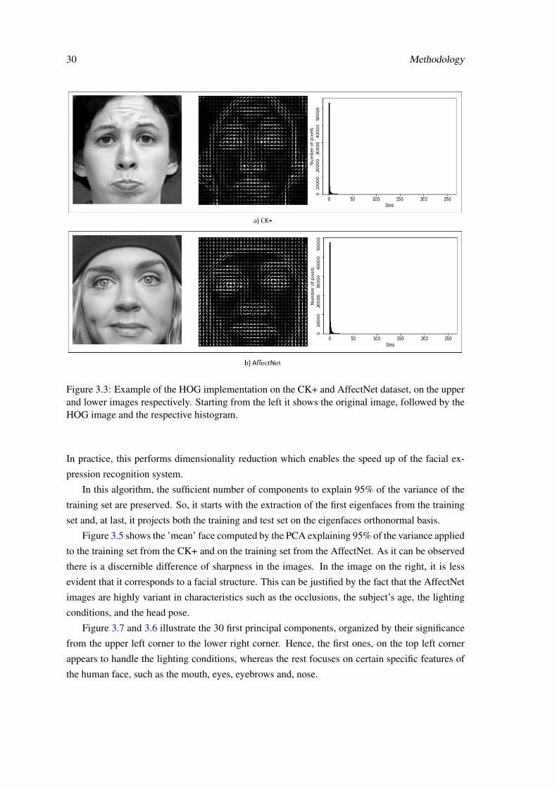
30 Methodology
Figure 3.3: Example of the HOG implementation on the CK+ and AffectNet dataset, on the upperand lower images respectively. Starting from the left it shows the original image, followed by theHOG image and the respective histogram.
In practice, this performs dimensionality reduction which enables the speed up of the facial ex-
pression recognition system.
In this algorithm, the sufficient number of components to explain 95% of the variance of the
training set are preserved. So, it starts with the extraction of the first eigenfaces from the training
set and, at last, it projects both the training and test set on the eigenfaces orthonormal basis.
Figure 3.5 shows the ’mean’ face computed by the PCA explaining 95% of the variance applied
to the training set from the CK+ and on the training set from the AffectNet. As it can be observed
there is a discernible difference of sharpness in the images. In the image on the right, it is less
evident that it corresponds to a facial structure. This can be justified by the fact that the AffectNet
images are highly variant in characteristics such as the occlusions, the subject’s age, the lighting
conditions, and the head pose.
Figure 3.7 and 3.6 illustrate the 30 first principal components, organized by their significance
from the upper left corner to the lower right corner. Hence, the first ones, on the top left corner
appears to handle the lighting conditions, whereas the rest focuses on certain specific features of
the human face, such as the mouth, eyes, eyebrows and, nose.
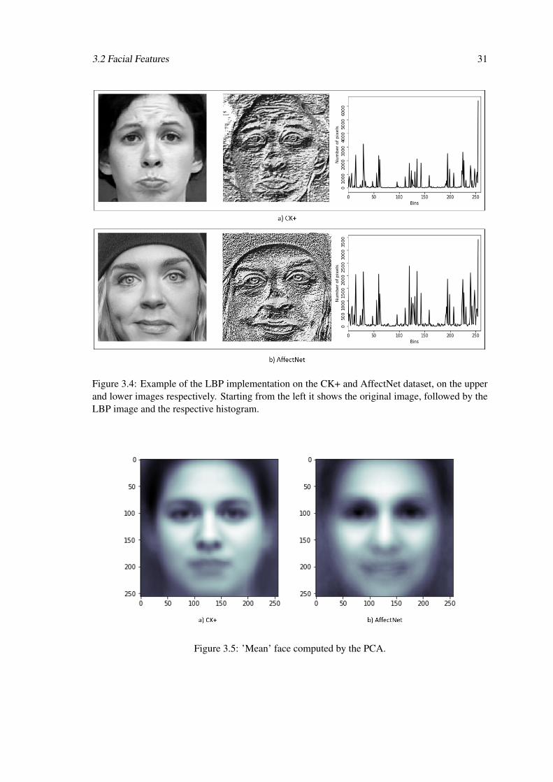
3.2 Facial Features 31
Figure 3.4: Example of the LBP implementation on the CK+ and AffectNet dataset, on the upperand lower images respectively. Starting from the left it shows the original image, followed by theLBP image and the respective histogram.
Figure 3.5: ’Mean’ face computed by the PCA.

32 Methodology
Figure 3.6: Representation of the first principal components on the CK+ dataset.
Figure 3.7: Representation of the first principal components on the AffectNet dataset.
3.3 Feature Selection
In the previous section, a vector of features was obtained. However, it is possible that not all the
features are needed to create a meaningful representation of face. That is what a feature selection
algorithm tries to find out, whether a smaller set of features would be able to achieve the same
or even superior accuracy comparing to the complete set of features. Such reduction would have
multiple advantages, as it would allow a better understanding of the features keeping only the
features that are relevant, minimizing the vector of features making the algorithms to run faster
and, at last, to avoid overfitting [87]. In Chapter 2, some feature selection algorithms were studied.
3.3.1 MI Based Approach
As studied in 2.5.3 the MI criterion [116] consists of obtaining a score which is determined by what
is shared or not between features. The MI’s principle was used as a straight measure to choose a
subset of features that enable the system to perform the most accurate separation of the aimed la-
bels. Other conventional feature selection techniques, for instance techniques based in correlation

3.4 Classification 33
when compared to the MI are not able to calculate the score for associations between random fea-
tures [117]. This approach might be advantageous when dealing with situations to which a linear
relations technique fails to deal with. In addition, it is not a computationally complex technique.
3.4 Classification
From the two datasets a set of seven emotions (anger, contempt, disgust, fear, happy, sad, surprise)
and, additionally, the neutral one were considered.
In this section, the methods used to classify the datasets for the above facial expressions will
be discussed. For this purpose, the goal was to find an accurate, robust, and feasible classifier. Of
the two types of machine learning techniques, supervised learning is the one used to train a model
on a known training set (considering both, the input and the output response data). Thereby, and
after having built the classification model it can be finally used to predict a new test set. This
experiment tested two distinct supervised learning algorithms, so the behaviour of the different
features could be analyzed: SVM and RF.
3.4.1 SVM
The SVM, previously studied in section 2.6.2, is one of the most used algorithms as it has the
ability to perform classification with high accuracy, outperforming other classification algorithms.
The feature vectors obtained through the HOG, LBP or PCA algorithm performed on the
training set, along with the respective labels, were used to feed the classifier. Then, a model is built
and the features were distributed depending on their associated label. By doing this, the features
that belong to different classes are separated from one another and positioned in the correspondent
group.
Some tests were carried out varying some parameters so it would be possible to analyze the
behaviour of the classifier, which parameters would have more influence and how it would affect
the system accuracy.
3.4.2 RF
The second method tested was the Random Forest, explained in section 2.6.4. The great perfor-
mance of the RF is due to the combination of a considerable number of interim predictions that
lead to a more reliable prediction in the end. Also, its randomness when selecting the features
from the training set that are feeding each tree allows the method to estimate the importance of
each feature in relation to the others.
As the SVM, the input for this classifier is also the output of the previously mentioned feature
extraction methods. An RF model with certain parameters is built and the model and those feature
vectors together with the labels are given to fit the model. At last, it makes the predictions to the
test set and provides a final prediction value.

34 Methodology
A vast set of parameters were tested in order to find the best parameter choice that would
achieve the highest accuracy, as well as to study the influence of each one the parameters.
3.5 Final Considerations
In this chapter, the proposed methodology for this project was described. By starting with the
choice of the datasets to the last step, the algorithms chosen for the classification. In order to
obtain a more reliable analysis more than one technique was tested at each step. The following
chapter presents the results of the implementation of these methods as well as its interpretation in
order to understand how feasible they are to perform the proposed task.

Chapter 4
Results and Discussion
This chapter covers the discussion and analysis of the results for all the methods implemented in
each step of the Methodology (Chapter 3). As it was mentioned before, each phase involved the
test of different approaches. The final goal was to understand how reliable an Automatic Facial
Expression Recognition system can be in different situations. For this purpose, whenever the
results were not satisfactory some modifications were made and even other techniques considered.
This entire process will be discussed as well as the respectively obtained outcomes.
4.1 Dataset
The initial step to perform any recognition task is to choose the adequate data. As in this case, the
focus was the benchmarking of different techniques to recognize facial expressions, a reliable and
well-known dataset was required. In this way, the CK+ was chosen. The fact that this dataset was
generated in a controlled environment and it is been used countless times since its release makes
it a valuable addition. A second dataset was also considered the AffectNet Database. The choice
for this dataset was due to the fact that this is a recent dataset, in-the-wild and with a large number
of samples. These characteristics reflect the current needs in the field.
4.1.1 The Extended Cohn – Kanade (CK+)
The CK+ is a publicly available dataset, and as it was stated before is an extension of the CK
database which the main purpose was to promote the development of automatic systems to de-
tect the individual’s facial expressions. This new version has augmented in 22 percent the posed
samples and added the spontaneous ones (see Figure 4.1). The subjects that were taking part in
the experiment were 210 adults which facial movements were recorded using the following equip-
ment: two hardware synchronized Panasonic AG-7500 cameras [11]. The age of the individuals
ranged from 18 to 50 years of age, given that sixty-nine percent were female, eighty-one percent
were Euro-American, thirteen percent Afro-American, and six percent from other groups. During
the experiment, the subjects were instructed to execute 23 facial displays which comprehended
35

36 Results and Discussion
both single and combined action units. In the observation room where the experiment was tak-
ing place, image sequences were obtained by the two cameras there positioned, one of them was
directly in front and the other was 30 degrees to the right of the subject [101]. In the end, the re-
sult was both an 8-bit grayscale and a 24-bit color values pixel arrays with dimension 640x490 or
640x480. The number of frames in the image sequences can vary between 10 and 30 and it always
starts and finishes with a neutral expression. However, the arranged sequence in the dataset only
includes the frames from the neutral to the peak of the expression (See Figure 4.2). This last one
characterizes the emotion label that is assigned to the alluding sequence. The group of the possible
labelled emotions can be seen in Figure 4.1 below: anger (e), contempt (f), disgust (a), fear (d),
happiness (b), neutral (h), sadness (g) and surprise (c).
Figure 4.1: Examples of the CK+ dataset. In the upper part, there are some images originally fromthe CK dataset and those below are the data included in the new version. Adapted from [11].
Figure 4.2: Images sequence obtained from a subject when the labelled emotion is “Surprise”.From [12].
4.1.2 AffectNet
AffectNet, which name arose from the merge of the words Affect and InterNet, is the largest
existing dataset only released in the second semester of 2017. This dataset contains approximately

4.1 Dataset 37
Table 4.1: Frequency of each expression represented in the peak frames on the CK+ database.
Expression NumberAngry (An) 45Contempt (Co) 18Disgust (Di) 59Fear (Fe) 25Happy (Ha) 69Sadness (Sa) 28Surprise (Su) 83
one million face images. Images that were gathered from the Internet through 3 search engines
(Bing, Google, and Yahoo) when queried with 1250 keywords associated with emotion vocabulary
in 6 distinct languages (English, Spanish, Portuguese, German, Arabic, and Farsi). Afterwards, a
bounding box for each face was found by using the OpenCV face recognition approach mentioned
above. Then, this bounding box was expanded in fifteen percent. Besides that, via regression
local binary features (a face alignment technique) [118] sixty-six facial landmarks points were
detected. The resolution of the face images is, on average, 425x425. In order to take some facial
characteristics, the Microsoft cognitive face API [119] was used and according to the outcome:
Forty-nine percent of the samples were identified as men and the average age is 33.01 years old,
with a standard deviation of 16.96 years. The Microsoft cognitive face API also allowed the
detection of the occurrence of some occlusions. For instance, eye (0.49 percent), forehead (4.5
percent) and mouth (1.08 percent) occlusions were found in the face images. Additionally, several
faces have eye (51.7 percent) and lip (41.4 percent) make-up, and others were wearing glasses
(9.63 percent). The dataset is branched in two different sets, such as:
• Manually Annotated;
• Automatically Annotated.
The present need of having an extensive dataset in the wild which would contain a huge num-
ber of the individual’s variation provided the justification for its creation. Apart from that, there
is also the fact that this dataset embraces more than one model of affect [120]. In this case two
different emotion models [121]: the categorical, which represents the discrete facial expressions,
for instance, here are considered seven distinct facial expressions; and the dimensional which is
the intensity of valence and arousal (see [122]). The manually annotated set, as the name implies is
an annotated set by expertise human labelers. It has around 420000 images which are labelled by
the annotators for the two models of affect aforementioned. The remaining images belong to the
automatically annotated set (more than 550000), which was obtained through the training of the
ResNext Neural Network on the manually annotated training set, achieving an average accuracy
of sixty-five percent.

38 Results and Discussion
4.1.2.1 Annotation Procedure
To perform the annotation of the face images some options were considered as the Amazon Me-
chanical Truck (MTurk), a crowd-sourcing service. Although it is a cheap and straightforward
approach to label large datasets, it is not fully reliable in terms of the quality of labelling. Since it
ranges significantly depending on the annotators. Also, the fact that it is required to annotate this
dataset in the dimensional model makes this task impossible for any annotator with no knowledge
in this model of affect. Thus, after taking in consideration these limitations the crowd-sourcing
service was discarded, and the solution found was hiring twelve annotators at the University of
Denver. These expertise annotators were given 450000 samples to perform the labelling of the
face in the images, each image annotated by one annotator. To annotate the two models of affect
(categorical and dimensional) a software application was designed (See Figure 4.3).
Figure 4.3: Software application used by the annotators to label into the categorical and dimen-sional models of affect. An image has only one face annotated (for instance, the one in the greenbox). From [13].
4.1.2.2 Annotation in the Categorical Model
Each sample was identified as one out of 11 emotion and non-emotion categorical labels. These
eleven labels are Neutral, Happiness, Sadness, Surprise, Fear, Disgust, Anger, Contempt, None,
Uncertain and Non-Face. Next, some of the categories will be explained as they are not so com-
mon. Specifically, the None label, which means “None of the eight emotions” [?] represents all
the images that the annotator could not assign to any of the 8 expressions. If it existed they could,
in some cases, belong to categories as shy, impressed or focused. On the other hand, the Non-Facerefers to images in which: the face detection algorithm does not draw the bounding box where the
face is located; the face is not a human face (e.g. can be a painting or an animation); in the face
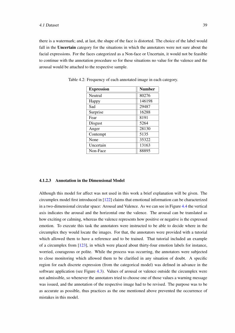
4.1 Dataset 39
there is a watermark; and, at last, the shape of the face is distorted. The choice of the label would
fall in the Uncertain category for the situations in which the annotators were not sure about the
facial expressions. For the faces categorized as a Non-face or Uncertain, it would not be feasible
to continue with the annotation procedure so for these situations no value for the valence and the
arousal would be attached to the respective sample.
Table 4.2: Frequency of each annotated image in each category.
Expression NumberNeutral 80276Happy 146198Sad 29487Surprise 16288Fear 8191Disgust 5264Anger 28130Contempt 5135None 35322Uncertain 13163Non-Face 88895
4.1.2.3 Annotation in the Dimensional Model
Although this model for affect was not used in this work a brief explanation will be given. The
circumplex model first introduced in [122] claims that emotional information can be characterized
in a two-dimensional circular space: Arousal and Valence. As we can see in Figure 4.4 the vertical
axis indicates the arousal and the horizontal one the valence. The arousal can be translated as
how exciting or calming, whereas the valence represents how positive or negative is the expressed
emotion. To execute this task the annotators were instructed to be able to decide where in the
circumplex they would locate the images. For that, the annotators were provided with a tutorial
which allowed them to have a reference and to be trained. That tutorial included an example
of a circumplex from [123], in which were placed about thirty-four emotion labels for instance,
worried, courageous or polite. While the process was occurring, the annotators were subjected
to close monitoring which allowed them to be clarified in any situation of doubt. A specific
region for each discrete expression (from the categorical model) was defined in advance in the
software application (see Figure 4.3). Values of arousal or valence outside the circumplex were
not admissible, so whenever the annotators tried to choose one of those values a warning message
was issued, and the annotation of the respective image had to be revised. The purpose was to be
as accurate as possible, thus practices as the one mentioned above prevented the occurrence of
mistakes in this model.

40 Results and Discussion
Figure 4.4: Images distributed in the Valence and Arousal dimensions of the circumplex model.From [13].
4.1.2.4 Inter-annotator agreement
The measure of the inter-annotator agreement defines how frequently the same annotation for a
specific category is made by multiple annotators. This means the labelers are systematic in their
annotation decision [124]. But, what is known already beforehand is that we should be aware that
there is a variation in the performance of the labelers and that is what has the interest in being
explored. The study of the annotation agreement among several annotators is a frequent practice
because, by doing this, annotations can be authenticated and boosted, as well as the ambiguities
identified. Hence, the main purpose can be achieved, and it can be made a meaningful use out of
the annotations. For this dataset, 36000 samples were provided to only two annotators, those sam-
ples were labelled and the annotation agreement between them measured afterwards. To produce a
reliable measurement during the whole process the annotators did not have any information about
the other’s choice for the annotation or even the query by which the image was found. As a result,
there was an agreement in 60.7 percent of the samples (see Figure 4.5 for more details).
4.1.3 AffectNet Adapted
As it was mentioned before, the AffectNet has around 420000 samples for the manually annotated
set, of which almost 300000 belonging to the expressions considered in this work. This proved to
be a limitation as it was computationally heavy for the available resources. So, since the multiple
attempts did not result in the desired outcome, this dataset, taken as a whole, was considered

4.1 Dataset 41
Figure 4.5: Percentages of the agreement between the two annotators for the different expressions.From [13].
impractical. However, there was still a great interest in the fact that this dataset would bring the
spontaneity of expressions close to a real-world setting as well as containing more than one face
in one image.
For this reason, only a part of this dataset was used, containing a number of samples similar
to the CK+ dataset to ensure its feasibility. Nevertheless, the creation of this subset followed the
characteristics of the AffectNet. Being, the percentage of men in the images (49%), the percent-
age of samples for each expression (see Table 4.3), the percentage of forehead, mouth, and eye
occlusions(see Table 4.4) and the percentage of other elements(see Table 4.5). These numbers
were originally obtained for the AffectNet dataset by the Microsoft cognitive face API. In the end,
a subset of 719 samples was created.
Table 4.3: Number of images and the correspondent percentage of each Expression on the Manu-ally Annotated set.
Expression Manually Annotated Images Percentage (%)Neutral 75374 25.83Happy 134915 46.25Sad 25959 8.90Surprise 14590 5.00Fear 6878 2.36Disgust 4303 1.48Anger 25382 8.70Contempt 4250 1.48Total 291651 100
Table 4.4: Percentage of the occlusions present in the AffectNet dataset.
Occlusion (%)Forehead 4.50Mouth 1.08Eye 0.49

42 Results and Discussion
Table 4.5: Percentage of other elements present in the images of AffectNet dataset.
Others (%)Glasses 9.63Eye make-up 51.07Lips make-up 41.4
4.1.4 Splitting Method: Train and Test Set
For the experiments, the datasets had to be split into two, the training and test set. In order to test
how different splits would affect the final result, 5 splits were considered. The referred splits took
the following proportions: 50:50, 60:40, 70:30, 80:20, 90:10. This procedure took into account
the number of samples of each expression for the split. For instance, if there would be 40 samples
for the happy expression and the aim was to perform a 50 : 50 split, the training set would get 20
samples for that same expression and the test set the remaining 20. The procedure was the same
for both the CK+ and AffectNet datasets.
4.2 Face Detector Validation
As proposed in the section 3.1, for the CK+ dataset, face detection was performed using Haar
Cascades. However, a validation test was needed to justify the use of this detector. Since the
AffecNet dataset provided the location of the faces in the images, a proper way of doing the
validation would be comparing the annotated coordinates with the coordinates that would result
from the implementation of the OpenCV1. approach on that same dataset.
To measure the accuracy of the face detector the evaluation metric considered was the IoU2.
The application of this metric only depends on having a ground truth and a predicted bounding
box. The ground truth corresponded to the location of faces provided with the AffectNet dataset,
whereas the predicted bounding boxes were the output of the classifier. The following expression
illustrates how IoU is calculated (see Figure 4.6):
IoU =Intersectionarea
Unionarea
In order to consider that a face was detected in the image, an overlap of at least 0.50 concern-
ing IoU was necessary as this is the standard value commonly used [126]. Otherwise, it would
be considered a failed detection. Additionally, if the output of the classifier corresponding to an
1In [13], it is only mentioned that "The OpenCV face recognition was used to detect faces in the images"2IoU was used in Computer Vision for the first time in the work [125], in which it was interpreted what could be
learned by the IoU loss limited to bounding boxes.

4.2 Face Detector Validation 43
Figure 4.6: On the right, an example of the overlapping area between two objects. On the left, anexample of the area of union of those objects.
empty vector of the predicting bounding box coordinates that would also be treated as a failed
detection.
Figure 4.7: Some samples with both the representation of the ground truth and the predictedbounding boxes.
As can be seen in Figure 4.7 above when a face was detected the predicted bounding box
coordinates were very close to those of the ground truth bounding box. The method was even able
to detect faces in situations where there was more than one person in the same image or where
there were multiple occlusions.
In contrast, Figure 4.8 addresses the cases in which the detection failed. By observing these
images a few characteristics that might be the reason for the failure in the detection can be easily

44 Results and Discussion
Figure 4.8: Some samples in which a face could not be detected in the image.
noticed. From left to right, what stands out most:
• 1st column, images containing the subject’s side view of the face;
• 2nd column, there’s also a variation in the head pose, plus an eye occlusion;
• 3rd and 4th columns, the images correspond to an enlarged and cropped face, not containing
a whole face;
• 5th column, the rotation of the face in the upper image as well as the poor lighting in the
lower one.
4.2.1 Face Detector Validation Approach Results
Primarily, the aim was to obtain vector coordinates that would define the predicted bounding box
to further comparison. However, a few times this did not happen and an empty vector was returned.
This has restricted the images that could potentially contain a face in 87.92%.
After this, the IoU metric could finally be calculated in 87.92% of the initially considered
images. The Table 4.6 shows the mean value of the IoU, which was calculated to each image that
had both the predicted bounding box and the ground truth coordinates. From those, 97.77% of the
predictions corresponded to a value of the IoU superior to 0.50. This value drops to 86.89% when
all the images are considered, including the ones discarded when no vector was returned.
These values mentioned above can be translated in the percentage of detected faces as the
condition of having an IoU value greater than 0.50 is guaranteed. This means that from the set
of images in which OpenCV performed a detection, 97.7% of the cases corresponded to face
detection, whereas, when considering the whole initial set of images, 86.89% was the percentage
of face detection.

4.2 Face Detector Validation 45
Therefore, the results obtained when implementing the Haar Feature-based Cascade Classifier
from the OpenCV library suggested that this approach would not be the most appropriate to be im-
plemented on the AffectNet dataset. However, it does not discard the use on the CK+ dataset since
this dataset does not contain images with settings as the shown in Figure 4.8. On the contrary, the
CK+ (see Figure 4.1 and 4.2) contains face images mostly in a frontal view taken in a controlled
environment where there was almost no variation in the lighting conditions. Furthermore, it was
known a priori that each image contained only one face to be detected.
Table 4.6: Results of the IoU evaluation metric.
IoU %Mean value 85.53
> 0.50 (when considering the set of images in which theOpenCV approach performed a detection)
97.77
> 0.50 (when considering the whole initial set of images) 86.77
46 Results and Discussion
4.3 Classifier Results
Having extracted the features from the two datasets and used them as an input to the classifiers,
the result of the prediction in the test set was obtained. The current section presents those results.
4.3.1 SVM Classifier Results
At this point, the SVM for classification from the machine learning package scikit-learn [127] was
used. Its implementation was built upon the libsvm from [128]. This is not an easily scalable
approach due to the fact that its fit time complexity is more than the square number of images.
Thus, it becomes difficult to use it in a large dataset with over ten thousand images. In order
to understand the influence of each parameter as well as to be able to achieve better results, the
parameters of the classifier were varied in a range of values. Additionally, to manage multi-class
classification an one-vs-one approach is implemented.
Parameters:
• C - is the control parameter that allows to effectively balance the misclassifications and the
margin’s width. If C corresponds to a large value, it will be avoided misclassifying the
samples which will lead to a smaller margin. On the contrary, if assumes a small value the
samples will be effortlessly misclassified and the margin will be enlarged. The tested C
values ranged from 1 (the default value) to 100000 with increments of the exponent with
base e: 1.00e+00, 1.00e+01, 1.00e+02, 5.00e+02, 1.00e+03, 5.00e+03, 1.00e+04,
5.00e+04, 1.00e+05.
• kernel - it defines which type of kernel is applied. The tested kernels were linear, polyno-
mial (poly) and radial basis function (rbf). The default kernel is the rbf.
• gamma - the parameter used by all the kernels except for the linear one. As this value
increases it also increases the effort to precisely fit the training set. The default value for
gamma is the inverse of the number of features. The gamma value ranged from the default
value defined by ’auto’ to 1: ’auto’,1.00e−04, 5.00e−04, 1.00e−03, 5.00e−03, 1.00e−02, 1.00e−01, 1.00.
• degree - this parameter is only considered when the kernel is the polynomial, its value
corresponds to the degree of the polynomial used. The default degree is equal to 3. For this
parameter were considered the following values: 1,2,3.

4.3 Classifier Results 47
Table 4.7: Results for the 50:50 split using the SVM classifier.
Split (train:test) 50:50Accuracy
(%)Parameters
C kernel gamma degree
HOG CK+ 87.30 500 rbf ’auto’ -AffectNet 67.13 500 poly 0.0005 2
LBP CK+ 79.68 100 rbf 0.1 -AffectNet 63.51 100 linear - -
PCA CK+ 77.14 100 rbf 0.0001 -AffectNet 54.60 10 rbf 0.001 -
Table 4.8: Results for the 60:40 split using the SVM classifier.
Split (train:test) 60:40Accuracy
(%)Parameters
C kernel gamma degree
HOG CK+ 90.48 500 rbf ’auto’ -AffectNet 69.26 100 rbf 0.0005 -
LBP CK+ 83.33 1000 rbf 0.01 -AffectNet 65.37 100 rbf 0.1 -
PCA CK+ 79.37 1 poly ’auto’ 1AffectNet 55.48 10 rbf 0.005 -
Table 4.9: Results for the 70:30 split using the SVM classifier.
Split (train:test) 70:30Accuracy
(%)Parameters
C kernel gamma degree
HOG CK+ 91.40 500 rbf ’auto’ -AffectNet 71.83 100 rbf 0.001 -
LBP CK+ 83.33 500 rbf 0.005 -AffectNet 67.61 500 rbf 0.005 -
PCA CK+ 79.57 1 poly 0.01 1AffectNet 58.22 10 rbf 0.005 -
Table 4.10: Results for the 80:20 split using the SVM classifier.
Split (train:test) 80:20Accuracy
(%)Parameters
C kernel gamma degree
HOG CK+ 94.31 500 rbf ’auto’ -AffectNet 72.86 1 poly 0.1 2
LBP CK+ 91.06 500 rbf 0.005 -AffectNet 67.14 100 rbf 0.01 -
PCA CK+ 86.18 10 poly 0.001 1AffectNet 60.00 100 rbf 0.001 -

48 Results and Discussion
Table 4.11: Results for the 90:10 split using the SVM classifier.
Split (train:test) 90:10Accuracy
(%)Parameters
C kernel gamma degree
HOG CK+ 96.55 500 poly 0.001 3AffectNet 70.00 1 linear - -
LBP CK+ 96.55 500 rbf 0.005 -AffectNet 67.14 100 rbf 0.01 -
PCA CK+ 93.10 10 rbf 0.0005 -AffectNet 57.14 10 rbf 0.005 -
Tables 4.7 to 4.11 present the obtained results for each of the considered splits. Each table
depicts the outcome for the different facial features (HOG, LBP, PCA) tested on the CK+ and the
AffectNet dataset. In addition, it details the parameters to which these results were obtained. Note
that the accuracy values presented correspond only to the highest accuracy achieved from the im-
plementation of the methods. However, is it important to have in mind that to obtain these values
the parameters were varied; only choosing, in the end, the best result. The system’s behaviour for
the different values of the parameters will be analyzed below (see Appendix A for more detailed
results).
Regarding the CK+ dataset, the 90:10 split generated the highest accuracy values for all the 3
algorithms (HOG, LBP, PCA). However, depending on one of those specific algorithms the pa-
rameters in use were different. On the contrary, for the AffectNet dataset the 70:30 split obtained
the best result for the LBP features and the 80:20 split for the HOG and PCA.
• For both datasets, the linear kernel produced a constant result regardless the C value for the
HOG and the PCA algorithm, 89.66% and 79.31% for the CK+; 71.43% and 57.86% for
the AffectNet dataset. The LBP, on the other hand, despite following the constant tendency
was disrupted for C equal to 10 corresponding to the peak of accuracy of 93.10%.
• For the rbf, the behaviour was similar for both datasets. For different values of C, the
variation of the accuracy occurred in a similar way which suggested that this parameter
had little impact on the system. In contrast, the variation of the value of gamma defined
the improvement or worsening of the results. C equal to 1 was proven not to be enough
to predict the images, as it presented a low accuracy specially when combined with small
values of gamma. This kernel generated the highest values of accuracy when using the LBP
and PCA features as the input of the SVM classifier on both datasets, for relatively small
values of C and gamma.
• The third kernel tested was the polynomial which implies the variation of 3 parameters. The
two already mentioned (C and gamma) and a third one exclusive for this kernel, the degree.

4.3 Classifier Results 49
The results, for the CK+ and AffectNet dataset indicate that the greater the value of the
degree, the greater the dependence on the other parameters to reach good accuracy values.
This means that for a value of the degree equal to 1, varying the remaining parameters does
not affect the outcome as much as for superior values of the degree. Except for the PCA
which produces the greatest decline in the accuracy for degree values superior to 1 to which
the classifier is not able to correctly predict the images.
4.3.2 RF Classifier Resuls
The RF classifier was implemented using the previously mentioned machine learning package
scikit-learn. This classifier fits multiple decision trees into multiple subsets of the input set and
increases the number of correctly predicted images as well as is able to better regulate overfitting
by using averaging [129].
Parameters:
• n_estimators - The number of estimators represents the number of trees considered in the
forest. The default value is 10. For the tests, this parameter ranged from 1 to 10000: 1, 100,
1000, 10000.
• max_features - This parameter defines the size of the subsets of features randomly gener-
ated that are to be taken into account when it is aimed to split a node. The default value for
classification is the square root of the number of features defined by ’auto’. This parameter
takes the value 1, ’auto’ and ’None’ which is the maximum number of features considered
(21632 for the hog, 12544 for the LBP, 129 and 196 for the PCA on the CK+ and AffectNet
respectively).
• max_depth - Corresponds to the maximum depth of each tree in the forest. The default
value is ’None’ which means that while not all the leaves are pure or possess a number of
samples inferior to the value of the parameter min_samples_split, the tree continues grow-
ing.
• min_samples_split - In order to know when to split a node, this parameter is used. Thus,
when the minimum number of samples is reached the internal node split occurs. The default
value is 2.
• min_samples_leaf - The min_samples_leaf follows the same concept as the previous pa-
rameter. In this case, it is defined the minimum samples needed at a leaf node. The default
value is 1.
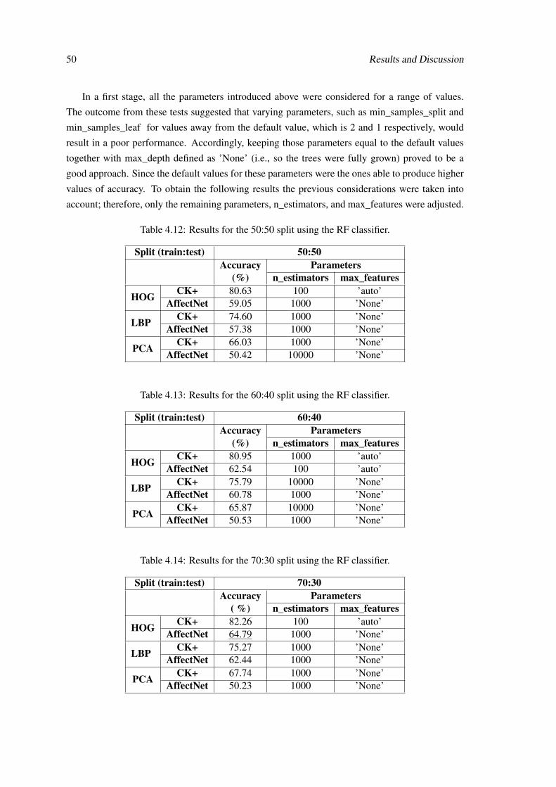
50 Results and Discussion
In a first stage, all the parameters introduced above were considered for a range of values.
The outcome from these tests suggested that varying parameters, such as min_samples_split and
min_samples_leaf for values away from the default value, which is 2 and 1 respectively, would
result in a poor performance. Accordingly, keeping those parameters equal to the default values
together with max_depth defined as ’None’ (i.e., so the trees were fully grown) proved to be a
good approach. Since the default values for these parameters were the ones able to produce higher
values of accuracy. To obtain the following results the previous considerations were taken into
account; therefore, only the remaining parameters, n_estimators, and max_features were adjusted.
Table 4.12: Results for the 50:50 split using the RF classifier.
Split (train:test) 50:50Accuracy
(%)Parameters
n_estimators max_features
HOG CK+ 80.63 100 ’auto’AffectNet 59.05 1000 ’None’
LBP CK+ 74.60 1000 ’None’AffectNet 57.38 1000 ’None’
PCA CK+ 66.03 1000 ’None’AffectNet 50.42 10000 ’None’
Table 4.13: Results for the 60:40 split using the RF classifier.
Split (train:test) 60:40Accuracy
(%)Parameters
n_estimators max_features
HOG CK+ 80.95 1000 ’auto’AffectNet 62.54 100 ’auto’
LBP CK+ 75.79 10000 ’None’AffectNet 60.78 1000 ’None’
PCA CK+ 65.87 10000 ’None’AffectNet 50.53 1000 ’None’
Table 4.14: Results for the 70:30 split using the RF classifier.
Split (train:test) 70:30Accuracy
( %)Parameters
n_estimators max_features
HOG CK+ 82.26 100 ’auto’AffectNet 64.79 1000 ’None’
LBP CK+ 75.27 1000 ’None’AffectNet 62.44 1000 ’None’
PCA CK+ 67.74 1000 ’None’AffectNet 50.23 1000 ’None’
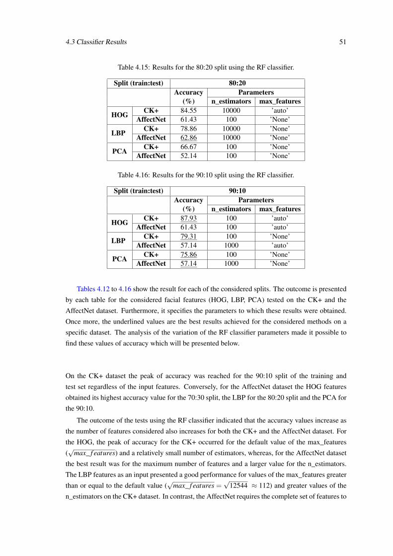
4.3 Classifier Results 51
Table 4.15: Results for the 80:20 split using the RF classifier.
Split (train:test) 80:20Accuracy
(%)Parameters
n_estimators max_features
HOG CK+ 84.55 10000 ’auto’AffectNet 61.43 100 ’None’
LBP CK+ 78.86 10000 ’None’AffectNet 62.86 10000 ’None’
PCA CK+ 66.67 100 ’None’AffectNet 52.14 100 ’None’
Table 4.16: Results for the 90:10 split using the RF classifier.
Split (train:test) 90:10Accuracy
(%)Parameters
n_estimators max_features
HOG CK+ 87.93 100 ’auto’AffectNet 61.43 100 ’auto’
LBP CK+ 79.31 100 ’None’AffectNet 57.14 1000 ’auto’
PCA CK+ 75.86 100 ’None’AffectNet 57.14 1000 ’None’
Tables 4.12 to 4.16 show the result for each of the considered splits. The outcome is presented
by each table for the considered facial features (HOG, LBP, PCA) tested on the CK+ and the
AffectNet dataset. Furthermore, it specifies the parameters to which these results were obtained.
Once more, the underlined values are the best results achieved for the considered methods on a
specific dataset. The analysis of the variation of the RF classifier parameters made it possible to
find these values of accuracy which will be presented below.
On the CK+ dataset the peak of accuracy was reached for the 90:10 split of the training and
test set regardless of the input features. Conversely, for the AffectNet dataset the HOG features
obtained its highest accuracy value for the 70:30 split, the LBP for the 80:20 split and the PCA for
the 90:10.
The outcome of the tests using the RF classifier indicated that the accuracy values increase as
the number of features considered also increases for both the CK+ and the AffectNet dataset. For
the HOG, the peak of accuracy for the CK+ occurred for the default value of the max_features
(√
max_ f eatures) and a relatively small number of estimators, whereas, for the AffectNet dataset
the best result was for the maximum number of features and a larger value for the n_estimators.
The LBP features as an input presented a good performance for values of the max_features greater
than or equal to the default value (√
max_ f eatures =√
12544 ≈ 112) and greater values of the
n_estimators on the CK+ dataset. In contrast, the AffectNet requires the complete set of features to

52 Results and Discussion
achieve its best result. As well as to the HOG, when considering the PCA features the parameters
variation produced approximately the same behaviour regardless of the number of estimators.
Additionally, the peak of accuracy occurred for the the maximum number of features for both
datasets.
4.3.3 Feature Selection Based on MI Results
To implement this approach the previously mentioned machine learning package scikit-learn was
used. The purpose is the estimation of the mutual information for a discrete variable. The obtained
MI’s score represents a positive value, it only takes the value zero when the considered variables
are independent. This algorithm is based on [130, 131].
In the previous sections some results were obtained considering the complete set of features.
What was not very clear was whether all the features were needed or not to achieve those values
of accuracy. Trying to provide an answer this feature selection approach was implemented for the
underlined values in Tables 4.7 to 4.11 and Tables 4.12 to 4.16, using the SVM and RF classifier,
respectively.
The outcome was, for the highest accuracy achieved on this study (the HOG features generated
from the CK+ dataset tested on the SVM) the same accuracy value, 96.55% with only 11000
features, a reduction of almost 50% in the number of the features (21632 to 11000). For the LBP
on the same dataset and classifier, it were necessary only 4000 features from the 12544 complete
set to achieve 96.55% of accuracy. The AffectNet had the same behaviour in this test being able
to reduce the number of features needed to keep the same value of accuracy.
The RF classifier provided an even higher performance since it was able to maintain the accu-
racy values as well as to reduce the number of required features. In this case, the optimal number
of features for the HOG considering the CK+ was 5000 achieving the same accuracy of 87.93%.
For the LBP on the same dataset the updated number of features was 1500 with an accuracy of
79.31%. For the AffectNet, the same number of features generated a slightly inferior value of
accuracy.
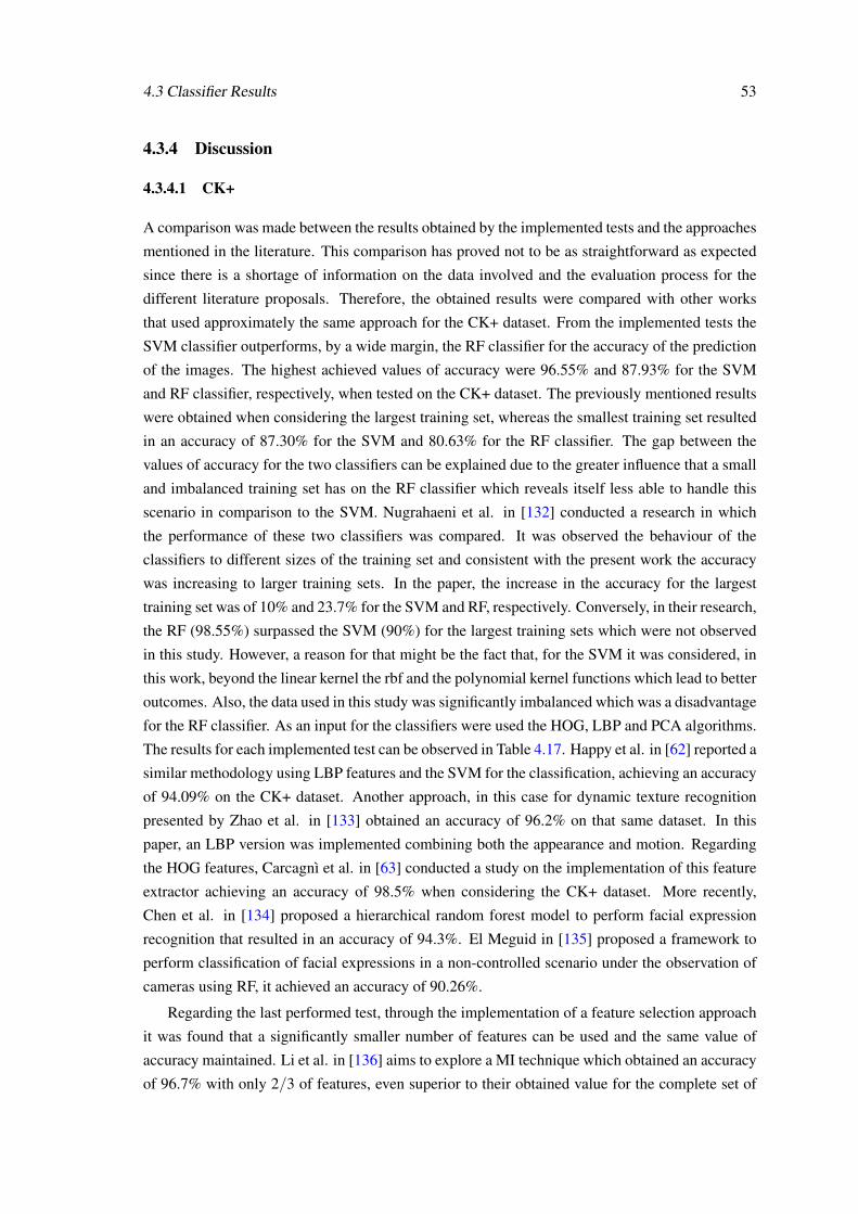
4.3 Classifier Results 53
4.3.4 Discussion
4.3.4.1 CK+
A comparison was made between the results obtained by the implemented tests and the approaches
mentioned in the literature. This comparison has proved not to be as straightforward as expected
since there is a shortage of information on the data involved and the evaluation process for the
different literature proposals. Therefore, the obtained results were compared with other works
that used approximately the same approach for the CK+ dataset. From the implemented tests the
SVM classifier outperforms, by a wide margin, the RF classifier for the accuracy of the prediction
of the images. The highest achieved values of accuracy were 96.55% and 87.93% for the SVM
and RF classifier, respectively, when tested on the CK+ dataset. The previously mentioned results
were obtained when considering the largest training set, whereas the smallest training set resulted
in an accuracy of 87.30% for the SVM and 80.63% for the RF classifier. The gap between the
values of accuracy for the two classifiers can be explained due to the greater influence that a small
and imbalanced training set has on the RF classifier which reveals itself less able to handle this
scenario in comparison to the SVM. Nugrahaeni et al. in [132] conducted a research in which
the performance of these two classifiers was compared. It was observed the behaviour of the
classifiers to different sizes of the training set and consistent with the present work the accuracy
was increasing to larger training sets. In the paper, the increase in the accuracy for the largest
training set was of 10% and 23.7% for the SVM and RF, respectively. Conversely, in their research,
the RF (98.55%) surpassed the SVM (90%) for the largest training sets which were not observed
in this study. However, a reason for that might be the fact that, for the SVM it was considered, in
this work, beyond the linear kernel the rbf and the polynomial kernel functions which lead to better
outcomes. Also, the data used in this study was significantly imbalanced which was a disadvantage
for the RF classifier. As an input for the classifiers were used the HOG, LBP and PCA algorithms.
The results for each implemented test can be observed in Table 4.17. Happy et al. in [62] reported a
similar methodology using LBP features and the SVM for the classification, achieving an accuracy
of 94.09% on the CK+ dataset. Another approach, in this case for dynamic texture recognition
presented by Zhao et al. in [133] obtained an accuracy of 96.2% on that same dataset. In this
paper, an LBP version was implemented combining both the appearance and motion. Regarding
the HOG features, Carcagnì et al. in [63] conducted a study on the implementation of this feature
extractor achieving an accuracy of 98.5% when considering the CK+ dataset. More recently,
Chen et al. in [134] proposed a hierarchical random forest model to perform facial expression
recognition that resulted in an accuracy of 94.3%. El Meguid in [135] proposed a framework to
perform classification of facial expressions in a non-controlled scenario under the observation of
cameras using RF, it achieved an accuracy of 90.26%.
Regarding the last performed test, through the implementation of a feature selection approach
it was found that a significantly smaller number of features can be used and the same value of
accuracy maintained. Li et al. in [136] aims to explore a MI technique which obtained an accuracy
of 96.7% with only 2/3 of features, even superior to their obtained value for the complete set of

54 Results and Discussion
features. Lajevardi et al. in [117] presented a study comparing different approaches to perform
feature selection for an optimal number of features of 4096 and increasing its overall accuracy in
approximately 5%.
Table 4.17: Summary of the best achieved results on the CK+ dataset.
RF SVMHOG 87.93 96.55LBP 79.31 96.55PCA 75.86 93.10
The obtained results in this study represent a good performance of the implemented algo-
rithms. In some cases, these results were outperformed by the literature. However, bearing in
mind that this is an extensively studied topic much has been done to improve the accuracy rate.
For instance, the development of improved versions of the considered algorithms is been used to
obtain considerably better results. Furthermore, in this study, it was considered imbalanced data.
All the facial expressions available on the CK+ dataset: anger (45), disgust (59), fear (25), happi-
ness (69), sadness (28), surprise (83), and contempt (18), plus the neutral (309). For the studied
literature in most of the cases the data was more balanced, and at least, one less facial expression
was considered, this means one less class, which is likely to be translated in an increase of the
accuracy rate.
4.3.4.2 AffectNet
The need to reach out to other scenarios where people were not performing the facial expressions
justified the choice of the AffectNet. The goal was to add an approximation of what would have
been the scenario to test these algorithms in the clinical environment application. Testing on this
dataset has shown some weaknesses at first because it was not feasible to test the complete dataset,
and second, as the methods implemented proved not to be robust enough to achieve accuracy
values close to the ones achieved on the CK+ dataset. The best results for this dataset can be
found below. They follow the same tendency as the CK+ dataset. The SVM surpasses the RF
for all the considered features. Also, the HOG features as an input obtain the highest accuracy
followed by the LBP and at last, the PCA whose performance is the poorest.
Conversely, in [137], a recent paper from Zeng et al., it is addressed the issue of the in-the-wild
datasets, and the example of the AffectNet is given as the annotations bias on this dataset trigger
inconsistent predictions. This means that for different labelled expressions it can be found similar
face images and that is likely to cause the classifier to wrongly predict the expression. In [137],
both the AffectNet and the CK+ were used to perform FER. Having in mind that this result can not
be used to prove the consistency of the obtained results in this study for the adapted AffectNet it is
still interesting to compare the obtained accuracy for both datasets when testing the same method
(an end-to-end trainable network LTNet). Thus, for both the AffectNet (the complete dataset) and
the CK+ dataset the achieved accuracy was 57.31% and 86.64%, respectively. This highlights

4.3 Classifier Results 55
how challenging it is to perform facial expression classification on the AffectNet, an in-the-wild
dataset, which is confirmed by the fact that even for the annotators this was not a straightforward
task as the agreement rate between them was not more than 60.7%.
Table 4.18: Summary of the best achieved results on the AffectNet dataset.
RF SVMHOG 64.79 72.86LBP 62.86 67.61PCA 57.14 60.00

56 Results and Discussion

Chapter 5
Conclusions and Future Work
5.1 Conclusions
Facial Expression Recognition can be seen as a trivial task, however, even humans or experience
annotators have difficulties to assertively identify the expression. The present work focused on the
automatic identification of expressions, by its face images.
The initial step consisted of studying the literature in order to be able to choose the most
adequate methods to perform FER. Once the methods were chosen it was the moment to search
for appropriate and relevant datasets which included both the images of the subjects performing
different expressions and the correspondent annotated labels for the expressions in the categorical
domain. This was the starting point to explore some Computer Vision techniques. One of the
datasets did not provide annotations for the face localization in the image, in this case, a face
detection algorithm had to be applied. Then, it were implemented methods to extract the features
that were able to represent the images in the most accurate way. From those methods, the first two
produced a representation for each image whereas the third one considered the whole training set
to build a model of representation.
Having a good representation for the images as well as the labels, the necessary requirements to
apply the classifiers were fulfilled. Those image faces could be classified in 7 different expressions,
such as happiness, sadness, surprise, fear, disgust, anger, contempt and additionally, the neutral.
Multiple experiments were carried out, testing the previously extracted features so it would be
inspected to which features the best accuracy was achieved.
The best performance was generated by the SVM classifier when applied to the HOG features
with 96.55% of accuracy for the CK+. The exact same approach achieved an accuracy of only
72.86% on the AffectNet dataset. At last, it was also found that for approximately less than 50%
of the total of features these accuracy values could be kept.
The number of expressions considered together with the imbalanced sets did not allow the sys-
tem to perform better. So, it would be expectable to achieve a higher value for the accuracy if fewer
expressions, as well as a more balanced set, would be taken into account for the classification.
57

58 Conclusions and Future Work
In short, the study allowed to draw some conclusions about the behaviour of a recognition
system. Although these approaches achieve good performance on the CK+ dataset, they proved
not to be the most adequate to deal with a dataset as the AffectNet. For that purpose, less conven-
tional approaches would have to be considered, for instance, deep Convolutional Neural Networks,
regarded as a valuable technique that allows learning straight from the images as well as take ad-
vantage of a large number of samples contained on the original AffectNet.
5.2 Future Work
Regarding the framework of this dissertation, the following steps are easy to identify. The creation
of a new dataset would be the first. This new dataset would contain pictures of patients already in a
clinical setting which would allow having as a starting point the subjects in the aimed environment.
Having the most appropriate dataset would help to ensure that the approach was reliably enough
and performed well in such a setting. This was not feasible to accomplish since this is a time-
bounded project and the fact that it would be needed to record sessions with real patients raises
major and complex ethical issues. The process to obtain the required authorizations would be
extensive and it was not guaranteed that would result in a positive response. Also, apart from
obtaining the samples, it would be also required to annotate them. For that, experienced annotators
willing to perform this task would have to be found.
Secondly, as it was mentioned before, primarily deep CNNs would have to be implemented.
In addition, the latest approaches and methods would have to start being explored. Again, the
time constraint, as well as the computational availability, have not made it possible to study and
introduce less conventional approaches.
At last, the final goal would be the application in the field and, in the case of wanting to pro-
vide the professionals with immediate feedback from the patient expressions a real-time approach
would be desired. The previous steps would presumably promote this step as this would be a
natural step forward.
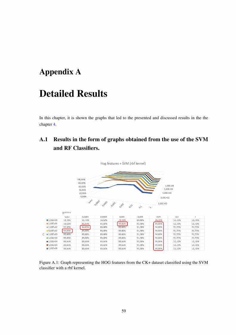
Appendix A
Detailed Results
In this chapter, it is shown the graphs that led to the presented and discussed results in the the
chapter 4.
A.1 Results in the form of graphs obtained from the use of the SVMand RF Classifiers.
Figure A.1: Graph representing the HOG features from the CK+ dataset classified using the SVMclassifier with a rbf kernel.
59

60 Detailed Results
Figure A.2: Graph representing the HOG features from the CK+ dataset classified using the SVMclassifier with a polynomial kernel (degree equal to 1).
Figure A.3: Graph representing the HOG features from the CK+ dataset classified using the SVMclassifier with a polynomial kernel (degree equal to 2).
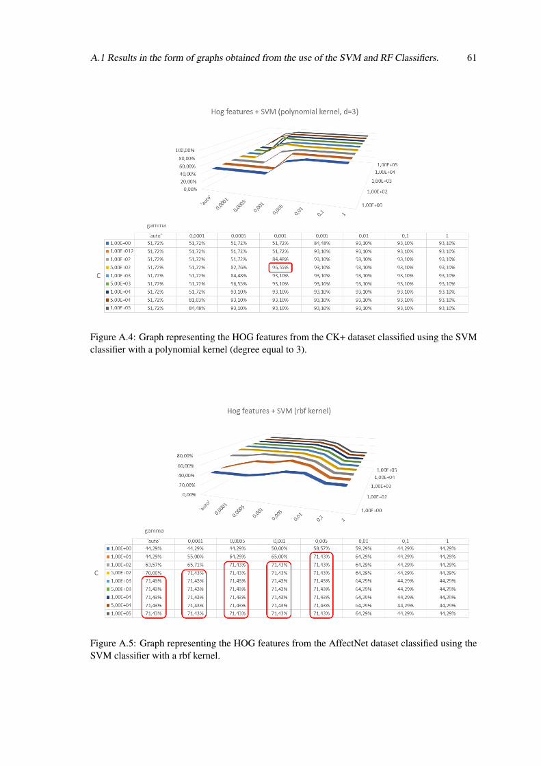
A.1 Results in the form of graphs obtained from the use of the SVM and RF Classifiers. 61
Figure A.4: Graph representing the HOG features from the CK+ dataset classified using the SVMclassifier with a polynomial kernel (degree equal to 3).
Figure A.5: Graph representing the HOG features from the AffectNet dataset classified using theSVM classifier with a rbf kernel.

62 Detailed Results
Figure A.6: Graph representing the HOG features from the AffectNet dataset classified using theSVM classifier with a polynomial kernel (degree equal to 1).
Figure A.7: Graph representing the HOG features from the AffectNet dataset classified using theSVM classifier with a polynomial kernel (degree equal to 2).

A.1 Results in the form of graphs obtained from the use of the SVM and RF Classifiers. 63
Figure A.8: Graph representing the HOG features from the AffectNet dataset classified using theSVM classifier with a polynomial kernel (degree equal to 3).
Figure A.9: Graph representing the LBP features from the CK+ dataset classified using the SVMclassifier with a rbf kernel.

64 Detailed Results
Figure A.10: Graph representing the LBP features from the CK+ dataset classified using the SVMclassifier with a polynomial kernel (degree equal to 1).
Figure A.11: Graph representing the LBP features from the CK+ dataset classified using the SVMclassifier with a polynomial kernel (degree equal to 2).

A.1 Results in the form of graphs obtained from the use of the SVM and RF Classifiers. 65
Figure A.12: Graph representing the LBP features from the CK+ dataset classified using the SVMclassifier with a polynomial kernel (degree equal to 3).
Figure A.13: Graph representing the LBP features from the AffectNet dataset classified using theSVM classifier with a rbf kernel.

66 Detailed Results
Figure A.14: Graph representing the LBP features from the AffectNet dataset classified using theSVM classifier with a polynomial kernel (degree equal to 1).
Figure A.15: Graph representing the LBP features from the AffectNet dataset classified using theSVM classifier with a polynomial kernel (degree equal to 2).
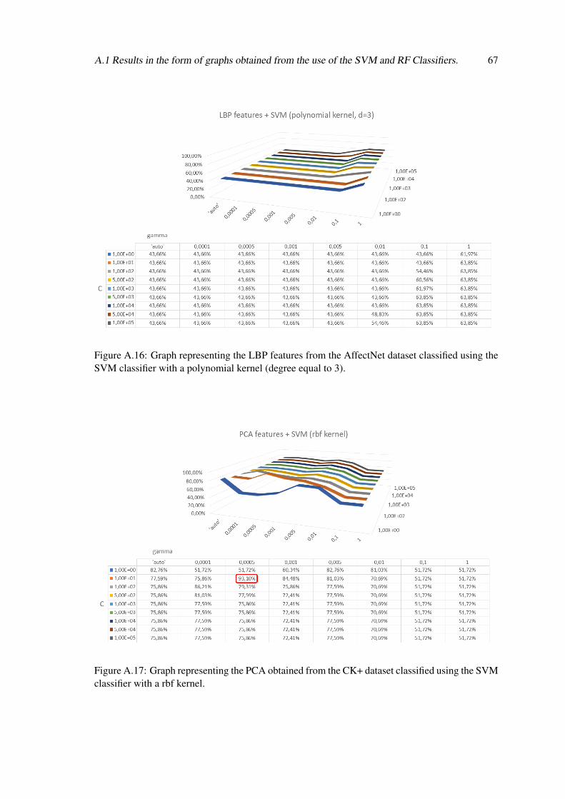
A.1 Results in the form of graphs obtained from the use of the SVM and RF Classifiers. 67
Figure A.16: Graph representing the LBP features from the AffectNet dataset classified using theSVM classifier with a polynomial kernel (degree equal to 3).
Figure A.17: Graph representing the PCA obtained from the CK+ dataset classified using the SVMclassifier with a rbf kernel.

68 Detailed Results
Figure A.18: Graph representing the PCA obtained from the CK+ dataset classified using the SVMclassifier with a polynomial kernel (degree equal to 1).
Figure A.19: Graph representing the PCA obtained from the CK+ dataset classified using the SVMclassifier with a polynomial kernel (degree equal to 2).

A.1 Results in the form of graphs obtained from the use of the SVM and RF Classifiers. 69
Figure A.20: Graph representing the PCA obtained from the CK+ dataset classified using the SVMclassifier with a polynomial kernel (degree equal to 3).
Figure A.21: Graph representing the PCA obtained from the AffectNet dataset classified using theSVM classifier with a rbf kernel.
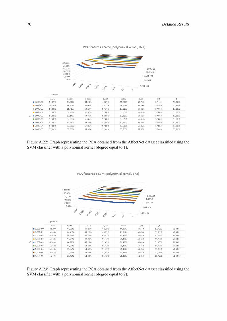
70 Detailed Results
Figure A.22: Graph representing the PCA obtained from the AffectNet dataset classified using theSVM classifier with a polynomial kernel (degree equal to 1).
Figure A.23: Graph representing the PCA obtained from the AffectNet dataset classified using theSVM classifier with a polynomial kernel (degree equal to 2).

A.1 Results in the form of graphs obtained from the use of the SVM and RF Classifiers. 71
Figure A.24: Graph representing the PCA obtained from the AffectNet classified using the SVMclassifier with a polynomial kernel (degree equal to 3).
Figure A.25: Graph representing the HOG features from the CK+ dataset classified using the RFclassifier.

72 Detailed Results
Figure A.26: Graph representing the HOG features from the AffectNet dataset classified using theRF classifier.
Figure A.27: Graph representing the LBP features from the CK+ dataset classified using the RFclassifier.

A.1 Results in the form of graphs obtained from the use of the SVM and RF Classifiers. 73
Figure A.28: Graph representing the LBP features from the AffectNet dataset classified using theRF classifier.
Figure A.29: Graph representing the PCA obtained from the CK+ dataset classified using the RFclassifier.

74 Detailed Results
Figure A.30: Graph representing the PCA obtained from the AffectNet dataset classified using theRF classifier.

References
[1] DCMA. Diagram body of anatomy. URL: https://anatomybodydiagram.com [lastaccessed 19.01.2019].
[2] Ciprian Adrian Corneanu, Marc Oliu Simón, Jeffrey F Cohn, and Sergio Escalera Guerrero.Survey on rgb, 3d, thermal, and multimodal approaches for facial expression recognition:History, trends, and affect-related applications. IEEE transactions on pattern analysis andmachine intelligence, 38(8):1548–1568, 2016.
[3] Y-I Tian, Takeo Kanade, and Jeffrey F Cohn. Recognizing action units for facial expressionanalysis. IEEE Transactions on pattern analysis and machine intelligence, 23(2):97–115,2001.
[4] C. A. Corneanu, M. O. Simon, J. F. Cohn, and S. E. Guerrero. Survey on rgb, 3d, ther-mal, and multimodal approaches for facial expression recognition: History, trends, andaffect-related applications. IEEE Transactions on Pattern Analysis Machine Intelligence,38(8):1548–1568, Aug. 2016. URL: doi.ieeecomputersociety.org/10.1109/TPAMI.2016.2515606, doi:10.1109/TPAMI.2016.2515606.
[5] Mario Rojas, David Masip, Alexander Todorov, and Jordi Vitria. Automatic prediction offacial trait judgments: Appearance vs. structural models. PloS one, 6(8):e23323, 2011.
[6] Matti Pietikäinen, Abdenour Hadid, Guoying Zhao, and Timo Ahonen. Local binarypatterns for still images. In Computer vision using local binary patterns, pages 13–47.Springer, 2011.
[7] OpenCV. Face recognition with opencv. URL: https://docs.opencv.org/2.4/modules/contrib/doc/facerec/facerec_tutorial.html [last accessed07.01.2019].
[8] Paul Viola and Michael Jones. Rapid object detection using a boosted cascade of simplefeatures. In Computer Vision and Pattern Recognition, 2001. CVPR 2001. Proceedings ofthe 2001 IEEE Computer Society Conference on, volume 1, pages I–I. IEEE, 2001.
[9] Derek Bradley and Gerhard Roth. Adaptive thresholding using the integral image. Journalof graphics tools, 12(2):13–21, 2007.
[10] Alfred V Aho and John E Hopcroft. The design and analysis of computer algorithms.Pearson Education India, 1974.
[11] Patrick Lucey, Jeffrey F Cohn, Takeo Kanade, Jason Saragih, Zara Ambadar, and IainMatthews. The extended cohn-kanade dataset (ck+): A complete dataset for action unitand emotion-specified expression. In Computer Vision and Pattern Recognition Workshops(CVPRW), 2010 IEEE Computer Society Conference on, pages 94–101. IEEE, 2010.
75

76 REFERENCES
[12] C Anitha, MK Venkatesha, and B Suryanarayana Adiga. A survey on facial expressiondatabases. International Journal of Engineering Science and Technology, 2(10):5158–5174,2010.
[13] Ali Mollahosseini, Behzad Hasani, and Mohammad H Mahoor. Affectnet: A databasefor facial expression, valence, and arousal computing in the wild. arXiv preprintarXiv:1708.03985, 2017.
[14] Evangelos Sariyanidi, Hatice Gunes, and Andrea Cavallaro. Automatic analysis of facialaffect: A survey of registration, representation, and recognition. IEEE transactions onpattern analysis and machine intelligence, 37(6):1113–1133, 2015.
[15] World Cancer Research Fund International. World cancer research fund.URL: https://www.wcrf.org/dietandcancer/cancer-trends/breast-cancer-statistics [last accessed 21.01.2019].
[16] Kenneth M Prkachin. Assessing pain by facial expression: facial expression as nexus. PainResearch and Management, 14(1):53–58, 2009.
[17] Paul Ekman and Harriet Oster. Facial expressions of emotion. Annual review of psychology,30(1):527–554, 1979.
[18] Philipp Michel. Support vector machines in automated emotion classification. ChurchillCollege, June, 2003.
[19] P Ekman. Basic emotions, handbook of cognition and emotion (pp. 45±60), 1999.
[20] Daniel Piepers and Rachel Robbins. A review and clarification of the terms “holis-tic,”“configural,” and “relational” in the face perception literature. Frontiers in psychology,3:559, 2012.
[21] Karsten Wolf. Measuring facial expression of emotion. Dialogues in clinical neuroscience,17(4):457, 2015.
[22] H Davies, I Wolz, J Leppanen, F Fernandez-Aranda, U Schmidt, and K Tchanturia. Facialexpression to emotional stimuli in non-psychotic disorders: A systematic review and meta-analysis. Neuroscience & Biobehavioral Reviews, 64:252–271, 2016.
[23] Ying Jiang. Measuring facial expression and emotional experience under diverse socialcontext in a negative emotional setting. Measuring Behavior 2014, 2014.
[24] Carl-Herman Hjortsjö. Man’s face and mimic language. Studen litteratur, 1969.
[25] E Friesen and P Ekman. Facial action coding system: a technique for the measurement offacial movement. Palo Alto, 1978.
[26] P EKMAN-WV FRIESEN-JC HAGER. Facial action coding system. the manual on cdrom, 2002.
[27] Ying-li Tian, Takeo Kanade, and Jeffrey F Cohn. Recognizing lower face action units forfacial expression analysis. In Automatic face and gesture recognition, 2000. proceedings.fourth ieee international conference on, pages 484–490. IEEE, 2000.
[28] Shichuan Du and Aleix M Martinez. Compound facial expressions of emotion: from basicresearch to clinical applications. Dialogues in clinical neuroscience, 17(4):443, 2015.

REFERENCES 77
[29] Michael A Sayette, Jeffrey F Cohn, Joan M Wertz, Michael A Perrott, and Dominic J Par-rott. A psychometric evaluation of the facial action coding system for assessing spontaneousexpression. Journal of Nonverbal Behavior, 25(3):167–185, 2001.
[30] Paul Ekman and Erika L Rosenberg. What the face reveals: Basic and applied studies ofspontaneous expression using the Facial Action Coding System (FACS). Oxford UniversityPress, USA, 1997.
[31] Zoran Duric, Wayne D Gray, Ric Heishman, Fayin Li, Azriel Rosenfeld, Michael JSchoelles, Christian Schunn, and Harry Wechsler. Integrating perceptual and cognitivemodeling for adaptive and intelligent human-computer interaction. Proceedings of theIEEE, 90(7):1272–1289, 2002.
[32] Hiroshi Ishiguro, Tetsuo Ono, Michita Imai, Takeshi Maeda, Takayuki Kanda, and RyoheiNakatsu. Robovie: an interactive humanoid robot. Industrial robot: An international jour-nal, 28(6):498–504, 2001.
[33] Patrick Lucey, Jeffrey F Cohn, Iain Matthews, Simon Lucey, Sridha Sridharan, JessicaHowlett, and Kenneth M Prkachin. Automatically detecting pain in video through facialaction units. IEEE Transactions on Systems, Man, and Cybernetics, Part B (Cybernetics),41(3):664–674, 2011.
[34] Sebastian Kaltwang, Ognjen Rudovic, and Maja Pantic. Continuous pain intensity esti-mation from facial expressions. In International Symposium on Visual Computing, pages368–377. Springer, 2012.
[35] Esra Vural, Müjdat Çetin, Aytül Erçil, Gwen Littlewort, Marian Bartlett, and Javier Movel-lan. Automated drowsiness detection for improved driving safety. 2008.
[36] Ashok Samal and Prasana A Iyengar. Automatic recognition and analysis of human facesand facial expressions: A survey. Pattern recognition, 25(1):65–77, 1992.
[37] Maja Pantic and Leon J. M. Rothkrantz. Automatic analysis of facial expressions: The stateof the art. IEEE Transactions on pattern analysis and machine intelligence, 22(12):1424–1445, 2000.
[38] Beat Fasel and Juergen Luettin. Automatic facial expression analysis: a survey. Patternrecognition, 36(1):259–275, 2003.
[39] Masakazu Matsugu, Katsuhiko Mori, Yusuke Mitari, and Yuji Kaneda. Subject indepen-dent facial expression recognition with robust face detection using a convolutional neuralnetwork. Neural Networks, 16(5-6):555–559, 2003.
[40] Motoi Suwa. A preliminary note on pattern recognition of human emotional expression.In Proc. of The 4th International Joint Conference on Pattern Recognition, pages 408–410,1978.
[41] Zhihong Zeng, Maja Pantic, Glenn I Roisman, and Thomas S Huang. A survey of affectrecognition methods: Audio, visual, and spontaneous expressions. IEEE transactions onpattern analysis and machine intelligence, 31(1):39–58, 2009.
[42] Dhwani Mehta, Mohammad Faridul Haque Siddiqui, and Ahmad Y Javaid. Facial emotionrecognition: A survey and real-world user experiences in mixed reality. Sensors, 18(2):416,2018.

78 REFERENCES
[43] Proyecto Fin De Carrera and Ion Marques. Face recognition algorithms. Master’s thesis inComputer Science, Universidad Euskal Herriko, 2010.
[44] Richard E Bellman. Adaptive control processes: a guided tour, volume 2045. Princetonuniversity press, 2015.
[45] Jundong Li, Kewei Cheng, Suhang Wang, Fred Morstatter, Robert P Trevino, Jiliang Tang,and Huan Liu. Feature selection: A data perspective. ACM Computing Surveys (CSUR),50(6):94, 2018.
[46] S Dhall and P Sethi. Geometric and appearance feature analysis for facial expression recog-nition. International Journal of Advanced Engineering Technology, 7(111):01–11, 2014.
[47] Girish Chandrashekar and Ferat Sahin. A survey on feature selection methods. Computers& Electrical Engineering, 40(1):16–28, 2014.
[48] Ron Kohavi and George H John. Wrappers for feature subset selection. Artificial intelli-gence, 97(1-2):273–324, 1997.
[49] Isabelle Guyon and André Elisseeff. An introduction to variable and feature selection.Journal of machine learning research, 3(Mar):1157–1182, 2003.
[50] George Forman. An extensive empirical study of feature selection metrics for text classifi-cation. Journal of machine learning research, 3(Mar):1289–1305, 2003.
[51] Marko Robnik-Šikonja and Igor Kononenko. Theoretical and empirical analysis of relieffand rrelieff. Machine learning, 53(1-2):23–69, 2003.
[52] Quanquan Gu, Zhenhui Li, and Jiawei Han. Generalized fisher score for feature selection.arXiv preprint arXiv:1202.3725, 2012.
[53] Hanchuan Peng, Fuhui Long, and Chris Ding. Feature selection based on mutual informa-tion criteria of max-dependency, max-relevance, and min-redundancy. IEEE Transactionson pattern analysis and machine intelligence, 27(8):1226–1238, 2005.
[54] Jiliang Tang, Salem Alelyani, and Huan Liu. Feature selection for classification: A review.Data classification: Algorithms and applications, page 37, 2014.
[55] Robert Tibshirani. Regression shrinkage and selection via the lasso. Journal of the RoyalStatistical Society. Series B (Methodological), pages 267–288, 1996.
[56] Hui Zou and Trevor Hastie. Regularization and variable selection via the elastic net. Journalof the Royal Statistical Society: Series B (Statistical Methodology), 67(2):301–320, 2005.
[57] Aleix Martinez and Shichuan Du. A model of the perception of facial expressions of emo-tion by humans: Research overview and perspectives. Journal of Machine Learning Re-search, 13(May):1589–1608, 2012.
[58] Zhengyou Zhang, Michael Lyons, Michael Schuster, and Shigeru Akamatsu. Compari-son between geometry-based and gabor-wavelets-based facial expression recognition usingmulti-layer perceptron. In Automatic Face and Gesture Recognition, 1998. Proceedings.Third IEEE International Conference on, pages 454–459. IEEE, 1998.

REFERENCES 79
[59] Karan Sikka, Abhinav Dhall, and Marian Bartlett. Exemplar hidden markov models forclassification of facial expressions in videos. In Proceedings of the IEEE Conference onComputer Vision and Pattern Recognition Workshops, pages 18–25, 2015.
[60] S Mahto and Y Yadav. A survey on various facial expression recognition techniques. Int.J. Adv. Res. Electr., Electron. Instrum. Eng, 3:13028–13031, 2014.
[61] Alka Gupta and ML Garg. A human emotion recognition system using supervised self-organising maps. In Computing for Sustainable Global Development (INDIACom), 2014International Conference on, pages 654–659. IEEE, 2014.
[62] SL Happy and Aurobinda Routray. Automatic facial expression recognition using featuresof salient facial patches. IEEE transactions on Affective Computing, 6(1):1–12, 2015.
[63] Pierluigi Carcagnì, Marco Del Coco, Marco Leo, and Cosimo Distante. Facial expressionrecognition and histograms of oriented gradients: a comprehensive study. SpringerPlus,4(1):645, 2015.
[64] Caifeng Shan, Shaogang Gong, and Peter W McOwan. Facial expression recognition basedon local binary patterns: A comprehensive study. Image and vision Computing, 27(6):803–816, 2009.
[65] Ju Jia, Yan Xu, Sida Zhang, and Xianglong Xue. The facial expression recognition methodof random forest based on improved pca extracting feature. In Signal Processing, Commu-nications and Computing (ICSPCC), 2016 IEEE International Conference on, pages 1–5.IEEE, 2016.
[66] Michel F Valstar, Bihan Jiang, Marc Mehu, Maja Pantic, and Klaus Scherer. The first facialexpression recognition and analysis challenge. In Automatic Face & Gesture Recognitionand Workshops (FG 2011), 2011 IEEE International Conference on, pages 921–926. IEEE,2011.
[67] Tanja Bänziger and Klaus R Scherer. Introducing the geneva multimodal emotion portrayal(gemep) corpus. Blueprint for affective computing: A sourcebook, pages 271–294, 2010.
[68] Michel F Valstar, Timur Almaev, Jeffrey M Girard, Gary McKeown, Marc Mehu, LijunYin, Maja Pantic, and Jeffrey F Cohn. Fera 2015-second facial expression recognition andanalysis challenge. In Automatic Face and Gesture Recognition (FG), 2015 11th IEEEInternational Conference and Workshops on, volume 6, pages 1–8. IEEE, 2015.
[69] Xing Zhang, Lijun Yin, Jeffrey F Cohn, Shaun Canavan, Michael Reale, Andy Horowitz,Peng Liu, and Jeffrey M Girard. Bp4d-spontaneous: a high-resolution spontaneous 3ddynamic facial expression database. Image and Vision Computing, 32(10):692–706, 2014.
[70] Gary McKeown, Michel Valstar, Roddy Cowie, Maja Pantic, and Marc Schroder. Thesemaine database: Annotated multimodal records of emotionally colored conversations be-tween a person and a limited agent. IEEE Transactions on Affective Computing, 3(1):5–17,2012.
[71] Wenchao Zhang, Shiguang Shan, Wen Gao, Xilin Chen, and Hongming Zhang. Local gaborbinary pattern histogram sequence (lgbphs): a novel non-statistical model for face represen-tation and recognition. In Computer Vision, 2005. ICCV 2005. Tenth IEEE InternationalConference on, volume 1, pages 786–791. IEEE, 2005.

80 REFERENCES
[72] Xuehan Xiong and Fernando De la Torre. Supervised descent method and its applicationsto face alignment. In Proceedings of the IEEE conference on computer vision and patternrecognition, pages 532–539, 2013.
[73] Michel F Valstar, Enrique Sánchez-Lozano, Jeffrey F Cohn, László A Jeni, Jeffrey M Gi-rard, Zheng Zhang, Lijun Yin, and Maja Pantic. Fera 2017-addressing head pose in the thirdfacial expression recognition and analysis challenge. In Automatic Face & Gesture Recog-nition (FG 2017), 2017 12th IEEE International Conference on, pages 839–847. IEEE,2017.
[74] Enrique Sánchez-Lozano, Brais Martinez, Georgios Tzimiropoulos, and Michel Valstar.Cascaded continuous regression for real-time incremental face tracking. In European Con-ference on Computer Vision, pages 645–661. Springer, 2016.
[75] John Lafferty, Andrew McCallum, and Fernando CN Pereira. Conditional random fields:Probabilistic models for segmenting and labeling sequence data. 2001.
[76] Minyoung Kim and Vladimir Pavlovic. Structured output ordinal regression for dynamicfacial emotion intensity prediction. In European conference on computer vision, pages649–662. Springer, 2010.
[77] Navneet Dalal and Bill Triggs. Histograms of oriented gradients for human detection. InComputer Vision and Pattern Recognition, 2005. CVPR 2005. IEEE Computer Society Con-ference on, volume 1, pages 886–893. IEEE, 2005.
[78] Timo Ojala, Matti Pietikäinen, and David Harwood. A comparative study of texture mea-sures with classification based on featured distributions. Pattern recognition, 29(1):51–59,1996.
[79] David G Lowe. Object recognition from local scale-invariant features. In Computer vision,1999. The proceedings of the seventh IEEE international conference on, volume 2, pages1150–1157. Ieee, 1999.
[80] David G Lowe. Distinctive image features from scale-invariant keypoints. Internationaljournal of computer vision, 60(2):91–110, 2004.
[81] Karl Pearson. Liii. on lines and planes of closest fit to systems of points in space. The Lon-don, Edinburgh, and Dublin Philosophical Magazine and Journal of Science, 2(11):559–572, 1901.
[82] Pablo Navarrete and Javier Ruiz-del Solar. Comparative study between differenteigenspace-based approaches for face recognition. In AFSS International Conference onFuzzy Systems, pages 178–184. Springer, 2002.
[83] Lindsay I Smith. A tutorial on principal components analysis. Technical report, 2002.
[84] Marian Stewart Bartlett, Javier R Movellan, and Terrence J Sejnowski. Face recognition byindependent component analysis. IEEE transactions on neural networks/a publication ofthe IEEE Neural Networks Council, 13(6):1450, 2002.
[85] Dulal Chakraborty, Sanjit Kumar Saha, and Md Al-Amin Bhuiyan. Face recognition usingeigenvector and principle component analysis. International Journal of Computer Applica-tions, 50(10), 2012.

REFERENCES 81
[86] Zhihong Zhang and Edwin R Hancock. Mutual information criteria for feature selection. InInternational Workshop on Similarity-Based Pattern Recognition, pages 235–249. Springer,2011.
[87] Valeria Fonti and Eduard Belitser. Feature selection using lasso. VU Amsterdam ResearchPaper in Business Analytics, 2017.
[88] Michael J Jones and Paul Viola. Robust real-time object detection. In Workshop on statis-tical and computational theories of vision, volume 266, page 56, 2001.
[89] Cha Zhang and Zhengyou Zhang. A survey of recent advances in face detection. 2010.
[90] Yoav Freund and Robert E Schapire. A decision-theoretic generalization of on-line learningand an application to boosting. Journal of computer and system sciences, 55(1):119–139,1997.
[91] Corinna Cortes and Vladimir Vapnik. Support-vector networks. Machine learning,20(3):273–297, 1995.
[92] Edgar Osuna, Robert Freund, and Federico Girosit. Training support vector machines: anapplication to face detection. In Computer vision and pattern recognition, 1997. Proceed-ings., 1997 IEEE computer society conference on, pages 130–136. IEEE, 1997.
[93] Bernd Heisele, Massimilinao Pontil, et al. Face detection in still gray images. Technicalreport, MASSACHUSETTS INST OF TECH CAMBRIDGE MA CENTER FOR BIO-LOGICAL AND . . . , 2000.
[94] Lior Rokach and Oded Maimon. Decision trees. In Data mining and knowledge discoveryhandbook, pages 165–192. Springer, 2005.
[95] J. Ross Quinlan. Induction of decision trees. Machine learning, 1(1):81–106, 1986.
[96] Tin Kam Ho. Random decision forests. In Document analysis and recognition, 1995.,proceedings of the third international conference on, volume 1, pages 278–282. IEEE, 1995.
[97] D Richard Cutler, Thomas C Edwards Jr, Karen H Beard, Adele Cutler, Kyle T Hess, Ja-cob Gibson, and Joshua J Lawler. Random forests for classification in ecology. Ecology,88(11):2783–2792, 2007.
[98] Leo Breiman. Bagging predictors. Machine learning, 24(2):123–140, 1996.
[99] Leo Breiman. Random forests. Machine learning, 45(1):5–32, 2001.
[100] Michael J Lyons, Shigeru Akamatsu, Miyuki Kamachi, Jiro Gyoba, and Julien Budynek.The japanese female facial expression (jaffe) database. In Proceedings of third internationalconference on automatic face and gesture recognition, pages 14–16, 1998.
[101] Takeo Kanade, Yingli Tian, and Jeffrey F Cohn. Comprehensive database for facial expres-sion analysis. In fg, page 46. IEEE, 2000.
[102] Maja Pantic, Michel Valstar, Ron Rademaker, and Ludo Maat. Web-based database forfacial expression analysis. In 2005 IEEE international conference on multimedia and Expo,page 5. IEEE, 2005.

82 REFERENCES
[103] Li-Fen Chen and Yu-Shiuan Yen. Taiwanese facial expression image database. Brain Map-ping Laboratory, Institute of Brain Science, National Yang-Ming University, Taipei, Taiwan,2007.
[104] Niki Aifanti, Christos Papachristou, and Anastasios Delopoulos. The mug facial expres-sion database. In Image analysis for multimedia interactive services (WIAMIS), 2010 11thinternational workshop on, pages 1–4. IEEE, 2010.
[105] Abhinav Dhall, Roland Goecke, Simon Lucey, Tom Gedeon, et al. Collecting large, richlyannotated facial-expression databases from movies. IEEE multimedia, 19(3):34–41, 2012.
[106] Ian J Goodfellow, Dumitru Erhan, Pierre Luc Carrier, Aaron Courville, Mehdi Mirza, BenHamner, Will Cukierski, Yichuan Tang, David Thaler, Dong-Hyun Lee, et al. Challengesin representation learning: A report on three machine learning contests. In InternationalConference on Neural Information Processing, pages 117–124. Springer, 2013.
[107] Lijun Yin, Xiaozhou Wei, Yi Sun, Jun Wang, and Matthew J Rosato. A 3d facial expressiondatabase for facial behavior research. In Automatic face and gesture recognition, 2006.FGR 2006. 7th international conference on, pages 211–216. IEEE, 2006.
[108] Arman Savran, Nese Alyüz, Hamdi Dibeklioglu, Oya Çeliktutan, Berk Gökberk, BülentSankur, and Lale Akarun. Bosphorus database for 3d face analysis. In European Workshopon Biometrics and Identity Management, pages 47–56. Springer, 2008.
[109] Lijun Yin, Xiaochen Chen, Yi Sun, Tony Worm, and Michael Reale. A high-resolution3d dynamic facial expression database. In Automatic Face & Gesture Recognition, 2008.FG’08. 8th IEEE International Conference on, pages 1–6. IEEE, 2008.
[110] James W Davis and Mark A Keck. A two-stage template approach to person detection inthermal imagery. In Application of Computer Vision, 2005. WACV/MOTIONS’05 Volume1. Seventh IEEE Workshops on, volume 1, pages 364–369. IEEE, 2005.
[111] Alexander Kramida, Yuri Ralchenko, Joseph Reader, et al. Nist atomic spectra database(ver. 5.2), 2015.
[112] Shangfei Wang, Zhilei Liu, Siliang Lv, Yanpeng Lv, Guobing Wu, Peng Peng, Fei Chen, andXufa Wang. A natural visible and infrared facial expression database for expression recog-nition and emotion inference. IEEE Transactions on Multimedia, 12(7):682–691, 2010.
[113] Hung Nguyen, Kazunori Kotani, Fan Chen, and Bac Le. A thermal facial emotion databaseand its analysis. In Pacific-Rim Symposium on Image and Video Technology, pages 397–408. Springer, 2013.
[114] Albert Ali Salah, Nicu Sebe, and Theo Gevers. Communication and automatic interpreta-tion of affect from facial expressions. In Affective Computing and Interaction: Psychologi-cal, Cognitive and Neuroscientific Perspectives, pages 157–183. IGI Global, 2011.
[115] Aliaa AA Youssif and Wesam AA Asker. Automatic facial expression recognition systembased on geometric and appearance features. Computer and Information Science, 4(2):115,2011.
[116] Roberto Battiti. Using mutual information for selecting features in supervised neural netlearning. IEEE Transactions on neural networks, 5(4):537–550, 1994.

REFERENCES 83
[117] Seyed Mehdi Lajevardi and Zahir M Hussain. Feature selection for facial expression recog-nition based on mutual information. In GCC Conference & Exhibition, 2009 5th IEEE,pages 1–5. IEEE, 2009.
[118] Shaoqing Ren, Xudong Cao, Yichen Wei, and Jian Sun. Face alignment at 3000 fps viaregressing local binary features. In Proceedings of the IEEE Conference on ComputerVision and Pattern Recognition, pages 1685–1692, 2014.
[119] Microsoft. Serviços cognitivos. URL: https://azure.microsoft.com/pt-pt/services/cognitive-services/ [last accessed 05.01.2019].
[120] Danielle Mathersul, Leanne M Williams, Patrick J Hopkinson, and Andrew H Kemp. In-vestigating models of affect: Relationships among eeg alpha asymmetry, depression, andanxiety. Emotion, 8(4):560, 2008.
[121] Lisa Feldman Barrett. Discrete emotions or dimensions? the role of valence focus andarousal focus. Cognition & Emotion, 12(4):579–599, 1998.
[122] James A Russell. A circumplex model of affect. Journal of personality and social psychol-ogy, 39(6):1161, 1980.
[123] Georgios Paltoglou and Michael Thelwall. Seeing stars of valence and arousal in blog posts.IEEE Transactions on Affective Computing, 4(1):116–123, 2013.
[124] Ron Artstein. Inter-annotator agreement. In Handbook of linguistic annotation, pages 297–313. Springer, 2017.
[125] Matthew B Blaschko and Christoph H Lampert. Learning to localize objects with structuredoutput regression. In European conference on computer vision, pages 2–15. Springer, 2008.
[126] Mark Everingham, Luc Van Gool, Christopher KI Williams, John Winn, and Andrew Zis-serman. The pascal visual object classes (voc) challenge. International journal of computervision, 88(2):303–338, 2010.
[127] F. Pedregosa, G. Varoquaux, A. Gramfort, V. Michel, B. Thirion, O. Grisel, M. Blon-del, P. Prettenhofer, R. Weiss, V. Dubourg, J. Vanderplas, A. Passos, D. Cournapeau,M. Brucher, M. Perrot, and E. Duchesnay. Scikit-learn: Machine learning in Python. Jour-nal of Machine Learning Research, 12:2825–2830, 2011.
[128] Chih-Chung Chang and Chih-Jen Lin. Libsvm: a library for support vector machines. ACMtransactions on intelligent systems and technology (TIST), 2(3):27, 2011.
[129] Scikit learn developers. sklearn.ensemble.randomforestclassifier. URL: https://scikit-learn.org/stable/modules/generated/sklearn.ensemble.RandomForestClassifier.html [last accessed 14.01.2019].
[130] Alexander Kraskov, Harald Stögbauer, and Peter Grassberger. Estimating mutual informa-tion. Physical review E, 69(6):066138, 2004.
[131] Brian C Ross. Mutual information between discrete and continuous data sets. PloS one,9(2):e87357, 2014.

84 REFERENCES
[132] Ratna Astuti Nugrahaeni and Kusprasapta Mutijarsa. Comparative analysis of machinelearning knn, svm, and random forests algorithm for facial expression classification. InTechnology of Information and Communication (ISemantic), International Seminar on Ap-plication for, pages 163–168. IEEE, 2016.
[133] Guoying Zhao and Matti Pietikainen. Dynamic texture recognition using local binary pat-terns with an application to facial expressions. IEEE transactions on pattern analysis andmachine intelligence, 29(6):915–928, 2007.
[134] Jingying Chen, Mulan Zhang, Xianglong Xue, Ruyi Xu, and Kun Zhang. An action unitbased hierarchical random forest model to facial expression recognition. pages 753–760,01 2017. doi:10.5220/0006274707530760.
[135] Mostafa K Abd El Meguid and Martin D Levine. Fully automated recognition of sponta-neous facial expressions in videos using random forest classifiers. IEEE Transactions onAffective Computing, 5(2):141–154, 2014.
[136] Peiyao Li, Son Lam Phung, A Bouzerdom, and Fok Hing Chi Tivive. Feature selectionfor facial expression recognition. In Visual Information Processing (EUVIP), 2010 2ndEuropean Workshop on, pages 35–40. IEEE, 2010.
[137] Jiabei Zeng, Shiguang Shan, and Xilin Chen. Facial expression recognition with inconsis-tently annotated datasets. In Proceedings of the European conference on computer vision(ECCV), pages 222–237, 2018.
Copyright © 2022 FDOKUMEN