Slowly oscillating periodic solutions of autonomous state-dependent delay equations

Nonlrneor Ana/.vs~r, Theory. Methods & Applicafrons. Vol. 19. No. 9, pp. X55-872. 1992. 0362-546X192 $5 00+ .OO

Printed in Great Britam. c) 1992 Pergamon Press Lfd

SLOWLY OSCILLATING PERIODIC SOLUTIONS OF AUTONOMOUS STATE-DEPENDENT DELAY EQUATIONS

Y. KUANG and H. L. SMITH?

Department of Mathematics, Arizona State University, Tempe, AZ 85287, U.S.A.

(Received 25 January 1991; received for publication 14 February 1992)

Key words andphrases: Slowly oscillating periodic solution, state-dependent delay equation, oscillation.

0. INTRODUCTION

IT HAS BEEN more than a dozen years since the peak of activity on the question of the existence of periodic, slowly oscillating, solutions of autonomous delay differential equations. Following the early work of Jones [l], Wright [2] and Grafton [3], the work of Nussbaum [4, 51 is to be specially noted for providing several new fixed point results and a global bifurcation theorem which are particularly useful for proving the existence of periodic solutions. Other important works include those of Hadeler and Tomiuk [6], Kaplan and Yorke [7], Chow [8], Chow and Hale [9], Alt [lo, 111 and Walther [12, 131. (See Hale’s book [14] for an overview.)

To the best of our knowledge, only Nussbaum [5] and Alt [ 1 l] considered the question of the existence of periodic solutions of autonomous state-dependent delay differential equations. Nussbaum considered a special equation, (0.3) below, in [5] but did not prove a general result. Alt [ 1 l] considered more complicated, integral threshold-type, state-dependent delays which have arisen in various models in epidemiology and structured population models. Alt obtained a theorem for a general class of state-dependent equations on which we comment below.

The lack of results on periodic solutions for state-dependent equations is probably explained by the fact that it is not clear what kinds of state-dependent delays are interesting or natural and on a lack of compelling examples of such equations arising from plausible mathematical models. However, some recent papers of Belair and Mackey [15] and Belair [16] contain some interesting state-dependent delay equations arising in economics and population biology. State-dependent delays of threshold type arise naturally in structured population models (see [lo, 111).

The motivation for this paper stems from consideration of the innocent-looking equation

x’(t) = -kx(t - r(x(t))) (0.1)

where r(x) is bell-shaped, e.g. r(x) = 01 emXZ + 1 - 01, 0 I 01 5 1. If k > 7r/2 and r(O) = 1, then the zero solution of (0.1) is unstable. A formal linearization would yield

z’(t) = -kz(t - 1)

which is known to be unstable for k > 7r/2. On the other hand, in case

lim r(x) = lim r(x) = r, > 0 x--m x- +m

t Research supported by NSF Grant DMS 8922654.

855

0 N e

L 0 r ,-

,-

,_

, a_

1

-

_ --

Autonomous state-dependent delay equations 857

then, near infinity, we have the formal linearization

z’(t) = -kz(t - ro)

which will be stable if r, < n/2. If k > 7r/2 and kr, < 7r/2, then one would naturally expect the possibility of periodic solutions or other interesting behavior. Figure 1 shows some numerically integrated solutions of (0.1).

As often happens, one thing leads to another, and we are led to a more general equation. Consider the differential delay equation

x’(f) = -f(x(t - @x(t)))) (0.2) where we assume

(F) f: R --$ R is locally Lipschitzian and

.Kf(x) > 0, x # 0.

(D) r: R + (0, m) is locally Lipschitzian. In addition, we assume that an a priori bound exists for solutions of (0.2) satisfying certain special initial conditions. More precisely, for N > 0 let r = r(N) = maxlr(x): 0 I x 5 N). Define

KN = (4: (-a, 0] -+ R: q5 is Lipschitzian on (-03, 01, 4 2 0,

4 is nondecreasing, 4(O) 5 Nand 4(--r) = 0).

Then our a priori bound assumption is (B) there exists A4 > 0, N > 0 such that

-M 5 x(t, 4) I N

for all t in the domain of existence of x(*, +), the solution of (0.2) satisfying x(t, 4) = 4(t), t 5 0, for every 4 E KN.

Our main result follows.

THEOREM A. Let (F), (D) and (B) hold and

s(0) *f’(O) > 5.

Then (0.2) has a nonconstant periodic solution x(t) of period w, greater than 2r(O), satisfying

-M < x(t) 5 N.

Furthermore, x(t) has precisely two zeros, Z, , zz , in [0, 01, both simple, 0 < Z, < zZ < w, with 22 - Zi > r(O).

We borrow the terminology “slowly oscillating” for the periodic solution guaranteed by the theorem since the separation between consecutive zeros is larger than r(O). See corollary 1.6 for more information concerning the periodic solution.

If x(t) satisfies (0.2), then y(t) = x(r(O)f) satisfies y’(t) = -r(O)f(y(t - 7(y(t))/s(O))) so we may assume without loss of generality that r(O) = 1. Hereafter, this will be assumed.

Alt observes in a concluding remark in [II] that his methods can be used to prove the existence of periodic solutions for (0.2) where t(x) = a(lxl), rr(0) > 0 and r~ is nondecreasing.

858 Y. KUANG and H. L. SMITH

J. Mallet-Paret and R. Nussbaum have announced very interesting work related to ours at the International Conference on Differential Equations and Applications to Biology and Population Dynamics (Claremont, California, January 1990). They consider a singularly perturbed equation of the form

&X’(I) = -f(x(t), x(t - r))

where r = r(x(t)) z 0 and f and rare given functions. They are able to describe the asymptotic shape of slowly oscillating solutions as E tends to zero under appropriate conditions on f and r. In a private communication, J. Mallet-Paret indicates that they obtain, as part of their work, an existence result for periodic solutions of this equation [17].

The key observation which we exploit in this paper is that if a solution x(l) of (0.2) satisfies x’(t,) = 0, then for t > t,, the solution “forgets” its history prior to t, - s(x(t,)), in the sense that t - r(x(t)) > t, - s(x(t,)) for all t > t,. With the aid of this simple observation, most of the proof of our theorem follows more or less standard lines. We set up a Poincare-like map from a compact, convex subset of the space of continuous functions on a compact interval into itself, which contains the zero function, and we use a theorem of Browder [ 181 on the existence of a nonejective fixed point (we show that 0 is an ejective fixed point). The theorem is proved in Section 1.

In Section 2, we give fairly general sufficient conditions for (B) to hold for some M, N > 0. These conditions hold, for example, if for some N > 0,

r(fN) lipf Ir-N,,vVl < 1

in which case we may take M = N. The notation lip f I[_ Y,Nl is used for

ess sup11 f’(x)\: -N I x 5 NJ,

the smallest Lipschitz constant for f I,_N,Nl. In addition, f bounded from below, or from above, and r is from above.

All our assumptions

-,r(x), then (0.1) has a nonconstant slowly oscillating periodic solution. If r(x) = 01 e-.” + (1 - a), 0 < o( < 1, then theorem A and proposition 2.2 imply the existence of a nonconstant periodic solution if

n/2 < k < 3/(2(1 - 00). As another example, consider,

x’(t) = -cYx(t - 1 - Ix(t)l)(l - x2(t)), (0.3)

mentioned by Halanay and Yorke [19]. For a solution x(t) of (0.3) satisfying Ix(t)1 < 1 the change of variables x(t) = tanh u(t) results in the equation

u’(f) = --01 tanh(u(t - s(u(t)))) where

T(U) = 1 + ltanh 4.

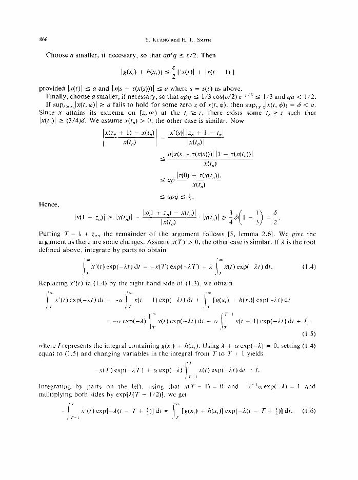
It is apparent that all the hypotheses of our theorem hold if o( > n/2 and hence (0.3) has a nontrivial slowly oscillating periodic solution satisfying -1 < x(t) < 1. See Fig. 2 for the

numerical solution of (0.3).


IO

09

08

07

06

05

04

03

0.2

01

Y 0

-0 I

-0 2

-03

-04

-05

-06

-07

-06

-09

-I 0

\

2 h k 6 lb 12 Ih 16 Ii ;o i2

r

Fig. 2. Numerical solution of (0.3) with o( = 2 and x(t) = 0.5, t 5 0.

Nussbaum [5] proved the existence of a periodic solution of the equation (0.3) by working in the space of C’ functions on a suitable interval and using a rather nonstandard fixed point theorem. Our result includes (0.3) and our proof appears to be simpler than the one in [5].

Our result may be applied to the delay logistic equation

x’(t) = rx(t)(l - x(t - 0(x(t))))

with suitable hypotheses on a(x), following the change of variables u = lnx, which yields

where r(u) = a(e”).

u’(t) = _r(e”“-““““’ _ 1)

We expect that our main result generalizes to equations of the form

x’(t) = -f(x(t),x(t - r(x(t)))), with suitable conditions on f.

In Section 2 we obtain sufficient conditions for solutions x(t), defined for t 2 0, to oscillate, i.e. to have arbitrarily large zeros. Our result is the following theorem.

THEOREM B. If (F) and (D) hold, s(0) = 1 and

f'(0) > e-l (0.4)

then every solution x(t) of (0.2), defined for f 2 0 and for which lim,,,t - s(x(t)) = 05, must oscillate.


I. EXISTENCE OF PERIODIC SOLUTIONS

In this section we prove the existence of periodic solutions of

x’(t) = -f(x(f - s(x(t)))).

We assume throughout this section that the following hold. (F) f: R + R is locally Lipschitzian and satisfies

xf(x) > 0, x # 0.

(D) T: R + (0, ~0) is locally Lipschitzian and r(0) = 1.

(1.1)

LEMMA 1.1. For each bounded, Lipschitzian function 4: (-m, 0] + R there exists a unique noncontinuable solution x(r, 4) of (1.1) defined for t E [0, a), 0 < w 5 ~0, x(t) = 4(t) for t 5 0.

If w < 00, then there exists t, 7 w such that Ix(t,J + ~0 as n + 00. If lim infi,i,,T(x) > 0,

then w = +03.

Proof. These are well-known results. See Halanay and Yorke [19], Grossman and York [20], Driver [21]. Uniqueness follows from [19, proposition 1.31. Since the right-hand side is bounded on bounded subsets of the space of bounded, Lipschitzian functions on (-co, 01, the behavior of x(r) as I --t o follows from [19, proposition 1.21. In the case of (1.1) it is especially easy to see. If Ix(t)1 is bounded on its maximal interval of existence, then its derivative is also bounded and thus lim t_,mx(t) exists. The solution can then be extended to a larger interval.

Alternatively, the entire lemma may easily be obtained by a careful application of the method of steps. n

Given a bounded, Lipschitzian function 4 on (-to, 0] we write x(r, 4) for the noncontinuable solution of (1.1) for t L 0 satisfying x(t) = 4(t) for t I 0. We will use this notation in case 4

is defined and Lipschitz continuous on some compact interval [-r, 0] provided it is known that t s(x(t, 4)) 2 -r for t 2 0.

LEMMA 1.2. Let x(t, 4) be a solution of (1.1) and suppose x’(t,,) = 0 for some t, 2 0. Then t - r(x(t)) > t,, - s(x(&,)) for all t > t,. If I,, > 0, then I - s(x(t)) < f, - T(x(t,J) for 0 I t < t, .

Proof. By (F), x(t,, ~ s(x(t,,))) = 0. Since 5 is locally Lipschitzian and x’(f,,) = 0, there exists q > 0 such that for 0 < t - to < q,

Thus, for t, < t < t,, + q,

or

Iwt)) - M4,))l < t - to.

t - t,, > T(dt)) - t(x(t,)),

f - 7(x(t)) > I,, - M&J)).

If the assertion of the lemma is false, there is a smallest t, > f, such that

f, ~ T(X(I,)) = 4) - M4,)) < t - e(t)) (1.2)


for t,, < t < t, . Obviously, x’(ti) = 0 sincef(x(t, - r(x(ti)))) = f(x(t, - s(x(t,)))) = ~‘(1,) = 0 and arguing as above, there exists 6 > 0 such that for 0 < It - t,I < 6,

lr(x(t)) - r(x(l,))l < It - t,I.

But this implies that for t, - 6 < t < t,,

t, - t > at,)) - ate)),

which contradicts (1.2). This completes the proof. n

Lemma 1.2 has an important consequence which we exploit later on. Namely, if x’(t,) = 0 for some t, 1 0, then the solution x(t) for t 2 I,, depends only on x(s) for s in the interval [I,, - s(x(f,)), t,,]. The solution “forgets” some of its past history.

For N > 0, let r = r(N) = max(s(x): 0 5 x 5 NJ and define

KN = 14 E C,.: 4(--r) = 0, 4 2 0, 4 is nondecreasing, lip 4 < CO and 4(O) 5 Nl.

C, = C([-r, 01, R) denotes the space of continuous functions on [--r, 0] with the uniform norm /I. 11. We introduce the following hypothesis.

(B) There exists N > 0, A4 > 0 such that

for all t in the domain of x( a, 4), and for all 4 E Kh;. If (B) holds for some N > 0, M > 0, then necessarily the domain of x(*, 4) = [0, ~0) for

every 4 E I?~, , by lemma 1.1, and hence the inequality holds for all t 2 0. We show below that t - s(x(t)) 2 -r for all t 2 0 for 4 E K,y. Set R = max(s(x): -M 5 x I NJ so R 2 r 1 1, and E = maxlf(.u): 0 5 x 5 Nl.

PROPOSITION 1.3. Assume that (B) holds, f’(0) > 1, $ E &\O, and x(t) = x(r, 4). Then: (i) there exists Z, = z,(4) 2 (+(O))/E such that x(r) > 0 and x’(t) 5 0 on [0, z,), x(z,) = 0

and ~‘(7,) < 0; (ii) there exists P = P(N) > 0 such that z,(4) 5 P for all 4 E K,&,\O;

(iii) there exists t, = t,(4) E (z, , L, + R] such that x’(t) < 0 on [z, , t,) and x’(r,) = 0; (iv) there exists zz = z,(4) > f, such that x(t) < 0, x’(t) > 0 on (t,, z2), x(zz) = 0 and

~‘(7,~) > 0. Moreover, Z* - Z, > I; (v) there exists Q = Q(M) > 0 such that ~~(4) 5 Q for all 4 E KV\O;

(vi) there exists t, = tz($) E (zz, zz + r] such that x(t) > 0, x’(t) > 0 on (z2, tz) and x’(tz) = 0.

Proof. Clearly x’(t) 5 0 for all t E [0, z,] where we take Z, = +os if x never vanishes. Define F(x) = minlf(u): x 5 II I Nl for 0 5 x 5 N so that F is Lipschitz, F(x) > 0 for x > 0, F is increasing and F(0) = 0. If Z, > r, then for r c: t 5 z,,

x’(t) = -f(x(t - s(x(t)))) 5 -F(x(t - r@(t)))) 4 -F(x(t))

since t - s(x(t)) > 0 andx(t - s(x(t))) 2 x(t). From standard differential inequality arguments,

x(t) 5 u(t), r<t<z,

862 Y. KUANC and H. L. SMITH

where u’(t) = -F(u(T)), U(T) = N.

Observe that u(t) is independent of 4 E f?N and that lim,,,u(t) = 0. Let k satisfy f ‘(0) > k > 1 and choose 6 > 0 such that f(x) > kx for 0 < x 5 6. Choose 6

smaller if necessary so that kr(x) 2 1 for 0 I x 5 6. From the previous paragraph, there exists T > r, depending only on N, such that x(t) I 6 for T I t I z, , if T < z,. If r + T + km’ < z,, then for r + T 5 t 5 r + T + k-’

x’(t) < -kx(t - s(x(t))) I -kx(r + T),

since, for the above range of t,

T < t - r(x(t)) 5 t - k-’ I r + T and x is decreasing. Hence

x(r + T + k-‘) < x(r + T) - kx(r + T)k-’ = 0,

a contradiction to our assumption that r + T + k-’ < z1 . We conclude that Z, % r + T + k-‘. Since x’(t) 2 -E for 0 I t I zl, it follows immediately that zi 2 4(0)/E. This establishes (i) and (ii) except for the assertion that x’(z,) < 0.

Assume that 4(t) = 0 for -r 5 t 5 d, d < 0, and 4(t) > 0 on (d, 01. If --$4(O)) > d, then x’(0) < 0 and we claim that t - r(x(t)) > d for all t > 0. The argument is exactly like that in lemma 1.2. If t, > 0 is the smallest positive time at which t - t(x(t)) = d, then x’(t,) = 0 and so there exists q > 0 such that

IrMt)) - r(%))l < If - f,l

if It - t,, < q. But then, for to - q < t < t,,

and hence t, - t > Mt”)) - Mt)),

t - T(X( t )) < t,, - t(x(t,)) = d.

Since 0 - s(4(0)) > d, the above inequality and the Intermediate Value Theorem imply the existence of t* E (0, to) at which t* - s(x(t *)) = d, contradicting the minimality of t,. Hence, our claim is valid and it follows that x’(t) < 0 for 0 5 t I z, . If -s(4(0)) = d, then x’(0) = 0 and, by lemma 1.2, t - r(x(t)) > d for all t > 0. Hence, again, x’(t) < 0 for 0 < t 5 z, . If -r(4(0)) < d, then x’(t) = 0 so long as t - r(x(t)) 5 d. Lemma 1.2 implies that the set of such t is an interval [0, t,,], to > 0, on which x(t) = 4(O). It follows that to - 5(4(O)) = d or t,, = d + r(4(0)). For t > to, t - $x(t)) > d, by lemma 1.2, and thus x’(t) < 0 for (t,, z,]. This completes the proof of (i) and (ii).

By lemma 1.2 and the arguments above, x’(t) < 0 for t 2 z, until time t, at which t, - s(x(t,)) = z,. By (B), t, = z, + r(x(t,)) i R + z, and x’(tl) = 0. By lemma 1.2, t - s(x(t)) > z, for t > t, implying that x’(t) > 0 for t, < t I zz, where z2 is the second positive zero of x(t) or +CD if no such zero exists.

But x(t) must have a second positive zero by arguments identical to those yielding the existence of its first zero. Indeed, by the remark following lemma 1.2, x(t), for t 2 t, is determined by the values x(s) for s in the interval [z, , t,], which are nonpositive and bounded below by -M. Thus, one can argue exactly as for the existence of Z, and its upper bound P, to show the existence of the second zero z,~ satisfying z,(4) 5 Q for all 4 E k,,,,\O. Thus (iv) and (v) hold. Since x’(zJ > 0, x(zZ - r(x(zz))) = x(z, - 1) < 0 so z2 - 1 > Z,


Fig. 3. The graph of x(t, $), $J E &.\O.

As x’(zJ > 0 and t - s(x(t)) > z1 for t > t, it follows that x’(t) > 0 for t 2 zz until such time t2 at which t2 - s(x(t2)) = z2. By (B), such a I, exists and t2 = zz + s(x(tJ) I z2 + r. This establishes (vi). n

It follows from proposition 1.3 that x(t, q5) has infinitely many zeros z,(4), n 2 1, which are simple and z, - z,_, > 1 for n 2 2, if (B) holds, 4 E KN\O and f’(0) > 1. Moreover, x’(t, 4) = 0 for t 2 z1 only at points t,(G), n 2 1, satisfying z, < t, < z~+~, n 2 1, where t, - r(x(t,)) = z, and x’(t) > 0 on (t,, tn+J, for n 2 1, n odd, and x’(t) < 0 on [z,, t,) and on (t,, tn+,), n L 2, n even. Figure 3 summarizes this information.

We note for later use that the hypothesis (B) was not used in proposition 1.3 (i) and (ii). The lower bound -A4 on the solution was used to show that t, < +m and to obtain the existence of z2. The upper bound N was then required to show that t, < 00.

Assuming that (B) holds and that L = max( If(x -A4 I x 5 N), we define

Observe that K is a compact, convex subset of C,. containing the zero function and that lip x( *, q5) I L for all 4 E I?y. Define the map T: K + C’, by:

(T4)(@ = [x(tz(+) + 0, @)I+, -r I e I 0,

if 4 E K\O and TO = 0. For I,V E R, I,v/+ = max(0, w). The following lemma will be used to establish the continuity of T.

LEMMA 1.4. Assume that (B) holds. Then there exists A > 0 such that

for $I, VI E K. Ix(t, 4) - x(t, w)l 5 I/$ - wll eA’, tro


Proof. This is a simple Gronwall estimate. Let p = lipf q = lip ~jt_~,,~, and recall that lipx(. , $) I L for any 4 E K. Put x(t) = x(t, 6) and y(t) = x(t, I,v), for 6, w E K. Then

” I Ix(t) - Y@)l 5 Ix(O) - YW +

I l f(x(s - MS)))) - f(y(s - T(YV(Q)))/ ds

,0

5 114 - VII + \ ‘k(s - MS))) - Y@ - r(y(s)))l ds

.o

5 114 - VII + I “p,LqlNs) - Y(+ + k - r(y(s))) - Y(S - T(Y(s)))II ds .O

-1

5 114 - w/I + I PI-b + llZ(s)ds .0

where Z(t) = sup, 5 f Ix(s) - y(s)l. Hence,

,I

Z(l) 5 II4 - VII + I AZ(s) ds .O

where A = p[Lq + 11. The assertion follows from Gronwall’s inequality. n

PROPOSITION 1.5. T maps K continuously into K with respect to the C, topology. If r4 = 4 E K70, then x(t, 4) is a periodic solution of period tz(+).

Proof. By proposition 1.3 (iv) and (vi), x(tz(+) + 0, 4) > 0 and x’(tZ(+) + 8, 4) > 0 for -r 5 z2 - t, < 0 < 0 and [x(tZ(4) + 8, +)I’ = 0 for -r 5 f3 % zz - t,, Hence, T$(-r) = 0,

Tg5 2 0 and T4 is nondecreasing on [-r, 01. (B) implies (T4)(0) = x(t,(+), 4) 5 N. Except possibly for a simple point, T4 is differentiable and ](T+)‘l 5 L. Thus, T$J E K.

Suppose T4 = 4 E K\O. By the remark following lemma 1.2, x(t, +), for t 2 t*(4), depends only on the values of x(s) for s in the interval [z,, t,], that is, x(t), t 2 t2, depends only on x(t, + e) for 22 - t, 5 8 2 0. Since r+ = 4, 4(Q) = x(t, + e) for zz - t, 5 Q 5 0, and so by uniqueness of solutions and the autonomous nature of (1. l), x(t, 4) is periodic of period tz(q5).

Lemma 1.4 together with proposition 1.3 (v) immediately imply the continuity of Tat 4 = 0. Let d, E K\O and zj = z,(9), i = 1,2. Given c, 0 < E < (z2 - z,)/2, choose

6 = inf]lx(t, 4)I: t 13 [0, z, - E] U [z, + c, z2 - cl).

By lemma 1.4, there exists q > 0 such that if I,Y E K and 111,~ - 411 < q, then

lx(t, 4) - x(t, w)l < a/2

on [0, zz]. Hence, x(t, I,V) > 6/2 on [0, z1 - E] and x(t, w) < -612 on [z, + E, z2 - E] so x(t, I,U)

has its first zero z,(w) E [z, - c, z, + e]. This establishes the continuity of z1 : K + (0, a) at 4. Similar arguments show that z2 is continuous on K\O. Recall that t2(q5) - s(x(t2(+), 4)) = ~~(4) for 4 E K\O and that t*(4) is the unique time t at which t - r(x(t, 4)) = zz. This fact, together with the estimate tz(+) 5 Q + r from proposition 1.3 (v) and (vi) immediately imply the continuity of t,: K\O + (0, Q + r]. Thus the map $I ,+ ~~~(~~(4) from K\O into C, is continuous. The continuity of T follows from the continuity of 4 ++ 6’. W


We remark that T is not continuous with respect to the usual Lipschitz norm on the space of Lipschitz functions on [-r, 01. This is because the operation of taking the positive part of a function fails to be continuous in this space.

COROLLARY 1.6. If Tqi = C$ E K\(O), then the tz($)-periodic solution x(t, +) has the following properties:

(i) x(t) has precisely two zeros in [0, t*(4)], namely zi and zZ, 0 < zi < zz < r2(4), both of which are simple. Moreover, zz - zi > 1 and t2 > 2;

(ii) x(t) has two extrema in (0, t2(qb)], namely 1, and tz, 0 < z, < t, < z2 < t2. x’(t) < 0 on (0, f,) and x’(t) > 0 on (tl, r,);

(iii) -M 5 x(t) 5 N for all t.

Proof. Most of the assertions are obvious from propositions 1.3 and 1.5 and the periodicity of x(t, (6). Note that as x’(t) < 0 for t E (t2, z3J it follows that x’(t) < 0 on (0, t,). Since x(t) is periodic and zz - z,i > 1, we have t2 = z3 - z, = z3 - zz + zz - z1 > 2. l

It follows from corollary 1.6 that consecutive zeros of the periodic solution x(t, 4) are separated by more than one time unit.

The next two results are patterned after similar ones in Nussbaum [S, lemmas 2.6 and 2.81. According to Nussbaum, the main idea for the next lemma is due to Wright [2].

LEMMA 1.7. Assume that (B) and f ‘(0) > n/2 hold. Then there exists a positive number a, independent of q5, such that for any 4 E K\O,

suplx(t, 4)I 2 0 I?&,

for all sufficiently large zeros z, of x(t, 4).

Proof. We express (1.1) as x’(t) = -cYx(t - I) + g(x;) f h(x,) (1.3)

where 01 = f’(O), g(x,) = olx(f - 1) - f(x(t - 1)) and h(x,) = f(x(t - 1)) - f(x(t - r(x(t)))).

Let 13 = ,!I + iv be the complex root of A -t CY e-’ = 0 satisfying I* > 0 and 0 < v < II (see, e.g. [14, lemma 11.4.11). Choose a positive number L‘ such that E < (I/~),u cos(v/2). Choose a > 0 such that if 1x1 I a then (ax - f(x)1 I (e/2)1x(. If 4 E K\O, then -M 5 x(t, 4) 5 N by (B) so we may estimate h(x,) along the solution x(t, 4) as follows,

Ih(x,)l 5 plx(t - 1) - x(t - r&(t)))1

5 PlX’(J)l I@(Q) - 1 I

5 Pdf(x(s - 7MW Ix(t)l

5 P24b@ - MaI Lw)l

where P = lipflL_M,Nl, q = lip ~l,_~,~, and s = s(t) lies between t - 1 and t - $x(t)). We assume t > R so t - r(x(t)) > 0. Then s > t - R and s - r(x(s)) > I - 2R.


Choose a smaller, if necessary, so that ap’q i e/2. Then

I&,) + h(x,)l 5 ; [lx(t)1 + 1x0 - I)11

provided /x(t)1 I a and Ix(s - r(x(s)))l 5 a where s = s(t) as above. Finally, choose a smaller, if necessary, so that apq 5 l/3 cos(u/2) e-p’2 5 l/3 and qa < l/2. If suptJx(t, @)I 2 a fails to hold for some zero z of x(t, $,), then sup,,,Ix(t, 4)/ = 6 < a.

Since x attains its extrema on [z,, co) at the t, L z, there exists some t, 2 z such that Ix(t,)l 2 (3/4)6. We assume x(t,) > 0, the other case is similar. Now

-a,, + 1) - x(t,,) IX'W lz,, + 1 ~ trill = x(f,) Ix(tJ I

5 PlX(S - MW I 1 - ~w,))I x(t,)

< ap IT(O) - Wfn))l x(t,,)

5 apq 5 f.

Hence,

1x(] z,)l lxU,,)I l-e1 + ~ + 2 z,) W,,)/ - . - =

i.a,,) I lx(t,,)l L -6 3

4 ( I ~ 1 J

3 6 -. 2

Putting T = 1 + z,,, the remainder of the argument follows [5, lemma 2.61. We give the argument as there are some changes. Assume x(T) > 0, the other case is similar. If ,I is the root defined above, integrate by parts to obtain

I

au1 ‘m x’(t)exp(-/lt)dt = -x(T)exp(-AT) + h

.T I x(t) exp(-At) dt. (1.4)

I 1.

Replacing x’(t) in (1.4) by the right-hand side of (1.3), we obtain

*cc

I

‘cc ‘cc

x’(t) exp(-i.t) dt = -CY I

x(t - l)exp(-ht)dt + I

Mx,) + 4x-,)1 ew(-i.f) dt . r , T , T

I

‘X 1 7+ I = --(Y exp( -A) x(t) exp(-At) dt - (Y

I x(r ~ l)exp(-J.t)dt + I,

, T q T

(1.5)

where I represents the integral containing g(x,) + /1(x,). Using /I + CY exp( -1,) = 0, setting (1.4) equal to (1.5) and changing variables in the integral from T to T + 1 yields

I

,I mx(T)exp(-iLT) + aexp(-A) x(t) exp(-At) dt = 1.

, I-I

Integrating by parts on the left, using that s(T - 1) = 0 and -I-‘cy exp(-,I) = 1 and multiplying both sides by exp[A( T - l/2)], we get

‘rn

I

*I x’(f)exp[-1(t - T + i)] dr =

I [g(x,) + /I(x,)] exp[-i,(r - T + $1 dt. (1.6)

, I--I , I-


The reader may now appreciate our passing from x(t,) to x(z, + 1) in the arguments above in order to achieve x(T - 1) = 0. Now we consider two cases: T I t,, and T > t, . In the former, we may continue exactly as in [5, lemma 2.61 since x’(t) 2 0 on [T - 1, T]:

Re *.(t)exp[ -i(r - T+ ;)I dt) 2 exp(-g)(cosi)x(T) 2 exp(-f)(cosi)i.

As the modulus of the right-hand side of (1.6) is less than E&(-’ exp(-p/2), we obtain that p/2 cos v/2 I a, a contradiction to our choice of E.

If t, < T, then

Re x’(t) exp[-l(t - T + +)I dt >

i

I” = x’(t) exp[-p(t - T + i)] cos v(t - T + t) dt

L T-l

" T

+

!

x'(t)exp[-~(t - T + i)] cos v(t - T + i)dt. t fn

Note that x’(t) 2 0 for T - 1 5 t 5 t, and x’(t) I 0 on t, 5 t I T < zn+l so the two integrals have opposite sign. The first integral on the right may be estimated exactly as in the previous case:

,‘z_Ix’(t)exp[ --/1(1 - T + :)I cos v(t - T + i) dt 2 exp(-g)(cosi)x(t,). I

(1.7)

We have for t, 5 t I T,

exp[-,4t - T + t)] cos v(t - T + i) I exp[-,&t, - T + +)] 5 1

since T - t, = lr(x(t,)) - r(O)1 5 qx(t,) I qa < l/2. Hence,

I

'T

x'(t) exp[-,u(t - T + ))] cos v(t - T + 4) dt * ‘,I

'T

2 I

x'(t) dt = x(T) - x(t,) = x’(s)(T - t,) 2 x’(s)qx(t,) 2 -upqx(t,) (1.8) t In

where f,, < s < T and we have used the estimate above for T - t,, Putting (1.7) and (1.8) together we have

Re x’(t) exp[-A(t - T + f)] dt >

e (exp(-;)(cosi) - *pq)x(tJ 2 iexp(-g)(cost)x(tJ 2 exp(-g)(cosJj) *i.

A contradiction is obtained exactly as in the previous case. W


THEOREM 1.8. Assume that (F), (D), (B) and f’(O) > n/2 hold. Then T has a nonzero fixed point in K.

Proof. We show that 0 is an ejective fixed point of T so that our result follows from a theorem of Browder [18] (see also [14, theorem 11.2.41) on the existence of a nonejective fixed point.

From lemma 1.7, \x(t,, +)I 2 a/2 for infinitely many integers n if $ E K\O. Let b < a/2 be such that max( f(x): 0 5 x I 6) < d(2R). If x(l,,, , 4) < b for every integer n 2 N, then

IGn+l 9 411 5 [;;;I: 1 f(x(s - ~(x(4)))I ds < & r(x(tz,+, 3 $1) < a/2

since tzn+, - S(x(tzn+ 1)) = zZn+ 1. This contradiction implies that x(tZn , 4) 2 b for infinitely

many n. As II T%)ll = x&, , $1, we see that 0 is an ejective fixed point of T. This proves the theorem. n

2. BOUNDEDNESS AND OSCILLATION PROPERTIES OF SOLUTIONS

In order to apply our main result, one must find a priori bounds for solutions x(t, 4) for 4 in a set l?,,, . More precisely, we must give sufficient conditions for the existence of A4 and N > 0 such that

-M 5 x(t, $) 5 N

for all t in the maximal interval of existence of x(t, @), for d, belonging to the set

l?,v = (4 E C,: 4(-r) = 0, q5 nondecreasing, lip q5 < co and 4(O) 5 N],

where r = max{r(x): 0 5 x 5 NJ. As noted in lemma 1.2, for 4 E EN, t - s(x(t, 4)) 2

all t in the interval of existence of x( *, 4), without assuming (2.1). We assume throughout this section that (F) and (D) of Section 1 hold. Define

F+(u) = max(f(x): 0 5 x 5 u),

for u 2 0. F-(u) = max(-f(x): --u 5 x I 01,

PROPOSITION 2.1. Suppose M, N > 0 satisfy

M

r(-M) > F+(N)

N __ > F-(M). r(N)

Then (2.1) holds for all $ E EN.

(2.1)

-r for

(2.2a)

(2.2b)


Proof. For I$ E z,,,\O, we argue as in proposition 1.3 (i) and (ii) that x’(t, 4) I 0 for 0 5 t I t1 5 M, where t, > z1 and t, = +oo is not yet ruled out. This argument did not make use of the a priori bound (B). If there exists to E (z,, t,] such that x(t) > -M for j < 4, and x(t,) = -M, then x’(s) < 0 so N 2 x(.s - T(x(s))) > 0 for z - 1 5 s < to. Hence,

I> fo -M=

I x’(s) ds z -F+(N)(t, - z,).

L ZI

Since t, - r(x(tJ) I z1 , to - z 5 T(-M) so

-M z -F+(N)r(-M),

contradicting (2.2a). Thus, we conclude that x(t) > -M on (zl, zZ). Now suppose that there exists t, E (zl , t2] such that x(t,) = N and x(t) < N for z2 5 t < lo. Then

* fo N=

1 x’(s) & 5 F-(M)(t, - ZJ 5 F-(M)r(N),

z2

since -M < x(s - 7(x(s))) < 0 for z2 < s < f, and since t, - r(x(t,,)) = to - r(N) I z2. Now we have a contradiction to (2.2b). Making use of lemma 1.2, we see this argument can be continued so that (2.1) holds for all t L 0. n

Some special cases where (2.2) hold are worth mentioning here. For example, if there exists N > 0 such that

r(+N) lipfl,-,,,, < 1, (2.3)

then (2.2) holds for M = N. If f is bounded from below and 7 is bounded from above, then (2.2) hold for all large N > 0 and M 2 M(N) > 0, where M(N) depends on N. A similar statement holds if f is bounded from above.

In our next result we drop our assumption that r(O) = 1 in order to allow a more appropriate scaling of time. See the remark following the proof.

PROPOSITION 2.2. Suppose that (F) and (D) hold for (1.1) and r(x) andf(x) satisfy:

(i) 5, = lim,,,, r(x) exist, 0 < T* < 3/2, t(x) is continuously differentiable for large 1x1 and liml,, _,xr’(x) = 0;

(ii) (Y = supjJf(x)/x]: x # 0) L= 1. Then x(t, $) is bounded provided that 4 is bounded and Lipschitzian on (-co, 01. Moreover, there is an N > 0, such that /x(l, $)( c: N for all 4 E EN.

Proof. Note that x(t, 4) is defined for all t 2 0 by lemma 1 .l. If the result is false, there is an x(t) = x(t, @), such that 4 is bounded and Lipschitzian on (-co, 01, and

lim sup,++,lx(t)l = a~. Denote 5 = max{# + r&)1. Choose p > 0, y > 0, M > 0, such that for 1x1 > M, T(X) < T, JxT’(x)J < ,8, and for lx1 1 > M, lx,/ > M, x,x, > 0, I s(x,) - T(XJ < y,

where p and y are such that nb - y + $ > T. Since ji’ and y can be chosen arbitrarily small for suitably large M, the latter inequality can be assumed.


If x(t) is monotone, then it is easy to see that x(r) must be bounded. Since x(r) is not bounded, it must be oscillatory. Without loss of generality, we assume in the following that there is a f > 0, such that x(f) > 2A4, x’(t) = 0, Ix(t)1 < x(F) for t 5 f. Thus

Denote x(i - $x(f))) = 0.

t, = i - s(x(T)),

f, = max(s,x(s) = +x(t), x(t) > +x(F), for t E (s, i]). We have

x(t,) = ix(F) =

which indicates that

Clearly,

I alI

I sII

-.fMf - Mt)))> dt < x(i) dt = x(T)(r, - to), I (0 I tu

+x(t) = I -f(x(t - TMt)))) dt I ‘I

< ! ” Ix(t - z(x(t)))l dt

c 11 ,I i

= I Ix(t - Wt)))l d(t - W(t))) + I ’ Ix(t - Mt)))l dMt)). * fl t fl

Since x(t) > M, we have r(x(F)) < 7. This leads to i - t, < r(x(T)) < r. Thus

‘i

I 1x0 - MfH)I dW(t)) =

I’

x’(t)T’(x(t))k - r@(t)))\ dt

t 11 c ‘I

< 2X(f)T&

Since lx’(r)\ = I-f(x(t - r(x(t))))l < x(i) for t 5 f, we have

Hence, Ix(t)1 = Ix(t) - W,,)I < x(f)lt - 41, t 5 i.

‘i-7(x(i))

kf - WU)))l d(r - s(x(t))) =

, \ r,-T(X(I,)) ‘x(f)l dt

1 10 zz

I r,-7(i(f,)) ‘x(t)l dt I

I 5 10

< x(f)& - r) dt I r,-i(x(r,))

= tX(f)(t - t, + T(X(t,)) - T(X(t)))‘.


Therefore, - -

ix(t)@ - t, + r(x(t,)) - r(x(i)# + 2x(t)Tp > )x(f),

which implies that

i-t,>JI_4sP-y.

Since r(x(t)) = t - t, = f - t, + t, - t,, we have

r(x(i)) > JI-4sp - y + + > r,

a contradiction to the fact that r(x) < T for 1x1 > M. The conclusion of the second part of the proposition follows by letting N = 2M. n

By resealing time appropriately, it is easy to see that if, in proposition 2.2, we assume the existence of T* > 0 and 0 < cy < co and only the single inequality cyr* < 3/2, then the conclusion of the proposition holds. As a consequence, if k(1 - a) < 3/2 in (0.1) with r(x) = o( emXZ + (1 - a), 0 5 LY < 1, then all solutions are uniformly bounded.

We say that x(t) is oscillatory if x(t) is defined for all large t and has arbitrarily large zeros. It is well known that every solution of

x’(t) = -ax(t - p)

oscillates if 01 > 0, /3 > 0 and alp > e-‘. A very nice proof of a more general result is given in [22] wherein the following lemma is established.

LEMMA 2.3 [22, proof of theorem]. If ol/3 > e-l, then there cannot exist a continuously differentiable function x(t) satisfying

for all large t. x’(t) + cYx(t - p) 5 0, x(t) > 0, x’(t) < 0

Our next result is based on the lemma.

THEOREM 2.4. If (F) and (D) hold and f’(0) > ee’, (2.4)

then every solution of (l.l), defined for t 2 0 and for which lim,,,t - s(x(t)) = +w, is oscillatory.

Proof. Choose k such thatf’(0) > k > em1 and r. < 1 with s,k > em’. Let 6 > 0 be such that If(x)1 > klxl and r(x) > r0 if /xl < 6.

If x(t) is an eventually positive solution, then for large t, x(t) > 0 and x’(t) < 0. It follows that lim (_-x(t) = I> 0 exists and

0 = Jlf”,x’(t) = -f (

lim x(t - s(x(t))) = -f(/). f-CC >


Thus, I = 0 so that for large t we have 0 < x(t) < 6 and x’(t) < 0. Then

0 = x’(t) + f(x(t - T&(t)))) > x’(t) + kx(t - 7(x(t))) 5 x’(t) + kx(t - 70)

holds for all large t, contradicting lemma 2.3. n

Acknowledgement-This research has, in some way, been motivated by a renewed interest in state-dependent delay equations by some participants of the recent period of concentration on Mathematical Physiology and Differential Delay Equations, organized chiefly by M. Mackey, at the IMA in the spring of 1990. The second author would like to thank the organizers of this period of concentration and also the staff at IMA for a very productive and enjoyable visit.

The authors are grateful to E. Lo for providing the numerical solutions displayed in Figs 1 and 2, using the numerical schemes developed in [23].

1.

2. 3.

4.

5.

6.

7.

8.

9.

10. II.

12.

13.

14. 15.

16.

17.

18. 19.

20.

21. 22.

23.

REFERENCES

JONES G. S., The existence of periodic solutions of f’(x) = -2f(x ~ I)(1 + f(x)), J. math. Analysis Applic. 5, 435-450 (1962). WRIGHT E. M., A nonlinear differential-difference equation, J. reine angew. M&h. 194, 66-87 (1955). GRAFTON R. B., A periodicity theorem for autonomous functional differential equations, J. d$f. Eqns 6, 87-109 (1969). NUSSBAUM R. D., Periodic solutions of some nonlinear, autonomous functional differential equations II, J. dqf. Eqns 14, 360-394 (1973). NUSSBAIJM R. D., Periodic solutions of some nonlinear, autonomous functional differential equations, Annuli. Mar. pura appl. IV, Ser. 101, 263-306 (1974). HADELER K. P. 8: TOMIUK J., Periodic solutions of difference-differential equations, Archs ration. Mech. Analysis 65, 87-95 (1977). KAPLAN J. L. & YORKE J. A., On the nonlinear differential delay equation x’(t) = -f(x-(t), x(l - I)), J. duy Eqns 23, 293-314 (1977). CHOW S. N., Existence of periodic solutions of autonomous functional differential equations, J. diff. Eqns 15, 350-378 (1974). CHOW S. N. & HALE J. K., Periodic solutions of autonomous equations, J. math. Analysis Applic. 66, 495-506 (1978). ALT W., Some periodicity criteria for functional differential eqt@iona, flunuscriptu marh. 23, 295-31; (1978). ALT W., Periodic solutions of some autonomous differential rquatioq.&with Functional Differenrial Equutions and Approx. of Fixed Points, ‘Bonn) 1 $4 !

variable tivy delay, Proc. Conf. on 8 Lecture Notes in Mulhematics

Vol. 730. Springer, Berlin (1979). WAI.THER H. O., Existence of a nonconstant periodic solution of a nonlinear autonomous functional differential equation representing the growth of a single species population, J. math. Biol. 1, 227-240 (1975). WALTHER H. O., On instability, w-limit sets and periodic solutions of nonlinear autonomous delay equations, in Funcfional Differential Equations and Approximation of Fixed Points (Edited by H. 0. PERTGEN and H. 0. WALTHER), pp. 489-503. Lecture Notes in Muthemarics, Vol. 730. Springer, Berlin (1979). HALE J. K., Theory of Funcrional Differenrial Equations. Springer, New York (1977). B~LAIR J. & MACKEY M. C., Consumer memory and price fluctuations in commodity markets: an integro- differential model, J. d$f. Eqns 1, 299-325 (1989). B~LAIR J., Population models with state-dependent delays, Proc. 2nd Int. Conf. on Mathematical Population Dynamics (preprint). MALLET-PARF.T J. & NUSSBAUM R., Periodic solutions of Etate-dependent differential-delay equations: I (private communication). BROWDER F. E., A further generalization of the Schauder fixed point theorem, Duke math. J. 32, 575-578 (1965). HALANAY A. & YORKE J. A., Some new results and problems in the theory of differential-delay equations, SIAM Rev. 13, 55-80 (1971). GROSSMAN S. & YORKE J. A., Asymptotic behavior and stability criteria for delay differential equations, J. d[ff Eqns 12, 236-255 (1972). DRIVER R. D., Ordinary and Delay Differential Equalions. Springer, New York. LADAS G., SFICAS Y. G. & STAVROULAKIS I. P., Necessary and sufficient conditions for oscillations, Am. math. Mon. 90, 637-640 (1983). JATKIEWI~Z Z. 91 Lo E., The numerical solution of neutral functional differential equations by Adam’s predictor corrector methods. Technical report No. 118, Arizona State University (1988).

Slowly oscillating periodic solutions of autonomous state-dependent delay equations

Documents

Transcript of Slowly oscillating periodic solutions of autonomous state-dependent delay equations