Quantum Microeconomics with Calculus - SmallParty.org
254
Quantum Microeconomics with Calculus Version 3.1 October 2004 Available with and without calculus at http://www.smallparty.org/yoram/quantum Email contact: [email protected] This work is licensed under the Creative Commons Attribution-NonCommercial License. To view a copy of this license, visit Creative Commons online at http://creativecommons.org/licenses/by-nc/2.0/ or send a letter to Creative Commons, 559 Nathan Abbott Way, Stanford, California 94305, USA.
-
Upload
khangminh22 -
Category
Documents
-
view
2 -
download
0
Transcript of Quantum Microeconomics with Calculus - SmallParty.org

Quantum Microeconomics
with Calculus
Version 3.1
October 2004
Available with and without calculus at
http://www.smallparty.org/yoram/quantum
Email contact: [email protected]
This work is licensed under the Creative Commons Attribution-NonCommercialLicense. To view a copy of this license, visit Creative Commons online at
http://creativecommons.org/licenses/by-nc/2.0/ or send a letter to CreativeCommons, 559 Nathan Abbott Way, Stanford, California 94305, USA.

ii

Contents
README.TXT vii
I One: The Optimizing Individual 1
1 Decision Theory 31.1 Decision Trees . . . . . . . . . . . . . . . . . . . . . . . . . . . . . 41.2 Example: Monopoly . . . . . . . . . . . . . . . . . . . . . . . . . 61.3 Math: Optimization and Calculus . . . . . . . . . . . . . . . . . . 8
2 Optimization and Risk 172.1 Reducing Risk with Diversification . . . . . . . . . . . . . . . . . 192.2 Math: Expected Value and Indifference Curves . . . . . . . . . . 21
3 Optimization over Time 273.1 Lump Sums . . . . . . . . . . . . . . . . . . . . . . . . . . . . . . 283.2 Annuities . . . . . . . . . . . . . . . . . . . . . . . . . . . . . . . 283.3 Perpetuities . . . . . . . . . . . . . . . . . . . . . . . . . . . . . . 313.4 Capital Theory . . . . . . . . . . . . . . . . . . . . . . . . . . . . 313.5 Math: Present Value and Budget Constraints . . . . . . . . . . . 34
4 Math: Trees and Fish 434.1 Trees . . . . . . . . . . . . . . . . . . . . . . . . . . . . . . . . . . 434.2 Fish . . . . . . . . . . . . . . . . . . . . . . . . . . . . . . . . . . 46
5 More Optimization over Time 535.1 Nominal and Real Interest Rates . . . . . . . . . . . . . . . . . . 535.2 Inflation . . . . . . . . . . . . . . . . . . . . . . . . . . . . . . . . 545.3 Mathematics . . . . . . . . . . . . . . . . . . . . . . . . . . . . . 56
6 Transition: Arbitrage 596.1 No Arbitrage . . . . . . . . . . . . . . . . . . . . . . . . . . . . . 596.2 Rush-Hour Arbitrage . . . . . . . . . . . . . . . . . . . . . . . . . 606.3 Financial Arbitrage . . . . . . . . . . . . . . . . . . . . . . . . . . 61
iii

iv CONTENTS
II One v. One, One v. Many 65
7 Cake-Cutting 677.1 Some Applications of Game Theory . . . . . . . . . . . . . . . . 677.2 Cake-Cutting: The Problem of Fair Division . . . . . . . . . . . . 697.3 The Importance of Trade . . . . . . . . . . . . . . . . . . . . . . 72
8 Economics and Social Welfare 778.1 Cost-Benefit Analysis . . . . . . . . . . . . . . . . . . . . . . . . 788.2 Pareto . . . . . . . . . . . . . . . . . . . . . . . . . . . . . . . . . 798.3 Examples . . . . . . . . . . . . . . . . . . . . . . . . . . . . . . . 80
9 Sequential Move Games 859.1 Backward Induction . . . . . . . . . . . . . . . . . . . . . . . . . 85
10 Simultaneous Move Games 9510.1 Dominance . . . . . . . . . . . . . . . . . . . . . . . . . . . . . . 9610.2 The Prisoners’ Dilemma . . . . . . . . . . . . . . . . . . . . . . . 9610.3 Finitely Repeated Games . . . . . . . . . . . . . . . . . . . . . . 98
11 Iterated Dominance and Nash Equilibrium 10111.1 Iterated Dominance . . . . . . . . . . . . . . . . . . . . . . . . . 10111.2 Nash Equilibrium . . . . . . . . . . . . . . . . . . . . . . . . . . . 10411.3 Infinitely Repeated Games . . . . . . . . . . . . . . . . . . . . . . 10611.4 Mixed Strategies . . . . . . . . . . . . . . . . . . . . . . . . . . . 10711.5 Math: Mixed Strategies . . . . . . . . . . . . . . . . . . . . . . . 108
12 Application: Auctions 11712.1 Kinds of Auctions . . . . . . . . . . . . . . . . . . . . . . . . . . 11812.2 Auction Equivalences . . . . . . . . . . . . . . . . . . . . . . . . . 12012.3 Auction Miscellany . . . . . . . . . . . . . . . . . . . . . . . . . . 122
13 Application: Marine Affairs 12713.1 An Economic Perspective . . . . . . . . . . . . . . . . . . . . . . 12813.2 A Brief History of Government Intervention . . . . . . . . . . . . 12813.3 ITQs to the Rescue? . . . . . . . . . . . . . . . . . . . . . . . . . 131
14 Transition: Game Theory v. Price Theory 13314.1 Monopolies in the Long Run . . . . . . . . . . . . . . . . . . . . 13414.2 Barriers to Entry . . . . . . . . . . . . . . . . . . . . . . . . . . . 135
III Many v. Many 137
15 Supply and Demand: The Basics 13915.1 The Story of Supply and Demand . . . . . . . . . . . . . . . . . . 14015.2 Math: The Algebra of Markets . . . . . . . . . . . . . . . . . . . 141

CONTENTS v
15.3 Shifts in Supply and Demand . . . . . . . . . . . . . . . . . . . . 142
16 Taxes 14916.1 A Per-Unit Tax Levied on the Sellers . . . . . . . . . . . . . . . . 14916.2 A Per-Unit Tax Levied on the Buyers . . . . . . . . . . . . . . . 15016.3 Tax Equivalence . . . . . . . . . . . . . . . . . . . . . . . . . . . 15216.4 Math: The Algebra of Taxes . . . . . . . . . . . . . . . . . . . . . 154
17 Elasticities 15917.1 The Price Elasticity of Demand . . . . . . . . . . . . . . . . . . . 16017.2 Elasticities of Supply (and Beyond) . . . . . . . . . . . . . . . . . 16317.3 Math: Elasticities and Calculus . . . . . . . . . . . . . . . . . . . 165
18 Supply and Demand: Some Details 16918.1 Deconstructing Supply and Demand . . . . . . . . . . . . . . . . 16918.2 Reconstructing Supply and Demand . . . . . . . . . . . . . . . . 17018.3 Math: The Algebra of Markets . . . . . . . . . . . . . . . . . . . 17118.4 On the Shape of the Demand Curve . . . . . . . . . . . . . . . . 17118.5 On the Shape of the Supply Curve . . . . . . . . . . . . . . . . . 17418.6 Comparing Supply and Demand . . . . . . . . . . . . . . . . . . 175
19 Margins 17719.1 Reinterpreting the Supply Curve . . . . . . . . . . . . . . . . . . 17719.2 Total Variable Cost and Producer Surplus . . . . . . . . . . . . . 17919.3 Reinterpreting the Demand Curve . . . . . . . . . . . . . . . . . 18019.4 Total Benefit and Consumer Surplus . . . . . . . . . . . . . . . . 18119.5 Conclusion: Carrots and Sticks . . . . . . . . . . . . . . . . . . . 182
20 Math: Deriving Supply and Demand Curves 18520.1 Cost Minimization . . . . . . . . . . . . . . . . . . . . . . . . . . 18520.2 Supply Curves . . . . . . . . . . . . . . . . . . . . . . . . . . . . 19320.3 Demand Curves . . . . . . . . . . . . . . . . . . . . . . . . . . . . 195
21 Transition: Welfare Economics 20721.1 From Theory to Reality . . . . . . . . . . . . . . . . . . . . . . . 209
Appendices &etc. 211
A Government in Practice 213A.1 Rules and Regulations . . . . . . . . . . . . . . . . . . . . . . . . 214
B Math: Monopoly and Oligopoly 219B.1 Monopoly: The Vanilla Version . . . . . . . . . . . . . . . . . . . 219B.2 Monopoly: The Chocolate-with-Sprinkles Version . . . . . . . . . 220B.3 Duopoly . . . . . . . . . . . . . . . . . . . . . . . . . . . . . . . . 222B.4 The Transition to Perfect Competition . . . . . . . . . . . . . . . 227
vi CONTENTS
Glossary 231
Index 238
README.TXT
quantum Physics. A minimum amount of a physical quantity whichcan exist and by multiples of which changes in the quantity occur.(Oxford English Dictionary)
The “quantum” of economics is the optimizing individual. All of economicsultimately boils down to the behavior of such individuals. Microeconomicsstudies their basic actions and interactions: individual markets, supply anddemand, the impact of taxes, monopoly, etc. Macroeconomics then lumpstogether these individual markets to study national and international issues:Gross National Product (GNP), growth, unemployment, etc.
In structure this book—which covers only microeconomics—is not unlike ahiking trip. We start out by putting our boots on and getting our gear together:in Part I we study the optimizing individual. Then we set out on our pathand immediately find ourselves hacking through some pretty thick jungle: evensimple interactions between just two people (Part II) can be very complicated!As we add even more people (in studying auctions, for example), things geteven more complicated, and the jungle gets even thicker. Then a miracle occurs:we add even more people, and a complex situation suddenly becomes simple.After hacking through thick jungle, we find ourselves in a beautiful clearing:competitive markets (Part III) are remarkably easy to analyze and understand.
Part I is the only truly mandatory part of this book, in that later chapterswill reference topics from this chapter. For students, this means that under-standing the basics from Part I is critical. For instructors, this means thatadding or removing material in later chapters should be fairly painless. In par-ticular, the text’s modular structure should provide smooth entry points forother material.
About This Book
My hope is for this book to become a successful open source endeavor a lathe Linux operating system (though on a much smaller scale). More on thenuts and bolts of what this means in a moment, but first some philosophizing.You can find out more about open source online1; of particular note is Eric S.
1http://www.opensource.org
vii

viii README.TXT
Raymond’s essay “The Cathedral and the Bazaar” (available in bookstores andalso online2). Two of the maxims from this essay are:
• If you treat your [users] as if they’re your most valuable resource, theywill respond by becoming your most valuable resource.
• (“Linus’s Law”) Given enough eyeballs, all bugs are shallow.
Raymond’s focus was on software, but I believe that these maxims also hold truefor textbooks. (In the context of textbooks, “users” are students and instruc-tors, and “bugs” are typos, arithmetic mistakes, confusing language, substantiveerrors, and other shortcomings.) Regardless, Raymond’s essay was one of theinspirations for this book.
Okay, back to the nuts and bolts. Legally, this book is licensed under theAttribution-NonCommercial License3 developed by Creative Commons4. Thedetails are on the websites listed above, but the basic idea is that the licenseallows you to use and/or modify this document for non-commercial purposes aslong as you credit Quantum Microeconomics as the original source. Combinethe legal stuff with the open source philosophy and here is what it all means. . .
. . . For students and instructors This book is freely available online5. (Oneadvantage of the online edition is that all the “online” links are clickable.) Pleasecontribute your comments, suggestions, and ideas for improvement: let me knowif you find a typo or a cool website, or even if there’s a section of the book thatyou just found confusing and/or in need of more work.6 If you’re looking forsomething more substantial to sink your teeth into, you can add or rewrite asection or create some new homework problems. Hopefully you will get somepersonal satisfaction from your contribution; instructors will hopefully offer ex-tra credit points as well.
. . . For writers and publishers I am happy to share the LATEX source codefor this book if you are interested in modifying the text and/or publishing yourown version. And I encourage you to submit something from your own area ofexpertise as a contribution to the text: the economic arguments for specializa-tion apply nicely in the world of textbook writing, and the alternative—havingone or two people write about such a broad subject—is an invitation for trouble.(For an example, see this excerpt online7.) As mentioned above, this book istypeset in LATEX, a free typesetting program which you can learn about online8
and/or from many mathematicians/scientists. You can also submit material inMicrosoft Word or some other non-LATEX format.
2http://www.openresources.com/documents/cathedral-bazaar/3http://creativecommons.org/licenses/by-nc/2.0/4http://creativecommons.org/5http://www.smallparty.org/yoram/quantum6Another lesson from The Cathedral and the Bazaar is that finding bugs is often harder
than fixing them.7http://www.smallparty.org/yoram/humor/globalwarming.html8http://www.ctan.org

ix
Acknowledgments
The individuals listed below commented on and/or contributed to this text.Thanks to their work, the text is much improved. Please note that listings(which are alphabetical) do not imply endorsement.
Yoram [email protected]
Seattle, WashingtonJune 2004
Melissa Andersen Aaron Finkle Noelwah Netusil
Kea Asato Jason Gasper Anh Nguyen
Heather Brandon Kevin Grant Elizabeth Petras
Gardner Brown Robert Halvorsen Karl Seeley
Katie Chamberlin Richard Hartman Amy Seward
Rebecca Charon Andy Herndon Pete Stauffer
Ruth Christiansen Rus Higley Linda Sturgis
Stacy Fawell Wen Mei Lin Brie van Cleve
Julie Fields Heather Ludemann Jay Watson

x README.TXT

Part I
One: The OptimizingIndividual
1

Chapter 1
Decision Theory
Two Zen monks walking through a garden stroll onto a small bridgeover a goldfish pond and stop to lean their elbows on the railing andlook contemplatively down at the fish. One monk turns to the otherand says, “I wish I were a fish; they are so happy and content.” Thesecond monk scoffs: “How do you know fish are happy? You’re not afish!” The reply of the first monk: “Ah, but how do you know whatI know, since you are not me?”
Economics is a social science, and as such tries to explain human behavior.Different disciplines—psychology, sociology, political science, anthropology—take different approaches, each with their own strengths and weaknesses; butall try to shed some light on human behavior and (as the joke suggests) allhave to make assumptions about how people work. The basic assumption ofeconomics is that decisions are made by optimizing individuals:
Decisions
Economics studies the act and implications of choosing. Without choice, thereis nothing to study. As Mancur Olson put it in The Logic of Collective Action:“To say a situation is ‘lost’ or hopeless is in one sense equivalent to saying it isperfect, for in both cases efforts at improvement can bring no positive results.”
Individuals
Economics assumes that the power to make choices resides in the hands ofindividuals. The approach that economists take in studying the behavior ofgroups of individuals (consumers, businesses, study groups, etc.) is to studythe incentives and behaviors of each individual in that group. Indeed, one ofthe key questions in economics—arguably the key question in economics—iswhether (and under what circumstances) individual decision-making leads toresults that are good for the group as a whole. (For a pessimistic view on this
3

4 CHAPTER 1. DECISION THEORY
issue, see the Prisoner’s Dilemma game in Chapter 10. For an optimistic view,see Chapter 21 or consider the words of Adam Smith, who wrote in 1776 that“[man is] led by an invisible hand to promote an end which was no part ofhis intention. . . . By pursuing his own interest he frequently promotes that ofsociety more effectually than when he really intends to promote it.”)
Optimization
Economics assumes that individuals try to do the best they can: profit-maximizingfirms try to make as much money as possible, utility-maximizing individuals tryto get as much utility (i.e., happiness) as possible, etc.
Although economics is unwavering in the assumption that individuals areoptimizing—i.e., that each has some objective—there is flexibility in determin-ing exactly what those objectives are. In particular, economics does not need toassume that individuals are selfish or greedy; their objectives may well includethe happiness of friends or family, or even of people they haven’t met in distantparts of the world. Economics also does not make value judgments about dif-ferent types of individuals; for example, economists do not say that people whoavoid risk are better or worse than people who seek out risk. We simply notethat, given identical choices, some people act in certain ways and other peopleact in other ways. In all cases, we assume that each individual is making thedecision that is in his or her best interest.
Of course, it is sometimes useful to make additional assumptions about theobjectives of various individuals. For example, economists usually assume thatfirms maximize profit. (For our purposes, profit is simply money in minusmoney out, also known as cash flow.1) Although the assumption of profitmaximization is useful, it does have some problems. One is that some firms(such as food co-operatives) have goals other than profit maximizing.
A deeper problem is that it is not entirely correct to attribute any goalswhatsoever to firms because firms are not optimizing individuals. Rather, afirm is a collection of individuals—workers, managers, stockholders, each withhis or her own objectives—that is unlikely to function seamlessly as a cohesiveoptimizing unit. (Recent scandals involving Enron and other companies provideample evidence of this fact.) While some branches of economics do analyzethe goings-on inside firms, in many cases it is valuable to simplify mattersby assuming—as we will throughout this book—that firms act like optimizingindividuals and that their objective is to maximize profit.
1.1 Decision Trees
We can imagine a simple process that optimizing individuals follow when makingdecisions: list all the options, then choose the best one. We can visualize this
1The ideas in Chapter 3 can be used to refine this definition to account for the changingvalue of money over time. Also note that there are a surprising number of different definitionsof profit, including “accounting profit” and “economic profit”.

1.1. DECISION TREES 5
Outcome 1
. . . Outcome 2
. . .
Outcome 3
. . .
Figure 1.1: A simple decision tree
process with the help of a decision tree. (See Figure 1.1.) The individualstarts at the left-most node on the tree, chooses between the various options,and continues moving along the branches until reaching one of the outcomeboxes at the end of the tree.
Comparing the items in the various outcome boxes, we can identify two sets:those which are in all the boxes and those which are not. Items that are inall the boxes are called sunk costs. For example, say you pay $20 to enteran all-you-can-eat restaurant. Once you enter and begin making choices aboutwhat to eat, the $20 you paid to get into the restaurant becomes a sunk cost:no matter what you order, you will have paid the $20 entrance fee.
The important thing about sunk costs is that they’re often not important. Ifthe same item is in all of the outcome boxes, it’s impossible to make a decisionsolely on the basis of that item. Sunk costs can provide important backgroundmaterial for making a decision, but the decision-making process depends cru-cially on items which are not in all the boxes. (These are sometimes calledopportunity costs.)
Once you think you’ve found the best choice, a good way to check your workis to look at some of the nearby choices. Such marginal analysis basicallyinvolves asking “Are you sure you don’t want one more?” or “Are you sureyou don’t want one less?” For example, imagine that an optimizing individualgoes to the grocery store, sees that oranges are 25 cents apiece (i.e., that themarginal cost of each orange is 25 cents), and decides to buy five. One nearbychoice is “Buy four”; since our optimizing individual chose “Buy five” instead,her marginal benefit from the fifth orange must be greater than 25 cents.Another nearby choice is “Buy six”; since our optimizing individual chose “Buyfive” instead, her marginal benefit from the sixth orange must be less than 25cents.
As an analogy for marginal analysis, consider the task of finding the highestplace on Earth. If you think you’ve found the highest place, marginal analysishelps you verify this by establishing a necessary condition: in order for somespot to be the highest spot on Earth, it is necessarily true that moving a little bitin any direction cannot take you any higher. Simple though it is, this principle

6 CHAPTER 1. DECISION THEORY
is actually quite useful for checking your work. (It is not, however, infallible:although all mountaintops pass the marginal analysis test, not all of them rankas the highest spot on Earth.)
1.2 Example: Monopoly
Recall that one of our assumptions is that firms are profit-maximizing. Thisassumption takes on extra significance in the case of monopoly (i.e., whenthere is only one seller of a good) because of the lack of competition. Wewill see in Part III that competition between firms imposes tight constraintson their behavior. In contrast, monopolists have the freedom to engage instrategic manipulation in order to maximize their profits. A key component ofthat freedom is the ability to set whatever price they want for their product.2
Indeed, we will see in Part II that monopolists will try to charge different peopledifferent prices based on their willingness to pay for the product in question.
For now, however, we will focus on the case of a monopolist who mustcharge all customers the same price. In this situation, the monopolist’s profit iscalculated according to
Profit = Total Revenue − Total Costs
= Price · Quantity − Total Costs
From this equation we can see two key ideas. First, a profit-maximizing monop-olist will try to minimize costs, just like any other firm; every dollar they savein costs is one more dollar of profit. So the idea that monopolists are slow andlazy doesn’t find much support in this model.3
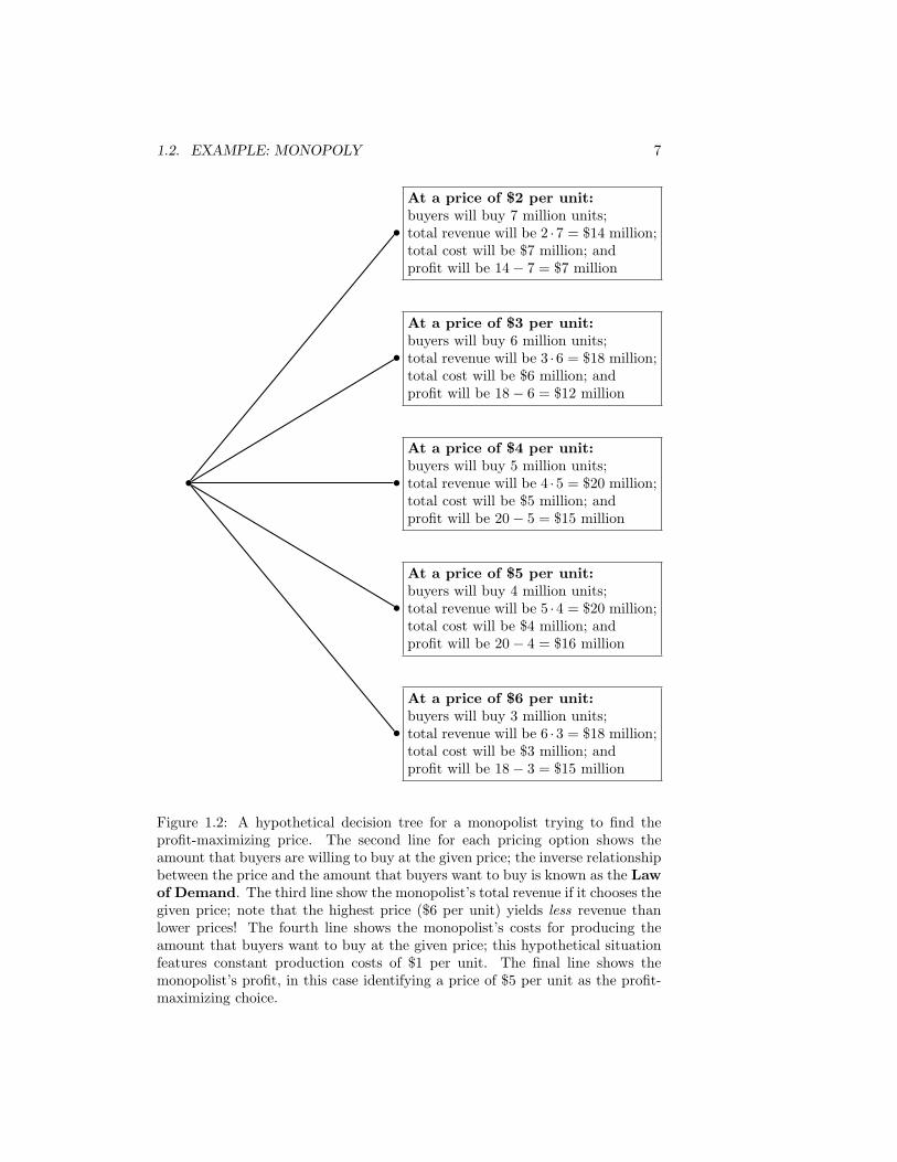
Second, we can catch a glimpse of the monopolist’s fundamental problem:it faces a trade-off between profit margin (making a lot of money on each unitby charging a high price) and volume (making a lot of money by selling a lot ofunits) The decision tree in Figure 1.2 shows some of the different price optionsfor a hypothetical monopolist; it also shows that a higher price will drive awaycustomers, thereby reducing the quantity that it sells. (This inverse relationshipbetween price and the quantity that customers want to buy is formally knownas the Law of Demand.) The monopolist would like to sell a large quantityfor a high price, but it is forced to choose between selling a smaller quantityfor a high price and selling a larger quantity for a low price. The decision treeshows that the monopolist’s optimal choice in the example is to choose a priceof $5 per unit.
2For this reason, monopolists are also known as price-setting firms, whereas firms in acompetitive market are known as price-taking firms.
3More progress can be made in this direction by studying government-regulated mo-
nopolies that are guaranteed a certain profit level by the government. Such firms are notalways allowed to keep cost savings that they find.
1.2. EXAMPLE: MONOPOLY 7
At a price of $2 per unit:buyers will buy 7 million units;total revenue will be 2 ·7 = $14 million;total cost will be $7 million; andprofit will be 14 − 7 = $7 million
At a price of $3 per unit:buyers will buy 6 million units;total revenue will be 3 ·6 = $18 million;total cost will be $6 million; andprofit will be 18 − 6 = $12 million
At a price of $4 per unit:buyers will buy 5 million units;total revenue will be 4 ·5 = $20 million;total cost will be $5 million; andprofit will be 20 − 5 = $15 million
At a price of $5 per unit:buyers will buy 4 million units;total revenue will be 5 ·4 = $20 million;total cost will be $4 million; andprofit will be 20 − 4 = $16 million
At a price of $6 per unit:buyers will buy 3 million units;total revenue will be 6 ·3 = $18 million;total cost will be $3 million; andprofit will be 18 − 3 = $15 million
Figure 1.2: A hypothetical decision tree for a monopolist trying to find theprofit-maximizing price. The second line for each pricing option shows theamount that buyers are willing to buy at the given price; the inverse relationshipbetween the price and the amount that buyers want to buy is known as the Lawof Demand. The third line show the monopolist’s total revenue if it chooses thegiven price; note that the highest price ($6 per unit) yields less revenue thanlower prices! The fourth line shows the monopolist’s costs for producing theamount that buyers want to buy at the given price; this hypothetical situationfeatures constant production costs of $1 per unit. The final line shows themonopolist’s profit, in this case identifying a price of $5 per unit as the profit-maximizing choice.

8 CHAPTER 1. DECISION THEORY
1.3 Math: Optimization and Calculus
Derivatives in theory
The derivative of a function f(x), writtend
dx[f(x)] or
d f(x)
dxor f ′(x), mea-
sures the instantaneous rate of change of f(x):
d
dx[f(x)] = lim
h→0
f(x + h) − f(x)
h.
Intuitively, derivatives measures slope: f ′(x) = −3 intuitively means that ifx increases by 1 then f(x) will decrease by 3. This intuition matches up withsetting h = 1, which yields
f ′(x) ≈ f(x + 1) − f(x)
1= f(x + 1) − f(x).
All of the functions we use in this class have derivatives (i.e., are differ-entiable), which intuitively means that they are smooth and don’t have kinksor discontinuities. The maximum and minimum values of such functions musteither be corner solutions—such as x = ∞, x = −∞, or (if we are trying tomaximize f(x) subject to x ≥ xmin) x = xmin—or interior solutions. Thevast majority of the problems in this class will have interior solutions.
At an interior maximum or minimum, the slope f ′(x) must be zero. Why?Well, if f ′(x) 6= 0 then either f ′(x) > 0 or f ′(x) < 0. Intuitively, this means thatyou’re on the side of a hill—if f ′(x) > 0 you’re going uphill, if f ′(x) < 0 you’reheading downhill—and if you’re on the side of a hill then you’re not at the top(a maximum) or at the bottom (a minimum). At the top and the bottom theslope f ′(x) will be zero.
To say the same thing in math: If f ′(x) 6= 0 then either f ′(x) > 0 orf ′(x) < 0. If f ′(x) > 0 then f(x + h) > f(x) (this comes from the definition ofderivative), so f(x) isn’t a maximum; and f(x − h) < f(x) (this follows fromcontinuity, i.e., the fact that f(x) is a smooth function), so f(x) isn’t a minimum.Similarly, if f ′(x) < 0 then f(x + h) < f(x) (this comes from the definition ofderivative), so f(x) isn’t a minimum; and f(x − h) > f(x) (this follows fromcontinuity), so f(x) isn’t a maximum. So the only possible (interior) maximaor minima must satisfy f ′(x) = 0, which is called a necessary first-ordercondition.
In sum: to find candidate values for (interior) maxima or minima, simply takea derivative and set it equal to zero, i.e., find values of x that satisfy f ′(x) = 0.
Such values do not have to be maxima or minima: the condition f ′(x) = 0is necessary but not sufficient. This is a more advanced topic that we willnot get into in this course, but for an example consider f(x) = x3. Settingthe derivative (3x2) equal to zero has only one solution: x = 0. But x = 0 is

1.3. MATH: OPTIMIZATION AND CALCULUS 9
neither a minimum nor a maximum value of f(x) = x3. The sufficient second-order condition has to do with the second derivative (i.e., the derivative of thederivative, written f ′′(x)). For a maximum, the sufficient second-order conditionis f ′′(x) < 0; this guarantees that we’re on a hill, so together with f ′(x) = 0it guarantees that we’re on the top of the hill. For a minimum, the sufficientsecond-order condition is f ′′(x) > 0; this guarantees that we’re in a valley, sotogether with f ′(x) = 0 it guarantees that we’re at the bottom of the valley.)
Partial derivatives
For functions of two or more variables such as f(x, y), it is often useful tosee what happens when we change one variable (say, x) without changing theother variables. (For example, what happens if we walk in the north-southdirection without changing our east-west position?) What we end up with is the
partial derivative with respect to x of the function f(x, y), written∂
∂x[f(x, y)]
or fx(x, y):∂
∂x[f(x, y)] = lim
h→0
f(x + h, y) − f(x, y)
h.
Partial derivatives measure rates of change or slopes in a given direction: fx(x, y) =3y intuitively means that if x increases by 1 and y doesn’t change then f(x, y)will increase by 3y. Note that “regular” derivatives and partial derivatives mean
the same thing for a function of only one variable:d
dx[f(x)] =
∂
∂x[f(x)].
At an (interior) maximum or minimum of a smooth function, the slope mustbe zero in all directions. In other words, the necessary first-order conditions arethat all partials must be zero: fx(x, y) = 0, fy(x, y) = 0, etc. Why? For thesame reasons we gave before: if one of the partials—say, fy(x, y)—is not zero,then moving in the y direction takes us up or down the side of a hill, and so wecannot be at a maximum or minimum value of the function f(x, y).
In sum: to find candidate values for (interior) maxima or minima, simplytake partial derivatives with respect to all the variables and set them equal tozero, e.g., find values of x and y that simultaneously satisfy fx(x, y) = 0 andfy(x, y) = 0.
As before, these conditions are necessary but not sufficient. This is an evenmore advanced topic than before, and we will not get into it in this course; allI will tell you here is that (1) the sufficient conditions for a maximum includefxx < 0 and fyy < 0, but these aren’t enough, (2) you can find the sufficient con-ditions in most advanced textbooks, e.g., Silberberg and Suen’s The Structure
of Economics, and (3) an interesting example to consider is f(x, y) =cos(x)
cos(y)around the point (0, 0).
One final point: Single variable derivatives can be thought of as a degeneratecase of partial derivatives: there is no reason we can’t write fx(x) instead of

10 CHAPTER 1. DECISION THEORY
f ′(x) or∂
∂xf(x) instead of
d
dxf(x). All of these terms measure the same thing:
the rate of change of the function f(x) in the x direction.
Derivatives in practice
To see how to calculate derivatives, let’s start out with a very simple function:the constant function f(x) = c, e.g., f(x) = 2. We can calculate the derivativeof this function from the definition:
d
dx(c) = lim
h→0
f(x + h) − f(x)
h= lim
h→0
c − c
h= 0.
So the derivative of f(x) = c isd
dx(c) = 0. Note that all values of x are
candidate values for maxima and/or minima. Can you see why?4
Another simple function is f(x) = x. Again, we can calculate the derivativefrom the definition:
d
dx(x) = lim
h→0
f(x + h) − f(x)
h= lim
h→0
(x + h) − x
h= lim
h→0
h
h= 1.
So the derivative of f(x) = x isd
dx(x) = 1. Note that no values of the function
f(x) = x are candidate values for maxima or minima. Can you see why?5
A final simple derivative involves the function g(x) = c · f(x) where c is aconstant and f(x) is any function:
d
dx[c · f(x)] = lim
h→0
c · f(x + h) − c · f(x)
h= c · lim
h→0
f(x + h) − f(x)
h.
The last term on the right hand side is simply the derivative of f(x), so the
derivative of g(x) = c · f(x) isd
dx[c · f(x)] = c · d
dx[f(x)].
More complicated derivatives
To differentiate (i.e., calculate the derivative of) a more complicated function,use various differentiation rules to methodically break down your problem untilyou get an expression involving the derivatives of the simple functions shownabove.
The most common rules are those involving the three main binary operations:addition, multiplication, and exponentiation.
• Additiond
dx[f(x) + g(x)] =
d
dx[f(x)] +
d
dx[g(x)].
4Answer: All values of x are maxima; all values are minima, too! Any x you pick givesyou f(x) = c, which is both the best and the worst you can get.
5Answer: There are no interior maxima or minima of the function f(x) = x.

1.3. MATH: OPTIMIZATION AND CALCULUS 11
Example:d
dx[x + 2] =
d
dx[x] +
d
dx[2] = 1 + 0 = 1.
Example:d
dx
[3x2(x + 2) + 2x
]=
d
dx
[3x2(x + 2)
]+
d
dx[2x] .
• Multiplicationd
dx[f(x) · g(x)] = f(x) · d
dx[g(x)] + g(x) · d
dx[f(x)] .
Example:d
dx[3x] = 3 · d
dx[x] + x · d
dx[3] = 3(1) + x(0) = 3.
(Note: this also follows from the result thatd
dx[c · f(x)] = c · d
dx[f(x)].)
Example:d
dx[x(x + 2)] = x · d
dx[(x + 2)] + (x + 2) · d
dx[x] = 2x + 2.
Example:d
dx
[3x2(x + 2)
]= 3x2 · d
dx[(x + 2)] + (x + 2) · d
dx
[3x2
].
• Exponentiationd
dx[f(x)a] = a · f(x)a−1 · d
dx[f(x)] .
Example:d
dx
[(x + 2)2
]= 2(x + 2)1 · d
dx[x + 2] = 2(x + 2)(1) = 2(x + 2).
Example:d
dx
[
(2x + 2)1
2
]
=1
2(2x + 2)−
1
2 · d
dx[2x + 2] = (2x + 2)−
1
2 .
Putting all these together, we can calculate lots of messy derivatives:
d
dx
[3x2(x + 2) + 2x
]=
d
dx
[3x2(x + 2)
]+
d
dx[2x]
= 3x2 · d
dx[x + 2] + (x + 2) · d
dx
[3x2
]+
d
dx[2x]
= 3x2(1) + (x + 2)(6x) + 2
= 9x2 + 12x + 2
Subtraction and division
The rule for addition also works for subtraction, and can be seen by treatingf(x) − g(x) as f(x) + (−1) · g(x) and using the rules for addition and mul-tiplication. Less obviously, the rule for multiplication takes care of division:d
dx
[f(x)
g(x)
]
=d
dx
[f(x) · g(x)−1
]. Applying the product and exponentiation
rules to this yields the quotient rule,6
6Popularly remembered as d
[Hi
Ho
]
=Ho · dHi − Hi · dHo
Ho · Ho.

12 CHAPTER 1. DECISION THEORY
• Divisiond
dx
[f(x)
g(x)
]
=g(x) · d
dxf(x) − f(x) · d
dxg(x)
[g(x)]2 .
Example:d
dx
[3x2 + 2
−ex
]
=−e2 · d
dx[3x2 + 2] − (3x2 + 2) · d
dx[−ex]
[−ex]2 .
Exponents
If you’re confused about what’s going on with the quotient rule, you may findvalue in the following rules about exponents, which we will use frequently:
xa · xb = xa+b (xa)b
= xab x−a =1
xa(xy)a = xaya
Examples: 22 · 23 = 25, (22)3 = 26, 2−2 = 14 , (2 · 3)2 = 22 · 32.
Other differentiation rules: ex and ln(x)
You won’t need the chain rule, but you may need the rules for derivativesinvolving the exponential function ex and the natural logarithm function ln(x).(Recall that e and ln are inverses of each other, so that e(ln x) = ln(ex) = x.)
• The exponential functiond
dx
[
ef(x)]
= ef(x) · d
dx[f(x)] .
Example:d
dx[ex] = ex · d
dx[x] = ex.
Example:d
dx
[
e3x2+2]
= e3x2+2 · d
dx
[3x2 + 2
]= e3x2+2 · (6x).
• The natural logarithm functiond
dx[ln f(x)] =
1
f(x)· d
dx[f(x)] .
Example:d
dx[lnx] =
1
x· d
dx[x] =
1
x.
Example:d
dx
[ln(3x2 + 2)
]=
1
3x2 + 2· d
dx
[3x2 + 2
]=
1
3x2 + 2(6x).
Partial derivatives
Calculating partial derivatives (say, with respect to x) is easy: just treat all theother variables as constants while applying all of the rules from above. So, forexample,
∂
∂x
[3x2y + 2exy − 2y
]=
∂
∂x
[3x2y
]+
∂
∂x[2exy] − ∂
∂x[2y]
= 3y∂
∂x
[x2
]+ 2exy ∂
∂x[xy] − 0
= 6xy + 2yexy.
1.3. MATH: OPTIMIZATION AND CALCULUS 13
Note that the partial derivative fx(x, y) is a function of both x and y. Thissimply says that the rate of change with respect to x of the function f(x, y)depends on where you are in both the x direction and the y direction.
We can also take a partial derivative with respect to y of the same function:
∂
∂y
[3x2y + 2exy − 2y
]=
∂
∂y
[3x2y
]+
∂
∂y[2exy] − ∂
∂y[2y]
= 3x2 ∂
∂y[y] + 2exy ∂
∂y[xy] − 2
= 3x2 + 2xexy − 2.
Again, this partial derivative is a function of both x and y.
Integration
The integral of a function, written∫ b
af(x) dx, measures the area under the
function f(x) between the points a and b. We won’t use integrals much, butthey are related to derivatives by the Fundamental Theorem(s) of Calculus:
∫ b
a
d
dx[f(x)] dx = f(b) − f(a)
d
ds
[∫ s
a
f(x) dx
]
= f(s)
Example:
∫ 1
0
x dx =
∫ 1
0
d
dx
[1
2x2
]
dx =1
2(12) − 1
2(02) =
1
2
Example:d
ds
[∫ s
0
x dx
]
= s.
Problems
1. A newspaper column in the summer of 2000 complained about the over-whelming number of hours being devoted to the Olympics by NBC and itsaffiliated cable channels. The columnist argued that NBC had establishedsuch an extensive programming schedule in order to recoup the millionsof dollars it had paid for the rights to televise the games. Do you believethis argument? Why or why not?
2. You win $1 million in the lottery, and the lottery officials offer you thefollowing bet: You flip a coin; if it comes up heads, you win an addi-tional $10 million. If it comes up tails, you lose the $1 million. Will theamount of money you had prior to the lottery affect your decision? (Hint:What would you do if you were already a billionaire? What if you werepenniless?) What does this say about the importance of sunk costs?

14 CHAPTER 1. DECISION THEORY
3. Alice the axe murderer is on the FBI’s Ten Most Wanted list for killing sixpeople. If she is caught, she will be convicted of these murders. The statelegislature decides to get tough on crime, and passes a new law sayingthat anybody convicted of murder will get the death penalty. Does thisserve as a deterrent for Alice, i.e., does the law give Alice an incentive tostop killing people? Does the law serve as a deterrent for Betty, who isthinking about becoming an axe murderer but hasn’t killed anybody yet?
4. A pharmaceutical company comes out with a new pill that prevents bald-ness. When asked why the drug costs so much, the company spokesmanreplies that the company needs to recoup the $10 billion it spent on re-search and development.
(a) Do you believe the spokesman’s explanation?
(b) If you said “Yes” above: Do you think the company would havecharged less for the drug if it had discovered it after spending only$5 million instead of $10 billion?
If you said “No” above: What alternative explanation might helpexplain why the drug company charges so much for its pill?
Calculus Problems
C-1. Explain the importance of taking derivatives and setting them equal tozero.
C-2. Use the definition of a derivative to prove that constants pass throughderivatives, i.e., that d
dx[(c · f(x)] = c · d
dx[f ′(x)].
C-3. Use the product rule to prove that the derivative of x2 is 2x. (Challenge:Do the same for higher-order integer powers, e.g., x30. Do not do this thehard way.)
C-4. Use the product and exponent rules to derive the quotient rule.
C-5. For each of the following functions, calculate the first derivative, the sec-ond derivative, and determine maximum and/or minimum values (if theyexist):
(a) x2 + 2
(b) (x2 + 2)2
(c) (x2 + 2)1
2
(d) −x(x2 + 2)1
2
(e) ln[
(x2 + 2)1
2
]
C-6. Calculate partial derivatives with respect to x and y of the following func-tions:

1.3. MATH: OPTIMIZATION AND CALCULUS 15
(a) x2y − 3x + 2y
(b) exy
(c) exy2 − 2y
C-7. Consider a market with demand curve q = 20 − 2p.
(a) Calculate the slope of the demand curve, i.e.,dq
dp. Is it positive or
negative? Does the sign of the demand curve match your intuition,i.e., does it make sense?
(b) Solve the demand curve to get p as a function of q. This is called aninverse demand curve.
(c) Calculate the slope of the inverse demand curve, i.e.,dp
dq. Is it related
to the slope of the demand curve?
C-8. Imagine that a monopolist is considering entering a market with demandcurve q = 20− p. Building a factory will cost F , and producing each unitwill cost 2 so its profit function (if it decides to enter) is π = pq − 2q −F .
(a) Substitute for p using the inverse demand curve and find the (interior)profit-maximizing level of output for the monopolist. Find the profit-maximizing price and the profit-maximizing profit level.
(b) For what values of F will the monopolist choose not to enter themarket?
C-9. (Profit maximization for a firm in a competitive market) Profit is π =p · q − C(q). If the firm is maximizing profits and takes p as given, findthe necessary first order condition for an interior solution to this problem,
both in general and in the case where C(q) =1
2q2 + 2q.
C-10. (Profit maximization for a non-price-discriminating monopolist) A mo-nopolist can choose both price and quantity, but choosing one essentiallydetermines the other because of the constraint of the market demandcurve: if you choose price, the market demand curve tells you how manyunits you can sell at that price; if you choose quantity, the market de-mand curve tells you the maximum price you can charge while still sellingeverything you produce. So: if the monopolist is profit-maximizing, findthe necessary first order condition for an interior solution to the monopo-list’s problem, both in general and in the case where the demand curve is
q = 20 − p and the monopolist’s costs are C(q) =1
2q2 + 2q.
C-11. (Derivation of Marshallian demand curves) Considered an individual whosepreferences can be represented by the utility function
U =
(100 − pZ · Z
pB
· Z) 1
2
.

16 CHAPTER 1. DECISION THEORY
If the individual chooses Z to maximize utility, find the necessary firstorder condition for an interior solution to this problem. Simplify to get
the Marshallian demand curve Z =50
pZ
.
C-12. Challenge (Stackleberg leader-follower duopoly) Consider a model withtwo profit-maximizing firms, which respectively produce q1 and q2 unitsof some good. The inverse demand curve is given by p = 20 − Q =20 − (q1 + q2).) Both firms have costs of C(q) = 2q. In this market, firm1 gets to move first, so the game works like this: firm 1 chooses q1, thenfirm 2 chooses q2, then both firms sell their output at the market pricep = 20 − (q1 + q2).
(a) Write down the maximization problem for Firm 1. What is/are itschoice variable(s)?
(b) Write down the maximization problem for Firm 2. What is/are itschoice variable(s)?
(c) What’s different between the two maximization problems? (Hint:Think about the timing of the game!) Think hard about this questionbefore going on!
(d) Take the partial derivative (with respect to q2) of Firm 2’s objectivefunction (i.e., the thing Firm 2 is trying to maximize) to find thenecessary first order condition for an interior solution to Firm 2’sproblem.
(e) Your answer to the previous problem should show how Firm 2’s choiceof q2 depends on Firm 1’s choice of q1, i.e., it should be a bestresponse function. Explain why this function is important to Firm1.
(f) Plug the best response function into Firm 1’s objective function andfind the necessary first order condition for an interior solution to Firm1’s problem.
(g) Solve this problem for q1, q2, p, and the profit levels of the two firms.Is there a first mover advantage or a second mover advantage?Can you intuitively understand why?

Chapter 2
Optimization and Risk
Motivating question: What is the maximum amount $x you would pay toplay a game in which you flip a coin and get $10 if it comes up heads and $0otherwise? (See Figure 2.1.)
The important issue in this game is your attitude toward risk. People whoare risk-averse buckle their seatbelts and drive safely and buy insurance andotherwise try to avoid risk; if you are this type of person you will be unwillingto pay $5 or more to play this game. People who are risk-loving go skydiving,drive crazy, or engage in other risk-seeking behaviors; if you are this type ofperson, you might be willing to pay more than $5 to play this game (or othertypes of risk games like the lottery or Las Vegas). People who are risk-neutralare ambivalent about risk; if you are this type of person, you’d be willing toplay this game for less than $5, you’d avoid playing the game for more than $5,and you would be indifferent about playing the game for exactly $5.
What’s the Deal with $5?
The deal is that $5 is the expected value of this game. Since you have a50% chance of getting $10 and a 50% chance of getting $0, it makes some senseto say that on average you’ll get $5. (Section 2.1 fleshes out this idea.) The
Gain nothing,lose nothingRefuse bet
50%: Win $10 − x
50%: Lose $xTake bet
Figure 2.1: A decision tree involving risk
17

18 CHAPTER 2. OPTIMIZATION AND RISK
concept of expected value provides a valuable perspective by condensing thisrisky situation into a single number. Note, however, that it conveys only oneperspective. In describing the average outcome, expected value fails to captureother aspects, such as the variability of the outcome.1
Mathematically, an expected value calculation weighs each possible outcomeby its likelihood, giving more weight to more likely outcomes and less weight toless likely outcomes. To calculate expected value, sum probability times valueover all possible outcomes:
Expected Value =∑
Outcomes i
Probability(i) · Value(i).
The Greek letter∑
(“sigma”) is the mathematical notation for summation,
e.g.,∑
y=1,2,3
y2 = 12+22+32 = 14. In the game described above, the two possible
outcomes are heads (H) and tails (T), so the expected value is
EV = Pr(H) · ($10) + Pr(T ) · ($0)
=1
2· ($10) +
1
2· ($0)
= $5.
If it costs $x to play the game, the overall expected value becomes $(5 − x).
Example: Fair and Unfair Bets
A fair bet is a bet with an expected value of zero. Flipping a coin and havingme pay you $x if it comes up heads and you pay me $x if it comes up tails isa fair bet (provided, of course, that the coin is not weighted). If x = 5, this isidentical to the game above in which you pay me $5 and then I pay you $10 ifthe coin comes up heads and nothing if the coin comes up tails.
An unfair bet is one with a expected value less than zero. If you go to acasino and play roulette, for example, you will see that the roulette wheel has38 numbers (the numbers 1–36, plus 0 and 00). If you bet $1 and guess theright number, you get back $36 (the dollar you bet plus 35 more); if you guessthe wrong number, you get back $0. So if you bet $1 on, say, number 8, thenthe expected value of the amount you’ll get back is
Pr(8) · ($36) + Pr(Not 8) · ($0) =1
38· ($36) +
37
38· ($0) ≈ $0.95.
Since it costs $1 to play and your expected return is only $0.95, the overallexpected value of betting $1 in roulette is −$0.05. So roulette, like other casinogames, is an unfair bet.
1The concept of variance attempts to convey this part of the story.

2.1. REDUCING RISK WITH DIVERSIFICATION 19
2.1 Reducing Risk with Diversification
Playing roulette once is obviously a high-risk endeavor. (Presumably this is partof what makes it attractive to gamblers.) It would therefore seem that owninga casino would also be a high-risk endeavor. But this is not the case.
To see why, consider flipping a fair coin, one where the probability of gettingheads is 50%. Flip the coin once, and the actual percentage of heads will beeither 0% or 100%. (In other words, the coin either comes up heads or it comesup tails.) Flip the coin twenty times, though, and the percentage of heads islikely to be pretty close to 50%. (Specifically, your odds are better than 7 in10 that the percentage of heads will be between 40% and 60%.) Flip the coinone hundred times and the odds are better than 95 in 100 that the percentageof heads will be between 40% and 60%. And flip the coin one thousand timesand the odds are better than 998 in 1000 that the percentage of heads will bebetween 45% and 55%.
These results stem from a statistical theorem called the law of large num-bers. In English, the law of large numbers says that if you flip a (fair) coin alarge number of times, odds are that the proportion of heads will be close to50%. (Details online2 and online3.) By extension, if each of a large number ofcoin flips pays $10 for heads and $0 for tails, odds are that you’ll come close toaveraging $5 per coin flip. It is no coincidence that $5 also happens to be theexpected value of this bet: repeat any bet a large number of times and odds arethat the payout per bet will be close to the expected value of the bet. This isthe sense in which expected value can be thought of as the average payout of abet.
Risk and roulette
To apply the law of large numbers to casinos, note that an individual gamblerwill play roulette only a few times, but that the casino plays roulette thousandsof times each day. The law of large numbers does not apply to the individualgambler, but it does apply to the casino. As a consequence, the individualgambler faces a great deal of risk, but the casino does not. Since the expectedvalue from betting $1 on roulette is −$0.05, odds are extremely good that thecasino will gain about $0.05 for each dollar wagered. As long as the mob doesn’tget involved, then, running a casino is not necessarily any riskier than running,say, a photocopy shop. (Go online4 for an amusing story that illustrates thispoint.)
Risk and the stock market
Another application of the law of large numbers is in the stock market, whereinvestors are often advised to diversify their portfolios. Compared to owning
2http://www.stat.berkeley.edu/˜stark/Java/lln.htm3http://www.ruf.rice.edu/˜lane/stat sim/binom demo.html4http://www.theonion.com/onion3920/casino has great night.html
20 CHAPTER 2. OPTIMIZATION AND RISK
one or two stocks, investors can reduce risk by owning many stocks. (One wayto do this is to own shares of mutual funds or index funds, companies whoseline of business is investing money in the stock market.)
To see how diversification can reduce risk, consider a coin flip that pays$100 if it comes up heads (H) and $0 if it comes up tails (T). The risk in thissituation is clear: either you win the whole $100 or you win nothing.
Now consider flipping two coins, each independently paying $50 for headsand $0 for tails. The four possible outcomes—all equally likely—are HH (paying$100), HT (paying $50), TH (paying $50), and TT (paying $0). Note that theexpected value in this situation is $50:
EV = Pr(HH) · ($100) + Pr(HT ) · ($50) + Pr(TH) · ($50) + Pr(TT ) · ($0)
=1
4· ($100) +
1
4· ($50) +
1
4· ($50) +
1
4· ($0) = $50.
This is the same expected value as in the one-coin flip situation described above.Compared to the one-coin flip, however, this two-coin flip is less risky: insteadof always winning everything or nothing, there is now a 50% chance of winningsomething in between. A risk-averse individual should prefer the two-coin flipover the one-coin flip because it has less variability. (In the language of statistics,the two-coin flip has lower variance. In English, the two-coin flip means thatyou aren’t putting all your eggs in one basket.)
The risk inherent in coin-flipping (or stock-picking) can be reduced evenfurther by spreading the risk out even more, i.e., through diversification. Fliptwenty coins, each independently paying $5 for heads and $0 for tails, and theprobability of getting an outcome that is “in the middle” (say, between $40 and$60) is over 70%. Flip one hundred coins, each independently paying $1 forheads and $0 for tails, and the odds of ending up between $40 and $60 is over95%. And flip one thousand coins, each independently paying $0.10 for headsand $0 for tails, and there is a 99.86% chance that you will end up with anamount between $45 and $55. The expected value in all of these situations is$50; what diversification does is reduce variance, so that with one thousand coinflips you are virtually guaranteed to end up with about $50.
These coin-flipping results follow directly from the law of large numbers. It isimportant to note, however, that there is an important difference between coin-flipping and stock-picking: while the outcome of one coin flip has no influenceon the outcome of the next coin flip, stocks have a tendency to go up or downtogether. (In statistical terms, coin flips are independent while the prices ofdifferent stocks are correlated.) The law of large numbers applies to risksthat are independent, so diversification of a stock market portfolio can reduceor eliminate risks that affect companies independently. But the law of largenumbers does not apply when risks are correlated: diversification cannot reducethe risk of stock market booms or busts or other systemic risks that affect theentire economy.
A final point is that diversification is not always painless. It’s easy to di-versify if you have no preference for one stock over another—and Chapter 6

2.2. MATH: EXPECTED VALUE AND INDIFFERENCE CURVES 21
suggests that this is a reasonable position to take. But if you have favoritesthen you have to balance risks against rewards: investing your life savings inyour favorite stock may give you the highest expected payoff, but it also ex-poses you to a great deal of risk; diversifying your portfolio reduces risk, but itmay also reduce your expected payoff. The optimal behavior in such situationsis the subject of portfolio selection theory, a branch of economics whosedevelopment helped win James Tobin the Nobel Prize in Economics in 1981.Professor Tobin died in 2002; his obituary in the New York Times (availableonline5) included the following story:
After he won the Nobel Prize, reporters asked him to explain theportfolio theory. When he tried to do so, one journalist interrupted,“Oh, no, please explain it in lay language.” So he described the the-ory of diversification by saying: “You know, don’t put your eggs inone basket.” Headline writers around the world the next day createdsome version of “Economist Wins Nobel for Saying, ‘Don’t Put Eggsin One Basket’.”
2.2 Math: Expected Value and Indifference Curves
A more mathematical treatment of this material allows us to do two additionalthings, both related to expected utility. First, we can see that there is a relation-ship between the second derivative of the utility function and the individual’sattitude toward risk. This result follows from comparing E (u(w)) and u (E(w))using a theorem called Jensen’s Inequality. The end result is this:
• For a concave utility function (u′′ < 0, e.g., u(w) =√
w) Jensen’s Inequal-ity says that E [u(w)] < u [E(w)], so this individual is risk averse.
• For a convex utility function (u′′ > 0, e.g., u(w) = w2) Jensen’s Inequalitysays that E [u(w)] > u [E(w)], so this individual is risk loving.
• For a linear utility function (u′′ = 0, e.g., u(w) = w) Jensen’s Inequalitysays that E [u(w)] = u [E(w)], so this individual is risk neutral.
The second additional topic is indifference: we can ask when an individualis indifferent (i.e., has no preference) between one risky situation and another, orbetween a risky situation and a riskless one. For example, consider an individualwho has a 40% chance of having wealth w1 and a 60% chance of having wealthw2. Her utility function is u(w) =
√w, and she maximizes expected utility,
E[u(w)] = .4√
w1 + .6√
w2. If (w1, w2) = (0, 100), her expected utility is .4√
0+
.6√
100 = .6(10) = 6. If (w1, w2) = (225, 0) her expected utility is .4√
225 +.6√
0 = .4(15) = 6. Since her expected utility is the same in both cases, she isindifferent between them.
In fact, there are an infinite number of pairs (w1, w2) that satisfy E[u(w)] =6. Figure 2.2 shows a graph of these points, which is a called an indifference
5http://cowles.econ.yale.edu/archive/people/tobin/nyt obit.htm

22 CHAPTER 2. OPTIMIZATION AND RISK
w2
w1
(0, 100)
(225, 0)
(36, 36)
Figure 2.2: An indifference curve corresponding to expected utility of 6
curve. In this case, the indifference curve corresponds to an expected utility of6: every point (w1, w2) on the curve gives our individual an expected utility of6, and so she is indifferent between any two of them.
In particular, note that the point (w1, w2) = (36, 36) lies on this indifferencecurve: E[u(w)] = .4
√36 + .6
√36 =
√36 = 6. In this situation our individual
has a 40% chance of having wealth w1 = 36 and a 60% chance of having wealthw2 = 36, i.e., a 100% chance of having wealth w = 36. This amount of wealth istherefore called the certainty equivalent wealth corresponding to an expectedutility of 6.
Example: An individual with initial wealth of 400 has a 10% chance of gettingin an accident. If she gets in an accident, she will lose 300; if she doesn’t,she loses nothing. She maximizes expected utility, and her utility function isu(w) =
√w.
1. What is the expected amount of money she will lose?
2. What is her expected utility?
3. What is her certainty equivalent wealth?
4. What is the maximum amount she would pay for full insurance? (Note:Full insurance totally insulates her from the risk of an accident. If shepays x for full insurance, her wealth will be 400− x regardless of whetheror not she gets in an accident.)
5. How much more is she willing to pay for insurance than would a risk-neutral individual? (This amount is called her risk premium.)
Answer: Her expected loss is .1(300) + .9(0) = 30. Her expected utility is.1√
400 − 300 + .9√
400 − 0 = 19. Her certainty equivalent wealth is w such

2.2. MATH: EXPECTED VALUE AND INDIFFERENCE CURVES 23
that having wealth of w with probability 1 gives her an expected utility of 19:√w = 19 =⇒ w = 361.
The maximum amount she would pay for full insurance is 400 − 361 = 39.This payment makes her indifferent between buying insurance, in which caseE[u(w)] = .1
√400 − 39 + .9
√400 − 39 =
√361 = 19, and not buying insurance,
in which case E[u(w)] = .1√
400 − 300+ .9√
400 − 0 = 19. To look at it anotherway: if she is offered insurance for some amount x < 39, she will take it becauseu(400 − x) > 19; if she is offered insurance for some amount x > 39, she willrefuse it because u(400 − x) < 19; if she is offered insurance for x = 39 she willbe indifferent between accepting and rejecting.
Finally, we can calculate her risk premium in this situation. She is willingto pay up to 39 for full insurance, but her expected loss is only 30; since a riskneutral individual would pay a maximum of 30 for full insurance, the difference(39 − 30 = 9) is her risk premium. Its source is risk aversion: our individual iswilling to pay money to avoid a fair bet. We can see that she is risk averse bycalculating the second derivative of the utility function u(w) =
√w: u′(w) =
12w−
1
2 , so u′′(w) = − 14w−
3
2 < 0.
Problems
1. You roll a six-sided die and win that amount (minimum $1, maximum $6).What is the expected value of this game?
2. With probability 1/3 you win $99, with probability 2/3 you lose $33.What is the expected value of this game?
3. Fun/Challenge (The Monty Hall Problem) The Monty Hall Problem getsits name from the TV game show Let’s Make A Deal, hosted by MontyHall. The scenario is this: Monty shows you three closed doors. Behindone of these doors is a new car. Behind the other two doors are goats (orsome other “non-prize”). Monty asks you to choose a door, but after youdo he does not show you what is behind the door you chose. Instead, heopens one of the other doors, revealing a goat, and then offers you theopportunity to switch to the remaining unopened door. [As an example,say you originally pick Door #1. Monty opens up Door #2, revealing agoat, and then offers you the opportunity to switch to from Door #1 toDoor #3.] What should you do?
4. Imagine that you are taking a multiple-guess exam. There are five choicesfor each question; a correct answer is worth 1 point, and an incorrectanswer is worth 0 points. You are on Problem #23, and it just so happensthat the question and possible answers for Problem #23 are in Hungarian.(When you ask your teacher, she claims that the class learned Hungarianon Tuesday. . . .)
(a) You missed class on Tuesday, so you don’t understand any Hungarian.What is the expected value of guessing randomly on this problem?

24 CHAPTER 2. OPTIMIZATION AND RISK
(b) Now imagine that your teacher wants to discourage random guessingby people like you. To do this, she changes the scoring system, sothat a blank answer is worth 0 points and an incorrect answer isworth x, e.g., x = − 1
2 . What should x be in order to make randomguessing among five answers a fair bet (i.e., one with an expectedvalue of 0)?
(c) Is the policy you came up with in the previous part going to dis-courage test-takers who are risk-averse? What about those who arerisk-loving?
(d) Your teacher ends up choosing x = − 13 , i.e., penalizing people 1/3rd
of a point for marking an incorrect answer. How much Hungarianwill you need to remember from your childhood in order to makeguessing a better-than-fair bet? In other words, how many answerswill you need to eliminate so that guessing among the remaininganswers yields an expected value strictly greater than 0?
5. Two businesses that involve lots of gambling are the casino business andthe insurance business. Are these businesses particularly risky to get in-volved in? Explain why or why not.
6. Howard Raiffa’s book Decision Analysis: Introductory Lectures on ChoicesUnder Uncertainty (New York: McGraw-Hill, 1997) does an extensiveanalysis of variations on the following basic problem.
There are 1,000 urns. Eight hundred of them are of type U1; each of thesecontain four red balls and six black balls. The remaining two hundred areof type U2; each of these contain nine red balls and one black ball. Oneof these 1,000 urns is chosen at random and placed in front of you; youcannot identify its type or see the balls inside it. Which one of the followingoptions maximizes your expected value, and what is that expected value?
Option 1 Guess that the urn is of type U1. If you are correct, you win$40.00. Otherwise, you lose $20.00.
Option 2 Guess that the urn is of type U2. If you are correct, you win$100.00. Otherwise, you lose $5.00.
Option 3 Refuse to play the game.
7. Challenge (One variation) Prior to choosing one of the three options de-scribed above, you can conduct at most one of the following investigations.(Note that you can also choose not to conduct any of these.) What strat-egy maximized your expected value, and what is that expected value?
Investigation 1 For a payment of $8.00, you can draw a single ball atrandom from the urn.
Investigation 2 For a payment of $12.00, you can draw two balls fromthe urn.
2.2. MATH: EXPECTED VALUE AND INDIFFERENCE CURVES 25
Investigation 3 For a payment of $9.00, you can draw a single ball fromthe urn, and then (after looking at it) decide whether or not youwant to pay $4.50 to draw another ball. (Whether or not you wantto replace the first ball before drawing the second is up to you.)
8. You’re a bidder in an auction for an antique vase. If you lose the auction,you get nothing. If you win the auction, assume that your gain is thedifference between the maximum amount you’d be willing to pay for thevase (say, $100) and the actual amount that you end up paying. (So ifyou pay $80, your gain is $20.)
(a) In a first-price sealed bid auction, you write down your bid b ona piece of paper and submit it to the auctioneer in a sealed envelope.After all the bids have been submitted, the auctioneer opens theenvelopes and finds the highest bidder. That bidder gets the item,and pays a price equal to their bid. If the probability of winning witha bid of b is Pr(b), write down an expected value calculation for thisauction.
(b) In a second-price sealed bid auction, everything’s the same ex-cept that the winning bidder (the person with the highest bid) pays aprice equal to the second-highest bid. Write down an expected valuecalculation for this auction if the probability of winning with a bidof b is Pr(b) and the highest bid less than b is c.
(c) Challenge From your answers above, can you figure out what kindof strategy (i.e., what bid b) will maximize your expected value inthe different auctions? In particular: should you bid your true value,b = $100, or should you bid more or less than your true value? (We’llstudy auctions more in Chapter 12.)

26 CHAPTER 2. OPTIMIZATION AND RISK
Chapter 3
Optimization over Time
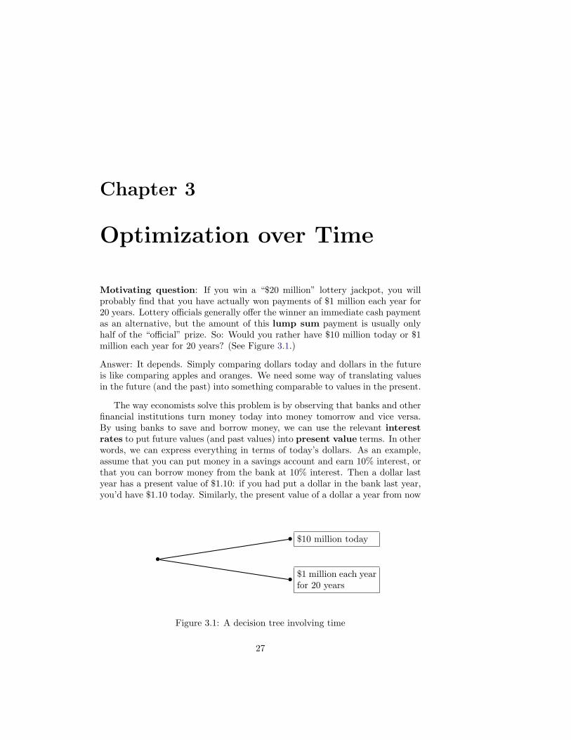
Motivating question: If you win a “$20 million” lottery jackpot, you willprobably find that you have actually won payments of $1 million each year for20 years. Lottery officials generally offer the winner an immediate cash paymentas an alternative, but the amount of this lump sum payment is usually onlyhalf of the “official” prize. So: Would you rather have $10 million today or $1million each year for 20 years? (See Figure 3.1.)
Answer: It depends. Simply comparing dollars today and dollars in the futureis like comparing apples and oranges. We need some way of translating valuesin the future (and the past) into something comparable to values in the present.
The way economists solve this problem is by observing that banks and otherfinancial institutions turn money today into money tomorrow and vice versa.By using banks to save and borrow money, we can use the relevant interestrates to put future values (and past values) into present value terms. In otherwords, we can express everything in terms of today’s dollars. As an example,assume that you can put money in a savings account and earn 10% interest, orthat you can borrow money from the bank at 10% interest. Then a dollar lastyear has a present value of $1.10: if you had put a dollar in the bank last year,you’d have $1.10 today. Similarly, the present value of a dollar a year from now
$10 million today
$1 million each yearfor 20 years
Figure 3.1: A decision tree involving time
27
28 CHAPTER 3. OPTIMIZATION OVER TIME
is about $.91: put $.91 in the bank today and in a year you’ll have about $1.00.So we can use interest rates to compare apples to apples instead of apples tooranges.
3.1 Lump Sums
Question: Say you’ve got $100 in a Swiss bank account at a 5% annual interestrate. How much will be in the account after 30 years?
Answer:
After 1 year: $100(1.05) = $100(1.05)1 = $105.00
After 2 years: $105(1.05) = $100(1.05)2 = $110.25
After 3 years: $110.25(1.05) = $100(1.05)3 = $115.76.
So after 30 years: $100(1.05)30 ≈ $432.19.
So the future value of a lump sum of $x invested for n years at interest rater is FV = x(1 + r)n. Although the future value formula can be useful in and ofitself, it also provides insight on the topic of present value:
Question: What if someone offers you $100 in 30 years; how much is that worthtoday if the interest rate is 5%?
Answer: The present value of $100 in 30 years is that amount of money which,if put in the bank today, would grow to $100 in 30 years.
Using the future value formula, we want to find x such that x(1.05)30 = 100.
Solving this we find that x =100
(1.05)30≈ $23.14. If you put $23.14 in the bank
today at 5% interest, after 30 years you’d have about $100.
So the present value of a lump sum payment of $x received at the endof n years at interest rate r is
PV =x
(1 + r)n.
3.2 Annuities
Question: What is the present value of receiving $100 at the end of each yearfor the next three years when the interest rate is 5%? (Unlike a lump sumpayment, we now have a stream of payments. A stream of annual payments iscalled an annuity.)
Idea: Imagine that you put those payments in a savings account when youreceive them. Now imagine another savings account into which you put someamount x today, and don’t make any more deposits or withdrawals, simplyletting the interest accumulate. Imagine that the two accounts have the same

3.2. ANNUITIES 29
balance after the third and final $100 deposit in account #1. Then the amountx is the present value of the annuity.
Answer: You’ve got three $100 payments. The present value of the first $100
payment, which comes after one year, is100
(1.05)1≈ 95.24. The present value of
the second $100 payment, which comes after two years, is100
(1.05)2≈ 90.70. And
the present value of the third $100 is100
(1.05)3≈ 86.38. So the present value of
the three payments together is about $95.24 + $90.70 + $86.38 = $272.32. Oneway to calculate the present value of an annuity, then, is to calculate the presentvalue of each year’s payment and then add them all together. Of course, thiscan get pretty tedious, e.g., if you’re trying to answer the lottery question atthe beginning of this chapter.
Is There an Easier Way?
Answer: Yes, and it involves some pretty mathematics. Here it is: We want tocalculate the present value (PV) of a 3-year $100 annuity:
PV =100
(1.05)1+
100
(1.05)2+
100
(1.05)3.
If we multiply both sides of this equation by 1.05, we get
1.05 · PV = 100 +100
(1.05)1+
100
(1.05)2.
Now we subtract the first equation from the second equation:
1.05 · PV − PV =
[
100 +100
(1.05)1+
100
(1.05)2
]
−[
100
(1.05)1+
100
(1.05)2+
100
(1.05)3
]
.
The left hand side of this equation simplifies to .05·PV. The right hand side alsosimplifies (all the middle terms cancel, hence the moniker telescoping seriesfor what mathematicians also call a geometric series), yielding
.05 · PV = 100 − 100
(1.05)3.
Dividing both sides by .05 and grouping terms, we get
PV = 100
1 − 1
(1.05)3
.05
.
This suggests an easier way of calculating annuities: At interest rate r, thepresent value of an annuity paying $x at the end of each year for the next

30 CHAPTER 3. OPTIMIZATION OVER TIME
n years is
PV = x
1 − 1
(1 + r)n
r
.
Example: Car Payments
Car dealers usually give buyers a choice between a lump sum payment (thecar’s sticker price of, say, $15,000) and a monthly payment option (say, $400 amonth for 36 months). The annuity formula can come in handy here becauseit allows you to compute the sticker price from the monthly payments, or viceversa. The applicability of the annuity formula stems from the fact that themonthly option essentially involves the dealer loaning you an amount of moneyequal to the sticker price. At the relevant interest rate, then, the sticker priceis the present value of the stream of monthly payments.
The only real complication here is that car payments are traditionally mademonthly, so we need to transform the dealer’s annual interest rate—the APR, orAnnual Percentage Rate—into a monthly interest rate. (Like the other formulasin this chapter, the annuity formula works not just for annual payments but alsofor payments made daily, weekly, monthly, etc. The only caveat is that you needto make sure that you use an interest rate r with a matching time frame, e.g.,a monthly interest rate for payments made monthly.) A good approximation ofthe monthly interest rate comes from dividing the annual interest rate by 12,so an APR of 6% translates into a monthly interest rate of about 0.5%, i.e.,r ≈ .005.1
With a monthly interest rate in hand, we can use the annuity formula totranslate monthly payment information (say, $400 a month for 36 months at0.5%) into a lump sum sticker price:
PV = 400
1 − 1
(1.005)36
.005
≈ $13, 148.
More frequently, you’ll want to transform the lump sum sticker price into amonthly payment amount, which you can do by solving the annuity formula forx, the monthly payment:
PV = x
1 − 1
(1 + r)n
r
=⇒ x = PV
r
1 − 1
(1 + r)n
.
1Because of compounding, a monthly interest rate of 0.5% actually corresponds to anannual interest rate of about 6.17%. See problem 11 for details and for information about acompletely accurate formula.

3.3. PERPETUITIES 31
Using this formula, we can figure out that a $15,000 sticker price with a 6%APR (i.e., a monthly interest rate of about 0.5%, i.e., r ≈ .005) translates into36 monthly payments of $456.33, or 60 monthly payments of $289.99.
3.3 Perpetuities
Question: What is the present value of receiving $100 at the end of each yearforever at a 5% interest rate?
Answer: Such a stream of payments is called a perpetuity,2 and it really isforever: after death, you can give the perpetuity away in your will! So whatwe’re looking for is
PV =100
(1.05)1+
100
(1.05)2+
100
(1.05)3+ . . .
To figure this out, we apply the same trick we used before. First multiplythrough by 1.05 to get
1.05 · PV = 100 +100
(1.05)1+
100
(1.05)2+
100
(1.05)3+ . . .
Then subtract the first term from the second term—note that almost everythingon the right hand side cancels!—to end up with
1.05 · PV − PV = 100.
This simplifies to PV =100
.05= $2, 000. In general, then, the present value of
a perpetuity paying $x at the end of each year forever at an interest rate ofr is
PV =x
r.
3.4 Capital Theory
We can apply the material from the previous sections to study investment de-cisions, also called capital theory. This topic has some rather unexpectedapplications, including natural resource economics.
Motivating question: You own a lake with a bunch of fish in it. You wantto maximize your profits from selling the fish. How should you manage thisresource? What information is important in answering this question?
Partial answer: The growth rate of fish, the cost of fishing (e.g., is fishing easierwith a bigger stock of fish?), the market price of fish over time. . . . Note thatone management option, called Maximum Sustainable Yield (MSY), is to
2Note that the word comes from perpetual, just like annuity comes from annual.

32 CHAPTER 3. OPTIMIZATION OVER TIME
(a) (b)
Figure 3.2: The Bank of America and the Bank of Fish
manage the lake so as to get the maximum possible catch that you can sustainyear after year forever, as shown in Figure 3.3. We will return to this optionshortly.
The key economic idea of this section is that fish are capital, i.e., fish arean investment, just like a savings account is an investment. To “invest in thefish”, you simply leave them alone, thereby allowing them to reproduce andgrow bigger so you can have a bigger harvest next year. This exactly parallelsinvesting in a savings account: you simply leave your money alone, allowing itto gain interest so you have a bigger balance next year.
In managing your lake, you need to compare your different options, whichare to invest in the bank (by catching and selling all the fish and putting theproceeds in the bank), or to invest in the fish (by not catching any of them,thereby allowing them to grow and reproduce to make more fish for next year),or some combination of the two (catching some of the fish and letting the restgrow and reproduce). This suggests that you need to compare the interest ratesyou get at the Bank of America with the interest rates you get at the Bank ofFish (see Figure 3.2).
This sounds easy, but there are lots of potential complications. To make theproblem tractable, let’s simplify matters by assuming that the cost of fishingis zero, that the market price of fish is constant over time at $1 per pound,and that the interest rate is 5%. Then one interesting result is that the profit-maximizing catch level is not the Maximum Sustainable Yield (MSY) definedabove and in Figure 3.3.
To see why, let’s calculate the present value of following MSY: each year youstart out with 100 pounds of fish, catch 10 pounds of fish, and sell them for $1
per pound, so the perpetuity formula gives us a present value of10
.05= $200.
Now consider an alternative policy: as before, you start out with 100 poundsof fish, but now you catch 32 pounds immediately, reducing the population to68. This lower population size corresponds to a sustainable yield of 9 pounds per

3.4. CAPITAL THEORY 33
100 200
5
10
Growth G(s)
Stock Size s
Figure 3.3: With an initial population of 100 pounds of fish, population growthover the course of one year amounts to 10 additional pounds of fish. Harvesting10 pounds returns the population to 100, at which point the process can beginagain. A population of 100 pounds of fish therefore produces a sustainableyield of 10 pounds per year; the graph shows that this is the maximum sus-tainable yield, i.e., the maximum amount that can be harvested year afteryear after year.
100 200
5
10
Growth G(s)
Stock Size s
68
9
Figure 3.4: With an initial population of about 68 pounds of fish, populationgrowth over the course of one year amounts to 9 additional pounds of fish,meaning that 9 pounds per year is the sustainable yield corresponding to aninitial population of 68 pounds of fish.

34 CHAPTER 3. OPTIMIZATION OVER TIME
year (as shown in Figure 3.4), so every year thereafter you can catch 9 pounds
of fish. The present value of this harvest policy is 32 +9
.05= $212, which is
more than the present value from the MSY policy!So MSY is not the optimal harvest plan: you can make more money by
catching additional fish and investing the proceeds in the Bank of America.Intuitively, the problem with the MSY policy is that population growth is aboutthe same whether you start out with 68 pounds of fish or 100 pounds of fish; atthe margin, then, the interest rate you’re getting at the Bank of Fish is reallylow. Since the return on those final 32 fish is so small, you’re better off catchingthem and putting the money in the bank.
Question: What happens if the fish are lousy at growing and reproducing?
Answer: Well, you’re tempted to kill them all right away, since the interest rateat the Bank of Fish is lousy. This is part of the explanation for the decimationof rockfish, orange roughy, and other slow-growing fish species.3
But other investments can be even worse than fish at growing and reproduc-ing. Consider oil, for example, or gold, or Microsoft stock—these don’t grow atall!4
So why do people invest in these things? It must be because they think theprice is going to go up. If I’m sitting on an oil well or a gold mine or someMicrosoft stock and I don’t think the price of oil or gold or Microsoft stock isgoing to increase faster than the interest rate at the Bank of America, I shouldwithdraw my capital from the Bank of Oil or the Bank of Gold or the Bank ofMicrosoft and put it in the Bank of America.
Phrases such as “fish are capital” or ”oil is capital” emphasize the economicperspective that fish, oil, and many other seemingly unrelated items are allinvestments. As such, an optimizing individual searching for the best investmentstrategy needs to examine these different “banks” and compare their rates ofreturn with each other and with the rate of return at an actual bank.
3.5 Math: Present Value and Budget Constraints
The first of two topics here is budget constraints. Consider an individual wholives for two time periods, today and tomorrow (which we will call periodst = 1 and t = 2, respectively). If he starts out with wealth of w = 100 andcan borrow or save money in a bank at an interest rate of 100 · r% = 20%,he has many different consumption options. For example, he could spend allhis money today and nothing tomorrow (i.e., (c1, c2) = (100, 0) where c1 isconsumption today and c2 is consumption tomorrow), or he could spend nothing
3Another part of the explanation is that these fish do not live in privately controlled lakesbut in oceans and other public areas where anyone who wants to can go fishing. The incentivesfor “investing in the fish” are much lower in such open-access fisheries, which are like a bankaccount for which everyone has an ATM card.
4Puzzle: What about stock splits?

3.5. MATH: PRESENT VALUE AND BUDGET CONSTRAINTS 35
c2
c1
(0, 120)
(100, 0)
(50, 60)
Figure 3.5: A budget constraint corresponding to a present value of 100
today and 100(1.20) tomorrow (i.e., (c1, c2) = (0, 120), or anything in between.The constraint on his spending (which is called the budget constraint) is thatthe present value of his spending must equal the present value of his wealth:
c1 +c2
1.20= 100.
Figure 3.5 shows the graph of this budget constraint, which we can rewrite asc2 = 1.20(100 − c1). Note that the slope of the budget constraint is −1.20 =−(1 + r), i.e., is related to the interest rate.
The budget constraint can also be used to compare different endowments(e.g., lottery payoffs). For example, an endowment of 50 in the first period and60 in the second period also lies on the budget constraint shown in Figure 3.5.The present value of this endowment is the x-intercept of the budget constraint,i.e., 100; the future value of this endowment is the y-intercept, i.e., 120.
Our next topic is continuous compounding.
Motivating question: If you had $100 in the bank and the interest rate was10% per year, would you rather have interest calculated every year or every sixmonths? In other words, would you rather get 10% at the end of each year or5% at the end of every six months?
Answer: Let’s compare future values at the end of one year. With an annualcalculation (10% every year) you end up with $100(1.1) = $110. With a semi-annual calculation (5% every six months) you end up with $100(1.05) = $105at the end of six months and $105(1.05) = $110.25 at the end of one year. Soyou should choose the semiannual compounding.

36 CHAPTER 3. OPTIMIZATION OVER TIME
The “bonus” from the semiannual calculation comes from the compound-ing of the interest: at the end of six months you get an interest payment on your$100 investment of $100(.05) = $5; at the end of one year you get an interestpayment on that interest payment of $5(.05) = $.25, plus an interest paymenton your original $100 investment of $100(.05) = $5.
Next: Let’s put $1 in the bank at an interest rate of 100% per year and seewhat happens if we make the compounding interval smaller and smaller:
• If we compound once a year we get $1(1 + 1) = $2.
• If we compound every month we get $1
(
1 +1
12
)12
≈ $2.61.
• If we compound every hour we get $1
(
1 +1
365 · 24
)(365·24)
≈ $2.718127.
Comparing this with the value of e ≈ 2.7182818 suggests that there might be aconnection, and there is: one definition of e is
e = limn→∞
(
1 +1
n
)n
.
A more general result about e leads to the following definition.
Definition: Continuous compounding is the limit reached by compoundingover shorter and shorter intervals. If the interest rate is 100 · r% per year andyou invest x with continuous compounding, after t years your investment will
be worth x · ert = x · limn→∞
(
1 +r
n
)n
.
Example: What is the present value of receiving $100 in 3 years at a 10%interest rate, compounded continuously?
Answer: We want an amount x such that x · e(.1)(3) = 100. The solution isx = 100 · e−.3 ≈ $74.08.
Problems
1. Say you have $100 in the bank today.
(a) How much will be in the bank after 30 years if the interest rate is5%? Call this amount y.
(b) What is the present value of receiving y after 30 years? Call thisamount z.
(c) How does z compare with the $100 you currently have in the bank?Can you explain why by looking at the relationship between the for-mulas for the present value and future value of lump sums?
3.5. MATH: PRESENT VALUE AND BUDGET CONSTRAINTS 37
2. Intuitively, how much difference do you think there is between an annuitypaying $100 each year for 1 million years and a perpetuity paying $100each year forever? Can you mathematically confirm your intuition byrelating the annuity formula to the perpetuity formula?
3. Explain the perpetuity formula in terms of “living off the interest”.
4. Consider a “$20 million” lottery payoff paying $1 million at the end ofeach year for 20 years.
(a) Calculate the present value of this payoff if the interest rate is 5%.
(b) Calculate the present value of the related perpetuity paying $1 millionat the end of each year forever.
(c) Assume that the lump sum payoff for your $20 million lottery is $10million, i.e., you can opt to get $10 million now instead of $1 millionat the end of each year for 20 years. Using trial and error, estimatethe interest rate r that makes the lump-sum payoff for the lotteryequal to the annuity payoff.
(d) Calculate the present value of winning $1 million at the beginning ofeach year for 20 years. Again, assume the interest rate is 5%. Hint:there are easy ways and hard ways to do this!
5. (The Rule of 72): A rule of thumb is that if you have money in the bank
at r% (e.g., 10%), then your money will double in72
ryears, e.g., 7.2 years
for a 10% interest rate.
(a) How many years will it actually take your money to double at 10%?(You can find the answer—plus or minus one year—through trial-and-error; if you know how to use logarithms, you can use them toget a more precise answer.) Compare the true answer with the Ruleof 72 approximation.
(b) Do the same with a 5% interest rate and a 100% interest rate.
(c) Do your results above suggest something about when the Rule of 72is a good approximation?
6. Investment #1 pays you $100 at the end of each year for the next 10 years.Investment #2 pays you nothing for the first four years, and then $200 atthe end of each year for the next six years.
(a) Calculate the present value of each investment if the interest rate is5%. Which one has a higher present value?
(b) Which investment has the greater present value at an interest rate of15%?
(c) Do higher interest rates favor investment #1 or #2? Can you explainwhy using intuition and/or math?
38 CHAPTER 3. OPTIMIZATION OVER TIME
(d) Can you think of any real-life decisions that have features like these?
7. Fun Compound interest has been called the Eighth Wonder of the World.Here’s why.
(a) Legend has it that the inventor of chess showed his game to the Kingof India (or maybe it was the Emperor of China), and the king wasso impressed he offered the inventor a reward. The inventor said thatall he wanted was one grain of rice for the first square of the board,two for the second, four for the third, and so on, doubling on eachof the 64 squares of the chessboard. This seemed reasonable enough,so the king agreed. How many grains of rice was the king supposedto deliver for the 64th square?
(b) On Day 1, somebody dropped a lily pad in a mountain pond. Thenumber of lily pads (and the percentage of pond they covered) dou-bled every day. On the 30th day, the pond was completely coveredin lily pads. On which day was the pond half-covered?
(c) How tall do you think a piece of paper would be if you could fold itin half again and again and again, 40 times? Estimate the thicknessof a piece of paper and then calculate this height.
Comment: These examples involve interest rates of 100% (i.e., doubling),but you will get similar results with much smaller interest rates as longas your time horizons are long enough. This is because all interest rateproblems share a common feature: constant doubling time. Put $100in the bank at 100% interest and it will double every year: $200, $400,$800,. . . At 1% interest it will take 70 years to double to $200, and every70 years thereafter it will double again (to $400, $800,. . . ). So if we call70 years a lifetime, we see that an annual interest rate of 1% is equivalentto a lifetime interest rate of 100%. So 1% growth and 100% growth aredifferent in degree but not in spirit.
8. Fun The Intergovernmental Panel on Climate Change reports that humanactivity (especially the burning of fossil fuels such as coal, oil, and naturalgas) is warming the earth. (Note: With the exception of this fact, all ofthe numbers &etc in this question are completely made up.)
(a) Assume that global warming will raise sea levels and increase thefrequency of hurricanes, leading to damages of $1 trillion (= 1012 =1, 000, 000, 000, 000) at the end of each year for the next seven years.What is the present value of that damage if the interest rate is 4%?[Note: If all the zeroes confuse you or your calculator, use $1,000,000or $1,000 instead.]
(b) Next, assume that the full damages you’ve calculated above will onlyoccur with probability 1/3. With probability 1/3 the damages willbe only half as big, and with probability 1/3 the damages will bezero. What is the expected value of the damage caused by global
3.5. MATH: PRESENT VALUE AND BUDGET CONSTRAINTS 39
warming? [Note: If you didn’t answer part 8a above, just assume forthis part that the total damage is $1,000,000.]
(c) Next, assume that the hurricanes &etc won’t happen for 100 years.Using an interest rate of 4%, take the expected damages you cal-culated in part 8b and compute the present value of having thatamount of damage occur 100 years in the future. [Note: If you didn’tanswer part 8b, just assume for this part that the total damage is$1,000,000.]
(d) What would be the present value of those damages if they won’toccur for 500 years?
9. The U.S. Federal Reserve Board (a.k.a. the Fed) recently took steps tolower interest rates in the U.S.: in January 2001 the Federal Funds rate was6.0%, and by June it was 4.0%. You’ll learn a whole bunch more about theFed in Econ 201 (and can get details about changes in the Federal Fundsrate at http://www.federalreserve.gov/fomc/fundsrate.htm), but we canalready understand something about Alan Greenspan and his mysteriousways.
(a) Pretend (you might not have to) that you’re a consumer. You’rethinking about borrowing some money to buy a new TV set (i.e.,you’re thinking about buying on credit). Since you can now get aloan at a lower interest rate, does the Fed’s action make it more likelyor less likely that you’ll decide to buy that TV set?
(b) There are a lot of consumers out there, all thinking rationally, justlike you. Is the Fed’s action likely to increase or decrease the totalamount of stuff that we buy?
(c) Pretend that you’re running a business. You have made a tidy profitof $100, and you’re trying to decide whether to put that $100 inthe bank or spend it on expanding your business. Does the Fed’saction make spending that money on expanding your business moreattractive or less attractive?
(d) There are a lot of CEOs out there, all thinking rationally, just likeyou. So will the Fed’s action tend to increase or decrease businessexpansions and economic activity?
(e) Pretend that you’re an investment guru. Somebody’s unsuspectinggrandmother has given you $100 to invest on her behalf, and you’retrying to decide whether to invest that money in the bank or buystock. Does the Fed’s action make investing in the stock marketmore attractive or less attractive?
(f) There are a lot of investment gurus out there, all thinking rationally,just like you. So is the Fed’s action likely to make the stock marketgo up or down?
10. Fun Here is some information from the National Archives:

40 CHAPTER 3. OPTIMIZATION OVER TIME
In 1803 the United States paid France $15 million ($15,000,000)for the Louisiana Territory—828,000 square miles of land westof the Mississippi River. The lands acquired stretched from theMississippi River to the Rocky Mountains and from the Gulf ofMexico to the Canadian border. Thirteen states were carvedfrom the Louisiana Territory. The Louisiana Purchase nearlydoubled the size of the United States, making it one of thelargest nations in the world.
At first glance, paying $15 million for half of the United States seems likequite a bargain! But recall that the Louisiana Purchase was almost 200years ago, and $15 million then is not the same as $15 million now. Beforewe can agree with General Horatio Grant, who told President Jeffersonat the time, “Let the Land rejoice, for you have bought Louisiana for asong,” we should calculate the present value of that purchase. So: it hasbeen about 200 years since the Louisiana Purchase. If President Jeffersonhad not completed that purchase and had instead put the $15 million ina bank account, how much would there be after 200 years at an interestrate of:
(a) 2%?
(b) 8%? (See problem 5 on page 58 for more about the Louisiana Pur-chase.)
11. It is sometimes useful to change interest rate time periods, i.e., to converta monthly interest rate into a yearly interest rate, or vice versa. As withall present value concepts, this is done by considering money in the bankat various points of time.
(a) To find an annual interest rate that is approximately equal to amonthly interest rate, multiply the monthly interest rate by 12. Usethis approximation to estimate an annual interest rate that is equiv-alent to a monthly rate of 0.5%.
(b) Assume you have $100 in the bank at a monthly interest rate of0.5%. How much money will actually be in the bank at the endof one year (12 months)? Use your answer to determine the actualannual interest rate that is equivalent to a monthly rate of 0.5%.
(c) To find a monthly interest rate that is approximately equal to anannual interest rate, divide the annual interest rate by 12. Use thisapproximation to estimate a monthly interest rate that is equivalentto an annual rate of 6%.
(d) Challenge Use logarithms to determine the actual monthly interestrate that is equivalent to an annual rate of 6%.
12. Fun (Thanks to Kea Asato.) The 2001 Publishers Clearing House “$10million sweepstakes” came with three payment options:

3.5. MATH: PRESENT VALUE AND BUDGET CONSTRAINTS 41
Yearly Receive $500,000 immediately, $250,000 at the end of Year 1 andevery year thereafter through Year 28, and $2.5 million at the end ofYear 29 (for a total of $10 million).
Weekly Receive $5,000 at the end of each week for 2,000 weeks (for atotal of $10 million).
Lump sum Receive $3.5 million immediately.
Calculate the present value of these payment options if the interest rateis 6% per year. What is the best option in this case? (See problem 6 onpage 58 for more about this problem.)

42 CHAPTER 3. OPTIMIZATION OVER TIME

Chapter 4
Math : Trees and Fish
4.1 Trees
Let f(t) be the size of a tree planted at time t = 0 (or, more correctly, theamount of lumber that can be harvested from such a tree). For the simplestcase, consider a tree farmer who cannot replant his tree, has no alternative useof the land, and has no harvesting or planting costs. We also assume that thereis no inflation, that the price of timber is constant at p, and that the real interestrate is 100 · r%, compounded continuously.
The farmer’s problem is to choose the harvest time t to maximize the presentvalue of the lumber, i.e., choose t to maximize
PV = pf(t)e−rt.
Taking a derivative with respect to the choice variable t and setting it equal tozero we get
pf ′(t)e−rt + pf(t)e−rt(−r) = 0 =⇒ pf ′(t) − r · pf(t) = 0.
This necessary first-order condition (NFOC) has two intuitive interpretations.The first comes from rewriting it as pf ′(t) = r · pf(t). The right hand side
here is the interest payment we will get if we cut the tree down and invest theproceeds pf(t) in the bank at interest rate r. The left hand side is the “interest”we will get from letting the tree grow, namely the value pf ′(t) of the additionaltimber we will get. Our NFOC says that we should cut the tree down whenthese interest payments are equivalent. Otherwise, we are not maximizing thepresent value of the lumber: if pf ′(t) > r · pf(t) then we should hold off oncutting down the tree because its interest payment is greater than the bank’s;if pf ′(t) < r · pf(t) then we should cut the tree down earlier because its interestpayment is less than the bank’s.
The second intuitive interpretation comes from rewriting the NFOC asf ′(t)
f(t)= r. Here the right hand side is the (instantaneous) interest rate you
43
44 CHAPTER 4. MATH: TREES AND FISH
get from investing in the bank, and the left hand side is the (instantaneous)interest rate you get from investing in the tree: if the tree adds 10 board-feetworth of lumber each year and currently contains 500 board-feet, then the tree’s
current growth rate is 2%:f ′(t)
f(t)=
10
500= .02. In this formulation the NFOC
says to cut the tree down when the interest rate from the tree equals the interest
rate from the bank. Iff ′(t)
f(t)> r then we should hold off on cutting down the
tree because it’s a better investment than the bank; iff ′(t)
f(t)< r then the tree
is a worse investment than the bank and we should have cut it down earlier.
Harvesting Costs
What if there’s a cost ch to cut down the tree? Intuitively, you should cut downthe tree later than in section 4.1 because by waiting you push the harvestingcost further into the future, which benefits you because the present value of thecost goes down.
Mathematically, our problem is to choose the harvest time t to maximizethe present value of the lumber, i.e., choose t to maximize
PV = [pf(t) − ch]e−rt.
Taking a derivative with respect to the choice variable t and setting it equal tozero we get
pf ′(t)e−rt + [pf(t) − ch]e−rt(−r) = 0 =⇒ pf ′(t) − r · [pf(t) − ch] = 0.
We can rewrite this as pf ′(t) + r · ch = r · pf(t), which has a nice intuitiveinterpretation. The left hand side is the return pf ′(t) we get from leaving thetree in the ground for another year, plus the return r · ch we get from anotheryear of investing the amount ch we need to cut the tree down. The right handside is the return r · pf(t) we get from cutting the tree down immediately andputting the proceeds in the bank.
Both the intuition and the math support our original guess, which is thatharvesting costs should induce the farmer to wait longer to cut down the tree.(Mathematically, this is because the term r · ch “boosts” the tree’s interest rate,making it look like a more valuable investment relative to the bank.)
Planting Costs
What if there’s a cost cp to planting the trees in the first place? Intuitively, theamount cp becomes sunk once you plant the trees; therefore it should not affectthe optimal rotation time.
Mathematically, our problem is to choose the harvest time t to maximizethe present value of the lumber, i.e., choose t to maximize
PV = pf(t)e−rt − cp.

4.1. TREES 45
Since cp is a constant, the choice of t that maximizes this objective function willbe the same one that maximizes the objective function in section 4.1. So we getthe same NFOC and the same optimal rotation time.
Having said that, it is important to note that cp is not irrelevant. For highenough values of cp, your present value from planting trees will become negative.In this case, your profit-maximizing choice is to not plant anything, which givesyou a present value of zero.
Replanting
Now assume there are no harvesting or replanting costs, but that you can replantthe tree. What is your optimal management policy? Well, first we need to figureout our objective function, because it’s no longer PV = pf(t)e−rt. There area couple of ways of figuring this out. One is to use brute force: assume thatyou cut the tree down and replant at times t, 2t, 3t, . . . Then the present valueof your timber is
PV = pf(t)e−rt + pf(t)e−2rt + pf(t)e−3rt + . . .
= pf(t)e−rt[1 + e−rt + e−2rt + . . .
]
= pf(t)e−rt · 1
1 − e−rt
=pf(t)
ert − 1(multiplying through by
ert
ertand cancelling).
A second way to look at this is to realize that cutting the tree down andreplanting essentially puts you in the same place you started, so that
PV = pf(t)e−rt + PVe−rt.
Rearranging this we get
PVert = pf(t) + PV =⇒ PV(ert − 1) = pf(t) =⇒ PV =pf(t)
ert − 1.
Having determined the thing we want to maximize (PV), we now take aderivative with respect to the choice variable t and set it equal to zero:
(ert − 1) · pf ′(t) − pf(t) · ert(r)
(ert − 1)2= 0.
Simplifying (multiplying through by the denominator and rearranging) we get
pf ′(t) = r · pf(t) · ert
ert − 1⇐⇒ f ′(t)
f(t)= r · ert
ert − 1.
The exact intuition behind this answer is not very clear, but we can learnsomething by comparing this answer with the answer we got previously (at the

46 CHAPTER 4. MATH: TREES AND FISH
start of section 4.1, when replanting was not possible). Sinceert
ert − 1> 1,
replanting “boosts” the interest rate paid by the bank, i.e., makes the banklook like a more attractive investment and the tree look like a less attractiveinvestment.
To see why, consider the optimal harvest time t∗ from the no-replanting
scenario, i.e., the time t∗ such thatf ′(t∗)
f(t∗)= r. At time t∗ with no replanting,
the farmer is indifferent between investing in the bank and investing in thetree. But at time t∗ with replanting, our NFOC says that something is wrong:f ′(t∗)
f(t∗)= r < r · ert∗
ert∗ − 1, meaning that the farmer should have cut the tree
down earlier and put the money in the bank. Why? Because cutting the treedown earlier allows the farmer to replant earlier, and replanting earlier increasesthe present value of the harvests from replanting. So there is some intuitionbehind the result that replanting should reduce the optimal harvest time.
All Together Now
What if there is replanting and also harvesting and/or planting costs? Thenyour problem is to choose t to maximize
PV = [pf(t) − ch]e−rt − cp + PVe−rt.
Solving this for PV (ugly!) and setting a derivative equal to zero would showthat harvesting costs and planting costs both increase the optimal rotation timecompared to section 4.1: increasing the rotation time pushes your harvestingand/or planting costs further into the future, which benefits you by decreasingtheir present value.
Alternative Use of the Land
What if there’s an alternative use of the land (e.g., building a factory) that youcan choose instead of planting trees? In this case you have two choices: eitherbuild the factory or plant trees. If you build the factory, your present value is,say, x. If you plant trees, your present value is given by the equations above.You should choose the option with the higher present value. If your optimalchoice is planting trees, the amount x will have no impact on your optimalrotation time.
4.2 Fish
Let’s say you inherit a small lake with a bunch of fish in it. Every fishingseason you catch a bunch of fish, and the ones that are left grow and reproduce,meaning that you’ll have more fish at the start of the next fishing season. Howmany fish should you catch each year in order to maximize the present value ofyour fish?
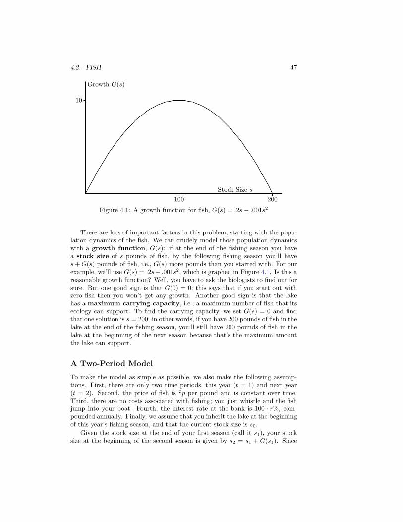
4.2. FISH 47
100 200
10
Growth G(s)
Stock Size s
Figure 4.1: A growth function for fish, G(s) = .2s − .001s2
There are lots of important factors in this problem, starting with the popu-lation dynamics of the fish. We can crudely model those population dynamicswith a growth function, G(s): if at the end of the fishing season you havea stock size of s pounds of fish, by the following fishing season you’ll haves + G(s) pounds of fish, i.e., G(s) more pounds than you started with. For ourexample, we’ll use G(s) = .2s− .001s2, which is graphed in Figure 4.1. Is this areasonable growth function? Well, you have to ask the biologists to find out forsure. But one good sign is that G(0) = 0; this says that if you start out withzero fish then you won’t get any growth. Another good sign is that the lakehas a maximum carrying capacity, i.e., a maximum number of fish that itsecology can support. To find the carrying capacity, we set G(s) = 0 and findthat one solution is s = 200; in other words, if you have 200 pounds of fish in thelake at the end of the fishing season, you’ll still have 200 pounds of fish in thelake at the beginning of the next season because that’s the maximum amountthe lake can support.
A Two-Period Model
To make the model as simple as possible, we also make the following assump-tions. First, there are only two time periods, this year (t = 1) and next year(t = 2). Second, the price of fish is $p per pound and is constant over time.Third, there are no costs associated with fishing; you just whistle and the fishjump into your boat. Fourth, the interest rate at the bank is 100 · r%, com-pounded annually. Finally, we assume that you inherit the lake at the beginningof this year’s fishing season, and that the current stock size is s0.
Given the stock size at the end of your first season (call it s1), your stocksize at the beginning of the second season is given by s2 = s1 + G(s1). Since

48 CHAPTER 4. MATH: TREES AND FISH
there are only two periods and no fishing costs, whatever you don’t catch thisyear you should catch next year. Your maximization problem, then, is to chooses1 to maximize the present value of your harvest,
PV = p(s0 − s1) + p
[s1 + G(s1)
1 + r
]
.
The first term here, p(s0 − s1), is your profit from catching and selling s0 − s1
pounds of fish now. The second term is the present value of your profit fromcatching and selling the remaining fish next year.
Taking a derivative with respect to s1 and setting it equal to zero we get anecessary first-order condition of
p(−1) + p · 1
1 + r· [1 + G′(s1)] = 0.
Multiplying through by1 + r
pwe get
−1 − r + 1 + G′(s1) = 0 =⇒ G′(s1) = r.
This NFOC has a nice interpretation. The right hand side, r, is the (instanta-neous) interest rate paid by the Bank of America. The left hand side, G′(s1), isthe (instantaneous) interest rate paid by the Bank of Fish: if you leave an extrapound of fish in the lake, after one year you’ll get a “fish interest payment”of G′(s1). So the NFOC says to equate the interest rate at the two banks: ifG′(s1) > r, you should increase s1 by leaving more fish in the lake, where they’llgrow at a faster rate than money in the bank; if G′(s1) < r, you should decreases1 by catching more fish and putting the proceeds in the bank, where the moneywill grow at a faster rate than the fish population.
What happens if the value of s1 that satisfies this equation is greater thans0?. Since we cannot catch negative amounts of fish, the best we can do ischoose the corner solution s1 = s0, i.e., catch zero fish this period. So thecomplete answer to our problem is to find s∗ that satisfies G′(s∗) = r and thenset s1 = min{s0, s
∗}. Technically, this is called a bang-bang solution. (Non-technical explanation: if s∗ < s0, you shoot the fish until s1 = s∗; if s∗ > s0,you shoot the fishermen!)
An Infinite-Period Model
Now let’s do an infinite-period fish model, using G(s) = .2s − .001s2 as ourgrowth function. To make the model as simple as possible, we also make thefollowing assumptions. First, the price of fish is $1 per pound and is constantover time. Second, there are no costs associated with fishing; you just whistleand the fish jump into your boat. Third, the interest rate at the bank is r = .05,i.e., 5%, compounded annually. Finally, we assume that you inherit the lake atthe beginning of this year’s fishing season, and that the current stock size iss = 110.

4.2. FISH 49
Given the current fish population, there is an intuitively appealing solution toyour fisheries management problem: follow a policy of Maximum SustainableYield (MSY). This says that you should harvest 10 pounds of fish this year,leaving you with a population of s = 100, which will grow to 100+G(100) = 110pounds by next fishing season, at which point you can harvest 10 pounds of fish,leaving you with a population of s = 100. . . We can see from the graph of G(s)(and from setting G′(s) = 0) that harvesting 10 pounds of fish every year is themaximum number of fish you can catch year after year, i.e., is the maximumsustainable yield.
If you follow this policy, the present value of your lake is (using the perpetuityformula)
PV = 10 +10
1.05+
10
(1.05)2+
10
(1.05)3+ . . . = 10 +
10
.05= 210.
This sounds pretty good, but now let’s do a little marginal analysis to seeif we can do better. Let’s change the MSY policy a little bit, as follows: let’s“borrow” some extra fish (say, 5 pounds) this year, and “return” them nextyear. Effectively what we’re doing here is borrowing from the Bank of Fish (bycatching the fish and selling them) and using that borrowed money to invest inthe Bank of America (by depositing it and letting it gain interest); in a yearwe’re going to unwind our investments by taking the proceeds from the Bank ofAmerica and using them to repay our loan from the Bank of Fish. Whether ornot this is a good idea depends on how the “interest rate” at the Bank of Fishcompares to the interest rate at the Bank of America.
Some numbers may make this more clear. What we’re going to do this yearis increase the harvest by 5 pounds of fish (to 15 pounds), so that at the end ofthe season there will be 110−15 = 95 pounds of fish in the lake. In a year therewill be 95 + G(95) = 104.975 pounds of fish in the lake. Next year we limit ourharvest to 4.975 pounds, leaving 100 pounds of fish in the lake at the end of thesecond season. This returns us to the MSY policy, and each year thereafter weharvest 10 pounds of fish.
What’s the present value of this? Well, it’s
PV = 15 +4.975
1.05+
10
(1.05)2+
10
(1.05)3+
10
(1.05)4+ . . .
= 15 +4.975
1.05+
1
1.05
[10
1.05+
10
(1.05)2+
10
(1.05)3+ . . .
]
= 15 +4.975
1.05+
1
1.05
[10
.05
]
≈ 15 + 4.74 + 190.48
= 210.22.
We’ve done better than MSY!Intuitively, what’s going on here is that the Bank of America is paying a
higher interest rate than the Bank of Fish; we therefore make more money by

50 CHAPTER 4. MATH: TREES AND FISH
borrowing a little bit from the Bank of Fish and investing it in the Bank ofAmerica. Let’s formalize this with math.
The math
Say you decide to catch M pounds of fish this year, leaving s pounds of fish inthe lake. In a year, then, you’ll have $M(1 + r) in the Bank of America ands+G(s) in the Bank of Fish. If this is the decision that maximizes your presentvalue, you can do no better by catching more fish this year or less fish this year,and then making up for it next year. Let’s see what the implications of this are.
First let’s try catching less fish this year, i.e., “lending” h pounds of fish tothe Bank of Fish for a year. (Note that lending to the Bank of Fish effectivelymeans borrowing from the Bank of America: by not catching those h poundsof fish, we’re reducing the amount of money we put in the Bank of Americaand therefore reducing the interest payment we’ll get.) So: lending h pounds offish to the Bank of Fish means that you catch M − h pounds of fish this year,leaving s + h pounds in the lake. In a year, you’ll have $(M − h)(1 + r) in theBank of America and s+h+G(s+h) in the Bank of Fish. You can then unwindthe investment by catching h + G(s + h)−G(s) pounds of fish and putting theproceeds in the Bank of America, leaving you with s+G(s) in the Bank of Fishand
[(M − h)(1 + r)] + [h + G(s + h) − G(s)] = M(1 + r) − h · r + G(s + h) − G(s)
in the Bank of America. Since your original choice of s was optimal, it must bethe case that you have less in the Bank of America now than you did before:
M(1 + r) − h · r + G(s + h) − G(s) ≤ M(1 + r).
Cancelling terms and rearranging we get
G(s + h) − G(s)
h≤ r.
The left hand side here looks exactly like the definition of a derivative, andletting h go to zero we get
G′(s) ≤ r.
This says that if s is the optimal number of fish to leave in the lake, then theinstantaneous interest rate G′(s) paid by the Bank of Fish must be no greaterthan the instantaneous interest rate r paid by the Bank of America. Otherwise,you could increase your present value by “lending” to the Bank of Fish.
A similar result follows when we consider “borrowing” h pounds of fish fromthe Bank of Fish for a year. (Here, borrowing from the Bank of Fish meansinvesting in the Bank of America: by catching an extra h pounds of fish, we canincrease the amount of money we put in the Bank of America.) The result weget here is that G′(s) ≥ r, i.e., that the instantaneous interest rate G′(s) paidby the Bank of Fish must be no less than the instantaneous interest rate r paid

4.2. FISH 51
by the Bank of America. Otherwise, you could increase your present value by“borrowing” from the Bank of Fish.
Combining our two answers, we see that the optimal stock size s must satisfy
G′(s) = r.
Back to our example
In the problem we started out with—G(s) = .2s − .001s2, r = .05, initial stockof 110 pounds of fish—the condition G′(s) = r comes out to
.2 − .002s = .05 =⇒ s = 75.
So the optimal stock size is 75 pounds of fish, meaning that you should catch110− 75 = 35 pounds the first year (thereby reducing the stock size to 75) andG(75) = 9.375 pounds each year thereafter (thereby maintaining the stock sizeat 75). Your present value from this management strategy is
PV = 35 +9.375
1.05+
9.375
(1.05)2+
9.375
(1.05)3+ . . .
= 35 +9.375
.05= 222.50
So 222.50 is the maximum present value you can get from your lake!
Problems
1. You’ve just inherited a plot of land, and decide to manage it so as tomaximize its present value. The land has no alternative use other thangrowing trees, so if you don’t plant anything your present value will bezero. Assume that there is no inflation, and that the price of lumber staysconstant at p per unit. The interest rate paid by the bank is 100 · r% peryear, compounded continuously. Trees grow according to f(t).
(a) (The basic problem) You cannot replant the trees, and there are nocosts associated with planting or cutting down your trees. Writedown the maximization problem and find the necessary first-ordercondition (NFOC) for optimal management. What is the intuitionbehind your result?
(b) (Harvesting costs) You cannot replant the trees, but cutting down thetrees costs you c. Write down the maximization problem and find thenecessary first-order condition for optimal management. Does har-vesting costs increase or decrease your optimal rotation time com-pared to (a)? What is the intuition behind this result?
(c) (Planting costs) You cannot replant the trees, and it costs you noth-ing to cut them down, but in order to plant the trees you need to

52 CHAPTER 4. MATH: TREES AND FISH
spend c today. Write down the maximization problem and find thenecessary first-order condition for optimal management. Does plant-ing costs increase or decrease your optimal rotation time comparedto (a)? What is the intuition behind this result? What role (if any)does c play in your decision? (Hint: What if c were $1 billion?)
(d) (Replanting) Now you can replant the trees; there are no costs associ-ated with planting or cutting. Write down the maximization problemand find the necessary first-order condition for optimal management.Does replanting increase or decrease your optimal rotation time com-pared to (a)? What is the intuition behind this result?
(e) (Challenge: all together now) Imagine that you can replant, but thatthere are also planting costs, or harvesting costs, or both. (In thecase of planting costs, assume that you replant new trees at the sameinstant that you cut down the old trees.) Try to think through theintuition of what would happen to optimal rotation time compared to(d) in these situations. Then write down the maximization problemand (if you’re brave) try to confirm your intuition.
(f) (Alternative uses) Assume (in any of these problems) that there is analternative use of the land that has a present value of x. What role(if any) does x play in your decision-making? (Hint: Think aboutyour answer in (c).)

Chapter 5
More Optimization overTime
Present value calculations are complicated by the existence of inflation, a gen-eral increase in prices over time. The presence of inflation requires us to distin-guish between nominal interest rates and real interest rates.
5.1 Nominal and Real Interest Rates
The nominal interest rate is the interest rate the bank pays. If you have$100 and you put it in a bank account paying 5% interest, in one year you’llhave 5% more money ($105). With inflation, however, having 5% more moneynext year doesn’t mean you’ll be able to buy 5% more stuff next year. Pricesnext year will be higher than prices today, so even though your bank accountbalance will be 5% higher in one year, your ability to buy stuff (formally calledyour purchasing power) will not be 5% greater. In fact, if the inflation rateis higher than 5%, your purchasing power will be lower next year even thoughyou have more money!
The real interest rate measures changes in purchasing power, and in doingso it properly accounts for inflation. For example, imagine that the nominalinterest rate in Colombia is 13% and the inflation rate is 9%. If you put 1,000Colombian pesos in the bank today, in one year you’ll have 13% more, i.e., 1,130pesos. But you won’t be able to buy 13% more stuff, because prices will haverisen by 9%: the same candy you can buy for 10 pesos today will cost 10.9 pesosnext year. To figure out the actual increase in your purchasing power (i.e., thereal interest rate), we need to compare your purchasing power today with yourpurchasing power in one year: today candy costs 10 pesos, so with your 1,000pesos you could buy 100 candies; next year candy will cost 10.9 pesos, so withyour 1,130 pesos you’d be able to buy 103.7 candies. Since putting your moneyin the bank for a year will enable you to buy 3.7% more candy, the real interestrate is 3.7%.
53

54 CHAPTER 5. MORE OPTIMIZATION OVER TIME
5.2 Inflation
As noted at the beginning of this chapter, inflation is a general increase in pricesover time. To measure inflation, economists look at how prices change for a“representative market basket” of goods and services: food, rent, transportation,education, haircuts, etc.1 If that market basket had a price of $10,000 in 1990and $12,900 in 2000, then we would say that the price level in the United Statesincreased 29% during the decade. (This was in fact the price increase over thatdecade; it is equivalent to an annual inflation rate of 2.6%.)
The most commonly used measure of inflation in the United States is theConsumer Price Index (CPI), which is shown in Figure 5.1a. According to theCPI, a market basket of goods and services that cost $100 in 2000 would havecost about $10 in 1925; in other words, the purchasing power of $100 in 2000was about the same as that of $10 in 1925. Taking inflation into account cantherefore produce significant shifts in perspective.
As an example, consider Figures 5.1b and 5.1c, both of which show averageU.S. gas prices between 1918 and 2002. Figure 5.1b features nominal prices:a gallon of gasoline actually sold for an average of $0.22 in 1925 and $1.56 in2000. This perspective shows gas prices increasing over time, with the late 1970smarking a striking transition between “low” and “high” gas prices.
The perspective in Figure 5.1c is quite different. It shows gas prices fallingover time, interrupted—but only temporarily—by price shocks in the 1930s andthe 1970s.2 These conclusions come from analyzing real gas prices: Figure 5.1cadjusts for inflation by putting everything in constant year 2000 dollars, i.e.,in terms of year 2000 purchasing power.
For a more explicit comparison between Figures 5.1b and 5.1c, consider theprice of a gallon of gasoline in 1925. Figure 5.1b asks this question: “What wasthe average price of gasoline in 1925?” The answer: about $0.22 per gallon. Incontrast, the question posed in Figure 5.1c is this: “What would the averageprice of gasoline have been in 1925 if the general price level in that year hadbeen the same as the general price level in the year 2000?” The answer: about$2.20 per gallon because, according to the CPI, the general price level in theyear 2000 was about 10 times higher than in 1925.
Because we have a good grasp of the purchasing power of today’s money(i.e., because we “know what a dollar [today] is worth”), it often makes sense touse the current year, or a recent year, as the base year for analyzing real prices.It is, however, possible to use any year as the base year; Figure 5.1d shows gasprices in constant 1925 dollars, i.e., in terms of 1925 purchasing power. Notethat the graph is identical to that in Figure 5.1c except for the labels on thevertical axis (1925 dollars versus year 2000 dollars).
1This would be as simple as it sounds if people bought the same stuff every year, butit isn’t because they don’t. Take an advanced economics course to learn how to deal withcomplications caused by changes in the representative market basket over time.
2The latter price shock resulted from successful collusion by the OPEC (Organization ofPetroleum Exporting Countries) cartel. The cause of the former price shock is not known tothis author—anybody want to do a research project?

5.2. INFLATION 55
1925 1950 1975 2000
25
50
75
100
125
(a) CPI, 1918–2002
1925 1950 1975 2000
$0.25
$0.50
$0.75
$1.00
$1.25
$1.50
$1.75
(b) Nominal gas prices, 1918–2002
1925 1950 1975 2000
$1.50
$2.00
$2.50
$3.00
(c) Real gas prices, in 2000 dollars
1925 1950 1975 2000
$0.15
$0.20
$0.25
$0.30
(d) Real gas prices, in 1925 dollars
Figure 5.1: Inflation and average U.S. gas prices, 1918–2002. Figure (a) showsthe Consumer Price Index (CPI) measure of inflation; note that there was aperiod of deflation (i.e., a general decrease in prices over time) during theGreat Depression that began in 1929. Figure (b) shows the average price for agallon of gasoline using nominal prices: a gallon of gasoline actually sold for anaverage of $0.22 in 1925 and $1.56 in 2000. Figure (c) shows average gas pricesusing real year 2000 dollars, meaning that it adjusts for inflation by puttingeverything in terms of year 2000 purchasing power. According to the CPI—shown in Figure (a)—a market basket that cost $100 in 2000 would have costabout $10 in 1925. It follows that the $0.22 price tag on a gallon of gasolinein 1925 is equivalent to about $2.20 in year 2000 dollars, as shown in Figure(c). Conversely, the $1.56 price tag on a gallon of gasoline in 2000 is equivalentto $0.156 in 1925 dollars; this can be seen in Figure (d), which shows averagegas prices using real 1925 dollars. (Source: Figures are based on AmericanPetroleum Institute data.)

56 CHAPTER 5. MORE OPTIMIZATION OVER TIME
5.3 Mathematics
We can get a mathematical formula relating the nominal interest rate, the realinterest rate, and the inflation rate by generalizing the approach from Sec-tion 5.1’s discussion of Colombia. If the nominal interest rate is n and theinflation rate is i, the real interest rate r is given by
1 + r =1 + n
1 + i, i.e., r =
1 + n
1 + i− 1.
Intuitively, the numerator (1 + n) tells you how much more money you’ll havein one year; the denominator (1 + i) tells you how much prices will have risenin one year; and dividing one by the other tells you how much more purchasingpower you’ll have in one year.
There is also a handy rule of thumb that works well when the inflation rateis small (say, less than 10%). To derive it, note that
r =1 + n
1 + i− 1 =
1 + n
1 + i− 1 + i
1 + i=
n − i
1 + i≈ n − i
when the inflation rate i is small because 1 + i ≈ 1. In short,
r ≈ n − i,
which in words says that the real interest rate is approximately equal to thenominal interest rate minus the inflation rate.
It is important to remember that the rule of thumb is an approximation thatworks well only when the inflation rate is small. For an example, return to theColombia calculation above, where the exact formula gives a real interest rateof 3.7%:
1 + .13
1 + .09− 1 = .037.
The rule of thumb estimates the real interest rate at 13% − 9% = 4%, whichis pretty close. In contrast, consider a nominal interest rate of 113% and aninflation rate of 109%. The rule of thumb again estimates the real interest rateat 4% (113%− 109% = 4%), but this time the real interest rate is actually only1.9%:
1 + 1.13
1 + 1.09− 1 = .019.
When to Use Which
It can be difficult to figure out when to use the nominal interest rate and whento use the real interest rate when computing present values. The only sure-firestrategy is to think about the goal, which is to figure out how much to put in thebank today to be able to afford a certain stream of income and expenses. Butthere are a couple of rules of thumb you can follow; two of them are describedin Problem 4.

5.3. MATHEMATICS 57
A final note here is that many microeconomic analyses (including many ofthe examples and descriptions in this text) simplify matters by assuming thatthe inflation rate is zero. In this case, real and nominal interest rates are equalto each other and it makes sense to refer to “the interest rate” without specifyingone or the other.
Problems
1. If a bank is paying 14.4% and inflation is 8%, calculate the real interestrate. Round to the nearest .1% (Hint: Think about purchasing powerrelative to a good whose price increases at the rate of inflation.) Use boththe true formula and the approximation and compare them.
2. Explain (as if to a non-economist) why the formula relating real and nom-inal interest rates makes sense. (Hint: Recall that the real interest ratemeasures increases in purchasing power, and think about how much moreof some good you’ll be able to purchase in one year if your bank accountpays the nominal interest rate and the good’s prices increases with infla-tion.)
3. Assume that the nominal interest rate is 10% per year and that the rateof inflation is 5% per year. Round all your answers as appropriate.
(a) You put $100 in the bank today. How much will be in your accountafter 10 years?
(b) You can buy an apple fritter (a type of donut) for $1 today. Theprice of donuts goes up at the rate of inflation. How much will anapple fritter cost after 10 years?
(c) Calculate x, the number of apple fritters you could buy for $100today. Then calculate y, the number of apple fritters you could buyafter ten years if you put that $100 in the bank. Finally, calculate
z = 100 · y − x
x. (The deal with z is that you can say, “If I put my
money in the bank, then after ten years I will be able to buy z%more apple fritters.”)
(d) Given the nominal interest rate and inflation rate above, calculatethe real interest rate to two significant digits (e.g., “3.81%”). Checkyour answer with the “rule of thumb” approximation.
(e) Calculate how much money you’d have after 10 years if you put$100 in the bank today at the real interest rate you calculated in theprevious question (3d). Compare your answer here with the resultfrom question 3c.
4. Here are a couple of rules of thumb concerning the use of real (rather thannominal) interest rates in present value calculations.

58 CHAPTER 5. MORE OPTIMIZATION OVER TIME
Use real when your payments are inflation-adjusted. Somebody of-fers to sell you a lemon tree that will bear 100 lemons at the end ofeach year. The price of lemons is $1.00/lemon right now, and will riseat the rate of inflation, which is 4% per year; the nominal interestrate is 6%.
(a) What is the present value of the lemon tree if it will bear fruitfor 5 years and then die?
(b) What if it will bear fruit forever?
Use real to calculate future purchasing power. You and a buddy winthe $20 million grand prize in a lottery, and you choose to accept alump sum payment of $10 million, which you divide equally. Yourbuddy immediately quits school and moves to Trinidad and Tobago.Being more cautious, you put your $5 million in a 40-year CD pay-ing 6%, figuring that after 40 years your wealth will have increased10-fold and so you’ll be able to buy 10 times more stuff. Are youfiguring correctly if the inflation rate is 4%?
5. Fun Recall the question from Chapter 3 concerning the Louisiana Pur-chase. That problem (#10 on page 39) asked you to calculate the presentvalue of the $15 million President Jefferson spent in 1803 to buy theLouisiana Territory from France, using interest rates of 2% and 8%. As-sume now that 2% was the real interest rate over that time period andthat 8% was the nominal interest rate over that time period. Which is thecorrect interest rate to use?
6. Fun Recall the question from Chapter 3 concerning the Publishers Clear-ing House sweepstakes. That problem (#12 on page 40) asked you tocalculate the present value of different payment options. In calculatingthose present values, should you use the real interest rate or the nominalinterest rate?

Chapter 6
Transition: Arbitrage
An economics professor and an economics student meet on their wayto class. The student spies a $10 bill on the ground and reaches downto pick it up. The professor says, “Don’t bother. If it really was a$10 bill, somebody else would have already picked it up.”
This purpose of this transitional chapter is to connect the first part of this book,which analyzes the actions of a single optimizing individual, with later parts,which analyze interactions between optimizing individuals. Our focus will beon the idea of arbitrage, which investorwords.com defines as “[an attempt]to profit by exploiting price differences of identical or similar financial instru-ments, on different markets or in different forms. The ideal version is risklessarbitrage.”
An example of riskless arbitrage is the simultaneous purchase and sale ofsome asset at different prices. If, for example, Microsoft stock is trading on theNew York Stock Exchange for $100 and on the NASDAQ stock exchange for$105, an individual trader can engage in arbitrage by simultaneously “buyinglow” (purchasing Microsoft stock on the New York Stock Exchange for $100per share) and “selling high” (selling Microsoft stock on NASDAQ for $105 pershare). The net result is a riskless gain of $5 per share.
More generally, the concept of arbitrage applies to assets that are similarrather than identical. In can also be used in contexts that don’t involve financialinstruments: a driver in rush-hour traffic who switches from a slow-moving laneinto a faster-moving one might reasonably be said to be engaging in arbitrage.
6.1 No Arbitrage
Arbitrage as a concept is centered on the optimizing individual; it is the in-dividual stockbroker, for example, who engages in arbitrage by simultaneouslybuying and selling some asset. The preceding chapters in this book had a sim-ilar focus. The following chapters focus on the interactions between optimizing
59
60 CHAPTER 6. TRANSITION: ARBITRAGE
individuals. One of the key questions will be: “What would a world full ofoptimizing individuals look like?”
It will take the rest of this chapter to develop a completely correct answerto that question in the context of arbitrage. There is, however, an almost com-pletely correct answer that is remarkably simple: in a world full of optimizingindividuals, there would be no opportunities for arbitrage. This “no arbitrage”result predicts that Microsoft stock will trade at the same price on the NewYork Stock Exchange and on NASDAQ. It also predicts that switching lanesduring rush hour is an exercise in futility because all the lanes are moving atthe same speed.
These predictions are examples of what David D. Friedman calls “hidden or-der”.1 Especially interesting is the fact that these social patterns emerge with-out conscious effort. Stockbrokers don’t intend to equate the price of Microsoftstock on the different exchanges, and nobody is “in charge” of the different lanesof traffic during rush hour; to the contrary, each stockbroker is only interestedin making money, and each driver is only interested in getting home as fast aspossible. Despite this, the aggregate result of these myopic activities is not chaosbut order. Finding such “hidden order”, one of the pleasures of economics, isthe focus of the rest of this book.
6.2 Rush-Hour Arbitrage
A completely correct statement about rush-hour traffic is that we should ex-pect different lanes to travel at approximately the same speed. The reason isthat rush-hour arbitrage is self-eliminating. If one lane does happen tobe moving a little bit faster, some drivers (the “explorers”) will change lanes,thereby gaining a few seconds. But the victory will be short-lived: all thoseexplorers shifting into the fast-moving lane will slow it down, and all those ex-plorers shifting out of slow-moving lanes will speed them up. The end result isthat the explorers—in their efforts to gain precious seconds—end up equalizingthe traffic speeds on the different lanes.
A curious note here is that the existence of explorers can help drivers whoare not explorers. These other drivers (the “sheep”) prefer to just pick a laneand relax rather than stress out over switching lanes all the time. In the ab-sence of explorers, this behavior would be risky: the other lane really mightbe moving faster. But the presence of explorers—and the fact that arbitrage isself-eliminating—means that the sheep can relax, comfortable in the knowledgethat the lane they choose is expected to move at approximately the same speedas any other lane.
Having examined the need for the “approximately” in the statement at thebeginning of this section—it turns out that explorers can get ahead, but onlyby a little—we now turn our attention to the “expect”. This word refers to theexpected value calculations of Chapter 2, and as in that chapter the term is
1Friedman’s excellent book is called Hidden Order: The Economics of Everyday Life
(Harper Business, 1996).

6.3. FINANCIAL ARBITRAGE 61
used to focus on what happens on average rather than what happens on anyparticular occasion. For example, if you have an even bet (flip a coin, win $1if it comes up heads, lose $1 if it comes up tails), the expected value of thatbet is $0. In hindsight—i.e., after the coin is flipped—it is easy to say whetheror not you should have taken the bet. Before the fact, though, all that can besaid is that on average you will neither gain nor lose by taking the bet.
Returning to rush hour, imagine that a second (identical) bridge is builtright next to the SR-520 bridge that currently connects Seattle and the Eastside.Despite the existence of explorers listening to radio traffic reports in the hopesof finding an arbitrage opportunity, we cannot say that the travel times on thetwo bridges will always be approximately equal: if there is a big accident on oneof the bridges right after you get on it, you will get home hours later than thelucky drivers who chose the other bridge. What we can say is that the expectedtravel times on the two bridges will be approximately equal. In hindsight—i.e.,after you cross the bridge—it is easy to say whether or not you should havetaken the other bridge. Before the fact, though, all that can be said is thaton average the bridge you choose will get you home in approximately the sameamount of time as the other bridge.
6.3 Financial Arbitrage
A nice analogy connects financial decisions and traffic decisions: think of thedifferent lanes of the freeway as different investment options (Microsoft stock,Intel stock, etc.), and think of travel speed as measuring the rate of return ofthe different investments (so that a fast-moving lane corresponds to a rapidlyincreasing stock price). Given these similarities, it is not surprising that thereare similarities in the economic analyses of these two phenomena. A completelycorrect statement about financial arbitrage turns out to be that we should expectcomparable investments to have comparable rates of return.
The word “comparable” is necessary because there is a lot more variety to befound in financial investments than in the lanes of traffic on the freeway. Beforewe discuss this in detail, note that—as with rush-hour arbitrage—economic rea-soning about financial arbitrage focuses on expectations. Just because differentstock prices have the same expected rate of return doesn’t mean that they willhave the same actual rate of return. If you look at the price of oil over the last30 years, or the price of internet stocks (amazon.com, webvan, Cisco) over thelast 5 years, you’ll see that their prices do not steadily increase at the rate ofinterest. But using hindsight to look back and say that you should have boughtor sold XYZ stock five years ago is like using hindsight to say that you shouldhave picked the winning lottery numbers prior to the drawing.
Another parallel with rush-hour arbitrage is that financial arbitrage isself-eliminating. The “explorers” in stock markets, for example, are invest-ment managers and others who spend a lot of time and effort trying to findstocks that are likely to go up in value faster than others. By selling stockin companies that are expected to perform poorly (thereby lowering the stock

62 CHAPTER 6. TRANSITION: ARBITRAGE
price, which makes the stock more attractive) and buying stock in companiesthat are expected to do well (thereby increasing the stock price, which makesthe stock less attractive), these explorers equalize the attractiveness of differentstocks. (We’ll see shortly that equal attractiveness doesn’t necessarily meanequal expected rates of return.)
As in the case of rush-hour arbitrage, the presence of financial “explorers”allows other investors (the “sheep”) to feel comfortable with just picking somestocks and sticking with them. This is a good thing because many people don’twant to (or, because they have day jobs, can’t) spend all their time investigatingstocks.
The fact that it takes time and effort to look for financial arbitrage opportu-nities is important because it allows us to paint a complete picture of how thewhole process works. The almost completely correct reasoning at the beginningof this chapter suggests that the reason there are no arbitrage opportunities isthat someone would have taken advantage of them if there were. But if there areno arbitrage opportunities, who would bother to look for them? And if nobodybothers to look for them, arbitrage opportunities might well exist. . . . (See thejoke at the beginning of this chapter for an example.)
A complete picture is that there are small discrepancies that occasionallyappear between the price of Microsoft stock on the New York Stock Exchangeand on NASDAQ; and there are people who profit from such discrepancies (and,by opposing, end them). But it is not right to think of these people as getting“free money” any more than it is right to think of other workers as gettingfree money when they get paid for a day’s work. As for the idea that thesepeople are making out like bandits, it is worth noting that looking for arbitrageopportunities can be thought of as a type of investment. As such, we have goodreason to think that the expected rate of return from this investment should becomparable to that from comparable investments such as working elsewhere onWall Street.
What Do We Mean by Comparable Investments?
For one thing, we mean investments that have similar liquidity: if you lock upyour money in a 5 year Certificate of Deposit (CD) that carries penalties forearly withdrawal, you can expect a higher rate of return than if you put yourmoney in a savings account that you can liquidate at any time.
Another issue is risk: as we saw before, people are often unwilling to takefair bets, meaning that they are risk-averse. So we should expect high-riskinvestments to have higher expected rates of return than low-risk investments.For example, junk bonds should have higher expected interest rates than U.S.government bonds because they involve uncertainty: if the companies sellingthose bonds go bankrupt, the bonds will be worthless. (This idea is tricky;see Problem 2 for an example.) If one-year junk bonds and U.S. governmentbonds have expected returns of 6% and 4% respectively, then the risk premiumassociated with the company’s junk bonds is the difference between the expectedrates of return: 6% − 4% = 2%. To compensate investors for the added risk of

6.3. FINANCIAL ARBITRAGE 63
lending money to a troubled company, the company must offer a higher expectedrate of return.
Curiously, the risk premium associated with stocks seems to be undeservedlylarge. Although stocks do go up and down, over time they mostly seem to go up,and they seem to go up quite fast: investing in the stock market has been a muchbetter investment than investing in bonds or in the Bank of America. Considerthe following information provided in a recent issue of The Schwab Investor:2
If you invested $2,000 each year from 1981-2000 in U.S. Treasury bonds, youwould have ended up with $75,000; if you invested that same amount in the stockmarket, you would have ended up with $282,000. (Even an unlucky investor, onewho invested at the worst time each year, would have ended up with $255,000.)In order to make bonds or other investments an appealing alternative to stocks,the risk premium associated with stocks would have to be quite large. Thiswhole issue is something of a mystery to economists, who call it the equitypremium puzzle. Figure it out and you’ll win the Nobel Prize in Economics.
Problems
1. Explain (as if to a non-economist) why comparable investments shouldhave comparable expected rates of return.
2. Consider a company that has a 10% chance of going bankrupt in the nextyear. To raise money, the company issues junk bonds paying 20%: if youlend the company $100 and they don’t go bankrupt, in one year you’ll getback $120. Of course, if the company does go bankrupt, you get nothing.What is the expected rate of return for this investment? If governmentbonds have a 3% expected rate of return, what is the risk premiumassociated with this investment?
3. Economic reasoning indicates that comparable investments should havecomparable expected rates of return. Do the following examples contradictthis theory? Why or why not?
(a) Microsoft stock has had a much higher rate of return over the lasttwenty years than United Airlines stock.
(b) Oil prices are not going up at the rate of interest.
(c) Junk bonds pay 20% interest while U.S. Treasury bonds pay only 4%interest.
(d) Banks in Turkey (even banks that have no risk of going bankrupt)pay 59% interest while banks in the U.S. only pay 4% interest.
2It would be better to have an unbiased source for this information. . .
64 CHAPTER 6. TRANSITION: ARBITRAGE

Part II
One v. One, One v. Many
65


Chapter 7
Cake-Cutting
A recently divorced woman finds a beat-up old bottle while walkingon the beach, and when she rubs it a Genie comes out and says, “Youhave three wishes. But I must warn you: whatever you wish for,your ex-husband will get ten times as much.” The woman thinks fora while and then says, “First, I’d like to be beautiful.” “Fine,” theGenie replies, “but remember—your ex-husband will be ten timesmore beautiful.” “That’s okay, I’ll still be gorgeous.” “Very well,”the Genie says, and makes it so. “And your second wish?” “I’d like tobe rich.” “Remember,” says the Genie, “your ex-husband will haveten times more money than you.” “That’s fine,” the woman replies,“I’ll still be able to buy whatever I want.” “Alright, whatever yousay,” the Genie replies. “And your third wish?” “I’d like to have amild heart attack.”
Having studied how optimizing individuals act, we now begin the study of howoptimizing individuals interact. The branch of economics that studies strategicinteractions between individuals is called game theory.
Some key issues to consider when analyzing or describing a strategic inter-action are the players (Who’s involved?); the strategies (What options doeseach player have?); the payoffs (What are the players’ outcomes from the var-ious strategy combinations?); the timeline (Who gets to act when?); and theinformation structure (Who knows what when?).
7.1 Some Applications of Game Theory
One application of game theory is, not surprisingly, to games. Here, for instance,is the introduction to Ken Binmore’s economic analysis of poker his book Funand Games: A Text on Game Theory :
Poker is a card game for which one needs about seven players for thevariants normally played to be entertaining. Neighborhood games
67

68 CHAPTER 7. CAKE-CUTTING
are often played for nickels and dimes, but there is really no pointin playing Poker except for sums of money that it would really hurtto lose. Otherwise, it is impossible to bluff effectively, and bluffingis what Poker is all about.
In other words, poker is all about strategic behavior: I don’t know what cardsyou have and you don’t know what cards I have, and I know that you don’tknow what cards I have, and you know that I know that you don’t know whatcards I have. . . .
Of course, poker is not the only interesting game of strategy. Others include
Evolutionary games When facing conflict, why are some species aggressive(“fight”) while others run (“flight”)? Why have some species evolved to bebig and strong and others to be small and quick? These are sample topicsfrom evolutionary game theory, one of the most successful applicationsof game theory.
Auctions How much should you bid in an auction? If you’re auctioning some-thing off, what kind of auction should you use? (Chapter 12 analyzesvarious kinds of auctions.)
Sports Should you go for the two-point conversion or the one-point conversion?Should you give in to a player’s (or an owner’s) contract demands or holdout for a better deal?
Business How should you go about invading another company’s turf, or stop-ping another company from invading your turf?
War The development of game theory in the 20th century slightly preceded theCold War. The ideas of game theory helped make John von Neumann,one of its pioneers, into a proponent of “preventative war”, i.e., nuking theU.S.S.R. before the Soviets could develop the atomic bomb and reply inkind. (He was fond of saying, “If you say why not bomb them tomorrow,I say why not today? If you say today at five o’clock, I say why notone o’clock?”) Game theory can help explain some features of the ColdWar, such as the 1972 ABM Treaty (in which the U.S. and the U.S.S.R.agreed to not pursue defenses against missile attacks) and the doctrine ofMutually Assured Destruction.
Fair division The problem that we are going to focus on in this chapter isa deceptively silly one: that of fairly dividing cake. Note, however, thatissues of fair division arise in many important circumstances (for example,in divorce settlements, where the property to be divided can be thought ofas the “cake”) and that cake and pie analogies are widely used to discussresource allocation problems, from George W. Bush’s campaign promiseto “make the pie higher” to this quote from John Maynard Keynes’s 1920essay The Economic Consequences of the Peace:

7.2. CAKE-CUTTING: THE PROBLEM OF FAIR DIVISION 69
[The economic system in Europe before World War I] dependedfor its growth on a double bluff or deception. On the one handthe laboring classes accepted. . . a situation in which they couldcall their own very little of the cake that they and nature andthe capitalists were co-operating to produce. And on the otherhand the capitalist classes were allowed to call the best part ofthe cake theirs and were theoretically free to consume it, on thetacit underlying condition that they consumed very little of itin practice. The duty of “saving” became nine-tenths of virtueand the growth of the cake the object of true religion.
7.2 Cake-Cutting: The Problem of Fair Division
The basic cake-cutting problem is for “Mom” to figure out a way to fairly dividea cake among two or more children. (If you’d prefer a more real-world example,think of a divorce settlement or the settling of an estate of somebody who diedwithout a will. In these cases, the couple’s assets, or the items in the estate,are comparable to the cake that must be divided, and the judge is comparableto Mom.)
Three aspects of the cake-cutting problem are of particular interest. First,the cake is not necessarily homogenous: there may be parts with lots of frostingand parts with only a little frosting, parts with lots of chocolate and parts with-out chocolate, etc. (The different parts of the cake correspond to the differentitems—cars, houses, kids, etc.—in a divorce or estate settlement.) Second, thepeople dividing the cake may have different values: one may love chocolate,another may hate chocolate. Finally, these values may not be known to Mom(or to the judge dividing the assets). Even if they were, what parent wantsto be in the middle of a cake-cutting argument? So what Mom is looking foris a mechanism through which the children can divide up the cake fairly andwithout rancor. In other words, Mom’s problem is one of mechanism design:
Motivating question: Let’s say you have two children, and you want them todivide the cake between them so that each child gets (in his or her opinion) atleast 50% of the cake. What should you do?
One answer: There’s a time-honored algorithm called Divide and Choose: haveone child cut the cake into two pieces, and the other child choose between them.Now each child can guarantee him- or herself at least 50% of the cake.
Another answer: Pass a long knife from left to right over the cake. When onechild calls out “Stop”, cut the cake at that point and give the slice to the leftof the knife to the child that called out. The remainder of the cake goes to thechild that was silent. (This is called a Moving Knife algorithm.)

70 CHAPTER 7. CAKE-CUTTING
Question: Imagine you’re one of the children participating in a Divide andChoose algorithm. Do you want to be the cutter or the chooser?
Answer: Well, it might depend on how well you can handle a knife and howfairly you can eyeball the cake. But on a deeper level it also depends on howmuch you know about the other child’s preferences, and how much they knowabout your preferences.1
If you know a lot about what they like, you can take advantage of thisinformation by choosing to cut the cake. You can then cut it in such a way thatyour sibling thinks the cake is split 51–49 but you think the cake is cut 40–60;if your sibling is optimizing, she’ll take the first piece (which she values as 51%of the cake) and you can make off with what is (in your valuation) 60% of thecake. (In the divorce analogy: if you know your soon-to-be-ex-spouse will doanything to keep the 1964 Mustang convertible, you should do the cutting: putthe convertible in one pile and everything else in the other pile!)
On the other hand, if you don’t know a lot about your sibling’s preferences,you might want to be the chooser. As long as your sibling doesn’t know a lotabout your preferences either, she’ll have to cut the cake so that it’s split 50–50according to her valuation; odds are that your valuation is different and you’llbe able to choose a piece that you value at more than 50%.
Side note: The importance of information will be a recurring theme in ouranalysis of game theory (and in fact in all of microeconomics).
Question: What can Mom do if she has three or more kids?
One answer: You can generalize the Moving Knife algorithm to deal with anynumber of children. Simply follow the same procedure (pass the knife over thecake from left to right, stop when one child calls out “Stop”, and give the sliceto the left to the child that called out), and then repeat with the remaining cakeand the remaining children. Each time you complete the procedure there’s lesscake remaining and one less child. With n children, repeating the Moving Knifealgorithm n − 1 times will successfully divide the cake.
Another answer: You can also generalize the Divide and Choose algorithm toget what’s called the Successive Pairs algorithm. It’s a little complicated, buthere’s how it works with three children: Have two of the children play Divideand Choose, so that each of them gets at least 50% of the cake. Then haveeach of those children divide their part into three pieces, and have the thirdchild choose one piece from each of those. The cake will thus have been cut intosix pieces, and each child will end up with two. (Exercise: Can you convinceyourself—or someone else—that each child will get at least 33% of the cake inhis or her estimation?)
Which of these solutions is better? Well, that depends on your goal. Amus-ingly, mathematicians concern themselves with how to fairly divide the cake
1In fact, it also depends on how much you know they know about your preferences, andhow much you know they know you know, and. . .

7.2. CAKE-CUTTING: THE PROBLEM OF FAIR DIVISION 71
Envy-Free Algorithm for Three Players
(Attributed to John Conway, Richard Guy, and/or John Selfridge)
Step 1 Have Player A cut the cake into three pieces.
Step 2 Have Player B rank the pieces from best to worst—X1,X2,X3—and then trim off a slice E ≥ 0 from X1 so thatX1
′ = X1 − E and X2 have the same value for Player B.
Step 3 Have Player C choose from among X1′,X2, and X3.
Step 4 If C did not choose X1′, give X1
′ to B and the remaining pieceto A. If C did choose X1
′, have B choose between X2 and X3;again, give the remaining piece to A.
Step 5 Either B or C received X1′. Call that person P1 and the other
person P2.
Step 6 Have P2 cut E into three pieces, and have those pieces chosenin the order P1, A, P2.
Figure 7.1: An envy-free algorithm for three players.
with the minimum number of cuts. This leads (like many questions mathemat-ical) into an amazingly connected realm of results about mathematical topicssuch as Ramsey partitions and graph theory.
Question: What if the object that you are dividing up is not a good (e.g.,cake) but a bad (e.g., chores)?
Answer: A few algorithms do exist for what is called dirty-work fair division.You can read more about them in a neat book called Cake-Cutting Algorithms:Be Fair If You Can.2
Question: How do you divide a cake between 3 children in an envy-freemanner, i.e., so that no child covets another child’s piece?
Answer: This problem went unsolved for many decades, but a variety of mod-erately complicated algorithms are now known. Figure 7.1 shows one, adaptedfrom Section 1.4 of Cake-Cutting Algorithms.
Fair Division
The issue of envy-freeness leads us to an important question: Does a divisionhave to be envy-free to be fair? More broadly, what do we mean by “fair”?
2Robertson, Jack and William Webb, Cake-Cutting Algorithms: Be Fair If You Can (Nat-ick, Mass.: A K Peters, 1998) [A mathematical treatment of the topic; quite readable, butthe mathematics get pretty intense]

72 CHAPTER 7. CAKE-CUTTING
In their books The Win-Win Solution: Guaranteeing Fair Shares to Every-body3 and Fair Division: From Cake-Cutting to Dispute Resolution4, StevenBrams and Alan Taylor identify the following criteria for fairness in divisionproblems:
Proportionality Each child should get at least 1n
thof the cake according to
his or her estimation.
Envy-free No child should covet another child’s share.
Equitability “Equitability [means that] both parties think they received thesame fraction of the total, as each of them values the different items. Forexample, equitability would hold if the husband believed he got 70% andthe wife believed she got 70%, which is quite a different story from hisbelieving that he got 51% and her believing that she got 90%.”
Pareto efficiency There is no other division of the cake that would make atleast one child better off and not make any child worse off.
Brams and Taylor then go on to describe their (patented!) Adjusted Winneralgorithm for achieving these goals and to apply this algorithm to real-worldsituations such as the Camp David peace accord and the Donald and IvanaTrump divorce.
7.3 The Importance of Trade
Observation of sandwich-swapping in any elementary school lunchroom will con-firm that the initial allocation of resources is often only the beginning of thestory. Just because “Mom” divides the cake in a certain way doesn’t mean thatthings will stay that way.
The possibility of trade is in fact of fundamental importance in economics.The reason is the close relationship between trade and the fourth criterion onBrams and Taylor’s list: Pareto efficiency, which specifies that there is no otherallocation of resources that would make at least one child better off withoutmaking anyone else worse off. If this criterion is not met, then it is possible toreallocate resources in such a way that at least one child would be better offand nobody would be worse off. In such Pareto inefficient situations, at leastone child would have a strong incentive to push for such a reallocation, e.g., bytrading with or bribing the other children to accept that alternative allocation.
To put it more simply: there is an inherent tension between trade and Paretoinefficient situations. Because of this antagonism, we should expect the possi-bility of trade to naturally lead towards Pareto efficient allocations of resources.
3Brams, Steven J. and Alan D. Taylor, The Win-Win Solution: Guaranteeing Fair Shares
to Everybody (New York: W.W. Norton, 1999) [A very easy-to-read popular guide by twogame theorists, one a political scientist, the other a mathematician].
4Brams, Steven J. and Alan D. Taylor, Fair Division: From Cake-Cutting to Dispute
Resolution (Cambridge University Press, 1996) [A theoretical treatment by the same folks].

7.3. THE IMPORTANCE OF TRADE 73
This is the essence of the Coase Theorem, which says that Pareto efficiencywill always be attained as long as there is costless bargaining. (Ronald Coasewon the 1991 Nobel Prize in Economics in part for discussing this issue.)
For another perspective on the Coase Theorem, consider what blues musi-cian B.B. King said during a discussion about Napster, the pioneering music-swapping website. Commenting on the copyright-infringement lawsuits filedagainst Napster by various recording labels and artists, B.B. said that “copy-right and things of that sort are something that will have to be worked out andthey will be worked out. I remember when they didn’t want you to have a VCR,but they worked it out and I think for the best. Smart people always get togetherand work it out.”5 Although B.B. has yet to win a Nobel Prize in Economics,his words get at the heart of the Coase Theorem: if there’s nothing stoppingpeople from trading, nothing should stop people from trading until they reacha Pareto efficient allocation of resources.6
The Coase Theorem indicates that attaining Pareto efficiency can be sur-prisingly simple. For example, here is a solution to the cake-cutting problemif all you are concerned about is Pareto efficiency: divide up the cake howeveryou like, and then allow the children to trade with each other!
The Coase Theorem also suggests that the idea of trade is deceptively simple.For an example that illustrates this point, see problem 5 on page 74; this problemaddresses the issue of comparative advantage.
Economics and Pareto Efficiency
Of the four elements of “fairness” described by Brams and Taylor, economicsfocuses almost exclusively on Pareto efficiency. This focus on Pareto efficiency,and the concomitant inattention to equity considerations or other elements offairness, leads economists to think rather differently than non-economists. (Thenext chapter, which discusses Pareto efficiency in more depth, presents examplessuch as taxation and monopoly.)
It is important to remember that Pareto efficiency is only one element of“fairness”. For example, giving all of the cake to one child satisfies the crite-rion of Pareto efficiency—it is not possible to make unlucky children better offwithout making the lucky child worse off—but that does not necessarily makeit a “good” or “fair” way to cut cake.
It is also important to understand why economists focus on Pareto efficiency.One reason, as discussed above, is that Pareto efficiency can be surprisinglyeasy to attain: simply let people trade. Brams and Taylor’s Adjusted Winner
5Yahoo Entertainment News, Sept. 13, 2000, emphasis added. Incidentally, the “they”who didn’t want you to have a VCR was the movie industry, which was afraid that peoplewould stop going out to the movies. For details, see the book Information Rules by CarlShapiro and Hal Varian.
6If bargaining is costly, of course, there is something stopping people from trading; soone implication of the Coase Theorem is that we should focus on impediments to bargaining.In the case of Napster, a variety of nasty issues led them into bankruptcy instead of into asuccessful bargain with the music industry. Nonetheless, it seems likely that smart people willeventually figure out a method for digital distribution of music over the internet.
74 CHAPTER 7. CAKE-CUTTING
algorithm notwithstanding, this is certainly not the case with other aspects of“fairness”.
A second reason also provides a strong contrast between Pareto efficiencyand other aspects of “fairness”: underneath their attractive exteriors, issuessuch as “proportionality” or “equitability” are fraught with difficulty. (What ifone child is bigger? What if one child has been misbehaving?) Pareto efficiency,on the other hand, has a claim to universal appeal. Although it is not easy toargue that all Pareto efficient allocations of resources are good (would you wantto live in a world where one person owned everything?), it is relatively easy toargue that all Pareto inefficient allocations of resources are in some meaningfulsense bad : if it’s possible to make someone better off without making anyoneelse worse off, why not do it?
A third reason and final reason is political feasibility. In the real world, therealready exists a certain distribution of resources; if you propose something thatwill make some people worse off, those people are likely to fight you tooth andnail. So economics largely concerns itself with squeezing the most value out ofthe existing situation: we take the initial distribution of resources as given andsee how we can improve upon it. In most (but not all) cases, opportunities forimprovement are closely related to making it easier for people to trade.
Problems
1. “Differences in opinion make fair division harder.” Do you agree or dis-agree? Explain why.
2. Challenge Can you convince yourself—or someone else—that each childcan get at least 1
nth of the cake (in his or her estimation) with the divide-
and-choose algorithm? How about with the moving-knife algorithm?
3. Explain (as if to a non-economist) the Coase Theorem and its implicationsfor the cake-cutting problem. (In other words, explain why the economist’ssolution to the cake-cutting problem hinges on allowing the children totrade after the initial allocation has been made.)
4. Challenge Show that an envy-free division is also proportional.
5. (Specialization and Gains from Trade) In this chapter we’re examining themechanisms of trade and the benefits of allowing people to trade. Hereis one (long, but not difficult) numerical example about trade, based onwhat is sometimes called the Robinson Crusoe model of an economy.
Imagine that Alice and Bob are stranded on a desert island. For food,they must either hunt fish or gather wild vegetables. Assume that theyeach have 6 hours total to devote to finding food each day, and assumethat they really like a balanced diet: at the end of the day, they eachwant to have equal amounts of fish and vegetables to eat. We are goingto examine the circumstances under which they can gain from trade.

7.3. THE IMPORTANCE OF TRADE 75
Story #1: Imagine that Alice is better than Bob at fishing (she can catch2 fish per hour, and he can only catch 1 per hour) and that Bob is betterthan Alice at gathering wild vegetables (he can gather 2 per hour, andshe can only gather 1). Economists would say that Alice has an absoluteadvantage over Bob in fishing and that Bob has an absolute advantageover Alice in gathering vegetables. Intuitively, do you think they can gainfrom trade? (Just guess!) Now, let’s find out for sure:
(a) If Alice and Bob could not trade (e.g., because they were on differentislands), how many hours would Alice spend on each activity, andhow much of each type of food would she end up with? How manyhours would Bob spend on each activity, and how much of each typeof food would he end up with? (Hint: Just play with the numbers,remembering that they each have six hours and want to get equalamounts of fish and vegetables.)
(b) Now, imagine that Alice and Bob can trade with each other. Considerthe following proposal: Alice will specialize in fishing, and Bob willspecialize in gathering vegetables. After they each devote six hoursto their respective specialties, they trade with each other as follows:Alice gives half her fish to Bob, and Bob gives half his vegetables toAlice. How many fish and how many vegetables will they each endup with in this case?
(c) Is this a Pareto improvement over the no-trade result in question 5a?
Story #2: Now, imagine that Alice is better than Bob at fishing (she cancatch 6 fish per hour, and he can only catch 1 per hour) and that Alice isalso better than Bob at gathering wild vegetables (she can gather 3 perhour, and he can only gather 2). Economists would say that Alice hasan absolute advantage over Bob in both fishing and gathering vegetables.Intuitively, do you think they can gain from trade? (Just guess!) Now,let’s find out for sure:
(d) If Alice and Bob could not trade (e.g., because they were on differentislands), how many hours would Alice spend on each activity, andhow much of each type of food would she end up with? How manyhours would Bob spend on each activity, and how much of each typeof food would he end up with?
(e) Now, imagine that Alice and Bob can trade with each other. Considerthe following proposal: Alice will specialize in fishing, increasing theamount of time that she spends fishing to 3 hours (leaving her with3 hours to gather vegetables); and Bob will specialize in gatheringvegetables, increasing the amount of time that he spends gatheringvegetables to 5 hours (leaving him 1 hour to fish). After they eachdevote six hours as described above, they will trade with each otheras follows: Alice gives 5 fish to Bob, and Bob gives 4 vegetables to

76 CHAPTER 7. CAKE-CUTTING
Alice. How many fish and how many vegetables will they each endup with in this case?
(f) Is this a Pareto improvement over the no-trade result in question 5d?
Now, forget about possible trades and think back to Alice and Bob’s pro-ductive abilities.
(g) What is Alice’s cost of vegetables in terms of fish? (In other words,how many fish must she give up in order to gain an additional veg-etable? To figure this out, calculate how many minutes it takes Aliceto get one vegetable, and how many fish she could get in that time.Fraction are okay.) What is Alice’s cost of fishing in terms of vegeta-bles?
(h) What is Bob’s cost of fishing in terms of vegetables? What is Bob’scost of vegetables in terms of fish?
(i) In terms of vegetables, who is the least-cost producer of fish?
(j) In terms of fish, who is the least-cost producer of vegetables?
The punch line: Having each party devote more time to their least-costproduct is the concept of comparative advantage.

Chapter 8
Economics and SocialWelfare
A priest, a psychologist, and an economist are playing a roundof golf when they get stuck behind two painfully slow golfers who,despite the assistance of a caddy, are four-putting every green andtaking all day to line up their shots.1 On the 8th hole, the threemen begin to vent their frustrations. The priest yells, “Holy Mary, Ipray that you should take some lessons before you play again.” Thepsychologist hollers, “What happened in your childhood that makesyou like to play golf so slowly?” The economist shouts, “I didn’texpect to spend this much time playing a round of golf!”
By the 9th hole they’ve had it, so they approach the caddy anddemand to be allowed to play through. “OK,” replies the caddy,“but you shouldn’t be so cruel. These are retired firemen who losttheir eyesight saving people in a fire; their blindness explains theirslow play.” The priest is mortified: “Here I am, a man of the cloth,and I’ve been swearing at the slow play of two blind men.” Thepsychologist is also mortified: “Here I am, trained to help otherswith their problems, and instead I’ve been complaining selfishly.”The economist ponders the situation and finally says, “OK, but nexttime why don’t they play at night?”
By suggesting a course of action, the economist in this joke is delving intowelfare economics, which attempts to make value judgments and policy rec-ommendations about what is best for society as a whole. Welfare economics isrooted in the ideas in Chapter 1 about decision trees: its objective is to considerall the options and then pick the best one. Instead of focusing on a single in-dividual, however, welfare economics seeks to pick the best outcome for societyas a whole.
1This joke is a modification of one on the JokEc webpage, available online at<http://netec.wustl.edu/JokEc.html>.
77

78 CHAPTER 8. ECONOMICS AND SOCIAL WELFARE
The problem, of course, is that “best” (like “fair”) is hard to define. Socialnorms play an important role in defining “best”, which explains why welfareeconomics is also called normative economics. In contrast, positive eco-nomics seeks to make predictions about the objective ramifications of variouschoices. The difference between positive and normative economics is the differ-ence between will and should : positive economics deals with what will happen;normative economics deals with what should happen.
This chapter explores two definitions of “best”, beginning with perhaps themost well-known application of welfare economics: cost-benefit analysis.
8.1 Cost-Benefit Analysis
The basic idea of cost-benefit analysis is to put dollar values on the costs andbenefits of each option under consideration and then add them up to get thenet benefits of each option. According to this measure of social welfare, the“best” option is the one with the largest net benefits, i.e., the biggest differencebetween benefits and costs. Note that many cost-benefit analyses limit the num-ber of options under consideration to two: the existing policy and a proposedalternative. If the benefits of switching to the new policy outweigh the costs,the new policy is said to be a cost-benefit improvement over the existingpolicy.2
For an example, consider a year 2000 cost-benefit analysis by the U.S. En-vironmental Protection Agency (EPA) of a proposal to tighten regulations onarsenic in drinking water. In order to compare the existing regulations with theproposed alternative, the analysis put dollar amounts on everything from thecost of new water treatment plants to the benefits of reduced death and illnessfrom arsenic-induced bladder cancer. (The EPA study valued a “statistical life”at $6.1 million in 1999 dollars.) The conclusion: the proposed alternative wasa cost-benefit improvement over the existing regulations.
This example highlights one of the controversial aspects of cost-benefit anal-ysis: the practice of assigning dollar values to things that aren’t usually valuedin monetary terms. In addition to ethical and philosophical issues, determiningthings like “the value of life” also poses theoretical and practical challenges foreconomists who actually do cost-benefit analysis.3
Perhaps less obvious is another controversial aspect of cost-benefit analysis:its focus on the quantities of costs and benefits ignores the distribution of thosecosts and benefits. Distribution is in fact irrelevant to the analysis: a policy thathelps the poor and hurts the rich receives the same treatment as a policy thatdoes the reverse. It is easy to argue that cost-benefit analysis is based on theprinciple of “a dollar is a dollar”, and to use that principle to weigh one person’slosses against another person’s gains in what economists call an interpersonal
2Economists often refer to this as a Kaldor-Hicks improvement; Nicholas Kaldor andJohn Hicks were economists who wrote key articles about this topic in 1939.
3You can learn more about these economic black arts by studying cost-benefit analysis,health economics, or environmental economics.

8.2. PARETO 79
utility comparison.It is less easy, but still possible, to argue that cost-benefit analysis is not
based on this principle and does not involve interpersonal utility comparisons.One such argument is that gains and losses will average out over time, so thatfollowing the prescriptions of cost-benefit analysis will, in the long run, makeeverybody better off. Perhaps more subtle is Nicholas Kaldor’s argument thateconomists should emphasize the possibility of everyone being better off, butthat actual distributional questions are the purview not of economists but ofpoliticians.
These are difficult issues, and it is in large part because of them that cost-benefit analysis, though useful in practice, is unattractive in theory. Fortunately,there is an alternative (and earlier) concept, one based on the work of Italianeconomist Vilfredo Pareto (1848-1923). The key difference between cost-benefitanalysis and the Pareto perspective is that—as explained in the next section—the latter does not tolerate losers, thereby avoiding the difficulties facing cost-benefit analysis. It is the Pareto perspective, to which we now turn, that is thefoundation of welfare economics.
8.2 Pareto
Consider again the comparison of an existing policy with some proposed alter-native, and recall that the new policy is a cost-benefit improvement over theexisting policy if the benefits of switching to the new policy outweigh the costs.In contrast, the new policy is a Pareto improvement over the existing policyif switching makes at least one person better off and makes nobody worse off.
This can be thought of as combining the requirement that the benefits out-weigh the costs with the requirement that nobody can be made worse off. Al-ternately, it can be thought of as requiring a separate cost-benefit analysis foreach person involved. Only if the benefits for each person are greater than (orequal to) the costs for that person can the new policy be described as a Paretoimprovement over the existing policy.
Note that the term “Pareto improvement over” can only be used to comparetwo options, e.g., by asking whether option X is a Pareto improvement overoption Y. The concept of Pareto improvement, like the concept of “taller”, is acomparative one. It makes no sense to say “Option X is a Pareto improvement”,just as it makes no sense to say “Maria is taller”.
Of course, there is a concept of “tallest” or “not the tallest”, and it does makesense to say “Maria is the tallest student”, meaning that no other student istaller than her, or “Maria is not the tallest student”, meaning that there is someother student who is taller than her. The related Pareto concepts are Paretoefficient and Pareto inefficient. Some option (call it A) is Pareto efficientif there is no other option B that is a Pareto improvement over A; similarly,option A is Pareto inefficient if there is some other option B that is a Paretoimprovement over A.4
4Pareto efficient allocations are sometimes referred to as being Pareto optimal or simply

80 CHAPTER 8. ECONOMICS AND SOCIAL WELFARE
It is also possible to define these terms without specifically mentioning Paretoimprovement. For an example, consider the cake-cutting problem or any otherresource allocation problem. Some allocation of resources A is said to be Paretoefficient if there is no other allocation of resources that would make least one per-son better off and make nobody worse off. Similarly, an allocation of resourcesA is said to be Pareto inefficient if there is another allocation of resources thatwould make at least one person better off and make nobody worse off.
Complications
First, the term “Pareto improvement” compares different allocations of re-sources. It makes no sense to say that allocation X is a Pareto improvement,just like it makes no sense to say that Las Vegas is southwest. (Southwest ofwhat?) What does make sense is to say that Las Vegas is southwest of Toronto,or that allocation X is a Pareto improvement over allocation Y.
This analogy between directions and Pareto improvements brings up anotherimportant issue: comparing two allocations of resources is not like comparingtwo numbers x and y, where either x ≥ y or y ≥ x. If X and Y are two allocationsof resources, it is not true that either X is a Pareto improvement over Y or Yis a Pareto improvement over X. For example, if X is the allocation in whichthe first child gets all the cake and Y is the allocation in which the secondchild get all the cake, neither is a Pareto improvement over the other. Again,the analogy with directions makes sense: comparing two allocations in terms ofPareto improvement is like comparing two cities to see if one is southwest of theother; it is possible that neither is southwest of the other.
Second, the terms “Pareto efficient” and “Pareto inefficient” apply to specificallocations of resources. Every allocation of resources is either Pareto efficient orinefficient. If it is inefficient, there exists (by definition) a Pareto improvementover it. If it is efficient, there does not exist any Pareto improvement overit. Moreover, there is usually not just one Pareto efficient allocation; in mostsituations there are many Pareto efficient allocations. For example, one Paretoefficient allocation in the cake-cutting game is to give the first child all the cake;then it is not possible to make the second child better off without making thefirst child worse off. But giving the second child the whole cake is also a Paretoefficient allocation!
8.3 Examples
As we saw in the last chapter, Pareto efficiency is only one component of “fair-ness”; the fact that it is the center of attention in economics produces a distinctperspective on the world. (The advantages and disadvantages of this perspectivewere discussed in Section 7.3 on pages 72–74.) For example, Pareto efficiency inthe cake-cutting problem can be attained simply by letting the children trade,so economists are likely to give less weight to the cake-cutting process itself
as efficient or optimal.
8.3. EXAMPLES 81
and more weight to the possibility of trade after the cake is cut. The economicperspective is also evident in the following examples.
Taxes and Monopoly Pricing
For the most part, what bothers normal people about taxes is having to paythem, and what bothers normal people about monopolies is that they chargetoo much. This is not what bothers economists about taxes or monopolies. Thereason is simple: a policy that results in some people handing money over to thegovernment (or to a monopolist) does not inherently result in Pareto inefficiency.
Consider, for example, a lump sum transfer in which the governmenttransfers money from me to you by taxing me $500 (a lump sum tax) andgiving that money to you (a lump sum payment). Such a policy is Paretoefficient: it is not possible to make me better off (e.g., by reducing my taxpayments) without making you worse off.
What bothers economists, curiously enough, is that the vast majority oftaxes are not lump sum taxes. Rather, they are taxes on behaviors such aspurchasing (sales taxes), working (income and payroll taxes), and investing(business taxes). These bother economists because people can avoid some or allof these taxes by changing their behavior (e.g., reducing the amount that theybuy, work, or invest), and it is these changes in behavior that lead to Paretoinefficiencies.
For an example, imagine that I am willing to pay up to $1500 for one vacationto Hawaii each year, and up to $1000 more for a second vacation to Hawaii eachyear. Happily, vacations cost only $800, so I take two trips each year. Nowimagine that the government imposes a $500 travel tax that raises the costof vacations to $1300; it gives the resulting revenue to you as a lump sumpayment. Note, however, that I will respond to the tax by taking only one tripeach year. It is the “lost trip” that results in a Pareto inefficient outcome, a lose-lose situation that economists call a deadweight loss. A Pareto improvementover this outcome would be for the government to only tax me for the first trip.You would not be any worse off (you’re not getting any money from the lost tripanyway), and I would be better off because I could take two trips to Hawaii,paying only $800 for the second trip, which I value at $1000.
.
Monopoly Pricing (Price Discrimination)
A firm has a monopoly when it is the only seller in a market. As notedpreviously, the high prices that make normal people dislike monopolies do notmake economists dislike monopolies. The reason is simple: high prices—evenexorbitant prices—are not evidence of Pareto inefficiency. It is not clear that itis possible to make consumers better off without making someone else (namely,the monopolist) worse off.
Consider, for example, a monopolist record company that can produce addi-tional copies of a Britney Spears CD for $2. Imagine further that that a million

82 CHAPTER 8. ECONOMICS AND SOCIAL WELFARE
college students are each willing to pay up to $10 for the CD and that a millioncollege graduates are each willing to pay up to $20 for the CD. If the monop-olist somehow costlessly learns about all this and then charges $10 for collegestudents and $20 for college graduates, it is engaging in group pricing, alsocalled third-degree price discrimination.5 If the monopolist then sells amillion CDs to each group, it will make [($20− $2) + ($10− $2)] = $26 million.This outcome is Pareto efficient : it is not possible to make college students orcollege graduates better off without making the monopolist worse off.
There are, however, other aspects of price discrimination that can result inPareto inefficient outcomes. One example involves mail-in rebates or coupons;there is something odd about having to cut out the UPC code from the box andfill out a form and waste a stamp to mail it all to some far-off place in order toget a $10 rebate check when they could have just given you a $10 instant rebateat the time of purchase. Indeed, this mail-in rebate leads to a Pareto inefficientoutcome: having an instant rebate would save both you and the manufacturertime and money. (If they’re going to have to send you $10 anyway, they mightas well avoid having to open your envelope, process your rebate, and waste astamp mailing you a check.)
The economics explanation of mail-in rebates is that they are a form ofversioning,6 also called screening or second-degree price discrimination.Instead of directly charging different prices to different groups, monopolistsengaged in versioning offer all potential customers the same menu of options, butthey design the menu in such a way that different types of customers will choosedifferent options. Mail-in rebates present customers with a menu consisting oftwo options: cut out the UPC code &etc in order to get the lower price, orpay $10 more and walk away with no strings attached. Different customers willchoose different options, and the monopolist will have succeeded in increasingits profits by charging different customers different prices.
A second instance of versioning concerns two IBM laser printers: the E-series version was cheaper and printed 5 pages per minute; the F-series versionwas more expensive and printed 10 pages per minute. In term of engineering,however, a computer magazine discovered that the only difference was that theE-Series printer had a chip in it that made it pause at the end of each line. Thisis clearly Pareto inefficient.
As a final example, airplane passengers may be interested in Jules Dupuit’sanalysis of similar circumstances in the railroad industry in France in 1849:
It is not because of the few thousand francs which have to be spentto put a roof over the third-class carriages or to upholster the third-class seats that some company or other has open carriages with
5These terms simply mean that different groups get charged different prices; discounts forstudents or seniors are common examples. The extreme case of group pricing is when eachgroup consists of only one person, i.e., when each person gets charged a different price; this iscalled personalized pricing or first-degree price discrimination.
6The terms “versioning”, “group pricing”, and “personalized pricing” come from CarlShapiro and Hal Varian’s book Information Rules: A Strategic Guide to the Network Economy
(Harvard Business School Press, 1999).

8.3. EXAMPLES 83
wooden benches. What the company is trying to do is to preventthe passengers who pay the second class fare from traveling thirdclass; it hits the poor, not because it wants to hurt them, but tofrighten the rich.
According to this analysis, which is supported by modern economic theory,people buying economy class tickets on airplanes get cramped seats and lousyfood in part to “frighten the rich” into riding first class. The resulting outcomeis Pareto inefficient: a Pareto improvement would be to force the rich to ridefirst class and then provide economy travelers with a much more comfortabletrip that costs only slightly more than before.
Monopoly (Uniform Pricing)
Unfortunately for monopolists (and perhaps for some potential consumers aswell), engaging in price discrimination is not always an option. The monopolistmay not know enough about different consumers to charge them different prices,or it may not be able to prevent resale. (If college students can buy CDsfor $10 and then resell them on eBay, record companies will have difficultyselling CDs to college graduates for $20.) In such cases monopolists have littlechoice but to adopt uniform pricing by charging everybody the same price.In the CD discussed earlier, the profit-maximizing choice under uniform pricingis for the monopolist to charge $20. (With a $20 price, college students aren’tgoing to buy the CD, so the monopolist makes and sells only one million CDs;profits are ($20 − $2) = $18 million. With a $10 price, students and graduatesboth buy CDs, so the monopolist makes and sells two million CDs; profits are[($10 − $2) + ($10 − $2)] = $16 million.)
The Pareto inefficiency here is clear: college students would pay up to $10for the CD, and the monopolist would incur costs of only $2 to produce addi-tional CDs. A Pareto improvement over the uniform pricing outcome is for themonopolist to continue to charge $20 to college graduates but to charge studentsa price between $2 and $10; then nobody is worse off and either students or themonopolist (or both) are better off.
In the case of uniform pricing, then, what bothers economists is not thehigh prices per se, but the fact that high prices cause some buyers to leave themarket before all gains from trade have been exhausted. It is these unrealizedgains from trade that are the source of inefficiency in uniform pricing.
Problems
1. Explain (as if to a non-economist) the following concepts, and use each ina sentence.
(a) Pareto inefficient
(b) Pareto improvement
84 CHAPTER 8. ECONOMICS AND SOCIAL WELFARE
(c) Pareto efficient
2. “A Pareto efficient outcome may not be good, but a Pareto inefficientoutcome is in some meaningful sense bad.”
(a) Give an example or otherwise explain, as if to a non-economist, thefirst part of this sentence, “A Pareto efficient outcome may not begood.”
(b) Give an example or otherwise explain, as if to a non-economist, thesecond part of this sentence, “A Pareto inefficient outcome is in somemeaningful sense bad.”
3. “Any Pareto efficient allocation is better than any Pareto inefficient allo-cation.”
(a) How would an economist define “better”? Can you add anything elseto that definition?
(b) Assume that we’re using the economist’s definition of “better”. Doyou agree with this claim? If so, explain. If not, provide a counter-example or otherwise explain.
4. Many magazines and newspapers have on-line archives containing articlesfrom past issues. As with many information commodities, is costs essen-tially nothing for the publisher to provide readers with archived material.But in many cases they charge a fee (usually about $1) to download anarticle from the archive.
(a) Sometimes the maximum I’m willing to pay is $.25, so instead ofdownloading it I just do without. Is this outcome efficient? If not,identify a Pareto improvement.)
(b) Imagine that the publisher could engage in perfect price discrimina-tion, i.e., could figure out the maximum amount that each reader iswilling to pay for each article, and then charge that amount. Wouldthe result be efficient?
(c) Explain briefly why the outcome described in question 4b is unlikelyto happen.

Chapter 9
Sequential Move Games
A sequential move game is a game in which the players take turns mov-ing; examples include chess and poker. These games can be analyzed using agame tree, essentially a multi-person extension of the decision trees we sawin Chapter 1. The label at each node of the game tree indicates which playerhas to move. The various branches coming out of that node identify the dif-ferent options for that player. When the player chooses, we move along thechosen branch, arriving at either another node (where it’s another player’s turnto move) or at the end of the game, where we find the different outcomes forthe various players.
Figure 9.1 shows an example, called the grenade game. This game has twoplayers: Player 2 has threatened to pull the pin on a grenade unless Player 1hands over $1 million. In the first round of the game Player 1 gives Player 2either $0 or $1 million. In the second round, Player 2 either pulls the pin on agrenade (killing both players) or does not. The outcome for each player dependson how much money they gain (or lose) and their health status.
9.1 Backward Induction
The fundamental solution concept in sequential move games is called backwardinduction. The main idea is to look ahead and reason back. In other words, youstart at the end of the game and move back towards the beginning, solving alongthe way by analyzing the choices of the different players. In this way the playerscan anticipate their opponents’ moves (and their opponents’ anticipations!).Here’s how backward induction works in the grenade game:
In order to figure out what to do, Player 1 needs to anticipate what Player2 will do. For example, if Player 1 pays the $1 million, we get the subgameshown in Figure 9.2. It seems safe to assume that Player 2 will not pull thepin. So if Player 1 pays the $1 million, he can anticipate that his payoff will be(Alive, −$1 million).
85

86 CHAPTER 9. SEQUENTIAL MOVE GAMES
1
2
Pay $1m
1: Dead, −$1m2: Dead, +$1m
Pull pin
1: Alive, −$1m2: Alive, +$1mDon’t pull pin
2Pay $0
1: Dead, −$02: Dead, +$0
Pull pin
1: Alive, −$02: Alive, +$0Don’t pull pin
Figure 9.1: The grenade game
Similarly, Player 1 can anticipate what will happen if he doesn’t pay the $1million. In this case, we get the subgame shown in Figure 9.3. As long asPlayer 2 is not suicidal, it again seems safe to assume that she will not pullthe pin. So if Player 1 refuses to pay the $1 million, he can anticipate that hispayoff will be (Alive, −$0 million).
Combining these results, Player 1 can anticipate that the game tree boilsdown to the decision tree shown in Figure 9.4: if he pays the $1 million, he’ll bealive and out $1 million; if he doesn’t pay the $1 million, he’ll be alive and outnothing. Clearly, Player 1 would rather keep the $1 million himself, so we cananticipate that the outcome of this game is for Player 1 to refuse to pay the $1million and for Player 2 to not pull the pin.
Why shouldn’t Player 1 be worried about ending up dead? Because Player
2
1: Dead, −$1m2: Dead, +$1m
Pull pin
1: Alive, −$1m2: Alive, +$1mDon’t pull pin
Figure 9.2: The upper subgame of the grenade game

9.1. BACKWARD INDUCTION 87
2
1: Dead, −$02: Dead, +$0
Pull pin
1: Alive, −$02: Alive, +$0Don’t pull pin
Figure 9.3: The lower subgame of the grenade game
2’s threat to pull the pin is a non-credible threat. Player 2 can threaten allshe wants, but when the time comes it’s not going to be in her self-interest topull the pin.
Question: How might Player 2 make this threat credible?
Answer: Change the structure of the game tree to eliminate her ability to opt-out; in other words, create a credible threat. For example, Player 2 could,prior to hitting Player 1 up for money, borrow $1m from the mafia, explicitlyrequesting that the mafia torture her if she doesn’t repay. Then Player 2 couldgo out and blow that money on wild parties. The day before the mafia comescalling, Player 2 hits up Player 1 for the money. The threat to pull the pin isnow credible, because Player 2 might prefer death by grenade to torture at thehands of the mafia.
1
1: Alive, −$1m2: Alive, +$1m
Don’t pull pin
1: Alive, −$02: Alive, +$0Don’t pull pin
Figure 9.4: The grenade game reduced to a decision tree
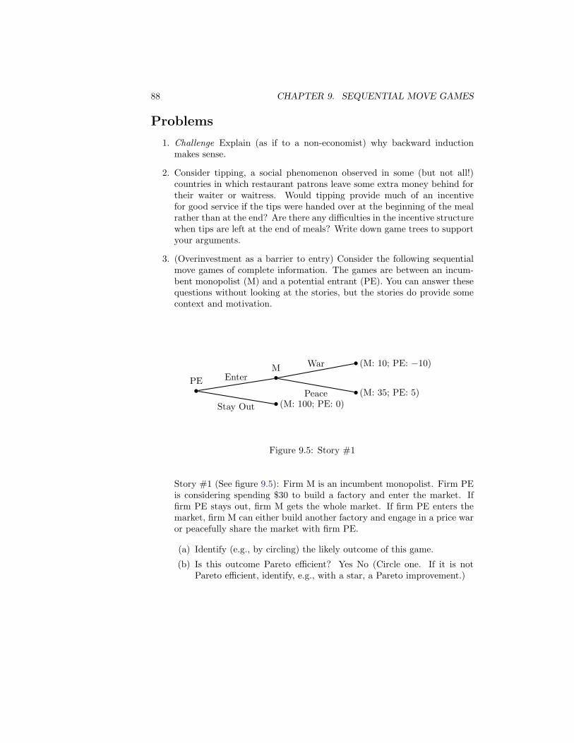
88 CHAPTER 9. SEQUENTIAL MOVE GAMES
Problems
1. Challenge Explain (as if to a non-economist) why backward inductionmakes sense.
2. Consider tipping, a social phenomenon observed in some (but not all!)countries in which restaurant patrons leave some extra money behind fortheir waiter or waitress. Would tipping provide much of an incentivefor good service if the tips were handed over at the beginning of the mealrather than at the end? Are there any difficulties in the incentive structurewhen tips are left at the end of meals? Write down game trees to supportyour arguments.
3. (Overinvestment as a barrier to entry) Consider the following sequentialmove games of complete information. The games are between an incum-bent monopolist (M) and a potential entrant (PE). You can answer thesequestions without looking at the stories, but the stories do provide somecontext and motivation.
PE
MEnter
(M: 10; PE: −10)War
(M: 35; PE: 5)Peace(M: 100; PE: 0)Stay Out
Figure 9.5: Story #1
Story #1 (See figure 9.5): Firm M is an incumbent monopolist. Firm PEis considering spending $30 to build a factory and enter the market. Iffirm PE stays out, firm M gets the whole market. If firm PE enters themarket, firm M can either build another factory and engage in a price waror peacefully share the market with firm PE.
(a) Identify (e.g., by circling) the likely outcome of this game.
(b) Is this outcome Pareto efficient? Yes No (Circle one. If it is notPareto efficient, identify, e.g., with a star, a Pareto improvement.)

9.1. BACKWARD INDUCTION 89
M
PE
Overinvest
MEnter
(M: 10; PE: −10)War
(M: 5; PE: 5)Peace(M: 70; PE: 0)Stay Out
PEDon’t Invest
MEnter
(M: 10; PE: −10)War
(M: 35; PE: 5)Peace(M: 100; PE: 0)Stay Out
Figure 9.6: Story #2
Story #2 (See figure 9.6): The monopolist (firm M) chooses whether ornot to overinvest by building a second factory for $30 even though onefactory is more than enough. Firm PE (the potential entrant) sees whatfirm M has done and decides whether to enter or stay out, and if PE entersthen M decides whether or not to engage in a price war.
(a) Identify (e.g., by circling) the likely outcome of this game.
(b) Is this outcome Pareto efficient? Yes No (Circle one. If it is notPareto efficient, identify, e.g., with a star, a Pareto improvement.)
4. (The Sticks Game) The sticks game works as follows: We put n sticks onthe table. Beginning with Player 1, the two players take turns removingeither one or two sticks. The player who removes the last stick must paythe other player $1.
(a) If there are 10 sticks on the table, which player would you rather be,and what strategy will you employ? [Hint: Use backwards induction!]
(b) Challenge If there are n sticks on the table, which player would yourather be? Can you describe a general strategy?
(c) Super Challenge (Note: I haven’t thought much about the secondquestion here, and in any case haven’t solved it.) Analyze this prob-lem when there are m piles of sticks (each turn one of the playerspicks one of the piles and removes one or two sticks from it) or whenthere are more than two players (the losing player must pay $1 toeach of the others).

90 CHAPTER 9. SEQUENTIAL MOVE GAMES
5. (The Ice Cream Pie Game, from Dixit and Nalebuff) Two players taketurns making take-it-or-leave-it offers about the division of an ice creampie. In the first round, the whole pie is available; if Player 2 accepts Player1’s proposal then the two players share the entire pie; if Player 2 rejectsPlayer 1’s proposal, half of the pie melts away, and we go to round two (inwhich Player 2 makes a take-it-or-leave-it offer about the division of theremaining pie). The game ends when an offer is accepted, or after the endof the nth period (at which point Mom eats the remaining pie, meaningthat the players get nothing).
(a) Predict the outcome of the game when there are 1, 2, and 3 periods.
(b) Now assume that 1/3rd of the pie (rather than 1/2) melts away eachperiod. Predict the outcome when there are 1, 2, and 3 periods.
(c) Hopefully your prediction is that the first offer made is always ac-cepted. Try to understand and explain (as if to a non-economist)why this happens.
6. Make up some game trees (players, options, payoffs, etc.) and solve themusing backward induction. It may help to exchange games and solutionswith a neighbor.
7. (The Draft Game, from Brams and Taylor) Three football teams (X, Y,Z) are involved in a draft for new players. There are six players to choosefrom (Center, Guard, Tailback, Quarterback, Halfback, Fullback), andthe draft works as follows: First X chooses a player, then Y chooses oneof the remaining five players, then Z chooses one of the remaining fourplayers (this constitutes the first round of the draft); the same procedureis repeated in the second round, at the end of which all six players aretaken.
The teams’ preferences are as follows:
Top choice Second Third Fourth Fifth Sixth
X C G T Q H F
Y H F G C Q T
Z T F H Q C G
Assume that the teams all know each others’ preferences. Then we canmodel the draft as a game tree, with team X choosing first &etc. Thecomplete game tree for this draft is quite involved, but trust me, it allboils down to the game tree shown in Figure 9.7.
The payoffs for this game are the players each team gets. For example,(CG, HQ, TF) indicates that team X gets the Center and the Guard (its

9.1. BACKWARD INDUCTION 91
X
Y
C
ZH
(CG, HF, TQ)T
(CG, HQ, FT)F
(CQ, GH, TF)G
YT
Z
H
(TC, HG, FQ)F
(TC, HF, QG)Q
ZF(TC, FG, HQ)H
(TC, FH, QG)Q
Figure 9.7: The draft game
#1 and #2 choices), team Y gets the Halfback and the Quarterback (#1and #2), and team Z gets the Tailback and the Fullback (#1 and #4).Clearly each team would prefer to get the players it likes the most, e.g.,team X prefers CT (or TC) to CQ or GQ.
(a) The “naive” strategy is for each team to choose its top choice amongthe available players every time it gets to pick. What is the outcomeof this strategy?
(b) If teams X and Y pursue this naive strategy by picking C and H inthe first round, should team Z also pursue this strategy, i.e., pick T?Briefly explain why or why not.
(c) What outcome do you expect from this game using backward induc-tion?
(d) Is the expected outcome you identified Pareto efficient? If so, explain.If not, identify a Pareto improvement.
(e) Statement 1: “In the first round, the optimal move for each team isto pick the best available player.” Statement 2: “In the second round,the optimal move for each team is to pick the best available player.”Explain why Statement 1 is false but Statement 2 is true.
(f) Challenge Prove that the game tree really does boil down to what’sshown on the previous page.

92 CHAPTER 9. SEQUENTIAL MOVE GAMES
8. Fun (The Hold-Up Problem) In the movie Butch Cassidy and the SundanceKid (1969), Paul Newman and Robert Redford play Wild West bankrobbers who are particularly fond of robbing the Union Pacific Railroad.The CEO of the railroad, Mr. E. H. Harriman, hires a “superposse” ofgunslingers to bring the two robbers to justice, dead or alive. After a long(and rather boring) chase scene, Butch and Sundance manage to escape.Afterwards, Butch reads about the superposse in the newspaper and hasthis to say:
A set-up like that costs more than we ever took...That crazyHarriman. That’s bad business. How long do you think I’d stayin operation if every time I pulled a job, it cost me money? Ifhe’d just pay me what he’s spending to make me stop robbin’him, I’d stop robbin’ him. [Screaming out the door at E. H.Harriman:] Probably inherited every penny you got! Thoseinherited guys—what the hell do they know?
(a) Is what Harriman is doing bad business? Explain why or why not.You answer may depend on the assumptions you make, so explic-itly state any and all assumptions. You might also want to draw agame tree, make up appropriate payoffs, and solve the game usingbackwards induction.
(b) “If he’d just pay me what he’s spending to make me stop robbin’him, I’d stop robbin’ him.” Assume this statement is true. Whatdoes it say about the efficiency or inefficiency of the situation?
(c) What do you think about the argument contained in the previousquote? Can you see why this is called the “hold-up problem”?
(d) The hold-up problem also applies to students working jointly onprojects and to firms engaged in joint ventures: after one membermakes an irreversible investment, the other member may try to rene-gotiate the terms of the deal. Explain how contracts might help inpreventing this difficulty, and why contracts wouldn’t work in thecase of Butch Cassidy.
9. Fun The IgoUgo travel guide Andiamo provides the following advice forcrossing the street in Rome: “First, stand towards a coffee bar and watch alocal or two. See how they boldly walk out into traffic? Now it’s your turn!Choose your moment but don’t hesitate for too long. Waiting for traffic toclear will not happen. When you appear to have the most lead-time, stepboldly off the curb and walk swiftly and confidently for the opposite sideof the street. Do not look at the traffic careening towards you—believe itor not, they will stop for you! But do not look at them—do not make eyecontact—this is an invitation for sport. Just walk briskly with your headup and your eyes on the prize- the opposite sidewalk.”
(a) “[D]o not make eye contact—this is an invitation for sport.” Explain.

9.1. BACKWARD INDUCTION 93
(b) Set up a game tree for this “pedestrian in Rome” game and solve it.
10. (The Centipede Game) There are 6 $1 bills on a table. Players 1 and 2take turns moving. Each turn the player moving takes either $1 (in whichcase it becomes the other player’s turn) or $2 (in which case the gameends). Each player wants to get as much money as possible.
(a) Draw a game tree for this game.
(b) Predict the outcome of this game.
(c) Is this outcome Pareto efficient? If so, explain briefly. If not, identifya Pareto improvement.
(d) Challenge Can you generalize this result when there are n bills onthe table? (Hint: Try induction.)
(e) Super Challenge Can you reconcile the previous answer with yourintuition about how this game might actually get played in real life?
11. Fun (The surprise exam paradox) Your class meets 5 days a week, andon Friday your teacher tells you that there will be a surprise exam nextweek, meaning (1) that there will be an exam, and (2) that it will be asurprise (i.e., you won’t be able to anticipate the night before the examthat the exam will be the next day). What can you conclude about theexam? Relate this problem to the Centipede Game discussed previously.

94 CHAPTER 9. SEQUENTIAL MOVE GAMES

Chapter 10
Simultaneous Move Games
Another kind of game is one of simultaneous moves: two or more playersmove at the same time (an example here is the game “Rock, Paper, Scissors”).Although it is possible to analyze these games using a game tree, it is ofteneasier to use a payoff matrix. An example is the duopoly1 game shown inFigure 10.1. There are two firms, Coke and Pepsi. The two firms simultaneouslychoose “high” or “low” prices. If they both choose high prices, they both makelarge profits: $4 million each. If they both choose low prices, they both makesmall profits: $3 million each. If one chooses a high price and one chooses a lowprice, customers will flock to the low-priced product; the low-pricing firm willmake $5 million and the high-pricing firm will make only $1 million. (Note: Byconvention, the row-playing firm (in this case, Coke) is called Firm 1, and thecolumn-playing firm (Pepsi) is called Firm 2. The payoffs in each box are listedin the order of the firms: (5, 1) indicates that Firm 1 (Coke) gets a payoff of 5and Firm 2 (Pepsi) gets a payoff of 1.)
Pepsi
High price Low price
CokeHigh price 4,4 1,5
Low price 5,1 3,3
Figure 10.1: The duopoly game
1A market with only two sellers is called a duopoly, just like a market with only one selleris called a monopoly.
95

96 CHAPTER 10. SIMULTANEOUS MOVE GAMES
10.1 Dominance
One perspective on this game comes from the observation that Coke alwaysmakes more money by choosing a low price regardless of what Pepsi does: ifPepsi chooses a low price, Coke gets $3 million by choosing a low price and only$1 million by choosing a high price; if Pepsi chooses a high price, Coke gets $5million by choosing a low price and only $4 million by choosing a high price. Inother words, “low price” is a strictly dominant strategy for Coke: no matterwhat Pepsi does, choosing the low price produces a higher payoff for Coke.
Similarly, we can see that “low price” is a strictly dominant strategy forPepsi. We can predict, therefore, that both firms will choose the low price,yielding profits of $3 million for each firm.
10.2 The Prisoners’ Dilemma
Figure 10.1 is one version of an important game called the Prisoners’ Dilemma.Another version (which explains the game’s name) is shown in Figure 10.2. Thestory is this: You are visiting an unnamed foreign country, waiting in line tobuy a Coke from a street vendor, when you and the guy in front of you in lineare arrested and put into separate jail cells. A police officer comes into your celland tells you that you and the other guy are under suspicion for armed robbery.The officer tells you that they can definitely convict both you and the other guyfor some minor crime (e.g., littering), but that they can’t convict either of youfor armed robbery unless one of you agrees to testify against the other. Theofficer would really like to have an armed robbery conviction on his record, sohe offers you a deal: if you confess, and the other guy doesn’t, you walk freeand the other guy gets locked up for 20 years. The officer also tells you (bigsurprise) that he’s making the same offer to the other guy: if the other guyconfesses, and you don’t, he walks free and you get 20 years in the clink. Whatif you both confess? Well, then you both get locked up for 5 years (for armedrobbery). And if you both keep quiet, you both get locked up for 1 year (forlittering). (This information is summarized in Figure 10.2.)
Player 2
Confess Keep quiet
Player 1Confess -5,-5 0,-20
Keep quiet -20,0 -1,-1
Figure 10.2: The Prisoners’ Dilemma

10.2. THE PRISONERS’ DILEMMA 97
Question: What is a good prediction for the Prisoners’ Dilemma game if bothplayers are optimizing?
Answer: The only reasonable prediction is for both of you to confess becauseconfessing is a strictly dominant strategy: no matter what the other guy does,the best thing for you to do is confess, and no matter what you do, the bestthing for the other guy to do is confess. Curiously, there is another outcomewhich both of you strictly prefer to this outcome: you’d both be better off (i.e.,it would be a Pareto improvement) if you both kept quiet. But the incentivestructure is such that you both confess!
The Prisoners’ Dilemma game has an amazing number of applications, allinvolving what are called collective action problems. For example:
• You and everybody else might like to drive your own cars to work, butperhaps we would all be better off with carpools or buses instead of trafficjams.
• Your firm and your rival firm might both make more money if you agreedto set higher prices, but if your rival sets higher prices you can make evenmore money by cheating on the deal and undercutting your rival’s prices.(Note: This is exactly what happened in the Coke and Pepsi game we sawearlier.)
• The different nations in OPEC (the Organization of Petroleum ExportingCountries) might all be better off if they agree to restrict the supply of oil(thereby raising the price, generating higher profits for all of them), buteach of them is tempted to secretly cheat on the deal and produce morethan their allotted quota.
• You and everybody else might like to burn wood in your fireplace, butif everybody does that we would have horrible air quality problems thatwould hurt us all.
• You and another classmate are assigned a joint project. The best outcomeis for each of you to do a decent amount of work, resulting in good gradesfor both of you. The temptation for both of you is to be a free-rider byslacking off, forcing your classmate to do all the work, and getting creditfor their effort. Of course, if both of you do this you’ll both get horriblegrades. . .
• Finally, it is worth noting that the Prisoners’ Dilemma game is a reason-able representation of some of the dangers of plea-bargaining. There reallyis a dilemma for those accused of crimes: suspects might agree to testifyagainst others out of their own self-interest, with harmful ramificationsfor the integrity of our criminal justice system.
How can we reach the cooperative outcome in the Prisoners’ Dilemma game?To examine this possibility, we’ll use the version of the Prisoners’ Dilemma gameshown in Figure 10.3; this version involves cash prizes rather than prison terms.

98 CHAPTER 10. SIMULTANEOUS MOVE GAMES
Player 2
D C
Player 1D 0,0 10,-5
C -5,10 1,1
Figure 10.3: Another version of the Prisoners’ Dilemma
The idea of dominant strategies makes for a clear prediction for this game:Player 1 plays D, Player 2 plays D, and each player gets nothing. Clearly thisoutcome is not Pareto efficient: the strategy combination (C, C) would alloweach player to get one dollar. So we can think of (C, C) as the cooperativestrategy and ask under what conditions we might be able to see this kind ofcooperative behavior.
10.3 Finitely Repeated Games
One possibility is to play the same game over and over again: perhaps theplayers can establish reputations and learn to trust each other, and then maybewe can get cooperative behavior. So we turn our attention to repeated games,in which a smaller game (called the stage game) is played over and over again(n times). We will take the Prisoners’ Dilemma game in Figure 10.3 as the stagegame, and see what the potential is for cooperation.
We know that if n = 1 (i.e., the stage game is only played once) the potentialfor cooperation is quite slim: playing D is a strictly dominant strategy for eachplayer: no matter what Player 2 does, Player 1 is better off playing D, and viceversa. So we should not expect to see cooperative behavior if the game is playedonly once.
An extension of this logic suggests that we should not expect to see cooper-ative behavior if the game is played twice, or 10 times, or even 100 times. Tosee this, apply backward induction: in the final game (whether it’s the secondplaying of the stage game or the 100th), playing D is a strictly dominant strat-egy for both players, so both players should expect the outcome (D, D) in thefinal game. We now look at the penultimate (second-to-last) game: knowingthat (D, D) will be the outcome in the final game, playing D becomes a strictlydominant strategy in the penultimate game as well! We continue working back-wards all the way to the beginning of the game, and conclude that the onlyrational prediction is for the players to play (D, D) in each of the stage games.So we cannot expect any cooperative behavior.
Digression: This theory does not match up well with reality. In classroomexperiments (or experiments on “regular people” conducted by experimentaleconomists), what tends to happen is this: if the stage game is repeated 10times, players will cooperate for about 5 or 6 stages, and then one player (or

10.3. FINITELY REPEATED GAMES 99
b
b
b bb
b
b bb
b
b bb
b
b bb
b
b b
(2,0) (1,2) (3,1) (2,3) (4,2)
(3,3)1 2 1 2 1$1
$2
$1
$2
$1
$2
$1
$2
$1
$2
Figure 10.4: The centipede game
possibly both players) will stop cooperating and the noncooperative outcome(D, D) occurs for the remainder of the game. Maybe people’s deductive powerssimply don’t work that well? Or maybe people’s deductive powers are strongerthan we give them credit for! For example, most people playing the gamein Figure 10.4 do better than game theory predicts. This game is called thecentipede game (because the game tree looks like a stick-figure centipede), andthe story behind it is this: There are six $1 bills on a table. Players 1 and 2 taketurns moving. On each turn the player moving takes either $2 from the table(in which case the game ends) or $1 (in which case it becomes the other player’sturn). The payoffs (which become much more impressive if you think of a gameinvolving six $100 bills instead of six $1 bills) are given at each terminal nodeof the game tree. (Exercise: Predict the outcome of this game using the toolsof game theory. Then ask yourself what strategy you would follow if you werePlayer 1, or if you were Player 2 and Player 1 started off by taking $1. Then,if you’re really looking for a challenge, try to make sense of the whole mess. Isthe theory wrong, or are the players wrong, or what?)
Problems
1. Everybody in City X drives to work, so commutes take two hours. Imaginethat a really good bus system could get everybody to work in 40 minutesif there were no cars on the road. There are only two hitches: (1) If thereare cars on the road, the bus gets stuck in traffic just like every othervehicle, and therefore (2) people can always get to their destination 20minutes faster by driving instead of taking the bus (the extra 20 minutescomes from walking to the bus stop, waiting for the bus, etc.).
(a) If such a bus system were adopted in City X and each resident ofCity X cared only about getting to work as quickly as possible, whatwould you expect the outcome to be?
(b) Is this outcome Pareto efficient? Explain briefly.
(c) “The central difficulty here is that each commuter must decide whatto do without knowing what the other commuters are doing. If you
100 CHAPTER 10. SIMULTANEOUS MOVE GAMES
knew what the others decided, you would behave differently.” Do youagree with this argument?
(d) What sort of mechanism do you suggest for reaching the optimaloutcome in this game? Hint: Make sure to think about enforcement!
2. (The Public/Private Investment Game) You are one of ten students in aroom, and all of you are greedy income-maximizers. Each student has$1 and must choose (without communicating with the others) whether toinvest it in a private investment X or a public investment Y. Each dollarinvested in the private investment X has a return of $2, which goes entirelyto the investor. Each dollar invested publicly has a return of $10, which isdivided equally among the ten students (even those who invest privately).So if six students invest publicly, the total public return is $60, dividedequally among the ten students; the four students who invested privatelyget an additional $2 each from their private investment.
(a) What outcome do you predict in the simultaneous-move game, i.e.,if all the students must write down their investment decisions at thesame time?
(b) Is this outcome Pareto efficient? If not, identify a Pareto improve-ment.
(c) “The central difficulty here is that the students must decide withoutknowing what the other students are doing. If you knew what theother students decided, you would behave differently.” Do you agreewith this argument?
(d) If communication were possible, what sort of mechanism do you sug-gest for reaching the optimal outcome in this game? Hint: Make sureto think about enforcement!
3. Consider the following game.
Player 2
D C
Player 1D −2,−2 10,−5
C −5, 10 1, 1
(a) What outcome do you expect if this game is played once? Explainbriefly.
(b) What outcome do you expect if this game is played twice? Explainbriefly.

Chapter 11
Iterated Dominance andNash Equilibrium
In the previous chapter we examined simultaneous move games in which eachplayer had a dominant strategy; the Prisoner’s Dilemma game was one example.In many games, however, one or more players do not have dominant strategies.This chapter explores two solution concepts that we can use to analyze suchgames.
The first solution concept, iterated dominance, is a refinement of the domi-nant strategies approach from the previous chapter, meaning that iterated dom-inance is a stronger technique that builds upon (or refines) the results of thedominant strategies approach. In other words: the idea of dominant strategiesoften allows us to narrow down our prediction for the outcome of a game; it-erated dominance allows us to narrow down our prediction at least as far, andsometimes further.
Unfortunately, this extra strength does not come for free. While dominantstrategies is a reasonably simple idea, iterated dominance is (while not exactlya Nobel-prize-winning concept) one step closer to rocket science. As such, itrequires more powerful assumptions about the intellectual capabilities of theoptimizing individuals who are playing the games.
The second solution concept in this chapter, Nash equilibrium, is a refine-ment of iterated dominance: Nash equilibrium allows us to narrow down ourprediction at least as far as iterated dominance, and sometimes further. Again,this extra strength does not come for free. Nonetheless, Nash equilibrium is oneof the central concepts in the study of strategic behavior—a fact which helpsexplain why Nash equilibrium is a Nobel-prize-winning concept.
11.1 Iterated Dominance
The transition from dominant strategies to iterated dominance involves twoideas. The first is this: even when a player doesn’t have a dominant strategy
101
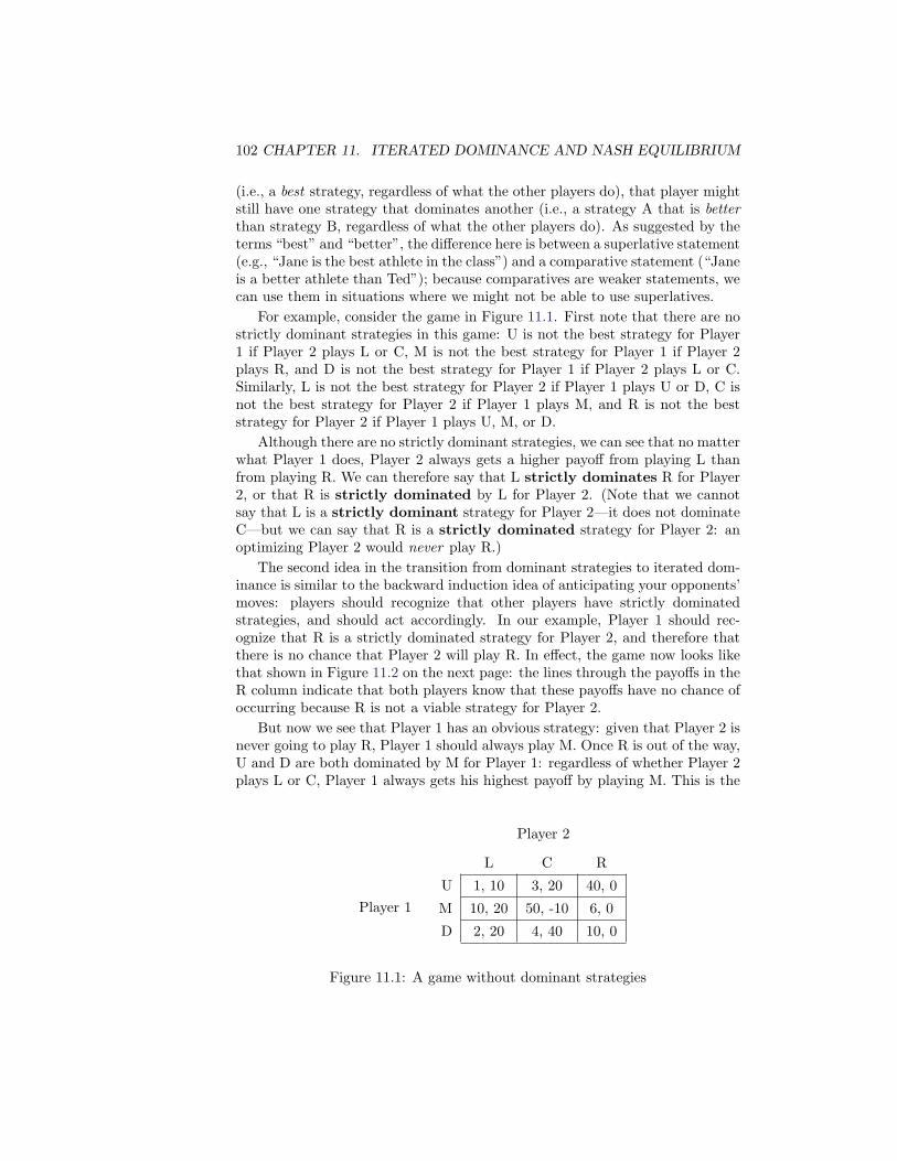
102 CHAPTER 11. ITERATED DOMINANCE AND NASH EQUILIBRIUM
(i.e., a best strategy, regardless of what the other players do), that player mightstill have one strategy that dominates another (i.e., a strategy A that is betterthan strategy B, regardless of what the other players do). As suggested by theterms “best” and “better”, the difference here is between a superlative statement(e.g., “Jane is the best athlete in the class”) and a comparative statement (“Janeis a better athlete than Ted”); because comparatives are weaker statements, wecan use them in situations where we might not be able to use superlatives.
For example, consider the game in Figure 11.1. First note that there are nostrictly dominant strategies in this game: U is not the best strategy for Player1 if Player 2 plays L or C, M is not the best strategy for Player 1 if Player 2plays R, and D is not the best strategy for Player 1 if Player 2 plays L or C.Similarly, L is not the best strategy for Player 2 if Player 1 plays U or D, C isnot the best strategy for Player 2 if Player 1 plays M, and R is not the beststrategy for Player 2 if Player 1 plays U, M, or D.
Although there are no strictly dominant strategies, we can see that no matterwhat Player 1 does, Player 2 always gets a higher payoff from playing L thanfrom playing R. We can therefore say that L strictly dominates R for Player2, or that R is strictly dominated by L for Player 2. (Note that we cannotsay that L is a strictly dominant strategy for Player 2—it does not dominateC—but we can say that R is a strictly dominated strategy for Player 2: anoptimizing Player 2 would never play R.)
The second idea in the transition from dominant strategies to iterated dom-inance is similar to the backward induction idea of anticipating your opponents’moves: players should recognize that other players have strictly dominatedstrategies, and should act accordingly. In our example, Player 1 should rec-ognize that R is a strictly dominated strategy for Player 2, and therefore thatthere is no chance that Player 2 will play R. In effect, the game now looks likethat shown in Figure 11.2 on the next page: the lines through the payoffs in theR column indicate that both players know that these payoffs have no chance ofoccurring because R is not a viable strategy for Player 2.
But now we see that Player 1 has an obvious strategy: given that Player 2 isnever going to play R, Player 1 should always play M. Once R is out of the way,U and D are both dominated by M for Player 1: regardless of whether Player 2plays L or C, Player 1 always gets his highest payoff by playing M. This is the
Player 2
L C R
Player 1
U 1, 10 3, 20 40, 0
M 10, 20 50, -10 6, 0
D 2, 20 4, 40 10, 0
Figure 11.1: A game without dominant strategies
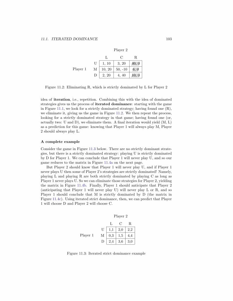
11.1. ITERATED DOMINANCE 103
Player 2
L C R
Player 1
U 1, 10 3, 20 ////40,///0
M 10, 20 50, -10 //6,///0
D 2, 20 4, 40 ////10,///0
Figure 11.2: Eliminating R, which is strictly dominated by L for Player 2
idea of iteration, i.e., repetition. Combining this with the idea of dominatedstrategies gives us the process of iterated dominance: starting with the gamein Figure 11.1, we look for a strictly dominated strategy; having found one (R),we eliminate it, giving us the game in Figure 11.2. We then repeat the process,looking for a strictly dominated strategy in that game; having found one (or,actually two: U and D), we eliminate them. A final iteration would yield (M, L)as a prediction for this game: knowing that Player 1 will always play M, Player2 should always play L.
A complete example
Consider the game in Figure 11.3 below. There are no strictly dominant strate-gies, but there is a strictly dominated strategy: playing U is strictly dominatedby D for Player 1. We can conclude that Player 1 will never play U, and so ourgame reduces to the matrix in Figure 11.4a on the next page.
But Player 2 should know that Player 1 will never play U, and if Player 1never plays U then some of Player 2’s strategies are strictly dominated! Namely,playing L and playing R are both strictly dominated by playing C as long asPlayer 1 never plays U. So we can eliminate those strategies for Player 2, yieldingthe matrix in Figure 11.4b. Finally, Player 1 should anticipate that Player 2(anticipating that Player 1 will never play U) will never play L or R, and soPlayer 1 should conclude that M is strictly dominated by D (the matrix inFigure 11.4c). Using iterated strict dominance, then, we can predict that Player1 will choose D and Player 2 will choose C.
Player 2
L C R
Player 1
U 1,1 2,0 2,2
M 0,3 1,5 4,4
D 2,4 3,6 3,0
Figure 11.3: Iterated strict dominance example

104 CHAPTER 11. ITERATED DOMINANCE AND NASH EQUILIBRIUM
L C R
U ////1,1 ////2,0 ////2,2
M 0,3 1,5 4,4
D 2,4 3,6 3,0
(a)
L C R
U ////1,1 ////2,0 ////2,2
M ////0,3 1,5 ////4,4
D ////2,4 3,6 ////3,0
(b)
L C R
U ////1,1 ////2,0 ////2,2
M ////0,3 ////1,5 ////4,4
D ////2,4 3,6 ////3,0
(c)
Figure 11.4: Solution to iterated strict dominance example
Question: Does the order of elimination matter?
Answer: Although it is not obvious, the end result of iterated strict dominanceis always the same regardless of the sequence of eliminations. In other words,if in some game you can either eliminate U for Player 1 or L for Player 2, youdon’t need to worry about which one to “do first”: either way you’ll end up atthe same answer.
A side note here is that this result only holds under iterated strict domi-nance, according to which we eliminate a strategy only if there is some otherstrategy that yields payoffs that are strictly higher no matter what the otherplayers do. If you eliminate a strategy when there is some other strategy thatyields payoffs that are higher or equal no matter what the other players do, youare doing iterated weak dominance, and in this case you will not always getthe same answer regardless of the sequence of eliminations. (For an examplesee problem 10.) This is a serious problem, and helps explain why we focus oniterated strict dominance.
11.2 Nash Equilibrium
Tenuous as it may seem, iterated strict dominance is not a very strong solutionconcept, meaning that it does not yield predictions in many games. An exampleis the game in Figure 11.5: there are no strictly dominant strategies and nostrictly dominated strategies.
So game theorists have come up with other solution concepts. The mostimportant one is called Nash equilibrium (abbreviated NE). A Nash equi-
Player 2
L C R
Player 1
U 5,1 2,0 2,2
M 0,4 1,5 4,5
D 2,4 3,6 1,0
Figure 11.5: Nash equilibrium example

11.2. NASH EQUILIBRIUM 105
librium occurs when the strategies of the various players are best responses toeach other. Equivalently but in other words: given the strategies of the otherplayers, each player is acting optimally. Equivalently again: No player can gainby deviating alone, i.e., by changing his or her strategy single-handedly.
In the game in Figure 11.5, the strategies (D, C) form a Nash equilibrium:if Player 1 plays D, Player 2 gets her best payoff by playing C; and if Player 2plays C, Player 1 gets his best payoff by playing D. So the players’ strategiesare best responses to each other; equivalently, no player can gain by deviatingalone. (Question: Are there any other Nash equilibria in this game?)
Algorithms for Finding Nash Equilibria
The best way to identify the Nash equilibria of a game is to first identify allof the outcomes that are not Nash equilibria; anything left must be a Nashequilibrium. For example, consider the game in Figure 11.5. The strategy pair(U, L) is not a Nash equilibrium because Player 2 can gain by deviating aloneto R; (U, C) is not a NE because Player 1 can gain by deviating alone to D(and Player 2 can gain by deviating alone to L or R); etc. If you go throughthe options one by one and cross out those that are not Nash equilibria, theremaining options will be Nash equilibria (See Figure 11.6a).
A shortcut (but one you should use carefully!) is to underline each player’sbest responses.1 To apply this to the game in Figure 11.5, first assume thatPlayer 2 plays L; Player 1’s best response is to play U, so underline the “5” inthe box corresponding to (U, L). Next assume that Player 2 plays C; Player 1’sbest response is to play D, so underline the “3” in the box corresponding to (D,C). Finally, assume that Player 2 plays R; Player 1’s best response is to playM, so underline the “4” in the box corresponding to (M, R). Now do the samething for Player 2: go through all of Player 1’s options and underline the bestresponse for Player 2. (Note that C and R are both best responses when Player1 plays M!) We end up with Figure 11.6b: the only boxes with both payoffsunderlined are (D, C) and (M, R), the Nash equilibria of the game.
L C R
U ////5,1 ////2,0 ////2,2
M ////0,4 ////1,5 4,5
D ////2,4 3,6 ////1,0
(a)
L C R
U 5,1 2,0 2,2
M 0,4 1,5 4,5
D 2,4 3,6 1,0
(b)
Figure 11.6: Finding Nash equilibria: (a) with strike-outs; (b) with underlinings
1It is easy to confuse the rows and columns and end up underlining the wrong things.Always double-check your answers by confirming that no player can gain by deviating alone.

106 CHAPTER 11. ITERATED DOMINANCE AND NASH EQUILIBRIUM
Some History
Nash equilibrium is one of the fundamental concepts of game theory. It is namedafter John Nash, a mathematician born in the early part of this century. Hecame up with his equilibrium concept while getting his Ph.D. in mathematicsat Princeton, then got a professorship at MIT, then went mad (e.g., claimedthat aliens were sending him coded messages on the front page of the New YorkTimes), then spent many years in and out of various mental institutions, thenslowly got on the road to recovery, then won the Nobel Prize in Economics in1994, and now putters around Princeton playing with computers. You can readmore about him in a fun book called A Beautiful Mind by Sylvia Nasar.2
11.3 Infinitely Repeated Games
We saw in the last chapter that there’s no potential for cooperation (at least intheory) if we play the Prisoner’s Dilemma game twice, or 50 times, or 50 milliontimes. What about infinitely many times?
In order to examine this possibility, we must first figure out exactly what itmeans to win (or lose) this game infinitely many times. Here it helps to use thepresent value concepts from Chapter 1: with an interest rate of 5%, winning $1in each round does not give you infinite winnings. Rather, the present value ofyour winnings (using the perpetuity formula, assuming you get paid at the end
of each round) is$1
.05= $20.
So: with an interest rate of r we can ask meaningful questions about thepotential for cooperation. One point that is immediately clear is that there isstill plenty of potential for non-cooperation: the strategies of playing (D, D)forever continue to constitute a Nash equilibrium of this game.
But perhaps there are other strategies that are also Nash equilibria. Becausethe game is played infinitely many times, we cannot use backward induction tosolve this game. Instead, we need to hunt around and look for strategies thatmight yield a cooperative Nash equilibrium.
One potentially attractive idea is to use a trigger strategy: begin by co-operating and assuming that the other player will cooperate (i.e., that bothplayers will play C), and enforce cooperation by threatening to return to the(D, D) equilibrium. Formally, the trigger strategy for each player is as follows:In the first stage, play C. Thereafter, if (C, C) has been the result in all previousstages, play C; otherwise, play D.
We can see that the cooperative outcome (C, C) will be the outcome in eachstage game if both players adopt such a trigger strategy. But do these strategiesconstitute a Nash equilibrium? To check this, we have to see if the strategiesare best responses to each other. In other words, given that Player 1 adopts
2There is also a movie of the same name, starring Russell Crowe. Unfortunately, it takessome liberties with the truth; it also does a lousy job of describing the Nash equilibriumconcept.

11.4. MIXED STRATEGIES 107
the trigger strategy above, is it optimal for Player 2 to adopt a similar triggerstrategy, or does Player 2 have an incentive to take advantage of Player 1?
To find out, let’s examine Player 2’s payoffs from cooperating and fromdeviating:
If Player 2 cooperates, she can expect to gain $1 at the end of each round,
yielding a present value payoff of$1
r. (If r = .05 this turns out to be $20.)
If Player 2 tries to cheat Player 1 (e.g., by playing D in the first round),Player 2 can anticipate that Player 1 will play D thereafter, so the bestresponse for Player 2 is to play D thereafter as well. So the best deviationstrategy for Player 2 is to play D in the first round (yielding a payoff of$10 since Player 1 plays C) and D thereafter (yielding a payoff of $0 eachround since Player 1 plays D also). The present value of all this is simply$10.
We can now compare these two payoffs, and we can see that cooperating is a
best response for Player 2 as long as$1
r≥ 10. Since the game is symmetric,
cooperating is a best response for Player 1 under same condition, so we have a
Nash equilibrium (i.e., mutual best responses) as long as$1
r≥ 10. Solving this
yields a critical value of r = .1. When r is below this value (i.e., the interestrate is less than 10%), cooperation is possible. When r is above this value (i.e.,the interest rate is greater than 10%), cheating is too tempting and the triggerstrategies do not form a Nash equilibrium. The intuition here is quite nice: Bycooperating instead of deviating, Player 2 accepts lower payoffs now (1 insteadof 10) in order to benefit from higher payoffs later (1 instead of 0). Higherinterest rates make the future less important, meaning that Player 2 benefitsless by incurring losses today in exchange for gains tomorrow. With sufficientlyhigh interest rates, Player 2 will take the money and run; but so will Player 1!
11.4 Mixed Strategies
Figure 11.7 shows another game, called the Battle of the Sexes. In thisgame, Player 1 prefers the opera, and Player 2 prefers wrestling, but what
Player 2
Opera WWF
Player 1Opera 2,1 0,0
WWF 0,0 1,2
Figure 11.7: The battle of the sexes

108 CHAPTER 11. ITERATED DOMINANCE AND NASH EQUILIBRIUM
both players really want above all is to be with each other. They both choosesimultaneously, though, and so cannot guarantee that they’ll end up together.(Imagine, for example, that they are at different work places and can’t reacheach other and must simply head to one of the two events after work and waitfor the other person at will-call.)
The Nash equilibriums of this game are (Opera, Opera) and (WWF, WWF).But there is another Nash equilibrium that is perhaps a little better at predictingreality: that equilibrium is for both players to play a mixed strategy, i.e., tochoose different strategies with various probabilities. (In this case, the mixedstrategy equilibrium is for Player 1 to choose opera with probability 2/3 andWWF with probability 1/3, and for Player 2 to choose opera with probability1/3 and WWF with probability 2/3. You should be able to use what you’velearned about expected value to show that these are mutual best responses.)One of the main results from game theory is that every finite game has atleast one Nash equilibrium. That Nash equilibrium may only exist in mixedstrategies, as in the following example.
Example: (Matching pennies, Figure 11.8). Players 1 and 2 each have apenny, and they put their pennies on a table simultaneously. If both show thesame face (both heads or both tails), Player 2 must pay $1 to Player 1; if oneis heads and the other is tails, Player 1 must pay $1 to Player 2.
Not surprisingly, the only NE in this game is for each player to play headswith probably 1/2 and tails with probability 1/2.
11.5 Math: Mixed Strategies
Consider the “Matching Pennies” game shown in Figure 11.8. There are no purestrategy Nash equilibria in this game, but intuitively it seems like randomizingbetween heads and tails (with probability 50% for each) might be a good strat-egy. To formalize this intuition we introduce the concept of mixed strategyNash equilibrium.
In a mixed strategy Nash equilibrium, players do not have to choose justone strategy (say, Heads) and play it with probability 1. Instead, they canspecify probabilities for all of their different options and then randomize (ormix) between them. To see how this might work in practice, a player whospecifies Heads with probability .3 and Tails with probability .7 could put 3
Player 2
Heads Tails
Player 1Heads 1,-1 -1,1
Tails -1,1 1,-1
Figure 11.8: Matching pennies
11.5. MATH: MIXED STRATEGIES 109
cards labeled Heads and 7 cards labeled Tails into a hat; when the times comesto actually play the game, she draws a card from the hat and plays accordingly.She may only play the game once, but her odds of playing Heads or Tails are .3and .7, respectively.
Finding Mixed Strategy Nash Equilibria
To find mixed strategy Nash equilibria, we can simply associate different proba-bilities with the different options for each player. This gets messy for big payoffmatrices, so we will restrict out attention to games (such as Matching Pennies)in which each player has only two options. In that game, let us define p to bethe probability that player 1 chooses Heads and q to be the probability thatplayer 2 chooses Heads. Since probabilities have to add up to 1, the probabilitythat players 1 and 2 choose Tails must be 1 − p and 1 − q, respectively.
Now let’s write down the expected payoff for player 1 given these strategies.With probability p player 1 chooses Heads, in which case he gets +1 if player2 chooses Heads (which happens with probability q) and −1 if player 2 choosesTails (which happens with probability 1 − q). With probability 1 − p player1 chooses Tails, in which case he gets −1 if player 2 chooses Heads (whichhappens with probability q) and +1 if player 2 chooses Tails (which happenswith probability 1 − q). So player 1’s expected value is
E(π1) = p[q(1) + (1 − q)(−1)] + (1 − p)[q(−1) + (1 − q)(1)]
= p(2q − 1) + (1 − p)(1 − 2q).
Similarly, player 2’s expected payoff is
E(π2) = q[p(−1) + (1 − p)(1)] + (1 − q)[p(1) + (1 − p)(−1)]
= q(1 − 2p) + (1 − q)(2p − 1).
Now, we want to find p and q that form a Nash equilibrium, i.e., that aremutual best responses. To do this, we take partial derivatives and set themequal to zero. Here’s why:
First, player 1 wants to choose p to maximize E(π1) = p(2q − 1) + (1 −p)(1 − 2q). One possibility is that a maximizing value of p is a corner solution,i.e., p = 0 or p = 1. These are player 1’s pure strategy options: p = 1 meansthat player 1 always plays Heads, and p = 0 means that player 1 always playsTails.
The other possibility is that there is an interior maximum, i.e., a maximumvalue of p with 0 < p < 1. In this case, the partial derivative of E(π1) withrespect to p must be zero:
∂E(π1)
∂p= 0 =⇒ 2q − 1 − (1 − 2q) = 0 =⇒ 4q = 2 =⇒ q =
1
2.
This tells us that any interior value of p is a candidate maximum as long asq = 1
2 . Mathematically, this makes sense because if q = 12 then player 1’s
110 CHAPTER 11. ITERATED DOMINANCE AND NASH EQUILIBRIUM
expected payoff (no matter what his choice of p) is always
E(π1) = p(2q − 1) + (1 − p)(1 − 2q) = p(0) + (1 − p)(0) = 0.
Intuitively, what is happening is that player 2 is randomly choosing betweenHeads and Tails. As player 1, any strategy you follow is a best response. Ifyou always play Heads, you will get an expected payoff of 0; if you always playTails, you will get an expected payoff of 0; if you play heads with probability .5or .3, you will get an expected payoff of 0.
Our conclusion regarding player 1’s strategy, then, is this: If player 2 choosesq = 1
2 , i.e., randomizes between Heads and Tails, then any choice of p is a bestresponse for player 1. But if player 2 chooses q 6= 1
2 , then player 1’s bestresponse is a pure strategy: if player 2 chooses q > 1
2 then player 1’s bestresponse is to always play Heads; if player 2 chooses q < 1
2 then player 1’s bestresponse is to always play Tails.
We can now do the math for player 2 and come up with a similar conclusion.Player 2’s expected payoff is E(π2) = q(1 − 2p) + (1 − q)(2p − 1). Any value ofq that maximizes this is either a corner solution (i.e., one of the pure strategiesq = 1 or q = 0) or an interior solution with 0 < q < 1, in which case
∂E(π2)
∂q= 0 =⇒ 1 − 2p − (2p − 1) = 0 =⇒ 4p = 2 =⇒ p =
1
2.
So if player 1 chooses p = 12 then any choice of q is a best response for player 2.
But if player 1 chooses p 6= 12 , then player 2’s best response is a pure strategy:
if player 1 chooses p > 12 then player 2’s best response is to always play Tails;
if player 1 chooses p < 12 then player 2’s best response is to always play Heads.
Now we can put our results together to find the Nash equilibrium in thisgame. If player 1’s choice of p is a best response to player 2’s choice of q theneither p = 1 or p = 0 or q = 1
2 (in which case any p is a best response). Andif player 2’s choice of q is a best response to player 1’s choice of p then eitherq = 1 or q = 0 or p = 1
2 (in which case any q is a best response).Three choices for player 1 and three choices for player 2 combine to give us
nine candidate Nash equilibria:
Four pure strategy candidates: (p = 1, q = 1), (p = 1, q = 0), (p = 0, q =1), (p = 0, q = 0).
One mixed strategy candidate: (0 < p < 1, 0 < q < 1).
Four pure/mixed combinations: (p = 1, 0 < q < 1), (p = 0, 0 < q <
1), (0 < p < 1, q = 1), (0 < p < 1, q = 0).
We can see from the payoff matrix that the four pure strategy candidates arenot mutual best responses, i.e., are not Nash equilibria. And we can quickly seethat the four pure/mixed combinations are also not best responses; for example,(p = 1, 0 < q < 1) is not a Nash equilibrium because if player 1 chooses p = 1then player 2’s best response is to choose q = 0, not 0 < q < 1.

11.5. MATH: MIXED STRATEGIES 111
But the mixed strategy candidate does yield a Nash equilibrium: player 1’schoice of 0 < p < 1 is a best response as long as q = 1
2 . And player 2’s choiceof 0 < q < 1 is a best response as long as p = 1
2 . So the players’ strategies aremutual best responses if p = q = 1
2 . This is the mixed strategy Nash equilibriumof this game.
Another Example
Consider the “Battle of the Sexes” game shown in Figure 11.7 and duplicatedbelow. Again, let p be the probability that player 1 chooses Opera and q bethe probability that player 2 chooses Opera (so that 1 − p and 1 − q are therespective probabilities that players 1 and 2 will choose WWF). Then player 1’sexpected payoff is
E(π1) = p[q(2) + (1 − q)(0)] + (1 − p)[q(0) + (1 − q)(1)]
= 2pq + (1 − p)(1 − q).
Similarly, player 2’s expected payoff is
E(π2) = q[p(1) + (1 − p)(0)] + (1 − q)[p(0) + (1 − p)(2)]
= pq + (1 − q)(2)(1 − p).
Now, we want to find p and q that form a Nash equilibrium, i.e., that are mutualbest responses. To do this, we take partial derivatives and set them equal tozero.
So: player 1 wants to choose p to maximize E(π1) = 2pq + (1 − p)(1 − q).Any value of p that maximizes this is either a corner solution (i.e., one of thepure strategies p = 1 or p = 0) or an interior solution with 0 < p < 1, in whichcase the partial derivative of E(π1) with respect to p must be zero:
∂E(π1)
∂p= 0 =⇒ 2q − (1 − q) = 0 =⇒ 3q = 1 =⇒ q =
1
3.
This tells us that any interior value of p is a candidate maximum as long asq = 1
3 . Mathematically, this makes sense because if q = 13 then player 1’s
expected payoff (no matter what his choice of p) is always
E(π1) = 2pq + (1 − p)(1 − q) =2
3p +
2
3(1 − p) =
2
3.
Player 2
Opera WWF
Player 1Opera 2,1 0,0
WWF 0,0 1,2
Figure 11.9: The battle of the sexes

112 CHAPTER 11. ITERATED DOMINANCE AND NASH EQUILIBRIUM
Our conclusion regarding player 1’s strategy, then, is this: If player 2 choosesq = 1
3 , then any choice of p is a best response for player 1. But if player 2chooses q 6= 1
3 , then player 1’s best response is a pure strategy: if player 2chooses q > 1
3 then player 1’s best response is to always play Opera; if player 2chooses q < 1
3 then player 1’s best response is to always play WWF.We can now do the math for player 2 and come up with a similar conclusion.
Player 2’s expected payoff is E(π2) = pq +(1− q)(2)(1− p). Any value of q thatmaximizes this is either a corner solution (i.e., one of the pure strategies q = 1or q = 0) or an interior solution with 0 < q < 1, in which case
∂E(π2)
∂q= 0 =⇒ p − 2(1 − p) = 0 =⇒ 3p = 2 =⇒ p =
2
3.
So if player 1 chooses p = 23 then any choice of q is a best response for player 2.
But if player 1 chooses p 6= 23 , then player 2’s best response is a pure strategy:
if player 1 chooses p > 23 then player 2’s best response is to always play Opera;
if player 1 chooses p < 23 then player 2’s best response is to always play WWF.
Now we can put our results together to find the Nash equilibrium in thisgame. If player 1’s choice of p is a best response to player 2’s choice of q theneither p = 1 or p = 0 or q = 1
3 (in which case any p is a best response). Andif player 2’s choice of q is a best response to player 1’s choice of p then eitherq = 1 or q = 0 or p = 2
3 (in which case any q is a best response).Three choices for player 1 and three choices for player 2 combine to give us
nine candidate Nash equilibria:
Four pure strategy candidates: (p = 1, q = 1), (p = 1, q = 0), (p = 0, q =1), (p = 0, q = 0).
One mixed strategy candidate: (0 < p < 1, 0 < q < 1).
Four pure/mixed combinations: (p = 1, 0 < q < 1), (p = 0, 0 < q <
1), (0 < p < 1, q = 1), (0 < p < 1, q = 0).
We can see from the payoff matrix that there are two Nash equilibria amongthe four pure strategy candidates: (p = 1, q = 1) and (p = 0, q = 0). Theother two are not Nash equilibria. We can also see that the four pure/mixedcombinations are not best responses; for example, (p = 1, 0 < q < 1) is not aNash equilibrium because if player 1 chooses p = 1 then player 2’s best responseis to choose q = 1, not 0 < q < 1.
But the mixed strategy candidate does yield a Nash equilibrium: player 1’schoice of 0 < p < 1 is a best response as long as q = 1
3 . And player 2’s choiceof 0 < q < 1 is a best response as long as p = 2
3 . So the players’ strategies aremutual best responses if p = 2
3 and q = 13 . This is the mixed strategy Nash
equilibrium of this game.So this game has three Nash equilibria: two in pure strategies and one in
mixed strategies.
11.5. MATH: MIXED STRATEGIES 113
Problems
1. Challenge Explain (as if to a non-economist) why iterated dominance makesense.
2. Super Challenge Explain (as if to a non-economist) why Nash equilibriummakes sense.
3. Show that there are no strictly dominant strategies in the game in Fig-ure 11.3 on page 103.
4. Fair Game Analyze games (a) through (e) on the following page(s). Firstsee how far you can get using iterated dominance. Then find the Nashequilibrium(s). If you can identify a unique outcome, determine whetherit is Pareto efficient. If it is not, identify a Pareto improvement.
5. Fair Game The game “Rock, Paper, Scissors” works as follows: You andyour opponent simultaneously choose rock, paper, or scissors. If you pickthe same one (e.g., if you both pick rock), you both get zero. Otherwise,rock beats scissors, scissors beats paper, and paper beats rock, and theloser must pay the winner $1.
(a) Write down the payoff matrix for this game.
(b) Does iterated dominance help you solve this game?
(c) Calculus/Challenge Can you find any mixed strategy Nash equilibria?
6. Challenge Prove that the pure strategy Nash equilibrium solutions are asubset of the iterated dominance solutions, i.e., that iterated dominancenever eliminates any pure strategy Nash equilibrium solutions.
7. Rewrite Story #1 from Overinvestment Game (from problem 3 in Chap-ter 8) as a simultaneous move game and identify the (pure strategy) Nashequilibria. Does your answer suggest anything about the relationship be-tween backward induction and Nash equilibrium?
8. Challenge Prove that backward induction solutions are a subset of Nashequilibrium solutions, i.e., that any backward induction solution is also aNash equilibrium solution. (Note: Backward induction is in fact a refine-ment of Nash equilibrium called “subgame perfect Nash equilibrium”.)
9. Fun/Challenge Section 11.3 describes a trigger strategy for yielding co-operating in the infinitely repeated Prisoner’s Dilemma game shown infigure 10.3. Can you think of another strategy that yields even higherplayoffs for the players? Can you show that it’s a Nash equilibrium?
10. Challenge The end of the section on iterated dominance mentioned thedangers of iterated weak dominance, namely that different sequences ofelimination can yield different predictions for the outcome of a game. Show

114 CHAPTER 11. ITERATED DOMINANCE AND NASH EQUILIBRIUM
(a)
Player 2
L C R
Player 1
U 0,3 2,1 5,0
M 4,8 3,2 8,3
D 3,7 6,3 6,8
(b)
Player 2
L C R
Player 1
U -1,4 7,3 5,2
M 2,0 5,-1 6,2
D 1,2 1,0 1,0
(c)
Player 2
L C R
Player 1
U 1,0 7,3 2,1
M 1,0 1,2 6,2
D 1,2 1,-3 1,0
(d)
Player 2
L C R
Player 1
U 3,-1 5,4 3,2
M -2,5 1,3 2,1
D 3,3 3,6 3,0
(e)
Player 2
L C R
Player 1
U 3,-1 1,0 -1,-1
M 1,-5 6,3 -7,-5
D -8,-10 -1,-3 -1,-1

11.5. MATH: MIXED STRATEGIES 115
Player 2
L R
Player 1
U 50, 10 6, 20
M 50, 10 8, 9
D 60, 15 8, 15
Figure 11.10: The dangers of iterated weak dominance
this using the game in Figure 11.10. (Hint: Note that U is weakly domi-nated by M for Player 1 and that M is weakly dominated by D for Player1.)
Calculus Problems
C-1. Find all Nash equilibria (pure and mixed) in the game shown in fig-ure 11.11. (Use p as the probability that Player 1 plays U and q as theprobability that Player 2 plays L.)
Player 2
L R
Player 1U 1, 3 0, 0
D 0, 0 3, 1
Figure 11.11: A game with a mixed strategy equilibrium
C-2. Find all Nash equilibria (pure and mixed) in the game shown in fig-ure 11.12. (Use p as the probability that Player 1 plays U and q as theprobability that Player 2 plays L.)
Player 2
L R
Player 1U 0, 0 -1, 5
D -2, 1 1, -2
Figure 11.12: Another game with a mixed strategy equilibrium

116 CHAPTER 11. ITERATED DOMINANCE AND NASH EQUILIBRIUM

Chapter 12
Application: Auctions
Jose robs a bank in Texas and hightails it across the border to Mexicowith the Texas Rangers in hot pursuit.1 They finally catch him in asmall town in Mexico, but the money is nowhere to be found. Andthe Rangers realize that they have another problem: they don’tspeak Spanish, and Jose doesn’t speak English.
Eventually, they find a translator. “Tell Jose we want the money!”The translator tells this to Jose, and Jose replies (in Spanish) “Tellthem to go to hell.” After the translator relates this, the Rangerspull out their guns and point them at Jose’s head: “Tell him that ifhe doesn’t give us the money, we’re going to kill him!” The transla-tor dutifully tells this to Jose, who begins to quake and says, “Tellthem I hid the money under the bridge.” The translator turns backto the Rangers: “Jose says he is not afraid to die.”
The morals of this story are that people don’t always do what we want them todo, and that people don’t always tell the truth. These morals are at the heartof our next topic: auctions.
Motivating question: Why use auctions?
Answer2: First, auctions are a fast way to sell miscellaneous goods, hence theiruse by the police in disposing of impounded cars and by collectors for sellingknickknacks on eBay. But speed of sale is also important for commodities witha short shelf life. The Aalsmeer Flower Auction in the Netherlands—the largestflower auction in the world, with $1 billion in sales each year—completes about50,000 auctions each morning, with each auction taking only a few seconds.(More on this below.)
Second, auctions prevent dishonest dealing between the seller’s agent andthe buyer. This can be quite important in government and business contracts.
1This joke is a modification of one in David D. Friedman’s book Hidden Order.2From Elmar Wolfstetter, Topics in Microeconomics: Industrial Organization, Auctions,
and Incentives (Cambridge University Press, 1999), p. 184.
117

118 CHAPTER 12. APPLICATION: AUCTIONS
For example, let’s say I’m a procurement manager for Company X, and mycompany needs 100 new copying machines. It just so happens that my brothersells copying machines, and I end up deciding to buy the machines from him.Now, my manager at Company X (and the company’s shareholders) might havesome questions about whether my brother’s copier was really the best choice,whether I got the best deal I could for Company X, &etc. Using an auctionmakes the whole process transparent and reduces opportunities for collusion.
Finally, auctions can reveal information about buyers’ valuations. This isperhaps the most common reason for using auctions. If you want to sell anitem but don’t know how much buyers are willing to pay for it, you can use anauction to force buyers to compete against each other. A natural byproduct ofthis competition is that buyers “show their hands” to the seller, revealing atleast something (and, as we will see below, sometimes everything!) about theirvaluation of the item being sold.
12.1 Kinds of Auctions
There are four standard auctions. The most common is the ascending priceopen auction, also called an English auction. In this auction the biddingstarts at a low value and bidders raise each other in small increments: “Fivedollars”, “Six dollars”, “Seven dollars”, and so on, until there are no furtherbids: “Going once, going twice, going three times, sold!” This is the type ofauction used most commonly on eBay.
A second type is the descending price open auction, also called a Dutchauction or a reverse auction or a reverse Dutch auction. In this auctionthe bid starts out at a high value and the auctioneer lowers the bid in smallincrements until someone calls out “Mine!”, pushes a button, or otherwise indi-cates a willingness to buy at the specified price. This type of auction, used in thewholesale flower market in the Netherlands (and elsewhere), is often conductedwith the help of a Dutch auction clock. (You can get a virtual tour of theAalsmeer Flower Auction, which completes 50,000 auctions each morning, sells$1 billion in flowers every year, and holds the Guinness record for the world’slargest commercial building, online.3) The auction starts after some (high) ask-ing price is posted, and every tick of the clock reduces the asking price; theauction ends as soon as some buyer stops the clock (and agrees to pay whateverprice it displays) by pushing their button.
(Here’s a neat visualization for comparing ascending and descending priceauctions. In an ascending price auction, the price starts out at a low level andgoes up; if we imagine that each bidder starts out standing up but sits downwhen the price exceeds their willingness to pay, the winner will be the last bidderstanding. In a descending price auction, the price starts out at a high level andgoes down; if we imagine that each bidder starts out sitting down but standsup when they’re willing to claim the object, the winner will be the first bidderstanding.)
3http://www.vba.nl

12.1. KINDS OF AUCTIONS 119
A third type is the first-price sealed bid auction. In this auction eachbidder writes down their bid and places it in a sealed envelope. The auctioneergathers up all the bids, opens the envelopes, and awards the item to the highestbidder. That bidder pays the highest bid, i.e., their own bid. So if you bid $10and are the highest bidder then you get the object and pay $10.
Finally, there is the second-price sealed bid auction. As in the first-pricesealed-bid auction, each bidder writes down their bid and places it in a sealedenvelope, and the auctioneer awards the item to the highest bidder. The winningbidder, however, pays only the second-highest bid price. So if the highest bid is$10 and the second-highest bid is $7, the person who bid $10 gets the object,but pays only $7.
Question: If you want to auction off an item, which kind of auction should youuse?
Answer: Tough! We’ll come back to this question at the end. To get an idea ofthe complexities involved, however, consider this question: What kind of moronwould run a second-price sealed-bid auction instead of a first-price sealed bidauction? To answer this, let’s ask yet another question:
Question: Do the bidders have identical strategies in the first- and second-pricesealed bid auctions?
Answer: No! Let us say that a buyer’s true value for some object is $100if that buyer is indifferent between having $100 and having the object. In afirst-price sealed bid auction, then, each buyer has a strong incentive to shadetheir bid, i.e., to bid less than their true value. If you’re indifferent betweenhaving $100 and having the object, bidding $100 for the object makes no sense:even if you win the auction you haven’t really gained anything. The only wayyou stand a chance of gaining something is by bidding less than your true value,in which case you “make a profit” if you have the winning bid. (See problem 5for mathematical details.) How much to shade your bid is a difficult question,since it depends on how much you think other people will bid, and how muchthey bid depends on how much they think you’ll bid. . . .
In contrast, second-price sealed bid auctions are truth-revealing, meaningthat the incentive for each buyer is to bid their true value. In fact, biddingyour true value is a (weakly) dominant strategy in a second-price sealed bidauction.
To see why, consider the highest bid not including your own. If this bidis less than your true value (say, a bid of $80 when your true value is $100),you cannot do better than bidding your true value: any bid you make that’smore than $80 would produce the same outcome (you win the auction and pay$80), and any bid you make that’s less than $80 would produce a worse outcome(you’d end up losing an auction that you would have rather won.)
A similar argument applies if the highest bid not including your own is morethan your true value (say, a bid of $120 when your true value is $100). Again,

120 CHAPTER 12. APPLICATION: AUCTIONS
you can do no better than bidding your true value: any bid you make that’s lessthan $120 would produce the same outcome (you lose the auction), and any bidyou make that’s more than $120 would produce a worse outcome (you’d end upwinning an auction that you would have rather lost).
In short: all you get out of bidding less than your true value in a second-pricesealed bid auction is the risk of losing an auction that you’d rather win, and allthat you get out of bidding more than your true value is the risk of winning anauction that you’d rather lose. So you cannot do better than bidding your truevalue in a second-price sealed bid auction.
Our conclusion: bidders have an incentive to shade their bids below theirtrue value in a first-price sealed bid auction, but not in a second-price sealed bidauction. So it’s no longer clear that first-price auctions will yield higher profitsthan second-price auctions!
12.2 Auction Equivalences
Imagine that you’re a bidder in a descending price (Dutch) auction, and thatnature calls just as the auction is about to start. If you’re lucky enough to havea trusted friend with you, what do you need to tell her so that she can bid foryou? Simple: all you need to tell her is the “stand-up” price indicating whenyou’d call out or push your button.
Now imagine that a case of food poisoning strikes all of the bidders just asthe auction is about to start, so that you all need to head off to the loo. Imaginefurther that your friend is a trusted friend of all the other bidders too, and thatthey all tell her their stand-up prices. Armed with all this information, yourfriend could participate in the auction on behalf of everyone.
Of course, your friend wouldn’t actually have to go through the auctionprocess in order to determine the outcome. Just by looking at all the bidders’stand-up prices, she can tell who’s going to win the auction: the bidder withthe highest stand-up price. And she can tell what price that winning bidder isgoing to pay: a price equal to that bidder’s stand-up price.
But this looks exactly like a first-price sealed bid auction! Indeed, an auc-tioneer tiring of a descending price auction could simply ask the bidders to writedown their stand-up prices and then award the item to the highest bidder inexchange for that bidder’s stand-up price.
The punch line: descending price auctions are strategically equivalent tofirst-price sealed bid auctions! Bidders should have identical strategies in thetwo auctions, and the outcomes of the two auctions should be identical.
A similar story shows that ascending price (English) auctions are strategi-cally equivalent to second-price sealed bid auctions. A bidder needing to usethe loo could simply tell a friend the “sit-down” price beyond which they’re notwilling to continue bidding. If the auctioneer could see these sit-down prices forall of the bidders, he could anticipate the outcome of the auction: the bidderwith the highest sit-down price would win and would pay an amount essentiallyequal to the second-highest sit-down price. (If the highest sit-down price was

12.2. AUCTION EQUIVALENCES 121
Let’s say you find something on eBay that you want... You’re willingto pay $25.00 for it, but the current bid price is only $2.25. You couldtake the long route and sit at your computer, outbidding each new biduntil you reach $25.00.Luckily, there’s a better way. Here’s how it works:
1. Decide the maximum you’re willing to pay and enter this amount.
2. eBay will now confidentially bid up to your maximum amount.In this way, you don’t have to keep an eye on your auction as itunfolds.
3. If other bidders outbid your maximum at the end of the auction,you don’t get the item. But otherwise, you’re the winner—andthe final price might even be less than the maximum you hadbeen willing to spend!
Remember: eBay will use only as much of your maximum bid as isnecessary to maintain your position as high bidder. Winning was nevereasier!
Figure 12.1: eBay’s Proxy Bidding feature
$100 and the second-highest was $20, everybody except for the highest bidderwould drop out at a price of about $20, at which point the auction would beover.4) For further supporting evidence, Figure 12.1 duplicates the online5 de-scription of the Proxy Bidding feature on the auction house eBay, which runsascending price auctions. Note that Proxy Bidding effectively turns ascendingprice auctions into second-price sealed-bid auctions!
In conclusion, the four auctions we began with can be divided into two pairsof strategically equivalent auctions. The auctions in each pair—one being theascending price auction and the second-price sealed bid auction, the other beingthe descending price auction and the first-price sealed bid auction—share thesame essential properties. For example, we showed earlier that bidding yourtrue value is a (weakly) dominant strategy in a second-price sealed bid auction;bidders in an ascending price auction also have a dominant strategy, namely tocontinue bidding as long as the asking price is less than your true value. Notealso that the existence of dominant strategies eliminates the strategic tensionfrom these auctions. In contrast, strategic tension is quite evident in the otherpair of auctions, which have no dominant strategies. There is an obvious elementof suspense in a descending price auction: the winning bidder wants to hold off
4The qualifying terms “essentially” and “about” are necessary because the exact determi-nation of the final price depends on the minimum bid increment—the minimum raise requiredover the previous bid—and the order of the bidding. For present purposes, it helps to thinkof the minimum bid increment as being $.01 or some other tiny amount.
5http://pages.ebay.com/help/buyerguide/bidding-prxy.html

122 CHAPTER 12. APPLICATION: AUCTIONS
on bidding until just before another bidder is going to bid. Less obvious isthe identical tension in first-price sealed bid auctions: the winning bidder herewants to bid only slightly more than the next-highest bidder.
We can now return to one of our earlier questions:
Question: If you want to auction off an item, which kind of auction should youuse?
Answer: We’ve already seen that ascending-price (English) and descending-price(Dutch) auctions are equivalent to second- and first-price sealed bid auctions,respectively. We’ve also seen that a first-price sealed-bid auction is not (asit seems as first) clearly superior to a second-price sealed bid auction becausebidders will shade their bids in a first-price auction. A more difficult resultthat requires some calculus (and some further assumptions) is that all of theseauctions yield the same expected revenue: if you have an item to auction off,your expected revenue is identical regardless of the type of auction you choose!This remarkable result is called the Revenue Equivalence Theorem.
12.3 Auction Miscellany
There are many other fascinating topics and results about auctions. Here are ahandful of examples to whet your appetite.
All-Pay Auctions
In an all-pay auction, the bidders all submit bids, and the object goes to thehighest bidder, but all bidders pay their bid price. So if you bid $10 and I bid$7, you win the object and pay $10, and I don’t win the object and pay $7.Examples include:
Political lobbying Each lobbying group “donates” money to politicians, hop-ing to win the favor of those politicians. The politician may respondby agreeing to the requests of the highest-paying donor. But the losinglobbying groups don’t get their money back!
Queueing (waiting in line) For example, for tickets to crowded shows. Inthis case the potential buyers pay with their time (time is money, remem-ber), and the folks who get turned away when the tickets are all sold donot get their time back.
Patent races In a research and development (R&D) contest, different firmsinvest (often large) sums of money in the hopes of being the first firm toinvent something. Those sums are lost even if the firm loses the race.

12.3. AUCTION MISCELLANY 123
The Winner’s Curse
Until this point we have been implicitly assuming that the bidders have inde-pendent values, meaning that my value of the object (e.g., a painting) isn’trelated to your value of the object. When the object is worth the same amountto all the bidders—for example, a jar of coins or an oil field, or maybe even a starbaseball player—we have a common values auction, and we can sometimessee a phenomenon called the winner’s curse.
The thing that makes a common values auction interesting is that none ofthe bidders know what that common value is. For example, the oil companiesbidding for the rights to the oil under a given plot of land might not know howmuch oil is really there. Instead, the different bidders must rely on estimations,some of which are probably higher than the true amount, some probably lower.We can imagine that on average they are correct, i.e., that their estimates fluc-tuate around the true amount. But if each bidder bids his or her own estimate,the winner will be the bidder with the highest estimate—an estimate that al-most certainly exceeds the true amount! Hence the winner’s curse: because herestimate is higher than the average estimate, the winner gets the rights to theoil; but because her estimate is higher than the average estimate, the amountof oil in the ground is almost certainly less than she thinks, meaning that shemight very well end up losing money in the end.6
Multi-Unit Auctions
The FCC (Federal Communications Commission) and similar bodies in othercountries have and continue to conduct spectrum auctions to allocate variouswavelengths of airspace (e.g., for use in wireless phones). These auctions havegenerated billions of dollars in revenue and are truly complicated. One com-plication arises because different areas are connected to each other: if you ownspectrum rights in Tacoma, your value for spectrum rights in Seattle is likely toincrease, and vice versa. What the FCC has done is use a multi-unit auction toauction off all this airspace at the same time.
Appropriately designing these auctions to maximize revenue is a thornyproblem for microeconomists, and experience has shown that serious strate-gic behavior can arise in these auctions. One example, a phenomenon calledcode bidding, is described in Figure 12.2 and the accompanying text, bothexcerpted from a working paper7 on the 1996-1997 FCC auction:
[Figure 12.2] shows all of the bids that were made on Marshalltown,block E and Waterloo, block E after round 24, and all of the bidson Rochester, block D after round 46. USWest and McLeod werecontesting Rochester, trading bids in rounds 52, 55, 58, and 59.
6A neat article on this topic involving jars of pennies and business students is Bazerman,M.H. and Samuelson, W.F. (1983), ”I won the auction but don’t want the prize”, Journal of
Conflict Resolution 27:618-634.7Peter Crampton and Jesse A. Schwartz, “Collusive Bidding in the FCC Spectrum Auc-
tions”, November 24, 1999.

124 CHAPTER 12. APPLICATION: AUCTIONS
Marshalltown, IA Rochester, MN Waterloo, IA
283 E 378 D 452 E
Round McLeod USWest McLeod USWest AT&T McLeod USWest
24 56,000 287,000
. . . . . . . . .
46 568,000
52 689,000
55 723,000
58 795,000
59 875,000 313,378
60 345,000
62 963,000
64 62,378 1,059,000
65 69,000
68 371,000
Figure 12.2: Code bidding in the FCC spectrum auction
Rather than continue to contest Rochester, raising the price for theeventual winner, USWest bumped McLeod from Waterloo in round59 with a code bid, $313,378. The “378” signified market 378—Rochester. USWest’s bid revealed that McLeod was being punishedon Waterloo for bidding on Rochester. In round 60, McLeod retookWaterloo, bidding $345,000, $58,000 more than its round 24 bid.But McLeod did not yet concede Rochester—it placed another bidon Rochester in round 62. USWest then used the same technique inround 64, punishing Marshalltown instead. USWest’s bid in round64 on Rochester won the license.
Problems
1. Fun/Challenge The website freemarkets.com runs procurement auctions:companies in need of supplies post information about their purchasingneeds (e.g., so and so many sheets of such and such kind of glass) andthe maximum amount they’re willing to pay for those purchases; biddersthen bid the price down, and the lowest bidder receives that price forthe specified products. The ads for freemarkets.com say things like, “At1pm, Company X posted a request for 1 million springs, and indicatedthat it was willing to pay up to $500,000. By 4pm, the price was down to

12.3. AUCTION MISCELLANY 125
$350,000.”
(a) Explain how an auction can help Company X get a low price onsprings.
(b) Is the example ad above impressive? Is it susceptible to gaming (i.e.,strategic manipulation)?
2. You’re a bidder in a second-price sealed-bid auction. Your task here is toexplain (as if to a mathematically literate non-economist) why you shouldbid your true value.
(a) Explain (as if to a non-economist) why you cannot gain by biddingless than your true value.
(b) Explain (as if to a non-economist) why you cannot gain by biddingmore than your true value.
3. You’re a bidder in a first-price sealed bid auction. Should you bid your truevalue, more than your true value, or less than your true value? Explainbriefly, as if to a mathematically literate non-economist.
4. Your mathematically literate but non-economist friend Jane owns one ofthe few original copies of Send This Jerk the Bedbug Letter!, a best-sellingbook about playing games with giant corporations. She decides to auctionoff the book to raise money for her new dot.com venture. She tells youthat she’s going to use a first-price sealed bid auction. You ask her whyshe doesn’t use a second-price sealed bid auction , and she looks at youlike you’re nuts: “Look, dummy, I’m trying to make as much money as Ican. Why would I charge the second-highest bid price when I can chargethe highest bid price?!?” Write a response.
5. We can use the expected value calculations from Chapter 2 to get anotherperspective on bidding in first- and second-price sealed bid auctions.
(a) The first step in calculating expected values is determining the differ-ent possible outcomes. So: what are the possible outcomes of bidding$x in an auction?
(b) Next: write down and simplify an expression for the expected valueof bidding $x in an auction. Use Value(Winning) to denote the valueof winning the auction. Assume that the value of losing the auctionis zero.
(c) Write down an expression for the expected value of bidding $x in afirst-price sealed bid auction. Assume that your gain or “profit” fromwinning an auction is the difference between your true value for theitem and the price you actually have to pay for it. Can you use thisexpected value expression to highlight the issues faced by a bidderin such an auction? For example, can you show mathematically whybidders should shade their bids?

126 CHAPTER 12. APPLICATION: AUCTIONS
(d) Write down an expression for the expected value of bidding $x in asecond-price sealed bid auction. (Again, assume that your gain or“profit” from winning an auction is the difference between your truevalue for the item and the price you actually have to pay for it.)Can you use this expected value expression to highlight the issuesfaced by a bidder in such an auction? For example, can you showmathematically why bidders should bid their true value?

Chapter 13
Application: Marine Affairs
What is owned by many is taken least care of, for all men regardmore what is their own than what others share with them.
—Aristotle, A Treatise on Government, Book 21
One place where laissez faire policies have definitely failed is in the water.Consider, for example, the history of the sea otter, an adorable marine mammalwhose original range stretched from coastal areas in northern Japan to Alaskaand down the west coast of North America to Baja California. Sea otters havemore hairs on each square centimeter of their bodies than the average humanbeing has on his or her entire head—giving them the unfortunate distinction ofhaving the most luxurious fur of any animal.
Although sea otters had peacefully co-existed with native populations, theydid not fare well after their discovery by Russian explorers in 1741. In that yearthere were perhaps 500,000 sea otters in the world. By the early 1900s therewere less than 2,000. Motivated by prices of up to $1,000 per pelt, huntersfrom Russia, Japan, and the United States drove the sea otter to the brink ofextinction in less than 200 years.
Thanks to government intervention, the story of the sea otter did not endthere. An international agreement ended the hunting of sea otters in 1911, andpopulations have rebounded. There are now an estimated 100,000 sea otters inAlaska, plus small populations elsewhere in North America (most famously inMonterey Bay, California).
The story of the sea otter is not unique. Another example is the SouthernAtlantic wreckfish, which live at such great depths that they went undiscoveredfor most of the twentieth century. Then, in the mid-1980s, one was accidentallycaught by a fisherman trying to recover lost equipment off the coast of Georgia.
1This chapter was written in conjunction with graduate students in the UW School ofMarine Affairs during a course on the microeconomics of marine affairs. Thanks to MelissaAndersen, Heather Brandon, Katie Chamberlin, Ruth Christiansen, Stacy Fawell, Julie Fields,Jason Gasper, Kevin Grant, Andy Herdon, Rus Higley, Heather Ludemann, Elizabeth Petras,Amy Seward, Pete Stauffer, Linda Sturgis, Brie van Cleve, and Jay Watson!
127

128 CHAPTER 13. APPLICATION: MARINE AFFAIRS
The fishery rapidly expanded, with catch totalling 30,000 pounds in 1987 and4,000,000 pounds in 1990. Fearing the decimation of the fishery, regulatorsestablished a catch limit of 2,000,000 pounds for the next year; that limit wasreached after only two months.
The same story is mirrored in the history of cod, rockfish, dogfish, and manyother fish species. Laissez faire policies led to overfishing, the collapse of fishstocks, and government intervention.
13.1 An Economic Perspective
Instead of leading to Pareto efficiency, laissez faire fishery policies lead to dis-aster. Is this a failure of the “invisible hand”, a case in which free marketsdon’t work? An economist’s answer might be yes and no, respectively. Yes, the“invisible hand” fails: letting everyone do whatever they want leads to a Paretoinefficient outcome. But no, the problems in fisheries are not caused by thepresence of markets. Indeed, economists argue that the problems in fisheriesare caused by the absence of markets.
To see why, recall from Chapter 3 that fish are capital. In other words,fish can be seen as an investment: like money left in a savings account, fishleft in the ocean will grow and multiply, yielding more fish to catch later. Aprofit-maximizing fisheries owner would compare the interest rate at the “Bankof Fish” with the interest rate at the Bank of America in order to determinehow many fish to catch this year and how many to leave for later.
The problem with fisheries, from the perspective of economics, is that thetheoretical “profit-maximizing fisheries owner” does not exist. Nobody ownsthe ocean, and nobody owns the fish in the ocean. In open access situations,anybody who wants to can go out and fish. An analogous investment situationwould be a savings account for which everybody has an ATM card.
The owners of such a savings account would have little incentive to investmoney in it, and the account would quickly become empty. Similarly, individualsin an open access fishery have little incentive to “invest in the fish” becausesomeone else is likely to come along and catch their investment, leaving themempty-handed. The result is a race for fish and the subsequent collapse of thefishery.
Economists therefore attribute fisheries problems to a lack of propertyrights, i.e., of ownership. Government intervention is therefore necessary inorder to prevent the Pareto inefficient outcome of overfishing.
13.2 A Brief History of Government Interven-tion
Governments responded to fisheries problems in a variety of ways. Many es-tablished a goal of Maximum Sustainable Yield, i.e., management with the goalof getting the maximum possible catch that can be sustained year after year
13.2. A BRIEF HISTORY OF GOVERNMENT INTERVENTION 129
forever. (See Figure 3.3 on page 33.) Although economists would quibble withthe establishment of MSY as the desired objective (see Section 3.4 for details),it is interesting to see how governments attempted to achieve this goal.
One tactic was the creation and extension of Exclusive Economic Zones:by 1980 many countries had given themselves sole rights to all fishing groundswithin 200 nautical miles of their shores.2 While kicking out foreigners providedsome temporary relief for fish stocks, it was not a permanent solution. To seewhy, consider the bank account analogy: investment in a savings account isunlikely to increase by changing from a situation in which everybody in theworld has an ATM card to one in which only Americans (to take one example)have such a card.
Another tactic was the determination of Total Allowable Catch (TAC) limits:by limiting the number of fish that could be caught each year, regulators hopedto allow fish stocks to recover and eventually reach an equilibrium at the desiredgoal of MSY. Fisheries managers instituted a number of policies designed to keeptotal catch within the desired limits. Such policies included banning new vesselsfrom entering a fishery; restricting fishing to certain types of equipment and/orcertain types of vessels; restricting the days during which fishing was allowed;and, ultimately, closing the fishery after the TAC limit was met.
To the extent that such policies succeeded in limiting total catch, they suc-ceeded in the long-term goal of promoting sustainable fisheries. Unfortunately,they failed to lead to Pareto efficient management of the fisheries in the short-term. Each fishing season now featured its own race for fish, with vessels des-perately trying to catch as many fish as possible before the TAC limit triggeredthe close of the fishery for that season.
The results were a mixture of tragedy and farce. Despite the TAC lim-its, new vessels continued to crowd into the fisheries. Where new vessels werebanned, existing vessels were rebuilt and equipped with high-tech electronics inorder to expand capacity. As a consequence of the expansion of fish-catchingcapacity, the TAC limits were reached in ever-shorter periods of time; shorterfishing seasons and other additional restrictions in turn led to even more capac-ity expansion, creating a vicious cycle. In the New England surf clam fishery,the amount of time that vessels were allowed to fish fell from 96 hours per weekin 1978 to under 3 hours per week in 1988. In British Columbia, the halibutseason shrank from 65 days in 1980 to 6 days in 1990. At the start of the 1994halibut season in Alaska, 2,400 fishing boats pulled up 24 million pounds of hal-ibut within 24 hours; this was more than half of the TAC limit, and the fisherywas closed shortly thereafter.
The race for fish—now evident each year rather than over time—was on witha vengeance. The result was Pareto inefficient for a number of reasons.
Danger The race for fish provided a huge incentive for fishing boats to head out
2For obvious reasons, the establishment of Exclusive Economic Zones greatly displeasedforeigners who were used to fishing in these areas. Iceland’s efforts led to three “Cod Wars”with Great Britain, the most serious of which (the Third Cod War, in 1975–76) featured anumber of boat rammings and the deployment of part of the British Navy.

130 CHAPTER 13. APPLICATION: MARINE AFFAIRS
as soon as the season began, regardless of the weather. This threatenedthe safety of vessels and the crews aboard them.
Wasted fish Fishing in stormy weather also led to lost gear: in 1990 lost gearkilled an estimated 2 million pounds of halibut in the Alaska fishery. APareto improvement would be to end the race for fish, or at least groundall vessels during bad weather. In fisheries that used nets, another prob-lem was compaction: so many fish were being caught in each haul thatthe fish in the bottom of the nets would get squashed. Again, a Paretoimprovement would be to end the race for fish; fishing boats could thenafford to pull their nets up more often, reducing compaction.
Overcapitalization in the fishing industry There was a tremendous over-investment in fishing capital (e.g., fishing boats, automatic hook baitersand other fancy fishing gear, etc.). After the TAC limit triggered the closeof the fishing season, the boats would return to dock, often to sit dormantuntil the next season. A Pareto improvement would be to end the racefor fish; given a longer fishing season, the same number of fish could becaught with less capital.
Overcapitalization in the processing industry With so many fish beingcaught in such short time frames, the race for fish led to overinvestmentin fish processing. As with fishing boats, factories for processing andfreezing fish would sit unused for much of the year, springing to life onlyduring the short fishing season. Again, ending the race for fish would leadto a Pareto improvement: given a longer fishing season, the same numberof fish could be processed with less capital.
Frozen fish Consumers prefer fresh fish, but short fishing seasons meant thatthey had to settle for frozen fish during much of the year.
Put it all together and the result was a dissipation of resource rents. InEnglish, this means that human beings were not receiving the maximum benefitfrom this natural resource. Since consumers are willing to pay a lot of money forfish that nature produces “for free”, the potential exists for somebody to get agreat deal: consumers should get highly valued fish for low prices, or fishermenshould make large profits, or both. In other words, the potential exists forsomebody to capture the resource rents associated with the fishery. But therace for fish squandered much of this potential bounty. Even though consumersplaced much higher values on fresh fish, they had to settle for frozen fish formuch of the year. Fishermen weren’t getting ahead either: they had to spend somuch money on capital (bigger fishing boats with fancy technology) that theydidn’t make much profit. In short, everybody lost.
It is important to note that the race for fish is not inevitable. The CoaseTheorem says that there are always incentives for individuals to bargain theirway out of Pareto inefficient situations, and in some fisheries this happened.Most notably, factory trawlers in the Pacific whiting fishery avoided the racefor fish by forming a co-operative that imposed limits on each vessel and put
13.3. ITQS TO THE RESCUE? 131
observers on each boat to make sure the limits were obeyed. Although participa-tion in the co-operative was voluntary, each owner knew that breaking the ruleswould result in an end of the co-operative and a return of the (unprofitable)race for fish the following season. In a repeated game, this trigger strategygives each firm an incentive to participate in the co-operative.
In short, the factory trawlers avoided the race for fish by colluding to fixharvest amounts. Its success, however, depended on the unique situation in thewhiting fishery: with only three firms in the market and a government-mandatedmoratorium on entry by other firms, the conditions for successful collusion wereperfect. As in normal markets, however, collusion between fishermen becomesmore difficult as the number of fishermen increases, and is extremely difficultwhen there is free entry into the fishery. These impediments to bargaining helpexplain why fishermen in most fisheries were collectively unable to stop the racefor fish.
13.3 ITQs to the Rescue?
To solve the short-term race for fish, economists advocate the use of IndividualTransferable Quotas (ITQs) in conjunction with limits on total allowable catch(TAC). Since the economics explanation for the race for fish is a lack of propertyrights, the economics solution is for the government to create property rights:give specific individuals the rights to a certain number of fish (a quota) duringeach season. ITQ systems even allow individuals to trade “their” fish, i.e., tobuy or sell these fishing rights. (Some fisheries use quotas but do not allow thesetrades; these policies are sometimes known as Individual Fishing Quotas ratherthan Individual Transferable Quotas.)
In theory, ITQs hold a great deal of promise. First, they end the race forfish: quota owners don’t have to worry about other fishermen stealing “their”fish. With their property rights secure, those individuals can then fish wheneverthey want to during the season. Second, the transferability of quotas provides anopportunity for additional Pareto improvements. Fishing vessels with low costscan purchase or lease quotas from vessels with high fishing costs; both partiesbenefit from this trade, and this Pareto improvement pushes the industry towardan efficient system of least-cost fishing. There is also some possibility (discussedbelow) that ITQs can promote the long-term sustainability of fisheries.
The economic theory of ITQs has been put to the test in Iceland and NewZealand, which rely heavily on ITQs. (They are also used in four fisheries inthe United States: surf clams/ocean quahog in New England, wreckfish in theSouth Atlantic, and halibut and sablefish in Alaska.) These experience suggestthree main conclusions about ITQs.
First, ITQs successfully eliminate the short-term race for fish. Lessdanger (in some cases), less waste, less overcapitalization in fishing and process-ing, more fresh fish for consumers, less dissipation of rents.
Second, adopting ITQs may not make everyone better off. Althoughthe race for fish is Pareto inefficient, it is not easy to make ITQs into a Pareto

132 CHAPTER 13. APPLICATION: MARINE AFFAIRS
improvement. Most obviously, fishermen who don’t get ITQs might be hurt:they now have to pay for permits in order to do something that they were pre-viously able to do for free. But there are other concerns as well. Rationalizationof the fishing industry might result in lower employment levels and other neg-ative impacts on fishing communities. Ending the race for fish might also hurtpeople in the boat-building industry: they benefit from overcapitalization in thefishing industry, and lose when overcapitalization ends. As a final example, fishprocessors might suffer short-term losses from the transition to ITQs. Dealingwith the sudden glut of fish that occurs with a race for fish requires lots ofprocessing capacity; ITQs spread the fishing season out over more time, so lessprocessing capacity is required. Processors who have built factories in antici-pation of a continued race for fish will therefore be hurt by the introduction ofITQs.
Finally, ITQs are not perfect. One concern is highgrading: fishermenmay attempt to fill their quota with the most highly valued specimens. Thismay lead to wasteful practices such as discarding fish of lower value. A sec-ond concern is concentration of ITQs in the hands of only a few individuals.Some fisheries now have rules preventing excessive consolidation. And thereis the perennial concern about equity: who should get the ITQs? Most fish-eries allocate quotas on the basis of historical catch, but this approach—likeall others—doesn’t please everybody. This issue is difficult for economists toanalyze because economics is largely silent when it comes to equity. Like theallocation of cake in the cake-cutting games discussed in Chapter 7, the initialallocation of ITQs is unimportant as far as economics is concerned. What isimportant is that the ITQs, once allocated, can be freely traded so as to producea Pareto efficient outcome.
ITQs and Sustainability
The role of ITQs in promoting sustainable fisheries is unclear. At first glance,ITQs are irrelevant to the long run sustainability of a fishery. After all, ITQsare designed to solve the race for fish in the short run, i.e., within a particularfishing season. Solving the race for fish in the long run requires an appropriatedetermination of the Total Allowable Catch (TAC) limit. If fisheries managersset the TAC limit too high, ITQs will do nothing to stop the collapse of a fishery.
Upon further reflection, however, ITQs may have a role after all. Fisheryquotas are often calculated as a percentage of the (TAC) limit. Since TAC levelswill go down in the future if overharvesting occurs in the present, quota ownershave some incentive to preserve stocks at sustainable levels. These incentivesmight lead quota owners to pressure fisheries managers to maintain a trulysustainable TAC limit. In contrast, the pressure in non-ITQ fisheries is often toincrease TAC for short-term gain at the expense of long-term sustainability.
This argument has its limits. Although all the ITQs together may benefitfrom sustainable management, each ITQ owner individually may not have muchof an incentive to push for sustainability. The Prisoner’s Dilemma rears itsugly head yet again. . . .

Chapter 14
Transition: Game Theory v.Price Theory
The chapter on auctions highlights the power of competition: in situations withonly one seller and lots of buyers, the seller can benefit by getting the buyers tocompete against each other. Even if the seller would be willing to sell for a lowprice, and even if the potential buyers know that the seller would be willing tosell for a low price, forcing the potential buyers to compete against each otherin an auction can generate a sale price much higher than the seller’s minimumprice.
A symmetric result occurs in situations with only one buyer and lots ofsellers. The buyer can then use an auction to get sellers to compete againsteach other.1 Even if the buyer would be willing to pay a very high price, andeven if the potential sellers know that the buyer would be willing to pay a highprice, forcing the potential sellers to compete against each other in an auctioncan generate a sale price much lower than the buyer’s maximum price.
In sum: with one seller and many buyers, competition helps the seller; withone buyer and many sellers, competition helps the buyer. An obvious question,then, is: what happens if there are many buyers and many sellers? This is thesubject matter of the next part of this text.
Our focus in Part II has been on game theory, i.e., interactions between twoor more optimizing individuals. Part III focuses more specifically on (1) marketinteractions, i.e., interactions between buyers and sellers; and (2) competitiveinteractions in which there are many buyers and many sellers, each small inrelation to the whole. Such situations are known as competitive markets;the branch of economics that studies competitive markets is price theory.
Price theory give us powerful tools for analyzing interactions between op-
1For example, a firm might hold an auction for some mechanical parts that it needs, or agovernment might auction off a contract to build a bridge; in a first-price sealed bid auction,the bidder with the lowest price would win the contract and would receive a payment each toits bid.
133

134 CHAPTER 14. TRANSITION: GAME THEORY V. PRICE THEORY
timizing individuals. But it is important to recognize the limitations of thesetools. In particular, they are only appropriate in competitive markets: theremust be many buyers, each small in relation to all the buyers together; andthere must be many sellers, each small in relation to all the sellers together.For a visual analogy, picture a sunny beach with no big rocks or boulders, justsmall grains of sand, each tiny in relation to the whole beach.
The theoretical ideal is sometimes (and somewhat redundantly) called a per-fectly competitive market. Of course, the theoretical ideal is just that: anideal. In reality, competitiveness is a matter of degrees. Some markets—such asthose for wheat, engineers, or houses—come quite close to the perfectly compet-itive idea, while others—such as the market for airplanes, which is dominated byBoeing and Airbus—are clearly not competitive. Another group of markets—such as the market for coffee, in which Starbucks is a significant buyer—comesomewhere in between, and it is not always easy to determine whether or notthe competitive model applies. In such situations, it can help to think aboutthe purpose of the competitive market restrictions.
That purpose is to ensure that any individual buyer or seller cannot affectthe market price or any other “big picture” variable. Each individual thereforetakes the market price as given; such an individual is called a price-taker. Thekey assumption in price theory is that all the buyers and sellers are price-takers.
As we will see, the importance of the price-taking assumption is that iteliminates opportunities for strategic behavior. If strategic behavior is possible,we must use the tools from Part II. The absence of meaningful strategic behaviorin competitive markets is what allows us to use the powerful tools from Part III.
14.1 Monopolies in the Long Run
Question: So monopolies can get big profits. What’s wrong with that?
For one thing, consumers “pay too much”. This may not be inefficient, but vot-ers (and hence politicians) may not be thrilled about big rich companies rakingin money hand over fist from poor consumers. Also, we have seen two sourcesof inefficiency from monopolies: a monopoly may engage in inefficient behavior(such as mail-in coupons) in order to price discriminate, and a monopoly thatcannot price discriminate may set a price that is inefficiently high (i.e., charge$25 instead of $10 even though the product costs nothing to produce and thereis one consumer who is willing to pay $10 and one consumer who is willing topay $25).
But there’s also something very right about monopolies making big profits:those profits entice other firms to enter the market. The first company thatmade scooters made a pile of money, but then other firms saw that there wasmoney to be made in scooters, and they started making scooters, too. So profitsserve as a signal to the market, and in getting high profits monopolies are sowingthe seeds of their own demise.
To make an analogy, recall that in Chapter 6 we compared different invest-

14.2. BARRIERS TO ENTRY 135
ments to the various lanes of traffic on a congested bridge. We concluded thatfinancial arbitrage should yield comparable expected returns for comparable in-vestments, just like transportation arbitrage should yield comparable expectedtravel times for all the different lanes. Now imagine that some adventurousdriver builds a new lane, or discovers a new route. At first this driver gets togo faster than everybody else, but it won’t be long before other drivers noticeand follow along. Eventually, the new lane should have the same travel time asall the other lanes.
In other words: If a company finds a new market and makes monopolyprofits, other businesses will try to enter that market. If and when they do,prices will fall and rates of return will be equalized with comparable investments.This is the topic of the coming chapters on competitive markets.
14.2 Barriers to Entry
If a company is to maintain a monopoly (and monopoly profits) in the long run,then, there must be something preventing other firms from entering the market.In other words, there must be one or more barriers to entry. These could belegal barriers, such as patents or copyrights that prevent others from copyingan innovation or work of art. (Question: Why do governments establish andenforce such barriers to entry if they lead to monopolies and monopoly pricing?)There might also be economic barriers to entry, e.g., control over a key asset oreconomies of scale.
Problems
1. Would you say that that market for new cars is a competitive market?Why or why not? How about the market for used cars?
136 CHAPTER 14. TRANSITION: GAME THEORY V. PRICE THEORY

Part III
Many v. Many
137


Chapter 15
Supply and Demand: TheBasics
If we go to the grocery store or to the gas station, what can we observe?Well, we can observe the quantity transacted (the number of units of milk orgas bought and sold) and we can observe the market price (the amount thebuyers pay the sellers for each unit). Figure 15.1a graphs these observables: themarket price P is on the vertical axis and the quantity transacted Q is on thehorizontal axis. (This somewhat counterintuitive set-up is explained further inChapter 19.)
The figure also shows an area representing their product, pq, which is totalrevenue and also total expenditure. (If the market price p is $2.00 per unitand the quantity transacted q is 1,000 units, then the total amount of moneythat changes hands—i.e., the total revenue for sellers, and the total expenditure
p
q
P
Q
(a)
P
Q
(b)
Figure 15.1: (a) the observables, p and q, and pq = total revenue (and/or totalexpenditure); (b) the observables changing over time. Note that we have thequantity transacted Q on the x-axis and the market price P on the y-axis.
139

140 CHAPTER 15. SUPPLY AND DEMAND: THE BASICS
for buyers—is $2,000. Graphically, we get a rectangle of height p, width q, andarea pq.)
If we go back to the grocery store or the gas station, we can see theseobservables change over time: milk goes on sale and the quantity transactedincreases, the price of gasoline increases and the quantity transacted decreases,etc. Graphically, we get Figure 15.1b.
15.1 The Story of Supply and Demand
The story of supply and demand attempts to explain what’s going on with p andq. The story is that the dot we see is really the intersection of two curves: themarket supply curve and the market demand curve. (See Figure 15.2.) Whenthe dot moves around, it is because these curves are moving.
The market supply curve (see Figure 15.2a) is a graphical presentationof hypothetical questions like these: If the market price were $6, how manyunits of this good would sellers want to sell? If the market price were $7, howmany units of this good would sellers want to sell? Put all these hypotheticalquestions together, and you get the market supply curve, which answers thefollowing question: If the market price were p, how many units of this goodwould sellers want to sell?
Similarly, the market demand curve (see Figure 15.2b) is a graphicalpresentation of hypothetical questions like these: If the market price were $6,how many units of this good would buyers want to buy? If the market pricewere $7, how many units of this good would buyers want to buy? Put all thesehypothetical questions together, and you get the market demand curve, whichanswers the following question: If the market price were p, how many units ofthis good would buyers want to buy?
Note from Figure 15.2 that supply and demand curves move in oppositedirections. The supply curve is upward sloping, indicating that as the price risessellers want to sell more (or, equivalently, that as the price falls sellers want tosell less). The demand curve is downward sloping, indicating that as the pricerises buyers want to buy less (or, equivalently, that as the price falls buyers wantto buy more).1 We will examine these slopes in more detail in Chapter 18.
Question: Why should we expect the observables p and q to show up at theintersection of the supply and demand curves?
Answer: Look at the price and quantity amounts at the intersection point inFigure 15.2c. The quantity that buyers are willing to buy at that price is equalto the quantity that sellers are willing to sell at that price. It is because of thisequality that this price is called the market-clearing price and the intersectionpoint is called the market equilibrium. Any outcome other than this marketequilibrium is incompatible with individual optimization. At any price higherthan the market-clearing price, the quantity that buyers want to buy is less
1This latter result is known as the Law of Demand.

15.2. MATH: THE ALGEBRA OF MARKETS 141
Supp
ly
P
Q
(a) A market supply curve
Dem
and
P
Q
(b) A market demand curve
Supp
ly
Dem
and
P
Q
(c) The market equilibrium
Figure 15.2: Supply and demand
than the quantity that sellers want to sell; this creates incentives for individualsellers to lower their prices and for individual buyers to seek out lower prices.At a price lower than the market-clearing price, the quantity that buyers wantto buy exceeds the quantity that sellers want to sell; this creates incentives forindividual buyers to increase their offers and for individual sellers to seek outhigher prices. Only at the intersection of the supply and demand curves doesthe quantity supplied equal the quantity demanded.
15.2 Math: The Algebra of Markets
The market equilibrium occurs at the intersection of the supply curve and thedemand curve, and therefore lies on both of these curves. Algebraically, thismeans that we can find the market equilibrium by simultaneously solving theequations for the supply and demand curves. If the supply curve is q = S(p)and the demand curve is q = D(p), then the market equilibrium is the point(p∗, q∗) such that q∗ = S(p∗) and q∗ = D(p∗).
142 CHAPTER 15. SUPPLY AND DEMAND: THE BASICS
For an example, consider the supply curve q = 15+2p and the demand curveq = 20 − 3p. We can solve these simultaneously by using the demand curve tosubstitute for q in the supply curve:
q = 15 + 2p =⇒ 20 − 3p = 15 + 2p =⇒ 5p = 5 =⇒ p = 1.
We can then use this value of p to find q from either the supply curve (q =15+2p = 17) or the demand curve (q = 20−3p = 17). So the market equilibriumoccurs at a price of p = 1 and a quantity of q = 17.
15.3 Shifts in Supply and Demand
A good way to think about the market equilibrium is to imagine that the demandcurve is blue and the supply curve is yellow. The market equilibrium (whichyou can imagine in green) comes at the point where the two curves intersect.The punch line—yellow and blue makes green!—carries an important lesson: thegreen dot has no independent existence of its own, and it doesn’t move unlesseither the yellow line or the blue line moves. In other words, the observables p
and q do not change unless either the demand curve or the supply curve changes.In many cases, outside events will affect only one of the two curves: a late
frost in Florida will affect the supply curve for orange juice but not the demandcurve; a news report on the health benefits of orange juice will affect the demandcurve for orange juice but not the supply curve. With only one of the two curveschanging, there are four basic patterns, as shown in Figure 15.3:
Demand increases An increase in demand means that buyers want to buymore than before at any given price. The demand curve shifts to the right,and the equilibrium price and quantity both increase. (See Figure 15.3a.)
Demand decreases A decrease in demand means that buyers want to buyless than before at any given price. The demand curve shifts to the left,and the equilibrium price and quantity both decrease. (See Figure 15.3b.)
Supply increases An increase in supply means that sellers want to sell morethan before at any given price. The supply curve shifts to the right ; theequilibrium price decreases and the equilibrium quantity increases. (SeeFigure 15.3c.)
Supply decreases A decrease in supply means that sellers want to sell lessthan before at any given price. The supply curve shifts to the left ; theequilibrium price increases and the equilibrium quantity decreases. (SeeFigure 15.3d.)
Note that an increase in either supply or demand shifts the relevant curve tothe right (at any price people want to buy or sell more) and that a decreasein either supply or demand shifts the relevant curve to the left (at any pricepeople want to buy or sell less). The curves move left or right, not up or down!

15.3. SHIFTS IN SUPPLY AND DEMAND 143
S
D(old)
D(new
)
P
Q(a) Demand increases
S
D(old)D
(new)
P
Q(b) Demand decreases
S(old)
D
S(n
ew)
P
Q(c) Supply increases
S(old)
D
S(n
ew)P
Q(d) Supply decreases
Figure 15.3: The four basic types of shifts in supply and demand. Note that anincrease in one of the curves results in a shift to the right, and that a decreaseresults in a shift to the left. So increases do not shift curves up, and decreasesdo not shift curves down.
This counterintuitive behavior stems from the fact that we have the quantitytransacted Q on the x-axis and the market price P on the y-axis. Chapter 19returns to this issue.
Problems
1. Explain, as if to a non-economist, why the intersection of the market sup-ply curve and the market demand curve identifies the market equilibrium.
2. For each item, indicate the likely impact on the supply and demand forwine. Then indicate the effect on the equilibrium price and quantity. Itmay help to use a graph.
(a) The legal drinking age for wine is lowered to 18.
144 CHAPTER 15. SUPPLY AND DEMAND: THE BASICS
(b) A fungus destroys part of the grape harvest. (Grapes are inputs inwine-making, as are labor, machinery, and glass.)
(c) The price of cheese increases. (Wine and cheese are complementsor complementary goods, as are skis and ski boots; monitors andkeyboards; and peanut butter and jelly.)
(d) The price of beer falls. (Beer and wine are substitutes, as areeyeglasses and contact lenses; burritos and hamburgers; and pensand pencils.)
3. For each item, indicate the likely impact on the supply and demand forpopsicles in Hawaii. Then indicate the effect on the equilibrium price andquantity. It may help to use a graph.
(a) More tourists visit Hawaii.
(b) An arsonist burns down half of the popsicle factories in Hawaii.
4. For each item, indicate the likely impact on the supply and demand forcodfish. Then indicate the effect on the equilibrium price and quantity. Itmay help to use a graph.
(a) News reports that cod contains lots of omega-3 fatty acids, which aregreat for your health.
(b) Overfishing drastically reduce the fish population.
5. For each item, indicate the likely impact on the supply and demand forpaperback books. Then indicate the effect on the equilibrium price andquantity. It may help to use a graph.
(a) The invention (and widespread use) of the printing press.
(b) The invention (and widespread use) of the television.
(c) The invention (and widespread use) of ”book lights” (the small clip-on lights that allow people to read at night without disturbing theirspouses/partners/etc.)
(d) News reports that reading books is a cure for stress and high bloodpressure.
(e) A decrease in the price of paper.
6. For each item, indicate the likely impact on the supply and demand forbulldozer operators and other skilled construction workers. (It may help tothink for a moment about who the suppliers and demanders are for theseservices.) Then indicate the effect on the equilibrium price and quantity.It may help to use a graph.
(a) The elimination of vocational programs that teach people how to usebulldozers.

15.3. SHIFTS IN SUPPLY AND DEMAND 145
(b) A huge increase in the number of well-paying service-sector jobs suchas computer programming.
(c) A fall in the price of bulldozers and other construction equipment.(To state the obvious: bulldozers and bulldozer operators are com-plements, like bread and butter or computers and monitors.)
(d) An increase in the wage for unskilled laborers. (To state the lessobvious: skilled labor (e.g., workers who can use bulldozers) and un-skilled labor (e.g., workers who can only use shovels) are substitutes,as are tea and coffee and planes, trains, and automobiles.)
7. A few years ago a libertarian named Joel Grus came to class, and one ofthe things he discussed was drug legalization. So: for each item below,indicate the likely impact on the supply and demand for cocaine. Thenindicate the effect on the equilibrium price and quantity. It may help touse a graph.
(a) Military aid to Columbia to help that country exterminate the cocaplant from which cocaine is made.
(b) Sentences of life in prison for cocaine traffickers and members of drug-selling gangs.
(c) Sentences of life in prison for buyers of cocaine.
(d) Drug treatment programs to try to help addicts stop using drugs.
(e) News reports that eating nutmeg has the same effect as snortingcocaine.2
(f) Finally: Imagine (hypothetically) that legalizing cocaine would haveno effect on the demand for that drug. Describe the impact of legal-ization on the market for cocaine.
(g) This question is a follow-up to the previous one: Would the legal-ization of cocaine necessarily lead to more money being spent oncocaine, i.e., would total expenditures necessarily go up?
8. For each item, indicate the likely impact on the supply and demand forbeef. Then indicate the effect on the equilibrium price and quantity. Itmay help to use a graph.
(a) Mad cow disease scares away meat-eating shoppers.
(b) All the cows in England are slaughtered and thrown into the ocean.
(c) New drugs make cows grow faster at lower cost to farmers.
(d) The price of chicken falls.
(e) News reports that eating red meat is bad for you.
2It doesn’t, really. But nutmeg is a hallucinogen, if taken by the tablespoonful. Based onmy experience as a camp counselor, I’d recommend against it: you’re almost sure to end upin the hospital, and maybe in the morgue. . . .

146 CHAPTER 15. SUPPLY AND DEMAND: THE BASICS
9. Read the following excerpt from the New York Times of October 27, 2000.
For 10 years, British officials consistently misled the pub-lic by deliberately playing down the possibility that mad-cowdisease could be transmitted to humans, an official report saidtoday. . . The 4,000-page report, published after a three-year in-vestigation. . . severely criticized the “culture of secrecy” thatcharacterized the government’s response to a crisis that haswreaked havoc with Britain’s once-proud beef industry, forcedthe slaughter of almost four million cows and led to the deathsso far of 77 Britons. . . “My own personal belief would be thatwe are more likely looking in the region of a few hundred toseveral thousand more” victims, Prof. Peter Smith, acting headof the government’s advisory committee on the disease, said ontelevision this morning. “But it must be said that we can’t ruleout tens of thousands.”
[It was] “a consuming fear of provoking an irrational publicscare”. . . that caused a government veterinary pathologist to la-bel “confidential” his first memo on mad-cow disease in 1986;that led John Gummer, then the agriculture minister, to make ashow of publicly feeding a hamburger to his 4-year-old daughter,Cordelia, in 1990; and that led Britain’s chief medical officer in1996 to declare, “I myself will continue to eat beef as part ofa varied and balanced diet.” . . . At the same time, governmentpolicy was marred by bureaucratic bungling, a lack of coordi-nation between departments and the fact that the Ministry ofAgriculture, Fisheries and Food had two somewhat contradic-tory missions: to protect consumers and to support the beefindustry.
(a) What was the effect of mad-cow disease on the demand curve forBritish beef? Draw a supply and demand graph and indicate theeffect on the equilibrium.
(b) What was the effect of mad-cow disease on the supply curve forBritish beef? Draw a supply and demand graph and indicate theeffect on the equilibrium.
(c) Combining your answers to the previous two questions, can you pre-dict with certainty what happened to the equilibrium price for Britishbeef? What about the equilibrium quantity?
(d) The British government put together quite a PR campaign in theireffect to avoid “an irrational public scare”. Would such a public scarehave pleased or displeased the following groups?
i. Die-hard beef eaters
ii. Die-hard chicken eaters
iii. Beef suppliers

15.3. SHIFTS IN SUPPLY AND DEMAND 147
iv. Chicken suppliers
10. Read the following excerpt from the New York Times of October 5, 2000.
The energy proposals that Mr. Bush, the Republican presiden-tial candidate, brought out last week—including opening partof the Arctic National Wildlife Refuge to exploration and incen-tives to promote coal and nuclear power—could test the willing-ness of Americans to rebalance environmental and energy pri-orities in the face of higher prices. For his part, Vice PresidentAl Gore, the Democratic presidential candidate, favors invest-ments in mass transit and incentives to encourage the use ofmore fuel-efficient vehicles and alternative energy sources.
The “energy crisis” was a big topic in the presidential race. (It might beinteresting to investigate how the real price of gasoline has changed overthe last 30 or so years.) For each item, indicate the likely impact on thesupply and demand for oil. Then indicate the effect on the equilibriumprice and quantity. It might help to use a graph. Please note that, inaddition to being refined to make gasoline for cars, oil is also used to heathomes and to produce electricity; coal and nuclear power are also used toproduce electricity.
(a) Opening part of the Arctic National Wildlife Refuge to oil explo-ration.
(b) Government incentives to promote coal and nuclear power.
(c) Government investments in mass transit.
(d) Government incentives to encourage the use of solar-powered vehicles.
(e) Will all of these policies reduce the price of oil? Yes No (Circle one)
(f) Will all of these policies reduce the consumption of oil? Yes No(Circle one)
(g) Is it correct that Bush’s proposals all address the supply side of theproblem?
(h) Is it correct that Gore’s proposals all address the demand side of theproblem?
11. Let’s look a little more closely at one of now-President Bush’s energyproposals: opening up the Arctic National Wildlife Refuge (ANWR) tooil drilling.
When you answered the previous question, you probably assumed thatthat oil would become available immediately, i.e., that oil companies couldimmediately begin extracting and selling that oil. (I wanted you to assumethat, so do not go back and rethink your answer above!) It turns out thatlife is more complicated than that: it takes time to build pipelines and

148 CHAPTER 15. SUPPLY AND DEMAND: THE BASICS
to drill oil wells into pristine Artic wilderness, so any oil that comes fromANWR will not reach the market for something like 5 years. This factbecame a source of contention during the presidential campaign, with AlGore arguing that opening ANWR would have no effect on current gasolineprices because of this 5-year time lag, and George W. Bush arguing. . . well,I don’t remember what his argument was, but it probably had somethingto do with fuzzy math and how when people take actions there have to beconsequences.
Unlike the majority of the American public, you now understand howsupply and demand works, and you should be able to assess the validity ofAl’s argument. You should try to do this on your own; otherwise (or onceyou try it on your own), the questions below can serve to guide and/orconfirm your thinking.
(a) Think ahead five years into the future (to 2006), when that oil fromANWR will finally reach the market. Indicate the effect this willhave on the market for oil five years from now. (You should draw asupply and demand graph.)
(b) Next: looking at your graph, what is the effect on the market pricefor oil in 2006? Will it be higher, lower, or the same?
(c) Next: Come back to the year 2001. We need to figure out the impactof that future price change on the market for oil today. So: imaginethat you own a bunch of oil. You’re trying to decide whether toinvest in the bank (by extracting and selling the oil and putting themoney in the bank) or to “invest in the oil” (by leaving the oil in theground until, say, 2006). Does your answer to the previous questionmake investing in oil look more attractive or less attractive?
(d) Next: As a result, are you likely to sell more oil this year or less oil?
(e) Finally, think about what this means in terms of your individualsupply curve, and remember that all the oil companies are thinkingjust like you. So: use a supply and demand graph to determine theeffect on oil prices today of opening up ANWR for oil drilling. Doestoday’s price go up, down, or stay the same?

Chapter 16
Taxes
Changes in the tax structure also affect the market equilibrium. We’re goingto devote considerable energy to the analysis of taxes, both because of theirimportance in real life and because their impact on the market can be quantified:we can figure out exactly what happens to the supply and demand curves. Theexample we’re going to use is the hypothetical market for gasoline shown inFigure 16.1.
16.1 A Per-Unit Tax Levied on the Sellers
Imagine that the government imposes a per-unit tax of $.40 per gallon onthe sellers of gasoline. (Later in this chapter we’ll discuss ad valorem taxes,which are taxes based on the sale amount, e.g., a 10% sales tax.) One thing isobvious: the demand curve for gasoline is not going to change because of a tax
$0.20
$0.40
$0.60
$0.80
$1.00
$1.20
$1.40
$1.60
$1.80
$2.00
1 2 3 4 5 6 7 8 9 10
Figure 16.1: A hypothetical market for gasoline, with price in dollars per gallonand quantity in millions of gallons per day.
149

150 CHAPTER 16. TAXES
on the sellers. So if p and q are going to change—and your intuition hopefullysuggests that they should—then something has to happen to the supply curve.
Consider how much sellers want to sell at a price of $1.40. Figure 16.1indicates that, without a tax, sellers want to sell 7 million gallons of gasoline atthat price. What we’re trying to figure out is how much the sellers want to sellat a price of $1.40 when there’s a tax of $.40 per gallon.
But this is easy! If the sellers receive $1.40 per gallon but have to pay atax of $.40 per gallon, what they end up with is $1.00 per gallon. So the sellersshould want to sell exactly as much at $1.40 per gallon with a $.40 tax as theywanted to sell at $1.00 per gallon without the tax. That amount, as we can seefrom Figure 16.1, is 5 million gallons.
The same logic applies along the entire supply curve. With a tax of $.40,sellers should want to sell exactly as much at a price of $x as they wanted tosell at a price of $(x − .40) without the tax. The resulting shift in the marketsupply curve is shown in Figure 16.2.
The punch line: To see the effect on the market equilibrium, we now lookto see where the new supply curve intersects the demand curve. (Recall thatnothing changes on the demand side because the tax is on the sellers). Before thetax, the market-clearing price was $1.00 per gallon; after the tax, the market-clearing price is $1.20 per gallon.
This result has a number of curious features. First, even though the amountof the tax is $.40, the market price doesn’t change by $.40. The market priceonly changes by $.20. Second, even though the $.40 per gallon tax is levied onthe sellers, the sellers do not end up worse off by $.40 per gallon. The sellersreceive $1.20 per gallon from the buyers, so after paying the tax of $.40 pergallon the sellers end up with $.80 per gallon. This is only $.20 per gallon lessthan the $1.00 per gallon that they received before the tax. Third, even thoughthe tax is levied on the sellers, the buyers do not come away unscathed. Insteadof paying $1.00 per gallon, the buyers are paying $1.20 per gallon; this is $.20more per gallon than they paid before the imposition of the tax. We will returnto these issues later in this chapter.
Fourth and finally, Figure 16.2 shows that a per-unit tax of $.40 on the sellersshifts the market supply curve up by $.40, the amount of the tax. Although wehave emphasized that supply and demand curves shift left or right—not up ordown—it turns out that this is not a coincidence. We will return to this issuein Chapter 19.
16.2 A Per-Unit Tax Levied on the Buyers
The logic described above applies in a wide variety of situations. To analyzead valorem taxes on the sellers (e.g., a 10% sales tax on sellers), note thatat a price of $1.00, sellers pay $.10 in tax, so they should want to sell the samequantity they wanted to sell at a price of $.90 without the tax. To analyzesubsidies (either per-unit or ad valorem), note that subsidies are just negativetaxes. For example, with a per-unit subsidy of $.40, sellers should want to sell

16.2. A PER-UNIT TAX LEVIED ON THE BUYERS 151
$0.20
$0.40
$0.60
$0.80
$1.00
$1.20
$1.40
$1.60
$1.80
$2.00
1 2 3 4 5 6 7 8 9 10
Figure 16.2: Effect of a $.40 per gallon tax on the sellers
at a market price of $1.00 the same amount that they wanted to sell at a priceof $1.40 without the subsidy.
The same logic also applies for taxes placed on the buyers instead of thesellers. Let’s do the $.40 per gallon gasoline tax example again, but this timewith the tax on the buyers. A key point here is this: The market price p iswhat the buyer pays the seller. When the tax is on the seller, the buyer paysthe seller the market price p and then the seller pays the government the tax.When the tax is on the buyer, the buyer pays the seller the market price p andthen the buyer pays the government the tax.
With that in mind, imagine the government imposes a $.40 per gallon taxon the buyers of gasoline. The supply curve for gasoline is not going to changebecause of a tax on the buyers, so if p and q are going to change, something hasto happen to the demand curve.
Consider how much buyers want to buy at a price of $1.40. Figure 16.1indicates that, without a tax, buyers want to buy 3 million gallons of gasolineat that price. What we’re trying to figure out is how much the buyers want tobuy at a price of $1.40 when there’s a tax of $.40 per gallon.
Again, this is easy. If the buyers pay the sellers $1.40 per gallon but have topay an additional tax of $.40 per gallon, what they end up paying is $1.80 pergallon. So the buyers should want to buy exactly as much at $1.40 per gallonwith a $.40 tax as they wanted to buy at $1.80 per gallon without the tax. Thatamount, as we can see from Figure 16.1, is 1 million gallons.
The same logic applies along the entire demand curve. With a tax of $.40,buyers should want to buy exactly as much at a price of $x as they wanted tobuy at a price of $(x + .40) without the tax. The resulting shift in the marketdemand curve is shown in Figure 16.3.
The punch line: To see the effect on the market equilibrium, we now simplyadd a supply curve. (Recall that nothing changes on the supply side becausethe tax is on the buyers.) Before the tax, the market-clearing price was $1.00per gallon; after the tax, the market-clearing price is $.80 per gallon.

152 CHAPTER 16. TAXES
$0.20
$0.40
$0.60
$0.80
$1.00
$1.20
$1.40
$1.60
$1.80
$2.00
1 2 3 4 5 6 7 8 9 10
Figure 16.3: Effect of a $.40 per gallon tax on the buyers
As with the result in the case of a tax on the sellers, this result has a numberof curious features. First, even though the amount of the tax is $.40, the marketprice doesn’t change by $.40. The market price only changes by $.20. Second,even though the $.40 per gallon tax is levied on the buyers, the buyers do not endup worse off by $.40 per gallon. The buyers pay $.80 per gallon to the sellersand $.40 per gallon in taxes, so in the end the buyers end up paying $1.20 pergallon. This is only $.20 per gallon more than the $1.00 per gallon that theypaid before the tax. Third, even though the tax is levied on the buyers, thesellers do not come away unscathed. Instead of receiving $1.00 per gallon, thesellers receive only $.80 per gallon; this is $.20 less per gallon than they receivedbefore the imposition of the tax. We will return to these issues later in thischapter.
Fourth and finally, Figure 16.3 shows that a per-unit tax of $.40 on thebuyers shifts the market demand curve down by $.40, the amount of the tax.Again, this is not a coincidence, and we will return to this issue in Chapter 19.
16.3 Tax Equivalence
Motivating questions: Which is better for buyers, a tax on buyers or a taxon sellers? What determines who bears the ultimate economic burden of thetax?
To answer this question, recall that the original (pre-tax) equilibrium was at 5million gallons, with buyers paying $1.00 per gallon and sellers receiving $1.00per gallon. The tax results are as follows.
When the tax is on the sellers The equilibrium quantity falls to 4 milliongallons and the market price rises from $1.00 to $1.20 per gallon. Afterthe imposition of the tax, the buyers pay $1.20 for each gallon of gasoline.
16.3. TAX EQUIVALENCE 153
The sellers receive $1.20 per gallon, but then pay $.40 in tax, so what thesellers really get is $.80 per gallon.
When the tax is on the buyers The equilibrium quantity falls to 4 milliongallons and the market price falls from $1.00 to $.80 per gallon. After theimposition of the tax, the sellers receive $.80 for each gallon of gasoline.The buyers pay $.80 per gallon to the seller, plus $.40 to the government,so what the buyers really pay is $1.20 per gallon.
Conclusion: The impact of the tax is the same regardless of whether it’s on thebuyers or on the sellers! When the tax is on the sellers, the sellers push some ofthe tax onto the buyers; when the tax is on the buyers, the buyers push someof the tax onto the sellers. The ultimate result of this battle is independent ofwho does the pushing: in both cases the economic impact of the tax is sharedby the two parties. Shifting the legal incidence of the tax from the buyer tothe seller (e.g., removing a tax on the buyer and imposing a similar tax on theseller) has no effect on the economic incidence of the tax. This is the taxequivalence result.
Question: Prior to the imposition of the $.40 tax, the buyers paid $1.00 pergallon and the sellers got $1.00 per gallon. After the imposition of the tax (oneither the buyers or the sellers), the buyers end up paying $1.20 per gallon, andthe sellers end up receiving $.80 per gallon. So the buyers and sellers are bothworse off by $.20 per gallon, meaning that they share the tax burden equally.Do buyers and the sellers always share the tax burden equally?
Answer: No.1 The guiding principle turns out to be this: taxes are paid by thosewho are least able to avoid them. The basic idea—to be formalized in the nextchapter—is that the distribution of the tax burden depends on the sensitivityof buyers and sellers to price changes. In the example above, buyers and sellersare equally sensitive to price changes, so they share the tax burden equally.
More generally, the party that is more sensitive to price changes will bear lessof the tax burden, and the party that is less sensitive to price changes will bearmore of the tax burden. When a tax is imposed, the party with the strongersensitivity to price changes can essentially say, “No! If you put the tax burdenon me, I’ll buy a lot less!” (or “I’ll sell a lot less!”). The party with the weakersensitivity to price changes can only say, “Well, if you put the tax burden onme, I’ll buy a little bit less” (or “I’ll sell a little bit less”). The result is thatthe party with the strongest sensitivity to price changes effectively pushes thelion’s share of the tax burden onto the other side.
1Note, however, that the combination of the two tax burdens always equals the amountof the tax. In the examples above, the buyers and sellers combined are worse off by $.40 pergallon, which is the amount of the tax. Confirming this summation result is a good way todouble-check your work. It should also make intuitive sense; after all, the government gets$.40 per gallon, and that money has to come from somewhere.

154 CHAPTER 16. TAXES
16.4 Math: The Algebra of Taxes
The key fact in the algebraic treatment of taxes is that the market price is theamount the buyer pays the seller. So if the market price is p and there’s a tax onthe buyers of $1 per unit, what buyers really have to pay is p + 1. For example,if the demand curve before the imposition of the tax is q = 7500 − 500p, thedemand curve after the imposition of a $1 per-unit tax will be
q = 7500 − 500(p + 1) =⇒ q = 7000 − 500p.
Similarly, if there’s a tax on the buyers of 20% and the market price is p, whatbuyers really have to pay is 1.2p (120% of p). If the before-tax demand curve isq = 7500 − 500p, the after-tax demand curve will be
q = 7500 − 500(1.2p) =⇒ q = 7500 − 600p.
The same logic applies to taxes on the sellers. If the market price is p andthere’s a tax on the sellers of $1 per unit, what sellers really get is only p−1. Forexample, if the supply curve before the imposition of the tax is q = 6000+800p,the supply curve after the imposition of a $1 per-unit tax will be
q = 6000 + 800(p − 1) =⇒ q = 5200 + 800p.
Similarly, if there’s a tax on the sellers of 20% and the market price is p, whatsellers really get is 100 − 20 = 80% of p, i.e., .8p; if the before-tax supply curveis q = 6000 + 800p, the after-tax supply curve will be
q = 6000 + 800(.8p) =⇒ q = 6000 + 640p.
Problems
1. Explain, as if to a mathematically literate non-economist, why taxes shiftthe supply and/or demand curves the way they do. (The same answerworks for sales taxes and per unit taxes, as well as for taxes on buyers andtaxes on sellers.)
2. Figure 16.4 shows a hypothetical market for oranges. Use it (and thereplicas on the following pages) to answer the questions in the remainingproblems in this chapter.

16.4. MATH: THE ALGEBRA OF TAXES 155
$0.20
$0.40
$0.60
$0.80
$1.00
$1.20
$1.40
$1.60
P ($/pound)
Q (millions of pounds per day)
1 2 3 4 5 6 7 8 9 10 11 12 13 14 15 16
Figure 16.4: A hypothetical market for oranges
(a) What is the equilibrium price and quantity? (Use correct units!)
(b) Calculate the slope of the supply curve and the slope of the demand
curve. (Recall that slope is rise over run, e.g., SD =∆p
∆q.) Calculate
the ratio of the slopes
(SD
SS
)
.
3. Suppose that the government imposes an excise tax of $.60 per pound onthe sellers of oranges.
$0.20
$0.40
$0.60
$0.80
$1.00
$1.20
$1.40
$1.60
P ($/pound)
Q (millions of pounds per day)
1 2 3 4 5 6 7 8 9 10 11 12 13 14 15 16
(a) Show the impact of this tax on the supply and demand curves.

156 CHAPTER 16. TAXES
(b) At the new equilibrium, how many oranges will people eat? (Usecorrect units!)
(c) Calculate the total tax revenue for the government from this tax.(Use correct units!)
(d) How much do the buyers pay for each pound of oranges?
(e) How much after-tax revenue do the sellers receive for each pound oforanges?
(f) Use your answers to the previous two questions to determine theeconomic incidence of the tax. In other words, calculate the amountof the tax burden borne by the buyers (TB) and by the sellers (TS),
and the ratioTB
TS
.
(g) Compare the tax burden ratio with the ratio of the slopes from prob-lem 2b. Can you explain the intuition behind this result?
4. Answer the same questions as in problem 3, but now suppose that thegovernment imposes a per-unit tax of $.60 per pound on the buyers oforanges. (Recall that the buyer now has to pay the government in additionto paying the seller.)
5. How do your answers in problem 4 compare with those in problem 3?What does this suggest about the difference between a per-unit tax onbuyers and a per-unit tax on sellers?
6. Answer the same questions as in problem 3, but now suppose that thegovernment imposes a sales tax of 50% on the sellers of oranges. (Witha sales tax, if sellers sell a pound of oranges for $1, they get to keep $.50and have to pay the government $.50; if they sell a pound of oranges for$2, they get to keep $1 and have to pay the government $1.)
7. Answer the same questions as in problem 3, but now suppose that thegovernment imposes a sales tax of 100% on the buyers of oranges. (Ifbuyers buy a pound of oranges for $1, they have to pay the seller $1 andthe government $1; if they buy a pound of oranges for $2, they have topay the seller $2 and the government $2.)
8. How do your answers in problem 7 compare with those in problem 6?What does this suggest about the difference between a sales tax on buyersand a sales tax on sellers?
Algebra Problems
A-1. Consider a market with demand curve q = 16 − 10p and supply curveq = −8 + 20p. (Here q is in millions of pounds per day and p is in dollarsper pound.

16.4. MATH: THE ALGEBRA OF TAXES 157
(a) Determine the market equilibrium price and quantity and the totalrevenue in this market.
(b) Calculate the price elasticity of demand and the price elasticity ofsupply at the market equilibrium.
(c) Imagine that the government imposes a $.60 per-unit tax on thebuyers. Write down the new market supply and demand curves, andfind the new market equilibrium price and quantity. How much ofthe tax burden is borne by the buyers, and how much by the sellers?Calculate the ratio of these tax burdens, and compare with the ratioof the elasticities calculated above.
(d) Now imagine that the government instead decides to impose a $.60per-unit tax on the sellers. How will this change things? Write downthe new market supply and demand curves, find the new marketequilibrium price and quantity, and compare with your answer fromabove (where the tax is on the buyer).
(e) Now imagine that the government instead decides to impose a salestax of 50% on the sellers. How will this change things? Write downthe new market supply and demand curves and find the new marketequilibrium price and quantity.
(f) Now imagine that the government instead decides to impose a 100%sales tax on the buyers. How will this change things? Write downthe new market supply and demand curves, find the new marketequilibrium price and quantity, and compare with your answer fromabove (where the tax is on the sellers).
A-2. Consider a world with 300 consumers, each with demand curve q = 25−2p,and 500 suppliers, each with supply curve q = 5 + 3p.
(a) Calculate the equations for the market demand curve and the marketsupply curve.
(b) Determine the market equilibrium price and quantity and the totalrevenue in this market.
(c) Calculate the price elasticity of demand and the price elasticity ofsupply at the market equilibrium. Then calculate their ratio.
(d) Imagine that the government imposes a $1 per-unit tax on the buyers.Write down the new market supply and demand curves, and findthe new market equilibrium price and quantity. How much of thetax burden is borne by the buyers, and how much by the sellers?Calculate the ratio of these tax burdens, and compare with the ratioof the elasticities calculated above.
(e) Now imagine that the government instead decides to impose a $1per-unit tax on the sellers. How will this change things? Write downthe new market supply and demand curves, find the new marketequilibrium price and quantity, and compare with your answer fromabove (where the tax is on the buyer).

158 CHAPTER 16. TAXES
(f) Now imagine that the government instead decides to impose a 50%sales tax on the sellers. Find the new market equilibrium price andquantity.
(g) Finally, imagine that the government instead decides to impose a100% sales tax on the buyers. Find the new market equilibrium priceand quantity, and compare with your answer from above (where thetax is on the seller).

Chapter 17
Elasticities
Let’s go back and look at the demand curve in a little more detail. One inter-esting question is this: how sensitive are buyers to changes in price? In otherwords, how much less (or more) will buyers hypothetically want to buy if theprice hypothetically goes up (or down) by a little bit?
This question is relevant, for example, in addressing global warming. Oneway to get people to use less gasoline or other fossil fuels linked to global warmingis to increase the price. This idea has led some environmentalists (and manyeconomists) to advocate the use of a carbon tax on gasoline and other fossilfuels. But what tax rate is needed to cut gasoline use by 5%, or by 10%? Theanswer depends in part on how sensitive buyers are to price changes.
One way to measure the sensitivity of demand is to just eyeball the slopeof the demand curve. Figure 17.1a shows a “flat” demand curve, one whichappears to be very sensitive to price changes: a small decrease (or increase)in price makes the quantity demanded go way up (or way down). Figure 17.1bshows a “steep” demand curve, one which appears to be very insensitive to price
P
Q
(a)
P
Q
(b)
Figure 17.1: (a) a “flat” demand curve; (b) a “steep” demand curve
159

160 CHAPTER 17. ELASTICITIES
changes: a small decrease (or increase) in price has only a small impact on thequantity demanded.
But there are some problems with the eyeballing approach. The most im-portant is that it is highly susceptible to changes in the graph’s scale. Graph thedemand curve for gasoline in dollars and it will look like Figure 17.1a: buyersappear to be very sensitive to price changes. But graph the demand curve forgasoline in pennies and it will look like Figure 17.1b: buyers will appear to beinsensitive to price changes. Similar difficulties affect the x-axis: the curve willlook different depending on whether we measure gasoline in gallons or barrels.
17.1 The Price Elasticity of Demand
It turns out that a more solid way of analyzing sensitivity is to put everythingin percentages. When we do this, the units become irrelevant: we get the sameanswer whether we’re using dollars or pennies, gallons or liters.
The price elasticity of demand at point A measures the percentagechange in quantity demanded (relative to the quantity demanded at point A)resulting from a 1% increase in the price (relative to the price at point A). Forexample, if a 1% increase in price (from the price at point A) results in a 5%reduction in quantity demanded (relative to that at point A), we say that theprice elasticity of demand at point A is −5. Furthermore,
• We say that demand at point A is unit elastic or has unitary elasticityif the percentage change in quantity demanded is equal in magnitude tothe percentage change in price. In English, this means that a change inprice causes a proportional change in the quantity demanded. In math,this means that the elasticity of demand is −1: a 1% increase in priceresults in a 1% decrease in quantity demanded.
• We say that demand at point A is elastic if the percentage change inquantity demanded is greater in magnitude than the percentage changein price. In English, this means that a small change in price causes thequantity demanded to increase more than proportionally : demand is verysensitive to price changes. In math, this means that the elasticity ofdemand is more negative than −1, e.g., −2: a 1% increase in price resultsin a 2% decrease in quantity demanded. Of occasional theoretic interestis the case of infinite sensitivity to price changes: demand is perfectlyelastic at point A when the elasticity is −∞.
• We say that demand at point A is inelastic if the percentage change inquantity demanded is smaller in magnitude than the percentage changein price. In English, this means that a small change in price causes thequantity demanded to increase less than proportionally ; demand is notvery sensitive to price changes. In math, this means that the elasticity ofdemand is more positive than −1, e.g., − 1
2 : a 1% increase in price resultsin only a 1
2% decrease in quantity demanded. Of occasional theoretic

17.1. THE PRICE ELASTICITY OF DEMAND 161
−∞ ︷ ︸︸ ︷
ElasticDemand
|−1
︷ ︸︸ ︷
InelasticDemand
|0
︷ ︸︸ ︷
InelasticSupply
|+1
︷ ︸︸ ︷
ElasticSupply
+∞
Figure 17.2: Elasticities (with thanks to Anh Nyugen)
interest is the case of completely insensitivity to price changes: demandis perfectly inelastic at point A when the elasticity is 0.
Question: What would it mean for the price elasticity of demand to be apositive number such as +1?
Answer: It would mean that a 1% increase in price would result in a 1% increasein quantity demanded. This means that the demand curve is upward sloping!We never see upward sloping demand curves, so price elasticities of demandare always negative numbers. Because demand elasticities are always negative,economists often talk about elasticities in terms of magnitude or absolute value.When we say that demand is more elastic at point A than at point B, we meanthat the elasticity is more negative at A than at B, e.g., −5 compared to −1.
To sum up in English If, at point A, a small change in price causes the quan-tity demanded to increase by a lot, demand at point A is elastic. If quan-tity demanded only changes by a little, demand at point A is inelastic.And if quantity demanded changes by a proportional amount, demand atpoint A has unit elasticity.
To sum up in math If, at point A, the price elasticity of demand is greaterin magnitude than −1 (e.g., −2), demand at point A is elastic. If theelasticity is lesser in magnitude than −1 (e.g., − 1
2 ), demand at point A isinelastic. And if the elasticity is equal to −1, demand at point A has unitelasticity.
To sum up in pictures See Figure 17.2. (Elasticities of supply are discussedin the next section.)
Calculating the Price Elasticity of Demand
To measure the price elasticity of demand at point A, we find some other con-venient point B that is near point A and calculate the percentage changes in
162 CHAPTER 17. ELASTICITIES
price and quantity demanded between them1:
ε(A) =% change in q
% change in p=
∆q
qA
∆p
pA
=∆q
∆p· pA
qA
=qB − qA
pB − pA
· pA
qA
.
Note that elasticities are always measured at a point. Even a straight linedemand curve will have different price elasticities of demand at different points!
Application: Elasticities and Total Revenue
Consider a shift in the supply curve that leads to a small increase in the marketprice. Since the demand curve remains unchanged, the new equilibrium willfeature a higher price and a lower quantity than the old equilibrium. So theimpact on total revenue, pq, is unclear: p goes up but q goes down.
To get a better sense of things, imagine that the small increase in the marketprice amounts to, say, one percent. If the quantity remained unchanged, then,total revenue would increase by one percent. But quantity does not remainunchanged. In fact, we have a name for the percentage change in quantitydemanded resulting from a one percent increase in price: the price elasticity ofdemand.
So we can use the price elasticity of demand to determine the impact ofa supply-induced price change on total revenue. If demand is elastic at ouroriginal equilibrium, a one percent increase in p will lower q by more than onepercent; the combined effect on pq will be to lower total revenue. If demand isinelastic at our original equilibrium, a one percent increase in p will lower q byless than one percent; the combined effect on pq will be to raise total revenue.2
Application: Elasticities and Monopoly Behavior
We can also use elasticities to get some results concerning monopoly behav-ior. Monopolists maximize profits, which are total revenue minus total costs.Although we need calculus to figure out exactly what price a monopolist willcharge, we can see here that monopolists will never choose a price at which de-mand is inelastic. To show this, imagine that the monopolist chooses a price atwhich demand is inelastic. Consider increasing the price by one percent. Thisprice increase will reduce the quantity demanded, so the monopolist doesn’thave to produce as much; this lowers the total costs of production. And totalrevenue increases because we’re on the inelastic portion of the demand curve.Both the higher total revenue and the lower total costs increase the firm’s prof-its, and we conclude that a monopolist will always increase its price until itreaches the elastic portion of the demand curve.
1If you do calculus, what we’re getting at isdq
dp·
pA
qA
.
2It follows from this that total revenue is maximized at the point of unit elasticity, wherethe elasticity of demand is −1.

17.2. ELASTICITIES OF SUPPLY (AND BEYOND) 163
17.2 Elasticities of Supply (and Beyond)
The sensitivity of demand to changes in price is not the only item of interest.For example, we might want to know the sensitivity of consumption to changesin wealth. In general, the X elasticity of Y measures the percentage change inY resulting from a 1% increase in X. (Again, elasticities are always measuredat a point, so the matter at hand is always the X elasticity of Y at some pointA.) So if someone tells you that the wealth elasticity of consumption at presentlevels is 3, she means that a 1% increase in wealth from today’s levels wouldincrease consumption by 3% (or, equivalently, that a 1% decrease in wealthwould decrease consumption by 3%).
As another example, consider the sensitivity of supply to changes in price,i.e., the price elasticity of supply. Like demand elasticities, supply elasticitiesare always measured at a point, so the matter at hand is always the priceelasticity of supply at some point A. Unlike demand elasticities, supply curvesare positive: a 1% increase in price results in an increase in the quantity supplied.Accordingly, the terms “elastic”, “inelastic”, and “unit elasticity” refer to themagnitude of the price elasticity of supply relative to +1. Supply at point A
is elastic if the price elasticity of supply at point A is greater than +1 andinelastic if the price elasticity of supply at point A is less than +1; supplyat point A has unit elasticity if the price elasticity of supply at point A isequal to +1. (See Figure 17.2 for a pictorial summary of supply and demandelasticities.)
Perfectly Elastic and Inelastic Supply
As with demand elasticities, supply elasticities have the extremes of perfectlyelastic supply (a price elasticity of supply of +∞) and perfectly inelasticsupply (a price elasticity of supply of 0). Unlike their analogues on the demandside, however, these extremes values on the supply side are of great interest.Short run supply curves can be perfectly inelastic at every point. Long run
supply curves can be perfectly elastic at every point.Figure 17.3a shows a supply curve that is perfectly inelastic at every point.
This supply curve is completely insensitive to price changes: no matter whatthe price, suppliers want to sell the same amount. This makes sense for certainshort run supply curves. Consider, for example, the short run supply curvefor apartments in Seattle. Suppliers cannot instantly respond to higher rentalprices by building more apartment buildings; it takes time to get permits, dothe construction, etc. Similarly, suppliers are unable to instantly respond tolower rental prices by taking apartment buildings off the market; it takes timeto convert apartments into condominiums, or to tear down apartment buildingsand build something else. In the short run, then, the supply of apartmentsis fixed: if there are 5,000 apartments in Seattle today, there will be 5,000apartments in Seattle next week, regardless of the rental price. In the shortrun, the supply curve for apartments is perfectly inelastic.
On the other extreme, Figure 17.3b shows a supply curve that is perfectly

164 CHAPTER 17. ELASTICITIES
P
Q
(a)
P
Q
(b)
Figure 17.3: (a) A supply curve that is perfectly inelastic at every point; (b)a supply curve that is perfectly elastic at every point
elastic at every point. This supply curve is infinitely sensitive to price changes:at any price higher than p, suppliers want to sell an infinite amount; at any pricelower than p, suppliers want to sell zero. This makes sense for certain long runsupply curves. Consider, for example, the long run supply curve for apple cider.In the long run, there is some price p at which the apple cider business generatesthe same rate of return as comparable investments. (Recall here the ideas fromChapter 6.) At a price of p, suppliers in the long run are indifferent betweeninvesting in the apple cider business and investing elsewhere. As a result, theyare indifferent concerning how much apple cider they want to sell at price p:they would be willing to sell one hundred gallons, one million gallons, or anyother amount.
At any price other than p, however, the rate of return in the apple cider busi-ness will be different than the rate of return from comparable investments. Justas drivers shift out of slow-moving lanes and into fast-moving ones—the prin-ciple of arbitrage—investors will respond by entering or exiting the apple ciderindustry. At any price higher than p, the apple cider business would generatehigher rates of return than comparable investments, so everybody would wantto sell apple cider; at any price higher than p, then, suppliers in the long runwould want to sell an infinite amount of apple cider. At any price lower than p,the apple cider business would generate lower rates of return than comparableinvestments, so nobody would want to sell apple cider; at any price lower thanp, then, suppliers in the long run would want to sell zero.
The end result is a a perfectly elastic long run supply curve: suppliers wantto sell zero units at any price less than p, they want to sell an infinite numberof units at any price above p, and they are indifferent concerning the number ofunits they want to sell at a price exactly equal to p.

17.3. MATH: ELASTICITIES AND CALCULUS 165
Application: Elasticities and Tax Incidence
A final application of elasticities is tax incidence: the ratio of the elasticities ofsupply and demand matches the ratio of the tax burdens. (See problem 3e.)Since elasticities measure sensitivity to price changes, we can see that the burdenof taxes falls most heavily on the party that is least able to avoid them (i.e., theparty that is least sensitive to price changes).
17.3 Math: Elasticities and Calculus
Without calculus, the price elasticity of demand at point A is defined as
ε(A) =% change in q
% change in p=
∆q
qA
∆p
pA
=∆q
∆p· pA
qA
.
The ratio∆q
∆papproximates the slope of the demand curve, so we can use
calculus to take the limit as ∆p and ∆q approach zero. The result is a morerobust definition of the price elasticity of demand at point A:
ε(A) =dq
dp· pA
qA
.
For example, if the demand curve is given by q = 50 − 2p, the slope of the
demand curve isdq
dp= −2. Then the price elasticity of demand at the point
p = 10, q = 30 is ε = −210
30= −2
3and the price elasticity of demand at the
point p = 20, q = 10 is ε = −220
10= −4.
Similarly, if the demand curve is given by q = 1000 − 2p2, the slope of the
demand curve isdq
dp= −4p. Then the price elasticity of demand at the point
p = 10, q = 800 is ε = −4(10)10
800= −1
2and the price elasticity of demand at
the point p = 20, q = 200 is ε = −4(20)20
200= −8.
We can use calculus to get a more definitive result about the relationshipbetween total revenue and the price elasticity of demand. Since total revenue isTR= pq and the demand curve tells us that q is a function of p, we can use theproduct rule to calculate the effect on total revenue of an increase in price:
dTR
dp=
d(pq)
dp= p
[d
dp(q)
]
+q
[d
dp(p)
]
= pdq
dp+q(1) = q
(p
q
dq
dp+ 1
)
= q(ε+1).
Since q is always positive, the sign ofdTR
dpdepends on the sign of ε + 1. If
demand is elastic, i.e., if the price elasticity of demand is ε < −1, then a price

166 CHAPTER 17. ELASTICITIES
increase will reduce total revenue; if demand is inelastic, i.e., if the price elasticityof demand is ε > −1, then a price increase will increase total revenue.
Other elasticities can be similarly defined in terms of derivatives. For exam-ple, the cross-price elasticity measures the impact of a change in the price ofgood 2 on the quantity demanded of good 1:
ε12(A) =% change in q1
% change in p2=
∆q1
q1A
∆p2
p2A
=∆q1
∆p2· p2A
q1A
=dq1
dp2· p2A
q1A
.
For example, if the demand curve for good 1 is given by q1 = 50−2p1− .5p2, the
partial derivative of the demand curve with respect to p2 is∂q1
∂p2= −.5. Then
the cross-price elasticity at the point p1 = 8, p2 = 10, q1 = 50−2(8)−.5(10) = 29
is ε = −.510
29= − 5
29.
Cross-price elasticities turn out to be useful for nailing down a concretedefinition for substitutes and complements. Good 2 is a substitute for good1 if an increase in the price of good 2 increases demand for good 1, i.e., if thecross-price elasticity is positive. Similarly, good 2 is a complement for good1 if an increase in the price of good 2 decreases demand for good 1, i.e., if thecross-price elasticity is negative.
Problems
1. Go over previous problems (and/or make up some of your own) and cal-culate the elasticities of demand and supply at various points.
2. Let’s compare short-run elasticities and long-run elasticities.
(a) Draw a demand curve. Label the axes (p and q) and label this curve“SR”. Pick a point on your demand curve (any point!). Assume thatthe curve you have drawn is a short-run demand curve, and that thepoint you have drawn is the short-run equilibrium. Now, assume thatthe market equilibrium in the long run is at the same point. Will thelong-run demand curve be flatter or steeper than the short-run curve?Draw in what the long-run demand curve might look like, labeling it“LR”. Explain. (Hint: Think about whether buyers’ responsivenessto price changes is likely to increase or decrease over time.)
(b) Draw a supply curve. Label the axes (p and q) and label this curve“SR”. Pick a point on your supply curve (any point!). Assume thatthe curve you have drawn is a short-run supply curve, and that thepoint you have drawn is the short-run equilibrium. Now, assume thatthe market equilibrium in the long run is at the same point. Will thelong-run supply curve be flatter or steeper than the short-run curve?
17.3. MATH: ELASTICITIES AND CALCULUS 167
Draw in what the long-run supply curve might look like, labeling it“LR”. Explain. (Hint: Think about whether sellers’ responsivenessto price changes is likely to increase or decrease over time.)
3. Figure 17.4 shows a hypothetical demand curve for oranges.
$0.20
$0.40
$0.60
$0.80
$1.00
$1.20
$1.40
$1.60
P ($/pound)
Q (millions of pounds per day)
Y
Z
X
1 2 3 4 5 6 7 8 9 10 11 12 13 14 15 16
Figure 17.4: A hypothetical market for oranges
(a) Calculate the price elasticity of demand at point Y.
(b) During normal years, the supply curve is such that point Y is theequilibrium. Of the other two points, one is the equilibrium dur-ing “bad” years (when frost damages the orange crop), and one isthe equilibrium during “good” years (when the orange crop thrives).Which one is point X?
(c) What is the total revenue at points X, Y, and Z? (Use correct units!)
(d) The orange growers’ profit is total revenue minus total costs. If totalcosts are the same in all years, do the growers have higher profits in“bad” years or “good” years? Can you explain what’s going on here?
(e) This demand curve is the same as in problems 2–8 in Chapter 16.Go back to those problems, calculate the price elasticity of supply atthe original equilibrium, and combine your answer there with youranswer from problem 3a above to calculate the ratio of the elasticities(
ǫS
ǫD
)
. Compare the results with the tax burden ratios and the slope
ratios you calculated in those previous problems.
4. Show mathematically that the ratio of the elasticities of supply and de-mand is the inverse of the ratio of the slopes of the supply and demand
curves, i.e.,
(ǫS
ǫD
)
=
(SD
SS
)
.

168 CHAPTER 17. ELASTICITIES
5. Very long run supply curves are often assumed to be perfectly elastic.
(a) Explain the intuition behind perfectly elastic long run supply curves.(Hint: Recall that comparable assets should have comparable ratesof return. Think about whether or not a random firm will decide tostart producing widgets.)
(b) Draw a graph of a perfectly elastic supply curve.
(c) Add a normal downward sloping demand curve to your graph. Thenuse the usual analysis to determine the incidence of a per-unit taxin this market. How much of the tax is paid by the buyers, and howmuch is paid by the sellers?

Chapter 18
Supply and Demand: SomeDetails
The great thing about supply and demand is that the basic ideas are relativelyeasy and extremely powerful. The previous chapters analyze a wide range ofsituations using only three concepts: market supply curves, market demandcurves, and market equilibrium.
This chapter looks at some details of supply and demand. Our focus willbe on two questions. First, where do market supply and demand curves comefrom, and how do they relate to the assumption in economics that decisionsare made by individuals and not by groups? Second, why do market supplyand demand curves have the shape they do? In particular, why do economistsusually assume that market demand curves are downward sloping, and thatmarket supply curves are upward sloping?
18.1 Deconstructing Supply and Demand
The answer to the first question is this: market supply and demand curves comefrom individual supply and demand curves, and individual supply and demandcurves come from individual optimization. This section deconstructs marketsupply and demand curves into individual supply and demand curves, and thenshows how the cornerstone for all of this analysis is individual optimization.
Recall that a market supply curve is a graph that answers the followingquestion: If the market price were p, how many units of this good would sellerswant to sell? An individual supply curve (say, for a particular firm) is agraph that answers the same question for that particular firm: If the marketprice were p, how many units of this good would that firm want to sell? Thelink to individual optimization is this: we can imagine the firm answering thisquestion by using a decision tree to write down all the different options (sell 4,sell 5, sell 6,. . . ) and pick the best one. (Recall decision trees from Chapter 1.)The answer that the firm comes up with at any particular price (e.g., “At a
169

170 CHAPTER 18. SUPPLY AND DEMAND: SOME DETAILS
Supp
ly
P
Q
(a) An individual supply curve
Dem
and
P
Q
(b) An individual demand curve
Figure 18.1: Individual supply and demand curves
price of $6, I would want to sell 4”) gives us one point on that firm’s individualsupply curve.
The same ideas apply to the demand side. Recall that a market demandcurve is a graph that answers the following question: If the market price werep, how many units of this good would buyers want to buy? An individualdemand curve (say, for a particular person) is a graph that answers the samequestion for that particular person: If the market price were p, how many unitsof this good would that person want to buy? Again, the link to individualoptimization is that we can imagine that person answering this question byusing a decision tree to write down all the different options (buy 4, buy 5, buy6, . . . ) and pick the best one. The answer that that person comes up with forany particular price (e.g., “At a price of $8, I would want to buy 6”) gives usone point on that person’s individual demand curve.
Note that individual supply and demand curves (see Figure 18.1) look justlike market supply curves (see Figure 15.2c). The only difference is that indi-vidual curves are scaled down. All the sellers together may want to sell onemillion units at a price of $5 per unit, but one individual seller may only wantto sell one thousand units at that price. Similarly, all the buyers together maywant to buy one million units at a price of $5 per unit, but one individual buyermay only want to buy ten units at that price.
18.2 Reconstructing Supply and Demand
The reconstruction begins with optimizing individuals, each with an individualsupply or demand curve. We can aggregate over all the individual sellers to getthe market supply curve (Table 18.2 and Figure 18.2), and over all the individualbuyers to get the market demand curve (Table 18.3 and Figure 18.3). Finally,we can put it all together by combining the market supply curve and the marketdemand curve (Table 18.4 and Figure 18.4).

18.3. MATH: THE ALGEBRA OF MARKETS 171
18.3 Math: The Algebra of Markets
Algebra allows us to easily aggregate individual demand or supply curves intomarket demand or supply curves. If, for example, there are 500 consumers, eachof whom wants to buy 3 units at a price of $10, then the buyers as a whole wantto buy 500 · 3 = 1500 units at a price of $10.
Mathematically, the market demand curve is simply the summation of allthe individual demand curves. For example, if there are 500 consumers in aneconomy, each with an individual demand curve of qi = 15 − p, then the totaldemand from the market is
qM = q1 + q2 + . . . + q500 = 500(15 − p) =⇒ qM = 7500 − 500p.
Similarly, if there are 500 consumers with individual demand curves of qi = 15−p
and 300 consumers with individual demand curves of qi = 30−2p, then the totaldemand from the market is
qM = 500(15 − p) + 300(30 − 2p) = 16500 − 1100p.
At a price of $10, the buyers want to buy 16500− 1100 · 10 = 5500 units. Eachof the 500 buyers with an individual demand curves of qi = 15 − p wants tobuy 15 − 10 = 5 units, for a total of 2500. And each of the 300 buyers withindividual demand curves of qi = 30 − 2p wants to buy 30 − 2 · 10 = 10 units,for a total of 3000.
The same approach works for market supply curves, which are simply sum-mations of individual supply curves. If there are 400 suppliers with individualsupply curves of qi = 15 + 2p, then the market supply curve is given by
qS = q1 + q2 + . . . + q400 = 400(15 + 2p) = 6000 + 800p.
18.4 On the Shape of the Demand Curve
We are now better able to answer the second question posed at the beginningof this chapter: why do market supply and demand curves have the shape theydo? We begin with the demand side, where a common assumption is that mar-ket demand curves are downward sloping, i.e., that as prices fall people want tobuy more and that as prices rise people want to buy less. A correct (if unsatis-fying) explanation for this assumption is this: we assume that market demandcurves are downward sloping because we assume that individual demand curvesare downward sloping. Aggregating a bunch of downward-sloping individualdemand curves produces a downward-sloping market demand curve.
Of course, this simply leads to another question: why do we assume thatindividual demand curves are downward sloping? There are two possible expla-nations:

172 CHAPTER 18. SUPPLY AND DEMAND: SOME DETAILS
If the price were 0 1 2 3 4 5
Firm 1 would want to sell 0 1 2 3 4 5
Firm 2 would want to sell 0 2 4 6 8 10
Together they would want to sell 0 3 6 9 12 15
Table 18.2: Aggregating supply
If the price were 0 1 2 3 4 5
Person 1 would want to buy 10 8 6 4 2 0
Person 2 would want to buy 5 4 3 2 1 0
Together they would want to buy 15 12 9 6 3 0
Table 18.3: Aggregating demand
If the price were 0 1 2 3 4 5
Sellers would want to sell 0 3 6 9 12 15
Buyers would want to buy 15 12 9 6 3 0
Table 18.4: Supply and demand together

18.4. ON THE SHAPE OF THE DEMAND CURVE 173
$1
$2
$3
$4
$5
1 2 3 4 5 6 7 8 9 10
Figure 18.2: Aggregating supply
$1
$2
$3
$4
$5
1 2 3 4 5 6 7 8 9 10
Figure 18.3: Aggregating demand
$1
$2
$3
$4
$5
1 2 3 4 5 6 7 8 9 10
Figure 18.4: Supply and demand together

174 CHAPTER 18. SUPPLY AND DEMAND: SOME DETAILS
The substitution effect suggests that a drop in price makes that good lookmore attractive relative to other goods. If Coke is on sale, I’m going tobuy less Pepsi and more Coke. In the lingo: I’m going to substitute outof Pepsi and substitute into Coke.
The income effect suggests that a drop in price is in some ways similar tomy having more income. Because the price of Coke has fallen, I can nowafford more of everything, and in particular I can afford more Coke.
Obviously, the income effect is not very important when it comes to soft drinks.Indeed, the substitution effect is usually more important than the income ef-fect. The dominance of the substitution effect is a good thing, because it isthe substitution effect that underlies our assumption about downward slopingdemand curves: as the price of some good relative to its substitutes goes up, thesubstitution effect causes people to buy less; as its relative price goes down, thesubstitution effect causes people to buy more.
Unfortunately, that is not all there is to it. Although the income effectis unlikely to be important in practice, there is no such restriction in theory.And this leads to a terrible complication. It turns out that the impact of theincome effect is theoretically unclear. For normal goods, the income effectreinforces the substitution effect: as in the Coke example above, a reductionin the price of Coke effectively boosts my income, which leads me to buy moreCoke. But for inferior goods the income effect works in the opposite direction:by effectively boosting my income, lower prices for inferior goods lead me to buyless of them. (An example here might be Ramen noodles,: as incomes rise, manyindividuals buy less Ramen, not more.) And since it is theoretically possiblefor the income effect to be more important than the substitution effect, it istheoretically possible for demand curves to be upward sloping : as the price ofsuch a Giffen good goes down, the impact on your income (i.e., the incomeeffect) is so strong that you end up buying less of that good. Equivalently, asthe price of a Giffen good goes up, the income effect is so strong that you endup buying more of that good.
Although all of this has significant implications for economic theory, the prac-tical implications are pretty minor. Economists argue about whether there hasever been even a single real-life situation featuring an upward sloping demandcurve.1 For practical purposes, then, it is perfectly reasonable to assume—aswe will throughout this book—that demand curves are downward sloping.
18.5 On the Shape of the Supply Curve
We now turn to the supply side, where our task is to analyze the assumption thatmarket supply curves are upward sloping. More precisely, our task is to analyzethe assumption that market supply curves are not downward sloping. (Recallthat we sometimes assume that supply curves are vertical or horizontal lines—perfectly inelastic or perfectly elastic—as in Figure 17.3.) As on the demand
1The focus of many such arguments is the Irish potato famine of 1845–49.

18.6. COMPARING SUPPLY AND DEMAND 175
side, we begin with a correct (if unsatisfying) answer: we assume that marketsupply curves are not downward sloping because we assume that individualsupply curves are not downward sloping. Aggregating a bunch of individualsupply curves that are not downward sloping produces a market supply curvethat is not downward sloping.
The obvious follow-up question is: why do we assume that individual supplycurves are not downward sloping? The reason is that it is theoretically impos-sible for a profit-maximizing firm to have a downward sloping supply curve. Adownward sloping supply curve would mean, for example, that a firm wouldwant to sell 1,000 units at a price of $1 per unit, but only 500 units at a priceof $2 per unit. This sort of behavior is incompatible with profit maximization:if the firm maximizes profits by producing 1,000 units at a price of $1 per unit,it must produce at least that many units in order to maximize profits at a priceof $2 per unit. (For a mathematical proof of this, see problem 1.)
18.6 Comparing Supply and Demand
A close reading of the preceding material in Part III suggests that supply curvesand demand curves have much in common. Indeed, many of the analyses ofdemand curves have followed essentially the same path as the analyses of supplycurves. In some cases the only difference is that the words “supply”, “sell”, and“sellers” were replaced with “demand”, “buy”, and “buyers”. What, then, arethe differences (if any) between supply and demand?
One apparent difference is that we usually think of demand curves as per-taining to people, and of supply curves as pertaining to firms. It turns out,however, that the important differences that do exist between optimizing firmsand optimizing individuals—notably, that firms have more flexibility to enter orexit markets in the long run—do not usually smoothly translate into differencesbetween supply and demand.2
The reason is that the connections between demand curves and people—andbetween supply curves and firms—are not as clear cut as they appear. Consider,for example, the labor market: here the sellers are individual people, and thebuyers are individual firms. Another example on the supply side is the housingmarket, where the sellers are individual people rather than firms. On the de-mand side, many market demand curves—such as those for electricity, shipping,and paper—reflect demand from individual firms instead of (or in addition to)demand from individual people. Firms’ demand curves for labor, raw materials,and other factors of production are called factor demand curves.
Close scrutiny suggests that even the “obvious” difference—that supplycurves are about selling and demand curves are about buying—is not sucha big deal. In fact, this distinction disappears entirely in the context of abarter economy. Instead of using money as a medium for exchange, such an
2One exception is the treatment of supply and demand in extremely short-run or long-runsituations. Long-run supply curves are often assumed to be perfectly elastic, as in Figure 17.3b.Demand curves, in contrast, do not exhibit perfect elasticity in the long run.
176 CHAPTER 18. SUPPLY AND DEMAND: SOME DETAILS
economy relies on the direct exchange of goods. (In the famous example fromthe story Jack and the Beanstalk, Jack trades the family cow for some beans.)Barter economies do not differentiate between buyers and sellers: Jack is both aseller of cows and a buyer of beans. This perspective is hidden in money-basedeconomies—we usually think about buying a car for $3,000, not about selling$3,000 for a car—but it is still valuable. The value is in the idea that there isreally no difference between supply and demand. They are two sides of the samecoin: the same terminology (e.g., elasticities) applies to both, and the analysison one side (e.g., taxes on the sellers) mirrors the analysis on the other side.In educational terms, this means that you get two for the price of one: masterhow either supply or demand works and mastery of the other should follow closebehind.
Problems
1. Challenge Show that it is theoretically impossible for a profit-maximizingfirm to have a downward-sloping supply curve. To put this into mathemat-ical terms, consider high and low prices (pH and pL, with pH > pL) andhigh and low quantities (qH and qL, with qH > qL). With a downward-sloping supply curve, qH would be the profit-maximizing quantity at pL
and qL would be the profit-maximizing quantity at pH . Your job is toshow that this is not possible. (Hint: Let C(q) be the cost of producingq units of output, so that profits are pq − C(q). To show that downwardsloping supply curves are impossible, assume that qH maximizes profitsat market price pL and then show that a firm facing market price pH willmake higher profits by producing qH instead of qL.)

Chapter 19
Margins
Recall that when we draw our familiar supply and demand graph, we put thequantity Q on the x-axis and the price P on the y-axis. This is sort of funny,since we spend all our time talking about Q as a function of P , i.e., askingquestions like, “At a price of $5, how many units will buyers want to buy?” So:
Question: Why don’t we graph P on the x-axis and Q on the y-axis?
Answer #1: It was a mistake, a typographical error in the first economicstextbook ever written (Alfred Marshall’s Principles of Economics, originallypublished in 1890). So it could be that we’re locked into this weird way oflooking at supply and demand in the same way that physicists are locked intodrawing circuit diagrams as if the current is composed of positively-chargedparticles rather than negatively-charged electrons.
Answer #2 (not necessarily contradictory): Just as we can look at Q as afunction of P (i.e., ask, “At a price of 5, how many units will buyers want tobuy? How many units will sellers want to sell?”), we can also look at P as afunction of Q by asking about marginal benefit and marginal cost.
19.1 Reinterpreting the Supply Curve
Consider, for example, a firm whose supply curve indicates that (1) at a price of$5 the firm wants to sell 10 units; and (2) at any price below $5 the firm wantsto sell less than 10 units. We can now ask the following question: What is thefirm’s marginal cost of producing the 10th unit? (Marginal cost is the costof producing an additional unit. The marginal cost of the 10th unit is the costdifferential between producing 10 units and producing only 9 units.)
The answer follows from profit maximization: the firm’s marginal cost ofproducing the 10th unit must be equal to $5. Since the firm wants to sell 10units at a price of $5, the marginal cost of the 10th unit cannot be greater than$5. (If the marginal cost of the 10th unit was, say, $6, the firm wouldn’t be
177

178 CHAPTER 19. MARGINS
P
Q
Figure 19.1: Every point on an individual (or market) supply curve is also apoint on an individual (or social) marginal cost curve
maximizing profits by selling 10 units at a price of $5; it would make $1 more inprofits by selling only 9 units.) And since the firm doesn’t want to sell 10 unitsat a price below $5, the marginal cost of the 10th unit must be at least $5. (Ifthe marginal cost of the 10th unit was, say, $4, the firm wouldn’t be maximizingprofits by selling only 9 units at market prices under $5; for example, with amarket price of $4.50, the firm would make $.50 more in profits by selling 10units instead of 9.) So the firm’s marginal cost of producing the 10th unit mustbe equal to $5.
It follows that the point on the graph corresponding to a price of $5 and aquantity of 10 units can be interpreted in two different ways. From the perspec-tive of the supply curve, it indicates that at a price of $5 the firm wants tosupply 10 units. From the perspective of the marginal cost curve, it indicatesthat the marginal cost of the 10th unit of production is $5. This is an exampleof a more general result: every point on an individual supply curve is also apoint on that individual’s marginal cost curve.1
The same result applies to the market as a whole: every point on the marketsupply curve is also a point on the social marginal cost curve. If the marketwants to sell 1 million units at a price of $5 but less than 1 million units at anyprice under $5, the marginal cost to society of producing the 1 millionth unitmust be $5.
The close connection between supply curves and marginal cost curves givesus two ways to think about the graph in Figure 19.1. If you start with a givenp, an individual (or market) supply curve will tell you how many units thatindividual supplier (or all the suppliers together) would want to sell at thatprice; and if you start with a given q, the individual (or social) marginal costcurve will tell you the marginal cost for that individual supplier (or all thesuppliers together) of producing that qth unit.
1This statement is sufficient for present purposes. As an advanced aside, however, notethat while the statement is true, its reverse is not. It turns out that the supply curve is onlypart of the upward-sloping section of the marginal cost curve, so there are some points on thefirm’s marginal cost curve that are not on the firm’s supply curve.
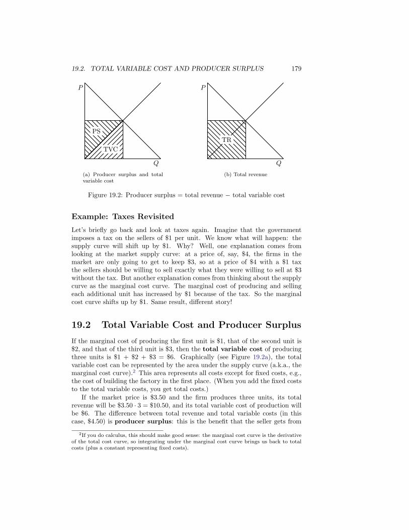
19.2. TOTAL VARIABLE COST AND PRODUCER SURPLUS 179
TVC
PS
P
Q
(a) Producer surplus and totalvariable cost
TR
P
Q
(b) Total revenue
Figure 19.2: Producer surplus = total revenue − total variable cost
Example: Taxes Revisited
Let’s briefly go back and look at taxes again. Imagine that the governmentimposes a tax on the sellers of $1 per unit. We know what will happen: thesupply curve will shift up by $1. Why? Well, one explanation comes fromlooking at the market supply curve: at a price of, say, $4, the firms in themarket are only going to get to keep $3, so at a price of $4 with a $1 taxthe sellers should be willing to sell exactly what they were willing to sell at $3without the tax. But another explanation comes from thinking about the supplycurve as the marginal cost curve. The marginal cost of producing and sellingeach additional unit has increased by $1 because of the tax. So the marginalcost curve shifts up by $1. Same result, different story!
19.2 Total Variable Cost and Producer Surplus
If the marginal cost of producing the first unit is $1, that of the second unit is$2, and that of the third unit is $3, then the total variable cost of producingthree units is $1 + $2 + $3 = $6. Graphically (see Figure 19.2a), the totalvariable cost can be represented by the area under the supply curve (a.k.a., themarginal cost curve).2 This area represents all costs except for fixed costs, e.g.,the cost of building the factory in the first place. (When you add the fixed coststo the total variable costs, you get total costs.)
If the market price is $3.50 and the firm produces three units, its totalrevenue will be $3.50 · 3 = $10.50, and its total variable cost of production willbe $6. The difference between total revenue and total variable costs (in thiscase, $4.50) is producer surplus: this is the benefit that the seller gets from
2If you do calculus, this should make good sense: the marginal cost curve is the derivativeof the total cost curve, so integrating under the marginal cost curve brings us back to totalcosts (plus a constant representing fixed costs).

180 CHAPTER 19. MARGINS
selling. Note that producer surplus is not the same thing as profit because wehaven’t accounted for fixed costs. Once we account for fixed costs, the profitthat is left over should be comparable to profits from comparable investments.(See Chapter 6.)
19.3 Reinterpreting the Demand Curve
Just as we’ve refashioned the supply curve as a marginal cost curve, we canrefashion the demand curve as a marginal benefit curve. Unfortunately, asin the analysis Chapter 18 concerning downward sloping demand curves, it turnsout that there are some theoretical complications.3 A more advanced course canaddress those complications; our approach will be to gloss over the theoreticaldifficulties in order to describe the basic ideas.
Consider an individual whose demand curve indicates that (1) at a priceof $5 she wants to buy 10 units; and (2) at any price above $5 she wants tobuy less than 10 units. We can now ask the following question: What is thisperson’s marginal benefit from obtaining the 10th unit? (Marginal benefitis the benefit from obtaining an additional unit. The marginal benefit of the10th unit is the difference in benefits between having 10 units and having only9 units.)
The answer follows from individual optimization: the individual’s marginalbenefit from obtaining the 10th unit must be equal to $5. Since she wants tobuy 10 units at a price of $5, the marginal benefit of the 10th unit cannot beless than $5. (If the marginal benefit of the 10th unit was, say, $4, she wouldn’tbe optimizing by buying 10 units at a price of $5; she would be better off bybuying only 9 units.) And since she doesn’t want to buy 10 units at a priceabove $5, the marginal benefit of the 10th unit must be at most $5. (If themarginal benefit of the 10th unit was, say, $6, she wouldn’t be optimizing ifshe bought only 9 units at market prices above $5; for example, with a marketprice of $5.50, she’d be better off buying 10 units instead of 9.) So her marginalbenefit from obtaining the 10th unit must be equal to $5.
It follows that the point on the graph corresponding to a price of $5 anda quantity of 10 units can be interpreted in two different ways. From the per-spective of the demand curve, it indicates that at a price of $5 this individualwants to buy 10 units. From the perspective of the marginal benefit curve,it indicates that the marginal benefit of obtaining the 10th unit of productionis $5. This is an example of a more general result: every point on an individualdemand curve is also a point on that individual’s marginal benefit curve.
The same result applies to the market as a whole: every point on the marketdemand curve is also a point on the social marginal benefit curve. If themarket wants to buy 1 million units at a price of $5 but less than 1 million unitsat any price over $5, the marginal benefit to society of obtaining the 1 millionthunit must be $5.
3Again, the complications stem from the income effect.

19.4. TOTAL BENEFIT AND CONSUMER SURPLUS 181
P
Q
Figure 19.3: Every point on an individual (or market) demand curve is also apoint on an individual (or social) marginal benefit curve
The close connection between demand curves and marginal benefit curvesgives us two ways to think about the graph in Figure 19.3. If you start with agiven p, an individual (or market) demand curve will tell you how many unitsthat individual buyer (or all the buyers together) would want to buy at thatprice; and if you start with a given q, the individual (or social) marginal benefitcurve will tell you the marginal benefit for that individual buyer (or all thebuyers together) of obtaining that qth unit.
Example: Taxes Revisited
Let’s briefly go back and look at taxes again. Imagine that the governmentimposes a tax on the buyers of $1 per unit. We know what will happen: thedemand curve will shift down by $1. Why? Well, one explanation comes fromlooking at the market demand curve: at a price of, say, $4, the buyers in themarket are going to end up paying $5, so at a price of $4 with a $1 tax the buyersshould be willing to buy exactly what they were willing to buy at $5 withoutthe tax. But another explanation comes from thinking about the demand curveas the marginal benefit curve. The marginal benefit of each additional unit hasdecreased by $1 because of the tax. So the marginal benefit curve shifts downby $1. Same result, different story!
19.4 Total Benefit and Consumer Surplus
If the marginal benefit of the first unit is $6, that of the second unit is $5, andthat of the third unit is $4, then the total benefit of having three units is$6 + $5 + $4 = $15. Graphically (see Figure 19.4a), the total benefit can berepresented by the area under the demand curve (a.k.a., the marginal benefitcurve).4
4Again, if you do calculus, this should make good sense: the marginal benefit curve is thederivative of the total benefit curve, so integrating under the marginal benefit curve brings us

182 CHAPTER 19. MARGINS
TB
P
Q
(a) Total benefit
CS
TE
P
Q
(b) Consumer surplus and totalexpenditure
Figure 19.4: Consumer surplus = total benefit − total expenditure
If the market price is $3.50 and our individual buys three units, her totalexpenditure will be $3.50 · 3 = $10.50 and her total benefit will be $15. Thedifference between total benefit and total expenditure (in this case, $4.50) isconsumer surplus: this is the benefit that the buyer gets from buying.5
The Whole Enchilada
Putting supply and demand together, we get Figure 19.5. Total revenue (TR,a.k.a. total expenditure, TE)—is producer surplus (PS) plus total variablecost (TVC). Total benefit (TB) is the area under the demand curve (a.k.a. themarginal benefit curve), so consumer surplus (CS) is CS = TB−TE. Total vari-able cost is the area under the supply curve (a.k.a. the marginal cost curve), soproducer surplus is PS = TR−TVC. Together producer surplus and consumersurplus constitute the gains from trade.
19.5 Conclusion: Carrots and Sticks
Another way to think about marginal benefit and marginal cost curves is interms of carrots and sticks. Incentives generally take one of two forms: rewards(i.e., carrots) or punishments (sticks). 6 You can think of the marginal benefit
back to total benefits (plus a constant).5Just as producer surplus doesn’t account for the seller’s fixed costs, consumer surplus
doesn’t account for the buyer’s fixed costs. For example, the consumer surplus you get fromtravelling around Hawaii doesn’t account for the cost of your plane ticket to get there.
6To get a donkey to move forward you can either tie a carrot to a pole and dangling it infront of the donkey, or you can hit the donkey with a stick. To analyze this to death evenmore, we can use a decision tree to analyze the donkey’s choices: go forward or do nothing.To get the donkey to go forward you can either make “Go forward” look attractive—e.g., witha carrot—or you can make “Do nothing” look unattractive—e.g., with a stick. Both are—atleast in theory—equally good as incentive mechanisms.

19.5. CONCLUSION: CARROTS AND STICKS 183
TVC
CS
PS
P
Q
Figure 19.5: The whole enchilada
curve as the carrot, and the marginal cost curve as the stick. The marginalbenefit curve (i.e., the demand curve) provides an incentive for sellers to producemore of good X, and the marginal cost curve (i.e., the supply curve) providesan incentive for buyers to consume less of good X.
Note that in competitive markets the market price, the marginal cost at theequilibrium quantity, and the marginal benefit at the equilibrium quantity areequal. This fact underlies many of the efficiency results that we will discuss inthe next chapter.

184 CHAPTER 19. MARGINS

Chapter 20
Math : Deriving Supply andDemand Curves
At a basic level, individual supply and demand curves come from individualoptimization: if at price p an individual or firm is willing to buy or sell q unitsof some good, it must because buying or selling q units of that good is optimalfor that individual or firm. But we can go into more depth here by actuallyderiving individual demand curves from utility maximization and individualsupply curves from profit maximization. A useful first step is to examine thecost minimization problem.
20.1 Cost Minimization
For individuals, the cost minimization problem is to achieve a specified level ofutility (say, U = 10) at least cost. For firms, the cost minimization problemis to produce a specified amount of output (say, Y = 10) at least cost. Theseproblems are identical: if you like, you can think of the individual as a firmwhose “product” is utility, or of the firm as an individual whose “utility” dependson output. We will reinforce this connection by using examples with similarnotation: the individual we will consider gets utility from drinking lattes (L)and eating cake (K); the firm we will consider produces output from inputs oflabor (L) and capital (K).
Utility Functions and Indifference Curves
Part I of this course introduced utility functions and indifference curves:if the individual’s utility function is U(L,K) = L
1
2 K1
2 (an example of a Cobb-Douglas utility function1), then the indifference curve corresponding to a
1The general form of a Cobb-Douglas utility function is U = LαKβ where α and β arepositive constants.
185

186 CHAPTER 20. MATH: DERIVING SUPPLY AND DEMAND CURVES
utility level of, say, 2 is the set of all consumption bundles that provide theindividual with a utility of 2.
In our example, the indifference curve corresponding to a utility level of 2contains the points (L = 1,K = 4), (L = 4,K = 1), and (L = 2,K = 2).
The equation for this indifference curve is L1
2 K1
2 = 2, which we can rewrite
as LK = 4 or K = 4L−1. The slope of this indifference curve,dK
dL= −4L−2,
measures the marginal rate of substitution (MRS) between lattes and cake:an individual with a utility level of 2 who currently has L lattes and K pieces ofcake would be willing to trade up to 4L−2 pieces of cake in order to gain an extralatte. Such a substitution would leave the individual on the same indifferencecurve, and therefore with the same utility.
An important result that will be useful later is that the slope of the indif-ference curve (i.e., the marginal rate of substitution) can also be written as
MRS = −∂U∂L∂U∂K
.
Here the numerator is the marginal utility of lattes (MUL =∂U
∂L), the extra
utility the individual would get from an additional latte. The denominator is the
marginal utility of cake (MUK =∂U
∂K), the extra utility the individual would
get from an additional piece of cake. Intuitively, the slope of the indifferencecurve tells us the maximum amount of cake the individual is willing to give upin order to receive one more latte. Since one more latte gives the individualMUL extra utility, the amount of cake the individual should be willing to giveup in order to get an additional latte is K such that MUK · K = MUL, i.e.,
K =MUL
MUK
. (For example, if the marginal utility of lattes is 3 and the marginal
utility of cake is 1, the individual should be willing to give up 3 pieces of caketo get one more latte.) It follows that the slope of the indifference curve is
MRS = −MUL
MUK
= −∂U∂L∂U∂K
.
Production Functions and Isoquants
Firms have structures analogous to utility functions and indifference curves;these are called production functions and isoquants. Given inputs of labor(L) and capital (K), the production function f(L,K) describes the quantity ofoutput that can be produced from these inputs. If the firm’s production functionis Y = L
1
2 K1
2 (an example of a Cobb-Douglas production function), thenthe isoquant corresponding to an output level of, say, 2 is the set of all inputbundles that the firm can use to produce 2 units of output.
In our example, the isoquant corresponding to an output level of 2 containsthe points (L = 1,K = 4), (L = 4,K = 1), and (L = 2,K = 2). The equation

20.1. COST MINIMIZATION 187
for this isoquant is L1
2 K1
2 = 2, which we can rewrite as LK = 4 or K = 4L−1.
The slope of this isoquant,dK
dL= −4L−2, measures the marginal rate of
technical substitution (MRTS) between labor and capital: a firm with anoutput target of 2 which currently has L units of labor and K units of capitalwould be willing to trade up to 4L−2 units of capital in order to gain an extraunit of labor. Such a substitution would leave the firm on the same isoquant,and therefore with the same output.
An important result that will be useful later is that the slope of the isoquantcan also be written as
MRTS = −∂f∂L∂f∂K
.
Here the numerator is the marginal product of labor (MPL =∂f
∂L), the extra
output the firm would get from an additional unit of labor. The denominator
is the marginal product of capital (MPK =∂f
∂K), the extra output the
firm would get from an additional unit of capital. Intuitively, the slope of theisoquant tells us the maximum amount of capital the firm is willing to give upin order to get one more unit of labor. Since one unit of labor allows the firmto produce MPL extra units of output, the amount of capital the firm shouldbe willing to give up in order to get an additional unit of labor is K such that
MPK · K = MPL, i.e., K =MPL
MPK
. (For example, if the marginal product of
labor is 3 and the marginal product of capital is 1, the firm should be willingto give up 3 units of capital to get one more unit of labor.) It follows that theslope of the isoquant is
MRTS = −MPL
MPK
= −∂f∂L∂f∂K
.
The Cost Function
If lattes and cake (or labor and capital) have unit prices of pL and pK , respec-tively, then the total cost of purchasing L units of one and K units of the otheris
C(L,K) = pLL + pKK.
The cost minimization problem for the individual is to choose L and K tominimize the cost necessary to reach a specified utility level (say, U = 2). Thecost minimization problem for the firm is to choose L and K to minimize thecost necessary to reach a specified output level (say, Y = 2). Mathematically,the individual wants to choose L and K to minimize pLL + pKK subject tothe constraint U(L,K) = 2; the firm wants to choose L and K to minimizepLL + pKK subject to the constraint f(L,K) = 2.
To solve this problem, we need to find the values of our choice variables (Land K) that minimize cost. Since two equations in two unknowns generally
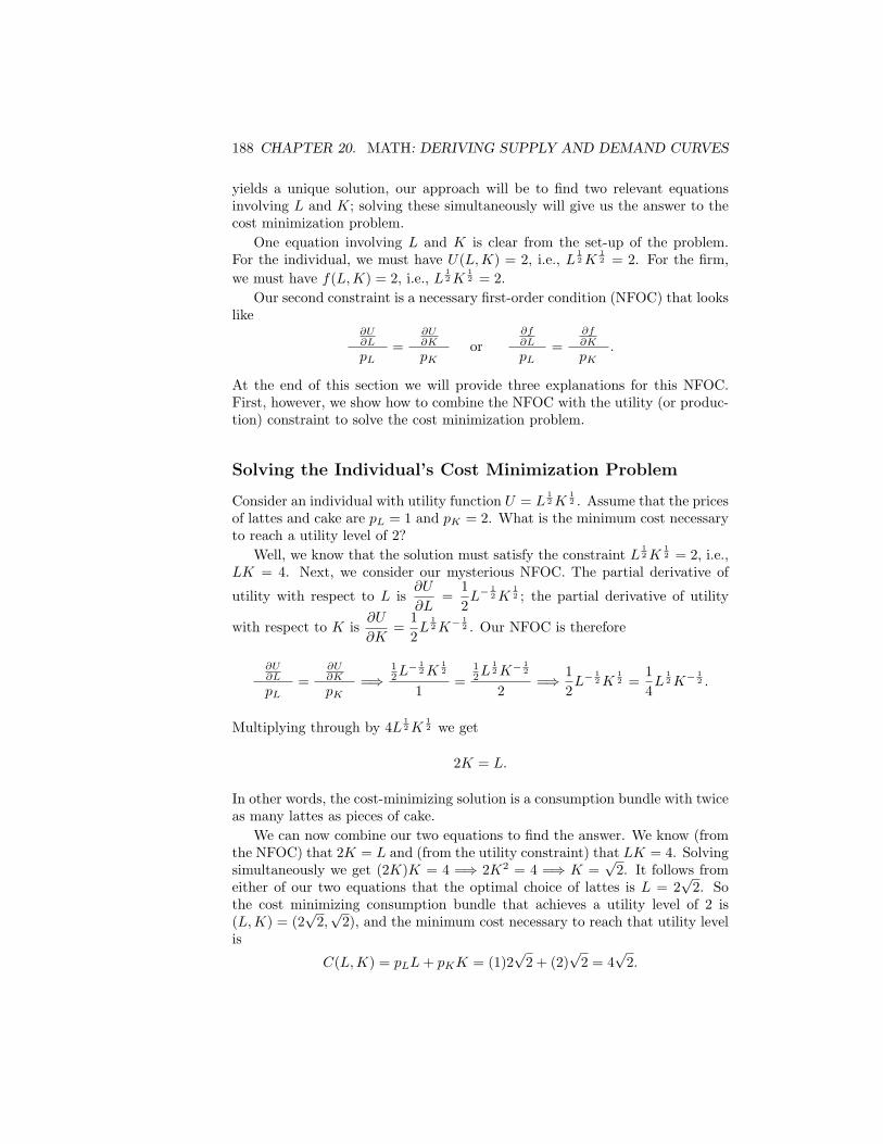
188 CHAPTER 20. MATH: DERIVING SUPPLY AND DEMAND CURVES
yields a unique solution, our approach will be to find two relevant equationsinvolving L and K; solving these simultaneously will give us the answer to thecost minimization problem.
One equation involving L and K is clear from the set-up of the problem.For the individual, we must have U(L,K) = 2, i.e., L
1
2 K1
2 = 2. For the firm,
we must have f(L,K) = 2, i.e., L1
2 K1
2 = 2.
Our second constraint is a necessary first-order condition (NFOC) that lookslike
∂U∂L
pL
=∂U∂K
pK
or∂f∂L
pL
=∂f∂K
pK
.
At the end of this section we will provide three explanations for this NFOC.First, however, we show how to combine the NFOC with the utility (or produc-tion) constraint to solve the cost minimization problem.
Solving the Individual’s Cost Minimization Problem
Consider an individual with utility function U = L1
2 K1
2 . Assume that the pricesof lattes and cake are pL = 1 and pK = 2. What is the minimum cost necessaryto reach a utility level of 2?
Well, we know that the solution must satisfy the constraint L1
2 K1
2 = 2, i.e.,LK = 4. Next, we consider our mysterious NFOC. The partial derivative of
utility with respect to L is∂U
∂L=
1
2L−
1
2 K1
2 ; the partial derivative of utility
with respect to K is∂U
∂K=
1
2L
1
2 K−1
2 . Our NFOC is therefore
∂U∂L
pL
=∂U∂K
pK
=⇒12L−
1
2 K1
2
1=
12L
1
2 K−1
2
2=⇒ 1
2L−
1
2 K1
2 =1
4L
1
2 K−1
2 .
Multiplying through by 4L1
2 K1
2 we get
2K = L.
In other words, the cost-minimizing solution is a consumption bundle with twiceas many lattes as pieces of cake.
We can now combine our two equations to find the answer. We know (fromthe NFOC) that 2K = L and (from the utility constraint) that LK = 4. Solvingsimultaneously we get (2K)K = 4 =⇒ 2K2 = 4 =⇒ K =
√2. It follows from
either of our two equations that the optimal choice of lattes is L = 2√
2. Sothe cost minimizing consumption bundle that achieves a utility level of 2 is(L,K) = (2
√2,√
2), and the minimum cost necessary to reach that utility levelis
C(L,K) = pLL + pKK = (1)2√
2 + (2)√
2 = 4√
2.

20.1. COST MINIMIZATION 189
Solving the Firm’s Cost Minimization Problem
Now consider a firm with production function Y = L1
2 K1
2 . The prices of capitaland labor are pL = 1 and pK = 2. What is the minimum cost necessary toproduce q units of output?
Well, we know that the solution must satisfy the constraint L1
2 K1
2 = q, i.e.,LK = q2. Next, we consider our mysterious NFOC. The partial derivative of the
production function with respect to L is∂f
∂L=
1
2L−
1
2 K1
2 ; the partial derivative
of the production function with respect to K is∂f
∂K=
1
2L
1
2 K−1
2 . Our NFOC
is therefore
∂f∂L
pL
=∂f∂K
pK
=⇒12L−
1
2 K1
2
1=
12L
1
2 K−1
2
2=⇒ 1
2L−
1
2 K1
2 =1
4L
1
2 K−1
2 .
Multiplying through by 4L1
2 K1
2 we get
2K = L.
In other words, the cost-minimizing solution is an input mix with twice as manyunits of labor as capital.
We can now combine our two equations to find the answer. We know (fromthe NFOC) that 2K = L and (from the utility constraint) that LK = q2.
Solving simultaneously we get (2K)K = q2 =⇒ 2K2 = q2 =⇒ K =q√2. It
follows from either of our two equations that the optimal choice of labor isL = q
√2. So the cost minimizing consumption bundle that achieves an output
level of q is (L,K) =
(
q√
2,q√2
)
, and the minimum cost necessary to reach
that output level is
C(L,K) = pLL + pKK =⇒ C(q) = (1)q√
2 + 2q√2
= 2q√
2.
The function C(q) is the firm’s cost function: specify how much output youwant the firm to produce and C(q) tells you the minimum cost necessary toproduce that amount of output. Note that we have transformed the cost functionfrom one involving L and K to one involving q; this will prove useful in derivingsupply curves.
Now that we’ve seen how to use the mysterious NFOC, let’s see why it makessense. The remainder of this section provides three explanations—one intuitive,one graphical, and one mathematical—for our NFOC,
∂U∂L
pL
=∂U∂K
pK
or∂f∂L
pL
=∂f∂K
pK
.
An Intuitive Explanation for the NFOC
The first explanation is an intuitive idea called the last dollar rule. If our cost-minimizing individual is really minimizing costs, shifting one dollar of spending
190 CHAPTER 20. MATH: DERIVING SUPPLY AND DEMAND CURVES
from cake to lattes cannot increase the individual’s utility level; similarly, shift-ing one dollar of spending from lattes to cake cannot increase the individual’sutility level. The individual should therefore be indifferent between spendinghis “last dollar” on lattes or on cake.
To translate this into mathematics, consider shifting one dollar of spendingfrom cake to lattes. Such a shift would allow the individual to spend one more
dollar on lattes, i.e., to buy1
pL
more lattes; this would increase his utility by
∂U
∂L· 1
pL
. (Recall that ∂U∂L
is the marginal utility of lattes.) But this shift would
require him to spend one less dollar on cake, i.e., to buy1
pK
fewer pieces of
cake; this would reduce his utility by∂U
∂K· 1
pK
. (Recall that ∂U∂K
is the marginal
utility of cake.) Taken as a whole, this shift cannot increase the individual’sutility level, so we must have
∂U
∂L· 1
pL
− ∂U
∂K· 1
pK
≤ 0 =⇒ ∂U
∂L
1
pL
≤ ∂U
∂K
1
pK
.
Now consider shifting one dollar of spending from lattes to cake. Such a shift
would allow the individual to spend one more dollar on cake, i.e., to buy1
pK
more pieces of cake; this would increase his utility by∂U
∂K
1
pK
. But this shift
would require him to spend one less dollar on lattes, i.e., to buy1
pL
fewer lattes;
this would reduce his utility by∂U
∂L
1
pL
. Overall, this shift cannot increase the
individual’s utility level, so we must have
∂U
∂K· 1
pK
− ∂U
∂L· 1
pL
≤ 0 =⇒ ∂U
∂K
1
pK
≤ ∂U
∂L
1
pL
.
Looking at the last two equations, we see that
∂U
∂L· 1
pL
≤ ∂U
∂K· 1
pK
and∂U
∂K· 1
pK
≤ ∂U
∂L· 1
pL
.
The only way both of these equations can hold is if
∂U
∂L· 1
pL
=∂U
∂K· 1
pK
i.e.,∂U∂L
pL
=∂U∂K
pK
.
So if the individual is minimizing cost, this equation must hold.The identical logic works for firms. If the firm is minimizing costs, shifting
one dollar of spending from capital to labor cannot increase the firm’s output;similarly, shifting one dollar of spending from labor to capital cannot increasethe firm’s output. The firm should therefore be indifferent between spending its“last dollar” on labor or on capital.

20.1. COST MINIMIZATION 191
Mathematically, we end up with
∂f∂L
pL
=∂f∂K
pK
.
With one extra dollar, the firm could hire1
pL
extra units of labor; the extra
output the firm could produce is therefore∂f
∂L· 1
pL
. (Recall that ∂f∂L
is the
marginal product of labor, i.e., the extra output the firm could produce withone extra unit of labor.) Similarly, spending an extra dollar on capital would
allow the firm to hire1
pK
extra units of capital; the extra output the firm could
produce is therefore∂f
∂K· 1
pK
. (Recall that ∂f∂K
is the marginal product of
capital, i.e., the extra output the firm could produce with one extra unit ofcapital.) If the firm is minimizing cost, it must be equating these two fractions.
A Graphical Explanation for the NFOC
The second explanation for the NFOC is graphical. Recall from Part I that anindividual’s budget constraint is the set of all consumption bundles (L,K)that an individual can purchase with a given budget. The line pLL+pKK = 10is the budget constraint corresponding to a budget of $10; we can rewrite this
as K =10 − pLL
pK
. The slope of the budget constraint,dK
dL= − pL
pK
, measures
the marginal rate of transformation between lattes and cake. In order to
afford an extra latte, the individual needs to give uppL
pK
pieces of cake in order
to stay within his budget. (For example, if lattes cost $1 and cake costs $.50per piece, he would have to give up 2 pieces of cake to afford one extra latte.)
Firms have structures analogous to budget constraints called isocosts: theset of all input bundles (L,K) that the firm can purchase with a given budget.The line pLL+pKK = 10 is the isocost corresponding to a budget of $10; we can
rewrite this as K =10 − pLL
pK
. The slope of the isocost,dK
dL= − pL
pK
, measures
the marginal rate of technical transformation between labor and capital.
In order to afford an extra unit of labor, the firm needs to give uppL
pK
units of
capital in order to stay within its budget. (For example, if labor costs $1 perunit and capital costs $.50 per unit, the firm would have to give up 2 units ofcapital to afford one extra unit of labor.)
Graphically, the cost minimization problem is for the individual to find thelowest budget constraint that intersects a specified indifference curve (or, equiva-lently, for the firm to find the lowest isocost that intersects a specified isoquant).We can see from Figure 20.1 that the solution occurs at a point where the bud-get constraint is tangent to the indifference curve (or, equivalently, where theisocost is tangent to the isoquant). At this point of tangency, the slope of the

192 CHAPTER 20. MATH: DERIVING SUPPLY AND DEMAND CURVES
K
L
Indifference curve or isoquant
Big budget
Goldilocks budget (just right)
Small budget
Figure 20.1: Minimizing costs subject to a utility (or output) constraint
indifference curve must equal the slope of the budget constraint:
−∂U∂L∂U∂K
= − pL
pK
=⇒∂U∂L
pL
=∂U∂K
pK
.
Equivalently, in the case of firms we have that the slope of the isoquant mustequal the slope of the isocost:
−∂f∂L∂f∂K
= − pL
pK
=⇒∂f∂L
pL
=∂f∂K
pK
.
A Mathematical Explanation for the NFOC
The third and final explanation for the NFOC comes from brute force math-ematics. The individual’s problem is to choose L and K to minimize costspLL + pKK subject to a utility constraint U(L,K) = U . It turns out that wecan solve this problem by writing down the Lagrangian
L = pLL + pKK + λ[U − U(L,K)].
(The Greek letter λ—pronounced “lambda”—is called the Lagrange multiplier;it has important economic meanings that you can learn more about in upper-level classes.) Magically, the necessary first-order conditions (NFOCs) for theindividual turn out to be
∂L
∂L= 0,
∂L
∂K= 0, and
∂L
∂λ= 0,

20.2. SUPPLY CURVES 193
i.e.,
pL − λ∂U
∂L= 0, pK − λ
∂U
∂K= 0, and U − U(K,L) = 0.
Solving the first two for λ we get
λ =pL
∂U∂L
and λ =pK
∂U∂K
.
Setting these equal to each other and rearranging yields the mysterious NFOC,
∂U∂L
pL
=∂U∂K
pK
.
The mathematics of the firm’s problem is identical: choose L and K tominimize costs pLL + pKK subject to a production constraint f(L,K) = Y .The Lagrangian is
L = pLL + pKK + λ[Y − f(L,K)]
and the necessary first-order conditions (NFOCs) are
∂L
∂L= 0,
∂L
∂K= 0, and
∂L
∂λ= 0,
i.e.,
pL − λ∂f
∂L= 0, pK − λ
∂f
∂K= 0, and Y − f(L,K) = 0.
Solving the first two for λ we get
λ =pL
∂f∂L
and λ =pK
∂f∂K
.
Setting these equal to each other and rearranging yields the firm’s NFOC,
∂f∂L
pL
=∂f∂K
pK
.
20.2 Supply Curves
The firm’s ultimate job is not to minimize costs but to maximize profits. Anexamination of profit maximization allows us to derive supply curves, whichshow how a change in the price of the firm’s output (p) affect the firm’s choiceof output (q), holding other prices constant. We will also be able to derive thefirm’s factor demand curves, which show how a change in the price of oneof the firm’s inputs (e.g., pL, the price of labor) affects the firm’s choice of howmany units of that input to purchase, holding other prices constant.
The caveat “holding other prices constant” arises because of graphical andmental limitations. Supply and demand graphs are only two-dimensional, so we

194 CHAPTER 20. MATH: DERIVING SUPPLY AND DEMAND CURVES
cannot use them to examine how multiple price changes affect the firm’s outputor input choices; this would require three- or more-dimensional graphs. In fact,what is really going on is this: the firm’s profit-maximizing level of output isa function of all of the input and output prices. If there are 5 inputs and 1output, there are 6 prices to consider. Seeing how the profit-maximizing levelof output changes as these prices change would require a seven-dimensionalgraph (six dimensions for the prices, and one dimension for the level of output).Unfortunately, we have a hard time visualizing seven-dimensional graphs. Tosolve this problem, we look at two-dimensional cross-sections of this seven-dimensional graph. By changing the output price while holding all of the inputprices constant, we are able to see (in two dimensions) how the output priceaffects the firm’s choice of output; in other words, we are able to see the firm’ssupply curve. Similarly, by changing the price of labor while holding all otherprices constant, we are able to see how the price of labor affects the firm’sprofit-maximizing choice of labor; this gives us the firm’s factor demand curvefor labor.
An important implication here is that the levels at which we hold other pricesconstant is important: the firm’s supply curve with input prices of pL = pK = 2will be different than its supply curve with input prices of pL = pK = 4.
Choosing Output to Maximize Profits
To derive the firm’s supply curve, we hold the input prices constant at specifiedlevels. We can therefore use the firm’s cost function C(q) (derived previously)to express the profit maximization problem as the problem of choosing outputq to maximize profits,
π(q) = pq − C(q).
To maximize this we take a derivative with respect to our choice variable andset it equal to zero. We get an NFOC of
dπ
dq= 0 =⇒ p − C ′(q) = 0 =⇒ p = C ′(q).
The right hand side here is the marginal cost of producing an additional unit ofoutput. The left hand side is the marginal benefit of producing an additionalunit of output, namely the market price p. The NFOC therefore says that aprofit-maximizing firm produces until the marginal cost of production is equal tothe output price; this is true as long as the firm’s profit-maximization problemhas an interior solution. It follows that the marginal cost curve is thesupply curve (as long as the firm’s profit-maximization problem has an interiorsolution2).
2At low prices, the firm’s optimal choice of output may be the corner solution q = 0. Inthese cases the marginal cost curve and the supply curve will not be the same.

20.3. DEMAND CURVES 195
Choosing Inputs to Maximize Profits
To get the factor demand curves, we express the firm’s objective in terms of itsinput choices: it wants to choose inputs L and K to maximize profits
π(L,K) = pf(L,K) − pLL − pKK.
To maximize this we take partial derivatives with respect to our choice variablesand set them equal to zero. For labor we get an NFOC of
∂π
∂L= 0 =⇒ p
∂f
∂L− pL = 0 =⇒ p
∂f
∂L= pL.
The right hand side here is the marginal cost of purchasing an additional unit oflabor, namely its market price pL. The left hand side is the marginal benefit ofpurchasing an additional unit of labor, namely the market price of the additionaloutput that can be produced with that extra labor: p is the market price of
output, and∂f
∂Lis the marginal product of labor, i.e., the extra output that can
be produced with one more unit of labor. Multiplying these yields the value ofthe marginal product of labor (V MPL). The NFOC therefore says that aprofit-maximizing firm purchases labor until the value of the marginal productof labor V MPL is equal to the cost of labor pL. If V MPL > pL then the firmcan increase profits by purchasing additional units of labor; if V MPL < pL thenthe firm can increase profits by purchasing fewer units of labor.
This NFOC turns out to yield the firm’s factor demand curve for labor.Given a fixed input of capital and a fixed output price p, the NFOC tells us howmuch labor the firm wants to hire as a function of the price of labor pL.
An identical analysis shows that a profit-maximizing firm must purchasecapital until the value of the marginal product of capital V MPK is equal to thecost of capital pK :
∂π
∂K= 0 =⇒ p
∂f
∂K− pK = 0 =⇒ p
∂f
∂K= pK .
This NFOC gives us the firm’s factor demand curve for capital.
20.3 Demand Curves
The individual’s ultimate job is not to minimize costs subject to a utility con-straint but to maximize utility subject to a budget constraint. An examinationof utility maximization allows us to derive demand curves, which show how achange in the price of some good (e.g., pL, the price of lattes) affects the in-dividual’s consumption choice for that good, holding other prices constant andholding the individual’s budget constant. We can also derive the individual’sEngel curves, which show how a change in the individual’s budget affects theindividual’s consumption choices for, say, lattes, holding all prices constant.
As in the case of firms, the caveat about holding things constant arisesbecause our graphs (and our minds) work best in only two dimensions. If the

196 CHAPTER 20. MATH: DERIVING SUPPLY AND DEMAND CURVES
K
L
U ≈ 2.12
Indifference curve for U = 3
U = 1
Budget of 6
Figure 20.2: Maximizing utility subject to a budget constraint of 6
individual’s utility level depends on five different consumption goods and hisbudget, his optimal choice of lattes (L) would be a seven-dimensional graph: fivedimensions for the prices of the different goods, one dimension for the budget,and one dimension for his optimal choice of L. Since we can’t visualize sevendimensions, we hold five of these dimensions constant and get a two-dimensionalcross-section. Holding the budget and the other four prices constant allows usto see how the price of lattes affects the individual’s optimal choice of lattes;this gives us the individual’s demand curve for lattes. Holding all of the pricesconstant allows us to see how the individual’s budget affects his choice of lattes;this give us the individual’s Engel curves for lattes. As in the case of firms, thelevels at which we hold various things constant is important: the individual’sdemand for lattes with a budget of $20 and a price of cake of $1 per piece willbe different than his demand for lattes with a budget of $30 and a price of cakeof $2 per piece.
Marshallian (Money Held Constant) Demand Curves
Consider the problem of choosing consumption amounts L and K to maximizeutility U(L,K) subject to a budget constraint pLL + pKK = C. Graphically,this problem (with pL = 1, pK = 2, and C = 6) and its solution are shown inFigure 20.2.
As with cost minimization, our solution method will be to find two equationsinvolving L and K and then solve them simultaneously. The first equation comesfrom the statement of the problem: L and K must satisfy the budget constraint,pLL + pKK = C.

20.3. DEMAND CURVES 197
The second equation turns out to be the same mysterious NFOC we foundin the case of cost minimization:
∂U∂L
pL
=∂U∂K
pK
.
Intuitively, this is because the utility-maximizing individual must still followthe last dollar rule: if he is choosing optimally, he should be indifferent betweenspending his last dollar on lattes or on cake. Graphically, we can see fromFigure 20.2 that the individual’s task is to choose the highest indifference curvethat lies on the relevant budget constraint; the optimum occurs at a point oftangency between the indifference curve and the budget constraint, meaningthat the slope of the indifference curve must equal the slope of the budgetconstraint. Mathematically, we can write down the relevant Lagrangian,
L = U(L,K) − λ[C − pLL − pKK].
The NFOCs include∂L
∂L= 0 and
∂L
∂K= 0, i.e.,
∂U
∂L−λpL = 0 and
∂U
∂K−λpK =
0. Solving these for λ and setting them equal to each other yields the desiredNFOC. Combining the budget constraint with the NFOC allow us to solve forthe individual’s Marshallian demand curves, Engel curves, &etc.
For example, consider an individual with a budget of $6 and a utility func-tion of U = L
1
2 K1
2 . The price of cake is pK = 2. What is this individual’sMarshallian demand curve for lattes?
To solve this problem, we substitute the budget (C = $6) and the price ofcake ($2 per piece) into the budget constraint to get pLL + 2K = 6. Next, wesubstitute the price of cake into the NFOC to get
∂U∂L
pL
=∂U∂K
pK
=⇒12L−
1
2 K1
2
pL
=12L
1
2 K−1
2
2=⇒ 1
2pL
L−1
2 K1
2 =1
4L
1
2 K−1
2 .
Multiplying through by 4pLL1
2 K1
2 we get
2K = pLL.
We now have two equations (pLL + 2K = 6 and 2K = pLL) in three un-knowns (L, K, and pL). We can eliminate K by using the second equationto substitute for 2K in the first equation: pLL + pLL = 6. This simplifies to2pLL = 6 or pLL = 3, which we can rewrite as
L =3
pL
.
This is the Marshallian demand curve for lattes when we fix the budget at 6and the price of cake at $2 per piece. If the price of lattes is pL = 1, the optimalchoice is L = 3; if the price of lattes is pL = 3, the optimal choice is L = 1.

198 CHAPTER 20. MATH: DERIVING SUPPLY AND DEMAND CURVES
K
L
Indifference curve for U = 2
Budget of 9Budget of ≈ 5.66Budget of 3
Figure 20.3: Minimizing costs subject to a utility constraint
Hicksian (Utility Held Constant) Demand Curves
For reasons to be discussed in the next section, it turns out that we shouldalso consider the demand curves that come from the cost minimization problemdiscussed previously: choose consumption amounts L and K to minimize costsC(L,K) = pLL+pKK subject to a utility constraint U(L,K) = U . Graphically,this problem (with pL = 1, pK = 2, and U = 2) and its solution are shown inFigure 20.3.
To solve this problem, we combine our utility constraint, U(L,K) = U , withthe usual NFOC,
∂U∂L
pL
=∂U∂K
pK
.
Combining the budget constraint with the NFOC allow us to solve for theindividual’s Hicksian demand curves.
For example, consider an individual with a utility constraint of U = 2 anda utility function of U = L
1
2 K1
2 . The price of cake is pK = 2. What is thisindividual’s Hicksian demand curve for lattes?
To solve this problem, we substitute the utility level (U = 2) into the utility
constraint to get L1
2 K1
2 = 2. Next, we substitute the price of cake ($2 perpiece) into the NFOC to get
∂U∂L
pL
=∂U∂K
pK
=⇒12L−
1
2 K1
2
pL
=12L
1
2 K−1
2
2=⇒ 1
2pL
L−1
2 K1
2 =1
4L
1
2 K−1
2 .

20.3. DEMAND CURVES 199
Multiplying through by 4pLL1
2 K1
2 we get
2K = pLL.
We now have two equations (L1
2 K1
2 = 2 and 2K = pLL) in three unknowns(L, K, and pL). We can eliminate K by using the second equation to substitutefor K in the first equation:
L1
2
(pLL
2
) 1
2
= 2 =⇒ L(pL
2
) 1
2
= 2 =⇒ L√
pL = 2√
2.
We can rewrite this as
L =2√
2√pL
This is the Hicksian demand curve for lattes when we fix utility at U = 2 andthe price of cake at $2 per piece. If the price of lattes is pL = 1, the optimalchoice is L = 2
√2; if the price of lattes is pL = 2, the optimal choice is L = 2.
Marshall v. Hicks
Why do we use both Marshallian and Hicksian demand curves? Well, the ad-vantage of the Marshallian demand curve is that it matches real life: peopleactually do have budget constraints, and they have to do the best they cansubject to those constraints. The advantage of the Hicksian demand curve isthat it makes for nice economic theory. For example, we can prove that Hick-sian demand curves are downward sloping: people buy less as prices rise. Andthe area underneath a Hicksian demand curve represents a useful concept calledconsumer surplus. Unfortunately, Marshallian demand curves do not havenice theoretical properties; Marshallian demand curves do not have to be down-ward sloping, and the area underneath a Marshallian demand curve does notrepresent consumer surplus (or anything else interesting).
We are therefore in the uncomfortable situation of getting pulled in twodifferent directions: reality pulls us toward Marshallian demand curves andtheory pulls us toward Hicksian demand curves. There is, however, a silver liningin this cloud: comparing Marshallian and Hicksian demand curves providesinsight into both of them.
Consider what happens if, say, the price of lattes increases. In the Mar-shallian approach, your purchasing power declines, and you will end up on alower indifference curve (i.e., with a lower utility level). In the Hicksian ap-proach, your budget adjusts upward to compensate you for the increased priceof lattes, and you end up on the same indifference curve (i.e., with the sameutility level). For this reason the Hicksian demand curve is also called the com-pensated demand curve, while the Marshallian demand curve is called theuncompensated demand curve.3
3Of course, the Hicksian compensation scheme can work against you, too. If the price oflattes decreases then the Marshallian approach puts you on a higher indifference curve, i.e.,with a higher utility level. The Hicksian approach reduces your budget so that you end up onthe same indifference curve, i.e., with the same utility level.

200 CHAPTER 20. MATH: DERIVING SUPPLY AND DEMAND CURVES
An obvious question here is: What exactly is the Hicksian (or compensated)demand curve compensating you for? This answer is, for changes in the pur-chasing power of your budget. The Hicksian approach increases or decreasesyour income so that you’re always on the same indifference curve, regardless ofprice changes. The Hicksian demand curve therefore represents a pure substi-tution effect: when the price of lattes increases in the Hicksian world, you buyfewer lattes—not because your budget is smaller, but because lattes now lookmore expensive compared to cake. This change in relative prices induces you tobuy fewer lattes and more cake, i.e., to substitute out of lattes and into cake.
The substitution effect is also present in the Marshallian approach. Whenthe price of lattes increases, you buy fewer lattes because of the change inrelative prices. But there is an additional factor: the increased price of lattesreduces your purchasing power . This is called an income effect because aloss of purchasing power is essentially a loss of income. Similarly, a decreasein the price of lattes increases your purchasing power; the income effect here isessentially a gain in income.
The Marshallian demand curve therefore incorporates both income and sub-stitution effects; the Hicksian demand curve only incorporates the substitutioneffect. If you take more economics, you can prove this mathematically using theSlutsky equation, which relates these two types of demand curves.
For our purposes, it is more important to do a qualitative comparison. Wecan prove that Hicksian demand curves are downward sloping (i.e., that peoplebuy fewer lattes when the price of lattes goes up) because the substitution effectalways acts in the opposite direction of the price change: when prices go up thesubstitution effect induces people to buy less, and when prices go down thesubstitution effect induces people to buy more.
The income effect is more difficult. For normal goods, an increase inincome leads you to buy more: your purchasing power rises, so you buy morevacations and more new computers &etc. But for inferior goods, an increasein your income leads you to buy less: your purchasing power rises, so you buyless Ramen and less used underwear &etc. In a parallel fashion, a reduction inyour income leads you to buy more inferior goods: you now have less money, soyou buy more Ramen and more used underwear &etc.
In sum, while the substitution effect always acts in the opposite directionof the price change, the income effect can go in either direction: increases ordecreases in income can either increase or decrease your optimal consumptionof some item, depending on whether the item is a normal good or an inferiorgood. In some instances (rare in practice but possible in theory), the incomeeffect for an inferior good can overwhelm the substitution effect. Consider,for example, an individual who consumes Ramen (an inferior good) and steak(a normal good). If the price of Ramen goes up, the substitution effect willlead the individual to substitute out of Ramen and into steak, i.e., to consumeless Ramen. But the increased price of Ramen will also reduce the individual’spurchasing power, and this income effect will lead him to consume more Ramen.If the income effect is strong enough, the overall result may be that an increasein the price of Ramen leads the individual to consume more Ramen. In other

20.3. DEMAND CURVES 201
words, we have an upward sloping Marshallian demand curve! A good with anupward sloping Marshallian demand curve is called a Giffen good.
Problems
C-1. Explain the importance of taking derivatives and setting them equal tozero.
C-2. Use intuition, graphs, or math to explain the “mysterious NFOC” (a.k.a.the last dollar rule).
C-3. Consider an individual with a utility function of U(L,K) = L2K.
(a) What is the equation for the indifference curve corresponding to autility level of 9000?
(b) What is the slope dKdL
of the indifference curve, i.e., the marginal rateof substitution?
(c) Explain intuitively what the marginal rate of substitution measures.
(d) Assume that the prices of L and K are pL = 2 and pK = 3. Writedown the problem for minimizing cost subject to the constraint thatutility must equal 9000. Clearly specify the objective function andthe choice variables.
(e) Explain how to go about solving this problem.
(f) Solve this problem, i.e., find the minimum cost required to reach autility level of 9000. What are the optimal choices of L and K?
C-4. Consider the production function f(L,K) = L1
4 K1
2 .
(a) What is the equation for the isoquant corresponding to an outputlevel of q?
(b) What is the slope dKdL
of the isoquant, i.e., the marginal rate of tech-nical substitution?
(c) Explain intuitively what the marginal rate of technical substitutionmeasures.
(d) Assume that the prices of L and K are pL = 2 and pK = 2. Writedown the problem for minimizing cost subject to the constraint thatoutput must equal q. Clearly specify the objective function and thechoice variables.
(e) Explain how to go about solving this problem.
(f) Solve this problem, i.e., find the minimum cost C(q) required toreach an output level of q. What are the optimal choices of L andK? (Note: these will be functions of q. You may wish to do the nextproblem first if you’re getting confused by all the variables.)

202 CHAPTER 20. MATH: DERIVING SUPPLY AND DEMAND CURVES
(g) What is the minimum cost required to reach an output level of 10?What are the optimal choices of L and K?
C-5. Consider the production function f(L,K) = L1
4 K1
2 . Assume (as above)that the firm’s input prices are pL = pK = 2; also assume that the priceof the firm’s output is p.
(a) Write down the problem of choosing output q to maximize profits.
Use the cost function C(q) ≈ 3.78q4
3 (which you derived above) torepresent costs. Clearly specify the objective function and the choicevariables.
(b) Explain how to go about solving this problem. Also explain why it’skosher to substitute C(q) into the profit function, i.e., explain whycost-minimization is a necessary condition for profit-maximization.
(c) Solve this problem to derive the firm’s supply curve. Use approxi-mations where helpful.
(d) If the price of output is p = 16, how much will the firm produce?What will its profits be?
C-6. The previous problems have dealt with long run cost curves and supplycurves, meaning that the firm has complete control over all of its inputs.In the short run, however, the firm cannot change its capital stock—itcan choose how much labor to hire, but it can’t build any new factories. Inthis problem we will examine short run cost curves and short run supplycurves.
(a) Assume that the firm’s production function is f(L,K) = L1
4 K1
2 , andthat capital is fixed at K = 4. What is the equation for the isoquantcorresponding to an output level of q?
(b) Assume further that the prices of L and K are pL = 2 and pK = 2.Write down the problem for minimizing cost subject to the constraintthat output must equal q. Clearly specify the objective function andthe choice variables.
(c) In a previous problem you provided an intuitive explanation for themarginal rate of technical substitution. Given that capital is fixed atK = 4, what is the relevance (if any) of this concept in the presentproblem?
(d) How will the price of capital pK affect the firm’s behavior?
(e) Solve this problem, i.e., find the minimum cost C(q) required to reachan output level of q. What is the optimal choice of L?
(f) Write down the profit maximization problem, using the function C(q)you found above. Calculate the firm’s short run supply curve.
C-7. Consider a firm with production function f(L,K) = L1
2 K1
2 and inputprices of pL = 1 and pK = 2.
20.3. DEMAND CURVES 203
(a) Calculate the supply curve for this firm. (Note: the related cost-minimization problem was done in the text, with an answer of C(q) =2q√
2.)
(b) How much will the firm supply at a price of p = 2? Hint: Thinkabout corner solutions!
(c) How much will the firm supply at a price of p = 4?
(d) Show that this firm’s production function exhibits constant returnsto scale, i.e., that doubling inputs doubles output, i.e., f(2L, 2K) =2f(L,K).
(e) Does the idea of constant returns to scale help explain the firm’sbehavior when p = 4? Hint: Think about this in the context of theobjective function. If it does help you explain the firm’s behavior, youmay find value in knowing that increasing returns to scale occurswhen doubling inputs more than doubles outputs, i.e., f(2L, 2K) >
2f(L,K), and that decreasing returns to scale occurs when dou-bling inputs less than doubles outputs, i.e., f(2L, 2K) < 2f(L,K).An industry with constant or increasing returns to scale can oftenlead to monopolization of production by a single company.
C-8. Consider an individual with a utility function of U(L,K) = L2K and abudget of M .
(a) Write down the utility-maximization problem. Clearly specify theobjective function and the choice variables. Use pL and pK as theprices of L and K.
(b) Explain how to go about solving this problem if you were given valuesof M , pL, and pK .
(c) Assume the prices of L and K are pL = 2 and pK = 3, and that theindividual’s budget is M = 90. Find the maximum level of utilitythis individual can reach with a budget of 90. What are the utility-maximizing choices of L and K?
(d) Calculate the individual’s Marshallian demand curve for lattes if theprice of K is pK = 3 and the budget is M = 90. Use pL for the priceof lattes. What is the slope of this demand curve when pL = 2?
(e) Calculate the individual’s Marshallian demand curve for cake if theprice of L is pL = 2 and the budget is M = 90. Use pK for the priceof cake. What is the slope of this demand curve when pK = 3?
(f) Calculate the individual’s Engel curves for lattes and cake if the priceof lattes is pL = 2 and the price of cake is pK = 3. Use M for theindividual’s budget.
C-9. Consider the same individual as above, with utility function U(L,K) =L2K. This time assume that the individual has a utility constraint ofU = 9000.

204 CHAPTER 20. MATH: DERIVING SUPPLY AND DEMAND CURVES
(a) Write down the cost-minimization problem. Clearly specify the ob-jective function and the choice variables. Use pL and pK as the pricesof L and K.
(b) Explain how to go about solving this problem if you were given valuesof pL, and pK .
(c) Assume the prices of L and K are pL = 2 and pK = 3. Find theminimum budget required to reach a utility level of 9000. What arethe cost-minimizing choices of L and K?
(d) Calculate the individual’s Hicksian demand curve for lattes if theprice of K is pK = 3. Use pL for the price of lattes. Calculate theslope of this demand curve when pL = 2.
(e) Calculate the individual’s Hicksian demand curve for cake if the priceof L is pL = 2. Use pK for the price of cake. Calculate the slope ofthis demand curve when pK = 3.
C-10. Compare the answers to the previous two problems, one involving a Mar-shallian demand curve and the other involving a Hicksian demand curve.The Marshallian problem asked you to maximize utility subject to a bud-get constraint of M = 90; you should have gotten a maximum utility ofU = 9000. The Hicksian problem asked you to minimize cost subject to autility constraint of U = 9000; you should have gotten a minimum budgetof M = 90.
(a) Explain why these two problems give symmetric answers.
C-11. Note: This problem and the next one involve integrals, and so they arenot fair game for the exam. However, they do explain a good bitabout what all these curves mean. If you can do integrals, I recommendthem. Previously you derived the cost function and supply curve for afirm with production function f(L,K) = L
1
4 K1
2 .
(a) Calculate the minimum cost necessary to reach an output level of x.
(b) Calculate the minimum cost necessary to reach an output level of y.Subtract one from the other.
(c) Calculate the integral between x and y of the marginal cost function.
(d) Compare your results. What does the area under the marginal costcurve measure? (Note: This is an example of the fundamental theo-rem of calculus, which relates integrals and derivatives.)
C-12. Not fair game for the exam Consider an individual with utility functionof x.
(a) Assume this individual is stuck with x pieces of cake. What is theminimum cost required to reach a utility level of x?

20.3. DEMAND CURVES 205
(b) Assume this individual is stuck with y piece of cake. What is theminimum cost required to reach a utility level of x? Subtract onefrom the other.
(c) Integrate under the Hicksian demand curve. Compare your results.
(d) Integrate under the Marshallian demand curve. Compare your re-sults.

206 CHAPTER 20. MATH: DERIVING SUPPLY AND DEMAND CURVES
Chapter 21
Transition: WelfareEconomics
The economic theory concerning the role of government focuses on the potentialfor governments to increase (or reduce) social welfare. This branch of economics,called welfare economics, is dominated by two theoretical results First, as amechanism for improving social welfare, free markets (i.e., letting people dowhatever they want) work pretty well. The fact is summed up in one of themost important theorems in economics:
First Welfare Theorem: Complete and competitive markets yield Paretoefficient outcomes.
In other words, competition exhausts all possible gains from trade. If you’reput in charge of the world and told to bring about an efficient allocation ofresources, the advice from the First Welfare Theorem is to ensure that marketsexist for all goods—i.e., that markets are complete—and that these markets arecompetitive. Once you’ve done that, all you need to do to get a Pareto efficientoutcome is sit back and allow people to trade freely. This amazing result issometimes called the Invisible Hand Theorem, a reference to the following quotefrom Adam Smith’s The Wealth of Nations, originally published in 1776:
[People are] at all times in need of the co-operation and assis-tance of great multitudes. . . . The woolen coat, for example. . . is theproduce of the joint labor of. . . [t]he shepherd, the sorter of the wool,the wool-comber or carder, the dyer, the scribbler, the spinner, theweaver, the fuller, the dresser, with many others. . . . [But man’s]whole life is scarce sufficient to gain the friendship of a few per-sons. . . and it is in vain for him to expect [help from] benevolenceonly. . . .
It is not from the benevolence of the butcher, the brewer, or thebaker that we expect our dinner, but from their regard to their own
207

208 CHAPTER 21. TRANSITION: WELFARE ECONOMICS
interest. We address ourselves, not to their humanity, but to theirself-love, and never talk to them of our own necessity but of theiradvantages. [Man is] led by an invisible hand to promote an endwhich was no part of his intention. Nor is it always the worse forsociety that it was no part of it. By pursuing his own interest hefrequently promotes that of society more effectually than when hereally intends to promote it.
As long as markets are complete and competitive, then, the First WelfareTheorem says that competition will result in a Pareto efficient outcome. Recallfrom Chapter 7, however, that there are usually many Pareto efficient allocationsof resources; the First Welfare Theorem tells us how to get one of them, but itdoesn’t indicate which one we will get, much less tell us how to get a particularone. This is an important issue, because Chapter 7 also shows that there’smore to life than Pareto efficiency: a world where Bill Gates owned everythingwould be Pareto efficient, but it doesn’t seem equitable, and it appears to leavesomething to be desired from the perspective of social welfare.
Fortunately, there is another theoretical result that provides a more well-rounded perspective on social welfare, most notably by addressing concernsabout equity as well as efficiency:
Second Welfare Theorem: Any Pareto efficient outcome can be reachedvia complete and competitive markets, provided that trade is preceded by anappropriate reallocation of resources (also called a lump sum transfer).
To see how this works, pretend again that you’re in charge of the world, but nowyour task is to achieve not just an efficient allocation of resources, but one thatit equitable as well. (For the sake of argument, assume that “equitable” involvesreducing the wealth disparities between, say, rich Americans and poor Ameri-cans, or between America and Africa.) To follow the prescription of the SecondWelfare Theorem, then, you should begin by reallocating resources, which in thiscase means taking a certain amount of money and other assets away from richAmericans and giving it to poor Americans, or—in the second example—takinga certain amount of money and other assets away from Americans in generaland giving it to Africans. Once you’ve done this, follow the instructions of theFirst Welfare Theorem: ensure that markets are complete and competitive, andthen just sit back and let people trade freely. Provided that you reallocatedresources in an appropriate way, you should end up with an outcome that isboth Pareto efficient and equitable.
The Second Welfare Theorem has two key messages. The first is that it ispossible—at least in theory—to achieve both efficiency and equity. There doesnot have to be a trade-off between equity—however this is defined—and Paretoefficiency. The second key message is that it is possible—at least in theory—toseparate these two issues. You can get efficiency by ensuring that there arecomplete and competitive markets; in doing so, you don’t need to worry aboutequity because equity can be dealt with separately. And you can get equity by

21.1. FROM THEORY TO REALITY 209
redistributing resources via lump sum transfers; in doing so, you don’t need toworry about efficiency because efficiency can be dealt with separately.
21.1 From Theory to Reality
The First and Second Welfare Theorems indicate that the role of government—at least in theory—can be limited to only two tasks: one is ensuring that thereare complete and competitive markets, and the other is reallocating resourcesin order to address equity concerns. Of course, the fact that such-and-such ispossible in theory does not mean that it is possible in reality. What, then,are the real-world implications of these results? That is, what do they suggestabout the role of government in practice?
Two particular implications are worth mentioning as a conclusion to thischapter and as food for thought:
Competitive markets deserve respect. Economists have a great deal of re-spect for competitive markets; they cannot take care of everything—forexample, they don’t address important equity concerns—but they canmake an important contribution to social welfare by promoting Paretoefficiency. This suggests that there should be a presumption in favor ofcompetitive markets: given a choice between a philosophy supporting gov-ernment intervention in competitive markets unless conditions A, B, or Care met and a philosophy opposing government intervention in competi-tive markets unless conditions A, B, or C are met, a strong case can bemade for the latter.
Lump sum transfers are key. The Second Welfare Theorem suggests thatthe ability to reallocation resources via lump sum transfers can make lifeeasy. Unfortunately, the obverse is also true: the inability to reallocationresources via lump sum transfers can make life difficult. In particular,the inability to carry out lump sum transfers can make trade-offs betweenefficiency and equity unavoidable.

210 CHAPTER 21. TRANSITION: WELFARE ECONOMICS

Appendices &etc.
211


Appendix A
Government in Practice
Perhaps the most obvious government activities from an economic perspectiveare the ones more directly related to money: the fiscal activities of taxing andspending. Table A.1 provides details on the size of governments—federal, state,and local—relative to the size of the U.S. economy as a whole (as measuredby Gross Domestic Product). As with the other tables in the chapter, dataare provided in three forms: dollars per person, percentages, and total dollaramounts. For example, the first of these shows that private spending in the U.S.amounted to over $25,000 per person in 2000; the second shows that governmentsaccounted for about 28% of U.S. GDP, with the federal government making upmore than half of that amount; and the third shows that the size of the U.S.economy in 2000 was almost $10 trillion.
More information can be found in Tables A.2, A.4, and A.3, which pro-vide overviews and select details of recent annual budgets for the U.S. (federal)government, the state of Washington, and the city of Seattle. Some comments:
• Almost half of federal spending went toward Social Security, Medicare(health care for the elderly), Medicaid (health care for the poor), andother so-called mandatory programs.
Per person Percent Total (billions)
Private spending $25,300 72% $7,110
State and local government 4,200 12% 1,180
Federal government 5,630 16% 1,580
Total U.S. GDP $35,140 100% $9,870
Table A.1: Breakdown of U.S. Gross Domestic Product (GDP), fiscal year 2000.(Population: 281 million. Items may not add to totals because of rounding.)Source: Office of Management and Budget.
213
214 APPENDIX A. GOVERNMENT IN PRACTICE
• The category of “non-defense discretionary” encompasses the Environ-mental Protection Agency, the FBI, the Departments of Agriculture, Com-merce, Education, and Transportation, and just about everything else thegovernment does except for the military and mandatory spending.
• Almost one-quarter of Washington state revenue comes from block grantsand other payments from the federal government. Such government-to-government payments limit the accuracy of Tables A.2–A.4 because ofdouble-counting: money that the federal government gives to the stateshows up twice (as a federal expenditure and a state expenditure) eventhough it is really only spent once.
• The Seattle figures are for the general subfund, which does not includecapital funds or special funds. Also excluded are budget figures for theCity-operated utilities that provide electricity and water and dispose ofsewage and garbage; the budget for these utilities in 2002 totaled $1.6billion, or $2,860 per person.
A.1 Rules and Regulations
Taxing and spending are only the most obvious economic activities of govern-ments. Another kind of activity is exemplified by minimum wage legislation;such laws have a significant impact on society and on the economy even thoughthey do not entail much direct government spending. Another example is theClean Air Act, an environmental law first passed in 1970. Among other man-dates that affected individuals and private companies, the law required somepower plants to put pollution-reducing scrubbers on their smokestacks. A re-cent analysis by the Environmental Protection Agency found that the costs ofthe Clean Air Act during its first twenty years (1970–1990) amounted to $523billion. It also estimated the benefits of that law over the same time period assomewhere between $6 trillion and $50 trillion.
From a broader perspective, governments establish the rules by which societyoperates. The court system settles disputes and acts to protect rights, includingprivate property rights. The U.S. Treasury prints money, and (as detailed incourses on macroeconomics) the Federal Reserve Board oversees its circulation.And anti-trust laws attempt to prevent mergers or collusion from weakening theforces of competition in economic activity.

A.1. RULES AND REGULATIONS 215
U.S. (federal) government, fiscal year 2000
Per person Percent Total
Money in (billions)
Personal income taxes $3,570 49.6% $1,000
Payroll taxes 2,320 32.2% 650
Corporate income taxes 740 10.2% 210
Excise taxes 250 3.4% 70
Estate and gift taxes 100 1.4% 30
Other revenue 223 3.1% 60
Total revenue $7,210 100.0% $2,030
Money out
“Mandatory” spending, e.g.: $3,380 46.9% $950
Social Security 1,440 20.0% 410
Medicare and Medicaid 1,110 15.4% 310
“Discretionary” spending, e.g.: 2,190 30.4% 620
National defense 1,050 14.6% 300
Non-defense discretionary 1,140 15.8% 320
Interest payments 790 11.0% 220
Total expenditures $6,360 88.3% $1,790
Budget surplus $840 11.7% $240
Table A.2: U.S. federal government revenue and expenditures, fiscal year 2000.(Population: 281 million. Not all detail-level items are shown. Items may notadd to totals because of rounding.) Source: Office of Management and Budget.

216 APPENDIX A. GOVERNMENT IN PRACTICE
Washington State, fiscal year 1999
Per person Percent Total
Money in (millions)
Sales and use taxes, e.g.: $1,200 36.1% $7,070
Retail sales and use tax 980 29.5% 5,790
Motor fuels taxes 130 3.9% 760
Alcohol and tobacco taxes 70 2.2% 430
Federal grants 790 23.3% 4,570
Business taxes, e.g.: 400 12.1% 2,370
Business and Occupations tax 310 9.4% 1,850
Property taxes, e.g.: 300 9.0% 1,770
State property tax 220 6.8% 1,330
Vehicle excise tax 60 1.9% 380
Other revenue, e.g.: 690 19.5% 3,820
Workers’ comp & unemployment 290 8.6% 1,680
School tuition and fees 94 2.8% 545
Lotto 20 0.6% 110
Total revenue $3,380 100.0% $19,600
Money out
Education, e.g.: $1,450 43.0% $8,430
K–12 education 920 27.1% 5,310
Higher education 530 15.7% 3,080
Human services, e.g.: 1,300 38.4% 7,530
Dept. of Social & Health Services 1,040 30.7% 6,020
Dept. of Corrections 80 2.4% 470
Other expenditures, e.g.: 630 18.6% 3,650
Government operations 230 6.8% 1,330
Transportation 130 3.8% 740
Bond retirement and interest 130 3.8% 740
Total expenditures $3,380 100.0% $19,600
Table A.3: Approximate Washington State government receipts and expendi-tures, fiscal year 1999. (Population: 5.8 million. Not all detail-level items areshown. Items may not add to totals because of rounding.) Source: WashingtonState Department of Revenue and other.

A.1. RULES AND REGULATIONS 217
City of Seattle, fiscal year 2002
Per person Percent Total
Money in (millions)
Taxes, e.g.: $950 83.1% $535
Property taxes 305 26.8% 172
Retail sales taxes 231 20.2% 130
Utilities business taxes 199 17.4% 112
Business and Occupations tax 195 17.1% 110
Other revenue, e.g.: 171 15.0% 96
Service charges 73 6.4% 41
Fines and forfeitures 30 2.6% 17
Government and private grants 21 1.9% 12
Licenses and permits 18 1.6% 10
Parking meter revenue 18 1.6% 10
Fund balance from 2001 23 2.0% 13
Total revenue $1,142 100.0% $643
Money out
Public safety $557 48.8% $314
Administration 165 14.5% 93
Arts, culture, and recreation 140 12.3% 79
Utilities and transportation 73 6.4% 41
Health and human services 71 6.2% 40
Neighborhoods/development 48 4.2% 27
Other expenditures 82 7.2% 46
Total expenditures $1,136 99.5% $640
Budget surplus $5 0.5% $3
Table A.4: City of Seattle general subfund receipts and expenditures, fiscal year2002. (Population: 560,000. Not all detail-level items are shown. Items maynot add to totals because of rounding.) Source: City of Seattle Budget Office.

218 APPENDIX A. GOVERNMENT IN PRACTICE
Appendix B
Math : Monopoly andOligopoly
B.1 Monopoly: The Vanilla Version
The vanilla version of monopoly features a monopolist who must charge everyonethe same price p. In this case the monopolist looks at her demand curve (say,q = 20 − p) and chooses p and q to maximize profits, which are revenues pq
minus costs (say, C(q) = 4q. Of course, the monopolist cannot choose just anypair (p, q) or else she would choose p = q = ∞; her choice is constrained byconsumer demand, i.e., by the demand curve q = 20 − p. In other words, themonopolist’s true problem is to choose p and q to maximize
π = pq − C(q)
subject to the constraint
q = D(p).
In our example, the monopolist’s problem is to choose p and q to maximizeπ = pq − 4q subject to q = 20 − p.
There are a number of ways to solve this problem (and we will return toconstrained maximization later in the quarter), but the easiest way for now isto solve the constraint for the inverse demand curve p(q) = D−1(q) (in ourexample, p(q) = 20 − q) and then eliminate the constraint by substituting thisvalue of p into the profit function. In other words, we reduce the monopolist’sproblem to that of choosing q to maximize
π = p(q) · q − C(q).
In our example, the monopolist’s problem is to choose q to maximize π =(20 − q) · q − 4q.
219
220 APPENDIX B. MATH: MONOPOLY AND OLIGOPOLY
Now we are on familiar ground: we take a derivative with respect to q andset it equal to zero to find candidate maxima. The derivative in our example is
dπ
dq= 0 =⇒ (20 − q) + (−1)(q) − 4 = 0 =⇒ 2q = 16 =⇒ q = 8.
So in our example, the profit-maximizing choice is q = 8, which implies p =20 − q = 12 and π = pq − C(q) = (12)(8) − 4(8) = 64.
In general,dπ
dq= 0 =⇒ p(q) + p′(q) · q − C ′(q) = 0. (B.1)
There are two interpretations of this. The standard interpretation is to rewritethis as
p(q) + p′(q) · q = C ′(q).
The left hand side here is d(pq)dq
, i.e., “marginal revenue”: producing and selling
an extra unit brings you a gain of p(q), but in order to sell that extra unityou need to lower the price on all units by p′(q), so there is a cost of p′(q) perunit, or p′(q) · q in total. So your marginal revenue from producing anotherunit is p(q) + p′(q) · q. The right hand side of this equation is marginal cost,so this equation tells the monopolist to produce until marginal revenue (theextra revenue you get from producing an additional unit) equals marginal cost(the extra cost of producing an additional unit.) This is a necessary first-ordercondition for profit-maximization. The various curves are shown in Figure B.1on page 221.
A second interpretation (which is totally non-standard) is to rewrite Equa-tion B.1 as
p(q) = C ′(q) − p′(q) · q.
The story behind this interpretation is that the monopolist has already sold abunch of units at a high price, but has sold them with guaranteed refunds: ifshe lowers her price, she guarantees to make up the difference to her previouscustomers. So: the left hand side here is the gain she can get p(q) she canget from selling an additional unit. The right hand side here is her cost: thecost of producing that extra unit (C ′(q)), plus the cost of refunding moneyto her previous customers; the price difference is p′(q) and she has q previouscustomers, so her refund cost is −p′(q) · q. (Note that p′(q) is negative, so−p′(q) · q is positive.) The various curves here are shown in Figure B.2 onpage 221.
B.2 Monopoly: The Chocolate-with-Sprinkles Ver-sion
As we can see from above, the difficulty facing the monopolist is that she hasto choose between selling only a few units for a high price or lots of units for a

B.2. MONOPOLY: THE CHOCOLATE-WITH-SPRINKLES VERSION 221
D
em
and
Marginal
Revenue Marg
inal Cost
P
Q
Figure B.1: The standard approach: curves representing demand, marginalrevenue, and marginal cost
D
em
and
Margina
l Social
Cost
Mar
gina
lM
onop
oly
Cos
t
P
Q
Figure B.2: A non-standard approach: curves representing demand, marginalsocial cost, and marginal monopoly cost

222 APPENDIX B. MATH: MONOPOLY AND OLIGOPOLY
low price. Wouldn’t it be great if she could sell to some people for a high priceand to other people for a lower price?
Well, yes, it would be for her (the monopolist). This is the case of the pricediscriminating monopoly: a monopoly that can charge different customersdifferent prices. The various types of price discrimination are discussed in thetext (on p. 76), and can be read about in more detail in books like InformationRules by Carl Shapiro and Hal Varian. Also discussed in the text are limitationson price discrimination such as resale: if customers can resell products (e.g., oneBay), monopolists will have a hard time selling the same product for differentprices.
The mathematics for modeling price discrimination are (slightly) beyond thelevel of this class, but you can study it in an advanced class on game theory(or in this class for an extra credit project). These models generally featuredifferent types of customers—e.g., business customers who are willing to pay alot of money for a high-speed printer and family customers who are willing topay less money for a low-speed printer. The trick is for the monopolist to designa mechanism that uses these differences to get as much money as possible fromher customers. For example, IBM approached its printer problem by producinga high-speed printer that it sold for a high price and a low-speed printer that itsold for a low price; a computer magazine analysis revealed that the two printerswere identical in all respects except one: the low-speed, slow-price printer hada chip in it that made it stop for a few seconds at the end of each line! (Thestory and others like it can be found in Shapiro and Varian’s book.)
The monopolist’s situation fits under the rubric of principal-agent prob-lems. These feature a principal (e.g., the monopolist, or an employer) andone or more agents (e.g., customers, or employees). Both the principal and theagent(s) have objective functions, but in general these objective functions aredifferent, e.g., the employer wants the employee to work hard but the employeewants to slack off as much as possible without getting fired. The trick is for theprincipal to design an incentive scheme that will induce the desired responsefrom the agent(s). Such schemes are constrained by the desires of the agent(s):if the employer asks for too much hard work, the employee will quit and findanother job; if the monopolist charges too much for its high-speed printer, thebusiness customers will buy the low-speed printer instead, or won’t buy anyprinter at all. These problems are (IMHO) lots of fun, and have really neatimplications that are sometimes visible in the real world.
B.3 Duopoly
Returning to a world without price discrimination, we can now consider whathappens in a market with two producers (i.e., a duopoly). We will study threedifferent scenarios: collusion (in which the firms work together), Cournot com-petition (in which the firms compete on the basis of quantity), and Stacklebergcompetition (in which one firm produces and then the other firm responds.)
The situation we will consider is the following: Coke and Pepsi are engaged
B.3. DUOPOLY 223
in monopolistic competition in the diet soft drink industry. Both firms havecosts C(q) = 5q, where q is measured in millions of gallons of syrup. Coke canset any price pC for each gallon of its syrup, and Pepsi can similarly choosepP , but both are constrained by their customers’ demand curves. Since the twoproducts are substitutes, their demand curves are interrelated, as indicated bythe inverse demand curves
pC = 20 − 2qC − qP
pP = 20 − 2qP − qC .
These inverse demand curves indicate that the maximum price that Coke cancharge is strongly influenced by the amount of Diet Coke it produces, and lessstrongly influenced by the amount of Diet Pepsi that Pepsi produces. The sameis true for Pepsi: the more Diet Pepsi they produce, the less they can charge;and the more Diet Coke Coke produces, the less Pepsi can charge.
Each company wants to maximize profits subject to the constraints of theirrespective demand curves. As in the monopoly situation above, we can substi-tute for the per-gallon prices pC and pP from the inverse demand curves to getthe following objective functions and choice variables:
Coke wants to choose qC to maximize πC = pC(qC , qP ) · qC − C(qC).
Pepsi wants to choose qP to maximize πP = pP (qC , qP ) · qP − C(qP ).
These objective functions simplify as
πC = (20 − 2qC − qP ) · qC − 5qC = (15 − qP )qC − 2q2C
πP = (20 − 2qP − qC) · qP − 5qP = (15 − qC)qP − 2q2P .
Collusion
In the collusive situation the companies work together to maximize their jointprofits. In other words, we imagine a situation in which a single firm (say,Microsoft) buys both Coke and Pepsi, somehow miraculously avoiding anti-trust scrutiny. In this case the owner has two choice variables (qC and qP ) andchooses them to maximize joint profits,
πC + πP = (15 − qP )qC − 2q2C + (15 − qC)qP − 2q2
P .
Our necessary first-order condition (NFOC) for an interior maximum is thatthe partial derivatives with respect to the choice variables must all equal zero,so we must have
∂(πC + πP )
∂qC
= 0 =⇒ 15 − qP − 4qC − qP = 0 =⇒ 4qC = 15 − 2qP
and
∂(πC + πP )
∂qP
= 0 =⇒ −qC + 15 − qC − 4qP = 0 =⇒ 4qP = 15 − 2qC .

224 APPENDIX B. MATH: MONOPOLY AND OLIGOPOLY
We now have a system of two simultaneous equations (4qC = 15 − 2qP and4qP = 15 − 2qC) in two unknown (qC and qP ). We can solve these, e.g., bysolving the first equation for qC and plugging into the second:
4qP = 15 − 2qC =⇒ 4qP = 15 − 2
(15 − 2qP
4
)
=⇒ 8qP = 30 − 15 + 2qP .
This simplifies to qP = 2.5, and we can plug this back in to either of our NFOCsto get qC = 2.5.
So the output choices that maximize joint profits are qC = qP = 2.5, and wecan plug these numbers into the joint profit function to get
πC + πP = (15 − qP )qC − 2q2C + (15 − qC)qP − 2q2
P = 37.5.
So if the two firms collude then they will each produce 2.5 million gallons ofsyrup and will have a combined profit of $37.5 million.
We can also use the inverse demand curves to find the prices they will charge,e.g., pC = 20−2qC −qP = 12.5 and pP = 20−2qP −qC = 12.5; so each firm willcharge $12.50 for each gallon of syrup. To check our answers, we can recalculateprofits (hopefully yielding 37.5) using
πC + πP = pC · qC − 2q2C + pP · qP − 2q2
P .
Cournot (Quantity) Competition
Our next scenario features what is called Cournot competition: the two firmssimultaneously choose quantities qC and qP , the prices follow from the inversedemand curves, and profits are determined accordingly.
In this case there is no joint profit maximization. Instead, Coke chooses itsquantity qC to maximize its profits,
πC = (20 − 2qC − qP ) · qC − 5qC = (15 − qP )qC − 2q2C
and Pepsi chooses its quantity qP to maximize its profits,
πP = (20 − 2qP − qC) · qP − 5qP = (15 − qC)qP − 2q2P .
The necessary first-order condition (NFOC) for an interior maximum toCoke’s problem is that the derivative with respect to its choice variable mustbe zero, i.e.,
dπC
dqC
= 0 =⇒ 15 − qP − 4qC = 0 =⇒ qC = 3.75 − .25qP .
This is the best response function for Coke. If Pepsi produces qP , thenCoke’s profit-maximizing choice of qC is qC = 3.75 − .25qP : if Pepsi producesqP = 2 then Coke’s best response is qC = 3.25; if Pepsi produces qP = 4 thenCoke’s best response is qC = 2.75; if Pepsi produces qP = 8 then Coke’s bestresponse is qC = 1.75; and if Pepsi produces qP = 16 then Coke’s best response

B.3. DUOPOLY 225
is qC = −.25, suggesting that we have a corner solution of qC = 0. (If Pepsiproduces qP = 16 then Coke’s inverse demand curve shows that Coke cannotcharge a price higher than 4, in which case it cannot cover its production costsand should therefore produce 0.)
Similarly, the necessary first-order condition (NFOC) for an interior maxi-mum to Pepsi’s problem is that the derivative with respect to its choice variablemust be zero, i.e.,
dπP
dqP
= 0 =⇒ 15 − qC − 4qP = 0 =⇒ qP = 3.75 − .25qC .
This is the best response function for Pepsi. If Coke produces qC , thenPepsi’s profit-maximizing choice of qP is qP = 3.75 − .25qC .
The Cournot solution to this game is to find mutual best responses, i.e., aNash equilibrium solution. (Since Cournot solved this problem before Nash wasborn, it doesn’t seem fair to call it the Nash equilibrium solution; it is, however,sometimes called the Nash-Cournot solution.)
To find the Cournot solution we simultaneously solve our two best responsefunctions, qC = 3.75− .25qP and qP = 3.75− .25qC . We can do this by pluggingqC into the second function and solving:
qP = 3.75− .25(3.75− .25qP ) =⇒ 4qP = 15− (3.75− .25qP ) =⇒ 3.75qP = 11.25
This simplifies to qP = 3; plugging into Coke’s best response function we getqC = 3.
So the outputs qC = 3 and qP = 3 are mutual best responses: if Cokeproduces 3 million gallons of Diet Coke, Pepsi’s best response (i.e., its profit-maximizing choice) is to produce 3 million gallons of Diet Pepsi. And if Pepsiproduces 3 million gallons of Diet Pepsi, Coke’s best response is to produce 3million gallons of Diet Coke.
We have therefore found the Cournot solution to this game: qC = qP = 3.We can now plug this answer into the various profit functions to get
πC = (15 − qP )qC − 2q2C = 18
and
πP = (15 − qC)qP − 2q2P = 18.
We can also solve for their respective prices from the inverse demand curves toget pC = pP = 11.
How does this compare with the cooperative outcome? Well, cooperatingyields joint profits of $37.5 million; under Cournot competition, the joint profitsare only $18 + $18 = $36 million. So the firms could do better by cooperat-ing, meaning that firms would be likely to collude (e.g., by fixing prices) if itweren’t illegal and if it were easy for them to communicate and write enforceablecontracts.

226 APPENDIX B. MATH: MONOPOLY AND OLIGOPOLY
Stackleberg (Leader-Follower) Competition
Our final scenario features what is called Stackleberg leader-follower com-petition: one firm (say, Coke) gets to play first, by choosing qC ; the secondfirm (Pepsi) then observes qC and subsequently chooses qP . The prices followfrom the inverse demand curves, and profits are determined accordingly.
This game is a lot like the Cournot game in that the choice variables arethe same and the objective functions look the same. The key difference is thatthe two firms are choosing sequentially rather than simultaneously. We musttherefore apply the tool of backward induction, starting with the second stageof the game (Pepsi’s choice).
Pepsi chooses second, so when it chooses qP it knows what Coke has de-cided to produce. It therefore takes qC as given and chooses its quantity qP tomaximize its profits,
πP = (20 − 2qP − qC) · qP − 5qP = (15 − qC)qP − 2q2P .
The necessary first-order condition (NFOC) for an interior maximum to Pepsi’sproblem is that the derivative with respect to its choice variable must be zero,i.e.,
dπP
dqP
= 0 =⇒ 15 − qC − 4qP = 0 =⇒ qP = 3.75 − .25qC .
This is the best response function for Pepsi. If Coke produces qC , thenPepsi’s profit-maximizing choice of qP is qP = 3.75 − .25qC .
So far this is exactly the same as the Cournot solution. The difference isthat Coke should anticipate that Pepsi will produce qP = 3.75− .25qC , so Cokeneeds to take this into account when it determines qC .
Coke’s problem, then, is to choose qC to maximize its profits,
πC = (20 − 2qC − qP ) · qC − 5qC = (15 − qP )qC − 2q2C
subject to the constraint that Pepsi will produce qP = 3.75 − .25qC .
To solve this problem, we can substitute the constraint into the objectivefunction to get
πC = (15 − qP )qC − 2q2C
= [15 − (3.75 − .25qC)]qC − 2q2C
= (11.25 + .25qC)qC − 2q2C
= 11.25qC − 1.75q2C .
The necessary first-order condition (NFOC) for an interior maximum to Coke’sproblem is that the derivative with respect to its choice variable must be zero,i.e.,
dπC
dqC
= 0 =⇒ 11.25 − 3.5qC = 0 =⇒ qC =11.25
3.5=
45
14≈ 3.214.

B.4. THE TRANSITION TO PERFECT COMPETITION 227
So Coke’s profit-maximizing strategy is to choose qC = 3.214. This choice of qC
will induce Pepsi to produce qP = 3.75 − .25qC ≈ 2.946 in accordance with itsbest-response functions. The resulting profit levels are then given by
πC = 11.25qC − 1.75q2C ≈ 18.08
andpiP = (15 − qC)qP − 2q2
P ≈ 17.36.
Two things are worth noting here. First, joint profits are about $35.4 million,even lower than under Cournot competition. Second, there is a first moveradvantagegames!first mover advantageduopoly!first mover advantage: Coke’sprofits are higher than Pepsi’s. This advantage comes from Coke’s ability tocommit. Commitment allows Coke to muscle its way into a greater marketshare and higher profits.
B.4 The Transition to Perfect Competition
What happens if we take a monopoly model and add more firms? Well, if weadd one firm we get duopoly. If we add additional firms we get oligopoly. Theinteresting thing about oligopoly is that it bridges the gap between monopoly(a market with just one firm) and competitive markets (a market with a largenumber of small firms).
To see how this works, consider a simple monopoly model: only one firmproduces soda, the demand curve for soda is q = 10−p, and the cost of producingsoda is C(q) = 2q. The monopolist chooses p and q to maximize π = pq−C(q) =pq − 2q subject to the constraint q = 10 − p. Equivalently, the monopolistchooses q to maximize π = (10 − q)q − 2q = 8q − q2. Setting a derivative equalto zero gives us 8 − 2q = 0, meaning that the monopolist will choose q = 4,p = 10 − q = 6, and get profits of π = pq − C(q) = 16.
Next: imagine that a second firm, also with costs C(q) = 2q, enters themarket and engages in Cournot competition with the first firm. The demandcurve is still q = 10− p, but now q = q1 + q2, i.e., the market output is the sumof each firm’s output. We can transform the demand curve q1 + q2 = 10−p intothe inverse demand curve, p = 10 − q1 − q2.
Now, firm 1 chooses q1 to maximize π1 = pq1−C(q1) = (10−q1−q2)q1−2q1 =(8−q2)q1−q2
1 . Setting a derivative equal to zero gives us 8−q2−2q1 = 0, whichrearranges as q1 = 4− .5q2. This is the best response function for firm 1: givenq2, it specifies the choice of q1 that maximizes firm 1’s profits.
Since the problem is symmetric, firm 2’s best response function is q2 =4 − .5q1. Solving these simultaneous to find the Cournot solution yields
q1 = 4 − .5(4 − .5q1) =⇒ .75q1 = 2 =⇒ q1 =8
3≈ 2.67.
We get the same result for q2, so the market price will be 10−q1−q2 =14
3≈ 4.67.

228 APPENDIX B. MATH: MONOPOLY AND OLIGOPOLY
Each firm will earn profits of
pqi − 2qi =14
3· 8
3− 2 · 8
3=
64
9≈ 7.11,
so industry profits will be about 2(7.11) = 14.22.Next: imagine that a third firm, also with costs C(q) = 2q, enters the market
and engages in Cournot competition with the first two firms. The demand curveis still q = 10 − p, but now q = q1 + q2 + q3. We can transform the demandcurve q1 + q2 + q3 = 10− p into the inverse demand curve, p = 10− q1 − q2 − q3.
Now, firm 1 chooses q1 to maximize π1 = pq1 − C(q1) = (10 − q1 − q2 −q3)q1 − 2q1 = (8 − q2 − q3)q1 − q2
1 . Setting a derivative equal to zero gives us8− q2 − q3 − 2q1 = 0, which rearranges as q1 = 4− .5(q2 + q3). This is the bestresponse function for firm 1: given q2 and q3, it specifies the choice of q1 thatmaximizes firm 1’s profits.
Since the problem is symmetric, firms 2 and 3 have similar best responsefunctions, q2 = 4 − .5(q1 + q3) and q3 = 4 − .5(q1 + q2), respectively. Solvingthese three best response functions simultaneous yields q1 = q2 = q3 = 2.(Note: the brute force method of solving these equations simultaneous gets abit messy. An easier way is to notice that the solution must be symmetric, i.e.,with q1 = q2 = q3; substituting for q2 and q3 in firm 1’s best response functionyields q1 = 4 − .5(2q1), which quickly leads to the solution.)
So with three firms we have each firm producing qi = 2; output price willtherefore be p = 10 − q1 − q2 − q3 = 4, and each firm will have profits ofπi = pqi −C(qi) = 4(2)− 2(2) = 4. Industry profits will therefore be 3(4) = 12.
If we step back, we can see a general trend: the total amount produced bythe industry is increasing (from 4 to 2(2.67) = 5.34 to 3(2) = 6), the price isdropping (from 6 to 4.67 to 4), and total industry profits are decreasing (from16 to 14.22 to 12).
We can generalize this by considering a market with n identical firms, eachwith costs C(q) = 2q. Facing a demand curve of q1 + q2 + . . . + qn = 10 − p,we can get an inverse demand curve of p = 10 − q1 − q2 − . . . − qn. Firm 1, forexample, will then choose q1 to maximize
π1 = pq1−C(q1) = (10−q1−q2−. . .−qn)(q1)−2q1 = (8−q2−q3−. . .−qn)q1−q21 .
Setting a derivative equal to zero gives us a necessary first order condition(NFOC) of 8− q2 − q3 − . . .− qn −2q1 = 0. The other firms will have symmetricsolutions, so in the end we must have q1 = q2 = . . . = qn. Substituting theseinto the NFOC gives us
8 − (n − 1)q1 − 2q1 = 0 =⇒ 8 − (n + 1)q1 = 0 =⇒ q1 =8
n + 1.
Each firm produces the same amount of output, so total industry output will be8n
n + 1. As n gets larger and larger, approaching infinity, total industry output
therefore approaches 8. The market price for any given n is p = 10− 8n
n + 1, so as

B.4. THE TRANSITION TO PERFECT COMPETITION 229
n approaches infinity the market price approaches 10− 8 = 2. Since productioncosts are C(q) = 2q, this means that firm profits approach zero as the numberof firms gets larger and larger. We will see in the next part of the course thatthe industry is converging to the competitive market outcome! So competitivemarkets can be thought of as a limiting case of oligopoly as the number of firmsgets very large. . .
Problems
1. Consider two firms, each with costs C(q) = 3q2. They produce identicalproducts, and the market demand curve is given by q1 +q2 = 10−p. Findeach firm’s output and the market price under (1) collusion, (2) Cournotcompetition, and (3) Stackleberg leader-follower competition. Also findtotal industry profits under collusion.
2. The same problem, only now Firm 1 has costs of C(q1) = 4q21 . (Firm 2’s
costs remain at C(q2) = 3q22 .)
3. The same problem, only now Firm 1 has costs of C(q1) = 3q21 and Firm 2
has costs of C(q2) = 4q22 .
4. The same problem, with each firm having costs of C(q) = 3q2, only nowthere is monopolistic competition, so that the inverse demand curve forFirm 1’s output is p1 = 10 − 2q1 − q2 and the inverse demand curve forFirm 2’s output is p2 = 10 − q1 − 2q2.
230 APPENDIX B. MATH: MONOPOLY AND OLIGOPOLY

Glossary
ad valorem tax A tax based on value or sale amount, as in a per-dollar salestax. (Compare with per-unit tax)
annuity A stream of annual payments for a finite number of years, as in a20-year lottery jackpot payment. (Compare with perpetuity)
arbitrage [An attempt] to profit by exploiting price differences of identical orsimilar financial instruments, on different markets or in different forms.The ideal version is riskless arbitrage (investorwords.com).
ascending price auction See Chapter 12 for descriptions of different kinds ofauctions.
auction A method of selling an item that involves pitting potential buyersagainst each other. See Chapter 12 for descriptions of the different kindsof auctions.
backward induction A solution concept for sequential move games thatinvolves reasoning backward from the end of the game tree to the begin-ning.
barrier to entry A legal or economic barrier that protects a monopoly bypreventing other firms from entering the market.
capital theory The branch of microeconomics dealing with investment deci-sions.
collective action problem A game, such as the prisoners’ dilemma, inwhich decisions that are individually optimal lead to results that are col-lectively sub-optimal (and, in particular, to results that are Pareto inef-ficient).
competitive market A market with many buyers, each small in relation toall the buyers together, and many sellers, each small in relation to allthe sellers together. Also called (somewhat redundantly) a perfectlycompetitive market.
complement Intuitively, a good that is used in combination with another good:bread is a complement to butter. (Compare with substitute)
231

232 GLOSSARY
consumer surplus The gains from trade accruing to the buyer. (Comparewith producer surplus)
decision tree A method of visualizing how individuals make decisions. Thebranches coming out of each node represent the range of possible choicesfor the individual at that point. (Compare with game tree)
demand curve A curve relating the market price to desired purchase amountsof some good. An individual demand curve relates how much of that goodsome individual wants to buy at any given price; a market demand curverelates how much of that good all of the buyers together want to buy atany given price.
descending price auction See Chapter 12 for descriptions of different kindsof auctions.
dominant strategy See strictly dominant strategy and weakly domi-nant strategy.
dominated strategy See strictly dominated strategy and weakly dom-inated strategy.
duopoly A market with only two sellers. (Compare with monopoly andoligopoly)
Dutch auction See Chapter 12 for descriptions of different kinds of auctions.
economics The study of the actions and interactions of optimizing individuals.See also microeconomics and macroeconomics
efficient See Pareto efficient
elastic Indicating an elasticity bigger than +1 or less than −1; used to describea relatively large degree of responsiveness, e.g., to price changes. (Comparewith unit elastic and inelastic)
elasticity A measure of responsiveness, as in the price elasticity of demand,which measures the percentage change in quantity demanded resultingfrom a one percent increase in price. In general, the x elasticity of y
measures the percentage change in y resulting from a one percent increasein x.
English auction See Chapter 12 for descriptions of different kinds of auctions.
expected value A probabilistic measure of the average outcome of a situationinvolving uncertainty.
experimental economics A branch of microeconomics that uses real-life ex-periments to test the predictions of economic theory, especially game the-ory.

233
fair bet A bet with an expected value of zero.
first price auction See Chapter 12 for descriptions of different kinds of auc-tions.
First Welfare Theorem See welfare theorems.
fiscal policy Government activities dealing with taxing and spending; in macroe-conomics, compare with monetary policy, which refers to government ac-tivity dealing with interest rates and the money market.
free-rider An individual who makes an individually optimal decision that isdetrimental to some larger group; for example, a student who does nowork in a group project.
future value An economic measure of the value at some point in the future ofresources in existence today. (Compare with present value)
game theory The branch of microeconomics dealing with strategic interac-tions between a small number of individuals, as in bargaining or auctions.(Compare with price theory)
game tree A method of visualizing sequential move games between individu-als. The branches coming out of each node represent the range of possiblechoices for the relevant player at that point. Note: A one-player gametree is called a decision tree.
income effect Together with substitution effect, the components of howindividuals respond to price changes. The income effect focuses on theeffect of price changes on income or purchasing power : a price decreaseeffectively increases one’s income (making it possible to buy more of ev-erything), while a price increase effectively reduces one’s income. Notethat the income effect moves in opposite directions for normal goodsand inferior goods.
inefficient See Pareto inefficient
inelastic Indicating an elasticity between −1 and +1; used to describe a rel-atively small degree of responsiveness, e.g., to price changes. (Comparewith unit elastic and elastic)
inferior good A good (such as Ramen noodles) that you buy less of as yourincome increases. (Compare with normal good)
inflation A general increase in prices over time.
input One good that is used to make another good, as with grapes and laborin wine-making.
iterated dominance A solution concept in game theory that involves the suc-cessive elimination of strictly dominated strategies.

234 GLOSSARY
lump sum payment A one-time payment, usually of cash. (Compare, e.g.,with annuity)
macroeconomics The branch of economics that studies national and inter-national issues: Gross National Product (GNP), growth, unemployment,etc. (Compare with microeconomics
marginal analysis Comparing choices with nearby choices, i.e., by makingmarginal changes. This is a powerful mathematical technique for identi-fying optimal choices: if a given choice is really optimal, making marginalchanges cannot bring improvement.
marginal x of y With some exceptions (such as the marginal rate of x), themarginal x of y is the extra amount of x resulting from one more unit of y.Examples include the marginal benefit of oranges (the extra benefitsome individual gets from one more orange), the marginal cost of labor(the extra cost of hiring one more worker), and the marginal product ofcapital (the extra amount of product—i.e., output—from one more unitof capital).
marginal revenue The extra amount of revenue a firm receives from sellingone more unit of some good.
market-clearing price See market price.
market equilibrium A solution concept for competitive markets featuringthe market price and the quantity that buyers want to buy at thatprice; called an equilibrium because that quantity is the same quantitythat sellers want to sell at that price.
market price The price of some good in a competitive market. Also calledthe market-clearing price because it is the price that clears the market,i.e., because the amount that sellers want to sell at that price is equal tothe amount that buyers want to buy at that price.
Maximum Sustainable Yield A resource management policy designed toyield the maximum possible harvest (e.g., of fish or trees) that can besustained indefinitely year after year.
microeconomics The branch of economics that studies individual markets,supply and demand, the impact of taxes, strategic interactions, monopoly,etc. (Compare with macroeconomics)
monopoly A market with only one seller. (Compare with duopoly and oligo-poly)
monopsony A market with only one buyer.

235
Nash equilibrium An important solution concept in game theory that is re-lated to iterated strict dominance and backward induction. A Nashequilibrium occurs when the strategies of the various players are best re-sponses to each other. Equivalently but in other words: given the strate-gies of the other players, each player is acting optimally. Equivalentlyagain: No player can gain by deviating alone, i.e., by changing his or herstrategy single-handedly.
nominal interest rate The interest rate in terms of cash; for example, theinterest rate at a bank is a nominal interest rate. Nominal interest ratesdo not account for inflation. (Compare with real interest rate)
normal good A good (such as fancy restaurant meals) that you buy more ofas your income increases. (Compare with inferior good)
oligopoly A market with only a few sellers; a duopoly is a specific example.(Compare with monopoly)
open-access resource A resource (such as an ocean fishery) that is open toeveryone; a commons.
Pareto efficient An allocation of resources such that it is not possible to makeany individual better off without making someone else worse off. If allo-cation A is Pareto efficient, there is no other allocation that is a Paretoimprovement over A.
Pareto improvement A method of comparing different resource allocations.Allocation B is a Pareto improvement over allocation A if nobody is worseoff with B than they were with A and at least one person is better off.
Pareto inefficient An allocation of resources such that it is possible to makeany individual better off without making someone else worse off. If allo-cation A is Pareto inefficient, there is at least one allocation B that is aPareto improvement over A.
payoff matrix A grid used to describe simultaneous move games.
per-unit tax A tax based on quantity, as in a per-gallon tax on gasoline.(Compare with ad valorem tax)
perfectly competitive market See competitive market.
perpetuity A stream of annual payments for an infinite number of years.(Compare with annuity)
present value An economic measure of the value today (i.e., at present) ofresources in the past or in the future. (Compare with future value)
price discrimination The practice of charging different customers differentprices for the same good; compare with uniform pricing. The types ofprice discrimination are described in Section 8.3.
236 GLOSSARY
price elasticity See elasticity.
price-taker An individual, for example a buyer or seller in a competitivemarket, who takes the market price as given because the scope of hisactivities are too small to affect big-picture variables.
price theory The branch of microeconomics dealing with market interactionsbetween a large number of individuals. (Compare with game theory)
prisoners’ dilemma In general, a prisoners’ dilemma is a simultaneous movegame with two or more players that features (1) symmetric strategies andpayoffs for all the players; (2) strictly dominant strategies for all theplayers; and (3) a predicted outcome that is Pareto inefficient. (Such prob-lems are also called collective action problems.) The phrase “prisoners’dilemma” may also refer to a specific game, one featuring two prisonerswho must choose whether or not to accept a plea-bargain that involvestestifying against the other prisoner.
producer surplus The gains from trade accruing to the seller. (Compare withconsumer surplus)
profit Loosely defined, money in minus money out. Slightly more accurate isto account for the changing value of money over time by defining profitas the present value of money in minus money out. Other definitionsconsider this to be accounting profit rather than economic profit, whichsubtracts out opportunity costs.
quantum Physics. A minimum amount of a physical quantity which can existand by multiples of which changes in the quantity occur (Oxford EnglishDictionary). The “quantum” of economics is the optimizing individual.
real interest rate The interest rate in terms of purchasing power, i.e., in termsof your ability to buy stuff. Real interest rates account for inflation.(Compare with nominal interest rate)
rent-seeking Behavior (usually by a monopolist) intended to increase profits.
repeated game A game in which a stage game is played multiple times.
Revenue Equivalence Theorem A theoretical result indicating that a widevariety of auctions all generate the same expected revenue. (Note thatthis only hold under certain conditions.)
risk A risk-averse individual prefers to avoid risks, a risk-loving individualprefers to take risks, and a risk-neutral individual is indifferent to risk.
risk premium An added payment made to avoid risk, or accepted to take onrisk.
Robinson Crusoe model A simple economic model based on Daniel Defoe’s1719 novel about life on a desert island for a shipwrecked sailor.
237
sales tax A tax—usually an ad valorem tax—on the sale of some good.
second price auction See Chapter 12 for descriptions of different kinds ofauctions.
Second Welfare Theorem See welfare theorems.
sequential move game A game, such as chess, in which players take turnsmoving. These games can be analyzed with game trees. (Compare withsimultaneous move game)
shading one’s bid An auction strategy involving lowering one’s bid.
simultaneous move game A game, such as Rock, Paper, Scissors, in whichplayers move simultaneously; one important example is the Prisoners’Dilemma. These games can be analyzed with payoff matrices. (Com-pare with sequential move game)
stage game A game, usually a simple one, that is played multiple times toyield a repeated game.
strictly dominant strategy A strategy for one player that yields a payoffthat is strictly greater than her payoff from any other strategy, regard-less of the other players’ strategies. (Compare with weakly dominantstrategy)
strictly dominated strategy A strategy for one player that yields a payoffthat is strictly less than his payoff from some other strategy, regardless ofthe other players’ strategies. (Compare with weakly dominated strat-egy)
subgame Generally used in reference to a game tree, a subgame is a subsetof a game, e.g., one section of a game tree.
substitute Intuitively, a good that can be used to replace another good: mar-garine is a substitute for butter. (Compare with complement)
substitution effect Together with income effect, the components of how in-dividuals respond to price changes. The substitution effect focuses on theeffect of price changes on relative prices: since a price increase in somegood makes it more expensive relative to similar goods, individuals willrespond by substituting out of the now-more-expensive good and substi-tuting into the related goods.
sunk cost A cost that will be borne regardless; for example, when decidingwhether or not to sell some stock, the amount you spend on buying thestock is a sunk cost. As in this example, sunk costs often are costs incurredin the past.
238 GLOSSARY
supply curve A curve relating the market price to desired sales amounts ofsome good. An individual supply curve relates how much of that goodsome individual wants to sell at any given price; a market supply curverelates how much of that good all of the sellers together want to sell atany given price.
tax See per-unit tax or ad valorem tax.
trigger strategy A strategy in repeated games that involves cooperating aslong as the other players also cooperate, but ending cooperation as soonas any of the other players stop cooperating.
unfair bet A bet with an expected value less than zero.
uniform pricing The practice of charging all customers the same price for thesame good; compare with price discrimination.
unit elastic Indicating an elasticity of exactly +1 or −1; used to describe adegree of responsiveness, e.g., to price changes, that is neither relativelylarge nor relatively small. (Compare with elastic and inelastic)
weakly dominant strategy A strategy for one player that yields a payoffthat is greater than or equal to his payoff from any other strategy, regard-less of the other players’ strategies. (Compare with strictly dominantstrategy)
weakly dominated strategy A strategy for one player that yields a payoffthat is less than or equal to her payoff from some other strategy, regard-less of the other players’ strategies. (Compare with strictly dominatedstrategy)
welfare economics The branch of microeconomics dealing with social welfare.
welfare theorems Two important results from welfare economics. TheFirst Welfare Theorem says that complete and competitive markets yielda Pareto efficient outcome. The Second Welfare Theorem says that anyPareto efficient outcome can be reached via complete and competitivemarkets, provided that trade is preceded by an appropriate reallocationof resources.
winner’s curse Used in reference to auctions, e.g., of oil-drilling rights, inwhich the winning bidder overbids. Note that this pertains only to common-value auctions.

Index
Aalsmeer Flower Auction, 117absolute advantage, 75annuity, 28, 29, 31, 37arbitrage, 59–63
equity premium puzzle, 63explorers and sheep, 60–62financial, 61–63no arbitrage result, 60rush-hour, 60–61
auction, 25, 68, 117–126all-pay, 122code bidding, 123common values, 123eBay, 121equivalences, 120–122FCC spectrum, 123independent values, 123multi-unit, 123Revenue Equivalence Theorem, 122shading one’s bid, 119types of, 118–119winner’s curse, 123
backward induction, 85Bank
of America, 32, 34, 48–51, 63of Fish, 32, 34, 48–51of Gold, 34of Microsoft, 34of Oil, 34
barriers to entry, 135Bazerman, M.H., 123benefit
total, 181best response function, 224Binmore, Ken, 67blue
and yellow makes green, 142Brams, Steven, 72, 90budget constraint, 35
and present value, 34–35business
game theory applied to, 68, 88
cake cutting algorithmsapplied to divorce and Middle East,
72cake-cutting algorithms, 67–76
Adjusted Winner, 72books about, 71, 72Divide and Choose, 69, 70
divide or choose?, 70Moving Knife, 69, 70objectives, 72Successive Pairs, 70three player envy-free, 71with many kids, 70
calculus, 8, 13, 122, 162, 165, 179, 181Camp David peace accord, 72capital
fish are, 32theory, 31–34
carbon tax, 159Cassidy, Butch, 92certainty equivalent, 22climate change, 38, 159Coase Theorem, 73Cobb-Douglas
production function, 186utility function, 185
collective action problem, 97comparative advantage, 76compensated demand curve, 199competitive markets, 133
239

240 INDEX
complementdefined using elasticity, 166
complementary good, 144compound interest, 38
continuous, 35, 36consumer surplus, 181continuous compounding, 35, 36Conway, John, 71corner solution, 48, 109–112, 194, 225cost
fixed, 179, 180, 182function, 189minimization, 185opportunity, 5sunk, 5, 13, 44total variable, 179
cost minimizationexplained graphically, 191explained intuitively, 189explained mathematically, 192for a firm, 189for an individual, 188last dollar rule, 189
Crampton, Peter, 123Crowe, Russell, 106
decision tree, 4, 5, 7, 17, 27, 85–87,169, 170
demand, 139, 169demand curve
and income effect, 200and substitution effect, 200factor, 193Hicksian (compensated), 198in terms of margins, 180income effect, 174increases and decreases, 142individual, 170inverse, 219market, 140, 170Marshal versus Hicks, 199Marshallian (uncompensated), 196substitution effect, 174
derivative, 8partial, 9
differentiation, see derivative, calculus
diversification, 19divorce settlement, 72Dixit, Avinash K., 90dominance
iterated, 103strict, 102weak, 104
duopoly, 95, 222collusion, 222, 223Cournot, 222, 224Stackleberg, 222, 226
eBay, 117, 121economic models
Robinson Crusoe, 74economics
basic assumption of, 3experimental, 98
elasticity, 159–168X elasticity of Y , 163and calculus, 165and monopoly behavior, 162and taxes, 165and total revenue, 162cross-price, 166elastic, 160formula, 161inelastic demand, 160price elasticity of demand, 160price elasticity of supply, 163short-run versus long-run, 166summed up
in English, 161in math, 161in pictures, 161
unit, 160versus slope, 159
Engel curve, 195equilibrium
market, 140Nash, 104
equity premium puzzle, 63evolution
game theory applied to, 68expected value, 17–25, 38, 60, 61, 108,
109, 125

INDEX 241
and indifference curve, 21–23experimental economics, 98
factor demand curve, 193fair bet, 18, 23, 24federal government, see governmentFederal Reserve Board, 39, 214first mover advantage, 227First Welfare Theorem, 207fish
are capital, 32economic management of, 46–51
bang-bang solution, 48Maximum Sustainable Yield, 31,
32, 34, 49open-access fishery, 34slow-growing, 34
free-rider, 97Friedman, David D., 60future value, 28, 35, 36
gamesubgame, 85theory, 67
game theoryapplications of, 68–69
game tree, 85games
Battle of the Sexes, 107centipede, 93centipede game, 99draft, 90duopoly, 95finitely repeated, 98grenade, 85–87ice cream pie, 90infinitely repeated, 106investment, 100matching pennies, 108pedestrian in Rome, 92poker, 67Prisoners’ Dilemma, 96–99Rock, Paper, Scissors, 95, 113sequential move, 85–93simultaneous move, 95–100sticks, 89
surprise exam paradox, 93Giffen good, 201global warming, 38, 159government
block grants, 214City of Seattle budget, 217federal budget, 215fiscal activities, 213regulatory activities, 214size of, 213Washington State budget, 216
greenyellow and blue makes, 142
Guy, Richard, 71
Hall, Monty, 23hand
invisible, 4, 207, 208Harriman, E.H., 92Hicksian (compensated) demand curve,
198
income effect, 174, 200indifference, 21indifference curve, 185
and expected value, 21–23induction
backward, 85inferior good, 174, 200inflation, 53–57insurance
full, 22integral, 179, 181integrals, 13interest
compound, 35, 36, 38nominal rate of, 53–57real rate of, 53–57rule of 72, 37
interior solution, 8, 110–112, 194inverse demand curve, 219invisible hand, 4, 207, 208isoquant, 186
jokes$10 bill on the ground, 59

242 INDEX
Jose the bank robber, 117three wishes, 67Zen monk, 3
Lagrangian, 192last dollar rule, 189latex (or LATEX), viiiLinux, viiliquidity, 62local government, see governmentlump sum, 27, 28, 37, 41, 58, 208, 209
macroeconomics, vii, 214marginal
analysis, 5, 49benefit, 5, 177, 180–183, 194, 195cost, 5, 177–183, 194, 195, 220,
221product (of labor/capital), 187, 191,
195value of, 195
rate of substitution (MRS), 186rate of technical substitution (MRTS),
187rate of technical transformation (MRTT),
191rate of transformation (MRT), 191revenue, 220, 221utility, 186, 190
margins, 177–183and demand curve, 180and supply curve, 177in terms of sticks and carrots, 182
marketcompetitive, 133demand curve, 140, 170equilibrium, 140market-clearing price, 140perfectly competitive, 134price, 139quantity transacted, 139supply curve, 140, 169total expenditure, 139total revenue, 139
Marshall, Alfred, 177Marshallian demand curve, 196
Maximum Sustainable Yield, 31, 32,34, 49
mechanism design, 69microeconomics, vii, 70monopoly, vii, 6, 81, 95, 134, 135, 162,
219–223, 227, 234and elasticity, 162barriers to entry, 135government-regulated, 6in the long run, 134price discrimination, 222uniform pricing, 83
Monty Hall Problem, 23
Nalebuff, Barry J., 90Napster, 73Nasar, Sylvia, 106Nash equilibrium, 104
algorithms for finding, 105mixed strategy, 107–112
Nash, John, 106necessary first-order condition, 8, 9, 43,
48, 188, 192, 193, 220, 223–226
Newman, Paul, 92Nobel Prize, 63
Coase, Ronald, 73King, B.B., 73Nash, John, 106
normal good, 174, 200
oligopoly, 227Olson, Mancur, 3OPEC, 97open source, viiopportunity cost, 5
Paretoefficient, 77–84improvement, 77–84inefficient, 77–84
Pareto, Vilfrado, 77patent race, 122payoff matrix, 95perpetuity, 31, 32, 37, 49, 106poker, 67

INDEX 243
present value, 27–29, 32, 34–37, 39–41,43–46, 48–51, 53, 57, 58, 106,107
and budget constraint, 34–35of annuity, 29of Louisiana Purchase, 39, 58of perpetuity, 31
price discrimination, 222price theory, 133price-taker, 134principal-agent problem, 222Prisoners’ Dilemma, 96–99
finitely repeated, 98producer surplus, 179production function, 186
Cobb-Douglas, 186profit, 4
accounting, 4economic, 4
purchasing power, 200
quantum, vii, 236
RaiffaHoward, 24
Ramen noodles, 174, 200Raymond, Eric S., viiiRedford, Robert, 92repeated game, 98repeated games
infinitely, 106trigger strategy, 106
risk, 4, 17, 21–24, 62, 63premium, 23, 62, 63
equity premium puzzle, 63reducing with diversification, 19
Robertson, Jack, 71Robinson Crusoe model, 74Rock, Paper, Scissors, 95, 113rule
last dollar, 189rule of 72, 37
Samuelson, W.F., 123Schwartz, Jesse A., 123Second Welfare Theorem, 208
Selfridge, John, 71Shapiro, Carl, 82, 222Silberberg, Eugene, 9slope, 155
and derivative, 8and elasticity, 165, 167and partial derivative, 9and tax burdens, 156, 167of budget constraint, 35, 191, 192,
197of indifference curve, 186, 191, 197of isocost, 191, 192of isoquant, 187, 192of supply/demand curve, 155, 159,
165, 167versus elasticity, 159
SmithAdam, 207
sportsgame theory applied to, 68, 90
stage game, 98state government, see governmentsubgame, 85substitute, 144
defined using elasticity, 166substitution effect, 174, 200Suen, Wing, 9sufficient second-order condition, 9supply, 139, 169supply curve
in terms of margins, 177increases and decreases, 142individual, 169market, 140, 169
surplusconsumer, 181producer, 179
taxcarbon, 159equivalence, 152–153per-unit, 149–152
taxes, 149–158and elasticity, 165in terms of margins, 179, 181
Taylor, Alan, 72, 90
244 INDEX
total benefit, 181tree
game, 85trees
economic management of, 43–46trigger strategy, 106Trump, Donald, 72
uncertainty, 62uncompensated demand curve, 199unfair bet, 18utility function, 185
Cobb-Douglas, 185
Varian, Hal, 82, 222variance, 18, 20von Neumann, John, 68
wargame theory applied to, 68
Webb, William, 71welfare economics, 207
First Welfare Theorem, 207policy implications, 209Second Welfare Theorem, 208
winner’s curse, 123Wolfstetter, Elmar, 117
yellowand blue makes green, 142