CEES303-Engineering Mechanics - Annamalai University
643
Lecture Notes UNIT – I 2021 Prepared by Dr. P. Ramesh, M.E., Ph.D., Associate Professor Department of Mechanical Engineering Faculty of Engineering and Technology Annamalai University Aug-2021 CEES303-Engineering Mechanics
-
Upload
khangminh22 -
Category
Documents
-
view
0 -
download
0
Transcript of CEES303-Engineering Mechanics - Annamalai University
Lecture Notes
UNIT – I
2021
Prepared by
Dr. P. Ramesh, M.E., Ph.D.,
Associate Professor
Department of Mechanical Engineering
Faculty of Engineering and Technology
Annamalai UniversityAug-2021
CEES303-EngineeringMechanics

CEES303-Engineering Mechanics 2021
Prepared by Dr. P. Ramesh, M.E., Ph.D., Associate Professor, Department of MechanicalEngineering, FEAT, Annamalai University. Page 2
SYLLABUS
ETES303 ENGINEERING MECHANICS L T P C3 0 0 3
COURSE OBJECTIVES To introduce the fundamentals of forces and their effects with their governing
laws. To understand the definitions of particle, body forces and their equilibrium
conditions. To understand and predict the forces and its related motions
UNIT-I Introduction to Engineering Mechanics-Force Systems-Basic concepts, Particleequilibrium in 2-D & 3-D; Rigid Body equilibrium; System of Forces, CoplanarConcurrent Forces, Components in Space – Resultant- Moment of Forces and itsApplication; Couples and Resultant of Force System, Equilibrium of System of Forces,Free body diagrams, Equations of Equilibrium of Coplanar Systems and SpatialSystems; Static Indeterminancy
UNIT-II Basic Structural Analysis covering, Equilibrium in three dimensions; Method ofSections; Method of Joints; How to determine if a member is in tension or compression;Simple Trusses; Zero force members; Beams & types of beams; Frames & MachinesCentroid and Centre of Gravity covering, Centroid of simple figures from first principle,centroid of composite sections; Centre of Gravity and its implications; Area moment ofinertia- Definition, Moment of inertia of plane sections from first principles, Theoremsof moment of inertia, Moment of inertia of standard sections and composite sections;Mass moment inertia of circular plate, Cylinder, Cone, Sphere, Hook.
UNIT-III Friction covering, Types of friction, Limiting friction, Laws of Friction, Staticand Dynamic Friction; Motion of Bodies, wedge friction, screw jack & differential screwjack.
Virtual Work and Energy Method- Virtual displacements, principle of virtual work forparticle and ideal system of rigid bodies, degrees of freedom. Active force diagram,systems with friction, mechanical efficiency. Conservative forces and potential energy(elastic and gravitational), energy equation for equilibrium. Applications of energymethod for equilibrium. Stability of equilibrium.
UNIT-IV Review of particle dynamics- Rectilinear motion; Plane curvilinear motion(rectangular, path, and polar coordinates). 3-D curvilinear motion; Relative andconstrained motion; Newton’s 2nd law (rectangular, path, and polar coordinates).Work-kinetic energy, power, potential energy.Impulse-momentum (linear, angular);Impact (Direct and oblique).
UNIT-V Introduction to Kinetics of Rigid Bodies covering, Basic terms, generalprinciples in dynamics; Types of motion, Instantaneous centre of rotation in planemotion and simple problems; D’Alembert’s principle and its applications in planemotion and connected bodies; Work energy principle and its application in planemotion of connected bodies; Kinetics of rigid body rotation

CEES303-Engineering Mechanics 2021
Prepared by Dr. P. Ramesh, M.E., Ph.D., Associate Professor, Department of MechanicalEngineering, FEAT, Annamalai University. Page 3
Mechanical Vibrations covering, Basic terminology, free and forced vibrations,resonance and its effects; Degree of freedom; Derivation for frequency and amplitude offree vibrations without damping and single degree of freedom system, simple problems,types of pendulum, use of simple, compound and torsion pendulums;
Tutorials from the above modules covering, To find the various forces and anglesincluding resultants in various parts of wall crane, roof truss, pipes, etc.; To verify theline of polygon on various forces; To find coefficient of friction between variousmaterials on inclined plan; Free body diagrams various systems including block-pulley;To verify the principle of moment in the disc apparatus; Helical block; To draw a loadefficiency curve for a screw jack
TEXT BOOKS1. Irving H. Shames (2006), Engineering Mechanics, 4th Edition, Prentice Hall2. F. P. Beer and E. R. Johnston (2011), Vector Mechanics for Engineers, Vol I -
Statics, Vol II, – Dynamics, 9th Ed, Tata McGraw Hill
REFERENCES1. R. C. Hibbler (2006), Engineering Mechanics: Principles of Statics and
Dynamics, Pearson Press.2. Andy Ruina and Rudra Pratap (2011), Introduction to Statics and Dynamics,
Oxford University Press3. Shanes and Rao (2006), Engineering Mechanics, Pearson Education,4. Hibler and Gupta (2010),Engineering Mechanics (Statics, Dynamics) by Pearson
Education5. Reddy Vijaykumar K. and K. Suresh Kumar(2010), Singer’s Engineering
Mechanics6. Bansal R.K.(2010), A Text Book of Engineering Mechanics, Laxmi Publications7. Khurmi R.S. (2010), Engineering Mechanics, S. Chand & Co.8. Tayal A.K. (2010), Engineering Mechanics, Umesh Publications
COURSE OUTCOMESAt the end of this course, students will able to
1. Understand the forces system in a mechanics.2. Analyze the structure and stability of mechanics.3. Understand the friction and energy in rigid bodies.4. Analyze the kinematics of motion in a particle.5. Analyze the kinematics and kinetics in rigid bodies.
Mapping of COs with POsCOs PO1 PO2 PO3 PO4 PO5 PO6 PO7 PO8 PO9 PO10 PO11 PO12CO1
CO2
CO3
CO4
CO5

CEES303-Engineering Mechanics 2021
Prepared by Dr. P. Ramesh, M.E., Ph.D., Associate Professor, Department of MechanicalEngineering, FEAT, Annamalai University. Page 4
Unit - I
Topics Covered in this notes (Part- I)
Introduction to Engineering Mechanics-Force Systems-Basic
concepts, Particle equilibrium in 2-D & 3-D; Rigid Body
equilibrium; System of Forces, Coplanar Concurrent Forces,
Components in Space – Resultant- Moment of Forces and its
Application; Couples and Resultant of Force System, Equilibrium
of System of Forces, Free body diagrams, Equations of
Equilibrium of Coplanar Systems and Spatial Systems; Static
Indeterminancy
Reference for the preparation of course material:
1. F. P. Beer and E. R. Johnston (2011), Vector Mechanics for Engineers,Vol I - Statics, Vol II, – Dynamics, 9th Ed, Tata McGraw Hill.
2. Khurmi R.S. (2010), Engineering Mechanics, S. Chand & Co.3. J.L. Meriam and L. G. Kraige, Engineering Mechanics –Statics, volume I,
Seventh edition, John Wiley & Sons, Inc.4. R. C. Hibbler, Engineering Mechanics: Principles of Statics and
Dynamics, Pearson Press.
CEES303-Engineering Mechanics 2021
Prepared by Dr. P. Ramesh, M.E., Ph.D., Associate Professor, Department of MechanicalEngineering, FEAT, Annamalai University. Page 5
Unit-1
FORCE SYSTEM IN A MECHANICS
MECHANICS:
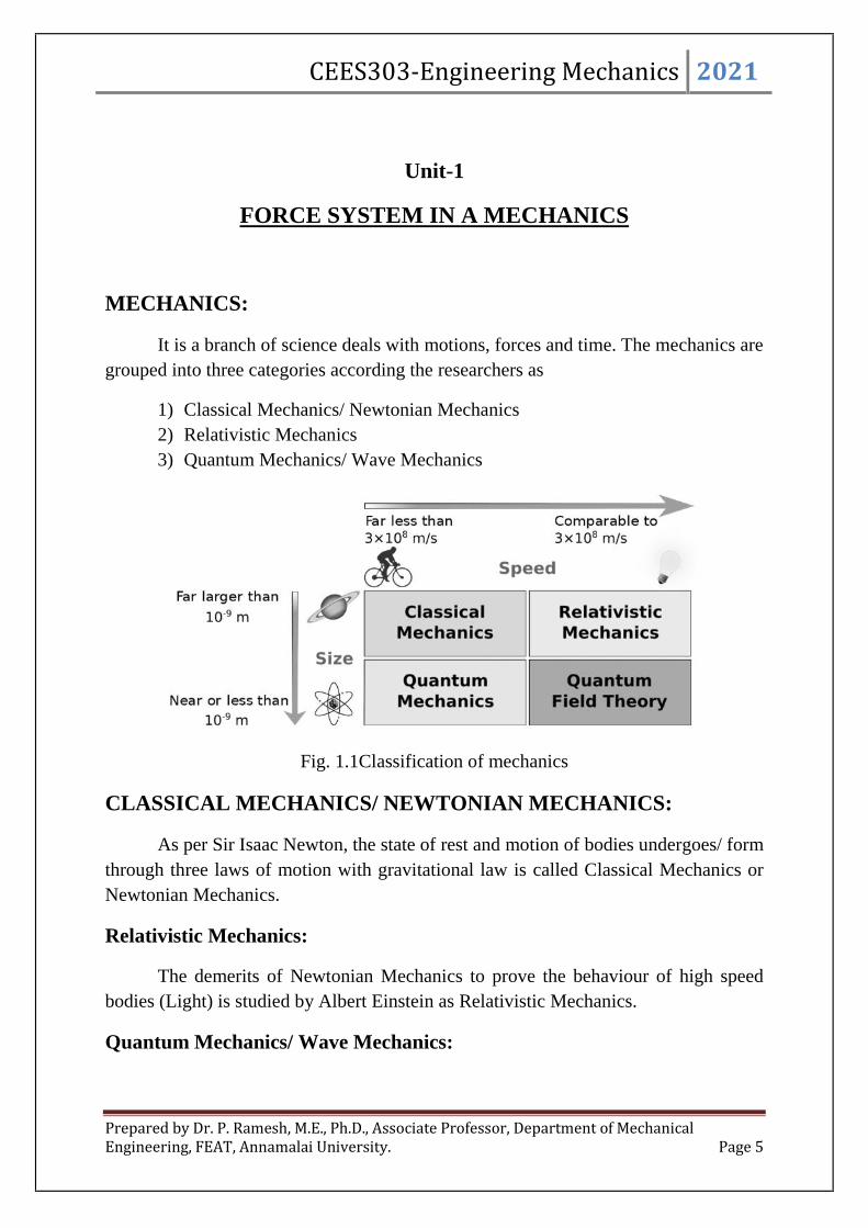
It is a branch of science deals with motions, forces and time. The mechanics aregrouped into three categories according the researchers as
1) Classical Mechanics/ Newtonian Mechanics2) Relativistic Mechanics3) Quantum Mechanics/ Wave Mechanics
Fig. 1.1Classification of mechanics
CLASSICAL MECHANICS/ NEWTONIAN MECHANICS:
As per Sir Isaac Newton, the state of rest and motion of bodies undergoes/ formthrough three laws of motion with gravitational law is called Classical Mechanics orNewtonian Mechanics.
Relativistic Mechanics:
The demerits of Newtonian Mechanics to prove the behaviour of high speedbodies (Light) is studied by Albert Einstein as Relativistic Mechanics.
Quantum Mechanics/ Wave Mechanics:
CEES303-Engineering Mechanics 2021
Prepared by Dr. P. Ramesh, M.E., Ph.D., Associate Professor, Department of MechanicalEngineering, FEAT, Annamalai University. Page 6
The demerits of Newtonian Mechanics to prove the behaviour of particles atthe atomic motion level is studied by Schrodinger and Broglie as QuantumMechanics.
ENGINEERING MECHANICS:
Many engineering field govern the laws of mechanics which state that thestability of work and termed as Engineering Mechanics. The engineers mostlyconsidered classical/ Newtonian mechanics because the entire engineering problemsare not dealt with in the atomic or high speed level.
CLASSIFICATION OF ENGINEERING MECHANICS:
Engineering mechanics depends on the application of body (Solid or fluid) inwhich the mechanics is discussed. It is classified as
1. Solid Mechanicsa. Rigid body of mechanics
i. Static mechanicsii. Dynamic mechanics
1. Kinematics of mechanics2. Kinetics of mechanics
b. Deformable body of mechanicsi. Theory of elasticity
ii. Theory of plasticity2. Fluid Mechanics
a. Ideal fluidb. Viscous fluidc. Incompressible fluid, etc.,
The solid body may be rigid and deformable. If the solid bodies are rigid andnegligible deformation then the body is termed as rigid body. The study of rigid ofbodies at rest is named as static mechanics and at motion is dynamic mechanics. Themotion of rigid bodies (Dynamic Mechanics) cause without any external force iscalled as Kinematics of Mechanics. Suppose the motion of rigid bodies dealt withforce is named as Kinetics of Mechanics.

CEES303-Engineering Mechanics 2021
Prepared by Dr. P. Ramesh, M.E., Ph.D., Associate Professor, Department of MechanicalEngineering, FEAT, Annamalai University. Page 7
a) Rigid body b) Deformable bodyFig.1.2 Types of solid body
If the solid bodies are deformable due to internal stress development is calledas Mechanics of Deformable or Strength of Materials or Mechanics of solids. Thedeformable bodies undergo the limit of stress acting on the body and classified astheory of elasticity and theory of plasticity
The behaviour of material varies under applied shear force to flows or deforms.The study of fluid motion is termed as Fluid Mechanics.
Fig. 1.3 classifications of Engineering Mechanics

CEES303-Engineering Mechanics 2021
Prepared by Dr. P. Ramesh, M.E., Ph.D., Associate Professor, Department of MechanicalEngineering, FEAT, Annamalai University. Page 8
BASIC CONCEPT OF MECHANICS:
There are many number of terms coincidence to understand the principle ofmechanics and they are following as
Space:
A body occupied by the region with geometrical coordinates system todetermines the position of linear and angular measurement.
Mass:
A space contains a quantity of mater in a body is known as mass. However, ithelps to measure the inertia of a body. The mass of a body remain same at space butthe weight of a body changes with gravitational force. Thereby the weight is theproduct of mass and gravitational force. Also the mass resists the change of velocity.
Time:
It is a parameter of dynamics of mechanics to measure the succession of events.
Example:
1) Earths rotates about its own axis and it is measured as number of days saysaround 365. An hour consists of a certain number of minutes as 60 seconds,a day of hours and a year of days.
Length:
It is a linear distance of measurement mostly the units are in metre.
Distance or path length:
It is total path length covered by an object during the entire journey withouttaking into consideration its direction it is a scalar quantity and it is always positivefor an objective in motion.
Displacement:
A particle or body moves from one position to another, the shortest distancebetween the initial and final position is said to be the magnitude of the displacementand it is directed from initial to final position.

CEES303-Engineering Mechanics 2021
Prepared by Dr. P. Ramesh, M.E., Ph.D., Associate Professor, Department of MechanicalEngineering, FEAT, Annamalai University. Page 9
Fig. 1.4 Motion of a body
Velocity:
It is defined as the rate of change of displacement (i.e., the displacementchanges with time)
Acceleration:
It is defined as the rate of change of velocity (i.e., the velocity changes withtime)
Momentum:
It is defined as the product of mass and velocity.
Force:
It is an action of a body on another. The action of force is characterized by itsmagnitude, by the direction of its action and by its point of application. Thereforeforce is vector quantity. A force may produce the following effects in the body, onwhich its acts;
a) It may change the motion of a body i.e., if a body is at rest, the force set itin motion. If the body is already in motion then the force may accelerate it.
b) It may retard the motion of a body.c) It may retard the forces, already acting on the body, thus bringing it to the
rest or in equilibrium.d) It may give rise to the internal stresses in the body, on which it acts.
PARTICLE:
A body as a particle when its dimensions are not considered to the subject ofposition or action of forces applied on it, particle has only mass and no size. In nature
Distance
Final position
Displacement
Initial position
CEES303-Engineering Mechanics 2021
Prepared by Dr. P. Ramesh, M.E., Ph.D., Associate Professor, Department of MechanicalEngineering, FEAT, Annamalai University. Page 10
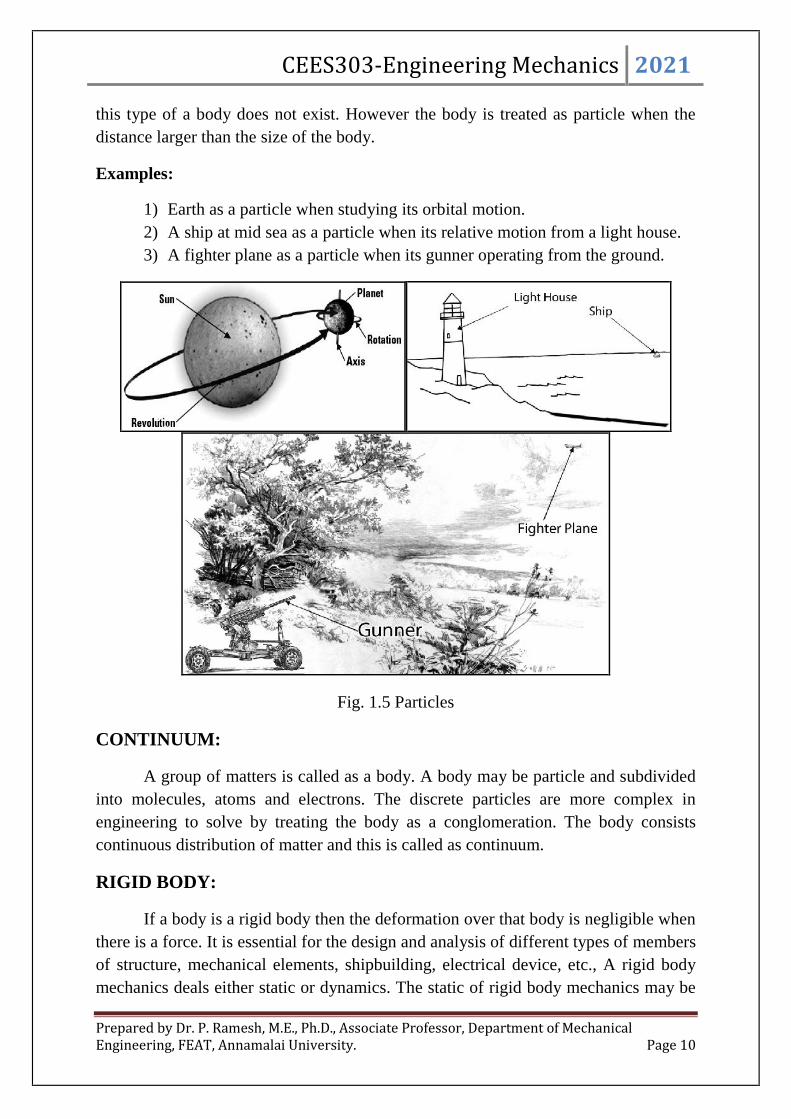
this type of a body does not exist. However the body is treated as particle when thedistance larger than the size of the body.
Examples:
1) Earth as a particle when studying its orbital motion.2) A ship at mid sea as a particle when its relative motion from a light house.3) A fighter plane as a particle when its gunner operating from the ground.
Fig. 1.5 Particles
CONTINUUM:
A group of matters is called as a body. A body may be particle and subdividedinto molecules, atoms and electrons. The discrete particles are more complex inengineering to solve by treating the body as a conglomeration. The body consistscontinuous distribution of matter and this is called as continuum.
RIGID BODY:
If a body is a rigid body then the deformation over that body is negligible whenthere is a force. It is essential for the design and analysis of different types of membersof structure, mechanical elements, shipbuilding, electrical device, etc., A rigid bodymechanics deals either static or dynamics. The static of rigid body mechanics may be
CEES303-Engineering Mechanics 2021
Prepared by Dr. P. Ramesh, M.E., Ph.D., Associate Professor, Department of MechanicalEngineering, FEAT, Annamalai University. Page 11
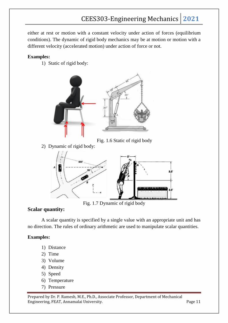
either at rest or motion with a constant velocity under action of forces (equilibriumconditions). The dynamic of rigid body mechanics may be at motion or motion with adifferent velocity (accelerated motion) under action of force or not.
Examples:1) Static of rigid body:
Fig. 1.6 Static of rigid body2) Dynamic of rigid body:
Fig. 1.7 Dynamic of rigid bodyScalar quantity:
A scalar quantity is specified by a single value with an appropriate unit and hasno direction. The rules of ordinary arithmetic are used to manipulate scalar quantities.
Examples:
1) Distance2) Time3) Volume4) Density5) Speed6) Temperature7) Pressure

CEES303-Engineering Mechanics 2021
Prepared by Dr. P. Ramesh, M.E., Ph.D., Associate Professor, Department of MechanicalEngineering, FEAT, Annamalai University. Page 12
8) Energy and9) Mass
Vector quantity:
A vector quantity must have magnitude as well as direction and obeys the lawsof vector addition.
Examples:
1) Displacement2) Velocity3) Acceleration4) Force5) Torque6) Moment and7) Momentum
Fig.1.8 Composition of forces
In the fig.1.7 the force F1 and F2 are two force vectors acted in a direction andmagnitude values. The equivalent force of vectors is R and it is represented by sum oftwo force vectors as R = F1+F2. The force vector R can be written as
).sin..(cos)(.)( 221121 jiFFFFnFFnFR myxyxmm
jFFiFFR myymxx .sin)(.cos)( 2121
jFFiFFjRiR myymxxyx .sin)(.cos)(.sin.cos 2121
xxxx FFFR 21 and
yyyx FFFR 21
Where, R – Resultant force of given two forces
mF -Magnitude of force F1 and F2.
F2F1
RF2
F1
R
F2
F2
CEES303-Engineering Mechanics 2021
Prepared by Dr. P. Ramesh, M.E., Ph.D., Associate Professor, Department of MechanicalEngineering, FEAT, Annamalai University. Page 13
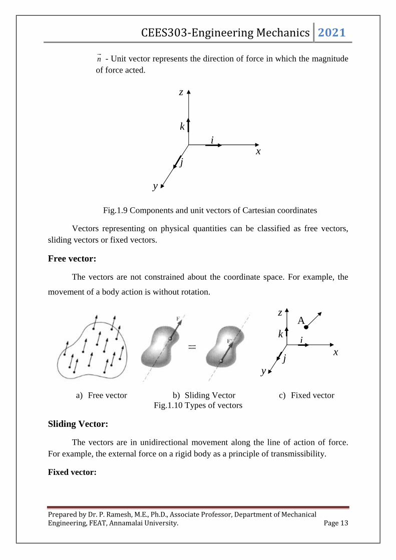
n - Unit vector represents the direction of force in which the magnitudeof force acted.
Fig.1.9 Components and unit vectors of Cartesian coordinates
Vectors representing on physical quantities can be classified as free vectors,sliding vectors or fixed vectors.
Free vector:
The vectors are not constrained about the coordinate space. For example, the
movement of a body action is without rotation.
a) Free vector b) Sliding Vector c) Fixed vectorFig.1.10 Types of vectors
Sliding Vector:
The vectors are in unidirectional movement along the line of action of force.For example, the external force on a rigid body as a principle of transmissibility.
Fixed vector:
x
z
y
ik
j
A
x
z
y
ik
j

CEES303-Engineering Mechanics 2021
Prepared by Dr. P. Ramesh, M.E., Ph.D., Associate Professor, Department of MechanicalEngineering, FEAT, Annamalai University. Page 14
The vectors are constrained about the coordinate space. For example the lineaction of a force on deformable body is fixed.
Fig.1.11 Geometry of vectors
LAWS OF MECHANICS:
Newton’s first law Newton’s second law Newton’s third law Newton’s law of gravitational Law of transmissibility of forces and Parallelogram law of forces
Newton’s first law:
A particle remains at rest or continuous to move with uniform velocity by thestate of equilibrium forces.
Fig. 1.12 Force systems in a particleNewton’s second law:
The acceleration of a particle is proportional to the vector sum of forces actingon it and is in the direction of this vector sum.
F1F2
F3
V
4
6
22 46
46 jiFF m
22 )25()17(
)25()17( jiFF m
(7, 5)
(1, 2)
F
F
jiFF m sincos
F
CEES303-Engineering Mechanics 2021
Prepared by Dr. P. Ramesh, M.E., Ph.D., Associate Professor, Department of MechanicalEngineering, FEAT, Annamalai University. Page 15
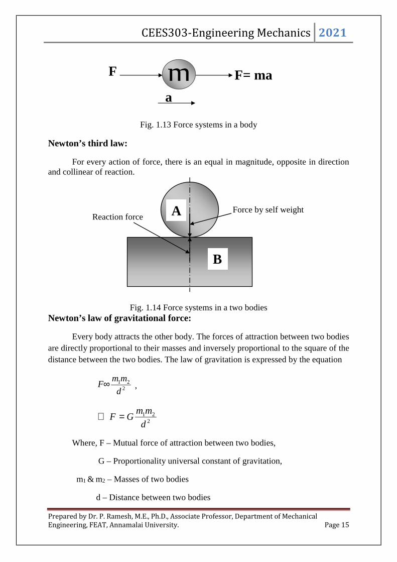
Fig. 1.13 Force systems in a body
Newton’s third law:
For every action of force, there is an equal in magnitude, opposite in directionand collinear of reaction.
Fig. 1.14 Force systems in a two bodiesNewton’s law of gravitational force:
Every body attracts the other body. The forces of attraction between two bodiesare directly proportional to their masses and inversely proportional to the square of thedistance between the two bodies. The law of gravitation is expressed by the equation
221
d
mmF ,
221
d
mmGF
Where, F – Mutual force of attraction between two bodies,
G – Proportionality universal constant of gravitation,
m1 & m2 – Masses of two bodies
d – Distance between two bodies
Reaction forceForce by self weightA
B
mF F= ma
a
CEES303-Engineering Mechanics 2021
Prepared by Dr. P. Ramesh, M.E., Ph.D., Associate Professor, Department of MechanicalEngineering, FEAT, Annamalai University. Page 16
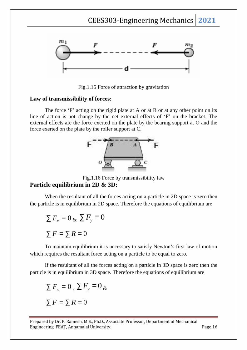
Fig.1.15 Force of attraction by gravitation
Law of transmissibility of forces:
The force ‘F’ acting on the rigid plate at A or at B or at any other point on itsline of action is not change by the net external effects of ‘F’ on the bracket. Theexternal effects are the force exerted on the plate by the bearing support at O and theforce exerted on the plate by the roller support at C.
Fig.1.16 Force by transmissibility lawParticle equilibrium in 2D & 3D:
When the resultant of all the forces acting on a particle in 2D space is zero thenthe particle is in equilibrium in 2D space. Therefore the equations of equilibrium are
0 xF & 0 yF
0 RF
To maintain equilibrium it is necessary to satisfy Newton’s first law of motionwhich requires the resultant force acting on a particle to be equal to zero.
If the resultant of all the forces acting on a particle in 3D space is zero then theparticle is in equilibrium in 3D space. Therefore the equations of equilibrium are
0 xF , 0 yF &
0 RF
CEES303-Engineering Mechanics 2021
Prepared by Dr. P. Ramesh, M.E., Ph.D., Associate Professor, Department of MechanicalEngineering, FEAT, Annamalai University. Page 17
Rigid body in equilibrium:
A rigid body is in equilibrium when it is not undergoing a change in rotationalor translational motion. This equilibrium requires that two conditions must be met.The first condition is related to the translational motion. The vector sum of the forceson the body must be zero.
0 F
The second condition is related to the rotational motion. When the forces donot act through a common point or pivot, they may cause the body to rotate, eventhough the vector sum of the forces may be zero. This requires introducing the idea ofmoment (torque) due to a force. A net moment (torque) will cause a body initially atrest to undergo rotation. Therefore, the sum of all the moment (torque) must be zero.
0 M
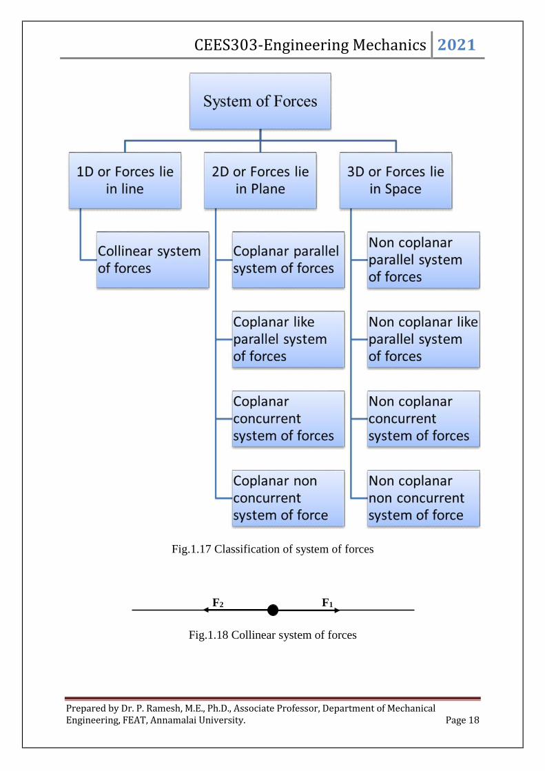
SYSTEM OF FORCES:
A system of forces consist number of forces act on a body simultaneously. Ifthese forces do not lie in a single plane then it is said the system of forces in space(3D). Whereas these forces lie in a single plane (2D) then it is a coplanar force system.
The line of action of forces pass through the single point is known asconcurrent force of system. The system of forces present in a line of action (1D) istermed as collinear force of system. The classifications of system of force as
1) One dimension (1D) or Forces lie in linea) Collinear
2) Two dimension (2D) or Forces lie in planea) Coplanar parallel forcesb) Coplanar like parallel forcesc) Coplanar concurrent forcesd) Coplanar non concurrent forces
3) Three dimension (3D) or Forces lie in spacea) Non coplanar parallel forcesb) Non coplanar like parallel forcesc) Non coplanar concurrent forcesd) Non coplanar non concurrent forces
CEES303-Engineering Mechanics 2021
Prepared by Dr. P. Ramesh, M.E., Ph.D., Associate Professor, Department of MechanicalEngineering, FEAT, Annamalai University. Page 18
Fig.1.17 Classification of system of forces
Fig.1.18 Collinear system of forces
F1F2

CEES303-Engineering Mechanics 2021
Prepared by Dr. P. Ramesh, M.E., Ph.D., Associate Professor, Department of MechanicalEngineering, FEAT, Annamalai University. Page 19
Fig.1.19 Planes of references in space coordinate
a) Coplanar parallel system of forces b) Coplanar like parallel system offorces
c) Coplanar concurrent system offorces
d) Coplanar non concurrent system offorces
Fig.1.20 Forces lie in a plane system
+X+Y
-Y-X
+X+Y
-Y-X
+X+Y+X+Y
+Z
-Z
+X
-X -Y
+Y

CEES303-Engineering Mechanics 2021
Prepared by Dr. P. Ramesh, M.E., Ph.D., Associate Professor, Department of MechanicalEngineering, FEAT, Annamalai University. Page 20
a) Non coplanar parallel system offorces
b) Non coplanar like parallel systemof forces
c) Non coplanar concurrent system offorces
d) Non coplanar non concurrentsystem of forces
Fig.1.21 Forces lie in a space system
Vector components of forces:
In space, a force can be resolved into mutually perpendicular componentswhose vector sum about the coordinates is equal to the given force. The componentsare parallel to the axes x, y and z with the unit vectors i, j and k. The rectangularcomponents are considered to resolve the problem related to the system of forces. It iscategoried as
1. Two dimension rectangular components:The most common two dimensionalresolution of a force vector is intorectangular components. It follows from theparallelogram rule that the vector F as shownin fig. is written as
yx FFF
+Z
+X+Y
-Y-X
-Z
+Z
+X+Y
-Y-X
-Z
+Z
+X+Y
+Z
+X+Y
Fig.1.22 Rectangularcomponents in two dimensions
CEES303-Engineering Mechanics 2021
Prepared by Dr. P. Ramesh, M.E., Ph.D., Associate Professor, Department of MechanicalEngineering, FEAT, Annamalai University. Page 21
Where Fx and Fy are vector components of F in the x and y direction.Each of the two vector components may be written as a scalar times theappropriate unit vector. In terms of the unit vectors i and j, the x component of
force is iFF xx . and the y component of force is jFF yy . and thus the force,
Where the scalars Fx and Fy are the x and y scalar components of thevector force, F.
The scalar components can be positive or negative depending on thequadrant into which F points. For the force vector as shown in fig. The x and yscalar components are both positive and are related to the magnitude anddirection of F by
cosFFx and sinFFy
Therefore, 22yx FFF and
x
y
F
F1tan
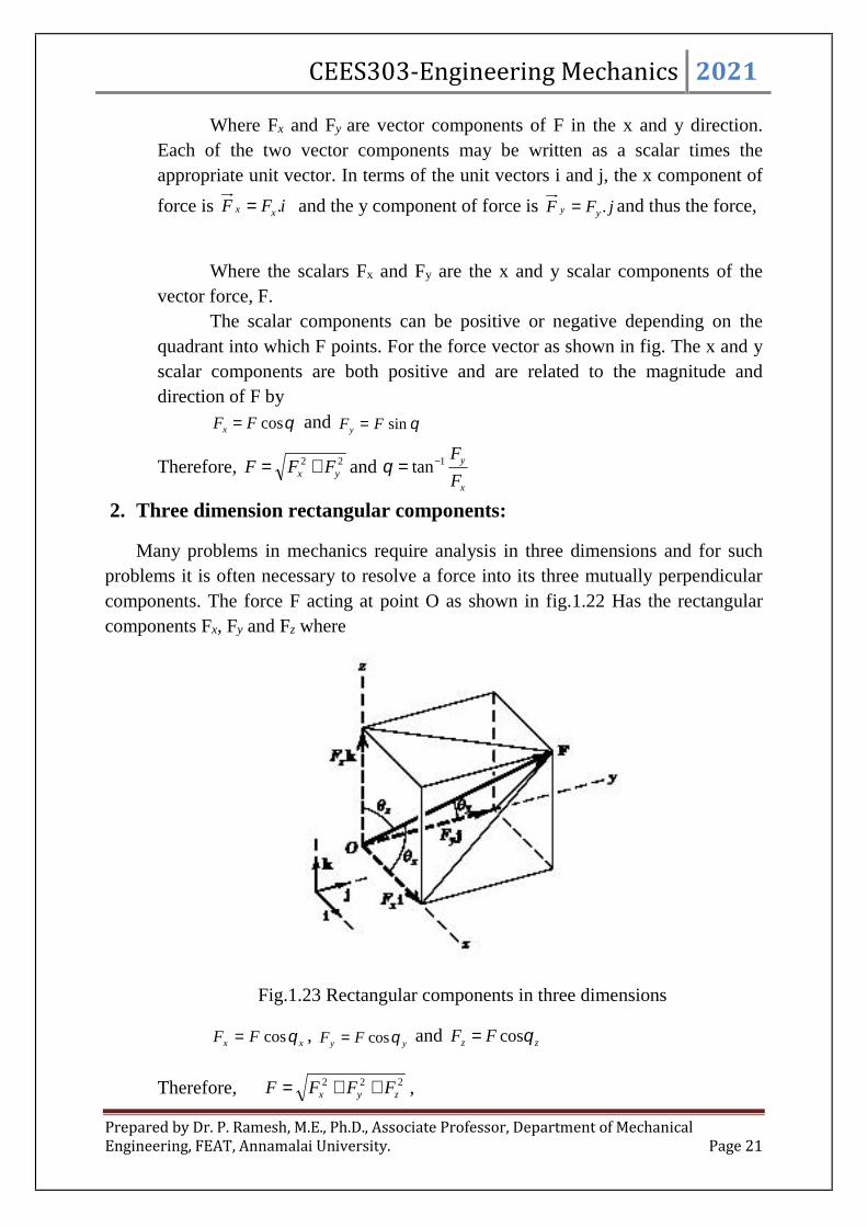
2. Three dimension rectangular components:
Many problems in mechanics require analysis in three dimensions and for suchproblems it is often necessary to resolve a force into its three mutually perpendicularcomponents. The force F acting at point O as shown in fig.1.22 Has the rectangularcomponents Fx, Fy and Fz where
Fig.1.23 Rectangular components in three dimensions
xx FF cos , yy FF cos and zz FF cos
Therefore, 222zyx FFFF ,

CEES303-Engineering Mechanics 2021
Prepared by Dr. P. Ramesh, M.E., Ph.D., Associate Professor, Department of MechanicalEngineering, FEAT, Annamalai University. Page 22
kFjFiFF zyx and
).cos.cos.(cos kjiFF zyxm
The unit vectors i, j and k are in the x, y and z directions respectively. Usingthe direction cosines of F which are xl cos , ym cos and zn cos ,
where 1222 nml , then the force as
)...( knjmilFF m
In the above equation, the right hand side of the force magnitude mF times a
unit vector Fn which characterizes the direction of F,
FmnFF
It is clear from the above equations that knjmilnF ... , which shows that the scalar
components of the unit vectors Fn are the direction cosines of the line of action of
force, F.
In solving three dimensional problems one must usually find the x, y and zscalar components of a force. In most cases the direction of a force is described by
a) Two points on the line of the forceb) Two angles which orient the line of action
a) The direction of a force by two point’s method:
If the coordinates of points A and B as shown in fig.1.23 are known then theforce F is written as
Fig.1.24 Cartesian coordinate system in a space

CEES303-Engineering Mechanics 2021
Prepared by Dr. P. Ramesh, M.E., Ph.D., Associate Professor, Department of MechanicalEngineering, FEAT, Annamalai University. Page 23
212
212
212
121212
)()()(
).().().(
zzyyxx
kzzjyyixxF
AB
ABFnFF mmFm
Thus the x, y and z scalar components of F are the scalar coefficients of theunit vectors i, j and k respectively.
b) The direction of a force by two angles method:Consider the geometry as shown in fig.1.24 to resolve force F into horizontal
and vertical components when angles and are known.
Fig.1.25 Spherical coordinate system in a space
cosFFxy and sinFFz ,
Now resolve the horizontal component Fxy into x and y components.
coscoscos FFF xyx and sincossin FFF xyy
Angles between two vectors:
If the angle between the force F and the direction specified by the unit vector n
is then from the dot product definition, the Fm.nF = Fncos = F cos, where
1 nn . Thus the angle between F and n is given by
m
Fm
F
nF1cos
In general the angle between any two vectors P and Q is
PQ
QP.cos 1

CEES303-Engineering Mechanics 2021
Prepared by Dr. P. Ramesh, M.E., Ph.D., Associate Professor, Department of MechanicalEngineering, FEAT, Annamalai University. Page 24
Fig.1.26 Vector angles in planes
If a force F is perpendicular to a line whose direction is specified by the unitvector n, then 0cos and Fm.nF=0.
Note: This relationship does not mean that either Fm or nF is zero as would be the casewith scalar multiplication where (A)(B) =0 requires that either A or B (or both) bezero.
The dot-product relationship applies to non intersecting vectors as well as tointersecting vectors. Thus the dot product of the non intersecting vectors P and Q as
shown in fig. is Q times the projection of P’ on Q, or P’Qcos = PQcos because P’and P are the same when treated as free vectors.
Problems:
SP1.1: The guy wire of the electric pole as shown in fig.1.26 makes 60o to thehorizontal and is subjected to 20 kN force. Find horizontal and vertical components ofthe force.
Fig.1.27 A guy wire of electric pole
Solution:
From the figure F is 20kN and is 60o, by the components of force method thescalar components of force Fm is 20kN.
).sin..(cos jiFF m
20kN
60o

CEES303-Engineering Mechanics 2021
Prepared by Dr. P. Ramesh, M.E., Ph.D., Associate Professor, Department of MechanicalEngineering, FEAT, Annamalai University. Page 25
jFiFF mm .sin..cos.
cos.mx FF and sin.my FF
The horizontal component of force is,
kNF ox 1060cos.20
The vertical component of force is,
kNF oy 32.1760sin.20
SP1.2: A block weighing W=10kN is resting on an inclined plane as shown infig.1.27. Determine its components normal to and parallel to the inclined plane.
Fig.1.28 A block resting in an inclined plane
Solution:
The given parameter as W = 10kN
From the given figure develop a space diagram to identify the forces in a block.
The plane makes an angle of 20o with the horizontal. Hence the normal to theplane makes an angle of 70o to the horizontal. That is 20o to the vertical. If ABrepresents the given force W to some scale AC represents the normal component and
20o
W
B
A
C
70o
20o
W

CEES303-Engineering Mechanics 2021
Prepared by Dr. P. Ramesh, M.E., Ph.D., Associate Professor, Department of MechanicalEngineering, FEAT, Annamalai University. Page 26
CB represents component parallel to the plane. From triangle ABC, the normalcomponent is
kNWAC oo 4.920cos1020cos
The parallel component is
kNSinWBC oo 42.320sin1020
SP1.3: Determine the scalar component of forces for the given parameters as shownin fig.1.28 in different ways.
Fig. 1.29 Force systems in a bracket
Solution:
There are three forces acted on the bracket at point A. The force F1 has linearand angular units. Therefore, the scalar components of F1 as

CEES303-Engineering Mechanics 2021
Prepared by Dr. P. Ramesh, M.E., Ph.D., Associate Professor, Department of MechanicalEngineering, FEAT, Annamalai University. Page 27
).sin..(cos11 jiFF m
jFiFF mm .sin..cos. 111
cos.11 mx FF and sin.11 my FF
From the figure, F1m is 600 N and is 35o
NF ox 49135cos.6001
NF oy 34435sin.6001
jiF .344.4911
The scalar component of F2 as for the Dimension about x axis is 4 units and y axis is 3units. The direction of x axis is opposite then the sign of dimension is negative.
2222)( yx
yjxiFF m
22223)4(
34 jiFF m
25
34
916
34222
jiF
jiFF mm
5
3
5
422
jiFF m
jFiFF mm 5
3.
5
4. 222
From the figure, F2m is 500N
NFF mx 4005
4.500
5
4.22

CEES303-Engineering Mechanics 2021
Prepared by Dr. P. Ramesh, M.E., Ph.D., Associate Professor, Department of MechanicalEngineering, FEAT, Annamalai University. Page 28
NFF my 30053
.50053
.22
jiF .300.4002 The scalar components of F3 as for the given dimension of two end points
detail which is at point A is (xA, yA) = (0,0) and point B is (xB, -yB) = (0.2,-0.4). Thenegative sign of yB indicates the direction is opposite.
2233)()(
)()(
ABAB
ABABm
yyxx
jyyixxFF
2233)04.0()02.0(
)04.0()02.0( jiFF m
2233)4.0()2.0(
4.02.0 jiFF m
)16.0()04.0(
4.02.033
jiFF m
45.0
4.02.0
2.0
4.02.0333
jiF
jiFF mm
jFiFF mm 45.0
4.0.
45.0
2.0. 333
From figure F3 is 800N, then
NFF
NFF
my
mx
11.71145.0
4.0.800
45.0
4.0.
56.35545.0
2.0.800
45.0
2.0.
33
33
jiF .11.711.56.3553

CEES303-Engineering Mechanics 2021
Prepared by Dr. P. Ramesh, M.E., Ph.D., Associate Professor, Department of MechanicalEngineering, FEAT, Annamalai University. Page 29
SP1.4: A machine component 1.5 m long and weight 1000 N is supported by tworopes AB and CD as shown in Fig.1.29 given below. Calculate the tensions T1 and T2
in the ropes AB and CD.
Fig. 1.30 Machine component
Solution:
The given data apart from dimensions of body and position is weight of a bodyas W = 1000N.
The sum of horizontal components of forces is equal to zero,
0coscos 21 TTFx , the negative sign indicates the direction of
component force. Therefore,
0coscos 21 TT
045cos60cos 21 oo TT
221 414.160cos
45cosTTT
o
o
The sum of Vertical components of forces is equal to zero,
T2 sin
W
T1T2
T2cos
T1 sin
T1cos

CEES303-Engineering Mechanics 2021
Prepared by Dr. P. Ramesh, M.E., Ph.D., Associate Professor, Department of MechanicalEngineering, FEAT, Annamalai University. Page 30
0sinsin 21 WTTFy , the negative sign indicates the direction of
load acting. Therefore,
0sinsin 21 WTT
0100045sin60sin 21 oo TT
Now, substitute the value of T1, then
0100045sin60sin414.1 22 oo TT
100093.1 2 T
NT 1.5182
NTT 6.7321.518414.1414.1 21
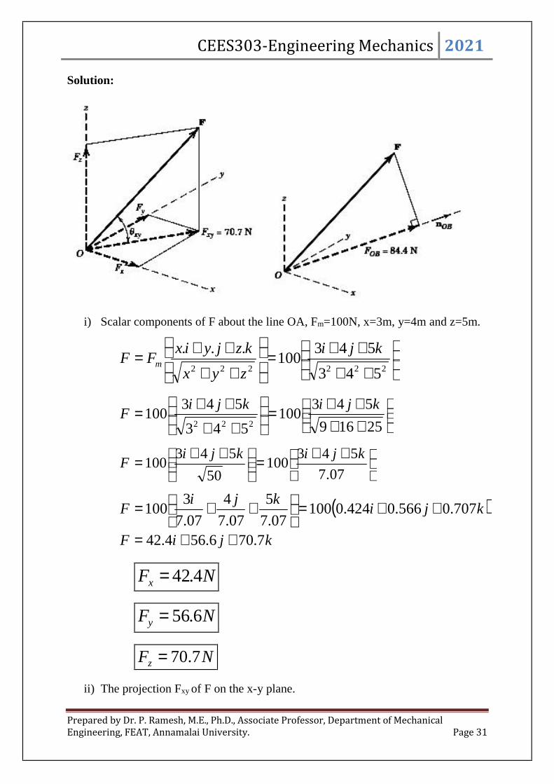
SP1.5: A force F with a magnitude of 100N is applied at the origin O of the axes x-y-zas shown in fig.1.30. The line of action of F passes through a point A whosecoordinates are 3m, 4m and 5m. Determine i) the scalar components of F, ii) theprojection Fxy of F on the x-y plane and iii) the projection FOB of F along the line OB.
Fig.1.31 Force system in a space coordinates
CEES303-Engineering Mechanics 2021
Prepared by Dr. P. Ramesh, M.E., Ph.D., Associate Professor, Department of MechanicalEngineering, FEAT, Annamalai University. Page 31
Solution:
i) Scalar components of F about the line OA, Fm=100N, x=3m, y=4m and z=5m.
222222 543
543100
... kji
zyx
kzjyixFF m
25169
543100
543
543100
222
kjikjiF
07.7
543100
50
543100
kjikjiF
kjikji
F 707.0566.0424.010007.7
5
07.7
4
07.7
3100
kjiF 7.706.564.42
NFx 4.42
NFy 6.56
NFz 7.70
ii) The projection Fxy of F on the x-y plane.

CEES303-Engineering Mechanics 2021
Prepared by Dr. P. Ramesh, M.E., Ph.D., Associate Professor, Department of MechanicalEngineering, FEAT, Annamalai University. Page 32
The cosine of angle between F and xy plane is
222
22
coszyx
yxxy
707.0543
43cos
222
22
xy
Therefore, NFF xyxy 7.70707.0100cos
iii) The projection FOB of F along the line OB. The dimension of OB from origin ofx is 6m, y is 6m and z is 2m.
222
222
266
266)7.706.562.42(
...
kjikji
zyx
kzjyixFFOB
kjikjiFOB 229.0688.0688.0)7.706.562.42(
NFOB 4.84)229.0)(7.70()688.0)(6.56()688.0)(4.42(
If the projection is represented as vector then,
222
...
zyx
kzjyixFF OBOB
)229.0688.0688.0(4.84266
2664.84
222kji
kjiFOB
kjiFOB 35.191.581.58

CEES303-Engineering Mechanics 2021
Prepared by Dr. P. Ramesh, M.E., Ph.D., Associate Professor, Department of MechanicalEngineering, FEAT, Annamalai University. Page 33
RESULTANT FORCE:
The resultant force, R is a force which produces the same effect of number offorces F1, F2, F3 and F4 are acting on particle as shown in fig.1.31. The differentmethods used to determine the resultant force of a number of given forces are asfollows
1) Graphical Method.2) Analytical Method
a) Geometrical resolution methodb) Algebraic sum of resolution method
Fig.1.32 Force systems in a particle
1) Graphical method for the resultant force:This method also named as polygon law of forces to find the resultant
force in magnitude and direction. The graphical or vector methods started with
the space drawing which shows the position of force vector acting on a particle.
The graphical method of vector force is continued by addition of force one by
one to the direction and magnitude of the suitable scale. The resultant force of
all forces is obtained by the line joining of start point of first vector force and
end point of last vector force is a magnitude value of resultant in that suitable
scale. The angle of direction is measured from first vector to the position of
resultant force.
Parallelogram law and triangle law of vectors can also be used to find
the resultant force graphically. This method gives a clear picture of the work
R
F1
F2
F3
F4
1
23
4
R

CEES303-Engineering Mechanics 2021
Prepared by Dr. P. Ramesh, M.E., Ph.D., Associate Professor, Department of MechanicalEngineering, FEAT, Annamalai University. Page 34
being carried out. However the main disadvantage is that it needs drawing aids
like pencil, scale, drawing sheets. Hence there is need for analytical method.
Problems:
SP1.6: A particle is acted upon by three forces equal to 50N, 100N and 130N alongthe three sides of an equilateral triangle taken in order. Find graphically the magnitudeand direction of the resultant force.
Solution by Graphical method:
Step 1: Draw the space/ position diagram as per given data and denote lettering forthe corners of vector force by A, B and C.
Step 2: Now start to draw the vector diagram for the above drawn space diagram withsuitable scale. The scale is selected for the force but the angular dimension not to bechanged. 100 N magnitude forces is taken as 10cm of linear scale. Only the length ofthe scale in cm is used to measure and marking but the denoted as original unit of N(Newton).
In this step draw a line from point as as a starting point of first force at length 5cmfor the 50N ended with point b along the direction as position in space diagram.
Step 3: The second force 100N is measured as 10cm and draw a line from b at 10cmlength in the direction specified by the space diagram say 120o from the first vectorforce which is at zero degree. Now mark letter c at the end point of second vectorforce.
as bF=50N
60o
100N
50N
130N
AB
C
60o
60o

CEES303-Engineering Mechanics 2021
Prepared by Dr. P. Ramesh, M.E., Ph.D., Associate Professor, Department of MechanicalEngineering, FEAT, Annamalai University. Page 35
Step 4: The third force 130 N measured as 13cm and draw a line from point c at 13cmlength in the direction specified by the space diagram as 120o from the second vectorforce which at 120o from horizontal. Now mark letter ae at the end point of thirdvector force because this vector force ended with starting point of first vector force.
Step 5: The vector force by the space diagram is completed and finally joins the linebetween starting point of first vector force as and ending point of third vector force ae
is known as resultant force of given vector forces by the method graphical.
Step 6: Now, measure the length between point as and ae in cm as 7cm and convertedinto the magnitude force scale as Resultant force R , 70N. Using protractor, measure
the angle of direction of the resultant force is 200o. From the direction of positive xthat is horizontal direction.
F=50N
F=100N
as b
120o
c
ae
120o
120o
F=130N
R
F=50N
F=100N
as b
120o
c
ae
120o
120o
F=130N
c
F=50N
F=100N
as b
120o
CEES303-Engineering Mechanics 2021
Prepared by Dr. P. Ramesh, M.E., Ph.D., Associate Professor, Department of MechanicalEngineering, FEAT, Annamalai University. Page 36
2) Analytical method for the resultant force:
a. Geometrical resolution method for the resultant force
This method is named as parallelogram law of forces and it states thattwo forces acting on a particle simultaneously by in magnitude anddirection which forms like a parallelogram to give the resultant force as adiagonal of parallelogram. The mathematical expression of resultant forcein magnitude and direction by the parallelogram law of force as
R = 2221
21 2 FCosFFF and
CosFF
SinF
21
21tan
Proof:
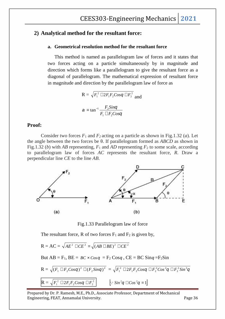
Consider two forces F1 and F2 acting on a particle as shown in Fig.1.32 (a). Letthe angle between the two forces be θ. If parallelogram formed as ABCD as shown inFig.1.32 (b) with AB representing, F1 and AD representing F2 to some scale, accordingto parallelogram law of forces AC represents the resultant force, R. Draw aperpendicular line CE to the line AB.
Fig.1.33 Parallelogram law of force
The resultant force, R of two forces F1 and F2 is given by,
R = AC = 2222 )( CEBEABCEAE
But AB = F1, BE = CosBC = F2 Cos , CE = BC Sin =F2Sin
R = 22
221 )()( SinFCosFF = 22
222
2212
1 2 SinFCosFCosFFF
R = 2221
21 2 FCosFFF 122 CosSin
CEES303-Engineering Mechanics 2021
Prepared by Dr. P. Ramesh, M.E., Ph.D., Associate Professor, Department of MechanicalEngineering, FEAT, Annamalai University. Page 37
The inclination of resultant force to the direction of F1 is given by , where
CosFF
SinF
BEAB
CE
AE
CE
21
2tan
CosFF
SinF
21
21tan
Particular cases:
1. When ,0 o R = 2221
21 2 FFFF =F1+F2
2. When ,90o R = 22
21 FF
3. When ,180 o R = 2221
21 2 FFFF =F1 - F2
4. When F1 = F2 = F, Then
)cos1(2 2 FR
2cos2
2cos22 22
FFR
b. Algebraic sum of force resolution for the resultant force
It states that the number of force resolutions in a given direction is equalto the resultant force resolution. The force resolution or resultant forceresolution is a component of forces without changing its effect on the body.The components of forces are mutually perpendicular to each other indirections. The magnitude of resultant force,
22 )()( yx FFR
22yxyx FFRR
nxxxx FFFF ...............21
nyyyy FFFF ...............21
The direction of resultant force,
x
y
F
F
tan

CEES303-Engineering Mechanics 2021
Prepared by Dr. P. Ramesh, M.E., Ph.D., Associate Professor, Department of MechanicalEngineering, FEAT, Annamalai University. Page 38
x
y
F
F1tan
Particular cases:
1. When, ,360270900 oooo andorandis xF is positive
2. When, ,0180 oo andis yF is positive
3. When, ,02709 oo andis xF is negative
4. When, oo andis 036018 , yF is negative
Problems:
SP1.7: Combine the two forces P and T which act on the fixed structure at B into asingle equivalent force R.
Fig.1.34 force system in a structure
Graphical Solution:
The scale used here is 4cm = 800 N and 3cm = 600N would be more suitablefor regular size paper and would give greater accuracy.
a) Space diagram b) Vector diagram
Ps
Te
Ts800N
600NR

CEES303-Engineering Mechanics 2021
Prepared by Dr. P. Ramesh, M.E., Ph.D., Associate Professor, Department of MechanicalEngineering, FEAT, Annamalai University. Page 39
Measurement of the length R is 2.6cmand direction of the resultant force R
yields the approximate results as NR 520 and o49
Geometric Solution:
From the triangle ABD, the angle is calculated as shown in above diagram.
CDAD
BD
AD
BD
tan
From triangle CBD,
660sin oBD and 660cos oCD
Therefore, 866.0)660(sin3
660sintan
o
o
o9.40)866.0(tan 1
The law of cosines or parallelogram law of force gives
NPTTPR o 5249.40cos8006002800600cos2 2222
From the law of sines, the angle which orients R. Thus,
o9.40sin
524
sin
600
, 750.0sin and o6.48
R=520N
Ps
Te
Ts800N
600N

CEES303-Engineering Mechanics 2021
Prepared by Dr. P. Ramesh, M.E., Ph.D., Associate Professor, Department of MechanicalEngineering, FEAT, Annamalai University. Page 40
Algebraic solution:
By using the x-y coordinate system on the given figure ,
NFR oxx 3469.40cos600800 and NFR o
yy 3939.40sin600
The magnitude and direction of the resultant force R as shown in figure 2.2care then
R= NRR yx 524)393(346 2222 and
o
x
y
R
R6.48
346
393tantan 11
SP1.8: A frame ABC is supported in part by cable DBE that passes through africtionless ring at B. Knowing that the tension in the cable is 385 N, determine thecomponents of the force exerted by the cable on the support at E.
Fig.1.35 Frame supported by a cableSolution:
The direction of a force by two point’s method in cable from E to B, then theforce F is written as
222 )()()(
).().().(
zzyyxx
zzyyxxmmFm
EBEBEB
kEBjEBiEBF
EB
EBFnFF
Where, Fm = 385 N, the dimension from origin for point B is Bx=480mm, By =0mm and Bz =600mm. At point E, Ex = 210mm, Ey = 400mm and Ez = 0mm.
CEES303-Engineering Mechanics 2021
Prepared by Dr. P. Ramesh, M.E., Ph.D., Associate Professor, Department of MechanicalEngineering, FEAT, Annamalai University. Page 41
Therefore,
222 )0600()4000()210480(
).0600().4000().210480(385
kjiF
222 )600()400()270(
).600().400().270(385
kjiF
770).600().400().270(
385kji
F
kjiF 300.200.135
Hence, NFx 135 , NFy 200 and NFz 300
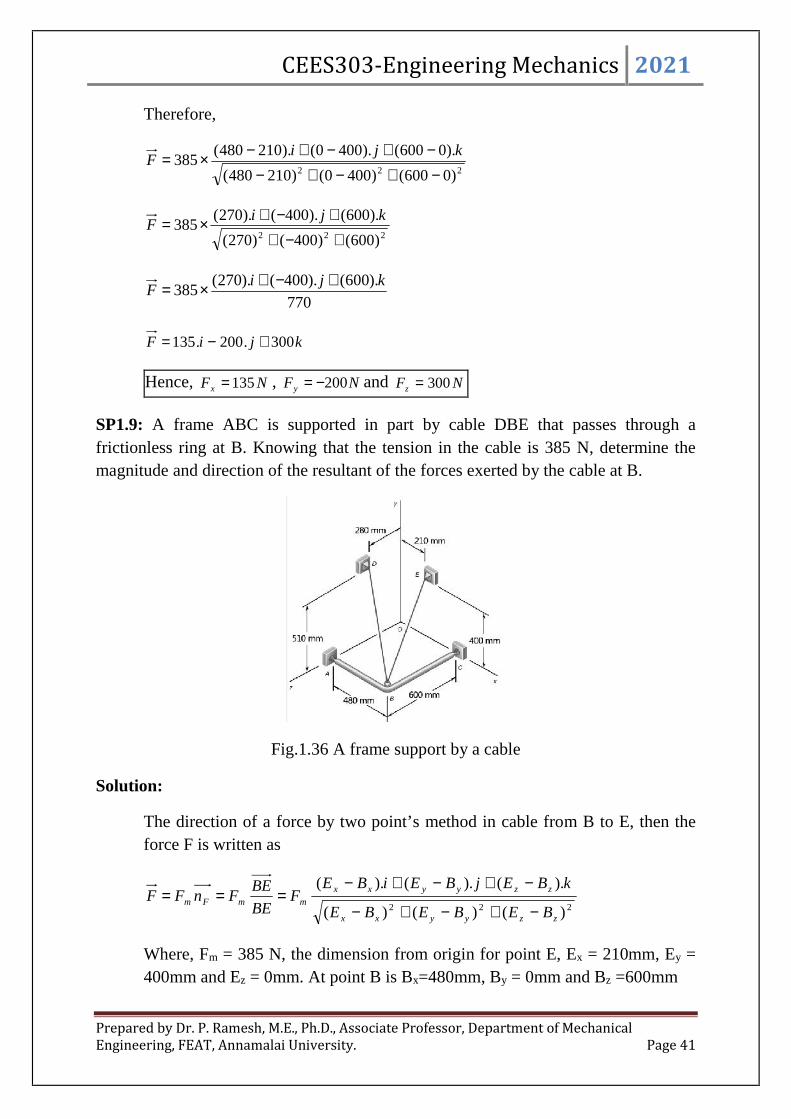
SP1.9: A frame ABC is supported in part by cable DBE that passes through africtionless ring at B. Knowing that the tension in the cable is 385 N, determine themagnitude and direction of the resultant of the forces exerted by the cable at B.
Fig.1.36 A frame support by a cable
Solution:
The direction of a force by two point’s method in cable from B to E, then theforce F is written as
222 )()()(
).().().(
zzyyxx
zzyyxx
mmFmBEBEBE
kBEjBEiBEF
BE
BEFnFF
Where, Fm = 385 N, the dimension from origin for point E, Ex = 210mm, Ey =400mm and Ez = 0mm. At point B is Bx=480mm, By = 0mm and Bz =600mm
CEES303-Engineering Mechanics 2021
Prepared by Dr. P. Ramesh, M.E., Ph.D., Associate Professor, Department of MechanicalEngineering, FEAT, Annamalai University. Page 42
Therefore,
222 )6000()0400()480210(
).6000().0400().480210(385
kjiFEB
222 )600()400()270(
).600().400().270(385
kjiFEB
770
).600().400().270(385
kjiFEB
kjiFEB 300.200.135
The direction of a force by two point’s method in cable from B to D, then theforce F is written as
222 )()()(
).().().(
zzyyxx
zzyyxxmmFm
BDBDBD
kBDjBDiBDF
BD
BDFnFF
Where, Fm = 385 N, the dimension from origin for point D, Dx = 0mm, Dy =510mm and Dz = 280mm. At point B is Bx=480mm, By = 0mm and Bz
=600mm.
Therefore,
222 )600280()0510()4800(
).600280().0510().4800(385
kjiFDB
222 )320()510()480(
).320().510().480(385
kjiFDB
770
).320().510().480(385
kjiFDB
kjiFDB 160.255.240
)160.255.240()300.200.135( kjikjiFFR DBEB
kjiR .460.455.375
222222 .)460(.)455(.)375( kjiR
NR 83.747

CEES303-Engineering Mechanics 2021
Prepared by Dr. P. Ramesh, M.E., Ph.D., Associate Professor, Department of MechanicalEngineering, FEAT, Annamalai University. Page 43
ox 1.120
83.747
375cos 1
oy 5.52
83.747
455cos 1
oz 0.128
83.747
460cos 1
MOMENT OF FORCE AND ITS APPLICATIONS:
The effect of force on a body about an axis influenced to rotate in addition tomove the body in the direction of its applications. The rotation of a body about an axisis known as moment of force or torque. The axis may be any line which intersects andis parallel to the line of action of the force. In most of the engineering applications thehandling of spanner is applied to tightened or loosened by the moment of force. Thedistance between the applied force and point of axis to rotate will either increase ordecrease the effort for the applications. If the distance is high then the less effort isrequired whereas the more effort is required for the lesser distance.
Fig.1.37 Moment of force
The magnitude of the moment or tendency of the force to rotate the body aboutthe axis at point O perpendicular to the plane of the body is proportional to the bothmagnitude of the force and to the moment arm distance d, which is the perpendiculardistance from the axis to the line of action of the force. Therefore the magnitude of themoment is defined as
FdM
O
MO
r
d
F
d
F

CEES303-Engineering Mechanics 2021
Prepared by Dr. P. Ramesh, M.E., Ph.D., Associate Professor, Department of MechanicalEngineering, FEAT, Annamalai University. Page 44
The moment is a vector M perpendicular to the plane of the body. The sense of
M depends on the direction in which F tends to rotate the body. The moment M
obeys all the rules of vector combination and any be considered a sliding vector with aline of action coinciding with the moment axis. The moments are the following twotypes.
1. Clockwise moments and2. Anticlockwise moments
Fig.1.38 Direction of moment of force
VARIGNON’S THEOREM
The distributive property of vector products can be used to determine themoment of the resultant of several concurrent forces. If several forces F1, F2, F3, andF4 are applied at the same point A as shown in fig.1.38 and it is denoted by letter ‘r’the position vector of A, it follows immediately as
4321 FrFrFrFrRr
Fig.1.39 Moment of force in a space
In words, the moment about a given point O of the resultant of severalconcurrent forces is equal to the sum of the moments of the various forces about thesame point O. This property, which was originally established by the Frenchmathematician Varignon (1654–1722) long before the introduction of vector algebra,is known as Varignon’s theorem. The relation ( Rr ) makes it possible to replace

CEES303-Engineering Mechanics 2021
Prepared by Dr. P. Ramesh, M.E., Ph.D., Associate Professor, Department of MechanicalEngineering, FEAT, Annamalai University. Page 45
the direct determination of the moment of a force F by the determination of themoments of two or more component forces.
APPLICATIONS OF MOMENTS:
There are many applications in the field of engineering for the use of momentsbut frequently the moments are applied for two cases. They are
1. Position of the resultant force
2. Levers.
1. Position of the Resultant force by Moments:
It is also known as analytical method for the resultant force. The position of aresultant force may be found out by moments as discussed below:
i) First of all, find out the magnitude and direction of the resultant force by themethod of algebraic sum of resolution as discussed earlier in this chapter.
ii) Now equate the moment of the resultant force with the algebraic sum ofmoments of the given system of forces about any point. This may also be found out byequating the sum of clockwise moments and that of the anticlockwise moments aboutthe point, through which the resultant force will pass.
2. Levers:
A lever is a rigid bar (straight, curved or bent) and is hinged at one point. It isfree to rotate about the hinged end called fulcrum. The common examples of the useof lever are crow bar, pair of scissors, fire tongs, etc. It may be noted that there is apoint for effort (called effort arm) and another point for overcoming resistance orlifting load (called load arm).
TYPES OF LEVERS:
Levers are natural in many variety and used for different applications but inthis section only discussed about
CEES303-Engineering Mechanics 2021
Prepared by Dr. P. Ramesh, M.E., Ph.D., Associate Professor, Department of MechanicalEngineering, FEAT, Annamalai University. Page 46
i) Simple levers and
ii) Compound levers
SIMPLE LEVERS:
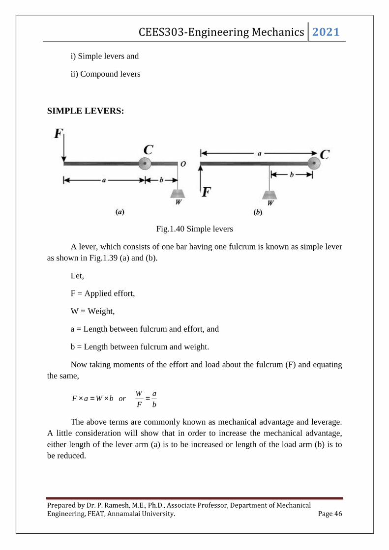
Fig.1.40 Simple levers
A lever, which consists of one bar having one fulcrum is known as simple leveras shown in Fig.1.39 (a) and (b).
Let,
F = Applied effort,
W = Weight,
a = Length between fulcrum and effort, and
b = Length between fulcrum and weight.
Now taking moments of the effort and load about the fulcrum (F) and equatingthe same,
b
a
F
WorbWaF
The above terms are commonly known as mechanical advantage and leverage.A little consideration will show that in order to increase the mechanical advantage,either length of the lever arm (a) is to be increased or length of the load arm (b) is tobe reduced.

CEES303-Engineering Mechanics 2021
Prepared by Dr. P. Ramesh, M.E., Ph.D., Associate Professor, Department of MechanicalEngineering, FEAT, Annamalai University. Page 47
COMPOUND LEVERS:
A lever which consists of a number of simple levers is known as a compoundlever, as shown in fig.1.40 (a) and (b).
Fig.1.41 Compound levers
A little consideration will show, that in a compound lever, the mechanicaladvantage (or leverage) is greater than that in a simple lever. Mathematically, leveragein a compound lever = Leverage of 1st lever × Leverage of 2nd lever × and so on. Theplatform weighing machine is an important example of a compound lever. Thismachine is used for weighing heavy loads such as trucks, wagons along with theircontents. On smaller scales, these machines are used in godowns and parcel offices oftransport companies for weighing consignment goods.
Problems:
SP1.9: A force of 20N is applied at an angle 70o to the edge of a door 1.2m wide asshown fig. Find the moment of the force about the hinge.
Fig.1.42 Force systems in a simple lever
1.2m
70o
20N
O A

CEES303-Engineering Mechanics 2021
Prepared by Dr. P. Ramesh, M.E., Ph.D., Associate Professor, Department of MechanicalEngineering, FEAT, Annamalai University. Page 48
Solution: method I,
We know that the moment of force about hinge, O
MO = d x F = 1.2 sin70o x 20 = 22.55 N-m
Method II: By component of force
We know that the moment of force about hinge, O
MO = r x (Fx+Fy) = r x Fx +r x Fy = 0 + 1.2 (20 sin70o)=22.55 N-m
The perpendicular distance from point O to A for the x component of force Fx
is zero.
r = 1.2m
70o
20N
O A
Fy=20sin70o
1.2m
70o
20N
O A
d=1.2sin70o

CEES303-Engineering Mechanics 2021
Prepared by Dr. P. Ramesh, M.E., Ph.D., Associate Professor, Department of MechanicalEngineering, FEAT, Annamalai University. Page 49
SP1.10: A force of 800 N acts on a bracket as shown in fig. Determine the moment ofthe force about B.
Fig.1.43 Force systems in a bracket
Solution:
The moment of force about B is obtained by forming the vector product
FrM ABB
Where, ABr is the vector drawn from B to A. The components of vector in
rectangular is
jmimrAB ).16.0().2.0( and
).60sin.60(cos800.sin.cos)800( jijiNF oo
).693.400 jiF
Therefore,
jijiFrM ABB 69340016.02.0
))(400(16.0))(693(2.0 ijjiM B
m-6.2020.646.138 NM B

CEES303-Engineering Mechanics 2021
Prepared by Dr. P. Ramesh, M.E., Ph.D., Associate Professor, Department of MechanicalEngineering, FEAT, Annamalai University. Page 50
SP1.11: Calculate the magnitude of the moment about the base point O of the 600Nforce in five different ways as shown in fig.1.43.
Fig.1.44 Force system in pole
Solution:
Method I: Determine the moment arm to the magnitude force F as 600N.
From the geometry of figure, d = a + b,
a = cos40o x 4 and b = sin40o x 2
d = 4cos40o + 2sin40o = 4.35m
The moment about O is clockwise and has the magnitude
MO = d x F = 4.35 x 600 = 2610 N-m
40o
40o
O
F=600N
da
b
b
2m
4m

CEES303-Engineering Mechanics 2021
Prepared by Dr. P. Ramesh, M.E., Ph.D., Associate Professor, Department of MechanicalEngineering, FEAT, Annamalai University. Page 51
Method II: Components of force
Fx= F x cos40o = 600cos40o = 460N
and Fy = F x sin40o = 600sin40o = 386N
By Varignon’s theorem, the moment of force becomes
MO = (Vertical distance x Fx) + (Horizontal distance x Fy)
MO = 4 x 460 +2 x 386 = 2610 N-m
Method III: By Law of transmissibility
Now move the force F (600N) without change of line of action to the intersectpoint of vertical axis from the point O is termed as Point B. The distance between thepoint O and B is measured vertically for the moment of force F1 (Fx) is d1 but thedistance between the point O and B horizontally for the moment of force F2 (Fy) iszero.
Therefore, d1 = 4+2tan40o = 5.68m and
The moment of force is
MO = d1 x Fx = 5.68 x 460 = 2610 N-m
40o
40o
40o
2m
4m
2m x tan40o

CEES303-Engineering Mechanics 2021
Prepared by Dr. P. Ramesh, M.E., Ph.D., Associate Professor, Department of MechanicalEngineering, FEAT, Annamalai University. Page 52
Method IV: By Law of transmissibility
Now move the force F (600N) without change of line of action to the intersectpoint of horizontal axis from the point O is termed as Point C. The distance betweenthe point O and C is measured vertically for the moment of force F1 (Fx) is zero but thedistance between the point O and C horizontally for the moment of force F2 (Fy) is d2.
Therefore, d2 = d1 x tan50o = 5.68 x tan50o = 6.77m
The moment of force is
MO = d2 x Fy = 6.77 x 386 = 2610 N-m
Method V: By vector expression
We know that, ).40sin.40(cos)..( jiFjrirFrM oomyxO
mNjijiM ooO -2610).40sin.40(cos600).4.2(
The negative sign indicates that the vector is in the negative z – direction. Themagnitude of the vector expression is MO = 2610 N-m.
40o
(90-40)= 50o
40o
2m5.68m
d2

CEES303-Engineering Mechanics 2021
Prepared by Dr. P. Ramesh, M.E., Ph.D., Associate Professor, Department of MechanicalEngineering, FEAT, Annamalai University. Page 53
SP1.12: A rectangular plate is supported by brackets at A and B and by a wire CD asshown in fig.1.44. Knowing that the tension in the wire is 200N, determine themoment about A of the force exerted by the wire on point C.
Fig.1.45 A rectangular plate supported by bracket
Solution:
The moment MA about A of the force F exerted by the wire on point C isobtained by forming the vector product
CDCAA FrM
Where, CAr is the vector drawn from A to C. The components of vector in
rectangular is
kmjimACrCA ).08.0(.0).3.0( and
CD
CDFF CDCD

CEES303-Engineering Mechanics 2021
Prepared by Dr. P. Ramesh, M.E., Ph.D., Associate Professor, Department of MechanicalEngineering, FEAT, Annamalai University. Page 54
m
kmjmimFCD 5.0
.32.0.24.0.3.0200
kjiFCD .128.96.120
Therefore,
kjikjiFrM CDCAA .128.96.12008.0.03.0
))(96(08.0))(120(08.0))(128(3.0))(96(3.0 jkikkijiM A
))(96(08.0))(120(08.0))(128(3.0))(96(3.0 ijjkM A
))(96(08.0))(120(08.0))(128(3.0))(96(3.0 ijjkM A
Alternative solution:
12896120
08.003.0
kji
FFF
zzyyxx
kji
M
zyx
ACACACA
kjiM A .8.288.28.68.7
COUPLES AND RESULTANT OF FORCE SYSTEM:
The two forces having equal in magnitude and unlike parallel line of action of
force is known as a couple. Consider the action of two equal and opposite forces F
and –F a distance‘d’ apart as shown in fig. These two forces cannot be combine into a
single force due to their sum of direction in everywhere is zero. The rotation is
produced by their effect. The combined moment of the two forces about an axis
normal to their plane and passing through any point such as O in their plane is the
couple MC. This couple has a magnitude (Scalar product)
FadaFM C )( or FdM C
The moment of a couple is also expressed by using vector algebra. The moment of
force F and –F is a cross product of distance from the point of moment (axis line about
O) and the line of action of force. The couple is written as
kjiM A .8.288.28.68.7

CEES303-Engineering Mechanics 2021
Prepared by Dr. P. Ramesh, M.E., Ph.D., Associate Professor, Department of MechanicalEngineering, FEAT, Annamalai University. Page 55
Fig.1.46 Couple
FrrFrFrM BABAC )()(
Where rA and rB are position vectors which run from point O to arbitrary points
A and B on the lines of action of F and –F respectively. Therefore, rrr BA then the couple written as
FrM C The couple of moment force not having the centre of moment about point O as
reference but it is free to rotate. The distance between the two unlike parallel vectors
is accounted to determine the couple of given forces. Fig. 1.45 (c) shows the couple
vector is counter clockwise by the lines of action of forces.
CLASSIFICATION OF COUPLES:
The couples are classified according to the direction of forces. They are
1. Clockwise couple and2. Counter clockwise couple
1. Clockwise couple:
A body is rotated by forces in the direction of clockwise is called clockwisecouple as shown in fig.1.46.

CEES303-Engineering Mechanics 2021
Prepared by Dr. P. Ramesh, M.E., Ph.D., Associate Professor, Department of MechanicalEngineering, FEAT, Annamalai University. Page 56
Fig.1.47 Clockwise couple2. Counter clockwise couple:
A body is rotated by forces in the direction counter clockwise then it is knownas counter clockwise couple as shown in fig.1.47.
Fig.1.48 Clockwise coupleCharacteristics of a couple:
A couple (whether clockwise or anticlockwise) has the followingcharacteristics:
1. The algebraic sum of the forces, constituting the couple, is zero.
2. The algebraic sum of the moments of the forces, constituting the couple,about any point is the same, and equal to the moment of the couple itself.
3. The couple cannot be balanced by a single force. But it can be balanced onlyby a couple of opposite sense.
4. Any number of coplanar couples can be reduced to a single couple, whosemagnitude will be equal to the algebraic sum of the moments of all the couples.
Resultant Couple Moment:
The sum of couple moment forces about the each couple moment force as afree vector and join together by the tail end of each couple is called as resultant couplemoment force. The resultant couple moment force is written as
CCn
CCCC MMMMMMR
........321
d
F
F
A B
d
F
F
A B

CEES303-Engineering Mechanics 2021
Prepared by Dr. P. Ramesh, M.E., Ph.D., Associate Professor, Department of MechanicalEngineering, FEAT, Annamalai University. Page 57
Problems:
SP1.13 A machine component of length 2.5 metres and height 1 metre is carriedupstairs by two men, who hold it by the front and back edges of its lower face. If themachine component is inclined at 30° to the horizontal and weighs 100 N, find howmuch of the weight each man supports?
Solution:
Given parameter: Length of machine component = 2.5 m; Height of thecomponent = 1 m; Inclination = 30° and weight of component = 100 N
Let, P = Weight supported by the man at A.
Q = Weight supported by the man at B.C = Point where the vertical line through the centre of gravity cuts the
lower face.
Fig.1.49Now join G (i.e., centre of gravity) with M (i.e., mid-point of AB) as shown in
Fig. 1.47.
From the geometry of the figure,
mBC
GM 5.02
1
2 and m
CDAM 25.1
2
5.2
2
Now, treat the vector force as couple moment say the force P and Weight of the
body W (P+Q=100). Therefore couple moment of force P is AEP which is equalsto the support carrying the load at point Q, such that the couple moment of Q is
EBQ
The AE is distance between couple moment of force P and body weight ‘W’.
Similarly the EB is distance between couple moment of force Q and bodyweight ‘W’.

CEES303-Engineering Mechanics 2021
Prepared by Dr. P. Ramesh, M.E., Ph.D., Associate Professor, Department of MechanicalEngineering, FEAT, Annamalai University. Page 58
The weight is shared by the two couple moment of force at point A and B bythe force P and Q respectively. Since the weight of the body W is P+Q.
100 QPW
The couple formed at both ends are equal and magnitude, therefore
EBQAEP ,
EBPAEP 100
oGMEMAMAE 30tan25.1
mAE 96.0)577.05.0(25.1
mAEABEB 54.196.05.2
EBPAEP 100
PPP 54.115454.1)100(96.0
15454.196.0 PP
1545.2 P
NP 6.615.2
154 Ans.
6.61100100 PQ
NQ 4.38 Ans.
SP1.14: Find the resultant couple moment forces for the given figure 1.50 as below.
Fig.1.50
400kN
250kN
250kN
500kN
500kN
400kN
7m
5m
1.5m

CEES303-Engineering Mechanics 2021
Prepared by Dr. P. Ramesh, M.E., Ph.D., Associate Professor, Department of MechanicalEngineering, FEAT, Annamalai University. Page 59
Solution:
Given parameter; the counter clockwise direction of couple moment force isconsidered as positive values.
Nm
M C
750
5005.11
Nm
M C
2000
40052
Nm
M C
1750
25073
We know that, the resultant of couple moment force is the sum of couple momentforce as
17502000750321 CCCCR MMMM
NmM CR 3000 ,
The negative sign implies the direction of couple moment force is in clockwisedirection.
SP1.15: Determine the distance of couple moment force on the lever has 400N asshown in fig.1.51.
Fig.1.51
F3=250 kN7m
F3=250 kNM3
CF2=400 kN
5mF2=400 kN M2
C
F1=500 kN
1.5m
F1=500 kN
M1C

CEES303-Engineering Mechanics 2021
Prepared by Dr. P. Ramesh, M.E., Ph.D., Associate Professor, Department of MechanicalEngineering, FEAT, Annamalai University. Page 60
Solution:
First considered the force has 200N to determine the couple moment force as
)0200())6060(0(200 jijmmmmiFrM CN
))(200)(120.0()0200()120.00( kjiji , ]0,0[ kijandjjii
k24 , The negative sign indicates the direction of couple moment force inclockwise.
Second considered the force has 400N to determine couple moment force about pointO, by treating as equivalent force system.
))400(0()260.0150.0(400 jijiFrM CN
Nm60)150.0(400 kk ]0,0[ kijandjjii
The negative sign indicates the direction of couple moment force in clockwise.
Therefore the total moment is CN
CN
C MMM 400200
Nm84Nm)6024( kkM C ,
Hence the total couple moment force of 400N is
)4000()60sin60cos( jijOCiOCFOCM ooC
kOCkOC )200()400(cos60(84 o
mmmOC 42042.0200
84

CEES303-Engineering Mechanics 2021
Prepared by Dr. P. Ramesh, M.E., Ph.D., Associate Professor, Department of MechanicalEngineering, FEAT, Annamalai University. Page 61
EQUILIBRIUM OF SYSTEM OF FORCE:
Equilibrium is a condition in static mechanics to keep the particle or rigid
bodies at rest. This is termed as the sum of all forces )( zyx FFFF or
resultant force R or the sum of moment force M or resultant moment force RM
is zero. In particle, the moment force and couple force is not present but only the
system of forces and resultant force were studied. This is due the assumption of size
and mass is negligible compared to the rigid bodies. The equilibrium condition for the
system of force satisfies the Newton’s second law of motion by writing the condition
as 0 maF . Therefore the acceleration of particle is zero (a=0) which means that
the velocity is constant or the move is remains at rest.
Example:
For a particle, 0)( zyx FFFF and 0R
For a rigid body, 0)( zyx FFFF , 0R , 0)( OM ,
0)( ORM and 0)()( RrMM ORA
FREE BODY DIAGRAM:
To form the equation of equilibrium, the various forces or moment or couple
must be considered for all the known and unknown forces which act on a particle or
rigid body. Without considered the real object of particle or rigid body, only the
number of all forces acts on the particle or rigid body is drawn by isolation and
separate from the surroundings which known as free body diagram (FBD). A system
may be a single body or a combination of connected bodies. The bodies may be rigid
or non-rigid. Before discuss about a free body diagram, the various types of supports
involved in a particle or rigid bodies are enumerated as below.

CEES303-Engineering Mechanics 2021
Prepared by Dr. P. Ramesh, M.E., Ph.D., Associate Professor, Department of MechanicalEngineering, FEAT, Annamalai University. Page 62
Table 1.1: Types of supports to describe system of force.
Sl.No.
Types of supports Free BodyDiagram
Description
COPLANAR SYSTEM
1.
Springs:
*The springs considered asun-deformed at initialdistance as lO is used tosupport a particle.* The length of the linearlyelastic spring will change inthe direction of the force, Fact on a particle.
)( OllkF . Where l is achange in length by forceand k is spring constant orstiffness.
2.
Cables and Pulleys: * A cable can support onlya tension or pulling force.
3.
Smooth contact: * An object rests on asmooth surface then thesurface will exert a force onthe object that is normal tothe surface at the point ofcontact.
4.
Flexible cable, belt chain orrope: Weight of cablenegligible
* Force exerted by aflexible cable is always atension away from the bodyin the direction of the cable.
5.
Flexible cable, belt chain orrope: Weight of cable notnegligible
* Force exerted by aflexible cable is always atension away from the bodyin the direction of the cable.
TT
F

CEES303-Engineering Mechanics 2021
Prepared by Dr. P. Ramesh, M.E., Ph.D., Associate Professor, Department of MechanicalEngineering, FEAT, Annamalai University. Page 63
6.
Rough surface:
* Rough surfaces arecapable of supporting atangential component F(Frictional force) as well asa normal component N ofthe resultant contact forceR.
7.
Roller support: type1* Roller, rocker or ballsupport transmits acompressive force normalto the supporting surface.
8.
Roller support: type2 * Roller, rocker or ballsupport transmits acompressive force normalto the supporting surface.
9.
Freely sliding guide: type1 * Collar or slider free tomove along smooth guides;can support force normal toguide only.
10.
Freely sliding guide: type2* Collar or slider free tomove along smooth guides;can support force normal toguide only.
11.
Pin connection: Not free toturn
* A pin not free to turn alsosupports a couple M withthe force components Fx andFy or a magnitude F anddirection.
12.
Pin connection: Free to turn
* A freely hinged pinconnection is capable ofsupporting a force in anydirection in the planenormal to the pin axis.Hence the component offorce along horizontal Fx
and vertical Fy or amagnitude of force F anddirection.
N
N
N
N
CEES303-Engineering Mechanics 2021
Prepared by Dr. P. Ramesh, M.E., Ph.D., Associate Professor, Department of MechanicalEngineering, FEAT, Annamalai University. Page 64
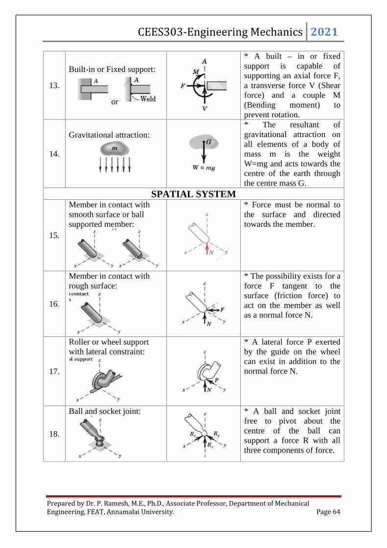
13.
Built-in or Fixed support:
or
* A built – in or fixedsupport is capable ofsupporting an axial force F,a transverse force V (Shearforce) and a couple M(Bending moment) toprevent rotation.
14.
Gravitational attraction:* The resultant ofgravitational attraction onall elements of a body ofmass m is the weightW=mg and acts towards thecentre of the earth throughthe centre mass G.
SPATIAL SYSTEM
15.
Member in contact withsmooth surface or ballsupported member:
* Force must be normal tothe surface and directedtowards the member.
16.
Member in contact withrough surface:
* The possibility exists for aforce F tangent to thesurface (friction force) toact on the member as wellas a normal force N.
17.
Roller or wheel supportwith lateral constraint:
* A lateral force P exertedby the guide on the wheelcan exist in addition to thenormal force N.
18.
Ball and socket joint: * A ball and socket jointfree to pivot about thecentre of the ball cansupport a force R with allthree components of force.

CEES303-Engineering Mechanics 2021
Prepared by Dr. P. Ramesh, M.E., Ph.D., Associate Professor, Department of MechanicalEngineering, FEAT, Annamalai University. Page 65
19.
Fixed connection:Embedded or welded
* In addition to threecomponents of force a fixedconnection can support acouple moment Mrepresented by its threecomponents.
20.
Thrust bearing support:* Thrust bearing is capableof supporting axial force Ry
as well as radial forces Rx
and Rz. Couples Mx and Mz
must in some cases beassumed zero in order toprovide staticaldeterminacy.
Procedure to draw Free Body Diagram (FBD):
The isolation of system which has number of system of force in a particle or
rigid bodies is discussed in different steps as follows;
1. First identify the minimum number of unknown force in a system and then
isolates this system to draw a free body diagram which means the various
forces acting in that systems.
2. Second the connected system to first steps is isolated and determines the
unknowns and so on.
3. Similarly the remaining steps are followed to determine the number of
unknowns.

CEES303-Engineering Mechanics 2021
Prepared by Dr. P. Ramesh, M.E., Ph.D., Associate Professor, Department of MechanicalEngineering, FEAT, Annamalai University. Page 66
Table 1.2: Free body diagrams for mechanisms and structures
Sl.No.
Mechanical Systems Free Body Diagram
1. Plane Truss: Weight of truss assumed negligiblecompared with P
2. Cantilever beam:
3. Beam: Smooth surface contact at A.
4. Frames and Machines: Rigid system ofinterconnected bodies analysed as a single unit.
Equations of Equilibrium of Coplanar Systems and Spatial
Systems:
In statics, the most of the problems are treated in equilibrium condition to
explore the known and unknown forces act on the particle or rigid body system. The
sum of all forces on the particle or the rigid body termed as resultant force is to be
zero which means equilibrium in state. Therefore the resultant force R and resultant
moment force M are both zero for the equilibrium body. The equations of equilibrium

CEES303-Engineering Mechanics 2021
Prepared by Dr. P. Ramesh, M.E., Ph.D., Associate Professor, Department of MechanicalEngineering, FEAT, Annamalai University. Page 67
for the different system of force are listed in the table 1.3. The general equations of
equilibrium as
0 FR and 0 MM R
Table 1.3: Types of force system in equilibrium conditions.
Sl.No. Types of force system Free Body
Diagram Equilibrium equations
LINEAR SYSTEM
1. Collinear:0 xF
COPLANAR SYSTEM
2. Concurrent at a point:0 xF , 0 yF
3. Parallel:
0 xF and 0 zM
4. Non concurrent:
0 xF , 0 yF and
0 zM
SPATIAL SYSTEM
5. Concurrent at a point:
0 xF , 0 yF and
0 zF
6. Concurrent with a line:
0 xF , 0 yF , 0 zF ,
0 yM and 0 zM
7. Parallel:
0 xF , 0 yM and
0 zM
8. Non concurrent:
0 xF , 0 yF , 0 zF ,
0 xM , 0 yM and
0 zM
CEES303-Engineering Mechanics 2021
Prepared by Dr. P. Ramesh, M.E., Ph.D., Associate Professor, Department of MechanicalEngineering, FEAT, Annamalai University. Page 68
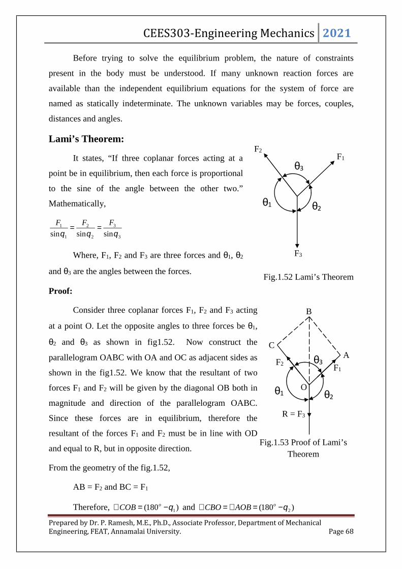
Fig.1.52 Lami’s Theorem
Fig.1.53 Proof of Lami’sTheorem
Before trying to solve the equilibrium problem, the nature of constraints
present in the body must be understood. If many unknown reaction forces are
available than the independent equilibrium equations for the system of force are
named as statically indeterminate. The unknown variables may be forces, couples,
distances and angles.
Lami’s Theorem:
It states, “If three coplanar forces acting at a
point be in equilibrium, then each force is proportional
to the sine of the angle between the other two.”
Mathematically,
3
3
2
2
1
1
sinsinsin FFF
Where, F1, F2 and F3 are three forces and 1, 2
and 3 are the angles between the forces.
Proof:
Consider three coplanar forces F1, F2 and F3 acting
at a point O. Let the opposite angles to three forces be 1,
2 and 3 as shown in fig1.52. Now construct the
parallelogram OABC with OA and OC as adjacent sides as
shown in the fig1.52. We know that the resultant of two
forces F1 and F2 will be given by the diagonal OB both in
magnitude and direction of the parallelogram OABC.
Since these forces are in equilibrium, therefore the
resultant of the forces F1 and F2 must be in line with OD
and equal to R, but in opposite direction.
From the geometry of the fig.1.52,
AB = F2 and BC = F1
Therefore, )180( 1 oCOB and )180( 2 oAOBCBO
1
F1
F2
F3
2
3
1
F1F2
R = F3
2
3
O
CA
B

CEES303-Engineering Mechanics 2021
Prepared by Dr. P. Ramesh, M.E., Ph.D., Associate Professor, Department of MechanicalEngineering, FEAT, Annamalai University. Page 69
)(180 CBOCOBBCO o
2121 180180180)180()180(180 ooooooBCO
oBCO 18021
But, o360321
Now substitute 321 360 o in oBCO 18021 then
33 180180360 oooBCO
Considered the triangle COB, then sine law as
BCO
OB
COB
CB
CBO
OC
sinsinsin
)180sin()180sin()180sin( 312
ooo
OBCBOC
Here, CB = OA and OB = OD
)sin()sin()sin( 312 ODOAOC
)sin()sin()sin( 3
3
1
1
2
2
FFF
Problems:
SP1.16: In a ship unloading a 3500 N automobile is supported by a cable. A rope is
tied to the cable at A and pulled in order to centre the automobile over its intended
position as shown in fig1.53. The angle between the cable and vertical is 2o while the
angle between the rope and the horizontal is 30o. Determine the tension in the rope.
Fig.1.54

CEES303-Engineering Mechanics 2021
Prepared by Dr. P. Ramesh, M.E., Ph.D., Associate Professor, Department of MechanicalEngineering, FEAT, Annamalai University. Page 70
Solution:
As per Lami’s theorem,
)30290sin()2180sin()3090sin( oooooAC
ooAB WTT
)122sin(
3500
)178sin()60sin( ooAC
oAB TT
)122sin(
3500
)60sin( ooABT
)122sin(
)60sin(3500o
o
ABT
NTAB 3575
)122sin(
3500
)178sin( ooACT
,)122sin(
)178sin(3500o
o
ACT
NTAC 144
SP1.17: Find the tension in cable BA and BC necessary to support the 100kg cylinder
as shown in fig.1.54
Fig.1.55
Solution:
The angle of force vector FAB from the geometry is
o87.364
3tan 1
TAB
TAC
W=3500N
2o
30o
Free body diagram

CEES303-Engineering Mechanics 2021
Prepared by Dr. P. Ramesh, M.E., Ph.D., Associate Professor, Department of MechanicalEngineering, FEAT, Annamalai University. Page 71
Free body diagram;
By law of sine or Lami’s theorem, we know that,
)4587.36180sin()87.3690sin()4590sin(
BDBCBA FFF
)4587.36180sin()87.3690sin()4590sin(
WFF BCBA
)4587.36180sin(
100
)87.3690sin(
kgFBC
NkgFBC 53.79389.80989.0
999.79
)4587.36180sin(
)87.3690sin(100
NkgFBA 42.70150.71989.0
71.70
)4587.36180sin(
)4590sin(100
NkgWFBD 981100
NkgFBC 53.79389.80
NkgFBA 42.70150.71
SP1.18: Find the required length of cord AC have the 8 kg lamp is suspended in the
position as shown in fig.1.55. The un-deformed length of spring AB is 0.4m and the
stiffness of spring is 300 N/m.
A
B
D
C
45o
90o
90o
36.87o
180o-45o-36.87o
W=100kg

CEES303-Engineering Mechanics 2021
Prepared by Dr. P. Ramesh, M.E., Ph.D., Associate Professor, Department of MechanicalEngineering, FEAT, Annamalai University. Page 72
Fig.1.56
Solution:
Free body diagram,
By law of sine or Lami’s theorem, we know that,
)30180sin()3090sin()90sin(
WFF ABAC
)30180sin(
8
)3090sin()90sin(
ABAC FF
)30180sin(
8
)3090sin(
ABF
,
NkgFAB 97.13586.135.0
93.6
)30180sin(
)3090sin(8
)30180sin(
8
)90sin( ACF
FAC
W= 10kg
FABA
30o

CEES303-Engineering Mechanics 2021
Prepared by Dr. P. Ramesh, M.E., Ph.D., Associate Professor, Department of MechanicalEngineering, FEAT, Annamalai University. Page 73
NkgFAC 96.156165.0
8
)30180sin(
)90sin(8
The force in the spring is find by the given data of spring constant and changein dimension, from this find the deformed position of spring as
300kFAB
mk
FAB 45.0300
97.135
Since the total deformed length of spring is
mll ABAB 85.045.04.0'
The horizontal distance between the point C and B is 2m as given in this
problem, This is the sum of the distance AB and horizontal distance AC is cos AC.
85.030cos)(cos2 ' oAB AClABACm
mAC 328.1866.0
15.1
30cos
85.02
mAC 328.1
SP1.19: Find the magnitude of the force C and T which along with the other threeforces act on the bridge truss joint as shown in fig.1.56.
Fig.1.57
Solution:
Case1: about x and y axes

CEES303-Engineering Mechanics 2021
Prepared by Dr. P. Ramesh, M.E., Ph.D., Associate Professor, Department of MechanicalEngineering, FEAT, Annamalai University. Page 74
Free body diagram;
0 xF , 01620sin40cos8 oo CT
8342.0766.0 CT ----- (1)
0 yF , 0320cos40sin oo CT
3940.0643.0 CT ----- (2)
The solution of equation is
kNT 09.9 and kNC 03.3
Case 2: about x’ and y’ axes
Free body diagram;
0' xF , 070cos50cos340cos1640cos8 oooo CT
057.8342.0 CT ----- (3)
0' yF , 040sin1640sin850sin370sin ooooC
844.2939.0 C ----- (4)
C=3.03 kN and T=9.1 kN
x’
8 kN
3 kN
T
C
16 kN 40o
20o
y'
x8 kN
3 kN
T
C
16 kN 40o
20o
y

CEES303-Engineering Mechanics 2021
Prepared by Dr. P. Ramesh, M.E., Ph.D., Associate Professor, Department of MechanicalEngineering, FEAT, Annamalai University. Page 75
Case 3: using vector force by unit vectors i and j in the x and y direction
0 F , 016)70sin70cos(3)40sin40(cos8 ijiCjjiTi oooo
Equating the coefficients of the unit vectors i and j terms to zero then
01670cos40cos8 oo CTi ----- (5)
070sin340sin oo CTj --- (6)
The solution of equation is
kNT 09.9 and kNC 03.3
SP1.20: Find the tension T in the cable which supports the 1000 N load with the
pulley arrangement as shown in fig.1.57. Each pulley is free to rotate about its bearing
and the weights of all parts are small compared with the load. Also determine the
magnitude of the total force on the bearing of pulley C.
Fig.1.58
Solution:
Free body diagram;

CEES303-Engineering Mechanics 2021
Prepared by Dr. P. Ramesh, M.E., Ph.D., Associate Professor, Department of MechanicalEngineering, FEAT, Annamalai University. Page 76
Now start to solve the problem from known values that is the pulley A has carryingthe load W,
0 AyF , 010002 AT
NTA 500
Pulley B,
0 ByF , 02 AB TT , 5002 BT
250BT
Pulley C,
0 CxF , 030cos x
oB FT , 030cos250 x
o F , NFx 217
0 CyF , 030sin yB
oB FTT , 025030sin250 y
o F , NFy 125
The magnitude of the total force on bearing of pulley C as
NFFF yx 250125217 2222
SP1.21: Find the magnitude T of the tension in the supporting cable and the
magnitude of the force on the pin at A for the jib crane as shown in fig.1.58. The beam
AB is a standard 0.5m I beam with a mass of 95 kg per meter of length.
TA
TB TB
W
TA TA
A B
TB
TB
Fx
Fy
C
30o

CEES303-Engineering Mechanics 2021
Prepared by Dr. P. Ramesh, M.E., Ph.D., Associate Professor, Department of MechanicalEngineering, FEAT, Annamalai University. Page 77
Fig.1.59
Solution:
Free body diagram
Taking moment about A,
0 AM , 066.4)12.05.2(10)12.05.15()25sin)(12.05()25cos(25.0 oo TT
kNT 61.19
Equating the sums of forces in the x and y directions to zero, then
0 xF , 025cos61.19 oxA , kNAx 77.17
0 yF , 066.425sin61.19 oyA , kNAy 37.6
The magnitude value at end A,
kNAAA yx 88.1837.677.17 2222
SP1.22: A 200 N force is applied to the handle of the hoist in the direction as shownin fig 1.59. The bearing A supports the thrust (force in the direction of the shaft axis)while bearing B supports only radial load (Load normal the shat axis). Find the massm which can be supported and the total radial force exerted on the shaft by eachbearing. Assume neither bearing to be capable of supporting a moment about a linenormal to the shaft axis.

CEES303-Engineering Mechanics 2021
Prepared by Dr. P. Ramesh, M.E., Ph.D., Associate Professor, Department of MechanicalEngineering, FEAT, Annamalai University. Page 78
Fig.1.60Solution:Free body diagram,
Taking moment about O, from the x-y projection
0 OM , 0)2.173(250)81.9(100 m , kgm 1.44
Taking moment about A, from the x-Z projection
0 AM , 0)7.70(250)7.70(175150 xB , NBx 4.35
0 xF , 07.704.35 xA , 4.35xA
Taking moment about A, from the y-Z projection
0 AM , 0)81.9)(1.44(250)2.173(175150 yB , NB y 520
0 yF , 0)81.9)(1.44(2.173520 yA , NAy 8.86
0 zF , NAz 7.70
The total radial forces on the bearing become
NAAA yxr 5.938.864.35 2222

CEES303-Engineering Mechanics 2021
Prepared by Dr. P. Ramesh, M.E., Ph.D., Associate Professor, Department of MechanicalEngineering, FEAT, Annamalai University. Page 79
NBBB yxr 5215204.35 2222
SP1.23: Find the tension in each cord used to support the 100 kg crate as shown infig.1.60.
Fig. 1.61
Solution:
Free body diagram,
iFF BB
kFjFiFkFjFiFF CCCo
Co
Co
CC 5.0707.05.060cos135cos120cos
kFjFiFkji
FF DDDDD 667.066.033.022)1(
221222
NkW )981()81.9(100
0 F , 0 WFFF DCB
0981667.066.033.05.0707.05.0 kkFjFiFkFjFiFiF DDDCCCB
Equating the unit vectors i, j and k equal to zero, then
0 xF , 033.05.0 DCB FFF ------- (1)

CEES303-Engineering Mechanics 2021
Prepared by Dr. P. Ramesh, M.E., Ph.D., Associate Professor, Department of MechanicalEngineering, FEAT, Annamalai University. Page 80
0 yF , 0667.0707.0 DC FF ------- (2)
0 zF , 0981667.05.0 DC FF ------ (3)
Solving the above equations 1, 2 and 3, then
NFC 813
NFD 862
NFB 694
STATIC INDETERMINACY:
A rigid body or rigid combination of elements treated as a single body, whichpossesses more external supports or constraints than are necessary to maintain anequilibrium position is called static indeterminacy.
Supports which can be removed without destroying the equilibrium conditionof the body are said to be redundant. The number of redundant supporting elementspresent corresponds to the degree of statically indeterminacy and equals the totalnumber of unknown external forces, minus the number of available independentequations of equilibrium.
Coplanar system
Spatial systema) Statically determinate b) Statically indeterminate
Fig.1.62 Constraints in a body

Lecture Notes
UNIT – 2
pfpf
2021
Prepared by
Dr. P. Ramesh, M.E., Ph.D.,
Associate Professor
Department of Mechanical Engineering
Faculty of Engineering and Technology
Annamalai UniversitySep-2021
CEES303-EngineeringMechanics

CEES303-Engineering Mechanics 2021
Prepared by Dr. P. Ramesh, M.E., Ph.D., Associate Professor, Department of MechanicalEngineering, FEAT, Annamalai University. Page 2
Unit - 2
Basic Structural Analysis covering, Equilibrium in threedimensions; Method of Sections; Method of Joints; How todetermine if a member is in tension or compression; SimpleTrusses; Zero force members; Beams & types of beams; Frames &Machines Centroid and Centre of Gravity covering, Centroid ofsimple figures from first principle, centroid of composite sections;Centre of Gravity and its implications; Area moment of inertia-Definition, Moment of inertia of plane sections from first principles,Theorems of moment of inertia, Moment of inertia of standardsections and composite sections; Mass moment inertia of circularplate, Cylinder, Cone, Sphere, Hook.
Reference for the preparation of course material:
1. F. P. Beer and E. R. Johnston (2011), Vector Mechanics for Engineers,Vol I - Statics, Vol II, – Dynamics, 9th Ed, Tata McGraw Hill.
2. Khurmi R.S. (2010), Engineering Mechanics, S. Chand & Co.3. J.L. Meriam and L. G. Kraige, Engineering Mechanics –Statics, volume I,
Seventh edition, John Wiley & Sons, Inc.
TEXT BOOKS1. Irving H. Shames (2006), Engineering Mechanics, 4th Edition, Prentice Hall2. F. P. Beer and E. R. Johnston (2011), Vector Mechanics for Engineers, Vol I -
Statics, Vol II, – Dynamics, 9th Ed, Tata McGraw Hill
REFERENCES1. R. C. Hibbler (2006), Engineering Mechanics: Principles of Statics and Dynamics,
Pearson Press.2. Khurmi R.S. (2010), Engineering Mechanics, S. Chand & Co.

CEES303-Engineering Mechanics 2021
Prepared by Dr. P. Ramesh, M.E., Ph.D., Associate Professor, Department of MechanicalEngineering, FEAT, Annamalai University. Page 3
Unit - 2
STRUCTURE AND STABILITY OF MECHANICS
The Engineering Mechanics deals with various forces like internal and external
force in different bodies. In the previous section the system of forces were studied to
examine the external force acting in a particle or rigid bodies on a smooth surfaces. The
internal forces of structure in which the self-weight is neglected is considered to
examine in the field of engineering that is forces of action and reaction between the
connected members. An engineering structure is any connected system of members
built to support or transfer forces and to safely withstand the loads applied to it. To
determine the forces internal to an engineering structure, this must dismember the
structure and analyse separate free-body diagrams of individual members or
combinations of members. This analysis requires careful application of Newton's third
law, which states that each action is accompanied by an equal and opposite reaction.
Statically determinate structure is considered to determine all unknown reactions
with adequate number of equilibrium equations. In this section the internal forces acting
in several types of structures to be analyse – namely trusses, beams and frames and
machines.
HOW TO DETERMINE IF A MEMBER IS IN TENSION ORCOMPRESSION;
The simple truss structure as shown in fig.2.1 is considered to demonstrate
whether the member of truss is in tension or compression. In previous chapter, the force
on various supports were studied and drawn the free body diagram to states that the
system is in equilibrium condition to determine the unknown external forces. Whereas
this section discuss about the unknown forces of both internal and external forces.
Fig.2.2 shows that the free body diagram of simple truss structure with unknown
external force at the ends of supports. The unknown internal forces on members AB,

CEES303-Engineering Mechanics 2021
Prepared by Dr. P. Ramesh, M.E., Ph.D., Associate Professor, Department of MechanicalEngineering, FEAT, Annamalai University. Page 4
BC, CD, DE, EF, FG, GH, HA, BH, CG and DF are to be determined by the method of
joints or the method of section. Before that the members to be specified the direction of
force acted on each joint by the force of tension or compression in members.
Fig.2.1 Simple truss element
Fig.2.2 Free body diagram of simple truss
a) Moment force atend E
b)Compressiveforce in a member
c) Tension in amember
d) Internal forcedirection
Fig.2.3 Forces at supports and members
W1W2
W3
H FG
W1W2
W3
A EB C DRx,A
Ry,ARy,E
F
W3
ED
Ry,E
Fe
Fe
Fi
Fi
Fe
Fe
Fi
Fi
F
E
Ry,E

CEES303-Engineering Mechanics 2021
Prepared by Dr. P. Ramesh, M.E., Ph.D., Associate Professor, Department of MechanicalEngineering, FEAT, Annamalai University. Page 5
The reaction force at end E takes moment about A and have rotation as shown in
fig.2.3 (a). The moment force by reaction force at end E applies the compressive force
on member EF. Therefore the compressive force by external (Fe) creates an internal
force (Fi) which towards the joint of member as shown in fig.2.3 (b). However the
member EF has compression due the moment force in counter clockwise at end E as
shown in fig.2.3 (c).
Fig.2.4 Representation of tension or compression force in a members
The moment force at end E by taking moment about A generates the compression
in a member EF. This direction is noted as towards the joint E and F. Similarly the
moment force at end A by taking moment about B takes the compression in a member
AH and denote towards the joint A and H. The compression of member AH and EF also
implies into the member HG and FG therefor it denoted towards the joint H, G and F
accordingly. The member AB is pulled by the load at joint B as W1. This will generates
tension in a member AB and therefore the direction is denoted away from the joint.
Similarly the member BC, CD, DE, BH, CH, CG, CF and DF have tension in a member
by the load W1, W2 and W3 accordingly. The tension and compression in a members of
simple truss structure is shown fig.2.4.
H FG
W1W2
W3
A EB C DRx,A
Ry,ARy,E
FC
FTFTFTFT
FT
FT FT
FT
FT
FCFC
FC

CEES303-Engineering Mechanics 2021
Prepared by Dr. P. Ramesh, M.E., Ph.D., Associate Professor, Department of MechanicalEngineering, FEAT, Annamalai University. Page 6
SIMPLE TRUSSES:
The basic element of a plane truss is the triangle. Three bars joined by pins at
their ends, Fig.2.5 (a), constitute a rigid frame. The term rigid is used to mean non
collapsible and also to mean that deformation of the members due to induced internal
strains is negligible. On the other hand, four or more bars pin-jointed to form a polygon
of as many sides constitute a non-rigid frame. We can make the non-rigid frame in
fig.2.5 (b) rigid, or stable, by adding a diagonal bar joining A and D or Band C and
thereby forming two triangles. We can extend the structure by adding additional units
of two end-connected bars, such as DE and CE or AF and DF, Fig.2.5(c), which are
pinned to two fixed joints. In this way the entire structure will remain rigid.
Structures built from a basic triangle in the manner described are known as
simple trusses. When more members are present than are needed to prevent collapse,
the truss is statically indeterminate. A statically indeterminate truss cannot be analysed
by the equations of equilibrium alone. Additional members or supports which are not
necessary for maintaining the equilibrium configuration are called redundant.
a) Three members b) Four members c) Nine members
Fig.2.5 Simple truss members
To design a truss we must first determine the forces in the various members and
then select appropriate sizes and structural shapes to withstand the forces. Several
assumptions are made in the force analysis of simple trusses. First, we assume all
members to be two-force members. A two-force member is one in equilibrium under
the action of two forces only, as defined in general terms with Fig. 2.6. Each member
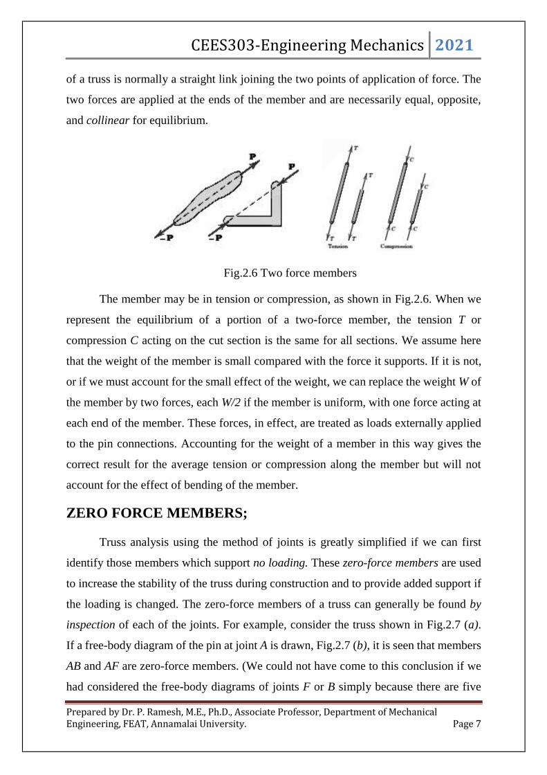
CEES303-Engineering Mechanics 2021
Prepared by Dr. P. Ramesh, M.E., Ph.D., Associate Professor, Department of MechanicalEngineering, FEAT, Annamalai University. Page 7
of a truss is normally a straight link joining the two points of application of force. The
two forces are applied at the ends of the member and are necessarily equal, opposite,
and collinear for equilibrium.
Fig.2.6 Two force members
The member may be in tension or compression, as shown in Fig.2.6. When we
represent the equilibrium of a portion of a two-force member, the tension T or
compression C acting on the cut section is the same for all sections. We assume here
that the weight of the member is small compared with the force it supports. If it is not,
or if we must account for the small effect of the weight, we can replace the weight W of
the member by two forces, each W/2 if the member is uniform, with one force acting at
each end of the member. These forces, in effect, are treated as loads externally applied
to the pin connections. Accounting for the weight of a member in this way gives the
correct result for the average tension or compression along the member but will not
account for the effect of bending of the member.
ZERO FORCE MEMBERS;
Truss analysis using the method of joints is greatly simplified if we can first
identify those members which support no loading. These zero-force members are used
to increase the stability of the truss during construction and to provide added support if
the loading is changed. The zero-force members of a truss can generally be found by
inspection of each of the joints. For example, consider the truss shown in Fig.2.7 (a).
If a free-body diagram of the pin at joint A is drawn, Fig.2.7 (b), it is seen that members
AB and AF are zero-force members. (We could not have come to this conclusion if we
had considered the free-body diagrams of joints F or B simply because there are five

CEES303-Engineering Mechanics 2021
Prepared by Dr. P. Ramesh, M.E., Ph.D., Associate Professor, Department of MechanicalEngineering, FEAT, Annamalai University. Page 8
unknowns at each of these joints.) In a similar manner, consider the free-body diagram
of joint D, Fig.2.7 (c). Here again it is seen that DC and DE are zero-force members.
From these observations, we can conclude that if only two non-collinear members form
a truss joint and no external load or support reaction is applied to the joint, the two
members must be zero-force members. The load on the truss in Fig.2.7 (a) is therefore
supported by only five members as shown in Fig.2.7 (d).
Fig. 2.7 Truss and zero force members
Now consider the truss shown in Fig.2.8 (a). The free-body diagram of the pin
at joint D is shown in Fig.2.8 (b). By orienting the y axis along members DC and DE
and the x axis along member DA, it is seen that DA is a zero-force member. Note that
this is also the case for member CA, Fig.2.8 (c). In general then, if three members form
a truss joint for which two of the members are collinear, the third member is a zero-

CEES303-Engineering Mechanics 2021
Prepared by Dr. P. Ramesh, M.E., Ph.D., Associate Professor, Department of MechanicalEngineering, FEAT, Annamalai University. Page 9
force member provided no external force or support reaction has a component that acts
along this member. The truss shown in Fig.2.8 (d) is therefore suitable for supporting
the load P.
Fig. 2.8 Truss and their forces
INTERNAL AND EXTERNAL REDUNDANCY:
If a plane truss has more external supports than are necessary to ensure a stable
equilibrium conditions, then the truss is said to be statically indeterminate. The extra
supports in that plane truss constitute external redundancy force.

CEES303-Engineering Mechanics 2021
Prepared by Dr. P. Ramesh, M.E., Ph.D., Associate Professor, Department of MechanicalEngineering, FEAT, Annamalai University. Page 10
If a truss has more internal members than are necessary to prevent collapse when
the truss is removed from its supports then the extra members constitute internal
redundancy and the truss is said to be statically indeterminate.
For a truss which is statically determinate externally there is a definite relation
between the number of its members and the number of its joints necessary for internal
stability without redundancy. The equilibrium of each truss joint is specified by two
scalar force equations such that all joints have the equation as 2J.
The entire truss is composed of ‘m’ number of two force members (m is a tension
or compression forces) and having the maximum of three unknown support reaction
which equals the twice of joint in a truss. Then the relation is stated as statically
determinate as
Jm 23
If Jm 23 then the truss is statically indeterminate which means more
number of members present in that truss.
If Jm 23 then the truss is not sufficient to hold the stable position thereby
the truss tends to collapse under load.
THE METHOD OF JOINTS:
In order to analyse or design a truss, it is necessary to determine the force in each
of its members. One way to do this is to use the method of joints. This method is based
on the fact that if the entire truss is in equilibrium, then each of its joints is also in
equilibrium. Therefore, if the free-body diagram of each joint is drawn, the force
equilibrium equations can then be used to obtain the member forces acting on each joint.
Since the members of a plane truss are straight two-force members lying in a single
plane, each joint is subjected to a force system that is coplanar and concurrent. As a
result, only 0 xF and 0 yF need to be satisfied for equilibrium.

CEES303-Engineering Mechanics 2021
Prepared by Dr. P. Ramesh, M.E., Ph.D., Associate Professor, Department of MechanicalEngineering, FEAT, Annamalai University. Page 11
For example, consider the pin at joint B of the truss in Fig.2.9 (a). Three forces
act on the pin, namely, the 500-N force and the forces exerted by members BA and BC.
The free-body diagram of the pin is shown in Fig.2.9 (b). Here, FBA is “pulling” on the
pin, which means that member BA is in tension; whereas FBC is “pushing” on the pin,
and consequently member BC is in compression. These effects are clearly demonstrated
by isolating the joint with small segments of the member connected to the pin, Fig.2.9
(c). The pushing or pulling on these small segments indicates the effect of the member
being either in compression or tension.
Fig.2.9 Method of joints
When using the method of joints, always start at a joint having at least one known
force and at most two unknown forces, as in Fig.2.9 (b). In this way, application of
0 xF and 0 yF yields two algebraic equations which can be solved for the two
unknowns. When applying these equations, the correct sense of an unknown member
force can be determined using one of two possible methods.
Method 1: The correct sense of direction of an unknown member force can, in many
cases, be determined “by inspection.” For example, FBC in fig.2.9 (b) must push on the
pin (compression) since its horizontal component, FBC sin 45o, must balance the 500 N

CEES303-Engineering Mechanics 2021
Prepared by Dr. P. Ramesh, M.E., Ph.D., Associate Professor, Department of MechanicalEngineering, FEAT, Annamalai University. Page 12
force ( 0 xF ). Likewise, FAB is a tensile force since it balances the vertical
component, FBC cos45o ( 0 yF ). In more complicated cases, the sense of an unknown
member force can be assumed; then, after applying the equilibrium equations, the
assumed sense can be verified from the numerical results. A positive answer indicates
that the sense is correct, whereas a negative answer indicates that the sense shown on
the free-body diagram must be reversed.
Method 2: Always assume the unknown member forces acting on the joint’s free-body
diagram to be in tension; i.e., the forces “pull” on the pin. If this is done, then numerical
solution of the equilibrium equations will yield positive scalars for members in tension
and negative scalars for members in compression. Once an unknown member force is
found, use its correct magnitude and sense (T or C) on subsequent joint free-body
diagrams.
Procedure using the method of joints:
1) Draw the free-body diagram of a joint having at least one known force and at
most two unknown forces. (If this joint is at one of the supports, then it may be
necessary first to calculate the external reactions at the support.)
2) Use one of the two methods described above for establishing the sense of an
unknown force.
3) Orient the x and y axes such that the forces on the free-body diagram can be
easily resolved into their x and y components and then apply the two force
equilibrium equations 0 xF and 0 yF . Solve for the two unknown
member forces and verify their correct sense.
4) Using the calculated results, continue to analyse each of the other joints.
Remember that a member in compression “pushes” on the joint and a member in
tension “pulls” on the joint. Also, be sure to choose a joint having at most two
unknowns and at least one known force.

CEES303-Engineering Mechanics 2021
Prepared by Dr. P. Ramesh, M.E., Ph.D., Associate Professor, Department of MechanicalEngineering, FEAT, Annamalai University. Page 13
Problems:
SP2.1: Determine the force in each member of the truss shown in Fig.2.10. Indicate
whether the members are in tension or compression.
Fig.2.10 Truss
Solution:
A free body diagram of the entire truss is draw as below
Applying the equations of equilibrium as
oFx , 0600 xC ,
Cx = 600N
0 CM , 0)4(600)3(400)6( yA
Ay=600N
oFy , 0400600 yC ,

CEES303-Engineering Mechanics 2021
Prepared by Dr. P. Ramesh, M.E., Ph.D., Associate Professor, Department of MechanicalEngineering, FEAT, Annamalai University. Page 14
Cy = 200N
The analysis can now start at either joint A or C. The choice is arbitrary since
there are one known and two unknown member forces acting on the pin at each of these
joints.
From the free-body diagram of joint A, FAB is assumed to be compressive and
FAD is tensile. Applying the equations of equilibrium, then
oFy , 05
4600 ABF ,
FAB = 750N (C)
oFx , 05
3 ABAD FF , 0)750(
5
3 ADF
FAD = 450N (T)
From the free-body diagram of joint D and the result of FAD, then
oFx , 06005
3 DBAD FF , 0600
5
3450 DBF
FDB = -250N (T)
oFy , 05
4 DBDC FF , 0)250(
5
4 DCF

CEES303-Engineering Mechanics 2021
Prepared by Dr. P. Ramesh, M.E., Ph.D., Associate Professor, Department of MechanicalEngineering, FEAT, Annamalai University. Page 15
FDC = 200N (c)
From the free-body diagram of joint D, then
oFx , 0600 CBF
FCB = 600N (C)
oFy , 0 yDC CF , 0200200
The above equation is used to check the solution.
SP2.2: Using the method of joints, determine all the zero-force members of the Fink
roof truss shown in Fig.2.11. Assume all joints are pin connected.
Fig.2.11 Fink roof truss
Solution:

CEES303-Engineering Mechanics 2021
Prepared by Dr. P. Ramesh, M.E., Ph.D., Associate Professor, Department of MechanicalEngineering, FEAT, Annamalai University. Page 16
Look for joint geometries that have three members for which two are collinear.
Now take joint G, then
0 yF , FGC = 0
By considered joint C, it not conclude that the member GC is a zero force
member because there are five unknown force at joint C. But GC is a zero force member
by means that 5 kN load at C must be supported by the members CB, CH, CF anf CD.
Now take joint D, then
0 yx FFR , FCD = 0
Joint F, then
0 yF , 0cos FCF , oSince 90 , FFC = 0
Joint B, Here the coordinates of x and y are taken in the direction of the members BH
and AB respectively. Then
0 xF , 02 BHF , FBH = 2 kN
Joint H, by taking vertical components
0 yF , 0sin2 HCHC SinF ,
Therefore 0HCF
THE METHOD OF SECTIONS:
When we need to find the force in only a few members of a truss, we can analyse
the truss using the method of sections. It is based on the principle that if the truss is in
equilibrium then any segment of the truss is also in equilibrium. For example, consider
the two truss members shown on the left in Fig.2.12. If the forces within the members
are to be determined, then an imaginary section, indicated by the blue line, can be used
to cut each member into two parts and thereby “expose” each internal force as
“external” to the free-body diagrams shown on the right. Clearly, it can be seen that

CEES303-Engineering Mechanics 2021
Prepared by Dr. P. Ramesh, M.E., Ph.D., Associate Professor, Department of MechanicalEngineering, FEAT, Annamalai University. Page 17
equilibrium requires that the member in tension (T) be subjected to a “pull,” whereas
the member in compression (C) is subjected to a “push”.
Fig.2.12 Internal forces in members
The method of sections can also be used to “cut” or section the members of an
entire truss. If the section passes through the truss and the free-body diagram of either
of its two parts is drawn, we can then apply the equations of equilibrium to that part to
determine the member forces at the “cut section.” Since only three independent
equilibrium equations ( 0 xF , 0 yF and 0 OM ) can be applied to the free-body
diagram of any segment, then we should try to select a section that, in general, passes
through not more than three members in which the forces are unknown.
For example, consider the truss in Fig.2.13 (a). If the forces in members BC, GC,
and GF are to be determined, then section aa would be appropriate. The free-body
diagrams of the two segments are shown in Figs.2.13 (b) and (c). Note that the line of
action of each member force is specified from the geometry of the truss, since the force
in a member is along its axis. Also, the member forces acting on one part of the truss
are equal but opposite of those acting on the other part—Newton’s third law. Members
BC and GC are assumed to be in tension since they are subjected to a “pull,” whereas
GF in compression since it is subjected to a “push.”
The three unknown member forces FBC, FGC and FGF can be obtained by applying
the three equilibrium equations to the free-body diagram in Fig.2.13 (b). If, however,

CEES303-Engineering Mechanics 2021
Prepared by Dr. P. Ramesh, M.E., Ph.D., Associate Professor, Department of MechanicalEngineering, FEAT, Annamalai University. Page 18
the free-body diagram in Fig.2.13 (c) is considered, the three support reactions Dx, Dy
and Ex will have to be known, because only three equations of equilibrium are available.
Fig. 2.13 Truss
When applying the equilibrium equations, we should carefully consider ways of
writing the equations so as to yield a direct solution for each of the unknowns, rather
than having to solve simultaneous equations. For example, using the truss segment in
Fig.2.13 (b) and summing moments about C would yield a direct solution for FGF. Since
FBC and FGC create zero moment about C. Likewise, FBC can be directly obtained by
summing moments about G. Finally, FGC can be found directly from a force summation
in the vertical direction since FGF and FBC have no vertical components. This ability to
determine directly the force in a particular truss member is one of the main advantages
of using the method of sections. Suppose the method of joints were used to determine
say the force in member GC it would be necessary to analyse joints A, B and G in
sequence. As in the method of joints, in this method of section also there are two ways
in which we can determine the correct sense of an unknown member force:

CEES303-Engineering Mechanics 2021
Prepared by Dr. P. Ramesh, M.E., Ph.D., Associate Professor, Department of MechanicalEngineering, FEAT, Annamalai University. Page 19
Procedure using the method of section:
1) Free-Body Diagram:
a) Make a decision on how to “cut” or section the truss through the members
where forces are to be determined.
b) Before isolating the appropriate section, it may first be necessary to
determine the truss’s support reactions. If this is done then the three
equilibrium equations will be available to solve for member forces at the
section.
c) Draw the free-body diagram of that segment of the sectioned truss which has
the least number of forces acting on it.
d) Use one of the two methods described above for establishing the sense of the
unknown member forces.
2) Equations of Equilibrium:
a) Moments should be summed about a point that lies at the intersection of the
lines of action of two unknown forces, so that the third unknown force can
be determined directly from the moment equation.
b) If two of the unknown forces are parallel, forces may be summed
perpendicular to the direction of these unknowns to determine directly the
third unknown force.
SP2.3: Find the forces included in members KL, CL and BC by the 20 kN load on the
cantilever truss as shown in fig.2.14.
Fig. 2.14 Cantilever truss

CEES303-Engineering Mechanics 2021
Prepared by Dr. P. Ramesh, M.E., Ph.D., Associate Professor, Department of MechanicalEngineering, FEAT, Annamalai University. Page 20
Solution:
The vertical components of the reaction at A and M are statically indeterminate
with the two fixed supports but all members other than A and M are statically
determinate.
From the given problem the force at KL, CL and CB is to find thereby the method
of joint is not suitable. This is due to the method of joints need many number of joints
as 13 to determine these force members. So the method of section simplifies to find the
particular force of member by passing the section through KL, CL and CB. The free
body diagram of left portion truss with statically determinate rigid body as below.
The sum of moment about L quickly verifies the assignment of CB as
compression and the sum of moment about C quickly disclose that KL is in tension. The
direction of CL is not quite so obvious until it observe that KL and CB intersect at a
point P to the right of G. The sum of moment about P eliminates reference to KL and
CB which shows that CL must be compressive to balance the moment of the 20 kN
force about P.
Now take moment about L and summing to equilibrium condition, then
The distance from B to G is five times of 4m i.e. dBG is 5x4=20m and L to B is
find from the geometry as HF+((MA-HF)/2) i.e. BL is 5+((9-5)/2)=7m.
0 LM , 0)()(20 CBCBBG dFd , 0)7()20(20 CBF
FCB = 57.14N
Next, take moment about C or P and summing to equilibrium condition, then

CEES303-Engineering Mechanics 2021
Prepared by Dr. P. Ramesh, M.E., Ph.D., Associate Professor, Department of MechanicalEngineering, FEAT, Annamalai University. Page 21
The distance from C to G is four times of 4m i.e. dCG is 4x4=16m and C to K is
5m. The horizontal force at K to L is determined as cos)( KLxKL FF , therefore is to
determine from the geometry of KLB’ (B’ is a point which obtains by line intersecting
from K and B). The height of B’L is 2m. Therefore cos is22 24
4
=
20
16
0 CM , 0)(cos)(20 CKKLCG dFd , 0)5(20
16)16(20 KLF
FKL = 71.1N
The distance from C to P is find from the similarity of geometry as KMA’ (A’ is
a point which obtains by the line intersecting from K and A) to PKC. Therefore
'
'
MA
KA
CK
PC
d
d
d
d ,
)59(
8
5 PCd
, md PC 104
85
The distance dPG = (dCG – dPC)= 16-10=6m
The vertical force at C to L is determined as cos)( CLyCL FF , therefore is to
determine from the geometry of CBL. Therefore BCL 90 .
4
25tan
CB
BL
d
dBCL
oBCL 26.604
7tan 1
=90-60.26=29.74o
Taking moment about P and summing to equilibrium conditions, then
0 PM , 0)()()(20 PCyCLPG dFd , 0))(cos()(20 PCCLPG dFd
0)10)(74.29cos()6(20 CLF
FCL = 13.82N

CEES303-Engineering Mechanics 2021
Prepared by Dr. P. Ramesh, M.E., Ph.D., Associate Professor, Department of MechanicalEngineering, FEAT, Annamalai University. Page 22
SP2.4: Determine the force in members GE, GC, and BC of the truss shown in Fig.
2.15. Indicate whether the members are in tension or compression.
Fig.2.15 simple truss
Solution:
Section aa in Fig.2.15 has been chosen since it cuts through the three members
whose forces are to be determined. In order to use the method of sections, however, it
is first necessary to determine the external reactions at A or D. Why? A free-body
diagram of the entire truss is shown in above figure. Applying the equations of
equilibrium, we have
0 xF , 0400 AxF ,
FAx = 400N
0 AM , 0)()(400)(1200 ADDyCEAC dFdd
0)12()3(400)8(1200 DyF
FDy = 900N

CEES303-Engineering Mechanics 2021
Prepared by Dr. P. Ramesh, M.E., Ph.D., Associate Professor, Department of MechanicalEngineering, FEAT, Annamalai University. Page 23
0 yF , 09001200 AyF
FAy = 300N
Free-Body Diagram:
For the analysis the free-body diagram of the left portion of the sectioned truss
will be used, since it involves the least number of forces,.
Equations of Equilibrium:
Summing moments about point G eliminates FGE and FGC and yields a direct
solution for FBC.
0 GM , 0)()()( GBBCGBAxBAAy dFdFdF
0)3()3(400)4(300 BCF
FBC = 800N
In same manner by summing moments about point C, then
0 CM , 0)()( GBGEBAAy dFdF
0)3()8(300 GEF
FGE = 800N
Since FBC and FGE have no vertical components summing forces in the y direction
directly yields FGC
0 yF , 05
3
GCAy FF , 0
5
3300
GCF
FGC = 500N

CEES303-Engineering Mechanics 2021
Prepared by Dr. P. Ramesh, M.E., Ph.D., Associate Professor, Department of MechanicalEngineering, FEAT, Annamalai University. Page 24
NOTE: Here it is possible to tell, by inspection, the proper direction for each unknown
member force. For example, 0 CM requires FGE to be compressive because it must
balance the moment of the 300-N force about C.
SPACE TRUSSES (EQUILIBRIUM IN THREE DIMENSIONS):
A space truss consists of members joined together at their ends to form a stable
three-dimensional structure. The simplest form of a space truss is a tetrahedron, formed
by connecting six members together, as shown in Fig.2.16 Any additional members
added to this basic element would be redundant in supporting the force P. A simple
space truss can be built from this basic tetrahedral element by adding three additional
members and a joint, and continuing in this manner to form a system of multi-connected
tetrahedrons.
Fig.2.16 Simple space truss
If the truss is statically determinate internally then the equation for any space
truss is satisfied as
Jm 36
If Jm 36 then the truss is statically indeterminate which means more
number of members present in that truss.
If Jm 36 then the truss is not sufficient to hold the stable position thereby
the truss tends to collapse under load.
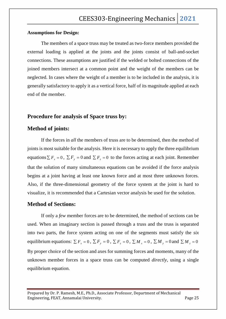
CEES303-Engineering Mechanics 2021
Prepared by Dr. P. Ramesh, M.E., Ph.D., Associate Professor, Department of MechanicalEngineering, FEAT, Annamalai University. Page 25
Assumptions for Design:
The members of a space truss may be treated as two-force members provided the
external loading is applied at the joints and the joints consist of ball-and-socket
connections. These assumptions are justified if the welded or bolted connections of the
joined members intersect at a common point and the weight of the members can be
neglected. In cases where the weight of a member is to be included in the analysis, it is
generally satisfactory to apply it as a vertical force, half of its magnitude applied at each
end of the member.
Procedure for analysis of Space truss by:
Method of joints:
If the forces in all the members of truss are to be determined, then the method of
joints is most suitable for the analysis. Here it is necessary to apply the three equilibrium
equations 0 xF , 0 yF and 0 zF to the forces acting at each joint. Remember
that the solution of many simultaneous equations can be avoided if the force analysis
begins at a joint having at least one known force and at most three unknown forces.
Also, if the three-dimensional geometry of the force system at the joint is hard to
visualize, it is recommended that a Cartesian vector analysis be used for the solution.
Method of Sections:
If only a few member forces are to be determined, the method of sections can be
used. When an imaginary section is passed through a truss and the truss is separated
into two parts, the force system acting on one of the segments must satisfy the six
equilibrium equations: 0 xF , 0 yF , 0 zF , 0 xM , 0 yM and 0 zM
By proper choice of the section and axes for summing forces and moments, many of the
unknown member forces in a space truss can be computed directly, using a single
equilibrium equation.

CEES303-Engineering Mechanics 2021
Prepared by Dr. P. Ramesh, M.E., Ph.D., Associate Professor, Department of MechanicalEngineering, FEAT, Annamalai University. Page 26
SP2.5: Determine the forces acting in the members of the space truss shown in Fig.2.17.
Indicate whether the members are in tension or compression.
Fig.2.17 Space truss
Solution:
Since there are one known force and three unknown forces acting at joint A, the
force analysis of the truss will begin at this joint.
Joint A: Expressing each force acting on the free-body diagram of joint A as a
Cartesian vector, we have
)(4 jP
jFF mABAB )(
)()( kFF mACAC
222 )()()(
)()()(
zzyyxx
zzyyxx
mAEAE
AEmAEAE
AEAEAE
kAEjAEiAEF
r
rFF
222 )2()2()2(
)20()02()02(
kjiFF mAEAE
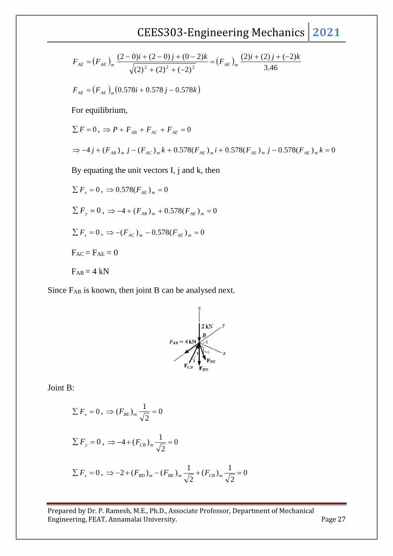
CEES303-Engineering Mechanics 2021
Prepared by Dr. P. Ramesh, M.E., Ph.D., Associate Professor, Department of MechanicalEngineering, FEAT, Annamalai University. Page 27
46.3
)2()2()2(
)2()2()2(
)20()02()02(222
kjiF
kjiFF mAEmAEAE
kjiFF mAEAE 578.0578.0578.0
For equilibrium,
0 F , 0 AEACAB FFFP
0)(578.0)(578.0)(578.0)()(4 kFjFiFkFjFj mAEmAEmAEmACmAB
By equating the unit vectors I, j and k, then
0 xF , 0)(578.0 mAEF
0 yF , 0)(578.0)(4 mAEmAB FF
0 zF , 0)(578.0)( mAEmAC FF
FAC = FAE = 0
FAB = 4 kN
Since FAB is known, then joint B can be analysed next.
Joint B:
0 xF , 02
1)( mBEF
0 yF , 02
1)(4 mCBF
0 zF , 02
1)(
2
1)()(2 mCBmBEmBD FFF
CEES303-Engineering Mechanics 2021
Prepared by Dr. P. Ramesh, M.E., Ph.D., Associate Professor, Department of MechanicalEngineering, FEAT, Annamalai University. Page 28
FBE = 0,
FCB = 5.65 kN
FBD = 2 kN
The scalar equations of equilibrium can now be applied to the forces acting on
the free body diagrams of joints D and C as
FDE = FDC = FCE = 0
BEAMS:
Beams are structural members which offer resistance to bending due to applied
loads. Most beams are long prismatic bars, and the loads are usually applied normal to
the axes of the bars. Beams are undoubtedly the most important of all structural
members, so it is important to understand the basic theory underlying their design. To
analyse the load-carrying capacities of a beam we must first establish the equilibrium
requirements of the beam as a whole and any portion of it considered separately.
Second, we must establish the relations between the resulting forces and the
accompanying internal resistance of the beam to support these forces. The first part of
this analysis requires the application of the principles of statics. The second part
involves the strength characteristics of the material and is usually treated in studies of
the mechanics of solids or the mechanics of materials.
Types of support:
The various types of supports and reactions developed are already discussed in
previous section of unit -1. But here at glance looks about the types as
1) Simple support
2) Roller support
3) Hinged or pinned support
4) Fixed support

CEES303-Engineering Mechanics 2021
Prepared by Dr. P. Ramesh, M.E., Ph.D., Associate Professor, Department of MechanicalEngineering, FEAT, Annamalai University. Page 29
Fig.2.18 Simple support
Fig.2.19 Roller support
Fig.2.20 Hinged or pinned support
Fig.2.21 Fixed support
A
RA
A
RA
A
RA
A
RA
A
RAy
RAx
A
RAy
RAx
RAy
RAx AMA

CEES303-Engineering Mechanics 2021
Prepared by Dr. P. Ramesh, M.E., Ph.D., Associate Professor, Department of MechanicalEngineering, FEAT, Annamalai University. Page 30
Types of Beams:
The beams are classified according to the types of supports as
1) Cantilever beam
2) Simply supported beam
3) One end hinged and other on roller type of beam
4) Overhanging beam
5) Both ends hinged beam
6) Propped cantilever beam and
7) Continuous beam
1) Cantilever beam:
If a beam is fixed at one end and other end is free which is not supported by any
it is called a cantilever beam. In this there are three reaction components at fixed end
such as RAx, RAy and MA as shown in fig.2.22 and no reaction components at free end.
Fig.2.22 Cantilever beam
2) Simply supported beam:
In this type of beam both ends are simply supported as shown in fig.2.23. There
is one reaction component at each end as RAy and RBy. They act at right angles to the
support and this type of beam can resist forces normal to the beam axis. In other words
the equilibrium condition that summation of forces parallel to axis equal to zero is to be
satisfied automatically by the loading condition. Hence two equation of equilibrium are
available.
A
MA
RAx
RAy
B
L

CEES303-Engineering Mechanics 2021
Prepared by Dr. P. Ramesh, M.E., Ph.D., Associate Professor, Department of MechanicalEngineering, FEAT, Annamalai University. Page 31
Fig.2.23 Simple supported beam
3) One end hinged and the other on roller:
As the name suggests one end of the beam is hinged and the other end is on roller
as shown in fig.2.24. At hinge the reaction can be in both direction and at roller end it
is at right angles to the roller support. The hinged end reaction in any direction can be
represented by its two components perpendicular to each other. Thus its reaction
components for such beam as RAx, RAy and RBy.
Fig.2.24 One end hinged and other end on roller
4) Overhanging beam:
If a beam is projecting beyond the support/ supports it is called an overhanging
beam as shown in fig.2.25 . The overhang may be on only one side or may be on both
sides.
A
RAx
RAy
B
LRBy
RAy
RAx
RBy
A B
L

CEES303-Engineering Mechanics 2021
Prepared by Dr. P. Ramesh, M.E., Ph.D., Associate Professor, Department of MechanicalEngineering, FEAT, Annamalai University. Page 32
a) Single overhang
b) Double overhang
Fig.2.25 Overhanging beam
5) Both ends hinged beam:
As the name suggested both ends of the beam are hinged. These are two reactioncomponents at each end, then the total reaction components are four such as RAx, RAy,RBx and RBy.
Fig. 2.26 Both ends hinged beam
RAy
RAx
RBy
A B
L
Over hang
RAy
RAx
RBy
A B
L
Over hangOver hang
RAy
RAx
RBy
A B
L
RBx

CEES303-Engineering Mechanics 2021
Prepared by Dr. P. Ramesh, M.E., Ph.D., Associate Professor, Department of MechanicalEngineering, FEAT, Annamalai University. Page 33
6) Propped cantilever beam:
In this type of beam one end of the beam is fixed and the other end is simply
supported or is on rollers. It has got four reaction components such as RAx, RAy RBy and
MA and it is shown fig.2.27
Fig.2.27 Propped cantilever beam
7) Continuous beam:
A beam having three or more supports is called continuous beam. In such beams
three or more reaction components exist as shown in fig.2.28.
a) Two length of continuous beam
b) Multi length continuous beams
Fig.2.28 Continuous beams
AMA
RAx
RAy
B
L
A
MA
RAx
RAy
C
L
RCy
D EB
RBy RDy RDy
REx

CEES303-Engineering Mechanics 2021
Prepared by Dr. P. Ramesh, M.E., Ph.D., Associate Professor, Department of MechanicalEngineering, FEAT, Annamalai University. Page 34
SUPPORT REDUNDANCY OF BEAMS:
The external support reactions can be calculated by the methods of statics alone
are called statically determinate beams. Therefore the number of unknown reactions are
equal to the number of independent equations of equilibrium such beams are cantilever
beams, simply supported beams, one end hinged and the other end on roller support,
and overhanging beams. The all reaction components of beam is determined by the
equations of equilibrium only. A beam like both ends hinged, propped cantilever and
continuous beams which has more supports with number of unknown reaction
components are more than needed to provide the number of available equations of
equilibrium is called statically indeterminate. To determine the support reactions for
such a beam we must consider its load-deformation properties in addition to the
equations of static equilibrium. Fig. 2.29 shows examples of both types of beams. In
this section, the analyses are carried only by statically determinate beams.
Fig.2.29 Support redundancy of beams
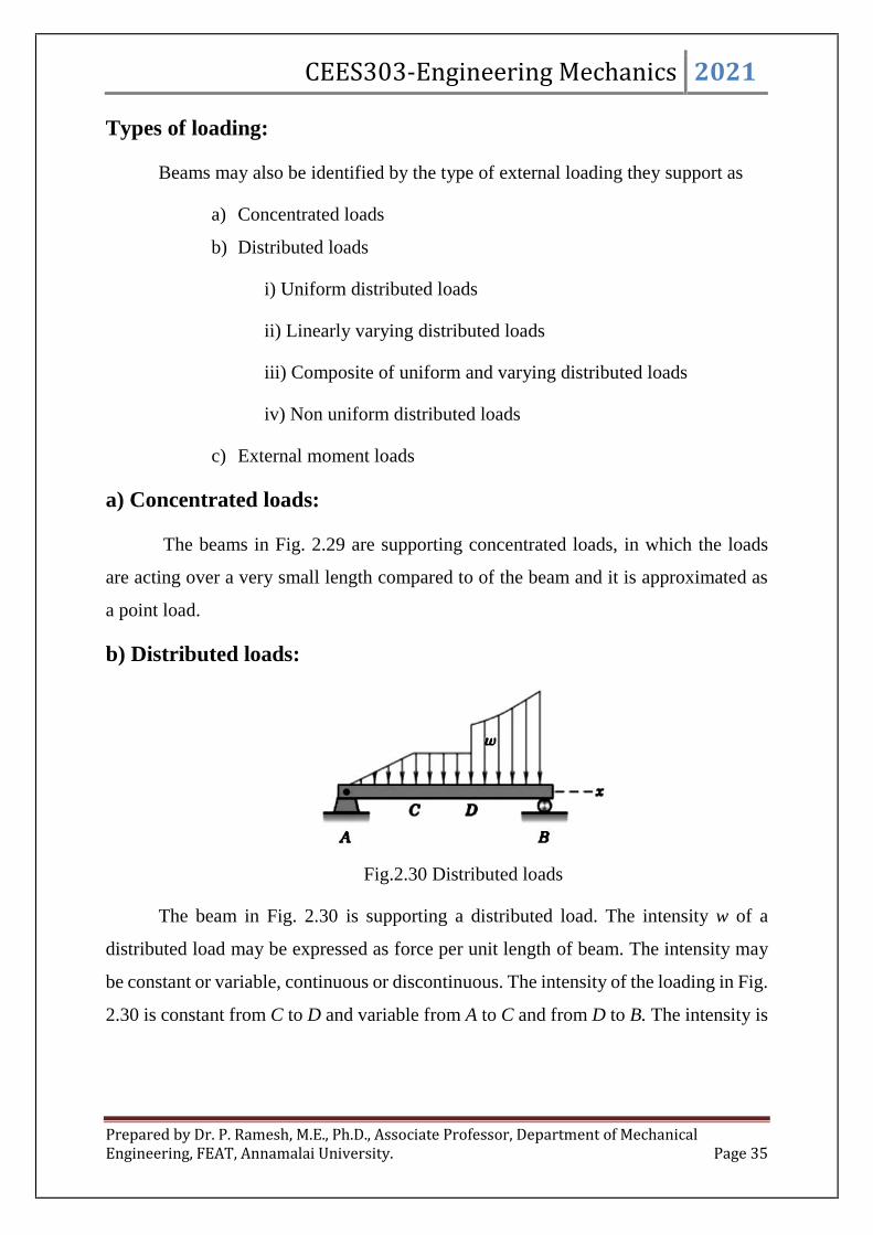
CEES303-Engineering Mechanics 2021
Prepared by Dr. P. Ramesh, M.E., Ph.D., Associate Professor, Department of MechanicalEngineering, FEAT, Annamalai University. Page 35
Types of loading:
Beams may also be identified by the type of external loading they support as
a) Concentrated loads
b) Distributed loads
i) Uniform distributed loads
ii) Linearly varying distributed loads
iii) Composite of uniform and varying distributed loads
iv) Non uniform distributed loads
c) External moment loads
a) Concentrated loads:
The beams in Fig. 2.29 are supporting concentrated loads, in which the loads
are acting over a very small length compared to of the beam and it is approximated as
a point load.
b) Distributed loads:
Fig.2.30 Distributed loads
The beam in Fig. 2.30 is supporting a distributed load. The intensity w of a
distributed load may be expressed as force per unit length of beam. The intensity may
be constant or variable, continuous or discontinuous. The intensity of the loading in Fig.
2.30 is constant from C to D and variable from A to C and from D to B. The intensity is

CEES303-Engineering Mechanics 2021
Prepared by Dr. P. Ramesh, M.E., Ph.D., Associate Professor, Department of MechanicalEngineering, FEAT, Annamalai University. Page 36
discontinuous at D, where it changes magnitude abruptly. Although the intensity itself
is not discontinuous at C, the rate of change of intensitydx
dwis discontinuous.
i) Uniform distributed loads:
Loading intensities which are constant over the length of beam is called
uniform distribution loads as shown in fig.2.31 , The resultant load R is
represented by the area formed by the intensity w (force per unit length of
beam) and the length L over which the force is distributed. The resultant
passes through the centroid of this area.
Fig.2.31 Uniform distributed loads
ii) Linearly varying distributed loads:
Loading intensities which are vary linearly over the length of beam is
called uniformly varying distributed loads as shown in fig.2.32. The resultant
load R is represented by the area formed by the intensity w (force per unit
length of beam) and the length L over which the force is distributed. The
resultant passes through the centroid of this area. The centroid area is L3
2
from zero intensity load and Resultant load is wL2
1.
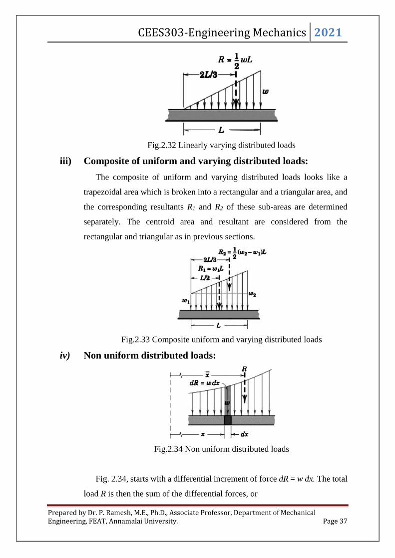
CEES303-Engineering Mechanics 2021
Prepared by Dr. P. Ramesh, M.E., Ph.D., Associate Professor, Department of MechanicalEngineering, FEAT, Annamalai University. Page 37
Fig.2.32 Linearly varying distributed loads
iii) Composite of uniform and varying distributed loads:
The composite of uniform and varying distributed loads looks like a
trapezoidal area which is broken into a rectangular and a triangular area, and
the corresponding resultants R1 and R2 of these sub-areas are determined
separately. The centroid area and resultant are considered from the
rectangular and triangular as in previous sections.
Fig.2.33 Composite uniform and varying distributed loads
iv) Non uniform distributed loads:
Fig.2.34 Non uniform distributed loads
Fig. 2.34, starts with a differential increment of force dR = w dx. The total
load R is then the sum of the differential forces, or

CEES303-Engineering Mechanics 2021
Prepared by Dr. P. Ramesh, M.E., Ph.D., Associate Professor, Department of MechanicalEngineering, FEAT, Annamalai University. Page 38
wdxR
As before, the resultant R is located at the centroid of the area under
consideration. The x-coordinate of this centroid is found by the principle of
moments xwdxxR or
xwdxR
x1
For the distribution as in Fig.2.34, the vertical coordinate of the centroid
need not be found. Once the distributed loads have been reduced to their
equivalent concentrated loads, the external reactions acting on the beam may
be found by a straightforward static analysis.
v) External moment loads:
Fig. 2.35 External moment loads
A beam may be subjected to external moments at certain points. In
fig.2.35 The beam subjected to a clockwise moment of MC at a distance x
from the support A.
SP2.6: Find the reactions developed in the cantilever beam as shown in fig.2.36.
Fig.2.36
x
A B
MC
AB
2m 1m
15 kN10kN/m 20 kN
60o

CEES303-Engineering Mechanics 2021
Prepared by Dr. P. Ramesh, M.E., Ph.D., Associate Professor, Department of MechanicalEngineering, FEAT, Annamalai University. Page 39
Solution:
First draw the free body diagram consist of reaction force developed at fixed
support A as shown below.
The equilibrium conditions about vertical,
0 yF , 01560sin20)( 10 oAy RR
01560sin20)210( oAyR , RAy = 52.32 kN
The equilibrium conditions about horizontal,
0 xF , 060cos20 oAxR , RAx = 10 kN
Taking moment about A ,
0 AM , 0315260sin201210 oAM
MA = 99.64 kN-m
SP2.7: Determine the reaction developed in the simply supported beam as shown in
fig.2.37.
AB
2m 1m
15 kN10kN/m 20 kN
60oMA
RAy
RAx

CEES303-Engineering Mechanics 2021
Prepared by Dr. P. Ramesh, M.E., Ph.D., Associate Professor, Department of MechanicalEngineering, FEAT, Annamalai University. Page 40
Fig.2.37
Solution:
The free body diagram of given space diagram as below
The varying distributed load may be split into a uniformly distributed load of 20
kN/m as in rectangular geometry and a linearly varying load from point C to point B.
The linearly varying load at end C is zero and point B is 40 kN/m(60-20).
Taking moment about B, then
0 BM , 043
1440
2
124206 AyR
RAy = 44.44 kN
The equilibrium equations for vertical force,
0 yF , 04402
1420 ByAy RR
0808044.44 ByR , RBy = 115.56 kN
2m 4m
AB
20 kN/m
60 kN/m
2m 4m
AB
20 kN/m
60 kN/m
C
RAy RBy
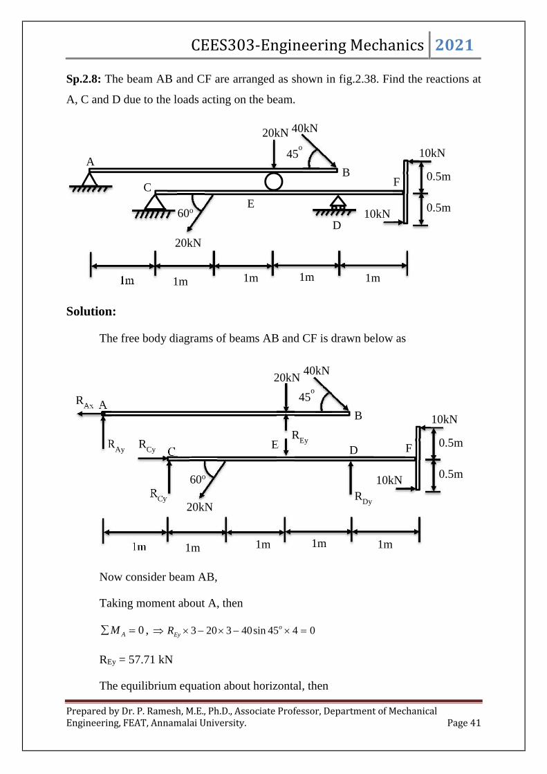
CEES303-Engineering Mechanics 2021
Prepared by Dr. P. Ramesh, M.E., Ph.D., Associate Professor, Department of MechanicalEngineering, FEAT, Annamalai University. Page 41
Sp.2.8: The beam AB and CF are arranged as shown in fig.2.38. Find the reactions at
A, C and D due to the loads acting on the beam.
Solution:
The free body diagrams of beams AB and CF is drawn below as
Now consider beam AB,
Taking moment about A, then
0 AM , 0445sin403203 oEyR
REy = 57.71 kN
The equilibrium equation about horizontal, then
AB
1m
CE
D
1m 1m 1m 1m
0.5m
0.5m10kN
10kN
F
60o
45o
40kN20kN
20kN
RAy
RAx
RCy
AB
1m
CE D
1m 1m 1m 1m
0.5m
0.5m10kN
10kN
F
60o
45o
RCy
REy
RDy
40kN20kN
20kN

CEES303-Engineering Mechanics 2021
Prepared by Dr. P. Ramesh, M.E., Ph.D., Associate Professor, Department of MechanicalEngineering, FEAT, Annamalai University. Page 42
0 xF , 045cos40 oAxR
RAx = 28.28 kN
The equilibrium equations about vertical, then
0 yF , 045sin4020 Eyo
Ay RR
071.5745sin4020 oAyR
RAy = -9.43kN
Here, the negative sign indicates the direction of reaction is downwards.
Consider beam CF,
Taking moment about C, then
0 CM , 01102160sin203 Eyo
Dy RR
0110271.57160sin203 oDyR
RDy = 40.91 kN
The equilibrium equations about horizontal is
0 xF , 060cos20 oCxR
RCx = 10 kN
The equilibrium equations about vertical is
0 yF , 060sin20 DyEyo
Cy RRR
091.4071.5760sin20 oCyR
RCy = 34.12 kN

CEES303-Engineering Mechanics 2021
Prepared by Dr. P. Ramesh, M.E., Ph.D., Associate Professor, Department of MechanicalEngineering, FEAT, Annamalai University. Page 43
FRAMES AND MACHINES:
Frames and machines are two types of structures which are often composed of
pin-connected multi-force members, i.e., members that are subjected to more than two
forces. Frames are used to support loads, whereas machines contain moving parts and
are designed to transmit and alter the effect of forces. Provided a frame or machine
contains no more supports or members than are necessary to prevent its collapse, the
forces acting at the joints and supports can be determined by applying the equations of
equilibrium to each of its members. Once these forces are obtained, it is then possible
to design the size of the members, connections, and supports using the theory of
mechanics of materials and an appropriate engineering design code.
Free-Body Diagrams.
In order to determine the forces acting at the joints and supports of a frame or
machine, the structure must be disassembled and the free-body diagrams of its parts
must be drawn. The following important points must be observed:
Isolate each part by drawing its outlined shape. Then show all the forces and/or
couple moments that act on the part. Make sure to label or identify each known
and unknown force and couple moment with reference to an established x, y
coordinate system. Also, indicate any dimensions used for taking moments. Most
often the equations of equilibrium are easier to apply if the forces are represented
by their rectangular components. As usual, the sense of an unknown force or
couple moment can be assumed.
Identify all the two-force members in the structure and represent their free-body
diagrams as having two equal but opposite collinear forces acting at their points
of application. By recognizing the two-force members, we can avoid solving an
unnecessary number of equilibrium equations.
Forces common to any two contacting members act with equal magnitudes but
opposite sense on the respective members. If the two members are treated as a
“system” of connected members, then these forces are “internal” and are not
shown on the free-body diagram of the system; however, if the free-body diagram

CEES303-Engineering Mechanics 2021
Prepared by Dr. P. Ramesh, M.E., Ph.D., Associate Professor, Department of MechanicalEngineering, FEAT, Annamalai University. Page 44
of each member is drawn, the forces are “external” and must be shown as equal
in magnitude and opposite in direction on each of the two free-body diagrams.
SP2.9: For the frame as shown in fig.2.39, draw the free body diagram of i) each
member, ii) the pins at B and A and iii) the two members connected together.
Fig.2.39
Solution:
Fig.2.39 b Fig.2.39 c
Part (a): By inspection, members BA and BC are not two-force members. Instead,
as shown on the free-body diagrams, Fig. 2.39 b, BC is subjected to a force from each
of the pins at B and C and the external force P. Likewise, AB is subjected to a force
from each of the pins at A and B and the external couple moment M. The pin forces are
represented by their x and y components.
Part (b). The pin at B is subjected to only two forces, i.e., the force of member
BC and the force of member AB. For equilibrium these forces (or their respective
components) must be equal but opposite, Fig. 2.39 c. Realize that Newton’s third law
is applied between the pin and its connected members, i.e., the effect of the pin on the

CEES303-Engineering Mechanics 2021
Prepared by Dr. P. Ramesh, M.E., Ph.D., Associate Professor, Department of MechanicalEngineering, FEAT, Annamalai University. Page 45
two members, Fig. 2.39 b, and the equal but opposite effect of the two members on the
pin, Fig. 2.39 c. In the same manner, there are three forces on pin A, Fig. 2.39 d, caused
by the force components of member AB and each of the two pin leafs.
Fig.2.39 d Fig.2.39 e
Part (c). The free-body diagram of both members connected together, yet
removed from the supporting pins at A and C, is shown in Fig. 2.39 e. The force
components Bx and By are not shown on this diagram since they are internal forces
(Fig. 2.39 b) and therefore cancel out. Also, to be consistent when later applying the
equilibrium equations, the unknown force components at A and C must act in the same
sense as those shown in Fig. 2.39 b.
SP2.10: A constant tension in the conveyor belt is maintained by using the device as
shown in fig.2.40. Draw the free body diagram of the frame and the cylinder that the
belt surrounds. The suspended blocks has a weight of W.
Fig.2.40

CEES303-Engineering Mechanics 2021
Prepared by Dr. P. Ramesh, M.E., Ph.D., Associate Professor, Department of MechanicalEngineering, FEAT, Annamalai University. Page 46
Solution:
SP2.11: For the frame as shown in fig.2.41, draw the free body diagrams of i) the entire
frame including the pulleys and cords, ii) the frame without the pulleys and cords and
iii) each of the pulleys.
Fig.2.41
Solution:
Fig.2.41 a Fig.2.41 b

CEES303-Engineering Mechanics 2021
Prepared by Dr. P. Ramesh, M.E., Ph.D., Associate Professor, Department of MechanicalEngineering, FEAT, Annamalai University. Page 47
Part (a): When the entire frame including the pulleys and cords is considered, the
interactions at the points where the pulleys and cords are connected to the frame become
pairs of internal forces which cancel each other and therefore are not shown on the free-
body diagram, Fig.2.41 a.
Part (b). When the cords and pulleys are removed, their effect on the frame must
be shown, Fig.2.41 b.
Part (c). The force components Bx, By, Cx, Cy of the pins on the pulleys, Fig. 2.41
c, are equal but opposite to the force components exerted by the pins on the frame,
Fig.2.41 c.
SP2.12: The 75-kg man as shown in Fig.2.41 attempts to lift the 40-kg uniform beam
off the roller support at B. Determine the tension developed in the cable attached to B
and the normal reaction of the man on the beam when this is about to occur.
Fig.2.42
Solution:
The free-body diagrams of the pulley E, the man, and the beam are shown in Fig.
2.42 b. Since the man must lift the beam off the roller B then NB = 0. When drawing
each of these diagrams, it is very important to apply Newton’s third law. The tensile
force in the cable will be denoted as T1.

CEES303-Engineering Mechanics 2021
Prepared by Dr. P. Ramesh, M.E., Ph.D., Associate Professor, Department of MechanicalEngineering, FEAT, Annamalai University. Page 48
Fig.2.42 a
Equations of Equilibrium: Using the free-body diagram of pulley E, About vertical, then
0 yF , 02 21 TT , T2 = 2T1 ------ (1)
Using the free body diagram of man for vertical components, then
0 yF , 0)81.9(752 1 TNm --------- (2)
Taking moment about A on the beam, then
0 AM , 05.1))81.9(40(8.031 mNT ----------- (3)
Solving equations 2 and 3 simultaneously for T1 and Nm then using equations (1) for T2
T1 = 256 N, Nm = 224 N and T2 = 512 N.
SP2.13: The frame supports the 400-kg load in the manner shown in fig.2.43. Neglect
the weights of the members compared with the forces induced by the load and compute
the horizontal and vertical components of all forces acting on each of the members.
Fig.2.43

CEES303-Engineering Mechanics 2021
Prepared by Dr. P. Ramesh, M.E., Ph.D., Associate Professor, Department of MechanicalEngineering, FEAT, Annamalai University. Page 49
Solution:First, the three supporting members which constitute the frame form a rigid
assembly can be analysed as a single unit. It also observe that the arrangement of theexternal supports makes the frame statically determinate.
From the free-body diagram of the entire frame we determine the externalreactions. Thus,
0 AM , 0)5()5.5(81.9400 DxR ,
RDx = 4.32 kN
0 xF , 0 DxAx RR , 032.4 AxR
RAx = 4.32 kN
0 yF , 0)81.9)(400( AyR
RAy = 3.92 kN
Next we dismember the frame and draw a separate free-body diagram of each
member. The diagrams are arranged in their approximate relative positions to aid in
keeping track of the common forces of interaction. The external reactions just obtained
are entered onto the diagram for AD. Other known forces are the 3.92-kN forces exerted
by the shaft of the pulley on the member BF, as obtained from the free body diagram of
the pulley. The cable tension of 3.92 kN is also shown acting on AD at its attachment
point.
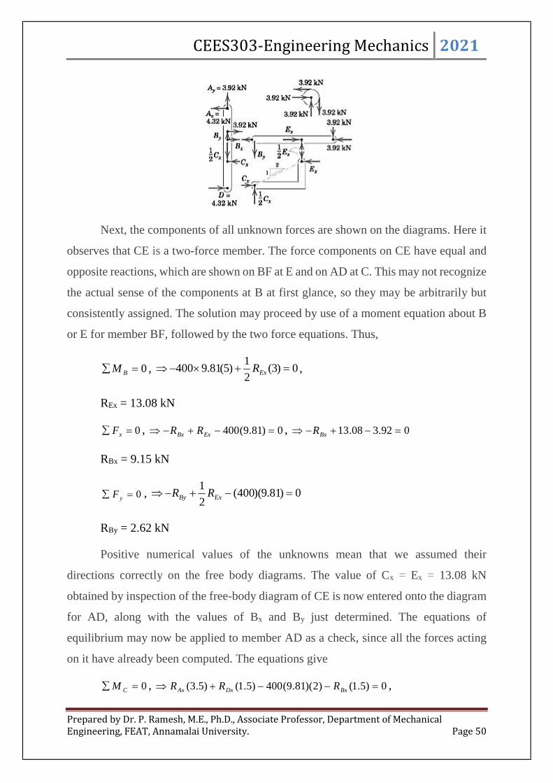
CEES303-Engineering Mechanics 2021
Prepared by Dr. P. Ramesh, M.E., Ph.D., Associate Professor, Department of MechanicalEngineering, FEAT, Annamalai University. Page 50
Next, the components of all unknown forces are shown on the diagrams. Here it
observes that CE is a two-force member. The force components on CE have equal and
opposite reactions, which are shown on BF at E and on AD at C. This may not recognize
the actual sense of the components at B at first glance, so they may be arbitrarily but
consistently assigned. The solution may proceed by use of a moment equation about B
or E for member BF, followed by the two force equations. Thus,
0 BM , 0)3(2
1)5(81.9400 ExR ,
REx = 13.08 kN
0 xF , 0)81.9(400 ExBx RR , 092.308.13 BxR
RBx = 9.15 kN
0 yF , 0)81.9)(400(2
1 ExBy RR
RBy = 2.62 kN
Positive numerical values of the unknowns mean that we assumed their
directions correctly on the free body diagrams. The value of Cx = Ex = 13.08 kN
obtained by inspection of the free-body diagram of CE is now entered onto the diagram
for AD, along with the values of Bx and By just determined. The equations of
equilibrium may now be applied to member AD as a check, since all the forces acting
on it have already been computed. The equations give
0 CM , 0)5.1()2)(81.9(400)5.1()5.3( BxDxAx RRR ,
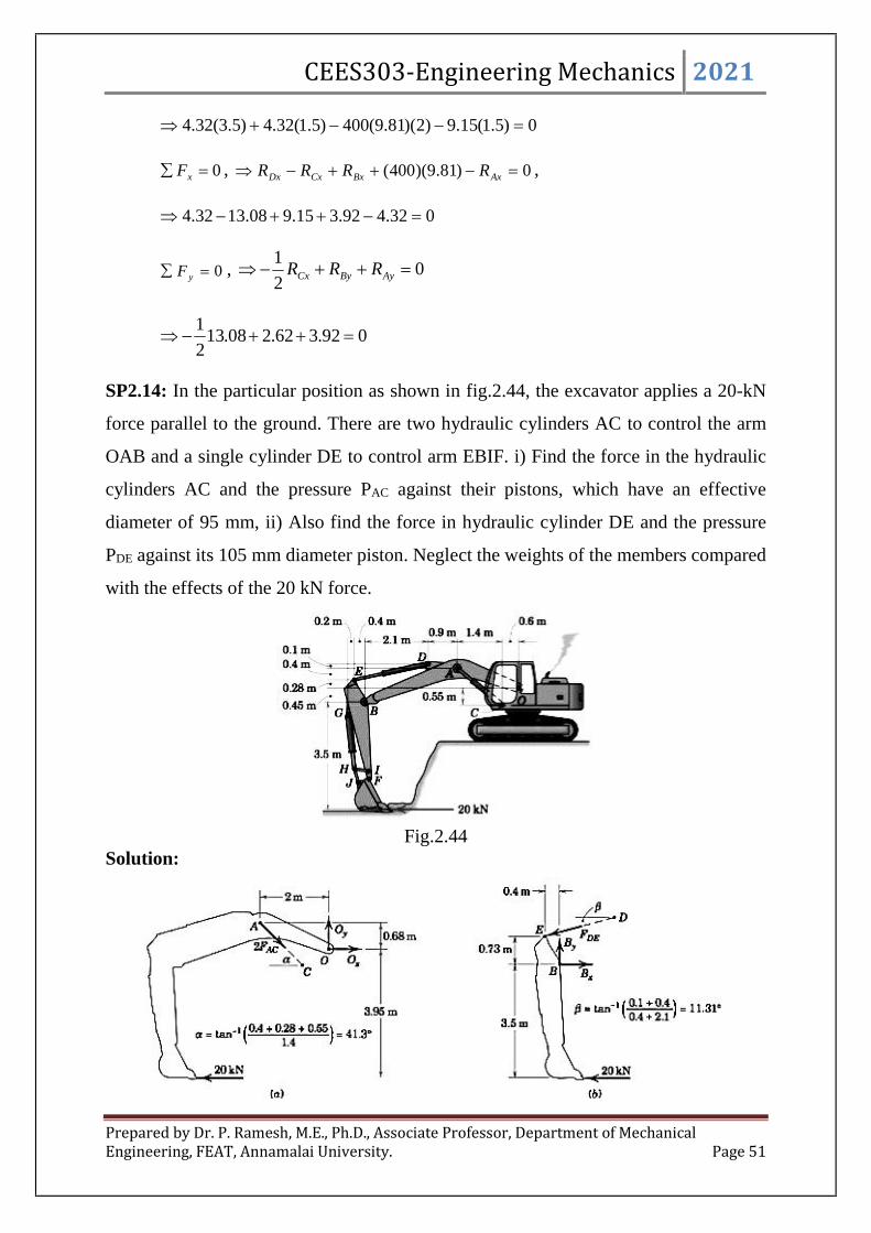
CEES303-Engineering Mechanics 2021
Prepared by Dr. P. Ramesh, M.E., Ph.D., Associate Professor, Department of MechanicalEngineering, FEAT, Annamalai University. Page 51
0)5.1(15.9)2)(81.9(400)5.1(32.4)5.3(32.4
0 xF , 0)81.9)(400( AxBxCxDx RRRR ,
032.492.315.908.1332.4
0 yF , 02
1 AyByCx RRR
092.362.208.132
1
SP2.14: In the particular position as shown in fig.2.44, the excavator applies a 20-kN
force parallel to the ground. There are two hydraulic cylinders AC to control the arm
OAB and a single cylinder DE to control arm EBIF. i) Find the force in the hydraulic
cylinders AC and the pressure PAC against their pistons, which have an effective
diameter of 95 mm, ii) Also find the force in hydraulic cylinder DE and the pressure
PDE against its 105 mm diameter piston. Neglect the weights of the members compared
with the effects of the 20 kN force.
Fig.2.44Solution:
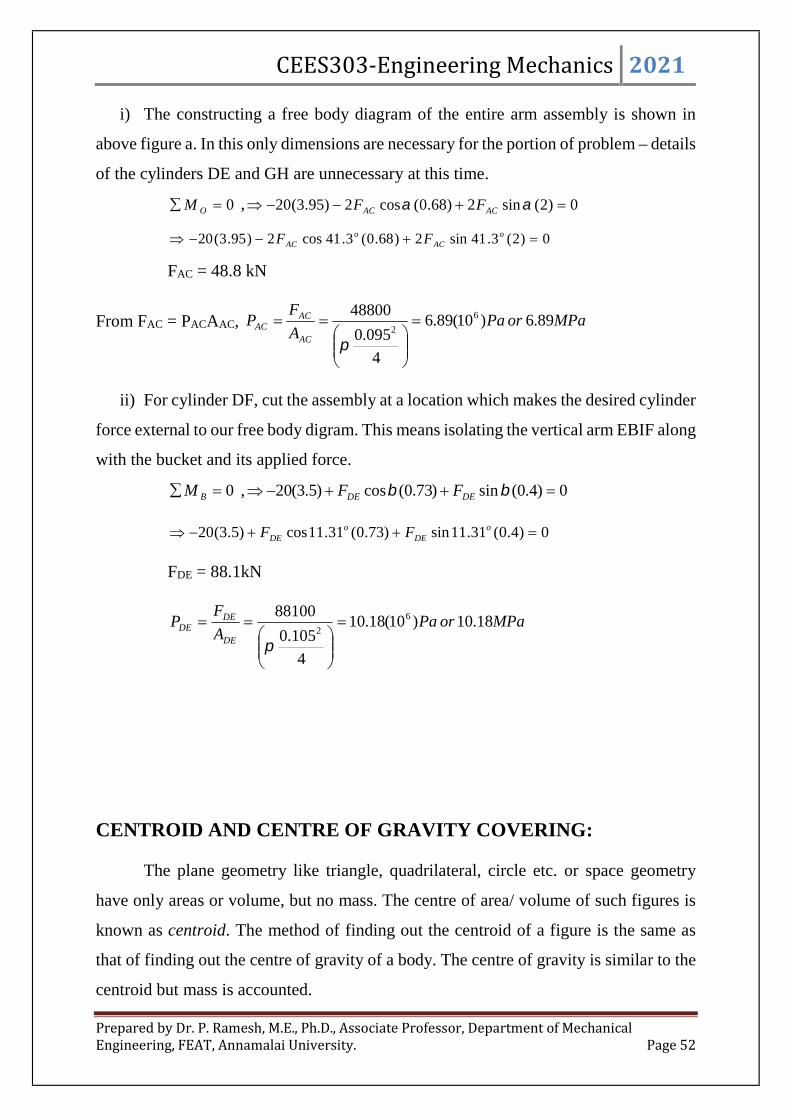
CEES303-Engineering Mechanics 2021
Prepared by Dr. P. Ramesh, M.E., Ph.D., Associate Professor, Department of MechanicalEngineering, FEAT, Annamalai University. Page 52
i) The constructing a free body diagram of the entire arm assembly is shown in
above figure a. In this only dimensions are necessary for the portion of problem – details
of the cylinders DE and GH are unnecessary at this time.
0 OM , 0)2(sin2)68.0(cos2)95.3(20 ACAC FF
0)2(3.41sin2)68.0(3.41cos2)95.3(20 oAC
oAC FF
FAC = 48.8 kN
From FAC = PACAAC, MPaorPaA
FP
AC
ACAC 89.6)10(89.6
4
095.0
48800 6
2
ii) For cylinder DF, cut the assembly at a location which makes the desired cylinder
force external to our free body digram. This means isolating the vertical arm EBIF along
with the bucket and its applied force.
0 BM , 0)4.0(sin)73.0(cos)5.3(20 DEDE FF
0)4.0(31.11sin)73.0(31.11cos)5.3(20 oDE
oDE FF
FDE = 88.1kN
MPaorPaA
FP
DE
DEDE 18.10)10(18.10
4
105.0
88100 6
2
CENTROID AND CENTRE OF GRAVITY COVERING:
The plane geometry like triangle, quadrilateral, circle etc. or space geometry
have only areas or volume, but no mass. The centre of area/ volume of such figures is
known as centroid. The method of finding out the centroid of a figure is the same as
that of finding out the centre of gravity of a body. The centre of gravity is similar to the
centroid but mass is accounted.

CEES303-Engineering Mechanics 2021
Prepared by Dr. P. Ramesh, M.E., Ph.D., Associate Professor, Department of MechanicalEngineering, FEAT, Annamalai University. Page 53
Difference between Centre of Gravity and Centroid:
Sl. No Centre of Gravity Centroid
1 The point where the total weight of
the body focuses upon
It is referred to the geometrical centre
of a body
2 It is the point where the gravitational
force (weight) acts on the body
It is referred to the centre of gravity
of uniform density objects
3 It is denoted by g It is denoted by c
4 Centre of Gravity in a uniform
gravitational field is the average of
all points, weighted by local density
or specific weight
The centroid is a point in a plane area
in such a way that the moment of area
about any axis throughout that point
is 0
5 It is a physical behaviour of the
object, a point where all the weight
of an object is acting
It is a geometrical behaviour. It is the
centre of measure of the amount of
geometry.
Methods for Centroid:
The centroid may be found out by any one of the following methods:
1. by geometrical considerations
2. by moments
3. by graphical method
As a matter of fact, the graphical method is a tedious and cumbersome method
for finding out the centroid of simple figures. So this graphical method is not include
here. Before to discuss the method of moments, the procedure for finding out the
centroid of simple figures by geometrical considerations as follows.

CEES303-Engineering Mechanics 2021
Prepared by Dr. P. Ramesh, M.E., Ph.D., Associate Professor, Department of MechanicalEngineering, FEAT, Annamalai University. Page 54
Centroid by Geometrical Considerations:
The centroid of simple figures may be found out from the geometry of the figure
as given below.
1. The centroid of uniform rod/ length is at its middle point.
2. The centroid of a rectangle (or a parallelogram) is at the point, where its
diagonals meet each other. It is also a middle point of the length as well as the
breadth of the rectangle as shown in Fig. 2.45.
Fig.2.45 Rectangular geometry
3. The centroid of a triangle is at the point, where the three medians (a median is a
line connecting the vertex and middle point of the opposite side) of the triangle
meet as shown in Fig. 2.46.
Fig.2.46
4. The centroid of a trapezium with parallel sides a and b is at a distance of
ab
abh 2
3measured form the side b as shown in Fig.2.47.
Fig.2.47 Trapezium

CEES303-Engineering Mechanics 2021
Prepared by Dr. P. Ramesh, M.E., Ph.D., Associate Professor, Department of MechanicalEngineering, FEAT, Annamalai University. Page 55
5. The centroid of a semicircle is at a distance of3
4rfrom its base measured along
the vertical radius as shown in Fig.2.48.
Fig.2.48 Semicircle
6. The centroid of a circular sector making semi-vertical angle is at a distance of
sin
3
2
rfrom the centre of the sector measured along the central axis as shown
in Fig.2.49.
Fig.2.49 Circular sector
7. The centroid of a cube is at a distance of2
lfrom every face (where l is the length
of each side).
8. The centroid of a sphere is at a distance of2
dfrom every point (where d is the
diameter of the sphere).
9. The centroid of a hemisphere is at a distance of8
3rfrom its base, measured along
the vertical radius as shown in Fig.2.50.

CEES303-Engineering Mechanics 2021
Prepared by Dr. P. Ramesh, M.E., Ph.D., Associate Professor, Department of MechanicalEngineering, FEAT, Annamalai University. Page 56
Fig.2.50 Hemisphere solid
10. The centroid of right circular solid cone is at a distance of4
hfrom its base,
measured along the vertical axis as shown in Fig.2.51.
Fig.2.51 Right circular solid
11. The centroid of a segment of sphere of a height h is at a distance of hr
hr
3
2
4
3 2
from the centre of the sphere measured along the height as shown in Fig.2.52.
Fig.2.52 Sphere segment
CENTROID BY FIRST PRINCIPLE (MOMENTS):
The centroid of a body may also be found out by moments as discussed below:
Consider a body of area A whose centroid is required to be found out. Divide the
body into small areas, whose centroids are known as shown in Fig.2.53. Let a1, a2, ….
etc., be the areas of the particles and (x1, y1), (x2, y2), (x3, y3), ...... be the co-ordinates of
the centroids from a fixed point O as shown in Fig.2.53.
Let x and y be the co-ordinates of the centroid of the body. From the first
principle of moments, we know that

CEES303-Engineering Mechanics 2021
Prepared by Dr. P. Ramesh, M.E., Ph.D., Associate Professor, Department of MechanicalEngineering, FEAT, Annamalai University. Page 57
Fig.2.53 Centroid by moments
...............332211 xaxaxaxA orA
axx
Similarly,A
ayy
Where, .....321 aaaA
AXIS OF REFERENCE:
The centroid of a body is always calculated with reference to some assumed axis
known as axis of reference (or sometimes with reference to some point of reference).
The axis of reference, of plane figures, is generally taken as the lowest line of the figure
for calculating y and the left line of the figure for calculating x .
CENTROID OF SYMMETRICAL SECTIONS:
Sometimes, the given section, whose centroid is required to be found out, is
symmetrical about X-X axis or Y-Y axis. In such cases, the procedure for calculating the
centroid of the body is very much simplified; as it has only to calculate either x or y .
This is due to the reason that the centre of gravity of the body will lie on the axis of
symmetry.
X
Y
x1
x2
x3
O

CEES303-Engineering Mechanics 2021
Prepared by Dr. P. Ramesh, M.E., Ph.D., Associate Professor, Department of MechanicalEngineering, FEAT, Annamalai University. Page 58
CENTROID OF UNSYMMETRICAL SECTIONS:
Sometimes, the given section, whose centroid is required to be found out, is not
symmetrical either about X-X axis or Y-Y axis. In such cases, it has to find out both the
values of x and y .
CENTROID OF SIMPLE FIGURES FROM FIRST PRINCIPLE:
The calculation of centroids falls within three distinct categories, depending on
whether it can model the shape of the body involved as a line, an area, or a volume.
(1) Lines: For a slender rod or wire of length L, cross-sectional area A, and density,
Fig.2.54, the body approximates a line segment, and AdLdm . If and A are
constant over the length of the rod, the coordinates of the centre of mass also
become the coordinates of the centroid C of the line segment, which, may be written
as
L
xdLx ,
L
ydLy and
L
zdLz
Fig.2.54 Slender rod or wire
Note that in general the centroid C will not line on the line. If the rod lies
on a single plane, such as the x-y plane only two coordinates need to be
calculated.
(2) Areas: When a body of density p has a small but constant thickness t, it can model
as a surface area A, Fig.2.55. The mass of an element becomes tdAdm . Again,

CEES303-Engineering Mechanics 2021
Prepared by Dr. P. Ramesh, M.E., Ph.D., Associate Professor, Department of MechanicalEngineering, FEAT, Annamalai University. Page 59
if p and t are constant over the entire area, the coordinates of the centre of mass of
the body also become the coordinates of the centroid C of the surface area, and the
coordinates may be written
A
xdAx ,
A
ydAy and
A
zdAz
The numerators in above equations are called the first moments of area. If the
surface is curved, as illustrated in Fig.2.55 with the shell segment, all three
coordinates will be involved. The centroid C for the curved surface will in general
not lie on the surface. If the area is a flat surface in, say, the x-y plane, only the
coordinates of C in that plane need to be calculated.
Fig.2.55 Surface area
(3) Volumes: For a general body of volume V and density p, the element has a mass
dVdm . The density cancels if it is constant over the entire volume, and the
coordinates of the centre of mass also become the coordinates of the centroid C of
the body.
V
xdVx ,
V
ydVy and
V
zdVz
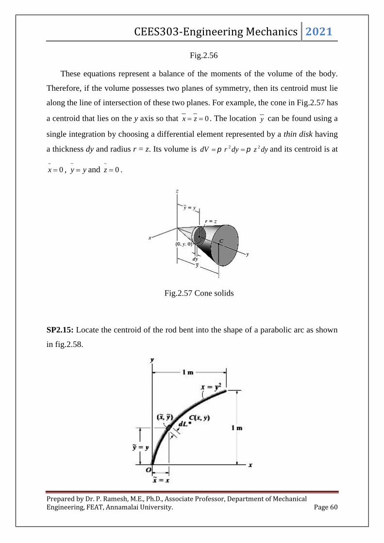
CEES303-Engineering Mechanics 2021
Prepared by Dr. P. Ramesh, M.E., Ph.D., Associate Professor, Department of MechanicalEngineering, FEAT, Annamalai University. Page 60
Fig.2.56
These equations represent a balance of the moments of the volume of the body.
Therefore, if the volume possesses two planes of symmetry, then its centroid must lie
along the line of intersection of these two planes. For example, the cone in Fig.2.57 has
a centroid that lies on the y axis so that 0 zx . The location y can be found using a
single integration by choosing a differential element represented by a thin disk having
a thickness dy and radius r = z. Its volume is dyzdyrdV 22 and its centroid is at
0~
x , yy ~
and 0~
z .
Fig.2.57 Cone solids
SP2.15: Locate the centroid of the rod bent into the shape of a parabolic arc as shown
in fig.2.58.
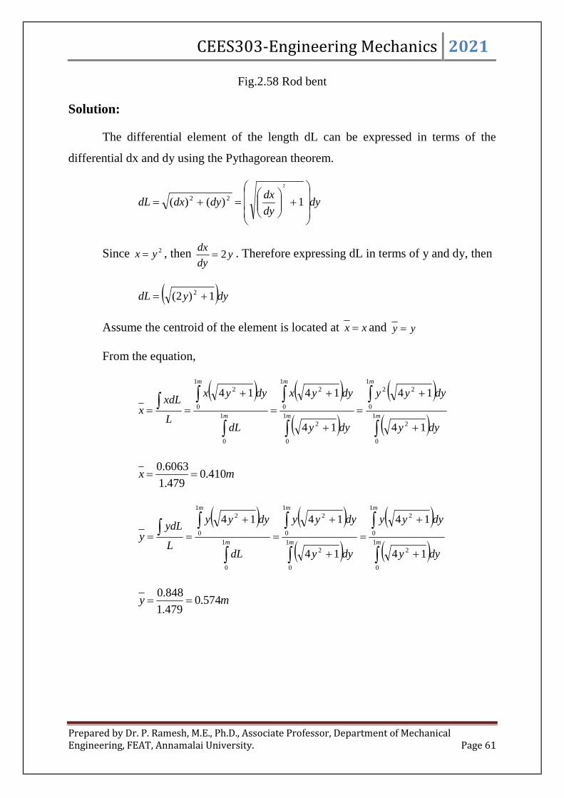
CEES303-Engineering Mechanics 2021
Prepared by Dr. P. Ramesh, M.E., Ph.D., Associate Professor, Department of MechanicalEngineering, FEAT, Annamalai University. Page 61
Fig.2.58 Rod bent
Solution:
The differential element of the length dL can be expressed in terms of the
differential dx and dy using the Pythagorean theorem.
dydy
dxdydxdL
1)()(
2
22
Since 2yx , then ydy
dx2 . Therefore expressing dL in terms of y and dy, then
dyydL 1)2( 2
Assume the centroid of the element is located at xx and yy
From the equation,
m
m
m
m
m
m
dyy
dyyy
dyy
dyyx
dL
dyyx
L
xdLx
1
0
2
1
0
22
1
0
2
1
0
2
1
0
1
0
2
14
14
14
1414
mx 410.0479.1
6063.0
m
m
m
m
m
m
dyy
dyyy
dyy
dyyy
dL
dyyy
L
ydLy
1
0
2
1
0
2
1
0
2
1
0
2
1
0
1
0
2
14
14
14
1414
my 574.0479.1
848.0

CEES303-Engineering Mechanics 2021
Prepared by Dr. P. Ramesh, M.E., Ph.D., Associate Professor, Department of MechanicalEngineering, FEAT, Annamalai University. Page 62
SP2.16: Locate the centroid of a circular arc as shown in fig.2.59
Fig.2.59 Circular arc
Solution:
Fig.2.59a
Assume that the given figure is a symmetry about x axis and make the centroid
by y axis is zero i.e 0y . A differential element of arc has length rddL expressed
in polar coordinates and the x – coordinate of the element is cosr . Applying the first
principle and substituting rL 2 in equation
L
xdLx ,
r
rdr
x
2
))(cos(
r
r
r
r
r
rx
2
)sin2(
2
))(sin((sin
2
sin 222
sinr
x
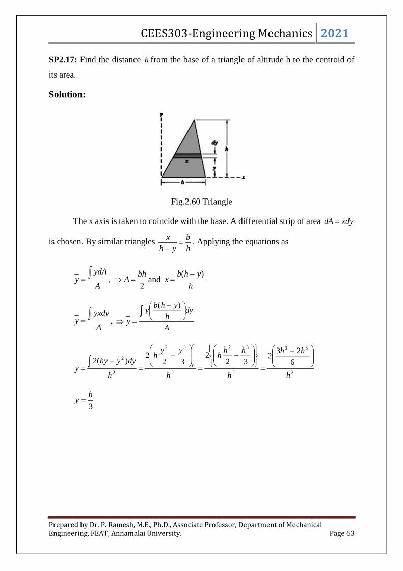
CEES303-Engineering Mechanics 2021
Prepared by Dr. P. Ramesh, M.E., Ph.D., Associate Professor, Department of MechanicalEngineering, FEAT, Annamalai University. Page 63
SP2.17: Find the distance h from the base of a triangle of altitude h to the centroid of
its area.
Solution:
Fig.2.60 Triangle
The x axis is taken to coincide with the base. A differential strip of area xdydA
is chosen. By similar trianglesh
b
yh
x
. Applying the equations as
A
ydAy ,
2
bhA and
h
yhbx
)(
A
yxdyy ,
A
dyh
yhby
y
)(
2
33
2
32
20
32
2
26
232
322
322
)(2
h
hh
h
hhh
h
yyh
h
dyyhyy
h
3
hy

CEES303-Engineering Mechanics 2021
Prepared by Dr. P. Ramesh, M.E., Ph.D., Associate Professor, Department of MechanicalEngineering, FEAT, Annamalai University. Page 64
SP2.18: Locate the centroid of the area of a circular sector with respect to its vertex.
Solution: method 1,
Fig.2.61 Circular sector
The x axis is chosen as the axis symmetry and 0y . The area may cover by
moving an element in the form of a partial circular ring as shown in the figure from the
centre to the outer periphery. The radius of the ring is ro and its thickness is odr , so that
its area is OO drrdA 2 .
The x coordinate to the centroid of the circular arc element is
sinOc
rx ,
where rO replaces r in the formula. Thus, the equations as
2
3
2
0sin
3
2
)(2
2
)2(sin
r
r
r
drrr
A
dAxx
r
OOO
c
sin
3
2 rx

CEES303-Engineering Mechanics 2021
Prepared by Dr. P. Ramesh, M.E., Ph.D., Associate Professor, Department of MechanicalEngineering, FEAT, Annamalai University. Page 65
Method 2:
Fig.2.61a
The area may also be covered by swinging a triangle of differential area about
the vertex and through the total angle of the sector. This triangle shown in the figure
and it has an area rdr
dA
2, where higher order terms are neglected. The centroid
of the triangular element of area is two thirds of its altitude from its vertex, so that the
x-coordinate to the centroid of the element is cos3
2rxc . The equation as
2
3
2
2sin
3
22
1cos
3
2
r
r
r
drr
A
dAxx
c
sin
3
2 rx
SP2.19: Locate the centroid for the area of a quarter circle as shown in fig.2.62
Fig.2.62 Quarter circle

CEES303-Engineering Mechanics 2021
Prepared by Dr. P. Ramesh, M.E., Ph.D., Associate Professor, Department of MechanicalEngineering, FEAT, Annamalai University. Page 66
Solution:
The area of the element is dR
RdRdA22
1 2
and the centroid of the
element (assumed as triangle) is located at cos3
2~
Rx and sin3
2~
Ry .
From the equations
3
4cos
3
2
2
2cos
3
2
2
0
2
0
2
0
2
2
0
2
2
0
2
0
~
R
d
dR
dR
dR
R
dA
dAx
dA
xdAx
3
4sin
3
2
2
2sin
3
2
2
0
2
0
2
0
2
2
0
2
2
0
2
0
~
R
d
dR
dR
dR
R
dA
dAy
dA
ydAy
SP2.20: Locate the centroid of the area as shown in fig.2.63
Fig.2.63
Solution: method 1
The area of the element is ydxdA , and its centroid is located at xx ~
and2
~ yy
From the equations,
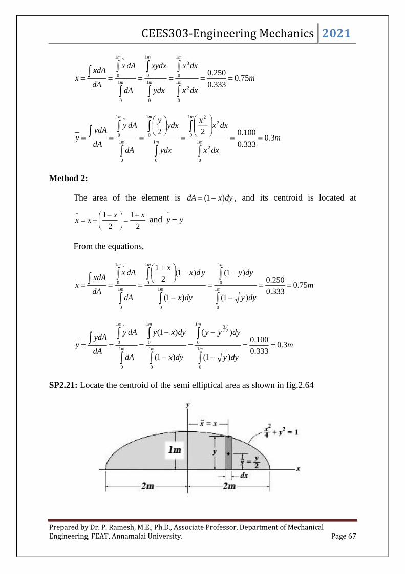
CEES303-Engineering Mechanics 2021
Prepared by Dr. P. Ramesh, M.E., Ph.D., Associate Professor, Department of MechanicalEngineering, FEAT, Annamalai University. Page 67
m
dxx
dxx
ydx
xydx
dA
dAx
dA
xdAx
m
m
m
m
m
m
75.0333.0
250.01
0
2
1
0
3
1
0
1
01
0
1
0
~
m
dxx
dxxx
ydx
ydxy
dA
dAy
dA
ydAy
m
m
m
m
m
m
3.0333.0
100.0221
0
2
1
0
22
1
0
1
01
0
1
0
~
Method 2:
The area of the element is dyxdA )1( , and its centroid is located at
2
1
2
1~ xxxx
and yy
~
From the equations,
m
dyy
dyy
dyx
ydxx
dA
dAx
dA
xdAx
m
m
m
m
m
m
75.0333.0
250.0
)1(
)1(
)1(
)1(2
1
1
0
1
01
0
1
01
0
1
0
~
m
dyy
dyyy
dyx
dyxy
dA
dAy
dA
ydAy
m
m
m
m
m
m
3.0333.0
100.0
)1(
)(
)1(
)1(
1
0
1
0
23
1
0
1
01
0
1
0
~
SP2.21: Locate the centroid of the semi elliptical area as shown in fig.2.64

CEES303-Engineering Mechanics 2021
Prepared by Dr. P. Ramesh, M.E., Ph.D., Associate Professor, Department of MechanicalEngineering, FEAT, Annamalai University. Page 68
Fig.2.64
Solution: Method 1
The area of the element is ydxdA and its centroid is located at xx ~
and2
~ yy
. Since the area is symmetrical about the y axis, then 0x .
From the equation,
m
dxx
dxx
ydx
ydxy
dA
dAy
dA
ydAy
m
m
m
m
m
m
m
m
m
m
m
m 424.034
41
41)(
22
2
2
2
2
2
2
2
2
22
2
2
2
~
Method 2:
The area of the element is xdydA and its centroid is located at 0~
x and yy ~
. Since the area is symmetrical about the y axis, then 0x . Here 212 yx
From the equation,
m
dyy
dyyy
xdy
xdyy
dA
dAy
dA
ydAy
m
m
m
m
m
m
424.034
14
14
)2(
)2(
1
0
2
1
0
2
1
0
1
01
0
1
0
~

CEES303-Engineering Mechanics 2021
Prepared by Dr. P. Ramesh, M.E., Ph.D., Associate Professor, Department of MechanicalEngineering, FEAT, Annamalai University. Page 69
SP2.22: Locate the centroid of the volume of a hemisphere of radius with respect to its
base.
Solution:
Fig.2.65 Hemisphere solids
With the axes chosen as shown in the figure, 0 zx by symmetry. The most
convenient is a circular slice of thickness dy parallel to the x – z plane. Since the
hemisphere intersect the y-z plane in the circle 222 rzy , the radius of the circular
slice is 22 rrz . The volume of the elemental slice becomes
dyyrdV )( 22
The equation becomes,
V
dVyy
c , rr
dyyrydyyry0
22
0
22 )()(
Where, yyc and integrating the above gives
43
4
1
3
2ryr , ry
8
3
CENTROID OF COMPOSITE SECTIONS:
A composite body consists of a series of connected “simpler” shaped bodies,
which may be rectangular, triangular, semi-circular, etc. Such a body can often be
sectioned or divided into its composite parts and, provided location of the centroid of

CEES303-Engineering Mechanics 2021
Prepared by Dr. P. Ramesh, M.E., Ph.D., Associate Professor, Department of MechanicalEngineering, FEAT, Annamalai University. Page 70
each of these parts are known, it can then eliminate the need for integration to determine
the centroid for the entire body. The centroid by moments is used as
....
......
321
332211
aaa
xaxaxa
A
axx
SP2.23: Find the centre of gravity of a 100mm x 150mm x 30mm of T section.
Solution:
Fig.2.66 T section
As the section is symmetrical about Y-Y axis, bisecting the web, therefore its
centre of gravity will lie on this axis. Split up the section into two rectangles ABCH and
DEFG.
Let bottom of the web FE be the axis of reference.
1) Rectangle ABCH,
21 300030100 mma and
mmy 1352
301501
2) Rectangle DEFG,
22 360030120 mma and
mmy 602
1202

CEES303-Engineering Mechanics 2021
Prepared by Dr. P. Ramesh, M.E., Ph.D., Associate Professor, Department of MechanicalEngineering, FEAT, Annamalai University. Page 71
We know that distance between centroid of the section and bottom of the flange
FE.
mmaa
yayay 1.94
36003000
)603600()1353000(
21
1111
SP2.24: Find the centroid of an unequal angle section 100mm x 80mm x 20mm.
Solution:
As the section is not symmetrical about any axis, therefore we have to find out
the values of x and y for the angle section. Split up the section into two rectangles.
Let left face of the vertical section and bottom face of the horizontal section be
axes of reference.
Fig.2.67 L section
1) Rectangle 1,
21 200020100 mma
mmx 102
201
and
mmy 502
1001
2) Rectangle 2,2
2 120020)2080( mma
mmx 502
60202
and
mmy 102
202

CEES303-Engineering Mechanics 2021
Prepared by Dr. P. Ramesh, M.E., Ph.D., Associate Professor, Department of MechanicalEngineering, FEAT, Annamalai University. Page 72
We know that distance between centroid of the section and left face.
mmaa
xaxax 25
12002000
)501200()102000(
21
1111
Similarly, distance between centroid of the section and bottom face.
mmaa
yayay 35
12002000
)101200()502000(
21
1111
SP2.25: Find the centroid of a segment of height 30mm of a sphere of radius 60mm.
Solution:
Fig.2.68 Segment of sphere
Let O be the centre of the given sphere and ABC is the segment of this sphere
as shown in figure. As the section is symmetrical about X-X axis, therefore its centre
of gravity lies on this axis.
Let O be the reference point. We know that centre of gravity of the segment of
sphere.
mmhr
hrx 5.40
)30603(4
)30602(3
)3(4
)2(3 22

CEES303-Engineering Mechanics 2021
Prepared by Dr. P. Ramesh, M.E., Ph.D., Associate Professor, Department of MechanicalEngineering, FEAT, Annamalai University. Page 73
SP2.26: Loacte the centroid of the wire as shown in fig.2.69
Fig.2.69 Wire geometry
Solution:
Fig.2.69
The wire is divided into three segments as shown in figure.
i)Segment 1:
mmrL 5.188601 , mmrx 601 ,
mmr
rd
dr
rd
rdr
L
ydL
y
L
2.386022
sin)(sin
2
0
2
0
2
2
0
2
001
and 01 z

CEES303-Engineering Mechanics 2021
Prepared by Dr. P. Ramesh, M.E., Ph.D., Associate Professor, Department of MechanicalEngineering, FEAT, Annamalai University. Page 74
ii) Segment :
mmL 402
02 x , mmy
y 202
22 and 02 z
iii) Segment:
mmL 203
03 x , 03 y and mmz
z 1023
3
We know that distance between centroid of the section
mmLLL
xLxLxLx 5.45
20405.188
)020()040()605.188(
321
332211
mmLLL
yLyLyLy 5.22
20405.188
)4020()2040()2.385.188(
321
332211
mmLLL
zLzLzLz 805.0
20405.188
)1020()040()05.188(
321
332211
SP2.27: A semi-circular area is removed from a trapezium as shown in fig.2.70 Find
the centroid of the remaining area.
Fig.2.70 Composite section
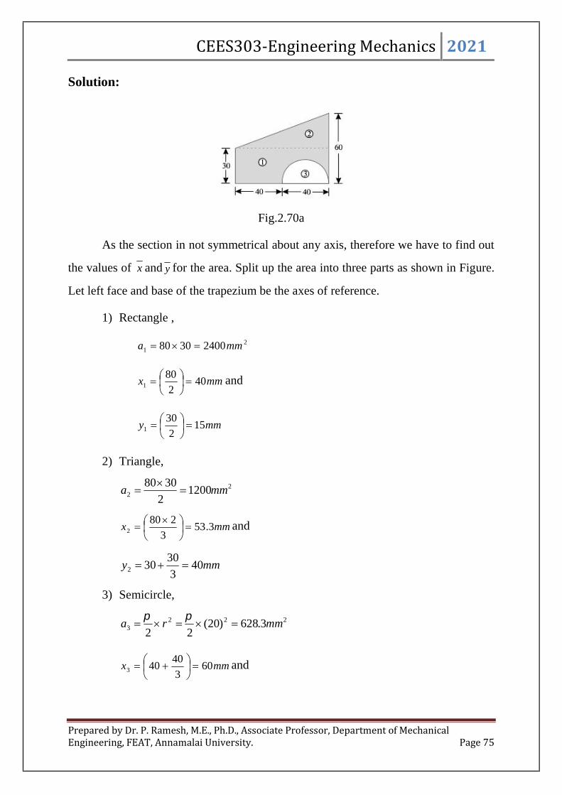
CEES303-Engineering Mechanics 2021
Prepared by Dr. P. Ramesh, M.E., Ph.D., Associate Professor, Department of MechanicalEngineering, FEAT, Annamalai University. Page 75
Solution:
Fig.2.70a
As the section in not symmetrical about any axis, therefore we have to find out
the values of x and y for the area. Split up the area into three parts as shown in Figure.
Let left face and base of the trapezium be the axes of reference.
1) Rectangle ,
21 24003080 mma
mmx 402
801
and
mmy 152
301
2) Triangle,
22 1200
2
3080mma
mmx 3.533
2802
and
mmy 403
30302
3) Semicircle,
2223 3.628)20(
22mmra
mmx 603
40403
and

CEES303-Engineering Mechanics 2021
Prepared by Dr. P. Ramesh, M.E., Ph.D., Associate Professor, Department of MechanicalEngineering, FEAT, Annamalai University. Page 76
mmr
y 5.83
204
3
43
We know that distance between centroid of the section and left face of trapezium.
mmaaa
xaxaxax 1.41
3.62812002400
)603.628()3.531200()402400(
321
331111
Similarly, distance between centroid of the section and base of the trapeium.
mmaaa
yayayay 5.26
3.62812002400
)5.83.628()401200()152400(
321
331111
SP2.28: A solid consists of a right circular and a hemisphere with a cone cut out from
the cylinder as shown in fig.2.71 Find the centroid of the body.
Fig.2.71 Composite solids
Solution:
As the solid is symmetrical about horizontal axis, therefore its centroid lie onb
this axis.
Let the left edge of the hemispherical portion € be the axis of reference.
i) Hemisphere ADE,
3331 14400060
3
2
3
2mmrv
and
mmr
x 5.378
605
8
51
ii) Right circular cylinder ABCD
3222 54000015060 mmhrv and
CEES303-Engineering Mechanics 2021
Prepared by Dr. P. Ramesh, M.E., Ph.D., Associate Professor, Department of MechanicalEngineering, FEAT, Annamalai University. Page 77
mmx 1358
605
2
150602
iii) Cone BCF
3223 18000015060
33mmhrv
and
mmx 5.1724
3150603
We know that distance between centroid of the solid and left edge of the
hemisphere, then
321
332211
vvv
xvxvxvx
75.93180000540000144000
)5.172180000()135540000()5.37144000(
x
CENTRE OF GRAVITY AND ITS IMPLICATIONS:
The centre of gravity is a geometric property of any object. The centre of gravity
is the average location of the weight of an object. It can completely describe
the motion of any object through space in terms of the translation of the centre of
gravity of the object from one place to another, and the rotation of the object about its
centre of gravity if it is free to rotate. If the object is confined to rotate about some other
point, like a hinge, it can still describe its motion.
In flight, both airplanes and rockets rotate about their centres of gravity. A kite,
on the other hand, rotates about the bridle point. But the trim of a kite still depends on
the location of the centre of gravity relative to the bridle point, because for every object
the weight always acts through the centre of gravity.
Determining the centre of gravity is very important for any flying object. How
do engineers determine the location of the centre of gravity for an aircraft which they
are designing? In general, determining the centre of gravity (cg) is a complicated

CEES303-Engineering Mechanics 2021
Prepared by Dr. P. Ramesh, M.E., Ph.D., Associate Professor, Department of MechanicalEngineering, FEAT, Annamalai University. Page 78
procedure because the mass (and weight) may not be uniformly distributed throughout
the object. The general case requires the use of calculus. If the mass is uniformly
distributed, the problem is greatly simplified. If the object has a line (or plane)
of symmetry, the centre of gravity lies on the line of symmetry. For a solid block of
uniform material, the centre of gravity is simply at the average location of the physical
dimensions. (For a rectangular block, 50 X 20 X 10, the centre of gravity is at the point
(25,10, 5) ). For a triangle of height h, the centre of gravity is at h/3, and for a semi-
circle of radius r, the centre of gravity is at3
4rwhere is ratio of the circumference of
the circle to the diameter.
For a general shaped object, there is a simple mechanical way to determine the centre
of gravity:
1. If just balance the object using a string or an edge, the point at which the object
is balanced is the centre of gravity. (Just like balancing a pencil on your finger!)
2. Another, more complicated way, is a two-step method shown on the slide.
In Step 1, you hang the object from any point and drop a weighted string
from the same point. Draw a line on the object along the string.
For Step 2, repeat the procedure from another point on the object and now
it has two lines drawn on the object which intersect. The centre of gravity is the
point where the lines intersect. This procedure works well for irregularly shaped
objects that are hard to balance.
If the mass of the object is not uniformly distributed, it must use calculus to
determine centre of gravity. It will use the symbol dW to denote the integration of a
continuous function with respect to weight. Then the centre of gravity can be
determined from:
dWxWx

CEES303-Engineering Mechanics 2021
Prepared by Dr. P. Ramesh, M.E., Ph.D., Associate Professor, Department of MechanicalEngineering, FEAT, Annamalai University. Page 79
Where x is the distance from a reference line, dw is an increment of weight,
and W is the total weight of the object. To evaluate the right side, it has to determine
how the weight varies geometrically. From the weight equation, we know that:
gmW
Where m is the mass of the object, and g is the gravitational constant. In turn,
the mass m of any object is equal to the density , of the object times the volume, V:
Vm
Now, it can combine the last two equations:
VgW
Then
dVgdW
)(),,( dzdydxgzyxdW
If it has a functional form for the mass distribution, then it can solve the equation for
the center of gravity:
dxdydzzyxgWgc ),,(..
where indicates a triple integral over dx, dy and dz. If don't know the
functional form of the mass distribution, it can numerically integrate the equation using
a spreadsheet. Divide the distance into a number of small volume segments and
determining the average value of the weight/volume (density times gravity) over that
small segment. Taking the sum of the average value of the weight/volume times the
distance times the volume segment divided by the weight will produce the centre of
gravity.

CEES303-Engineering Mechanics 2021
Prepared by Dr. P. Ramesh, M.E., Ph.D., Associate Professor, Department of MechanicalEngineering, FEAT, Annamalai University. Page 80
MOMENT OF INERTIA:
The moment of a force (F) about a point, is the product of the force and
perpendicular distance (d) between the point and the line of action of the force
(i.e.M=dF). This moment is also called first moment of force. If this moment is again
multiplied by the perpendicular distance (d) between the point and the line of action of
the force i.e. FdFddM 2).( , then this quantity is called moment of the moment of
a force or second moment of force or moment of inertia (briefly written as M.I. or I).
Sometimes, instead of force, area or mass of a figure or body is taken into consideration.
Then the second moment is known as second moment of area or second moment of
mass. But all such second moments are broadly termed as moment of inertia.
AREA MOMENT OF INERTIA- DEFINITION:
Consider a plane area, whose moment of inertia is required to be found out.
Split up the whole area into a number of small elements.
Let a1, a2, a3, ... = Areas of small elements, and
r1, r2, r3, ... = Corresponding distances of the elements from the line about
which the moment of inertia is required to be found out.
Now the moment of inertia of the area,
233
22
21 .... arrararaI

CEES303-Engineering Mechanics 2021
Prepared by Dr. P. Ramesh, M.E., Ph.D., Associate Professor, Department of MechanicalEngineering, FEAT, Annamalai University. Page 81
MOMENT OF INERTIA OF PLANE SECTIONS FROM FIRST
PRINCIPLES:
Fig.2.72 Moment of inertia of plane sections
The moment of inertia of an area may also be found out by the method of
integration as discussed below:
Consider a plane figure, whose moment of inertia is required to be found out
about X-X axis and Y-Y axis as shown in Fig.2.72. Let us divide the whole area into a
no. of strips. Consider one of these strips.
Let dA = Area of the strip
x = Distance of the centre of gravity of the strip on X-X axis and
y = Distance of the centre of gravity of the strip on Y-Y axis.
We know that the moment of inertia of the strip about Y-Y axis
= dA . x2
Now the moment of inertia of the whole area may be found out by integrating
above equation. i.e.,
2.xdAIYY
X
Y
y
x
O

CEES303-Engineering Mechanics 2021
Prepared by Dr. P. Ramesh, M.E., Ph.D., Associate Professor, Department of MechanicalEngineering, FEAT, Annamalai University. Page 82
Similarly 2.ydAI xx
THEOREMS OF MOMENT OF INERTIA:
1. Theorem of parallel axis
2. Theorem of perpendicular axis
1) Theorem of parallel axis:
It states, If the moment of inertia of a plane area about an axis through its centre
of gravity is denoted by IG, then moment of inertia of the area about any other axis AB,
parallel to the first, and at a distance ‘h’ from the centre of gravity is given by:
2ahII GAB
where , IAB = Moment of inertia of the area about an axis AB,
IG = Moment of Inertia of the area about its centre of gravity
a = Area of the section, and
h = Distance between centre of gravity of the section and axis AB.
Fig.2.73 Circular lamina
Proof:
Consider a strip of a circle, whose moment of inertia is required to be found out
about a line AB as shown in Figure.
Let da = Area of the strip,
y = Distance of the strip from the centre of gravity the section and
h = Distance between centre of gravity of the section and the axis AB.

CEES303-Engineering Mechanics 2021
Prepared by Dr. P. Ramesh, M.E., Ph.D., Associate Professor, Department of MechanicalEngineering, FEAT, Annamalai University. Page 83
We know that moment of inertia of the whole section about an axis passing
through the centre of gravity of the section
= da. y2
and moment of inertia of the whole section about an axis passing through its centre of
gravity,
2..ydaIG ∴ Moment of inertia of the section about the axis AB,
)2()( 222 hyyhdayhdaI AB
).2().().( 22 dahydaydahI AB
02 GAB IahI
It may be noted that ∑ h2 . da = a h2 and ∑ y2 . da = IG
Now the ∑ y. da is the algebraic sum of moments of all the areas about an axis through
centre of gravity of the section and is equal to ya.. , where y is the distance between
the section and the axis passing through the centre of gravity, which obviously is zero.
2) Theorem of perpendicular axis
It states, If IXX and IYY be the moments of inertia of a plane section about two
perpendicular axis meeting at O, the moment of inertia IZZ about the axis Z-Z,
perpendicular to the plane and passing through the intersection of X-X and Y-Y is given
by:
YYXXZZ III
Fig.2.74 Theorem of perpendicular axis
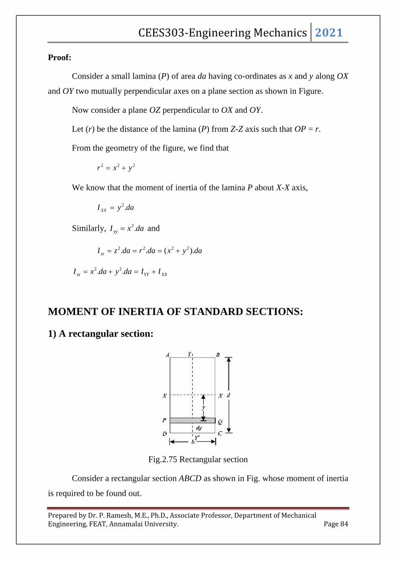
CEES303-Engineering Mechanics 2021
Prepared by Dr. P. Ramesh, M.E., Ph.D., Associate Professor, Department of MechanicalEngineering, FEAT, Annamalai University. Page 84
Proof:
Consider a small lamina (P) of area da having co-ordinates as x and y along OX
and OY two mutually perpendicular axes on a plane section as shown in Figure.
Now consider a plane OZ perpendicular to OX and OY.
Let (r) be the distance of the lamina (P) from Z-Z axis such that OP = r.
From the geometry of the figure, we find that
222 yxr
We know that the moment of inertia of the lamina P about X-X axis,
dayI XX .2
Similarly, daxI yy .2 and
dayxdardazI zz ).(.. 2222
XXYYzz IIdaydaxI .. 22
MOMENT OF INERTIA OF STANDARD SECTIONS:
1) A rectangular section:
Fig.2.75 Rectangular section
Consider a rectangular section ABCD as shown in Fig. whose moment of inertia
is required to be found out.

CEES303-Engineering Mechanics 2021
Prepared by Dr. P. Ramesh, M.E., Ph.D., Associate Professor, Department of MechanicalEngineering, FEAT, Annamalai University. Page 85
Let b = Width of the section and
d = Depth of the section.
Now consider a strip PQ of thickness dy parallel to X-X axis and at a distance y
from it as shown in the figure∴ Area of the strip = b.dy
We know that moment of inertia of the strip about X-X axis,
= Area × y2 = (b. dy) y2 = b. y2. dy
Now the moment of inertia of the whole section may be found out by integrating the
above equation for the whole length of the lamina i.e. from2
d to
2
d.
2
2
2
2
22 ...
d
d
d
dxx dyybdyybI
123
232
3
333
2
2
3 bdddb
ybI
d
dxx
Similarly,
12
3dbI xx
2) Circular Section:
Fig.2.76 Circular section
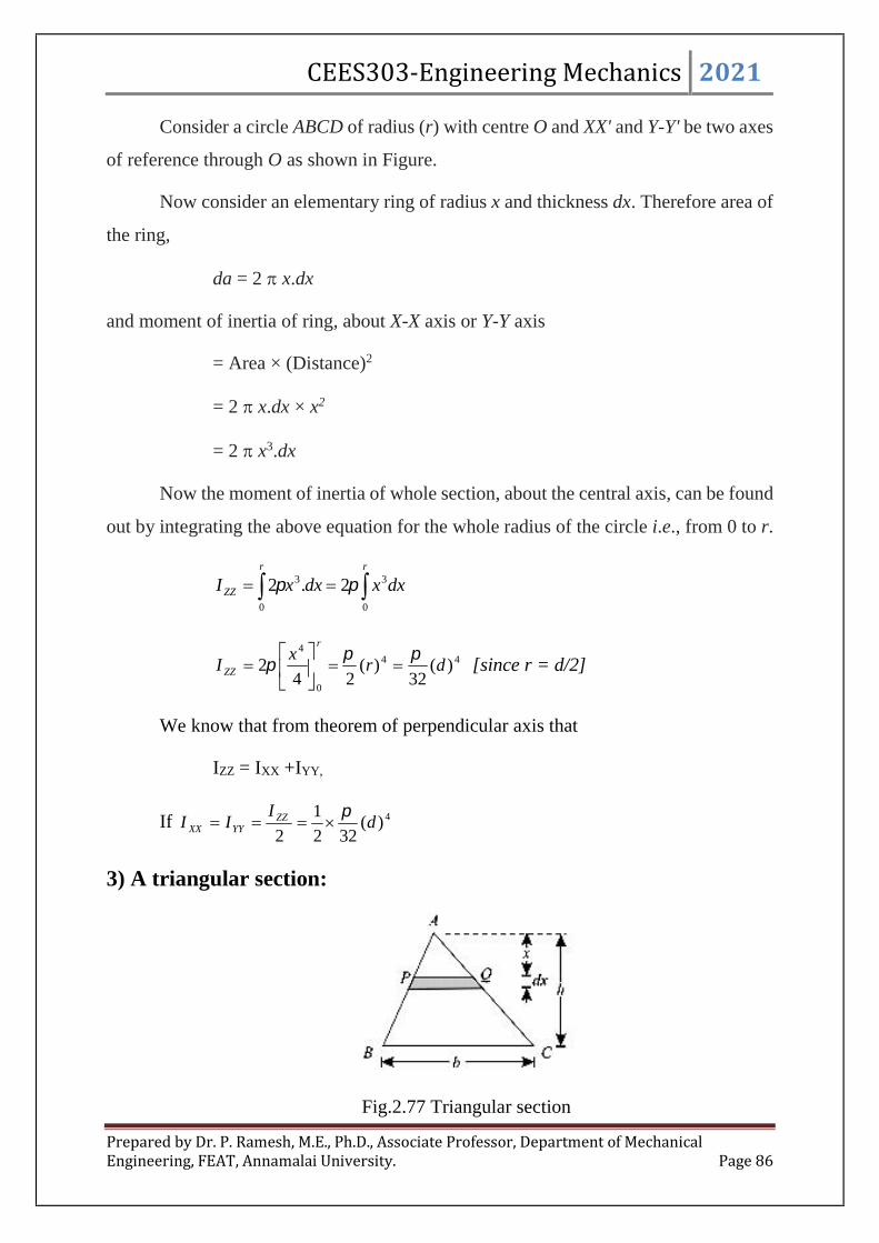
CEES303-Engineering Mechanics 2021
Prepared by Dr. P. Ramesh, M.E., Ph.D., Associate Professor, Department of MechanicalEngineering, FEAT, Annamalai University. Page 86
Consider a circle ABCD of radius (r) with centre O and XX' and Y-Y' be two axes
of reference through O as shown in Figure.
Now consider an elementary ring of radius x and thickness dx. Therefore area of
the ring,
da = 2 x.dx
and moment of inertia of ring, about X-X axis or Y-Y axis
= Area × (Distance)2
= 2 x.dx × x2
= 2 x3.dx
Now the moment of inertia of whole section, about the central axis, can be found
out by integrating the above equation for the whole radius of the circle i.e., from 0 to r.
rr
ZZ dxxdxxI0
3
0
3 2.2
44
0
4
)(32
)(24
2 drx
Ir
ZZ
[since r = d/2]
We know that from theorem of perpendicular axis that
IZZ = IXX +IYY,
If 4)(322
1
2d
III ZZ
YYXX
3) A triangular section:
Fig.2.77 Triangular section

CEES303-Engineering Mechanics 2021
Prepared by Dr. P. Ramesh, M.E., Ph.D., Associate Professor, Department of MechanicalEngineering, FEAT, Annamalai University. Page 87
Consider a triangular section ABC whose moment of inertia is required to be
found out.
Let, b = Base of the triangular section and
h = Height of the triangular section.
Now consider a small strip PQ of thickness dx at a distance of x from the vertex
A as shown in Fig. 7.8. From the geometry of the figure, we find that the two triangles
APQ and ABC are similar.
Therefore
h
x
BC
PQ or
h
bx
h
xBCPQ
.[since BC = base = b]
We know that area of the strip PQ
dxh
bx.
and moment of inertia of the strip about the base BC
= Area × (Distance)2 dxxhh
bxxhdx
h
bx 22 )()(
Now moment of inertia of the whole triangular section may be found out by
integrating the above equation for the whole height of the triangle i.e., from 0 to h.
h
BC dxxhh
bxI
0
2)(
hh
BC dxhxxxhh
bdxhxxh
h
bxI
0
232
0
22 )2()2(
123
2
42
3
0
3422 bhhxxhx
h
bI
h
BC
We know that distance between centre of gravity of the triangular section and
base BC.

CEES303-Engineering Mechanics 2021
Prepared by Dr. P. Ramesh, M.E., Ph.D., Associate Professor, Department of MechanicalEngineering, FEAT, Annamalai University. Page 88
3
hd
Since, the moment of inertia of the triangular section about an axis through its centre of
gravity and parallel to X-X axis.
2adII BCG
363212
323 bhhbhbhIG
Note: The moment of inertia of section about an axis through its vertex and parallel to
the base
436
9
3
2
236
33232 bhbhhbhbh
adIG
Moment of inertia of composite sections:
The moment of inertia of a composite section may be found out by the following
steps:
1. First of all, split up the given section into plane areas (i.e., rectangular,
triangular, circular etc., and find the centre of gravity of the section).
2. Find the moments of inertia of these areas about their respective centres of
gravity.
3. Now transfer these moment of inertia about the required axis (AB) by the
Theorem of Parallel Axis, i.e.,
2ahII GAB
where IG = Moment of inertia of a section about its centre of gravity and parallel
to the axis.
a = Area of the section,
h = Distance between the required axis and centre of gravity of the
section.
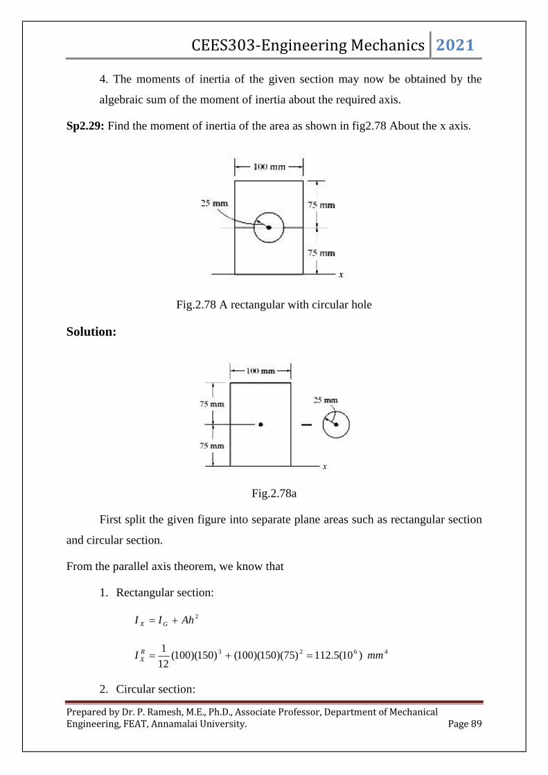
CEES303-Engineering Mechanics 2021
Prepared by Dr. P. Ramesh, M.E., Ph.D., Associate Professor, Department of MechanicalEngineering, FEAT, Annamalai University. Page 89
4. The moments of inertia of the given section may now be obtained by the
algebraic sum of the moment of inertia about the required axis.
Sp2.29: Find the moment of inertia of the area as shown in fig2.78 About the x axis.
Fig.2.78 A rectangular with circular hole
Solution:
Fig.2.78a
First split the given figure into separate plane areas such as rectangular section
and circular section.
From the parallel axis theorem, we know that
1. Rectangular section:
2AhII GX
4623 )10(5.112)75)(150)(100()150)(100(12
1mmI R
X
2. Circular section:

CEES303-Engineering Mechanics 2021
Prepared by Dr. P. Ramesh, M.E., Ph.D., Associate Professor, Department of MechanicalEngineering, FEAT, Annamalai University. Page 90
46224 )10(4.11)75()25()25(4
1mmI C
X
Composite section:
4666 )10(1.101)10(4.11)10(5.112 mmIII CX
RXX
SP2.30: Find the moments of inertia for the cross sectional area of the member as shown
in fig.2.79 about the x and y centroid axes.
Fig.2.79
Solution:
Fig.2.79a
First split the given figure into separate plane areas such as rectangular section
and denoted each section as A, B and D.

CEES303-Engineering Mechanics 2021
Prepared by Dr. P. Ramesh, M.E., Ph.D., Associate Professor, Department of MechanicalEngineering, FEAT, Annamalai University. Page 91
From the parallel axis theorem, we know that
1. Rectangular section A and D:
2AhII GX
4623 )10(1425)200)(300)(100()300)(100(12
1mmI A
X
4623 )10(1900)250)(100)(300()100)(300(12
1mmI C
Y
2. Rectangular section B:
463 )10(500)100)(600(12
1mmI B
X
463 )10(18000)600)(100(12
1mmI B
Y
Composite section:
46666 )10(2900)10(1425)10(50)10(1425 mmIIII DX
CX
AXX
46666 )10(5600)10(1900)10(1800)10(1900 mmIIII DY
CY
AYY
MASS MOMENT OF INERTIA:
Fig.2.80 Rigid body
The mass moment of inertia of a body is a measure of the body’s resistance to
angular acceleration. Since it is used in dynamics to study rotational motion. Consider
the rigid body as shown in Fig.2.80. It define the mass moment of inertia of the body
about the z axis as
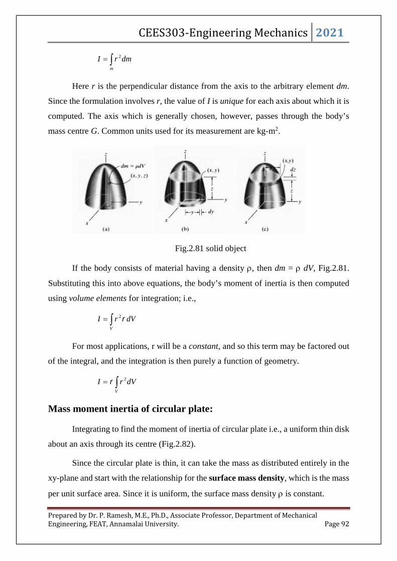
CEES303-Engineering Mechanics 2021
Prepared by Dr. P. Ramesh, M.E., Ph.D., Associate Professor, Department of MechanicalEngineering, FEAT, Annamalai University. Page 92
m
dmrI 2
Here r is the perpendicular distance from the axis to the arbitrary element dm.
Since the formulation involves r, the value of I is unique for each axis about which it is
computed. The axis which is generally chosen, however, passes through the body’s
mass centre G. Common units used for its measurement are kg-m2.
Fig.2.81 solid object
If the body consists of material having a density , then dm = dV, Fig.2.81.
Substituting this into above equations, the body’s moment of inertia is then computed
using volume elements for integration; i.e.,
V
dVrI 2
For most applications, r will be a constant, and so this term may be factored out
of the integral, and the integration is then purely a function of geometry.
V
dVrI 2
Mass moment inertia of circular plate:
Integrating to find the moment of inertia of circular plate i.e., a uniform thin disk
about an axis through its centre (Fig.2.82).
Since the circular plate is thin, it can take the mass as distributed entirely in the
xy-plane and start with the relationship for the surface mass density, which is the mass
per unit surface area. Since it is uniform, the surface mass density is constant.
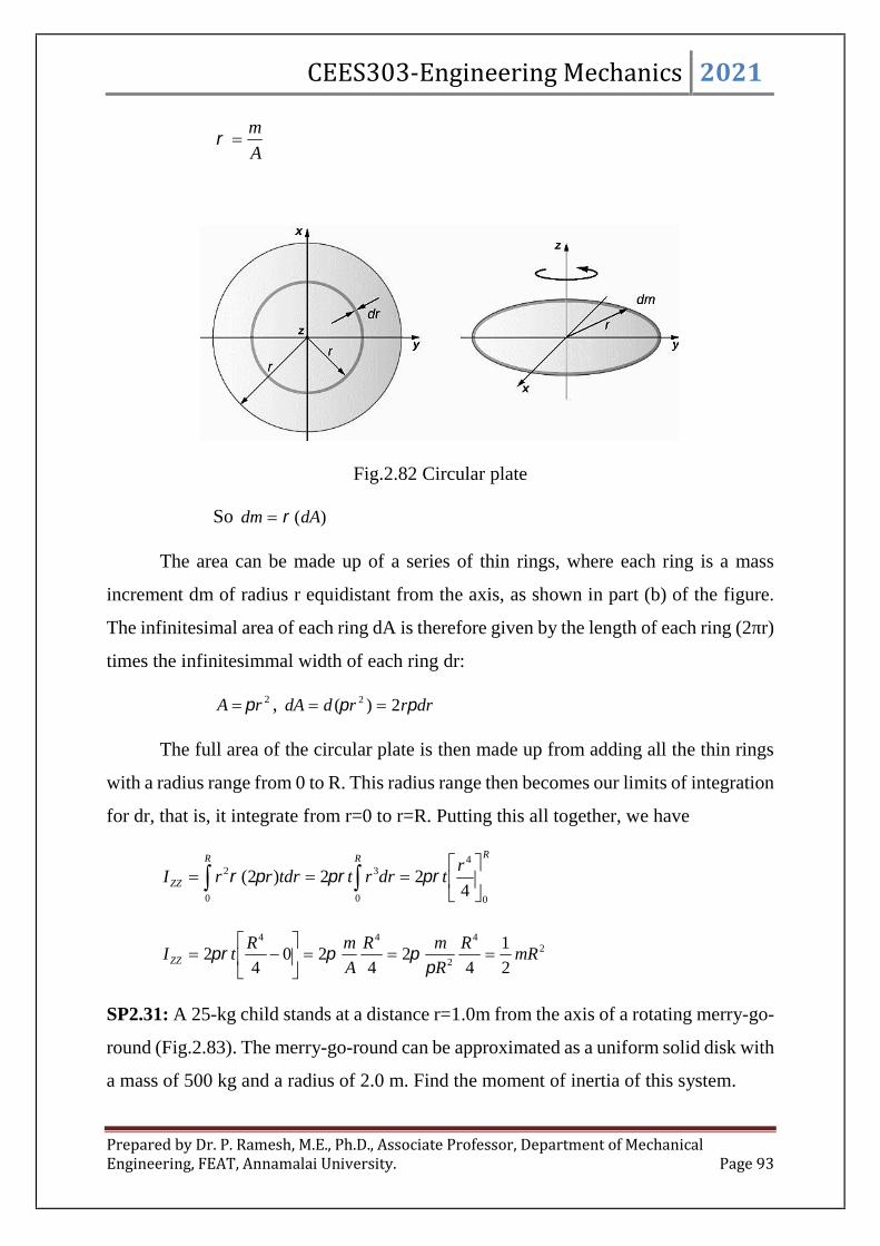
CEES303-Engineering Mechanics 2021
Prepared by Dr. P. Ramesh, M.E., Ph.D., Associate Professor, Department of MechanicalEngineering, FEAT, Annamalai University. Page 93
A
m
Fig.2.82 Circular plate
So )(dAdm
The area can be made up of a series of thin rings, where each ring is a mass
increment dm of radius r equidistant from the axis, as shown in part (b) of the figure.
The infinitesimal area of each ring dA is therefore given by the length of each ring (2πr)
times the infinitesimmal width of each ring dr:
2rA , drrrddA 2)( 2
The full area of the circular plate is then made up from adding all the thin rings
with a radius range from 0 to R. This radius range then becomes our limits of integration
for dr, that is, it integrate from r=0 to r=R. Putting this all together, we have
R RR
ZZ
rtdrrttdrrrI
0 0
4
0
32
422)2(
24
2
44
2
1
42
420
42 mR
R
R
mR
A
mRtIZZ
SP2.31: A 25-kg child stands at a distance r=1.0m from the axis of a rotating merry-go-
round (Fig.2.83). The merry-go-round can be approximated as a uniform solid disk with
a mass of 500 kg and a radius of 2.0 m. Find the moment of inertia of this system.

CEES303-Engineering Mechanics 2021
Prepared by Dr. P. Ramesh, M.E., Ph.D., Associate Professor, Department of MechanicalEngineering, FEAT, Annamalai University. Page 94
Fig.2.83 Merry – go – round with child
Solution:
For the child, 2rmI CC and for the merry – go – round 2
2
1rmI mm . Therefore
222 .1025100025)2)(500(2
1)1(25 mkgI total
Mass moment inertia of Cylinder:
Fig.2.84 Cylinder solids
The shell element is considered to resolve the mass moment of inertia of cylinder
as shown in fig.2.84b. Thus only a single integration is required. The volume of the
element is dV=(2r)(h)dr and so its mass is dm=dV = (2hrdr). Since the entire
element lies at the same distance r from the z axis, the moment of inertia of the element
is
R
m
Z hRdrrhdmrZdI0
232
22

CEES303-Engineering Mechanics 2021
Prepared by Dr. P. Ramesh, M.E., Ph.D., Associate Professor, Department of MechanicalEngineering, FEAT, Annamalai University. Page 95
Since the mass of the cylinder is
2
0
2 hRrdrhdmmR
m
Then,
2
2
1mRIZZ
Mass moment inertia of Cone:
Fig.2.85 Moment of inertia of cone
A circular slice of radius r and thickness dx is chosen as the volume element. By
the similarity of the triangle xh
Rr . The volume of element dxrdV 2 and its
elemental mass dxrdVdm 2 . Also to recall the moment of inertia of elemental
disc which is
dxrrdxrdmr 4222
2
1
2
1
2
1
We know that, xh
Rr
The moment of inertia about the X-axis of the cone is
hhhh
XX
x
h
Rdxx
h
Rdxx
h
RrdmI
0
5
4
4
0
44
4
0
4
0
2
522
1
2
1)
2
1(
dx
O
x
r x
h

CEES303-Engineering Mechanics 2021
Prepared by Dr. P. Ramesh, M.E., Ph.D., Associate Professor, Department of MechanicalEngineering, FEAT, Annamalai University. Page 96
1052
45
4
4 hRh
h
RI XX
But mass of the cone
33
2
0
3
2
2
0
22
2
0
2 hRx
h
Rdxx
h
Rdxrm
hhh
Therefore,
2
10
3mRIXX
Mass moment inertia of Sphere:
Fig.2.86 Moment of inertia 0f sphere
A circular slice of radius y and thickness dx is chosen as the volume element.
The volume of element dxydV 2
2
1 and its mass dxydVdm 2
2
1 . The moment
of inertia about the x-axis of the elemental cylinder is
dxxrdxyydxyydmdI XX
22222222
222
1)(
Where is the constant density of the sphere. The total moment of inertia about
the axis is
5222
15
8)(
2rdxxrI
r
r
XX

CEES303-Engineering Mechanics 2021
Prepared by Dr. P. Ramesh, M.E., Ph.D., Associate Professor, Department of MechanicalEngineering, FEAT, Annamalai University. Page 97
Since the mass of the sphere is
r
r
r
r
r
rm
xxrdxxrdxydmm
)
3()(
32222
3333
23
2
3
4
3
2
3
2)
3()
3( r
rrrrr
rrrm
Therefore,
223
5
2
5
2
3
4mrrrI XX

Lecture Notes
UNIT – 3 2021
Prepared by
Dr. P. Ramesh, M.E., Ph.D.,
Associate Professor
Department of Mechanical Engineering
Faculty of Engineering and Technology
Annamalai UniversityAug-2021
CEES303-EngineeringMechanics

CEES303-Engineering Mechanics 2021
Prepared by Dr. P. Ramesh, M.E., Ph.D., Associate Professor, Department of MechanicalEngineering, FEAT, Annamalai University. Page 2
Unit - 3
Friction covering, Types of friction, Limiting friction, Laws of
Friction, Static and Dynamic Friction; Motion of Bodies, wedge
friction, screw jack & differential screw jack.
Virtual Work and Energy Method- Virtual displacements,
principle of virtual work for particle and ideal system of rigid
bodies, degrees of freedom. Active force diagram, systems with
friction, mechanical efficiency. Conservative forces and potential
energy (elastic and gravitational), energy equation for equilibrium.
Applications of energy method for equilibrium. Stability of
equilibrium.
Reference for the preparation of course material:
1. F. P. Beer and E. R. Johnston (2011), Vector Mechanics for Engineers,Vol I - Statics, Vol II, – Dynamics, 9th Ed, Tata McGraw Hill.
2. Khurmi R.S. (2010), Engineering Mechanics, S. Chand & Co.3. J.L. Meriam and L. G. Kraige, Engineering Mechanics –Statics, volume I,
Seventh edition, John Wiley & Sons, Inc.
TEXT BOOKS1. Irving H. Shames (2006), Engineering Mechanics, 4th Edition, Prentice Hall2. F. P. Beer and E. R. Johnston (2011), Vector Mechanics for Engineers, Vol I -
Statics, Vol II, – Dynamics, 9th Ed, Tata McGraw Hill
REFERENCES1. R. C. Hibbler (2006), Engineering Mechanics: Principles of Statics and Dynamics,
Pearson Press.2. Khurmi R.S. (2010), Engineering Mechanics, S. Chand & Co.

CEES303-Engineering Mechanics 2021
Prepared by Dr. P. Ramesh, M.E., Ph.D., Associate Professor, Department of MechanicalEngineering, FEAT, Annamalai University. Page 3
Unit - 3
Friction and Energy of Rigid Bodies
FRICTION:
A force that resist the movement of two contacting surfaces that slide relative to
one other is known as friction force or friction. This force always acts tangent to the
surface at the point of contact and is directed so as to oppose the possible or existing
motion between the surfaces.
In some types of machines and processes, this want to minimize the retarding
effect of friction forces. Examples are bearings of all types, power screws, gears, the
flow of fluids in pipes, and the propulsion of aircraft and missiles through the
atmosphere. In other situations this to maximize the effects of friction, as in brakes,
clutches, belt drives, and wedges. Wheeled vehicles depend on friction for both starting
and stopping, and ordinary walking depends on friction between the shoe and the
ground.
Friction forces are present throughout nature and exist in all machines no matter
how accurately constructed or carefully lubricated. A machine or process in which
friction is small enough to be neglected is said to be ideal. When friction must be taken
into account, the machine or process is termed real. In all cases where there is sliding
motion between parts, the friction forces result in a loss of energy which is dissipated
in the form of heat. Wear is another effect of friction.
TYPES OF FRICTION;
The types of frictional resistance encountered in mechanics are
a) Dry Friction:
Dry friction occurs when the unlubricated surfaces of two solids are in
contact under a condition of sliding or a tendency to slide. A friction force

CEES303-Engineering Mechanics 2021
Prepared by Dr. P. Ramesh, M.E., Ph.D., Associate Professor, Department of MechanicalEngineering, FEAT, Annamalai University. Page 4
tangent to the surfaces of contact occurs both during the interval leading up
to impending slippage and while slippage takes place. The direction of this
friction force always opposes the motion or impending motion. This type of
friction is also called Coulomb friction. The principles of dry or Coulomb
friction were developed largely from the experiments of Coulomb in 1781
and from the work of Morin from 1831 to 1834. Although we do not yet have
a comprehensive theory of dry friction. This dry friction is followed as
i) Static friction:
It is the friction experienced by a body when it is rest or it is the
friction when the body tends to move.
ii) Dynamic friction:
It is the friction experience by a body when it is in motion. It is
also called kinetic friction. The dynamic friction is of the following two
types;
1) Sliding friction:
It is the friction experienced by a body when it slides over
another body.
2) Rolling friction:
It is the friction, experienced by a body when it rolls over
another.
b) Fluid Friction:
Fluid friction occurs when adjacent layers in a fluid (liquid or gas) are
moving at different velocities. This motion causes frictional forces between fluid
elements, and these forces depend on the relative velocity between layers. When
there is no relative velocity, there is no fluid friction. Fluid friction depends not
only on the velocity gradients within the fluid but also on the viscosity of the
fluid, which is a measure of its resistance to shearing action between fluid layers.
Fluid friction is treated in the study of fluid mechanics and will not be discussed
here.

CEES303-Engineering Mechanics 2021
Prepared by Dr. P. Ramesh, M.E., Ph.D., Associate Professor, Department of MechanicalEngineering, FEAT, Annamalai University. Page 5
c) Internal Friction:
Internal friction occurs in all solid materials which are subjected to
cyclical loading. For highly elastic materials the recovery from deformation
occurs with very little loss of energy due to internal friction. For materials which
have low limits of elasticity and which undergo appreciable plastic deformation
during loading, a considerable amount of internal friction may accompany this
deformation. The mechanism of internal friction is associated with the action of
shear deformation, which is discussed in references on materials science.
LIMITING FRICTION:
It has been observed that when a body, lying over another body, is gently pushed,
it does not move because of the frictional force, which prevents the motion. It shows
that the force of the hand is being exactly balanced by the force of friction, acting in the
opposite direction. If again push the body, a little harder, it is still found to be in
equilibrium. It shows that the force of friction has increased itself so as to become equal
and opposite to the applied force. Thus the force of friction has a remarkable property
of adjusting its magnitude, so as to become exactly equal and opposite to the applied
force, which tends to produce motion. There is, however, a limit beyond which the force
of friction cannot increase. If the applied force exceeds this limit, the force of friction
cannot balance it and the body begins to move, in the direction of the applied force.
This maximum value of frictional force, which comes into play, when a body just begins
to slide over the surface of the other body, is known as limiting friction. It may be noted
that when the applied force is less than the limiting friction, the body remains at rest,
and the friction is called static friction, which may have any value between zero and
limiting friction.
LAWS OF FRICTION
Prof. Coulomb, after extensive experiments, gave some laws of friction, which
may be grouped under the following heads :
1. Laws of static friction, and

CEES303-Engineering Mechanics 2021
Prepared by Dr. P. Ramesh, M.E., Ph.D., Associate Professor, Department of MechanicalEngineering, FEAT, Annamalai University. Page 6
2. Laws of kinetic or dynamic friction.
LAWS OF STATIC FRICTION
Following are the laws of static friction as
1. The force of friction always acts in a direction, opposite to that in which
the body tends to move, if the force of friction would have been absent.
2. The magnitude of the force of friction is exactly equal to the force,
which tends to move the body.
3. The magnitude of the limiting friction bears a constant ratio to the
normal reaction between the two surfaces. Mathematically:
tConsR
Ftan ------- (3.1)
Where, F = Limiting friction, and
R = Normal reaction.
4. The force of friction is independent of the area of contact between the
two surfaces.
5. The force of friction depends upon the roughness of the surfaces.
LAWS OF KINETIC OR DYNAMIC FRICTION:
Following are the laws of kinetic or dynamic friction as
1. The force of friction always acts in a direction, opposite to that in which
the body is moving.
2. The magnitude of kinetic friction bears a constant ratio to the normal
reaction between the two surfaces. But this ratio is slightly less than that
in case of limiting friction.
3. For moderate speeds, the force of friction remains constant. But it
decreases slightly with the increase of speed.

CEES303-Engineering Mechanics 2021
Prepared by Dr. P. Ramesh, M.E., Ph.D., Associate Professor, Department of MechanicalEngineering, FEAT, Annamalai University. Page 7
MECHANISM OF DRY FRICTION:
Consider a solid block of mass ‘m’ resting on a horizontal surface, as shown in
Fig.3.1 (a). Assume that the contacting surfaces have some roughness. The experiment
involves the application of a horizontal force ‘P’ which continuously increases from
zero to a value sufficient to move the block and give it an appreciable velocity. The
free-body diagram of the block for any value of ‘P’ is shown in Fig.3.1 (b), where the
tangential friction force exerted by the plane on the block is labelled ‘F’. This friction
force acting on the body will always be in a direction to oppose motion or the tendency
toward motion of the body. There is also a normal force N which in this case equals
‘mg’ and the total force ‘R’ exerted by the supporting surface on the block is the
resultant of ‘N’ and ‘F’.
A magnified view of the irregularities of the mating surfaces, Fig.3.2 (c), helps
us to visualize the mechanical action of friction. Support is necessarily intermittent and
exists at the mating humps. The direction of each of the reactions on the block, R1, R2,
R3, etc., depends not only on the geometric profile of the irregularities but also on the
extent of local deformation at each contact point. The total normal force ‘N’ is the sum
of the n-components of the R's, and the total frictional force ‘F’ is the sum of the t-
components of the R's. When the surfaces are in relative motion, the contacts are more
nearly along the tops of the humps, and the t-components of the R's are smaller than
when the surfaces are at rest relative to one another. This observation helps to explain
the well-known fact that the force ‘P’ necessary to maintain motion is generally less
than that required to start the block when the irregularities are more nearly in mesh.
If perform the experiment and record the friction force ‘F’ as a function of ‘P’,
then obtain the relation shown in Fig.3.1 (d). When ‘P’ is zero, equilibrium requires that
there be no friction force. As ‘P’ is increased, the friction force must be equal and
opposite of ‘P’ as long as the block does not slip. During this period the block is in
equilibrium, and all forces acting on the block must satisfy the equilibrium equations.
Finally, it reach a value of ‘P’ which causes the block to slip and to move in the direction
of the applied force. At this same time the friction force decreases slightly and abruptly.
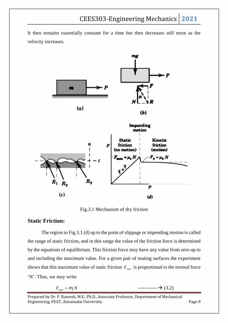
CEES303-Engineering Mechanics 2021
Prepared by Dr. P. Ramesh, M.E., Ph.D., Associate Professor, Department of MechanicalEngineering, FEAT, Annamalai University. Page 8
It then remains essentially constant for a time but then decreases still more as the
velocity increases.
Fig.3.1 Mechanism of dry friction
Static Friction:
The region in Fig.3.1 (d) up to the point of slippage or impending motion is called
the range of static friction, and in this range the value of the friction force is determined
by the equations of equilibrium. This friction force may have any value from zero up to
and including the maximum value. For a given pair of mating surfaces the experiment
shows that this maximum value of static friction maxF is proportional to the normal force
‘N’. Thus, we may write
NF Smax ------------ (3.2)

CEES303-Engineering Mechanics 2021
Prepared by Dr. P. Ramesh, M.E., Ph.D., Associate Professor, Department of MechanicalEngineering, FEAT, Annamalai University. Page 9
Where k s is the proportionality constant, called the coefficient of static
friction.
Be aware that Eqn. 3.2 describes only the limiting or maximum value of the static
friction force and not any lesser value. Thus, the equation applies only to cases where
motion is impending with the friction force at its peak value. For a condition of static
equilibrium when motion is not impending, the static friction force is
NF S ------------ (3.3)
KINETIC / DYNAMIC FRICTION:
After slippage occurs, a condition of kinetic friction accompanies the ensuing
motion. Kinetic friction force is usually somewhat less than the maximum static friction
force. The kinetic friction force Fk is also proportional to the normal force. Thus,
NF kk ------------ (3.4)
Where k is the coefficient of kinetic friction. It follows that k is generally
less than S · As the velocity of the block increases, the kinetic friction decreases
somewhat, and at high velocities, this decrease may be significant. Coefficients of
friction depend greatly on the exact condition of the surfaces, as well as on the relative
velocity, and are subject to considerable uncertainty.
Because of the variability of the conditions governing the action of friction, in
engineering practice it is frequently difficult to distinguish between a static and a kinetic
coefficient, especially in the region of transition between impending motion and
motion. Well-greased screw threads under mild loads, for example, often exhibit
comparable frictional resistance whether they are on the verge of turning or whether
they are in motion.
In the engineering literature it frequently find expressions for maximum static
friction and for kinetic friction written simply as NF . It is understood from the
problem at hand whether maximum static friction or kinetic friction is described.

CEES303-Engineering Mechanics 2021
Prepared by Dr. P. Ramesh, M.E., Ph.D., Associate Professor, Department of MechanicalEngineering, FEAT, Annamalai University. Page 10
Although it will frequently distinguish between the static and kinetic coefficients, in
other cases no distinction will be made, and the friction coefficient will be written
simply as . In those cases it must decide which of the friction conditions, maximum
static friction for impending motion or kinetic friction, is involved. It emphasizes again
that many problems involve a static friction force which is less than the maximum value
at impending motion, and therefore under these conditions the friction relation Eqn.3.2
cannot be used.
Fig.3.1 (c) shows that rough surfaces are more likely to have larger angles
between the reactions and the n-direction than are smoother surfaces. Thus, for a pair
of mating surfaces, a friction coefficient reflects the roughness, which is a geometric
property of the surfaces. With this geometric model of friction, it describes mating
surfaces as "smooth" when the friction forces they can support are negligibly small. It
is meaningless to speak of a coefficient of friction for a single surface.
FRICTION ANGLES:
The direction of the resultant ‘R’ in Fig.3.1 (b) measured from the direction of
‘N’ is specified byN
Ftan . When the friction force reaches its limiting static value
Fmax, the angle reaches a maximum value S, Thus,
SS tan ---------- (3.5)
When slippage is occurring, the angle has a value k corresponding to the
kinetic friction force. In like manner,
kk tan ---------- (3.6)
In practice it often see the expression tan , in which the coefficient of
friction may refer to either the static or the kinetic case, depending on the particular
problem. The angle S is called the angle of static friction, and the angle k is called the
angle of kinetic friction. The friction angle for each case clearly defines the limiting
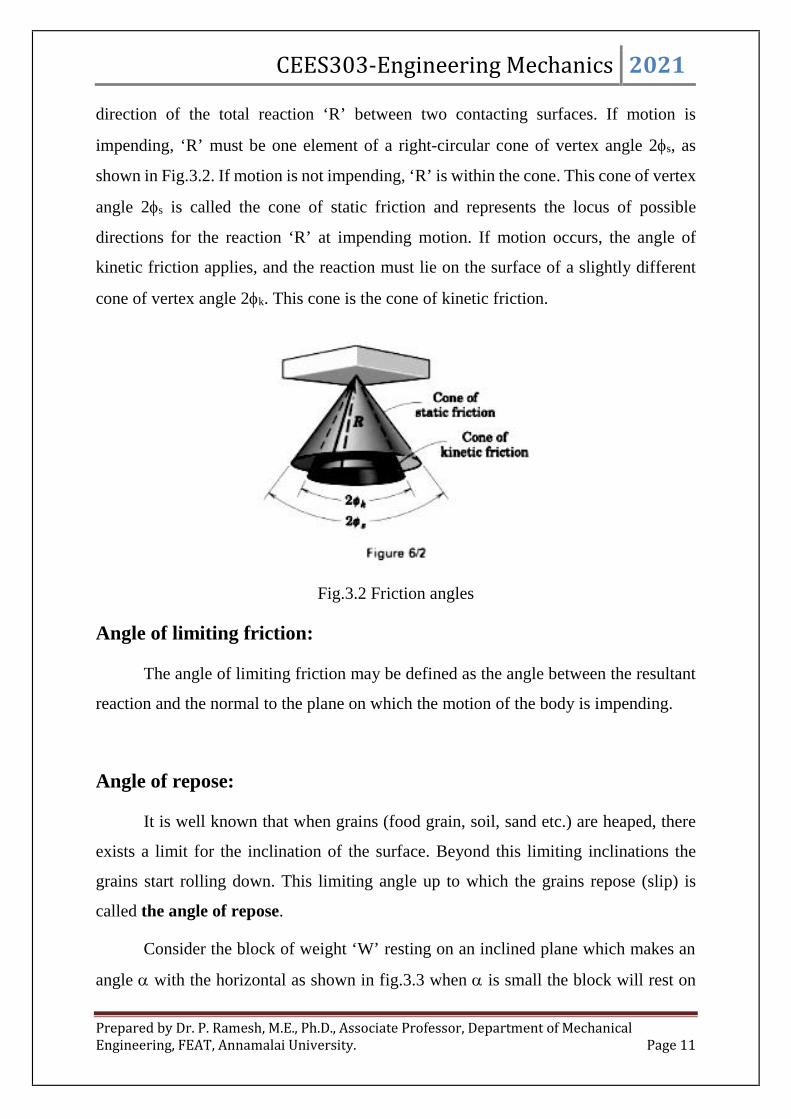
CEES303-Engineering Mechanics 2021
Prepared by Dr. P. Ramesh, M.E., Ph.D., Associate Professor, Department of MechanicalEngineering, FEAT, Annamalai University. Page 11
direction of the total reaction ‘R’ between two contacting surfaces. If motion is
impending, ‘R’ must be one element of a right-circular cone of vertex angle 2s, as
shown in Fig.3.2. If motion is not impending, ‘R’ is within the cone. This cone of vertex
angle 2s is called the cone of static friction and represents the locus of possible
directions for the reaction ‘R’ at impending motion. If motion occurs, the angle of
kinetic friction applies, and the reaction must lie on the surface of a slightly different
cone of vertex angle 2k. This cone is the cone of kinetic friction.
Fig.3.2 Friction angles
Angle of limiting friction:
The angle of limiting friction may be defined as the angle between the resultant
reaction and the normal to the plane on which the motion of the body is impending.
Angle of repose:
It is well known that when grains (food grain, soil, sand etc.) are heaped, there
exists a limit for the inclination of the surface. Beyond this limiting inclinations the
grains start rolling down. This limiting angle up to which the grains repose (slip) is
called the angle of repose.
Consider the block of weight ‘W’ resting on an inclined plane which makes an
angle with the horizontal as shown in fig.3.3 when is small the block will rest on

CEES303-Engineering Mechanics 2021
Prepared by Dr. P. Ramesh, M.E., Ph.D., Associate Professor, Department of MechanicalEngineering, FEAT, Annamalai University. Page 12
the plane. If is increased gradually a stage is reached at which the block start sliding
down the plane. The angle for which motion is impending is called the angle of
repose. Thus the maximum inclination of the plane on which a body, free from external
forces can repose (sleep) is called Angle of repose.
Fig.3.3 Angle of repose
Consider the equilibrium of the block shown in fig.3.3. Since the surface of
contact is not smooth, not only normal reaction, but frictional force also develops. Since
the body tends to slide downward, the frictional force will be up the plane.
Forces normal to the plane = 0, gives
cosWN --------- (3.7)
Forces parallel to the plane = 0, gives
sinWF --------- (3.8)
Dividing eqn. by eqn. we get,
N
Ftan --------- (3.9)
If is the value of when motion is impending frictional force will be limiting
friction and hence
tantan N
For --------- (3.10)
W
F
N

CEES303-Engineering Mechanics 2021
Prepared by Dr. P. Ramesh, M.E., Ph.D., Associate Professor, Department of MechanicalEngineering, FEAT, Annamalai University. Page 13
Therefore,
Thus the value of angle of repose is same as the value of limiting angle of repose.
Factors Affecting Friction:
The friction force is essentially independent of the apparent or projected area of
contact.
The true contact area is much smaller than the projected value, since only the peaks
of the contacting surface irregularities support the load.
Even relatively small normal loads result in high stresses at these contact points.
As the normal force increases, the true contact area also increases as the material
undergoes yielding, crushing, or tearing at the points of contact.
Dry friction are the generation of high local temperatures and adhesion at contact
points, relative hardness of mating surfaces, and the presence of thin surface films
of oxide, oil, dirt, or other substances.
TYPES OF FR ICTION PROBLEMS:
Now recognize the following three types of problems encountered in
applications involving dry friction. The first step in solving a friction problem is to
identify its type.
1. In the first type of problem, the condition of impending motion is known to
exist. Here a body which is in equilibrium is on the verge of slipping, and the friction
force equals the limiting static friction NF Smax . The equations of equilibrium also
hold.
2. In the second type of problem, neither the condition of impending motion nor
the condition of motion is known to exist. To determine the actual friction conditions,
in this first assume static equilibrium and then solve for the friction force ‘F’ necessary
for equilibrium. Three outcomes are possible:

CEES303-Engineering Mechanics 2021
Prepared by Dr. P. Ramesh, M.E., Ph.D., Associate Professor, Department of MechanicalEngineering, FEAT, Annamalai University. Page 14
(a) NFF S max : Here the friction force necessary for equilibrium can be
supported, and therefore the body is in static equilibrium as assumed. This
emphasize that the actual friction force ‘F’ is less than the limiting value Fmax
given by Eqn.3.2 and that F is determined solely by the equations of equilibrium.
(b) NFF S max : Since the friction force ‘F’ is at its maximum value Fmax
motion impends, as discussed in problem type (1). The assumption of static
equilibrium is valid.
(c) NFF S max : Clearly this condition is impossible, because the surfaces
cannot support more force than the maximum NS . The assumption of
equilibrium is therefore invalid, and motion occurs. The friction force F is equal
to Nk from Eqn. 3.4.
3. In the third type of problem, relative motion is known to exist between the
contacting surfaces, and thus the kinetic coefficient of friction clearly applies. For this
problem type, Eqn.3.4 always gives the kinetic friction force directly.
Problems:
SP3.1: Block A weighing 1000N rests over block B which weighs 2000N as shown in
fig.3.4 Block A is tied to wall with a horizontal string. If the coefficient of friction
between blocks A and B is 0.25 and between B and floor is 1/3 what should be the value
of P to move the block (B), if 1) P is horizontal and 2) F acts at 30o upwards to
horizontal?
Fig.3.4
A
BP

CEES303-Engineering Mechanics 2021
Prepared by Dr. P. Ramesh, M.E., Ph.D., Associate Professor, Department of MechanicalEngineering, FEAT, Annamalai University. Page 15
Solution:
a) Find the value of P, if that force is horizontal
Fig.3.4a
The free body diagrams of the two blocks are shown in above figure. It may be
noted that the frictional forces F1 and F2 are to be marked in the opposite directions of
impending relative motion. Considering the block A, then the equilibrium equations of
vertical,
0 yF , 01 AWN , NN 10001
Since F1 is limiting friction,
25.01
1 N
F, 25.0
10001
F
NF 2501
The equilibrium equations of horizontal,
0 xF , 01 TF , NT 250
WA =1000N
WB = 2000NP
B
AT
F1
F1N1
N2
F2

CEES303-Engineering Mechanics 2021
Prepared by Dr. P. Ramesh, M.E., Ph.D., Associate Professor, Department of MechanicalEngineering, FEAT, Annamalai University. Page 16
Now considering the block B, then the equilibrium equations of vertical,
0 yF , 012 NWN B , NN 3000100020002
Since F2 is limiting friction,
3
1
2
2 N
F,
3
1
30002
F
NF 10002
The equilibrium equations of horizontal,
0 xF , 021 FFP , NP 12501000250
P=1250N
b) Find the value of P, if that force is inclined at 30o to horizontal
Fig.3.4b
The free body diagrams of the two blocks are shown in above figure. It may
be noted that the frictional forces F1 and F2 are to be marked in the opposite
WA =1000N
WB = 2000N
P
B
AT
F1
F1N1
N2
F2
30o

CEES303-Engineering Mechanics 2021
Prepared by Dr. P. Ramesh, M.E., Ph.D., Associate Professor, Department of MechanicalEngineering, FEAT, Annamalai University. Page 17
directions of impending relative motion. Considering the block A, then the
equilibrium equations of vertical,
0 yF , 01 AWN , NN 10001
Since F1 is limiting friction,
25.01
1 N
F, 25.0
10001
F
NF 2501
The equilibrium equations of horizontal,
0 xF , 01 TF , NT 250
Now considering the block B, then the equilibrium equations of vertical,
0 yF , 030sin12 oB PNWN ,
100020005.02 PN , 30005.02 PN
PN 5.030002
Since F2 is limiting friction,
3
1
2
2 N
F, 3
1
5.030002
P
F
PPF3
5.010005.03000
3
12
The equilibrium equations of horizontal,
0 xF , 030cos 21 FFP o ,
03
5.0100025030cos
PP o
12503
5.030cos
oP
P=1210.43N

CEES303-Engineering Mechanics 2021
Prepared by Dr. P. Ramesh, M.E., Ph.D., Associate Professor, Department of MechanicalEngineering, FEAT, Annamalai University. Page 18
SP3.2: What is the maximum load (W) which a force P equal to 5 kN will hold up if
the coefficient of friction at C is 0.2 in the arrangement as shown in fig.3.5. Neglect
other friction and weight of the member. If W is 3 kN and P is 4.5 kN what are the
normal and tangential forces transmitted at C?
Fig.3.5
Solution:
The force P is 5 kN and The coefficient of friction at C is 0.2 ()
a) Find maximum load W:
Fig.3.5a
Taking moment about A of beam AB, then
1m 0.5 m
W
75 mm50 mm
B
P
C
A
1m 0.5 m
B
P
C
RAy RCy
RAy

CEES303-Engineering Mechanics 2021
Prepared by Dr. P. Ramesh, M.E., Ph.D., Associate Professor, Department of MechanicalEngineering, FEAT, Annamalai University. Page 19
0 AM , 0 ABACCy dPdR
0)5.1(5)1( CyR
kNRCy 5.7)5.1(5
Fig.3.5b
Now consider Pulley, the limiting friction of pulley as
2.0 cyR
F
kNF 5.15.72.0
Now taking moments about the centre of the pulley,
0 CentrePulleyM , 0)75.0()5.0( FW
0)75.0(5.1)5.0( W
kNW 25.2
b) Normal and tangential forces transmitted at C:
Now consider a weight W equal to 3 kN suspended from the pulley and a force
P equal to 4.5 kN applied at B.
Let Rcy is Normal force or normal reaction at C and
F is Tangential force at C
W
75 mm50 mm
RCyF

CEES303-Engineering Mechanics 2021
Prepared by Dr. P. Ramesh, M.E., Ph.D., Associate Professor, Department of MechanicalEngineering, FEAT, Annamalai University. Page 20
Again consider equilibrium of the beam. Taking moments about the hinge A and
equating the same
0 AM , 0 ABACCy dPdR
0)5.1(5.4)1( CyR
kNRCy 75.6)5.1(5.4
We know that the tangential force at C will be the frictional force between the
pulley and beam. Again taking moments about the centre of the pulley and equating the
same.
0 CentrePulleyM , 0)5.0()75.0( WF
kNWF 275.0
5.03)
75.0
5.0(
SP3.3: What should be the value of as shown in fig.3.6. If that will make the motion
of 900N block the plane to impend? The coefficient of friction for all contact surfaces
is 1/3.
Fig.3.6
300N
900N

CEES303-Engineering Mechanics 2021
Prepared by Dr. P. Ramesh, M.E., Ph.D., Associate Professor, Department of MechanicalEngineering, FEAT, Annamalai University. Page 21
Solution:
Fig.3.6a
The free body diagram of the block is as shown in figure above. The block has
9000 N is on the verge of moving downward. Hence the frictional forces F1 and F2 act
up on the plane on 900N block.
Considered the equilibrium equations of normal to the plane for the block has
300N as
0 planetonormalForces , then
0cos3001 N --------- (1)
From the law of friction,
3
1
1
1 N
F, cos300
3
1
3
111 NF
cos1001 F --------- (2)
Considered the equilibrium equations of normal to the plane for the block has
900N as
0 planetonormalForces , then
0cos90012 NN
300N
900N
F1
F2
F2
N2
N1
90o -

CEES303-Engineering Mechanics 2021
Prepared by Dr. P. Ramesh, M.E., Ph.D., Associate Professor, Department of MechanicalEngineering, FEAT, Annamalai University. Page 22
cos1200cos900cos3002 N --------- (3)
From the law of friction,
3
1
2
2 N
F, cos1200
3
1
3
122 NF
cos4002 F -------- (4)
The equilibrium equations of parallel to the plane for the block has 900N as
0sin90021 FF
sin900cos400cos100
sin900cos500
9
5
900
500tan
o05.299
5tan 1
SP3.4: What is the value of P in the system as shown in fig.3.7 to cause the motion of
500 N block to the right side? Assume the pulley is smooth and the coefficient of friction
between other contact surfaces is 0.20.
Fig.3.7
500N30o
60o
P
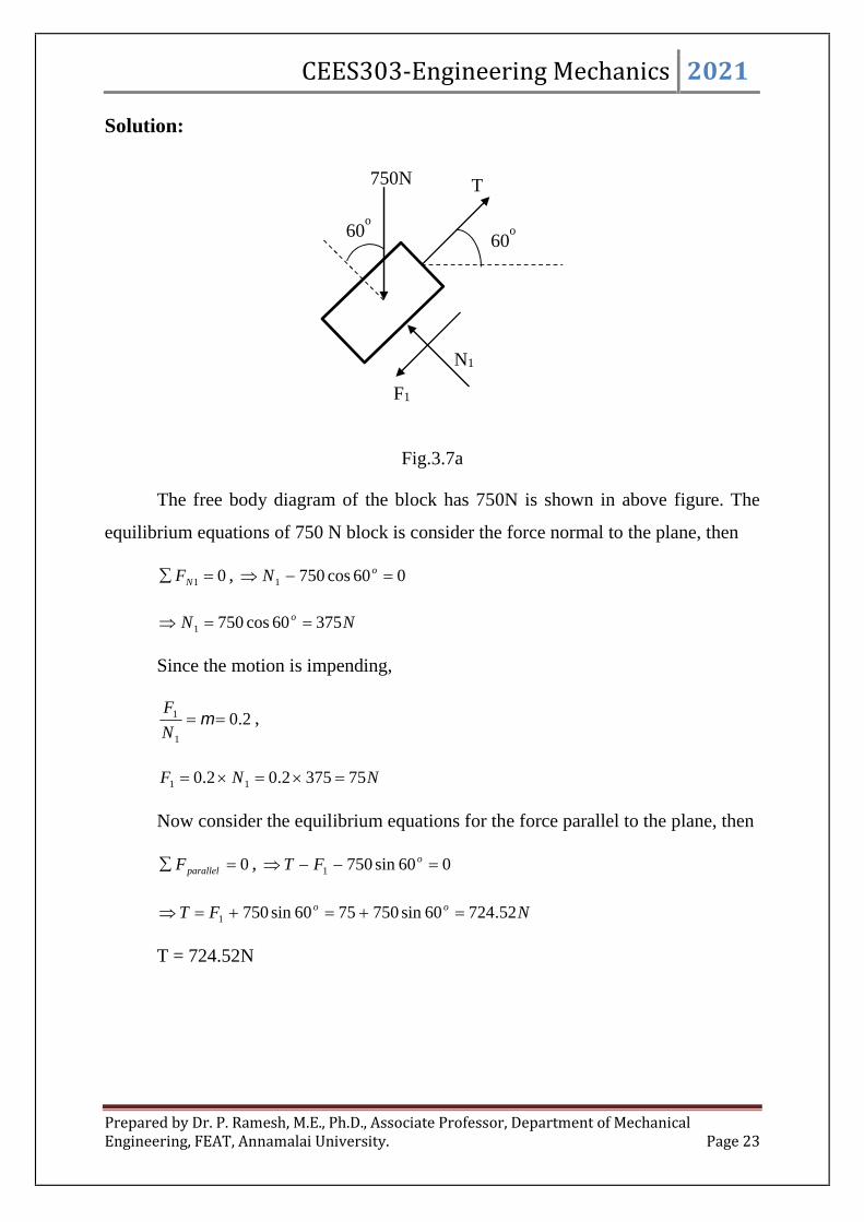
CEES303-Engineering Mechanics 2021
Prepared by Dr. P. Ramesh, M.E., Ph.D., Associate Professor, Department of MechanicalEngineering, FEAT, Annamalai University. Page 23
Solution:
Fig.3.7a
The free body diagram of the block has 750N is shown in above figure. The
equilibrium equations of 750 N block is consider the force normal to the plane, then
01 NF , 060cos7501 oN
NN o 37560cos7501
Since the motion is impending,
2.01
1 N
F,
NNF 753752.02.0 11
Now consider the equilibrium equations for the force parallel to the plane, then
0 parallelF , 060sin7501 oFT
NFT oo 52.72460sin7507560sin7501
T = 724.52N
60o60
o
750N
F1
N1
T

CEES303-Engineering Mechanics 2021
Prepared by Dr. P. Ramesh, M.E., Ph.D., Associate Professor, Department of MechanicalEngineering, FEAT, Annamalai University. Page 24
Fig.3.7b
The free body diagram of the block has 500N is shown in above figure. The
equilibrium equations of 500N block is consider the vertical force, then
0 yF , 030sin5002 oPN
PN 5.05002
From the law of friction, then
2.02
2 N
F
PPNF 1.01005.05002.02.0 22
The equilibrium equations of 500N block is consider the Horizontal force, then
0 xF , 030cos 2 FTP o
0)1.0100(52.72430cos PP o
52.82410052.724)1.030(cos oP
P=853.52 N
30o
500N
F2
N2
P
T

CEES303-Engineering Mechanics 2021
Prepared by Dr. P. Ramesh, M.E., Ph.D., Associate Professor, Department of MechanicalEngineering, FEAT, Annamalai University. Page 25
SP3.5: Two blocks connected by a horizontal link AB are supported on two rough
planes as shown in fig.3.8 The coefficient of friction between the block A and horizontal
surface is 0.4. The limiting angle of friction between block B and inclined plane is 20o.
What is the smallest weight W of the block A for which equilibrium of the system can
exist, if the weight of block B is 5 kN?
Fig.3.8
Solution:
Fig.3.8a
The free body diagram of the block B is as shown in above figure and the limiting
friction as
o
N
F20tan
1
1
30o
A B
30o
BF1
N1
60o
5 kN
T

CEES303-Engineering Mechanics 2021
Prepared by Dr. P. Ramesh, M.E., Ph.D., Associate Professor, Department of MechanicalEngineering, FEAT, Annamalai University. Page 26
The equilibrium equations of block B for vertical force as
0 yF , 0560sin30sin 11 oo FN
560sin20tan5.0 011 oNN
kNN 133.61
oNNF 20tan133.620tan111
F1 = 2.232 kN
The equilibrium equations of block B for horizontal force as
0 xF , 030cos60cos 11 oo NFT
oooo NFT 30cos133.660cos232.230cos60cos 11
T = 4.196 kN
Fig.3.8b
The free body diagram of the block A is as shown in above figure and the
equilibrium equations of block A for Horizontal force as
0 xF , 02 TF
kNTF 196.42
The limiting friction as
A
W
F2
N2
T

CEES303-Engineering Mechanics 2021
Prepared by Dr. P. Ramesh, M.E., Ph.D., Associate Professor, Department of MechanicalEngineering, FEAT, Annamalai University. Page 27
4.02
2 N
F,
4.0
196.4
4.02
2 F
N
N2 = 10.49kN
The equilibrium equations of block A for vertical force as
0 yF , 02 NW
W=10.49kN
WEDGES:
Fig.3.9 Wedge friction
A wedge is, usually, of a triangular or trapezoidal in cross-section. It is,
generally, used for slight adjustments in the position of a body i.e. for tightening fits or
keys for shafts. Sometimes, a wedge is also used for lifting heavy weights as shown in
Fig.3.9. It will be interesting to know that the problems on wedges are basically the
problems of equilibrium on inclined planes. Thus these problems may be solved either
by the equilibrium method or by applying Lami’s theorem.
Now consider a wedge ABC, which is used to lift the body DEFG.
Let W = Weight of the body DEFG,
P = Force required to lift the body, and
µ = Coefficient of friction on the planes AB, AC and DE
Such that, tan
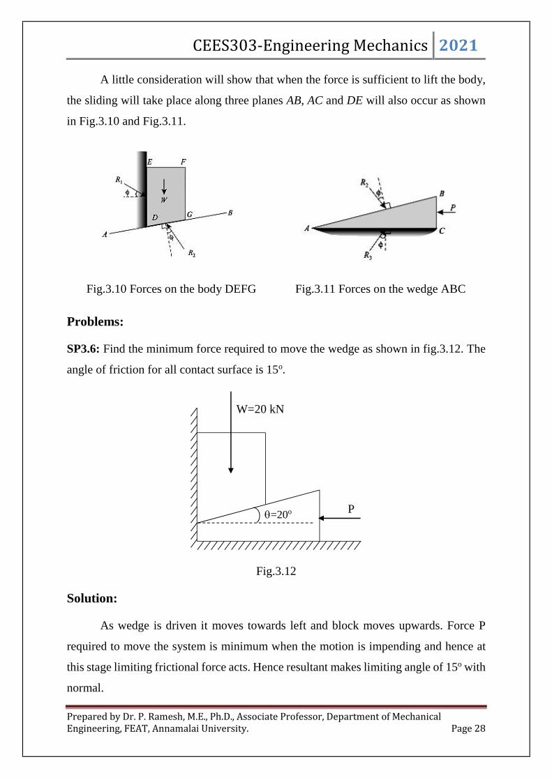
CEES303-Engineering Mechanics 2021
Prepared by Dr. P. Ramesh, M.E., Ph.D., Associate Professor, Department of MechanicalEngineering, FEAT, Annamalai University. Page 28
A little consideration will show that when the force is sufficient to lift the body,
the sliding will take place along three planes AB, AC and DE will also occur as shown
in Fig.3.10 and Fig.3.11.
Fig.3.10 Forces on the body DEFG Fig.3.11 Forces on the wedge ABC
Problems:
SP3.6: Find the minimum force required to move the wedge as shown in fig.3.12. The
angle of friction for all contact surface is 15o.
Fig.3.12
Solution:
As wedge is driven it moves towards left and block moves upwards. Force P
required to move the system is minimum when the motion is impending and hence at
this stage limiting frictional force acts. Hence resultant makes limiting angle of 15o with
normal.
W=20 kN
=20o P

CEES303-Engineering Mechanics 2021
Prepared by Dr. P. Ramesh, M.E., Ph.D., Associate Professor, Department of MechanicalEngineering, FEAT, Annamalai University. Page 29
Fig.3.12a
The free body diagrams for block and wedge are shown in above figure. The
force on block and wedge are redrawn in figure as given below. So that Lami’s theorem
can be applied conveniently.
Fig.3.12b
W=20 kN
=20o P
R1
R2
R2
R3
15o
15o
35o20
o
15o
35o
15o
R2
R1
20 kN
R2
R3
15o
35o
P
BlockWedge

CEES303-Engineering Mechanics 2021
Prepared by Dr. P. Ramesh, M.E., Ph.D., Associate Professor, Department of MechanicalEngineering, FEAT, Annamalai University. Page 30
Applying Lamis’s theorem to the system of forces on block, then
ooO
RR
140sin
20
75sin145sin21
oo
R
140sin
20
145sin1
R1 = 17.847 kN
oo
R
140sin
20
75sin2
R2 = 30.047 kN
Now applying Lamis’s theorem to the system of forces on wedge, then
ooo
RRP
125sin105sin130sin32
105sin
047.30
130sin
o
P
P = 23.835 kN
oo
R
125sin105sin
047.30 3
R3 = 25.48 kN
SP3.7: A 15o wedge A has to be driven for tightening a body B loaded with 1000 N
weight as shown in fig.3.13. If the angle of friction for all the surfaces is 14o find the
force P which should be applied to the wedge.
Fig.3.13

CEES303-Engineering Mechanics 2021
Prepared by Dr. P. Ramesh, M.E., Ph.D., Associate Professor, Department of MechanicalEngineering, FEAT, Annamalai University. Page 31
Solution:
Fig.3.13
The free body diagram of body B is as shown in above figure (a). The equilibrium
equations of body B for horizontal force is
0 xF , 0)1415cos(14sin 21 oo RR
8746.02419.0 21 RR
221 616.32419.0
8746.0RRR
The equilibrium equations of body B for vertical force is
0 yF , 0100014cos)1415sin( 12 oo RR
010009703.0616.34848.0 22 RR
10004848.051.32 R
NR 6.3302
The free body diagram of Wedge A is as shown in above figure (b). The
equilibrium equations of wedge A for horizontal force is
0 xF , 0)1415cos(14cos 23 oo RR
08746.06.3309703.03 R

CEES303-Engineering Mechanics 2021
Prepared by Dr. P. Ramesh, M.E., Ph.D., Associate Professor, Department of MechanicalEngineering, FEAT, Annamalai University. Page 32
NR 9.2973
The equilibrium equations of wedge A for vertical force is
0 yF , 0)1415sin(14sin 23 oo RRP
4848.06.3302419.09.297)1415sin(14sin 23 oo RRP
NP 3.232
SCREW JACK:
Fig.3.14 Screw jack
This is a device commonly used to lift heavy loads. Screw jack works on the
principle same as that of inclined plane. A typical section of the screw jack is shown in
fig.3.14.
The device consists of a nut and a screw. Monolithically cast nut and stand form
the body of the jack. The load is carried by the screw head fitted onto the screw as
shown in the figure. The body (consisting of nut) is fixed and the screw is rotated by
means of a lever.
The axial distance moved by the nut (or by the screw, relative to each other)
when it makes one complete revolution is known as lead of the screw head. The

CEES303-Engineering Mechanics 2021
Prepared by Dr. P. Ramesh, M.E., Ph.D., Associate Professor, Department of MechanicalEngineering, FEAT, Annamalai University. Page 33
distance between consecutive thread is called pitch (of a screw thread). If the screw is
single threaded, then lead of the screw is equal to the pitch. If the screw is double
threaded then lead of the screw is twice the pitch.
Let ‘R’ be the length of the lever and d be the mean diameter of the screw.
Let a load W be lifted using an effort P.
Fig.3.15 Plan view of screw jack
Fig.3.16 Geometry of effort and circumference of screw
If an effort P is applied at the lever end it is equivalent to an effort P1 at the screw
[fig.3.15] and P1 is given by the condition:
21
dPRP
R
d P
R1
P1
P
d

CEES303-Engineering Mechanics 2021
Prepared by Dr. P. Ramesh, M.E., Ph.D., Associate Professor, Department of MechanicalEngineering, FEAT, Annamalai University. Page 34
d
PRP
21
Now consider one complete revolution of the lever. The load W is lifted up by a
distance p equal to the lead of the screw. This can be compared with that of inclined
plane having inclination is
d
p
1tan
Where, p – lead of the screw
d – mean diameter of screw
Fig.3.17 Force system of screw in upward
Applying an effort P at the end of the lever is as good as applying an effort P1 (at
the screw) on this inclined plane (fig.3.17).
Resolving horizontally i.e., parallel to P1
sin11 RP
Where, R1 is resultant reaction and
is limiting angle of friction.
Resolving vertically
cos1RW
Dividing equation by equation
W
P
P1
R1F

CEES303-Engineering Mechanics 2021
Prepared by Dr. P. Ramesh, M.E., Ph.D., Associate Professor, Department of MechanicalEngineering, FEAT, Annamalai University. Page 35
CosR
SinR
W
P
1
11
tan1 WP
But,d
PRP
21
Therefore, tan2
Wd
PR
tan2
WR
dP
We have, tan
Where, is the coefficient of friction.
Then,
tantan1
tantan
2
WR
dP
tan1
tan
2
WR
dP
Where,d
P
tan
Fig.3.18 Force system of screw in downward
If the load is descending then the friction will be acting in the reverse direction
so that the resultant reaction R shifts as shown in fig.3.18
Then the equation changes to
W
P
P1
R1
F
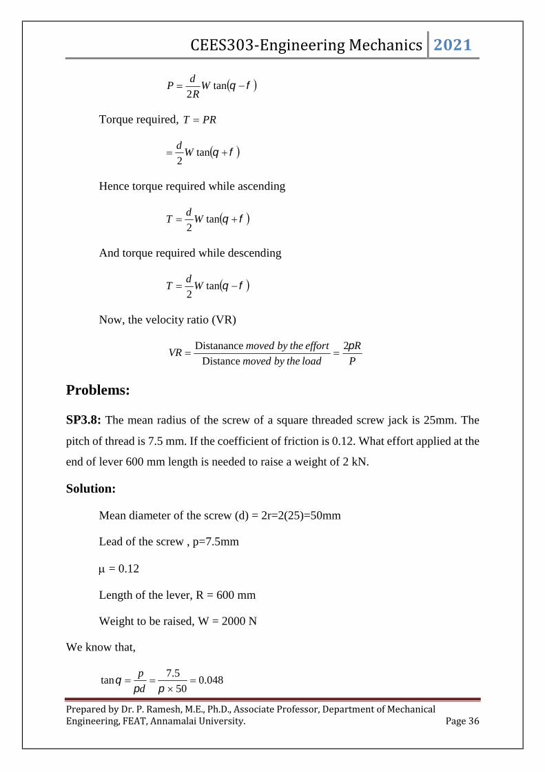
CEES303-Engineering Mechanics 2021
Prepared by Dr. P. Ramesh, M.E., Ph.D., Associate Professor, Department of MechanicalEngineering, FEAT, Annamalai University. Page 36
tan2
WR
dP
Torque required, PRT
tan2
Wd
Hence torque required while ascending
tan2
Wd
T
And torque required while descending
tan2
Wd
T
Now, the velocity ratio (VR)
P
R
loadthebymoved
effortthebymovedVR
2
Distance
Distanance
Problems:
SP3.8: The mean radius of the screw of a square threaded screw jack is 25mm. The
pitch of thread is 7.5 mm. If the coefficient of friction is 0.12. What effort applied at the
end of lever 600 mm length is needed to raise a weight of 2 kN.
Solution:
Mean diameter of the screw (d) = 2r=2(25)=50mm
Lead of the screw , p=7.5mm
= 0.12
Length of the lever, R = 600 mm
Weight to be raised, W = 2000 N
We know that,
048.050
5.7tan
d
p

CEES303-Engineering Mechanics 2021
Prepared by Dr. P. Ramesh, M.E., Ph.D., Associate Professor, Department of MechanicalEngineering, FEAT, Annamalai University. Page 37
048.0tan 1
12.0tan
12.0tan 1
The effort required at mean diameter of the screw to raise the weight is
NWP 338)048.0(12.01
048.012.02000
tan1
tan
Now, the effort applied at the end of the lever may be found out from the relation
21
dPRP
2
503386001 P
NP 1.141
SP3.9: A screw jack raises a load 40 kN. The screw is square threaded having three
threads per 20mm length and 40mm in diameter. Find the force required at the end of a
lever 400mm long measured from the axis of the screw, if the coefficient of friction
between screw and nut is 0.12.
Solution:
Screw diameter, d=40mm,
Lead of the screw, mmp 667.63
20
Load, W = 40 kN
Lever length. R = 400mm
= 0.12
We have,
tan1
tan
2
WR
dP
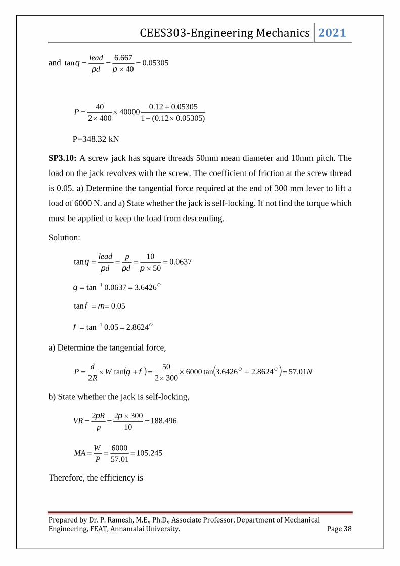
CEES303-Engineering Mechanics 2021
Prepared by Dr. P. Ramesh, M.E., Ph.D., Associate Professor, Department of MechanicalEngineering, FEAT, Annamalai University. Page 38
and 05305.040
667.6tan
d
lead
)05305.012.0(1
05305.012.040000
4002
40
P
P=348.32 kN
SP3.10: A screw jack has square threads 50mm mean diameter and 10mm pitch. The
load on the jack revolves with the screw. The coefficient of friction at the screw thread
is 0.05. a) Determine the tangential force required at the end of 300 mm lever to lift a
load of 6000 N. and a) State whether the jack is self-locking. If not find the torque which
must be applied to keep the load from descending.
Solution:
0637.050
10tan
d
p
d
lead
O6426.30637.0tan 1
05.0tan
O8624.205.0tan 1
a) Determine the tangential force,
NWR
dP OO 01.578624.26426.3tan6000
3002
50tan
2
b) State whether the jack is self-locking,
496.18810
30022
p
RVR
245.10501.57
6000
P
WMA
Therefore, the efficiency is

CEES303-Engineering Mechanics 2021
Prepared by Dr. P. Ramesh, M.E., Ph.D., Associate Professor, Department of MechanicalEngineering, FEAT, Annamalai University. Page 39
%83.555583.0496.188
245.105
VR
MA
Hence the efficiency of screw jack is greater than 50%, then the screw jack is not self -
locking.
The torque required to keep the load from descending is
mmNWd
T OO 3.2048624.26426.3tan6002
50tan
2
DIFFERENTIAL SCREW JACK:
Differential screw jack is an improvement over simple screw jack. A typical
differential screw jack is shown in fig.3. It consists of two threaded elements A and B.
Both A and B have threads in the same direction (right handed). The element A is a
cylinder which has threads on both its outer and inner surfaces. The threads on the outer
surface of the element A fits into the nut C which also functions as the base of the whole
mechanism. The threads on the element B fit into the threads cut on the inner surface of
A. Thus the element A acts as a screw for the nut C and also as a nut for the element B.
With the help of a lever inserted in the holes made on the top of the block D, which is
attached to the element B, block D can be rotated. When D is rotated, A rotates with it.
Rotation of B is prevented by suitable arrangement.
Let DA and dB be the mean diameters of the screws A and B respectively.
Let PA and PB be the pitch of the screws A and B respectively and PA be greater
than PB.
If the lever is rotated through one complete revolution then the height through
which the element A moves up is equals to PA
In the meantime the element B moves down with respect to C.
The distance through which B comes down is equals to PB.
Therefore, net height through which load is lifted is equal to (PA – PB).
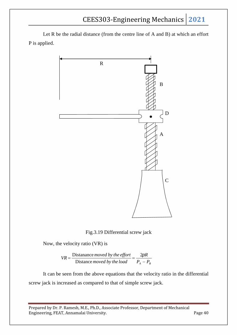
CEES303-Engineering Mechanics 2021
Prepared by Dr. P. Ramesh, M.E., Ph.D., Associate Professor, Department of MechanicalEngineering, FEAT, Annamalai University. Page 40
Let R be the radial distance (from the centre line of A and B) at which an effort
P is applied.
Fig.3.19 Differential screw jack
Now, the velocity ratio (VR) is
BA PP
R
loadthebymoved
effortthebymovedVR
2
Distance
Distanance
It can be seen from the above equations that the velocity ratio in the differential
screw jack is increased as compared to that of simple screw jack.
B
R
D
A
C

CEES303-Engineering Mechanics 2021
Prepared by Dr. P. Ramesh, M.E., Ph.D., Associate Professor, Department of MechanicalEngineering, FEAT, Annamalai University. Page 41
Problems:
SP3.11: The following are the specifications for a differential screw jack;
a) Pitch of smaller screw is 5mm,
b) Pitch of larger screw is 10mm and
c) Lever arm length from the centre of screw is 500mm
The screw jack raises a load of 15 kN with an effort of 185N. Determine the efficiency
of the differential screw jack at this load. If the above jack can raise a load of 40 kN
with an effort of 585 N, determine the law of machine.
Solution:
Now PA = 10mm
PB = 5mm
Lever arm length, R= 500mm
We know that. The velocity ratio
32.628510
50022
BA PP
RVR
The mechanical advantage,
08.81185
15000
P
WMA
The efficiency of machine
%9.12129.032.628
08.81
VR
MA
To find law of machine:
Let law of machine be CmWP
From first case: Cm 15000185 -------- (1)
From second case: Cm 50000585 ------- (2)

CEES303-Engineering Mechanics 2021
Prepared by Dr. P. Ramesh, M.E., Ph.D., Associate Professor, Department of MechanicalEngineering, FEAT, Annamalai University. Page 42
Subtracting eqn. (1) from eqn. (2) then
m 35000400 ,350
4 m ------------ (3)
Substituting the eqn. (3) in eqn. (1) then we get
C 15000350
4185
NC 57.13
Therefore, the law of machine is
57.13350
4 WP
WORK OF A FORCE:
Fig.3.20 Work of a force
Consider the constant force F acting on the body shown in fig3.20 (a), whose
movement along the plane from A to A' is represented by the vector s, called the
displacement of the body. By definition the work U done by the force F on the body
during this displacement is the component of the force in the direction of the
displacement times the displacement, or
sFU cos
From fig.3.20 (b) it seems that the same result is obtained if multiply the
magnitude of the force by the component of the displacement in the direction of the
force. This gives
cossFU

CEES303-Engineering Mechanics 2021
Prepared by Dr. P. Ramesh, M.E., Ph.D., Associate Professor, Department of MechanicalEngineering, FEAT, Annamalai University. Page 43
Because this obtains the same result regardless of the direction in which it
resolves the vectors, it concludes that work U is a scalar quantity.
Fig.3.21 Work of a force act opposite of the displacement
Work is positive when the working component of the force is in the same
direction as the displacement. When the working component is in the direction opposite
to the displacement, fig.3.21, the work done is negative. Thus,
sFsFU coscos
Fig.3.22 Force moves along the path
Now generalize the definition of work to account for conditions under which the
direction of the displacement and the magnitude and direction of the force are variable.
Fig.3.22 (a) shows a force F acting on a body at a point A which moves along the path
shown from A1 to A2. Point A is located by its position vector r measured from some
arbitrary but convenient origin O. The infinitesimal displacement in the motion from A
to A' is given by the differential change dr of the position vector. The work done by the
force F during the displacement dr is defined as
CEES303-Engineering Mechanics 2021
Prepared by Dr. P. Ramesh, M.E., Ph.D., Associate Professor, Department of MechanicalEngineering, FEAT, Annamalai University. Page 44
drFdU .
If F denotes the magnitude of the force F and ds denotes the magnitude of the
differential displacement dr, the definition of the dot product to obtain.
cosFdsdU
It may again interpret this expression as the force component cosF in the
direction of the displacement times the displacement, or as the displacement component
ds cos in the direction of the force times the force, as represented in fig.3.22 (b). If it
expresses F and dr in terms of their rectangular components, then
kdzjdyidxkFjFiFdU zyx .
dzFdyFdxF zyx
To obtain the total work U done by F during a finite movement of point A from
A1 to A2, fig.3.22 (a), It integrates dU between these positions. Thus,
dzFdyFdxFdrFU zyx. or
dsFU cos
To carry out this integration, it must know the relation between the force
components and their respective coordinates, or the relations between F and s and
between cos and s.
In the case of concurrent forces which are applied at any particular point on a
body, the work done by their resultant equals the total work done by the several forces.
This is because the component of the resultant in the direction of the displacement
equals the sum of the components of the several forces in the same direction.
WORK OF A COUPLE:
In addition to the work done by forces, couples also can do work. In fig.3.23 (a)
the couple M acts on the body and changes its angular position by an amount d. The

CEES303-Engineering Mechanics 2021
Prepared by Dr. P. Ramesh, M.E., Ph.D., Associate Professor, Department of MechanicalEngineering, FEAT, Annamalai University. Page 45
work done by the couple is easily determined from the combined work of the two forces
which constitute the couple. In part b of the figure it represents the couple by two equal
and opposite forces F and -F acting at two arbitrary points A and B such that MlbF .
During the infinitesimal movement in the plane of the figure, line AB moves to A"B'.
Now take the displacement of A in two steps, first, a displacement drB equal to that of
B and, second, a displacement drA/B (read as the displacement of A with respect to B)
due to the rotation about B. Thus the work done by F during the displacement from A
to A' is equal and opposite in sign to that due to -F acting through the equal displacement
from B to B'. Therefore conclude that no work is done by a couple during a translation
(movement without rotation).
Fig.3.23 Work of a couple
During the rotation, however, F does work equal to FbddrF BA /. , where
bddr BA / and where d is the infinitesimal angle of rotation in radians. Since FbM
, then
MddU
The work of the couple is positive if M has the same sense as d (clockwise in
this illustration), and negative if M has a sense opposite to that of the rotation. The total
work of a couple during a finite rotation in its plane becomes.
MdU

CEES303-Engineering Mechanics 2021
Prepared by Dr. P. Ramesh, M.E., Ph.D., Associate Professor, Department of MechanicalEngineering, FEAT, Annamalai University. Page 46
VIRTUAL DISPLACEMENTS:
A virtual displacement is a first-order differential change in a linear or angular
position. This change is fictitious in that it is an assumed movement which need not
take place in reality. Mathematically, a virtual displacement is treated the same as a
differential change in an actual movement. The symbol is used for the differential
virtual change and the usual symbol d for the differential change in a real movement.
Relating the linear and angular virtual displacements of the parts of a mechanical
system during a virtual movement consistent with the constraints is often the most
difficult part of the analysis.
To do this,
1. Write the geometric relationships which describe the configuration of
the system.
2. Establish the differential changes in the positions of parts of the system
by differentiating the geometric relationship to obtain expressions for the
differential virtual movements.
VIRTUAL WORK:
The definitions of the work of a force and a couple have been presented in terms
of actual movements expressed by differential displacements having magnitudes of dr
and d. Consider now an imaginary or virtual displacement of a body in static
equilibrium, which indicates a displacement or rotation that is assumed and does not
actually exist. These movements are first-order differential quantities and will be
denoted by the symbols dr and d (delta r and delta ), respectively. The virtual work
done by a force having a virtual displacement r is
rFU cos
Similarly when a couple undergoes a virtual rotation in the plane of the couple
forces, the virtual work is
MU
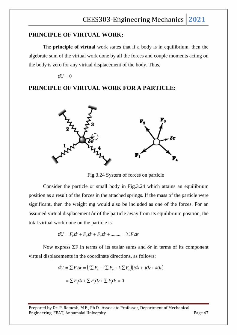
CEES303-Engineering Mechanics 2021
Prepared by Dr. P. Ramesh, M.E., Ph.D., Associate Professor, Department of MechanicalEngineering, FEAT, Annamalai University. Page 47
PRINCIPLE OF VIRTUAL WORK:
The principle of virtual work states that if a body is in equilibrium, then the
algebraic sum of the virtual work done by all the forces and couple moments acting on
the body is zero for any virtual displacement of the body. Thus,
0U
PRINCIPLE OF VIRTUAL WORK FOR A PARTICLE:
Fig.3.24 System of forces on particle
Consider the particle or small body in Fig.3.24 which attains an equilibrium
position as a result of the forces in the attached springs. If the mass of the particle were
significant, then the weight mg would also be included as one of the forces. For an
assumed virtual displacement r of the particle away from its equilibrium position, the
total virtual work done on the particle is
rFrFrFrFU ............. 321
Now express F in terms of its scalar sums and r in terms of its component
virtual displacements in the coordinate directions, as follows:
zkyjxiFkFiFirFU zyx ..
0 zFyFxF zyx
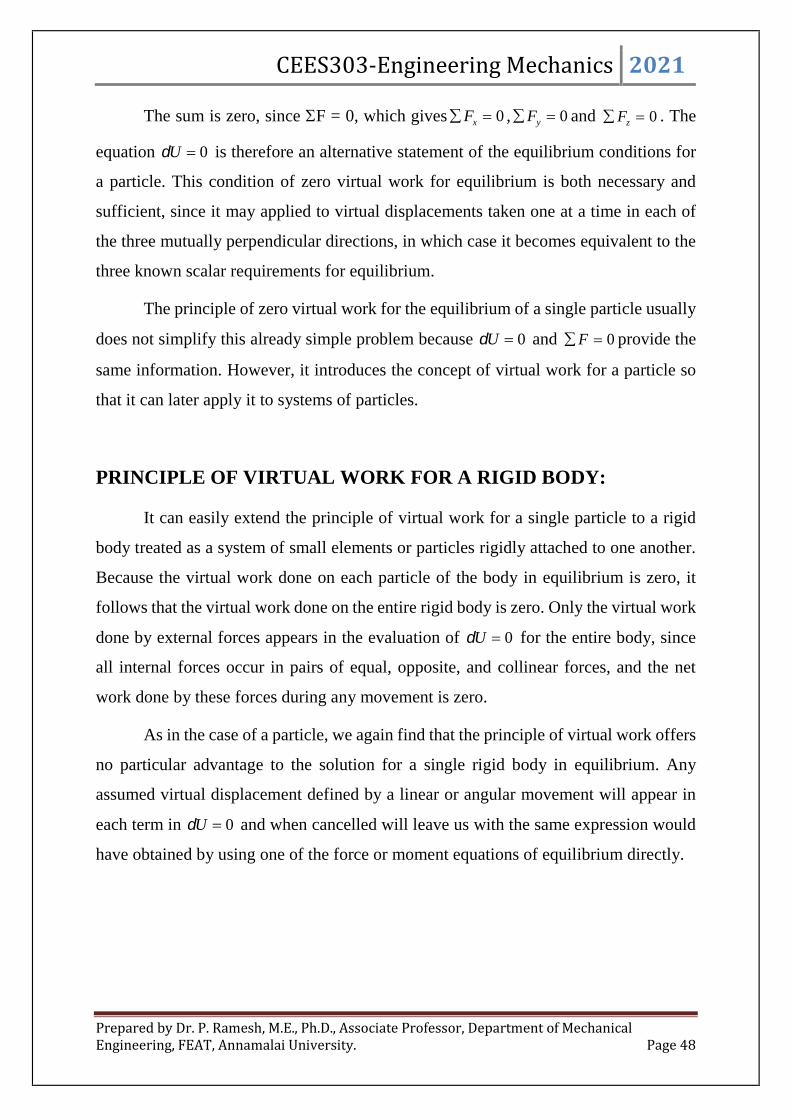
CEES303-Engineering Mechanics 2021
Prepared by Dr. P. Ramesh, M.E., Ph.D., Associate Professor, Department of MechanicalEngineering, FEAT, Annamalai University. Page 48
The sum is zero, since F = 0, which gives 0 xF , 0 yF and 0 zF . The
equation 0U is therefore an alternative statement of the equilibrium conditions for
a particle. This condition of zero virtual work for equilibrium is both necessary and
sufficient, since it may applied to virtual displacements taken one at a time in each of
the three mutually perpendicular directions, in which case it becomes equivalent to the
three known scalar requirements for equilibrium.
The principle of zero virtual work for the equilibrium of a single particle usually
does not simplify this already simple problem because 0U and 0F provide the
same information. However, it introduces the concept of virtual work for a particle so
that it can later apply it to systems of particles.
PRINCIPLE OF VIRTUAL WORK FOR A RIGID BODY:
It can easily extend the principle of virtual work for a single particle to a rigid
body treated as a system of small elements or particles rigidly attached to one another.
Because the virtual work done on each particle of the body in equilibrium is zero, it
follows that the virtual work done on the entire rigid body is zero. Only the virtual work
done by external forces appears in the evaluation of 0U for the entire body, since
all internal forces occur in pairs of equal, opposite, and collinear forces, and the net
work done by these forces during any movement is zero.
As in the case of a particle, we again find that the principle of virtual work offers
no particular advantage to the solution for a single rigid body in equilibrium. Any
assumed virtual displacement defined by a linear or angular movement will appear in
each term in 0U and when cancelled will leave us with the same expression would
have obtained by using one of the force or moment equations of equilibrium directly.
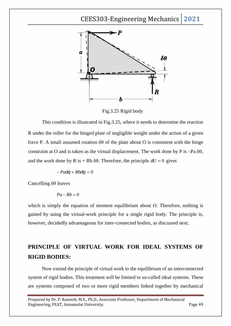
CEES303-Engineering Mechanics 2021
Prepared by Dr. P. Ramesh, M.E., Ph.D., Associate Professor, Department of MechanicalEngineering, FEAT, Annamalai University. Page 49
Fig.3.25 Rigid body
This condition is illustrated in Fig.3.25, where it needs to determine the reaction
R under the roller for the hinged plate of negligible weight under the action of a given
force P. A small assumed rotation of the plate about O is consistent with the hinge
constraint at O and is taken as the virtual displacement. The work done by P is –Pa ,
and the work done by R is + Rb . Therefore, the principle 0U gives
0 RbPa
Cancelling leaves
0 RbPa
which is simply the equation of moment equilibrium about O. Therefore, nothing is
gained by using the virtual-work principle for a single rigid body. The principle is,
however, decidedly advantageous for inter-connected bodies, as discussed next.
PRINCIPLE OF VIRTUAL WORK FOR IDEAL SYSTEMS OF
RIGID BODIES:
Now extend the principle of virtual work to the equilibrium of an interconnected
system of rigid bodies. This treatment will be limited to so-called ideal systems. These
are systems composed of two or more rigid members linked together by mechanical

CEES303-Engineering Mechanics 2021
Prepared by Dr. P. Ramesh, M.E., Ph.D., Associate Professor, Department of MechanicalEngineering, FEAT, Annamalai University. Page 50
connections which are incapable of absorbing energy through elongation or
compression, and in which friction is small enough to be neglected.
Fig.3.26 Ideal systems of rigid bodies
Fig.3.26 (a) shows a simple example of an ideal system where relative motion
between its two parts is possible and where the equilibrium position is determined by
the applied external forces P and F. It can identify three types of forces which act in
such an interconnected system. They are as follows:
(1) Active forces: These are external forces capable of doing virtual work during
possible virtual displacements. In fig.3.26 (a) forces P and Fare active forces
because they would do work as the links move.
(2) Reactive forces: These are forces which act at fixed support positions where
no virtual displacement takes place in the direction of the force. Reactive forces
do no work during a virtual displacement. In fig.3.26 (b) the horizontal force FB
exerted on the roller end of the member by the vertical guide can do no work
because there can be no horizontal displacement of the roller. The reactive force
FO exerted on the system by the fixed support at O also does no work because O
cannot move.
(3) Internal forces: These are forces in the connections between members.
During any possible movement of the system or its parts, the net work done by the
internal forces at the connections is zero. This is so because the internal forces always
exist in pairs of equal and opposite forces, as indicated for the internal forces FA and

CEES303-Engineering Mechanics 2021
Prepared by Dr. P. Ramesh, M.E., Ph.D., Associate Professor, Department of MechanicalEngineering, FEAT, Annamalai University. Page 51
-FA at joint A in fig.3.26 (c). The work of one force therefore necessarily cancels the
work of the other force during their identical displacements.
DEGREES OF FREEDOM:
Fig.3.27 One degree of freedom systems
The number of degrees of freedom of a mechanical system is the number of
independent coordinates needed to specify completely the configuration of the system.
Fig.3.27 shows three examples of one degree-of-freedom systems. Only one coordinate
is needed to establish the position of every part of the system. The coordinate can be a
distance or an angle.
Fig.3.28 Two degree of freedom systems
Fig.3.28 shows three examples of two – degree – of freedom systems where
two independent coordinates are needed to determine the configuration of the system.

CEES303-Engineering Mechanics 2021
Prepared by Dr. P. Ramesh, M.E., Ph.D., Associate Professor, Department of MechanicalEngineering, FEAT, Annamalai University. Page 52
By the addition of more links to the mechanism in the right-hand figure, there is no limit
to the number of degrees of freedom which can be introduced.
The principle of virtual work 0U may be applied as many times as there are
degrees of freedom. With each application, it allows only one independent coordinate
to change at a time while holding the others constant. In this treatment of virtual work
in this section, consider only one-degree-of-freedom systems.
SYSTEMS WITH FRICTION:
Fig.3.29 Friction in a system
When sliding friction is present to any appreciable degree in a mechanical
system, the system is said to be "real." In real systems some of the positive work done
on the system by external active forces (input work) is dissipated in the form of heat
generated by the kinetic friction forces during movement of the system. When there is
sliding between contacting surfaces, the friction force does negative work because its
direction is always opposite to the movement of the body on which it acts. This negative
work cannot be regained.
Thus, the kinetic friction force Nk acting on the sliding block in fig.3.29 (a)
does work on the block during the displacement x in the amount of xk N . During a
virtual displacement x, the friction force does work equal to xNxk . The static

CEES303-Engineering Mechanics 2021
Prepared by Dr. P. Ramesh, M.E., Ph.D., Associate Professor, Department of MechanicalEngineering, FEAT, Annamalai University. Page 53
friction force acting on the rolling wheel in Fig.3.29 (b), on the other hand, does no
work if the wheel does not slip as it rolls.
In Fig.3.29 (c) the moment Mf about the centre of the pinned joint due to the
friction forces which act at the contacting surfaces does negative work during any
relative angular movement between the two parts. Thus, for a virtual displacement
between the two parts, which have the separate virtual displacements 1 and 2 as
shown, the negative work done is 2121 fff MMM , or simply fM
. For each part, Mf is in the sense to oppose the relative motion of rotation.
A major advantage of the method of virtual work is in the analysis of an entire
system of connected members without taking them apart. If there is appreciable kinetic
friction internal to the system, it becomes necessary to dismember the system to
determine the friction forces. In such cases the method of virtual work finds only limited
use.
MECHANICAL EFFICIENCY:
Because of energy loss due to friction, the output work of a machine is always
less than the input work. The ratio of the two amounts of work is the mechanical
efficiency . Thus,
workinput
workoutput
The mechanical efficiency of simple machines which have a single degree of
freedom and which operate in a uniform manner may be determined by the method of
work by evaluating the numerator and denominator of the expression fore during a
virtual displacement.
Fig.3.30 Connected body

CEES303-Engineering Mechanics 2021
Prepared by Dr. P. Ramesh, M.E., Ph.D., Associate Professor, Department of MechanicalEngineering, FEAT, Annamalai University. Page 54
As an example, consider the block being moved up the inclined plane in fig.3.30.
For the virtual displacement s shown, the output work is that necessary to elevate the
block, or mg s sin. The input work is smgT cosmgsins k . The efficiency
of the inclined plane is, therefore,
cot1
1
scossin
sins
kkmg
mg
Fig.3.31 Simple screw jack
As a second example, consider the screw jack described in previous and shown
in fig.3.31. tanWrM gives the moment M required to raise the load W, where
the screw has a mean radius r and a helix angle , and where the friction angle is
k 1tan . During a small rotation of the screw, the input work
. tanWr M . The output work is that required to elevate the load, or
tanWr . Thus the efficiency of the jack can be expressed as
)tan(
tan
) tan(
tan
Wr
Wr
As friction is decreased, c/J becomes smaller, and the efficiency approaches unity.

CEES303-Engineering Mechanics 2021
Prepared by Dr. P. Ramesh, M.E., Ph.D., Associate Professor, Department of MechanicalEngineering, FEAT, Annamalai University. Page 55
Problems:
SP3.12: Determine the force exerted by the vice on the block when a given force P is
applied at C as shown in fig.3.32. Assume that there is no friction.
Fig.3.32
Solution:
The above free body diagram shows that the reactive and active forces in a system.
Consider the work done by the external forces for a virtual displacement. Now is
a positive increment to as shown in free body diagram. As per the virtual work
method, the only forces P and Q produces non-zero work.
Bx increases while yC decreases then
The positive increment for Bx is BQB xQUx . The negative sign
indicates opposite sense of movement.

CEES303-Engineering Mechanics 2021
Prepared by Dr. P. Ramesh, M.E., Ph.D., Associate Professor, Department of MechanicalEngineering, FEAT, Annamalai University. Page 56
The negative increment for yC is CPC yPUy . The
negative sign indicates the same sense of above.
The principle of virtual work is
0U , 0 PQ UU
0 CBPQ yPxQUU
The terms xB and yC are expressed as , then
sin2lxB and coslyC
Now differentiate w.r.t , then
cos2lxB and sinlyC
Therefore,
0sincos2 lPlQyPxQ CB
0sincos2 PlQl
tan2
1PQ
SP3.13: Find the magnitude of the couple M required to maintain the equilibrium of
the mechanism.
Fig.3.33

CEES303-Engineering Mechanics 2021
Prepared by Dr. P. Ramesh, M.E., Ph.D., Associate Professor, Department of MechanicalEngineering, FEAT, Annamalai University. Page 57
Solution:
Fig.3.33a
Now apply the principle of virtual work, then
0U , 0 PM UU
0 DxPM
We know that,
cos3lxD
Differentiate w.r.t. ,
sin3lxD
Therefore, 0sin3 lPM
sin3PlM
SP3.14: Determine the angle for equilibrium of the two member linkage as shown in
fig.3.34a. Each member has a mass of 10kg.

CEES303-Engineering Mechanics 2021
Prepared by Dr. P. Ramesh, M.E., Ph.D., Associate Professor, Department of MechanicalEngineering, FEAT, Annamalai University. Page 58
Fig.3.34 a
Solution:
Fig.3.34b
The position of F and W can be specified by the position coordinates xB and yW as
cos12Bx , sin2 Bx
sin12
1Wy , cos5.0 Wy
The principle of virtual work is
0U , 0 BWW xFyWyW
0sin225cos5.01.98cos5.081.9
Since 0, then
0sin50cos1.98
o0.6350
1.98tan 1

CEES303-Engineering Mechanics 2021
Prepared by Dr. P. Ramesh, M.E., Ph.D., Associate Professor, Department of MechanicalEngineering, FEAT, Annamalai University. Page 59
SP3.15: Determine the required force P in fig.3.35a needed to maintain equilibrium of
the scissors linkage when =60o. The spring is un-stretched when =30o. Neglect the
mass of the links.
Fig.3.35
Solution:
The position of Fs and P can be specified by the position coordinates xB and xD
as
sin3.0Bx , cos3.0 Bx
sin3.03Dx , cos9.0 Dx
The principle of virtual work is
0U , 0 DBs xPxF
ksFs ,
Where, k is the stiffness of spring constant and s is the change in position that is change
in length minus un-stretched length. If k is 5000N/m, un-stretched length is 0.3sin30o
and Change in length is 0.3sin, Then
NF os 750sin150030sin3.0sin3.05000

CEES303-Engineering Mechanics 2021
Prepared by Dr. P. Ramesh, M.E., Ph.D., Associate Professor, Department of MechanicalEngineering, FEAT, Annamalai University. Page 60
Hence,
0750sin1500 DB xPx
0cos9.0cos3.0750sin1500 P
0cossin4502259.0 P
Since cos 0, then
250sin500 P
When =60o, then
25060sin500 oP
P=183N
SP3.16: If the box as shown in fig.3.36a has a mass 10kg determine the couple moment
M needed to maintain equilibrium when =60o. Neglect the mass of the members.
Fig.3.36
Solution:
The position of W and M can be specified by the position coordinates yE and
as
byE sin45.0 , cos45.0 Ey
The principle of virtual work is
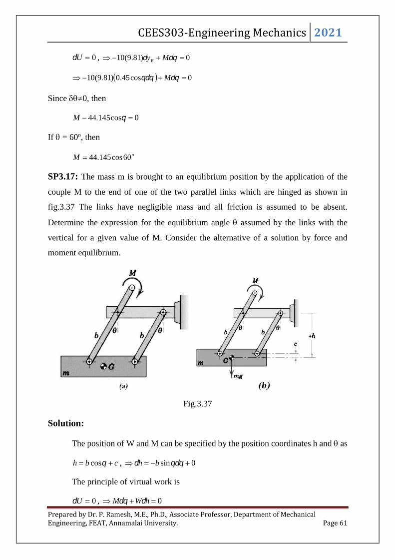
CEES303-Engineering Mechanics 2021
Prepared by Dr. P. Ramesh, M.E., Ph.D., Associate Professor, Department of MechanicalEngineering, FEAT, Annamalai University. Page 61
0U , 0)81.9(10 MyE
0cos45.0)81.9(10 M
Since 0, then
0cos145.44 M
If = 60o, then
oM 60cos145.44
SP3.17: The mass m is brought to an equilibrium position by the application of the
couple M to the end of one of the two parallel links which are hinged as shown in
fig.3.37 The links have negligible mass and all friction is assumed to be absent.
Determine the expression for the equilibrium angle assumed by the links with the
vertical for a given value of M. Consider the alternative of a solution by force and
moment equilibrium.
Fig.3.37
Solution:
The position of W and M can be specified by the position coordinates h and as
cbh cos , 0sin bh
The principle of virtual work is
0U , 0 hWM

CEES303-Engineering Mechanics 2021
Prepared by Dr. P. Ramesh, M.E., Ph.D., Associate Professor, Department of MechanicalEngineering, FEAT, Annamalai University. Page 62
0)sin( bmgM
Since 0, then
sinmgbM
mgb
M1sin
SP3.18: For link OA in the horizontal position as shown in fig.3.38 Determine the force
P on the sliding collar which will prevent OA from rotating under the action of the
couple M. Neglect the mass of the moving parts.
Fig.3.38
Solution:
The position of P and M can be specified by the position coordinates x and
about the point O. From the right triangle for which link AB has length as
222 yxb
Differentiate the above equation to obtain displacement along x and y, then
022 yyxx
yx
yx
The vertical displacement at point A is ay
The principle of virtual work is
0U , 0 xPM

CEES303-Engineering Mechanics 2021
Prepared by Dr. P. Ramesh, M.E., Ph.D., Associate Professor, Department of MechanicalEngineering, FEAT, Annamalai University. Page 63
0
a
x
yPM
Since 0, then
ha
Mx
ya
MxP
SP3.19: Determine the reaction RA and RB developed in the simply supported beam
shown in fig.3.39 using virtual work method.
Fig.3.39
Solution:
Fig.3.39a
Let RA and RB be the reactions at supports A and B. let y displacement be given
to beam at B without giving any displacement at A as shown in above free body
diagram.
The corresponding displacement for the beam at 20 kN load and 40 kN load at
points are y3
1and y
3
2respectively.
2m 2m 2m
20 kN 40 kN
A B

CEES303-Engineering Mechanics 2021
Prepared by Dr. P. Ramesh, M.E., Ph.D., Associate Professor, Department of MechanicalEngineering, FEAT, Annamalai University. Page 64
By the principle of virtual work,
0U , 03
240
3
1200 yRyyR BA
03
80
3
20
yRB
Since y0, then
03
80
3
20
BR
Therefore,
R=33.33 kN
Fig.3.39b
Now consider the virtual displacement from the support at B, then the
corresponding displacement for the beam at 20 kN load and 40 kN load at points are
'3
2y and '
3
1y respectively. The principle of virtual work is
0'U , 00'3
140'
3
220' BA RyyyR
0'3
40
3
40
yRA
Since y0, then
03
40
3
40AR
RA = 26.67 kN
A B

CEES303-Engineering Mechanics 2021
Prepared by Dr. P. Ramesh, M.E., Ph.D., Associate Professor, Department of MechanicalEngineering, FEAT, Annamalai University. Page 65
SP3.20: Determine the reactions in the overhanging beam as shown in fig.3.40 using
virtual work method.
Fig.3.40
Solution:
Fig.3.40a
Let RA and RB be the reactions at supports A and B. let y86 displacement be
given to beam at B without giving any displacement at A as shown in above free body
diagram.
The corresponding displacement for the beam at 20 kN load , 60 kN and 30 kN
load at points are y8
1, y
8
4and y respectively.
By the principle of virtual work,
1m 4m 2m
20 kN 30 kN60 kN
6m
A B
A B

CEES303-Engineering Mechanics 2021
Prepared by Dr. P. Ramesh, M.E., Ph.D., Associate Professor, Department of MechanicalEngineering, FEAT, Annamalai University. Page 66
0U , 0308
6
8
460
8
1200 yyRyyR BA
0308
6
8
240
8
20
y
RB
Since y0, then
8
20
8
24030
6
8BR
RB = 76.67 kN
Fig.3.40b
Now consider the virtual displacement from the support at B, then the corresponding
displacement for the beam at 20 kN load , 60 kN and 30 kN load at points are 'y , '7
2y
and '7
2y respectively.
The principle of virtual work is
0'U , 0'7
2300'
7
260'20'
7
6 yRyyyR BA
0'7
60
7
12020
7
6
yRA
Since y0, then
7
60
7
12020
6
7AR
RA = 33.33 kN
A B

CEES303-Engineering Mechanics 2021
Prepared by Dr. P. Ramesh, M.E., Ph.D., Associate Professor, Department of MechanicalEngineering, FEAT, Annamalai University. Page 67
SP3.21: Determine the reaction RA in the overhanging beam as shown in fig.3.41 by
virtual work method.
Fig.3.41
Solution:
Fig.3.41a
Now consider the virtual displacement from the support at B, then the
corresponding displacement for the beam
At point A is y ,
At point B is y5
3,
At point R is y5
4
At point C is5
y
A
20 kN/m
2mE
1m1.5mDB C
20 kN
20 kN-m
1.5m
A
1m
E
1m1.5m
DB C
1.5m1m
R=wl

CEES303-Engineering Mechanics 2021
Prepared by Dr. P. Ramesh, M.E., Ph.D., Associate Professor, Department of MechanicalEngineering, FEAT, Annamalai University. Page 68
At point D is 0 and
At point E is y5
1
The principle of virtual work is
0'U , 05
1200
5
140
5
4220 yRyyyR BA
04832 yRA
Since y0, then
4832 AR
RA = 20 kN
SP3.22: What is the value of P in the system as shown in fig.3.42 to cause the motion
of 500 N block to the right side? Assume the pulley is smooth and the coefficient of
friction between other contact surfaces is 0.20.
Fig.3.42
500N30o
60o
P
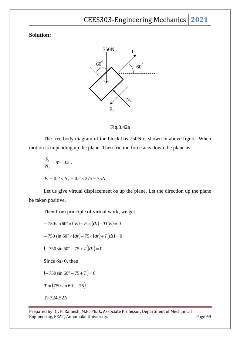
CEES303-Engineering Mechanics 2021
Prepared by Dr. P. Ramesh, M.E., Ph.D., Associate Professor, Department of MechanicalEngineering, FEAT, Annamalai University. Page 69
Solution:
Fig.3.42a
The free body diagram of the block has 750N is shown in above figure. When
motion is impending up the plane. Then friction force acts down the plane as
2.01
1 N
F,
NNF 753752.02.0 11
Let us give virtual displacement s up the plane. Let the direction up the plane
be taken positive.
Then from principle of virtual work, we get
060sin750 1 sTsFso
07560sin750 sTsso
07560sin750 sTo
Since s0, then
07560sin750 To
7560sin750 oT
T=724.52N
60o60
o
750N
F1
N1
T

CEES303-Engineering Mechanics 2021
Prepared by Dr. P. Ramesh, M.E., Ph.D., Associate Professor, Department of MechanicalEngineering, FEAT, Annamalai University. Page 70
Fig.3.42b
The free body diagram of the block has 500N is shown in above figure. When
motion is impending up the plane. Then friction force acts down the plane as
2.02
2 N
F,
PNPNF o 1.0100)30sin500(2.02.0 22
Let us give virtual displacement s up the plane. Let the direction up the plane
be taken positive.
Then from principle of virtual work, we get
030cos 2 sTsFsP o
052.724)1.0100(87.0 ssPsP
052.724)1.0100(87.0 sPP
Since s0, then
052.82497.0 P
97.0
52.824P
P=850.02N
30o
500N
F2
N2
P
T

CEES303-Engineering Mechanics 2021
Prepared by Dr. P. Ramesh, M.E., Ph.D., Associate Professor, Department of MechanicalEngineering, FEAT, Annamalai University. Page 71
SP3.23: Determine the force P required to make the motion impending to the left for
the system of connected bodies as shown in fig.3.43a. Coefficient of friction for all
contacting surface is 0.25. Pulleys are smooth.
Fig.3.43
Solution:
Since motion is impending to the left, frictional forces are acting in the directions
shown in fig.3.43b.
NNF 5.6225025.025.0 11
NNF o 78.17645cos100025.025.0 22
NNF 5.1250025.025.0 33
Let us give a virtual displacement towards left. Taking the displacement of the
system to left as positive, then the virtual work equation is
045sin1000 321 sFsFssFsP o
0)45sin1000( 321 sFFFP o
Since s0, then
321 45sin1000 FFFP o , 12578.1767075.62 P
P=1071.38N
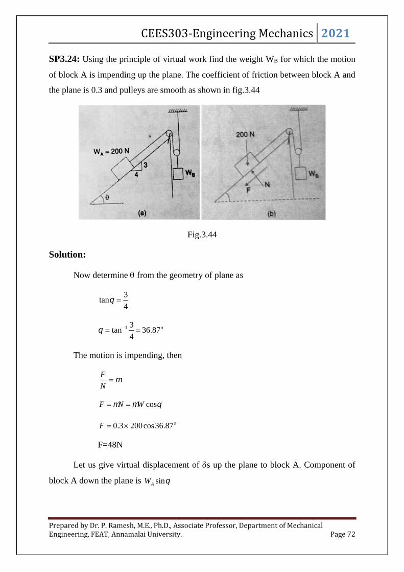
CEES303-Engineering Mechanics 2021
Prepared by Dr. P. Ramesh, M.E., Ph.D., Associate Professor, Department of MechanicalEngineering, FEAT, Annamalai University. Page 72
SP3.24: Using the principle of virtual work find the weight WB for which the motion
of block A is impending up the plane. The coefficient of friction between block A and
the plane is 0.3 and pulleys are smooth as shown in fig.3.44
Fig.3.44
Solution:
Now determine from the geometry of plane as
4
3tan
o87.364
3tan 1
The motion is impending, then
N
F
cosWNF
oF 87.36cos2003.0
F=48N
Let us give virtual displacement of s up the plane to block A. Component of
block A down the plane is sinAW

CEES303-Engineering Mechanics 2021
Prepared by Dr. P. Ramesh, M.E., Ph.D., Associate Professor, Department of MechanicalEngineering, FEAT, Annamalai University. Page 73
The component normal to the plane do not do any work since thre is no
displacement normal to the plane.
When block A moves by s, weight B moves down by2
s
Hence the virtual work equation is
0
2sin200
sWsFs B
02
sin200
s
WF B
Since s0, then
02
sin200
BW
F
02
4887.36sin200
BW
4887.36sin2002 oBW
WB = 336 N
SP3.25: Ladder AB of length 4m and weight 200 N is held in position by applying
force P as shown in fig.3.45. Assuming smooth wall and floor determine the force P. If
instead of force P for preventing from slipping, a horizontal rope is tied at a distance of
1m from A, what is the tension in the rope?
Fig.3.45
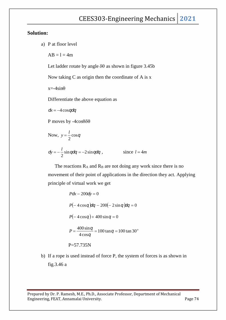
CEES303-Engineering Mechanics 2021
Prepared by Dr. P. Ramesh, M.E., Ph.D., Associate Professor, Department of MechanicalEngineering, FEAT, Annamalai University. Page 74
Solution:
a) P at floor level
AB = l = 4m
Let ladder rotate by angle as shown in figure 3.45b
Now taking C as origin then the coordinate of A is x
x=-4sin
Differentiate the above equation as
cos4x
P moves by -4cos
Now, cos2
ly
sin2sin2
l
y , since ml 4
The reactions RA and RB are not doing any work since there is no
movement of their point of applications in the direction they act. Applying
principle of virtual work we get
0200 yxP
0sin2200cos4 P
0sin400cos4 P
oP 30tan100tan100cos4
sin400
P=57.735N
b) If a rope is used instead of force P, the system of forces is as shown in
fig.3.46 a

CEES303-Engineering Mechanics 2021
Prepared by Dr. P. Ramesh, M.E., Ph.D., Associate Professor, Department of MechanicalEngineering, FEAT, Annamalai University. Page 75
Fig.3.46
The system of forces in this case are as shown in fig.3.46b Taking C as origin.
sin3Dx
Differentiate the above equation as
cos3Dx
cos2Gy
Differentiate the above equation as
sin2Gy
There is no displacement in the direction of RA and RB. Hence from the principle
of virtual work,
0200 GD yxT
0sin2200cos3 T
0sin400cos3 T
Since 0, then
sin400cos3 T , oT 30tan3
400tan
3
400
T=76.98N
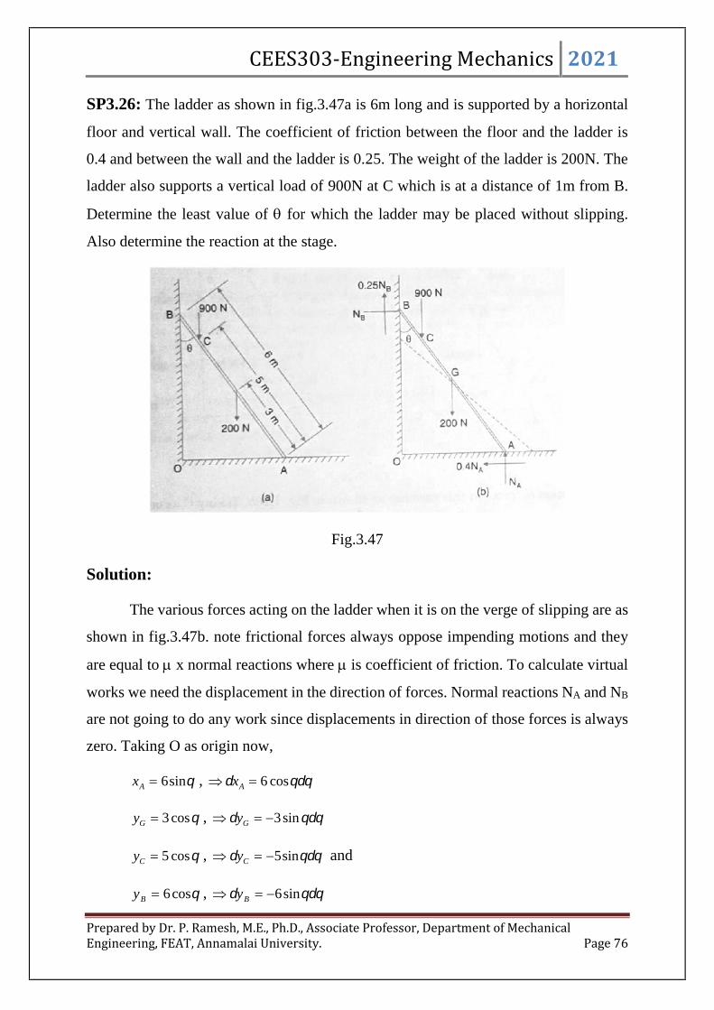
CEES303-Engineering Mechanics 2021
Prepared by Dr. P. Ramesh, M.E., Ph.D., Associate Professor, Department of MechanicalEngineering, FEAT, Annamalai University. Page 76
SP3.26: The ladder as shown in fig.3.47a is 6m long and is supported by a horizontal
floor and vertical wall. The coefficient of friction between the floor and the ladder is
0.4 and between the wall and the ladder is 0.25. The weight of the ladder is 200N. The
ladder also supports a vertical load of 900N at C which is at a distance of 1m from B.
Determine the least value of for which the ladder may be placed without slipping.
Also determine the reaction at the stage.
Fig.3.47
Solution:
The various forces acting on the ladder when it is on the verge of slipping are as
shown in fig.3.47b. note frictional forces always oppose impending motions and they
are equal to x normal reactions where is coefficient of friction. To calculate virtual
works we need the displacement in the direction of forces. Normal reactions NA and NB
are not going to do any work since displacements in direction of those forces is always
zero. Taking O as origin now,
sin6Ax , cos6 Ax
cos3Gy , sin3 Gy
cos5Cy , sin5 Cy and
cos6By , sin6 By

CEES303-Engineering Mechanics 2021
Prepared by Dr. P. Ramesh, M.E., Ph.D., Associate Professor, Department of MechanicalEngineering, FEAT, Annamalai University. Page 77
Applying principles of virtual work we get,
0)sin6(25.0)sin5(900)sin3(200cos64.0 BA NN
Since 0, then
0sin5.1sin4500sin600cos4.2 BA NN
From the equilibrium conditions,
0 xF , BA NN 4.0 and
0 yF , 020090025.0 BA NN
11004.025.0 AA NN
NA = 1000N
Hence, NB = 0.4 x 1000 = 400N
Substituting these value in above equations then we get,
0sin4005.1sin4500sin600cos10004.2
cos2400sin4500 ,4500
2400tan
o073.28
SP3.27: Determine the force in the member FH of the truss shown in fig.3.48 Each
load is 10 kN and all triangles are equilaterals with sides 4m.
Fig.3.48

CEES303-Engineering Mechanics 2021
Prepared by Dr. P. Ramesh, M.E., Ph.D., Associate Professor, Department of MechanicalEngineering, FEAT, Annamalai University. Page 78
Solution:
Fig.3.48
Due to symmetry, kNloadtotalRR BA 357102
1
2
1
Take section 1-1 as shown in fig.3.a and consider left side portion as shown in fig.3.48b.
Imagine a rotation of about point G.
Vertical displacement of A = 12
Vertical displacement of B = 10
Vertical displacement of D = 6 and
Vertical displacement of F = 2
Horizontal displacement of FFH=2 tan 60o towards right
Therefore from the principle of virtual displacement, we have
060tan2210610101012 oFHA FR
20601001260tan2 Ao
FH RF ,oFHF
60tan2
240
FFH=-69.28 kN
The negative sign indicates the direction of FFH is to be reverted and is
compressive force.

CEES303-Engineering Mechanics 2021
Prepared by Dr. P. Ramesh, M.E., Ph.D., Associate Professor, Department of MechanicalEngineering, FEAT, Annamalai University. Page 79
SP3.28: Determine the force developed in the member DF of the truss shown in
fig.3.49
Fig.3.49
Solution:
Take the section 1-1 as shown in fig.3.49a and consider left side portion. Imagine
a virtual rotation at support E. Then
Vertical displacement of point A = 10
Vertical displacement of point B = 5
Vertical displacement of point D = 0 and
Horizontal displacement of point D = 5
Therefore, from virtual work principle,
0545cos510010100 oDFF
150051001010045cos5 oDFF
kNFoDF 26.4242300
45cos5
1500 (tensile)

CEES303-Engineering Mechanics 2021
Prepared by Dr. P. Ramesh, M.E., Ph.D., Associate Professor, Department of MechanicalEngineering, FEAT, Annamalai University. Page 80
SP3.29: Neglecting the friction determine the effort required to lift a load by the screw
jack as shown in fig.3.50 Take pitch of the jack =p.
Fig.3.50
Solution:
Let P be the effort required. Let a virtual rotation be given to effort.
Therefore virtual work done by P = PR
For one full rotation of effort, the load moves by distance p definition of pitch)
Therefore for rotation distance through which weight W moves = 2
P
From virtual work principle total work done is zero.
2
pWPR ,
R
WpP
2
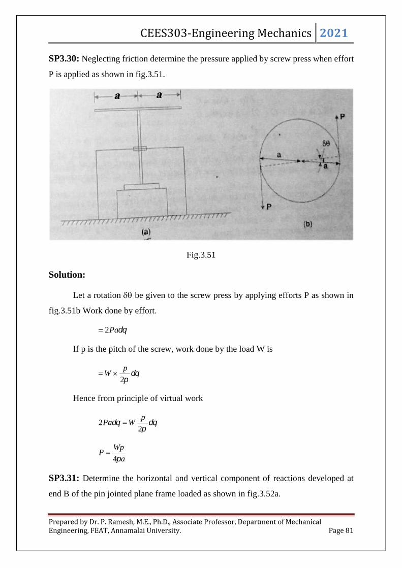
CEES303-Engineering Mechanics 2021
Prepared by Dr. P. Ramesh, M.E., Ph.D., Associate Professor, Department of MechanicalEngineering, FEAT, Annamalai University. Page 81
SP3.30: Neglecting friction determine the pressure applied by screw press when effort
P is applied as shown in fig.3.51.
Fig.3.51
Solution:
Let a rotation be given to the screw press by applying efforts P as shown in
fig.3.51b Work done by effort.
Pa2
If p is the pitch of the screw, work done by the load W is
2
pW
Hence from principle of virtual work
2
2p
WPa
a
WpP
4
SP3.31: Determine the horizontal and vertical component of reactions developed at
end B of the pin jointed plane frame loaded as shown in fig.3.52a.

CEES303-Engineering Mechanics 2021
Prepared by Dr. P. Ramesh, M.E., Ph.D., Associate Professor, Department of MechanicalEngineering, FEAT, Annamalai University. Page 82
Fig.3.52
Solution:
i) Horizontal reaction:
Removing the restrain to support B and allowing it to roll in x direction with
a horizontal force HB, let the angle of rotation of the members of frame be
.
Now, sinayC , cosayC
Similarly, sinayD cosayD
cos6ax sin6ax
Considering work done by all the active forces, virtual work equation is
0)()()( xHyPyP BDC
0sin6coscos aHPaPa B
cot3sin6
cos2 PPH B
ii) Vertical reaction:
Let y be vertical displacement given to joint B after removing restraint in
vertical direction. The corresponding vertical force at B be VB.
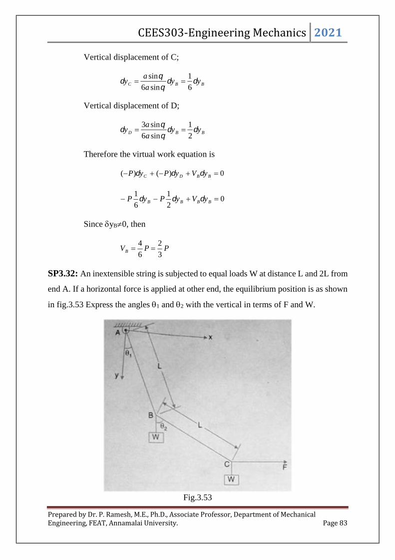
CEES303-Engineering Mechanics 2021
Prepared by Dr. P. Ramesh, M.E., Ph.D., Associate Professor, Department of MechanicalEngineering, FEAT, Annamalai University. Page 83
Vertical displacement of C;
BBC yya
ay
6
1
sin6
sin
Vertical displacement of D;
BBD yya
ay
2
1
sin6
sin3
Therefore the virtual work equation is
0)()( BBDC yVyPyP
02
1
6
1 BBBB yVyPyP
Since yB0, then
PPVB 3
2
6
4
SP3.32: An inextensible string is subjected to equal loads W at distance L and 2L from
end A. If a horizontal force is applied at other end, the equilibrium position is as shown
in fig.3.53 Express the angles 1 and 2 with the vertical in terms of F and W.
Fig.3.53

CEES303-Engineering Mechanics 2021
Prepared by Dr. P. Ramesh, M.E., Ph.D., Associate Professor, Department of MechanicalEngineering, FEAT, Annamalai University. Page 84
Solution:
With respect to the coordinate system as shown in fig.3.53 the three active force
are W, W and F. It is a system of two degrees of freedom in which 1 and 2 can vary
independently.
Therefore the principle of virtual work is
022
11
UUU
Keeping 1 constant and varying 2 the principle of virtual equation is
0 xFyW C
0sincos 222
222
LFLW
0cossin 22 FLWL
W
F2tan
Now, keeping 2 constant and varying 1,
1cosLyB
11sin LyB
21 coscos LLyC
Since 2 is constant,
11sin LyC
21 sinsin LLxC
Since 2 is constant,
11cos LxC
The principle of virtual work is

CEES303-Engineering Mechanics 2021
Prepared by Dr. P. Ramesh, M.E., Ph.D., Associate Professor, Department of MechanicalEngineering, FEAT, Annamalai University. Page 85
0 CCB xFyWyW
0cossinsin 111111 LFLWLW
W
F
2tan 1
CONSERVATIVE FORCES:
When a force does work that depends only upon the initial and final positions of
the force, and it is independent of the path it travels, then the force is referred to as a
conservative force. The weight of a body and the force of a spring are two examples of
conservative forces.
a) Weight:
Fig.3.54 Displacement of rigid body
Consider a block of weight W that travels along the path as shown in
fig.3.54 (a). When it is displaced up the path by an amount dr, then the work is
W.drdU or dydrdU W cosW , as shown in fig.3.54 (b). In this case,
the work is negative since W acts in the opposite sense of dy. Thus, if the block
moves from A to B, through the vertical displacement h, the work is
WhWdyUh
0
The weight of a body is therefore a conservative force, since the work
done by the weight depends only on the vertical displacement of the body, and
is independent of the path along which the body travels.

CEES303-Engineering Mechanics 2021
Prepared by Dr. P. Ramesh, M.E., Ph.D., Associate Professor, Department of MechanicalEngineering, FEAT, Annamalai University. Page 86
b) Spring Force:
Fig.3.55 Deformation of elastic body
Now consider the linearly elastic spring as shown in fig.3.55, which
undergoes a displacement ds. The work done by the spring force on the block is
ksdsdsFdU s . The work is negative because Fs acts in the opposite sense
to that of ds. Thus, the work of F when the block is displaced from s = s1 to s =
s2 is
2
122 2
1
2
11
1
ksksksdsUs
s
Here the work depends only on the spring’s initial and final positions s1
and s2, measured from the spring’s un-stretched position. Since this result is
independent of the path taken by the block as it moves, then a spring force is also
a conservative force.
Friction: In contrast to a conservative force, consider the force of friction exerted on a
sliding body by a fixed surface. The work done by the frictional force depends on the
path; the longer the path, the greater the work. Consequently, frictional forces are non-
conservative, and most of the work done by them is dissipated from the body in the
form of heat.

CEES303-Engineering Mechanics 2021
Prepared by Dr. P. Ramesh, M.E., Ph.D., Associate Professor, Department of MechanicalEngineering, FEAT, Annamalai University. Page 87
POTENTIAL ENERGY:
A conservative force can give the body the capacity to do work. This capacity
measured as potential energy, depends on the location or “position” of the body
measured relative to a fixed reference position or datum. The concept of potential
energy is useful for determining the stability of equilibrium by two methods. They are
1) Elastic potential Energy
2) Gravitational potential energy
1) Elastic Potential Energy:
The work done on an elastic member is stored in the member in the form of
elastic potential energy Ve. This energy is potentially available to do work on some
other body during the relief of its compression or extension.
Fig.3.56 Elastic potential energy
xx
e kxdxFdxV00
, or
2
2
1kxVe

CEES303-Engineering Mechanics 2021
Prepared by Dr. P. Ramesh, M.E., Ph.D., Associate Professor, Department of MechanicalEngineering, FEAT, Annamalai University. Page 88
Thus, the potential energy of the spring equals the triangular area in the diagram
of F versus x from 0 to x.
During an increase in the compression of the spring from x1 to x2, the work done
on the spring equals its change in elastic potential energy or
21
222
12
1
xxkkxdxVx
xe
which equals the trapezoidal area from x1 to x2.
During a virtual displacement x of the spring, the virtual work done on the
spring is the virtual change in elastic potential energy.
xkxxFVe
During a decrease in the compression of the spring as it is relaxed from x = x2 to
x = x1, the change (final minus initial) in the potential energy of the spring is negative.
Consequently, if x is negative, Ve is also negative.
When we have a spring in tension rather than compression, the work and energy
relations are the same as those for compression, where x now represents the elongation
of the spring rather than its compression. While the spring is being stretched, the force
again acts in the direction of the displacement, doing positive work on the spring and
increasing its potential energy.
Because the force acting on the movable end of a spring is the negative of the
force exerted by the spring on the body to which its movable end is attached, the work
done on the body is the negative of the potential energy change of the spring.
A torsional spring, which resists the rotation of a shaft or another element, can
also store and release potential energy. If the torsional stiffness, expressed as torque per
radian of twist, is a constant kT, and if is the angle of twist in radians, then the resisting
torque is TkM . The potential energy becomes
0
dkV Te or
2
2
1Te kV
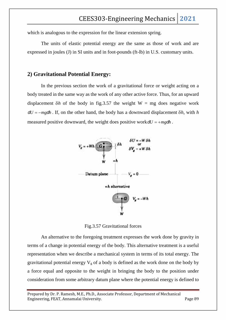
CEES303-Engineering Mechanics 2021
Prepared by Dr. P. Ramesh, M.E., Ph.D., Associate Professor, Department of MechanicalEngineering, FEAT, Annamalai University. Page 89
which is analogous to the expression for the linear extension spring.
The units of elastic potential energy are the same as those of work and are
expressed in joules (J) in SI units and in foot-pounds (ft-lb) in U.S. customary units.
2) Gravitational Potential Energy:
In the previous section the work of a gravitational force or weight acting on a
body treated in the same way as the work of any other active force. Thus, for an upward
displacement h of the body in fig.3.57 the weight W = mg does negative work
hmgU . If, on the other hand, the body has a downward displacement h, with h
measured positive downward, the weight does positive work hmgU .
Fig.3.57 Gravitational forces
An alternative to the foregoing treatment expresses the work done by gravity in
terms of a change in potential energy of the body. This alternative treatment is a useful
representation when we describe a mechanical system in terms of its total energy. The
gravitational potential energy Vg of a body is defined as the work done on the body by
a force equal and opposite to the weight in bringing the body to the position under
consideration from some arbitrary datum plane where the potential energy is defined to

CEES303-Engineering Mechanics 2021
Prepared by Dr. P. Ramesh, M.E., Ph.D., Associate Professor, Department of MechanicalEngineering, FEAT, Annamalai University. Page 90
be zero. The potential energy, then, is the negative of the work done by the weight.
When the body is raised, for example, the work done is converted into energy which is
potentially available, since the body can do work on some other body as it returns to its
original lower position. If consider Vg to be zero at h = 0, fig.3.57, then at a height h
above the datum plane, the gravitational potential energy of the body is
mghVg
If the body is a distance h below the datum plane, its gravitational potential
energy is mgh .
Fig.3.58 Gravitation forces with reference datum
Note that the datum plane for zero potential energy is arbitrary because only the
change in potential energy matters, and this change is the same no matter where it places
the datum plane. Note also that the gravitational potential energy is independent of the
path followed in arriving at a particular level h. Thus, the body of mass m as shown in
fig.3.58has the same potential-energy change no matter which path it follows in going
from datum plane 1 to datum plane 2 because h is the same for all three paths.
The virtual change in gravitational potential energy is simply
hmgVg
where oh is the upward virtual displacement of the mass centre of the body. If the mass
centre has a downward virtual displacement, then Vg is negative.
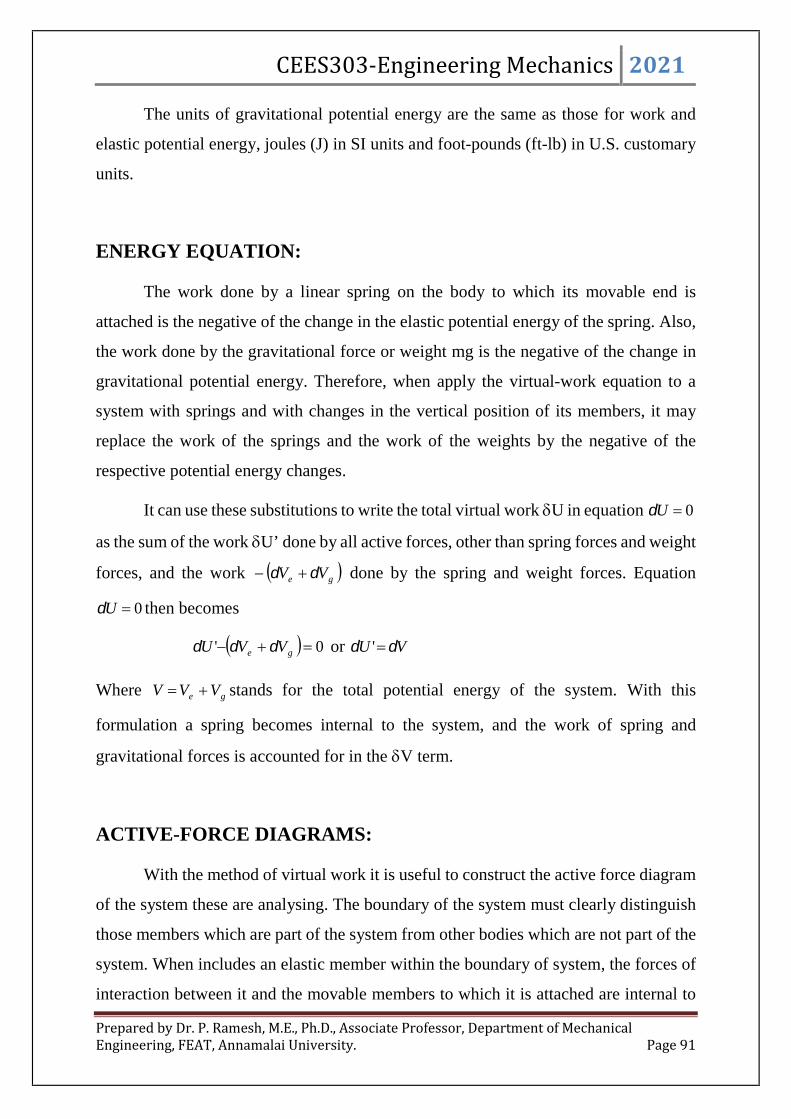
CEES303-Engineering Mechanics 2021
Prepared by Dr. P. Ramesh, M.E., Ph.D., Associate Professor, Department of MechanicalEngineering, FEAT, Annamalai University. Page 91
The units of gravitational potential energy are the same as those for work and
elastic potential energy, joules (J) in SI units and foot-pounds (ft-lb) in U.S. customary
units.
ENERGY EQUATION:
The work done by a linear spring on the body to which its movable end is
attached is the negative of the change in the elastic potential energy of the spring. Also,
the work done by the gravitational force or weight mg is the negative of the change in
gravitational potential energy. Therefore, when apply the virtual-work equation to a
system with springs and with changes in the vertical position of its members, it may
replace the work of the springs and the work of the weights by the negative of the
respective potential energy changes.
It can use these substitutions to write the total virtual work U in equation 0U
as the sum of the work U’ done by all active forces, other than spring forces and weight
forces, and the work ge VV done by the spring and weight forces. Equation
0U then becomes
0' ge VVU or VU '
Where ge VVV stands for the total potential energy of the system. With this
formulation a spring becomes internal to the system, and the work of spring and
gravitational forces is accounted for in the V term.
ACTIVE-FORCE DIAGRAMS:
With the method of virtual work it is useful to construct the active force diagram
of the system these are analysing. The boundary of the system must clearly distinguish
those members which are part of the system from other bodies which are not part of the
system. When includes an elastic member within the boundary of system, the forces of
interaction between it and the movable members to which it is attached are internal to

CEES303-Engineering Mechanics 2021
Prepared by Dr. P. Ramesh, M.E., Ph.D., Associate Professor, Department of MechanicalEngineering, FEAT, Annamalai University. Page 92
the system. Thus these forces need not be shown because their effects are accounted for
in the Ve term. Similarly, weight forces are not shown because their work is accounted
for in the Vg term.
Fig.3.59 Active force diagrams
Fig.3.59 illustrates the difference between the use of equation 0U and
0' ge VVU or VU ' . It consider the body in part of the figure to be a
particle for simplicity, and it assumes that the virtual displacement is along the fixed
path. The particle is in equilibrium under the action of the applied forces F1 and F2, the
gravitational force mg, the spring force kx, and a normal reaction force. In fig.3.59 (b),
where the particle alone is isolated, U includes the virtual work of all forces shown on
the active-force diagram of the particle. (The normal reaction exerted on the particle by
the smooth guide does no work and is omitted.). In Fig.3.59 (c) the spring is included
in the system, and U’ is the virtual work of only F1 and F2, which are the only external
forces whose work is not accounted for in the potential energy terms. The work of the
weight mg is accounted for in the Vg term, and the work of the spring force is included
in the Ve term.

CEES303-Engineering Mechanics 2021
Prepared by Dr. P. Ramesh, M.E., Ph.D., Associate Professor, Department of MechanicalEngineering, FEAT, Annamalai University. Page 93
STABILITY OF EQUILIBRIUM:
Fig.3.60 Mechanical system changes with gravitational and elastic potential
energy
Consider now the case of a mechanical system where movement is accompanied
by changes in gravitational and elastic potential energies and where no work is done on
the system by non-potential forces. The mechanism as shown in fig3.60 is an example
of such a system. With 0'U the virtual-work relation, equation 0' ge VVU
or VU ' , becomes
0 ge VV or 0V
The above equation expresses the requirement that the equilibrium configuration
of a mechanical system is one for which the total potential energy V of the system has
a stationary value. For a system of one degree of freedom where the potential energy
and its derivatives are continuous functions of the single variable, say, x, which
describes the configuration, the equilibrium condition 0V is equivalent
mathematically to the requirement
0dx
dV
The above equation states that a mechanical system is in equilibrium when the
derivative of its total potential energy is zero. For systems with several degrees of
freedom the partial derivative of V with respect to each coordinate in turn must be zero
for equilibrium.

CEES303-Engineering Mechanics 2021
Prepared by Dr. P. Ramesh, M.E., Ph.D., Associate Professor, Department of MechanicalEngineering, FEAT, Annamalai University. Page 94
Fig.3.61 Stability of equilibrium
There are three conditions under which equation 0dx
dVapplies, namely, when
the total potential energy is a minimum (stable equilibrium), a maximum (unstable
equilibrium), or a constant (neutral equilibrium). Fig.3.39 shows a simple example of
these three conditions. The potential energy of the roller is clearly a minimum in the
stable position, a maximum in the unstable position, and a constant in the neutral
position.
It may also characterize the stability of a mechanical system by noting that a
small displacement away from the stable position results in an increase in potential
energy and a tendency to return to the position of lower energy. On the other hand, a
small displacement away from the unstable position results in a decrease in potential
energy and a tendency to move farther away from the equilibrium position to one of
still lower energy. For the neutral position a small displacement one way or the other
results in no change in potential energy and no tendency to move either way.
When a function and its derivatives are continuous, the second derivative is
positive at a point of minimum value of the function and negative at a point of maximum
value of the function. Thus, the mathematical conditions for equilibrium and stability
of a system with a single degree of freedom x are:
0dx
dVmEquilibriu
0table2
2
dx
VdS

CEES303-Engineering Mechanics 2021
Prepared by Dr. P. Ramesh, M.E., Ph.D., Associate Professor, Department of MechanicalEngineering, FEAT, Annamalai University. Page 95
0table2
2
dx
VdUns
The second derivative of V may also be zero at the equilibrium position, in which
case we must examine the sign of a higher derivative to ascertain the type of
equilibrium. When the order of the lowest remaining nonzero derivative is even, the
equilibrium will be stable or unstable according to whether the sign of this derivative is
positive or negative. If the order of the derivative is odd, the equilibrium is classified as
unstable, and the plot of V versus x for this case appears as an inflection point in the
curve with zero slope at the equilibrium value.
Stability criteria for multiple degrees of freedom require more advanced
treatment. For two degrees of freedom, for example, it uses a Taylor- series expansion
for two variables.
Problems:
SP3.33: The 10 kg cylinder is suspended by the spring which has a stiffness of 2kN/m.
Plot the potential energy V of the system and show that it is minimum at the equilibrium
position.
Fig.3.62
Solution:
The elastic potential energy for an arbitrary position x is

CEES303-Engineering Mechanics 2021
Prepared by Dr. P. Ramesh, M.E., Ph.D., Associate Professor, Department of MechanicalEngineering, FEAT, Annamalai University. Page 96
2
2
1kxVe
The gravitational potential energy for an arbitrary position x is
mgxVg
The total potential energy is
mgxkxVVV ge 2
2
1
The equilibrium of potential energy is obtained by
0dx
dV, 0 mgkx
dx
dV
k
mgx
mx 049.02000
81.910
X=49mm
Substituting numerical values gives
049.081.910)049.0)(2000(2
1 2 V
The minimum value at equilibrium position of potential energy is
mNV 4.2
The below plot shows the different forms of potential energies. The minim value
of V occurs at x = 0.049m where 0dx
dVand
2
2
dx
Vdis positive.
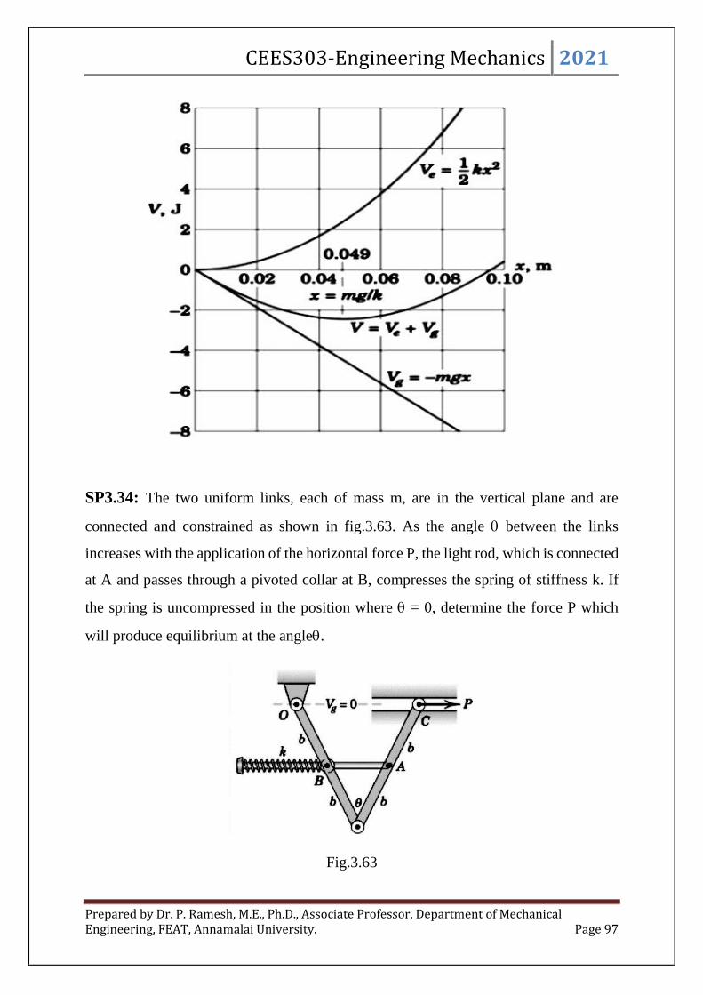
CEES303-Engineering Mechanics 2021
Prepared by Dr. P. Ramesh, M.E., Ph.D., Associate Professor, Department of MechanicalEngineering, FEAT, Annamalai University. Page 97
SP3.34: The two uniform links, each of mass m, are in the vertical plane and are
connected and constrained as shown in fig.3.63. As the angle between the links
increases with the application of the horizontal force P, the light rod, which is connected
at A and passes through a pivoted collar at B, compresses the spring of stiffness k. If
the spring is uncompressed in the position where = 0, determine the force P which
will produce equilibrium at the angle.
Fig.3.63

CEES303-Engineering Mechanics 2021
Prepared by Dr. P. Ramesh, M.E., Ph.D., Associate Professor, Department of MechanicalEngineering, FEAT, Annamalai University. Page 98
Solution:
The compression x of the spring is the distance which A has moved away from
B, which is2
sin2
bx
The elastic potential energy of the spring is
2
2
1kxVe ,
2sin2
2sin2
2
1 222
kbbkVe
With the datum for zero gravitational potential energy taken through the support
at O for convenience, the expression is
2cos22
bmgmgxVg
The distance between O and C is2
sin4
b , so that the virtual work done by P is
2sin4'
bPU
The principle of virtual work is
0' VU , 0' ge VVU
02
cos22
sin22
sin4 22
mgbkbbP
0sin2
cos2
sin22
cos2 2
mgbkbPb
Since 0, then
2tan
2
1
2sin
mgkbP
SP3.35: The ends of the uniform bar of mass m side freely in the horizontal and vertical
guides. Examine the stability conditions for the positions of equilibrium. The spring of
stiffness k is un-deformed when x =0.

CEES303-Engineering Mechanics 2021
Prepared by Dr. P. Ramesh, M.E., Ph.D., Associate Professor, Department of MechanicalEngineering, FEAT, Annamalai University. Page 99
Fig.3.64
Solution:
The system consists of the spring and the bar. Since there are no external active
forces the given sketch serves as the active force diagram. It will take the x axis as the
datum for zero gravitational potential energy. In the displaced position the elastic and
gravitational potential energies are
222 sin2
1
2
1kbkxVe and cos
2
bmgVg
The total potential energy is then,
cos2
1sin
2
1 22 mgbkbVVV ge
The equilibrium occurs for 0d
dV, so that
0sin2
1cossin
2
1cossin 22
mgbkbmgbkb
d
dV
The two solutions to this equation are given by
0sin andkb
mg
2cos
Now determine the stability by examining the sign of the second derivative of V
for each of the two equilibrium positions. The second derivative is

CEES303-Engineering Mechanics 2021
Prepared by Dr. P. Ramesh, M.E., Ph.D., Associate Professor, Department of MechanicalEngineering, FEAT, Annamalai University. Page 100
cos2
1sincos 222
2
2
mgbkbd
Vd
cos2
11cos2 22
2
2
mgbkbd
Vd
Solution 1: 0sin , =0
kb
mgkbmgbkb
d
Vd
21
2
112 22
2
2
Ifb
mgk
2 , Then )(
2
2
stablevaluepossitivedx
Vd
Ifb
mgk
2 , Then )(
2
2
unstablevalueNegativedx
Vd
Thus, if the spring is sufficiently stiff, the bar will return to the vertical position
even though there is no force in the spring at that position.
Solution 2:
kb
mg
2cos ,
kb
mg
2cos 1
1
222
11
22
22
22
2
2
kb
mgkb
kb
mgmgb
kb
mgkb
d
Vd
Since the cosine must be less than unity, then this solution is limited to the case
whereb
mgk
2 , which makes the second derivative of V negative. Thus equilibrium for
solution 2 is never stable. Ifb
mgk
2 , then no longer have solution 2 since the spring
will be too weak to maintain equilibrium at a value of between 0 and 90o.
SP3.36: The uniform link as shown in fig.3.65a has a mass of 10kg. If the spring is un-
stretched when =0o, determine the angle for equilibrium and investigate the stability
at the equilibrium position.

CEES303-Engineering Mechanics 2021
Prepared by Dr. P. Ramesh, M.E., Ph.D., Associate Professor, Department of MechanicalEngineering, FEAT, Annamalai University. Page 101
Fig.3.65
Solution:
The datum is established at the bottom of the link as shown in fig.3.65b. When
the link is located in the arbitrary position, the spring increases its potential energy by
stretching and the weight decreases its potential energy. Hence
WyksVVV ge 2
2
1
Since coslsl or cos1 ls and cos2
ly then
cos
2
1cos1
2
1 22 WklV
The equilibrium condition,
0sin2
sincos12
Wlkl
d
dVor
0sin2
cos1
Wkll
This equation is satisfied by 0sin , =0o,, Therefore,
o
kl
W8.53
6.02002
81.9101cos
21cos 11

CEES303-Engineering Mechanics 2021
Prepared by Dr. P. Ramesh, M.E., Ph.D., Associate Professor, Department of MechanicalEngineering, FEAT, Annamalai University. Page 102
The second derivative of V is
cos2
sinsincoscos 222
2 Wlkllkl
d
Vd
cos2
2coscos22
2 Wlkl
d
Vd
Substituting values for the constant with =0o and =53.8o, Then
ooo
od
Vd0cos
2
6.081.910)0cos0(cos)6.0(200 2
0
2
2
04.290
2
2
od
Vd
(Unstable equilibrium at =0o)
ooo
od
Vd8.53cos
2
6.081.910)6.107cos8.53(cos)6.0(200 2
8.532
2
09.468.53
2
2
od
Vd
(Stable equilibrium at =53.8o)
SP3.37: If the spring AD as shown in fig.3.66a has a stiffness of 18 kN/m and is un-
stretched when = 60o, determine the angle for equilibrium. The load has a mass of
1.5 Mg. Investigate the stability at the equilibrium position.
Fig.3.66

CEES303-Engineering Mechanics 2021
Prepared by Dr. P. Ramesh, M.E., Ph.D., Associate Professor, Department of MechanicalEngineering, FEAT, Annamalai University. Page 103
Solution:
The gravitational potential energy for the load with respect to the fixed datum as
shown in fig.3.66b is
hhmgyVg 14715sin58860sin4)81.9(1500
Where h is a constant distance. From the geometry of the system, the elongation
of the spring when the load is on the platform is
2cos460cos4cos4 os
Thus, the elastic potential energy of the system is
222 2cos490002cos4180002
1
2
1 ksVe
The potential energy function for the system is therefore
22cos4900014715sin58860 hVVV ge
When the system is in equilibrium, then
0)sin4)(2cos4(18000sin58860 d
dV
0sin144000cossin288000cos58860
Since cossin22sin , then
0sin1440002sin144000cos58860
Solving by trail and error, then
o18.28 and o51.45
Taking the second derivative of equation, then
cos1440002cos288000sin588602
2
d
Vd
Substituting o18.28 , then
0604022
2
d
Vd(Unstable)

CEES303-Engineering Mechanics 2021
Prepared by Dr. P. Ramesh, M.E., Ph.D., Associate Professor, Department of MechanicalEngineering, FEAT, Annamalai University. Page 104
Now, o51.45
0640732
2
d
Vd(Stable)
SP3.38: The uniform block having a mass m rests on the top surface of the half
cylinder, fig.3.67a. Show that this is a condition of unstable equilibrium if h >2R.
Fig.3.67
Solution:
The datum is established at the base of the cylinder, fig.3.67b. If the block is
displaced by an amount u from the equilibrium position, the potential function is
mgyVVV ge 0
From the geometry of fig.3.b,
sincos2
Rh
Ry
Thus,
sincos
2R
hRmgV
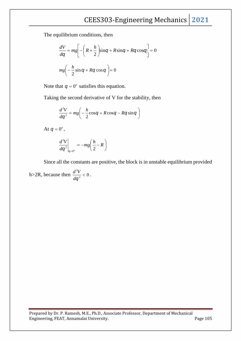
CEES303-Engineering Mechanics 2021
Prepared by Dr. P. Ramesh, M.E., Ph.D., Associate Professor, Department of MechanicalEngineering, FEAT, Annamalai University. Page 105
The equilibrium conditions, then
0cossinsin2
RR
hRmg
d
dV
0cossin2
R
hmg
Note that o0 satisfies this equation.
Taking the second derivative of V for the stability, then
sincoscos
22
2
RRh
mgd
Vd
At o0 ,
Rh
mgd
Vd
o 20
2
2
Since all the constants are positive, the block is in unstable equilibrium provided
h>2R, because then 02
2
d
Vd.

Lecture Notes
UNIT – 4 2021
Prepared by
Dr. P. Ramesh, M.E., Ph.D.,
Associate Professor
Department of Mechanical Engineering
Faculty of Engineering and Technology
Annamalai UniversityAug-2021
CEES303-EngineeringMechanics

CEES303-Engineering Mechanics 2021
Prepared by Dr. P. Ramesh, M.E., Ph.D., Associate Professor, Department of MechanicalEngineering, FEAT, Annamalai University. Page 2
Unit - 4
Review of particle dynamics- Rectilinear motion; Plane curvilinear
motion (rectangular, path, and polar coordinates). 3-D curvilinear
motion; Relative and constrained motion; Newton’s 2nd law
(rectangular, path, and polar coordinates). Work-kinetic energy,
power, potential energy. Impulse-momentum (linear, angular);
Impact (Direct and oblique).
Reference for the preparation of course material:
1. F. P. Beer and E. R. Johnston (2011), Vector Mechanics for Engineers,Vol I - Statics, Vol II, – Dynamics, 9th Ed, Tata McGraw Hill.
2. Khurmi R.S. (2010), Engineering Mechanics, S. Chand & Co.3. J.L. Meriam and L. G. Kraige, Engineering Mechanics –Statics, volume I,
Seventh edition, John Wiley & Sons, Inc.
TEXT BOOKS1. Irving H. Shames (2006), Engineering Mechanics, 4th Edition, Prentice Hall2. F. P. Beer and E. R. Johnston (2011), Vector Mechanics for Engineers, Vol I -
Statics, Vol II, – Dynamics, 9th Ed, Tata McGraw Hill
REFERENCES1. R. C. Hibbler (2006), Engineering Mechanics: Principles of Statics and Dynamics,
Pearson Press.2. Khurmi R.S. (2010), Engineering Mechanics, S. Chand & Co.

CEES303-Engineering Mechanics 2021
Prepared by Dr. P. Ramesh, M.E., Ph.D., Associate Professor, Department of MechanicalEngineering, FEAT, Annamalai University. Page 3
Unit - 4
Review of particle Dynamics
Kinematics is the branch of dynamics which describes the motion of bodies
without reference to the forces which either cause the motion or are generated as a result
of the motion. Kinematics is often described as the “geometry of motion.” Some
engineering applications of kinematics include the design of cams, gears, linkages, and
other machine elements to control or produce certain desired motions, and the
calculation of flight trajectories for aircraft, rockets, and spacecraft. A thorough working
knowledge of kinematics is a prerequisite to kinetics, which is the study of the
relationships between motion and the corresponding forces which cause or accompany
the motion.
PARTICLE MOTION:
Fig.4.1 Particle motion

CEES303-Engineering Mechanics 2021
Prepared by Dr. P. Ramesh, M.E., Ph.D., Associate Professor, Department of MechanicalEngineering, FEAT, Annamalai University. Page 4
A particle is a body whose physical dimensions are so small compared with the
radius of curvature of its path that treats the motion of the particle as that of a point. For
example, the wingspan of a jet transport flying between Los Angeles and New York is
of no consequence compared with the radius of curvature of its flight path, and thus the
treatment of the airplane as a particle or point is an acceptable approximation.
It describes the motion of a particle in a number of ways, and the choice of the
most convenient or appropriate way depends a great deal on experience and on how the
data are given. Let us obtain an overview of the several methods developed in this
section by referring to fig.4.1, which shows a particle P moving along some general
path in space. If the particle is confined to a specified path, as with a bead sliding along
a fixed wire, its motion is said to be constrained. If there are no physical guides, the
motion is said to be unconstrained. A small rock tied to the end of a string and whirled
in a circle undergoes constrained motion until the string breaks, after which instant its
motion is unconstrained.
RECTILINEAR MOTION:
Fig.4.2 Rectilinear motion
Consider a particle P moving along a straight line, fig.4.2 shows that the position
of ‘P’ at any instant of time t can be specified by its distance ‘s’ measured from some
convenient reference point O fixed on the line. At time t + Δ t the particle has moved to
P' and its coordinate becomes s + Δs. The change in the position coordinate during the
interval Δ t is called the displacement, Δs of the particle. The displacement would be
negative if the particle moved in the negative s-direction.

CEES303-Engineering Mechanics 2021
Prepared by Dr. P. Ramesh, M.E., Ph.D., Associate Professor, Department of MechanicalEngineering, FEAT, Annamalai University. Page 5
a) Velocity and Acceleration:
The average velocity of the particle during the interval Δt is the displacement
divided by the time interval ort
svav
. As Δt becomes smaller and approaches zero
in the limit, the average velocity approaches the instantaneous velocity of the particle,
which ist
sv
t
0
lim or
sdt
dsV ----------- (4.1)
Thus, the velocity is the time rate of change of the position coordinate s. The
velocity is positive or negative depending on whether the corresponding displacement
is positive or negative.
The average acceleration of the particle during the interval Δ t is the change in
its velocity divided by the time interval ort
vaav
. As Δ t becomes smaller and
approaches zero in the limit, the average acceleration approaches the instantaneous
acceleration of the particle, which ist
va
t
0
lim or
vdt
dva or
sdt
sda
2
2
----------- (4.2)
The acceleration is positive or negative depending on whether the velocity is
increasing or decreasing. Note that the acceleration would be positive if the particle had
a negative velocity which was becoming less negative. If the particle is slowing down,
the particle is said to be decelerating.
Velocity and acceleration are actually vector quantities, as it will see for
curvilinear motion in forthcoming sections. For rectilinear motion, where the direction
of the motion is that of the given straight-line path, the sense of the vector along the
path is described by a plus or minus sign. In curvilinear motion, it will account for the
changes in direction of the velocity and acceleration vectors as well as their changes in
magnitude.

CEES303-Engineering Mechanics 2021
Prepared by Dr. P. Ramesh, M.E., Ph.D., Associate Professor, Department of MechanicalEngineering, FEAT, Annamalai University. Page 6
By eliminating the time dt between equation 4.1 and 4.2, then the differential
equation relating displacement, velocity, and acceleration as
dsadvv or dsssds
--------- (4.3)
b) Uniform acceleration motion:
When the velocity of the body changes by equal amounts in equal intervals of
time, then the body is said to have uniform acceleration motion. Consider equation 4.2
asdt
dva . Here the acceleration ‘a’ is treated as constant then the velocity is changes
form initial velocity to final velocity as vu and time changes from t=0 to t=t.
To find
velocity as a function of time,
velocity as a function of position and
position as a function of time
while keeping the acceleration as constant.
Now the integration of equation 4.2 gives the velocity as a function of time, then
tt
t
tt
t
v
u
dtadtadv00
.
10 Ctav ttt
vu
1Catv -------------- (4.4)
To eliminate the constant C1, Substitute the initial condition when t=0 then v=u,
therefore, the equation 4.4 as
1)0( Cau
uC 1 -------------- (4.5)
Now substitute the equation 4.5 into the equation 4.4 then

CEES303-Engineering Mechanics 2021
Prepared by Dr. P. Ramesh, M.E., Ph.D., Associate Professor, Department of MechanicalEngineering, FEAT, Annamalai University. Page 7
atuV ---------- (4.6) [Velocity as a function of time]
The equation 4.1 is taken to find the position as a function of time, then
dt
dsv
dtvds -------------- (4.7)
Now substitute the equation 4.6 into the equation 4.7 to get
dttauds ------- (4.8)
The equation 4.8 is now integrate to obtain position as a function of time, then
ts
dtatuds00
2
2
2C
atuts
When, t=0, s=0, then
02 C
Therefore,
2
2
1atuts -------- (4.9) [Position as a function of time]
From equation 4.6 obtain time and substitute in equation 4.9 to get the velocity
as a function of position. Therefore
atuv
a
uvt
The equation 4.9 as,
2
2
1atuts

CEES303-Engineering Mechanics 2021
Prepared by Dr. P. Ramesh, M.E., Ph.D., Associate Professor, Department of MechanicalEngineering, FEAT, Annamalai University. Page 8
2
2
1
a
uva
a
uvus
222
2
22
1uvuv
a
a
a
uuvs
222
2
1
2
1u
aa
vuv
aa
u
a
uvs
22
2
1
2
1u
av
as ,
a
uvs
2
22
sauv 222 ----------- (4.10) [Velocity as a function of position]
The equation of motion with uniform acceleration,
The velocity as a function of time is atuv ,
The position as a function of time is2
2
1atuts and
The velocity as a function of position is sauv 222
c) Uniform velocity motion:
When the velocity of the body remains constant throughout the period of time
then the body is said to be uniform velocity motion. Therefore when the body moves
with uniform velocity, the rate of change of velocity is zero and hence the acceleration
is also zero.
The equation 4.6 and 4.10 becomes to get the initial velocity is equals to final
velocity. The only one equation is suite to get function from equation 4.9.
Therefore, the equation of motion with uniform velocity from equation 4.9 as
uts or vts --------------- (4.11)
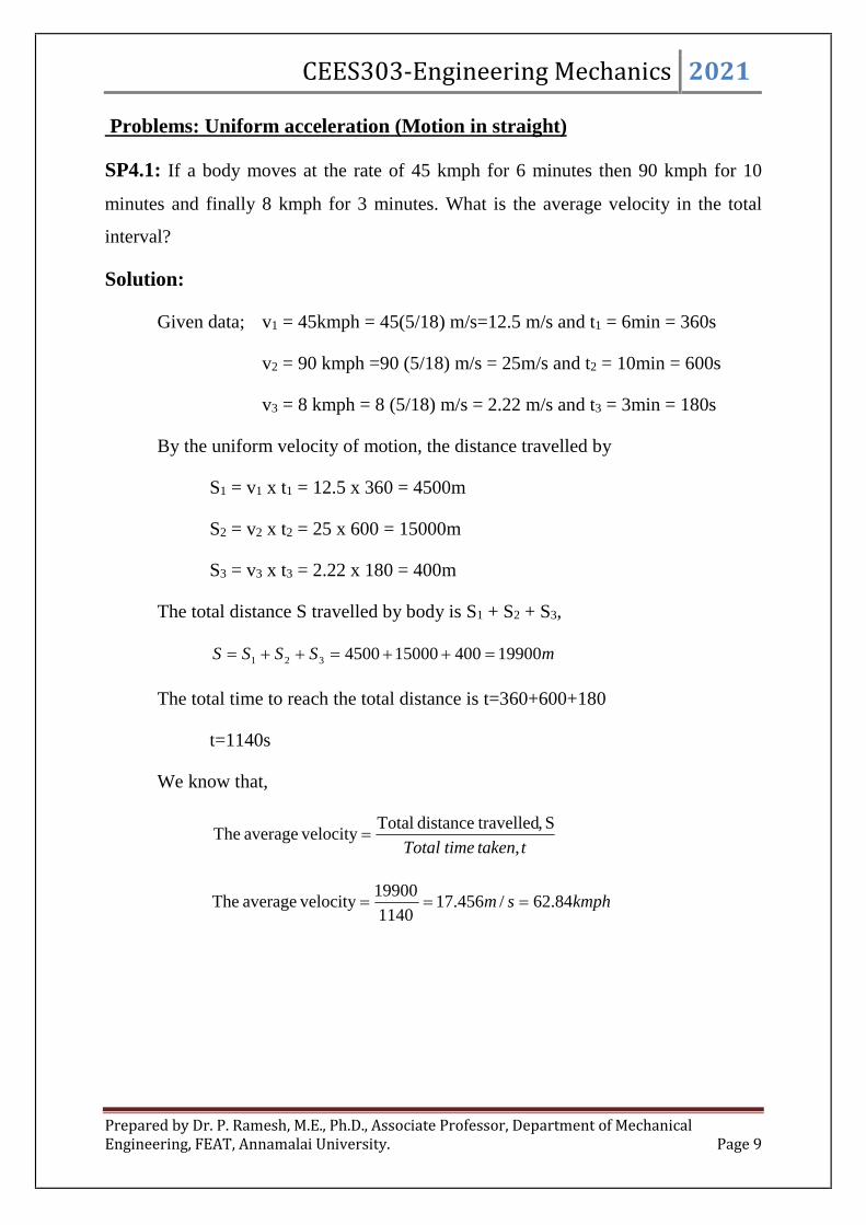
CEES303-Engineering Mechanics 2021
Prepared by Dr. P. Ramesh, M.E., Ph.D., Associate Professor, Department of MechanicalEngineering, FEAT, Annamalai University. Page 9
Problems: Uniform acceleration (Motion in straight)
SP4.1: If a body moves at the rate of 45 kmph for 6 minutes then 90 kmph for 10
minutes and finally 8 kmph for 3 minutes. What is the average velocity in the total
interval?
Solution:
Given data; v1 = 45kmph = 45(5/18) m/s=12.5 m/s and t1 = 6min = 360s
v2 = 90 kmph =90 (5/18) m/s = 25m/s and t2 = 10min = 600s
v3 = 8 kmph = 8 (5/18) m/s = 2.22 m/s and t3 = 3min = 180s
By the uniform velocity of motion, the distance travelled by
S1 = v1 x t1 = 12.5 x 360 = 4500m
S2 = v2 x t2 = 25 x 600 = 15000m
S3 = v3 x t3 = 2.22 x 180 = 400m
The total distance S travelled by body is S1 + S2 + S3,
mSSSS 19900400150004500321
The total time to reach the total distance is t=360+600+180
t=1140s
We know that,
ttakentimeTotal ,
S, travelleddistanceTotal velocityaverageThe
kmphsm 84.62/456.171140
19900 velocityaverageThe
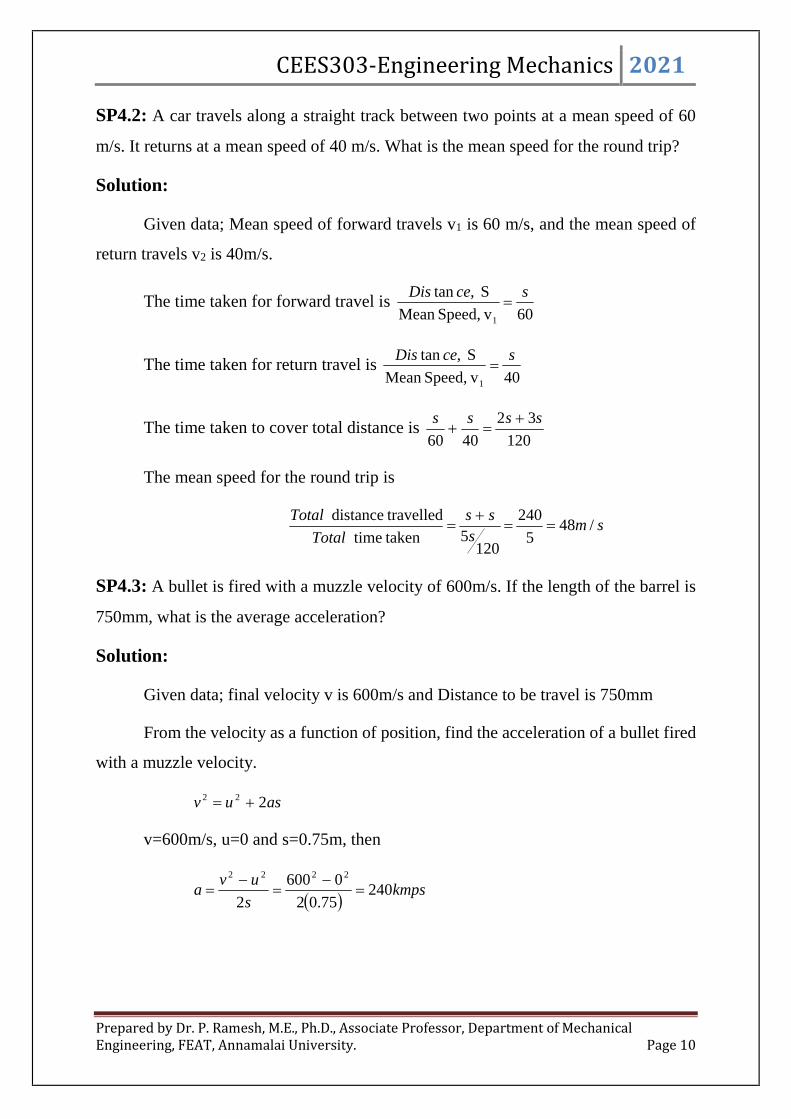
CEES303-Engineering Mechanics 2021
Prepared by Dr. P. Ramesh, M.E., Ph.D., Associate Professor, Department of MechanicalEngineering, FEAT, Annamalai University. Page 10
SP4.2: A car travels along a straight track between two points at a mean speed of 60
m/s. It returns at a mean speed of 40 m/s. What is the mean speed for the round trip?
Solution:
Given data; Mean speed of forward travels v1 is 60 m/s, and the mean speed of
return travels v2 is 40m/s.
The time taken for forward travel is60 vSpeed,Mean
S,tan
1
sceDis
The time taken for return travel is40 vSpeed,Mean
S,tan
1
sceDis
The time taken to cover total distance is120
32
4060
ssss
The mean speed for the round trip is
sms
ss
Total
Total/48
5
240
1205 taken time
travelleddistance
SP4.3: A bullet is fired with a muzzle velocity of 600m/s. If the length of the barrel is
750mm, what is the average acceleration?
Solution:
Given data; final velocity v is 600m/s and Distance to be travel is 750mm
From the velocity as a function of position, find the acceleration of a bullet fired
with a muzzle velocity.
asuv 222
v=600m/s, u=0 and s=0.75m, then
kmpss
uva 240
75.02
0600
2
2222

CEES303-Engineering Mechanics 2021
Prepared by Dr. P. Ramesh, M.E., Ph.D., Associate Professor, Department of MechanicalEngineering, FEAT, Annamalai University. Page 11
SP4.4: A car is moving with a velocity of 20m/s. The car is brought to rest by applying
brakes in 4 secs. Determine a) the retardation and b) distance travelled by the car after
applying brakes.
Solution:
Given data; u=20m/s, v=0m/s, t=4sec
By the equation of motion atuv find the acceleration as
2/54
200sm
t
uva
The negative sign indicates the retardation.
Distance travelled by the car after applying brakes is obtain from the equation of
motion as
2
2
1atuts
ms 40452
1420 2
SP4.5: on turning a corner a motorist rushing at 20m/s, find a child on the road 50m
ahead. He instantly stops the engine and applies brakes so as to stop the car with in 10
m of the child. Calculate a) retardation and b) time required to stop the car.
Solution:
Given data; u=20m/s, SMC =50m, v=0m/s and SMS = 50-10=40m
From the relation, aSuv 222
402200 22 a
a=-5m/s2
From the relation, atuv
t)5(200
t = 4sec.

CEES303-Engineering Mechanics 2021
Prepared by Dr. P. Ramesh, M.E., Ph.D., Associate Professor, Department of MechanicalEngineering, FEAT, Annamalai University. Page 12
SP4.6: Three marks A, B and C at distance of 100m each are made along a straight
road. A car starting from rest and with uniform acceleration passes the mark A and takes
10 sec to reach B and further 8 seconds to reach the mark C. Calculate a) acceleration
of the car, b) the velocity of car at A, c) the velocity of car at B and d) the distance of
the mark A from starting point.
Solution;
Given data; tAB = 10sec, tBC = 8sec, SAB = 100m, and SBC = 100m
Consider the motion from A to B, by the relation of position as a function of time
is
2
2
1atutS
S=SAB =100m, u=vA, v = vB, tAB = 10sec
2102
110100 avA
1001050 Ava ----------- (i)
Consider the motion from A to C, by the relation of position as a function of time
is
2
2
1atutS
S=SAC =1200m, u=vA, v = vC, tAC = 18sec
2182
118200 avA
20018162 Ava ------------- (ii)
Solve equation i and ii then
a = 0.28m/s2 and vA = 8.61 m/s
Consider the motion from starting point O to A, by the relation of velocity as a
function of position is

CEES303-Engineering Mechanics 2021
Prepared by Dr. P. Ramesh, M.E., Ph.D., Associate Professor, Department of MechanicalEngineering, FEAT, Annamalai University. Page 13
asuv 222
u = 0, a = 0.28m/s2 , and vA = 8.61m/s
S28.02061.8 22
S = 133.4m
Consider the motion from A to B, by the relation of velocity as a function of position is
asuv 222
100222 avv AB
10028.0261.8 22 Bv
VB = 11.39m/s
SP4.7: A burglar’s car had a start with an acceleration of 2m/s2. A police vigilant party
came after 5 seconds and continued to chase the burglar’s car with a uniform velocity
of 20m/s. Find the time taken in which the police van will overtake the car.
Solution:
Consider the uniform acceleration motion of the burglar’s car and let‘t’ be the
time taken by the burglar’s car while overtaking by the police van.
2
2
1atutS
u = 0m/s, a = 2m/s2
Therefore, 2tS -------- (i)
Consider the uniform velocity motion of police van, then
S = vt = 20 (t-5)
S = 20t – 100 ------- (ii)
Substitute the equation i in ii gives,
100202 tt

CEES303-Engineering Mechanics 2021
Prepared by Dr. P. Ramesh, M.E., Ph.D., Associate Professor, Department of MechanicalEngineering, FEAT, Annamalai University. Page 14
0100202 tt
0)10( 2 t
t = 10sec.
Therefore, the time for police van to overtake is t-5 = 10-5 = 5sec
SP4.8: A train is uniformly accelerated and passes successive kilometre stones with
velocities at 18 kmph and 36 kmph respectively. Calculate the velocity when it passes
the third kilometre stone. Also find time taken for each of these two intervals of one
kilometre.
Solution:
Consider the motion of the train between A and B, where u = vA =
18kmph=18(5/18) m/s=5m/s, and v = vB = 36kmph = 36 (5/18)m/s=10 m/s and S =
1000m. By the relation, aSuv 222 ,
10002510 22 a
a = 0.038 m/s2
Consider the motion of the train between B and C, where u = vB = 10m/s, v = vC,
a=0.038m/s2 and S = 1000m. By the relation aSuv 222 ,
1000038.021022 Cv
smvC /23.13
To find the time interval ‘t’ when motion between A and B, where u = 5m/s, v =
10m/s and a = 0.038m/s2. By the relation, atuv
t038.0510
t = 133.3sec.
To find the time interval ‘t’ when motion between B and C, where u = 10m/s, v
= 13.23m/s and a = 0.038m/s2. By the relation, atuv
t038.01023.13

CEES303-Engineering Mechanics 2021
Prepared by Dr. P. Ramesh, M.E., Ph.D., Associate Professor, Department of MechanicalEngineering, FEAT, Annamalai University. Page 15
t = 86.08sec.
SP4.9: A body is moving with uniform acceleration and covers 20m in 4th second and
30m in 8th second. Determine a) the initial velocity of the body and b) acceleration of
the body.
Solution:
Let S4 is a distance travelled at time t = 4seconds and S3 is a distance travelled
at time t = 3 seconds. Therefore the distance travelled during 4th seconds is S4 – S3.
By the relation of motion, 2
2
1atutS , where t = 4 second, then
auauS 8442
14 2
4
Similarly, auauS 5.4332
13 2
3
Hence, 20)5.43()84(34 auauSS
205.3 au ------- (i)
Similarly for 8th seconds
auauS 32882
18 2
8
Similarly, auauS 5.24772
17 2
7
Hence, 30)5.247()328(78 auauSS
305.7 au ------- (ii)
Now subtract equation 1 in 2, then
20305.35.7 auau
104 a
a = 2.5m/s2.
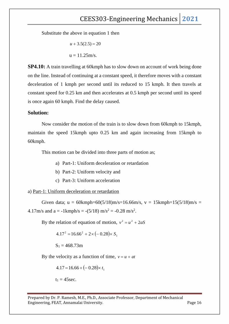
CEES303-Engineering Mechanics 2021
Prepared by Dr. P. Ramesh, M.E., Ph.D., Associate Professor, Department of MechanicalEngineering, FEAT, Annamalai University. Page 16
Substitute the above in equation 1 then
20)5.2(5.3 u
u = 11.25m/s.
SP4.10: A train travelling at 60kmph has to slow down on account of work being done
on the line. Instead of continuing at a constant speed, it therefore moves with a constant
deceleration of 1 kmph per second until its reduced to 15 kmph. It then travels at
constant speed for 0.25 km and then accelerates at 0.5 kmph per second until its speed
is once again 60 kmph. Find the delay caused.
Solution:
Now consider the motion of the train is to slow down from 60kmph to 15kmph,
maintain the speed 15kmph upto 0.25 km and again increasing from 15kmph to
60kmph.
This motion can be divided into three parts of motion as;
a) Part-1: Uniform deceleration or retardation
b) Part-2: Uniform velocity and
c) Part-3: Uniform acceleration
a) Part-1: Uniform deceleration or retardation
Given data; u = 60kmph=60(5/18)m/s=16.66m/s, v = 15kmph=15(5/18)m/s =
4.17m/s and a = -1kmph/s = -(5/18) m/s2 = -0.28 m/s2.
By the relation of equation of motion, aSuv 222
122 28.0266.1617.4 S
S1 = 468.73m
By the velocity as a function of time, atuv
128.066.1617.4 t
t1 = 45sec.
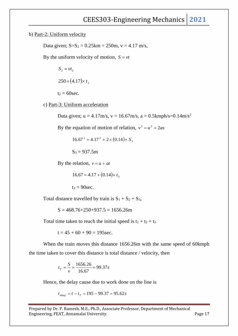
CEES303-Engineering Mechanics 2021
Prepared by Dr. P. Ramesh, M.E., Ph.D., Associate Professor, Department of MechanicalEngineering, FEAT, Annamalai University. Page 17
b) Part-2: Uniform velocity
Data given; S=S2 = 0.25km = 250m, v = 4.17 m/s,
By the uniform velocity of motion, vtS
22 vtS
217.4250 t
t2 = 60sec.
c) Part-3: Uniform acceleration
Data given; u = 4.17m/s, v = 16.67m/s, a = 0.5kmph/s=0.14m/s2
By the equation of motion of relation, asuv 222
322 14.0217.467.16 S
S3 = 937.5m
By the relation, atuv
314.017.467.16 t
t3 = 90sec.
Total distance travelled by train is S1 + S2 + S3,
S = 468.76+250+937.5 = 1656.26m
Total time taken to reach the initial speed is t1 + t2 + t3
t = 45 + 60 + 90 = 195sec.
When the train moves this distance 1656.26m with the same speed of 60kmph
the time taken to cover this distance is total distance / velocity, then
sv
StT 37.99
67.16
26.1656
Hence, the delay cause due to work done on the line is
sttt Tdelay 62.9537.99195

CEES303-Engineering Mechanics 2021
Prepared by Dr. P. Ramesh, M.E., Ph.D., Associate Professor, Department of MechanicalEngineering, FEAT, Annamalai University. Page 18
SP4.11: In a 100m race an athlete accelerates uniformly from the start to his maximum
velocity in a distance of 4m and runs the remaining distance with that velocity. If he
finishes the race in 10.4 secs, Find a) his initial acceleration and b) his maximum
velocity.
Solution:
The motion of the athlete can be divided into two parts;
Part-1: uniform acceleration
Data given; u1 =0, v1 = vmax, S1 = 4m, t = t1
By the relation, 1111 tauv
11max 0 tav
1
max1 a
vt --------- (1)
By the relation, 112
12
1 2 Sauv
420 122
max av
8
2max
1
va --------- (2)
Substitute, the equation 2 in equation 1, then
max2max
max1
8
8vv
vt
Part-2: Uniform velocity
Total time, t = 10.4 sec.
The time taken for uniform velocity is total time minus the time taken to reach
the uniform velocity from start.
Therefore, 12 ttt

CEES303-Engineering Mechanics 2021
Prepared by Dr. P. Ramesh, M.E., Ph.D., Associate Professor, Department of MechanicalEngineering, FEAT, Annamalai University. Page 19
max2
84.10
vt
The remaining distance from the reach of uniform velocity S2 is S – S1
S2 = 100-4 = 96m
By the relation, S2 = v2t2, where v2 is vmax
maxmax
84.1096
vv
84.1096 max v
smv /10max
Hence, 222
max1 /5.12
8
10
8sm
va
SP4.12: A bus is beginning to move with an acceleration of 0.3 m/s2. A man who is
12m behind the bus starts running at 3m/s to catch the bus. After how many seconds
will the man be able to catch the bus?
Solution:
The motion of bus is uniform acceleration and the motion of the man is uniform
velocity. The time for catching the bus by the man is equal to the time for travelling by
the bus from start. Hence the time ‘t’is same for both the motion’s
Part-1: Bus (Uniform acceleration)
Data given, u=0, aB = 0.3m/s2,
By the relation, 2
2
1atutS
23.02
10 BB tS
215.0 BB tS ---------------- (i)
Part-2: Man (Uniform velocity)

CEES303-Engineering Mechanics 2021
Prepared by Dr. P. Ramesh, M.E., Ph.D., Associate Professor, Department of MechanicalEngineering, FEAT, Annamalai University. Page 20
Data given, BM SS 12 ,
By the relation, MMM tvS
MB tS 312
123 MB tS ---------- (ii)
Now substitute the eqn. ii into the eqn. i then
215.0123 BM tt
Here, tM = tB, then
012315.0 2 MM tt
By solving, it gives
t = 14.47 s or 5.52 s
SP4.13: Two trains A and B leave the same station in parallel lines. Trains A starts
with a uniform acceleration of 0.15 m/s2 and attains a speed of 27 kmph. Then the steam
is reduced to keep speed constant. Train B leaves 40 secs later with uniform acceleration
of 0.3 m/s2 to attain maximum speed of 54 kmph. When and where will B overtake A?
Solution:
Since the both train starts from same station while overtaking the distance
travelled by the both the trains remain same. i.e., SA = SB.
Part-1: uniform acceleration
Train-A:
Data given, u = 0, v = 27kmph = 7.5m/s, aA = 0.15 m/s2.
By the relation, atuv
t15.005.7
t = 50sec.
By the relation, 21 2
1atutS A
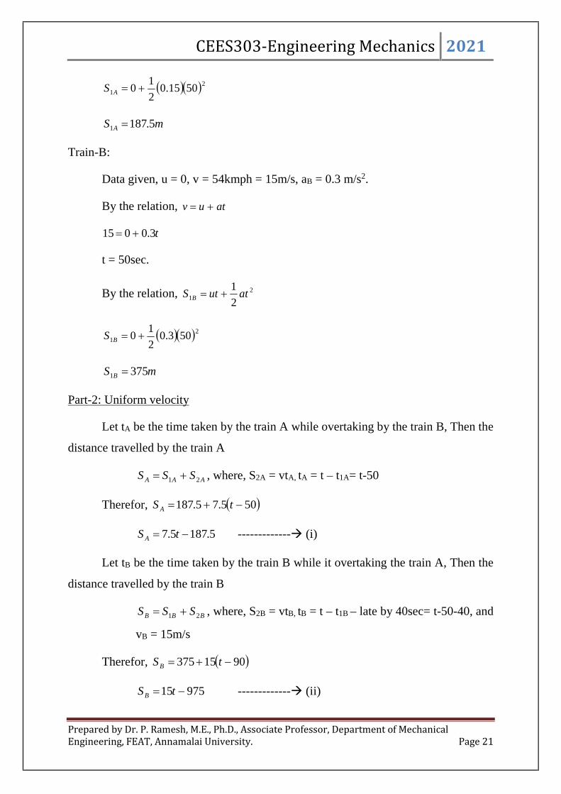
CEES303-Engineering Mechanics 2021
Prepared by Dr. P. Ramesh, M.E., Ph.D., Associate Professor, Department of MechanicalEngineering, FEAT, Annamalai University. Page 21
21 5015.02
10 AS
mS A 5.1871
Train-B:
Data given, u = 0, v = 54kmph = 15m/s, aB = 0.3 m/s2.
By the relation, atuv
t3.0015
t = 50sec.
By the relation, 21 2
1atutS B
21 503.02
10 BS
mS B 3751
Part-2: Uniform velocity
Let tA be the time taken by the train A while overtaking by the train B, Then the
distance travelled by the train A
AAA SSS 21 , where, S2A = vtA, tA = t – t1A= t-50
Therefor, 505.75.187 tS A
5.1875.7 tS A ------------- (i)
Let tB be the time taken by the train B while it overtaking the train A, Then the
distance travelled by the train B
BBB SSS 21 , where, S2B = vtB, tB = t – t1B – late by 40sec= t-50-40, and
vB = 15m/s
Therefor, 9015375 tSB
97515 tSB ------------- (ii)

CEES303-Engineering Mechanics 2021
Prepared by Dr. P. Ramesh, M.E., Ph.D., Associate Professor, Department of MechanicalEngineering, FEAT, Annamalai University. Page 22
Now equating the eqn. i and ii by keeping SA is equal to SB gives
SB = 600m and t = 65s.
SP4.14: Two cars are travelling towards each other on a single lane road at velocities
12 m/s and 9 m/s respectively. When 100m apart both drivers realise the situation and
apply their brakes. They succeed in stopping simultaneously and just short of colliding.
Assume constant deceleration for each case, find a) time required for cars to stop, b)
deceleration of each car and c) the distance travelled by each car while slowing down.
Solution:
Both the cars stop simultaneously. Hence times remain same. Let SA and SB be
the distance travelled by the two cars.
msS BA 100
Considering the motion of first car A, where u = 12m/s, v = 0m/s, S = SA
By the relation, atuv v
taA 120
ta A
12
By the relation, 2
2
1tautS AA
2
2
112 tatS AA
212
2
112 t
ttS A
tS A 6 -------- (i)
Now considering the motion of car B, where u = 9m/s, v = 0m/s, S = 100-SA
By the relation, atuv v
taB 90
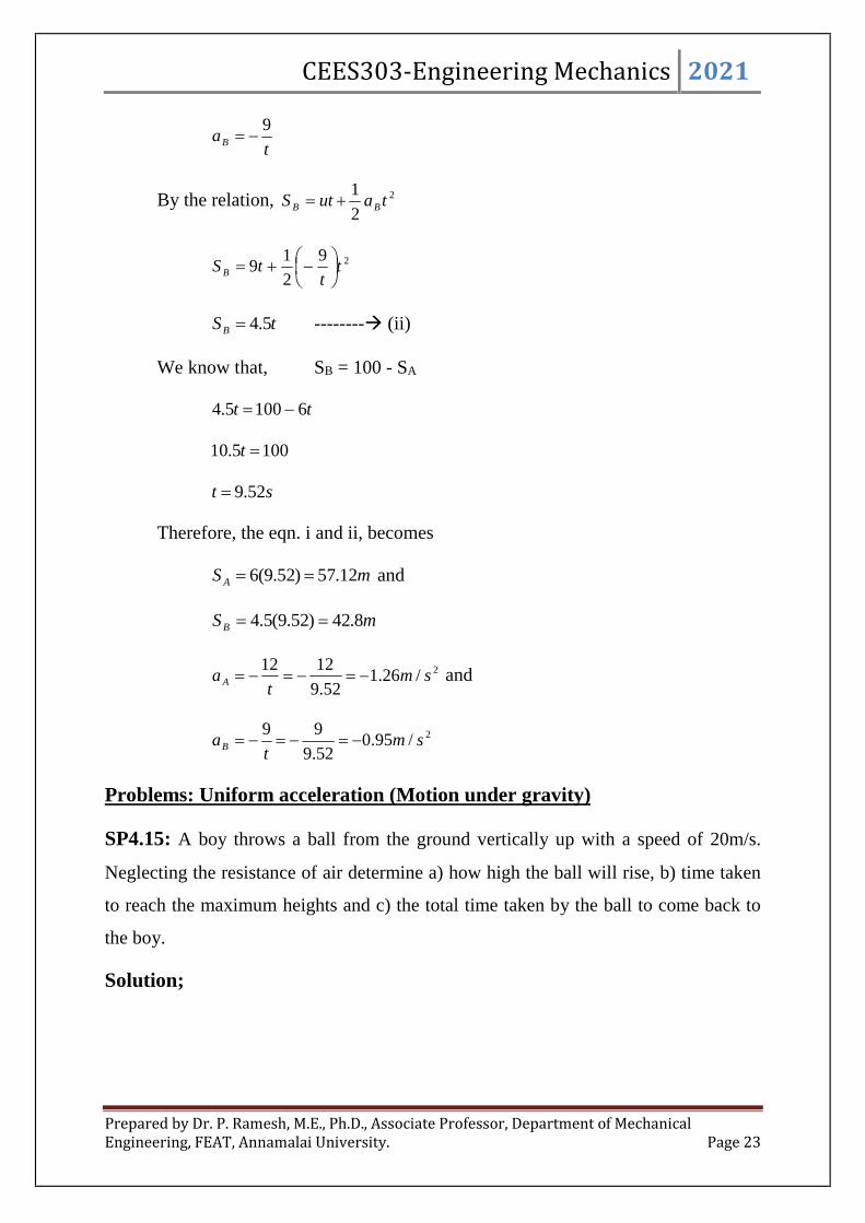
CEES303-Engineering Mechanics 2021
Prepared by Dr. P. Ramesh, M.E., Ph.D., Associate Professor, Department of MechanicalEngineering, FEAT, Annamalai University. Page 23
taB
9
By the relation, 2
2
1tautS BB
29
2
19 t
ttS B
tSB 5.4 -------- (ii)
We know that, SB = 100 - SA
tt 61005.4
1005.10 t
st 52.9
Therefore, the eqn. i and ii, becomes
mS A 12.57)52.9(6 and
mSB 8.42)52.9(5.4
2/26.152.9
1212sm
ta A and
2/95.052.9
99sm
taB
Problems: Uniform acceleration (Motion under gravity)
SP4.15: A boy throws a ball from the ground vertically up with a speed of 20m/s.
Neglecting the resistance of air determine a) how high the ball will rise, b) time taken
to reach the maximum heights and c) the total time taken by the ball to come back to
the boy.
Solution;

CEES303-Engineering Mechanics 2021
Prepared by Dr. P. Ramesh, M.E., Ph.D., Associate Professor, Department of MechanicalEngineering, FEAT, Annamalai University. Page 24
SP4.16: A particle is dropped from the top of a tower 200m high and another particle
is projected at the same time vertically upwards from the foot of the tower so as to meet
the first particle at a height of 50m. Find the velocity of projection of the second particle.
Solution:
Fig.4.3
Fig.4.4

CEES303-Engineering Mechanics 2021
Prepared by Dr. P. Ramesh, M.E., Ph.D., Associate Professor, Department of MechanicalEngineering, FEAT, Annamalai University. Page 25
SP4.17: A stone is thrown vertically up from the top of tower with a certain velocity.
It reaches ground in 5.64 sec. A second stone thrown down from the same tower with
the same initial velocity reaches the ground in 3.6sec. Determine a) the height of the
tower and b) the initial velocity of the stones.
Solution:
Fig.4.5

CEES303-Engineering Mechanics 2021
Prepared by Dr. P. Ramesh, M.E., Ph.D., Associate Professor, Department of MechanicalEngineering, FEAT, Annamalai University. Page 26
SP4.18: A stone was thrown vertically from the ground with a velocity of 49m/s. After2 sec. another stone was thrown vertically upwards from the same place. If both thestones strike the ground at the same time, find the velocity with which the second stonewas thrown. Take g = 9.8m/s2.
Solution:

CEES303-Engineering Mechanics 2021
Prepared by Dr. P. Ramesh, M.E., Ph.D., Associate Professor, Department of MechanicalEngineering, FEAT, Annamalai University. Page 27
SP4.19: A body falling freely under the action of gravity passes two points 10m apart
vertically in 0.2sec. From what height above the higher point did it start to fall?
Solution:
SP4.20: A stone dropped into well is heard to strike the water after 4sec. find the depth
of the well if the velocity of the sound is 350m/s.
Solution:
Fig.4.6
Fig.4.7

CEES303-Engineering Mechanics 2021
Prepared by Dr. P. Ramesh, M.E., Ph.D., Associate Professor, Department of MechanicalEngineering, FEAT, Annamalai University. Page 28
SP4.21: A particle falling under gravity falls 20m in a certain second. Find the time
required to cover next 20m.
Solution:
Fig.4.8
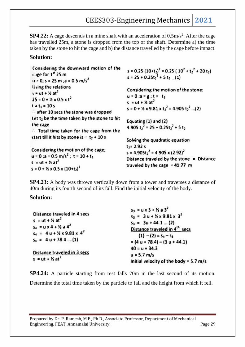
CEES303-Engineering Mechanics 2021
Prepared by Dr. P. Ramesh, M.E., Ph.D., Associate Professor, Department of MechanicalEngineering, FEAT, Annamalai University. Page 29
SP4.22: A cage descends in a mine shaft with an acceleration of 0.5m/s2. After the cagehas travelled 25m, a stone is dropped from the top of the shaft. Determine a) the timetaken by the stone to hit the cage and b) the distance travelled by the cage before impact.
Solution:
SP4.23: A body was thrown vertically down from a tower and traverses a distance of40m during its fourth second of its fall. Find the initial velocity of the body.
Solution:
SP4.24: A particle starting from rest falls 70m in the last second of its motion.
Determine the total time taken by the particle to fall and the height from which it fell.

CEES303-Engineering Mechanics 2021
Prepared by Dr. P. Ramesh, M.E., Ph.D., Associate Professor, Department of MechanicalEngineering, FEAT, Annamalai University. Page 30
Solution:
SP4.25: Sounding rockets are used for conducting experiments in the upper
atmosphere. One such rocket is fired vertically upwards with a constant acceleration of
40m/s2. All the fuel in the rocket is consumed in 25 sec and the rocket then ascends like
a free particle decelerating under the influence of gravity. A) Determine the velocity of
the rocket at the instant when all the fuel is consumed, B) What is the maximum altitude
reached? C) Determine the time taken to reach the maximum altitude and D) Find the
total time taken to reach the ground from the start.
Solution:
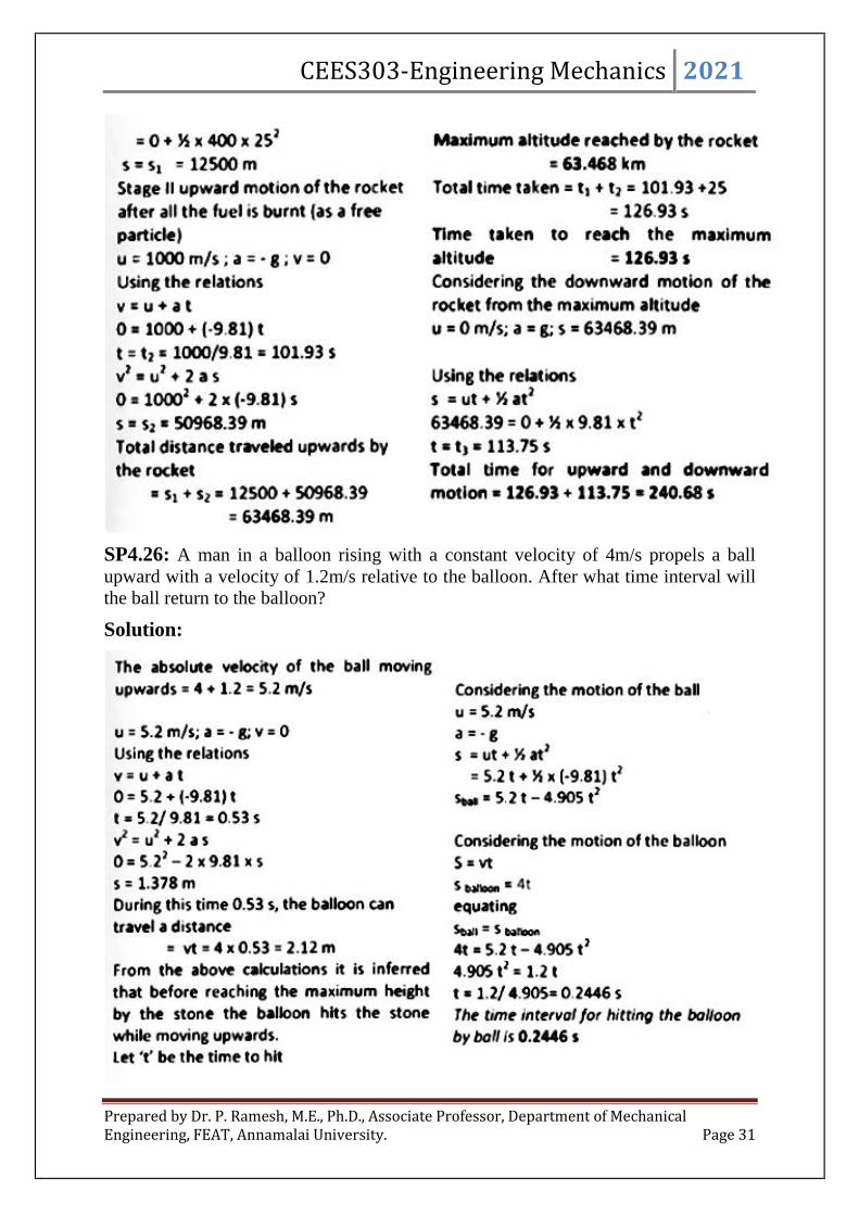
CEES303-Engineering Mechanics 2021
Prepared by Dr. P. Ramesh, M.E., Ph.D., Associate Professor, Department of MechanicalEngineering, FEAT, Annamalai University. Page 31
SP4.26: A man in a balloon rising with a constant velocity of 4m/s propels a ballupward with a velocity of 1.2m/s relative to the balloon. After what time interval willthe ball return to the balloon?
Solution:

CEES303-Engineering Mechanics 2021
Prepared by Dr. P. Ramesh, M.E., Ph.D., Associate Professor, Department of MechanicalEngineering, FEAT, Annamalai University. Page 32
SP4.27: A Juggler keeps three balls going with one hand, so that at any instant two arein the air and one in the hand. If each ball rises to a height of ‘h’ show that each ballstays in the hand for h4515.0 sec.
Solution:
SP4.29: Water drips from a faucet at the rate of 6 drops per second. The faucet is
200mm above the sink. When one drop strikes the sink how far is the next drop above
the sink?
Solution:
Fig.4.9
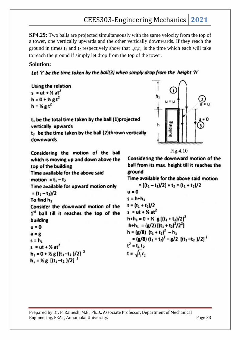
CEES303-Engineering Mechanics 2021
Prepared by Dr. P. Ramesh, M.E., Ph.D., Associate Professor, Department of MechanicalEngineering, FEAT, Annamalai University. Page 33
SP4.29: Two balls are projected simultaneously with the same velocity from the top ofa tower, one vertically upwards and the other vertically downwards. If they reach theground in times t1 and t2 respectively show that 21tt is the time which each will taketo reach the ground if simply let drop from the top of the tower.
Solution:
Fig.4.10

CEES303-Engineering Mechanics 2021
Prepared by Dr. P. Ramesh, M.E., Ph.D., Associate Professor, Department of MechanicalEngineering, FEAT, Annamalai University. Page 34
Problems: Motion under variable acceleration
SP4.30: A car moves along a straight line whose equation of motion is given by
32 2312 tttS , where S is in metre and t in seconds. Calculate a) the velocity and
acceleration at start and b) the acceleration when velocity is zero.
Solution:
SP4.31: The equation of motion of a particle moving in a straight line is given by
32 2318 tttS , where S in metre and t in seconds. Find the velocity and acceleration
at start, the time when the particle reaches its maximum velocity and the maximum
velocity of the particle.
Solution:

CEES303-Engineering Mechanics 2021
Prepared by Dr. P. Ramesh, M.E., Ph.D., Associate Professor, Department of MechanicalEngineering, FEAT, Annamalai University. Page 35
SP4.32: The motion of a particle moving in a straight line is given by the expression
523 23 tttS , where S is the displacement in metre and t is the time in seconds.
Determine a) the velocity and acceleration after 4 seconds, b) maximum or minimum
velocity and time at which velocity is zero.
Solution:
SP4.33: The acceleration of a point moving on a vertical line is given by the equation
2012 ta . It is known that its displacement mS 10 at time 0t and that its
displacement. mS 10 at time .sec5t Derive the equation of its motion.
Solution:

CEES303-Engineering Mechanics 2021
Prepared by Dr. P. Ramesh, M.E., Ph.D., Associate Professor, Department of MechanicalEngineering, FEAT, Annamalai University. Page 36
SP4.34: The acceleration of a point in rectilinear motion is given by the equation,
8.9a . It is known that the velocity v is zero and the displacement S is +25m when
t=0. Determine the equation of the displacement.
Solution;
SP4.35: A particle moves along a horizontal straight line with an acceleration 31
6Sa
when t = 2sec, its displacement S = +27m and its velocity v = +27m/s. Calculate the
velocity and acceleration of the point when t = 4sec.
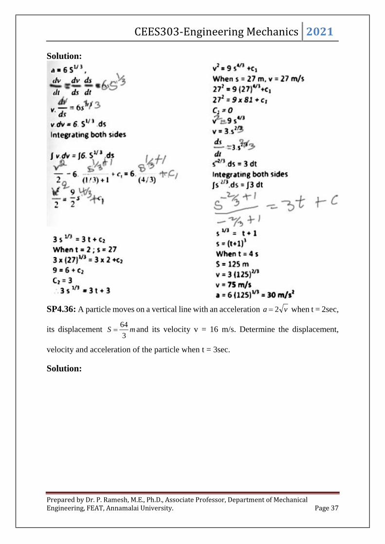
CEES303-Engineering Mechanics 2021
Prepared by Dr. P. Ramesh, M.E., Ph.D., Associate Professor, Department of MechanicalEngineering, FEAT, Annamalai University. Page 37
Solution:
SP4.36: A particle moves on a vertical line with an acceleration va 2 when t = 2sec,
its displacement mS3
64 and its velocity v = 16 m/s. Determine the displacement,
velocity and acceleration of the particle when t = 3sec.
Solution:

CEES303-Engineering Mechanics 2021
Prepared by Dr. P. Ramesh, M.E., Ph.D., Associate Professor, Department of MechanicalEngineering, FEAT, Annamalai University. Page 38
SP4.37: A train starting from rest is uniformly accelerated. The acceleration at any
instant is 110
vm/s2 , where v is the velocity of the train, in m/s at that instant. Find the
distance in which the train will attain a velocity of 36kmph.
Solution:

CEES303-Engineering Mechanics 2021
Prepared by Dr. P. Ramesh, M.E., Ph.D., Associate Professor, Department of MechanicalEngineering, FEAT, Annamalai University. Page 39
SP4.38: A small projectile is fired vertically downwards into fluid medium with an
initial velocity of 60 m/s. If the projectile experiences a deceleration which is equal to
34.0 va m/s2. Where v is measured in m/s, determine the velocity v and position S
in 4 seconds after the projectile is fired.
Solution:
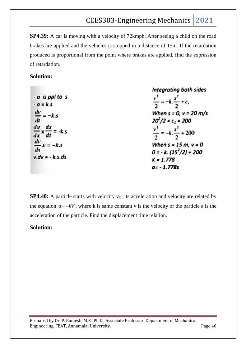
CEES303-Engineering Mechanics 2021
Prepared by Dr. P. Ramesh, M.E., Ph.D., Associate Professor, Department of MechanicalEngineering, FEAT, Annamalai University. Page 40
SP4.39: A car is moving with a velocity of 72kmph. After seeing a child on the road
brakes are applied and the vehicles is stopped in a distance of 15m. If the retardation
produced is proportional from the point where brakes are applied, find the expression
of retardation.
Solution:
SP4.40: A particle starts with velocity vO, its acceleration and velocity are related by
the equation kVa , where k is same constant v is the velocity of the particle a is the
acceleration of the particle. Find the displacement time relation.
Solution:

CEES303-Engineering Mechanics 2021
Prepared by Dr. P. Ramesh, M.E., Ph.D., Associate Professor, Department of MechanicalEngineering, FEAT, Annamalai University. Page 41
SP4.41: A particle moves along a horizontal straight line such that its velocity is given
by ttsmv 63)/( 2 , where t is the time in second. If it is initially located at the origin
O, determine the distance travelled during the time interval t = 0 to t = 3.5 sec., the
average velocity and the average speed of the particle during this time interval.
Solution:
Fig.4.11

CEES303-Engineering Mechanics 2021
Prepared by Dr. P. Ramesh, M.E., Ph.D., Associate Professor, Department of MechanicalEngineering, FEAT, Annamalai University. Page 42
PLANE CURVILINEAR MOTION:
The motion of a particle along a curved path which lies in a single plane. This
motion is a special case of the more general three dimensional motion as discussed
above and illustrated in fig.4.1. If let the plane of motion be the x-y plane, for instance,
then the coordinates z and of fig.4.1 are both zero and R becomes the same as r. As
mentioned previously, the vast majority of the motions of points or particles
encountered in engineering practice can be represented as plane motion.
Fig.4.12 Plane curve linear motion
Consider now the continuous motion of a particle along a plane curve as
represented in fig.4.12. At time ‘t’ the particle is at position A, which is located by the
position vector ‘r’ measured from some convenient fixed origin O. If both the
a) b) c)

CEES303-Engineering Mechanics 2021
Prepared by Dr. P. Ramesh, M.E., Ph.D., Associate Professor, Department of MechanicalEngineering, FEAT, Annamalai University. Page 43
magnitude and direction of ‘r’ are known at time ‘t’, then the position of the particle is
completely specified. At time t + Δt, the particle is at A', located by the position vector
r + Δr. This combination is vector addition and not scalar addition.
a) Displacement
The displacement of the particle during time Δt is the vector Δr which represents
the vector change of position and is clearly independent of the choice of origin. If an
origin were chosen at some different location, the position vector ‘r’ would be changed,
but Δr would be unchanged. The distance actually travelled by the particle as it moves
along the path from A to A' is the scalar length Δs measured along the path. Thus, it
distinguish between the vector displacement Δr and the scalar distance Δs.
b) Velocity
The average velocity of the particle between A and A' is defined ast
rvav
,
which is a vector whose direction is that of Δr and whose magnitude is the magnitude
of Δr divided by Δt. The average speed of the particle between A and A' is the scalar
quotientt
s
. Clearly, the magnitude of the average velocity and the speed approach one
another as the interval Δt decreases and A and A' become closer together. The
instantaneous velocity ‘v’ of the particle is defined as the limiting value of the average
velocity as the time interval approaches zero. Thus,
t
rV
t
0
lim ------------ (4.12)
It observes that the direction of Δr approaches that of the tangent to the path as
Δt approaches zero and, thus, the velocity v is always a vector tangent to the path.
Now extend the basic definition of the derivative of a scalar quantity to include
a vector quantity and write
rdt
drv ------------- (4.13)
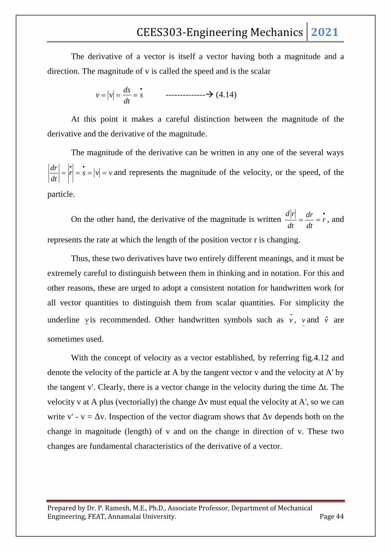
CEES303-Engineering Mechanics 2021
Prepared by Dr. P. Ramesh, M.E., Ph.D., Associate Professor, Department of MechanicalEngineering, FEAT, Annamalai University. Page 44
The derivative of a vector is itself a vector having both a magnitude and a
direction. The magnitude of v is called the speed and is the scalar
sdt
dsv v -------------- (4.14)
At this point it makes a careful distinction between the magnitude of the
derivative and the derivative of the magnitude.
The magnitude of the derivative can be written in any one of the several ways
vsrdt
dr
v and represents the magnitude of the velocity, or the speed, of the
particle.
On the other hand, the derivative of the magnitude is written
rdt
dr
dt
rd, and
represents the rate at which the length of the position vector r is changing.
Thus, these two derivatives have two entirely different meanings, and it must be
extremely careful to distinguish between them in thinking and in notation. For this and
other reasons, these are urged to adopt a consistent notation for handwritten work for
all vector quantities to distinguish them from scalar quantities. For simplicity the
underline v is recommended. Other handwritten symbols such as v ,~v and v̂ are
sometimes used.
With the concept of velocity as a vector established, by referring fig.4.12 and
denote the velocity of the particle at A by the tangent vector v and the velocity at A' by
the tangent v'. Clearly, there is a vector change in the velocity during the time Δt. The
velocity v at A plus (vectorially) the change Δv must equal the velocity at A', so we can
write v' - v = Δv. Inspection of the vector diagram shows that Δv depends both on the
change in magnitude (length) of v and on the change in direction of v. These two
changes are fundamental characteristics of the derivative of a vector.

CEES303-Engineering Mechanics 2021
Prepared by Dr. P. Ramesh, M.E., Ph.D., Associate Professor, Department of MechanicalEngineering, FEAT, Annamalai University. Page 45
c) Acceleration
The average acceleration of the particle between A and A' is defined ast
v
,
which is a vector whose direction is that of Δv. The magnitude of this average
acceleration is the magnitude of Δv divided by Δt. The instantaneous acceleration a of
the particle is defined as the limiting value of the average acceleration as the time
interval approaches zero. Thus,
t
va
t
0
lim
By definition of the derivative, then
vdt
dva -------------- (4.15)
As the interval Δt becomes smaller and approaches zero, the direction of the
change Δv approaches that of the differential change dv and, thus, of a. The acceleration
a, then, includes the effects of both the change in magnitude of v and the change of
direction of v. It is apparent, in general, that the direction of the acceleration of a particle
in curvilinear motion is neither tangent to the path nor normal to the path. It observes
that the acceleration component which is normal to the path points toward the centre of
curvature of the path.
1) RECTANGULAR COORDINATES (X- Y):
This system of coordinates is particularly useful for describing motions where
the x- and y-components of acceleration are independently generated or determined.
The resulting curvilinear motion is then obtained by a vector combination of the x- and
y-components of the position vector, the velocity, and the acceleration.
a) Vector Representation
The particle path of fig.4.12 is shown again in fig.4.13 along with x- and y-axes.
The position vector r, the velocity v, and the acceleration ‘a’ of the particle as developed

CEES303-Engineering Mechanics 2021
Prepared by Dr. P. Ramesh, M.E., Ph.D., Associate Professor, Department of MechanicalEngineering, FEAT, Annamalai University. Page 46
in previous are represented in fig.4.13 together with their x- and y-components. With
the aid of the unit vectors i and j, it can write the vectors r, v, and a in terms of their x-
and y-components. Thus,
Fig.4.13 Particle motion in x and y plane
jyixrva
jyixrv
yjxir
---------- (4.16)
As differentiate with respect to time, it observes that the time derivatives of the
unit vectors are zero because their magnitudes and directions remain constant. The
scalar values of the components of v and a are merely
xvx ,
yv y ,
xva xx and
yva yy . (As drawn in fig.4.13, a is in the negative x-direction, so that
x would be
a negative number). As observed previously, the direction of the velocity is always
tangent to the path, and from the figure it is clear that
222yx vvv , 22
yx vvv andx
y
v
vtan
222yx aaa and 22
yx aaa
If the angle is measured counter clockwise from the x-axis to v for the
configuration of axes shown, then it can also observe thatx
y
v
v
dx
dy tan . If the
coordinates x and y are known independently as functions of time, x = ƒ1 (t) and y =

CEES303-Engineering Mechanics 2021
Prepared by Dr. P. Ramesh, M.E., Ph.D., Associate Professor, Department of MechanicalEngineering, FEAT, Annamalai University. Page 47
ƒ2(t), then for any value of the time it can combine them to obtain r. Similarly, combine
their first derivatives
x and
y to obtain v and their second derivatives
x and
y to obtain
a. On the other hand, if the acceleration components ax and ay are given as functions of
the time, it can integrate each one separately with respect to time, once to obtain vx and
vy and again to obtain x = ƒ1(t) and y = ƒ2(t). Elimination of the time t between these
last two parametric equations gives the equation of the curved path y = ƒ(x).
From the foregoing discussion it can see that the rectangular coordinate
representation of curvilinear motion is merely the superposition of the components of
two simultaneous rectilinear motions in the x- and y-directions. Therefore, everything
covered in rectilinear motion and it can be applied separately to the x-motion and to the
y-motion.
b) Projectile Motion
An important application of two-dimensional kinematic theory is the problem of
projectile motion. For a first treatment of the subject, it neglects aerodynamic drag and
the curvature and rotation of the earth, and assume that the altitude change is small
enough so that the acceleration due to gravity can be considered constant. With these
assumptions, rectangular coordinates are useful for the trajectory analysis.
Fig.4.14 Projectile motion
For the axes shown in fig.4.14, the acceleration components are
0xa and ga y

CEES303-Engineering Mechanics 2021
Prepared by Dr. P. Ramesh, M.E., Ph.D., Associate Professor, Department of MechanicalEngineering, FEAT, Annamalai University. Page 48
Integration of these accelerations follows the results obtained previously for
uniform/ constant acceleration motion and yields
0xx vv and gtvv yy 0
tvxx x 00 and 2
00 2
1gttvyy y
02
0
2 2 yygvv yy
In all these expressions, the subscript zero denotes initial conditions, frequently
taken as those at launch where, for the case illustrated, x0 = y0 = 0. Note that the quantity
g is taken to be positive throughout this text.

CEES303-Engineering Mechanics 2021
Prepared by Dr. P. Ramesh, M.E., Ph.D., Associate Professor, Department of MechanicalEngineering, FEAT, Annamalai University. Page 49
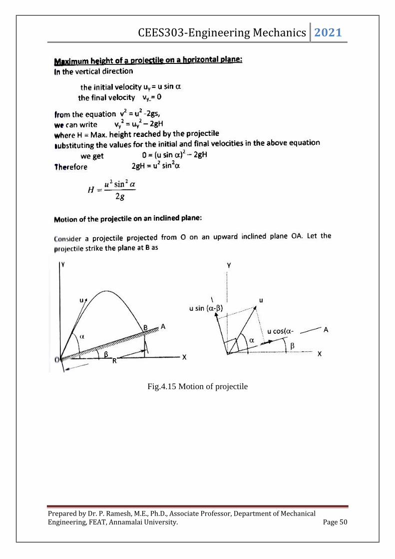
CEES303-Engineering Mechanics 2021
Prepared by Dr. P. Ramesh, M.E., Ph.D., Associate Professor, Department of MechanicalEngineering, FEAT, Annamalai University. Page 50
Fig.4.15 Motion of projectile

CEES303-Engineering Mechanics 2021
Prepared by Dr. P. Ramesh, M.E., Ph.D., Associate Professor, Department of MechanicalEngineering, FEAT, Annamalai University. Page 51
Fig.4.16

CEES303-Engineering Mechanics 2021
Prepared by Dr. P. Ramesh, M.E., Ph.D., Associate Professor, Department of MechanicalEngineering, FEAT, Annamalai University. Page 52
Problems:
SP.4.42: The curvilinear motion of a particle is defined by tvx 1650 and
24100 ty , where vx is in metres per second, y is in metres and t is in seconds. It is
also known that x = 0 when t = 0. Plot the path of the particle and determine its velocity
and acceleration when the position y = 0 is reached.
Solution:
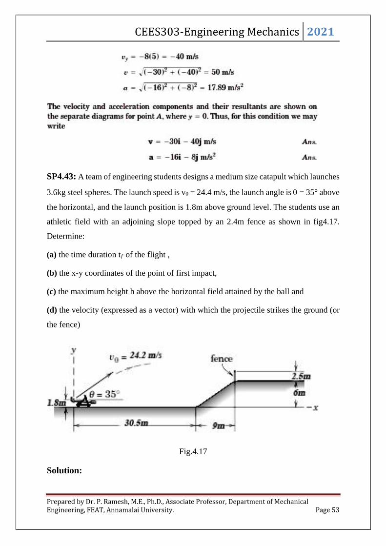
CEES303-Engineering Mechanics 2021
Prepared by Dr. P. Ramesh, M.E., Ph.D., Associate Professor, Department of MechanicalEngineering, FEAT, Annamalai University. Page 53
SP4.43: A team of engineering students designs a medium size catapult which launches
3.6kg steel spheres. The launch speed is v0 = 24.4 m/s, the launch angle is = 35° above
the horizontal, and the launch position is 1.8m above ground level. The students use an
athletic field with an adjoining slope topped by an 2.4m fence as shown in fig4.17.
Determine:
(a) the time duration tƒ of the flight ,
(b) the x-y coordinates of the point of first impact,
(c) the maximum height h above the horizontal field attained by the ball and
(d) the velocity (expressed as a vector) with which the projectile strikes the ground (or
the fence)
Fig.4.17
Solution:

CEES303-Engineering Mechanics 2021
Prepared by Dr. P. Ramesh, M.E., Ph.D., Associate Professor, Department of MechanicalEngineering, FEAT, Annamalai University. Page 54
Now make the assumption of constant gravitational acceleration and no
aerodynamic drag. With the latter assumption, the 3.6 kg weight of the projectile is
irrelevant. Using the given x-y coordinate system, this is being by checking the y-
displacement at the horizontal position of the fence.
tvxx x 00 , to35cos2.24095.30 , 994.1 t
2
00 2
1gttvyy y , 2994.181.9
2
1994.135sin2.248.1 oy ,
my 976.9
a) Because the y – coordinate of the top of the fence is 6 + 2.5 = 8.5m, the projectile
clears the fence. Now find the flight time by setting y = 6m,
2
00 2
1ffy gttvyy , 281.9
2
135sin2.248.16 ff
o tt , st f 485.2
fx tvxx 00 , 485.235cos2.240 ox , x 49.26m
b) Thus the point of first impact is (x,y) = (49.26, 6)
c) For the maximum height:
02
0
2 2 yygvv yy , 8.181.9235sin2.24022 ho , mh 489.11
d) For the impact velocity:
0xx vv , smv ox /823.1935cos2.24
gtvv yy 0
, smv oy /498.10485.281.935sin2.24
So the impact velocity is jismv 498.10823.19)/(
SP4.44: An aircraft moving horizontal at 108 kmph at an altitude of 1000m towards a
target on the ground, releases a bomb which hits it. Estimate the horizontal distance of
the aircraft from the target, when it released the bomb. Calculate also the direction and
magnitude of the velocity with which the bomb hits the target.
Solution:
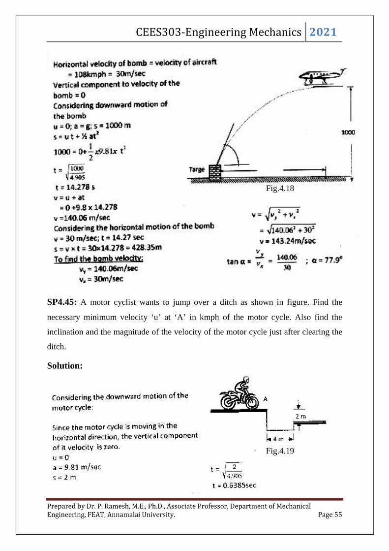
CEES303-Engineering Mechanics 2021
Prepared by Dr. P. Ramesh, M.E., Ph.D., Associate Professor, Department of MechanicalEngineering, FEAT, Annamalai University. Page 55
SP4.45: A motor cyclist wants to jump over a ditch as shown in figure. Find the
necessary minimum velocity ‘u’ at ‘A’ in kmph of the motor cycle. Also find the
inclination and the magnitude of the velocity of the motor cycle just after clearing the
ditch.
Solution:
Fig.4.18
Fig.4.19

CEES303-Engineering Mechanics 2021
Prepared by Dr. P. Ramesh, M.E., Ph.D., Associate Professor, Department of MechanicalEngineering, FEAT, Annamalai University. Page 56
SP4.46: A shot is fired horizontally from the top of a tower with velocity of 100 m/s.
If the shot hits the ground after 2 sec, find the height of the tower and the distance from
the foot of the tower, where the strikes the ground.
Solution:
SP4.47: An airplane is flying on a straight level course at 200 kmph at a height of
1000m above the ground. An anti-craft gun located on the ground fires a shell with an
initial velocity of 300m/s at the instant when the plane is vertically above it. At what
inclination, to the horizontal should the gun be fired to hit the plane? What time after
firing the gun shell will hit the plane? What will then be the horizontal distance of the
plane from the gun?
Solution:
Fig.4.20

CEES303-Engineering Mechanics 2021
Prepared by Dr. P. Ramesh, M.E., Ph.D., Associate Professor, Department of MechanicalEngineering, FEAT, Annamalai University. Page 57
SP4.48: If a particle is projected inside a horizontal tunnel which is 5m high with avelocity of 60m/s., find the greatest possible range and the corresponding angle ofprojection.
Solution:

CEES303-Engineering Mechanics 2021
Prepared by Dr. P. Ramesh, M.E., Ph.D., Associate Professor, Department of MechanicalEngineering, FEAT, Annamalai University. Page 58
SP4.49: A particle is projected from the base of a hill whose shape is that of a rightcircular cone with axis vertical. The projectile grazes the vertex and strikes the hill againat a point on the base. If be the semi – cone angle, h its height, u the initial velocity ofthe projectile and the angle of projection measured from the horizontal show that
cot2tan and
2
tan2
22
ghu .
Solution:
SP4.50: A cricket ball shot by a batsman from a height of 1.8m at an angle of 30o with
horizontal with a velocity of 18m/s is caught by a field man at a height of 0.6m from
the ground. How far apart were the two players?
Solution:
Fig.4.22

CEES303-Engineering Mechanics 2021
Prepared by Dr. P. Ramesh, M.E., Ph.D., Associate Professor, Department of MechanicalEngineering, FEAT, Annamalai University. Page 59
SP4.51: A projectile is aimed at a mark on a horizontal plane through the point ofprojection. It falls 12m short when the angle of projection is 15o while it overshoots themark by 24m when the angle is 45o. Find the angle of projection to hit the mark. Assumeno air resistance.
Solution:
Fig.4.24

CEES303-Engineering Mechanics 2021
Prepared by Dr. P. Ramesh, M.E., Ph.D., Associate Professor, Department of MechanicalEngineering, FEAT, Annamalai University. Page 60
SP4.52: A projectile is fired from the edge of a 150m high cliff with the initial velocity
of 180m/s at an angle of elevation of 300 with the horizontal. Neglecting air resistances
find a) the greatest elevation above the ground reached by the projectile, b) time
required to strike the ground, c) the horizontal distance from the gun to the point where
the projectile strikes the ground and d) the velocity with which the projectile strikes the
ground.
Solution:
SP4.53: A rocket is fired at an angle of 80o to the horizontal and moves with constant
acceleration of 50m/s2. All the fuel in the rocket is burnt out in 20sec. and the rocket
continues as a free particle under the influence of gravity. Assume that the rocket flies
Fig.4.25
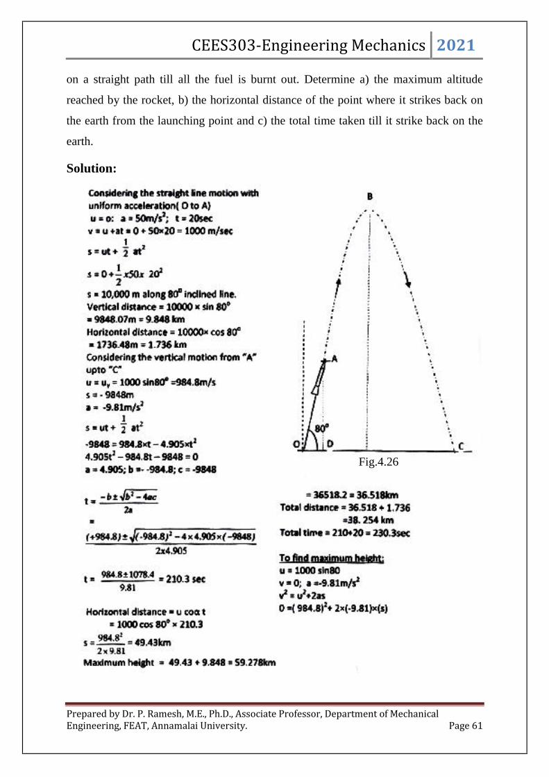
CEES303-Engineering Mechanics 2021
Prepared by Dr. P. Ramesh, M.E., Ph.D., Associate Professor, Department of MechanicalEngineering, FEAT, Annamalai University. Page 61
on a straight path till all the fuel is burnt out. Determine a) the maximum altitude
reached by the rocket, b) the horizontal distance of the point where it strikes back on
the earth from the launching point and c) the total time taken till it strike back on the
earth.
Solution:
Fig.4.26

CEES303-Engineering Mechanics 2021
Prepared by Dr. P. Ramesh, M.E., Ph.D., Associate Professor, Department of MechanicalEngineering, FEAT, Annamalai University. Page 62
SP4.54: Find the least initial velocity which a projectile may have so that it may clear
a wall 3.6m high and 4.8m distance from the point of projection and strike the horizontal
plane through the foot of the wall at distance 3.6m beyond the wall. The point of
projection is at the same level as the foot of the wall.
Solution:
SP4.55: Two guns are pointed at each other, one upward at an angle of 30o and the
other at the same angle of depression, the nozzles being 30m apart. If the guns are shot
simultaneously with velocities of 350m/s upwards and 300m/s, downwards
respectively, find when and where they will meet.
Solution:
Fig.4.27
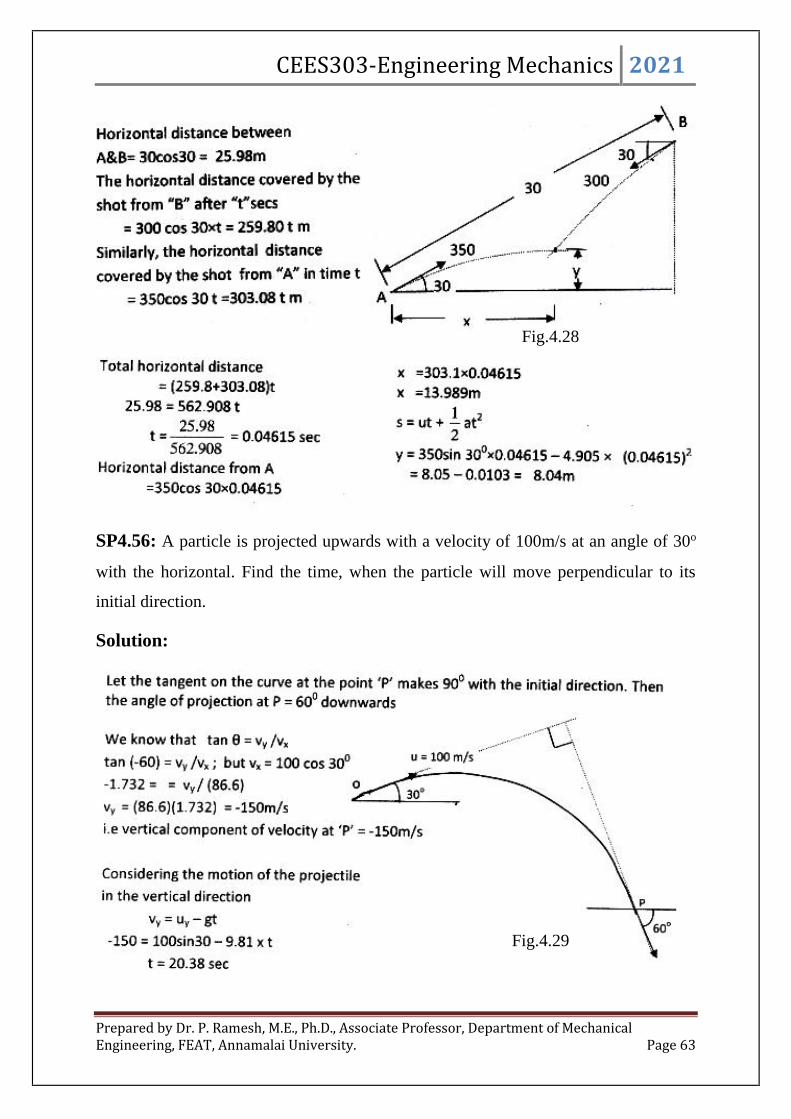
CEES303-Engineering Mechanics 2021
Prepared by Dr. P. Ramesh, M.E., Ph.D., Associate Professor, Department of MechanicalEngineering, FEAT, Annamalai University. Page 63
SP4.56: A particle is projected upwards with a velocity of 100m/s at an angle of 30o
with the horizontal. Find the time, when the particle will move perpendicular to its
initial direction.
Solution:
Fig.4.28
Fig.4.29

CEES303-Engineering Mechanics 2021
Prepared by Dr. P. Ramesh, M.E., Ph.D., Associate Professor, Department of MechanicalEngineering, FEAT, Annamalai University. Page 64
SP5.57: A projectile is fired with a velocity of 500m/s at an elevation of 30o. find the
velocity and direction of the projectile after 30sec. of its firing.
Solution:
SP4.58: Two adjacent guns having the same muzzle velocity of 350m/s fire
simultaneously at angles of 1 and 2 for the same target situated at the range of 4200m.
Find the time difference between the hits.
Solution:
Fig.4.30
Fig.4.31
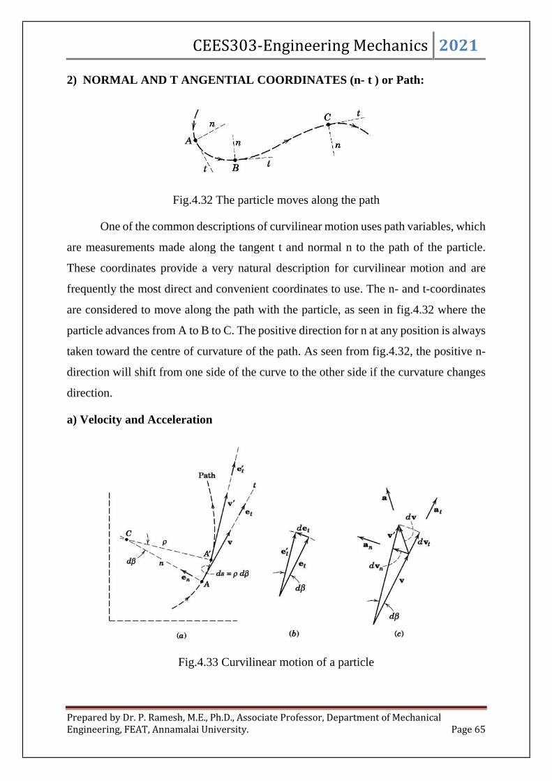
CEES303-Engineering Mechanics 2021
Prepared by Dr. P. Ramesh, M.E., Ph.D., Associate Professor, Department of MechanicalEngineering, FEAT, Annamalai University. Page 65
2) NORMAL AND T ANGENTIAL COORDINATES (n- t ) or Path:
Fig.4.32 The particle moves along the path
One of the common descriptions of curvilinear motion uses path variables, which
are measurements made along the tangent t and normal n to the path of the particle.
These coordinates provide a very natural description for curvilinear motion and are
frequently the most direct and convenient coordinates to use. The n- and t-coordinates
are considered to move along the path with the particle, as seen in fig.4.32 where the
particle advances from A to B to C. The positive direction for n at any position is always
taken toward the centre of curvature of the path. As seen from fig.4.32, the positive n-
direction will shift from one side of the curve to the other side if the curvature changes
direction.
a) Velocity and Acceleration
Fig.4.33 Curvilinear motion of a particle

CEES303-Engineering Mechanics 2021
Prepared by Dr. P. Ramesh, M.E., Ph.D., Associate Professor, Department of MechanicalEngineering, FEAT, Annamalai University. Page 66
Now use the coordinates n and t to describe the velocity ‘v’ and acceleration ‘a’
for the curvilinear motion of a particle. For this purpose, now introduce unit vectors en
in the n-direction and et in the t-direction, as shown in fig.4.33a for the position of the
particle at point A on its path. During a differential increment of time dt, the particle
moves a differential distance ds along the curve from A to A'. With the radius of
curvature of the path at this position designated by to obtain the differential distance
as
dds , where is in radians.
It is unnecessary to consider the differential change in between A and A'
because a higher-order term would be introduced which disappears in the limit. Thus,
the magnitude of the velocity can be writtendt
d
dt
dsv
, and it can write the velocity
as the vector
tt eve
v ----------- (4.17)
The acceleration a of the particle was defined in earlier asdt
dva , and it observed
from fig.4.12 that the acceleration is a vector which reflects both the change in
magnitude and the change in direction of v. Now differentiate v in equation 4.17 by
applying the ordinary rule for the differentiation of the product of a scalar and a vector
and get
tt
t evevdt
ved
dt
dva
-------- (4.18)
where the unit vector et now has a nonzero derivative because its direction
changes.
To find
te now analyse the change in et during a differential increment of motion
as the particle moves from A to A' in fig.4.33a. The unit vector et correspondingly
changes to e't, and the vector difference det is shown in part b of the fig4.33. The vector

CEES303-Engineering Mechanics 2021
Prepared by Dr. P. Ramesh, M.E., Ph.D., Associate Professor, Department of MechanicalEngineering, FEAT, Annamalai University. Page 67
det in the limit has a magnitude equal to the length of the arc ddet obtained by
swinging the unit vector et through the angle d expressed in radians.
The direction of det is given by en. Thus it can write dede nt . Dividing by d
gives
nt e
d
de
--------- (4.19)
Dividing by dt gives nt e
dt
d
dt
de
, which can be written as
nt ee
-------- (4.20)
With the substitution of equation 4.20 and
from the relation
v , then the
equation 4.18 for the acceleration becomes
tn evev
a
2
-------- (4.21)
Where,
vv
an2
2
svat
22tn aaa ---------- (4.22)
Now stress that
vat is the time rate of change of the speed v. Finally noted that
dt
dvat . This relation however finds little use because this have
some reason to compute
.

CEES303-Engineering Mechanics 2021
Prepared by Dr. P. Ramesh, M.E., Ph.D., Associate Professor, Department of MechanicalEngineering, FEAT, Annamalai University. Page 68
b) Circular motion:
Circular motion is an important special case of plane curvilinear motion where
the radius of curvature becomes the constant radius r of the circle and the angle is
replaced by the angle measured from any convenient radial reference to OP as shown
in fig.4.34
Fig.4.34 Circular motion
The velocity and the acceleration components for the motion of the particle P
become
rva
vrr
rv
a
rv
t
n
2
22
2
------ (4.23)
Problems:
SP4.59: To anticipate the dip and hump in the road the driver of a car applies her brakes
to produce a uniform deceleration. Her speed is 100kmph at the bottom A of the dip and
50kmph at the top C of the hump which is 120m along the road from A. If the passengers
experience a total acceleration of 3m/s2 at A and if the radius of curvature of the hump
at C is 150m, calculate a) the radius of curvature at A, b) the acceleration at the
inflection point B and c) the total acceleration at C.

CEES303-Engineering Mechanics 2021
Prepared by Dr. P. Ramesh, M.E., Ph.D., Associate Professor, Department of MechanicalEngineering, FEAT, Annamalai University. Page 69
Fig.4.35
Solution:
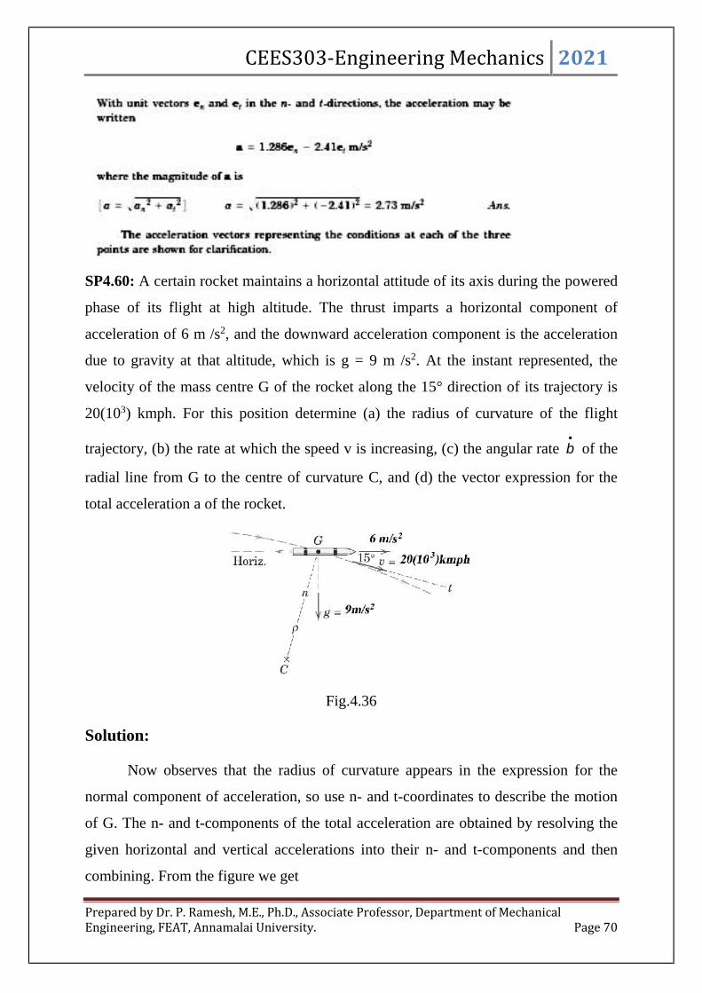
CEES303-Engineering Mechanics 2021
Prepared by Dr. P. Ramesh, M.E., Ph.D., Associate Professor, Department of MechanicalEngineering, FEAT, Annamalai University. Page 70
SP4.60: A certain rocket maintains a horizontal attitude of its axis during the powered
phase of its flight at high altitude. The thrust imparts a horizontal component of
acceleration of 6 m /s2, and the downward acceleration component is the acceleration
due to gravity at that altitude, which is g = 9 m /s2. At the instant represented, the
velocity of the mass centre G of the rocket along the 15° direction of its trajectory is
20(103) kmph. For this position determine (a) the radius of curvature of the flight
trajectory, (b) the rate at which the speed v is increasing, (c) the angular rate
of the
radial line from G to the centre of curvature C, and (d) the vector expression for the
total acceleration a of the rocket.
Fig.4.36
Solution:
Now observes that the radius of curvature appears in the expression for the
normal component of acceleration, so use n- and t-coordinates to describe the motion
of G. The n- and t-components of the total acceleration are obtained by resolving the
given horizontal and vertical accelerations into their n- and t-components and then
combining. From the figure we get

CEES303-Engineering Mechanics 2021
Prepared by Dr. P. Ramesh, M.E., Ph.D., Associate Professor, Department of MechanicalEngineering, FEAT, Annamalai University. Page 71
2/14.715sin615cos9 sma oon
2/12.815cos615sin9 sma oot
a) The radius of curvature of the flight trajectory from
2van ,
m
a
v
n
6
3
1032.414.7
6.31020
The radius of curvature of the flight trajectory is m61032.4
b) The rate at which the speed v is increasing
tav
, 2/12.8 smv
c) The angular rate
of the radial line from G to the centre of the curvature C,
v ,
sradv
/1085.121032.4
6.31020
4
6
3
d) The vector expression for the total acceleration a of the rocket,
ttnn eaeaa , tn eesma 12.814.7)/( 2
3) POLAR COORDINATES (r - ):
Fig.4.37 Polar coordinates motion of a particle
Now consider the third description of plane curvilinear motion, namely, polar
coordinates where the particle is located by the radial distance r from a fixed point and

CEES303-Engineering Mechanics 2021
Prepared by Dr. P. Ramesh, M.E., Ph.D., Associate Professor, Department of MechanicalEngineering, FEAT, Annamalai University. Page 72
by an angular measurement to the radial line. Polar coordinates are particularly useful
when a motion is constrained through the control of a radial distance and an angular
position or when an unconstrained motion is observed by measurements of a radial
distance and an angular position. Fig.4.37 (a) shows the polar coordinates r and which
locate a particle traveling on a curved path. An arbitrary fixed line, such as the x-axis,
is used as a reference for the measurement of . Unit vectors er and e are established
in the positive r- and - directions, respectively. The position vector r to the particle at
A has a magnitude equal to the radial distance r and a direction specified by the unit
vector er. Thus, express the location of the particle at A by the vector
rrer --------------- (4.24)
a) Time Derivatives of the Unit Vectors
To differentiate this relation with respect to time to obtain
rv and
va , now
need expressions for the time derivatives of both unit vectors er and e. It obtains
re and
e in exactly the same way it derived
te in the preceding article. During time dt the
coordinate directions rotate through the angle d, and the unit vectors also rotate
through the same angle from er and e to er' and e', as shown in fig.4.37 (b). It noted
that the vector change der is in the plus -direction and that de is in the minus r-
direction. Because their magnitudes in the limit are equal to the unit vector as radius
times the angle d in radians, it can write them as deder and dede r . If divide
these equations by d, Then
e
d
der and red
de
If, on the other hand, it divides that by dt, then have
edt
d
dt
der
and
redt
d
dt
de
or simply
eer
and ree
--------- (4.25)

CEES303-Engineering Mechanics 2021
Prepared by Dr. P. Ramesh, M.E., Ph.D., Associate Professor, Department of MechanicalEngineering, FEAT, Annamalai University. Page 73
b) Velocity
Now ready to differentiate r = rer with respect to time. Using the rule for
differentiating the product of a scalar and a vector gives
rr reerrv
With the substitution of
re from equation 4.25, the vector expression for the
velocity becomes
ererv r
----------- (4.26)
Where,
rvr ,
rv and 22vvv r
The r – component of v is merely the rate at which the vector r stretches. The -
component of v is due to the rotation of r.
c) Acceleration
Now differentiate the expression for v to obtain the acceleration
va . Note that
the derivative of er
will produce three terms, since all three factors are variable. Thus,
erererererva rr
Substitution of
re and
e from equation 4.e and collecting terms give
errerra r
22 ----------- (4.27)
Where,
2rrar ,
rra 2 and 22aaa r
Now it can write the - component alternatively as
21
rdt
d
ra

CEES303-Engineering Mechanics 2021
Prepared by Dr. P. Ramesh, M.E., Ph.D., Associate Professor, Department of MechanicalEngineering, FEAT, Annamalai University. Page 74
Which can be verified easily by carrying out the differentiation. This form of a
will be useful when it treats the angular momentum of particles.
d) Circular motion;
For motion in a circular path with r constant, the components of equation
ererv r
and equation errerra r
22 become simply
0rv ,
rv ,
2rar and
ra
This description is the same as that obtained n- and t- components, where the -
and t – directions coincide but the positive r-direction is in the negative n-direction.
Thus nr aa for circular motion centred at the origin of the polar coordinates.
The expressions for ra and a in scalar form can also be obtained by direct
differentiation of the coordinate relations x = rcos and y = r sin to obtain
xa x and
ya y . Each of these rectangular components of acceleration can then be resolved r-
and - components which when combined will yield the expressions of equation
errerra r
22
Problems:
SP4.61: Rotation of the radially slotted arm is governed by 302.02.0 tt , where
is in radians and t is in seconds. Simultaneously the power screw in the arm engages the
slider B and controls its distance from O according to 204.02.0 tr , where r is in
metres and t is in second. Calculate the magnitude of the velocity and acceleration of
the slider for the instant when t = 3s.

CEES303-Engineering Mechanics 2021
Prepared by Dr. P. Ramesh, M.E., Ph.D., Associate Professor, Department of MechanicalEngineering, FEAT, Annamalai University. Page 75
Fig.4.38
Solution:

CEES303-Engineering Mechanics 2021
Prepared by Dr. P. Ramesh, M.E., Ph.D., Associate Professor, Department of MechanicalEngineering, FEAT, Annamalai University. Page 76
SP4.62: A tracking radar lies in the vertical plane of the path of a rocket which is
coasting in unpowered flight above the atmosphere. For the instant when =30o, the
tracking data given r = 8(104) m, smr /1200
and sdeg/80.0
. The acceleration of
the rocket is due only to gravitational attraction and for its particular altitude is 9.20m/s2
vertically down. For these conditions determine the velocity v of the rocket and the
values of
r and
.

CEES303-Engineering Mechanics 2021
Prepared by Dr. P. Ramesh, M.E., Ph.D., Associate Professor, Department of MechanicalEngineering, FEAT, Annamalai University. Page 77
Fig.4.39
Solution:
The components of velocity from equation ererv r
are
rvr , smvr /1200
rv , smv /1117180
08.0108 4
22vvv r , smv /163911171200 22
Since the total acceleration of the rocket is g = 9.20 m/s2 down, it can easily find
its r – and - components for the given position. As shown in the figure, they are
2/97.730cos20.9 sma or
2/60.430sin20.9 sma o

CEES303-Engineering Mechanics 2021
Prepared by Dr. P. Ramesh, M.E., Ph.D., Associate Professor, Department of MechanicalEngineering, FEAT, Annamalai University. Page 78
Now equate these values to the polar coordinate expressions for ra and a which
contain the unknowns
r and
. Thus from equation, errerra r
22
2rrar , 2
4
18008.010897.7
r , 2/63.7 smr
rra 2 ,
18008.01200210860.4 4
, 24 /1061.3 srad
SP4.63: A flywheel increases its speed from 30rpm to 60rpm in 10sec. Calculate a) the
angular acceleration and b) number of revolutions made by the wheel in these 10
seconds.
Solution:
SP4.64: A pulley starting from rest is given an acceleration of 0.5 rad/s2. What will be
its speed in rpm at the end of 2min? If then it is uniformly retarded at the rate of 0.3
rad/s2, in how many minutes the pulley will come to rest.
Solution:

CEES303-Engineering Mechanics 2021
Prepared by Dr. P. Ramesh, M.E., Ph.D., Associate Professor, Department of MechanicalEngineering, FEAT, Annamalai University. Page 79
SP4.65: A wheel rotates for 5 sec. with a constant angular acceleration and describes
during this time 100 radians. It then rotates with a constant angular velocity during the
next five sec. and describes 80 radians. Find the initial angular velocity and the angular
acceleration.
Solution:
SP4.66: A swing bridge turns through 90o in 2min. The bridge is uniformly accelerated
from rest for the first 40 sec. Subsequently it turns with a uniform angular velocity for
the next 60 sec. Then the motion of the bridge is uniformly retard for the last 20 sec.
Find a) angular acceleration, b) maximum angular velocity and c) angular retardation
of the bridge.
Solution:
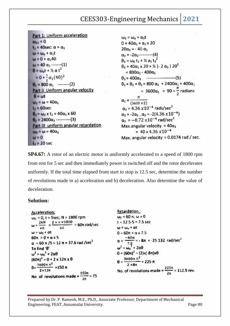
CEES303-Engineering Mechanics 2021
Prepared by Dr. P. Ramesh, M.E., Ph.D., Associate Professor, Department of MechanicalEngineering, FEAT, Annamalai University. Page 80
SP4.67: A rotor of an electric motor is uniformly accelerated to a speed of 1800 rpm
from rest for 5 sec and then immediately power is switched off and the rotor decelerates
uniformly. If the total time elapsed from start to stop is 12.5 sec, determine the number
of revolutions made in a) acceleration and b) deceleration. Also determine the value of
deceleration.
Solution:

CEES303-Engineering Mechanics 2021
Prepared by Dr. P. Ramesh, M.E., Ph.D., Associate Professor, Department of MechanicalEngineering, FEAT, Annamalai University. Page 81
SP4.68: A car is moving at 72kmph, if the wheels are 75cm diameter, find the angular
velocity of wheel about its axis. If the car comes to rest in a distance of 20m under a
uniform retardation, find the angular retardation of the wheels.
Solution:
SP4.69: A step pulley shown in fig.4. starts from rest and accelerates at 2rad/s2. What
time is required for block A to move 20m? Find also the velocity of A and B at that
time.
Solution:
SP.4.70: One end of a cord is wrapped around a pulley of 1.5m diameter while a block
is attached to the other end. The pulley is given an angular acceleration of 2 rpm per
second. Find the displacement, velocity and acceleration of the block 5 sec. after the
system was at rest.
Fig.4.40

CEES303-Engineering Mechanics 2021
Prepared by Dr. P. Ramesh, M.E., Ph.D., Associate Professor, Department of MechanicalEngineering, FEAT, Annamalai University. Page 82
Solution;
SP4.71: A horizontal bar of length 1.5m and of small cross-section rotates about the
vertical axis through one end. It accelerates uniformly from 1200 rpm to 1500 rpm in
an interval of 5 sec. What is the linear velocity at the beginning and at the end of the
interval? What are the normal and tangential components of the acceleration of the mid-
point of the bar after 5 sec. after the acceleration begins?
Solution:
SP4.72: What is the smallest radius which should be used for a high way curve if the
normal component of the accelerations of a car travelling at 72kmph is not to exceed
0.72m/s2?
Solution:
Fig.4.41
Fig.4.42

CEES303-Engineering Mechanics 2021
Prepared by Dr. P. Ramesh, M.E., Ph.D., Associate Professor, Department of MechanicalEngineering, FEAT, Annamalai University. Page 83
SP4.73: A point describes a circular path of radius 1.2m. The angular velocity and
angular acceleration of a radius to the point at a certain instant are 4 rad/sec, and 2 rad/s2,
both clockwise. If the angular acceleration is constant, determine for the given instant
and at 4 sec. later the normal and tangential components of acceleration of the point and
the angle turned through in 4 sec.
Solution:
SP4.74: A motorist is travelling on a curved sections of high way of radius 750m at the
speed of 100 kmph. The motorist suddenly applies brakes, causing the automobile to
slow down at a constant rate. Knowing that after 8sec. the speed has been reduced to
75kmph, determine the acceleration of the automobile immediately after the brakes
have been applied.
Solution:

CEES303-Engineering Mechanics 2021
Prepared by Dr. P. Ramesh, M.E., Ph.D., Associate Professor, Department of MechanicalEngineering, FEAT, Annamalai University. Page 84
SP4.75: A bus starts from rest on a curve of 300m radius and accelerates at the constant
tangential acceleration of 0.75m/s2. Determine the distance and time that the bus will
travel before the magnitude of its total acceleration is 0.9m/s2.
Solution:
Fig.4.43

CEES303-Engineering Mechanics 2021
Prepared by Dr. P. Ramesh, M.E., Ph.D., Associate Professor, Department of MechanicalEngineering, FEAT, Annamalai University. Page 85
SP4.76: A car enters a curved section of the road of length equal to the quarter of a
circle of radius 100m at 18kmph and leaves at 36kmph. If the car is travelling with a
constant tangential acceleration, find the magnitude and direction of acceleration a)
when it enters the curve and b) when it leave the curve.
Solution:
Fig.4.44
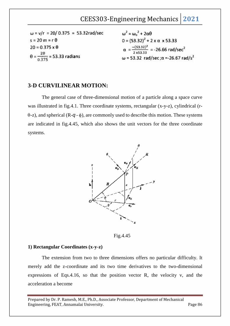
CEES303-Engineering Mechanics 2021
Prepared by Dr. P. Ramesh, M.E., Ph.D., Associate Professor, Department of MechanicalEngineering, FEAT, Annamalai University. Page 86
3-D CURVILINEAR MOTION:
The general case of three-dimensional motion of a particle along a space curve
was illustrated in fig.4.1. Three coordinate systems, rectangular (x-y-z), cylindrical (r-
-z), and spherical (R- - ), are commonly used to describe this motion. These systems
are indicated in fig.4.45, which also shows the unit vectors for the three coordinate
systems.
Fig.4.45
1) Rectangular Coordinates (x-y-z)
The extension from two to three dimensions offers no particular difficulty. It
merely add the z-coordinate and its two time derivatives to the two-dimensional
expressions of Eqs.4.16, so that the position vector R, the velocity v, and the
acceleration a become

CEES303-Engineering Mechanics 2021
Prepared by Dr. P. Ramesh, M.E., Ph.D., Associate Professor, Department of MechanicalEngineering, FEAT, Annamalai University. Page 87
kzjyixRva
kzjyixRv
zkyjxiR
--------- (4.28)
Note that in three dimensions we are using R in place of r for the position vector.
2) Cylindrical Coordinates (r- -z)
If we understand the polar-coordinate description of plane motion, then there
should be no difficulty with cylindrical coordinates because all that is required is the
addition of the z-coordinate and its two time derivatives. The position vector R to the
particle for cylindrical coordinates is simply
zkreR r
In place of equation ererv r
for plane motion, it can write the velocity as
kzererv r
------- (4.29)
Where,
rvr ,
rv ,
zvz and 222zr vvvv
Similarly the acceleration is written by the adding the z – component to equation
errerra r
22 which gives us
kzerrerra r
22 --------- (4.30)
Where,
2rrar ,
21
2 rdt
d
rrra ,
zaz and
222zr aaaa
Whereas the unit vectors er and e have non zero time derivatives due to the
changes in their directions, it notes athat the unit vector k in the z-direction remains
fixed in direction and therefore has a zero time derivative.

CEES303-Engineering Mechanics 2021
Prepared by Dr. P. Ramesh, M.E., Ph.D., Associate Professor, Department of MechanicalEngineering, FEAT, Annamalai University. Page 88
3) Spherical Coordinates (R- - ):
Spherical coordinates R, , are utilized when a radial distance and two angles
are utilized to specify the position of a particle, as in the case of radar measurements,
for example. Derivation of the expression for the velocity v is easily obtained, but the
expression for the acceleration ‘a’ is more complex because of the added geometry.
Consequently, only the results will be cited here. First it designates the unit vectors eR,
e, e as shown in fig.4.45. Note that the unit vector eR is in the direction in which the
particle P would move if R increases but and are held constant. The unit vector e
is in the direction in which P would move if increases while R and are held constant.
Finally, the unit vector e is in the direction in which P would move if increases while
R and are held constant. The resulting expressions for v and a are
evevevv rr ----------- (4.31)
Where,
RvR , cos
Rv and
Rv
And
eaeaeaa RR --------- (4.32)
Where,
222 cosRRRaR ,
sin2cos 2
RR
dt
d
Ra and
cossin
1 22 RRdt
d
Ra
Linear algebraic transformations between any two of the three coordinate-system
expressions for velocity or acceleration can be developed. These transformations make
it possible to express the motion component in rectangular coordinates, for example, if
the components are known in spherical coordinates, or vice versa. These
transformations are easily handled with the aid of matrix algebra and a simple computer
program.
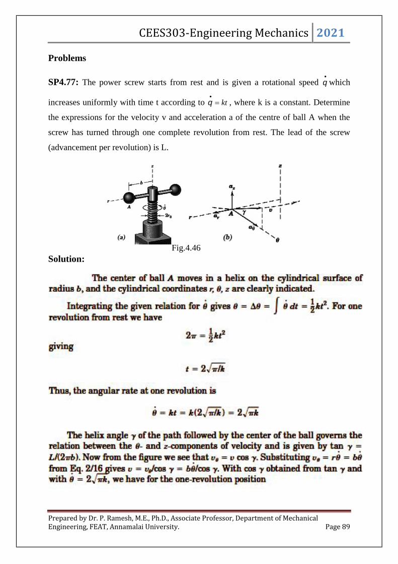
CEES303-Engineering Mechanics 2021
Prepared by Dr. P. Ramesh, M.E., Ph.D., Associate Professor, Department of MechanicalEngineering, FEAT, Annamalai University. Page 89
Problems
SP4.77: The power screw starts from rest and is given a rotational speed
which
increases uniformly with time t according to kt
, where k is a constant. Determine
the expressions for the velocity v and acceleration a of the centre of ball A when the
screw has turned through one complete revolution from rest. The lead of the screw
(advancement per revolution) is L.
Solution:Fig.4.46
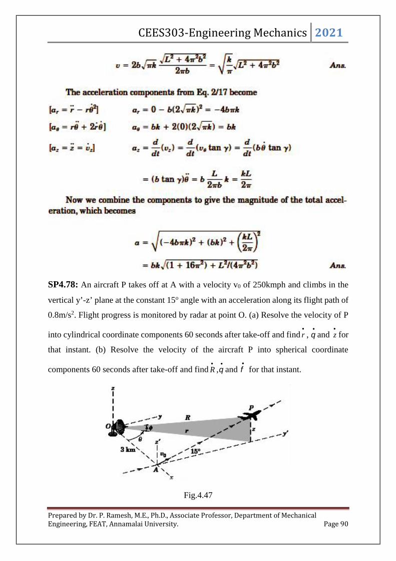
CEES303-Engineering Mechanics 2021
Prepared by Dr. P. Ramesh, M.E., Ph.D., Associate Professor, Department of MechanicalEngineering, FEAT, Annamalai University. Page 90
SP4.78: An aircraft P takes off at A with a velocity v0 of 250kmph and climbs in the
vertical y’-z’ plane at the constant 15o angle with an acceleration along its flight path of
0.8m/s2. Flight progress is monitored by radar at point O. (a) Resolve the velocity of P
into cylindrical coordinate components 60 seconds after take-off and find
r ,
and
z for
that instant. (b) Resolve the velocity of the aircraft P into spherical coordinate
components 60 seconds after take-off and find
R ,
and
for that instant.
Fig.4.47
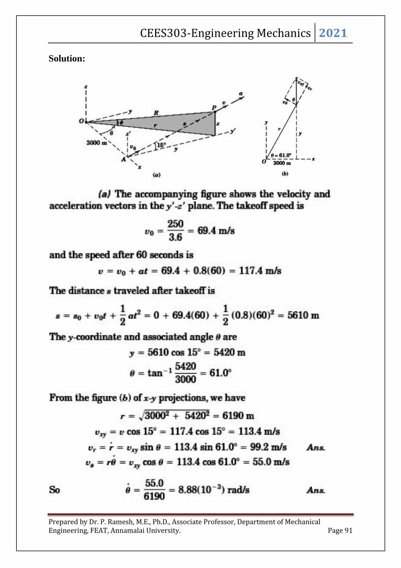
CEES303-Engineering Mechanics 2021
Prepared by Dr. P. Ramesh, M.E., Ph.D., Associate Professor, Department of MechanicalEngineering, FEAT, Annamalai University. Page 91
Solution:
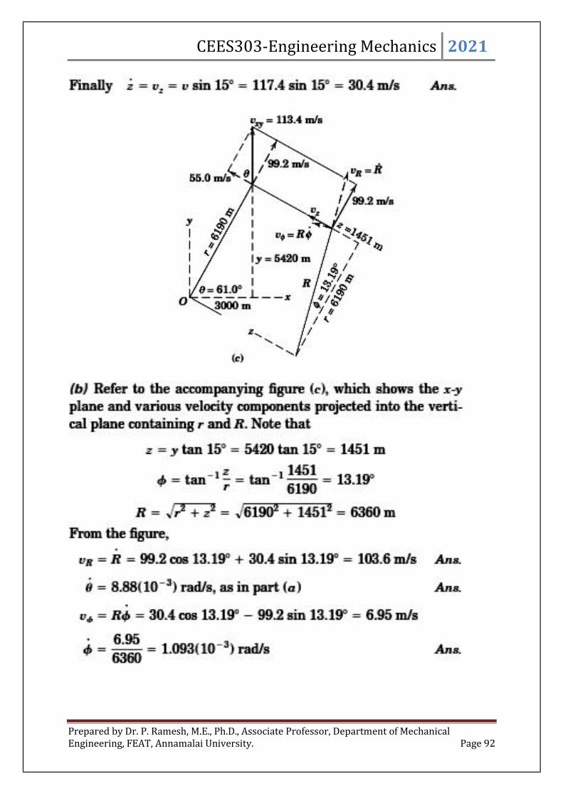
CEES303-Engineering Mechanics 2021
Prepared by Dr. P. Ramesh, M.E., Ph.D., Associate Professor, Department of MechanicalEngineering, FEAT, Annamalai University. Page 92

CEES303-Engineering Mechanics 2021
Prepared by Dr. P. Ramesh, M.E., Ph.D., Associate Professor, Department of MechanicalEngineering, FEAT, Annamalai University. Page 93
RELATIVE MOTION (TRANSLATING AXES):
In the previous sections, we have described particle motion using coordinates
referred to fixed reference axes. The displacements, velocities and accelerations so
determined are termed absolute. It is not always possible or convenient, however, to use
a fixed set of axes to describe or to measure motion. In addition, there are many
engineering problems for which the analysis of motion is simplified by using
measurements made with respect to a moving reference system. These measurements,
when combined with the absolute motion of the moving coordinate system, enable us
to determine the absolute motion in question. This approach is called a relative-motion
analysis.
Now consider two particles A and B which may have separate curvilinear
motions in a given plane or in parallel planes, fig.4.48. We will arbitrarily attach the
origin of a set of translating (nonrotating) axes x-y to particle B and observe the motion
of A from our moving position on B.
Fig.4.48
The position vector of A as measured relative to the frame x-y is yjxir BA r ,
where the subscript notation “A / B” means “A relative to B” or “A with respect to B.”
The unit vectors along the x- and y-axes are i and j, and x and y are the coordinates of
‘A’ measured in the x-y frame. The absolute position of B is defined by the vector rB
measured from the origin of the fixed axes X-Y. The absolute position of A is seen,
therefore, to be determined by the vector
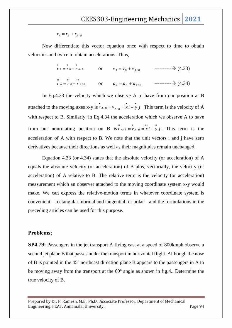
CEES303-Engineering Mechanics 2021
Prepared by Dr. P. Ramesh, M.E., Ph.D., Associate Professor, Department of MechanicalEngineering, FEAT, Annamalai University. Page 94
BABA rrr /
Now differentiate this vector equation once with respect to time to obtain
velocities and twice to obtain accelerations. Thus,
BABA rrr /
or BABA vvv / ---------- (4.33)
BABA rrr /
or BABA aaa / ---------- (4.34)
In Eq.4.33 the velocity which we observe A to have from our position at B
attached to the moving axes x-y is jyixvr BABA
// . This term is the velocity of A
with respect to B. Similarly, in Eq.4.34 the acceleration which we observe A to have
from our nonrotating position on B is jyixvr BABA
// . This term is the
acceleration of A with respect to B. We note that the unit vectors i and j have zero
derivatives because their directions as well as their magnitudes remain unchanged.
Equation 4.33 (or 4.34) states that the absolute velocity (or acceleration) of A
equals the absolute velocity (or acceleration) of B plus, vectorially, the velocity (or
acceleration) of A relative to B. The relative term is the velocity (or acceleration)
measurement which an observer attached to the moving coordinate system x-y would
make. We can express the relative-motion terms in whatever coordinate system is
convenient—rectangular, normal and tangential, or polar—and the formulations in the
preceding articles can be used for this purpose.
Problems;
SP4.79: Passengers in the jet transport A flying east at a speed of 800kmph observe a
second jet plane B that passes under the transport in horizontal flight. Although the nose
of B is pointed in the 45o northeast direction plane B appears to the passengers in A to
be moving away from the transport at the 60o angle as shown in fig.4.. Determine the
true velocity of B.

CEES303-Engineering Mechanics 2021
Prepared by Dr. P. Ramesh, M.E., Ph.D., Associate Professor, Department of MechanicalEngineering, FEAT, Annamalai University. Page 95
Solution:
Fig.4.49
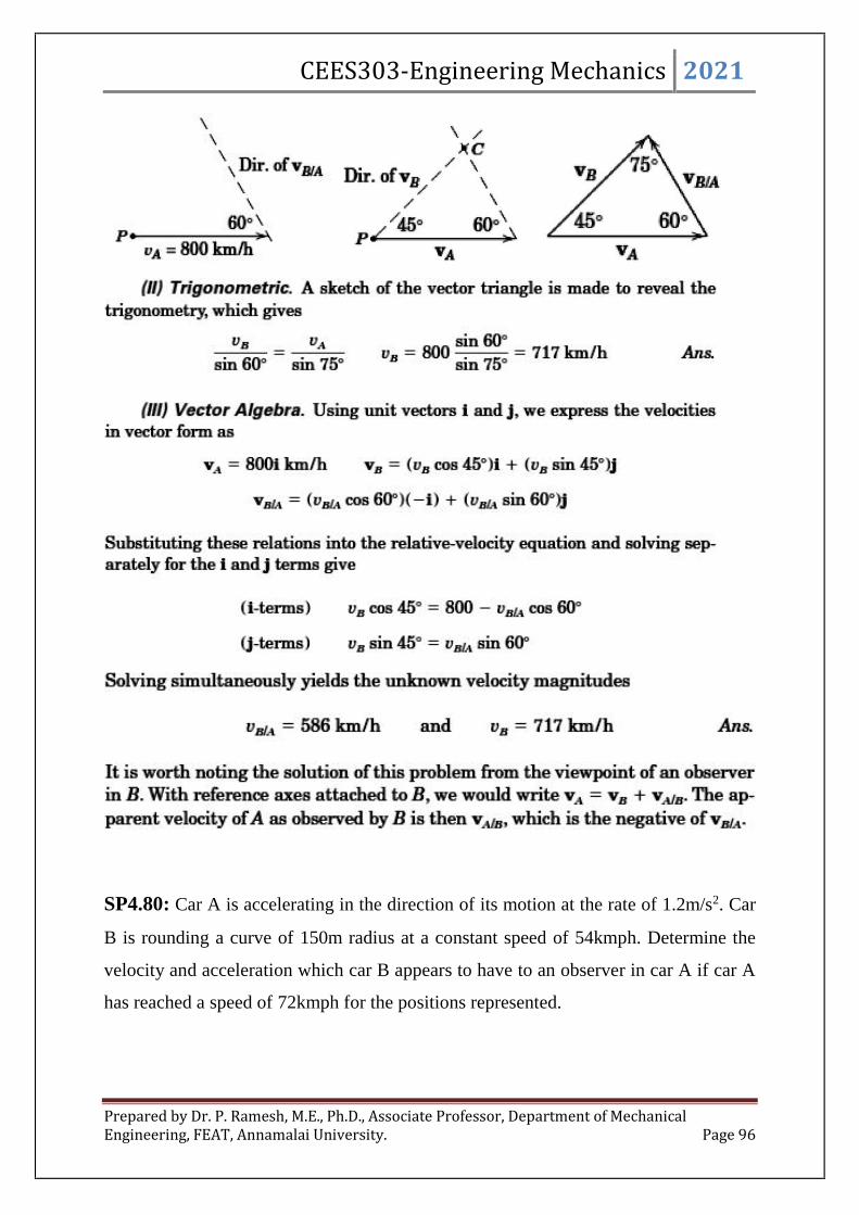
CEES303-Engineering Mechanics 2021
Prepared by Dr. P. Ramesh, M.E., Ph.D., Associate Professor, Department of MechanicalEngineering, FEAT, Annamalai University. Page 96
SP4.80: Car A is accelerating in the direction of its motion at the rate of 1.2m/s2. Car
B is rounding a curve of 150m radius at a constant speed of 54kmph. Determine the
velocity and acceleration which car B appears to have to an observer in car A if car A
has reached a speed of 72kmph for the positions represented.

CEES303-Engineering Mechanics 2021
Prepared by Dr. P. Ramesh, M.E., Ph.D., Associate Professor, Department of MechanicalEngineering, FEAT, Annamalai University. Page 97
Fig.4.50
Solution:
Now choose non rotating reference axes attached to car A since the motion of B
with respect to A is desired.
Velocity; The relative velocity equation is BAAB vvv / and the velocities of A and B
for the position considered have the magnitudes
smvA /206.3
72 and smvB /15
6.3
54
The triangle of velocity vectors is drawn in the sequence required by the
equation, and application of the law of cosines and the law of sines gives
smvvvvv BAABBA /03.1860cos15202152060cos2 2222/
sin60sin/ BBA vv , o
BA
B
v
v1.4660sin
03.18
15sin60sinsin 1
/
1
Acceleration; The relative acceleration equation is BAAB aaa / . The acceleration of
A is given and the acceleration of B is normal to the curve in the n-direction and has the
magnitude
2van , 2
2
/5.1150
15smaB

CEES303-Engineering Mechanics 2021
Prepared by Dr. P. Ramesh, M.E., Ph.D., Associate Professor, Department of MechanicalEngineering, FEAT, Annamalai University. Page 98
The triangle of acceleration vectors is drawn in the sequence required by the
equation as illustrated. Solving for the x and y components of aA/B gives us
2/ /0990.02.130cos5.1 sma o
xAB
2/ /750.030sin5.1 sma o
yAB
From which 222/ /757.0750.00990.0 sma AB
The direction of ABa / may be specified by the angle which, by the law of sines
becomes
30sin
757.0
sin
5.1
, o5.9730sin
757.0
5.1sin 1
SP.4.81: A passenger train 250m long moving with a velocity of 72 kmph overtakes a
goods train moving on a parallel path in the same direction completely in 45 sec. if the
length of the goods train is 200m determine the speed of goods train.
Solution:
Fig.4.51

CEES303-Engineering Mechanics 2021
Prepared by Dr. P. Ramesh, M.E., Ph.D., Associate Professor, Department of MechanicalEngineering, FEAT, Annamalai University. Page 99
SP4.82: Two trains A and B are moving on parallel tracks with velocity 72 kmph and
36 kmph in the same direction. The driver of train A finds that it took 42 sec. to overtake
train B. While driver of train B find that train A took 30 sec. to overtake him. Determine
a) Length of each train and b) time taken for complete overtaking. If the two trains move
in opposite direction with the same velocities, how much time is taken for complete
crossing.
Solution:
smkmphvA /2072 , smkmphvB /1036 , LA = length of train A, and LB =
length of train B.
To overtake the train B by train A, time taken is 42 seconds, then
mtvvL BAB 42042)1020(
When the trains moving in the same direction, for complete overtaking the distance to
be travelled as
m720300420
Therefore, ttvv BA )1020(720 , st 2430
720
SP4.83: A railway coach having an ordinary cross seat arrangement is travelling at
14.4kmph. A person runs at 5m/s on the platform. In what direction he must run so that
he may enter parallel to the seats? Also find the velocity with which he entered.
Solution:
smkmphvT /44.14 ,Fig.4.52

CEES303-Engineering Mechanics 2021
Prepared by Dr. P. Ramesh, M.E., Ph.D., Associate Professor, Department of MechanicalEngineering, FEAT, Annamalai University. Page 100
The relative velocity of the passenger with respect to the train
smvvv TPTP /345 2222/
o86.364
3tan 1
SP4.84: A cyclist travelling east with a speed of 2m/s feels the wind to be blowing
directly from north. On doubling his speed he feels the wind to blow from north-east.
Find the direction and the speed of the wind.
Solution:
Let OC1 – Cycle velocity = 2m/s
OC2 – Cycle velocity = 4m/s
C1W – Feels wind is blowing from North
C2W – Feels wind is blowing from North East
OW – Wind velocity
From the right angled triangle C1C2W,
C1C2=C1W = 2m/s,
Hence, smOW /828.222 22
To find direction, o452
2tan 1
Therefore, the Wind is blowing from North West.
Fig.4.53

CEES303-Engineering Mechanics 2021
Prepared by Dr. P. Ramesh, M.E., Ph.D., Associate Professor, Department of MechanicalEngineering, FEAT, Annamalai University. Page 101
SP4.85: Two ships A and b leave a part at the same time. The ship A is travelling north
– west at 32kmph and ship B 40o south of west at 24kmph. Determine a) the speed of
the ship B relative to ship A and b) after what time they will be 150km apart?
Solution:
SP4.86: A steam ship is travelling north at the rate of 20kmph and there is a windblowing from north –east at 30kmph. Find the direction in which the smoke from thechimney will appear to an observer sitting on the ship.
Solution:
OS – Ship velocity = 20kmph
OW – Wind velocity = 30kmph
From the triangle SOW, the angle SOW is 135o
SW – Relative velocity of the ship with respect to wind
oWSv 135cos203022030 22
/
kmphv WS 35.46/
Using law of sine,
sin
30
135sin/
oWSv
, ooSin
22.273035.46
135sin 1
The direction of smoke from the chimney is 27.22o
Fig.4.54
Fig.4.55

CEES303-Engineering Mechanics 2021
Prepared by Dr. P. Ramesh, M.E., Ph.D., Associate Professor, Department of MechanicalEngineering, FEAT, Annamalai University. Page 102
SP4.87: When a cyclist is riding at 20kmph he finds the rain meeting him at an angle
of 45o with vertical. When he rides at 12kmph, he meets the rain at an angle of 30o with
the vertical. Find the magnitude and direction of the absolute velocity of the rain.
Solution:
SP4.88: Car A when at a distance of 32.5m north of a crossing was observed to start
from rest and travelling towards the crossing with a constant acceleration of 1m/s2. At
the same instant another car B was observed to be just at the crossing and travelling east
at a constant speed of 36kmph. Find the position, velocity and acceleration of car A
relative to car B 5 seconds after the observation.
Solution:
Car A is moving with uniform acceleration towards crossing;
0u , a = 1m/s2, t = 5s
Using the relation,
Fig.4.56
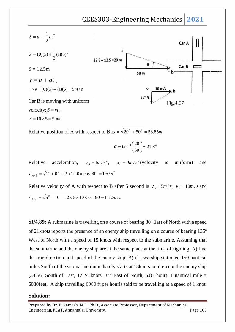
CEES303-Engineering Mechanics 2021
Prepared by Dr. P. Ramesh, M.E., Ph.D., Associate Professor, Department of MechanicalEngineering, FEAT, Annamalai University. Page 103
2
2
1atutS
2)5)(1(2
1)5)(0( S
S = 12.5m
atuv ,
smv /5)5)(1()5)(0(
Car B is moving with uniform
velocity; vtS ,
mS 50510
Relative position of A with respect to B is m85.535020 22
o8.2150
20tan 1
Relative acceleration, 2/1 smaA , 2/0 smaB (velocity is uniform) and
222/ /190cos01201 sma o
BA
Relative velocity of A with respect to B after 5 second is smvA /5 , smvB /10 and
smv BA /2.1190cos10521052/
SP4.89: A submarine is travelling on a course of bearing 80o East of North with a speed
of 21knots reports the presence of an enemy ship travelling on a course of bearing 135o
West of North with a speed of 15 knots with respect to the submarine. Assuming that
the submarine and the enemy ship are at the same place at the time of sighting. A) find
the true direction and speed of the enemy ship, B) if a warship stationed 150 nautical
miles South of the submarine immediately starts at 18knots to intercept the enemy ship
(34.66o South of East, 12.24 knots, 34o East of North, 6.85 hour). 1 nautical mile =
6080feet. A ship travelling 6080 ft per houris said to be travelling at a speed of 1 knot.
Solution:
Fig.4.57

CEES303-Engineering Mechanics 2021
Prepared by Dr. P. Ramesh, M.E., Ph.D., Associate Professor, Department of MechanicalEngineering, FEAT, Annamalai University. Page 104
CONSTRAINED MOTION:
Sometimes the motions of particles are interrelated because of the constraints
imposed by interconnecting members. In such cases it is necessary to account for these
constraints in order to determine the respective motions of the particles.
Fig.4.58a
Fig.4.58b

CEES303-Engineering Mechanics 2021
Prepared by Dr. P. Ramesh, M.E., Ph.D., Associate Professor, Department of MechanicalEngineering, FEAT, Annamalai University. Page 105
1) One Degree of Freedom
Fig.4.59
Consider first the very simple system of two interconnected particles A and B
shown in fig.4.59. It should be quite evident by inspection that the horizontal motion of
A is twice the vertical motion of B. Nevertheless we will use this example to illustrate
the method of analysis which applies to more complex situations where the results
cannot be easily obtained by inspection. The motion of B is clearly the same as that of
the centre of its pulley, so we establish position coordinates y and x measured from a
convenient fixed datum. The total length of the cable is
bryr
xL 12 2
2
------------ (4.36)
With L, r2, r1 and b all constant, the first and second time derivatives of the
equation give
yx 20 or BA vv 20 ---------- (4.37)
yx 20 or BA aa 20 ----------- (4.38)
The velocity and acceleration constraint equations indicate that, for the
coordinates selected, the velocity of A must have a sign which is opposite to that of the
velocity of B, and similarly for the accelerations. The constraint equations are valid for

CEES303-Engineering Mechanics 2021
Prepared by Dr. P. Ramesh, M.E., Ph.D., Associate Professor, Department of MechanicalEngineering, FEAT, Annamalai University. Page 106
the motion of the system in either direction. We emphasize that
xvA is positive to the
left and that
yvB is positive down.
Because the results do not depend on the lengths or pulley radii, we should be
able to analyze the motion without considering them. In the lower-left portion of
fig.4.59 is shown an enlarged view of the horizontal diameter A'B'C' of the lower pulley
at an instant of time. Clearly, A' and A have the same motion magnitudes, as do B and
B'. During an infinitesimal motion of A', it is easy to see from the triangle that B' moves
half as far as A' because point C as a point on the fixed portion of the cable momentarily
has no motion. Thus, with differentiation by time in mind, we can obtain the velocity
and acceleration magnitude relationships by inspection. The pulley, in effect, is a wheel
which rolls on the fixed vertical cable. The system of fig.4.59 is said to have one degree
of freedom since only one variable, either x or y, is needed to specify the positions of
all parts of the system.
2) Two Degrees of Freedom
The system with two degrees of freedom is
shown in fig.4.60. Here the positions of the lower
cylinder and pulley C depend on the separate
specifications of the two coordinates yA and yB. The
lengths of the cables attached to cylinders A and B
can be written, respectively, as
tconsyyL DAA tan2 - (4.39)
tconsyyyyL DCCBB tan)(2 - (4.40)
and their time derivatives are
DA yy
20 and DCB yyy
20 -- (4.41)
DA yy
20 and DCB yyy
20 - (4.42)
Fig.4.60

CEES303-Engineering Mechanics 2021
Prepared by Dr. P. Ramesh, M.E., Ph.D., Associate Professor, Department of MechanicalEngineering, FEAT, Annamalai University. Page 107
Eliminating the terms in Dy
and Dy
gives
042
CBA yyy or 042 CBA vvv -------- (4.43)
042
CBA yyy or 042 CBA aaa -------- (4.44)
It is clearly impossible for the signs of all three terms to be positive
simultaneously. So, for example, if both A and B have downward (positive) velocities,
then C will have an upward (negative) velocity.
These results can also be found by inspection of the motions of the two pulleys
at C and D. For an increment dyA (with yB held fixed), the centre of D moves up an
amount2
Ady, which causes an upward movement
4Ady
of the centre of C. For an
increment dyB (with y held fixed), the center of C moves up a distance2
Bdy. A
combination of the two movements gives an upward movement
24BA
C
dydydy ---- (4.45)
so that24BA
C
vvv as before. Visualization of the actual geometry of the motion is
an important ability.
A second type of constraint where the direction of the connecting member
changes with the motion is illustrated in the second of the two sample problems which
follow.
Problems:
SP4.90: In the pulley configuration as shown in fig.4.61 cylinder A has a downward
velocity of 0.3m/s. Determine the velocity of B. Solve in two ways.

CEES303-Engineering Mechanics 2021
Prepared by Dr. P. Ramesh, M.E., Ph.D., Associate Professor, Department of MechanicalEngineering, FEAT, Annamalai University. Page 108
Fig.4.61
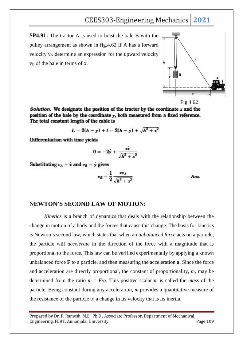
CEES303-Engineering Mechanics 2021
Prepared by Dr. P. Ramesh, M.E., Ph.D., Associate Professor, Department of MechanicalEngineering, FEAT, Annamalai University. Page 109
SP4.91: The tractor A is used to hoist the bale B with the
pulley arrangement as shown in fig.4.62 If A has a forward
velocity vA determine an expression for the upward velocity
vB of the bale in terms of x.
NEWTON’S SECOND LAW OF MOTION:
Kinetics is a branch of dynamics that deals with the relationship between the
change in motion of a body and the forces that cause this change. The basis for kinetics
is Newton’s second law, which states that when an unbalanced force acts on a particle,
the particle will accelerate in the direction of the force with a magnitude that is
proportional to the force. This law can be verified experimentally by applying a known
unbalanced force F to a particle, and then measuring the acceleration a. Since the force
and acceleration are directly proportional, the constant of proportionality, m, may be
determined from the ratio m = F/a. This positive scalar m is called the mass of the
particle. Being constant during any acceleration, m provides a quantitative measure of
the resistance of the particle to a change in its velocity that is its inertia.
Fig.4.62
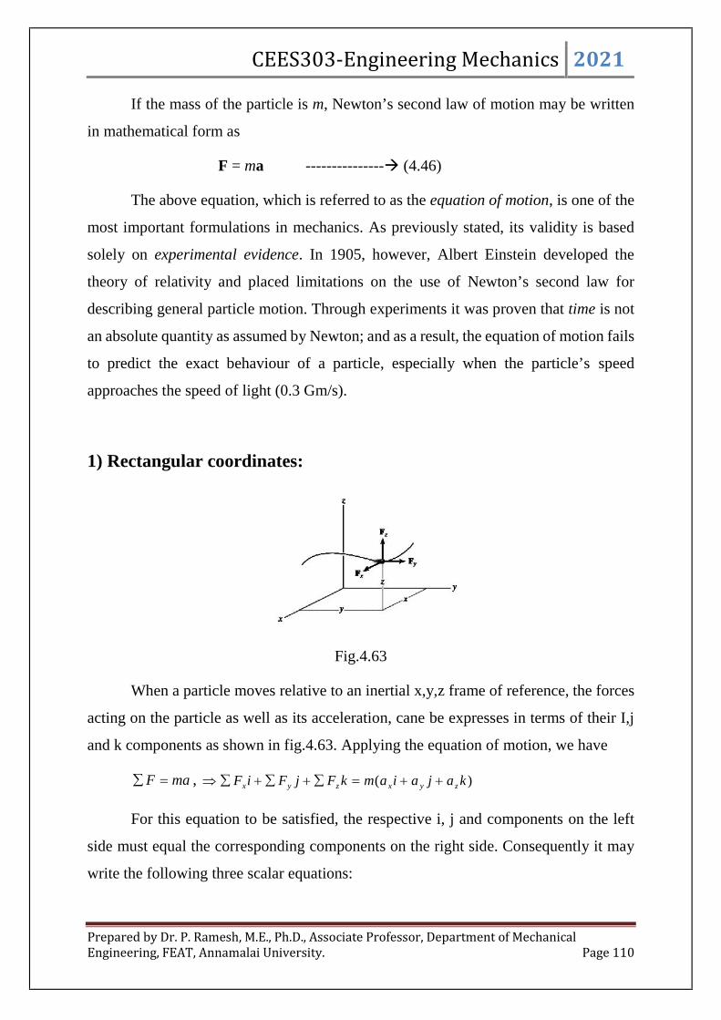
CEES303-Engineering Mechanics 2021
Prepared by Dr. P. Ramesh, M.E., Ph.D., Associate Professor, Department of MechanicalEngineering, FEAT, Annamalai University. Page 110
If the mass of the particle is m, Newton’s second law of motion may be written
in mathematical form as
F = ma --------------- (4.46)
The above equation, which is referred to as the equation of motion, is one of the
most important formulations in mechanics. As previously stated, its validity is based
solely on experimental evidence. In 1905, however, Albert Einstein developed the
theory of relativity and placed limitations on the use of Newton’s second law for
describing general particle motion. Through experiments it was proven that time is not
an absolute quantity as assumed by Newton; and as a result, the equation of motion fails
to predict the exact behaviour of a particle, especially when the particle’s speed
approaches the speed of light (0.3 Gm/s).
1) Rectangular coordinates:
Fig.4.63
When a particle moves relative to an inertial x,y,z frame of reference, the forces
acting on the particle as well as its acceleration, cane be expresses in terms of their I,j
and k components as shown in fig.4.63. Applying the equation of motion, we have
maF , )( kajaiamkFjFiF zyxzyx
For this equation to be satisfied, the respective i, j and components on the left
side must equal the corresponding components on the right side. Consequently it may
write the following three scalar equations:

CEES303-Engineering Mechanics 2021
Prepared by Dr. P. Ramesh, M.E., Ph.D., Associate Professor, Department of MechanicalEngineering, FEAT, Annamalai University. Page 111
zz
yy
xx
maF
maF
maF
------------ (4.47)
Where, the acceleration and resultant force are given by,
kajaiaa zyx , 222zyx aaaa --------- (4.48)
kFjFiFF zyx , 222zyx FFFF (4.49)
In particular, if the particle is constrained to move only in the x-y plane then the first
two of these equations are used to specify the motion.
Problems:
SP4.92: The 50kg crate as shown in fig.4.64 rests on a horizontal surface for which the
coefficient of kinetic friction is k = 0.3. If the crate is subjected to a 400-N towing
force, determine the velocity of the crate in 3seconds starting from rest.
Fig.4.64
Solution:

CEES303-Engineering Mechanics 2021
Prepared by Dr. P. Ramesh, M.E., Ph.D., Associate Professor, Department of MechanicalEngineering, FEAT, Annamalai University. Page 112
Fig.4.64
SP4.93: A 10 kg projectile is fired vertically upward from the ground with an initial
velocity of 50m/s as shown in fig.4. Determine the maximum height to which it will
travel if (a) atmospheric resistance is neglected; and b) atmospheric resistance is
measured as FD = (0.01v2)N, where v is the speed of the projectile at any instant
measured in m/s.

CEES303-Engineering Mechanics 2021
Prepared by Dr. P. Ramesh, M.E., Ph.D., Associate Professor, Department of MechanicalEngineering, FEAT, Annamalai University. Page 113
Fig.4.65
Solution:

CEES303-Engineering Mechanics 2021
Prepared by Dr. P. Ramesh, M.E., Ph.D., Associate Professor, Department of MechanicalEngineering, FEAT, Annamalai University. Page 114
SP4.94: A smooth 2 kg collar as shown in fig.4.66 is attached to a spring having a
stiffness k = 3 N/m and an un-stretched length of 0.75m. If the collar is released from
rest at A, determine its acceleration and the normal force of the rod on the collar at the
instant y=1m.
Fig.4.66

CEES303-Engineering Mechanics 2021
Prepared by Dr. P. Ramesh, M.E., Ph.D., Associate Professor, Department of MechanicalEngineering, FEAT, Annamalai University. Page 115
Solution:
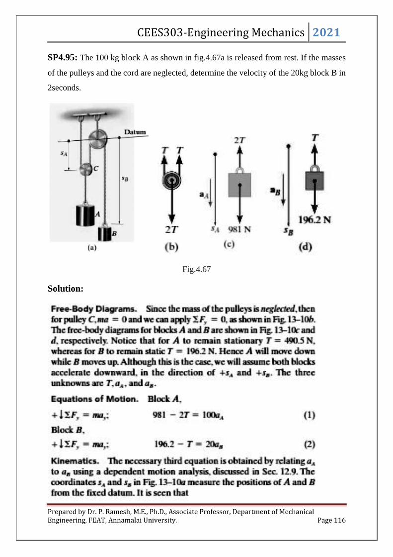
CEES303-Engineering Mechanics 2021
Prepared by Dr. P. Ramesh, M.E., Ph.D., Associate Professor, Department of MechanicalEngineering, FEAT, Annamalai University. Page 116
SP4.95: The 100 kg block A as shown in fig.4.67a is released from rest. If the masses
of the pulleys and the cord are neglected, determine the velocity of the 20kg block B in
2seconds.
Fig.4.67
Solution:

CEES303-Engineering Mechanics 2021
Prepared by Dr. P. Ramesh, M.E., Ph.D., Associate Professor, Department of MechanicalEngineering, FEAT, Annamalai University. Page 117
SP4.96: The baggage truck A has a weight of 4kN as shown in fig.4.68 and tows a 2.5
kN cart B and a 1.5kN cart C. for a short time the driving frictional force developed at
the wheels of the truck is NtFA )180( , where t is in seconds. If the truck starts from
rest, determine its speed in 2 second. Also what is the horizontal force acting on the
coupling between the truck and cart B at this instant? Neglect the size of the truck and
carts.
Fig.4.68
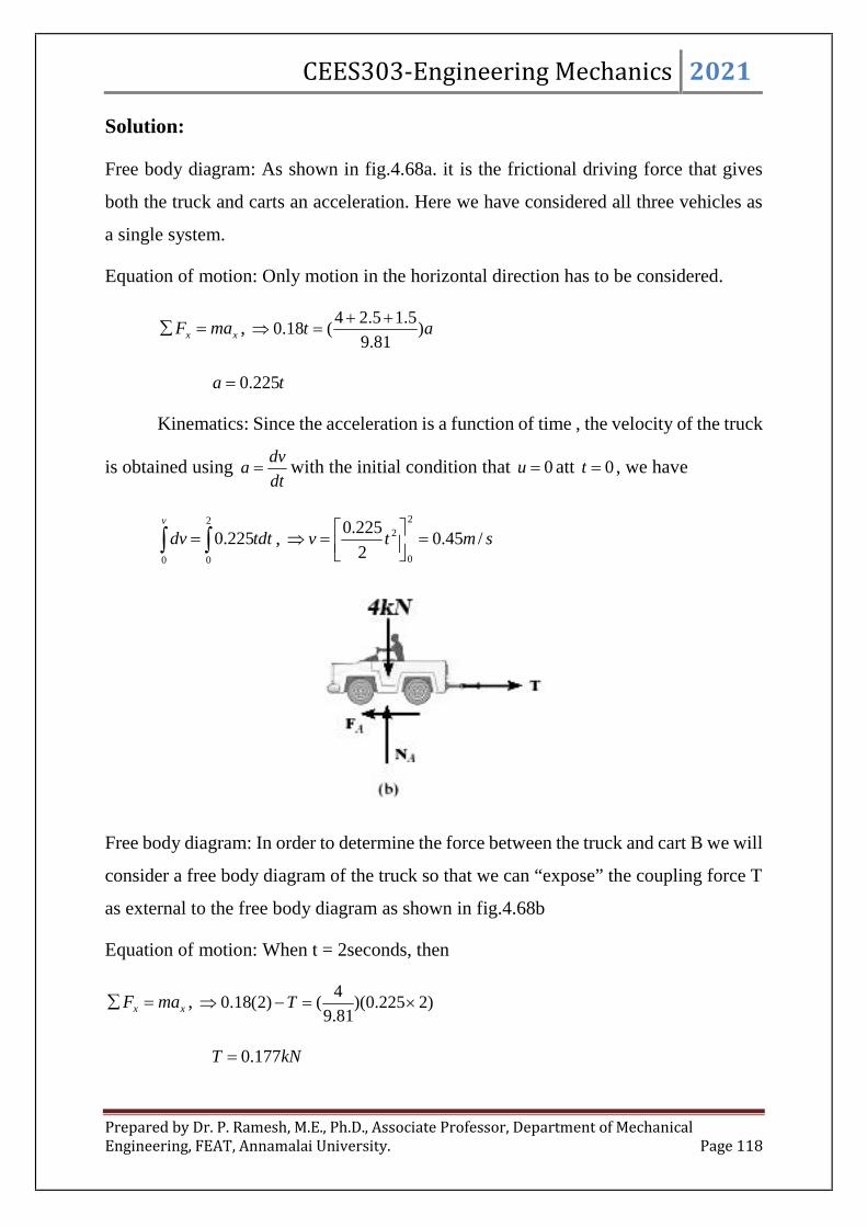
CEES303-Engineering Mechanics 2021
Prepared by Dr. P. Ramesh, M.E., Ph.D., Associate Professor, Department of MechanicalEngineering, FEAT, Annamalai University. Page 118
Solution:
Free body diagram: As shown in fig.4.68a. it is the frictional driving force that gives
both the truck and carts an acceleration. Here we have considered all three vehicles as
a single system.
Equation of motion: Only motion in the horizontal direction has to be considered.
xx maF , at )81.9
5.15.24(18.0
ta 225.0
Kinematics: Since the acceleration is a function of time , the velocity of the truck
is obtained usingdt
dva with the initial condition that 0u att 0t , we have
2
00
225.0 tdtdvv
, smtv /45.02
225.02
0
2
Free body diagram: In order to determine the force between the truck and cart B we will
consider a free body diagram of the truck so that we can “expose” the coupling force T
as external to the free body diagram as shown in fig.4.68b
Equation of motion: When t = 2seconds, then
xx maF , )2225.0)(81.9
4()2(18.0 T
kNT 177.0
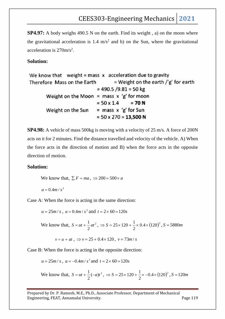
CEES303-Engineering Mechanics 2021
Prepared by Dr. P. Ramesh, M.E., Ph.D., Associate Professor, Department of MechanicalEngineering, FEAT, Annamalai University. Page 119
SP4.97: A body weighs 490.5 N on the earth. Find its weight , a) on the moon where
the gravitational acceleration is 1.4 m/s2 and b) on the Sun, where the gravitational
acceleration is 270m/s2.
Solution:
SP4.98: A vehicle of mass 500kg is moving with a velocity of 25 m/s. A force of 200N
acts on it for 2 minutes. Find the distance travelled and velocity of the vehicle. A) When
the force acts in the direction of motion and B) when the force acts in the opposite
direction of motion.
Solution:
We know that, maF , a 500200
2/4.0 sma
Case A: When the force is acting in the same direction:
smu /25 , 2/4.0 sma and st 120602
We know that, 2
2
1atutS , 21204.0
2
112025 S , mS 5880
atuv , 1204.025 v , smv /73
Case B: When the force is acting in the opposite direction:
smu /25 , 2/4.0 sma and st 120602
We know that, 2)(2
1tautS , 21204.0
2
112025 S , mS 120
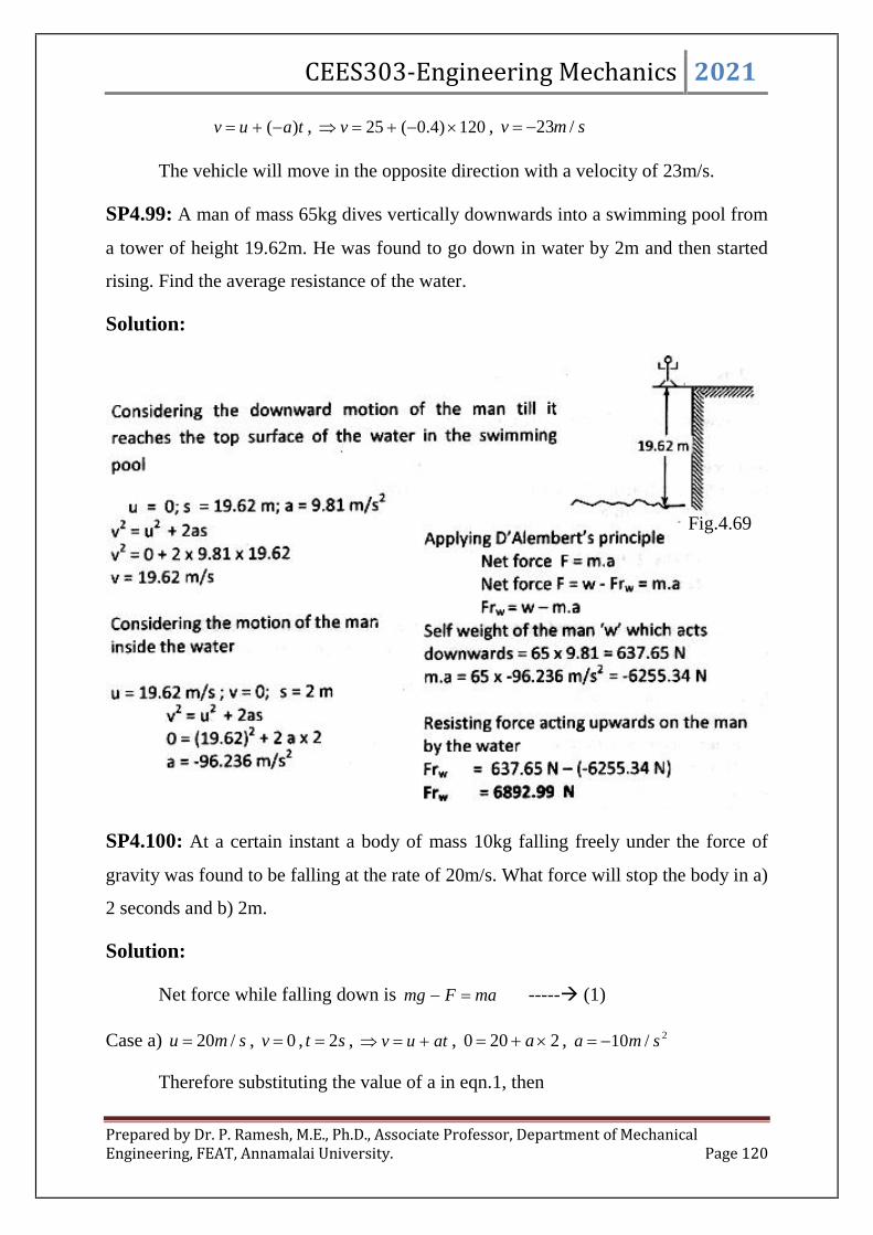
CEES303-Engineering Mechanics 2021
Prepared by Dr. P. Ramesh, M.E., Ph.D., Associate Professor, Department of MechanicalEngineering, FEAT, Annamalai University. Page 120
tauv )( , 120)4.0(25 v , smv /23
The vehicle will move in the opposite direction with a velocity of 23m/s.
SP4.99: A man of mass 65kg dives vertically downwards into a swimming pool from
a tower of height 19.62m. He was found to go down in water by 2m and then started
rising. Find the average resistance of the water.
Solution:
SP4.100: At a certain instant a body of mass 10kg falling freely under the force of
gravity was found to be falling at the rate of 20m/s. What force will stop the body in a)
2 seconds and b) 2m.
Solution:
Net force while falling down is maFmg ----- (1)
Case a) smu /20 , 0v , st 2 , atuv , 2200 a , 2/10 sma
Therefore substituting the value of a in eqn.1, then
Fig.4.69

CEES303-Engineering Mechanics 2021
Prepared by Dr. P. Ramesh, M.E., Ph.D., Associate Professor, Department of MechanicalEngineering, FEAT, Annamalai University. Page 121
)10(1081.910 F
NF 1.198
Case a) smu /20 , 0v , mS 2 , aSuv 222 , 22200 22 a , 2/100 sma
Therefore substituting the value of a in eqn.1, then
)100(1081.910 F
NF 1.1098
SP4.101: A 1 Mg car has to be accelerated from rest to 72kmph in a distance of 100m
on a level road. The resistance to motion is 150N. Determine the tractive force needed
by the car.
Solution:

CEES303-Engineering Mechanics 2021
Prepared by Dr. P. Ramesh, M.E., Ph.D., Associate Professor, Department of MechanicalEngineering, FEAT, Annamalai University. Page 122
SP4.102: A 100kg rocket is fired vertically, if the thrust of the rocket is 5000N and the
burn time is 10 seconds. Determine the maximum altitude attained by the rocket.
Solution:
SP4.103: A body of mass 10kg is moving over a smooth surface, whose equation of
motion is given by the relation 225 ttS where S in meter and t in seconds. Find the
magnitude of force responsible for the motion.
Solution:
SP4.104: An elevator having mass 2500kg and is moving vertically downwards with
a constant acceleration starting from rest, It travels a distance of 35m during an interval
of 10seconds. Find the cable tension during this time. Neglecting all other resistance to
motion, what are the limits of cable tension?
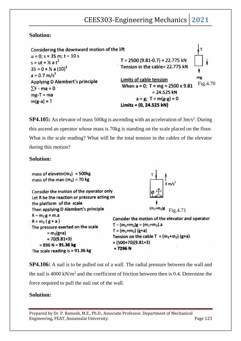
CEES303-Engineering Mechanics 2021
Prepared by Dr. P. Ramesh, M.E., Ph.D., Associate Professor, Department of MechanicalEngineering, FEAT, Annamalai University. Page 123
Solution:
SP4.105: An elevator of mass 500kg is ascending with an acceleration of 3m/s2. During
this ascend an operator whose mass is 70kg is standing on the scale placed on the floor.
What is the scale reading? What will be the total tension in the cables of the elevator
during this motion?
Solution:
SP4.106: A nail is to be pulled out of a wall. The radial pressure between the wall and
the nail is 4000 kN/m2 and the coefficient of friction between then is 0.4. Determine the
force required to pull the nail out of the wall.
Solution:
Fig.4.70
Fig.4.71

CEES303-Engineering Mechanics 2021
Prepared by Dr. P. Ramesh, M.E., Ph.D., Associate Professor, Department of MechanicalEngineering, FEAT, Annamalai University. Page 124
SP4.107: 1 kN block rests on a horizontal plane as shown in fig.4.72 Find the
magnitude of the force P required to give the block an acceleration of 3 m/s2 to the right.
The coefficient of the friction between the block and the plane is 0.25.
Fig.4.72
Solution:
SP4.108: A vehicle of mass 200 tonnes has a frictional resistance of 50N per tonne.
Speed of the train at the top of an incline of 1 in 80, is 45 kmph. Find the speed of the
train after running down the incline for 1km.

CEES303-Engineering Mechanics 2021
Prepared by Dr. P. Ramesh, M.E., Ph.D., Associate Professor, Department of MechanicalEngineering, FEAT, Annamalai University. Page 125
Solution:
SP4.109: A body of mass 500kg initially at rest at A 50m from B on an 15% upgrade
is allowed to slide down as shown in fig.4.73 If the coefficient of friction between the
body and the plane is 0.1, find the velocity of the body at B. Also find the distance
through which the body will travel beyond B on the level plane.
Fig.4.73
Solution:
SP4.110: A truck is moving down a 10o incline. When the driver applies brakes with
the result that the truck decelerates at a steady rate of 1m/s2. Investigate whether a mass
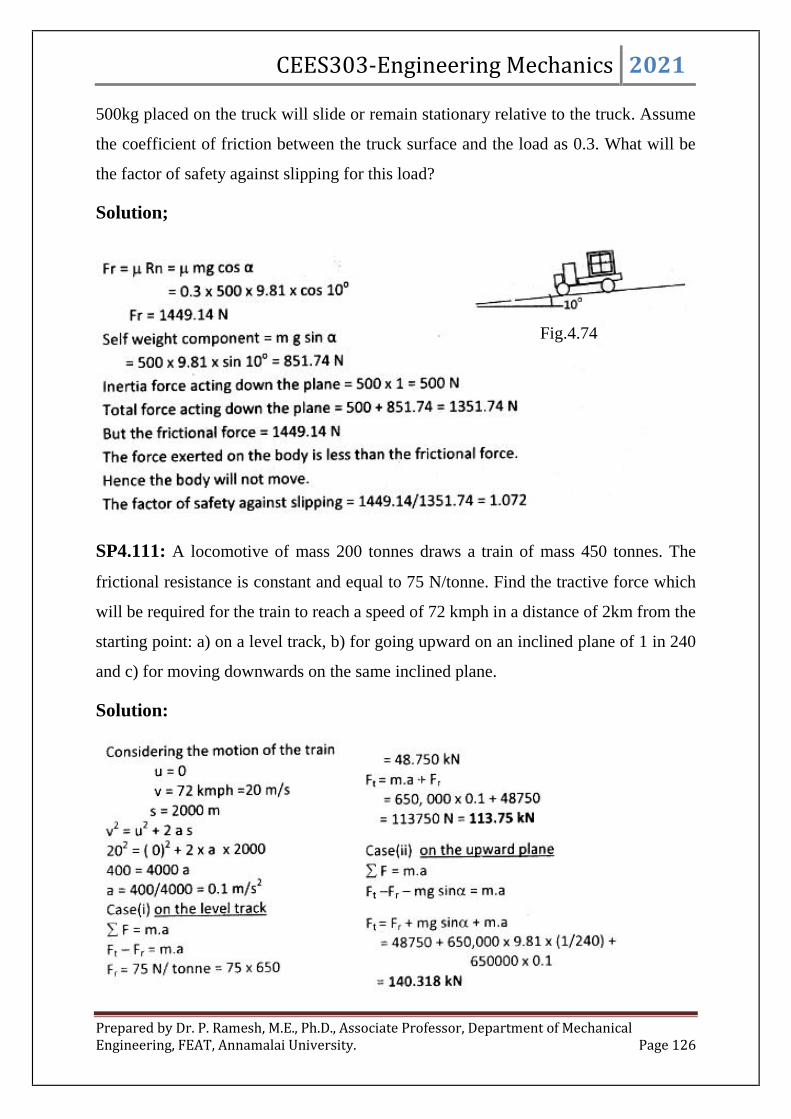
CEES303-Engineering Mechanics 2021
Prepared by Dr. P. Ramesh, M.E., Ph.D., Associate Professor, Department of MechanicalEngineering, FEAT, Annamalai University. Page 126
500kg placed on the truck will slide or remain stationary relative to the truck. Assume
the coefficient of friction between the truck surface and the load as 0.3. What will be
the factor of safety against slipping for this load?
Solution;
SP4.111: A locomotive of mass 200 tonnes draws a train of mass 450 tonnes. The
frictional resistance is constant and equal to 75 N/tonne. Find the tractive force which
will be required for the train to reach a speed of 72 kmph in a distance of 2km from the
starting point: a) on a level track, b) for going upward on an inclined plane of 1 in 240
and c) for moving downwards on the same inclined plane.
Solution:
Fig.4.74
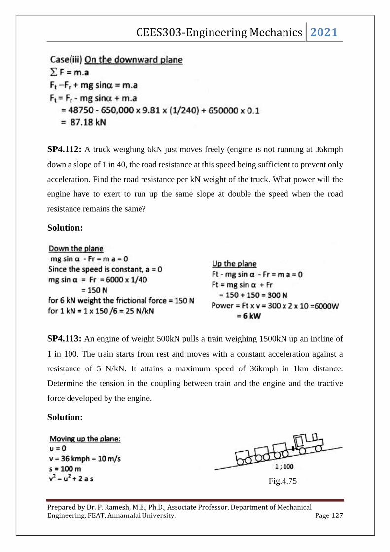
CEES303-Engineering Mechanics 2021
Prepared by Dr. P. Ramesh, M.E., Ph.D., Associate Professor, Department of MechanicalEngineering, FEAT, Annamalai University. Page 127
SP4.112: A truck weighing 6kN just moves freely (engine is not running at 36kmph
down a slope of 1 in 40, the road resistance at this speed being sufficient to prevent only
acceleration. Find the road resistance per kN weight of the truck. What power will the
engine have to exert to run up the same slope at double the speed when the road
resistance remains the same?
Solution:
SP4.113: An engine of weight 500kN pulls a train weighing 1500kN up an incline of
1 in 100. The train starts from rest and moves with a constant acceleration against a
resistance of 5 N/kN. It attains a maximum speed of 36kmph in 1km distance.
Determine the tension in the coupling between train and the engine and the tractive
force developed by the engine.
Solution:
Fig.4.75

CEES303-Engineering Mechanics 2021
Prepared by Dr. P. Ramesh, M.E., Ph.D., Associate Professor, Department of MechanicalEngineering, FEAT, Annamalai University. Page 128
SP4.114: A train weighing 200kN moves down a slope of 1 in 150 at 18 kmph and
engine develops 3.5kW. What power will be required to pull the train up the slope at
the same speed?
Solution:
SP4.115: Two blocks A and B are held on
an inclined plane 5m apart as shown in
fig.4. The coefficient of friction between
the block A and B and the inclined plane
are 0.2 and 0.1 respectively. If the block
begin to slide down the plane
simultaneously calculate the time and
distance travelled by each block before collision.
Fig.4.76
Fig.4.77

CEES303-Engineering Mechanics 2021
Prepared by Dr. P. Ramesh, M.E., Ph.D., Associate Professor, Department of MechanicalEngineering, FEAT, Annamalai University. Page 129
Solution:
SP4.116: A horizontal force P = 70N is exerted on mass A = 16kg as shown in fig.4.
The coefficient of friction between A and the horizontal plane is 0.25. B has a mass of
4kg and the coefficient of friction between it
and the plane is 0.5. The cord between the two
masses makes an angle of 10o with horizontal.
What is the tension in the cord?
Solution:
Fig.4.78
Fig.4.79

CEES303-Engineering Mechanics 2021
Prepared by Dr. P. Ramesh, M.E., Ph.D., Associate Professor, Department of MechanicalEngineering, FEAT, Annamalai University. Page 130
SP4.117: Determine the tension in the string and acceleration of two blocks of mass
150kg and 50kg connected by a string and a frictionless and weightless pulley as shown
in fig.4.80
Fig.4.80
Solution:

CEES303-Engineering Mechanics 2021
Prepared by Dr. P. Ramesh, M.E., Ph.D., Associate Professor, Department of MechanicalEngineering, FEAT, Annamalai University. Page 131
SP4.118: Determine the resulting motion of the body ‘A’ assuming the pulleys to be
smooth and weightless as shown in fig.4. If the system starts from rest determine the
velocity of the body ‘A’ after 10 seconds.
Solution:
SP4.119: Two rough planes inclined at 30o and 15o to the horizontal and of the same
height are placed back to back. Masses of 15kg is placed on 30o plane and 5kg is placed
on the 15o plane and are connected
by a string over the top of the
planes. If the coefficient of friction
be 0.3, find from fundamentals the
resulting acceleration.
Solution:
Fig.4.81
Fig.4.82

CEES303-Engineering Mechanics 2021
Prepared by Dr. P. Ramesh, M.E., Ph.D., Associate Professor, Department of MechanicalEngineering, FEAT, Annamalai University. Page 132
SP4.120: A block of wood ‘A’ of mass 5kg is resting on a table. A string attached to
‘A’ runs over a pulley and carries a mass of 5kg at the other end. A wooden block is of
mass 3kg is placed on the top of block ‘A’ and is held fixed by means of a string. The
coefficient of kinetic friction between A and the table is 0.25 and between B and A is
0.4. Determine acceleration of block A.
Solution:
Fig.4.83
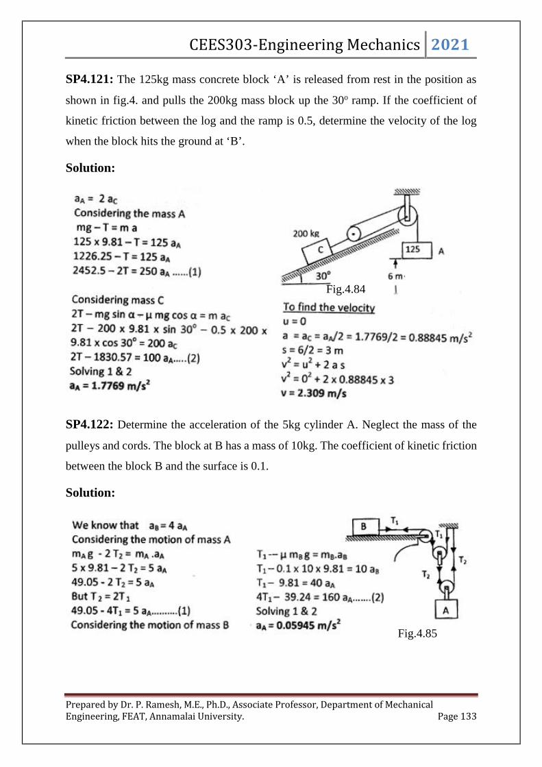
CEES303-Engineering Mechanics 2021
Prepared by Dr. P. Ramesh, M.E., Ph.D., Associate Professor, Department of MechanicalEngineering, FEAT, Annamalai University. Page 133
SP4.121: The 125kg mass concrete block ‘A’ is released from rest in the position as
shown in fig.4. and pulls the 200kg mass block up the 30o ramp. If the coefficient of
kinetic friction between the log and the ramp is 0.5, determine the velocity of the log
when the block hits the ground at ‘B’.
Solution:
SP4.122: Determine the acceleration of the 5kg cylinder A. Neglect the mass of the
pulleys and cords. The block at B has a mass of 10kg. The coefficient of kinetic friction
between the block B and the surface is 0.1.
Solution:
Fig.4.84
Fig.4.85

CEES303-Engineering Mechanics 2021
Prepared by Dr. P. Ramesh, M.E., Ph.D., Associate Professor, Department of MechanicalEngineering, FEAT, Annamalai University. Page 134
2) Normal and Tangential Coordinates or Path variable:
Fig.4.86
When a particle moves along a curved path which is known, the equation of
motion for the particle may be written in the tangential, normal, and bi-normal
directions, as shown in fig.4.86. Note that there is no motion of the particle in the bi-
normal direction, since the particle is constrained to move along the path. We have
maF
ntbbnntt mamaeFeFeF
This equation is satisfied provided
0b
nn
tt
F
maF
maF
--------------- (4.50)
Recall that )(dt
dvat represents the time rate of change in the magnitude of
velocity. So if tF acts in the direction of motion, the particle’s speed will increase
whereas if it acts in the opposite direction, the particle will slow down. Likewise,
)(2
v
an represents the time rate of change in the velocity’s direction. It is caused by
nF , which always acts in the positive n direction, i.e., towards the paths centre of
curvature. For this reason it is often referred to as the centripetal force.
CEES303-Engineering Mechanics 2021
Prepared by Dr. P. Ramesh, M.E., Ph.D., Associate Professor, Department of MechanicalEngineering, FEAT, Annamalai University. Page 135
Centripetal force:
The force which acts along the radius of the circle at every point and is always
directed towards the centre of the circle along which the body moves is known as
centripetal force. Its magnitude is rm 2 .
Centrifugal force:
The force which acts opposite to the centripetal force is known as centrifugal
force. The centrifugal force always acts away from the centre of the path, or in other
words the centrifugal force always tends to throw the body from the centre of circular
path. Its magnitude is rm 2 .
Super elevation or Cant or Banking:
We see that whenever a roadway ( or railway) is laid on a curved path, then both
the edges are not at the same level. In such a case the outer edge is always higher than
the inner one. This is done to keep the vehicle in equilibrium while in motion.
The body which is moving along a curved path is subjected to the following
forces:
a) Its own weight (mg)
b) Centrifugal force ( rm 2 or mv2/r)
The resultant of these forces is inclined with the vertical as shown in fig.4. It may
be noted that if the curved path be made level then the resultant force will be inclined
at some angle with the vertical and thus the reactions on both the supports of a vehicle
will not be equal which will affect the equilibrium of the vehicle.
To counterbalance this effect and to maintain equilibrium of the vehicle the
surface of the path is made perpendicular to the resultant by raising the outer edge of

CEES303-Engineering Mechanics 2021
Prepared by Dr. P. Ramesh, M.E., Ph.D., Associate Professor, Department of MechanicalEngineering, FEAT, Annamalai University. Page 136
the roadway (or outer rail of the railway). The amount by which the outer edge of rail
is raised is known as cant or super elevation.
Need for banking of roads and super elevation of rails:
When a vehicle moves around a flat curve, a radial outward force mv2/r is
experienced increasing the pressure on the outer wheel and decreasing the pressure on
the inner wheel. It creates discomfort to passengers. Apart from this, speed is to be
reduced considerably on curved path to avoid skidding and over turning. If the road is
banked or the track is given super elevation, the following may be achieved:
a) Skidding and overturning avoided
b) Higher speed permitted
c) Lateral pressure eliminated giving comfort to passenger
d) Excess wear and tear of wheels avoided
From the figure;
Weighttan
forcelCentrifuga
rg
v
g
r
mg
rm 222
- (4.51)
It may be noted from the above
expression that the super elevation is
independent of the mass of the body.
For rails,rg
v
G
S 2
tan (4.52)
Where, S – Height through which outer
wheel is lifted
G – Gauge length
a)
b)Fig.4.87

CEES303-Engineering Mechanics 2021
Prepared by Dr. P. Ramesh, M.E., Ph.D., Associate Professor, Department of MechanicalEngineering, FEAT, Annamalai University. Page 137
Maximum velocity to avoid skidding away of a vehicle on a level
circular path:
To avoid skidding:
ForcelCentrifugaFr or FrForcelCentrifuga
We know that,
Fr – Friction force
= Coefficient of friction x normal reaction
= x R
Therefore,
RForcelCentrifuga
mgr
mv
2
rgv 2
rgv
rgv max ------- (4.53)
Maximum velocity to avoid overturning of a vehicle on a level circular
path:
Let h – height of centre of gravity of the vehicle from the road,
RA, RB – reactions in the wheels A and B
2a – distance between the two wheels
Taking moments about B, then
022
r
hmvamgaRA
r
hmvamgaRA
2
2
Fig.4.88
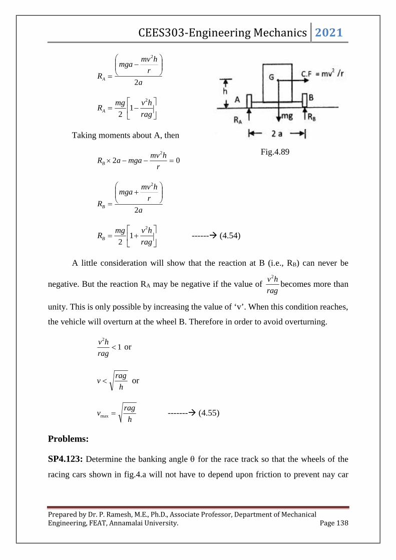
CEES303-Engineering Mechanics 2021
Prepared by Dr. P. Ramesh, M.E., Ph.D., Associate Professor, Department of MechanicalEngineering, FEAT, Annamalai University. Page 138
a
r
hmvmga
RA 2
2
rag
hvmgRA
2
12
Taking moments about A, then
022
r
hmvmgaaRB
a
r
hmvmga
RB 2
2
rag
hvmgRB
2
12
------ (4.54)
A little consideration will show that the reaction at B (i.e., RB) can never be
negative. But the reaction RA may be negative if the value ofrag
hv2
becomes more than
unity. This is only possible by increasing the value of ‘v’. When this condition reaches,
the vehicle will overturn at the wheel B. Therefore in order to avoid overturning.
12
rag
hvor
h
ragv or
h
ragv max ------- (4.55)
Problems:
SP4.123: Determine the banking angle for the race track so that the wheels of the
racing cars shown in fig.4.a will not have to depend upon friction to prevent nay car
Fig.4.89

CEES303-Engineering Mechanics 2021
Prepared by Dr. P. Ramesh, M.E., Ph.D., Associate Professor, Department of MechanicalEngineering, FEAT, Annamalai University. Page 139
from sliding up or down the track. Assume the cars have negligible size, a mass m, and
travel around the curve of radius with a constant speed v.
Fig.4.90
Solution:
SP4.124: Determine the maximum speed v which the sliding block may have as it
passes point A without losing contact with the surface.

CEES303-Engineering Mechanics 2021
Prepared by Dr. P. Ramesh, M.E., Ph.D., Associate Professor, Department of MechanicalEngineering, FEAT, Annamalai University. Page 140
Fig.4.91
Solution:
SP4.125: Small objects are released from rest at A and slide down the smooth circular
surface of radius R to a conveyor B. Determine the expression for the normal contact
force N between the guide and each object in terms of and specify the correct angular
velocity of the conveyor pulley of radius r to prevent any sliding on the belt as the
objects transfer to the conveyor.

CEES303-Engineering Mechanics 2021
Prepared by Dr. P. Ramesh, M.E., Ph.D., Associate Professor, Department of MechanicalEngineering, FEAT, Annamalai University. Page 141
Fig.4.92
Solution:
SP4.126: A 1500kg car enters a section of curved road in the horizontal plane and
slows down at a uniform rate from a speed of 100kmph at A to a speed of 50kmph as it
passes C. The radius of curvature of the road at A is 400m and at C is 80m. Determine
the total horizontal force exerted by the road on the tires at positions A, B and C. Point
B is the inflection point where the curvature changes direction.
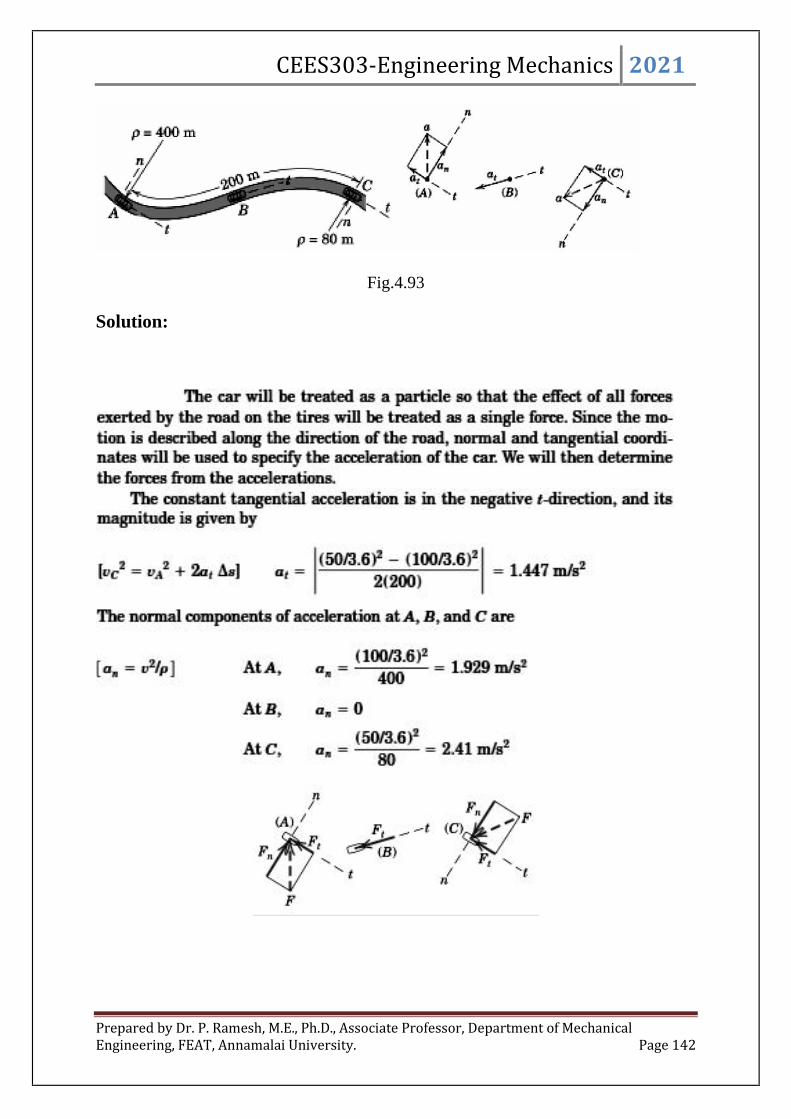
CEES303-Engineering Mechanics 2021
Prepared by Dr. P. Ramesh, M.E., Ph.D., Associate Professor, Department of MechanicalEngineering, FEAT, Annamalai University. Page 142
Fig.4.93
Solution:

CEES303-Engineering Mechanics 2021
Prepared by Dr. P. Ramesh, M.E., Ph.D., Associate Professor, Department of MechanicalEngineering, FEAT, Annamalai University. Page 143
SP4.127: Compute the magnitude v of the velocity required for the spacecraft S to
maintain a circular orbit of altitude 200mile above the surface of the earth.
Fig.4.94
Solution:
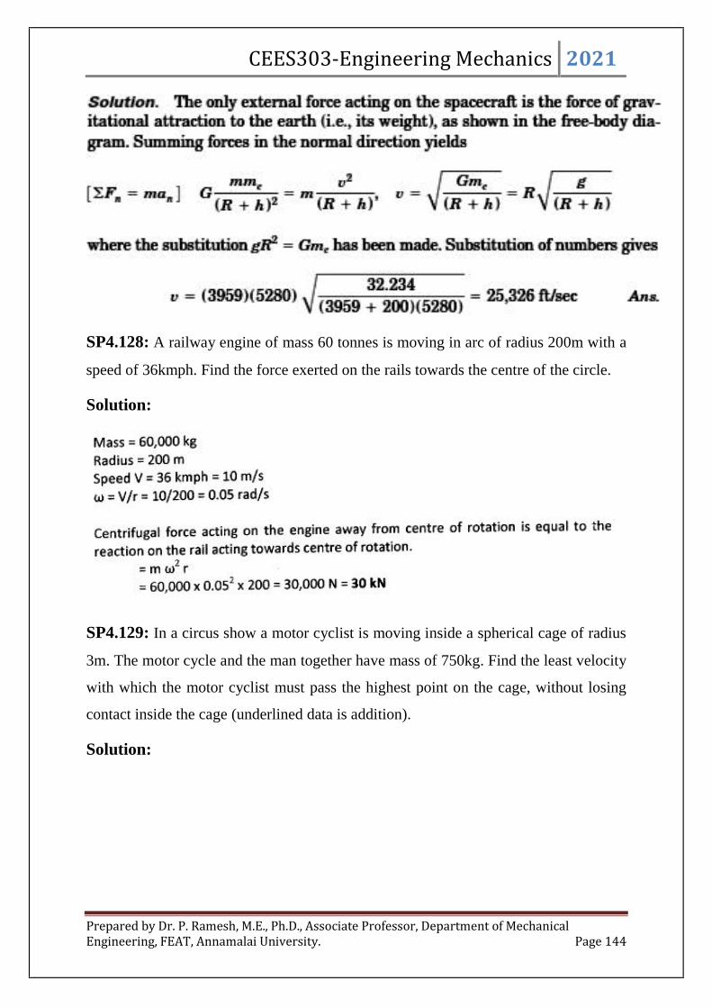
CEES303-Engineering Mechanics 2021
Prepared by Dr. P. Ramesh, M.E., Ph.D., Associate Professor, Department of MechanicalEngineering, FEAT, Annamalai University. Page 144
SP4.128: A railway engine of mass 60 tonnes is moving in arc of radius 200m with a
speed of 36kmph. Find the force exerted on the rails towards the centre of the circle.
Solution:
SP4.129: In a circus show a motor cyclist is moving inside a spherical cage of radius
3m. The motor cycle and the man together have mass of 750kg. Find the least velocity
with which the motor cyclist must pass the highest point on the cage, without losing
contact inside the cage (underlined data is addition).
Solution:
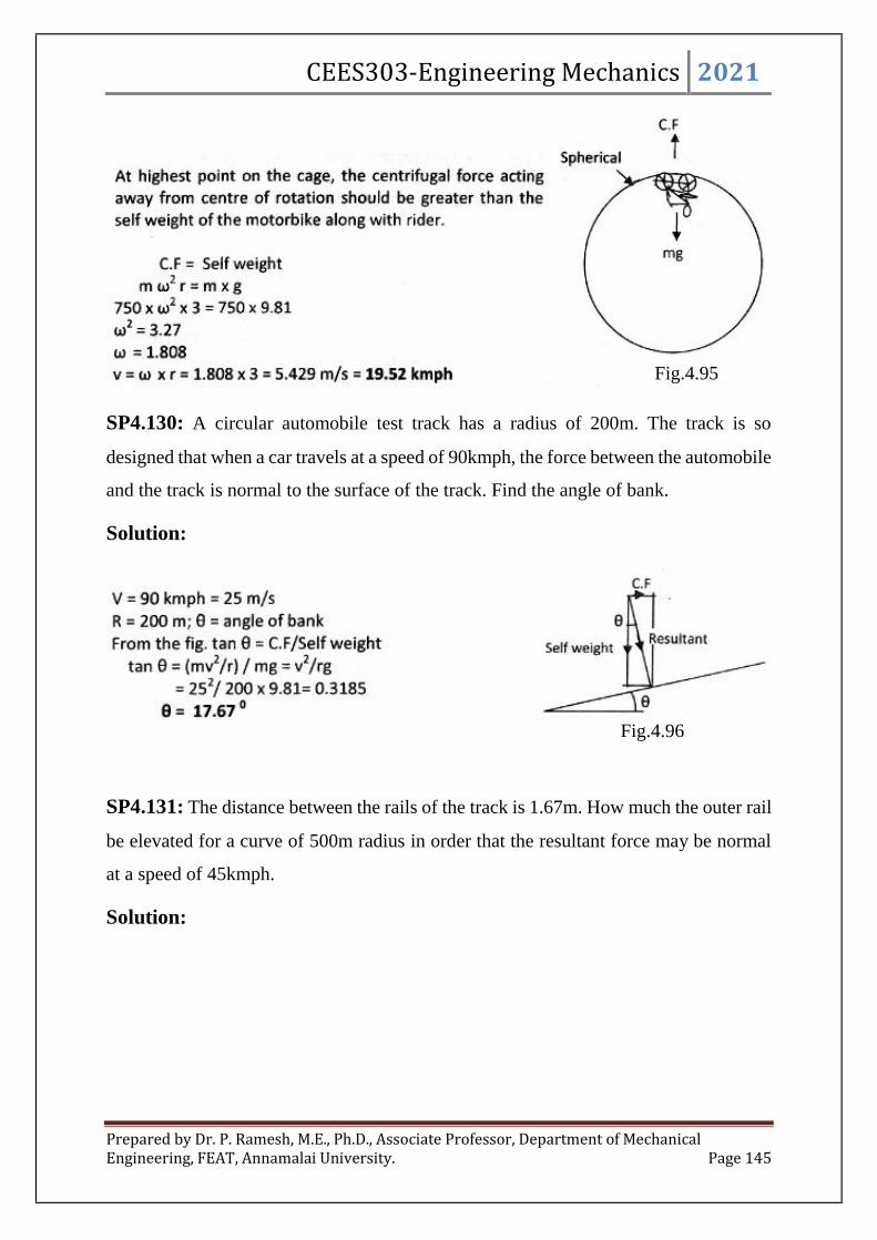
CEES303-Engineering Mechanics 2021
Prepared by Dr. P. Ramesh, M.E., Ph.D., Associate Professor, Department of MechanicalEngineering, FEAT, Annamalai University. Page 145
SP4.130: A circular automobile test track has a radius of 200m. The track is so
designed that when a car travels at a speed of 90kmph, the force between the automobile
and the track is normal to the surface of the track. Find the angle of bank.
Solution:
SP4.131: The distance between the rails of the track is 1.67m. How much the outer rail
be elevated for a curve of 500m radius in order that the resultant force may be normal
at a speed of 45kmph.
Solution:
Fig.4.95
Fig.4.96

CEES303-Engineering Mechanics 2021
Prepared by Dr. P. Ramesh, M.E., Ph.D., Associate Professor, Department of MechanicalEngineering, FEAT, Annamalai University. Page 146
SP4.132: A cyclist riding at 5m/s has to turn a corner. What is the least radius of the
curve he has to describe if the coefficient of friction between the tyre and the road be
0.25?
Solution:
SP4.133: A vehicle of mass 1000kg is to turn on a circular curve of 40m radius. The
height of its centre of gravity above the road level is 0.75m and the distance between
the centre lines of the wheel is 1.2m. Find the speed at which the vehicle should be run
in order to avoid overturning.
Solution:
SP4.134: A vehicle weighing 10kN is to turn a circular corner of radius 100m on a
level road with a speed of 10m/s. The height of its centre of gravity above the road is
Fig.4.97
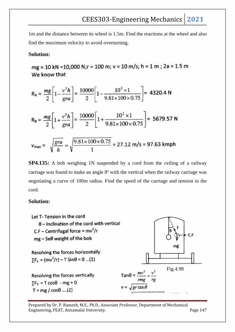
CEES303-Engineering Mechanics 2021
Prepared by Dr. P. Ramesh, M.E., Ph.D., Associate Professor, Department of MechanicalEngineering, FEAT, Annamalai University. Page 147
1m and the distance between its wheel is 1.5m. Find the reactions at the wheel and also
find the maximum velocity to avoid overturning.
Solution:
SP4.135: A bob weighing 1N suspended by a cord from the ceiling of a railway
carriage was found to make an angle 8o with the vertical when the railway carriage was
negotiating a curve of 100m radius. Find the speed of the carriage and tension in the
cord.
Solution:
Fig.4.98

CEES303-Engineering Mechanics 2021
Prepared by Dr. P. Ramesh, M.E., Ph.D., Associate Professor, Department of MechanicalEngineering, FEAT, Annamalai University. Page 148
SP4.136: An automobile is negotiating a curve of radius 100m. The distance between
the centre to centre of the wheel is 1.2m and height of the centre of gravity of the
automobile is 0.75m above the ground. Find the maximum speed to avoid overturning.
Solution:
SP4.137: A motor cycle rider travelling at 18kmph has to turn a corner. Find the least
radius of the curve he should follow for the same travelling if the coefficient of friction
between the tyres and the road is 0.2.
Solution:
SP4.138: A curve of 200m radius on a high way is banked for a speed of 72kmph so
that at the speed the force exerted on a car by the road is normal to the surface of the
road. A) Determine what the bank angle should be and B) if the = 0.6, what is the
maximum speed at which the car can travel without skidding?
Solution:

CEES303-Engineering Mechanics 2021
Prepared by Dr. P. Ramesh, M.E., Ph.D., Associate Professor, Department of MechanicalEngineering, FEAT, Annamalai University. Page 149
SP4.139: A small block of weight rests on a horizontal turn table at a distance of r=1m
from the centre of the turn table. Find the maximum uniform speed the turn table can
have without slipping of the block. Assume =0.5.
Solution:
Polar coordinates:
When all the forces acting on a particle are resolved into polar components i.e
along the unit vector direction er and e as shown in fig.4.100, the equation of motion
can be expressed as
maF
Fig.4.99

CEES303-Engineering Mechanics 2021
Prepared by Dr. P. Ramesh, M.E., Ph.D., Associate Professor, Department of MechanicalEngineering, FEAT, Annamalai University. Page 150
emaemaeFeF rtrrr
Fig.4.100
This equation is satisfied provided
maF
maF rr --------------- (4.56)
Where,
2rrar and
rra 2
Problems:
SP4.140: Tube A rotates about the vertical O axis with
a constant angular rate
and contains a small
cylindrical plug B of mass m whose radial position is
controlled by the cord which passes freely through the
tube and shaft and is woynd around the drum of radius
b. Determine the tension T in the cord and the horizontal
component F of force exerted by the tube on the plug if
the constant angular rate of rotation of the drum is 0
first in the direction for case (a) and second in the
direction for case(b). Neglect friction.
Solution:Fig.4.101

CEES303-Engineering Mechanics 2021
Prepared by Dr. P. Ramesh, M.E., Ph.D., Associate Professor, Department of MechanicalEngineering, FEAT, Annamalai University. Page 151
SP4.141: The smooth 0.5kg double collar as in fig.4.102 can freely slide on arm AB
and the circular guide rod. If the arm rotates with a constant angular velocity of
srd /3
, determine the force the arm exerts on the collar at the instant =45o. Motion
is the horizontal plane.
Fig.4.102
Solution:

CEES303-Engineering Mechanics 2021
Prepared by Dr. P. Ramesh, M.E., Ph.D., Associate Professor, Department of MechanicalEngineering, FEAT, Annamalai University. Page 152
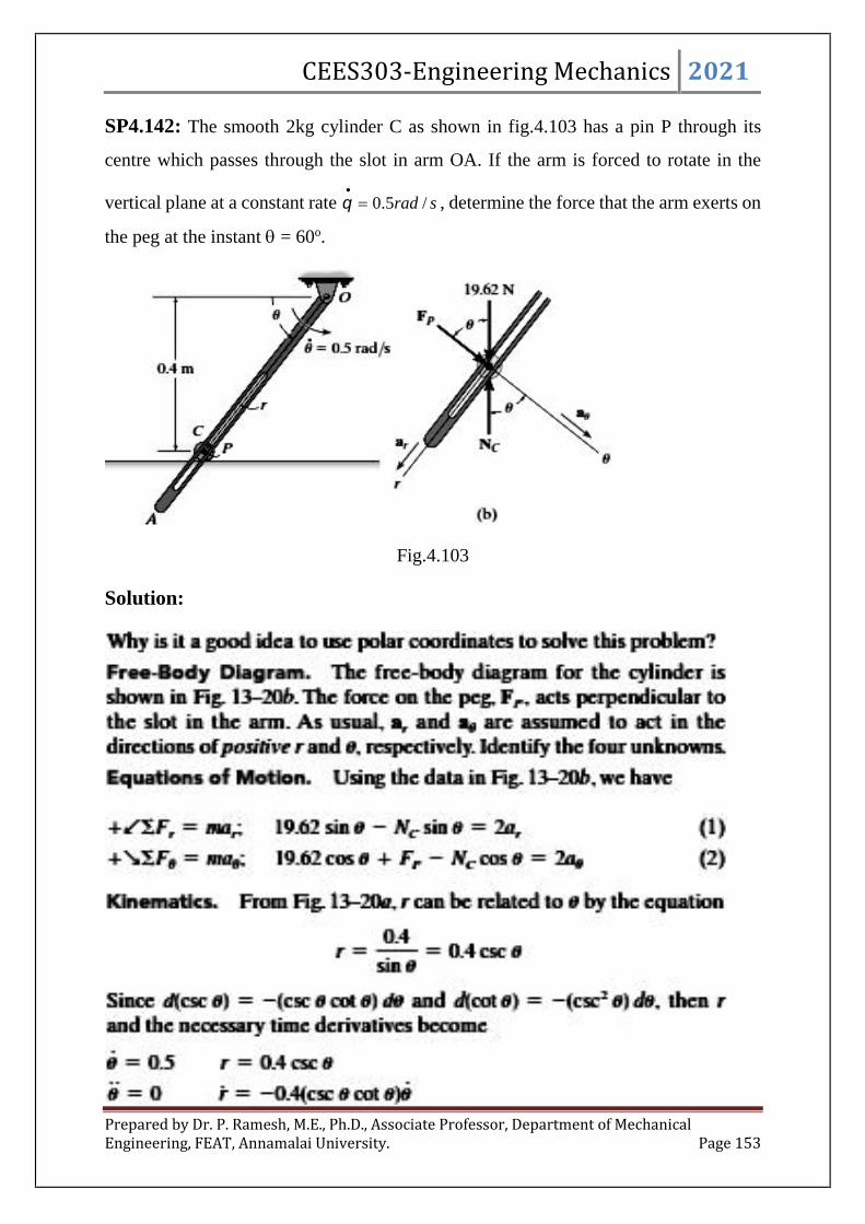
CEES303-Engineering Mechanics 2021
Prepared by Dr. P. Ramesh, M.E., Ph.D., Associate Professor, Department of MechanicalEngineering, FEAT, Annamalai University. Page 153
SP4.142: The smooth 2kg cylinder C as shown in fig.4.103 has a pin P through its
centre which passes through the slot in arm OA. If the arm is forced to rotate in the
vertical plane at a constant rate srad /5.0
, determine the force that the arm exerts on
the peg at the instant = 60o.
Fig.4.103
Solution:

CEES303-Engineering Mechanics 2021
Prepared by Dr. P. Ramesh, M.E., Ph.D., Associate Professor, Department of MechanicalEngineering, FEAT, Annamalai University. Page 154
SP4.143: A can C having a mass of 0.5kg moves along a grooved horizontal slot as
shown in fig.4.104. The slot is in the form of a spiral which is defined by the equation
mr )1.0( where is in radians. If the arm OA rotates with a constant rate srad /4
in the horizontal plane, determine the force it exerts on the can at the instant rad .
Neglect friction and the size of the can.
Fig.4.104
Solution:
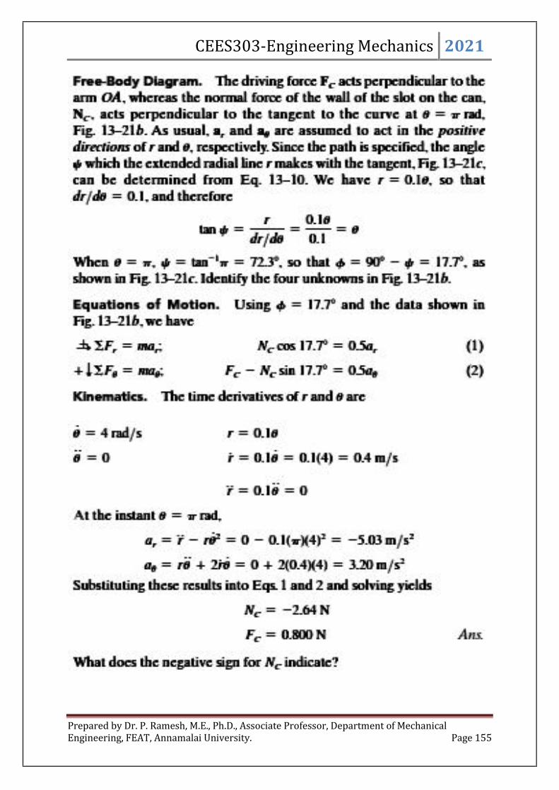
CEES303-Engineering Mechanics 2021
Prepared by Dr. P. Ramesh, M.E., Ph.D., Associate Professor, Department of MechanicalEngineering, FEAT, Annamalai University. Page 155

CEES303-Engineering Mechanics 2021
Prepared by Dr. P. Ramesh, M.E., Ph.D., Associate Professor, Department of MechanicalEngineering, FEAT, Annamalai University. Page 156
WORK AND KINETIC ENERGY:
Fig.4.105
Now develop the quantitative meaning of the term “work’. Fig.4.105 shows a
force F acting on a particle at A which moves along the path shown. The position vector
r measured from some convenient origin O locates the particle as it passes point A, and
dr is the differential displacement associated with an infinitesimal movement from A to
A'. The work done by the force F during the displacement dr is defined as
drFdU . ------- (4.57)
The magnitude of this dot product is dU = F ds cos , where is the angle
between F and dr and where ds is the magnitude of dr. This expression may be
interpreted as the displacement multiplied by the force component Ft = F cos in the
direction of the displacement, as represented by the dashed lines in fig.4.105b.
Alternatively, the work dU may be interpreted as the force multiplied by the
displacement component ds cos in the direction of the force, as represented by the full
lines in fig.4.105b.
With this definition of work, it should be noted that the component Fn = F sin
normal to the displacement does no work. Thus, the work dU may be written as
dsFdU t

CEES303-Engineering Mechanics 2021
Prepared by Dr. P. Ramesh, M.E., Ph.D., Associate Professor, Department of MechanicalEngineering, FEAT, Annamalai University. Page 157
Work is positive if the working component F is in the direction of the
displacement and negative if it is in the opposite direction. Forces which do work are
termed active forces. Constraint forces which do no work are termed reactive forces.
Now formally compute the work associated with three frequently occurring
forces: constant forces, spring forces, and weights.
(1) Work Associated with a Constant External Force.
Fig.4.106
Consider the constant force P applied to the body as it moves from position 1 to
position 2, fig.4.106. With the force P and the differential displacement dr written as
vectors, the work done on the body by the force is
idxjPiPdrFU ).(sincos.2
1
21
cos)(coscos 12
2
1
21 PLxxPdxPUx
x
-------- (4.58)
As previously discussed, this work expression may be interpreted as the force
component P cos times the distance L travelled. Should be between 90° and 270°,
the work would be negative. The force component P sin normal to the displacement
does no work.
(2) Work Associated with a Spring Force.

CEES303-Engineering Mechanics 2021
Prepared by Dr. P. Ramesh, M.E., Ph.D., Associate Professor, Department of MechanicalEngineering, FEAT, Annamalai University. Page 158
Fig.4.107
Now consider here the common linear spring of stiffness k where the force
required to stretch or compress the spring is proportional to the deformation x, as shown
in fig.4.107a. It is to determine the work done on the body by the spring force as the
body undergoes an arbitrary displacement from an initial position x1 to a final position
x2. The force exerted by the spring on the body is F = -kxi, as shown in fig.4.107b. From
the definition of work, we have
)(2
1)).((. 2
221
2
1
2
1
21 xxkkxdxidxkxidrFUx
x
---------- (4.59)
If the initial position is the position of zero spring deformation so that x1 = 0,
then the work is negative for any final position x2 ≠ 0. This is verified by recognizing
that if the body begins at the un-deformed spring position and then moves to the right,
the spring force is to the left; if the body begins at x1 = 0 and moves to the left, the
spring force is to the right. On the other hand, if we move from an arbitrary initial
position x1 ≠ 0 to the un-deformed final position x2 = 0, we see that the work is positive.
In any movement toward the un-deformed spring position, the spring force and the
displacement are in the same direction.
In the general case, of course, neither x1 nor x2 is zero. The magnitude of the
work is equal to the shaded trapezoidal area of fig.4.107a. In calculating the work done
on a body by a spring force, care must be taken to ensure that the units of k and x are
consistent. If x is in meters (or feet), k must be in N/ m (or lb /ft). In addition, be sure

CEES303-Engineering Mechanics 2021
Prepared by Dr. P. Ramesh, M.E., Ph.D., Associate Professor, Department of MechanicalEngineering, FEAT, Annamalai University. Page 159
to recognize that the variable x represents a deformation from the un-stretched spring
length and not the total length of the spring.
The expression F = kx is actually a static relationship which is true only when
elements of the spring have no acceleration. The dynamic behaviour of a spring when
its mass is accounted for is a fairly complex problem which will not be treated here. We
shall assume that the mass of the spring is small compared with the masses of other
accelerating parts of the system, in which case the linear static relationship will not
involve appreciable error.
(3) Work Associated with Weight.
Fig.4.108
Case (a) g = constant. If the altitude variation is sufficiently small so that the
acceleration of gravity g may be considered constant, the work done by the weight mg
of the body shown in fig.4.108a as the body is displaced from an arbitrary altitude y1 to
a final altitude y2 is
)()).((. 12
2
1
2
1
2
1
21 yymgdymgdyjdximgjdrFUy
y
- (4.60)
Now see that horizontal movement does not contribute to this work. We also
note that if the body rises (perhaps due to other forces not shown), then 012 yy and
this work is negative. If the body falls, 012 yy and the work is positive.
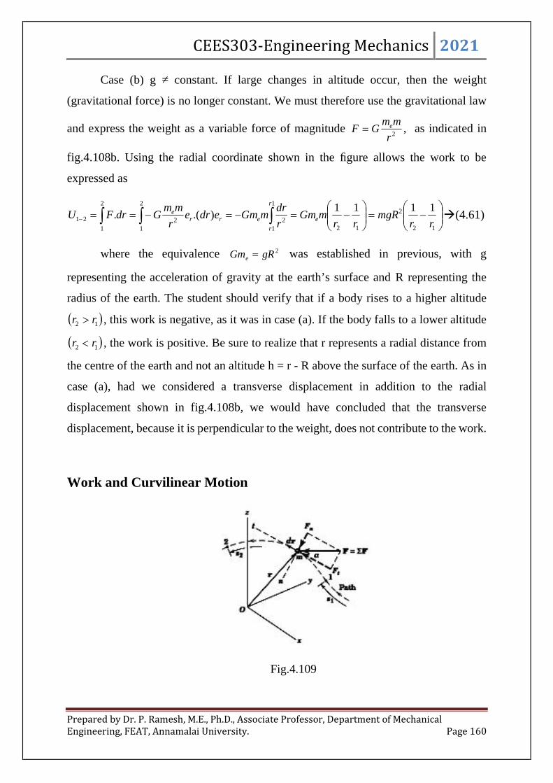
CEES303-Engineering Mechanics 2021
Prepared by Dr. P. Ramesh, M.E., Ph.D., Associate Professor, Department of MechanicalEngineering, FEAT, Annamalai University. Page 160
Case (b) g ≠ constant. If large changes in altitude occur, then the weight
(gravitational force) is no longer constant. We must therefore use the gravitational law
and express the weight as a variable force of magnitude2r
mmGF e , as indicated in
fig.4.108b. Using the radial coordinate shown in the figure allows the work to be
expressed as
2
1
1
1 12
2
1222
2
1
21
1111).(.
r
r
eerre
rrmgR
rrmGm
r
drmGmedre
r
mmGdrFU (4.61)
where the equivalence 2gRGme was established in previous, with g
representing the acceleration of gravity at the earth’s surface and R representing the
radius of the earth. The student should verify that if a body rises to a higher altitude
12 rr , this work is negative, as it was in case (a). If the body falls to a lower altitude
12 rr , the work is positive. Be sure to realize that r represents a radial distance from
the centre of the earth and not an altitude h = r - R above the surface of the earth. As in
case (a), had we considered a transverse displacement in addition to the radial
displacement shown in fig.4.108b, we would have concluded that the transverse
displacement, because it is perpendicular to the weight, does not contribute to the work.
Work and Curvilinear Motion
Fig.4.109
CEES303-Engineering Mechanics 2021
Prepared by Dr. P. Ramesh, M.E., Ph.D., Associate Professor, Department of MechanicalEngineering, FEAT, Annamalai University. Page 161
Now consider the work done on a particle of mass m, fig.4.109, moving along a
curved path under the action of the force F, which stands for the resultant F of all
forces acting on the particle. The position of m is specified by the position vector r, and
its displacement along its path during the time dt is represented by the change dr in its
position vector. The work done by F during a finite movement of the particle from point
1 to point 2 is
2
1
2
1
21 .s
s
tdsFdrFu ----- (4.62)
where the limits specify the initial and final end points of the motion.
When we substitute Newton’s second law F = ma, the expression for the work
of all forces becomes
2
1
2
1
21 .. drmadrFU --------- (4.63)
But dsadra t. , where at is the tangential component of the acceleration of m. In
terms of the velocity v of the particle, Eq.2/3 gives vdvdsat . Thus, the expression for
the work of F becomes
2
1
21
22
2
1
21 2
1. vvmmvdvdrFU
v
v
------ (4.64)
where the integration is carried out between points 1 and 2 along the curve, at
which points the velocities have the magnitudes v1 and v2, respectively.
Principle of Work and Kinetic Energy
The kinetic energy T of the particle is defined as
2
2
1mvT -------------- (4.65)
and is the total work which must be done on the particle to bring it from a state of rest
to a velocity v. Kinetic energy T is a scalar quantity with the units of N-m or joules (J)
CEES303-Engineering Mechanics 2021
Prepared by Dr. P. Ramesh, M.E., Ph.D., Associate Professor, Department of MechanicalEngineering, FEAT, Annamalai University. Page 162
in SI units and ft-lb in U.S. customary units. Kinetic energy is always positive,
regardless of the direction of the velocity.
Equation 21
2221 2
1vvmU may be restated as
TTTU 1221 ------------ (4.66)
which is the work-energy equation for a particle. The equation states that the
total work done by all forces acting on a particle as it moves from point 1 to point 2
equals the corresponding change in kinetic energy of the particle. Although T is always
positive, the change ΔT may be positive, negative, or zero. When written in this concise
form, Eq. TTTU 1221 tells us that the work always results in a change of kinetic
energy.
Alternatively, the work-energy relation may be expressed as the initial kinetic
energy T1 plus the work done U1-2 equals the final kinetic energy T2, or
2211 TUT --------------- (4.67)
When written in this form, the terms correspond to the natural sequence of events.
Clearly, the two forms TTTU 1221 and 2211 TUT are equivalent.
POWER:
The capacity of a machine is measured by the time rate at which it can do work
or deliver energy. The total work or energy output is not a measure of this capacity since
a motor, no matter how small, can deliver a large amount of energy if given sufficient
time. On the other hand, a large and powerful machine is required to deliver a large
amount of energy in a short period of time. Thus, the capacity of a machine is rated by
its power, which is defined as the time rate of doing work.
Accordingly, the power P developed by a force F which does an amount of work
U isdt
drF
dt
dUP . . Because
dt
dris the velocity v of the point of application of the
force, we have

CEES303-Engineering Mechanics 2021
Prepared by Dr. P. Ramesh, M.E., Ph.D., Associate Professor, Department of MechanicalEngineering, FEAT, Annamalai University. Page 163
vFP . ------- (4.68)
Power is clearly a scalar quantity, and in SI it has the units of N-m/s = J/s. The
special unit for power is the watt (W), which equals one joule per second (J/s). In U.S.
customary units, the unit for mechanical power is the horsepower (hp). These units and
their numerical equivalences are
1 W = 1 J/s
1 hp = 550 ft-lb/sec = 33,000 ft-lb/min
1 hp = 746 W = 0.746 kW
EFFICIENCY
The ratio of the work done by a machine to the work done on the machine during
the same time interval is called the mechanical efficiency m of the machine. This
definition assumes that the machine operates uniformly so that there is no accumulation
or depletion of energy within it. Efficiency is always less than unity since every device
operates with some loss of energy and since energy cannot be created within the
machine. In mechanical devices which involve moving parts, there will always be some
loss of energy due to the negative work of kinetic friction forces. This work is converted
to heat energy which, in turn, is dissipated to the surroundings. The mechanical
efficiency at any instant of time may be expressed in terms of mechanical power P by
input
output
m P
P ----------- (4.69)
In addition to energy loss by mechanical friction, there may also be electrical and
thermal energy loss, in which case, the electrical efficiency e and thermal efficiency
t are also involved. The overall efficiency in such instances is
tem ------------ (4.70)
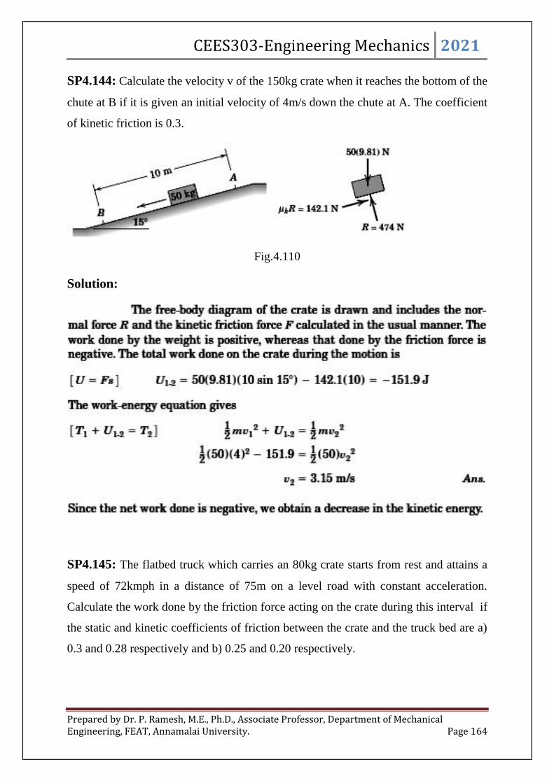
CEES303-Engineering Mechanics 2021
Prepared by Dr. P. Ramesh, M.E., Ph.D., Associate Professor, Department of MechanicalEngineering, FEAT, Annamalai University. Page 164
SP4.144: Calculate the velocity v of the 150kg crate when it reaches the bottom of the
chute at B if it is given an initial velocity of 4m/s down the chute at A. The coefficient
of kinetic friction is 0.3.
Fig.4.110
Solution:
SP4.145: The flatbed truck which carries an 80kg crate starts from rest and attains a
speed of 72kmph in a distance of 75m on a level road with constant acceleration.
Calculate the work done by the friction force acting on the crate during this interval if
the static and kinetic coefficients of friction between the crate and the truck bed are a)
0.3 and 0.28 respectively and b) 0.25 and 0.20 respectively.

CEES303-Engineering Mechanics 2021
Prepared by Dr. P. Ramesh, M.E., Ph.D., Associate Professor, Department of MechanicalEngineering, FEAT, Annamalai University. Page 165
Fig.4.111
Solution:
SP4.146: The 50kg block at A is mounted on rollers so that it moves along the fixed
horizontal rail with negligible friction under the action of the constant 300N force in the
cable. The block is released from rest at A, with the spring to which it is attached

CEES303-Engineering Mechanics 2021
Prepared by Dr. P. Ramesh, M.E., Ph.D., Associate Professor, Department of MechanicalEngineering, FEAT, Annamalai University. Page 166
extended an initial amount x1 = 0.233m. The spring has a stiffness k = 80N/m. Calculate
the velocity v of the block as it reaches position B.
Fig.4.112
Solution:

CEES303-Engineering Mechanics 2021
Prepared by Dr. P. Ramesh, M.E., Ph.D., Associate Professor, Department of MechanicalEngineering, FEAT, Annamalai University. Page 167
SP4.147: The power winch A hoists the 360kg log up the 30o incline at a constant
speed of 1.2m/s. If the power output of the winch is 4kW, compute the coefficient of
kinetic friction k between the log and the incline. If the power is suddenly increased to
6 kW, what is the corresponding instantaneous acceleration a of the log?
Fig.4.113
Solution:
From the free body diagram of the log we get N = 360(9.81) cos 30o = 3060N an
the kinetic friction force becomes 3060 k. For constant speed the forces are in
equilibrium so that
0 xF , 030sin)81.9(36030602 okT , 17663060 kT
The power output of the winch gives the tension in the cable
TvP , Nv
PT 3330
2.1
4000
Substituting T gives, 176630603330 k , 513.0 k
When the power is increased, the tension momentarily becomes
TvP , Nv
PT 5000
2.1
6000
and the corresponding acceleration is given by

CEES303-Engineering Mechanics 2021
Prepared by Dr. P. Ramesh, M.E., Ph.D., Associate Professor, Department of MechanicalEngineering, FEAT, Annamalai University. Page 168
xx maF , ao 36030sin)81.9(360)513.0(30605000
2/63.4 sma
SP4.148: A satellite of mass m is put into an elliptical orbit around the earth. At point
A its distance from the earth is h1 = 500 km and it has a velocity v1 = 30000kmph.
Determine the velocity v2 of the satellite as it reaches point B, a distance h2 = 1200km
from the earth.
Fig.4.114
Solution:

CEES303-Engineering Mechanics 2021
Prepared by Dr. P. Ramesh, M.E., Ph.D., Associate Professor, Department of MechanicalEngineering, FEAT, Annamalai University. Page 169
SP4.149: A train of mass 100 tonnes is pulled by an engine on a level track at a constant
speed of 45 kmph. The resistance due to friction is 1% of the train weight. Find the
power of the engine.
Solution:
SP4.150: The mass of a car is 4.5 tonnes. The tractive resistance on the level track is
50 N per tonne. Find the power required to propel the car at a uniform speed of 45 kmph;
a) up an incline 1 in 300, b) on the level track and c) down an incline of 1 in 300. Take
efficiency of the motors and drive as 70%.
Solution:

CEES303-Engineering Mechanics 2021
Prepared by Dr. P. Ramesh, M.E., Ph.D., Associate Professor, Department of MechanicalEngineering, FEAT, Annamalai University. Page 170
SP4.151: A train of mass 300 tonnes moves down a slope of 1 in 200 at 45 kmph with
the engine developing 75 kW. Find the power required to pull the train up the slope with
the same velocity.
Solution:
SP4.152: An engine of mass 50 tonnes pulls a train of mass 300 tonnes up an incline
of 1 in 100. The train starts from rest and moves with a constant acceleration against a
total resistance of 50N per tonne. If the train attains a speed of 36 kmph in a distance of
1km, find the tension in the coupling between the engine and the train. Also find the
power exerted by the engine.
Solution:
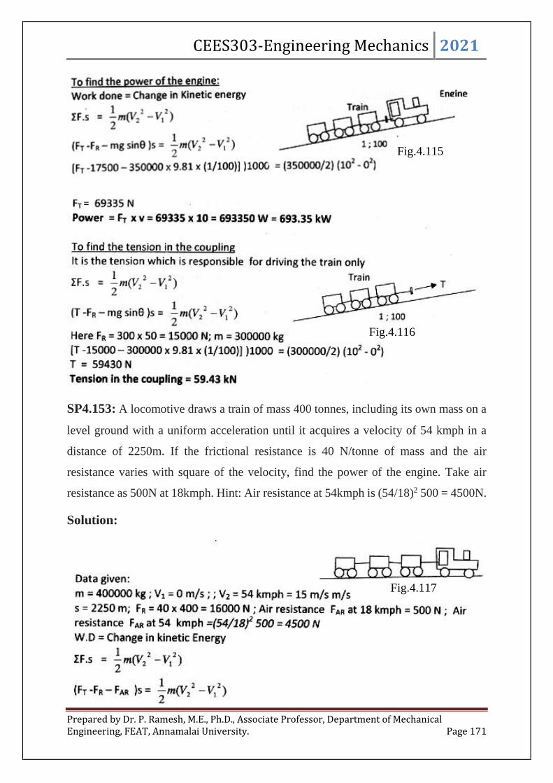
CEES303-Engineering Mechanics 2021
Prepared by Dr. P. Ramesh, M.E., Ph.D., Associate Professor, Department of MechanicalEngineering, FEAT, Annamalai University. Page 171
SP4.153: A locomotive draws a train of mass 400 tonnes, including its own mass on a
level ground with a uniform acceleration until it acquires a velocity of 54 kmph in a
distance of 2250m. If the frictional resistance is 40 N/tonne of mass and the air
resistance varies with square of the velocity, find the power of the engine. Take air
resistance as 500N at 18kmph. Hint: Air resistance at 54kmph is (54/18)2 500 = 4500N.
Solution:
Fig.4.115
Fig.4.116
Fig.4.117

CEES303-Engineering Mechanics 2021
Prepared by Dr. P. Ramesh, M.E., Ph.D., Associate Professor, Department of MechanicalEngineering, FEAT, Annamalai University. Page 172
SP4.154: A man wishes to move the solid block of wooden box of 1m cube to a
distance of 5m with the least amount of work. If the block weighs 1 kN and the
coefficient of frictions is 0.3, find whether he should tip it or slide it.
Solution:
SP4.155: A man of mass 65kg jumps in a swimming pool from a tower of height
19.62m. He was found to go down in water by 2m and then started rising. Find the
average resistance of water.
Solution:
Fig.4.118

CEES303-Engineering Mechanics 2021
Prepared by Dr. P. Ramesh, M.E., Ph.D., Associate Professor, Department of MechanicalEngineering, FEAT, Annamalai University. Page 173
SP4.156: A bullet of mass 81 gram and moving with a velocity of 300m/s is fired into
a block of wood and it penetrates to a depth of 100mm. If the bullet moving with the
same velocity, were fired into a similar piece of wood 50mm thick, with what velocity
would it emerge? Find also the force of resistance, assuming it to be uniform.
Solution:
SP4.157: In a police investigation of tyre marks, it was concluded that a car while in
motion along a straight level road has skidded for a total of 60m after the brakes are
applied. If the coefficient of friction is 0.5, what was the probable speed of the car just
before the brakes were applied?
Fig.4.119
Fig.4.120

CEES303-Engineering Mechanics 2021
Prepared by Dr. P. Ramesh, M.E., Ph.D., Associate Professor, Department of MechanicalEngineering, FEAT, Annamalai University. Page 174
Solution:
SP4.158: A block of 2500N rests on a horizontal plane. The coefficient of friction
between the block and the plane is 0.3. The block is pulled by a force of 1000N acting
at an angle 30o to the horizontal. Find the velocity of the block after it moves over a
distance of 30m starting from rest. If the force is then removed, how much further will
it move?
Solution:
SP4.159: A car of mass 1500 kg is uniformly accelerated. Its speed increased from
50kmph to 75kmph after travelling a distance of 200m. The resistance to the motion of
the car is 0.2% of the weight of the car. Determine a) the maximum power required and
b) the power required to maintain a constant speed of 75kmph.
Fig.4.121

CEES303-Engineering Mechanics 2021
Prepared by Dr. P. Ramesh, M.E., Ph.D., Associate Professor, Department of MechanicalEngineering, FEAT, Annamalai University. Page 175
Solution:
SP4.160: A gangman pushes a 250kg trolley for a distance of 50m along straight
railway track with a force F = 100 – 2x, where x is the distance travelled in metres and
F in N. The resistance to motion is 25N. Determine a) the velocity of the trolley when
it has travelled 50m starting from rest and b) the total distance travelled by the trolley
before coming to rest.
Solution:

CEES303-Engineering Mechanics 2021
Prepared by Dr. P. Ramesh, M.E., Ph.D., Associate Professor, Department of MechanicalEngineering, FEAT, Annamalai University. Page 176
SP4.161: Two bodies A and B of masses m1 and m2 (m2>m1) are connected by an
inextensible string passing over a frictionless pulley. The system is initially at rest with
the body A resting on the ground and the body B at a height ‘h’ from the ground. When
B is released, determine the speed at which it will hit the ground.
Solution:
SP4.162: Determine the total work done on a 5kg
body that is pulled 6m up a rough plane inclined 30o
with the horizontal as shown in fig.4. Assume the
coefficient of friction as 0.2. What is the speed after
travelling a distance of 6m from the start?
Solution:
Fig.4.122
Fig.4.123

CEES303-Engineering Mechanics 2021
Prepared by Dr. P. Ramesh, M.E., Ph.D., Associate Professor, Department of MechanicalEngineering, FEAT, Annamalai University. Page 177
SP4.163: Two block A and B of masses 100 kg
and 150 kg are connected by a string as shown in
fig.4. If the system is released from rest, find the
velocity of the block A after it has moved a
distance of 1m. Assume the coefficient of friction
between the block A and the horizontal plane as
0.2.
Solution:
Fig.4.123a
Fig.4.124
Fig.4.124a

CEES303-Engineering Mechanics 2021
Prepared by Dr. P. Ramesh, M.E., Ph.D., Associate Professor, Department of MechanicalEngineering, FEAT, Annamalai University. Page 178
SP4.164: A block of weight ‘w’ slides down an inclined plane from rest, from an
elevation h, as shown in fig.4.125 Find the velocity of the block when it reaches the
point B.
Solution:
SP4.165: A 20kg package is projected up a 20o incline with an initial velocity of 12m/s.
Knowing that the coefficient of kinetic friction between the package and the incline is
0.15. Determine a) the maximum distance ‘x’ that the package will move up the plane,
b) the velocity of the package as it returns to the original position and c) the total amount
of energy dissipated due to friction.
Solution:
Fig.4.125
Fig.4.126

CEES303-Engineering Mechanics 2021
Prepared by Dr. P. Ramesh, M.E., Ph.D., Associate Professor, Department of MechanicalEngineering, FEAT, Annamalai University. Page 179
POTENTIAL ENERGY:
In the previous section on work and kinetic energy, it is isolated a particle or a
combination of joined particles and determined the work done by gravity forces, spring
forces, and other externally applied forces acting on the particle or system. This to
evaluate U in the work-energy equation. In the present section it will introduce the
concept of potential energy to treat the work done by gravity forces and by spring forces.
This concept will simplify the analysis of many problems.
a) Gravitational Potential Energy
Fig.4.127
Now consider first the motion of a particle of mass m in close proximity to the
surface of the earth, where the gravitational attraction (weight) mg is essentially
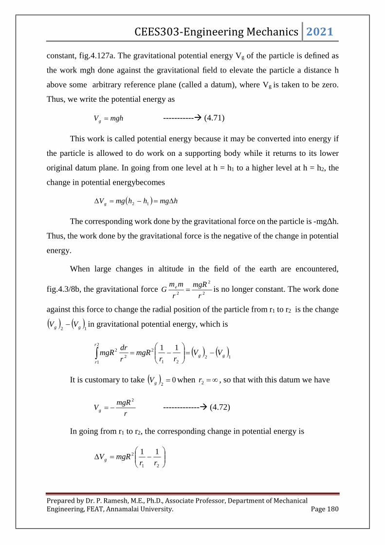
CEES303-Engineering Mechanics 2021
Prepared by Dr. P. Ramesh, M.E., Ph.D., Associate Professor, Department of MechanicalEngineering, FEAT, Annamalai University. Page 180
constant, fig.4.127a. The gravitational potential energy Vg of the particle is defined as
the work mgh done against the gravitational field to elevate the particle a distance h
above some arbitrary reference plane (called a datum), where Vg is taken to be zero.
Thus, we write the potential energy as
mghVg ----------- (4.71)
This work is called potential energy because it may be converted into energy if
the particle is allowed to do work on a supporting body while it returns to its lower
original datum plane. In going from one level at h = h1 to a higher level at h = h2, the
change in potential energybecomes
hmghhmgVg 12
The corresponding work done by the gravitational force on the particle is -mgΔh.
Thus, the work done by the gravitational force is the negative of the change in potential
energy.
When large changes in altitude in the field of the earth are encountered,
fig.4.3/8b, the gravitational force2
2
2 r
mgR
r
mmG e is no longer constant. The work done
against this force to change the radial position of the particle from r1 to r2 is the change
12 gg VV in gravitational potential energy, which is
12
2
1 21
2
2
2 11gg
r
r
VVrr
mgRr
drmgR
It is customary to take 02gV when 2r , so that with this datum we have
r
mgRVg
2
------------- (4.72)
In going from r1 to r2, the corresponding change in potential energy is
21
2 11
rrmgRVg
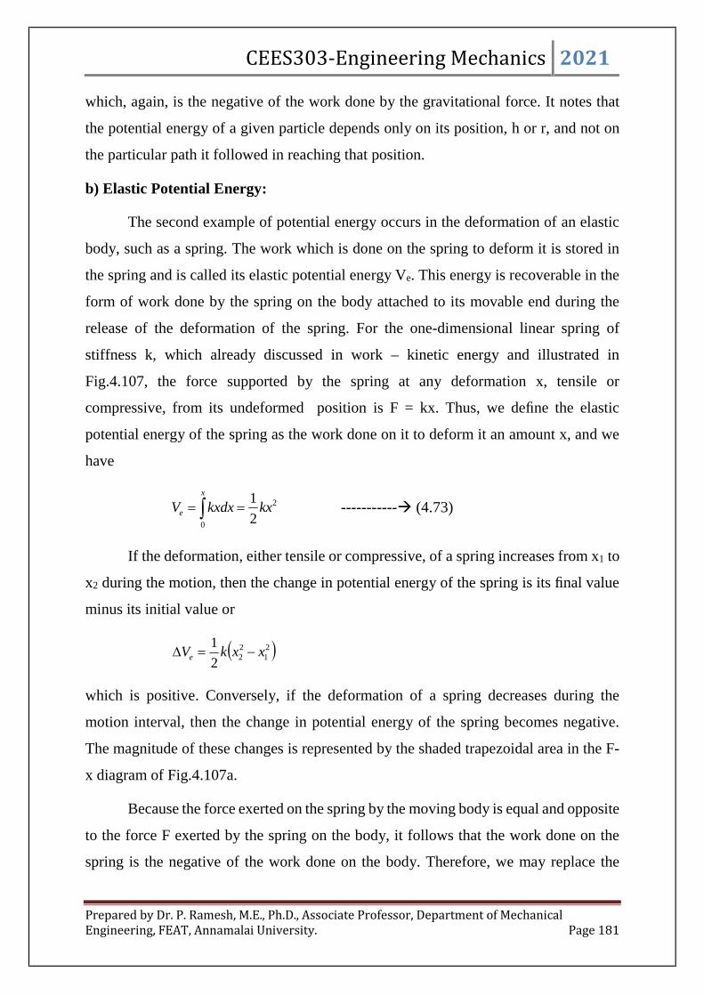
CEES303-Engineering Mechanics 2021
Prepared by Dr. P. Ramesh, M.E., Ph.D., Associate Professor, Department of MechanicalEngineering, FEAT, Annamalai University. Page 181
which, again, is the negative of the work done by the gravitational force. It notes that
the potential energy of a given particle depends only on its position, h or r, and not on
the particular path it followed in reaching that position.
b) Elastic Potential Energy:
The second example of potential energy occurs in the deformation of an elastic
body, such as a spring. The work which is done on the spring to deform it is stored in
the spring and is called its elastic potential energy Ve. This energy is recoverable in the
form of work done by the spring on the body attached to its movable end during the
release of the deformation of the spring. For the one-dimensional linear spring of
stiffness k, which already discussed in work – kinetic energy and illustrated in
Fig.4.107, the force supported by the spring at any deformation x, tensile or
compressive, from its undeformed position is F = kx. Thus, we define the elastic
potential energy of the spring as the work done on it to deform it an amount x, and we
have
2
0 2
1kxkxdxV
x
e ----------- (4.73)
If the deformation, either tensile or compressive, of a spring increases from x1 to
x2 during the motion, then the change in potential energy of the spring is its final value
minus its initial value or
21222
1xxkVe
which is positive. Conversely, if the deformation of a spring decreases during the
motion interval, then the change in potential energy of the spring becomes negative.
The magnitude of these changes is represented by the shaded trapezoidal area in the F-
x diagram of Fig.4.107a.
Because the force exerted on the spring by the moving body is equal and opposite
to the force F exerted by the spring on the body, it follows that the work done on the
spring is the negative of the work done on the body. Therefore, we may replace the

CEES303-Engineering Mechanics 2021
Prepared by Dr. P. Ramesh, M.E., Ph.D., Associate Professor, Department of MechanicalEngineering, FEAT, Annamalai University. Page 182
work U done by the spring on the body by -ΔVe, the negative of the potential energy
change for the spring, provided the spring is now included within the system.
c) Work-Energy Equation:
Fig.4.128
With the elastic member included in the system, we now modify the work-energy
equation to account for the potential-energy terms. If U’1-2 stands for the work of all
external forces other than gravitational forces and spring forces, we may write Eq.
TTTU 1221 as TVVU eg '
21 or
VTU '
21 ------------- (4.74)
where ΔV is the change in total potential energy, gravitational plus elastic.
This alternative form of the work-energy equation is often far more convenient
to use than Eq. TTTU 1221 , since the work of both gravity and spring forces is
accounted for by focusing attention on the end-point positions of the particle and on the
end-point lengths of the elastic spring. The path followed between these end-point
positions is of no consequence in the evaluation of gV and eV .
22'
2111 VTUVT ---------- (4.75)
To help clarify the difference between the use of Eqs. TTTU 1221 and
VTU '
21 , fig.4.128 shows schematically a particle of mass m constrained to

CEES303-Engineering Mechanics 2021
Prepared by Dr. P. Ramesh, M.E., Ph.D., Associate Professor, Department of MechanicalEngineering, FEAT, Annamalai University. Page 183
move along a fixed path under the action of forces F1 and F2, the gravitational force
W=mg, the spring force F, and the normal reaction N. In fig.4.128b, the particle is
isolated with its free-body diagram. The work done by each of the forces F1, F2, W, and
the spring force F = kx is evaluated, say, from A to B, and equated to the change ΔT in
kinetic energy using Eq. TTTU 1221 . The constraint reaction N, if normal to the
path, will do no work. The alternative approach is shown in fig.4.128c, where the spring
is included as a part of the isolated system. The work done during the interval by F1 and
F2 is the U'1-2-term of Eq. VTU '
21 with the changes in elastic and gravitational
potential energies included on the energy side of the equation.
We note with the first approach that the work done by F = kx could require a
somewhat awkward integration to account for the changes in magnitude and direction
of F as the particle moves from A to B. With the second approach, however, only the
initial and final lengths of the spring are required to evaluate ΔVe. This greatly simplifies
the calculation.
For problems where the only forces are gravitational, elastic, and nonworking
constraint forces, the U’-term of Eq. 22'
2111 VTUVT is zero, and the energy
equation becomes
2211 VTVT or 21 EE ----------- (4.76)
Where, E = T +V is the total mechanical energy of the particle and its attached
spring. When E is constant we see that transfers of energy between kinetic and potential
may take place as long as the total mechanical energy T+V does not change. Equation
above expresses the law of conservation of dynamical energy.
Problems:
SP4.166: The 3kg slider is released from rest at position 1 and slides with negligible
friction in a vertical plane along the circular rod. The attached spring has a stiffness of
350N/m and has an un-stretched length of 0.6m. Determine the velocity of the slider as
it passes position 2.

CEES303-Engineering Mechanics 2021
Prepared by Dr. P. Ramesh, M.E., Ph.D., Associate Professor, Department of MechanicalEngineering, FEAT, Annamalai University. Page 184
Fig.4.129
Solution:
The work done by the weight and the spring force on the slider will be treated
using potential energy methods. The reaction of the rod on the slider is normal to the
motion and does work no work. Hence 0'21 U . We define the datum to be at the level
of position 1, so that the gravitational potential energies are
01 V and JmghV 66.17)6.0)(81.9(32
The initial and final elastic (Spring) potential energies are
JkxV 63)6.0)(350(2
1
2
1 2211
JkxV 81.10)6.026.0)(350(2
1
2
1 2222
Substitution into the alternative work – energy equation yields
22'
2111 VTUVT , 81.1066.17)3(2
10630 2
2 v
smv /82.62
SP4.167: The 10kg slider moves with negligible friction up the inclined guide. The
attached spring has a stiffness of 60N/m and is stretched 0.6m in position A, where the
slider is released from rest. The 250N force is constant and the pulley offers negligible

CEES303-Engineering Mechanics 2021
Prepared by Dr. P. Ramesh, M.E., Ph.D., Associate Professor, Department of MechanicalEngineering, FEAT, Annamalai University. Page 185
resistance to the motion of the cord. Calculated the velocity vc of the slider as it passes
point C.
Fig.4.130
Solution:
SP4.168: The system shown is released from rest with the lightweight slender bas OA
in the vertical position as shown in fig.4.131. The torsional spring at O is undeflected
in the initial position and exerts a restoring moment of magnitude kT on the bar, where

CEES303-Engineering Mechanics 2021
Prepared by Dr. P. Ramesh, M.E., Ph.D., Associate Professor, Department of MechanicalEngineering, FEAT, Annamalai University. Page 186
is the counter clockwise angular deflection of the bar. The string S is attached to point
C of the bar and slips without friction through a vertical hole in the support surface. For
the values mA = 2kg, mB = 4kg, L = 0.5m and kT = 13N-m/rad; a) determine the speed
vA of particle A when reaches 90o. and b) Plot vA as a function of over the range
o900 . Identify the maximum value of vA and the value of at which this
maximum occurs.
Fig.4.131
Solution:
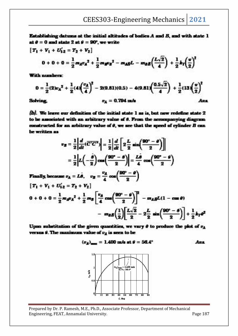
CEES303-Engineering Mechanics 2021
Prepared by Dr. P. Ramesh, M.E., Ph.D., Associate Professor, Department of MechanicalEngineering, FEAT, Annamalai University. Page 187
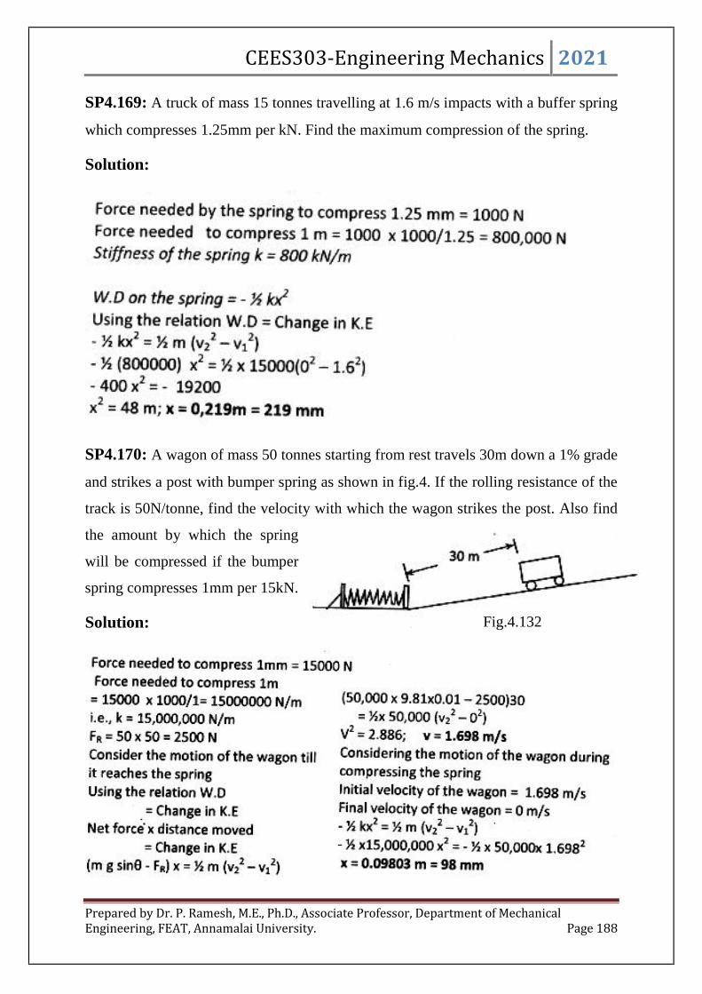
CEES303-Engineering Mechanics 2021
Prepared by Dr. P. Ramesh, M.E., Ph.D., Associate Professor, Department of MechanicalEngineering, FEAT, Annamalai University. Page 188
SP4.169: A truck of mass 15 tonnes travelling at 1.6 m/s impacts with a buffer spring
which compresses 1.25mm per kN. Find the maximum compression of the spring.
Solution:
SP4.170: A wagon of mass 50 tonnes starting from rest travels 30m down a 1% grade
and strikes a post with bumper spring as shown in fig.4. If the rolling resistance of the
track is 50N/tonne, find the velocity with which the wagon strikes the post. Also find
the amount by which the spring
will be compressed if the bumper
spring compresses 1mm per 15kN.
Solution: Fig.4.132

CEES303-Engineering Mechanics 2021
Prepared by Dr. P. Ramesh, M.E., Ph.D., Associate Professor, Department of MechanicalEngineering, FEAT, Annamalai University. Page 189
SP4.171: A block of mass 5 kg resting on a 30o inclined plane is released. The block
after travelling a distance of 0.5m along the inclined plane hits a spring of stiffness
15N/cm. Find the maximum compression of the spring. Assume the coefficient of
friction if 0.2.
Solution:
SP4.172: A ball of mass m is dropped on to a spring of stiffness k from
a height h. Find the maximum deflection of the spring. Assume m =
5kg, k = 500 N/m, h = 10cm.
Solution:
Fig.4.133
Fig.4.134
Fig.4.135
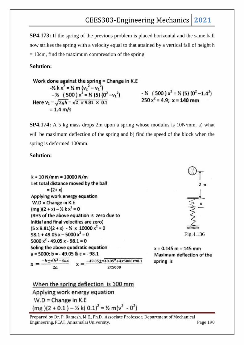
CEES303-Engineering Mechanics 2021
Prepared by Dr. P. Ramesh, M.E., Ph.D., Associate Professor, Department of MechanicalEngineering, FEAT, Annamalai University. Page 190
SP4.173: If the spring of the previous problem is placed horizontal and the same ball
now strikes the spring with a velocity equal to that attained by a vertical fall of height h
= 10cm, find the maximum compression of the spring.
Solution:
SP4.174: A 5 kg mass drops 2m upon a spring whose modulus is 10N/mm. a) what
will be maximum deflection of the spring and b) find the speed of the block when the
spring is deformed 100mm.
Solution:
Fig.4.136

CEES303-Engineering Mechanics 2021
Prepared by Dr. P. Ramesh, M.E., Ph.D., Associate Professor, Department of MechanicalEngineering, FEAT, Annamalai University. Page 191
SP4.175: A 2kg block is released from rest on an inclined plane making an angle of
30o to the horizontal. The block starts from A and slides down a distance of 0.5m and
strikes a spring with a stiffness of 4 kN/m. The coefficient of friction between the
inclined plane and the block is 0.3. Determine a) the amount of spring will be
compressed, b) the distance of block will be rebound up the plane from the compressed
position and c) maximum velocity of the block.
Solution:
Fig.4.137

CEES303-Engineering Mechanics 2021
Prepared by Dr. P. Ramesh, M.E., Ph.D., Associate Professor, Department of MechanicalEngineering, FEAT, Annamalai University. Page 192
SP4.176: In the above problem determine the initial velocity of block should be given
at A so that the block rebounds and comes to rest at A.
Solution:

CEES303-Engineering Mechanics 2021
Prepared by Dr. P. Ramesh, M.E., Ph.D., Associate Professor, Department of MechanicalEngineering, FEAT, Annamalai University. Page 193
SP4.177: A 30 kg block is dropped from a height of 2m onto the 10kg pan of a spring
scale. Assuming the impact to be perfectly plastic, determine the maximum deflection
of the pan. The spring constant is 20kN/m.
Solution:
SP4.178: A collar of mass 5kg can slide
along a vertical bar as shown in fig.4. The
spring attached to the collar is in
undeformed state of length 200mm and
stiffness 500 N/m. If the collar is suddenly
released, find the velocity of the collar if
it moves 150mm down as shown in fig.4.
Solution:
Fig.4.138
Fig.4.139

CEES303-Engineering Mechanics 2021
Prepared by Dr. P. Ramesh, M.E., Ph.D., Associate Professor, Department of MechanicalEngineering, FEAT, Annamalai University. Page 194
SP4.179: A spring is used to stop a 60kg package which is sliding on a horizontal
surface. The spring has a constant k = 20kN/m and is held by cables so that it is initially
compressed 120mm. Knowing that the package has a velocity of 2.5m/s in the position
as shown in fig.4. and that the maximum additional deflection of the spring is 40mm,
determine a) the coefficient of kinetic friction between the package and surface, and b)
the velocity of the package as it passes again through the position as shown in fig.4.
Solution:
Fig.4.140

CEES303-Engineering Mechanics 2021
Prepared by Dr. P. Ramesh, M.E., Ph.D., Associate Professor, Department of MechanicalEngineering, FEAT, Annamalai University. Page 195
SP4.180: A bullet of mass 30 gram is fired into a body of mass 10kg which is
suspended by a string 0.8m long. Due to this impact the body swings through an angle
30o. Find the velocity of the bullet.
Solution:
SP4.181: A hammer of mass 500 gram hits a nail of mass 25 gram with a velocity of
5m/s and drives it into a fixed wooden block by 25mm. Find the resistance offered by
the wooden block.
Solution:
Fig.4.141
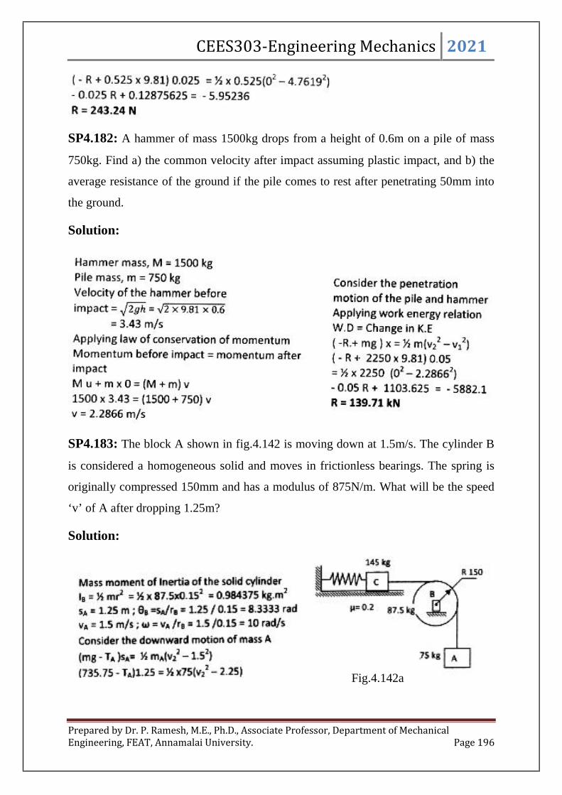
CEES303-Engineering Mechanics 2021
Prepared by Dr. P. Ramesh, M.E., Ph.D., Associate Professor, Department of MechanicalEngineering, FEAT, Annamalai University. Page 196
SP4.182: A hammer of mass 1500kg drops from a height of 0.6m on a pile of mass
750kg. Find a) the common velocity after impact assuming plastic impact, and b) the
average resistance of the ground if the pile comes to rest after penetrating 50mm into
the ground.
Solution:
SP4.183: The block A shown in fig.4.142 is moving down at 1.5m/s. The cylinder B
is considered a homogeneous solid and moves in frictionless bearings. The spring is
originally compressed 150mm and has a modulus of 875N/m. What will be the speed
‘v’ of A after dropping 1.25m?
Solution:
Fig.4.142a

CEES303-Engineering Mechanics 2021
Prepared by Dr. P. Ramesh, M.E., Ph.D., Associate Professor, Department of MechanicalEngineering, FEAT, Annamalai University. Page 197
SP4.184: Block A and B have masses of 45kg and 60kg respectively. The drum has a
moment of inertia I = 16kg-m2. Through what distance will A fall before it reaches a
speed of 2m/s?
Solution:
Fig.4.142b
Fig.4.143a

CEES303-Engineering Mechanics 2021
Prepared by Dr. P. Ramesh, M.E., Ph.D., Associate Professor, Department of MechanicalEngineering, FEAT, Annamalai University. Page 198
IMPULSE AND MOMENTUM:
In the previous two sections, it focused attention on the equations of work and
energy, which are obtained by integrating the equation of motion F = ma with respect
to the displacement of the particle. It found that the velocity changes could be expressed
directly in terms of the work done or in terms of the overall changes in energy. In the
next section, it will integrate the equation of motion with respect to time rather than
displacement. This approach leads to the equations of impulse and momentum. These
equations greatly facilitate the solution of many problems in which the applied forces
act during extremely short periods of time (as in impact problems) or over specified
intervals of time.
1) LINEAR IMPULSE AND LINEAR MOMENTUM
Consider again the general curvilinear motion in space of a particle of mass m,
fig.4.144, where the particle is located by its position vector r measured from a fixed
origin O. The velocity of the particle is
rv and is tangent to its path (shown as a dashed
Fig.4.143b
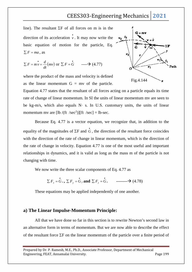
CEES303-Engineering Mechanics 2021
Prepared by Dr. P. Ramesh, M.E., Ph.D., Associate Professor, Department of MechanicalEngineering, FEAT, Annamalai University. Page 199
line). The resultant F of all forces on m is in the
direction of its acceleration
v . It may now write the
basic equation of motion for the particle, Eq.
maF , as
mvdt
dvmF
or
GF ---- (4.77)
where the product of the mass and velocity is defined
as the linear momentum G = mv of the particle.
Equation 4.77 states that the resultant of all forces acting on a particle equals its time
rate of change of linear momentum. In SI the units of linear momentum mv are seen to
be kg-m/s, which also equals N· s. In U.S. customary units, the units of linear
momentum mv are [lb /(ft /sec2)][ft /sec] = lb-sec.
Because Eq. 4.77 is a vector equation, we recognize that, in addition to the
equality of the magnitudes of F and
G , the direction of the resultant force coincides
with the direction of the rate of change in linear momentum, which is the direction of
the rate of change in velocity. Equation 4.77 is one of the most useful and important
relationships in dynamics, and it is valid as long as the mass m of the particle is not
changing with time.
We now write the three scalar components of Eq. 4.77 as
xx GF
, yy GF
and zz GF
-------- (4.78)
These equations may be applied independently of one another.
a) The Linear Impulse-Momentum Principle:
All that we have done so far in this section is to rewrite Newton’s second law in
an alternative form in terms of momentum. But we are now able to describe the effect
of the resultant force F on the linear momentum of the particle over a finite period of
Fig.4.144

CEES303-Engineering Mechanics 2021
Prepared by Dr. P. Ramesh, M.E., Ph.D., Associate Professor, Department of MechanicalEngineering, FEAT, Annamalai University. Page 200
time simply by integrating Eq.4.77 with respect to the time t. Multiplying the equation
by dGFdt , which we integrate from time t1 to the time t2 to obtain
GGGFdtt
t
12
2
1
------------- (4.79)
Here the linear momentum at time t2 is G2 = mv2 and the linear moment at time
t1 is G1 = mv1. The product of force and time is defined as the linear impulse of the
force, and Eq.4.79 states that the total linear impulse on m equals the corresponding
change in linear momentum of m. Alternatively, we may write Eq.4.79 as
2
2
1
1 GFdtGt
t
------------(4.80)
which says that the initial linear momentum of the body plus the linear impulse applied
to it equals its final linear momentum. The impulse integral is a vector which, in general,
may involve changes in both magnitude and direction during the time interval. Under
these conditions, it will be necessary to express F and G in component form and then
combine the integrated components. The components of Eq.4.80 are the scalar
equations
z
t
t
zz
y
t
t
yy
x
t
t
xx
vmdtFvm
vmdtFvm
vmdtFvm
2
2
1
1
2
2
1
1
2
2
1
1
---------------- (4.81)
These three scalar impulse-momentum equations are completely independent.
Whereas Eq.4.79 clearly stresses that the external linear impulse causes a
change in the linear momentum, the order of the terms in Eqs.4.80 and 4.81 corresponds
to the natural sequence of events. While the form of Eq.4.79 may be best for the
experienced dynamicist, the form of Eqs.4.80 and 4.81 is very effective for the beginner.

CEES303-Engineering Mechanics 2021
Prepared by Dr. P. Ramesh, M.E., Ph.D., Associate Professor, Department of MechanicalEngineering, FEAT, Annamalai University. Page 201
Fig.4.145
We now introduce the concept of the impulse-momentum diagram. Once the
body to be analysed has been clearly identified and isolated, we construct three drawings
of the body as shown in Fig.4.145. In the first drawing, we show the initial momentum
mv1, or components thereof. In the second or middle drawing, we show all the external
linear impulses (or components thereof). In the final drawing, we show the final linear
momentum mv2 (or its components). The writing of the impulse- momentum equations
4.81 then follows directly from these drawings, with a clear one-to-one correspondence
between diagrams and equation terms.
We note that the centre diagram is very much like a free-body diagram, except
that the impulses of the forces appear rather than the forces themselves. As with the
free-body diagram, it is necessary to include the effects of all forces acting on the body,
except those forces whose magnitudes are negligible.
In some cases, certain forces are very large and of short duration. Such forces
are called impulsive forces. An example is a force of sharp impact. We frequently
assume that impulsive forces are constant over their time of duration, so that they can
be brought outside the linear-impulse integral. In addition, we frequently assume that
non-impulsive forces can be neglected in comparison with impulsive forces. An
example of a non-impulsive force is the weight of a baseball during its collision with a
bat—the weight of the ball (about 5 oz) is small compared with the force (which could
be several hundred pounds in magnitude) exerted on the ball by the bat.

CEES303-Engineering Mechanics 2021
Prepared by Dr. P. Ramesh, M.E., Ph.D., Associate Professor, Department of MechanicalEngineering, FEAT, Annamalai University. Page 202
Fig.4.146
There are cases where a force acting on a particle varies with the time in a manner
determined by experimental measurements or by other approximate means. In this case
a graphical or numerical integration must be performed. If, for example, a force F acting
on a particle in a given direction varies with the time t as indicated in Fig.4.146, then
the impulse, 2
1
t
t
Fdt , of this force from t1 to t2 is the shaded area under the curve.
b) Conservation of Linear Momentum
If the resultant force on a particle is zero during an interval of time, we see that
Eq. 4.77 requires that its linear momentum G remain constant. In this case, the linear
momentum of the particle is said to be conserved. Linear momentum may be conserved
in one coordinate direction, such as x, but not necessarily in the y- or z-direction. A
careful examination of the impulse-momentum diagram of the particle will disclose
whether the total linear impulse on the particle in a particular direction is zero. If it is,
the corresponding linear momentum is unchanged (conserved) in that direction.
Consider now the motion of two particles a and b which interact during an
interval of time. If the interactive forces F and -F between them are the only unbalanced
forces acting on the particles during the interval, it follows that the linear impulse on
particle a is the negative of the linear impulse on particle b. Therefore, from Eq.4.79,
the change in linear momentum ΔGa of particle a is the negative of the change ΔGb in
linear momentum of particle b. So we have ΔGa = -ΔGb or Δ (Ga+ Gb) = 0. Thus, the

CEES303-Engineering Mechanics 2021
Prepared by Dr. P. Ramesh, M.E., Ph.D., Associate Professor, Department of MechanicalEngineering, FEAT, Annamalai University. Page 203
total linear momentum G = Ga + Gb of the two particles remains constant during the
interval, and we write
0G or 21 GG ----------- (4.82)
Equation 4.82 expresses the principle of conservation of linear momentum.
Problems:
SP4.185: A tennis player strikes the tennis ball with her racket when the ball is at the
uppermost point of its trajectory as shown in fig.4.147. The horizontal velocity of the
ball just before impact with the racket is v1 =15m/s, and just after impact its velocity is
v2 =21m/s directed at the 15o angle as shown. If the 60 gram ball is in contact with the
racket for 0.02 seconds, determine the magnitude of the average force R exerted by the
racket on the ball. Also determine the angle made by R with the horizontal.
Fig.4.147
Solution:
Fig.4.147a

CEES303-Engineering Mechanics 2021
Prepared by Dr. P. Ramesh, M.E., Ph.D., Associate Professor, Department of MechanicalEngineering, FEAT, Annamalai University. Page 204
2
2
1
1 )()( x
t
t
xx vmdtFvm , )15cos21(06.0)02.0()15(06.0 oxR
NRx 9.105
2
2
1
1 )()( y
t
t
yy vmdtFvm ,
)15sin21(06.0)02.0)(81.9(06.0)02.0()0(06.0 oyR
NR y 89.16
We note that the impact force Ry = 16.89N is considerably larger than the
0.06(9.81)=0.589N weight of the ball. Thus the weight mg a non – impulsive force
could have been neglected as small in comparison with Ry. Had we neglect the weight
the computed value of Ry would have been 16.31N.
We now determine the magnitude and direction of R as
NRRR yx 2.10789.169.105 2222
o
x
y
R
R07.9
9.105
89.16tantan 11
SP4.186: A 0.2kg particle moves in the vertical y-z
plane (z up, y horizontal) under the action of its weight
and a force F which varies with time. The linear
momentum of the particle in newton-seconds is given
by the expression ktjtG 43
23
2
3 32 , where t is
the time in seconds. Determine F and its magnitude for
the instant when t=2seconds.
Solution:
The weight expressed as a vector is -0.2(9.81)k N. Thus the force
momentum equation becomes.
Fig.4.148

CEES303-Engineering Mechanics 2021
Prepared by Dr. P. Ramesh, M.E., Ph.D., Associate Professor, Department of MechanicalEngineering, FEAT, Annamalai University. Page 205
GF , kttjktjtdt
dkF 232 234
3
23
2
3)81.9(2.0
For t = 2sec, kjkjkF 04.66)2(2)2(3)81.9(2.0 2 N
Thus, NF 51.804.66 22
SP4.187: A particle with a mass of 0.5kg has a velocity of 10m/s in the x – direction
at time t=0. Forces F1 and F2 act on the particle and their magnitudes change with time
according to the graphical schedule shown in fig.4.149. Determine the velocity v2 of the
particle at the end of the 3s interval. The motion occurs in the horizontal x-y plane.
Fig.4.149
Solution:

CEES303-Engineering Mechanics 2021
Prepared by Dr. P. Ramesh, M.E., Ph.D., Associate Professor, Department of MechanicalEngineering, FEAT, Annamalai University. Page 206
SP4.188: The loaded 150kg skip is rolling down
the incline at 4m/s when a force P is applied to
the cable as shown at time t=0. The force P is
increased uniformly with the time until it reaches
600N at t=4s, after which time it remains constant
at this value. Calculate a) the time t’ at which the
skip reverses its direction and b) the velocity v of
the skip at t=8s. Treat the skip as a particle.
Solution:
Fig.4.150

CEES303-Engineering Mechanics 2021
Prepared by Dr. P. Ramesh, M.E., Ph.D., Associate Professor, Department of MechanicalEngineering, FEAT, Annamalai University. Page 207
SP4.189: The 50kg bullet travelling at 600m/s strikes the
4kg block centrally and is embedded within it. If the block
slides on a smooth horizontal plane with a velocity of 12m/s
in the direction shown prior to impact, determine the
velocity v2 of the block and embedded bullet immediately
after impact.
Solution:
Fig.4.151
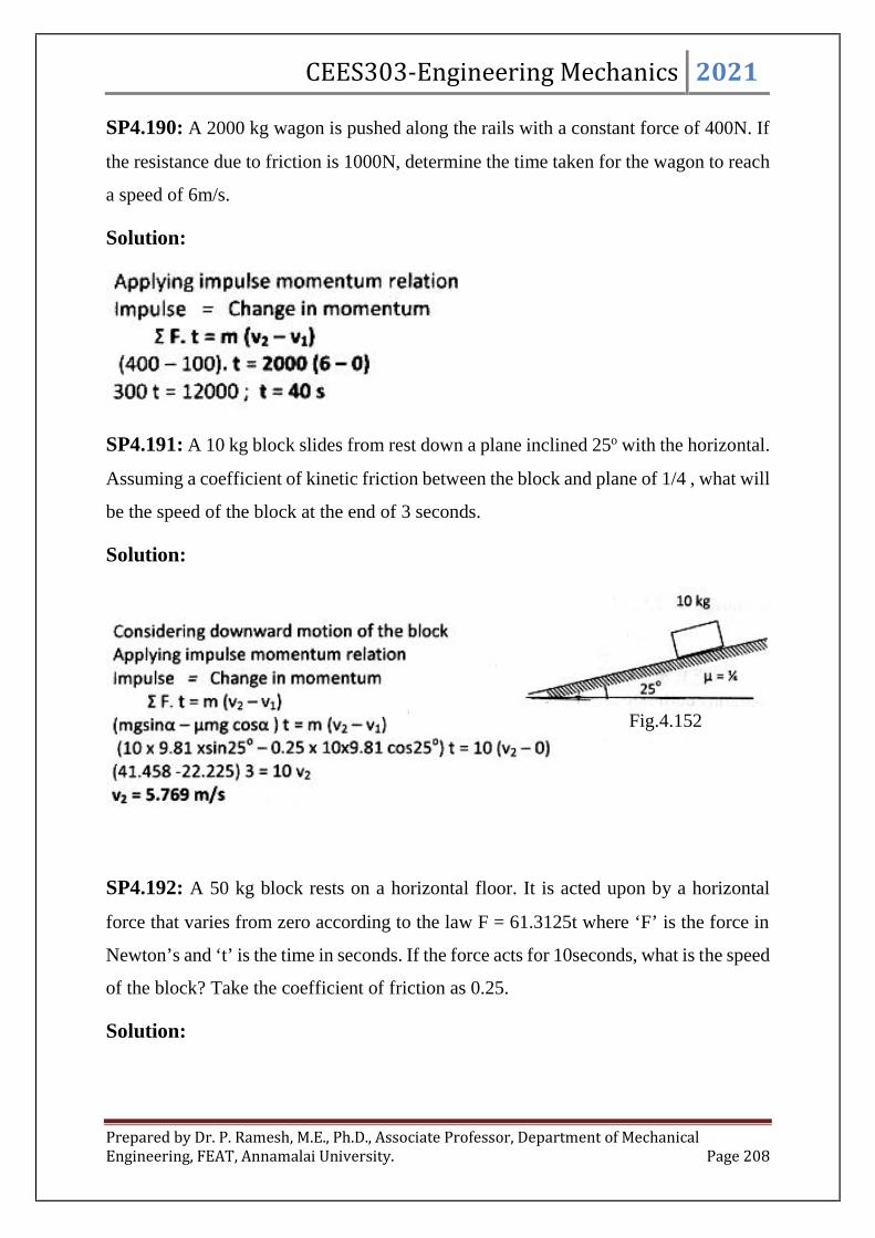
CEES303-Engineering Mechanics 2021
Prepared by Dr. P. Ramesh, M.E., Ph.D., Associate Professor, Department of MechanicalEngineering, FEAT, Annamalai University. Page 208
SP4.190: A 2000 kg wagon is pushed along the rails with a constant force of 400N. If
the resistance due to friction is 1000N, determine the time taken for the wagon to reach
a speed of 6m/s.
Solution:
SP4.191: A 10 kg block slides from rest down a plane inclined 25o with the horizontal.
Assuming a coefficient of kinetic friction between the block and plane of 1/4 , what will
be the speed of the block at the end of 3 seconds.
Solution:
SP4.192: A 50 kg block rests on a horizontal floor. It is acted upon by a horizontal
force that varies from zero according to the law F = 61.3125t where ‘F’ is the force in
Newton’s and ‘t’ is the time in seconds. If the force acts for 10seconds, what is the speed
of the block? Take the coefficient of friction as 0.25.
Solution:
Fig.4.152

CEES303-Engineering Mechanics 2021
Prepared by Dr. P. Ramesh, M.E., Ph.D., Associate Professor, Department of MechanicalEngineering, FEAT, Annamalai University. Page 209
SP4.193: A 1.5 kg block starts from rest on a smooth horizontal plane under the action
of horizontal force F which varies according to the equation 253 ttF . Determine the
maximum speed. Since the surface is smooth, friction force is zero.
Solution:
Fig.4.153

CEES303-Engineering Mechanics 2021
Prepared by Dr. P. Ramesh, M.E., Ph.D., Associate Professor, Department of MechanicalEngineering, FEAT, Annamalai University. Page 210
SP4.194: The rolling resistance for the car shown in
fig.4. is 150N/tonne. The initial velocity of the car is
5m/s up the incline. Determine the time in which the car
will come to rest.
Solution:
SP4.195: The 40kg block as shown in fig.4. is moving
up initially with a speed of 2.5m/s. What constant
value of P will give it an upward speed of 5m/s is 12
seconds? Assume that the pulleys are frictionless and
the coefficient of friction between the blocks and the
plane is 0.1.
Solution:
Fig.4.154
Fig.4.154a
Fig.4.155

CEES303-Engineering Mechanics 2021
Prepared by Dr. P. Ramesh, M.E., Ph.D., Associate Professor, Department of MechanicalEngineering, FEAT, Annamalai University. Page 211
SP4.196: A glass of marble, whose weight is 0.2N, falls a height
of 10m and rebounds to a height of 8m. Find the impulse and the
average force between the marble and the floor, if the time during
which they are in contact is 0.1 seconds.
Solution:
SP4.197: A ball of mass 100 gram is moving towards a bat with a velocity of 25m/s as
shown in fig.4. When hit by a bat the ball attains a velocity of 40m/s. If the bat and the
ball are in contact for a period of 0.015seconds, determine the average impulse force
exerted by the bat on the ball during the impact.
Solution:
Fig.4.156

CEES303-Engineering Mechanics 2021
Prepared by Dr. P. Ramesh, M.E., Ph.D., Associate Professor, Department of MechanicalEngineering, FEAT, Annamalai University. Page 212
SP4.198: A gun of mass 3 tonne fires horizontally a shell of mass 50kg with a velocity
of 300m/s. What is the velocity with which the gun will recoil? Also determine the
uniform force required to stop the gun in 0.25seconds.
Solution:
SP4.199: A bullet weighing 0.3N and moving at 600m/s penetrates the 40N body
shown in fig.4. and emerges with a velocity of 180m/s. How far and how long will the
block move, if the coefficient of friction between the body and the horizontal floor is
0.3.
Solution:
Fig.4.157

CEES303-Engineering Mechanics 2021
Prepared by Dr. P. Ramesh, M.E., Ph.D., Associate Professor, Department of MechanicalEngineering, FEAT, Annamalai University. Page 213
SP4.200: A car weighing 50kN and moving at 54kmph along a main road collides with
a lorry of weight 100kN which emerges at 18kmph from a cross road at right angles to
main road. If the two vehicle lock after collision, what will be the magnitude and
direction of the resulting velocity.
Solution:
Fig.4.158
Fig.4.159

CEES303-Engineering Mechanics 2021
Prepared by Dr. P. Ramesh, M.E., Ph.D., Associate Professor, Department of MechanicalEngineering, FEAT, Annamalai University. Page 214
SP4.201: A man of mass 50kg stands at the one end of a 5m long floating boat of mass
250kg. If the man walks towards the other end of the boat at a steady rate of 1m/s w.r.to
the boat, determine a) the velocity of the boat as observed from the ground and b) the
distance by which the boat get shifted.
Solution:
SP4.202: Two men m1 of mass 50kg and m2 of mass 75kg dive off the end of a boat of
mass M = 250kg so that their relative velocity with respect to the boat is 4m/s. If the
boat is initially at rest, find its velocity if a) two men dive simultaneously, b) the man
of mass 75kg dives first followed by the man of mass 50kg and c) the man of mass 50kg
dives first followed by the man of mass 75kg.
Solution:
Fig.4.160

CEES303-Engineering Mechanics 2021
Prepared by Dr. P. Ramesh, M.E., Ph.D., Associate Professor, Department of MechanicalEngineering, FEAT, Annamalai University. Page 215
2) ANGULAR IMPULSE AND ANGULAR MOMENTUM:
In addition to the equations of linear impulse and linear momentum, there exists
a parallel set of equations for angular impulse and angular momentum. First, we define
the term angular momentum. Fig.4.162a shows a particle P of mass m moving along a
Fig.4.161
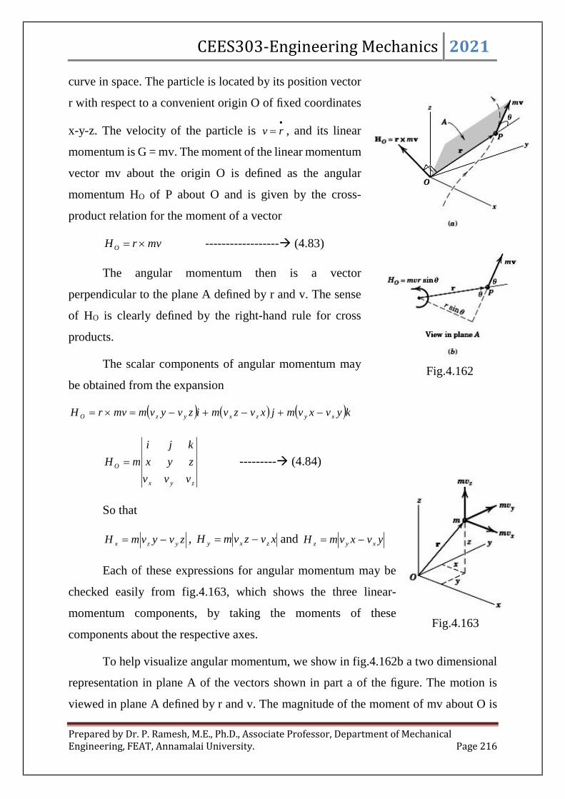
CEES303-Engineering Mechanics 2021
Prepared by Dr. P. Ramesh, M.E., Ph.D., Associate Professor, Department of MechanicalEngineering, FEAT, Annamalai University. Page 216
curve in space. The particle is located by its position vector
r with respect to a convenient origin O of fixed coordinates
x-y-z. The velocity of the particle is
rv , and its linear
momentum is G = mv. The moment of the linear momentum
vector mv about the origin O is defined as the angular
momentum HO of P about O and is given by the cross-
product relation for the moment of a vector
mvrH O ------------------ (4.83)
The angular momentum then is a vector
perpendicular to the plane A defined by r and v. The sense
of HO is clearly defined by the right-hand rule for cross
products.
The scalar components of angular momentum may
be obtained from the expansion
kyvxvmjxvzvmizvyvmmvrH xyzxyzO
zyx
O
vvv
zyx
kji
mH --------- (4.84)
So that
zvyvmH yzx , xvzvmH zxy and yvxvmH xyz
Each of these expressions for angular momentum may be
checked easily from fig.4.163, which shows the three linear-
momentum components, by taking the moments of these
components about the respective axes.
To help visualize angular momentum, we show in fig.4.162b a two dimensional
representation in plane A of the vectors shown in part a of the figure. The motion is
viewed in plane A defined by r and v. The magnitude of the moment of mv about O is
Fig.4.162
Fig.4.163
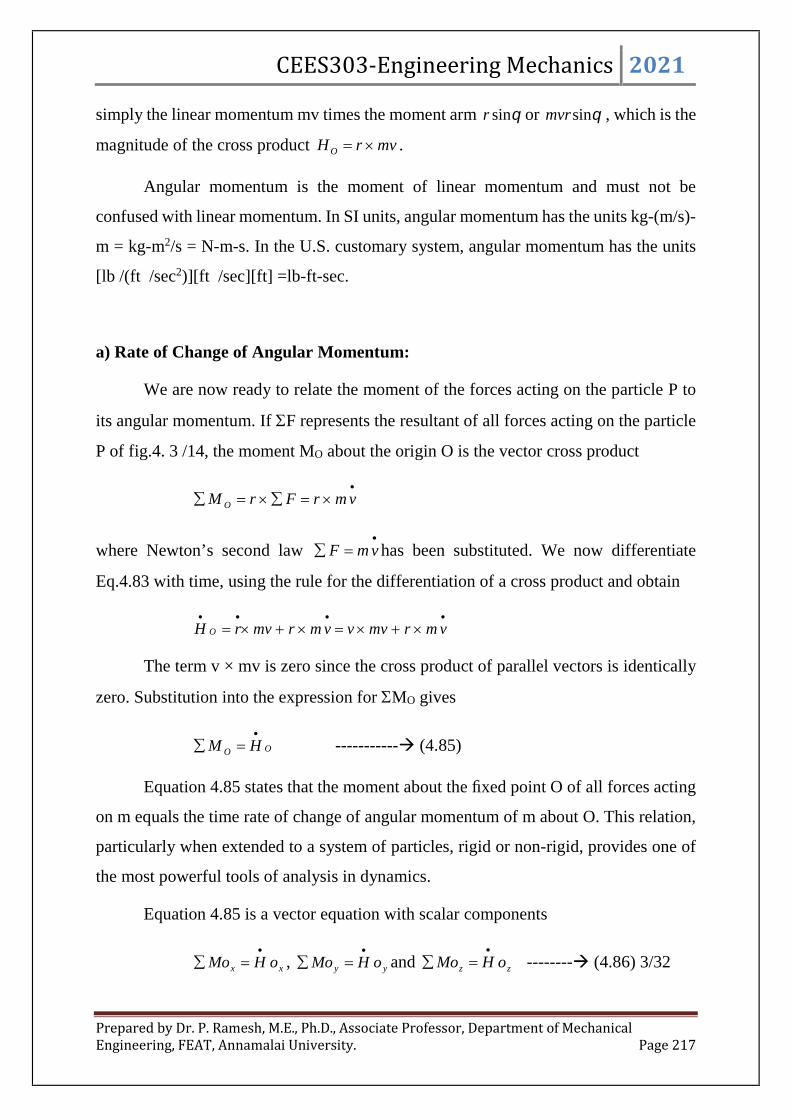
CEES303-Engineering Mechanics 2021
Prepared by Dr. P. Ramesh, M.E., Ph.D., Associate Professor, Department of MechanicalEngineering, FEAT, Annamalai University. Page 217
simply the linear momentum mv times the moment arm sinr or sinmvr , which is the
magnitude of the cross product mvrH O .
Angular momentum is the moment of linear momentum and must not be
confused with linear momentum. In SI units, angular momentum has the units kg-(m/s)-
m = kg-m2/s = N-m-s. In the U.S. customary system, angular momentum has the units
[lb /(ft /sec2)][ft /sec][ft] =lb-ft-sec.
a) Rate of Change of Angular Momentum:
We are now ready to relate the moment of the forces acting on the particle P to
its angular momentum. If F represents the resultant of all forces acting on the particle
P of fig.4. 3 /14, the moment MO about the origin O is the vector cross product
vmrFrM O
where Newton’s second law
vmF has been substituted. We now differentiate
Eq.4.83 with time, using the rule for the differentiation of a cross product and obtain
vmrmvvvmrmvrH O
The term v × mv is zero since the cross product of parallel vectors is identically
zero. Substitution into the expression for MO gives
OO HM
----------- (4.85)
Equation 4.85 states that the moment about the fixed point O of all forces acting
on m equals the time rate of change of angular momentum of m about O. This relation,
particularly when extended to a system of particles, rigid or non-rigid, provides one of
the most powerful tools of analysis in dynamics.
Equation 4.85 is a vector equation with scalar components
xx oHMo
, yy oHMo
and zz oHMo
-------- (4.86) 3/32

CEES303-Engineering Mechanics 2021
Prepared by Dr. P. Ramesh, M.E., Ph.D., Associate Professor, Department of MechanicalEngineering, FEAT, Annamalai University. Page 218
b) The Angular Impulse-Momentum Principle:
Equation 4.85 gives the instantaneous relation between the moment and the time
rate of change of angular momentum. To obtain the effect of the moment MO on the
angular momentum of the particle over a finite period of time, we integrate Eq. 4.85
from time t1 to time t2. Multiplying the equation by dt gives OO dHdtM , which we
integrate to obtain
2
112
t
t
OOOO HHHdtM ------- (4.87)
Where 222 mvrH O and 111 mvrH O . The product of moment and time is
defined as angular impulse, and Eq. 4.87 states that the total angular impulse on m about
the fixed point O equals the corresponding change in angular momentum of m about O.
Alternatively, we may write Eq. 4.87 as
22
11 O
t
t
OO HdtMH --------- (4.88)
which states that the initial angular momentum of the particle plus the angular impulse
applied to it equals its final angular momentum. The units of angular impulse are clearly
those of angular momentum, which are N-m-s or kg-m2/s in SI units and lb-ft-sec in
U.S. customary units.
As in the case of linear impulse and linear momentum, the equation of angular
impulse and angular momentum is a vector equation where changes in direction as well
as magnitude may occur during the interval of integration. Under these conditions, it is
necessary to express MO and HO in component form and then combine the integrated
components. The x-component of Eq. 4.88 is
22
11 x
t
t
xx HodtMoHo or
2
2
11
zvyvmdtMozvyvm yz
t
t
xyz ----------- (4.89)

CEES303-Engineering Mechanics 2021
Prepared by Dr. P. Ramesh, M.E., Ph.D., Associate Professor, Department of MechanicalEngineering, FEAT, Annamalai University. Page 219
where the subscripts 1 and 2 refer to the values of the respective quantities at times t1and
t2. Similar expressions exist for the y- and z-components of the angular impulse-
momentum equation.
c) Plane-Motion Applications
The foregoing angular-impulse and angular-momentum relations have been
developed in their general three-dimensional forms. Most of the applications of interest
to us, however, can be analysed as plane motion problems where moments are taken
about a single axis normal to the plane of motion. In this case, the angular momentum
may change magnitude and sense, but the direction of the vector remains unaltered.
Fig.4.164
Thus, for a particle of mass m moving along a curved path in the x-y plane,
fig.4.164, the angular momenta about O at points 1 and 2 have the magnitudes
11111 dmvmvrH O and 22222 dmvmvrH O , respectively. In the illustration
both 1OH and 2OH are represented in the counter clockwise sense in accord with the
direction of the moment of the linear momentum. The scalar form of Eq. 4.88 applied
to the motion between points 1 and 2 during the time interval t1 to t2 becomes
22
11 O
t
t
oO HdtMH or 2
1
2211 sint
t
dmvdtFrdmv

CEES303-Engineering Mechanics 2021
Prepared by Dr. P. Ramesh, M.E., Ph.D., Associate Professor, Department of MechanicalEngineering, FEAT, Annamalai University. Page 220
This example should help clarify the relation between the scalar and vector forms
of the angular impulse-momentum relations.
Whereas Eq. 4.87 clearly stresses that the external angular impulse causes a
change in the angular momentum, the order of the terms in Eqs. 4.88 and 4.89
corresponds to the natural sequence of events. Equation 4.88 is analogous to Eq.4.80,
just as Eq. 4.85 is analogous to Eq. 4.77.
As was the case for linear-momentum problems, we encounter impulsive (large
magnitude, short duration) and non-impulsive forces in angular-momentum problems.
d) Conservation of Angular Momentum
If the resultant moment about a fixed point O of all forces acting on a particle is
zero during an interval of time, Eq. 4.85 requires that its angular momentum HO about
that point remain constant. In this case, the angular momentum of the particle is said to
be conserved. Angular momentum may be conserved about one axis but not about
another axis. A careful examination of the free-body diagram of the particle will
disclose whether the moment of the resultant force on the particle about a fixed point is
zero, in which case, the angular momentum about that point is unchanged (conserved).
Consider now the motion of two particles a and b which interact during an
interval of time. If the interactive forces F and -F between them are the only unbalanced
forces acting on the particles during the interval, it follows that the moments of the equal
and opposite forces about any fixed point O not on their line of action are equal and
opposite. If we apply Eq. 4.87 to particle a and then to particle b and add the two
equations, we obtain ΔHa + ΔHb = 0 (where all angular momenta are referred to point
O). Thus, the total angular momentum for the system of the two particles remains
constant during the interval, and we write
0 OH or 21 OO HH ----------- (4.90)
which expresses the principle of conservation of angular momentum.
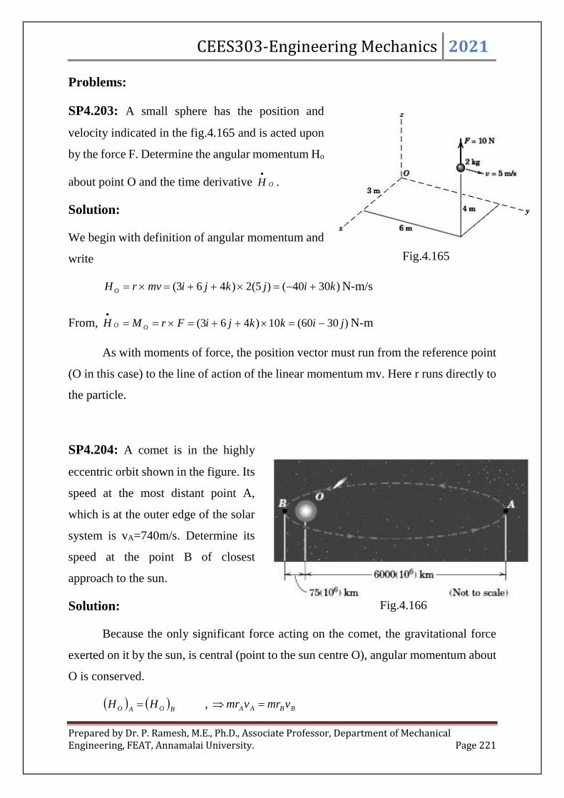
CEES303-Engineering Mechanics 2021
Prepared by Dr. P. Ramesh, M.E., Ph.D., Associate Professor, Department of MechanicalEngineering, FEAT, Annamalai University. Page 221
Problems:
SP4.203: A small sphere has the position and
velocity indicated in the fig.4.165 and is acted upon
by the force F. Determine the angular momentum Ho
about point O and the time derivative OH
.
Solution:
We begin with definition of angular momentum and
write
)3040()5(2)463( kijkjimvrH O N-m/s
From, )3060(10)463( jikkjiFrMH OO
N-m
As with moments of force, the position vector must run from the reference point
(O in this case) to the line of action of the linear momentum mv. Here r runs directly to
the particle.
SP4.204: A comet is in the highly
eccentric orbit shown in the figure. Its
speed at the most distant point A,
which is at the outer edge of the solar
system is vA=740m/s. Determine its
speed at the point B of closest
approach to the sun.
Solution:
Because the only significant force acting on the comet, the gravitational force
exerted on it by the sun, is central (point to the sun centre O), angular momentum about
O is conserved.
BOAO HH , BBAA vmrvmr
Fig.4.165
Fig.4.166

CEES303-Engineering Mechanics 2021
Prepared by Dr. P. Ramesh, M.E., Ph.D., Associate Professor, Department of MechanicalEngineering, FEAT, Annamalai University. Page 222
smr
vrv
B
AAB /59200
1075
740)10(60006
6
SP4.205: The assembly of the light rod and
two end masses is at rest when it is struck by
the falling wad of putty travelling with speed
v1 as shown. The putty adheres to and travels
with the right – hand end mass. Determine the
angular velocity 2
of the assembly just after
impact. The pivot at O is frictionless and all three masses may be assumed to be
particles.
Solution:
SP4.206: A small mass particle is given an initial velocity
v0 tangent to the horizontal rim of a smooth hemispherical
bowl at a radius r0 from the vertical centre line as shown at
point A. As the particle slides past point B, a distance h
below A and a distance r from the vertical centreline, its
velocity v makes an angle with the horizontal tangent to
the bowl through B. Determine .
Solution:
Fig.4.167
Fig.4.168

CEES303-Engineering Mechanics 2021
Prepared by Dr. P. Ramesh, M.E., Ph.D., Associate Professor, Department of MechanicalEngineering, FEAT, Annamalai University. Page 223
SP4.207: A flywheel having mass 500kg has hub 100mm in diameter supported on
bearings. The flywheel has a radius of gyration of 500mm and it is turning at 240rpm.
The coefficient of friction is 0.08. Determine the elapsed time until the flywheel comes
to rest because of bearing friction.
Solution:
Fig.4.169

CEES303-Engineering Mechanics 2021
Prepared by Dr. P. Ramesh, M.E., Ph.D., Associate Professor, Department of MechanicalEngineering, FEAT, Annamalai University. Page 224
SP4.208: A solid cylinder as shown in fig.4. is supported on
frictionless bearings. Find the angular velocity of the cylinder
and the tension T in the rope 8 seconds after the system is
released from rest.
Solution:
SP4.209: In fig.4. a mass less rope carries two masses of 5kg and 7
kg when hanging on a pulley of mass 5kg radius 600mm and radius
of gyration of 450mm. How long will it take to change the speed of
the masses from 3m/s to 6m/s. a) when the friction in the bearing is
not considered and b) when considering the friction in the bearing of
radius 100mm and is 0.05.
Solution:
Fig.4.170
Fig.4.171
Fig.4.172

CEES303-Engineering Mechanics 2021
Prepared by Dr. P. Ramesh, M.E., Ph.D., Associate Professor, Department of MechanicalEngineering, FEAT, Annamalai University. Page 225
Fig.4.172a

CEES303-Engineering Mechanics 2021
Prepared by Dr. P. Ramesh, M.E., Ph.D., Associate Professor, Department of MechanicalEngineering, FEAT, Annamalai University. Page 226
SP4.210: Determine the mass of B necessary to cause the 50kg mass A to change its
speed from 4m/s to 8m/s in 6 seconds. Assume the drum rotates in frictionless bearings.
Fig.4.173
Solution:
Fig.4.173a

CEES303-Engineering Mechanics 2021
Prepared by Dr. P. Ramesh, M.E., Ph.D., Associate Professor, Department of MechanicalEngineering, FEAT, Annamalai University. Page 227
SP4.211: The drum shown in fig.4.174 has a mass of 300kg and
a radius of gyration with respect to its mass centre G of 500mm.
What will be the time for the angular speed to change uniformly
from 100 to 300 rad/s?
Solution:
SP4.212: A jet of water 50mm diameter exerts a force of 1200N on a flat vane
perpendicular to the stream. What is the nozzle speed of the jet?
Solution:
Fig.4.174
Fig.4.174a
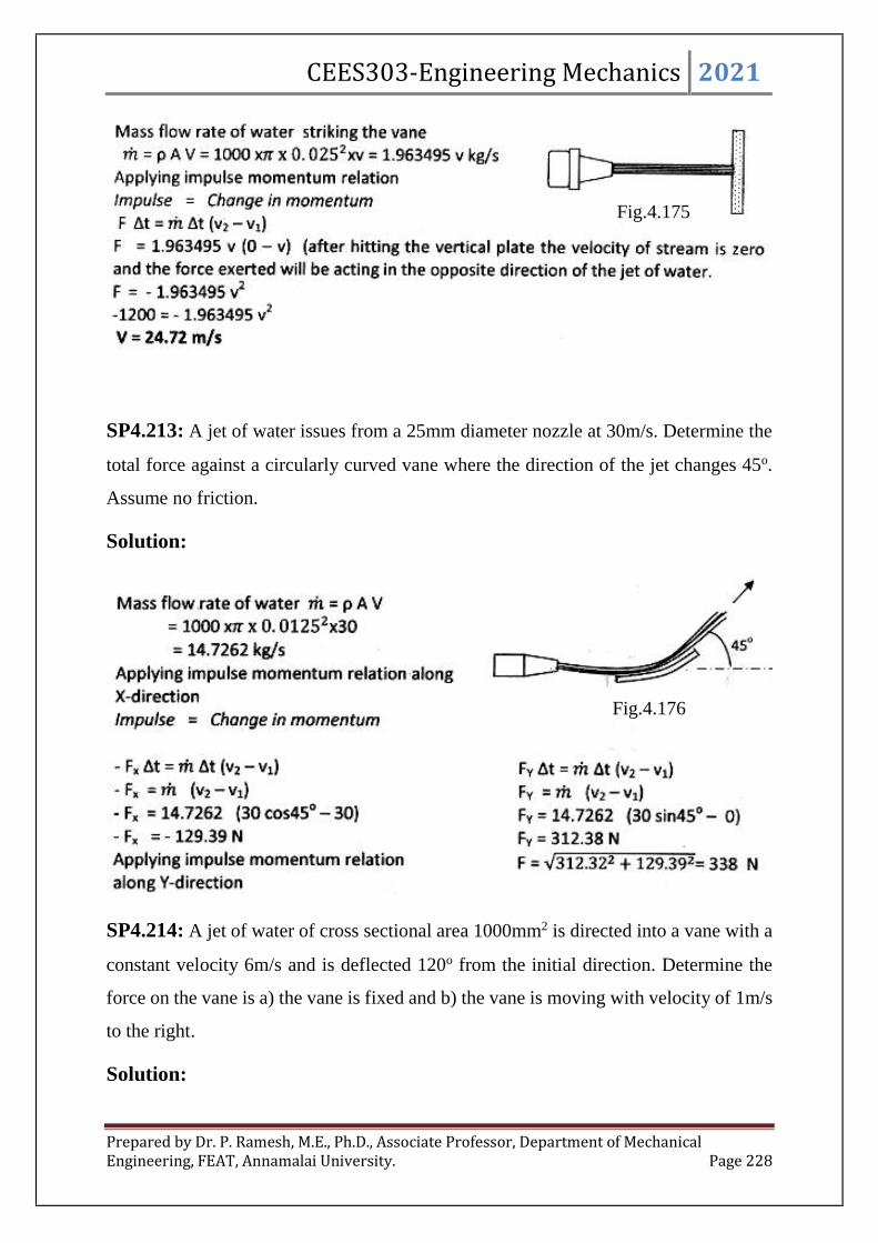
CEES303-Engineering Mechanics 2021
Prepared by Dr. P. Ramesh, M.E., Ph.D., Associate Professor, Department of MechanicalEngineering, FEAT, Annamalai University. Page 228
SP4.213: A jet of water issues from a 25mm diameter nozzle at 30m/s. Determine the
total force against a circularly curved vane where the direction of the jet changes 45o.
Assume no friction.
Solution:
SP4.214: A jet of water of cross sectional area 1000mm2 is directed into a vane with a
constant velocity 6m/s and is deflected 120o from the initial direction. Determine the
force on the vane is a) the vane is fixed and b) the vane is moving with velocity of 1m/s
to the right.
Solution:
Fig.4.175
Fig.4.176

CEES303-Engineering Mechanics 2021
Prepared by Dr. P. Ramesh, M.E., Ph.D., Associate Professor, Department of MechanicalEngineering, FEAT, Annamalai University. Page 229
SP4.215: A stream of water 2700mm2 in cross section and moving horizontally with a
speed of 30m/s splits into two equal parts against the fixed vane. Assume no friction
between the water and the blade, determine the force of water on the blade.
Solution:
Fig.4.177
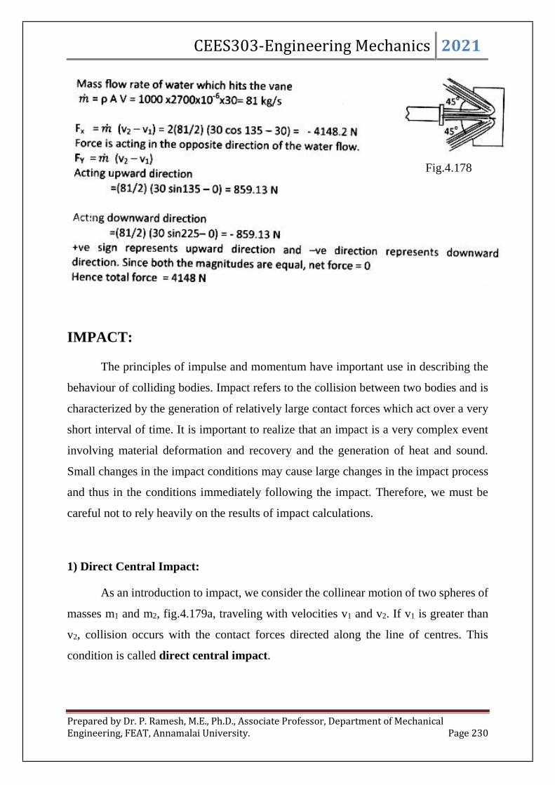
CEES303-Engineering Mechanics 2021
Prepared by Dr. P. Ramesh, M.E., Ph.D., Associate Professor, Department of MechanicalEngineering, FEAT, Annamalai University. Page 230
IMPACT:
The principles of impulse and momentum have important use in describing the
behaviour of colliding bodies. Impact refers to the collision between two bodies and is
characterized by the generation of relatively large contact forces which act over a very
short interval of time. It is important to realize that an impact is a very complex event
involving material deformation and recovery and the generation of heat and sound.
Small changes in the impact conditions may cause large changes in the impact process
and thus in the conditions immediately following the impact. Therefore, we must be
careful not to rely heavily on the results of impact calculations.
1) Direct Central Impact:
As an introduction to impact, we consider the collinear motion of two spheres of
masses m1 and m2, fig.4.179a, traveling with velocities v1 and v2. If v1 is greater than
v2, collision occurs with the contact forces directed along the line of centres. This
condition is called direct central impact.
Fig.4.178

CEES303-Engineering Mechanics 2021
Prepared by Dr. P. Ramesh, M.E., Ph.D., Associate Professor, Department of MechanicalEngineering, FEAT, Annamalai University. Page 231
Fig.4.179
Following initial contact, a short period of increasing deformation takes place
until the contact area between the spheres ceases to increase. At this instant, both
spheres, fig.4.179b, are moving with the same velocity v0. During the remainder of
contact, a period of restoration occurs during which the contact area decreases to zero.
In the final condition shown in part c of the figure, the spheres now have new velocities
v1’ and v2', where v1' must be less than v2'. All velocities are arbitrarily assumed positive
to the right, so that with this scalar notation a velocity to the left would carry a negative
sign. If the impact is not overly severe and if the spheres are highly elastic, they will
regain their original shape following the restoration. With a more severe impact and
with less elastic bodies, a permanent deformation may result.
Because the contact forces are equal and opposite during impact, the linear
momentum of the system remains unchanged. Thus, we apply the law of conservation
of linear momentum and write
'' 22112211 vmvmvmvm ------------- (4.91)
We assume that any forces acting on the spheres during impact, other than the
large internal forces of contact, are relatively small and produce negligible impulses
compared with the impulse associated with each internal impact force. In addition, we
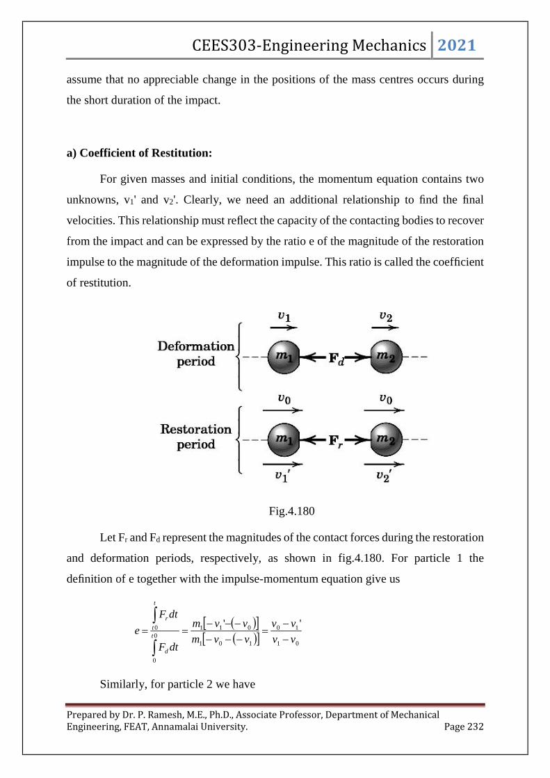
CEES303-Engineering Mechanics 2021
Prepared by Dr. P. Ramesh, M.E., Ph.D., Associate Professor, Department of MechanicalEngineering, FEAT, Annamalai University. Page 232
assume that no appreciable change in the positions of the mass centres occurs during
the short duration of the impact.
a) Coefficient of Restitution:
For given masses and initial conditions, the momentum equation contains two
unknowns, v1' and v2'. Clearly, we need an additional relationship to find the final
velocities. This relationship must reflect the capacity of the contacting bodies to recover
from the impact and can be expressed by the ratio e of the magnitude of the restoration
impulse to the magnitude of the deformation impulse. This ratio is called the coefficient
of restitution.
Fig.4.180
Let Fr and Fd represent the magnitudes of the contact forces during the restoration
and deformation periods, respectively, as shown in fig.4.180. For particle 1 the
definition of e together with the impulse-momentum equation give us
01
10
101
0110
0
0 ''
vv
vv
vvm
vvm
dtF
dtF
et
d
t
t
r
Similarly, for particle 2 we have

CEES303-Engineering Mechanics 2021
Prepared by Dr. P. Ramesh, M.E., Ph.D., Associate Professor, Department of MechanicalEngineering, FEAT, Annamalai University. Page 233
20
02
202
0220
0
0 ''
vv
vv
vvm
vvm
dtF
dtF
et
d
t
t
r
We are careful in these equations to express the change of momentum (and
therefore Δv) in the same direction as the impulse (and thus the force). The time for the
deformation is taken as t0 and the total time of contact is t. Eliminating v0 between the
two expressions for e gives us
approachof velocityrelative
separationof velocityrelative''
21
12
vv
vve -------(4.92)
If the two initial velocities v1 and v2 and the coefficient of restitution e are known,
then Eqs. 4.91 and 4.92 give us two equations in the two unknown final velocities v1'
and v2'.
b) Energy Loss during Impact
Impact phenomena are almost always accompanied by energy loss, which may
be calculated by subtracting the kinetic energy of the system just after impact from that
just before impact. Energy is lost through the generation of heat during the localized
inelastic deformation of the material, through the generation and dissipation of elastic
stress waves within the bodies, and through the generation of sound energy.
According to this classical theory of impact, the value e = 1 means that the
capacity of the two particles to recover equals their tendency to deform. This condition
is one of elastic impact with no energy loss. The value e = 0, on the other hand, describes
inelastic or plastic impact where the particles cling together after collision and the loss
of energy is a maximum. All impact conditions lie somewhere between these two
extremes.

CEES303-Engineering Mechanics 2021
Prepared by Dr. P. Ramesh, M.E., Ph.D., Associate Professor, Department of MechanicalEngineering, FEAT, Annamalai University. Page 234
Fig.4.181
Also, it should be noted that a coefficient of restitution must be associated with
a pair of contacting bodies. The coefficient of restitution is frequently considered a
constant for given geometries and a given combination of contacting materials.
Actually, it depends on the impact velocity and approaches unity as the impact velocity
approaches zero as shown schematically in fig.4.181. A handbook value for e is
generally unreliable.
2) Oblique Central Impact
We now extend the relationships developed for direct central impact to the case
where the initial and final velocities are not parallel, fig.4.182. Here spherical particles
of mass m1 and m2 have initial velocities v1 and v2 in the same plane and approach each
other on a collision course, as shown in part a of the figure. The directions of the velocity
vectors are measured from the direction tangent to the contacting surfaces, fig.4.182b.
Thus, the initial velocity components along the t- and n-axes are (v1)n = -v1sin1, (v1)t =
v1cos1, (v2)n = v2sin2 and (v2)t=v2cos2. Note that (v1)n is a negative quantity for the
particular coordinate system and initial velocities shown.
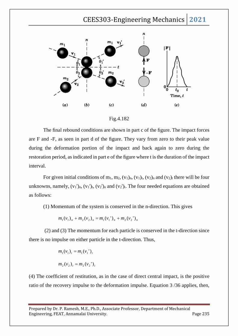
CEES303-Engineering Mechanics 2021
Prepared by Dr. P. Ramesh, M.E., Ph.D., Associate Professor, Department of MechanicalEngineering, FEAT, Annamalai University. Page 235
Fig.4.182
The final rebound conditions are shown in part c of the figure. The impact forces
are F and -F, as seen in part d of the figure. They vary from zero to their peak value
during the deformation portion of the impact and back again to zero during the
restoration period, as indicated in part e of the figure where t is the duration of the impact
interval.
For given initial conditions of m1, m2, (v1)n, (v1)t, (v2)n and (v2)t there will be four
unknowns, namely, (v1')n, (v1')t, (v2')n and (v2')t. The four needed equations are obtained
as follows:
(1) Momentum of the system is conserved in the n-direction. This gives
nnnn vmvmvmvm )'()'()()( 22112211
(2) and (3) The momentum for each particle is conserved in the t-direction since
there is no impulse on either particle in the t-direction. Thus,
tt vmvm )'()( 1111
tt vmvm )'()( 2222
(4) The coefficient of restitution, as in the case of direct central impact, is the positive
ratio of the recovery impulse to the deformation impulse. Equation 3 /36 applies, then,

CEES303-Engineering Mechanics 2021
Prepared by Dr. P. Ramesh, M.E., Ph.D., Associate Professor, Department of MechanicalEngineering, FEAT, Annamalai University. Page 236
to the velocity components in the n-direction. For the notation adopted with fig.4.182,
we have
nn
nn
vv
vve
21
12 ''
Once the four final velocity components are found, the angles 1’ and 2’ of
fig.4.182 may be easily determined.
Problems:
SP4.216: The ram of a pile driver has a mass of 800kg and is released from rest 2m
above the top of the 2400kg pile. If the ram rebounds to a height of 0.1m after impact
with the pile, calculate a) the velocity vp’ of the pile immediately after impact, b) the
coefficient of restitution e and c) the percentage loss of energy due to the impact.
Fig.4.183
Solution:

CEES303-Engineering Mechanics 2021
Prepared by Dr. P. Ramesh, M.E., Ph.D., Associate Professor, Department of MechanicalEngineering, FEAT, Annamalai University. Page 237
SP4.217: A ball is projected onto the heavy plate with a velocity of 16m/s at the 30o
angle shown. If the effective coefficient of restitution is 0.5, compute the rebound
velocity v’ and its angle ’.
Fig.4.184
Solution:
Let the ball be denoted body 1 and the plate body 2. The mass of heavy plate
may be considered infinite and its corresponding velocity zero after impact. The
coefficient of restitution is applied to the velocity components normal to the plate in the
direction of the impact force and gives
nn
nn
vv
vve
21
12 ''
,
030sin16
'05.0 1
o
nv, smv n /4)'( 1
Momentum of the ball in the t- direction is unchanged since, with assumed
smooth surface there is no force acting on the ball in that direction. Thus,

CEES303-Engineering Mechanics 2021
Prepared by Dr. P. Ramesh, M.E., Ph.D., Associate Professor, Department of MechanicalEngineering, FEAT, Annamalai University. Page 238
tt vmvm '11 , smvv ott /86.1330cos16)'( 11
The rebound velocity v’ and its angle ’ are then
smvvv tn /42.1486.134''' 2221
21
o
t
n
v
v10.16
86.13
4tan
'
'tan' 1
1
11
SP4.218: Spherical particle 1 has a velocity v1 = 6m/s in the direction shown and
collides with spherical particle 2 of equal mass and diameter and initially at rest. If the
coefficient of restitution for these conditions is e = 0.6, determine the resulting motion
of each particle following impact. Also calculate the percentage loss of energy due to
the impact.
Fig.4.185
Solution:

CEES303-Engineering Mechanics 2021
Prepared by Dr. P. Ramesh, M.E., Ph.D., Associate Professor, Department of MechanicalEngineering, FEAT, Annamalai University. Page 239
SP4.219: A ball of mass 1 kg moving with a velocity of 2m/s impinges directly on a
ball of mass 2kg at rest. The first ball, after impinging comes to rest. Find the velocity
of the second ball after the impact and the coefficient of restitution.
Solution:
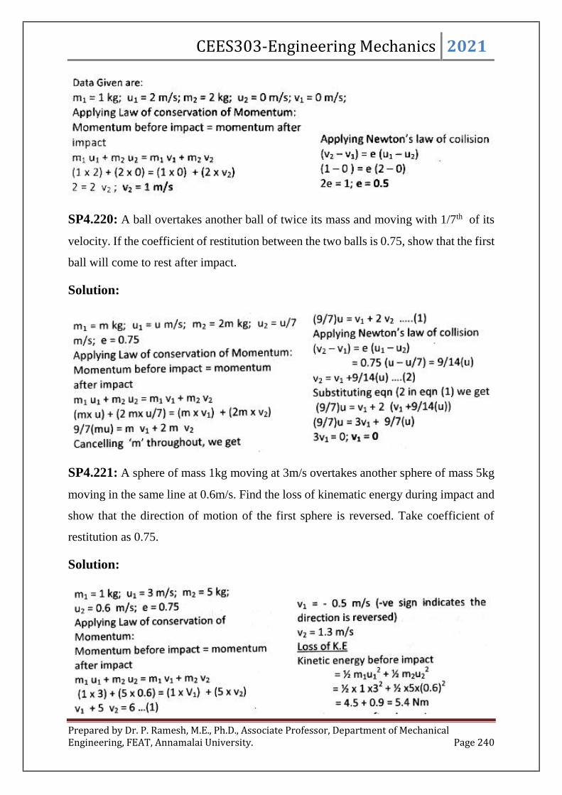
CEES303-Engineering Mechanics 2021
Prepared by Dr. P. Ramesh, M.E., Ph.D., Associate Professor, Department of MechanicalEngineering, FEAT, Annamalai University. Page 240
SP4.220: A ball overtakes another ball of twice its mass and moving with 1/7th of its
velocity. If the coefficient of restitution between the two balls is 0.75, show that the first
ball will come to rest after impact.
Solution:
SP4.221: A sphere of mass 1kg moving at 3m/s overtakes another sphere of mass 5kg
moving in the same line at 0.6m/s. Find the loss of kinematic energy during impact and
show that the direction of motion of the first sphere is reversed. Take coefficient of
restitution as 0.75.
Solution:

CEES303-Engineering Mechanics 2021
Prepared by Dr. P. Ramesh, M.E., Ph.D., Associate Professor, Department of MechanicalEngineering, FEAT, Annamalai University. Page 241
SP4.222: Two bodies one of which is 400N with a velocity of 8m/s and the other of
250N with a velocity of 12m/s move towards each other along a straight line and
impinge centrally. Find the velocity of each body after impact if the coefficient of
restitution is 0.8.
Solution:
SP4.223: Three spherical balls of mass 2 kg, 6 kg and 12 kg are moving in the same
direction with velocity 12 m/s, 4 m/s and 2 m/s respectively. If the ball of mass 2 kg
impinges with the ball of mass 6 kg which in turn impinges with the ball of mass 12 kg.
Prove that the balls of mass 2 kg and 6 kg will be brought to rest by the impacts. Assume
the balls to be perfectly elastic.
Solution:
Fig.4.186

CEES303-Engineering Mechanics 2021
Prepared by Dr. P. Ramesh, M.E., Ph.D., Associate Professor, Department of MechanicalEngineering, FEAT, Annamalai University. Page 242
SP4.224: Two identical balls each of mass ‘m’ collide with velocities as shown in fig.4.
Find the final velocities of the balls after the impact. Assume e = 0.9.
Solution:
Fig.4.187
Fig.4.188
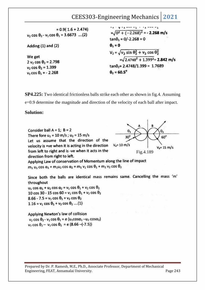
CEES303-Engineering Mechanics 2021
Prepared by Dr. P. Ramesh, M.E., Ph.D., Associate Professor, Department of MechanicalEngineering, FEAT, Annamalai University. Page 243
SP4.225: Two identical frictionless balls strike each other as shown in fig.4. Assuming
e=0.9 determine the magnitude and direction of the velocity of each ball after impact.
Solution:
Fig.4.189

CEES303-Engineering Mechanics 2021
Prepared by Dr. P. Ramesh, M.E., Ph.D., Associate Professor, Department of MechanicalEngineering, FEAT, Annamalai University. Page 244
SP4.226: A smooth spherical ball A of mass 120 gram is moving from
left to right with a velocity of 2m/s in a horizontal plane. Another
identical ball B travelling in a perpendicular direction with a velocity 6
m/s collides with A in such a way that the line of impact is in the
direction of motion of ball B. Assuming e=0.8, determine the velocity
of the balls A and B after the impact.
Solution:
Fig.4.190

CEES303-Engineering Mechanics 2021
Prepared by Dr. P. Ramesh, M.E., Ph.D., Associate Professor, Department of MechanicalEngineering, FEAT, Annamalai University. Page 245
SP4.227: From a point on a smooth floor of a room, a toy ball is shot to hit a wall by
rolling on the floor. The ball then returns back to the point of projection. If the time take
by the ball in returning is twice the time taken in reaching the wall, find the coefficient
of restitution between the ball and wall.
Solution:
SP4.228: A ball is dropped from a height ho =1 m on a smooth floor.
Knowing that the height of the first bounce is h1 = 0.81m, determine
a) the coefficient of restitution and b) the expected height of the
second bounce.
Solution:
Fig.4.191
Fig.4.192

CEES303-Engineering Mechanics 2021
Prepared by Dr. P. Ramesh, M.E., Ph.D., Associate Professor, Department of MechanicalEngineering, FEAT, Annamalai University. Page 246
SP4.229: From what height must a heavy elastic ball be dropped on a floor so that after
rebounding thrice, it will reach a height of 16m. Take 315.0e .
Solution:
Fig.4.193
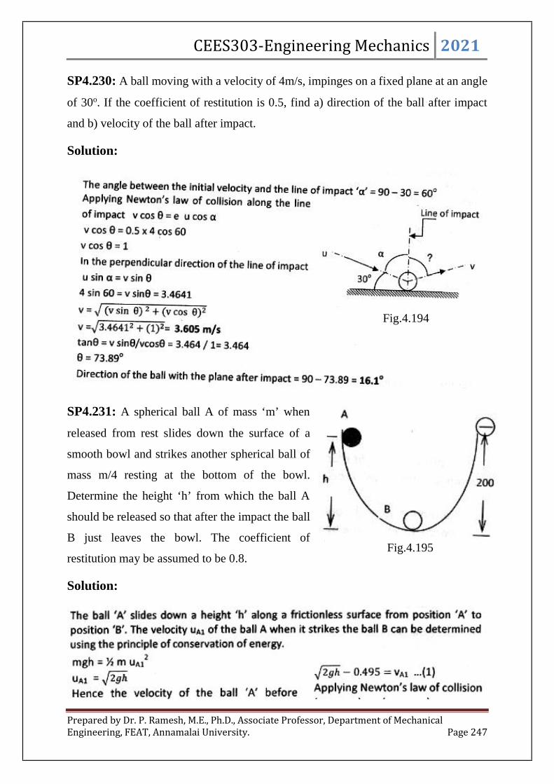
CEES303-Engineering Mechanics 2021
Prepared by Dr. P. Ramesh, M.E., Ph.D., Associate Professor, Department of MechanicalEngineering, FEAT, Annamalai University. Page 247
SP4.230: A ball moving with a velocity of 4m/s, impinges on a fixed plane at an angle
of 30o. If the coefficient of restitution is 0.5, find a) direction of the ball after impact
and b) velocity of the ball after impact.
Solution:
SP4.231: A spherical ball A of mass ‘m’ when
released from rest slides down the surface of a
smooth bowl and strikes another spherical ball of
mass m/4 resting at the bottom of the bowl.
Determine the height ‘h’ from which the ball A
should be released so that after the impact the ball
B just leaves the bowl. The coefficient of
restitution may be assumed to be 0.8.
Solution:
Fig.4.194
Fig.4.195

CEES303-Engineering Mechanics 2021
Prepared by Dr. P. Ramesh, M.E., Ph.D., Associate Professor, Department of MechanicalEngineering, FEAT, Annamalai University. Page 248
SP4.232: Two equal balls are in contact on a table; a third equal ball strikes them
simultaneously and remains at rest after the impact. Show that the coefficient of
restitution is 2/3.
Solution:
SP4.233: A 1 kg ball traverses a frictionless
tube shown in fig.4 falling through a height of
2m. It then strikes a 2 kg ball hung from a rope
1.2 m long. Determine the height to which the
hanging ball will rise if the coefficient if
restitution is 0.7.
Solution:
Fig.4.196
Fig.4.197
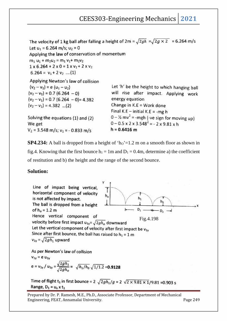
CEES303-Engineering Mechanics 2021
Prepared by Dr. P. Ramesh, M.E., Ph.D., Associate Professor, Department of MechanicalEngineering, FEAT, Annamalai University. Page 249
SP4.234: A ball is dropped from a height of ‘hO’=1.2 m on a smooth floor as shown in
fig.4. Knowing that the first bounce h1 = 1m and D1 = 0.4m, determine a) the coefficient
of restitution and b) the height and the range of the second bounce.
Solution:
Fig.4.198

CEES303-Engineering Mechanics 2021
Prepared by Dr. P. Ramesh, M.E., Ph.D., Associate Professor, Department of MechanicalEngineering, FEAT, Annamalai University. Page 250

Lecture Notes
UNIT – 5 2021
Prepared by
Dr. P. Ramesh, M.E., Ph.D.,
Associate Professor
Department of Mechanical Engineering
Faculty of Engineering and Technology
Annamalai UniversityDec-2021
CEES303-EngineeringMechanics

CEES303-Engineering Mechanics 2021
Prepared by Dr. P. Ramesh, M.E., Ph.D., Associate Professor, Department of MechanicalEngineering, FEAT, Annamalai University. Page 2
Unit - 5
Introduction to Kinetics of Rigid Bodies covering, Basic terms, general
principles in dynamics; Types of motion, Instantaneous centre of rotation in
plane motion and simple problems; D’Alembert’s principle and its applications
in plane motion and connected bodies; Work energy principle and its
application in plane motion of connected bodies; Kinetics of rigid body rotation
Mechanical Vibrations covering, Basic terminology, free and forced vibrations,
resonance and its effects; Degree of freedom; Derivation for frequency and
amplitude of free vibrations without damping and single degree of freedom
system, simple problems, types of pendulum, use of simple, compound and
torsion pendulums;
Reference for the preparation of course material:
1. F. P. Beer and E. R. Johnston (2011), Vector Mechanics for Engineers,Vol I - Statics, Vol II, – Dynamics, 9th Ed, Tata McGraw Hill.
2. Khurmi R.S. (2010), Engineering Mechanics, S. Chand & Co.3. J.L. Meriam and L. G. Kraige, Engineering Mechanics –Statics, volume I,
Seventh edition, John Wiley & Sons, Inc.4. S.S.Bhavikatti and K.G. Rajashekarappa, Engineering Mechanics (Third
Edition), New Age International (P) Limited, Publishers.
TEXT BOOKS1. Irving H. Shames (2006), Engineering Mechanics, 4th Edition, Prentice Hall2. F. P. Beer and E. R. Johnston (2011), Vector Mechanics for Engineers, Vol I -
Statics, Vol II, – Dynamics, 9th Ed, Tata McGraw Hill
REFERENCES1. R. C. Hibbler (2006), Engineering Mechanics: Principles of Statics and Dynamics,
Pearson Press.2. Khurmi R.S. (2010), Engineering Mechanics, S. Chand & Co.

CEES303-Engineering Mechanics 2021
Prepared by Dr. P. Ramesh, M.E., Ph.D., Associate Professor, Department of MechanicalEngineering, FEAT, Annamalai University. Page 3
Unit - 5
Dynamics of Rigid Bodies
BASIC TERMS:
1) Motion:
A body is said to be in motion if it is changing its position with respect to
a reference point. A person on a scooter is in motion when referred to the road
but is at rest when referred to the scooter itself. In most problems, the reference
point is implied. For all engineering problems, any fixed point on the earth is an
implied reference point. Other examples of implied reference points are centre
of the earth for the study of satellite motion, centre of the sun for the study of
motion of the solar system and mass centre of the solar system for the study of
interplanetary motion. In this only engineering problems have been taken up and
hence any fixed point on the earth is an implied reference point while considering
motion of the body.
2) Distance and displacement:
Let a body move along the path as shown in fig.5.1 by hatched line and
the time taken by the body to move from A to B be t, then the distance moved
by the body in time t is the distance measured along the hatched line. Distance is
a scalar quantity since it has only magnitude.
Fig.5.1 Distance

CEES303-Engineering Mechanics 2021
Prepared by Dr. P. Ramesh, M.E., Ph.D., Associate Professor, Department of MechanicalEngineering, FEAT, Annamalai University. Page 4
Displacement in this time interval is the linear distance AB which makes
angle with the axis. Displacement of the body in a time interval may be defined
as the linear distance between the two positions of the body in the beginning and
at the end of the time interval. Since, displacement has the magnitude and
direction, it is a vector quantity.
3) Speed and Velocity:
The rate of change of distance with respect to time is defined as speed
whereas the rate of change of displacement with respect to time is called velocity.
Speed has the magnitude only, whereas velocity has both magnitude and
direction. Hence speed is a scalar quantity while velocity is a sector quantity.
If ‘s’ is the displacement in interval ‘t’, the average velocity ‘v’ is given
byt
s.
Velocity of a particle at a given instant is called instantaneous velocity
and is given by the limiting value of the ratiot
s at time ‘t’ when both s and t are
very small. Let s be the small displacement in a small time t. the instantaneous
velocity is given by the expression
dt
ds
t
sv
t
0lim --------------- (5.1)
In SI units, metre is the unit for displacement and second is the unit of
time. Hence from equation 5.1 it may be observed that unit of velocity is m/s.
Many a times kilometre per hour (kmph) is also used as unit of velocity. The
relation between the two units is given by:
sm
s
mkmph
18
5
6060
100011
4) Acceleration and retardation:
Rate of change of velocity with respect to time is called acceleration.
Hence mathematically acceleration a is given by

CEES303-Engineering Mechanics 2021
Prepared by Dr. P. Ramesh, M.E., Ph.D., Associate Professor, Department of MechanicalEngineering, FEAT, Annamalai University. Page 5
dt
dva ----------- (5.2)
The acceleration may be positive or negative. The positive acceleration is
simply referred as acceleration and the negative acceleration is called as
retardation or deceleration.
From equations 5.1 and 5.2, we get
2
2
dt
sd
dt
ds
dt
d
dt
dva
--------- (5.3)
The unit of velocity in SI units is m/s. The unit of acceleration which is
rate of change of velocity with respect to time (Eqn.5.2) is m/s2.
GENERAL PRINCIPLES IN DYNAMICS:
Study of dynamics needs not only the devices to measure the force and length
but also time. Lack of availability of accurate time measuring devices delayed the
development of dynamics as compared to that of statics. Galileo (1564 – 1642) made
useful observations which led to development of dynamics. Sir Isaac Newton (1642-
1727) generalized Galileo’s observations and came out with experimental proof for
what are now known as Newton’s first law and second law.
Newton’s first law has been stated in unit -1 as everybody continues in its state
of rest or of uniform motion, unless it is acted by some external agency. In other words,
if a body is subjected to a balanced system of force, it will continue to be in the state of
rest or of uniform motion. Thus,
A body acted by a balanced system of forces has no acceleration.
In unit- 1 and 4, Newton’s second law has been stated as the rate of change of
momentum is directly proportional to the impressed force, and takes in the direction, in
which the force acts. This statement and the definition of unit of a force lead to the
famous equation.
Force = mass x acceleration

CEES303-Engineering Mechanics 2021
Prepared by Dr. P. Ramesh, M.E., Ph.D., Associate Professor, Department of MechanicalEngineering, FEAT, Annamalai University. Page 6
maF ------------ (5.4)
Hence many a times engineers state Newton’s second law as when an unbalanced
system forces acts on a particle, the particle moves with an acceleration proportional to
the resultant force and it takes place in the direction of the resultant force.
It may be observed that the Newton’s first law is only a particular case of the
second law. That is when the resultant force is zero, the acceleration also will be zero.
Newton’s third law states that for every action there is an equal and opposite
reaction. This has been frequently used in statics for drawing free body diagrams and
will be used in dynamics also while treating kinetics problems.
Newton’s law of gravitation is another important principle in dynamics. This law
states that any two particles of masses m1 and m2 separated by distance r, attract each
other with a force directly proportional to their masses and inversely proportional to
square of their distance. Thus the force F in fig.5.2 is given by
221
r
mmF
221
r
mmGF ------------ (5.5)
Fig.5.2
Where, G is constant of proportionality and is called universal constant of gravitation.
The force of attraction on a body by the earth is called weight of the body. Let
m be the mass of the body and W its weight. Then substituting in equation 5.5.
WF

CEES303-Engineering Mechanics 2021
Prepared by Dr. P. Ramesh, M.E., Ph.D., Associate Professor, Department of MechanicalEngineering, FEAT, Annamalai University. Page 7
mm 1
Mm 2
Rr
Where, M is mass of the earth and R is its radius, we get
mgR
mMGW
2----------- (5.6)
Where,2R
MGg ----------- (5.7)
The radius of earth along polar axis is 63, 56400 m and along equatorial axis is
63, 28375 m. Hence weight of a body varies from place to place. It is slightly more
when the body is near the pole compared to when it is at equator. However, the variation
is small. Hence the earth radius R is considered to be the same in all directions. The
variation in distances of the bodies considered in engineering problems is very small
compared to radius of the earth. Hence it is sufficiently accurate in most engineering
computations to assume value of g, and hence that of weight of a body, as constant.
Comparing equation 5.6 with equation 5.4 we can call g as acceleration due to gravity
and its value is found to be 9.81 m/s2. The weight W is the force always directed towards
centre of the earth, i.e. in vertically downward direction.
TYPES OF MOTION:
A body may move in any direction in space. In this unit, motion in a single plane
only is considered. This type of motion is called plane motion. Plane motion may be
classified as
a) Translation
b) Rotation
c) General plane motion
a) Translation:

CEES303-Engineering Mechanics 2021
Prepared by Dr. P. Ramesh, M.E., Ph.D., Associate Professor, Department of MechanicalEngineering, FEAT, Annamalai University. Page 8
A motion is said to be translation, if a straight line drawn on the moving body
remains parallel to its original position at any time. During translation if the path traced
by a point is straight line it is called rectilinear translation as shown in fig 5.3 and if the
path is a curve one it is called curvilinear translation.
Fig.5.3 Rectilinear translation
Fig.5.4 Curvilinear translation
In the study of the motion of a particles, rectilinear translation and curvilinear
translation are usually referred as linear motion and curvilinear motion.
b) Rotation:
A motion is said to be rotation if all particles of a rigid body move in a concentric
circle as shown in fig.5.5

CEES303-Engineering Mechanics 2021
Prepared by Dr. P. Ramesh, M.E., Ph.D., Associate Professor, Department of MechanicalEngineering, FEAT, Annamalai University. Page 9
Fig.5.5 Rotation of a rigid body
c) General plane motion:
The general plane motion is a combination of both translation and rotation.
Common examples of such motion are points on wheels of moving vehicles, ladder
sliding down from its position against wall etc.
INSTANTANEOUS CENTRE OF ROTATION IN PLANE MOTION:
In the previous sections, the velocity of a point on a rigid body in plane motion
by adding the relative velocity due to rotation about a convenient reference point to the
velocity of the reference point. Now solve the problem by choosing a unique reference
point which momentarily has zero velocity. As far as velocities are concerned, the body
may be considered to be in pure rotation about an axis, normal to the plane of motion,
passing through this point. This axis is called the instantaneous axis of zero velocity,
and the intersection of this axis with the plane of motion is known as the instantaneous
centre of zero velocity or the instantaneous centre of rotation. This approach provides
us with a valuable means for visualizing and analysing velocities in plane motion.

CEES303-Engineering Mechanics 2021
Prepared by Dr. P. Ramesh, M.E., Ph.D., Associate Professor, Department of MechanicalEngineering, FEAT, Annamalai University. Page 10
Fig. 5.6 Location of instantaneous centre
a) Locating the Instantaneous Centre
The existence of the instantaneous centre is easily shown. For the body in Fig.
5.6, assume that the directions of the absolute velocities of any two points A and B on
the body are known and are not parallel. If there is a point about which A has absolute
circular motion at the instant considered, this point must lie on the normal to v through
A. Similar reasoning applies to B, and the intersection of the two perpendiculars fulfils
the requirement for an absolute centre of rotation at the instant considered. Point C is
the instantaneous centre of zero velocity and may lie on or off the body. If it lies off the
body, it may be visualized as lying on an imaginary extension of the body. The
instantaneous centre need not be a fixed point in the body or a fixed point in the plane.
If also know the magnitude of the velocity of one of the points, say, vA, we may
easily obtain the angular velocity of the body and the linear velocity of every point in
the body. Thus, the angular velocity of the body, Fig. 5.6a, is
A
A
r
v --------------- (5.8)
which, of course, is also the angular velocity of every line in the body. Therefore, the
velocity of B is AABBB vrrrv )/( . Once the instantaneous centre is located, the
direction of the instantaneous velocity of every point in the body is readily found since
it must be perpendicular to the radial line joining the point in question with C. If the
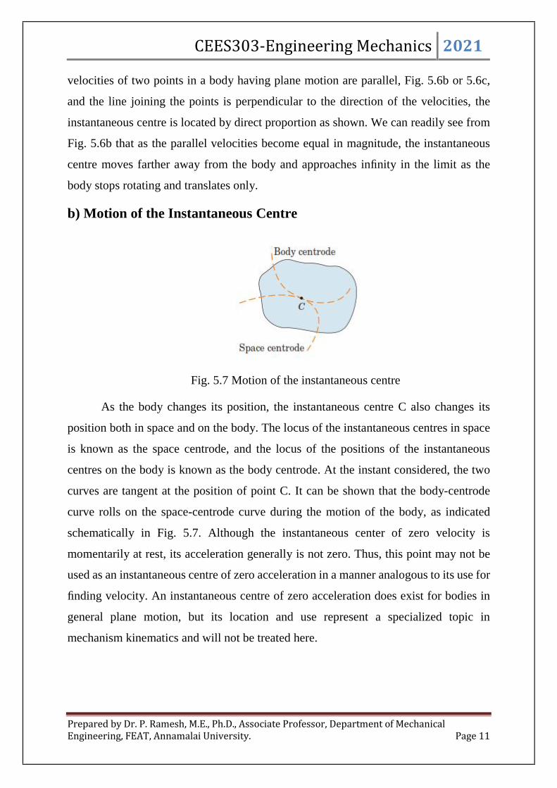
CEES303-Engineering Mechanics 2021
Prepared by Dr. P. Ramesh, M.E., Ph.D., Associate Professor, Department of MechanicalEngineering, FEAT, Annamalai University. Page 11
velocities of two points in a body having plane motion are parallel, Fig. 5.6b or 5.6c,
and the line joining the points is perpendicular to the direction of the velocities, the
instantaneous centre is located by direct proportion as shown. We can readily see from
Fig. 5.6b that as the parallel velocities become equal in magnitude, the instantaneous
centre moves farther away from the body and approaches infinity in the limit as the
body stops rotating and translates only.
b) Motion of the Instantaneous Centre
Fig. 5.7 Motion of the instantaneous centre
As the body changes its position, the instantaneous centre C also changes its
position both in space and on the body. The locus of the instantaneous centres in space
is known as the space centrode, and the locus of the positions of the instantaneous
centres on the body is known as the body centrode. At the instant considered, the two
curves are tangent at the position of point C. It can be shown that the body-centrode
curve rolls on the space-centrode curve during the motion of the body, as indicated
schematically in Fig. 5.7. Although the instantaneous center of zero velocity is
momentarily at rest, its acceleration generally is not zero. Thus, this point may not be
used as an instantaneous centre of zero acceleration in a manner analogous to its use for
finding velocity. An instantaneous centre of zero acceleration does exist for bodies in
general plane motion, but its location and use represent a specialized topic in
mechanism kinematics and will not be treated here.

CEES303-Engineering Mechanics 2021
Prepared by Dr. P. Ramesh, M.E., Ph.D., Associate Professor, Department of MechanicalEngineering, FEAT, Annamalai University. Page 12
Procedure:
Fig.5.6
First of all draw the initial and final positions of the rigid link as AB and A1B1
respectively.
Join AA1 and BB1.
Draw PQ right bisector of AA1 and RS right bisector of BB1.
Extend the two right bisector PQ and RS to meet at O. Which is required centre
of rotation or instantaneous centre as shown in fig. 5.6.
Let =Angular velocity of the rod AB about A.
Linear velocity of point A.
OAvA orOA
vA ------------- (i)
Similarly,OB
vB ------------- (ii)
Equating equations (i) and(ii),OA
OB
v
v
A
B
The direction of vA and vB will be at right angles to OA and OB respectively as
shown in fig.5.6
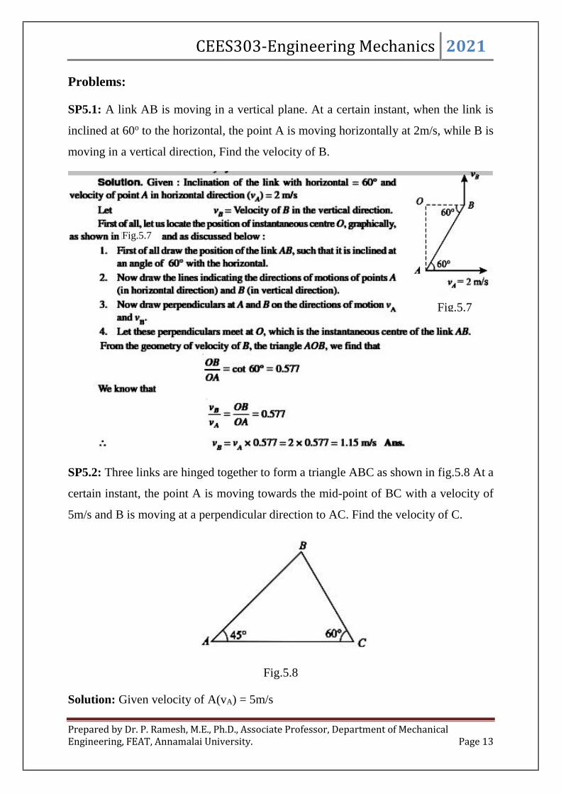
CEES303-Engineering Mechanics 2021
Prepared by Dr. P. Ramesh, M.E., Ph.D., Associate Professor, Department of MechanicalEngineering, FEAT, Annamalai University. Page 13
Problems:
SP5.1: A link AB is moving in a vertical plane. At a certain instant, when the link is
inclined at 60o to the horizontal, the point A is moving horizontally at 2m/s, while B is
moving in a vertical direction, Find the velocity of B.
SP5.2: Three links are hinged together to form a triangle ABC as shown in fig.5.8 At a
certain instant, the point A is moving towards the mid-point of BC with a velocity of
5m/s and B is moving at a perpendicular direction to AC. Find the velocity of C.
Fig.5.8
Solution: Given velocity of A(vA) = 5m/s
Fig.5.7
Fig.5.7
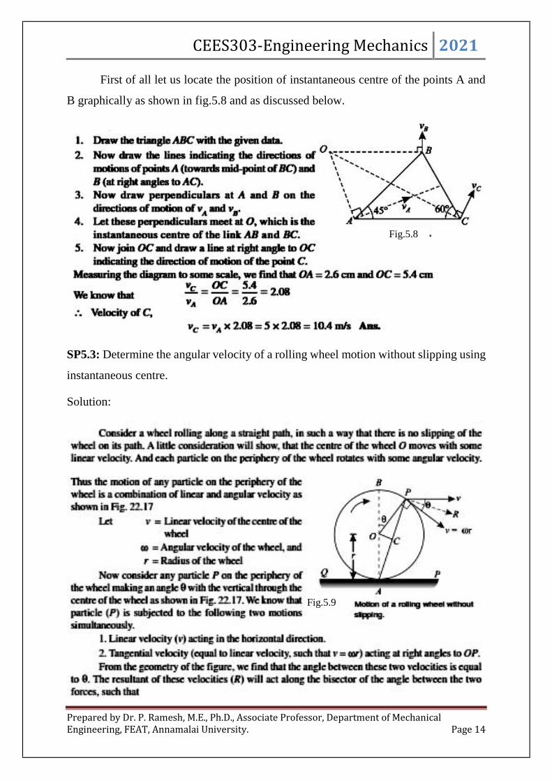
CEES303-Engineering Mechanics 2021
Prepared by Dr. P. Ramesh, M.E., Ph.D., Associate Professor, Department of MechanicalEngineering, FEAT, Annamalai University. Page 14
First of all let us locate the position of instantaneous centre of the points A and
B graphically as shown in fig.5.8 and as discussed below.
SP5.3: Determine the angular velocity of a rolling wheel motion without slipping using
instantaneous centre.
Solution:
Fig.5.8
Fig.5.9
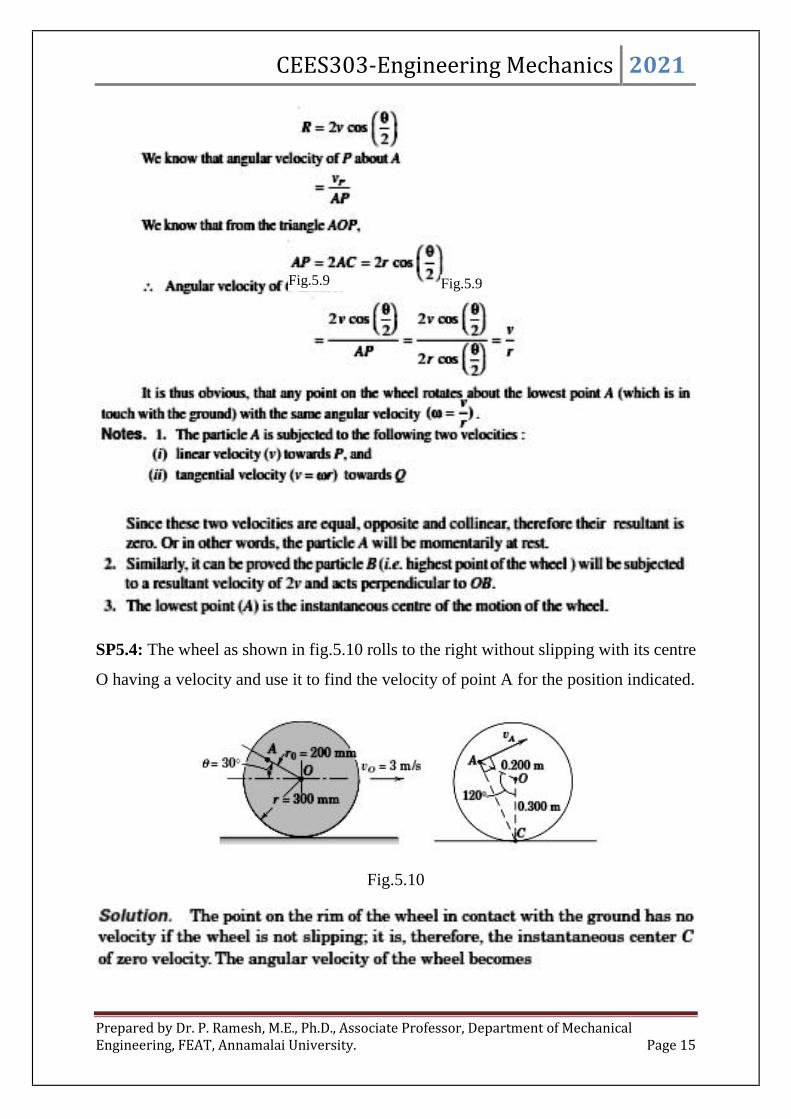
CEES303-Engineering Mechanics 2021
Prepared by Dr. P. Ramesh, M.E., Ph.D., Associate Professor, Department of MechanicalEngineering, FEAT, Annamalai University. Page 15
SP5.4: The wheel as shown in fig.5.10 rolls to the right without slipping with its centre
O having a velocity and use it to find the velocity of point A for the position indicated.
Fig.5.10
Fig.5.9Fig.5.9

CEES303-Engineering Mechanics 2021
Prepared by Dr. P. Ramesh, M.E., Ph.D., Associate Professor, Department of MechanicalEngineering, FEAT, Annamalai University. Page 16
SP5.5: Arm OB of the linkage has a clockwise angular velocity of 10 rad/sec in the
position shown where = 45o. Determine the velocity of A, the velocity of D and the
angular velocity of link AB for the position as shown in fig.5.11
Fig.5.11

CEES303-Engineering Mechanics 2021
Prepared by Dr. P. Ramesh, M.E., Ph.D., Associate Professor, Department of MechanicalEngineering, FEAT, Annamalai University. Page 17
SP5.6: Determine the velocity of piston of a reciprocating pump using instantaneous
centre method as shown in fig.5.12
Fig.5.12 velocity of a piston of reciprocating pump
Solution:
Fig.5.12
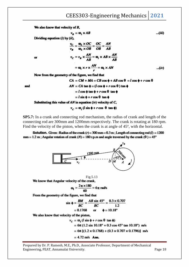
CEES303-Engineering Mechanics 2021
Prepared by Dr. P. Ramesh, M.E., Ph.D., Associate Professor, Department of MechanicalEngineering, FEAT, Annamalai University. Page 18
SP5.7: In a crank and connecting rod mechanism, the radius of crank and length of theconnecting rod are 300mm and 1200mm respectively. The crank is rotating at 180 rpm.Find the velocity of the piston, when the crank is at angle of 45o, with the horizontal.
Fig.5.13

CEES303-Engineering Mechanics 2021
Prepared by Dr. P. Ramesh, M.E., Ph.D., Associate Professor, Department of MechanicalEngineering, FEAT, Annamalai University. Page 19
D’ALEMBERT’S PRINCIPLE AND ITS APPLICATIONS IN
PLANE MOTION AND CONNECTED BODIES:
French mathematician Jean le Rond d’ Alembert proved in 1743 that the
newton’s second law of motion is applicable not only to the motion of a particle but
also to the motion of a body and looked at equation amF from different angle. The
equation amF may be written as
0 amF ---------- (5.9)
The term “ am ” may be looked as a force of magnitude am , applied in the
opposite direction of motion and is termed as the inertia force or reverse effective force.
D’Alembert looks at equation 5.9 as an equation of equilibrium and states that the
system of forces acting on a body in motion is in dynamic equilibrium with the
inertia force of the body. This is known as D’Alembert’s principle.
Let the body shown in fig.5.14 be subjected to a system of forces causing the
body to move with an acceleration a in the direction of the resultant. Then apply a force
equal to “ am ” in the reversed direction of acceleration as shown in fig.5.14. Now
according to D’Alembert’s principle, the equation of equilibrium 0 xF and 0 yF
may be used for the system of forces shown in fig.5.15.
Fig.5.14 Motion of a body Fig.5.15 The system of forces in
equilibrium
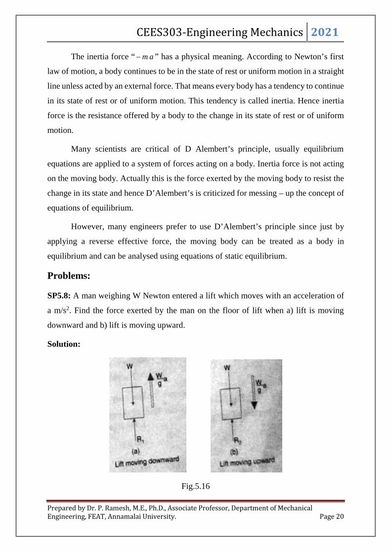
CEES303-Engineering Mechanics 2021
Prepared by Dr. P. Ramesh, M.E., Ph.D., Associate Professor, Department of MechanicalEngineering, FEAT, Annamalai University. Page 20
The inertia force “ am ” has a physical meaning. According to Newton’s first
law of motion, a body continues to be in the state of rest or uniform motion in a straight
line unless acted by an external force. That means every body has a tendency to continue
in its state of rest or of uniform motion. This tendency is called inertia. Hence inertia
force is the resistance offered by a body to the change in its state of rest or of uniform
motion.
Many scientists are critical of D Alembert’s principle, usually equilibrium
equations are applied to a system of forces acting on a body. Inertia force is not acting
on the moving body. Actually this is the force exerted by the moving body to resist the
change in its state and hence D’Alembert’s is criticized for messing – up the concept of
equations of equilibrium.
However, many engineers prefer to use D’Alembert’s principle since just by
applying a reverse effective force, the moving body can be treated as a body in
equilibrium and can be analysed using equations of static equilibrium.
Problems:
SP5.8: A man weighing W Newton entered a lift which moves with an acceleration of
a m/s2. Find the force exerted by the man on the floor of lift when a) lift is moving
downward and b) lift is moving upward.
Solution:
Fig.5.16
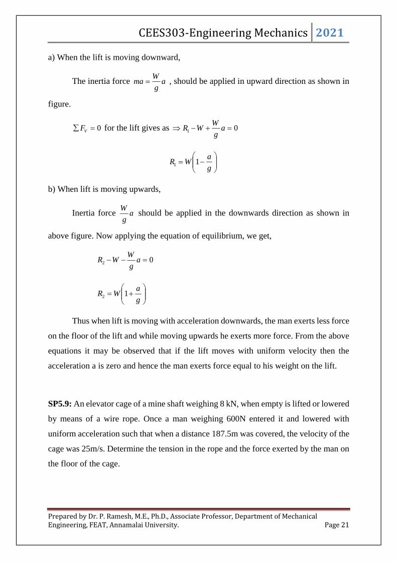
CEES303-Engineering Mechanics 2021
Prepared by Dr. P. Ramesh, M.E., Ph.D., Associate Professor, Department of MechanicalEngineering, FEAT, Annamalai University. Page 21
a) When the lift is moving downward,
The inertia force ag
Wma , should be applied in upward direction as shown in
figure.
0 VF for the lift gives as 01 ag
WWR
g
aWR 11
b) When lift is moving upwards,
Inertia force ag
Wshould be applied in the downwards direction as shown in
above figure. Now applying the equation of equilibrium, we get,
02 ag
WWR
g
aWR 12
Thus when lift is moving with acceleration downwards, the man exerts less force
on the floor of the lift and while moving upwards he exerts more force. From the above
equations it may be observed that if the lift moves with uniform velocity then the
acceleration a is zero and hence the man exerts force equal to his weight on the lift.
SP5.9: An elevator cage of a mine shaft weighing 8 kN, when empty is lifted or lowered
by means of a wire rope. Once a man weighing 600N entered it and lowered with
uniform acceleration such that when a distance 187.5m was covered, the velocity of the
cage was 25m/s. Determine the tension in the rope and the force exerted by the man on
the floor of the cage.

CEES303-Engineering Mechanics 2021
Prepared by Dr. P. Ramesh, M.E., Ph.D., Associate Professor, Department of MechanicalEngineering, FEAT, Annamalai University. Page 22
SP5.10: A motorist travelling at a speed of 70 kmph suddenly applies brakes and halts
after skidding 50m. Determine, 1) the time required to stop the car and 2) the coefficient
of friction between the tyres and the road.
Fig.5.17

CEES303-Engineering Mechanics 2021
Prepared by Dr. P. Ramesh, M.E., Ph.D., Associate Professor, Department of MechanicalEngineering, FEAT, Annamalai University. Page 23
SP5.11: A block weighing 1 kN rests on a horizontal plane as shown in fig.5.19 Findthe magnitude of the force P required to give the block an acceleration of 3m/s2 to theright. The coefficient of friction between the block and the plane is 0.25.
Fig.5.19
Fig.5.18
Fig.5.18
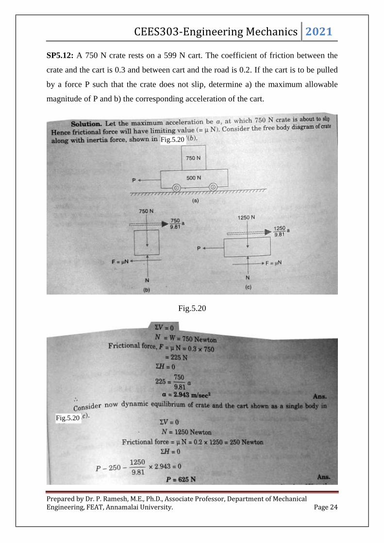
CEES303-Engineering Mechanics 2021
Prepared by Dr. P. Ramesh, M.E., Ph.D., Associate Professor, Department of MechanicalEngineering, FEAT, Annamalai University. Page 24
SP5.12: A 750 N crate rests on a 599 N cart. The coefficient of friction between the
crate and the cart is 0.3 and between cart and the road is 0.2. If the cart is to be pulled
by a force P such that the crate does not slip, determine a) the maximum allowable
magnitude of P and b) the corresponding acceleration of the cart.
Fig.5.20
Fig.5.20
Fig.5.20

CEES303-Engineering Mechanics 2021
Prepared by Dr. P. Ramesh, M.E., Ph.D., Associate Professor, Department of MechanicalEngineering, FEAT, Annamalai University. Page 25
SP5.13: A body weighing 1200 N rests on a rough plane inclined at 12o to the
horizontal. It is pulled up the plane by means of a light flexible rope running parallel to
the plane and passing over a light frictionless pulley at the top of the plane as shown in
fig.5.21 The portion of the rope beyond the pulley hangs vertically down and carries a
weight of 800 N at its end. If the coefficient of friction for the plane and the body is 0.2
find a) tension in the rope, b) acceleration with which the body moves up the plane and
c) the distance moved by the body in 3 seconds after starting from rest.
Fig.5.21

CEES303-Engineering Mechanics 2021
Prepared by Dr. P. Ramesh, M.E., Ph.D., Associate Professor, Department of MechanicalEngineering, FEAT, Annamalai University. Page 26
SP5.14: Two weights 800 N and 200 N are connected by a thread and they move along
a rough horizontal plane under the action of a force 400 N applied to the 800 N weight
as shown in fig. 5.22 The coefficient of friction between the sliding surface of the
weights and the plane is 0.3. Using D’Alembert’s principle determine the acceleration
of the weight and tension in the thread.
Fig.5.22
Fig.5.22

CEES303-Engineering Mechanics 2021
Prepared by Dr. P. Ramesh, M.E., Ph.D., Associate Professor, Department of MechanicalEngineering, FEAT, Annamalai University. Page 27
SP5.15; Two rough planes inclined at 30o and 60o to horizontal are placed back to back
as shown in fig.5.23 The blocks of weights 50N and 100N are placed on the faces and
are connected by a string running parallel to planes and passing over a frictionless
pulley. If the coefficient of friction between planes and blocks is 1/3, find the resulting
acceleration and tension in the string.
Solution: Let the assembly move down the 60o plane by an acceleration ‘a’ m/s2. Free
body diagrams of 100N and 50N blocks along with inertia forces are shown in figure.
Fig.5.23

CEES303-Engineering Mechanics 2021
Prepared by Dr. P. Ramesh, M.E., Ph.D., Associate Professor, Department of MechanicalEngineering, FEAT, Annamalai University. Page 28
SP5.16: Two blocks A and B released from rest on a 30o incline when they are 18m
apart. The coefficient of friction under the upper block A is 0.2 and that under the lower
block B is 0.4. In what time block A reaches the block B? After they touch and move
as a single unit, what will be the contact force between them? Weights of the block A
and B are 100N and 80N respectively.
Fig.5.24 (a, b, c)

CEES303-Engineering Mechanics 2021
Prepared by Dr. P. Ramesh, M.E., Ph.D., Associate Professor, Department of MechanicalEngineering, FEAT, Annamalai University. Page 29
5.24 5.24

CEES303-Engineering Mechanics 2021
Prepared by Dr. P. Ramesh, M.E., Ph.D., Associate Professor, Department of MechanicalEngineering, FEAT, Annamalai University. Page 30
SP5.17: Two bodies weighing 300N and 450N are hung to the ends of a rope passing
over an ideal pulley as shown in fig.5.25 with what acceleration the heavier body comes
down? What is the tension in the string?
Solution: Let a be the acceleration with which the system moves and T be the tension
in the string. Free body diagrams of 300N block and 450N blocks along with inertia
forces are shown in figure.
Fig.5.24
Fig.5.25

CEES303-Engineering Mechanics 2021
Prepared by Dr. P. Ramesh, M.E., Ph.D., Associate Professor, Department of MechanicalEngineering, FEAT, Annamalai University. Page 31
SP5.18: Determine the tension in the string and accelerations of blocks A and B
weighing 1500N and 500N connected by an inextensible string as shown in fig.5.26.
Assume pulleys as frictionless and weightless.
Solution: In this pulley system, it may be observed that if 1500N moves downward by
distance x, 500 N block moves up by 2x. Hence if acceleration of 1500N block is a that
of 500N block is 2a. The free body diagrams of 1500N and 500N blocks are shown in
figure along with inertia forces. According to D’Alembert’s principle the system of
forces shown in figure may be treated to be in equilibrium.
Fig.5.26
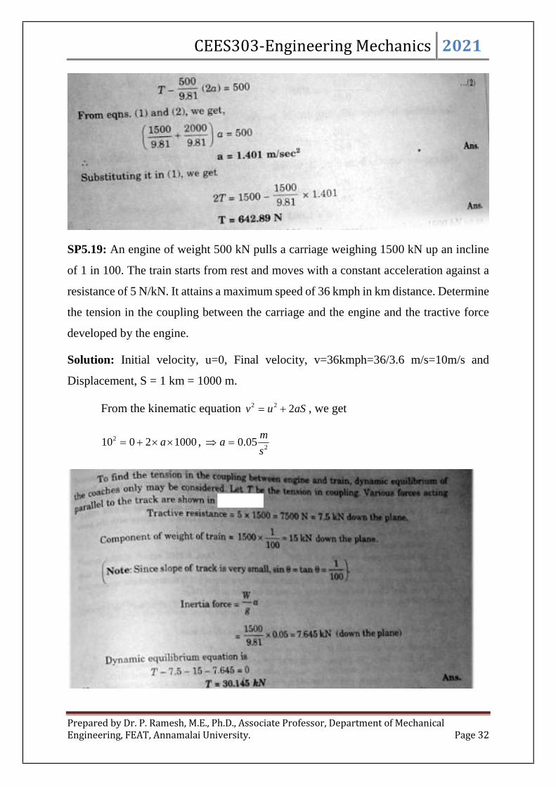
CEES303-Engineering Mechanics 2021
Prepared by Dr. P. Ramesh, M.E., Ph.D., Associate Professor, Department of MechanicalEngineering, FEAT, Annamalai University. Page 32
SP5.19: An engine of weight 500 kN pulls a carriage weighing 1500 kN up an incline
of 1 in 100. The train starts from rest and moves with a constant acceleration against a
resistance of 5 N/kN. It attains a maximum speed of 36 kmph in km distance. Determine
the tension in the coupling between the carriage and the engine and the tractive force
developed by the engine.
Solution: Initial velocity, u=0, Final velocity, v=36kmph=36/3.6 m/s=10m/s and
Displacement, S = 1 km = 1000 m.
From the kinematic equation aSuv 222 , we get
100020102 a ,2
05.0s
ma

CEES303-Engineering Mechanics 2021
Prepared by Dr. P. Ramesh, M.E., Ph.D., Associate Professor, Department of MechanicalEngineering, FEAT, Annamalai University. Page 33
WORK ENERGY PRINCIPLE AND ITS APPLICATIONS IN
PLANE MOTION OF CONNECTED BODIES:
In previous section, kinetic problems were solved using D’Alembert’s dynamic
equilibrium condition. In this section, another approach called Work – Energy approach
is used to solve kinetic problems. This method is advantageous over D’Alembert’s
method when the problem involves velocities rather than acceleration. The terms work,
energy and power are explained first, then the work energy equation is derived. Using
this equation a number of kinetic problems are solved.
a) Work:
The work done by a force on a moving body is defined as the product of the force
and the distance moved in the direction of the force. In fig.5. 28, various forces acting
on a particle are shown. If the particle moves a distance s in x direction, from A to B,
then the work done by various forces are as given below:
Fig.5.27
Fig.5.27

CEES303-Engineering Mechanics 2021
Prepared by Dr. P. Ramesh, M.E., Ph.D., Associate Professor, Department of MechanicalEngineering, FEAT, Annamalai University. Page 34
Force Work done
P1 P1 s
P2 + P2 (-s) = - P2 s
P3 P3 x 0 = 0
P4 P4 s cos
The general expression for work done by a force P is P s cos, where is the
angle between the force and the direction of motion. This expression may be rearranged
as P cos x s giving the new definition of work done. Thus work done by a force may
be defined as the product of component of force in the direction of motion and the
distance moved.
From the definition of work, it is obvious that unit of work is obtained by
multiplying unit of force by unit of length. Hence if newton is unit of force and metre
is unit of displacement, unit of work will be N-m. One N-m of work is denoted by the
term Joule (J). Hence one Joule may be defined as the amount of work done by the one
Newton force when the particle moves 1 metre in the direction of that force.
The other commonly used units are: kilo joules kJ (i.e., kN-m) or milli Joule mJ
(N-mm) etc.
b) Work done by a varying force:
Fig.5.29 Varying force
Fig.5.28

CEES303-Engineering Mechanics 2021
Prepared by Dr. P. Ramesh, M.E., Ph.D., Associate Professor, Department of MechanicalEngineering, FEAT, Annamalai University. Page 35
Let the varying force acting at any instance on the particle be P. Now if the
particle moves a small distance s, then the work done by the force is P x s. Work done
by the force in moving the body by a distance s is P s. Thus if a force versus
displacement curve is drawn as shown in fig.5.29 , the area under the curve gives the
work done by the force. If the variation of P is in a regular fashion, then
PdsPs ------------ (5.10)
c) Energy:
Energy is defined as the capacity to do work. There are many forms of energy
like heat energy, mechanical energy, electrical energy and chemical energy. In
engineering mechanics we are interested in mechanical energy. This energy may be
classified into potential energy and
kinetic energy.
Potential energy is the capacity
to do work due to the position of the
body. A body of weight ‘W’ held at a
height h possesses an energy Wh.
Kinetic energy is the capacity to do work due to motion of the body. Consider a
car moving with a velocity v m/s. If the engine is stopped, it still moves forward, doing
work against frictional resistance and stops at a certain distance s. From the kinematic
of the motion, we have
aSu 20 2 ,S
ua
2
2
From D’Alembert’s principle,
0 ag
WF
02
2
S
u
g
WF ,
gS
WuF
2
2
Fig.5.30

CEES303-Engineering Mechanics 2021
Prepared by Dr. P. Ramesh, M.E., Ph.D., Associate Professor, Department of MechanicalEngineering, FEAT, Annamalai University. Page 36
gS
WuSFdoneWork
2
2
----------------- (5.11)
This work is done by the energy stored initially in the body.
Therefore, 2
2
1v
g
WrgyKineticene , ---------------- (5.12)
Where v is the velocity of the body
Unit of energy is same as that of work, since it is nothing but capacity to do work.
It is measured in Joules J (N-m) or kilo Joules kJ (i.e., kN-m).
d) Power:
Power is defined as time rate of doing work. Unit of power is Watt (w) and is
defined as one Joule of work done in one second. In practice kilowatt is the commonly
used unit which is equal to 1000 watts. Horse power is the unit used in MKS and FPS
systems.
1 metric H.P = 735.75 watts and 1 British H.P = 745.8 watts
e) Work energy equation for
translation:
Consider the body as shown in fig.5.31
subject to a system of forces F1, F2, … and
moving with an acceleration a in x – direction.
Let its initial velocity at A be u and final velocity
when it moves distance AB = s be v. Then the resultant of system of the forces must be
in x – direction. Let
xFR -------- (5.13)
From Newton’s second law of motion,
ag
WR
Multiplying both sides by elementary distance ds, we get
Fig.5.31

CEES303-Engineering Mechanics 2021
Prepared by Dr. P. Ramesh, M.E., Ph.D., Associate Professor, Department of MechanicalEngineering, FEAT, Annamalai University. Page 37
adsg
WRds
dsds
dvv
g
WRds [
ds
dvva ]
vdvg
WRds
Integrating both sides for the motion from A to B we get,
v
u
S
vdvg
WRds
0
v
u
v
g
WRS
2
2
22
2uv
g
WRS
Now R.S is the work done by the forces acting on the body. 2
2v
g
Wis final kinetic
energy andg
Wu
2
2
is initial kinetic energy. Hence we can say, work done in a motion is
equal to change in kinetic energy. That is,
Work done = Final kinetic energy – Initial kinetic energy (5.14)
The equation 5.14 Is called Work Energy Equation.
This work energy equation may be stated as the work done by a system of forces
acting on a body during a displacement is equal to the change in kinetic energy of the
body during the same displacement.
Using this work energy equation a number of kinetic problems can be solved.
This will be found more useful than D’Alembert’s principle when we are not interested
in finding acceleration in the problem, but mainly interested in velocity and distance.
f) Work done by a spring:
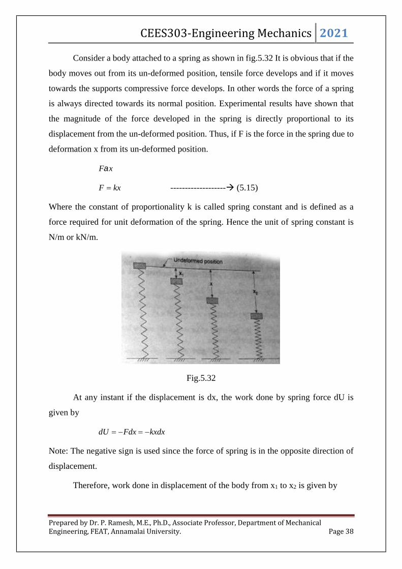
CEES303-Engineering Mechanics 2021
Prepared by Dr. P. Ramesh, M.E., Ph.D., Associate Professor, Department of MechanicalEngineering, FEAT, Annamalai University. Page 38
Consider a body attached to a spring as shown in fig.5.32 It is obvious that if the
body moves out from its un-deformed position, tensile force develops and if it moves
towards the supports compressive force develops. In other words the force of a spring
is always directed towards its normal position. Experimental results have shown that
the magnitude of the force developed in the spring is directly proportional to its
displacement from the un-deformed position. Thus, if F is the force in the spring due to
deformation x from its un-deformed position.
xF
kxF ------------------- (5.15)
Where the constant of proportionality k is called spring constant and is defined as a
force required for unit deformation of the spring. Hence the unit of spring constant is
N/m or kN/m.
Fig.5.32
At any instant if the displacement is dx, the work done by spring force dU is
given by
kxdxFdxdU
Note: The negative sign is used since the force of spring is in the opposite direction of
displacement.
Therefore, work done in displacement of the body from x1 to x2 is given by
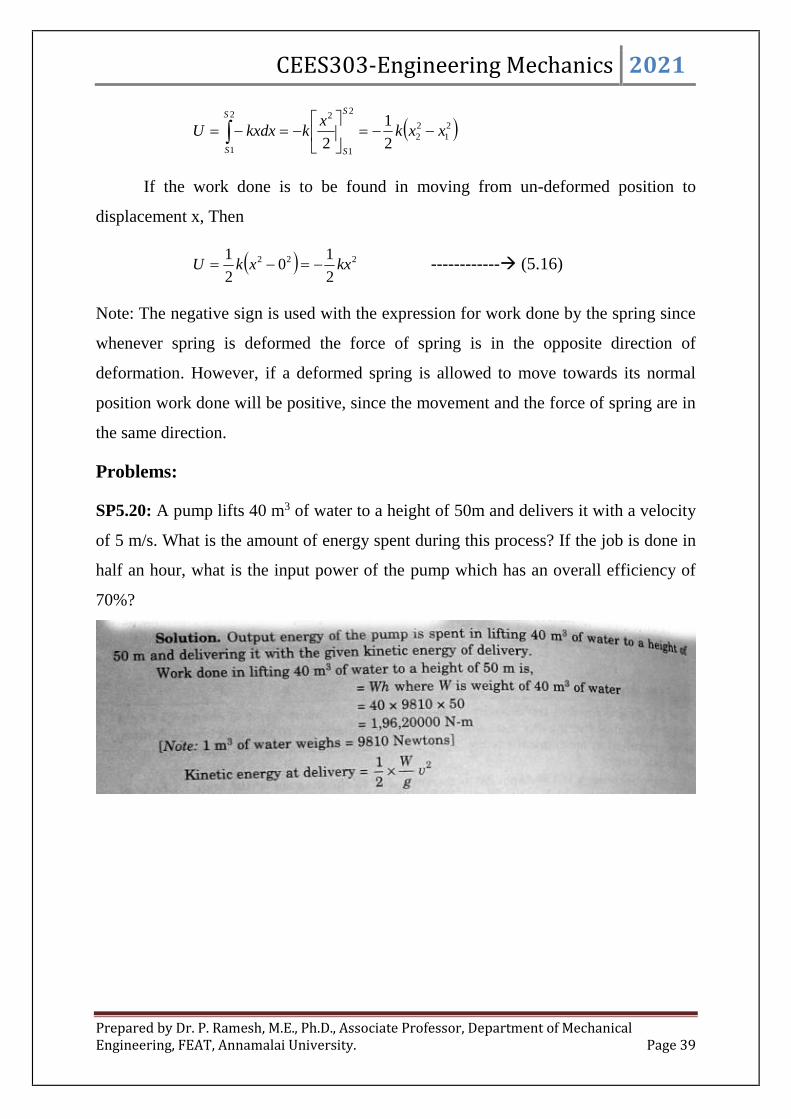
CEES303-Engineering Mechanics 2021
Prepared by Dr. P. Ramesh, M.E., Ph.D., Associate Professor, Department of MechanicalEngineering, FEAT, Annamalai University. Page 39
2122
2
1
22
1 2
1
2xxk
xkkxdxU
S
S
S
S
If the work done is to be found in moving from un-deformed position to
displacement x, Then
222
2
10
2
1kxxkU ------------ (5.16)
Note: The negative sign is used with the expression for work done by the spring since
whenever spring is deformed the force of spring is in the opposite direction of
deformation. However, if a deformed spring is allowed to move towards its normal
position work done will be positive, since the movement and the force of spring are in
the same direction.
Problems:
SP5.20: A pump lifts 40 m3 of water to a height of 50m and delivers it with a velocity
of 5 m/s. What is the amount of energy spent during this process? If the job is done in
half an hour, what is the input power of the pump which has an overall efficiency of
70%?

CEES303-Engineering Mechanics 2021
Prepared by Dr. P. Ramesh, M.E., Ph.D., Associate Professor, Department of MechanicalEngineering, FEAT, Annamalai University. Page 40
SP5.21: A bullet of mass 30 gram is fired into body of mass 10kg which is suspended
by a spring 0.8m long. Due to this impact, the body swings through an angle 30o. Find
the velocity of the bullet.
Fig.5.33

CEES303-Engineering Mechanics 2021
Prepared by Dr. P. Ramesh, M.E., Ph.D., Associate Professor, Department of MechanicalEngineering, FEAT, Annamalai University. Page 41
KINETICS OF RIGID BODY ROTATION:
Consider the wheel as shown in fig.5.34 rotating about its axis in clockwise
direction with an acceleration . Let m be mass of an element at
a distance r from the axis of rotation. If p be the resulting force
on this element.
amp , where a is tangential acceleration
But a = r, where is angular acceleration
rmp
Rotational moment Mt due to this force p is given by
rpM t
2rmM t
2rmMM tt
2rmM t
IM t , where I is mass moment of inertia of the rotating body
Thus, IM t ------------- (5.17)
Note the similarly between the expression IM t and amF used in linear
motion.
Force causes linear motion while rotational moment cause angular motion. The
force is equal to the product of mass and the linear acceleration whereas rotational
moment is the product of mass moment of inertia and the angular acceleration.
Fig.5.34

CEES303-Engineering Mechanics 2021
Prepared by Dr. P. Ramesh, M.E., Ph.D., Associate Professor, Department of MechanicalEngineering, FEAT, Annamalai University. Page 42
The product of the mass moment of inertia and the angular velocity of a rotating
body is called Angular momentum. Thus
ImomentumAngular --------------- (5.18)
Kinetic Energy of Rotating Bodies:
Consider the rotating body as shown in fig.5.35 with
angular velocity . Let m be mass of an element which is at a
distance r from the axis of rotation. Hence, if v is the linear
velocity
rv
Now, Kinetic energy of the elemental mass
2
2
1vm
Therefore, K.E. of the rotating body
2
2
1vm
22
2
1 rm
22
2
1rm
But from the definition of mass moment of inertia,
2rmI
Therefore, 2
2
1. IEK
Fig.5.35

CEES303-Engineering Mechanics 2021
Prepared by Dr. P. Ramesh, M.E., Ph.D., Associate Professor, Department of MechanicalEngineering, FEAT, Annamalai University. Page 43
Particulars Linear motion Angular motion
1 Displacement S
2 Initial velocity u 0
3 Final velocity V
4 Acceleration a
5 Formula for final velocity atuv t 0
6 Formula for displacement 2
2
1atutS 2
0 2
1tt
7 Formula in terms of
displacement, velocity and
acceleration
aSuv 222 220
2
8 Force causing motion maF IM t
9 Momentum mv I
10 Kinetic energy 2
2
1mv 2
2
1I

CEES303-Engineering Mechanics 2021
Prepared by Dr. P. Ramesh, M.E., Ph.D., Associate Professor, Department of MechanicalEngineering, FEAT, Annamalai University. Page 44
Problems,
SP5.22: Derive an expression for the fluctuation energy of flywheel.
Fig.5.36

CEES303-Engineering Mechanics 2021
Prepared by Dr. P. Ramesh, M.E., Ph.D., Associate Professor, Department of MechanicalEngineering, FEAT, Annamalai University. Page 45
SP5.23: A flywheel of an engine has a mass of 6.5 tonnes and radius of gyration 1.8
metres. If the maximum and minimum speeds of the flywheel are 120 rpm and 118 rpm
respectively, find the fluctuation of energy.
SP5.24: A flywheel of mass 8 tonnes starts from rest and gets up a speed of 180 rpm in
3 minutes. Find the average torque exerted on it, if the radius of gyration of the flywheel
is 60cm.
SP5.25: A flywheel is made up of steel ring 40mm thick and 200mm wide plate with
mean diameter of 2 metres. If initially the flywheel is rotating at 300 rpm, find the time
taken by the wheel in coming to rest due to frictional couple of 100 N-m. Take mass
density of the stell as 7900 kg/m3. Neglect the effect of the spokes.

CEES303-Engineering Mechanics 2021
Prepared by Dr. P. Ramesh, M.E., Ph.D., Associate Professor, Department of MechanicalEngineering, FEAT, Annamalai University. Page 46
SP5.26: A flywheel weighing 50 kN and having radius of gyration 1metre loses its
speed from 400 rpm to 280 rpm in 2 minutes. Calculate i) the retarding torque acting on
it, ii) change in its kinetic energy during the above period and iii) change in its angular
momentum during the same period.
Solution:

CEES303-Engineering Mechanics 2021
Prepared by Dr. P. Ramesh, M.E., Ph.D., Associate Professor, Department of MechanicalEngineering, FEAT, Annamalai University. Page 47
SP5.27: A pulley of weight 400N has a radius 0f 0.6m. A block of 600N is suspended
by a tight rope wound round the pulley, the other end being attached to the pulley as
shown in fig.5.37 Determine the resulting acceleration of the weight and the tension in
the rope.

CEES303-Engineering Mechanics 2021
Prepared by Dr. P. Ramesh, M.E., Ph.D., Associate Professor, Department of MechanicalEngineering, FEAT, Annamalai University. Page 48
SP5.28: The composite pulley shown in fig.5. weighs 800 N and has a radius of gyration
of 0.6 m. The 2000 N and 4000 N blocks are attached to the pulley by inextensible
strings as shown in the figure. Neglecting weight of the strings, determine the tension
in the strings and angular acceleration of the pulley.
Fig.5.37
Fig.5.38

CEES303-Engineering Mechanics 2021
Prepared by Dr. P. Ramesh, M.E., Ph.D., Associate Professor, Department of MechanicalEngineering, FEAT, Annamalai University. Page 49
SP5.29: A cylinder weighing 500N is welded to a 1m long uniform bar of 200N as
shown in fig.5.39 Determine the acceleration with which the assembly will rotate about
point A, if released from rest in horizontal position. Determine the reaction of A at this
instant.
Fig.5.39

CEES303-Engineering Mechanics 2021
Prepared by Dr. P. Ramesh, M.E., Ph.D., Associate Professor, Department of MechanicalEngineering, FEAT, Annamalai University. Page 50
SP5.30: Road AB weighing 200N is welded to the rod CD weighing 100N as shown in
fig.5.40 The assembly is hinged at A and is freely held. Determine the instantaneous
vertical and horizontal reactions of A when a horizontal force of 300N acts at a distance
of 0.75m from A.

CEES303-Engineering Mechanics 2021
Prepared by Dr. P. Ramesh, M.E., Ph.D., Associate Professor, Department of MechanicalEngineering, FEAT, Annamalai University. Page 51
SP5.31: A train loaded with cars has a total mass of 6 tonnes is hauled up an incline of
1 in 30 by a rope coiled on a winding drum at the top of the incline. The drum is 1.0m
in diameter and has a mass of 1 tonnes and has a radius of gyration of 0.45m. The drum
Fig.5.40

CEES303-Engineering Mechanics 2021
Prepared by Dr. P. Ramesh, M.E., Ph.D., Associate Professor, Department of MechanicalEngineering, FEAT, Annamalai University. Page 52
axle friction is negligible. If a torque of 3 kN-m is applied to the drum from a driving
motor, determine the tension in the rope.
Fig.5.41

CEES303-Engineering Mechanics 2021
Prepared by Dr. P. Ramesh, M.E., Ph.D., Associate Professor, Department of MechanicalEngineering, FEAT, Annamalai University. Page 53
Fig.5.42
Fig.5.42
SP5.32:

CEES303-Engineering Mechanics 2021
Prepared by Dr. P. Ramesh, M.E., Ph.D., Associate Professor, Department of MechanicalEngineering, FEAT, Annamalai University. Page 54

CEES303-Engineering Mechanics 2021
Prepared by Dr. P. Ramesh, M.E., Ph.D., Associate Professor, Department of MechanicalEngineering, FEAT, Annamalai University. Page 55
SP5.33: Derive the force of friction and acceleration relation for motion of a body
rolling on a rough horizontal plane without slipping.
Fig.5.43

CEES303-Engineering Mechanics 2021
Prepared by Dr. P. Ramesh, M.E., Ph.D., Associate Professor, Department of MechanicalEngineering, FEAT, Annamalai University. Page 56

CEES303-Engineering Mechanics 2021
Prepared by Dr. P. Ramesh, M.E., Ph.D., Associate Professor, Department of MechanicalEngineering, FEAT, Annamalai University. Page 57
Fig.5.44
SP5.34:
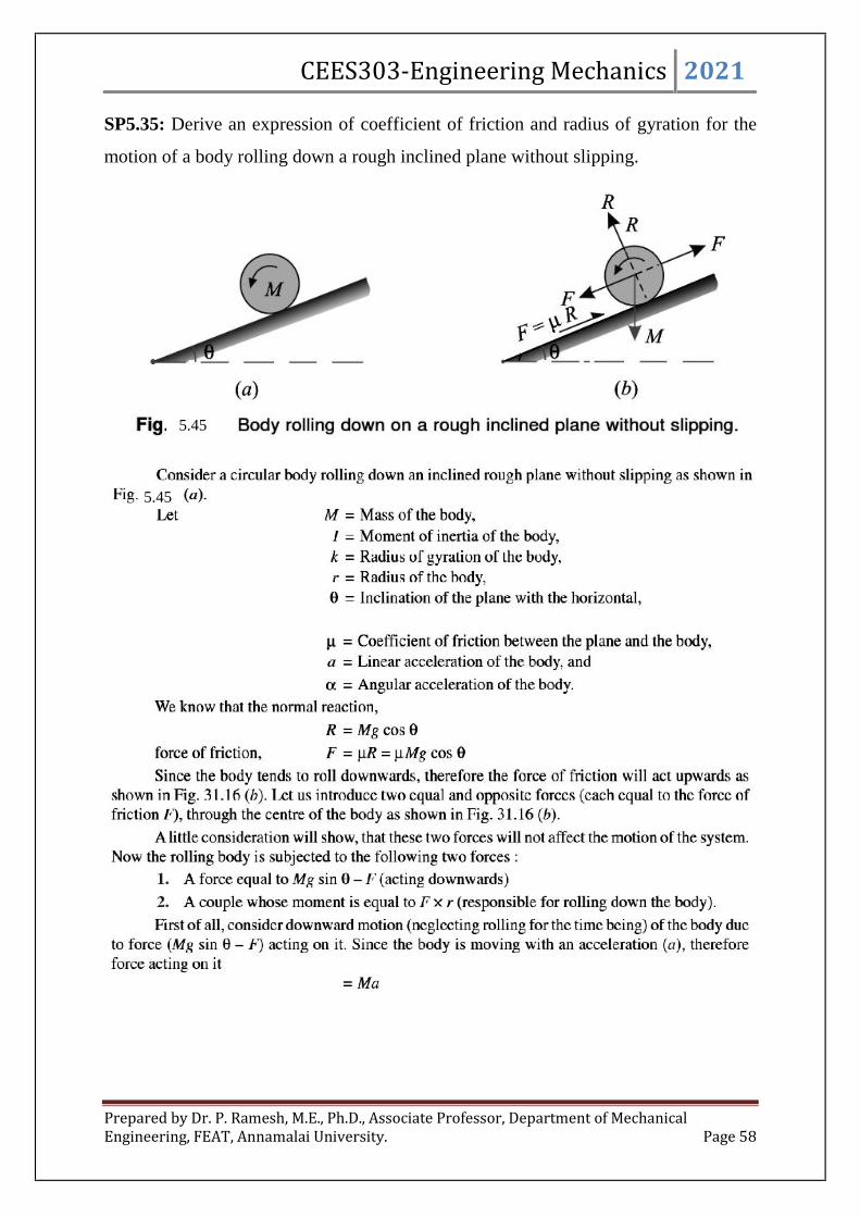
CEES303-Engineering Mechanics 2021
Prepared by Dr. P. Ramesh, M.E., Ph.D., Associate Professor, Department of MechanicalEngineering, FEAT, Annamalai University. Page 58
SP5.35: Derive an expression of coefficient of friction and radius of gyration for the
motion of a body rolling down a rough inclined plane without slipping.
5.45
5.45

CEES303-Engineering Mechanics 2021
Prepared by Dr. P. Ramesh, M.E., Ph.D., Associate Professor, Department of MechanicalEngineering, FEAT, Annamalai University. Page 59

CEES303-Engineering Mechanics 2021
Prepared by Dr. P. Ramesh, M.E., Ph.D., Associate Professor, Department of MechanicalEngineering, FEAT, Annamalai University. Page 60
SP5.36: A sphere rolls down a plane inclined at 30o to the horizontal. Find the minimum
value of the coefficient of friction between the sphere and the plane, so that the sphere
may roll without slipping.
SP5.37: A solid uniformly thick wheel of radius 1 m and mass 40 kg is released withno initial velocity at the top of an inclined plane, which makes an angle of 30o with thehorizontal. It rolls down without slipping. Determine i) the minimum value ofcoefficient of friction, ii) the velocity of the centre of the wheel after it has travelled adistance 4m down the inclined plane.

CEES303-Engineering Mechanics 2021
Prepared by Dr. P. Ramesh, M.E., Ph.D., Associate Professor, Department of MechanicalEngineering, FEAT, Annamalai University. Page 61
MECHANICAL VIBRATIONS COVERING:
A mechanical vibration is the motion of a particle or a body which oscillates
about a position of equilibrium. Most vibrations in machines and structures are
undesirable because of the increased stresses and energy losses which accompany them.
They should therefore be eliminated or reduced as much as possible by appropriate
design. The analysis of vibrations has become increasingly important in recent years
owing to the current trend toward higher-speed machines and lighter structures. There
is every reason to expect that this trend will continue and that an even greater need for
vibration analysis will develop in the future.
The analysis of vibrations is a very extensive subject to which entire texts have
been devoted. This study will therefore be limited to the simpler types of vibrations,
namely, the vibrations of a body or a system of bodies with one degree of freedom. A
mechanical vibration generally results when a system is displaced from a position of
stable equilibrium. The system tends to return to this position under the action of
restoring forces (either elastic forces, as in the case of a mass attached to a spring, or
gravitational forces, as in the case of a pendulum). But the system generally reaches its
original position with a certain acquired velocity which carries it beyond that position.
Since the process can be repeated indefinitely, the system keeps moving back and forth
across its position of equilibrium. The time interval required for the system to complete
a full cycle of motion is called the period of the vibration. The number of cycles per
unit time defines the frequency, and the maximum displacement of the system from its
position of equilibrium is called the amplitude of the vibration.
When the motion is maintained by the restoring forces only, the vibration is said
to be a free vibration. When a periodic force is applied to the system, the resulting
motion is described as a forced vibration. When the effects of friction can be neglected,
the vibrations are said to be un-damped. However, all vibrations are actually damped to
some degree. If a free vibration is only slightly damped, its amplitude slowly decreases
until, after a certain time, the motion comes to a stop. But if damping is large enough to
prevent any true vibration, the system then slowly regains its original position. A

CEES303-Engineering Mechanics 2021
Prepared by Dr. P. Ramesh, M.E., Ph.D., Associate Professor, Department of MechanicalEngineering, FEAT, Annamalai University. Page 62
damped forced vibration is maintained as long as the periodic force which produces the
vibration is applied. The amplitude of the vibration, however, is affected by the
magnitude of the damping forces.
Basic terminology:
1. Periodic Motion2. Time Period3. Cycle4. Frequency5. Amplitude6. Natural Frequency7. The fundamental mode of vibration8. Degree of freedom9. Simple harmonic motion10.Damping11. Resonance12. Mechanical System
1. Periodic Motion:
The motion which repeats itself after an equal interval of times is calledPeriodic motion.
2. Time Period:
This is defined as time to complete one cycle is called a Time period and it isnormally expressed in seconds (s).
3. Cycle:
It is motion completed during one time period.
4. Frequency:
This is defined as the number of cycles describes in one second. This SI unit isHertz.
5. Amplitude:
The maximum displacement of the vibrating body from its equilibrium position.
6. Natural frequency:
When no external force acts on the system after giving its an initial displacement,the body vibrates. The vibration is called as free vibration and the frequency is calledNatural frequency. This is expressed in rad/sec or Hertz.
CEES303-Engineering Mechanics 2021
Prepared by Dr. P. Ramesh, M.E., Ph.D., Associate Professor, Department of MechanicalEngineering, FEAT, Annamalai University. Page 63
7. The fundamental mode of vibration:
The fundamental mode of vibration is the model having the lowest natural
frequency
8. Degree of Freedom:
The minimum number of independent coordinates require to specify the motionof a system at any instant is known as the degree of freedom.
9. Simple Harmonic Motion:
The motion of the body to and fro about a fixed point is called simple harmonic
motion.
10. Damping:
It is resistance to the motion of a vibrating body. The vibration associated withthe resistance is known as Damped Vibration.
11. Resonance:
When the frequency of external excitation is equal to the natural frequency ofthe vibrating body, the amplitude of vibration becomes excessively large. This conceptis called resonance.
12. Mechanical System:
The system consists of Mass, stiffness, and damping are known as a mechanical
system.
FREE AND FORCED VIBRATIONS:
1) Free vibration:
If a system, after an initial disturbance is left to vibrate on its own, the ensuing
vibration is known as free vibration. No external force acts on the system. The oscillat
ion of a simple pendulum is an example of free vibration.

CEES303-Engineering Mechanics 2021
Prepared by Dr. P. Ramesh, M.E., Ph.D., Associate Professor, Department of MechanicalEngineering, FEAT, Annamalai University. Page 64
Types of free vibrations:
A) Linear / Longitudinal vibrations: When the disc is displaced vertically
downwards by an external force and released as shown in the figure 4, all the
particles of the rod and disc move parallel to the axis of shaft. The rod is
elongated and shortened alternately and thus the tensile and compressive stresses
are induced alternately in the rod. The vibration occurs is known as
Linear/Longitudinal vibrations.
B) Transverse vibrations: When the rod is displaced in the transverse direction by
an external force and released as shown in the figure 5, all the particles of rod
and disc move approximately perpendicular to the axis of the rod. The shaft is
straight and bends alternately inducing bending stresses in the rod. The vibration
occurs is known as transverse vibrations.
C) Torsional vibrations: When the rod is twisted about its axis by an external force
and released as shown in the figure 6, all the particles of the rod and disc move
in a circle about the axis of the rod. The rod is subjected to twist and torsional
shear stress is induced. The vibration occurs is known as torsional vibrations.
2) Forced vibration:
If a system is subjected to an external force (often a
repeating type of force), the resulting vibration is known as forced vibration.
RESONANCE AND ITS EFFECTS:
If the frequency of the external force coincides with one of the natural
frequencies of the system, a condition known as resonance occurs and the system
undergoes dangerously large oscillations. Failures of such structures as buildings,
bridges, turbines and airplane wings have been associated with the occurrence of
resonance.

CEES303-Engineering Mechanics 2021
Prepared by Dr. P. Ramesh, M.E., Ph.D., Associate Professor, Department of MechanicalEngineering, FEAT, Annamalai University. Page 65
DEGREE OF FREEDOM:
The minimum number of independent coordinates required to determine
completely the positions of all parts of a system at any instant of time defines the degree
of freedom of the system.
A single degree of freedom system requires only one coordinate to describe its
position at any instant of time.
Fig.5.46 Single degree of freedom
Fig.5.47 Simple pendulum
For the simple pendulum in the fig.5. , the motion can be stated either in terms
of or x and y. If the coordinates x and y are used to describe the motion, it must be
recognized that these coordinates are not independent. They are related to each other
through the relation.
222 lyx --------- (5.19)
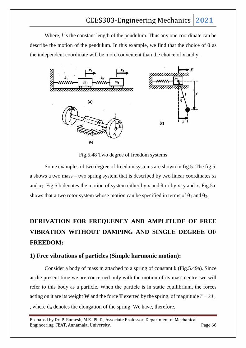
CEES303-Engineering Mechanics 2021
Prepared by Dr. P. Ramesh, M.E., Ph.D., Associate Professor, Department of MechanicalEngineering, FEAT, Annamalai University. Page 66
Where, l is the constant length of the pendulum. Thus any one coordinate can be
describe the motion of the pendulum. In this example, we find that the choice of as
the independent coordinate will be more convenient than the choice of x and y.
Fig.5.48 Two degree of freedom systems
Some examples of two degree of freedom systems are shown in fig.5. The fig.5.
a shows a two mass – two spring system that is described by two linear coordinates x1
and x2. Fig.5.b denotes the motion of system either by x and or by x, y and x. Fig.5.c
shows that a two rotor system whose motion can be specified in terms of 1 and 2.
DERIVATION FOR FREQUENCY AND AMPLITUDE OF FREE
VIBRATION WITHOUT DAMPING AND SINGLE DEGREE OF
FREEDOM:
1) Free vibrations of particles (Simple harmonic motion):
Consider a body of mass m attached to a spring of constant k (Fig.5.49a). Since
at the present time we are concerned only with the motion of its mass centre, we will
refer to this body as a particle. When the particle is in static equilibrium, the forces
acting on it are its weight W and the force T exerted by the spring, of magnitude stkdT
, where dst denotes the elongation of the spring. We have, therefore,

CEES303-Engineering Mechanics 2021
Prepared by Dr. P. Ramesh, M.E., Ph.D., Associate Professor, Department of MechanicalEngineering, FEAT, Annamalai University. Page 67
stkdW
Fig.5.49
Suppose now that the particle is displaced through a distance xm from its
equilibrium position and released with no initial velocity. If xm has been chosen smaller
than dst, the particle will move back and forth through its equilibrium position; a
vibration of amplitude xm has been generated. Note that the vibration can also be
produced by imparting a certain initial velocity to the particle when it is in its
equilibrium position x=0 or, more generally, by starting the particle from any given
position x=x0 with a given initial velocity v0.
To analyze the vibration, let us consider the particle in a position P at some
arbitrary time t (Fig. 5.49b). Denoting by x the displacement OP measured from the
equilibrium position O (positive downward), we note that the forces acting on the
particle are its weight W and the force T exerted by the spring which, in this position,
has a magnitude xdkT st . Recalling that stkdW , we find that the magnitude of the
resultant F of the two forces (positive downward) is
kxxdkWF st )( ---------- (5.20)
Thus the resultant of the forces exerted on the particle is proportional to the
displacement OP measured from the equilibrium position. Recalling the sign

CEES303-Engineering Mechanics 2021
Prepared by Dr. P. Ramesh, M.E., Ph.D., Associate Professor, Department of MechanicalEngineering, FEAT, Annamalai University. Page 68
convention, we note that F is always directed toward the equilibrium position O.
Substituting for F into the fundamental equation F= m a and recalling that a is the second
derivative
x of x with respect to t, we write
0
kxxm ------------ (5.21)
Note that the same sign convention should be used for the acceleration
x and for
the displacement x, namely, positive downward.
The motion defined by Eq. 5.21 is called a simple harmonic motion. It is
characterized by the fact that the acceleration is proportional to the displacement and of
opposite direction. We can verify that each of the functions
t
m
kx sin1 and
t
m
kx cos2 satisfies Eq.5.21. These functions, therefore, constitute two particular
solutions of the differential equation 5.21. The general solution of Eq. 5.21 is obtained
by multiplying each of the particular solutions by an arbitrary constant and adding.
Thus, the general solution is expressed as
t
m
kCt
m
kCxCxCx cossin 212211 --------- (5.22)
We note that x is a periodic function of the time t and does, therefore, represent
a vibration of the particle P. The coefficient of t in the expression we have obtained is
referred to as the natural circular frequency of the vibration and is denoted by vn. We
have
Natural circular frequency =m
kVn --------- (5.23)
Substituting form
kinto Eq. 5.22, we write
tVCtVCx nn cossin 21 -------- (5.24)
This is the general solution of the differential equation
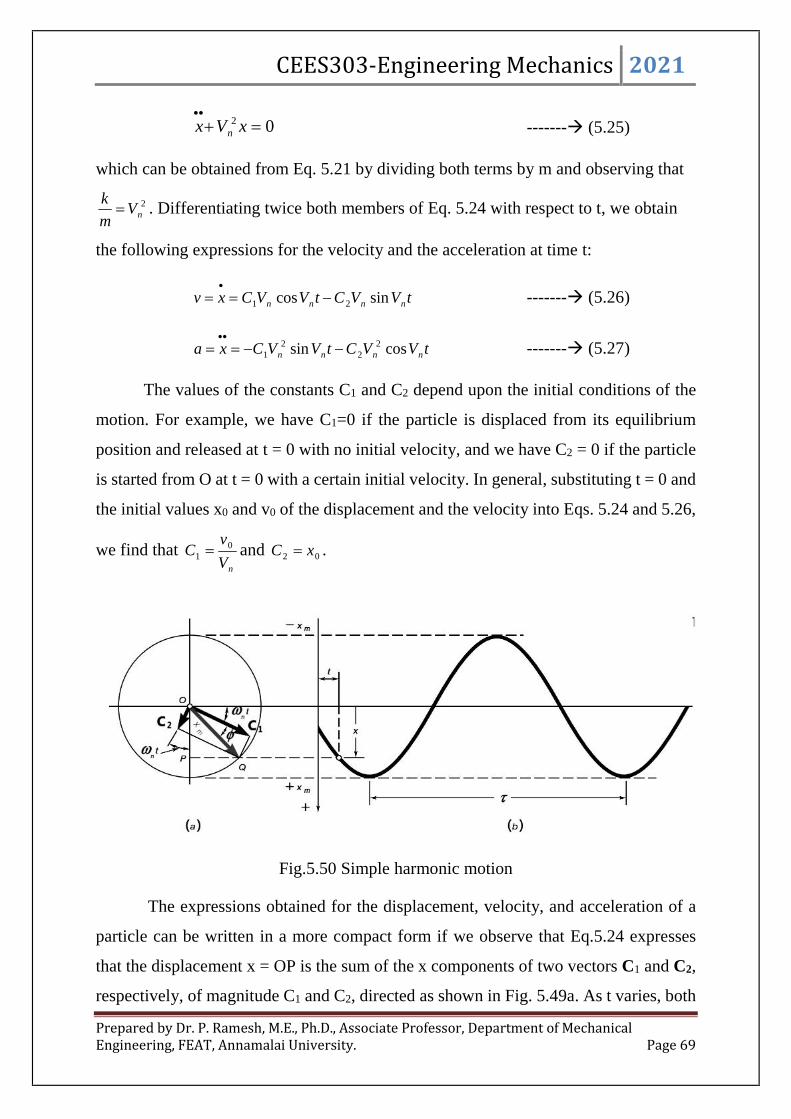
CEES303-Engineering Mechanics 2021
Prepared by Dr. P. Ramesh, M.E., Ph.D., Associate Professor, Department of MechanicalEngineering, FEAT, Annamalai University. Page 69
02
xVx n ------- (5.25)
which can be obtained from Eq. 5.21 by dividing both terms by m and observing that
2nV
m
k . Differentiating twice both members of Eq. 5.24 with respect to t, we obtain
the following expressions for the velocity and the acceleration at time t:
tVVCtVVCxv nnnn sincos 21
------- (5.26)
tVVCtVVCxa nnnn cossin 22
21
------- (5.27)
The values of the constants C1 and C2 depend upon the initial conditions of the
motion. For example, we have C1=0 if the particle is displaced from its equilibrium
position and released at t = 0 with no initial velocity, and we have C2 = 0 if the particle
is started from O at t = 0 with a certain initial velocity. In general, substituting t = 0 and
the initial values x0 and v0 of the displacement and the velocity into Eqs. 5.24 and 5.26,
we find thatnV
vC 0
1 and 02 xC .
Fig.5.50 Simple harmonic motion
The expressions obtained for the displacement, velocity, and acceleration of a
particle can be written in a more compact form if we observe that Eq.5.24 expresses
that the displacement x = OP is the sum of the x components of two vectors C1 and C2,
respectively, of magnitude C1 and C2, directed as shown in Fig. 5.49a. As t varies, both
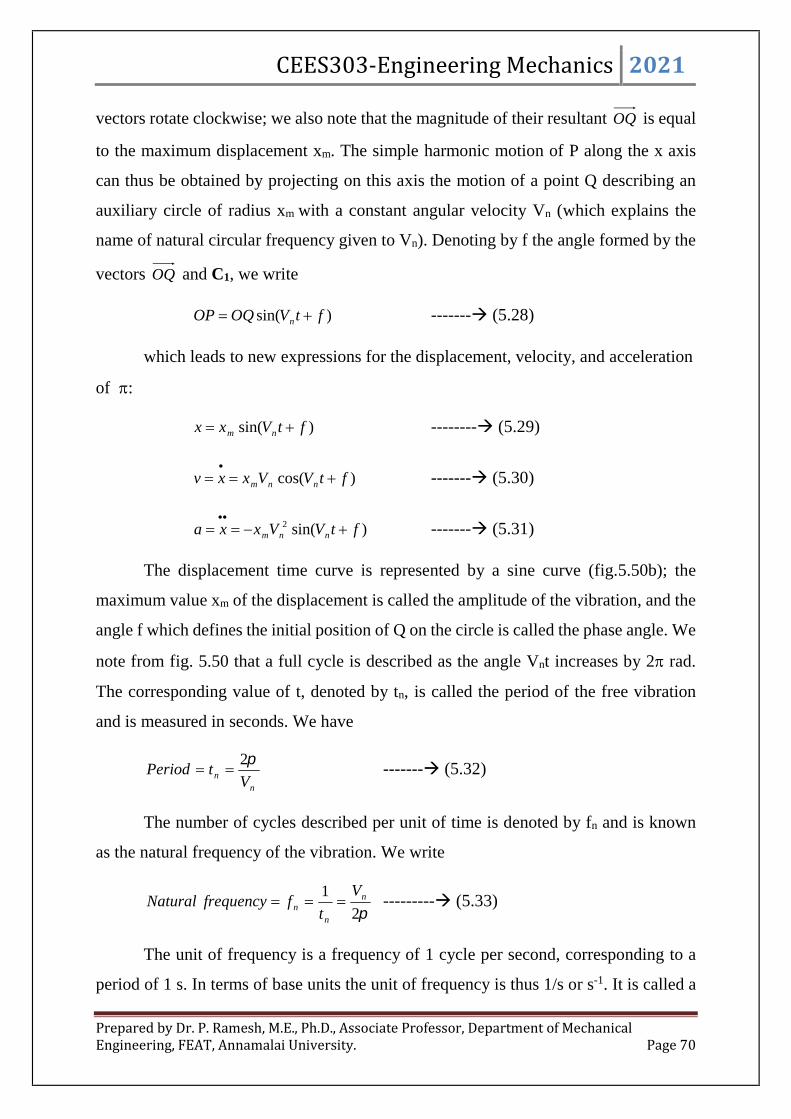
CEES303-Engineering Mechanics 2021
Prepared by Dr. P. Ramesh, M.E., Ph.D., Associate Professor, Department of MechanicalEngineering, FEAT, Annamalai University. Page 70
vectors rotate clockwise; we also note that the magnitude of their resultant OQ is equal
to the maximum displacement xm. The simple harmonic motion of P along the x axis
can thus be obtained by projecting on this axis the motion of a point Q describing an
auxiliary circle of radius xm with a constant angular velocity Vn (which explains the
name of natural circular frequency given to Vn). Denoting by f the angle formed by the
vectors OQ and C1, we write
)sin( ftVOQOP n ------- (5.28)
which leads to new expressions for the displacement, velocity, and acceleration
of :
)sin( ftVxx nm -------- (5.29)
)cos( ftVVxxv nnm
------- (5.30)
)sin(2 ftVVxxa nnm
------- (5.31)
The displacement time curve is represented by a sine curve (fig.5.50b); the
maximum value xm of the displacement is called the amplitude of the vibration, and the
angle f which defines the initial position of Q on the circle is called the phase angle. We
note from fig. 5.50 that a full cycle is described as the angle Vnt increases by 2 rad.
The corresponding value of t, denoted by tn, is called the period of the free vibration
and is measured in seconds. We have
nn V
tPeriod2
------- (5.32)
The number of cycles described per unit of time is denoted by fn and is known
as the natural frequency of the vibration. We write
2
1 n
nn
V
tffrequencyNatural --------- (5.33)
The unit of frequency is a frequency of 1 cycle per second, corresponding to a
period of 1 s. In terms of base units the unit of frequency is thus 1/s or s-1. It is called a

CEES303-Engineering Mechanics 2021
Prepared by Dr. P. Ramesh, M.E., Ph.D., Associate Professor, Department of MechanicalEngineering, FEAT, Annamalai University. Page 71
hertz (Hz) in the SI system of units. It also follows from Eq. 5.33 that a frequency of 1
s-1 or 1 Hz corresponds to a circular frequency of 2 rad/s. In problems involving
angular velocities expressed in revolutions per minute (rpm), we have
Hzsrpm60
1
60
11 1 , or 1 rpm = (2/60) rad/s.
Recalling that Vn was defined in Eqn.5.23 in terms of the constant k of the spring
and the mass m of the particle, we observe that the period and the frequency are
independent of the initial conditions and of the amplitude of the vibration. Note that tn
and fn depend on the mass rather than on the weight of the particle and thus are
independent of the value of g.
The velocity-time and acceleration-time curves can be represented by sine
curves of the same period as the displacement-time curve, but with different phase
angles. From Eqs. 5.30 and 5.31, we note that the maximum values of the magnitudes
of the velocity and acceleration are
nmm Vxv and 2nmm Vxa ----------- (5.34)
Fig.5. 51
Since the point Q describes the auxiliary circle, of radius xm, at the constant
angular velocity Vn, its velocity and acceleration are equal, respectively, to the
expressions (5.34). Recalling Eqs. (5.30) and (5.31), we find, therefore, that the velocity

CEES303-Engineering Mechanics 2021
Prepared by Dr. P. Ramesh, M.E., Ph.D., Associate Professor, Department of MechanicalEngineering, FEAT, Annamalai University. Page 72
and acceleration of P can be obtained at any instant by projecting on the x axis vectors
of magnitudes nmm Vxv and 2nmm Vxa representing, respectively, the velocity and
acceleration of Q at the same instant (Fig.5.51).
The results obtained are not limited to the solution of the problem of a mass
attached to a spring. They can be used to analyze the rectilinear motion of a particle
whenever the resultant F of the forces acting on the particle is proportional to the
displacement x and directed toward O. The fundamental equation of motion F 5 ma can
then be written in the form of Eq. (5.25), which is characteristic of a simple harmonic
motion. Observing that the coefficient of x must be equal to 2nV , we can easily determine
the natural circular frequency Vn of the motion. Substituting the value obtained for Vn
into Eqs. (5.32) and (5.33), we then obtain the period tn and the natural frequency fn of
the motion.
2. Free vibrations of rigid bodies
The analysis of the vibrations of a rigid body or of a system of rigid bodies
possessing a single degree of freedom is similar to the analysis of the vibrations of a
particle. An appropriate variable, such as a distance x or an angle u, is chosen to define
the position of the body or system of bodies, and an equation relating this variable and
its second derivative with respect to t is written. If the equation obtained is of the same
form as (5.25), i.e., if we have
02
xVx n or 02
uVu n ------- (5.35)
the vibration considered is a simple harmonic motion. The period and natural frequency
of the vibration can then be obtained by identifying Vn and substituting its value into
Eqs. (5.32) and (5.33).
In general, a simple way to obtain one of Eqs. (5.35) is to express that the system
of the external forces is equivalent to the system of the effective forces by drawing a
free-body-diagram equation for an arbitrary value of the variable and writing the

CEES303-Engineering Mechanics 2021
Prepared by Dr. P. Ramesh, M.E., Ph.D., Associate Professor, Department of MechanicalEngineering, FEAT, Annamalai University. Page 73
appropriate equation of motion. We recall that our goal should be the determination of
the coefficient of the variable x or u, not the determination of the variable itself or of
the derivative
x or
u . Setting this coefficient equal 2nV , we obtain the natural circular
frequency vn, from which tn and fn can be determined.
Fig.5.52
The method we have outlined can be used to analyze vibrations which are truly
represented by a simple harmonic motion, or vibrations of small amplitude which can
be approximated by a simple harmonic motion. As an example, let us determine the
period of the small oscillations of a square plate of side 2b which is suspended from the
midpoint O of one of its sides (Fig. 5.52a). We consider the plate in an arbitrary position
defined by the angle u that the line OG forms with the vertical and draw a free-body-
diagram equation to express that the weight W of the plate and the components Rx and
Ry of the reaction at O are equivalent to the vectors mat and man and to the couple AI
(Fig. 5.52b). Since the angular velocity and angular acceleration of the plate are equal,
respectively, to
u and
u magnitudes of the two vectors are, respectively,
umb and2
umb
while the moment of the couple is
uI . In previous applications of this method, we tried
whenever possible to assume the correct sense for the acceleration. Here, however, we
must assume the same positive sense for u and
u in order to obtain an equation of the
form (5.35). Consequently, the angular acceleration
u will be assumed positive counter
clockwise, even though this assumption is obviously unrealistic. Equating moments
about O, we write

CEES303-Engineering Mechanics 2021
Prepared by Dr. P. Ramesh, M.E., Ph.D., Associate Professor, Department of MechanicalEngineering, FEAT, Annamalai University. Page 74
uIbumbubW )()sin(
Noting that 222
3
222
12
1mbbbmI and mgW , we obtain
0sin5
3
ub
gu -------- (5.36)
Comparison with (5.35) shows that the equation obtained is that of a simple
harmonic motion and that the natural circular frequency Vn of the oscillations is equal
to (3g/5b)1/2. Substituting into (5.32), we find that the period of the oscillations is
g
bP
V
Pt
nn 3
52
2 -------- (5.37)
The result obtained is valid only for oscillations of small amplitude. A more
accurate description of the motion of the plate is obtained by comparing Eqs. (5.35).
We note that the two equations are identical if we choose l equal to 5b/3. This means
that the plate will oscillate as a simple pendulum of length l= 5b/3. The point A of the
plate located on line OG at a distance l= 5b/3from O is defined as the centre of
oscillation corresponding to O (Fig. 5.52a).
TYPES OF PENDULUMS:
It is common to differentiate between four types of pendulums:
1. Simple or Mathematical Pendulum:
Fig.5.53 Simple pendulum
CEES303-Engineering Mechanics 2021
Prepared by Dr. P. Ramesh, M.E., Ph.D., Associate Professor, Department of MechanicalEngineering, FEAT, Annamalai University. Page 75
A simple pendulum, in its simplest form, consists of a heavy bob suspended
at the end of a light inextensible, flexible string and the other end of the string is fixed
at O as shown in fig5.53
Let l = Length of the string in metres, and
m = Mass of the bob in kg (such that its weight is m.g newtons).
We know that the pendulum is in equilibrium, when the bob is at A. If the
bob is brought to B or C and released, it will start vibrating between the positions B
and C with A as the mean position.
It has been observed that if the angle ∠ AOC is very small, the bob will move
with simple harmonic motion.
Consider the equilibrium of the system at C. The weight mg of the bob can
be resolved into two components i.e., mg cos θ and mg sin θ at right angles to each
other.
The component mg cos θ will act along the thread. This will balance the
tension in the string as shown in fig. 5.53. The other component mg sin θ, being
unbalanced, will give rise to an acceleration in the direction CA.
Let a = Acceleration caused by the component.∴ Force responsible for this acceleration
= mg sin θ --------- (5.38)
We also know that the force
= Mass × Acceleration = m.a ---------- (5.39)
Equating equations (5.38) and (5.39),
ma = mg sin θ∴ a = g sin θ
Since the angle θ is very small, therefore substituting sin θ = θ in the above
equation,
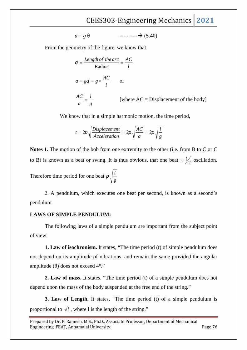
CEES303-Engineering Mechanics 2021
Prepared by Dr. P. Ramesh, M.E., Ph.D., Associate Professor, Department of MechanicalEngineering, FEAT, Annamalai University. Page 76
a = g θ ---------- (5.40)
From the geometry of the figure, we know that
l
ACarctheofLength
Radius
l
ACgga or
g
l
a
AC [where AC = Displacement of the body]
We know that in a simple harmonic motion, the time period,
g
l
a
AC
onAccelerati
ntDisplacemet 222
Notes 1. The motion of the bob from one extremity to the other (i.e. from B to C or C
to B) is known as a beat or swing. It is thus obvious, that one beat 21 oscillation.
Therefore time period for one beatg
l
2. A pendulum, which executes one beat per second, is known as a second’s
pendulum.
LAWS OF SIMPLE PENDULUM:
The following laws of a simple pendulum are important from the subject point
of view:
1. Law of isochronism. It states, “The time period (t) of simple pendulum does
not depend on its amplitude of vibrations, and remain the same provided the angular
amplitude (θ) does not exceed 4°.”
2. Law of mass. It states, “The time period (t) of a simple pendulum does not
depend upon the mass of the body suspended at the free end of the string.”
3. Law of Length. It states, “The time period (t) of a simple pendulum is
proportional to l , where l is the length of the string.”

CEES303-Engineering Mechanics 2021
Prepared by Dr. P. Ramesh, M.E., Ph.D., Associate Professor, Department of MechanicalEngineering, FEAT, Annamalai University. Page 77
4. Law of gravity. It states, “The time period (t) of a simple pendulum is
inversely proportional to g . where g is the acceleration due to gravity.”
Notes. The above laws of a simple pendulum are true from the equation of the time
period i.e.
g
lt 2
2. Compound or Physical Pendulum : A rigid body suspended from a
fixed horizontal axis. The body may oscillate in a vertical plane due to the action of
gravity.
Fig.5.54 Compound pendulum
A compound pendulum, in its simplest form, consists of a rigid body suspended
vertically at O and oscillating with a small amplitude under the action of the force of
gravity. At some instant, let the position of the rigid body be at its extreme position as
shown in fig.5.54.
Let m = mass of the pendulum
h = Distance between point of suspension (O) and the centre of
gravity (G) of the body.
A little consideration will show, that if the pendulum is given a small angular
displacement θ, then the moment of the couple tending to restore the pendulum in the
equilibrium position OA
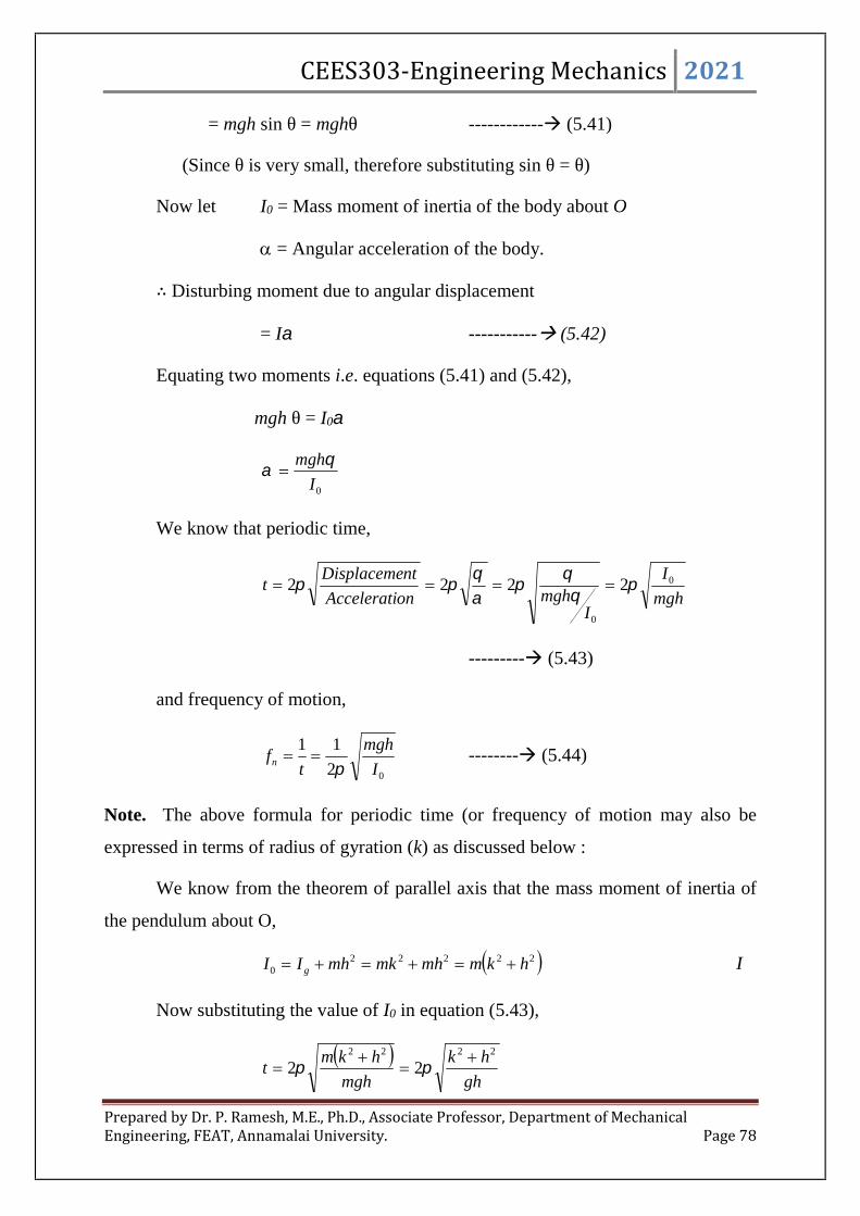
CEES303-Engineering Mechanics 2021
Prepared by Dr. P. Ramesh, M.E., Ph.D., Associate Professor, Department of MechanicalEngineering, FEAT, Annamalai University. Page 78
= mgh sin θ = mghθ ------------ (5.41)
(Since θ is very small, therefore substituting sin θ = θ)
Now let I0 = Mass moment of inertia of the body about O
= Angular acceleration of the body.∴ Disturbing moment due to angular displacement
= I ----------- (5.42)
Equating two moments i.e. equations (5.41) and (5.42),
mgh θ = I0
0I
mgh
We know that periodic time,
mgh
I
ImghonAccelerati
ntDisplacemet 0
0
2222
--------- (5.43)
and frequency of motion,
02
11
I
mgh
tfn
-------- (5.44)
Note. The above formula for periodic time (or frequency of motion may also be
expressed in terms of radius of gyration (k) as discussed below :
We know from the theorem of parallel axis that the mass moment of inertia of
the pendulum about O,
222220 hkmmhmkmhII g I
Now substituting the value of I0 in equation (5.43),
gh
hk
mgh
hkmt
2222
22
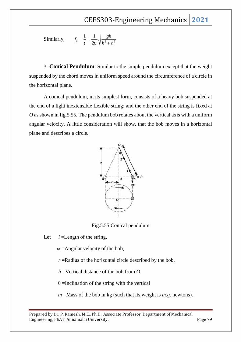
CEES303-Engineering Mechanics 2021
Prepared by Dr. P. Ramesh, M.E., Ph.D., Associate Professor, Department of MechanicalEngineering, FEAT, Annamalai University. Page 79
Similarly,222
11
hk
gh
tfn
3. Conical Pendulum: Similar to the simple pendulum except that the weight
suspended by the chord moves in uniform speed around the circumference of a circle in
the horizontal plane.
A conical pendulum, in its simplest form, consists of a heavy bob suspended at
the end of a light inextensible flexible string; and the other end of the string is fixed at
O as shown in fig.5.55. The pendulum bob rotates about the vertical axis with a uniform
angular velocity. A little consideration will show, that the bob moves in a horizontal
plane and describes a circle.
Fig.5.55 Conical pendulum
Let l =Length of the string,
ω =Angular velocity of the bob,
r =Radius of the horizontal circle described by the bob,
h =Vertical distance of the bob from O,
θ =Inclination of the string with the vertical
m =Mass of the bob in kg (such that its weight is m.g. newtons).

CEES303-Engineering Mechanics 2021
Prepared by Dr. P. Ramesh, M.E., Ph.D., Associate Professor, Department of MechanicalEngineering, FEAT, Annamalai University. Page 80
We know that the pendulum is in equilibrium, when the bob is at A. But when
the bob is made to rotate, it will move outwards due to centrifugal force. Now consider
equilibrium of the bob at C. We know that at this point, the forces acting on it are:
1. Weight (equal to mg) of the bob acting downwards in Newton’s.
2. Tension in the string (equal to T) in Newton’s.
3. Centrifugal force (P equal to mω2r) in Newton’s.
Resolving the forces horizontally and equating the same,
T sin θ = mω2r --------------- (5.45)
or
lm
l
rrmrm
T 222
sin
------------- (5.46)
Now taking moments about O, and equating the same,
mgrhrm )( 2
h
g 2
We know that the periodic time (i.e. time taken by the bob for one revolution),
g
ht
22
and now resolving the forces vertically and equating the same,
mgT cos ---------- (5.47)
orh
mgl
lhmgmg
T cos
--------- (5.48)
Now dividing equation (5.45) by (5.47),
mg
rm
T
T 2
cos
sin

CEES303-Engineering Mechanics 2021
Prepared by Dr. P. Ramesh, M.E., Ph.D., Associate Professor, Department of MechanicalEngineering, FEAT, Annamalai University. Page 81
g
r2
tan
-------- (5.49)
4. Torsional Pendulum: A disk fixed to a slender rod. The rod is fastened to
a fixed frame. If the disk is twisted it will oscillate back and forth about the axis of the
rod.
Fig.5.56 Torsional pendulum
USE OF SIMPLE PENDULUM:
The applications of simple pendulums are
a) Clock
b) Car Shock Absorbers
c) Musical Instruments
d) Bungee Jumping
e) Diving Board
f) The Process of Hearing
g) Earthquake-proof buildings
h) Metronome
a) Clock:
Depending on the type of clock and the era that it was made, either a large
pendulum or a vibrating quartz crystal will keep time. This motion of the pendulum or
crystal must be periodic, in order to ensure that the time shown will be accurate. The

CEES303-Engineering Mechanics 2021
Prepared by Dr. P. Ramesh, M.E., Ph.D., Associate Professor, Department of MechanicalEngineering, FEAT, Annamalai University. Page 82
oscillators have a constant period because they are in Simple Harmonic Motion. This
allows them to keep time accurately. This accurate time is more than just for
convenience. It is a necessity when navigating using celestial marks like the Sun or stars
because the position of the Sun and stars in the sky changes with the time of day.
It is also important that the period is independent of the amplitude of oscillation.
This is because the conditions in a grandfather clock can vary, and affect the amplitude
of oscillation. No matter how the amplitude varies, the time shown is always constant.
b) Car Shock Absorbers:
Springs attached to the wheels of a car help ensure a smoother ride for the
passengers. When the car hits a bump in the road, the wheels of the car rise up. If the
car did not have shock absorbers, the whole car will be thrown up and down, causing
an extremely uncomfortable and possibly dangerous ride.
When there are springs in the car, the wheel will rise, compressing the spring
while the car body remains relatively stationary. The restoring force on the compressed
spring will push the car wheel back into place.
However, when the spring is put into SHM by the bump in the road, it continues
to bounce up and down even though the unevenness that triggered the motion is gone.
This is why cars contain shock absorbers, which are usually pistons filled with a viscous
liquid, to damp the oscillations quickly. This is an example of over damping.
c) Musical Instruments
Sound itself is produced from oscillations of the air. In a string instrument such
as a violin or a guitar, bowing or plucking the string provides the force needed to make
the string oscillate and produce sound. In a wind instrument like a trumpet, the
vibrations are caused by the player's lips while the sound is caused by exciting the air
molecules by blowing across the opening in a flute. In a percussion instrument like the
triangle, the vibrations occur when the instrument is struck.
The vibration produced in the string, column of air or body of the instrument
causes standing waves to be formed, which produces sound.

CEES303-Engineering Mechanics 2021
Prepared by Dr. P. Ramesh, M.E., Ph.D., Associate Professor, Department of MechanicalEngineering, FEAT, Annamalai University. Page 83
d) Bungee Jumping
When a long, elastic cord is tied to the ankles of a person, who then jumps off a
bridge or a platform, setting off a series of vertical oscillations.
The amplitude of the oscillations is calculated very carefully, because an error
could mean the loss of a life. This sport must be undertaken only with high safety
precautions to prevent injury.
e) Diving Board
This oscillating system is known as a cantilever, which is defined as abeam fixed
at only one end.
As the person on the edge of the board jumps up and down on the end of the
diving board, the board and the person undergo SHM. This motion is affected by the
force constant of the board (a stiffer board will not oscillate as much) and the weight of
the person (a heavier person will cause greater amplitude of oscillation).
f) Hearing
The basic function of our ears, hearing, cannot be possible without SHM. The
sound waves travel through the air and when they hit the eardrum, they cause the
eardrum to vibrate. This movement is passed to the brain, which then translates these
signals into complex sounds that we are able to hear clearly.
g) Metronome
A metronome generates rhythmic ticks in order to help musicians to play a piece
at a constant speed. The structure is a variation of the pendulum. In this case, the
oscillating arm is anchored at the bottom. A counterweight is fixed within the
metronome to counter-balance a second weight that is on the oscillating arm and the
period can be varied by sliding the weight up and down the arm, thus changing the
moment of the oscillation.
The restoring force in this case is gravity acting on the fixed counterweight. The
nearer the weight is to the bottom of the arm, the faster it will swing and generate ticks.
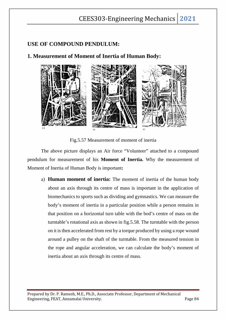
CEES303-Engineering Mechanics 2021
Prepared by Dr. P. Ramesh, M.E., Ph.D., Associate Professor, Department of MechanicalEngineering, FEAT, Annamalai University. Page 84
USE OF COMPOUND PENDULUM:
1. Measurement of Moment of Inertia of Human Body:
Fig.5.57 Measurement of moment of inertia
The above picture displays an Air force “Volunteer” attached to a compound
pendulum for measurement of his Moment of Inertia. Why the measurement of
Moment of Inertia of Human Body is important:
a) Human moment of inertia: The moment of inertia of the human body
about an axis through its centre of mass is important in the application of
biomechanics to sports such as dividing and gymnastics. We can measure the
body’s moment of inertia in a particular position while a person remains in
that position on a horizontal turn table with the bod’s centre of mass on the
turntable’s rotational axis as shown in fig.5.58. The turntable with the person
on it is then accelerated from rest by a torque produced by using a rope wound
around a pulley on the shaft of the turntable. From the measured tension in
the rope and angular acceleration, we can calculate the body’s moment of
inertia about an axis through its centre of mass.
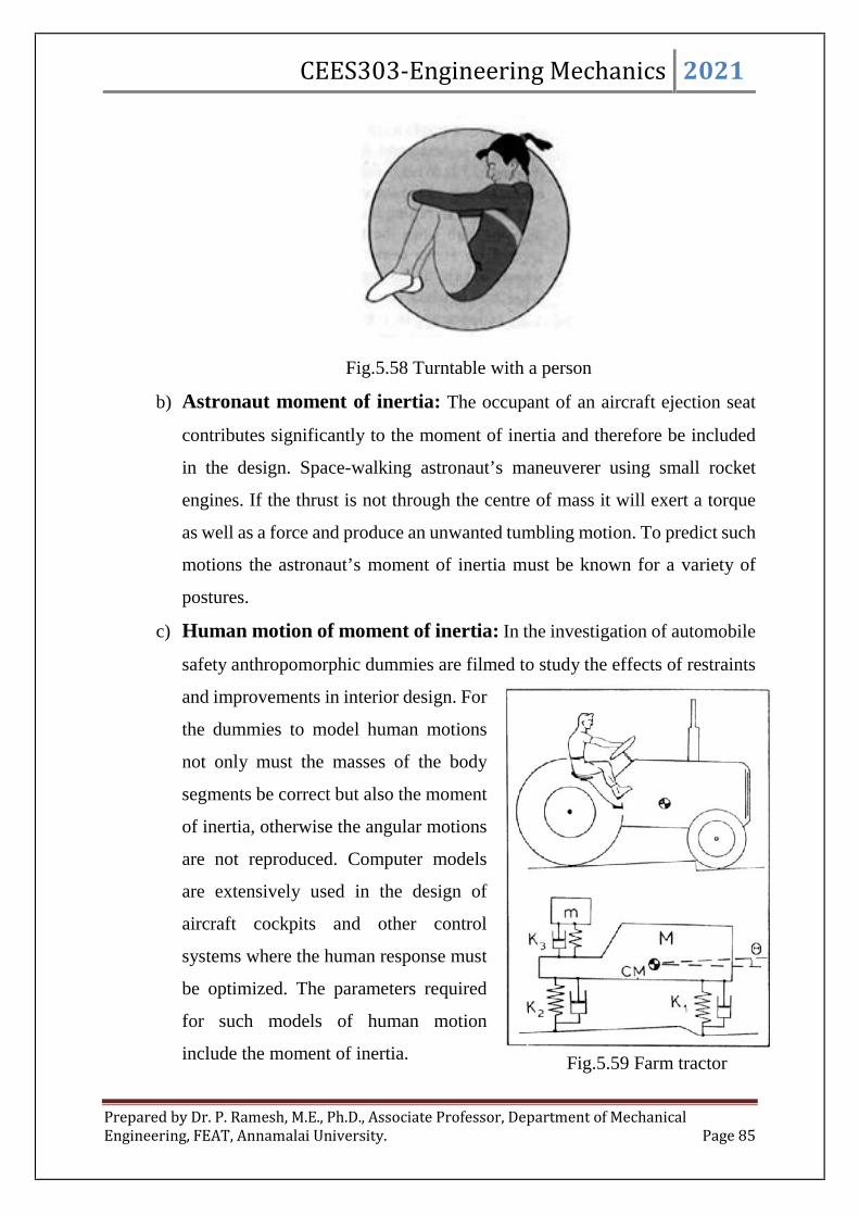
CEES303-Engineering Mechanics 2021
Prepared by Dr. P. Ramesh, M.E., Ph.D., Associate Professor, Department of MechanicalEngineering, FEAT, Annamalai University. Page 85
Fig.5.58 Turntable with a person
b) Astronaut moment of inertia: The occupant of an aircraft ejection seat
contributes significantly to the moment of inertia and therefore be included
in the design. Space-walking astronaut’s maneuverer using small rocket
engines. If the thrust is not through the centre of mass it will exert a torque
as well as a force and produce an unwanted tumbling motion. To predict such
motions the astronaut’s moment of inertia must be known for a variety of
postures.
c) Human motion of moment of inertia: In the investigation of automobile
safety anthropomorphic dummies are filmed to study the effects of restraints
and improvements in interior design. For
the dummies to model human motions
not only must the masses of the body
segments be correct but also the moment
of inertia, otherwise the angular motions
are not reproduced. Computer models
are extensively used in the design of
aircraft cockpits and other control
systems where the human response must
be optimized. The parameters required
for such models of human motion
include the moment of inertia. Fig.5.59 Farm tractor

CEES303-Engineering Mechanics 2021
Prepared by Dr. P. Ramesh, M.E., Ph.D., Associate Professor, Department of MechanicalEngineering, FEAT, Annamalai University. Page 86
2) Farm Tractors:
Form tractors determining conditions of operation and human comfortability.
These are used for slow speed use over uneven ground and therefore, unlike cars and
trucks, do not have spring suspension. The rough ride can lead back to injuries and
health problem. A computer model is shown in fig.5.59 The figure shows a dynamic
model of a tractor. The tractor of mass M and moment of inertia I is supported by the
tries, represented by a damped spring K1 and K2. The motion of the operator m
supported by the seat, damped spring k3 is studied as the tractor goes on uneven ground.
3. Sail – Boat:
Fig.5.60 Sail boat
The total weight of the sailboat has a major effect on its speed. A heavy boat
floats lower and causes a disturbance while moving. The compound pendulum concept
helps in determining conditions for operation.
USE OF TORSION PENDULUM:
Torsion pendulums are often used for time-keeping purposes. For instance, the
balance wheel in a mechanical wristwatch is a torsion pendulum in which the restoring
torque is provided by a coiled spring.
There are two important applications of torsional pendulum:
1. Bodies which are having geometrically defined shape are called regular
bodies. It is possible to evaluate the moment of inertia of regular bodies
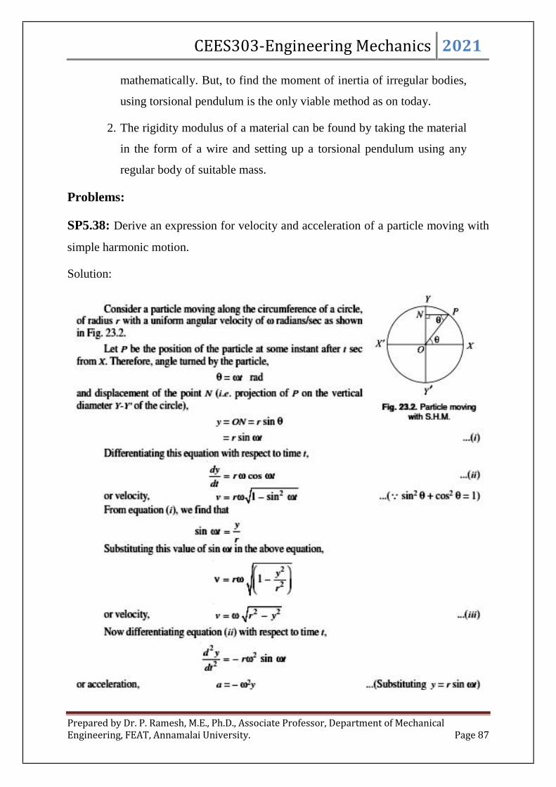
CEES303-Engineering Mechanics 2021
Prepared by Dr. P. Ramesh, M.E., Ph.D., Associate Professor, Department of MechanicalEngineering, FEAT, Annamalai University. Page 87
mathematically. But, to find the moment of inertia of irregular bodies,
using torsional pendulum is the only viable method as on today.
2. The rigidity modulus of a material can be found by taking the material
in the form of a wire and setting up a torsional pendulum using any
regular body of suitable mass.
Problems:
SP5.38: Derive an expression for velocity and acceleration of a particle moving with
simple harmonic motion.
Solution:

CEES303-Engineering Mechanics 2021
Prepared by Dr. P. Ramesh, M.E., Ph.D., Associate Professor, Department of MechanicalEngineering, FEAT, Annamalai University. Page 88
SP5.39:
SP5.40:

CEES303-Engineering Mechanics 2021
Prepared by Dr. P. Ramesh, M.E., Ph.D., Associate Professor, Department of MechanicalEngineering, FEAT, Annamalai University. Page 89
SP5.41:

CEES303-Engineering Mechanics 2021
Prepared by Dr. P. Ramesh, M.E., Ph.D., Associate Professor, Department of MechanicalEngineering, FEAT, Annamalai University. Page 90
SP5.42:

CEES303-Engineering Mechanics 2021
Prepared by Dr. P. Ramesh, M.E., Ph.D., Associate Professor, Department of MechanicalEngineering, FEAT, Annamalai University. Page 91
SP5.43:
SP5.44:

CEES303-Engineering Mechanics 2021
Prepared by Dr. P. Ramesh, M.E., Ph.D., Associate Professor, Department of MechanicalEngineering, FEAT, Annamalai University. Page 92
SP5.45: Derive an expression for maximum velocity and acceleration of a particle
moving with simple harmonic motion.
Solution:

CEES303-Engineering Mechanics 2021
Prepared by Dr. P. Ramesh, M.E., Ph.D., Associate Professor, Department of MechanicalEngineering, FEAT, Annamalai University. Page 93
SP5.47:
SP5.46:

CEES303-Engineering Mechanics 2021
Prepared by Dr. P. Ramesh, M.E., Ph.D., Associate Professor, Department of MechanicalEngineering, FEAT, Annamalai University. Page 94
SP5.48:
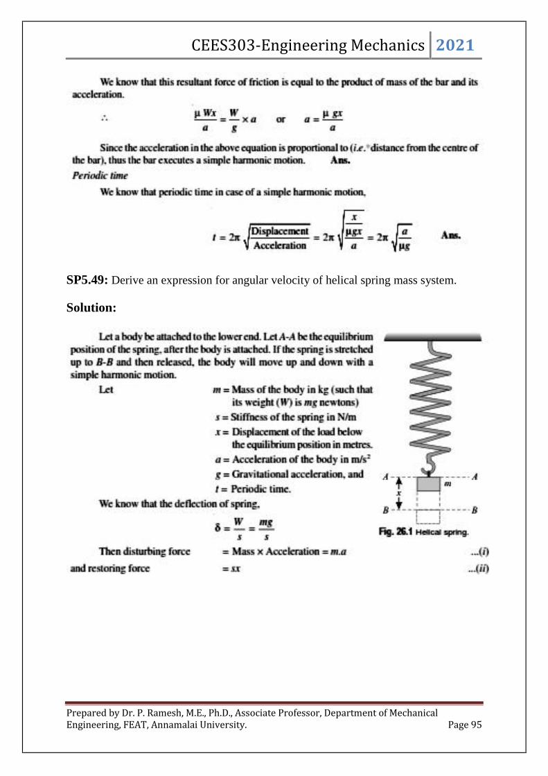
CEES303-Engineering Mechanics 2021
Prepared by Dr. P. Ramesh, M.E., Ph.D., Associate Professor, Department of MechanicalEngineering, FEAT, Annamalai University. Page 95
SP5.49: Derive an expression for angular velocity of helical spring mass system.
Solution:
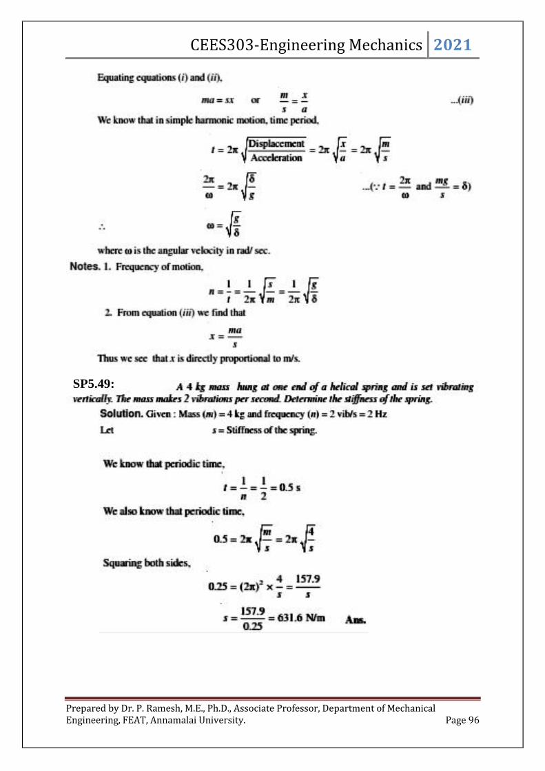
CEES303-Engineering Mechanics 2021
Prepared by Dr. P. Ramesh, M.E., Ph.D., Associate Professor, Department of MechanicalEngineering, FEAT, Annamalai University. Page 96
SP5.49:
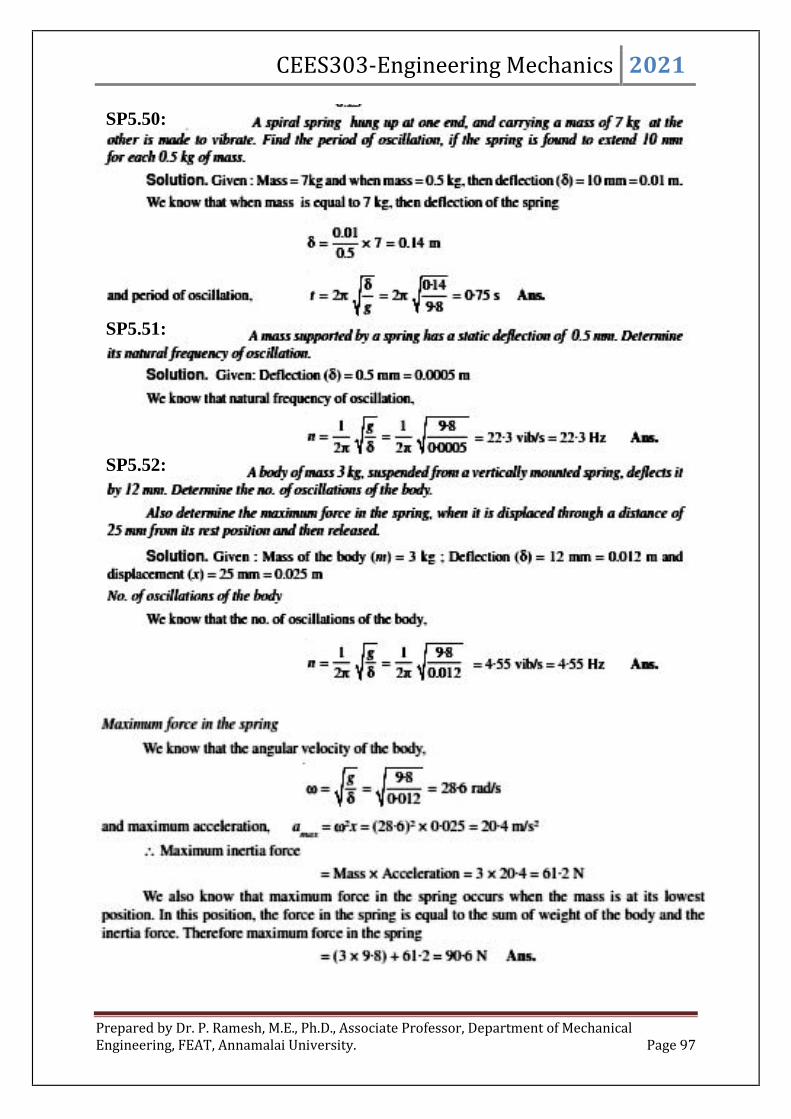
CEES303-Engineering Mechanics 2021
Prepared by Dr. P. Ramesh, M.E., Ph.D., Associate Professor, Department of MechanicalEngineering, FEAT, Annamalai University. Page 97
SP5.50:
SP5.51:
SP5.52:

CEES303-Engineering Mechanics 2021
Prepared by Dr. P. Ramesh, M.E., Ph.D., Associate Professor, Department of MechanicalEngineering, FEAT, Annamalai University. Page 98
SP5.53:
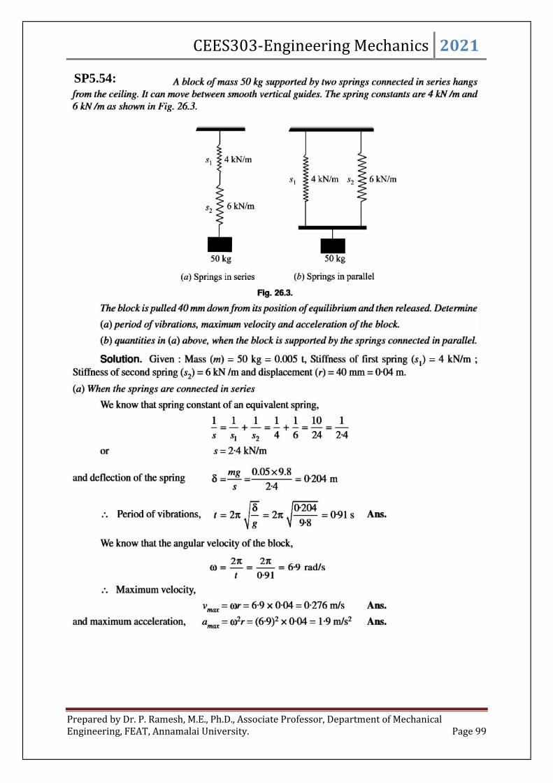
CEES303-Engineering Mechanics 2021
Prepared by Dr. P. Ramesh, M.E., Ph.D., Associate Professor, Department of MechanicalEngineering, FEAT, Annamalai University. Page 99
SP5.54:
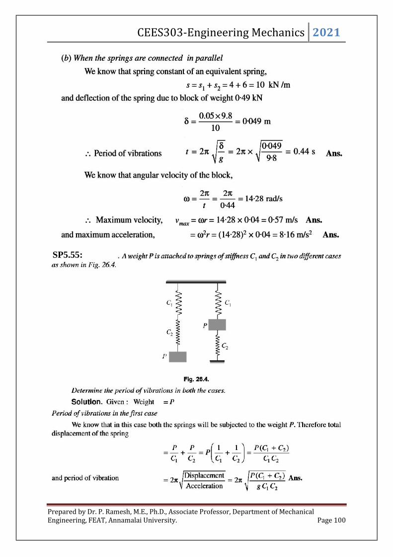
CEES303-Engineering Mechanics 2021
Prepared by Dr. P. Ramesh, M.E., Ph.D., Associate Professor, Department of MechanicalEngineering, FEAT, Annamalai University. Page 100
SP5.55:

CEES303-Engineering Mechanics 2021
Prepared by Dr. P. Ramesh, M.E., Ph.D., Associate Professor, Department of MechanicalEngineering, FEAT, Annamalai University. Page 101
SP5.56:

CEES303-Engineering Mechanics 2021
Prepared by Dr. P. Ramesh, M.E., Ph.D., Associate Professor, Department of MechanicalEngineering, FEAT, Annamalai University. Page 102
SP5.57:

CEES303-Engineering Mechanics 2021
Prepared by Dr. P. Ramesh, M.E., Ph.D., Associate Professor, Department of MechanicalEngineering, FEAT, Annamalai University. Page 103
SP5.58: Derive an expression for gain or loss in the no. of oscillation due to change in
the length of string or acceleration due to gravity of a simple pendulum.
Solution:

CEES303-Engineering Mechanics 2021
Prepared by Dr. P. Ramesh, M.E., Ph.D., Associate Professor, Department of MechanicalEngineering, FEAT, Annamalai University. Page 104
SP5.59:
SP5.60:

CEES303-Engineering Mechanics 2021
Prepared by Dr. P. Ramesh, M.E., Ph.D., Associate Professor, Department of MechanicalEngineering, FEAT, Annamalai University. Page 105
SP5.61: Derive an expression for gain or loss in the no. of oscillation due to change in
the position of a simple pendulum.
Solution:
Consider a simple pendulum oscillating with a simple harmonic motion.

CEES303-Engineering Mechanics 2021
Prepared by Dr. P. Ramesh, M.E., Ph.D., Associate Professor, Department of MechanicalEngineering, FEAT, Annamalai University. Page 106
SP5.62:

CEES303-Engineering Mechanics 2021
Prepared by Dr. P. Ramesh, M.E., Ph.D., Associate Professor, Department of MechanicalEngineering, FEAT, Annamalai University. Page 107
SP5.63:
SP5.64:

CEES303-Engineering Mechanics 2021
Prepared by Dr. P. Ramesh, M.E., Ph.D., Associate Professor, Department of MechanicalEngineering, FEAT, Annamalai University. Page 108
SP5.65:
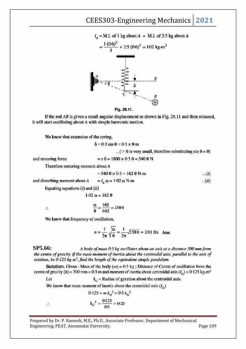
CEES303-Engineering Mechanics 2021
Prepared by Dr. P. Ramesh, M.E., Ph.D., Associate Professor, Department of MechanicalEngineering, FEAT, Annamalai University. Page 109
SP5.66:

CEES303-Engineering Mechanics 2021
Prepared by Dr. P. Ramesh, M.E., Ph.D., Associate Professor, Department of MechanicalEngineering, FEAT, Annamalai University. Page 110
SP5.67:

CEES303-Engineering Mechanics 2021
Prepared by Dr. P. Ramesh, M.E., Ph.D., Associate Professor, Department of MechanicalEngineering, FEAT, Annamalai University. Page 111