arX

iv:0

809.

4728

v3 [

hep-

th]

30 A

pr 2

009

KIAS-P08059arXiv:0809.4728

Emergent Spacetime and The Origin of Gravity

Hyun Seok Yang∗

School of Physics, Korea Institute for Advanced Study, Seoul 130-012, Korea

ABSTRACT

We present an exposition on the geometrization of the electromagnetic force. We show that, in

noncommutative (NC) spacetime, there always exists a coordinate transformation to locally eliminate

the electromagnetic force, which is precisely the Darboux theorem in symplectic geometry. As a con-

sequence, the electromagnetism can be realized as a geometrical property of spacetime like gravity.

We show that the geometrization of the electromagnetic force in NC spacetime is the origin of grav-

ity, dubbed as the emergent gravity. We discuss how the emergent gravity reveals a novel, radically

different picture about the origin of spacetime. In particular, the emergent gravity naturally explains

the dynamical origin of flat spacetime, which is absent in Einstein gravity. This spacetime picture

turns out to be crucial for a tenable solution of the cosmological constant problem.

PACS numbers: 11.10.Nx, 02.40.Gh, 04.50.+h

Keywords: Emergent Gravity, Noncommutative Field Theory,Symplectic Geometry

April 30, 2009

∗hsyang@kias.re.kr

1 Deformation Theory

One of the main trends in modern physics and mathematics is tostudy a theory of deformations. De-

formations are performed first to specify a particular structure (e.g., complex, symplectic, or algebraic

structures) which one wants to deform, and then to introducea deformation parameter[~] such that

the limit [~] → 0 recovers its parent theory. The most salient examples of thedeformation theo-

ries are Kodaira-Spencer theory, deformation quantization, quantum group, etc. in mathematics and

quantum mechanics, string theory, noncommutative (NC) field theory, etc. in physics. Interestingly,

consequences after the deformation are often radical: A theory with [~] 6= 0 is often qualitatively

different from its parent theory and reveals a unification ofphysical or mathematical structures (e.g.,

wave-particle duality, mirror symmetry, etc.).

Let us focus on the deformation theories appearing in physics. Our mission is to deform some

structures of a point-particle theory in classical mechanics. There could be several in general, but the

most salient ones among them are quantum mechanics, string theory and NC field theory, which we

call ~-deformation,α′-deformation andθ-deformation, respectively. The deformation parameter[~]

(which denotes a generic one) is mostly a dimensionful constant and plays a role of a conversion factor

bridging two different quantities, e.g.,p = 2π~/λ for the famous wave-particle duality in quantum

mechanics. The introduction of the new constant[~] into the theory is not a simple addition but often

a radical change of the parent theory triggering a new physics. Let us reflect the new physics sprouted

up from the[~]-deformation, which never exists in the[~] = 0 theory.

Quantum mechanics is the formulation of mechanics in NC phase space

[xi, pk] = i~δik. (1.1)

The deformation parameter~ is to deform a commutative Poisson algebra of observables inphase

space into NC one. This~-deformation (quantum mechanics) has activated revolutionary changes

of classical physics. One of the most prominent physics is the wave-particle duality whose striking

physics could be embodied in the two-slit experiment.

String theory can be regarded as a deformation of point-particle theory in the sense that zero-

dimensional point particles are replaced by one-dimensional extended objects, strings, whose size

is characterized by the parameterα′. This α′-deformation also results in a fundamental change of

physics, which has never been observed in a particle theory.It is rather a theory of gravity (or grandil-

oquently a theory of everything). One of the striking consequences due to theα′-deformation is

‘T-duality’, which is a symmetry between small and large distances, symbolically represented by

R↔ α′

R. (1.2)

The T-duality is a crucial ingredient for various string dualities and mirror symmetry.

NC field theory is the formulation of field theory in NC spacetime

[ya, yb]⋆ = iθab. (1.3)

1

See [1, 2] for a review of this subject. We will consider only space-noncommutativity throughout the

paper in spite of the abuse of the term ‘NC spacetime’ and argue in Section 4.1 that “Time” emerges in

a different way. This NC spacetime arises from introducing asymplectic structureB = 12Babdy

a∧dyb

and then quantizing the spacetime with its Poisson structure θab ≡ (B−1)ab, treating it as a quantum

phase space. In other words, the spacetime (1.3) becomes a NCphase space. Therefore the NC

field theory, which we callθ-deformation, is mathematically very similar to quantum mechanics.

They are all involved with a NC⋆-algebra generated by Eq.(1.1) or Eq.(1.3). Indeed we will find

many parallels. Another naive observation is that theθ-deformation (NC field theory) would be

much similar to theα′-deformation from the viewpoint of deformation theory since the deformation

parametersα′ andθ equally carry the dimension of(length)2. A difference is that theθ-deformation

is done in the field theory framework. We will further elaborate the similarity in this paper.

What is a new physics due to theθ-deformation ? A remarkable fact is that translations in NC

directions are an inner automorphism of NC⋆-algebraAθ, i.e.,eik·y ⋆ f(y) ⋆ e−ik·y = f(y + θ · k) for

any f(y) ∈ Aθ or, in its infinitesimal form,

[ya, f(y)]⋆ = iθab∂bf(y). (1.4)

In this paper we will denote NC fields (or variables) with the hat as in Eq.(1.4) but we will omit the hat

for NC coordinatesya in Eq.(1.3) for notational convenience. We will show that theθ-deformation is

seeding in it the physics of theα′-deformation as well as the~-deformation, so to answer the question

in the Table 1.

Theory Deformation New physics

Quantum mechanics ~ wave-particle duality

String theory α′ T-duality

NC field theory θab ?

Table 1.[~]-deformations and their new physics

This paper is organized as follows. In Section 2 we review thepicture of emergent gravity pre-

sented in [3] with a few refinements. First we consolidate some results well-known from string theory

to explain why there always exists a coordinate transformation to locally eliminate the electromag-

netic force as long as D-brane worldvolumeM supports a symplectic structureB, i.e.,M becomes a

NC space. That is, the NC spacetime admits a novel form of the equivalence principle, known as the

Darboux theorem, for the geometrization of the electromagnetism. It turns out [3] that the Darboux

theorem as the equivalence principle in symplectic geometry is the essence of emergent gravity. See

the Table 2. In addition we add a new observation that the geometrization of the electromagnetism

in theB-field background can be nicely understood in terms of the generalized geometry [4, 5]. Re-

cently there have been considerable efforts [6, 7, 8, 9, 10, 11, 12, 3, 13, 14, 15, 16, 17, 18, 19, 20] to

construct gravity from NC field theories. The emergent gravity has also been suggested to resolve the

cosmological constant problem and dark energy [21, 15].

2

In Section 3, we put the arguments in Section 2 on a firm foundation using the background inde-

pendent formulation of NC gauge theory [22, 23]. In Sec. 3.1,we first clarify based on the argument

in [14] that the emergent gravity from NC gauge theory is essentially a largeN duality consistent

with the AdS/CFT duality [24]. And then we move onto the geometric representation of NC field

theory using the inner automorphism (1.4) of the NC spacetime (1.3). In Sec. 3.2, we show how to

explicitly determine a gravitational metric emerging fromNC gauge fields and show that the equa-

tions of motion for NC gauge fields are mapped to the Einstein equations for the emergent metric.

This part consists of our main new results generalizing the emergent gravity in [12, 3] for self-dual

gauge fields. In the course of the derivation, we find that NC gauge fields induce an exotic form of

energy, dubbed as the Liouville energy-momentum tensor. A simple analysis shows that this Liouville

energy mimics the several aspects of dark energy, so we suggest the energy as a plausible candidate

of dark energy. In Sec. 3.3, the emergent gravity is further generalized to the nontrivial background

of nonconstantθ induced by an inhomogenous condensation of gauge fields. In Sec. 3.4, we discuss

the spacetime picture revealed from NC gauge fields. We also confirm the observation in [15] that the

emergent gravity reveals a remarkably beautiful and consistent picture about the dynamical origin of

flat spacetime.

In Section 4 we speculate how to understand “Time” and matterfields in the context of emergent

geometry. As a first step, we elucidate in Sec. 4.1 how the well-known ‘minimal coupling’ of matters

with gauge fields can be understood as a symplectic geometry in phase space. There are two important

works [25, 26] for this understanding. Based on the symplectic geometry of particles, in Sec. 4.2,

we suggest a K-theory picture for matter fields such as quarksand leptons adopting the Fermi-surface

scenario in [27, 28] where non-Abelian gauge fields are understood as collective modes acting on the

matter fields.

In Section 5, we address the problem on the existence of spin-2 bound states which presupposes

the basis of emergent gravity. Although we don’t know any rigorous proof, we outline some posi-

tive evidences for the bound states using the relation to theAdS/CFT duality. We further notice an

interesting similarity between the BCS superconductivity[29] and the emergent gravity about some

dynamical mechanism for the spin-0 and spin-2 bound states,respectively. See the Table 3. We also

discuss the issues on the Lorentz symmetry breaking and the nonlocality in NC field theories from

the viewpoint of emergent spacetime.

In Section 6, we summarize the message uncovered by the emergent gravity picture with some

closing remarks.

The calculational details in Section 3 are deferred to two Appendices. In Appendix A we give a

self-contained proof of the equivalence between self-dualNC electromagnetism and self-dual Einstein

gravity, first shown in [12], for completeness. The self-dual case will provide a clear picture to

appreciate what the emergent gravity is, which will also be useful to consider a general situation of

emergent gravity. In Appendix B the equivalence is generalized to arbitrary NC gauge fields.

3

2 Geometrization of Forces

One of the guiding principles in modern physics is the geometrization of forces, i.e., to view physical

forces as a reflection of the curvature of the geometry of spacetime or internal space. In this line of

thought, gravity is quite different from the other three forces - the electromagnetic, the weak, and

the strong interactions. It is a manifestation of the curvature of spacetime while the other three are a

manifestation of the curvature of internal spaces. If it makes sense to pursue a unification of forces, in

which the four forces are different manifestations of a single force, it would be desirable to reconcile

gravity with the others and to find a general categorical structure of physical forces: Either to find

a rationale that gravity is not a fundamental force or to find aframework that the other three forces

are also geometrical properties of spacetime. We will show these two features are simultaneously

realized in NC spacetime, at least, for the electromagnetism.

2.1 Einstein’s happiest thought

The geometrization of forces is largely originated with Albert Einstein, whose general theory of rel-

ativity is to view the gravity as a metric field of spacetime which is determined by the distribution of

matter and energy. The remarkable vision of gravity in termsof the geometry of spacetime has been

based on the local equivalence of gravitation and inertia, or the local cancellation of the gravitational

field by local inertial frames - the equivalence principle. Einstein once recalled that the equivalence

principle was the happiest thought of his life.

The equivalence principle guarantees that it is “always” possible at any spacetime point of interest

to find a coordinate system, sayξα, such that the effects of gravity will disappear over a differential

region in the neighborhood of that point. (Precisely speaking, the neighborhood should be taken small

enough so that the variation of gravity within the region maybe neglected.) For a particle moving

freely under the influence of purely gravitational force, the equation of motion in terms of the freely

falling coordinate systemξα is thusd2ξα

dτ 2= 0 (2.1)

with dτ the proper time

dτ 2 = ηαβdξαdξβ. (2.2)

We will use the metricηαβ with signature(−+ + · · · ) throughout the paper.

Suppose that we perform a coordinate transformation to find the corresponding equations in a

laboratory at rest, which may be described by a Cartesian coordinate systemxµ. The freely falling

coordinatesξα are then functions of thexµ, that is,ξα = ξα(x). The freely falling particle in the

laboratory coordinate system now obeys the equation of motion

d2xµ

dτ 2+ Γµ

νλ

dxν

dτ

dxλ

dτ= 0 (2.3)

4

where

dτ 2 = gµν(x)dxµdxν (2.4)

and

gµν(x) = ηαβ∂ξα

∂xµ

∂ξβ

∂xν. (2.5)

It turns out that Eq.(2.3) is the geodesic equation moving onthe shortest possible path between two

points through the curved spacetime described by the metric(2.5). In the end the gravitational force

manifests itself only as the geometry of spacetime.

In accordance with the principle of general covariance the laws of physics must be independent of

the choice of spacetime coordinates. That is, Eq.(2.3) is true in all coordinate systems. For example,

under a coordinate transformationxµ → x′µ, the metric transforms into

g′µν(x′) =

∂xλ

∂x′µ∂xσ

∂x′νgλσ(x) (2.6)

and Eq.(2.3) transforms into the geodesic equation in the spacetime described by the metric (2.6).

The significance of the equivalence principle in conjunction with the principle of covariance lies in

its statement that there “always” exists a locally inertialframe at an arbitrary pointP in spacetime

whereg′αβ(P ) = ηαβ andΓ′µαβ(P ) = 0. But the second derivatives ofg′αβ at P cannot all be set to

zero unless the spacetime is flat. This coordinate system is precisely the freely falling coordinatesξα

in Eq.(2.1), i.e.,ξα = x′α(x), so the metric atP in the original system can consistently be written as

the form (2.5).

But a routine calculation using the metric (2.5) leads to identically vanishing curvature tensors.

Thus one may claim that the geometry described by the metric (2.5) is always flat. Of course it should

not be the case. Remember that the metric (2.5) in thex-coordinate system should be understood

at a pointP since it has been obtained from the local inertial frameξα whereg′αβ(P ) = ηαβ and

Γ′µαβ(P ) = 0 are satisfied only at that point. In order to calculate the curvature tensors correctly,

one needs to extend the local inertial frame atP to an infinitesimal neighborhood. A special and

useful realization of such a local inertial frame is a Riemann normal coordinate system [30] (where

we choose the pointP as a coordinate origin, i.e.,ξα|P = xµ|P = 0)

ξα(x) = xα +1

2Γα

µν(P )xµxν +1

6

(Γα

µβΓβνλ + ∂λΓ

αµν

)(P )xµxνxλ + · · · , (2.7)

which can be checked using Eq.(2.6) with the identificationx′α = ξα. One can then arrive at a metric

g′αβ(x) = ηαβ −1

3Rαµβν(P )xµxν − 1

6DλRαµβν(P )xλxµxν + · · · . (2.8)

2.2 Darboux theorem as the equivalence principle in symplectic geometry

What about other forces ? Is it possible to realize, for example, the electromagnetism as a geometrical

property of spacetime like gravity ? To be specific, we are wondering whether or not there “always”

5

exists any coordinate transformation to eliminate the electromagnetic force at least locally. The usual

wisdom says no since there is no analogue of the equivalence principle for the geometrization of the

electromagnetic force. But one has to recall that this wisdom has been based on the usual concept

of geometry, i.e., Riemannian geometry in commutative spacetime. Surprisingly, the conventional

wisdom turns out to be no longer true in NC spacetime, which isbased on symplectic geometry in

sharp contrast to the Riemannian geometry.

We will show that it is “always” possible to find a coordinate transformation to eliminate locally

the electromagnetic force if and only if spacetime supportsa symplectic structure, viz., NC spacetime.

To be definite, we will proceed with string theory although anelegant and rigorous approach can be

done using the formalism of deformation quantization [31].See [3] for some arguments based on the

latter approach.

A scheme to introduce gauge fields in string theory is by meansof boundary interactions or via

boundary conditions of open strings, aside from through theKaluza-Klein compactifications in type

II or heterotic string theories. With a compact notation, the open or closed string action reads as1

S =1

4πα′

∫

Σ

|dX|2 −∫

Σ

B −∫

∂Σ

A, (2.9)

whereX : Σ→ M is a map from an open or closed string worldsheetΣ to a target spacetimeM and

B(Σ) = X∗B(M) andA(∂Σ) = X∗A(M) are pull-backs of spacetime fields to the worldsheetΣ

and the worldsheet boundary∂Σ, respectively.

The string action (2.9) respects the following local symmetries.

(I) Diff(M)-symmetry:

X → X ′ = X ′(X) ∈ Diff(M) (2.10)

and the corresponding transformations of target fieldsB andA including also a target metric (hidden)

in the first term of Eq.(2.9).

(II) Λ-symmetry:

(B, A)→ (B − dΛ, A+ Λ) (2.11)

where the gauge parameterΛ is a one-form inM . A simple application of Stokes’ theorem imme-

diately verifies the symmetry (2.11). Note that theΛ-symmetry is present only whenB 6= 0. When

B = 0, the symmetry (2.11) is reduced toA→ A+ dλ, which is the ordinaryU(1) gauge symmetry.

The above two local symmetries in string theory must also be realized as the symmetries in low

energy effective theory. We well understand the root of the symmetry (2.10) since the string action

(2.9) describes a gravitational theory in target spacetime. The diffeomorphism symmetry (2.10) cer-

tainly signifies the emergence of gravity in the target spaceM . A natural question is then what is a

root of theΛ-symmetry (2.11).

1Although we will focus on the open string theory, our arguments in this section also hold for a closed string theory

where the string worldsheetΣ is a compact Riemann surface without boundary, so the last term in Eq.(2.9) is absent.

6

Unfortunately, as far as we know, there has been no serious investigation about a physical conse-

quence of the symmetry (2.11). As a provoking comment, let usfirst point out that theΛ-symmetry

(2.11) is as large as the Diff(M)-symmetry (2.10) (supposing that the rank ofB is equal to the di-

mension ofM) and is present only whenB 6= 0, so a stringy symmetry by nature. Indeed this is a

broad hint that there will be a radical change of physics whenB 6= 0 – the new physics due to the

θ-deformation in the Table 1.

To proceed with a general context, let us first discuss a geometrical interpretation of theΛ-

symmetry without specifying low energy effective theories. Suppose that the two-formB ∈ Λ2(M)

is closed inM , i.e., dB = 0, and nondegenerate, i.e., nowhere vanishing inM .2 One can then re-

gard the two-formB as a symplectic structure onM and the pair(M,B) as a symplectic manifold.

The symplectic geometry is a less intuitive type of geometrybut it should be familiar with classical

mechanics, especially, the Hamiltonian mechanics [32] and, more prominently, quantum mechanics.

The symplectic geometry respects an important property, known as the Darboux theorem [33],

stating that every symplectic manifold of the same dimension is locally indistinguishable. More

precisely, let(M,ω) be a symplectic manifold. Then in a neighborhood of eachP ∈ M , there is a

local coordinate chart in whichω is a constant, i.e.,(M,ω) ∼= (R2n,∑dqi ∧ dpi). For our purpose,

we will use its refined version - the Moser lemma [34] - describing a cohomological condition for

two symplectic structures to be equivalent. Given two-formsω andω′ such that[ω] = [ω′] ∈ H2(M)

andωt = ω + t(ω′ − ω) is symplectic∀t ∈ [0, 1], then there exists a diffeomorphismφt : M → M

such thatφ∗t (ωt) = ω. This implies that allωt are related by coordinate transformations generated by

a vector fieldXt satisfying

ιXtωt + A = 0 (2.12)

whereω′−ω = dA. In terms of local coordinates, there always exists a coordinate transformationφ1

whose pullback mapsω′ = ω + dA to ω, i.e.,φ1 : y 7→ x = x(y) so that

∂xα

∂ya

∂xβ

∂ybω′

αβ(x) = ωab(y). (2.13)

The Moser lemma (2.13) stating that the symplectic manifolds (M,ω0) and(M,ω1) are strongly

isotopic is a global statement and will be applied to our problem as follows. For a symplectic man-

ifold (M,ω1 = B + F ) whereF = dA, by the Darboux theorem, one can always find a local

coordinate chart(U ; y1, · · · , y2n) centered atp ∈ M and valid on the neighborhoodU such that

ω0(p) = 12Babdy

a ∧ dyb whereBab is a constant symplectic matrix of rank2n. Then there are

two symplectic structures onU ; the givenω1 = B + F andω0 = B. Consider a smooth family

ωt = ω0 + t(ω1−ω0) of symplectic forms joiningω0 toω1. Now the Moser lemma (2.13) implies that

there exists a global diffeomorphismφ : M ×R → M such thatφ∗t (ωt) = ω0, 0 ≤ t ≤ 1. If there

2In string theory,H = dB ∈ Λ3(M) is not necessarily zero. We don’t know much about this case, so we will restrict

to the symplectic case. But the connection with the generalized geometry, to be shortly discussed later, might be helpful

to understand more general cases.

7

exists such a diffeomorphism, in terms of the associated time-dependent vector fieldXt ≡ dφt

dt φ−1

t ,

one would have for all0 ≤ t ≤ 1 thatLXtωt + dωt

dt= 0 which can be reduced to Eq.(2.12). One

can pointwise solve the Moser’s equation (2.12) to obtain a unique smooth family of vector fields

Xt, 0 ≤ t ≤ 1, generating the global diffeomorphismφt satisfying dφt

dt= Xt φt. So everything

boils down to solving the Moser’s equation (2.12) forXt.

First one may solve the equation (2.12) att → 0 to determineX0 = X0(y) onU in terms of the

Darboux coordinatesya and extend to all0 ≤ t ≤ 1 by integration [35]. After integration, one can

find a local isotopyφ : U × [0, 1]→ M with φ∗t (ωt) = ω0 for all t ∈ [0, 1]. Let us denote the resulting

coordinate transformationφ1(y) on U generated by the vector fieldX1 asxa(y) = ya + Xa1 (y).

(Compare the result with Eq.(2.22) whereXa1 (y) := θabAb(y).) This is the result we want to get from

the data(M,ω1 = B + F ) by performing a coordinate transformation (2.13) onto a local Darboux

chart. Therefore sometimes we will simply refer the Darbouxtheorem to Eq.(2.13) in a loose sense

as long as the physical meaning is clear.

The string action (2.9) indicates that, whenB 6= 0, its natural group of symmetries includes not

only the diffeomorphism (2.10) in Riemannian geometry but also theΛ-symmetry (2.11) in sym-

plectic geometry. According to the Darboux theorem (precisely, the Moser lemma stated above), the

local change of symplectic structure due to theΛ-symmetry (2.11) (or theB-field transformation)

can always be translated into a diffeomorphism symmetry as in Eq.(2.13). This fact implies that the

Λ-symmetry (2.11) should be considered as a par with diffeomorphisms. It turns out [3] that the

Darboux theorem in symplectic geometry plays the same role as the equivalence principle in general

relativity for the geometrization of the electromagnetic force. These geometrical structures inherent

in the string action (2.9) are summarized below.

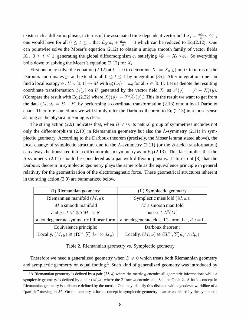
(I) Riemannian geometry (II) Symplectic geometry

Riemannian manifold(M, g): Symplectic manifold(M,ω):

M a smooth manifold M a smooth manifold

andg : TM ⊗ TM → R andω ∈ Λ2(M)

a nondegenerate symmetric bilinear forma nondegenerate closed 2-form, i.e.,dω = 0

Equivalence principle: Darboux theorem:

Locally, (M, g) ∼= (R2n,∑dxµ ⊗ dxµ) Locally, (M,ω) ∼= (R2n,

∑dqi ∧ dpi)

Table 2. Riemannian geometry vs. Symplectic geometry

Therefore we need a generalized geometry whenB 6= 0 which treats both Riemannian geometry

and symplectic geometry on equal footing.3 Such kind of generalized geometry was introduced by

3A Riemannian geometry is defined by a pair(M, g) where the metricg encodes all geometric informations while a

symplectic geometry is defined by a pair(M, ω) where the 2-formω encodes all. See the Table 2. A basic concept in

Riemannian geometry is a distance defined by the metric. One may identify this distance with a geodesic worldline of a

“particle” moving inM . On the contrary, a basic concept in symplectic geometry is an area defined by the symplectic

8

N. Hitchin [4] in 2002 and further developed by M. Gualtieri and G. R. Cavalcanti [5]. Generalized

complex geometry unites complex and symplectic geometriessuch that it interpolates between a

complex structureJ and a symplectic structureω by viewing each as a complex (or symplectic)

structureJ on the direct sum of the tangent and cotangent bundleE = TM ⊕ T ∗M . A generalized

complex structureJ : E → E is a generalized almost complex structure, satisfyingJ 2 = −1 and

J ∗ = −J , whose sections are closed under the Courant bracket4

[X + ξ, Y + η]C = [X, Y ] + LXη − LY ξ −1

2d(ιXη − ιY ξ

), (2.14)

whereLX is the Lie derivative along the vector fieldX andd (ι) is the exterior (interior) product.

An important point in generalized geometry is that the symmetries ofE, i.e., the endomorphisms

ofE (the group of orthogonal Courant automorphisms ofE), are the composition of a diffeomorphism

of M and aB-field transformation defined byeB(X + ξ) = X + ξ + ιXB for anyX + ξ ∈ E, where

B is an arbitrary closed 2-form. ThisB-field transformation can be identified with theΛ-symmetry

(2.11) as follows. Let(M,B) be a symplectic manifold whereB = dξ, locally, by the Poincare

lemma. TheΛ-symmetry (2.11) can then be understood as a shift of the canonical 1-form,ξ → ξ−Λ,

which is theB-field transformation with the identificationΛ = −ιXB. With this notation, theB-field

transformation is equivalent toB → B + LXB sincedB = 0. We thus see that the generalized

complex geometry provides a natural geometric framework toincorporate simultaneously the two

local symmetries in Eq.(2.10) and Eq.(2.11). That is,

Courant automorphism = Diff(M)⊕ Λ− symmetry. (2.15)

One can introduce a generalized metric onTM ⊕ T ∗M by reducing the structure groupU(n, n)

to U(n) × U(n). It turns out [5] that the metric onTM ⊕ T ∗M compatible with the natural pairing

〈X + ξ, Y + η〉 = 12

(ξ(Y ) + η(X)

)is equivalent to a choice of metricg onTM and 2-formB. 5 We

structure. One may regard this area as a minimal worldsheet swept by a “string” moving inM . Amusingly, the Rieman-

nian geometry is probed by particles while the symplectic geometry would be probed by strings. But we know that a

Riemannian geometry (or gravity) is emergent from strings !This argument, though naive, glimpses the reason why the

θ-deformation in the Table 1 goes parallel to theα′-deformation.4WhenH = dB is not zero, the Courant bracket onE is ‘twisted’ by the real, closed 3-formH in the following way

[X + ξ, Y + η]H = [X + ξ, Y + η]C + ιY ιXH.

See [5] for more details, in particular, a relation to gerbes.5A reduction toU(n)×U(n) is equivalent to the existence of two generalized almost complex structuresJ1,J2 where

J1 andJ2 commute and a generalized Kahler metricG = −J1J2 is positive definite. This structure is known as the

generalized Kahler or bi-Hermitian structure [5]. Any generalized Kahler metricG takes the form

G =

−g−1B g−1

g −Bg−1B Bg−1

=

1 0

B 1

0 g−1

g 0

1 0

−B 1

,

which is theB-field transformation of a bare Riemannian metricg as long as the 2-formB is closed. Interestingly the

9

now introduce a DBI “metric”g+ κB : TM → T ∗M which mapsX to ξ = (g+ κB)(X). Consider

the Courant automorphism (2.15) which is a combination of aB-field transformation followed by a

diffeomorphismφ : M →M

X + ξ → φ−1∗ X + φ∗(ξ + ιXB). (2.16)

The above action transforms the DBI metricg + κB according to

g + κB → φ∗(g + κ(B + LXB)

). (2.17)

The Moser lemma (2.13) then implies that there always existsa diffeomorphismφ such thatφ∗(B +

LXB) = B. In terms of local coordinatesφ : y → x = x(y), Eq.(2.17) then reads as

(g + κB′)αβ(x) =∂ya

∂xα

(g′ab(y) + κBab(y)

) ∂yb

∂xβ(2.18)

whereB′ = B + LXB and

g′ab(y) =∂xα

∂ya

∂xβ

∂ybgαβ(x). (2.19)

One can immediately see that the diffeomorphism (2.18) between two different DBI metrics is a direct

result of the Moser lemma (2.13). We will see that the identity (2.18) leads to a remarkable relation

between symplectic (or Poisson) geometry and complex (or Riemannian) geometry.

2.3 DBI action as a generalized geometry

We observed that the presence of a nowhere vanishing (closed) 2-formB in spacetimeM calls for a

generalized geometry, where the two local symmetries in Eq.(2.15) are treated on equal footing. A

crucial point in the generalized geometry is that the spaceΛ2(M) of closed 2-forms inM appears

as a part of spacetime geometry, as embodied in Eq.(2.18), inaddition to the Diff(M) symmetry

being a local isometry of Riemannian geometry. This suggests that, whenB 6= 0, it is possible to

realize a completely new geometrization of a physical forcebased on symplectic geometry rather than

Riemannian geometry. So a natural question is: What is the force ?

We will show that the force is indeed the electromagnetic force and there exists a novel form of

the equivalence principle, i.e., the Darboux theorem, for the geometrization of the electromagnetism.

In other words, Eq.(2.13) implies that there always exists acoordinate transformation to locally elimi-

nate the electromagnetic force as long as the D-brane worldvolumeM supports a symplectic structure

B, i.e.,M becomes a NC space. Furthermore,U(1) gauge transformations in NC spacetime become

a ‘spacetime’ symmetry rather than an ‘internal’ symmetry,which already suggests that the electro-

magnetism in NC spacetime can be realized as a geometrical property of spacetime like gravity.

metric partg −Bg−1B : TM → T ∗M in the generalized Kahler metricG is exactly of the same form as the open string

metric in aB-field [22].

10

Let us now discuss the physical consequences of the generalized geometry, especially, the impli-

cations of theΛ-symmetry (2.11) in the context of the low energy effective theory of open strings in

the background of an NS-NS 2-formB. We will use the effective field theory description in order to

broadly illuminate what kind of new physics arises from a field theory in the B-field background, i.e.,

a NC field theory. It will provide a clear-cut picture about the new physics though it is not quite rig-

orous. In the next section we will put the arguments here on a firm foundation using the background

independent formulation of NC gauge theory.

A low energy effective field theory deduced from the open string action (2.9) describes an open

string dynamics on a(p + 1)-dimensional D-brane worldvolume. The dynamics of D-branes is de-

scribed by open string field theory whose low energy effective action is obtained by integrating out

all the massive modes, keeping only massless fields which areslowly varying at the string scale

κ ≡ 2πα′. For aDp-brane in closed string background fields, the action describing the resulting low

energy dynamics is given by

S =2π

gs(2πκ)p+1

2

∫dp+1x

√det(g + κ(B + F )) +O(

√κ∂F, · · · ), (2.20)

whereF = dA is the field strength ofU(1) gauge fields. The DBI action (2.20) respects the two local

symmetries, (2.10) and (2.11), as expected.

(I) Diff(M)-symmetry: Under a local coordinate transformation φ−1 : xα 7→ x′α where worldvol-

ume fields also transform in usual way

(B′ + F ′)ab(x′) =

∂xα

∂x′a∂xβ

∂x′b(B + F )αβ(x) (2.21)

together with the metric transformation (2.6), the action (2.20) is invariant.

(II) Λ-symmetry: One can easily see that the action (2.20) is invariant under the transformation

(2.11) with any 1-formΛ.

Note that ordinaryU(1) gauge symmetry is a special case of Eq.(2.11) where the gaugeparameter

Λ is exact, namely,Λ = dλ, so thatB → B, A → A + dλ. Indeed theU(1) gauge symmetry is a

diffeomorphism (known as a symplectomorphism) generated by a vector fieldX satisfyingLXB = 0.

We see here that the gauge symmetry becomes a ‘spacetime’ symmetry rather than an ‘internal’ sym-

metry, as well as an infinite-dimensional and non-Abelian symmetry whenB is nowhere vanishing.

This fact unveils a connection between NC gauge fields and spacetime geometry.

The geometrical data of D-branes, that is a derived categoryin mathematics, are specified by the

triple (M, g,B) whereM is a smooth manifold equipped with a Riemannian metricg and a sym-

plectic structureB. One can see from the action (2.20) that the data come only into the combination

(M, g,B) = (M, g + κB), which is the DBI metric (2.17) to embody a generalized geometry. In fact

the ‘D-manifold’ defined by the triple(M, g,B) describes the generalized geometry [4, 5] which con-

tinuously interpolates between a symplectic geometry(|κBg−1| ≫ 1) and a Riemannian geometry

(|κBg−1| ≪ 1). An important point is that the electromagnetic forceF should appear in the gauge

11

invariant combinationΩ = B + F due to theΛ-symmetry (2.11), as shown in Eq.(2.20). Then the

Darboux theorem (2.13) with the identificationω′ = Ω andω = B states that one can “always” elim-

inate the electromagnetic forceF by a suitable local coordinate transformation as far as the 2-formB

is nondegenerate. Therefore the Darboux theorem in symplectic goemetry bears an analogy with the

equivalence principle in Section 2.1.

Let us represent the local coordinate transformφ : y 7→ x = x(y) in Eq.(2.13) as follows

xa(y) ≡ ya + θabAb(y), (2.22)

whereθab is a Poisson structure onM , i.e., θab =(

1B

)ab. 6 This particular form of expression has

been motivated by the fact thatω′ab(x) = ωab(y) in the case ofF = dA = 0, so the second term

in Eq.(2.22) should take care of the deformation of the symplectic structure coming fromF = dA.

As was shown above,U(1) gauge transformations are generated by a Hamiltonian vector field Xλ

satisfyingιXλB + dλ = 0 and the action ofXλ onxa(y) is given by

δxa(y) ≡ Xλ(xa) = xa, λθ

= θab(∂bλ+ Ab, λθ

), (2.23)

where the last expression presumes a constantθab. The above transformation will be identified with

the NCU(1) gauge transformation after a NC deformation, soAa(y) turns out to be NC gauge fields.

The coordinatesxa(y) in (2.22) will play a special role, since they are backgroundindependent [23]

as well as gauge covariant [36].

We showed before that the local equivalence (2.13) between symplectic structures brings in the

diffeomorphic equivalence (2.18) between two different DBI metrics, which in turn leads to a remark-

able identity between DBI actions [37]:∫dp+1x

√det(g(x) + κ(B + F )(x)

)=

∫dp+1y

√det(h(y) + κB(y)

). (2.24)

Note that gauge field fluctuations now appear as an induced metric on the brane given by

hab(y) =∂xα

∂ya

∂xβ

∂ybgαβ(x). (2.25)

The identity (2.24) can also be obtained by considering the coordinate transformations (2.6) and (2.21)

satisfying(B′ + F ′)ab(x′) = Bab(x

′). This kind of coordinate transformation always exists thanks

to the Darboux theorem (2.13). Note that all these underlying structures are very parallel to general

relativity (see Section 2.1). For instance, considering the fact that a diffeomorphismφ ∈ Diff(M) acts

onE asX + ξ 7→ φ−1∗ X + φ∗ξ, we see that the covariant coordinatesxa(y) in Eq.(2.22) correspond

6A Poisson structure is a skew-symmetric, contravariant 2-tensorθ = θab∂a ∧ ∂b ∈∧2

TM which defines a skew-

symmetric bilinear mapf, gθ = 〈θ, df ⊗ dg〉 = θab∂af∂bg for f, g ∈ C∞(M), so-called, a Poisson bracket. So we get

θab(y) = ya, ybθ.

12

to the locally inertial coordinatesξα(x) in Eq.(2.1) while the coordinatesya play the same role as the

laboratory Cartesian coordinatesxµ in Eq.(2.3).

We will now discuss important physical consequences we can get from the identity (2.24).

(1) The identity (2.24) says that gauge field fluctuations on arigid D-brane are equivalent to

dynamical fluctuations of the D-brane itself without gauge fields. Indeed this picture is omnipresent

in string theory with the name of open-closed string dualityalthough it is not formulated in this way.

(2) The identity (2.24) cannot be true whenB = 0, i.e., spacetime is commutative. In this case

theΛ-symmetry is reduced to ordinaryU(1) gauge symmetry. The gauge symmetry has no relation

to a diffeomorphism symmetry and it is just an internal symmetry rather than a spacetime symmetry.

(3) Let us consider a curved D-brane in a constant B-field background whose shape is described

by an induced metrichab. We may consider the right-hand side of Eq.(2.24) with a constantBconst

as the corresponding DBI action. The induced metrichab can be represented as in Eq.(2.25) with a

flat metricgαβ(x) = δαβ . The nontrivial shape of the curved D-brane described by themetrichab can

then be translated in the left-hand side of Eq.(2.24) into a nontrivial condensate of gauge fields on a

flat D-brane given by

Bab(x) =(Bconst + Fback(x)

)ab. (2.26)

The converse is also suggestive. Any symplectic 2-form on a noncompact space can be written as

the form (2.26) whereBconst is an asymptotic value of the 2-formBab(x), i.e., Fback(x) → 0 at

|x| → ∞. And the gauge field configurationFback(x) can be interpreted as a curved D-brane manifold

in theBconst background. Thus we get an intriguing result that a curved D-brane with a canonical

symplectic 2-form (or a constant Poisson structure) is equivalently represented as a flat D-brane with

an inhomogeneous symplectic 2-form (or a nonconstant Poisson structure). Our argument here also

implies a fascinating result thatBconst, a uniform condensation of gauge fields in a vacuum, would be

a ‘source’ of flat spacetime. Later we will return to this point with an elaborated viewpoint.

(4) One can expand the right-hand side of Eq.(2.24) around the backgroundB, arriving at the

following result [37]∫dp+1y

√det(h(y) + κB(y)

)

=

∫dp+1y

√det(κB)(

1 +1

4κ2gacgbdxa, xbθxc, xdθ + · · ·

)(2.27)

wherexa, xbθ is a Poisson bracket (defined in footnote 6) between the covariant coordinates (2.22).

For constantB andg, Eq.(2.27) is equivalent to the IKKT matrix model [38] aftera quantizationa

la Dirac, i.e.,xa, xbθ ⇒ −i[xa, xb]⋆, which is believed to describe the nonperturbative dynamics of

the type IIB string theory. Furthermore one can show that Eq.(2.27) reduces to a NC gauge theory,

using the relation

[xa, xb]⋆ = −i(θ(F − B)θ

)ab

(2.28)

13

where the NC field strength is given by

Fab = ∂aAb − ∂bAa − i[Aa, Ab]⋆. (2.29)

Therefore the identity (2.24) is, in fact, the Seiberg-Witten equivalence between commutative and NC

DBI actions [22].

(5) It was explicitly demonstrated in [12, 3] how NC gauge fields manifest themselves as a space-

time geometry, as Eq.(2.27) glimpses this geometrization of the electromagnetic force. Surprisingly

it turns out [12] that self-dual electromagnetism in NC spacetime is equivalent to self-dual Einstein

gravity. (We rigorously show this equivalence in Appendix A.) For example,U(1) instantons in NC

spacetime are actually gravitational instantons [11]. This picture also reveals a beautiful geometrical

structure that self-dual NC electromagnetism perfectly fits with the twistor space describing curved

self-dual spacetime. The deformation of symplectic (or Kahler) structure of a self-dual spacetime due

to the fluctuation of gauge fields appears as that of complex structure of the twistor space.

(6) All these properties appearing in the geometrization ofelectromagnetism may be summarized

in the context of derived category. More closely, ifM is a complex manifold whose complex structure

is given byJ , we see that dynamical fields in the left-hand side of Eq.(2.24) act only as the deforma-

tion of symplectic structureΩ(x) = B + F (x) in the triple(M,J,Ω), while those in the right-hand

side of Eq.(2.24) appear only as the deformation of complex structureJ ′(y) in the triple(M ′, J ′, B)

through the metric (2.25). In this notation, the identity (2.24) can thus be written as follows

(M,J,Ω) ∼= (M ′, J ′, B). (2.30)

The equivalence (2.30) is very reminiscent of the homological mirror symmetry [39], stating the

equivalence between the category of A-branes (derived Fukaya category corresponding to the triple

(M,J,Ω)) and the category of B-branes (derived category of coherentsheaves corresponding to the

triple (M ′, J ′, B)).

There is a subtle but important difference between the Riemannian geometry and symplectic ge-

ometry. Strictly speaking, the equivalence principle in general relativity is a point-wise statement at

any given pointP while the Darboux theorem in symplectic geometry is defined in an entire neigh-

borhood aroundP . This is the reason why there exist local invariants, e.g., curvature tensors, in

Riemannian geometry while there is no such kind of local invariant in symplectic geometry.7 This

raises a keen puzzle about how Riemannian geometry is emergent from symplectic geometry though

their local geometries are in sharp contrast to each other.

7If the equivalence principle held over an entire neighborhood of a pointP , curvature tensors would identically vanish.

Indeed the existence of local invariants such as Riemann curvature tensors results from the implicit assumption that itis

always possible to discriminate total gravitational fieldsbetween two arbitrary nearby spacetime points (see Sec. 2.1).

This exhibits a sign that there will be a serious conflict between the equivalence principle and the Heisenberg’s uncertainty

principle. In this perspective, it seems like a vain attemptto mix with water and oil to try to quantize Einstein gravity

itself, which is based on Riemann curvature tensors of whichthe equivalence principle is in the heart.

14

We suggest a following resolution. A symplectic structureB is nowhere vanishing. In terms of

physicist language, this means that there is an (inhomogeneous in general) condensation of gauge

fields in a vacuum, i.e.,

〈Bab(x)〉vac = θ−1ab (x). (2.31)

Let us consider a constant symplectic structure for simplicity. The background (2.31) then corre-

sponds to a uniform condensation of gauge fields in a vacuum given by〈A0a〉vac = −Baby

b. It will

be suggestive to rewrite the covariant coordinates (2.22) as (actually to invoke a renowned Goldstone

bosonϕ = 〈ϕ〉+ h)8

xa(y) = θab(−〈A0

b〉vac + Ab(y)). (2.32)

This naturally suggests some sort of spontaneous symmetry breaking whereya are vacuum expecta-

tion values ofxa(y), specifying the background (2.31) as usual, andAb(y) are fluctuating (dynamical)

coordinates (fields).

Note that the vacuum (2.31) picks up a particular symplecticstructure, introducing a typical length

scale||θ|| = l2nc. This means that theΛ-symmetryG in Eq.(2.11) is spontaneously broken to the

symplectomorphismH preserving the vacuum (2.31) [3]. TheΛ-symmetry is the local equivalence

between two symplectic structures belonging to the same cohomology class. But the transformation

in Eq.(2.11) will not preserve the vacuum (2.31) except its subgroup generated by the gauge parameter

Λ = dλ which is equal to the NCU(1) gauge symmetry (2.23).9 So the deformations of the vacuum

manifold (2.31) by NC gauge fields take values in the coset spaceG/H, which is equivalent to the

gauge orbit space of NC gauge fields or the physical configuration space of NC electromagnetism

[3]. The spontaneous symmetry breaking also explains why only ordinaryU(1) gauge symmetry is

observed at large scales≫ lnc. We argued in [3] that the spontaneous symmetry breaking (2.31)

will explain why Einstein gravity, carrying local curvature invariants, can emerge from symplectic

geometry.10 In other words, Riemannian geometry would simply be a resultof coarse-graining of

symplectic geometry at the scales& lnc like as the Einstein gravity in string theory where the former

simply corresponds to the limitα′ → 0.

8In this respect, it would be interesting to quote a recent comment of A. Zee [40]: “The basic equation for the graviton

field has the same formgµν = ηµν +hµν . This naturally suggests thatηµν = 〈gµν〉 and perhaps some sort of spontaneous

symmetry breaking.” We will show later that this pattern is not an accidental happening.9We will show later that a constant shift of the symplectic structure,B → B′ = B + δB, does not affect any physics,

so a symmetry of the theory, although it readjusts the vacuum(2.31).10Here we are not saying that symplectic geometry is missing animportant ingredient. Instead our physics simply

requires to distinguish the background (nondynamical) andfluctuating (dynamical) parts of a symplectic structure. This

will be a typical feature appearing in a background independent theory.

15

3 Emergent Gravity

Sometimes a naive reasoning also suggests a road in mist. What is quantum gravity ? Quantum

gravity means to quantize gravity. Gravity, according to Einstein’s general relativity, is the dynamics

of spacetime geometry which is usually described by a Hausdorff spaceM while quantizationa

la Dirac will require a phase space structure of spacetime as a prequantization. The phase space

structure of spacetimeM can be specified by introducing a symplectic structureω onM . Therefore

our naive reasoning implies that the pair(M,ω), a symplectic manifold, might be a proper starting

point for quantum gravity, where fluctuations of spacetime geometry would be fluctuations of the

symplectic structureω and the quantization of symplectic manifold(M,ω) could be performed via

the deformation quantizationa la Kontsevich [31].11 This state of art is precisely the situation we have

encountered in the previous section for the generalized geometry emerging from the string theory (2.9)

whenB 6= 0.

A symplectic structureB = 12Babdy

a ∧ dyb defines a Poisson structureθab ≡ (B−1)ab onM (see

footnote 6) wherea, b = 1, . . . , 2n. From now on, we will refer to a constant symplectic structure

unless otherwise specified. The Dirac quantization with respect to the Poisson structureθab then leads

to a quantum phase space (1.3). And the argument in Section 2.3 also explains why a condensation

of gauge fields in a vacuum, Eq.(2.31), gives rise to the NC spacetime (1.3), i.e.,

〈Bab〉vac = (θ−1)ab ⇔ [ya, yb]⋆ = iθab ⇔ [ai, a†j] = δij, (3.1)

whereai anda†j with i, j = 1, · · · , n are annihilation and creation operators, respectively, inthe

Heisenberg algebra of ann-dimensional harmonic oscillator.

It is a well-known fact from quantum mechanics that the representation space of NCR2n is given

by an infinite-dimensional, separable Hilbert space

H = |~n〉 ≡ |n1, · · · , nn〉, ni = 0, 1, · · · (3.2)

which is orthonormal, i.e.,〈~n|~m〉 = δ~n~m and complete, i.e.,∑∞

~n=0 |~n〉〈~n| = 1. Note that every NC

space can be represented as a theory of operators in the Hilbert spaceH, which consists of NC⋆-

algebraAθ like as a set of observables in quantum mechanics. Thereforeany fieldΦ ∈ Aθ in the NC

space (3.1) becomes an operator acting onH and can be expanded in terms of the complete operator

basis

Aθ = |~n〉〈~m|, ni, mj = 0, 1, · · · , (3.3)

11This quantization scheme is different from the usual canonical quantization of gravity where metricsg and their con-

jugatesπg constitute fundamental variables for quantization, i.e.,a phase space(g, πg). We believe that the conventional

quantization scheme is much like an escapade to quantize an elasticity of solid (e.g., sound waves) or hydrodynamics and

it is supposed to be failed due to the choice of wrong variables for quantization, since it turns out that Riemannian metrics

are not fundamental variables but collective (or composite) variables.

16

that is,

Φ(y) =∑

~n,~m

Φ~n~m|~n〉〈~m|. (3.4)

One may use the ‘Cantor diagonal method’ to put then-dimensional positive integer lattice inHinto a one-to-one correspondence with the infinite set of natural numbers (i.e.,1-dimensional positive

integer lattice):|~n〉 ↔ |n〉, n = 1, · · · , N → ∞. In this one-dimensional basis, Eq.(3.4) can be

relabeled as the following form

Φ(y) =

∞∑

n,m=1

Φnm |n〉〈m|. (3.5)

One can regardΦnm in Eq.(3.5) as components of anN ×N matrixΦ in theN →∞ limit. We then

get the following relation [1, 2, 14]:

Any field on NC R2n ∼= N ×N matrix at N →∞. (3.6)

If Φ is a real field, thenΦ should be a Hermitian matrix. The relation (3.6) means that aNC field can

be regarded as a master field of a largeN matrix.

We have to point out that our statements in the previous section about emergent geometries should

be understood in the ‘semi-classical’ limit where the Moyal-Weyl commutator,−i[f , g]⋆, can be

reduced to the Poisson bracketf, gθ. Now the very notion of a point in NC spaces such as Eq.(3.1)

is doomed but replaced by a state inH. So the usual concept of geometry based on smooth manifolds

would be replaced by a theory of operator algebra, e.g., NC geometrya la Connes [41], or a theory

of deformation quantizationa la Kontsevich [31]. Thus our next mission is how to lift our previous

‘semi-classical’ arguments to the full NC world. A nice observation to do this is that a NC algebraAθ

generated by the NC coordinates (1.3) is mathematically equivalent to the one generated by the NC

phase space (1.1).

In classical mechanics, the set of possible states of a system forms a Poisson manifold and the ob-

servables that we want to measure are smooth functions inC∞(M), forming a commutative (Poisson)

algebra. In quantum mechanics, the set of possible states isa Hilbert spaceH and the observables

are self-adjoint operators acting onH, forming a NC⋆-algebra. Pleasingly, there are two paths to

represent the NC algebra. One is the matrix mechanics where the observables are represented by ma-

trices in an arbitrary basis inH. The other is the deformation quantization where, instead of building

a Hilbert space from a Poisson manifold and associating an algebra of operators to it, the quantization

is understood as a deformation of the algebra of classical observables. We are only concerned with the

algebra to deform the commutative product inC∞(M) to a NC, associative product. Two approaches

have one to one correspondence through the Weyl-Moyal map [1].

Similarly, there are two different realizations of the NC algebraAθ. One is the “matrix represen-

tation” we already introduced in Eq.(3.6). The other is to map the NC⋆-algebraAθ to a differential

algebra using the inner automorphism, a normal subgroup of the full automorphism group, inAθ.

We call it “geometric representation”, which will be used inSec.3.2. The geometric representation

17

is quite similar to the dynamical evolution of a system in theHeisenberg picture in which the time-

evolution of dynamical variables is defined by the inner automorphism of the NC⋆-algebra generated

by the coordinates in Eq.(1.1). Of course, the two representations of a NC field theory should de-

scribe an equivalent physics. Now we will apply these two pictures to NC field theories to see what

the equivalence between them implies.

3.1 Matrix representation

First we apply the matrix representation (3.6) to NCU(1) gauge theory onRD = RdC ×R2n

NC where

thed-dimensional commutative spacetimeRdC will be taken with either Lorentzian or Euclidean sig-

nature.12 We will be brief since most technical details could be found in [14]. We decomposeD-

dimensional coordinatesXM (M = 1, · · · , D) into d-dimensional commutative ones, denoted as

zµ (µ = 1, · · · , d), and2n-dimensional NC ones, denoted asya (a = 1, · · · , 2n), satisfying the

relation (3.1). Likewise,D-dimensional gauge fieldsAM(z, y) are also decomposed in a similar way

DM = ∂M − iAM (z, y) ≡ (Dµ, Da)(z, y)

= (Dµ,−iκBabΦb)(z, y) (3.7)

whereDµ = ∂µ − iAµ(z, y) are covariant derivatives alongRdC and Ψa(z, y) ≡ κBabΦ

b(z, y) =

Babxb(z, y) are adjoint Higgs fields of mass dimension defined by the covariant coordinates (2.22).

Here, the matrix representation means that NCU(1) gauge fieldsΞM(z, y) ≡ (Aµ, Ψa)(z, y) are

represented asN ×N matrices in theN →∞ limit as Eq.(3.5), i.e.,

ΞM(z, y) =

∞∑

n,m=1

(ΞM)nm(z) |n〉〈m|. (3.8)

Note that theN×N matricesΞM(z) = (Aµ,Ψa)(z) in Eq.(3.8) are now regarded as gauge and Higgs

fields inU(N →∞) gauge theory ond-dimensional commutative spacetimeRdC . One can then show

that, adopting the matrix representation (3.8), the NCU(1) gauge theory onRdC ×R2n

NC is “exactly”

mapped to theU(N →∞) Yang-Mills theory ond-dimensional spacetimeRdC

SB = − 1

4g2Y M

∫dDX(FMN − BMN) ⋆ (FMN −BMN )

= −(2πκ)4−d2

2πgs

∫ddzTr

(1

4FµνF

µν +1

2DµΦaDµΦa − 1

4[Φa,Φb]2

)(3.9)

12The generalized Darboux theorem was proved in [5], stating that anym-dimensional generalized complex manifold,

via a diffeomorphism and a B-field transformation, looks locally like the product of an open set inCk with an open set

in the standard symplectic space(R2m−2k,∑

dqi ∧ dpi). The integerk is called the type of the generalized complex

structure, which is not necessarily constant but may rathervary throughout the manifold – the jumping phenomenon. The

type can jump up, but always by an even number. Here we will consider the situation where the typek is constant over

the manifold.

18

where the matrixBMN =

(0 0

0 Bab

)is the background symplectic 2-form (3.1) of rank2n. For

notational simplicity, we have hidden all constant metricsin Eq.(3.9). Otherwise, we refer [14] for

the general expression.

We showed before thatU(1) gauge symmetry in NC spaces is actually a spacetime symmetry

(diffeomorphisms generated byX vector fields satisfyingLXB = 0) where the NCU(1) gauge

transformation acts on the covariant derivatives in (3.7) as

DM → D′M = U(X) ⋆ DM ⋆ U(X)−1 (3.10)

for any NC group elementU(X) ∈ U(1). Indeed the idea that NC gauge symmetries are spacetime

symmetries was discussed long ago by many people. An exposition of these works can be found in

[2]. The gauge transformation (3.10) can be represented in the matrix representation (3.5). The gauge

symmetry now acts as unitary transformations on the Fock spaceHwhich is denoted asUcpt(H). This

NC gauge symmetryUcpt(H) is so large thatUcpt(H) ⊃ U(N) (N →∞) [42]. The NCU(1) gauge

transformations in Eq.(3.10) are now transformed intoU(N) gauge transformations onRdC (where

we completeUcpt(H) with U(N) in the limitN →∞) given by

(Dµ,Ψa)→ (Dµ,Ψa)′ = U(z)(Dµ,Ψa)U(z)−1 (3.11)

for any group elementU(z) ∈ U(N). Thus a NC gauge theory in the matrix representation can be

regarded as a largeN gauge theory.

As was explained above, the equivalence bewteen a NCU(1) gauge theory in higher dimensions

and a largeN gauge theory in lower dimensions is an exact map. What is the physical consequence

of this exact equivalence ?

Indeed one can get a series of matrix models from the NCU(1) gauge theory (3.9). For instance,

the IKKT matrix model ford = 0 [38], the BFSS matrix model ford = 1 [43] and the matrix string

theory ford = 2 [44]. The most interesting case is that the 10-dimensional NCU(1) gauge theory on

R4C × R6

NC is equivalent to the bosonic part of 4-dimensionalN = 4 supersymmetricU(N) Yang-

Mills theory, which is the largeN gauge theory of the AdS/CFT duality [24]. Note that all these

matrix models or largeN gauge theories are a nonperturbative formulation of stringor M theories.

Therefore it should not be so surprising that aD-dimensional gravity could be emergent from thed-

dimensionalU(N →∞) gauge theory, according to the largeN duality or AdS/CFT correspondence

and thus from theD-dimensional NC gauge theory in Eq.(3.9). We will show further evidences that

the action (3.9) describes a theory of (quantum) gravity.

A few remarks are in order.

(1) The equivalence (3.9) raises a far-reaching question about the renormalization property of

NC field theory. If we look at the first action in Eq.(3.9), the theory superficially seems to be non-

renormalizable forD > 4 since the coupling constantg2Y M ∼ m4−D has a negative mass dimension.

But this non-renormalizability appears as a fake if we use the second action in Eq.(3.9). The resulting

19

coupling constant, denoted asg2d ∼ m4−d, in the matrix action (3.9) depends only on the dimension

of the commutative spacetime rather than the entire spacetime [14].

The change of dimensionality is resulted from the relationship (3.6) where all dependence of NC

coordinates appears as matrix degrees of freedom. An important point is that the NC space (1.3) now

becomes ann-dimensional positive integer lattice (fiberedn-torusTn, but whose explicit dependence

is mysteriously not appearing in the matrix action (3.9)). Thus the transition from commutative to NC

spaces accompanies the mysterious cardinality transitiona la Cantor from aleph-one (real numbers)

to aleph-null (natural numbers). Of course this transitionis akin to that from classical to quantum

world in quantum mechanics. The transition from a continuumspace to a discrete space should be

radical even affecting the renormalization property [45].

Actually the matrix regularization of a continuum theory isan old story, for instance, a relativistic

membrane theory in light-front coordinates (see, for example, a review [46] and references therein).

The matrix regularization of the membrane theory on a Riemann surface of any genus is based on

the fact that the symmetry group of area-preserving diffeomorphisms can be approximated byU(N).

This fact in turn alludes that adjoint fields inU(N) gauge theory should contain multiple branes with

arbitrary topologies. In this sense it is natural to think ofthe matrix theory (3.9) as a second quantized

theory from the point of view of the target space [46].

(2) From the above construction, we know that the number of adjoint Higgs fieldsΦa is equal

to the rank of the B-field (3.1). Therefore the matrix theory in Eq.(3.9) can be defined in different

dimensions by changing the rank of theB-field. This change of dimensionality appears in the matrix

theory as the ‘matrix T-duality’ (see Sec. VI.A in [46]) defined by13

iDµ Φa. (3.12)

Applying the matrix T-duality (3.12) to the action (3.9), onone hand, one can arrive at the 0-

dimensional IKKT matrix model (in the case of Euclidean signature) or the 1-dimensional BFSS

matrix model (in the case of Lorentzian signature). On the other hand, one can also go up toD-

dimensional pureU(N) Yang-Mills theory given by

SC = − 1

4g2Y M

∫dDXTrFMNF

MN . (3.13)

Note that theB-field is now completely disappeared, i.e., the spacetime iscommutative. In fact the

T-duality between Eq.(3.9) and Eq.(3.13) is an analogue of the Morita equivalence on a NC torus

13One can change the dimensionality of the matrix model by any integer number by the matrix T-duality (3.12) while the

rank of theB-field can be changed only by an even number. Hence it is not obvious what kind of background can explain

the NC field theory with an odd number of adjoint Higgs fields. Aplausible guess is that there is a 3-formCµνρ which

reduces to the 2-formB in Eq.(3.1) by a circle compactification, so may be of M-theory origin. Unfortunately, we don’t

know how to construct a corresponding NC field theory with the3-form background, although very recent developments

seem to go toward that direction.

20

stating that NCU(1) gauge theory with rationalθ = M/N is equivalent to an ordinaryU(N) gauge

theory [22].

(3) One may notice that the second action in Eq.(3.9) can alsobe obtained by a dimensional

reduction of the action (3.13) fromD-dimensions tod-dimensions. However there is a subtle but

important difference between these two.

A usual boundary condition for NC gauge fields in Eq.(3.9) is thatFMN → 0 at |X| → ∞. So the

following maximally commuting matrices

[Φa,Φb] = 0 ∼= Φa = diag(φa1, · · · , φa

N), ∀a (3.14)

could not be a vacuum solution of Eq.(3.9) (see Eq.(2.28)), while they could be for the Yang-Mills

theory dimensionally reduced from Eq.(3.13). The vacuum solution of Eq.(3.9) is rather Eq.(3.1).

A proper interpretation for the contrast will be that the flatspaceR2n in Eq.(3.9) is nota priori

given but defined by (or emergent from) the background (3.1).(We will show this fact later.) But, in

Eq.(3.13), a flatD-dimensional spacetimeRD already exists, so it is no longer needed to specify a

background for the spacetime, contrary to Eq.(3.9). It was shown by Witten [47] that the low-energy

theory describing a system ofN parallel Dp-branes in flat spacetime is the dimensional reduction of

N = 1, (9+1)-dimensional super Yang-Mills theory to(p + 1) dimensions. The vacuum solution

describing a condensation ofN parallel Dp-branes in flat spacetime is then given by Eq.(3.14). So

a natural inference is that the condensation ofN parallel Dp-branes in Eq.(3.14) is described by a

different class of vacua from the background (3.1).

3.2 Geometric representation

Now we move onto the geometric representation of a NC field theory. A crux is that translations in

NC directions are an inner automorphism of the NC⋆-algebraAθ generated by the coordinates in

Eq.(3.1),

e−ikaBabyb

⋆ f(z, y) ⋆ eikaBabyb

= f(z, y + k) (3.15)

for any f(z, y) ∈ Aθ. Its infinitesimal form defines the inner derivation (1.4) ofthe algebraAθ. It

might be worthwhile to point out that the inner automorphism(3.15) is nontrivial only in the case

of a NC algebra. In other words, commutative algebras do not possess any inner automorphism. In

addition, Eq.(3.15) clearly shows that (finite) space translations are equal to (large) gauge transforma-

tions.14 It is a generic feature in NC spaces that an internal symmetryof physics turns into a spacetime

symmetry, as we already observed in Eq.(2.23).

14It may be interesting to compare with a similar relation on a commutative space

elµ∂µf(z, y)e−lµ∂µ = f(z + l, y). (3.16)

A crucial difference is that translations in commutative space are an outer automorphism sinceelµ∂µ is not an element

of the underlying⋆-algebra. So every points in commutative space are distinguishable, i.e., unitarily inequivalent while

every “points” in NC space are indistinguishable, i.e., unitarily equivalent. As a result, one loses the meaning of “points”

21

If electromagnetic fields are present in the NC space (3.1), covariant objects, e.g., Eq.(3.7), under

the NCU(1) gauge transformation should be introduced. As an innocent generalization of the inner

automorphism (3.15), let us consider the following “dynamical” inner automorphism

ekM bDM ⋆ f(X) ⋆ e−kM bDM = W (X,Ck) ⋆ f(X + k) ⋆ W (X,Ck)−1 (3.17)

where

ekM bDM ≡ W (X,Ck) ⋆ ekM∂M (3.18)

with ∂M ≡ (∂µ,−iBabyb) and we used Eqs.(3.15) and (3.16) which can be summarized with a com-

pact form

ekM∂M ⋆ f(X) ⋆ e−kM∂M = f(X + k). (3.19)

To understand Eq.(3.17), first notice thatekM bDM is a covariant object under NCU(1) gauge transfor-

mations according to Eq.(3.10) and so one can get

ekM bDM → ekM bD′

M = U(X) ⋆ ekM bDM ⋆ U(X)−1

= U(X) ⋆ W (X,Ck) ⋆ U(X + k)−1 ⋆ ekM∂M (3.20)

where Eq.(3.19) was used. Eq.(3.20) indicates thatW (X,Ck) is an extended object whose extension

is proportional to the momentumkM . IndeedW (X,Ck) is the open Wilson line, well-known in NC

gauge theories, defined by

W (X,Ck) = P⋆ exp(i

∫ 1

0

dσ∂σξM(σ)AM(X + ξ(σ))

), (3.21)

whereP⋆ denotes path ordering with respect to the⋆-product along the pathCk parameterized by

ξM(σ) = kMσ. (3.22)

The most interesting feature in NC gauge theories is that there do not exist local gauge invariant

observables in position space as Eq.(3.15) shows that the ‘locality’ and the ‘gauge invariance’ cannot

be compatible simultaneously in NC space. Instead NC gauge theories allow a new type of gauge

invariant observables which are nonlocal in position spacebut localized in momentum space. These

are the open Wilson lines in Eq.(3.21) and their descendantswith arbitrary local operators attached at

their endpoints. It turns out [48] that these nonlocal gaugeinvariant operators behave very much like

strings ! Indeed this behavior might be expected from the outset since both theories carry their own

in NC spacetime. This is a consequence of the fact that the setof prime ideals defining the spectrum of the algebraAθ

is rather small forθ 6= 0 contrary to the commutative case. Note that, after turning on ~, the relation (3.16) turns into

an inner automorphism of NC algebra generated by the NC phasespace (1.1) sinceelµ∂µ = ei~

lµpµ is now an algebra

element. Another intriguing difference is that the translation in (3.16) is parallel to the generator∂µ while the translation

in (3.15) is transverse to the generatorya due to the antisymmetry ofBab. It would be interesting to contemplate this fact

from the perspective in the footnote 3.

22

non-locality scales set byα′ (string theory) andθ (NC gauge theories) which are equally of dimension

of (length)2, as advertised in the Table 1.

The inner derivation (1.4) in the presence of gauge fields is naturally covariantized by considering

an infinitesimal version of the dynamical inner automorphism (3.17)15

ad bDA[f ](X) ≡ [DA, f ]⋆(X) = DM

A (z, y)∂f(X)

∂XM+ · · ·

≡ DA[f ](X) +O(θ3), (3.23)

whereDµA = δµ

A since we define[∂µ, f(X)]⋆ = ∂f(X)∂zµ . It is easy to check that the covariant inner

derivation (3.23) satisfies the Leibniz rule and the Jacobi identity, i.e.,

ad bDA[f ⋆ g] = ad bDA

[f ] ⋆ g + f ⋆ ad bDA[g], (3.24)

(ad bDA

⋆ ad bDB− ad bDB

⋆ ad bDA

)[f ] = ad[ bDA, bDB]⋆

[f ]. (3.25)

In particular, one can derive from Eq.(3.25) the following identities

ad[ bDA, bDB]⋆[f ](X) = −i[FAB , f ]⋆(X) = [DA, DB][f ](X) + · · · (3.26)

[ad bDA, [ad bDB

, ad bDC]⋆]⋆[f ](X) = −i[DAFBC , f ]⋆(X) ≡ RABC

M(X)∂Mf(X) + · · · .(3.27)

Note that the ellipses in the above equations correspond to higher order derivative corrections gener-

ated by generalized vector fieldsDA.

We want to emphasize that the leading order of the map (3.23) is nothing but the Poisson algebra.

It is well-known [32] that, for a given Poisson algebra(C∞(M), ·, ·θ), there exists a natural map

C∞(M)→ TM : f 7→ Xf between smooth functions inC∞(M) and vector fields inTM such that

Xf (g) = g, fθ (3.28)

for anyg ∈ C∞(M). Indeed the assignment between a Hamiltonian functionf and the corresponding

Hamiltonian vector fieldXf is the Lie algebra homomophism in the sense

Xf,gθ= −[Xf , Xg] (3.29)

where the right-hand side represents the Lie bracket between the Hamiltonian vector fields. One can

see that the Hamiltonian vector fields onM are the limit where the star-commutator−i[DA, f ]⋆ is

replaced by the Poisson bracketDA, fθ or the Lie derivativeLDA(f).

The properties, (3.24) and (3.25), show that the adjoint action (3.23) can be identified with the

derivations of the NC algebraAθ, which naturally generalizes the notion of vector fields. Inaddition

15From now on, for our later purpose, we denote the indices carried by the covariant objects in Eq.(3.7) withA, B, · · ·to distinguish them from those in the local coordinatesXM . The indicesA, B, · · · will be raised and lowered using the

flat Lorentzian metricηAB andηAB.

23

their dual space will generalize that of 1-forms. Noting that the above NC differential algebra recovers

the ordinary differential algebra at the leading order of NCdeformations, it should be obvious that

almost all objects known from the ordinary differential geometry find their counterparts in the NC

case; e.g., a metric, connection, curvature and Lie derivatives, and so forth. Actually, according to the

Lie algebra homomorphism (3.29),DA(X) = DMA (X) ∂

∂XM in the leading order of the map (3.23) can

be identified with ordinary vector fields inTM whereM is any D-dimensional (pseudo-)Riemannian

manifold. More precisely, theD-dimensional NCU(1) gauge fieldsDM(X) = (Dµ, Da)(X) at the

leading order appear as vector fields (frames in tangent bundle) on aD-dimensional manifoldM

given by

Dµ(X) = ∂µ + Aaµ(X)

∂

∂ya, Da(X) = Db

a(X)∂

∂yb, (3.30)

where

Aaµ ≡ −θab∂Aµ

∂yb, Db

a ≡ δba − θbc∂Aa

∂yc. (3.31)

Thus the map in Eq.(3.23) definitely leads to the vector fields

DA(X) = (∂µ + Aaµ∂a, D

ba∂b) (3.32)

or with matrix notation16

DMA (X) =

(δνµ Aa

µ

0 Dba

). (3.33)

One can easily check from Eq.(3.31) thatDA’s in Eq.(3.32) take values in the Lie algebra of volume-

preserving vector fields, i.e.,∂MDMA = 0. One can also determine the dual basisDA = DA

MdXM ∈

T ∗M defined by Eq.(A.1) which is given by

DA(X) =(dzµ, V a

b (dyb − Abµdz

µ))

(3.34)

or with matrix notation

DAM(X) =

(δνµ −V a

b Abµ

0 V ab

)(3.35)

whereV caD

bc = δb

a.

Through the dynamical inner automorphism (3.17), NCU(1) gauge fieldsAM(X) orU(N →∞)

gauge-Higgs system(Aµ,Φa) in the action (3.9) are mapped to vector fields inTM (to be general “a

NC tangent bundle”TMθ) defined by Eq.(3.23). This is a remarkably transparent way to get aD-

dimensional gravity emergent from NC gauge fields or largeN gauge fields. We provide in Appendix

16We notice that this structure shares a striking similarity with the Kaluza-Klein construction of non-Abelian gauge

fields from a higher dimensional Einstein gravity [49]. (Ourmatrix convention is swapping the row and column in

[49].) We will discuss in Sec. 5 a possible origin of the similarity between the Kaluza-Klein theory and the emergent

gravity. A very similar Kaluza-Klein type origin of gravityfrom NC gauge theory was also noticed in the earlier work [8]

where it was shown that a particular reduction of NC gauge theory captures the qualitative manner in which NC gauge

transformations realize general covariance.

24

A a rigorous proof of the equivalence between self-dual NC electromagnetism and self-dual Einstein

gravity, originally first shown in [12], to illuminate how the map (3.23) achieves the duality between

NC gauge fields and Riemannian geometry.

Now our next goal is obvious; the emergent gravity in general. Since the equation of motion

(A.34) for self-dual NC gauge fields is mapped to the Einsteinequation (A.22) for self-dual four-

manifolds, one may anticipate that the equations of motion for arbitrary NC gauge fields would be

mapped to the vacuum Einstein equations, in other words,

DAFAB = 0?⇐⇒ EMN ≡ RMN −

1

2gMNR = 0 (3.36)

together with the Bianchi identities

D[AFBC] = 0?⇐⇒ RM [ABC] = 0. (3.37)

(We will often use the notationΓ[ABC] = ΓABC +ΓBCA+ΓCAB for the cyclic permutation of indices.)

After some thought one may find that the guess (3.36) is not a sound reasoning since it should be

implausible if arbitrary NC gauge fields allow only Ricci flatmanifolds. Furthermore we know well

that the NCU(1) gauge theory (3.9) will recover the usual Maxwell theory in the commutative limit.

But if Eq.(3.36) is true, the Maxwell has been lost in the limit. Therefore we conclude that the guess

(3.36) must be something wrong.

We need a more careful musing about the physical meaning of emergent gravity. The emergent

gravity proposes to take Einstein gravity as a collective phenomenon of gauge fields living in NC

spacetime much like the superconductivity in condensed matter physics where it is understood as a

collective phenomenon of Cooper pairs (spin-0 bound statesof two electrons). It means that the origin

of gravity is the collective excitations of NC gauge fields atscales∼ l2nc = |θ|which are described by a

new order parameter, probably of spin-2, and they should be responsible to gravity even at large scales

≫ lnc, like as the classical physics emerges as a coarse graining of quantum phenomena when~≪ 1

(the correspondence principle). Therefore the emergent gravity presupposes a spontaneous symmetry

breaking of some big symmetry (see the Table 3) to trigger a spin-2 order parameter (graviton as a

Cooper pair of two gauge fields). If any, “the correspondenceprinciple” for the emergent gravity will

be that it should recover the Maxwell theory (possibly with some other fields) coupling to the Einstein

gravity in commutative limit|θ| → 0 or at large distance scales≫ lnc.17 Then the Maxwell theory

will appear in the right-hand side of the Einstein equation as an energy-momentum tensor, i.e.,

EMN =8πGD

c4TMN (3.38)

whereGD is the gravitational Newton constant inD dimensions.

17This is not to say that the electromagnetism is only relevantto the emergent gravity. The weak and the strong forces

should play a role in some way which we don’t know yet. But we guess that they will affect only a microscopic structure

of spacetime since they are short range forces. See Section 4for some related discussion.

25

Let us first discuss the consequence of the gravitational correspondence principle postponing to

Section 5 the question about the existence of spin-2 bound states in NC spacetime. According to the

above scheme, we are regarding the NCU(1) gauge theory in Eq.(3.9) as a theory of gravity. Hence

the parameters,gY M and|θ|, defining the NC gauge theory should be related to the gravitational New-

ton constantGD defining the emergent gravity inD dimensions. A dimensional analysis (recovering

~ andc too) simply shows thatGD~

2

c2∼ g2

Y M |Pfθ| 1n (3.39)

where2n is the rank ofθab. Suppose thatgY M is nonzero and alwaysc = 1 in Eq.(3.39). One can

take a limit|θ| → 0 and~ → 0 simultaneously such thatGD is nonzero. In this limit we will get

the classical Einstein gravity coupling with the Maxwell theory which we are interested in. Instead

one may take a limit|θ| → 0 andGD → 0 simultaneously, but~ 6= 0. This limit will correspond

to quantum electrodynamics. On the other hand, the classical Maxwell theory will correspond to the

limit, GD~2

|Pfθ|1n∼ g2

Y M = constant, whenGD → 0, ~→ 0 and|θ| → 0.18

We will check the above speculation by showing that Eq.(3.38) is correct equations of motion for

emergent gravity. Indeed we will find the Einstein gravity with the energy-momentum tensor given by

Maxwell fields and a “Liouville” field related to the volume factor in Eq.(3.48). But we will see that

the guess (3.37) is generally true. Note that self-dual gauge fields have a vanishing energy-momentum

tensor that is the reason why the self-dual NC gauge fields simply satisfy the relation in Eq.(3.36).

We will use the notation in Appendix A with obvious minor changes for a D-dimensional Lorentzian

manifold. Define structure equations of the vectorsDA ∈ TM as

[DA, DB] = −fABCDC (3.40)

wherefABµ = 0, ∀A,B for the basis (3.32). From the experience of the self-dual case, we know that

the vector fieldsDA are related to the orthonormal frames (vielbeins)EA by DA = λEA where the

conformal factorλ will be determined later. (This situation is reminiscent ofthe string frame (DA)

and the Einstein frame (EA) in string theory.) Hence the D-dimensional metric is givenby

ds2 = ηABEA ⊗ EB

= λ2ηABDA ⊗DB = λ2ηABD

AMD

BN dXM ⊗ dXN (3.41)

whereEA = λDA. In particular, the dual basis (3.34) determines its explicit form up to a conformal

factor as [50]

ds2 = λ2(ηµνdz

µdzν + δabVac V

bd (dyc −Ac)(dyd −Ad)

)(3.42)

18As a completely different limit, one may keep|θ| nonzero whilegY M → 0. Note that this limit does not necessarily

mean that NC gauge theories are non-interacting since, for an adjoint scalar fieldφ as an example,Daφ = ∂aφ −i gY M

~c[Aa, φ]⋆ = ∂aφ + gY M θbc

~c∂ bAa

∂yb

∂ bφ∂yc + · · · , recovering the original form of gauge coupling.gY M θbc

~ccan be nonzero

depending on the limit under control. The relation (3.39) implies that there exist gravitational (GD 6= 0) and non-

gravitational (GD = 0) theories for the case at hand. Unfortunately we did not understand what they are.

26

whereAa = Aaµdz

µ. The structure functionfABC is also conformally mapped to Eq.(A.11) with

fABC = λfAB

C −DA log λδCB +DB log λδC

A . (3.43)

In the case ofD = 4, Eq.(3.26) immediately shows that the leading order of self-dual NC gauge

fields described by Eq.(A.34) reduces to the following self-duality equation

fABE = ±1

2εAB

CDfCDE. (3.44)

We proved in Appendix A that the metric (3.42) satisfying Eq.(3.44) describes self-dual Einstein

manifolds where the conformal factorλ2 is given by Eq.(A.32).

Now let us fix the conformal factorλ2 in the metric (3.41). By anSO(d−1, 1)×SO(2n) rotation

of basis vectorsEA, we can impose the condition that

fBAB ≡ φA = (3−D)EA log λ (3.45)

and Eq.(3.43) in turn implies

fBAB ≡ ρA = 2DA log λ. (3.46)

Note thatfABµ = 0, ∀A,B which is the reason why one has to use onlySO(d − 1, 1) × SO(2n)

rotations to achieve the condition (3.45) (see the footnote23 for a similar argument for self-dual

gauge fields). Eq.(3.45) means that the vector fieldsEA are volume preserving with respect to a

D-dimensional volume formv = λ(3−D)vg where

vg = E1 ∧ · · · ∧ED (3.47)

and then the vector fieldsDA are volume preserving with respect to the volume formvD = λ(2−D)vg.

(See Eq.(A.31) for its proof.) Therefore we get19

λ2 = vD(D1, · · · , DD). (3.48)

Since∂MDMA = 0, we know that the invariant volume is given byvD = dz1∧· · ·∧dzd∧dy1∧· · ·∧dy2n.

Therefore we finally get

λ2 = det−1V ab . (3.49)

In terms of the structure functions one can get the map in Eq.(3.27)

− i[DAFBC , f ]⋆ =(DAfBC

D − fBCEfAE

D)DD[f ] + · · · . (3.50)

19One can directly check Eq.(3.46) as follows. ActingLDAon both sides of Eq.(3.48), we

get LDA

(vD(D1, · · · , DD)

)= (LDA

vD)(D1, · · · , DD) +∑D

B=1 vD(D1, · · · ,LDADB, · · · , DD) =

(LDAvD)(D1, · · · , DD) +

∑DB=1 vD(D1, · · · , [DA, DB], · · · , DD) = (∇ · DA + fBA

B)vD(D1, · · · , DD) =

(2DA log λ)vD(D1, · · · , DD). Since LDAvD = (∇ · DA)vD = 0, Eq.(3.46) is deduced. Conversely, if

fBAB = 2DA log λ, DA’s all preserve the volume formvD, i.e.,LDA

vD = (∇ ·DA)vD = 0.

27

In other words, one can get the following maps for the equations of motion and the Bianchi identities

DAFAB = 0 ⇐⇒ ηAB(DAfBC

D − fBCEfAE

D)

= 0, (3.51)

D[AFBC] = 0 ⇐⇒ D[AfBC]D − f[BC

EfA]ED = 0. (3.52)

The spacetime geometry described by the metric (3.41) or (3.42) is an emergent gravity arising

from NC gauge fields whose underlying theory is defined by the action (3.9). The fundamental vari-

ables in our approach are of course gauge fields which should be subject to Eqs.(3.51) and (3.52). A

spacetime metric is defined by NC (or non-Abelian) gauge fields and regarded as a collective vari-

able (a composite or bilinear of gauge fields). Therefore ourgoal is to show that the equations of

motion (3.51) for NC gauge fields together with the Bianchi identity (3.52) can be rewritten using

the map (3.23) as the Einstein equation for the metric (3.41). In other words, the Einstein equation

EMN = 8πGDTMN is nothing but the equation of motion for NC gauge fields represented from the

(emergent) spacetime point of view.

Our strategy is the following. First note that the Riemann curvature tensors defined by Eq.(B.6)

have been expressed with the orthonormal basisEA. Since we will impose on them Eqs.(3.51) and

(3.52), it will be useful to represent them with the gauge theory basisDA. As a consequence, it will

be shown that Einstein manifolds emerge from NC gauge fields after imposing Eqs.(3.51) and (3.52).

All calculations can straightforwardly be done using the relations (3.43) and (B.10). All the details

show up in Appendix B.

The result is very surprising. The emergent gravity derivedfrom NC gauge fields predicts a

new form of energy which we call the “Liouville” energy-momentum tensor. Indeed this form of

energy was also noticed in [17] with a nonvanishing Ricci scalar. The terminology is attributed to the

following fact. The vector fieldsDA are volume preserving with respect to the symplectic volume

vD (see the footnote 19). ThusvD is constant along integral curves ofDA, in which caseDA are

called incompressible with respect tovD and which is known as theLiouville theoremin Hamiltonian

mechanics [32]. (See [30] for the Liouville theorem in curved spacetime.) Superficially this seems to

imply that spacetime behaves like an incompressible fluid sothat spacetime volume does not change

along the flow generated by the vector fieldDA. But we have to be careful to interpret the geometrical

meaning of the Liouville theorem because the symplectic volumevD is different from the Riemannian

volumevg = λ(D−2)vD in Eq.(3.47). Furthermore, as we showed in Appendix B, the vector field

DA contributes to both sides of the Einstein equation (3.38). So the spacetime volume given byvg

can change along the flow described by the vector fieldDA and its shape may also change in very

complicated ways. But this kind of a local expansion, distortion and twisting of spacetime manifold

will spend some energy, which should be supplied from the right-hand side. This picture may be

clarified by looking at the so-called Raychaudhuri equation[51, 52].

The Raychaudhuri equation is evolution equations of the expansion, shear and rotation of flow

lines along the flow generated by a vector field in a backgroundspacetime. Here we introduce an

affine parameterτ labeling points on the curves of the flow. Given a timelike unit vector fielduM ,

28

i.e.,uMuM = −1, the Raychaudhuri equation inD dimensions is given by

Θ− uM;M + ΣMNΣMN − ΩMNΩMN +

1

D − 1Θ2 = −RMNu

MuN . (3.53)

Θ = uM;M represents the expansion/contraction of volume andΘ = dΘ

dτwhile uM = uM

;NuN

represents the acceleration due to nongravitational forces, e.g., the Lorentz force.ΣMN andΩMN are

the shear tensor and the vorticity tensor, respectively, which are all orthogonal touM , i.e.,ΣMNuN =

ΩMNuN = 0. The Einstein equation (3.38) can be rewritten as

RMN = 8πGD

(TMN −

1

2gMNTP

P)

(3.54)

whereTMN = EAME

BNTAB. In four dimensions, one can see from Eq.(3.54) that the right-hand side

of Eq.(3.53) is given by

− RMNuMuN = − 1

2λ2uMuN(ρMρN + ΨMΨN )− 8πG4T

(M)MN u

MuN (3.55)

where the Lorentzian energy-momentum tensor in Eq.(3.54) can be read off from Eq.(B.37) and

Eq.(B.38) having in mind the footnote 26.

Suppose that all the terms except the expansion evolutionΘ on the left-hand side of Eq.(3.53) as

well as the Maxwell termT (M)MN in Eq.(3.55) vanish or become negligible. In this case the Raychaud-

huri equation reduces to

Θ = − 1

2λ2uMuN(ρMρN + ΨMΨN). (3.56)

Note that the Ricci scalar is given byR = 12λ2 g

MN(ρMρN +ΨMΨN). ThereforeR < 0 whenρM and

ΨM are timelike whileR > 0 whenρM andΨM are spacelike. Remember that our metric signature

is (− + ++). So, for the timelike perturbations,Θ < 0 which means that the volume of a three

dimensional spacelike hypersurface orthogonal touM decreases. However, if spacelike perturbations

are dominant, the volume of the three dimensional spacelikehypersurface can expand. For example,

consider the most symmetric perturbations as in Eq.(B.50),i.e.,

〈ρAρB〉 =1

4ηABρ

2C , 〈ΨAΨB〉 =

1

4ηABΨ2

C . (3.57)

More precisely, one can decompose the perturbation (3.56) into trace (scalar), anti-symmetric (vector)

and symmetric-traceless (tensor) parts. Since we look at only the scalar perturbation in Eq.(3.53),

simply assume that the vector and tensor modes are negligible for some reasons, e.g., the cosmological

principle. In this case, Eq.(3.56) becomes

Θ =1

8λ2gMN(ρMρN + ΨMΨN) > 0. (3.58)

The perturbation (3.57) does not violate the energy condition sinceuMuNT(L)MN = 1

64πG4λ2 gMN(ρMρN+

ΨMΨN) > 0. See Eq.(3.95). This means that the spacetime geometry is ina de Sitter phase. Thus

29

we see that the Liouville energy-momentum tensor can act as asource of gravitational repulsion. We

will further discuss in Section 3.4 this energy as a plausible candidate of dark energy.

Up to now we have considered fluctuations around the vacuum (3.1) corresponding to a uniform

condensation of gauge fields. In this case if we turn off all fluctuations, i.e.,AM = 0 in Eq.(3.23), the

metric (3.41) or (3.42) simply reduces to a flat spacetime. Wehave to point out that the fluctuations

need not be small. Our ignorance of the next leading order,O(θ3), in Eq.(3.23) corresponds to the

limit of slowly varying fields,√

2πα′|∂FF| ≪ 1, in the sense keeping field strengths (without restriction

on their size) but not their derivatives [3]. Since the Riccicurvature (B.27) is purely determined by

fABC ∼ FAB (see Eq.(B.39)), this approximation corresponds to the limit of slowly varying curvatures

compared to the NC scale|θ| ∼ l2nc but without restriction on their size. This implies that NC effects

should be important for a violently varying spacetime, e.g., near the curvature singularity, as expected.

3.3 General NC spacetime

Now the question is how to generalize the emergent gravity picture to the case of a nontrivial vac-

uum, e.g., Eq.(2.26), describing an inhomogeneous condensate of gauge fields. The Poisson structure

Θab(x) = ( 1B

)ab(x) is nonconstant in this case, so the corresponding NC field theory is defined by a

nontrivial star-product

[Y a, Y b]e⋆ = iΘab(Y ) (3.59)

whereY a denote vacuum coordinates which are designed with the capital letters to distinguish them

from ya for the constant vacuum (3.1). The star product[f , g]e⋆ for f , g ∈ AΘ can be perturbatively

computed via the deformation quantization [31]. There are excellent earlier works [53] especially

relevant for the analysis of the DBI action as a generalized geometry though a concrete formulation

of NC field theories for a general NC spacetime is still out of reach.

Recall that we are interested in the commutative limit so that

− i[f , g]e⋆ = Θab(Y )∂f(Y )

∂Y a

∂g(Y )

∂Y b+ · · ·

≡ f, gΘ + · · · (3.60)

for f , g ∈ AΘ. Using the Poisson bracket (3.60), we can similarly realizethe Lie algebra homo-

mophismC∞(M) → TM : f 7→ Xf between a Hamiltonian functionf and the corresponding

Hamiltonian vector fieldXf . To be specific, for any given functionf ∈ C∞(M), we can always

assign a Hamiltonian vector fieldXf defined byXf(g) = g, fΘ with some functiong ∈ C∞(M).

Then the following Lie algebra homomophism holds

Xf,gΘ= −[Xf , Xg] (3.61)

as long as the Jacobi identity for the Poisson bracketf, gΘ holds or, equivalently, the Schouten-

Nijenhuis bracket for the Poisson structureΘab vanishes [31].

30

Furthermore there is a natural automorphismD(~) which acts on star-products [31]:

f ⋆ g = D(~)(D(~)−1(f) ⋆ D(~)−1(g)

). (3.62)

In the commutative limit whereD(~) ≈ 1, Eq.(3.62) reduces to the following condition

f, gΘ = f, gθ. (3.63)

Let us explain what Eq.(3.63) means. Forf = Y a(y) andg = Y b(y), Eq.(3.63) implies that

Θab(Y ) = θcd∂Ya

∂yc

∂Y b

∂yd(3.64)

whose statement is, of course, equivalent to the Moser lemma(2.13). Also notice that Eq.(3.63)

defines diffeomorphisms between vector fieldsX ′f (g) ≡ g, fΘ andXf(g) ≡ g, fθ such that

X ′f

a=∂Y a

∂ybXb

f . (3.65)

Indeed the automorphism (3.62) corresponds to a global statement that the two star-products involved

are cohomologically equivalent in the sense that they generate the same Hochschild cohomology [31].

It is still premature to know the precise form of the full NC field theory defined by the star product

(3.60). Even the commutative limit where the star commutator reduces to the Poisson bracket in

Eq.(3.60) still bears some difficulty since the derivativesof Θab appear here and there. For example,

Bab(Y )Y b, fΘ =∂f

∂Y a+ Θbc∂Bad

∂Y bY d ∂f

∂Y c. (3.66)

In particular,Bab(Y )Y b, fΘ 6= ∂f∂Y a . There is no simple way to realize the derivative∂

∂Y a as an

inner derivation.20 Now we will suggest an interesting new approach for the nontrivial background

(2.26) based on the remark (3) in Section 2.3.

Let us return to the remark (3). Denote the nontrivial B-fieldin Eq.(2.26) as

Bab(x) = (B + F (x))ab (3.67)

whereBab =(θ−1)

abdescribes a constant background such as Eq.(3.1) whileF (x) = dA(x) de-

scribes an inhomogeneous condensate of gauge fields. Then the left-hand side of Eq.(2.24) is of the

form g + κ(B + F) whereF = dA with A(x) = A(x) + A(x). It should be completely conceiv-

able that it can be mapped to the NC gauge theory of the gauge field A(x) in the constantB-field

20To be precise, we have to point out that the extra term in Eq.(3.66) can be ignored under the limit of our considera-

tion. We are considering the limit of slowly varying fields where the derivative of field strengths is ignored (see the last

paragraph in Section 3.2). Then Eq.(3.66) defines the inner derivation in this limit. We expect the analysis in this limit

will be very straightforward. But we will not push to this direction because the coming new approach seems to provide a

more clear insight for the emergent geometry.

31

background according to the Seiberg-Witten equivalence [22]. Let us denote the corresponding NC

gauge field asAa ≡ Ba + Ca. The only notable point is that the gauge fieldAa has an inhomogeneous

background partBa andCa describes fluctuations around this background. This situation should be

familiar, for example, with a gauge theory in an instanton (or soliton) background.

So everything goes parallel to the previous case. We will suppose a general situation so that the

background gauge fieldsAµ(z, y) as well asBb(z, y) depend onzµ. Let us introduce the following

covariant coordinates

Xa(z, y) = ya + θabAb(z, y) = ya + θabBb(z, y) + θabCb(z, y)

≡ Y a(z, y) + θabCb(z, y) (3.68)

where we identified the vacuum coordinatesY a in Eq.(3.59) because we have to recover them after

completely turning off the fluctuationCb. Now the covariant derivativeDM in Eq.(3.7) can be defined

in the exactly same way

DM = ∂M − iAM (z, y) = (Dµ,−iBabXb)(z, y) (3.69)

where∂M = (∂µ,−iBabyb). In addition the NC fieldsDA in Eq.(3.69) (see the footnote 15) can be

mapped to vector fields in the same way as Eq.(3.23).

Since the results in Section 3.2 can be applied to arbitrary NC gauge fields in the constantB-field,

the same formulae can be applied to the present case at hand with the understanding that the vector

fieldsDA in Eq.(3.23) refer to total gauge fields including the background. This means that the vector

fieldsDA = λEA ∈ TM reduce toDA = λEA after completely turning off the fluctuations where

DA is determined by the background(∂µ − iAµ(z, y),−iBabYb(z, y)) andλ satisfies the relation

λ2 = vD(D1, · · · , DD). (3.70)

Therefore the metric for the background is given by

ds2 = ηABEA ⊗ EB

= λ2ηABDA ⊗ DB = λ2ηABD

AMD

BN dXM ⊗ dXN . (3.71)

Of course we have implicitly assumed that the backgroundDA also satisfies Eqs.(3.51)-(3.52). In

four dimensions, for instance, we know that the metric (3.71) describes Ricci-flat four manifolds if

DA satisfies the self-duality equation (3.44).

Now let us look at the picture of the right-hand side of Eq.(2.24). After applying the Darboux

transform (2.13) for the symplectic structure (3.67), the right-hand side becomes of the formhab(y)+

κ(Bab + Fab(y)) where

Fab(y) =∂xα

∂ya

∂xβ

∂ybFαβ(x) ≡ ∂aAb(y)− ∂bAa(y) (3.72)

32

and the metrichab(y) is given by Eq.(2.25). Note that in this picture the gauge fields Aa(y) are

regarded as fluctuations propagating in the backgroundhab(y) andBab. Therefore it would be rea-

sonable to interpret the right-hand side of Eq.(2.24) as a NCgauge theory of the gauge fieldAa(y)

defined by the canonical NC space (3.1) but in curved space described by the metrichab(y).

Although the formulation of NC field theory in a generic curved spacetime is still a challenging

problem, we want to speculate on how to formulate the emergent gravity within this picture since

the underlying picture for the identity (2.24) is rather transparent. In this regard, the results in [53]

would be useful. In this approach the inhomogeneous condensate of gauge fields in the vacuum (3.67)

appears as an explicit background metric, which implies that the metric (3.41) in this picture will be

replaced by

ds2 = gABEA ⊗ EB

= Λ2gABDA ⊗DB = Λ2gABD

AMD

BN dXM ⊗ dXN (3.73)

wheregAB is the metric in the space spanned by the noncoordinate basesEA = ΛDA [49]. Since

the anholonomic basisDA in Eq.(3.73) is supposed to be flat when the fluctuations are turned off,

i.e., Fab = 0, the metricΛ2gAB will correspond to the background metrichab(y) in the DBI action

(2.24). Since the metric (3.73) has the Riemannian volume form vg =√−gE1 ∧ · · · ∧ED instead of

Eq.(3.47), the volume formvD = Λ(2−D)vg in Eq.(3.48) will be given by

vD =√−gΛ2D1 ∧ · · · ∧DD. (3.74)

So the functionΛ in Eq.(3.73) will satisfy the condition

√−gΛ2 = vD(D1, · · · , DD). (3.75)

And it is easy to infer that√−gΛ2 → 1 for vanishing fluctuations sinceDA becomes flat for that

case.

According to the metric (3.73), the indicesA,B, · · · will be raised and lowered using the metric

gAB. As usual, the torsion free condition (B.3) for the metric (3.73) will be imposed to get the

relation (B.4) whereωABC = gBDωAD

C andfABC = gCDfABD. SincegAB is not a flat metric,ωA

BC

in Eq.(B.1) or Eq.(B.2) will actually be the Levi-Civita connections in noncoordinate bases rather

than the spin connections, but we will keep the notation for convenience. And the condition that the

metric (3.73) is covariantly constant, i.e.,∇C

(gABE

A ⊗ EB)

= 0, leads to the relation [49]

ωABC =1

2

(EAgBC − EBgCA + ECgAB

)+

1

2

(fABC − fBCA + fCAB

). (3.76)

The curvature tensors have exactly the same form as Eq.(B.6).

All the calculations in Appendix B can be repeated in this case although the details will be much

more complicated. We will not perform this calculation since it seems to be superfluous at this stage.

33

But we want to draw some interesting consequences from the natural requirement that the metric

(3.73) must be equivalent to the metric (3.41) or (3.42) in general, not only for backgrounds.

Let us summarize the two pictures we have employed. Let us indicate the first picture with (L)

and the second picture with (R). When all fluctuations are vanishing, we have the following results:

(L) : ds2 = λ2ηABDAMD

BN dXM ⊗ dXN

= λ2(ηµνdz

µdzν + δabVac V

bd (dyc −Ac)(dyd −Ad)

)(3.77)

vD = dz1 ∧ · · · ∧ dzd ∧ dy1 ∧ · · · ∧ dy2n (3.78)

λ2 = det−1V ab (3.79)

(R) : ds2 = Λ2gMNdXM ⊗ dXN (3.80)

vD = dz1 ∧ · · · ∧ dzd ∧ dy1 ∧ · · · ∧ dy2n (3.81)

Λ2 =1√−g . (3.82)

One can immediately see that (L) and (R) are equal each other if gMN = ηABDAMD

BN . Indeed,

this equivalence is nothing but the geometric manifestation of the equivalence (2.24). Therefore we

conjecture that the equivalence between the two pictures (L) and (R) remains true even after including

all fluctuations.

Now let us examine whether the action (3.9) allows a conformally flat metric as a solution. First

we point out thatΛ2 = 1 for the flat metricgMN = ηMN as Eq.(3.82) immediately shows. This can

also be seen from the picture (L). Since we putAc = 0, gMN = ηMN corresponds to a coordinate

transformationya → ya such thatV ab dy

b = dya. This coordinate transformation can be expressed

asDba = ∂yb

∂ya using Eq.(3.31). That is, the coordinateya is a solution of the equationDayb ≡ ∂yb

∂ya +

Aa, ybθ = δb

a. Thus we can replace the vector fieldDa ∈ TM by ∂∂ya in the space described by the

coordinates(zµ, ya). Then Eq.(3.70) is automatically satisfied since the volumeform (3.78) is equal

to vD = det−1V ab dz1∧· · ·∧dzd∧dy1∧· · ·∧dy2n = λ2dz1∧· · ·∧dzd∧dy1∧· · ·∧dy2n. Because we

already putAµ = 0, the vector fields inTM are now represented byDA[f ](zµ, ya) =(

∂∂zµ ,

∂∂ya )[f ],

which implies∀ fABC = 0. Thereforeλ should be a constant due to the relation (3.46).

Thereby we see that the conformally flat metric is instead given by the vector fieldDA = φ(z, y)∂A,

which corresponds to the coordinate transformationszµ → zµ, ya → ya such thatdzµ = φ−1dzµ and

V ab dy

b = φ−1dya. In this case the metric (3.77) and the volume form (3.78) aregiven by

ds2 = φD−2(ηµνdz

µdzν + dyadya)

(3.83)

vD = dz1 ∧ · · · ∧ dzd ∧ dy1 ∧ · · · ∧ dy2n (3.84)

where we used Eq.(3.82), i.e.,Λ2 = λ2 = φD. For the vector fieldDA = φ(z, y)∂A, the equation of

motion (3.51) becomes

0 = DAFAB, fθ = φ(∂Aφ∂Aφ+ φ∂A∂Aφ)∂Bf − φ(∂Aφ∂Bφ+ φ∂A∂Bφ)∂Af (3.85)

34

for any reference functionf = f(z, y).

We will try two kinds of simple ansatz

(I) : φ = φ(τ) where τ = z0, (3.86)

(II) : φ = φ(ρ) where ρ2 =

2n∑

a=1

yaya. (3.87)

One can find for the ansatz (I) that Eq.(3.85) leads to the equation ddτ

(φdφ

dτ

)= 0 and soφ(τ) =

γ√τ + τ0. In four dimensions, this solution describes an expanding cosmological solution [30, 52]. It

is interesting that the expanding cosmological solution comes out from “pure” NC electromagnetism

(3.9) without any source term.21

However, for the ansatz (II), we found that onlyφ = constant can be a solution. This seems to be

true in general. Hence we claim that a conformally flat metricfor the ansatz (II) is trivial. A source

term might be added to the action (3.9) to realize a nontrivial solution. The solution for the ansatz (II)

should be interesting because theAdSp × Sq space withq + 1 = 2n belongs to this class and it can

be described by Eq.(3.83) by choosing

φD−2 =L2

ρ2. (3.88)

In particular,AdS5 × S5 space is given by the case,d = 4, n = 3, that is,

ds2 =L2

ρ2

(ηµνdz

µdzν + dyadya)

=L2

ρ2

(ηµνdz

µdzν + dρ2)

+ L2dΩ25. (3.89)

We hope to address in the near future what kind of source term should be added to get the conformal

factor (3.88). Eq.(3.88) looks like a potential of codimension-2n Coulomb sources inD dimensions

when we identify the harmonic functionH(ρ)1

n−1 = φD−2 = L2/ρ2, which presumably corresponds

to the vacuum (3.14).

3.4 Hindsights

We want to ponder on the spacetime picture revealed from NC gauge fields and the emergent gravity

we have explored so far.

The most remarkable picture emerging from NC gauge fields is about the origin of flat spacetime,

which is absent in Einstein gravity. Of course the notoriousproblem for emergent time is elusive

as ever. We will refer to the emergence of spaces only here, but we will discuss in Section 4 how

“Emergent Time” would be defined in the context of emergent gravity.

21In comoving coordinates, the metric (3.83) is of the formds2 = −dt2 + a(t)2dx2 wheret = 23γτ

32 anda(t)2 =

γ2τ ≡ αt23 . Sincea(t) ∝ t

23(1+w) , we see that this metric corresponds to a universe characterized by the equation of state

p = ρ, i.e.,w = 1. It has been argued in [54] that thep = ρ cosmology corresponds to the most holographic background

and the most entropic initial condition for the universe. Wethank Qing-Guo Huang for drawing our attention to [54].

35

Note that the flat spacetime is a geometry of special relativity rather than general relativity and the

special relativity is a theory about kinematics rather thandynamics. Hence the general relativity says

nothing about the dynamical origin of flat spacetime since the flat spacetime defining a local inertial

frame is assumed to bea priori given without reference to its dynamical origin. So there isa blind

point about the dynamical origin of spacetime in general relativity.

Our scheme for the emergent gravity implies that the uniformcondensation of gauge fields in a

vacuum (3.1) will be a source of flat spacetime. Now we will clarify the dynamical origin of flat

spacetime based on the geometric representation in Section3.2. We will equally refer to the commu-

tative spacetimeRdC with the understanding that it has been T-dualized from a fully NC space (except

time) in the sense of Eq.(3.12) although the transition fromNC to commutative ones is mysterious

(see the remark (1) in Section 3.1). Therefore we will regard∂µ in Eq.(3.23) as a background part

since it is related toya/κ via the matrix T-duality (3.12).

The basic principle for the emergent gravity is the map (3.23) or the correspondence (3.28) be-

tween NC fields inAθ and vector fields inTM . The most notable point is that we necessarily need a

Poisson (or symplectic) structure onM , viz., NC spacetime, to achieve the correspondence between

Aθ andΓ(TM), sections of tangent bundleTM → M . Basically theθ-deformation (1.3) introduces

the duality between NC gauge fields and spacetime geometry. The crux is that there exists a novel

form of the equivalence principle, guaranteed by the globalMoser lemma, for the electromagnetism

in the context of symplectic geometry. In this correspondence a flat spacetime is coming from the con-

stant background itself defining the NC spacetime (3.1). This observation, trivial at the first glance,

was the crucial point for the proposal in [15] to resolve the cosmological constant problem.

We know that the uniform condensation of stress-energy in a vacuum will appear as a cosmolog-

ical constant in Einstein gravity. For example, if we shift amatter LagrangianLM by a constantΛ,

that is,

LM → LM − 2Λ, (3.90)

this shift results in the change of the energy-momentum tensor of matter byTMN → TMN − ΛgMN

in the Einstein equation (3.38) although the equations of motion for matters are invariant under the

shift [21]. Definitely thisΛ-term will appear as a cosmological constant in Einstein gravity and it has

an observable physical effect. For example, a flat spacetimeis no longer a solution of the Einstein

equation in the case ofΛ 6= 0.

The emergent gravity defined by the action (3.9) responds completely differently to the constant

shift (3.90). To be specific, let us consider a constant shiftof the backgroundBMN → BMN +δBMN .

Then the action (3.9) in the new background becomes

SB+δB = SB +1

2g2Y M

∫dDXFMNδBMN −

1

4g2Y M

∫dDX

(δB2

MN − 2BMNδBMN

). (3.91)

The last term in Eq.(3.91) is simply a constant and thus it will not affect the equations of motion

(3.51). The second term is a total derivative and so it will vanish if FMN well behaves at infinity. (It

36

is a defining property in the definition of a star product that∫dDXf ⋆ g =

∫dDXf · g. Then the

second term should vanish as far asAM → 0 at infinity.) If spacetime has a nontrivial boundary, the

second term could be nonvanishing at the boundary which willchange the theory under the shift. We

will not consider a nontrivial spacetime boundary since theboundary term is not an essential issue

in the cosmological constant problem, though there would bean interesting physics at the boundary.

Then we get the resultSB+δB∼= SB. Indeed this is the Seiberg-Witten equivalence between NC field

theories defined by the noncommutativityθ′ = 1B+δB

andθ = 1B

[22]. Although the vacuum (3.1)

readjusts itself under the shift, the Hilbert spacesHθ′ andHθ in Eq.(3.2) are completely isomorphic if

and only ifθ andθ′ are nondegenerate constants. Furthermore the vector fieldsin Eq.(3.23) generated

by B + δB andB backgrounds are equally flat as long as they are constant. We also observed in

Eq.(B.44) that the background gauge field does not contribute to the energy-momentum tensor.

Therefore we conclude that the constant shift of energy density such as Eq.(3.90) is a symmetry of

the theory (3.9) although the action (3.9) defines a theory ofgravity in the sense of emergent gravity.

Thus the emergent gravity is completely immune from the vacuum energy. In other words,the vacuum

energy does not gravitateunlike as Einstein gravity. This was an underlying logic in [15] why the

emergent gravity can resolve the cosmological constant problem.

One has realized that the cosmological constant can be interpreted as a measure of the energy

density of the vacuum. One finds that the resulting energy density is of the form

ρvac =1

V

∑

k

1

2~ωk ∼ ~k4

max (3.92)

wherekmax is a certain momentum cutoff below which an underlying theory can be trusted. Thus

the vacuum energy (3.92) may be understood as a vast accumulation of harmonic oscillators in space.

Note that the vacuum (3.1) is also the uniform condensation of harmonic oscillators in space. The

immune difference is that the harmonic oscillator in Eq.(3.92) is defined by the NC phase space (1.1)

while the harmonic oscillator in Eq.(3.1) is defined by the NCspace (1.3).

The current framework of quantum field theory, which has beenconfirmed by extremely sophis-

ticated experiments, mostly predicts the vacuum energy of the orderρvac ∼ (1018GeV )4. The real

problem is that this huge energy couples to gravity in the framework of Einstein gravity and so re-

sults in a bizarre contradiction with contemporary astronomical observations. This is the notorious

cosmological constant problem.

But we have observed that the emergent gravity shows a completely different picture about the

vacuum energy. The vacuum energy (3.92) does not gravitate regardless of how large it is as we

explained above. So there is no cosmological constant problem in emergent gravity. More remarkable

picture in emergent gravity is that the huge energyMP l = (8πG)−1/2 ∼ 1018GeV is actually the

origin of the flat spacetime. Here the estimation of the vacuum energy for the condensate (3.1), for

example,ρvac ∼ |Bab|2 ∼ M4P in four dimensions, is coming from our identification of the Newton

constant (3.39). In other words, the emergent gravity says that a flat spacetime is not free gratis but a

result of the Planck energy condensation in a vacuum.

37

An important point is that the vacuum (3.1) triggered by the Planck energy condensation causes

the spacetime to be NC and the NC spacetime is the essence of emergent gravity. Since the flat

spacetime is emergent from the uniform vacuum (3.1) and the Lorentz symmetry is its spacetime

symmetry, the dynamical origin of flat spacetime implies that the Lorentz symmetry is also emergent

from the NC spacetime (3.1). In addition, if the vacuum (3.1)was triggered by the Planck energy

condensation, the flat spacetime as well as the Lorentz symmetry should be very robust against any

perturbations since the Planck energy is the maximum energyin Nature.

Furthermore the noble picture about the dynamical origin ofthe flat spacetime may explain why

gravity is so weak compared to other forces. Let us look at Eq.(2.22). As we know,ya is a background

part defining a flat spacetime and the gauge fieldAa describes dynamical fluctuations around the flat

spacetime. (As we mentioned at the beginning of this section, the commutative space in Eq.(3.7) can

also be incorporated into this picture using the T-duality (3.12).) One may imagine these fluctuations

as shaking the background spacetime lattice defined by the Fock space (3.2), which generates grav-

itational fields. But the background lattice is very solid since the stiffness of the lattice is supposed

to be the Planck scale. In other words, the gravity generatedby the deformations of the spacetime

lattice (3.2) will be very weak since it is suppressed by the background stiffness of the Planck scale.

So, ironically, the weakness of gravitational force may be due to the fact that the flat spacetime is

originated from the Planck energy.

The emergent gravity thus reveals a remarkably beautiful and consistent picture about the origin

of flat spacetime. Does it also say something about dark energy ?

Over the past ten or twenty years, several magnificent astronomical observations have confirmed

that our Universe is composed of 5 % ordinary matters and radiations while 23 % dark matter and 72

% dark energy. The observed value of the dark energy turned out to be very very tiny, say,

∆ρobs ≤ (10−12GeV )4 (3.93)

which is desperately different from the theoretical estimation (3.92) by the order of10120. What is the

origin of the tiny dark energy (3.93) ?

We suggested in [15] that the dark energy (3.93) is originated from vacuum fluctuations around

the primary background (3.1). Since the background spacetime (3.1) is NC, any UV fluctuations of

the Planck scaleLP in the NC spacetime will be necessarily paired with IR fluctuations of a typical

scaleLH related to the size of cosmic horizon in our Universe due to the UV/IR mixing [55]. A

simple dimensional analysis shows that the energy density of the vacuum fluctuation is of the order

∆ρ ∼ 1

L2PL

2H

(3.94)

which is numerically in agreement with the observed value (3.93) up to a factor [15]. It should be

remarked that the vacuum fluctuation (3.94) will be an inevitable consequence if our picture about the

dynamical origin of flat spacetime is correct. If the vacuum (3.1) or equivalently the flat spacetime

is originated from the Planck energy condensation (it should be the case if the identification (3.39) is

38

correct), the energy density of the vacuum (3.1) will beρvac ∼M4P l which is the conventionally identi-

fied vacuum energy predicted by quantum field theories. Thus it is natural to expect that cosmological

fluctuations around the vacuum (3.1) or the flat spacetime will add a tiny energy∆ρ to the vacuum

so that the total energy density is equal toρ ∼ M4P l

(1 +

L2P

L2H

)sinceL2

P ≡ 8πG4 andL2H ≡ 1/Λ are

only the relevant scales in the Einstein equation (3.38) with TMN = − Λ8πG4

gMN = −M4P l

(LP

LH

)2gMN

[21]. Since the first term does not gravitate, the second term(3.94) will be the leading contribution to

the deformation of spacetime curvature, leading to possibly a de Sitter phase. It should be remarked

that the fluctuation (3.94) is of the finite sizeLH . So one cannot apply the argument (3.91) since∆ρ

is not constant over the entire spacetime even if it is constant over a Hubble patch.

Now we will argue that the Liouville energy (B.38) may (or can) explain the dark energy (3.94).

First let us perform the Wick rotation for the energy-momentum tensor (B.38) using the rule in the

footnote 26 to get the Lorentzian energy-momentum tensor inthe 4-dimensional spacetime. It is then

given by

T(L)MN =

1

16πG4λ2

(ρMρN + ΨMΨN −

1

2gMN(ρ2

P + Ψ2P ))

(3.95)

whereρM = 2∂Mλ andΨM = EAMΨA. First of all we emphasize that we already checked in Eq.(3.56)

that it can exert a negative pressure causing an expansion ofuniverse, possibly leading to a de Sitter

phase. We also pointed out below Eq.(B.51) that it can behavelike a cosmological constant, i.e.,

ρ = −p, in a constant (or almost constant) curvature spacetime. Another important property is that

the Liouville energy (3.95) is vanishing for the flat spacetime. So it should be small if the spacetime

is not so curved.

To be more quantitative, let us consider the fluctuation (3.57) and look at the energy density

uMuNT(L)MN along the flow represented by a timelike unit vectoruM as in Eq.(3.55). Note that the

Riemannian volume is given byvg = λ2v4 = λ2d4x. Also recall thatΨM is the Hodge-dual to the

3-formH in Eq.(B.47). ThusuMρM anduMΨM refer to the volume change of a three dimensional

spacelike hypersurface orthogonal touM . Assume that the radius of the three dimensional hypersur-

face isR(τ) at timeτ , whereτ is an affine parameter labeling the curve of the flow. Then it isreason-

able to expect thatuMρM ≈ uMΨM ≈ 2λ/R(τ) where we simply assumed thatuMρM ≈ uMΨM .

Then we approximately get

uMuNT(L)MN ∼

1

8πG4R2. (3.96)

If we identify the radiusR with the size of cosmic horizon,LH , the energy density (3.96) reproduces

the dark energy (3.94) up to a factor.

4 Electrodynamics as a Symplectic Geometry

This section does contain mostly speculations. We will not intend any rigor. Rather we will revisit

the~-deformation (1.1) to reinterpret the electrodynamics of acharged particle in terms of symplectic

39

geometry defined in phase space. We want to point out its beautiful aspects since in our opinion it

has not been well appreciated by physicists. Furthermore itwill provide a unifying view aboutU(1)

gauge theory in terms of symplectic geometry. Neverthelessour main motivation for the revival is to

get some glimpse on how to introduce matter fields within the framework of emergent gravity. As a

great bonus, it will also outfit us with a valuable insight about how to define “Time” in the sense of

emergent spacetime.

4.1 Hamiltonian dynamics and emergent time

Let us start to revisit the derivation of the Darboux theorem(2.13) due to Moser [34]. A remarkable

point in the Moser’s proof is that there always exists a one-parameter family of diffeomorphisms

generated by a smooth time-dependent vector fieldXt satisfyingιXtωt + A = 0 for the change of a

symplectic structure within the same cohomology class fromω toωt = ω+t(ω′−ω) for all 0 ≤ t ≤ 1

whereω′ − ω = dA. The evolution of the symplectic structure is locally described by the flowφt of

Xt starting atφ0 = identity. (Of course the “time”t here is just an affine parameter labeling the flow.

At this stage it does not necessarily refer to a physical time.) By the Lie derivative formula, we have

d

dt

(φ∗

tωt

)= φ∗

t

(LXtωt

)+ φ∗

t

dωt

dt

= φ∗tdιXtωt + φ∗

t (ω′ − ω) = φ∗

t

(ω′ − ω − dA) = 0. (4.1)

Thusφ∗1ω

′ = φ∗0ω = ω, soφ1 provides a chart describing the evolution fromω to ω′ = ω + dA.

A whole point of the emergent gravity is the global existenceof the one-parameter family of

diffeomorphismsφt describing the local deformation of a symplectic structuredue to the electromag-

netic force. Therefore the electromagnetism in NC spacetime is nothing but a symplectic geometry

(at the leading order or commutative limit). Now our question is how to understand matter fields or

particles in the context of emergent geometry or symplecticgeometry.

As a first step, we want to point out that the coupling of a charged particle withU(1) gauge fields

is beautifully understood in the context of symplectic geometry [25, 26]. This time the symplectic

geometry of matters is involved with the~-deformation (1.1) rather than theθ-deformation (1.3)

which is the symplectic geometry of gravity. It is rather natural that matters or particles are described

by the symplectic geometry of the phase space since the particles by definition are prescribed by

their positions and momenta besides their intrinsic charges, e.g., spin, electric charge, isospin, etc.

We will consider only the electric charge among their internal charges for simplicity. We refer some

interesting works [25, 26, 56, 57] addressing this problem.

Let (M,ω) be a symplectic manifold. One can properly choose local canonical coordinatesya =

(q1, p1, · · · , qn, pn) in M such that the symplectic structureω can be written in the form

ω =n∑

i=1

dqi ∧ dpi. (4.2)

40

Thenω ∈ ∧2 T ∗M can be thought as a bundle mapTM → T ∗M . Sinceω is nondegenerate at any

point y ∈ M , we can invert this map to obtain the mapϑ ≡ ω−1 : T ∗M → TM . This cosymplectic

structureϑ ∈ ∧2 TM is called the Poisson structure ofM which defines a Poisson bracket·, ·ϑ.

See the footnote 6. In a local chart with coordinatesya, we have

f, gϑ =

2n∑

a,b=1

ϑab ∂f

∂ya

∂g

∂yb. (4.3)

LetH : M → R be a smooth function on a Poisson manifoldM . The vector fieldXH defined by

ιXHω = dH is called the Hamiltonian vector field with the energy functionH. We define a dynamical

flow by the differential equation

df

dt= XH(f) +

∂f

∂t= f,Hϑ +

∂f

∂t. (4.4)

A solution of the above equation is a functionf such that for any pathγ : [0, 1]→ M we have

df(γ(t))

dt= f,Hϑ(γ(t)) +

∂f(γ(t))

∂t. (4.5)

The dynamics of a charged particle in an external static magnetic field is described by the Hamil-

tonian

H =1

2m

(p− eA

)2(4.6)

which is obtained by the free HamiltonianH0 = p2

2mwith the replacement

p′ = p− eA. (4.7)

Here the electric charge of an electron isqe = −e ande is a coupling constant identified withgY M .

The symplectic structure (4.2) leads to the Hamiltonian vector fieldXH given by

XH =∂H

∂pi

∂

∂qi− ∂H

∂qi

∂

∂pi. (4.8)

Then the Hamilton’s equation (4.4) reduces to the well-known Lorentz force law

mdv

dt= ev ×B. (4.9)

An interesting observation [25] (orginally due to Jean-Marie Souriau) is that the Lorentz force law

(4.9) can be derived by keeping the HamiltonianH = H0 but instead shifting the symplectic structure

ω → ω′ = ω − eB (4.10)

whereB(q) = 12Bij(q)dq

i∧dqj . In this case the Hamiltonian vector fieldXH defined byιXHω′ = dH

is given by

XH =∂H

∂pi

∂

∂qi−(∂H∂qi− eBij

∂H

∂pj

) ∂

∂pi. (4.11)

41

Then one can easily check that the Hamilton’s equation (4.4)with the vector field (4.11) reproduces

the Lorentz force law (4.9). Actually one can show that the symplectic structureω′ in Eq.(4.10)

introduces a NC phase space [1] such that the momentum space becomes NC, i.e.,[p′i, p′j] = −i~eBij .

If a particle is interacting with electromagnetic fields, the influence of the magnetic fieldB = dA

is described by the ‘minimal coupling’ (4.7) and the new momentap′ = −i~(∇− i e~A) are covariant

underU(1) gauge transformations. Let us point out that the minimal coupling (4.7) can be understood

as the Darboux transformation (2.13) betweenω andω′. Consider the coordinate transformation

ya 7→ xa(y) = (Q1, P1, · · · , Qn, Pn)(q, p) such that

n∑

i=1

dqi ∧ dpi =

n∑

i=1

dQi ∧ dPi −e

2

n∑

i,j=1

Bij(Q)dQi ∧ dQj (4.12)

but the Hamiltonian is unchanged, i.e.,H = P2

2m. The condition (4.12) is equivalent to the following

equations

∂qi

∂Qj

∂pi

∂Qk− ∂qi

∂Qk

∂pi

∂Qj= −eBjk,

∂qi

∂Qj

∂pi

∂Pk

− ∂qi

∂Pj

∂pi

∂Qk= δk

j , (4.13)

∂qi

∂Pj

∂pi

∂Pk

− ∂qi

∂Pk

∂pi

∂Pj

= 0.

The above equations are solved by

qi = Qi, pi = Pi + eAi(Q). (4.14)

In summary the dynamics of a charged particle in an electromagnetic field has two equivalent

descriptions:

(H =

(p− eA)2

2m,ω)(q, p) ∼=

(H =

P2

2m,ω′ = ω − eB

)(Q,P ). (4.15)

The equivalence (4.15) can easily be generalized to a time-dependent backgroundAµ = (A0,A)(q, t)

with the HamiltonianH = 12m

(p− eA

)2+ eA0. The Hamilton’s equation (4.4) in this case becomes

mdv

dt= e(E + v×B

). (4.16)

The equivalence (4.15) now means that the Lorentz force law (4.16) can be obtained by the Hamil-

tonian vector field (4.11) with the HamiltonianH = p2

2m+ eA0 by noticing that the time dependence

of the external fields now appears as the explicitt-dependence of momentapi = pi(t). Indeed the

electric fieldE appears as the combinationE = −∇A0 + 1e

∂p

∂t. But note that the coordinates(qi, pi)

in Eq.(4.11) correspond to(Qi, Pi) in the notation (4.12) and so∂p

∂t= −e∂A

∂tby Eq.(4.14).

42

In a very charming paper [26], Dyson explains the Feynman’s view about the electrodynamics

of a charged particle. Feynman starts with an assumption that a particle exists with positionqi and

velocity qi satisfying commutation relations

[qi, qj] = 0, m[qi, qj ] = i~δij . (4.17)

Then he asks a question: What is the most general form of forces appearing in the Newton’s equation

consistent with the commutation relation (4.17) ? Remarkably he ends up with the electromagnetic

force (4.16). In a sense, the Feynman’s result is a no-go theorem for the consistent interaction of

particles in quantum mechanics. The only room for some modification to the Feynman’s argument

seems to introduce internal degrees of freedom such as spin,isospin, color, etc [56]. Then a particle

motion is defined onR3 × F with an internal spaceF . The dynamics of the particle carrying an

internal charge inF is defined by a symplectic structure onT ∗R3 × F . See [56] for some details.

The Feynman’s approach clearly shows that the electromagnetism is an inevitable structure in

quantum particle dynamics. Furthermore, as emphasized by Dyson, the Feynman’s formulation shows

that nonrelativistic Newtonian mechanics and relativistic Maxwell equations are coexisting peace-

fully. This is due to the gauge symmetry that the Lorentz force (4.16) is generated by the minimal

couplingpµ → Pµ ≡ pµ − eAµ. Moreover, Souriau and Sternberg show that the minimal coupling

can be encoded into the deformation of symplectic structure, which can be summarized as the rela-

tivistic form [57]: ω = −dξ → ω′ = ω−eF = −d(ξ+eA

)whereξ = PµdQ

µ andA = Aµ(Q)dQµ.

Therefore the Maxwell equationdF = 0 is simply interpreted as the closedness of the symplectic

structure.

Now we have perceived that the dynamics of a charged particlecan be interpreted as a symplectic

geometry in phase space. The evolution of the system is described by the dynamical flow (4.5)

generated by a Hamiltonian vector field, e.g., Eq.(4.8), fora given HamiltonianH. Basically, the

time in the Hamilton’s equation (4.4) is an affine parameter to trace out the history of a particle and

it is operationally defined by the Hamiltonian. Therefore the time in the Hamiltonian dynamics is

intrinsically assigned to the particle itself. But we have to notice that, only when the symplectic

structure is fixed for a given Hamiltonian, the evolution of the system is completely determined by

the evolution equation (4.4). In this case the dynamics of the system can be formulated in terms of an

evolution with a single time parameter. In other words, we have a globally well-defined time for the

evolution of the system. This is the usual situation we consider in classical mechanics.

We observed the equivalence (4.15) for the dynamics of a charged particle. Let us consider a

dynamical evolution described by the change of a symplecticstructure fromω to ωt = ω + t(ω′ − ω)

for all 0 ≤ t ≤ 1 whereω′ − ω = −edA. The Moser lemma (4.1) says that there always exists

a one-parameter family of diffeomorphisms generated by a smooth time-dependent vector fieldXt

satisfyingιXtωt = eA. Although the vector fieldXt defines a dynamical one-parameter flow, the

vector fieldXt is in general not even a locally Hamiltonian sincedA = B 6= 0. The evolution of the

system in this case is locally described by the flowφt of Xt starting atφ0 = identity but it is no more

43

a (locally) Hamiltonian flow. That is, there is no well-defined or global time for the particle system.

The flow can be a (locally) Hamiltonian, i.e.,φt = identity for all 0 ≤ t ≤ 1, only for dA = 0. In

other words, the time flowφt of Xt defined on a local chart describes a local evolution of the system.

Let us summarize the above situation by looking at the familiar picture in Eq.(4.15) by fixing

the symplectic structure but instead changing the Hamiltonian. (Note that the magnetic field in the

Lorentz force (4.9) does not do any work. So there is no energyflow during the evolution.) At time

t = 0, the system is described by the free HamiltonianH0 but it ends up with the Hamiltonian (4.6) at

time t = 1. Therefore the dynamics of the system cannot be described with a single time parameter

covering the entire period0 ≤ t ≤ 1. We can introduce at most a local time duringδt < ǫ on a local

patch and smoothly adjust to a neighboring patch. To say, a clock of the particle will tick each time

with a different rate since the Hamiltonian of the particle is changing during time evolution.

We have faced a similar situation in theθ-deformation (1.3) as summarized in Eq.(4.1). Of course

one should avoid a confusion between the dynamical evolution of particle system related to the phase

space (1.1) and the dynamical evolution of spacetime geometry related to the NC space (1.3). But

we should get an important lesson from Souriau and Sternberg[25] that the Hamiltonian dynamics in

the presence of electromagnetic fields can be described by the deformation of symplectic structure of

phase space. More precisely, we observed that the emergent geometry is defined by a one-parameter

family of diffeomorphisms generated by a smooth vector fieldXt satisfyingιXtωt + A = 0 for the

change of a symplectic structure within the same cohomologyclass fromω to ωt = ω + t(ω′ − ω)

for all 0 ≤ t ≤ 1 whereω′ − ω = dA. The vector fieldXt is in general not a Hamiltonian flow,

so any global time cannot be assigned to the evolution of the symplectic structureωt. But, if there

is no fluctuation of symplectic structure, i.e.,F = dA = 0 or A = −dH, there can be a globally

well-defined Hamiltonian flow. In this case we can define a global time by introducing a unique

Hamiltonian such that the time evolution is defined bydf/dt = XH(f) = f,Hθ=ω−1 everywhere.

In particular, when the initial symplectic structureω is constant (homogeneous), a clock will tick

everywhere at the same rate. Note that this situation happens for the constant background (3.1) from

which a flat spacetime emerges as we observed in Section 3.4. But, if ω is not constant, the time

evolution will not be uniform over the space and a clock will tick at the different rate at different

places. This is consistent with Einstein gravity since a nonconstantω corresponds to a curved space

in our picture.

We suggest the concept of “Time” in emergent gravity as a contact manifold(R ×M, ω) where

(M,ω) is a symplectic manifold andω = π∗2ω is defined by the projectionπ2 : R×M → M, π2(t, p) =

p. See Section 5.1 in [32] for time dependent Hamiltonian systems. A question is then how to re-

cover the (local) Lorentz symmetry in the end. As we pointed out above, if(M,ω) is a canonical

symplectic manifold, i.e.,M = R2n andω=constant, a(2n+ 1)-dimensional Lorentz symmetry will

appear from the contact manifold(R×M, ω). (So our(3 + 1)-dimensional Lorentzian world needs

a more general argument. See the footnote 13.) Once again, the Darboux theorem says that there

always exists a local coordinate system where the symplectic structure is of the canonical form. See

44

the Table 2. Then it is quite plausible that the local Lorentzsymmetry would be recovered in the

previous way on a local Darboux chart. Furthermore, the Feynman’s argument [26] implies that the

Lorentz symmetry is just derived from the symplectic structure on the contact manifold(R×M, ω).

For example, one can recover the gauge symmetry along the time direction by defining the Hamil-

tonianH = A0 + H ′ and the time evolution of a spacetime geometry by the Hamilton’s equation

D0f ≡ df/dt+ A0, feθ=eω−1 = f,H ′eθ=eω−1 . And then one may interpret the Hamilton’s equation

as the infinitesimal version of an inner automorphism like Eq.(3.17), which was indeed used to define

the vector fieldD0(X) in Eq.(3.30).

Our proposal for the emergent time is based on the fact that a symplectic manifold(M,ω) always

admits a Hamiltonian dynamical system onM defined by a Hamiltonian vector fieldXH , i.e.,ιXHω =

dH. The purpose to pose the issue of “Emergent Time” is to initiate and revisit this formidable

issue after a deeper understanding of emergent gravity. We refer here some related works for future

references: Our proposal is closely related to the picture in [58], where the time is basically defined

by a one-parameter group of automorphisms of a von Neumann algebra. Note that the deformation

quantization of a Poisson manifold [31] also exhibits a similar automorphismD(~) in Eq.(3.62) acting

on star-products. Section 5.5 in [32] and Chapter 21 in [30] (and references therein) provide an

exposition on infinite-dimensional Hamiltonian systems, especially, the Hamiltonian formulation of

Einstein gravity.

4.2 Matter fields from NC spacetime

Now let us pose our original problem about what matters are inemergent geometry. We will not

intend to solve the problem. Instead we will suggest a plausible picture based on the Fermi-surface

scenario in [27, 28]. We will return to this problem with moredetails in the next publication.

Particles are by definition characterized by their positions and momenta besides their intrinsic

charges, e.g., spin, isospin and an electric charge. They should be replaced by a matter field in a

relativistic quantum theory in order to incorporate pair creations and annihilations. Moreover, in a

NC space such as (3.1), the very notion of a point is replaced by a state in the Hilbert space (3.2) and

thus the concept of particles (and matter fields too) becomesambiguous. So a genuine question is

what is the most natural notion of a particle or a corresponding matter field in the NC⋆-algebra (3.3).

We suggest it should be a K-theory object in the sense of [27].

Let us briefly summarize the K-theory picture in [27]. Horava considers nonrelativistic fermions

in (d+ 1)-dimensional spacetime havingN complex components. Gapless excitations are supported

on a(d− p)-dimensional Fermi surfaceΣ in (k, ω) space. Consider an inverse exact propagator

Gaa′

= δa′

a (iω − k2/2m+ µ) + Πaa′

(k, ω) (4.18)

whereΠaa′

(k, ω) is the exact self-energy anda, a′ = 1, · · · , N . Assuming thatG has a zero along a

submanifoldΣ of dimensiond−p in the(d+1)-dimensional(k, ω) space, the question of stability of

45

the manifoldΣ of gapless modes reduces to the classification of the zeros ofthe matrixG that cannot

be lifted by small perturbationsΠaa′

. Consider a sphereSp wrapped aroundΣ in the transversep+ 1

dimensions in order to classify stable zeros. The matrixG is nondegenerate along thisSp and therefore

defines a map

G : Sp → GL(N,C) (4.19)

from Sp to the group of nondegenerate complexN ×N matrices. If this map represents a nontrivial

class in thepth homotopy groupπp(GL(N,C)), the zero alongΣ cannot be lifted by a small deforma-

tion of the theory. The Fermi surface is then stable under small perturbations, and the corresponding

nontrivial element ofπp(GL(N,C)) represents the topological invariant responsible for the stability

of the Fermi surface. As a premonition, we mention that it is enough to regard the Fermi surface

Σ as a (stable) vacuum manifold with a sharp Fermi momentumpF where all small excitations are

supported, regardless of fermions themselves.

A remarkable point is that there is the so-called stable regime atN > p/2 whereπp(GL(N,C))

is independent ofN . In this stable regime, the homotopy groups ofGL(N,C) or U(N) define a

generalized cohomology theory, known as K-theory [59, 60, 61]. In K-theory which involves vector

bundles and gauge fields, any smooth manifoldX is assigned an Abelian groupK(X). Aside from a

deep relation to D-brane charges and RR fields in string theory [59, 60], the K-theory is also deeply

connected with the theory of Dirac operators, index theorem, Riemannian geometry, NC geometry,

etc. [41].

Let us look at the action (3.9) recalling that it describes fluctuations around a vacuum, e.g.,

Eq.(3.1). One may identify the map (4.19) with the gauge-Higgs system(Aµ,Φa)(z) as the maps

from RdC to U(N → ∞). More precisely, let us identify the(d − p)-dimensional Fermi surfaceΣ

with R2nNC described by Eq.(3.1) and the(p + 1)-dimensional transverse space withX = Rd

C. In

this case the Fermi surfaceΣ is defined by the vacuum (3.1) whose natural energy scale is the Planck

energyEP l as we observed in Section 3.4, so the Fermi momentumpF is basically given byEP l.

The magic of Fermi surface physics is that gapless excitations near the Fermi surface easily forget the

possibly huge background energy.

Now we want to consider gapless fluctuations supported on theFermi surfaceΣ. The matrix

action in Eq.(3.9) shows thatRdC is not only a hypersurface but also supports aU(N → ∞) gauge

bundle. This is the reason [60, 61] whyK(X) comes into play to classify the topological class of

excitations in theU(N) gauge-Higgs system. As we observed in Section 3.4, a genericfluctuation

in Eq.(3.23) will noticeably deform the background spacetime lattice defined by the Fock space (3.2)

and it will generate non-negligible gravitational fields. But our usual concept of particle is that it does

not appreciably disturb the ambient gravitational field. This means that the gapless excitation should

be a sufficiently localized state inR2nNC . In other words, the state is described by a compact operator

in Aθ, e.g., a Gaussian rapidly vanishing away fromy ∼ y0 or the matrix elements for a compact

operatorΦ ∈ Aθ in the representation (3.5) are mostly vanishing excepts a few elements. A typical

example satisfying these properties is NC solitons, e.g., GMS solitons [62].

46

Since a gauge invariant observable in NC gauge theory is characterized by its momentum variables

as we discussed in Section 3.2, it will be rather useful to represent the state in momentum space.

Another natural property we impose is that it should be stable up to pair creations and annihilations.

Therefore it must be generated by the K-theory group of the map (4.19) [59, 60, 61], where we will

identify the NC⋆-algebraAθ with GL(N,C) using the relation (3.6). Note that the map (4.19) is

contractible to the group of maps fromX toU(N).

With the above requirements in mind, let us find an explicit construction of a topologically non-

trivial excitation. It is well-known [61] that this can be done using an elegant construction due to

Atiyah, Bott and Shapiro (ABS) [63]. The construction uses the gamma matrices of the transverse

rotation groupSO(p, 1) for X = RdC to construct explicit generators ofπp(U(N)) whered = p+ 1.

Let X be even dimensional andS± be two irreducible spinor representations ofSpin(d) Lorentz

group andpµ (µ = 0, 1, · · · , p) be the momenta alongX, transverse toΣ in (k, ω). We define

the gamma matricesΓµ : S+ → S− of SO(p, 1) to satisfyΓµ,Γν = 2ηµν . At present we are

considering excitations around the constant vacuum (3.1) and so the vacuum geometry is flat. But, if

we considered excitations in a nontrivial vacuum such as Eq.(3.67), the vacuum manifold might be

curved. So the Clifford algebra in this case would be replaced by Γµ,Γν = 2gµν where the metric

gµν is given by Eq.(3.71). Finally we introduce an operatorD : H× S+ →H× S− [27] such that

D = Γµpµ + · · · (4.20)

which is regarded as a linear operator acting on a Hilbert spaceH, possibly much smaller than the

Fock space (3.2), as well as the spinor vector spaceS±.

The ABS construction implies [27, 28] that the Dirac operator (4.20) is a generator ofπp(U(N))

as a nontrivial topology in momentum space(k, ω) where the low lying excitations in Eq.(4.19) near

the Fermi surfaceΣ carry K-theory charges and so they are stable. Such modes aredescribed by

coarse-grained fermionsχA(ω,p, θ) with θ denoting collective coordinates onΣ andp being the

spatial momenta normal toΣ [27]. The ABS construction determines the rangeN of the indexA

carried by the coarse-grained fermionsχA to beN = 2[p/2]n ≤ N complex components. The precise

form of the fermionχA depends on its K-theory charge whose explicit representation onH×S± will

be determined later. And we will apply the Feynman’s approach [26] to see what the multiplicityn

means. For a moment, we putn = 1. At low energies, the dispersion relation of the fermionχA near

the Fermi surface is given by the relativistic Dirac equation

iΓµ∂µχ + · · · = 0 (4.21)

with possible higher order corrections in higher energies.Thus we get a spinor of the Lorentz group

SO(p, 1) from the ABS construction as a topological solution in momentum space. For example,

in four dimensions, i.e.,p = 3, χA has two complex components and so it describes a chiral Weyl

fermion.

Although the emergence of(p+ 1)-dimensional spinors is just a consequence due to the fact that

the ABS construction uses the Clifford algebra to constructexplicit generators ofπp(U(N)), it is

47

mysterious and difficult to understand its physical origin.But we believe that the fermionic nature of

the excitationχ is originated from some unknown Planck scale physics. For example, if the Dirac op-

erator (4.20) is coming from GMS solitons [62] inR2nNC , the GMS solitons correspond to eigenvalues

of N ×N matrices in Eq.(3.6). As is well known fromc = 1 matrix models, the eigenvalues behave

like fermions, although it is the (1+1)-dimensional sense,after integrating out off-diagonal interac-

tions. Another evidence is the stringy exclusion principle[64] that the AdS/CFT correspondence puts

a limit on the number of single particle states propagating on the compact spherical component of the

AdSp × Sq geometry which corresponds to the upper bound onU(1) charged chiral primaries on the

compact spaceSq.

It should be important to clearly understand the origin of the fermionic nature of particles arising

from the vacuum (3.1). The crux seems to be the mysterious connection between the Clifford modules

and K-theories [63]. Another related problem is that we didn’t yet understand the dynamical origin

of the particle symplectic structure (4.2). Is it similarlypossible to get some insight about the particle

mass and dark matters from the dynamical origin of the symplectic structure (4.2) as we did in Section

3.4 for the dark energy ? If the vacuum (3.1) acts as a Fermi surface for quarks and leptons, is it a

symptom that the local electroweak symmetry can be broken dynamically without Higgs ?

Now let us address the problem how to determine the multiplicity n of the coarse-grained fermions

χαa where we decomposed the indexA = (αa) with α the spinor index of theSO(d) Lorentz group

anda = 1, · · · , n an internal index of ann-dimensional representation of some compact symmetry

G. One may address this problem by considering the quantum particle dynamics onX × Σ and

repeating the Feynman’s question. To be specific, we restrict (collective) coordinates ofΣ, denoted

asQI (I = 1, · · · , n2 − 1), to Lie algebra variables such as the particle isospins or colors. So the

commutation relations we consider are

[QI , QJ ] = if IJKQK , (4.22)

[qi, QI ] = 0 (4.23)

together with the commutation relations (4.17) determinedby the symplectic structure (4.2) onT ∗Rp.

Then the question is: What is the most general form of forces consistent with the commutation

relations (4.17), (4.22) and (4.23) ? It was already answered in [56] that the answer is just the non-

Abelian version of the Lorentz force law (4.16) with an additional set of equations coming from

the condition that the commutation relation (4.23) should be preserved during time evolution, i.e.,ddt

[qi, QI ] = 0. This condition can be solved by the so-called Wong’s equations

QI + f IJKAJi Q

K qi = 0. (4.24)

The Wong’s equations just say that the internal chargeQI is parallel-transported along the trajectory

of the particle under the influence of the non-Abelian gauge fieldAJi .

Therefore the quantum particle dynamics onX × Σ naturally requires to introduce non-Abelian

gauge fields in the representation of the Lie algebra (4.22).And the dynamics of the particle carrying

48

an internal charge inΣ should be defined by a symplectic structure onT ∗X × Σ. But note that we

have a natural symplectic structure onΣ defined by Eq.(3.1). Also note that we have onlyU(1) gauge

fields onX×Σ in Eq.(3.7). So the problem is how to get the Lie algebra generators in Eq.(4.22) from

the spaceΣ = R2nNC and how to get the non-Abelian gauge fieldsAI

µ(z) onX from theU(1) gauge

fields onX × Σ wherezµ = (t, qi).

The problem is solved by noting that then-dimensional harmonic oscillator in quantum mechanics

can realizeSU(n) symmetries (see the Chapter 14 in [65]). The generators of theSU(n) symmetry

on the Fock space (3.2) are given by

QI = a†iTIikak (4.25)

where the creation and annihilation operators are given by Eq.(3.1) andT I ’s are constantn × n

matrices satisfying[T I , T J ] = if IJKTK with the same structure constants as Eq.(4.22). It is easy to

check that theQI ’s satisfy theSU(n) Lie algebra (4.22). We introduce the number operatorQ0 ≡ a†iai

and identify with aU(1) generator. The operatorC =∑

I QIQI is the quadratic Casimir operator of

theSU(n) Lie algebra and commutes with allQI ’s. Thus one may identifyC with an additionalU(1)

generator.

Let ρ(V ) be a representation of the Lie algebra (4.22) in a vector space V . We take ann-

dimensional representation inV = Cn or preciselyV = L2(Cn), a square integrable Hilbert space.

Now we expand theU(1) gauge fieldAM (z, y) in Eq.(3.7) in terms of theSU(n) basis (4.25)

AM(z, y) =

∞∑

n=0

∑

Ii∈ρ(V )

AI1···In

M (z, ρ, λn) QI1 · · ·QIn

= AM(z) + AIM(z, ρ, λ1) Q

I + AIJM (z, ρ, λ2) Q

IQJ + · · · (4.26)

whereρ andλn are eigenvalues ofQ0 andC, respectively, in the representationρ(V ). The expansion

(4.26) is formal but it is assumed that each term in Eq.(4.26)belongs to the irreducible representation

of ρ(V ). Thus we getSU(n) gauge fieldsAIµ as well as adjoint scalar fieldsAI

a in addition toU(1)

gauge fieldsAM(z) as low lying excitations.

Note that the coarse-grained fermionχ in Eq.(4.21) behaves as a relativistic particle in the space-

time X = RdC and a stable excitation as long as the Fermi surfaceΣ is topologically stable. In

addition to these fermionic excitations, there will also bebosonic excitations arising from changing

the position inX of the surfaceΣ or deformations of the surfaceΣ itself. But the latter effect (as

gravitational fields inΣ) will be very small and so can be ignored since we are interested in the low

energy behavior of the Fermi surfaceΣ. Then the gauge fields in Eq.(4.26) represent collective modes

for the change of the position inX = RdC of the surfaceΣ [28]. They can be regarded as collective

dynamical fields in the vicinity of the Fermi surfaceΣ acting on the fermions in Eq.(4.21).

Therefore we regard the Dirac operator (4.20) as an operatorD : H × S+ → H × S− where

H = L2(Cn) and introduce a minimal coupling with theU(1) andSU(n) gauge fields in Eq.(4.26)

by the replacementpµ → pµ − eAµ −AIµQ

I . Then the Dirac equation (4.21) becomes

iΓµ(∂µ − ieAµ − iAIµQ

I)χ+ · · · = 0. (4.27)

49

Here we see that the coarse-grained fermionχ in the homotopy classπp(U(N)) is in the fundamental

representation ofSU(n). So we identify the multiplicityn in the ABS construction (4.21) with the

number of colors. Unfortunately the role of the adjoint scalar fields in Eq.(4.26) is not obvious from

the Feynman’s approach.

The most interesting case in Eq.(3.9) is thatp = 3 andn = 3, that is, 10-dimensional NCU(1)

gauge theory onR4C × R6

NC . In this case Eq.(4.27) is the 4-dimensional Dirac equationwhereχ

is a quark, anSU(3) multiplet of chiral Weyl fermions, coupling with gluonsAIµ(z), SU(3) gauge

fields for the color chargeQI , as well as photonsAµ(z), U(1) gauge fields for the electric chargee.

One may consider a similar ABS construction in the vector spaceV = C2 ×C, i.e., by breaking the

SU(3) symmetry toSU(2)× U(1), to getSU(2) gauge fields and chiral Weyl fermions. In this case

QI (I = 1, 2, 3) in Eq.(4.25) are the famous Schwinger representation ofSU(2) Lie algebra.

5 Musing on Noncommutative Spacetime

It is a well-accepted consensus that at very short distances, e.g., the Planck scaleLP , the spacetime

is no longer commutating due to large quantum effects and a NCgeometry will play a role at short

distances. In addition, the spacetime geometry at the Planck scale is not fixed but violently fluctuating,

as represented as spacetime foams. Therefore the NC geometry arising at very short distances has to

be intimately related to quantum gravity. The Moyal space (1.3) is the simplest and the most natural

example of NC spacetime. Thus it should be expected that the physical laws defined in the NC

spacetime (1.3), for instance, a NC field theory, essentially refer to a theory of (quantum) gravity.

This is the reason why theθ-deformation in the Table 1 must be radical as much as the~-deformation.

Unfortunately, the NC field theory has not been explored as a theory of gravity so far. It has been

studied as a theory of particles within the conventional framework of quantum field theory. But we

have to recognize that the NC field theory is a quantum field theory defined in a highly nontrivial

vacuum (3.1). It should be different from usual quantum fieldtheories defined in a trivial vacuum.

So we should be careful to correctly identify order parameters for fluctuations around the vacuum

(3.1). We may have a wrong choice of the order parameter if we naively regard the NC field theory

as a theory of particles only. As an illustrating example, inorder to describe the superconductivity

atT . Tc, it is important to consider an effect of the background lattice and phonon exchange with

electrons. The interaction of electrons with the background lattice is resulted in a new order parameter,

the so-called Cooper pairs, and a new attractive force between them. We know that it is impossible to

have a bound state of two electrons, the Cooper pair, in a trivial vacuum, i.e., without the background

lattice. Thus the superconductivity is an emergent phenomenon from electrons moving in a nontrivial

background lattice.

We observed that the vacuum (3.1) endows the spacetime with asymplectic structure whose sur-

prising consequences, we think, have been considerably explored in this paper. For example, it brings

to the correspondence (3.6) implying the largeN duality or the gauge/gravity duality. These features

50

do not arise in ordinary quantum field theories. So it would bedesirable to seriously contemplate

about the theoretical structure of NC field theories from thespacetime point of view.

5.1 Graviton as a Cooper pair

Graviton is a spin-2 particle. Therefore the emergent gravity, if the picture is true, should come from

a composite of two spin-1 gauge bosons, not from gauge fields themselves.22 Unfortunately, there

is no rigorous proof that the bound state of two spin-1 gauge bosons does exist in NC spacetime.

But an interesting point is that NC spacetime is more preferable to the formation of bound states

compared to commutative spacetime. See, for example, [66].Salient examples are GMS solitons [62]

and NCU(1) instantons [67], which are not allowed in a commutative spacetime. Furthermore there

are many logical evidences that it will be true, especially inferred from the matrix formulation of NC

gauge theory as we briefly discuss below.

For definiteness, let us consider the case withd = 4 andn = 3 for the action (3.9), that is, 10-

dimensional NCU(1) gauge theory onR4C ×R6

NC . The matrix representation in the action (3.9) is

precisely equal to the bosonic part of 4-dimensionalN = 4 supersymmetricU(N) Yang-Mills theory

which is known to be equivalent to the type IIB string theory on AdS5 × S5 space [24]. Therefore

the 10-dimensional gravity emergent from NC gauge theory will essentially be the same as the one

in the AdS/CFT duality. The bulk gravitongµν(z, ρ) in the AdS/CFT duality, whose asymptotics at

ρ = 0 is given by the metric (3.89), is defined by the coupling to theenergy-momentum tensorTµν(z)

in theU(N) gauge theory. The energy-momentum tensorTµν(z) is a spin-2 composite operator in

the gauge theory rather than a fundamental field. This means that the bulk graviton is holographically

defined as a bound state of two spin-1 gauge bosons. Schematically, we have the following relation

(1⊗ 1)S 2⊕ 0 or ⊂ ⊗ ⊃ ©. (5.1)

Indeed the core relation (5.1) has underlain the unificationtheories since Kaluza and Klein. In

early days people have tried the scheme(←) under the name of the Kaluza-Klein theory. A basic idea

in the Kaluza-Klein theory (including string theory) is to construct spin-1 gauge fields plus gravity in

lower dimensions from spin-2 gravitons in higher dimensions. An underlying view in this program is

that a “fundamental” theory exists as a theory of gravity in higher dimensions and a lower dimensional

theory of spin-1 gauge fields is derived from the higher dimensional gravitational theory. Though it

is mathematically beautiful and elegant, it seems to be physically unnatural if the higher spin theory

should be regarded as a more fundamental theory.

After the discovery of D-branes in string theory, people have realized that the scheme(→) is also

possible, which is now known as the open-closed string duality or the gauge/gravity duality. But the

scheme(→) comes into the world in a delicate way since there is a generalno-go theorem known

as the Weinberg-Witten theorem [68, 69], stating that an interacting graviton cannot emerge from an

22We thank Piljin Yi for raising this critical issue.

51

ordinary quantum field theory in the same spacetime. One has to notice, however, that Weinberg and

Witten introduced two basic assumptions to prove this theorem. The first hidden assumption is that

gravitons and gauge fields live in the same spacetime. The second assumption is the existence of a

Lorentz-covariant stress-energy tensor. The AdS/CFT duality [24] realizes the emergent gravity by

relaxing the first assumption in the way that gravitons live in a higher dimensional spacetime than

gauge fields. As we observed in Section 3.4, the NC field theoryis even more radical in the sense that

the Lorentz symmetry is not a fundamental symmetry of the theory but emergent from the vacuum

algebra (3.1) defined by a uniform configuration of NC gauge fields.

Another ingredient supporting the existence of the spin-2 bound states is that the vacuum (3.1)

in NC gauge theory signifies the spontaneous symmetry breaking of theΛ-symmetry (2.11) [3]. If

one considers a small fluctuation around the vacuum (3.1) parameterized by Eq.(2.32), the spacetime

metric given by Eq.(3.42) looks like

gMN = ηMN + hMN (5.2)

whereηMN = 〈gMN〉 is the flat metric determined by the uniform condensation of gauge fields in the

vacuum. As a fluctuating (quantum) field, the existence of thevacuum expectation value in the metric

〈gMN〉 = ηMN also implies some sort of spontaneous symmetry breaking as Zee anticipated in [40]

(see the footnote 8). We see here that they indeed have the same origin. If one look at the Table 2, one

can see a common property that both a Riemannian metricg and a symplectic structureω should be

nondegenerate, i.e., nowhere vanishing onM . In the context of physics whereg andω are regarded

as a field, the nondegeneracy means a nonvanishing vacuum expectation value. We refer to [3] more

discussions about the spontaneous symmetry breaking.

Instead we will discuss an interesting similarity between the BCS superconductivity [29] and

the emergent gravity to get some insight into the much more complicated spontaneous symmetry

breaking for theΛ-symmetry (2.11). A superconductor of any kind is nothing more or less than a

material in which theG = U(1) gauge symmetry is spontaneously broken toH = Z2 which is the

180o phase rotation preserved by Cooper pairs [70]. The spontaneous breakdown of electromagnetic

gauge invariance arises because of attractive forces between electrons via lattice vibrations near the

Fermi surface. In consequence of this spontaneous symmetrybreaking, products of any even num-

ber of electron fields have non-vanishing expectation values in a superconductor, captured by the

relation 12⊗ 1

2= 0 ⊕ 1. As we mentioned above, the emergent gravity reveals a similar pattern of

spontaneous symmetry breaking though much more complicated where theΛ-symmetry (2.11), or

equivalentlyG = Diff(M), is spontaneously broken to the symplectomorphism(2.23), or equivalently

H = U(1)NC gauge symmetry. The spontaneous breakdown of theΛ-symmetry orG = Diff(M) is

induced by the condensate (3.1) of gauge fields in a vacuum andconceivably the vacuum (3.1) can

act as a Fermi surface for low energy excitations, as we discussed in Section 4.2.

Then we may find a crude but inciting analogy between the BCS superconductivity and the emer-

gent gravity:

52

Theory Superconductivity Emergent gravity

Microscopic degree of freedom electron gauge field

Order parameter Cooper pair graviton

G U(1) Diff(M)

H Z2 U(1)NC

Control parameter Tc

T− 1 θab

Macroscopic description Laudau-Ginzburg Einstein gravity

Microscopic description BCS gauge theory

Table 3. Superconductivity vs. Emergent gravity

The Landau-Ginzburg theory is a phenomenological theory ofsuperconductivity where the free

energy of a superconductor nearT ≈ Tc can be expressed in terms of a complex order parameter,

describing Cooper pairs [70]. Of course this situation is analogous to the emergent gravity in the

sense that Einstein gravity as a macroscopic description ofNC gauge fields is manifest only at the

commutative limit, i.e.,|θ| → 0. Although we should be cautious to employ the analogy in the Table

3, it may be worthwhile to remark that the flux tubes or Abrikosov vortices in type II superconductors,

realized as a soliton solution in the Landau-Ginzburg theory, seem to be a counterpart of black holes

in the emergent gravity. We think the Table 3 could serve as a guidepost more than a plain analogy to

understand a detailed structure of emergent gravity.

5.2 Fallacies on noncommutative spacetime

As was remarked before, a NC spacetime arises as a result of large quantum fluctuations at very short

distances. So the conventional spacetime picture gained from a classical and weak gravity regime will

not be naively extrapolated to the Planck scale. Indeed we perceived that a NC geometry reveals a

novel, radically different picture about the origin of spacetime.

But the orthodox approach so far has regarded the NC spacetime described by Eq.(3.1), for in-

stance, as an additional background condensed on an alreadyexisting spacetime. For example, field

theories defined on the NC spacetime have been studied from the conventional point of view based

on the traditional spacetime picture. Then the NC field theory is realized with unpleasant features,

breaking the Lorentz symmetry and locality which are two fundamental principles underlying quan-

tum field theories. A particle in local quantum field theoriesis defined as a state in an irreducible

representation of the Poincare symmetry and internal symmetries. This concept of the particle be-

comes ambiguous in the NC field theory due to not only the lack of the Lorentz symmetry but also

the non-Abelian nature of spacetime. Furthermore the nonlocality in NC field theories appears as a

perplexing UV/IR mixing in nonplanar Feynman diagrams in perturbative dynamics [55]. This would

appear to spoil the renormalizability of these theories [1].

53

Therefore the NC field theory is not an eligible generalization of quantum field theory framework

as a theory of particles. However, these unpleasant aspectsof the NC field theory turn into a welcome

property or turn out to be a fallacy whenever one realizes it as a theory of gravity. We believe that

the nonperturbative dynamics of gravity is intrinsically nonlocal. A prominent evidence is coming

from the holographic principle [71] which states that physical degrees of freedom in gravitational

theories reside on a lower dimensional screen where gauge fields live. The AdS/CFT duality [24] is

a thoroughly tested example of the holographic principle. Recently it was shown in [18, 19] that the

UV/IR mixing in NC gauge theories can be interpreted as a manifestation of gravitational nonlocality

in the context of emergent gravity. This elegant shift of wing signifies an internal consistency of

emergent gravity.

The basic idea of emergent gravity is to view the gravity as a collective phenomenon of gauge

fields. According to Einstein, the gravity is nothing but thedynamics of spacetime geometry. This

perspective implies that there is no prescribed notion of spacetime. The spacetime must also be

emergent from or defined by gauge fields if the picture is anyway correct. We observed in Section

3.4 that the emergent gravity reveals a novel and consistentpicture about the dynamical origin of

spacetime. The most remarkable angle is the dynamical origin of flat spacetime, which is absent in

Einstein gravity. It turned out that the Lorentz symmetry aswell as the flat spacetime is nota priori

given in the beginning but emergent from or defined by the uniform condensation (3.1) of gauge fields.

In the prospect, the Lorentz symmetry is not broken by the background (3.1) but rather emergent at

the cost of huge energy condensation in the vacuum. Thus the emergent gravity also comes to the

rescue of the Lorentz symmetry breaking in NC field theories.

But we want to point out an intriguing potential relation between the dark energy (3.94) and a

possible tiny violation of the Lorentz symmetry. We observed that the energy density (3.94) is due

to the cosmological vacuum fluctuation around the flat spacetime and does generate an observable

effect of spacetime structure, e.g., an expansion of universe. Furthermore, since the tiny energy

(3.94) represents a deviation from the flat spacetime over the cosmological scale, it may have another

observable effect of spacetime structure; a very tiny violation of the Lorentz symmetry. Amusingly,

the dark energy scale∼ 2×10−3eV given by (3.93) is of the same order of magnitude as the neutrino

mass. This interesting numerical coincidence may imply some profound relation between the neutrino

mass and the tiny violation of the Lorentz symmetry [72].

6 Discussion

Mathematicians do not study objects, but relations betweenobjects. Thus, they are free

to replace some objects by others so long as the relations remain unchanged. Content to

them is irrelevant: they are interested in form only.

– Henri Poincare (1854-1912)

54

Recent developments in string and M theories, especially, after the discovery of D-branes, have

constantly revealed that string and M theories are not very different from quantum field theories.

Indeed a destination of nonperturbative formulations of string and M theories has often been quantum

field theories again. For instance, the AdS/CFT duality and the matrix models in string and M theories

are only a few salient examples. It seems to insinuate a message that quantum field theories already

contain ‘quantum gravity’ in some level. At least we have to contemplate our credulous belief that

the string and M theories should be superordinate to quantumfield theories. Certainly we are missing

the first (dynamical) principle to derive the quantum gravity from quantum field theories.

Throughout the paper, we have emphasized that quantum field theories in NC spacetime are radi-

cally different from their commutative counterparts and they should be regarded as a theory of gravity

rather than a theory of particles. So the important message we want to draw is that theθ-deformation

in the Table 1 should be seriously considered as a foundationfor quantum gravity. In other words, the

first principle would be the geometrization of gauge fields based on the symplectic and NC geometry.

It my be possible that the NC geometry also underlies the fundamentals of string theory.

In this paper, we have mostly focussed on the commutative limit, θ → 0, where the Einstein

gravity manifests itself as a macroscopic spacetime geometry of NC ⋆-algebra defined by gauge fields

in NC spacetime. That is, Einstein gravity is just a low energy effective theory of NC gauge fields or

largeN matrices. So we naturally wonder what happens in a deep NC space. An obvious guess is

that a usual concept of spacetime based on a smooth geometry will be doomed. Instead an operator

algebra, e.g.,⋆-algebra defined by NC gauge fields, will define a relational fabric between NC gauge

fields, whose prototype at macroscopic world emerges as a smooth spacetime geometry. In a deep NC

space, an algebra between objects is more fundamental. A geometry is a secondary concept defined

by the algebra. Indeed the motto in emergent gravity is that an algebra defines a geometry. In this

scheme, one has to specify an underlying algebra to talk about a corresponding geometry. So the

Poincare’s declaration above may also refer to physicistswho are studying quantum gravity.

Acknowledgments

We are grateful to Chiang-Mei Chen, Kuerak Chung, Hoil Kim, Kyung Kiu Kim, Otto Kong, John

Madore, Stefan Muller, John J. Oh, Kwon Park, M. Sivakumar and Harold Steinacker for helpful

discussions at some stage of this work.

55

A A Proof of the Equivalence between Self-dual NC Electromag-

netism and Self-dual Einstein Gravity

Here we present a self-contained and friendly proof of the equivalence between self-dual NC elec-

tromagnetism and self-dual Einstein gravity [12]. Our proof here closely follows the result in [73]

applying our observation (3.23), of course, decisive for the equivalence, that NC gauge fields can

be mapped to (generalized) vector fields through the inner automorphism (3.17). The self-dual case

here will be a useful guide for deriving the general equivalence between NCU(1) gauge theories and

Einstein gravity presented in Appendix B.

We introduce at each spacetime point inM a local frame of reference in the form of 4 linearly

independent vectors (vierbeins or tetrads)EA = EMA ∂M ∈ TM which are chosen to be orthonormal,

i.e.,EA · EB = δAB. The basisEA determines a dual basisEA = EAMdX

M ∈ T ∗M by

〈EA, EB〉 = δAB. (A.1)

The above pairing leads to the relationEAME

MB = δA

B. The metric is the most basic invariant defined

by the vectors inTM or T ∗M ,

( ∂∂s

)2

= δABEA ⊗ EB = δABEMA EN

B ∂M ⊗ ∂N

≡ gMN(X) ∂M ⊗ ∂N (A.2)

or

ds2 = δABEA ⊗EB = δABE

AME

BN dXM ⊗ dXN

≡ gMN(X) dXM ⊗ dXN . (A.3)

Under local frame rotations inSO(4) the vectors transform according to

EA(X)→ E ′A(X) = EB(X)ΛB

A(X),

EA(X)→ E ′A(X) = ΛAB(X)EB(X) (A.4)

whereΛAB(X) ∈ SO(4). The spin connectionsωM(X) constitute gauge fields with respect to the

localSO(4) rotations

ωM → ΛωMΛ−1 + Λ∂MΛ−1 (A.5)

and the covariant derivative is defined by

DMEA = ∂MEA − ωMB

AEB,

DMEA = ∂ME

A + ωMA

BEB. (A.6)

56

The connection one-formωAB = ωM

ABdX

M satisfies the Cartan’s structure equations [30],

TMNA = ∂ME

AN − ∂NE

AM + ωM

ABE

BN − ωN

ABE

BM , (A.7)

RMNA

B = ∂MωNA

B − ∂NωMA

B + ωMA

CωNC

B − ωNA

CωMC

B, (A.8)

where we introduced the torsion two-formTA = 12TMN

AdXM ∧ dXN and the curvature two-form

RAB = 1

2RMN

ABdX

M ∧ dXN . Now we impose the torsion free condition,TMNA = DME

AN −

DNEAM = 0, to recover the standard content of general relativity, which eliminatesωM as an indepen-

dent variable, i.e.,

ωMBC =1

2EA

M (fABC − fBCA + fCAB)

= −ωMCB, (A.9)

where

fABC = EMA EN

B (∂MENC − ∂NEMC). (A.10)

Note thatfABC are the structure functions of the vectorsEA ∈ TM defined by

[EA, EB] = −fABCEC . (A.11)

Here raising and lowering the indicesA,B, · · · are insignificant with Euclidean signature but we have

kept track of the position of the indices for another use withLorentzian signature.

Since the spin connectionωMAB and the curvature tensorRMNAB are antisymmetric on theAB

index pair, one can decompose them into a self-dual part and an anti-self-dual part as follows

ωMAB = ω(+)aM ηa

AB + ω(−)aM ηa

AB, (A.12)

RMNAB = F(+)aMN ηa

AB + F(−)aMN ηa

AB (A.13)

where the4× 4 matricesηaAB andηa

AB for a = 1, 2, 3 are ’t Hooft symbols defined by

ηaij = ηa

ij = εaij , i, j ∈ 1, 2, 3,ηa

4i = ηai4 = δai. (A.14)

We list some identities of the ’t Hooft tensors

η(±)aAB = ±1

2εAB

CDη(±)aCD , (A.15)

η(±)aAB η

(±)aCD = δACδBD − δADδBC ± εABCD, (A.16)

εABCDη(±)aDE = ∓(δECη

(±)aAB + δEAη

(±)aBC − δEBη

(±)aAC ), (A.17)

η(±)aAB η

(∓)bAB = 0, (A.18)

η(±)aAC η

(±)bBC = δabδAB + εabcη

(±)cAB , (A.19)

η(±)aAC η

(∓)bBC = η

(∓)bAC η

(±)aBC (A.20)

57

whereη(+)aAB = ηa

AB andη(−)aAB = ηa

AB. (Since the above ’t Hooft tensors are defined in EuclideanR4

where the flat metricδAB is used, we don’t concern about raising and lowering the indices.)

Using the identities (A.19) and (A.20), it is easy to see thatthe (anti-)self-dual curvature in

Eq.(A.13) is purely determined by the (anti-)self-dual spin connection without any mixing, i.e.,

F(±)aMN = ∂Mω

(±)aN − ∂Nω

(±)aM − 2εabcω

(±)bM ω

(±)cN . (A.21)

Of course all these separations are due to the fact,SO(4) = SU(2)L×SU(2)R, stating that anySO(4)

rotations can be decomposed into self-dual and anti-self-dual rotations. Sinceεabc is the structure

constant ofSU(2) Lie algebra, i.e.,[τa, τ b] = 2iεabcτ c whereτa’s are the Pauli matrices, one may

identify ω(±)aM with SU(2)L,R gauge fields andF (±)a

MN with their field strengths.

In consequence we have arrived at the following important property. If the spin connection is

self-dual, i.e.,ω(−)aM = 0, the curvature tensor is also self-dual, i.e.,F

(−)aMN = 0. Conversely, if the

curvature is self-dual, i.e.,F (−)aMN = 0, one can always choose a self-dual spin connection by a suitable

gauge choice sinceF (−)aMN = 0 requires thatω(−)a

M is a pure gauge. Therefore, in this self-dual gauge,

the problem of finding a self-dual solution to the Einstein equation [74]

RMNAB = ±1

2εAB

CDRMNCD (A.22)

is equivalent to one of finding self-dual spin connections

ωEAB = ±1

2εAB

CDωECD (A.23)

whereωCAB = EMC ωMAB. Note that a metric satisfying the self-duality equation (A.22), known as

the gravitational instanton, is necessarily Ricci-flat becauseRMBAB = ±1

6εA

BCDRM [BCD] = 0. The

gravitational instantons defined by Eq.(A.22) are then obtained by solving the first-order differential

equations given by Eq.(A.23).

Now contractingεFEAB on both sides of Eq.(A.23) leads to the relation

ω[ABC] = ∓εABCDφD (A.24)

whereφD = ωEDE andω[ABC] = ωABC + ωBCA + ωCAB. From Eqs.(A.9) and (A.10) together with

Eq.(A.24), we get

fABC = ωABC − ωBAC = −ωACB − ωBAC − ωCBA + ωCBA

= ±εACBDφD − ωCAB (A.25)

and so

− ωCAB = fABC ± εABCDφD. (A.26)

The self-duality equation (A.23) now can be understood as that of the right-hand side of Eq.(A.26)

with respect to theAB index pair. In addition the combinationφ[AδB]C ∓ εABCDφD also satisfies

58

the same type of the self-duality equation with respect to the AB index pair. So we see that the

combinationfABC + φ[Aδ

CB] also satisfies the same self-duality equation

fABE + φ[Aδ

EB] = ±1

2εAB

CD(fCD

E + φ[CδED]

). (A.27)

Let us introduce a volume formv = λ−1vg for some functionλ where

vg = E1 ∧ E2 ∧ E3 ∧ E4. (A.28)

Suppose thatEA’s preserve the volume formv, i.e.,LEAv = 0 which is always possible, as rigorously

proved in [75], by considering anSO(4) rotation (A.4) of basis vectors and choosing the functionλ

properly23. This leads to the relationLEAv = (∇ ·EA−EA log λ)v = 0. Since∇ ·EA = −ωBA

B =

−φA, we get the identityφA = −EA log λ for the volume formv. DefineDA ≡ λEA ∈ TM . Then

we have

[DA, DB] = λ(−fAB

C + EA log λδCB −EB log λδC

A

)DC

= −λ(fAB

C + φ[AδCB]

)DC . (A.29)

Finally we get from Eq.(A.27) the following self-duality equation [76, 73]

[DA, DB] = ±1

2εAB

CD[DC , DD]. (A.30)

Conversely one can proceed with precisely reverse order to show that the vector fieldsDAsatisfying Eq.(A.30) describe the self-dual spin connections satisfying Eq.(A.23). Note that the vector

fieldsDA now preserve a new volume formv4 = λ−2vg which can be seen as follows

0 = LEA(λ−1vg) = d

(ιEA

(λ−1vg))

= d(ιλEA

(λ−2vg))

= d(ιDA

v4

)= LDA

v4. (A.31)

The functionλ in terms ofv4 is therefore given by

λ2 = v4(D1, D2, D3, D4) (A.32)

and the metric is determined by Eq.(A.3) as

ds2 = λ2δABDA ⊗DB = λ2δABD

AMD

BN dXM ⊗ dXN (A.33)

whereEA = λDA.

In summary Eqs.(A.22), (A.23) and (A.30) are equivalent each other (up to a gauge choice) and

equally describe self-dual Einstein gravity.

23Since we imposed the vanishing of (anti-)self-dual spin connections,ω(+)aM = 0 or ω

(−)aM = 0, a remaining symmetry

is SU(2)L,R up to a rigid rotation. Together with the functionλ, so totally four free parameters, it is enough to achieve

the conditionLEAv = 0.

59

Now Eq.(A.30) clearly exposes to us that the self-dual Einstein gravity looks very much like the

self-duality equation in gauge theory. Indeed one can easily see from Eq.(3.26) that the self-dual

Einstein gravity in the form of Eq.(A.30) appears as the leading order of the self-dual NC gauge fields

described by

FAB = ±1

2εAB

CDFCD. (A.34)

This completes the proof of the equivalence between self-dual NC electromagnetism onR4NC or

R2C ×R2

NC and self-dual Einstein gravity.

B Einstein Equations from Gauge Fields

In this section we will generalize the equivalence between the emergent gravity and the Einstein grav-

ity to arbitrary NC gauge fields. We show that the dynamics of NCU(1) gauge fields at a commutative

limit can be understood as the Einstein gravity described byEq.(3.38) where the energy momentum

tensor is given by usual Maxwell fields and by an unusual “Liouville” field related to the conformal

factor (or the size of spacetime) given by Eq.(3.48). In the end, we will find some remarkable physics

regarding to a novel structure of spacetime.

In a non-coordinate (anholonomic) basisEA satisfying the commutation relation (A.11), the

spin connectionsωAB

C are defined by

∇AEC = ωAB

CEB (B.1)

where∇A ≡ ∇EAis the covariant derivative in the direction of a vector fieldEA. Acting on the dual

basisEA, they are given by

∇AEB = −ωA

BCE

C . (B.2)

Since we will impose the torsion free condition, i.e.,

T (A,B) = ∇[AEB] − [EA, EB] = 0, (B.3)

the spin connections are related to the structure functions

fABC = −ωACB + ωBCA. (B.4)

The Riemann curvature tensors in the basisEA are defined by

R(A,B) = [∇A,∇B]−∇[A,B] (B.5)

or in component form

RABC

D = 〈EC , R(EA, EB)ED〉= EAωB

CD − EBωA

CD + ωA

CEωB

ED − ωB

CEωA

ED + fAB

EωEC

D. (B.6)

60

Imposing the condition that the metric (3.41) is covariantly constant, i.e.,

∇C

(ηABE

A ⊗EB)

= 0, (B.7)

or, equivalently,

ωCAB = −ωCBA, (B.8)

the spin connectionsωCAB then have the same number of components asfABC . Thus Eq.(B.4) has a

unique solution and it is precisely given by Eq.(A.9). In coordinate (holonomic) bases∂M , dXM,

the curvature tensors (B.6) also coincide with Eq.(A.8). The definition (B.5) together with the metric-

ity condition (B.8) immediately leads to the following symmetry property

RABCD = −RABDC = −RBACD. (B.9)

As we remarked in Section 3.2, we want to represent the Riemann curvature tensors in Eq.(B.6)

in terms of the gauge theory basisDA in order to use the equations of motion (3.51) and the Bianchi

identity (3.52). Using the relation (3.43), the spin connections in Eq.(A.9) are given by

λωABC =1

2(fABC − fBCA + fCAB)−DB log ληCA +DC log ληAB. (B.10)

It is then straightforward to calculate each term in Eq.(B.6). We list the results:

EAωBCD = − 1

2λ2DA log λ(fBCD − fCDB + fDBC)

+1

λ2ηBDDA log λDC log λ− 1

λ2ηBCDA log λDD log λ

+1

2λ2DA(fBCD − fCDB + fDBC)

+1

λ2

(ηBCDADD log λ− ηBDDADC log λ

), (B.11)

ωACEωBE

D =1

4λ2ηEF (fACE − fCEA + fEAC)(fBFD − fFDB + fDBF )

+1

2λ2ηEF

(ηAC(fBED − fEDB + fDBE)− ηBD(fACE − fCEA + fEAC)

)DF log λ

+1

2λ2

((fACB − fCBA + fBAC)DD log λ− (fBAD − fADB + fDBA)DC log λ

)

+1

λ2

(ηBDDA log λDC log λ− ηABDC log λDD log λ + ηACDB log λDD log λ

)

− 1

λ2ηACηBDη

EFDE log λDF log λ, (B.12)

61

fABEωECD =

1

2λ2fAB

E(fECD − fCDE + fDEC)

+1

λ2(fABCDD log λ− fABDDC log λ)

+1

2λ2

((fBCD − fCDB + fDBC)DA log λ− (fACD − fCDA + fDAC)DB log λ

)

+1

λ2

(ηBCDA log λDD log λ− ηBDDA log λDC log λ

)

+1

λ2

(ηADDB log λDC log λ− ηACDB log λDD log λ

). (B.13)

Substituting these expressions into Eq.(B.6), the curvature tensors are given by

RABCD =1

λ2

[1

2DA(fBCD − fCDB + fDBC)

+ηBCDADD log λ− ηBDDADC log λ

+1

4ηEF (fACE − fCEA + fEAC)(fBFD − fFDB + fDBF )

+1

2ηEF

(ηAC(fBED − fEDB + fDBE)− ηBD(fACE − fCEA + fEAC)

)DF log λ

+1

2

((fACB − fCBA + fBAC)DD log λ− (fBAD − fADB + fDBA)DC log λ

)

+ηBDDA log λDC log λ+ ηACDB log λDD log λ

−ηACηBDηEFDE log λDF log λ

− A↔ B

]

+1

λ2

[12fAB

E(fECD − fCDE + fDEC) + (fABCDD log λ− fABDDC log λ)]. (B.14)

Using Eq.(B.14), the Ricci tensorsRAC ≡ ηBDRABCD and the Ricci scalarR ≡ ηACRAC are

accordingly determined as

RAC =1

λ2

[− 1

2(D − 4)(DADC +DCDA) log λ− ηACη

BDDBDD log λ

+(D − 2)DA log λDC log λ− (D − 4)ηACηBDDB log λDD log λ

+1

2(D − 4)ηBD

(fABC − fBCA

)DD log λ

−1

2ηBDDB(fACD − fCDA + fDAC)

+1

4ηBDηEF fBECfDFA +

1

2ηBDfAB

E(fECD − fCDE)], (B.15)

R =1

λ2

[− 2(D − 3)ηACDADC log λ− (D − 2)(D − 5)ηACDA log λDC log λ

+1

4ηACηBDfAB

E(2fECD − fCDE)], (B.16)

62

where we have used the relation (3.46) and

1

4ηBDηEF (fBCE − fCEB + fEBC)(fAFD − fFDA + fDAF )

=1

2ηBDfAB

EfDEC −1

4ηBDηEF fBECfDFA. (B.17)

Up to now we have not used Eqs.(3.51) and (3.52). We have simply calculated curvature tensors

for an arbitrary metric (3.41). Now we will impose on the curvature tensors the equations of motion

Eq.(3.51) and the Bianchi identity (3.52). First note the following identity

R(EA, EB)EC +R(EB, EC)EA +R(EC , EA)EB

= [EA, [EB, EC ]] + [EB, [EC , EA]] + [EC , [EA, EB]] (B.18)

which can be derived using the condition (B.3). The Jacobi identity then impliesR[ABC]D = 0. Since

DA = λEA, we have the relation[D[A, [DB, DC]]] = λ3[E[A, [EB, EC]]] where all the terms containing

the derivations ofλ cancel each other. Thus the first Bianchi identityR[ABC]D = 0 follows from the

Jacobi identity[D[A, [DB, DC]]] = 0. Then Eq.(3.52) confirms that the guess (3.37) is pleasinglytrue,

i.e.,

D[AFBC] = 0 ⇐⇒ R[ABC]D = 0. (B.19)

One can also directly check Eq.(B.19) using the expression (B.14):

R[ABC]D =1

λ2

(D[AfBC]D − f[BC

EfA]ED

)= 0. (B.20)

Let us summarize the algebraic symmetry of curvature tensors determined by the properties about

the torsion and the tangent-space group:

RABCD = −RABDC = −RBACD, (B.21)

R[ABC]D = 0, (B.22)

RABCD = RCDAB (B.23)

where the last symmetry can be derived by using the others. Therefore it is obvious that the vector

fieldsDA ∈ TM satisfying Eq.(3.52) describe a usual (pseudo-)Riemannian manifold.

Some useful properties can be further deduced. Contractingthe indicesC andD in Eq.(3.52)

leads to

DAρB −DBρA + fABCρC = DCfAB

C (B.24)

and the left-hand side identically vanishes due to Eq.(3.40) with Eq.(3.46). Thus we get

DCfABC = 0. (B.25)

Similarly, from Eq.(3.51), we get

ηABDADB log λ =1

2DAρ

A = −1

2ηABfAC

DfBDC . (B.26)

63

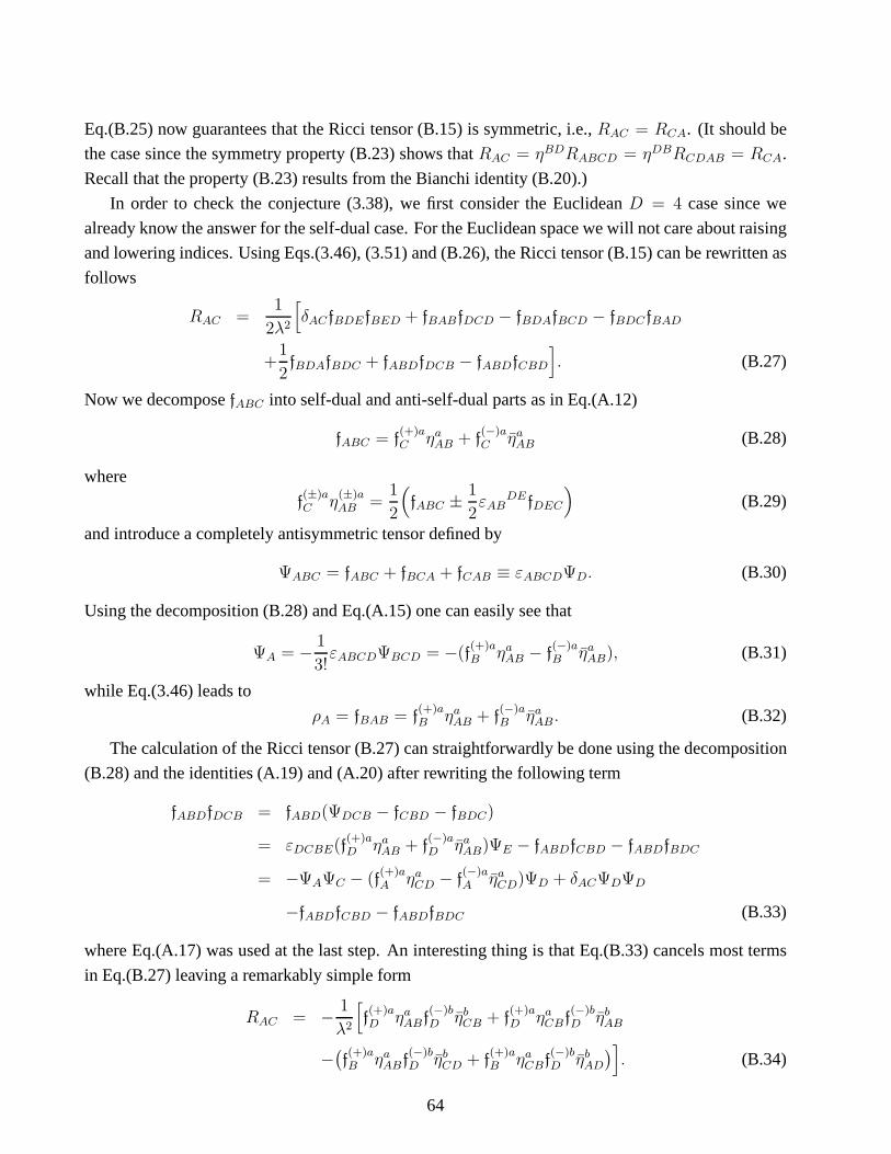
Eq.(B.25) now guarantees that the Ricci tensor (B.15) is symmetric, i.e.,RAC = RCA. (It should be

the case since the symmetry property (B.23) shows thatRAC = ηBDRABCD = ηDBRCDAB = RCA.

Recall that the property (B.23) results from the Bianchi identity (B.20).)

In order to check the conjecture (3.38), we first consider theEuclideanD = 4 case since we

already know the answer for the self-dual case. For the Euclidean space we will not care about raising

and lowering indices. Using Eqs.(3.46), (3.51) and (B.26),the Ricci tensor (B.15) can be rewritten as

follows

RAC =1

2λ2

[δACfBDEfBED + fBABfDCD − fBDAfBCD − fBDCfBAD

+1

2fBDAfBDC + fABDfDCB − fABDfCBD

]. (B.27)

Now we decomposefABC into self-dual and anti-self-dual parts as in Eq.(A.12)

fABC = f(+)aC ηa

AB + f(−)aC ηa

AB (B.28)

where

f(±)aC η

(±)aAB =

1

2

(fABC ±

1

2εAB

DEfDEC

)(B.29)

and introduce a completely antisymmetric tensor defined by

ΨABC = fABC + fBCA + fCAB ≡ εABCDΨD. (B.30)

Using the decomposition (B.28) and Eq.(A.15) one can easilysee that

ΨA = − 1

3!εABCDΨBCD = −(f

(+)aB ηa

AB − f(−)aB ηa

AB), (B.31)

while Eq.(3.46) leads to

ρA = fBAB = f(+)aB ηa

AB + f(−)aB ηa

AB. (B.32)

The calculation of the Ricci tensor (B.27) can straightforwardly be done using the decomposition

(B.28) and the identities (A.19) and (A.20) after rewritingthe following term

fABDfDCB = fABD(ΨDCB − fCBD − fBDC)

= εDCBE(f(+)aD ηa

AB + f(−)aD ηa

AB)ΨE − fABDfCBD − fABDfBDC

= −ΨAΨC − (f(+)aA ηa

CD − f(−)aA ηa

CD)ΨD + δACΨDΨD

−fABDfCBD − fABDfBDC (B.33)

where Eq.(A.17) was used at the last step. An interesting thing is that Eq.(B.33) cancels most terms

in Eq.(B.27) leaving a remarkably simple form

RAC = − 1

λ2

[f(+)aD ηa

ABf(−)bD ηb

CB + f(+)aD ηa

CBf(−)bD ηb

AB

−(f(+)aB ηa

ABf(−)bD ηb

CD + f(+)aB ηa

CBf(−)bD ηb

AD

)]. (B.34)

64

Note that the right-hand side of Eq.(B.34) is purely interaction terms between the self-dual and

anti-self-dual parts in Eq.(B.28). (The same result was also obtained in [75].) Therefore, if NC gauge

fields satisfy the self-duality equation (3.44), they describe a Ricci-flat manifold, i.e.,RAC = 0. Of

course, this result is completely consistent with that in Appendix A. Moreover we see the reason

why self-dual NC gauge fields satisfy the Einstein equation (3.38) with vanishing energy-momentum

tensor.

Finally we can calculate the Einstein tensor to find the form of the energy-momentum tensor

defined by Eq.(3.38):

EAB = RAB −1

2δABR

= − 1

λ2

(f(+)aD ηa

ACf(−)bD ηb

BC + f(+)aD ηa

BC f(−)bD ηb

AC

)

+1

λ2

(f(+)aC ηa

ACf(−)bD ηb

BD + f(+)aC ηa

BC f(−)bD ηb

AD − δABf(+)aD ηa

CDf(−)bE ηb

CE

)(B.35)

where the Ricci scalarR is given by

R =2

λ2f(+)aB ηa

ABf(−)bC ηb

AC . (B.36)

We have adopted the conventional view that the gravitational field is represented by the spacetime

metric itself. The problem then becomes one of finding field equations to relate the metric (3.41) to

the energy-momentum distribution. According to our scheme, Eq.(B.35) should correspond to such

field equations, i.e., the Einstein equations. In other words, if we are clever enough, we should be

able to find the NC gauge theory described by Eqs.(3.51) and (3.52) starting from the Einstein gravity

described by Eqs.(B.22) and (B.35) by properly reversing our above derivation as we have explicitly

demonstrated it for the self-dual case in Appendix A.

As we explained in Section 3.2, we want to identify Eq.(B.35)with an energy-momentum tensor.

First note that the Ricci scalarR, (B.36), is nonvanishing for a generic case. This means thatthere

is an extra field contribution to the energy-momentum tensorin addition to Maxwell fields whose

energy-momentum tensor is traceless. Since the extra field energy-momentum tensor turns out to be

basically a gradient volume energy (see the latter part of Sec. 3.2), we call it the “Liouville” energy-

momentum tensor. A similar result was also obtained in [17] where it was dubbed as the ‘Poisson’

energy. Since the first term in Eq.(B.35) is traceless due to Eq.(A.18), it would be a candidate of the

Maxwell energy-momentum tensor while the second term wouldbe the Liouville energy-momentum

tensor. So we tentatively make the following identificationfor the Maxwell energy-momentum tensor

65

T(M)AB and the Liouville energy-momentum tensorT

(L)AB

8πG4

c4T

(M)AB = − 1

λ2

(f(+)aD ηa

ACf(−)bD ηb

BC + f(+)aD ηa

BC f(−)bD ηb

AC

),

= − 1

λ2

(fACDfBCD −

1

4δABfCDEfCDE

), (B.37)

8πG4

c4T

(L)AB =

1

λ2

(f(+)aC ηa

ACf(−)bD ηb

BD + f(+)aC ηa

BC f(−)bD ηb

AD − δABf(+)aD ηa

CDf(−)bE ηb

CE

),

=1

2λ2

(ρAρB −ΨAΨB −

1

2δAB(ρ2

C −Ψ2C))

(B.38)

where we have used the decomposition (B.29) and the relation

f(+)aB ηa

AB =1

2(ρA −ΨA), f

(−)aB ηa

AB =1

2(ρA + ΨA).

We have anticipated that the energy-momentum tensor (B.37)will be related to that of Maxwell

fields since both are definitely traceless in four dimensions. So our problem is how to rewrite the

energy-momentum tensor in terms of NC fields in⋆-algebraAθ, denoted asTAB(Aθ), using the ex-

pression (B.37) defined inTM , denoted asTAB(TM). In other words, we want to translateTAB(TM)

into anAθ-valued energy momentum tensor. This problem is quite subtle.

Recall that NC fields are identified with vector fields inTM through the map (3.23) at the leading

order. For example, we get the following identification fromEq.(3.26)

− i[FAB, f ]⋆ = FAB, fθ + · · · = [DA, DB][f ] + · · ·= −fAB

CDC [f ] + · · · . (B.39)

Note that Eq.(B.39) is nothing but the Lie algebra homomorphism (3.29) for the Poisson algebra. But

a NC field regarded as an element of NC⋆-algebraAθ in general lives in a Hilbert spaceH, e.g.,

the Fock space (3.2) while the vector fieldsDA in Eq.(3.23) are defined in the real vector spaceTM .

Furthermore we see from Eqs.(3.23) and (B.39) that “anti-Hermitian” operators in NC algebraAθ

such as the NC fieldsDA and−iFAB are mapped to real vector fields inTM . Thus we have the

bizarre correspondence between geometry defined inTM and NC algebraAθ24

Anti−Hermitian operators on H ⇔ Real vector fields on TM. (B.40)

In order to identifyAθ-valued quantities fromTM-valued ones, it is first necessary to analytically

continue the real vector spaceTM to a complex vector spaceTMC. At the same time, the real vector

fieldDA is replaced by a self-adjoint operatorDA in TMC and the structure equation (3.40) instead

has the form

[DA,DB] = ifABCDC . (B.41)

24It might be remarked that the transition fromTM toAθ is analogous to that from classical mechanics (anR-world)

to quantum mechanics (aC-world). See Section 5.4 in [32] for the exposition of the similar problem in the context of

quantum mechanics.

66

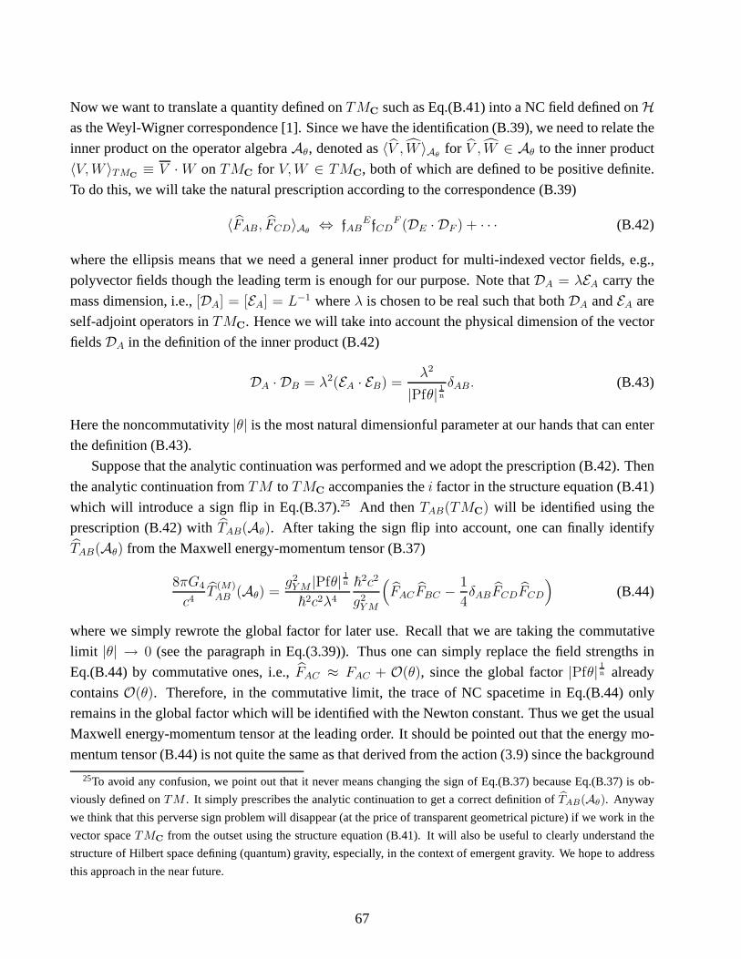
Now we want to translate a quantity defined onTMC such as Eq.(B.41) into a NC field defined onHas the Weyl-Wigner correspondence [1]. Since we have the identification (B.39), we need to relate the

inner product on the operator algebraAθ, denoted as〈V , W 〉Aθfor V , W ∈ Aθ to the inner product

〈V,W 〉TMC≡ V ·W onTMC for V,W ∈ TMC, both of which are defined to be positive definite.

To do this, we will take the natural prescription according to the correspondence (B.39)

〈FAB, FCD〉Aθ⇔ fAB

EfCDF (DE · DF ) + · · · (B.42)

where the ellipsis means that we need a general inner productfor multi-indexed vector fields, e.g.,

polyvector fields though the leading term is enough for our purpose. Note thatDA = λEA carry the

mass dimension, i.e.,[DA] = [EA] = L−1 whereλ is chosen to be real such that bothDA andEA are

self-adjoint operators inTMC. Hence we will take into account the physical dimension of the vector

fieldsDA in the definition of the inner product (B.42)

DA · DB = λ2(EA · EB) =λ2

|Pfθ| 1nδAB. (B.43)

Here the noncommutativity|θ| is the most natural dimensionful parameter at our hands thatcan enter

the definition (B.43).

Suppose that the analytic continuation was performed and weadopt the prescription (B.42). Then

the analytic continuation fromTM to TMC accompanies thei factor in the structure equation (B.41)

which will introduce a sign flip in Eq.(B.37).25 And thenTAB(TMC) will be identified using the

prescription (B.42) withTAB(Aθ). After taking the sign flip into account, one can finally identify

TAB(Aθ) from the Maxwell energy-momentum tensor (B.37)

8πG4

c4T

(M)AB (Aθ) =

g2Y M |Pfθ| 1n~2c2λ4

~2c2

g2Y M

(FACFBC −

1

4δABFCDFCD

)(B.44)

where we simply rewrote the global factor for later use. Recall that we are taking the commutative

limit |θ| → 0 (see the paragraph in Eq.(3.39)). Thus one can simply replace the field strengths in

Eq.(B.44) by commutative ones, i.e.,FAC ≈ FAC + O(θ), since the global factor|Pfθ| 1n already

containsO(θ). Therefore, in the commutative limit, the trace of NC spacetime in Eq.(B.44) only

remains in the global factor which will be identified with theNewton constant. Thus we get the usual

Maxwell energy-momentum tensor at the leading order. It should be pointed out that the energy mo-

mentum tensor (B.44) is not quite the same as that derived from the action (3.9) since the background

25To avoid any confusion, we point out that it never means changing the sign of Eq.(B.37) because Eq.(B.37) is ob-

viously defined onTM . It simply prescribes the analytic continuation to get a correct definition ofTAB(Aθ). Anyway

we think that this perverse sign problem will disappear (at the price of transparent geometrical picture) if we work in the

vector spaceTMC from the outset using the structure equation (B.41). It willalso be useful to clearly understand the

structure of Hilbert space defining (quantum) gravity, especially, in the context of emergent gravity. We hope to address

this approach in the near future.

67

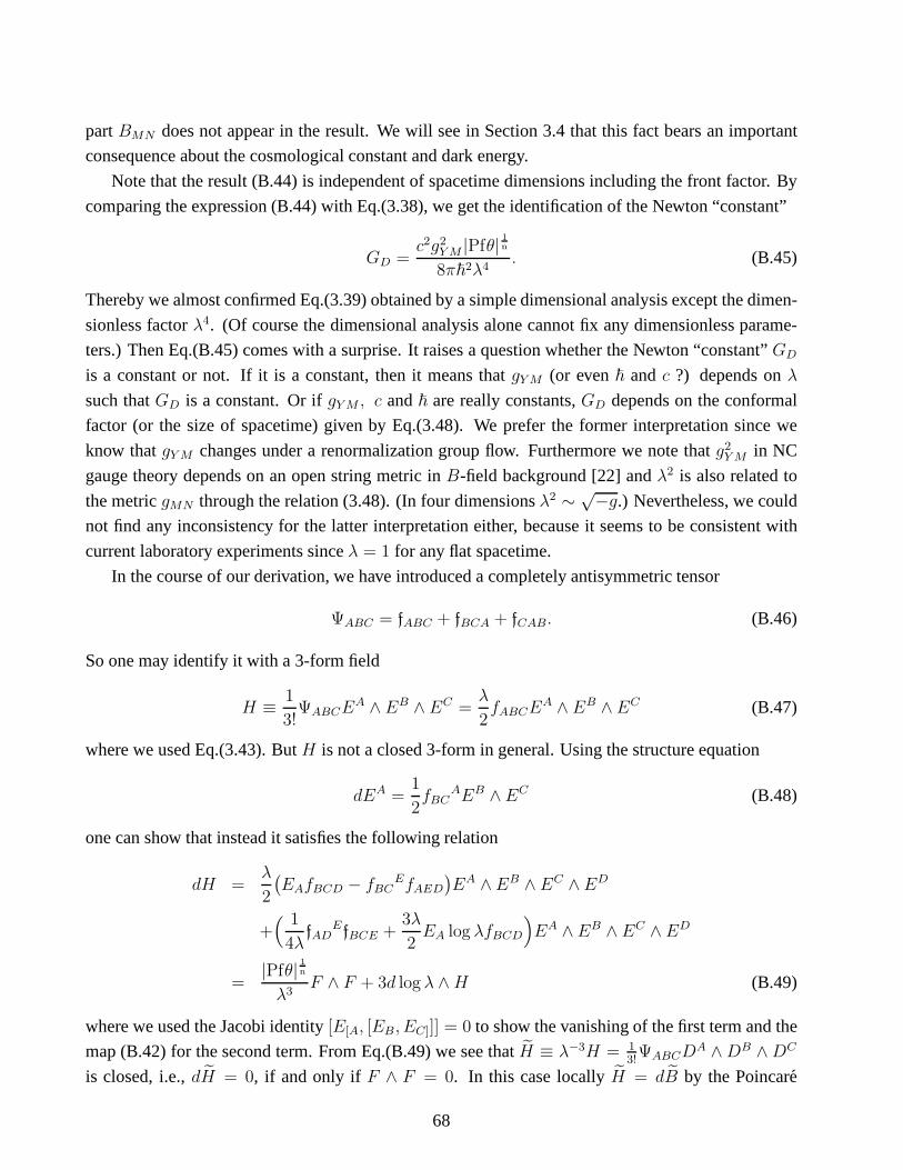
partBMN does not appear in the result. We will see in Section 3.4 that this fact bears an important

consequence about the cosmological constant and dark energy.

Note that the result (B.44) is independent of spacetime dimensions including the front factor. By

comparing the expression (B.44) with Eq.(3.38), we get the identification of the Newton “constant”

GD =c2g2

Y M |Pfθ| 1n8π~2λ4

. (B.45)

Thereby we almost confirmed Eq.(3.39) obtained by a simple dimensional analysis except the dimen-

sionless factorλ4. (Of course the dimensional analysis alone cannot fix any dimensionless parame-

ters.) Then Eq.(B.45) comes with a surprise. It raises a question whether the Newton “constant”GD

is a constant or not. If it is a constant, then it means thatgY M (or even~ andc ?) depends onλ

such thatGD is a constant. Or ifgY M , c and~ are really constants,GD depends on the conformal

factor (or the size of spacetime) given by Eq.(3.48). We prefer the former interpretation since we

know thatgY M changes under a renormalization group flow. Furthermore we note thatg2Y M in NC

gauge theory depends on an open string metric inB-field background [22] andλ2 is also related to

the metricgMN through the relation (3.48). (In four dimensionsλ2 ∼ √−g.) Nevertheless, we could

not find any inconsistency for the latter interpretation either, because it seems to be consistent with

current laboratory experiments sinceλ = 1 for any flat spacetime.

In the course of our derivation, we have introduced a completely antisymmetric tensor

ΨABC = fABC + fBCA + fCAB. (B.46)

So one may identify it with a 3-form field

H ≡ 1

3!ΨABCE

A ∧ EB ∧ EC =λ

2fABCE

A ∧ EB ∧ EC (B.47)

where we used Eq.(3.43). ButH is not a closed 3-form in general. Using the structure equation

dEA =1

2fBC

AEB ∧EC (B.48)

one can show that instead it satisfies the following relation

dH =λ

2

(EAfBCD − fBC

EfAED

)EA ∧EB ∧ EC ∧ED

+( 1

4λfAD

EfBCE +3λ

2EA log λfBCD

)EA ∧EB ∧ EC ∧ ED

=|Pfθ| 1nλ3

F ∧ F + 3d log λ ∧H (B.49)

where we used the Jacobi identity[E[A, [EB, EC]]] = 0 to show the vanishing of the first term and the

map (B.42) for the second term. From Eq.(B.49) we see thatH ≡ λ−3H = 13!

ΨABCDA ∧DB ∧DC

is closed, i.e.,dH = 0, if and only if F ∧ F = 0. In this case locallyH = dB by the Poincare

68

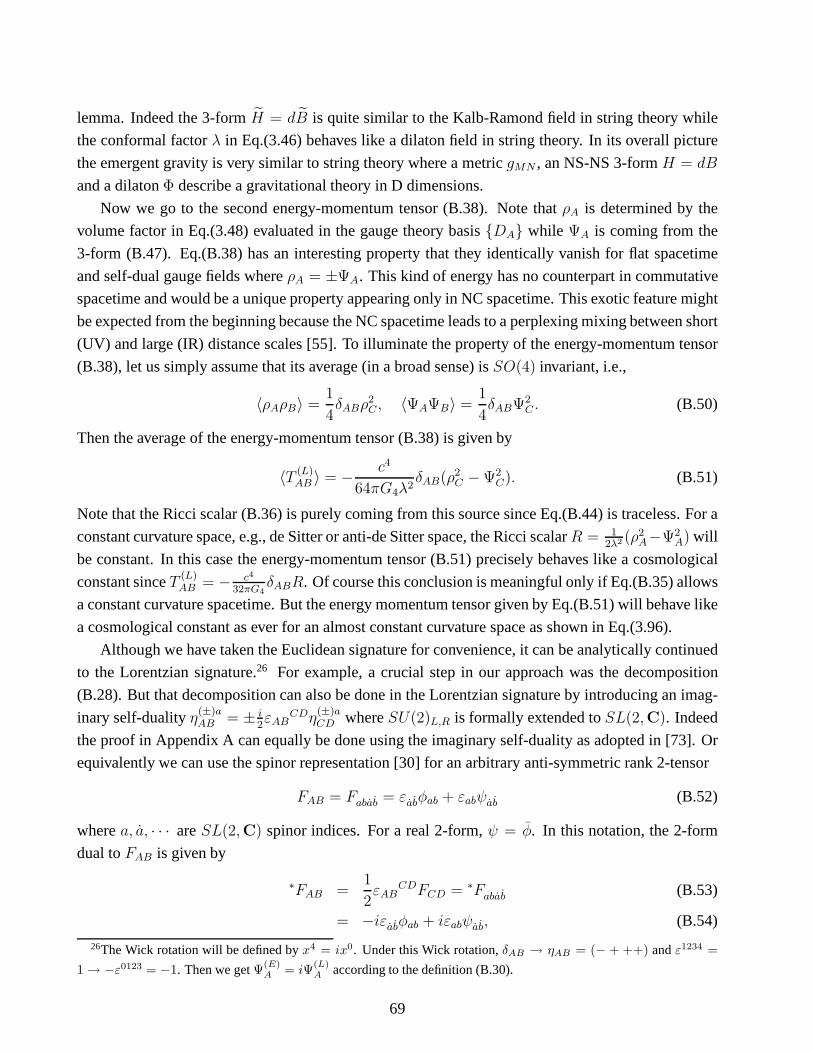
lemma. Indeed the 3-formH = dB is quite similar to the Kalb-Ramond field in string theory while

the conformal factorλ in Eq.(3.46) behaves like a dilaton field in string theory. Inits overall picture

the emergent gravity is very similar to string theory where ametricgMN , an NS-NS 3-formH = dB

and a dilatonΦ describe a gravitational theory in D dimensions.

Now we go to the second energy-momentum tensor (B.38). Note that ρA is determined by the

volume factor in Eq.(3.48) evaluated in the gauge theory basis DA while ΨA is coming from the

3-form (B.47). Eq.(B.38) has an interesting property that they identically vanish for flat spacetime

and self-dual gauge fields whereρA = ±ΨA. This kind of energy has no counterpart in commutative

spacetime and would be a unique property appearing only in NCspacetime. This exotic feature might

be expected from the beginning because the NC spacetime leads to a perplexing mixing between short

(UV) and large (IR) distance scales [55]. To illuminate the property of the energy-momentum tensor

(B.38), let us simply assume that its average (in a broad sense) isSO(4) invariant, i.e.,

〈ρAρB〉 =1

4δABρ

2C , 〈ΨAΨB〉 =

1

4δABΨ2

C . (B.50)

Then the average of the energy-momentum tensor (B.38) is given by

〈T (L)AB 〉 = − c4

64πG4λ2δAB(ρ2

C −Ψ2C). (B.51)

Note that the Ricci scalar (B.36) is purely coming from this source since Eq.(B.44) is traceless. For a

constant curvature space, e.g., de Sitter or anti-de Sitterspace, the Ricci scalarR = 12λ2 (ρ

2A−Ψ2

A) will

be constant. In this case the energy-momentum tensor (B.51)precisely behaves like a cosmological

constant sinceT (L)AB = − c4

32πG4δABR. Of course this conclusion is meaningful only if Eq.(B.35) allows

a constant curvature spacetime. But the energy momentum tensor given by Eq.(B.51) will behave like

a cosmological constant as ever for an almost constant curvature space as shown in Eq.(3.96).

Although we have taken the Euclidean signature for convenience, it can be analytically continued

to the Lorentzian signature.26 For example, a crucial step in our approach was the decomposition

(B.28). But that decomposition can also be done in the Lorentzian signature by introducing an imag-

inary self-dualityη(±)aAB = ± i

2εAB

CDη(±)aCD whereSU(2)L,R is formally extended toSL(2,C). Indeed

the proof in Appendix A can equally be done using the imaginary self-duality as adopted in [73]. Or

equivalently we can use the spinor representation [30] for an arbitrary anti-symmetric rank 2-tensor

FAB = Fabab = εabφab + εabψab (B.52)

wherea, a, · · · areSL(2,C) spinor indices. For a real 2-form,ψ = φ. In this notation, the 2-form

dual toFAB is given by

∗FAB =1

2εAB

CDFCD = ∗Fabab (B.53)

= −iεabφab + iεabψab, (B.54)

26The Wick rotation will be defined byx4 = ix0. Under this Wick rotation,δAB → ηAB = (− + ++) andε1234 =

1→ −ε0123 = −1. Then we getΨ(E)A = iΨ

(L)A according to the definition (B.30).

69

that is,∗Fabab = iFabba = −iFbaab. (B.55)

For the sake of completeness we will also considerD = 2 andD = 3 cases. For convenience

we consider the Euclidean signature again for both cases. (TheD = 2 case should be Euclidean

in our context since we don’t want to consider time-space noncommutativity.) From now on we set

~ = c = 1.

In two dimensions, the analysis is simple. So we immediatelylist the formulas:

fABC ≡ εABΨC , (B.56)

ρA = fBAB = 2DA log λ, (B.57)

ΨA = εABρB = 2εABDB log λ, (B.58)

DAρA = −ρAρA = −ΨAΨA, (B.59)

DAΨA = 0, (B.60)

RABCD =1

2εABεCDR =

1

2(δACδBD − δADδBC)R, (B.61)

R =2

λ2(DADA log λ− 2DA log λDA log λ). (B.62)

Of course it is a bit lengthy to directly check Eq.(B.61) fromEq.(B.14).

Using the equation of motion (B.59), the Ricci scalar (B.62)can be rewritten as

R = − 2

λ2ρAρA = − 2

λ2ΨAΨA = − 8

λ2DA log λDA log λ. (B.63)

The Einstein equation in two dimensions can be written as

RAB =1

2δABR = − 1

2λ2δABfCDEfCDE. (B.64)

An interesting thing in Eq.(B.63) is that the Ricci scalar isalways negative unlike as the 4-dimensional

case whereR = 12λ2 (ρ

2A − Ψ2

A). Hence Eq.(B.64) describes only hyperbolic (negative curvature)

Riemann surfaces but most Riemann surfaces belong to this class.

From Eq.(B.64) one can see that the case withFAB = 0 corresponds to parabolic (curvature 0)

Riemann surfaces which include a planeR2 and a torusT2. Then a natural question is where the

different topology forR2 andT2 comes from. Note that there are still background gauge fieldsgiven

by Eq.(3.1) although thefluctuationsare vanishing. (Two-dimensional gauge fields do not have any

physical degrees of freedom but encode only a topological information. So thefluctuationshere mean

the variation of a topological shape.) We observe that, thoughB ∈ H2(M) in Eq.(3.1) is constant, it

reveals its topology through the first cohomology groupH1(M) which measures the obstruction for

symplectic vector fields to be globally Hamiltonian (see thefootnote 3 in [3]). That is the only source

we can imagine for the origin of the topology of Riemann surfaces. We believe that the topology

70

of the fluctuationFAB in Eq.(B.64) similarly appears in hyperbolic Riemann surfaces with a higher

genus. Then a natural question is about a rational (positivecurvature) Riemann surface, i.e.,S2. It

may be necessary to introduce a mass term as a potential term.We leave it for a future work.27

Now we go over toD = 3 case. In three dimensionsfABC have totally 9 components. We will

decompose them into9 = 1 + 3 + 5 as follows

fABC = εABCΨ + εABD(ρDC + ϕDC) (B.65)

where the first term is totally anti-symmetric part like Eq.(B.46) and the second term is anti-symmetric,

ρDC = −ρCD, and the third term is symmetric,ϕDC = ϕCD, and traceless,ϕCC = 0. Eq.(3.46) then

leads to the relationρAB = 12εABCρC . Therefore we get the following decomposition

fABC = εABCΨ +1

2(δACρB − δBCρA) + εABDϕDC . (B.66)

In other words, the symmetric part can be deduced from Eq.(B.66) as follows

ϕAB =1

2εACDfCDB −

1

2εABCρC − δABΨ. (B.67)

Using the variables in Eq.(B.66), the equations of motion (3.51) can be written as

DBfBCA = −2δACΨ2 −ΨϕAC +1

4(δACρBρB − ρAρC) (B.68)

+3

2εACBΨρB + εCBDρBϕDA +

1

2εACBρDϕBD + ϕABϕCB. (B.69)

Contracting the indicesA andC in the above equation leads to the relation

DAρA = 6Ψ2 − 1

2ρAρA − ϕABϕAB. (B.70)

Using the above results, it is straightforward though a bit lengthy to calculate the Ricci tensor (B.15)

RAC = − 1

λ2

(fABDfCBD −

1

4δACfBEDfBED

)

+1

4λ(∇AρC +∇CρA) +

1

2λ2ρAρC (B.71)

and the Ricci scalar (B.16)

R =1

λ∇AρA +

1

2λ2

(ρAρA − 9Ψ2

). (B.72)

Since the first term in Eq.(B.15) is nonvanishing while it wasabsent in four dimensions, we introduced

the covariant derivative of the “Liouville” fieldρA defined by

∇AρC = EAρC − ωAB

CρB (B.73)

27In this respect, the work [77] by H. Shimada should be interesting. He showed that the topology of a membrane in

matrix theory can be captured by a Hamiltonian function defined on a Riemann surface. The Hamiltonian function for a

nontrivial Riemann surface is in general given by a Morse function containing several nondegenerate critical points, e.g.,

a height function, where the topology of a membrane is realized as the Morse topology.

71

and then we used the following relation derived from Eq.(B.10)

∇AρC +∇CρA =1

λ

(DAρC +DCρA − (fABC + fCBA)ρB + δACρBρB − ρAρC

). (B.74)

Also the expression (B.72) has been achieved after using therelation

fABCfABC = 18Ψ2 − 2λ∇AρA. (B.75)

Finally we can get the 3-dimensional Einstein equation induced from the NCU(1) gauge fields

EAB = RAB −1

2δABR

= 8πG3

(T

(M)AB + T

(L)AB

)(B.76)

where the Maxwell energy-momentum tensor and the Liouvilleenergy-momentum tensor are, respec-

tively, given by

T(M)AB = − 1

8πG3λ2

(fACDfBCD −

1

4δABfCDEfCDE

)(B.77)

T(L)AB =

1

16πG3λ2

(1

2

(∇AρB + ∇BρA + ρAρB

)

−δAB

(∇CρC +

1

2(ρCρC − 9Ψ2)

))(B.78)

where∇A = λ∇A.

Following the exactly same strategy as the four dimensionalcase, one can identifyT (M)AB (Aθ) from

Eq.(B.77) getting the same form as Eq.(B.44). Once again we get an exotic form of energy described

by Eq.(B.78) in addition to the usual Maxwell energy-momentum tensor. This energy density is

also related to the gradient volume energy. (See Section 3.2.) But the explicit form is different

from the four dimensional one, Eq.(B.38). This difference is due to the fact that the first term in

Eq.(B.15), which appears as the covariant derivative termsin Eq.(B.78), is absent in four dimensions.

An interesting thing in Eq.(B.78) is thatρA behaves like a massive field whose mass is vanishing in flat

spacetime sinceλ = 1 in that case. We further discuss in Section 3.4 about the physical implications

of the Liouville energy-momentum tensor.

In higherD ≥ 5 dimensions, the calculation of the energy-momentum tensorfrom Eq.(B.15)

becomes more complicated. The 3-form field (B.47) contributes nontrivially to the energy-momentum

tensor. We have not tried to find its concrete form. We hope to attack this problem in the near future.

72

References

[1] M. R. Douglas and N. A. Nekrasov, Noncommutative field theory, Rev. Mod. Phys.73 (2001)

977,hep-th/0106048; R. J. Szabo, Quantum field theory on noncommutative spaces,Phys.

Rep.378(2003) 207,hep-th/0109162.

[2] R. J. Szabo, Symmetry, gravity and noncommutativity, Class. Quantum Grav.23 (2006) R199,

hep-th/0606233.

[3] H. S. Yang, Emergent Gravity from Noncommutative Spacetime, to appear in Int. J. Mod. Phys.

A, hep-th/0611174.

[4] N. Hitchin, Generalized Calabi-Yau manifolds, Quart. J. Math. Oxford Ser.54 (2003) 281,

math.DG/0209099.

[5] M. Gualtieri, Generalized complex geometry,math.DG/0401221; math.DG/0703298; G.

R. Cavalcanti, New aspects of theddc-lemma,math.DG/0501406.

[6] J. Madore and J. Mourad, Quantum space-time and classical gravity, J. Math. Phys.39 (1998)

423,gr-qc/9607060.

[7] S. I. Vacaru, Gauge and Einstein gravity from non-abelian gauge models on noncommutative

spaces, Phys. Lett.B498(2001) 74,hep-th/0009163.

[8] E. Langmann and R. J. Szabo, Teleparallel gravity and dimensional reductions of noncommuta-

tive gauge theory, Phys. Rev.D64 (2001) 104019,hep-th/0105094.

[9] V. O. Rivelles, Noncommutative field theories and gravity, Phys. Lett.B558 (2003) 191,

hep-th/0212262.

[10] H. S. Yang, Exact Seiberg-Witten Map and Induced Gravity from Noncommutativity, Mod.

Phys. Lett.A21 (2006) 2637,hep-th/0402002; R. Banerjee and H. S. Yang, Exact Seiberg-

Witten map, induced gravity and topological invariants in noncommutative field theories, Nucl.

Phys.B708(2005) 434,hep-th/0404064.

[11] M. Salizzoni, A. Torrielli and H. S. Yang, ALE spaces from noncommutative U(1) instantons via

exact Seiberg-Witten map, Phys. Lett.B634 (2006) 427,hep-th/0510249; H. S. Yang and

M. Salizzoni, Gravitational Instantons from Gauge Theory,Phys. Rev. Lett.96 (2006) 201602,

hep-th/0512215.

[12] H. S. Yang, Instantons and Emergent Geometry,hep-th/0608013.

73

[13] H. S. Yang, On The Correspondence Between Noncommuative Field Theory And Gravity, Mod.

Phys. Lett.A22 (2007) 1119,hep-th/0612231; Noncommutative Spacetime and Emergent

Gravity, Bulgarian Journal of Physics35 (s1) (2008) 323, published as Proceedings “Lie The-

ory and Its Applications in Physics VII”, ed. V. K. Dobrev et al. (Heron Press, Sofia, 2008),

arXiv:0711.0234.

[14] H. S. Yang, Noncommutative Electromagnetism As A LargeN Gauge Theory,

arXiv:0704.0929.

[15] H. S. Yang, Emergent Gravity And The Cosmological Constant Problem,

arXiv:0711.2797; Emergent Spacetime and The Cosmological Constant, Int. J.Mod.

Phys.A23 (2008) 2181,arXiv:0803.3272.

[16] B. Muthukumar,U(1) gauge invariant noncommutative Schrodinger theory and gravity, Phys.

Rev.D71(2005) 105007,hep-th/0412069; A. H. Fatollahi, Particle dynamics and emergent

gravity, Phys. Lett.B665(2008) 257,arXiv:0805.1159.

[17] M. Buric, T. Grammatikopoulos, J. Madore and G. Zoupanos, Gravity and the structure of non-

commutative algebras, J. High Energy Phys.04 (2006) 054,hep-th/0603044; M. Buric, J.

Madore and G. Zoupanos, WKB Approximation in Noncommutative Gravity, SIGMA3 (2007)

125,arXiv:0712.4024.

[18] H. Steinacker, Emergent gravity from noncommutative gauge theory, J. High Energy Phys.12(2007) 049,arXiv:0708.2426.

[19] H. Grosse, H. Steinacker and M. Wohlgenannt, Emergent gravity, matrix models and

UV/IR mixing, J. High Energy Phys.04 (2008) 023,arXiv:0802.0973; D. Klammer

and H. Steinacker, Fermions and emergent noncommutative gravity, ibid. 08 (2008) 074,

arXiv:0805.1157.

[20] H. Steinacker, Emergent Gravity and Noncommutative Branes from Yang-Mills Matrix Models,

Nucl. Phys.B810(2009) 1,arXiv:0806.2032.

[21] T. Padmanabhan, Dark Energy and Gravity, Gen. Rel. Grav. 40 (2008) 529,

arXiv:0705.2533; Gravity as an emergent phenomenon: A Conceptual description,

AIP Conference Proceedings989 (2007) 114,arXiv:0706.1654; Dark Energy and its

Implications for Gravity,arXiv:0807.2356.

[22] N. Seiberg and E. Witten, String theory and noncommutative geometry, J. High Energy Phys.

09 (1999) 032,hep-th/9908142.

[23] N. Seiberg, A note on background independence in noncommutative gauge theories, matrix

model and tachyon condensation, J. High Energy Phys.09 (2000) 003,hep-th/0008013.

74

[24] J. M. Maldacena, The Large N Limit of Superconformal Field Theories and Supergravity, Adv.

Theor. Math. Phys.2 (1998) 231,hep-th/9711200; S. S. Gubser, I. R. Klebanov and A. M.

Polyakov, Gauge Theory Correlators from Non-Critical String Theory, Phys. Lett.B428(1998)

105,hep-th/9802109; E. Witten, Anti De Sitter Space And Holography, Adv. Theor.Math.

Phys.2 (1998) 253,hep-th/9802150.

[25] S. Sternberg, Minimal coupling and the symplectic mechanics of a classical particle in the pres-

ence of a Yang-Mills field, Proc. Natl. Acad. Sci.74 (1977) 5253.

[26] F. J. Dyson, Feynman’s proof of the Maxwell equations, Am. J. Phys.58 (1990) 209.

[27] P. Horava, Stability of Fermi Surfaces and K Theory, Phys. Rev. Lett.95 (2005) 016405,

hep-th/0503006.

[28] G. E. Volovik, Quantum Phase Transitions from Topologyin Momentum Space, Lect. Notes

Phys. 718 (2007) 31, cond-mat/0601372; Fermi-point scenario of emergent gravity,

arXiv:0709.1258.

[29] J. Bardeen, L. N. Cooper and J. R. Schrieffer, Theory of Superconductivity, Phys. Rev.108(1957) 1175.

[30] C. W. Misner, K. S. Thorne and J. A. Wheeler,Gravitation(W. H. Freeman and Company, New

York, 1973).

[31] M. Kontsevich, Deformation Quantization of Poisson Manifolds, Lett. Math. Phys.66 (2003)

157,q-alg/9709040.

[32] R. Abraham and J. E. Marsden,Foundations of Mechanics(Addison-Wesley, Reading, 1978).

[33] G. Darboux, Sur le probleme de Pfaff, Bull. Sci. Math.6 (1882) 14-36, 49-68.

[34] J. Moser, On the volume elements on a manifold, Trans. Amer. Math. Soc.120(1965) 286.

[35] B. Jurco and P. Schupp, Noncommutative Yang-Mills from equivalence of star products, Eur.

Phys. J.C14 (2000) 367,hep-th/0001032.

[36] J. Madore, S. Schraml, P. Schupp and J. Wess, Gauge theory on noncommutative spaces, Eur.

Phys. J.C16 (2000) 161,hep-th/0001203.

[37] L. Cornalba, D-brane Physics and Noncommutative Yang-Mills Theory, Adv. Theor. Math.

Phys.4 (2000) 271,hep-th/9909081.

75

[38] N. Ishibashi, H. Kawai, Y. Kitazawa and A. Tsuchiya, A large-N reduced model as superstring,

Nucl. Phys.B498 (1997) 467,hep-th/9612115; H. Aoki, N. Ishibashi, S. Iso, H. Kawai,

Y. Kitazawa and T. Tada, Non-commutative Yang-Mills in IIB matrix model, Nucl. Phys.B565(2000) 176,hep-th/9908141.

[39] M. Kontsevich, Homological Algebra of Mirror Symmetry, alg-geom/9411018.

[40] A. Zee, Gravity and its Mysteries: Some Thoughts and Speculations, Int. J. Mod. Phys.A23(2008) 1295,arXiv:0805.2183.

[41] A. Connes,Noncommutative Geometry(Academic Press, San Diego, CA, 1994).

[42] J. A. Harvey, Topology of the Gauge Group in Noncommutative Gauge Theory,

hep-th/0105242; F. Lizzi, R. J. Szabo and A. Zampini, Geometry of the gauge algebra in

noncommutative Yang-Mills theory, J. High Energy Phys.08 (2001) 032,hep-th/0107115.

[43] T. Banks, W. Fischler, S. H. Shenker and L. Susskind,M theory as a matrix model: A conjecture,

Phys. Rev.D55 (1997) 5112,hep-th/9610043.

[44] L. Motl, Proposals on nonperturbative superstring interactions,hep-th/9701025; R. Di-

jkgraaf, E. Verlinde and H. Verlinde, Matrix string theory,Nucl. Phys.B500 (1997) 43,

hep-th/9703030.

[45] H. Grosse and R. Wulkenhaar, Renormalisation ofφ4-Theory on Noncommutative IR4 in the

Matrix Base, Commun. Math. Phys.256 (2005) 305,hep-th/0401128; P. Aschieri, T.

Grammatikopoulos, H. Steinacker and G. Zoupanos, Dynamical generation of fuzzy extra di-

mensions, dimensional reduction and symmetry breaking, J.High Energy Phys.09 (2006) 026,

hep-th/0606021.

[46] W. Taylor, M(atrix) theory: matrix quantum mechanics as a fundamental theory, Rev. Mod.

Phys.73 (2001) 419,hep-th/0101126.

[47] E. Witten, Bound states of strings andp-branes, Nucl. Phys.B460 (1996) 335,

hep-th/9510135.

[48] D. J. Gross, A. Hashimoto and N. Itzhaki, Observables ofNon-Commutative Gauge Theories,

Adv. Theor. Math. Phys.4 (2000) 893,hep-th/0008075.

[49] Y. M. Cho and P. G. O. Freund, Non-Abelian gauge fields as Nambu-Goldstone fields, Phys.

Rev.D12 (1975) 1711.

[50] R. S. Ward, TheSU(∞) chiral model and self-dual vacuum spaces, Class. Quantum Grav. 7(1990) L217.

76

[51] A. Raychaudhuri, Relativistic Cosmology. I, Phys. Rev. 98 (1955) 1123.

[52] S. W. Hawking and G. F. R. Ellis,The Large Scale Structure of Space-Time(Cambridge Univ.

Press, 1973).

[53] L. Cornalba, Corrections to the abelian Born-Infeld action arising from noncommutative geom-

etry, J. High Energy Phys.09 (2000) 017,hep-th/9912293; On the general structure of the

nonAbelian Born-Infeld action, Adv. Theor. Math. Phys.4 (2002) 1259,hep-th/0006018;

L. Cornalba and R. Schiappa, Nonassociative Star Product Deformations for D-Brane World-

Volumes in Curved Backgrounds, Commun. Math. Phys.225(2002) 33,hep-th/0101219.

[54] T. Banks and W. Fischler, An Holographic Cosmology,hep-th/0111142.

[55] S. Minwalla, M. Van Raamsdonk and N. Seiberg, Noncommutative perturbative dynamics, J.

High Energy Phys.02 (2000) 020,hep-th/9912072.

[56] C. R. Lee, The Feynman-Dyson proof of the gauge field equations, Phys. Lett.A148 (1990)

146; S. Tanimura, Relativistic Generalization and Extension to the Non-Abelian Gauge Theory

of Feynman’s Proof of the Maxwell Equations, Ann. Phys.220 (1992) 229; J. F. Carinena, L.

A. Ibort, G. Marmo and A. Stern, The Feynman problem and the inverse problem for Poisson

dynamics, Phys. Rep.263(1995) 153.

[57] V. Guillemin and S. Sternberg,Symplectic Techniques in Physics(Cambridge Univ. Press, 1984).

[58] A. Connes and C. Rovelli, Von Neumann algebra automorphisms and time-thermodynamics

relation in generally covariant quantum theories, Class. Quant. Grav. 11 (1994) 2899,

gr-qc/9406019; M. Heller and W. Sasin, Emergence of time, Phys. Lett.A250 (1998) 48,

gr-qc/9711051.

[59] R. Minasian and G. Moore, K-theory and Ramond-Ramond charge, J. High Energy Phys.11(1997) 002,hep-th/9710230; P. Horava, Type-IIA D-branes, K-Theory and Matrix Theory,

Adv. Theor. Math. Phys.2 (1998) 1373,hep-th/9812135.

[60] E. Witten,D-branes and K-theory, J. High Energy Phys.12 (1998) 019,hep-th/9810188;

Overview of K theory applied to strings, Int. J. Mod. Phys.A16 (2001) 693,

hep-th/0007175.

[61] K. Olsen and R. J. Szabo, Constructing D-Branes from K-Theory, Adv. Theor. Math. Phys.3(1999) 889,hep-th/9907140; J. A. Harvey, Komaba Lectures on Noncommutative Solitons

and D-Branes,hep-th/0102076.

[62] R. Gopakumar, S. Minwalla and A. Strominger, Noncommutative solitons, J. High Energy Phys.

05 (2000) 020,hep-th/0003160.

77

[63] M. F. Atiyah, R. Bott and A. Shapiro, Clifford Modules, Topology3 (suppl.1) (1964) 3.

[64] J. Maldacena and A. Strominger,AdS3 black holes and a stringy exclusion principle, J. High

Energy Phys.12 (1998) 005,hep-th/9804085; J. McGreevy, L. Susskind and N. Toumbas,

Invasion of the giant gravitons from anti-de Sitter space, J. High Energy Phys.06 (2000) 008.

hep-th/0003075.

[65] H. Georgi,Lie Algebras in Particle Physics: From Isospin to Unified Theories(Advanced Book

Program, 1999).

[66] D. V. Vassilevich and A. Yurov, Space-time noncommutativity tends to create bound states,

Phys. Rev.D69 (2004) 105006,hep-th/0311214; A. H. Fatollahi and A. Jafari, On

bound states of photons in noncommutative U(1) gauge theory, Eur. Phys. J.C46 (2006) 235,

hep-th/0503078.

[67] N. Nekrasov and A. Schwarz, Instantons on Noncommutative IR4 and (2,0) Superconformal Six

Dimensional Theory, Commun. Math. Phys.198(1998) 689,hep-th/9802068.

[68] S. Weinberg and E. Witten, Phys. Lett.96B (1980) 59.

[69] F. Loebbert, The Weinberg-Witten theorem on massless particles: An essay, Annalen Phys.

(Berlin) 17 (2008) 803.

[70] S. Weinberg,The Quantum Theory of Fields, vol. 2 (Cambridge Univ. Press, 1996), Section

21.6; From BCS to the LHC, CERN Courier, Jan. 21 (2008); E. Witten, From superconductors

and four-manifolds to weak interactions, Bull. Amer. Math.Soc.44 (2007) 361.

[71] G. ’t Hooft, Dimensional Reduction in Quantum Gravity,gr-qc/9310026; L. Susskind, The

world as a hologram, J. Math. Phys.36 (1995) 6377,hep-th/9409089.

[72] S. L. Glashow, A. Halprin, P. I. Krastev, C. N. Leung and J. Pantaleone, Remarks on neu-

trino tests for special relativity, Phys. Rev.D56 (1997) 2433,hep-ph/9703454; S. Coleman

and S. L. Glashow, High-energy tests of Lorentz invariance,Phys. Rev.D59 (1999) 116008,

hep-ph/9812418; A. G. Cohen and S. L. Glashow, Very Special Relativity, Phys. Rev. Lett.

97 (2006) 021601,hep-ph/0601236.

[73] L. J. Mason and E. T. Newman, A Connection Between the Einstein and Yang-Mills Equations,

Commun. Math. Phys.121(1989) 659.

[74] G. W. Gibbons and S. W. Hawking, Gravitational Multi-instantons, Phys. Lett.78B (1978) 430.

[75] J. D. E. Grant,LsdiffM and the Einstein equations, Class. Quantum Grav.13 (1996) L1,

gr-qc/9411059; Self-dual two-forms and divergence-free vector fields,gr-qc/9702001.

78

[76] A. Ashtekar, T. Jabobson and L. Smolin, A New Characterization Of Half-Flat Solutions to

Einstein’s Equation, Commun. Math. Phys.115(1988) 631.

[77] H. Shimada, Membrane topology and matrix regularization, Nucl. Phys.B685 (2004) 297,

hep-th/0307058.

79