Anisotropic Diffusion PDE’s for Multi-Channel ImageRegularization : Framework and Applications

David Tschumperle∗ Rachid Deriche⋆

∗ Image Team, GREYC / ENSICAEN - UMR CNRS 6072, 6 Bd du MarechalJuin, 14050 Caen Cedex, France.

⋆ Odyssee Project Team, INRIA/ENPC/ENS - INRIA, 2004 Route des Lucioles, BP 93, 06902 Sophia Antipolis, France.

Abstract

We review recent methods based on diffusion PDE’s (Partial Differential Equations) for the purpose of multi-channelimage regularization. Such methods have the ability to smooth multi-channel images anisotropically and can preserve thenimage contours while removing noise or other undesired local artifacts. We point out the pros and cons of the existing equa-tions, providing at each time a local geometric interpretation of the corresponding processes. We focus then on an alternateand generic tensor-driven formulation, able to regularizeimages while specifically taking the curvatures of local image struc-tures into account. This particular diffusion PDE variant is actually well suited for the preservation of thin structures andgives regularization results where important image features can be particularly well preserved compared to its competitors.A direct link between this curvature-preserving equation and a continuous formulation of the Line Integral Convolution tech-nique (Cabral and Leedom, 1993) is demonstrated. It allows the design of a very fast and stable numerical scheme whichimplements the multi-valued regularization method by successive integrations of the pixel values along curved integral lines.Besides, the proposed implementation, based on a fourth-order Runge Kutta numerical integration, can be applied with asubpixel accuracy and preserves then thin image structuresmuch better than classical finite-differences discretizations, usu-ally chosen to implement PDE-based diffusions. We finally illustrate the efficiency of this diffusion PDE’s for multi-channelimage regularization - in terms of speed and visual quality -with various applications and results on color images, includingimage denoising, inpainting and edge-preserving interpolation.

Keywords : Multi-Channel Images Regularization, Anisotropic Smoothing, Diffusion PDE’s, Tensor-Valued Geometry,Denoising, Inpainting, Nonlinear Interpolation.

Preliminary Notations

- Throughout this chapter, we will represent amulti-channelor multi-valued imageby a continuous functionI : Ω → Rn,

whereΩ ⊂ R2 is the definition domain of the image (basically a2D rectangleW ×H) andn ∈ N

+ is the dimension of eachvector-valued image pixelI(X) located atX = (x y)T ∈ Ω. The notationIi stands for theith channelof the imageI.Note thatIi can be considered itself as a scalar-valued imageIi : Ω → R. Thus, we have

∀X = (x, y) ∈ Ω, I(X) =(

I1(X) I2(X) ... In(X)

)T

For the common case of color images, we naturally getn = 3, i.e. three vector components (R,G,B) per pixel, retrievedrespectively from the red (I1), green (I2) and blue (I3) channels of a color imageI.

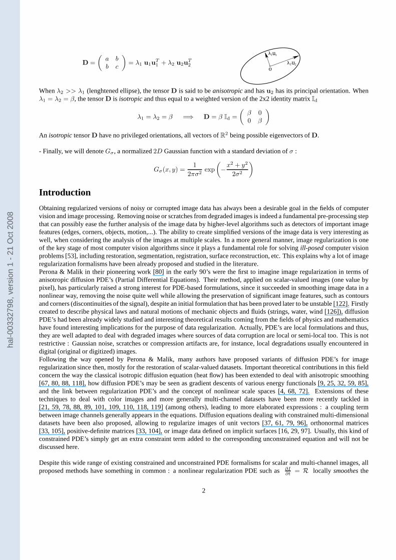
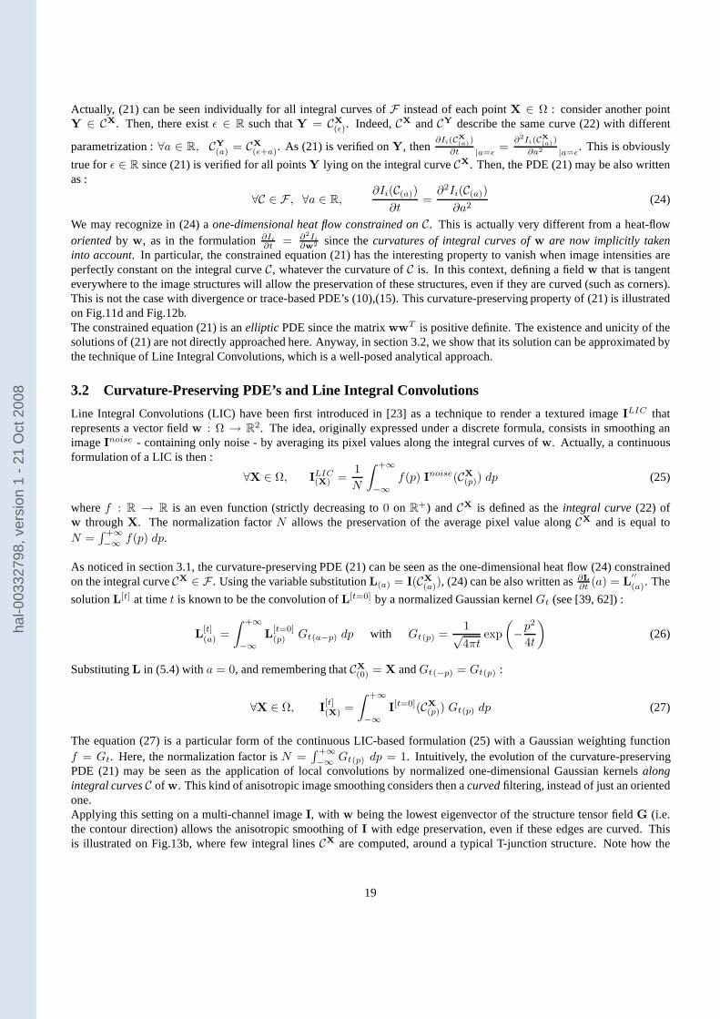
- We will also intensely use2nd-order diffusion tensorsin equations described in this chapter. A diffusion tensorD isassimilated to a2× 2 symmetricandpositive-definitematrix, having then two positive eigenvaluesλ1, λ2 and two associatedorthonormal eigenvectorsu1⊥u2. Theshapeof a tensorD may be seen as anellipse, oriented by the vector basisu1⊥u2

and elongated byλ1 andλ2, as illustrated below.

1

hal-0

0332

798,

ver

sion

1 -

21 O

ct 2

008

Author manuscript, published in "Advances in Imaging and Electron Physics (AIEP) (2007) 145--209"

D =

(

a bb c

)

= λ1 u1uT1 + λ2 u2u

T2

λ1u1

λ2u2

o

Whenλ2 >> λ1 (lenghtened ellipse), the tensorD is said to beanisotropicand hasu2 has its principal orientation. Whenλ1 = λ2 = β, the tensorD is isotropicand thus equal to a weighted version of the 2x2 identity matrix Id

λ1 = λ2 = β =⇒ D = β Id =

(

β 00 β

)

An isotropictensorD have no privileged orientations, all vectors ofR2 being possible eigenvectors ofD.

- Finally, we will denoteGσ, a normalized2D Gaussian function with a standard deviation ofσ :

Gσ(x, y) =1

2πσ2exp

(

−x2 + y2

2σ2

)

Introduction

Obtaining regularized versions of noisy or corrupted imagedata has always been a desirable goal in the fields of computervision and image processing. Removing noise or scratches from degraded images is indeed a fundamental pre-processing stepthat can possibly ease the further analysis of the image databy higher-level algorithms such as detectors of important imagefeatures (edges, corners, objects, motion,...). The ability to create simplified versions of the image data is very interesting aswell, when considering the analysis of the images at multiple scales. In a more general manner, image regularization is oneof the key stage of most computer vision algorithms since it plays a fundamental role for solvingill-posedcomputer visionproblems [53], including restoration, segmentation, registration, surface reconstruction, etc. This explains why alot of imageregularization formalisms have been already proposed and studied in the literature.Perona & Malik in their pioneering work [80] in the early 90’swere the first to imagine image regularization in terms ofanisotropic diffusion PDE’s (Partial Differential Equations). Their method, applied on scalar-valued images (one value bypixel), has particularly raised a strong interest for PDE-based formulations, since it succeeded in smoothing image data in anonlinear way, removing the noise quite well while allowingthe preservation of significant image features, such as contoursand corners (discontinuities of the signal), despite an initial formulation that has been proved later to be unstable [122]. Firstlycreated to describe physical laws and natural motions of mechanic objects and fluids (strings, water, wind [126]), diffusionPDE’s had been already widely studied and interesting theoretical results coming from the fields of physics and mathematicshave found interesting implications for the purpose of dataregularization. Actually, PDE’s are local formulations and thus,they are well adapted to deal with degraded images where sources of data corruption are local or semi-local too. This is notrestrictive : Gaussian noise, scratches or compression artifacts are, for instance, local degradations usually encountered indigital (original or digitized) images.Following the way opened by Perona & Malik, many authors haveproposed variants of diffusion PDE’s for imageregularization since then, mostly for the restoration of scalar-valued datasets. Important theoretical contributions in this fieldconcern the way the classical isotropic diffusion equation(heat flow) has been extended to deal with anisotropic smoothing[67, 80, 88, 118], how diffusion PDE’s may be seen as gradientdescents of various energy functionals [9, 25, 32, 59, 85],and the link between regularization PDE’s and the concept ofnonlinear scale spaces [4, 68, 72]. Extensions of thesetechniques to deal with color images and more generally multi-channel datasets have been more recently tackled in[21, 59, 78, 88, 89, 101, 109, 110, 118, 119] (among others), leading to more elaborated expressions : a coupling termbetween image channels generally appears in the equations.Diffusion equations dealing with constrained multi-dimensionaldatasets have been also proposed, allowing to regularize images of unit vectors [37, 61, 79, 96], orthonormal matrices[33, 105], positive-definite matrices [33, 104], or image data defined on implicit surfaces [16, 29, 97]. Usually, this kind ofconstrained PDE’s simply get an extra constraint term addedto the corresponding unconstrained equation and will not bediscussed here.

Despite this wide range of existing constrained and unconstrained PDE formalisms for scalar and multi-channel images,allproposed methods have something in common : a nonlinear regularization PDE such as∂I∂t = R locally smoothesthe

2

hal-0

0332

798,

ver

sion

1 -

21 O

ct 2

008

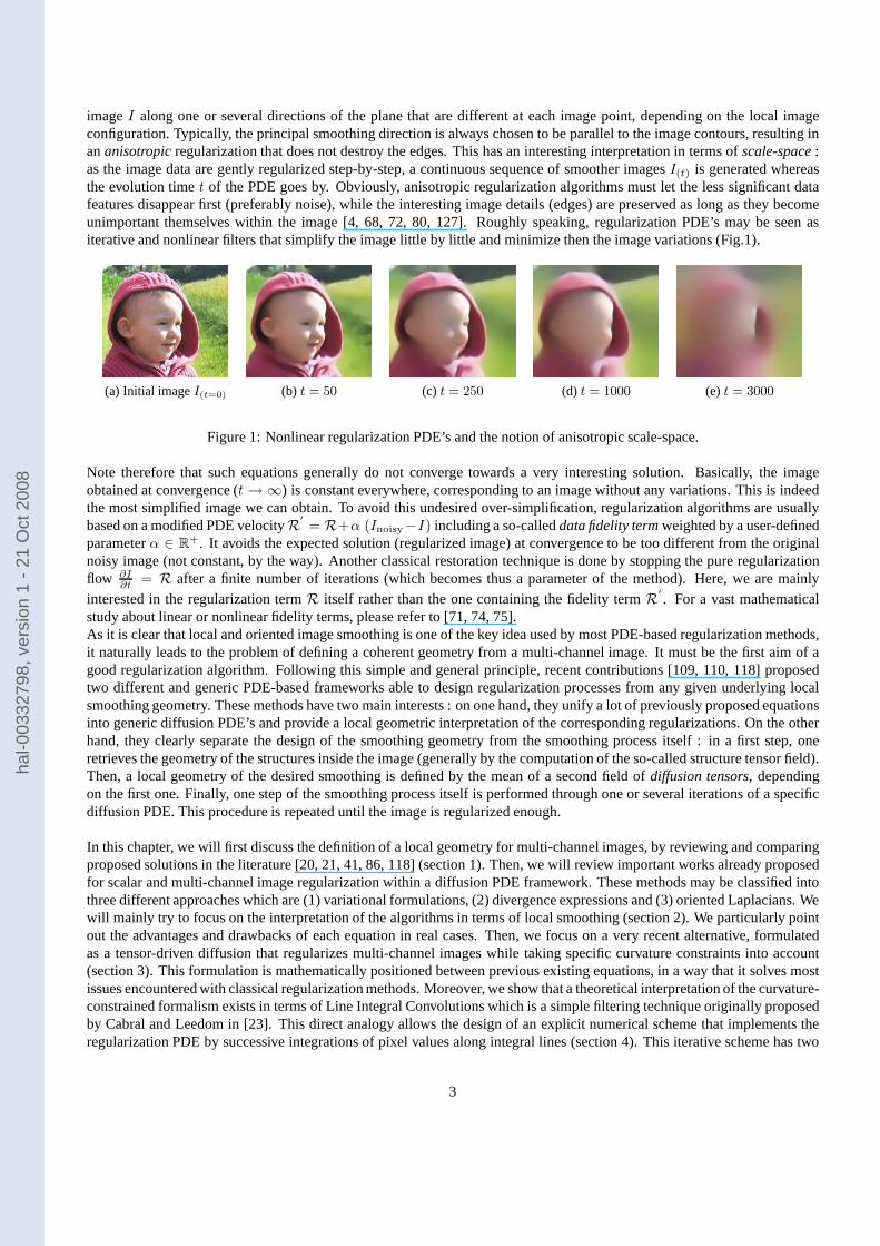
imageI along one or several directions of the plane that are different at each image point, depending on the local imageconfiguration. Typically, the principal smoothing direction is always chosen to be parallel to the image contours, resulting inananisotropicregularization that does not destroy the edges. This has an interesting interpretation in terms ofscale-space:as the image data are gently regularized step-by-step, a continuous sequence of smoother imagesI(t) is generated whereasthe evolution timet of the PDE goes by. Obviously, anisotropic regularization algorithms must let the less significant datafeatures disappear first (preferably noise), while the interesting image details (edges) are preserved as long as they becomeunimportant themselves within the image [4, 68, 72, 80, 127]. Roughly speaking, regularization PDE’s may be seen asiterative and nonlinear filters that simplify the image little by little and minimize then the image variations (Fig.1).

(a) Initial imageI(t=0) (b) t = 50 (c) t = 250 (d) t = 1000 (e) t = 3000

Figure 1: Nonlinear regularization PDE’s and the notion of anisotropic scale-space.

Note therefore that such equations generally do not converge towards a very interesting solution. Basically, the imageobtained at convergence (t → ∞) is constant everywhere, corresponding to an image withoutany variations. This is indeedthe most simplified image we can obtain. To avoid this undesired over-simplification, regularization algorithms are usuallybased on a modified PDE velocityR′

= R+α (Inoisy−I) including a so-calleddata fidelity termweighted by a user-definedparameterα ∈ R

+. It avoids the expected solution (regularized image) at convergence to be too different from the originalnoisy image (not constant, by the way). Another classical restoration technique is done by stopping the pure regularizationflow ∂I

∂t = R after a finite number of iterations (which becomes thus a parameter of the method). Here, we are mainlyinterested in the regularization termR itself rather than the one containing the fidelity termR′

. For a vast mathematicalstudy about linear or nonlinear fidelity terms, please referto [71, 74, 75].As it is clear that local and oriented image smoothing is one of the key idea used by most PDE-based regularization methods,it naturally leads to the problem of defining a coherent geometry from a multi-channel image. It must be the first aim of agood regularization algorithm. Following this simple and general principle, recent contributions [109, 110, 118] proposedtwo different and generic PDE-based frameworks able to design regularization processes from any given underlying localsmoothing geometry. These methods have two main interests :on one hand, they unify a lot of previously proposed equationsinto generic diffusion PDE’s and provide a local geometric interpretation of the corresponding regularizations. On the otherhand, they clearly separate the design of the smoothing geometry from the smoothing process itself : in a first step, oneretrieves the geometry of the structures inside the image (generally by the computation of the so-called structure tensor field).Then, a local geometry of the desired smoothing is defined by the mean of a second field ofdiffusion tensors, dependingon the first one. Finally, one step of the smoothing process itself is performed through one or several iterations of a specificdiffusion PDE. This procedure is repeated until the image isregularized enough.

In this chapter, we will first discuss the definition of a localgeometry for multi-channel images, by reviewing and comparingproposed solutions in the literature [20, 21, 41, 86, 118] (section 1). Then, we will review important works already proposedfor scalar and multi-channel image regularization within adiffusion PDE framework. These methods may be classified intothree different approaches which are (1) variational formulations, (2) divergence expressions and (3) oriented Laplacians. Wewill mainly try to focus on the interpretation of the algorithms in terms of local smoothing (section 2). We particularlypointout the advantages and drawbacks of each equation in real cases. Then, we focus on a very recent alternative, formulatedas a tensor-driven diffusion that regularizes multi-channel images while taking specific curvature constraints into account(section 3). This formulation is mathematically positioned between previous existing equations, in a way that it solves mostissues encountered with classical regularization methods. Moreover, we show that a theoretical interpretation of thecurvature-constrained formalism exists in terms of Line Integral Convolutions which is a simple filtering technique originally proposedby Cabral and Leedom in [23]. This direct analogy allows the design of an explicit numerical scheme that implements theregularization PDE by successive integrations of pixel values along integral lines (section 4). This iterative schemehas two

3

hal-0

0332

798,

ver

sion

1 -

21 O

ct 2

008

main advantages compared to classical PDE implementations: on one hand, it preserves thin image structures remarkablywell, since it naturally works at a sub-pixel accuracy, thanks to the use of a fourth-order Runge Kutta integration. On theother hand, the algorithm is able to run up to three times faster than classical explicit schemes since it is unconditionallystable, even for large PDE time steps. The described method makes diffusion PDE’s a generic and very efficient approach forsolving image processing problems needing multi-channel image regularization.We finally illustrate this effectiveness, in terms of computational speed and visual quality, with results on color image restora-tion, color image inpainting and non-linear resizing, among all possible applications in the area of image regularization(section 5).

1 Defining a Local Geometry for Multi-Channel Images

1.1 Local geometric features

As stated in the introduction, image regularization may be seen as a filter that reduces local pixel variations. More precisely,one wants to smooth a multi-channel imageI : Ω → R

n while preserving its edges (discontinuities in the image intensities),i.e. performs a local smoothing mostly along directions of the edges, avoiding a smoothing orthogonal to these edges. Ata first glance, a naive idea would be to apply a scalar-valued regularization filter on each channelIi of the multi-channelimageI, doing this independently for eachi = 1...n. But, the correlation between image channels would be ignored in thiscase, and it might cause important disparities in the smoothing behavior, since local smoothing directions and amplitudescould be very different from each channel to another. Such decoupled regularization methods generally lead to undesirableover-smoothing effects destroying significant edge structures in the image.Multi-channel image regularization is rather based on a coherent image smoothing which locally uses the same smoothingdirections and amplitudes for all image channelsIi. Naturally, this means that one has first to measure thelocal geometryofa multi-channel imageI. Such a geometry consists actually in the definition of theseimportant features at each image pointX = (x, y) ∈ Ω of I :

- Two orthogonal directionsθ+(X) , θ−(X) ∈ S1 (unit vectors ofR2) directed respectively across and along the edges (gen-

erally the maximum and minimum variations of the image intensities atX). The directionθ− generally correspondsto the edge direction, when there is one, whileθ+ naturally extends the notion ofgradient directionfor multi-channelimages.

- A corresponding variation normN (X) measuring thelocal strengthof an edge. This is the extension of thevectorgradient normfor multi-channel images.

In order to construct such a vector geometry, different approaches have been considered so far and are detailed below.

1.2 Geometry from a scalar feature

One simple method consists in computing first a scalar imagef(I), using a vector to scalar functionf : Rn → R that would

ideally model thehuman perceptionof vector-valued edges. It is particularly conceivable forcolor images : one may choosefor instance the lightness function (perceptual response to the luminance) coming from theCIELAB color base [81] :

f = L∗ = 116 g(Y ) − 16 with Y = 0.2125R+ 0.7154G+ 0.0721B

whereg : R → R is defined by

g(s) = 3√s if s > 0.008856

g(s) = 7.787s+ 16116 else

Thus, we may define a vector-valued local vector geometryN , θ+, θ− of I by choosing

θ+ =∇f(I)

‖∇f(I)‖

θ− ⊥ θ+

and N = ‖∇f(I)‖

4

hal-0

0332

798,

ver

sion

1 -

21 O

ct 2

008

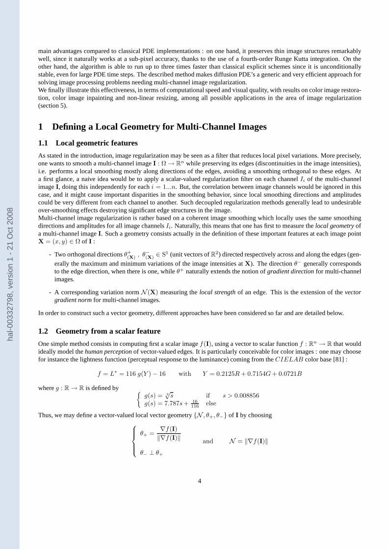
However, this method has two major drawbacks. First, this isnot always possible to easily define a significant functionf formulti-channel images (particularly when the number of channel isn > 3). Second, there are mathematically no functionsf that can detect all possible vector-valued variations. Forinstance, the lightness function defined above will not be able todetectiso-lightnessvector contours in a color image. It is the case for the image illustrated on Fig.2 : the contours insidethe colored yin-yang symbol will not be detected byN = ‖∇f(I)‖, sincef(I) is constant therein. As a consequence,the smoothing performed here will be either isotropic or oriented in a wrong direction : the existing color edges inside theyin-yang symbol will be probably blurred.

(a) Red channelR (b) Green channelG (c) Blue channelB(d) Color image(R, G, B)

(e) Lightness(scalar) imageL∗

Figure 2: Using lightnessL∗ to detect geometry of a color image fail for iso-lightness contours.

1.3 Di Zenzo multi-valued geometry

In order to overcome this limitation, a very elegant solution has been proposed by Di Zenzo in [41]. He considers a multi-channel imageI : Ω → R

n as a vector field, and looks for the local variations of the vector norm‖dI‖2, mainly given by avariation matrixG = (gi,j). We get :

dI = Ix dx+ Iy dy where Ix =∂I

∂xand Iy =

∂I

∂y(∈ R

n)

then‖dI‖2 = dIT dI = ‖Ix‖2 dx2 + 2 ITx Iy dxdy + ‖Iy‖2 dy2

i.e.

‖dI‖2 = dXT G dX where G =

n∑

i=1

∇Ii ∇ITi and dX =

(

dxdy

)

G is denoted as thestructure tensor. It sums variation contributions from each image channelIi. It is easy to see thatG is a2 × 2 symmetric and semi positive-definite matrix. Its coefficients (gi,j) are simply :

g11 =∑n

i=1 I2ix

g12 = g21 =∑n

i=1 IixIiy

g22 =∑n

i=1 I2iy

In the common case of color imagesI = (R,G,B), G is defined as :

G =

(

R2x +G2

x +B2x RxRy +GxGy +BxBy

RxRy +GxGy +BxBy R2y +G2

y +B2y

)

(1)

The interesting point aboutG is that its positive eigenvaluesλ+/− give the maximum and the minimum values of‖dI‖2 whilethe orthogonal eigenvectorsθ+ andθ− are the correspondingorientationsof these extrema, and are formally given by :

λ+/− =g11 + g22 ±

√∆

2and θ+/− //

(

2 g12g22 − g11 ±

√∆

)

(2)

5

hal-0

0332

798,

ver

sion

1 -

21 O

ct 2

008

where∆ = (g11 − g22)2 + 4 g2

12 . The vectorsθ± are normalized to the unit vector afterward.With this simple and efficient approach, Di Zenzo opened a natural way to deal with the local vector geometry of multi-channel images, through the use of theoriented orthogonal basis(θ+ , θ−) and thevariations measures(λ+, λ−). Aslight variant has been proposed by Weickert in [118]. He rather proposed to study the eigenvalues and eigenvectors of aGaussian-smoothed versionGσ of the structure tensorG :

Gσ =n∑

i=1

[(

∇Iiα∇ITiα)

∗Gσ]

where ∇Iiα = ∇(Ii ∗Gα) (3)

whereGα andGσ are 2D Gaussian kernels with variances respectively equal to α andσ. User-defined parametersα andσ have an influence on the smoothness of the obtained structuretensor field, and by extension, on the regularity of theretrieved vector-valued image geometry. It is worth to notice that eigenvalues ofGσ are well adapted to discriminate differentgeometric cases :

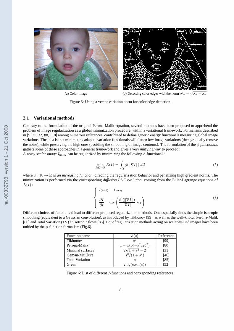
- Whenλ+ ≃ λ− ≃ 0, there are very few vector variations around the current point X = (x, y) : the region isalmostflat and does not contain any edges or corners (it is the case for the inside of the strips in Fig.3a). For this configuration,the variation normN we have to define should be low.

- Whenλ+ ≫ λ−, there are a lot of vector variations. The current point may be located on avector edge(it is the casefor the edges of the strips in Fig.3a). For this configuration, the variation normN should be high.

- Whenλ+ ≃ λ− ≫ 0, we are located on asaddle point of the vector surface, which can be possibly acorner structurein the image (for instance, the intersections of the strips in Fig.3a). In this caseN should be even higher than forthe previous configuration. Regularization algorithms have indeed a tendency to smooth corners fastly. A very highvariation measure estimated on corner points would attenuate the smoothing there, which is often a desired effect.

Actually, a lot of proposed regularization algorithms acting on multi-channel images have implicitly or explicitly based theirsmoothing behavior from these Di Zenzo’s attributes. In particular, three different choices of vector gradient normsN havebeen proposed so far in the literature to measure vector-valued variations :

- N =√

λ+, as a natural extension of the scalar gradient norm viewed asthe value of maximum variations[20, 86, 87](Fig.3b and Fig.4b). This norm will not particularly give importance to corners compared to straight edges.

- N− =√

λ+ − λ−, also calledcoherence norm, have been chosen in [89, 114, 116]. Note that this norm failstodetect discontinuities that are saddle points of the vector-valued surface. This is illustrated on the intersections of thestrips (Fig.3c), as well as in the center and left-right parts of the child’s eye (Fig.4c). This will mainly perturb anyregularization process that uses this norm since some colored sharp corners, considered as homogeneous regions, willbe probably over-smoothed.

- N+ =√

λ+ + λ−, also denoted by‖∇I‖ is often chosen [14, 21, 78, 96, 104, 105] since it detects edges and cornersin a good way, and is easy to compute. Indeed, it does not require an eigenvalue decomposition ofG as the other normsdid, because

N+ = ‖∇I‖ =√

trace(G) =

√

√

√

√

n∑

i=1

‖∇Ii‖2 (4)

Moreover, the normN+ has the interesting property of giving preferences to certain corners (Fig.3d). This is veryvaluable for image restoration purposes, since the smoothing can be attenuated on high-curvature structures which areclassically hard to preserve.

Note that for the scalar case (n = 1), the structure tensor calculus reduces to :

when n = 1 , ‖dI‖2 = dX G1 dX where G1 = ∇I∇IT =

(

I2x IxIy

IxIy I2y

)

6

hal-0

0332

798,

ver

sion

1 -

21 O

ct 2

008

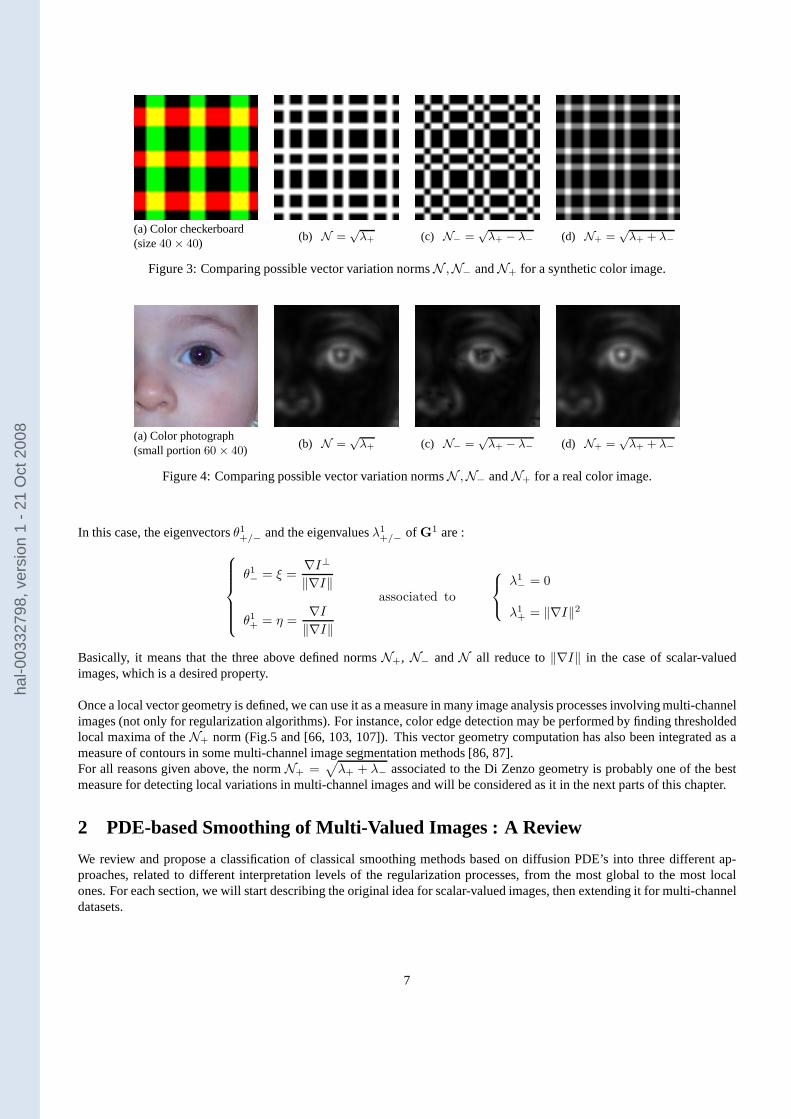
(a) Color checkerboard(size40 × 40)

(b) N =√

λ+ (c) N− =√

λ+ − λ− (d) N+ =√

λ+ + λ−

Figure 3: Comparing possible vector variation normsN ,N− andN+ for a synthetic color image.

(a) Color photograph(small portion60 × 40)

(b) N =√

λ+ (c) N− =√

λ+ − λ− (d) N+ =√

λ+ + λ−

Figure 4: Comparing possible vector variation normsN ,N− andN+ for a real color image.

In this case, the eigenvectorsθ1+/− and the eigenvaluesλ1+/− of G1 are :

θ1− = ξ =∇I⊥‖∇I‖

θ1+ = η =∇I‖∇I‖

associated to

λ1− = 0

λ1+ = ‖∇I‖2

Basically, it means that the three above defined normsN+, N− andN all reduce to‖∇I‖ in the case of scalar-valuedimages, which is a desired property.

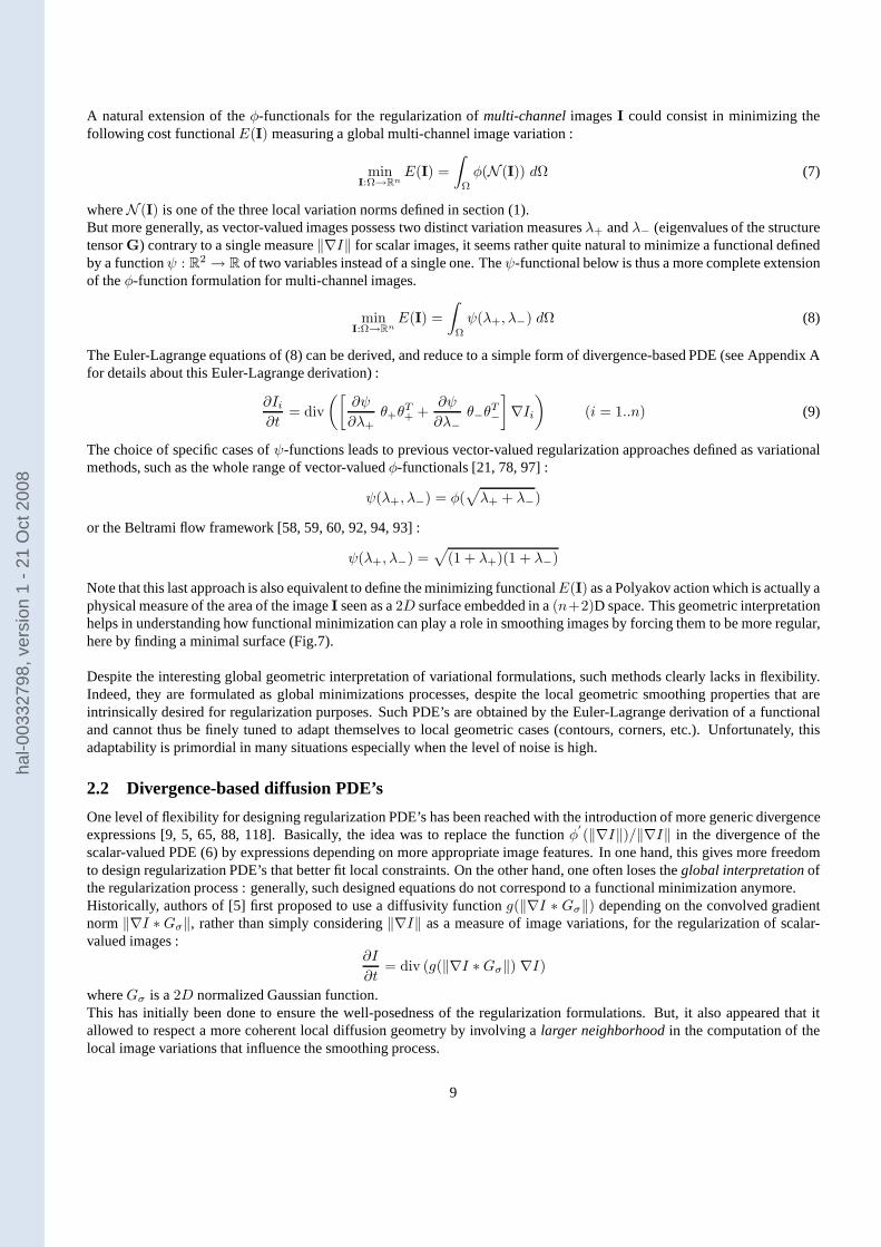
Once a local vector geometry is defined, we can use it as a measure in many image analysis processes involving multi-channelimages (not only for regularization algorithms). For instance, color edge detection may be performed by finding thresholdedlocal maxima of theN+ norm (Fig.5 and [66, 103, 107]). This vector geometry computation has also been integrated as ameasure of contours in some multi-channel image segmentation methods [86, 87].For all reasons given above, the normN+ =

√

λ+ + λ− associated to the Di Zenzo geometry is probably one of the bestmeasure for detecting local variations in multi-channel images and will be considered as it in the next parts of this chapter.

2 PDE-based Smoothing of Multi-Valued Images : A Review

We review and propose a classification of classical smoothing methods based on diffusion PDE’s into three different ap-proaches, related to different interpretation levels of the regularization processes, from the most global to the mostlocalones. For each section, we will start describing the original idea for scalar-valued images, then extending it for multi-channeldatasets.

7

hal-0

0332

798,

ver

sion

1 -

21 O

ct 2

008

(a) Color image (b) Detecting color edges with the normN+ =√

λ+ + λ−

Figure 5: Using a vector variation norm for color edge detection.

2.1 Variational methods

Contrary to the formulation of the original Perona-Malik equation, several methods have been proposed to apprehend theproblem of image regularization as a global minimization procedure, within a variational framework. Formalisms describedin [9, 25, 32, 88, 118] among numerous references, contributed to define generic energy functionals measuring global imagevariations. The idea is that minimizing adapted variation functionals will flatten low image variations (then gradually removethe noise), while preserving the high ones (avoiding the smoothing of image contours). The formulation of theφ-functionalsgathers some of these approaches in a general framework and gives a very unifying way to proceed :A noisyscalar imageInoisy can be regularized by minimizing the followingφ-functional :

minI:Ω→R

E(I) =

∫

Ω

φ(‖∇I‖) dΩ (5)

whereφ : R → R is an increasing function, directing the regularization behavior and penalizing high gradient norms. Theminimization is performed via the correspondingdiffusion PDE evolution, coming from the Euler-Lagrange equations ofE(I) :

I(t=0) = Inoisy

∂I

∂t= div

(

φ′

(‖∇I‖)‖∇I‖ ∇I

) (6)

Different choices of functionsφ lead to different proposed regularization methods. One especially finds the simple isotropicsmoothing (equivalent to a Gaussian convolution), as introduced by Tikhonov [99], as well as the well-known Perona-Malik[80] and Total Variation (TV) anisotropic flows [85]. Lot of regularization methods acting on scalar-valued images havebeenunified by theφ-function formalism (Fig.6).

Function name φ(s) ReferenceTikhonov s2 [99]Perona-Malik 1 − exp(−s2/K2) [80]Minimal surfaces 2

√1 + s2 − 2 [31]

Geman-McClure s2/(1 + s2) [46]Total Variation s [85]Green 2log(cosh(s)) [52]

Figure 6: List of differentφ-functions and corresponding references.

8

hal-0

0332

798,

ver

sion

1 -

21 O

ct 2

008

A natural extension of theφ-functionals for the regularization ofmulti-channelimagesI could consist in minimizing thefollowing cost functionalE(I) measuring a global multi-channel image variation :

minI:Ω→Rn

E(I) =

∫

Ω

φ(N (I)) dΩ (7)

whereN (I) is one of the three local variation norms defined in section (1).But more generally, as vector-valued images possess two distinct variation measuresλ+ andλ− (eigenvalues of the structuretensorG) contrary to a single measure‖∇I‖ for scalar images, it seems rather quite natural to minimizea functional definedby a functionψ : R

2 → R of two variables instead of a single one. Theψ-functional below is thus a more complete extensionof theφ-function formulation for multi-channel images.

minI:Ω→Rn

E(I) =

∫

Ω

ψ(λ+, λ−) dΩ (8)

The Euler-Lagrange equations of (8) can be derived, and reduce to a simple form of divergence-based PDE (see Appendix Afor details about this Euler-Lagrange derivation) :

∂Ii∂t

= div

([

∂ψ

∂λ+θ+θ

T+ +

∂ψ

∂λ−θ−θ

T−

]

∇Ii)

(i = 1..n) (9)

The choice of specific cases ofψ-functions leads to previous vector-valued regularization approaches defined as variationalmethods, such as the whole range of vector-valuedφ-functionals [21, 78, 97] :

ψ(λ+, λ−) = φ(√

λ+ + λ−)

or the Beltrami flow framework [58, 59, 60, 92, 94, 93] :

ψ(λ+, λ−) =√

(1 + λ+)(1 + λ−)

Note that this last approach is also equivalent to define the minimizing functionalE(I) as a Polyakov action which is actually aphysical measure of the area of the imageI seen as a2D surface embedded in a(n+2)D space. This geometric interpretationhelps in understanding how functional minimization can play a role in smoothing images by forcing them to be more regular,here by finding a minimal surface (Fig.7).

Despite the interesting global geometric interpretation of variational formulations, such methods clearly lacks in flexibility.Indeed, they are formulated as global minimizations processes, despite the local geometric smoothing properties thatareintrinsically desired for regularization purposes. Such PDE’s are obtained by the Euler-Lagrange derivation of a functionaland cannot thus be finely tuned to adapt themselves to local geometric cases (contours, corners, etc.). Unfortunately, thisadaptability is primordial in many situations especially when the level of noise is high.

2.2 Divergence-based diffusion PDE’s

One level of flexibility for designing regularization PDE’shas been reached with the introduction of more generic divergenceexpressions [9, 5, 65, 88, 118]. Basically, the idea was to replace the functionφ

′

(‖∇I‖)/‖∇I‖ in the divergence of thescalar-valued PDE (6) by expressions depending on more appropriate image features. In one hand, this gives more freedomto design regularization PDE’s that better fit local constraints. On the other hand, one often loses theglobal interpretationofthe regularization process : generally, such designed equations do not correspond to a functional minimization anymore.Historically, authors of [5] first proposed to use a diffusivity function g(‖∇I ∗ Gσ‖) depending on the convolved gradientnorm‖∇I ∗Gσ‖, rather than simply considering‖∇I‖ as a measure of image variations, for the regularization of scalar-valued images :

∂I

∂t= div (g(‖∇I ∗Gσ‖) ∇I)

whereGσ is a2D normalized Gaussian function.This has initially been done to ensure the well-posedness ofthe regularization formulations. But, it also appeared that itallowed to respect a more coherent local diffusion geometryby involving a larger neighborhoodin the computation of thelocal image variations that influence the smoothing process.

9

hal-0

0332

798,

ver

sion

1 -

21 O

ct 2

008

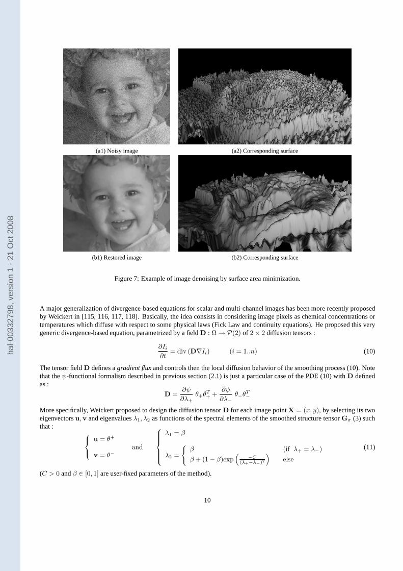
(a1) Noisy image (a2) Corresponding surface

(b1) Restored image (b2) Corresponding surface

Figure 7: Example of image denoising by surface area minimization.

A major generalization of divergence-based equations for scalar and multi-channel images has been more recently proposedby Weickert in [115, 116, 117, 118]. Basically, the idea consists in considering image pixels as chemical concentrations ortemperatures which diffuse with respect to some physical laws (Fick Law and continuity equations). He proposed this verygeneric divergence-based equation, parametrized by a fieldD : Ω → P(2) of 2 × 2 diffusion tensors :

∂Ii∂t

= div (D∇Ii) (i = 1..n) (10)

The tensor fieldD defines agradient fluxand controls then the local diffusion behavior of the smoothing process (10). Notethat theψ-functional formalism described in previous section (2.1)is just a particular case of the PDE (10) withD definedas :

D =∂ψ

∂λ+θ+θ

T+ +

∂ψ

∂λ−θ−θ

T−

More specifically, Weickert proposed to design the diffusion tensorD for each image pointX = (x, y), by selecting its twoeigenvectorsu,v and eigenvaluesλ1, λ2 as functions of the spectral elements of the smoothed structure tensorGσ (3) suchthat :

u = θ+

v = θ−and

λ1 = β

λ2 =

β (if λ+ = λ−)

β + (1 − β)exp(

−C(λ+−λ−)2

)

else

(11)

(C > 0 andβ ∈ [0, 1] are user-fixed parameters of the method).

10

hal-0

0332

798,

ver

sion

1 -

21 O

ct 2

008

The tensorD is computed at each image point as :D = λ1uuT + λ2vvT .

It is worth to notice that the tensor fieldD is the same for all image channelsIi, ensuring that allIi are smoothed by acommon multi-channel geometry, which takes the correlation between image channels into account (sinceD depends onGσ), contrary to a uncorrelated channel-by-channel approach.

Weickert assumed that the tensor shape at each pointX = (x, y) of the fieldD give the preferred smoothing geometry at thispoint. The idea behind the choice (11) was then :

- On almost constant regions, we haveλ+ ≃ λ− ≃ 0 and then we will getλ1 ≃ λ2 ≃ β, i.eD ≃ α Id. The tensorD isthen defined to beisotropic in flat regions.

- Along image contours, we have

λ+ ≫ λ− ≫ 0 and as a result, λ2 > λ1 > 0

Here, the diffusion tensorD will be thenanisotropic, mainly directed by the smoothed directionθ− of the imagecontours.

However, it is important to notice that the amplitudes and directions of the local smoothing performed by the divergence-based PDE (10) are actually not precisely defined by the eigencharacteristics (shapes) of the diffusion tensorD atX. Thismay lead to a smoothing behavior that is not expected, as illustrated by the simple following example. Suppose we want toanisotropically smooth a scalar imageI : Ω → R everywhere along the gradient direction∇I‖∇I‖ with a constant strength of1.This is of course for illustration purposes, since all imagediscontinuities would be destroyed by choosing such a smoothinggeometry. Intuitively, we would defineD at each pointX ∈ Ω as :

∀X ∈ Ω, D(X) =

( ∇I‖∇I‖

)( ∇I‖∇I‖

)T

leading to the simplification of (10) as

∂I

∂t= div

(

1

‖∇I‖2∇I∇IT∇I

)

= div (∇I) = ∆I

where∆I = ∂2I∂x2 + ∂2I

∂y2 stands for the Laplacian ofI. As noticed in [62], the evolution of this well knownheat flow equation

is similar to the convolution of the imageI by a normalized Gaussian kernelGσ with a varianceσ =√

2 t. So, this particularchoice ofanisotropictensorsD leads to anisotropicsmoothing behavior, without preferred smoothing orientations. Note thatchoosingD = Id (identity matrix) would give exactly the same result : different tensors fieldsD with very different shapes(isotropic or anisotropic) may define the same regularization behavior. Actually, the divergence is a differential operator, sothe equation (10) implicitly depends on thespatial variationsof the tensor fieldD. Clearly, the divergence equation (10)hampers the design of a significantpointwisesmoothing behavior.

2.3 Oriented heat flows

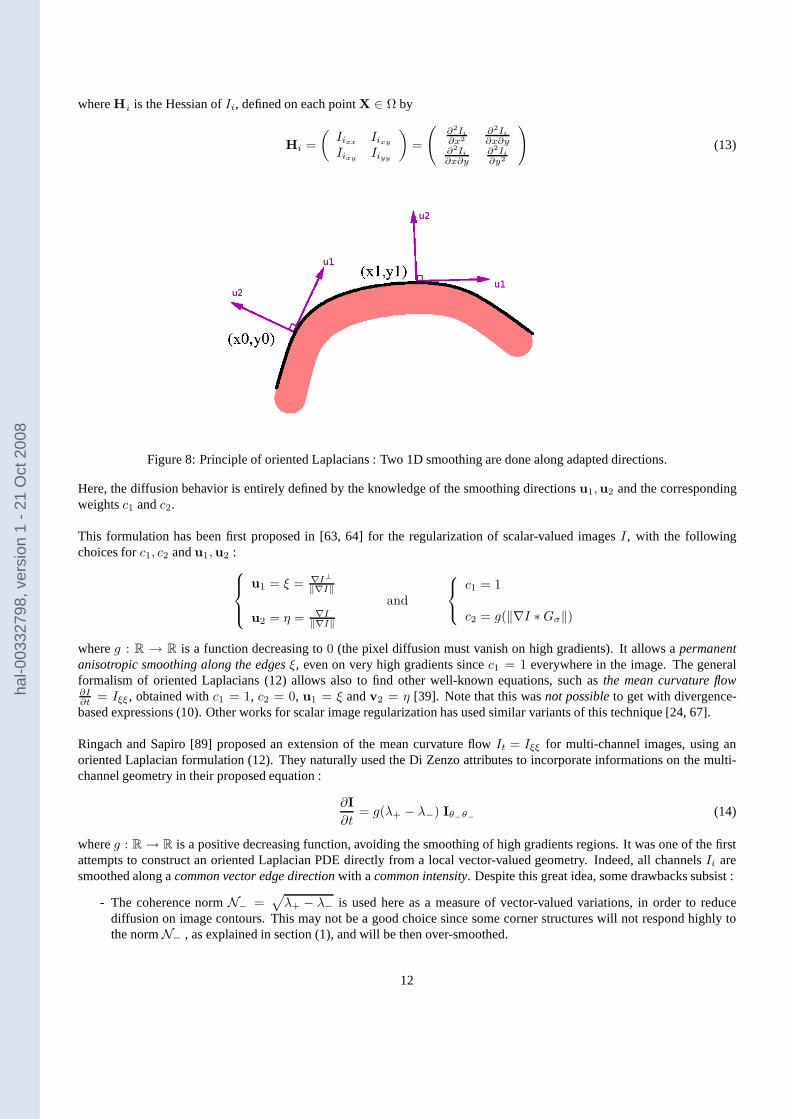
Oriented heat flows, also named oriented Laplacians formulations consider that a local smoothing process can be decomposedinto two orthogonal and uni-dimensional heat flows respectively oriented along two directionsu1 andu2 (these vectors form-ing an orthonormal basis) associated with two smoothing amplitudesc1 andc2. The smoothing amplitudes and orientationsare naturally different for each image point, since they adapt themselves to the local configuration of the image (Fig.8). Theresulting equation is written as the sum of these two heat flows :

∂I

∂t= c1Iu1u1 + c2Iu2u2 (12)

whereu1 andu2 are unit orthogonal vectors andc1, c2 ≥ 0.Iu1u1 andIu2u2 denote the second derivatives ofI in the directionsu1 andu2 and their vector components are formallydefined as :

∀i = 1..n, Iiu1u1= uT1 Hiu1 and Iiu2u2

= uT2 Hiu2

11

hal-0

0332

798,

ver

sion

1 -

21 O

ct 2

008

whereHi is the Hessian ofIi, defined on each pointX ∈ Ω by

Hi =

(

IixxIixy

IixyIiyy

)

=

(

∂2Ii

∂x2∂2Ii

∂x∂y∂2Ii

∂x∂y∂2Ii

∂y2

)

(13)

Figure 8: Principle of oriented Laplacians : Two 1D smoothing are done along adapted directions.

Here, the diffusion behavior is entirely defined by the knowledge of the smoothing directionsu1,u2 and the correspondingweightsc1 andc2.

This formulation has been first proposed in [63, 64] for the regularization of scalar-valued imagesI, with the followingchoices forc1, c2 andu1,u2 :

u1 = ξ = ∇I⊥‖∇I‖

u2 = η = ∇I‖∇I‖

and

c1 = 1

c2 = g(‖∇I ∗Gσ‖)

whereg : R → R is a function decreasing to0 (the pixel diffusion must vanish on high gradients). It allows apermanentanisotropic smoothing along the edgesξ, even on very high gradients sincec1 = 1 everywhere in the image. The generalformalism of oriented Laplacians (12) allows also to find other well-known equations, such asthe mean curvature flow∂I∂t = Iξξ, obtained withc1 = 1, c2 = 0, u1 = ξ andv2 = η [39]. Note that this wasnot possibleto get with divergence-based expressions (10). Other works for scalar image regularization has used similar variants of this technique [24, 67].

Ringach and Sapiro [89] proposed an extension of the mean curvature flowIt = Iξξ for multi-channel images, using anoriented Laplacian formulation (12). They naturally used the Di Zenzo attributes to incorporate informations on the multi-channel geometry in their proposed equation :

∂I

∂t= g(λ+ − λ−) Iθ−θ− (14)

whereg : R → R is a positive decreasing function, avoiding the smoothing of high gradients regions. It was one of the firstattempts to construct an oriented Laplacian PDE directly from a local vector-valued geometry. Indeed, all channelsIi aresmoothed along acommon vector edge directionwith acommon intensity. Despite this great idea, some drawbacks subsist :

- The coherence normN− =√

λ+ − λ− is used here as a measure of vector-valued variations, in order to reducediffusion on image contours. This may not be a good choice since some corner structures will not respond highly tothe normN− , as explained in section (1), and will be then over-smoothed.

12

hal-0

0332

798,

ver

sion

1 -

21 O

ct 2

008

- In flat regions (N− → 0), the diffusion is made along a single directionθ−, which is mainly directed by the noise sinceno coherent structures exist in these regions. Undesired texture effects result from this mono-directional smoothing.This is particularly true here, since contrary to decoupledregularizations, vector components arenot blendedwiththis method (the diffusions in all image channelsIi follow a common direction). Isotropic smoothing would be moreadapted in order to remove noise in such flat regions.

2.4 Trace-based diffusion PDE’s

A simple generalization of oriented Laplacians have been proposed in [101, 109, 110]. The idea relies on the use of a genericdiffusion tensor fieldT : Ω → P(2) to describe the diffusion geometry of the equation (12), instead of separately describinglocal directionsθ+, θ− and amplitudesc1, c2 of smoothing. Actually, the proposed equation was just a rewrite of the previousPDE (12), using atraceoperator :

∀i = 1, .., n,∂Ii∂t

= trace(THi) (15)

whereHi stands for the Hessian ofIi (13) and the tensor fieldT is computed as :

∀X ∈ Ω, T(X) = c1 u1uT1 + c2 v2v

T2

Note that in this case, each channelIi of I is also smoothed with a common tensor fieldT.Actually, equations (12) and (15) are strictly equivalent,but this last one makes clearly appear the separation of the smoothinggeometry (defined by the tensor fieldT) from the smoothing itself. This is actually close to the idea of the Weickert’s methodthat led to the divergence PDE (10) : the regularization problem simplifies now to the design of a tensor fieldT adapted to theconsidered application. But in the case of trace-based PDE’s, the tensor field that defines the local smoothing behavior hasthe interesting property ofunicity : two differenttensor fields will necessarily lead todifferentsmoothing behaviors. Indeed,equation (15) has a simple geometric interpretation in terms of local filteringwith oriented Gaussian kernels.Indeed, let consider first thatT is a constant tensor field. Then, it can be demonstrated that the formal solution of the PDE(15) is (see Appendix B for details) :

Ii(t) = Ii(t=0)∗ G(T,t) (i = 1..n) (16)

where ∗ stands for the convolution operator andG(T,t) is anoriented Gaussian kernel, defined by :

G(T,t)(X) =1

4πtexp

(

−XTT−1X

4t

)

with X = (x y)T (17)

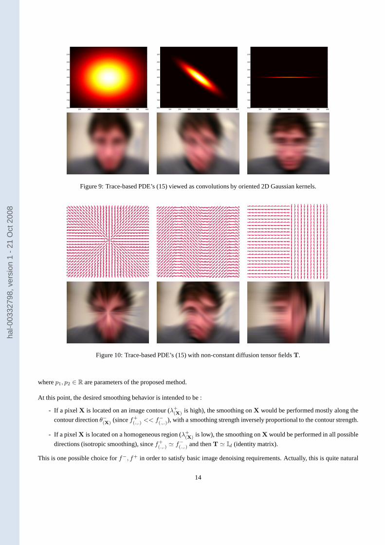
This is in fact a generalization of the Koenderink’s idea [62], who proved this property in the field of computer vision forthesimpler case of theisotropic diffusion tensorT = Id, resulting in the well-knownheat flowequation :∂Ii

∂t = ∆Ii.Fig.9 illustrates three Gaussian kernelsG(T,t)(x, y) respectively obtained with isotropic and anisotropic tensorsT and thecorresponding evolutions of the diffusion PDE (15) on a color image. It is worth to notice that the Gaussian kernelsG(T,t)

give the classical representations of the tensorsT with ellipses. Conversely, it is clear that the tensorsT represent the exactgeometry of the smoothing performed by the PDE (15).WhenT is not constant (which is generally the case), i.e. represents a fieldΩ → P(2) of variable diffusion tensors, the PDE(15) becomesnonlinearbut can be viewed as the application of temporally and spatially varying local masksGT,t(X) overthe imageI. Fig.10 illustrates three examples of spatially varying tensor fieldsT, represented with fields of ellipsoids, andthe corresponding evolutions of (15) on a color image. As before,the shape of each tensorT gives the exact geometry of thelocal smoothing processperformed by the trace-based PDE (15) point by point. As the trace is not a differential operator, thelocal interpretation of the smoothing process as a convolution with an oriented Gaussian mask is valid here.

In the same way that structure tensors code for each image pixel X the main directions of the edgesθ− as well as the edgestrengthλ+ + λ−, the diffusion tensor fieldT will code similarly the preferred local smoothing directions as well as thedesired smoothing amplitudes along these directions, for each image pixelX. Of course,T(X) must depend on the localgeometry ofI, and is thus defined from the spectral elementsλ−, λ+ andθ−, θ+ of the smoothed structure tensorGσ. Forimage denoising purposes, the choice proposed in [101, 109,110] is :

c1 = f−(λ+,λ−) =

1

(1 + λ+ + λ−)p1and c2 = f+

(λ+,λ−) =1

(1 + λ+ + λ−)p2with p1 < p2 (18)

13

hal-0

0332

798,

ver

sion

1 -

21 O

ct 2

008

100 200 300 400 500 600 700 800

100

200

300

400

500

600

700

800100 200 300 400 500 600 700 800

100

200

300

400

500

600

700

800100 200 300 400 500 600 700 800

100

200

300

400

500

600

700

800

Figure 9: Trace-based PDE’s (15) viewed as convolutions by oriented 2D Gaussian kernels.

Figure 10: Trace-based PDE’s (15) with non-constant diffusion tensor fieldsT.

wherep1, p2 ∈ R are parameters of the proposed method.

At this point, the desired smoothing behavior is intended tobe :

- If a pixel X is located on an image contour (λ+(X) is high), the smoothing onX would be performed mostly along the

contour directionθ−(X) (sincef+(.,.) << f−

(.,.)), with a smoothing strength inversely proportional to the contour strength.

- If a pixelX is located on a homogeneous region (λ+(X) is low), the smoothing onX would be performed in all possible

directions (isotropic smoothing), sincef+(.,.) ≃ f−

(.,.) and thenT ≃ Id (identity matrix).

This is one possible choice forf−, f+ in order to satisfy basic image denoising requirements. Actually, this is quite natural

14

hal-0

0332

798,

ver

sion

1 -

21 O

ct 2

008

to design a smoothing behavior from the image structurebeforeapplying the regularization process itself.The trace-based equation (15) has been a great attempt to separate the smoothing geometry from the smoothing process itself,while providing a geometrical interpretation on how the smoothing is performed. It proved some natural links between PDE’sand other local filtering techniques, as the Bilateral Filtering [11, 100]. Another similar approach based on non-Gaussianconvolution kernels has been also proposed for the specific case of the Beltrami Flow in [92].But the fact that the trace equation (15) behaves locally as an oriented Gaussian smoothing whose strength and orientation isdirectly related to the tensorT(X) has a major drawback. Indeed, on curved structures (like corners), this Gaussian behavioris not desirable: when the local variation of the edge orientationθ− is high, a Gaussian filter tends toroundcorners, evenby conducting the smoothing only alongθ−. This is due to the fact that an oriented Gaussian mask isnot curved itself.This classical behavior is also best known as the “mean curvature flow” effect, characterized by the PDE∂I∂t = ∂2

I

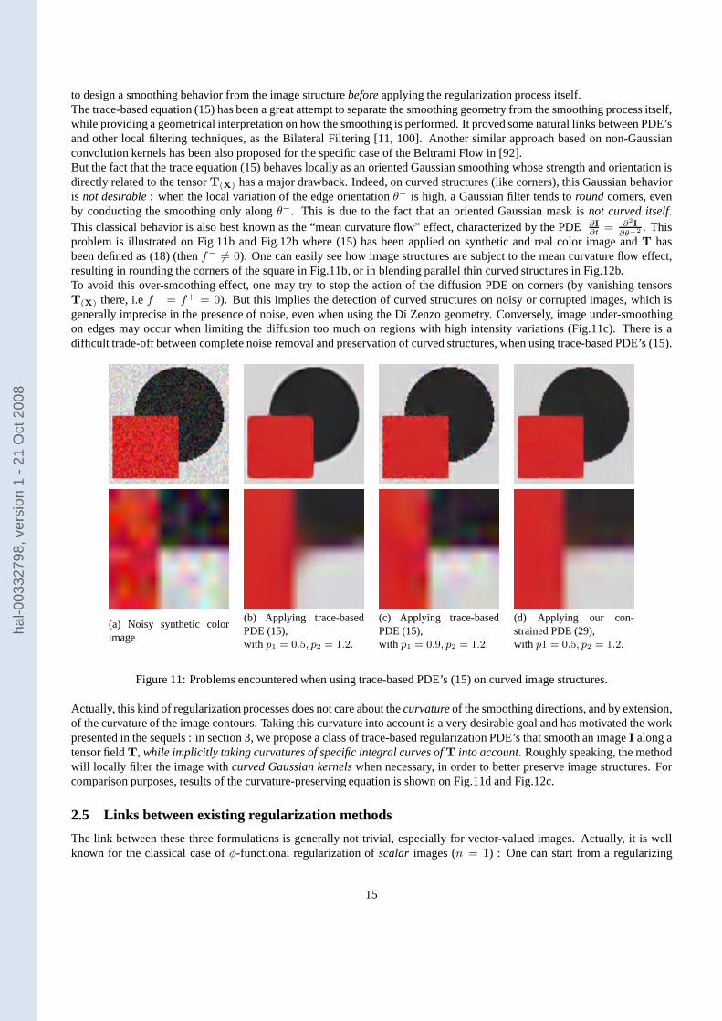
∂θ−2 . Thisproblem is illustrated on Fig.11b and Fig.12b where (15) hasbeen applied on synthetic and real color image andT hasbeen defined as (18) (thenf− 6= 0). One can easily see how image structures are subject to the mean curvature flow effect,resulting in rounding the corners of the square in Fig.11b, or in blending parallel thin curved structures in Fig.12b.To avoid this over-smoothing effect, one may try to stop the action of the diffusion PDE on corners (by vanishing tensorsT(X) there, i.ef− = f+ = 0). But this implies the detection of curved structures on noisy or corrupted images, which isgenerally imprecise in the presence of noise, even when using the Di Zenzo geometry. Conversely, image under-smoothingon edges may occur when limiting the diffusion too much on regions with high intensity variations (Fig.11c). There is adifficult trade-off between complete noise removal and preservation of curved structures, when using trace-based PDE’s (15).

(a) Noisy synthetic colorimage

(b) Applying trace-basedPDE (15),with p1 = 0.5, p2 = 1.2.

(c) Applying trace-basedPDE (15),with p1 = 0.9, p2 = 1.2.

(d) Applying our con-strained PDE (29),with p1 = 0.5, p2 = 1.2.

Figure 11: Problems encountered when using trace-based PDE’s (15) on curved image structures.

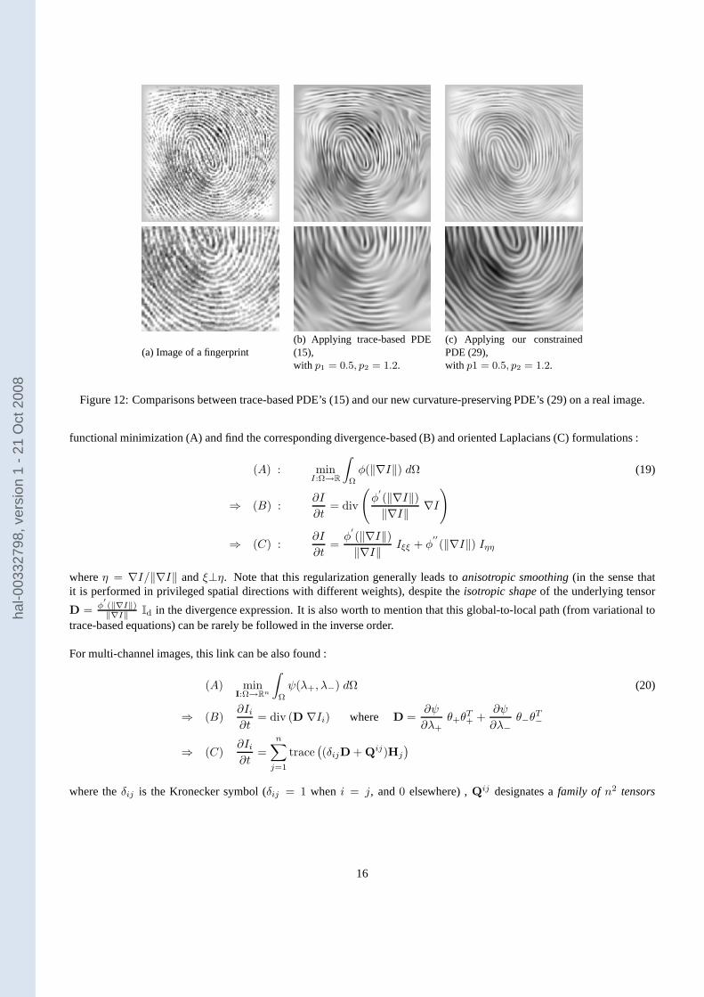
Actually, this kind of regularization processes does not care about thecurvatureof the smoothing directions, and by extension,of the curvature of the image contours. Taking this curvature into account is a very desirable goal and has motivated the workpresented in the sequels : in section 3, we propose a class of trace-based regularization PDE’s that smooth an imageI along atensor fieldT, while implicitly taking curvatures of specific integral curves ofT into account. Roughly speaking, the methodwill locally filter the image withcurved Gaussian kernelswhen necessary, in order to better preserve image structures. Forcomparison purposes, results of the curvature-preservingequation is shown on Fig.11d and Fig.12c.

2.5 Links between existing regularization methods

The link between these three formulations is generally not trivial, especially for vector-valued images. Actually, itis wellknown for the classical case ofφ-functional regularization ofscalar images (n = 1) : One can start from a regularizing

15

hal-0

0332

798,

ver

sion

1 -

21 O

ct 2

008

(a) Image of a fingerprint(b) Applying trace-based PDE(15),with p1 = 0.5, p2 = 1.2.

(c) Applying our constrainedPDE (29),with p1 = 0.5, p2 = 1.2.

Figure 12: Comparisons between trace-based PDE’s (15) and our new curvature-preserving PDE’s (29) on a real image.

functional minimization (A) and find the corresponding divergence-based (B) and oriented Laplacians (C) formulations:

(A) : minI:Ω→R

∫

Ω

φ(‖∇I‖) dΩ (19)

⇒ (B) :∂I

∂t= div

(

φ′

(‖∇I‖)‖∇I‖ ∇I

)

⇒ (C) :∂I

∂t=φ

′

(‖∇I‖)‖∇I‖ Iξξ + φ

′′

(‖∇I‖) Iηη

whereη = ∇I/‖∇I‖ andξ⊥η. Note that this regularization generally leads toanisotropic smoothing(in the sense thatit is performed in privileged spatial directions with different weights), despite theisotropic shapeof the underlying tensor

D = φ′(‖∇I‖)‖∇I‖ Id in the divergence expression. It is also worth to mention that this global-to-local path (from variational to

trace-based equations) can be rarely be followed in the inverse order.

For multi-channel images, this link can be also found :

(A) minI:Ω→Rn

∫

Ω

ψ(λ+, λ−) dΩ (20)

⇒ (B)∂Ii∂t

= div (D ∇Ii) where D =∂ψ

∂λ+θ+θ

T+ +

∂ψ

∂λ−θ−θ

T−

⇒ (C)∂Ii∂t

=

n∑

j=1

trace(

(δijD + Qij)Hj

)

where theδij is the Kronecker symbol (δij = 1 when i = j, and0 elsewhere) ,Qij designates afamily of n2 tensors

16

hal-0

0332

798,

ver

sion

1 -

21 O

ct 2

008

(i, j = 1..n), defined as the symmetric parts of the following matricesPij (i.e, Qij = (Pij + PijT

)/2 ) :

Pij = α ∇ITi ∇IjId

+ 2

(

∂α

∂λ+θ+θ

T+ +

∂α

∂λ−θ−θ

T−

)

∇Ij∇ITi G

+ 2

(

(α+∂β

∂λ+)θ+θ

T+ + (α+

∂β

∂λ−)θ−θ

T−

)

∇Ij∇ITi

withα = f1(λ+,λ−)−f2(λ+,λ−)

λ+−λ−and β = λ+f2(λ+,λ−)−λ−f1(λ+,λ−)

λ+−λ−

and

f1 =∂ψ

∂λ+and f2 =

∂ψ

∂λ−The development (A)⇒(B) from the functional to the divergence formulation is detailed in Appendix A. The development(B)⇒(C) from the divergence to the trace-based equation is detailed in Appendix C. This last development initially proposedin [109, 110] unifies a whole range of previously proposed vector-valued regularization algorithms (variational and divergencebased PDE’s) into an extended trace-based equation, composed of several channel-diffusion contributionsthat have directgeometric interpretations in terms of local filtering by Gaussian kernels. Though the geometric interpretation of the overallsum of trace equations is not direct, it is interesting to seethatadditional diffusion tensorsQij clearly appear in the traceexpressions, and contribute to modify the inner tensorD, which is finally not representative of the smoothing behavior. Moregenerally, tensors appearing in traces and divergences generally lead to different smoothing behaviors.

3 Curvature-Preserving PDE’s

The framework ofcurvature-preserving PDE’s, first introduced in [102] defines a specific variant of multi-channel diffusionPDE’s. Its goal is to provide a generic tensor-driven regularization method as the divergence-based PDE (10) and trace-basedPDE (15), but also focuses on the preservation of thin curvedstructures. We review this very efficient formalism and showhow it can be understood from a local smoothing geometry viewpoint.

3.1 The single direction case

To illustrate the general idea of curvature-preserving PDE’s, we first focus on image regularization along avector fieldw : Ω → R

2 instead of a tensor fieldT. We consider then a local smoothing everywhere along a single direction w

‖w‖ , with

a smoothing strength‖w‖. We denote the two spatial components ofw by w(X) = (u(X) v(X))T .

Thecurvature-preservingregularization PDE that smoothesI alongw is defined by :

∀i = 1, . . . , n,∂Ii∂t

= trace(

wwT Hi

)

+ ∇ITi Jww (21)

whereJw stands for the Jacobian ofw , andHi is the Hessian ofIi.

Jw =

∂u∂x

∂u∂y

∂v∂x

∂v∂y

and Hi =

∂2Ii

∂x2∂2Ii

∂x∂y

∂2Ii

∂x∂y∂2Ii

∂y2

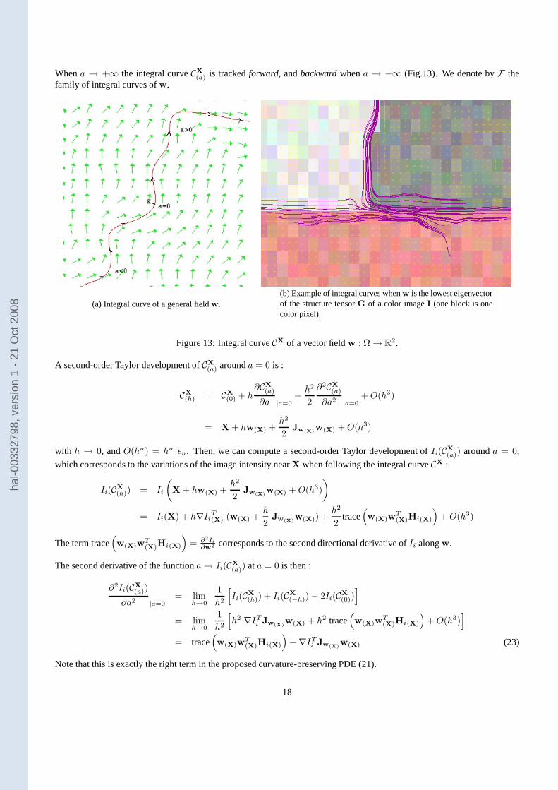
The PDE (21) adds a term∇ITi Jww to the trace-based equation (15) that smoothesI alongw with locally oriented Gaussiankernels (see section 2.4). This extra term naturally depends on the variation of the vector fieldw. Let us explain how (21) isrelated tow.

Let CX

(a) be the curve defining theintegral curveof w, starting fromX and parametrized bya ∈ R :

CX

(0) = X

∂CX

(a)

∂a = w(CX

(a))

(22)

17

hal-0

0332

798,

ver

sion

1 -

21 O

ct 2

008

Whena → +∞ the integral curveCX

(a) is trackedforward, andbackwardwhena → −∞ (Fig.13). We denote byF thefamily of integral curves ofw.

(a) Integral curve of a general fieldw.(b) Example of integral curves whenw is the lowest eigenvectorof the structure tensorG of a color imageI (one block is onecolor pixel).

Figure 13: Integral curveCX of a vector fieldw : Ω → R2.

A second-order Taylor development ofCX

(a) arounda = 0 is :

CX

(h) = CX

(0) + h∂CX

(a)

∂a |a=0+h2

2

∂2CX

(a)

∂a2 |a=0+O(h3)

= X + hw(X) +h2

2Jw(X)

w(X) +O(h3)

with h → 0, andO(hn) = hn ǫn. Then, we can compute a second-order Taylor development ofIi(CX

(a)) arounda = 0,

which corresponds to the variations of the image intensity nearX when following the integral curveCX :

Ii(CX

(h)) = Ii

(

X + hw(X) +h2

2Jw(X)

w(X) +O(h3)

)

= Ii(X) + h∇IiT(X) (w(X) +h

2Jw(X)

w(X)) +h2

2trace

(

w(X)wT(X)Hi(X)

)

+O(h3)

The term trace(

w(X)wT(X)Hi(X)

)

= ∂2Ii

∂w2 corresponds to the second directional derivative ofIi alongw.

The second derivative of the functiona→ Ii(CX

(a)) ata = 0 is then :

∂2Ii(CX

(a))

∂a2 |a=0= lim

h→0

1

h2

[

Ii(CX

(h)) + Ii(CX

(−h)) − 2Ii(CX

(0))]

= limh→0

1

h2

[

h2 ∇ITi Jw(X)w(X) + h2 trace

(

w(X)wT(X)Hi(X)

)

+O(h3)]

= trace(

w(X)wT(X)Hi(X)

)

+ ∇ITi Jw(X)w(X) (23)

Note that this is exactly the right term in the proposed curvature-preserving PDE (21).

18

hal-0

0332

798,

ver

sion

1 -

21 O

ct 2

008

Actually, (21) can be seen individually for all integral curves ofF instead of each pointX ∈ Ω : consider another pointY ∈ CX. Then, there existǫ ∈ R such thatY = CX

(ǫ). Indeed,CX andCY describe the same curve (22) with different

parametrization :∀a ∈ R, CY

(a) = CX

(ǫ+a). As (21) is verified onY, then∂Ii(CX

(a))

∂t |a=ǫ =∂2Ii(CX

(a))

∂a2 |a=ǫ. This is obviously

true forǫ ∈ R since (21) is verified for all pointsY lying on the integral curveCX. Then, the PDE (21) may be also writtenas :

∀C ∈ F , ∀a ∈ R,∂Ii(C(a))

∂t=∂2Ii(C(a))

∂a2(24)

We may recognize in (24) aone-dimensional heat flow constrained onC. This is actually very different from a heat-floworientedby w, as in the formulation∂Ii

∂t = ∂2Ii

∂w2 since thecurvatures of integral curves ofw are now implicitly takeninto account. In particular, the constrained equation (21) has the interesting property to vanish when image intensities areperfectly constant on the integral curveC, whatever the curvature ofC is. In this context, defining a fieldw that is tangenteverywhere to the image structures will allow the preservation of these structures, even if they are curved (such as corners).This is not the case with divergence or trace-based PDE’s (10),(15). This curvature-preserving property of (21) is illustratedon Fig.11d and Fig.12b.The constrained equation (21) is anelliptic PDE since the matrixwwT is positive definite. The existence and unicity of thesolutions of (21) are not directly approached here. Anyway,in section 3.2, we show that its solution can be approximatedbythe technique of Line Integral Convolutions, which is a well-posed analytical approach.

3.2 Curvature-Preserving PDE’s and Line Integral Convolutions

Line Integral Convolutions (LIC) have been first introducedin [23] as a technique to render a textured imageILIC thatrepresents a vector fieldw : Ω → R

2. The idea, originally expressed under a discrete formula, consists in smoothing animageInoise - containing only noise - by averaging its pixel values alongthe integral curves ofw. Actually, a continuousformulation of a LIC is then :

∀X ∈ Ω, ILIC(X) =1

N

∫ +∞

−∞f(p) Inoise(CX

(p)) dp (25)

wheref : R → R is an even function (strictly decreasing to0 on R+) andCX is defined as theintegral curve(22) of

w throughX. The normalization factorN allows the preservation of the average pixel value alongCX and is equal toN =

∫ +∞−∞ f(p) dp.

As noticed in section 3.1, the curvature-preserving PDE (21) can be seen as the one-dimensional heat flow (24) constrainedon the integral curveCX ∈ F . Using the variable substitutionL(a) = I(CX

(a)), (24) can be also written as∂L∂t (a) = L′′

(a). The

solutionL[t] at timet is known to be the convolution ofL[t=0] by a normalized Gaussian kernelGt (see [39, 62]) :

L[t](a) =

∫ +∞

−∞L

[t=0](p) Gt(a−p) dp with Gt(p) =

1√4πt

exp

(

−p2

4t

)

(26)

SubstitutingL in (5.4) witha = 0, and remembering thatCX

(0) = X andGt(−p) = Gt(p) :

∀X ∈ Ω, I[t](X) =

∫ +∞

−∞I[t=0](CX

(p)) Gt(p) dp (27)

The equation (27) is a particular form of the continuous LIC-based formulation (25) with a Gaussian weighting functionf = Gt. Here, the normalization factor isN =

∫ +∞−∞ Gt(p) dp = 1. Intuitively, the evolution of the curvature-preserving

PDE (21) may be seen as the application of local convolutionsby normalized one-dimensional Gaussian kernelsalongintegral curvesC of w. This kind of anisotropic image smoothing considers then acurvedfiltering, instead of just an orientedone.Applying this setting on a multi-channel imageI, with w being the lowest eigenvector of the structure tensor fieldG (i.e.the contour direction) allows the anisotropic smoothing ofI with edge preservation, even if these edges are curved. Thisis illustrated on Fig.13b, where few integral linesCX are computed, around a typical T-junction structure. Note how the

19

hal-0

0332

798,

ver

sion

1 -

21 O

ct 2

008

streamlines rotate when arriving at the junction, with a sub-pixel precision. The streamlines have been computed with a4th-order Runge-Kutta scheme.

Note that (27) is an analytical solution of (21) whenw does not evolve over time. This property is generally not verifiedwhen dealing with general nonlinear regularization PDE’s,where the smoothing geometry is re-evaluated at each time step(thus defining a temporal non-linearity). In order to get ridof this kind of non-linearity, we will then to perform severalsuccessive iterations of the LIC scheme (27), where the vector field w is updated at each iteration. This is actually a goodway of approximating (21). Classical explicit schemes usually consider the smoothing geometryw as constant betweentwo successive PDE iterationsI[t] andI[t+dt]. Thus, the curvature-preserving equation (21) will be efficiently discretized byseveral iterations of the LIC formulation (27). This will bedetailed in section 4.

3.3 Between Traces and Divergences

We illustrate here how the curvature-preserving PDE (21) may be regarded compared to trace and divergence expressions(10), (15), for the case of single direction smoothingT = wwT .In this case, the divergence PDE (10) may be developed as :

div(

wwT ∇Ii)

= div

u2 ∂Ii

∂x + uv ∂Ii

∂y

uv ∂Ii

∂x + v2 ∂Ii

∂y

=

(

u2 ∂2Ii∂x2

+ 2uv∂2Ii∂x∂y

+ v2 ∂2Ii∂y2

)

+ ∇ITi

2u ∂u∂x + u ∂v

∂y + v ∂u∂y

2v ∂v∂y + u ∂v

∂x + v ∂u∂x

= trace(

wwTHi

)

+ ∇ITi

u ∂u∂x + v ∂u

∂y

u ∂v∂x + v ∂v

∂y

+

u ∂u∂x + u ∂v

∂y

v ∂u∂x + v ∂v

∂y

= trace(

wwTHi

)

+ ∇ITi Jww + div(w)∇ITi w

Thus, we recognize in these three different terms :

- The first term corresponds to the trace PDE (15), that smoothes locallyI alongw, using oriented Gaussian kernels.

- The two first terms correspond to thecurvature-constrainedregularization PDE (21), that smoothes locallyI alongw

while taking the curvature of integral curvesC of w into account.

- The three terms together correspond to the classical divergence PDE (10) that performs local diffusions ofI alongw. This last term div(w)∇ITi w is mainly responsible for the perturbations of the effective smoothing direction, asdescribed in section 2.2. It is not desirable for image regularization purposes.

It is interesting to observe that the curvature-constrained PDE (21) is then “mathematically” positioned between the trace (15)and divergence formulations (10), and allows at the same time the full respect of the pre-defined smoothing directionsw,while preserving curved images structures.Note that we can also write the curvature-preserving PDE (21) as a divergence-based PDE minus a constraint term :

trace(

wwTHi

)

+ ∇ITi Jww = div(

wwT ∇Ii)

− div(w)∇ITi w

Two particular cases of directionsw are worth studying, in the case of scalar-valued images (n = 1) :

- Whenw = ∇I⊥‖∇I‖ (isophote direction), then ∇ITJww = −Iww, vanishing then the velocity of the curvature-

preserving evolution equation (21), by counterbalancing the trace-based term (which is nothing more than themeancurvature motionin this case). No smoothing will be then performed. This is quite natural since pixel along theisophotes have constant values, so averaging those values should not modify the image. Note by comparison that thevelocity of the corresponding divergence-based expression div

(

wwT ∇Ii)

also vanishes here.

20

hal-0

0332

798,

ver

sion

1 -

21 O

ct 2

008

- Whenw = ∇I‖∇I‖ (gradient direction), then ∇ITJww = 0, and the velocity of the curvature-preserving PDE (21)

becomes simplyIww, which really corresponds to a smoothing of the image along the gradient direction (the same asthe unconstrained trace-based PDE (15)). Note by comparison that the velocity of the corresponding divergence-basedexpression is∆I in this case, which corresponds to an isotropic smoothing ofthe image, instead of an anisotropic one.

These two particular cases allows to better understand the difference of regularization behaviors between the trace, divergenceand curvature-preserving formulations.Note also that in case wherew is a divergence free field (i.e div(w) = 0), the divergence-based PDE (10) and the curvature-preserving formulation (21) are strictly equivalent. Thisis very rarely the case anyway.

3.4 Extension to multi-directional smoothing

In [102], the single-direction smoothing PDE (21) has been extended so that it can deal with a tensor-valued geometryT :Ω → P(2), instead of a vector-valued geometryw. This is important, since a diffusion tensor describes muchmore complexsmoothing behaviors than single directions. In particular, it may represents bothanisotropicor isotropic regularizationbehaviors. The extension of the curvature-preserving PDE (21) is not straightforward : the notions of curvature and integralcurves of tensors-valued fieldsT are not as natural as with direction fieldsw.To tackle this problem, we proposed to locally decompose a tensor-driven smoothing process into several vector-drivensmoothing processes along different orientations. We firstnotice that

∫ π

α=0

aαaTα dα =

π

2Id where aα =

cosα

sinα

Then, any2 × 2 tensorT may be written as :

T =2

π

√T

(∫ π

α=0

aαaTα dα

)√T

where√

T =√

f+uuT +√

f−vvT stands for the square root ofT = f+uuT + f−vvT . One can easily verify that(√

T)2 = T and(√

T)T =√

T. Thus, the tensorT may be decomposed as :

T =2

π

∫ π

α=0

√Taαa

Tα

√TTdα

=2

π

∫ π

α=0

(√

Taα)(√

Taα)T dα (28)

We have split the tensorT into a sum ofatomic tensors(√

Taα)(√

Taα)T , each being purely anisotropic and directedonly along the direction of the vector

√Taα ∈ R

2. The equation (28) naturally suggests to decompose any tensor-drivenregularization PDE into a sum of single direction smoothingprocesses, each of them respecting the overall geometryT. Forinstance :

- If T = Id (identity matrix), the tensor is isotropic and :∀α ∈ [0, π],√

Taα = aα. The resulting smoothing will bethen performed in all directionsaα of the plane with the same strength.

- If T = uuT (whereu ∈ S1), the tensor is purely anisotropic and :∀α ∈ [0, π],√

Taα = (uT aα)u. The resultingsmoothing will be then performed only along the directionu of the tensorT.

Then, using (28) and considering that each single directionsmoothing must be done with a curvature-preserving approach(21), we end up with the following curvature-constrained regularization PDE, acting on a multi-channel imageI : Ω → R

n

and driven by a tensor-valued smoothing geometryT :

∀i = 1, . . . , n,∂Ii∂t

=2

π

∫ π

α=0

trace(

(√

Taα)(√

Taα)THi

)

+ ∇ITi J√Taα

√Taα dα

21

hal-0

0332

798,

ver

sion

1 -

21 O

ct 2

008

which can be simplified as :

∀i = 1, . . . , n,∂Ii∂t

= trace(THi) +2

π∇ITi

∫ π

α=0

J√Taα

√Taα dα (29)

whereaα = (cosα sinα)T , andJ√Taα

stands for the Jacobian of the vector fieldΩ →√

Taα. Note that this kind ofsmoothing decomposition along all orientations of the plane can be also found in [113]. As in the single direction smoothingcase, (29) may be seen as a trace-based equation (15), where an extra term has been added in order to respect the curvatureof all integral lines passing through the tensor-valued geometryT.

4 Implementation considerations

In order to implement the regularization method (29), one can benefit from the LIC-based interpretation of curvature-preserving PDE’s presented in section 3.2. Indeed, we can explicitly discretize (29) by the following Euler scheme :

I[t+dt] = I[t] +2dt

N

(

N−1∑

k=0

R(√

Taα)

)

whereα = kπ/N (in the interval[0, π]), dt is the usual temporal discretization step andR(w) represents a discretization ofthe mono-directional smoothing PDE velocity (21) that preserve curvatures along a vector fieldw. If we write this expression

as :I[t+dt] = 1N

(

∑N−1k=0 I[t] + 2dt R(

√Taα)

)

, we may express it as the averaging of different Gaussian-pondered LIC’s

along vector fields√

Taα :

I[t+dt] =1

N

(

N−1∑

k=0

I[t]

LIC(√

Taα)

)

,

where each Gaussian variance has a standard deviationdt.Basically, the difficulty here is the LIC computation, whichneeds the tracking of integral curves of a vector field. Here,weused a very simple method based on the classical Runge-Kutta[83] integration scheme. Faster LIC implementations havebeen proposed in [95] but do not deal with Gaussian ponderingfunctions, as needed here.This simple observation leads then to the following fast algorithm for the implementation of one iteration of the curvature-preserving PDE (29) :

- Compute the smoothed structure tensor fieldGσ from I[t] :

Gσ = Gσ ∗n∑

i=1

(

∂I[t]i

∂x

)2 (

∂I[t]i

∂x

)(

∂I[t]i

∂y

)

(

∂I[t]i

∂x

)(

∂I[t]i

∂y

) (

∂I[t]i

∂y

)2

σ will depend on the noise scale. We used relatively low values(between0 and1.5) for our experiments in section 5.

- Compute the eigenvaluesλ+, λ− and eigenvectorsθ+, θ− of Gσ.

- Compute the smoothing geometry tensor fieldT from Gσ : T = 1(1+λ++λ−)p1

θ−θ−T

+ 1(1+λ++λ−)p2

θ+θ+T

- For allα in [0, π] (discretized with a user-fixed stepdα) :

- Compute the vector fieldw =√

T aα.

- Perform a Line Integral Convolution ofI[t] alongCX in the forward and backward directions.

- Average all LIC’s computed in step 4.

The main parameters of the algorithm arep1, p2, σ, dt and the number of PDE iterationsnb that are applied. The character-istics of this scheme, compared to the classical finite-difference one is :

22

hal-0

0332

798,

ver

sion

1 -

21 O

ct 2

008

- It allows the preservation of thin image structures from a numerical point of view : the smoothing is performed alongintegral curves ofw, with a sub-pixel accuracy. Precise4th Runge-Kutta interpolation [83] is used to track the integralcurvesC in the image.

- It allows to choose very large time stepsdt, since the scheme we proposed is unconditionally stable. Indeed,dt issimply proportional to the overall smoothing variance of the Gaussian-pondering convolutions done alongC ∈ F .

- As a result, the regularization algorithm performs very fast. Very few iterations are necessary to get the result, evenif each iteration is more time-consuming. For our applications, presented in section 5, we were even able to chooseonly nb = 1 iteration with very large time stepsdt. In fact, this leads to a rough approximation of (29), since we lostthe temporal non-linearity property of the PDE. But for images with few noise, this gave surprisingly good results.Actually, the spatial non-linearity seems to play a more important role than the temporal non-linearity in the PDEevolution.

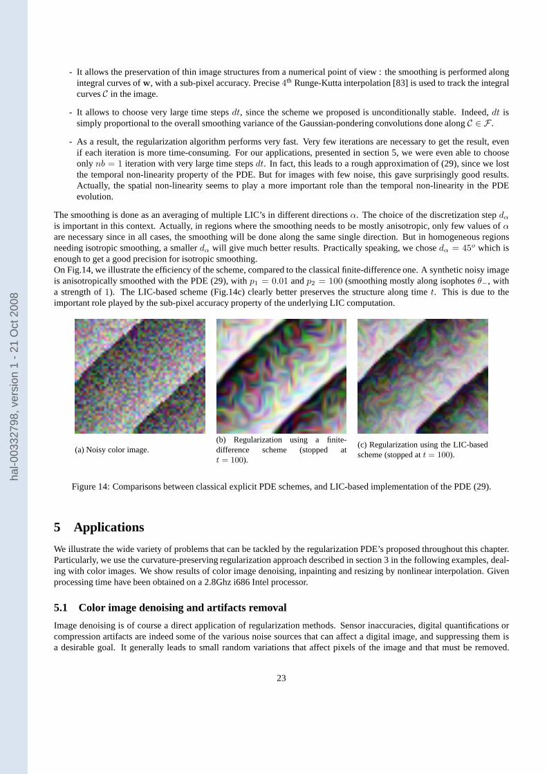
The smoothing is done as an averaging of multiple LIC’s in different directionsα. The choice of the discretization stepdαis important in this context. Actually, in regions where thesmoothing needs to be mostly anisotropic, only few values ofαare necessary since in all cases, the smoothing will be done along the same single direction. But in homogeneous regionsneeding isotropic smoothing, a smallerdα will give much better results. Practically speaking, we chosedα = 45o which isenough to get a good precision for isotropic smoothing.On Fig.14, we illustrate the efficiency of the scheme, compared to the classical finite-difference one. A synthetic noisyimageis anisotropically smoothed with the PDE (29), withp1 = 0.01 andp2 = 100 (smoothing mostly along isophotesθ−, witha strength of1). The LIC-based scheme (Fig.14c) clearly better preservesthe structure along timet. This is due to theimportant role played by the sub-pixel accuracy property ofthe underlying LIC computation.

(a) Noisy color image.(b) Regularization using a finite-difference scheme (stopped att = 100).

(c) Regularization using the LIC-basedscheme (stopped att = 100).

Figure 14: Comparisons between classical explicit PDE schemes, and LIC-based implementation of the PDE (29).

5 Applications

We illustrate the wide variety of problems that can be tackled by the regularization PDE’s proposed throughout this chapter.Particularly, we use the curvature-preserving regularization approach described in section 3 in the following examples, deal-ing with color images. We show results of color image denoising, inpainting and resizing by nonlinear interpolation. Givenprocessing time have been obtained on a 2.8Ghz i686 Intel processor.

5.1 Color image denoising and artifacts removal

Image denoising is of course a direct application of regularization methods. Sensor inaccuracies, digital quantifications orcompression artifacts are indeed some of the various noise sources that can affect a digital image, and suppressing themisa desirable goal. It generally leads to small random variations that affect pixels of the image and that must be removed.

23

hal-0

0332

798,

ver

sion

1 -

21 O

ct 2

008

In Fig.15-19, we illustrate how the curvature-preserving PDE framework (29) can be successfully applied to remove suchartifacts while preserving the essential structures of theprocessed images.

- Fig.15 shows an application of the regularization method on the famous512 × 512 “Baboon” color image, artificiallydegraded by adding uncorrelated Gaussian noise on(R,G,B). This color image has been then denoised with equation(29). Thanks to the proposed LIC-based numerical implementation, only one PDE iteration has been necessary todenoise the image, with parametersp1 = 0.5, p2 = 0.7, σ = 1.5 anddt = 50. Processing time is19.3 seconds for theentire image.

- Fig.16 illustrates a real case where a color photograph hasbeen digitized from a grainy paper, leading to the apparitionof watered effects on the digital picture. Using the PDE-based regularization method (29) allows to clearly removethe grains while preserving quite fine structures (palm treeleafs). Shown image is a152 × 133 portion of the originalone. Only one PDE iteration has been necessary, withp1 = 0.5, p2 = 0.7, σ = 1 anddt = 10. Processing time is11seconds for the entire image (size586 × 367).

- Fig.17 shows the restoration of a digital photograph shot under low luminosity conditions by a cellular phone. Suchdevices have usually poor quality cameras, leading to the apparition of important digital noise (more precisely, Poissonnoise) on the acquired color images. Processed color image has a size of262× 280 and has been restored in4 seconds(one PDE iteration), with parametersp1 = 0.2, p2 = 0.5, σ = 2, dt = 120. Note how the curvature-preservingPDE (29) is able to adapt itself locally to the multi-channelimage geometry, in order to preserve thin structures whileremoving the noise quite well.

- Image regularization can also be useful when dealing with other types of noise. The enhancement of JPEG-compressedimage is such an example of interest. Fig.18 illustrate the suppression of compression artifacts in color images. AJPEG compressed color image of size283× 249, where the JPEG quality ratio has been set to10% is processed by themulti-channel image regularization algorithm. Usual block effects inherent to the DCT compression are visible on thecompressed image. One PDE iteration is applied then, withp1 = 0.5, p2 = 0.9, σ = 2, dt = 200, in order to get theregularized result (right). Processing time is5.4 seconds for the entire image.

- Fig.19 illustrates another regularization with a different type of noise. This time, the regularization method is used toimprove a digital true-color image quantified in256 colors by the Floyd-Steinberg algorithm (size=355 × 287) whichintroduces some dithering effects in the image. One PDE iteration has been applied here, withp1 = 0.5, p2 = 0.8,σ = 1, dt = 30. A 136 × 118 portion of the image is shown. Processing time is12.8 seconds for the entire image.This kind of reconstruction may be interesting for image compression algorithms, allowing them to retrieve a true colorimages, even by storing them with a quantified palette.

5.2 Color image inpainting

Image inpainting is a very new and challenging application,which consists in filling-in missing image regions (defined bythe user) byguessing pixel valuessuch that the reconstructed image still looks natural. Basically, the user provides onecolor imageI : Ω → R

3, and onemaskimageM : Ω → 0, 1. The inpainting algorithm must fill-in the regions whereM(X) = 1, by the mean of some intelligent interpolations. Inpainting algorithms can be used for instance to remove variousstructures in images (scratches, logos or real objects) that are usually bigger than other image artifacts. Image inpainting hasbeen first proposed as a method based on a variational formulation by Masnou and Morel [70], followed by many solutionsbased on diffusion or transport PDE’s [15, 17, 30, 109, 110].It is also worth to cite some papers related to inpainting withoutuse of PDE’s [38, 55], among others.In this article, we see the inpainting process as a direct application of the proposed curvature-preserving PDE (29). Weapply the diffusion equation only on the regions to inpaint,allowing the neighbor pixels of these regions to diffuse inside : anonlinear completion of the image data along isophotes directions is thus naturally done, reconstructing the missing parts ofthe image, since the performed smoothing tries to follow a coherent multi-valued image geometry computed from the knownparts of the image. We illustrate the concept of inpainting with PDE’s in Fig.20-24.

- Fig.20 illustrates a simple case where one wants to remove text from a color image, by guessing the pixel colors behindthe text. The mask used here is easily detected from the degraded image by considering only green pixels. Result of

24

hal-0

0332

798,

ver

sion

1 -

21 O

ct 2

008

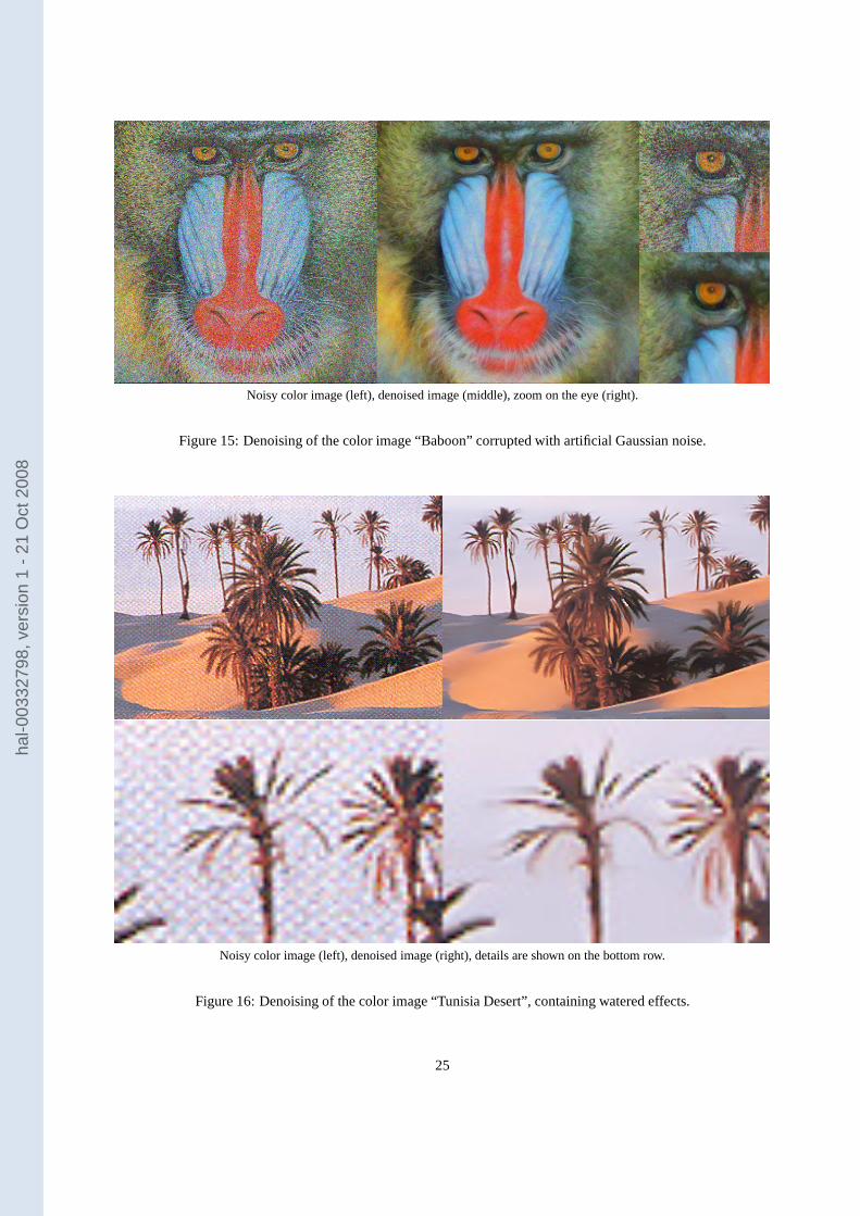
Noisy color image (left), denoised image (middle), zoom on the eye (right).

Figure 15: Denoising of the color image “Baboon” corrupted with artificial Gaussian noise.

Noisy color image (left), denoised image (right), details are shown on the bottom row.

Figure 16: Denoising of the color image “Tunisia Desert”, containing watered effects.

25

hal-0

0332

798,

ver

sion

1 -

21 O

ct 2

008

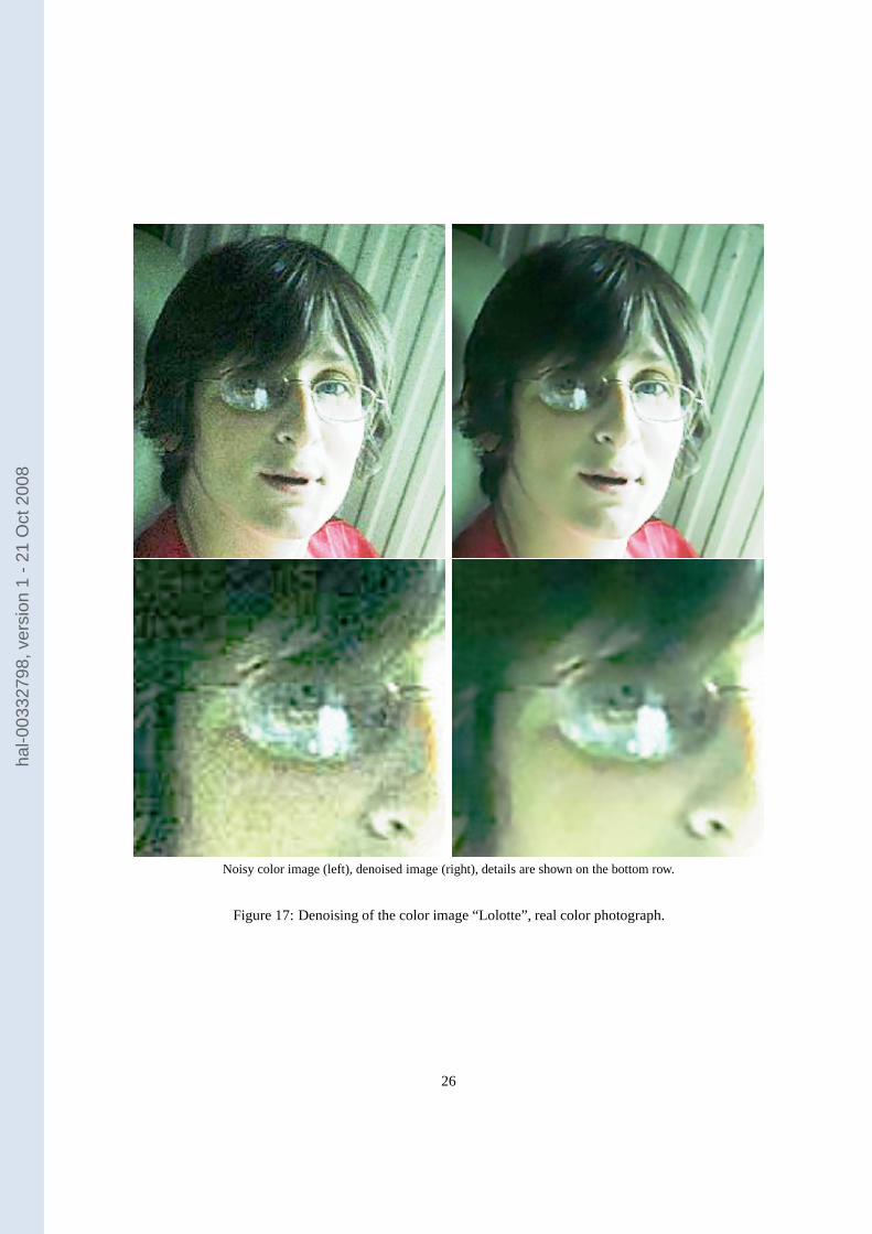
Noisy color image (left), denoised image (right), details are shown on the bottom row.

Figure 17: Denoising of the color image “Lolotte”, real color photograph.

26

hal-0

0332

798,

ver

sion

1 -

21 O

ct 2

008

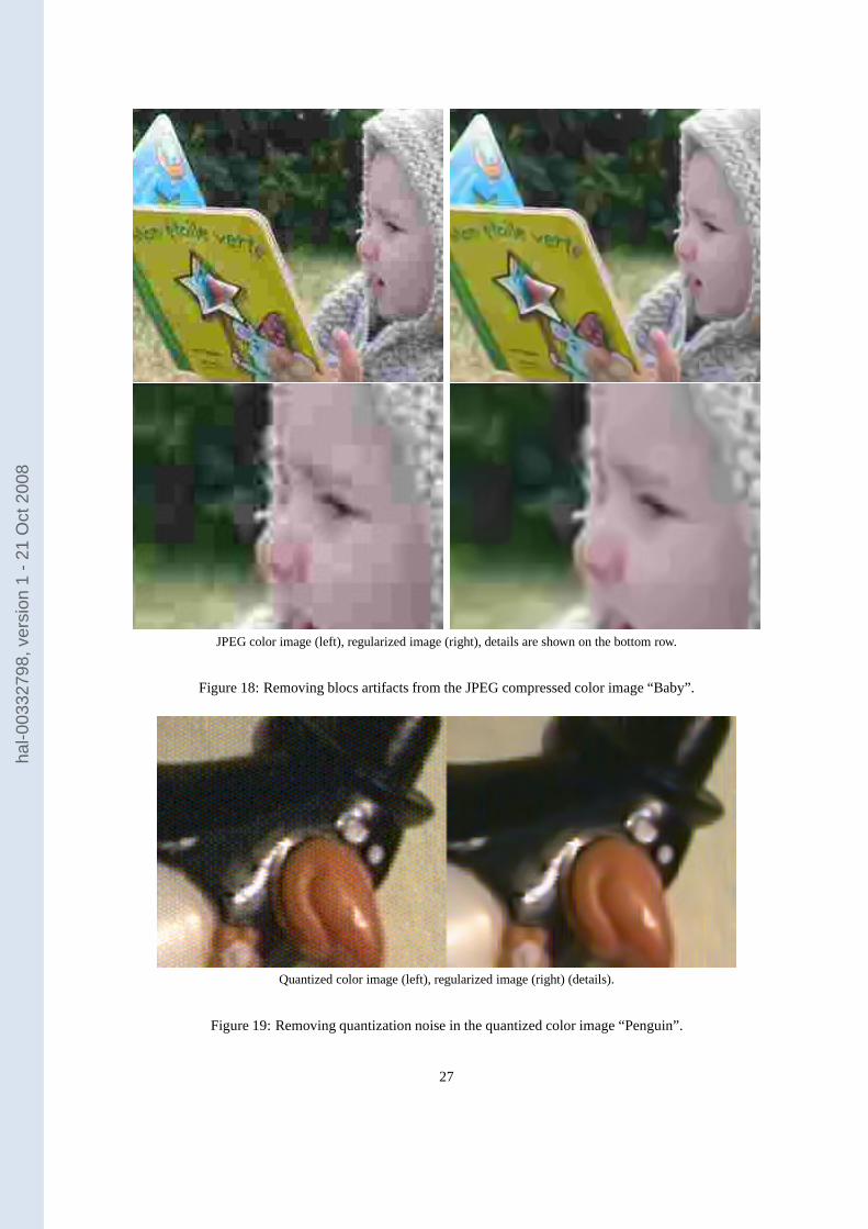
JPEG color image (left), regularized image (right), details are shown on the bottom row.

Figure 18: Removing blocs artifacts from the JPEG compressed color image “Baby”.

Quantized color image (left), regularized image (right) (details).

Figure 19: Removing quantization noise in the quantized color image “Penguin”.

27

hal-0

0332

798,

ver

sion

1 -

21 O

ct 2

008

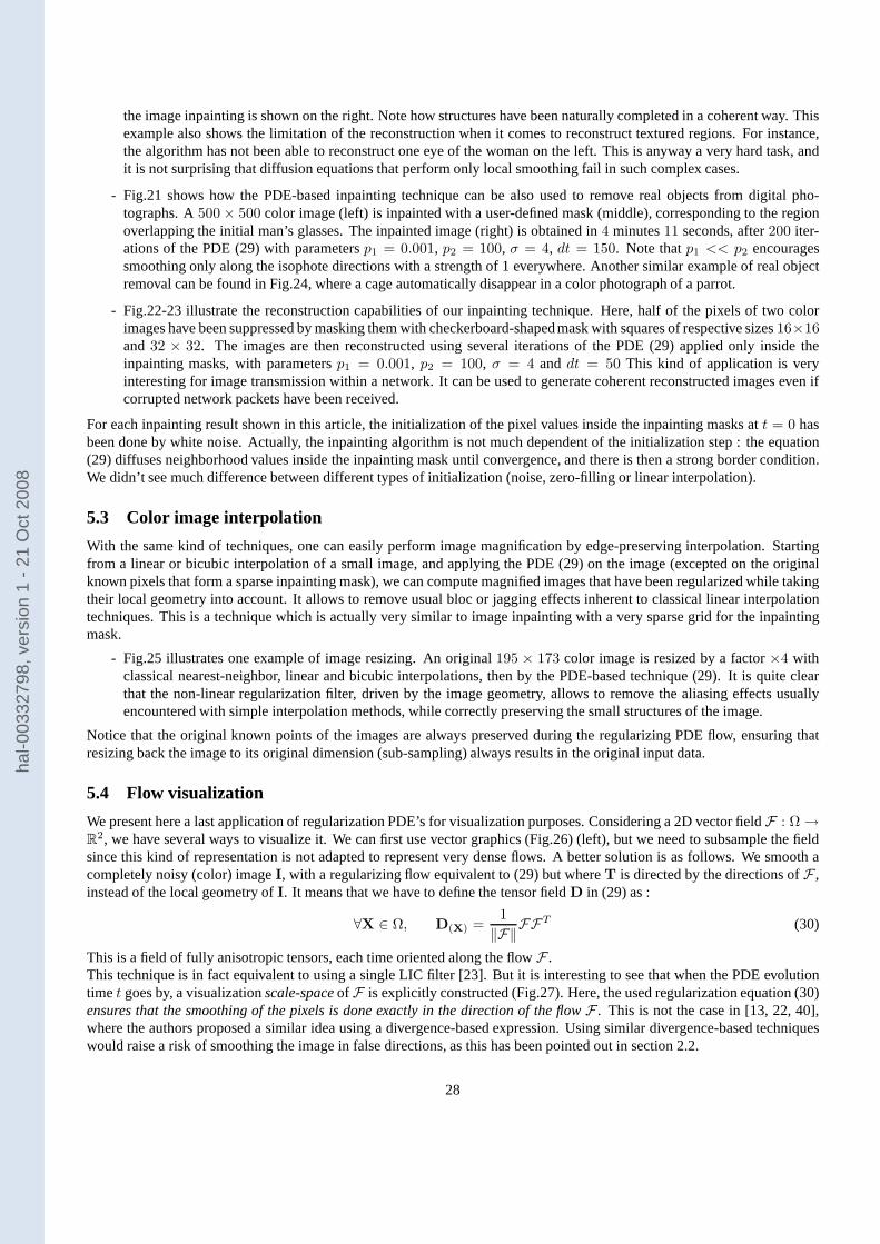
the image inpainting is shown on the right. Note how structures have been naturally completed in a coherent way. Thisexample also shows the limitation of the reconstruction when it comes to reconstruct textured regions. For instance,the algorithm has not been able to reconstruct one eye of the woman on the left. This is anyway a very hard task, andit is not surprising that diffusion equations that perform only local smoothing fail in such complex cases.

- Fig.21 shows how the PDE-based inpainting technique can bealso used to remove real objects from digital pho-tographs. A500 × 500 color image (left) is inpainted with a user-defined mask (middle), corresponding to the regionoverlapping the initial man’s glasses. The inpainted image(right) is obtained in4 minutes11 seconds, after200 iter-ations of the PDE (29) with parametersp1 = 0.001, p2 = 100, σ = 4, dt = 150. Note thatp1 << p2 encouragessmoothing only along the isophote directions with a strength of 1 everywhere. Another similar example of real objectremoval can be found in Fig.24, where a cage automatically disappear in a color photograph of a parrot.

- Fig.22-23 illustrate the reconstruction capabilities ofour inpainting technique. Here, half of the pixels of two colorimages have been suppressed by masking them with checkerboard-shapedmask with squares of respective sizes16×16and32 × 32. The images are then reconstructed using several iterations of the PDE (29) applied only inside theinpainting masks, with parametersp1 = 0.001, p2 = 100, σ = 4 anddt = 50 This kind of application is veryinteresting for image transmission within a network. It canbe used to generate coherent reconstructed images even ifcorrupted network packets have been received.

For each inpainting result shown in this article, the initialization of the pixel values inside the inpainting masks att = 0 hasbeen done by white noise. Actually, the inpainting algorithm is not much dependent of the initialization step : the equation(29) diffuses neighborhood values inside the inpainting mask until convergence, and there is then a strong border condition.We didn’t see much difference between different types of initialization (noise, zero-filling or linear interpolation).

5.3 Color image interpolation

With the same kind of techniques, one can easily perform image magnification by edge-preserving interpolation. Startingfrom a linear or bicubic interpolation of a small image, and applying the PDE (29) on the image (excepted on the originalknown pixels that form a sparse inpainting mask), we can compute magnified images that have been regularized while takingtheir local geometry into account. It allows to remove usualbloc or jagging effects inherent to classical linear interpolationtechniques. This is a technique which is actually very similar to image inpainting with a very sparse grid for the inpaintingmask.

- Fig.25 illustrates one example of image resizing. An original 195 × 173 color image is resized by a factor×4 withclassical nearest-neighbor, linear and bicubic interpolations, then by the PDE-based technique (29). It is quite clearthat the non-linear regularization filter, driven by the image geometry, allows to remove the aliasing effects usuallyencountered with simple interpolation methods, while correctly preserving the small structures of the image.

Notice that the original known points of the images are always preserved during the regularizing PDE flow, ensuring thatresizing back the image to its original dimension (sub-sampling) always results in the original input data.

5.4 Flow visualization

We present here a last application of regularization PDE’s for visualization purposes. Considering a 2D vector fieldF : Ω →R

2, we have several ways to visualize it. We can first use vector graphics (Fig.26) (left), but we need to subsample the fieldsince this kind of representation is not adapted to represent very dense flows. A better solution is as follows. We smooth acompletely noisy (color) imageI, with a regularizing flow equivalent to (29) but whereT is directed by the directions ofF ,instead of the local geometry ofI. It means that we have to define the tensor fieldD in (29) as :

∀X ∈ Ω, D(X) =1

‖F‖FFT (30)

This is a field of fully anisotropic tensors, each time oriented along the flowF .This technique is in fact equivalent to using a single LIC filter [23]. But it is interesting to see that when the PDE evolutiontimet goes by, a visualizationscale-spaceof F is explicitly constructed (Fig.27). Here, the used regularization equation (30)ensures that the smoothing of the pixels is done exactly in the direction of the flowF . This is not the case in [13, 22, 40],where the authors proposed a similar idea using a divergence-based expression. Using similar divergence-based techniqueswould raise a risk of smoothing the image in false directions, as this has been pointed out in section 2.2.

28

hal-0

0332

798,

ver

sion

1 -

21 O

ct 2

008

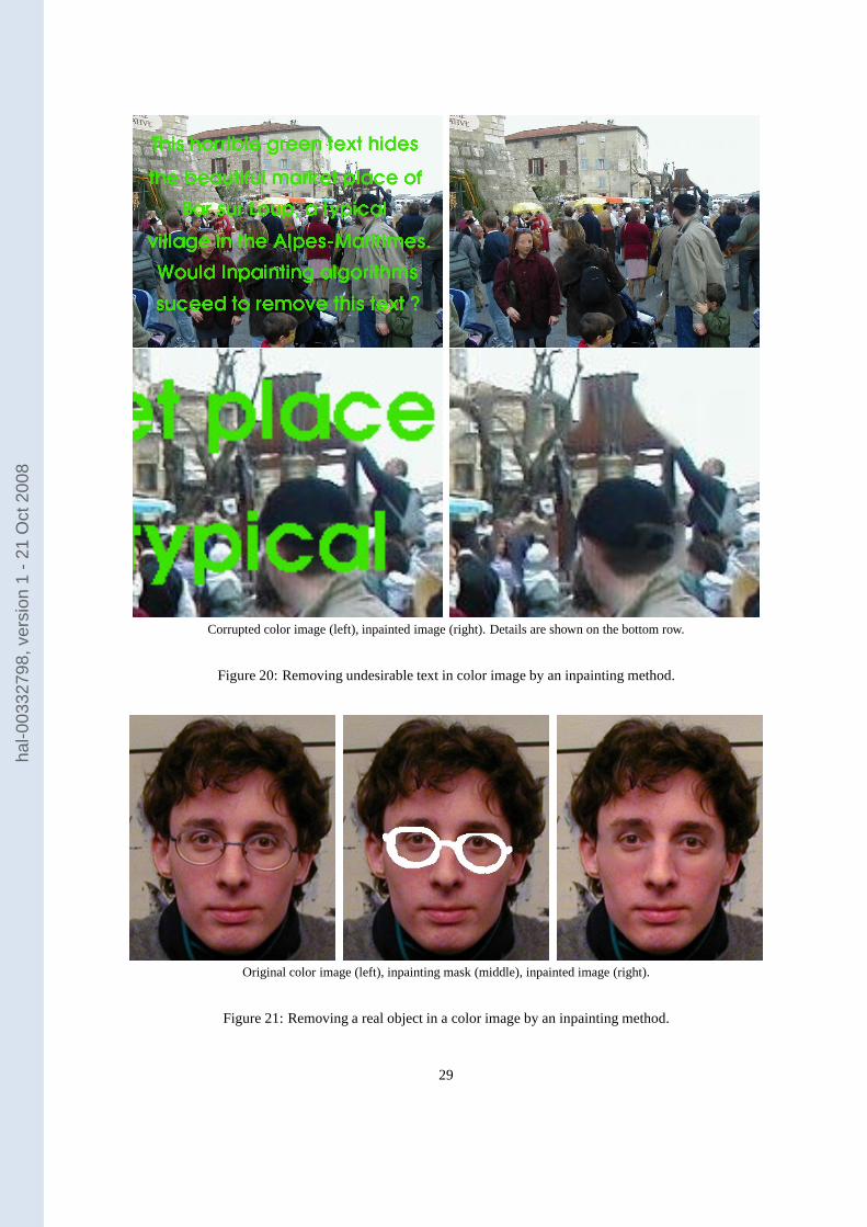
Corrupted color image (left), inpainted image (right). Details are shown on the bottom row.

Figure 20: Removing undesirable text in color image by an inpainting method.

Original color image (left), inpainting mask (middle), inpainted image (right).

Figure 21: Removing a real object in a color image by an inpainting method.

29

hal-0

0332

798,

ver

sion

1 -

21 O

ct 2

008

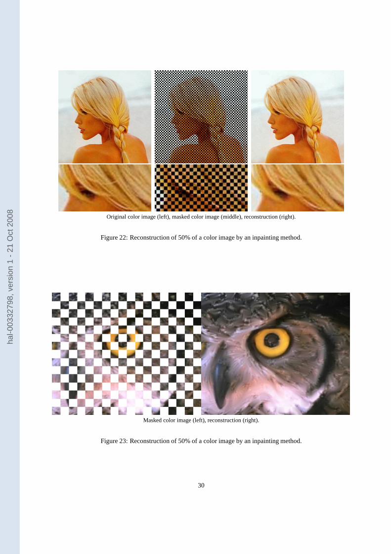
Original color image (left), masked color image (middle), reconstruction (right).

Figure 22: Reconstruction of 50% of a color image by an inpainting method.

Masked color image (left), reconstruction (right).

Figure 23: Reconstruction of 50% of a color image by an inpainting method.

30

hal-0

0332

798,

ver

sion

1 -

21 O

ct 2

008

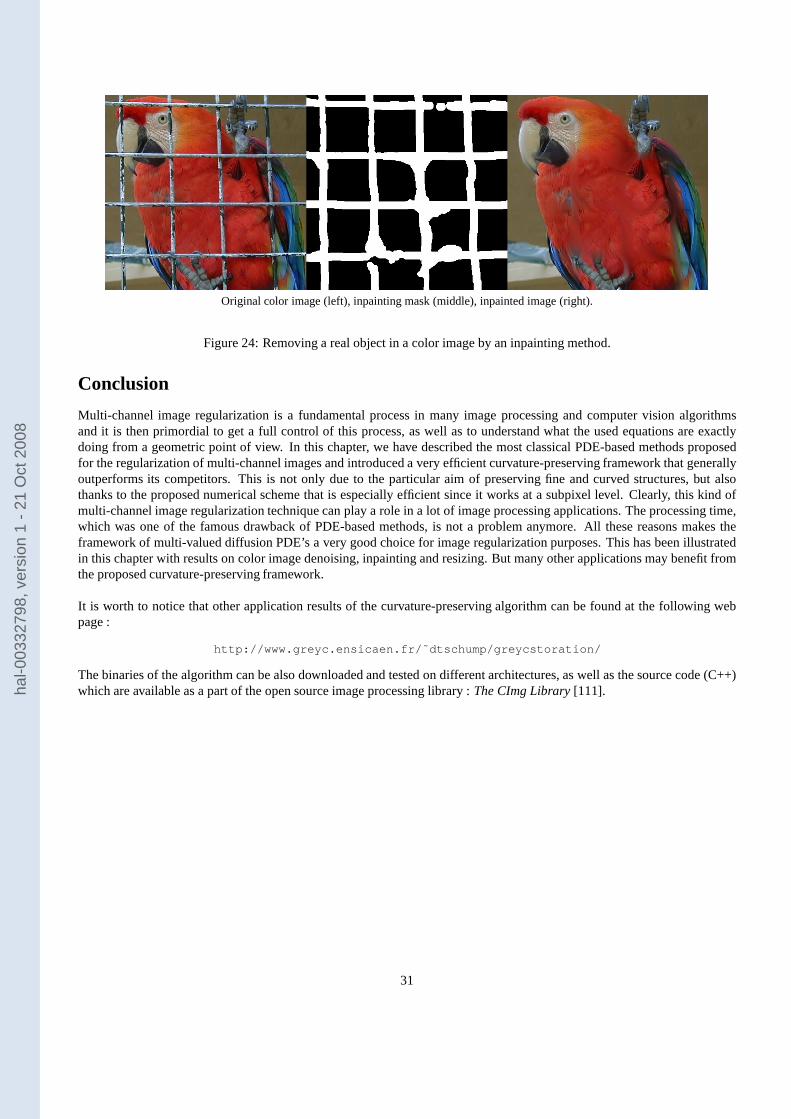
Original color image (left), inpainting mask (middle), inpainted image (right).

Figure 24: Removing a real object in a color image by an inpainting method.

Conclusion

Multi-channel image regularization is a fundamental process in many image processing and computer vision algorithmsand it is then primordial to get a full control of this process, as well as to understand what the used equations are exactlydoing from a geometric point of view. In this chapter, we havedescribed the most classical PDE-based methods proposedfor the regularization of multi-channel images and introduced a very efficient curvature-preserving framework that generallyoutperforms its competitors. This is not only due to the particular aim of preserving fine and curved structures, but alsothanks to the proposed numerical scheme that is especially efficient since it works at a subpixel level. Clearly, this kind ofmulti-channel image regularization technique can play a role in a lot of image processing applications. The processingtime,which was one of the famous drawback of PDE-based methods, isnot a problem anymore. All these reasons makes theframework of multi-valued diffusion PDE’s a very good choice for image regularization purposes. This has been illustratedin this chapter with results on color image denoising, inpainting and resizing. But many other applications may benefit fromthe proposed curvature-preserving framework.

It is worth to notice that other application results of the curvature-preserving algorithm can be found at the followingwebpage :

http://www.greyc.ensicaen.fr/˜dtschump/greycstorati on/

The binaries of the algorithm can be also downloaded and tested on different architectures, as well as the source code (C++)which are available as a part of the open source image processing library : The CImg Library[111].

31

hal-0

0332

798,

ver

sion

1 -

21 O

ct 2

008

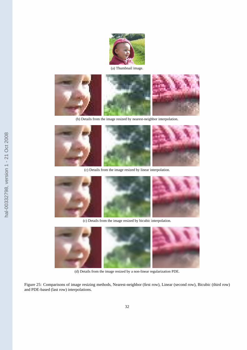
(a) Thumbnail image.

(b) Details from the image resized by nearest-neighbor interpolation.

(c) Details from the image resized by linear interpolation.

(c) Details from the image resized by bicubic interpolation.

(d) Details from the image resized by a non-linear regularization PDE.

Figure 25: Comparisons of image resizing methods, Nearest-neighbor (first row), Linear (second row), Bicubic (third row)and PDE-based (last row) interpolations.

32

hal-0

0332

798,

ver

sion

1 -

21 O

ct 2

008

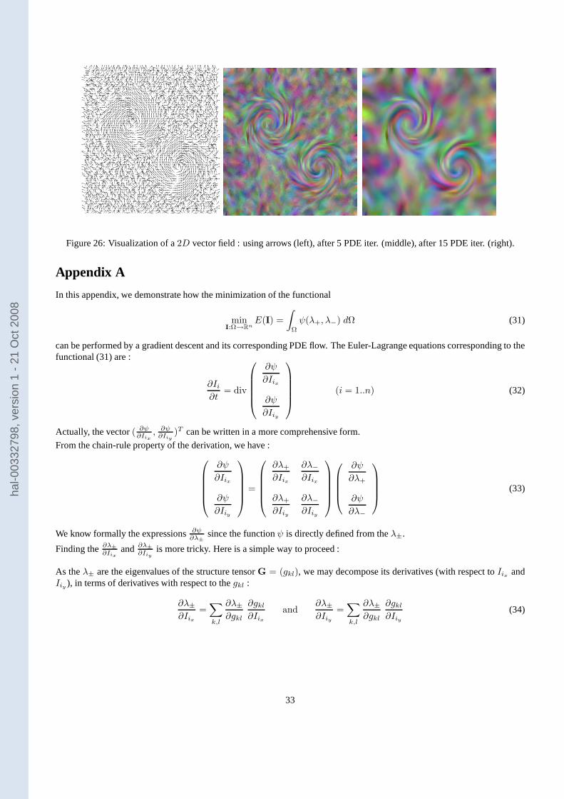
Figure 26: Visualization of a2D vector field : using arrows (left), after 5 PDE iter. (middle), after 15 PDE iter. (right).

Appendix A

In this appendix, we demonstrate how the minimization of thefunctional

minI:Ω→Rn

E(I) =

∫

Ω

ψ(λ+, λ−) dΩ (31)

can be performed by a gradient descent and its correspondingPDE flow. The Euler-Lagrange equations corresponding to thefunctional (31) are :

∂Ii∂t

= div

∂ψ

∂Iix

∂ψ

∂Iiy

(i = 1..n) (32)

Actually, the vector( ∂ψ∂Iix

, ∂ψ∂Iiy

)T can be written in a more comprehensive form.

From the chain-rule property of the derivation, we have :

∂ψ

∂Iix

∂ψ

∂Iiy

=

∂λ+

∂Iix

∂λ−∂Iix

∂λ+

∂Iiy

∂λ−∂Iiy

∂ψ

∂λ+

∂ψ

∂λ−

(33)

We know formally the expressions∂ψ∂λ±since the functionψ is directly defined from theλ±.

Finding the∂λ±

∂Iixand ∂λ±

∂Iiyis more tricky. Here is a simple way to proceed :

As theλ± are the eigenvalues of the structure tensorG = (gkl), we may decompose its derivatives (with respect toIix andIiy ), in terms of derivatives with respect to thegkl :

∂λ±∂Iix

=∑

k,l

∂λ±∂gkl

∂gkl∂Iix

and∂λ±∂Iiy

=∑

k,l

∂λ±∂gkl

∂gkl∂Iiy

(34)

33

hal-0

0332

798,

ver

sion

1 -

21 O

ct 2

008

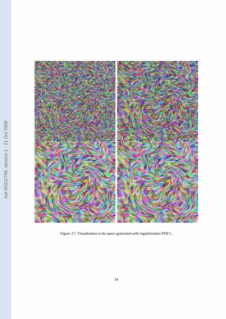
Figure 27: Visualization scale-space generated with regularization PDE’s.

34

hal-0

0332

798,

ver

sion

1 -

21 O

ct 2

008

The expressions∂gkl

∂Iixand ∂gkl

∂Iiyare particularly simple :

∂g11∂Iix

= 2Iix

∂g11∂Iiy

= 0

and

∂g12∂Iix

= Iiy

∂g12∂Iiy

= Iix

and

∂g22∂Iix

= 0

∂g22∂Iiy

= 2Iiy

i.e (34) can be written as :

∂λ±∂Iix

∂λ±∂Iiy

=

2∂λ±∂g11

∂λ±∂g12

∂λ±∂g12

2∂λ±∂g22

∇Ii (35)

Thus, one last obstacle remains to be crossed, that is findingthe formal expressions of∂λ±

∂gkl.

Remind that theλ± andθ± are the eigenvalues and eigenvectors of the structure tensor G :

G = λ+ θ+θT+ + λ− θ−θ

T−

The derivation of this tensor, with respect to one of its coefficientgkl is :

∂G

∂gkl=

∂λ+

∂gklθ+θ

T+ +

∂λ−∂gkl

θ−θT− (36)

+ λ+∂θ+∂gkl

θT+ + λ−∂θ−∂gkl

θT−

+ λ+ θ+∂θT+∂gkl

+ λ− θ−∂θT−∂gkl

Moreover, as theθ± are unitary and orthogonal eigenvectors, we have :

θT+θ+ = θT−θ− = 1

θT+θ− = θT−θ+ = 0and

∂θT+∂gkl

θ+ = θT+∂θ+∂gkl

= 0

∂θT−∂gkl

θ− = θT−∂θ−∂gkl

= 0

(37)

We first multiply the equation (36) byθT± at the left, byθ± at the right, then use the properties (37). It allows high simplifi-cations, and leads to these two relations :

∂λ+

∂gkl= θT+

∂G

∂gklθ+ and

∂λ−∂gkl

= θT−∂G

∂gklθ− (38)

Equations (38) formally tell us how eigenvalues of a diffusion tensorG vary with respect to a particular coefficientgkl of G.Actually, this interesting property can be proved for any symmetric matrix. For instance, authors of [77] proposed a similardemonstration in a purely matrix form, leading to the same result. They used it to deal with general covariance matrices.

Moreover in our case, the matrices∂G∂gklare very simple to write :

∂G

∂g11=

(

1 00 0

)

,∂G

∂g12=

(

0 11 0

)

and∂G

∂g22=

(

0 00 1

)

With all these elements, we can express (35) as :

∂λ+

∂Iix

∂λ+

∂Iiy

= 2 θ+θT+∇Ii and

∂λ−∂Iix

∂λ−∂Iiy

= 2 θ−θT−∇Ii (39)

35

hal-0

0332

798,

ver

sion

1 -

21 O

ct 2

008

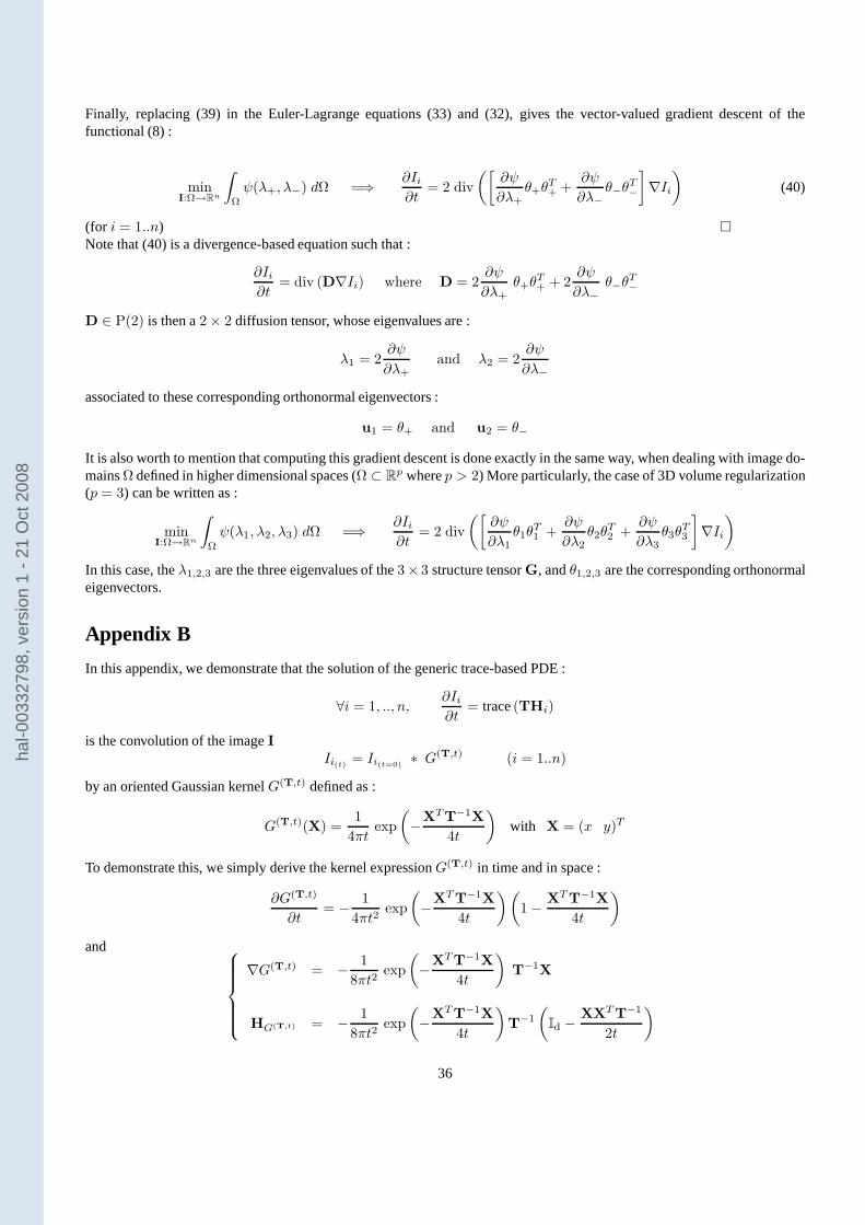
Finally, replacing (39) in the Euler-Lagrange equations (33) and (32), gives the vector-valued gradient descent of thefunctional (8) :

minI:Ω→Rn

∫

Ω

ψ(λ+, λ−) dΩ =⇒ ∂Ii∂t

= 2 div

([

∂ψ

∂λ+θ+θ

T+ +

∂ψ

∂λ−θ−θ

T−

]

∇Ii)

(40)

(for i = 1..n)

Note that (40) is a divergence-based equation such that :

∂Ii∂t

= div (D∇Ii) where D = 2∂ψ

∂λ+θ+θ

T+ + 2

∂ψ

∂λ−θ−θ

T−

D ∈ P(2) is then a2 × 2 diffusion tensor, whose eigenvalues are :

λ1 = 2∂ψ

∂λ+and λ2 = 2

∂ψ

∂λ−

associated to these corresponding orthonormal eigenvectors :

u1 = θ+ and u2 = θ−

It is also worth to mention that computing this gradient descent is done exactly in the same way, when dealing with image do-mainsΩ defined in higher dimensional spaces (Ω ⊂ R

p wherep > 2) More particularly, the case of 3D volume regularization(p = 3) can be written as :

minI:Ω→Rn

∫

Ω

ψ(λ1, λ2, λ3) dΩ =⇒ ∂Ii∂t

= 2 div

([

∂ψ

∂λ1θ1θ

T1 +

∂ψ

∂λ2θ2θ

T2 +

∂ψ

∂λ3θ3θ

T3

]

∇Ii)

In this case, theλ1,2,3 are the three eigenvalues of the3× 3 structure tensorG, andθ1,2,3 are the corresponding orthonormaleigenvectors.

Appendix B

In this appendix, we demonstrate that the solution of the generic trace-based PDE :

∀i = 1, .., n,∂Ii∂t

= trace(THi)

is the convolution of the imageIIi(t) = Ii(t=0)

∗ G(T,t) (i = 1..n)

by an oriented Gaussian kernelG(T,t) defined as :

G(T,t)(X) =1

4πtexp

(

−XTT−1X

4t

)

with X = (x y)T

To demonstrate this, we simply derive the kernel expressionG(T,t) in time and in space :

∂G(T,t)

∂t= − 1

4πt2exp

(

−XTT−1X

4t

)(

1 − XTT−1X

4t

)

and

∇G(T,t) = − 1

8πt2exp

(

−XTT−1X

4t

)

T−1X

HG(T,t) = − 1

8πt2exp

(

−XTT−1X

4t

)

T−1

(

Id − XXTT−1

2t

)

36

hal-0

0332

798,

ver

sion

1 -

21 O

ct 2

008

where∇G(T,t) andHG(T,t) are respectively the gradient and the Hessian ofG(T,t).It means that

trace (T HG(T,t)) = − 1

8πt2exp

(

−XTT−1X

4t

)

trace

(

Id − XXTT−1

2t

)

= − 1

8πt2exp

(

−XTT−1X

4t

)(

2 − XTT−1X

2t

)

=∂G(T,t)

∂t

And as the convolution is a linear operation, we have

∂(Ii0 ∗G(T,t))

∂t= Ii0 ∗

∂G(T,t)

∂t= Ii0 ∗ trace (T HG(T,t))

= trace(

T HIi0∗G(T,t)

)

as well aslimt→0

(Ii(t) ∗G(T,t)) = Ii0

which tells us that the initial condition att = 0 is coherent both for the PDE and the convolution process, since the GaussianfunctionG(T,t) is normalized. This statement is thus true for each instantt of the PDE flow.

Appendix C

In this appendix, we develop tensor-driven divergence PDE’s into their trace-based counterpart. Most divergence-basedregularization PDE’s acting on multivalued images have thefollowing form :

∂Ii∂t

= div (D∇Ii) (i = 1..n) (41)

whereD is a diffusion tensor basedonly on first orderoperators. The fact is thatD is often computed from the structuretensorG =

∑nj=1 ∇Ij∇ITj and depends mainly on the spatial derivativesIix andIiy . Intuitively, as the divergencediv () =

∂∂x + ∂

∂y is itself a first order derivative operator, we should be ableto write (41) only with first and second spatial derivativesIix , Iiy , Iixx

, IixyandIiyy

. Thus, it could be expressed with oriented Laplacians in each image channelIi as well, i.e anexpression based on the trace operator∂Ii

∂t = trace (DHi).

We want to make the link between the two different diffusion tensorsD andT in the divergence-based and trace-basedregularization PDE’s, in the case whenD is not constant:

∂Ii∂t

= div (D∇Ii) and∂Ii∂t

= trace (THi)

As we noticed in the previous section, these two formulations are almost equivalent, up to an additional term depending onthevariation of the tensor fieldD :

div (D∇Ii) = trace (DHIi) + ∇ITi ~div (D) (42)

where ~div () is thematrix divergence.A natural idea is then to decompose the additional term∇ITi ~div (D) into oriented Laplacians, expressed with additionaldiffusion tensorsQ in the trace operator.

For this purpose, we will consider that the divergence tensor D is defined at each pointX ∈ Ω by

D = f1(λ+, λ−) θ+θT+ + f2(λ+, λ−) θ−θ

T− with f1/2 : R

2 → R (43)

37

hal-0

0332

798,

ver

sion

1 -

21 O

ct 2

008

It means thatD is only expressed from the eigenvaluesλ± and the eigenvectorsθ± of the structure tensorG :

G = λ+ θ+θT+ + λ− θ−θ

T−

This is indeed a very generic hypothesis that is verified by the majority of the proposed vector-valued regularization methods,for instance the one proposed in Appendix A :

∂Ii∂t

= div (D∇Ii) with (43) and

f1(λ+, λ−) = 2∂ψ

∂λ+

f2(λ+, λ−) = 2∂ψ

∂λ−

In order to develop the additional diffusion term∇ITi ~div (D) in the equation (42), we propose to writeD as a linearcombination ofG andId :

D = α(λ+, λ−)G + β(λ+, λ−)Id (44)

i.e we separate theisotropicandanisotropicparts ofD, with

α =f1(λ+, λ−) − f2(λ+, λ−)

λ+ − λ−and β =

λ+f2(λ+, λ−) − λ−f1(λ+, λ−)

λ+ − λ−(45)

Indeed, we have

αG + βId =f1 − f2λ+ − λ−

(λ+ θ+θT+ + λ− θ−θ

T−) +

λ+f2 − λ−f1λ+ − λ−

(θ+θT+ + θ−θ

T−)

=1

λ+ − λ−

[

θ+θT+ (λ+f1 − λ−f1) + θ−θ

T− (λ+f2 − λ−f2)

]

= f1 θ+θT+ + f2 θ−θ

T−

= D

Here we assumed thatλ+ 6= λ− (i.e the structure tensorG is anisotropic). Anyway, ifG is isotropic, one generally choosesanisotropicdiffusion tensorD too, in the divergence operator of (42), i.ef1(λ+, λ−) = f2(λ+, λ−). In this case, we chooseα = 0 andβ = f1(λ+, λ−).

This decomposition is useful to rewrite the matrix divergence ~div (D) into :

~div (D) = α ~div (G) + G∇α+ ∇β (46)

and the additional term of the equation (42) would be computed as :

∇IT ~div (D) = trace(

~div (D)∇ITi)

= αtrace(

~div (G)∇ITi)

(47)

+ trace(

G∇α∇ITi)

(48)

+ trace(

∇β∇ITi)

(49)

In the following, we propose to find formal expressions of (47), (48) and (49).

• First, remember that the structure tensorG is defined as :

G =n∑

j=1

∇Ij∇IjT

38

hal-0

0332

798,

ver

sion

1 -

21 O

ct 2

008

We have then :

~div (G) =

n∑

j=1

~div

(

I2jx

IjxIjyIjxIjy I2

jy

)

=

n∑

j=1

(

2 IjxIjxx+ IjxIjyy

+ IjyIjxy

IjxIjxy+ IjyIjxx

+ 2 IjyIjyy

)

=

n∑

j=1

(

Ijx(Ijxx+ Ijyy

)Ijy (Ijxx

+ Ijyy)

)

+

(

IjxIjxx+ IjyIjxy

IjxIjxy+ IjyIjyy

)

=

n∑

j=1

∆Ij∇Ij + Hj∇Ij

where∆Ij andHj are respectively the Laplacian and the Hessian of the image componentIj .Then, we can write the expression 47 as :

αtrace(

~div (G)∇IiT)

=

n∑

j=1

αtrace(

Hj

[

∇IiT∇IjId + ∇Ij∇IiT])

(50)

• We finally have to compute∇α and∇β, in the expression (48) and (49). This can be done by the decomposition :

∇α =∂α

∂λ+∇λ+ +

∂α

∂λ−∇λ− and ∇β =

∂β

∂λ+∇λ+ +

∂β

∂λ−∇λ− (51)

and as theλ±, eigenvalues of the structure tensorG, depends on theIjx andIjy :

∇λ± =

(

λ±x

λ±y

)

=

n∑

j=1

( ∂λ±

∂IjxIjxx

+ ∂λ±

∂IjyIjxy

∂λ±

∂IjxIjxy

+ ∂λ±

∂IjyIjyy

)

=

n∑

j=1

HIj

∂λ±

∂Ixj

∂λ±

∂Iyj

In Appendix A, we derived eigenvalues of a structure tensorG, with respect to the spatial image derivatives. We ended upwith the following relation :

∂λ±

∂Ixj

∂λ±

∂Iyj

= 2θ±θT±∇Ij

Then,

∇λ± =

n∑

j=1

2Hjθ±θT±∇Ij (52)

We can replace (52) into the expressions of (51), in order to find the spatial gradients ofα andβ :

∇α =

n∑

j=1

2Hj

(

∂α

∂λ+θ+θ

T+ +

∂α

∂λ−θ+θ

T+

)

∇Ij

∇β =

n∑

j=1

2Hj

(

∂β

∂λ+θ+θ

T+ +

∂β

∂λ−θ+θ

T+

)

∇Ij

(53)

Using (53), we finally compute the two missing parts (48) and (49) of the additional term∇ITi ~div (D) :

39

hal-0

0332

798,

ver

sion

1 -

21 O

ct 2

008

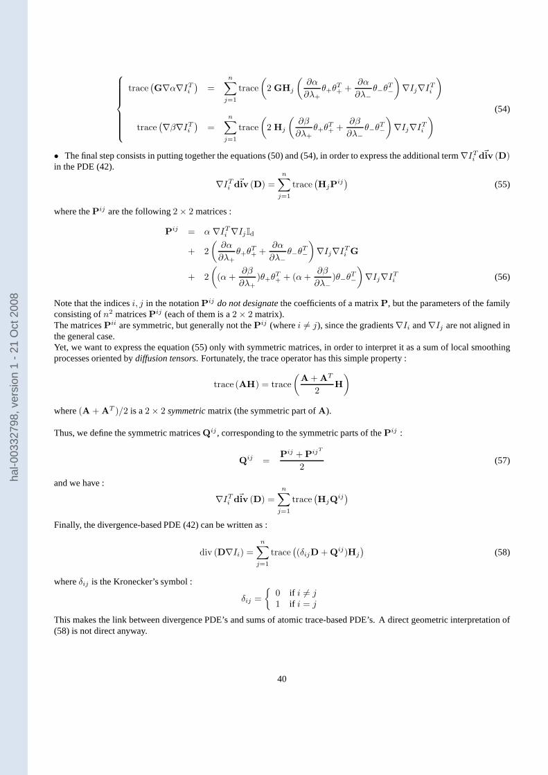
trace(

G∇α∇ITi)

=n∑

j=1

trace

(

2 GHj

(

∂α

∂λ+θ+θ

T+ +

∂α

∂λ−θ−θ

T−

)

∇Ij∇ITi)

trace(

∇β∇ITi)

=

n∑

j=1

trace

(

2 Hj

(

∂β

∂λ+θ+θ

T+ +

∂β

∂λ−θ−θ

T−

)

∇Ij∇ITi)

(54)

• The final step consists in putting together the equations (50) and (54), in order to express the additional term∇ITi ~div (D)in the PDE (42).

∇ITi ~div (D) =n∑

j=1

trace(

HjPij)

(55)

where thePij are the following2 × 2 matrices :

Pij = α ∇ITi ∇IjId

+ 2

(

∂α

∂λ+θ+θ

T+ +

∂α

∂λ−θ−θ

T−

)

∇Ij∇ITi G

+ 2

(

(α +∂β

∂λ+)θ+θ

T+ + (α+

∂β

∂λ−)θ−θ

T−

)

∇Ij∇ITi (56)

Note that the indicesi, j in the notationPij do not designatethe coefficients of a matrixP, but the parameters of the familyconsisting ofn2 matricesPij (each of them is a2 × 2 matrix).The matricesPii are symmetric, but generally not thePij (wherei 6= j), since the gradients∇Ii and∇Ij are not aligned inthe general case.Yet, we want to express the equation (55) only with symmetricmatrices, in order to interpret it as a sum of local smoothingprocesses oriented bydiffusion tensors. Fortunately, the trace operator has this simple property :

trace (AH) = trace

(

A + AT

2H

)

where(A + AT )/2 is a2 × 2 symmetricmatrix (the symmetric part ofA).

Thus, we define the symmetric matricesQij , corresponding to the symmetric parts of thePij :

Qij =Pij + PijT

2(57)

and we have :

∇ITi ~div (D) =

n∑

j=1

trace(

HjQij)

Finally, the divergence-based PDE (42) can be written as :

div (D∇Ii) =

n∑

j=1

trace(

(δijD + Qij)Hj

)

(58)

whereδij is the Kronecker’s symbol :

δij =

0 if i 6= j1 if i = j

This makes the link between divergence PDE’s and sums of atomic trace-based PDE’s. A direct geometric interpretation of(58) is not direct anyway.

40

hal-0

0332

798,

ver

sion

1 -

21 O

ct 2

008

References

[1] R. Abraham, J.E Marsden, and T.S. Ratiu.Manifolds, Tensor Analysis, and Applications.Springer-Verlag, New York,1991.

[2] J.F. Abramatic and L.M. Silverman.Non linear restoration of noisy images.IEEE Transactions on Pattern Analysis andMachine Intelligence (PAMI), 4(2):141–149, 1982.

[3] L. Alvarez, R. Deriche, and F. Santana.Recursivity and PDE’s in image processing.15th International Conference onPattern Recognition, volume I, pp 242–248, 2000.

[4] L. Alvarez, F. Guichard, P.L. Lions, and J.M. Morel.Axioms and fundamental equations of image processing.Archivefor Rational Mechanics and Analysis, Vol.123, No.3, pp.199–257, 1993.

[5] L. Alvarez, P.L. Lions, and J.M. Morel.Image selective smoothing and edge detection by nonlinear diffusion (II). SIAMJournal of Numerical Analysis, 29:845–866, 1992.

[6] L. Alvarez and L. Mazorra.Signal and Image Restoration using Shock Filters and Anisotropic Diffusion.SIAM Journalof Numerical Analysis, Vol.31, No.2, pp.590–605, 1994.

[7] L. Alvarez. Images and PDE’s.Images, Wavelets and PDEs, vol.219 of Lecture Notes in Control and InformationSciences, Springer, 1996.

[8] H.C. Andrews and B.R. Hunt.Digital Image Restoration. Signal Processing, Prentice Hall, Englewood Cliffs, N.J.,1977.

[9] G. Aubert and P. Kornprobst.Mathematical Problems in Image Processing: Partial Differential Equations and theCalculus of Variations, Vol.147 of Applied Mathematical Sciences, Springer-Verlag, 2002.

[10] M. Ashikhmin. Synthesizing Natural Textures.ACM Symposium on Interactive 3D Graphics, Research Triangle Park,NorthCarolina, pp.217–226, 2001.

[11] D. Barash.Bilateral filtering and anisotropic diffusion : Towards a unified viewpoint.Technical report, HP LaboratoriesIsrael, 2000.

[12] F. Barbaresco.Spatial denoising of statistical parameters estimation byBeltrami diffusion on embedding siegel space.Physics in Signal and Image Processing (PSIP), 2003.

[13] J. Becker, T. Preusser, and M. Rumpf.PDE methods in flow simulation post processing.Computing and Visualizationin Science, 3(3):159–167, 2000.

[14] M. Bertalmio, L.T. Cheng, S. Osher, and G. Sapiro.Variational problems and partial differential equations on implicitsurfaces: The framework and examples in image processing and pattern formation.UCLA Research Report, June 2000.

[15] M. Bertalmio, G. Sapiro, V. Caselles, and C. Ballester.Image inpainting.Proceedings of the SIGGRAPH, pp.417–424.ACM Press, Addison Wesley Longman, 2000.

[16] M. Bertalmio, L.T. Cheng, S. Osher, and G. Sapiro.Variational Problems and Partial Differential Equations on ImplicitSurfaces.Computing and Visualization in Science, Vol.174, No.2, pp.759–780, 2001.

[17] M. Bertalmio, L. Vese, G. Sapiro, and S. Osher.Simultaneous Structure and Texture Image Inpainting. IEEE Transac-tions on Image Processing, Vol.12, No.8, pp.882–889, 2003.

[18] M.J. Black, G. Sapiro, D.H. Marimont, and D. Heeger.Robust anisotropic diffusion.IEEE Transaction on ImageProcessing, Vol.7, No.3, pp.421–432, 1998.

[19] L. Blanc-Feraud, P. Charbonnier, G. Aubert, and M. barlaud.Nonlinear image processing : Modeling and fast algorithmfor regularization with edge detection.Proceedings of the International Conference on Image Processing (ICIP), pp.474–477, Washington, USA, 1995.

41

hal-0

0332

798,

ver

sion

1 -

21 O

ct 2

008

[20] P. Blomgren.Total Variation Methods for Restoration of Vector Valued Images.PhD thesis, Department of Mathematics,University of California, Los Angeles, 1998.

[21] P. Blomgren and T.F. Chan.Color tv: Total variation methods for restoration of vector-valued images.IEEE Transac-tions on Image Processing, 7(3):304–309, 1998.

[22] D. Buerkle, T. Preusser, and M. Rumpf.Transport and diffusion in timedependent flow visualization. Proceedings IEEEVisualization, 2001.

[23] B. Cabral and L.C. Leedom.Imaging vector fields using line integral convolution.SIGGRAPH’93, in ComputerGraphics Vol.27, pp.263–272, 1993.

[24] R. Carmona and S. Zhong.Adaptive Smoothing Respecting Feature Directions.IEEE Transactions on Image Processing,Vol.7, No.3, pp.353–358, 1998.

[25] A. Chambolle and P.L. Lions.Image recovery via total variation minimization and related problems. NumerischeMathematik, Vol.76, No.2, pp.167–188, 1997.

[26] T. Chan, S.H. Kang, and J. Shen.Euler’s elastica and curvature based inpainting.SIAM Journal of Applied Mathe-matics, 2002.

[27] T.F. Chan, S.H. Kang, and J. Shen.Total variation denoising and enhancement color images based on the cb and hsvcolor models.Journal of Visual Communication and Image Representation,12(4), 2000.

[28] T.F. Chan and J. Shen.Non-texture inpainting by curvature-driven diffusions (CDD). Journal of Visual Communicationand Image Representation, 12(4):436–449, 2001.

[29] T. Chan and J. Shen.Variational restoration of non-flat image features : Modelsand algorithms.SIAM Journal ofApplied Mathematics, Vol.61, No.4, pp.1338–1361, 2000.

[30] T. Chan and J. Shen.Mathematical models for local deterministic inpaintings.Technical Report 00-11, Department ofMathematics, UCLA, Los Angeles, 2000.

[31] P. Charbonnier, G. Aubert, M. Blanc-Feraud, and M. Barlaud. Two deterministic half-quadratic regularization algo-rithms for computed imaging.Proceedings of the International Conference on Image Processing (ICIP), volume II, pages168–172, 1994.

[32] P. Charbonnier, L. Blanc-Feraud, G. Aubert, and M. Barlaud.Deterministic edge-preserving regularization in computedimaging. IEEE Transactions on Image Processing, 6(2):298–311, 1997.

[33] C. Chefd’hotel, D. Tschumperle, R. Deriche, and O. Faugeras. Regularizing Flows for Constrained Matrix-ValuedImages.Journal of Mathematical Imaging and Vision, Vol.20, No.2, pp.147-162, 2004.

[34] M.T. Chu. A list of matrix flows with applications.Technical report, Department of Mathematics, North Carolina StateUniversity, 1990.

[35] M.T. Chu. Matrix differential equations : A continuous realization process for linear algebra problems.Technicalreport, Department of Mathematics, North Carolina State University, 1990.

[36] G.H. Cottet and L. Germain.Image processing through reaction combined with nonlineardiffusion. Mathematics ofComputation, 61(204):659–673, 1993.

[37] O. Coulon, D.C. Alexander, and S.R. Arridge.A regularization scheme for diffusion tensor magnetic resonance images.17th International Conference on Information Processing in Medical Imaging, LNCS, Vol.2082, pp.92–105, 2001.

[38] A. Criminisi, P. Perez, and K. Toyama.Object Removal by Exemplar-based InpaintingIEEE Conference on ComputerVision and Pattern Recognition (CVPR), Vol.2, pp.721–728,2003.

[39] R. Deriche and O. Faugeras.Les EDP en traitement des images et vision par ordinateur.Traitement du Signal, Vol.13,No.6, 1997.

42

hal-0

0332

798,

ver

sion

1 -

21 O

ct 2

008

[40] U. Diewald, T. Preusser, and M. Rumpf.Anisotropic diffusion in vector field visualization on euclidian domains andsurfaces.IEEE Transactions on Visualization and Computer Graphics,6(2):139–149, 2000.

[41] S. Di Zenzo A note on the gradient of a multi-image.Computer Vision, Graphics and Image Processing, Vol.33,pp.116-125, 1986.

[42] L. Florack. Image Structure. Kluwer Academic Publishers, 1997.

[43] M. A. Forstner and E. Gulch.A fast operator for detection and precise location of distinct points, corners and centersof circular features.Proceedings of the Intercommission Workshop of the International Society for Photogrammetry andRemote Sensing, Interlaken, Switzerland, 1987.

[44] B.R. Frieden.Restoring with maximum likelihood and maximum entropy.Journal Optical Society, 62:511–518, 1972.

[45] S. Geman and D. Geman.Stochastic relaxation, Gibbs distributions, and the Bayesian restoration of images.IEEETransactions on Pattern Analysis and Machine Intelligence(PAMI), 6(6):721–741, 1984.

[46] S. Geman and D.E. McClure. Bayesian image analysis: an application to single photon emission tomography.Proc. ofthe Statistical Computing Section p.12-18, Washington D.C, 1985

[47] G. Gerig, O. Kubler, R. Kikinis, and F. Jolesz.Nonlinear anisotropic filtering of MRI data.IEEE TMI, 11(2):221–231,1992.

[48] G. Gilboa, N. Sochen, and Y Zeevi.Forward-and-backward diffusion processes for adaptativeimage enhancement anddenoising.IEEE Transactions on Image Processing, 2002.

[49] G. Gilboa, N. Sochen, and Y. Zeevi.Regularized shock filters and complex diffusion.Proceedings of ECCV’02, pages399–413, Copenhaguen/Denmark.

[50] G. Gilboa, N. Sochen, and Y.Y. Zeevi.Complex Diffusion Processes for Image Filtering.Proceedings of ECCV’02,Copenhaguen/Denmark.

[51] G.H. Granlund and H. Knutsson.Signal Processing for Computer Vision. Kluwer Academic Publishers, 1995.

[52] P.J. Green. Bayesian reconstruction from emission tomography data using a modified em algorithm.IEEE Trans. Med.Imaging, MI-9(1):84–93, March 1990.

[53] J. Hadamard.Lectures on the Cauchy Problem in Linear Partial Differential Equations.Yale University Press, NewHaven, 1923.

[54] B.R. Hunt. TTe application of constrained least squares estimation toimage restoration by digital computer.IEEETrans. Computers, C-22(9):805–812, 1973.

[55] J. Jia and C.K. TangImage Repairing : Robust Image Synthesis by AdaptiveND Tensor Voting.IEEE Conference onComputer Vision and Pattern Recognition (CVPR), Vol.1, pp.643–650, 2003.

[56] JPEG Consortium Web Page.http://www.jpeg.org

[57] S. Kichenassamy.The Perona–Malik paradox.SIAM Journal of Applied Mathematics, 57(5):1328–1342, 1997.

[58] R. Kimmel, R. Malladi, and N. Sochen.Image processing via the Beltrami operator.Proceedings of the 3rd AsianConference on Computer Vision, vol 1, pp.574–581, Hong Kong, 1998.

[59] R. Kimmel, R. Malladi, and N. Sochen.Images as embedded maps and minimal surfaces: movies, color, texture, andvolumetric medical images.International Journal of Computer Vision (IJCV), 39(2):111–129, 2000.

[60] R. Kimmel and N. Sochen.Geometric-variational approach for color image enhancement and segmentation.Scale-Space Theories in Computer Vision, Scale-Space’99, vol.1682 of LNCS, pp.295–305. Springer, 1999.

[61] R. Kimmel and N. Sochen.Orientation diffusion or how to comb a porcupine.Journal of Visual Communication andImage Representation, Vol.13, pp.238–248, 2002.

43

hal-0

0332

798,

ver

sion

1 -

21 O

ct 2

008

[62] J.J. Koenderink.The structure of images.Biological Cybernetics, 50:363–370, 1984.

[63] P. Kornprobst.Contributionsa la Restauration d’Images eta l’Analyse de Sequences: Approches Variationnelles etSolutions de Viscosite. PhD thesis, Universite de Nice-Sophia Antipolis, 1998.

[64] P. Kornprobst, R. Deriche, and G. Aubert.Image restoration via PDE’s.First Annual Symposium on Enabling Tech-nologies for Law Enforcement and Security - SPIE Conference2942, Boston, Massachusetts, USA, 1996.

[65] P. Kornprobst, R. Deriche, and G. Aubert.Nonlinear operators in image restoration.Proceedings of the IEEE Interna-tional Conference on Computer Vision and Pattern Recognition (CVPR), pp.325–331, Puerto Rico, 1997.

[66] A. Koschan. A comparative study on color edge detection.Proceedings of the 2nd Asian Conference on ComputerVision, ACCV’95, pages 574–578.

[67] K. Krissian. Multiscale Analysis : Application to Medical Imaging and 3DVessel Detection.Ph.D. Thesis, INRIA-Sophia Antipolis/France, 2000.

[68] T. Lindeberg.Scale-Space Theory in Computer Vision. Kluwer Academic Publishers, 1994.

[69] L. Lucido, R. Deriche, L. Alvarez, and V. Rigaud.Sur quelques schemas numeriques de resolution d’equations auxderivees partielles pour le traitement d’images.Rapport de Recherche 3192, INRIA, 1997.

[70] S. Masnou and J-M. Morel.Level Lines Based Disocclusion.IEEE International Conference on Image Processing(ICIP), Vol.3, pp.259-263, 1998.

[71] Y. Meyer Oscillatory patterns in image processing and nonlinear evolution equations.University Lecture Series, vol.22, American Mathematical Society, Providence, 2001.

[72] M. Nielsen, L. Florack, and R. Deriche.Regularization, scale-space and edge detection filters.Journal of MathematicalImaging and Vision (JMIV), 7(4):291–308, 1997.

[73] M. Nikolova. Local strong homogeneity of a regularized estimator.SIAM Journal of Applied Mathematics, 61(2):633–658, 2000.

[74] M. Nikolova. Image restoration by minimizing objective functions with nonsmooth data-fidelity terms.IEEE Workshopon Variational and Level Set Methods (VLSM), pp. 11–19, Vancouver, Canada, 2001.

[75] M. Nikolova and M. Ng.Fast image reconstruction algorithms combining half-quadratic regularization and precondi-tioning. Proceedings of the International Conference on Image Processing. IEEE Signal Processing Society, 2001.

[76] S. Osher and L.I. Rudin.Feature-oriented image enhancement using shock filters.SIAM Journal of Numerical Analysis,Vol.27, No.4, pp.919–940, 1990.

[77] T. Papadopoulo and M.I.A. Lourakis.Estimating the jacobian of the singular value decomposition: Theory and appli-cations.Research Report 3961, INRIA Sophia-Antipolis, 2000.

[78] A. Pardo and G. Sapiro.Vector probability diffusion.Proceedings of the International Conference on Image Processing(ICIP). IEEE Signal Processing Society, 2000.

[79] P. Perona.Orientation diffusions.IEEE Transactions on Image Processing, Vol.7, No.3, pp.457–467, 1998.

[80] P. Perona and J. Malik.Scale-space and edge detection using anisotropic diffusion. IEEE Transactions on PatternAnalysis and Machine Intelligence (PAMI), 12(7):629–639,1990.

[81] C.A. Poynton. Poynton’s colour FAQ (www.inforamp.net/ poynton). Web page, 1995.

[82] T. Preusser and M. Rumpf.Anisotropic nonlinear diffusion in flow visualization.IEEE Visualization Conference, 1999.

[83] W.H. Press, B.P. Flannery, S.A. Teukolsky, and W.T. Vetterling. Runge-Kutta Methodin Numerical Recipes in FOR-TRAN: The Art of Scientific Computing, Cambridge UniversityPress, pp. 704-716, 1992.

44

hal-0

0332

798,

ver

sion

1 -

21 O

ct 2

008

[84] Bart M. ter Haar Romeny.Geometry-driven diffusion in computer vision. Computational imaging and vision. KluwerAcademic Publishers, 1994.

[85] L. Rudin, S. Osher, and E. Fatemi.Nonlinear total variation based noise removal algorithms.Physica D, Vol.60,pp.259–268, 1992.

[86] G. Sapiro.Vector-Valued Active Contours.Proceedings of the International Conference on Computer Vision and PatternRecognition (CVPR), pp.680–685, San Francisco, 1996. IEEE.

[87] G. Sapiro.Color snakes.Computer Vision and Image Understanding, 68(2), 1997.

[88] G. Sapiro.Geometric Partial Differential Equations and Image Analysis. Cambridge University Press, 2001.

[89] G. Sapiro and D.L. Ringach.Anisotropic diffusion of multivalued images with applications to color filtering. IEEETransactions on Image Processing, 5(11):1582–1585, 1996.

[90] H. Scharr and J. Weickert.An anisotropic diffusion algorithm with optimized rotation invariance. G. Sommer, N.Kruger, C. Perwass (Eds.), Mustererkennung 2000, Springer, Berlin, pp.460–467, 2000.

[91] J. Shah.Curve evolution and segmentation functionals: Applications to color images.Proceedings of the InternationalConference on Image Processing (ICIP), pp.461–464, 1996.

[92] N. Sochen, R. Kimmel, and A.M. Bruckstein.Diffusions and confusions in signal and image processing.Journal ofMathematical Imaging and Vision (JMIV), 14(3):195–209, 2001.

[93] N. Sochen.On affine invariance in the Beltrami framework for vision.IEEE Workshop on Variational and Level SetMethods (VLSM), pp.51–56, Vancouver/Canada.

[94] N. Sochen, R. Kimmel, and R. Malladi.A geometrical framework for low level vision.IEEE Transaction on ImageProcessing, Special Issue on PDE based Image Processing, 7(3):310–318, 1998.

[95] D. Stalling and H.C. Hege.Fast and Resolution Independent Line Integral Convolution. ACM SIGGRAPH, 22ndAnnual Conference on Computer Graphics and Interactive Technique, pp.249–256, 1995.

[96] B. Tang, G. Sapiro, and V. Caselles.Direction diffusion.International Conference on Computer Vision (ICCV), 1998.

[97] B. Tang, G. Sapiro, and V. Caselles.Diffusion of general data on non-flat manifolds via harmonicmaps theory : Thedirection diffusion case.International Journal of Computer Vision (IJCV), 36(2):149–161, 2000.

[98] S. Teboul, L. Blanc-Feraud, G. Aubert, and M. Barlaud.Variational approach for edge-preserving regularizationusingcoupled PDE’s.IEEE Transaction on Image Processing, Special Issue on PDE based Image Processing, 7(3):387–397,1998.

[99] A.N. Tikhonov.Regularization of incorrectly posed problems.Soviet. Math. Dokl., 4:1624–1627, 1963.

[100] C. Tomasi and R. Manduchi.Bilateral filtering for gray and color images.Proceedings of the IEEE InternationalConference on Computer Vision (ICCV), pp.839–846, 1998.

[101] D. Tschumperle.PDE’s Based Regularization of Multivalued Images and Applications. PhD thesis, Universite deNice-Sophia Antipolis, 2002.

[102] D. Tschumperle.Fast Anisotropic Smoothing of Multi-Valued Images using Curvature-Preserving PDE’s.InternationalJournal of Computer Vision (IJCV), vol.68, No.1, pp.65-82,2006.

[103] D. Tschumperle and R. Deriche.Constrained and unconstrained PDE’s for vector image restoration. Proceedings ofthe 10th Scandinavian Conference on Image Analysis (SCIA),pp.153–160, Bergen, Norway, 2001.

[104] D. Tschumperle and R. Deriche.Diffusion tensor regularization with constraints preservation.IEEE Computer SocietyConference on Computer Vision and Pattern Recognition (CVPR), Kauai Marriott, Hawaii, 2001.

45

hal-0

0332

798,

ver

sion

1 -

21 O

ct 2

008

[105] D. Tschumperle and R. Deriche.Regularization of orthonormal vector sets using coupled PDE’s. IEEE Workshop onVariational and Level Set Methods (VLSM), pp.3–10, Vancouver, Canada, 2001.

[106] D. Tschumperle and R. DericheDiffusion PDE’s on Vector-Valued Images : Local Approach and Geometric Viewpoint.IEEE Signal Processing Magazine, Vol.19, No.5, pp.16–25, 2002.

[107] D. Tschumperle and R. Deriche.Diffusion PDE’s on Vector-Valued images.IEEE Signal Processing Magazine,19(5):16–25, 2002.

[108] D. Tschumperle and R. Deriche.Orthonormal Vector Sets Regularization with PDE’s and Aplications. InternationJournal of Computer Vision (IJCV), 2002.

[109] D. Tschumperle and R. DericheVector-Valued Image Regularization with PDE’s : A Common Framework for DifferentApplications.IEEE Conference on Computer Vision and Pattern Recognition(CVPR), Vol.1, pp-651–656, 2003.

[110] D. Tschumperle and R. DericheVector-Valued Image Regularization with PDE’s : A Common Framework for DifferentApplications.IEEE Transactions on Pattern Analysis and Machine Intelligence (PAMI), Vol.27, No.4, 2005.

[111] D. Tschumperle.The CImg Library :http://cimg.sourceforge.net . The C++ Template Image ProcessingLibrary.

[112] L.A. Vese and S. Osher.Numerical methods for p-harmonic flows and applications to image processing.CAM Report01-22, UCLA, 2001.

[113] J. Weickert.Anisotropic Diffusion Filters for Image Processing Based Quality Control. 7th European Conference onMathematics in Industry, pp.355–362, 1994.

[114] J. Weickert.Anisotropic Diffusion in Image Processing. PhD thesis, University of Kaiserslautern, Germany, Laboratoryof Technomathematics, January 1996.

[115] J. Weickert.Theoretical foundations of anisotropic diffusion in imageprocessing.Computing Supplement, 11:221–236, 1996.

[116] J. Weickert.Coherence-enhancing diffusion of colour images.7th National Symposium on Pattern Recognition andImage Analysis, April 1997.

[117] J. Weickert. A review of nonlinear diffusion filtering.Scale-Space Theory in Computer Vision, Lecture Notes inComputer Science (Springer, Berlin), 1252:3–28, 1997.

[118] J. Weickert.Anisotropic Diffusion in Image Processing.Teubner-Verlag, Stuttgart, 1998.

[119] J. Weickert.Coherence-Enhancing Diffusion of Colour Images.Image and Vision Computing, Vol.17, pp.199–210,1999.

[120] J. Weickert Coherence-Enhancing Shock Filters.Pattern Recognition, 25th DAGM Symposium, LNCS, Vol.2781,pp.1–8, 2003.

[121] J. Weickert and B. Benhamouda.A semidiscrete nonlinear scale-space theory and its relation to the Perona–MalikparadoxAdvances in Computer Vision, Springer, pages 1–10, Wien, 1997.

[122] J. Weickert and B. Benhamouda.Why the Perona-Malik filter works.Technical Report 97/22, Department of ComputerScience, University of Copenhagen, 1997.

[123] J. Weickert and T. Brox.Diffusion and Regularization of Vector and Matrix-valued Images.Inverse Problems, ImageAnalysis, and Medical Imaging, Vol.313 of Contemporary Mathematics, pp.251–268, 2002.

[124] J. Weickert and C. Schnorr.A theoretical framework for convex regularizers in pde-based computation of imagemotion. International Journal of Computer Vision (IJCV), 45(3):245–264, 2001.

[125] L.Y Wei and M. LevoyFast Texture Synthesis using Tree-structured Vector Quantization. ACM SIGGRAPH, Inter-national Conference on Computer Graphics and Interactive Techniques, pp.479–488, 2000.

46

hal-0

0332

798,

ver

sion

1 -

21 O

ct 2

008

[126] P. Wesseling.Principles of Computational Fluid Dynamics.Springer-Verlag Berlin Heidelberg New York., 2000.

[127] A.P. Witkin. Scale-space filtering.International Joint Conference on Artificial Intelligence, pp.1019–1021, 1983.

[128] A. Yezzi.Modified curvature motion for image smoothing and enhancement. IEEE Transactions on Image Processing,pp 345–352, vol. 7, No 3, 1998.

47

hal-0

0332

798,

ver

sion

1 -

21 O

ct 2

008