Lectures on Differential Equations - UC Homepages
477
-
Upload
khangminh22 -
Category
Documents
-
view
0 -
download
0
Transcript of Lectures on Differential Equations - UC Homepages

Contents1
Introduction vii2
1 First Order Equations 13
1.1 Integration by Guess-and-Check . . . . . . . . . . . . . . . . . 14
1.2 First Order Linear Equations . . . . . . . . . . . . . . . . . . 45
1.2.1 The Integrating Factor . . . . . . . . . . . . . . . . . . 56
1.3 Separable Equations . . . . . . . . . . . . . . . . . . . . . . . 107
1.3.1 Problems . . . . . . . . . . . . . . . . . . . . . . . . . 138
1.4 Some Special Equations . . . . . . . . . . . . . . . . . . . . . 199
1.4.1 Homogeneous Equations . . . . . . . . . . . . . . . . . 1910
1.4.2 The Logistic Population Model . . . . . . . . . . . . . 2211
1.4.3 Bernoulli’s Equations . . . . . . . . . . . . . . . . . . 2512
1.4.4∗ Riccati’s Equations . . . . . . . . . . . . . . . . . . . . 2613
1.4.5∗ Parametric Integration . . . . . . . . . . . . . . . . . . 2714
1.4.6 Some Applications . . . . . . . . . . . . . . . . . . . . 2915
1.5 Exact Equations . . . . . . . . . . . . . . . . . . . . . . . . . 3116
1.6 Existence and Uniqueness of Solution . . . . . . . . . . . . . . 3617
1.7 Numerical Solution by Euler’s method . . . . . . . . . . . . . 3718
1.7.1 Problems . . . . . . . . . . . . . . . . . . . . . . . . . 3919
1.8∗ The Existence and Uniqueness Theorem . . . . . . . . . . . . 4720
1.8.1 Problems . . . . . . . . . . . . . . . . . . . . . . . . . 5221
2 Second Order Equations 5622
2.1 Special Second Order Equations . . . . . . . . . . . . . . . . . 5623
2.1.1 y is not present in the equation . . . . . . . . . . . . . 5724
2.1.2 x is not present in the equation . . . . . . . . . . . . . 5925
2.1.3∗ The Trajectory of Pursuit . . . . . . . . . . . . . . . . 6126
2.2 Linear Homogeneous Equations with Constant Coefficients . . 6327
ii

CONTENTS iii
2.2.1 The Characteristic Equation Has Two Distinct Real1
Roots . . . . . . . . . . . . . . . . . . . . . . . . . . . 642
2.2.2 The Characteristic Equation Has Only One (Repeated)3
Real Root . . . . . . . . . . . . . . . . . . . . . . . . . 664
2.3 The Characteristic Equation Has Two Complex Conjugate5
Roots . . . . . . . . . . . . . . . . . . . . . . . . . . . . . . . 676
2.3.1 Euler’s Formula . . . . . . . . . . . . . . . . . . . . . 677
2.3.2 The General Solution . . . . . . . . . . . . . . . . . . 688
2.3.3 Problems . . . . . . . . . . . . . . . . . . . . . . . . . 709
2.4 Linear Second Order Equations with Variable Coefficients . . 7310
2.5 Some Applications of the Theory . . . . . . . . . . . . . . . . 7811
2.5.1 The Hyperbolic Sine and Cosine Functions . . . . . . 7812
2.5.2 Different Ways to Write the General Solution . . . . . 7813
2.5.3 Finding the Second Solution . . . . . . . . . . . . . . . 8014
2.5.4 Problems . . . . . . . . . . . . . . . . . . . . . . . . . 8115
2.6 Non-homogeneous Equations . . . . . . . . . . . . . . . . . . 8316
2.7 More on Guessing of Y (t) . . . . . . . . . . . . . . . . . . . . 8717
2.8 The Method of Variation of Parameters . . . . . . . . . . . . 8918
2.9 The Convolution Integral . . . . . . . . . . . . . . . . . . . . 9219
2.9.1 Differentiation of Integrals . . . . . . . . . . . . . . . . 9220
2.9.2 Yet Another Way to Compute a Particular Solution . 9221
2.10 Applications of Second Order Equations . . . . . . . . . . . . 9322
2.10.1 Vibrating Spring . . . . . . . . . . . . . . . . . . . . . 9423
2.10.2 Problems . . . . . . . . . . . . . . . . . . . . . . . . . 9624
2.10.3 A Meteor Approaching the Earth . . . . . . . . . . . . 10325
2.10.4 Damped Oscillations . . . . . . . . . . . . . . . . . . . 10526
2.11 Further Applications . . . . . . . . . . . . . . . . . . . . . . . 10627
2.11.1 Forced and Damped Oscillations . . . . . . . . . . . . 10728
2.11.2 An Example of a Discontinuous Forcing Term . . . . . 10829
2.11.3 Oscillations of a Pendulum . . . . . . . . . . . . . . . 10930
2.11.4 Sympathetic Oscillations . . . . . . . . . . . . . . . . . 11031
2.12 Oscillations of a Spring Subject to a Periodic Force . . . . . . 11232
2.12.1 The Fourier Series . . . . . . . . . . . . . . . . . . . . 11333
2.12.2 Vibrations of a Spring Subject to a Periodic Force . . 11734
2.13 Euler’s Equation . . . . . . . . . . . . . . . . . . . . . . . . . 11835
2.14 Linear Equations of Order Higher Than Two . . . . . . . . . 12236
2.14.1 The Polar Form of Complex Numbers . . . . . . . . . 12237
2.14.2 Linear Homogeneous Equations . . . . . . . . . . . . . 12338
2.14.3 Non-Homogeneous Equations . . . . . . . . . . . . . . 12639
2.14.4 Problems . . . . . . . . . . . . . . . . . . . . . . . . . 12740

iv CONTENTS
2.15 Oscillation and Comparison Theorems . . . . . . . . . . . . . 1351
3 Using Infinite Series to Solve Differential Equations 1432
3.1 Series Solution Near a Regular Point . . . . . . . . . . . . . . 1433
3.1.1 Maclauren and Taylor Series . . . . . . . . . . . . . . 1434
3.1.2 A Toy Problem . . . . . . . . . . . . . . . . . . . . . . 1465
3.1.3 Using Series When Other Methods Fail . . . . . . . . 1476
3.2 Solution Near a Mildly Singular Point . . . . . . . . . . . . . 1537
3.2.1∗ Derivation of J0(x) by Differentiation of the Equation 1598
3.3 Moderately Singular Equations . . . . . . . . . . . . . . . . . 1609
3.3.1 Problems . . . . . . . . . . . . . . . . . . . . . . . . . 16610
4 The Laplace Transform 17311
4.1 The Laplace Transform And Its Inverse . . . . . . . . . . . . 17312
4.1.1 Review of Improper Integrals . . . . . . . . . . . . . . 17313
4.1.2 The Laplace Transform . . . . . . . . . . . . . . . . . 17414
4.1.3 The Inverse Laplace Transform . . . . . . . . . . . . . 17615
4.2 Solving The Initial Value Problems . . . . . . . . . . . . . . . 17816
4.2.1 Step Functions . . . . . . . . . . . . . . . . . . . . . . 18117
4.3 The Delta Function and Impulse Forces . . . . . . . . . . . . 18518
4.4 Convolution and the Tautochrone Curve . . . . . . . . . . . . 18819
4.5 Distributions . . . . . . . . . . . . . . . . . . . . . . . . . . . 19320
4.5.1 Problems . . . . . . . . . . . . . . . . . . . . . . . . . 19521
5 Linear Systems of Differential Equations 20522
5.1 The Case of Distinct Eigenvalues . . . . . . . . . . . . . . . . 20523
5.1.1 Review of Vectors and Matrices . . . . . . . . . . . . . 20524
5.1.2 Linear First Order Systems with Constant Coefficients 20725
5.2 A Pair of Complex Conjugate Eigenvalues . . . . . . . . . . . 21226
5.2.1 Complex Valued and Real Valued Solutions . . . . . . 21227
5.2.2 The General Solution . . . . . . . . . . . . . . . . . . 21328
5.2.3 Non-Homogeneous Systems . . . . . . . . . . . . . . . 21529
5.3 The Exponential of a Matrix . . . . . . . . . . . . . . . . . . 21630
5.3.1 Problems . . . . . . . . . . . . . . . . . . . . . . . . . 22131
5.4 Floquet Theory and Massera’s Theorem . . . . . . . . . . . . 23032
5.5 Solutions of Planar Systems Near the Origin . . . . . . . . . . 23933
5.5.1 Linearization and the Hartman-Grobman Theorem . . 24234
5.5.2 Phase Plane and the Prufer Transformation . . . . . . 24435
5.5.3 Problems . . . . . . . . . . . . . . . . . . . . . . . . . 24636
5.6 Controllability and Observability . . . . . . . . . . . . . . . . 25137

CONTENTS v
5.6.1 The Cayley-Hamilton Theorem . . . . . . . . . . . . . 2511
5.6.2 Controllability of Linear Systems . . . . . . . . . . . . 2522
5.6.3 Observability . . . . . . . . . . . . . . . . . . . . . . . 2553
6 Non-Linear Systems 2594
6.1 The Predator-Prey Interaction . . . . . . . . . . . . . . . . . 2595
6.2 Competing Species . . . . . . . . . . . . . . . . . . . . . . . . 2646
6.3 An Application to Epidemiology . . . . . . . . . . . . . . . . 2707
6.4 Lyapunov’s Stability . . . . . . . . . . . . . . . . . . . . . . . 2738
6.4.1 Stable Systems . . . . . . . . . . . . . . . . . . . . . . 2789
6.5 Limit Cycles . . . . . . . . . . . . . . . . . . . . . . . . . . . 28010
6.6 Periodic Population Models . . . . . . . . . . . . . . . . . . . 28611
6.6.1 Problems . . . . . . . . . . . . . . . . . . . . . . . . . 29512
7 The Fourier Series and Boundary Value Problems 30513
7.1 The Fourier Series for Functions of an Arbitrary Period . . . 30514
7.1.1 Even and Odd Functions . . . . . . . . . . . . . . . . 30815
7.1.2 Further Examples and the Convergence Theorem . . . 31016
7.2 The Fourier Cosine and the Fourier Sine Series . . . . . . . . 31317
7.3 Two Point Boundary Value Problems . . . . . . . . . . . . . 31618
7.3.1 Problems . . . . . . . . . . . . . . . . . . . . . . . . . 31819
7.4 The Heat Equation and the Method of Separation of Variables 32220
7.5 Laplace’s Equation . . . . . . . . . . . . . . . . . . . . . . . 33021
7.6 The Wave Equation . . . . . . . . . . . . . . . . . . . . . . . 33522
7.6.1 Non-Homogeneous Problems . . . . . . . . . . . . . . 33823
7.6.2 Problems . . . . . . . . . . . . . . . . . . . . . . . . . 34124
7.7 Calculating Earth’s Temperature and Queen Dido’s Problem 34625
7.7.1 The Complex Form of the Fourier Series . . . . . . . . 34626
7.7.2 The Temperatures Inside the Earth and Wine Cellars 34827
7.7.3 The Isoperimetric Inequality . . . . . . . . . . . . . . 35028
7.8 Laplace’s Equation on Circular Domains . . . . . . . . . . . . 35229
7.9 Sturm-Liouville Problems . . . . . . . . . . . . . . . . . . . . 35730
7.9.1 The Fourier-Bessel Series . . . . . . . . . . . . . . . . 36131
7.9.2 Cooling of a Cylindrical Tank . . . . . . . . . . . . . . 36332
7.9.3 Cooling of a Rectangular Bar . . . . . . . . . . . . . . 36433
7.10 Green’s Function . . . . . . . . . . . . . . . . . . . . . . . . . 36634
7.10.1 Problems . . . . . . . . . . . . . . . . . . . . . . . . . 37035
7.11 The Fourier Transform . . . . . . . . . . . . . . . . . . . . . . 37636
7.12 Problems on Infinite Domains . . . . . . . . . . . . . . . . . . 37837
7.12.1 Evaluation of Some Integrals . . . . . . . . . . . . . . 37838

vi CONTENTS
7.12.2 The Heat Equation for −∞ < x <∞ . . . . . . . . . 3791
7.12.3 Steady State Temperatures for the Upper Half Plane . 3812
7.12.4 Using the Laplace Transform for a Semi-Infinite String 3823
7.12.5 Problems . . . . . . . . . . . . . . . . . . . . . . . . . 3834
8 Elementary Theory of PDE 3855
8.1 Wave Equation: Vibrations of an Infinite String . . . . . . . . 3856
8.2 Semi-Infinite String: Reflection of Waves . . . . . . . . . . . . 3927
8.3 Bounded String: Multiple Reflections . . . . . . . . . . . . . . 3968
8.4 Neumann Boundary Conditions . . . . . . . . . . . . . . . . . 3999
8.5 Non-Homogeneous Wave Equation . . . . . . . . . . . . . . . 40210
8.5.1 Problems . . . . . . . . . . . . . . . . . . . . . . . . . 40611
8.6 First Order Linear Equations . . . . . . . . . . . . . . . . . . 41012
8.6.1 Problems . . . . . . . . . . . . . . . . . . . . . . . . . 41613
8.7 Laplace’s Equation: Poisson’s Integral Formula . . . . . . . . 41814
8.8 Some Properties of Harmonic Functions . . . . . . . . . . . . 42015
8.9 The Maximum Principle . . . . . . . . . . . . . . . . . . . . . 42316
8.10 The Maximum Principle for the Heat Equation . . . . . . . . 42617
8.10.1 Uniqueness on an Infinite Interval . . . . . . . . . . . 42818
8.11 Dirichlet’s Principle . . . . . . . . . . . . . . . . . . . . . . . 43119
8.12 Classification Theory for Two Variables . . . . . . . . . . . . 43420
8.12.1 Problems . . . . . . . . . . . . . . . . . . . . . . . . . 44021
9 Numerical Computations 44722
9.1 The Capabilities of Software Systems, Like Mathematica . . 44723
9.2 Solving Boundary Value Problems . . . . . . . . . . . . . . . 45124
9.3 Solving Nonlinear Boundary Value Problems . . . . . . . . . 45225
9.4 Direction Fields . . . . . . . . . . . . . . . . . . . . . . . . . 45526
References . . . . . . . . . . . . . . . . . . . . . . . . . . . . . . . 45627
Appendix . . . . . . . . . . . . . . . . . . . . . . . . . . . . . . . 46128
.1 The Chain Rule and Its Descendants . . . . . . . . . . . . . . 46129
.2 Partial Fractions . . . . . . . . . . . . . . . . . . . . . . . . . 46230
.3 Eigenvalues and Eigenvectors . . . . . . . . . . . . . . . . . . 46431
.4 Matrix Functions and the Norm . . . . . . . . . . . . . . . . . 46732
Introduction1
This book is based on several courses that I taught at the University of2
Cincinnati. Chapters 1-4 are based on the course “Differential Equations”3
for sophomores in science and engineering. Only some basic concepts of mul-4
tivariable calculus are used (functions of two variables and partial deriva-5
tives), and they are reviewed in the text. Chapters 7 and 8 are based on the6
course “Fourier Series and PDE”, and they should provide a wide choice of7
material for the instructors. Chapters 5 and 6 were used in graduate ODE8
courses, providing most of the needed material. Some of the sections of this9
book are outside of the scope of usual courses, but I hope they will be of10
interest to students and instructors alike. The book has a wide range of11
problems.12
I attempted to share my enthusiasm for the subject, and write a textbook13
that students will like to read. While some theoretical material is either14
quoted, or just mentioned without proof, my goal was to show all of the15
details when doing problems. I tried to use plain language and not to be too16
wordy. I think that an extra word of explanation has often as much potential17
to confuse a student, as to be helpful. I also tried not to overwhelm students18
with new information. I forgot who said it first: “one should teach the truth,19
nothing but the truth, but not the whole truth”.20
I hope that experts will find this book useful as well. It presents several21
important topics that are hard to find in the literature: Massera’s theorem,22
Lyapunov’s inequality, Picone’s form of Sturm’s comparison theorem, “side-23
ways” heat equation, periodic population models, “hands on” numerical24
solution of nonlinear boundary value problems, the isoperimetric inequality,25
etc. The book also contains new exposition of some standard topics. We26
have completely revamped the presentation of the Frobenius method for se-27
ries solution of differential equations, so that the “regular singular points”28
are now hopefully in the past. In the proof of the existence and uniqueness29
theorem, we replaced the standard Picard iterations with monotone itera-30
vii
viii INTRODUCTION
tions, which should be easier for students to absorb. There are many other1
fresh touches throughout the book. The book contains a number of inter-2
esting non-standard problems, including some original ones, published by3
the author over the years in the Problem Sections of SIAM Review, EJDE,4
and other journals. All of the challenging problems are provided with hints,5
making them easy to solve for instructors. We use asterisk (or star) to6
identify non-standard problems.7
How important are differential equations? Here is what Isaac Newton8
said: “It is useful to solve differential equations”. And what he knew was9
just the beginning. Today differential equations are used widely in science10
and engineering. This book presents many applications as well. Some of11
these applications are very old, like the tautochrone problem considered by12
Christian Huygens in 1659. Some applications, like when a drone is targeting13
a car, are modern. Differential Equations is also a beautiful subject, which14
lets students see Calculus “in action”.15
I attempted to start each topic with simple examples, to keep the presen-16
tation focused, and to show all of the details. I think this book is suitable17
for self-study. However, instructor can help in many ways. He (she) will18
present the subject with the enthusiasm it deserves, draw more pictures,19
talk about the history, and his jokes will supplement the lame ones in the20
book.21
I am very grateful to the MAA Book Board, including Steve Kennedy,22
Stan Seltzer and the whole group of anonymous reviewers, for providing23
me with detailed lists of corrections and suggested changes. Their help was24
crucial in making considerable improvements of the manuscript.25
It is a pleasure to thank Ken Meyer and Dieter Schmidt for constant26
encouragement while I was writing this book. I also wish to thank Ken27
for reading the entire book, and making a number of useful suggestions,28
like doing Fourier series early, with applications to periodic vibrations and29
radio tuning. I wish to thank Roger Chalkley, Tomasz Adamowicz, Dieter30
Schmidt, and Ning Zhong for a number of useful comments. Many useful31
comments came from students in my classes. They liked the book, and that32
provided me with the biggest encouragement.33
Chapter 11
First Order Equations2
First order equations occur naturally in many applications, making them an3
important object to study. They are also used throughout this book, and are4
of great theoretical importance. Linear first order equations, the first class5
of the equations we study, turns out to be of particular importance. Sepa-6
rable, exact and homogeneous equations are also used throughout the book.7
Applications are made to population modeling, and to various physical and8
geometrical problems. If a solution cannot be found by a formula, we prove9
that solution still exists, and indicate how it can be computed numerically.10
1.1 Integration by Guess-and-Check11
Many problems in differential equations end with a computation of an inte-12
gral. One even uses the term “integration of a differential equation” instead13
of “solution”. We need to be able to compute integrals quickly, which can14
be done by using the approach of this section. For example, one can write15
down16∫
x3ex dx = x3ex − 3x2ex + 6xex − 6ex + c
very quickly, avoiding three integrations by parts.17
Recall the product rule18
(fg)′ = fg′ + f ′g .
Example 1∫
xex dx. We need to find the function, with the derivative19
equal to xex. If we try a guess: xex, then its derivative20
(xex)′ = xex + ex
1

2 CHAPTER 1. FIRST ORDER EQUATIONS
has an extra term ex. To remove this extra term, we subtract ex from the1
initial guess, so that2
∫
xex dx = xex − 6ex + c.
By differentiation, we verify that this is correct. Of course, integration by3
parts may also be used.4
Example 2∫
x cos 3x dx. Starting with the initial guess1
3x sin 3x, with5
the derivative equal to x cos 3x+ 13 sin 3x, we compute6
∫
x cos 3x dx =1
3x sin 3x+
1
9cos 3x+ c.
Example 3∫ π
0x cos 3x dx =
[
1
3x sin 3x+
1
9cos 3x
]
|π0
= −2
9.7
We see that the initial guess is the product f(x)g(x), chosen in such a8
way that f(x)g′(x) gives the integrand.9
Example 4∫
xe−5x dx. Starting with the initial guess −1
5xe−5x, we10
compute11∫
xe−5x dx = −1
5xe−5x − 1
25e−5x + c.
12
Example 5∫
x2 sin 3x dx. The initial guess is −1
3x2 cos 3x. Its derivative13
(
−1
3x2 cos 3x
)′= x2 sin 3x− 2
3x cos 3x
has an extra term −2
3x cos 3x. To remove this term, we modify our guess:14
−1
3x2 cos 3x+
2
9x sin 3x. Its derivative15
(
−1
3x2 cos 3x+
2
9x sin 3x
)′= x2 sin 3x+
2
9sin 3x
still has an extra term2
9sin 3x. So we make the final adjustment16
∫
x2 sin 3x dx = −1
3x2 cos 3x+
2
9x sin 3x+
2
27cos 3x+ c .

1.1. INTEGRATION BY GUESS-AND-CHECK 3
This is easier than integrating by parts twice.1
Example 6∫
x√
x2 + 4 dx. We begin by rewriting the integral as∫
x(
x2 + 4)1/2
dx.2
One usually computes this integral by a substitution u = x2 + 4, with3
du = 2x dx. Forgetting a constant multiple for now, the integral becomes4∫
u1/2 du. Ignoring a constant multiple again, this evaluates to u3/2. Re-5
turning to the original variable, we have our initial guess(
x2 + 4)3/2
. Dif-6
ferentiation7
d
dx
(
x2 + 4)3/2
= 3x(
x2 + 4)1/2
gives us the integrand with an extra factor of 3. To fix that, we multiply8
the initial guess by 13 :9
∫
x√
x2 + 4 dx =1
3
(
x2 + 4)3/2
+ c.
10
Example 7∫
1
(x2 + 1)(x2 + 4)dx. Instead of using partial fractions, let11
us try to split the integrand as12
1
x2 + 1− 1
x2 + 4.
This is off by a factor of 3. The correct formula is13
1
(x2 + 1)(x2 + 4)=
1
3
(
1
x2 + 1− 1
x2 + 4
)
.
Then14∫
1
(x2 + 1)(x2 + 4)dx =
1
3tan−1 x− 1
6tan−1 x
2+ c .
15
Sometimes one can guess the splitting twice, as in the following case.16
Example 8∫
1
x2 (1− x2)dx.17
1
x2 (1− x2)=
1
x2+
1
1− x2=
1
x2+
1
(1 − x)(1 + x)=
1
x2+
1
2
1
1 − x+
1
2
1
1 + x.
Then (for |x| < 1)18
∫
1
x2 (1− x2)dx = −1
x− 1
2ln(1− x) +
1
2ln(1 + x) + c .

4 CHAPTER 1. FIRST ORDER EQUATIONS
1.2 First Order Linear Equations1
Background2
Suppose we need to find a function y(x) so that3
y′(x) = x.
We have a differential equation, because it involves a derivative of the un-4
known function. This is a first order equation, as it only involves the first5
derivative. Solution is, of course,6
y(x) =x2
2+ c,(2.1)
where c is an arbitrary constant. We see that differential equations have7
infinitely many solutions. The formula (2.1) gives us the general solution.8
Then we can select the solution that satisfies an extra initial condition. For9
example, for the problem10
y′(x) = x(2.2)
y(0) = 5
we begin with the general solution given in formula (2.1), and then evaluate11
it at x = 012
y(0) = c = 5.
So that c = 5, and solution of the problem (14.10) is13
y(x) =x2
2+ 5.
The problem (14.10) is an example of an initial value problem. If the vari-14
able x represents time, then the value of y(x) at the initial time x = 0 is15
prescribed to be 5. The initial condition may be prescribed at other values16
of x, as in the following example:17
y′ = y
y(1) = 2e .
Here the initial condition is prescribed at x = 1, e denotes the Euler number18
e ≈ 2.718. Observe that while y and y′ are both functions of x, we do not19
spell this out. This problem can also be solved using calculus. Indeed, we20
are looking for a function y(x), with the derivative equal to y(x). This is a21

1.2. FIRST ORDER LINEAR EQUATIONS 5
property of the function ex, and its constant multiples. The general solution1
is2
y(x) = cex,
and the initial condition gives3
y(1) = ce = 2e,
so that c = 2. The solution is then4
y(x) = 2ex.
We see that the main effort is in finding the general solution. Selecting5
c, to satisfy the initial condition, is usually easy.6
Recall from calculus that7
d
dxeg(x) = eg(x)g′(x).
In case g(x) is an integral, we have8
d
dxe∫
p(x)dx = p(x)e∫
p(x)dx,(2.3)
because the derivative of the integral∫
p(x) dx is p(x).9
1.2.1 The Integrating Factor10
Let us find the general solution of the important class of equations11
y′ + p(x)y = g(x),(2.4)
where p(x) and g(x) are given functions. This is a linear equation, because12
y′ + p(x)y is a linear combination of the unknown functions y and y′, for13
each fixed x.14
Calculate the function15
µ(x) = e∫
p(x)dx ,
and its derivative16
µ′(x) = p(x)e∫
p(x)dx = p(x)µ .(2.5)
We now multiply the equation (2.4) by µ(x), giving17
µy′ + p(x)µy = µg(x) .(2.6)

6 CHAPTER 1. FIRST ORDER EQUATIONS
Let us use the product rule and the formula (2.5) to calculate the derivative1
d
dx[µy] = µy′ + µ′y = µy′ + p(x)µy .
So that we may rewrite the equation (2.6) in the form2
d
dx[µy] = µg(x) .(2.7)
This relation allows us to compute the general solution. Indeed, we know the3
function on the right. By integration, we express µ(x)y(x) =∫
µ(x)g(x) dx,4
and then solve for y(x).5
In practice one needs to memorize the formula for the integrating factor6
µ(x), and the form (2.7) of our equation (2.4). When computing µ(x), we7
shall always take the constant of integration to be zero, c = 0, because the8
method works for any c.9
Example 1 Solve10
y′ + 2xy = x11
y(0) = 2 .
Here p(x) = 2x, and g(x) = x. Compute12
µ(x) = e∫
2xdx = ex2.
The equation (2.7) takes the form13
d
dx
[
ex2y]
= xex2.
Integrate both sides, and then perform integration by a substitution u = x214
(or use guess-and-check)15
ex2y =
∫
xex2dx =
1
2ex
2+ c .
Solving for y, gives16
y(x) =1
2+ ce−x2
.
From the initial condition17
y(0) =1
2+ c = 2,

1.2. FIRST ORDER LINEAR EQUATIONS 7
so that c =3
2. Answer: y(x) =
1
2+
3
2e−x2
.1
Example 2 Solve2
y′ +1
ty = cos 2t , y(π/2) = 1 .
Here the independent variable is t, y = y(t), but the method is, of course,3
the same. Compute (for t > 0)4
µ(t) = e∫
1t
dt = eln t = t ,
and then by (2.7)5
d
dt[ty] = t cos 2t .
Integrate both sides, and perform integration by parts6
ty =
∫
t cos 2t dt =1
2t sin 2t+
1
4cos 2t+ c .
Divide by t7
y(t) =1
2sin 2t+
1
4
cos 2t
t+c
t.
The initial condition gives8
y(π/2) = −1
4
1
π/2+
c
π/2= 1 .
Solve for c (multiplying by π/2)9
c = π/2 +1
4,
and the solution is10
y(t) =1
2sin 2t+
1
4
cos 2t
t+π/2 + 1
4
t.(2.8)
The solution y(t) defines a curve, called the integral curve, for this intial-11
value problem. The initial condition tells us that y = 1 when t = π/2, so12
that the point (π/2, 1) lies on the integral curve. What is the maximal13
interval on which the solution (2.8) is valid? I.e., starting with the initial14
point t = π/2, how far can we continue the solution to the left and to the15
right of the initial point? We see from (2.8) that the maximal interval is16

8 CHAPTER 1. FIRST ORDER EQUATIONS
(0,∞). As t tends to 0 from the right, y(t) tends to +∞. At t = 0, the1
solution y(t) is undefined.2
Example 3 Solve3
xdy
dx+ 2y = sinx , y(−π) = −2 .
Here the equation is not in the form (2.4), for which the theory applies. We4
divide the equation by x5
dy
dx+
2
xy =
sinx
x.
Now the equation is in the right form, with p(x) =2
xand g(x) =
sinx
x.6
Using the properties of logarithms, compute7
µ(x) = e∫
2x
dx = e2 ln |x| = elnx2= x2.
And then8
d
dx
[
x2y]
= x2 sinx
x= x sinx.
Integrate both sides, and perform integration by parts9
x2y =
∫
x sinx dx = −x cos x+ sinx+ c,
giving us the general solution10
y(x) = −cos x
x+
sinx
x2+
c
x2.
The initial condition implies11
y(−π) = −1
π+
c
π2= −2.
Solve for c:12
c = −2π2 + π.
13
Answer: y(x) = −cosx
x+
sinx
x2+
−2π2 + π
x2. This solution is valid on the14
interval (−∞, 0) (that is how far it can be continued to the left and to the15
right, starting from the initial point x = −π).16

1.3. SEPARABLE EQUATIONS 9
Example 4 Solve1
dy
dx=
1
y − x, y(1) = 0 .
We have a problem: not only this equation is not in the right form, this is2
a nonlinear equation, because1
y − xis not a linear function of y (it is not3
of the form ay + b, for any fixed x). We need a little trick. Let us pretend4
that dy and dx are numbers, and take the reciprocals of both sides of the5
equation, getting6
dx
dy= y − x,
or7
dx
dy+ x = y.
Let us now think of y as independent variable, and x as a function of y,8
x = x(y). Then the last equation is linear, with p(y) = 1 and g(y) = y. We9
proceed as usual: µ(y) = e∫
1dy = ey, and10
d
dy[eyx] = yey.
Integration gives11
eyx =
∫
yey dy = yey − ey + c,
and solving for x we obtain12
x(y) = y − 1 + ce−y.
To find c, we need an initial condition. The original initial condition tells13
us that y = 0 for x = 1. For the inverse function x(y) this translates to14
x(0) = 1. So that c = 2.15
Answer: x(y) = y − 1 + 2e−y (see the Figure 1.1).16
Rigorous justification of this method is based on the formula for the17
derivative of the inverse function, that we recall next. Let y = y(x) be18
some function, and y0 = y(x0). Let x = x(y) be its inverse function. Then19
x0 = x(y0), and we have20
dx
dy(y0) =
1dydx(x0)
.

10 CHAPTER 1. FIRST ORDER EQUATIONS
0.5 1.0 1.5 2.0 2.5 3.0x
-1
1
2
3
y
Figure 1.1: The integral curve x = y− 1 + 2e−y, with the initial point (1, 0)
marked
1.3 Separable Equations1
Background2
Suppose we have a function F (y), and y in turn depends on x, y = y(x). So3
that, in effect, F depends on x. To differentiate F with respect to x, we use4
the chain rule from calculus:5
d
dxF (y(x)) = F ′(y(x))
dy
dx.
The Method6
Given two functions F (y) and G(x), let us use the corresponding lower case7
letters to denote their derivatives, so that F ′(y) = f(y) and G′(x) = g(x),8
and correspondingly∫
f(y) dy = F (y) + c,∫
g(x) dx = G(x) + c. Our goal9
is to solve the following equation10
f(y)dy
dx= g(x).(3.1)
This is a nonlinear equation.11

1.3. SEPARABLE EQUATIONS 11
Using the upper case functions, this equation becomes1
F ′(y)dy
dx= G′(x).
By the chain rule, we rewrite this as2
d
dxF (y) =
d
dxG(x).
If derivatives of two functions are the same, these functions differ by a3
constant, so that4
F (y) = G(x) + c.(3.2)
This gives the desired general solution! If one is lucky, it may be possible to5
solve this relation for y as a function of x. If not, maybe one can solve for6
x as a function of y. If both attempts fail, one can use a computer implicit7
plotting routine to draw the integral curves, given by (3.2).8
We now describe a simple procedure, which leads from the equation9
(3.1) to its solution (3.2). Let us pretend that dydx is not a notation for the10
derivative, but a ratio of two numbers dy and dx. Clearing the denominator11
in (3.1)12
f(y) dy = g(x) dx.
We have separated the variables, everything involving y is now on the left,13
while x appears only on the right. Integrate both sides:14
∫
f(y) dy =
∫
g(x) dx,
which gives us immediately the solution (3.2).15
Example 1 Solve16
dy
dx= x
(
y2 + 9)
.
To separate the variables, we multiply by dx, and divide by y2 + 917
∫
dy
y2 + 9dy =
∫
x dx .
So that the general solution is18
1
3arctan
y
3=
1
2x2 + c ,

12 CHAPTER 1. FIRST ORDER EQUATIONS
which can be solved for y1
y = 3 tan
(
3
2x2 + 3c
)
= 3 tan
(
3
2x2 + c
)
.
On the last step we replaced 3c, which is an arbitrary constant, by c.2
Example 2 Solve3
(
xy2 + x)
dx+ ex dy = 0 .
This is an example of a differential equation, written in differentials. (Di-4
viding through by dx, we can put it into a familiar form xy2 +x+exdy
dx= 0,5
although there is no need to do that.)6
By factoring, we are able to separate the variables:7
ex dy = −x(y2 + 1) dx ,8
∫
dy
y2 + 1= −
∫
xe−x dx ,
9
tan−1 y = xe−x + e−x + c .
Answer: y(x) = tan(
xe−x + e−x + c)
.10
Example 3 Find all solutions of11
dy
dx= y2 .
We separate the variables, and obtain12
∫
dy
y2=
∫
dx , −1
y= x+ c , y = − 1
x+ c.
However, division by y2 is possible only if y2 6= 0. The case when y2 = 013
leads to another solution: y = 0. Answer: y = − 1
x + c, and y = 0.14
When performing a division by a non-constant expression, one needs to15
check if any solutions are lost, when this expression is zero. (If you divide16
the quadratic equation x(x − 1) = 0 by x, the root x = 0 is lost. If you17
divide by x− 1, the root x = 1 is lost.)18
Recall the fundamental theorem of calculus:19
d
dx
∫ x
af(t) dt = f(x) ,
1.3. SEPARABLE EQUATIONS 13
for any constant a. The integral∫ xa f(t) dt gives us an antiderivative of f(x),1
so that we may write2
∫
f(x) dx =
∫ x
af(t) dt+ c .(3.3)
Here we can let c be an arbitrary constant, and a fixed, or the other way3
around.4
Example 4 Solve5
dy
dx= ex
2y2 , y(1) = −2 .
Separation of variables6∫
dy
y2=
∫
ex2dx
gives on the right an integral that cannot be evaluated in elementary func-7
tions. We shall change it to a definite integral, as in (3.3). It is convenient8
to choose a = 1, because the initial condition is given at x = 1:9
∫
dy
y2=
∫ x
1et
2dt + c ,
10
−1
y=
∫ x
1et
2dt+ c .
When x = 1, we have y = −2, which gives c = 12 (using that
∫ 11 e
t2 dt = 0).11
Answer: y(x) = − 1∫ x1 e
t2 dt+ 12
. For any x, the integral∫ x1 e
t2 dt can be12
quickly computed by a numerical integration method, for example, by using13
the trapezoidal rule.14
1.3.1 Problems15
I. Integrate by Guess-and-Check.16
1.
∫
xe5x dx. Answer. xe5x
5− e5x
25+ c.17
2.
∫
x cos 2x dx. Answer. xsin 2x
2+
cos 2x
4+ c.18
3.
∫
(2x+ 1) sin 3x dx. Answer. −(2x+ 1)cos3x
3+
2
9sin 3x+ c.19

14 CHAPTER 1. FIRST ORDER EQUATIONS
4.
∫
xe−12x dx. Answer. e−x/2(−4 − 2x) + c.1
5.
∫
x2e−x dx. Answer. −x2e−x − 2xe−x − 2e−x + c.2
6.
∫
x2 cos 2x dx. Answer.1
2x cos 2x+
(
1
2x2 − 1
4
)
sin 2x+ c.3
7.
∫
x√x2 + 1
dx. Answer.√
x2 + 1 + c.4
8.
∫ 1
0
x√x2 + 1
dx. Answer.√
2 − 1.5
9.
∫
1
(x2 + 1)(x2 + 9)dx. Answer.
1
8tan−1 x− 1
24tan−1 x
3+ c.6
10.
∫
x
(x2 + 1)(x2 + 2)dx. Answer.
1
2ln(
x2 + 1)
− 1
2ln(
x2 + 2)
+ c.7
8
11.
∫
dx
x3 + 4x. Answer.
1
4lnx− 1
8ln(
x2 + 4)
+ c.9
12.
∫
(lnx)5
xdx. Answer.
1
6(lnx)6 + c.10
13.
∫
x2ex3dx. Answer.
1
3ex
3+ c.11
14.
∫ π
0x sinnx dx, where n is a positive integer.12
Answer. −πn
cosnπ =π
n(−1)n+1.13
15.
∫
e2x sin 3x dx. Answer. e2x(
2
13sin 3x− 3
13cos 3x
)
+ c.14
Hint: Look for the antiderivative in the form Ae2x sin 3x+Be2x cos 3x, and15
determine the constants A and B by differentiation.16
16.
∫ ∞
2
dx
x (lnx)2. Answer.
1
ln 2.17
17.
∫
x3e−x dx. Answer. −x3e−x − 3x2e−x − 6xe−x − 6e−x + c.18
II. Find the general solution of the linear problems.19
1. y′ − y sinx = sinx. Answer. y = −1 + ce− cosx.20
2. y′ +1
xy = cos x. Answer. y =
c
x+ sinx+
cos x
x.21

1.3. SEPARABLE EQUATIONS 15
3. xy′ + 2y = e−x. Answer. y =c
x2− (x+ 1)e−x
x2.1
4. x4y′ + 3x3y = x2ex. Answer. y =c
x3+
(x− 1)ex
x3.2
5.dy
dx= 2x(x2 + y). Answer. y = cex
2 − x2 − 1.3
6. xy′ − 2y = xe1/x. Answer. y = cx2 − x2e1/x.4
7. y′ + 2y = sin 3x. Answer. y = ce−2x +2
13sin 3x− 3
13cos 3x.5
8. x(
yy′ − 1)
= y2.6
Hint: Set v = y2. Then v′ = 2yy′, and one obtains a linear equation for7
v = v(x). Answer. y2 = −2x+ cx2.8
III. Find the solution of the initial value problem, and state the maximum9
interval on which this solution is valid.10
1. y′ − 2y = ex, y(0) = 2. Answer. y = 3e2x − ex; (−∞,∞).11
2. y′ +1
xy = cos x, y(
π
2) = 1. Answer. y =
cosx+ x sinx
x; (0,∞).12
13
3. xy′ + 2y =sinx
x, y(
π
2) = −1. Answer. y = −π
2 + 4 cosx
4x2; (0,∞).14
4. xy′ + (2 + x)y = 1, y(−2) = 0.15
Answer. y =1
x+
3e−x−2
x2− 1
x2; (−∞, 0).16
5. x(y′ − y) = ex, y(−1) =1
e. Answer. y = ex ln |x|+ ex; (−∞, 0).17
18
6. (t+ 2)dy
dt+ y = 5, y(1) = 1. Answer. y =
5t− 2
t+ 2; (−2,∞).19
7. ty′ − 2y = t4 cos t, y(π/2) = 0.20
Answer. y = t3 sin t+ t2 cos t− π
2t2; (−∞,∞). Solution is valid for all t.21
8. t ln tdr
dt+ r = 5tet, r(2) = 0. Answer. r =
5et − 5e2
ln t; (1,∞).22
9. xy′ + 2y = y′ +1
(x− 1)2, y(−2) = 0.23
16 CHAPTER 1. FIRST ORDER EQUATIONS
Answer. y =ln |x− 1| − ln 3
(x− 1)2=
ln(1 − x) − ln 3
(x− 1)2; (−∞, 1).1
10.dy
dx=
1
y2 + x, y(2) = 0.2
Hint: Considerdx
dy, and obtain a linear equation for x(y).3
Answer. x = −2 + 4ey − 2y − y2.4
11∗. Find a solution (y = y(t)) of y′+y = sin2t, which is a periodic function.5
6
Hint: Look for a solution in the form y(t) = A sin 2t+ B cos 2t, substitute7
this expression into the equation, and determine the constants A and B.8
Answer. y =1
5sin 2t− 2
5cos 2t.9
12∗. Show that the equation y′ +y = sin 2t has no other periodic solutions.10
Hint: Consider the equation that the difference of any two solutions satisfies.11
12
13∗. For the equation13
y′ + a(x)y = f(x)
assume that a(x) ≥ a0 > 0, where a0 is a constant, and f(x) → 0 as x→ ∞.14
Show that any solution tends to zero as x→ ∞.15
Hint: Write the integrating factor as µ(x) = e∫ x
0a(t)dt ≥ ea0x, so that µ(x) →16
∞ as x→ ∞. Then express17
y =
∫ x0 µ(t)f(t) dt+ c
µ(x),
and use L’Hospital’s rule.18
14∗. Assume that in the equation (for y = y(t))19
y′ + ay = f(t)
the continuous function f(t) satisfies |f(t)| ≤M for all −∞ < t <∞, where20
M and a are positive constants. Show that there is only one solution, call21
it y0(t), which is bounded for all −∞ < t < ∞. Show that limt→∞ y0(t) =22
0, provided that limt→∞ f(t) = 0, and limt→−∞ y0(t) = 0, provided that23

1.3. SEPARABLE EQUATIONS 17
limt→−∞ f(t) = 0. Show also that y0(t) is a periodic function, provided that1
f(t) is a periodic function.2
Hint: Using the integrating factor eat, express3
eaty(t) =
∫ t
αeasf(s) ds+ c .
Select c = 0, and α = −∞. Then y0(t) = e−at∫ t−∞ easf(s) ds, and |y0(t)| ≤4
e−at∫ t−∞ eas|f(s)| ds ≤ M
a . In case limt→−∞ f(t) = 0, a similar argument5
shows that |y0(t)| ≤ εa , for −t large enough. In case limt→∞ f(t) = 0, use6
L’Hospital’s rule.7
IV. Solve by separating the variables.8
1.dy
dx=
2
x(y3 + 1). Answer.
y4
4+ y − 2 ln |x| = c.9
2. ex dx− y dy = 0, y(0) = −1. Answer. y = −√
2ex − 1.10
3. (x2y2 + y2) dx− yx dy = 0.11
Answer. y = ex2
2+ln |x|+c = c |x| ex2
2 (writing ec = c).12
4. y′ = x2√
4 − y2. Answer. y = 2 sin
(
x3
3+ c
)
, and y = ±2.13
5. y′(t) = ty2(1 + t2)−1/2, y(0) = 2. Answer. y = − 2
2√t2 + 1 − 3
.14
6. (y− xy + x− 1) dx+ x2 dy = 0, y(1) = 0. Answer. y =e− e
1xx
e.15
7. x2y2y′ = y− 1. Answer.y2
2+ y+ ln |y− 1| = −1
x+ c, and y = 1.16
8. y′ = ex2y, y(2) = 1. Answer. y = e
∫ x
2et2 dt.17
9. y′ = xy2 + xy, y(0) = 2. Answer. y =2e
x2
2
3 − 2ex2
2
.18
10. y′ − 2xy2 = 8x, y(0) = −2.19
Hint: There are infinitely many choices for c, but they all lead to the same20
solution.21
Answer. y = 2 tan
(
2x2 − π
4
)
.22

18 CHAPTER 1. FIRST ORDER EQUATIONS
11. y′(t) = y − y2 − 1
4.1
Hint: Write the right hand side as −14 (2y − 1)2.2
Answer. y =1
2+
1
t+ c, and y = 1
2 .3
12.dy
dx=y2 − y
x.4
Answer.
∣
∣
∣
∣
y − 1
y
∣
∣
∣
∣
= ec|x|, and also y = 0 and y = 1.5
13.dy
dx=y2 − y
x, y(1) = 2. Answer. y =
2
2 − x.6
14. y′ = (x+ y)2, y(0) = 1.7
Hint: Set x+ y = z, where z = z(x) is a new unknown function.8
Answer. y = −x + tan(x+ π4 ).9
15. Show that one can reduce10
y′ = f(ax+ by)
to a separable equation. Here a and b are constants, f = f(z) is an arbitrary11
function.12
Hint: Set ax+ by = z, where z = z(x) is a new unknown function.13
16. A particle is moving on a polar curve r = f(θ). Find the function f(θ)14
so that the speed of the particle is 1, for all θ.15
Hint: x = f(θ) cos θ, y = f(θ) sin θ, and then16
speed2 =
(
dx
dθ
)2
+
(
dy
dθ
)2
= f ′2(θ) + f2(θ) = 1 ,
or f ′ = ±√
1 − f2.17
Answer. f(θ) = ±1, or f(θ) = ± sin(θ + c). (r = sin(θ + c) is a circle of18
radius 12 with center on the ray θ =
π
2− c, and passing through the origin.)19
20

1.4. SOME SPECIAL EQUATIONS 19
17∗. Find the differentiable function f(x) satisfying the following functional1
equation (for all x and y)2
f(x+ y) =f(x) + f(y)
1 − f(x)f(y).
Hint: By setting x = y = 0, conclude that f(0) = 0. Then f ′(x) =3
limy→0
f(x+ y) − f(x)
y= c
(
1 + f2(x))
, where c = f ′(0).4
Answer. f(x) = tan c x.5
1.4 Some Special Equations6
Differential equations that are not linear are called nonlinear. In this section7
we encounter several classes of nonlinear equations that can be reduced to8
linear ones.9
1.4.1 Homogeneous Equations10
Let f(t) be a given function. Setting here t =y
x, we obtain a function11
f(y
x), which is a function of two variables x and y, but it depends on them12
in a special way. One calls functions of the form f(y
x) homogeneous. For13
example,y − 4x
x− yis a homogeneous function, because we can put it into the14
form (dividing both the numerator and the denominator by x)15
y − 4x
x− y=
yx − 4
1 − yx
,
so that here f(t) = t−41−t .16
Our goal is to solve homogeneous equations17
dy
dx= f(
y
x).(4.1)
Set v =y
x. Since y is a function of x, the same is true of v = v(x). Solving18
for y, y = xv, we express by the product rule19
dy
dx= v + x
dv
dx.

20 CHAPTER 1. FIRST ORDER EQUATIONS
Switching to v in (4.1), gives1
v + xdv
dx= f(v).(4.2)
This is a separable equation! Indeed, after taking v to the right, we can2
separate the variables3
∫
dv
f(v)− vdv =
∫
dx
x.
After solving this equation for v(x), we can express the original unknown4
y = xv(x).5
In practice, one should try to remember the formula (4.2).6
Example 1 Solve7
dy
dx=x2 + 3y2
2xy8
y(1) = −2 .
To see that this equation is homogeneous, we rewrite it as (dividing both9
the numerator and the denominator by x2)10
dy
dx=
1 + 3(y
x
)2
2 yx
.
Set v =y
x, or y = xv. Using that dy
dx = v + x dvdx , obtain11
v + xdv
dx=
1 + 3v2
2v.
Simplify:12
xdv
dx=
1 + 3v2
2v− v =
1 + v2
2v.
Separating the variables gives13
∫
2v
1 + v2dv =
∫
dx
x.
We now obtain the solution, by performing the following steps (observe that14
ln c is another way to write an arbitrary constant):15
ln (1 + v2) = lnx+ ln c = ln cx ,

1.4. SOME SPECIAL EQUATIONS 21
1
1 + v2 = cx ,2
v = ±√cx− 1 ,
3
y(x) = xv = ±x√cx− 1 .
From the initial condition4
y(1) = ±√c− 1 = −2 .
It follows that we need to select “minus”, and c = 5.5
Answer: y(x) = −x√
5x− 1.6
There is an alternative (equivalent) definition: a function f(x, y) is called7
homogeneous if8
f(tx, ty) = f(x, y), for all constants t.
If this condition holds, then setting t =1
x, we see that9
f(x, y) = f(tx, ty) = f(1,y
x) ,
so that f(x, y) is a function ofy
x, and the old definition applies. It is easy to10
check that f(x, y) = x2+3y2
2xy from the Example 1 satisfies the new definition.11
12
Example 2 Solve13
dy
dx=
y
x+√xy, with x > 0, y ≥ 0 .
It is more straightforward to use the new definition to verify that the function14
f(x, y) = yx+
√xy is homogeneous. For all t > 0, we have15
f(tx, ty) =(ty)
(tx) +√
(tx)(ty)=
y
x+√xy
= f(x, y) .
Letting y/x = v, or y = xv, we rewrite this equation as16
v + xv′ =xv
x+√x xv
=v
1 +√v.

22 CHAPTER 1. FIRST ORDER EQUATIONS
We proceed to separate the variables:1
xdv
dx=
v
1 +√v− v = − v3/2
1 +√v,
2∫
1 +√v
v3/2dv = −
∫
dx
x,
3
−2v−1/2 + ln v = − lnx+ c .
The integral on the left was evaluated by performing division, and splitting4
it into two pieces. Finally, we replace v by y/x, and simplify:5
−2
√
x
y+ ln
y
x= − lnx+ c ,
6
−2
√
x
y+ ln y = c .
We obtained an implicit representation of a family of solutions. One can7
solve for x, x = 14y (c− ln y)2.8
When separating the variables, we had to assume that v 6= 0 (in order9
to divide by v3/2). In case v = 0, we obtain another solution: y = 0.10
1.4.2 The Logistic Population Model11
Let y(t) denote the number of rabbits on a tropical island at time t. The12
simplest model of population growth is13
y′ = ay
y(0) = y0 .
Here a > 0 is a given constant, called the growth rate. This model assumes14
that initially the number of rabbits was equal to some number y0 > 0,15
while the rate of change of population, given by y′(t), is proportional to16
the number of rabbits. The population of rabbits grows, which results in a17
faster and faster rate of growth. One expects an explosive growth. Indeed,18
solving the equation, we get19
y(t) = ceat .
From the initial condition y(0) = c = y0, which gives us y(t) = y0eat, an20
exponential growth. This is the notorious Malthusian model of population21

1.4. SOME SPECIAL EQUATIONS 23
growth. Is it realistic? Yes, sometimes, for a limited time. If the initial1
number of rabbits y0 is small, then for a while their number may grow2
exponentially.3
A more realistic model, which can be used for a long time, is the logistic4
model:5
y′ = ay − by2(4.3)
y(0) = y0 .
Here a, b and y0 are given positive constants, and y = y(t). Writing this6
equation in the form7
y′ = by
(
a
b− y
)
,
we see that when 0 < y < ab , we have y′(t) > 0 and y(t) is increasing, while8
in the case y > ab we have y′(t) < 0 and y(t) is decreasing.9
If y0 is small, then for small t, y(t) is small, so that the by2 term is10
negligible, and we have exponential growth. As y(t) increases, the by2 term11
is not negligible anymore, and we can expect the rate of growth of y(t) to get12
smaller and smaller, and y(t) to tend to a finite limit. (Writing the equation13
as y′ = (a − b y)y, we can regard the a − b y term as the rate of growth.)14
In case the initial number y0 is large (when y0 > a/b), the quadratic on the15
right in (4.3) is negative, so that y′(t) < 0, and the population decreases. If16
y0 = a/b, then y′(0) = 0, and we expect that y(t) = a/b for all t. We now17
solve the equation (4.3) to confirm our guesses.18
This equation can be solved by separating the variables. Instead, we use19
another technique that will be useful in the next section. Divide both sides20
of the equation by y2:21
y−2y′ = ay−1 − b.
Introduce a new unknown function v(t) = y−1(t) =1
y(t). By the generalized22
power rule, v′ = −y−2y′, so that we can rewrite the last equation as23
−v′ = av − b,
or24
v′ + av = b.
This is a linear equation for v(t)! To solve it, we follow the familiar steps,25
and then we return to the original unknown function y(t):26
µ(t) = e∫
a dt = eat,

24 CHAPTER 1. FIRST ORDER EQUATIONS
0.2 0.4 0.6 0.8 1.0 1.2 1.4t
0.5
1.0
1.5
2.0
2.5
y
Figure 1.2: The solution of y′ = 5y − 2y2, y(0) = 0.2
1
d
dt
[
eatv]
= beat,
2
eatv = b
∫
eat dt =b
aeat + c,
3
v =b
a+ ce−at,
4
y(t) =1
v=
1ba + ce−at
.
To find the constant c, we use the initial condition5
y(0) =1
ba + c
= y0 ,
6
c =1
y0− b
a.
We conclude:7
y(t) =1
ba +
(
1y0
− ba
)
e−at.
Observe that limt→+∞ y(t) = a/b, no matter what initial value y0 we take.8
The number a/b is called the carrying capacity. It tells us the number of9
rabbits, in the long run, that our island will support. A typical solution10
curve, called the logistic curve is given in Figure 1.2.11

1.4. SOME SPECIAL EQUATIONS 25
1.4.3 Bernoulli’s Equations1
Let us solve the equation2
y′(t) = p(t)y(t) + g(t)yn(t).
Here p(t) and g(t) are given functions, n is a given constant. The logistic3
model above is just a particular example of Bernoulli’s equation.4
Proceeding similarly to the logistic equation, we divide this equation by yn:5
y−ny′ = p(t)y1−n + g(t).
Introduce a new unknown function v(t) = y1−n(t). Compute v′ = (1 −6
n)y−ny′, so that y−ny′ = 11−nv
′, and rewrite the equation as7
v′ = (1− n)p(t)v + (1− n)g(t).
This is a linear equation for v(t)! After solving for v(t), we calculate the8
solution y(t) = v1
1−n (t).9
Example Solve10
y′ = y +t√y.
Writing this equation in the form y′ = y + ty−1/2, we see that this is11
Bernoulli’s equation, with n = −1/2, so that we need to divide through12
by y−1/2. But that is the same as multiplying through by y1/2, which we13
do, obtaining14
y1/2y′ = y3/2 + t .
We now let v(t) = y3/2, v′(t) = 32y
1/2y′, obtaining a linear equation for v,15
which is solved as usual:16
2
3v′ = v + t , v′ − 3
2v =
3
2t,
17
µ(t) = e−∫
32
dt = e−32t ,
d
dt
[
e−32tv]
=3
2te−
32t,
18
e−32tv =
∫
3
2te−
32t dt = −te− 3
2t − 2
3e−
32t + c,
19
v = −t− 2
3+ ce
32t .
Returning to the original variable y, gives the answer: y =
(
−t− 2
3+ ce
32t)2/3
.20

26 CHAPTER 1. FIRST ORDER EQUATIONS
1.4.4 ∗ Riccati’s Equations1
Let us try to solve the equation2
y′(t) + a(t)y(t) + b(t)y2(t) = c(t).
Here a(t), b(t) and c(t) are given functions. In case c(t) = 0, this is3
Bernoulli’s equation, which we can solve. For general c(t), one needs some4
luck to solve this equation. Namely, one needs to guess some solution p(t),5
which we refer to as a particular solution. Then a substitution y(t) =6
p(t) + z(t) produces Bernoulli’s equation for z(t)7
z′ + (a+ 2bp)z + bz2 = 0 ,
which can be solved.8
There is no general way to find a particular solution, which means that9
one cannot always solve Riccati’s equation. Occasionally one can get lucky.10
11
Example 1 Solve12
y′ + y2 = t2 − 2t .
We see a quadratic polynomial on the right, which suggests to look for a13
particular solution in the form y = at + b. Substitution into the equation14
produces a quadratic polynomial on the left too. Equating the coefficients15
in t2, t and constant terms, gives three equations to find a and b. In general,16
three equations with two unknowns will have no solutions, but this is a lucky17
case, with the solution a = −1, b = 1, so that p(t) = −t+ 1 is a particular18
solution. Substituting y(t) = −t+1+v(t) into the equation, and simplifying,19
we get20
v′ + 2(1− t)v = −v2 .
This is Bernoulli’s equation. Divide through by v2, and then set z =1
v,21
z′ = − v′
v2, to get a linear equation:22
v−2v′ + 2(1− t)v−1 = −1 , z′ − 2(1 − t)z = 1 ,
23
µ = e−∫
2(1−t)dt = et2−2t ,
d
dt
[
et2−2tz
]
= et2−2t ,
24
et2−2tz =
∫
et2−2t dt .
1.4. SOME SPECIAL EQUATIONS 27
The last integral cannot be evaluated through elementary functions (Math-1
ematica can evaluate it through a special function, called Erfi). So we2
leave this integral unevaluated. One gets z from the last formula, after3
which one expresses v, and finally y. The result is a family of solutions:4
y(t) = −t+ 1 +et
2−2t
∫
et2−2t dt
. (The usual arbitrary constant c is now “inside”5
of the integral. Replacing∫
et2−2t dt by
∫ ta e
s2−2s ds will give a formula for6
y(t) that can be used for computations and graphing.) Another solution:7
y = −t+ 1 (corresponding to v = 0).8
Example 2 Solve9
y′ + 2y2 =6
t2.(4.4)
We look for a particular solution in the form y(t) = a/t, and calculate a = 2,10
so that p(t) = 2/t is a particular solution (a = −3/2 is also a possibility).11
The substitution y(t) = 2/t+ v(t) produces Bernoulli’s equation12
v′ +8
tv + 2v2 = 0 .
Solving it, gives v(t) =7
c t8 − 2t, and v = 0. The solutions of (4.4) are13
y(t) =2
t+
7
c t8 − 2t, and also y =
2
t.14
Let us outline an alternative approach to the last problem. Setting15
y = 1/z in (4.4), then clearing the denominators, gives16
− z′
z2+ 2
1
z2=
6
t2,
17
−z′ + 2 =6z2
t2.
This is a homogeneous equation, which we can solve.18
There are some important ideas that we learned in this subsection.19
Knowledge of one particular solution may help to “crack open” the equation,20
and get other solutions. Also, the form of this particular solution depends21
on the equation.22
1.4.5 ∗ Parametric Integration23
Let us solve the initial value problem (here y = y(x))24
y =√
1 − y′2(4.5)
y(0) = 1 .

28 CHAPTER 1. FIRST ORDER EQUATIONS
This equation is not solved for the derivative y′(x). Solving for y′(x), and1
then separating the variables, one can indeed find the solution. Instead, let2
us assume that3
y′(x) = sin t,
where t is a parameter (upon which both x and y will depend). From the4
equation (4.5):5
y =
√
1 − sin2 t =√
cos2 t = cos t,
assuming that cos t ≥ 0. Recall the differentials: dy = y′(x) dx, or6
dx =dy
y′(x)=
− sin t dt
sin t= −dt,
so thatdx
dt= −1, which gives7
x = −t+ c.
We obtained a family of solutions in parametric form (valid if cos t ≥ 0)8
x = −t+ c
y = cos t .
Solving for t, t = −x+ c, gives y = cos(−x+ c). From the initial condition,9
calculate that c = 0, giving us the solution y = cosx. This solution is10
valid on infinitely many disjoint intervals where cos x ≥ 0 (because we see11
from the equation (4.5) that y ≥ 0). This problem admits another solution:12
y = 1.13
For the equation14
y′5 + y′ = x
we do not have an option of solving for y′(x). Parametric integration appears15
to be the only way to solve it. We let y′(x) = t, so that from the equation,16
x = t5 + t, and dx = dxdt dt = (5t4 + 1) dt. Then17
dy = y′(x) dx = t(5t4 + 1) dt ,
so thatdy
dt= t(5t4 +1), which gives y = 5
6 t6 + 1
2 t2 +c. We obtained a family18
of solutions in parametric form:19
x = t5 + t
y = 56 t
6 + 12t
2 + c .
If an initial condition is given, one can determine the value of c, and20
then plot the solution.21

1.4. SOME SPECIAL EQUATIONS 29
1.4.6 Some Applications1
Differential equations arise naturally in geometric and physical problems.2
Example 1 Find all positive decreasing functions y = f(x), with the3
following property: the area of the triangle formed by the vertical line going4
down from the curve, the x-axis and the tangent line to this curve is constant,5
equal to a > 0.6
-
6
s
s s x
y
(x0, f(x0))
y = f(x)
x1x0
@@
@@
@@
The triangle formed by the tangent line, the line x = x0, and the x-axis7
Let (x0, f(x0)) be an arbitrary point on the graph of y = f(x). Draw8
the triangle in question, formed by the vertical line x = x0, the x-axis, and9
the tangent line to this curve. The tangent line intersects the x-axis at some10
point x1, lying to the right of x0, because f(x) is decreasing. The slope of11
the tangent line is f ′(x0), so that the point-slope equation of the tangent12
line is13
y = f(x0) + f ′(x0)(x− x0) .
At x1, we have y = 0, so that14
0 = f(x0) + f ′(x0)(x1 − x0) .
Solve this for x1, x1 = x0 −f(x0)
f ′(x0). It follows that the horizontal side of our15
triangle is − f(x0)
f ′(x0), while the vertical side is f(x0). The area of this right16

30 CHAPTER 1. FIRST ORDER EQUATIONS
triangle is then1
−1
2
f2(x0)
f ′(x0)= a .
(Observe that f ′(x0) < 0, so that the area is positive.) The point x0 was2
arbitrary, so that we replace it by x, and then we replace f(x) by y, and3
f ′(x) by y′:4
−1
2
y2
y′= a , or − y′
y2=
1
2a.
We solve this differential equation by taking the antiderivatives of both sides:5
1
y=
1
2ax+ c .
Answer: y(x) =2a
x+ 2ac. This is a family of hyperbolas. One of them is6
y =2a
x.7
Example 2 A tank holding 10L (liters) originally is completely filled with8
water. A salt-water mixture is pumped into the tank at a rate of 2L per9
minute. This mixture contains 0.3 kg of salt per liter. The excess fluid is10
flowing out of the tank at the same rate (2L per minute). How much salt11
does the tank contain after 4 minutes?12
BBN���
BBN
CCW
AAU
Salt-water mixture pumped into a full tank
13
Let t be the time (in minutes) since the mixture started flowing, and let14
y(t) denote the amount of salt in the tank at time t. The derivative, y′(t),15
approximates the rate of change of salt per minute, and it is equal to the16
difference between the rate at which salt flows in, and the rate it flows out.17
The salt is pumped in at a rate of 0.6 kg per minute. The density of salt at18
time t isy(t)
10(so that each liter of the solution in the tank contains
y(t)
10kg19

1.5. EXACT EQUATIONS 31
of salt). Then, the salt flows out at the rate 2y(t)
10= 0.2 y(t) kg/min. The1
difference of these two rates gives y′(t), so that2
y′ = 0.6− 0.2y .
This is a linear differential equation. Initially, there was no salt in the tank,3
so that y(0) = 0 is our initial condition. Solving this equation together with4
the initial condition, we have y(t) = 3 − 3e−0.2t. After 4 minutes, we have5
y(4) = 3 − 3e−0.8 ≈ 1.65 kg of salt in the tank.6
Now suppose a patient has alcohol poisoning, and doctors are pumping7
in water to flush his stomach out. One can compute similarly the weight8
of poison left in the stomach at time t. (An example is included in the9
Problems.)10
1.5 Exact Equations11
This section covers exact equations. While this class of equations is rather12
special, it often occurs in applications.13
Let us begin by recalling partial derivatives. If a function f(x) = x2 + a14
depends on a parameter a, then f ′(x) = 2x. If g(x) = x2 + y3, with a15
parameter y, we havedg
dx= 2x. Another way to denote this derivative16
is gx = 2x. We can also regard g as a function of two variables, g =17
g(x, y) = x2 + y3. Then the partial derivative with respect to x is computed18
by regarding y to be a parameter, gx = 2x. Alternative notation:∂g
∂x= 2x.19
Similarly, a partial derivative with respect to y is gy =∂g
∂y= 3y2. The20
derivative gy gives us the rate of change in y, when x is kept fixed.21
The equation (here y = y(x))22
y2 + 2xyy′ = 0
can be easily solved, if we rewrite it in the equivalent form23
d
dx
(
xy2)
= 0.
Then xy2 = c, and the solution is24
y(x) = ± c√x.

32 CHAPTER 1. FIRST ORDER EQUATIONS
We wish to play the same game for general equations of the form1
M(x, y) +N (x, y)y′(x) = 0.(5.1)
Here the functions M(x, y) and N (x, y) are given. In the above example,2
M = y2 and N = 2xy.3
Definition The equation (5.1) is called exact if there is a function ψ(x, y),4
with continuous derivatives up to second order, so that we can rewrite (5.1)5
in the form6
d
dxψ(x, y) = 0.(5.2)
The solution of the exact equation is (c is an arbitrary constant)7
ψ(x, y) = c.(5.3)
There are two natural questions: what conditions on M(x, y) and N (x, y)8
will force the equation (5.1) to be exact, and if the equation (5.1) is exact,9
how does one find ψ(x, y)?10
Theorem 1.5.1 Assume that the functions M(x, y), N (x, y), My(x, y) and11
Nx(x, y) are continuous in some disc D : (x− x0)2 + (y− y0)
2 < r2, around12
some point (x0, y0). Then the equation (5.1) is exact in D if and only if the13
following partial derivatives are equal14
My(x, y) = Nx(x, y) , for all points (x, y) in D.(5.4)
This theorem makes two claims: if the equation is exact, then the partials15
are equal, and conversely, if the partials are equal, then the equation is16
exact.17
Proof: 1. Assume that the equation (5.1) is exact, so that it can be18
written in the form (5.2). Performing the differentiation in (5.2), using the19
chain rule, gives20
ψx + ψyy′ = 0 .
But this equation is the same as (5.1), so that21
ψx = M
ψy = N .
Taking the second partials22
ψxy = My
ψyx = Nx .
1.5. EXACT EQUATIONS 33
We know from calculus that ψxy = ψyx, therefore My = Nx.1
2. Assume that My = Nx. We will show that the equation (5.1) is then2
exact by producing ψ(x, y). We have just seen that ψ(x, y) must satisfy3
ψx = M(x, y)(5.5)
ψy = N (x, y) .
Take the antiderivative in x of the first equation4
ψ(x, y) =
∫ x
x0
M(t, y) dt+ h(y) ,(5.6)
where h(y) is an arbitrary function of y, and x0 is an arbitrary number. To5
determine h(y), substitute the last formula into the second line of (5.5)6
ψy(x, y) =
∫ x
x0
My(t, y) dt+ h′(y) = N (x, y) ,
or7
h′(y) = N (x, y)−∫ x
x0
My(t, y) dt ≡ p(x, y) .(5.7)
Observe that we denoted by p(x, y) the right side of the last equation. It8
turns out that p(x, y) does not really depend on x! Indeed, taking the partial9
derivative in x,10
∂
∂xp(x, y) = Nx(x, y)−My(x, y) = 0 ,
because it was given to us that My(x, y) = Nx(x, y). So that p(x, y) is a11
function of y only, or p(y). The equation (5.7) takes the form12
h′(y) = p(y) .
We determine h(y) by integration, and use it in (5.6) to get ψ(x, y). ♦13
Recall that the equation in differentials14
M(x, y) dx+N (x, y) dy = 0
is an alternative form of (5.1), so that it is exact if and only if My = Nx, for15
all x and y.16
Example 1 Consider17
ex sin y + y3 − (3x− ex cos y)dy
dx= 0 .

34 CHAPTER 1. FIRST ORDER EQUATIONS
Here M(x, y) = ex sin y + y3, N (x, y) = −3x+ ex cos y. Compute1
My = ex cos y + 3y2
Nx = ex cos y − 3 .
The partials are not the same, this equation is not exact, and our theory2
does not apply.3
Example 2 Solve (for x > 0)4
(
y
x+ 6x
)
dx+ (lnx− 2) dy = 0 .
Here M(x, y) =y
x+ 6x and N (x, y) = lnx− 2. Compute5
My =1
x= Nx ,
and so the equation is exact. To find ψ(x, y), we observe that the equations6
(5.5) take the form7
ψx =y
x+ 6x
8
ψy = lnx− 2 .
Take the antiderivative in x of the first equation9
ψ(x, y) = y lnx+ 3x2 + h(y) ,
where h(y) is an arbitrary function of y. Substitute this ψ(x, y) into the10
second equation11
ψy = lnx+ h′(y) = lnx− 2 ,
which gives12
h′(y) = −2 .
Integrating, h(y) = −2y, and so ψ(x, y) = y lnx + 3x2 − 2y, giving us the13
solution14
y lnx + 3x2 − 2y = c .
We can solve this relation for y, y(x) =c− 3x2
lnx− 2. Observe that when solving15
for h(y), we chose the integration constant to be zero, because at the next16
step we set ψ(x, y) equal to c, an arbitrary constant.17
1.6. EXISTENCE AND UNIQUENESS OF SOLUTION 35
Example 3 Find the constant b, for which the equation1
(
2x3e2xy + x4ye2xy + x)
dx+ bx5e2xy dy = 0
is exact, and then solve the equation with that b.2
Here M(x, y) = 2x3e2xy +x4ye2xy +x, and N (x, y) = bx5e2xy. Setting equal3
the partials My and Nx, we have4
5x4e2xy + 2x5ye2xy = 5bx4e2xy + 2bx5ye2xy .
One needs b = 1 for this equation to be exact. When b = 1, the equation5
becomes6(
2x3e2xy + x4ye2xy + x)
dx+ x5e2xy dy = 0 ,
and we already know that it is exact. We look for ψ(x, y) by using (5.5), as7
in Example 28
ψx = 2x3e2xy + x4ye2xy + x9
ψy = x5e2xy .
It is easier to begin this time with the second equation. Taking the an-10
tiderivative in y, in the second equation,11
ψ(x, y) =1
2x4e2xy + h(x) ,
where h(x) is an arbitrary function of x. Substituting ψ(x, y) into the first12
equation gives13
ψx = 2x3e2xy + x4ye2xy + h′(x) = 2x3e2xy + x4ye2xy + x .
This tells us that h′(x) = x, h(x) = 12x
2, and then ψ(x, y) = 12x
4e2xy + 12x
2.14
Answer:1
2x4e2xy +
1
2x2 = c, or y =
1
2xln
(
2c− x2
x4
)
.15
Exact equations are connected with conservative vector fields. Recall16
that a vector field F(x, y) =< M(x, y), N (x, y) > is called conservative if17
there is a function ψ(x, y), called the potential, such that F(x, y) = ∇ψ(x, y).18
Recalling that the gradient ∇ψ(x, y) =< ψx, ψy >, we have ψx = M , and19
ψy = N , the same relations that we had for exact equations.20
36 CHAPTER 1. FIRST ORDER EQUATIONS
1.6 Existence and Uniqueness of Solution1
We consider a general initial value problem2
y′ = f(x, y)
y(x0) = y0 ,
with a given function f(x, y), and given numbers x0 and y0. Let us ask two3
basic questions: is there a solution of this problem, and if there is, is the4
solution unique?5
Theorem 1.6.1 Assume that the functions f(x, y) and fy(x, y) are contin-6
uous in some neighborhood of the initial point (x0, y0). Then there exists a7
solution, and there is only one solution. The solution y = y(x) is defined on8
some interval (x1, x2) that includes x0.9
One sees that the conditions of this theorem are not too restrictive,10
so that the theorem tends to apply, providing us with the existence and11
uniqueness of solution. But not always!12
Example 1 Solve13
y′ =√y
y(0) = 0 .
The function f(x, y) =√y is continuous (for y ≥ 0), but its partial derivative14
in y, fy(x, y) = 12√
y , is not even defined at the initial point (0, 0). The15
theorem does not apply. One checks that the function y = x2
4 solves our16
initial value problem (for x ≥ 0). But here is another solution: y(x) = 0.17
(Having two different solutions of the same initial value problem is like18
having two primadonnas in the same theater.)19
Observe that the theorem guarantees existence of solution only on some20
interval (it is not “happily ever after”).21
Example 2 Solve for y = y(t)22
y′ = y2
y(0) = 1 .
Here f(t, y) = y2, and fy(t, y) = 2y are continuous functions. The theorem23
applies. By separation of variables, we determine the solution y(t) =1
1 − t.24
As time t approaches 1, this solution disappears, by going to infinity. This25
phenomenon is sometimes called the blow up in finite time.26

1.7. NUMERICAL SOLUTION BY EULER’S METHOD 37
1.7 Numerical Solution by Euler’s method1
We have learned a number of techniques for solving differential equations,2
however the sad truth is that most equations cannot be solved (by a formula).3
Even a simple looking equation like4
y′ = x+ y3(7.1)
is totally out of reach. Fortunately, if you need a specific solution, say the5
one satisfying the initial condition6
y(0) = 1 ,(7.2)
it can be easily approximated using the method developed in this section (by7
the Theorem 1.6.1, such solution exists, and it is unique, because f(x, y) =8
x+ y3 and fy(x, y) = 3y2 are continuous functions).9
In general, we shall deal with the problem10
y′ = f(x, y)
y(x0) = y0 .
Here the function f(x, y) is given (in the example above we had f(x, y) =11
x+ y3), and the initial condition prescribes that solution is equal to a given12
number y0 at a given point x0. Fix a step size h, and let x1 = x0 + h,13
x2 = x0 + 2h, . . . , xn = x0 + nh. We will approximate y(xn), the value of14
the solution at xn. We call this approximation yn. To go from the point15
(xn, yn) to the point (xn+1, yn+1) on the graph of solution y(x), we use the16
tangent line approximation:17
yn+1 ≈ yn + y′(xn)(xn+1 − xn) = yn + y′(xn)h = yn + f(xn, yn)h .
(We expressed y′(xn) = f(xn, yn) from the differential equation. Because18
of the approximation errors, the point (xn, yn) is not exactly lying on the19
solution curve y = y(x), but we pretend that it does.) The resulting formula20
is easy to implement, it is just one computational loop, starting with the21
initial point (x0, y0).22
One continues the computations until the points xn go as far as needed.23
Decreasing the step size h, will improve the accuracy. Smaller h’s will require24
more steps, but with the power of modern computers, that is not a prob-25
lem, particularly for simple examples, like the problem (7.1), (7.2), which is26

38 CHAPTER 1. FIRST ORDER EQUATIONS
0.1 0.2 0.3� � � x
1
2
3
�y
�x � � y1� �
x� � y2� �x � � y3�
y y�x
�
Figure 1.3: The numerical solution of y′ = x+ y3, y(0) = 1
discussed next. In that example x0 = 0, y0 = 1. If we choose h = 0.05, then1
x1 = 0.05, and2
y1 = y0 + f(x0, y0)h = 1 + (0 + 13) 0.05 = 1.05.
Continuing, we have x2 = 0.1, and3
y2 = y1 + f(x1, y1)h = 1.05 + (0.05 + 1.053) 0.05 ≈ 1.11 .
Next, x3 = 0.15, and4
y3 = y2 + f(x2, y2)h = 1.11 + (0.1 + 1.113) 0.05 ≈ 1.18 .
These computations imply that y(0.05) ≈ 1.05, y(0.1) ≈ 1.11, and y(1.15) ≈5
1.18. If you need to approximate the solution on the interval (0, 0.4), you6
have to make five more steps. Of course, it is better to program a computer.7
A computer computation reveals that this solution tends to infinity (blows8
up) at x ≈ 0.47. The Figure 1.3 presents the solution curve, computed by9
Mathematica, as well as the three points we computed by Euler’s method.10
Euler’s method is using the tangent line approximation, or the first two11
terms of the Taylor series approximation. One can use more terms of the12
Taylor series, and develop more sophisticated methods (which is done in13
books on numerical methods, and implemented in software packages, like14
Mathematica). But here is a question: if it is so easy to compute numerical15

1.7. NUMERICAL SOLUTION BY EULER’S METHOD 39
approximation of solutions, why bother learning analytical solutions? The1
reason is that we seek not just to solve a differential equation, but to under-2
stand it. What happens if the initial condition changes? The equation may3
include some parameters, what happens if they change? What happens to4
solutions in the long term?5
1.7.1 Problems6
I. Determine if the equation is homogeneous, and if it is, solve it.7
1.dy
dx=y + 2x
x, with x > 0. Answer. y = x (2 lnx+ c).8
2. (x+ y) dx− x dy = 0. Answer. y = x (ln |x| + c).9
3.dy
dx=x2 − xy + y2
x2. Answer. y = x
(
1 − 1
ln |x| + c
)
, and y = x.10
4.dy
dx=y2 + 2x
y.11
5. y′ =y2
x2+y
x, y(1) = 1. Answer. y =
x
1 − lnx.12
6. y′ =y2
x2+y
x, y(−1) = 1. Answer. y = − x
1 + ln |x| .13
7.dy
dx=y2 + 2xy
x2, y(1) = 2. Answer. y =
2x2
3 − 2x.14
8. xy′ − y = x tany
x. Answer. sin
y
x= cx.15
9. xy′ =x2
x+ y+ y. Answer. y = −x ± x
√
2 ln |x| + c .16
10. y′ =x2 + y2
xy, y(1) = −2. Answer. y = −x
√2 lnx+ 4.17
11. y′ =y + x−1/2y3/2
√xy
, with x > 0, y > 0. Answer. 2
√
y
x= lnx+ c.18
12. x3y′ = y2 (y − xy′)
. Answer. ln |y|+ 1
2
(
y
x
)2
= c, and y = 0.19
13∗. A function f(x, y) is called quasi-homogeneous if for any constant α20
f(αx, αpy) = αp−1f(x, y) ,

40 CHAPTER 1. FIRST ORDER EQUATIONS
with some constant p.1
(i) Letting α = 1x , and v = y
xp , verify that2
f(x, y) = xp−1g(v) ,
where g(v) is some function of one variable.3
(ii) Consider a quasi-homogeneous equation4
y′ = f(x, y) ,
where f(x, y) is a quasi-homogeneous function. Show that a change of vari-5
ables v = yxp produces a separable equation.6
(iii) Solve7
y′ = x+y2
x3.
Hint: Denoting f(x, y) = x+y2
x3, we have f(αx, α2y) = αf(x, y), so that8
p = 2. Letting v = yx2 , or y = x2v, we get9
xv′ = 1 − 2v + v2 .
Answer. y = x2(
1 − 1ln |x|+c
)
.10
II. Solve the following Bernoulli’s equations.11
1. y′(t) = 3y − y2. Answer. y =3
1 + ce−3t, and y = 0.12
2. y′ − 1
xy = y2, y(2) = −2. Answer. y =
2x
2 − x2.13
3. xy′ + y + xy2 = 0, y(1) = 2. Answer. y =2
x (1 + 2 lnx).14
4. y′ + y = xy3, y(0) = −1. Answer. y = −√
2√2x+ e2x + 1
.15
5.dy
dx=y2 + 2x
y. Answer. y = ±
√
−1 − 2x+ ce2x.16
6. y′ + x 3√y = 3y. Answer. y = ±
(
x
3+
1
6+ ce2x
) 32
, and y = 0.17
Hint: When dividing the equation by 3√y, one needs to check if y = 0 is a18
solution, and indeed it is.19

1.7. NUMERICAL SOLUTION BY EULER’S METHOD 41
7. y′ + y = −xy2. Answer. y =1
cex − x− 1, and y = 0.1
8. y′+xy = y3, y(1) = −1
e. Answer. y = − 1
√
−2ex2 ∫ x
1 e−t2 dt+ e(x
2+1).2
3
9. The equation4
dy
dx=y2 + 2x
y
could not be solved in the preceding problem set, because it is not homo-5
geneous. Can you solve it now? Answer. y = ±√
ce2x − 2x− 1.6
7
10. y′ =x
ye2x + y. Answer. y = ±ex
√
x2 + c.8
11. Solve the Gompertz population model (a and b are positive constants)9
dx
dt= x (a− b lnx) , x > 1 .
Hint: Setting y = lnx, obtain y′ = a − by.10
Answer. x(t) = ea/bec e−bt.11
12. Solve12
x(y′ − ey) + 2 = 0 .
Hint: Divide the equation by ey, then set v = e−y , obtaining a linear equa-13
tion for v = v(x). Answer. y = − ln(
x+ cx2)
.14
13.dy
dx=
y
x+ x2y.15
Hint: Considerdx
dy, and obtain Bernoulli’s equation for x(y).16
Answer. x =2y
c− y2.17
III. 1. Use parametric integration to solve18
y′3 + y′ = x .
Answer. x = t3 + t, y =3
4t4 +
1
2t2 + c.19

42 CHAPTER 1. FIRST ORDER EQUATIONS
2. Use parametric integration to solve1
y = ln(1 + y′2) .
Answer. x = 2 tan−1 t+ c, y = ln(1 + t2). Another solution: y = 0.2
3. Use parametric integration to solve3
y′ + sin(y′) = x , y(0) = 0 .
Answer. x = t+ sin t, y =1
2t2 + t sin t+ cos t− 1.4
4. Solve the logistic model (for 0 < y < 3)5
y′(t) = 3y − y2 , y(0) = 1
as a separable equation. What is the carrying capacity? What is limt→∞
y(t)?6
7
Answer. y(t) =3
1 + 2e−3t, lim
t→∞y(t) = 3.8
5. A tank is completely filled with 100L of water-salt mixture, which initially9
contains 10 kg of salt. Water is flowing in at a rate of 5L per minute. The10
new mixture flows out at the same rate. How much salt remains in the tank11
after an hour?12
Answer. Approximately 0.5 kg.13
6. A tank is completely filled with 100L of water-salt mixture, which initially14
contains 10 kg of salt. A water-salt mixture is flowing in at a rate of 3L15
per minute, and each liter of it contains 0.1 kg of salt. The new mixture16
flows out at the same rate. How much salt is contained in the tank after t17
minutes?18
Answer. 10 kg.19
7. Water is being pumped into patient’s stomach at a rate of 0.5L per minute20
to flush out 300 grams of alcohol poisoning. The excess fluid is flowing out at21
the same rate. The stomach holds 3L. The patient can be discharged when22
the amount of poison drops to 50 grams. How long should this procedure23
last?24
Answer. t = 6 ln6 ≈ 10.75 minutes.25
8. Temperature in a room is maintained at 70◦. If an object at 100◦ is26
placed in this room, it cools down to 80◦ in 5 minutes. A bowl of soup at27

1.7. NUMERICAL SOLUTION BY EULER’S METHOD 43
190◦ is placed in this room. The soup is ready to eat at 130◦. How many1
minutes one should wait?2
Hint: If y(t) is the temperature after t minutes, it is natural to assume that3
the speed of cooling is proportional to the difference of temperatures, so4
that5
y′ = −k(y − 70)
for some constant k > 0. We are given that y(5) = 80, provided that6
y(0) = 100. This allows us to calculate k = ln 35 . Then assuming that7
y(0) = 190, one calculates t such that y(t) = 130.8
Answer. t = 5ln 2
ln 3≈ 3.15 minutes.9
9. Find all curves y = f(x) with the following property: if you draw a10
tangent line at any point (x0, f(x0)) on this curve, and continue the tangent11
line until it intersects the x-axis, then the point of intersection is x0/2.12
Answer. y = cx2. (A family of parabolas.)13
10. Find all positive decreasing functions y = f(x), with the following14
property: in the triangle formed by the vertical line going down from the15
curve, the x-axis and the tangent line to this curve, the sum of two sides16
adjacent to the right angle is a constant, equal to b > 0.17
Answer. y − b lny = x+ c.18
11. Find all positive decreasing functions y = f(x), with the following19
property: for the tangent line at (x0, f(x0)), the length of the segment20
between the point (x0, f(x0)) and the y-axis is equal to 1, for all 0 < x0 ≤ 1.21
22
Answer. y = −√
1 − x2 − lnx + ln[
1 +√
1 − x2]
+ c. This historic curve23
(first studied by Huygens in 1692) is called the tractrix.24
12. Find all curves y = f(x) such that the point of intersection of the25
tangent line at (x0, f(x0)) with the x-axis is equidistant from the origin and26
the point (x0, f(x0)), at any x0.27
Answer. x2 + y2 = cy, a family of circles. (Hint: The differential equation28
y′ =2xy
x2 − y2is homogeneous.)29
13. Solve Riccati’s equation30
y′ + 2exy − y2 = ex + e2x .

44 CHAPTER 1. FIRST ORDER EQUATIONS
Answer. y = ex, and y = ex − 1
x+ c.1
14. Solve Riccati’s equation2
y′ + (2ex + 2) y − exy2 = ex + 2 .
Answer. y = 1, and y = 1 +1
ex + ce2x.3
15∗. (From the Putnam competition, 2009) Show that any solution of4
y′ =x2 − y2
x2(y2 + 1)
satisfies limx→∞ y(x) = ∞.5
Hint: Using “partial fractions”, rewrite this equation as6
y′ =1 + 1/x2
y2 + 1− 1
x2.
Then y′(x) > − 1x2 , which precludes y(x) from going to −∞. So, either y(x)7
is bounded, or it goes to +∞, as x → ∞ (possibly along some sequence).8
If y(x) is bounded when x is large, then y′(x) exceeds a positive constant9
for all large x, and therefore y(x) tends to infinity, a contradiction (observe10
that 1/x2 becomes negligible for large x). Finally, if y(x) failed to tend to11
infinity as x→ ∞ (while going to infinity over a subsequence), it would have12
infinitely many points of local minimum, at which y = x, a contradiction.13
16. Solve the integral equation14
y(x) =
∫ x
1y(t) dt+ x+ 1 .
Hint: Differentiate the equation, and also evaluate y(1).15
Answer. y = 3ex−1 − 1.16
IV. Determine if the equation is exact, and if it is, solve it.17
1. (2x+ 3x2y) dx+ (x3 − 3y2) dy = 0. Answer. x2 + x3y − y3 = c.18
2. (x+sin y) dx+(x cosy−2y) dy = 0. Answer.1
2x2 +x sin y−y2 = c.19
20
3.x
x2 + y4dx+
2y3
x2 + y4dy = 0. Answer. x2 + y4 = c.21

1.7. NUMERICAL SOLUTION BY EULER’S METHOD 45
4. Find a simpler solution for the preceding problem.1
5. (6xy−cos y) dx+(3x2+x siny+1) dy = 0. Answer. 3x2y−x cos y+y = c.2
3
6. (2x−y) dx+(2y−x) dy = 0, y(1) = 2. Answer. x2+y2−xy = 3.4
5
7. 2x
(
1 +√
x2 − y
)
dx−√
x2 − y dy = 0. Answer. x2 +2
3
(
x2 − y)3
2 = c.6
7
8. (yexy sin 2x+ 2exy cos 2x+ 2x) dx+(xexy sin 2x− 2) dy = 0, y(0) = −2.8
9
Answer. exy sin 2x+ x2 − 2y = 4.10
9. Find the value of b for which the following equation is exact, and then11
solve the equation, using that value of b12
(yexy + 2x) dx+ bxexy dy = 0 .
Answer. b = 1, y =1
xln(c− x2).13
10. Verify that the equation14
(2 sin y + 3x) dx+ x cos y dy = 0
is not exact, however if one multiplies it by x, the equation becomes exact,15
and it can be solved. Answer. x2 sin y + x3 = c.16
11. Verify that the equation17
(x− 3y) dx+ (x+ y) dy = 0
is not exact, however it can be solved as a homogeneous equation.18
Answer. ln |y − x|+ 2x
x− y= c.19
V. 1. Find three solutions of the initial value problem20
y′ = (y − 1)1/3, y(1) = 1 .
Is it desirable in applications to have three solutions of the same initial21
value problem? What “went wrong”? (Why the existence and uniqueness22
Theorem 1.6.1 does not apply here?)23
46 CHAPTER 1. FIRST ORDER EQUATIONS
Answer. y(x) = 1, and y(x) = 1 ±(
2
3x− 2
3
) 32
.1
2. Find all y0, for which the following problem has a unique solution2
y′ =x
y2 − 2x, y(2) = y0 .
Hint: Apply the existence and uniqueness Theorem 1.6.1.3
Answer. All y0 except ±2.4
3. Show that the functionx|x|4
solves the problem5
y′ =√
|y|y(0) = 0 ,
for all x. Can you find another solution?6
Hint: Consider separately the cases when x > 0, x < 0, and x = 0.7
4. Show that the problem (here y = y(t))8
y′ = y2/3
y(0) = 0
has infinitely many solutions.9
Hint: Consider y(t) that is equal to zero for t < a, and to (t−a)3
27 for t ≥ a,10
where a > 0 is any constant.11
5. (i) Apply Euler’s method to12
y′ = x(1 + y), y(0) = 1 .
Take h = 0.25, and do four steps, obtaining an approximation for y(1).13
(ii) Take h = 0.2, and do five steps of Euler’s method, obtaining another14
approximation for y(1).15
(iii) Solve the above problem exactly, and determine which one of the two16
approximations is better.17
6. Write a computer program to implement Euler’s method for18
y′ = f(x, y), y(x0) = y0 .
It involves a simple loop: yn+1 = yn + hf(x0 + nh, yn), n = 0, 1, 2, . . ..19

1.8.∗ THE EXISTENCE AND UNIQUENESS THEOREM 47
1.8 ∗ The Existence and Uniqueness Theorem1
In this section, for the initial value problem2
y′ = f(x, y)(8.3)
y(x0) = y0 ,
we prove a more general existence and uniqueness theorem than the Theorem3
1.6.1 stated above.4
Define a rectangular box B around the initial point (x0, y0) to be the set5
of points (x, y), satisfying x0 − a ≤ x ≤ x0 + a and y0 − b ≤ y ≤ y0 + b,6
for some positive a and b. It is known from calculus that in case f(x, y) is7
continuous on B, it is bounded on B, so that for some constant M > 08
|f(x, y)| ≤M, for all points (x, y) in B .(8.4)
Theorem 1.8.1 Assume that the function f(x, y) is continuous on B, and9
for some constant L > 0, it satisfies (the Lipschitz condition)10
|f(x, y2)− f(x, y1)| ≤ L|y2 − y1|,(8.5)
for any two points (x, y1) and (x, y2) in B. Then the initial value problem11
(8.3) has a unique solution, which is defined for x on the interval (x0 −12
bM , x0 + b
M ), in case bM < a, and on the interval (x0 − a, x0 + a) if b
M ≥ a.13
Proof: Assume, for definiteness, that bM < a, and the other case is14
similar. We shall prove the existence of solutions first, and let us restrict to15
the case x > x0 (the case when x < x0 is similar). Integrating the equation16
in (8.3) over the interval (x0, x), we convert the initial value problem (8.3)17
into an equivalent integral equation18
y(x) = y0 +
∫ x
x0
f(t, y(t)) dt .(8.6)
(If y(x) solves (8.6), then y(x0) = y0, and by differentiation y′ = f(x, y).)19
By (8.4), obtain20
−M ≤ f(t, y(t)) ≤M ,(8.7)
and then any solution of (8.6) lies between two straight lines21
y0 −M(x− x0) ≤ y(x) ≤ y0 +M(x− x0) .

48 CHAPTER 1. FIRST ORDER EQUATIONS
For x0 ≤ x ≤ x0 + bM these lines stay in the box B, reaching its upper and1
lower boundaries at x = x0 + bM . (In the other case, when b
M ≥ a, these2
lines stay in B for all x0 ≤ x ≤ x0 + a.) We denote ϕ(x) = y0 +M(x− x0),3
and call this function a supersolution, while ψ(x) = y0 −M(x−x0) is called4
a subsolution.5
-
6
u������
HHHHHH
sx0
ss
sss
x0 + ax0 − ax
y0
y0 + b
y0 − b
Bϕ(x)
ψ(x)
y(x)
y
The functions ϕ(x) and ψ(x) exiting the box B
6
1. A special case. Let us make an additional assumption that f(x, y) is7
increasing in y, so that if y2 > y1, then f(x, y2) > f(x, y1), for any two8
points (x, y1) and (x, y2) in B. We shall construct a solution of (8.3) as the9
limit of a sequence of iterates ψ(x), y1(x), y2(x), . . . , yn(x), . . ., defined as10
follows11
y1(x) = y0 +
∫ x
x0
f(t, ψ(t)) dt ,
12
y2(x) = y0 +
∫ x
x0
f(t, y1(t)) dt , . . . , yn(x) = y0 +
∫ x
x0
f(t, yn−1(t)) dt .
We claim that for all x on the interval x0 < x ≤ x0 + bM , the following13
inequalities hold14
ψ(x) ≤ y1(x) ≤ y2(x) ≤ · · · ≤ yn(x) ≤ · · · .(8.8)
Indeed, f(t, ψ(t)) ≥ −M , by (8.7), and then15
y1(x) = y0 +
∫ x
x0
f(t, ψ(t)) dt≥ y0 −M(x− x0) = ψ(x) ,

1.8.∗ THE EXISTENCE AND UNIQUENESS THEOREM 49
giving us the first of the inequalities in (8.8). Then1
y2(x) − y1(x) =
∫ x
x0
[f(t, y1(t)) − f(t, ψ(t))] dt ≥ 0 ,
using the just established inequality ψ(x) ≤ y1(x), and the monotonicity2
of f(x, y). So that y1(x) ≤ y2(x), and the other inequalities in (8.8) are3
established similarly. Next, we claim that for any x on the interval x0 <4
x ≤ x0 + bM , all of these iterates lie below the supersolution ϕ(x), so that5
ψ(x) ≤ y1(x) ≤ y2(x) ≤ · · · ≤ yn(x) ≤ · · · ≤ ϕ(x) .(8.9)
Indeed, f(t, ψ(t)) ≤M , by (8.7), giving6
y1(x) = y0 +
∫ x
x0
f(t, ψ(t)) dt ≤ y0 +M(x− x0) = ϕ(x) ,
proving the first inequality in (8.9), and that the graph of y1(x) stays in the7
box B, for x0 < x ≤ x0 + bM . Then8
y2(x) = y0 +
∫ x
x0
f(t, y1(t)) dt ≤ y0 +M(x− x0) = ϕ(x) ,
and so on, for all yn(x).9
At each x in (x0, x0 + bM ), the numerical sequence {yn(x)} is non-10
decreasing, bounded above by the number ϕ(x). Hence, this sequence has11
a limit which we denote by y(x). The sequence f(x, yn(x)) is also non-12
decreasing, and it converges to f(x, y(x)). By the monotone convergence13
theorem, we may pass to the limit in the recurrence relation14
yn(x) = y0 +
∫ x
x0
f(t, yn−1(t)) dt ,(8.10)
concluding that y(x) gives the desired solution of the integral equation (8.6).15
(If one starts the recurrence relation (8.10) with the supersolution φ(x),16
one obtains similarly a decreasing sequence of iterates converging to a solu-17
tion of (8.6).)18
2. The general case. Define g(x, y) = f(x, y)+Ay. If we choose the constant19
A large enough, then the new function g(x, y) will be increasing in y, for20
(x, y) ∈ B. Indeed, using the Lipschitz condition (8.5),21
g(x, y2) − g(x, y1) = f(x, y2) − f(x, y1) +A (y2 − y1)

50 CHAPTER 1. FIRST ORDER EQUATIONS
1
≥ −L (y2 − y1) + A (y2 − y1) = (A− L) (y2 − y1) > 0 ,
for any two points (x, y1) and (x, y2) in B, provided that A > L, and y2 > y1.2
We now consider an equivalent equation (recall that g(x, y) = f(x, y)+Ay)3
y′ + Ay = f(x, y) +Ay = g(x, y) .
Multiplying both sides by the integrating factor eAx, we put this equation4
into the form5
d
dx
[
eAxy]
= eAxg(x, y) .
Set z(x) = eAxy(x), then y(x) = e−Axz(x), and the new unknown function6
z(x) satisfies7
z′ = eAxg(
x, e−Axz)
(8.11)
z(x0) = eAx0y0 .
The function eAxg(
x, e−Axz)
is increasing in z. The special case applies,8
so that the solution z(x) of (8.11) exists. Then y(x) = e−Axz(x) gives the9
desired solution of (8.3).10
Finally, we prove the uniqueness of solution. Let u(x) be another solution11
of (8.6) on the interval (x0, x0 + bM ), so that12
u(x) = y0 +
∫ x
x0
f(t, u(t)) dt .
Subtracting this from (8.6), gives13
y(x) − u(x) =
∫ x
x0
[f(t, y(t))− f(t, u(t))] dt .
Assume first that x is in [x0, x0 + 12L ]. Then using the Lipschitz condition14
(8.5), we estimate15
|y(x)− u(x)| ≤∫ x
x0
|f(t, y(t))− f(t, u(t))| dt ≤ L
∫ x
x0
|y(t))− u(t)| dt16
≤ L(x− x0) max[x0,x0+
12L
]|y(x)− u(x)| ≤ 1
2max
[x0,x0+12L
]|y(x)− u(x)| .
It follows that17
max[x0,x0+
12L
]|y(x)− u(x)| ≤ 1
2max
[x0,x0+1
2L]|y(x)− u(x)| .

1.8.∗ THE EXISTENCE AND UNIQUENESS THEOREM 51
But then max[x0,x0+1
2L] |y(x)−u(x)| = 0, so that y(x) = u(x) on [x0, x0+
12L ].1
Let x1 = x0 + 12L . We just proved that y(x) = u(x) on [x0, x0 + 1
2L ], and2
in particular y(x1) = u(x1). Repeating (if necessary) the same argument on3
[x1, x1 + 12L ], and so on, we will eventually conclude that y(x) = u(x) on4
(x0, x0 + bM ). ♦5
Observe that the Lipschitz condition (8.5) follows from the easy to check6
requirement that the function fy(x, y) is continuous in the box B.7
We shall need the following important tool.8
Lemma 1.8.1 (Bellman-Gronwall Lemma) Assume that for x ≥ x0, the9
functions u(x) and a(x) are continuous, and satisfy u(x) ≥ 0, a(x) ≥ 0.10
Assume that for some number K > 0 we have11
u(x) ≤ K +
∫ x
x0
a(t)u(t) dt, for x ≥ x0 .(8.12)
Then12
u(x) ≤ Ke
∫ x
x0a(t)dt
, for x ≥ x0 .(8.13)
Proof: Divide the inequality (8.12) by its right hand side (which is13
positive)14
a(x)u(x)
K +∫ xx0a(t)u(t) dt
≤ a(x) .
Integrating both sides over (x0, x) (the numerator of the fraction on the left15
is equal to the derivative of its denominator), gives16
ln
(
K +
∫ x
x0
a(t)u(t) dt
)
− lnK ≤∫ x
x0
a(t) dt ,
which implies that17
K +
∫ x
x0
a(t)u(t) dt ≤ Ke
∫ x
x0a(t)dt
.
Using the inequality (8.12) once more, we get (8.13). ♦18
In addition to the initial value problem (8.3), with f(x, y) satisfying the19
Lipschitz condition (8.5), consider20
z′ = f(x, z)(8.14)
z(x0) = z0 .
52 CHAPTER 1. FIRST ORDER EQUATIONS
If z0 = y0, then z(x) = y(x) for all x ∈ B, by the Theorem 1.8.1 (observe1
that the Lipschitz condition (8.5) implies the continuity of f(x, y) on B).2
Now suppose that z0 6= y0, but |z0 − y0| is small. We claim that z(x) and3
y(x) will remain close over any bounded interval (x0, x0 + p), provided that4
both solutions exist on that interval, and |z0 − y0| is small enough. This5
fact is known as the continuous dependence of solutions, with respect to the6
initial condition.7
We begin the proof of the claim by observing that z(x) satisfies8
z(x) = z0 +
∫ x
x0
f(t, z(t)) dt .
From this formula we subtract (8.6), and then estimate9
z(x) − y(x) = z0 − y0 +
∫ x
x0
[f(t, z(t))− f(t, y(t))] dt ;
10
|z(x)− y(x)| ≤ |z0 − y0| +∫ x
x0
|f(t, z(t))− f(t, y(t))| dt11
≤ |z0 − y0|+∫ x
x0
L |z(t) − y(t)| dt .
(We used the triangle inequality for numbers: |a+ b| ≤ |a|+ |b|, the triangle12
inequality for integrals: |∫ xx0g(t) dt| ≤
∫ xx0
|g(t)| dt, and the condition (8.5).)13
By the Bellman-Gronwall lemma14
|z(x)− y(x)| ≤ |z0 − y0| eL(x−x0) ≤ |z0 − y0| eLp, for x ∈ (x0, x0 + p) ,
so that z(x) and y(x) remain close over the interval (x0, x0 + p), provided15
that |z0 − y0| is small enough.16
1.8.1 Problems17
1. Assume that the function u(x) ≥ 0 is continuous for x ≥ 1, and for some18
number K > 0, we have19
xu(x) ≤ K +
∫ x
1u(t) dt, for x ≥ 1 .
Show that u(x) ≤ K, for x ≥ 1.20
2. Assume that the functions a(x) ≥ 0, and u(x) ≥ 0 are continuous for21
x ≥ x0, and we have22
u(x) ≤∫ x
x0
a(t)u(t) dt, for x ≥ x0 .

1.8.∗ THE EXISTENCE AND UNIQUENESS THEOREM 53
Show that u(x) = 0, for x ≥ x0. Then give an alternative proof of the1
uniqueness part of the Theorem 1.8.1.2
Hint: Let K → 0 in the Bellman-Gronwall lemma.3
3. Assume that the functions a(x) ≥ 0, and u(x) ≥ 0 are continuous for4
x ≥ x0, and we have5
u(x) ≤∫ x
x0
a(t)u2(t) dt, for x ≥ x0 .
Show that u(x) = 0, for x ≥ x0.6
Hint: Observe that u(x0) = 0. When t is close to x0, u(t) is small. But then7
u2(t) < u(t). (Alternatively, one may treat the function a(t)u(t) as known,8
and use the preceding problem.)9
4. Show that if a function x(t) satisfies10
0 ≤ dx
dt≤ x2 for all t, and x(0) = 0,
then x(t) = 0 for all t ∈ (−∞,∞).11
Hint: Show that x(t) = 0 for t > 0. In case t < 0, introduce new variables12
y and s, by setting x = −y and t = −s, so that s > 0.13
5. Assume that the functions a(x) ≥ 0, and u(x) ≥ 0 are continuous for14
x ≥ x0, and we have15
u(x) ≤ K +
∫ x
x0
a(t) [u(t)]m dt , for x ≥ x0 ,(8.15)
with some constants K > 0 and 0 < m < 1. Show that16
u(x) ≤[
K1−m + (1 −m)
∫ x
x0
a(t) dt
]1
1−m
, for x ≥ x0 .
This fact is known as Bihari’s inequality. Show also that the same inequality17
holds in case m > 1, under an additional assumption that18
K1−m + (1 −m)
∫ x
x0
a(t) dt > 0 , for all x ≥ x0 .
Hint: Denote the right hand side of (8.15) by w(x). Then w(x0) = K, and19
w′ = a(x)um ≤ a(x)wm .
Divide by wm, and integrate over (x0, x).20

54 CHAPTER 1. FIRST ORDER EQUATIONS
6. For the initial value problem1
y′ = f(x, y) , y(x0) = y0 ,
or the corresponding integral equation2
y(x) = y0 +
∫ x
x0
f(t, y(t)) dt ,
the Picard iterations are defined by the recurrence relation3
yn+1(x) = y0 +
∫ x
x0
f(t, yn(t)) dt , n = 0, 1, 2, . . . ,
starting with y0(x) = y0. (Picard’s iterations are traditionally used to prove4
the existence and uniqueness Theorem 1.8.1.)5
(i) Compute the Picard iterations for6
y′ = y , y(0) = 1 ,
and compare them with the exact solution.7
(ii) Compute the Picard iterates y1(x) and y2(x) for8
y′ = 2xy2 , y(0) = 1 ,
and compare them with the exact solution, for |x| small.9
Hint: The exact solution may be written as a series y(x) = 1 + x2 + x4 +10
x6 + · · ·.11
Answer. y0(x) = 1, y1(x) = 1+ x2, y2(x) = 1 +x2 + x4 + x6
3 . The difference12
|y(x)− y2(x)| is very small, for |x| small.13
7. Let y(x) be the solution for x > 0 of the equation14
y′ = f(x, y) , y(0) = y0 .
Assume that |f(x, y)| ≤ a(x)|y|+b(x), with positive functions a(x) and b(x)15
satisfying∫∞0 a(x) dx < ∞,
∫∞0 b(x) dx < ∞. Show that |y(x)| is bounded16
for all x > 0.17
Hint: Apply the Bellman-Gronwall lemma to the corresponding integral18
equation.19

1.8.∗ THE EXISTENCE AND UNIQUENESS THEOREM 55
8. Assume that for x ≥ x0 the continuous functions y(x), f(x) and g(x) are1
non-negative, and2
y(x) ≤ f(x) +
∫ x
x0
g(t)y(t) dt , for x ≥ x0 .
Show that3
y(x) ≤ f(x) +
∫ x
x0
g(t)f(t)e∫ x
tg(u) du dt , for x ≥ x0 .
Hint: Denote I(x) =∫ xx0g(t)y(t) dt. Since I ′(x) = g(x)y(x) ≤ g(x)I(x) +4
g(x)f(x), it follows that5
d
dx
[
e−∫ x
x0g(u) du
I(x)
]
≤ e−∫ x
x0g(u) du
g(x)f(x) .
Integration over [x0, x] gives I(x) ≤ ∫ xx0g(t)f(t)e
∫ x
tg(u) du dt.6

Chapter 21
Second Order Equations2
The central topic of this chapter involves linear second order equations with3
constant coefficients. These equations, while relatively easy to solve, are4
of great importance, particularly for their role in modeling mechanical and5
electrical oscillations. Several sections deal with such applications. Some6
non-standard applications are also included: the motion of a meteor, cou-7
pled pendulums, and the path of a military drone. Then we study Euler’s8
equation with variable coefficients, and higher order equations. The chapter9
concludes with a more advanced topic of oscillation theory.10
2.1 Special Second Order Equations11
Probably the simplest second order equation is12
y′′(x) = 0.
Taking the antiderivative13
y′(x) = c1 .
We denoted an arbitrary constant by c1, because we expect another arbitrary14
constant to make an appearance. Indeed, taking another antiderivative, we15
get the general solution16
y(x) = c1x+ c2 .
This example suggests that general solutions of second order equations de-17
pend on two arbitrary constants.18
General second order equations for the unknown function y = y(x) can19
often be written as20
y′′ = f(x, y, y′),
56

2.1. SPECIAL SECOND ORDER EQUATIONS 57
where f is a given function of its three variables. One cannot expect all such1
equations to be solvable, as we could not even solve all first order equations.2
In this section we study special second order equations, which are reducible3
to first order equations, greatly increasing their chances to be solved.4
2.1.1 y is not present in the equation5
Let us solve for y(t) the equation6
ty′′ − y′ = t2 .
The derivatives of y are present in this equation, but not the function y itself.7
We denote y′(t) = v(t), and v(t) is our new unknown function. Clearly,8
y′′(t) = v′(t), and the equation becomes9
tv′ − v = t2 .
This is a first order equation for v(t)! This equation is linear, so that we10
solve it as usual. Once v(t) is calculated, the solution y(t) is determined by11
integration. Details:12
v′ − 1
tv = t ,
13
µ(t) = e−∫
1t
dt = e− ln t = eln1t =
1
t,
14
d
dt
[
1
tv
]
= 1 ,
15
1
tv = t+ c1 ,
16
y′ = v = t2 + c1t ,17
y(t) =t3
3+ c1
t2
2+ c2 .
Here c1 and c2 are arbitrary constants.18
For the general case of equations with y not present19
y′′ = f(x, y′) ,
the change of variables y′ = v results in the first order equation20
v′ = f(x, v) .

58 CHAPTER 2. SECOND ORDER EQUATIONS
Let us solve the following equation for y(x):1
y′′ + 2xy′2
= 0 .
Again, y is missing in this equation. Setting y′ = v, with y′′ = v′, gives a2
first order equation:3
v′ + 2xv2 = 0 ,4
dv
dx= −2xv2 .
The last equation has a solution v = 0, or y′ = 0, giving y = c, the first5
family of solutions. Assuming that v 6= 0, we separate the variables6
∫
dv
v2dv = −
∫
2x dx ,
7
−1
v= −x2 − c1 ,
8
y′ = v =1
x2 + c1.
Let us now assume that c1 > 0. Then9
y(x) =
∫
1
x2 + c1dx =
1√c1
arctanx√c1
+ c2 ,
the second family of solutions. If c1 = 0 or c1 < 0, we get two more different10
formulas for solutions! Indeed, in case c1 = 0, or y′ =1
x2, an integration11
gives y = −1
x+ c3, the third family of solutions. In case c1 < 0, we can12
write (replacing c1 by −c21, with a new c1)13
y′ =1
x2 − c21=
1
(x− c1)(x+ c1)=
1
2c1
[
1
x− c1− 1
x+ c1
]
.
Integration gives the fourth family of solutions14
y =1
2c1ln |x− c1| −
1
2c1ln |x+ c1| + c4 .
Prescribing two initial conditions is appropriate for second order equa-15
tions. Let us solve16
y′′ + 2xy′2 = 0 , y(0) = 0 , y′(0) = 1 .

2.1. SPECIAL SECOND ORDER EQUATIONS 59
We just solved this equation, so that as above1
y′(x) =1
x2 + c1.
From the second initial condition y′(0) = 1c1
= 1, giving c1 = 1. It follows2
that y′(x) = 1x2+1 , and then y(x) = arctanx + c2. From the first initial3
condition y(0) = c2 = 0. Answer: y(x) = arctanx.4
2.1.2 x is not present in the equation5
Let us solve for y(x)6
y′′ + yy′3 = 0 .
All three functions appearing in the equation are functions of x, but x itself7
is not present in the equation. On the curve y = y(x), the slope y′ is a8
function of x, but it is also a function of y. We set y′ = v(y), and v(y) will9
be the new unknown function. By the chain rule10
y′′(x) =d
dxv(y) = v′(y)
dy
dx= v′v ,
and our equation takes the form11
v′v + yv3 = 0 .
This is a first order equation! To solve it, we begin by factoring12
v(
v′ + yv2)
= 0.
If the first factor is zero, y′ = v = 0, we obtain a family of solutions y = c.13
Setting the second factor to zero14
dv
dy+ yv2 = 0 ,
gives a separable equation. We solve it by separating the variables15
−∫
dv
v2=
∫
y dy ,
16
1
v=y2
2+ c1 =
y2 + 2c12
,17
dy
dx= v =
2
y2 + 2c1.

60 CHAPTER 2. SECOND ORDER EQUATIONS
To find y(x) we need to solve another first order equation ( dydx = 2
y2+2c1).1
Separating the variables:2
∫
(
y2 + 2c1)
dy =
∫
2 dx ,
3
y3/3 + 2c1y = 2x+ c2 ,
giving a second family of solutions.4
For the general case of equations with x not present5
y′′ = f(y, y′) ,
the change of variables y′ = v(y) produces a first order equation for v = v(y)6
vv′ = f(y, v) .
Let us solve for y(x):7
y′′ = yy′ , y(0) = −2 , y′(0) = 2 .
In this equation x is missing, and we could solve it as in the preceding8
example. Instead, write this equation as9
d
dxy′ =
d
dx
(
1
2y2)
,
and integrate, to get10
y′(x) =1
2y2(x) + c1 .
Evaluate the last equation at x = 0, and use the initial conditions:11
2 =1
2(−2)2 + c1 ,
so that c1 = 0. Then12
dy
dx=
1
2y2 .
Solving this separable equation gives y = − 112x+ c2
. Using the first initial13
condition again, calculate c2 = 12 . Answer: y = − 2
x + 1.14

2.1. SPECIAL SECOND ORDER EQUATIONS 61
2.1.3 ∗ The Trajectory of Pursuit1
Problem. A car is moving along a highway (the x axis) with a constant2
speed a. A drone is flying in the skies (at a point (x, y), which depends3
on time t), with a constant speed v. Find the trajectory for the drone, so4
that the tangent line always passes through the car. Assume that the drone5
starts at a point (x0, y0), and the car starts at x0.6
Solution. If X gives the position of the car, we can express the slope of the7
tangent line as follows ( dydx = − tan θ, where θ is the angle the tangent line8
makes with the x-axis)9
dy
dx= − y
X − x.(1.1)
s
@@@Rs st
x
y
(x, y)
(x0, y0)
x0
y = f(x)
X
θ -
6
@@
@@@
10
Since the velocity of the car is constant, X = x0 + at. Then (1.1) gives11
x0 + at− x = −y dxdy
.
Differentiate this formula with respect to y, and simplify (here x = x(y))12
dt
dy= −1
ayd2x
dy2.(1.2)
On the other hand, v =ds
dt, and ds =
√
dx2 + dy2, so that13
dt =1
vds =
1
v
√
dx2 + dy2 = −1
v
√
(
dx
dy
)2
+ 1 dy ,

62 CHAPTER 2. SECOND ORDER EQUATIONS
and then1
dt
dy= −1
v
√
(
dx
dy
)2
+ 1 .(1.3)
(Observe thatdt
dy< 0, so that minus is needed in front of the square root.)2
Comparing (1.2) with (1.3), and writing x′(y) =dx
dy, x′′(y) =
d2x
dy2, we arrive3
at the equation of motion for the drone4
y x′′(y) =a
v
√
x′2(y) + 1 .
The unknown function x(y) is not present in this equation. Therefore set5
x′(y) = p(y), with x′′(y) = p′(y), obtaining a first order equation for p(y),6
which is solved by separating the variables7
ydp
dy=a
v
√
p2 + 1 ,
8∫
dp√
p2 + 1=a
v
∫
dy
y.
The integral on the left is computed by a substitution p = tan θ, giving9
ln
(
p+√
p2 + 1
)
=a
v(ln y + ln c) ,
10
p+√
p2 + 1 = cyav (with a new c) .
Write the last formula as11
√
p2 + 1 = cyav − p ,(1.4)
and square both sides, getting12
1 = c2y2av − 2cy
av p .
Solve this for p = x′(y):13
x′(y) =1
2cy
av − 1
2cy−
av .
The constant c we determine from (1.4). At t = 0, p = x′(y0) = 0, and so14
c = y−a
v0 . (At t = 0, the drone is pointed vertically down, because the car is15
directly under it.) Then16
x′(y) =1
2
(
y
y0
) av
− 1
2
(
y
y0
)−av
.
2.2. LINEAR HOMOGENEOUS EQUATIONS WITH CONSTANT COEFFICIENTS63
Integrating, and using that x(y0) = x0, we finally obtain (assuming v 6= a)1
x(y) =y0
2(1 + a/v)
[
(
y
y0
)1+av
− 1
]
− y02(1− a/v)
[
(
y
y0
)1−av
− 1
]
+ x0 .
2.2 Linear Homogeneous Equations with Constant2
Coefficients3
We wish to find solution y = y(t) of the equation4
ay′′ + by′ + cy = 0 ,(2.1)
where a, b and c are given numbers. This is arguably the most important5
class of differential equations, because it arises when applying Newton’s sec-6
ond law of motion (or when modeling electric oscillations). If y(t) denotes7
displacement of an object at time t, then this equation relates the displace-8
ment with velocity y′(t) and acceleration y′′(t). The equation (2.1) is linear,9
because it involves a linear combination of the unknown function y(t), and10
its derivatives y′(t) and y′′(t). The term homogeneous refers to the right11
hand side of this equation being zero.12
Observe that if y(t) is a solution, then so is 2y(t). Indeed, substitute13
2y(t) into the equation:14
a(2y)′′ + b(2y)′ + c(2y) = 2(
ay′′ + by′ + cy)
= 0 .
The same argument shows that c1y(t) is a solution for any constant c1. If15
y1(t) and y2(t) are two solutions, a similar argument will show that y1(t) +16
y2(t) and y1(t)−y2(t) are also solutions. More generally, a linear combination17
of two solutions, c1y1(t) + c2y2(t), is also a solution, for any constants c118
and c2. Indeed,19
a (c1y1(t) + c2y2(t))′′ + b (c1y1(t) + c2y2(t))
′ + c (c1y1(t) + c2y2(t))
= c1 (ay′′1 + by′1 + cy1) + c2 (ay′′2 + by′2 + cy2) = 0 .
This fact is called the linear superposition property of solutions.20
We now try to find a solution of the equation (2.1) in the form y = ert,21
where r is a constant to be determined. We have y′ = rert and y′′ = r2ert,22
so that the substitution into the equation (2.1) gives23
a(r2ert) + b(rert) + cert = ert(
ar2 + br+ c)
= 0 .

64 CHAPTER 2. SECOND ORDER EQUATIONS
Dividing by a positive quantity ert, obtain1
ar2 + br+ c = 0 .
This is a quadratic equation for r, called the characteristic equation. If r is2
a root (solution) of this equation, then ert solves our differential equation3
(2.1). When solving a quadratic equation, it is possible to encounter two4
real roots, one (repeated) real root, or two complex conjugate roots. We5
shall look at these cases in turn.6
2.2.1 The Characteristic Equation Has Two Distinct Real7
Roots8
Assume that the roots r1 and r2 are real, and r2 6= r1. Then er1t and er2t9
are two solutions, and their linear combination gives us the general solution10
y(t) = c1er1t + c2e
r2t .
As there are two constants to play with, one can prescribe two additional11
conditions for the solution to satisfy.12
Example 1 Solve13
y′′ + 4y′ + 3y = 0
y(0) = 2
y′(0) = −1 .
Assuming that y(t) gives displacement of a particle, we prescribe that at time14
zero the displacement is 2, and the velocity is −1. These two conditions are15
usually referred to as the initial conditions, and together with the differential16
equation, they form an initial value problem. The characteristic equation is17
r2 + 4r+ 3 = 0 .
Solving it (say by factoring as (r + 1)(r+ 3) = 0), gives the roots r1 = −1,18
and r2 = −3. The general solution is then19
y(t) = c1e−t + c2e
−3t .
Calculate y(0) = c1 + c2. Compute y′(t) = −c1e−t − 3c2e−3t, and therefore20
y′(0) = −c1 − 3c2. The initial conditions tell us that21
c1 + c2 = 2
−c1 − 3c2 = −1 .

2.2. LINEAR HOMOGENEOUS EQUATIONS WITH CONSTANT COEFFICIENTS65
We have two equations to find two unknowns c1 and c2. Obtain: c1 = 5/2,1
and c2 = −1/2 (say by adding the equations).2
Answer: y(t) =5
2e−t − 1
2e−3t.3
Example 2 Solve4
y′′ − 4y = 0 .
The characteristic equation is5
r2 − 4 = 0 .
Its roots are r1 = −2, and r2 = 2. The general solution is then6
y(t) = c1e−2t + c2e
2t .
More generally, for the equation7
y′′ − a2y = 0 (a is a given constant),
the general solution is8
y(t) = c1e−at + c2e
at .
This should become automatic, because such equations appear often.9
Example 3 Find the constant a, so that the solution of the initial value10
problem11
9y′′ − y = 0, y(0) = 2, y′(0) = a
is bounded as t→ ∞, and find that solution.12
We begin by writing down (automatically!) the general solution13
y(t) = c1e− 1
3t + c2e
13t .
Compute y′(t) = −1
3c1e
− 13t +
1
3c2e
13t, and then the initial conditions give14
y(0) = c1 + c2 = 2
y′(0) = −13c1 + 1
3c2 = a .
Solving this system of two equation for c1 and c2 (by multiplying the second15
equation through by 3, and adding the result to the first equation), gives16
c2 = 1 + 32a, and c1 = 1 − 3
2a. The solution is17
y(t) =
(
1 − 3
2a
)
e−13t +
(
1 +3
2a
)
e13t .

66 CHAPTER 2. SECOND ORDER EQUATIONS
In order for this solution to stay bounded as t→ ∞, the coefficient in front1
of e13t must be zero. So that 1 + 3
2a = 0, and a = −23 . The solution then2
becomes y(t) = 2e−13t.3
Finally, recall that if r1 and r2 are roots of the characteristic equation,4
then we can factor the characteristic polynomial as5
ar2 + br + c = a(r − r1)(r− r2) .(2.2)
2.2.2 The Characteristic Equation Has Only One (Repeated)6
Real Root7
This is the case when r2 = r1. We still have one solution y1(t) = er1t. Of8
course, any constant multiple of this function is also a solution, but to form9
a general solution we need another truly different solution, as we saw in the10
preceding case. It turns out that y2(t) = ter1t is that second solution, and11
the general solution is then12
y(t) = c1er1t + c2te
r1t .
To justify that y2(t) = ter1t is a solution, we begin by observing that in13
this case the formula (2.2) becomes14
ar2 + br+ c = a(r − r1)2 .
Square out the quadratic on the right as ar2 − 2ar1r + ar21. Because it is15
equal to the quadratic on the left, the coefficients of both polynomials in r2,16
r, and the constant terms are the same. We equate the coefficients in r:17
b = −2ar1 .(2.3)
To substitute y2(t) into the equation, we compute its derivatives y′2(t) =18
er1t + r1ter1t = er1t (1 + r1t), and similarly y′′2 (t) = er1t
(
2r1 + r21t)
. Then19
ay′′2 + by′2 + cy2 = aer1t(
2r1 + r21t)
+ ber1t (1 + r1t) + cter1t
20
= er1t (2ar1 + b) + ter1t(
ar21 + br1 + c)
= 0 .
In the last line, the first bracket is zero because of (2.3), and the second21
bracket is zero because r1 solves the characteristic equation.22
Example 1 Solve 9y′′ + 6y′ + y = 0.23

2.3. THE CHARACTERISTIC EQUATION HAS TWO COMPLEX CONJUGATE ROOTS67
The characteristic equation1
9r2 + 6r + 1 = 0
has a double root r = −13 . The general solution is then2
y(t) = c1e− 1
3t + c2te
− 13t .
Example 2 Solve3
y′′ − 4y′ + 4y = 0
y(0) = 1, y′(0) = −2 .
The characteristic equation4
r2 − 4r + 4 = 0
has a double root r = 2. The general solution is then5
y(t) = c1e2t + c2te
2t .
Here y′(t) = 2c1e2t + c2e
2t + 2c2te2t, and from the initial conditions6
y(0) = c1 = 1
y′(0) = 2c1 + c2 = −2 .
From the first equation c1 = 1, and then c2 = −4. Answer: y(t) = e2t−4te2t.7
2.3 The Characteristic Equation Has Two Com-8
plex Conjugate Roots9
In this section we complete the theory of linear equations with constant10
coefficients. The following important fact will be needed.11
2.3.1 Euler’s Formula12
Recall Maclauren’s formula13
ez = 1 + z +1
2!z2 +
1
3!z3 +
1
4!z4 +
1
5!z5 + · · · .

68 CHAPTER 2. SECOND ORDER EQUATIONS
Let z = i θ, where i =√−1 is the imaginary unit, and θ is a real number.1
Calculating the powers, and separating the real and imaginary parts, gives2
ei θ = 1 + i θ + 12!(i θ)
2 + 13!(i θ)
3 + 14!(i θ)
4 + 15!(i θ)
5 + · · ·= 1 + i θ − 1
2!θ2 − 1
3! i θ3 + 1
4!θ4 + 1
5!i θ5 + · · ·
=(
1 − 12!θ
2 + 14!θ
4 + · · ·)
+ i(
θ − 13!θ
3 + 15!θ
5 + · · ·)
= cos θ + i sin θ .
We derived Euler’s formula:3
ei θ = cos θ + i sin θ .(3.1)
Replacing θ by −θ, gives4
e−i θ = cos(−θ) + i sin(−θ) = cos θ − i sin θ .(3.2)
Adding the last two formulas, we express5
cos θ =ei θ + e−i θ
2.(3.3)
Subtracting from (3.1) the formula (3.2), and dividing by 2i6
sin θ =ei θ − e−i θ
2i.(3.4)
The last two formulas are also known as Euler’s formulas.7
2.3.2 The General Solution8
Recall that to solve the equation9
ay′′ + by′ + cy = 0(3.5)
one needs to solve the characteristic equation10
ar2 + br+ c = 0 .
Assume now that its roots are complex. Complex roots come in conjugate11
pairs: if p+ iq is one root, then p− iq is the other, and we may assume that12
q > 0. These roots are, of course, different, so that we have two solutions13
z1 = e(p+iq)t, and z2 = e(p−iq)t. The problem with these solutions is that14
they are complex-valued. Adding z1 + z2, gives another solution of (3.5).15
2.3. THE CHARACTERISTIC EQUATION HAS TWO COMPLEX CONJUGATE ROOTS69
Dividing this new solution by 2, we get yet another solution. So that the1
function y1(t) =z1 + z2
2is a solution of our equation (3.5), and similarly2
the function y2(t) =z1 − z2
2iis another solution. Using the formula (3.3),3
compute4
y1(t) =e(p+iq)t + e(p−iq)t
2= epte
iqt + e−iqt
2= ept cos qt .
This is a real valued solution of our equation! Similarly,5
y2(t) =e(p+iq)t − e(p−iq)t
2i= ept e
iqt − e−iqt
2i= ept sin qt
is our second solution. The general solution is then6
y(t) = c1ept cos qt+ c2e
pt sin qt .
Example 1 Solve y′′ + 4y′ + 5y = 0.7
The characteristic equation8
r2 + 4r + 5 = 0
can be solved quickly by completing the square:9
(r+ 2)2 + 1 = 0 , (r + 2)2 = −1 ,
10
r + 2 = ±i , r = −2 ± i .
Here p = −2, q = 1, and the general solution is11
y(t) = c1e−2t cos t+ c2e
−2t sin t .
Example 2 Solve y′′ + y = 0.12
The characteristic equation13
r2 + 1 = 0
has roots ±i. Here p = 0 and q = 1, and the general solution is y(t) =14
c1 cos t+ c2 sin t.15
More generally, for the equation16
y′′ + a2y = 0 (a is a given constant),

70 CHAPTER 2. SECOND ORDER EQUATIONS
the general solution is1
y(t) = c1 cos at+ c2 sinat .
This should become automatic, because such equations appear often.2
Example 3 Solve3
y′′ + 4y = 0, y(π/3) = 2, y′(π/3) = −4 .
The general solution is4
y(t) = c1 cos 2t+ c2 sin 2t .
Compute y′(t) = −2c1 sin 2t+ 2c2 cos 2t. From the initial conditions5
y(π/3) = c1 cos2π
3+ c2 sin
2π
3= −1
2c1 +
√3
2c2 = 2
6
y′(π/3) = −2c1 sin2π
3+ 2c2 cos
2π
3= −
√3c1 − c2 = −4 .
This gives c1 =√
3 − 1, c2 =√
3 + 1. Answer:7
y(t) = (√
3 − 1) cos2t+ (√
3 + 1) sin 2t .
2.3.3 Problems8
I. Solve the second order equations, with y missing.9
1. 2y′ y′′ = 1. Answer. y = ±2
3(x+ c1)
3/2 + c2.10
2. xy′′ + y′ = x. Answer. y =x2
4+ c1 lnx+ c2.11
3. y′′ + y′ = x2. Answer. y =x3
3− x2 + 2x+ c1e
−x + c2.12
4. xy′′ + 2y′ = (y′)2, y(1) = 0, y′(1) = 1. Answer. y = 2 tan−1 x− π
2.13
14
5. y′′ + 2xy′2 = 0 , y(0) = 0 , y′(0) = −4. Answer. y = ln
∣
∣
∣
∣
2x− 1
2x+ 1
∣
∣
∣
∣
.15
II. Solve the second order equations, with x missing.16
1. yy′′− 3 (y′)3 = 0. Answer. 3 (y ln y − y)+ c1y = −x+ c2, and y = c.17

2.3. THE CHARACTERISTIC EQUATION HAS TWO COMPLEX CONJUGATE ROOTS71
2. yy′′+(y′)2 = 0. Answer. y2 = c1+c2x (this includes the y = c family).1
2
3. y′′ = 2yy′, y(0) = 0, y′(0) = 1. Answer. y = tanx.3
4. y′′ = 3y2y′ + y′, y(0) = 1, y′(0) = 2. Answer. y =
√
e2x
2 − e2x.4
5∗. y′′y = 2xy′2, y(0) = 1, y′(0) = −4.5
Hint: Write:6
y′′y − y′2 = (2x− 1)y′2;y′′y − y′2
y′2= 2x− 1; −
(
y
y′
)′= 2x− 1 .
Integrating, and using the initial conditions7
− y
y′= x2 − x +
1
4=
(2x− 1)2
4.
Answer. y = e4x
2x−1 .8
III. Solve the linear second order equations, with constant coefficients.9
1. y′′ + 4y′ + 3y = 0. Answer. y = c1e−t + c2e
−3t.10
2. y′′ − 3y′ = 0. Answer. y = c1 + c2e3t.11
3. 2y′′ + y′ − y = 0. Answer. y = c1e−t + c2e
12t.12
4. y′′ − 3y = 0. Answer. y = c1e−√
3t + c2e√
3t.13
5. 3y′′ − 5y′ − 2y = 0. Answer. y = c1e− 1
3t + c2e
2t.14
6. y′′ − 9y = 0, y(0) = 3, y′(0) = 3. Answer. y = e−3t + 2e3t.15
7. y′′ + 5y′ = 0, y(0) = −1, y′(0) = −10. Answer. y = −3 + 2e−5t.16
8. y′′ +y′−6y = 0, y(0) = −2, y′(0) = 3. Answer. y = −7
5e−3t − 3e2t
5.17
18
9. 4y′′ − y = 0. Answer. y = c1e− 1
2t + c2e
12t.19
10. 3y′′− 2y′− y = 0, y(0) = 1, y′(0) = −3. Answer. y = 3e−t/3 − 2et.20
21
11. 3y′′ − 2y′ − y = 0, y(0) = 1, y′(0) = a.22
Find the value of a for which the solution is bounded, as t→ ∞.23

72 CHAPTER 2. SECOND ORDER EQUATIONS
Answer. y =1
4(3a+ 1)et − 3
4(a− 1)e−t/3, a = −1
3.1
IV. Solve the linear second order equations, with constant coefficients.2
1. y′′ + 6y′ + 9y = 0. Answer. y = c1e−3t + c2te
−3t.3
2. 4y′′ − 4y′ + y = 0. Answer. y = c1e12t + c2te
12t.4
3. y′′ − 2y′ + y = 0, y(0) = 0, y′(0) = −2. Answer. y = −2tet.5
4. 9y′′ − 6y′ + y = 0, y(0) = 1, y′(0) = −2. Answer. y =1
3et/3(3− 7t).6
V.7
1. Using Euler’s formula, compute: (i) eiπ (ii) e−iπ/2 (iii) ei3π48
(iv) e2πi (v)√
2ei9π4 (vi)
(
cosπ
5+ i sin
π
5
)5
.9
2. Show that sin 2θ = 2 sin θ cos θ, and cos 2θ = cos2 θ − sin2 θ.10
Hint: Begin with ei2θ = (cos θ + i sinθ)2. Apply Euler’s formula on the left,11
and square out on the right. Then equate the real and imaginary parts.12
3∗. Show that13
sin 3θ = 3 cos2 θ sin θ − sin3 θ, and cos 3θ = −3 sin2 θ cos θ + cos3 θ .
Hint: Begin with ei3θ = (cos θ + i sinθ)3. Apply Euler’s formula on the left,14
and “cube out” on the right. Then equate the real and imaginary parts.15
VI. Solve the linear second order equations, with constant coefficients.16
1. y′′ + 4y′ + 8y = 0. Answer. y = c1e−2t cos 2t+ c2e
−2t sin 2t.17
2. y′′ + 16y = 0. Answer. y = c1 cos 4t+ c2 sin 4t.18
3. y′′−4y′+5y = 0, y(0) = 1, y′(0) = −2. Answer. y = e2t cos t−4e2t sin t.19
20
4. y′′ + 4y = 0, y(0) = −2, y′(0) = 0. Answer. y = −2 cos 2t.21
5. 9y′′ + y = 0, y(0) = 0, y′(0) = 5. Answer. y = 15 sin1
3t.22
6. y′′ − y′ + y = 0. Answer. y = et2
(
c1 cos
√3
2t+ c2 sin
√3
2t
)
.23
7. 4y′′ + 8y′ + 5y = 0, y(π) = 0, y′(π) = 4. Answer. y = −8eπ−t cos1
2t.24

2.4. LINEAR SECOND ORDER EQUATIONS WITH VARIABLE COEFFICIENTS73
8. y′′ + y = 0, y(π/4) = 0, y′(π/4) = −1. Answer. y = − sin(t− π/4).1
VII.2
1. Consider the equation (y = y(t))3
y′′ + by′ + cy = 0 ,
with positive constants b and c. Show that all of its solutions tend to zero,4
as t→ ∞.5
2. Consider the equation6
y′′ + by′ − cy = 0 ,
with positive constants b and c. Assume that some solution is bounded, as7
t→ ∞. Show that this solution tends to zero, as t→ ∞.8
3. Explain why y1 = te−t and y2 = e3t cannot be both solutions of9
ay′′ + by′ + cy = 0 ,
no matter what the constants a, b and c are.10
4. Solve the non-linear equation11
ty′′y + y′y − ty′2 = 0 .
Hint: Consider the derivative ofty′
y. Answer. y = c2t
c1 .12
2.4 Linear Second Order Equations with Variable13
Coefficients14
In this section we present some theory of second order linear equations with15
variable coefficients. Several applications will appear in the following sec-16
tion. Also, this theory explains why the general solutions from the preceding17
sections give all solutions of the corresponding equations.18
Linear Systems19
Recall that a system of two equations (here the numbers a, b, c, d, g and h20
are given, while x and y are the unknowns)21
a x+ b y = g
c x+ d y = h
74 CHAPTER 2. SECOND ORDER EQUATIONS
has a unique solution, if and only if the determinant of this system is non-1
zero,
∣
∣
∣
∣
∣
a bc d
∣
∣
∣
∣
∣
= ad − bc 6= 0. This fact is justified by explicitly solving the2
system:3
x =dg − bh
ad− bc, y =
ah− cg
ad− bc.
It is also easy to justify that a determinant is zero,
∣
∣
∣
∣
∣
a bc d
∣
∣
∣
∣
∣
= 0, if and only4
if its columns are proportional, so that a = γb and c = γd, for some constant5
γ.6
General Theory7
We consider an initial value problem for linear second order equations8
y′′ + p(t)y′ + g(t)y = f(t)(4.1)
y(t0) = α
y′(t0) = β .
The coefficient functions p(t) and g(t), and the function f(t) are assumed to9
be given. The constants t0, α and β are also given, so that at some initial10
“time” t = t0, the values of the solution and its derivative are prescribed. It11
is natural to ask the following questions. Is there a solution to this problem?12
If there is, is the solution unique, and how far can it be continued?13
Theorem 2.4.1 Assume that the functions p(t), g(t) and f(t) are contin-14
uous on some interval (a, b) that includes t0. Then the problem (4.1) has a15
solution, and only one solution. This solution can be continued to the left16
and to the right of the initial point t0, so long as t remains in (a, b).17
If the functions p(t), g(t) and f(t) are continuous for all t, then the18
solution can be continued for all t, −∞ < t < ∞. This is a stronger19
conclusion than what we had for first order equations (where blow up in finite20
time was possible). Why? Because the equation here is linear. Linearity21
pays!22
Corollary 2.4.1 Let z(t) be a solution of (4.1) with the same initial data23
as y(t): z(t0) = α and z′(t0) = β. Then z(t) = y(t) for all t.24
2.4. LINEAR SECOND ORDER EQUATIONS WITH VARIABLE COEFFICIENTS75
Let us now study the homogeneous equation (for y = y(t))1
y′′ + p(t)y′ + g(t)y = 0 ,(4.2)
with given coefficient functions p(t) and g(t). Although this equation looks2
relatively simple, its analytical solution is totally out of reach, in general.3
(One has to either solve it numerically, or use infinite series.) In this sec-4
tion we study some theoretical aspects. In particular, we shall prove that5
a linear combination of two solutions, which are not constant multiples of6
one another, gives the general solution (a fact that we intuitively used for7
equations with constant coefficients). The equation (4.2) always has a solu-8
tion y(t) = 0 for all t, called the trivial solution. We shall study primarily9
non-trivial solutions.10
We shall need a concept of the Wronskian determinant of two functions11
y1(t) and y2(t), or the Wronskian, for short:12
W (t) =
∣
∣
∣
∣
∣
y1(t) y2(t)y′1(t) y′2(t)
∣
∣
∣
∣
∣
= y1(t)y′2(t) − y′1(t)y2(t) .
(Named in honor of Polish mathematician J.M. Wronski, 1776-1853.) Some-13
times the Wronskian is written as W (y1, y2)(t) to stress its dependence on14
y1(t) and y2(t). For example,15
W (cos 2t, sin 2t)(t) =
∣
∣
∣
∣
∣
cos 2t sin 2t
−2 sin 2t 2 cos 2t
∣
∣
∣
∣
∣
= 2 cos2 2t+ 2 sin2 2t = 2 .
Given the Wronskian and one of the functions, one can determine the16
other one.17
Example If f(t) = t, and W (f, g)(t) = t2et, find g(t).18
Solution: Here f ′(t) = 1, and so19
W (f, g)(t) =
∣
∣
∣
∣
∣
t g(t)1 g′(t)
∣
∣
∣
∣
∣
= tg′(t)− g(t) = t2et .
This is a linear first order equation for g(t). We solve it as usual, obtaining20
g(t) = tet + ct .
If g(t) = cf(t), with some constant c, we compute that W (f, g)(t) = 0,21
for all t. The converse statement is not true. For example, the functions22
f(t) = t2 and23
g(t) =
{
t2 if t ≥ 0−t2 if t < 0

76 CHAPTER 2. SECOND ORDER EQUATIONS
are not constant multiples of one another, but W (f, g)(t) = 0. This is1
seen by computing the Wronskian separately in case t ≥ 0, and for t < 0.2
(Observe that g(t) is a differentiable function, with g′(0) = 0.)3
Theorem 2.4.2 Let y1(t) and y2(t) be two solutions of (4.2), and W (t) is4
their Wronskian. Then5
W (t) = ce−∫
p(t)dt.(4.3)
where c is some constant.6
This is a remarkable fact! Even though we do not know y1(t) and y2(t), we7
can compute their Wronskian.8
Proof: Differentiate the Wronskian W (t) = y1(t)y′2(t) − y′1(t)y2(t):9
W ′ = y1y′′2 + y′1y
′2 − y′1y
′2 − y′′1y2 = y1y
′′2 − y′′1y2 .
Because y1 is a solution of (4.2), we have y′′1 + p(t)y′1 + g(t)y1 = 0, or10
y′′1 = −p(t)y′1 − g(t)y1, and similarly y′′2 = −p(t)y′2 − g(t)y2. With these11
formulas, we continue12
W ′ = y1 (−p(t)y′2 − g(t)y2)− (−p(t)y′1 − g(t)y1) y2
= −p(t) (y1y′2 − y′1y2) = −p(t)W .
We obtained a linear first order equation for W (t), W ′ = −p(t)W . Solving13
it, gives (4.3). ♦14
Corollary 2.4.2 We see from (4.3) that either W (t) = 0 for all t, when15
c = 0, or else W (t) is never zero, in case c 6= 0.16
Theorem 2.4.3 Let y1(t) and y2(t) be two non-trivial solutions of (4.2),17
and W (t) is their Wronskian. Then W (t) = 0 for all t, if and only if y1(t)18
and y2(t) are constant multiples of each other.19
We just saw that if two functions are constant multiples of each other, then20
their Wronskian is zero, while the converse statement is not true, in general.21
But if these functions happen to be solutions of (4.2), then the converse22
statement is true.23
Proof: Assume that the Wronskian of two solutions y1(t) and y2(t) is zero.24
In particular it is zero at any point t0, so that25
∣
∣
∣
∣
∣
y1(t0) y2(t0)y′1(t0) y′2(t0)
∣
∣
∣
∣
∣
= 0 .

2.4. LINEAR SECOND ORDER EQUATIONS WITH VARIABLE COEFFICIENTS77
When a 2 × 2 determinant is zero, its columns are proportional. Let us1
assume the second column is equal to γ times the first one, where γ is some2
number, so that y2(t0) = γy1(t0) and y′2(t0) = γy′1(t0). We may assume3
that γ 6= 0, because otherwise we would have y2(t0) = y′2(t0) = 0, and then4
y2(t) would be the trivial solution, contrary to our assumptions. Consider5
the function z(t) = y2(t)/γ. This function is a solution of the homogeneous6
equation (4.2), and it has initial values z(t0) = y1(t0) and z′(t0) = y′1(t0),7
the same as y1(t). By Corollary 2.4.1, it follows that z(t) = y1(t), so that8
y2(t) = γy1(t), for all t. ♦9
Definition We say that two solutions y1(t) and y2(t) of (4.2) form a funda-10
mental set, if for any other solution z(t), we can find two constants c01 and11
c02, so that z(t) = c01y1(t) + c02y2(t). In other words, the linear combination12
c1y1(t) + c2y2(t) gives us all solutions of (4.2).13
Theorem 2.4.4 Let y1(t) and y2(t) be two solutions of (4.2), that are not14
constant multiples of one another. Then they form a fundamental set.15
Proof: Let y(t) be any solution of the equation (4.2). Let us try to find the16
constants c1 and c2, so that z(t) = c1y1(t)+ c2y2(t) satisfies the same initial17
conditions as y(t), so that18
z(t0) = c1y1(t0) + c2y2(t0) = y(t0)(4.4)
z′(t0) = c1y′1(t0) + c2y
′2(t0) = y′(t0) .
This is a system of two linear equations to find c1 and c2. The determinant19
of this system is just the Wronskian of y1(t) and y2(t), evaluated at t0. This20
determinant is not zero, because y1(t) and y2(t) are not constant multiples21
of one another. (This determinant is W (t0). If W (t0) = 0, then W (t) = 022
for all t, by the Corollary 2.4.2, and then by the Theorem 2.4.3, y1(t) and23
y2(t) would have to be constant multiples of one another, contrary to our24
assumption.) It follows that the 2 × 2 system (4.4) has a unique solution25
c1 = c01, c2 = c02. The function z(t) = c01y1(t) + c02y2(t) is then a solution of26
the same equation (4.2), satisfying the same initial conditions, as does y(t).27
By the Corollary 2.4.1, y(t) = z(t) for all t. So that any solution y(t) is a28
particular case of the general solution c1y1(t) + c2y2(t). ♦29
Finally, we mention that two functions are called linearly independent, if30
they are not constant multiples of one another. So that two solutions y1(t)31
and y2(t) form a fundamental set, if and only if they are linearly independent.32

78 CHAPTER 2. SECOND ORDER EQUATIONS
-3 -2 -1 1 2 3t
5
10
15
y
y = cosh t
Figure 2.1: The cosine hyperbolic function
2.5 Some Applications of the Theory1
We shall give some practical applications of the theory from the last section.2
But first, we recall the functions sinh t and cosh t.3
2.5.1 The Hyperbolic Sine and Cosine Functions4
One defines5
cosh t =et + e−t
2, and sinh t =
et − e−t
2.
In particular, cosh 0 = 1, sinh 0 = 0. Observe that cosh t is an even function,6
while sinh t is odd. Compute:7
d
dtcosh t = sinh t and
d
dtsinh t = cosh t .
These formulas are similar to those for cosine and sine. By squaring out,8
one sees that9
cosh2 t− sinh2 t = 1, for all t.
(There are other similar formulas.) We see that the derivatives, and the10
algebraic properties of the new functions are similar to those for cosine and11
sine. However, the graphs of sinh t and cosh t look totally different: they are12
not periodic, and they are unbounded, see Figures 2.1 and 2.2.13
2.5.2 Different Ways to Write the General Solution14
For the equation15
y′′ − a2y = 0(5.1)

2.5. SOME APPLICATIONS OF THE THEORY 79
-3 -2 -1 1 2 3t
-15
-10
-5
5
10
15
y
y = sinh t
Figure 2.2: The sine hyperbolic function
you remember that the functions e−at and eat form a fundamental set, and1
y(t) = c1e−at + c2e
at is the general solution. But y = sinhat is also a2
solution, because y′ = a coshat and y′′ = a2 sinh at = a2y. Similarly, coshat3
is a solution. It is not a constant multiple of sinhat, so that together they4
form another fundamental set, and we have another form of the general5
solution of (5.1)6
y = c1 cosh at+ c2 sinh at .
This is not a “new” general solution, as it can be reduced to the old one, by7
expressing cosh at and sinh at through the exponentials. However, the new8
form is useful.9
Example 1 Solve: y′′ − 4y = 0, y(0) = 0, y′(0) = −5.10
Write the general solution as y(t) = c1 cosh 2t + c2 sinh 2t. Using that11
cosh 0 = 1 and sinh 0 = 0, gives y(0) = c1 = 0. With c1 = 0, we12
update the solution: y(t) = c2 sinh2t. Compute y′(t) = 2c2 cosh2t, and13
y′(0) = 2c2 = −5, giving c2 = −52 . Answer: y(t) = −5
2 sinh2t.14
Yet another form of the general solution of (5.1) is15
y(t) = c1e−a(t−t0) + c2e
a(t−t0),
where t0 is any number. (Both functions e−a(t−t0) and ea(t−t0) are solutions16
of (5.1).)17
Example 2 Solve: y′′ − 9y = 0, y(2) = −1, y′(2) = 9.18
We select t0 = 2, writing the general solution as19
y(t) = c1e−3(t−2) + c2e
3(t−2) .

80 CHAPTER 2. SECOND ORDER EQUATIONS
Compute y′(t) = −3c1e−3(t−2) + 3c2e
3(t−2), and use the initial conditions1
c1 + c2 = −1
−3c1 + 3c2 = 9 .
Calculate c1 = −2, and c2 = 1. Answer: y(t) = −2e−3(t−2) + e3(t−2).2
One can write general solutions, centered at t0, for other simple equations3
as well. For the equation4
y′′ + a2y = 0
the functions cosa(t−t0) and sina(t−t0) are both solutions, for any value of5
t0, and they form a fundamental set (because they are not constant multiples6
of one another). We can then write the general solution as7
y = c1 cos a(t− t0) + c2 sina(t− t0) .
Example 3 Solve: y′′ + 4y = 0, y(π5 ) = 2, y′(π
5 ) = −6.8
Write the general solution as9
y = c1 cos 2(t− π
5) + c2 sin 2(t− π
5) .
Using the initial conditions, we quickly compute c1 = 2, and c2 = −3.10
Answer: y = 2 cos 2(t− π
5) − 3 sin 2(t− π
5).11
2.5.3 Finding the Second Solution12
Next we solve Legendre’s equation (for −1 < t < 1)13
(1− t2)y′′ − 2ty′ + 2y = 0 .
It has a solution y = t. (Lucky!) We need to find another solution in the14
fundamental set. Divide this equation by 1− t2, to put it into the form (4.2)15
from the previous section:16
y′′ − 2t
1 − t2y′ +
2
1 − t2y = 0 .
Denote another solution in the fundamental set by y(t). By the Theorem17
2.4.2, we can calculate the Wronskian of the two solutions:18
W (t, y) =
∣
∣
∣
∣
∣
t y(t)1 y′(t)
∣
∣
∣
∣
∣
= ce
∫
2t1−t2
dt.

2.5. SOME APPLICATIONS OF THE THEORY 81
Set here c = 1, because we need just one solution, which is not a constant1
multiple of the solution y = t. Then2
ty′ − y = e
∫
2t1−t2
dt= e− ln(1−t2) =
1
1 − t2.
This is a linear equation, which is solved as usual:3
y′ − 1
ty =
1
t(1 − t2), µ(t) = e−
∫
1/t dt = e− ln t =1
t,
4
d
dt
[
1
ty
]
=1
t2(1− t2),
1
ty =
∫
1
t2(1− t2)dt .
The last integral was calculated above, by the guess-and-check method, so5
that6
y = t
∫
1
t2 (1− t2)dt = t
[
−1
t− 1
2ln(1 − t) +
1
2ln(1 + t)
]
= −1+1
2t ln
1 + t
1 − t.
Again, we took the constant of integration c = 0, because we need just one7
solution, which is not a constant multiple of the solution y = t. Answer:8
y(t) = c1t+ c2
(
−1 +1
2t ln
1 + t
1 − t
)
.9
2.5.4 Problems10
I. 1. Find the Wronskians of the following functions.11
(i) f(t) = e3t, g(t) = e−12t. Answer. −7
2e
52t.12
(ii) f(t) = e2t, g(t) = te2t. Answer. e4t.13
(iii) f(t) = et cos 3t, g(t) = et sin 3t. Answer. 3e2t.14
(iv) f(t) = cosh 4t, g(t) = sinh 4t. Answer. 4.15
2. If f(t) = t2, and the Wronskian W (f, g)(t) = t5et, find g(t).16
Answer. g(t) = t3et − t2et + ct2.17
3. If f(t) = e−t, and the Wronskian W (f, g)(t) = t, find g(t) given that18
g(0) = 0. Answer. g(t) =tet
2+e−t
4− et
4.19
4. Assume that f(t) > 0, g(t) > 0 and W (f, g)(t) = 0 for all t. Show that20
g(t) = cf(t), for some constant c.21

82 CHAPTER 2. SECOND ORDER EQUATIONS
Hint: Expressg′
g=f ′
f, then integrate.1
5. Let y1(t) and y2(t) be any two solutions of2
y′′ − t2y = 0 .
Show that W (y1(t), y2(t))(t) = constant.3
II. Express the solution, by using the hyperbolic sine and cosine functions.4
1. y′′ − 4y = 0, y(0) = 0, y′(0) = −13 . Answer. y = −1
6sinh 2t.5
2. y′′ − 9y = 0, y(0) = 2, y′(0) = 0. Answer. y = 2 cosh3t.6
3. y′′ − y = 0, y(0) = −3, y′(0) = 5. Answer. y = −3 cosh t+ 5 sinh t.7
III. Solve the problem, by using the general solution centered at the initial8
point.9
1. y′′ + y = 0, y(π/8) = 0, y′(π/8) = 3. Answer. y = 3 sin(t− π/8).10
2. y′′ + 4y = 0, y(π/4) = 0, y′(π/4) = 4.11
Answer. y = 2 sin 2(t− π/4) = 2 sin(2t− π/2) = −2 cos 2t.12
3. y′′−2y′−3y = 0, y(1) = 1, y′(1) = 7. Answer. y = 2e3(t−1)−e−(t−1).13
14
4. y′′ − 9y = 0, y(2) = −1, y′(2) = 15.15
Answer. y = − cosh 3(t− 2) + 5 sinh3(t− 2).16
IV. For the following equations one solution is given. Using Wronskians,17
find the second solution, and the general solution.18
1. y′′ − 2y′ + y = 0, y1(t) = et.19
2. t2y′′ − 2ty′ + 2y = 0, y1(t) = t.20
Answer. y = c1t+ c2t2.21
3. (1 + t2)y′′ − 2ty′ + 2y = 0, y1(t) = t.22
Answer. y = c1t+ c2(t2 − 1).23
4. (t− 2)y′′ − ty′ + 2y = 0, y1(t) = et.24
Answer. y = c1et + c2
(
−t2 + 2t− 2)
.25
5. ty′′ + 2y′ + ty = 0, y1(t) = sin tt . Answer. y = c1
sin t
t+ c2
cos t
t.26

2.6. NON-HOMOGENEOUS EQUATIONS 83
6. ty′′ − (t+ 1)y′ − (2t− 2)y = 0.1
Hint: Search for y1(t) in the form y = eat.2
Answer. y = c1e2t + c2(3t+ 1)e−t.3
V. 1. Show that the functions y1 = t, and y2 = sin t, cannot be both4
solutions of5
y′′ + p(t)y′ + g(t)y = 0 ,
no matter what p(t) and g(t) are.6
Hint: Consider W (y1, y2)(0), then use the Corollary 2.4.2.7
2. Assume that the functions y1 = 1, and y2 = cos t, are both solutions of8
some equation of the form9
y′′ + p(t)y′ + g(t)y = 0 .
What is the equation?10
Hint: Use the Theorem 2.4.2 to determine p(t), then argue that g(t) must11
be zero. Answer. The equation is12
y′′ − cot ty′ = 0 .
3. Let us return to Legendre’s equation13
(1 − t2)y′′ − 2ty′ + 2y = 0 , −1 < t < 1 ,
for which one solution, y1 = t, is known. Show that the substitution y = tv14
produces an equation for v(t), which can be reduced to a separable first15
order equation by letting v′ = z. Solve this equation, to produce the second16
solution y2 in the fundamental set. This technique is known as reduction of17
order.18
2.6 Non-homogeneous Equations19
This section deals with non-homogeneous equations20
y′′ + p(t)y′ + g(t)y = f(t) .(6.1)
Here the coefficient functions p(t) and g(t), and the non-zero function f(t)21
are given. The corresponding homogeneous equation is22
y′′ + p(t)y′ + g(t)y = 0 .(6.2)

84 CHAPTER 2. SECOND ORDER EQUATIONS
Assume that the general solution of the corresponding homogeneous equa-1
tion is known: y(t) = c1y1(t) + c2y2(t). Our goal is to find the general2
solution of the non-homogeneous equation. Suppose that we can find some-3
how a particular solution Y (t) of the non-homogeneous equation, so that4
Y ′′ + p(t)Y ′ + g(t)Y = f(t) .(6.3)
From the equation (6.1) subtract the equation (6.3):5
(y − Y )′′ + p(t)(y − Y )′ + g(t)(y − Y ) = 0 .
We see that the function v = y− Y is a solution the homogeneous equation6
(6.2), and then v(t) = c1y1(t) + c2y2(t), for some constants c1 and c2. We7
express y = Y + v, giving8
y(t) = Y (t) + c1y1(t) + c2y2(t) .
In words: the general solution of the non-homogeneous equation is equal to9
the sum of any particular solution of the non-homogeneous equation, and10
the general solution of the corresponding homogeneous equation.11
Finding a particular solution Y (t) is the subject of this section (and12
the following two sections). We now study the method of undetermined13
coefficients.14
Example 1 Find the general solution of15
y′′ + 9y = −4 cos 2t .
The general solution of the corresponding homogeneous equation16
y′′ + 9y = 0
is y(t) = c1 cos 3t + c2 sin 3t. We look for a particular solution in the form17
Y (t) = A cos 2t. Substitute this in, then simplify:18
−4A cos 2t+ 9A cos2t = −4 cos 2t,19
5A cos 2t = −4 cos 2t ,
giving A = −45 , and Y (t) = −4
5 cos 2t. Answer: y(t) = −4
5cos 2t+c1 cos 3t+20
c2 sin 3t.21
This was an easy example, because the y′ term was missing. If y′ term22
is present, we need to look for Y (t) in the form Y (t) = A cos 2t+B sin 2t.23

2.6. NON-HOMOGENEOUS EQUATIONS 85
Prescription 1 If the right side of the equation (6.1) has the form a cosαt+1
b sinαt, with constants a, b and α, then look for a particular solution in2
the form Y (t) = A cosαt + B sinαt. More generally, if the right side of3
the equation has the form (at + b) cosαt + (ct + d) sinαt, involving linear4
polynomials, then look for a particular solution in the form Y (t) = (At +5
B) cosαt+ (Ct+ D) sinαt. Even more generally, if the polynomials are of6
higher power, we make the corresponding adjustments.7
Example 2 Solve y′′ − y′ − 2y = −4 cos 2t+ 8 sin 2t.8
We look for a particular solution Y (t) in the form y(t) = A cos 2t+B sin 2t.9
Substitute y(t) into the equation, then combine the like terms:10
−4A cos 2t− 4B sin 2t− (−2A sin 2t+ 2B cos 2t) − 2 (A cos 2t+B sin 2t)
= −4 cos 2t+ 8 sin 2t ,11
(−6A− 2B) cos 2t+ (2A− 6B) sin 2t = −4 cos 2t+ 8 sin 2t .
Equating the corresponding coefficients12
−6A− 2B = −4
2A− 6B = 8 .
Solving this system, gives A = 1 and B = −1, so that Y (t) = cos 2t− sin 2t.13
The general solution of the corresponding homogeneous equation14
y′′ − y′ − 2y = 0
is y = c1e−t + c2e
2t. Answer: y(t) = cos 2t− sin 2t+ c1e−t + c2e
2t.15
Example 3 Solve y′′ + 2y′ + y = t− 1.16
On the right we see a linear polynomial. We look for particular solution in17
the form Y (t) = At+B. Substituting this in, gives18
2A+ At+ B = t− 1 .
Equating the corresponding coefficients, we get A = 1, and 2A+B = −1, so19
that B = −3. Then, Y (t) = t−3. The general solution of the corresponding20
homogeneous equation21
y′′ + 2y′ + y = 0
is y = c1e−t + c2te
−t. Answer: y(t) = t− 3 + c1e−t + c2te
−t.22

86 CHAPTER 2. SECOND ORDER EQUATIONS
Example 4 Solve y′′ + y′ − 2y = t2.1
On the right we have a quadratic polynomial (two of its coefficients happened2
to be zero). We look for a particular solution as a quadratic Y (t) = At2 +3
Bt+ C. Substituting this in, gives4
2A+ 2At+B − 2(At2 + Bt+C) = t2 .
Equating the coefficients in t2, t, and the constant terms, gives5
−2A = 1
2A− 2B = 0
2A+B − 2C = 0 .
From the first equation, A = −12 , from the second one, B = −1
2 , and from6
the third, C = A + 12B = −3
4 . So that Y (t) = −12 t
2 − 12t− 3
4 . The general7
solution of the corresponding homogeneous equation is y(t) = c1e−2t + c2e
t.8
Answer: y(t) = −1
2t2 − 1
2t− 3
4+ c1e
−2t + c2et.9
The last two examples lead to the following prescription.10
Prescription 2 If the right hand side of the equation (6.1) is a polynomial11
of degree n: a0tn + a1t
n−1 + · · ·+ an−1t+ an, look for a particular solution12
as a polynomial of degree n: A0tn + A1t
n−1 + · · · + An−1t + An, with the13
coefficients to be determined.14
And on to the final possibility.15
Prescription 3 If the right side of the equation (6.1) is a polynomial of de-16
gree n, times an exponential :(
a0tn + a1t
n−1 + · · ·+ an−1t+ an
)
eαt, look17
for a particular solution as a polynomial of degree n times the same expo-18
nential:(
A0tn + A1t
n−1 + · · ·+ An−1t+An
)
eαt, with the coefficients to be19
determined.20
Example 5 Solve y′′ + y = te−2t.21
We look for a particular solution in the form Y (t) = (At+B)e−2t . Compute22
Y ′(t) = Ae−2t−2(At+B)e−2t, Y ′′(t) = −4Ae−2t+4(At+B)e−2t. Substitute23
Y (t) into the equation:24
4Ate−2t − 4Ae−2t + 4Be−2t +Ate−2t +Be−2t = te−2t .
Divide by e−2t, then equate the coefficients in t, and the constant terms25
5A = 1
−4A+ 5B = 0 ,

2.7. MORE ON GUESSING OF Y (T ) 87
which gives A = 1/5 and B = 4/25, so that Y (t) = ( 15 t+ 4
25)e−2t. Answer:1
y(t) = (1
5t+
4
25)e−2t + c1 cos t+ c2 sin t.2
Example 6 Solve y′′ − 4y = t2 + 3et, y(0) = 0, y′(0) = 2.3
One can find Y (t) as a sum of two pieces, Y (t) = Y1(t) + Y2(t), where Y1(t)4
is any particular solution of5
y′′ − 4y = t2 ,
and Y2(t) is any particular solution of6
y′′ − 4y = 3et .
(Indeed, adding the identities Y ′′1 − 4Y1 = t2 and Y ′′
2 − 4Y2 = 3et, gives7
Y ′′−4Y = t2 +3et.) Using our prescriptions, Y1(t) = −14t
2 − 18 , and Y2(t) =8
−et. The general solution is y(t) = −14 t
2 − 18 − et + c1 cosh 2t + c2 sinh 2t.9
Calculate: c1 = 9/8, and c2 = 3/2.10
Answer: y(t) = −1
4t2 − 1
8− et +
9
8cosh 2t+
3
2sinh2t.11
2.7 More on Guessing of Y (t)12
The prescriptions from the previous section do not always work. In this13
section we sketch a “fix”. A more general method for finding Y (t) will be14
developed in the next section.15
Example 1 Solve y′′ + y = sin t.16
We try Y (t) = A sin t+B cos t, according to the Prescription 1. Substituting17
Y (t) into the equation gives18
0 = sin t ,
which is impossible. Why did we “strike out”? Because A sin t and B cos t19
are solutions of the corresponding homogeneous equation. Let us multiply20
the initial guess by t, and try Y = At sin t+Bt cos t. Calculate Y ′ = A sin t+21
At cos t+B cos t−Bt sin t, and Y ′′ = 2A cos t−At sin t− 2B sin t−Bt cos t.22
Substitute Y into our equation, and simplify:23
2A cos t− At sin t− 2B sin t− Bt cos t+ At sin t+Bt cos t = sin t ,24
2A cos t− 2B sin t = sin t .
We conclude that A = 0, and B = −1/2, so that Y = −12 t cos t.25
Answer: y = −12 t cos t+ c1 sin t+ c2 cos t.26

88 CHAPTER 2. SECOND ORDER EQUATIONS
This example prompts us to change the strategy. We now begin by solv-1
ing the corresponding homogeneous equation. The Prescriptions from the2
previous section are now the Initial Guesses for the particular solution. We3
now describe the complete strategy, which is justified in the book of W.E.4
Boyce and R.C. DiPrima.5
If any of the functions, appearing in the Initial Guess, is a solution of the6
corresponding homogeneous equation, multiply the entire Initial Guess by7
t, and look at the new functions. If some of them are still solutions of the8
corresponding homogeneous equation, multiply the entire Initial Guess by t2.9
This is guaranteed to work. (Of course, if none of the functions appearing in10
the Initial Guess is a solution of the corresponding homogeneous equation,11
then the Initial Guess works.)12
In the preceding example, the Initial Guess involved the functions sin t13
and cos t, both solutions of the corresponding homogeneous equation. After14
we multiplied the Initial Guess by t, the new functions t sin t and t cos t are15
not solutions of the corresponding homogeneous equation, and the new guess16
worked.17
Example 2 Solve y′′ + 4y′ = 2t− 5.18
The fundamental set of the corresponding homogeneous equation19
y′′ + 4y′ = 0
consists of the functions y1(t) = 1, and y2(t) = e−4t. The Initial Guess,20
according to the Prescription 2, Y (t) = At + B, is a linear combination of21
the functions t and 1, and the second of these functions is a solution of the22
corresponding homogeneous equation. We multiply the Initial Guess by t,23
obtaining Y (t) = t(At+ B) = At2 + Bt. This is a linear combination of t224
and t, both of which are not solutions of the corresponding homogeneous25
equation. Substituting Y (t) into the equation, gives26
2A+ 4(2At+ B) = 2t− 5 .
Equating the coefficients in t, and the constant terms, we have27
8A = 2
2A+ 4B = −5 ,
giving A = 1/4, and B = −11/8. The particular solution is Y (t) = t2
4 − 118 t.28
Answer: y(t) =t2
4− 11
8t+ c1 + c2e
−4t.29

2.8. THE METHOD OF VARIATION OF PARAMETERS 89
Example 3 Solve y′′ + 2y′ + y = te−t.1
The fundamental set of the corresponding homogeneous equation consists of2
the functions y1(t) = e−t, and y2(t) = te−t. The Initial Guess, according to3
the Prescription 3, (At+B)e−t = Ate−t + Be−t, is a linear combination of4
the same two functions. We multiply the Initial Guess by t: t(At+B)e−t =5
At2e−t+Bte−t . The new guess is a linear combination of the functions t2e−t6
and te−t. The first of these functions is not a solution of the corresponding7
homogeneous equation, but the second one is. Therefore, we multiply the8
Initial Guess by t2: Y = t2(At+B)e−t = At3e−t +Bt2e−t. It is convenient9
to write Y = (At3 + Bt2)e−t, and we substitute this in:10
(6At+ 2B)e−t − 2(3At2 + 2Bt)e−t + (At3 +Bt2)e−t
+2[
(3At2 + 2Bt)e−t − (At3 + Bt2)e−t]
+ (At3 +Bt2)e−t = te−t .
Divide both sides by e−t, and simplify:11
6At+ 2B = t .
It follows that12
6A = 1
2B = 0 ,
giving A = 1/6, and B = 0. Answer: y(t) =1
6t3e−t + c1e
−t + c2te−t.13
2.8 The Method of Variation of Parameters14
We now present a more general way to find a particular solution of the15
non-homogeneous equation16
y′′ + p(t)y′ + g(t)y = f(t) .(8.1)
Let us assume that y1(t) and y2(t) form a fundamental solution set for the17
corresponding homogeneous equation18
y′′ + p(t)y′ + g(t)y = 0 .(8.2)
(So that c1y1(t) + c2y2(t) gives the general solution of (8.2).) We look for a19
particular solution of (8.1) in the form20
Y (t) = u1(t)y1(t) + u2(t)y2(t) ,(8.3)
90 CHAPTER 2. SECOND ORDER EQUATIONS
with some functions u1(t) and u2(t), that shall be chosen to satisfy the1
following two equations2
u′1(t)y1(t) + u′2(t)y2(t) = 0(8.4)
u′1(t)y′1(t) + u′2(t)y
′2(t) = f(t) .
We have a system of two linear equations to find u′1(t) and u′2(t). Its deter-3
minant4
W (t) =
∣
∣
∣
∣
∣
y1(t) y2(t)y′1(t) y′2(t)
∣
∣
∣
∣
∣
is the Wronskian of y1(t) and y2(t). By the Theorem 2.4.3, W (t) 6= 0 for5
all t, because y1(t) and y2(t) form a fundamental solution set. By Cramer’s6
rule (or by elimination), the solution of (8.4) is7
u′1(t) = −f(t)y2(t)
W (t)(8.5)
8
u′2(t) =f(t)y1(t)
W (t).
The functions u1(t) and u2(t) are then computed by integration. We shall9
show that Y (t) = u1(t)y1(t) + u2(t)y2(t) is a particular solution of the non-10
homogeneous equation (8.1). Let us compute the derivatives of Y (t), in11
order to substitute Y (t) into the equation (8.1). Obtain:12
Y ′(t) = u′1(t)y1(t)+u′2(t)y2(t)+u1(t)y
′1(t)+u2(t)y
′2(t) = u1(t)y
′1(t)+u2(t)y
′2(t).
Here the first two terms have disappeared (they add up to zero), thanks to13
the first equation in (8.4). Next:14
Y ′′(t) = u′1(t)y′1(t) + u′2(t)y
′2(t) + u1(t)y
′′1 (t) + u2(t)y
′′2 (t)
= f(t) + u1(t)y′′1 (t) + u2(t)y
′′2 (t) ,
by using the second equation in (8.4). Then15
Y ′′ + pY ′ + gY = f(t) + u1y′′1 + u2y
′′2 + p(u1y
′1 + u2y
′2) + g(u1y1 + u2y2)
= f(t) + u1(y′′1 + py′1 + gy1) + u2(y
′′2 + py′2 + gy2)
= f(t) ,
which proves that Y (t) is a particular solution of (8.1). (Both brackets are16
zero, because y1(t) and y2(t) are solutions of the corresponding homogeneous17
equation (8.2).)18

2.8. THE METHOD OF VARIATION OF PARAMETERS 91
In practice, one begins by writing down the formulas (8.5).1
Example 1 Find the general solution of2
y′′ + y = tan t .
The fundamental set of the corresponding homogeneous equation3
y′′ + y = 0
consists of y1 = sin t and y2 = cos t. Their Wronskian4
W (t) =
∣
∣
∣
∣
∣
sin t cos tcos t − sin t
∣
∣
∣
∣
∣
= − sin2 t− cos2 t = −1 ,
and the formulas (8.5) give5
u′1(t) = tan t cos t = sin t6
u′2(t) = − tan t sin t = −sin2 t
cos t.
Integrating, u1(t) = − cos t. We set the constant of integration to zero, be-7
cause we only need one particular solution. Integrating the second formula,8
u2(t) = −∫
sin2 t
cos tdt = −
∫
1 − cos2 t
cos tdt =
∫
(− sec t+ cos t) dt
9
= − ln | sec t+ tan t| + sin t .
We have a particular solution (Y = u1y1 + u2y2)10
Y (t) = − cos t sin t+(− ln | sec t+tan t|+sin t) cos t = − cos t ln | sec t+tan t| .
Answer: y(t) = − cos t ln | sec t+ tan t| + c1 sin t+ c2 cos t.11
Example 2 Let us revisit the equation12
y′′ + 2y′ + y = te−t ,
for which we needed to use a modified prescription in the preceding section.13
The fundamental set of the corresponding homogeneous equation14
y′′ + 2y′ + y = 0
consists of y1 = e−t and y2 = te−t, and their Wronskian is W (y1, y2)(t) =15
e−2t. Then by the formulas (8.5), u′1 = −t2, giving u1 = − t3
3 , and u′2 = t,16
giving u2 = t2
2 . Obtain Y = u1y1 + u2y2 = 16 t
3e−t. Answer: y(t) =17
1
6t3e−t + c1e
−t + c2te−t.18
92 CHAPTER 2. SECOND ORDER EQUATIONS
2.9 The Convolution Integral1
This section introduces the convolution integral, which allows quick compu-2
tation of a particular solution Y (t), in case of constant coefficients.3
2.9.1 Differentiation of Integrals4
If g(t, s) is a continuously differentiable function of two variables, then the5
integral∫ ba g(t, s) ds depends on a parameter t (s is a dummy variable). This6
integral is differentiated as follows7
d
dt
∫ b
ag(t, s) ds =
∫ b
agt(t, s) ds ,
where gt(t, s) denotes the partial derivative in t. To differentiate the integral8
∫ ta g(s) ds, one uses the fundamental theorem of calculus:9
d
dt
∫ t
ag(s) ds = g(t) .
The integral∫ ta g(t, s) ds depends on a parameter t, and it also has t as its10
upper limit. It is known from calculus that11
d
dt
∫ t
ag(t, s) ds =
∫ t
agt(t, s) ds+ g(t, t) ,
so that, in effect, we combine the previous two formulas. Let now z(t) and12
f(t) be some functions, then the last formula gives13
d
dt
∫ t
az(t− s)f(s) ds =
∫ t
az′(t− s)f(s) ds+ z(0)f(t) .(9.1)
2.9.2 Yet Another Way to Compute a Particular Solution14
We consider the non-homogeneous equation15
y′′ + py′ + gy = f(t) ,(9.2)
where p and g are given numbers, and f(t) is a given function. Let z(t)16
denote the solution of the corresponding homogeneous equation, satisfying17
z′′ + pz′ + gz = 0, z(0) = 0, z′(0) = 1 .(9.3)

2.10. APPLICATIONS OF SECOND ORDER EQUATIONS 93
Then we can write a particular solution of (9.2) as a convolution integral1
Y (t) =
∫ t
0z(t− s)f(s) ds .(9.4)
To justify this formula, we compute the derivatives of Y (t), by using the2
formula (9.1), and the initial conditions z(0) = 0 and z′(0) = 1:3
Y ′(t) =
∫ t
0z′(t− s)f(s) ds+ z(0)f(t) =
∫ t
0z′(t− s)f(s) ds ,
4
Y ′′(t) =
∫ t
0z′′(t− s)f(s) ds+ z′(0)f(t) =
∫ t
0z′′(t− s)f(s) ds+ f(t) .
Then5
Y ′′(t) + pY ′(t) + gY (t)
=∫ t0 [z′′(t− s) + pz′(t− s) + gz(t− s)] f(s) ds+ f(t) = f(t) .
Here the integral is zero, because z(t) satisfies the homogeneous equation6
in (9.3), with constant coefficients p and g, at all values of its argument t,7
including t− s.8
Example Let us now revisit the equation9
y′′ + y = tan t .
Solving10
z′′ + z = 0, z(0) = 0, z′(0) = 1 ,
gives z(t) = sin t. Then11
Y (t) =
∫ t
0sin(t− s) tan s ds .
Writing sin(t−s) = sin t cos s−cos t sin s, and integrating, it is easy to obtain12
the solution we had before.13
2.10 Applications of Second Order Equations14
One of the main applications of differential equations is to model mechanical15
and electrical oscillations. This section is mostly devoted to oscillations of16
springs, like the springs used in our cars.17

94 CHAPTER 2. SECOND ORDER EQUATIONS
2.10.1 Vibrating Spring1
-ss
y
Spring at rest
0-s
syy(t)
Extended spring
02
If a spring is either extended or compressed, it will oscillate around its3
equilibrium position. We direct the y-axis along the spring, with the origin4
chosen at the equilibrium position. Let y = y(t) denote the displacement5
of a spring from its natural position. Its motion is governed by Newton’s6
second law7
ma = f .
The acceleration a = y′′(t). We assume that the only force f , acting on the8
spring, is its own restoring force, which by Hooke’s law is f = −ky, for small9
displacements. Here the physical constant k > 0 describes the stiffness (or10
the hardness) of the spring. Then11
my′′ = −ky .
Divide both sides by the mass m of the spring, and denote k/m = ω2 (so12
that ω =√
k/m), obtaining13
y′′ + ω2y = 0 .
The general solution, y(t) = c1 cosωt + c2 sinωt, gives us the harmonic14
motion of the spring.15
To understand the solution better, let us write y(t) as16
y(t) =√
c21 + c22
(
c1√c21+c22
cosωt+ c2√c21+c22
sinωt
)
= A( c1
A cosωt+ c2A sinωt
)
,
where we denoted A =√
c21 + c22. Observe that ( c1A )2 + ( c2
A )2 = 1, which17
means that we can find an angle δ, such that cos δ = c1A , and sin δ = c2
A .18
Then our solution takes the form19
y(t) = A (cosωt cos δ + sinωt sin δ) = A cos(ωt− δ) .
2.10. APPLICATIONS OF SECOND ORDER EQUATIONS 95
We conclude that any harmonic motion is just a shifted cosine curve of1
amplitude A =√
c21 + c22, and of period2π
ω. The larger ω is, the smaller2
is the period, and the oscillations are more frequent. So that ω gives us3
the frequency of oscillations, called the natural frequency of the spring. The4
constants c1 and c2 can be computed, once the initial displacement y(0),5
and the initial velocity y′(0) are prescribed.6
Example 1 Solving the initial value problem7
y′′ + 4y = 0, y(0) = 3, y′(0) = −8
one gets y(t) = 3 cos 2t− 4 sin 2t. This solution is a periodic function, with8
the amplitude 5, the frequency 2, and the period π.9
The equation10
y′′ + ω2y = f(t)(10.1)
models the case when an external force, with acceleration equal to f(t), is11
applied to the spring. Indeed, the corresponding equation of motion is now12
my′′ = −ky +mf(t) ,
from which we get (10.1), dividing by m.13
Let us consider the case of a periodic forcing term14
y′′ + ω2y = a sin νt ,(10.2)
where a > 0 is the amplitude of the external force, and ν is the forcing fre-15
quency. If ν 6= ω, we look for a particular solution of this non-homogeneous16
equation in the form Y (t) = A sin νt. Substituting this in, gives A =17
a
ω2 − ν2. The general solution of (10.2), which is y(t) =
a
ω2 − ν2sin νt +18
c1 cosωt + c2 sinωt, is a superposition (sum) of the harmonic motion, and19
the response term (a
ω2 − ν2sin νt) to the external force. We see that the20
solution is still bounded, although not periodic anymore, for general ν and21
ω, as a sum of functions of different periods 2πν and 2π
ω (such functions are22
called quasiperiodic).23
A very important case is when ν = ω, so that the forcing frequency is24
the same as the natural frequency. Then a particular solution has the form25
Y (t) = At sin νt + Bt cos νt, so that solutions become unbounded, as time26
t increases. This is the case of resonance, when a bounded external force27

96 CHAPTER 2. SECOND ORDER EQUATIONS
5 10 15 20 25 30t
-6
-4
-2
2
4
6
y
y = -1
4t cos 2t
Figure 2.3: The graph of the secular term y = −14 t cos 2t, oscillating between
the lines y = −14 t, and y = 1
4t
produces unbounded response. Large displacements will break the spring.1
Resonance is a serious engineering concern.2
Example 2 y′′ + 4y = sin 2t, y(0) = 0, y′(0) = 1.3
Both the natural and forcing frequencies are equal to 2. The fundamental set4
of the corresponding homogeneous equation consists of sin 2t and cos 2t. We5
search for a particular solution in the form Y (t) = At sin 2t+Bt cos 2t, corre-6
sponding to a modified prescription (alternatively, one can use the variation7
of parameters method). As before, we compute Y (t) = −14 t cos 2t. Then the8
general solution is y(t) = −14 t cos 2t+ c1 cos 2t+ c2 sin 2t. Using the initial9
conditions, calculate c1 = 0 and c2 = 58 , so that y(t) = −1
4 t cos 2t+ 58 sin 2t.10
The term −14 t cos 2t introduces oscillations, with the amplitude 1
4 t increas-11
ing without bound, as time t→ ∞. (It is customary to call such unbounded12
term a secular term, which seems to imply that the harmonic terms are13
divine.)14
2.10.2 Problems15
I. Solve the following non-homogeneous equations.16
1. 2y′′−3y′+y = 2 sin t. Answer. y = c1et/2+c2e
t+3
5cos t− 1
5sin t.17
18
2. y′′ + 4y′ + 5y = 2 cos 2t− 3 sin 2t.19
Answer. y =2
5cos 2t+
1
5sin 2t+ c1e
−2t cos t+ c2e−2t sin t.20
2.10. APPLICATIONS OF SECOND ORDER EQUATIONS 97
3. y′′ − y′ = 5 sin2t. Answer. y = c1 + c2et +
1
2cos 2t− sin 2t.1
4. y′′ + 9y = 2 cos νt, ν 6= 3 is a constant.2
Answer. y =2
9− ν2cos νt+ c1 cos 3t+ c2 sin 3t.3
5. y′′ + 2y′ + y = 2t cos t.4
Hint: By Prescription 1, look for a particular solution in the form y =5
(At+B) cos t+(Ct+D) sin t. Answer. y = cos t+(t−1) sin t+c1e−t+c2te
−t.6
7
6. y′′ − 2y′ + y = t+ 2. Answer. y = t+ 4 + c1et + c2e
tt.8
7. y′′+4y = t2−3t+1. Answer. y =1
8
(
2t2 − 6t+ 1)
+c1 cos 2t+c2 sin 2t.9
10
8. y′′ − 9y = e5t. Answer. y =e5t
16+ c1e
−3t + c2e3t.11
9. y′′ − 4y = te3t, y(0) = 0, y′(0) = 1.12
Answer. y =
(
1
5t− 6
25
)
e3t − 13
50e−2t +
1
2e2t.13
10. 2y′′ + y′ − y = (5t2 + t− 1)e−2t.14
Answer. y =1
5e−2t
(
5t2 + 15t+ 16)
+ c1et/2 + c2e
−t.15
11. 4y′′ + 8y′ + 5y = 5t− sin t.16
Answer. y = t− 8
5+
8
65cos t− 1
65sin t+ c1e
−t cost
2+ c2e
−t sint
2.17
12. y′′ + y = 2e4t + t2.18
Answer. y =2
17e4t + t2 − 2 + c1 cos t+ c2 sin t.19
13. y′′ − y′ = 2 sin t− cos 2t.20
Answer. y = cos t− sin t+1
5cos 2t+
1
10sin 2t+ c1 + c2e
t.21
14. For the first order equation22
y′ − x2y = 2x− x4
the integrating factor µ = e−x3
3 leads to an intractable integral. Instead,23
look for a particular solution as a quadratic polynomial, and add to it the24
general solution of the corresponding homogeneous equation.25

98 CHAPTER 2. SECOND ORDER EQUATIONS
Answer. y = x2 + cex3
3 .1
II. Solve the non-homogeneous equations (using the modified prescriptions).2
3
1. y′′ + y = 2 cos t. Answer. y = t sin t+ c1 cos t+ c2 sin t.4
2. y′′ + y′ − 6y = −e2t. Answer. y = −1
5e2tt+ c1e
−3t + c2e2t.5
3. y′′ + 2y′ + y = 2e−t. Answer. y = t2e−t + c1e−t + c2te
−t.6
4. y′′ − 2y′ + y = tet. Answer. y =t3et
6+ c1e
t + c2tet.7
5. y′′ − 4y′ = 2 − cos t. Answer. y = − t
2+
cos t
17+
4 sin t
17+ c1e
4t + c2.8
6. 2y′′ − y′ − y = 3et. Answer. y = tet + c1e− 1
2t + c2e
t.9
III. Write down the form in which one should look for a particular solution,10
but DO NOT compute the coefficients.11
1. y′′ + y = 2 sin 2t− cos 3t− 5t2e3t + 4t.12
Answer. A cos 2t+B sin 2t+C cos 3t+D sin 3t+(
Et2 + Ft+G)
e3t+Ht+I .13
2. y′′ + y = 4 cos t− cos 5t+ 8.14
Answer. t (A cos t+B sin t) + C cos 5t+D sin 5t+ E.15
3. y′′ − 4y′ + 4y = 3te2t + sin4t− t2.16
Answer. t2 (At+B) e2t +C cos 4t+D sin 4t+Et2 + Ft+G.17
IV. Find a particular solution, by using the method of variation of parame-18
ters, and then write down the general solution.19
1. y′′ + y′ − 6y = 5e2t. Answer. y = te2t + c1e−3t + c2e
2t.20
2. y′′ − 2y′ + y =et
1 + t2.21
Answer. y = c1et + c2te
t − 1
2et ln(1 + t2) + tet tan−1 t.22
3. y′′ + y = sin t. Answer. y = − t
2cos t+ c1 cos t+ c2 sin t.23
4. y′′ + 9y = −2e3t.24

2.10. APPLICATIONS OF SECOND ORDER EQUATIONS 99
Hint: Similar integrals were considered in Section 1.1. For this equation it1
is easier to use the Prescription 3 from Section 2.6.2
Answer. y = −e3t
9+ c1 cos 3t+ c2 sin 3t.3
5. y′′ + 2y′ + y =e−t
t. Answer. y = −te−t + te−t ln t+ c1e
−t + c2te−t.4
6. y′′ +4y′ +4y =e−2t
t2. Answer. y = −e−2t (1 + ln t)+c1e
−2t +c2te−2t.5
6
7. y′′ − 4y = 8e2t. Answer. y = 2te2t + c1e−2t + c2e
2t.7
8. y′′ +y = sec t. Answer. y = c1 cos t+ c2 sin t+cos t ln | cos t|+ t sin t.8
9. y′′ + 3y′ = 6t. Answer. y = t2 − 2
3t+ c1e
−3t + c2.9
10. y′′ − y′ − 2y = e−t. y(0) = 1, y′(0) = 0.10
Answer. y =4
9e2t +
1
9e−t (3t− 5).11
11. y′′ + 4y = sin2t, y(0) = 0, y′(0) = 1.12
Answer. y = −1
4t cos 2t+
5
8sin 2t.13
12. 2y′′ + 2y′ − 4y = e−2t.14
Hint: Put this equation into the right form for the variation of parameters15
formula (8.5).16
Answer. y = −1
6te−2t + c1e
−2t + c2et.17
13. 4y′′ + 4y′ + y = 3tet. Answer. y =1
9et (3t− 4) + c1e
− t2 + c2te
− t2 .18
V. Verify that the functions y1(t) and y2(t) form a fundamental solution19
set for the corresponding homogeneous equation, and then use variation of20
parameters to find the general solution.21
1. t2y′′ − 2y = t3 − 1. y1(t) = t2, y2(t) = t−1.22
Hint: Begin by putting this equation into the right form to use (8.5).23
Answer. y =1
2+
1
4t3 + c1t
2 + c21
t.24
2. ty′′ − (1 + t)y′ + y = t2e3t. y1(t) = t+ 1, y2(t) = et.25

100 CHAPTER 2. SECOND ORDER EQUATIONS
Answer. y =1
12e3t(2t− 1) + c1(t+ 1) + c2e
t.1
3. x2y′′ + xy′ +(
x2 − 1
4
)
y = x3/2. (Non-homogeneous Bessel’s equation.)2
y1(x) = x−1/2 cosx, y2(x) = x−1/2 sinx.3
Answer. y = x−1/2 (1 + c1 cos x+ c2 sinx).4
4∗. (3t3 + t)y′′ + 2y′ − 6ty = 4 − 12t2. y1(t) =1
t, y2(t) = t2 + 1.5
Hint: Use Mathematica to compute the integrals.6
Answer. y = 2t+ c11
t+ c2(t
2 + 1).7
VI.8
1. Use the convolution integral, to solve9
y′′ + y = t2, y(0) = 0, y′(0) = 1 .
Answer. y = t2 − 2 + 2 cos t+ sin t.10
2. (i) Show that y(t) =
∫ t
0
(t− s)n−1
(n− 1)!f(s) ds gives a solution of the n-th11
order equation12
y(n) = f(t) .
(This formula lets you compute n consecutive antiderivatives at once.)13
Hint: Use the formula (9.1).14
(ii) Solve the following integral equation15
y(t) +
∫ t
0(t− s) y(s) ds = t .
Hint: Differentiate the equation twice, and also evaluate y(0), y′(0).16
Answer. y = sin t.17
3∗. For the equation18
u′′ + (1 + f(t))u = 0
assume that |f(t)| ≤ ct1+α , with positive constants α and c, for t ≥ 1.19
(i) Show that all solutions are bounded as t→ ∞.20
Hint: Consider the “energy” of the solution E(t) = 12u
′2 + 12u
2. Then21
E ′ = −f(t)uu′ ≤ |f(t)||u′u| ≤ |f(t)|(
1
2u′2 +
1
2u2)
≤ c
t1+αE .

2.10. APPLICATIONS OF SECOND ORDER EQUATIONS 101
(ii) Show that this equation has two solutions such that for t→ ∞1
u1(t) = cos t+O
(
1
tα
)
, u2(t) = sin t+O
(
1
tα
)
.
(The “big O” O(
1tα
)
denotes any function, whose absolute value is bounded2
by consttα , as t→ ∞.)3
Hint: Take f(t)u to the right hand side, and treat it as a known function.4
Then for any 1 < t < a5
u(t) = cos t+
∫ a
tsin(t− s)f(s)u(s) ds ,
gives the unique solution of our equation, satisfying the initial conditions6
u(a) = cosa, u′(a) = − sin a. This solution is written using an integral7
involving itself. Since u(s) is bounded, | ∫ at sin(t− s)f(s)u(s) ds| ≤ c1
tα .8
4∗. For the equation9
u′′ − (1 + f(t))u = 0
assume that |f(t)| ≤ ct1+α , with positive constants α and c, for t ≥ 1. Show10
that the equation has two solutions such that for t→ ∞11
u1(t) = et(
1 +O
(
1
tα
))
, u2(t) = e−t(
1 +O
(
1
tα
))
.
12
Hint: Expressing a solution as u(t) = et +∫ t1 sinh(t−s)f(s)u(s) ds, estimate13
|u(t)| ≤ et +1
2et∫ t
1e−s|f(s)| |u(s)| ds .
Apply Bellman-Gronwall’s lemma to show that z(t) = e−t|u(t)| is bounded,14
and therefore |u(t)| ≤ cet. Then for any 1 < t < a15
u(t) = et −∫ a
tsinh(t− s)f(s)u(s) ds ,
and estimate the integral as above. (Similar questions are discussed in a16
nice old book by R. Bellman [2].)17
5∗. In the equation18
y′′ ± a4(x)y = 0
102 CHAPTER 2. SECOND ORDER EQUATIONS
make a substitution y = b(x)u to obtain1
b2(
b2u′)′
+(
b′′b3 ± a4b4)
u = 0 .
Select b(x) = 1a(x) , then make a change of the independent variable x → t,2
so that dxdt = 1
a2 , or t =∫
a2(x) dx. Show that u = u(t) satisfies3
u′′ +(
±1 +1
a3
(
1
a
)
xx
)
u = 0 .
This procedure is known as the Liouville transformation. It often happens4
that 1a3
(
1a
)
xx→ 0 as t→ ∞.5
6∗. Apply the Liouville transformation to the equation6
y′′ + e2xy = 0 .(10.3)
Hint: Here a(x) = e12x, t = ex, 1
a3
(
1a
)
xx= 1
4e−2x = 1
4t2 . Obtain:7
u′′ +(
1 +1
4t2
)
u = 0 .
Conclude that the general solution of (10.3) satisfies8
y = c1e−x/2 cos(ex) + c2e
−x/2 sin(ex) + O(
e−32x)
, as x→ ∞ .
9
7∗. Apply the Liouville transformation to the equation10
xy′′ − y = 0 .
Conclude that the general solution satisfies11
y = c1x14 e2
√x + c2x
14 e−2
√x +O
(
x−14 e2
√x)
, as x→ ∞ .
VII.12
1. A spring has natural frequency ω = 2. Its initial displacement is −1, and13
the initial velocity is 2. Find its displacement y(t) at any time t. What is14
the amplitude of the oscillations?15
Answer. y(t) = sin 2t− cos 2t, A =√
2.16

2.10. APPLICATIONS OF SECOND ORDER EQUATIONS 103
2. A spring of mass 2 lb is hanging down from the ceiling, and its stiffness1
constant is k = 18. Initially, the spring is pushed up 3 inches, and is given2
velocity of 2 inch/sec, directed downward. Find the displacement of the3
spring y(t) at any time t, and the amplitude of oscillations. (Assume that4
the y axis is directed down from the equilibrium position.)5
Answer. y(t) = 23 sin 3t− 3 cos3t, A =
√853 .6
3. A spring has natural frequency ω = 3. An outside force, with acceleration7
f(t) = 2 cos νt, is applied to the spring. Here ν is a constant, ν 6= 3. Find8
the displacement of the spring y(t) at any time t. What happens to the9
amplitude of oscillations in case ν is close to 3?10
Answer. y(t) =2
9 − ν2cos νt+ c1 cos 3t+ c2 sin 3t.11
4. Assume that ν = 3 in the preceding problem. Find the displacement of12
the spring y(t) at any time t. What happens to the spring in the long run?13
Answer. y(t) =1
3t sin 3t+ c1 cos 3t+ c2 sin 3t.14
5. Consider dissipative (or damped) motion of a spring15
y′′ + αy′ + 9y = 0 .
Write down the solution, assuming that α < 6. What is the smallest value16
of the dissipation constant α, which will prevent the spring from oscillating?17
18
Answer. No oscillations for α ≥ 6.19
6. Consider forced vibrations of a dissipative spring20
y′′ + αy′ + 9y = sin 3t .
Write down the general solution for21
(i) α = 022
(ii) α 6= 0.23
What does friction do to the resonance?24
2.10.3 A Meteor Approaching the Earth25
Let r = r(t) denote the distance of some meteor from the center of the Earth.26
The motion of the meteor is governed by Newton’s law of gravitation27
mr′′ = −mMG
r2.(10.4)
104 CHAPTER 2. SECOND ORDER EQUATIONS
Here m is the mass of the meteor, M denotes the mass of the Earth, and1
G is the universal gravitational constant. Let a be the radius of the Earth.2
If an object is sitting on Earth’s surface, then r = a, and the acceleration3
r′′ = −g, the gravity of Earth, so that from (10.4)4
g =MG
a2.
Then MG = ga2, and we can rewrite (10.4) as5
r′′ = −g a2
r2.(10.5)
We could solve this equation by letting r′ = v(r), because the independent6
variable t is missing. Instead, to obtain the solution in a more instructive7
way, let us multiply both sides of the equation by r′, and write the result as8
r′r′′ + ga2
r2r′ = 0 ,
9
d
dt
(
1
2r′2 − g
a2
r
)
= 0 ,
10
1
2r′2(t) − g
a2
r(t)= c .(10.6)
So that the energy of the meteor, E(t) =1
2r′2(t)−g a
2
r(t), remains constant at11
all time. (That is why the gravitational force field is called conservative.) We12
can now express r′(t) = −√
2c+ 2ga2
r(t) , and calculate the motion of meteor13
r(t) by separation of variables. However, as we are not riding on the meteor,14
this seems to be not worth the effort. What really concerns us is the velocity15
of impact, when the meteor hits the Earth, which is discussed next.16
Let us assume that the meteor “begins” its journey with zero velocity17
r′(0) = 0, and at a distance so large that we may assume r(0) = ∞. Then18
the energy of the meteor at time t = 0 is zero, E(0) = 0. As the energy19
remains constant at all time, the energy at the time of impact is also zero.20
At the time of impact, we have r = a, and the velocity of impact we denote21
by v (r′ = v). Then from (10.6)22
1
2v2(t) − g
a2
a= 0 ,

2.10. APPLICATIONS OF SECOND ORDER EQUATIONS 105
and the velocity of impact is1
v =√
2ga .
Food for thought: the velocity of impact is the same, as it would have been2
achieved by free fall from height a.3
Let us now revisit the harmonic oscillations of a spring:4
y′′ + ω2y = 0 .
Similarly to the meteor case, multiply this equation by y′:5
y′y′′ + ω2yy′ = 0 ,6
d
dt
(
1
2y′2 +
1
2ω2y2
)
= 0 ,
7
E(t) =1
2y′2 +
1
2ω2y2 = constant .
With the energy E(t) being conserved, no wonder the motion of the spring8
was periodic.9
2.10.4 Damped Oscillations10
We add an extra term to our model of spring motion:11
my′′ = −ky − k1y′ ,
where k1 is another positive constant. It represents an additional force,12
which is directed in the opposite direction, and is proportional to the velocity13
of motion y′. This can be either air resistance or friction. Denoting k1/m =14
α > 0, and k/m = ω2, rewrite the equation as15
y′′ + αy′ + ω2y = 0 .(10.7)
Let us see what effect the extra term αy′ has on the energy of the spring,16
E(t) = 12y
′2 + 12ω
2y2. We differentiate the energy, and express from the17
equation (10.7), y′′ = −αy′ − ω2y, obtaining18
E ′(t) = y′y′′ + ω2yy′ = y′(−αy′ − ω2y) + ω2yy′ = −αy′2 .
It follows that E ′(t) ≤ 0, and the energy decreases. This is an example of a19
dissipative motion. We expect the amplitude of oscillations to decrease with20
time. We call α the dissipation (or damping) coefficient.21

106 CHAPTER 2. SECOND ORDER EQUATIONS
To solve the equation (10.7), write down its characteristic equation1
r2 + αr + ω2 = 0 .
The roots are r =−α ±
√α2 − 4ω2
2.2
There are three cases to consider.3
(i) α2 − 4ω2 < 0. (The dissipation coefficient α is small.) The roots are4
complex. If we denote α2 − 4ω2 = −q2, with q > 0, the roots are −α2± i
q
2.5
The general solution6
y(t) = c1e−α
2t sin
q
2t+ c2e
−α2
t cosq
2t
exhibits damped oscillations (the amplitude of oscillations tends to zero, as7
t→ ∞).8
(ii) α2 − 4ω2 = 0. There is a double real root −α2
. The general solution9
y(t) = c1e−α
2t + c2te
−α2
t
tends to zero as t→ ∞, without oscillating.10
(iii) α2 − 4ω2 > 0. The roots are real and distinct. If we denote q =11 √α2 − 4ω2, then the roots are r1 =
−α− q
2, and r2 =
−α + q
2. Both roots12
are negative, because q < α. The general solution13
y(t) = c1er1t + c2e
r2t
tends to zero as t → ∞, without oscillating. We see that large enough14
dissipation coefficient α “kills” the oscillations.15
2.11 Further Applications16
This section begins with forced vibrations in presence of damping. It turns17
out that any amount of damping “kills” the resonance, and the largest am-18
plitude of oscillations occurs when the forcing frequency ν is a little smaller19
than the natural frequency ω. Then oscillations of a pendulum, and of two20
coupled pendulums, are studied.21

2.11. FURTHER APPLICATIONS 107
2.11.1 Forced and Damped Oscillations1
It turns out that even a little damping is enough to avoid resonance. Con-2
sider the equation3
y′′ + αy′ + ω2y = sinνt(11.1)
modeling forced vibrations of a spring in the presence of damping. Our the-4
ory tells us to look for a particular solution in the form Y (t) = A1 cos νt+5
A2 sin νt. Once the constants A1 and A2 are determined, we can use trigono-6
metric identities to put this solution into the form7
Y (t) = A sin(νt− γ) ,(11.2)
with the constants A > 0 and γ depending on A1 and A2. So, let us look for8
a particular solution directly in the form (11.2). We transform the forcing9
term as a linear combination of sin(νt− γ) and cos(νt− γ):10
sin νt = sin ((νt− γ) + γ) = sin(νt− γ) cosγ + cos(νt− γ) sinγ .
Substitute Y (t) = A sin(νt− γ) into the equation (11.1):11
−Aν2 sin(νt− γ) + Aαν cos(νt− γ) +Aω2 sin(νt− γ) =
sin(νt− γ) cosγ + cos(νt− γ) sinγ .
Equating the coefficients in sin(νt− γ) and cos(νt− γ), gives12
A(ω2 − ν2) = cos γ(11.3)
Aαν = sin γ .
Square both of these equations, and add the results13
A2(ω2 − ν2)2 +A2α2ν2 = 1 ,
which allows us to calculate A:14
A =1
√
(ω2 − ν2)2 + α2ν2.
To calculate γ, divide the second equation in (11.3) by the first15
tan γ =αν
ω2 − ν2, or γ = tan−1 αν
ω2 − ν2.
We computed a particular solution16
Y (t) =1
√
(ω2 − ν2)2 + α2ν2sin(νt− γ), where γ = tan−1 αν
ω2 − ν2.
108 CHAPTER 2. SECOND ORDER EQUATIONS
We now make a physically reasonable assumption that the damping co-1
efficient α is small, so that α2 − 4ω2 < 0. Then the characteristic equation2
for the homogeneous equation corresponding to (11.1)3
r2 + αr + ω2 = 0
has a pair of complex roots −α2 ± iβ, where β =
√4ω2−α2
2 . The general4
solution of (11.1) is then5
y(t) = c1e−α
2t cos βt+ c2e
−α2
t sin βt+1
√
(ω2 − ν2)2 + α2ν2sin(νt− γ) .
The first two terms of this solution are called the transient oscillations,6
because they quickly tend to zero, as the time t goes on (“sic transit gloria7
mundi”). So that the third term, Y (t), describes the oscillations in the8
long run. We see that oscillations of Y (t) are bounded, no matter what is9
the frequency ν of the forcing term. The resonance is gone! Moreover, the10
largest amplitude of Y (t) occurs not at ν = ω, but at a slightly smaller11
value of ν. Indeed, the maximal amplitude happens when the quantity in12
the denominator, (ω2 − ν2)2 + α2ν2, is the smallest. This quantity is a13
quadratic in ν2. Its minimum occurs when ν2 = ω2 − α2
2 , or ν =√
ω2 − α2
2 .14
2.11.2 An Example of a Discontinuous Forcing Term15
We now consider equations with a jumping force function. A simple function16
with a jump at some number c, is the Heaviside step function17
uc(t) =
{
0 if t < c1 if t ≥ c
.
Example For t > 0, solve the problem18
y′′ + 4y = f(t)
y(0) = 0, y′(0) = 3 ,
where19
f(t) =
{
0 if t < π/4
t+ 1 if t ≥ π/4.
Physical interpretation: no external force is applied to the spring before the20
time t = π/4, and the force is equal to t+1 afterwards. The forcing function21
can be written as f(t) = uπ/4(t)(t+ 1).22

2.11. FURTHER APPLICATIONS 109
The problem naturally breaks down into two parts. When 0 < t < π/4,1
we are solving2
y′′ + 4y = 0 .
Its general solution is y(t) = c1 cos 2t+c2 sin 2t. Using the initial conditions,3
calculate c1 = 0, c2 = 32 , so that4
y(t) =3
2sin 2t, for t ≤ π/4 .(11.4)
At later times, when t ≥ π/4, our equation is5
y′′ + 4y = t+ 1 .(11.5)
But what are the new initial conditions at the time t = π/4? Clearly, we6
can get them from (11.4):7
y(π/4) =3
2, y′(π/4) = 0 .(11.6)
The general solution of (11.5) is y(t) = 14 t+ 1
4 + c1 cos 2t+ c2 sin 2t. Calcu-8
lating c1 and c2 from the initial conditions in (11.6), gives y(t) = 14 t+ 1
4 +9
18 cos 2t+ ( 5
4 − π16) sin2t. Answer:10
y(t) =
32 sin 2t, if t < π/4
14 t+ 1
4 + 18 cos 2t+ ( 5
4 − π16 ) sin2t, if t ≥ π/4
.
Observe that the solution y(t) is continuous at t = π/4.11
2.11.3 Oscillations of a Pendulum12
@@
@@
@@
@
a
t?
��
g
mϕ
θ
l
Gravity acting on a pendulum, ϕ = π2− θ
13

110 CHAPTER 2. SECOND ORDER EQUATIONS
Assume that a small ball of mass m is attached to one end of a rigid rod1
of length l, while the other end of the rod is attached to the ceiling. Assume2
also that the mass of the rod itself is so small, that it can be neglected.3
Clearly, the ball will move on an arch of a circle of radius l. Let θ = θ(t)4
be the angle that the pendulum makes with the vertical line, at the time5
t. We assume that θ > 0 if the pendulum is to the left of the vertical line,6
and θ < 0 to the right of the vertical. If the pendulum moves by an angle7
θ radians, it covers the distance lθ = lθ(t). It follows that lθ′(t) gives its8
velocity, and lθ′′(t) the acceleration. We assume that the only force acting9
on the mass is the force of gravity. Only the projection of this force on10
the tangent line to the circle is active, which is mg cos(π2 − θ) = mg sin θ.11
Newton’s second law of motion gives12
mlθ′′(t) = −mg sin θ .
(Minus, because the force works to decrease the angle θ, when θ > 0, and to13
increase θ, if θ < 0.) Denoting g/l = ω2, we obtain the pendulum equation14
θ′′(t) + ω2 sin θ(t) = 0 .
If the oscillation angle θ(t) is small, then sin θ(t) ≈ θ(t), giving us again a15
harmonic oscillator16
θ′′(t) + ω2θ(t) = 0 ,
this time as a model of small oscillations of a pendulum.17
2.11.4 Sympathetic Oscillations18
Suppose that we have two pendulums hanging from the ceiling, and they are19
coupled (connected) through a weightless spring. Let x1 denote the angle20
the left pendulum makes with the vertical line. We consider this angle to21
be positive if the pendulum is to the left of the vertical line, and x1 < 0 if22
the pendulum is to the right of the vertical line. Let x2 be the angle the23
right pendulum makes with the vertical, with the same assumptions on its24
sign. We assume that x1 and x2 are small in absolute value, which means25
that each pendulum separately can be modeled by a harmonic oscillator.26
For the coupled pendulums the model is27
x′′1 + ω2x1 = −k(x1 − x2)(11.7)
x′′2 + ω2x2 = k(x1 − x2) ,
where k > 0 is a physical constant, describing the stiffness of the coupling28
spring. Indeed, if x1 > x2 > 0, then the coupling spring is extended, so that29

2.11. FURTHER APPLICATIONS 111
the spring tries to contract, and in doing so it pulls back the left pendulum,1
while pulling forward (accelerating) the right pendulum. (Correspondingly,2
the forcing term is negative in the first equation, and positive in the second3
one.) In case 0 < x1 < x2, the spring is compressed, and as it tries to4
expand, it accelerates the first (left) pendulum, and slows down the second5
(right) pendulum. We shall solve the system (11.7), together with the simple6
initial conditions7
x1(0) = a, x′1(0) = 0, x2(0) = 0, x′2(0) = 0 ,(11.8)
which correspond to the first pendulum beginning with a small displacement8
angle a, and zero initial velocity, while the second pendulum is at rest.9
��
��
��
�
q q�
��
��
���
a
t t
x1
x2
Two pendulums connected by a weightless spring
10
Add the equations in (11.7), and call z1 = x1 + x2. Obtain11
z′′1 + ω2z1 = 0, z1(0) = a, z′1(0) = 0 .
The solution of this initial value problem is z1(t) = a cosωt. Subtracting12
the second equation in (11.7) from the first one, and calling z2 = x1 − x2,13
gives z′′2 + ω2z2 = −2kz2, or14
z′′2 + (ω2 + 2k)z2 = 0, z2(0) = a, z′2(0) = 0 .
Denoting ω2 + 2k = ω21 , or ω1 =
√ω2 + 2k, we have z2(t) = a cosω1t.15
Clearly, z1 + z2 = 2x1. Then16
x1 =z1 + z2
2=a cosωt + a cosω1t
2= a cos
ω1 − ω
2t cos
ω1 + ω
2t ,(11.9)
using a trigonometric identity on the last step. Similarly,17
x2 =z1 − z2
2=a cosωt− a cosω1t
2= a sin
ω1 − ω
2t sin
ω1 + ω
2t .(11.10)

112 CHAPTER 2. SECOND ORDER EQUATIONS
We now analyze the solution, given by the formulas (11.9) and (11.10).1
If k is small (the coupling is weak), then ω1 is close to ω, and so their2
difference ω1 − ω is small. It follows that both cosω1 − ω
2t and sin
ω1 − ω
2t3
change very slowly with time t. Rewrite the solution as4
x1 = A cosω1 + ω
2t, and x2 = B sin
ω1 + ω
2t ,
where we regard A = a cosω1 − ω
2t, and B = a sin
ω1 − ω
2t, as slowly vary-5
ing amplitudes. We interpret this by saying that the pendulums oscillate6
with the frequencyω1 + ω
2, and with slowly varying amplitudes A and B.7
(The amplitudes A and B are also periodic. Oscillations with periodically8
varying amplitudes are known as beats, see Figure 2.4.)9
At times t, when cosω1 − ω
2t is zero, and the first pendulum is at rest10
(x1 = 0), the amplitude of the second pendulum satisfies | sin ω1 − ω
2t| = 1,11
obtaining its largest possible absolute value. There is a complete exchange12
of energy: when one of the pendulums is doing the maximal work, the other13
one is resting. We see “sympathy” between the pendulums. Observe also14
that A2 +B2 = a2. This means that the point (x1(t), x2(t)) lies on the circle15
of radius a in the (x1, x2) plane, for all t.16
Example Using Mathematica, we solved a particular case of (11.7)17
x′′1 + x1 = −0.1(x1 − x2)
x′′2 + x2 = 0.1(x1 − x2)
x1(0) = 2 , x′1(0) = 0 , x2(0) = x′2(0) = 0 .
The graphs of x1(t) and x2(t) in Figure 2.4 both exhibit beats. Observe18
that maximal amplitude of each of these functions occurs at times when the19
amplitude of the other function is zero.20
2.12 Oscillations of a Spring Subject to a Periodic21
Force22
This section develops the Fourier series, one of the most important concepts23
of mathematics. Application is made to periodic vibrations of a spring.24

2.12. OSCILLATIONS OF A SPRING SUBJECT TO A PERIODIC FORCE113
50 100 150 200 250 300
-2
-1
1
2
x1
50 100 150 200 250 300
-2
-1
1
2
x2
Figure 2.4: Oscillations of coupled pendulums: beats
2.12.1 The Fourier Series1
For vectors in three dimensions, one of the central notions is that of the2
scalar product (also known as the “inner product”, or the “dot product”).3
Namely, if x =
x1
x2
x3
and y =
y1y2y3
, then their scalar product is4
(x, y) = x1y1 + x2y2 + x3y3 .
Scalar product can be used to compute the length of a vector ||x|| =√
(x, x),5
and the angle θ between the vectors x and y6
cos θ =(x, y)
||x|| ||y|| .
In particular, the vectors x and y are orthogonal (perpendicular) if (x, y) =7
0. If i, j and k are the unit coordinate vectors, then (x, i) = x1, (x, j) = x2,8
and (x, k) = x3. Writing x = x1i+ x2j + x3k, we express9
x = (x, i)i+ (x, j)j + (x, k)k .(12.1)

114 CHAPTER 2. SECOND ORDER EQUATIONS
This formula gives probably the simplest example of the Fourier Series.1
We shall now consider functions f(t) that are periodic, with period 2π.2
Such functions are determined by their values on any interval of length 2π.3
So let us consider them on the interval (−π, π). Given two functions f(t)4
and g(t), we define their scalar product as5
(f, g) =
∫ π
−πf(t) g(t) dt .
We call the functions orthogonal if (f, g) = 0. For example, (sin t, cos t) =6
∫ π−π sin t cos t dt = 0, so that sin t and cos t are orthogonal. (Observe that the7
orthogonality of these functions has nothing to do with the angle at which8
their graphs intersect.) The notion of scalar product allows us to define the9
norm of a function10
||f || =√
(f, f) =
√
∫ π
−πf2(t) dt .
For example,11
|| sin t|| =
√
∫ π
−πsin2 t dt =
√
∫ π
−π
(
1
2− 1
2cos 2t
)
dt =√π .
Similarly, for any positive integer n, || sinnt|| =√π, || cosnt|| =
√π, and12
||1|| =√
2π.13
We now consider an infinite set of functions14
1, cos t, cos 2t, . . . , cosnt, . . . , sin t, sin 2t, . . . , sinnt, . . . .
They are all mutually orthogonal. This is because15
(1, cosnt) =
∫ π
−πcosnt dt = 0 ,
16
(1, sinnt) =
∫ π
−πsinnt dt = 0 ,
17
(cosnt, cosmt) =
∫ π
−πcosnt cosmtdt = 0, for all n 6= m ,
18
(sinnt, sinmt) =
∫ π
−πsinnt sinmtdt = 0, for all n 6= m,
19
(sinnt, cosmt) =
∫ π
−πsinnt cosmtdt = 0, for any n and m.

2.12. OSCILLATIONS OF A SPRING SUBJECT TO A PERIODIC FORCE115
The last three integrals are computed by using trigonometric identities. If1
we divide these functions by their norms, we shall obtain an orthonormal2
set of functions3
1√2π,
cos t√π,
cos 2t√π, . . . ,
cosnt√π, . . . ,
sin t√π,
sin 2t√π, . . . ,
sinnt√π, . . . ,
which is similar to the coordinate vectors i, j and k. It is known that these4
functions form a complete set, so that “any” function f(t) can be represented5
as their linear combination. Similarly to the formula for vectors (12.1), we6
decompose an arbitrary function f(t) as7
f(t) = α01√2π
+∞∑
n=1
(
αncosnt√
π+ βn
sinnt√π
)
,
where8
α0 = (f(t),1√2π
) =1√2π
∫ π
−πf(t) dt ,
9
αn = (f(t),cosnt√
π) =
1√π
∫ π
−πf(t) cosnt dt ,
10
βn = (f(t),sinnt√π
) =1√π
∫ π
−πf(t) sinnt dt .
It is customary to denote a0 = α0/√
2π, an = αn/√π, and bn = βn/
√π, so11
that the Fourier Series takes the final form12
f(t) = a0 +∞∑
n=1
(an cosnt+ bn sinnt) ,
with the coefficients given by13
a0 =1
2π
∫ π
−πf(t) dt ,
14
an =1
π
∫ π
−πf(t) cosnt dt ,
15
bn =1
π
∫ π
−πf(t) sinnt dt .
16
The Pythagorean theorem takes the form17
||f ||2 = α20 +
∞∑
n=1
(
α2n + β2
n
)
,

116 CHAPTER 2. SECOND ORDER EQUATIONS
or1
1
π
∫ π
−πf2(x) dx = 2a2
0 +∞∑
n=1
(
a2n + b2n
)
,
which is known as Parseval’s identity.2
-
6
t
y
��
��
��
��
��
��
��
��
��
��
��
��c c c c c cc c c c c c
−3π −π π 3π 5π 7π
The saw-tooth function
3
Example Let f(t) be a function of period 2π, which is equal to t+ π on4
the interval (−π, π). This is the saw-tooth function. It is not defined at the5
points nπ and −nπ, with n odd, but this does not affect the integrals that6
we need to compute. Compute7
a0 =1
2π
∫ π
−π(t+ π) dt =
1
4π(t+ π)2
∣
∣
∣
π
−π= π .
Integrating by parts (or using guess-and-check)8
an =1
π
∫ π
−π(t+ π) cosnt dt =
[
1
π(t+ π)
sinnt
n+
cosnt
n2π
]
∣
∣
∣
π
−π= 0 ,
because sinnπ = 0, and cosine is an even function. Similarly9
bn =1
π
∫ π
−π(t+ π) sinnt dt =
[
1
π(t+ π)(−cosnt
n) +
sinnt
n2π
]
∣
∣
∣
π
−π
10
= −2
ncosnπ = −2
n(−1)n =
2
n(−1)n+1 .
(Observe that cosnπ is equal to 1 for even n, and to −1 for odd n, which11
may be combined as cosnπ = (−1)n.) The Fourier series for the function12
f(t) is then13
f(t) = π +∞∑
n=1
2
n(−1)n+1 sinnt ,

2.13. EULER’S EQUATION 117
which is valid on (−∞,∞) (with the exception of points nπ and −nπ, with1
n odd). Restricting to the interval (−π, π), gives2
t+ π = π +∞∑
n=1
2
n(−1)n+1 sinnt, for −π < t < π .
It might look that we did not accomplish much by expressing a simple3
function t + π through an infinite series. However, one can now express4
solutions of differential equations through Fourier series.5
2.12.2 Vibrations of a Spring Subject to a Periodic Force6
Consider the model7
y′′ + ω2y = f(t) ,
where y = y(t) is the displacement of a spring, ω > 0 is a constant (the8
natural frequency), and f(t) is a given function of period 2π, the acceleration9
of an external force. This equation also models oscillations in electrical10
circuits. Expressing f(t) by its Fourier series, rewrite this model as11
y′′ + ω2y = a0 +∞∑
n=1
(an cosnt+ bn sinnt) .
Let us assume that ω 6= n, for any integer n (to avoid resonance). According12
to our theory, we look for a particular solution in the form Y (t) = A0 +13
∑∞n=1 (An cosnt+ Bn sinnt). Substituting this in, we find14
Y (t) =a0
ω2+
∞∑
n=1
(
an
ω2 − n2cosnt+
bnω2 − n2
sinnt
)
.
The general solution is then15
y(t) =a0
ω2+
∞∑
n=1
(
an
ω2 − n2cosnt+
bnω2 − n2
sinnt
)
+ c1 cosωt + c2 sinωt .
We see that the coefficients in the m-th harmonics (in cosmt and sinmt)16
are large, provided that the natural frequency ω is selected to be close to m.17
That is basically what happens, when one is turning the tuning knob of a18
radio set. (The knob controls ω, while your favorite station broadcasts at a19
frequency m, so that its signal has the form f(t) = am cosmt+ bm sinmt.)20
118 CHAPTER 2. SECOND ORDER EQUATIONS
2.13 Euler’s Equation1
This section covers an important class of equations with variable coefficients.2
The understanding of Euler’s equations will play a crucial role when infinite3
series are used in Chapter 3 to solve differential equations.4
Preliminaries5
What is the meaning of 3√
2 ? Or, more generally, what is the definition of6
the function tr, where r is any real number? Here it is: tr = eln tr = er ln t.7
We see that the function tr is defined only for t > 0. The function |t|r is8
defined for all t 6= 0, but what is the derivative of this function?9
More generally, if f(t) is a differentiable function, the function f(|t|) is10
differentiable for all t 6= 0 (|t| is not differentiable at t = 0). Let us define11
the following step function12
sign(t) =
{
1 if t > 0
−1 if t < 0.
Observe that13
d
dt|t| = sign(t) , for all t 6= 0 ,
as follows by considering separately the cases t > 0, and t < 0.14
The chain rule gives15
d
dtf(|t|) = f ′(|t|) sign(t) , for all t 6= 0 .(13.1)
In particular, ddt |t|r = r|t|r−1sign(t), for all t 6= 0. Also16
d
dtln |t| =
sign(t)
|t| =1
t, for all t 6= 0 .(13.2)
The Important Class of Equations17
Euler’s equation has the form (here y = y(t))18
at2y′′ + bty′ + cy = 0 ,(13.3)
where a, b and c are given numbers. Assume first that t > 0. We look19
for a solution in the form y = tr , with the constant r to be determined.20
Substituting this in, gives21
at2r(r− 1)tr−2 + btrtr−1 + ctr = 0 .

2.13. EULER’S EQUATION 119
Dividing by a positive quantity tr1
ar(r − 1) + br+ c = 0(13.4)
gives us a quadratic equation, called the characteristic equation. There are2
three possibilities with respect to its roots, which we consider next.3
Case 1 There are two real and distinct roots r1 6= r2. Then tr1 and tr24
are two solutions, which are not constant multiples of each other, and the5
general solution (valid for t > 0) is6
y(t) = c1tr1 + c2t
r2 .
If r1 is either an integer, or a fraction with an odd denominator, then tr17
is also defined for t < 0. If the same is true for r2, then the above general8
solution is valid for all t 6= 0. For other r1 and r2, this solution is not even9
defined for t < 0.10
We claim that y(t) = |t|r1 gives a solution of Euler’s equation, which11
is valid for all t 6= 0. Indeed, calculate y′(t) = r1|t|r1−1sign(t), y′′(t) =12
r1(r1−1)|t|r1−2 (sign(t))2 = r1(r1−1)|t|r1−2, and then substituting y(t) into13
Euler’s equation (13.3) gives14
at2 r1(r1 − 1)|t|r1−2 + bt r1|t|r1−1sign(t) + c|t|r1
15
= |t|r1 (ar1(r1 − 1) + br1 + c) = 0 ,
because t sign(t) = |t|, and r1 is a root of characteristic equation. So that16
y(t) = c1|t|r1 + c2|t|r2
gives a general solution valid for all t 6= 0.17
Example 1 Solve 2t2y′′ + ty′ − 3y = 0.18
The characteristic equation19
2r(r− 1) + r− 3 = 0
has roots r1 = −1, and r2 = 32 . The general solution y(t) = c1t
−1 + c2t32 is20
valid only for t > 0, while y(t) = c1|t|−1 + c2|t|32 is valid for t 6= 0.21
Example 2 Solve t2y′′ + 2ty′ − 2y = 0.22
The characteristic equation23
r(r− 1) + 2r− 2 = 0

120 CHAPTER 2. SECOND ORDER EQUATIONS
has roots r1 = −2, and r2 = 1. The general solution y(t) = c1t−2 + c2t is1
valid not just for t > 0, but for all t 6= 0. Another general solution valid for2
all t 6= 0 is y(t) = c1|t|−2 + c2|t| = c1t−2 + c2|t|. This is a truly different3
function! Why such an unexpected complexity? If one divides this equation4
by t2, then the functions p(t) = 2/t and g(t) = −2/t2 from our general5
theory, are both discontinuous at t = 0. We have a singularity at t = 0,6
and, in general, the solution y(t) is not even defined at t = 0 (as we see in7
this example), and that is the reason for the complexity. However, when8
solving initial value problems, it does not matter which form of the general9
solution one uses. For example, if we prescribe some initial conditions at10
t = −1, then both forms of the general solution can be continued only on11
the interval (−∞, 0), and on that interval both forms are equivalent.12
We now turn to the cases of equal roots, and of complex roots, for the13
characteristic equation. One could proceed similarly to the linear equations14
with constant coefficients. Instead, to understand what lies behind the nice15
properties of Euler’s equation, we make a change of independent variables16
from t to a new variable s, by letting t = es, or s = ln t. By the chain rule17
dy
dt=dy
ds
ds
dt=dy
ds
1
t.
Using the product rule, and then the chain rule,18
d2y
dt2=
d
dt(dy
ds)1
t− dy
ds
1
t2=d2y
ds2ds
dt
1
t− dy
ds
1
t2=d2y
ds21
t2− dy
ds
1
t2.
Then Euler’s equation (13.3) becomes19
ad2y
ds2− a
dy
ds+ b
dy
ds+ cy = 0 .
This is a linear equations with constant coefficients! It can be solved for any20
a, b and c. Let us use primes again to denote the derivatives in s in this21
equation. Then it becomes22
ay′′ + (b− a)y′ + cy = 0 .(13.5)
Its characteristic equation23
ar2 + (b− a)r + c = 0(13.6)
is exactly the same as (13.4).24

2.13. EULER’S EQUATION 121
We now return to Euler’s equation, and its characteristic equation (13.4).1
2
Case 2 r1 is a double root of the characteristic equation (13.4), i.e., r1 is3
a double root of (13.6). Then y = c1er1s + c2se
r1s is the general solution4
of (13.5). Returning to the original variable t, by substituting s = ln t, and5
simplifying (using that er1 ln t = tr1), obtain6
y(t) = c1tr1 + c2t
r1 ln t .
This general solution of Euler’s equation is valid for t > 0. More generally,7
it is straightforward to verify that8
y(t) = c1|t|r1 + c2|t|r1 ln |t|
gives us the general solution of Euler’s equation, valid for all t 6= 0.9
Case 3 p± iq are complex roots of the characteristic equation (13.4). Then10
y = c1eps cos qs+ c2se
ps sin qs is the general solution of (13.5). Returning to11
the original variable t, by substituting s = ln t, we get the general solution12
of Euler’s equation13
y(t) = c1tp cos(q ln t) + c2t
p sin(q ln t) ,
valid for t > 0. One verifies that replacing t by |t|, gives the general solution14
of Euler’s equation, valid for all t 6= 0:15
y(t) = c1|t|p cos(q ln |t|) + c2|t|p sin(q ln |t|) .
Example 3 Solve t2y′′ − 3ty′ + 4y = 0, t > 0.16
The characteristic equation17
r(r− 1)− 3r+ 4 = 0
has a double root r = 2. The general solution: y = c1t2 + c2t
2 ln t.18
Example 4 Solve t2y′′ − 3ty′ + 4y = 0, y(1) = 4, y′(1) = 7.19
Using the general solution from the preceding example, calculate c1 = 4 and20
c2 = −1. Answer: y = 4t2 − t2 ln t.21
Example 5 Solve t2y′′ + ty′ + 4y = 0, y(−1) = 0, y′(−1) = 3.22
The characteristic equation23
r(r− 1) + r + 4 = 0

122 CHAPTER 2. SECOND ORDER EQUATIONS
has a pair of complex roots ±2i. Here p = 0, q = 2, and the general solution,1
valid for both positive and negative t, is2
y(t) = c1 cos(2 ln |t|) + c2 sin(2 ln |t|) .
From the first initial condition, y(−1) = c1 = 0, so that y(t) = c2 sin(2 ln |t|).3
Using the chain rule and the formula (13.2)4
y′(t) = c2 cos(2 ln |t|) 2
t,
and then y′(−1) = −2c2 = 3, giving c2 = −3/2. Answer: y(t) = −3
2sin(2 ln |t|).5
6
Example 6 Solve t2y′′ − 3ty′ + 4y = t− 2, t > 0.7
This is a non-homogeneous equation. Look for a particular solution in the8
form Y = At + B, and obtain Y = t − 1
2. The fundamental solution set9
of the corresponding homogeneous equation is given by t2 and t2 ln t, as we10
saw in Example 3 above. The general solution is y = t− 1
2+ c1t
2 + c2t2 ln t.11
2.14 Linear Equations of Order Higher Than Two12
Differential equations of order higher than two occur frequently in applica-13
tions, for example when modeling vibrations of a beam.14
2.14.1 The Polar Form of Complex Numbers15
For a complex number x + iy, one can use the point (x, y) to represent it.16
This turns the usual plane into the complex plane. The point (x, y) can also17
be identified by its polar coordinates (r, θ). We shall always take r > 0.18
Then19
z = x+ iy = r cos θ + ir sin θ = r(cos θ + i sin θ)
gives us the polar form of a complex number z. Using Euler’s formula, we20
can also write z = reiθ. For example, −2i = 2ei3π2 , because the point (0,−2)21
has polar coordinates (2, 3π2 ). Similarly, 1 + i =
√2ei
π4 , and −1 = eiπ (real22
numbers are just particular cases of complex ones).23
There are infinitely many ways to represent a complex number using po-24
lar coordinates z = rei(θ+2πm), where m is any integer (positive or negative).25
Let n be a positive integer. We now compute the n-th root(s) of z:26
z1/n = r1/nei(θn
+ 2πmn
), m = 0, 1, . . . , n− 1 .(14.1)

2.14. LINEAR EQUATIONS OF ORDER HIGHER THAN TWO 123
Here r1/n is the positive n-th root of the positive number r. (The “high1
school” n-th root.) Clearly,(
z1/n)n
= z. When m varies from 0 to n − 1,2
we get different values, and then the roots repeat themselves. There are n3
complex n-th roots of any complex number (and in particular, of any real4
number). All of these roots lie on a circle of radius r1/n around the origin,5
and the difference in the polar angles between any two neighbors is 2π/n.6
-
6
&%'$ss
ss 2
The four complex fourth roots of −16, on the circle of radius 27
Example 1 Solve the equation: z4 + 16 = 0.8
We need the four complex roots of −16 = 16ei(π+2πm). The formula (14.1)9
gives10
(−16)(1/4) = 2ei(π4+πm
2), m = 0, 1, 2, 3 .
When m = 0, the root is 2eiπ4 = 2(cos π
4 + i sin π4 ) =
√2 + i
√2. The other11
roots, 2ei3π4 , 2ei
5π4 and 2ei
7π4 , are computed similarly. They come in two12
complex conjugate pairs:√
2± i√
2 and −√
2± i√
2. In the complex plane,13
they all lie on the circle of radius 2, and the difference in the polar angles14
between any two neighbors is π/2.15
Example 2 Solve the equation: r3 + 8 = 0.16
We need the three complex cube roots of −8. One of them is r1 = −2 = 2eiπ,17
and the other two lie on the circle of radius 2, at an angle 2π/3 away, so18
that r2 = 2eiπ/3 = 1 +√
3i, and r3 = 2e−iπ/3 = 1−√
3i. (Alternatively, the19
root r = −2 is easy to guess. Then factor r3 + 8 = (r+ 2)(r2 − 2r+ 4), and20
set the second factor to zero, to find the other two roots.)21
2.14.2 Linear Homogeneous Equations22
Let us consider fourth order equations23
a0y′′′′ + a1y
′′′ + a2y′′ + a3y
′ + a4y = 0 ,(14.2)
124 CHAPTER 2. SECOND ORDER EQUATIONS
with given numbers a0, a1, a2, a3, and a4. Again, we search for a solution in1
the form y(t) = ert, with a constant r to be determined. Substituting this2
in, and dividing by the positive exponent ert, we obtain the characteristic3
equation4
a0r4 + a1r
3 + a2r2 + a3r + a4 = 0 .(14.3)
If one has an equation of order n5
a0y(n) + a1y
(n−1) + · · ·+ an−1y′ + any = 0 ,(14.4)
with constant coefficients, then the corresponding characteristic equation is6
a0rn + a1r
n−1 + · · ·+ an−1r + an = 0 .(14.5)
The fundamental theorem of algebra says that any polynomial of degree7
n has n roots in the complex plane, counted according to their multiplicity8
(double root is counted as two roots, and so on). The characteristic equation9
(14.3) has four roots.10
The theory is similar to the second order case. We need four different11
solutions of (14.2), so that every solution is not a linear combination of the12
other three (for the equation (14.4) we need n different solutions). Every root13
of the characteristic equation must “pull its weight”. If the root is simple,14
it brings in one solution, if it is repeated twice, then two solutions. (Three15
solutions, if the root is repeated three times, and so on.) The following cases16
may occur for the n-th order equation (14.4).17
Case 1 r1 is a simple real root. Then it brings er1t into the fundamental18
set.19
Case 2 r1 is a real root repeated s times. Then it brings the following s20
solutions into the fundamental set: er1t, ter1t, . . . , ts−1er1t.21
Case 3 p+iq and p−iq are simple complex roots. They contribute: ept cos qt22
and ept sin qt into the fundamental set.23
Case 4 p+iq and p−iq are repeated s times each. They bring the following24
2s solutions into the fundamental set: ept cos qt and ept sin qt, tept cos qt and25
tept sin qt, . . . , ts−1ept cos qt and ts−1ept sin qt.26
The cases 1 and 3 are justified as for the second order equations. The27
other two cases are discussed in the Problems.28
Example 1 Solve y′′′′ − y = 0.29

2.14. LINEAR EQUATIONS OF ORDER HIGHER THAN TWO 125
The characteristic equation is1
r4 − 1 = 0 .
We solve it by factoring2
(r− 1)(r+ 1)(r2 + 1) = 0 .
The roots are −1, 1, −i, i. The general solution: y(t) = c1e−t + c2e
t +3
c3 cos t+ c4 sin t.4
Example 2 Solve y′′′ − 3y′′ + 3y′ − y = 0.5
The characteristic equation is6
r3 − 3r2 + 3r− 1 = 0 .
This is a cubic equation. You probably did not study how to solve it by7
Cardano’s formula. Fortunately, you must remember that the quantity on8
the left is an exact cube:9
(r − 1)3 = 0 .
The root r = 1 is repeated 3 times. The general solution: y(t) = c1et +10
c2tet + c3t
2et.11
Let us suppose that you did not know the formula for cube of a differ-12
ence. Then one can guess that r = 1 is a root. This means that the cubic13
polynomial can be factored, with one factor being r− 1. The other factor is14
then found by the long division. The other factor is a quadratic polynomial,15
and its roots are easy to find.16
Example 3 Solve y′′′ − y′′ + 3y′ + 5y = 0.17
The characteristic equation is18
r3 − r2 + 3r + 5 = 0 .
We need to guess a root. The procedure for guessing a root (for textbook19
examples) is a simple one: try r = 0, r = ±1, r = ±2, and then give up.20
One sees that r = −1 is a root, r1 = −1. It follows that the first factor is21
r + 1, and the second factor is found by the long division:22
(r+ 1)(r2 − 2r+ 5) = 0 .
The roots of the quadratic are r2 = 1 − 2i, and r3 = 1 + 2i. The general23
solution: y(t) = c1e−t + c2e
t cos 2t+ c3et sin 2t.24
126 CHAPTER 2. SECOND ORDER EQUATIONS
Example 4 Solve y′′′′ + 2y′′ + y = 0.1
The characteristic equation is2
r4 + 2r2 + 1 = 0 .
It can be solved by factoring3
(r2 + 1)2 = 0 .
(Or one could set z = r2, and obtain a quadratic equation for z.) The4
roots are −i, i, each repeated twice. The general solution: y(t) = c1 cos t+5
c2 sin t+ c3t cos t+ c4t sin t.6
Example 5 Solve y′′′′ + 16y = 0.7
The characteristic equation is8
r4 + 16 = 0 .
Its solutions are the four complex roots of −16, computed earlier:√
2±i√
2,9
and −√
2 ± i√
2. The general solution:10
y(t) = c1e√
2 t cos(√
2 t)+c2e√
2 t sin(√
2 t)+c3e−√
2 t cos(√
2 t)+c4e−√
2 t sin(√
2 t) .
Example 6 Solve y(5) + 9y′′′ = 0.11
The characteristic equation is12
r5 + 9r3 = 0 .
Factoring r3(r2 + 9) = 0, we see that the roots are: 0, 0, 0, −3i, 3i. The13
general solution: y(t) = c1 + c2t+ c3t2 + c4 cos 3t+ c5 sin 3t.14
2.14.3 Non-Homogeneous Equations15
The theory is parallel to the second order case. Again, a particular solu-16
tion is needed, to which we add the general solution of the corresponding17
homogeneous equation.18
Example Solve y(5) + 9y′′′ = 3t− sin 2t.19
General solution of the corresponding homogeneous equation was found in20
the Example 6. A particular solution is produced in the form Y (t) = Y1(t)+21
Y2(t), where Y1(t) is a particular solution of22
y(5) + 9y′′′ = 3t ,

2.14. LINEAR EQUATIONS OF ORDER HIGHER THAN TWO 127
and Y2(t) is a particular solution of1
y(5) + 9y′′′ = − sin 2t .
We guess that Y1(t) = At4, and compute A = 172 , and that Y2(t) = B cos 2t,2
which gives B = − 140 . So that Y (t) = 1
72t4 − 1
40 cos 2t.3
Answer: y(t) = 172 t
4 − 140 cos 2t+ c1 + c2t+ c3t
2 + c4 cos 3t+ c5 sin 3t.4
2.14.4 Problems5
I. Solve the non-homogeneous equations with discontinuous forcing function.6
7
1. y′′ + 9y = f(t), where f(t) = 0 for 0 < t < π, and f(t) = t for t > π,8
y(0) = 0, y′(0) = −2. Answer:9
y(t) =
−23 sin 3t, if t ≤ π
19 t+
π9 cos 3t− 17
27 sin 3t, if t > π.
10
2. y′′ + y = f(t), where f(t) = 0 for 0 < t < π, and f(t) = t for t > π,11
y(0) = 2, y′(0) = 0.12
II. Find the general solution, valid for t > 0.13
1. t2y′′ − 2ty′ + 2y = 0. Answer. y = c1t+ c2t2.14
2. t2y′′ + ty′ + 4y = 0. Answer. y = c1 cos(2 ln t) + c2 sin(2 ln t).15
3. t2y′′ + 5ty′ + 4y = 0. Answer. y = c1t−2 + c2t
−2 ln t.16
4. t2y′′ + 5ty′ + 5y = 0. Answer. y = c1t−2 cos(ln t) + c2t
−2 sin(ln t).17
5. t2y′′ − 3ty′ = 0. Answer. y = c1 + c2t4.18
6. y′′ +1
4t−2y = 0. Answer. y = c1
√t+ c2
√t ln t.19
7. 2t2y′′ + 5ty′ + y = 0. Answer. y = c1t− 1
2 + c2t−1.20
8. 9t2y′′ − 3ty′ + 4y = 0. Answer. y = c1t2/3 + c2t
2/3 ln t.21
9. 4x2y′′(x) + 4xy′(x) + y(x) = 0, x > 0.22
Answer. y = c1 cos
(
1
2lnx
)
+ c2 sin
(
1
2lnx
)
.23

128 CHAPTER 2. SECOND ORDER EQUATIONS
10. Find the general solution of1
y′′ +3
ty′ +
5
t2y =
1
t3, t > 0 .
Hint: Look for a particular solution in the form y = At .2
Answer. y =1
4t+ c1
cos(2 ln t)
t+ c2
sin(2 ln t)
t.3
11. Use variation of parameters to find the general solution of4
y′′ +3
ty′ +
5
t2y =
ln t
t3, t > 0 .
Answer. y =ln t
4t+ c1
cos(2 ln t)
t+ c2
sin(2 ln t)
t.5
12. Find the general solution of6
t3y′′′ + t2y′′ − 2ty′ + 2y = 0 .
Hint: Look for a solution in the form y = tr .7
Answer. y = c11
t+ c2t+ c3t
2.8
III. Find the general solution, valid for all t 6= 0.9
1. t2y′′ + ty′ + 4y = 0. Answer. y = c1 cos(2 ln |t|) + c2 sin(2 ln |t|).10
2. 2t2y′′ − ty′ + y = 0. Answer. y = c1
√
|t| + c2|t|. (y = c1
√
|t| + c2t is11
also a correct answer.)12
3. 4t2y′′−4ty′+13y = 0. Answer. y = c1|t| cos
(
3
2ln |t|
)
+c2|t| sin(
3
2ln |t|
)
.13
14
4. 9t2y′′ + 3ty′ + y = 0. Answer. y = c1|t|1/3 + c2|t|1/3 ln |t|.15
5. 2ty′′ + y′ = 0. Answer. y = c1 + c2
√
|t|.16
6. 2t2y′′ − ty′ + y = t2 − 3.17
Hint: Look for a particular solution as Y = At2 + Bt+C.18
Answer. y =1
3t2 − 3 + c1
√
|t| + c2|t|.19
7. 2t2y′′ − ty′ + y = t3. Hint: Look for a particular solution as Y = At3.20
21

2.14. LINEAR EQUATIONS OF ORDER HIGHER THAN TWO 129
Answer. y =1
10t3 + c1
√
|t|+ c2|t|.1
8. 2(t+ 1)2y′′ − 3(t+ 1)y′ + 2y = 0, t 6= −1.2
Hint: Look for a solution in the form y = (t+ 1)r.3
Answer. c1
√
|t+ 1|+ c2(t+ 1)2.4
9. Solve the following integro-differential equation5
4y′(t) +
∫ t
0
y(s)
(s+ 1)2ds = 0 , t > −1 .
Hint: Differentiate the equation, and observe that y′(0) = 0.6
Answer. y = c[
2 (t+ 1)1/2 − (t+ 1)1/2 ln (t+ 1)]
.7
IV. Solve the following initial value problems.8
1. t2y′′− 2ty′ + 2y = 0, y(1) = 2, y′(1) = 5. Answer. y = −t+ 3t2.9
10
2. t2y′′−3ty′+4y = 0, y(−1) = 1, y′(−1) = 2. Answer. y = t2−4t2 ln |t|.11
12
3. t2y′′+3ty′−3y = 0, y(−1) = 1, y′(−1) = 2. Answer. y = −3
4t−3−1
4t.13
14
4. t2y′′−ty′+5y = 0, y(1) = 0, y′(1) = 2. Answer. y = t sin(2 ln t).15
16
5. t2y′′+ty′+4y = 0, y(−1) = 0, y′(−1) = 4. Answer. y = −2 sin (2 ln |t|).17
18
6. 6t2y′′+ty′+y = 0, y(2) = 0, y′(2) = 1. Answer. y = 12
[
(
t
2
)1/2
−(
t
2
)1/3]
.19
20
7. ty′′ + y′ = 0, y(−3) = 0, y′(−3) = 1. Answer. y = 3 ln3 − 3 ln |t|.21
8. 2t2y′′ − ty′ + y = 0, y(−1) = 0, y′(−1) = 12 . Answer. y = t+
√
|t|.22
V. Solve the polynomial equations.23
1. r3 − 1 = 0. Answer. The roots are 1, ei2π3 , ei
4π3 .24
2. r3 + 27 = 0. Answer. −3, 32 − 3
√3
2 i, 32 + 3
√3
2 i.25
3. r4 − 16 = 0. Answer. ±2 and ±2i.26
130 CHAPTER 2. SECOND ORDER EQUATIONS
4. r3 − 3r2 + r + 1 = 0. Answer. 1, 1 −√
2, 1 +√
2.1
5. 2r3 − 5r2 + 4r − 1 = 0. Answer.1
2, 1, 1.2
6. r3 + 2r2 + r + 2 = 0. Answer. −2, −i, i.3
7. 3r4 + 5r3 + r2 − r = 0. Answer. 0,1
3, −1, −1.4
8. r4 + 1 = 0. Answer. eiπ4 , ei
3π4 , ei
5π4 , ei
7π4 .5
9. r4 + 4 = 0. Answer. 1 + i, 1 − i, −1 + i, −1 − i.6
10. r4 + 8r2 + 16 = 0. Answer. 2i and −2i are both double roots.7
11. r4 + 5r2 + 4 = 0. Answer. ±i and ±2i.8
12. r6 + r4 + 4r2 + 4 = 0.9
Hint: Write the equation as r2(r4 + 4) + r4 + 4 = 0.10
Answer. ±i, 1± i, −1 ± i.11
VI. Find the general solution.12
1. y′′′−y = 0. Answer. y = c1et+c2e
−t/2 cos
√3
2t+c3e
−t/2 sin
√3
2t.13
14
2. y′′′ − 5y′′ + 8y′ − 4y = 0. Answer. y = c1et + c2e
2t + c3te2t.15
3. y′′′−3y′′+y′ +y = 0. Answer. y = c1et +c2e
(1−√
2)t +c3e(1+
√2)t.16
17
4. y′′′ − 3y′′ + y′ − 3y = 0. Answer. y = c1e3t + c2 cos t+ c3 sin t.18
5. y(4)−8y′′+16y = 0. Answer. y = c1e−2t+c2e
2t+c3te−2t+c4te
2t.19
20
6. y(4) + 8y′′ + 16y = 0.21
Answer. y = c1 cos 2t+ c2 sin 2t+ c3t cos 2t+ c4t sin 2t.22
7. y(4) + y = 0.23
Answer. y = c1et√2 cos
t√2
+c2et√2 sin
t√2
+c3e− t√
2 cost√2
+c4e− t√
2 sint√2.24
25
8. y′′′−y = t2. Answer. y = −t2+c1et+c2e−t/2 cos
√3
2t+c3e
−t/2 sin
√3
2t.26
27

2.14. LINEAR EQUATIONS OF ORDER HIGHER THAN TWO 131
9. y(6)−y′′ = 0. Answer. y = c1+c2t+c3e−t+c4e
t+c5 cos t+c6 sin t.1
2
10. 2y′′′ − 5y′′ + 4y′ − y = 0. Answer. y = c1e12t + c2e
t + c3tet.3
11. y(5) − 3y′′′′ + 3y′′′ − 3y′′ + 2y′ = 0.4
Answer. y = c1 + c2et + c3e
2t + c4 cos t+ c5 sin t.5
12. y(8) − y(6) = sin t.6
Answer. y =1
2sin t+ c1 + c2t+ c3t
2 + c4t3 + c5t
4 + c6t5 + c7e
−t + c8et.7
13. y′′′′ + 4y = 4t2 − 1.8
Answer. y = t2 − 1
4+ c1e
t cos t+ c2et sin t+ c3e
−t cos t+ c4e−t sin t.9
14. y′′′′ − 2y′′′ − 8y′ + 16y = 27e−t.10
Answer. y = e−t + c1e2t + c2te
2t + c3e−t cos
√3t+ c4e
−t sin√
3t.11
VII. Solve the following initial value problems.12
1. y′′′ + 4y′ = 0, y(0) = 1, y′(0) = −1, y′′(0) = 2.13
Answer. y = 32 − 1
2 cos 2t− 12 sin 2t.14
2. y′′′′ + 4y = 0, y(0) = 1, y′(0) = −1, y′′(0) = 2, y′′′(0) = 3.15
Answer. y = −18e
t (cos t− 5 sin t) + 38e
−t (3 cos t− sin t).16
3. y′′′ + 8y = 0, y(0) = 0, y′(0) = 1, y′′(0) = −2.17
Answer. y = −13e
−2t + 13e
t cos√
3 t.18
4. y(5)+y(4) = 1, y(0) = 1, y′(0) = −1, y′′(0) = 1, y′′′(0) = −1, y′′′′(0) = 2.19
20
Answer. y =t4
24+ e−t.21
5. y′′′′ + y′′′ + y′′ + y′ = 0, y(0) = 0, y′(0) = 3, y′′(0) = −1, y′′′(0) = −1.22
Answer. y = 1− e−t + 2 sin t.23
6. y′′′′ − 3y′′ − 4y = 0, y(0) = 1, y′(0) = −1, y′′(0) = 4, y′′′(0) = 1.24
Answer. y = cosh2t− sin t.25
7. y(5) − y′ = 0, y(0) = 2, y′(0) = 0, y′′(0) = 1, y′′′(0) = 0, y′′′′(0) = 1.26
132 CHAPTER 2. SECOND ORDER EQUATIONS
Hint: Write the general solution as y = c1 + c2 cos t + c3 sin t + c4 cosh t +1
c5 sinh t. Answer. y = 1 + cosh t.2
VIII.3
1. Write the equation (14.4) in the operator form4
L[y] = a0y(n) + a1y
(n−1) + · · ·+ an−1y′ + any = 0 .(14.6)
Here L[y] is a function of a function y(t), or an operator.5
(i) Show that6
L[ert] = ert(
a0rn + a1r
n−1 + · · ·+ an−1r + an
)
.(14.7)
(ii) Assume that r1 is a real root of the characteristic equation (14.5), which7
is repeated s times, so that8
a0rn + a1r
n−1 + · · ·+ an−1r + an = a0(r − r1)sq(r) ,
where q(r) is a polynomial of degree n − s, with q(r1) 6= 0. Differentiate9
the equation (14.7) in r, and set r = r1, to show that ter1t is a solution of10
(14.6). Show that er1t, ter1t, . . . , ts−1er1t are solutions of (14.6).11
(iii) Assume that p + iq and p − iq are roots of the characteristic equation12
(14.5), each repeated s times. By above, z1 = tke(p+iq)t and z2 = tke(p−iq)t13
are solutions of (14.6), for k = 0, 1, . . . , s−1. By considering z1+z22 and z1−z2
2i ,14
justify that these roots bring the following 2s solutions into the fundamental15
set: ept cos qt and ept sin qt, tept cos qt and tept sin qt, . . ., ts−1ept cos qt and16
ts−1ept sin qt.17
2. Find the linear homogeneous differential equation of the lowest possible18
order, which has the following functions as its solutions: 1, e−2t, sin t.19
Answer. y′′′′ + 2y′′′ + y′′ + 2y′ = 0.20
3. Find the general solution of21
(t+ 1)2y′′ − 4(t+ 1)y′ + 6y = 0 .
Hint: Look for the solution in the form y = (t+ 1)r.22
Answer. y = c1(t+ 1)2 + c2(t+ 1)3.23
4. Find the general solution of24
ty′′′ + y′′ = 1 .

2.14. LINEAR EQUATIONS OF ORDER HIGHER THAN TWO 133
Answer. y =t2
2+ c1 (t ln t− 1) + c2t+ c3.1
5. Solve the following nonlinear equation (y = y(t))2
2y′y′′′ − 3y′′2 = 0 .
(This equation is connected to the Schwarzian derivative, defined as S(y(t)) =3
y′′′(t)y′(t) − 3
2
(
y′′(t)y′(t)
)2.)4
Hint: Write this equation as5
y′′′
y′′=
3
2
y′′
y′,
then integrate, to get6
y′′ = c1y′(3/2)
.
Let y′ = v, and obtain a first order equation.7
Answer. y =1
c1t+ c2+ c3, and also y = c4t+ c5. (Equivalently, the answer8
can be written as y =c1t+ c2c3t+ c4
.)9
6. Consider the nonlinear equation10
y′′(t) + a(t)y3(t) = 0, 0 ≤ t <∞ ,
where a(t) is a continuously differentiable function, and a(t) ≥ a0 > 0 for11
all t ≥ 0, a0 is a constant. Assume that either a′(t) > 0, or a′(t) < 0 for all12
t ∈ [0,∞). Show that any solution remains bounded on [0,∞).13
Hint: Consider the “energy” function E(t) = 12y
′2(t) + 14a(t)y
4(t). Using14
the equation, E ′(t) = 14a
′(t)y4(t). In case a′(t) < 0 for all t, the energy15
is decreasing, and so y(t) is bounded. In case a′(t) > 0 for all t, we have16
E ′(t) = 14a
′(t)y4(t) ≤ a′(t)E(t)a(t) , or
E′(t)E(t) ≤ a′(t)
a(t) . Integrating this over (0, t),17
we get E(t) ≤ a(t)E(0)a(0) , which implies that 1
4y4(t) ≤ E(0)
a(0) = constant.18
7. Find the homoclinic solutions of (a is a given number, u = u(x))19
u′′−a2u+2u3 = 0, −∞ < x <∞, u(−∞) = u′(−∞) = u(∞) = u′(∞) = 0 .
Hint: Multiply the equation by u′, and integrate:20
u′2 − a2u2 + u4 = constant = 0.
134 CHAPTER 2. SECOND ORDER EQUATIONS
Solve this equation for u′, to obtain a first order separable equation.1
Answer. u(x) =a
cosha(x− c), for any number c.2
8. (i) Solve the nonlinear equation (y = y(t))3
y′′ − 1
y3= 0 , y(0) = q , y′(0) = p ,
with the given numbers q 6= 0 and p.4
Hint: Multiply the equation by y′ to get5
d
dt
(
y′2 + y−2)
= 0 .
Integration gives6
y′2 + y−2 = p2 +1
q2.(14.8)
Now multiply the equation by y:7
yy′′ − y−2 = 0 .(14.9)
Using (14.8),8
yy′′ =1
2
(
y2)′′
− y′2
=1
2
(
y2)′′
+ y−2 − p2 − 1
q2
Setting v = y2, obtain from (14.9)9
v′′ = 2
(
p2 +1
q2
)
, v(0) = q2 , v′(0) = 2pq .
Answer. y = ±√
(
p2 +1
q2
)
t2 + 2pqt+ q2, with “plus” if q > 0, and “mi-10
nus” if q < 0.11
(ii) Solve Pinney’s equation (a > 0 is a constant)12
y′′ + a2y − 1
y3= 0 , y(0) = q 6= 0 , y′(0) = p .
Hint: Proceed similarly, and show that v = y2 satisfies13
v′′ + 4a2v = 2
(
p2 + a2q2 +1
q2
)
, v(0) = q2 , v′(0) = 2pq .

2.15. OSCILLATION AND COMPARISON THEOREMS 135
Answer. y =
√
(a2q4 − p2q2 − 1) cos(2at) + 2apq3 sin(2at) + p2q2 + a2q4 + 1√2aq
.1
2
(iii) Let u(x) and v(x) be the solutions of the linear equation3
y′′ + a(x)y = 0 ,(14.10)
for which u(x0) = q, u′(x0) = p, and v(x0) = 0, v′(x0) = 1q . Here a(x) is a4
given function, q 6= 0, p and x0 are given numbers. Use the Theorem 2.4.25
to show that their Wronskian W (x) = W (u, v)(x) satisfies6
W (x) = u′(x)v(x)− u(x)v′(x) = 1 , for all x .
(iv) Consider Pinney’s equation (more general than the one in part (ii))7
y′′ + a(x)y +c
y3= 0 , y(x0) = q 6= 0 , y′(x0) = p ,
with a given function a(x) and a constant c 6= 0. Show that its solution is8
y(x) = ±√
u2(x) − cv2(x) ,
where one takes “plus” if q > 0, and “minus” if q < 0.9
Hint: Substituting y =√
u2(x)− cv2(x) into Pinney’s equation, and using10
that u′′ = −a(x)u and v′′ = −a(x)v, obtain11
y′′ + a(x)y +c
y3= −c [u′(x)v(x)− u(x)v′(x)]2 − 1
[u2(x)− cv2(x)]32
= 0 .
2.15 Oscillation and Comparison Theorems12
The equation13
y′′ + n2y = 0
has a solution y(t) = sinnt. The larger is n, the more roots this solution has,14
and so it oscillates faster. In 1836, J.C.F. Sturm discovered the following15
theorem.16
Theorem 2.15.1 (The Sturm Comparison Theorem.) Let y(t) and v(t) be17
respectively non-trivial solutions of the following equations18
y′′ + b(t)y = 0 ,(15.1)
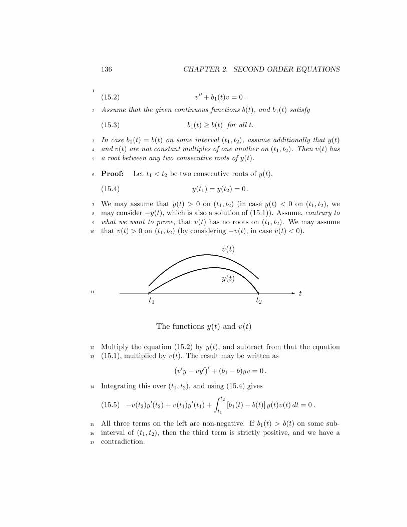
136 CHAPTER 2. SECOND ORDER EQUATIONS
1
v′′ + b1(t)v = 0 .(15.2)
Assume that the given continuous functions b(t), and b1(t) satisfy2
b1(t) ≥ b(t) for all t.(15.3)
In case b1(t) = b(t) on some interval (t1, t2), assume additionally that y(t)3
and v(t) are not constant multiples of one another on (t1, t2). Then v(t) has4
a root between any two consecutive roots of y(t).5
Proof: Let t1 < t2 be two consecutive roots of y(t),6
y(t1) = y(t2) = 0 .(15.4)
We may assume that y(t) > 0 on (t1, t2) (in case y(t) < 0 on (t1, t2), we7
may consider −y(t), which is also a solution of (15.1)). Assume, contrary to8
what we want to prove, that v(t) has no roots on (t1, t2). We may assume9
that v(t) > 0 on (t1, t2) (by considering −v(t), in case v(t) < 0).10
-
y(t)
v(t)
t1t
t2
The functions y(t) and v(t)
11
Multiply the equation (15.2) by y(t), and subtract from that the equation12
(15.1), multiplied by v(t). The result may be written as13
(
v′y − vy′)′
+ (b1 − b)yv = 0 .
Integrating this over (t1, t2), and using (15.4) gives14
−v(t2)y′(t2) + v(t1)y′(t1) +
∫ t2
t1
[b1(t) − b(t)]y(t)v(t) dt = 0 .(15.5)
All three terms on the left are non-negative. If b1(t) > b(t) on some sub-15
interval of (t1, t2), then the third term is strictly positive, and we have a16
contradiction.17

2.15. OSCILLATION AND COMPARISON THEOREMS 137
Now consider the remaining case when b1(t) = b(t) for all t ∈ (t1, t2),1
so that the equations (15.1) and (15.2) coincide on (t1, t2), and v(t) is a2
solution of (15.1). We claim that v(t) cannot vanish at t1 and at t2, so3
that v(t1) > 0, and v(t2) > 0. Indeed, in case v(t1) = 0, we consider4
the function z(t) =y′(t1)v′(t1)
v(t). This function is a solution of (15.1), and5
z(t1) = y(t1) = 0, z′(t1) = y′(t1), so that by the uniqueness of solutions6
for initial value problems, z(t) = y(t) for all t ∈ (t1, t2), and then y(t) and7
v(t) are constant multiples of one another on (t1, t2), which is not allowed.8
It follows that v(t1) > 0, and similarly we prove that v(t2) > 0. Clearly,9
y′(t1) ≥ 0 and y′(t2) ≤ 0. The uniqueness Theorem 2.4.1 for initial value10
problems implies that y′(t1) > 0, and y′(t2) < 0 (otherwise, if say y′(t1) = 0,11
then y(t) = 0 for all t, by Theorem 2.4.1). Then the first two terms in (15.5)12
are strictly positive, and we have a contradiction in (15.5). ♦13
In case y(t) and v(t) are two solutions of the same equation (15.1),14
which are not constant multiples of one another, the theorem implies that15
their roots interlace, which means that between any two roots of one of the16
solutions there is a root of the other one.17
By a similar argument, one proves the following version of the Sturm18
comparison theorem, involving a differential inequality.19
Lemma 2.15.1 Assume that the functions u(t) and v(t) are twice contin-20
uously differentiable, and they satisfy21
v′′ + q(t)v = 0, v(a) = 0 ,22
u′′ + q(t)u ≥ 0, u(a) = 0, u′(a) > 0 ,(15.6)
on some interval (a, b) (with a given continuous function q(t)). Then v(t)23
oscillates faster than u(t), provided that both functions are positive. Namely,24
(i) if v(t) > 0 on (a, b), then u(t) > 0 on (a, b).25
(ii) If, on the other hand, u(t) > 0 on (a, b) and u(b) = 0, then v(t) must26
vanish on (a, b].27
Proof: As in Theorem 2.15.1, obtain28
(
v′u− vu′)′ ≤ 0, for x ∈ (a, b) .(15.7)
Let us prove (i). Assume that v(t) > 0 on (a, b), and contrary to what we29
want to prove, u(ξ) = 0 at some ξ ∈ (a, b).30

138 CHAPTER 2. SECOND ORDER EQUATIONS
Case 1. The inequality in (15.6) is strict on some sub-interval of (a, ξ). The1
the same is then true for the inequality (15.7). Integrating (15.7) over (a, ξ),2
obtain3
−v(ξ)u′(ξ) < 0 ,
which is a contradiction (because v(ξ) > 0, u′(ξ) ≤ 0).4
Case 2. Assume that u′′ + q(t)u = 0 on (a, ξ). Then u(t) and v(t) are5
solutions of the same equation on (a, ξ), and u(a) = v(a) = 0. It follows6
that u(t) and v(t) are constant multiples of one another, but u(ξ) = 0, while7
v(ξ) > 0, a contradiction, proving the first part of the lemma.8
The second statement of the lemma is proved similarly. ♦9
We shall need the following formula from calculus, discovered by an10
Italian mathematician Mauro Picone in 1909.11
Lemma 2.15.2 (Picone’s Identity) Assume that the functions a(t) and a1(t)12
are differentiable, the functions u(t) and v(t) are twice differentiable, and13
v(t) > 0 for all t. Then14
[
u
v
(
vau′ − ua1v′)]′
= u(au′)′ − u2
v(a1v
′)′ + (a− a1)u′2 + a1
(
u′ − u
vv′)2
.
Proof: The derivative on the left is equal to15
u′v − uv′
v2
(
vau′ − ua1v′)+
u
v
(
v(au′)′ − u(a1v′)′)
+(a−a1)u
vu′v′ ≡ A+B+C .
The middle term B is equal to the first two terms on the right in Picone’s16
identity. It remains to prove that A+C is equal to the sum of the last two17
terms on the right in Picone’s identity. We expand A and C, and after a18
cancellation, obtain19
A+C = (a−a1)u′2+a1
[
u′2 − 2u
vu′v′ + v′2
(
u
v
)2]
= (a−a1)u′2+a1
(
u′ − u
vv′)2
,
completing the proof. ♦20
We now turn to the general second order equations21
p(t)u′′ + q(t)u′ + r(t)u = 0 .(15.8)
2.15. OSCILLATION AND COMPARISON THEOREMS 139
Assume that the functions p(t), q(t) and r(t) are differentiable, with p(t) > 01
for all t. We divide this equation by p(t)2
u′′ +q(t)
p(t)u′ +
r(t)
p(t)u = 0 ,
and then multiply by the integrating factor a(t) = e∫
q(t)p(t)
dt. Denoting b(t) =3
a(t)r(t)
p(t), we arrive at4
(
a(t)u′)′
+ b(t)u = 0 ,(15.9)
which is known as the self-adjoint form of (15.8).5
With the help of his clever identity, M. Picone was able to give the6
following generalization of the Sturm comparison theorem.7
Theorem 2.15.2 Let u(t) and v(t) be respectively solutions of (15.9), and8
(
a1(t)v′)′ + b1(t)v = 0 .
Assume that the differentiable functions a(t), a1(t), and the continuous func-9
tions b(t), b1(t) satisfy10
b1(t) ≥ b(t), and 0 < a1(t) ≤ a(t) for all t.
In case a1(t) = a(t) and b1(t) = b(t) on some interval (t1, t2), assume11
additionally that u(t) and v(t) are not constant multiples of one another on12
(t1, t2). Then v(t) has a root between any two consecutive roots of u(t).13
Proof: The proof is similar to that of the Sturm comparison theorem.14
Let t1 < t2 be two consecutive roots of u(t),15
u(t1) = u(t2) = 0 .(15.10)
Again, we may assume that u(t) > 0 on (t1, t2). Assume, contrary to what we16
want to prove, that v(t) has no roots on (t1, t2). We may assume that v(t) >17
0 on (t1, t2). Apply Picone’s identity to u(t) and v(t). Expressing from the18
corresponding equations, (a(t)u′)′ = −b(t)u and (a1(t)v′)′ = −b1(t)v, we19
rewrite Picone’s identity as20
[
u
v
(
vau′ − ua1v′)]′
= (b1 − b)u2 + (a− a1)u′2 + a1
(
u′ − u
vv′)2
.

140 CHAPTER 2. SECOND ORDER EQUATIONS
Integrating this over (t1, t2), and using (15.10), gives1
0 =
∫ t2
t1
(b1 − b)u2 dt+
∫ t2
t1
(a− a1)u′2 dt+
∫ t2
t1
a1
(
u′ − u
vv′)2
dt .
(In case v(t1) = 0, we have v′(t1) > 0, by the uniqueness of solutions for2
initial value problems. Then limt→t1
u2
v= lim
t→t1
2uu′
v′= 0. Similarly, in case3
v(t2) = 0, the upper limit vanishes for the integral on the left.) The integrals4
on the right are non-negative. We obtain an immediate contradiction, unless5
a1(t) = a(t) and b1(t) = b(t) for all t ∈ (t1, t2). In such a case, we must also6
have u′ − u
vv′ = 0 on (t1, t2) (so that all three integrals vanish). But then7
u′
u=v′
v, and integrating we see that u(t) and v(t) are constant multiples of8
one another, contradicting our assumption. ♦9
Our next goal is the famous Lyapunov inequality. It will follow from the10
next lemma. Define q+(t) = max(q(t), 0), the positive part of the function11
q(t). Similarly, one defines q−(t) = min(q(t), 0), the negative part of the12
function q(t). Clearly, q(t) = q+(t) + q−(t).13
Lemma 2.15.3 Assume that u(t) is twice continuously differentiable, and14
it satisfies the following conditions on some interval (0, b) (here q(t) is a15
given continuous function)16
u′′ + q(t)u = 0, u(0) = u(b) = 0, u(t) > 0 on (0, b) .(15.11)
Then17∫ b
0q+(t) dt >
4
b.
Proof: From (15.11) it follows that18
u′′ + q+(t)u = −q−(t)u ≥ 0 .
Let v(t) be the solution of (c is any positive number)19
v′′ + q+(t)v = 0, v(0) = 0, v′(0) = c > 0 .(15.12)
By Lemma 2.15.1, v(t) must vanish on (0, b]. Let t2 ∈ (0, b] be the first root20
of v(t), so that v(t) > 0 on (0, t2). (In case q−(t) ≡ 0, we have t2 = b,21
because v(t) is a constant multiple of u(t).) Integrating (15.12) (treating22
q+(t)v as a known quantity),23
v(t) = ct−∫ t
0(t− s)q+(s)v(s) ds, for t ∈ [0, t2] .(15.13)

2.15. OSCILLATION AND COMPARISON THEOREMS 141
From v(t2) = 0, it follows that c =1
t2
∫ t2
0(t2 − s)q+(s)v(s) ds. Substituting1
this back into (15.13), we express2
v(t) =t
t2
∫ t2
0(t2 − s)q+(s)v(s) ds−
∫ t
0(t− s)q+(s)v(s) ds , for t ∈ [0, t2] .
Breaking the first integral,∫ t20 =
∫ t0 +
∫ t2t , we continue:3
t2v(t) =
∫ t
0[t(t2 − s) − t2(t− s)] q+(s)v(s) ds+ t
∫ t2
t(t2 − s)q+(s)v(s) ds
4
= (t2 − t)
∫ t
0sq+(s)v(s) ds+ t
∫ t2
t(t2 − s)q+(s)v(s) ds .
Let t0 be the point of maximum of v(t) on (0, t2), v(t0) > 0. Estimate5
v(s) < v(t0) in both integrals on the right, then evaluate the last formula at6
t0, and cancel v(t0). Obtain:7
t2 < (t2 − t0)
∫ t0
0sq+(s) ds+ t0
∫ t2
t0
(t2 − s)q+(s) ds
8
<
∫ t0
0(t2 − s)sq+(s) ds+
∫ t2
t0
s(t2 − s)q+(s) ds =
∫ t2
0(t2 − s)sq+(s) ds .
Dividing by t2, gives9
1 <
∫ t2
0(1− s
t2)sq+(s) ds ≤
∫ b
0(1− s
b)sq+(s) ds <
∫ b
0
b
4q+(s) ds ,
which implies our inequality. (On the last step we estimated the function10
(1 − s
b)s by its maximum value of
b
4.) ♦11
Theorem 2.15.3 (Lyapunov’s inequality) If a non-trivial solution of the12
equation13
u′′ + q(t)u = 0
has two roots on an interval [a, b], then14
∫ b
aq+(t) dt >
4
b− a.

142 CHAPTER 2. SECOND ORDER EQUATIONS
Proof: Let t1 and t2 be two consecutive roots of u(t), a ≤ t1 < t2 ≤ b.1
We may assume that u(t) > 0 on (t1, t2), and use the above lemma2
∫ b
aq+(t) dt ≥
∫ t2
t1q+(t) dt >
4
t2 − t1≥ 4
b− a.
(We may declare the point t1 to be the origin, to use the above lemma.) ♦3
4
Remarkably, the constant 4 appears in another well-known and useful5
inequality.6
Theorem 2.15.4 (Hardy’s inequality) Assume that f(x) is a continuously7
differentiable function on [0, b], where b > 0 is arbitrary, and f(0) = 0.8
Then9∫ b
0
f2(x)
x2dx ≤ 4
∫ b
0f ′2(x) dx .
Proof: Write10
f ′2 =
[
12x
−1f + x1/2(
x−1/2f)′]2
= 14x
−2f2 +(
x−1/2f)(
x−1/2f)′
+
(
x1/2(
x−1/2f)′)2
.
Integrating both sides, and dropping a non-negative term on the right11
∫ b
0f ′2(x) dx ≥
∫ b
0
1
4x−2f2 dx+
∫ b
0
(
x−1/2f) (
x−1/2f)′dx ≥ 1
4
∫ b
0x−2f2 dx ,
because∫ b0
(
x−1/2f) (
x−1/2f)′dx = 1
2x−1f2(x) |b
0= 1
2b−1f2(b) ≥ 0. (Ob-12
serve that limx→0 x−1f2(x) = limx→0
f(x)x · limx→0 f(x) = f ′(0) · 0 = 0.) ♦13
14

Chapter 31
Using Infinite Series to Solve2
Differential Equations3
“Most” differential equations cannot be solved by a formula. One traditional4
approach involves using infinite series to approximate solutions near some5
point a. (Another possibility is to use numerical methods, which is discussed6
in Chapters 1 and 9.) We begin with the case when the point a is regular,7
and it is possible to compute all derivatives of solutions at x = a, and then8
write down the corresponding Taylor’s series. Turning to singular a, we9
distinguish the easier case when a is a simple root of the leading coefficient10
(we call such equations mildly singular). Then we show that the case when11
a is a double root of the leading coefficient can often be reduced to a mildly12
singular case, by a change of variables.13
3.1 Series Solution Near a Regular Point14
3.1.1 Maclauren and Taylor Series15
Infinitely differentiable functions can often be represented by a series16
f(x) = a0 + a1x+ a2x2 + · · ·+ anx
n + · · · .(1.1)
Letting x = 0, we see that a0 = f(0). Differentiating (1.1), and then letting17
x = 0, shows that a1 = f ′(0). Differentiating (1.1) twice, and then letting18
x = 0, gives a2 =f ′′(0)
2. Continuing this way, we see that an =
f (n)(0)
n!,19
143

144CHAPTER 3. USING INFINITE SERIES TO SOLVE DIFFERENTIAL EQUATIONS
giving us the Maclauren series1
f(x) = f(0) + f ′(0)x+f ′′(0)
2!x2 + · · ·+ f (n)(0)
n!xn + · · · =
∞∑
n=0
f (n)(0)
n!xn .
It is known that for each f(x) there is a number R, so that the Maclauren2
series converges for x inside the interval (−R,R), and diverges outside of3
this interval, when |x| > R. We call R the radius of convergence. For some4
f(x), we have R = ∞ (for example, for sinx, cosx, ex), while for some series5
R = 0, and in general 0 ≤ R ≤ ∞.6
Computing the Maclauren series for some specific functions, gives:7
sinx = x− x3
3!+x5
5!− x7
7!+ · · · =
∞∑
n=0
(−1)n x2n+1
(2n+ 1)!,
8
cos x = 1 − x2
2!+x4
4!− x6
6!+ · · · =
∞∑
n=0
(−1)n x2n
(2n)!,
9
ex = 1 + x+x2
2!+x3
3!+x4
4!+ · · · =
∞∑
n=0
xn
n!,
10
1
1 − x= 1 + x+ x2 + · · ·+ xn + · · · =
∞∑
n=0
xn .
The last series, called the geometric series, converges on the interval (−1, 1),11
so that R = 1.12
Maclauren’s series gives an approximation of f(x), for x close to zero.13
For example, sinx ≈ x gives a reasonably good approximation for |x| small.14
If we add one more term of the Maclauren series: sinx ≈ x− x3
6, then, say15
on the interval (−1, 1), we get an excellent approximation, see Figure 3.1.16
If one needs the Maclauren series for sinx2, one begins with a series for17
sinx, and then replaces each x by x2, obtaining18
sinx2 = x2 − x6
3!+x10
5!+ · · · =
∞∑
n=0
(−1)n x4n+2
(2n+ 1)!.
One can split Maclauren’s series into a sum of series with either even or19
odd powers:20
∞∑
n=0
f (n)(0)
n!xn =
∞∑
n=0
f (2n)(0)
(2n)!x2n +
∞∑
n=0
f (2n+1)(0)
(2n+ 1)!x2n+1 .
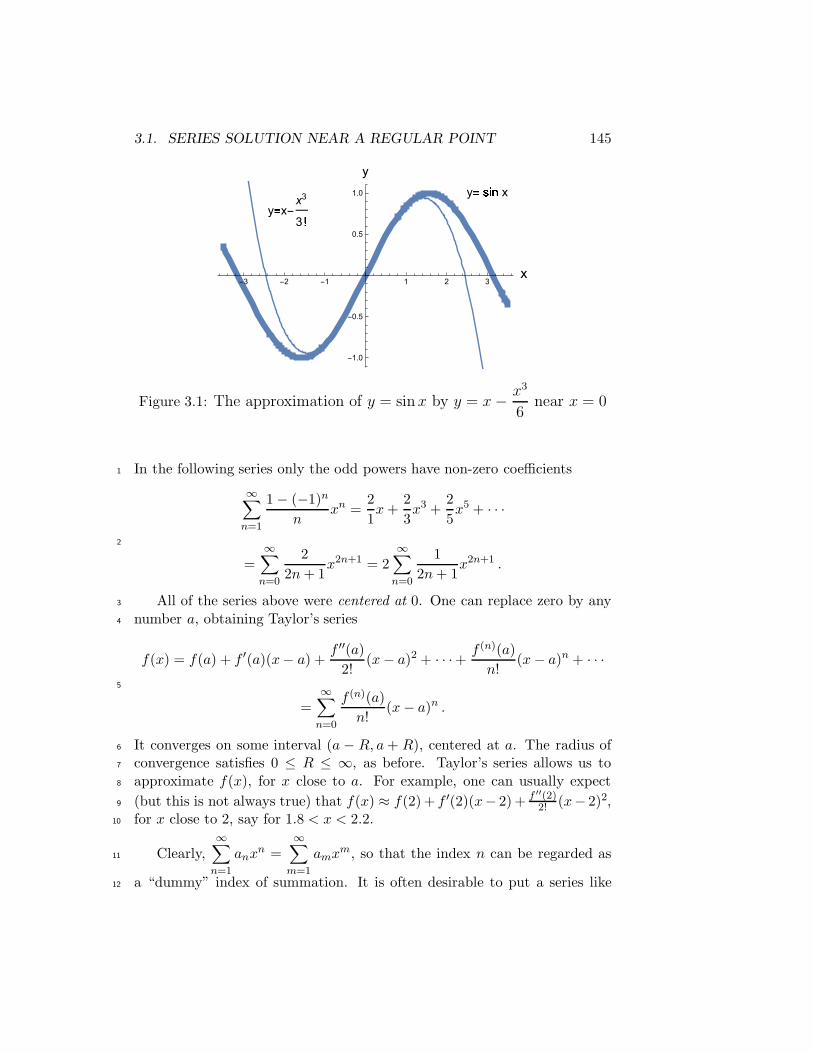
3.1. SERIES SOLUTION NEAR A REGULAR POINT 145
-3 -2 -1 1 2 3x
-1.0
-0.5
0.5
1.0
y
y� � � xy� x-x
3
3 �
Figure 3.1: The approximation of y = sinx by y = x− x3
6near x = 0
In the following series only the odd powers have non-zero coefficients1
∞∑
n=1
1 − (−1)n
nxn =
2
1x+
2
3x3 +
2
5x5 + · · ·
2
=∞∑
n=0
2
2n+ 1x2n+1 = 2
∞∑
n=0
1
2n+ 1x2n+1 .
All of the series above were centered at 0. One can replace zero by any3
number a, obtaining Taylor’s series4
f(x) = f(a) + f ′(a)(x− a) +f ′′(a)
2!(x− a)2 + · · ·+ f (n)(a)
n!(x− a)n + · · ·
5
=∞∑
n=0
f (n)(a)
n!(x− a)n .
It converges on some interval (a − R, a+ R), centered at a. The radius of6
convergence satisfies 0 ≤ R ≤ ∞, as before. Taylor’s series allows us to7
approximate f(x), for x close to a. For example, one can usually expect8
(but this is not always true) that f(x) ≈ f(2) + f ′(2)(x− 2) + f ′′(2)2! (x− 2)2,9
for x close to 2, say for 1.8 < x < 2.2.10
Clearly,∞∑
n=1
anxn =
∞∑
m=1
amxm, so that the index n can be regarded as11
a “dummy” index of summation. It is often desirable to put a series like12

146CHAPTER 3. USING INFINITE SERIES TO SOLVE DIFFERENTIAL EQUATIONS
∞∑
n=1
n
n + 4xn+1 into the form
∑
anxn. We set n + 1 = m, or n = m − 1,1
and get2
∞∑
n=1
n
n+ 4xn+1 =
∞∑
m=2
m− 1
m+ 3xm =
∞∑
n=2
n− 1
n+ 3xn .
The same result can be accomplished in one step, by the shift of the index3
of summation: n → n − 1, or replacing each occurrence of n by n − 1, and4
incrementing by 1 the limit(s) of summation.5
3.1.2 A Toy Problem6
Let us begin with the equation (here y = y(x))7
y′′ + y = 0 ,
for which we already know the general solution. Let us denote by y1(x) the8
solution of the initial value problem9
y′′ + y = 0, y(0) = 1, y′(0) = 0 .(1.2)
By y2(x) we denote the solution of the same equation, together with the10
initial conditions y(0) = 0, y′(0) = 1. Clearly, y1(x) and y2(x) are not11
constant multiples of each other. Therefore, they form a fundamental set,12
giving us the general solution y(x) = c1y1(x) + c2y2(x).13
Let us now compute y1(x), the solution of (1.2). From the initial condi-14
tions, we already know the first two terms of its Maclauren series15
y(x) = y(0) + y′(0)x+y′′(0)
2x2 + · · ·+ y(n)(0)
n!xn + · · · .
To get more terms, we need to compute the derivatives of y(x) at zero. From16
the equation (1.2), y′′(0) = −y(0) = −1. We now differentiate the equation17
(1.2), getting y′′′ + y′ = 0, and then set x = 0 to obtain18
y′′′(0) = −y′(0) = 0 .
Differentiating again, gives y′′′′ + y′′ = 0, and setting x = 0,19
y′′′′(0) = −y′′(0) = 1 .
On the next step:20
y(5)(0) = −y′′′(0) = 0 .

3.1. SERIES SOLUTION NEAR A REGULAR POINT 147
We see that all derivatives of odd order vanish at x = 0, while the derivatives1
of even order alternate between 1 and −1. The Maclauren series is then2
y1(x) = 1 − x2
2!+x4
4!− · · · = cos x .
Similarly, we compute the series representation for y2(x):3
y2(x) = x− x3
3!+x5
5!− · · · = sinx .
We shall solve the equations with variable coefficients4
P (x)y′′ +Q(x)y′ + R(x)y = 0 ,(1.3)
where continuous functions P (x), Q(x) and R(x) are given. We shall always5
denote by y1(x) the solution of (1.3) satisfying the initial conditions y(0) = 1,6
y′(0) = 0, and by y2(x) the solution of (1.3) satisfying the initial conditions7
y(0) = 0, y′(0) = 1. If one needs to solve (1.3), together with the given8
initial conditions9
y(0) = α, y′(0) = β ,
then the solution is10
y(x) = αy1(x) + βy2(x) .
Indeed, y(0) = αy1(0) + βy2(0) = α, and y′(0) = αy′1(0) + βy′2(0) = β.11
3.1.3 Using Series When Other Methods Fail12
Let us try to find the general solution of the equation13
y′′ + xy′ + 2y = 0 .
This equation has variable coefficients, and none of the previously consid-14
ered methods will apply here. Our goal is to use the Maclauren series15
∑∞n=0
y(n)(0)n! xn to approximate solutions near x = 0.16
We shall derive a formula for y(n)(0), and use it to calculate the solutions17
y1(x) and y2(x), defined in the preceding subsection. From the equation we18
express y′′(0) = −2y(0). Differentiate the equation19
y′′′ + xy′′ + 3y′ = 0 ,
which gives y′′′(0) = −3y′(0). Differentiate the last equation again20
y′′′′ + xy′′′ + 4y′′ = 0 ,

148CHAPTER 3. USING INFINITE SERIES TO SOLVE DIFFERENTIAL EQUATIONS
and get: y′′′′(0) = −4y′′(0). In general, we get a recurrence relation1
y(n)(0) = −ny(n−2)(0), n = 2, 3, . . . .(1.4)
By a convention, y(0)(x) = y(x), so that y(0)(0) = y(0).2
Let us begin with the computation of y2(x), for which we use the initial3
conditions y(0) = 0, y′(0) = 1. Then, using the recurrence relation (1.4),4
obtain5
y′′(0) = −2y(0) = 0 ,6
y′′′(0) = −3y′(0) = −3 · 1 ,7
y′′′′(0) = −4y′′(0) = 0 .
It is clear that all derivatives of even order are zero at x = 0. Let us continue8
with the derivatives of odd order:9
y(5)(0) = −5y′′′(0) = (−1)2 5 · 3 · 1 ,10
y(7)(0) = −7y′′′(0) = (−1)3 7 · 5 · 3 · 1 .And in general,11
y(2n+1)(0) = (−1)n (2n+ 1) · (2n− 1) · · · 3 · 1 .
Then the Maclauren series for y2(x) is12
y2(x) =∞∑
n=0
y(n)(0)
n!xn = x+
∞∑
n=1
y(2n+1)(0)
(2n+ 1)!x2n+1
13
= x+∞∑
n=1
(−1)n (2n+ 1) · (2n− 1) · · · 3 · 1(2n+ 1)!
x2n+1
14
= x+∞∑
n=1
(−1)n 1
2n · (2n− 2) · · · 4 · 2 x2n+1 .
One can also write this solution as y2(x) =∞∑
n=0
(−1)n 1
2nn!x2n+1.15
To compute y1(x), we use the initial conditions y(0) = 1, y′(0) = 0. Sim-16
ilarly to the above, we see from the recurrence relation that all derivatives17
of odd order vanish at x = 0, while the even ones satisfy18
y(2n)(0) = (−1)n 2n · (2n− 2) · · · 4 · 2 , for n = 1, 2, 3, . . . .
3.1. SERIES SOLUTION NEAR A REGULAR POINT 149
This leads to1
y1(x) = 1+∞∑
n=1
(−1)n y(2n)(0)
(2n)!x2n = 1+
∞∑
n=1
(−1)n 1
(2n− 1) · (2n− 3) · · ·3 · 1 x2n .
The general solution:2
y(x) = c1
(
1 +∞∑
n=1
(−1)n
(2n− 1)(2n− 3) · · ·3 · 1x2n
)
+ c2
∞∑
n=0
(−1)n 1
2nn!x2n+1 .
We shall need a formula for repeated differentiation of a product of two3
functions. Starting with the product rule (fg)′ = f ′g + fg′, express4
(fg)′′ = f ′′g + 2f ′g′ + fg′′ ,5
(fg)′′′ = f ′′′g + 3f ′′g′ + 3f ′g′′ + fg′′′ ,
and in general, for the n-th derivative:6
(fg)(n) = f (n)g + nf (n−1)g′ +n(n− 1)
2f (n−2)g′′ + · · ·(1.5)
7
+n(n − 1)
2f ′′g(n−2) + nf ′g(n−1) + fg(n) .
(Convention: f (0) = f .) This formula is similar to the binomial formula for8
the expansion of (x + y)n. Using the summation notation, we can write it9
as10
(fg)(n) =n∑
k=0
(
n
k
)
f (n−k) g(k) ,
where
(
n
k
)
=n!
k!(n− k)!are the binomial coefficients.11
The formula (1.5) simplifies considerably in case f(x) = x, or if f(x) = x2:12
(xg)(n) = ng(n−1) + xg(n) ,13
(x2g)(n) = n(n − 1)g(n−2) + 2nxg(n−1) + x2g(n) .
We shall use Taylor’s series centered at x = a, y(x) =∞∑
n=0
y(n)(a)
n!(x−a)n,14
to solve linear second order equations with variable coefficients15
P (x)y′′ +Q(x)y′ + R(x)y = 0 ,

150CHAPTER 3. USING INFINITE SERIES TO SOLVE DIFFERENTIAL EQUATIONS
where the functions P (x), Q(x) and R(x) are given. A number a is called a1
regular point if P (a) 6= 0. If P (a) = 0, then x = a is called a singular point.2
If a is a regular point, we can compute y(n)(a) from the equation, as in the3
examples above. If the point a is singular, it is not even possible to compute4
y′′(a) from the equation.5
Example 1 (2 + x2)y′′ − xy′ + 4y = 0.6
For this equation, any a is a regular point. Let us find the general solution7
as an infinite series, centered at a = 0, the Maclauren series for y(x). We8
differentiate both sides of this equation n times. When we use the formula9
(1.5) to differentiate the first term, only the last three terms are non-zero,10
because the derivatives of 2+x2, of order three and higher, are zero. Obtain11
[
(2 + x2)y′′](n)
=n(n− 1)
22y(n) + n(2x)y(n+1) + (2 + x2)y(n+2) .
When we differentiate n times xy′, only the last two terms survive, giving12
[
xy′](n)
= ny(n) + xy(n+1) .
It follows that n differentiations of our equation produce13
n(n− 1)
22y(n) + n(2x)y(n+1) + (2 + x2)y(n+2) −ny(n) − xy(n+1) + 4y(n) = 0 .
Set here x = 0. Several terms vanish. Combining the like terms, we get14
2y(n+2)(0) +(
n2 − 2n+ 4)
y(n)(0) = 0 ,
which gives us the recurrence relation15
y(n+2)(0) = −(
n2 − 2n+ 4)
2y(n)(0) .
This relation is too involved to get a general formula for y(n)(0) as a function16
of n. However, it can be used to crank out the derivatives at zero, as many17
as you wish.18
To compute y1(x), we use the initial conditions y(0) = 1 and y′(0) = 0.19
It follows from the recurrence relation that all of the derivatives of odd order20
are zero at x = 0. Setting n = 0 in the recurrence relation, obtain21
y′′(0) = −2y(0) = −2 .

3.1. SERIES SOLUTION NEAR A REGULAR POINT 151
When n = 2,1
y′′′′(0) = −2y′′(0) = 4 .
Using these derivatives in the Maclauren series, gives2
y1(x) = 1 − x2 +1
6x4 + · · · .
To compute y2(x), we use the initial conditions y(0) = 0 and y′(0) = 1.3
It follows from the recurrence relation that all of the derivatives of even4
order are zero. When n = 1, we get5
y′′′(0) = −3
2y′(0) = −3
2.
Setting n = 3, obtain6
y(5)(0) = −7
2y′′′(0) =
21
4.
Using these derivatives in the Maclauren series, we conclude7
y2(x) = x− 1
4x3 +
7
160x5 + · · · .
The general solution:8
y(x) = c1y1(x) + c2y2(x) = c1
(
1− x2 +1
6x4 + · · ·
)
9
+c2
(
x− 1
4x3 +
7
160x5 + · · ·
)
.
Suppose that we wish to solve the above equation, together with the10
initial conditions: y(0) = −2, y′(0) = 3. Then y(0) = c1y1(0) + c2y2(0) =11
c1 = −2, and y′(0) = c1y′1(0) + c2y
′2(0) = c2 = 3. It follows that y(x) =12
−2y1(x) + 3y2(x). If one needs to approximate y(x) near x = 0, say on the13
interval (−0.3, 0.3), then14
y(x) ≈ −2
(
1 − x2 +1
6x4)
+ 3
(
x− 1
4x3 +
7
160x5)
will provide an excellent approximation.15
Example 2 y′′ − xy′ + y = 0, a = 0.16
Differentiating this equation n times gives17
y(n+2)(x) − ny(n)(x) − xy(n+1)(x) + y(n)(x) = 0 .

152CHAPTER 3. USING INFINITE SERIES TO SOLVE DIFFERENTIAL EQUATIONS
Setting here x = 0, we obtain the recurrence relation1
y(n+2)(0) = (n− 1)y(n)(0) .
To compute y1(x), we use the initial conditions y(0) = 1, y′(0) = 0. Then2
all derivatives of odd order vanish, y(2n+1)(0) = 0, as follows by repeated3
application of the recurrence relation. We now compute the derivatives of4
even order. Setting n = 0 in the recurrence relation gives: y′′(0) = −y(0) =5
−1. When n = 2, we get y′′′′(0) = y′′(0) = −1, and then y(6)(0) = 3y′′′′(0) =6
−1 · 3, at n = 4. We continue, y(8)(0) = 5y(6)(0) = −1 · 3 · 5, and in general7
y(2n)(0) = −1 · 3 · 5 · · · (2n− 3) .
Then8
y1(x) = 1 +∞∑
n=1
y(2n)(0)
(2n)!x2n +
∞∑
n=0
y(2n+1)(0)
(2n+ 1)!x2n+1
9
= 1−∞∑
n=1
1 · 3 · 5 · · · (2n− 3)
(2n)!x2n = 1 −
∞∑
n=1
1
2 · 4 · · ·2n(2n− 1)x2n
10
= 1 −∞∑
n=1
1
2n n!(2n− 1)x2n = −
∞∑
n=0
1
2n n!(2n− 1)x2n .
To compute y2(x), we use the initial conditions y(0) = 0, y′(0) = 1. Then11
all derivatives of even order vanish, y(2n)(0) = 0, as follows by repeated12
application of the recurrence relation. Setting n = 1 in the recurrence13
relation gives: y′′′(0) = 0, and so all derivatives of odd order vanish as well.14
We conclude that y2(x) = x. The general solution is15
y(x) = c1
∞∑
n=0
1
2n n!(2n− 1)x2n + c2x .
Example 3 Approximate the general solution of Airy’s equation16
y′′ − xy = 0 ,
near x = 1. This equation was encountered in 1838 by G.B. Airy, in his17
study of optics.18
We need to compute Taylor’s series about the regular point a = 1, which is19
y(x) =∞∑
n=0
y(n)(1)
n!(x− 1)n. From the equation,20
y′′(1) = y(1) .

3.2. SOLUTION NEAR A MILDLY SINGULAR POINT 153
To get higher derivatives, we differentiate our equation n times, and then1
set x = 1, to get the recurrence relation2
y(n+2)(x) − ny(n−1)(x) − xy(n)(x) = 0 ,3
y(n+2)(1) = ny(n−1)(1) + y(n)(1), n = 1, 2, . . . .(1.6)
To compute y1(x), we use the initial conditions y(1) = 1, y′(1) = 0.4
Then5
y′′(1) = y(1) = 1 .
Setting n = 1 in the recurrence relation (1.6), gives6
y(3)(1) = y(1) + y′(1) = 1 .
When n = 2,7
y(4)(1) = 2y′(1) + y′′(1) = 1 .
Then, for n = 3,8
y(5)(1) = 3y′′(1) + y′′′(1) = 4 .
Obtain9
y1(x) = 1 +(x− 1)2
2+
(x− 1)3
6+
(x− 1)4
24+
(x− 1)5
30+ · · · .
Again, it does not seem possible to get a general formula for the coefficients.10
To compute y2(x), we use the initial conditions y(1) = 0, y′(1) = 1.11
Then y′′(1) = y(1) = 0. Setting n = 1 in the recurrence relation (1.6), gives12
y(3)(1) = y(1)+ y′(1) = 1. When n = 2, y(4)(1) = 2y′(1)+ y′′(1) = 2. Then,13
for n = 3, y(5)(1) = 3y′′(1) + y′′′(1) = 1. Obtain14
y2(x) = x− 1 +(x− 1)3
6+
(x− 1)4
12+
(x− 1)5
120+ · · · .
The general solution is, of course, y(x) = c1y1(x) + c2y2(x).15
3.2 Solution Near a Mildly Singular Point16
We consider again the equation17
P (x)y′′ +Q(x)y′ + R(x)y = 0 ,
with given functions P (x), Q(x) and R(x) that are continuous near a point a,18
at which we wish to compute solution as a series y(x) =∞∑
n=0
y(n)(a)
n!(x−a)n.19

154CHAPTER 3. USING INFINITE SERIES TO SOLVE DIFFERENTIAL EQUATIONS
If P (a) = 0, we have a problem: one cannot compute y′′(a) from the equation1
(and the same problem occurs for higher derivatives). However, if a is a2
simple root of P (x), it turns out that one can still use series to produce a3
solution. Namely, we assume that P (x) = (x − a)P1(x), with P1(a) 6= 0.4
We call x = a a mildly singular point. Dividing the equation by P1(x), and5
calling q(x) = Q(x)P1(x) , r(x) = R(x)
P1(x) , we put it into the form6
(x− a)y′′ + q(x)y′ + r(x)y = 0 .
The functions q(x) and r(x) are continuous near a. In case a = 0, the7
equation becomes8
xy′′ + q(x)y′ + r(x)y = 0 .(2.1)
For this equation we cannot expect to obtain two linearly independent so-9
lutions, by prescribing y1(0) = 1, y′1(0) = 0, and y2(0) = 0, y′2(0) = 1, the10
way we did before. This equation is singular at x = 0 (the functions q(x)x11
andr(x)x are discontinuous at x = 0, and so the existence and uniqueness12
Theorem 2.4.1 from Chapter 2 does not apply).13
Example 1 Let us try to solve:14
xy′′ − y′ = 0, y(0) = 0, y′(0) = 1 .
Multiplying through by x, we obtain Euler’s equation with the general so-15
lution y(x) = c1x2 + c2. Then y′(x) = 2c1x, and y′(0) = 0 6= 1. This initial16
value problem has no solution. However, if we change the initial conditions,17
and consider the problem18
xy′′ − y′ = 0, y(0) = 1, y′(0) = 0 ,
then there are infinitely many solutions y = 1 + c1x2.19
We therefore lower our expectations, and we shall be satisfied to compute20
just one series solution of (2.1). It turns out that in most cases it is possible21
to calculate a series solution of the form y(x) =∑∞
n=0 anxn, starting with22
a0 = 1, which corresponds to y(0) = 1. (If a0 6= 1, then 1a0y(x) is another23
solution of (2.1), which begins with 1. So that we shall always assume that24
a0 = 1. The possibility of a0 = 0 is considered later.)25
Example 2 Find a series solution, centered at a = 0, of26
xy′′ + 3y′ − 2y = 0 .

3.2. SOLUTION NEAR A MILDLY SINGULAR POINT 155
It is convenient to multiply this equation by x:1
x2y′′ + 3xy′ − 2xy = 0 .(2.2)
Look for a solution in the form2
y =∞∑
n=0
anxn = a0 + a1x+ a2x
2 + a3x3 + · · · ,
with a0 = 1. Calculate3
y′ =∞∑
n=1
annxn−1 = a1 + 2a2x+ 3a3x
2 + · · · ,
4
y′′ =∞∑
n=2
ann(n− 1)xn−2 = 2a2 + 6a3x+ · · · .
Observe that each differentiation “kills” a term. Substituting y =∑∞
n=0 anxn
5
into the equation (2.2), gives6
∞∑
n=2
ann(n − 1)xn +∞∑
n=1
3annxn −
∞∑
n=0
2anxn+1 = 0 .(2.3)
The third series is not “lined up” with the other two. We therefore shift the7
index of summation, replacing n by n − 1 in that series, obtaining8
∞∑
n=0
2anxn+1 =
∞∑
n=1
2an−1xn .
Then (2.3) becomes9
∞∑
n=2
ann(n − 1)xn +∞∑
n=1
3annxn −
∞∑
n=1
2an−1xn = 0 .(2.4)
We shall use the following fact: if∑∞
n=1 bnxn = 0 for all x, then bn = 0 for10
all n = 1, 2, . . .. Our goal is to combine the three series in (2.4) into a single11
one, so that we can set all of the resulting coefficients to zero. The x term is12
present in the second and the third series, but not in the first. However, we13
can start the first series at n = 1, because at n = 1 the coefficient is zero.14
So that (2.4) becomes15
∞∑
n=1
ann(n − 1)xn +∞∑
n=1
3annxn −
∞∑
n=1
2an−1xn = 0 .

156CHAPTER 3. USING INFINITE SERIES TO SOLVE DIFFERENTIAL EQUATIONS
Now for all n ≥ 1, the xn term is present in all three series, so that we can1
combine these series into one series. We therefore just set the sum of the2
coefficients to zero3
ann(n − 1) + 3ann − 2an−1 = 0 .
Solve for an, to get the recurrence relation4
an =2
n(n+ 2)an−1 , n ≥ 1 .
Starting with a0 = 1, compute a1 =2
1 · 3 , then5
a2 =2
2 · 4 a1 =22
(1 · 2)(3 · 4)=
23
2! 4!,
6
a3 =2
3 · 5 a2 =24
3! 5!,
and, in general, an =2n+1
n! (n+ 2)!.7
Answer: y(x) = 1 +∞∑
n=1
2n+1
n! (n+ 2)!xn =
∞∑
n=0
2n+1
n! (n+ 2)!xn.8
Example 3 Find a series solution, centered at a = 0, of9
xy′′ − 3y′ − 2y = 0 .
This equation is a small modification of the preceding one, so that we can10
quickly derive the recurrence relation:11
an =2
n(n− 4)an−1 , n ≥ 1 .(2.5)
If we start with a0 = 1, and proceed as before, then at n = 4 the denominator12
is zero, and the computation stops! To avoid the trouble at n = 4, we look13
for the solution in the form y =∞∑
n=4
anxn. Substituting this series into the14
equation15
x2y′′ − 3xy′ − 2xy = 0
(which is the original equation, multiplied by x), gives16
∞∑
n=4
ann(n− 1)xn −∞∑
n=4
3annxn −
∞∑
n=4
2anxn+1 = 0 .

3.2. SOLUTION NEAR A MILDLY SINGULAR POINT 157
The coefficient in x4, which is a4(4 · 3 − 3 · 4), is zero for any choice of a4.1
We can then begin the first two series at n = 5:2
∞∑
n=5
ann(n − 1)xn −∞∑
n=5
3annxn −
∞∑
n=4
2anxn+1 = 0 .(2.6)
Shifting n → n − 1 in the last series in (2.6), we see that the recurrence3
relation (2.5) holds for n ≥ 5. We choose a4 = 1, and use the recurrence4
relation (2.5) to calculate a5, a6, etc.5
Compute: a5 =2
5 · 1a4 =2
5 · 1, a6 =2
6 · 2a5 =22
6 · 5 · 2 · 1 = 2422
6!2!, and in6
general, an = 242n−4
n!(n− 4)!.7
Answer: y(x) = x4 + 24∞∑
n=5
2n−4
n!(n− 4)!xn = 24
∞∑
n=4
2n−4
n!(n− 4)!xn.8
Our experience with the previous two problems can be summarized as9
follows (convergence of the series is proved in more advanced books).10
Theorem 3.2.1 Consider the equation (2.1). Assume that the functions11
q(x) and r(x) have convergent Maclauren series expansions on some in-12
terval (−δ, δ). If q(0) is not a non-positive integer (q(0) is not equal to13
0,−1,−2, . . .), one can find a series solution of the form y(x) =∞∑
n=0
anxn,14
starting with a0 = 1. In case q(0) = −k, where k is a non-negative integer,15
one can find a series solution of the form y(x) =∞∑
n=k+1
anxn, starting with16
ak+1 = 1. In both cases, the series for y(x) is convergent on (−δ, δ).17
We now turn to one of the most important examples of this chapter.18
Example 4 x2y′′ + xy′ + (x2 − ν2)y = 0.19
This is the Bessel equation, which is of great importance in mathematical20
physics! It depends on a real parameter ν. It is also called Bessel’s equation21
of order ν. Its solutions are called Bessel’s functions of order ν. We see22
that a = 0 is not a mildly singular point, for ν 6= 0. (Zero is a double root of23
x2.) But in case ν = 0, one can cancel x, putting Bessel’s equation of order24
zero into the form25
xy′′ + y′ + xy = 0 ,(2.7)
so that a = 0 is a mildly singular point. We shall find the solution of this26
equation, as a series centered at a = 0, the Maclauren series for y(x).27

158CHAPTER 3. USING INFINITE SERIES TO SOLVE DIFFERENTIAL EQUATIONS
We put the equation (2.7) back into the form1
x2y′′ + xy′ + x2y = 0 ,
and look for solution in the form y =∑∞
n=0 anxn, with a0 = 1. Substitute2
this in:3 ∞∑
n=2
ann(n− 1)xn +∞∑
n=1
annxn +
∞∑
n=0
anxn+2 = 0 .
In the last series we replace n by n− 2:4
∞∑
n=2
ann(n− 1)xn +∞∑
n=1
annxn +
∞∑
n=2
an−2xn = 0 .
None of the three series has a constant term. The x term is present only in5
the second series. Its coefficient is a1, and so6
a1 = 0 .
The terms involving xn, starting with n = 2, are present in all series, so that7
(after combining the series)8
ann(n− 1) + ann + an−2 = 0 ,
giving9
an = − 1
n2an−2 .
This recurrence relation tells us that all odd coefficients are zero, a2n+1 =10
0. Starting with a0 = 1, compute a2 = − 1
22a0 = − 1
22, a4 = − 1
42a2 =11
(−1)21
22 42, a6 = − 1
62a4 = (−1)3
1
22 42 62, and in general,12
a2n = (−1)n 1
22 42 62 · · · (2n)2= (−1)n 1
(2 · 4 · 6 · · · 2n)2= (−1)n 1
22n(n!)2.
We then have13
y(x) = 1 +∞∑
n=1
a2nx2n = 1 +
∞∑
n=1
(−1)n 1
22n(n!)2x2n =
∞∑
n=0
(−1)n 1
22n(n!)2x2n .
We obtained Bessel’s function of order zero of the first kind, with the cus-14
tomary notation: J0(x) =∞∑
n=0
(−1)n 1
22n (n!)2x2n.15

3.2. SOLUTION NEAR A MILDLY SINGULAR POINT 159
5 10 15 20x
- � � �-0.2
0.2
� � �� � �� � �1.0
y
y� J0 � x�
Figure 3.2: The graph of Bessel’s function J0(x)
3.2.1∗ Derivation of J0(x) by Differentiation of the Equation1
It turns out that one can obtain J0(x) by differentiating the equation, and2
using the initial conditions y(0) = 1 and y′(0) = 0, even though the point3
a = 0 is singular.4
Differentiate the equation (2.7) n times, and then set x = 0:5
ny(n+1) + xy(n+2) + y(n+1) + ny(n−1) + xy(n) = 0 ;
6
ny(n+1)(0) + y(n+1)(0) + ny(n−1)(0) = 0 .
(It is not always true that xy(n+2) → 0 as x → 0. However, in case of the7
initial conditions y(0) = 1, y′(0) = 0 that is true, as was justified in author’s8
paper [16].) We get the recurrence relation9
y(n+1)(0) = − n
n + 1y(n−1)(0) .
We use the initial conditions y(0) = 1, y′(0) = 0. Then all derivatives of10
odd order vanish, while11
y(2n)(0) = −2n− 1
2ny(2n−2)(0) = (−1)2
2n− 1
2n
2n− 3
2n− 4y(2n−4)(0) = . . .
12
= (−1)n (2n− 1)(2n− 3) · · · 3 · 12n(2n− 2) · · ·2 y(0) = (−1)n (2n− 1)(2n− 3) · · · 3 · 1
2n n!.

160CHAPTER 3. USING INFINITE SERIES TO SOLVE DIFFERENTIAL EQUATIONS
Then1
y(x) =∞∑
n=0
y(2n)(0)
(2n)!x2n =
∞∑
n=0
(−1)n 1
22n (n!)2x2n .
We obtained again Bessel’s function of order zero of the first kind, J0(x) =2
∞∑
n=0
(−1)n 1
22n (n!)2x2n.3
In case of the initial conditions y(0) = 0 and y′(0) = 1, there is no4
solution of Bessel’s equation (2.7) (the recurrence relation above is not valid,5
because the relation xy(n+2) → 0 as x→ 0 is not true in this case). In fact,6
the second solution of Bessel’s equation cannot possibly be continuously7
differentiable at x = 0. Indeed, by the Theorem 2.4.2 from Chapter 2,8
the Wronskian of any two solutions is equal to ce−∫
1x
dx =c
x, so that9
W (y1, y2) = y1y′2−y′1y2 = c
x . The solution J0(x) satisfies J0(0) = 1, J ′0(0) =10
0. Therefore, the other solution, or its derivative, must be discontinuous11
at x = 0. It turns out that the other solution, called Bessel’s function of12
the second type, and denoted Y0(x), has a term involving lnx in its series13
representation, see the book of J. Bowman [3] for a concise introduction.14
Bessel’s function of order ν of the first kind is denoted by Jν(x). Sim-15
ilarly to J0(x), the function Jν(x) is continuous at x = 0, and it has an16
infinite sequence of roots, tending to infinity, see [3].17
3.3 Moderately Singular Equations18
This section deals only with series centered at zero, so that a = 0, and the19
general case is similar. We consider the equation20
x2y′′ + xp(x)y′ + q(x)y = 0 ,(3.1)
where the given functions p(x) and q(x) are assumed to be infinitely differ-21
entiable functions, that can be represented by their Maclauren series22
p(x) = p(0) + p′(0)x+ 12p
′′(0)x2 + · · ·(3.2)
q(x) = q(0) + q′(0)x+ 12q
′′(0)x2 + · · · .
(Observe the special form of the coefficient function in front of y′.) If it so23
happens that q(0) = 0, then q(x) has a factor of x, and one can divide24
the equation (3.1) by x, to obtain a mildly singular equation. So that25
the difference with the preceding section is that we now allow the case of26

3.3. MODERATELY SINGULAR EQUATIONS 161
q(0) 6= 0. Observe also that in case p(x) and q(x) are constants, the equation1
(3.1) is Euler’s equation, that was studied in Section 2.13. This connection2
with Euler’s equation is the “guiding light” of the theory that follows.3
We change to a new unknown function v(x), by letting y(x) = xrv(x),4
with a constant r to be specified. With y′ = rxr−1v + xrv′, and5
y′′ = r(r−1)xr−2v+2rxr−1v′+xrv′′, we substitute y(x) into (3.1), obtaining6
xr+2v′′ + xr+1v′ (2r+ p(x)) + xrv [r(r− 1) + rp(x) + q(x)] = 0 .(3.3)
Now choose r to satisfy the following characteristic equation7
r(r − 1) + rp(0) + q(0) = 0 .(3.4)
(We shall only consider the case when this quadratic equation has two real8
and distinct roots.) In view of (3.2), the quantity in the square bracket in9
(3.3) then becomes10
rp′(0)x+ r1
2p′′(0)x2 + · · ·+ q′(0)x+
1
2q′′(0)x2 + · · · ,
so that it has a factor of x. We take this factor out, and divide the equation11
(3.3) by xr+1, obtaining a mildly singular equation. We conclude that the12
substitution y(x) = xrv(x), with r being a root of (3.4), produces a mildly13
singular equation for v(x), that was analyzed in the preceding section.14
If r1 and r2 are real roots of the characteristic equation (3.4), then we get15
solutions of (3.1) in the form y1 = xr1v1(x) and y2 = xr2v2(x), where v1(x)16
and v2(x) are solutions of the corresponding mildly singular equations. This17
approach will produce a fundamental set of (3.1), except if r1 and r2 are18
either the same or differ by an integer. In those cases y1(x) and y2(x) may19
coincide, and one needs a different method to construct another solution,20
see the book of W.E. Boyce and R.C. DiPrima [4].21
Example 1 Solve 2x2y′′ − xy′ + (1 + x)y = 0.22
To put this equation into the right form (3.1), divide it by 2:23
x2y′′ − 1
2xy′ + (
1
2+
1
2x)y = 0 .(3.5)
Here p(x) = −12 and q(x) = 1
2 + 12x. The characteristic equation is then24
r(r− 1)− 1
2r+
1
2= 0 .

162CHAPTER 3. USING INFINITE SERIES TO SOLVE DIFFERENTIAL EQUATIONS
Its roots are r = 12 , and r = 1.1
The case r = 12 . We know that the substitution y = x
12 v will produce2
a mildly singular equation for v(x). Substituting this y into our equation3
(3.5) (or using (3.3)), gives4
x5/2v′′ +1
2x3/2v′ +
1
2x3/2v = 0 .
Dividing by x3/2, produces a mildly singular equation5
xv′′ +1
2v′ +
1
2v = 0 .
Multiply this equation by 2x, for convenience,6
2x2v′′ + xv′ + xv = 0 ,(3.6)
and look for a solution in the form v(x) =∑∞
n=0 anxn. Substituting v(x)7
into (3.6), gives8
∞∑
n=2
2ann(n− 1)xn +∞∑
n=1
annxn +
∞∑
n=0
anxn+1 = 0 .(3.7)
To line up the powers, shift n → n − 1 in the last series. The first series9
we may begin at n = 1, instead of n = 2, because its coefficient at n = 1 is10
zero. Then (3.7) becomes11
∞∑
n=1
2ann(n− 1)xn +∞∑
n=1
annxn +
∞∑
n=1
an−1xn = 0 .
Combine these series into a single series, and set its coefficients to zero12
2ann(n − 1) + ann+ an−1 = 0 ,
which gives us the recurrence relation13
an = − 1
n(2n− 1)an−1 .
Starting with a0 = 1, compute a1 = − 1
1 · 1, a2 = − 1
2 · 3 a1 = (−1)21
(1 · 2) (1 · 3),14
a3 = − 1
3 · 5 a2 = (−1)31
(1 · 2 · 3) (1 · 3 · 5), and in general15
an = (−1)n 1
n! · 1 · 3 · 5 · · · (2n− 1).

3.3. MODERATELY SINGULAR EQUATIONS 163
We obtained the first solution:1
y1(x) = x1/2v(x) = x1/2
[
1 +∞∑
n=1
(−1)n 1
n! · 1 · 3 · 5 · · · (2n− 1)xn
]
.
The case r = 1. Set y = xv. Substituting this y into (3.5), and simplifying2
x3v′′ +3
2x2v′ +
1
2x2v = 0 .
Dividing by x2, gives a mildly singular equation3
xv′′ +3
2v′ +
1
2v = 0 .
Multiply this equation by 2x, for convenience,4
2x2v′′ + 3xv′ + xv = 0 ,(3.8)
and look for a solution in the form v =∑∞
n=0 anxn. Substituting v(x) into5
(3.8), obtain6
∞∑
n=2
2ann(n− 1)xn +∞∑
n=1
3annxn +
∞∑
n=0
anxn+1 = 0 .
We start the first series at n = 1, and make a shift n → n − 1 in the third7
series:8 ∞∑
n=1
2ann(n− 1)xn +∞∑
n=1
3annxn +
∞∑
n=1
an−1xn = 0 .
Setting the coefficient of xn to zero,9
2ann(n − 1) + 3ann + an−1 = 0 ,
gives us the recurrence relation10
an = − 1
n(2n + 1)an−1 .
Starting with a0 = 1, compute a1 = − 1
1 · 3, a2 = − 1
2 · 5 a1 = (−1)21
(1 · 2) (1 · 3 · 5),11
a3 = − 1
3 · 7 a2 = (−1)31
(1 · 2 · 3) (1 · 3 · 5 · 7), and in general12
an = (−1)n 1
n! · 1 · 3 · 5 · · · (2n+ 1).

164CHAPTER 3. USING INFINITE SERIES TO SOLVE DIFFERENTIAL EQUATIONS
The second solution is then1
y2(x) = x
[
1 +∞∑
n=1
(−1)n 1
n! · 1 · 3 · 5 · · · (2n+ 1)xn
]
.
The general solution is, of course, y(x) = c1y1 + c2y2.2
Example 2 Solve x2y′′ + xy′ + (x2 − 1
9)y = 0.3
This is Bessel’s equation of order 13 . Here p(x) = 1, and q(x) = x2 − 1
9 . The4
characteristic equation5
r(r − 1) + r − 1
9= 0
has roots r = −13 , and r = 1
3 .6
The case r = −13 . Set y = x−
13 v. Compute y′ = −1
3x− 4
3 v + x−13 v′, y′′ =7
49x
− 73 v − 2
3x− 4
3 v′ + x−13 v′′. Substituting this y in and simplifying, produces8
a mildly singular equation9
xv′′ +1
3v′ + xv = 0 .
Multiply this equation by 3x10
3x2v′′ + xv′ + 3x2v = 0 ,(3.9)
and look for a solution in the form v =∑∞
n=0 anxn. Substituting this series11
into (3.9), gives12
∞∑
n=2
3ann(n− 1)xn +∞∑
n=1
annxn +
∞∑
n=0
3anxn+2 = 0 .
We shift n→ n− 2 in the last series:13
∞∑
n=2
3ann(n− 1)xn +∞∑
n=1
annxn +
∞∑
n=2
3an−2xn = 0 .
The x term is present only in the second series. Its coefficient must be zero,14
so that15
a1 = 0 .(3.10)
The term xn, with n ≥ 2, is present in all three series. Setting its coefficient16
to zero17
3ann(n− 1) + ann + 3an−2 = 0 ,

3.3. MODERATELY SINGULAR EQUATIONS 165
gives us the recurrence relation1
an = − 3
n(3n − 2)an−2 .
All odd coefficients are zero (because of (3.10)), while for the even ones our2
recurrence relation gives3
a2n = − 3
2n(6n− 2)a2n−2 .
Starting with a0 = 1, compute a2 = − 3
2 · 4, a4 = (−1)232
(2 · 4) (4 · 10),4
a6 = (−1)332
(2 · 4 · 6) (4 · 10 · 16), and in general,5
a2n = (−1)n 3n
(2 · 4 · · ·2n) (4 · 10 · · ·(6n− 2)).
The first solution is then6
y1(x) = x−1/3
[
1 +∞∑
n=1
(−1)n 3n
(2 · 4 · · ·2n) (4 · 10 · · ·(6n− 2))x2n
]
.
7
The case r = 13 . Set y = x
13 v. Compute y′ = 1
3x− 2
3 v + x13 v′,8
y′′ = −29x
− 53 v + 2
3x− 2
3 v′ + x13 v′′. Substituting this y into our equation and9
simplifying, produces a mildly singular equation10
xv′′ +5
3v′ + xv = 0 .
Multiply the last equation by 3x11
3x2v′′ + 5xv′ + 3x2v = 0 ,
and look for a solution in the form v =∑∞
n=0 anxn. Substituting this in, we12
conclude again that a1 = 0, and that the following recurrence relation holds13
an = − 3
n(3n + 2)an−2 .
It follows that all odd coefficients are zero, while the even ones satisfy14
a2n = − 3
2n(6n+ 2)a2n−2 = − 1
2n(2n+ 2/3)a2n−2 .
We then derive the second solution15
y2(x) = x1/3
[
1 +∞∑
n=1
(−1)n 1
(2 · 4 · · ·2n) ((2 + 2/3) · (4 + 2/3) · · ·(2n+ 2/3))x2n
]
.
16

166CHAPTER 3. USING INFINITE SERIES TO SOLVE DIFFERENTIAL EQUATIONS
3.3.1 Problems1
I. Find the Maclauren series of the following functions, and state their radius2
of convergence3
1. sinx2. 2.1
1 + x2. 3. xe−x3
.4
II. 1. Find the Taylor series of f(x) centered at a.5
(i) f(x) = sinx, a = π2 . (ii) f(x) = ex, a = 1. (iii) f(x) =
1
x, a = 1.6
7
2. Show that∞∑
n=1
1 + (−1)n
n2xn =
1
2
∞∑
n=1
1
n2x2n.8
3. Show that∞∑
n=1
1 − cosnπ
n3xn =
∞∑
n=1
2
(2n− 1)3x2n−1.9
Hint: cosnπ = (−1)n.10
4. Show that∞∑
n=0
n+ 3
n! (n+ 1)xn+1 =
∞∑
n=1
n+ 2
(n− 1)! nxn.11
5. Show that∞∑
n=0
an xn+2 =
∞∑
n=2
an−2 xn.12
6. Show that∞∑
n=0
n+ 3
n! (n+ 1)xn+2 =
∞∑
n=2
n+ 1
(n− 2)! (n− 1)xn.13
7. Expand the n-th derivative:[
(x2 + x)g(x)](n)
.14
Answer. n(n− 1)g(n−2)(x) + n(2x+ 1)g(n−1)(x) + (x2 + x)g(n)(x).15
8. Find the n-th derivative:[
(x2 + x)e2x](n)
.16
Answer. 2n−2e2x[
n(n− 1) + 2n(2x+ 1) + 4(x2 + x)]
.17
9. Expand the n-th derivative:[
xy′](n)
.18
Answer. ny(n) + xy(n+1).19
10. Expand the n-th derivative:[(
x2 + 1)
y′′](n)
.20
Answer. n(n− 1)y(n) + 2nxy(n+1) +(
x2 + 1)
y(n+2).21

3.3. MODERATELY SINGULAR EQUATIONS 167
11. Let y(x) =∞∑
n=0
anxn. Show that1
y′(x) =∞∑
n=1
annxn−1, and y′′(x) =
∞∑
n=2
ann(n− 1)xn−2.2
12. Let y(x) =∞∑
n=1
1
n!(n− 1)!xn. Show that3
y′′(x) =∞∑
n=2
1
(n− 1)!(n− 2)!xn−2, and xy′′(x) =
∞∑
n=1
1
n!(n− 1)!xn.4
Conclude that y(x) is a solution of5
xy′′ − y = 0 .
Can you solve this equation by another method? Hint: Probably not.6
III. Find the general solution, using power series centered at a (find the7
recurrence relation, and two linearly independent solutions).8
1. y′′ − xy′ − y = 0, a = 0.9
Answer. y1(x) =∞∑
n=0
x2n
2nn!, y2(x) =
∞∑
n=0
1
1 · 3 · 5 · · · (2n+ 1)x2n+1.10
2. y′′ − xy′ + 2y = 0, a = 0.11
Answer. y1(x) = 1 − x2, y2(x) = x− 1
6x3 − 1
120x5 − · · · .12
3. (x2 + 1)y′′ + xy′ + y = 0, a = 0.13
Answer. The recurrence relation: y(n+2)(0) = −(n2 + 1)y(n)(0).14
y1(x) = 1 − 12x
2 + 524x
4 − · · ·, y2(x) = x− 1
3x3 +
1
6x5 − · · · .15
4. (x2 + 1)y′′ + 3xy′ + y = 0, a = 0.16
Answer. The recurrence relation: y(n+2)(0) = −(n+ 1)2y(n)(0).17
y1(x) =∞∑
n=0
(−1)n 1 · 3 · · · (2n− 1)
2nn!x2n,18
y2(x) =∞∑
n=0
(−1)n 2 · 4 · · ·2n1 · 3 · 5 · · · (2n+ 1)
x2n+1.19
5. (x2 + 1)y′′ − xy′ + y = 0, a = 0.20
Answer. The recurrence relation: y(n+2)(0) = −(n− 1)2y(n)(0).21

168CHAPTER 3. USING INFINITE SERIES TO SOLVE DIFFERENTIAL EQUATIONS
y1(x) = 1 +∞∑
n=1
(−1)n 12 · 32 · · · (2n− 3)2
(2n)!x2n, y2(x) = x.1
6. y′′ − xy = 0, a = 2.2
Answer. y1(x) = 1 + (x− 2)2 +1
3(x− 2)3 +
1
6(x− 2)4 +
1
15(x− 2)5 · · · ,3
y2(x) = (x− 2) +1
3(x− 2)3 +
1
12(x− 2)4 +
1
30(x− 2)5 + · · · .4
7. y′′ − xy′ − y = 0, a = 1.5
Answer. y1(x) = 1 +1
2(x− 1)2 +
1
6(x− 1)3 +
1
6(x− 1)4 + · · · ,6
y2(x) = (x− 1) +1
2(x− 1)2 +
1
2(x− 1)3 +
1
4(x− 1)4 + · · · .7
8. y′′ + (x+ 2)y′ + y = 0, a = −2.8
Answer. The recurrence relation: y(n+2)(−2) = −(n + 1)y(n)(−2). y1(x) =9
∞∑
n=0
(−1)n 1
2nn!(x+ 2)2n, y2(x) =
∞∑
n=0
(−1)n 1
1 · 3 · 5 · · · (2n+ 1)(x+ 2)2n+1.10
9. y′′ + (x+ 1)y′ − y = 0.11
Answer. The recurrence relation: y(n+2)(−1) = −(n− 1)y(n)(−1).12
y1(x) = 1 +∞∑
n=1
(−1)n−1 1
2nn!(2n− 1)(x+ 1)2n, y2(x) = x+ 1.13
10. xy′′ + y = 0, a = −2.14
Answer. The recurrence relation: y(n+2)(−2) =1
2
[
ny(n+1)(−2) + y(n)(−2)]
.15
y1(x) = 1 +1
4(x+ 2)2 +
1
24(x+ 2)3 + · · ·,16
17
y2(x) = x+ 2 +1
12(x+ 2)3 +
1
48(x+ 2)4 + · · ·.18
11. y′′ + x2y = 0, a = 1.19
Hint: Before using the recurrence relation20
y(n+2)(1) = −n(n− 1)y(n−2)(1)− 2ny(n−1)(1)− y(n)(1) ,
calculate from the equation y′′(1) = −y(1), and y′′′(1) = −2y(1)− y′(1).21
Answer. y1(x) = 1 − 1
2(x− 1)2 − 1
3(x− 1)3 − 1
24(x− 1)4 + · · ·,22
y2(x) = x− 1− 1
6(x− 1)3 − 1
6(x− 1)4 + · · ·.23
3.3. MODERATELY SINGULAR EQUATIONS 169
IV. 1. Find the solution of the initial value problem, using power series1
centered at 02
y′′ − xy′ + 2y = 0, y(0) = 1, y′(0) = 2 .
Answer. y = 1 + 2x− x2 − 1
3x3 + · · · .3
2. Find the solution of the initial value problem, using power series centered4
at 25
y′′ − 2xy = 0, y(2) = 1, y′(2) = 0 .
Answer. y = 1 + 2(x− 2)2 +1
3(x− 2)3 +
2
3(x− 2)4 + · · · .6
3. Find the solution of the initial value problem, using power series centered7
at −18
y′′ + xy = 0, y(−1) = 2, y′(−1) = −3 .
Answer. y = 2− 3(x+ 1) + (x+ 1)2 − 5
6(x+ 1)3 + · · · .9
4. Find the solution of the initial value problem, using power series centered10
at 011
(1 + x2)y′′ − 2xy′ + 2y = 0 , y(0) = 1, y′(0) = −2 .
Hint: Differentiate the equation to conclude that y′′′(x) = 0 for all x, so12
that y(x) is a quadratic polynomial. Answer. y = 1 − 2x− x2.13
V. Find one series solution of the following mildly singular equations, cen-14
tered at a = 015
1. 2xy′′ + y′ + xy = 0.16
Answer. y = 1− x2
2 · 3 +x4
2 · 4 · 3 · 7 − x6
2 · 4 · 6 · 3 · 7 · 11+ · · ·17
= 1 +∞∑
n=1
(−1)nx2n
2nn! 3 · 7 · 11 · · ·(4n− 1).18
2. xy′′ + y′ − y = 0.19
Answer. y =∞∑
n=0
xn
(n!)2.20
3. xy′′ + 2y′ + y = 0.21
Answer. y =∞∑
n=0
(−1)n
n!(n+ 1)!xn.22
170CHAPTER 3. USING INFINITE SERIES TO SOLVE DIFFERENTIAL EQUATIONS
4. xy′′ + y′ − 2xy = 0.1
Answer. y = 1 +∞∑
n=1
1
2n(n!)2x2n =
∞∑
n=0
1
2n(n!)2x2n.2
5. xy′′ + y′ + xy = 0.3
Answer. y =∞∑
n=0
(−1)n 1
22n(n!)2x2n.4
VI. 1. Find one series solution in the form y =∞∑
n=5
anxn of the following5
mildly singular equation, centered at a = 06
xy′′ − 4y′ + y = 0 .
Answer. y = x5 + 120∞∑
n=6
(−1)n−5
n!(n− 5)!xn = 120
∞∑
n=5
(−1)n−5
n!(n− 5)!xn.7
2. Find one series solution of the following mildly singular equation, centered8
at a = 09
xy′′ − 2y′ − 2y = 0 .
Hint: Look for a solution in the form y =∞∑
n=3
anxn, starting with a3 = 1.10
Answer. y = x3 + 6∞∑
n=4
2n−3
n!(n− 3)!xn = 6
∞∑
n=3
2n−3
n!(n− 3)!xn.11
3. Find one series solution of the following mildly singular equation, centered12
at a = 013
xy′′ + y = 0 .
Hint: Look for a solution in the form y =∞∑
n=1
anxn, starting with a1 = 1.14
Answer. y = x+∞∑
n=2
(−1)n−1
n!(n− 1)!xn =
∞∑
n=1
(−1)n−1
n!(n− 1)!xn.15
4. Recall that Bessel’s function J0(x) is a solution of (for x > 0)16
xy′′ + y′ + xy = 0 .

3.3. MODERATELY SINGULAR EQUATIONS 171
Show that the “energy” E(x) = y′2(x) + y2(x) is a decreasing function.1
Conclude that each maximum value of J0(x) is greater than the absolute2
value of the minimum value that follows it, which in turn is larger than the3
next maximum value, and so on (see the graph of J0(x)).4
5. Show that the absolute value of the slope of the tangent line decreases at5
each consecutive root of J0(x).6
Hint: Use the energy function E(x) from the preceding problem.7
VII. We assume that a = 0 for all problems of this set.8
1. Verify that the Bessel equation of order 1/29
x2y′′ + xy′ + (x2 − 1/4)y = 0
has a moderate singularity at zero. Write down the characteristic equation,10
and find its roots.11
(i) Corresponding to the root r = 1/2, perform a change of variables y =12
x1/2v, and obtain a mildly singular equation for v(x). Solve that equation,13
to obtain one of the solutions of the Bessel equation.14
Answer. y = x1/2
[
1 +∞∑
n=1
(−1)nx2n
(2n+ 1)!
]
= x−1/2
[
x+∞∑
n=1
(−1)nx2n+1
(2n+ 1)!
]
=15
x−1/2 sinx.16
(ii) Corresponding to the root r = −1/2, perform a change of variables17
y = x−1/2v, and obtain a mildly singular equation for v(x). Solve that18
equation, to obtain the second solution of the Bessel equation.19
Answer. y = x−1/2 cosx.20
(iii) Find the general solution.21
Answer. y = c1x−1/2 sinx+ c2x
−1/2 cos x.22
2. Find the fundamental solution set of the Bessel equation of order 3/223
x2y′′ + xy′ + (x2 − 9/4)y = 0 .
Answer. y1 = x32
[
1 +∞∑
n=1
(−1)n x2n
n! 22n (1 + 32 )(2 + 3
2 ) · · · (n+ 32 )
]
,24
y2 = x−32
[
1 +∞∑
n=1
(−1)n x2n
n! 22n (1− 32)(2− 3
2 ) · · ·(n− 32)
]
.25

172CHAPTER 3. USING INFINITE SERIES TO SOLVE DIFFERENTIAL EQUATIONS
3. Find the fundamental solution set of1
2x2y′′ + 3xy′ − (1 + x)y = 0 .
Answer. y1 = x12
[
1 +∞∑
n=1
xn
n! 2n (1 + 32 )(2 + 3
2 ) · · · (n+ 32 )
]
,2
y2 = x−1
[
1− x−∞∑
n=2
xn
n! 1 · 3 · · ·(2n− 3)
]
.3
4. Find the fundamental solution set of4
9x2y′′ + (2 − x2)y = 0 .
Answer. y1 = x13
(
1 +x2
5 · 6 +x4
5 · 6 · 11 · 12+ · · ·
)
,5
y2 = x23
(
1 +x2
6 · 7 +x4
6 · 7 · 12 · 13+ · · ·
)
.6
5. Find the fundamental solution set of7
9x2y′′ + (2 + x)y = 0 .
6. Find the fundamental solution set of8
2x2y′′ + 3xy′ − (x2 + 1)y = 0 .
Answer. y1 = x12
(
1 +x2
14+
x4
616+ · · ·
)
, y2 = x−1
(
1 +x2
2+x4
40+ · · ·
)
.9

Chapter 41
The Laplace Transform2
The method of Laplace Transform is prominent in engineering, and in fact3
it was developed by an English electrical engineer - Oliver Heaviside (1850-4
1925). We present this method in great detail, show its many uses, and make5
an application to the historic tautochrone problem. The chapter concludes6
with a brief presentation of distribution theory.7
4.1 The Laplace Transform And Its Inverse8
4.1.1 Review of Improper Integrals9
The mechanics of computing the integrals, involving infinite limits, is similar10
to that for integrals with finite end-points. For example,11
∫ ∞
0e−2t dt = −1
2e−2t |∞
0=
1
2.
Here we did not set the upper limit t = ∞, but rather computed the limit12
as t → ∞ (the limit is zero). This is an example of a convergent integral.13
On the other hand, the integral14
∫ ∞
1
1
tdt = ln t |∞
1
is divergent, because ln t has an infinite limit as t → ∞. When computing15
improper integrals, we use the same techniques of integration, in essentially16
the same way. For example17
∫ ∞
0te−2t dt =
[
−1
2te−2t − 1
4e−2t
]
|∞0
=1
4.
173
174 CHAPTER 4. THE LAPLACE TRANSFORM
Here the antiderivative is computed by the guess-and-check method (or by1
integration by parts). The limit at infinity is computed by L’Hospital’s rule2
to be zero.3
4.1.2 The Laplace Transform4
Let the function f(t) be defined on the interval [0,∞). Let s > 0 be a5
positive parameter. We define the Laplace transform of f(t) as6
F (s) =
∫ ∞
0e−stf(t) dt = L(f(t)),
provided that this integral converges. It is customary to use the correspond-7
ing capital letters to denote the Laplace transform (so that the Laplace8
transform of g(t) is denoted by G(s), of h(t) by H(s), etc.). We also use the9
operator notation for the Laplace transform: L(f(t)).10
We now build up a collection of Laplace transforms.11
L(1) =
∫ ∞
0e−st dt = −e
−st
s|∞0
=1
s,
12
L(t) =
∫ ∞
0e−stt dt =
[
−e−stt
s− e−st
s2
]
|∞0
=1
s2.
Using integration by parts (n is a positive integer)13
L(tn) =
∫ ∞
0e−sttn dt = −e
−sttn
s|∞0
+n
s
∫ ∞
0e−sttn−1 dt =
n
sL(tn−1) .
(Here limt→∞ e−sttn = limt→∞ tn
est = 0, after n applications of L’Hospital’s14
rule.) With this recurrence relation, we now compute L(t2) =2
sL(t) =15
2
s· 1
s2=
2
s3, L(t3) =
3
sL(t2) =
3!
s4, and in general16
L(tn) =n!
sn+1.
The next class of functions are the exponentials eat, where a is some number:17
L(eat) =
∫ ∞
0e−steat dt = − 1
s − ae−(s−a)t |∞
0=
1
s − a, provided that s > a.
Here we had to assume that s > a, to obtain a convergent integral.18

4.1. THE LAPLACE TRANSFORM AND ITS INVERSE 175
Next we observe that for any constants c1 and c21
L(c1f(t) + c2g(t)) = c1F (s) + c2G(s),(1.1)
because a similar property holds for integrals (and the Laplace transform2
is an integral). This formula expands considerably the set of functions for3
which one can write down the Laplace transform. For example, with a > 0,4
L(cosh at) = L(1
2eat +
1
2e−at) =
1
2
1
s − a+
1
2
1
s + a=
s
s2 − a2, for s > a .
Similarly,5
L(sinhat) =a
s2 − a2, for s > a .
The formula (1.1) holds with an arbitrary number of terms, and it allows to6
compute the Laplace transform of any polynomial. For example,7
L(
2t5 − 3t2 + 5)
= 2L(t5) − 3L(t2) + 5L(1) =240
s6− 6
s3+
5
s.
Compute8
L(cosat) =
∫ ∞
0e−st cosat dt =
e−st(a sinat− s cosat)
s2 + a2|∞0
=s
s2 + a2.
(One guesses that the antiderivative of e−st cosat is of the formAe−st cosat+9
Be−st sin at, and then evaluates the constants A and B by differentiation.)10
Similarly,11
L(sinat) =
∫ ∞
0e−st sinat dt = −e
−st(s sinat+ a cosat)
s2 + a2|∞0
=a
s2 + a2.
For example,12
L(
cos2 3t)
= L(
1
2+
1
2cos 6t
)
=1
2s+
s
2(s2 + 36).
If c is some number, then13
L(ectf(t)) =
∫ ∞
0e−stectf(t) dt =
∫ ∞
0e−(s−c)tf(t) dt = F (s− c) .
We derived the shift formula:14
L(ectf(t)) = F (s− c) .(1.2)

176 CHAPTER 4. THE LAPLACE TRANSFORM
For example,1
L(
e5t sin 3t)
=3
(s− 5)2 + 9.
(Start with L (sin 3t) = 3s2+9 , and then perform the shift s → s − 5, to2
account for the extra exponential factor e5t.) Another example:3
L(
e−2t cosh3t)
=s+ 2
(s+ 2)2 − 9.
In the last example c = −2, so that s− c = s+ 2. Similarly,4
L(
ett5)
=5!
(s − 1)6.
4.1.3 The Inverse Laplace Transform5
This is just going from F (s) back to f(t). We denote it by L−1 (F (s)) = f(t).6
We have7
L−1 (c1F (s) + c2G(s)) = c1f(t) + c2g(t) ,
corresponding to the formula (1.1), read backward. Each of the formulas for8
the Laplace Transform leads to the corresponding formula for its inverse:9
L−1(
1
sn+1
)
=tn
n!,
10
L−1(
s
s2 + a2
)
= cosat ,
11
L−1(
1
s2 + a2
)
=1
asinat ,
12
L−1(
1
s− a
)
= eat ,
and so on. For example,13
L−1(
1
4s2 + 1
)
=1
4L−1
(
1
s2 + 14
)
=1
2sin
t
2.
To compute L−1, one often uses partial fractions, as well as the inverse14
of the shift formula (1.2)15
L−1(F (s− c)) = ectf(t) ,(1.3)

4.1. THE LAPLACE TRANSFORM AND ITS INVERSE 177
which is also called the shift formula.1
Example 1 Find L−1(
3s− 5
s2 + 4
)
.2
Breaking this fraction into a difference of two fractions, obtain3
L−1(
3s− 5
s2 + 4
)
= 3L−1(
s
s2 + 4
)
− 5L−1(
1
s2 + 4
)
= 3 cos2t− 5
2sin 2t .
4
Example 2 Find L−1(
2
(s− 5)4
)
.5
We recognize that a shift by 5 is performed in the function2
s4. Begin by6
inverting this function, L−1(
2
s4
)
=t3
3, and then account for the shift,7
according to the shift formula (1.3):8
L−1(
2
(s− 5)4
)
= e5t t3
3.
9
Example 3 Find L−1(
s + 7
s2 − s− 6
)
.10
Factor the denominator, and use partial fractions11
s+ 7
s2 − s − 6=
s + 7
(s− 3)(s+ 2)=
2
s− 3− 1
s+ 2,
which gives12
L−1(
s+ 7
s2 − s − 6
)
= 2e3t − e−2t .
13
The method of partial fractions is reviewed in the Appendix.14
Example 4 Find L−1
(
s3 + 2s2 − s + 12
s4 + 10s2 + 9
)
.15
Again, we factor the denominator, and use partial fractions16
s3 + 2s2 − s+ 12
s4 + 10s2 + 9=s3 + 2s2 − s+ 12
(s2 + 1)(s2 + 9)=
−14s+ 5
4
s2 + 1+
54s + 3
4
s2 + 9,
which leads to17
L−1
(
s3 + 2s2 − s+ 12
s4 + 10s2 + 9
)
=1
4(− cos t+ 5 sin t+ 5 cos3t+ sin3t) .
178 CHAPTER 4. THE LAPLACE TRANSFORM
Example 5 Find L−1(
2s− 1
s2 + 2s+ 5
)
.1
One cannot factor the denominator, so we complete the square2
2s− 1
s2 + 2s+ 5=
2s − 1
(s+ 1)2 + 4=
2(s+ 1)− 3
(s+ 1)2 + 4,
and then adjust the numerator, so that it involves the same shift as in the3
denominator. Without the shift, we have the function2s− 3
s2 + 4, with the4
inverse Laplace transform equal to 2 cos 2t − 32 sin 2t. By the shift formula5
(1.3), obtain6
L−1(
2s− 1
s2 + 2s+ 5
)
= 2e−t cos 2t− 3
2e−t sin 2t .
4.2 Solving The Initial Value Problems7
Integrating by parts,8
L(y′(t)) =
∫ ∞
0e−sty′(t) dt =
[
e−sty(t)]
|∞0
+s
∫ ∞
0e−sty(t) dt .
Let us assume that y(t) does not grow too fast, as t → ∞, so that |y(t)| ≤9
beat, for some positive constants a and b. If we now require that s > a, then10
the limit as t→ ∞ is zero, while the lower limit gives −y(0). We conclude11
L(y′(t)) = −y(0) + sY (s) .(2.1)
This formula shows that the Laplace transform of the derivative of y(t) is12
obtained from the Laplace transform of y(t) by a simple algebraic operation.13
To compute the Laplace transform of y′′(t), we use the formula (2.1) twice14
L(y′′(t)) = L((y′(t))′) = −y′(0)+sL(y′(t)) = −y′(0)−sy(0)+s2Y (s) .(2.2)
In general,15
L(y(n)(t)) = −y(n−1)(0) − sy(n−2)(0)− · · · − sn−1y(0) + snY (s) .(2.3)
Example 1 Solve y′′ + 3y′ + 2y = 0, y(0) = −1, y′(0) = 4.16
Apply the Laplace transform to both sides of the equation. Using the lin-17
earity of the Laplace transform (the formula (1.1)), and that L(0) = 0,18
obtain19
L(y′′) + 3L(y′) + 2L(y) = 0 .

4.2. SOLVING THE INITIAL VALUE PROBLEMS 179
By the formulas (2.1), (2.2), and our initial conditions (L (y(t)) = Y (s)):1
−y′(0)− sy(0) + s2Y (s) + 3 (−y(0) + sY (s)) + 2Y (s) = 0 ,2
−4 + s + s2Y (s) + 3 (1 + sY (s)) + 2Y (s) = 0 ,3
(
s2 + 3s+ 2)
Y (s) + s − 1 = 0 .
Solve for Y (s):4
Y (s) =1− s
s2 + 3s + 2.
To get the solution, it remains to find the inverse Laplace transform y(t) =5
L−1(Y (s)). We factor the denominator, and use partial fractions6
1 − s
s2 + 3s+ 2=
1 − s
(s+ 1)(s+ 2)=
2
s+ 1− 3
s + 2.
Answer: y(t) = 2e−t − 3e−2t.7
Of course, this problem could also be solved without using the Laplace8
transform. The Laplace transform gives an alternative solution method, it9
is more convenient for discontinuous forcing functions, and in addition, it10
provides a tool that can be used in more involved situations, for example,11
to solve partial differential equations.12
Example 2 Solve y′′ − 4y′ + 5y = 0, y(0) = 1, y′(0) = −2.13
Apply the Laplace transform to both sides of the equation. Using the initial14
conditions, obtain15
2 − s+ s2Y (s) − 4 (−1 + sY (s)) + 5Y (s) = 0 ,16
Y (s) =s− 6
s2 − 4s + 5.
To invert the Laplace transform, we complete the square in the denominator,17
and then produce the same shift in the numerator:18
Y (s) =s− 6
s2 − 4s+ 5=
(s − 2) − 4
(s− 2)2 + 1.
Using the shift formula, leads to the answer: y(t) = e2t cos t− 4e2t sin t.19
Example 3 Solve20
y′′ + ω2y = 5 cos2t, ω 6= 2,
y(0) = 1, y′(0) = 0 .

180 CHAPTER 4. THE LAPLACE TRANSFORM
This problem models a spring, with the natural frequency ω, subjected to1
an external force of frequency 2. Applying the Laplace transform to both2
sides of the equation, and using the initial conditions, we get3
−s + s2Y (s) + ω2Y (s) =5s
s2 + 4,
4
Y (s) =5s
(s2 + 4)(s2 + ω2)+
s
s2 + ω2.
The second term is easy to invert. To find the inverse Laplace transform of5
the first term, we use the guess-and-check method (or partial fractions)6
s
(s2 + 4)(s2 + ω2)=
1
ω2 − 4
[
s
s2 + 4− s
s2 + ω2
]
.
Answer: y(t) =5
ω2 − 4(cos 2t− cosωt) + cosωt.7
When ω approaches 2, the amplitude of the oscillations becomes large.8
To treat the case of resonance, when ω = 2, we need one more formula.9
Differentiate in s both sides of the formula10
F (s) =
∫ ∞
0e−stf(t) dt ,
to obtain11
F ′(s) = −∫ ∞
0e−sttf(t) dt = −L(tf(t)) ,
or12
L(tf(t)) = −F ′(s) .
For example,13
L(t sin 2t) = − d
dsL(sin 2t) = − d
ds
(
2
s2 + 4
)
=4s
(s2 + 4)2.(2.4)
Example 4 Solve (a case of resonance)14
y′′ + 4y = 5 cos 2t,
y(0) = 0, y′(0) = 0 .
Using the Laplace transform, obtain15
s2Y (s) + 4Y (s) =5s
s2 + 4,

4.2. SOLVING THE INITIAL VALUE PROBLEMS 181
1
Y (s) =5s
(s2 + 4)2.
Then, using (2.4), y(t) =5
4t sin 2t. We see that the amplitude of oscillations2
(which is equal to 54 t) tends to infinity with time.3
Example 5 Solve the initial value problem for the fourth order equation4
y′′′′ − y = 0,
y(0) = 1, y′(0) = 0, y′′(0) = 1, y′′′(0) = 0 .
Applying the Laplace transform, using the formula (2.3), and our initial5
conditions, obtain6
−y′′′(0)− sy′′(0)− s2y′(0) − s3y(0) + s4Y (s) − Y (s) = 0 ,
7
(s4 − 1)Y (s) = s3 + s ,8
Y (s) =s3 + s
s4 − 1=
s(s2 + 1)
(s2 − 1)(s2 + 1)=
s
s2 − 1.
We conclude that y(t) = cosh t.9
4.2.1 Step Functions10
Sometimes an external force acts only over some time interval. One uses11
step functions to model such forces. The basic step function is the Heaviside12
function uc(t), defined for any positive constant c by13
uc(t) =
0 if 0 ≤ t < c
1 if t ≥ c.
-
6
1
c
uc(t)
t
u
The Heaviside step function uc(t)
b14

182 CHAPTER 4. THE LAPLACE TRANSFORM
(Oliver Heaviside, 1850 - 1925, was a self-taught English electrical engineer.)1
Using uc(t), we can build up other step functions. For example, the function2
u1(t) − u3(t) is equal to 1 for 1 ≤ t < 3, and is zero otherwise. Indeed3
u1(t) − u3(t) =
0− 0 = 0 , if 0 ≤ t < 11− 0 = 1 , if 1 ≤ t < 3
1− 1 = 0 , if t ≥ 3
.
-
6
1
1 3
u1(t) − u3(t)
t
u
The graph of u1(t) − u3(t)
bb
4
The function [u1(t) − u3(t)] t2 models a force that is equal to t2 for 1 ≤5
t < 3, and is zero for other t.6
Compute:7
L(uc(t)) =
∫ ∞
0e−stuc(t) dt =
∫ ∞
ce−st dt =
e−cs
s.
Correspondingly,8
L−1
(
e−cs
s
)
= uc(t) .
For example, if f(t) is equal to 3 for 2 ≤ t < 7, and is equal to zero for all9
other t ≥ 0, then f(t) = 3 [u2(t) − u7(t)], and10
L(f(t)) = 3L(u2(t))− 3L(u7(t)) = 3e−2s
s− 3
e−7s
s.
We compute the Laplace transform of the following “shifted” function,11
which “begins” at t = c (it is zero for 0 < t < c):12
L (uc(t)f(t− c)) =
∫ ∞
0e−stuc(t)f(t− c) dt =
∫ ∞
ce−stf(t− c) dt .
In the last integral we change the variable t→ z, by setting t− c = z. Then13
dt = dz, and the integral becomes14
∫ ∞
0e−s(c+z)f(z) dz = e−cs
∫ ∞
0e−szf(z) dz = e−csF (s) .

4.2. SOLVING THE INITIAL VALUE PROBLEMS 183
The result is another pair of shift formulas:1
L (uc(t)f(t− c)) = e−csF (s) ,(2.5)
2
L−1 (e−csF (s))
= uc(t)f(t− c) .(2.6)
-
6
t
y
-
6
t
y
c
y = f(t) y = uc(t)f(t− c)
bThe function y = uc(t)f(t− c)
3
For example,4
L (u1(t)(t− 1)) = e−sL(t) =e−s
s2.
Using that L−1(
1s2+1
)
= sin t, obtain5
L−1(
e−πs 1
s2 + 1
)
= uπ(t) sin(t− π) = −uπ(t) sin t .
Example 1 Solve6
y′′ + 9y = u2(t) − u4(t), y(0) = 1, y′(0) = 0 .
Here the forcing term is equal to 1, for 2 ≤ t < 4, and is zero for other t.7
Taking the Laplace transform, then solving for Y (s), we have8
s2Y (s) − s + 9Y (s) =e−2s
s− e−4s
s,
9
Y (s) =s
s2 + 9+ e−2s 1
s(s2 + 9)− e−4s 1
s(s2 + 9).
Using the guess-and-check method (or partial fractions)10
1
s(s2 + 9)=
1
9
[
1
s− s
s2 + 9
]
,

184 CHAPTER 4. THE LAPLACE TRANSFORM
and therefore1
L−1(
1
s(s2 + 9)
)
=1
9− 1
9cos 3t .
Using (2.6), we conclude2
y(t) = cos 3t+ u2(t)
[
1
9− 1
9cos 3(t− 2)
]
− u4(t)
[
1
9− 1
9cos 3(t− 4)
]
.
Observe that the solution undergoes jumps in its behavior at t = 2, and3
at t = 4, which corresponds to the force being switched on at t = 2, and4
switched off at t = 4.5
Example 2 Solve6
y′′ + 4y = g(t), y(0) = 0, y′(0) = 0 ,
where g(t) is the ramp function:7
g(t) =
{
t if 0 ≤ t < 1
1 if t ≥ 1.
Express8
g(t) = t (1− u1(t)) + u1(t) = t− u1(t)(t− 1) ,
so that by the shift formula (2.5) its Laplace transform is9
G(s) =1
s2− e−s 1
s2.
Take the Laplace transform of the equation:10
s2Y (s) + 4Y (s) =1
s2− e−s 1
s2,
11
Y (s) =1
s2(s2 + 4)− e−s 1
s2(s2 + 4)=
1/4
s2− 1/4
s2 + 4− e−s
[
1/4
s2− 1/4
s2 + 4
]
.
Using the shift formula (2.6), we conclude that12
y(t) =1
4t− 1
8sin 2t− u1(t)
[
1
4(t− 1)− 1
8sin 2(t− 1)
]
.
-
6
1
��
��
1
y = g(t)
t
y
The ramp function y = g(t)
13

4.3. THE DELTA FUNCTION AND IMPULSE FORCES 185
4.3 The Delta Function and Impulse Forces1
Imagine a rod so thin that we may consider it to be one dimensional and so2
long that we assume it to extend for −∞ < t <∞, along the t axis. Assume3
that the function ρ(t) gives the density of the rod (weight per unit length).4
If we subdivide the interval (−N,N ), for some N > 0, using the points t1,5
t2, . . . , tn, at a distance ∆t = 2Nn apart, then the weight of the piece i can6
be approximated by ρ(ti)∆t, andn∑
i=1
ρ(ti)∆t gives an approximation of the7
total weight. Passing to the limit, letting ∆t → 0, and N → ∞, we get the8
exact value of the weight:9
w = lim∆t→0
n∑
i=1
ρ(ti)∆t =
∫ ∞
−∞ρ(t) dt .
Assume now that the rod is moved to a new position in the (t, y) plane,10
with each point (t, 0) moved to a point (t, f(t)), where f(t) is a given func-11
tion. What is the work needed for this move? For the piece i, the work is12
approximated by f(ti)ρ(ti)∆t. The total work is then13
Work =
∫ ∞
−∞ρ(t)f(t) dt .
Assume now that the rod has unit weight, w = 1, and the entire weight14
is pushed into a single point t = 0. The resulting distribution of weight is15
called the delta distribution or the delta function, and is denoted δ(t). In16
view of the discussion above, it has the following properties:17
(i) δ(t) = 0, for t 6= 0,18
(ii)
∫ ∞
−∞δ(t) dt = 1 (unit weight),19
(iii)
∫ ∞
−∞δ(t)f(t) dt = f(0).20
The last formula holds, because work is expended only to move the weight21
1 at t = 0, the distance of f(0). Observe that δ(t) is not a usual function,22
like the ones studied in calculus. (If a usual function is equal to zero, except23
at one point, its integral is zero, over any interval.) One can think of δ(t)24
as the limit of the following sequence of functions (a delta sequence)25
fε(t) =
12ε if −ε ≤ t ≤ ε
0 for other t
,
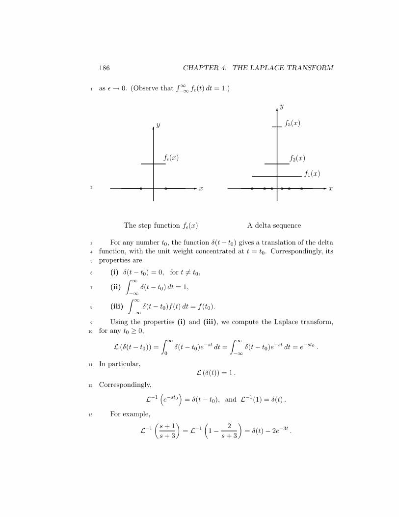
186 CHAPTER 4. THE LAPLACE TRANSFORM
as ε→ 0. (Observe that∫∞−∞ fε(t) dt = 1.)1
-
6
-
6
b bfε(x)
x
y
The step function fε(x) A delta sequence
bb b bf2(x)
f1(x)bb
f5(x)
x
y
2
For any number t0, the function δ(t− t0) gives a translation of the delta3
function, with the unit weight concentrated at t = t0. Correspondingly, its4
properties are5
(i) δ(t− t0) = 0, for t 6= t0,6
(ii)
∫ ∞
−∞δ(t− t0) dt = 1,7
(iii)
∫ ∞
−∞δ(t− t0)f(t) dt = f(t0).8
Using the properties (i) and (iii), we compute the Laplace transform,9
for any t0 ≥ 0,10
L (δ(t− t0)) =
∫ ∞
0δ(t− t0)e
−st dt =
∫ ∞
−∞δ(t− t0)e
−st dt = e−st0 .
In particular,11
L (δ(t)) = 1 .
Correspondingly,12
L−1(
e−st0)
= δ(t− t0), and L−1(1) = δ(t) .
For example,13
L−1(
s+ 1
s+ 3
)
= L−1(
1 − 2
s + 3
)
= δ(t) − 2e−3t .

4.3. THE DELTA FUNCTION AND IMPULSE FORCES 187
2 4 6 8t
0.5
1.0
1.5
y
Figure 4.1: Spring’s response to an impulse force
Other physical quantities may be concentrated at a single point. In1
the following example we consider forced vibrations of a spring, with the2
external force concentrated at t = 2. We say that an external impulse force3
is applied at t = 2.4
Example Solve the initial value problem5
y′′ + 2y′ + 5y = 6 δ(t− 2), y(0) = 0, y′(0) = 0 .
Applying the Laplace transform, then solving for Y (s) and completing the6
square, obtain7
(s2 + 2s+ 5)Y (s) = 6e−2s ,8
Y (s) =6e−2s
s2 + 2s + 5= e−2s 6
(s+ 1)2 + 4.
By the shift formula L−1(
1
(s+ 1)2 + 4
)
=1
2e−t sin 2t, and using the second9
shift formula (2.6), we conclude that10
y(t) = 3u2(t)e−(t−2) sin 2(t− 2) .
Before the time t = 2, the external force is zero. Coupled with zero initial11
conditions, this leaves the spring at rest for t ≤ 2. The impulse force at t = 212
sets the spring in motion, but the vibrations quickly die down, because of13
the heavy damping; see the Figure 4.1 for the graph of y(t).14

188 CHAPTER 4. THE LAPLACE TRANSFORM
4.4 Convolution and the Tautochrone Curve1
The problem2
y′′ + y = 0, y(0) = 0, y′(0) = 1
has solution y = sin t. If we now add a forcing term g(t), and consider3
y′′ + y = g(t), y(0) = 0, y′(0) = 0 ,
then the solution is4
y(t) =
∫ t
0sin(t− v)g(v) dv,(4.1)
as we saw in the section on convolution integrals. Motivated by this formula,5
we now define the concept of convolution of two functions f(t) and g(t)6
f ∗ g =
∫ t
0f(t− v)g(v) dv .
The result is a function of t, which is also denoted as (f ∗ g) (t). The formula7
(4.1) can now be written as8
y(t) = sin t ∗ g(t) .
Another example of convolution:9
t ∗ t2 =
∫ t
0(t− v)v2 dv = t
∫ t
0v2 dv −
∫ t
0v3 dv =
t4
3− t4
4=t4
12.
If you compute t2 ∗ t, the answer is the same. More generally, for any two10
continuous functions f(t) and g(t)11
g ∗ f = f ∗ g .
Indeed, making a change of variables v → u, by letting u = t−v, we express12
g ∗ f =
∫ t
0g(t− v)f(v) dv = −
∫ 0
tg(u)f(t− u) du
13
=
∫ t
0f(t− u)g(u) du= f ∗ g .
It turns out that the Laplace transform of a convolution is equal to the14
product of the Laplace transforms:15
L (f ∗ g) = F (s)G(s) .

4.4. CONVOLUTION AND THE TAUTOCHRONE CURVE 189
Indeed,1
L (f ∗ g) =
∫ ∞
0e−st
∫ t
0f(t− v)g(v) dvdt =
∫ ∫
De−stf(t− v)g(v) dvdt ,
where the double integral on the right hand side is taken over the region D2
of the tv-plane, which is an infinite wedge 0 < v < t in the first quadrant.3
We now evaluate this double integral by using the reverse order of repeated4
integrations:5
∫ ∫
De−stf(t− v)g(v) dvdt =
∫ ∞
0g(v)
(∫ ∞
ve−stf(t− v) dt
)
dv .(4.2)
For the integral in the brackets, we make a change of variables t → u, by6
letting u = t− v,7
∫ ∞
ve−stf(t− v) dt =
∫ ∞
0e−s(v+u)f(u) du = e−svF (s) ,
and then the right hand side of (4.2) is equal to F (s)G(s).8
6
t
v
��
��
��
��
�
-
@@
@@@
@
D
@@
@@
@@
@@
@@
@@@
The infinite wedge D
9
We conclude a useful formula10
L−1 (F (s)G(s)) = (f ∗ g)(t) .
For example,11
L−1
(
s2
(s2 + 4)2
)
= cos 2t ∗ cos 2t =
∫ t
0cos 2(t− v) cos 2v dv .
Using that12
cos 2(t− v) = cos 2t cos 2v + sin2t sin 2v ,

190 CHAPTER 4. THE LAPLACE TRANSFORM
we conclude1
L−1
(
s2
(s2 + 4)2
)
= cos 2t
∫ t
0cos2 2v dv + sin 2t
∫ t
0sin 2v cos 2v dv
2
=1
2t cos 2t+
1
4sin 2t .
Example Consider the vibrations of a spring at resonance3
y′′ + y = −3 cos t, y(0) = 0, y′(0) = 0 .
Taking the Laplace transform, compute4
Y (s) = −3s
(s2 + 1)2.
Writing Y (s) = −3 1s2+1
· ss2+1
, we invert it as5
y(t) = −3 sin t ∗ cos t = −3
2t sin t ,
because6
sin t ∗ cos t =
∫ t
0sin(t− v) cosv dv =
∫ t
0[sin t cos v − cos t sin v] cos v dv
7
= sin t
∫ t
0cos2 v dv − cos t
∫ t
0sin v cos v dv
8
=1
2t sin t+
1
4sin 2t sin t− 1
2cos t sin2 t =
1
2t sin t .
We see again that the amplitude of oscillations, which is 12t, tends to infinity9
with time t.10
The Tautochrone curve11
Assume that we have a curve through the origin in the first quadrant of the12
xy-plane, and a particle slides down this curve, under the influence of the13
force of gravity. The initial velocity at the starting point is assumed to be14
zero. We wish to find the curve so that the time T it takes to reach the15
bottom at (0, 0) is the same, for any starting point (x, y). This historic curve,16
called the tautochrone (which means loosely “the same time” in Latin), was17
found by Christian Huygens in 1673. He was motivated by the construction18
of a clock pendulum with the period independent of its amplitude.19

4.4. CONVOLUTION AND THE TAUTOCHRONE CURVE 191
Let (x1, v) be any intermediate position of the particle, v < y. Let1
s = f(v) be the length of the curve from (0, 0) to (x1, v). Of course, the2
length s depends also on the time t, andds
dtgives the speed of the particle.3
The kinetic energy of the particle at (x1, v) is due to the decrease of its4
potential energy (m is the mass of the particle):5
1
2m
(
ds
dt
)2
= mg(y − v) .
-
6
x
y
tt (x, y)
(x1, v)s
�
The Tautochrone curve
6
By the chain rule,ds
dt=ds
dv
dv
dt= f ′(v)
dv
dt, so that7
1
2
(
f ′(v)dv
dt
)2
= g(y − v) ,
8
f ′(v)dv
dt= −
√
2g√y − v .
(Minus, because the function v(t) is decreasing, while f ′(v) > 0.) We sepa-9
rate the variables, and integrate10
∫ y
0
f ′(v)√y − v
dv =
∫ T
0
√
2g dt =√
2g T .(4.3)
192 CHAPTER 4. THE LAPLACE TRANSFORM
(Over the time interval (0, T ), the particle descends from v = y to v = 0.)1
To find the function f ′, we need to solve the integral equation (4.3), which2
may be written as3
y−1/2 ∗ f ′(y) =√
2g T .(4.4)
Recall that in Problems we had the formula L(
t−12
)
=
√
π
s, or in terms of4
the variable y5
L(
y−12
)
=
√
π
s.(4.5)
Now apply the Laplace transform to the equation (4.4), and get6
√
π
sL (f ′(y)) =
√
2g T1
s.
Solving for L (f ′(y)), gives7
L(
f ′(y))
=T
π
√
2g
√
π
s=
√a
√
π
s,
where we denoted a =T 2
π22g. Using (4.5) again8
f ′(y) =√ay−1/2 .(4.6)
We have ds =√
dx2 + dy2, and so f ′(y) =ds
dy=
√
1 +
(
dx
dy
)2
. Use this9
expression in (4.6):10
√
1 +
(
dx
dy
)2
=√a
1√y.(4.7)
This is a first order differential equation. One could solve it fordx
dy, and11
then separate the variables. But it appears easier to use the parametric12
integration technique. To do that, we solve this equation for y13
y =a
1 +(
dxdy
)2 ,(4.8)
and set14
dx
dy=
1 + cos θ
sin θ,(4.9)

4.5. DISTRIBUTIONS 193
where θ is a parameter. Using (4.9) in (4.8), express1
y = asin2 θ
sin2 θ + (1 + cos θ)2= a
sin2 θ
2 + 2 cos θ=a
2
1 − cos2 θ
1 + cos θ=a
2(1 − cos θ) .
It follows that dy = a2 sin θ dθ. Then from (4.9), we get2
dx =1 + cos θ
sin θdy =
a
2(1 + cos θ) dθ .
Compute x by integration, obtaining3
x =a
2(θ + sin θ), y =
a
2(1− cos θ) ,
which is a parametric representation of the tautochrone. The name of this4
curve is cycloid, and it appears in many other applications.5
4.5 Distributions6
A function f(t) converts a number t into a number f(t). (Sometimes we do7
not use all real t, but restrict f(t) to a smaller domain.) Functionals convert8
functions into numbers. We shall allow only “nice” functions to be plugged9
into functionals.10
A function ϕ(t), defined on the interval (−∞,∞), is said to be of compact11
support if it is equal to zero outside of some bounded interval (a, b). Func-12
tions that are infinitely differentiable on (−∞,∞), and of compact support,13
are called test functions. We shall reserve writing ϕ(t) exclusively for test14
functions.15
Definition Distribution is a linear functional on test functions. Notation:16
(f, ϕ). (A test function ϕ(t) goes in, the number (f, ϕ) is the output. One17
usually also assumes (f, ϕ) to be continuous in ϕ, but we do not need that18
in a brief presentation.)19
Example 1 Let f(t) be any continuous function. Define the distribution20
(f, ϕ) =
∫ ∞
−∞f(t)ϕ(t) dt .(5.10)
Convergence is not a problem here, because the integrand vanishes outside21
of some bounded interval. This functional is linear, because22
(f, c1ϕ1 + c2ϕ2) =
∫ ∞
−∞f(t) (c1ϕ1 + c2ϕ2) dt

194 CHAPTER 4. THE LAPLACE TRANSFORM
1
= c1
∫ ∞
−∞f(t)ϕ1 dt+ c2
∫ ∞
−∞f(t)ϕ2 dt = c1(f, ϕ1) + c2(f, ϕ2) ,
for any two constants c1 and c2, and any two test functions ϕ1(t) and ϕ2(t).2
This way “usual” functions can be viewed as distributions. The formula3
(5.10) lets us consider f(t) in the sense of distributions.4
Example 2 The Delta distribution. Define5
(δ(t), ϕ) = ϕ(0) .
(Compare this with (5.10), and the intuitive formula∫∞−∞ δ(t)ϕ(t) dt = ϕ(0)6
from Section 4.3.) We see that in the realm of distributions the delta function7
δ(t) sits next to usual functions, as an equal member of the club.8
Assume that f(t) is a differentiable function. Viewing f ′(t) as a distri-9
bution, we have10
(f ′, ϕ) =
∫ ∞
−∞f ′(t)ϕ(t) dt = −
∫ ∞
−∞f(t)ϕ′(t) dt = −(f, ϕ′) ,
using integration by parts (recall that ϕ(t) is zero outside of some bounded11
interval). Motivated by this formula, we now define the derivative of any12
distribution f :13
(f ′, ϕ) = −(f, ϕ′) .
In particular,14
(δ′, ϕ) = −(δ, ϕ′) = −ϕ′(0) .
(So that δ′ is another distribution. We know how it acts on test functions.)15
Similarly, (δ′′, ϕ) = −(δ′, ϕ′) = ϕ′′(0), and in general16
(δ(n), ϕ) = (−1)nϕ(n)(0) .
We see that all distributions are infinitely differentiable! In particular, all17
continuous functions are infinitely differentiable, if we view them as distri-18
butions.19
Example 3 The Heaviside function20
H(t) =
0 if −∞ ≤ t < 0
1 if t ≥ 0

4.5. DISTRIBUTIONS 195
has a jump at t = 0. Clearly, H(t) is not differentiable at t = 0. But, in the1
sense of distributions, we claim that2
H ′(t) = δ(t) .
Indeed,3
(H ′(t), ϕ) = −(H(t), ϕ′) = −∫ ∞
0ϕ′(t) dt = ϕ(0) = (δ(t), ϕ) .
Example 4 The function |t| is not differentiable at t = 0. But, in the4
sense of distributions,5
|t|′ = 2H(t)− 1 .
Indeed,6
(|t|′, ϕ) = −(|t|, ϕ′) = −∫ 0
−∞(−t)ϕ′(t) dt−
∫ ∞
0tϕ′(t) dt .
Integrating by parts in both integrals, we continue7
(|t|′, ϕ) = −∫ 0
−∞ϕ(t) dt+
∫ ∞
0ϕ(t) dt = (2H(t)− 1, ϕ) .
4.5.1 Problems8
I. Find the Laplace transform of the following functions.9
1. 5 + 2t3 − e−4t. Answer.5
s+
12
s4− 1
s+ 4.10
2. 2 sin 3t− t3. Answer.6
s2 + 9− 6
s4.11
3. cosh 2t− e4t. Answer.s
s2 − 4− 1
s − 4.12
4. e2(t−1). Answer.1
e2(s− 2).13
5. e2t cos 3t. Answer.s− 2
(s− 2)2 + 9.14
6.t3 − 3t
t. Answer.
2
s3− 3
s.15
7. e−3tt4. Answer.24
(s+ 3)516
196 CHAPTER 4. THE LAPLACE TRANSFORM
8. sin2 2t. Answer.1
2s− s
2(s2 + 16).1
9. sin 2t cos 2t. Answer.2
s2 + 16.2
10. sinh t cosh t. Answer.1
s2 − 4.3
11. |t− 2|. Answer.2e−2s + 2s− 1
s2.4
Hint: Split the integral into two pieces.5
12. f(t) = t for 1 < t < 3, and f(t) = 0 for all other t > 0.6
Answer. F (s) =e−s(s+ 1)
s2− e−3s(3s+ 1)
s2.7
II. Find the inverse Laplace transform of the following functions.8
1.1
s2 + 4− 2
s3. Answer.
1
2sin 2t− t2.9
2.s
s2 − 9− 2
s + 3. Answer. cosh3t− 2e−3t.10
3.1
s2 + s. Answer. 1 − e−t.11
4.1
s2 − 3s. Answer.
1
3e3t − 1
3.12
5.1
s3 − 7s+ 6. Answer.
1
5e2t − 1
4et +
1
20e−3t.13
6.1
s3 + s. Answer. 1 − cos t.14
7.1
(s2 + 1)(s2 + 4). Answer.
1
3sin t− 1
6sin 2t.15
8.s
s4 + 5s2 + 4. Answer.
1
3cos t− 1
3cos 2t.16
9.1
s2 + 2s+ 10. Answer.
1
3e−t sin 3t.17
10.1
s2 + s− 2. Answer.
1
3et − 1
3e−2t.18
11.s
s2 + s+ 1. Answer. e−
12t
[
cos
√3
2t− 1√
3sin
√3
2t
]
.19

4.5. DISTRIBUTIONS 197
12.s− 1
s2 − s − 2. Answer.
1
3e2t +
2
3e−t.1
13.s+ 3
4s2 + 1. Answer.
1
4cos
t
2+
3
2sin
t
2.2
14.s
4s2 − 4s+ 5. Answer. e
12t(
1
4cos t+
1
8sin t
)
.3
15.s+ 2
s3 − 3s2 + 2s. Answer. 1 − 3et + 2e2t.4
16.s3 − s
s4 + 5s2 + 4. Answer. −2
3cos t+
5
3cos 2t.5
17.s2 + 2
s3 − 2s2 + 2s. Answer. 1 + 2et sin t.6
18∗. (i) Considerp(s)
q(s), where q(s) = (s − s1)(s− s2) · · · (s− sn) with some7
numbers s1, s2, . . . , sn, and p(s) is a polynomial of degree less than n. By8
the method of partial fractions9
p(s)
q(s)=
a1
s− s1+
a2
s − s2+ · · ·+ an
s − sn,(5.11)
for some numbers a1, a2, . . . , an. Show that a1 = p(s1)q′(s1) , and derive similar10
formulas for the other ai’s.11
Hint: Multiply (5.11) by s−s1, take the limit as s→ s1, and use L’Hospital’s12
rule.13
(ii) Show that14
L−1(
p(s)
q(s)
)
=n∑
i=1
p(si)
q′(si)esit .
(iii) Calculate L−1
(
s2 + 5
(s− 1)(s− 2)(s− 3)
)
. Answer. y = 3et−9e2t+7e3t.15
16
III. Using the Laplace transform, solve the following initial value problems.17
18
1. y′′ + 3y′ + 2y = 0, y(0) = −1, y′(0) = 2. Answer. y = −e−2t.19
2. y′′ + 2y′ + 5y = 0, y(0) = 1, y′(0) = −2.20
Answer. 12e
−t (2 cos 2t− sin 2t).21

198 CHAPTER 4. THE LAPLACE TRANSFORM
3. y′′+y = sin2t, y(0) = 0, y′(0) = 1. Answer. y =5
3sin t−1
3sin 2t.1
2
4. y′′ + 2y′ + 2y = et, y(0) = 0, y′(0) = 1.3
Answer. y =1
5et − 1
5e−t (cos t− 3 sin t).4
5. y′′′′ − y = 0, y(0) = 0, y′(0) = 1, y′′(0) = 0, y′′′(0) = 0.5
Answer. y =1
2sin t+
1
2sinh t.6
6. y′′′′ − 16y = 0, y(0) = 0, y′(0) = 2, y′′(0) = 0, y′′′(0) = 8.7
Answer. y = sinh 2t.8
7. y′′′ + 3y′′ + 2y′ = 0, y(0) = 0, y′(0) = 0, y′′(0) = −1.9
Answer. y = −1
2− e−2t
2+ e−t.10
8. y′′′ + 3y′′ + 3y′ + y = e−t, y(0) = 0, y′(0) = 0, y′′(0) = 0.11
Answer. y =t3e−t
6.12
IV.13
1. (a) Let s > 0. Show that14
∫ ∞
−∞e−sx2
dx =
√
π
s.
15
Hint: Denote I =
∫ ∞
−∞e−sx2
dx. Then16
I2 =
∫ ∞
−∞e−sx2
dx
∫ ∞
−∞e−sy2
dy =
∫ ∞
−∞
∫ ∞
−∞e−s(x2+y2) dA .
This is a double integral over the entire xy-plane. Evaluate it by using the17
polar coordinates, to obtain I2 = πs .18
(b) Show that L(
t−12
)
=
√
π
s.19
Hint: L(
t−12
)
=
∫ ∞
0t−
12 e−st dt. Make a change of variables t → x, by20
letting x = t12 . Then L
(
t−12
)
= 2
∫ ∞
0e−sx2
dx =
∫ ∞
−∞e−sx2
dx =
√
π
s.21

4.5. DISTRIBUTIONS 199
2. Show that
∫ ∞
0
sinx
xdx =
π
2.1
Hint: Consider f(t) =
∫ ∞
0
sin tx
xdx, and calculate its Laplace transform2
F (s) = π2
1s .3
3. Solve the following system of differential equations4
dx
dt= 2x− y, x(0) = 4
5
dy
dt= −x+ 2y, y(0) = −2 .
Answer. x(t) = et + 3e3t, y(t) = et − 3e3t.6
4. Solve the following non-homogeneous system of differential equations7
x′ = 2x− 3y + t, x(0) = 0
y′ = −2x + y, y(0) = 1 .
Answer. x(t) = e−t − 9
16e4t +
1
16(−7+ 4t), y(t) = e−t +
3
8e4t +
1
8(−3+ 4t).8
V.9
1. A function f(t) is equal to 1 for 1 ≤ t < 5, and is equal to 0 for all10
other t ≥ 0. Represent f(t) as a difference of two step functions, and find11
its Laplace transform.12
Answer. f(t) = u1(t) − u5(t), F (s) =e−s
s− e−5s
s.13
2. A function g(t) is equal to 1 for 0 ≤ t < 5, and is equal to −2 for t ≥ 5.14
Represent g(t) using step functions, and find its Laplace transform.15
Answer. g(t) = 1 − 3u5(t), G(s) =1
s− 3
e−5s
s.16
3. A function h(t) is equal to −2 for 0 ≤ t < 3, to 4 for 3 ≤ t < 7, and17
to zero for t ≥ 7. Represent h(t) using step functions, and find its Laplace18
transform.19
Answer. h(t) = −2 + 6u3(t) − 4u7(t), H(s) = −2
s+ 6
e−3s
s− 4
e−7s
s.20
4. A function k(t) is equal to t for 0 ≤ t < 4, and to 4 for t ≥ 4. Represent21
k(t) using step functions, and find its Laplace transform.22

200 CHAPTER 4. THE LAPLACE TRANSFORM
Answer. k(t) = t (1 − u4(t)) + 4u4(t) = t− u4(t) (t− 4), K(s) =1
s2− e−4s
s2,1
by using the second shift formula (2.5).2
5. Find the Laplace transform of t2−2u4(t). Answer. F (s) =2
s3−2
e−4s
s.3
4
6. Sketch the graph of the function u2(t) − 2u3(t) + 4u6(t), and find its5
Laplace transform.6
7. Find the inverse Laplace transform of1
s2
(
2e−s − 3e−4s)
.7
Answer. 2u1(t)(t− 1)− 3u4(t)(t− 4).8
8. Find the inverse Laplace transform of e−2s 3s− 1
s2 + 4.9
Answer. u2(t)
[
3 cos2(t− 2)− 1
2sin 2(t− 2)
]
.10
9. Find the inverse Laplace transform of e−s 1
s2 + s− 6.11
Answer. u1(t)
(
1
5e2t−2 − 1
5e−3t+3
)
.12
10. Find the inverse Laplace transform of e−π2s 1
s2 + 2s+ 5, and simplify the13
answer.14
Answer. −1
2uπ/2(t)e
−t+π/2 sin 2t.15
11. Solve16
y′′ + y = 4u1(t) − u5(t), y(0) = 2, y′(0) = 0.
Answer. 2 cos t+ 4u1(t) [1 − cos(t− 1)]− u5(t) [1 − cos(t− 5)].17
12. Solve18
y′′ + 3y′ + 2y = u2(t), y(0) = 0, y′(0) = −1.
Answer. y(t) = e−2t − e−t + u2(t)
[
1
2− e−(t−2) +
1
2e−2(t−2)
]
.19
13. Solve20
y′′ + 4y = uπ(t) sin t, y(0) = −1, y′(0) = 1.
Hint: Write sin t = − sin(t− π), and use the shift formula (2.5).21
Answer. y(t) = − cos 2t+1
2sin 2t+ uπ(t)
(
1
3sin t+
1
6sin 2t
)
.22
4.5. DISTRIBUTIONS 201
14. Solve1
y′′ + y = g(t), y(0) = 0, y′(0) = 0 ,
where2
g(t) =
{
t if 0 ≤ t < ππ if t ≥ π
.
Answer. y(t) = t− sin t− uπ(t) (t− π + sin t).3
VI.4
1. Show that L(
u′c(t))
= L (δ(t− c)), c > 0.5
This formula shows that u′c(t) = δ(t− c).6
2. Find the Laplace transform of δ(t− 4)− 2u4(t).7
3. Find the inverse Laplace transform ofs+ 1
s+ 3. Answer. δ(t) − 2e−3t.8
4. Find the inverse Laplace transform ofs2 + 1
s2 + 2s+ 2.9
Answer. δ(t) − e−t(2 cos t− sin t).10
5. Solve11
y′′ + y = δ(t− π), y(0) = 0, y′(0) = 2.
Answer. y(t) = 2 sin t− uπ(t) sin t.12
6. Solve13
y′′ + 2y′ + 10y = δ(t− π), y(0) = 0, y′(0) = 0.
Answer. y(t) = −1
3uπ(t)e−t+π sin 3t.14
7. Solve15
4y′′ + y = δ(t), y(0) = 0, y′(0) = 0.
Answer. y(t) =1
2sin
1
2t.16
8. Solve17
4y′′ + 4y′ + 5y = δ(t− 2π), y(0) = 0, y′(0) = 1.
Answer. y(t) = e−12t sin t+
1
4u2π(t) e−
12(t−2π) sin t.18
9. Show that L (δ(t− t0)f(t)) = e−st0f(t0).19
10. Solve20
y′′ + 4y = δ(t− π
3) cos t, y(0) = 0, y′(0) = 0.

202 CHAPTER 4. THE LAPLACE TRANSFORM
Answer. y(t) =1
4uπ/3(t) sin2(t− π
3).1
VII.2
1. Show that sin t ∗ 1 = 1 − cos t. (Observe that sin t ∗ 1 6= sin t.)3
2. Show that f(t) ∗ δ(t) = f(t), for any f(t).4
(So that the delta function plays the role of unity for convolution.)5
3. Find the convolution t ∗ t. Answer.t3
6.6
4. Find the convolution t ∗ sinat. Answer.at− sin at
a2.7
5. Find the convolution cos t ∗ cos t.8
Hint: cos(t− v) = cos t cos v+ sin t sin v. Answer.1
2t cos t+
1
2sin t.9
10
6. Using convolutions, find the inverse Laplace transform of the following11
functions12
(a)1
s3(s2 + 1). Answer.
t2
2∗ sin t =
t2
2+ cos t− 1.13
(b)s
(s+ 1)(s2 + 9). Answer. −e
−t
10+
1
10cos 3t+
3
10sin 3t.14
(c)s
(s2 + 1)2. Answer.
1
2t sin t.15
(d)1
(s2 + 9)2. Answer.
1
54sin 3t− 3
54t cos 3t.16
7. Solve the following initial value problem at resonance17
y′′ + 9y = cos 3t, y(0) = 0, y′(0) = 0.
Answer. y(t) =1
6t sin 3t.18
8. Solve the initial value problem with a given forcing term g(t)19
y′′ + 4y = g(t), y(0) = 0, y′(0) = 0.
Answer. y(t) =1
2
∫ t
0sin 2(t− v)g(v) dv.20

4.5. DISTRIBUTIONS 203
9. Find f(t) given that1
L (t ∗ f(t)) =1
s4(s2 + 1).
Answer. t− sin t.2
10. Find the Laplace transform of
∫ t
0e−(t−v) cos v dv.3
Answer. L(
e−t)
L (cos t) =s
(s+ 1)(s2 + 1).4
11. Solve the following Volterra’s integral equation5
y(t) +
∫ t
0(t− v)y(v) dv = cos 2t .
Answer. y(t) = −1
3cos t+
4
3cos 2t.6
12. By using the Laplace transform, calculate t ∗ t ∗ t. Answer.t5
5!.7
VIII.8
1. Find the second derivative of |t| in the sense of distributions.9
Answer. 2δ(t).10
2. Find f(t), such that (n is a positive integer)11
f (n)(t) = δ(t) .
Answer. f(t) =
{
0 if t < 0tn−1
(n−1)! if t ≥ 0.12
3. Let f(t) =
{
t2 if t < 0t2 + 5 if t ≥ 0
.13
Show that f ′(t) = 2t+ 5δ(t).14
Hint: f(t) = t2 + 5H(t).15
4. Consider a family of functions fε(t) =ε
π (t2 + ε2), ε > 0. Show that in16
the sense of distributions17
limε→0
fε(t) = δ(t) .

204 CHAPTER 4. THE LAPLACE TRANSFORM
One refers to fε(t) as a delta sequence. (Other delta sequences can be found1
in the book of M. Renardy and R.C. Rogers [25].)2
Hint: (fε, ϕ) =
∫ ∞
−∞
εϕ(t)
π (t2 + ε2)dt =
∫ ∞
−∞
ϕ(εz)
π (z2 + 1)dz3
→ ϕ(0)
∫ ∞
−∞
1
π (z2 + 1)dz = ϕ(0) = (δ, ϕ) .
5. (i) The function K(x, t) = 12√
πkte−
x2
4kt is known as the heat kernel (k > 04
is a constant). Show that in the sense of distributions5
limt→0
K(x, t) = δ(x) .
(ii) Conclude that6
limt→0
K(x, t) ∗ f(x) = limt→0
1
2√πkt
∫ ∞
−∞e−
(x−y)2
4kt f(y) dy = f(x) .
(iii) Show that the function K(x, t) satisfies the heat equation7
Kt = kKxx .
(iv) Conclude that the function u(x, t) = K(x, t) ∗ f(x) satisfies8
ut = kuxx , u(x, 0) = f(x) .

Chapter 51
Linear Systems of2
Differential Equations3
We begin this chapter by solving systems of linear differential equations4
with constant coefficients, using the eigenvalues and eigenvectors of the cor-5
responding coefficient matrices. Then we study the long term properties of6
these systems, and the notion of the exponential of a matrix. We develop7
the Floquet theory for systems with periodic coefficients, and make an appli-8
cation to Massera’s theorem. We classify the pictures at the origin for 2× 29
systems, and discuss the controllability and observability of linear systems.10
5.1 The Case of Distinct Eigenvalues11
The case when the coefficient matrix has distinct eigenvalues turns out to12
be the easiest. We begin by recalling the basic notions of matrix theory.13
5.1.1 Review of Vectors and Matrices14
Recall that given two vectors15
C1 =
a1
a2
a3
, C2 =
b1b2b3
,
205

206CHAPTER 5. LINEAR SYSTEMS OF DIFFERENTIAL EQUATIONS
we can add them as C1 + C2 =
a1 + b1a2 + b2a3 + b3
, or multiply by a constant x:1
xC1 =
xa1
xa2
xa3
. More generally, we can compute the linear combination2
x1C1 + x2C2 =
x1a1 + x2b1x1a2 + x2b2x1a3 + x2b3
,
for any two constants x1 and x2.3
We shall be dealing only with the square matrices, like the following 3×34
matrix5
A =
a11 a12 a13
a21 a22 a23
a31 a32 a33
.(1.1)
We shall view A as a row of column vectors A =[
C1 C2 C3
]
, where6
C1 =
a11
a21
a31
, C2 =
a12
a22
a32
, C3 =
a13
a23
a33
.
The product of a matrix A and of a vector x =
x1
x2
x3
is defined as the7
vector8
Ax = C1x1 + C2x2 +C3x3 .
(This definition is equivalent to the more traditional one, that you might9
have seen before.) We get10
Ax =
a11x1 + a12x2 + a13x3
a21x1 + a22x2 + a23x3
a31x1 + a32x2 + a33x3
.
Two vectors C1 and C2 are called linearly dependent if one of them is a11
constant multiple of the other, so that C2 = aC1, for some number a. (The12
zero vector is linearly dependent with any other vector.) Linearly dependent13
vectors C1 and C2 go along the same line. If the vectors C1 and C2 do not14

5.1. THE CASE OF DISTINCT EIGENVALUES 207
go along the same line, they are linearly independent. Three vectors C1, C21
and C3 are called linearly dependent if one of them is a linear combination2
of the others, e.g., if C3 = aC1 + bC2, for some numbers a, b. This means3
that C3 lies in the plane determined by C1 and C2, so that all three vectors4
lie in the same plane. If C1, C2 and C3 do not lie in the same plane, they5
are linearly independent.6
A system of 3 equations with 3 unknowns7
a11x1 + a12x2 + a13x3 = b1a21x1 + a22x2 + a23x3 = b2a31x1 + a32x2 + a33x3 = b3
(1.2)
can be written in the matrix form8
Ax = b ,
where A is the 3×3 matrix above, and b =
b1b2b3
is the given vector of the9
right hand sides. Recall that the system (1.2) has a unique solution for any10
vector b if and only if the columns of the matrix A are linearly independent.11
(In that case, the determinant |A| 6= 0, and the inverse matrix A−1 exists.)12
5.1.2 Linear First Order Systems with Constant Coefficients13
We wish to find the functions x1(t), x2(t) and x3(t) that solve the following14
system of equations, with given constant coefficients a11, . . . , a33,15
x′1 = a11x1 + a12x2 + a13x3(1.3)
x′2 = a21x1 + a22x2 + a23x3
x′3 = a31x1 + a32x2 + a33x3 ,
subject to the given initial conditions16
x1(t0) = α, x2(t0) = β, x3(t0) = γ .
We may write this system using matrix notation:17
x′ = Ax, x(t0) = x0 ,(1.4)

208CHAPTER 5. LINEAR SYSTEMS OF DIFFERENTIAL EQUATIONS
where x(t) =
x1(t)x2(t)
x3(t)
is the unknown vector function, A is the 3 × 31
matrix (1.1) of the coefficients, and x0 =
α
βγ
is the vector of initial2
conditions. Indeed, on the left in (1.3) we have components of the vector3
x′(t) =
x′1(t)x′2(t)x′3(t)
, while on the right we see the components of the vector4
Ax.5
Let us observe that given two vector functions y(t) and z(t), which are6
solutions of the system x′ = Ax, their linear combination c1y(t) + c2z(t) is7
also a solution of the same system, for any constants c1 and c2. Our system8
of differential equations is linear, because it involves only linear combinations9
of the unknown functions.10
We now search for a solution of (1.4) in the form11
x(t) = eλtξ ,(1.5)
with a constant λ, and a vector ξ, with entries independent of t. Substituting12
this into (1.4), we have13
λeλtξ = A(
eλtξ)
,
giving14
Aξ = λξ .
So that if λ is an eigenvalue of A, and ξ the corresponding eigenvector, then15
(1.5) gives us a solution of the problem (1.4). Observe that the same is true16
for any square n× n matrix A. Let λ1, λ2 and λ3 be the eigenvalues of our17
3 × 3 matrix A. There are several cases to consider.18
Case 1 The eigenvalues of A are real and distinct. It is known from matrix19
theory that the corresponding eigenvectors ξ1, ξ2 and ξ3 are then linearly20
independent. We know that eλ1tξ1, eλ2tξ2 and eλ3tξ3 are solutions of our21
system (1.4), so that their linear combination22
x(t) = c1eλ1tξ1 + c2e
λ2tξ2 + c3eλ3tξ3(1.6)
also solves the system (1.4). We claim that (1.6) gives the general solution23
of our system, meaning that it is possible to determine the constants c1, c2,24
5.1. THE CASE OF DISTINCT EIGENVALUES 209
and c3 to satisfy any initial conditions:1
x(t0) = c1eλ1t0ξ1 + c2e
λ2t0ξ2 + c3eλ3t0ξ3 = x0 .(1.7)
This is a system of three linear equations with three unknowns c1, c2, and2
c3. The matrix of this system is non-singular, because its columns, eλ1t0ξ1,3
eλ2t0ξ2 and eλ3t0ξ3, are linearly independent (observe that these columns4
are constant multiples of the linearly independent vectors ξ1, ξ2 and ξ3).5
Therefore, we can find a unique solution triple c1, c2, and c3 of the system6
(1.7). Then x(t) = c1eλ1tξ1 + c2e
λ2tξ2 + c3eλ3tξ3 is the desired solution of7
our initial value problem (1.4).8
Example 1 Solve the system9
x′ =
[
2 11 2
]
x, x(0) =
[
−12
]
.
10
This is a 2×2 system, so that there are only two terms in (1.6). We compute11
the eigenvalues λ1 = 1, and the corresponding eigenvector ξ1 =
[
−11
]
, and12
λ2 = 3, with the corresponding eigenvector ξ2 =
[
1
1
]
. The general solution13
is then14
x(t) = c1et
[
−1
1
]
+ c2e3t
[
1
1
]
,
or in components15
x1(t) = −c1et + c2e3t
x2(t) = c1et + c2e
3t .
Turning to the initial conditions,16
x1(0) = −c1 + c2 = −1
x2(0) = c1 + c2 = 2 .
Calculate c1 = 3/2, c2 = 1/2. Answer:17
x1(t) = −32e
t + 12e
3t
x2(t) = 32e
t + 12e
3t .
210CHAPTER 5. LINEAR SYSTEMS OF DIFFERENTIAL EQUATIONS
Case 2 The eigenvalue λ1 is double, λ2 = λ1, λ3 6= λ1, however, λ1 has1
two linearly independent eigenvectors ξ1 and ξ2. Let ξ3 denote again an2
eigenvector corresponding to λ3. This vector cannot lie in the plane spanned3
by ξ1 and ξ2, and then the vectors ξ1, ξ2 and ξ3 are linearly independent.4
The general solution is given again by the formula (1.6), with λ2 replaced5
by λ1:6
x(t) = c1eλ1tξ1 + c2e
λ1tξ2 + c3eλ3tξ3 .
To satisfy the initial conditions, we get a linear system for c1, c2 and c37
c1eλ1t0ξ1 + c2e
λ1t0ξ2 + c3eλ3t0ξ3 = x0 ,
which has a unique solution, because its matrix has linearly independent8
columns. (Linearly independent eigenvectors is the key here!)9
Example 2 Solve the system10
x′ =
2 1 11 2 11 1 2
x , x(0) =
10
−4
.
Expanding the determinant of A− λI in the first row, we write the charac-11
teristic equation as12
(2− λ)[
(2− λ)2 − 1]
− (2 − λ− 1) + 1 + λ− 2 = 0 ,
13
(2 − λ)(1− λ)(3− λ) − 2(1− λ) = 0 ,14
(1− λ) [(2 − λ)(3− λ)− 2] = 0 .
The roots are: λ1 = 1, λ2 = 1, λ3 = 4. We calculate that the double15
eigenvalue λ1 = 1 has two linearly independent eigenvectors ξ1 =
−10
1
16
and ξ2 =
0
−11
. The other eigenvalue λ3 = 4 has the corresponding17
eigenvector ξ3 =
11
1
. The general solution is then18
x(t) = c1et
−10
1
+ c2e
t
0−1
1
+ c3e
4t
11
1
.

5.1. THE CASE OF DISTINCT EIGENVALUES 211
Or, in components,1
x1(t) = −c1et + c3e4t
x2(t) = −c2et + c3e4t
x3(t) = c1et + c2e
t + c3e4t .
Using the initial conditions, calculate c1 = −2, c2 = −1, and c3 = −1.2
Answer:3
x1(t) = 2et − e4t
x2(t) = et − e4t
x3(t) = −3et − e4t .
Proceeding similarly, we can solve the initial value problem (1.4) for any4
n×n matrix A, provided that all of its eigenvalues are real, and it has a full5
set of n linearly independent eigenvectors. Recall that if an n× n matrix A6
is symmetric (aij = aji, for all i and j), then all of its eigenvalues are real.7
The eigenvalues of a symmetric matrix may be repeated, but there is always8
a full set of n linearly independent eigenvectors. So that one can solve the9
initial value problem (1.4) for any system with a symmetric matrix.10
Case 3 The eigenvalue λ1 has multiplicity two (λ1 is a double root of the11
characteristic equation, λ2 = λ1), λ3 6= λ1, but λ1 has only one linearly12
independent eigenvector ξ. The eigenvalue λ1 brings in only one solution13
eλ1tξ. By analogy with the second order equations, we try teλ1tξ for the14
second solution. However, this vector function is a scalar multiple of the15
first solution, so that it is linearly dependent with it, at any t = t0. We16
modify our guess:17
x(t) = teλ1tξ + eλ1tη ,(1.8)
and choose a vector η, to obtain a second linearly independent solution.18
Substituting (1.8) into our system (1.4), and using that Aξ = λ1ξ, obtain19
eλ1tξ + λ1teλ1tξ + λ1e
λ1tη = λ1teλ1tξ + eλ1tAη.
Cancelling a pair of terms, and dividing by eλ1t, we simplify this to20
(A− λ1I)η = ξ .(1.9)
Even though the matrix A− λ1I is singular (its determinant is zero), it can21
be shown (using the Jordan normal form) that the linear system (1.9) always22
has a solution η, called generalized eigenvector. We see from (1.9) that η23

212CHAPTER 5. LINEAR SYSTEMS OF DIFFERENTIAL EQUATIONS
is not a multiple of ξ. Using this η in (1.8), gives us the second linearly1
independent solution, corresponding to λ = λ1. (Observe that c η is not a2
generalized eigenvector for any constant c 6= 1, unlike the usual eigenvectors.3
If η is a generalized eigenvector, then so is η + cξ, for any constant c.)4
Example 3 Solve the system5
x′ =
[
1 −11 3
]
x .
This matrix has a double eigenvalue λ1 = λ2 = 2, and only one linearly inde-6
pendent eigenvector ξ =
[
1−1
]
. We have one solution: x1(t) = e2t
[
1−1
]
.7
The system (1.9) to determine the vector η =
[
η1
η2
]
takes the form8
−η1 − η2 = 1
η1 + η2 = −1 .
Discard the second equation, because it is a multiple of the first. The first9
equation has infinitely many solutions. But all we need is just one solution,10
that is not a multiple of ξ. So we set η2 = 0, which gives η1 = −1. We11
computed the second linearly independent solution:12
x2(t) = te2t
[
1−1
]
+ e2t
[
−10
]
.
The general solution is then13
x(t) = c1e2t
[
1
−1
]
+ c2
(
te2t
[
1
−1
]
+ e2t
[
−1
0
])
.
5.2 A Pair of Complex Conjugate Eigenvalues14
5.2.1 Complex Valued and Real Valued Solutions15
Recall that one differentiates complex valued functions much the same way,16
as the real ones. For example,17
d
dteit = ieit ,
5.2. A PAIR OF COMPLEX CONJUGATE EIGENVALUES 213
where i =√−1 is treated the same way as any other constant. Any complex1
valued function f(t) can be written in the form f(t) = u(t)+iv(t), where u(t)2
and v(t) are real valued functions. It follows by the definition of derivative3
that f ′(t) = u′(t) + iv′(t). For example, using Euler’s formula,4
d
dteit =
d
dt(cos t+ i sin t) = − sin t+ i cos t = i(cos t+ i sin t) = ieit .
Any complex valued vector function x(t) can also be written as x(t) =5
u(t) + iv(t), where u(t) and v(t) are real valued vector functions. Again, we6
have x′(t) = u′(t) + iv′(t).7
If x(t) = u(t) + iv(t) is a complex valued solution of our system (1.4),8
then9
u′(t) + iv′(t) = A (u(t) + iv(t)) .
Equating the real and imaginary parts, we see that both u(t) and v(t) are10
real valued solutions of our system (1.4).11
5.2.2 The General Solution12
Assume that the matrix A has a pair of complex conjugate eigenvalues p+iq13
and p−iq. They need to contribute two linearly independent solutions. The14
eigenvector corresponding to p+ iq is complex valued, which we may write15
as ξ+ iη, where ξ and η are real valued vectors. Then x(t) = e(p+iq)t(ξ+ iη)16
is a solution of our system. To get two real valued solutions, we take the17
real and the imaginary parts of this solution. Obtain:18
x(t) = ept(cos qt+ i sin qt)(ξ + iη)
= ept(cos qt ξ − sin qt η) + iept(sin qt ξ + cos qt η) .
So that19
u(t) = ept(cos qt ξ − sin qt η) ,20
v(t) = ept(sin qt ξ + cos qt η)
give us two real valued solutions. In case of a 2 × 2 matrix (when there are21
no other eigenvalues), the general solution is22
x(t) = c1u(t) + c2v(t) .(2.1)
(If one uses the other eigenvalue p− iq, and the corresponding eigenvector,23
the answer is the same.) We show in the exercises that one can choose the24
constants c1 and c2 to satisfy any initial condition x(t0) = x0.25

214CHAPTER 5. LINEAR SYSTEMS OF DIFFERENTIAL EQUATIONS
Example 1 Solve the system1
x′ =
[
1 −22 1
]
x, x(0) =
[
21
]
.
Calculate the eigenvalues λ1 = 1 + 2i and λ2 = 1 − 2i. The eigenvector2
corresponding to λ1 is
[
i
1
]
. So that we have a complex valued solution3
e(1+2i)t
[
i1
]
. Using Euler’s formula, rewrite it as4
et(cos 2t+ i sin 2t)
[
i1
]
= et[
− sin 2tcos 2t
]
+ iet[
cos 2tsin 2t
]
.
The real and imaginary parts give us two linearly independent solutions, so5
that the general solution is6
x(t) = c1et
[
− sin 2tcos 2t
]
+ c2et
[
cos 2tsin 2t
]
.
In components7
x1(t) = −c1et sin 2t+ c2et cos 2t
x2(t) = c1et cos 2t+ c2e
t sin 2t .
From the initial conditions8
x1(0) = c2 = 2
x2(0) = c1 = 1 ,
so that c1 = 1, and c2 = 2. Answer:9
x1(t) = −et sin 2t+ 2et cos 2t
x2(t) = et cos 2t+ 2et sin 2t .
Example 2 Solve the system10
x′ =
2 −1 21 0 2
−2 1 −1
x .

5.2. A PAIR OF COMPLEX CONJUGATE EIGENVALUES 215
1
One calculates the eigenvalue λ1 = 1, and the corresponding eigenvector2
0
21
. One of the solutions is then et
0
21
. The other two eigenvalues are3
λ2 = i and λ3 = −i. The eigenvector corresponding to λ2 = i is
−1 − i−1 − i
1
.4
giving us a complex valued solution eit
−1 − i
−1 − i1
. We rewrite it as5
(cos t+ i sin t)
−1 − i
−1 − i1
=
− cos t+ sin t
− cos t+ sin tcos t
+ i
− cos t− sin t
− cos t− sin tsin t
Taking its real and imaginary parts gives us two more linearly independent6
solutions, so that the general solution is7
x(t) = c1et
0
21
+ c2
− cos t+ sin t
− cos t+ sin tcos t
+ c3
− cos t− sin t
− cos t− sin tsin t
.
8
Examining the form of the solutions in all of the above cases, we see9
that if all eigenvalues of a matrix A are either negative or have negative real10
parts, then limt→∞ x(t) = 0 (all components of the vector x(t) tend to zero).11
5.2.3 Non-Homogeneous Systems12
Similarly to the case of a single equation, the general solution of a non-13
homogeneous system14
x′ = Ax+ f(t) ,
with a given vector-function f(t), is the sum of any particular solution Y (t)15
of this system and the general solution of the corresponding homogeneous16
system17
x′ = Ax .
Sometimes one can guess the form of Y (t).18

216CHAPTER 5. LINEAR SYSTEMS OF DIFFERENTIAL EQUATIONS
Example 3 Solve the system1
x′ =
[
2 11 2
]
x+
[
e−t
0
]
.
We look for a particular solution in the form Y (t) =
[
Ae−t
Be−t
]
, and calculate2
A = −38 , B = 1
8 , so that Y (t) =
[
−38e
−t
18e
−t
]
. The general solution of the3
corresponding homogeneous system was found in the Example 1.4
Answer. x(t) =
[
−38e
−t
18e
−t
]
+ c1et
[
−11
]
+ c2e3t
[
11
]
.5
Later on we shall develop the method of variation of parameters for6
non-homogeneous systems.7
5.3 The Exponential of a Matrix8
In matrix notation, a linear system with a square matrix A,9
x′ = Ax, x(0) = x0(3.1)
looks like a single equation. In case A and x0 are constants, the solution of10
(3.1) is11
x(t) = eAtx0 .(3.2)
In order to write the solution of our system in the form (3.2), we shall define12
the notion of the exponential of a matrix. First, we define powers of a matrix:13
A2 = A · A, A3 = A2 · A, and so on, using repeated matrix multiplications.14
Starting with the Maclauren series15
ex = 1 + x+x2
2!+x3
3!+x4
4!+ · · · =
∞∑
n=0
xn
n!,
we define (I is the identity matrix)16
eA = I +A +A2
2!+A3
3!+A4
4!+ · · · =
∞∑
n=0
An
n!.
So that eA is the sum of infinitely many matrices, and each entry of eA is17
an infinite series. It can be shown that all of these series are convergent for18

5.3. THE EXPONENTIAL OF A MATRIX 217
any matrix A, so that we can compute eA for any square matrix A (we shall1
prove this fact for diagonalizable matrices). If O denotes a square matrix2
with all entries equal to zero, then eO = I .3
We have4
eAt = I +At+A2t2
2!+A3t3
3!+A4t4
4!+ · · · ,
and then5
d
dteAt = A+A2t+
A3t2
2!+A4t3
3!+ · · · = AeAt .
We conclude by a direct substitution that the formula (3.2) gives the solution6
of the initial-value problem (3.1). (Observe that x(0) = eOx0 = x0.)7
Example 1 Let A =
[
a 00 b
]
, where a and b are constants. Then8
An =
[
an 0
0 bn
]
, and we have9
eA =
[
1 + a+ a2
2! + a3
3! + · · · 0
0 1 + b+ b2
2! + b3
3! + · · ·
]
=
[
ea 00 eb
]
.
10
Example 2 Let A =
[
0 −11 0
]
. Calculate: A2 = −I , A3 = −A, A4 = I .11
Then for any constant t12
eAt =
[
1 − t2/2! + t4/4! + · · · −t+ t3/3!− t5/5! + · · ·t− t3/3! + t5/5! + · · · 1 − t2/2! + t4/4! + · · ·
]
=
[
cos t − sin tsin t cos t
]
.
The last example lets us express the solution of the system13
x′1 = −x2, x1(0) = α(3.3)14
x′2 = x1, x2(0) = β
in the form15
[
x1(t)x2(t)
]
= eAt
[
αβ
]
=
[
cos t − sin tsin t cos t
][
αβ
]
,
which is rotation of the initial vector
[
αβ
]
by the angle t, counterclockwise.16
We see that the integral curves of our system are circles in the (x1, x2) plane.17

218CHAPTER 5. LINEAR SYSTEMS OF DIFFERENTIAL EQUATIONS
This makes sense, because the velocity vector
[
x′1x′2
]
=
[
−x2
x1
]
is always1
perpendicular to the position vector
[
x1
x2
]
.2
Observe that the system (3.3) is equivalent to the equation3
x′′1 + x1 = 0 ,
modeling a harmonic oscillator.4
Recall that we can write a square matrix5
A =
a11 a12 a13
a21 a22 a23
a31 a32 a33
as a row of column vectors A = [C1 C2 C3], where C1 =
a11
a21
a31
, C2 =6
a12
a22
a32
, and C3 =
a13
a23
a33
. Then the product of the matrix A and of a7
vector x =
x1
x2
x3
is defined as the vector8
Ax = C1x1 + C2x2 +C3x3 .
If B is another 3× 3 matrix, whose columns are the vectors K1,K2 and K3,9
we define the product of the matrices A and B as follows:10
AB = A [K1 K2 K3] = [AK1 AK2 AK3] .
(This definition is equivalent to the traditional one, which is giving the ij-11
element of the product: (AB)ij =3∑
k=1
aikbkj.) In general, AB 6= BA.12
Let Λ be a diagonal matrix Λ =
λ1 0 0
0 λ2 00 0 λ3
. Compute the product13
AΛ =
A
λ1
0
0
A
0λ2
0
A
00
λ3
= [λ1C1 λ2C2 λ3C3] .

5.3. THE EXPONENTIAL OF A MATRIX 219
So that multiplying a matrix A from the right by a diagonal matrix Λ,1
results in the columns of A being multiplied by the corresponding entries2
of Λ. (Multiplication of a matrix A from the left by a diagonal matrix Λ,3
results in the rows of A being multiplied by the corresponding entries of Λ.)4
5
Assume now that the matrix A has three linearly independent eigenvec-6
tors E1, E2, and E3, so that AE1 = λ1E1, AE2 = λ2E2, and AE3 = λ3E37
(the eigenvalues λ1, λ2 and λ3 are not necessarily different). Form a matrix8
S = [E1 E2 E3]. Observe that S has an inverse matrix S−1. Calculate9
AS = [AE1 AE2 AE3] = [λ1E1 λ2E2 λ3E3] = S Λ .
Multiplying both sides from the left by S−1, obtain10
S−1AS = Λ .(3.4)
Similarly,11
A = S Λ S−1 .(3.5)
One refers to the formulas (3.4) and (3.5) as giving the diagonalization of the12
matrix A. We see that any matrix with a full set of three linearly indepen-13
dent eigenvectors can be diagonalized. An n×n matrix A is diagonalizable,14
if it has a complete set of n linearly independent eigenvectors. In particular,15
symmetric matrices are diagonalizable.16
If A is diagonalizable, so that the formula (3.5) holds, then A2 = AA =17
S Λ S−1 S Λ S−1 = S Λ2 S−1, and in general An = S Λn S−1. We then have18
(for any real scalar t)19
eAt =∞∑
n=0
Antn
n!=
∞∑
n=0
S Λntn S−1
n!= S
∞∑
n=0
Λn tn
n!S−1 = S eΛtS−1 .
The following important theorem holds for any n × n matrix.20
Theorem 5.3.1 Assume that all eigenvalues of the matrix A are either21
negative or have negative real parts. Then all solutions of the system22
x′ = Ax
tend to zero as t→ ∞.23

220CHAPTER 5. LINEAR SYSTEMS OF DIFFERENTIAL EQUATIONS
We can prove this theorem in the case when A is diagonalizable. Indeed,1
then we have2
x(t) = eAtx(0) = S eΛt S−1x(0) .
The matrix eΛt is a diagonal one, and its entries, eλ1t, eλ2t, . . . , eλnt, tend3
to zero as t→ ∞, so that x(t) → 0 as t→ ∞.4
In general, eA+B 6= eA eB. This is because AB 6= BA for matrices,5
in general. (One way to show that ex+y = ex ey is to expand all three6
exponentials in power series, and show that the series on the left is the same7
as the one on the right. In the process, we use that xy = yx for numbers.)8
But eaI+A = eaIeA, because (aI)A = A(aI) (a is any number). For example,9
if A =
[
2 −1
1 2
]
, then A = 2I +
[
0 −1
1 0
]
, and we have10
eAt = e2tIe
[
0 −tt 0
]
= e2tI
[
cos t − sin tsin t cos t
]
11
=
[
e2t 00 e2t
] [
cos t − sin tsin t cos t
]
= e2t
[
cos t − sin tsin t cos t
]
.
Non-Homogeneous Systems12
We shall solve the initial value problem13
x′ = Ax + f(t), x(t0) = x0 ,(3.6)
where f(t) is a given vector function, and A is a constant square matrix.14
The solution is15
x(t) = eA(t−t0)x0 + eAt∫ t
t0
e−Asf(s) ds .(3.7)
How does one think of this formula? In case of one equation (when A is a16
number) we have an easy linear equation (with the integrating factor µ =17
e−At), for which (3.7) gives the solution. We use that ddte
A(t−t0) = AeA(t−t0)18
to justify this formula for matrices.19
Example 3 Solve20
x′ =
[
0 −11 0
]
x+
[
1t
]
, x(0) =
[
03
]
.

5.3. THE EXPONENTIAL OF A MATRIX 221
By (3.7)1
x(t) = eAt
[
0
3
]
+ eAt∫ t
0e−As
[
1
s
]
ds .
We have2
eAt =
[
cos t − sin tsin t cos t
]
, e−As =
[
cos s sin s− sin s cos s
]
,
3
e−As
[
1s
]
=
[
cos s sin s− sin s cos s
] [
1s
]
=
[
cos s + s sin s− sin s+ s cos s
]
.
Then4
∫ t
0e−As
[
1s
]
ds =
[
∫ t0 (cos s+ s sin s) ds
∫ t0 (− sin s+ s cos s) ds
]
=
[
−t cos t+ 2 sin t−2 + 2 cos t+ t sin t
]
;
5
eAt∫ t
0e−As
[
1s
]
ds =
[
−t+ 2 sin t2 − 2 cos t
]
.
We conclude that6
x(t) =
[
−3 sin t3 cos t
]
+
[
−t+ 2 sin t2 − 2 cos t
]
=
[
−t− sin t2 + cos t
]
,
or, in components, x1(t) = −t− sin t, x2(t) = 2 + cos t.7
An easier approach for this particular system is to convert it to a single8
equation9
x′′1 + x1 = −t, x1(0) = 0, x′1(0) = −2 ,
with the solution x1(t) = −t− sin t, and then x2 = −x′1 + 1 = 2 + cos t.10
5.3.1 Problems11
I. Solve the following systems of differential equations.12
1. x′ =
[
1 −2
2 −4
]
x. Answer. x(t) = c1e−3t
[
1
2
]
+ c2
[
2
1
]
.13
2. x′ =
[
1 −1
2 −1
]
x. Answer. x(t) = c1
[
cos t− sin t
2 cos t
]
+c2
[
cos t+ sin t
2 sin t
]
.14
15
3. x′ =
2 1 11 2 1
1 1 2
x.16

222CHAPTER 5. LINEAR SYSTEMS OF DIFFERENTIAL EQUATIONS
Answer. x(t) = c1e4t
111
+ c2e
t
−101
+ c3e
t
−110
.1
4. x′ =
[
3 10 3
]
x. Check your answer by reducing this system to a second2
order equation for x1(t).3
Answer. x(t) = c1e3t
[
1
0
]
+ c2e3t
(
t
[
1
0
]
+
[
0
1
])
.4
5. x′ =
−1 0 00 2 1
0 0 2
x.5
Answer. x(t) = c1e−t
100
+ c2e
2t
010
+ c3e
2t
t
010
+
001
.6
6. x′ =
[
3 11 3
]
x, x(0) =
[
1−3
]
. Answer.7
x1(t) = 2e2t − e4t
x2(t) = −2e2t − e4t .
7. x′ =
[
0 1
1 0
]
x, x(0) =
[
2
1
]
. Check your answer by reducing this8
system to a second order equation for x1(t). Answer.9
x1(t) = 12e
−t + 32e
t
x2(t) = −12e
−t + 32e
t .
8. x′ =
−2 2 3
−2 3 2−4 2 5
x, x(0) =
0
12
. Answer.10
x1(t) = −3et − 2e2t + 5e3t
x2(t) = −4e2t + 5e3t
x3(t) = −3et + 5e3t .

5.3. THE EXPONENTIAL OF A MATRIX 223
9. x′ =
4 0 1−2 1 0
−2 0 1
x, x(0) =
−25
0
. Answer.1
x1(t) = 2e2t − 4e3t
x2(t) = 5et − 4e2t + 4e3t
x3(t) = −4e2t + 4e3t .
10. x′ =
2 1 1
1 2 11 1 2
x, x(0) =
−2
32
. Answer.2
x1(t) = −3et + e4t
x2(t) = 2et + e4t
x3(t) = et + e4t .
11. x′ =
1 4 0
−4 −7 00 0 5
x, x(0) =
−2
61
. Answer.3
x1(t) = 2e−3t(−1 + 8t)
x2(t) = −2e−3t(−3 + 8t)
x3(t) = e5t .
12. x′ =
[
0 −22 0
]
x, x(0) =
[
−21
]
. Check your answer by reducing4
this system to a second order equation for x1(t). Answer.5
x1(t) = −2 cos 2t− sin 2t
x2(t) = cos 2t− 2 sin2t .
13. x′ =
[
3 −2
2 3
]
x, x(0) =
[
0
1
]
. Answer.6
x1(t) = −e3t sin 2t
x2(t) = e3t cos 2t .
14. x′ =
1 2 2−1 1 0
0 −2 −1
x, x(0) =
−11
2
. Answer.7
x1(t) = − cos t+ 5 sin t
224CHAPTER 5. LINEAR SYSTEMS OF DIFFERENTIAL EQUATIONS
x2(t) = −et + 2 cos t+ 3 sin t
x3(t) = et + cos t− 5 sin t .
15. x′ =
0 −3 03 0 4
0 −4 0
x, x(0) =
10
3
. Answer.1
x1(t) = 15 (9 cos 5t− 4)
x2(t) = 3 sin 5t
x3(t) = 35 (4 cos 5t+ 1) .
16. Solve the second order system2
x′′ =
[
6 2
−5 −1
]
x .
Hint: The system3
x′′ = Ax(3.8)
has a solution of the form x = eλtξ, provided that λ2 is an eigenvalue of4
A, and ξ the corresponding eigenvector. If λ1 > 0 and λ2 > 0 are the5
eigenvalues of a 2 × 2 matrix A with the corresponding eigenvectors ξ1 and6
ξ2, then the general solution of (3.8) is7
x = c1e−√
λ1 tξ1 + c2e√
λ1 tξ1 + c3e−√
λ2 tξ2 + c4e√
λ2 tξ2 .
Answer. x = c1e−2t
[
−11
]
+ c2e2t
[
−11
]
+ c3e−t
[
−25
]
+ c4et
[
−25
]
.8
17. (i) Solve the second order system9
x′′ =
[
0 44 0
]
x .
Hint: If the matrix A has a negative eigenvalue λ = −p2, corresponding10
to an eigenvector ξ, then x = cos pt ξ and x = sinpt ξ are solutions of the11
system (3.8).12
Answer. x = c1e−2t
[
1
1
]
+ c2e2t
[
1
1
]
+ c3 cos 2t
[
1
−1
]
+ c4 sin 2t
[
1
−1
]
.13
14

5.3. THE EXPONENTIAL OF A MATRIX 225
(ii) Verify the answer by converting this system to a single equation:1
x′′′′1 − 16x1 = 0 .
18. Solve the non-homogeneous system2
x′ =
[
0 −1
3 4
]
x+
[
e2t
−5e2t
]
.
Answer. x(t) = e2t
[
−3
7
]
+ c1et
[
−1
1
]
+ c2e3t
[
−1
3
]
.3
19. Solve the non-homogeneous system4
x′ =
[
1 −1
1 1
]
x +
[
1
t
]
, x(0) =
[
4
1
]
.
Hint: Look for a particular solution in the form Y (t) =
[
At+ B
Ct+D
]
.5
Answer. x1 = − t2 + 5et cos t− 1
2et sin t− 1, x2 = 1−t
2 + 12e
t(cos t+ 10 sin t).6
II.7
1. Show that all solutions of the system x′ =
[
−a b
−b −a
]
x, with positive8
constants a and b, satisfy9
limt→∞
x1(t) = 0, and limt→∞
x2(t) = 0 .
2. Write the equation (here b and c are constants, y = y(t))10
y′′ + by′ + cy = 0
as a system of two first order equations, by letting x1(t) = y(t), x2(t) =11
y′(t). Compute the eigenvalues for the matrix of this system. Show that12
all solutions tend to zero, as t → ∞, provided that b and c are positive13
constants.14
3. Consider the system15
x′1 = ax1 + bx216
x′2 = cx1 + dx2 ,
with given constants a, b, c and d. Assume that a+ d < 0 and ad− bc > 0.17
Show that all solutions tend to zero, as t → ∞ (x1(t) → 0, and x2(t) → 0,18
as t→ ∞).19

226CHAPTER 5. LINEAR SYSTEMS OF DIFFERENTIAL EQUATIONS
Hint: Show that the eigenvalues for the matrix of this system are either1
negative, or have negative real parts.2
4. (i) Let A be a 3 × 3 constant matrix. Suppose that all solutions of3
x′ = Ax are bounded as t → +∞, and as t → −∞. Show that every4
solution is periodic, and there is a common period for all solutions.5
Hint: One of the eigenvalues of A must be zero, and the other two purely6
imaginary.7
(ii) Assume that a constant 3×3 matrix A is skew-symmetric, which means8
that AT = −A. Show that one of the eigenvalues of A is zero, and the other9
two are purely imaginary.10
Hint: Observe that aji = −aij , aii = 0, and then calculate the characteristic11
polynomial.12
5. Let x(t) and y(t) be two solutions of the system13
x′ = Ax ,
with an n×n matrix A. Show that 5x(t), and x(t)+y(t) are also solutions.14
Show that the same is true for c1x(t) + c2y(t), with any numbers c1 and c2.15
Are the above conclusions true if the entries of A depend on t ?16
6. (i) Suppose that p+iq is an eigenvalue of A, and ξ+iη is a corresponding17
eigenvector. Show that p − iq is also an eigenvalue of A, and ξ − iη is a18
corresponding eigenvector. (A is an n× n matrix with real entries.)19
(ii) Show that ξ and η are linearly independent. (There is no complex20
number c, such that η = c ξ.)21
Hint: Linear dependence of ξ and η would imply linear dependence of the22
eigenvectors ξ + iη and ξ − iη.23
(iii) Show that the formula (2.1) gives the general solution of the 2×2 system24
x′ = Ax, so that we can choose c1 and c2, with x(t0) = x0, for any initial25
condition.26
Hint: Decompose x0 as a linear combination of ξ and η, and then find c127
and c2.28
7. Consider the following system with a non-constant matrix29
x′ =
[
−1 + 32 cos2 t 1 − 3
2 cos t sin t−1 − 3
2 cos t sin t −1 + 32 sin2 t
]
x .

5.3. THE EXPONENTIAL OF A MATRIX 227
Show that the eigenvalues of the matrix are −14 ±
√7
4 i, yet it has an un-1
bounded solution x(t) = et2
[
− cos tsin t
]
.2
This example shows that for systems with variable coefficients3
x′ = A(t)x
the assumption that the eigenvalues of A(t) are either negative or have4
negative real parts does not imply that all solutions tend to zero (not even5
if A(t) is a periodic matrix).6
Hint: To compute the eigenvalues, calculate the trace and the determinant7
of A(t).8
III.9
1. Let A =
[
0 1
0 0
]
. Show that10
eAt =
[
1 t0 1
]
.
2. Let A =
0 1 0
0 0 10 0 0
. Show that11
eAt =
1 t 12t
2
0 1 t
0 0 1
.
3. Let A =
−3 1 0
0 −3 10 0 −3
. Show that12
eAt = e−3t
1 t 12t
2
0 1 t
0 0 1
.
4. Let A =
0 −1 0
1 0 00 0 2
. Show that13
eAt =
cos t − sin t 0sin t cos t 0
0 0 e2t
.

228CHAPTER 5. LINEAR SYSTEMS OF DIFFERENTIAL EQUATIONS
5. Let A =
3 −1 01 3 0
0 0 2
. Show that1
eAt =
e3t cos t −e3t sin t 0
e3t sin t e3t cos t 00 0 e2t
.
6. Let A =
0 −1 00 0 00 0 −2
. Show that2
eAt =
1 −t 00 1 0
0 0 e−2t
.
7. Let A =
[
0 1
1 0
]
. Show that3
eAt =
[
cosh t sinh tsinh t cosh t
]
.
8. Consider4
J =
−2 1 0 0
0 −2 1 00 0 −2 1
0 0 0 −2
,
a Jordan block. Show that5
eJt = e−2t
1 t 12 t
2 13! t
3
0 1 t 12 t
2
0 0 1 t0 0 0 1
.
9. Show that the series for eA converges for any diagonalizable matrix A.6
Hint: If A = SΛS−1, then eA = SeΛS−1.7
10. Show that for any square matrix A8
AeAt = eAtA .
Is it true that A2eAt = eAtA2 ?9
5.3. THE EXPONENTIAL OF A MATRIX 229
11. Show that for any square matrix A, and any constants t and s1
eAteAs = eAseAt = eA(t+s) .
12. Two square matrices of the same size, A and B, are said to commute if2
AB = BA. Show that then3
eAeB = eA+B .
13. Show that for any n× n matrix A4
(
eA)−1
= e−A .
14. Show that for any positive integer m5
(
eA)m
= emA .
15. Let A be a square matrix. Show that all entries of eAt are non-negative6
for t ≥ 0 if and only if7
aij ≥ 0 , for all i 6= j .(3.9)
Hint: For small t, eAt ≈ I+At, so that if all entries of eAt are non-negative,8
then (3.9) holds. The same formula also shows that if (3.9) holds, then all9
entries of eAt are non-negative, if t > 0 is small. To see that the same is10
true for all t > 0, write11
eAt =(
eAtm
)m,
for any integer m > 0, and observe that the product of two matrices with12
all entries non-negative has all entries non-negative.13
16. Show that14(
eA)T
= eAT.
17. (i) Let λ be an eigenvalue of a square matrix A, corresponding to an15
eigenvector x. Show that eA has an eigenvalue eλ, corresponding to the16
same eigenvector x.17
Hint: If Ax = λx, then18
eAx =∞∑
k=0
Akx
k!=
∞∑
k=0
λk
k!x = eλx .

230CHAPTER 5. LINEAR SYSTEMS OF DIFFERENTIAL EQUATIONS
(ii) Show that there is no 2 × 2 matrix A with real entries, such that1
eA =
[
−1 0
0 −2
]
.
(iii) Show that the determinant |eA| of the matrix eA is positive, so that eA2
is non-singular.3
5.4 Floquet Theory and Massera’s Theorem4
Logs of Negative Numbers, and Logs of Matrices5
We wish to give a meaning to the natural logarithm ln(−2). We regard −26
as a complex number −2 + 0 i. Writing it in the polar form −2 = 2eiπ =7
2ei(π+2πm), where m is any integer, suggests that8
ln(−2) = ln 2 + i(π + 2πm), m = 0,±1,±2, . . . .
If z = reiθ 6= 0 is any complex number, we define9
ln z = ln r+ i(θ + 2πm), m = 0,±1,±2, . . . .
Observe that ln z is a multi-valued function.10
Given any non-singular square matrix C (so that the determinant |C| =11
detC 6= 0), it is known that one can find a square matrix B, such that12
eB = C. It is natural to write: B = lnC. For example,13
ln
[
cos t − sin t
sin t cos t
]
=
[
0 −tt 0
]
.
In case C is a diagonal matrix, just take the logs of the diagonal entries,14
to compute lnC. If C is diagonalizable, so that C = SΛS−1, and the15
diagonal matrix Λ has non-zero entries, then lnC = S ln ΛS−1. Observe16
that the entries of lnC are complex valued, and that lnC is not unique. For17
a general matrix C, one needs the Jordan normal form to compute lnC,18
which is outside of the scope of this book.19
Linear Dependence and Independence of Vectors20
Given n-dimensional vectors x1, x2, . . . , xk, we play the following game:21
choose the numbers c1, c2, . . . , ck so that22
c1x1 + c2x2 + · · ·+ ckxk = 0 .(4.1)

5.4. FLOQUET THEORY AND MASSERA’S THEOREM 231
There is an easy way to “win”: take all ci = 0. We declare this way to be1
illegal (like off-side in soccer, or false start in football). If we can choose2
the constants so that at least one of them is not zero, and (4.1) holds, we3
call the vectors x1, x2, . . . , xk linearly dependent. Otherwise, if the only way4
to make (4.1) hold is by “cheating”, or by taking c1 = c2 = · · · = ck = 0,5
then the vectors are called linearly independent. Assume that the vectors6
x1, x2, . . . , xk are linearly dependent, and say c1 6= 0. Then from (4.1)7
x1 = −c2c1x2 − · · · − ck
c1xk ,
so that one of the vectors is a linear combination of the others.8
Recall that if the columns of n × n matrix A are linearly independent,9
then the determinant detA 6= 0, and the inverse matrix A−1 exists. In such10
a case, the system11
Ax = b(4.2)
is solvable for any vector b (x = A−1b). In case detA = 0, the system (4.2)12
is solvable only for “lucky” b, which we describe next. Consider the system13
AT v = 0 ,(4.3)
where AT is the transpose matrix. In case detA = 0, the system (4.2) is14
solvable if and only if (b, v) = 0, where v is any solution (4.3). (Observe15
that detAT = detA = 0, so that (4.3) has non-zero solutions.) This fact is16
known as the Fredholm alternative. Here (b, v) = bTv is the scalar (inner)17
product. (The book by G. Strang [32] has more details.)18
Recall also that (Ax, y) = (x, ATy) for any square matrix A, and vectors19
x and y.20
The Fundamental Solution Matrix21
We consider systems of the form (here x = x(t) is an n-dimensional vector)22
x′ = A(t)x(4.4)
where the n× n matrix A(t) depends on t. Assume that the vectors23
x1(t), x2(t), . . . , xn(t) are linearly independent (at all t) solutions of this24
system. We use these vectors as columns of the matrix25
X(t) = [x1(t) x2(t) . . . xn(t)] .
This n × n matrix X(t) is called a fundamental solution matrix or a fun-26
damental matrix, for short. If, moreover, X(0) = I (the identity matrix),27

232CHAPTER 5. LINEAR SYSTEMS OF DIFFERENTIAL EQUATIONS
we call X(t) the normalized fundamental matrix. We claim that the general1
solution of (4.4) is2
x(t) = c1x1(t) + c2x2(t) + · · ·+ cnxn(t) = X(t)c ,
where c is the column vector c = [c1 c2 . . . cn]T , and ci’s are arbitrary con-3
stants. Indeed, if y(t) is any solution of (4.4), we choose the vector c0, so4
that X(0)c0 = y(0) (or c0 = X−1(0)y(0)). Then the two solutions of (4.4),5
X(t)c0 and y(t), have the same initial values at t = 0. By the uniqueness of6
solution theorem (see the Theorem 6.1.1 below), y(t) = X(t)c0.7
Let Y (t) be another fundamental matrix Y (t) = [y1(t) y2(t) . . . yn(t)].8
Its first column y1(t) is a solution of (4.4), and so y1(t) = X(t)d1, where9
d1 is a constant n-dimensional vector. Similarly, y2(t) = X(t)d2, and so on.10
Form an n× n matrix D = [d1 d2 . . . dn], with constant entries. Then11
Y (t) = X(t)D,(4.5)
by the rules of matrix multiplication. Observe that the matrix D is non-12
singular (det(Y (t)) = det(X(t)) det(D), and det(Y (t)) 6= 0).13
Observe that any fundamental matrix X satisfies the equation (4.4), so14
that15
X ′ = A(t)X .(4.6)
Indeed, the first column on the left, which is x′1, is equal to the first column16
on the right, which is Ax1, etc.17
We now develop the variation of parameters method for the non-homogeneous18
system19
x′ = A(t)x+ f(t) .(4.7)
Since X(t)c is the general solution of the corresponding homogeneous system20
(4.4), the general solution of (4.7) has the form21
x(t) = X(t)c+ Y (t) ,
where Y (t) is any particular solution of (4.7). We search for Y (t) in the22
form x = X(t)c(t), with the appropriate vector-function c(t). Substituting23
this into (4.7), and using (4.6), we see that c(t) must satisfy24
X(t)c′(t) = f(t) ,

5.4. FLOQUET THEORY AND MASSERA’S THEOREM 233
so that c(t) =∫ tt0X−1(s)f(s) ds, with arbitrary number t0. It follows that1
the general solution of (4.7) is given by2
x(t) = X(t)c+X(t)
∫ t
t0
X−1(s)f(s) ds .(4.8)
In case the matrix A of the system (4.4) has constant entries, one can use3
X(t) = eAt as the fundamental solution matrix, and recover the solution4
formula (3.7) above.5
If X(t) is the normalized fundamental matrix, and t0 = 0, then c = x(0),6
and (4.8) becomes7
x(t) = X(t)x(0) +X(t)
∫ t
0X−1(s)f(s) ds .(4.9)
Periodic Systems8
We now consider n× n systems with periodic coefficients9
x′ = A(t) x, with A(t+ p) = A(t) .(4.10)
We assume that all entries of the n × n matrix A(t) are functions of the10
period p. Any solution x(t) of (4.10) satisfies this system at all times t, in11
particular at the time t+ p, so that12
x′(t+ p) = A(t+ p) x(t+ p) ,
which implies that13
x′(t+ p) = A(t) x(t+ p) .
We conclude that x(t+ p) is also a solution of (4.10). Let X(t) be a funda-14
mental matrix of (4.10), then so is X(t+ p), and by (4.5)15
X(t+ p) = X(t)D,(4.11)
with some non-singular n×nmatrixD, with constant entries. Let the matrix16
B be such that eBp = D, so that e−Bp = D−1, and B = 1p lnD (the entries17
of B are complex numbers, in general). Define the matrix P (t) = X(t)e−Bt.18
Then X(t) = P (t)eBt. We claim that P (t+p) = P (t). Indeed, using (4.11),19
P (t+ p) = X(t+ p)e−B(t+p) = X(t)DE−BpeBt = X(t)eBt = P (t) .
We have just derived the following Floquet Theorem.20

234CHAPTER 5. LINEAR SYSTEMS OF DIFFERENTIAL EQUATIONS
Theorem 5.4.1 Any fundamental matrix of the system (4.10) is of the form1
X(t) = P (t)eBt, where the matrix P (t) is p-periodic, and B is a constant2
matrix. (The entries of B and P (t) are complex numbers, in general.)3
The eigenvalues (possibly complex) of the matrix D = eBp are called4
the Floquet multipliers. Assume that ρi is a Floquet multiplier, and ci is5
a corresponding eigenvector of eBp. Consider x(t) = X(t)ci = P (t)eBtci, a6
solution of our system (4.10). It satisfies7
x(t+ p) = P (t+ p)eB(t+p)ci = P (t)eBteBpci = ρiP (t)eBtci = ρix(t) ,
so that8
x(t+ p) = ρix(t) .(4.12)
In particular, the system (4.10) has a periodic solution (satisfying x(t+p) =9
x(t)), exactly when one of the Floquet multipliers is equal to 1. (If one of10
the Floquet multipliers is equal to −1, then the system (4.10) has a solution11
of the period 2p.)12
The general solution of the periodic system (4.10) is13
x(t) = P (t)eBtc .(4.13)
The matrix P (t) is periodic, and therefore it is bounded. We see that14
x(t) → 0, as t → ∞, exactly when the eigenvalues of B are either nega-15
tive or have negative real parts. The eigenvalues λi’s of B are called the16
characteristic exponents. The Floquet multipliers ρi’s are the eigenvalues17
of eBp, so that ρi = eλip, or λi =1
plnρi. It follows that if the (complex)18
modulus of all Floquet multipliers is < 1, then all characteristic exponents19
λi are either negative or have negative real parts, and then all solutions20
of the system (4.10) tend to zero, as t → ∞. On the other hand, if some21
Floquet multiplier ρi has complex modulus greater than one, then iterating22
(4.12) gives x(t+np) = ρni x(t), for any integer n, concluding that x(t) is an23
unbounded solution of the system (4.10).24
Returning to the formula (4.13), denote y(t) = eBtc. Then25
y′ = By .(4.14)
It follows that the change of variables x(t) → y(t), given by26
x = P (t)y ,

5.4. FLOQUET THEORY AND MASSERA’S THEOREM 235
transforms the periodic system (4.10) into the system (4.14) with constant1
coefficients.2
In case X(t) is the normalized fundamental matrix, D = X(p) by (4.11),3
so that4
X(t+ p) = X(t)X(p) ,
and the matrix X(p) is called the monodromy matrix.5
Mathieu’s and Hill’s equations6
Mathieu’s equation for y = y(t) has the form7
y′′ + (δ + ε cos 2t) y = 0 ,(4.15)
depending on two constant parameters δ > 0 and ε. If ε = 0, one obtains8
a harmonic oscillator which models small vibrations of pendulum attached9
to the ceiling (discussed in Chapter 2). If the support of the pendulum (or10
the ceiling itself) moves periodically in the vertical direction, one is led to11
Mathieu’s equation (4.15). We shall discuss a more general Hill’s equation12
y′′ + a(t)y = 0 ,(4.16)
with a given p-periodic function a(t), so that a(t+ p) = a(t) for all t. For13
Mathieu’s equation, p = π.14
Let y1(t) be the solution of (4.16), satisfying the initial conditions y(0) =15
1 and y′(0) = 0, and let y2(t) be the solution of (4.16), with y(0) = 0 and16
y′(0) = 1, the normalized solutions. Letting x1(t) = y(t), and x2(t) = y′(t),17
one converts Hill’s equation (4.16) into a system18
x′ = A(t)x ,(4.17)
with x(t) =
[
x1(t)x2(t)
]
, and A(t) =
[
0 1−a(t) 0
]
. Since A(t + p) = A(t),19
the Floquet theory applies. The matrix X(t) =
[
y1(t) y2(t)
y′1(t) y′2(t)
]
gives the20
normalized fundamental solution matrix of (4.17), and so the Floquet mul-21
tipliers are the eigenvalues ρ1 and ρ2 of the monodromy matrix D = X(p).22
The sum of the eigenvalues, ρ1 + ρ2 = trX(p) = y1(p) + y′2(p) ≡ β, a quan-23
tity which is easily computed numerically. Since trA(t) = 0, it follows by24
Liouville’s formula (presented in Problems) that25
ρ1ρ2 = |X(p)| = |X(0)| = |I | = 1 .(4.18)

236CHAPTER 5. LINEAR SYSTEMS OF DIFFERENTIAL EQUATIONS
It follows that ρ1 and ρ2 are roots of the quadratic equation1
ρ2 − βρ+ 1 = 0 ,
which are ρ =β±
√β2−42 .2
Case 1. Assume that |β| > 2. The Floquet multipliers are ρ1 and ρ2 real3
and distinct, and by (4.18), one of them is greater than 1 in absolute value.4
By the Floquet theory, the system (4.17), and hence Hill’s equation has5
unbounded solutions. One says that Hill’s equation is unstable in this case.6
Case 2. Assume that |β| < 2. The Floquet multipliers ρ1 and ρ2 are7
complex and distinct, and by (4.18), both have complex modulus equal to8
one, |ρ1| = |ρ2| = 1. Since ρ2 6= ρ1, one can diagonalize X(p):9
X(p) = S
[
ρ1 00 ρ2
]
S−1 ,
where the entries of S and S−1 are complex constants. Any number t can10
be written in the form t = t0 +np, with some integer n and t0 ∈ [0, p). Then11
iterating the relation X(t0 + p) = X(t0)X(p), obtain12
X(t) = X(t0 + np) = X(t0)X(p)n = X(t0)S
[
ρn1 0
0 ρn2
]
S−1 .
Clearly, |ρn1 | = |ρn
2 | = 1, for any n. It follows that the fundamental matrix13
X(t) has bounded entries for all t, and then all solutions of the system14
(4.17) (which are given by x(t) = X(t)c) are bounded. One says that Hill’s15
equation is stable in this case.16
Case 3. β = 2. Then ρ1 = ρ2 = 1. The system (4.17) has a p-periodic solu-17
tion. (The other solution in the fundamental set is known to be unbounded.)18
19
Case 4. β = −2. Then ρ1 = ρ2 = −1. The system (4.17) has a solution20
of period 2p. (The other solution in the fundamental set is known to be21
unbounded.)22
Massera’s Theorem23
We now consider non-homogeneous periodic systems24
x′ = A(t)x+ f(t), with A(t+ p) = A(t), f(t+ p) = f(t) ,(4.19)
5.4. FLOQUET THEORY AND MASSERA’S THEOREM 237
where f(t) is a given p-periodic vector function. The following spectacular1
theorem is due to the Uruguayan mathematician J.L. Massera (published in2
1950).3
Theorem 5.4.2 Assume that the system (4.19) has a bounded solution, for4
t ≥ 0. Then the system (4.19) has a p-periodic solution.5
Observe that this theorem provides a strong conclusion, with the mini-6
mum of assumptions.7
Proof: Let z(t) be a bounded solution, whose existence is assumed in8
the statement of the theorem, and let X(t) be the normalized fundamental9
matrix of x′ = A(t)x, so that by (4.9)10
z(t) = X(t)z(0) +X(t)
∫ t
0X−1(s)f(s) ds .
In particular,11
z(p) = X(p)z(0)+ b ,
where we denoted b = X(p)∫ p0 X
−1(s)f(s) ds. By the periodicity of our12
system, z(t+ p) is also a solution of (4.19), which is equal to z(p) at t = 0.13
Therefore, using (4.9) again,14
z(t+ p) = X(t)z(p) +X(t)
∫ t
0X−1(s)f(s) ds .
Then15
z(2p) = X(p)z(p) + b = X(p) (X(p)z(0) + b) + b = X2(p)z(0) +X(p)b+ b .
By induction, for any integer m > 0,16
z(mp) = Xm(p)z(0) +m−1∑
k=0
Xk(p)b .(4.20)
For any solution of (4.19),17
x(t) = X(t)x(0) +X(t)
∫ t
0X−1(s)f(s) ds .
We obtain a p-periodic solution, with x(p) = x(0), provided that the initial18
vector x(0) satisfies19
(I −X(p))x(0) = b ,(4.21)

238CHAPTER 5. LINEAR SYSTEMS OF DIFFERENTIAL EQUATIONS
where, as before, b = X(p)∫ p0 X
−1(s)f(s) ds.1
Assume, contrary to what we want to prove, that the system (4.19) has no2
p-periodic solutions. Then the system (4.21) has no solutions. This implies3
that det (I −X(p)) = 0, and then det (I −X(p))T = det (I −X(p)) = 0. It4
follows that the system5
(I −X(p))T v = 0(4.22)
has non-trivial solutions, and, by the Fredholm alternative, we can find a6
non-trivial solution v0 of (4.22), which satisfies7
(b, v0) 6= 0 .(4.23)
(Otherwise, the system (4.21) would have solutions.) From (4.22), v0 =8
X(p)Tv0, then X(p)Tv0 = X2(p)Tv0, which gives v0 = X2(p)Tv0, and in-9
ductively we get10
v0 = Xk(p)Tv0, for all positive integers k.(4.24)
We now take the scalar product of (4.20) with v0, and use (4.24):11
(z(mp), v0) = (Xm(p)z(0), v0) +m−1∑
k=0
(Xk(p)b, v0)
12
= (z(0), Xm(p)Tv0) +m−1∑
k=0
(b, Xk(p)Tv0) = (z(0), v0) +m(b, v0) → ∞ ,
as m → ∞, in view of (4.23). But z(t) is bounded (and so (z(mp), v0) is13
bounded). We have a contradiction, which implies that the system (4.19)14
has a p-periodic solution. ♦15
There is a similar Massera’s theorem that deals with second order non-16
linear equations (here x = x(t))17
x′′ + f(t, x) = 0 ,(4.25)
where the function f(x, t) is assumed to be continuous, differentiable in x,18
and p-periodic in t, so that19
f(t+ p, x) = f(t, x) , for all t and x.(4.26)
Theorem 5.4.3 In addition to (4.26), assume that all solutions of (4.25)20
continue for all t > 0, and one of the solutions, x0(t), is bounded for all21
t > 0 (so that |x0(t)| < M for some M > 0, and all t > 0). Then (4.25)22
has a p-periodic solution.23
For a proof, and an interesting historical discussion, see P. Murthy [20].24

5.5. SOLUTIONS OF PLANAR SYSTEMS NEAR THE ORIGIN 239
5.5 Solutions of Planar Systems Near the Origin1
We now describe the solution curves in the x1x2-plane, near the origin (0, 0),2
of the system3
x′ = Ax ,(5.1)
with a constant 2 × 2 matrix A =
[
a11 a12
a21 a22
]
, and x =
[
x1
x2
]
.4
If the eigenvalues of A are real and distinct, λ1 6= λ2, with the corre-5
sponding eigenvectors ξ1 and ξ2, we know that the general solution is6
x(t) = c1eλ1tξ1 + c2e
λ2tξ2 .
We study the behavior of solutions as t→ ±∞, and distinguish between the7
following cases.8
(i) Both eigenvalues are negative, λ1 < λ2 < 0. The values of c1 and c2 are9
determined by the initial conditions. If c2 = 0, then x(t) = c1eλ1tξ1 tends10
to the origin (0, 0) as t→ ∞, along the vector ξ1 (or −ξ1). If c2 6= 0, then11
x(t) ≈ c2eλ2tξ2 , for large t > 0 .
The solution curves (x1(t), x2(t)) tend to the origin (0, 0) as t → ∞, and12
they are tangent to the vector ξ2. The origin is called a stable node.13
��
��
���
��
���
��
��
���
��
��
cb�
*
�
HHHHHHHj
YHHHHH
Stable node Unstable node
��
��
���
��
��
���bc��
��
����
��
��
HHHHHY
HHHHHj
��
�
�
ξ1
ξ2
14
(ii) Both eigenvalues are positive, λ1 > λ2 > 0. If c2 = 0, then x(t) =15
c1eλ1tξ1 tends to the origin (0, 0) as t→ −∞, along the vector ξ1 (or −ξ1).16
So that solutions emerge from the origin along the vectors ±ξ1. If c2 6= 0,17
then18
x(t) ≈ c2eλ2tξ2, as t→ −∞ .
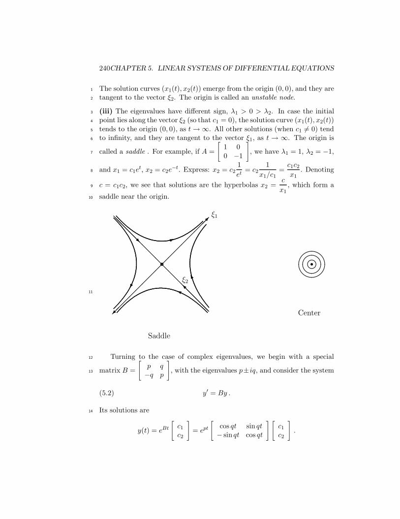
240CHAPTER 5. LINEAR SYSTEMS OF DIFFERENTIAL EQUATIONS
The solution curves (x1(t), x2(t)) emerge from the origin (0, 0), and they are1
tangent to the vector ξ2. The origin is called an unstable node.2
(iii) The eigenvalues have different sign, λ1 > 0 > λ2. In case the initial3
point lies along the vector ξ2 (so that c1 = 0), the solution curve (x1(t), x2(t))4
tends to the origin (0, 0), as t→ ∞. All other solutions (when c1 6= 0) tend5
to infinity, and they are tangent to the vector ξ1, as t → ∞. The origin is6
called a saddle . For example, if A =
[
1 0
0 −1
]
, we have λ1 = 1, λ2 = −1,7
and x1 = c1et, x2 = c2e
−t. Express: x2 = c21
et= c2
1
x1/c1=c1c2x1
. Denoting8
c = c1c2, we see that solutions are the hyperbolas x2 =c
x1, which form a9
saddle near the origin.10
��
��
��
��
��
��
��
���
@@
@@
@@
@@
@@
@@
@@
@@
cb
@@
@@I
@@
@@R
K
Y�
*
Saddle
ξ1
ξ2
Center
ab&%'$l����
11
Turning to the case of complex eigenvalues, we begin with a special12
matrix B =
[
p q−q p
]
, with the eigenvalues p±iq, and consider the system13
y′ = By .(5.2)
Its solutions are14
y(t) = eBt
[
c1c2
]
= ept
[
cos qt sin qt− sin qt cos qt
] [
c1c2
]
.

5.5. SOLUTIONS OF PLANAR SYSTEMS NEAR THE ORIGIN 241
If p = 0, then any initial vector
[
c1c2
]
is rotated clockwise around the origin1
(infinitely many times, as t → ∞). We say that the origin is a center. If2
p < 0, the solutions spiral into the origin. The origin is called a stable spiral.3
If p > 0, we have an unstable spiral.4
Assume now that A is a 2 × 2 matrix with complex eigenvalues p ± iq,5
q 6= 0. Let ξ = u+iv be an eigenvector corresponding to p+iq, where u and6
v are real vectors. We have A(u+iv) = (p+iq)(u+iv) = pu−qv+i(pv+qu),7
and separating the real and imaginary parts8
Au = pu− qv, and Av = qu+ pv .(5.3)
We form a 2 × 2 matrix P = [u v], which has the vectors u and v as its9
columns. Then, using (5.3)10
AP = [Au Av] = [pu− qv qu+ pv] = [u v]
[
p q−q p
]
= PB ,
where B is the special matrix considered above. We now make a change of11
variables x = Py, transforming (5.1) to12
Py′ = APy = PBy ,
and then to the system (5.2), that we have analyzed above (P−1, the inverse13
of P exists, because the vectors u and v are linearly independent, which is14
justified in the exercises). We conclude that the origin is a center if p = 0,15
a stable spiral if p < 0, and an unstable spiral if p > 0. If the determinant16
|P | > 0, the motion on these curves is clockwise, and in case |P | < 0, the17
motion is counterclockwise. (Recall that the solution curves of y′ = By18
move clockwise.)19
cba�U
�
Stable spiral Unstable spiral
cba K
�
�
�
20
242CHAPTER 5. LINEAR SYSTEMS OF DIFFERENTIAL EQUATIONS
One often denotes the unknown functions by x(t) and y(t). Then the1
system (5.1) takes the form2
dxdt = a11x+ a12y
dydt = a21x+ a22y .
Dividing the second equation by the first, we can write this system as a3
single equation4
dy
dx=a21x+ a22y
a11x+ a12y,
although one can no longer distinguish the direction along the integral5
curves.6
5.5.1 Linearization and the Hartman-Grobman Theorem7
We now briefly discuss nonlinear planar systems. Chapter 6 will be entirely8
devoted to nonlinear systems.9
Suppose that a nonlinear system (for x = x(t) and y = y(t))10
x′ = f(x, y)(5.4)
y′ = g(x, y) ,
with differentiable functions f(x, y) and g(x, y), has a rest point (x0, y0),11
which is defined by12
f(x0, y0) = g(x0, y0) = 0 .
By Taylor’s formula, we approximate for (x, y) near (x0, y0)13
f(x, y) ≈ fx(x0, y0)(x− x0) + fy(x0, y0)(y − y0) ,
g(x, y) ≈ gx(x0, y0)(x− x0) + gy(x0, y0)(y − y0) .
Letting x−x0 = u and y−y0 = v, with x′ = u′ and y′ = v′, we approximate14
the system (5.4) by the linear system15
u′ = fx(x0, y0)u+ fy(x0, y0)v(5.5)
v′ = gx(x0, y0)u+ gy(x0, y0)v
This approximation is valid for (u, v) close to (0, 0), which corresponds to16
(x, y) being near (x0, y0). One calls (5.5) the linearized system. Its matrix17
A =
[
fx(x0, y0) fy(x0, y0)gx(x0, y0) gy(x0, y0)
]

5.5. SOLUTIONS OF PLANAR SYSTEMS NEAR THE ORIGIN 243
is called the Jacobian matrix. We analyzed the behavior of linear systems1
near the rest point (0, 0) in the preceding section. The natural question2
is whether the picture near (0, 0) for the linearized system (5.4) remains3
similar for the nonlinear system (5.4) near (x0, y0). The Hartman-Grobman4
theorem says that this is the case if the Jacobian matrix A does not have5
purely imaginary or zero eigenvalues. So that if the linearized system has a6
stable or unstable node, or a stable or unstable spiral, or a saddle at (0, 0),7
the picture remains similar for the nonlinear system near (x0, y0). On the8
other hand, in case of a center, the picture may be different.9
The Hartman-Grobman theorem also holds for n × n matrices, and the10
rest point which does not have purely imaginary or zero eigenvalues is called11
hyperbolic. For the proof, and the precise statement, see the book of M.W.12
Hirsh and S. Smale [13].13
Example 1 The system14
x′ = −y − x(
x2 + y2)
(5.6)
y′ = x− y(
x2 + y2)
has a unique rest point at x0 = 0, y0 = 0. Indeed, to find the rest points we15
solve16
−y − x(
x2 + y2)
= 0
x− y(
x2 + y2)
= 0 .
Multiplying the first equation by x, the second one by y, and adding the17
results gives18
−(
x2 + y2)2
= 0 ,
or x = y = 0. The linearized system at the rest point (0, 0),19
u′ = −v(5.7)
v′ = u ,
has a center at (0, 0), and its trajectories are circles around (0, 0). The20
Hartman-Grobman theorem does not apply. It turns out that the trajec-21
tories of (5.6) spiral into (0, 0) (so that (0, 0) is a stable spiral). Indeed,22
multiplying the first equation of (5.6) by x, the second one by y, adding23
the results, and calling ρ = x2 + y2, we see that 12ρ
′ = −ρ2. This gives24
ρ(t) = 12t+c → 0, as t→ ∞.25

244CHAPTER 5. LINEAR SYSTEMS OF DIFFERENTIAL EQUATIONS
Example 2 The system1
x′ = −y + xy2(5.8)
y′ = x− x2y
has a rest point (0, 0). The linearized system at the rest point (0, 0) is again2
given by (5.7), so that (0, 0) is a center. We claim that (0, 0) is a center3
for the original system (5.8) too. Indeed, multiplying the first equation4
in (5.8) by x, the second one by y, and adding the results, we see that5
d
dt
(
x2 + y2)
= 0, or6
x2 + y2 = c ,
and all trajectories are circles around the origin.7
The system (5.8) has another rest point: (1, 1). The Jacobian matrix at8
(1, 1) is
[
1 1
−1 −1
]
. It has zero as a double eigenvalue, and so it does not9
belong to any of the types of the rest points that we considered.10
Example 3 The rest points of the system11
x′ = 2x− y + 2(5.9)
y′ = xy
are (0, 2) and (−1, 0). (xy = 0 implies that either x = 0, or y = 0.) The12
Jacobian matrix at (0, 2) is
[
2 −1
2 0
]
. Its eigenvalues are 1± i, so that the13
linearized system has an unstable spiral at (0, 0). By the Hartman-Grobman14
theorem, solutions of (5.9) spiral out of (0, 2). The Jacobian matrix at15
(−1, 0) is
[
2 −10 −1
]
. Its eigenvalues are 2 and −1. The linearized system16
has a saddle at (0, 0), and by the Hartman-Grobman theorem, the system17
(5.9) has a saddle at (−1, 0).18
5.5.2 Phase Plane and the Prufer Transformation19
We saw that some 2 × 2 systems can be transformed into a single second20
order equation. Often one transforms the opposite way. For example, in the21
equation22
y′′(t) − a(t)y(t) = 0(5.10)
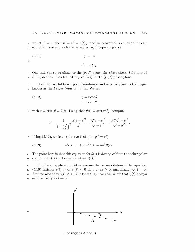
5.5. SOLUTIONS OF PLANAR SYSTEMS NEAR THE ORIGIN 245
we let y′ = v, then v′ = y′′ = a(t)y, and we convert this equation into an1
equivalent system, with the variables (y, v) depending on t :2
y′ = v(5.11)
3
v′ = a(t)y .
One calls the (y, v) plane, or the (y, y′) plane, the phase plane. Solutions of4
(5.11) define curves (called trajectories) in the (y, y′) phase plane.5
It is often useful to use polar coordinates in the phase plane, a technique6
known as the Prufer transformation. We set7
y = r cos θ(5.12)
y′ = r sin θ ,
with r = r(t), θ = θ(t). Using that θ(t) = arctan y′
y , compute8
θ′ =1
1 +(
y′
y
)2
y′′y − y′2
y2=y′′y − y′2
y2 + y′2=a(t)y2 − y′2
y2 + y′2.
Using (5.12), we have (observe that y2 + y′2 = r2)9
θ′(t) = a(t) cos2 θ(t) − sin2 θ(t) .(5.13)
The point here is that this equation for θ(t) is decoupled from the other polar10
coordinate r(t) (it does not contain r(t)).11
To give an application, let us assume that some solution of the equation12
(5.10) satisfies y(t) > 0, y′(t) < 0 for t > t0 ≥ 0, and limt→∞ y(t) = 0.13
Assume also that a(t) ≥ a1 > 0 for t > t0. We shall show that y(t) decays14
exponentially as t → ∞.15
6
-` ` ` ` ` ` `A
By
y′
The regions A and B
16

246CHAPTER 5. LINEAR SYSTEMS OF DIFFERENTIAL EQUATIONS
We are given that the trajectory (y(t), y′(t)) lies in the fourth quadrant1
of the phase plane. Consider the line θ = 2π − ε, or2
y′ = tan (2π − ε) y = − tan ε y(5.14)
in the fourth quadrant of the phase plane (the dashed line in the picture).3
We claim that for ε small, the trajectory (y(t), y′(t)) cannot go above this4
line (or into the region B in the picture). Indeed, assuming the contrary, we5
can find6
θ(t) ∈ (2π − ε, 2π) ,(5.15)
with ε small, so that cos θ(t) ≈ 1 and sin θ(t) ≈ 0. It follows from (5.13)7
that8
θ′(t) >1
2a1 .(5.16)
The function θ(t) is increasing, which implies that (5.16) continues to hold,9
so long as (5.15) does. Then at some finite time t1, we have θ(t1) = 2π, which10
corresponds to y′(t1) = 0, contradicting our assumption that y′(t) < 0 for11
all t. It follows that the trajectory has to stay below the dashed line (or in12
the region A), so that13
y′(t) < − tan ε y .
Integrating this inequality over (t0, t), we conclude14
y(t) < y(t0)e− tan ε (t−t0) ,
which implies the exponential decay.15
5.5.3 Problems16
I.17
1. Consider a 2 × 2 system18
x′ = Ax .(5.17)
Assume that λ1 is repeated eigenvalue of A (λ2 = λ1), which has two linearly19
independent eigenvectors. Show that the solutions are x(t) = eλ1tc, which20
are straight lines through the origin in the x1x2-plane (c is an arbitrary21
vector). (If λ1 < 0, solutions along all of these lines tend to the origin, as22
t → ∞, and we say that the origin is a stable degenerate node. If λ1 > 0,23
the origin is called an unstable degenerate node.)24
2. Assume that λ1 is repeated eigenvalue of A (λ2 = λ1), which has only25
one linearly independent eigenvector ξ. If λ1 < 0 show that all solutions of26

5.5. SOLUTIONS OF PLANAR SYSTEMS NEAR THE ORIGIN 247
(5.17) approach the origin in the x1x2-plane as t→ ∞, and they are tangent1
to ξ (again one says that the origin is a stable degenerate node). If λ1 > 02
show that all solutions of (5.17) approach the origin in the x1x2-plane as3
t→ −∞, and they are tangent to ξ (an unstable degenerate node).4
Hint: Recall that using the generalized eigenvector η, the general solution5
of (5.17) is6
x(t) = c1eλ1t ξ + c2
(
teλ1t ξ + eλ1tη)
.
7
3. Consider the system8
dx
dt= ax+ by(5.18)
9
dy
dt= mx+ ny ,
where a, b, m and n are real numbers.10
(i) Put this system into the form11
(mx+ ny) dx− (ax+ by)dy = 0 .(5.19)
Hint: Expressdy
dx.12
(ii) Assume that (0, 0) is a center for (5.18). Show that the equation (5.19)13
is exact, and solve it.14
Hint: One needs n = −a (and also that b and m have the opposite signs),15
in order for the matrix of (5.18) to have purely imaginary eigenvalues.16
Answer. mx2 + nxy − by2 = c, a family of closed curves around (0, 0).17
(iii) Justify that the converse statement is not true.18
Hint: For example, if one takes a = 1, b = 1, m = 3, and n = −1, then the19
equation (5.19) is exact, but (0, 0) is a saddle.20
II. Identify the rest point at the origin (0, 0). Sketch the integral curves21
near the origin, and indicate the direction in which they are traveled for22
increasing t.23
1. x′ =
[
3 22 3
]
x. Answer. Unstable node.24
2. x′ =
[
−2 14 1
]
x. Answer. Saddle.25

248CHAPTER 5. LINEAR SYSTEMS OF DIFFERENTIAL EQUATIONS
3. x′ =
[
0 1−4 0
]
x. Answer. Center.1
4.2x′ = 2x+ 4y
y′ = −5x− 7y .
Answer. Stable node. (Observe that the variables here are x and y, rather3
than x1 and x2.)4
5.5
dxdt = x − 2y
dydt = 4x− 3y .
Answer. Stable spiral.6
6.dy
dx=
x− y
4x+ y.7
Hint: Convert to a system form for x(t) and y(t), with A =
[
1 −1
4 1
]
.8
Answer. Unstable spiral.9
7. x′ =
[
−1 5−2 1
]
x. Answer. Center.10
8.dy
dx=x
y. Answer. Saddle. Solution: y2 − x2 = c.11
9. x′ =
[
−3 0
0 −3
]
x.12
Answer. Stable degenerate node. Solution: x1(t) = c1e−3t, x2(t) = c2e
−3t.13
10.dy
dx=y
x. Answer. Degenerate node.14
11. x′ =
[
1 1
α 1
]
x, α is a constant.15
Answer. Saddle for α > 1, unstable node for 0 < α < 1, unstable degenerate16
node when α = 0, unstable spiral if α < 0.17
III. Find all of the rest points for the following systems, and identify their18
type, for both the corresponding linearized system and the original system.19
20

5.5. SOLUTIONS OF PLANAR SYSTEMS NEAR THE ORIGIN 249
1.1 x′ = 2x+ y2 − 1
y′ = 6x− y2 + 1 .
Answer. (0, 1) is a saddle, (0,−1) is an unstable spiral for both systems.2
2.3
x′ = y − 2
y′ = x2 − 2y .
Answer. (2, 2) is a saddle, (−2, 2) is a stable spiral for both systems.4
3.5
x′ = y − x
y′ = (x− 2)(y + 1) .
Answer. (−1,−1) is a stable node, (2, 2) is a saddle for both systems.6
4.7
x′ = −3y + x(
x2 + y2)
y′ = 3x+ y(
x2 + y2)
.
Answer. (0, 0) is a center for the linearized system, and an unstable spiral8
for the nonlinear system.9
IV. 1. (i) Justify the formula for differentiation of a determinant10
d
dt
∣
∣
∣
∣
∣
a(t) b(t)c(t) d(t)
∣
∣
∣
∣
∣
=
∣
∣
∣
∣
∣
a′(t) b′(t)c(t) d(t)
∣
∣
∣
∣
∣
+
∣
∣
∣
∣
∣
a(t) b(t)c′(t) d′(t)
∣
∣
∣
∣
∣
.
(ii) Consider a system11
x′ = A(t)x ,(5.20)
with a 2 × 2 matrix A = [aij(t)]. Let X(t) =
[
x11(t) x12(t)x21(t) x22(t)
]
be its12
fundamental matrix, so that the vectors
[
x11(t)x21(t)
]
and
[
x12(t)x22(t)
]
are two13
linearly independent solutions of (5.20). The determinant W (t) = |X(t)| is14
called the Wronskian of (5.20). Show that for any number t015
W (t) = W (t0)e
∫ t
t0trA(s) ds
,(5.21)
where the trace trA(t) = a11(t) + a22(t).16

250CHAPTER 5. LINEAR SYSTEMS OF DIFFERENTIAL EQUATIONS
Hint: Calculate1
W ′ =
∣
∣
∣
∣
∣
x′11(t) x′12(t)x21(t) x22(t)
∣
∣
∣
∣
∣
+
∣
∣
∣
∣
∣
x11(t) x12(t)x′21(t) x′22(t)
∣
∣
∣
∣
∣
.(5.22)
Using properties of determinants, calculate2
∣
∣
∣
∣
∣
x′11(t) x′12(t)
x21(t) x22(t)
∣
∣
∣
∣
∣
=
∣
∣
∣
∣
∣
a11x11 + a12x21 a11x12 + a12x22
x21 x22
∣
∣
∣
∣
∣
3
=
∣
∣
∣
∣
∣
a11x11 a11x12
x21 x22
∣
∣
∣
∣
∣
= a11W .
Similarly, the second determinant in (5.22) is equal to a22W . Then4
W ′ = (a11 + a22)W = trAW .
(iii) Show that the formula (5.21), called Liouville’s formula, holds also in5
case of n× n systems (5.20).6
2. Consider the system7
x′ = Ax ,(5.23)
where A is an n × n matrix with constant entries. Show that eAt is the8
normalized fundamental solution matrix.9
Hint: Recall that x(t) = eAtc gives the general solution. Choosing the first10
entry of the vector c to be one, and all other entries zero, conclude that the11
first column of eAt is a solution of (5.23).12
3. (i) Consider the system13
x′ = A(t)x ,(5.24)
where A(t) is an n×n matrix with all entries continuous on (t0,∞). Derive14
the following Wazewski inequality (for t > t0)15
||x(t0)||e∫ t
t0λ(s)ds ≤ ||x(t)|| ≤ ||x(t0)||e
∫ t
t0Λ(s) ds
,
where λ(t) and Λ(t) are the smallest and the largest eigenvalues of the matrix16
12
(
A+ AT)
, and ||x(t)|| is the length of the vector x(t).17
Hint: Observe that the matrix 12
(
A+ AT)
is symmetric, so that all of its18
eigenvalues are real. Then integrate the inequality19
d
dt||x(t)||2 =
d
dtxTx = xT
(
A+ AT)
x ≤ 2Λ(t)||x(t)||2 .
(ii) Let A(t) =
[
−et t3
−t3 −3
]
. Show that all solutions of (5.24) tend to zero,20
as t→ ∞.21

5.6. CONTROLLABILITY AND OBSERVABILITY 251
5.6 Controllability and Observability1
5.6.1 The Cayley-Hamilton Theorem2
Recall that the eigenvalues λ1 , λ2 , . . . , λn of an n× n matrix A are roots of3
the characteristic equation4
|A− λI | = 0 .
The determinant |A − λI | is an n-th degree polynomial in λ, called the5
characteristic polynomial :6
p(λ) = a0λn + a1λ
n−1 + · · ·+ an−1λ+ an ,
with some coefficients a0 , a1 , . . . , an.7
Cayley-Hamilton Theorem Any square matrix A is a root of its own8
characteristic polynomial, so that9
p(A) = a0An + a1A
n−1 + · · ·+ an−1A + anI = O ,
where O is the zero matrix.10
Proof: We begin by assuming that the matrix A is diagonalizable, so that11
A = S diag (λ1 , λ2 , . . . , λn)S−1. Here diag (λ1 , λ2 , . . . , λn) is the diagonal12
matrix with entries λ1 , λ2 , . . . , λn, and S is a non-singular matrix. Recall13
that Ak = S diag(
λk1 , λ
k2 , . . . , λ
kn
)
S−1, for any integer k, and then14
p(A) = S diag (p(λ1), p(λ2) , . . . , p(λn))S−1 = SOS−1 = O .
The proof for the general case can be given by a continuity argument,15
which we sketch next. An arbitrarily small perturbation of any matrix A16
produces a matrix B with distinct eigenvalues, and hence diagonalizable17
(over complex numbers). We have p(B) = O, by above, while the matrix18
p(A) is arbitrarily close to p(B), and therefore p(A) = O. ♦19
We shall use the following corollary of this theorem.20
Proposition 5.6.1 (i) For any integer s ≥ n, the matrix As is a linear21
combination of I, A , A2 , . . . , An−1.22
(ii) The matrix eA is also a linear combination of I, A , A2 , . . . , An−1.23
Proof: Performing the long division of polynomials, write24
λs = p(λ)q(λ) + r(λ) ,
252CHAPTER 5. LINEAR SYSTEMS OF DIFFERENTIAL EQUATIONS
where q(λ) is a polynomial of degree s − n, and r(λ) is a polynomial of1
degree n − 1, r(λ) = r0λn−1 + · · · + rn−2λ + rn−1, with some coefficients2
r0 , . . . , rn−2 , rn−1. Then, using the Cayley-Hamilton theorem3
As = p(A)q(A) + r(A) = r(A) = r0An−1 + · · ·+ rn−2A+ rn−1I ,
concluding the proof of the first part. The second part follows from the4
definition of the exponential eA =∑∞
s=0As
s! . ♦5
5.6.2 Controllability of Linear Systems6
We consider the linear system7
x′ = Ax+ Bu(t) .(6.1)
Here x(t) ∈ Rn is the unknown vector function, with the components x1(t),8
x2(t), . . . , xn(t), while the vector function u(t) ∈ Rm, m ≥ 1, is at our9
disposal, the control. The n × n matrix A and the n × m matrix B have10
constant coefficients, and are given. If we regard u(t) as known, then solving11
the non-homogeneous system (6.1) with the initial condition x(0) = x0 gives12
x(t) = eAtx0 +
∫ t
0eA(t−s)Bu(s) ds .
One says that the integral curve x(t) is generated by the control vector u(t),13
with x(0) = x0.14
Definition We say that the system (6.1) is controllable if, given any duration15
p and two arbitrary points x0, xp ∈ Rn, there exists a continuous vector16
function u(t) from [0, p] to Rm, such that the integral curve x(t) generated17
by u(t) with x(0) = x0 satisfies x(p) = xp.18
In other words, controllability means that19
xp = eApx0 +
∫ p
0eA(p−s)Bu(s) ds ,
for some u(t), or20
∫ p
0eA(p−t)Bu(t) dt = xp − eApx0 .(6.2)
We form Kalman’s controllability matrix21
K =(
B AB A2B . . . An−1B)
.

5.6. CONTROLLABILITY AND OBSERVABILITY 253
(The first m columns of K are those of B, the next m columns are given1
by AB, and so on.) The type (or size) of K is n × nm. Observe that2
rankK ≤ n.3
Theorem 5.6.1 (R. Kalman) The system (6.1) is controllable if and only4
if5
rankK = n .
Proof: Define the matrices6
C(t) = eA(p−t)B , and G =
∫ p
0C(t)CT (t) dt ,
where CT is the transpose of C. The matrix function C(t) is of type n×m,7
while the constant matrix G is of type n × n.8
We claim that controllability of (6.1) is equivalent to G being invertible.9
Assume that G is invertible. We shall show that the vector10
u(t) = BT eAT (p−t)G−1
(
xp − eApx0
)
gives the desired control. Indeed,11
∫ p
0eA(p−t)Bu(t) dt =
(∫ p
0eA(p−t)BBT eA
T (p−t) dt
)
G−1(
xp − eApx0
)
12
= GG−1(
xp − eApx0
)
= xp − eApx0 ,
and the system (6.1) is controllable by (6.2).13
Conversely, assume now that the system (6.1) is controllable. We wish to14
show that G is invertible. Assume, on the contrary, that G is not invertible.15
Then its rows are linearly dependent. Therefore there exists a non-zero16
column vector v ∈ Rn, such that17
vTG = 0 .(6.3)
(If v1, v2 , . . . , vn are the entries of v, while g1, g2 , . . . , gn are the rows of G,18
then (6.3) is equivalent to v1g1 + v2g2 + · · ·+ vngn = 0.) Then19
0 = vTGv =
∫ p
0vTC(t)CT (t)v dt =
∫ p
0||vTC(t)||2 dt .
It follows that20
vTC(t) = 0 , for all t ∈ [0, p] .(6.4)

254CHAPTER 5. LINEAR SYSTEMS OF DIFFERENTIAL EQUATIONS
Because the system (6.1) is controllable, for any x0 and xp we can find u(t)1
so that (6.2) holds, or2
∫ p
0C(t)u(t) dt = xp − eApx0 .
Choose now x0 = 0, and any xp such that vTxp 6= 0. Using (6.4), we have3
0 =
∫ p
0vTC(t)u(t) dt = vTxp 6= 0 ,
a contradiction, proving that G is invertible.4
We complete the proof by showing that G being invertible is equivalent5
to rankK = n. Assume that G is not invertible. Then (6.4) holds for some6
vector v 6= 0, as we saw above. Write7
vTC(t) = vT eA(p−t)B =∞∑
i=0
vTAiB
i!(p− t)i = 0 , for all t ∈ [0, p] .(6.5)
It follows that vTAiB = 0 for all i ≥ 0, which implies that vTK = 0.8
(Recall that vTK is a linear combination of the rows of K.) This means9
that the rows of K are linearly dependent, so that rankK < n. By the10
logical contraposition, if rankK = n, then G is invertible.11
Conversely, assume that rankK < n. Then we can find a non-zero vector12
v ∈ Rn, such that13
vTK = 0 .
By the definition of K this implies that vTAiB = 0 for i = 0, 1, . . . , n − 1.14
By the Proposition 5.6.1 we conclude that vTAiB = 0 for all i ≥ 0. Then15
by (6.5), vTC(t) = 0. It follows that16
vTG =
∫ p
0vTC(t)CT (t) dt = 0 ,
so that that the rows of G are linearly dependent, and then G is not invert-17
ible. Hence, if G is invertible, then rankK = n. ♦18
19
Example 1 The system (we use (x, y) instead of (x1, x2))20
x′ = u(t)
y′ = x

5.6. CONTROLLABILITY AND OBSERVABILITY 255
is controllable. Here B =
[
1
0
]
, A =
[
0 0
1 0
]
, K =
[
1 0
0 1
]
, rankK = 2.1
2
Writing this system as a single equation y′′ = u(t), we see that the height3
y(t) of an object, and its velocity y′(t) = x(t), can be jointly controlled with4
a jet pack (which controls the acceleration function u(t)).5
Example 2 The system6
x′ = u(t)
y′ = −u(t)
is not controllable. Here B =
[
1
−1
]
, A =
[
0 0
0 0
]
, K =
[
1 0
−1 0
]
, and7
rankK = 1.8
Writing this system as (x+ y)′ = 0, we conclude that x(t) + y(t) =9
constant, independently of the control u(t). It follows that, for example,10
the point (1, 1) cannot be possibly be steered to (2,−3), since 1+1 6= 2−3.11
5.6.3 Observability12
We now consider a control-observation process13
x′ = Ax +Bu(6.6)
v = Cx .
Here the first equation corresponds to using the control vector u(t) to steer14
the solution x(t), as in the preceding section, so that x ∈ Rn, u ∈ Rm, and15
we assume that the given matrices A of type n×n and B of type n×m have16
constant entries. The second equation involves a q × n observation matrix17
C with constant entries, and an observation vector v(t) ∈ Rq. (If C is the18
n × n identity matrix, then v(t) is just x(t).)19
Definition We say that the system (6.6) is observable if for every time20
interval (t0, t1) the knowledge of the input-output pair (u(t), v(t)) over (t0, t1)21
uniquely determines the initial state x(t0).22
Define the following n× n matrix function23
P (t) =
∫ t
t0
eAT (s−t0)CTCeA(s−t0) ds .
Lemma 5.6.1 The system (6.6) is observable if and only if P (t) is invert-24
ible for all t > t0.25

256CHAPTER 5. LINEAR SYSTEMS OF DIFFERENTIAL EQUATIONS
Proof: Assume that the system (6.6) is observable, but P (t1) is singular,1
at some t1 > t0, contrary to the statement of the lemma. Then we can find2
a non-zero vector x0 ∈ Rn satisfying P (t1)x0 = 0. It follows that3
0 = xT0 P (t1)x0 =
∫ t1
t0
||CeA(t−t0)x0||2 ds ,
and then4
CeA(t−t0)x0 = 0 , for all t ∈ (t0, t1) .(6.7)
Set u(t) ≡ 0. Then x(t) = eA(t−t0)x(t0) is the corresponding solution of5
(6.6), for any initial vector x(t0). We have, in view of (6.7),6
v(t) = CeA(t−t0)x(t0) = CeA(t−t0) (x(t0) + αx0) ,
for any constant α. Hence, the input-output pair (0, v(t)) does not determine7
uniquely the initial state at t0, contrary to the assumption of observability.8
It follows that P (t) is invertible for all t > t0.9
Conversely, assume that P (t1) is invertible, at some t1 > t0. Express10
v(t) = CeA(t−t0)x(t0) + C
∫ t
t0
eA(t−s)Bu(s) ds .
Multiplying both sides by eAT (t−t0)CT , and integrating over (t0, t1) gives11
P (t1)x(t0) =∫ t1t0eA
T (t−t0)CT v(t) dt
− ∫ t1t0eA
T (t−t0)CT(
C∫ tt0eA(t−s)Bu(s) ds
)
dt .
Since P (t1) is invertible, x(t0) is uniquely determined by the values of u(t)12
and v(t) over the interval (t0, t1), and so (6.6) is observable. ♦13
We now consider Kalman’s observability matrix, of type qn× n,14
N =
C
CA...CAn−1
.
(Its first q rows are those of C, CA gives the next q rows, and so on.) Clearly,15
rankN ≤ n.16
Theorem 5.6.2 (R. Kalman) The system (6.6) is observable if and only if17
rankN = n.18

5.6. CONTROLLABILITY AND OBSERVABILITY 257
Proof: If the rank of N is less than n, its columns are linearly dependent,1
so that for some non-zero vector a ∈ Rn we have Na = 0, or equivalently2
Ca = CAa = · · · = CAn−1a = 0 .
The Proposition 5.6.1 implies that3
CeA(s−t0)a = 0 , for all s > t0 .
Multiplying by eAT (s−t0)CT , and integrating over (t0, t), we conclude that4
P (t)a = 0 for all t > t0, which implies that P (t) is not invertible, and the5
system (6.6) is not observable by Lemma 5.6.1. By logical contraposition, if6
the system (6.6) is observable, then rankN = n.7
Conversely, assume that rankN = n. Let x(t0) and x(t0) be two initial8
states corresponding to the same input-output pair (u(t), v(t)). We wish9
to show that x(t0) = x(t0), so that the system (6.6) is observable. The10
difference z(t) ≡ x(t)−x(t) satisfies z′ = Az, and also Cz = Cx(t)−Cx(t) =11
v(t) − v(t) = 0, so that12
CeA(t−t0) [x(t0) − x(t0)] = 0 , for all t ≥ t0 .
(Notice that z(t) = eA(t−t0)z(t0).) By taking the first n− 1 derivatives, and13
setting t = t0, we conclude14
CAk [x(t0) − x(t0)] = 0 , k = 0, 1, . . . , n− 1 ,
which is equivalent to N [x(t0) − x(t0)] = 0. Since N has full rank, its15
columns are linearly independent, and therefore x(t0)− x(t0) = 0. ♦16
Notice that observability does not depend on the matrix B.17
Problems18
1. Calculate the controllability matrix K, and determine if the system is19
controllable.20
(i)21 x′1 = x1 + 2x2 + u(t)
x′2 = 2x1 + x2 + u(t) .
Answer. K =
[
1 3
1 3
]
, rankK = 1, not controllable.22
(ii)23

258CHAPTER 5. LINEAR SYSTEMS OF DIFFERENTIAL EQUATIONS
x′ = x1 + 2x2 − 2u(t)
x′2 = 2x1 + x2 .
Answer. K =
[
−2 −2
0 −4
]
, rankK = 2, controllable.1
2. Let A =
[
1 24 3
]
. Calculate eA.2
Hint: By the Proposition 5.6.13
eA = αA+ βI ,
for some constants α and β. The eigenvalues of A are −1 and 5, which4
implies that the eigenvalues of eA are e−1 and e5, while the eigenvalues of5
αA + βI are −α+ β and 5α + β. It follows that6
e−1 = −α+ β
e5 = 5α+ β .
Solve this system for α and β.7
Answer. 16
[
2e5 + 4e−1 2e5 − 2e−1
4e5 − 4e−1 4e5 + 2e−1
]
.8

Chapter 61
Non-Linear Systems2
We begin this chapter with applications to ecology of two species, including3
both competing species and predator-prey interactions, and to epidemiolog-4
ical modeling. Then we study some important general aspects of non-linear5
systems, including Lyapunov’s stability and limit cycles. Finally, we include6
an in-depth presentation of periodic ecological models.7
6.1 The Predator-Prey Interaction8
In 1925, Vito Volterra’s future son-in-law, biologist Umberto D’Ancona, told9
him of the following puzzle. During the World War I, when ocean fishing10
almost ceased, the ratio of predators (like sharks) to prey (like tuna) had11
increased. Why did sharks benefit more from the decreased fishing? (While12
the object of fishing is tuna, sharks are also caught in the nets.)13
The Lotka-Volterra Equations14
Let x(t) and y(t) give respectively the numbers of prey (tuna) and predators15
(sharks), as functions of time t. Let us assume that in the absence of sharks,16
tuna would obey the Malthusian model17
x′(t) = ax(t),
with some growth rate a > 0. (It would grow exponentially, x(t) = x(0)eat.)18
In the absence of tuna, we assume that the number of sharks would decrease19
exponentially, and satisfy20
y′(t) = −cy(t),
259

260 CHAPTER 6. NON-LINEAR SYSTEMS
with some c > 0, because its other prey is less nourishing. Clearly, the1
presence of sharks will decrease the rate of growth of tuna, while tuna is2
good for sharks. The model is:3
x′(t) = a x(t)− b x(t) y(t)(1.1)
y′(t) = −c y(t) + d x(t) y(t) ,
with two more given positive constants b and d. The x(t)y(t) term is pro-4
portional to the number of encounters between sharks and tuna. These5
encounters decrease the growth rate of tuna, and increase the growth rate6
of sharks. Notice that both equations are nonlinear, and we are interested7
in solutions with x(t) > 0, and y(t) > 0. The system (1.1) represents the8
famous Lotka-Volterra model. Alfred J. Lotka was an American mathemati-9
cian, who developed similar ideas at about the same time as V. Volterra.10
A fascinating story of Vito Volterra’s life and work, and of life in Italy11
in the first half of the 20-th Century, is told in a very nice book of Judith12
R. Goodstein [14].13
Analysis of the Model14
Remember the energy being constant for a vibrating spring? We have some-15
thing similar here. It turns out that any solution (x(t), y(t)) of (1.1) satisfies16
a ln y(t) − b y(t) + c lnx(t) − d x(t) = C = constant ,(1.2)
for all time t. To justify that, let us introduce the function F (x, y) =17
a ln y − b y + c lnx − d x. We wish to show that F (x(t), y(t)) = constant.18
Using the chain rule, and expressing the derivatives from the equations (1.1),19
we have20
d
dtF (x(t), y(t)) = Fxx
′ + Fyy′ = c
x′(t)x(t)
− dx′(t) + ay′(t)y(t)
− by′(t)
21
= c(a−by(t))−d(ax(t)−bx(t)y(t))+a(−c+dx(t))−b(−cy(t)+dx(t)y(t))22
= 0 ,
proving that F (x(t), y(t)) does not change with time t.23
We assume that the initial numbers of both sharks and tuna are given:24
x(0) = x0 > 0, y(0) = y0 > 0 .(1.3)
The Lotka-Volterra system, together with the initial conditions (1.3), de-25
termines both populations (x(t), y(t)) at all time t, by the existence and26
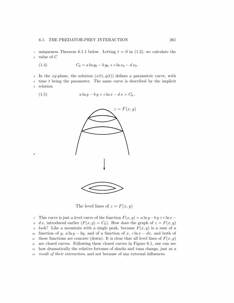
6.1. THE PREDATOR-PREY INTERACTION 261
uniqueness Theorem 6.1.1 below. Letting t = 0 in (1.2), we calculate the1
value of C2
C0 = a ln y0 − b y0 + c lnx0 − d x0 .(1.4)
In the xy-plane, the solution (x(t), y(t)) defines a parametric curve, with3
time t being the parameter. The same curve is described by the implicit4
relation5
a ln y − b y + c lnx− d x = C0 .(1.5)
?
The level lines of z = F (x, y)
z = F (x, y)
6
This curve is just a level curve of the function F (x, y) = a ln y−b y+c lnx−7
d x, introduced earlier (F (x, y) = C0). How does the graph of z = F (x, y)8
look? Like a mountain with a single peak, because F (x, y) is a sum of a9
function of y, a ln y − by, and of a function of x, c lnx − dx, and both of10
these functions are concave (down). It is clear that all level lines of F (x, y)11
are closed curves. Following these closed curves in Figure 6.1, one can see12
how dramatically the relative fortunes of sharks and tuna change, just as a13
result of their interaction, and not because of any external influences.14

262 CHAPTER 6. NON-LINEAR SYSTEMS
1 2 3 4Prey
0.5
1.0
1.5
2.0
2.5
3.0
Predator
Figure 6.1: The integral curves of the Lotka-Volterra system
Properties of the Solutions1
In Figure 6.1 we present a picture of three integral curves, computed by2
Mathematica in the case when a = 0.7, b = 0.5, c = 0.3 and d = 0.2. All3
solutions are closed curves, and there is a dot in the middle (corresponding4
to a rest point at (1.5, 1.4)).5
When x0 = c/d, and y0 = a/b, or when the starting point is (c/d, a/b),6
we calculate from the Lotka-Volterra equations that x′(0) = 0, and y′(0) =7
0. The solution is then x(t) = c/d, and y(t) = a/b for all t, as follows8
by the existence and uniqueness Theorem 6.1.1, which is reviewed at the9
end of this section. The point (c/d, a/b) is called a rest point. (In the10
above example, the coordinates of the rest point were x0 = c/d = 1.5, and11
y0 = a/b = 1.4.) All other solutions (x(t), y(t)) are periodic, because they12
represent closed curves. For each trajectory, there is a number T , a period,13
so that x(t+T ) = x(t) and y(t+T ) = y(t). This period changes from curve14
to curve, and it is larger the further the solution curve is from the rest point.15
(This monotonicity property of the period was proved only around 1985 by16
Franz Rothe [26], and Jorg Waldvogel [34].) The motion along the integral17
curves is counterclockwise (at the points due east of the rest point, one has18
x′ = 0, and y′ > 0).19
Divide the first of the Lotka-Volterra equations by the solution x(t), and20
then integrate over its period T :21
x′(t)x(t)
= a− by(t) ,
22∫ T
0
x′(t)x(t)
dt = aT − b
∫ T
0y(t) dt .

6.1. THE PREDATOR-PREY INTERACTION 263
But
∫ T
0
x′(t)x(t)
dt = lnx(t) |T0
= 0, because x(T ) = x(0), by periodicity. It1
follows that2
1
T
∫ T
0y(t) dt = a/b .
Similarly, we derive3
1
T
∫ T
0x(t) dt = c/d .
We have a remarkable fact: the averages of both x(t) and y(t) are the same4
for all solutions. Moreover, these averages are equal to the coordinates of5
the rest point.6
The Effect of Fishing7
Extensive fishing decreases the growth rate of both tuna and sharks. The8
new model is9
x′(t) = (a− α)x(t) − b x(t) y(t)
y′(t) = −(c+ β)y(t) + d x(t) y(t) ,
where α and β are two more given positive constants, related to the intensity10
of fishing. (There are other ways to model fishing.) As before, we compute11
the average numbers of both tuna and sharks12
1
T
∫ T
0x(t) dt = (c+ β)/d,
1
T
∫ T
0y(t) dt = (a− α)/b .
We see an increase for the average number of tuna, and a decrease for the13
sharks, as a result of moderate amount of fishing (assuming that α < a).14
Conversely, decreased fishing increases the average number of sharks, giving15
us an explanation of U. D’Ancona’s data. This result is known as Volterra’s16
principle. It applies also to insecticide treatments. If such a treatment17
destroys both the pests and their predators, it may be counter-productive,18
and produce an increase of the number of pests!19
Biologists have questioned the validity of both the Lotka-Volterra model,20
and of the way we have accounted for fishing (perhaps, they cannot accept21
the idea of two simple differential equations ruling the oceans). In fact, it is22
more common to model fishing, using the system23
x′(t) = ax(t) − b x(t) y(t)− h1(t)
y′(t) = −cy(t) + d x(t) y(t)− h2(t) ,
with some given positive functions h1(t) and h2(t).24

264 CHAPTER 6. NON-LINEAR SYSTEMS
The Existence and Uniqueness Theorem for Systems1
Similarly to the case of one equation, we can expect (under some mild con-2
ditions) that an initial value problem for a system of differential equations3
has a solution, and exactly one solution.4
Theorem 6.1.1 Consider an initial value problem for the system5
x′(t) = f(t, x(t), y(t)) , x(t0) = x0
y′(t) = g(t, x(t), y(t)) , y(t0) = y0 ,
with given numbers x0 and y0. Assume that the functions f(t, x, y), g(t, x, y),6
and their partial derivatives fx, fy, gx and gy are continuous in some three-7
dimensional region containing the point (t0, x0, y0). Then this system has a8
unique solution (x(t), y(t)), defined on some interval |t− t0| < h.9
The statement is similar in case of n equations10
x′i = fi(t, x1, x2, . . . , xn) , xi(t0) = x0i , i = 1, 2, . . . , n ,
where x0i are given numbers. If the functions fi, and all of their partial11
derivatives ∂fi∂xj
are continuous in some n + 1-dimensional region containing12
the initial point(
t0, x01, x
02, . . . , x
0n
)
, then this system has a unique solution13
(x1(t), x2(t), . . . , xn(t)), defined on some interval |t− t0| < h.14
One can find the proof in the book of D.W. Jordan and P. Smith [15].15
6.2 Competing Species16
-
6
t
x
a
Solution curves for the logistic model
17

6.2. COMPETING SPECIES 265
When studying the logistic population model (here x = x(t) > 0 gives1
the number of rabbits)2
x′ = x(a− x) ,(2.1)
we were able to analyze the behavior of solutions, even without solving3
this equation. Indeed, the quadratic polynomial x(a − x) is positive for4
0 < x < a, and then x′(t) > 0, so that x(t) is an increasing function.5
The same quadratic is negative for x > a, and so x(t) is decreasing in this6
range. If x(0) = a, then x(t) = a, for all t, by the uniqueness part of the7
existence and uniqueness Theorem 1.8.1. So that the solution curves look as8
in the figure above. Here a is the carrying capacity, which is the maximum9
sustainable number of rabbits. (In Chapter 2 the logistic model had the10
form x′ = ax − bx2. Letting here x = 1b z, gives z′ = az − z2, which is the11
equation (2.1).)12
If x(0) is small, the solution grows exponentially at first, and then the13
rate of growth gets smaller and smaller, which is a typical logistic curve.14
The point x = a is a rest point, and we can describe the situation by the15
following one-dimensional picture (the arrows indicate that solutions tend16
to a):17
-c ca0
x- �
The logistic equation has a stable rest point x = a, and an unstable one x = 0
18
The rest point x = a is called stable rest point, because solutions of the19
equation (2.1), with x(0) close to a, tend to a as t → ∞ (limt→∞ x(t) = a).20
The point x = 0 is an unstable rest point, because solutions of (2.1), starting21
near x = 0, tend away from it.22
In general, the point x0 is called a rest point of the equation (x = x(t))23
x′ = g(x) ,(2.2)
with a differentiable function g(x), if g(x0) = 0. It is stable (or attractive) if24
g′(x0) < 0. The solutions of (2.2), with x(0) near x0, tend to x0 as t → ∞.25
The rest point x0 is unstable (or repellent) if g′(x0) > 0. The solutions of26
(2.2) move away from it. In case g′(x0) = 0, further analysis is needed.27

266 CHAPTER 6. NON-LINEAR SYSTEMS
Suppose now that we also have a population y(t) of deer, modeled by a1
logistic equation2
y′ = y(d− y) ,
with the carrying capacity d > 0. Suppose that rabbits and deer live on the3
same tropical island, and they compete (for food, water and hiding places).4
The Lotka-Volterra model of their interaction is5
x′ = x (a− x− by)(2.3)
y′ = y (d− cx− y) .
The first equation tells us that the presence of deer effectively decreases the6
carrying capacity of rabbits (making it a − by), and the positive constant7
b quantifies this influence. Similarly, the positive constant c measures how8
detrimental the presence of rabbits is for deer. What predictions will follow9
from the model (2.3)? And how do we analyze this model, since solving the10
nonlinear system (2.3) is not possible? We shall consider the system (2.3)11
together with the initial conditions12
x(0) = α, y(0) = β .(2.4)
The given initial numbers of the animals, α > 0 and β > 0, determine the13
initial point (α, β) in the xy-plane. We claim that any solution of (2.3),14
(2.4) satisfies x(t) > 0 and y(t) > 0 for all t > 0. Indeed, write the first15
equation in (2.3) as16
x′ = A(t)x , where A(t) = a− x(t) − by(t) .
Then x(t) = α e∫ t
0A(s) ds > 0. One shows similarly that y(t) > 0. We shall17
consider the system (2.3) only in the first quadrant of the xy-plane, where18
x > 0 and y > 0.19
Similarly to the case of a single logistic equation, we look at the points20
where the right hand sides of (2.3) are zero:21
a− x− by = 0(2.5)
d− cx− y = 0 .
These equations give us two straight lines, called the null-clines of the system22
(2.3). Both of these lines have negative slopes in the (x, y) plane. In the first23
quadrant these lines may intersect either once, or not at all, depending on24

6.2. COMPETING SPECIES 267
the values of a, b, c and d, and that will determine the long turn predictions.1
The point of intersection of null-clines is a rest point. It follows that there2
is at most one rest point in the first quadrant.3
We shall denote by I the null-cline a − x − by = 0. Above this straight4
line, we have a−x− by < 0, which implies that x′(t) < 0, and the motion is5
to the left in the first quadrant. Below the null-cline I, the motion is to the6
right. We denote by II the null-cline d − cx − y = 0. Above II, y′(t) < 0,7
and the motion is down, while below II the point (x(t), y(t)) moves up.8
(For example, if a point lies above both I and II, the motion is to the left9
and down, in the “southwest” direction. If a point is above I but below10
II, the motion is northwest, etc.) The system (2.3) has the trivial solution11
(0, 0) (x = 0, and y = 0), and two semi-trivial solutions (a, 0) and (0, d).12
The solution (a, 0) corresponds to deer becoming extinct, while (0, d) means13
there are no rabbits. Observe that the semi-trivial solution (a, 0) is the x-14
intercept of the null-cline I, while the second semi-trivial solution (0, d) is15
the y-intercept of the null-cline II. The behavior of solutions, in the long16
turn, will depend on whether the null-clines intersect in the first quadrant17
or not. We consider the following cases.18
-
6
x
y
AAAAAAAAA
d
d
a/b
d/c a
d
III3 2
1��
@@R
?-
���
Non-intersecting null-clines, with the semitrivial solutions circled
19
Case 1: The null-clines do not intersect (in the first quadrant). Assume20
first that the null-cline I lies above of II, so that a/b > d and a > d/c. The21
null-clines divide the first quadrant into three regions. In the region 1 (above22
both clines), the motion is southwest, in the region 2 it is southeast, and in23

268 CHAPTER 6. NON-LINEAR SYSTEMS
the region 3 northeast. On the cline I, the motion is due south, and on the1
cline II due east. Regardless of the initial point (α, β), all trajectories tend2
to the semi-trivial solution (a, 0), as t→ ∞. (The trajectories starting in the3
region 3, will enter the region 2, and then tend to (a, 0). The trajectories4
starting in the region 2, will stay in that region and tend to (a, 0). The5
trajectories starting in the region 1, will tend to (a, 0) by either staying in6
this region, or through the region 2.)7
This case corresponds to the extinction of deer, and rabbits reaching8
their maximum sustainable number a.9
In case the null cline II lies above of I, when a/b < d and a < d/c,10
a similar analysis shows that all solutions tend to the semi-trivial solution11
(0, d), as t → ∞. So that the species, which has its null-cline on top, wins12
the competition, and drives the other one to extinction.13
Case 2: The null-clines intersect (in the first quadrant). Their point of14
intersection (a− bd
1− bc,d− ac
1 − bc) is a solution of the system (2.5), a rest point.15
Its stability depends on which of the following sub-cases hold. Observe16
that the null clines intersect the x and y axes at four points, two of which17
correspond to the semi-trivial solutions.18
-
6
x
y
d
a
HHHHHHHHHHHHHHHHHH
JJ
JJ
JJJ
JJJ
JJJJ
d
d
uIII3 4
12 ��
@@R
���
@@I
Intersecting null-clines, with the semitrivial solutions on the inside (circled)
19
Sub-case (a): The semi-trivial solutions lie on the inside (relative to the20
other two points of intersection), so that a < d/c, and d < a/b. The null21
clines divide the first quadrant into four regions. In all four regions, the22

6.2. COMPETING SPECIES 269
motion is eventually toward the rest point. Solutions starting in the region 2,1
will always stay in this region. Indeed, on the boundary between the regions2
1 and 2, the motion is due south, and on the border between the regions3
2 and 3, the trajectories travel due east. So that solutions, starting in the4
region 2, stay in this region, and they tend to the rest point (a− bd
1− bc,d− ac
1− bc).5
Similarly, solutions starting in the region 4, never leave this region, and they6
tend to the same rest point, as t→ ∞. If a solution starts in the region 1, it7
may stay in this region, and tend to the rest point, or it may enter either one8
of the regions 2 or 4, and then tend to the rest point. Similarly, solutions9
which begin in the region 3, will tend to the rest point (a− bd
1− bc,d− ac
1− bc),10
either by staying in this region, or through the regions 2 or 4 (depending on11
the initial conditions).12
This is the case of co-existence of the species. For any initial point (α, β),13
with α > 0 and β > 0, we have limt→∞
x(t) =a− bd
1− bc, and lim
t→∞y(t) =
d− ac
1 − bc.14
Sub-case (b): The semi-trivial solutions are on the outside, so that a > d/c15
and d > a/b. In the regions 2 and 4, the motion is now away from the rest16
point. On the lower boundary of the region 2, the motion is due north, and17
on the upper border, the motion is due west. So that the trajectories starting18
in the region 2, stay in this region, and tend to the semitrivial solution (0, d).19
Similarly, solutions starting in the region 4, will stay in this region, and tend20
to the semitrivial solution (a, 0). A typical solution starting in the region 1,21
will either enter the region 2 and tend to (0, d), or it will enter the region22
4 and tend to (a, 0) (this will depend on the initial conditions). The same23
conclusion holds for the region 3. The result is that one of the species dies24
out, what is known as competitive exclusion of the species. (Linearizing the25
Lotka-Volterra system (2.3) at the rest point, one calculates that the rest26
point is a saddle, in view of the Hartman-Grobman theorem. Hence, there27
is a solution curve entering the rest point, while a typical trajectory tends28
to one of the semi-trivial solutions.)29
What is the reason behind the drastic difference in the long time dy-30
namics for the above sub-cases? The second equation in (2.3) tells us that31
the effective carrying capacity of the second species is d− cx(t) < d, so that32
y(t) < d in the long run. For the first species, the effective carrying capacity33
is a− by(t), and in the sub-case (a) (when bd < a), we have34
a− by(t) > a− bd > 0 ,

270 CHAPTER 6. NON-LINEAR SYSTEMS
so that the first species can survive even when the number of the second1
species is at its maximum sustainable level. Similarly, one checks that the2
second species can survive, assuming that the number of the first species is3
at its maximum sustainable level. In this sub-case, the competing species4
do not affect each other too strongly, and so they can co-exist.5
-
6
x
y
d
a
HHHHHHHHHHHHHHHHHH
JJJ
JJJ
JJJ
JJJ
JJ
d
u
dIII3 4
12 ��
@@I
���
@@R
Intersecting null-clines, with the semitrivial solutions on the outside (circled)
6
6.3 An Application to Epidemiology7
Suppose that a group of people comes down with an infectious disease. Will8
the number of sick people grow and cause an epidemic? What measures9
should public health officials take? We shall analyze a way to model the10
spread of an infectious disease.11
Let I(t) be the number of infected people at time t that live in the12
community (sick people that are hospitalized, or otherwise removed from13
the community, do not count in I(t)). Let S(t) be the number of susceptible14
people, the ones at risk of catching the disease. The following model was15
proposed in 1927 by W.O. Kermack and A.G. McKendrick16
dS
dt= −rSI(3.1)
17
dI
dt= rSI − γI ,

6.3. AN APPLICATION TO EPIDEMIOLOGY 271
with some positive constants r and γ. The first equation reflects the fact1
that the number of susceptible people decreases, as some people catch the2
infection (and so they join the group of infected people). The rate of decrease3
of S(t) is proportional to the number of “encounters” between the infected4
and susceptible people, which in turn is proportional to the product SI . The5
number r > 0 gives the infection rate. The first term in the second equation6
tells us that the number of infected people would increase at exactly the7
same rate, if it was not for the second term. The second term, −γI , is due8
to some infected people being removed from the population (people who9
died from the disease, people who have recovered and developed immunity,10
and sick people who are isolated from the community), which decreases the11
infection rate dI/dt. The coefficient γ is called the removal rate. To the12
equations (3.1) we add the initial conditions13
S(0) = S0, I(0) = I0 ,(3.2)
with given numbers S0 - the initial number of susceptible people, and I0 -14
the initial number of infected people. Solving the equations (3.1) and (3.2),15
will give us a pair of functions (S(t), I(t)), which determines a parametric16
curve in the (S, I) plane. Alternatively, this curve can be described, if we17
express I as a function of S.18
-
6��+ JJ]
S
I
a (S0, I0)
ρSf
a(S0, I0)
�+
The solution curves of the system (3.1)19

272 CHAPTER 6. NON-LINEAR SYSTEMS
Express1
dI
dS=dI/dt
dS/dt=rSI − γI
−rSI = −1 +γ
r
1
S= −1 + ρ
1
S,
denoting γ/r = ρ. Taking the antiderivative, and using the initial conditions2
(3.2), we obtain3
I = −S + ρ lnS + I0 + S0 − ρ lnS0 .(3.3)
Depending on the initial point (S0, I0), we get a different integral curve from4
(3.3). On all of these curves, the maximum value of I is achieved at S = ρ5
( dIdS (ρ) = 0). The motion on the integral curves is from right to left, because6
we see from the first equation in (3.1) that S(t) is a decreasing function of7
time t. If the initial point (S0, I0) satisfies S0 > ρ, then the function I(t)8
grows at first, and then declines, see the picture. In this case we say that9
an epidemic occurs. If, on the other hand, the initial number of susceptible10
people is below ρ, then the number of infected people I(t) declines and tends11
to zero, and we say that the initial outbreak has been successfully contained.12
The number ρ is called the threshold value.13
To avoid an epidemic, public health officials should try to increase the14
threshold value ρ (to make it more likely that S0 < ρ), by increasing the15
removal rate γ (recall that ρ = γ/r), which is achieved by isolating sick16
people. Notice also the following harsh conclusion: if a disease kills people17
quickly, then the removal rate γ is high, and such a disease may be easier18
to contain.19
In some cases it is easy to estimate the number of people, that will get20
sick during an epidemic. Assume that I0 is so small that we can take I0 = 0,21
while S0 is a little larger than the threshold value ρ, so that S0 = ρ + ν,22
where ν > 0 is a small value. As time t increases, I(t) tends to zero, while23
S(t) approaches some final number, call it Sf (look at the integral curves24
again). We conclude from (3.3) that25
Sf − ρ lnSf = S0 − ρ lnS0 .(3.4)
The function I(S) = S − ρ lnS takes its global maximum at S = ρ. Such a26
function is almost symmetric with respect to ρ, for S close to ρ, as can be27
seen from the three term Taylor series expansion of I(S) at S = ρ. It follows28
from (3.4) that the points S0 and Sf are approximately equidistant from ρ,29
so that Sf ≈ ρ − ν. The total number of people, who will get sick during30
an epidemic is then S0 − Sf ≈ 2ν. (This fact is known as the Threshold31
Theorem of epidemiology, see for example M. Braun [5].)32

6.4. LYAPUNOV’S STABILITY 273
6.4 Lyapunov’s Stability1
We consider a nonlinear system of equations for the unknown functions x(t)2
and y(t):3
x′ = f(x, y), x(0) = α(4.1)
y′ = g(x, y), y(0) = β ,
with some given differentiable functions f(x, y) and g(x, y), and the initial4
values α and β. By the existence and uniqueness Theorem 6.1.1, the problem5
(4.1) has a unique solution.6
Recall that a point (x0, y0) is called rest point if7
f(x0, y0) = g(x0, y0) = 0 .
Clearly, the pair of constant functions x(t) = x0 and y(t) = y0 is a solution8
of (4.1). If we solve the system (4.1) with the initial data x(0) = x0 and9
y(0) = y0, then x(t) = x0 and y(t) = y0 for all t (by uniqueness of the10
solution), so that our system is at rest for all time. Now suppose that the11
initial conditions are perturbed from (x0, y0). Will our system come back to12
rest at (x0, y0)?13
A differentiable function L(x, y) is called Lyapunov’s function at (x0, y0),14
if the following two conditions hold:15
L(x0, y0) = 0 ,
L(x, y) > 0, for (x, y) in some neighborhood of (x0, y0) .
How do the level lines16
L(x, y) = c(4.2)
look, near the point (x0, y0)? If c = 0, then (4.2) is satisfied only at (x0, y0).17
If c > 0, and small, the level lines are closed curves around (x0, y0), and the18
smaller c is, the closer the level line is to (x0, y0).19
Along a solution (x(t), y(t)) of our system (4.1), Lyapunov’s function is20
a function of t: L(x(t), y(t)). Now assume that for all solutions (x(t), y(t))21
starting near (x0, y0), we have22
d
dtL(x(t), y(t))< 0 , for all t > 0 ,(4.3)
so that the function L(x, y) is decreasing along the solutions. Then one23
expects that (x(t), y(t)) → (x0, y0), as t → ∞, and we say that the rest24

274 CHAPTER 6. NON-LINEAR SYSTEMS
point (x0, y0) is asymptotically stable. (As t increases, the solution point1
(x(t), y(t)) moves to the level lines that are closer and closer to (x0, y0).)2
Using the chain rule and the equations (4.1), we rewrite (4.3) as3
d
dtL(x(t), y(t)) = Lxx
′ + Lyy′ = Lxf(x, y) + Lyg(x, y)< 0 .(4.4)
The following Lyapunov’s theorem is now intuitively clear (a proof can be4
found in the book of M.W. Hirsh and S. Smale [13]).5
Theorem 6.4.1 The rest point (x0, y0) is asymptotically stable, provided6
that there is a Lyapunov function, satisfying7
Lx(x, y)f(x, y) + Ly(x, y)g(x, y)< 0 , for all (x, y) near (x0, y0) .
-
6
x
y
(x(t), y(t))
An integral curve cutting inside the level lines of L(x, y)
'&
$%
'
&
$
%�� ��t
JJ
JJ
8
One typically assumes that (x0, y0) = (0, 0), which can always be ac-9
complished by declaring the point (x0, y0) to be the origin. Then L(x, y) =10
ax2 + cy2, with suitable positive constants a and c, is often a good choice of11
a Lyapunov’s function.12
Example 1 The system13
x′ = −2x+ xy2
y′ = −y − 3x2y
has a unique rest point (0, 0). With L(x, y) = ax2 + cy2, calculate14
d
dtL(x(t), y(t)) = 2axx′ + 2cyy′ = 2ax(−2x+ xy2) + 2cy(−y − 3x2y) .
6.4. LYAPUNOV’S STABILITY 275
If we choose a = 3 and c = 1, this simplifies to1
d
dtL(x(t), y(t)) = −12x2 − 2y2 < 0 , for all (x, y) 6= (0, 0) .
The rest point (0, 0) is asymptotically stable.2
Observe that the integral curves of this system cut inside of any ellipse3
3x2 + y2 = A, and as we vary the positive constant A, these ellipses fill out4
the entire xy-plane. It follows that all solutions of this system tend to (0, 0),5
as t→ ∞. One says that the domain of attraction of the rest point (0, 0) is6
the entire xy-plane.7
Example 2 The system8
x′ = −2x+ y4
y′ = −y + x5
has a rest point (0, 0). (There is one more rest point at(
21/19, 25/19)
.) For9
small |x| and |y|, the nonlinear terms (y4 and x5) are negligible. If we drop10
these nonlinear terms, then both of the resulting equations, x′ = −2x and11
y′ = −y, have all solutions tending to zero as t→ ∞. Therefore, we expect12
the asymptotic stability of (0, 0). Choosing L(x, y) = x2 + y2, compute13
ddtL(x(t), y(t)) = 2xx′ + 2yy′ = 2x(−2x+ y4) + 2y(−y + x5)
= −4x2 − 2y2 + 2xy4 + 2x5y < −2(x2 + y2) + 2xy4 + 2x5y
= −2r2 + 2r5 cos θ sin4 θ + 2r6 cos5 θ sin θ < 0 ,
provided that the point (x, y) belongs to a disc Bδ : x2 + y2 < δ2, with a14
sufficiently small δ, as is clear by using the polar coordinates (r is small,15
r < δ). Hence, any solution, with the initial point (x(0), y(0)) in Bδ, and16
δ sufficiently small, tends to zero as t → ∞. The rest point (0, 0) is in-17
deed asymptotically stable. Its domain of attraction includes Bδ , with δ18
sufficiently small. (If the initial point (x(0), y(0)) is not close to the origin,19
solutions of this system will typically go to infinity in finite time.)20
Example 3 If we drop the nonlinear terms in the system,21
x′ = y − x3(4.5)
y′ = −x − y5 ,
with a unique rest point at (0, 0), the resulting linear system22
x′ = y(4.6)
y′ = −x

276 CHAPTER 6. NON-LINEAR SYSTEMS
is equivalent to the harmonic oscillator x′′+x = 0, for which all solutions are1
periodic, and do not tend to zero. (The point (0, 0) is a center for (4.6).) It2
is the nonlinear terms that make the rest point (0, 0) asymptotically stable3
for the original system (4.5). Indeed, taking L(x, y) = x2 + y2, we have4
d
dtL(x(t), y(t)) = 2xx′ + 2yy′ = −2x4 − 2y6 < 0 , for all (x, y) 6= (0, 0) .
The domain of attraction of the rest point (0, 0) is the entire xy-plane.5
Example 4 The system6
x′ = −y + y(
x2 + y2)
(4.7)
y′ = x− x(
x2 + y2)
has a rest point (0, 0). Multiply the first equation by x, the second one by7
y, and add the results. Obtain:8
xx′ + yy′ = 0 ,
9
d
dt
(
x2 + y2)
= 0 ,
10
x2 + y2 = c2 .
The solution curves (x(t), y(t)) are circles around the origin. (If x(0) = a11
and y(0) = b, then x2(t)+y2(t) = a2 + b2.) If a solution starts near (0, 0), it12
stays near (0, 0), but it does not tend to (0, 0). In such a case, we say that13
the rest point (0, 0) is stable, although it is not asymptotically stable.14
Here is a more formal definition: a rest point (x0, y0) of (4.1) is called15
stable in the sense of Lyapunov if given any ε > 0 one can find δ > 0,16
so that the solution curve (x(t), y(t)) lies within the distance ε of (x0, y0)17
for all t > 0, provided that (x(0), y(0)) is within the distance δ of (x0, y0).18
Otherwise, the rest point (x0, y0) is called unstable. In addition to the rest19
point (0, 0), the system (4.7) has a whole circle x2 + y2 = 1 of rest points.20
All of them are unstable, because the solutions on nearby circles move away21
from any point on x2 + y2 = 1.22
Example 5 The system23
x′ = −y + x(
x2 + y2)
(4.8)
y′ = x+ y(
x2 + y2)

6.4. LYAPUNOV’S STABILITY 277
has a unique rest point (0, 0). Again, we multiply the first equation by x,1
the second one by y, and add the results. Obtain:2
xx′ + yy′ =(
x2 + y2)2
.
Denoting ρ = x2 + y2, we rewrite this as3
1
2
dρ
dt= ρ2 .
Thendρ
dt> 0, so that the function ρ = ρ(t) is increasing. Integration gives4
ρ(t) =ρ0
1 − 2ρ0t, where ρ0 = x2(0) + y2(0) > 0 .
Solutions do not remain near (0, 0), no matter how close to this point we5
start. In fact, solutions move infinitely far away from (0, 0), as t → 1
2ρ0. It6
follows that the rest point (0, 0) is unstable. It turns out that solutions of7
the system (4.8) spiral out of the rest point (0, 0).8
To show that solutions move on spirals, we compute the derivative of the9
polar angle, θ = tan−1 y
x, along the solution curves. Using the chain rule10
dθ
dt= θxx
′ + θyy′ =
1
1 + y2
x2
(
− y
x2
)
x′ +1
1 + y2
x2
(
1
x
)
y′
11
=xy′ − yx′
x2 + y2=x(
x+ y(x2 + y2))
− y(
−y + x(x2 + y2))
x2 + y2= 1 ,
so that θ = t + c. It follows that θ → −∞ as t → −∞, and the point12
(x(t), y(t)) moves on a spiral. We see that solutions of the system (4.8) spiral13
out (counterclockwise) of the rest point (0, 0) (corresponding to t → −∞),14
and tend to infinity, as t→ 1
2ρ0.15
Example 6 For the system with three variables16
x′ = −3x+ y(
x2 + z2 + 1)
y′ = −y − 2x(
x2 + z2 + 1)
z′ = −z − x2z3 ,

278 CHAPTER 6. NON-LINEAR SYSTEMS
one checks that (0, 0, 0) is the only rest point. We search for a Lyapunov1
function in the form L(x, y, z) = 12
(
ax2 + by2 + cz2)
. Compute2
dL
dt= axx′+byy′+czz′ = −3ax2+xy
(
x2 + z2 + 1)
(a−2b)−by2−cx2z4−cz2 .
We havedL
dt< 0 for (x, y, z) 6= (0, 0, 0), if a = 2b. In particular, we may3
select b = 1, a = 2, and c = 1, to prove that (0, 0, 0) is asymptotically4
stable. (Lyapunov’s theorem holds for systems with three or more variables5
too. Solutions cut inside the level surfaces of L(x, y, z).)6
6.4.1 Stable Systems7
An n×n matrix A is called a stable matrix, if all of its eigenvalues are either8
negative, or they are complex numbers with negative real parts (which can9
also be stated as Reλi < 0, for any eigenvalue of A). For a stable matrix A,10
all entries of eAt tend exponentially to zero as t→ ∞:11
|(
eAt)
ij| ≤ ae−bt ,(4.9)
for some positive constants a and b, and for all i and j. (Here(
eAt)
ijdenotes12
the ij-element of eAt.) Indeed, x(t) = eAtx(0) gives solution of the system13
x′ = Ax ,(4.10)
so that eAt is the normalized fundamental solution matrix, and each column14
of eAt is a solution of (4.10). On the other hand, each solution of (4.10)15
contains factors of the type eRe λi t, as was developed in Chapter 5, justifying16
(4.9). For a stable matrix A, all solutions of the system x′ = Ax tend to17
zero, as t→ ∞, exponentially fast. If a matrix A is stable, so is its transpose18
AT , because the eigenvalues of AT are the same as those of A, and so the19
estimate (4.9) holds for AT too.20
We now solve the following matrix equation: given a stable matrix A,21
find a positive definite matrix B so that22
ATB +BA = −I ,(4.11)
where I is the identity matrix. We shall show that a solution of (4.11) is23
given by24
B =
∫ ∞
0eA
T teAt dt .(4.12)

6.4. LYAPUNOV’S STABILITY 279
By definition, to integrate a matrix, we integrate all of its entries. In view of1
the estimate (4.9), all of these integrals in (4.12) are convergent as t → ∞.2
We have BT = B (using that(
eAt)T
= eAT t), and3
xTBx =
∫ ∞
0xT eA
T teAtx dt =
∫ ∞
0
(
eAtx)T
eAtx dt =
∫ ∞
0||eAtx||2 dt > 0 ,
for any x 6= 0, proving that the matrix B is positive definite. (Recall that4
||y|| denotes the length of a vector y.) Express5
ATB + BA =
∫ ∞
0
[
AT eAT teAt + eA
T teAtA]
dt
6
=
∫ ∞
0
d
dt
[
eAT teAt
]
dt = eAT teAt|∞
0= −I,
as claimed (the upper limit vanishes by (4.9)).7
We now consider a nonlinear system8
x′ = Ax+ h(x) ,(4.13)
with a constant n × n matrix A, and a column vector function9
h(x) = [h1(x) h2(x) . . . hn(x)]T , where x = (x1, x2, . . . , xn). (So that h(x)10
is a given vector function of the variables x1, x2, . . . , xn.) We assume that11
h(0) = 0, so that the system (4.13) has a trivial solution x = 0 (x = 0 is a12
rest point). We shall denote by ||x|| and ||h(x)||, the length of the vectors x13
and h(x) respectively.14
Theorem 6.4.2 Assume that the matrix A is stable, h(0) = 0, and15
limx→0
||h(x)||||x|| = 0 .(4.14)
Then the trivial solution of (4.13), x = 0, is asymptotically stable, so that16
any solution x(t), with ||x(0)|| small enough, satisfies limt→∞ x(t) = 0.17
Proof: Let the positive definite matrixB be given by (4.12), so that (4.11)18
holds. The quadratic form L(x) = xTBx is a Lyapunov function, because19
L(0) = 0 and L(x) > 0 for all x 6= 0. We shall show that ddtL(x(t)) < 0,20
so that Lyapunov’s theorem applies. Taking the transpose of the equation21
(4.13), obtain22
(
xT)′
= xTAT + hT .

280 CHAPTER 6. NON-LINEAR SYSTEMS
Using (4.11), and then the condition (4.14), gives1
d
dtL(x(t)) =
(
xT)′Bx + xTBx′ =
(
xTAT + hT)
Bx + xTB(Ax+ h)
2
= xT(
ATB + BA)
x+ hTBx + xTBh = −||x||2 + hTBx + xTBh < 0 ,
provided that ||x|| is small enough. (By (4.14), for any ε > 0, we have3
||h(x)|| < ε||x||, for ||x|| small enough. Then ||hTBx|| ≤ ||h|| ||B|| ||x|| <4
ε||B|| ||x||2, and the term xTBh is estimated similarly. The norm of a matrix5
is defined as ||B|| =√
∑ni,j=1 b
2ij, see the Appendix.) ♦6
6.5 Limit Cycles7
We consider the system (with x = x(t), y = y(t))8
x′ = f(x, y) , x(0) = x0(5.1)
y′ = g(x, y) , y(0) = y0 .
Here f(x, y) and g(x, y) are given differentiable functions. Observe that9
these functions do not change with t (unlike f(t, x, y) and g(t, x, y)). Sys-10
tems like (5.1) are called autonomous. The initial point (x0, y0) is also given.11
By the existence and uniqueness Theorem 6.1.1, this problem has a solution12
(x(t), y(t)), which defines a curve (a trajectory) in the (x, y) plane, parame-13
terized by t. If this curve is closed, we call the solution a limit cycle. (The14
functions x(t) and y(t) are then periodic.) If (x(t), y(t)) is a solution of (5.1),15
the same is true for (x(t− α), y(t− α)), where α is any number. Indeed,16
(x(t), y(t)) satisfies the system (5.1) at any t, and in particular at t− α.17
Example 1 One verifies directly that the unit circle x = cos t, y = sin t is18
a limit cycle for the system19
x′ = −y + x(
1 − x2 − y2)
(5.2)
y′ = x+ y(
1 − x2 − y2)
.
To see the dynamical significance of this limit cycle, we multiply the first20
equation by x, the second one by y, add the results, and call ρ = x2 +y2 > 021
(ρ is the square of the distance from the point (x, y) to the origin). Obtain22
1
2ρ′ = ρ(1− ρ) .(5.3)
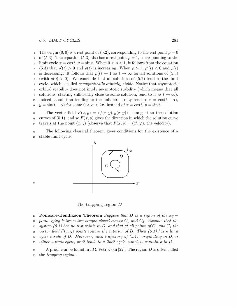
6.5. LIMIT CYCLES 281
The origin (0, 0) is a rest point of (5.2), corresponding to the rest point ρ = 01
of (5.3). The equation (5.3) also has a rest point ρ = 1, corresponding to the2
limit cycle x = cos t, y = sin t. When 0 < ρ < 1, it follows from the equation3
(5.3) that ρ′(t) > 0 and ρ(t) is increasing. When ρ > 1, ρ′(t) < 0 and ρ(t)4
is decreasing. It follows that ρ(t) → 1 as t → ∞ for all solutions of (5.3)5
(with ρ(0) > 0). We conclude that all solutions of (5.2) tend to the limit6
cycle, which is called asymptotically orbitally stable. Notice that asymptotic7
orbital stability does not imply asymptotic stability (which means that all8
solutions, starting sufficiently close to some solution, tend to it as t → ∞).9
Indeed, a solution tending to the unit circle may tend to x = cos(t − α),10
y = sin(t− α) for some 0 < α < 2π, instead of x = cos t, y = sin t.11
The vector field F (x, y) = (f(x, y), g(x, y)) is tangent to the solution12
curves of (5.1), and so F (x, y) gives the direction in which the solution curve13
travels at the point (x, y) (observe that F (x, y) = (x′, y′), the velocity).14
The following classical theorem gives conditions for the existence of a15
stable limit cycle.16
-
6
x
y
The trapping region D
'
&
$
%�� ���
@R
D
C2
C1
17
Poincare-Bendixson Theorem Suppose that D is a region of the xy −18
plane lying between two simple closed curves C1 and C2. Assume that the19
system (5.1) has no rest points in D, and that at all points of C1 and C2 the20
vector field F (x, y) points toward the interior of D. Then (5.1) has a limit21
cycle inside of D. Moreover, each trajectory of (5.1), originating in D, is22
either a limit cycle, or it tends to a limit cycle, which is contained in D.23
A proof can be found in I.G. Petrovskii [22]. The region D is often called24
the trapping region.25

282 CHAPTER 6. NON-LINEAR SYSTEMS
For practice, let us apply the Poincare-Bendixson theorem to the system1
(5.2) (we already know that x = cos t, y = sin t is a limit cycle). One checks2
that (0, 0) is the only rest point. (Setting the right hand sides of (5.2) to3
zero, one gets y/x = −x/y, so that x = y = 0.) Let C1 be the circle of radius4
1/2 around the origin, C2 the circle of radius 2 around the origin, and D5
the region between them. On C1, F (x, y) =(
−y + 34x, x+ 3
4y)
. The scalar6
product of this vector with (x, y) is 34x
2 + 34y
2 > 0. Hence, F (x, y) points7
outside of C1, and into D. On C2, F (x, y) = (−y − 3x, x− 3y). The scalar8
product of this vector with (x, y) is −3x2 − 3y2 < 0, and F (x, y) points into9
D. We conclude that there is a limit cycle in D, confirming what we already10
know.11
Example 2 To model oscillations connected to glycolysis (the process12
of cells breaking down sugar to obtain energy) the following model was13
proposed by E.E. Sel’kov [28]14
x′ = −x + ay + x2y(5.4)
y′ = b− ay − x2y .
Here a and b are positive parameters. The unknown functions x(t) and y(t)15
represent some biological quantities, and are also assumed to be positive.16
-
6
x
y
� ��@
@@
@@
@@
@@
@@@I
���
@@R
��
-�
ba
(b, ba)
x+ y = b+ ba
b + ba
D
C1
The trapping region D \D1 (D1 is the disc inside C1)
17
To prove the existence of a limit cycle, we shall construct a trapping18
region. Consider the four-sided polygon D in the xy-plane bounded by the19
part of x-axis, 0 < x < b + ba , by the part of y-axis, 0 < y < b
a , by the20
horizontal line y = ba , with 0 < x < b, and finally by the line x+ y = b+ b
a ,21

6.5. LIMIT CYCLES 283
see the figure. We claim that the vector field of this system, F (x, y) =1(
−x + ax+ x2y, b− ay − x2y)
, points inside of D, on the boundary of D.2
Indeed, y′ > 0 when y = 0 (on the lower side) and the trajectories go up,3
y′ < 0 when y = ba (on the upper side) and the trajectories go down. On4
the left side, x = 0, we have x′ > 0, and the trajectories travel to the right.5
Turning to the right hand side, observe that by adding the equations in6
(5.4), we get7
(x+ y)′ = b− x < 0 , for x > b .
Hence, the trajectories travel from the line x + y = b + ba (the right side)8
toward the lines x+y = c, with c < b+ ba , which corresponds to the interior9
of D.10
We now look for the rest points. Setting the right hand side of the11
first equation to zero, we get y = xx2+a . Similarly, from the second equa-12
tion, y = bx2+a
. We conclude that x = b, and y = bb2+a
< ba . The13
only rest point (b, bb2+a
) lies inside D. To determine the stability of this14
rest point, we consider its linearized system, with the Jacobian matrix15
A =
[
fx(x, y) fy(x, y)gx(x, y) gy(x, y)
]
evaluated at the rest point (b, bb2+a
) :16
A =
[
−1 + 2xy a+ x2
−2xy −a− x2
]
∣
∣
∣
∣
(
b, bb2+a
) =
[
−1 + 2 b2
b2+aa + b2
−2 b2
b2+a−a − b2
]
.
The eigenvalues of A satisfy λ1 λ2 = detA = a+ b2 > 0, λ1 + λ2 = trA. If17
trA = −b4 + (2a− 1)b2 + a+ a2
b2 + a> 0 ,(5.5)
then λ1 and λ2 are either both positive, or both are complex numbers with18
positive real parts. In the first case, the rest point (b, bb2+a) is an unstable19
node, and in the second case it is an unstable spiral, for both the linearized20
system and for (5.3), in view of the Hartman-Grobman theorem. Hence,21
on a small circle C1 around the rest point, bounding the disc we call D1,22
trajectories point out of D1 (outside of C1). Let now D denote the region23
D, with the disc D1 removed, D = D \D1. Then, under the condition (5.5),24
D is a trapping region, and by the Poincare-Bendixson theorem there exists25
a stable limit cycle of (5.2), lying in D.26
The condition (5.5) is equivalent to27
b2 − b4 − 2ab2 − a− a2 > 0 ,

284 CHAPTER 6. NON-LINEAR SYSTEMS
0.5 1.0 1.5 2.0 2.5 3.0x
0.5
1.0
1.5
2.0
2.5
y
Figure 6.2: The limit cycle of Sel’kov system (5.4) for a = 0.07, b = 0.5
which holds if b is small, and a is even smaller. Still this result is biologically1
significant. Computations show that the limit cycle is unique, and it attracts2
all trajectories originating in the first quadrant of the xy-plane. In Figure 6.23
we present Mathematica’s computation of the limit cycle (thick) for Sel’kov4
system (5.4), with a = 0.07, b = 0.5. One sees that the trajectories both on5
the inside and on outside of the limit cycle converge quickly to it. The rest6
point at (0.5, 1.5625) is marked.7
Sometimes one wishes to prove that limit cycles do not exist in some8
region. Recall that a region is called simply-connected if it has no holes.9
Dulac-Bendixson Criterion Assume that f(x, y), fx(x, y) and gy(x, y)10
are continuous in some simply-connected region R of the xy-plane, and11
fx(x, y) + gy(x, y)
does not change sign on R (it is either positive for all points in R, or negative12
everywhere on R). Then the system (5.1) has no closed trajectories inside13
R.14
Proof: Any solution (x(t), y(t)) of (5.1), for a ≤ t ≤ b, determines a curve15
6.6. PERIODIC POPULATION MODELS 285
C (or a trajectory) in the xy-plane. We evaluate the following line integral1
∫
Cg(x, y) dx−f(x, y) dy =
∫ b
a
[
g(x(t), y(t)) x′(t) − f(x(t), y(t)) y′(t)]
dt = 0 ,
(5.6)using the equations (5.1). If (x(t), y(t)) is a limit cycle inside R, then (5.6)2
holds, moreover the curve C is closed, and it encloses some region P inside3
R. By Green’s formula, the line integral4
∫
Cg(x, y) dx− f(x, y) dy = −
∫∫
P[fx(x, y) + gy(x, y)] dA
is either positive or negative, contradicting (5.6). ♦5
Exactly the same proof produces a more general result.6
Theorem 6.5.1 (Dulac-Bendixson Criterion) Assume that f(x, y), fx(x, y)7
and gy(x, y) are continuous in some region R of the xy-plane, and there is8
a differentiable function h(x, y), which is positive on R, so that9
∂
∂x[h(x, y)f(x, y)]+
∂
∂y[h(x, y)g(x, y)](5.7)
does not change sign on R. Then the system (5.1) has no closed trajectories10
inside R.11
Example 3 The Lotka-Volterra model of two competing species12
x′ = x (a− bx− cy)(5.8)
y′ = y (d− ex − ky) ,
with positive constants a,b,c,d,e and k, has no limit cycles in the first quad-13
rant of the xy-plane. Indeed, select h(x, y) = 1xy > 0 for x, y > 0. Then the14
expression (5.7) becomes15
∂
∂x
(
a− bx− cy
y
)
+∂
∂y
(
d− ex − ky
x
)
= − by− k
x< 0 ,
for x, y > 0. It follows that the system (5.8) has no limit cycles in the first16
quadrant of the xy-plane.17

286 CHAPTER 6. NON-LINEAR SYSTEMS
6.6 Periodic Population Models1
Population models become much harder to analyze in case the coefficients2
vary with time t. However, if all coefficients are periodic functions of the3
same period, it is still possible to obtain detailed description of the solutions.4
5
We begin by considering the logistic equation6
x′ = x (a(t) − b(t)x) ,(6.1)
modeling the number of rabbits x(t) at time t. We are only interested in7
positive solutions, x(t) > 0 for all t. The given continuous functions a(t) and8
b(t) are assumed to be periodic, with the period p, so that a(t+ p) = a(t),9
and b(t+p) = b(t) for all t. The periodicity of a(t) and b(t) can be attributed10
to seasonal variations. For example, the carrying capacity a(t) is likely to11
be higher in summer, and lower, or even negative, in winter. We assume12
that the average value of a(t) is positive, so that13
∫ p
0a(s) ds > 0 ,(6.2)
and that the self-limitation coefficient b(t) satisfies14
b(t) > 0 , for all t .(6.3)
This equation is of Bernoulli’s type. We divide it by x215
x′
x2=a(t)
x− b(t) ,
and set y =1
x. Then y′ = − x′
x2, and we obtain a linear equation16
y′ + a(t)y = b(t)(6.4)
that is easy to analyze.17
Lemma 6.6.1 The problem (6.4) has a positive solution of period p. This18
solution is unique, and it attracts all other solutions of (6.4), as t→ ∞.19
Proof: With the integrating factor µ = e∫ t
0a(s)ds, the solution of (6.4),20
satisfying an initial condition y(0) = y0, is found as follows21
d
dt[µ(t)y(t)] = µ(t)b(t) ,

6.6. PERIODIC POPULATION MODELS 287
1
y(t) =1
µ(t)y0 +
1
µ(t)
∫ t
0µ(s)b(s) ds .
This solution is periodic, provided that y(p) = y(0) = y0 (as justified in2
Problems), implying that3
y0 =1
µ(p)y0 +
1
µ(p)
∫ p
0µ(s)b(s) ds ,
which we write as4
(µ(p)− 1)y0 =
∫ p
0µ(s)b(s) ds .
Since µ(p) > 1 (by the assumption (6.2)), we can solve this equation for y05
y0 =1
µ(p)− 1
∫ p
0µ(s)b(s) ds > 0 ,
obtaining the initial value y0, which leads to a positive solution y(t) of period6
p.7
If z(t) is another solution of (6.4), the difference w(t) = z(t) − y(t)8
satisfies9
w′ + a(t)w = 0 .
Integrating, w(t) = e−∫ t
0a(s)dsw(0) → 0, as t → ∞ (by the assumption10
(6.2)), proving that all solutions tend to y(t). In particular, this fact implies11
that the periodic solution y(t) is unique. ♦12
This lemma makes possible the following complete description of the13
dynamics for the logistic equation.14
Theorem 6.6.1 Assume that the continuous p-periodic functions a(t), b(t)15
satisfy the conditions (6.2) and (6.3). Then the equation (6.1) has a positive16
solution of period p. This solution is unique, and it attracts all other positive17
solutions of (6.1), as t→ ∞.18
Proof: By Lemma 6.6.1, there is a positive p-periodic solution y(t) of19
(6.4). Then x(t) =1
y(t)gives a positive p-periodic solution of (6.1). If20
z(t) is another positive solution of (6.1), then the same lemma tells us that21
1
x(t)− 1
z(t)→ 0 as t → ∞, which implies that x(t) − z(t) → 0 as t → ∞.22
(Observe that z(t) is bounded. Indeed, it follows from the equation (6.1)23
that z(t) is decreasing for large enough z, so that a(t) − b(t)z < 0, which24

288 CHAPTER 6. NON-LINEAR SYSTEMS
holds if z > max a(t)min b(t) . Then z ≤ maxa(t)
min b(t) .) It follows that the p-periodic1
solution x(t) attracts all other positive solutions of (6.1), and there is only2
one p-periodic solution. ♦3
The following corollary says that an increase in carrying capacity will4
increase the p-periodic solution of (6.1). This is natural, because the p-5
periodic solution attracts all other solutions (“a rising tide lifts all boats”).6
Corollary 6.6.1 Let x1(t) be the positive p-periodic solution of7
x′1 = x1(a1(t) − b(t)x1) ,
where the p-periodic function a1(t) satisfies a1(t) > a(t) for all t. Then8
x1(t) > x(t) for all t (x(t) is the positive p-periodic solution of (6.1)). More-9
over, if a1(t) is close to a(t), then x1(t) is close to x(t).10
Proof: Set y1 =1
x1, and y =
1
x. As before, y′ + a(t)y = b(t), and11
y′1 + a1(t)y1 = b(t) .
Let z(t) = y(t) − y1(t). Then z(t) is a p-periodic solution of12
z′ + a(t)z = (a1(t) − a(t))y1(t) > 0 .(6.5)
By Lemma 6.6.1, the periodic solution of this equation is positive, so that13
z(t) > 0 for all t, and then y(t) > y1(t), which implies that x(t) < x1(t) for14
all t.15
Turning to the second statement, we are now given that the right hand16
side of (6.5) is small. Going over the construction of the p-periodic solution17
in Lemma 6.6.1, we see that z(t) is small as well. ♦18
We consider next another model for a population x(t) > 0 of rabbits19
x′ = x (x− a(t)) (b(t)− x) .(6.6)
The given continuous functions a(t) and b(t) are assumed to be positive,20
periodic with period p, and satisfying 0 < a(t) < b(t) for all t. If 0 < x(t) <21
a(t), it follows from the equation that x′(t) < 0, and x(t) decreases. When22
a(t) < x(t) < b(t), the population grows. So that a(t) gives a threshold23
for population growth. (If the number of rabbits falls too low, they have a24
problem meeting the “significant others”.)25
Let us assume additionally that the maximum value of a(t) lies below26
the minimum value of b(t):27
max−∞<t<∞
a(t) < min−∞<t<∞
b(t) .(6.7)

6.6. PERIODIC POPULATION MODELS 289
Theorem 6.6.2 If a(t) and b(t) are continuous p-periodic functions sat-1
isfying (6.7), then the equation (6.6) has exactly two positive solutions of2
period p.3
Proof: We denote by x(t, x0) the solution of (6.6), satisfying the initial4
condition x(0) = x0, so that x(0, x0) = x0. To prove the existence of two5
solutions, we define the Poincare map x0 → T (x0), by setting T (x0) =6
x(p, x0). The function T (x0) is continuous (by the continuous dependence7
of solutions, with respect to the initial condition). Define the numbers A =8
min−∞<t<∞ b(t)− ε, B = max−∞<t<∞ b(t)+ ε, and the interval I = (A,B).9
If ε > 0 is chosen so small that max−∞<t<∞ a(t) < min−∞<t<∞ b(t) − ε,10
then we claim that the map T takes the interval I into itself. Indeed, if11
x0 = A, then from the equation x′(0) > 0, and x(t, x0) is increasing, for12
small t. At future times, the solution curve cannot cross below x0, because13
again we have x′(t) > 0, if x(t) = x0. It follows that x(p, x0) > x0, or14
T (A) > A. Similarly, we show that T (B) < B. The continuous function15
T (x) − x is positive at x = A, and negative at x = B. By the intermediate16
value theorem T (x) − x has a root x on the interval I = (A,B), so that17
there is a fixed point x such that T (x) = x. Then x(p, x) = x, which implies18
that x(t, x) is a p-periodic solution.19
The second periodic solution is obtained by considering the map T1,20
defined by setting T1(x0) = x(−p, x0), corresponding to solving the equation21
(6.6) backward in time. As in the case of T , we see that T1 is a continuous22
map, taking the interval T1 = ( min−∞<t<∞
a(t)− ε, max−∞<t<∞
a(t) + ε) into itself23
(for small ε > 0). T1 has a fixed point on I1, giving us the second p-periodic24
solution. So that the equation (6.6) has at least two positive p-periodic25
solutions.26
To prove that there are at most two positive p-periodic solutions of (6.6),27
we need the following two lemmas, which are also of independent interest.28
Lemma 6.6.2 Consider the equation (for w(t))29
w′ = c(t)w ,(6.8)
with a given continuous p-periodic function c(t). This equation has a non-30
zero p-periodic solution, if and only if31
∫ p
0c(s) ds = 0 .
290 CHAPTER 6. NON-LINEAR SYSTEMS
Proof: Integrating the equation (6.8), gives w(t) = w(0)e∫ t
0c(s) ds. Using1
the periodicity of c(t), we see that2
w(t+ p) = w(0)e∫ t+p
0c(s) ds = w(0)e
∫ t
0c(s) ds+
∫ t+p
tc(s) ds
3
= w(0)e∫ t
0c(s) dse
∫ p
0c(s) ds = w(0)e
∫ t
0c(s) ds = w(t) ,
exactly when∫ p0 c(s) ds = 0. ♦4
Lemma 6.6.3 Consider the nonlinear equation (with a continuous function5
f(t, x), which is twice differentiable in x)6
x′ = f(t, x) .(6.9)
Assume that the function f(t, x) is p-periodic in t, and convex in x:7
f(t+ p, x) = f(t, x), for all t, and x > 0 ,8
fxx(t, x) > 0, for all t, and x > 0 .
Then the equation (6.9) has at most two positive p-periodic solutions.9
Proof: Assume, on the contrary, that we have three positive p-periodic10
solutions: x1(t) < x2(t) < x3(t) (solutions of (6.9) do not intersect, by the11
existence and uniqueness theorem). Set w1 = x2 − x1, and w2 = x3 − x2.12
These functions are p-periodic, and they satisfy13
w′1 = f(t, x2)− f(t, x1) =
∫ 1
0
d
dθf (t, θx2 + (1 − θ)x1) dθ
14
=
∫ 1
0fx (t, θx2 + (1− θ)x1) dθ w1 ≡ c1(t)w1 ,
15
w′2 = f(t, x3)− f(t, x2) =
∫ 1
0
d
dθf (t, θx3 + (1 − θ)x2) dθ
16
=
∫ 1
0fx (t, θx3 + (1− θ)x2) dθ w2 ≡ c2(t)w2 .
(We denoted by c1(t) and c2(t) the corresponding integrals.) The function17
fx is increasing in x (because fxx > 0). It follows that c2(t) > c1(t) for all18
t, and so c1(t) and c2(t) cannot both satisfy the condition of Lemma 6.6.2.19
We have a contradiction with Lemma 6.6.2. (Observe that w1(t) and w2(t)20
are p-periodic solutions of the equations w′1 = c1(t)w1, and w′
2 = c2(t)w2.)21
♦22

6.6. PERIODIC POPULATION MODELS 291
Returning to the proof of the theorem, we rewrite (6.6) as1
x′ = −x3 + (a(t) + b(t))x2 − a(t)b(t)x .
Divide by x3:2
x′
x3= −1 +
(a(t) + b(t))
x− a(t)b(t)
x2.
We set here u =1
x2, so that u′ = −2x−3x′, and obtain3
u′ = 2 − 2(a(t) + b(t))√u+ 2a(t)b(t)u .(6.10)
Clearly, the positive p-periodic solutions of the equations (6.6) and (6.10) are4
in one-to-one correspondence. But the right hand side in (6.10) is convex in5
u. By Lemma 6.6.3, both of the equations (6.10) and (6.6) have at most two6
positive p-periodic solutions. It follows that the equation (6.6) has exactly7
two positive p-periodic solutions. ♦8
Let x1(t) < x2(t) denote the two positive p-periodic solutions of (6.6),9
provided by the above theorem, and let x(t, x0) denote again the solution of10
this equation, with the initial condition x(0) = x0. It is not hard to show11
that x(t, x0) → x2(t) as t → ∞, if x0 belongs to either one of the intervals12
(x2(0),∞), or (x1(0), x2(0)). On the other hand, x(t, x0) → 0 as t → ∞, if13
x0 ∈ (0, x1(0)). So that the larger p-periodic solution x2(t) is asymptotically14
stable, while the smaller one x1(t) is unstable.15
We consider next the case of two competing species, with the populations16
x(t) and y(t), satisfying the Lotka-Volterra system17
x′ = x(a(t) − bx− cy)(6.11)18
y′ = y(d(t)− ex− fy) .
The given functions a(t) and d(t) are assumed to be periodic, with the pe-19
riod p, so that a(t+p) = a(t), and d(t+p) = d(t) for all t. We do not assume20
a(t) and d(t) to be positive, but assume that they have positive averages21
over (0, p). The positive numbers b, c, e and f are given. As before, the22
periodicity of a(t) and d(t) may be attributed to seasonal variations. The23
numbers c and e are called the interaction coefficients. They quantify how24
detrimental are the species for each other. It seems reasonable to assume25
that the self-limitation coefficients b and f , as well as the interaction coeffi-26
cients c and e change less with the seasons than the carrying capacities, and27
so we assumed them to be constants in this model.28

292 CHAPTER 6. NON-LINEAR SYSTEMS
We may regard the first equation as a logistic equation for x(t), with the1
carrying capacity equal to a(t) − cy(t). We see that each species in effect2
diminishes the carrying capacity of the other one, as they compete for food,3
hiding places, etc. The largest population of the first species occurs, if the4
second one goes extinct, so that y(t) = 0 for all t. Then the first equation5
becomes6
x′ = x(a(t) − bx) .(6.12)
By the Theorem 6.6.1, this equation has a unique positive p-periodic solu-7
tion, which we denote by X(t). The pair (X(t), 0) is a p-periodic solution of8
our system (6.11), called a semi-trivial solution. If Y (t) denotes the unique9
positive p-periodic solution of10
y′ = y(d(t)− fy) ,(6.13)
then (0, Y (t)) is the other semi-trivial solution.11
The following theorem describes a case, when the dynamics of the Lotka-12
Volterra system is similar to that of a single logistic equation.13
Theorem 6.6.3 Denoting A =∫ p0 a(t) dt, D =
∫ p0 d(t) dt, assume that A >14
0, D > 0, and15
fA − cD > 0, and bD− eA > 0 .(6.14)
Then the system (6.11) has a unique positive (in both components) p-periodic16
solution, to which all other positive solutions of (6.11) tend, as t→ ∞.17
Proof: The largest possible periodic solutions X(t) and Y (t) (defined by18
(6.12) and (6.13)) occur when the competitor species is extinct. Denote by19
ξ(t) the positive p-periodic solution of the logistic equation20
x′ = x(a(t) − bx− cY (t)) .
Here the first species is forced to compete with the maximal periodic solution21
for the second species. Similarly, we denote by η(t) the positive p-periodic22
solution of the logistic equation23
y′ = y(d(t)− eX − fy) .
(To prove the existence of ξ(t), we need to show that∫ p0 (a(t) − cY (t)) dt >24
0. Dividing the equation Y ′ = Y (d(t) − fY ) by Y and integrating, we25
have∫ p0 Y (t) dt = D
f . Then∫ p0 (a(t) − cY (t)) dt = A − cD
f > 0, by the first26
condition in (6.14). The existence of η(t) is proved similarly.)27

6.6. PERIODIC POPULATION MODELS 293
We shall construct a p-periodic solution of our system (6.11) as the limit1
of the p-periodic approximations (xn, yn), defined as follows: x1 = X(t),2
y1 = η(t), while (x2(t), y2(t)) are respectively the p-periodic solutions of the3
following two logistic equations4
x′2 = x2(a(t)− bx2 − cy1) ,
5
y′2 = y2(d(t)− ex2 − fy2) .
So that we compute x2(t), and immediately use it to compute y2(t). Using6
the Corollary 6.6.1, we see that7
x2(t) < x1(t), and y1(t) < y2(t) for all t .
(Or think “ecologically”: x2 is computed when the first species faces some8
competition, while x1 = X(t) was computed without competition, so that9
x2(t) < x1(t); y2 is computed when the second species faces weaker com-10
petition, than when y1 was computed, so that y1(t) < y2(t).) In general,11
once (xn(t), yn(t)) is computed, we obtain (xn+1(t), yn+1(t)) by finding the12
p-periodic solutions of the logistic equations13
x′n+1 = xn+1(a(t) − bxn+1 − cyn) ,(6.15)
14
y′n+1 = yn+1(d(t)− exn+1 − fyn+1) .
By the same reasoning as above, we show that for all t15
ξ(t) < xn(t) < · · · < x2(t) < x1(t), and y1(t) < y2(t) < · · · < yn(t) < Y (t) .
At each t, xn(t) is a monotone and bounded sequence of numbers, which has16
a limit. We denote xp(t) = limt→∞ xn(t), and similarly yp(t) = limt→∞ yn(t).17
Passing to the limit in the equations (6.15) (or rather in their integral ver-18
sions), we see that (xp(t), yp(t)) is a positive p-periodic solution of (6.11).19
20
Next, we prove that there is only one positive p-periodic solution of21
(6.11). Let (x(t), y(t)) be any positive p-periodic solution of (6.11). We22
divide the first equation in (6.11) by x(t), and integrate over (0, p). By23
periodicity,
∫ p
0
x′(t)x(t)
dt = lnx(t)|p0
= 0. Then24
b
∫ p
0x(t) dt+ c
∫ p
0y(t) dt = A .

294 CHAPTER 6. NON-LINEAR SYSTEMS
Similarly, from the second equation in (6.11)1
e
∫ p
0x(t) dt+ f
∫ p
0y(t) dt = D .
Solving these two equations for the integrals, we get2
∫ p
0x(t) dt =
fA − cD
bf − ce> 0,
∫ p
0y(t) dt =
bD − eA
bf − ec> 0 .(6.16)
(Observe that our conditions (6.14) imply that bf − ec > 0.) Let now3
(x(t), y(t)) be another positive p-periodic solution of (6.11). Clearly, x(t) <4
x1(t) = X(t), y(t) > y1(t) = η(t). We prove inductively that x(t) < xn(t),5
and y(t) > yn(t). Letting n → ∞, we have x(t) ≤ xp(t), and y(t) ≥ yp(t).6
Since by (6.16),7
∫ p
0xp(t) dt =
∫ p
0x(t) dt , and
∫ p
0yp(t) dt =
∫ p
0y(t) dt ,
we conclude that x(t) = xp(t), and y(t) = yp(t).8
Turning to the stability of (xp(t), yp(t)), we now define another sequence9
of iterates (xn, yn). Beginning with x1 = ξ(t), y1 = Y (t), once the iterate10
(xn(t), yn(t)) is computed, we obtain (xn+1(t), yn+1(t)) by calculating the11
p-periodic solutions of the following two logistic equations12
y′n+1 = yn+1(d(t)− exn − fyn+1) ,13
x′n+1 = xn+1(a(t)− bxn+1 − cyn+1) .
(So that we compute yn+1(t), and immediately use it to compute xn+1(t).)14
By the same reasoning as above, we show that for all n15
x1 < x2 < · · · < xn < xn(t) < · · ·< x2(t) < x1(t) ,
and16
y1(t) < y2(t) < · · ·< yn(t) < yn(t) < · · ·< y2(t) < y1(t) .
As before, (xn, yn) tends to a positive p-periodic solution of (6.11), which by17
the uniqueness must be (xp(t), yp(t)). We conclude that the periodic solution18
is approximated from both below and above by the monotone sequences,19
xp(t) = limn→∞
xn(t) = limn→∞
xn(t), and yp(t) = limn→∞
yn(t) = limn→∞
yn(t).20
Next, we sketch a proof that any positive solution, (x(t), y(t)) of (6.11),21
tends to the unique positive p-periodic solution (xp(t), yp(t)), as t → ∞.22
The idea is to show inductively that for any integer n, and any ε > 023
xn(t) − ε < x(t) < xn(t) + ε, and yn(t) − ε < y(t) < yn(t) + ε ,(6.17)
6.6. PERIODIC POPULATION MODELS 295
for t large enough. Indeed, the inequality yn(t) − ε < y(t) implies that1
x′ < x(a(t) − bx− cyn + cε) .
Then x(t) lies below the solution of2
x′ = x(a(t) − bx− cyn + cε) ,(6.18)
with the same initial condition. Any positive solution of (6.18) tends to the3
p-periodic solution of that equation, which, by the Corollary 6.6.1, is close4
to the p-periodic solution of5
x′ = x(a(t) − bx− cyn) ,
or close to xn+1. So that the estimate of y(t) from below in (6.17) leads to6
the estimate of x(t) from above in (6.17), at n + 1. This way we establish7
the inequalities (6.17) at the next value of n. ♦8
This theorem appeared first in the author’s paper [17]. The idea to use9
monotone iterations, to prove that all positive solutions tend to the periodic10
one, is due to E.N. Dancer [7], who used it in another context.11
6.6.1 Problems12
I.13
1. (i) Find and classify the rest points of14
x′(t) = x(x+ 1)(x− 2) .
Hint: The sign of x′(t) changes at x = −1, x = 0, and x = 2.15
Answer. The rest points are x = −1 (unstable), x = 0 (stable), and x = 216
(unstable).17
(ii) Let y(t) be the solution of18
y′(t) = y(y + 1)(y − 2) , y(0) = 3 .
Find limt→∞ y(t), and limt→−∞ y(t).19
Answer. ∞, and 2.20
(iii) What is the domain of attraction of the rest point x = 0?21
Answer. (−1, 2).22

296 CHAPTER 6. NON-LINEAR SYSTEMS
2. Consider a population model with a threshold for growth1
x′ = x(x− 1)(5− x) .
(i) Find and classify the rest points.2
Answer. The rest points are x = 0 (stable), x = 1 (unstable), and x = 53
(stable).4
(ii) Calculate limt→∞ x(t) for the following cases:5
(a) x(0) ∈ (0, 1), (b) x(0) > 1.6
Answer. (a) limt→∞ x(t) = 0, (b) limt→∞ x(t) = 5.7
3. (i) Find and classify the rest points of8
x′ = x2(2 − x) .
Answer. The rest points are x = 2 (stable) and x = 0 (neither stable or9
unstable).10
(ii) Calculate limt→∞ x(t) for the following cases:11
(a) x(0) < 0, (b) x(0) > 0.12
Answer. (a) limt→∞ x(t) = 0, (b) limt→∞ x(t) = 2.13
4. (i) Find and classify the rest point(s) of14
x′ = −x2 .
(ii) Solve this equation to show that limt→∞ x(t) = 0, for any value of x(0).15
16
5. (i) Show that the rest point (0, 0) is asymptotically stable for the system17
x′1 = −2x1 + x2 + x1x2
x′2 = x1 − 2x2 + x31 .
(ii) Find the general solution of the corresponding linearized system18
x′1 = −2x1 + x2
x′2 = x1 − 2x2 ,
and discuss its behavior as t→ ∞.19

6.6. PERIODIC POPULATION MODELS 297
6. Show that the rest point (0, 0) is asymptotically stable for the system1
x′ = −5y − x(x2 + y2)
y′ = x− y(x2 + y2) ,
and its domain of attraction is the entire xy-plane.2
Hint: Use L(x, y) = 15x
2 + y2.3
7. (i) The equation (for y = y(t))4
y′ = y2(1− y)
has the rest points y = 0 and y = 1. Discuss their Lyapunov’s stability.5
Answer: y = 1 is asymptotically stable, y = 0 is unstable.6
(ii) Find limt→∞
y(t) in the following cases:7
(a) y(0) < 0, (b) 0 < y(0) < 1, (c) y(0) > 1.8
Answer. (a) limt→∞ y(t) = 0, (b) limt→∞ y(t) = 1, (c) limt→∞ y(t) = 1.9
8. Show that the rest point (0, 0) is stable, but not asymptotically stable,10
for the system11
x′ = −yy′ = x3 .
Hint: Use L(x, y) = 12x
4 + y2.12
9. (i) Convert the nonlinear equation13
y′′ + f(y)y′ + y = 0
into a system, by letting y = x1, and y′ = x2. Answer:14
x′1 = x2
x′2 = −x1 − f(x1)x2 .
(ii) Show that the rest point (0, 0) of this system is asymptotically stable,15
provided that f(x1) > 0 for all x1 6= 0. What does this imply for the original16
equation?17
Hint: Use L = 12x
21 + 1
2x22.18

298 CHAPTER 6. NON-LINEAR SYSTEMS
10. Show that the rest point (0, 0) is asymptotically stable for the system1
x′1 = x2
x′2 = −g(x1) − f(x1)x2 ,
provided that f(x1) > 0, and x1g(x1) > 0, for all x1 6= 0.2
Hint: Use L =∫ x10 g(s) ds + 1
2x22. Observe that L(x1, x2) > 0, for all3
(x1, x2) 6= (0, 0).4
What conclusion can one draw for the equation5
y′′ + f(y)y′ + g(y) = 0 ?
11. Consider the system6
x′ = −x3 + 4y(
z2 + 1)
y′ = −y5 − x(
z2 + 1)
z′ = −z − x4z3 .
(i) Show that (0, 0, 0) is the only rest point, and it is asymptotically stable.7
8
(ii) If we drop the nonlinear terms, we get a linear system9
x′ = 4y
y′ = −xz′ = −z .
Show that any solution of this system moves on an elliptic cylinder, and it10
tends to the xy-plane, as t → ∞. Conclude that the rest point (0, 0, 0) is11
not asymptotically stable. Is it stable?12
12. (i) Show that the rest point (0, 0, 0) is Lyapunov stable, but not asymp-13
totically stable for the system14
x′1 = x2 + x3 + x2x3(6.19)
x′2 = −x1 + x3 − 2x1x3
x′3 = −x1 − x2 + x1x2 .
Hint: Solutions of (6.19) lie on spheres x21 + x2
2 + x23 = c (where c = x2
1(0) +15
x22(0) + x2
3(0)).16
(ii) Find all of the rest points of (6.19).17
6.6. PERIODIC POPULATION MODELS 299
Consider the 3×3 algebraic system obtained by setting the right hand sides1
of (6.19) to zero. If one of the variables is zero, so are the other two. In2
case x1 6= 0, x2 6= 0, and x3 6= 0, obtain a linear system with infinitely many3
solutions for y1 = 1x1
, y2 = 1x2
, y3 = 1x3
dividing the first equation by x2x3,4
the second one by x1x3, and the third one by x1x2.5
Answer. (x1, x2, x3) =(
t, tt−1 ,
t1−2t
)
, where t is arbitrary, but t 6= 1, t 6= 12 .6
13. Show that the rest point (1, 1) is asymptotically stable for the system7
x′ = −3x− y + xy + 3
y′ = −2x− y + x2 + 2 .
Hint: Set x = X + 1, y = X + 1, to get a system for (X, Y ).8
II.9
1. Show that for any positive solution of the system10
x′ = x (5 − x− 2y)
y′ = y (2 − 3x− y)
we have limt→∞
(x(t), y(t)) = (5, 0).11
2. Show that for any positive solution of the system12
x′ = x(
2 − x− 12y)
y′ = y (3− x− y)
we have limt→∞
(x(t), y(t)) = (1, 2).13
3. Find limt→∞
(x(t), y(t)) for the initial value problem14
x′ = x (3 − x− y) , x(0) = 52
y′ = y (4 − 2x− y) , y(0) = 14 .
What if the initial conditions are x(0) = 0.1 and y(0) = 3 ?15
Answer. (3, 0). For the other initial conditions: (0, 4).16
4. Discuss the long term behavior (as t → ∞) of positive solutions of the17
system18
x′ = x (3 − x− y)
y′ = y (4 − 2x− y) .

300 CHAPTER 6. NON-LINEAR SYSTEMS
5. Show that any solution with x(0) > 0 and y(0) > 0 satisfies x(t) > 0 and1
y(t) > 0 for all t > 0, and then discuss the long term behavior of positive2
solutions of the system3
x′ = x (6 − 3x− 2y)
y′ = y(
2 − 18x
2 − y)
.
Hint: The second null-cline is a parabola, but the same analysis applies.4
Answer. Any positive solution satisfies limt→∞ x(t) = 6−2√
7, and limt→∞ y(t) =5
3√
7 − 6.6
III.7
1. Show that the ellipse x = 2 cos t, y = sin t is a stable limit cycle for the8
system9
x′ = −2y + x(
1 − 14x
2 − y2)
y′ = 12x+ y
(
1 − 14x
2 − y2)
.
Hint: Show that ρ = 14x
2 + y2 satisfies ρ′ = 2ρ(1− ρ).10
2. Consider the system11
x′ = x− y − x3
y′ = x+ y − y3 .
(i) Show that the origin (0, 0) is the only rest point.12
Hint: Show that the curves x− y−x3 = 0 and x+ y− y3 = 0 intersect only13
at the origin. This can be done either by hand, or (better) by computer.14
(ii) Show that the origin (0, 0) is an unstable spiral.15
(iii) Show that the system has a limit cycle.16
Hint: Compute the scalar product of F =(
x− y − x3, x+ y − y3)
, and the17
vector (x, y), then switch to the polar coordinates. Obtain18
x2 +y2 −x4 −y4 = x2 +y2 −(
x2 + y2)2
+2x2y2 = r2− r4 +2r4 cos2 θ sin2 θ
19
< r2 − 1
2r4 < 0 , for r large .
Conclude that the annulus ρ2 ≤ x2 +y2 ≤ R2 is a trapping region, provided20
that ρ > 0 is small, and R > 0 is large. Apply the Hartman-Grobman21
theorem.22

6.6. PERIODIC POPULATION MODELS 301
3. Show that the system1
x′ = x(
2 − x− y3)
y′ = y(
4x− 3y − x2)
has no limit cycles in the positive quadrant x, y > 0.2
Hint: Use the Theorem 6.5.1, with h(x, y) =1
xy.3
4. Show that the equation (for x = x(t))4
x′′ + f(x)x′ + g(x) = 0
has no periodic solutions, provided that either f(x) > 0, or f(x) < 0, for all5
real x.6
Hint: Periodic solutions would imply limit cycles for the corresponding sys-7
tem (for x1 = x and x2 = x′). Use the Dulac-Bendixson criterion.8
5. Show that the condition (5.5) holds, provided that a < 18 , and b2 lies9
between the roots of the quadratic x2 + (2a− 1)x+ a+ a2.10
6. Consider a gradient system11
x′1 = −Vx1(x1, x2)(6.20)
x′2 = −Vx2(x1, x2) ,
where V (x1, x2) is a given twice differentiable function. (Denoting x =12
(x1, x2) and V = V (x), one may write this system in the gradient form13
x′ = −∇V (x).)14
(i) Show that a point P = (x01, x
02) is a rest point of (6.20) if and only if P15
is a critical point of V (x1, x2).16
(ii) Show that V (x1(t), x2(t)) is a strictly decreasing function of t for any17
solution (x1(t), x2(t)), except if (x1(t), x2(t)) is a rest point.18
(iii) Show that no limit cycles are possible for gradient system (6.20).19
(iv) Let (a, b) be a point of strict local minimum of V (x1, x2). Show that20
(a, b) is asymptotically stable rest point of (6.20).21
Hint: Use L(x1, x2) = V (x1, x2) − V (a, b) as Lyapunov’s function.22
(v) Show that the existence and uniqueness Theorem 6.1.1 applies to (6.20).23
24

302 CHAPTER 6. NON-LINEAR SYSTEMS
7. Consider a Hamiltonian system1
x′1 = Vx1(x1, x2)(6.21)
x′2 = −Vx2(x1, x2) ,
where V (x1, x2) is a given twice differentiable function.2
(i) Show that3
V (x1(t), x2(t)) = constant ,
for any solution (x1(t), x2(t)).4
(ii) Show that a point P = (x01, x
02) is a rest point of (6.21) if and only if P5
is a critical point of V (x1, x2).6
(iii) Show that no asymptotically stable rest points are possible for Hamil-7
tonian system (6.21).8
(iv) Let (a, b) be a point of strict local minimum or maximum of V (x1, x2).9
Show that (a, b) is a center for (6.21).10
(v) Show that the trajectories of (6.20) are orthogonal to the trajectories of11
(6.21), at all points (x1, x2).12
8. In the Lotka-Volterra predator-prey system (1.1) let p = lnx, and13
q = ln y. Show that for the new unknowns p(t) and q(t) one obtains a14
Hamiltonian system, with V (p, q) = c p− d ep + a q − b eq.15
9. Consider the system (x(t) is a vector in Rn)16
x′ = [A +B(t)] x , t > t0 ,(6.22)
where A is an n×n matrix with constant entries, and the n×n matrix B(t)17
satisfies∫∞t0
||B(t)|| dt < ∞. Assume that the eigenvalues of A are either18
negative or have negative real parts (recall that such matrices are called19
stable). Show that limt→∞ x(t) = 0, for any solution of (6.22).20
Hint: Treating the B(t)x(t) term as known, one can regard (6.22) as a21
non-homogeneous system, and write its solution as22
x(t) = eA(t−t0)x(t0) +
∫ t
t0
eA(t−s)B(s)x(s) ds .
By (4.9), the norm ||eAt|| ≤ ae−bt, for some constants a > 0 and b > 0, with23
t > 0. Then24
||x(t)|| ≤ Ke−bt + a
∫ t
t0
e−b(t−s)||B(s)|| ||x(s)|| ds ,

6.6. PERIODIC POPULATION MODELS 303
where K = aebt0 ||x(t0)||. Letting u(t) = ebt||x(t)||, obtain1
||u(t)|| ≤ K + a
∫ t
t0
||B(s)|| ||u(s)|| ds .
Apply the Bellman-Gronwall lemma.2
IV. 1. Consider the linear equation3
x′ = a(t)x+ b(t) ,(6.23)
with given p-periodic functions a(t) and b(t).4
(i) Let x(t) be some solution of (6.23). Show that x(t+ p) is also a solution5
of (6.23).6
Hint: x(t) satisfies (6.23) at all t, in particular at t+ p.7
(ii) Let x(t) be a solution of (6.23), such that x(p) = x(0). Show that x(t)8
is a p-periodic function.9
Hint: x(t) and x(t+ p) are two solutions of (6.23) that coincide at t = 0.10
2. Consider a generalized logistic model11
x′ = x2 (a(t) − b(t)x) ,
with positive p-periodic functions a(t) and b(t). Show that there is a unique12
positive p-periodic solution, which attracts all other positive solutions, as13
t→ ∞.14
Hint: Show that the Poincare map x0 → x(p, x0) takes the interval (ε,M)15
into itself, provided that ε > 0 is small and M is large. For the uniqueness16
part, show that y(t) = 1x(t) satisfies17
y′ = −a(t) + b(t)1
y.
The difference of any two positive p-periodic solutions of the last equation18
satisfies w′ = c(t)w, with a negative c(t).19
3. (Another example of Fredholm alternative.) Consider the equation20
x′ + a(t)x = 1 ,(6.24)
with a p-periodic function a(t).21

304 CHAPTER 6. NON-LINEAR SYSTEMS
(i) Assume that∫ p0 a(t) dt = 0. Show that the problem (6.24) has no p-1
periodic solution.2
Hint: Let z(t) > 0 be a p-periodic solution of3
z′ − a(t)z = 0 .
Combining this equation with (6.24), conclude that∫ p0 z(t) dt = 0, which is4
a contradiction.5
(ii) Assume that∫ p0 a(t) dt 6= 0. Show that the problem (6.24) has a p-6
periodic solution, and moreover this solution satisfies∫ p0 x(t) dt 6= 0.7
Hint: Solve (6.24), with initial condition x(0) = α, and select α so that8
x(p) = x(0) = α.9
4. Consider the logistic model10
x′ = a(t)x− b(t)x2 ,
with p-periodic functions a(t) and b(t). Assume that∫ p0 a(t) dt = 0, and11
b(t) > 0 for all t. Show that this equation has no non-trivial p-periodic12
solutions.13
Hint: Any non-trivial solution satisfies either x(t) > 0 or x(t) < 0, for all t.14
Divide the equation by x(t), and integrate over (0, p).15

Chapter 71
The Fourier Series and2
Boundary Value Problems3
The central theme of this chapter involves various types of Fourier series,4
and the method of separation of variable, which is prominent in egineering5
and science. The three main equations of mathematical physics, the wave,6
the heat, and the Laplace equations, are derived and studied in detail. The7
Fourier transform method is developed, and applied to problems on infinite8
domains. Non-standard applications include studying temperatures inside9
the Earth, and the isoperimetric inequality.10
7.1 The Fourier Series for Functions of an Arbi-11
trary Period12
Recall that in Chapter 2 we studied the Fourier series for functions of period13
2π. Namely, if a function g(t) has period 2π, it can be represented by the14
Fourier series15
g(t) = a0 +∞∑
n=1
(an cosnt+ bn sinnt) ,
with the coefficients given by16
a0 =1
2π
∫ π
−πg(t) dt ,
17
an =1
π
∫ π
−πg(t) cosnt dt ,
18
bn =1
π
∫ π
−πg(t) sinnt dt .
305

306CHAPTER 7. THE FOURIER SERIES AND BOUNDARY VALUE PROBLEMS
Observe that the knowledge of a 2π-periodic function g(t) over the interval1
(−π, π] is sufficient to describe this function for all t ∈ (−∞,∞).2
Suppose now that f(x) has a period 2L, where L > 0 is any number.3
Consider an auxiliary function g(t) = f(L
πt). Then g(t) has period 2π, and4
we can represent it by the Fourier series5
f(L
πt) = g(t) = a0 +
∞∑
n=1
(an cosnt+ bn sinnt) ,
with the coefficients6
a0 =1
2π
∫ π
−πg(t) dt =
1
2π
∫ π
−πf(L
πt) dt ,
7
an =1
π
∫ π
−πg(t) cosnt dt =
1
π
∫ π
−πf(L
πt) cosnt dt ,
8
bn =1
π
∫ π
−πg(t) sinnt dt =
1
π
∫ π
−πf(L
πt) sinnt dt .
Set here9
x =L
πt, or t =
π
Lx .
Then the Fourier series takes the form10
f(x) = a0 +∞∑
n=1
(
an cosnπ
Lx+ bn sin
nπ
Lx
)
,(1.1)
and making a change of variables t→ x, by setting t =π
Lx with dt =
π
Ldx,11
we express the coefficients as12
a0 =1
2L
∫ L
−Lf(x) dx ,
13
an =1
L
∫ L
−Lf(x) cos
nπ
Lx dx ,(1.2)
14
bn =1
L
∫ L
−Lf(x) sin
nπ
Lx dx .
The formula (1.1) gives the desired Fourier series for functions of period15
2L. Its coefficients are computed using the formulas (1.2). Observe that one16
needs the values of f(x) only on the interval (−L, L), when computing the17
coefficients.18
7.1. THE FOURIER SERIES FOR FUNCTIONS OF AN ARBITRARY PERIOD 307
Suppose that a function g(x) is defined on some interval (−L, L). The1
function G(x) is called the periodic extension of g(x), provided that2
(i) G(x) = g(x) , for −L < x < L
(ii) G(x) is periodic with period 2L .
Observe that G(x) is defined for all x, except for x = nπ with integer n.3
Example Let f(x) be the function of period 6, which on the interval4
(−3, 3) is equal to x.5
Here L = 3, and f(x) = x on the interval (−3, 3). The Fourier series has6
the form7
f(x) = a0 +∞∑
n=1
(
an cosnπ
3x+ bn sin
nπ
3x
)
.
The functions x, and x cos nπ3 x are odd, and so8
a0 =1
6
∫ 3
−3x dx = 0 ,
9
an =1
3
∫ 3
−3x cos
nπ
3x dx = 0 .
The function x sin nπ3 x is even, giving10
bn =1
3
∫ 3
−3x sin
nπ
3x dx =
2
3
∫ 3
0x sin
nπ
3x dx
11
=2
3
[
− 3
nπx cos
nπ
3x+
9
n2π2sin
nπ
3x
]
∣
∣
∣
3
0= − 6
nπcosnπ =
6
nπ(−1)n+1 ,
because cosnπ = (−1)n. We conclude that12
f(x) =∞∑
n=1
6
nπ(−1)n+1 sin
nπ
3x .
Restricting to the interval (−3, 3), we have13
x =∞∑
n=1
6
nπ(−1)n+1 sin
nπ
3x, for −3 < x < 3 .
Outside of the interval (−3, 3) this Fourier series converges not to x, but to14
the periodic extension of x, which is the function f(x) that we started with.15
16

308CHAPTER 7. THE FOURIER SERIES AND BOUNDARY VALUE PROBLEMS
We see that it is sufficient to know f(x) on the interval (−L, L), in order1
to compute its Fourier coefficients. If f(x) is defined only on (−L, L), it can2
still be represented the Fourier series (1.1). Outside of (−L, L), this Fourier3
series converges to the 2L-periodic extension of f(x).4
7.1.1 Even and Odd Functions5
Our computations in the preceding example were aided by the nice proper-6
ties of even and odd functions, which we review next.7
A function f(x) is called even if8
f(−x) = f(x) for all x .
Examples include cos x, x2, x4, and in general x2n, for any even power 2n.9
The graph of an even function is symmetric with respect to the y axis. It10
follows that11∫ L
−Lf(x) dx = 2
∫ L
0f(x) dx ,
for any even function f(x), and any constant L.12
A function f(x) is called odd if13
f(−x) = −f(x) for all x 6= 0 .
(This definition allows f(x) to be discontinuous at x = 0; but if f(x) is14
continuous at x = 0, then it implies that f(0) = 0.) Examples include sinx,15
tanx, x, x3, and in general x2n+1, for any odd power 2n + 1. (The even16
functions “eat” minus, while the odd ones “pass it through.”) The graph of17
an odd function is symmetric with respect to the origin. It follows that18
∫ L
−Lf(x) dx = 0 ,
for any odd function f(x), and any constant L. Products of even and odd19
functions are either even or odd:20
even · even = even , even · odd = odd , odd · odd = even .
If f(x) is even, then bn = 0 for all n (as integrals of odd functions), and21
the Fourier series (1.1) becomes22
f(x) = a0 +∞∑
n=1
an cosnπ
Lx ,
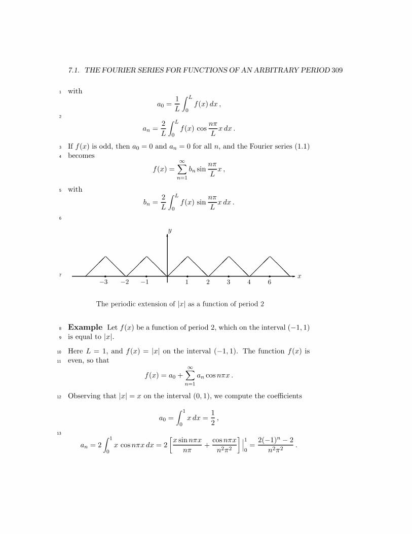
7.1. THE FOURIER SERIES FOR FUNCTIONS OF AN ARBITRARY PERIOD 309
with1
a0 =1
L
∫ L
0f(x) dx ,
2
an =2
L
∫ L
0f(x) cos
nπ
Lx dx .
If f(x) is odd, then a0 = 0 and an = 0 for all n, and the Fourier series (1.1)3
becomes4
f(x) =∞∑
n=1
bn sinnπ
Lx ,
with5
bn =2
L
∫ L
0f(x) sin
nπ
Lx dx .
6
-
6
x
y
��
��
��
��
��
��
��
��
��
��@@
@@
@@
@@
@@
@@
@@
@@
@@
@@1 2 3 4 6−1−2−3
r r r r rThe periodic extension of |x| as a function of period 2
7
Example Let f(x) be a function of period 2, which on the interval (−1, 1)8
is equal to |x|.9
Here L = 1, and f(x) = |x| on the interval (−1, 1). The function f(x) is10
even, so that11
f(x) = a0 +∞∑
n=1
an cosnπx .
Observing that |x| = x on the interval (0, 1), we compute the coefficients12
a0 =
∫ 1
0x dx =
1
2,
13
an = 2
∫ 1
0x cosnπx dx = 2
[
x sinnπx
nπ+
cosnπx
n2π2
]
∣
∣
∣
1
0=
2(−1)n − 2
n2π2.

310CHAPTER 7. THE FOURIER SERIES AND BOUNDARY VALUE PROBLEMS
Restricting to the interval (−1, 1)1
|x| = 1
2+
∞∑
n=1
2(−1)n − 2
n2π2cosnπx, for −1 < x < 1 .
Outside of the interval (−1, 1), this Fourier series converges to the periodic2
extension of |x|, or to the function f(x).3
Observing that an = 0 for even n, one can also write the answer as4
|x| =1
2−
∞∑
k=0
4
(2k + 1)2π2cos(2k + 1)πx , for −1 < x < 1 .
(All odd n can be obtained in the form n = 2k + 1, with k = 0, 1, 2, . . ..)5
7.1.2 Further Examples and the Convergence Theorem6
Even and odd functions are very special. A “general” function is neither7
even nor odd.8
Example 1 On the interval (−2, 2), represent the function9
f(x) =
{
1 for −2 < x ≤ 0
x for 0 < x < 2
by its Fourier series.10
This function is neither even nor odd (and also it is not continuous, with a11
jump at x = 0). Here L = 2, and the Fourier series has the form12
f(x) = a0 +∞∑
n=1
(
an cosnπ
2x+ bn sin
nπ
2x
)
.
Compute13
a0 =1
4
∫ 0
−21 dx+
1
4
∫ 2
0x dx = 1 ,
where we broke the interval of integration into two pieces, according to the14
definition of f(x). Similarly15
an =1
2
∫ 0
−2cos
nπ
2x+
1
2
∫ 2
0x cos
nπ
2x dx =
2 (−1 + (−1)n)
n2π2,
16
bn =1
2
∫ 0
−2sin
nπ
2x+
1
2
∫ 2
0x sin
nπ
2x dx =
(−1 − (−1)n)
nπ.

7.1. THE FOURIER SERIES FOR FUNCTIONS OF AN ARBITRARY PERIOD 311
On the interval (−2, 2) we have1
f(x) = 1 +∞∑
n=1
(
2 (−1 + (−1)n)
n2π2cos
nπ
2x+
(−1 − (−1)n)
nπsin
nπ
2x
)
.
The quantity −1 + (−1)n is equal to zero if n is even, and to −2 if n is odd.2
The quantity −1− (−1)n is equal to zero if n is odd, and to −2 if n is even.3
All even n can be obtained in the form n = 2k, with k = 1, 2, 3, . . ., and all4
odd n can be obtained in the form n = 2k − 1, with k = 1, 2, 3, . . .. We can5
then rewrite the Fourier series as6
f(x) = 1−∞∑
k=1
(
4
(2k − 1)2π2cos
(2k − 1)π
2x+
1
kπsinkπx
)
, for −2 < x < 2 .
Outside of the interval (−2, 2), this series converges to the extension of f(x),7
as a function of period 4.8
Example 2 Find the Fourier series of f(x) = 2 sinx + sin2 x, on the9
interval (−π, π).10
Here L = π, and the Fourier series takes the form11
f(x) = a0 +∞∑
n=1
(an cosnx+ bn sinnx) .
Let us spell out several terms of this series:12
f(x) = a0 + a1 cosx+ a2 cos 2x+ a3 cos 3x+ · · ·+ b1 sinx + b2 sin 2x+ · · · .
Using the trigonometric formula sin2 x = 12 − 1
2 cos 2x, write13
f(x) =1
2− 1
2cos 2x+ 2 sinx .
This is the desired Fourier series! Here a0 = 12 , a2 = −1
2 , b1 = 2, and all14
other coefficients are zero. In effect, this function is its own Fourier series.15
Example 3 Find the Fourier series of f(x) = 2 sinx + sin2 x, on the16
interval (−2π, 2π).17
This time L = 2π, and the Fourier series has the form18
f(x) = a0 +∞∑
n=1
(
an cosn
2x+ bn sin
n
2x
)
.

312CHAPTER 7. THE FOURIER SERIES AND BOUNDARY VALUE PROBLEMS
As before, we rewrite f(x)1
f(x) =1
2− 1
2cos 2x+ 2 sinx .
And again this is the desired Fourier series! This time a0 = 12 , a4 = −1
2 ,2
b2 = 2, and all other coefficients are zero.3
To discuss the convergence properties of Fourier series, we need the con-4
cept of piecewise smooth functions. These are functions that are continuous5
and differentiable, except for discontinuities at some isolated points. In case6
a discontinuity happens at some point x0, we assume that the limit from7
the left f(x0−) exists, as well as the limit from the right f(x0+). (So that8
at a point of discontinuity either f(x0) is not defined, or f(x0−) 6= f(x0+),9
or f(x0) 6= limx→x0 f(x).)10
Theorem 7.1.1 Let f(x) be a piecewise smooth function of period 2L. Then11
its Fourier series12
a0 +∞∑
n=1
(
an cosnπ
Lx+ bn sin
nπ
Lx
)
converges to f(x) at any point x where f(x) is continuous. If f(x) has a13
discontinuity at x, the Fourier series converges to14
f(x−) + f(x+)
2.
The proof can be found in the book of H.F. Weinberger [36]. (At jump15
points, the Fourier series tries to be fair, and it converges to the average of16
the limits from the left and from the right.)17
Let now f(x) be defined on [−L, L]. Let us extend it as a function of18
period 2L. Unless it so happens that f(−L) = f(L), the extended function19
will have jumps at x = −L and x = L. Then this theorem implies the next20
one.21
Theorem 7.1.2 Let f(x) be a piecewise smooth function defined on [−L, L].22
Let x be a point inside (−L, L). Then its Fourier series23
a0 +∞∑
n=1
(
an cosnπ
Lx+ bn sin
nπ
Lx
)

7.2. THE FOURIER COSINE AND THE FOURIER SINE SERIES 313
converges to f(x) at any point x where f(x) is continuous. If f(x) has a1
discontinuity at x, the Fourier series converges to2
f(x−) + f(x+)
2.
At both end points, x = −L and x = L, the Fourier series converges to3
f(−L+) + f(L−)
2.
(The average of the limits from the right and from the left, at −L and L4
respectively.)5
7.2 The Fourier Cosine and the Fourier Sine Series6
Suppose a function f(x) is defined on the interval (0, L). How do we repre-7
sent f(x) by a Fourier series? We can compute Fourier series for functions8
defined on (−L, L), but f(x) “lives” only on (0, L).9
One possibility is to extend f(x) as an arbitrary function on (−L, 0) (by10
drawing randomly any graph on (−L, 0)). This gives us a function defined11
on (−L, L), which we may represent by its Fourier series, and then use12
this series only on the interval (0, L), where f(x) lives. So that there are13
infinitely many ways to represent f(x) by a Fourier series on the interval14
(0, L). However, two of these Fourier series stand out, the ones when the15
extension produces either an even or an odd function.16
Let f(x) be defined on the interval (0, L). We define its even extension17
to the interval (−L, L), as follows18
fe(x) =
{
f(x) for 0 < x < Lf(−x) for −L < x < 0
.
(Observe that fe(0) is left undefined.) The graph of fe(x) is obtained by19
reflecting the graph of f(x) with respect to the y-axis. The function fe(x)20
is even on (−L, L), and so its Fourier series has the form21
fe(x) = a0 +∞∑
n=1
an cosnπ
Lx ,(2.1)
with the coefficients22
a0 =1
L
∫ L
0fe(x) dx =
1
L
∫ L
0f(x) dx ,
314CHAPTER 7. THE FOURIER SERIES AND BOUNDARY VALUE PROBLEMS
1
an =2
L
∫ L
0fe(x) cos
nπ
Lx dx =
2
L
∫ L
0f(x) cos
nπ
Lx dx ,
because fe(x) = f(x) on the interval of integration (0, L). We now restrict2
the series (2.1) to the interval (0, L), obtaining3
f(x) = a0 +∞∑
n=1
an cosnπ
Lx , for 0 < x < L ,(2.2)
with4
a0 =1
L
∫ L
0f(x) dx ,(2.3)
5
an =2
L
∫ L
0f(x) cos
nπ
Lx dx .(2.4)
The series (2.2), with the coefficients computed using the formulas (2.3) and6
(2.4), is called the Fourier cosine series of f(x).7
Where is fe(x) now? It disappeared. We used it as an artifact of con-8
struction, like scaffolding.9
Example 1 Find the Fourier cosine series of f(x) = x+2, on the interval10
(0, 3).11
The series has the form12
f(x) = a0 +∞∑
n=1
an cosnπ
3x for 0 < x < 3 .
Compute13
a0 =1
3
∫ 3
0(x+ 2) dx =
7
2,
14
an =2
3
∫ 3
0(x+ 2) cos
nπ
3x dx =
6 (−1 + (−1)n)
n2π2.
Answer:15
x+2 =7
2+
∞∑
n=1
6 (−1 + (−1)n)
n2π2cos
nπ
3x =
7
2−12
∞∑
k=1
1
(2k − 1)2π2cos
(2k − 1)π
3x .
Assume again that f(x) is defined only on the interval (0, L). We now16
define its odd extension to the interval (−L, L), as follows17
fo(x) =
{
f(x) for 0 < x < L−f(−x) for −L < x < 0
.
7.2. THE FOURIER COSINE AND THE FOURIER SINE SERIES 315
The graph of fo(x) is obtained by reflecting the graph of f(x) with respect1
to the origin. Observe that fo(0) is not defined. (If f(0) is defined, but2
f(0) 6= 0, this extension is still discontinuous at x = 0.) The function fo(x)3
is odd on (−L, L), and so its Fourier series has only the sine terms:4
fo(x) =∞∑
n=1
bn sinnπ
Lx ,(2.5)
with the coefficients5
bn =2
L
∫ L
0fo(x) sin
nπ
Lx dx =
2
L
∫ L
0f(x) sin
nπ
Lx dx ,
because on the interval of integration (0, L), fo(x) = f(x). We restrict the6
series (2.5) to the interval (0, L), obtaining7
f(x) =∞∑
n=1
bn sinnπ
Lx , for 0 < x < L ,(2.6)
with8
bn =2
L
∫ L
0f(x) sin
nπ
Lx dx .(2.7)
The series (2.6), with the coefficients computed using the formula (2.7), is9
called the Fourier sine series of f(x).10
Example 2 Find the Fourier sine series of f(x) = x + 2, on the interval11
(0, 3).12
Compute13
bn =2
3
∫ 3
0(x+ 2) sin
nπ
3x dx =
4 − 10(−1)n
nπ.
We conclude that14
x+ 2 =∞∑
n=1
4 − 10(−1)n
nπsin
nπ
3x, for 0 < x < 3 .
Clearly this series does not converge to f(x) at the end points x = 0 and15
x = 3 of our interval (0, 3). But inside (0, 3), we do have convergence.16
We now discuss the convergence issue. The Fourier sine and cosine series17
were developed by using the Fourier series on (−L, L). It follows from the18
convergence Theorem 7.1.1 that inside of (0, L), both of these series converge19
to f(x) at points of continuity, and tof(x−) + f(x+)
2if f(x) is discontin-20
uous at x. At both end points x = 0 and x = L, the Fourier sine series21
converges to 0 (as can be seen directly from the series), while the Fourier22
cosine series converges to f(0+) and f(L−) respectively. (The extension of23
fe(x) as a function of period 2L has no jumps at x = 0 and x = L.)24

316CHAPTER 7. THE FOURIER SERIES AND BOUNDARY VALUE PROBLEMS
7.3 Two Point Boundary Value Problems1
We shall need to find non-trivial solutions y = y(x) of the problem2
y′′ + λy = 0, 0 < x < L(3.1)
y(0) = y(L) = 0 ,
on an interval (0, L). Here λ is a real number. Unlike initial value problems,3
where the values of the solution and its derivative are prescribed at some4
point, here we prescribe that the solution vanishes at x = 0 and at x = L,5
which are the end-points (the boundary points) of the interval (0, L). The6
problem (3.1) is an example of a boundary value problem. Of course, y(x) = 07
is a solution of our problem (3.1), which is called the trivial solution. We8
wish to find non-trivial solutions. What are the values of the parameter λ,9
for which non-trivial solutions are possible?10
The form of the general solution depends on whether λ is positive, neg-11
ative or zero, so that there are three cases to consider.12
Case 1. λ < 0. We may write λ = −ω2, with some ω > 0 (ω =√−λ), and13
our equation takes the form14
y′′ − ω2y = 0 .
Its general solution is y = c1e−ωx + c2e
ωx. The boundary conditions15
y(0) = c1 + c2 = 0 ,16
y(L) = e−ωLc1 + eωLc2 = 0 ,
give us two equations to determine c1 and c2. From the first equation c2 =17
−c1, and then from the second equation c1 = 0. So that c1 = c2 = 0, and18
the only solution is y = 0, the trivial solution.19
Case 2. λ = 0. The equation takes the form20
y′′ = 0 .
Its general solution is y = c1 + c2x. The boundary conditions21
y(0) = c1 = 0 ,22
y(L) = c1L+ c2 = 0 ,
give us c1 = c2 = 0, so that y = 0. We struck out again in the search for a23
non-trivial solution.24

7.3. TWO POINT BOUNDARY VALUE PROBLEMS 317
Case 3. λ > 0. We may write λ = ω2, with some ω > 0 (ω =√λ), and our1
equation takes the form2
y′′ + ω2y = 0 .
Its general solution is y = c1 cosωx+c2 sinωx. The first boundary condition,3
y(0) = c1 = 0 ,
tells us that c1 = 0. We update the general solution: y = c2 sinωx. The4
second boundary condition gives5
y(L) = c2 sinωL = 0 .
One possibility for this product to be zero, is c2 = 0. That would lead again6
to the trivial solution. What saves us is that sinωL = 0, for some “lucky”7
ω’s, namely when ωL = nπ, or ω = ωn =nπ
L, and then λn = ω2
n =n2π2
L2,8
n = 1, 2, 3, . . .. The corresponding solutions are c2 sinnπ
Lx, or we can simply9
write them as sinnπ
Lx, because a constant multiple of a solution is also a10
solution of (3.1).11
To recapitulate, non-trivial solutions of the boundary value problem (3.1)12
occur at the infinite sequence of λ’s, λn =n2π2
L2, called the eigenvalues, and13
the corresponding solutions yn = sinnπ
Lx are called the eigenfunctions.14
Next, we search for non-trivial solutions of the problem15
y′′ + λy = 0, 0 < x < L
y′(0) = y′(L) = 0 ,
in which the boundary conditions are different. As before, we see that in16
case λ < 0, there are no non-trivial solutions. The case λ = 0 turns out17
to be different: any non-zero constant is a non-trivial solution. So that18
λ0 = 0 is an eigenvalue, and y0 = 1 is the corresponding eigenfunction.19
In case λ > 0, we get infinitely many eigenvalues λn =n2π2
L2, with the20
corresponding eigenfunctions yn = cosnπ
Lx, n = 1, 2, 3, . . ..21
318CHAPTER 7. THE FOURIER SERIES AND BOUNDARY VALUE PROBLEMS
7.3.1 Problems1
I. 1. Is the integral
∫ 3/2
−1tan15 x dx positive or negative?2
Hint: Consider first∫ 1−1 tan15 x dx. Answer. Positive.3
2. Show that any function can be written as a sum of an even function and4
an odd function.5
Hint: f(x) = f(x)+f(−x)2 + f(x)−f(−x)
2 .6
3. Let g(x) = x on the interval [0, 3).7
(i) Find the even extension of g(x). Answer. ge(x) = |x|, defined on (−3, 3).8
9
(ii) Find the odd extension of g(x). Answer. go(x) = x, defined on (−3, 3).10
11
4. Let h(x) = −x3 on the interval [0, 5). Find its even and odd extensions,12
and state the interval on which they are defined.13
Answer. he(x) = −|x|3 and h0(x) = −x3, both defined on (−5, 5).14
5. Let f(x) = x2 on the interval [0, 1). Find its even and odd extensions,15
and state the interval on which they are defined.16
Answer. fo(x) = x|x|, defined on (−1, 1).17
6. Differentiate the functions f(x) = x|x|p−1 and g(x) = |x|p, with p > 1.18
Hint: The function f(x) is odd, so that f ′(x) is even. Begin by computing19
f ′(x) for x > 0.20
Answer. f ′(x) = p|x|p−1, g′(x) = px|x|p−2.21
7. Assume that f(x) has period 2π. Show that the function∫ x0 f(t) dt is22
also 2π-periodic, if and only if∫ 2π0 f(t) dt = 0.23
8. Assume that f(x) has period T . Show that for any constant a24
∫ T+a
af ′(x)ef(x) dx = 0 .
II. Find the Fourier series of a given function over the indicated interval.25
1. f(x) = sinx cosx+ cos2 2x on (−π, π).26
Answer. f(x) = 12 + 1
2 cos 4x+ 12 sin 2x.27
2. f(x) = sinx cosx+ cos2 2x on (−2π, 2π).28

7.3. TWO POINT BOUNDARY VALUE PROBLEMS 319
Answer. f(x) = 12 + 1
2 cos 4x+ 12 sin 2x.1
3. f(x) = sinx cosx+ cos2 2x on (−π/2, π/2).2
Answer. f(x) = 12 + 1
2 cos 4x+ 12 sin 2x.3
4. f(x) = x+ x2 on (−π, π).4
Answer. f(x) =π2
3+
∞∑
n=1
(
4(−1)n
n2cosnx +
2(−1)n+1
nsinnx
)
.5
5. (i) f(x) =
{
1 for 0 < x < π
−1 for −π < x < 0on (−π, π).6
Answer. f(x) = 4π
(
sinx+ 13 sin 3x+ 1
5 sin 5x+ 17 sin 7x+ · · ·
)
.7
(ii) Set x = π2 in the last series, to conclude that8
π
4= 1 − 1
3+
1
5− 1
7+ · · · .
6. f(x) = 1 − |x| on (−2, 2).9
Answer. f(x) =∞∑
n=1
4
n2π2(1 − (−1)n) cos
nπ
2x.10
7. f(x) = x|x| on (−1, 1).11
Answer. f(x) =∞∑
n=1
−2(
n2π2 − 2)
(−1)n − 4
n3π3sinnπx.12
8. Let f(x) =
{
1 for −1 < x < 0
0 for 0 < x < 1on (−1, 1). Sketch the graphs of f(x)13
and of its Fourier series. Then calculate the Fourier series of f(x) on (−1, 1).14
15
Answer. f(x) =1
2−
∞∑
k=1
2
(2k − 1)πsin(2k− 1)πx.16
9. Let f(x) =
{
x for −2 < x < 0
−1 for 0 < x < 2on (−2, 2). Sketch the graphs of17
f(x) and of its Fourier series. Then calculate the Fourier series of f(x) on18
(−2, 2).19
III. Find the Fourier cosine series of a given function over the indicated20
interval.21
320CHAPTER 7. THE FOURIER SERIES AND BOUNDARY VALUE PROBLEMS
1. f(x) = cos 3x− sin2 3x on (0, π).1
Answer. f(x) = −1
2+ cos 3x+
1
2cos 6x.2
2. f(x) = cos 3x− sin2 3x on (0, π3 ).3
Answer. f(x) = −1
2+ cos 3x+
1
2cos 6x.4
3. f(x) = x on (0, 2).5
Answer. f(x) = 1 +∞∑
n=1
−4 + 4(−1)n
n2π2cos
nπ
2x.6
4. f(x) = sinx on (0, 2).7
Hint: sin ax cos bx = 12 sin(a− b)x+ 1
2 sin(a+ b)x.8
Answer. f(x) =1
2(1− cos 2) +
∞∑
n=1
4 ((−1)n cos 2 − 1)
n2π2 − 4cos
nπ
2x.9
5. f(x) = sin4 x on (0, π2 ).10
Answer. f(x) =3
8− 1
2cos 2x+
1
8cos 4x.11
IV. Find the Fourier sine series of a given function over the indicated interval.12
13
1. f(x) = 5 sinx cosx on (0, π).14
Answer. f(x) =5
2sin 2x.15
2. f(x) = 1 on (0, 3).16
Answer. f(x) =∞∑
n=1
2
nπ(1 − (−1)n) sin
nπ
3x.17
3. f(x) = x on (0, 2).18
Answer. f(x) =∞∑
n=1
4
nπ(−1)n+1 sin
nπ
2x.19
4. f(x) = sinx on (0, 2).20
Hint: sin ax sin bx = 12 cos(a− b)x− 1
2 cos(a+ b)x.21
Answer. f(x) =∞∑
n=1
(−1)n+1 2nπ sin 2
n2π2 − 4sin
nπ
2x.22

7.3. TWO POINT BOUNDARY VALUE PROBLEMS 321
5. f(x) = sin3 x on (0, π).1
Hint: ei3x =(
eix)3
. Use Euler’s equation on both sides, then compare the2
imaginary parts.3
Answer.3
4sinx− 1
4sin 3x.4
6. f(x) =
{
x for 0 < x < π2
π − x for π2 < x < π
on (0, π).5
Answer. f(x) =∞∑
n=1
4
πn2sin
nπ
2sinnx.6
7. f(x) = x− 1 on (0, 3).7
Answer. f(x) = −∞∑
n=1
2 + 4(−1)n
nπsin
nπ
3x.8
V.9
1. Find the eigenvalues and the eigenfunctions of10
y′′ + λy = 0, 0 < x < L, y′(0) = y(L) = 0 .
Answer. λn =π2(n+ 1
2 )2
L2, yn = cos
π(n+ 12 )
Lx.11
2. Find the eigenvalues and the eigenfunctions of12
y′′ + λy = 0, 0 < x < L, y(0) = y′(L) = 0 .
Answer. λn =π2(n+ 1
2 )2
L2, yn = sin
π(n+ 12 )
Lx.13
3. Find the eigenvalues and the eigenfunctions of14
y′′ + λy = 0, y(x) is a 2π periodic function .
Answer. λ0 = 0 with y0 = 1, and λn = n2 with yn = an cosnx+ bn sinnx.15
4. Find all non-trivial solutions of an integro-differential equation16
y′′ +(∫ 1
0y2(x) dx
)
y = 0, 0 < x < 1, y(0) = y(1) = 0 .
Hint:∫ 10 y
2(x) dx is a constant.17
Answer. y = ±√
2n sinnπx, with integer n ≥ 1.18

322CHAPTER 7. THE FOURIER SERIES AND BOUNDARY VALUE PROBLEMS
5∗. Show that the fourth order problem (with a > 0)1
y′′′′ − a4y = 0, 0 < x < 1, y(0) = y′(0) = y(1) = y′(1) = 0
has non-trivial solutions (eigenfunctions) if and only if a satisfies2
cosa =1
cosh a.
Show graphically that there are infinitely many such a’s, and calculate the3
corresponding eigenfunctions.4
Hint: The general solution is y(x) = c1 cosax + c2 sinax + c3 coshax +5
c4 sinh ax. From the boundary conditions obtain two equation for c3 and c4.6
7.4 The Heat Equation and the Method of Sepa-7
ration of Variables8
6
- xx Lx+ ∆x
u
u(x, t)
��
Heat flows in at x+ ∆x, and escapes at x
9
Suppose we have a rod of length L, so thin that we may assume it to be one10
dimensional, extending along the x-axis, for 0 ≤ x ≤ L. Assume that the11
surface of the rod is insulated, so that heat can travel only to the left or to12
the right along the rod. We wish to determine the temperature u = u(x, t)13
at any point x of the rod, and at any time t > 0. Consider an element14
(x, x+ ∆x) of the rod, of length ∆x. The amount of heat (in calories) that15
this element holds we approximate by16
cu(x, t)∆x .

7.4. THE HEAT EQUATION AND THE METHOD OF SEPARATION OF VARIABLES 323
Indeed, the amount of heat ought to be proportional to the temperature1
u = u(x, t), and to the length ∆x. A physical constant c > 0 reflects the2
rod’s capacity to store heat (c also makes the physical units right, so that3
the product is in calories). The rate of change of the amount of heat is4
cut(x, t)∆x ,
where ut(x, t) denotes the partial derivative in t. The change in the amount5
of heat occurs because of the heat flow through the end-points of the interval6
(x, x + ∆x). The function u(x, t) is likely to be monotone over the small7
interval (x, x + ∆x), so let us assume that u(x, t) in increasing in x over8
(x, x+ ∆x) (think of t as fixed). At the right end-point x+ ∆x, heat flows9
into our element, because to the right of this point the temperatures are10
higher. The heat flow per unit time (called the heat flux) is assumed to be11
c1ux(x+ ∆x, t) ,
or proportional to the rate of temperature increase (c1 > 0 is another phys-12
ical constant). Similarly, at the left end-point x13
c1ux(x, t)
calories of heat are lost per unit time. The equation of heat balance is then14
cut(x, t)∆x = c1ux(x+ ∆x, t)− c1ux(x, t) .
Divide by c∆x, and callc1c
= k15
ut(x, t) = kux(x+ ∆x, t) − ux(x, t)
∆x.
And finally, we let ∆x→ 0, obtaining the heat equation16
ut = kuxx .
It gives an example of a partial differential equation, or a PDE for short.17
(So far we studied ordinary differential equations, or ODE’s, with unknown18
functions depending on only one variable.)19
If u1(x, t) and u2(x, t) are two solutions of the heat equation, then so is20
c1u1(x, t)+c2u2(x, t), for any constants c1 and c2, as can be seen by a direct21
substitution. The situation is similar in case of three or more solutions. This22
superposition property of solutions could be taken as a definition of linear23

324CHAPTER 7. THE FOURIER SERIES AND BOUNDARY VALUE PROBLEMS
PDE. More formally, an equation is called linear if it depends linearly on the1
unknown function and its derivatives. We shall consider only linear PDE’s2
in this chapter.3
Suppose now that initially, or at the time t = 0, the temperatures inside4
the rod could be obtained from a given function f(x), while the temperatures5
at the end-points, x = 0 and x = L, are kept at 0 degree Celsius at all time6
t (think that the end-points are kept on ice). To determine the temperature7
u(x, t) at all points x ∈ (0, L), and all time t > 0, we need to solve8
ut = kuxx for 0 < x < L, and t > 0(4.1)
u(x, 0) = f(x) for 0 < x < L
u(0, t) = u(L, t) = 0 for t > 0 .
Here the second line represents the initial condition, and the third line gives9
the boundary conditions.10
Separation of Variables11
We search for a solution of (4.1) in the form u(x, t) = F (x)G(t), with the12
functions F (x) and G(t) to be determined. From the equation (4.1)13
F (x)G′(t) = kF ′′(x)G(t) .
Divide by kF (x)G(t):14
G′(t)kG(t)
=F ′′(x)F (x)
.
On the left we have a function of t only, while on the right we have a function15
of x only. In order for them to be the same, they must be both equal to the16
same constant, which we denote by −λ17
G′(t)kG(t)
=F ′′(x)F (x)
= −λ .
This gives us two differential equations, for F (x) and G(t),18
G′(t)kG(t)
= −λ ,(4.2)
and19
F ′′(x) + λF (x) = 0 .

7.4. THE HEAT EQUATION AND THE METHOD OF SEPARATION OF VARIABLES 325
From the boundary condition at x = 0,1
u(0, t) = F (0)G(t) = 0 .
This implies that F (0) = 0 (setting G(t) = 0, would give u = 0, which does2
not satisfy the initial condition in (4.1)). Similarly, we have F (L) = 0, using3
the other boundary condition. So that F (x) satisfies4
F ′′(x) + λF (x) = 0, F (0) = F (L) = 0 .(4.3)
We studied this problem in the preceding section. Non-trivial solutions occur5
only at λ = λn =n2π2
L2. Corresponding solutions are6
Fn(x) = sinnπ
Lx (and their multiples) .
With λ = λn = n2π2
L2 the equation (4.2) becomes7
G′(t)G(t)
= −kn2π2
L2.(4.4)
Solving these equations for all n8
Gn(t) = bne−k n2π2
L2 t ,
where bn’s are arbitrary constants. We have constructed infinitely many9
functions10
un(x, t) = Gn(t)Fn(x) = bne−k n2π2
L2 tsin
nπ
Lx ,
which satisfy the PDE in (4.1), and the boundary conditions. By linearity,11
their sum12
u(x, t) =∞∑
n=1
un(x, t) =∞∑
n=1
bne−k n2π2
L2 t sinnπ
Lx(4.5)
also satisfies the PDE in (4.1), and the boundary conditions. We now turn13
to the initial condition:14
u(x, 0) =∞∑
n=1
bn sinnπ
Lx = f(x) .(4.6)
We need to represent f(x) by its Fourier sine series, which requires15
bn =2
L
∫ L
0f(x) sin
nπ
Lx dx .(4.7)

326CHAPTER 7. THE FOURIER SERIES AND BOUNDARY VALUE PROBLEMS
Conclusion: the series1
u(x, t) =∞∑
n=1
bne−k n2π2
L2 tsin
nπ
Lx ,(4.8)
with bn’s calculated using (4.7), gives the solution of our problem (4.1).2
Observe that going from the Fourier sine series of f(x) to the solution of3
our problem (4.1) involves just putting in the additional factors e−k n2π2
L2 t.4
In practice, one should memorize the formula (4.8).5
Example 1 Find the temperature u(x, t) satisfying6
ut = 5uxx for 0 < x < 2π, and t > 0
u(x, 0) = 2 sinx− 3 sinx cosx for 0 < x < 2π
u(0, t) = u(2π, t) = 0 for t > 0 .
Here k = 5, and L = 2π. The Fourier sine series on (0, 2π) has the form7
∑∞n=1 bn sin n
2 x. Writing the initial temperatures as8
2 sinx− 3 sinx cosx = 2 sinx− 3
2sin 2x ,
we see that this function is its own Fourier sine series, with b2 = 2, b4 = −32 ,9
and all other coefficients equal to zero. According to (4.8), the solution is10
u(x, t) = 2e−5 22π2
(2π)2tsinx− 3
2e−5 42π2
(2π)2tsin 2x = 2e−5t sinx− 3
2e−20t sin 2x .
By the time t = 1, the first term of the solution totally dominates the second11
one, so that u(x, t) ≈ 2e−5t sinx for t > 1.12
Example 2 Solve13
ut = 2uxx for 0 < x < 3, and t > 0
u(x, 0) = x− 1 for 0 < x < 3
u(0, t) = u(3, t) = 0 for t > 0 .
Here k = 2, and L = 3. We begin by calculating the Fourier sine series14
x− 1 =∞∑
n=1
bn sinnπ
3x ,
with15
bn =2
3
∫ 3
0(x− 1) sin
nπ
3x dx = −2 + 4(−1)n
nπ.

7.4. THE HEAT EQUATION AND THE METHOD OF SEPARATION OF VARIABLES 327
Then, we put in the appropriate exponential factors, according to (4.8).1
Solution:2
u(x, t) = −∞∑
n=1
2 + 4(−1)n
nπe−2 n2π2
9t sin
nπ
3x .
What is the value of this solution? The initial temperatures, u(x, 0) =3
x − 1, are negative for 0 < x < 1, and positive for 1 < x < 3. Again, very4
quickly (by the time t = 1), the first term (n = 1) dominates all others, and5
then6
u(x, t) ≈ 2
πe−
2π2
9t sin
π
3x ,
so that the temperatures become positive at all points, because the first7
harmonic sin π3 x > 0, on the interval (0, 3). For large t, the temperatures8
tend exponentially to zero, while retaining the shape of the first harmonic.9
Assume now that the rod is insulated at the end-points x = 0 and x = L.10
Recall that the flux at x = 0 (the amount of heat flowing per unit time) is11
proportional to ux(0, t). Since there is no heat flow at x = 0 for all t, we12
have ux(0, t) = 0, and similarly ux(L, t) = 0. If the initial temperatures are13
prescribed by f(x), one needs to solve14
ut = kuxx for 0 < x < L, and t > 0(4.9)
u(x, 0) = f(x) for 0 < x < L
ux(0, t) = ux(L, t) = 0 for t > 0 .
It is natural to expect that in the long run the temperatures inside the rod15
will average out, and be equal to the average of the initial temperatures,16
1L
∫ L0 f(x) dx.17
Again, we search for a solution in the form u(x, t) = F (x)G(t). Sepa-18
ration of variables shows that G(t) still satisfies (4.4), while F (x) needs to19
solve20
F ′′(x) + λF (x) = 0, F ′(0) = F ′(L) = 0 .
Recall that nontrivial solutions of this problem occur only at λ = λ0 = 0,21
and at λ = λn = n2π2
L2 . The corresponding solutions are22
F0(x) = 1, Fn(x) = cosnπ
Lx (and their multiples) .
Solving (4.4) for n = 0, and for all n = 1, 2, 3, . . ., gives23
G0 = a0, Gn(t) = ane−k n2π2
L2 t ,

328CHAPTER 7. THE FOURIER SERIES AND BOUNDARY VALUE PROBLEMS
where a0 and an’s are arbitrary constants. We constructed infinitely many1
functions2
u0(x, t) = G0(t)F0(x) = a0, un(x, t) = Gn(t)Fn(x) = ane−k n2π2
L2 t cosnπ
Lx ,
satisfying the PDE in (4.9), and the boundary conditions. By linearity, their3
sum4
u(x, t) = u0(x, t) +∞∑
n=1
un(x, t) = a0 +∞∑
n=1
ane−k n2π2
L2 t cosnπ
Lx(4.10)
also satisfies the PDE in (4.9), and the boundary conditions. To satisfy the5
initial condition6
u(x, 0) = a0 +∞∑
n=1
an cosnπ
Lx = f(x)
one needs to represent f(x) by its Fourier cosine series, for which we calculate7
a0 =1
L
∫ L
0f(x) dx, an =
2
L
∫ L
0f(x) cos
nπ
Lx dx .(4.11)
Conclusion: the series8
u(x, t) = a0 +∞∑
n=1
ane−k n2π2
L2 t cosnπ
Lx ,(4.12)
with an’s computed using (4.11), gives the solution of our problem (4.9).9
Observe that going from the Fourier cosine series of f(x) to the solution of10
the problem (4.9) involves just putting in the additional factors e−k n2π2
L2 t.11
As t → ∞, u(x, t) → a0, which is equal to the average of the initial12
temperatures. The first term of the series dominates all others, and so13
u(x, t) ≈ a0 + a1e−k π2
L2 tcos π
Lx, for t not too small, say for t > 1.14
Example 3 Solve15
ut = 3uxx for 0 < x < π/2, and t > 0
u(x, 0) = 2 cos2 x − 3 cos2 2x for 0 < x < π/2
ux(0, t) = ux(π/2, t) = 0 for t > 0 .
Here k = 3, and L = π/2. The Fourier cosine series has the form a0 +16
∑∞n=1 an cos 2nx. Writing17
2 cos2 x− 3 cos2 2x = −1
2+ cos 2x− 3
2cos 4x ,

7.4. THE HEAT EQUATION AND THE METHOD OF SEPARATION OF VARIABLES 329
we see that this function is its own Fourier cosine series, with a0 = −12 ,1
a1 = 1, a2 = −32 , and all other coefficients equal to zero. Putting in the2
exponential factors, according to (4.12), we arrive at the solution:3
u(x, t) = −1
2+ e−12t cos 2x− 3
2e−48t cos 4x .
Example 4 Solve4
ut = 3uxx − au for 0 < x < π, and t > 0
u(x, 0) = 2 cosx+ x2 for 0 < x < π
ux(0, t) = ux(π, t) = 0 for t > 0 ,
where a is a positive constant. The extra term −au is an example of a lower5
order term. Its physical significance is that the rod is no longer insulated,6
and heat freely radiates through its side, with the ambient temperature7
outside of the rod being zero. Indeed, the heat balance relation leading to8
this equation is9
ut ∆x = 3 [ux(x+ ∆x, t)− ux(x, t)]− au(x, t)∆x .
If u(x, t) > 0, heat radiates out, and if u(x, t) < 0, heat enters through the10
side of the rod.11
Let v(x, t) be the new unknown function, defined by12
u(x, t) = e−atv(x, t) .
Calculate ut = −ae−atv+e−atvt, and uxx = e−atvxx. Then v(x, t) solves the13
problem14
vt = 3vxx for 0 < x < π, and t > 0(4.13)
v(x, 0) = 2 cosx+ x2 for 0 < x < π
vx(0, t) = vx(π, t) = 0 for t > 0 ,
which we know how to handle. Because 2 cosx is its own Fourier cosine15
series on the interval (0, π), we expand x2 in the Fourier cosine series (and16
then add 2 cosx). Obtain17
x2 = a0 +∞∑
n=1
an cosnx ,
where18
a0 =1
π
∫ π
0x2 dx =
π2
3,

330CHAPTER 7. THE FOURIER SERIES AND BOUNDARY VALUE PROBLEMS
1
an =2
π
∫ π
0x2 cosnx dx =
4(−1)n
n2.
Then2
2 cosx+x2 = 2 cosx+π2
3+
∞∑
n=1
4(−1)n
n2cosnx =
π2
3−2 cos x+
∞∑
n=2
4(−1)n
n2cosnx .
Using (4.12), the solution of (4.13) is3
v(x, t) =π2
3− 2e−3t cos x+
∞∑
n=2
4(−1)n
n2e−3n2t cosnx .
Answer: u(x, t) =π2
3e−at − 2e−(3+a)t cos x+
∞∑
n=2
4(−1)n
n2e−(3n2+a)t cosnx.4
7.5 Laplace’s Equation5
We now study heat conduction in a thin two-dimensional rectangular plate:6
0 ≤ x ≤ L, 0 ≤ y ≤M . Assume that both sides of the plate are insulated, so7
that heat travels only in the xy-plane. Let u(x, y, t) denote the temperature8
at a point (x, y), and time t > 0. It is natural to expect that the heat9
equation in two dimensions takes the form10
ut = k (uxx + uyy) .(5.1)
Indeed, one can derive (5.1) similarly to the way we have derived the one-11
dimensional heat equation, see e.g., the book of L. Evans [9].12
The boundary of our plate consists of four line segments. Let us assume13
that the side lying on the x-axis is kept at 1 degree Celsius, so that u(x, 0) =14
1 for 0 ≤ x ≤ L, while the other three sides are kept at 0 degree Celsius15
(they are kept on ice), so that u(x,M) = 0 for 0 ≤ x ≤ L, and u(0, y) =16
u(L, y) = 0 for 0 ≤ y ≤M . The heat will flow from the warmer side toward17
the three sides on ice. While the heat will continue its flow indefinitely,18
eventually the temperatures will stabilize (we can expect temperatures to19
be close to 1 near the warm side, and close to 0 near the icy sides). Stable20
temperatures do not change with time, so that u = u(x, y). Then ut = 0,21
and the equation (5.1) becomes Laplace’s equation:22
uxx + uyy = 0 .(5.2)
7.5. LAPLACE’S EQUATION 331
one of the three main equations of mathematical physics (along with the heat1
and the wave equations). Mathematicians use the notation: ∆u = uxx+uyy ,2
while engineers seem to prefer ∇2u = uxx + uyy . The latter notation has3
to do with the fact that computing the divergence of the gradient of u(x, y)4
gives ∇·∇u = uxx+uyy. Solutions of Laplace’s equation are called harmonic5
functions.6
To find the steady state temperatures u = u(x, y) for our example, we7
need to solve the problem8
uxx + uyy = 0 for 0 < x < L, and 0 < y < M
u(x, 0) = 1 for 0 < x < L
u(x,M) = 0 for 0 < x < L
u(0, y) = u(L, y) = 0 for 0 < y < M .
We apply the separation of variables technique, looking for a solution in the9
form10
u(x, y) = F (x)G(y) ,
with the functions F (x) and G(y) to be determined. Substitution into the11
Laplace equation gives12
F ′′(x)G(y) = −F (x)G′′(y) .
Divide both sides by F (x)G(y):13
F ′′(x)F (x)
= −G′′(y)G(y)
.
The function on the left depends on x only, while the one the right depends14
only on y. In order for them to be the same, they must be both equal to15
the same constant, which we denote by −λ16
F ′′(x)F (x)
= −G′′(y)G(y)
= −λ .
Using the boundary conditions, we obtain17
F ′′ + λF = 0, F (0) = F (L) = 0 ,(5.3)18
G′′ − λG = 0, G(M) = 0 .(5.4)
Nontrivial solutions of (5.3) occur at λ = λn = n2π2
L2 , and they are Fn(x) =19
Bn sin nπL x, with arbitrary constants Bn. We solve the problem (5.4) with20

332CHAPTER 7. THE FOURIER SERIES AND BOUNDARY VALUE PROBLEMS
λ = n2π2
L2 , obtaining Gn(y) = sinh nπL (y − M). (Recall that the general1
solution of the equation in (5.4) may be taken in the form G = c1 sinh nπL (y+2
c2).) We conclude that the functions3
un(x, y) = Fn(x)Gn(y) = Bn sinnπ
Lx sinh
nπ
L(y −M)
satisfy Laplace’s equation, and the three zero boundary conditions. The4
same is true for their sum5
u(x, y) =∞∑
n=1
Fn(x)Gn(y) =∞∑
n=1
Bn sinhnπ
L(y −M) sin
nπ
Lx .
It remains to satisfy the boundary condition at the warm side:6
u(x, 0) =∞∑
n=1
Bn sinhnπ
L(−M) sin
nπ
Lx = 1 .
We need to choose Bn’s, so that Bn sinh nπL (−M) are the Fourier sine series7
coefficient of f(x) = 1, i.e.,8
Bn sinhnπ
L(−M) =
2
L
∫ L
0sin
nπ
Lx dx =
2 (1 − (−1)n)
nπ,
which gives9
Bn = −2 (1 − (−1)n)
nπ sinh nπML
.
Answer:10
u(x, y) = −∞∑
n=1
2 (1 − (−1)n)
nπ sinh nπML
sinhnπ
L(y −M) sin
nπ
Lx .
Recall that the general solution of (ω is a constant, y = y(x))11
y′′ − ω2y = 0
can be written in three ways: y = c1e−ωx+c2e
ωx, y = c1 coshωx+c2 sinhωx,12
and y = c1 sinhω(x + c2). We used the third form when solving for G(y),13
while the second one is convenient if the initial conditions are prescribed at14
x = 0.15

7.5. LAPLACE’S EQUATION 333
Example Find the steady state temperatures1
uxx + uyy = 0 for 0 < x < 1, and 0 < y < 2
u(x, 0) = 0 for 0 < x < 1
u(x, 2) = 0 for 0 < x < 1
u(0, y) = 0 for 0 < y < 2
u(1, y) = y for 0 < y < 2 .
(The warm side is now x = 1.) Look for a solution in the form u(x, y) =2
F (x)G(y). After separating the variables, it is convenient to use λ (instead3
of −λ) to denote the common value of two functions4
F ′′(x)F (x)
= −G′′(y)G(y)
= λ .
Using the boundary conditions, obtain5
G′′ + λG = 0, G(0) = G(2) = 0 ,6
F ′′ − λF = 0, F (0) = 0 .
The first problem has non-trivial solutions at λ = λn = n2π2
4 , and they are7
Gn(y) = Bn sin nπ2 y. We then solve the second equation with λ = n2π2
4 ,8
obtaining Fn(x) = sinh nπ2 x. It follows that the functions9
un(x, y) = Fn(x)Gn(y) = Bn sinhnπ
2x sin
nπ
2y
satisfy the Laplace equation, and the three zero boundary conditions. The10
same is true for their sum11
u(x, y) =∞∑
n=1
Fn(x)Gn(y) =∞∑
n=1
Bn sinhnπ
2x sin
nπ
2y .
It remains to satisfy the boundary condition at the fourth side:12
u(1, y) =∞∑
n=1
Bn sinhnπ
2sin
nπ
2y = y .
We need to choose Bn’s, so that Bn sinh nπ2 are the Fourier sine series coef-13
ficient of y on the interval (0, 2):14
Bn sinhnπ
2=
∫ 2
0y sin
nπ
2y dy =
4(−1)n+1
nπ,

334CHAPTER 7. THE FOURIER SERIES AND BOUNDARY VALUE PROBLEMS
which gives1
Bn =4(−1)n+1
nπ sinh nπ2
.
Answer: u(x, y) =∞∑
n=1
4(−1)n+1
nπ sinh nπ2
sinhnπ
2x sin
nπ
2y.2
Our computations in the above examples were aided by the fact that3
three out of the four boundary conditions were zero (homogeneous). A4
general boundary value problem has the form5
uxx + uyy = 0 for 0 < x < L, and 0 < y < M(5.5)
u(x, 0) = f1(x) for 0 < x < L
u(x,M) = f2(x) for 0 < x < L
u(0, y) = g1(y) for 0 < y < M
u(L, y) = g2(y) for 0 < y < M,
with given functions f1(x), f2(x), g1(y) and g2(y). Because this problem is6
linear, we can break it into four sub-problems, each time keeping one of the7
boundary conditions, and setting the other three to zero. Namely, we look8
for solution in the form9
u(x, y) = u1(x, y) + u2(x, y) + u3(x, y) + u4(x, y) ,
where u1 is found by solving10
uxx + uyy = 0 for 0 < x < L, and 0 < y < M
u(x, 0) = f1(x) for 0 < x < L
u(x,M) = 0 for 0 < x < L
u(0, y) = 0 for 0 < y < M
u(L, y) = 0 for 0 < y < M,
u2 is computed from11
uxx + uyy = 0 for 0 < x < L, and 0 < y < M
u(x, 0) = 0 for 0 < x < L
u(x,M) = f2(x) for 0 < x < L
u(0, y) = 0 for 0 < y < M
u(L, y) = 0 for 0 < y < M,

7.6. THE WAVE EQUATION 335
u3 is computed from1
uxx + uyy = 0 for 0 < x < L, and 0 < y < M
u(x, 0) = 0 for 0 < x < L
u(x,M) = 0 for 0 < x < L
u(0, y) = g1(y) for 0 < y < M
u(L, y) = 0 for 0 < y < M,
and u4 is obtained by solving2
uxx + uyy = 0 for 0 < x < L, and 0 < y < M
u(x, 0) = 0 for 0 < x < L
u(x,M) = 0 for 0 < x < L
u(0, y) = 0 for 0 < y < M
u(L, y) = g2(y) for 0 < y < M.
We solve each of these four problems, using separation of variables, as in the3
examples considered previously.4
7.6 The Wave Equation5
We consider vibrations of a guitar string (or a similar elastic string). We6
assume that the motion of the string is transverse, so that it goes only up7
and down (and not sideways). Let u(x, t) denote the displacement of the8
string at a point x and time t, and our goal is to calculate u(x, t). The9
motion of an element of the string (x, x + ∆x) is governed by Newton’s10
second law of motion11
ma = f .(6.1)
The acceleration a = utt(x, t). If ρ denotes the density of the string, then12
the mass of the element is m = ρ∆x. (The string is assumed to be uniform,13
so that ρ > 0 is a constant.) We also assume that the internal tension is the14
only force acting on this element, and that the magnitude of the tension T15
is constant throughout the string. Our final assumption is that the slope of16
the string ux(x, t) is small, for all x and t. Observe that ux(x, t) = tan θ, the17
slope of the tangent line to the function u = u(x), with t fixed. The vertical18
(acting) component of the force at the right end-point of our element is19
T sin θ ≈ T tan θ = Tux(x+ ∆x, t) ,

336CHAPTER 7. THE FOURIER SERIES AND BOUNDARY VALUE PROBLEMS
because for small angles θ, sin θ ≈ tan θ ≈ θ. At the left end-point, the1
vertical component of the force is Tux(x, t), and the equation (6.1) becomes2
ρ∆x utt(x, t) = Tux(x+ ∆x, t) − Tux(x, t) .
Divide both sides by ρ∆x, and denote T/ρ = c23
utt(x, t) = c2ux(x+ ∆x, t)− ux(x, t)
∆x.
Letting ∆x→ 0, we obtain the wave equation4
utt(x, t) = c2uxx(x, t) .
-
6
x
u
���>
��9
Tθ
T
x x+ ∆x
Forces acting on an element of a string
5
We consider now the vibrations of a string of length L, which is fixed at6
the end-points x = 0 and x = L, with given initial displacement f(x), and7
given initial velocity g(x):8
utt = c2uxx for 0 < x < L, and t > 0
u(0, t) = u(L, t) = 0 for t > 0
u(x, 0) = f(x) for 0 < x < L
ut(x, 0) = g(x) for 0 < x < L .
Perform separation of variables, by setting u(x, t) = F (x)G(t), and obtaining9
F (x)G′′(t) = c2F ′′(x)G(t) ,

7.6. THE WAVE EQUATION 337
1
G′′(t)c2G(t)
=F ′′(x)F (x)
= −λ .
Using the boundary conditions, gives2
F ′′ + λF = 0, F (0) = F (L) = 0 ,
3
G′′ + λc2G = 0 .
Nontrivial solutions of the first problem occur at λ = λn = n2π2
L2 , and they4
are Fn(x) = sin nπL x. The second equation then takes the form5
G′′ +n2π2
L2c2G = 0 .
Its general solution is6
Gn(t) = bn cosnπc
Lt+Bn sin
nπc
Lt ,
where bn and Bn are arbitrary constants. The function7
u(x, t) =∞∑
n=1
Fn(x)Gn(t) =∞∑
n=1
(
bn cosnπc
Lt+ Bn sin
nπc
Lt
)
sinnπ
Lx
satisfies the wave equation, and the boundary conditions. It remains to8
satisfy the initial conditions. Compute9
u(x, 0) =∞∑
n=1
bn sinnπ
Lx = f(x) ,
which requires that10
bn =2
L
∫ L
0f(x) sin
nπ
Lx dx ,(6.2)
and11
ut(x, 0) =∞∑
n=1
Bnnπc
Lsin
nπ
Lx = g(x) ,
which implies that12
Bn =2
nπc
∫ L
0g(x) sin
nπ
Lx dx .(6.3)

338CHAPTER 7. THE FOURIER SERIES AND BOUNDARY VALUE PROBLEMS
Answer:1
u(x, t) =∞∑
n=1
(
bn cosnπc
Lt+Bn sin
nπc
Lt
)
sinnπ
Lx ,(6.4)
with bn’s computed by (6.2), and Bn’s by (6.3).2
The last formula shows that the motion of the string is periodic in time,3
similarly to the harmonic motion of a spring (the period is 2πLπc ). This is4
understandable, because we did not account for the dissipation of energy in5
our model of vibrating string.6
Example Find the displacements u = u(x, t)7
utt = 9uxx for 0 < x < π, and t > 0
u(0, t) = u(π, t) = 0 for t > 0
u(x, 0) = 2 sinx for 0 < x < π
ut(x, 0) = 0 for 0 < x < π .
Here c = 3 and L = π. Because g(x) = 0, all Bn = 0, while bn’s are the8
Fourier sine series coefficients of 2 sinx on the interval (0, π), so that b1 = 2,9
and all other bn = 0. Using (6.4), gives the answer: u(x, t) = 2 cos 3t sinx.10
To interpret this answer, we use a trigonometric identity to write11
u(x, t) = sin(x− 3t) + sin(x+ 3t) .
The graph of y = sin(x− 3t) in the xy-plane is obtained by translating the12
graph of y = sinx by 3t units to the right. Drawing these graphs on the13
same screen, for different times t, we see a wave traveling to the right with14
speed 3. Similarly, the graph of sin(x+3t) is a wave traveling to the left with15
speed 3. Our solution is the sum, or the superposition, of these two waves.16
For the general wave equation, the wave speed is given by c.17
7.6.1 Non-Homogeneous Problems18
Let us solve the following problem19
utt − 4uxx = x for 0 < x < 3, and t > 0
u(0, t) = 1 for t > 0
u(3, t) = 2 for t > 0
u(x, 0) = 0 for 0 < x < 3
ut(x, 0) = 1 for 0 < x < 3 .

7.6. THE WAVE EQUATION 339
This problem does not fit the pattern studied so far. Indeed, the x term1
on the right makes the equation non-homogeneous, and the boundary con-2
ditions are non-homogeneous (non-zero) too. We look for solution in the3
form4
u(x, t) = U(x) + v(x, t) .
We ask of the function U(x) to take care of all of our problems (to remove5
the non-homogeneous terms), and satisfy6
−4U ′′ = x
U(0) = 1, U(3) = 2 .
Integrating twice, gives7
U(x) = − 1
24x3 +
17
24x+ 1 .
Then the function v(x, t) = u(x, t)− U(x) satisfies8
vtt − 4vxx = 0 for 0 < x < 3, and t > 0
v(0, t) = 0 for t > 0
v(3, t) = 0 for t > 0
v(x, 0) = −U(x) = 124x
3 − 1724x− 1 for 0 < x < 3
vt(x, 0) = 1 for 0 < x < 3 .
This is a homogeneous problem, of the type considered in the preceding9
section! Here c = 2 and L = 3. Separation of variables (or the formula10
(6.4)) gives11
v(x, t) =∞∑
n=1
(
bn cos2nπ
3t+ Bn sin
2nπ
3t
)
sinnπ
3x ,
with12
bn =2
3
∫ 3
0
(
1
24x3 − 17
24x− 1
)
sinnπ
3x dx = − 2
nπ+
27 + 8n2π2
2n3π3(−1)n ,
13
Bn =1
nπ
∫ 3
0sin
nπ
3x dx =
3 − 3(−1)n
n2π2.
Answer:14
u(x, t) = − 1
24x3 +
17
24x + 1

340CHAPTER 7. THE FOURIER SERIES AND BOUNDARY VALUE PROBLEMS
1
+∞∑
n=1
[(
− 2
nπ+
27 + 8n2π2
2n3π3(−1)n
)
cos2nπ
3t+
3− 3(−1)n
n2π2sin
2nπ
3t
]
sinnπ
3x .
2
In the non-homogeneous wave equation3
utt − c2uxx = F (x, t) ,(6.5)
the term F (x, t) represents the acceleration of an external force applied to4
the string. Indeed, the ma = f equation for an element of a string, in the5
presence of an external force, takes the form6
ρ∆x utt = T [ux(x+ ∆x, t)− ux(x, t)] + ρ∆xF (x, t) .
Dividing by ρ∆x, and letting ∆x→ 0 (as before), we obtain (6.5). It follows7
that the ρ∆xF (x, t) term is an extra force, and F (x, t) is its acceleration.8
Non-homogeneous problems for the heat equation are solved similarly.9
Example Let us solve the problem10
ut − 2uxx = 1 for 0 < x < 1, and t > 0
u(x, 0) = x for 0 < x < 1
u(0, t) = 0 for t > 0
u(1, t) = 3 for t > 0 .
Again, look for solution in the form11
u(x, t) = U(x) + v(x, t) ,
with U(x) satisfying12
−2U ′′ = 1
U(0) = 0, U(1) = 3 .
Integrating, we calculate13
U(x) = −1
4x2 +
13
4x .
The function v(x, t) = u(x, t)− U(x) satisfies14
vt − 2vxx = 0 for 0 < x < 1, and t > 0
v(x, 0) = x− U(x) = 14x
2 − 94x for 0 < x < 1
v(0, t) = v(1, t) = 0 for t > 0 .

7.6. THE WAVE EQUATION 341
To solve the last problem, we begin by expanding the initial temperature1
v(x, 0) in its Fourier sine series2
1
4x2 − 9
4x =
∞∑
n=1
bn sinnπx ,
with3
bn = 2
∫ 1
0
(
1
4x2 − 9
4x
)
sinnπx dx =−1 +
(
1 + 4n2π2)
(−1)n
n3π3.
Then, using (4.8),4
v(x, t) =∞∑
n=1
−1 +(
1 + 4n2π2)
(−1)n
n3π3e−2n2π2t sinnπx .
Answer:5
u(x, t) = −1
4x2 +
13
4x+
∞∑
n=1
−1 +(
1 + 4n2π2)
(−1)n
n3π3e−2n2π2t sinnπx .
7.6.2 Problems6
I. Solve the following problems, and explain their physical significance.7
1.8 ut = 2uxx for 0 < x < π, and t > 0
u(x, 0) = sinx− 3 sinx cosx for 0 < x < π
u(0, t) = u(π, t) = 0 for t > 0 .
Answer. u(x, t) = e−2t sinx− 3
2e−8t sin 2x.9
2.10 ut = 2uxx for 0 < x < 2π, and t > 0
u(x, 0) = sinx− 3 sinx cosx for 0 < x < 2π
u(0, t) = u(2π, t) = 0 for t > 0 .
Answer. u(x, t) = e−2t sinx− 3
2e−8t sin 2x.11
3.12 ut = 5uxx for 0 < x < 2, and t > 0
u(x, 0) = x for 0 < x < 2
u(0, t) = u(2, t) = 0 for t > 0 .

342CHAPTER 7. THE FOURIER SERIES AND BOUNDARY VALUE PROBLEMS
Answer. u(x, t) =∞∑
n=1
4(−1)n+1
nπe−
5n2π2
4t sin
nπ
2x.1
4.2 ut = 3uxx for 0 < x < π, and t > 0
u(x, 0) =
{
x for 0 < x < π2
π − x for π2 < x < π
for 0 < x < π
u(0, t) = u(π, t) = 0 for t > 0 .
Answer. u(x, t) =∞∑
n=1
4
πn2e−3n2t sin
nπ
2sinnx.3
5.4 ut = uxx for 0 < x < 3, and t > 0
u(x, 0) = x+ 2 for 0 < x < 3
u(0, t) = u(3, t) = 0 for t > 0 .
Answer. u(x, t) =∞∑
n=1
4 − 10(−1)n
nπe−
n2π2
9t sin
nπ
3x.5
6.6 ut = uxx for 0 < x < 3, and t > 0
u(x, 0) = x+ 2 for 0 < x < 3
ux(0, t) = ux(3, t) = 0 for t > 0 .
Answer. u(x, t) =7
2+
∞∑
n=1
6(−1 + (−1)n)
n2π2e−
n2π2
9t cos
nπ
3x.7
7.8 ut = 2uxx for 0 < x < π, and t > 0
u(x, 0) = cos4 x for 0 < x < π
ux(0, t) = ux(π, t) = 0 for t > 0 .
Answer. u(x, t) =3
8+
1
2e−8t cos 2x+
1
8e−32t cos 4x.9
8.10 ut = 3uxx + u for 0 < x < 2, and t > 0
u(x, 0) = 1− x for 0 < x < 2
ux(0, t) = ux(2, t) = 0 for t > 0 .
Answer. u(x, t) =∞∑
k=1
8
π2(2k − 1)2e
(
− 3(2k−1)2π2
4+1
)
tcos
(2k − 1)π
2x.11

7.6. THE WAVE EQUATION 343
9. Show that the following functions are harmonic: u(x, y) = a, v(x, y) =1
sinmx sinhmy, w(x, y, z) = 1√x2+y2+z2
(a and m are constants).2
10. If u(x, y) is a harmonic function, show that v(x, y) = u
(
x√x2+y2
, y√x2+y2
)
3
is also harmonic. (The map (x, y) →(
x√x2+y2
, y√x2+y2
)
is called the Kelvin4
transform with respect to the unit circle.)5
11.6 uxx + uyy = 0 for 0 < x < 2, and 0 < y < 3
u(x, 0) = u(x, 3) = 5 for 0 < x < 2
u(0, y) = u(2, y) = 5 for 0 < y < 3 .
Hint: Look for a simple solution.7
12.8 uxx + uyy = 0 for 0 < x < 2, and 0 < y < 3
u(x, 0) = 5 for 0 < x < 2
u(x, 3) = 0 for 0 < x < 2
u(0, y) = u(2, y) = 0 for 0 < y < 3 .
13.9 uxx + uyy = 0 for 0 < x < 2, and 0 < y < 1
u(x, 0) = u(x, 1) = 0 for 0 < x < 2
u(0, y) = y for 0 < y < 1
u(2, y) = 0 for 0 < y < 1 .
14.10 uxx + uyy = 0 for 0 < x < π, and 0 < y < 1
u(x, 0) = 0 for 0 < x < π
u(x, 1) = 3 sin 2x for 0 < x < π
u(0, y) = u(π, y) = 0 for 0 < y < 1 .
Answer. u(x, y) =3
sinh 2sin 2x sinh2y.11
15.12 uxx + uyy = 0 for 0 < x < 2π, and 0 < y < 2
u(x, 0) = sinx for 0 < x < 2π
u(x, 2) = 0 for 0 < x < 2π
u(0, y) = 0 for 0 < y < 2
u(2π, y) = y for 0 < y < 2 .
Answer. u(x, y) = − 1
sinh 2sinh(y−2) sinx+
∞∑
n=1
4(−1)n+1
nπ sinhnπ2sinh
nπ
2x sin
nπ
2y.13
14
16.15
344CHAPTER 7. THE FOURIER SERIES AND BOUNDARY VALUE PROBLEMS
utt − 4uxx = 0 for 0 < x < π, and t > 0
u(x, 0) = sin 2x for 0 < x < π
ut(x, 0) = −4 sin 2x for 0 < x < π
u(0, t) = u(π, t) = 0 for t > 0 .
Answer. u(x, t) = cos 4t sin 2x− sin 4t sin 2x.1
17.2 utt − 4uxx = 0 for 0 < x < 1, and t > 0
u(x, 0) = 0 for 0 < x < 1
ut(x, 0) = x for 0 < x < 1
u(0, t) = u(1, t) = 0 for t > 0 .
Answer. u(x, t) =∞∑
n=1
(−1)n+1
n2π2sin 2nπt sinnπx.3
18.4 utt − 4uxx = 0 for 0 < x < 1, and t > 0
u(x, 0) = −3 for 0 < x < 1
ut(x, 0) = x for 0 < x < 1
u(0, t) = u(1, t) = 0 for t > 0 .
Answer. u(x, t) =∑∞
n=1
[
6nπ ((−1)n − 1) cos 2nπt+ (−1)n+1
n2π2 sin 2nπt]
sinnπx.5
6
19. Use separation of variables to obtain the solution of7
utt − c2uxx = 0 for 0 < x < L, and t > 0
u(x, 0) = f(x) for 0 < x < L
ut(x, 0) = g(x) for 0 < x < L
ux(0, t) = ux(L, t) = 0 for t > 0
in the form u(x, t) = a0 + A0t +∑∞
n=1
(
an cos nπcL t+ An sin nπc
L t)
cos nπL x,8
and express the coefficients as integrals.9
20. Solve10
utt − 9uxx = 0 for 0 < x < π, and t > 0
u(x, 0) = 4 for 0 < x < π
ut(x, 0) = cos2 x for 0 < x < π
ux(0, t) = ux(π, t) = 0 for t > 0 .

7.6. THE WAVE EQUATION 345
Answer. u(x, t) = 4 + 12 t+
112 sin 6t cos 2x.1
II. Solve the following non-homogeneous problems. You may leave the com-2
plicated integrals unevaluated.3
1.4ut = 5uxx, for 0 < x < 1, and t > 0
u(0, t) = 0 for t > 0
u(1, t) = 1 for t > 0
u(x, 0) = 0 for 0 < x < 1 .
Answer. u(x, t) = x+∞∑
n=1
2(−1)n
nπe−5n2π2t sinnπx.5
2.6ut = 2uxx for 0 < x < π, and t > 0
u(x, 0) = xπ for 0 < x < π
u(0, t) = 0 for t > 0
u(π, t) = 1 for t > 0 .
Hint: U(x) =x
π.7
3.8ut = 2uxx + 4x for 0 < x < 1, and t > 0
u(x, 0) = 0 for 0 < x < 1
u(0, t) = 0 for t > 0
u(1, t) = 0 for t > 0 .
Hint: U(x) = 13(x− x3).9
4.10utt = 4uxx + x for 0 < x < 4, and t > 0
u(x, 0) = x for 0 < x < 4
ut(x, 0) = 0 for 0 < x < 4
u(0, t) = 1 for t > 0
u(4, t) = 3 for t > 0 .
Hint: U(x) = 1 + 76x− 1
24x3.11
5.12ut = kuxx + f(x, t) for 0 < x < π, and t > 0
u(x, 0) = 0 for 0 < x < π
u(0, t) = 0 for t > 0
u(π, t) = 0 for t > 0 .
Here f(x, t) is a given function, k > 0 is a given number.13

346CHAPTER 7. THE FOURIER SERIES AND BOUNDARY VALUE PROBLEMS
Hint: Expand f(x, t) =∑∞
n=1 fn(t) sinnx, with fn(t) = 2π
∫ π0 f(x, t) sinnx dx.1
Writing u(x, t) =∑∞
n=1 un(t) sinnx, one has2
u′n + kn2un = fn(t), un(0) = 0 .
6. Solve3
ut = uxx + t sin 3x for 0 < x < π, and t > 0
u(x, 0) = 0 for 0 < x < π
u(0, t) = 0 for t > 0
u(π, t) = 0 for t > 0 .
Answer. u(x, t) =(
t9 − 1
81 + 181e
−9t)
sin 3x.4
7.7 Calculating Earth’s Temperature and Queen5
Dido’s Problem6
7.7.1 The Complex Form of the Fourier Series7
Recall that a real valued function f(x), defined on (−L, L), can be repre-8
sented by the Fourier series9
f(x) = a0 +∞∑
n=1
(
an cosnπ
Lx+ bn sin
nπ
Lx
)
,(7.1)
with10
a0 =1
2L
∫ L
−Lf(x) dx, an =
1
L
∫ L
−Lf(x) cos
nπ
Lx dx ,
11
bn =1
L
∫ L
−Lf(x) sin
nπ
Lx dx .
Using Euler’s formulas: cos θ = eiθ+e−iθ
2 , and sin θ = eiθ−e−iθ
2i , write (7.1) as12
f(x) = a0 +∞∑
n=1
(
anei
nπL
x + e−i nπL
x
2+ bn
einπL
x − e−i nπL
x
2i
)
.
Combining the similar terms, we rewrite this as13
f(x) =∞∑
n=−∞cne
i nπL
x ,(7.2)

7.7. CALCULATING EARTH’S TEMPERATURE AND QUEEN DIDO’S PROBLEM347
where c0 = a0, and1
cn =
an2 − bni
2 for n > 0
a−n
2 + b−n i2 for n < 0
.
We see that cm = c−m, for any integerm, where the bar denotes the complex2
conjugate. (The same fact also follows by taking the complex conjugate of3
(7.2).)4
Using the formulas for an and bn, and Euler’s formula, we have for n > 05
cn =1
L
∫ L
−Lf(x)
cos nπL x− i sin nπ
L x
2dx =
1
2L
∫ L
−Lf(x)e−i nπ
Lx dx .
In case n ≤ 0, the formula for cn is exactly the same.6
The series (7.2), with the coefficients7
cn =1
2L
∫ L
−Lf(x)e−i nπ
Lx dx, n = 0,±1,±2, . . .(7.3)
is called the complex form of the Fourier series.8
Recall that for any real a9
∫
eiax dx =eiax
a+ c ,(7.4)
as follows by Euler’s formula.10
Example Find the complex form of the Fourier series of the function11
12
f(x) =
{
−1 for −2 < x < 01 for 0 < x < 2
, defined on (−2, 2).13
Here L = 2. Calculate c0 =1
4
∫ 2
−2f(x) dx = 0. Using (7.3), (7.4) and Euler’s14
formula, calculate for n 6= 015
cn =1
4
(∫ 0
−2(−1)e−i nπ
2x dx+
∫ 2
01e−i nπ
2x dx
)
=i
nπ[−1 + (−1)n] ,
so that (with the sum taken over n 6= 0)16
f(x) =∞∑
n=−∞
i
nπ[−1 + (−1)n] ei
nπ2
x .

348CHAPTER 7. THE FOURIER SERIES AND BOUNDARY VALUE PROBLEMS
7.7.2 The Temperatures Inside the Earth and Wine Cellars1
Suppose that the average daily temperature in some area, for the t-th day2
of the year, is given by the function f(t), 0 ≤ t ≤ 365. (So that t = 343
corresponds to February 3.) We assume f(t) to be periodic, with the period4
T = 365. What is the temperature x cm inside the Earth, for any t?5
-
?
t
x
The sideways heat equation
ut = kuxx6
Assume that x is not too large, so that we may ignore the geothermal7
effects. Direct the x-axis downward, inside the Earth, with x = 0 corre-8
sponding to Earth’s surface. Direct the t-axis horizontally, and solve the9
heat equation for u = u(x, t)10
ut = kuxx, u(0, t) = f(t) for x > 0, and −∞ < t <∞ .(7.5)
Geologists tell us that k = 2 · 10−3 cm2
sec (see [30]).11
Observe that the “initial condition” is now prescribed along the t-axis,12
and the “evolution” happens along the x-axis. This is sometimes referred to13
as the sideways heat equation. We represent f(t) by its complex Fourier se-14
ries (L = T2 , for T -periodic functions, corresponding to the interval (−T
2 ,T2 ))15
f(t) =∞∑
n=−∞cne
i 2nπT
t .
Similarly, we expand the solution u = u(x, t)16
u(x, t) =∞∑
n=−∞un(x)ei
2nπT
t .
The coefficients un(x) are complex valued functions of x. Using this series17
in (7.5), gives for n 6= 018
u′′n = p2nun, un(0) = cn, with p2
n =2inπ
kT.(7.6)

7.7. CALCULATING EARTH’S TEMPERATURE AND QUEEN DIDO’S PROBLEM349
Depending on whether n is positive or negative, we can write1
2in = (1± i)2|n| ,
and then2
pn = (1± i)qn, with qn =√
|n|πkT .
(It is plus in case n > 0, and minus for n < 0.) Solving the equation in3
(7.6), gives4
un(x) = ane(1±i)qnx + bne
−(1±i)qnx .
We must set here an = 0, to avoid solutions with complex modulus becoming5
infinite as x→ ∞. Then, using the initial condition in (7.6), for n 6= 06
un(x) = cne−(1±i)qnx .
In case n = 0, the bounded solution of (7.6) is7
u0(x) = c0 .
Obtain8
u(x, t) =∞∑
n=−∞cne
−qnxei[2nπT
t−(±)qnx] .(7.7)
Write cn in its polar form, for n > 0,9
cn = |cn|eiγn ,
with some real numbers γn, and transform (7.7) as follows:10
u(x, t) = c0 +∑∞
n=1 e−qnx
[
cnei( 2nπ
Tt−qnx) + c−ne
−i( 2nπT
t−qnx)]
= c0 +∑∞
n=1 e−qnx
[
cnei( 2nπ
Tt−qnx) + cne
i( 2nπT
t−qnx)]
= c0 +∑∞
n=1 2|cn|e−qnx cos(
2nπT t+ γn − qnx
)
,
using that cn = c−n, and that z + z = 2Re(z).11
We see that the amplitude 2|cn|e−qnx of the n-th term is damped expo-12
nentially in x, and this damping is increasing with n, so that the first term13
is dominant, giving14
u(x, t) ≈ c0 + 2|c1|e−q1x cos
(
2π
Tt+ γ1 − q1x
)
.

350CHAPTER 7. THE FOURIER SERIES AND BOUNDARY VALUE PROBLEMS
When x changes, the cosine term is a shift of the function cos 2πT t, giving1
us a wave along the x-axis. If we select x so that γ1 − q1x = 0, we have a2
complete phase shift, so that the warmest temperatures at this depth occur3
in winter (when t ≈ 0), and the coolest temperatures in summer (when4
t ≈ T/2 = 182.5). This value of x is a good depth for a wine cellar. Not5
only the seasonal variations are very small, but they will also counteract any6
influence of air flow into the cellar.7
The material of this section is based on the book of A. Sommerfeld [30],8
see p. 68. I became aware of this application through the wonderful lectures9
of Henry P. McKean at Courant Institute, NYU, in the late seventies.10
7.7.3 The Isoperimetric Inequality11
Complex Fourier series can be used to prove the following Wirtinger’s inequality :12
any continuously differentiable function x(s), which is periodic of period 2π,13
and has average zero, so that
∫ 2π
0x(s) ds = 0, satisfies14
∫ 2π
0x2(s) ds ≤
∫ 2π
0x′2(s) ds .
Indeed, we represent x(s) by its complex Fourier series x(s) =∞∑
n=−∞xne
ins15
with the coefficients satisfying x−n = xn for n 6= 0, and16
x0 =1
2π
∫ 2π
0x(s) ds = 0 .
Calculate:17
∫ 2π
0x2(s) ds =
∫ 2π
0
∞∑
n=−∞xne
ins∞∑
m=−∞xme
ims ds
18
=∞∑
n,m=−∞xnxm
∫ 2π
0ei(n+m)s ds = 2π
∞∑
n=−∞xnx−n = 2π
∞∑
n=−∞|xn|2 ,
because the integral
∫ 2π
0eiks ds is zero for any integer k 6= 0, and is equal19
to 2π for k = 0. (So that∫ 2π0 ei(n+m)s ds is equal to 2π if m = −n, and to20
zero for all other m.)21

7.7. CALCULATING EARTH’S TEMPERATURE AND QUEEN DIDO’S PROBLEM351
Since x′(s) =∞∑
n=−∞inxne
ins, a similar computation gives1
∫ 2π
0x′2(s) ds = 2π
∞∑
n=−∞n2|xn|2 ,
and Wirtinger’s inequality follows. (The term corresponding to n = 0 is2
zero in both series.)3
According to Virgil, the queen Dido of Carthage (circa 800 B.C.) had4
a long rope to enclose land, which would become hers. Dido used the rope5
to form a circle, which became the city of Carthage. We shall show that6
she made the optimal choice: among all closed curves of length L, circle7
encloses the largest area. If a circle has length L, then its radius is r =L
2π,8
and its area is πr2 =L2
4π. We wish to show that the area A of any region9
enclosed by a rope of length L satisfies10
A ≤ L2
4π.
This fact is known as the isoperimetric inequality.11
We may assume that L = 2π, corresponding to r = 1, by declaring12
r =L
2πto be the new unit of length. Then we need to show that the area13
A of any region enclosed by a closed curve of length L = 2π satisfies14
A ≤ π .
If we use the arc-length parameterization for any such curve (x(s), y(s)),15
then x(s) and y(s) are periodic functions of the period 2π (after traveling16
the distance 2π, we come back to the original point on the curve). Recall17
that for the arc-length parameterization, the tangent vector(
x′(s), y′(s))
is18
of unit length, so that x′2(s) + y′2(s) = 1 for all s. Then19
2π = L =
∫ 2π
0
√
x′2(s) + y′2(s) ds =
∫ 2π
0
[
x′2(s) + y′2(s)]
ds .(7.8)
We may assume that γ =
∫ 2π
0x(s) ds = 0. (If not, consider the shifted20
curve (x(s)− γ
2π, y(s)), for which this condition holds.)21

352CHAPTER 7. THE FOURIER SERIES AND BOUNDARY VALUE PROBLEMS
According to Green’s formula, the area A enclosed by a closed curve1
(x(s), y(s)) is given by the line integral
∫
x dy over this curve, which eval-2
uates to
∫ 2π
0x(s)y′(s) ds. Using the numerical inequality ab ≤ 1
2a2 + 1
2b2,3
Wirtinger’s inequality and (7.8), we conclude4
A =
∫ 2π
0x(s)y′(s) ds ≤ 1
2
∫ 2π
0
[
x2(s) + y′2(s)]
ds
5
≤ 1
2
∫ 2π
0
[
x′2(s) + y′
2(s)]
ds = π ,
justifying the isoperimetric inequality.6
7.8 Laplace’s Equation on Circular Domains7
Polar coordinates (r, θ) will be appropriate for circular domains, and it turns8
out that the Laplacian in the polar coordinates is9
∆u = uxx + uyy = urr +1
rur +
1
r2uθθ .(8.1)
To justify (8.1), we begin by writing10
u(x, y) = u(r(x, y), θ(x, y)) ,
with11
r = r(x, y) =√
x2 + y2, θ = θ(x, y) = arctany
x.(8.2)
By the chain rule12
ux = urrx + uθθx ,13
uxx = urrr2x + 2urθrxθx + uθθθ
2x + urrxx + uθθxx .
Similarly14
uyy = urrr2y + 2urθryθy + uθθθ
2y + urryy + uθθyy ,
and so15
uxx + uyy = urr
(
r2x + r2y
)
+ 2urθ (rxθx + ryθy) + uθθ
(
θ2x + θ2y
)
+ur (rxx + ryy) + uθ (θxx + θyy) .

7.8. LAPLACE’S EQUATION ON CIRCULAR DOMAINS 353
Straightforward differentiation, using (8.2), shows that1
r2x + r2y = 1 ,
2
rxθx + ryθy = 0 ,3
θ2x + θ2y =1
r2,
4
rxx + ryy =1
r,
5
θxx + θyy = 0 ,
and the formula (8.1) follows.6
We now consider a circular plate: x2 + y2 < R2, or r < R in polar7
coordinates (R > 0 is its radius). The boundary of the plate consists of the8
points (R, θ), with 0 ≤ θ < 2π. Assume that the temperatures u(R, θ) at9
the boundary points are prescribed by a given function f(θ), of period 2π.10
What are the steady state temperatures u(r, θ) inside the plate?11
We are searching for the function u(r, θ) of period 2π in θ that solves12
what is known as the Dirichlet boundary value problem (when the value of13
the unknown function is prescribed on the boundary):14
∆u = urr + 1rur + 1
r2uθθ = 0, for r < R(8.3)
u(R, θ) = f(θ) .
Perform separation of variables, looking for solution in the form u(r, θ) =15
F (r)G(θ). Substituting this u(r, θ) into the equation (8.3), gives16
F ′′(r)G(θ) +1
rF ′(r)G(θ) = − 1
r2F (r)G′′(θ) .
Multiply both sides by r2, and divide by F (r)G(θ):17
r2F ′′(r) + rF ′(r)F (r)
= −G′′(θ)G(θ)
= λ .
This gives18
G′′ + λG = 0, G(θ) is 2π periodic,(8.4)
r2F ′′(r) + rF ′(r)− λF (r) = 0 .

354CHAPTER 7. THE FOURIER SERIES AND BOUNDARY VALUE PROBLEMS
The first problem, of eigenvalue type, was considered in a problem set previ-1
ously. It has non-trivial solutions when λ = λn = n2 (n is a positive integer),2
and when λ = λ0 = 0, and these solutions are3
Gn(θ) = An cosnθ + Bn sinnθ, G0 = A0 ,
with arbitrary constantsA0, An and Bn. The second equation in (8.4), when4
λ = λn = n2, becomes5
r2F ′′(r) + rF ′(r) − n2F (r) = 0 .
This is Euler’s equation! Its general solution is6
F (r) = c1rn + c2r
−n .(8.5)
We need to select c2 = 0, to avoid infinite temperature at r = 0, so that7
Fn(r) = rn. When λ = λ0 = 0, the second equation in (8.4) is8
r2F ′′(r) + rF ′(r) = 0 ,
for which the general solution is F (r) = c1 ln r+c2. Again, we need to select9
c1 = 0, and then F0(r) = 1. The function10
u(r, θ) = F0(r)G0(θ)+∞∑
n=1
Fn(r)Gn(θ) = A0 +∞∑
n=1
rn (An cosnθ +Bn sinnθ)
satisfies the Laplace equation for r < R. The boundary condition requires11
u(R, θ) = A0 +∞∑
n=1
Rn (An cosnθ + Bn sinnθ) = f(θ) .
Expand f(θ) in its Fourier series12
f(θ) = a0 +∞∑
n=1
(an cosnθ + bn sinnθ) ,(8.6)
with the coefficients13
a0 =1
2π
∫ 2π
0f(θ) dθ , an =
1
π
∫ 2π
0f(θ) cosnθ dθ ,(8.7)
14
bn =1
π
∫ 2π
0f(θ) sinnθ dθ (n ≥ 1) .

7.8. LAPLACE’S EQUATION ON CIRCULAR DOMAINS 355
(For 2π-periodic functions, integrals over (−π, π) are equal to the corre-1
sponding integrals over (0, 2π).) Then we need to select A0 = a0, AnRn = an2
and BnRn = bn, so that An =
1
Rnan and Bn =
1
Rnbn. Conclusion: the so-3
lution of (8.3) is given by4
u(r, θ) = a0 +∞∑
n=1
(
r
R
)n
(an cosnθ + bn sinnθ) ,(8.8)
with the coefficients calculated by (8.7).5
We see that the solution of (8.3) can be obtained from the Fourier series6
of f(θ), by just putting in the additional factors,(
rR
)n. Observe also that7
f(θ) needs to be defined only on (0, 2π), according to (8.7), so that the8
requirement that f(θ) is 2π-periodic can now be removed.9
Example 1 Solve10
∆u = 0 for x2 + y2 < 4
u = x2 − 3y on x2 + y2 = 4 .
Using that x = 2 cos θ, and y = 2 sin θ on the boundary, write11
f(θ) = x2 − 3y = 4 cos2 θ − 6 sin θ = 2 + 2 cos2θ − 6 sin θ .
The last function is its own Fourier series, with a0 = 2, a2 = 2, b1 = −6,12
and all other coefficients are zero. The formula (8.8) gives the solution (here13
R = 2):14
u(r, θ) = 2 + 2
(
r
2
)2
cos 2θ − 6r
2sin θ = 2 +
1
2r2 cos 2θ − 3r sin θ .
In Cartesian coordinates this solution is (using that cos 2θ = cos2 θ− sin2 θ)15
u(x, y) = 2 +1
2(x2 − y2) − 3y .
Consider next the exterior problem16
∆u = urr + 1rur + 1
r2uθθ = 0 , for r > R(8.9)
u(R, θ) = f(θ) .
Physically, we have a plate with the disc r < R removed. Outside of this17
disc, the plate is so large, that we can think that it extends to infinity.18

356CHAPTER 7. THE FOURIER SERIES AND BOUNDARY VALUE PROBLEMS
Temperatures are prescribed by f(θ) on the boundary of the plate, and the1
solution of (8.9) will give the steady state temperatures.2
Perform separation of variables, following the same steps as above, and3
in (8.5) this time select c1 = 0, to avoid infinite temperatures as r → ∞.4
Conclusion: the solution of the exterior problem (8.9) is given by5
u(r, θ) = a0 +∞∑
n=1
(
R
r
)n
(an cosnθ + bn sinnθ) ,
with the coefficients taken from the Fourier series of f(θ), as given in (8.7).6
Again, going from the Fourier series of f(θ) to the solution of (8.9), involves7
just putting in the additional factors(
Rr
)n.8
Example 2 Solve the exterior problem (R = 3)9
∆u = 0, for x2 + y2 > 9
u = x2 on x2 + y2 = 9 .
Writing f(θ) = x2 = (3 cosθ)2 = 9 cos2 θ = 92 + 9
2 cos 2θ, obtain10
u =9
2+
9
2
(
3
r
)2
cos 2θ =9
2+
81
2
r2(
cos2 θ − sin2 θ)
r4=
9
2+
81
2
x2 − y2
(x2 + y2)2.
11
Consider next the Neumann boundary value problem12
∆u = urr + 1rur + 1
r2uθθ = 0, for r < R(8.10)
ur(R, θ) = f(θ) .
It describes the steady state temperatures inside the disc r < R, with the13
heat flux f(θ) prescribed on the boundary of the disc. By separation of14
variables, obtain as above15
u(r, θ) = A0 +∞∑
n=1
rn (An cosnθ + Bn sinnθ) .(8.11)
The boundary condition requires16
ur(R, θ) =∞∑
n=1
nRn−1 (An cosnθ + Bn sinnθ) = f(θ) .(8.12)

7.9. STURM-LIOUVILLE PROBLEMS 357
This is impossible to arrange, unless the constant term is zero in the Fourier1
series of f(θ), which implies that2
∫ 2π
0f(θ) dθ = 0 .(8.13)
(Observe that the constant term is zero in the series on the left in (8.12). The3
same must be true for f(θ) on the right.) The condition (8.13) is a necessary4
condition for the Neumann problem to have solutions. If the condition (8.13)5
holds, we choose An and Bn to satisfy nRn−1An = 1π
∫ 2π0 f(θ) cosnθ dθ, and6
nRn−1Bn = 1π
∫ 2π0 f(θ) sinnθ dθ, while A0 is arbitrary.7
To recapitulate, the Neumann problem (8.10) is solvable only if the con-8
dition (8.13) holds, otherwise it has no solutions. If the condition (8.13)9
holds, the formula (8.11) gives infinitely many solutions (“feast-or-famine”).10
7.9 Sturm-Liouville Problems11
Let us recall the eigenvalue problem12
y′′ + λy = 0, 0 < x < L
y(0) = y(L) = 0 ,
on some interval (0, L). Its eigenfunctions, sin nπL x, n = 1, 2, . . ., are the13
building blocks of the Fourier sine series on (0, L). These eigenfunctions are14
orthogonal on (0, L), which means that∫ L0 sin nπ
L x sin mπL x dx = 0 for any15
m 6= n. Similarly, the eigenfunctions of16
y′′ + λy = 0, 0 < x < L
y′(0) = y′(L) = 0 ,
which are: 1, cos nπL x, n = 1, 2, . . ., give rise to the Fourier cosine series on17
(0, L). It turns out that under some conditions, solutions of other eigenvalue18
problems lead to their own types of Fourier series on (0, L).19
Recall that given a general linear second order equation20
P (x)y′′ +Q(x)y′ + R(x)y = 0 ,
with P (x) > 0, one can divide this equation by P (x), and then multiply by21
the integrating factor p(x) = e∫
Q(x)P(x)
dx, to put it into the self-adjoint form22
(
p(x)y′)′
+ r(x)y = 0 ,

358CHAPTER 7. THE FOURIER SERIES AND BOUNDARY VALUE PROBLEMS
with r(x) = p(x)R(x)P (x) .1
On an arbitrary interval (a, b), we consider an eigenvalue problem for2
equations in the self-adjoint form3
(
p(x)y′)′
+ λr(x)y = 0 , for a < x < b ,(9.1)
together with the homogeneous boundary conditions4
αy(a) + βy′(a) = 0, γy(b) + δy′(b) = 0 .(9.2)
The differentiable function p(x) and the continuous function r(x) are given,5
and both are assumed to be positive on [a, b]. The boundary conditions in6
(9.2) are called separated boundary conditions, with the first one involving7
the values of the solution and its derivative only at x = a, and the other8
one uses the values only at the right end-point x = b. The constants α, β,9
γ and δ are given, however to prevent the possibility that both constants10
in the same boundary condition are zero, we assume that α2 + β2 6= 0, and11
γ2 + δ2 6= 0. By the eigenfunctions we mean non-trivial (non-zero) solutions12
of (9.1), satisfying the boundary conditions in (9.2), and the corresponding13
values of λ are called the eigenvalues.14
Theorem 7.9.1 Assume that y(x) is an eigenfunction of the problem (9.1),15
(9.2), corresponding to an eigenvalue λ, while z(x) is an eigenfunction corre-16
sponding to an eigenvalue µ, and λ 6= µ. Then y(x) and z(x) are orthogonal17
on (a, b) with weight r(x), which means that18
∫ b
ay(x)z(x) r(x) dx= 0 .
Proof: The eigenfunction z(x) satisfies19
(p(x)z′)′ + µr(x)z = 0(9.3)
αz(a) + βz′(a) = 0, γz(b) + δz′(b) = 0 .
Multiply the equation (9.1) by z(x), and subtract from that the equation20
(9.3) multiplied by y(x). Obtain21
(
p(x)y′)′z(x)− (p(x)z′)′ y(x) + (λ− µ)r(x)y(x)z(x) = 0 .
Rewrite this as22
[
p(y′z − yz′)]′
+ (λ− µ)r(x)y(x)z(x) = 0 .

7.9. STURM-LIOUVILLE PROBLEMS 359
Integrating over [a, b], gives1
[
p(y′z − yz′)]
|ba
+(λ− µ)
∫ b
ay(x)z(x) r(x) dx= 0 .(9.4)
We shall show that2
p(b)(
y′(b)z(b)− y(b)z′(b))
= 0 ,(9.5)
and3
p(a)(
y′(a)z(a)− y(a)z′(a))
= 0 .(9.6)
Then the first term in (9.4) is zero. It follows that the second term in (9.4)4
is also zero, and therefore∫ ba y(x)z(x) r(x) dx= 0, because λ− µ 6= 0.5
We shall justify (9.5), while the proof of (9.6) is similar. Consider first6
the case when δ = 0. Then the corresponding boundary conditions simplify7
to read y(b) = 0, z(b) = 0, and (9.5) follows. In the other case, when δ 6= 0,8
we express y′(b) = −γδy(b), z′(b) = −γ
δz(b), and then9
y′(b)z(b)− y(b)z′(b) = −γδy(b)z(b) +
γ
δy(b)z(b) = 0 ,
and (9.5) follows, which concludes the proof. ♦10
Theorem 7.9.2 The eigenvalues of the problem (9.1), (9.2) are real num-11
bers.12
Proof: Assume, on the contrary, that an eigenvalue λ is not real, so that13
λ 6= λ, and the corresponding eigenfunction y(x) is complex valued. Taking14
the complex conjugates of (9.1) and (9.2), gives15
(
p(x)y′)′
+ λr(x)y = 0
16
αy(a) + βy′(a) = 0, γy(b) + δy′(b) = 0 .
It follows that λ is also an eigenvalue, and y is the corresponding eigenfunc-17
tion. By the preceding Theorem 7.9.118
∫ b
ay(x)y(x) r(x) dx=
∫ b
a|y(x)|2 r(x) dx = 0 .
The second integral involves a non-negative function, and it can be zero only19
if y(x) = 0, for all x. But an eigenfunction cannot be zero function. We20

360CHAPTER 7. THE FOURIER SERIES AND BOUNDARY VALUE PROBLEMS
have a contradiction, which was caused by the assumption that λ is not real.1
It follows that only real eigenvalues are possible. ♦2
Example On the interval (0, π), we consider the eigenvalue problem3
y′′ + λy = 0, 0 < x < π(9.7)
y(0) = 0, y′(π)− y(π) = 0 ,
and calculate its eigenvalues and the corresponding eigenvectors.4
The general solution depends on the sign of λ.5
Case 1. λ < 0. We may write λ = −k2, with k > 0. The general solution6
is then y = c1e−kx + c2e
kx. Using the boundary conditions, compute c1 =7
c2 = 0, so that y = 0, and there are no negative eigenvalues.8
Case 2. λ = 0. The general solution is y = c1x + c2. Again, calculate9
c1 = c2 = 0, and λ = 0 is not an eigenvalue.10
Case 3. λ > 0. We may write λ = k2, with k > 0. The general solution is11
then y = c1 cos kx + c2 sin kx, and c1 = 0 by the first boundary condition.12
The second boundary condition implies that13
c2 (k cos kπ − sinkπ) = 0 .
We need c2 6= 0, to get a non-trivial solution, therefore the quantity in the14
bracket must be zero, which implies that15
tan kπ = k .(9.8)
This equation has infinitely many solutions, 0 < k1 < k2 < k3 < . . ., as can16
be seen by drawing the graphs of y = k and y = tan kπ in the ky-plane.17
We obtain infinitely many eigenvalues λi = k2i , and the corresponding eigen-18
functions yi = sinkix, i = 1, 2, 3, . . . . (Observe that −ki’s are also solutions19
of (9.8), but they lead to the same eigenvalues and eigenfunctions.) Using20
that tan kiπ = ki, or sinkiπ = ki cos kiπ, and recalling two trigonometric21
identities, we verify that for all i 6= j22
∫ π
0sinkix sinkjx dx =
1
2
∫ π
0[cos(ki − kj)x− cos(ki + kj)x] dx
23
=sin(ki − kj)π
2(ki − kj)− sin(ki + kj)π
2(ki + kj)24
=1
k2i − k2
j
(kj cos kjπ sin kiπ − ki cos kiπ sin kjπ) = 0 ,

7.9. STURM-LIOUVILLE PROBLEMS 361
proving directly that the eigenfunctions are orthogonal, which serves to il-1
lustrate the Theorem 7.9.1 above.2
It is known that the problem (9.1), (9.2) has infinitely many eigenvalues,3
and the corresponding eigenfunctions yj(x) allow us to do Fourier series.4
This means that we can represent on the interval (a, b) any f(x), for which5
∫ ba f
2(x)r(x) dx is finite, as6
f(x) =∞∑
j=1
cjyj(x) , for a < x < b .(9.9)
One says that the eigenfunctions yj(x) form a complete set. To find the7
coefficients, multiply both sides by yi(x)r(x), and integrate over (a, b)8
∫ b
af(x)yi(x)r(x) dx=
∞∑
j=1
cj
∫ b
ayj(x)yi(x)r(x) dx .
By the Theorem 7.9.1, for all j 6= i, the integrals on the right are zero. So9
that the sum on the right is equal to ci∫ ba y
2i (x)r(x) dx. Therefore10
ci =
∫ ba f(x)yi(x)r(x) dx∫ ba y
2i (x)r(x) dx
.(9.10)
For the example (9.7) considered above, the corresponding Fourier series11
takes the form12
f(x) =∞∑
j=1
ci sinkix , for 0 < x < π ,
for any f(x) satisfying∫ π0 f
2(x) dx <∞, with the coefficients13
ci =
∫ π0 f(x) sinkix dx∫ π0 sin2 kix dx
.
Using a symbolic software, like Mathematica, it is easy to compute approx-14
imately ki’s, and the integrals for ci’s. The book of H. Weinberger [36] has15
more information on the validity of the expansion (9.9).16
7.9.1 The Fourier-Bessel Series17
Consider the following eigenvalue problem: on the interval (0, R) determine18
non-trivial solutions F = F (r) of19
F ′′ + 1rF
′ + λF = 0(9.11)
F ′(0) = 0, F (R) = 0 .

362CHAPTER 7. THE FOURIER SERIES AND BOUNDARY VALUE PROBLEMS
Rewrite this equation in the self-adjoint form (9.1) as1
(
rF ′)′ + λrF = 0 .
Then, by the Theorem 7.9.1, any two eigenfunctions of (9.11), corresponding2
to different eigenvalues, are orthogonal on (0, R) with weight r.3
We shall reduce the equation in (9.11) to Bessel’s equation of order zero.4
To this end, make a change of variables r → x, by letting r = 1√λx. By the5
chain rule6
Fr = Fx
√λ, Frr = Fxxλ .
Then the problem (9.11) becomes7
λFxx + 11√λ
x
√λFx + λF = 0
Fx(0) = 0, F (√λR) = 0 .
Divide by λ, and use primes again to denote the derivatives in x8
F ′′ + 1xFx + F = 0
F ′(0) = 0, F (√λR) = 0 .
This equation is Bessel’s equation of order zero. The Bessel function J0(x),9
which was considered in Chapter 3, satisfies this equation, as well as the10
condition F ′(0) = 0. Recall that the function J0(x) has infinitely many11
positive roots r1 < r2 < r3 < · · ·. In order to satisfy the second boundary12
condition, we need13 √λR = ri , i = 1, 2, 3, . . . ,
so that λ = λi =r2i
R2 . Returning to the original variable r (observe that14
F (x) = F (√λr)), gives us the eigenvalues and the corresponding eigenfunc-15
tions of the problem (9.11):16
λi =r2iR2
, Fi(r) = J0
(
riRr
)
, i = 1, 2, 3, . . . .
The Fourier-Bessel series is then the following expansion, using the eigen-17
functions J0
( riR r)
,18
f(r) =∞∑
j=1
ciJ0
(
riRr
)
, for 0 < r < R ,(9.12)
7.9. STURM-LIOUVILLE PROBLEMS 363
and the coefficients ci are given by (in view of (9.10))1
ci =
∫R0 f(r)J0(
riR r)r dr
∫ R0 J2
0 ( riR r)r dr
.(9.13)
This expansion is valid for any f(r), with∫ R0 f2(r)r dr finite. Using Mathe-2
matica, it is easy to compute ci’s numerically, and to work with the expansion3
(9.12).4
7.9.2 Cooling of a Cylindrical Tank5
It is known that the heat equation in three spacial dimensions is (see e.g.,6
the book of H. Weinberger [36])7
ut = k (uxx + uyy + uzz) , k > 0 is a constant .
Suppose that we have a cylindrical tank x2 + y2 ≤ R2, 0 ≤ z ≤ H , and the8
temperatures inside it are independent of z, so that u = u(x, y, t). The heat9
equation then becomes10
ut = k (uxx + uyy) .
Assume also that the boundary of the cylinder is kept at zero temperature,11
while the initial temperatures, u(x, y, 0), are prescribed to be f(r), where r12
is the polar radius. Because the initial temperatures do not depend on the13
polar angle θ, it is natural to expect that u = u(x, y, t) is independent of θ14
too, so that u = u(r, t). Then the Laplacian becomes15
uxx + uyy = urr +1
rur +
1
r2uθθ = urr +
1
rur .
Under these assumptions, we need to solve the following problem16
ut = k(
urr + 1rur
)
for 0 < r < R, and t > 0(9.14)
ur(0, t) = 0, u(R, t) = 0 for t > 0
u(r, 0) = f(r) ,
with a given function f(r). The condition ur(0, t) = 0 was added, because17
we expect the temperatures to have a critical point in the middle of the18
tank, for all time t.19
Use separation variables, writing u(r, t) = F (r)G(t). Substitute this20
product into our equation, then divide both sides by kF (r)G(t):21
F (r)G′(t) = k
(
F ′′(r)) +1
rF ′(r)
)
G(t) ,

364CHAPTER 7. THE FOURIER SERIES AND BOUNDARY VALUE PROBLEMS
1
G′(t)kG(t)
=F ′′(r)) + 1
rF′(r)
F (r)= −λ ,
which gives2
F ′′ + 1rF
′ + λF = 0(9.15)
F ′(0) = 0, F (R) = 0 ,
and3
G′(t)kG(t)
= −λ .(9.16)
The eigenvalue problem (9.15) for F (r) was solved in the preceding section,4
giving the eigenvalues λi =r2iR2
and the corresponding eigenfunctions Fi(r) =5
J0(riRr). Using λ = λi =
r2iR2
in (9.16), compute6
Gi(t) = cie−k
r2iR2 t
.
The function7
u(r, t) =∞∑
i=1
cie−k
r2i
R2 tJ0(
riRr)(9.17)
satisfies our equation, and the boundary conditions. The initial condition8
u(r, 0) =∞∑
i=1
ciJ0(riRr) = f(r)
will hold, if we choose ci’s to be the coefficients of the Fourier-Bessel series,9
given by (9.13). Conclusion: the series in (9.17), with ci’s computed by10
(9.13), gives the solution to our problem.11
7.9.3 Cooling of a Rectangular Bar12
Consider a function of two variables f(x, y) defined on a rectangle 0 < x < L,13
0 < y < M . Regarding x as a primary variable, we may represent f(x, y)14
by the Fourier sine series on (0, L)15
f(x, y) =∞∑
n=1
fn sinnπ
Lx ,(9.18)

7.9. STURM-LIOUVILLE PROBLEMS 365
where1
fn =2
L
∫ L
0f(x, y) sin
nπ
Lx dx .
Clearly each fn is a function of y, fn = fn(y). We now represent fn(y) by2
Fourier sine series on (0,M)3
fn(y) =∞∑
m=1
bnm sinmπ
My ,(9.19)
with the constants4
bnm =2
M
∫ M
0fn(y) sin
mπ
My dy .
Using (9.19) in (9.18) we obtain the double Fourier sine series5
f(x, y) =∞∑
n=1
∞∑
m=1
bnm sinnπ
Lx sin
mπ
My ,
where6
bnm =4
LM
∫ M
0
∫ L
0f(x, y) sin
nπ
Lx sin
mπ
My dx dy .(9.20)
Similarly one could develop the double cosine series, or mixed ”sine-7
cosine” series.8
Next, we solve the problem (for u = u(x, y, t))9
ut = k (uxx + uyy) , 0 < x < L , 0 < y < M
u(x, 0, t) = u(x,M, t) = 0, 0 < x < L
u(0, y, t) = u(L, y, t) = 0, 0 < y < M
u(x, y, 0) = f(x, y) ,
describing cooling of a rectangular plate, with all four sides kept on ice10
(temperature zero), and with the initial temperatures prescribed by a given11
function f(x, y).12
Use separation of variables, setting u(x, y, t) = F (x)G(y)H(t) in our13
equation, and then divide by kF (x)G(y)H(t):14
H ′(t)kH(t)
=F ′′(x)F (x)
+G′′(y)G(y)
= −λ .(9.21)

366CHAPTER 7. THE FOURIER SERIES AND BOUNDARY VALUE PROBLEMS
The first of these relations gives1
H ′(t)kH(t)
= −λ .(9.22)
In the second one, F ′′(x)F (x)
+ G′′(y)G(y)
= −λ, we separate the variables further2
F ′′(x)F (x)
= −λ− G′′(y)G(y)
= −µ ,
which gives the familiar eigenvalue problems3
F ′′ + µF = 0 , 0 < x < L, F (0) = F (L) = 0 ,4
G′′ + (λ− µ)G = 0 , 0 < y < M, G(0) = G(M) = 0 .
It follows that µn = n2π2
L2 , Fn(x) = sin nπL x, and then λnm = n2π2
L2 + m2π2
M2 ,5
Gnm(y) = sin mπM y. From (9.22), Hnm(t) = e
−k
(
n2π2
L2 +m2π2
M2
)
t. The sum6
u(x, y, t) =∞∑
n=1
∞∑
m=1
bnme−k
(
n2π2
L2 +m2π2
M2
)
tsin
nπ
Lx sin
mπ
My ,
with the coefficients bnm computed by (9.20), gives the solution of our prob-7
lem.8
7.10 Green’s Function9
We wish to solve the non-homogeneous boundary value problem10
(p(x)y′)′ + r(x)y = f(x), a < x < b(10.1)
y(a) = 0, y(b) = 0 ,
where the equation is written in self-adjoint form. Here p(x), r(x) and f(x)11
are given differentiable functions, and we assume that p(x) > 0, and r(x) > 012
on [a, b]. We shall also consider the corresponding homogeneous equation13
(
p(x)y′)′
+ r(x)y = 0 ,(10.2)
and the corresponding homogeneous boundary value problem14
(p(x)y′)′ + r(x)y = 0(10.3)
y(a) = 0, y(b) = 0 .
7.10. GREEN’S FUNCTION 367
Recall the concept of the Wronskian determinant of two functions y1(x) and1
y2(x), or the Wronskian, for short:2
W (x) =
∣
∣
∣
∣
∣
y1(x) y2(x)
y′1(x) y′2(x)
∣
∣
∣
∣
∣
= y1(x)y′2(x)− y′1(x)y2(x) .
Lemma 7.10.1 Let y1(x) and y2(x) be any two solutions of the homoge-3
neous equation (10.2). Then p(x)W (x) is a constant.4
Proof: We need to show that (p(x)W (x))′ = 0. Compute5
(p(x)W (x))′ = y′1p(x)y′2 + y1 (p(x)y′2)
′ − p(x)y′1y′2 − (p(x)y′1)
′ y2= y1 (p(x)y′2)
′ − (p(x)y′1)′ y2 = −r(x)y1y2 + r(x)y1y2 = 0 .
On the last step we expressed (p(x)y′1)′ = −r(x)y1, and (p(x)y′2)
′ = −r(x)y2,6
by using the equation (10.2), which both y1 and y2 satisfy. ♦7
We make the following fundamental assumption: the homogeneous bound-8
ary value problem (10.3) has only the trivial solution y = 0. Define y1(x) to9
be a non-trivial solution of the homogeneous equation (10.2), together with10
the condition y(a) = 0 (which can be computed e.g., by adding a second11
initial condition y′(a) = 1). By our fundamental assumption, y1(b) 6= 0.12
Similarly, we define y2(x) to be a non-trivial solution of the homogeneous13
equation (10.2) together with the condition y(b) = 0. By the fundamental14
assumption, y2(a) 6= 0. The functions y1(x) and y2(x) form a fundamental15
set of the homogeneous equation (10.2) (they are not constant multiples of16
one another). To find a solution of the non-homogeneous equation (10.1),17
we use the variation of parameters method, and look for solution in the form18
y(x) = u1(x)y1(x) + u2(x)y2(x) ,(10.4)
with the functions u1(x) and u2(x) satisfying the formulas (10.6) and (10.7)19
below. We shall additionally require that these functions satisfy20
u1(b) = 0, u2(a) = 0 .(10.5)
Then y(x) in (10.4) satisfies our boundary conditions y(a) = y(b) = 0, and21
gives the desired solution of the problem (10.1).22
We put the equation (10.1) into the form considered in Chapter 223
y′′ +p′(x)p(x)
y′ +r(x)
p(x)y =
f(x)
p(x).

368CHAPTER 7. THE FOURIER SERIES AND BOUNDARY VALUE PROBLEMS
Then by the formulas (8.5) in Chapter 2, we have1
u′1(x) = −y2(x)f(x)
p(x)W (x)= −y2(x)f(x)
K,(10.6)
2
u′2(x) =y1(x)f(x)
p(x)W (x)=y1(x)f(x)
K,(10.7)
where W is the Wronskian of y1(x) and y2(x), and by K we denote the3
constant that p(x)W (x) is equal to, by Lemma 7.10.1.4
Integrating (10.7), and using the condition u2(a) = 0, we get5
u2(x) =
∫ x
a
y1(ξ)f(ξ)
Kdξ .
Similarly, integrating (10.6), and using the condition u1(b) = 0, gives6
u1(x) =
∫ b
x
y2(ξ)f(ξ)
Kdξ .
Using these functions in (10.4), we get the solution of our problem (10.1)7
y(x) = y1(x)
∫ b
x
y2(ξ)f(ξ)
Kdξ + y2(x)
∫ x
a
y1(ξ)f(ξ)
Kdξ .(10.8)
It is customary to define Green’s function8
G(x, ξ) =
y1(x)y2(ξ)K for a ≤ x ≤ ξ
y2(x)y1(ξ)K for ξ ≤ x ≤ b ,
(10.9)
so that the solution (10.8) can be written as9
y(x) =
∫ b
aG(x, ξ)f(ξ)dξ .(10.10)
(Break this integral as∫ ba =
∫ xa +
∫ bx . In the first integral, ξ ≤ x, so that10
G(x, ξ) is given by the second formula in (10.9).)11
Example 1 Find Green’s function, and the solution of the problem12
y′′ + y = f(x) , for 0 < x < 1
y(0) = 0, y(1) = 0 .

7.10. GREEN’S FUNCTION 369
The function sin(x − a) solves the corresponding homogeneous equation1
y′′ + y = 0, for any constant a. Therefore, we may take y1(x) = sinx, and2
y2(x) = sin(x− 1) (giving y1(0) = y2(1) = 0). Compute3
W = y1(x)y′2(x) − y′1(x)y2(x) = sinx cos(x− 1)− cosx sin(x− 1) = sin 1 ,
which follows by using that cos(x− 1) = cosx cos 1 + sinx sin 1, and sin(x−4
1) = sinx cos 1 − cosx sin 1. Then5
G(x, ξ) =
sinx sin(ξ−1)sin 1 for 0 ≤ x ≤ ξ
sin(x−1) sin ξsin 1 for ξ ≤ x ≤ 1 ,
and the solution is6
y(x) =
∫ 1
0G(x, ξ)f(ξ)dξ .
Example 2 Find Green’s function, and the solution of the problem7
x2y′′ − 2xy′ + 2y = f(x) , for 1 < x < 2
y(1) = 0, y(2) = 0 .
The corresponding homogeneous equation8
x2y′′ − 2xy′ + 2y = 0
is Euler’s equation, with the general solution y(x) = c1x + c2x2. We then9
find y1(x) = x− x2, and y2(x) = 2x− x2 (y1(1) = y2(2) = 0). Compute10
W = y1(x)y′2(x)− y′1(x)y2(x) = (x− x2)(2− 2x) − (1 − 2x)(2x− x2) = x2 .
Turning to the construction of G(x, ξ), we observe that our equation is not11
in the self-adjoint form. To put it into the right form, divide the equation12
by x213
y′′ − 2
xy′ +
2
x2y =
f(x)
x2,
and then multiply the new equation by the integrating factor, µ = e∫
(− 2x)dx =14
e−2 lnx =1
x2, obtaining15
(
1
x2y′)′
+2
x4y =
f(x)
x4.

370CHAPTER 7. THE FOURIER SERIES AND BOUNDARY VALUE PROBLEMS
Here p(x) =1
x2, and K = p(x)W (x) = 1. Then1
G(x, ξ) =
{
(x− x2)(2ξ − ξ2) for 1 ≤ x ≤ ξ
(2x− x2)(ξ − ξ2) for ξ ≤ x ≤ 2 ,
and the solution is2
y(x) =
∫ 2
1G(x, ξ)
f(ξ)
ξ4dξ .
Finally, we observe that the same construction works for general sepa-3
rated boundary conditions (9.2). If y1(x) and y2(x) are the solutions of the4
corresponding homogeneous equation, satisfying the boundary conditions5
at x = a and at x = b respectively, then the formula (10.9) gives Green’s6
function.7
7.10.1 Problems8
I. Find the complex form of the Fourier series for the following functions on9
the given interval.10
1. f(x) = x on (−2, 2).11
Answer. x =∑∞
n=−∞2i(−1)n
nπ einπ2
x.12
2. f(x) = ex on (−1, 1).13
Answer. ex =∞∑
n=−∞(−1)n (1 + inπ)(e− 1
e )
2(1 + n2π2)einπx.14
3. f(x) = sin2 x on (−π, π).15
Answer. −14e
−i2x + 12 − 1
4ei2x.16
4. f(x) = sin 2x cos 2x on (−π/2, π/2).17
Answer. i4e
−i4x − i4e
i4x.18
5. Suppose a real valued function f(x) is represented by its complex Fourier19
series on (−L, L)20
f(x) =∞∑
n=−∞cn e
i nπL
x .
(i) By taking the complex conjugates of both sides, show that cn = c−n for21
all n.22

7.10. GREEN’S FUNCTION 371
(ii) Multiply both sides by e−i mπL
x, and integrate over (−L, L), to conclude1
that2
cn =1
2L
∫ L
−Lf(x)e−i nπ
Lx dx, n = 0,±1,±2, . . . .
6. Let u(t) be a differentiable function of period T , satisfying
∫ T
0u(t) dt = 0.3
Prove the following Poincare’s inequality4
|u(t)| ≤√T
2√
3
(
∫ T
0u′2(t) dt
)12
for all t .
Hint: Represent u(t) by its complex Fourier series: u(t) =∑
n6=0
cnei 2π
Tnt
5
(with c0 = 0 by our condition). Then u′(t) =∑
n6=0
i2π
Tncn e
i 2πT
nt, and6
∫ T
0u′2(t) dt =
4π2
T
∑
n6=0
n2|cn|2. We have (using that∑∞
n=11n2 = π2
6 )7
|u(t)| ≤∑
n6=0
|cn| ≤
∑
n6=0
1
n2
12
∑
n6=0
n2|cn|2
12
=π√3
√T
2π
(
∫ T
0u′2(t) dt
) 12
.
8
II. Solve the following problems on circular domains, and describe their9
physical significance.10
1.11 ∆u = 0, r < 3
u(3, θ) = 4 cos2 θ .
Answer. u = 2 +2
9r2 cos 2θ = 2 +
2
9(x2 − y2).12
2.13 ∆u = 0, r > 3
u(3, θ) = 4 cos2 θ .
Answer. u = 2 +18
r2cos 2θ = 2 + 18
x2 − y2
(x2 + y2)2.14
3.15 ∆u = 0, r < 2
u(2, θ) = y2 .
Answer. u = 2 − 1
2(x2 − y2).16

372CHAPTER 7. THE FOURIER SERIES AND BOUNDARY VALUE PROBLEMS
4.1 ∆u = 0, r > 2
u(2, θ) = y2 .
Answer. u = 2 − 8x2 − y2
(x2 + y2)2.2
5.3 ∆u = 0, r < 1
u(1, θ) = cos4 θ .
Hint: cos4 θ =(
1+cos 2θ2
)2.4
6.5 ∆u = 0, r < 1
u(1, θ) = θ .
Hint: Extend f(θ) = θ as a 2π periodic function, equal to θ on [0, 2π]. Then6
an =1
π
∫ π
−πf(θ) cosnθdθ =
1
π
∫ 2π
0f(θ) cosnθdθ =
1
π
∫ 2π
0θ cosnθdθ ,
and compute similarly a0, and bn’s.7
Answer. u = π −∞∑
n=1
2
nrn sinnθ.8
7. Solve the exterior problem9
∆u = 0, r > 3
u(3, θ) = θ + 2 .
Answer. u = π + 2 − 2∞∑
n=1
3n
nr−n sinnθ.10
8. Solve the problem, and write the answer in the Cartesian coordinates11
uxx + uyy = 0 inside r < 2,
u = x2 − y on r = 2 .
Answer. u(x, y) = 1 + 14
(
x2 − y2)
+ y.12
9. Find the steady state temperatures inside the disc x2 + y2 < 9, if the13
temperatures on its boundary are prescribed by the function y2 − x.14
Answer. u(x, y) =9
2− x− 1
2(x2 − y2).15

7.10. GREEN’S FUNCTION 373
10. Determine if the following Neumann problem is solvable, and if it is,1
find its solutions2
∆u = 0, r < 3
ur(3, θ) = sin θ cos θ − 2 sin 3θ .
Answer. u =1
12r2 sin 2θ − 2
27r3 sin 3θ + c.3
11. Determine if the following Neumann problem is solvable, and if it is,4
find its solutions5
∆u = 0, r < 1
ur(1, θ) = sin2 θ − 2 sin 3θ .
III. 1. Find the eigenvalues and the eigenfunctions of6
y′′ + λy = 0, y(0) + y′(0) = 0, y(π) + y′(π) = 0 .
Answer. λn = n2, yn = sinnx − n cosnx, and also λ = −1 with y = e−x.7
2. Identify graphically the eigenvalues, and find the eigenfunctions of8
y′′ + λy = 0, y(0) + y′(0) = 0, y(π) = 0 .
3. (i) Find the eigenvalues and the eigenfunctions of (a is a constant)9
y′′ + ay′ + λy = 0, y(0) = y(L) = 0 .
Answer. λn = a2
4 + n2π2
L2 , yn(x) = e−a2x sin nπ
L x.10
(ii) Use separation of variables to solve11
ut = uxx + aux, 0 < x < L
u(0, t) = u(L, t) = 0
u(x, 0) = f(x) .
Answer. u(x, t) =∑∞
n=1 bne−(
a2
4+n2π2
L2
)
te−
a2x sin nπ
L x, bn =
∫ L
0f(x)yn(x)dx∫ L
0y2
n(x)dx.12
4. (i) Find the eigenvalues and the eigenfunctions of13
x2y′′ + 3xy′ + λy = 0, y(1) = y(e) = 0 .

374CHAPTER 7. THE FOURIER SERIES AND BOUNDARY VALUE PROBLEMS
Answer. λn = 1 + n2π2, yn(x) = x−1 sin (nπ lnx).1
(ii) Put this equation into the self-adjoint form (p(x)y′)′ + λr(x)y = 0, and2
verify that the eigenfunctions are orthogonal with weight r(x).3
Hint: Divide the equation by x2, and verify that x3 is the integrating factor,4
so that p(x) = x3 and r(x) = x.5
(iii) Use separation of variables to solve6
ut = x2uxx + 3xux , 1 < x < e
u(1, t) = u(e, t) = 0
u(x, 0) = f(x) .
Answer. u(x, t) =∑∞
n=1 bne−λntyn(x), bn =
∫ e
1f(x)yn(x)x dx∫ e
1y2
n(x)x dx.7
5. Show that the eigenfunctions of8
y′′′′ + λy = 0, y(0) = y′(0) = y(L) = y′(L) = 0
corresponding to different eigenvalues, are orthogonal on (0, L).9
Hint:10
y′′′′z − yz′′′′ =d
dx
(
y′′′z − y′′z′ + y′z′′ − yz′′′)
.
6. Consider an eigenvalue problem11
(p(x)y′)′ + λr(x)y = 0, αy(0) + βy′(0) = 0, γy(π) + δy′(π) = 0 .
Assume that the given functions p(x) and r(x) are positive, while α and β12
are non-zero constants of different sign, and γ and δ are non-zero constants13
of the same sign. Show that all eigenvalues are positive.14
Hint: Multiply the equation by y(x) and integrate over (0, π). Perform an15
integration by parts.16
7. Find the eigenvalues and the eigenfunctions of (u = u(r))17
u′′(r) +2
ru′(r) + λu(r) = 0 , 0 < r < π , u′(0) = u(π) = 0 .
Hint: Write the equation in the form (ru)′′ + λ (ru) = 0.18
Answer. λm = m2, ym = sinmrr , m = 1, 2, 3, . . ..19
7.10. GREEN’S FUNCTION 375
8. Find the eigenvalues and the eigenfunctions of1
u′′(r) +n− 1
ru′(r) + λu(r) = 0 , 0 < r < 1 , u′(0) = u(1) = 0 ,
where n is a positive integer.2
Hint: The change of variables u(r) = r2−n
2 v(r) transforms this equation into3
Bessel’s equation of order n−22 , with solution v(r) = Jn−2
2
(√λ r)
.4
Answer. um(r) = r2−n
2 Jn−22
(
λn−22
, m r)
, λm = λ2n−2
2,m
, m = 1, 2, 3, . . .,5
where λn−22
,m denotes the m-th root of Jn−22
(r).6
9. Find the eigenvalues and the eigenfunctions of (F = F (t), α is a constant)7
F ′′ +1
tF ′ + λt2αF = 0 , 0 < t < 1 , F ′(0) = F (1) = 0 .
Hint: Show that the change of variables r = tα+1
α+1 transforms this problem8
into (9.11), with R = 1α+1 .9
Answer. λi = (α+ 1)2ri, Fi = J0(
ritα+1
)
, where ri are the roots of J0.10
10. Solve11
ut = 3 (uxx + uyy) , 0 < x < π , 0 < y < π
u(x, 0, t) = u(x, π, t) = 0, 0 < x < π
u(0, y, t) = u(π, y, t) = 0, 0 < y < π
u(x, y, 0) = sinx cosx sin y .
Answer. u(x, y, t) = 12e
−15t sin 2x sin y.12
11. (i) Solve13
ut = uxx + uyy , 0 < x < 3 , 0 < y < 2
u(x, 0, t) = u(x, 2, t) = 0, 0 < x < 3
u(0, y, t) = u(3, y, t) = 0, 0 < y < 2
u(x, y, 0) = xy − y .
Answer.14
u(x, y, t) =∞∑
n,m=1
8(−1)m + 16(−1)n+m
nmπ2e−(
n2π2
9+m2π2
4
)
tsin
nπ
3x sin
mπ
2y .
(ii) Find the eigenvalues and the corresponding eigenfunctions of the Lapla-15
cian on the rectangle (0, 3)× (0, 2)16
376CHAPTER 7. THE FOURIER SERIES AND BOUNDARY VALUE PROBLEMS
uxx + uyy + λu = 0, 0 < x < 3 , 0 < y < 2
u(x, 0, t) = u(x, 2, t) = 0, 0 < x < 3
u(0, y, t) = u(3, y, t) = 0, 0 < y < 2 .
1
Answer. λmn = n2π2
9 + m2π2
4 , unm(x, y) = sin nπ3 x sin mπ
2 y (m, n = 1, 2, . . .).2
3
IV. Find Green’s function and the solution of the following problems.4
1.5 y′′ + y = f(x) a < x < b
y(a) = 0, y(b) = 0 .
Answer. G(x, ξ) =
sin(x−a) sin(ξ−b)sin(b−a) for a ≤ x ≤ ξ
sin(x−b) sin(ξ−a)sin(b−a) for ξ ≤ x ≤ b .
6
2.7 y′′ + y = f(x) 0 < x < 2
y(0) = 0, y′(2) + y(2) = 0 .
Hint: y1(x) = sinx, y2(x) = − sin(x− 2) + cos(x− 2).8
3.9 x2y′′ + 4xy + 2y = f(x) 1 < x < 2
y(1) = 0, y(2) = 0 .
Answer. G(x, ξ) =
{
(x−1 − x−2)(ξ−1 − 2ξ−2) for 1 ≤ x ≤ ξ
(ξ−1 − ξ−2)(x−1 − 2x−2) for ξ ≤ x ≤ 2 ,10
y(x) =∫ 21 G(x, ξ)ξ2f(ξ) dξ.11
7.11 The Fourier Transform12
This section develops the concept of the Fourier Transform, a very impor-13
tant tool for both theoretical and applied PDE. Applications are made to14
physically significant problems on infinite domains.15
Recall the complex form of the Fourier series. A function f(x), defined16
on (−L, L), can be represented by the series17
f(x) =∞∑
n=−∞cne
i nπL
x ,(11.1)

7.11. THE FOURIER TRANSFORM 377
with the coefficients1
cn =1
2L
∫ L
−Lf(ξ)e−i nπ
Lξ dξ, n = 0,±1,±2, . . . .(11.2)
We substitute (11.2) into (11.1):2
f(x) =∞∑
n=−∞
1
2L
∫ L
−Lf(ξ)ei
nπL
(x−ξ) dξ .(11.3)
Now assume that the interval (−∞,∞) along some axis, which we call the3
s-axis, is subdivided into pieces, using the subdivision points sn = nπL . The4
length of each interval is ∆s = πL . We rewrite (11.3) as5
f(x) =1
2π
∞∑
n=−∞
∫ L
−Lf(ξ)eisn(x−ξ) dξ∆s .(11.4)
so that we can regard f(x) as a Riemann sum of a certain function of s, over6
the interval (−∞,∞). Let now L → ∞. Then ∆s → 0, and the Riemann7
sum in (11.4) converges to8
f(x) =1
2π
∫ ∞
−∞
∫ ∞
−∞f(ξ)eis(x−ξ) dξds .
This formula is known as the Fourier integral. Our derivation of it is made9
rigorous in more advanced books. Rewrite this integral as10
f(x) =1√2π
∫ ∞
−∞eisx
(
1√2π
∫ ∞
−∞f(ξ)e−isξ dξ
)
ds .(11.5)
We define the Fourier transform by11
F (s) =1√2π
∫ ∞
−∞f(ξ)e−isξ dξ .
The inverse Fourier transform is then12
f(x) =1√2π
∫ ∞
−∞eisxF (s) ds .
As with the Laplace transform, we use capital letters to denote the Fourier13
transforms. We shall also use the operator notation F (f(x)) = F (s).14
Example Let f(x) =
{
1 for |x| ≤ a
0 for |x| > a .15

378CHAPTER 7. THE FOURIER SERIES AND BOUNDARY VALUE PROBLEMS
Using Euler’s formula, we compute the Fourier transform:1
F (s) =1√2π
∫ a
−ae−isξ dξ =
2√2π
eias − e−ias
2is=
√
2
π
sinas
s.
2
Assume that f(x) → 0, as x→ ±∞. Integrating by parts3
F (f ′(x)) =1√2π
∫ ∞
−∞f ′(ξ)e−isξ dξ =
is√2π
∫ ∞
−∞f(ξ)e−isξ dξ = isF (s) .
(The boundary term1√2πf(ξ)e−isξ |∞
−∞is zero, because |e−isξ | = 1.) It4
follows that5
F (f ′′(x)) = isF (f ′(x)) = −s2F (s) .(11.6)
These formulas for F (f ′(x)) and F (f ′′(x)) are similar to the corresponding6
formulas for the Laplace transform.7
7.12 Problems on Infinite Domains8
7.12.1 Evaluation of Some Integrals9
The following integral occurs often10
I =
∫ ∞
−∞e−x2
dx =√π .(12.1)
We justify this formula as follows:11
I2 =
∫ ∞
−∞e−x2
dx
∫ ∞
−∞e−y2
dy =
∫ ∞
−∞
∫ ∞
−∞e−x2−y2
dxdy
12
=
∫ 2π
0
∫ ∞
0e−r2
r drdθ = π ,
and (12.1) follows. We used polar coordinates to evaluate the double inte-13
gral.14
We shall show that for any x15
y(x) ≡∫ ∞
0e−z2
cos xz dz =
√π
2e−
x2
4 .(12.2)
Using integration by parts, compute (d denotes the differential)16
y′(x) =
∫ ∞
0e−z2
(−z sinxz) dz =1
2
∫ ∞
0sinxz d
(
e−z2)

7.12. PROBLEMS ON INFINITE DOMAINS 379
1
= −x2
∫ ∞
0e−z2
cosxz dz ,
which implies that2
y′(x) = −x2y(x) .(12.3)
By (12.1)3
y(0) =
√π
2.(12.4)
Solving the differential equation (12.3), together with the initial condition4
(12.4), justifies the formula (12.2).5
The last integral we need, is just a Laplace transform (a is a constant)6
∫ ∞
0e−sy cos as ds =
y
y2 + a2.(12.5)
7.12.2 The Heat Equation for −∞ < x <∞7
We shall solve the initial value problem8
ut = kuxx −∞ < x <∞, t > 0(12.6)
u(x, 0) = f(x) −∞ < x <∞ .
Here u(x, t) gives the temperature at a point x, and time t, for an infinite9
bar. (The bar is very long, so that we assume it to be infinite.) The initial10
temperatures are prescribed by the given function f(x), and k > 0 is a given11
constant.12
The Fourier transform of the solution13
F (u(x, t)) =1√2π
∫ ∞
−∞u(x, t)e−isx dx = U(s, t)(12.7)
depends on s and also on t, which we may regard as a parameter, at the14
moment. Observe that F (ut(x, t)) = Ut(s, t), as follows by differentiating15
(12.7) in t. Applying the Fourier transform to the problem (12.6), and using16
(11.6), obtain17
Ut = −ks2UU(s, 0) = F (u(x, 0)) = F (f(x)) = F (s) ,

380CHAPTER 7. THE FOURIER SERIES AND BOUNDARY VALUE PROBLEMS
where F (s) is the Fourier transform of f(x). Integrating this initial value1
problem for U as a function of t (we now regard s as a parameter)2
U(s, t) = F (s)e−ks2t .
To obtain the solution of (12.6), we apply the inverse Fourier transform, and3
get4
u(x, t) = 1√2π
∫∞−∞ eisxF (s)e−ks2t ds = 1
2π
∫∞−∞
∫∞−∞ eis(x−ξ)−ks2tf(ξ) dξds
= 12π
∫∞−∞
(
∫∞−∞ eis(x−ξ)−ks2t ds
)
f(ξ) dξ ,
after switching the order of integration. We denote by K the integral in the5
brackets, K =∫∞−∞ eis(x−ξ)−ks2t ds. To evaluate K, we use Euler’s formula6
K =
∫ ∞
−∞[cos s(x− ξ) + i sins(x− ξ)] e−ks2t ds = 2
∫ ∞
0cos s(x−ξ)e−ks2t ds ,
because cos s(x − ξ) is an even function of s, and sin s(x − ξ) is an odd7
function of s. To evaluate the last integral, we make a change of variables8
s→ z, by setting9 √kt s = z ,
and then use the integral in (12.2):10
K =2√kt
∫ ∞
0e−z2
cos
(
x− ξ√kt
z
)
dz =
√π√kte−
(x−ξ)2
4kt .
With K evaluated, we get the solution of (12.6):11
u(x, t) =1
2√πkt
∫ ∞
−∞e−
(x−ξ)2
4kt f(ξ) dξ .(12.8)
This formula is important for both PDE’s and Probability Theory. The12
function K(x, t) = 12√
πkte−
x2
4kt is known as the heat kernel. (Recall from13
Chapter 4 that one may write u(x, t) = K(x, t)∗f(x), with limt→0 K(x, t) =14
δ(x), and limt→0 u(x, t) = f(x), where ∗ denotes the convolution.)15
Assume now that the function f(x), giving the initial temperatures, is16
positive on some small interval (−ε, ε), and is zero outside of this interval.17
Then u(x, t) > 0 for all x ∈ (−∞,∞) and t > 0. Not only the temperatures18
become positive far from the heat source, this happens practically instan-19
taneously! This is known as the infinite propagation speed, which points20
to an imperfection of our model. Observe, however, that for this f(x), the21
temperatures given by (12.8) are negligible for large |x|.22

7.12. PROBLEMS ON INFINITE DOMAINS 381
7.12.3 Steady State Temperatures for the Upper Half Plane1
We shall solve the boundary value problem2
uxx + uyy = 0 −∞ < x <∞, y > 0(12.9)
u(x, 0) = f(x) −∞ < x <∞ .
Here u(x, y) will provide the steady state temperature, at a point (x, y)3
of an infinite plate, occupying the upper half of the xy-plane. The given4
function f(x) prescribes the temperatures at the boundary y = 0 of the5
plate. We looking for the solution that is bounded, as y → ∞. (Without6
this assumption the solution is not unique: if u(x, y) is a solution of (12.9),7
then so is u(x, y) + cy, for any constant c.)8
Applying the Fourier transform in x, U(s, y) = 1√2π
∫∞−∞ u(ξ, y)e−isξ dξ,9
gives (observe that F (uyy(x, t)) = Uyy(s, t))10
Uyy − s2U = 0(12.10)
U(s, 0) = F (s) .
The general solution of the equation in (12.10) is11
U(s, y) = c1e−sy + c2e
sy .
When s > 0, we select c2 = 0, so that U (and therefore u) is bounded as12
y → ∞. Then c1 = F (s), from the initial condition in (12.10), giving us13
U(s, y) = F (s)e−sy , when s > 0 .
When s < 0, we select c1 = 0, to get a bounded solution. Then c2 = F (s),14
giving us15
U(s, y) = F (s)esy, when s < 0 .
Combining both cases, we conclude that the bounded solution of (12.10) is16
U(s, y) = F (s)e−|s|y .
It remains to compute the inverse Fourier transform17
u(x, y) =1√2π
∫ ∞
−∞eisx−|s|yF (s) ds =
1
2π
∫ ∞
−∞f(ξ)
(∫ ∞
−∞eis(x−ξ)−|s|y ds
)
dξ ,
after switching the order of integration. We evaluate the integral in the18
brackets by using Euler’s formula, the fact that cos s(x−ξ) is even in s, and19
sin s(x− ξ) is odd in s, and (on the last step) the formula (12.5):20
∫ ∞
−∞eis(x−ξ)−|s|y ds = 2
∫ ∞
0e−sy cos s(x− ξ) ds =
2y
(x− ξ)2 + y2.

382CHAPTER 7. THE FOURIER SERIES AND BOUNDARY VALUE PROBLEMS
The solution of (12.9), known as Poisson’s formula, is then1
u(x, y) =y
π
∫ ∞
−∞
f(ξ) dξ
(x− ξ)2 + y2.
This integral converges, provided that f(ξ) does not grow too fast as2
ξ → ±∞.3
7.12.4 Using the Laplace Transform for a Semi-Infinite String4
Imagine a string extending for 0 < x < ∞, which is initially at rest. Its5
left end-point, x = 0, undergoes periodic vibrations, with the displacements6
given by A sinωt, where A and ω are constants. We wish to find the dis-7
placements u(x, t) at any point x > 0 and time t > 0, assuming that the8
displacements are bounded.9
We need to solve the following initial-boundary value problem for the10
wave equation, with a given c > 0,11
utt = c2uxx , x > 0
u(x, 0) = ut(x, 0) = 0 , x > 0
u(0, t) = A sinωt , t > 0 .
Take the Laplace transform of the equation in the variable t, denoting12
U(x, s) = L (u(x, t)). Using the initial and boundary conditions, we get13
s2U = c2Uxx(12.11)14
U(0, s) =Aω
s2 + ω2.
The general solution of the equation in (12.11) is15
U(x, s) = c1escx + c2e
− scx .
To get a solution bounded as x → +∞, we select c1 = 0. Then c2 = Aωs2+ω216
by the initial condition in (12.11), giving17
U(x, s) = e−xcs Aω
s2 + ω2.
Taking the inverse Laplace transform, and using the formula (2.5) from18
Chapter 4, gives the solution19
u(x, t) = Aux/c(t) sin ω(t− x/c) ,

7.12. PROBLEMS ON INFINITE DOMAINS 383
where ux/c(t) is the Heaviside step function. This formula shows that at any1
point x > 0, the solution is zero for 0 < t < x/c (the time it takes for the2
signal to travel from 0 to x). For t > x/c, the motion of the string at x is3
identical with the motion at x = 0, but is delayed in time, by the value of4
x/c.5
7.12.5 Problems6
1. Find the Fourier transform of the function f(x) =
{
1 − |x| for |x| ≤ 10 for |x| > 1
.7
8
Answer. F (s) =
√
2
π
1
s2(1− cos s).9
2. Find the Fourier transform of f(x) = e−|x|.10
Answer. F (s) =
√
2
π
1
s2 + 1.11
3. Find the Fourier transform of f(x) = e−x2
2 .12
Answer. F (s) = e−s2
2 . (Hint: Use the formula (12.2).)13
4. Find the Fourier transform of f(x) = e−ax2, where a > 0 is a constant.14
Answer. F (s) =1√2ae−
s2
4a .15
5. Solve the heat conduction problem16
ut − uxx = 0 −∞ < x <∞, t > 0
u(x, 0) = e−x2 −∞ < x <∞ .
Answer. u(x, t) =1√
1 + 4te−
x2
1+4t .17
6. Show that for any constant a18
(i) F (f(x)eiax) = F (s − a).19
(ii) F (f(ax)) =1
aF (s
a) (a 6= 0).20
7. Find a non-trivial solution of the boundary value problem21
uxx + uyy = 0 −∞ < x <∞, y > 0
u(x, 0) = 0 −∞ < x <∞ .
384CHAPTER 7. THE FOURIER SERIES AND BOUNDARY VALUE PROBLEMS
Hint: Assume that u depends only on y.1
This example shows that our physical intuition may fail for unbounded do-2
mains.3
8. Use Poisson’s formula to solve4
uxx + uyy = 0 −∞ < x <∞, y > 0
u(x, 0) = f(x) −∞ < x <∞ ,
where f(x) =
{
1 for |x| ≤ 10 for |x| > 1
.5
Answer. u(x, y) =1
π
(
tan−1 x+ 1
y− tan−1 x− 1
y
)
.6
9. The famous Black-Scholes equation for the price of a stock option is (here7
V = V (S, t))8
Vt + aS2VSS + bSVS − rV = 0 ,
where a, b and r are positive constants. By a change of variables, reduce9
this equation to the heat equation.10
Hint: If the Vt term was not present, we would have Euler’s equation. This11
suggests to set x = ln s. Then let τ = −at. Obtain:12
Vτ = Vxx + 2αVx − r
aV ,
where we denoted 2α = b/a − 1. Multiply the last equation by eαx, and13
denote w = eαxV . Obtain:14
wτ = wxx −(
α2 +r
a
)
w .
Finally, multiply this equation by the integrating factor e(α2+ ra)τ , and denote15
z = e(α2+ ra)τw. Conclude:16
zτ = zxx .

Chapter 81
Elementary Theory of PDE2
This chapter continues the study of the three main equations of mathemat-3
ical physics: wave, heat and Laplace’s equations. We now deal with the4
theoretical aspects: propagation and reflection of waves, maximum princi-5
ples, harmonic functions, Poisson’s integral formulas, variational approach.6
Classification theory is presented, and it shows that the three main equa-7
tions are representative of all linear second order equations. First order8
PDE’s are solved by reducing them to ODE’s along the characteristic lines.9
8.1 Wave Equation: Vibrations of an Infinite String10
Waves11
The graph of y = (x − 1)2 is a translation of the parabola y = x2, by one12
unit to the right. The graph of y = (x − t)2 is a translation of the same13
parabola by t units. If we think of t as time, and draw these translations on14
the same screen, we get a wave of speed one, traveling to the right. Similarly,15
y = (x − ct)2 is a wave of speed c. The same reasoning applies for other16
functions. So that y = f(x − ct) is a wave of speed c traveling to the right,17
while y = f(x+ ct) describes a wave of speed c traveling to the left.18
Transverse Vibrations of a Guitar String: d’Alembert’s Formula19
Assume that an elastic string extends along the x-axis, for −∞ < x < ∞,20
and we wish to find its transverse displacements u = u(x, t), as a function21
of the position x and the time t. As in Chapter 7, we need to solve the wave22
equation, together with the initial conditions:23
utt − c2uxx = 0 for −∞ < x <∞, and t > 0(1.1)
385
386 CHAPTER 8. ELEMENTARY THEORY OF PDE
u(x, 0) = f(x) for −∞ < x <∞ut(x, 0) = g(x) for −∞ < x <∞ .
Here f(x) is given initial displacement, g(x) is given initial velocity, and1
c > 0 is a given constant.2
We look for classical solutions, which means that u(x, t) has two contin-3
uous derivatives in x and t (ux, ut, uxx, uxt, and utt are continuous). We4
perform a change of variables (x, t) → (ξ, η), with the new variables (ξ, η)5
given by6
ξ = x− ct
η = x+ ct .
Compute the partial derivatives: ξx = 1, ηx = 1, ξt = −c, and ηt = c. We7
may think of solution as u(x, t) = u(ξ(x, t), η(x, t)). Using the chain rule,8
we express9
ux = uξξx + uηηx = uξ + uη ,10
uxx = (ux)x = (uξ + uη)ξ+(uξ + uη)η = uξξ+uξη+uηξ+uηη = uξξ+2uξη+uηη
(using that uηξ = uξη). Similarly11
ut = uξξt + uηηt = −cuξ + cuη ,
12
utt = −c (−cuξξ + cuηξ) + c (−cuξη + cuηη) = c2 (uξξ − 2uξη + uηη) .
Substituting these expressions of utt and uxx into the wave equation, and13
simplifying, we get14
uξη = 0 .
Since (uξ)η = 0, integration in η gives15
uξ = F (ξ) ,
where F (ξ) is an arbitrary function. Integrating once more16
u(ξ, η) =
∫
F (ξ)dξ +G(η) = F (ξ) +G(η) .
Here G(η) is an arbitrary function of η. The antiderivative of F (ξ) is an17
arbitrary function, which we again denote by F (ξ). Returning to the original18
variables, we have the general solution19
u(x, t) = F (x− ct) +G(x+ ct) .(1.2)
8.1. WAVE EQUATION: VIBRATIONS OF AN INFINITE STRING 387
Observe that the wave equation has an overwhelmingly large number of so-1
lutions, because its general solution depends on two arbitrary functions.2
Turning to the initial conditions, compute3
ut(x, t) = −cF ′(x− ct) + cG′(x+ ct) .
We have4
u(x, 0) = F (x) +G(x) = f(x)(1.3)
ut(x, 0) = −cF ′(x) + cG′(x) = g(x) .
Integrating the second equation in (1.3) gives5
−cF (x) + cG(x) =
∫ x
γg(τ)dτ ,
where γ is any constant. Adding to this formula the first equation in (1.3),6
multiplied by c, produces7
G(x) =1
2f(x) +
1
2c
∫ x
γg(τ)dτ .
From the first equation in (1.3)8
F (x) =1
2f(x)− 1
2c
∫ x
γg(τ)dτ .
Using these expressions in (1.2), we get9
u(x, t) =1
2f(x− ct) − 1
2
∫ x−ct
γg(τ)dτ +
1
2f(x+ ct) +
1
2c
∫ x+ct
γg(τ)dτ .
Writing −∫ x−ctγ g(τ)dτ =
∫ γx−ct g(τ)dτ , we combine both integrals into one:10
u(x, t) =f(x− ct) + f(x+ ct)
2+
1
2c
∫ x+ct
x−ctg(τ)dτ .
We derived the famous d’Alembert formula (published in 1747, see the11
Wikipedia article).12
In case g(x) = 0, this formula gives13
u(x, t) =f(x− ct) + f(x+ ct)
2,

388 CHAPTER 8. ELEMENTARY THEORY OF PDE
which is a superposition (sum) of a wave traveling to the right and a wave1
traveling to the left, both of speed c. (The same conclusion is true for general2
g(x), just look at the formula (1.2).)3
6
- x
u
f(x)
@@
@
1�
��
−1
1 t = 0
-
6
x
u
HHH
t = 1
2
���
−32 −1
212
32
12
-
6
x
ut = 1
Snapshots of u(x, t) in case of pinched string
HHH���
HHH���
12
−2 21−1
-
6
x
u
HHH���
HHH���
t = 3
2
−32−5
232
52
12−1
2
12
4
Example: Pinched String. We solve5
utt − uxx = 0 for −∞ < x <∞, and t > 0(1.4)
u(x, 0) = f(x) for −∞ < x <∞ut(x, 0) = 0 for −∞ < x <∞ ,

8.1. WAVE EQUATION: VIBRATIONS OF AN INFINITE STRING 389
where1
f(x) =
x+ 1 if −1 ≤ x ≤ 01 − x if 0 ≤ x ≤ 1
0 if |x| > 1 .
The initial displacement f(x) resembles a “pinch” (see the snapshot at t =2
0), while the initial velocity is zero. By d’Alembert’s formula3
u(x, t) =1
2f(x− t) +
1
2f(x+ t) .
This expression implies that the initial “pinch” breaks into two pinches of4
similar shape, but half of the original magnitude, with one of them traveling5
to the right, and the other one to the left, both with speed 1. We present6
the snapshots of u(x, t) at t = 0 (the initial pinch), t = 12 , t = 1, and t = 3
2 .7
-
6
x
t
JJ
JJJ
JJJ
JJ
t(x0, t0)
x0 − ct0 x0 + ct0
vv
The domain of dependence (thick) of the point (x0, t0)
x− ct = x0 − ct0x+ ct = x0 + ct0
8
We now define the important concept of characteristic lines. A family9
of parallel straight lines in the (x, t) plane (with t > 0, and α a constant)10
x− ct = α
are called the left characteristic lines, or the left characteristics for short.11
They all have the slope 1c > 0, and varying the constant α produces a specific12
line, parallel to all others. Given any point (x0, t0) (with t0 > 0), we can13
select a left characteristic, passing through it, namely14
x− ct = x0 − ct0 .

390 CHAPTER 8. ELEMENTARY THEORY OF PDE
Let us follow this line for decreasing t until it intersects the x-axis. This1
happens at x = x0 − ct0. Similarly, a family of parallel straight lines in the2
(x, t) plane, given by x+ ct = α, are called the right characteristics. They3
all have the slope −1c < 0. The right characteristic passing through (x0, t0)4
is5
x+ ct = x0 + ct0 .
It intersects the x-axis at x = x0 + ct0. The string’s displacement at any6
point (x0, t0) is (according to d’Alembert’s formula)7
u(x0, t0) =f(x0 − ct0) + f(x0 + ct0)
2+
1
2c
∫ x0+ct0
x0−ct0
g(τ)dτ .
Geometrically, u(x0, t0) is equal to the average of the values of f(x) at the8
points where the characteristics, passing through (x0, y0), intersect the x-9
axis, plus 12c times the integral of g(x) between these points. One calls the10
interval [x0 − ct0, x0 + ct0] the domain of dependence of the point (x0, t0).11
Given a point (x0, 0) on the x-axis, the characteristics passing through it12
are x+ ct = x0 and x− ct = x0. The region between these characteristics is13
called the region of influence of the point (x0, 0). If a point (x, t) lies outside14
of this region, the value of the solution u(x, t) is not influenced by the values15
of f(x) and g(x) at (or near) x0.16
We say that a function f(x) has compact support, if f(x) is identically17
zero outside of some bounded interval [a, b]. In such a case, it is customary18
to say that f(x) lives on [a, b].19
Lemma 8.1.1 Assume that the initial data f(x) and g(x) are of compact20
support. Then the solution u(x, t) of the problem (1.1) is of compact support,21
for any fixed t.22
Proof: If f(x) and g(x) live on [a, b], then u(x, t) lives on [a− ct, b+ ct],23
for any fixed t, as follows by d’Alembert’s formula (just draw the regions of24
influence of (a, 0), and of (b, 0)). ♦25
6
-tx0
x
t
x− ct = x0x+ ct = x0
The region of influence of the point (x0, 0)
JJ
JJ
JJ
JJ
26

8.2. SEMI-INFINITE STRING: REFLECTION OF WAVES 391
We define the energy of a string to be1
E(t) =1
2
∫ ∞
−∞
[
u2t (x, t) + c2u2
x(x, t)]
dx .
Theorem 8.1.1 Assume that the initial data f(x) and g(x) are of compact2
support. Then the energy of a string is constant, for any solution u(x, t) of3
the wave equation in (1.1).4
Proof: We shall show that E ′(t) = 0 for all t. Indeed,5
E ′(t) =
∫ ∞
−∞
[
ututt + c2uxuxt
]
dx =
∫ ∞
−∞
[
ututt − c2uxxut
]
dx
6
=
∫ ∞
−∞ut(utt − c2uxx) dx = 0 .
On the second step we performed integration by parts, with the boundary7
terms vanishing by the Lemma 8.1.1. On the last step we used that u(x, t)8
satisfies the wave equation. ♦9
This theorem implies that for all t10
E(t) = E(0) =1
2
∫ ∞
−∞
[
u2t (x, 0) + c2u2
x(x, 0)]
(1.5)
11
=1
2
∫ ∞
−∞
[
g2(x) + c2f ′2(x)]
dx .
Theorem 8.1.2 The problem (1.1) has a unique solution.12
Proof: Assume that v(x, t) is another solution of (1.1), in addition to13
the solution u(x, t) given by d’Alembert’s formula. Call w(x, t) = u(x, t)−14
v(x, t). Then w(x, t) satisfies the wave equation (1.1) with zero initial data15
(w(x, 0) = wt(x, 0) = 0). By (1.5)16
E(t) =
∫ ∞
−∞
[
w2t (x, t) + c2w2
x(x, t)]
dx = E(0) = 0 ,
for all t. It follows that wt(x, t) = 0, and wx(x, t) = 0 for all x and t, so17
that w(x, t) = constant. Setting t = 0, we see that this constant is zero.18
We conclude that w(x, t) = 0 for all x and t, which means that v(x, t) is19
identical to u(x, t). ♦20

392 CHAPTER 8. ELEMENTARY THEORY OF PDE
8.2 Semi-Infinite String: Reflection of Waves1
Suppose that a string extends along the positive x-axis, for 0 < x < ∞,2
and we assume that its left end-point is kept in a fixed position, so that its3
displacement is zero at x = 0, for all t, u(0, t) = 0 (the Dirichlet boundary4
condition). To find the displacements u(x, t), we need to solve the wave5
equation, together with initial and boundary conditions:6
utt − c2uxx = 0 for 0 < x <∞, and t > 0(2.1)
u(x, 0) = f(x) for 0 < x <∞ut(x, 0) = g(x) for 0 < x <∞
u(0, t) = 0 for t > 0 ,
with given initial displacement f(x), and initial velocity g(x).7
Recall the concept of the odd extension. If f(x) is defined on (0,∞),8
then its odd extension9
fo(x) =
{
f(x) for x > 0−f(−x) for x < 0
is defined for all x 6= 0. Geometrically, this amounts to reflecting the graph10
of f(x) with respect to the origin. (fo(x) is left undefined at x = 0.) The11
resulting function fo(x) is odd, satisfying fo(−x) = −fo(x) for all x 6= 0.12
If fo(x) and go(x) are the odd extensions of the functions f(x) and g(x)13
respectively, then we claim that the solution of the problem (2.1) is14
u(x, t) =fo(x− ct) + fo(x+ ct)
2+
1
2c
∫ x+ct
x−ctgo(τ)dτ .(2.2)
Indeed, we already know that this formula gives a solution of the wave15
equation, and that u(x, 0) = fo(x) = f(x), and ut(x, 0) = go(x) = g(x), for16
x > 0. As for the boundary condition, we have17
u(0, t) =fo(−ct) + fo(ct)
2+
1
2c
∫ ct
−ctgo(τ)dτ = 0 .
Example 1 Solve18
utt − uxx = 0 for 0 < x <∞, and t > 0
u(x, 0) = x for 0 < x <∞ut(x, 0) = x2 for 0 < x <∞
u(0, t) = 0 for t > 0 .

8.2. SEMI-INFINITE STRING: REFLECTION OF WAVES 393
We have (here c = 1)1
u(x, t) =fo(x− t) + fo(x+ t)
2+
1
2
∫ x+t
x−tgo(τ)dτ ,(2.3)
with fo(x) = x, and go(x) =
{
x2 for x ≥ 0−x2 for x < 0
.2
Case 1. t ≤ x. Then x− t ≥ 0, and3
u(x, t) =x− t+ x+ t
2+
1
2
∫ x+t
x−tτ2dτ = x+ x2t+
1
3t3 .
4
Case 2. t > x. Then x − t < 0, and the integral term in (2.3) needs to be5
split into two pieces:6
u(x, t) =x− t+ x + t
2− 1
2
∫ 0
x−tτ2dτ +
1
2
∫ x+t
0τ2dτ = x+ xt2 +
1
3x3 .
Answer. u(x, t) =
x+ x2t+ 13 t
3 for t ≤ x
x+ xt2 + 13x
3 for t > x.7
We now return to the formula (2.2). If x − ct ≥ 0, then we can replace8
fo(x) and go(x) by f(x) and g(x) respectively. In case x− ct < 0, we claim9
that the formula (2.2) gives10
u(x, t) =−f(−x+ ct) + f(x+ ct)
2+
1
2c
∫ x+ct
−x+ctg(τ)dτ .(2.4)
Indeed, observe that −x + ct = − (x− ct) > 0, and∫ −x+ctx−ct go(τ)dτ = 0.11
Then12
∫ x+ct
x−ctgo(τ)dτ =
∫ −x+ct
x−ctgo(τ)dτ +
∫ x+ct
−x+ctgo(τ)dτ =
∫ x+ct
−x+ctg(τ)dτ .
In case g(x) = 0, it follows from (2.4) that13
u(x0, t0) =−f(−x0 + ct0) + f(x0 + ct0)
2,(2.5)
so that instead of computing f(x) at x0− ct0, we compute f(x) at the point14
symmetric with respect to x = 0. We say that the left characteristic got15

394 CHAPTER 8. ELEMENTARY THEORY OF PDE
reflected when it hit the t-axis, and the opposite sign is the way to account1
(or the “price to pay”) for a reflected wave.2
-
6
x
t
JJ
JJ
JJJ
JJJ
b
JJ
JJ
JJ]
(x0, t0)
x0 − ct0 x0 + ct0
bb
bJJ
JJ
JJ
−x0 + ct0
JJJ]
�
Reflection at the boundary point x = 0
3
Example 2 Pinched string. We solve4
utt − uxx = 0 for 0 < x <∞, and t > 0
u(x, 0) = f(x) for 0 < x <∞ut(x, 0) = 0 for 0 < x <∞
u(0, t) = 0 for t > 0 ,
where5
f(x) =
x− 1 if 1 ≤ x ≤ 2
−x+ 3 if 2 ≤ x ≤ 30 for all other x
.(2.6)
(This is the pinch considered earlier, shifted two units to the right, and6
centered at x = 2.) Using the odd extension fo(x), we write the solution of7
this problem on (−∞,∞):8
u(x, t) =fo(x− t) + fo(x+ t)
2.(2.7)
On the interval (−∞,∞), the graph of fo(x) includes the original positive9
pinch on the interval (1, 3), and a negative pinch of the same shape over10
(−3,−1) (fo(x) is zero for other x). By (2.7), each pinch breaks into two11

8.3. BOUNDED STRING: MULTIPLE REFLECTIONS 395
half-pinches, and the four half-pinches set in motion, as above. We then1
translate our results to the original (physical) interval (0,∞).2
Conclusion: the original “pinch” f(x) breaks into two pinches of similar3
shape, but half of the magnitude, with one of them traveling to the right,4
and the other one moving to the left, both with speed 1. At the time t = 1,5
the left half-pinch reaches the x = 0 end-point. By the time t = 3, it6
completely reflects and becomes negative, of the same triangle shape. Then7
both half-pinches (one of them is positive, and the other one negative) travel8
to the right, for all t > 3.9
6
- x
u
f(x)
@@
@
32�
��
1
1 t = 0
6
- x
u
t = 1
4321
12
HHH���
HHH���
6
- x
u
t = 3
54321
12
−12
������
HHHHHH
-
-
Snapshots of a semi-infinite pinched string
10

396 CHAPTER 8. ELEMENTARY THEORY OF PDE
8.3 Bounded String: Multiple Reflections1
Assume that the string is finite, extending over some interval 0 < x < L,2
and at both end-points the displacement is zero for all time. We need to3
solve4
utt − c2uxx = 0 for 0 < x < L, and t > 0(3.1)
u(x, 0) = f(x) for 0 < x < L
ut(x, 0) = g(x) for 0 < x < L
u(0, t) = u(L, t) = 0 for t > 0 ,
with given initial displacement f(x), and the initial velocity g(x).5
Let fo(x) be the odd extension of f(x) from (0, L) to (−L, L), and then6
we extend fo(x) to (−∞,∞) as a function of period 2L. We call this new7
extended function f(x). Similarly, we define the extension g(x) of g(x).8
On the original interval (0, L) these extensions agree with f(x) and g(x)9
respectively. Clearly, f (x) and g(x) are odd on (−∞,∞). In addition, both10
of these functions are odd with respect to L, which means that11
f(L+ x) = −f(L− x), and g(L+ x) = −g(L− x), for all x .
It turns out that the solution of (3.1) is12
u(x, t) =f (x− ct) + f(x+ ct)
2+
1
2c
∫ x+ct
x−ctg(τ)dτ .(3.2)
Indeed, comparing with d’Alemberts’s formula, we see that this function sat-13
isfies the wave equation, and the initial conditions. Turning to the boundary14
conditions, we have15
u(0, t) =f(−ct) + f(ct)
2+
1
2c
∫ ct
−ctg(τ)dτ = 0 ,
because f(x) and g(x) are odd. At the other end point16
u(L, t) =f(L− ct) + f(L+ ct)
2+
1
2c
∫ L+ct
L−ctg(τ)dτ = 0 ,
because f(x) and g(x) are odd with respect to L.17
Consider now the case g(x) = 0. Then18
u(x, t) =f(x− ct) + f(x+ ct)
2.(3.3)

8.3. BOUNDED STRING: MULTIPLE REFLECTIONS 397
Similarly to the above, we reflect the characteristics when they reach either1
the t-axis, or the line x = L. This time, when we continue the characteristics2
backward in time, multiple reflections are possible, from both the t-axis (the3
line x = 0), and from the line x = L, before the x-axis is reached. By4
examining the graph of f(x), one can see that the formula (3.3) implies that5
the result (or the “price”) of each reflection is change of sign. So, if after6
3 reflections the left characteristic arrives at a point A inside (0, L), then7
its contribution is f(x− ct) = −f(A). If it took 10 reflections for the right8
characteristic to arrive at a point B ∈ (0, L), then we have f (x+ct) = f(B).9
10
Example 1 Find u(1/4, 1), u(1/4, 2) and u(1/4, 3) for the problem11
utt − uxx = 0 for 0 < x < 2, and t > 0
u(x, 0) = f(x) = x2 for 0 < x < 2
ut(x, 0) = 0 for 0 < x < 2
u(0, t) = u(2, t) = 0 for t > 0 .
Here c = 1, so that the left characteristics have slope 1, and the right ones12
have slope −1. When finding the solution at (1/4, 1), the left characteristic is13
reflected once, coming down at x = 3/4, while the right one is not reflected,14
coming down at x = 5/4, giving15
u(1/4, 1) = −1
2f(3/4) +
1
2f(5/4) =
1
2.
To find the solution at (1/4, 2), both characteristics are reflected once, and16
both are coming down at the same point x = 7/4, giving17
u(1/4, 2) = −1
2f(7/4)− 1
2f(7/4) = −49
16.
When computing u(1/4, 3), the left characteristic is reflected twice, coming18
down at x = 5/4. The right characteristic is reflected once, coming down at19
x = 3/4, giving20
u(1/4, 3) =1
2f(5/4)− 1
2f(3/4) =
1
2.
Example 2 Pinched string. We solve21
utt − uxx = 0 for 0 < x < 8, and t > 0
u(x, 0) = f(x) for 0 < x < 8
ut(x, 0) = 0 for 0 < x < 8
u(0, t) = u(8, t) = 0 for t > 0 ,

398 CHAPTER 8. ELEMENTARY THEORY OF PDE
with the initial displacement1
f(x) =
x− 3 if 3 ≤ x ≤ 4
−x + 5 if 4 ≤ x ≤ 50 for all other x ∈ [0, 8]
.
6
x
x = 8
u
f(x)
@@
@
543�
��
1
t = 0
-�
6
x
u
t = 3
7621
12
HHH���
HHH���
6
x
u
t = 5
21 6
712
−12
���HHH
���HHH
- �
6x
u
−f(x)
��
�
543@@
@−1 t = 8-�
Snapshots of a bounded pinched string
2
The same pinch we considered above is now centered at x = 4 (see the3
snapshot at t = 0). Reasoning as in the case of semi-infinite string, the4
formula (3.3) implies that the initial “pinch” breaks into two pinches of5
similar shape, but half of the magnitude, with one of them traveling to the6
right, and the other one to the left, both with speed 1. When the left half-7
pinch reaches the x = 0 end-point, at the time t = 3, it gradually reflects and8
at t = 5 becomes negative, of the same shape. When the right half-pinch9
8.4. NEUMANN BOUNDARY CONDITIONS 399
reaches the x = 8 end-point, at the same time t = 3, it also reflects and1
becomes negative, of the same shape. Then both half-pinches travel toward2
each other, turning at t = 8 into the exact negative of the original pinch.3
Then the negative pinch splits up into two halves, traveling to the left and4
to the right, and becoming positive after the next round of reflections. Then5
both half-pinches travel toward each other, turning at t = 16 into exactly the6
original pinch. Then everything is repeated. The result is periodic in time7
motion (of the period 16), consistent with the formulas obtained previously8
by separation of variables.9
8.4 Neumann Boundary Conditions10
We consider again a semi-infinite string, 0 < x < ∞. Assume that at the11
x = 0 end-point, the string is allowed to slide freely up and down, but it12
is attached to a clamp, which makes its slope zero. So that the condition13
ux(0, t) = 0 is prescribed at the boundary point x = 0, which is referred to14
as the Neumann boundary condition. We are led to solve the problem15
utt − c2uxx = 0 for 0 < x <∞, and t > 0(4.1)
u(x, 0) = f(x) for 0 < x <∞ut(x, 0) = g(x) for 0 < x <∞
ux(0, t) = 0 for t > 0 ,
with given initial displacement f(x), and the initial velocity g(x).16
Define fe(x), the even extension of f(x), by17
fe(x) =
{
f(x) for x > 0
f(−x) for x < 0.
The function fe(x) is even, defined for all x 6= 0. The graph of fe(x) can be18
obtained by reflecting the graph of f(x) with respect to the y-axis. (fe(x)19
is left undefined at x = 0.) Similarly, define ge(x) to be the even extension20
of g(x). We claim that the solution of (4.1) is given by21
u(x, t) =fe(x− ct) + fe(x+ ct)
2+
1
2c
∫ x+ct
x−ctge(τ)dτ .
Indeed, we know (comparing with d’Alembert’s solution) that this formula22
gives a solution of the wave equation, and that u(x, 0) = fe(x) = f(x), and23
400 CHAPTER 8. ELEMENTARY THEORY OF PDE
ut(x, 0) = ge(x) = g(x), for x > 0. Turning to the boundary condition,1
compute2
ux(x, t) =f ′e(x− ct) + f ′e(x+ ct)
2+
1
2c[ge(x+ ct) − ge(x− ct)] ,
and therefore3
ux(0, t) =f ′e(−ct) + f ′e(ct)
2+
1
2c[ge(ct)− ge(−ct)] = 0 ,
using that the derivative of an even function is an odd function.4
Example 1 Solve5
utt − 4uxx = 0 for 0 < x <∞, and t > 0
u(x, 0) = x2 for 0 < x <∞ut(x, 0) = x for 0 < x <∞ux(0, t) = 0 for t > 0 .
We have (x2)e = x2 and (x)e = |x|. The solution is6
u(x, t) =(x− 2t)2 + (x+ 2t)2
2+
1
4
∫ x+2t
x−2t|τ | dτ .
Considering two cases, depending on the sign of x− 2t, we calculate7
u(x, t) =
{
x2 + 4t2 + xt for x− 2t ≥ 054x
2 + 5t2 for x− 2t < 0 .
In case g(x) = 0, the solution of (4.1) is8
u(x, t) =
f(x−ct)+f(x+ct)2 for x ≥ ct
f(−x+ct)+f(x+ct)2 for x < ct .
If a wave is reflected, we evaluate f(x) at the point where the reflected wave9
comes down on the x-axis (and do not change the sign).10
Only a small adjustment is required for bounded strings:11
utt − c2uxx = 0 for 0 < x < L, and t > 0(4.2)
u(x, 0) = f(x) for 0 < x < L
ut(x, 0) = g(x) for 0 < x < L
ux(0, t) = ux(L, t) = 0 for t > 0 .

8.4. NEUMANN BOUNDARY CONDITIONS 401
Let fe(x) be the even extension of f(x) from (0, L) to (−L, L), and then1
we extend fe(x) to (−∞,∞) as a function of period 2L. We call this new2
extended function f(x). Similarly, we define the extension g(x) of g(x).3
On the original interval (0, L) these extensions agree with f(x) and g(x)4
respectively. Clearly, f(x) and g(x) are even functions on (−∞,∞). In5
addition, both of these functions are even with respect to L, which means6
that7
f(L+ x) = f(L− x), and g(L+ x) = g(L− x), for all x .
6
- x
u
f(x)
@@
@
32�
��
1
1 t = 0
6
- x
u
t = 1
4321
12
HHH���
HHH���
6
- x
u
t = 3
54321
12
HHH���
HHH���
- -
Semi-infinite pinched string with the Neumann condition
8
It is straightforward to verify that the solution of (4.2) is given by9
u(x, t) =f(x− ct) + f (x+ ct)
2+
1
2c
∫ x+ct
x−ctg(τ)dτ .(4.3)

402 CHAPTER 8. ELEMENTARY THEORY OF PDE
It is now a simple exercise to draw pictures for a pinched string, for both1
semi-infinite and bounded strings (at end-points, the reflected half-pinch2
keeps the same sign).3
Example 2 Pinched string. We solve4
utt − uxx = 0 for 0 < x <∞, and t > 0
u(x, 0) = f(x) for 0 < x <∞ut(x, 0) = 0 for 0 < x <∞ux(0, t) = 0 for t > 0 ,
where f(x) is the familiar pinch, centered at x = 2:5
f(x) =
x− 1 if 1 ≤ x ≤ 2
−x+ 3 if 2 ≤ x ≤ 30 for all other x
.
Using the formula (4.3) (here g(x) = 0) we conclude that the original “pinch”6
f(x) breaks into two pinches of similar shape, but half of the magnitude,7
with one of them traveling to the right, and the other one moving to the8
left, both with speed 1. At the time t = 1, the left half-pinch reaches the9
x = 0 end-point. By the time t = 3, it completely bounces off the left end-10
point and stays positive, of the same triangle shape. Then both positive11
half-pinches travel to the right, for all t > 3.12
8.5 Non-Homogeneous Wave Equation13
Let us recall Green’s formula from calculus. If a closed curve C encloses14
a region D in the xt-plane, then for continuously differentiable functions15
P (x, t) and Q(x, t) we have16
∫
CP (x, t) dx+Q(x, t) dt =
∫∫
D[Qx(x, t)− Pt(x, t)] dxdt .
We now consider non-homogeneous equations17
utt − c2uxx = F (x, t) for −∞ < x <∞, and t > 0(5.1)
u(x, 0) = f(x) for −∞ < x <∞ut(x, 0) = g(x) for −∞ < x <∞ .
Here F (x, t) is given acceleration of the external force acting on the string,18
as was explained in Chapter 7. The initial displacement f(x), and the initial19
velocity g(x) are also given.20

8.5. NON-HOMOGENEOUS WAVE EQUATION 403
For any point (x0, t0), we denote by ∆ the characteristic triangle, formed1
by the characteristic lines passing through (x0, t0), and the x-axis, with the2
vertices at (x0 − ct0, 0), (x0 + ct0, 0) and (x0, t0). By Γ we denote the3
boundary curve of ∆. Using Green’s formula, and our equation4
∫
Γut dx+ c2ux dt = −
∫∫
D
(
utt − c2uxx
)
dxdt = −∫∫
∆F (x, t) dxdt .(5.2)
-
6
x
t
JJ
JJJ
JJJ
JJ-
�
JJ
JJ
JJ]
(x0, t0)
Γ1
∆
x0 − ct0 x0 + ct0
Γ2Γ3
The characteristic triangle ∆
5
We now calculate the line integral on the left, by breaking the boundary6
Γ into three pieces Γ1, Γ2 and Γ3, which are the line segments joining the7
vertices of ∆. The integral over Γ is the sum of the integrals over Γ1, Γ28
and Γ3. Along Γ1, we have t = 0 and dt = 0. Then9
∫
Γ1
ut dx+ c2ux dt =
∫
Γ1
ut(x, 0) dx=
∫ x0+ct0
x−ct0
g(τ)dτ .
The equation of Γ2 is x + ct = x0 + ct0, and so dx + cdt = 0. We replace10
dx = −cdt, and dt = −1cdx, obtaining11
∫
Γ2ut dx+ c2ux dt = −c ∫Γ2
ux dx+ ut dt = −c ∫Γ2du
= −c [u(x0, t0)− u(x0 + ct0, 0)] = −c [u(x0, t0) − f(x0 + ct0)] .
The equation of Γ3 is x − ct = x0 − ct0, and so dx − cdt = 0. We replace12
dx = cdt, and dt = 1cdx, obtaining13
∫
Γ3
ut dx+c2ux dt = c
∫
Γ3
ux dx+ut dt = c
∫
Γ3
du = c [f(x0 − ct0) − u(x0, t0)] .

404 CHAPTER 8. ELEMENTARY THEORY OF PDE
Using these three integrals in (5.2), we express1
u(x0, t0) =f(x0 − ct0) + f(x0 + ct0)
2+
1
2c
∫ x0+ct0
x0−ct0
g(τ)dτ+1
2c
∫∫
∆F (x, t) dxdt .
Finally, we replace (x0, t0) → (x, t), and in the double integral rename the2
dummy variables (x, t) → (ξ, η), obtaining the solution3
u(x, t) =f(x− ct) + f(x+ ct)
2+
1
2c
∫ x+ct
x−ctg(τ)dτ(5.3)
4
+1
2c
∫∫
∆F (ξ, η) dξdη .
This formula reduces to d’Alembert’s formula in case F (x, t) = 0. Ob-5
serve also that the characteristic triangle ∆ depends on x and t.6
Example Solve7
utt − 9uxx = x for −∞ < x <∞, and t > 0
u(x, 0) = 0 for −∞ < x <∞ut(x, 0) = x2 for −∞ < x <∞ .
By (5.3):8
u(x0, t0) =1
6
∫ x0+3t0
x0−3t0τ2dτ +
1
6
∫∫
∆x dxdt .
The first integral is equal to 118
[
(x0 + 3t0)3 − (x0 − 3t0)
3]
= x20t0 +3t30. The9
double integral is evaluated as follows:10
∫∫
∆x dxdt =
∫ t0
0
(∫ −3t+x0+3t0
3t+x0−3t0
x dx
)
dt
11
=1
2
∫ t0
0
[
(−3t+ x0 + 3t0)2 − (3t+ x0 − 3t0)
2]
dt
12
= − 1
18(−3t+ x0 + 3t0)
3 |t00− 1
18(3t+ x0 − 3t0)
3 |t00
= 3x0t20 .
So that u(x0, t0) = x20t0 + 3t30 + 1
2x0t20. Replacing (x0, t0) → (x, t), we13
conclude14
u(x, t) = x2t+ 3t3 +1
2xt2 .
8.5. NON-HOMOGENEOUS WAVE EQUATION 405
Duhamel’s Principle1
Consider the problem2
utt − c2uxx = F (x, t) for −∞ < x <∞, and t > 0(5.4)
u(x, 0) = 0 for −∞ < x <∞ut(x, 0) = 0 for −∞ < x <∞ ,
with homogeneous (zero) initial conditions. Its solution at a point (x0, t0),3
written as a repeated integral, is4
u(x0, t0) =1
2c
∫∫
∆F (x, t) dxdt =
1
2c
∫ t0
0
(∫ −ct+x0+ct0
ct+x0−ct0F (x, t) dx
)
dt
5
=
∫ t0
0
(
1
2c
∫ −cη+x0+ct0
cη+x0−ct0
F (x, η) dx
)
dη .
On the last step we changed the “dummy” variable t to η. We now consider6
a family of problems, depending on a parameter η: find U(x, t) solving7
Utt − c2Uxx = 0 for −∞ < x <∞, and t > η(5.5)
U(x, η) = 0 for −∞ < x <∞Ut(x, η) = F (x, η) for −∞ < x <∞ .
Here the initial conditions are prescribed at the time moment t = η, and the8
force term F (x, t) now acts as the initial velocity. The solution U depends9
also on the parameter η, so that U = U(x, t, η). By adjusting d’Alembert’s10
formula (the initial time is now t = η), the solution of (5.5) at a point (x0, t0)11
is12
U(x0, t0, η) =1
2c
∫ −cη+x0+ct0
cη+x0−ct0
F (x, η) dx .
(The left and the right characteristics are continued backward from the point13
(x0, t0) until they intersect the line t = η.) The solution of the original14
problem (5.4) is then15
u(x0, t0) =
∫ t0
0U(x0, t0, η) dη .
We see that the force term F (x, t) is being distributed as the initial velocities16
at times η (0 < η < t0), and at the time t0 we integrate (sum up) the effects17
of these initial velocities.18
Similar approach works for many other evolution equations, which are19
equations involving the “time” variable.20

406 CHAPTER 8. ELEMENTARY THEORY OF PDE
8.5.1 Problems1
1. Solve the initial value problem, and describe its physical significance.2
Here u = u(x, t). Simplify your answer.3
utt − 4uxx = 0 −∞ < x <∞, t ≥ 0
u(x, 0) = x −∞ < x <∞,
ut(x, 0) = cosx −∞ < x <∞.
Answer. u(x, t) = x+ 12 cosx sin 2t.4
2. Find the values of the solution u(3, 1) and u(1, 3) for the following problem5
utt − uxx = 0 0 < x <∞, t ≥ 0
u(x, 0) = x2 0 < x <∞,
ut(x, 0) = x 0 < x <∞,
u(0, t) = 0 t ≥ 0 .
Answer. u(3, 1) = 13, u(1, 3) = 9.6
3. Solve the initial-boundary value problem, and describe its physical sig-7
nificance8
utt − 4uxx = 0 0 < x <∞, t ≥ 0
u(x, 0) = x 0 < x <∞,
ut(x, 0) = cosx 0 < x <∞,
ux(0, t) = 0 t ≥ 0 .
Answer. u(x, t) =|x−2t|+|x+2t|
2 + 12 cosx sin 2t.9
4. Solve the non-homogeneous boundary value problem, and describe its10
physical significance. Simplify your answer.11
utt − 4uxx = x −∞ < x <∞, t ≥ 0
u(x, 0) = 0 −∞ < x <∞,
ut(x, 0) = 0 −∞ < x <∞.
Answer. u(x, t) = 12xt
2.12
5. Solve the non-homogeneous boundary value problem13
utt − 4uxx = x+ 3t −∞ < x <∞, t ≥ 0
u(x, 0) = 0 −∞ < x <∞,
ut(x, 0) = cosx −∞ < x <∞.
8.5. NON-HOMOGENEOUS WAVE EQUATION 407
Answer. u(x, t) = 12
(
xt2 + t3 + cos x sin 2t)
.1
6. Solve the initial-boundary value problem, and describe its physical sig-2
nificance3
utt − 4uxx = 0 0 < x <∞, t ≥ 0
u(x, 0) = x 0 < x <∞,
ut(x, 0) = sinx 0 < x <∞,
u(0, t) = 0 t ≥ 0 .
Answer. u(x, t) = x+ 12 sinx sin 2t.4
7. Solve the following initial-boundary value problem, and describe its phys-5
ical significance6
utt − 4uxx = 0 0 < x <∞, t ≥ 0
u(x, 0) = x2 0 < x <∞,
ut(x, 0) = cos x 0 < x <∞,
u(0, t) = 0 t ≥ 0 .
8. Find u(3, 1) and u(1, 3) for the solution of the following problem7
utt − 4uxx = 0 0 < x <∞, t ≥ 0
u(x, 0) = x+ 1 0 < x <∞,
ut(x, 0) = 0 0 < x <∞u(0, t) = 0 .
Answer. u(3, 1) = 4, and u(1, 3) = 1.8
9. Solve9
utt = uxx, 0 < x <∞, t > 0
u(x, 0) = x2,
ut(x, 0) = x,
u(0, t) = 0 .
Answer. u(x, t) =
x2 + xt+ t2 for t ≤ x
3xt for t > x.10

408 CHAPTER 8. ELEMENTARY THEORY OF PDE
10. Find u(3, 1) and u(1, 3) for the solution of the following problem1
utt − 4uxx = 0 0 < x <∞, t ≥ 0
u(x, 0) = x+ 1 0 < x <∞,
ut(x, 0) = 0 0 < x <∞ux(0, t) = 0 .
Answer. u(3, 1) = 4, and u(1, 3) = 7.2
11. Find u(1/2, 2) and u(1/3, 3) for the following problem3
utt − uxx = 0 0 < x < 2, t ≥ 0
u(x, 0) = x 0 < x < 2,
ut(x, 0) = 0 0 < x < 2,
u(0, t) = u(2, t) = 0 t ≥ 0 .
Answer. u(1/2, 2) = −32 , u(1/3, 3) = 1
3 .4
12. Find u(1/2, 2) and u(1/3, 3) for the following problem5
utt − uxx = 0 0 < x < 2, t ≥ 0
u(x, 0) = x 0 < x < 2,
ut(x, 0) = 0 0 < x < 2,
ux(0, t) = ux(2, t) = 0 t ≥ 0 .
Answer. u(1/2, 2) = 32 , u(1/3, 3) = 1.6
13. Consider a wave equation with a lower order term (a > 0 is a constant)7
utt − 4uxx + aut = 0 −∞ < x <∞, t ≥ 0 .
Assume that the solution u(x, t) is of compact support. Show that the8
energy E(t) = 12
∫∞−∞
(
u2t + 4u2
x
)
dx is a decreasing function.9
14. (Equipartition of energy). For the initial value problem10
utt − c2uxx = 0 for −∞ < x <∞, and t > 0
u(x, 0) = f(x), ut(x, 0) = g(x), for −∞ < x <∞
assume that f(x) and g(x) are of compact support. Define the kinetic energy11
k(t) = 12
∫∞−∞ u2
t (x, t) dx, and the potential energy p(t) = 12
∫∞−∞ c2u2
x(x, t) dx12
(so that E(t) = k(t)+p(t) is the total energy, considered before). Show that13
k(t) = p(t) , for large enough time t .

8.5. NON-HOMOGENEOUS WAVE EQUATION 409
Hint: From d’Alembert’s formula1
ux =f ′(x− ct) + f ′(x+ ct)
2+g(x+ ct)− g(x− ct)
2c,
2
ut =−cf ′(x− ct) + cf ′(x+ ct)
2+g(x+ ct) + g(x− ct)
2.
Then3
u2t − c2u2
x = (ut − cux) (ut + cux)
= (g(x− ct)− cf ′(x− ct)) (cf ′(x+ ct) + g(x+ ct)) = 0 ,
for large t, because both x− ct and x+ ct will leave the intervals on which4
f(x) and g(x) live.5
14. Let u(x, t) be a solution of the heat equation6
ut = 5uxx 0 < x < 1, t > 0
u(0, t) = u(1, t) = 0 .
Show that E(t) =∫ 10 u
2(x, t) dx is a decreasing function.7
15. Show that u(x, t) = 0 is the only solution of the nonlinear equation8
ut = 5uxx − u3 + uux 0 < x < 1, t > 0
u(0, t) = u(1, t) = 0 t > 0
u(x, 0) = 0 0 < x < 1 .
Hint: Show that E(t) =∫ 10 u
2(x, t) dx is a decreasing function.9
16. Think of some function. Then write down two solutions of the wave10
equation11
utt − 9uxx = 0 ,
connected to that function.12
Hint: I thought of f(z) =z
sin 5z, and obtained two solutions13
u1(x, t) =x− 3t
sin 5(x− 3t), and u2(x, t) =
x+ 3t
sin 5(x+ 3t).14
17. Let v(x, t) be a complex-valued solution of a nonlinear Schroedinger’s15
equation (i =√−1)16
ivt + vxx + 2v|v|2 = 0 ,

410 CHAPTER 8. ELEMENTARY THEORY OF PDE
where |v| denotes the complex modulus of v(x, t). Find the standing wave1
solution in the form v(x, t) = eimtu(x), with a real valued u(x), and a2
constant m > 0.3
Hint: Recall that u(x) =√
mcosh
√m(x−c)
are homoclinic solutions of4
u′′ −mu+ 2u3 = 0 .
Answer. v(x, t) = eimt√
mcosh
√m(x−c)
, with arbitrary constant c. (Other solu-5
tions of Schroedinger’s equation are also possible.)6
8.6 First Order Linear Equations7
Recall that curves in the xy-plane can be described by parametric equations8
x = x(s) and y = y(s), where s is a parameter, a ≤ s ≤ b. Along such a9
curve, any function u = u(x, y) becomes a function of s, u = u(x(s), y(s)),10
and by the chain rule11
d
dsu(x(s), y(s)) = ux(x(s), y(s)) x′(s) + uy(x(s), y(s)) y
′(s) .
We wish to find u = u(x, y), solving the first order equation12
a(x, y)ux + b(x, y)uy + c(x, y)u = f(x, y) ,(6.1)
where continuously differentiable functions a(x, y) and b(x, y), and continu-13
ous functions c(x, y) and f(x, y) are given.14
Consider a system of two ODE’s15
dx
ds= a(x, y)(6.2)
16
dy
ds= b(x, y) ,
depending on some parameter s, with the initial conditions17
x(0) = x0, y(0) = y0 .(6.3)
By the existence and uniqueness Theorem 6.1.1, there exists a unique solu-18
tion (at least locally near the initial point (x0, y0)) x = x(s) and y = y(s),19
which defines a curve, called the characteristic curve or the characteristic,20

8.6. FIRST ORDER LINEAR EQUATIONS 411
for short. So that we can find a characteristic, passing through any point1
(x0, y0). Along the characteristic curve, our equation (6.1) becomes2
du
ds+ c(x(s), y(s))u= f(x(s), y(s)) .
The original PDE becomes an ODE along the characteristic curve!3
One often chooses either x or y as the parameter on characteristics.4
Observe that from (6.2)5
dy
dx=dy/ds
dx/ds=b(x, y)
a(x, y).(6.4)
If x is chosen as the parameter on the characteristics, then y = y(x), and6
d
dxu(x, y) = ux + uy
dy
dx= ux + uy
b(x, y)
a(x, y).
Dividing (6.1) by a(x, y), we rewrite it as (we assume that a(x, y) 6= 0)7
du
dx+c(x, y)
a(x, y)u =
f(x, y)
a(x, y).
Then we solve this ODE along the characteristics, beginning at a point where8
u(x, y) is prescribed. (Here y = y(x), and we solve for u = u(x).)9
If y is chosen as the parameter, then x = x(y), and by (6.4)10
d
dyu(x, y) = ux
dx
dy+ uy = ux
a(x, y)
b(x, y)+ uy .
Dividing (6.1) by b(x, y), we rewrite it as (assuming that b(x, y) 6= 0)11
du
dy+c(x, y)
b(x, y)u =
f(x, y)
b(x, y),
giving an ODE for u = u(y).12
Example 1 Find u = u(x, y), solving13
ux + uy = 1(6.5)
u(x, 0) = ex .
Here the solution (or the “data”) is prescribed along the x-axis. By (6.4),14
the equation to find the characteristics is15
dy
dx= 1 .

412 CHAPTER 8. ELEMENTARY THEORY OF PDE
The characteristics are the straight lines y = x+c. The one passing through1
a point (x0, y0) is2
y = x+ y0 − x0 .
-
6
x
y
s�
��
��
��
(x0, y0)
x0 − y0
s���
��
Integrating along the characteristic line
3
It intersects the x axis at x = x0 − y0. Choosing x as the parameter, the4
equation in (6.5) becomes5
du
dx= 1 .
We integrate this equation along the characteristic line, between the points6
(x0 − y0, 0) and (x0, y0), or between the parameter values of x = x0 − y07
(where y = 0) and x = x0 (where y = y0)8
∫ x0
x0−y0
du
dxdx =
∫ x0
x0−y0
dx ,
9
u(x0, y0) − u(x0 − y0, 0) = y0 ,10
u(x0, y0) = u(x0 − y0, 0) + y0 = ex0−y0 + y0 .
(The data in the second line of (6.5) was used on the last step.) Finally,11
replace the arbitrary point (x0, y0) by (x, y). Answer: u(x, y) = ex−y + y.12
Example 2 Find u = u(x, y), solving13
ux + cosx uy = sinx(6.6)
u(0, y) = sin y .
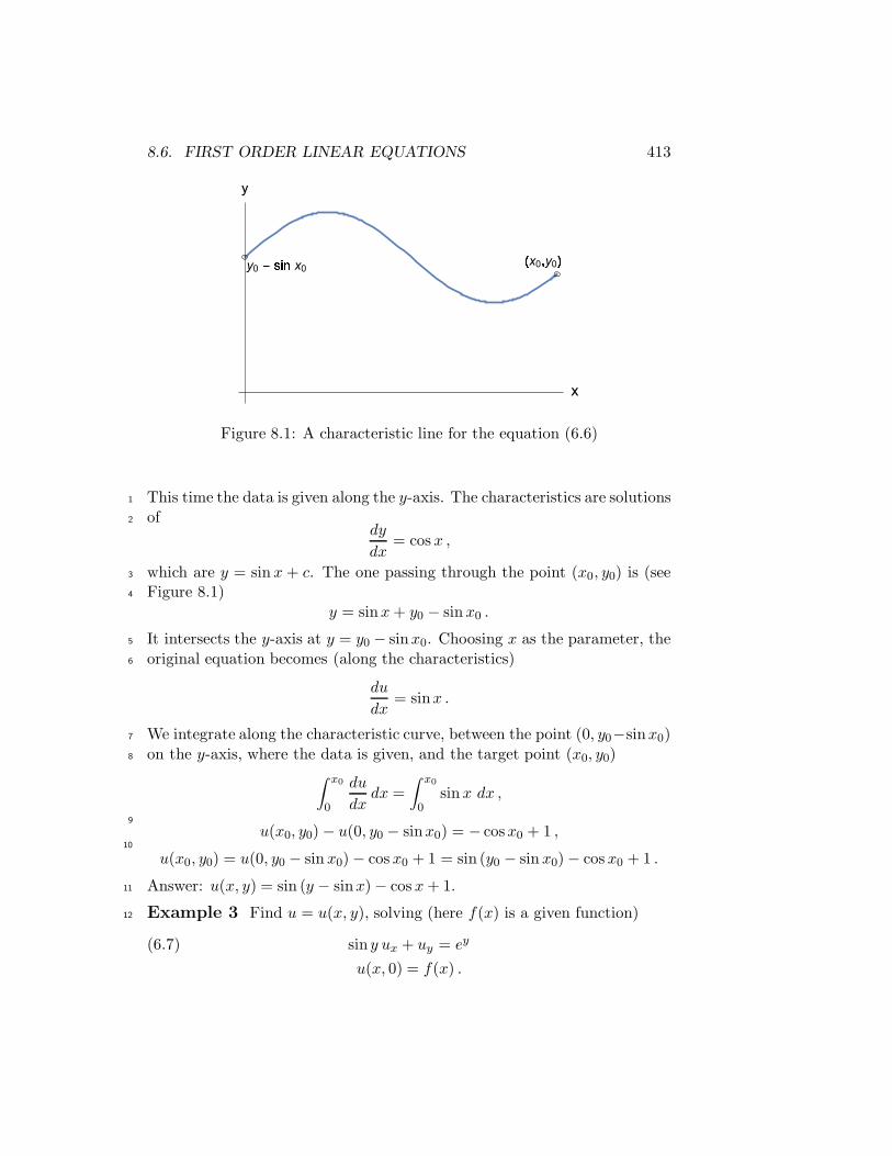
8.6. FIRST ORDER LINEAR EQUATIONS 413
x
y
�x0 � y0 �y0 - � � � x0
Figure 8.1: A characteristic line for the equation (6.6)
This time the data is given along the y-axis. The characteristics are solutions1
of2
dy
dx= cos x ,
which are y = sinx + c. The one passing through the point (x0, y0) is (see3
Figure 8.1)4
y = sinx+ y0 − sinx0 .
It intersects the y-axis at y = y0 − sinx0. Choosing x as the parameter, the5
original equation becomes (along the characteristics)6
du
dx= sinx .
We integrate along the characteristic curve, between the point (0, y0−sinx0)7
on the y-axis, where the data is given, and the target point (x0, y0)8
∫ x0
0
du
dxdx =
∫ x0
0sinx dx ,
9
u(x0, y0) − u(0, y0 − sinx0) = − cosx0 + 1 ,10
u(x0, y0) = u(0, y0 − sinx0) − cos x0 + 1 = sin (y0 − sinx0) − cos x0 + 1 .
Answer: u(x, y) = sin (y − sinx) − cos x+ 1.11
Example 3 Find u = u(x, y), solving (here f(x) is a given function)12
sin y ux + uy = ey(6.7)
u(x, 0) = f(x) .

414 CHAPTER 8. ELEMENTARY THEORY OF PDE
x
y �x0 � y0
-1! x0 ! " # $ y0
Figure 8.2: A characteristic line for the equation (6.7)
The data f(x) is given along the x-axis. The characteristics are solutions of1
dx
dy= sin y ,
which are x = − cos y + c. The one passing through the point (x0, y0) is2
x = − cos y + x0 + cos y0 .(6.8)
It intersects the x-axis at x = −1 + x0 + cos y0. We shall use y as the3
parameter. (One cannot use x as the parameter, because solving (6.8) for4
y = y(x) produces multiple answers.) The original equation becomes (along5
the characteristics)6
du
dy= ey .
We integrate along the characteristic curve, between the points (−1 + x0 +7
cos y0, 0) and (x0, y0), or between the parameter values of y = 0 (where8
x = −1 + x0 + cos y0) and y = y0 (where x = x0)9
∫ y0
0
du
dydy =
∫ y0
0ey dy ,

8.6. FIRST ORDER LINEAR EQUATIONS 415
1
u(x0, y0) − u(−1 + x0 + cos y0, 0) = ey0 − 1 ,2
u(x0, y0) = u(−1 + x0 + cos y0, 0) + ey0 − 1 = f(−1 + x0 + cos y0) + ey0 − 1 .
Answer: u(x, y) = f(−1 + x+ cos y) + ey − 1. (This expression may also be3
seen as the general solution of our equation, considering the function f(x)4
to be arbitrary.)5
Example 4 Find u = u(x, y), solving6
xux − yuy + u = x(6.9)
u = 1 on y = x .
The data is given along the line y = x. The characteristics are the solutions7
of8
dy
dx= −y
x,
which are the hyperbolas y =c
x. The one passing through the point (x0, y0)9
is10
y =x0y0x
.(6.10)
Let us begin by assuming that the point (x0, y0) lies in the first quadrant of11
the xy-plane, so that x0 > 0 and y0 > 0. The characteristic (6.10) intersects12
the line y = x at the point(√x0y0,
√x0y0
)
. Taking x as the parameter, our13
PDE becomes (after dividing by x)14
du
dx+
1
xu = 1 ,
or15
d
dx(xu) = x .
We integrate along the characteristic curve, between the points(√x0y0,
√x0y0
)
16
and (x0, y0), or between x =√x0y0 (where y =
√x0y0) and x = x0 (where17
y = y0), obtaining18
∫ x0
√x0y0
d
dx(xu) dx =
∫ x0
√x0y0
x dx ,
19
x0u(x0, y0) −√x0y0u(
√x0y0,
√x0y0) =
1
2x2
0 −1
2x0y0 .

416 CHAPTER 8. ELEMENTARY THEORY OF PDE
(It does not matter which of the limits of integration is larger,√x0y0 or x0.)1
By the initial condition, u(√x0y0,
√x0y0) = 1, and then2
u(x0, y0) =
√
y0x0
+1
2x0 −
1
2y0 .
In case the point (x0, y0) lies in the third quadrant, we obtain the same result.3
In case the point (x0, y0) lies in either the second or the fourth quadrants,4
our method does not apply, because the characteristic hyperbolas do not5
intersect the line y = x.6
Answer: u(x, y) =
√
y
x+
1
2x− 1
2y, in case the point (x, y) lies in either the7
first or the third quadrants, and no solution exists if the point (x, y) lies in8
either the second or the fourth quadrants.9
-
6
��
��
��
��
x
y
y = x
srsr (x0, y0)
x0√x0y0
-
Integrating along the characteristic hyperbola
10
We conclude by observing that the curve, on which the data is prescribed,11
cannot be a characteristic (or have a part, which is a characteristic). Indeed,12
if solution is known at some point on a characteristic, it can be computed13
at all other points along the same characteristic line, and therefore solution14
cannot be arbitrary prescribed on this characteristic line.15
8.6.1 Problems16
1. Solve the problem17
ux + uy = 1
u(x, 0) = ex ,
by using y as a parameter.18

8.6. FIRST ORDER LINEAR EQUATIONS 417
2. Solve the problem1
xux − yuy + u = x
u = 1 on y = x ,
in case the point (x, y) lies in the third quadrant of the xy-plane.2
Answer. u(x, y) =
√
y
x+
1
2x− 1
2y.3
3. Solve for u = u(x, y)4
xux + yuy + u = x,
u = 1 on the line x+ y = 1 .
Answer. u(x, y) =1
x+ y+x
2− x
2(x+ y)2.5
4. Find u = u(x, y), solving6
sin y ux + uy = x
u(x, 0) = x2 .
Hint: Use y as a parameter. Express x as a function of y, when integrating7
along the characteristic curve.8
Answer. u(x, y) = (x+ cos y − 1)2 − sin y + y cos y + xy.9
5. Find the general solution of10
2ux + uy = x .
Hint: Denote by f(x) the values of u(x, y) on the x-axis.11
Answer. u(x, y) = f(x− 2y) + xy − y2, where f is an arbitrary function.12
6. Show that the following problem has no solution13
2ux + uy = x
u(x, 12x) = x2 .
Hint: Compare the data line and the characteristics.14
7. (i) Find the general solution of15
xux − yuy + u = x ,

418 CHAPTER 8. ELEMENTARY THEORY OF PDE
which is valid in the second quadrant of the xy-plane.1
Hint: Let u = f(x) on y = −x, where f(x) is an arbitrary function.2
Answer. u(x, y) =√
− yx f(−√−xy) + 1
2x+ 12y.3
(ii) Show that the problem (6.9) above has no solution in the second quad-4
rant.5
8. Solve the problem (here f(y) is an arbitrary function)6
xux + 2yuy + yxu = 0
u = f(y) on the line x = 1 .
Answer. u(x, y) = e(
y
x2 −yx
)
f
(
y
x2
)
.7
8.7 Laplace’s Equation: Poisson’s Integral Formula8
A Trigonometric Sum9
Let ρ and α be two real numbers, with 0 < ρ < 1. We claim that10
1
2+
∞∑
n=1
ρn cosnα =1− ρ2
2 (1 − 2ρ cosα+ ρ2).(7.1)
We begin the proof by recalling the geometric series: for any complex number11
z, with the modulus |z| < 1, one has12
∞∑
n=0
zn =1
1 − z.
Consider a complex number z = ρeiα. Then |z| = ρ < 1, and by Euler’s13
formula14
zn = ρneinα = ρn (cosnα + i sinnα) .
It follows that15
Re zn = ρn cosnα ,
where Re denotes the real part of a complex number. Then16
1
2+
∞∑
n=1
ρn cosnα = Re
[
1
2+
∞∑
n=1
zn
]
= Re
[
1
2+
1
1 − z− 1
]
= Re
[
1 + z
2(1− z)
]
17
=1
2Re
[
1 + ρeiα
1 − ρeiα
]
=1
2Re
[
1 + ρ cosα+ iρ sinα
1 − ρ cosα− iρ sinα
]
=1 − ρ2
2 (1− 2ρ cosα+ ρ2).
On the last step we multiplied both the numerator and the denominator by18
1 − ρ cosα+ iρ sinα (the complex conjugate of the denominator).19

8.7. LAPLACE’S EQUATION: POISSON’S INTEGRAL FORMULA 419
Laplace’s Equation on a Disc1
Recall from Chapter 7 that in order to solve the following boundary value2
problem in polar coordinates (on a disc r < R)3
∆u = urr + 1rur + 1
r2uθθ = 0, for r < R, 0 ≤ θ < 2π(7.2)
u(R, θ) = f(θ), for 0 ≤ θ < 2π ,
we begin by expanding the given piecewise smooth function f(θ) into its4
Fourier series5
f(θ) = a0 +∞∑
n=1
an cosnθ + bn sinnθ ,
with the coefficients given by6
a0 =1
2π
∫ 2π
0f(φ) dφ ,
7
an =1
π
∫ 2π
0f(φ) cosnφ dφ ,
8
bn =1
π
∫ 2π
0f(φ) sinnφ dφ .
The solution of the problem (7.2) is then9
u(r, θ) = a0 +∞∑
n=1
(
r
R
)n
(an cosnθ + bn sinnθ) .(7.3)
Recall that this solution represents the steady state temperatures inside the10
disc x2 + y2 < R2, provided that the temperatures on the boundary circle11
x2 + y2 = R2 are prescribed by the function f(θ).12
We now substitute the integral formulas for an’s and bn’s into (7.3), and13
denote ρ = rR , obtaining14
u(r, θ) =1
π
∫ 2π
0
[
1
2+
∞∑
n=1
ρn (cosnφ cosnθ + sinnφ sinnθ)
]
f(φ) dφ .
Observing that cosnφ cosnθ + sinnφ sinnθ = cosn(θ − φ), and using the15
formula (7.1), the sum in the square bracket becomes16
1
2+
∞∑
n=1
ρn cosn(θ−φ) =1 − ρ2
2 (1 − 2ρ cos(θ − φ) + ρ2)=
R2 − r2
2 (R2 − 2Rr cos(θ − φ) + r2).

420 CHAPTER 8. ELEMENTARY THEORY OF PDE
We conclude Poisson’s integral formula1
u(r, θ) =1
2π
∫ 2π
0
R2 − r2
R2 − 2Rr cos(θ − φ) + r2f(φ) dφ ,(7.4)
which gives the solution of the boundary value problem (7.2). The function2
R2 − r2
R2 − 2Rr cos θ + r2is called Poisson’s kernel.3
Recall that solutions of the Laplace equation4
∆u = uxx + uyy = 0
are called harmonic functions. Poisson’s integral formula implies that one5
can find a harmonic function inside of any disc x2+y2 < R2, with arbitrarily6
prescribed values on the boundary of the disc. Poisson’s integral formula is7
suitable for numerical computations.8
Throughout this chapter we consider only the classical solutions, which9
means that u(x, y) has all derivatives in x and y of first and second order,10
which are continuous functions.11
8.8 Some Properties of Harmonic Functions12
Setting r = 0 in Poisson’s formula gives the solution at the origin:13
u(0, 0) =1
2π
∫ 2π
0f(φ) dφ =
1
2π
∫ 2π
0u(R, φ) dφ .
So that u(0, 0) is equal to the average of the values of u on the circle of any14
radius R around (0, 0). Any point in the xy-plane may be declared to be15
the origin. We therefore conclude the mean value property : the value of a16
harmonic function at any point (x0, y0) is equal to the average of the values17
of u(x, y) on a circle of any radius R around the point (x0, y0).18
If a closed curve C encloses a bounded domain D, then we denote19
D = D ∪ C. D is called the closure of D. One often writes ∂D to20
denote the boundary curve C. It is known from calculus that a contin-21
uous on D function u(x, y) takes on its maximum and minimum values.22
This means that at some point (x1, y1) ∈ D, u(x1, y1) = maxD
u(x, y), and23
u(x2, y2) = minD
u(x, y), at a point (x2, y2) ∈ D.24

8.8. SOME PROPERTIES OF HARMONIC FUNCTIONS 421
Theorem 8.8.1 (Strong maximum principle) A function u(x, y) which is1
harmonic in a domain D cannot take on its maximum value at points inside2
D, unless u(x, y) is a constant.3
Proof: Denote M = maxD u(x, y), and assume that u(x0, y0) = M at4
some point (x0, y0) ∈ D. We shall show that u(x, y) = M for all points5
(x, y) ∈ D. Let the number R > 0 be so small that the circle of radius R6
around the point (x0, y0) lies inside D. The values of u(x, y) on that circle7
are ≤ M , and in fact they have to be equal to M , because otherwise their8
average would be less than M , but that average is equal to u(x0, y0) = M .9
We conclude that u(x, y) = M , at all points inside of any circle around10
(x0, y0), which lies inside D. Let now (x1, y1) be any other point in D. Join11
(x0, y0) to (x1, y1) by any path, and cover that path by small overlapping12
circles, each lying inside D. Repeating the same argument for all circles, we13
conclude that u(x1, y1) = M . ♦14
kk����"!# &%'$&%'$&%'$
s
s
(x0, y0)
(x1, y1)
D
Overlapping circles joining (x0, y0) to (x1, y1) inside D
15
The strong maximum principle has the following physical interpretation:16
for steady state temperatures (which harmonic functions represent), one17
cannot have a point in D which is hotter than all of its neighbors.18
Similarly, one has the strong minimum principle: a function u(x, y),19
which is harmonic in a domain D, cannot take on its minimum value inside20

422 CHAPTER 8. ELEMENTARY THEORY OF PDE
D, unless u(x, y) is a constant. So where do harmonic functions assume1
their maximum and minimum values? On the boundary ∂D. A function2
harmonic in the entire plane, like u(x, y) = x2 − y2, has no points of local3
maximum and of local minimum in the entire plane, but if you restrict this4
function to, say, a unit disc x2 + y2 ≤ 1, then it takes on its maximum and5
minimum values on the boundary x2 + y2 = 1.6
We shall need the following estimate of the Poisson kernel:7
R2 − r2
R2 − 2Rr cos(θ − φ) + r2≤ R2 − r2
R2 − 2Rr+ r2=
(R− r)(R+ r)
(R− r)2=R+ r
R− r,
which is obtained by estimating − cos(θ − φ) ≥ −1, then simplifying. Simi-8
larly,9
R2 − r2
R2 − 2Rr cos(θ − φ) + r2≥ R2 − r2
R2 + 2Rr+ r2=R− r
R+ r,
which is obtained by estimating − cos(θ−φ) ≤ 1, and simplifying. Combin-10
ing11
R− r
R+ r≤ R2 − r2
R2 − 2Rr cos(θ − φ) + r2≤ R+ r
R− r.
Consider again the boundary value problem (7.2), and assume that f(φ) ≥ 0,12
for all φ. Using Poisson’s integral formula (7.4), we have13
R− r
R+ r
1
2π
∫ 2π
0f(φ) dφ ≤ u(r, θ) ≤ R+ r
R− r
1
2π
∫ 2π
0f(φ) dφ .
By the mean value property, we conclude that for any non-negative function14
u(r, θ), which is harmonic inside x2 + y2 < R2, the following Harnack’s15
inequalities hold16
R− r
R+ ru(0, 0) ≤ u(r, θ) ≤ R+ r
R− ru(0, 0) .(8.1)
(The assumption that u(r, θ) ≥ 0 was needed to assure that f(φ) = u(R, φ) ≥17
0.)18
Theorem 8.8.2 (Liouville’s Theorem) If a function u(x, y) ≥ 0 is har-19
monic in the entire plane, then u(x, y) = constant.20
Proof: The estimates (8.1) hold for allR. (Observe that f(φ) = u(R, φ) ≥21
0.) Keeping (r, θ) fixed, we let R→ ∞ in (8.1). Then22
u(r, θ) = u(0, 0) = constant, for any (r, θ) ,

8.9. THE MAXIMUM PRINCIPLE 423
as claimed. ♦1
Suppose now that a function u(x, y) is harmonic and non-negative, de-2
fined on the disc BR : x2 + y2 ≤ R2. We also consider the disc r ≤ R/2 (or3
x2 + y2 ≤ R2/4), which we denote by BR/2. Using (8.1), we estimate4
maxBR/2
u(x, y) ≤ R+ 12R
R− 12R
u(0, 0) = 3u(0, 0) .
Similarly,5
minBR/2
u(x, y) ≥ R− 12R
R+ 12R
u(0, 0) =1
3u(0, 0) .
We conclude that6
maxBR/2u(x, y)
minBR/2u(x, y)
≤ 9 ,
for any non-negative harmonic function, defined on the disc x2 + y2 ≤ R2.7
This fact reflects the strong averaging property of harmonic functions. (More8
generally, for each bounded domain there is a bound on the ratio of the9
maximum value over the minimum value for any non-negative harmonic10
function defined on some larger domain.)11
8.9 The Maximum Principle12
In this section we consider two important classes of functions that include13
harmonic functions. Not all of these functions satisfy the strong maximum14
principle. We now describe a substitute property. Recall that D denotes a15
bounded domain, with the boundary C, and D = D ∪ C.16
Theorem 8.9.1 (Maximum principle) Assume that17
∆u(x, y) ≥ 0 for all (x, y) ∈ D .(9.1)
Then u(x, y) takes on its maximum value on the boundary, so that18
maxD
u(x, y) = maxC
u(x, y) .(9.2)
Functions satisfying the inequality (9.1) are called subharmonic in D.19
This theorem asserts that subharmonic functions take on their maximum20
values at the boundary of the domain. (The possibility that the maximum21
value is also taken on at points inside D, is not excluded here.)22

424 CHAPTER 8. ELEMENTARY THEORY OF PDE
Proof: Consider, first, an easy case when the inequality in (9.1) is strict1
∆u(x, y) > 0 for all (x, y) ∈ D .(9.3)
We claim that u(x, y) cannot have points of local maximum inside D. In-2
deed, if (x0, y0) ∈ D was a point of local maximum, then uxx(x0, y0) ≤ 03
and uyy(x0, y0) ≤ 0, and therefore4
∆u(x0, y0) = uxx(x0, y0) + uyy(x0, y0) ≤ 0 ,
contradicting (9.3). It follows that the maximum of u(x, y) on D is achieved5
on the boundary curve C, so that (9.2) holds, and moreover6
u(x, y) < maxC
u(x, y) for all (x, y) ∈ D .
Turning to the general case, consider the function v(x, y) = u(x, y) +7
ε(x2 + y2), with some ε > 0. Then8
∆v(x, y) = ∆u(x, y) + 4ε > 0 ,
and by the easy case, considered above,9
u(x, y) < v(x, y) < maxC
v(x, y) ≤ maxC
u(x, y) + εK for all (x, y) ∈ D ,
where K is any constant exceeding x2 + y2 on the bounded closed curve C.10
Letting ε→ 0, we conclude that11
u(x, y) ≤ maxC
u(x, y) for all (x, y) ∈ D ,
which implies (9.2). ♦12
The following minimum principle holds for the superharmonic functions,13
defined as the functions satisfying ∆u(x, y) ≤ 0 on D.14
Theorem 8.9.2 Assume that15
∆u(x, y) ≤ 0 for all (x, y) ∈ D .
Then u(x, y) takes on its minimum on the boundary, so that16
minD
u(x, y) = minCu(x, y) .

8.9. THE MAXIMUM PRINCIPLE 425
Harmonic functions are both subharmonic and superharmonic, and so1
they assume their minimum and maximum values on the boundary C. If2
a harmonic function is zero on C, it has to be zero on D. (This fact also3
follows from the strong maximum principle.) It follows that the Dirichlet4
problem for Poisson’s equation5
∆u = f(x, y) for (x, y) ∈ D
u = g(x, y) for (x, y) ∈ C
has at most one solution, for any given functions f(x, y) and g(x, y). Indeed,6
if u(x, y) and v(x, y) are two solutions, then their difference u(x, y)−v(x, y) is7
harmonic inD function, which is zero on C. It follows that u(x, y)−v(x, y) =8
0, so that u(x, y) = v(x, y) for all (x, y) ∈ D.9
Occasionally one can use the maximum principle to find the maximum10
value of a function on a bounded domain.11
Example Find the maximum value of u(x, y) = 2x4−3xy2+y6+x2+x−2y12
on the closed square [0, 1]× [0, 1], where 0 ≤ x, y ≤ 1.13
Setting the partials ux and uy to zero, would lead to an intractable 2×214
nonlinear system. Instead, we calculate15
∆u(x, y) = 24x2 + 2 − 6x+ 30y4 ≥ 24x2 − 6x+ 2 > 0, for all (x, y) .
By the maximum principle, the maximum value of u(x, y) occurs at the16
boundary of the square. The boundary of the square consists of four line17
segments, and on each segment u(x, y) is a simple function of one variable.18
Examining these line segments in turn, one sees that the maximum value of19
u(x, y) is equal to 4, and it occurs at the point x = 1, y = 0.20
The reasoning behind the maximum principle may be used to analyze21
some nonlinear equations. Consider, for example, the Dirichlet problem22
∆u = u3 for (x, y) ∈ D
u = 0 for (x, y) ∈ C .
This problem has the trivial solution u(x, y) = 0. It turns out that there are23
no other solutions. Indeed, if a solution u(x, y) was positive at some points in24
D, it would have a point of global maximum (x0, y0) ∈ D, with u(x0, y0) > 0.25
At that point, ∆u(x0, y0) ≤ 0, while u3(x0, y0) > 0. We have a contradiction26
with our equation, at the point (x0, y0), which implies that u(x, y) cannot27
take on positive values. Similarly, one shows that u(x, y) cannot take on28
negative values. It follows that u(x, y) = 0 is the only solution.29

426 CHAPTER 8. ELEMENTARY THEORY OF PDE
Maximum and minimum principles also hold in the presence of lower1
order terms (derivatives of the first order).2
Theorem 8.9.3 Assume that for all (x, y) ∈ D we have3
∆u(x, y) + a(x, y)ux(x, y) + b(x, y)uy(x, y) ≥ 0 ,(9.4)
where a(x, y) and b(x, y) are given continuous functions. Then u(x, y) takes4
on its maximum value on the boundary C, so that5
maxD
u(x, y) = maxC
u(x, y) .
Proof: Assume, first, that the inequality in (9.4) is strict. If there was a6
point of maximum (x0, y0) inside D, then ux(x0, y0) = uy(x0, y0) = 0, and7
uxx(x0, y0) ≤ 0, uyy(x0, y0) ≤ 0. Evaluating the strict inequality (9.4) at8
(x0, y0), we would have a contradiction, proving the theorem in this case.9
The proof of the general case is similar to that for the Theorem 8.9.1. ♦10
8.10 The Maximum Principle for the Heat Equa-11
tion12
Recall from Chapter 7 that in case of a bounded interval (0, L), a typical13
problem involving the heat equation is14
ut − kuxx = F (x, t) 0 < x < L, 0 < t ≤ T(10.1)
u(x, 0) = f(x) 0 < x < L
u(0, t) = a(t) 0 < t ≤ T
u(L, t) = b(t) 0 < t ≤ T ,
with given continuous functions (called the data) F (x, t), a(t), b(t) and f(x),15
and a given constant k > 0. We assume that the final time T <∞. The data16
is prescribed on the parabolic boundary Γ, which is defined to be consisting17
of the lines x = 0, x = L (for 0 < t ≤ T ), and the segment 0 ≤ x ≤ L18
of the x-axis. The solution must be determined in the parabolic domain19
D = (0, L) × (0, T ], where 0 < x < L and 0 < t ≤ T . We shall denote20
D = D ∪ Γ.21
Recall from calculus that if a differentiable function v(t), defined on some22
interval [0, T ], has a local maximum at some t0 ∈ (0, T ) then v′(t0) = 0, while23
if a local maximum (relative to [0, T ]) occurs at T , then v′(T ) ≥ 0.24

8.10. THE MAXIMUM PRINCIPLE FOR THE HEAT EQUATION 427
Theorem 8.10.1 (The maximum principle) Assume that F (x, t) ≤ 0 for1
all (x, t) ∈ D, or2
ut − kuxx ≤ 0 , for all (x, t) ∈ D .(10.2)
Then u(x, t) takes on its maximum value on the parabolic boundary, so that3
maxD
u(x, t) = maxΓ
u(x, t) .(10.3)
(In particular, if u(x, t) ≤ 0 on Γ, then u(x, t) ≤ 0 on D.)4
Proof: Again, we consider first the case of strict inequality5
ut − kuxx < 0 , for all (x, t) ∈ D .(10.4)
We claim that u(x, t) cannot assume its maximum value at a point (x0, t0)6
in D. Assume, on the contrary, that (x0, t0) ∈ D is a point of maximum of7
u(x, t). If t0 < T , then ut(x0, t0) = 0 and −uxx(x0, t0) ≥ 0, contradicting the8
inequality (10.4), evaluated at (x0, t0). In case t0 = T , we have uxx(x0, t0) ≤9
0, and from (10.4) we get ut(x0, t0) < 0. But then u(x0, t) is larger than10
u(x0, t0) at times t a little before t0, in contradiction with (x0, t0) being a11
point of maximum. So that the point of maximum (of u(x, t) on D) occurs12
on the parabolic boundary Γ, and13
u(x, t) < maxΓ
u(x, t) , for all (x, t) ∈ D ,(10.5)
which implies (10.3).14
Turning to the general case, we denoteM = maxΓ
u(x, t), and let v(x, t) =15
u(x, t) + εx2, with a constant ε > 0. Then16
vt − kvxx = ut − kuxx − 2kε < 0 ,
so that strict inequality holds for v(x, t), and then by (10.5)17
u(x, t) < v(x, t) < maxΓ
v(x, t) ≤M + εL2 for all (x, t) ∈ D .
Letting ε→ 0, we conclude that18
u(x, t) ≤M , for all (x, t) ∈ D ,
which implies (10.3). ♦19
Similarly, one establishes the following minimum principle.20

428 CHAPTER 8. ELEMENTARY THEORY OF PDE
Theorem 8.10.2 Assume that F (x, t) ≥ 0 for all (x, t) ∈ D, or in other1
words,2
ut − kuxx ≥ 0 for all (x, t) ∈ D .
Then u(x, t) takes on its minimum value on the parabolic boundary, and3
minD
u(x, t) = minΓu(x, t) .
(In particular, if u(x, t) ≥ 0 on Γ, then u(x, t) ≥ 0 on D.)4
For the homogeneous heat equation, where F (x, t) = 0, both minimum5
and maximum principles apply. As a consequence, the problem (10.1) has6
at most one solution (one shows that the difference of any two solutions is7
zero).8
We have the following comparison theorem.9
Theorem 8.10.3 Assume we have two functions u(x, t) and v(x, t), such10
that11
ut − kuxx ≥ vt − kvxx in D, and u ≥ v on Γ .
Then u(x, t) ≥ v(x, t) in D.12
Proof: The function w(x, t) = u(x, t) − v(x, t) satisfies wt − kwxx ≥ 0 in13
D, and w ≥ 0 on Γ. By the minimum principle w ≥ 0 in D. ♦14
More information on maximum principles may be found in a nice book15
of M.H. Protter and H.F. Weinberger [24].16
8.10.1 Uniqueness on an Infinite Interval17
We begin with discussion of a remarkable function18
g(t) =
{
e−1t2 for t 6= 0
0 for t = 0.
This function is positive for t 6= 0, however g(0) = 0, and g′(0) = g′′(0) =19
g′′′(0) = · · · = 0, so that all derivatives at t = 0 are zero. Indeed,20
g′(0) = limt→0
g(t)− g(0)
t= lim
t→0
e−1t2
t.

8.10. THE MAXIMUM PRINCIPLE FOR THE HEAT EQUATION 429
Letting1
t= u, we evaluate this limit by using L’Hospital’s rule:1
limt→0
e− 1
t2
t= lim
u→∞ue−u2
= limu→∞
u
eu2 = limu→∞
1
2ueu2 = 0 .
It follows that2
g′(t) =
{
2t3 e
− 1t2 for t 6= 0
0 for t = 0.
The derivatives g′′(0), g′′′(0), and so on, are evaluated similarly.3
The initial value problem on the entire x-axis4
ut − uxx = 0 for −∞ < x <∞, t > 0(10.6)
u(x, 0) = 0 for −∞ < x <∞
has the trivial solution u(x, t) = 0. Surprisingly, this problem also has non-5
trivial solutions! Here is one of them:6
u(x, t) =∞∑
k=0
g(k)(t)
(2k)!x2k ,(10.7)
where g(t) is the function just defined. (It is not hard to show that this series7
converges for all x, and all t > 0.) Clearly u(x, 0) = 0, because g(k)(0) = 08
for any derivative k. Compute9
uxx =∞∑
k=1
g(k)(t)
(2k− 2)!x2k−2 =
∞∑
i=0
g(i+1)(t)
(2i)!x2i = ut ,
where we shifted the index of summation, k → i, by letting k − 1 = i.10
It follows that the problem11
ut − uxx = F (x, t) for −∞ < x <∞, t > 0(10.8)
u(x, 0) = g(x) for −∞ < x <∞
has infinitely many solutions, provided that it has one solution. Indeed, to12
any solution one may add a constant multiple of the function in (10.7), to13
get other solutions.14
The function g(t) appears in other counterexamples, or the examples that15
challenge our intuition. For example, the Maclauren series for g(t) is a sum16
of zeroes, and it converges to zero, not to g(t).17

430 CHAPTER 8. ELEMENTARY THEORY OF PDE
We shall show that the problem (10.8) has at most one bounded solution,1
which means that |u(x, t)| < M for some constant M > 0, and all −∞ <2
x < ∞, and t > 0. This fact will follow immediately from the following3
theorem.4
Theorem 8.10.4 Assume that we have a solution u(x, t) of the problem5
ut − kuxx = 0 for −∞ < x <∞, t > 0(10.9)
u(x, 0) = 0 for −∞ < x <∞ ,
which is a bounded (for all x and t) function. Then u(x, t) = 0, for all x6
and t.7
Proof: We are given that |u(x, t)| ≤ M for some M > 0, and all x and t8
(or −M ≤ u(x, t) ≤ M). In the region D : −L < x < L, 0 < t ≤ T , with9
some positive constants L and T , we consider the comparison function10
v(x, t) =2M
L2
(
1
2x2 + kt
)
.
One calculates11
vt − kvxx = 0 .
On the parabolic boundary of the region D we have12
v(x, 0) =M
L2x2 ≥ 0 = u(x, 0) ,
13
v(±L, t) = M +2Mk
L2t ≥M ≥ u(±L, t) .
By the comparison Theorem 8.10.314
u(x, t) ≤ v(x, t) in D .
The function −v(x, t) satisfies15
(−v)t − k(−v)xx = 0 ,
16
−v(x, 0) = −ML2x2 ≤ 0 = u(x, 0) ,
17
−v(±L, t) = −M − 2Mk
L2t ≤ −M ≤ u(±L, t) .
8.11. DIRICHLET’S PRINCIPLE 431
Using the comparison Theorem 8.10.3 again, we conclude that1
−v(x, t) ≤ u(x, t) ≤ v(x, t) in D ,
which gives2
|u(x, t)| ≤ v(x, t) =2M
L2
(
1
2x2 + kt
)
.
Letting here L→ ∞, we conclude that u(x, t) = 0 for any fixed x and t. ♦3
4
As a consequence, we have the following uniqueness theorem.5
Theorem 8.10.5 For any given functions F (x, t) and f(x), the problem6
ut − kuxx = F (x, t) for −∞ < x <∞, t > 0
u(x, 0) = f(x) for −∞ < x <∞
has at most one bounded solution.7
Proof: The difference of any two bounded solutions would be a bounded8
solution of the problem (10.9), which is zero by the preceding theorem. ♦9
8.11 Dirichlet’s Principle10
Recall the concept of divergence a vector field F = (P (x, y, z), Q(x, y, z), R(x, y, z))11
divF = ∇ · F = Px(x, y, z) +Qy(x, y, z) +Rz(x, y, z) .
An example of a vector field is given by the gradient of any functionw(x, y, z),12
namely ∇w = (wx(x, y, z), wy(x, y, z), wz(x, y, z)). One calculates13
div (∇w) = wxx +wyy + wzz = ∆w .(11.10)
Suppose that a bounded domain D in (x, y, z) space, is bounded by a14
closed and smooth surface S. The divergence theorem reads:15
∫
DdivF dV =
∫
SF · n dS .
Here∫
D denotes the triple integral overD,∫
S is the surface (double) integral16
over S, n is the unit normal vector pointing outside ofD (n is changing from17
point to point on S), F · n denotes the scalar product of two vectors, and18

432 CHAPTER 8. ELEMENTARY THEORY OF PDE
dV = dx dy dz is the volume element. Applying the divergence theorem to1
(11.10) gives2∫
D∆w dV =
∫
S∇w · n dS =
∫
S
∂w
∂ndS ,
where ∂w∂n denotes the directional derivative in the direction of n.3
Given two functions u(x, y, z) and v(x, y, z), one calculates4
div (v∇u) = ∆u v + ∇u · ∇v .
By the divergence theorem5
∫
D(∆u v + ∇u · ∇v) dV =
∫
Ddiv (v∇u) dV =
∫
Sv∇u · n dS ,
or6∫
D∆u v dV = −
∫
D∇u · ∇v dV +
∫
S
∂u
∂nv dS .(11.11)
This formula is called Green’s identity; it extends the integration by parts7
formula to higher dimensions.8
We now apply Green’s identity to give another proof of the uniqueness9
of solution of the Dirichlet problem for Poisson’s equation.10
Theorem 8.11.1 Given any f(x, y, z) and g(x, y, z), there exists at most11
one solution of the boundary value problem12
∆u = f(x, y, z) in D(11.12)
u = g(x, y, z) on S .
Proof: Assume that there are two solutions u(x, y, z) and v(x, y, z). Their13
difference w = u− v satisfies14
∆w = 0 in D , w = 0 on S .
We multiply the last equation by w, and integrate overD. In view of (11.11)15
0 =
∫
Dw∆w dV = −
∫
D∇w · ∇w dV +
∫
Sw∂w
∂ndS = −
∫
D|∇w|2 dV .
(We used that∫
S w∂w∂n dS = 0, because w = 0 on S; |∇w| denotes the16
length of the gradient vector.) It follows that ∇w = 0, so that w(x, y, z) is17
a constant. This constant is zero, because of the boundary condition. So18
that w = u− v ≡ 0, and then u ≡ v in D. ♦19

8.11. DIRICHLET’S PRINCIPLE 433
Dirichlet’s principle says that the solution of the boundary value problem1
(11.12) minimizes the following energy functional2
J(u) =
∫
D
[
1
2|∇u|2 + uf
]
dV .
among all functions satisfying the boundary condition in (11.12). (Here |∇u|3
denotes the length of the gradient vector, |∇u|2 = ∇u · ∇u.)4
Theorem 8.11.2 Assume that u(x, y, z) is a solution of (11.12). Then5
J(u) = minwJ(w) , where w = g(x, y, z) on S .(11.13)
Conversely, if u(x, y, z) satisfies (11.13), then it is a solution of the boundary6
value problem (11.12).7
Proof: Part 1. If u is a solution of (11.12), then u−w = 0 on S. Multiply8
the equation in (11.12) by u−w, integrate over D, and use Green’s identity9
0 =
∫
D[∆u (u− w)− f(u−w)] dV =
∫
D[−∇u · ∇(u− w)− f(u−w)] dV .
(Observe that∫
S∂u∂n (u−w) dS = 0.) It follows that10
∫
D
[
|∇u|2 + uf]
dV =
∫
D[∇u · ∇w +wf ] dV(11.14)
11
≤ 1
2
∫
D|∇u|2 dV +
∫
D
[
1
2|∇w|2 + wf
]
dV .
On the last step we used the Cauchy-Schwarz inequality for vectors ∇u ·12
∇w ≤ |∇u| |∇w|, followed by the numerical inequality ab ≤ 12a
2 + 12b
2.13
Rearranging the terms in (11.14), we conclude that J(u) ≤ J(w) for any w,14
satisfying w = g on S.15
Part 2. Conversely, assume that u minimizes J(u) among the functions w,16
satisfying w = g on S. Fix any v(x, y, z), satisfying v = 0 on S. Then17
for any number ε the function u + εv is equal to g on S, and therefore18
J(u) ≤ J(u + εv). It follows that the function j(ε) = J(u + εv) has a19
minimum at ε = 0, and therefore j ′(0) = 0. Calculate20
j(ε) = J(u+ εv) =
∫
D
[
1
2(∇u+ ε∇v) · (∇u+ ε∇v) + (u+ εv) f
]
dV
21
=ε2
2
∫
D|∇v|2 dV + ε
∫
D(∇u · ∇v + vf) dV +
∫
D
(
1
2|∇u|2 + uf
)
dV .

434 CHAPTER 8. ELEMENTARY THEORY OF PDE
It follows that1
0 = j ′(0) =
∫
D(∇u · ∇v + vf) dV =
∫
D(−∆u+ f) v dV ,
using Green’s formula on the last step. Since the function v is arbitrary2
(except for the condition v = 0 on S), we conclude that ∆u = f in D. ♦3
One often refers to the functions w satisfyingw = g on S as the competing4
functions. Among the competing functions one searches for the minimizer5
of J(u), which provides the solution of the boundary value problem (11.12).6
This approach is suitable for numerical computations.7
8.12 Classification Theory for Two Variables8
The equation9
ϕ(x, y) = c ,(12.15)
where ϕ(x, y) is a differentiable function of two variables, and c is a constant,10
defines implicitly a function y = y(x). Differentiating (12.15) using the chain11
rule gives12
ϕx(x, y) + ϕy(x, y)y′(x) = 0 ,
and then13
y′(x) = −ϕx
ϕy,(12.16)
assuming that ϕy(x, y) 6= 0.14
We wish a solution z = z(x, y) of the following nonlinear first order PDE15
a(x, y)z2x + b(x, y)zxzy + c(x, y)z2
y = 0 ,(12.17)
with given continuous functions a(x, y), b(x, y) and c(x, y). Similarly to16
linear first order equations, one needs to solve an ODE.17
Lemma 8.12.1 Assume that the function y(x), which is implicitly defined18
by ϕ(x, y) = c, solves the equation19
a(x, y)y′2 − b(x, y)y′ + c(x, y) = 0 ,(12.18)
and ϕy(x, y) 6= 0 for all x and y. Then z = ϕ(x, y) is a solution of (12.17).20

8.12. CLASSIFICATION THEORY FOR TWO VARIABLES 435
Proof: Substituting y′(x) = −ϕx
ϕyinto (12.18), and then clearing the1
denominators gives2
a(x, y)ϕ2x + b(x, y)ϕxϕy + c(x, y)ϕ2
y = 0 ,
so that ϕ(x, y) is a solution of (12.17). ♦3
The equation (12.18) is just a quadratic equation for y′(x). Its solutions4
are5
y′(x) =b±
√b2 − 4ac
2a.(12.19)
One finds y(x) by integration, in case b2 − 4ac ≥ 0.6
Example 1 Find two solutions of7
xz2x + (x+ y)zxzy + yz2
y = 0 .(12.20)
The equation (12.18) takes the form8
x
(
dy
dx
)2
− (x+ y)dy
dx+ y = 0 .
Solving this quadratic equation gives9
dy
dx=x+ y ±
√
(x+ y)2 − 4xy
2x=x+ y ± (x− y)
2x.
When we take “plus”, we obtain dydx = 1 or y = x+ c. We put this function10
into an implicit form y − x = c, which gives us the first solution z1(x, y) =11
y − x. In case of “minus”, we get12
dy
dx=y
x.
The solution of this equation is y = cx, or yx = c in implicit form. The13
second solution is z2(x, y) = yx . There are other solutions of the equation14
(12.20), for example z3(x, y) = c, or the negatives of z1(x, y) and z2(x, y).15
Recall that the wave equation was solved by introducing new variables16
ξ and η, which reduced it to a simpler form. We consider now more general17
equations18
a(x, y)uxx + b(x, y)uxy + c(x, y)uyy + d(x, y)ux + e(x, y)uy = 0 ,(12.21)
with given continuous coefficient functions a(x, y), b(x, y), c(x, y), d(x, y)19
and e(x, y), and the unknown function u = u(x, y). We make a change of20

436 CHAPTER 8. ELEMENTARY THEORY OF PDE
variables ξ = ξ(x, y) and η = η(x, y), and look for the twice differentiable1
functions ξ(x, y) and η(x, y), which will make this equation simpler. We2
assume that the change of variables is non-singular, meaning that one can3
solve for x and y as functions of ξ and η, so that we can go back to the original4
variables after solving the equation in the new variables ξ and η. This is5
known to be the case, provided that the Jacobian (or Jacobian determinant)6
J = ξxηy − ξyηx 6= 0 ,(12.22)
a condition we shall assume to hold.7
Writing8
u(x, y) = u(ξ(x, y), η(x, y)) ,
we use the chain rule to calculate the derivatives:9
ux = uξξx + uηηx ,
10
uxx = uξξξ2x + 2uξηξxηx + uηηη
2x + uξξxx + uηηxx .
Similarly11
uxy = uξξξxξy + uξη (ξxηy + ηxξy) + uηηηxηy + uξξxy + uηηxy ,
12
uyy = uξξξ2y + 2uξηξyηy + uηηη
2y + uξξyy + uηηyy .
We use these expressions in (12.21) to obtain13
Auξξ +Buξη +Cuηη + · · · = 0 ,(12.23)
with the new coefficient functions14
A = aξ2x + bξxξy + cξ2y ,(12.24)
15
B = 2aξxηx + b (ξxηy + ξyηx) + 2cξyηy ,16
C = aη2x + bηxηy + cη2
y ,
and where the terms not shown in (12.23) involve the first derivatives uξ17
and uη, the lower order terms.18
The equation (12.23) will be simpler if one chooses ξ(x, y) and η(x, y)19
to be the solutions of (12.17), called the characteristic functions (or char-20
acteristics, for short). The number of real valued characteristic functions21
depends on the sign of b2(x, y)− 4a(x, y)c(x, y) (see (12.19)). The equation22
(12.21) is called23

8.12. CLASSIFICATION THEORY FOR TWO VARIABLES 437
hyperbolic at a point (x0, y0), if b2(x0, y0) − 4a(x0, y0)c(x0, y0) > 0,1
parabolic at a point (x0, y0), if b2(x0, y0) − 4a(x0, y0)c(x0, y0) = 0,2
elliptic at a point (x0, y0), if b2(x0, y0)− 4a(x0, y0)c(x0, y0) < 0.3
In the the hyperbolic case, the change of variables ξ = ξ(x, y) and η =4
η(x, y) makes A = C = 0, and dividing the equation (12.23) by B 6= 0, we5
obtain the canonical form6
uξη + · · · = 0 ,
similarly to the wave equation.7
How did we know that B 6= 0? This fact follows by the formula8
B2 − 4AC = (b2 − 4ac)J2 .
which is verified by using the above expressions for A, B and C. The same9
formula also shows that the type of an equation is preserved by a non-singular10
change of variables (J 6= 0).11
In the the parabolic case, when12
b2 − 4ac = 0 ,(12.25)
there is only one characteristic function ξ(x, y). Choosing ξ = ξ(x, y), we13
make A = 0, eliminating one term in (12.23). We choose η = η(x, y), where14
the function η(x, y) is almost arbitrary, with the only requirement being15
that the Jacobian J (defined in (12.22)) is non-zero. Comparing (12.19)16
with (12.16), and using (12.25)17
b
2a= −ξx
ξy,
or18
2aξx + bξy = 0 .
Then19
B = ηx (2aξx + bξy) + ηy (2cξy + bξx) = ηyξy
(
2c+ bξxξy
)
20
= ηyξy
(
2c− b2
2a
)
=ηyξy(4ac− b2)
2a= 0 .
The result is the canonical form of parabolic equations21
uηη + · · · = 0 ,

438 CHAPTER 8. ELEMENTARY THEORY OF PDE
which is consistent with the heat equation.1
In the elliptic case there are no real characteristic functions, however2
there are two complex conjugate ones ξ(x, y) and ξ(x, y). Making the change3
of variables ξ = ξ(x, y) and η = ξ(x, y), we obtain similarly to the hyperbolic4
case5
uξη + · · · = 0 .(12.26)
(The coefficients of the lower order terms are complex valued, in general.)6
We now make a further change of variables (ξ, η) → (α, β):7
α =ξ − η
2i, β =
ξ + η
2,
which takes (12.26) into the canonical form for elliptic equations8
uαα + uββ + · · · = 0 .(12.27)
The resulting change of variables (x, y) → (α, β) is real valued, and so the9
lower terms in (12.27) have real valued coefficients.10
Example 2 Let us find the canonical form of the equation11
x2uxx − y2uyy − 2yuy = 0 .(12.28)
Here b2 − 4ac = 4x2y2, so that the equation is hyperbolic at all points of12
the xy-plane, except for the coordinate axes. The equation (12.19) takes the13
form14
y′ =±√
4x2y2
2x2= ±y
x,
assuming that xy > 0. The solution of y′ = yx is y = cx or y
x = c. So that15
ξ = yx . The solution of y′ = − y
x is y = cx or xy = c. So that η = xy. The16
change of variables17
ξ =y
x, η = xy
produces the canonical form of our equation18
uξη +1
2ξuη = 0 .
One can now solve the original equation (12.28). Setting v = uη, we obtain19
an ODE20
vξ = − 1
2ξv
8.12. CLASSIFICATION THEORY FOR TWO VARIABLES 439
with the solution v = ξ−12F (η), where F (η) is an arbitrary function. So1
that uη = ξ−12F (η). Another integration in η gives u = ξ−
12F (η) + G(ξ),2
where G(ξ) is an arbitrary function. Returning to the original variables, one3
concludes that u(x, y) =√
xyF (xy)+G( y
x) is the general solution of (12.28).4
5
Example 3 The equation6
x2uxx − 2xyuxy + y2uyy + xux + yuy = 0 .
is of parabolic type for all x and y. The equation (12.19) becomes7
y′ = −yx,
with the general solution y = cx . This leads to ξ = xy, and we choose8
arbitrarily η = y. (The Jacobian J = ξxηy − ξyηx = y 6= 0, under the9
assumption that y 6= 0.) This change of variables produces the canonical10
form11
ηuηη + uη = 0 .
Writing the last equation in the form (ηuη)η = 0, and integrating twice in12
η, we obtain its general solution13
u = F (ξ) log |η|+G(ξ) ,
with arbitrary functions F (ξ) and G(ξ). The general solution of the original14
equation is then15
u(x, y) = F (xy) log |y| +G(xy) , for y 6= 0 .
Example 4 Tricomi’s equation16
uxx + xuyy = 0
changes type: it is elliptic for x > 0, parabolic for x = 0, and hyperbolic for17
x < 0. Let us find its canonical form in the elliptic case x > 0. The equation18
(12.19) gives19
y′ = ±i√x ,
or y = ±23 ix
32 + c. The complex-valued characteristics are ξ = y+ 2
3 ix32 and20
ξ = y− 23 ix
32 . Then α = ξ−η
2i = 23x
32 , and β = ξ+η
2 = y. We have ux = uααx,21
uxx = uααα2x + uααxx = uααx + uα
12x
− 12 , and uyy = uββ. The equation22
transforms as23
x (uαα + uββ) +1
2x−
12uα = 0 ,

440 CHAPTER 8. ELEMENTARY THEORY OF PDE
which leads to the canonical form1
uαα + uββ +1
3αuα = 0 .
The wave equation is the main example of hyperbolic equations, the heat2
equation is the best known parabolic equation, and Laplace’s equation is an3
example, as well as the canonical form, for elliptic equations. Our study4
of these three main equations suggests what to expect of other equations5
of the same type: sharp signals and finite propagation speed for hyperbolic6
equations, diffusion and infinite propagation speed for parabolic equations,7
maximum principles and smooth solutions for elliptic equations. These facts8
are justified in more advanced PDE books, see e.g., L. Evans [9].9
8.12.1 Problems10
I. 1. Assume that the function u(x, y) is harmonic in the entire plane, and11
u(x, y) > −12 for all (x, y). Show that u(x, y) is a constant.12
Hint: Consider v(x, y) = u(x, y) + 12.13
2. Assume that the function u(x, y) is harmonic in the entire plane, and14
u(x, y) < 0 for all (x, y). Show that u(x, y) is a constant.15
Hint: Consider v(x, y) = −u(x, y).16
3. Prove that a harmonic in the entire plane function cannot be bounded17
from below, or from above, unless it is a constant.18
4. Assume that the function u(x, y) is harmonic in D, and u(x, y) = 5 on19
∂D. Show that u(x, y) = 5 in D.20
5. Calculate the integral∫ 2π0
R2−r2
R2−2Rr cos(θ−φ)+r2 dφ, where R, r and θ are21
parameters.22
Hint: Identify this integral with the solution of a certain Dirichlet problem,23
given by Poisson’s integral formula.24
6. Let D be the square: −1 < x < 1, −1 < y < 1. Assume that u(x, y)25
satisfies26
∆u = −1 in D , u = 0 on ∂D .
Show that1
4≤ u(0, 0) ≤ 1
2.27
Hint: Consider v(x, y) = u(x, y) + 14
(
x2 + y2)
, and ∆v.28

8.12. CLASSIFICATION THEORY FOR TWO VARIABLES 441
7. Show that any solution of the nonlinear problem1
∆u+ u2(1− u) = 0 in D, u = 0 on ∂D
satisfies 0 ≤ u ≤ 1.2
Hint: Show that u(x, y) cannot take on a maximum value, which is greater3
than 1, and a negative minimum value.4
8. Let a(x, y) > 0 be a given positive function. Show that the problem5
∆u− a(x)u = 0 in D
u = 0 on ∂D
has only the trivial solution u(x) = 0.6
9. Find the absolute maximum of u(x, y) = y4 +2x2y2 +x4 −x2 +y2 on the7
disc x2 + y2 ≤ 4.8
10. Show that the nonlinear problem9
∆u(x, y) + yux(x, y)− 2xuy(x, y)− u5(x, y) = 0 in D, u = 0 on ∂D
has no non-trivial solutions.10
11. Show that the solution of11
ut − 5uxx = x2 + t2 − t+ 1 0 < x < 4, t > 0
u(x, 0) = 0 0 < x < 4
u(0, t) = 1 t > 0
u(4, t) = sin t t > 0
is positive for 0 < x < 4, 0 < t < π.12
12. Assume that the function u(x, y) is harmonic, satisfying u(0, 0) = 0 and13
u(1, 0) = 3. Show that u(x, y) cannot be non-negative for all (x, y) satisfying14
x2 + y2 ≤ 4.15
Hint: Use the mean value property.16
13. Assume that the function u(x, y) is harmonic, satisfying u(0, 0) = 117
and u(0, 1) = 10. Show that u(x, y) cannot be non-negative for all (x, y)18
satisfying x2 + y2 ≤ 4.19
Hint: Use Harnack’s inequality, or (8.1).20

442 CHAPTER 8. ELEMENTARY THEORY OF PDE
14. Assume that u(x, t) satisfies1
ut − uxx + c(x, t)u ≥ 0 for 0 < x < L, 0 < t < T ,2
u(x, 0) ≥ 0, u(0, t) ≥ 0, u(L, t) ≥ 0 for 0 < x < L, 0 < t < T ,
where c(x, t) is any function satisfying |c(x, t)| ≤ M for all 0 < x < L,3
0 < t < T , and some constant M > 0. Show that4
u(x, t) ≥ 0 for 0 < x < L, 0 < t < T .
Hint: Assume first that c(x, t) > 0, and get a contradiction at any point,5
where u(x, t) assumes a negative minimum. If u(x, t) = eαtv(x, t), then6
v(x, t) satisfies7
vt − vxx + (α+ c(x, t))v ≥ 0 ,
and α + c(x, t) > 0, if the constant α is chosen large enough.8
15. Show that there is at most one solution of the nonlinear problem9
ut − uxx + u2 = 0 for (x, t) ∈ D = (0, L)× (0, T ] ,
if the values of u(x, t) are prescribed on the parabolic boundary Γ.10
16. (i) Let f(v) be a convex function for all v ∈ R. Assume that ϕ(x) > 011
on (a, b), and∫ ba ϕ(x) dx = 1. Prove Jensen’s inequality12
f
(
∫ b
au(x)ϕ(x) dx
)
≤∫ b
af (u(x))ϕ(x) dx ,
for any function u(x) defined on (a, b).13
Hint: A convex function lies above any of its tangent lines, so that for any14
p and q15
f(q) ≥ f(p) + f ′(p)(q − p) .
Set here q = u(x) and p =∫ ba u(x)ϕ(x) dx16
f(u(x)) ≥ f
(
∫ b
au(x)ϕ(x) dx
)
+ f ′(p)
[
u(x) −∫ b
au(x)ϕ(x) dx
]
.
Multiply both sides by ϕ(x), and integrate over (a, b).17
(ii) Consider a nonlinear heat equation18
ut = uxx + f(u) , 0 < x < π , t > 0
u(0, t) = u(π, t) = 0
u(x, 0) = u0(x) .

8.12. CLASSIFICATION THEORY FOR TWO VARIABLES 443
Assume that f(u) is a convex function for all u ∈ R. Assume there is an u,1
so that f(u) − u > 0 for u > u, and∫∞u
duf(u)−u < ∞. Assume finally that2
12
∫ π0 u0(x) sinx dx > u. Show that the solution blows up in finite time.3
Hint: Multiply the equation by ϕ(x) = 12 sinx and integrate over (0, π).4
Denote v(t) = 12
∫ π0 u(x, t) sinx dx. Integrating by parts twice, we express5
12
∫ π0 uxx(x, t) sinx dx = −1
2
∫ π0 u(x, t) sinx dx = −v(t). Applying Jensen’s6
inequality gives7
dv
dt≥ −v + f(v) ,
or dv−v+f(v) ≥ dt. It follows that v(t) becomes infinite by the time t =8
∫∞u
dvf(v)−v <∞.9
(iii) Let f(u) = u2, u0(x) = 4 sinx. Show that the solution becomes un-10
bounded by the time t = ln ππ−1 .11
Hint: Here dvdt ≥ −v + v2 and v(0) = π.12
II. 1. Find two solutions of13
z2x − yz2
y = 0 .
Answer. z = 2√y − x, and z = 2
√y + x. (Also, z = −2
√y + x, and14
z = −2√y − x.)15
2. Show that the change of variables ξ = ξ(x, y), η = η(x, y) takes the16
equation17
a(x, y)uxx + b(x, y)uxy + c(x, y)uyy + d(x, y)ux + e(x, y)uy = 0
into18
Auξξ + Buξη + Cuηη +Duξ +Euη = 0 ,
with A, B and C given by (12.24), and19
D = aξxx + bξxy + cξyy + dξx + fξy ,20
E = aηxx + bηxy + cηyy + dηx + fηy .
3. Find the canonical form for the equation21
uxx − yuyy − 1
2uy = 0
in the upper half plane y > 0, and then find the general solution.22
444 CHAPTER 8. ELEMENTARY THEORY OF PDE
Answer. ξ = 2√y − x, and η = 2
√y + x leads to uξη = 0, and then1
u(x, y) = F (2√y − x) +G(2
√y + x).2
4. Show that Tricomi’s equation3
uxx + xuyy = 0
is of a different type for x < 0, x = 0, and x > 0. For each type find the4
corresponding canonical form.5
Answer. In case x < 0, this equation is of hyperbolic type, and its canonical6
form is7
uξη +1
6(ξ − η)(uξ − uη) = 0 .
5. Find the canonical form for the equation8
x2uxx + 2xyuxy + y2uyy + xux + yuy = 0 .
Hint: The equation is of parabolic type, for all x and y. Calculate ξ = x y,9
and choose η = x (arbitrarily).10
6. (i) Let us re-visit the first order equation11
a(x, y)ux + b(x, y)uy + c(x, y)u = f(x, y) .(12.29)
Assume that the function y(x), which is implicitly defined by ϕ(x, y) = c,12
satisfies the equation13
dy
dx=b(x, y)
a(x, y).
Show that the change of variables (x, y) → (ξ, η), given by ξ = ϕ(x, y) and14
η = y (chosen arbitrarily) transforms the equation (12.29) into15
buη + cu = d .
(ii) Find the general solution of16
aux + buy = 0 , a and b are non-zero constants .
Answer. u(x, y) = f(bx− ay), where f is an arbitrary function.17
(iii) Find the general solution of18
−xux + yuy + u = x .
8.12. CLASSIFICATION THEORY FOR TWO VARIABLES 445
Answer. u(x, y) = y2 + f(xy)
y , where f is an arbitrary function.1
III. 1. Show that the Neumann problem2
∆u = f(x, y, z) in D ,∂u
∂n= 0 on S
has no solution if∫
D f(x, y, z) dV 6= 0. (Here and in the problems that3
follow, we denote S = ∂D.)4
2. Show that the difference of any two solutions of the Neumann problem5
∆u = f(x, y, z) in D ,∂u
∂n= g(x, y, z) on S
is a constant.6
3. Let D be a domain in (x, y, z) space, bounded by a closed and smooth7
surface S, and let n = (n1, n2, n3) denote the unit normal vector on S8
pointing outside ofD (n as well as its components n1, n2 and n3 are functions9
of (x, y, z)). Consider a vector field F = (u(x, y, z), 0, 0), with a continuously10
differentiable function u(x, y, z).11
(i) Use the divergence theorem to show that12
∫
Dux dV =
∫
Sun1 dS .
Derive similar formulas for∫
D uy dV , and for∫
D uz dV .13
(ii) Show that the nonlinear Dirichlet problem14
∆u+ uux = 0 in D , u = 0 on S
has only the trivial solution u = 0.15
Hint: Multiply the equation by u, and write u2ux = 13
∂∂xu
3. Then integrate16
over D.17
(iii) Let v(x, y, z) be another continuously differentiable function. Derive18
the integration by parts formula19
∫
Duxv dV = −
∫
Duxv dV +
∫
Suv n1 dS .
Derive similar formulas for∫
D uyv dV , and for∫
D uzv dV .20

446 CHAPTER 8. ELEMENTARY THEORY OF PDE
(iv) Show that the nonlinear Dirichlet problem1
∆u+ xu2ux = 0 in D , u = 0 on S
has only the trivial solution u = 0.2
Hint: Multiply the equation by u, and write u3ux = 14
∂∂xu
4. Then integrate3
over D.4
4. Consider a nonlinear boundary value problem5
∆u = f(u) in D
u = g(x, y, z) on S ,
with an increasing function f(u). Show that there is at most one solution.6
Hint: Let v be another solution. Then7
∆(u− v) = f(u)− f(v) in D , u− v = 0 on S.
Multiply by u− v, and integrate over D8
∫
D|∇(u− v)|2 dV = −
∫
D[f(u) − f(v)] (u− v) dV ≤ 0 .
5. (i) Let D be a three-dimensional domain, bounded by a closed and smooth9
surface S. Derive the second Green’s identity10
∫
D(∆u v − ∆v u) dV =
∫
S
(
∂u
∂nv − ∂v
∂nu
)
dS .
Hint: Interchange u and v in (11.11), then subtract the formulas.11
(ii) Consider the nonlinear Dirichlet problem12
∆u = f(u) in D , u = 0 on S .
Assume thatf(u)
u is increasing for all u > 0. Show that it is impossible to13
have two solutions of this problem satisfying u(x) > v(x) > 0 for all x ∈ D.14
15
Hint: Integrate the identity: ∆u v − ∆v u = uv(
f(u)u − f(v)
v
)
.16
6. Assume that the functions u(x) = u (x1, x2, . . . , xn) andw(x) = w (x1, x2, . . . , xn)17
are twice continuously differentiable, with u(x) > 0. Let ξ(t) be a continu-18
ously differentiable function. Derive the following Picone’s identity19
div
[
ξ
(
w
u
)
(u∇w− w∇u)]
= ξ
(
w
u
)
(u∆w−w∆u)+ξ′(
w
u
)
u2
∣
∣
∣
∣
∇(
w
u
)∣
∣
∣
∣
2
.

Chapter 91
Numerical Computations2
Easy to use software packages, like Mathematica, provide an effective tool for3
solving differential equations. In this chapter some computational methods4
are described in general, and not too much tied to Mathematica, as there5
are other excellent software choices. (However, the author is a Mathematica6
enthusiast, and hopefully the readers will share in the excitement.) Initial7
value problems (including the case of systems), and boundary value prob-8
lems, both linear and nonlinear, are discussed. The chapter concludes with9
the topic of direction fields.10
9.1 The Capabilities of Software Systems, Like Math-11
ematica12
Mathematica uses the command DSolve to solve differential equations ana-13
lytically (by a formula). This is not always possible, but Mathematica does14
seem to know the solution methods that we studied in Chapters 1 and 2.15
For example, to solve the equation16
y′ = 2y − sin2 x, y(0) = 0.3 ,(1.1)
we enter the commands17
sol = DSolve@8y'@xD � 2 y@xD - Sin@xD^2, y@0D � .3<, y@xD, xDz@x_D = y@xD �. sol@@1DDPlot@z@xD, 8x, 0, 1<D
Mathematica returns the solution, y(x) = −0.125 cos2x+0.175e2x+0.125 sin2x+18
0.25, and plots its graph, which is given in Figure 9.1.19
447

448 CHAPTER 9. NUMERICAL COMPUTATIONS
0.2 0.4 0.6 0.8 1.0x
0.5
1.0
1.5
y
Figure 9.1: The solution of the equation (1.1)
If you are new to Mathematica, do not worry about its syntax now. Try1
to solve other equations by making the obvious modifications to the above2
commands.3
If one needs the general solution of this equation, the command is4
DSolve[y′[x] ==2y[x]-Sin[x]ˆ2, y[x],x]5
Mathematica returns:6
y(x) → e2xc[1] +1
8(−Cos[2x] + Sin[2x] + 2) .
Observe that c[1] is Mathematica’s way to write an arbitrary constant c, and7
that the answer is returned as a “replacement rule” (and that was the reason8
for an extra command in the preceding example). Equations of second (and9
higher) order are solved similarly. To solve the following resonant problem10
y′′ + 4y = 8 sin 2t, y(0) = 0, y′(0) = −2 ,
we enter11
DSolve[{y′′[t]+4y[t] == 8 Sin[2t], y[0]==0, y′[0]==-2 }, y[t], t]12
// Simplify13
and Mathematica returns the solution y(t) = −2t cos 2t, which involves un-14
bounded oscillations.15
When we try to use the DSolve command to solve the nonlinear equation16
y′ = 2y3 − sin2 x ,

9.1. THE CAPABILITIES OF SOFTWARE SYSTEMS, LIKE MATHEMATICA 449
Mathematica thinks for a while, and then it throws this equation back at1
us. It cannot solve it, and most likely, nobody can. However, we can use2
Euler’s method to compute a numerical approximation of the solution if an3
initial condition is provided; for example, we can find a numerical solution4
of5
y′ = 2y3 − sin2 x , y(0) = 0.3 .(1.2)
Mathematica can also compute the numerical approximation of this solution.6
Instead of Euler’s method it uses a much more sophisticated method. The7
command is NDSolve. We enter the following commands:8
sol = NDSolve@8y'@xD � 2 y@xD^3 - Sin@xD^2, y@0D � .3<, y, 8x, 0, 3<Dz@x_D = y@xD �. sol@@1DDPlot@z@xD, 8x, 0, 1<, AxesLabel ® 8"x", "y"<D
Mathematica produced the graph of the solution, which is given in Figure9
9.2. Mathematica returns the solution as an interpolation function, which10
means that after computing the values of the solution at a sequence of points,11
it joins the points on the graph by a smooth curve. The solution function12
(it is z(x) in our implementation), and its derivatives, can be evaluated at13
any point. The computed solution is practically indistinguishable from the14
exact solution. When one uses the NDSolve command to solve the problem15
(1.1), and then plots the solution, the resulting graph is practically identical16
to the graph of the exact solution given in Figure 9.1.17
0.2 0.4 0.6 0.8 1.0x
0.05
0.10
0.15
0.20
0.25
0.30
y
Figure 9.2: The solution curve of the equation (1.2)
The NDSolve command can also be used for systems of differential equa-18

450 CHAPTER 9. NUMERICAL COMPUTATIONS
In[21]:= Clear@"`*"Dsol =
NDSolve@88x'@tD � -y@tD + y@tD^2, y'@tD � x@tD<, 8x@0D � 0.2, y@0D � 0.3<<, 8x, y<, 8t, 0, 20<DOut[22]= 88x ® InterpolatingFunction@880., 20.<<, <>D, y ® InterpolatingFunction@880., 20.<<, <>D<<
In[24]:= ParametricPlot@8x@tD �. sol@@1, 1DD, y@tD �. sol@@1, 2DD<, 8t, 0, 20<D
Out[24]=
-0.3 -0.2 -0.1 0.1 0.2 0.3
-0.3
-0.2
-0.1
0.1
0.2
0.3
0.4
Figure 9.3: The solution of the system (1.3)
tions. For example, let x = x(t) and y = y(t) be solutions of1
x′ = −y + y2, x(0) = 0.2(1.3)
y′ = x, y(0) = 0.3 .
Once the solution is computed, the solution components x = x(t), y = y(t),2
define a parametric curve in the xy-plane, which we draw. The commands,3
and the output, are given in Figure 9.3. (The first command tells Mathemat-4
ica: “forget everything.” This is a good practice with heavy usage.) If you5
play with other initial conditions, in which |x(0)| and |y(0)| are small, you6
will discover that the rest point (0, 0) is a center, meaning that the solutions7
near (0, 0) are closed loops.8

9.2. SOLVING BOUNDARY VALUE PROBLEMS 451
9.2 Solving Boundary Value Problems1
Given the functions a(x) and f(x), we wish to find the solution y = y(x) of2
the following boundary value problem, on some interval [a, b],3
y′′ + a(x)y = f(x), a < x < b(2.1)
y(a) = y(b) = 0 .
The general solution of the equation in (2.1) is, of course,4
y(x) = Y (x) + c1y1(x) + c2y2(x) ,(2.2)
where Y (x) is any particular solution, and y1(x), y2(x) are two solutions of5
the corresponding homogeneous equation6
y′′ + a(x)y = 0 ,(2.3)
which are not constant multiples of one another. To compute y1(x), we use7
the NDSolve command to solve the homogeneous equation (2.3), with the8
initial conditions9
y1(a) = 0, y′1(a) = 1 .(2.4)
To compute y2(x), we solve (2.3), with the initial conditions10
y2(b) = 0, y′2(b) = −1 .(2.5)
(Mathematica has no problem solving differential equations “backward” on11
(a, b).) Observe that the values of y′1(a) and y′2(b) could have been replaced12
by any other non-zero numbers. To find a particular solution Y (x), we13
may solve the equation in (2.1), with any initial conditions, say Y (a) = 0,14
Y ′(a) = 1. We have computed the general solution (2.2). It remains to pick15
the constants c1 and c2 to satisfy the boundary conditions. Using (2.4),16
y(a) = Y (a) + c1y1(a) + c2y2(a) = Y (a) + c2y2(a) = 0 ,
so that c2 = −Y (a)
y2(a). We assume here that y2(a) 6= 0, otherwise our problem17
(2.1) is not solvable for general f(x). Similarly, using (2.5),18
y(b) = Y (b) + c1y1(b) + c2y2(b) = Y (b) + c1y1(b) = 0 ,
giving c1 = − Y (b)
y1(b), assuming that y1(b) 6= 0. The solution of our problem19
(2.1) is then20
y(x) = Y (x) − Y (b)
y1(b)y1(x)−
Y (a)
y2(a)y2(x) .

452 CHAPTER 9. NUMERICAL COMPUTATIONS
Clear@"`*"Dlin :=
ModuleB8s1, s2, s3, y1, y2, Y<,s1 = NDSolve@8 y''@xD + a@xD y@xD � 0, y@0D � 0, y¢@0D � 1<, y, 8x, 0, 1<D;s2 = NDSolve@8 y''@xD + a@xD y@xD � 0, y@1D � 0, y¢@1D � -1<, y, 8x, 0, 1<D;s3 = NDSolve@8 y''@xD + a@xD y@xD � f@xD, y@0D � 0, y¢@0D � 1<, y, 8x, 0, 1<D;
y1@x_D = y@xD �. s1@@1DD;y2@x_D = y@xD �. s2@@1DD;Y@x_D = y@xD �. s3@@1DD;
z@x_D := Y@xD -Y@1Dy1@1D
y1@xD -Y@0Dy2@0D
y2@xD ;
F
Figure 9.4: The solution module for the problem (2.1)
a@x_D = ã^x;
f@x_D = -3 x + 1;
lin
Plot@z@xD, 8x, 0, 1<, AxesLabel ® 8"x", "z"<D
Figure 9.5: Solving the problem (2.6)
Mathematica’s subroutine, or module, to produce this solution, called lin, is1
given in Figure 9.4. We took a = 0, and b = 1.2
For example, entering the commands in Figure 9.5, produces the graph3
of the solution for the boundary value problem4
y′′ + exy = −3x+ 1, 0 < x < 1, y(0) = y(1) = 0 ,(2.6)
which is given in Figure 9.6.5
9.3 Solving Nonlinear Boundary Value Problems6
Review of Newton’s Method7
Suppose that we wish to solve the equation8
f(x) = 0 ,(3.1)

9.3. SOLVING NONLINEAR BOUNDARY VALUE PROBLEMS 453
Figure 9.6: Solution of the problem (2.6)
with a given function f(x). For example, in case f(x) = e2x − x − 2, the1
equation2
e2x − x− 2 = 0
has a solution on the interval (0,1) (because f(0) = −1 < 0, and f(1) =3
e2 − 1 > 0), but this solution cannot be expressed by a formula. Newton’s4
method produces a sequence of iterates {xn} to approximate a solution of5
(3.1). If the iterate xn is already computed, we use the linear approximation6
f(x) ≈ f(xn) + f ′(xn)(x− xn), for x close to xn .
Then we replace the equation (3.1) by7
f(xn) + f ′(xn)(x− xn) = 0 ,
solve this linear equation for x, and declare its solution x to be our next8
approximation, so that9
xn+1 = xn − f(xn)
f ′(xn), n = 1, 2, . . . , beginning with some x0 .
Newton’s method does not always converge, but when it does, the conver-10
gence is usually super fast. To explain that, let us denote by x∗ the (true)11
solution of (3.1). Then |xn −x∗| gives the error of the approximation on the12
n-th step. Under some mild conditions on f(x), it can be shown that13
|xn+1 − x∗| < c|xn − x∗|2 ,with some constant c > 0. Let us suppose that c = 1 and |x0 − x∗| = 0.1.14
Then the errors of approximation are estimated as follows: |x1 − x∗| <15
|x0 −x∗|2 = 0.12 = 0.01, |x2−x∗| < |x1−x∗|2 < 0.012 = 0.0001, |x3 −x∗| <16
|x2 − x∗|2 < 0.00012 = 0.00000001. We see that x3 is practically the exact17
solution!18

454 CHAPTER 9. NUMERICAL COMPUTATIONS
A Class of Nonlinear Boundary Value Problems1
We wish to solve the nonlinear boundary value problem2
y′′ + g(y) = e(x), a < x < b(3.2)
y(a) = y(b) = 0 ,
with given functions g(y) and e(x).3
We shall use Newton’s method to produce a sequence of iterates {yn(x)}4
to approximate one of the solutions of (3.2). (The problem (3.2) may have5
multiple solutions.) We begin with some initial guess y0(x). If the iterate6
yn(x) is already computed, we use the linear approximation7
g(y) ≈ g(yn) + g′(yn)(y − yn) ,
and replace (3.2) with the linear problem8
y′′ + g(yn(x)) + g′(yn(x))(y − yn(x)) = e(x), a < x < b(3.3)
y(a) = y(b) = 0 .
The solution of this problem we declare to be our next approximation,9
yn+1(x). We rewrite (3.3) as10
y′′ + a(x)y = f(x), a < x < b
y(a) = y(b) = 0 ,
with the known functions11
a(x) = g′(yn(x)) ,12
f(x) = −g(yn(x)) + g′(yn(x))yn(x) + e(x) ,
and call on the procedure lin from the preceding section to solve (3.3), and13
produce yn+1(x). If the initial guess y0(x) is chosen not too far from one14
of the actual solutions, then four or five iterations of Newton’s method will15
usually produce an excellent approximation!16
Example We solved the nonlinear boundary value problem17
y′′ + y3 = 2 sin 4πx− x, 0 < x < 1(3.4)
y(0) = y(1) = 0 .
The commands are given in Figure 9.7. (The procedure lin has been ex-18
ecuted before these commands.) We started with y0(x) = 1 (yold[x]= 119

9.4. DIRECTION FIELDS 455
in Mathematica’s code). We did five iterations of Newton’s method. The1
solution (the function z[x]) is plotted in Figure 9.8.2
The resulting solution is very accurate, and we verified it by the following3
independent calculation. We used Mathematica to calculate the slope of4
this solution at zero, z′[0] ≈ 0.00756827, and then we solved the equation5
in (3.4), together with the initial conditions y(0) = 0, y′(0) = 0.007568276
(using the NDSolve command). The graph of this solution y(x) is identical7
to the one in Figure 9.8.8
e@x_D = 2 Sin@4 Π xD - x;
yold@x_D = 1;
g@y_D = y^3;
st = 5;
For@i = 1, i £ st, i++,
a@x_D = g'@yold@xDD;f@x_D = e@xD - g@yold@xDD + g'@yold@xDD yold@xD ;lin;
yold@x_D = z@xD;D
Figure 9.7: Solving the problem (3.4)
9.4 Direction Fields9
The equation (here y = y(x))10
y′ = cos 2y + 2 sin2x(4.1)
cannot be solved analytically (like most equations). If we add an initial11
condition, we can find the corresponding solution, by using the NDSolve12
command. But this is just one solution. Can we visualize a bigger picture?13
The right hand side of the equation (4.1) gives us the slope of the solution14
passing through the point (x, y) (for example, if cos 2y + 2 sin 2x > 0, then15
the solution y(x) is increasing at (x, y)). The vector < 1, cos 2y + 2 sin 2x >16
is called the direction vector. If the solution is increasing at (x, y), this vector17
points up, and the faster is the rate of increase, the larger is the amplitude18
of the direction vector. If we plot the direction vectors at many points, the19

456 CHAPTER 9. NUMERICAL COMPUTATIONS
Figure 9.8: Solution of the nonlinear problem (3.4)
result is called the direction field, which can tell us at a glance how various1
solutions are behaving. In Figure 9.9, the direction field for the equation2
(4.1) is plotted using Mathematica’s command3
VectorPlot[{1,Cos[2y]+2Sin[2x] },{x,0,6.5},{y,0,5 }].
The reader should also try Mathematica’s command4
StreamPlot[{1,Cos[2y]+2Sin[2x] },{x,0,6.5},{y,0,5 }] ,
which draws a number of solution curves of (4.1).5
How will the solution of (4.1), with the initial condition y(0) = 1, behave?6
Imagine a particle placed at the initial point (0, 1) (see Figure 9.9). The7
direction field, or the “wind,” will take it a little down, but soon the direction8
of motion will be up. After a while, a strong downdraft will take the particle9
much lower, but eventually it will be going up again. In Figure 9.10, we give10
the actual solution of11
y′ = cos 2y + 2 sin2x, y(0) = 1 ,(4.2)
produced using the NDSolve command. It confirms the behavior suggested12
by the direction field.13

9.4. DIRECTION FIELDS 457
1 2 3 4 5 6x
1
2
3
4
5
y
Figure 9.9: The direction field for the equation (4.1)
Figure 9.10: The solution of the initial value problem (4.2)
Bibliography1
[1] S. Ahmad and M. Rama Mohana Rao, Theory of Ordinary Differen-2
tial Equations. With applications in biology and engineering. Affiliated3
East-West Press Pvt. Ltd., New Delhi, 1999.4
[2] R. Bellman, Stability Theory of Differential Equations. McGraw-Hill5
Book Company, Inc., New York-Toronto-London, 1953.6
[3] F. Bowman, Introduction to Bessel Functions. Dover Publications Inc.,7
New York 1958.8
[4] W.E. Boyce and R.C. DiPrima, Elementary Differential Equations and9
Boundary Value Problems. John Wiley and Sons, Inc., New York-10
London-Sydney 1965.11
[5] M.W. Braun, Differential Equations and their Applications. An intro-12
duction to applied mathematics. Fourth edition. Texts in Applied Math-13
ematics, 11. Springer-Verlag, New York, 1993.14
[6] C.K. Chui and G. Chen, Linear Systems and Optimal Control. Springer15
Series in Information Sciences, 18. Springer-Verlag, Berlin, 1989.16
[7] E.N. Dancer, On the existence and uniqueness of positive solutions for17
competing species model with diffusion, Trans. Amer. Math. Soc. 326,18
829-859 (1991).19
[8] B.P. Demidovic, Lectures on the Mathematical Theory of Stability (in20
Russian) Izdat. Nauka, Moscow 1967.21
[9] L. Evans, Partial Differential Equations. Graduate Studies in Mathe-22
matics, 19. American Mathematical Society, Providence, RI, 1998.23
[10] A.F. Filippov, A Collection of Problems in Differential Equations (in24
Russian), Izdat. Nauka, Moscow 1970.25
[11] J.K. Hale, Ordinary Differential Equations. Second edition. Robert E.26
Krieger Publishing Co., Inc., Huntington, N.Y., 1980.27
458
BIBLIOGRAPHY 459
[12] S.P. Hastings and J.B. McLeod, Classical Methods in Ordinary Dif-1
ferential Equations. With applications to boundary value problems.2
Graduate Studies in Mathematics, 129. American Mathematical So-3
ciety, Providence, RI, 2012.4
[13] M.W. Hirsch and S. Smale, Differential Equations, Dynamical Systems,5
and Linear Algebra. Pure and Applied Mathematics, Vol. 60. Academic6
Press [A subsidiary of Harcourt Brace Jovanovich, Publishers], New7
York-London, 1974.8
[14] J.R. Goodstein, The Volterra Chronicles. The life and times of an9
extraordinary mathematician 1860–1940. History of Mathematics, 31.10
American Mathematical Society, Providence, RI; London Mathematical11
Society, London, 2007.12
[15] D.W. Jordan and P. Smith, Nonlinear Ordinary Differential Equations.13
Second edition. Oxford Applied Mathematics and Computing Science14
Series. The Clarendon Press, Oxford University Press, New York, 1987.15
16
[16] P. Korman, Computation of radial solutions of semilinear equations,17
Electron. J. Qual. Theory Differ. Equ., No. 13, 14 pp. (electronic) (18
2007).19
[17] P. Korman, Some new results on the periodic competition model, J.20
Math. Anal. Appl. 171, no. 1, 131-138 (1992).21
[18] R.C. McOwen, Partial Differential Equations. Second Edition. Pearson22
Education, New Jersey, 2003.23
[19] K.R. Meyer, G.R. Hall and D. Offin, Introduction to Hamiltonian Dy-24
namical Systems and the N-body Problem. Second edition. Applied25
Mathematical Sciences, 90. Springer, New York, 2009.26
[20] P. Murthy, Periodic solutions of two-dimensional forced systems: the27
Massera theorem and its extension, J. Dynam. Differential Equations28
10, no. 2, 275-302 (1998).29
[21] Yu.S. Ochan, Collection of Problems in Mathematical Physics (in Rus-30
sian), Moscow, 1973.31
[22] I.G. Petrovskii, Ordinary Differential Equations. Revised English edi-32
tion. Translated from the Russian and edited by Richard A. Silverman.33
Prentice-Hall, Inc., Englewood Cliffs, N.J. 1966.34
[23] Y. Pinchover and J. Rubinstein, An Introduction to Partial Differential35
Equations. Cambridge University Press, Cambridge, 2005.36

460 BIBLIOGRAPHY
[24] M.H. Protter and H.F. Weinberger, Maximum Principles in Differential1
Equations. Corrected reprint of the 1967 original. Springer-Verlag, New2
York, 1984.3
[25] M. Renardy and R.C. Rogers, An Introduction to Partial Differential4
Equations. Second edition. Texts in Applied Mathematics, 13. Springer-5
Verlag, New York, 2004.6
[26] F. Rothe, The periods of the Volterra -Lotka system, J. Reine Angew.7
Math. 355, 129-138 (1985).8
[27] D.A. Sanchez, Ordinary Differential Equations. A brief eclectic tour.9
Classroom Resource Materials Series. Mathematical Association of10
America, Washington, DC, 2002.11
[28] E.E. Sel’kov, Self-Oscillations in Glycolysis, European J. Biochem. 4,12
79-86 (1968).13
[29] A. Sommerfeld, Mechanics. Lecture Notes On Theoretical Physics, Vol.14
I, Academic Press, New York-London, 1964.15
[30] A. Sommerfeld, Partial Differential Equations in Physics. Translated16
by Ernst G. Straus. Academic Press, Inc., New York, N. Y., 1949.17
[31] W.W. Stepanow, Lehrbuch der Differentialgleichungen. Fifth German18
edition. Translated from the sixth Russian edition. Hochschulbucher fur19
Mathematik [University Books for Mathematics], 20. VEB Deutscher20
Verlag der Wissenschaften, Berlin, 1982.21
[32] G. Strang, Linear Algebra and Its Applications, 4th ed. Brooks/Cole,22
Cengage Learning, 2008.23
[33] S.H. Strogatz, Nonlinear Dynamics and Chaos, With Applications to24
Physics, Biology, Chemistry and Engineering. Westview Press 1994.25
[34] J. Waldvogel, The period in the Lotka -Volterra system is monotonic,26
J. Math. Anal. Appl. 114, no. 1, 178-184 (1986).27
[35] P. Waltman, A Second Course in Elementary Differential Equations,28
Academic Press, New York-London, 1986.29
[36] H.F. Weinberger, A First Course in Partial Differential Equations with30
Complex Variables and Transform Methods. Blaisdell Publishing Co.31
Ginn and Co., New York-Toronto-London, 1965.32
[37] E.C. Young, Partial Differential Equations. An introduction. Allyn and33
Bacon, Inc., Boston, Mass., 1972.34

.1. THE CHAIN RULE AND ITS DESCENDANTS 461
.1 The Chain Rule and Its Descendants1
The chain rule2
d
dxf(g(x)) = f ′(g(x))g′(x)
allows us to differentiate the composition of two functions f(x) and g(x).3
In particular, if f(x) = xr with a constant r, then f ′(x) = rxr−1, and we4
conclude5
d
dx[g(x)]r = r [g(x)]r−1 g′(x) ,(1.3)
the generalized power rule. In case f(x) = ex, we have6
d
dxeg(x) = eg(x)g′(x) .(1.4)
In case f(x) = lnx, we get7
d
dxln g(x) =
g′(x)g(x)
.(1.5)
These are children of the chain rule. These formulas should be memorized8
separately, even though they can derived from the chain rule. If g(x) = ax,9
with a constant a, then by (1.4)10
d
dxeax = aeax .
This grandchild of the chain rule should be also memorized separately. For11
example, ddxe
−x = −e−x.12
The chain rule also lets us justify the following integration formulas (a13
and b are constants):14
∫
dx
x2 + a2=
1
atan−1 x
a+ c ,
15∫
dx
ax+ b=
1
aln |ax+ b|+ c ,
16∫
g′(x)g(x)
dx = ln |g(x)|+ c .
The situation is similar for functions of two or more variables. If u =17
u(x, y), while x = x(t) and y = y(t), then u is really a function of t and18
du
dt= ux
dx
dt+ uy
dy
dt,(1.6)

462 BIBLIOGRAPHY
where ux and uy are the partial derivatives. If y = y(x), it follows that1
du
dx= ux + uy
dy
dx.
The equation (c is a constant)2
u(x, y) = c
defines implicitly a function y = y(x). Differentiating this equation, we have3
ux + uydy
dx= 0 ,
which gives the formula for implicit differentiation:4
dy
dx= −ux(x, y)
uy(x, y).
If u = u(ξ, η), while ξ = ξ(x, y) and η = η(x, y), then (1.6) is adjusted5
to give6
∂u
∂x= uξ
∂ξ
∂x+ uη
∂η
∂x,∂u
∂y= uξ
∂ξ
∂y+ uη
∂η
∂y.
If u = u(x), and x = x(t, s), then7
∂u
∂t= u′
∂x
∂t,∂u
∂s= u′
∂x
∂s.
For example, if u(t, s) = f(t−2s), where f is some function of one variable,8
then ut = f ′(t− 2s), utt = f ′′(t− 2s). us = −2f ′(t− 2s), uss = 4f ′′(t− 2s),9
so that u(t, s) satisfies the following wave equation10
utt − 4uss = 0 .
.2 Partial Fractions11
This method is needed for both computing integrals, and inverse Laplace12
transforms. We have13
x+ 1
x2 + x − 2=
x+ 1
(x− 1)(x+ 2)=
A
x− 1+
B
x+ 2.
The first step is to factor the denominator. We now look for the constants A14
and B so that the original fraction is equal to the sum of two simpler ones.15
Adding the fractions on the right, we need16
x+ 1
(x− 1)(x+ 2)=A(x+ 2) + B(x− 1)
(x− 1)(x+ 2).

.2. PARTIAL FRACTIONS 463
Both fractions have the same denominator. We need to arrange for the1
numerators to be the same:2
A(x+ 2) +B(x − 1) = x + 1 ;3
(A+B)x + 2A−B = x+ 1 .
Equating the coefficients of the two linear polynomials, gives4
A+B = 15
2A− B = 1 .
We calculate A = 23 , B = 1
3 . Conclusion:6
x+ 1
x2 + x− 2=
2/3
x − 1+
1/3
x+ 2.
7
Our next example8
s2 − 1
s3 + s2 + s=
s2 − 1
s(s2 + s+ 1)=A
s+
Bs + C
s2 + s + 1
involves a quadratic factor in the denominator that cannot be factored (an9
irreducible quadratic). Adding the fractions on the right, we need10
A(s2 + s + 1) + s(Bs + C) = s2 − 1 .
Equating the coefficients of the two quadratic polynomials, we get11
A+B = 112
A+ C = 013
A = −1 ,
so that A = −1, B = 2, C = 1. Conclusion:14
s2 − 1
s3 + s2 + s= −1
s+
2s+ 1
s2 + s + 1.
The denominator of the next example,s− 1
(s+ 3)2 (s2 + 3)involves a prod-15
uct of a square of a linear factor and an irreducible quadratic. The way to16
proceed is:17
s− 1
(s+ 3)2 (s2 + 3)=
A
s+ 3+
B
(s+ 3)2+Cs +D
s2 + 3.
As before, we calculate A = − 112 , B = −1
3 , C = D = 112 . Conclusion:18
s − 1
(s+ 3)2 (s2 + 3)= − 1
12(s+ 3)− 1
3(s+ 3)2+
s+ 1
12 (s2 + 3).

464 BIBLIOGRAPHY
.3 Eigenvalues and Eigenvectors1
The vector z =
[
1−1
]
is very special for the matrix B =
[
3 11 3
]
. We2
have3
B z =
[
3 1
1 3
][
1
−1
]
=
[
2
−2
]
= 2
[
1
−1
]
= 2z ,
so that Bz = 2z. We say that z is an eigenvector of B, corresponding to an4
eigenvalue 2. In general, we say that a vector x 6= 0 is an eigenvector of a5
square matrix A, corresponding to an eigenvalue λ if6
Ax = λx .(3.7)
If A is 2× 2, then in components an eigenvector must satisfy x =
[
x1
x2
]
6=7
[
00
]
. In case A is 3× 3, then we need x =
x1
x2
x3
6=
00
0
.8
If c 6= 0 is any constant, then9
A (cx) = cAx = cλx = λ (cx) ,
which implies that cx is also an eigenvector of the matrix A, corresponding10
to the eigenvalue λ. In particular, c
[
1−1
]
gives us the eigenvectors of the11
matrix B above, corresponding to the eigenvalue λ = 2.12
We now rewrite (3.7) in the form13
(A− λI)x = 0 ,(3.8)
where I is the identity matrix. This is a homogeneous system of linear14
equations. To have non-zero solutions, its determinant must be zero:15
|A− λI | = 0 .(3.9)
This is a polynomial equation for λ, called the characteristic equation. If the16
matrix A is 2× 2, this is a quadratic equation, and it has two roots λ1 and17
λ2. In case A is 3× 3, this is a cubic equation, and it has three roots λ1, λ218
and λ3, and so on for larger A. To calculate the eigenvectors corresponding19
to λ1, we solve the system20
(A− λ1I)x = 0 ,
.3. EIGENVALUES AND EIGENVECTORS 465
and proceed similarly for other eigenvalues.1
Example 1 Consider B =
[
3 1
1 3
]
.2
The characteristic equation3
|B − λI | =
∣
∣
∣
∣
∣
3 − λ 11 3 − λ
∣
∣
∣
∣
∣
= (3 − λ)2 − 1 = 0
has the roots λ1 = 2 and λ2 = 4. (Because: 3 − λ = ±1, λ = 3 ± 1.) We4
already know that c
[
1−1
]
are the eigenvectors for λ1 = 2, so let us compute5
the eigenvectors for λ2 = 4. We need to solve the system (A− 4I)x = 0 for6
x =
[
x1
x2
]
, which is7
−x1 + x2 = 08
x1 − x2 = 0 .
The second equation is superfluous, and the first one gives x1 = x2. If we9
let x2 = 1, then x1 = 1 so that
[
11
]
, and more generally c
[
11
]
gives us10
the eigenvectors corresponding to λ2 = 4.11
If an eigenvalue λ has multiplicity two (it is a double root of the char-12
acteristic equation) then it may have either two linearly independent eigen-13
vectors, or only one. In the case there are two, x1 and x2, then Ax1 = λx114
and Ax2 = λx2, and for any constants c1 and c215
A (c1x1 + c2x2) = c1Ax1 + c2Ax2 = c1λx1 + c2λx2 = λ (c1x1 + c2x2) ,
so that c1x1 + c2x2 is an eigenvector corresponding to λ.16
Example 2 A =
2 1 11 2 1
1 1 2
.17
The characteristic equation18
∣
∣
∣
∣
∣
∣
∣
2 − λ 1 11 2− λ 1
1 1 2 − λ
∣
∣
∣
∣
∣
∣
∣
= −λ3 + 6λ2 − 9λ+ 4 = 0
is a cubic equation, so we need to guess a root. λ1 = 1 is a root. We then19
factor20
λ3 − 6λ2 + 9λ− 4 = (λ− 1)(
λ2 − 5λ+ 4)
.
466 BIBLIOGRAPHY
Setting the second factor to zero, we find the other two roots λ2 = 1 and1
λ3 = 4. Turning to the eigenvectors, let us begin with the simple eigenvalue2
λ3 = 4. We need to solve the system (A − 4I)x = 0 for x =
x1
x2
x3
, or3
−2x1 + x2 + x3 = 0
4
x1 − 2x2 + x3 = 05
x1 + x2 − 2x3 = 0 .
The third equation is superfluous, because adding the first two equations6
gives the negative of the third. We are left with7
−2x1 + x2 + x3 = 0
8
x1 − 2x2 + x3 = 0 .
There are more variables to play with, than equations to satisfy. We are free9
to set x3 = 1, and then solve the system for x1 and x2, obtaining x1 = 1 and10
x2 = 1. Conclusion: c
1
11
are the eigenvectors corresponding to λ3 = 4.11
To find the eigenvectors of the double eigenvalue λ1 = 1, one needs to12
solve the system (A− I)x = 0, or13
x1 + x2 + x3 = 0
14
x1 + x2 + x3 = 015
x1 + x2 + x3 = 0 .
Discarding both the second and the third equations, we are left with16
x1 + x2 + x3 = 0 .
Now both x2 and x3 are free variables. Letting x3 = 1 and x2 = 0, we17
calculate x1 = −1, so that
−10
1
is an eigenvector. Letting x3 = 0 and18

.4. MATRIX FUNCTIONS AND THE NORM 467
x2 = 1, gives x1 = −1, so that
−11
0
is an eigenvector. Conclusion: the1
linear combination, or the span, of these eigenvectors2
c1
−1
01
+ c2
−1
10
,
with arbitrary constants c1 and c2, gives us all eigenvectors, corresponding3
to λ1 = 1, or the eigenspace of λ1 = 1.4
For the matrix A =
[
1 4−4 −7
]
, the eigenvalues are equal λ1 = λ2 =5
−3, but there is only one linearly independent eigenvector: c
[
−1
1
]
.6
.4 Matrix Functions and the Norm7
If A(t) is an m×n matrix with the entries aij, i = 1, 2, . . .m, j = 1, 2, . . .n,8
with the entries depending on t, it is customary to write A(t) = [aij(t)].9
The transpose matrix is then AT (t) = [aji]. The derivative matrix A′(t) =10
limh→0A(t+h)−A(t)
h = [limh→0aij(t+h)−aij (t)
h ] = [a′ij] is computed by differen-11
tiating all of the entries. Correspondingly,∫
A(t) dt = [∫
aij(t) dt]. Clearly12
d
dtAT (t) =
(
A′(t))T
.
If it is admissible to multiply the matrices A(t) and B(t), then using the13
product rule from calculus, one justifies the product rule for matrices14
d
dt[A(t)B(t)] = A′(t)B(t) +A(t)B′(t) .
Let x =
[
x1
x2
]
be any constant vector. Consider15
y =
[
cos t − sin tsin t cos t
][
x1
x2
]
.
The vector y is the rotation of the vector x by an angle t, counterclockwise.16
Changing t to −t, one concludes that the vector
[
cos t sin t
− sin t cos t
] [
x1
x2
]
is17
the result of rotation of x =
[
x1
x2
]
by an angle t clockwise.18

468 BIBLIOGRAPHY
If x = (x1, x2, . . . , xn)T and y = (y1, y2, . . . , yn)T are two n-dimensional1
vectors, then the scalar (inner) product is defined as2
(x, y) = x1y1 + x2y2 + · · ·+ xnyn =n∑
i=1
xiyi .
The norm (length) of an n-dimensional vector x is defined by3
||x||2 = (x, x) =n∑
i=1
x2i .
The Cauchy-Schwartz inequality states:4
(x, y) ≤ ||x|| ||y|| .
If A is an n× n matrix, then5
(Ax, y) =(
x, ATy)
.
Let A be an n × n matrix, given by its columns A = [C1 C2 . . .Cn]. (C1 is6
the first column of A, etc.) Define the norm ||A|| of A, as follows7
||A||2 =n∑
i=1
||Ci||2 =n∑
i=1
n∑
j=1
a2ij .
Clearly8
|aij| ≤ ||A|| , for all i and j .(4.10)
If x = (x1, x2, . . . , xn)T , we claim that9
||Ax|| ≤ ||A|| ||x|| .(4.11)
Indeed, using the Cauchy-Schwartz inequality10
||Ax||2 =∑n
i=1
(
∑nj=1 aijxj
)2≤∑n
i=1
(
∑nj=1 a
2ij
∑nj=1 x
2j
)
= ||x||2∑ni=1
∑nj=1 a
2ij = ||A||2 ||x||2 .
Let B be an n× n matrix, given by its columns A = [K1K2 . . .Kn]. Recall11
that AB = [AK1AK2 . . .AKn]. (AK1 is the first column of the product12
AB, etc.) Then, using (4.11),13
||AB||2 =n∑
i=1
||AKi||2 ≤ ||A||2n∑
i=1
||Ki||2 = ||A||2||B||2 ,

.4. MATRIX FUNCTIONS AND THE NORM 469
which implies that1
||AB|| ≤ ||A|| ||B|| .Similar inequalities hold for arbitrary number of matrices, which are not nec-2
essarily square matrices. For example, if a product ABC of three matrices3
is defined, then4
||ABC|| ≤ ||A|| ||B|| ||C|| .Similarly one proves the inequalities like5
||A+B + C|| ≤ ||A||+ ||B|| + ||C|| ,(4.12)
for an arbitrary number of matrices of the same type. The inequalities (4.10)6
and (4.12) imply that the exponential of any square matrix A7
eA =∞∑
k=0
1
k!Ak
is convergent (in each component). Since integral of a matrix function B(t)8
is the limit of its Riemann sum, it follows that9
||∫ t2
t1
B(t) dt|| ≤∫ t2
t1
||B(t)|| dt .