UC Irvine - eScholarship

UC IrvineUC Irvine Previously Published Works

TitlePhysics at a 100 TeV pp collider: Higgs and EW symmetry breaking studies

Permalinkhttps://escholarship.org/uc/item/92c7q8wn

AuthorsContino, RCurtin, DKatz, Aet al.

Publication Date2016-06-30

Copyright InformationThis work is made available under the terms of a Creative Commons Attribution License, availalbe at https://creativecommons.org/licenses/by/4.0/ Peer reviewed

eScholarship.org Powered by the California Digital LibraryUniversity of California

https://escholarship.org/uc/item/92c7q8wn

https://escholarship.org/uc/item/92c7q8wn#author

https://creativecommons.org/licenses/by/4.0/

https://escholarship.org

http://www.cdlib.org/

CERN-TH-2016-113

Physics at a 100 TeV pp collider: Higgs and EW symmetry breakingstudies

Editors:R. Contino1,2, D. Curtin3, A. Katz1,4, M. L. Mangano1, G. Panico5, M. J. Ramsey-Musolf6,7,G. Zanderighi1

Contributors:C. Anastasiou8, W. Astill9, G. Bambhaniya21, J. K. Behr10,11, W. Bizon9, P. S. Bhupal Dev12,D. Bortoletto10, D. Buttazzo22 Q.-H. Cao13,14,15, F. Caola1, J. Chakrabortty16, C.-Y. Chen17,18,19,S.-L. Chen15,20, D. de Florian23, F. Dulat8, C. Englert24, J. A. Frost10, B. Fuks25, T. Gherghetta26,G. Giudice1, J. Gluza27, N. Greiner28, H. Gray29, N. P. Hartland10, V. Hirschi30, C. Issever10,T. Jelinski27, A. Karlberg9, J. H. Kim31,32,33, F. Kling34, A. Lazopoulos8, S. J. Lee35,36, Y. Liu13,G. Luisoni1, O. Mattelaer37, J. Mazzitelli23,38, B. Mistlberger1, P. Monni9, K. Nikolopoulos39,R. N Mohapatra3, A. Papaefstathiou1, M. Perelstein40, F. Petriello41, T. Plehn42, P. Reimitz42,J. Ren43, J. Rojo10, K. Sakurai37, T. Schell42, F. Sala44, M. Selvaggi45, H.-S. Shao1, M. Son31,M. Spannowsky37, T. Srivastava16, S.-F. Su34, R. Szafron46, T. Tait47, A. Tesi48, A. Thamm49,P. Torrielli50, F. Tramontano51, J. Winter52, A. Wulzer53, Q.-S. Yan54,55,56, W. M. Yao57,Y.-C. Zhang58, X. Zhao54, Z. Zhao54,59, Y.-M. Zhong60

1 CERN, TH Department, CH-1211 Geneva, Switzerland.2 EPFL, Lausanne, Switzerland.3Maryland Center for Fundamental Physics, Department of Physics, University of Maryland, CollegePark, MD 20742, USA4Université de Genève, Department of Theoretical Physics and Center for Astroparticle Physics, 24quai E. Ansermet, CH-1211, Geneva 4, Switzerland5 IFAE, Universitat Autònoma de Barcelona, E-08193 Bellaterra, Barcelona6 Amherst Center for Fundamental Interactions, Physics Department,University of MassachusettsAmherst, Amherst, MA 01003, USA7 Kellogg Radiation Laboratory, California Institute of Technology, Pasadena, CA 91125 USA8 Institute for Theoretical Physics, ETH Zürich, 8093 Zürich, Switzerland9 Rudolf Peierls Centre for Theoretical Physics, 1 Keble Road, University of Oxford, UK10 Physics Department, 1 Keble Road, University of Oxford, United Kingdom11 Deutsches Elektronen-Synchrotron (DESY), Notkestrasse 85, D-22607 Hamburg, Germany12 Max-Planck-Institut für Kernphysik, Saupfercheckweg 1, D-69117 Heidelberg, Germany13 Department of Physics and State Key Laboratory of Nuclear Physics and Technology, PekingUniversity, Beijing 100871, China14 Collaborative Innovation Center of Quantum Matter, Beijing 100871, China15 Center for High Energy Physics, Peking University, Beijing 100871, China16 Department of Physics, Indian Institute of Technology, Kanpur-208016, India17 Department of Physics, Brookhaven National Laboratory, Upton, New York 11973, USA18 Department of Physics and Astronomy, University of Victoria, Victoria, British Columbia V8P 5C2,Canada19 Perimeter Institute for Theoretical Physics, Waterloo, Ontario N2J 2W9, Canada

1

arX

iv:1

606.

0940

8v1

[he

p-ph

] 3

0 Ju

n 20

16

20 Key Laboratory of Quark and Lepton Physics (MoE) and Institute of Particle Physics, Central ChinaNormal University, Wuhan 430079, China21 Theoretical Physics Division, Physical Research Laboratory, Ahmedabad-380009, India22 Physik-Institut, Universität Zürich, CH-8057 Zürich, Switzerland23 International Center for Advanced Studies (ICAS), UNSAM, Campus Miguelete, 25 de Mayo yFrancia, (1650) Buenos Aires, Argentina24 SUPA, School of Physics and Astronomy, University of Glasgow, Glasgow G12 8QQ, UK25 Sorbonne Universités, UPMC Univ. Paris 06, UMR 7589, LPTHE, F-75005 Paris, France. CNRS,UMR 7589, LPTHE, F-75005 Paris, France26 School of Physics and Astronomy, University of Minnesota, Minneapolis, MN 55455, USA27 Institute of Physics, University of Silesia, Uniwersytecka 4, 40-007 Katowice, Poland28 Physik Institut, Universität Zürich, Winterthurerstrasse 190, CH-8057 Zürich, Switzerland29 CERN, EP Department, CH-1211 Geneva, Switzerland.30 SLAC, National Accelerator Laboratory, 2575 Sand Hill Road, Menlo Park, CA 94025-7090, USA31 Department of Physics, Korea Advanced Institute of Science and Technology, 335 Gwahak-ro,Yuseong-gu, Daejeon 305-701, Korea32 Center for Theoretical Physics of the Universe, IBS, 34051 Daejeon, Korea33 Center for Axion and Precision Physics Research, IBS, 34141 Daejeon, Korea34 Department of Physics, University of Arizona, Tucson, AZ 85721, USA35 Department of Physics, Korea University, Seoul 136-713, Korea36 School of Physics, Korea Institute for Advanced Study, Seoul 130-722, Korea37 IPPP, Department of Physics, University of Durham, Science Laboratories, South Road, Durham,DH1 3LE, UK38 Departamento de Fisica and IFIBA, FCEyN, Universidad de Buenos Aires, (1428) Pabellon 1 CiudadUniversitaria, Capital Federal, Argentina39 School of Physics and Astronomy, University of Birmingham, Birmingham, B15 2TT, UnitedKingdom40Laboratory for Elementary Particle Physics, Cornell University, Ithaca, NY 14853, USA41 Northwestern University, Department of Physics and Astronomy, 2145 Sheridan Road, Evanston,Illinois 60208-3112, USA42 Institut für Theoretische Physik, Universität Heidelberg, Germany43 Department of Physics, University of Toronto, Toronto, Ontario, Canada M5S1A744 2LPTHE, CNRS, UMR 7589, 4 Place Jussieu, F-75252, Paris, France45 Centre for Cosmology, Particle Physics and Phenomenology CP3, Université Catholique de Louvain,Chemin du Cyclotron, 1348 Louvain la Neuve, Belgium46 Department of Physics, University of Alberta, Edmonton, AB T6G 2E1, Canada47 Department of Physics and Astronomy, University of California, Irvine, CA 92697, USA48 Enrico Fermi Institute, University of Chicago, Chicago, IL 60637, USA49 PRISMA Cluster of Excellence and Mainz Institute for Theoretical Physics, Johannes GutenbergUniversity, 55099 Mainz, Germany50 Dipartimento di Fisica, Università di Torino, and INFN, Sezione di Torino,Via P. Giuria 1, I-10125, Turin, Italy51 Università di Napoli “Federico II” and INFN, Sezione di Napoli, 80126 Napoli, Italy52Department of Physics and Astronomy, Michigan State University, East Lansing, MI 48824, USA53Dipartimento di Fisica e Astronomia, Università di Padova and INFN, Sezione di Padova, viaMarzolo 8, I-35131 Padova, Italy54 School of Physical Sciences, University of Chinese Academy of Sciences, Beijing 100049, P. R.China55 Center for High-Energy Physics, Peking University, Beijing 100871, P. R. China56 Center for future high energy physics, Chinese Academy of Sciences 100049, P. R. China

2

57 Lawrence Berkeley National Lab (LBNL), One Cyclotron Rd, Berkeley, CA94720, USA58 Service de Physique Théorique, Université Libre de Bruxelles, Boulevard du Triomphe, CP225, 1050Brussels, Belgium59 Department of Physics, University of Siegen, 57068 Siegen, Germany60 C.N. Yang Institute for Theoretical Physics, Stony Brook University, Stony Brook, New York 11794,USA

AbstractThis report summarises the physics opportunities for the study of Higgs bosonsand the dynamics of electroweak symmetry breaking at the 100 TeV pp col-lider.

Contents

1 Foreword . . . . . . . . . . . . . . . . . . . . . . . . . . . . . . . . . . . . . . . . . . . . 5

2 Introduction . . . . . . . . . . . . . . . . . . . . . . . . . . . . . . . . . . . . . . . . . . 5

3 SM Higgs production . . . . . . . . . . . . . . . . . . . . . . . . . . . . . . . . . . . . . 7

3.1 Inclusive gg → H production . . . . . . . . . . . . . . . . . . . . . . . . . . . . . . . . 7

3.2 Higgs plus jet and Higgs pT spectrum in gg → H . . . . . . . . . . . . . . . . . . . . . 14

3.3 Higgs plus jets production in gg → H . . . . . . . . . . . . . . . . . . . . . . . . . . . 19

3.4 Associated V H production . . . . . . . . . . . . . . . . . . . . . . . . . . . . . . . . . 29

3.5 VBF Higgs production . . . . . . . . . . . . . . . . . . . . . . . . . . . . . . . . . . . 32

3.6 Associated ttH production . . . . . . . . . . . . . . . . . . . . . . . . . . . . . . . . . 43

3.7 Rare production modes . . . . . . . . . . . . . . . . . . . . . . . . . . . . . . . . . . . 49

4 Prospects for measurements of SM Higgs properties . . . . . . . . . . . . . . . . . . . . . 51

4.1 Higgs acceptance . . . . . . . . . . . . . . . . . . . . . . . . . . . . . . . . . . . . . . 52

4.2 Small-BR H final states at intermediate pT . . . . . . . . . . . . . . . . . . . . . . . . . 55

4.3 Associated V H production . . . . . . . . . . . . . . . . . . . . . . . . . . . . . . . . . 58

4.4 Measurement of top Yukawa coupling from the ttH/ttZ ratio . . . . . . . . . . . . . . 61

4.5 Combined determination of yt and Γ(H) from ttH vs tttt production . . . . . . . . . . 63

4.6 Rare SM Exclusive Higgs decays . . . . . . . . . . . . . . . . . . . . . . . . . . . . . . 67

5 Multi-Higgs production . . . . . . . . . . . . . . . . . . . . . . . . . . . . . . . . . . . . 73

5.1 Parametrizing the Higgs interactions . . . . . . . . . . . . . . . . . . . . . . . . . . . . 73

5.2 Double Higgs production from gluon fusion . . . . . . . . . . . . . . . . . . . . . . . . 78

5.3 Triple Higgs production and the quartic Higgs self-coupling . . . . . . . . . . . . . . . . 97

6 BSM aspects of Higgs physics and EWSB . . . . . . . . . . . . . . . . . . . . . . . . . . 106

6.1 Introduction . . . . . . . . . . . . . . . . . . . . . . . . . . . . . . . . . . . . . . . . . 106

6.2 Overview . . . . . . . . . . . . . . . . . . . . . . . . . . . . . . . . . . . . . . . . . . 106

6.3 Electroweak Phase Transition and Baryogenesis . . . . . . . . . . . . . . . . . . . . . . 113

6.4 Dark Matter . . . . . . . . . . . . . . . . . . . . . . . . . . . . . . . . . . . . . . . . . 122

6.5 The Origins of Neutrino Mass and Left-right symmetric model . . . . . . . . . . . . . . 125

6.6 Naturalness . . . . . . . . . . . . . . . . . . . . . . . . . . . . . . . . . . . . . . . . . 136

6.7 BSM Higgs Sectors . . . . . . . . . . . . . . . . . . . . . . . . . . . . . . . . . . . . . 146

4

1 ForewordA 100 TeV pp collider is under consideration, by the high-energy physics community [1, 2], as an im-portant target for the future development of our field, following the completion of the LHC and High-luminosity LHC physics programmes. The physics opportunities and motivations for such an ambitiousproject were recently reviewed in [3]. The general considerations on the strengths and reach of very highenergy hadron colliders have been introduced long ago in the classic pre-SSC EHLQ review [4], and apossible framework to establish the luminosity goals of such accelerator was presented recently in [5].

The present document is the result of an extensive study, carried out as part of the Future CircularCollider (FCC) study towards a Conceptual Design Report, which includes separate Chapters dedicatedto Standard Model physics [6], physics of the Higgs boson and EW symmetry breaking (this Cjapter),physics beyond the Standard Model [7], physics of heavy ion collisions [8] and physics with the FCCinjector complex [9]. Studies on the physics programme of an e+e− collider (FCC-ee) and ep collider(FCC-eh) at the FCC facility are proceeding in parallel, and preliminary results are documented in [10](for FCC-ee) and in [11] (for the LHeC precursor of FCC-eh).

2 IntroductionDespite its impressive success in accounting for a wide range of experimental observations, the StandardModel (SM) leaves many of our most important questions unanswered:

– Why does the universe contain more matter than anti-matter?– What is the identity of the dark matter and what are its interactions?– Why are the masses of neutrinos so much smaller than those of all other known elementary

fermions?

The discovery [12, 13] of the Higgs-like scalar [14–19] at the LHC highlights additional theoreticalpuzzles. The scalar sector is the “obscure" sector of the SM, in the sense that it is the least understoodpart of the theory. The principles dictating its structure are still unclear. This is to be contrasted withthe gauge sector, which logically follows from an elegant symmetry principle and has all the features ofa fundamental structure. Not surprisingly, many of the open problems of the SM are connected to theHiggs sector. For example, the stability of the Higgs mass [20] and of the Electroweak (EW) scale ingeneral against UV-sensitive radiative corrections motivates additional symmetry structures near the TeVscale. To address these questions, possible theoretical extensions of the SM have been proposed. Theirexperimental manifestations can be direct, via the production of new particles, or indirect, via deviationsof the Higgs properties from their SM predictions.

With its higher energy and the associated increase in parton luminosity, a 100 TeV pp colliderwould provide an unprecedented potential to both detect new particles, and to explore in detail the Higgsboson properties, uniquely complementing the capabilities at the LHC and possible future e+e− collid-ers. This Chapter is dedicated to a first assessment of this potential.

In the first Section we review what is known today about the production properties of the 125 GeVHiggs boson at 100 TeV. We present evidence that the increased energy does not introduce uncertain-ties larger than those already established from the studies for the LHC [21–23]. Furthermore, the largeproduction rates available at 100 TeV open new opportunities to optimize the balance between statisticaluncertainties, background contamination, and systematic uncertainties of both theoretical and experimen-tal origin. The second Section illustrates these ideas with a few concrete examples of possible precisionattainable at 100 TeV. These are not intended to provide a robust and definitive assessment of the ultimategoals; this would be premature, since both the theoretical landscape (higher-order corrections, resumma-tions, PDFs, and event simulation tools in general) and the future detectors’ performance potential arefar from being known. Rather, these examples suggest possible new directions, which on paper and inthe case of idealized analysis scenarios offer exciting opportunities to push the precision and the reach

5

of Higgs physics into a domain that will hardly be attainable by the LHC (although some of these ideasmight well apply to the HL-LHC as well).

The third Section addresses the determination of the Higgs self-coupling and the measurement ofthe Higgs potential. This is important for several reasons. In the SM, the shape of the Higgs potential iscompletely fixed by the mass and vacuum expectation value of the Higgs field. Therefore, an independentmeasurement of the trilinear and quadrilinear Higgs self-interactions provides important additional testsof the validity of the SM. This test is quite non-trivial. Indeed, as discussed in the final Section, in manyBeyond-the-SM (BSM) scenarios sizable corrections to the Higgs self-couplings are predicted, which, insome cases, can lead to large deviations in multi-Higgs production processes but not in other observables.In these scenarios, an analysis of the non-linear Higgs couplings can be more sensitive to new-physicseffects than other direct or indirect probes [24, 25]. This Section includes an overview of the productionrates for multiple Higgs production, including those of associated production and in the vector-bosonfusion channel. This is followed by a detailed up-to-date study of the possible precision with which thetriple Higgs coupling can be measured, and a first assessment of the potential to extract information onthe quartic coupling.

Determining the structure of the Higgs potential is also important to understand the features of theEW phase transition, whose properties can have significant implications for cosmology. For instance, astrong first order transition could provide a viable scenario to realize baryogenesis at the EW scale (seefor example [26] and references therein). In the SM the EW transition is known to be rather weak (for aHiggs mass mh ∼ 70− 80 GeV, only a cross-over is predicted), so that it is not suitable for a successfulbaryogenesis. Many BSM scenarios, however, predict modifications in the Higgs potential that lead tofirst order EW transitions, whose strength could allow for a viable baryogenesis. An additional aspectrelated to the structure of the Higgs potential is the issue of the stability of the EW vacuum (see forinstance Ref. [27]). The final Section of this Chapter will address these questions in great detail. ThisSection will also study the impact of studies in the Higgs sector on the issue of Dark Matter, on the originof neutrino masses, and on naturalness. Extensions of the SM affecting the Higgs sector of the theoryoften call for the existence of additional scalar degrees of freedom, either fundamental or emergent.Such Beyond the SM (BSM) Higgs sectors frequently involve new singlet or electroweak-charged fields,making their discovery at the LHC challenging. The prospects for their direct observation at 100 TeVwill be presented in the final part of the Section.

The results and observations presented throughout this document, in addition to put in perspectivethe crucial role of a 100 TeV pp collider in clarifying the nature of the Higgs boson and electroweaksymmetry breaking, can be used as benchmarks to define detector performance goals, or to exercise newanalysis concepts (focused, for example, on the challenge of tagging multi-TeV objects such as top andbottom quarks, or Higgs and gauge bosons). Equally important, they will hopefully trigger completeanalyses, as well as new ideas and proposals for interesting observables. Higgs physics at 100 TeV willnot just be a larger-statistics version of the LHC, it will have the potential of being a totally new ballgame.

6

3 SM Higgs productionWe discuss in this Section the 125 GeV SM Higgs boson production properties at 100 TeV, covering totalrates and kinematical distributions. Multiple Higgs production is discussed in Section 5.

For ease of reference, and for the dominant production channels, we summarize in Table 1 thecentral values of the total cross sections that will be described in more detail below. The increases withrespect to the LHC energy are very large, ranging from a factor of ∼ 10 for the V H (V = W,Z)associated production, to a factor of ∼ 60 for the ttH channel. As will be shown in this section, muchlarger increases are expected for kinematic configurations at large transverse momentum.

With these very large rate increases, it is important to verify that the relative accuracy of the pre-dictions does not deteriorate. We shall therefore present the current estimates of theoretical systematics,based on the available calculations of QCD and electroweak perturbative corrections, and on the knowl-edge of the proton parton distribution functions (PDFs). With the long time between now and the possibleoperation of the FCC-hh, the results shown here represent only a crude and conservative picture of theprecision that will eventually be available. But it is extremely encouraging that, already today, the typicalsystematical uncertainties at 100 TeV, whether due to missing higher-order effects or to PDFs, are com-parable to those at 14 TeV. This implies that, in perspective, the FCC-hh has a great potential to performprecision measurements of the Higgs boson. A first assessment of this potential will be discussed in thenext Section.

In addition to the standard production processes, we document, in the last part of this Section, therates of rarer channels of associated production (e.g. production with multiple gauge bosons). Theseprocesses could allow independent tests of the Higgs boson properties, and might provide channels withimproved signal over background, with possibly reduced systematic uncertainties. We hope that the firstresults shown here will trigger some dedicated phenomenological analysis. For a recent overview ofHiggs physics at 33 and 100 TeV, see also [28].

gg → H V BF HW± HZ ttH

(Sect 3.1) (Sect 3.5) (Sect 3.4) (Sect 3.4) (Sect 3.6)

σ(pb) 802 69 15.7 11.2 32.1

σ(100 TeV)/σ(14 TeV) 16.5 16.1 10.4 11.4 52.3

Table 1: Upper row: cross sections at a 100 TeV collider for the production of a SM Higgs boson in gg fusion,vector boson fusion, associated production with W and Z bosons, and associated production with a tt pair. Lowerrow: rate increase relative to 14 TeV [29]. The details of the individual processes are described in the relevantsubsections.

3.1 Inclusive gg → H productionIn this section we analyse the production of a Standard Model Higgs boson via the gluon fusion produc-tion mode at a 100 TeV proton proton collider. As at the LHC with 13 TeV this particular productionmode represents the dominant channel for the production of Higgs bosons.

We relate perturbative QFT predictions to the cross section at a√S = 100 TeV collider using the

general factorisation formula

σ = τ∑ij

∫ 1

τ

dz

z

∫ 1

τz

dx

xfi (x) fj

( τzx

) σij(z)z

, (1)

where σij are the partonic cross sections for producing a Higgs boson from a scattering of partons i and

7

j, and fi and fj are the corresponding parton densities. We have defined the ratios

τ =m2H

Sand z =

m2H

s. (2)

Here, s is the partonic center of mass energy. In the wake of the LHC program tremendous efforts havebeen made from the phenomenology community to improve the theoretical predictions for the Higgsboson cross section. In this section we want to briefly review the various ingredients for a state of the artprediction for the FCC and discuss the associated uncertainties. To this end we split the partonic crosssection as follows.

σij ' RLO (σij,EFT + σij,EW ) + δσLOij,ex;t,b,c + δσNLOij,ex;t,b,c + δtσNNLOij,EFT . (3)

The relatively low mass of the Higgs boson in comparison to the top threshold allows the use ofan effective theory in which we regard a limit of infinite top quark mass and only consider the effectsof massless five-flavour QCD on the gluon fusion cross section. This effective theory is described by aneffective Lagrangian [30–34]

LEFT = LQCD,5 −1

3πC H GaµνG

µνa , (4)

where the Higgs boson is coupled to the Yang-Mills Lagrangian of QCD via a Wilson coefficient [35–37] and LQCD,5 is the QCD Lagrangian with five massless quark flavours. The cross section σij,EFTis the partonic cross section for Higgs production computed in this effective theory. It captures thedominant part of the gluon fusion production mode [38–41]. Recently, it was computed through N3LOin perturbation theory [42].

Effects due to the fact that the top mass is finite need to be included in order to make precisionpredictions for the inclusive Higgs boson production cross section. At LO and NLO in QCD the fulldependence on the quark masses is known [43–50].

First, to improve the behaviour of the effective theory cross section we rescale σij,EFT with theconstant ratio

RLO ≡σLOex;t

σLOEFT

, (5)

where σLOex;t is the leading order cross section in QCD computed under the assumption that only the top

quark has a non-vanishing Yukawa coupling. σLOEFT is the leading order effective theory cross section.

In order to also include important effects due to the non-vanishing Yukawa coupling of the bottom andcharm quark we correct our cross section prediction at LO with δσLOij,ex;t,b,c and at NLO with δσNLOij,ex;t,b,c.These correction factors account for the exactly known mass dependence at LO and NLO beyond therescaled EFT. The exact mass dependence at NNLO is presently unknown. However, corrections dueto the finite top mass beyond the rescaled EFT have been computed as an expansion in the inverse topmass [51–53]. We account for these effects with the term δtσ

NNLOij,EFT .

Besides corrections due to QCD it is important to include electroweak corrections to the inclusiveproduction cross section. The electroweak corrections to the LO cross section at first order in the weakcoupling were computed [54, 55] and an approximation to mixed higher order corrections at first orderin the weak as well as the strong coupling exists [56]. We account for these corrections with σij,EW .

Next, we study the numerical impact of the aforementioned contributions on the Higgs boson crosssection at 100 TeV and estimate the respective uncertainties. We implemented the effects mentionedabove into a soon to be released version of the code iHixs [57, 58] and evaluated the cross sectionwith the setup summarised in table 2. Throughout the following analysis we choose parton distributionfunctions provided by ref. [59]. For a detailed analysis of the various sources of uncertainties at 13 TeVwe refer the interested reader to ref. [60].

8

√S 100TeV

mh 125GeVPDF PDF4LHC15_nnlo_100

as(mZ) 0.118mt(mt) 162.7 (MS)mb(mb) 4.18 (MS)

mc(3GeV ) 0.986 (MS)µ = µR = µF 62.5 (= mh/2)

Table 2: Setup

3.1.1 Effective TheoryThe Higgs boson cross section is plagued by especially large perturbative QCD corrections. The dom-inant part of these corrections is captured by the effective field theory description of the cross sectionintroduced in eq. (4). As a measure for the uncertainty of the partonic cross section due to the truncationof the perturbative series we regard the dependence of the cross section on the unphysical scale µ ofdimensional regularisation. We will choose a central scale µcentral = mh

2 for the prediction of the centralvalue of our cross section and vary the scale in the interval µ ∈

[mh4 ,mh

]to obtain an estimate of the

uncertainty due to missing higher orders.

First, we investigate the dependence of σij,EFT computed through different orders in perturbationtheory on the hadronic center of mass energy S as plotted in fig. 1. One can easily see that an increase of

Fig. 1: The effective theory gluon fusion cross section at all perturbative orders through N3LO in the scale interval[mh

4 ,mh

]as a function of the collider energy

√S.

the center of mass energy leads to a more than linear increase of the production cross section. Further-more, we observe that higher orders in perturbation theory play an important role for precise predictionsfor the Higgs boson cross section. The lower orders dramatically underestimate the cross section andparticular the scale uncertainty. Only with the recently obtained N3LO corrections [42] the perturbativeseries finally stabilises and the uncertainty estimate due to scale variations is significantly reduced.

9

In fig. 2 we plot the effective theory K-factor for various orders in perturbation theory.

K(n) =σNnLO

EFT

σLOEFT

. (6)

Here, σNnLOEFT is the hadronic Higgs production cross section based on the effective theory prediction

through NnLO. One can easily see that QCD corrections become slightly more important as we increasethe center of mass energy. The relative size of the variation of the cross section due to variation of thecommon scale µ is roughly independent of the center of mass energy of the proton collider.

Fig. 2: QCD K-factor for the effective theory Higgs production cross section as a function of the hadronic centerof mass energy.

3.1.2 Quark Mass EffectsFirst, let us discuss the quality of the effective theory approach considered above. The cross sectionobtained with this approach corresponds to the leading term in an expansion of the partonic cross sectionin δ = s

4m2t. In fig 3 we plot the gluon luminosity for Higgs production as a function of z. The area

that represents the production of gluons with a partonic center of mass energy larger than 2mt is shadedin red and in green for the complement. In ∼ 96% of all events in which a gluon pair has large enoughenergy to produce a Higgs boson the expansion parameter δ is smaller than one and the effective theorycan be expected to perform reasonably well. In comparison, at 13 TeV δ is smaller than one for ∼ 98%of all gluon pairs that are produced with a center of mass energy larger than the Higgs boson mass.

Next, let us asses the performance of the rescaled effective theory quantitatively. The rescalingby the ratio RLO = 1.063 provides a reasonable approximation of the cross section with full top massdependence. If we consider the exact corrections due to the top quark through NLO we find only amild correction of 2.8% on top of the rescaled effective theory NLO cross section. At NNLO the exactdependence of the QCD cross section on the top quark mass is unknown and only higher order termsin the expansion in δ are available. These amount to 1.1% of the total cross section. Following therecommendation of ref. [51] we assign a matching uncertainty of δ 1

mt

= ±1% due to the incomplete

NNLO corrections.

10

Fig. 3: Higgs production gluon luminosity at a 100 TeV proton proton collider. The area shaded in red correspondsto partonic center of mass energy larger than 2mt and the green area to partonic center of mass energy less than2mt.

Of considerable importance are effects due to the interference of amplitudes coupling light quarksto the Higgs and amplitudes with the usual top quark Yukawa interaction. At LO and NLO we finddestructive interference of these contributions and we include them as part of σNLOij,ex;t,b,c. Currently, nocomputation of interference effects of light and heavy quark amplitudes at NNLO is available and weasses the uncertainty due to these missing contributions via

δtbc = ±∣∣∣∣∣σNLOex;t − σNLO

ex;t,b,c

σNLOex;t

∣∣∣∣∣RLOδσNNLOEFT

σ= ±0.8%. (7)

Here, σNLOex;t and σNLO

ex;t,b,c are the hadronic cross sections based on NLO partonic cross sections containingmass effects from the top quark only and mass effects from the top, bottom and charm quark respectively.δσNNLO

EFT is the NNLO correction to the cross section resulting from the effective theory partonic crosssection.

Parametric uncertainties due to the imprecise knowledge of the quark masses are small and weneglect in all further discussions.

3.1.3 Electroweak correctionsElectroweak corrections at O(α) were computed in ref. [54]. These corrections contain only virtualcontributions and are thus independent of the energy. We currently include them as

σij,EW = κEW × σij,EFT , (8)

where κEW is the rescaling factor arising due to the electroweak corrections. Electroweak correctionsbeyond O(α) where approximated in ref. [56]. We also include those effects and assign residual uncer-tainty of δEW = ±1% on the total cross section due to missing higher order mixed electroweak and QCDcorrections [60].

Electroweak corrections for Higgs production in gluon fusion in association with a jet were com-puted by [61]. These turn out to be negligible for the inclusive cross section.

11

3.1.4 αS and PDF uncertaintiesThe strong coupling constant and the parton distribution functions are quantities that are extracted froma large set of diverse measurements. Naturally, there is an uncertainty associated with these quantitiesthat has to be taken into account when deriving predictions for the Higgs boson production cross section.Here, we follow the prescription outlined by the PDF4LHC working group in ref. [59] to derive the PDFand αS uncertainty for the Higgs production cross section. We find

δPDF = ±2.5%, δαS = ±2.9%. (9)

In fig. 4 we plot the PDF and αS uncertainty for the effective theory cross section as a function of thescale µ normalised to its central value.

Fig. 4: PDF and αS uncertainty of the effective theory cross section as a function of the pertubative scale µnormalised to the central value of σEFF(µ).

We want to remark that the predictions obtained here are subject to the choice of the parton dis-tribution functions. Especially choosing parton distribution functions and strong coupling constant ac-cording to ref. [62, 63] results in quantitatively different predictions. This discrepancy is not covered bycurrent uncertainty estimates and should be resolved.

Currently, parton distributions are obtained using cross sections computed up to at most NNLO. Aswe combine these NNLO parton distribution functions with the effective theory cross section computedat N3LO we have to assign an uncertainty for the miss-match. As a measure for this uncertainty δPDF-theowe use

δPDF-theo = ±1

2

∣∣∣∣∣σNNLOEFT, NNLO − σNNLO

EFT, NLO

σNNLOEFT, NNLO

∣∣∣∣∣ = ±2.7%. (10)

Here, σNNLOEFT, NnLO is the hadronic cross section resulting from the convolution of the effective theory

NNLO partonic cross section with NnLO parton distribution functions. For both orders we use PDF setsprovided by the PDF4LHC working group [59].

12

δPDF δαS δscale δPDF-theo δEW δtbc δ 1mt

± 2.5% ± 2.9% +0.8%−1.9% ± 2.7% ± 1% ± 0.8% ± 1%

Table 3: Various sources of uncertainties of the inclusive gluon fusion Higgs production cross section at a 100TeV proton-proton collider.

3.1.5 SummaryIn this section we have discussed state-of-the-art predictions for the inclusive Higgs boson productioncross section via gluon fusion at a 100 TeV proton-proton collider. This inclusive cross section will beaccessible experimentally at percent level precision and an in-depth theoretical understanding of thisobservable is consequently paramount to a successful Higgs phenomenology program at the FCC.

Already now we are in the position to derive high-precision predictions for this cross section. Thecurrent state-of-the-art prediction with its associated uncertainties is:

σ = 802 pb +6.1%−7.2%(δtheo)+2.5%

−2.5%(δPDF)+2.9%−2.9%(δαs). (11)

A more detailed summary of all sources of uncertainties we included can be found in tab. 3. In eq. (11)we combined all but the PDF and αS uncertainty linearly to obtain one theoretical uncertainty δtheo forthe gluon fusion Higgs production cross section at 100 TeV. It is interesting to see how the inclusive crosssection is comprised of the different contributions discussed above. The breakdown of the cross sectionis

802pb = 223.7 pb (LO, RLO × EFT)

+ 363.1 pb (NLO, RLO × EFT)

− 37.2 pb ((t, b, c), exact NLO)

+ 181.1 pb (NNLO, RLO × EFT)

+ 8.2 pb (NNLO, 1/mt)

+ 39.5 pb (Electro-Weak)

+ 23.6 pb (N3LO, RLO × EFT). (12)

The experimental and theoretical advances in anticipation of a 100 TeV collider will help to elevatethe inclusive Higgs production cross section to an unprecedented level of precision that will enable futurecollider studies to tackle the precision frontier. Improvements of the experimental methods and extractionmethods as well as refined theoretical predictions will lead to more precise determinations of the strongcoupling constant and of the parton distributions. This will serve to greatly reduce the dominant sourcesof uncertainty that plague the Higgs cross section at the current level of precision. One of the mostimportant advances for precision in anticipation of a 100 TeV collider will be the extraction of N3LOparton distribution functions. This will unlock the full benefit of the N3LO calculation of partonic crosssection and lead to a significant reduction of the residual uncertainty. Another milestone for theoreticalpredictions will be computation of the NNLO partonic cross sections with full dependence on the quarkmasses. This computation would simultaneously shrink the uncertainties due to δtbc as well as δ 1

mt

.

Furthermore, an improved understanding of electroweak effects will be highly desirable. In particular afull calculation of the mixed QCD and electroweak corrections to Higgs production will lead to a bettercontrol of the residual uncertainties and bring the inclusive Higgs cross section to an even higher level ofprecision.

13

3.2 Higgs plus jet and Higgs pT spectrum in gg → H

In this section we study the production of Higgs in gluon fusion in association with one extra jet andmore in general we analyze the transverse momentum spectrum of the Higgs. Results in this section areobtained using MCFM [64] and [65].

3.2.1 Jet veto efficienciesAt 100 TeV, extra jet radiation is enhanced and a significant fraction of Higgs boson events is produced inassociation with one or more extra jets. To quantify this statement, in Fig. 5 we plot the jet veto efficiencyat 100 TeV, defined as the fraction of exactly 0-jet events in the total Higgs sample

ε(pt,veto) ≡ 1− Σ1−jet,incl(pt,veto)

σtot, (13)

as well as the one-jet inclusive cross section as a function of the jet transverse momentum requirement,Σ1−jet,incl(pt,veto) ≡

∫∞pt,veto

dσdpt,jet

dpt,jet. Throughout this section, jets are reconstructed with the anti-kt

ε(p

t,ve

to)

Efficiency, scheme a(RF-Q-R0),b, Q=0.33-0.75*mH

NNLO

NNLO+NNLL+LLR 0

0.1 0.2 0.3 0.4 0.5 0.6 0.7 0.8 0.9

1

20 40 60 80 100 120 140

rati

o t

o N

NLO

pt,veto [GeV]

0.7

0.8

0.9

1

1.1

1.2

1.3

20 40 60 80 100 120 140

pp 100 TeV, anti-kt R = 0.4

HEFT, µR = µF = mH/2, JVE a(7 scl.,Q,R0),b

NNPDF2.3(NNLO), αs = 0.118

Σ1-

jet,

incl(p

t,ve

to)

[pb]

1-Jet incl. XS, scheme a(RF-Q-R0),b, Q=0.33-0.75*mH

NLO

NLO+NNLL+LLR

0

100

200

300

400

500

600

700

20 40 60 80 100 120 140

rati

o t

o N

LO

pt,veto [GeV]

0.7 0.8 0.9

1 1.1 1.2 1.3 1.4 1.5 1.6 1.7

20 40 60 80 100 120 140

pp 100 TeV, anti-kt R = 0.4

HEFT, µR = µF = mH/2, JVE a(7 scl.,Q,R0),b

NNPDF2.3(NNLO), αs = 0.118

Fig. 5: Jet veto efficiency (left) and 1-jet inclusive cross section for Higgs production in gluon fusion at 100 TeV,see text for details.

algorithm with R = 0.4. No rapidity cut on the jet is applied. The efficiency and one-jet cross sectionshown in Fig. 5 are computed both in pure fixed-order perturbation theory (red/solid) and matched toNNLL lnmH/pt,veto and LL jet-radius lnR resummation (blue/hatched). The uncertainties are obtainedwith the Jet-Veto-Efficiency method, see [66] for details. For a jet pt of ∼ 60 GeV, Fig. 5 shows thatabout 30% of the total Higgs cross section comes from events with one or more jets. Also, for jettransverse momenta larger than ∼ 60 GeV it is also clear from Fig. 5 that pure fixed-order perturbationtheory provides an excellent description of the jet efficiencies and cross sections. All-order resummationeffects become sizable at smaller transverse momenta, where however soft physics effects like underlyingevent and MPI may play an important role at the centre-of-mass energies considered in this report.

3.2.2 The Higgs pT spectrumWe now study the Higgs cross-section as a function of a cut on the transverse momentum of the Higgsboson σ(pT,H > pt,cut). Recently, NNLO predictions for the Higgs transverse momentum spectrumbecame available [65,67–70]. Unfortunately, all these computations are performed in the Higgs EffectiveTheory approximation, where the top quark is integrated out and the Higgs couples directly to gluons

14

Fig. 6: Higgs differential (top) and integrated (bottom) pt spectrum, comparing the results of the calculation withthe exact mtop dependence, and in the effective field theory (EFT) approximation.

via a point-like effective interaction. As such, they are only reliable for energy scales well below thetop mass. In the full theory, the Higgs transverse momentum distribution is only known at leading order.In Fig. 6, we compare the LO distributions for the effective mt → ∞ and full (resolved top) theory.This figure clearly shows the breakdown of the Higgs Effective Theory at high pt. Finite top quarkeffects at high pt are more important than perturbative QCD corrections, despite the latter being large.To quantify this statement, we show in the left panel of Fig. 7 the LO, NLO and NNLO predictions forthe transverse momentum spectrum in the effective theory. We see that QCD corrections can lead to∼ 100% corrections, while Fig. 6 shows that the full theory deviates from the effective one by 1-2 orderof magnitudes in the high pt regime. Because of this, in this section we will use the LO prediction withfull quark mass dependence, which as we already said is the best result available right now. Given its LOnature, these predictions are affected by a very large scale uncertainty. To choose an optimal scale for LOpredictions, we study the perturbative convergence in the effective theory. In Fig. 7 we show the impactof higher order corrections for the central scale µ =

√m2H + p2

t,H/2. With this choice, the impact ofhigher order corrections is somewhat reduced, and we will use this as a default for all the predictions inthis section. Fig. 7 suggests that this should be a good approximation in the whole pt range consideredhere up to a factor of about 2.

15

dσ/dp t

,H[fb/20GeV

] LONLO

NNLO

10

100

1000

Ratio

pt,H [GeV]

12

100 150 200 250 300 350 400 450 500

dσ/dp t

,H[fb/100

GeV

] LONLO

0.001

0.01

0.1

1

10

Ratio

pt,H [GeV]

12

1000 2000 3000 4000 5000

Fig. 7: Scale variation study. Note that at high pt there is a large uncertainty coming from PDFs.

σ(p

⊥,H>p c

ut)

[fb]

pcut [GeV]

all

gg

qg

qq

1e− 05

0.0001

0.001

0.01

0.1

1

10

100

1000

1000 2000 3000 4000 5000 6000 7000 8000

Fig. 8: Channel decomposition of the Higgs total cross section, as a function of the Higgs transverse momentum.See text for details.

From the result in Fig. 6 it is clear that even for very large values of the Higgs transverse momen-tum the cross section is non negligible. This, combined with a projected luminosity target in the ab−1

range, will allow for detailed studies of Higgs boson production at very high transverse momentum inall the major decay channels. To quantify this statement, in Tab. 4 we report the value of the transversemomentum cut pt,cut for which σ(pt,H > pt,cut) is larger than ∼ 1 fb/1 ab. Fig. 6 also indicates that ata 100 TeV collider a detailed study of the structure of the ggH coupling would be possible through ananalysis of the Higgs transverse momentum shape. Indeed, it will be possible to investigate the energydependence of the ggH coupling from scales ∼ mH all the way up to the multi-TeV regime. This canprovide valuable information on possible BSM effects in the Higgs sector, see e.g. [71] for a generaldiscussion and [72] for a more targeted analysis at a 100 TeV collider. In this context, it may also beinteresting to study the channel decomposition of the full result. For our scale choice, this is shown inFig. 3.2.2. We see a cross-over between a gg-dominated regime to a qg dominated regime around ∼ 2.5TeV. We conclude a general analysis of differential distributions for Higgs production in association withone extra jet by showing in Fig. 9 the Higgs and jet rapidity distributions at 100 TeV compared with thesame at 13 TeV. It is clear that a wider rapidity coverage is desirable at 100 TeV.

Finally, we consider differential distributions of Higgs decay products. As a case of study, weconsider the H → WW channel and study the kinematics distributions of the final state leptons. Weconsider two scenarios, one with a mild cut p⊥,H > 60 GeV on the Higgs transverse momentum and onewith a much harder cut p⊥,H > 1 TeV. For reference, the total cross section for pp → H → WW →2l2ν in the two cases is σ = 470/0.1 fb for the low/high cut. Results are shown in Fig. 10. Whilethe di-lepton invariant mass shape is very stable with respect to the pt cut, both the di-lepton pt andazimuthal separation shapes change significantly. As expected, the pt,ll spectrum shifts towards higher

16

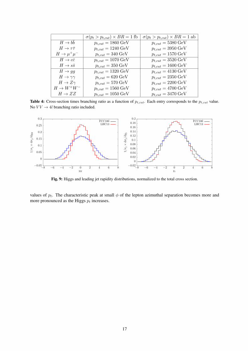
σ(pt > pt,cut)×BR = 1 fb σ(pt > pt,cut)×BR = 1 ab

H → bb pt,cut = 1860 GeV pt,cut = 5380 GeVH → τ τ pt,cut = 1240 GeV pt,cut = 3950 GeV

H → µ+µ− pt,cut = 340 GeV pt,cut = 1570 GeV

H → cc pt,cut = 1070 GeV pt,cut = 3520 GeVH → ss pt,cut = 350 GeV pt,cut = 1600 GeV

H → gg pt,cut = 1320 GeV pt,cut = 4130 GeVH → γγ pt,cut = 620 GeV pt,cut = 2350 GeVH → Zγ pt,cut = 570 GeV pt,cut = 2200 GeV

H →W+W− pt,cut = 1560 GeV pt,cut = 4700 GeVH → ZZ pt,cut = 1050 GeV pt,cut = 3470 GeV

Table 4: Cross-section times branching ratio as a function of pt,cut. Each entry corresponds to the pt,cut value.No V V → 4l branching ratio included.

1/σj×

dσj/dy H

yH

FCC100LHC13

−0.05

0

0.05

0.1

0.15

0.2

0.25

0.3

−8 −6 −4 −2 0 2 4 6 8

1/σj×

dσj/dy j

yj

FCC100LHC13

−0.02

0

0.02

0.04

0.06

0.08

0.1

0.12

0.14

0.16

0.18

0.2

−8 −6 −4 −2 0 2 4 6 8

Fig. 9: Higgs and leading jet rapidity distributions, normalized to the total cross section.

values of pt. The characteristic peak at small φ of the lepton azimuthal separation becomes more andmore pronounced as the Higgs pt increases.

17

1/σ×

dσ/dm

ll

mll

pt,H > 60 GeVpt,H > 1000 GeV

0

0.02

0.04

0.06

0.08

0.1

0.12

0 20 40 60 80 100

1/σ×

dσ/dp ⊥

,ll

p⊥,ll


0

0.1

0.2

0.3

0.4

0.5

0.6

0.7

0.8

0 500 1000 1500 2000

1/σ×

dσ/d

∆φ,ll

∆φll


0

0.1

0.2

0.3

0.4

0.5

0.6

0.7

0.8

0 0.5 1 1.5 2 2.5 3

Fig. 10: Normalized differential distributions for the pp→ H →WW → 2l2ν process. Results for two values ofcuts on the Higgs transverse momentum are shown, see text for details.

18

3.3 Higgs plus jets production in gg → H

In this section we present NLO QCD results for the production of a Standard Model Higgs boson inassociation with up to three jets in gluon-gluon fusion (GGF). If not stated differently, the computationsare done in the approximation of an infinitely heavy top quark using the same effective field theoryLagrangian presented in Eq. (4).

Gluon–gluon fusion is not only the largest Higgs boson production channel, but, as already shownin Section 3.1, it is also characterized by very large higher-order corrections. Although less dramaticthan in the fully inclusive case of Higgs boson production, the production in association with jets alsosuffers from large corrections due to NLO effects. In this section we will study how this changes whenthe center-of-mass energy increases from 14 to 100 TeV.

Gluon fusion is also the largest background for Higgs boson production through vector bosonfusion (VBFH). Despite the very peculiar experimental signature of the VBFH channel, whose topologyallows to define fiducial cuts which reduce the backgrounds dramatically, the contamination from GGFremains a very important aspect at LHC energies. It is therefore interesting to study the impact of typicalVBFH-type selection cuts on the GGF background also at FCC energies.

Another important aspect to keep in mind, is the limited range of validity of the effective fieldtheory description, in which the top quark is integrated out. As already shown for the inclusive case inprevious sections, finite top quark and bottom quark mass effects can become large when the transverseenergy is large enough to resolve the quark loop that couples the Higgs boson to gluons. At the end ofthis section, we will investigate the impact of these corrections presenting LO results in the full theory.

3.3.1 Computational setupThe computation is performed using the setup developed for an analogous analysis at 8 and 13 TeV [73],and is based on the automated tools GOSAM [74, 75] and SHERPA [76], linked via the interface definedin the Binoth Les Houches Accord [77, 78].

The one-loop amplitudes are generated with GOSAM, and are based on an algebraic generation ofd-dimensional integrands using a Feynman diagrammatic approach. The expressions for the amplitudesare generated employing QGRAF [79], FORM [80, 81] and SPINNEY [82]. For the reduction of thetensor integrals at running time, we used NINJA [83, 84], which is an automated package carrying outthe integrand reduction via Laurent expansion [85], and ONELOOP [86] for the evaluation of the scalarintegrals. Unstable phase space points are detected automatically and reevaluated with the tensor integrallibrary GOLEM95 [87–89]. The tree-level matrix elements for the Born and real-emission contribution,and the subtraction terms in the Catani-Seymour approach [90] have been evaluated within SHERPA

using the matrix element generator COMIX [91].

Using this framework we stored NLO events in the form of ROOT Ntuples. Details about theformat of the Ntuples generated by SHERPA can be found in [92]. The predictions presented in thefollowing were computed using Ntuples at 14 and 100 TeV with generation cuts specified by

pT, jet > 25 GeV and |ηjet| < 10 ,

and for which the Higgs boson mass mH and the Higgs vacuum expectation value v are set to mH =125 GeV and v = 246 GeV, respectively. To improve the efficiency in performing the VBFH analysisusing the selection cuts described below, a separate set of Ntuples was generated. This set includesan additional generation cut on the invariant mass of the two leading transverse momentum jets. Togenerated large dijet masses from scratch, we require mj1j2 > 1600 GeV.

The results reported here are obtained by clustering jets with the anti-kT algorithm [93, 94] em-ploying a cone radius of R = 0.4. We utilized the implementation as provided by the FASTJET pack-age [95], and also relied on using the CT14nlo PDF set [96] in the calculations presented here. In order

19

Numbers in pb σ14 TeVLO σ14 TeV

NLO σ100 TeVLO σ100 TeV

NLO NLO Ratio

H+1 jet

pT, jet > 30 GeV 9.39+38%−26% 15.4+15%

−15% 217+21%−17% 336+10%

−9% 21.8

pT, jet > 50 GeV 5.11+39%−26% 8.49+15%

−15% 135+22%−18% 215+11%

−10% 25.3

pT, jet > 100 GeV 1.66+40%−27% 2.73+15%

−16% 58.2+24%−19% 92.1+11%

−11% 33.7

pT, jet > 300 GeV 0.11+43%−28% 0.17+15%

−16% 8.51+28%−21% 13.2+11%

−11% 77.6

H+2 jets

pT, jet > 30 GeV 3.60+57%−34% 5.40+12%

−18% 148+40%−27% 174−2%

−8% 32.2

pT, jet > 50 GeV 1.25+58%−34% 1.96+15%

−19% 65.0+41%−27% 83.7+3%

−11% 42.7

pT, jet > 100 GeV 0.22+58%−34% 0.36+17%

−20% 17.7+42%−28% 24.6+8%

−13% 68.3

pT, jet > 300 GeV 6.35 · 10−3 +57%−34% 1.03 · 10−2 +17%

−20% 1.41+43%−28% 2.07+10%

−14% 202.9

H+3 jets

pT, jet > 30 GeV 1.22+76%−40% 1.77+9%

−21% 89.0+58%−34% 84.3−24%

−5% 47.6

pT, jet > 50 GeV 0.29+75%−40% 0.46+15%

−23% 29.8+58%−34% 32.9−10%

−10% 71.5

pT, jet > 100 GeV 3.07 · 10−2 +74%−40% 4.95 · 10−2 +19%

−23% 5.61+57%−34% 7.04+1%

−14% 142.1

pT, jet > 300 GeV 2.97 · 10−4 +71%−39% 4.86 · 10−4 +20%

−23% 0.24+56%−34% 0.34+9%

−16% 700.2

Table 5: Total inclusive cross sections for the production of a Higgs boson in association with one, two or threejets at LO and NLO in QCD. Numbers are reported for center-of-mass energies of 14 and 100 TeV and four choicesof transverse momentum cuts on the jets, namely pT, jet > 30, 50, 100 and 300 GeV. The last column shows theratios between the NLO cross sections at the two center-of-mass energies. The uncertainty estimates are obtainedfrom standard scale variations.

to assess the impact of varying the transverse momentum threshold for the jets, we apply four differentcuts at

pT, jet > 30, 50, 100 and 300 GeV ,

and keep the same cut on ηjeta s in the Ntuples generation. For the VBFH analysis, we then applyadditional cuts as described further below in Section 3.3.3

The renormalization and factorization scales were set equal, and are defined as

µR = µF =H ′T2

=1

2

(√m2H + p2

T,H +∑i

|pT, ji |). (14)

The sum runs over all partons accompanying the Higgs boson in the event. Theoretical uncertainties areestimated in the standard way by varying the central scale by factors of 0.5 and 2.

3.3.2 Gluon fusion resultsWe start by summarizing in Table 5 the total inclusive cross sections for the production of a Higgs bosonin gluon-gluon fusion accompanied by one, two or three additional jets. We show results at LO andNLO in QCD for pp collisions at 14 and 100 TeV. Furthermore, the total cross sections are given forfour different pT, jet cuts on the jets. In the last column we show the ratio of the NLO result for 100 TeVover the NLO result for 14 TeV. This ratio significantly increases when the pT, jet cut is tightened, andit also strongly increases as a function of the jet multiplicities. This can be easily understood by thefact that in a 100 TeV environment, the cuts appear much less severe than for 14 TeV; their impact on

20

0.0

0.2

0.4

0.6

0.8

1.0

1.2

H+

n(pT,j

et)/

H+

n(pT,r

ef)

Ratio wrt. softer pT,jet threshold.NLO/NLO

0.5

1.0

1.5

2.0

NL

O/L

O

Differential K-factor.

0.5

1.0

1.5

2.0

NL

O/L

O


0 100 200 300 400 500

Higgs boson transverse momentum: pT,H [GeV]

0.5

1.0

1.5

2.0

NL

O/L

O


10−3

10−2

10−1

100

101

dσ/dp T

,H[p

b/G

eV]

GoSam + Sherpapp→H + 1, 2, 3 jets at 100 TeV

CT14nlo, R = 0.4 anti-kT, |ηjet| < 10, pT,jet = 100 GeV, pT,ref = 50 GeV

LO H+1

LO H+2

LO H+3

NLO H+1

NLO H+2

NLO H+3

0.0

0.2

0.4

0.6

0.8

1.0

1.2

H+

n(pT,j

et)/

H+

n(pT,r

ef)


0.5

1.0

1.5

2.0

NL

O/L

O


0.5

1.0

1.5

2.0

NL

O/L

O


−6 −4 −2 0 2 4 6Higgs boson rapidity: yH

0.5

1.0

1.5

2.0

NL

O/L

O


10−5

10−4

10−3

10−2

10−1

100

101

102

103

dσ/dy H

[pb

]



LO H+1

LO H+2

LO H+3

NLO H+1

NLO H+2

NLO H+3

Fig. 11: The transverse momentum spectrum pT,H and the rapidity distribution yH of the Higgs boson at 100 TeVfor the three production modes H+1, 2, 3 jets. Results are shown at LO and NLO including the effect from standardscale variations and imposing a jet threshold of pT, jet > 100 GeV. The second panel depicts the NLO ratios takenwrt. reference results obtained with pT, jet > 50 GeV; the other ratio plot panels display the differential K-factorsfor the different jet multiplicities.

the lower energy is therefore larger. For the same reasons, this pattern is also found for the number ofjets. With rising center-of-mass energy, it becomes easier to produce additional jets, which leads to theenhancement of the inclusive cross section ratio.

Turning to more exclusive observables, Figure 11 shows (to the left) the transverse momentumdistribution and (to the right) the rapidity distribution of the Higgs boson at 100 TeV with a transversemomentum requirement on the jets of pT, jet > 100 GeV. The different colours denote the various jetmultiplicities. The brighter bands show the LO predictions with their respective uncertainties, whereasthe NLO results are displayed by darker bands. As we deal with fixed-order predictions, we observefor the pT,H distributions – as expected – Sudakov shoulder effects decreasing in their extent at pT ∼100, 200 and 300 GeV for the one-jet, two-jet and three-jet final states, respectively. The uppermostratio plot shows the results for pT, jet > 100 GeV divided by the corresponding results of the same jetmultiplicity, but with a pT, jet threshold of 50 GeV. As expected this ratio gets smaller for higher jetmultiplicities, which means the more jets are present, the more sensitively the cross section changesin response to a jet threshold increase. In the one-jet case we find that the ratio turns one for pT,H >200 GeV. Below this value, the 50 GeV threshold sample contains event topologies that are absent forpT, jet > 100 GeV. The ratio will hence be smaller than one. For example, a configuration consistingof a jet with pT = 99.9 GeV and a real emission of size pT = 99.8 GeV will be present for 50 GeVthresholds but be missed by the higher pT, jet sample. Lastly we note that the size of the K-factorsdecreases for jettier final states. We also observe that the 100 TeV environment allows for a wide range

21

0.0

0.2

0.4

0.6

0.8

1.0

1.2

H+

n/

H+

n-1

Inclusive n-jet fraction wrt. (n− 1)-jet cross section.NLO/NLO

0.5

1.0

1.5

2.0

NL

O/L

O


0.5

1.0

1.5

2.0

NL

O/L

O


0 100 200 300 400 500


0.5

1.0

1.5

2.0

NL

O/L

O


10−5

10−4

10−3

10−2

10−1

100

101

dσ/dp T

,H[p

b/G

eV]

GoSam + Sherpapp→H + 2 jets at 100 TeV

CT14nlo, R = 0.4 anti-kT, |ηjet| < 10

LO @ pT,jet = 30 GeV



NLO @ pT,jet = 30 GeV



0.0

0.2

0.4

0.6

0.8

1.0

1.2

H+

n/

H+

n-1


0.5

1.0

1.5

2.0

NL

O/L

O


0.5

1.0

1.5

2.0

NL

O/L

O


−5 0 5Leading-jet rapidity: yj1

0.5

1.0

1.5

2.0

NL

O/L

O


10−3

10−2

10−1

100

101

102

103

dσ/dy j

1[p

b]









Fig. 12: The transverse momentum spectrum pT,H of the Higgs boson and the rapidity distribution yj1 of theleading jet, both of which shown at LO and NLO, and for different transverse momentum requirements on thejets in H+2-jet scatterings as produced at a 100 TeV pp collider. The comparison to the H+1-jet case at NLOis visualized in the first ratio plot, followed by the canonical NLO versus LO ratio plots for the different pT, jet

values. All uncertainty envelopes originate from standard scale variations by factors of two.

of Higgs boson rapidities independent of the jet multiplicity. One easily gains two absolute units wrt. thecapabilities of the LHC.

The left plot of Figure 12 shows again transverse momentum distributions of the Higgs boson,however in this case we only consider the curves for H + 2 jets at 100 TeV. Here, we examine theimpact of tightening the transverse momentum cut on the jets. The typical shoulder present for pT, jet >30 GeV progressively disappears for increasing values of pT, jet such that the corresponding distributionfor pT, jet > 300 GeV becomes almost flat in the range from 100 to 500 GeV. In the right plot ofFigure 12, the analogous comparison for the rapidity of the leading jet is presented. As expected, thesuccessively harder jet constraints lead to a more central production of the jets reducing the rapidityrange where the differential cross section is larger than 1 fb by about six units. In both plots of Figure 12,the first ratio plot highlights the behaviour of the fraction between the inclusive results for H+2 jets andH+1 jet. While for the Higgs boson transverse momentum, this fraction varies considerably and canreach one in phase space regions of near-zero as well as large pT,H (earmarking the important two-jetregions), for the leading jet rapidity, the maximum occurs always at yj1 = 0 decreasing from about 0.6to 0.2 once the jet transverse momentum cut is tightened. This shows that the leading jet tends to beproduced more centrally in events of higher jet multiplicity. An increase of the transverse momentumcut also has consequences on the size and shape of the NLO corrections. This is shown in the lowerinsert plots. In general, for sharper cuts, the higher-order corrections become larger but flatter over theconsidered kinematical range. Similar results are also obtained for the H+3-jet process.

22

0.0

0.2

0.4

0.6

0.8

1.0

1.2

H+

n(pT,j

et)/

H+

n(pT,r

ef)


0.5

1.0

1.5

2.0

NL

O/L

O


0.5

1.0

1.5

2.0

NL

O/L

O


100 200 300 400 500

Leading-jet transverse momentum: pT,j1 [GeV]

0.5

1.0

1.5

2.0

NL

O/L

O


10−5

10−4

10−3

10−2

10−1

100

101

dσ/dp T

,j1

[pb

/GeV

]



LO H+1

LO H+2

LO H+3

NLO H+1

NLO H+2

NLO H+3

0.0

0.2

0.4

0.6

0.8

1.0

1.2

H+

n/

H+

n-1


0.5

1.0

1.5

2.0

NL

O/L

O


0.5

1.0

1.5

2.0

NL

O/L

O


100 200 300 400 500

Leading-jet transverse momentum: pT,j1 [GeV]

0.5

1.0

1.5

2.0

NL

O/L

O


10−5

10−4

10−3

10−2

10−1

100

101

dσ/dp T

,j1

[pb

/GeV

]









Fig. 13: The transverse momentum distribution pT, j1 of the leading jet at an FCC energy of 100 TeV for thethree production modes of H+1, 2, 3 jets (left) and varying jet-pT thresholds exemplified for the case of H+2-jetproduction (right). The layout of the plot to the left (right) is the same as used in Figure 11 (Figure 12).

Figure 13 focuses on the leading jet transverse momentum. The plot on the left hand side comparespredictions for H+1, 2, 3 jets with one another at LO and NLO for a jet threshold of pT, jet > 100 GeV.The scheme of the lower ratio plots is equal to the one of Figure 11. For pT,j1 ≈ 300 GeV, we see that60% (30%) of the inclusive two-jet (three-jet) events (using the reference jet threshold) have a second jetat or above a transverse momentum of 100 GeV. The plot on the right hand side instead shows the effectof the different jet transverse momentum constraints for H+2 jets production at 100 TeV, following thecolour convention and the scheme of Figure 12. For lower jet thresholds, the two-jet cross section risesquickly with increasing lead-jet pT to the same order of magnitude as the one-jet cross section. We findthat an increase of the jet-pT constraint helps slow down this behavior sufficiently.

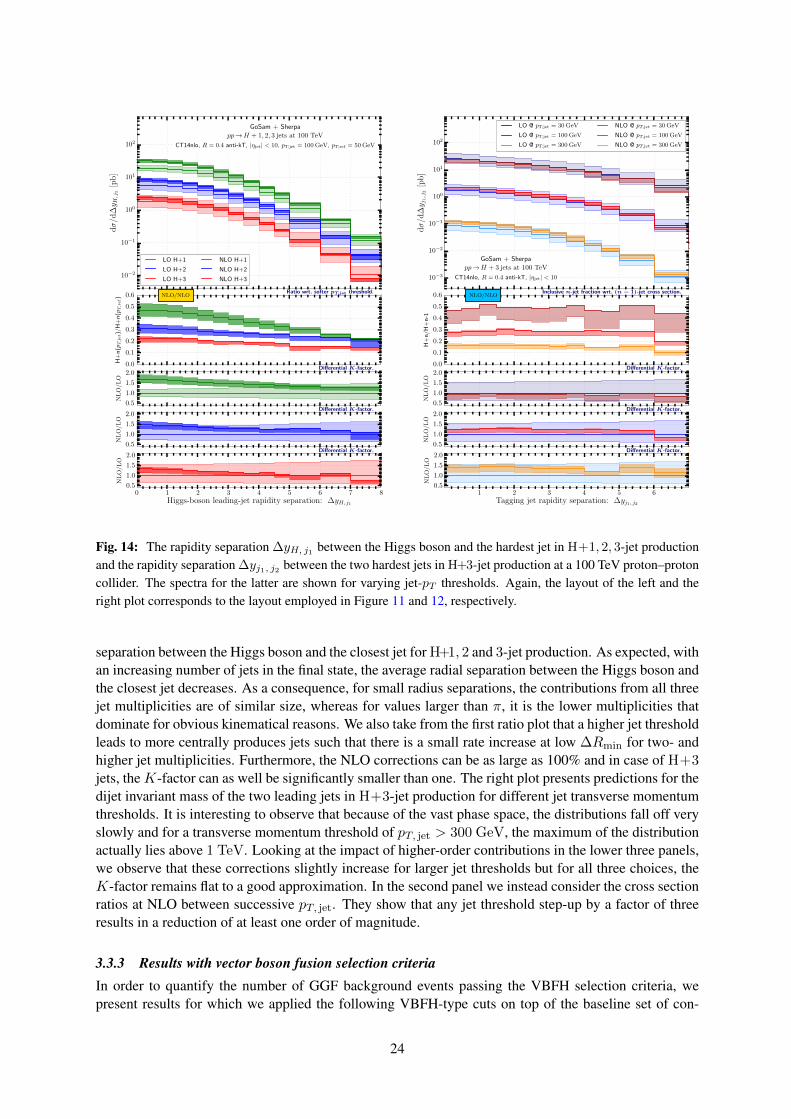
The plots of Figure 14 show the rapidity separation between the Higgs boson and the leading jet(on the left) and between the two leading jets (on the right). In the former case, the distributions showthe results for the three different final state multiplicities, whereas in the latter case, the curves refer tothe H+3-jet process and compare the impact of the different jet transverse momentum cuts. For bothobservables, the large production rates and the huge available phase space allow to have differential crosssections, which for separations as large as three units in ∆y, are only a factor of two smaller than the onesat zero rapidity separation. Independent of the jet multiplicity, both NLO corrections as well as tighterjet definitions trigger enhancements in the ∆yH, j1 distribution (left panel) for configurations where theHiggs boson and the leading jet are close in rapidity. For the ∆yj1, j2 variable (right panel), a ratheruniform behaviour is found while changing the jet threshold: the three-jet over two-jet fraction as wellas the K-factors remain rather constant over the entire ∆y range.

Additional two-particle observables are presented in Figure 15. The left plot shows the radial

23

0.0

0.1

0.2

0.3

0.4

0.5

0.6

H+

n(pT,j

et)/

H+

n(pT,r

ef)


0.5

1.0

1.5

2.0

NL

O/L

O


0.5

1.0

1.5

2.0

NL

O/L

O


0 1 2 3 4 5 6 7 8Higgs-boson leading-jet rapidity separation: ∆yH, j1

0.5

1.0

1.5

2.0

NL

O/L

O


10−2

10−1

100

101

102

dσ/d

∆y H

,j1

[pb

]



LO H+1

LO H+2

LO H+3

NLO H+1

NLO H+2

NLO H+3

0.0

0.1

0.2

0.3

0.4

0.5

0.6

H+

n/

H+

n-1


0.5

1.0

1.5

2.0

NL

O/L

O


0.5

1.0

1.5

2.0

NL

O/L

O


1 2 3 4 5 6Tagging jet rapidity separation: ∆yj1, j2

0.5

1.0

1.5

2.0

NL

O/L

O


10−3

10−2

10−1

100

101

102

dσ/d

∆y j

1,j

2[p

b]









Fig. 14: The rapidity separation ∆yH, j1 between the Higgs boson and the hardest jet in H+1, 2, 3-jet productionand the rapidity separation ∆yj1, j2 between the two hardest jets in H+3-jet production at a 100 TeV proton–protoncollider. The spectra for the latter are shown for varying jet-pT thresholds. Again, the layout of the left and theright plot corresponds to the layout employed in Figure 11 and 12, respectively.

separation between the Higgs boson and the closest jet for H+1, 2 and 3-jet production. As expected, withan increasing number of jets in the final state, the average radial separation between the Higgs boson andthe closest jet decreases. As a consequence, for small radius separations, the contributions from all threejet multiplicities are of similar size, whereas for values larger than π, it is the lower multiplicities thatdominate for obvious kinematical reasons. We also take from the first ratio plot that a higher jet thresholdleads to more centrally produces jets such that there is a small rate increase at low ∆Rmin for two- andhigher jet multiplicities. Furthermore, the NLO corrections can be as large as 100% and in case of H+3jets, theK-factor can as well be significantly smaller than one. The right plot presents predictions for thedijet invariant mass of the two leading jets in H+3-jet production for different jet transverse momentumthresholds. It is interesting to observe that because of the vast phase space, the distributions fall off veryslowly and for a transverse momentum threshold of pT, jet > 300 GeV, the maximum of the distributionactually lies above 1 TeV. Looking at the impact of higher-order contributions in the lower three panels,we observe that these corrections slightly increase for larger jet thresholds but for all three choices, theK-factor remains flat to a good approximation. In the second panel we instead consider the cross sectionratios at NLO between successive pT, jet. They show that any jet threshold step-up by a factor of threeresults in a reduction of at least one order of magnitude.

3.3.3 Results with vector boson fusion selection criteriaIn order to quantify the number of GGF background events passing the VBFH selection criteria, wepresent results for which we applied the following VBFH-type cuts on top of the baseline set of con-

24

0.0

0.2

0.4

0.6

0.8

1.0

1.2

H+

n(pT,j

et)/

H+

n(pT,r

ef)


0.5

1.0

1.5

2.0

NL

O/L

O


0.5

1.0

1.5

2.0

NL

O/L

O


0 1 2 3 4 5Minimum H-jet geometric separation: ∆Rmin, H, jk

0.5

1.0

1.5

2.0

NL

O/L

O


10−2

10−1

100

101

102

103

dσ/d

∆R

min,H,jk

[pb

]



LO H+1

LO H+2

LO H+3

NLO H+1

NLO H+2

NLO H+3

10−2

10−1

100

H+

n(pT,j

et)/

H+

n(pT,p

rev

)

Ratio wrt. previous pT,jet threshold.NLO/NLO

0.5

1.0

1.5

2.0

NL

O/L

O


0.5

1.0

1.5

2.0

NL

O/L

O


0 200 400 600 800 1000

Leading dijet mass: mj1j2 [GeV]

0.5

1.0

1.5

2.0

NL

O/L

O


10−6

10−5

10−4

10−3

10−2

10−1

100

101

dσ/dmj 1j 2

[pb

/GeV

]









Fig. 15: The geometric separation ∆Rmin, H, jk between the Higgs boson and the jet closest to it, and the invariantmass distribution of the leading dijet system at a 100 TeV proton–proton collider. For the former, distributions areshown for H+1, 2, 3-jet production, while for the latter, the jet-pT thresholds are varied to show the correspondingdistributions obtained from H+3-jet events. The colour coding and plot layout is as previously described with theonly exception that the upper ratios in the left panel are taken between successive pT, jet results for the same jetmultiplicity.

straints defined in the previous section:

mj1j2 > 1600 GeV , |∆yj1, j2 | > 6.5 , yj1 · yj2 < 0 . (15)

In Table 6 the total cross sections for a center-of-mass energy of 100 TeV are summarized. Differentialdistributions will be discussed in a slightly different context in one of the later sections, see Section 3.5,together with the results obtained from the VBF@NNLO computations.

3.3.4 Finite quark mass effectsIt is well known that the infinitely large top quark mass approximation has a restricted validity range,and that for energies large enough to resolve the massive top quark loop, the deviations start to becomesizeable. In order to quantify better the effects due to finite quark masses, in the following we compareLO predictions in the effective theory with computations in the full theory. We consider here onlymassive top quarks running in the loop. The effect of massive bottom quarks for a center-of-mass energyof 100 TeV can be safely neglected. For the top quark mass, we use mt = 172.3 GeV. Compared to theresults shown in the previous section, we now impose a more restrictive cut on the pseudo-rapidity of thejets, demanding |ηjet| < 4.4; the impact of this cut is however fairly minimal on the observables that weare considering.

25


NLO

H+2 jets

pT, jet > 30 GeV 4.60+56%−33% 4.70−17%

−7%

pT, jet > 50 GeV 1.71+56%−34% 1.98−6%

−11%

pT, jet > 100 GeV 0.26+57%−34% 0.31−3%

−13%

pT, jet > 300 GeV 5.10 · 10−3 +58%−34% 6.20 · 10−3 −1%

−14%

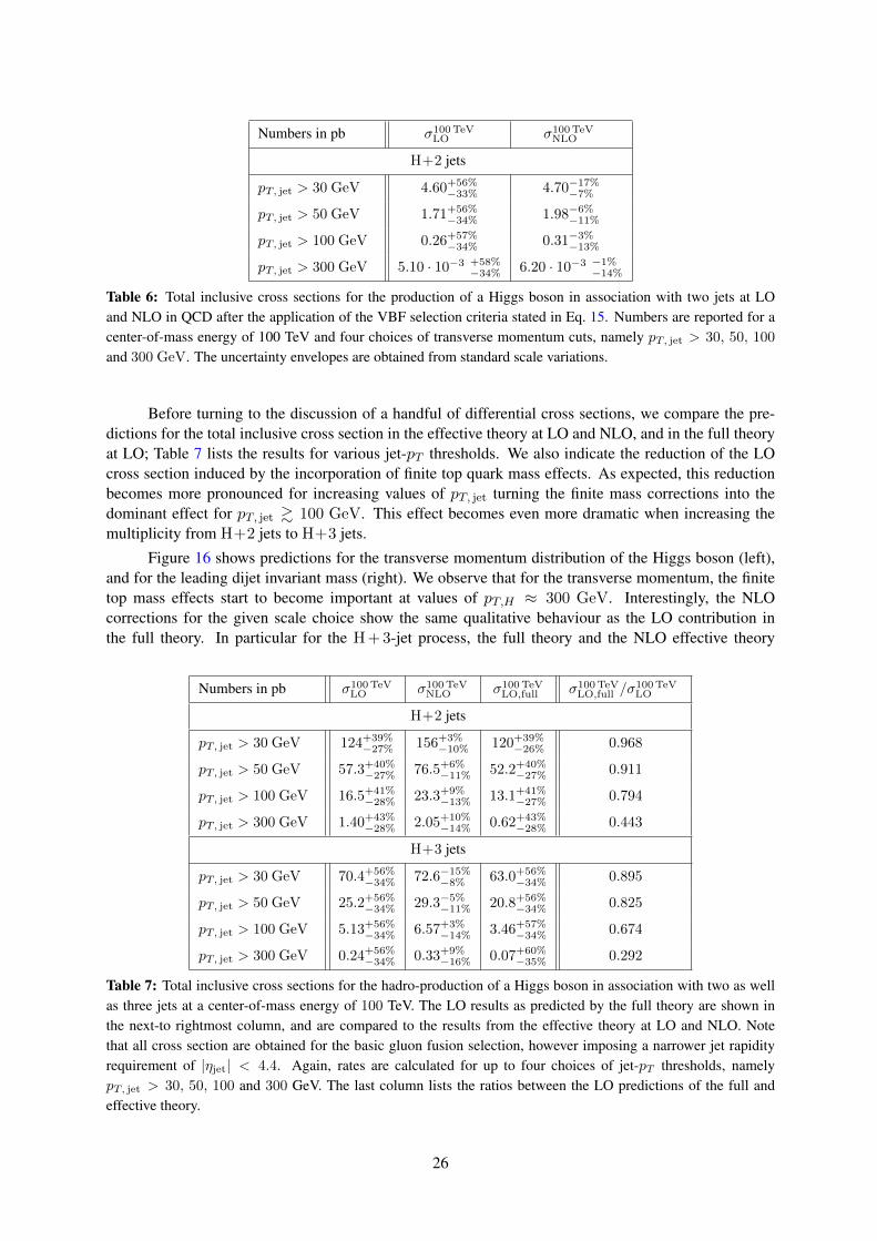
Table 6: Total inclusive cross sections for the production of a Higgs boson in association with two jets at LOand NLO in QCD after the application of the VBF selection criteria stated in Eq. 15. Numbers are reported for acenter-of-mass energy of 100 TeV and four choices of transverse momentum cuts, namely pT, jet > 30, 50, 100

and 300 GeV. The uncertainty envelopes are obtained from standard scale variations.

Before turning to the discussion of a handful of differential cross sections, we compare the pre-dictions for the total inclusive cross section in the effective theory at LO and NLO, and in the full theoryat LO; Table 7 lists the results for various jet-pT thresholds. We also indicate the reduction of the LOcross section induced by the incorporation of finite top quark mass effects. As expected, this reductionbecomes more pronounced for increasing values of pT, jet turning the finite mass corrections into thedominant effect for pT, jet & 100 GeV. This effect becomes even more dramatic when increasing themultiplicity from H+2 jets to H+3 jets.

Figure 16 shows predictions for the transverse momentum distribution of the Higgs boson (left),and for the leading dijet invariant mass (right). We observe that for the transverse momentum, the finitetop mass effects start to become important at values of pT,H ≈ 300 GeV. Interestingly, the NLOcorrections for the given scale choice show the same qualitative behaviour as the LO contribution inthe full theory. In particular for the H + 3-jet process, the full theory and the NLO effective theory


NLO σ100 TeVLO,full σ100 TeV

LO,full /σ100 TeVLO

H+2 jets

pT, jet > 30 GeV 124+39%−27% 156+3%

−10% 120+39%−26% 0.968

pT, jet > 50 GeV 57.3+40%−27% 76.5+6%

−11% 52.2+40%−27% 0.911

pT, jet > 100 GeV 16.5+41%−28% 23.3+9%

−13% 13.1+41%−27% 0.794

pT, jet > 300 GeV 1.40+43%−28% 2.05+10%

−14% 0.62+43%−28% 0.443

H+3 jets

pT, jet > 30 GeV 70.4+56%−34% 72.6−15%

−8% 63.0+56%−34% 0.895

pT, jet > 50 GeV 25.2+56%−34% 29.3−5%

−11% 20.8+56%−34% 0.825

pT, jet > 100 GeV 5.13+56%−34% 6.57+3%

−14% 3.46+57%−34% 0.674

pT, jet > 300 GeV 0.24+56%−34% 0.33+9%

−16% 0.07+60%−35% 0.292

Table 7: Total inclusive cross sections for the hadro-production of a Higgs boson in association with two as wellas three jets at a center-of-mass energy of 100 TeV. The LO results as predicted by the full theory are shown inthe next-to rightmost column, and are compared to the results from the effective theory at LO and NLO. Notethat all cross section are obtained for the basic gluon fusion selection, however imposing a narrower jet rapidityrequirement of |ηjet| < 4.4. Again, rates are calculated for up to four choices of jet-pT thresholds, namelypT, jet > 30, 50, 100 and 300 GeV. The last column lists the ratios between the LO predictions of the full andeffective theory.

26

10−1

100

X/

LO

H+

2

only H+2

Ratio wrt. LO using mt →∞ approximation.

0 100 200 300 400 500


10−1

100

X/

LO

H+

3

only H+3


10−2

10−1

100

101

dσ/dp T

,H[p

b/G

eV]

GoSam + Sherpapp→H + 2, 3 jets at 100 TeV

CT14nlo, R = 0.4 anti-kT, |ηjet| < 4.4, pT,jet = 30 GeV

LO H+2 (×10)

LO H+3

LO H+2 mt (×10)

LO H+3 mt

NLO H+2 (×10)

NLO H+3

100

X/

LO

H+

2

only H+2


0 200 400 600 800 1000

Leading dijet mass: mj1j2 [GeV]

100

X/

LO

H+

3

only H+3


10−2

10−1

100

101

dσ/dmj 1j 2

[pb

/GeV

]



LO H+2 (×10)

LO H+3

LO H+2 mt (×10)

LO H+3 mt

NLO H+2 (×10)

NLO H+3

Fig. 16: The impact of finite top quark mass effects in the loop-induced emission of a Higgs boson in GGF H+n-jet production at a 100 TeV proton–proton collider. LO results based on the full and effective theory as well asNLO results using the effective theory are shown (to the left) for the transverse momentum spectrum, pT,H , of theHiggs boson and (to the right) for the invariant mass distribution, mj1j2 , of the leading dijet system. The H+2-jetand H+3-jet predictions are grouped in separate ratio plots using the respective LO results as their reference.Uncertainty bands are derived from standard scale variations.

seem to almost give the same prediction, except for the size of the scale variations. On the contrarythe predictions for the invariant mass distributions in the full theory only mildly deviate from the onescomputed in the effective theory; again the tails are somewhat softer. For both H+2 jets and H+3 jets,the NLO predictions remain within the respective scale uncertainties of the LO results over the wholerange shown in the figure. In addition, the shapes of the NLO effective and LO full theory show a fairlysimilar behaviour. In the two-jet case there is however a clear rate difference due to the considerablygreater-than-one K-factor.

The last figure exemplifies how severe deviations can become between the full and effective theorydescription for the hardness of transverse particle/jet production. This is nicely demonstrated by means ofthe HT, jets distribution shown to the left of Figure 17. The finite top quark mass effects clearly dominateover the NLO corrections calculated in the effective theory. The H+2-jet case in particular demonstratesthe extreme and opposite behaviour of both effects – a large K-factor on the one side versus an evenmore effective suppression of the HT tail on the other side by about 70-80%. While the finite masseffects always suppress the rate for hard jet production, the NLO corrections can lead to an enhancementas seen for H+2 jets as well as to a reduction as we observe in the H+3-jet case.

As in the previous figure, we contrast two different types of observables with each other. Inthe right panel of Figure 17 we therefore display an angular correlation, more precisely we show theazimuthal angle separation between the leading and subleading jet. This kind of observable is importantin precision coupling measurements, and although the corrections tend to be much smaller, they have tobe understood in detail to satisfy the demand for high precision. Here, both the NLO corrections andfinite mass effects lead to similar shape changes, suppressing small-angle contributions while the back-to-back configurations receive an (effective) enhancement (due to the finite mt treatment). This time, we

27

10−1

100

X/

LO

H+

2

only H+2


200 400 600 800 1000

Jet pT scalar sum: HT, jets [GeV]

10−1

100

X/

LO

H+

3

only H+3


10−3

10−2

10−1

100

101

dσ/dHT,j

ets

[pb

/GeV

]



LO H+2 (×10)

LO H+3

LO H+2 mt (×10)

LO H+3 mt

NLO H+2 (×10)

NLO H+3

100

X/

LO

H+

2

only H+2


0.0 0.5 1.0 1.5 2.0 2.5 3.0Tagging jet azimuthal angle separation: ∆φj1, j2

100

X/

LO

H+

3

only H+3


100

101

102

103

dσ/d

∆φj 1,j

2[p

b]



LO H+2 (×10)

LO H+3

LO H+2 mt (×10)

LO H+3 mt

NLO H+2 (×10)

NLO H+3

Fig. 17: Finite top quark mass effects in GGF-based H+n-jet production arising from collisions of protons at100 TeV. The jets-only scalar sum of transverse momenta, HT, jets, and the azimuthal angle distribution, ∆φj1, j2 ,between the leading and subleading jet are shown to the left and right, respectively. The differential spectra (andassociated uncertainties from scale variations) were obtained from the full theory at LO, and the effective theoryat LO (providing the references) and NLO. The upper ratio plot contains the H+2-jet predictions while the lowerone depicts those for H+3 jets.

notice a slight increase of the mt effects (from 10% to 20%) for the final states of higher jet multiplicity.

3.3.5 ConclusionsIn this section we studied the associate production of a Standard Model Higgs boson in association withup to three jets in gluon–gluon fusion. We compared LO and NLO QCD predictions for several differentcuts on the transverse momentum of the jets and also produced results with VBFH-type cuts, whichare compared with VBF predictions in Section 3.5. Because of the large center-of-mass energy and thehuge available phase space, the production rates become much larger compared to LHC energies. Thiscan be observed in particular when comparing the relative size of contributions coming from differentmultiplicities. In the last part of this section, we studied the impact of finite quark mass effects. Fortypical jet transverse momentum cuts, which at FCC energies are likely to be of the order of 100 GeV,these corrections are non-negligible and their impact is in general larger than NLO QCD corrections inthe effective theory. Moreover, all quantities that are related to measuring the transverse activity of theH+n-jet processes will receive significant corrections reducing the cross section in the hard regions.

28

3.4 Associated V H productionAssociate production of the Higgs and gauge bosons mostly arises from the Higgs-strahlung processesqq → V ∗ → V H (V = W,Z). These provide direct probes of the V V H couplings.

Cross sections for HV associated production in hadron collisions are studied since long. For theinclusive cross sections, up to NNLO QCD corrections are available in the program vh@nnlo [97–99].Furthermore, programs have been developed for the computation of fully differential distributions includ-ing NNLO QCD corrections [100–103], the EW corrections [104, 105] and event generators matchingand merging NLO QCD corrections for VH+jets production to parton showers [106–108]. Finally, thecomputation of NNLO QCD corrections matched with parton shower has been worked out in ref. [109],reweighting events samples obtained with the code presented in ref. [106] with the histograms obtainedwith the program of ref. [102] and relying for the level of accuracy on the theorems presented in [110].The results in Table 8 have been obtained using vh@nnlo and the NNPDF30_nnlo_as_0118 [111] pdfset. The central renormalisation and factorisation scales have been set both to the mass of the HV sys-tem. For the estimate of the scale uncertainty reported in the table, we varied them independently up toa factor of 3 with the constraint µf · µr ≤ 2.

σtot[pb] δPDF [pb] δscale[pb] σDY [pb] σggHV [pb] σtop[pb]

HW 15.710 ±0.024 +0.010−0.020 15.403 − 0.307

HZ 11.178 ±0.022 +0.062−0.044 8.946 2.069 0.163

Table 8: Total cross sections σ(V H), including up to NNLO QCD corrections, and respective PDF and PDFuncertainties.

Figure 9 shows the cross sections for the WH process, with different selection cuts for the asso-ciated jet activity.

σNNLO [fb] @ 100 TeVHW+(→ He+νe)

no cuts no jets with at least 1 jet with at least 1 jet with at least 1 jet withpT > 100 GeV pT > 100 GeV pT > 500 GeV pT > 1 TeV

539 444 94.7 5.20 0.817HW−(→ He−νe)

no cuts no jets with at least 1 jet with at least 1 jet with at least 1 jet withpT > 100 GeV pT > 100 GeV pT > 500 GeV pT > 1 TeV

425 350.6 74.37 3.718 0.541

Table 9: HW fiducial cross sections in fb at NNLO accuracy for the different selection cuts on the jet activity.

As was the case for the Higgs production processes discussed so far, collisions at 100 TeV allowto extend the kinematic reach of V H final states to rather extreme configurations, where the V H pairis produced with huge invariant mass, or at very large pT . Production at large invariant mass is of phe-nomenological interest for several reasons. For example, it provides the leading source of irreduciblebackground for the detection of exotic new particles (e.g. new gauge bosons) decaying to V H . Fur-thermore, prodution at large invariant mass probes the V V H coupling in the region where the Q2 of thevirtual gauge boson is far off shell. This could exhibit sensitivity to the presence of higher-dimension ef-fective operators, potentially beyond what can be tested from the precise determination of theH → V V ∗

decay branching ratios. Figure 18 (left panel) shows that, with over 10 ab−1 of integrated luminosity,the SM rate will extend all the way out to M(V H) ∼ 20 TeV. In these configurations, with Higgs andgauge bosons with a transverse momentum of several TeV, it is likely that one will be able to effectively

29

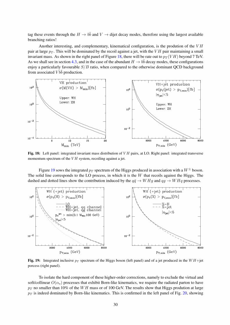
tag these events through the H → bb and V → dijet decay modes, therefore using the largest availablebranching ratios!

Another interesting, and complementary, kinematical configuration, is the prodution of the V Hpair at large pT . This will be dominated by the recoil against a jet, with the V H pair maintaining a smallinvariant mass. As shown in the right panel of Figure 18, there will be rate out to pT (V H) beyond 7 TeV.As we shall see in section 4.3, and in the case of the abundantH → bb decay modes, these configurationsenjoy a particularly favourable S/B ratio, when compared to the otherwise dominant QCD backgroundfrom associated V bb production.

Fig. 18: Left panel: integrated invariant mass distribution of V H pairs, at LO. Right panel: integrated transversemomentum spectrum of the V H system, recoiling against a jet.

Figure 19 sows the integrated pT spectrum of the Higgs produced in association with aW± boson.The solid line corresponds to the LO process, in which it is the W that recoils against the Higgs. Thedashed and dotted lines show the contribution induced by the qq →WHg and qg →WHq processes.

Fig. 19: Integrated inclusive pT spectrum of the Higgs boson (left panel) and of a jet produced in the WH+jetporcess (right panel).

To isolate the hard component of these higher-order corrections, namely to exclude the virtual andsoft/collinear O(αs) processes that exhibit Born-like kinematics, we require the radiated parton to havepT no smaller than 10% of the WH mass or of 100 GeV. The results show that Higgs prodution at largepT is indeed dominated by Born-like kinematics. This is confirmed in the left panel of Fig. 20, showing

30

the back-to-back feature of the ∆R(WH) distribution (normalized to 1), for various pT (H) thresholds.We notice the very different shape of the ∆R(WH) distribution when events are tagged by the presenceof a large pT jet (see central plot of Fig. 20).

Fig. 20: ∆R correlation between the H and W boson, in events tagged by the presence of a high-pT Higgs (left)and of a high-pT jet (central panel). Right panel: transverse momentum of the Higgs boson, relative to that of theW boson, in events with a high-pT jet. All distributions are normalized to 1.

31

3.5 VBF Higgs productionIn this section we study the production of a Standard Model Higgs through Vector Boson Fusion (VBFH)at a 100 TeV proton-proton collider. As is the case at 13 TeV, VBFH has the second largest Higgsproduction cross section and is interesting on its own for a multitude of reasons: 1) it is induced alreadyat tree-level; 2) the transverse momentum of the Higgs is non-zero at lowest order which makes it suitablefor searches for invisible decays; 3) it can be distiguished from background processes due to a signatureof two forward jets. This last property is very important, as the inclusive VBF signal is completelydrowned in QCD Hjj production. One of the aims of this section is to study how well typical VBF cutssuppress this background at a 100 TeV proton-proton machine.

3.5.1 GeneratorsFixed order LO predictions for and QCD corrections to VBFH have been obtained usingPROVBFH [112] which is based on POWHEG’s fully differential NLO QCD calculation for Higgsproduction in association with three jets via VBF [113, 114], and an inclusive NNLO QCD calcula-tion [115]. NLO-EW corrections are obtained with HAWK [104, 116]. NLO interfaced to a PartonShower (NLO+PS) results have been obtained using the POWHEG-BOX [117–120] together with ver-sion 6.428 of PYTHIA [121] with the Perugia Tune P12 [122]. QCD Hjj results are obtained as insection 3.3.

3.5.2 Parameters√S 100 TeV

MH 125 GeVPDF MMHT2014nnlo68cl & CT14nnlo

as(MZ) 0.118MZ 91.1876 GeVMW 80.385 GeVΓZ 2.4952 GeVΓW 2.085 GeVGF 1.16637× 10−5GeV−1

nf 5

µ2 = µ2R = µ2

FMH

2

√(MH

2

)2+ p2

t,H

Table 10: Setup

For the purpose of this study we have used the EW parameters shown in Table 10 together withtree-level electroweak relations to obtain the weak mixing angle, θW , and the electromagnetic coupling,αEW

sin2 θW = 1−M2W /M

2Z , αEW =

√2GFM

2W sin2 θW /π. (16)

We include no off-shell effects for the Higgs Boson but include Breit-Wigner propagators for theW and Z boson. In order to estimate scale uncertainties we vary µ up and down a factor 2 while keepingµR = µF . We use a diagonal CKM matrix. When reconstructing jets we use the anti-kt algorithm [93,94]as implemented in FASTJET [95] with radius parameter R = 0.4.

For VBFH predictions we have used the MMHT2014NNLO68CL [123] PDF set and for QCDHjj predictions we have used the CT14NNLO [96] PDF set as implemented in LHAPDF [124]. Inorder to include photon induced contributions to the NLO-EW corrections we have employed the

32

NNPDF2.3QED [125] PDF set, which includes a photon PDF. It is worth noticing that the relativeEW correction factor only very mildly depends on the PDF set, so that the induced error arising fromusing different PDFs can be safely assumed to be contained in the other theoretical uncertainties.

3.5.3 Inclusive VBF productionDue to the massive vector bosons exchanged in VBFH production the cross section is finite even whenboth jets become fully unresolved in fixed-order calculations. In Table 11 we present the fully inclusiveLO cross section and both NNLO-QCD and NLO-EW corrections. The NNLO-QCD corrections arecalculated in the DIS-like approximation (Structure Function Approximation) [126] where there is nocross-talk between the upper and lower quark line in the VBF diagram. This approximation is exactat LO and NLO but formally excludes a number of diagrams at NNLO. These contributions have beenshown to be tiny under typical VBF cuts and can therefore safely be neglected [116,127,128]. The NLO-EW corrections include both t- and u-channel contributions but exclude the s-channel contributions tobe consistent with the Structure Function Approximation. The s-channel contribution should hence betreated as a background to the VBF signal.

Table 11: Total VBF cross section including QCD and EW corrections and their uncertainties for a 100 TeVproton-proton collider. σVBF is obtained using eq. (17) where σDIS

NNLOQCD is the total VBFH cross section com-puted to NNLO accuracy in QCD, δEW is the relative EW induced corrections and σγ is the cross section inducedby incoming photons. For comparison, the LO order cross section, σLO, is also shown.

σVBF[pb] ∆scale[%] σLO[pb] σDISNNLOQCD[pb] δEW[%] σγ[pb]

69.0 +0.85−0.46 80.6 73.5 −7.3 0.81

In order to compute the VBF cross section we we combine the NNLO-QCD and NLO-EW cor-rections in the following way

σVBF = σDISNNLOQCD(1 + δEW) + σγ , (17)

where σDISNNLOQCD is the NNLO-QCD prediction in the DIS-like approximation, δEW is the relative

EW correction factor and σγ is the photon induced contribution. The combined corrections to the LOcross section is about 14% with QCD and EW corrections contributing an almost equal amount. Thescale uncertainty ∆scale is due to varying µ by a factor 2 up and down in the QCD calculation alonekeeping µF = µR. For comparison the total QCD and EW corrections at 14 TeV amount to about 7%and the QCD induced scale variations to about 0.4%.

3.5.4 VBF cutsIn order to separate the VBFH signal from the main background of QCD Hjj production we will extendtypical VBF cuts used at the LHC to a 100 TeV proton-proton collider. These cuts take advantage of thefact that VBFH production, and VBF production in general, has a very clear signature of two forward jetsclearly separated in rapidity. Examining the topology of a typical VBFH production diagram it becomesvery clear that this is the case because the two leading jets are essential remnants of the two collidingprotons. Since the pt of the jets will be governed by the mass scale of the weak vector bosons and theenergy by the PDFs the jets will typically be very energetic and in opposite rapidity hemispheres.

As is clear from figure 21 the hardest jet in VBFH production peaks at around 60 GeV. As dis-cussed above this value is set by the mass of the weak vector bosons and hence the pt spectra of thetwo hardest jets are very similar to what one finds at the LHC. From this point of view and in order to

33

no cuts

dσ/d

p t,j 1

[pb/

GeV

]

pt, j1 [GeV]

vbf/qcd Hjj 100TeV

LO VBF

10-3

10-2

10-1

100

0 50 100 150 200

no cuts

dσ/d

p t,j 2

[pb/

GeV

]

pt, j2 [GeV]

vbf/qcd Hjj 100TeV

LO VBFLO QCD

10-3

10-2

10-1

100

101

102

0 50 100 150 200

Fig. 21: Left panel: The pt of the hardest jet in VBFH production at 100 TeV. We require at least two jets in theevent but apply no other cuts; right panel: The pt of the second hardest jet in VBFH and QCD Hjj production at100 TeV.

maximise the VBFH cross section one should keep jets with pt,cut > 30 GeV. Here we present resultsfor pt,cut = 30, 50, 100 GeV to study the impact of the jet cut on both the VBFH signal and QCD Hjjbackground. We only impose the cut on the two hardest jets in the event.

To establish VBF cuts at 100 TeV we first study the variables which are typically used at the LHC.These are the dijet invariant mass, Mjj , the rapidity separation between the two leading jets, ∆yjj , theseparation between the two leading jets in the rapidity-azimuthal angle plane, ∆Rjj and the azimuthalangle between the two leading jet φjj . In Figure 22 we show Mjj and ∆yjj after applying a cut onthe two leading jets of pt > 30 GeV and requiring that the two leading jets are in opposite detectorhemispheres. This last cut removes around 60% of the background while retaining about 80% of thesignal.

pt,j > 30 GeVyj1yj2<0

dσ/d

Mjj

[pb/

GeV

]

Mjj [GeV]

vbf/qcd Hjj 100TeV

LO VBFLO QCD

10-4

10-3

10-2

10-1

0 1000 2000 3000 4000 5000 6000

pt,j > 30 GeVyj1yj2<0

dσ/dΔ

y jj [

pb]

Δyjj

vbf/qcd Hjj 100TeV

LO VBFLO QCD

-1

0

1

2

3

4

5

6

7

8

-15 -10 -5 0 5 10 15

Fig. 22: Left panel: The invariant dijet mass Mjj of the two hardest jets in VBFH and QCD Hjj production at 100

TeV. right panel: The rapidity separation of the two hardest jets ∆yjj in VBFH and QCD Hjj production at 100

TeV.

In order to suppress the QCD background a cut of ∆yjj > 6.5 is imposed. This cut also sig-nificantly reduces the QCD Mjj peak and shifts the VBF peak to about 2400 GeV. In order to further

34

suppress the QCD background we impose Mjj > 1600 GeV. After these cuts have been applied, andrequiring pt,j > 30 GeV, the VBF signal to QCD background ratio is roughly 3 with a total NNLO-QCDVBF cross section of about 12 pb. From Figure 23 it is clear that one could also impose a cut on φjj toimprove the suppression whereas a cut on ∆Rjj would not help to achieve that. We hence state the VBFcuts that we will be using throughout this section are

Mj1j2 > 1600GeV, ∆yj1j2 > 6.5, yj1yj2 < 0. (18)

where j1 is the hardest jet in the event and j2 is the second hardest jet. At a 13 TeV machine theVBFH cross section is O(1pb) under typical VBF cuts.

pt,j > 30 GeVyj1yj2<0Δyjj>6.5Mjj>1600 GeVdσ

/dφ

jj [p

b]

φjj

vbf/qcd Hjj 100TeV

LO VBFLO QCD

0

1

2

3

4

5

6

0 0.5 1 1.5 2 2.5 3

pt,j > 30 GeVyj1yj2<0Δyjj>6.5Mjj>1600 GeV

dσ/dΔ

R jj [

pb]

ΔRjj

vbf/qcd Hjj 100TeV

LO VBFLO QCD

-1

0

1

2

3

4

5

6

6 7 8 9 10 11 12 13 14

Fig. 23: Left panel: The azimuthal angle φjj between the two hardest jets in VBFH and QCD Hjj production at100 TeV. right panel: The rapidity-azimuthal angle separation of the two hardest jets ∆Rjj in VBFH and QCD Hjjproduction at 100 TeV.

In table 12 we show the fiducial cross section obtained after applying the VBF cuts of eq. (18) toVBFH and QCD Hjj production. The cross sections are reported at the three different jet pt cut values30, 50, 100 GeV. All numbers are computed at LO. It is clear from the table that requiring a somewhathigher jet pt cut than 30 GeV leads to a lower S/

√B ratio. In going from 30 GeV to 50 GeV this

reduction is however small.

Table 12: Fiducial VBFH and QCD Hjj cross sections for a 100 TeV proton-proton collider at LO under the VBFcuts of (18). The numbers are obtained using the setup of Table 10 using the CT14nnlo PDF. S/

√B is defined

as the ratio between the VBFH signal and the square root of the QCD background at an integrated luminosity of20 ab−1.

σ(pt,j > 30 GeV) [pb] σ(pt,j > 50 GeV) [pb] σ(pt,j > 100 GeV) [pb]VBFH 14.1 7.51 1.08QCD Hjj 5.04 1.97 0.331

S/√B@(20 ab−1) 28100 24200 8500

In table 13 we show for comparison the cross sections obtained after only applying the three jetpt cuts. As expected the VBFH signal is drowned in the QCD background. It is worth noticing that theS/√B ratio is still very large when one assumes an integrated luminosity of 20 ab−1 and that it declines

as the jet cut is increased.

35

Table 13: Total VBFH and QCD Hjj cross sections for a 100 TeV proton-proton collider at LO with a cut on thetwo hardest jets. The numbers are obtained using the setup of Table 10 using the CT14nnlo PDF. S/

√B is defined

as the ratio between the VBFH signal and the square root of the QCD background at an integrated luminosity of20 ab−1.

σ(pt,j > 30 GeV) [pb] σ(pt,j > 50 GeV) [pb] σ(pt,j > 100 GeV) [pb]VBFH 51.3 28.5 5.25QCD Hjj 166 78.6 23.9

S/√B@(20 ab−1) 17900 14300 4900

3.5.5 Perturbative correctionsThe results shown in the previous section were all computed at LO. Here we briefly investigate theimpact of NNLO-QCD, NLO-EW and parton shower corrections to the VBF cross section computedwith pt,j > 30 GeV and under the VBF cuts of eq. (18) at a 100 TeV collider. We also compare to theNLO-QCD predictions for QCD Hjj production.

In table 14 we show the best prediction for σVBF as obtained by eq. (17) and compare it to the samecross section obtained by showering POWHEG events with PYTHIA6 but including no effects beyondthe parton shower itself. The NLO-EW and NNLO-QCD corrections are found to be of roughly the sameorder, and amount to a total negative correction of∼ 23%. As was the case for the inclusive cross sectionthe corrections are a factor two larger than at 14 TeV. Even though the perturbative corrections to QCDHjj production are negative, the effect of including higher order corrections is that the S/

√B ratio at an

integrated luminosity of 20 ab−1 is decreased from 28100 to 24300.

Table 14: Fiducial VBF cross section including QCD and EW corrections and their uncertainties for a 100 TeVproton-proton collider. For comparison the QCD induced Hjj cross section is also shown. At fixed-order QCDcorrections are included at NNLO and EW corrections at NLO.

Process σfid[pb] ∆scale[%] σQCD[pb] δEW[%] σγ[pb]VBFH (NNLO-QCD/NLO-EW) 10.8 ±1.0 12.1 −12.6 0.22VBFH (NLO+PS) 11.9 +0.56

−0.41 11.9 - -QCD Hjj (NLO) 4.70 +0

−17 4.70 - -

In figs. 24-27 we show comparisons between VBFH and QCD Hjj production computed at NNLOand NLO in QCD respecitvely. We have applied the VBF cuts of eq. (18). Also shown is the k-factor forVBFH production going from LO to NLO and NLO to NNLO. Note that the QCD Hjj predictions havebeen obtained with the effective theory setup described in Section 3.1 and hence the pt spectra should notbe trusted beyond 2Mt. Furthermore, in the left plots of figs. 24 and 25 we notice a large scale depen-dence of the QCD Hjj predictions for higher values of the transverse momentum of the leading jet andof the Higgs boson. This is probably due to a not optimal choice of scale, which for the downward vari-ation suffers from large cancellations among the different NLO contributions (Born, virtual, integratedsubtraction terms and real radiation minus subtraction terms). We observe that increasing the minimumtransverse momentum cut improves the behaviour, whereas chosing a fixed scale instead of a dynamicalone makes it even worse. The exact origin of this large scale dependence needs further investigation.

As can be seen from the plots the VBF cuts have suppressed the background QCD Hjj productionin all corners of phasespace. One could still imagine further optimising these cuts, for example byrequiring φjj in the vicinty of π

2 or a slightly larger invariant dijet mass. We note in particular thatrequiring that the Higgs Boson has a transverse momentum greater than 40 GeV seems to favour the

36

VBFH signal. Since a cut on the transverse momentum of the decay products of the Higgs would nomatter what have to be imposed, this improves the efficiency of the VBF cuts in realistic experimentalsetups.

VBF CUTSpp 100 TeV

dσ/d

p t,j

1 [pb/

GeV

]

NNLO-VBFHNLO-QCD Hjj

10-6

10-5

10-4

10-3

10-2

10-1

100

k-fa

ctor

for V

BFH

pt, j1 [GeV]

(NLO/LO)(NNLO/NLO)

0.6

0.7

0.8

0.9

1

1.1

100 200 300 400 500 600

VBF CUTSpp 100 TeV

dσ/d

p t,j

2 [pb/

GeV

]


10-7

10-6

10-5

10-4

10-3

10-2

10-1

100

k-fa

ctor

for V

BFH

pt, j2 [GeV]

(NLO/LO)(NNLO/NLO)

0.6

0.7

0.8

0.9

1

1.1

100 200 300 400 500 600

Fig. 24: Comparison between NNLO predictions for VBFH production at NLO predicitions for QCD Hjj pro-ductionunder the VBF cuts of eq. (18). The bands represent scale uncertainties obtained by varying µF = µRby a factor two up and down. For the VBFH production the statistical uncertainty is represented by the verticalline. No statistical uncertainties are shown for the QCD Hjj result. The lower panel shows the k-factor for VBFHproduction going to LO to NLO and NLO to NNLO. Left panel: Transverse momentum of the leading jet. RightPanel: Transverse momentum of the subleading jet.

3.5.6 Differential distributionsIn addition to the distributions already presented, we here show a number of distributions to indicate thekinematical reach of the VBFH channel at 100 TeV. Assuming an integrated luminosity of 20 ab−1 westudy how many events will be produced with a Higgs whose transverse momentum exceeds pt,min. Infigs. 28 and 29 we show this distribution for various cut configurations. This variable is particularlyinteresting in the context of anomalous couplings in the weak sector. It can be seen that even under VBFcuts and requiring hard jets, a number of Higgs bosons with transverse momentum of the order 6 TeVwill be produced in this scenario.

In fig. 30 we show the same distribution but fully inclusively and at various perturbative orders.Also shown is the k-factor going from LO to NLO and from NLO to NNLO. The perturbative correctionsto this variable are modest as it is not sensitive to real radiation at the inclusive level. After applying VBFcuts and jet cuts the low pt,H -spectrum receives moderate corrections whereas the corrections at largervalues of pt,H can become very large as indicated in fig. 25.

In fig. 31 we show how many events will be produced with a dijet invariant mass exceeding Mmin

at various cut configurations. Because the two hardest jets in the VBFH event are typically the protonremnants the invariant dijet mass can become very large. As can be seen from the figure, even afterapplying VBF cuts and requiring very hard jets hundreds of events with an invariant dijet mass largerthan 60 TeV is expected. This is of interest when probing for BSM physics at the very highest scales. Itis also worth noticing that the tail of the distribution is almost unaffected by the VBF cuts, as the VBFcuts are optimised to favour high invariant dijet events.

37

VBF CUTSpp 100 TeV

dσ/d

p t,H

[pb/

GeV

]


10-5

10-4

10-3

10-2

10-1

k-fa

ctor

for V

BFH

pt,H [GeV]

(NLO/LO)(NNLO/NLO)

0.6

0.7

0.8

0.9

1

1.1

100 200 300 400 500 600

VBF CUTSpp 100 TeV

dσ/d

Mjj

[pb/

TeV

]


0

0.5

1

1.5

2

2.5

3

3.5

k-fa

ctor

for V

BFH

Mjj [GeV]

(NLO/LO)(NNLO/NLO)

0.6

0.7

0.8

0.9

1

1.1

2000 2500 3000 3500 4000 4500 5000 5500 6000

Fig. 25: Comparison between NNLO predictions for VBFH production at NLO predicitions for QCD Hjj pro-duction under the VBF cuts of eq. (18). The bands represent scale uncertainties obtained by varying µF = µRby a factor two up and down. For the VBFH production the statistical uncertainty is represented by the verticalline. No statistical uncertainties are shown for the QCD Hjj result. The lower panel shows the k-factor for VBFHproduction going to LO to NLO and NLO to NNLO. Left panel: Transverse momentum of the Higgs Boson. RightPanel: Invariant mass of the dijet pair.

VBF CUTSpp 100 TeV

dσ/d

|Δy j

j| [p

b]


0

0.5

1

1.5

2

2.5

3

3.5

4

4.5

5

k-fa

ctor

for V

BFH

|Δyjj|

(NLO/LO)(NNLO/NLO)

0.6

0.7

0.8

0.9

1

1.1

7 8 9 10 11 12 13

VBF CUTSpp 100 TeV

dσ/dΔ

Rjj

[pb]


0

0.5

1

1.5

2

2.5

3

3.5

4

4.5

5

k-fa

ctor

for V

BFH

ΔRjj

(NLO/LO)(NNLO/NLO)

0.6

0.7

0.8

0.9

1

1.1

7 8 9 10 11 12 13

Fig. 26: Comparison between NNLO predictions for VBFH production at NLO predicitions for QCD Hjj pro-duction under the VBF cuts of eq. (18). The bands represent scale uncertainties obtained by varying µF = µRby a factor two up and down. For the VBFH production the statistical uncertainty is represented by the verticalline. No statistical uncertainties are shown for the QCD Hjj result. The lower panel shows the k-factor for VBFHproduction going to LO to NLO and NLO to NNLO. Left panel: Absolute value of the rapiridy separation betweenthe two leading jets. Right Panel: Distance between the two leading jets in the rapidity-azimuthal plane.

38

VBF CUTSpp 100 TeV

dσ/dφ

jj [p

b]


0

1

2

3

4

5

k-fa

ctor

for V

BFH

φjj

(NLO/LO)(NNLO/NLO)

0.6

0.7

0.8

0.9

1

1.1

0 0.5 1 1.5 2 2.5 3

Fig. 27: Comparison between NNLO predictions for VBFH production at NLO predicitions for QCD Hjj pro-duction under the VBF cuts of eq. (18). The bands represent scale uncertainties obtained by varying µF = µRby a factor two up and down. For the VBFH production the statistical uncertainty is represented by the verticalline. No statistical uncertainties are shown for the QCD Hjj result. The lower panel shows the k-factor for VBFHproduction going to LO to NLO and NLO to NNLO. Shown here is the azimuthal angle between the two leadingjets.

3.5.7 Detector implicationsThe requirement that the two hardest jets are in opposite detector hemispheres and are separated by atleast 6.5 units of rapidity, means that a symmetric detector in the style of ATLAS or CMS must havea rapidity reach well above 3.25. In fact, looking at fig. 32, which shows the fraction of events whichsatisfy max(|yj1 |, |yj2 |) > ymin for various cut configurations, it becomes clear that a detector with arapidity reach of 4.5 would at best only retain 40% of the VBFH events after VBF cuts are applied. Sincea jet with pt = 30 GeV can be produced at a rapidity of ∼ 8 whereas a jet with pt = 100 GeV can onlybe produced with rapidities up to ∼ 6.8, the required rapidity reach of the detector will also depend onhow well soft jets can measured and controlled at 100 TeV. In all cases a rapidity reach above 6 seems tobe desirable.

39

pt,j1, pt,j2 > pt,cut20 ab-1

N(p

t,H>

p t,m

in)

pt,min [TeV]

VBFH 100TeV

pt,cut = 30 GeVpt,cut = 50 GeV

pt,cut = 100 GeV

103

104

105

106

107

108

109

1010

0 0.5 1 1.5 2


N(p

t,H>

p t,m

in)

pt,min [TeV]

VBFH 100TeV


pt,cut = 100 GeV

10-1

100

101

102

103

104

105

2 3 4 5 6 7 8 9 10

Fig. 28: The total number of VBFH events produced with pt,H > pt,min at a 100 TeV collider with an integratedluminosity of 20 ab−1 under three different jet pt cuts. Left panel: pt,H in the range 0-2 TeV. Right panel: pt,H inthe range 2-10 TeV.

pt,j1, pt,j2 > pt,cut

yj1yj2<0Δyjj>6.5Mjj>1600 GeV

20 ab-1

N(p

t,H>

p t,m

in)

pt,min [TeV]

VBFH 100TeV


pt,cut = 100 GeV

103

104

105

106

107

108

109

0 0.5 1 1.5 2



20 ab-1

N(p

t,H>

p t,m

in)

pt,min [TeV]

VBFH 100TeV


pt,cut = 100 GeV

10-2

10-1

100

101

102

103

104

2 3 4 5 6 7 8 9 10

Fig. 29: The total number of VBFH events produced with pt,H > pt,min at a 100 TeV collider with an integratedluminosity of 20 ab−1under three different jet pt cuts and with the VBF cuts of eq. (18) applied. Left panel: pt,Hin the range 0-2 TeV. Right panel: pt,H in the range 2-10 TeV.

40

NO CUTS20 ab-1

N(p

t,H>

p t,m

in)

pt,min [TeV]

VBFH 100TeV

LONLO

NNLO

100101102103104105106107108109

1010

0 2 4 6 8 10

NO CUTS

Ratio

pt,min [TeV]

VBFH 100TeV

NLO/LONNLONLO

0.85

0.9

0.95

1

1.05

1.1

1.15

0 2 4 6 8 10

Fig. 30: The total number of VBFH events produced with pt,H > pt,min at a 100 TeV collider with an integratedluminosity of 20 ab−1 with no cuts applied. Left panel: Spectrum computed at LO, NLO and NNLO in QCD. Dueto the small corrections the difference between the three curves is hard to see by eye. Right panel: The k-factorgoing from LO to NLO and NLO to NNLO.


N(M

jj> M

min

)

Mmin [TeV]

VBFH 100TeV


pt,cut = 100 GeV

10-2

100

102

104

106

108

1010

0 10 20 30 40 50 60 70 80



20 ab-1

N(M

jj> M

min

)

Mmin [TeV]

VBFH 100TeV


pt,cut = 100 GeV

10-210-1100101102103104105106107108109

0 10 20 30 40 50 60 70 80

Fig. 31: The total number of VBFH events produced withMj1j2 > Mmin at a 100 TeV collider with an integratedluminosity of 20 ab−1. Left panel: Three different jet pt cuts applied but no VBF cuts applied. Right panel: VBFcuts of eq. (18) and three different jet pt cuts applied.

41


%(m

ax(|y

j 1|,|y

j 2|)>

ym

in)

ymin

VBFH 100TeV


pt,cut = 100 GeV

0

20

40

60

80

100

120

0 1 2 3 4 5 6 7 8


yj1yj2<0Δyjj>6.5Mjj>1600 GeV%

(max

(|yj 1

|,|yj 2

|)> y

min

)

ymin

VBFH 100TeV


pt,cut = 100 GeV

0

20

40

60

80

100

120

3 4 5 6 7 8

Fig. 32: The total fraction of events where max(|yj1 |, |yj2 |) > ymin at a 100 TeV collider. Left panel: Threedifferent jet pt cuts applied but no VBF cuts applied. Right panel: VBF cuts of eq. (18) and three different jet ptcuts applied.

42

3.6 Associated ttH productionThe ttH process provides the most direct probe of the interaction of the Higgs boson with the top quark.Theoretical calculations have been completed including NLO QCD [129,130] and EW [131] corrections.NLO corrections have recently been extended to the case of unstable top quarks, in the dilepton finalstate [132].

In this section, we collect results for the total production cross sections and for some key kinemat-ical distributions. In particular, we update and extend parts of the study presented in Ref. [133], whereit was shown that tight correlations between scale and PDF uncertainties lead to very precise predictionsfor the ratio of ttH and ttZ production. We focus in this section on the discussion of rate and theoreticalsystematics, and in Section 4.4 we review the prospects for measurements of ytop.

All results shown here were obtained using the MADGRAPH5_AMC@NLO code [134], whichincludes both NLO QCD and EW corrections, in the case of stable top quarks. Additional details, andthe results for 13 TeV, can be found in Ref. [133]. The default parameter set used here is given by:

Parameter value Parameter valueGµ 1.1987498350461625 · 10−5 nlf 5mt 173.3 vyt 173.3mW 80.419 mZ 91.188mH 125.0 α−1 128.930

µR = µF = µ0 =∑

f∈final statesmT,f/2 is the default for the central choice of renormalization and fac-torization scales, where mT,f is the transverse mass of the final particle f . This scale choice interpolatesbetween the dynamical scales that were shown in Refs. [129,130] to minimize the pT dependence of theNLO/LO ratios for the top and Higgs spectra. The scale variation systematics is obtained covering thestandard range 0.5µ0 ≤ µR,F ≤ 2µ0, with µR and µF varying independently.

Table 15 shows the total cross section results, at the LO in the EW effects. The first row shows theresults of the MSTW2008 NLO [135] sets, which will be used as a default for the other results of thissection. The second row uses the more recent PDF4LHC15 [136] recommendation, which combines thesystematics from the following NLO PDF sets: NNPDF3.0 [111], MMHT2014 [123] and CT14 [96].The difference between MSTW2008 and PDF4LHC15 is at the level of 3%, which is compatible withthe quoted uncertainty on the ttH cross section.

Here, and in following tables and figures, we include the results for the ttZ process as well, andfor the ttH/ttZ ratios. As discussed in detail in [133], there are strong correlations among the sourcesof systematic uncertainty for these two processes, leading to very robust predictions for their ratios. Inparticular, all the results shown here relative to ttH/ttZ ratios will enforce the full correlation of thesystematics induced by the PDF variations and by parameters such as mtop,H , and will assume likewisea complete correlation between the scale variations.

Table 15 shows that the scale uncertainty of the individual processes, in the range of ±9%, isreduced in the ratio to ±1.5%. The PDF uncertainty on the ratio is at the permille level, and the compar-

σ(ttH)[pb] σ(ttZ)[pb] σ(ttH)σ(ttZ)

MSTW2008 33.9+7.1%+2.2%−8.3%−2.2% 57.9+8.9%+2.2%

−9.5%−2.4% 0.585+1.3%+0.3%−2.0%−0.2%

PDF4LHC15 32.8+6.9%+1.6%−8.1%−1.6% 56.0+8.8%+1.5%

−9.3%−1.5% 0.586+1.3%+0.12%−2.0%−0.12%

Table 15: Total cross sections σ(ttH) and σ(ttZ) and the ratios σ(ttH)/σ(ttZ) with NLO QCD. The resultsinclude the renormalization/factorization scale and PDF+αs uncertainties.

43

α(mZ) scheme Gµ scheme



NLO QCD 33.9 57.9 0.585 32.9 56.3 0.585

O(α2Sα

2) Weak −0.73 −2.15 0.027 −0.90

O(α2Sα

2) EW −0.65 −2.0 0.14 −0.77

NLO QCD+Weak 33.1 55.8 0.594 32.9 55.4 0.594

NLO QCD+EW 33.2 55.9 0.594 33.1 55.6 0.595

Table 16: Effect of the EW NLO corrections, in the α(mZ) and Gµ schemes.


default 33.9+7.1%−8.3% 57.9+8.9%

−9.5% 0.585+1.3%−2.0%

µ0 = mt +mH,Z/2 39.0+9.8%−9.6% 67.2+11%

−11% 0.580+1.2%−1.8%

mt = ytopv = 174.1 GeV 33.9 57.2 0.592

mt = ytopv = 172.5 GeV 33.7 58.6 0.576

mH = 126.0 GeV 33.2 57.9 0.575

Table 17: Results with NLO QCD corrections at 100 TeV by varying some parameter values. In the first two rowswe include the renormalization/factorization scale uncertainties.

ison of the old MSTW2008 result with the most recent PDF4LHC15 one confirms the reliability of thisestimate.

The effect of the NLO EW corrections in two different schemes is shown in Table 16. The shiftof the individual ttH and ttZ is at the level of few percent, and depends on the EW scheme and onthe process. The ratio shifts with respect to the LO EW result by less than 2%, and the EW schemedependence is at the permille level. This suggests that the residual uncertainty of the cross-section ratiodue to higher-order EW corrections should be significantly below the percent level.

We explore further variations in our default parameter set in Table 17. There, we remove the PDFuncertainties, which are practically unaffected by these parameter changes. Choosing the fixed valueµ0 = mt + mH,Z/2 for the central choice of the renormalization and factorization scales, modifies theratio σ(ttH)/σ(ttZ) by 1%− 1.5%, consistent with the range established using the dynamical scale.

For mt, we consider a variation in the range of mt = 173.3± 0.8 GeV. We notice that σ(ttH) ispractically constant. This is due to the anti-correlation between the increase (decrease) in rate due to purephase-space, and the decrease (increase) in the strength of ytop, when the top mass is lower (higher). ThettZ process is vice versa directly sensitive to mt at the level of ±1.5% over the ±0.8 GeV range, andthis sensitivity is reflected in the variation of the cross-section ratio. We notice, however, that if we keptthe value of ytop fixed when we change mt, the dynamical effect on the rate would be totally correlated,and the ratio would remain constant to within a few permille, as shown in Table 18. This shows that theratio is only sensitive to the strength of ytop, and only minimally to the precise value of mt.

Finally, we observe a ∼ 2% shift in σ(ttH) (and therefore in the ratios) when mH is changed by1 GeV, which is a gross underestimate of the precision with which the Higgs mass is [137] and will soonbe known.

44


mt = 174.1 GeV 23.88 37.99 0.629

mt = 172.5 GeV 24.21 38.73 0.625

Table 18: LO results for different top masses, keeping the top Yukawa coupling fixed at ytopv = 173.3 GeV.

10-6

10-5

10-4

10-3

10-2

10-1

100

101

102

σ(p T

,H >

pTm

in)

[pb]

t-tH production at 100 TeVMSTW 2008 NLO,Dynamical Scale, NLO QCD

MadGraph5_aMC@NLO

100

101

102

0 200 400 600

0.8 0.9

1 1.1 1.2 Relative scale uncertainties

0.95

1

1.05

0 1000 2000 3000 4000 5000 6000 7000

pTmin [GeV]

Relative PDF uncertainties

10-6

10-5

10-4

10-3

10-2

10-1

100

101

102

σ(p T

,t >

pTm

in)

[pb]

t-tH production at 100 TeVMSTW 2008 NLO,Dynamical Scale, NLO QCD

MadGraph5_aMC@NLO

100

101

102

0 200 400 600

0.8 0.9


0.95

1

1.05

0 1000 2000 3000 4000 5000 6000 7000

pTmin [GeV]


Fig. 33: Integrated transverse momentum distributions for the Higgs boson (left) and (anti-)top quark (right), inthe ttH process at a 100 TeV collider.

In summary, we quote, as the best estimate for the ttH cross section at 100 TeV (with mH =125 GeV and mtop = 173.3 GeV), the following:

σ(ttH)[pb] = 32.1+6.9%

−8.1% scale± 1.6%PDF4LHC15 ± 0.3%mtop (19)

This includes the full EW corrections, and accounts for a ±0.8 GeV uncertainty in the top mass.

3.6.1 Kinematical distributionsAs shown in the study of other production processes, one of the key features of the 100 TeV collider is theexistence of large production rates even with kinematical configurations at extremely large energy. Forthe ttH process, this is well illustrated by Fig. 33, which gives the cross sections for production of theHiggs (left) and top quark (right) above a given pT threshold. With the expected FCC-hh luminosities,the production will extend well beyond pT ∼ 5 TeV. We note that the spectra are very stable against scaleand PDF systematics, the former staying within a 10% window. In Fig. 34 we also plot the integratedcross section for producing t, t and H all above a given pT threshold, in configurations in which thesethree objects are pair-wise separated by ∆R > 1 and 2.

Any experimental analysis, and in particular the boosted approach that will be used in Section 4.4,will restrict the phase-space available to the final states. To preserve the precision in the theoreticalprediction of the ratio of total ttH and ttZ cross sections, it is crucial to ensure that the reduction insystematics uncertainties carries over to the description of final states after kinematical cuts have been

45

Fig. 34: Integrated distributions for the pT of the Higgs boson (upper solid line), the maximum pT of top andantitop quarks (upper dashed line), and for the minimum pT of t, t nd H , with different cuts on the ∆R separationamong different objects.

0.6

0.7

0.8

0.9

1

1.1

σt- tH(p

T,H

> p

Tm

in)/

σt- tZ(p

T,Z

> p

Tm

in)

t-tH and t-tZ production at 100 TeVMSTW 2008 NLO,Dynamical Scale, NLO QCD

Ratio over σt-tH(pT,H > 0)/σt-tZ(pT,Z > 0)

MadGraph5_aMC@NLO

0.6

0.7

0.8

0.9

1

1.1

0 100 200 300 400 500

0.96 0.98


0.995

1

1.005

0 500 1000 1500

pTmin [GeV]


0.6

0.7

0.8

0.9

1

1.1

1.2

σt- tH(p

T,t

> p

Tm

in)/

σt- tZ(p

T,t

> p

Tm

in)


Ratio over σt-tH(pT,t > 0)/σt-tZ(pT,t > 0)

MadGraph5_aMC@NLO

0.6

0.7

0.8

0.9

1

1.1

1.2

0 100 200 300 400 500

0.96 0.98


0.995

1

1.005

0 500 1000 1500

pTmin [GeV]


Fig. 35: Scale and PDF systematics of ratios of integrated pT spectra for different observables, at 100 TeV. Fromleft to right: pT of the boson, pT of the top quark.

applied. The following results will give some concrete examples, focused on the discussion of scale andPDF systematics.

We show in Fig. 35 the ratio of the integrated pT spectra of various final-state objects X:σ[ttH](pT,X > pT,min)/σ[ttZ](pT,X > pT,min). On the left, X = H(Z) for the ttH (ttZ) process. Inthe middle, X = t and on the right X is the tt system. We normalize the ratios to 1 at pT,min = 0, so thatthe resulting uncertainties correspond to the systematics in the extrapolation of the ratio of differentialdistributions to the ratio of the total rates. The three upper panels show that the ratios are not a constant,and can change buy up to 20% up to pT = 500 GeV. The relative uncertainties, separately for the scaleand PDF variation (MSTW2008 NLO set), are shown in the lower plots. The scale uncertainties reach avalue of ±2% for the boson pT spectra, ±1% for the top, and ±3% for the pT of the tt pair. The PDFuncertainties remain well below the percent level throughout.

46

0.3

0.4

0.5

0.6

0.7

0.8σt- tH

(pT

,H >

pT

min

)/σt- tZ

(pT

,Z >

pT

min

)

t-tH and t-tZ production at 100 TeVDynamical Scale, NLO QCD MSTW

CT10

NNPDF

MadGraph5_aMC@NLO

0.96 0.98

1 1.02 1.04

0 100 200 300 400 500

pTmin [GeV]

Ratio over the central value of MSTW

0.3

0.4

0.5

0.6

0.7

0.8

σt- tH(p

T,t

> p

Tm

in)/

σt- tZ(p

T,t

> p

Tm

in)

t-tH and t-tZ production at 100 TeVDynamical Scale, NLO QCD MSTW

CT10

NNPDF

MadGraph5_aMC@NLO

0.96 0.98

1 1.02 1.04

0 100 200 300 400 500

pTmin [GeV]

Ratio over the central value of MSTW

Fig. 36: Three PDF sets systematics of ratios of integrated pT spectra for different observables, at 100 TeV. Fromleft to right: pT of the boson, pT of the top quark.

0.3

0.4

0.5

0.6

0.7

0.8

σt- tH(p

T,H

> p

Tm

in)/

σt- tZ(p

T,Z

> p

Tm

in)

t-tH and t-tZ production at 100 TeVMSTW 2008 NLO,Dynamical Scale

NLO QCD α(mZ)

NLO QCD GµNLO QCD+Weak α(mZ)

NLO QCD+Weak Gµ

MadGraph5_aMC@NLO

0.99 1

1.01 1.02 1.03

0 100 200 300 400 500

pTmin [GeV]

Ratio over NLO QCD α(mZ) 0.3

0.4

0.5

0.6

0.7

0.8

σt- tH(p

T,t

> p

Tm

in)/

σt- tZ(p

T,t

> p

Tm

in)

t-tH and t-tZ production at 100 TeVMSTW 2008 NLO,Dynamical Scale

NLO QCD α(mZ)

NLO QCD GµNLO QCD+Weak α(mZ)

NLO QCD+Weak Gµ

MadGraph5_aMC@NLO

0.99 1

1.01 1.02 1.03

0 100 200 300 400 500

pTmin [GeV]

Ratio over NLO QCD α(mZ)

Fig. 37: EW scheme dependence and weak corrections of ratios of integrated pT spectra for different observables,at 100 TeV. From left to right: pT of the boson, pT of the top quark.

These results imply that the relative shapes of the pT spectra can be controlled with a precisionthat remains consistent with the overall goal of a percent-level extraction of the relative rates. There isno doubt that future NNLO calculations of both processes will improve this even further. Very precisemeasurements of the shape of the Z boson spectra in ttZ events using e.g. the very clean leptonic Zdecay will also help confirming the accuracy of the predicted pT spectra and reduce a possible left-overuncertainty.

47

0.3

0.4

0.5

0.6

0.7

0.8

σt- tH(p

T,H

> p

Tm

in)/

σt- tZ(p

T,Z

> p

Tm

in)


default

µ0=mt+mH,Z/2

mt=172.5 GeV

mt=174.1 GeV

mH=126.0 GeV

MadGraph5_aMC@NLO

0.98 0.99

1 1.01 1.02

0 100 200 300 400 500

pTmin [GeV]

Ratio over default 0.3

0.4

0.5

0.6

0.7

0.8

σt- tH(p

T,t

> p

Tm

in)/

σt- tZ(p

T,t

> p

Tm

in)


default

µ0=mt+mH,Z/2

mt=172.5 GeV

mt=174.1 GeV

mH=126.0 GeV

MadGraph5_aMC@NLO

0.98 0.99

1 1.01 1.02

0 100 200 300 400 500

pTmin [GeV]

Ratio over default

Fig. 38: Other systematics of ratios of integrated pT spectra for different observables, at 100 TeV. From left toright: pT of the boson, pT of the top quark.

48

3.7 Rare production modesThe first section of table 19 [138], obtained with the MadGraph5_aMC@NLO code [134], reports the ratefor associated production of a SM Higgs boson with a single top. The cross section is in excess of 5picobarns at 100 TeV, and displays a considerable increase with collider energy.

This remarkable growth, together with the sensitivity of this process to the sign of the top Yukawacoupling yt [139], makes this reaction a golden channel for a precise measurement of the latter. It hasbeen shown [140] that already at the 14-TeV LHC it is possible to put loose bounds on the sign of yt,mainly with a semileptonically decaying top quark, and in the H → bb and H → γγ decay channels.At 100 TeV the situation will improve considerably: the NLO cross section for the main irreduciblebackground to tH(→ γγ)j production, namely tγγj QCD production, has a growth ρ comparable tothat of the signal, hence the significance of the signal, in comparison with the LHC, is expected to scaleat least with the square root of the number of events. Moreover, the sensitivity of the signal to yt is onlyslightly reduced at 100 TeV with respect to 8 TeV, as shown explicitly in the left panel of figure 39.

The second part of table 19 and the right panel of figure 39 [138] detail the cross section for aHiggs in association with a pair of gauge bosons (see also [141] for a recent analysis). Rates for thesechannels are smaller than for single top, of the order of a few tens of femtobarns at 100 TeV, but stillaccessible. Theoretical systematics are typically below 10%, and the rate growth with energy is mild,compatibly with the fact that these processes are qq-driven.

These rare channels are interesting as they can add some power to constrain possible anomalousHiggs couplings to vector-boson (and fermion) pairs, which in turn has implications on the analysis ofperturbative unitarity at high energy and strong links with the study of anomalous triple-vector-bosonvertices [142, 143]. In particular the pp → HW+W− process, the one with the largest cross section inthis category, has been shown [144] to be promising in this respect already at the high-luminosity LHC,and will considerably benefit from the rate increase of a factor of roughly forty at 100 TeV.

Process σNLO(8 TeV) [fb] σNLO(100 TeV) [fb] ρ

pp → Htj 2.07 · 101 +2%−1%

+2%−2% 5.21 · 103 +3%

−5%+1%−1% 252

pp → HW+W− (4FS) 4.62 · 100 +3%−2%

+2%−2% 1.68 · 102 +5%

−6%+2%−1% 36

pp → HZW± 2.17 · 100 +4%−4%

+2%−2% 9.94 · 101 +6%

−7%+2%−1% 46

pp → HW±γ 2.36 · 100 +3%−3%

+2%−2% 7.75 · 101 +7%

−8%+2%−1% 33

pp → HZγ 1.54 · 100 +3%−2%

+2%−2% 4.29 · 101 +5%

−7%+2%−2% 28

pp → HZZ 1.10 · 100 +2%−2%

+2%−2% 4.20 · 101 +4%

−6%+2%−1% 38

Table 19: Production of a Higgs boson at 8 and 100 TeV. The rightmost column reports the ratio ρ of the 100-TeV to the 8-TeV cross sections [138]. Theoretical uncertainties are due to scale and PDF variations, respectively.Processes pp→ Htj does not feature any jet cuts.

49

104

105

-2 -1 0 1 2

mN

LO[fb

]

yt/yt(SM)

Htj dependence on yt at NLO in QCD

pp A Htj at 8 TeV (x252)pp A Htj at 100 TeV

MadGraph5_aMC@NLO

100

101

102

103

104

8 13 14 25 33 50 75 100

mN

LO[fb

]

3s[TeV]

HV(V) production at pp colliders at NLO in QCD

pp A HWpp A HZpp A HWW (4FS)pp A HZWpp A HWa

pp A HZapp A HZZ M

adGraph5_aMC@NLO

Fig. 39: Left panel: sensitivity of pp → Htj to yt at 8 and 100 TeV; right panel: cross section for associatedproduction of a Higgs and up to two electroweak vector bosons [138].

50

Fig. 40: Integrated Higgs transverse momentum rates, for various production channels, with 20 ab−1. The light-dotted horizontal lines in the left (right) panel correspond to the production of 105 (10) events with a Higgs decayto the indicated final states.

4 Prospects for measurements of SM Higgs propertiesTable 20 shows the number of Higgs bosons produced at 100 TeV with an integrated luminosity of20 ab−1. For reference, we compare these rates to what was available at the end of the LHC run 1, andwhat will be available at the end of the full HL-LHC programme, namely 3 ab−1 at 14 TeV.

N100 N100/N8 N100/N14

gg → H 16× 109 4× 104 110VBF 1.6× 109 5× 104 120WH 3.2× 108 2× 104 65ZH 2.2× 108 3× 104 85ttH 7.6× 108 3× 105 420

Table 20: Indicative total event rates at 100 TeV (N100), and statistical increase with respect to the statistics ofthe LHC run 1 (N8) and the HL-LHC (N14), for various prodution channels. We define here N100 = σ100 TeV ×20 ab−1, N8 = σ8 TeV × 20 fb−1, N14 = σ14 TeV × 3 ab−1.

Naive scaling leads to a potential for improvements in the statistical precision in the range of fewhundreds w.r.t to run 1, and of order 10-20 w.r.t. HL-LHC. As is well known, the HL-LHC itself willalready be systematics dominated for several measurements. But with such a huge increase in rate and,as we shall see, in kinematic reach, one can envisage new approaches to both precision measurementsand to the exploration of new phenomena in the production dynamics. Furthermore, these rates will pushthe search for rare or forbidden Higgs decays well beyond the LHC reach.

The most remarkable feature of Higgs production at 100 TeV is not just the rate increase w.r.t. theLHC, but the extreme kinematical range over which the Higgs bosons are distributed. Figure 40 showsthe integrated pH spectra for the dominant production processes, and prompts several important remarks.

To start with, we highlight the remarkable statistics. Horizontal light-dotted lines in the figuresshow the pT (H) values corresponding to samples of 105 (left) and 10 (right) events, for various final

51

states. The former statistics are possibly suitable for percent-level measurements, the latter indicate themost extreme pT values at which measurements of Higgs production dynamics are in principle possible.This could have relevance, for example, in the context of searches for new physics, where Higgses couldeither be part of a signal, or a background.

Secondly, we note that the hierarchy of rates among the different processes, shown for examplein Table 20, is only valid for the bulk of the production. As pT (H) grows above ∼ 500 GeV, ttHemerges as the most abundant source of large-pT Higgses. Moving to yet larger pT , even VBF andeventually associated V H production come to be more important than gg → H . The key reason for thisis the form-factor-like suppression of the ggH vertex at large virtuality, when the finite-mtop effects areproperly accounted for.

This observation has important implications for the measurements. For example, while dedicatedcuts are needed to extract the VBF Higgs-production signal from the inclusive gg → H + X Higgssample, at large pT the dominant source of irreducible background is top production. The separation ofttH from VBF when pT (H) > 1 TeV can rely on kinematic and event-shape discriminators, which arelikely more powerful and efficient than the usual VBF cuts. This may also have important implications onthe detector, since optimal acceptance to VBF cuts requires instrumentation in the very difficult forwardη region.

Large Higgs pT values, furthermore, make it possible to consider using the otherwise disfavouredH → bb decay mode, thanks to the higher and higher discrimination power of jet-structure techniques.The ability to use this high-BR decay, extends considerably the accessible pT (H) range. Lower-BR finalstates, such asH → γγ, ZZ∗, Zγ or µ+µ−, remain nevertheless usable for precision measurements (i.e.event rates in excess of 104), over a broad range of pT .

In this Section we shall elaborate in some more detail on these ideas. One could organize thediscussion according to final state (e.g. addressing the issue of how to best measure a given BR from aglobal fit of several production channels), or according to production channel (e.g. to compare differentdecays in the same channel, in order to remove possible production systematics from the precise determi-nation of BR ratios). We shall adopt a mixed approach and, as emphasized above, we shall not analyze inquantitative terms all sources of theoretical and experimental uncertainties. Several of the studies shownhere were done including only the leading relevant order of pertubation theory. We include the dominantsources of backgrounds, and make crude, and typically optimistic, assumptions about the relevant de-tector performance issues. The key purpose is to show what is in principle possible, and postpone morerigorous studies to future work.

4.1 Higgs acceptanceWe present here some reference results to document the detector acceptance for Higgs decay final states,as a function of the pseudorapidity coverage and of the minimum pT thresholds. These results can orientthe choices in the optimal detector layout.

Figure 41 shows the detector acceptance, for different pT thresholds, for 2-body Higgs decays(e.g. H → bb, H → γγ, H → µ+µ−). Each box corresponds to Higgs bosons produced in gg fusion, atvarious fixed values of the Higgs transverse momentum (pT (H) = 0, 50, 100, 200, 500 and 1000 GeV).For each pT (H) value we consider a minimum pT cut (pT,min) for the two decay products (0, 20, 30 and40 GeV), and show the acceptance as a function of the largest |η| (ηmax). The acceptance is defined withrespect to the total sample of events produced at the given value of pT (H).

The largest sensitivity to pT,min is present for values of pT (H) around 50 − 100 GeV, since theboost in this range will suppress the acceptace for the decay particle produced in the backward directionwith respect to the Higgs direction. For the largest values of pT (H), the acceptance is much less sensitiveto pT,min, and is well optimized in the central region |η| < 2.5.

Figure 42 shows similar results, for the 3-body decay H → Zγ → µ+µ−γ. The pT,min and η

52

Fig. 41: Detector acceptance, as a function of the maximal pseudorapidity coverage ηmax, for the 2-body decayof Higgs bosons produced in gg fusion at various pT values (this applies, e.g., to H → bb, γγ or µ+µ−). Thedifferent lines refer to different thresholds in the minimum pT of the decay particles.

Fig. 42: Same as Fig. 41, for the decay H → Zγ → µ+µ−γ. The pT and ηmax cuts apply to both muons and tothe photon.

cuts here are applied to all decay products. At pT (H) = 0 there is no acceptance for pT,min ≥ 30 GeV,since the photon energy in the H rest frame is of order 30 GeV (up to a negligible effect due to the finiteZ width). For these decays, the overall loss in acceptance due to the pT threshold is always significant,as shown by the large-η limit of the distributions.

The strong pT,min dependence is emphasized even more in the 4-body decays, such as H →WW ∗ → 2`2ν and H → ZZ∗ → 4`, whose acceptance plots are shown in Figs. 43 and 44. For 4-lepton decays, we consider also the acceptance of asymmetric cuts, such as those used at the LHC. Theyappear as absolutely necessary, at least for pT (H) values below ∼ 500 GeV, since the decay kinematics

53

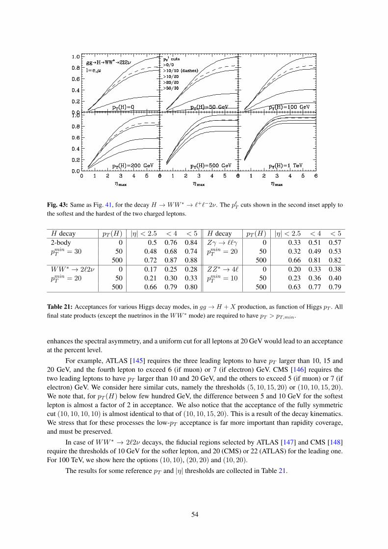
Fig. 43: Same as Fig. 41, for the decay H → WW ∗ → `+`−2ν. The p`T cuts shown in the second inset apply tothe softest and the hardest of the two charged leptons.

H decay pT (H) |η| < 2.5 < 4 < 5 H decay pT (H) |η| < 2.5 < 4 < 5

2-body 0 0.5 0.76 0.84 Zγ → ``γ 0 0.33 0.51 0.57pminT = 30 50 0.48 0.68 0.74 pminT = 20 50 0.32 0.49 0.53

500 0.72 0.87 0.88 500 0.66 0.81 0.82WW ∗ → 2`2ν 0 0.17 0.25 0.28 ZZ∗ → 4` 0 0.20 0.33 0.38pminT = 20 50 0.21 0.30 0.33 pminT = 10 50 0.23 0.36 0.40

500 0.66 0.79 0.80 500 0.63 0.77 0.79

Table 21: Acceptances for various Higgs decay modes, in gg → H +X production, as function of Higgs pT . Allfinal state products (except the nuetrinos in the WW ∗ mode) are required to have pT > pT,min.

enhances the spectral asymmetry, and a uniform cut for all leptons at 20 GeV would lead to an acceptanceat the percent level.

For example, ATLAS [145] requires the three leading leptons to have pT larger than 10, 15 and20 GeV, and the fourth lepton to exceed 6 (if muon) or 7 (if electron) GeV. CMS [146] requires thetwo leading leptons to have pT larger than 10 and 20 GeV, and the others to exceed 5 (if muon) or 7 (ifelectron) GeV. We consider here similar cuts, namely the thresholds (5, 10, 15, 20) or (10, 10, 15, 20).We note that, for pT (H) below few hundred GeV, the difference between 5 and 10 GeV for the softestlepton is almost a factor of 2 in acceptance. We also notice that the acceptance of the fully symmetriccut (10, 10, 10, 10) is almost identical to that of (10, 10, 15, 20). This is a result of the decay kinematics.We stress that for these processes the low-pT acceptance is far more important than rapidity coverage,and must be preserved.

In case of WW ∗ → 2`2ν decays, the fiducial regions selected by ATLAS [147] and CMS [148]require the thresholds of 10 GeV for the softer lepton, and 20 (CMS) or 22 (ATLAS) for the leading one.For 100 TeV, we show here the options (10, 10), (20, 20) and (10, 20).

The results for some reference pT and |η| thresholds are collected in Table 21.

54

Fig. 44: Same as Fig. 41, for the decay H → ZZ∗ → 4 charged leptons. The p`T cuts shown in the second insetapply to the softest through the hardest of the four charged leptons.

4.2 Small-BRH final states at intermediate pTWe consider here H decays with BRs in the range of 10−3−10−4, such as H → γγ, H → γZ, H → 4`and µ+µ−. At a fully inclusive level, these events are produced by the millions; a thorough analysis ofthe potential for precise measurements from these large samples requires a detailed understanding of theexperimental environment, starting from the consideration of the impact of hundreds, if not thousands,of pileup events. This is work for future studies.

We discuss here instead the possible interest to study these final states in decays of Higgs bosonsproduced with pT values of a few 100 GeV, where rates are still large, but S/B ratios are typically betterthan for the inclusive samples, and the experimental environment is possibly easier (e.g. production ismore central than for the fully inclusive Higgs sample, and the higher pT ’s can improve the reconstructionof the primary vertex and the resolution of multiple pileup events). A possible target of such studies is avery precise (percent level of better) measurement of the relative decay BRs: the production ratio betweendifferent final states will in fact remove several of the dominant systematics intrinsic in the absolute ratemeasurements, such as the integrated luminosity or the theoretical production rate uncertainty.

4.2.1 H → γγ

Figure 45 (left plot) shows the pT spectrum of diphotons from H decays (BR = 2.3× 10−3), and fromthe dominant irreducible background, namely QCD γγ production (for a discussion of pp→ γγ, see theVolume “Standard Model physics at 100 TeV” of this report). The QCD contribution is constrained byan invariant mass cut, |m(γγ)−125 GeV| < 4 GeV. This is rather conservative even by today standards,where current analyses point at resolutions in this channel of about 1-2 GeV. But the energy resolutionwill degrade at the values of photon energies considered in the regime of large pT (H), so we take 4 GeVas an indicative benchmark. The size of the background, for a reasonable range of resolution, scaleslinearly.

The background considered in this plot includes all sources (qq, qg and gg initial states), and issubject to an isolation constraint, which plays however a negligible role, since the diphoton pair at largepT at this order of perturbation theory mostly recoils against the partons. We note that the S/B ratio isof O(1) in this region, much larger than for the low pT (H) sample, where it drops well below 1/10. The

55

Fig. 45: Left: Integrated transverse momentum rates (20 ab−1) for a photon pair with mass close to the Higgsmass: signal and QCD background. Right: S/B, significance of the signal, and potential statistical accuracy of thesample.

statistical precision, in presence of this background, remains below 1% up to pT (H) ∼ 600 GeV.

4.2.2 H → µ+µ−

Figure 46 (left plot) shows the pT spectrum of dimuons from H decays (BR = 2.2 × 10−4), and fromthe leading irreducible background, namely Drell-Yan (DY) µ+µ− production, dominated by the tail ofthe Z∗/γ distribution (see e.g. the ATLAS [149] and CMS [150] analyses).

The DY contribution is constrained by an invariant mass cut, |m(γγ) − 125 GeV| < 1 GeV.This is better than the resolution of today’s LHC experiments: the signal full width at half maximumestimated by CMS for events with one central muon, for example, varies in the range 4-5 GeV [150]),but 1 GeV is consistent with the improvement in the muon pT resolution by a factor of O(5), projectedfor the 100 TeV detectors.

The DY background includes qq and qg initial states. Contrary to the γγ decay, the S/B fordimuons deteriorates at larger pT (H), but still allows for a precision in the rate measurement better than2% for pT (H) up to∼ 200 GeV. This could allow for a 1% determination of the muon Yukawa coupling,yµ, relative to the Hγγ coupling.

4.2.3 H → ZZ∗ andH → Zγ

We consider here H → ZZ∗ and H → Zγ, with leptonic decays of the Z boson to electron or muonpairs (BR = 1.3 × 10−4 and BR = 1.1 × 10−4, respectively). The rates for signals and leadingirreducible backgrounds are given in Figs. 47 and 48.

We considered for these plots the following acceptance cuts:

– H → ZZ∗ → 4`: pT (`) > 10 GeV, |η(`)| < 2.5

– H → Zγ → 2`γ: pT (`, γ) > 20 GeV, |η(`, γ)| < 2.5

We notice that, as shown in the acceptance plots of Fig. 44, at large pT (H) the cut pT (`) > 10 GeVfor all 4 leptons has an acceptance almost identical to that of the asymmetric cut 10/10/15/20 GeV. With

56

Fig. 46: Left: Integrated transverse momentum rates (20 ab−1) for a muon pair with mass close to the Higgs mass:signal and DY background. Right: S/B, significance of the signal, and potential statistical accuracy of the sample.

Fig. 47: Integrated transverse momentum rates (20 ab−1) for a four-lepton final state (` = e, µ), with mass closeto the Higgs mass: signal and QCD background.

reference to that figure, we also point out that increasing the η range and reducing the threshold for thepT of the softest lepton, would each increase the signal rate by a factor of 2.

We assume here once again 4 GeV as mass resolution for both the 3- and 4-body final states. Forthe 4-lepton final state, the S/B ratio was already larger than 1 in the 8 TeV run of the LHC; due to greaterincrease in the gluon PDF relative to the quark one, the QCD background at 100 TeV becomes negligible.A 1% determination of the rate is statistically possible for pT (H) <∼ 300 GeV. Likewise, the S/B ratiofor Zγ improves significantly as pT (H) is increased, and becomes larger than 0.5 above ∼ 300 GeV.In this region the statistical precision is better than 2%, allowing for a percent-level measurement of theHZγ coupling relative to Hγγ.

57

Fig. 48: Left: Integrated transverse momentum rates (20 ab−1) for a dimuon+photon pair system with mass closeto the Higgs mass: signal and QCD background. Right: S/B, significance of the signal, and potential statisticalaccuracy of the sample.

4.3 Associated V H productionWe consider here some examples of possible measurements of WH production, in the H → bb finalstate. As in the previous discussion, we do not attempt to optimize the detection of the fully inclu-sive sample, but examine the opportunities offered by production in kinematical configuration that areunconventional at the LHC, and where the 100 TeV collider could offer prospects for interesting newmeasurements.

We start by the case ofWH production at large invariant mass. As shown before, this is dominatedby the Born-level topologies, with the W and H recoiling against each other. The largest backgrounds tothe H → bb decay are the QCD associated production of Wbb, and the large-mass tail of the Z boson inWZ∗, with Z∗ → bb. For these kinematics, top quark production is not an important background. Theintegrated mass spectra of signal and backgrounds are shown in the left panel of Fig. 49. We model thebackground with a parton-level calculation, require the bb pair to have an invariant mass in the range of100–150 GeV, and both W and bb system are in the region |η| < 2.5. The rates include the branchingratio for the decays W → `ν (` = e, µ).

Of course the invariant mass on the bb pair provides only a very crude picture of the potential tosuppress the QCD Wbb background. The application of the standard H → bb tagging techniques [151],developed for boosts in the range of few hundred GeV, may require important adaptations and optimiza-tion in the multi-TeV regime, where the whole Higgs-jet is contained with a cone of radius smaller thanR = 0.1. In the accompanying SM Volume of this Report [6], the tagging of multi-TeV gauge bosonsfrom the decay of resonances with masses in the 5-40 TeV range is discussed. Gauge boson hadronicdecays can be tagged with efficiencies in the range of 80%, with suppression factors of order 20-100 fornormal QCD jets of comparable pT . This performance is comparable to the effectiveness of the naivembb cut we applied: the dotted line in Fig. 49 shows in fact the background level obtained by requestingthe bb pair to be contained within a jet of radius R = 1, without any mass cut. The reduction due tothe mass cut is a factor of order 10-20. The very large S/B shown in Fig. 49 shows that there is plentyof room to cope with the challenge of identifying these hyper-boosted H → bb jets and rejecting theirbackgrounds.

As a further example of possible applications, we consider the other kinematical configurations ofinterest, namely WH production in presence of a high-pT jet. For the signal, the dominant process if

58

Fig. 49: Left: Integrated invariant mass rate (20 ab−1) for aWbb pair, withW → `ν (` = e, µ) and |mbb−mH | <25 GeV: signal and QCD background. Right: S/B, significance of the signal, and potential statistical accuracy ofthe sample.

qq → gW ∗ → gWH , where the Higgs is simply radiated off the high-pT W that recoils against the jet.As shown in Section 3.4, this leads to a strong correlation between the W and H direction, resulting ina ∆R(WH) distribution peaked at small values. For the background, on the other hand, the dominantproduction dynamics is given by the process qg → q(g → bb), with the W radiated from the initial orfinal state quarks. In this case, there is no strong correlation between the bb and the W : if anything, theymuch prefer to be produced back to back.

Fig. 50: Angular correlation between the W boson and the bb pair for signal (short dashes) and QCD background(dashes) in final states with a jet of pT > 500 GeV (left) and 1 TeV (right). The solid curve denotes the sum ofsignal and QCD background. No W branching ratio is included.

This is shown very clearly in Fig. 50, which shows the ∆R(WH) distribution for the background(dashed histograms) and for the Higgs signal (short-dashed histograms), for different thresholds on thejet pT . A simple cut on ∆R(WH) < 1 leads to an order of magnitude reduction of the background,

59

while maintaining the largest fraction of the signal. This is shown in the second panel of Fig. 51, wherethe two dashed (continuous, red) lines give the background (signal) before and after the ∆R cut. Thecut brings the S/B ratio to the level of 1, with sufficient statistics to exceed the percent level precisionin the signal extraction. Further background rejection can likely be obtained by cutting on the W bosontransverse momentum, which is harder for the signal.

It is clear that more work is needed for a reliable assessment of the potential for interesting andprecise measurements using the associated V H production channels. The application and extension ofH → bb tagging and background rejection techniques will certainly also lead to valuable input to thedetector design process, both in the calorimeter and tracker areas. There is also room for the use of finalstates other than bb. We trust that these topics will be picked up for the studies towards the FCC-hhConceptual Design Report.

Fig. 51: Left panel: same as the previous Figure, with pT > 2 TeV. Right: Signal and background rates, as afunction of the jet pT threshold, before and after a ∆R(WH) < 1 cut. No W branching ratio included.

60

4.4 Measurement of top Yukawa coupling from the ttH/ttZ ratioThe ttH production process can be studied for a variety of Higgs decay channels. We collect in Table 22the event rates for potentially interesting Higgs decays combined with ttH production, for an integratedluminosity of 20 ab−1 at 100 TeV. These numbers include the branching ratio for the mixed lepton-hadrontt→ `ν`+ jets decay (` = e, µ), in addition to the relevant Higgs branching ratios.

Since analysis cuts and efficiencies will further reduce these rates, the otherwise very clean H →4` will hardly meet the target of the 1% precision. In the case of H → γγ, basic parton level cuts suchas:

pT,γ,b,j > 25 GeV , |ηγ,b,j | < 2.5 , ∆Rjj,bb,bj > 0.4

pT,` > 20 GeV , |η`| < 2.5 (20)

leave around 5 · 104 events with 20 ab−1, while the ttγγ background, subject to a |mγγ − 125| < 5 GeVcut, is almost a factor of 10 smaller. The H → 2`2ν final state has also a potentially interesting rate,which will deserve a dedicated study.

The large rate for H → bb decays allows to consider boosted topologies, placing tight cuts onthe emerging jets, and drastically reducing the various sources of backgrounds. Figure 33 shows, forexample, that requesting pT,H > 500 GeV gives a rate of O(1) pb, or 10M events with 10 ab−1. Thisimproved statistics also allows us to rely on a well-measured and similarly peaked ttZ → tt bb signal toreduce systematic and theoretical uncertainties, as anticipated in Section 3.6, and discussed in detail inRef. [133]. We summarize here these findings, and update the results of that work to a broader range ofHiggs pT . We refer to Ref. [133] for the details.

The analysis models the first HEPTOPTAGGER application to ttH production withH → bb [152],and builds on the recent improvements in the HEPTOPTAGGER2 [153] and in the BDRS Higgs tag-ger [151], which reduce background sculpting and increase the signal statistics.

We consider the final states:

pp→ ttH → (bjj) (b`ν) (bb), (b`ν) (bjj) (bb) . (21)

and the leading backgrounds:

pp→ tt bb, the main irreducible QCD backgroundpp→ ttZ, including the Z-peak in the mbb distributionpp→ tt+jets with fake-bottoms tags

The analysis requires:

1. an isolated lepton with |y`| < 2.5 and pT,` > 15 GeV.

2. a tagged top (R = 1.8, pT,j > 200 GeV, |y(t)j | < 4) without any b-tag requirement

3. a tagged Higgs jet with two b-tags inside (R = 1.2, pT,j > 200 GeV, |y(H)j | < 2.5)

4. a b-tagged jet (R = 0.6, pT,j > 30 GeV, |yb| < 2.5) outside the top and Higgs fat jets, correspond-ing to the top decaying semileptonically.

H → 4` H → γγ H → 2`2ν H → bb

2.6 · 104 4.6 · 105 2.0 · 106 1.2 · 108

Table 22: ttH event rates for various Higgs decay modes, with 20 ab−1 at 100 TeV, assuming tt→ `ν+jets. Hereand for Higgs decays, ` can be either an electron or a muon.

61

The mbb distribution provides the sidebands to control the ttbb and tt+jets backgrounds, and a sec-ond mass peak from the ttZ mass peak. All Monte Carlo event samples are generated at leading or-der, using MadGraph5 [154] with NNPDF2.3 parton densities [155], showering and hadronization viaPythia8 [156] and the fast detector simulation with Delphes3 [157, 158]. The jet clustering and theanalysis are done with FastJet3 [95], a modified BDRS Higgs tagger [151, 152] and the HEPTOPTAG-GER2 [153]. All b-tags require a parton-level b-quark within ∆R < 0.3 and assume a b-tagging efficiencyof 50% and a mis-tagging probability of 1%.

Figure 52 shows the reconstructed mbb spectrum for the signal and the backgrounds, varying thepT threshold of the top and Higgs tagged fat jets in steps of 100 GeV from 200 up to 500 GeV.

0 100 200 300 400 5000

10

20

30

40

50

60

70

310×

[GeV]recm

10 GeV1

recdmdN

3 b-tags, 200 GeV

HttZttjtt

bbtt

0 100 200 300 400 5000

5

10

15

20

25

310×

[GeV]recm

10 GeV1

recdmdN

3 b-tags, 300 GeV

HttZttjtt

bbtt

0 100 200 300 400 5000

1

2

3

4

5

6

7

310×

[GeV]recm

10 GeV1

recdmdN

3 b-tags, 400 GeV

HttZttjtt

bbtt

0 100 200 300 400 5000

0.5

1

1.5

2

2.5

310×

[GeV]recm

10 GeV1

recdmdN

3 b-tags, 500 GeV

HttZttjtt

bbtt

Fig. 52: Recontructed mbb for a pT threshold from 200 GeV to 500 GeV (the roughness of the distributions is aconsequence of limited MC statistics).

For the 200 GeV cut, and the signal region mbb ∈ [104, 136] GeV, we arrive at a signal-to-background ratio around S/B ≈ 1/3 and a Gaussian significance S/

√B = 120, assuming an integrated

luminosity of L = 20 ab−1. The error on the number of nominally NS = 44700 signal events is givenby two terms. First, we assume that we can determine NS from the total number of events NS + NB

using a perfect determination of NB from the side bands. Second, the side band mbb ∈ [160, 296] GeVwith altogether Nside = 135000 events and a relative uncertainty of 1/

√Nside introduces a statistical

uncertainty ∆NB , altogether leading to

∆NS =

[(√NS +NB

)2+ (∆NB)2

]1/2

62

=

[(√NS +NB

)2+

(NB√Nside

)2]1/2

= 0.013NS . (22)

For the Yukawa coupling this translates into a relative error of around 1%. The first term alone wouldgive ∆NS = 0.010NS .

The analysis for larger pT cuts leads to the numbers in the following table:

pT,min[GeV] NS NB NS +NB NSideband ∆NS/NS NS/NB NS/√NB

250 29400 74700 104000 155000 0.013 0.39 107300 18800 39000 57900 116000 0.014 0.48 95350 13300 27500 40800 79800 0.017 0.48 80400 8970 16700 25600 50300 0.020 0.54 69450 5950 9810 15800 35100 0.023 0.61 60500 3830 5730 9560 24400 0.027 0.67 51

For the signal region we count NS in the region with NS/NB > 1/5, for the sideband region we requireNS/NB < 1/10. The corresponding mbb distribution is binned in steps of 10 GeV. NB is the sum of allttbb, tt+ jets and ttZ events combined. We notice that the precision on the number of extracted signalevents, ∆NS/NS , remains at the level of 1-2% over a broad range transverse momenta, providing animportant validation of the robustness of the analysis.

More details, and the results of the combined Crystal Ball fit of the Z and H signals, are given inRef. [133]. The continuum side band and the second peak offer two ways to control the backgrounds aswell as the translation of the tt bb rate into a measurement of the Yukawa coupling. We therefore find thatytop could be measured to around 1% with a 100 TeV collider and an integrated luminosity of 20 ab−1.This is an order of magnitude improvement over the expected LHC reach, with significantly improvedcontrol over the critical uncertainties.

There exist additional, complementary opportunities offered by the ttH study. For example, theH → γγ decay could allow a direct measurement of the ratio of branching ratios B(H → γγ)/B(H →bb). It would serve as a complementary, although indirect, probe of the ttH coupling. Furthermore,H → 2`2ν could also be interesting, since there is enough rate to explore the regime pT,H mH ,which, especially for the e±µ∓νν final state, could be particularly clean.

4.5 Combined determination of yt and Γ(H) from ttH vs tttt productionPrecise information of Higgs boson, e.g. its mass, width, spin, parity, and couplings, should shed light onnew physics beyond the Standard Model. In this section we discuss the measurements of two importantproperties of the Higgs boson, the total width (ΓH ) and its coupling to top-quark (yHtt), through the ttHand tttt productions at a 100 TeV pp collider. The top Yukawa-coupling can be measured in the ttHproduction. An ultimate precision of about 1% is expected at a 100 TeV pp collider in the channel ofpp → ttH → ttbb with an integrated luminosity (L) of 20 ab−1, assuming the H → bb branching ratiois the same as in the SM. However, this assumption may not be valid in NP models; for example, ΓHmight differ from the SM value (ΓSM

H ) in the case that the Higgs boson decays into a pair of invisibleparticles. It is important to find a new experimental input to relax the assumption. Four top-quark (tttt)production provides a powerful tool to probe the top-quark Yukawa coupling, and in addition, combiningthe ttH and tttt productions also determines ΓH precisely [159].

Under the narrow width approximation, the production cross section of pp→ ttH → ttbb is

σ(pp→ ttH → ttbb) = σSM(pp→ ttH → ttbb)× κ2tκ

2b

ΓSMH

ΓH

≡ σSM(pp→ ttH → ttbb)× µbbttH ,(23)

63

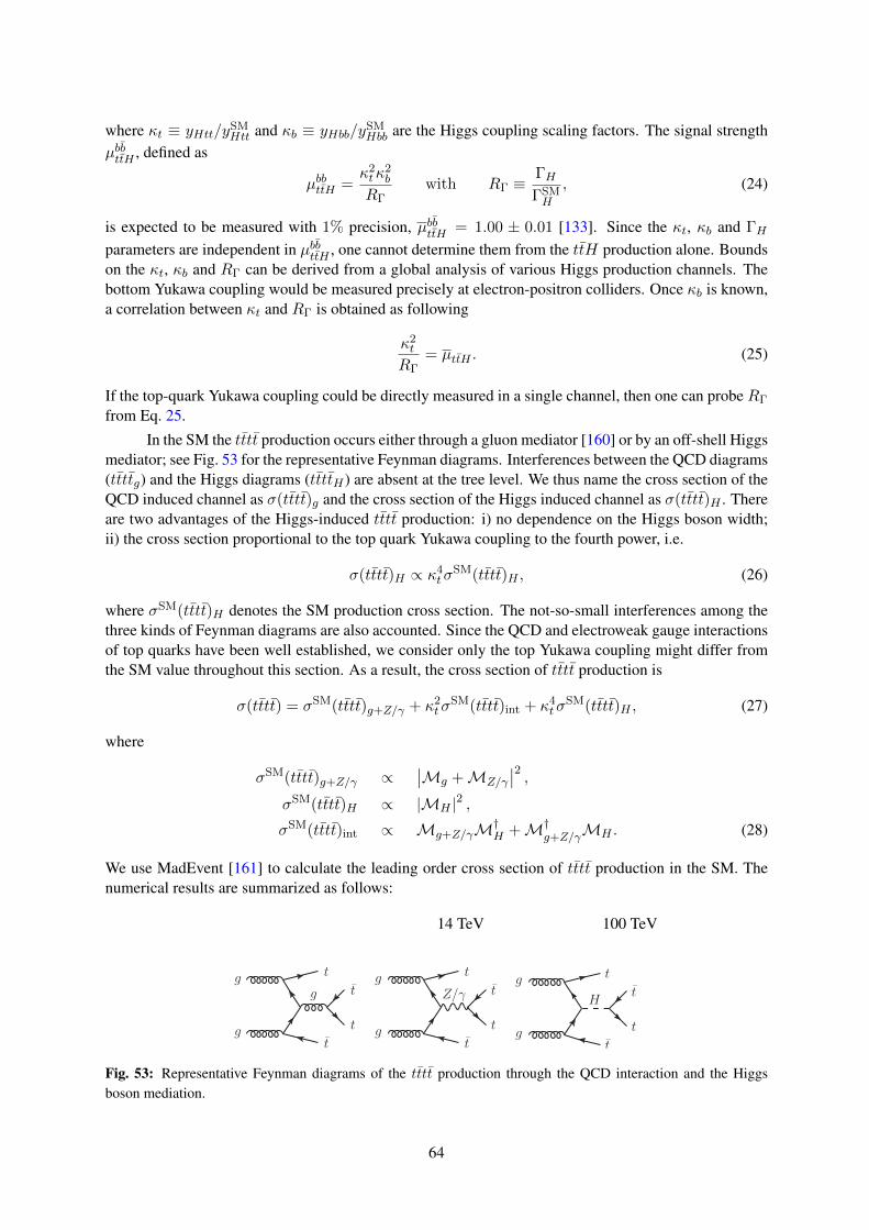
where κt ≡ yHtt/ySMHtt and κb ≡ yHbb/y

SMHbb are the Higgs coupling scaling factors. The signal strength

µbbttH , defined as

µbbttH =κ2tκ

2b

RΓwith RΓ ≡

ΓH

ΓSMH

, (24)

is expected to be measured with 1% precision, µbbttH = 1.00 ± 0.01 [133]. Since the κt, κb and ΓH

parameters are independent in µbbttH , one cannot determine them from the ttH production alone. Boundson the κt, κb and RΓ can be derived from a global analysis of various Higgs production channels. Thebottom Yukawa coupling would be measured precisely at electron-positron colliders. Once κb is known,a correlation between κt and RΓ is obtained as following

κ2t

RΓ= µttH . (25)

If the top-quark Yukawa coupling could be directly measured in a single channel, then one can probe RΓ

from Eq. 25.

In the SM the tttt production occurs either through a gluon mediator [160] or by an off-shell Higgsmediator; see Fig. 53 for the representative Feynman diagrams. Interferences between the QCD diagrams(ttttg) and the Higgs diagrams (ttttH ) are absent at the tree level. We thus name the cross section of theQCD induced channel as σ(tttt)g and the cross section of the Higgs induced channel as σ(tttt)H . Thereare two advantages of the Higgs-induced tttt production: i) no dependence on the Higgs boson width;ii) the cross section proportional to the top quark Yukawa coupling to the fourth power, i.e.

σ(tttt)H ∝ κ4tσ

SM(tttt)H , (26)

where σSM(tttt)H denotes the SM production cross section. The not-so-small interferences among thethree kinds of Feynman diagrams are also accounted. Since the QCD and electroweak gauge interactionsof top quarks have been well established, we consider only the top Yukawa coupling might differ fromthe SM value throughout this section. As a result, the cross section of tttt production is

σ(tttt) = σSM(tttt)g+Z/γ + κ2tσ

SM(tttt)int + κ4tσ

SM(tttt)H , (27)

where

σSM(tttt)g+Z/γ ∝∣∣Mg +MZ/γ

∣∣2 ,σSM(tttt)H ∝ |MH |2 ,σSM(tttt)int ∝ Mg+Z/γM†H +M†g+Z/γMH . (28)

We use MadEvent [161] to calculate the leading order cross section of tttt production in the SM. Thenumerical results are summarized as follows:

14 TeV 100 TeV

g

g

t

t

t

tgg

g

t

t

t

t

H

g

g

t

t

t

tZ/γ

Fig. 53: Representative Feynman diagrams of the tttt production through the QCD interaction and the Higgsboson mediation.

64

σSM(tttt)g+Z/γ : 12.390 fb, 3276 fb,

σSM(tttt)H : 1.477 fb, 271.3 fb,

σSM(tttt)int : −2.060 fb, −356.9 fb. (29)

The numerical results shown above are checked with CalcHEP [162]. The NLO QCD corrections to thettttg background is calculated in Ref. [163], which is about 4934 fb with 25% uncertainty. Unfortunately,as the QCD corrections to the interference and electroweak contributions is not available yet, a tree-levelsimulation of the signal process is used to estimate the accuracy of Higgs width measurement.

A special signature of the four top-quark events is the same-sign charged leptons (SSL) from thetwo same-sign top quarks. The ATLAS and CMS collaborations have extensively studied the same signlepton pair signal at the LHC [164,165]. The other two top quarks are demanded to decay hadronically inorder to maximize the production rate. Therefore, the topology of the signal event consists of two same-sign charged leptons, four b-quarks, four light-flavor quarks, and two invisible neutrinos. In practice itis challenging to identify four b-jets. Instead, we demand at least 5 jets are tagged and three of themare identified as b-jets. The two invisible neutrinos appear as a missing transverse momentum (6ET ) inthe detector. Thus, the collider signature of interests to us is two same-sign leptons, at least five jets andthree of them tagged as b-jets, and a large 6ET .

The SM backgrounds for same-sign leptons can be divided into three categories: i) prompt same-sign lepton pair from SM rare process, including di-boson and W±W±jj; ii) fake lepton, which comesfrom heavy quark jet, namely b-decays, and the dominant one is the tt + X events [166]; iii) chargemisidentification. As pointed out by the CMS collaboration [165], the background from charge mis-identification is generally much smaller and stays below the few-percent level. We thus ignore this typeof backgrounds in our simulation and focus on those non-prompt backgrounds tt + X and rare SMprocesses contributions. For four top quark production process another feature worthy being specified isthat multiple b-jets decay from top quark appear in the final state. Same-sign lepton plus multiple b-jetshas a significant discrimination with the backgrounds. From above analysis, it is clear that the majorbackgrounds are tt+X and W±W±jj. Another SM processes can contribute the same-sign lepton aredi-boson, while it can be highly suppressed by the request of multiple jets in the final state. Therefore wefocus on the tt+X , W±W±jj and tttt(g) backgrounds below. The cross section of the tt production iscalculated with the next-to-leading-order(NLO) QCD correction using MCFM package [64]. The NLOQCD corrections to the ttZ and ttW background are taken into account by multiplying the leading ordercross sections with a constant K-factor; for example, KF = 1.17 for the ttZ and KF = 2.20 for thettW production [6].

Both the signal and background events are generated at the parton level using MadEvent [161] atthe 100 TeV proton-proton collider. We use Pythia [156] to generate parton showering and hadronizationeffects. The Delphes package [157] is used to simulate detector smearing effects in accord to a fairlystandard Gaussian-type detector resolution given by δE/E = A/

√E/GeV⊕B, whereA is a sampling

term and B is a constant term. For leptons we take A = 5% and B = 0.55%, and for jets we takeA = 100% and B = 5%. We require the charged lepton has a transverse momentum p`T greater than 20GeV, rapidity |η`| ≤ 2.5 and its overlap with jets ∆Rj` =

√(∆η)2 + (∆φ)2 ≥ 0.4. The 6ET is then

defined to balance the total transverse momentum of visible objects.

Figure 54 displays the numbers of reconstructed jets (a) and b-tagged jets (b) in the signal andbackground processes. It is clear that the signal event exhibits often five or more jets. Demanding at leastthree identified b-jets would efficiently reject those SM backgrounds. In the simulation we impose a setof kinematics cuts as follows:

pj,`T ≥ 20 GeV, |ηj,`| < 2.5, 6ET ≥ 150 GeV,

N`± = 2, Njets ≥ 6, Nb−jets ≥ 3,

mT ≥ 100 GeV, HT ≥ 800 GeV. (30)

65

Number of jets0 5 10 15

Eve

nts

Num

ber

0

500

1000

tttWttZt

WWjj)γt(g+Z/ttt ×100

t(h)ttt ×1000

(a)

Number of b-jets0 2 4 6

Eve

nts

Num

ber

0

500

1000

1500

2000tt

tWt

tZt

WWjj

)γt(g+Z/ttt ×100

t(h)ttt ×1000

(b)

Fig. 54: The numbers of the reconstructed jets (a) and b-tagged jets (b) in the signal and background events atthe 100 TeV collider with an integrated luminosity of 1 fb−1. To better character the signal distribution the crosssection has been rescaled to 1000 times. No cuts except for same-sign lepton pair have been applied.

Table 23: Number of the signal and background events at the 100 TeV pp collider with an integrated luminosityof 1 ab−1. The kinematics cuts listed in each row are applied sequentially.

Basic SSL Jets 6ET mT HT

ttttH 271300 3227.1 1010.6 412.4 242.8 222.5ttttg+Z/γ 3276000 32366.9 11056.5 4193.3 2620.8 2407.9ttttint -356900 -4040.1 -1275.9 -467.5 -273.0 -253.4tt 3.22× 1010 3802170 33411 0 0 0

ttW+ 2596250 91917.4 1222.2 509.2 356.5 356.5ttW− 1810460 81234.8 1585.5 629.4 399.4 387.3ttZ 4311270 306908 3995.6 1109.9 665.9 621.5

W±W±jj 275500 39097.4 2.188 0 0 0

Here mT denotes the transverse mass of the leading charged lepton (`1) and the 6ET , defined as

mT =

√2p`1T 6ET (1− cos ∆φ), (31)

where ∆φ is the azimuthal angle between the `1 lepton and the 6ET . The mT cut is to remove thosebackgrounds involving leptonically decayed W bosons. The HT is the the scalar sum of the transversemomenta of all the visible particles and the missing energy 6ET .

Table 23 shows the numbers of the signal and the background events after a series of kinematicscuts at the 100 TeV proton-proton collider with an integrated luminosity of 1 ab−1. The tttt productionthrough the QCD interaction and the production through the Higgs boson mediator share similar kine-matics, therefore, both the QCD and Higgs mediated productions exhibit similar efficiencies for eachcut shown in Table 23; see the second and third columns. It might be possible to distinguish the twocontributions using the so-called color pull technique [167]. The major backgrounds in the SM are fromthe ttW± and ttZ productions.

After applying the cuts given in Eq. 30, the tttt production from the QCD and electroweak gaugeinteractions dominates over the SM backgrounds; see Table. 23. The tttt production in the SM can be

66

μ _

_

-

-

-

κ

Γ

Fig. 55: Relative uncertainty on the signal strength µttH projected in the plane κt and RΓ at a 100 TeV hadroncollider with 20 ab−1 for the Higgs decay modes H → bb (red band). The yellow (green, blue) vertical banddenotes the limit 0.927 ≤ κt ≤ 1.051 ( 0.952 ≤ κt ≤ 1.038, 0.962 ≤ κt ≤ 1.031 ) corresponding to the 1σ signaluncertainty with the integrated luminosity of 10 ab−1 (20 ab−1, 30 ab−1).

measured at a 5σ confidence level with an integrated luminosity of 8.95 fb−1. We thus expect the ttttproduction to be discovered soon after the operation of the 100 TeV machine. The great potential enablesus to discuss the precision of measuring the top Yukawa coupling in the tttt production. We estimate thesignal statistical fluctuation as

∆NS =√NS +NB, (32)

assuming that the events number satisfies the Gaussian distribution. The signal uncertainty is ∆NS =0.0095NS for L = 10 ab−1, ∆NS = 0.0067NS for L = 20 ab−1, and ∆NS = 0.0055NS for L =30 ab−1, respectively. We interpret the uncertainty of the signal event as the uncertainty of the topYukawa coupling, i.e.

∆NS = δκt

[2σSM(tttt)int + 4σSM(tttt)H

]× L+O(δκ2

t ), (33)

where δκt ≡ κt−1 and the SM cross sections refer to the values after all the cuts shown in the last columnin Table 23. It yields a precision of κt measurement as follows: 0.927 ≤ κt ≤ 1.051 for L = 10 ab−1,0.952 ≤ κt ≤ 1.038 for L = 20 ab−1, and 0.962 ≤ κt ≤ 1.031 for L = 30 ab−1, respectively.

Figure 55 displays the correlation between RΓ and κt imposed by the projected µbbttH measure-ment [133]; see the red band. The expectations of the κt measurement in the tttt production are alsoplotted where the yellow (green, blue) contour region denotes the uncertainty of κt with L = 10 ab−1

(20 ab−1, 30 ab−1), respectively. Combining both the ttH and tttt productions imposes a tightbound on the Higgs boson width; for example, 0.85 ΓSM

H ≤ ΓH ≤ 1.12 ΓSMH for L = 10 ab−1,

0.89 ΓSMH ≤ ΓH ≤ 1.09 ΓSM

H for for L = 20 ab−1, and 0.91 ΓSMH ≤ ΓH ≤ 1.08 ΓSM

H for L = 30 ab−1,respectively.

4.6 Rare SM Exclusive Higgs decaysThe measurement of the rare exclusive decays H → V γ, where V denotes a vector meson, would allowa unique probe of the Higgs coupling to light quarks. While the absolute value of the bottom-quark

67

h

γ

h

γ

h

γ

γ/Z

Fig. 56: Direct (left and center) and indirect (right) contributions to the H → V γ decay amplitude. The blobrepresents the non-perturbative meson wave function. The crossed circle in the third diagram denotes the off-shellH → γγ∗ and H → γZ∗ amplitudes, which in the SM arise first at one-loop order.

Yukawa coupling can be accessed by measuring b-tagged jets in the associated production of the Higgsboson with a W or Z boson, this method becomes progressively more difficult for the lighter-quarkcouplings. Advanced charm-tagging techniques may allow some access to the charm-quark Yukawacoupling [168], but no other way of directly measuring even lighter-quark couplings is currently known.The small branching ratios for these exclusive decays renders them inaccessible at future e+e− colliders.The program of measuring these decay modes is therefore unique to hadron-collider facilities. The largeHiggs boson production rate at a proposed 100 TeV collider makes this facility an ideal place to measurethese otherwise inaccessible quantities.

The possibility of measuring rare exclusive Higgs decays was first pointed out in [169, 170], andthe theoretical framework for their prediction was further developed in [171–173]. Our discussionfollows closely the techniques introduced in these works, and we only summarize the salient featureshere. We begin our discussion of the theoretical predictions for these modes by introducing the effectiveYukawa Lagrangian

L = −∑q

κqmq

vH qLqR −

∑q 6=q′

yqq′√2H qLq

′R + h.c. , (34)

where in the SM κq = 1 while the flavor-changing Yukawa couplings yqq′ vanish. The effective La-grangian leads to two categories of exclusive Higgs decays: flavor-conserving decays involving the κqcouplings, where V = ρ, ω, φ, J/ψ,Υ(nS), and flavor-violating decays involving the yqq′ couplings,where V = B∗0s , B

∗0d ,K

∗0, D∗0. In view of the very strong indirect bounds on flavor off-diagonal Higgscouplings to light quarks [174], the flavor-violating decays H → V γ are bound to be very stronglysuppressed. We will therefore restrict our discussion here to flavor-conserving processes.

The exclusive decaysH → V γ are mediated by two distinct mechanisms, which interfere destruc-tively.

– In the indirect process, the Higgs boson decays (primarily through loops involving heavy topquarks or weak gauge bosons) to a real photon γ and a virtual γ∗ or Z∗ boson, which then convertsinto the vector meson V . This contribution only occurs for the flavor-conserving decay modes.The effect of the off-shellness of the photon and the contribution involving theHγZ∗ coupling aresuppressed by m2

V /M2H and hence are very small [173].

– In the direct process, the Higgs boson decays into a pair of a quark and an antiquark, one of whichradiates off a photon. This mechanism introduces the dependence of the decay amplitude on theκq parameters. The formation of the vector meson out of the quark-antiquark pair involves somenon-trivial hadronic dynamics.

The relevant lowest-order Feynman diagrams contributing to the direct and indirect processes are shownin Figure 56.

68

We begin by outlining the calculation of the indirect amplitude. The virtual photon of Z bosoncouples to the vector meson through the matrix element of a local current, which can be parameterized interms of a single hadronic parameter: the vector-meson decay constant fV . This quantity can be obtaineddirectly from experimental data. In particular, the leptonic decay rate of the vector meson can be writtenas

Γ(V → l+l−) =4πQ2

V f2V

3mVα2(mV ) , (35)

where QV is the relevant combination of quark electric charges. The effective couplings Hγγ∗ andHγZ∗ vertices, which appear in the indirect amplitude, can be calculated with high accuracy in the SM.The by far dominant contributions involve loop diagrams containing heavy top quarks or W bosons. Thetwo-loop electroweak and QCD corrections to this amplitude are known, and when combined shift theleading one-loop expression by less than 1% for the measured value of the Higgs boson mass [175].However, physics beyond the SM could affect these couplings in a non-trivial way, either through modi-fications of the Htt and HW+W− couplings or by means of loops containing new heavy particles. Themeasurement of the light-quark couplings to the Higgs should therefore be considered together with theextraction of the effective Hγγ coupling. As pointed out in [173], by taking the ratio of the H → V γand H → γγ branching fractions one can remove this sensitivity to unknown new contributions to theHγγ coupling.

We now consider the theoretical prediction for the direct amplitude. This quantity cannot bedirectly related to data, unlike the indirect amplitude. Two theoretical approaches have been used to cal-culate this contribution. The hierarchy MH mV implies that the vector meson is emitted at very highenergy EV mV in the Higgs-boson rest frame. The partons making up the vector meson can thus bedescribed by energetic particles moving collinear to the direction of V . This kinematic hierarchy allowsthe QCD factorization approach [176, 177] to be utilized. Up to corrections of order (ΛQCD/MH)2 forlight mesons, and of order (mV /MH)2 for heavy vector mesons, this method can be used to express thedirect contribution to the H → V γ decay amplitude as a perturbatively calculable hard-scattering coef-ficient convoluted with the leading-twist light-cone distribution amplitude (LCDA) of the vector meson.This approach was pursued in [173], where the full next-to-leading order (NLO) QCD corrections werecalculated and large logarithms of the form [αs ln(MH/mV )]n were resummed at NLO, and in [170],where an initial LO analysis was performed. The dominant theoretical uncertainties remaining afterthis calculation are parametric uncertainties associated with the non-perturbative LCDAs of the vectormesons. Thanks to the high value µ ∼ MH of the factorization scale, however, the LCDAs are close tothe asymptotic form φV (x, µ) = 6x(1 − x) attained for µ → ∞, and hence the sensitivity to yet notwell known hadronic parameters turns out to be mild. For the heavy vector mesons V = J/ψ,Υ(nS),the quark and antiquark which form the meson are slow-moving in the V rest frame. This allows thenon-relativistic QCD framework (NRQCD) [178] to be employed to facilitate the calculation of the di-rect amplitude. This approach was pursued in [171], where the NLO corrections in the velocity v ofthe quarks in the V rest frame, the next-to-leading order corrections in αs, and the leading-logarithmicresummation of collinear logarithms were incorporated into the theoretical predictions. The dominanttheoretical uncertainties affecting the results for H → J/ψ γ and H → Υ(nS) γ after the inclusion ofthese corrections are the uncalculated O(v4) and O(αsv

2) terms in the NRQCD expansion.

Table 24 collects theoretical predictions for the various H → V γ branching fractions in the SM.The inclusion of NLO QCD corrections and resummation help to reduce the theoretical uncertainties.There is in general good agreement between the results obtained by different groups. The H → φγbranching ratio obtained in [173] is lower than that found in [170] because of an update of the φ-mesondecay constant performed in the former work. Also, in [173] the effects of ρ–ω–φ mixing are taken intoaccount. One observes that the H → V γ branching fractions are typically of order few times 10−6,which makes them very challenging to observe. The most striking feature of the results shown in thetable concerns the H → Υ(nS) γ modes, whose branching fractions are very strongly suppressed. Thissuppression results from an accidental and almost perfect cancellation between the direct and indirect

69

Mode Branching Fraction [10−6]Method NRQCD [171] LCDA LO [170] LCDA NLO [173]

Br(H → ρ0γ) – 19.0± 1.5 16.8± 0.8Br(H → ωγ) – 1.60± 0.17 1.48± 0.08Br(H → φγ) – 3.00± 0.13 2.31± 0.11

Br(H → J/ψ γ) 2.79 +0.16−0.15 – 2.95± 0.17

Br(H → Υ(1S) γ) (0.61 +1.74−0.61) · 10−3 – (4.61 + 1.76

− 1.23) · 10−3

Br(H → Υ(2S) γ) (2.02 +1.86−1.28) · 10−3 – (2.34 + 0.76

− 1.00) · 10−3

Br(H → Υ(3S) γ) (2.44 +1.75−1.30) · 10−3 – (2.13 + 0.76

− 1.13) · 10−3

Table 24: Theoretical predictions for the H → V γ branching ratios in the SM, obtained using differenttheoretical approaches.

amplitudes, as first pointed out in [169]. In the case of H → Υ(1S) γ the cancellation is so perfectthat the small imaginary part of the direct contribution induced by one-loop QCD corrections gives theleading contribution to the decay amplitude. The fact that this imaginary part was neglected in [171]explains why a too small branching fraction for this mode was obtained there.

4.6.1 Experimental prospectsThe considered rare exclusive Higgs boson decays to a quarkonium and a photon, are – currently – theonly available means to probe the quark Yukawa coupling in the first and second generation. The onlyexception being, as pointed out earlier, the possibility to implement advanced charm-tagging techniques,specifically to probe the charm-quark Yukawa coupling. As a result, these Higgs boson decays areparticulary interesting from an experimental perspective, both as signatures unique to the hadron colliderprogramme and as experimental topologies. Furthermore, similar rare and exclusive decays of the W±

and Z bosons have also attracted interest [172, 179, 180], offering a physics programme in precisionquantum chromodynamics (QCD), electroweak physics, and physics beyond the SM.

Using 20.3 fb−1 of 8 TeV proton-proton collision data, the ATLAS Collaboration has performeda search for Higgs and Z boson decays to J/ψ γ and Υ(nS) γ (n = 1, 2, 3) [181]. No significantexcess has been observed and 95% confidence level upper limits were placed on the respective branchingratios. In the J/ψ γ final state the limits are 1.5 × 10−3 and 2.6 × 10−6 for the Higgs and Z bosondecays, respectively, while in the Υ(1S, 2S, 3S) γ final states the limits are (1.3, 1.9, 1.3) × 10−3 and(3.4, 6.5, 5.4) × 10−6, respectively. The CMS Collaboration has placed a 95% C.L. upper limit of1.5 × 10−3 on the h → J/ψ γ branching ratio [182]. In all cases, the SM production rate for theobserved Higgs boson is assumed. Currently, no other direct experimental constraint on these decays isavailable.

The scope of these early experimental investigations is two-fold: On one hand to provide the firstdirect experimental constraints on these quantities, and on the other hand to map the experimental chal-lenges involved in such searches. Looking to the future, the ATLAS Collaboration estimated the expectedsensitivity for Higgs and Z boson decays to a J/ψ and a photon, assuming up to 3000 fb−1 of data col-lected with the ATLAS detector at the centre-of-mass energy of 14 TeV, during the operation of the HighLuminosity LHC (HL-LHC). The expected sensitivity for the h→ J/ψ γ branching ratio, assuming 300and 3000 fb−1 at 14 TeV, is 153 × 10−6 and 44 × 10−6, respectively [183]. The corresponding sensi-tivities for the Z → J/ψ γ branching ratios are 7 × 10−7 and 4.4 × 10−7, respectively [183]. In thisanalysis, the same overall detector performance as in LHC Run 1 is assumed, while an analysis optimi-sation has been performed and a multivariate discriminant using the same kinematic information as thepublished analysis [181] has been introduced. The main limiting factor in reaching SM sensitivity wasidentified to be the number of expected signal events, where only about 3 events were expected following

70

h [GeV]

TTransverse Momentum, p

0 10 20 30 40 50 60 70 80 90 100

Arb

itrar

y U

nits

0

0.01

0.02

0.03

0.04

0.05 = 14 TeVsγ-K+ K→ γφ →h

KaonT

Leading p Kaon

TSub-leading pPhoton

Fig. 57: Transverse momentum distribution of decay products in h→ φγ → K+K−γ decays [184].

the complete event selection for the complete HL-LHC. Moreover, as the search sensitivity approachesthe SM expectation for the h → J/ψ γ branching ratio, the contribution from h → µµγ decays, with anon-resonant dimuon pair, needs to be included. These can be separated efficiently from the h→ J/ψ γsignal, using dimuon mass information.

Moving to the lighter quarks, the Higgs boson coupling to the strange-quark can be probed throughthe h → φγ decay. The subsequent φ → K+K− decay features a large branching ratio of about 49%and gives access to a simple final state of a hard photon recoiling against two collimated high transversemomentum tracks, as can be seen in Fig. 57. With the SM branching ratio prediction presented inTable 24, about 6.5 events are expected to be produced with 100 fb−1 at 14 TeV. For the first generationquarks, the h → ωγ and h → ργ are being considered, followed by the ω → π+π−π0 and ρ →π+π− decays, both with large branching ratios of about 89% and 100%, respectively. The correspondingexpected number of events, assuming the SM branching ratios for these decays, are about 7.6 and 96,respectively. The experimental acceptance for these decays, assuming reasonable geometrical acceptanceand transverse momentum requirements, is expected to range between 40 and 70% [184]. It is noted thatthe search for ωγ and ργ final states is further complicated due to the large natural width of the ρ mesonand the ω-ρ interference.

These rare decays to a vector meson and a photon feature very interesting and experimentallychallenging boosted topologies. The signature is distinct, but the QCD backgrounds require carefulconsideration. A primary challenge arises from the trigger availability to collect the required datasets. Inthe considered cases, the decay signature is a photon of large transverse momentum that is isolated fromhadronic activity, recoiling against a narrow hadronic jet. It is important to consider such signatures,early on in designing the trigger system. Fast track finding and reconstruction in the inner detector,available at an early stage in the trigger could help suppress backgrounds.

At the FCC-hh environment, the large production cross-section for the signal and the large ex-pected integrated luminosity alleviates the main issue confronted by the studies at the LHC and theHL-LHC, namely the small expected yields. With 20 ab−1 at the centre-of-mass energy of 100 TeV, afactor 100 increase in the produced Higgs boson, with respect to HL-LHC, is expected. This substantialincrease in the signal yield, will also allow for more effective event categorisation to further suppress thebackgrounds. Production based signatures, like the vector-boson-fusion or production in association witha leptonically decayingW or Z boson will be exploited. Furthermore, enhancement in the sensitivity can

71

be expected by exploiting the boosted regime, where the Higgs boson is produced with substantial trans-verse momentum. Early studies on this have been performed at the LHC [181], and careful evaluation ofthe potential at 100 TeV is needed.

72

5 Multi-Higgs productionIn the previous sections we focused on processes involving the production of a single Higgs boson,which allow one to test with high accuracy the linear Higgs interactions, most noticeably those involvinggauge bosons and third-generation SM fermions. These processes, however, cannot be used to directlyprobe interactions containing two or more Higgs fields, whose determination is of primary importancefor analyzing the Higgs potential. Non-linear Higgs vertices can be accessed by looking at channels inwhich multiple Higgs bosons are produced either alone or in association with additional objects. In thissection we will consider these channels with the aim of understanding the precision with which the Higgspotential could be determined at a future 100 TeV hadron collider.

5.1 Parametrizing the Higgs interactionsAs we already mentioned, the main aim of the analyses that we will present in this section is to estimatethe precision with which the Higgs potential can be probed through the exploitation of multi-Higgsproduction processes. It is thus useful to parametrize the relevant Higgs self-interactions in a generalform. In the language of an effective field theory, we can write the Higgs self-interaction Lagrangian as

L = −1

2m2hh

2 − λ3m2h

2vh3 − λ4

m2h

8v2h4 , (36)

where v = 246 GeV denotes the Higgs vacuum expectation value. The SM Lagrangian is obtained bysetting λ3 = λ4 = 1; in this case the terms in Eq. (36) provide the whole Higgs potential. On thecontrary, in BSM scenarios, higher-order operators are in general also present, as for instance contactinteractions involving higher-powers of the Higgs field or additional derivatives.

The use of the parametrization in Eq. (36) can be fully justified in an effective-field-theory frame-work in which an expansion in powers of the momenta is valid. Namely, we assume that each additionalderivative in the effective Lagrangian is accompanied by a factor 1/m∗, where m∗ is a mass scale thatbroadly characterize a possible new-physics dynamics. In this way the contribution of higher-derivativeterms to low-energy observables is suppressed by additional powers of E2/m2

∗, guaranteeing that theeffective theory is valid for energy scales E m∗. For most of the processes we are going to considerthe kinematic distributions are peaked mostly at threshold. Hence an analysis focusing on the total crosssection can be interpreted in the effective-field-theory context provided that the new physics is at the TeVscale or beyond (m∗ & 1 TeV).1 It is important to stress that the parametrization in Eq. (36) does notrely on any expansion in powers of the Higgs field. Operators involving more than four powers of h arein fact irrelevant for the processes we are considering and can be safely neglected.

In the case in which, in addition to the derivative expansion, we can also rely on an expansion inpowers of the Higgs field, the most relevant new-physics effects can be described in terms of dimension-6operators [185–187]. If the Higgs is part of an SU(2)L doubletH , only two effective operator contributeto the modification of the Higgs self-interactions, namely2

∆L6 ⊃cH2v2

∂µ(H†H)∂µ(H†H)− c6

v2

m2h

2v2(H†H)3 , (37)

where H denotes the Higgs doublet. These operators induce corrections to the trilinear and quadrilinearHiggs interactions, whose size is given by

λ3 = 1− 3

2cH + c6 , λ4 = 1− 25

3cH + 6 c6 . (38)

1Possible issues with the effective description can instead arise in analyses focused on the high-energy tails of the invariantmass distributions.

2We neglect a third operator OT = (H†←→D µH)(H†

←→D µH), since it breaks the custodial symmetry and is constrained by

the EW precision measurements to have a very small coefficient.

73

It is important to stress that the operator OH modifies several observables that can be also testedin single-Higgs processes. For instance, it induces an overall rescaling of the linear couplings of theHiggs field to the SM gauge bosons and to the fermions. The present LHC data already constrain thesecorrections not to exceed the ∼ 10% level. Moreover future lepton colliders could test these effectswith very high accuracy, reaching a precision of the order of a few percent [188]. The operator O6,on the other hand, modifies only the Higgs self-interactions, and it can thus be tested directly only incollider processes involving multiple Higgs production. Notice that, if the relevant new-physics effectsare entirely due to O6, the deviations in the trilinear and quadrilinear Higgs couplings are correlated.

Analogously to the parametrization of the Higgs potential, possible deviations in the Higgs cou-plings to the gauge bosons can be parametrized by

L =

(m2WWµW

µ +m2Z

2ZµZ

µ

)(1 + 2cV

h

v+ c2V

h2

v2

). (39)

These interactions are relevant for interpreting double Higgs production in the VBF channel. The SMLagrangian is recovered for cV = c2V = 1.

5.1.1 Estimate of the size of new-physics correctionsAs we already mentioned, the measurement of multi-Higgs production processes can provide a signifi-cant test of the validity of the SM. It is however also important to assess its impact in context of BSMscenarios. In this case, multi-Higgs processes can be used to discover new-physics effects or, in the caseof a good agreement with the SM prediction, can be translated into exclusions on the parameter spaceof BSM models. Obviously the impact on the various BSM scenarios crucially depends on the size ofthe expected deviations in the Higgs potential and in the other Higgs couplings and on the possibility ofdisentangling these effects from other possible corrections due to the presence of new resonances. In thefollowing we will provide some estimates of these effects in a few motivated BSM contexts. 3

As a preliminary observation, notice that in BSM scenarios multiple Higgs production can bemodified in different ways. A first obvious effect comes from non-standard Higgs interactions, that ismodified couplings already present in the SM or new (non-renormalizable) interactions. 4 An additionaleffect can arise from the presence of new resonances, which can contribute through tree-level or loopdiagrams. In particular, if the new-physics is light, multi-Higgs production can receive resonant contri-butions from the on-shell production of one or more resonances which afterwards decay into multi-Higgsfinal states. Obviously, in the latter case a different search strategy must be employed to study the di-rect production of new states, either through multi-Higgs production channels or in related processes.Searches for resonant double-Higgs production have already been performed at the LHC [191–193].

If the new physics is relatively heavy, it is still useful to perform a non-resonant search for multi-Higgs production using a parametrization in terms of effective Higgs couplings. Indeed, since multi-Higgs production cross sections are typically peaked not far from the kinematic threshold, a new-physicsscale m∗ & 1 TeV is high enough to ensure that resonant production gives a subleading contributionto the total rates. Therefore, the impact of the new physics on the total cross section can be reliablydescribed in terms of effective operators.

Let us now discuss the expected size of the corrections to the Higgs vertices. For definitenesswe will concentrate on the effects relevant for Higgs pair production (triple Higgs production can beanalyzed along the same lines). The set of Higgs interactions relevant for the various production channels

3For additional details see Ref. [189].4For example, new multi-Higgs interactions are typically present in theories where the Higgs boson is a composite state

of new strongly-coupled dynamics. In these scenarios the non-linear Higgs dynamics implies the presence of new non-renormalizable Higgs interactions (see for instance Ref. [190]).

74

is [194, 195]

L ⊃(m2WWµW

µ +m2Z

2ZµZ

µ

)(1 + 2cV

h

v+ c2V

h2

v2

)− λ3

m2h

2vh3

− mttt

(1 + ct

h

v+ c2t

h2

2v2

)+

g2s

4π2

(cgh

v+ c2g

h2

2v2

)GaµνG

aµν , (40)

where the SM corresponds to cV = c2V = 1, ct = 1, λ3 = 1 and c2t = cg = c2g = 0. Notice that,in addition to the dependence on the Higgs trilinear interaction, Higgs pair production is influenced byseveral other vertex modifications. In particular, the gluon fusion process is also sensitive to correctionsto the Yukawa coupling of the top quark (and, in a much milder way, of the bottom quark), as well as tothe presence of new contact interactions with gluons, which could arise from loop contributions of newheavy states. In the case of Vector Boson Fusion (VBF), modified Higgs couplings to the gauge fieldsare also relevant.

In generic new-physics scenarios, corrections to all these couplings are present and can have com-parable size. Let us start by estimating these corrections in theories where the Higgs arises as a Nambu-Goldstone boson (NGB) from some new strongly-coupled dynamics. In this case the SILH power count-ing implies [186, 190]

δλ3, δcV , δc2V , δct, c2t ∼v2

f2, δcg, c2g ∼

v2

f2

λ2

g2∗, (41)

where g∗ denotes the typical coupling strength of the strong dynamics, while f is defined as f = m∗/g∗.The corrections to couplings that are forbidden by the Goldstone symmetry are suppressed if the latteris broken by a small amount. In particular, contact interactions with gluons are generated proportionalto (the square of) some weak spurion coupling λ, while corrections to the top Yukawa coupling and tothe trilinear Higgs coupling are suppressed respectively by the factors yt and m2

h/2v2 (notice that these

factors have been already included in the definition of Eq. (40)).

It is apparent from Eq. (41) that in theories respecting the SILH power counting the correctionsto the various Higgs couplings are all of comparable order. Higgs pair production is thus affected by allthese effects simultaneously. In order to disentangle them and extract the Higgs self-interactions one thusneeds to use additional measurements (as for instance single-Higgs production channels) and to adopt amore refined analysis strategy which makes use of kinematic distributions [189].

There are however other new-physics scenarios where the corrections to the Higgs self-couplingscan be enhanced and become larger than those to the other couplings. One scenario of this kind isobtained by assuming that the Higgs is a generic composite state (not a NGB as assumed before) from anew strongly-coupled dynamics. In this case the corrections to the Higgs self-interactions are enhancedby a factor 2v2g2

∗/m2h compared to the SILH case. One thus expects δλ3 ∼ g2

∗v4/f2m2

h, which can besizable even if v2/f2 1 (in which case the corrections to the linear Higgs couplings are small). Theprice to pay for this enhancement, however, is an additional tuning that is required to keep the higgs masssmall, since one would naturally expect m2

h ∼ m2∗.

Another scenario which leads to large corrections mainly to the Higgs self-couplings is obtainedby considering a new strong dynamics coupled to the SM through a Higgs portal [189]: Lint = λH†HO,where O is a composite operator and λ is the coupling strength. In this case one finds

δcV ∼ δc2V ∼ δct ∼ c2t ∼λ2

g4∗

v2

f2, δλ3 ∼

2v2λ

m2h

λ2

g4∗

v2

f2. (42)

The corrections to the Higgs trilinear self-coupling can be dominant if λ > m2h/(2v

2) ' 0.13. In thisscenario it is thus possible to obtain δλ3 ∼ 1, while keeping the corrections to the other Higgs couplingsat the few percent level.

For other possible new physics giving rise to a modified Higgs potential see also Section 6 of thisreport.

75

process σ(14 TeV) (fb) σ(100 TeV) (fb) accuracy

HH (ggf) 45.05+4.4%−6.0% ± 3.0%± 10% 1749+5.1%

−6.6% ± 2.7%± 10% NNLL matched to NNLO

HHjj (VBF) 1.94+2.3%−2.6% ± 2.3% 80.3+0.5%

−0.4% ± 1.7% NLO

HHZ 0.415+3.5%−2.7% ± 1.8% 8.23+5.9%

−4.6% ± 1.7% NNLO

HHW+ 0.269+0.33%−0.39% ± 2.1% 4.70+0.90%

−0.96% ± 1.8% NNLO

HHW− 0.198+1.2%−1.3% ± 2.7% 3.30+3.5%

−4.3% ± 1.9% NNLO

HHtt 0.949+1.7%−4.5% ± 3.1% 82.1+7.9%

−7.4% ± 1.6% NLO

HHtj 0.0364+4.2%−1.8% ± 4.7% 4.44+2.2%

−2.6% ± 2.4% NLO

HHH 0.0892+14.8%−13.6% ± 3.2% 4.82+12.3%

−11.9% ± 1.8% NLO

Table 25: Cross sections for production of two or three SM Higgs bosons, including associated production chan-nels, at a 14 TeV and 100 TeV hadron collider [29]. The cross sections are computed by choosing µ = Mhh/2

(µ = Mhhh/2 in the case of triple production). The error intervals correspond to scale variation and PDF + αsuncertainty. In HH production in the gluon-fusion channel a conservative 10% uncertainty is included to take intoaccount the effects of the infinite top-mass approximation (see Section 5.2.1).

10-3

10-2

10-1

100

101

102

103

104

8 13 14 25 33 50 75 100

σ NLO

[fb]

√s[TeV]

HH production at pp colliders at NLO in QCD

MH=125 GeV, MSTW2008 NLO pdf (68%cl)

pp→HH (EFT loop-improved)

pp→HHjj (VBF)

pp→ttHH pp→WHH

pp→tjHH

pp→ZHH

MadGraph5_aMC@NLO

Fig. 58: Cross sections as a function of the collider COM energy. From ref. [196].

5.1.2 Production cross sections and summary of resultsTo conclude this introduction, we present an overview of the various multi-Higgs production channelsand we quickly summarize the results of the analyses that will be presented in details in the followingsubsections.

Table 25, extracted from the results of Ref. [29], reports the rates for SM Higgs pair and tripleproduction, including channels of associated production with jets, gauge bosons and top quarks. Thedependence of the production rates on the center-of-mass (COM) energy of the collider is shown inFig. 58. As for single-Higgs production, the dominant channel for Higgs pair production is gluon fusion,with a rate of 1750 fb, which constitutes more than 90% of the total production rate. With respect to the14 TeV LHC, the gluon-fusion rate is enhanced by a factor ∼ 40. The second more significant channelis pair production in association with a top pair, whose cross section is 82 fb, closely followed by VBFwith a rate of 80 fb. Notice that the relative importance of these two channels is reversed with respect tothe 14 TeV LHC case, where VBF was about twice larger than HHtt. The remaining pair production

76

10-1

100

101

102

-4 -3 -2 -1 0 1 2 3 4

σ (N

)LO

[fb]

λ/λSM

pp→HH (EFT loop-improved)

pp→HHjj (VBF)

pp→ttHH

pp→WHH

pp→ZHHpp→tjHH

HH production at 14 TeV LHC at (N)LO in QCDMH=125 GeV, MSTW2008 (N)LO pdf (68%cl)

MadGraph5_aMC@NLO

Fig. 59: Dependence of total cross sections on the Higgs trilinear coupling at 14 TeV. From ref. [196].

process precision on σSM 68% CL interval on Higgs self-couplings

HH → bbγγ 3% λ3 ∈ [0.97, 1.03]

HH → bbbb 5% λ3 ∈ [0.9, 1.5]

HH → bb4` O(25%) λ3 ∈ [0.6, 1.4]

HH → bb`+`− O(15%) λ3 ∈ [0.8, 1.2]

HH → bb`+`−γ − −HHH → bbbbγγ O(100%) λ4 ∈ [−4,+16]

Table 26: Expected precision (at 68% CL) on the SM cross section and 68% CL interval on the Higgs trilinear andquartic self-couplings (in SM units). All the numbers are obtained for an integrated luminosity of 30 ab−1 and donot take into account possible systematic errors.

modes, in association with a gauge boson or with tj, play a secondary role, since their cross section is atmost ∼ 8 fb. Finally, triple Higgs production has a cross section around 5 fb.

As we already mentioned, the main aim of the analyses reported in this section is to determine theprecision with which the SM production rates and the Higgs self-couplings can be measured. It is thusimportant to analyze the dependence of the cross section on the Higgs self-couplings. The productionrates for the Higgs pair production channels are shown in Fig. 59 as a function of the trilinear Higgscoupling λ3. Although the plot shows the rates for the 14 TeV LHC, it is approximately valid also at100 TeV. One can see that for λ3 ∼ 1, i.e. for values close to the SM one, a significant reduction in thecross section is present in the gluon-fusion and VBF channels and, even more, in the HHtj channel.This feature decreases the signal significance for the SM case. However, it allows one to more easilydifferentiate scenarios with a modified trilinear coupling (especially if λ3 < 1), since in these cases alarge increase in the cross section is present.

In the following we will present a few analyses focused on the most important multi-Higgs pro-duction channels. Here we summarize the main results. In particular, the expected precisions on theextraction of the SM signal cross section and the Higgs self-couplings are listed in Table 26.

Due to the sizable cross section, the gluon-fusion mode lends itself to the exploitation of severalfinal states. As at the 14 TeV LHC, the bbγγ final state remains the “golden” channel, since it retainsa significant signal rate and allows one to efficiently keep the backgrounds under control. From this

77

g

g h

h

t

g

g h

h

th

Fig. 60: Diagrams contributing to the Higgs pair production process through gluon fusion (an additional diagramobtained by crossing the box one is not shown).

channel a statistical precision of the order of 1 − 2% is expected on the SM signal cross section, whilethe Higgs trilinear coupling could be determined with a precision of order 3− 4%. These numbers haveto be compared with the precision expected at a possible future high-energy lepton collider, at which theHiggs trilinear coupling is expected to be measurable with a precision∼ 16% for a COM energy∼ 1 TeVand 2 ab−1 integrated luminosity [197–199]. A better precision, of around 12%, is only achievable witha 3 TeV collider and 2 ab−1 integrated luminosity [200, 201]. Other final states, namely bbbb and finalstates containing leptons, can also lead to a measurement of the SM signal, although in these cases theexpected significance is lower than in the bbγγ channel.

Finally, the Higgs quartic self-coupling can be probed through the triple Higgs production channel.In this case the most promising final state seems to be bbbbγγ, whose cross section is however small. Thischannel could allow an order-one determination of the SM production rate and could constrain the quarticcoupling in the range λ4 ∈ [−4,+16].

5.2 Double Higgs production from gluon fusionWe start the presentation of the analyses of the various Higgs pair production channels by considering thegluon-fusion process, which, as we saw, provides the dominant contribution to the total rate. At 100 TeV,the gluon fusion cross section computed at NNLL (matched to NNLO) accuracy is 1750 fb [29]. Atpresent, this result is affected by a significant uncertainty (of the order of 10%) due to the fact that theNLO and NNLO contributions are only known in the infinite top mass limit. A discussion of the currentstatus of the computations and of the sources of uncertainties will be provided in Subsection 5.2.1.

In the SM the gluon fusion process receives contributions from two types of diagrams (see Fig. 60).The box-type diagrams, which depend on the top Yukawa couplings, and the triangle-type one, whichin addition to the top Yukawa also includes the trilinear Higgs self-interaction. In the SM a partialcancellation between these two kinds of diagrams is present, which leads to a ∼ 50% suppression of thetotal cross section. The behavior of the box and the triangle diagrams at high

√s = mhh mt,mh is

quite different however. The corresponding amplitudes scale as

A ∼αs4πy2t , A4 ∼ λ3

αs4πy2t

m2h

s

(log

m2t

s+ iπ

)2

. (43)

From these equations it is apparent that, due to the presence of the off-shell Higgs propagator, the tri-angle diagram is suppressed for high s. This implies that the Higgs trilinear coupling affects the mhh

distribution mostly at threshold, while the tail at large invariant mass is mostly determined by the boxcontribution.

The shape of the Higgs pair invariant mass distribution for the SM signal is shown in Fig. 61 [202].The central line corresponds to the choice µF = µR = Mhh/2 for the factorization and renormalizationscales, and the band illustrates the scale uncertainty, evaluated by varying independently the above scalesin the range µ0/2 ≤ µR, µF ≤ 2µ0 with the constraint 1/2 ≤ µR/µF < 2, where µ0 is the central scale.The lower panel shows the ratio with respect to the central value, and it can be seen that the scaleuncertainty is roughly constant in the whole range, being of the order of ±5%. One can see that thepeak of the distribution is at mhh ∼ 400 GeV and some suppression is present close to threshold. The

78

300 400 500 600 700 800 900

0.5

1.0

2.0

5.0

10.0

dΣ

dM

hhH

fb

GeVL

NNLO+NNLL 100 TeV

Μ0=Mhh 2 PDF4LHC15

300 400 500 600 700 800 9000.90

0.95

1.00

1.05

1.10

Mhh H GeVL

Fig. 61: The invariant mass distribution at NNLO+NNLL [202] for a 100 TeV collider, with the correspondingscale uncertainty. The lower panel shows the ratio with respect to the central prediction.

(GeV)hhm0 200 400 600 800 1000 1200

Nor

mal

ized

rate

0

0.01

0.02

0.03

0.04

0.05

(GeV)hhm0 500 1000 1500 2000 2500 3000 3500 4000

Nor

mal

ized

rate

-610

-510

-410

-310

-210

-110

Fig. 62: Comparison between the normalized mhh distributions for the SM signal. The solid and dotted linescorrespond to

√s = 14 TeV and

√s = 100 TeV respectively. The distributions have been computed at LO

retaining the full top mass dependence. The plots are taken from Ref. [189].

suppression is a consequence of the partial cancellation between the box and triangle diagrams that, aswe already mentioned, is present in the SM.

The invariant mass distribution at a 14 TeV collider is similar to the one at 100 TeV. The com-parison between the two distributions is shown in Fig. 62. The position of the peak and the thresholdbehavior is unchanged. The tail of the distribution, on the other hand, is significantly larger at a 100 TeVcollider, starting from mhh & 700 GeV. This modification of the tail, however, has only a small impacton the total production rate, which is still dominated by the peak region 300 GeV . mhh . 600 GeV.

Non-standard Higgs interactions, in particular the couplings with the top (either a modifiedYukawa or the non-renormalizable interaction hhtt) and the contact interactions with the gluons (seeEq. (40)), lead to corrections that are not suppressed at highmhh. Therefore they can significantly changethe tail of the kinematic distribution at large invariant mass. An analysis exploiting the differential mhh

79

distribution can thus be helpful to disentangle possible corrections to the various Higgs couplings [189].This kind of analysis goes however beyond the scope of the present report. Here we will analyze onlythe inclusive total signal rate and focus on scenarios in which the Higgs trilinear coupling is significantlymodified, while the corrections to the other couplings are negligible.

As already mentioned, the sizable production cross section via gluon fusion allows one to considervarious decay channels for an experimental search. In the following we will describe some preliminaryanalyses that focus on the most relevant final states with the aim of determining the precision with whichthe SM signal can be extracted. In particular the bbγγ channel will be presented in Subsection 5.2.2, thebbbb channel in Subsection 5.2.3 and finally the rare final states containing leptons in Subsection 5.2.4.

Before discussing the details of the analyses we briefly discuss in the next subsection the presentstatus of the computation of the SM Higgs pair production in gluon fusion, pointing out, in particular,the various sources of theoretical uncertainty.

5.2.1 Status of SM gluon fusion cross section computationIn the last years, a lot of effort has been devoted towards the improvement of the theoretical predictionof the SM Higgs pair production cross section via gluon fusion. Even though this loop-induced pro-cess is known in an exact way only at LO in the QCD perturbative expansion [203–205], very usefulapproximations are available for the higher-order corrections.

One main approach, exploited extensively for the calculation of the single-Higgs production crosssection, consists in working in the large top-mass approximation, in which the Higgs has a direct effectivecoupling to gluons. Within this approximation, the LO becomes a tree-level contribution, and higher-order corrections can be computed. In this way, both the NLO [206] and NNLO [207] corrections havebeen obtained, together with threshold resummation effects at NNLL accuracy [202, 208]. The QCDcorrections were found to be large, resulting in about a 50% increase from LO to NLO, and a still sizeable∼ 20% increment from NLO to NNLO at a collider center-of-mass energy of 100 TeV (corrections areeven larger for lower energies). Of course, in order to use these results, an estimate of the accuracy ofthe approximation is needed.

Two different approaches have been used to estimate the finite top-mass effects at NLO. InRefs. [209, 210] the analysis was performed through the computation of subleading terms in the 1/mt

expansion. By evaluating the deviation of the results containing powers of 1/mt from the infinite top-mass prediction, the authors estimate that the effective theory is accurate to±10% at NLO [210]. On theother hand, in Ref. [211] the exact one-loop real emission contributions were included via a reweightingtechnique, finding in this way that the NLO total cross section decreases by about 10%. The pure EFTresult reproduces well the shape of the Higgs pair invariant mass distribution obtained retaining the exactreal contributions. It is worth mentioning that this is not the case for all the distributions, and for instancethe EFT fails to reproduce the region where the Higgs pair system has a large transverse momentum.Based on the two studies described above, it is possible to estimate the current accuracy of the largetop-mass approximation to be ±10% for the total cross section.5

The final result for the SM cross section for hadron colliders with center-of-mass energy Ecm =14 TeV and Ecm = 100 TeV are listed in Table 25 together with the size of the different theoreticaluncertainty. These results are computed at NNLO+NNLL accuracy using the PDF4LHC recommenda-tion for the parton flux [136], and the values mh = 125 GeV and mt = 172.5 GeV for the Higgs andtop quark masses. The scale uncertainty at NNLO+NNLL is quite small, as it is also the case for thePDF and αS uncertainty. Therefore, theoretical uncertainties are currently driven by the use of the largetop-mass approximation. It is worth noticing that, once the exact NLO becomes available, the remaining

5Recently the complete computation of the NLO cross section including the finite-top-mass corrections has been per-formed [212]. The results are at present available only for the 14 TeV LHC and show a ∼ 10% reduction of the cross sectionwith respect to the approximate results.

80

EFT uncertainty at NNLO is expected to be at most ±5% [210].

5.2.2 TheHH → bbγγ channelIn this section we analyze the HH → bbγγ channel, which has been singled out in the literature as theprocess that can lead to the highest SM signal significance and highest precision in the measurementof the Higgs trilinear coupling. This channel has a relatively small branching ratio (BR ' 0.264% inthe SM), which somewhat limits the signal yield (in the SM the total rate for this channel at a 100 TeVpp collider is ' 4.6 fb). The presence of two photons, however, allows one to efficiently keep thebackground under control while preserving a fair fraction of the signal events.

Various studies included an analysis of this channel at future high-energy hadron colliders, focus-ing mainly on the extraction of the Higgs trilinear coupling [213–215], or performing a global analysisof the impact of the modifications of the various Higgs couplings [189]. The differences among theseanalyses stem mainly from different assumptions about the detector performance, a different treatmentof the backgrounds and the choice of benchmark integrated luminosity. In the following we will present(in a summarized form) the results of a new analysis of the HH → bbγγ final state, specifically fo-cused on the extraction of the trilinear Higgs coupling in a SM-like scenario [216]. Differently frommost of the previous ones, this new analysis is tailored specifically on a 100 TeV future hadron collider,with the primary purpose of estimating how much the achievable precision is influenced by the detectorperformance.

5.2.2.1 Simulation setup

The parton-level generation of the signal and the backgrounds is performed by usingMadGraph5_aMC@NLO (version 2.3.3) [154] and the parton density functions cteq6l1 [217]. The signalis generated at LO retaining the finite-top-mass effects and afterwards rescaled by a k-factor in orderto match the NNLL gluon-fusion SM cross section (see Table 25). The analysis includes the followingmain backgrounds: the non-resonant processes bbγγ, bbjγ (with one fake photon), bjγγ and jjγγ (re-spectively with one and two fake b-jets), 6 and the resonant processes bbh and tth. The cross sectionsfor each background process after the acceptance cuts of Table 27 are given in Table 29. The bbγγ andbjγγ samples are generated by matching up to one extra parton at the matrix-element level. 7 In the caseof bbγγ, matching accounts for the bulk of the NLO correction to the cross section, as virtual effects aresmall for this process, see Ref. [189]. The remaining backgrounds are instead generated at LO withoutmatching and rescaled by the following k-factors to take into account higher-order effects: k = 1.08 forbbjγ, k = 1.3 for tth, k = 0.87 for bbh and k = 1.43 for γγjj.

Showering and hadronization effects are included for the signal and background samples by usingthe pythia6 package [121]. The simulation of the underlying event has been found to have a minorimpact on the analysis and, therefore, has been omitted for simplicity. Detector simulation effects areincluded by using the Delphes package (version 3.3.1) [157] with a custom card that describes the FCC-hh detector parametrization. A more detailed discussion of the benchmarks used for the calorimetersperformance parametrization will be given in the next subsection.

The tagging of b-jets and photons is performed by using the Delphes flavor tagging informationthat associates each jet with a parton after showering. Events are then re-weighted according to the b-and photon-tagging probabilities. The following benchmark efficiencies are considered: The b-taggingprobabilities are chosen to be constant throughout the detector and independent of the transverse mo-menta, with values pb→b = 0.75, pc→b = 0.1 and pj→b = 0.01, for b, c and light jet tagging to b-jets

6Here j denotes a jet initiated by a gluon or a light quark u, d, s, c. For simplicity bjγγ denotes the sum of the processeswhere the b-jet is initiated by either a b quark or an anti-b quark.

7The kT -MLM matching scheme has been used with matching scale 35 GeV and matching parameter xqcut = 25 GeV.

81

Acceptance cuts Final selection

γ isolation R = 0.4(pT (had)/pT (γ) < 0.15)

γ isolation R = 0.4(pT (had)/pT (γ) < 0.15)

jets: anti-kT , parameter R = 0.4 jets: anti-kT , parameter R = 0.4

|ηb,γ,j | < 6 |ηb,γ | < 4.5

pT (b), pT (γ), pT (j) > 35 GeV pT (b1), pT (γ1) > 60 GeV

pT (b2), pT (γ2) > 35 GeV

mbb ∈ [60, 200] GeV mbb ∈ [100, 150] GeV

mγγ ∈ [100, 150] GeV |mγγ −mh| < 2.0, 2.5, 4.5 GeV

pT (bb), pT (γγ) > 100 GeV

∆R(bb),∆R(γγ) < 3.5

no isolated leptons with pT > 25 GeV

Table 27: List of cuts at the acceptance level (left column) and final cuts (right column) used for the analysis. Thefinal cuts are optimized to increase the precision on the trilinear Higgs self-coupling. The three values listed for thefinal cuts on the mγγ invariant mass are used in the “low”, “medium” and “high” detector performance scenarios.

respectively. The light-jet-to-photon mis-tagging probability is parametrized via the function

pj→γ = α exp(−pT,j/β) , (44)

where α and β are parameters whose benchmark values are set to α = 0.01 and β = 30 GeV. Photonsare assumed to be reconstructed with an efficiency that depends on η, namely

95% for |η| ≤ 1.5

90% for 1.5 < |η| ≤ 4

80% for 4 < |η| ≤ 6

, (45)

provided that they have a transverse momentum pT (γ) > 10 GeV.

5.2.2.2 Benchmark scenarios for the detector performance

In the analysis three benchmark scenarios for the detector performance are considered, denoted in the fol-lowing as “Low”, “Medium” and “High” performance scenarios. These three benchmarks are simulatedthrough Delphes by implementing different choices for the energy resolution in the electromagnetic andhadronic calorimeters cells. For this purpose the variance of the energy distribution in a single cell isparametrized by the following formula

∆E =√a2E2 + b2E , (46)

where E is measured in GeV and the values of the a and b parameters are listed in Table 28. The energyoutput is then assumed to follow a log-normal distribution, namely the logE variable follows a Gaussiandistribution. The advantage of this distribution lies in the fact that it tends asymptotically to the usualnormal distribution for large E and provides only positive values for the energy. For a more detaileddiscussion about the setup used for the Delphes simulation we refer the reader to Ref. [216].

82

ECAL HCAL|η| ≤ 4 4 < |η| ≤ 6 |η| ≤ 4 4 < |η| ≤ 6

a b a b a b a b

Low 0.02 0.2 0.01 0.1 0.05 1.0 0.05 1.0

Medium 0.01 0.1 0.01 0.1 0.03 0.5 0.05 1.0

High 0.007 0.06 0.01 0.1 0.01 0.3 0.03 0.5

Table 28: Parameters defining the energy resolution in the electromagnetic (ECAL) and hadronic (HCAL)calorimeter cells for the “Low”, “Medium” and “High” detector performance benchmarks.

[GeV]γγm

110 115 120 125 130 135 140

Nor

mal

ized

rat

e/0.

5GeV

0

0.02

0.04

0.06

0.08

0.1

0.12

0.14

0.16

0.18

CAL Resolution=High

CAL Resolution=Med

CAL Resolution=Low

[GeV]bbm

0 20 40 60 80 100 120 140 160 180 200

Nor

mal

ized

rat

e/5G

eV

0

0.01

0.02

0.03

0.04

0.05

0.06

0.07 CAL Resolution=High

CAL Resolution=Med

CAL Resolution=Low

Fig. 63: Distribution of the reconstructed invariant mass of the photon pair (left panel) and bottom pair (rightpanel) for the signal. The plots show how the distributions vary in the “Low” (red curve), “Medium” (blue curve)and “High” (black curve) detector performance benchmarks.

As it will be discussed later on, the detector performance can have a significant impact on theanalysis and on the achievable precision in the measurements of the signal cross section and Higgs self-couplings. The finite energy resolution of the calorimeter induces a smearing in the reconstruction ofthe photon- and bottom-pair invariant masses, which are crucial observables for differentiating signaland background events. The distributions of the reconstructed invariant masses mγγ and mbb are shownin Fig. 63, for the three detector performance benchmarks. One can see that the impact on the photoninvariant mass can be sizable. In the “Low” performance benchmark the width of the distribution is∆mγγ ' 3 GeV, while it decreases to' 2 GeV and' 1.5 GeV in the “Medium” and “High” benchmarksrespectively. This means that a cut on the mγγ invariant mass can be twice more effective in the “High”benchmark than in the “Low” one in reducing backgrounds containing non-resonant photons (as forinstance the non-resonant bbγγ background).

The reconstruction of the bottom pair invariant mass mbb is instead only marginally affected bythe calorimeters energy resolution, as can be seen from the right panel of Fig. 63. In all cases thedistribution is peaked at the Higgs mass and at half-height it is contained in the region∼ [100, 145] GeV.The reconstruction of the mbb invariant mass, on the other hand, is highly affected in the presence of astrong magnetic field in the detector. In order to be able to bend very energetic charge particles, indeed,a very intense magnetic field is needed. As a benchmark value, B = 6 T has been chosen in the analysis.The problem with such a magnetic field is the fact that low-energy charged particles (with a transverse

83

[GeV]bbm

0 20 40 60 80 100 120 140 160 180 200

Nor

mal

ized

rat

e/5G

eV

0

0.01

0.02

0.03

0.04

0.05

0.06

0.07

0.08

0.09B=6T, JES=1.135

B=6T, JES=1.0

B=0T, JES=1.0

Fig. 64: Distribution of the reconstructed bottom pair invariant mass for different values of the detector magneticfield B and of the JES correction. The red curve corresponds to the case with no magnetic field B = 0 T and noJES correction rJES = 1, the dot-dashed black curve corresponds to B = 6 T and rJES = 1, and the solid blackcurve corresponds to B = 6 T and rJES = 1.135.

momentum pT . 5 GeV) do not reach the electromagnetic calorimeter, so that it is difficult to reconstructtheir energy. This effect can be significant in processes that happen dominantly at “low-energy”, as inthe case of double Higgs production where the bulk of the cross section comes from the threshold region.Figure 64 shows that a strong magnetic field can distort thembb distribution and shift its peak (by roughly5 GeV forB = 6 T). Such shift, together with the energy loss in the reconstruction of the bmomenta, canbe partially compensated by a rescaling of the jet energy scale (JES).8 As shown in the figure, a rescalingof the jets’ four-momentum by a factor rJES = 1.135 is sufficient to shift back the distribution and moveits peak to the value mbb ' mh.

5.2.2.3 Analysis strategy

As discussed in the introduction, the main aim of the analysis described here is to determine the achiev-able precision on the SM signal cross section and on the Higgs trilinear coupling. For this purpose asimple cut-and-count strategy focused on the inclusive event rate can be used. More sophisticated anal-ysis strategies, as for instance an exclusive one that also takes into account the differential distributions,could be useful in disentangling different new-physics effects (see for instance Ref. [189]).

In optimizing the selection cuts two different strategies can in principle be used: one can eithermaximize the precision on the SM signal or that on the Higgs trilinear coupling. The two procedures leadto significantly different sets of cuts. The effect of a change in the Higgs self-coupling mostly affectsthe threshold behavior, thus “looser” cuts aimed at preserving a large fraction of the threshold eventsimprove the precision on λ3. On the other hand, the threshold region is also the one that has a largerbackground, hence harder cuts might be convenient to improve the precision on the SM signal rate.

For the analysis presented here, cuts have been optimized to maximize the precision on λ3. Thischoice is motivated by the fact that the SM signal significance is always quite high, and optimizing forthe extraction of the Higgs trilinear coupling does not degrade significantly the precision on the signal

8Actual experimental analyses adopt more sophisticated jet calibration procedures and particle flow techniques are usuallyused to cope with these effects. The simple rescaling applied in the analysis discussed here should be thus considered as arough approximation of a more accurate experimental procedure.

84

Process Acceptance cuts [fb] Final selection [fb] Events (L = 30 ab−1)

h(bb)h(γγ) (SM) 0.73 0.40 12061

bbjγ 132 0.467 13996

jjγγ 30.1 0.164 4909

tth(γγ) 1.85 0.163 4883

bbγγ 47.6 0.098 2947

bbh(γγ) 0.098 7.6× 10−3 227

bjγγ 3.14 5.2× 10−3 155

Total background 212 1.30 27118

Table 29: Cross section for SM signal and main backgrounds after the acceptance and final cuts of Table 27. Thelast column shows the number of signal and background events after the final cuts for an integrated luminosity of30 ab−1.

cross section. In fact, the sensitivity to the signal cross section depends mildly on the choice of the cuts(provided they do not vary dramatically). On the contrary, the precision on the Higgs trilinear is muchmore sensitive to variations of the cuts.

The set of benchmark cuts are listed in Table 27. Mild pT cuts are imposed on the photons andb-quarks, namely pT (b1), pT (γ1) > 60 GeV and pT (b2), pT (γ2) > 35 GeV, where b1,2, γ1,2 denote thehardest/softest b-quark and photon. Stronger cuts are imposed on the transverse momentum of the photonand b pair, pT (bb), pT (γγ) > 100 GeV. All the reconstructed objects are required to be within a rapidity|ηb,γ | < 4.5, while the separation between the two photons and the two b-quarks is required to be not toolarge, namely ∆R(bb),∆R(γγ) < 3.5. Notice that the angular cuts imposed on ∆R are milder than theones typically used in the previous literature [189,213–215]. The invariant mass of the b pair is requiredto be in the window mbb ∈ [100, 150] GeV. For the invariant mass of the photon pair, three differentwindows are used optimized for each detector performance scenario: |mγγ −mh| < 2.0, 2.5, 4.5 GeVfor the “High”, “Medium” and “Low” performance benchmarks respectively. As discussed in Subsec-tion 5.2.2.2, these choices of invariant mass windows allow one to retain a sufficiently large fraction ofthe signal events.

The signal and background cross sections after the acceptance and final selection cuts are given inTable 29. One can see that the most significant background after all cuts is bbjγ, followed by jjγγ andtth. Another non-negligible contribution comes from the irreducible process bbγγ. The backgroundsbbh and bjγγ turn out to be negligible instead.

Notice that other double Higgs production channels, in particular ttHH and VBF, provide an ad-ditional contribution to the signal of the order of 10%. Given the high precision on the SM signal rate andon the Higgs trilinear coupling, these contributions should be taken into account in a full experimentalanalysis. However, the inclusion of these effects is not expected to change significantly the estimatedprecision on the Higgs trilinear coupling presented in the following.

5.2.2.4 Results

The results in Table 29 suggest that, with an integrated luminosity of L = 30 ab−1, a precision on the SMsignal of the order of 1.6% can be obtained, corresponding to S/

√S +B ' 61. By a simple rescaling,

one can see that already with L = 500 fb−1 a 13% determination of the cross section is possible. Noticethat these results, as well as those presented in the following, include only the statistical uncertaintiesand are obtained by neglecting the theoretical error on the prediction of the signal and the systematicuncertainty on the overall determination of the background rates. Anticipating the size of these effects

85

1 2 3 4 5 6 7

∆mγγ [GeV]

0.025

0.030

0.035

0.040

0.045

0.050

∆λ

precision on λ vs. diphoton mass window: mγγ=mH ±∆mγγ (L = 30.0 ab−1 )

detector parametrization:

Low

Med

High

1 2 3 4 5 6

|ηmax|

0.030

0.035

0.040

0.045

∆λ

precision on λ vs. coverage |ηmax| for "Med" parametrization (L = 30.0 ab−1 )

photons

b-jets

Fig. 65: Estimated precision on the measurement of the Higgs trilinear self-coupling. The left panel shows to resultas a function of the cut on the invariant mass os the photon pair ∆mγγ for the three detector benchmark scenarios,“Low” (dot-dashed red), “Medium” (dashed green) and “High” (solid black). In the right panel the result is shownas a function of the cut on the maximal rapidity of the reconstructed objects ηmax assuming the “Medium” detectorbenchmark (the solid red and dashed green curves correspond to a variation of the photon and b-jets acceptancesrespectively). All the results have been obtained for an integrated luminosity of 30 ab−1.

for a future 100 TeV collider is a difficult task. An estimate of the impact of some of the possiblesystematic errors and of the geometry and performances of the detector is provided in the following.

As illustrated by the left panel of Fig. 65, a maximal precision on the Higgs trilinear couplingof the order of 3.4% can be obtained in the “Medium” detector performance benchmark. The figureshows that this value crucially depends on the size of the photon invariant mass window used to selectthe events. If the size of the window is modified, the precision on the Higgs trilinear can be substantiallydegraded (especially for smaller sizes of the window, which reduce the amount of reconstructed signalevents). In the “Low” and “High” scenarios a precision of respectively 4.1% and 3.2% seems to beachievable.

Let us now discuss how the precision changes by varying the most important parameters related tothe detector geometry and performances, namely the η coverage, the b-tagging efficiencies and the photonmis-tagging rate. For this purpose the “Medium” performance scenario will be taken as a reference andeach parameter varied separately.

The precision on λ3 is shown in the right panel of Fig. 65 as a function of the maximal rapiditycoverage ηmax for photons and b-jets. One can see that extending the coverage beyond |ηmax| ∼ 3.5 doesnot lead to any substantial improvement. In other words, having a larger coverage in rapidity does notseem a crucial feature for the extraction of the Higgs self coupling, and a reach up to |ηmax| = 2.5 − 3could be considered to be an acceptable compromise.

A more crucial role is instead played by the b-tagging efficiencies and rejection rates, as shownin Fig. 66. The reconstruction efficiency for the b-jets is the most important parameter, since it directlycontrols the signal reconstruction rate. A minimal efficiency pb→b ' 0.75 is necessary to achieve a goodprecision on the Higgs trilinear coupling. A value pb→b ' 0.6 already degrades the achievable precisionto ' 4.0%. The mistag rates for charm-jets pc→b plays a marginal role and does not affect too much theprecision on λ3 as long as pc→b . 0.2. The impact of the light-quark and gluon jets mistag rate pj→bis even milder and does not influence the result as long as pj→b . 0.05. Finally, the lower right panelof Fig. 66 shows how the precision on λ3 changes when the mistag rate of fake photons from jets ismodified. The curve is obtained by varying the overall coefficient α in Eq. (44) (values on the horizontalaxis) and keeping fixed the functional dependence on pT,j with β = 30 GeV. One can see that high

86

0.4 0.5 0.6 0.7 0.8 0.9 1.00.02

0.03

0.04

0.05

0.06

∆λ

pb→b

0.00 0.05 0.10 0.15 0.20 0.25 0.300.028

0.030

0.032

0.034

0.036

0.038

0.040

pc→b

0.00 0.01 0.02 0.03 0.04 0.05

0.031

0.032

0.033

0.034

0.035

∆λ

pj→b

0.00 0.01 0.02 0.03 0.04 0.050.025

0.030

0.035

0.040

0.045

0.050pj→γ

precision on λ vs. tagging rates for "Med" parametrization (L = 30.0 ab−1 )

Fig. 66: Estimated precision on the measurement of the Higgs trilinear self-coupling as a function of the b-taggingefficiency. Each plot shows how the precision changes by varying only one parameter, namely the b reconstructionefficiency pb→b (upper left), the c→ b mistag rate (upper right), the j → b mistag rate (lower left) and the j → γ

mistag rate (lower right). In the case of the j → γ mistag, on the horizontal axis we give the coefficient α of themistag function in Eq. (44). All the results have been obtained in the “Medium” detector performance scenariowith an integrated luminosity of 30 ab−1.

mistag rates (α ∼ 0.05) can significantly affect the achievable precision. This is a consequence of thefact that the main background, bbjγ, contains one fake photon from jet mis-tagging. Keeping α below0.02 is enough not to affect significantly the precision on λ3.

To conclude, we briefly comment on the possible impact of the theoretical error on the signalcross section and of the systematic uncertainties on the overall background rate. Table 30 shows howthe precision on the Higgs trilinear coupling varies as a function of the relative error on the signal crosssection, ∆S ≡ ∆σ(pp → hh)/σ(pp → hh), and of an overall rescaling of the total background bya factor rB . Notice that an actual experimental analysis will most likely extract the background ratedirectly from the data (by fitting for instance the mγγ distribution away from the Higgs peak, as donefor the diphoton channel in single-Higgs production). The rescaling factor rB should be thus consideredas a way to assess the impact of the error associated with the MonteCarlo calculation of the backgroundrate in Table 29. The actual systematic uncertainty on the background rate in an experimental analysiswill likely be much smaller, and possibly negligible. In the limit in which the systematic uncertainty(theory error + pdfs uncertainty) on the signal cross section becomes larger than its statistical error, theprecision on the Higgs trilinear measurement saturates to' 2∆S . Since the statistical error on the signalrate is expected to be small (of the order of 3 − 4%), the systematic uncertainty can easily become the

87

∆S = 0.00 ∆S = 0.01 ∆S = 0.015 ∆S = 0.02 ∆S = 0.025

rB = 0.5 2.7% 3.4% 4.1% 4.9% 5.8%

rB = 1.0 3.4% 3.9% 4.6% 5.3% 6.1%

rB = 1.5 3.9% 4.4% 5.0% 5.7% 6.4%

rB = 2.0 4.4% 4.8% 5.4% 6.0% 6.8%

rB = 3.0 5.2% 5.6% 6.0% 6.6% 7.3%

Table 30: Impact of the systematic uncertainties on the precision on the trilinear Higgs coupling. The precision onλ3 is shown for different values of the systematic uncertainty on the signal, ∆S , and of the rescaling factor for thetotal background rate rB . The “Medium” detector performance scenario and an integrated luminosity of 30 ab−1

have been assumed.

main limitation in the extraction of λ3. At present, as already discussed, the computation of the signalhas a ∼ 10% uncertainty due to the use of the infinite top mass approximation. It is highly probable thatfinite-mass computations will become available in the near future. The remaining uncertainty from scalevariation at NNLL order is still ∼ 5%, while the pdf error is ∼ 3%. Without further improvements onthese two issues, the systematic uncertainty will be the main limiting factor in the determination of λ3

and the maximal precision would be limited to δλ3/λ3 ∼ 10%.

5.2.3 TheHH → bbbb channelIn the analysis of the bbγγ final state presented in the previous subsection, a large fraction of the doubleHiggs production cross section was sacrificed in order to select a clean final state, for which the back-ground levels can be easily kept under control. In this subsection a different strategy is considered whichmakes use of the final state with the largest branching ratio, namely bbbb. The total cross section forthis final state is 580 fb at a hadronic 100 TeV collider, which is two order of magnitude larger thanthe bbγγ one. The level of backgrounds one needs to cope with, however, is much larger thus severelycomplicating the signal extraction.

One of the possible advantages of the bbbb final state is the fact that it provides a reasonablenumber of events in the tail at large invariant masses of the Higgs pair. This, in principle, allows one toanalyse the high-energy kinematic regime much better than other final states with smaller cross sections.As we discussed before, the tail of the mhh distribution is not particularly sensitive to the change of thetrilinear Higgs coupling, which mostly affects the kinematic distribution at threshold. However it can bemore sensitive to other new-physics effects, such as deviations induced by dimension-6 and dimension-8effective operators that induce a contact interaction between the Higgs and the gluons (see for instancethe discussion in Ref. [189]). The analysis of these effects, although interesting and worth studyingfurther, goes beyond the scope of the present report. In the following we will concentrate only on theSM case and on the extraction of the Higgs trilinear coupling and we will discuss an analysis based on arecent feasibility study at the 14 TeV LHC [218],9 with suitable modifications for the 100 TeV case.

5.2.3.1 Monte Carlo samples generation

Higgs pair production in the gluon-fusion channel is simulated at LO thorugh MadGraph5_aMC@NLO [134,211] by using the recently developed functionalities for loop-induced processes [221]. The calculationis performed in the nf = 4 scheme and the renormalization and factorization scales are taken to beµF = µR = HT /2. The NNPDF 3.0 nf = 4 LO set [111] is adopted with αs(m2

Z) = 0.118, interfacedvia LHAPDF6 [124]. To achieve the correct higher-order value of the integrated cross-section, the LOsignal sample is rescaled to match the NNLO+NNLL inclusive calculation [202, 207]. Parton level

9Other studies of Higgs pair production in the same final state at the LHC can be found in Refs. [219, 220].

88

signal events are then showered with Pythia8 [156, 222] (version v8.201) using the Monash 2013tune [223], based on the NNPDF2.3LO PDF set [125, 155]. Background samples are generated at LOwith SHERPA [76] (v2.1.1) and rescaled to known higher-order results, using the same K-factors asin [218]. The input PDFs and scales are the same as for the signal samples. In order to keep the analysissimple enough, only the irreducible QCD 4b background is included. This background is one of the mostimportant at the LHC, together with bbjj, and is thus expected to provide a rough estimate of the totalbackground also at 100 TeV. Single Higgs production processes and electroweak backgrounds are muchsmaller and are also neglected.

5.2.3.2 Analysis strategy

After the parton shower, final state particles are clustered using the jet reconstruction algorithms ofFastJet [93, 95] (v3.1.0). First of all, small-R jets are reconstructed with the anti-kT algorithm [94]with R = 0.4, and required to have transverse momentum pT ≥ 40 GeV and pseudo-rapidity |η| < 2.5.In addition large-R jets are defined, reconstructed with anti-kT withR = 1.0. These are required to havepT ≥ 200 GeV, lie in the |η| < 2.0 region and satisfy the BDRS mass-drop tagger (MDT) [151]. Finally,small-R subjets are constructed by clustering all final-state particles with anti-kT with R = 0.3, that arethen ghost-associated to the large-R jets [224]. These are required to satisfy the condition pT > 50 GeVand |η| < 2.5. For the boosted and intermediate categories, which involve large-R jets, a number of jetsubstructure variables [225, 226] are used in the analysis: the kT -splitting scale [151, 227], the ratio of2-to-1 subjettiness τ21 [228, 229], and the ratios of energy correlation functions (ECFs) C(β)

2 [230] andD

(β)2 [231].

For each jet definition a different b-tagging strategy is adopted. A small-R jet is tagged as a b-jetwith probability fb if it contains at least one b-quark among its constituents with pT ≥ 15 GeV [232]. Ifno b-quarks are found among its constituents, a jet with pT ≥ 15 GeV can be still be tagged as a b-jetwith a mistag rate of fl (fc) in the case of a light (charm) jet constituent. Large-R jets are b-tagged byghost-associating anti-kT R = 0.3 (AKT03) subjets to the original large-R jets [224, 226, 233, 234]. Alarge-R jet is considered to be b-tagged if the leading and subleading AKT03 subjets are both individuallyb-tagged, with the same criteria as for the small-R jets. The treatment of the b-jet mis-identification fromlight and charm jets is the same as for the small-R jets. For the b-tagging probability fb, along with theb-mistag probability of light (fl) and charm (fc) jets, the following values are used: fb = 0.8, fl = 0.01and fc = 0.1.

The analysis strategy follows the scale-invariant resonance tagging method of Ref. [235]. Ratherthan restricting to a specific event topology, it consistently combines the information from three possibletopologies: boosted, intermediate and resolved, with the optimal cuts for each category being determinedseparately. The three categories are defined as follows. Events are classified in the boosted category ifthey contain at least two large-R jets, with the two leading jets being b-tagged. They are classified in theintermediate category if there is exactly one b-tagged, large-R jet, which is assigned to be the leadingHiggs candidate. In addition, at least two b-tagged small-R jets are required, which must be separatedwith respect to the large-R jet by ∆R ≥ 1.2. Finally, events are assigned to the resolved categoryif they contain at least four b-tagged small-R jets. The two Higgs candidates are reconstructed out ofthe leading four small-R jets in the event by minimizing the relative difference of dijet masses. In allcategories, once a Higgs boson candidate has been identified, its invariant mass is required to lie withina fixed window of width 80 GeV, symmetric around the nominal Higgs boson mass of mh = 125 GeV.The object and event selection are deliberately loose since their optimization is performed through aMultivariate Analysis (MVA) strategy.

89

0.0 0.2 0.4 0.6 0.8 1.0ANN output cut

0

5

10

15

20

S/√ B

Resolved

Intermediate

Boosted

FCC100, L=10 ab−1

0.0 0.2 0.4 0.6 0.8 1.0ANN output cut

10-4

10-3

10-2

10-1

100

S/B

Resolved

Intermediate

Boosted

FCC100, L=10 ab−1

Fig. 67: The values of the signal significance, S/√B, and of the signal over background ratio, S/B, for the

boosted, intermediate and resolved categories as a function of the cut ycut in the ANN output. Only the 4b QCDbackground is considered here. The ycut = 0 results are those at the end of the cut-based analysis.

Category Nev signal Nev back S/√B S/B

Boostedycut = 0 5 · 104 8 · 107 6 6 · 10−4

ycut = 0.99 2 · 104 1 · 106 22 2 · 10−2

Intermediateycut = 0 3 · 104 1 · 108 3 3 · 10−4

ycut = 0.98 2 · 104 2 · 106 10 7 · 10−3

Resolvedycut = 0 1 · 105 8 · 108 4 1 · 10−4

ycut = 0.95 6 · 104 2 · 107 15 4 · 10−3

Table 31: Post-MVA results, for the optimal value of the ANN discriminant ycut in the three categories, comparedwith the corresponding pre-MVA results (ycut = 0). We quote the number of signal and background eventsexpected for L = 10 ab−1, the signal significance S/

√B and the signal over background ratio S/B. In this table,

only the irreducible QCD 4b background has been considered.

5.2.3.3 Results

Following Ref. [218], a preliminary cut-based analysis is performed, followed by a MVA procedureaimed at the optimization of the separation between signal and backgrounds. The specific type of MVAthat it is used is a multi-layer feed-forward artificial neural network (ANN), known as perceptron or deepneural network. The MVA inputs are the set of kinematic variables describing the signal and backgroundevents which satisfy the requirements of the cut-based analysis, including the jet substructure variables.The output of the trained ANNs allows for the identification, in a fully automated way, of the mostrelevant variables for the discrimination between signal and background.

The results for the signal significance S/√B and the signal-over-background ratio S/B at a

100 TeV collider are shown in Fig. 67 as a function of the ANN output cut ycut for the three categories.A total integrated luminosity of L = 10 ab−1 is assumed, and only the irreducible QCD 4b backgroundis included. The values for ycut = 0 correspond to those at the end of the loose cut-based analysis. Onecan observe how in the three categories there is a marked improvement both in signal significance and inthe signal over background ratio as compared to the pre-MVA results. In Table 31 the post-MVA resultsare given for the optimal value of the ANN discriminant ycut in the three categories, compared with thecorresponding pre-MVA results (ycut = 0). The number of signal and background events expected foran integrated luminosity of L = 10 ab−1 is also quoted.

From Fig. 67 and Table 31 one can observe that the statistical significance of the three categories

90

is very large, with a post-MVA value of S/√B ' 20 in the boosted category. However, one also finds

that, as compared to the LHC case, the QCD 4b multijet background increases more rapidly than thesignal and thus S/B is actually smaller than at 14 TeV [218]. Achieving percent values in S/B requiresvery hard cuts on the value of the ANN output ycut. At 100 TeV the boosted category is the mostpromising one: not only it benefits from the highest signal significances, it also exhibits the best signalover background ratio. The result is analogous to the one found at 14 TeV [218], where the significanceof the three categories was quite similar, with the boosted one being the best without pile-up, and theresolved one exhibiting the higher significance in the simulations with pile-up. Unfortunately, as it wasalready mentioned and will be further discussed below, the boosted category is the less sensitive to theHiggs self-coupling, and thus a measurement of the trilinear will depend to good extent on the resolvedcategory. The smallness of S/B indicates that at a 100 TeV collider, even more that at 14 TeV, thefeasibility of the measurement of the σ(hh→ bbbb) cross-section will depend strongly on how small thesystematic uncertainties will be, in particular those associated to the background determination.

5.2.3.4 Extracting the Higgs self-coupling.

The extraction of the trilinear coupling λ3 from the corresponding cross-section is complicated by thedestructive interference between diagrams that depend on λ3 and those that do not. Here a first estimateis provided of the accuracy on the Higgs self-coupling that can be obtained from the bbbb final state.A robust estimate would require a careful study of the impact of experimental systematic uncertainties,which is beyond the scope of this report. Therefore, a number of simplifying assumptions will be used,in particular a very simple estimate of the total systematic uncertainty in the cross-section measurement,which is the limiting factor in the extraction of λ3.

The sensitivity in the Higgs self-coupling is defined by the χ2 estimator

χ2(λ3) ≡ [σ(hh, λ3)− σ(hh, λ3 SM)]2

(δstatσ)2 + (δsysσ)2 , (47)

where λ3 is the Higgs self-coupling, λ3 SM = 1 is its SM value, σ(hh, λ3) is the post-MVA signalcross-section for a given value of λ3, and δstatσ and δsysσ are respectively the statistical and system-atic uncertainties in the cross-section measurement. Signal samples for a range of λ3 values have beenprocessed by the same analysis chain, including the MVA (which is not re-trained), as for the SM sam-ples. The 68% CL range for the extraction of λ3 is found using the usual parameter-fitting criterion todetermine the values ±δλ3 for which the cross-section satisfies

χ2(λ3 SM+δλ3−δλ3) = χ2(λ3 SM) + 1 . (48)

Figure 68 shows the σ(hh → bbbb) cross-section at various steps of the cut-flow: generator level, afterkinematical cuts [218], after b-tagging and finally after the MVA. The results in the resolved (left plot)and boosted (right plot) categories are shown as a function of the Higgs self-coupling λ3. For the MVAcut, a representative value of ycut ' 0.7 has been used. One finds that, although the MVA is onlytrained on the SM sample, the signal selection efficiency of the MVA is relatively flat when λ3 is varied,reflecting the fact that the signal kinematics do not change dramatically. From the plots one can alsosee that the resolved category (low and medium Higgs pT ) is more sensitive to variations of λ than theboosted one (large Higgs pT ), as indicated by the shallower minimum of the latter after the b-tagging andMVA cuts. This reflects the fact that the triangle diagram (which depends on the Higgs self-coupling) isdominant near the threshold region.

Imposing the condition Eq. (48), 68% confidence level intervals are derived on the Higgs self-coupling λ3 in the boosted, resolved and intermediate categories, for different assumptions on the totalsystematic error in the measured cross-section. The ranges that are found are reported in Table 32. Asexpected, the results depend strongly on the assumption for the systematic uncertainty on the measured

91

3 3

Fig. 68: The σ(hh → bbbb) cross-section at various steps of the cut-flow: generator level, after kinematical cuts,after b-tagging and finally after the MVA. We show the results in the resolved (left plot) and boosted (right plot)categories, as as a function of the Higgs self-coupling λ3. For the MVA, a representative value of the ANN outputof ycut ' 0.7 has been used in this plot.

cross-section. In the optimistic scenario of a measurement with δsysσ = 25%, the best performancecomes from the resolved category, where at the 68% CL the trilinear can be determined to lie in theinterval λ3 ∈ [0.9, 1.5]. Looser constrains are derived from the intermediate and from the boosted cate-gory. On the other hand, for δsysσ = 100%, the constraints in all three categories degrade substantially,especially for λ3 ≥ 1, due to the negative interference effects.

δsysσ = 25% δsysσ = 100%

Boosted λ3 ∈ [−0.1, 2.2] λ3 ∈ [−1.5, > 9]

Intermediate λ3 ∈ [0.7, 1.6] λ3 ∈ [−0.4, > 9]

Resolved λ3 ∈ [0.9, 1.5] λ3 ∈ [−0.1, 7]

Table 32: The 68% confidence level intervals on the Higgs self-coupling λ3 obtained from the condition Eq. (48)in the boosted, resolved and intermediate categories. We consider two different assumptions on the total systematicerror in the measured cross-section, δsys = 25% and δsys = 100%.

5.2.4 Additional modes with leptonsDue to the considerable increase of the Higgs pair production cross section at 100 TeV, it is conceivablethat rare, but potentially cleaner, final states become accessible [236]. This is for instance the case fordecay channels including leptons. In the following we will examine the final states containing a pair ofb-jets and 2 or more leptons, namely hh → (bb)(ZZ∗) → (bb)(4`), hh → (bb)(WW ∗)/(τ+τ−) →(bb)(`+`−), hh→ (bb)(µ+µ−) and hh→ (bb)(Zγ)→ (bb)(`+`−γ).

5.2.4.1 Simulation setup and detector performance

The signal events are generated at LO using the Herwig++ event generator [237,238] interfaced with theOpenLoops package for the one-loop amplitudes [239, 240]. The backgrounds are generated with theMadGraph 5/aMC@NLO package [134,241,242], at NLO QCD. The only exception is the tt background,which is generated at LO and merged with the Herwig++ parton shower using the MLM algorithm,including tt + 1 parton matrix elements. For the latter, the cross section is normalized to the total

92

NLO result. All simulations include modelling of hadronization as well as the underlying event throughmultiple parton interactions, as they are available in Herwig++. No simulation of additional interactingprotons (pile-up) is included in this study. The CT10nlo pdf set [243] is used for all simulations.

The detector effects are included by smearing the momenta of all reconstructed objects and intro-ducing suitable reconstruction efficiencies. The smearing and efficiency parameters for jets and muonsare taken from Ref. [244], while for electrons follow Ref. [245]. Jets are reconstructed by using the anti-kt algorithm available in the FastJet package [93,95], with a radius parameter R = 0.4. Only jets withpT > 40 GeV and |η| < 3 are considered in the analysis. The jet-to-lepton mis-identification probabilityis taken to be pj→` = 0.0048 × exp(−0.035pTj/GeV), following Ref. [214]. A transverse momentumcut pT > 20 GeV is applied on all the leptons, which are also required to lie in the pseudorapidity range|η| < 2.5. An isolation criterion is also applied by considering a lepton isolated if it has

∑i pT,i less than

15% of its transverse momentum in a cone of ∆R = 0.2 around it. The tagging of b jets is simulatedby looking for jets containing B-hadrons in the range |η| < 2.5. The tagging efficiency is assumed tobe 70%, with a mis-tagging probability of 1% for light-flavor jets. Mis-tagged c-jets are not included inthe analysis, since their contributions is estimated to be negligible. Finally no smearing is applied to themissing transverse energy.10

In addition to the previous parametrization of the detector effects (denoted as‘LHC’ parametriza-tion in the following), an ‘ideal’ parametrization is also considered obtained by setting all efficiencies to100% (within the same acceptance regions for jets and leptons) and by removing all momentum smearingeffects. The mis-tagging rates for b-jets, leptons and photon are kept identical in both parametrizations.However, additional backgrounds due to mis-tagging are not particularly important for the channels con-sidered here, provided that they remain at the levels estimated for the high-luminosity LHC.

5.2.4.2 The hh→ (bb)(4`) channel

At a 100 TeV collider, the cross section for the final state hh→ (bb)(4`) increases to about 0.26 fb. Theanalysis strategy is focused on the reconstruction of all the relevant objects in the hard process, namelythe two b-jets and the 4 leptons. The events are selected by demanding the presence of two pairs of leptonsof opposite charge and same flavor, as well as two identified b-jets. To simulate a possible 4-leptontrigger, the following staggered cuts are imposed on the leptons: pT,`1,2,3,4 > 35, 30, 25, 20 GeV.

Since the signal is not expected to possess a large amount of missing transverse energy, a furthercut /ET < 100 GeV is imposed. To further reduce the background it is also useful to add a cut on thelepton separations. Since the distance between all leptons in the hh signal is substantially smaller thanin most of the background processes, a cut ∆R(`1, `j) < 1.0, with j = 2, 3, 4, is imposed. Thebackgrounds coming from processes with multiple Z bosons can be reduced by rejecting events withtwo on-shell Z’s, namely rejecting the event if there are two combinations of same-flavor opposite-signleptons with an invariant mass m`+`− ∈ [80, 100] GeV. No single pair of same-flavor opposite-signleptons is allowed with a mass above 120 GeV. Finally, the mass windows for the reconstruction of thetwo Higgs bosons are chosen as

Mbb ∈ [100, 150] GeV , M4` ∈ [110, 140] GeV, (50)

and no cut on the total invariant mass of all the reconstructed objects is imposed.

After the cuts, the most relevant backgrounds are the ones coming from top pair production inassociation with an Higgs or aZ boson. The cross section and event yield of all the analyzed backgrounds

10Due to the large cross section, in order to generate the tt samples the following generation-level cuts are applied on thefinal-state objects (`+bν`)(`

′−bν`′):

pT,b > 40 GeV , pT,` > 30 GeV , |η`| < 2.5 , 0.1 < ∆(b, b),∆(`, `) < 2.0 . (49)

93

are listed, together with the signal, in Table 33. For simplicity, only the mis-tagging of a single lepton areconsidered, with the dominant process in this case being W±Zh. Processes with multiple mis-taggedleptons are estimated to be totally negligible.

channel σ(100 TeV) (fb) N30 ab−1(ideal) N30 ab−1(LHC)

hh→ (bb)(`+`−`′+`′−) 0.26 130 41

tth→ (`+bν`)(`′−bν`′)(2`) 193.6 304 109

ttZ→ (`+bν`)(`′−bν`′)(2`) 256.7 66 25

Zh→ (bb)(4`) 2.29 O(1) O(1)

ZZZ→ (4`)(bb) 0.53 O(1) O(1)

bbh→ bb(4`) (pT,b > 15 GeV) 0.26 O(10) O(1)

ZZh→ (4`)(bb) 0.12 O(10−2) O(10−2)

ZZjj→ (4`) + fake bb 781.4 O(10−1) O(10−1)

hZjj→ (4`) + fake bb 68.2 O(10−2) O(10−2)

W±ZZj→ (`ν`)(`+`−)(bb) + fake ` 7.5 O(10−1) O(10−1)

W±Zhj→ (`ν`)(`+`−)(bb) + fake ` 1.4 O(10−1) O(10−2)

Table 33: Signal and relevant backgrounds for the (bb)(`+`−`′+`′−) channel. The second column reports the

cross section after the generation cuts (for the bbh channel the additional cut listed in the table is imposed atgeneration level). The third and fourth columns show the number of events, N30 ab−1 , after the cuts for the ‘ideal’and ‘LHC’ detector parametrizations obtained by assuming an integrated luminosity of 30 ab−1.

As a result of the analysis one gets that, for the SM signal in the ideal detector parametrization,S/√B + S ' 5.8 (with S/B ' 0.35). This corresponds to an estimated precision of O(20%) on the

SM cross section, which roughly corresponds to a precision of O(30%) on the Higgs trilinear coupling.In the case of the LHC parametrization one instead has S/

√B + S ' 3.1 (with S/B ' 0.31), which

corresponds to a precision of O(30%) on the SM cross section and of O(40%) on the Higgs trilinear.11

5.2.4.3 The hh→ (bb)(`+`−)(+/ET ) channel

As a second channel we consider the final state that includes a bb and two oppositely-charged leptons.This final state receives contributions from three different hh decay modes. The largest one comes fromhh → (bb)(W+W−) with the W ’s decaying (either directly, or indirectly through taus) to electronsor muons. The second-largest contribution comes from hh → (bb)(τ+τ−), with both taus decayingto electrons or muons. Both these channels include final-state neutrinos, and hence are associated withlarge missing energy. A third, smaller contribution comes from hh → (bb)(µ+µ−), i.e. through thedirect decay of one Higgs boson to muons.

Due to the different origin of the leptons in the three processes, the kinematics varies substan-tially. As already mentioned, in (bb)(W+W−) and (bb)(τ+τ−) large missing energy is expected. Inthe (bb)(τ+τ−) channel, the τ leptons are light compared to the Higgs boson, hence the leptons and theneutrinos in their decays are expected to be collimated. On the contrary, in (bb)(W+W−) both W ’s areheavy, one being most of the time on-shell and the other off-shell with MW ∗ peaking at ∼ 40 GeV. Inorder to take into account the different kinematics of the various sub-processes, two separate signal re-gions are constructed. The first aims at capturing events containing rather large missing energy, targetingthe (bb)(W+W−) and (bb)(τ+τ−) channels, whereas the second is aimed towards events with minimalmissing energy that are expected to characterize the (bb)(µ+µ−) channel.

The object reconstruction strategy in the two signal regions is similar. Events with two taggedb-jets and two isolated leptons are considered, with isolation criteria equal to those used in the hh →

11In order to estimate the precision on the trilinear Higgs coupling λ3 it is assumed that the dependence of the total crosssection on λ3 is the same as the one before the cuts.

94

observable SR/E SRµ/ET > 100 GeV < 40 GeVpT,`1 > 60 GeV > 90 GeVpT,`2 > 55 GeV > 60 GeV∆R(`1, `2) < 0.9 ∈ (1.0, 1.8)

M`` ∈ (50, 80) GeV ∈ (120, 130) GeVpT,b1 > 90 GeV > 90 GeVpT,b2 > 80 GeV > 80 GeV∆R(b1, b2) ∈ (0.5, 1.3) ∈ (0.5, 1.5)

Mbb ∈ (110, 140) GeV ∈ (110, 140) GeVMbb`` > 350 GeV > 350 GeVMreco. > 600 GeV none

Table 34: Cuts defining the two signal regions constructed in the analysis of the hh→ (bb)(`+`−)(+/ET ) channel.The signal regions SR/E and SRµ are optimized for the channels with and without missing transverse energyrespectively.

(bb)(4`) analysis of subsection 5.2.4.2. In addition to the standard observables characterizing the finalstate objects, it is useful to introduce a further quantity, Mreco., aimed at reconstructing the invariantmass of the Higgs decaying into leptons and neutrinos. Mreco. is constructed by assuming that themissing energy arising from neutrinos in the decays of the τ leptons is collinear to the observed leptons:

Mreco. = [pb1 + pb2 + (1 + f1)p`1 + (1 + f2)p`2 ]2 , (51)

where pbi , pì are the observed momenta of the i-th b-jet and i-th lepton and f1,2 are constants of pro-portionality between the neutrino and lepton momenta from the decay of the two τ leptons, namelypνi = fipì . The latter can be calculated from the observed missing transverse energy by inverting themissing transverse momentum balance relation L · f = /E, where L is the matrix Lji = pjì , in which thesuperscript denotes the component of the i-th lepton momentum, j = x, y and E and f are the vectors/E = (/E

x, /E

y) and f = (f1, f2).

The two signal regions are denoted by SR/E and SRµ. The former is optimized for a signal withsignificant missing transverse energy and is aimed at the decay modes (bb)(W+W−), (bb)(τ+τ−). Thesecond region SRµ is instead focused on events with minimal missing energy, as in the (bb)(µ+µ−)channel. The cuts defining the two signal regions are listed in Table 34.

The main irreducible backgrounds for the (bb)(`+`−)(+/ET ) final state include the following pro-cesses: tt with subsequent semi-leptonic decays of both top quarks; bbZ with decays of the Z bosonto leptons; bbh with subsequent decays of the Higgs boson to two leptons; and the resonant hZ andZZ backgrounds. The two largest reducible backgrounds are also considered, coming from the mis-tagging of a jet to a single lepton in the bbW± channel and the mis-tagging of a bb pair in the `+`−+ jetsbackground. 12 As before, no mis-identification of c-jets to b-jets is included.

The signal and background cross section are shown in Table 35, where the expected number ofsignal and background events in the signal region SR/E is also reported for the ‘LHC’ and the ‘ideal’detector parametrizations. Notice that, since the same set of cuts is used for both parametrizations, the‘ideal’ case does not necessarily provide a substantial improvement in the signal efficiency. This happensin particular for the (bb)(W+W−) sample. The high signal yield in this channel allows one to determinethe SM-like hh production with fair accuracy. In the ‘ideal’ case, with 30 ab−1 integrated luminosity, a

12This last background has been estimated by simulating `+`−+ 1 parton at NLO.

95


hh→ (bb)(W+W−)→ (bb)(`′+ν`′`−ν`) 27.16 209 199

hh→ (bb)(τ+τ−)→ (bb)(`′+ν`′ ντ `−ν`ντ ) 14.63 385 243

tt→ (`+bν`)(`′−bν`′) (cuts as in Eq. 49) 25.08× 103 343+232

−94 158+153−48

bbZ→ bb(`+`−) (pT,b > 30 GeV) 107.36× 103 2580+2040−750 4940+2250

−1130

ZZ→ bb(`+`−) 356.0 O(1) O(1)

hZ→ bb(`+`−) 99.79 498 404

bbh→ bb(`+`−) (pT,b > 30 GeV) 26.81 O(10) O(10)

bbW± → bb(`±ν`) + fake ` (pT,b > 30 GeV) 1032.6 O(10−1) O(10−1)

`+`−+jets→ (`+`−) + fake bb 2.14× 103 O(10−1) O(10−1)

Table 35: Signal and background cross sections for the (bb)(`+`− + /E) channel. Due to the limited MonteCarlostatistics, the estimated number of events for the tt and bbZ backgrounds has a rather limited precision (the 1σ

interval is given in the table together with the central value).


hh→ (bb)(µ+µ−) 0.42 86 18

tt→ (`+bν`)(`′−bν`′) (cuts as in Eq. 49) 25.08× 103 480+1100

−140 158+150−48

bbZ→ bb(`+`−) (pT,b > 30 GeV) 107.36× 103 < 740 490+1130−140

ZZ→ bb(`+`−) 356.0 O(1) O(1)

hZ→ bb(`+`−) 99.79 O(1) 25

bbh→ bb(`+`−) (pT,b > 30 GeV) 26.81 O(10) O(10)

bbW± → bb(`±ν`) + fake ` (pT,b > 30 GeV) 1032.6 O(10−1) O(10−1)

`+`−+jets→ (`+`−) + fake bb 2.14× 103 O(10−1) O(10−1)

Table 36: Signal and background cross sections for the (bb)(µ+µ−) channel. Due to the limited MonteCarlostatistics, the estimated number of events for the tt and bbZ backgrounds has a rather limited precision. The 1σ

interval is given in the table together with the central value. For the case of bbZ in the ‘ideal’ parametrization, welist the 1σ-equivalent region, since no events were left after the cuts.

large statistical significance S/√B + S ∼ 9.4 is expected with S/B ∼ 0.17, allowing a determination

of the total SM cross section with a precision of O(10%). This corresponds to an estimated precisionon the Higgs trilinear coupling of O(10%). In the ‘LHC’ parametrization, the statistical significanceremains fairly high, S/

√B + S ∼ 5.7 with S/B ∼ 0.08, leading to a precision of O(20%) on the SM

cross section and O(20%) on the Higgs trilinear.

On the other hand, the prospects for the (bb)(µ+µ−) channel after the SRµ cuts are applied arerather bleak: with 30 ab−1 of integrated luminosity, only a handful of events are expected with the‘LHC’ detector parametrization with a few hundred background events, even imposing hard transversemomentum cuts on the muons and a tight mass window on the di-muon invariant mass around the Higgsboson mass. Because of the latter cut, turning to the ‘ideal’ situation improves the signal efficiencysubstantially, since the smearing of the muon momenta is absent. Despite this, only O(80) events wouldbe obtained with 30 ab−1 integrated luminosity with a similar number of background events as for the‘LHC’ parametrization. Hence, barring any significant enhancements of the rate due to new physics,the (bb)(µ+µ−) contribution to the hh → (bb)(`+`−) final state is not expected to provide significantinformation.

96

5.2.4.4 The hh→ (bb)(`+`−γ) channel

The hh → (bb)(`+`−γ) channel in the SM has a cross section σSM ' 0.21 fb, only slightly lower thanthe hh→ (bb)(4`) one. The backgrounds are, however, substantially larger. An estimate of the relevanceof this channel can be obtained by including only the most significant irreducible backgrounds, namelythose from bbZγ, ttγ, and hZγ, as well as the dominant reducible ones, where a photon is mis-taggedin bbZ or tt production.

Events are selected by requiring two leptons of the same flavor with pT,`1,2 > 40, 35 GeV, twoanti-kt R = 0.4 b-jets with pT,b1,2 > 60, 40 GeV, /ET < 80 GeV and a photon with pT,γ > 40 GeV.No isolation requirements are imposed on the photon. The additional cuts are imposed: ∆R(`1, `2) <1.8, ∆R(`1, γ) < 1.5 and 0.5 < ∆R(b1, b2) < 2.0. The invariant mass of the b-jet pair is required to bein the range 100 < Mbb < 150 GeV, while the system of the two leptons and the photon must have aninvariant mass lying in the rage 100 GeV < M`+`−γ < 150 GeV.

Even after these cuts, the bbZγ background dominates the final sample, giving a signal-to-background ratio of O(0.02− 0.03) with only O(100) signal events with 30 ab−1 integrated luminosity.Therefore, this channel is not expected to provide significant information on the double Higgs productionprocess at a 100 TeV pp collider, unless a significant alteration of the hh channel is present due to newphysics effects.

5.3 Triple Higgs production and the quartic Higgs self-couplingIn this section we discuss the prospects for the measurement of the triple-Higgs production process. Themain relevance of this channel lies in the possibility of directly accessing the quadrilinear Higgs self-coupling. The very small production cross section, however, makes the measurement of λ4 extremelychallenging.

Early work on triple-Higgs production showed that lepton colliders can not access this channel.For instance, at an e+e− machine with a center-of-mass energy of

√s = 1 TeV, the cross section of

the process e+e− → ZHHH is only 0.4 ab [246], leading to just 1.2 signal events when assuming thedesigned integrated luminosity of 3 ab−1.

The situation can instead be more favorable at high-energy hadron colliders. In this case the mainproduction channel is gluon fusion, while production modes in association with a gauge bosons, namelyWHHH + X and ZHHH + X , have a negligible cross section [247]. At the 14 TeV LHC the totalSM production cross section is of the order of 0.1 fb [211, 248, 249], which is too small to be observedwith the current designed luminosity. On the other hand, at a 100 TeV hadron collider, similarly to whathappens for double-Higgs production, the gluon fusion cross section increases by almost two orders ofmagnitude with respect to the LHC value, reaching about 5 fb (see Table 25). This leads to a reasonableamount of signal events to perform a dedicated analysis.

g

g

fh

h

h

g

g

f h

h

h

g

g

fh

h

h

g

g

f

h

h

h

Fig. 69: Example Feynman diagrams contributing to Higgs boson triple production via gluon fusion in the StandardModel. The vertices highlighted with blobs indicate either triple (blue) or quartic (red) self-coupling contributions.

The main diagrams contributing to the gluon fusion channel are shown in Fig. 69. It turns out that,exactly as in the double-Higgs process, the main contribution to the amplitude comes from the diagramsthat do not contain the multi-Higgs interactions, namely the pentagon ones. The diagrams with a trilinearand a quadrilinear Higgs coupling, on the other hand, are significantly suppressed. The dependence ofthe total cross section on the Higgs self couplings is thus expected to be quite mild. This expectation

97

is indeed confirmed by Fig. 70, which shows the total cross section as a function of the Higgs quarticcoupling. A modification of the Higgs quartic self-coupling has also a marginal impact on the kinematicdistributions, as shown in Fig. 71. These results suggest that the extraction of the λ4 coupling is a verychallenging task, and can be problematic unless the triple-Higgs production channel can be measuredwith quite good accuracy.

20 15 10 5 0 5 10 15 20λ4

0

5

10

15

20

25

30

35σLO[fb]

σLO=0.0528λ 24 −0.47λ4 +3.82

SM

Loop-Induced Triple Higgs production

Fig. 70: Inclusive LO cross-section for gg → HHH as a function of the λ4 parameter. Details on the computationcan be found in Ref. [250].

0.00

0.05

0.10

0.15

0.20

0.25

0.30

0.35

dσ

d

√ S

[ab/GeV

] triple higgs production @100 TeV

SMλ4 =0

scale uncertainty

MadG

raph5_a

MC

@N

LO

400 600 800 1000 1200 1400√S [GeV]

0.40.60.81.01.2

SM/λ4 =0 scale uncertainty

0.00

0.05

0.10

0.15

0.20

0.25

0.30

dσ

dPT[ab/GeV

] triple higgs production @100 TeV

SMλ4 =0

scale uncertainty

MadG

raph5_a

MC

@N

LO

0 100 200 300 400 500

PH1

T[GeV]

0.40.60.81.01.2

SM/λ4 =0 scale uncertainty

Fig. 71: Dependence of the differential cross-section for the triple Higgs production channel on the Higgs quarticself-coupling. The left and right panels show the

√s and pH1

T distributions for the benchmark points λ4 = 1 (SM)and λ4 = 0.

One of the most promising decay channel to observe the triple-Higgs production process is pp→HHH → bbbbγγ. This channel combines a clear enough final state, which can be used discriminate thesignal against the various backgrounds, and a relatively large cross section. In the following subsectionswe will describe the three analyses of Refs. [250–252], which focus on scenarios with different b-taggingefficiency, namely 60%, 70% and 80%. The 60% b-tagging benchmark can be considered as a pessimisticscenario since it assumes the current b-tagging working point at the LHC. The other two analyses, on theother hand, give an idea of how much the prospects for measuring triple-Higgs production can improvewith a higher detector performance.

98

(GeV) Hrec m

100 110 120 130 140 150

Fra

ctio

n of

Eve

nts

0

0.02

0.04

0.06

0.08

0.1

0.12

0.14

0.16 Signal

Background

(GeV) γγ m100 110 120 130 140 150

Fra

ctio

n of

Eve

nts

0

0.02

0.04

0.06

0.08

0.1

0.12

0.14

0.16 Signal

Background

Fig. 72: Distributions of the reconstructed Higgs mass mrecH and invariant mass of the di-photon system mγγ for

the signal and background events.

5.3.1 Pessimistic hypothesis: 60% b-tagging efficiencyLet us first consider a “pessimistic” scenario in which the b-tagging efficiency is 60% [250]. The signalevents are generated at LO (using the MadLoop/aMC@NLO [253] and GoSam [75] packages) and theNLO effects are taken into account through a rescaling by a k-factor k = 2. Two types of backgroundsare considered, namely pp → bbjjγγ and pp → Htt. Parton shower and hadronization effects for thesignal events are also included by using PYTHIA [121,156], while detector effects are taken into accountthrough DELPHES 3.0 [157, 254]. In all the simulations the PDF set CTEQ6L1 [255] is used.

Jets are clustered using the anti-kt algorithm [94] as implemented in FASTJET [95] with a cone ofradius R = 0.5 and minimum pT (j) = 30 GeV. For photon identification, the maximum reconstructionefficiency is assumed to be 95%, for transverse momentum pT (γ) > 10 GeV and rapidity |η(γ)| ≤ 2.5,whereas it decreases to 85% for 2.5 < |η(γ)| ≤ 5.0. Pile-up effects are neglected. The b-taggingprocedure is implemented by mimicking the 60% b-jet efficiency LHC working point. The (mis-)taggingefficiencies vary as a function of the transverse momentum pT and rapidity η of the jets. For a transversemomentum of pT (j) = 120 GeV, the b-tagging efficiencies for (b, c, light) jets are (0.6, 0.1, 0.001),while they drop to (0.28, 0.046, 0.001) at pT (j) = 30 GeV.

In order to suppress the large background and select the most relevant events, several preselectioncuts are introduced.

1. Only events with 4 or 5 jets are considered, including at least 2 tagged b-jets. The transversemomenta of the jets are required to be pT (j) > 30 GeV.

2. The events are required to contain exactly 2 isolated photons with pT (γ) > 30 GeV.3. The total number of jets reconstructed by the detector is required to be ≤ 5 (this cut aims at

suppressing the pp→ ttH background with fully hadronic tt decays, where t→ bW+).4. Events with MET > 50 GeV are vetoed (this cut aims at decreasing the pp→ ttH background).

In order to cope with the combinatoric issues, a “Higgs reconstructed mass” mrecH is constructed by

considering all possible jet pairings and selecting the permutation that minimizes the χ-squared fit tothree decaying particles with a mass mrec

H . Events with large χ-square (χ2 > 6.1) are discarded. Thereconstructed Higgs mass is then required to be in the window |mrec

H − 126 GeV | < 5.1 GeV. A similarchi-square technique [256] is used to look for the presence of a top final state and reject those type ofevents. The distribution of the reconstructed mass mrec

H and of the photons invariant mass mγγ is shownin Fig. 72 for the signal and backgrounds events.

99

Signal bbjjγγ Htt S/B S/√B

preselection 50 2.3× 105 2.2× 104 2.5× 10−4 0.14

χ2H,min < 6.1 26 4.6× 104 9.9× 103 5.0× 10−4 0.14

|mrecH − 126 GeV| < 5.1 GeV 20 1.7× 104 7.0× 103 8.1× 10−4 0.15

Table 37: Signal sensitivity in the “pessimistic” scenario after each group of selection cuts is imposed. Theintegrated luminosity is assumed to be 30 ab−1.

The impact of the various cuts listed before is shown in Table 37. The ratio S/B can be enhancedby almost one order of magnitude, but the signal significance S/

√S +B ' 0.15 remains quite poor.

The small size of the signal cross section, combined with the smearing induced by the finite detectorresolution, prevents an efficient suppression of the background. More sophisticated analysis strategies(multivariate approaches and boosted decision trees) or the variation of the number of tagged b-jets do notsubstantially modify the results and only allow a marginal improvement in the signal significance. Withsuch low sensitivity and weak dependence of the cross-section on the Higgs quartic self-coupling, theanalysis considered in this subsection is expected to lead to a determination of λ4 in the range [−20, 30]with an integrated luminosity of 30 ab−1.

5.3.2 Intermediate hypothesis: 70% b-tagging efficiencyThe second scenario considered is an “intermediate” one in which the b-tagging efficiency is assumed tobe 70% [252]. For this analysis the signal and background events are generated by convoluting the LOhard-scattering matrix elements (calculated by MADGRAPH5_AMC@NLO) with the NNPDF 2.3 setof parton densities [125]. To take into account NLO effects the background samples are conservativelyrescaled by including a k-factor of 2. All generated final-state particles are required to have a transverse-momentum pT > 15 GeV, a pseudorapidity |η| < 5 and to be isolated from each other by an angulardistance, in the transverse plane, of ∆R > 0.4. Parton shower, hadronization, underlying event and pile-up effects are not included. Detector effects are taken into account by including generic reconstructionfeatures based on the ATLAS detector performances, namely a smearing of the momentum and energyof the photons and jets [245, 257]. In particular, photons can be remarkably well reconstructed with aresolution that only weakly depends on the energy. One consequently expects that a relatively narrowpeak, centered on the true Higgs-boson mass value, will emerge in the diphoton invariant-mass spectrum.As already mentioned, the b-tagging efficiency is assumed to be 70% and the related mistagging rates fora c-jet and a light jet are taken to be 18% and 1% respectively [258].

Events are preselected by demanding that they contain at least four central jets and exactly twocentral photons with |η| < 2.5. The transverse momenta of the four leading jets are required to be greaterthan 50, 30, 20 and 15 GeV, and the ones of the two photons to satisfy pγ1T > 35 GeV and pγ2T > 15 GeV.In order to reduce the signal contamination from jets misidentified as photons, isolation constraints onthe photons are imposed, namely the transverse energy lying in a cone of radius R = 0.3 centered oneach photon is required to be smaller than 6 GeV [259]. After the preselection, the two Higgs bosonsoriginating from the four jets are reconstructed and their invariant masses mjjk (with k = 1, 2) arerequired to satisfy |mh −mjjk | < 15 GeV. In order to solve possible combinatorics issues, the correcttwo dijet systems are selected as the combination of jets that minimizes the mass asymmetry

∆jj1,jj2 =mjj1 −mjj2

mjj1 +mjj2

. (52)

The third Higgs boson is reconstructed from the diphoton system whose invariant mass mγγ is requiredto be in a window |mh −mγγ | < M with M ∈ [1, 5] GeV. For the minimal number of b-tagged jets,

100

Selection step Signal γγbbjj γγZbbjj γγtt Significance

Preselection 2.6 ab 4.2× 106 ab 5.3× 104 ab 1.1× 105 ab 6× 10−3 σ

|mh −mjj1,2 | < 15 GeV 2.0 ab 1.7× 105 ab 1.8× 103 ab 1.1× 104 ab 0.021σ

|mh −mγγ | < 5 GeV 2.0 ab 6.9× 103 ab 68 ab 500 ab 0.1σ

mjjjj < 600 GeV 1.7 ab 6.9× 103 ab 68 ab 280 ab 0.089σ

Nminb = 2 1.4 ab 1.3× 103 ab 27 ab 74 ab 0.17σ

Nminb = 3 1.1 ab 160 ab 3.5 ab 12 ab 0.37σ

Nminb = 4 0.42 ab 1.3 ab 0.27 ab 0.26 ab 1.3σ



Nminb = 2 1.3 ab 890 ab 17 ab 25 ab 0.19σ

Nminb = 3 1.1 ab 76 ab 0.33 ab 5.2 ab 0.54σ

Nminb = 4 0.40 ab 0.62 ab 1.7× 10−3 ab 0.15 ab 1.7σ



Nminb = 2 1.0 ab 590 ab 17 ab 17 ab 0.18σ

Nminb = 3 0.84 ab 59 ab 0.33 ab 1.7 ab 0.48σ

Nminb = 4 0.31 ab 0.54 ab 1.7× 10−3 ab 0.065 ab 1.5σ

Table 38: Effects of the selection strategy in the “intermediate” analysis for the SM case. The signal and back-ground cross sections after each of the selection steps is shown. The last column shows the signal significancecomputed for a luminosity 20 ab−1.

Nminb , different options are considered, namely Nmin

b ∈ [2, 4]. Finally the invariant mass of the four-jetsystem is required to be smaller than 600 GeV. This cut has the advantage of significantly reducing theγγtt background without affecting the signal since jets arising from a top quark decay are generallyharder. As a result, the dominant sources of background consist of γγbbjj, γγZ(→ bb)jj and γγtt.13

The effects of the selection strategy for the SM case are shown in Table 38. In the table the resultsare given for different choices of the diphoton invariant-mass resolution M and of the minimum numberof required b-tagged jetsNmin

b . For allM values, a requirement of four b-tagged jets is needed in order toachieve a fair sensitivity to the signal. With this choice a significance around 1.7σ can be obtained. Thesignal significance σ as a function of the Higgs trilinear and quartic self-couplings is shown in Fig. 73for a luminosity of 20 ab−1. In the figure two benchmarks withM = 5 GeV andM = 2 GeV are shown.In both benchmarks 4 tagged b-jets are required, since this choice maximizes the significance.14

A strong dependence on the Higgs trilinear coupling κ3 ≡ λ3 − 1 is found due to the jet andphoton pT distributions that are harder when κ3 is large and positive, while the analysis turns out tobe less sensitive to the quartic Higgs coupling κ4 ≡ λ4 − 1. For the benchmark value M = 2 GeV,Nminb = 4 (left panel of Fig. 73), a good fraction of the parameter space is covered at the 3σ level

for negative κ3 values. On the other hand, in the SM case (κ3 = κ4 = 0) a signal significance of atmost ∼ 2σ can be obtained. In all studied setups, the significance isolines closely follow the total crosssection and thus it is very challenging to get any sensitivity for positive shifts in the Higgs self couplings(κ3,4 > 0).

13The additional backgrounds h(→ γγ)h(→ bb)Z(→ bb) and h(→ γγ)bbbb are also considered in the analysis, but arefound to give a negligible contribution.

14Analogous plots for M = 1 GeV and for a different number of tagged b-jets can be found in the original paper [252].

101

1

1.5

2

3

4

5

6

7

8

M = 2 GeVNb

min = 4ℒ = 20 ab-1

-2 -1 0 1 2

-2

-1

0

1

2

κ3

κ4

σ

0.5

1.5

3

5

7

9

1

1.5

22

3

4

5

6

7

M = 5 GeVNb

min = 4ℒ = 20 ab-1

-2 -1 0 1 2

-2

-1

0

1

2

κ3

κ4

σ

1

2

4

6

8

Fig. 73: Sensitivity of the FCC to the production of a triple-Higgs system decaying into a γγbbbb final state fortwo different choices of the M in the “intermediate” scenario.

5.3.3 Optimistic hypothesis: 80% b-tagging efficiencyAs a final case consider the “optimistic” scenario with a b-tagging efficiency of 80% [251]. In thisanalysis a cut of |η| < 5 and pT > 400 MeV is introduced on all particles of all event samples consid-ered. Jets are reconstructed from hadrons using the anti-kt algorithm [93, 95], with a radius parameterof R = 0.4. Only jets with pT > 40 GeV and |η| < 3.0 are kept (this includes b-jets). An idealreconstruction efficiency of 100% is assumed for the photons, which are required to satisfy the condi-tions |η| < 3.5 and pT > 40 GeV. A crude estimate of the detector effects is included through jet-to-photon mis-identification probability and an heavy flavour (mis-)tagging efficiency. The jet-to-photonmis-identification probability is set to pj→γ = 10−3 and is assumed to be constant in the whole kine-matic range considered. A flat b-jet identification rate of 80% is assumed, while the mis-tagging of alight jet to bottom-quark-initiated jet is set to be 1%. All photons are required to be isolated, namely in acone of radius ∆R = 0.2 around the photon, the sum of the transverse momenta of particles, i.e.

∑i pT,i,

should be less than 15% of the photon transverse momentum. The jet momenta are not smeared since alarge (60 − 80 GeV) invariant bb mass window is considered in the analysis. The photon momenta arealso not smeared, reflecting the fact that the photon momentum resolution at LHC is already at the∼ 1%level.

Given the large cross sections of processes with high-multiplicity final states at a 100 TeV collider,the only processes fully generated at parton level are those that include true photons and true b-quarks.This implies that light extra jets are generated only at the parton shower level, which is included viaHERWIG++ [237,238,260–262].15 Additional phase-space cuts applied to the samples bbbb, bbbbγ, bbbbγγand bbγγ are shown in Table 39.

As a requirement for the signal sample, four b-jets, or light jets mis-identified as b-jets, are requiredwith |η| < 3.0, with transverse momenta pT,b1,2,3,4 > 80, 50, 40, 40 GeV, where the subscripts 1, 2,3, 4 denote the first, second, third and fourth hardest b-jets respectively. Two photons, or jets mis-identified as photons, are required with |η| < 3.0 and pT,γ1,2 > 70, 40 GeV. Due to the fact that it isimpossible for the majority of b-jets to identify whether they originated from a b-quark or an anti-b-quark,there exists a 3-fold combinatorial ambiguity in combining b-jets into the two Higgs boson candidates.As a simple choice, the highest-pT b-jet is paired with its closest b-jet in ∆R =

√∆η2 + ∆φ2, while

15HERWIG++ is also used to simulate hadronization and underlying event effects. Pile-up events, instead, are not considered.

102

observable PS cut

pT,b > 35 GeV, at least one > 70 GeV

|ηb| < 3.2

pT,γ > 35 GeV, at least one > 70 GeV

|ηγ | < 3.5

∆Rγγ > 0.2

mγγ ∈ [90, 160] GeV

Table 39: The phase-space cuts imposed on the background samples bbbb, bbbbγ, bbbbγγ, bbγγ in the “optimistic”scenario.

other two remaining b-jets are paired together.16 The invariant masses of the b-jet paired are constructed,mclose,1bb and mclose,2

bb respectively, which are required to be mclose,1bb ∈ [100, 160] GeV and mclose,2

bb ∈[90, 170] GeV. The rather large mass windows are chosen so as to retain most of the already rare signal.Moreover, the distance between the highest-pT b-jet and the corresponding paired one is constructed andrestricted to be within ∆Rclose,1

bb ∈ [0.2, 1.6].17 The invariant mass of the photon pair is required to be ina small window around the measured Higgs boson mass mγγ ∈ [124, 126] GeV.18 Finally, the distancebetween the two photons is required to be within ∆Rγγ ∈ [0.2, 4.0]. The selection cuts are summarizedin Table 40.

observable selection cut

pT,b1,2,3,4 > 80, 50, 40, 40 GeV|ηb| < 3.0

mclose,1bb ∈ [100, 160] GeV

mclose,2bb ∈ [90, 170] GeV

∆Rclose,1bb ∈ [0.2, 1.6]

∆Rclose,2bb no cut

pT,γ1,2 > 70, 40 GeV|ηγ | < 3.5

∆Rγγ ∈ [0.2, 4.0]

mγγ ∈ [124, 126] GeV

Table 40: Final selection cuts imposed in the “optimistic” analysis of the (bb)(bb)(γγ) final state.

The signal cross section after the cuts as well as the list of background processes considered in theanalysis is given in Table 41. The most significant backgrounds are the QCD production of bbbbγγ, alongwith all processes involving the production of only two Higgs boson in association with extra jets of QCDorigin. More precisely, the latter class of processes closely reproduces the kinematic distribution of thesignal, since in this case the tight di-photon mass window is of no help. Moreover, the Higgs bosons in di-Higgs production processes are harder on average than those in hhh, thus passing transverse momentumcuts easily. This background could be tackled in future studies with a h → bb tagging algorithm basedon the jet substructure analysis techniques that exploit the differences between the energy spread of fat

16An alternative method based on the minimization of the squared sum of (mbb −mh) from each b-jet combination yieldsresults that differ by only O(1%) compared to the simpler ∆R method.

17The distance between the other paired b-jets was not found to have significant discriminating power.18This cut implies that the di-photon resolution must be better than ∼ 1 GeV at the FCC-hh. The current resolution at the

LHC is 1− 2 GeV, [263,264] and thus it is not unreasonable to expect a marginally improved resolution at the detectors of thefuture collider.

103

process σLO (fb) σNLO × BR× Ptag (ab) εanalysis N cuts30 ab−1

hhh→ (bb)(bb)(γγ), SM 2.89 5.4 0.06 9.7

bbbbγγ 1.28 1050 2.6× 10−4 8.2

hZZ, (NLO) (ZZ → (bb)(bb)) 0.817 0.8 0.002 1

hhZ, (NLO)(Z → (bb)) 0.754 0.8 0.007 1

hZ, (NLO) (Z → (bb)) 8.02× 103 1130 O(10−5) 1

bbbbγ + jets 2.95× 103 2420 O(10−5) O(1)

bbbb + jets 5.45× 103 4460 O(10−6) 1

bbγγ + jets 98.7 4.0 O(10−5) 1

hh + jets, SM 275 593 7× 10−4 12.4

Table 41: List of the various processes considered in the “optimistic” analysis of the (bb)(bb)(γγ) final state. Theparton-level cross section, including the cuts given in the main text is presented as well as the analysis efficiencyand the expected number of events at 30 ab−1. A flat k-factor of k = 2.0 has been applied to all tree-level processes(including hh+jets) as an estimate of the expected increase in cross section from LO to NLO. The hZZ, hhZ andhZ processes have been produced at NLO and hence no k-factor is applied.

b-jets originating from Higgs decay and the one of fat b-jets from QCD gluon splitting 19. The expectedsensitivity to triple Higgs production in the SM obtained with this analysis is S/

√B ∼ 2.1 for 30 ab−1,

with S/B ∼ 0.5. Finally, assuming that the trilinear Higgs coupling is not modified from the SM value,it can be estimated that the λ4 parameter can be constrained to the range λ4 ∈ [∼ −4,∼ +16] at 95%confidence level with an integrated luminosity of 30 ab−1 .

5.3.4 Prospects of measuring the Higgs quartic self-couplingThe comparison among the three analyses presented in this section allows one to draw some generalconclusions about the possibility to measure the triple-Higgs production cross section and to extract theHiggs quadrilinear self-coupling.

A crucial element that determines the experimental sensitivity are the efficiency and the fake re-jection rates of the b-tagging procedure. The “pessimistic” and ”intermediate” analyses indeed show thattwo and even three b-tags are not sufficient to efficiently suppress the large backgrounds. In particular,as it can be seen from Table 38, the γγbbjj background can only be kept under control with 4 b-tags,a choice that allows one to reduce it to a level comparable with the SM signal yield. In this situationthe overall efficiency of the b-tagging procedure becomes an essential ingredient to determine the sen-sitivity of the search. An increase in the reconstruction efficiency from the 60% level assumed in the“pessimistic” analysis to the 70% used in the “intermediate” one already implies an enhancement of thesignal by almost a factor two. An 80% efficiency would instead increase the number of reconstructedsignal events by a factor three. A minimal b-tagging efficiency of 70% seems thus necessary to achievesome sensitivity to the signal.

It must be however noticed that an increase in the b-tagging efficiency can be effective only if itcan be achieved by keeping the fake rejection rates to an acceptable level (namely at most ∼ 1% for thelight jets and 10 − 20% for c-jets). Indeed, in all the analyses the main backgrounds include some withfake b-jets (e.g. γγbbjj in the “pessimistic” and “intermediate” analyses and hhjj in the “optimistic”one).

Another element that can significantly affect the analysis is the experimental resolution in the19Note that the additional two b-jets in hh+jets and hZ+jets have been generated by gluon splitting into bb performed by the

shower Monte Carlo program.

104

reconstruction of the invariant mass of the di-photon system, mγγ . This resolution affects linearly thesize of the backgrounds containing two photons not coming from an Higgs boson decay, as in the caseof the γγbbjj and γγbbbb non-resonant backgrounds. As it can be seen from the “pessimistic” and”intermediate” analyses (see in particular the cut-flow in Table 38) a resolution around 1 − 2 GeV is aminimal requirement for the analysis to be effective.

An important ingredient to be further investigated is the relevance of the various backgrounds inthe analysis when showering and detector effects are included. From the available analyses, it seems thatdifferent choices for the cut strategy can be used, which lead to comparable sensitivity to the signal, butsignificantly change the relevance of the various backgrounds.

Summarizing the results of the “intermediate” and “optimistic” analyses, it seems that in a realisticsituation a signal comparable to the SM one would lead to a significance around 2σ. This would allowan O(1) determination of the production cross section. The situation could get better if a modificationof the trilinear Higgs coupling is present. In particular a negative shift in λ3 would lead to a significantincrease in the signal cross section allowing for a higher significance as shown in Fig. 73.

The prospects for extracting the quartic Higgs self-coupling, unfortunately, are not very promising.As mentioned before, the dependence of the HHH production cross section on λ4 is very mild (seeFig. 71) and an order-one change in the signal can only be obtained for large deviations (|δλ4| & 5)with respect to the SM value. As a reference result we can quote the one obtained in the “optimistic”scenario, in which the quartic self-coupling, in the absence of modifications of the other Higgs couplings,is expected to be constrained in the range λ4 ∈ [∼ −4,∼ +16] with an integrated luminosity of 30 ab−1.

105

6 BSM aspects of Higgs physics and EWSB6.1 IntroductionIn this chapter, we explore the discovery potential of BSM Higgs sectors at a 100 TeV collider. Indoing so we draw upon a rich literature, as well as several original studies. An overview is provided inSection 6.2, where we briefly review some of the motivations for BSM Higgs sectors which are exploredin more detail in later sections. We also identify the most important unique physics opportunities at a100 TeV collider, especially in connection to Higgs physics. These represent measurements or insightsinto BSM scenarios that are qualitatively impossible to glean from the LHC or a lepton collider program.Finally, we argue that a 100 TeV collider is uniquely versatile as a tool for exploring BSM Higgs sectors,since it acts as both a high-energy direct production machine as well as an intensity-frontier precisiontool for exploring the uncolored TeV scale. This perspective provides guidance for future detector design,especially regarding the reconstruction of soft or exotic objects, to ensure that the full discovery potentialof a 100 TeV collider is realized.

More detail is provided in Sections 6.3 - 6.6. We outline the motivation for BSM Higgs sectorsin the context of several unresolved mysteries: the dynamics of the electroweak phase transition andits possible connection to baryogenesis, the nature of dark matter, the origins of neutrino masses, andsolutions to the Hierarchy Problem. In each case, we identify the most promising signatures at a 100TeV collider, and outline the vital role such a machine would play in testing these extensions of the SMvia its exploration of BSM Higgs sectors.

Finally, we examine the reach of a 100 TeV collider for general BSM Higgs sectors in Section 6.7,with particular attention paid to the mass reach of heavy Higgs direct production in 2HDM and singletextensions of the SM scalar sector. Such extensions are relevant in their own right, but also occur aspart of more complete theories which address the above-mentioned mysteries. The high mass reach of a100 TeV collider makes direct production of new Higgs states one of the most important and promisingphysics goals.

6.2 Overview6.2.1 Motivations for BSM Higgs SectorsHere we briefly summarize the most important motivations for the existence of BSM Higgs sectors, bothexperimentally and theoretically. This is explored in more detail in Sections 6.3 - 6.6. Additional detailson the cosmological implications of BSM Higgs sectors and their phenomenological consequences maybe found in Refs. [265, 266].

6.2.1.1 The Electroweak Phase Transition and Baryogenesis

It is well-known that the SM cannot explain the origin of the matter-antimatter asymmetry, characterizedby the tiny baryon-to-photon ratio [267]:

YB =nBs

= (8.59± 0.11)× 10−11 (Planck) (53)

where nB (s) is the baryon number (entropy) density. This tiny baryon asymmetry of the universe(BAU) nevertheless comprises roughly 5% of the present cosmic energy density. Explaining why itis not significantly smaller is a key challenge for BSM physics. While it is possible that the universebegan with a non-zero BAU, the inflationary paradigm implies that the survival of any appreciable BAUat the end of inflation would have been highly unlikely. Thus, one looks to the particle physics of thepost-inflationary universe to account for the observed value of YB .

The necessary particle physics ingredients, identified by Sakharov [268] nearly half a century ago,include:

1. baryon number violation;

106

2. C- and CP-violation; and3. either departure from equilibrium dynamics or CPT-violation.

While the SM contains the first ingredient in the guise of electroweak sphalerons, it fails with respectthe second and third. The known CP-violation associated with the SM CKM matrix is too feeble tohave produced an appreciable YB , and the SM universe was never sufficiently out-of-equilibrium to havepreserved it, even if it had been sufficiently large. Consequently, BSM interactions are needed to remedythese shortcomings.

A number of theoretically attractive BSM baryogenesis scenarios have been developed over theyears, with greater or lesser degrees of testability. From the high energy collider standpoint one of themost interesting possibilities is electroweak baryogenesis (EWBG) (for a recent review, see Ref. [269]).EWBG requires that electroweak symmetry breaking (EWSB) occur via a strong, first order electroweakphase transition (EWPT). For the SM universe, lattice studies indicate EWSB takes place through a crossover transition, as the observed mass the of the Higgs-like scalar is to heavy to allow for a first ordertransition. Nevertheless, the presence of additional scalar fields in BSM Higgs scenarios could allow fora first order transition in a variety of ways, as discussed in detail in Section 6.3.

Present measurements of Higgs properties imply that these new scalars are unlikely to be chargedunder SU(3)C . Since they must couple to the SM Higgs scalar in order to affect the thermal historyof EWSB, they necessarily also contribute to the Higgs production cross section in gluon-gluon fusionif they are charged under SU(3)C . Recent model-independent studies as well as analyses of the “lightstop" catalyzed EWPT in the MSSM and simple extensions [270–272], indicate that a strong first orderEWPT is usually incompatible with Higgs signal data if the new scalar is colored. Consequently, anynew scalars that enable a first order EWPT are likely to be SU(3)C singlets.

Present data still allow for first order EWPT-viable scalar sector extensions to contain SU(2)L ×U(1)Y non-singlets as well as scalars that carry no SM charges and that interact with the Higgs solely viaHiggs portal interactions. In either case, discovery at the LHC and possibly future e+e− is possible, butprobing the landscape of possible scenarios will require a higher energy pp collider, given the genericallysmall production cross sections. A detailed discussion appears in Section 6.3.

In considering the EWPT, several additional observations are worth bearing in mind. First, theexistence of a strong first order EWPT is a necessary condition for successful EWBG, but not a guaranteethat the BAU was produced during the era of EWSB. The CP-violation associated with the BSM Higgssectors may still have been too feeble. In this respect, probes of BSM CP-violation with searches forpermanent electric dipole moments of atoms, molecules, nucleons and nuclei provide a powerful probe,as do studies of CP-violating observables in heavy flavor systems under certain circumstances. Second,there exist well-motivated weak scale baryogenesis scenarios that do not rely on a first order EWPT, suchas the recently introduced “WIMPY baryogenesis" paradigm [273]. Nevertheless, since our emphasis inthis section falls on BSM Higgs, we will concentrate on the implications for EWBG.

Against this backdrop, understanding the thermal history of EWSB is interesting in its own right,independent from the EWBG implications. For example, it could have implications for the generation ofprimordial gravitational waves [274]. By analogy, we note that exploring the phase diagram of QCD hasbeen a topic of intense theoretical and experimental effort for several decades, involving a combinationof lattice QCD studies and experiments at the Relativistic Heavy Ion Collider and ALICE detector at theLHC. With the additional motivations for BSM Higgs sectors to be discussed below, it is interesting toask about the implications of these SM extensions for the phase diagram of the electroweak sector of themore complete theory that enfolds the SM. Both discovery of new scalars as well as detailed probes ofthe scalar potential will in principle allow us to flesh out the thermal history of EWSB.

107

6.2.1.2 Dark Matter

The astrophysical and cosmological evidence for the existence of Dark Matter is overwhelming. How-ever, these observations almost entirely rely on DM’s gravitational interactions, revealing little informa-tion about its identity or interactions with the SM. Determining just what constitutes the DM, how itinteracts, and why it comprises roughly 27% of the energy density of the present universe is one of thekey challenges at the interface of particle physics and cosmology. From a particle physics standpoint,many BSM theories admit a variety of DM candidates of various types (cold DM, axions, etc.) but thelack of a signal to date leaves all possibilities open.

Experimentally, a host of dark matter direct detection experiments are looking for nuclear recoilsfrom collisions with ambient DM, under the assumption that interactions are not too weak. The sensi-tivity of these searches has increased tremendously, and one expects that they will enter the neutrino-background dominated regime in the next few decades. If a signal is detected, additional measurementsfrom either astrophysics or collider experiments would not only corroborate the existing evidence fordark matter but would help reveal its particle nature and interactions. Indeed, recent astrophysical obser-vations, such as the positron excess observed by the Pamela, Fermi-LAT, and AMS-02, or the excess ofgamma rays at 2.2 GeV from the galactic center, provide tantalizing clues and have inspired a flurry ofparticle physics model-building. Even if these indirect signatures prove to be entirely of astrophysicalorigin and direct detection experiments continue yield null results,20 cosmological constraints like theDM relic abundance and its effect on large-scale structure formation could still point towards certaininteractions with the SM.

Colliders can probe dark matter through direct production of pairs of dark matter particles, χ.Since dark matter is stable on cosmological timescales, the process pp → χχ is unobservable sinceχ leaves no visible trace in the detector. Consequently, one must look for a visible signature arisingfrom production of additional visible particles in association with χ pairs. The standard collider searchstrategy involves pp → χχ + X , where X may be a jet, SM gauge boson, or even the SM Higgs boson– the so-called “mono-X plus missing energy" signature. Depending on the specific dark matter model,the reach in Mχ anticipated by the end of the LHC high luminosity phase is projected to be a few TeV.

Dark matter can either be a part of the scalar sector, or connected to the SM via a scalar portal.Furthermore, it is possible that the dark matter mass and nature of its interactions would make observationin the mono-X plus MET channel inaccessible at the LHC. For example, if the Higgs sector is extendedin inert-doublet models [275] to include a dark matter candidate, which is very hard to detect at the LHCfor masses heavier than a few hundred GeV. The situation is even more severe for scalars in non-doubletelectroweak representations, which typically requires a mass in the 2-3 TeV range in order to saturate theobserved relic abundance under a thermal dark matter scenario (lighter states would annihilate away tooquickly due to gauge interactions). The corresponding production cross section can be far too small tobe LHC accessible, but with the higher energy and associated parton luminosity, a 100 TeV pp collidercould allow for discovery. The extended scalar sector associated with such a scenario would also providerich opportunities for discovery and characterization.

The conclusions are similar for scenarios where scalars are responsible for the interactions of DMwith the SM. For example, if the DM is part of a hidden sector, it may communicate solely to the SMHiggs sector through the exchange of a SM gauge singlet scalar, making the Higgs sector our only portalto the dark sector. Direct searches for this mediator or for dark matter production through the mediatorare complementary to direct detection experiments. The high mass reach and luminosity of a 100 TeVcollider allows it to probe TeV-scale mediator and dark matter masses [276, 277], a feat which is verydifficult to accomplish for most scenarios at the LHC. This will be discussed in more detail in Section 6.4.

20While a few direct detection experiments have reported positive signals, they remain inconclusive

108

6.2.1.3 Origins of Neutrino Mass

Explaining the origin of the small scale of neutrino masses, relative to the masses of the other knownelementary fermions, remains a forefront challenge for particle and nuclear physics. While the Higgsmechanism thus far appears to account for the non-vanishing masses of the charged fermions and elec-troweak gauge bosons, the significantly smaller scale of the active neutrino masses, as inferred fromneutrino oscillation and nuclear β-decay, suggests that an alternate mechanism may be responsible inthis sector. The longstanding, theoretically favored explanation, the see saw mechanism, postulates theexistence of additional fields whose interactions with the SM lepton doublets violates total lepton number.The fields may be right-handed, electroweak gauge singlet neutrinos; scalars that transform as tripletsunder SU(2)L; or fermions that transform as electroweak triplets. These three possibilities correspond tothe Type I, II, and III see-saw mechanisms, respectively (for a recent review, see, e.g., Ref. [278]).21 Thelight neutrino masses are inversely proportional to the mass scale Λ of the new fields, with

mν ∼Cv2

Λ(54)

where v = 246 GeV is the weak scale and C involves one or more of the coupling constants in thespecific realization.

For C ∼ O(1) one has Λ ∼ O(1014 − 1015) GeV, a scale that is clearly inaccessible to terrestrialexperiments. However, there exist a well-motivated variations on the conventional see-saw mechanismin which Λ may be at the TeV scale, such as low-scale see-saw scenarios or radiative neutrino massmodels. In this case, direct production of the new fields may be accessible in high-energy pp collisions.Of particular interest to this chapter are situations involving new scalars, as in the Type II see-saw mech-anism or radiative neutrino mass models. A discussion of the opportunities for discovery of these newscalars and their neutrino mass-related properties with a 100 TeV pp collider appears in Section 6.5.

6.2.1.4 Naturalness

The SM can be viewed as a Wilsonian effective field theory with a finite momentum cutoff Λ, param-eterizing the scale at which new degrees of freedom appear. In that case, the EW scale is not stablewith respect to quantum corrections from the UV. This Hierarchy Problem is most transparent in theexpression for the physical Higgs mass parameter in the SM Lagrangian, which sets the electroweakscale:

µ2 = µ20 +

3y2t

4π2Λ2 + . . . , (55)

where the first term is the bare Higgs mass term and the second term is the dominant radiative contribu-tion, which arises from top quarks at one-loop. If Λ is much higher than a TeV these loop correctionsare much larger than the physical Higgs mass, meaning the EW scale is tuned. Naturalness, as a guidingprinciple for BSM model building, suggests one of the following:22

(a) New degrees of freedom appear at the TeV scale to regulate this quadratic divergence, therebyprotecting the Higgs mass from large UV contributions. This motivates supersymmetric solutionsto the hierarchy problem, where stops below a TeV cancel the top loop.

(b) The Higgs ceases to be a sensible degree of freedom above the TeV scale. This is the case fortechni-color, or more recently Composite Higgs type solutions to the Hierarchy Problem.

21Note that in left-right symmetric models, the Type II see-saw mechanism contains a parallel structure involving SU(2)Rscalars.

22The only known counterexample to this reasoning is the so-called “dynamical solution" to the hierarchy problem, therelaxion [279]. The minimal relaxion scenario has no interesting predictions for the collider experiments. However, it is not yetclear that a full consistent relaxion model, consistent with the cosmological constraints, exists.

109

There is, at least naively, some tension between the expectations of Naturalness and null results fromrecent LHC searches. Even so, standard supersymmetric or composite theories could still show up atLHC run 2. Some scenarios, including more exotic theoretical realizations of naturalness, could escapedetection at the LHC all-together. This makes it vital to study their signatures at a 100 TeV collider.

Given the direct connection between the Higgs boson and the Hierarchy Problem, it is not surpris-ing that Naturalness is strongly connected to BSM Higgs sectors. This is explored in detail in Section 6.6.

For example, supersymmetric theories feature larger Higgs sectors than the single SM doublet inorder to cancel anomalies; the MSSM realizes a particular subset of Type 2 Two-Higgs Doublet models.Direct production of additional TeV-scale Higgs states will therefore be an important physics goal of a100 TeV collider. The existence of top partners or the composite nature of the Higgs can also changethe Higgs couplings to SM particles at loop- and tree-level respectively. Additional light states can bepart of these extended Higgs sectors. This makes exotic Higgs decays an attractive signature, given thehuge production rates for the SM-like Higgs boson at a 100 TeV collider. Finally, the full structure ofthe natural theory implies the existence of additional EW-charged states at or near the TeV scale, such asvector resonances in Composite Higgs theories or EWinos in supersymmetry.

An especially enticing scenario for the 100 TeV collider are theories of Neutral Naturalness, likethe Twin Higgs [280] or Folded SUSY [281]. In these theories, the quadratically divergent top contri-bution to the Higgs mass is cancelled at one-loop by colorless top partner states, which only carry EWquantum numbers or can even be SM singlets. While there are some very attractive discovery avenues forthe LHC, many cases can only be probed at future lepton and hadron colliders. This can lead to a plethoraof signatures, including exotic Higgs decays to long-lived particles, direct production of uncolored toppartners through the Higgs portal, and Higgs coupling deviations or direct production of new singletstates due to mixing effects. Perhaps the most exciting possibility is discovering many states carryingSM charges with masses in the 5 - 10 TeV range, which are predicted by all known UV completions ofNeutral Naturalness. The 100 TeV collider is the only machine that would allow us to explore the fullsymmetry underlying these theories.

6.2.1.5 BSM Scalar Sectors

We discussed above several theories or frameworks which address the strength of the electroweak phasetransition, the hierarchy problem, dark matter, and the origin of neutrino masses. All of them involveextended scalar sectors. However, the list of scenarios we study is not exhaustive, and no matter wherewe turn, BSM model building often involves modifying the Higgs sector. For example, Flavor is usuallyseen as a problem in theories with more elaborate Higgs sectors because heavy Higgs mass eigenstatesare not necessarily aligned in flavor space, leading to unacceptable tree-level contributions to FCNC pro-cesses. This problem could turn into a virtue, as the richer Higgs-induced flavor structure may be usedto explain the pattern of quark and lepton masses. Examples are the extension of the flavor symmetryto the Higgs sector [282], the gauging of the flavor group [283], the Froggatt-Nielsen scheme [284],or higher-dimensional Yukawa couplings [285, 286]. The purported instability of the SM scalar po-tential [27, 287, 288] may also motivate extended scalar sectors. It can be interpreted as indicating theexistence of new particles, and introducing new Higgs bosons is the most economical solution [289–295].

These considerations suggest that maybe the right question is not why additional Higgs bosonsshould exist, but rather why they shouldn’t exist. The argument in favor of the SM Higgs structure isusually based on an Occam’s razor criterion: simplicity and minimality. But are simplicity and mini-mality really conceptual ingredients of the SM? Wouldn’t logical simplicity prefer a gauge structure forEW breaking (such as technicolor) rather than the introduction of scalar particles with new non-gaugeinteractions? Are three generations of quarks and leptons the choice preferred by minimality? Indeed,the existence of an enlarged Higgs sector is an almost inescapable consequence of theoretical construc-tions that address the naturalness problem with new dynamics. As an extreme conclusion, one could say

110

that an enlarged scalar sector is a good discriminator between theories with or without dynamical expla-nations of the hierarchy at the weak scale. The discovery of new Higgs bosons would strike a mortalblow to the logical arguments in favor of an anthropic explanation of the hierarchy. Also cosmologicalrelaxation mechanisms [279] would be disfavored by the uncovering of an extended Higgs sector.

All of this provides ample motivation to study extended scalar sectors as theoretical structuresin their own right. The possibilities include EW sterile scalars (e.g. in models motivated by EWSBor Neutral Naturalness), or more complicated landscape of the scalar particles, like, for example, intheories of partial compositeness. Probably one of most famous scenarios of the extended higgs sectoris a so-called two-higgs doublets model (2HDM). A particular version of the 2HDM is inevitably a partof the supersymmetrized version of the SM, motivated by naturalness. However, 2HDM is an attractivescenario of its own, not necessarily motivated by naturalness and any other BSM scenario.

For this reason, we pay special attention to the direct production reach of a 100 TeV collider fornew scalar states. Previous studies [296] indicate a multi-TeV reach for new Higgs doublets and TeV-reach for new singlet scalar states in most scenarios. We discuss this in more detail, in Section 6.7. Wealso provide a theoretical overview of the 2HDM and explain the parts of parameter space that are stillrelevant in light of LHC results.

6.2.2 Unique Opportunities at 100 TeVHere we summarize the most important Higgs-related measurements for which a 100 TeV collider isuniquely suited, compared to the LHC or planned future lepton colliders.

6.2.2.1 Measurement of the Higgs self-coupling

The Higgs cubic coupling reveals direct information about the shape of the Higgs potential near ourvacuum, and can be determined from measurements of non-resonant di-Higgs production. Unfortunately,such a measurement is extremely difficult. The HL-LHC can only determine this cubic coupling withO(100%) precision (see [297–299] and [189, 213, 300, 301]), and proposed lepton colliders with sub-TeV center-of-mass energies are expected to have similar or slightly better precisions (see [199, 302]).A 1 TeV ILC program with 2 ab−1 of luminosity could yield one-sigma precision of 16% [197–199].

Fortunately, the 100 TeV collider is the ultimate machine for measuring the self-interaction of theHiggs boson. The study in Section 5 found that 3− 4% statistical precision is achievable with 30ab−1 ofluminosity, see Table 26. Inclusion of systematic errors could lead to a precision of about 5 − 6% withthe same luminosity, see Table 30 and the discussions in [189, 213, 214].

Higgs self-coupling measurements with . 5% precision are required to exclude a strong elec-troweak phase transition in Z2 symmetric singlet scalar extensions of the SM, and provide an importantprobe of mixed singlet scenarios that is orthogonal to precision Higgs coupling measurements (to otherSM particles) at lepton colliders. Such precision is also required to exclude certain neutral top part-ner scenarios, which can provide additional probes of neutral naturalness [303], and may also providesensitivity for low-scale neutrino see-saws.

Regardless of any BSM motivation, measuring the shape of the Higgs potential around our vacuumis a worthy goal of precision Higgs physics in itself, and one which can only be carried out with any realprecision at a 100 TeV machine.

6.2.2.2 Direct production of new electroweak states

A 100 TeV collider would be sensitive to EW-charged BSM states with masses of 5 − 10 TeV. Thischapter contains or summarizes several studies of direct Higgs production in scenarios with extendedscalar sectors that demonstrate this point, but even for squeezed fermion spectra like EWinos in splitSUSY, a 100 TeV collider can have sensitivity to multi-TeV masses [304–306].

111

This has crucial implications for many fundamental questions in particle physics. Many models ofnew physics contain additional Higgs doublets or triplets, including supersymmetry, or possible mecha-nisms for generating the neutrino mass or inducing a strong EWPT. A reach for multi-TeV EW states alsohas relevance for naturalness: it could allow EWinos in split-SUSY to be detected [305], and it wouldallow direct production of states that are part of the UV completion for theories of neutral naturalness.Most such UV completions also contain heavy colored states around 5-10 TeV, which are an obvioustarget for a 100 TeV collider, but even in models where such colored states might be avoided, it seemsdifficult to avoid new EW states. Therefore, the capability of probing heavy EW states allows the 100TeV machine to probe theories of naturalness, possibly exhaustively [303].

6.2.2.3 Direct production of new singlet states

A 100 TeV collider allows us to probe the most challenging aspect of the TeV-scale: SM singlets. Singletswith sub-TeV masses occur in many BSM extensions, motivated by Neutral Naturalness, a strong EWPT,the NMSSM, etc. These states are notoriously hard to probe at the LHC, and too heavy to produce at mostproposed lepton colliders. Searches for di-higgs or di-Z final states at 100 TeV are sensitive to singletscalar masses up to about a TeV, and in some cases significantly above a TeV, depending on the model.A pp center-of-mass energy of 100 TeV with 30ab−1 is needed to exhaustively probe a sub-TeV singletthat induces a strong phase transition, both with and without Higgs mixing. For heavier mixed singlets,the FCC-hh could extend the discovery reach up to several TeV and down to Higgs-singlet mixing anglesbelow 0.001.

6.2.2.4 Ultra-rare exotic Higgs decays

A 100 TeV collider with O(10ab−1) of luminosity produces ∼ 1010 SM-like Higgs bosons. Even whenaccounting for triggering requirements (which may well be absent at such a machine) this enormous rateallows for the detection of exotic Higgs decays with tiny branching fractions smaller than 10−8, as longas the final states are conspicuous enough to stand out from the SM background. Exotic Higgs decaysare motivated for a myriad of reasons in many BSM scenarios (see e.g. [307]). For example, the Higgsportal is the lowest-dimensional interaction one can add between the SM sector and a hidden sector.This makes exotic Higgs decays a prime discovery channel of new physics, as long as the new states arerelatively light. This was demonstrated for dark photons in [308] and for displaced decays in the contextof Neutral Naturalness by [309], but applies to any theory which produces ultra-rare exotic Higgs decayswith conspicuous final states.

6.2.2.5 High-Precision High-Energy Measurements

A somewhat under-appreciated capability of the 100 TeV collider is the potential for high-energy high-precision measurements. A good example was studied by [310], which showed that dilepton measure-ments of Drell-Yan production at 100 TeV can be sensitive to new states with EW charges around a TeV.This is especially important since such a measurement is almost completely model-independent, depend-ing only on the masses and gauge charges of new particles, and being completely independent of decaymodes etc, which could in some scenarios serve to hide the signatures of new states. This measurementis complementary to another high-precision measurement that is possible at the 100 TeV collider: thedetermination of the hγγ coupling with percent-level precision, see Section 4.2.1.

An important application of this model-independent measurement is to theories of Neutral Natu-ralness, which includes scenarios with electroweak-charged top partners that are neutral under SM color.The results of [310] were used in [303] to argue that such EW-charged top partners would be detectableat a 100 TeV collider with masses of at least 2 TeV or more, depending on multiplicity. This exhauststhe natural range of top partner masses in an untuned theory, and essentially guarantees discovery if thehierarchy problem is solved by such states.

112

Another application are theories of a strong EWPT, which can be induced by new light bosonswith masses around a few hundred GeV. If these new degrees of freedom carry SM gauge charges,detecting their effect in the DY spectrum would be an orthogonal, model-independent way to guaranteetheir discovery.

6.2.2.6 Searches for invisible states

There is ample motivation to search for new invisible (stable) states at colliders, the most obvious onebeing Dark Matter. Such searches are notoriously difficult at the LHC, but the 100 TeV collider will besensitive to scalar mediators as well as dark matter masses of more than a TeV using for mono-X + METor dijet+MET searches.

Another important motivation is the Z2 symmetric singlet extension of the SM, which can induce astrong EWPT. A VBF jets + MET search, exploiting pair production of the singlets, is vital in excludingthe entire EWBG-viable parameter space of this model, and requires 30ab−1 of luminosity at a 100 TeVcollider.

6.2.3 Probing the Intensity Frontier at 100 TeVThe study of new physics opportunities in general, and BSM Higgs physics in particular, leads us toan important complementary perspective on the role of a 100 TeV collider. Of course, one of the mostimportant reasons for increasing the center-of-mass energy is to increase the reach for direct productionof heavy new states. However, an equally important reason is the huge increase in the production rateof light states like the 125 GeV Higgs. In producing ∼ 1010 Higgs bosons the 100 TeV collider hasno equal in measuring certain Higgs-related processes, such as rare decays and the self-coupling. Simi-larly, relatively light states near a TeV (compared to

√s) with sufficiently weak interactions can only be

discovered at a 100 TeV collider. This includes some singlet scalar states, or an electroweak multipletwhose neutral component contributes substantially to the dark matter relic density.

In that sense, the 100 TeV collider acts as an intensity frontier experiment for uncolored physicsnear the TeV-scale. This has several important implications for detector design. It is vital to maintainsensitivity for relatively soft final states, which may arise from the decay of e.g. the SM-like Higgs. Theability to reconstruct soft b-jets with pT ∼ O(20GeV) and long-lived particle decays that decay (ideally)only O(50µm) from the interaction point are important for realizing the full discovery potential of sucha machine. Triggers might also be a concern: at such high center-of-mass energies, trigger strategiesanalogous to current LHC operation would miss many important low-mass processes. This providespowerful motivation to realize trigger-less operation (or at least, full event reconstruction at low triggerlevel so that interesting soft physics can be directly selected for).

6.3 Electroweak Phase Transition and BaryogenesisAs indicated in the Overview, determining the thermal history of EWSB is both interesting in its ownright and relevant to the possibility of electroweak baryogenesis (EWBG). The latter requires a strongfirst order EWPT. From this standpoint, the object of interest is the finite-temperature effective action Seff

whose space-time independent component is the effective potential Veff(T, ϕ). Here, ϕ denotes the vevsof the scalar fields in the theory and T is the temperature. A first order EWPT can arise when Veff(T, ϕ)contains a barrier between the electroweak symmetric minimum (vanishing vevs for all fields that carrySM gauge charges) and the EWSB minimum. In principle, such a situation could have pertained to theSM universe, as thermal gauge boson loops induce a barrier between the broken and symmetric phases.In practice, the effect is too feeble to lead to a first order EWPT. More specifically, the character of theSM EWSB transition depends critically on the Higgs quartic self-coupling, λ ∝ m2

h/v2. The maximum

value for this coupling that is compatible with a first order phase transition corresponds to an upperbound on mh between 70 and 80 GeV [311–313], clearly well below the experimental value. For a 125

113

GeV Higgs, lattice studies indicate that the EWSB transition in the SM is of a cross-over type with nopotential for baryon number generation.

Nevertheless, well-motivated BSM scenarios can lead to a first order phase transition that mayprovide the necessary conditions for EWBG. The barrier between the two phases can arise from a numberof effects, either singly or in combination:

1. finite-temperature loops involving BSM degrees of freedom;2. large zero-temperature loop effects from new BSM states with sizable Higgs couplings;3. new tree-level interactions;4. additional contributions to mh that allow λ to be smaller than its SM value.

In addition, the presence of such effects may lead to a richer thermal history than in a purely SM uni-verse. One of the most compelling opportunities for the FCC-hh is to explore as fully as possible theset of possibilities for the finite-temperature EWSB dynamics. In what follows, we briefly review thepresent theoretical situation, followed by a discussion of representative scenarios that may be particularlyinteresting for a 100 TeV proton-proton collider. More detailed discussions may be found in two whitepapers [265, 266].

6.3.1 Theoretical StudiesHere we classify BSM scenarios according to the dynamics by which they generate a strong, first orderEWPT.

First order transitions induced by BSM thermal loops. The MSSM represents the most widely-consideredBSM scenario that, in principle, could give rise to a loop-induced, strong first order EWPT (SFOEWPT).The effect relies on contributions to Veff(T, ϕ) from stops, whose coupling to the Higgs field isO(1) andwhose contribution is NC-enhanced. Generation of a SFOEWPT requires that at least one of the stopmass eigenstates be relatively light, with mass mt ∼ O(100 GeV) in our vacuum [314]. Such a lightstop requires a tachyonic soft mass-squared parameter, and allowing for the possibility of a stable color-and charge-breaking vacuum associated with a non-vanishing stop vev. Recent theoretical work indicatesthat for the “light stop scenario" the universe may undergo a SFOEWPT transition to the color-symmetricHiggs phase and that the latter is metastable with respect to a deeper color-breaking phase. However,the lifetime of the Higgs phase is longer than the age of the universe, so once the universe lands there athigh-T , it stays there [315].

Unfortunately, LHC Higgs data now preclude this interesting possibility within the MSSM [270,271], even if one augments the scalar potential by “hard" SUSY-breaking operators beyond theMSSM [272]. On the other hand, in a more general framework, loop-induced SFOEWPT remains aviable possibility. The reason is that supersymmetry rigidly relates the stop-Higgs coupling to the SMtop Yukawa; without this assumption, new scalar fields may have stronger couplings to the Higgs, andhence have a stronger effect on the EWPT dynamics through loops. If the new scalar field responsiblefor the SFOEWPT is colored, the deviations in the Higgs coupling to gluons induced by its loops willbe sufficiently large to be discovered in the upcoming runs of the LHC and HL-LHC, unless some can-cellation mechanism is operational [316]. However, the scalar responsible for the SFOEWPT may alsobe charged only under electroweak interactions, or in fact be a complete SM-gauge singlet. (In the lattercase, both tree-level and loop-level modifications of the potential may be important; see below.) In thesescenarios, the LHC Higgs program alone will not be sufficient to conclusively probe the parameter spacewhere the SFOEWPT occurs, leaving this important task for future colliders. Among the most importantmeasurements that will constrain such scenarios are the precision measurements of the hγγ and hZZcouplings at the HL-LHC and electron-positron Higgs factories, and the measurement of the Higgs cubiccoupling at the 100 TeV proton-proton collider [316, 317].

114

Zero-temperature loop effects. It is possible for thermal loops from W and Z bosons to generate aSFOEWPT even for a 125 GeV Higgs mass, so long as the shape of the potential differs from the SMcase. This can be realized if there are relatively large (but still perturbative) couplings between theHiggs and some new degrees of freedom. Non-analytical zero-temperature loop corrections can thenlift the EWSB minimum, effectively reducing the depth of the potential well and allowing SM thermalcontributions to generate the potential energy barrier required for a strong first order transition. Notethat unlike in the above scenario of BSM thermal loops, the new degrees of freedom generating thesezero-temperature loop corrections do not have to be so light as to be in thermal contact with the plasmaduring the phase transition. This has been studied in many contexts, most recently in [318] with a focuson 100 TeV signatures, most importantly O(10%) deviations in the Higgs cubic coupling.

Tree-level barriers. A promising avenue appears to entail BSM scenarios that contain gauge singletscalars or scalars carrying only electroweak gauge charges. The former class has received the mostattention in recent years, both in the context of the NMSSM and in non-supersymmetric singlet exten-sions. For these scenarios the phase transition dynamics may rely on a tree-level barrier between theelectroweak symmetric and broken phases. (Tree-level effects can also generate a strong phase transitionin the 2HDM, though this mechanism has not yet been fully explored.23) Thermal loops, of course, alsocontribute to Veff(T, ϕ), and they are essential for symmetry restoration at high T . It is important to notethat both the electroweak symmetric and broken phases may involve non-vanishing vevs for the singletfields. The transition to the EWSB phase may, thus, proceed first through a “singlet phase" [318–320], apossibility that can lead to a stronger first order EWPT than if the transition to a joint Higgs-singlet phaseoccurs in a single step [319]. The possibilities of a SFOEWPT associated with a tree-level barrier in sin-glet extensions have been studied extensively in both supersymmetric and non-supersymmetric contexts.As we discuss below, work completed to date indicates that there exist interesting opportunities to probethis class of scenarios with a 100 TeV pp collider.

Combinations. Within the context of the singlet extension, one may also encounter a SFOEWPT evenin the absence of a tree-level barrier. The presence of a quartic singlet-Higgs operator may reduce theeffective quartic coupling at high-T . In conduction with the gauge loop-induced barrier, a SFOEWPTmay arise [319]. A possibility of more recent interest is multi-step EWSB that involves a combinationof thermal loop- and tree-level dynamics [321–323]. Multi-step transitions may arise in BSM scenariosinvolving new electroweak scalar multiplets, generically denoted here as φ. For non-doublet represen-tations, a SFOEWPT to a phase of non-vanishing 〈φ〉 may occur as a result of a loop-induced barrier,followed by a first order transition to the Higgs phase associated with a tree-level barrier generated by aφ†φH†H interaction. The baryon asymmetry may be produced during the first step, assuming the pres-ence of appropriate sources of CP-violation [323], and transferred to the Higgs phase during the secondstep provided that electroweak sphalerons are not re-excited and that the entropy injection associatedwith the second transition is sufficiently modest. Measurements of Higgs diphoton decay signal strengthprovide an important probe of this possibility if the new scalar masses are relatively light. For heaviernew scalars, direct production may provide an interesting avenue for a 100 TeV collider.

6.3.2 Representative ScenariosHere, we concentrate in more detail on those scenarios for which dedicated studies have been performedfor a 100 TeV pp collider. In doing so, we emphasize that exploration of the EWPT with a 100 TeVcollider is a relatively new area of investigation and that there exists considerable room for additionaltheoretical work. Thus, our choice of representative scenarios is not intended to be exhaustive but ratheris dictated by the presence of existing, quantitative studies. For purely organizational purposes, wegroup these scenarios according to the transformation properties of the BSM scalars under SM gaugesymmetries.

23Private Communication with Jose Miguel No.

115

Scalar singlet extensions. The simplest extension of the SM scalar sector entails the addition of a single,real gauge singlet S. In the NMSSM, of course, the new singlet must be complex, but many of the genericEWPT features of well-motivated singlet extensions can be studied using the real singlet extension, the“xSM". The most general, renormalizable potential has the form24

V (H,S) = −µ2(H†H

)+ λ

(H†H

)2+a1

2

(H†H

)S (56)

+a2

2

(H†H

)S2 +

b22S2 +

b33S3 +

b44S4 .

The presence of the cubic operators implies that S will have a non-vanishing vev at T = 0. Diagonalizingthe resulting mass-squared matrix for the two neutral scalars leads to the mass eigenstates(

h1

h2

)=

(cos θ sin θ− sin θ cos θ

)(hs

)(57)

The mixing angle θ and h1,2 masses m1,2 are functions of the parameters in Eq. (56) and of the doubletand singlet vevs, once the minimization conditions are imposed.

For positive b2, the cubic operator H†HS will induce a barrier between the origin and the EWSBminimum wherein both 〈H0〉 and 〈S〉 are non-vanishing25. For an appropriate range of the potentialparameters the transition to the EWSB can be strongly first order. For b2 < 0, a minimum along theS-direction will occur with singlet vev 〈S〉 = x0. It is possible that the Higgs portal operator H†HS2

can generate a barrier between the (〈H0〉,〈S〉 = (0, x0) minimum and an EWSB minimum wherein〈H0〉 6= 0, even in the absence of cubic terms in Eq. (56) . The thermal history in the latter case involvesa two-step transition to the EWSB vacuum, with a first step to the (0, x0), followed by a second transitionto the EWSB vacuum [318, 319]. Under suitable conditions, the latter transition may also be stronglyfirst order. Studies carried out to date indicate [318,319,324] that a SFOEWPT can arises when the massm2 of the singlet-like scalar is less than one TeV for perturbative values of the couplings in in Eq. (56).The phenomenological probes for this scenario are discussed in Section 6.3.3 below.

For much larger masses, it is appropriate to integrate the singlet out of the theory, leading toadditional terms in the effective Higgs Lagrangian of the form [325]

Leff ⊃a2

1

m4S

OH −(a2

1a2

m4S

− 2a32b3m6S

)O6 (58)

where

OH =1

2

(∂µH

†H)2

(59)

O6 = (H†H)3 . (60)

A SFOEWPT can arise if2v4

m2H

<m2S

a21a2

<6v4

m2H

. (61)

Precision Higgs studies, such as a measurement of σ(e+e− → Zh) or the Higgs cubic coupling, couldprobe this regime.

An instructive special case of the xSM is obtained by imposing a Z2 symmetry on the potentialin Eq. (56). The number of free parameters in this scenario, which was studied in detail by the authorsof ref. [318], is reduced to just three (singlet mass, quartic coupling and Higgs portal coupling), making

24We eliminate a term linear in S by a linear shift in the field by a constant.25In the region where S > 0 one must have a1 < 0 for this to occur.

116

Nonperturbative λS required

for V (v,0) < V (0,w)

(tree-level)

One-Loop

Analysis of EWPT

breaks down

μS2> 0

Nonperturbative λS required to avoid

negative runaways (tree-level)

μS2 < 0

two-stepEWPT

one-stepEWPT

μS2> 0

-

-

[]

λ

Fig. 74: Summary of the Z2-symmetric singlet’s parameter space for a strong EWPT, from [318]. mS is thephysical singlet mass at the EWSB vacuum, while λHS = a2/2, µ2

S = b2 and λS = b4 in the notation of Eq. (56).All 100 TeV sensitivity projections assume 30ab−1 of luminosity. Gray shaded regions require non-perturbativeλS > 8 and are not under theoretical control. Red shaded region with red boundary: a strong two-step PT fromtree-effects is possible for some choice of λS . Orange shaded region with orange boundary: a strong one-stepPT from zero-temperature loop-effects is possible. Gray-Blue shading in top-right corner indicates the one-loopanalysis becomes unreliable for λHS & 5(6) in the one-step (two-step) region. In the blue shaded region, higgstriple coupling is modified by more than 10% compared to the SM, which could be excluded at the 2σ [214] orbetter, see Table 26. In the green shaded region, a simple collider analysis yields S/

√B ≥ 2 for VBF production

of h∗ → SS. (Confirmed in later collider study by [326].) In the purple shaded region, δσZh is shifted by morethan 0.6%, which can be excluded by TLEP. Note that both EWBG preferred regions are excludable by XENON1Tif S is a thermal relic.

it amenable to full exploration via analytical methods. It also serves as a useful “experimental worst-case” benchmark scenario of a SFOEWPT, since the the Z2 symmetry turns off most of the signatures ofgeneric singlet extensions by precluding doublet-singlet mixing.

In the Z2-symmetric xSM, a SFOEWPT can occur in two ways. For b2 < 0, a two-step transitionvia the vacuum with a singlet vev can be made very strong for some range of self-couplings b4. Forb2 > 0 and large Higgs-portal couplings, zero-temperature loop effects lift the EWSB vacuum, allowingSM thermal loops to generate the necessary potential barrier. This is illustrated as the red and orangeshaded/outlined regions in Fig. 74.

This scenario is almost completely invisible at the LHC, and only part of the relevant parameterspace can be probed at lepton colliders. However, as we will review in Section 6.3.3 below, a 100 TeVcollider can probe the entire EWBG-viable parameter space in this scenario, via either direct singlet pairproduction or measurements of the Higgs cubic coupling. This demonstrates the tremendous discoverypotential for EWBG contributed by such a machine.

Electroweak scalar multiplets. Extensions of the SM scalar sector containing new color neutral, elec-

117

troweak multiplets arise in a variety of contexts, including type-II see-saw models, GUTs, and simpledark matter scenarios. The most widely-considered possibility is likely the two-Higgs doublet model(2HDM). In the general case where the origins of the 2HDM operators are not constrained by SUSY,it has been shown that a SFOEWPT can arise through a suitable choice of potential parameters. Theprecise dynamics responsible are not yet fully understood, but one likely candidate are tree-level effectsthat generate a barrier26. However, it has been found [327,328] that a phenomenological consequence isthe existence of the exotic decay channel for the CP-odd neutral scalar: A0 → ZH0. It appears likelythat this scenario will be well-probed through LHC A0 searches using this decay mode. Consequently,we will not consider it further here.

For non-doublet electroweak multiplets, denoted here φ, the ρ-parameter constrains the T = 0neutral vev to be rather small. As a result, the tree-level barriers associated with cubic operators are notpronounced. On the other hand, it is possible the EWSB occurs twice: first along the φ0 direction withvanishing H0, and subsequently to the non-zero Higgs vacuum with small or vanishing φ0 vev. Thefirst transition may be strongly first order, leading to the conditions needed for EWBG. The resultingbaryon asymmetry will be transferred to the Higgs phase during the second step if the entropy injectionis not too large. Studies of the phase transition dynamics and phenomenological tests have been reportedin Ref. [321] for a concrete illustration with a real triplet, and general considerations outlined in thesubsequent work of Ref. [322] The corresponding CP-violating dynamics needed for baryon asymmetrygeneration have been discussed in general terms in Ref. [323] along with a concrete illustration of itsviability. To date, no work has been completed on the probes using a 100 TeV pp collider. However, thenew electroweak states must generally be pair produced. The corresponding phase space considerations,along with the electroweak scale cross sections, make this class of scenarios an interesting opportunityfor a next generation hadronic collider.

While the signal associated with direct production is highly model dependent, the deviations ofthe Higgs boson couplings from the SM values more generic in the presence of the EW scalar. One ofthe most important observables in this case is hγγ coupling, which is necessarily affected due to the newlight EW charged states running in the loop. In the next subsection we will estimate the deviations andcomment on the prospects of the 100 TeV machine.

6.3.3 Prospective signaturesWhile there exist a number of studies analyzing the prospects for LHC probes of the EWPT (for a reviewand references, see, e.g. Ref. [269]), relatively few have focused on the prospects for a next generationhigh energy pp collider. Here, we review work completed to date, following the same organization as inSection 6.3.2.

Gauge Singlets. We start by considering the Z2-symmetric xSM, which was studied in detail by theauthors of ref. [318]. Remarkably, despite the fact that this model represents an experimental worst-casescenario for EWBG, all parameter regions with a SFOEWPT can be probed at a 100 TeV collider.

Unlike the general xSM, this scenario has only a handful of signatures. The singlet can only bepair-produced via the H†HS2 operator through the processes pp → h∗ → SS and pp → h∗ → SSjj,where the former corresponds to gluon fusion production of the off-shell Higgs and the latter to VBFproduction. A search for VBF-tagged dijets + MET can be sensitive to SS production, though mono-jetanalyses are also worth exploring in more detail. Singlet loops will modify the Higgs cubic couplingand Zh coupling at the ∼ 10% and ∼ 0.5% level respectively. The former are best measured at the100 TeV collider, see [214] and Table 26, while the latter can be detected at lepton colliders like FCC-ee [188, 329–331]. As Fig. 74 shows, direct singlet pair production (green region) is sensitive to thetwo-step phase transition, while measurements of the Higgs cubic coupling (blue region) are sensitive tothe one-step region. This allows the 100 TeV collider to achieve full coverage of the parameter space

26Private Communication with Jose Miguel No.

118

viable for EWBG.

The authors of Ref. [318] observe that since S is stable, it constitutes a dark matter candidate,a possibility that has been considered widely by other studies, most recently [332]. The XENON 1Tdirect detection search could probe the entire SFOEWPT-viable region, well in advance of the initiationof the FCC-hh program. Non-observation of a direct detection signal, however, would not precludethis scenario. In principle, introduction of small Z2-breaking terms would render the singlet-like stateunstable, thereby evading DM direct detection searches. For a sufficiently long decay length, SS wouldnevertheless appear as MET, leaving the VBF channel as the only viable probe under these conditions.Furthermore, even if a dark matter signal is detected, collider studies will be necessary to determine thenature of the new particles, and their possible connection to the EWPT.

The general xSM has many more signatures, since the presence of Z2 breaking operators in thepotential can lead to non-negligible doublet-singlet mixing. In this case, one may directly produce thesinglet-like state h2, with reduction in production cross section by sin2 θ compared to the SM Higgsproduction cross section. For a given m2, it will decay the same final states as would a pure SM Higgsof that mass. However, for m2 > 2m1, the decay h2 → h1h1 becomes kinematically allowed, leadingto the possibility of resonant di-Higgs production. Studies of this possibility have been carried out forthe LHC [333–336], and there exist promising possibilities for both discovery and exclusion if h2 isrelatively light. The resonant di-Higgs cross section can be significantly larger than the non-resonant SMdi-Higgs cross section, so observation of this process could occur as early as Run II of the LHC.

Nonetheless, we are again led to the conclusion that a full probe of the SFOEWPT-viable xSMvia resonant di-Higgs production will likely require a 100 TeV pp collider. Recently, the authors ofRef. [337] have investigated the discovery reach for the LHC and future pp colliders for the SFOEWPT-viable parameter space of the xSM. After scanning over the parameters in the potential (56) and identi-fying choices that lead to a SFOEWPT, the authors selected points yielding the maximum and minimumσ(pp → h2) × BR(h2 → h1h1). Results were grouped by mh2 in bins 50 GeV-wide, and a set of22 benchmark parameter sets chosen (11 each for the minimum and maximum resonant di-Higgs sig-nal strength). Two sets of final states were considered: bbγγ and 4τ . After taking into account SMbackgrounds and combining the prospective reach for the two channels, the significance Nσ for eachbenchmark point was computed using a boosted decision tree analysis. Results are shown in Fig. 75.The left panel compares the reach of the high-luminosity phase of the LHC with that of a 100 TeV ppcollider with 3 and 30 ab−1, respectively. It is apparent that under this “best case" study, wherein nopile up or detector effects have been included, the discovery reach of a 100 TeV pp collider could covernearly all of the SFOEWPT-viable parameter space with 30 ab−1. For the LHC, the reach with thesetwo channels is more limited. We note that inclusion of pile up an detector effects will likely degrade thediscovery potential. However, for this best case analysis, the significance lies well above 5σ for nearlyall of the SFOEWPT-viable parameter space. Thus, we expect this discovery potential to persist evenwith a more realistic analysis.

In this context, it is also interesting to ask whether 100 TeV is the optimal energy for this probe.To address this question, the authors of Ref. [337] performed a similar study for

√s = 50 and 200 TeV

as well. The results are given in the right panel of Fig. 75. Unsurprisingly, the reach of a 200 TeVcollider would exceed that of a 100 TeV machine, with the advantage being particularly pronounced forthe higher mass region. On the other hand, for lower

√s, one would begin to lose discovery potential

in the high mass region and face less room for degradation of the significance once pile up and detectorperformance are considered.

Measurements of the Higgs trilinear self-coupling provide an alternate probe of the EWPT [317].In the absence of a Z2 symmetry, this coupling will be modified by a combination of the parameters inthe potential and the non-zero mixing angle. The opportunities for probing this effect at the LHC andvarious prospective future colliders are illustrated in Fig. 76, where the the critical temperature for theEWPT is plotted vs. the trilinear self coupling g111. The SM value corresponds to the solid vertical black

119

400 500 600 700 800

0.1

1

10

100

m2 (GeV)

Nσ

/

/

/

σ

400 500 600 700 800

510

50100

5001000

m2 (GeV)

Nσ

/

/

/

σ

Fig. 75: Physics reach for a SFOEWPT in the xSM with the LHC and a higher energy pp collider, con-sidering resonant di-Higgs production in the bbγγ and 4τ channels [337]. For each panel, vertical axis givesthe significance Nσ for each of the 22 SFOEWPT-viable benchmark points (see text), combining the signifi-cance of the two channels. For a given colored band, the upper (lower) edges give the maximum (minimum)σ(pp → h2) × BR(h2 → h1h1). Left panel: comparison of the reach for the high luminosity phase of the LHCwith a 100 TeV pp collider at two different integrated luminosities. Right panel: comparison of the reach with 30ab−1 at three different center of mass energies.

line. The colored vertical bands indicate the prospective sensitivities of the LHC and future colliders.The black dots indicate results of a scan over the parameters in Eq. (56) that lead to a SFOEWPT, takinginto account present LHC, electroweak precision, and LEP Higgs search constraints. It is clear thatsignificant modifications of the self-coupling can occur. Moreover, even in the absence of an observeddeviation at the LHC or future e+e− colliders, there exists significant opportunities for discovery with anext generation pp collider.

0 10 20 30 40 50 600

50

100

150

200g111SM

g111

Tc

8% -13% -30% -50% -

Fig. 76: Correlation between the critical temperature and SM-like Higgs scalar self-coupling in the singlet-extended SM with a strong first-order electroweak phase transition, adapted from Ref. [324]. Colors indicateprospective sensitivities of the HL-LHC (purple), CEPC/FCC-ee (red), ILC (green), and SPPC/FCC-hh (yellow).The latter was assumed to be 8%, but the precision may be as good as 3%, see Table 26.

Non-trivial representations of the SM. In this case, where the strong EWPT is induced by thermal loopsof the new degrees of freedom, we expect strong deviations of the higgs couplings to gg, γγ and γZare expected. These couplings are the most important, because at the SM these couplings show up atone-loop at the LO, and therefore any new light state might potentially lead to strong deviations from theSM. We will focus here on the first two coyplings, namely gg and γγ. While the latter can be relativelyprecisely probed at hadron colliders via appropriate decay mode of the higgs, the former affects the

120

dominant higgs production mode.

The expected deviations of the coupling to the gg is the case of the colored scalars is appreciable.We illustrate this on an example of the SU(3)c triplet with the EW quantum numbers 1−4/3 on Fig. 77.In this example we overlay the contours of the deviations from the SM higgs couplings on the strengthof the EWPT, which we parametrize as

ξ ≡ vcTc

(62)

where vc stands for the higgs VEV at the temperature of the PT, and Tc is the temperature of the PT.27

The value of ξ is calculated in the one-loop approximation. In principle one demands ξ & 1 for the strong1st order PT, however, given the order one uncertainties one usually gets in thermal loops calculation,even nominally smaller values of ξ in this approximation might be viable. As we clearly see from heremost of the valid parameter space for the triplet has either been already probed at the LHC, are will beprobed in LHC13 or VLHC.

0.5

0.5

0.50.5

0.5

0.9

0.90.90.9

0.9

0.9

1.31.31.3

1.3

1.3

1.3 1.3

1.3

0.17

0.25

0.37

1.5 2.0 2.5 3.0150

200

250

300

350

k

mfHGe

VL

h=1, f~H3, 1L-4ê3, hgg

0.5

0.5

0.50.5

0.5

0.9

0.90.90.9

0.9

0.9

1.31.31.3

1.3

1.3

1.3 1.3

1.3

0.15

0.25

0.45

1.5 2.0 2.5 3.0150

200

250

300

350

k

mfHGe

VL

h=1, f~H3, 1L-4ê3, hgg

Fig. 77: Orange contours: deviations (in percent from SM) of the hgg and hγγ couplings from the SM values inthe presence of the diquark with the quantum numbers 1−4/3. In the shaded region there is no one-step transitionto the EW vacuum. The black solid lines stand for the strength of the EW phase transition ξ. The plots are fromRef. [316]

The situation is different one we consider EW-charged colorless states. Here the main deviationsare in γγ and γZ channels. We will show the deviations in the first channel, to the best of our knowledgethe deviations in γZ have not yet been explored in the context. On the other hand, deviations of hγγcouplings can be as small as 5% in the relevant part of parameter space. While the HL-LHC is may besensitivity to diphoton decay branching ratio at the few percent level, the FCC-pp will be able to makeimportant gains in addressing this option, see Section 4.2.1. We illustrate this point on Fig. 78. Althoughit is not clear whether the HL-LHC will be able to achieve the absolute sensitivity required to completelyprobe this possibility (better than 5%), substantial gains can be made by measuring the ratios of thevarious cross sections, for example the BRs of γγ relative to ZZ∗ [339, 340]

27The quantity ξ is not, in general, gauge invariant [338]. A more rigorous, gauge invariant characterization of the strengthof the EWPT requires computation of the sphaleron energy and a careful treatment of Tc. These computations are also subjectto additional theoretical uncertainties. For a detailed, discussion, see [338]. In what follows, we will treat it as a rough “rule ofthumb", deferring a gauge invariant analysis to future studies.

121

0.5

0.50.5

0.5

0.5

0.50.50.50.5

0.9

0.9

0.9

1.3

1.3

1.3

1.3

0.035

0.05

0.09

1.6 1.8 2.0 2.2 2.4 2.6 2.8150

200

250

300

k

mfHGe

VL

h=1, f~H1,2L-1ê2, hgg

0.5

0.50.5

0.5

0.5

0.5

0.9

0.9

0.035

0.055

0.131.6 1.8 2.0 2.2 2.4 2.6 2.8

150

200

250

300

k

mfHGe

VL

h=1, f~H1,1L1, hgg

Fig. 78: Expected deviation of hγγ couplings in case of EW-charged scalars with quantum numbers 1, 2,−1/2

(left panel) and 1, 1, 1 (right panel) from Ref. [316]. Same labeling as Fig. 77.

6.3.4 EWPT: The discovery landscapeGiven the relatively small set of studies dedicated to probes of the EWPT at a 100 TeV collider, itwould be premature to draw far-reaching conclusions about the range of opportunities for the FCC-hh.Indeed, the importance of engaging the community in performing these investigations was one of thekey conclusions to the recent ACFI workshop that focused on this physics [266]. Nonetheless, the workperformed to date points to what is likely a rich opportunity. As indicated in Fig. 75, for the simplest BSMscenario yielding a SFOEWPT, the LHC will begin to “scratch the surface", whereas the FCC-hh wouldprovide an essentially exhaustive probe, which is also illustrated by Fig. 74. Moreover,

√s = 100 TeV

appears to be close to the minimum needed for discovery.

Of course, it is possible that if this scenario is realized in nature, the parameters will put it inan LHC-accessible region. In this case, the FCC-hh could provide confirmation relatively early in itsoperation, and could then be used to explore additional signatures, such as small deviations of the Higgstrilinear coupling from its SM value (see Fig. 76). Importantly, these observables provide an orthogonalprobe of EWBG compared to, for example, measurements of Higgs mixing at lepton colliders throughHiggs coupling measurements, since the Higgs self coupling and mixing angle are not correlated inxSM scenarios with a SFOEWPT [324]. While the 100 TeV collider may be able to probe EWBGexhaustively, it seems especially unlikely that such new physics could escape detection at both the 100TeV and a lepton collider. This complementarity provides a strong argument for the construction of bothmachines.

6.4 Dark MatterAn extended Higgs sector offers new possibilities for dark matter candidates and new avenues for thedark matter to communicate with the Standard Model states. In general, there is a wide variety of theo-retical constructs exhibiting this feature, including models where the dark matter is a scalar, fermion, orvector particle, and constructions where it is either an electroweak singlet or part of an SU(2) multiplet,charged under the electroweak interaction. Similarly, there are a variety of possibilities for the SU(2)representations of the extended Higgs sector. If the couplings are large enough, this class of theoriesresults in potentially visible phenomena resulting from dark matter annihilation, scattering with heavynuclei, and production at high energy colliders. Colliders offer a particular opportunity when the interac-

122

tions between the dark matter and the standard model are suppressed at low momentum transfer, whichsuppresses its annihilation and/or scattering with heavy nuclei, because the ambient dark matter in thegalaxy is highly non-relativistic, with v ∼ 10−4.

6.4.1 Landscape of Current ModelsIn the limit in which the mediator particles are heavy compared to all energies of interest, all theoriesflow to a universal effective field theory (EFT) consisting of the Standard Model plus the dark matter,and residual non-renormalizable terms in the form of contact interactions which connect them [341–346]. The EFT limit has been widely studied using data from run I of the LHC. At the same time, itis recognized that theories in which the mediators are light enough to play an active role in colliderphenomenology are of great interest, and simplified model descriptions including such particles havebeen widely discussed [347–349].

We can discriminate between various classes of simplified models using scalar particles to com-municate with a secluded sector:

6.4.1.1 Inert multiplet models

In inert models, the Standard Model is extended by a scalar multiplet in a certain electroweak represen-tation:

L = LSM +1

2∂µφ∂

µφ− 1

2m2φφ

2 − cφ|H2||φ2| − λφ|φ2|2, (63)

where H is the SM-like Higgs doublet, and φ is the additional scalar field that may be a SM gaugesinglet or charged under SM electroweak symmetry. Note that this construction contains a Z2 symme-try φ → −φ, such that (provided φ does not develop a vacuum expectation value, and thus mix withthe SM Higgs) its lightest component is stable. Cases in which φ is an even-dimensional SU(2) repre-sentation are generically in tension with null searches for scattering with nuclei, but odd-dimensionalSU(2) representations remain relatively unconstrained [350, 351]. For recent studies for the case whenφ transforms non-trivially under SM electroweak symmetry, see, e.g. [352, 353]. Scenarios wherein φis a gauge singlet (real or complex) correspond to setting the Z2-breaking coefficients a1 = b3 = 0 inEq. (56) and identifying b2 → m2

φ, a2 → 2cφ, and b4 → 4λφ. This scenario has been studied exten-sively in Refs. [289,290,318,320,332,354–359]. An extension to the 2HDM plus a real singlet has beenconsidered in Refs. [357, 360].

6.4.1.2 Higgs-multiplet mixing models

If the Z2 symmetry is broken, either explicitly by including a trilinear interaction such as φ|H|2, orspontaneously by engineering a potential for φwhich results in it obtaining a vacuum expectation value, itwill mix with the SM Higgs. In general, this removes the possibility that φ itself will play the role of darkmatter, but it may nonetheless serve as the portal to the dark sector if it couples to the dark matter. Forexample, if φ and the dark matter χ are both electroweak singlets, the only renormalizable interactionsof χ respecting a Z2 are with φ. Through mixing with the Higgs, φ picks up coupling to the StandardModel, and thus serves as the bridge between the two sectors (as does the SM Higgs) [354, 361, 362].

An special case occurs when φ is a complex singlet [290,320,356]. In this scenario, if the potentialcontains a global U(1) symmetry that is both spontaneously and softly broken, the massive Goldstonemode can serve as a dark matter candidate while the remaining degree of freedom mixes with the SMHiggs boson.

6.4.1.3 Vector mediators

While scalar mediators can be directly related to Higgs phenomenology, either by mixing additionalscalar degrees of freedom with the Standard Model Higgs field, or by involving the Higgs boson in

123

the production of new scalar particles, spin-1 mediators connecting the visible and dark sector is aninteresting alternative. A vector mediator can arise from extended or additional gauge sectors to theStandard Model gauge group. Often a second Higgs boson is needed for the vector mediator to acquire amass in a gauge invariant way. Such scenarios can for example arise from radiative symmetry breakingin the dark sector [363, 364].

6.4.1.4 Fermionic Dark Matter

Fermionic dark matter can communicate with the Standard Model through the Higgs portal provided thedark matter is charged under the electroweak group. Coupling to the SM Higgs requires a combinationof a n-dimensional representation with an n + 1-dimensional one, and an appropriate choice of hyper-charge. Given current constraints, this is a region of particular interest in the MSSM, and can also berepresented by simplified models, including the “singlet-doublet" [365–367], “doublet-triplet" [368], and“triplet-quadruplet" [369] implementations. The generic feature in such models is electroweak-chargedmatter, which the relic abundance suggests typically has TeV scale masses. In the absence of additionalingredients, this is a regime which is difficult or impossible to probe effectively at LHC energies, but istypically within reach of a 100 TeV future collider.

6.4.2 SignaturesWhen the mediators are heavy compared to the typical parton energies, all theories flow to a universalset of effective field theories, and lead to signatures in which the dark matter is produced directly (withadditional radiation to trigger) through contact interactions. Projections for the limits on such interactionsat 100 TeV were derived in [370].

For models discussed in Sec. 6.4.1.1, a neutral scalar of the multiplet φ could act as DM candidate.If then mφ < mH/2 the decay H → φφ contributes to the total Higgs width ΓH and can be probed insearches for invisible Higgs decays [371]. If realised within the Higgs portal model of Eq. 63, with onlytwo free parameters, this scenario is very predictive. We show the branching ratio of the Higgs boson intothe stable particle φ in Fig. 79 (left). Current LHC limits [372–374] reach as low as BR(H → inv) .30%, while an extrapolation to 3000 fb−1 yields BR(H → inv) . 5% [375] if systematic uncertaintiesscale with 1/

√L.

It has been pointed out that off-shell Higgs measurements can set an indirect limit on the totalHiggs width [376], which could in turn result in a limit on Higgs decays into dark matter candidates,however such an interpretation is highly model-dependent [377] and can only be invoked on a case-by-case basis [378].

If mφ > mH/2 2-φ-production in association with one or two jets or a pair of heavy quarks canbe probed at future hadron colliders. The authors of [326, 379] find the VBF configuration to be mostpromising to limitmφ and cφ of Eq. 63. For a combined limit onmφ and cφ in the mono-jet, tth and VBFchannel see Figure 79 (middle). Increasing the collision energy from

√s = 14 TeV to

√s = 100 TeV

and the integrated luminosity from 3 ab−1 to 30 ab−1 extends the testable parameter range significantly,e.g. for mφ = 200 GeV from cφ = 2.7 to cφ ≤ 0.7 at 95% C.L. Requesting φ to contribute to a certainfraction of the relic dark matter density results in the contours of Fig. 79 (right).

In the context of models of Secs. 6.4.1.2 and 6.4.1.3 possible signatures at future colliders can befar more diverse than modified Higgs branching ratios or final states with missing energy. Depending onthe particle content and their representations mixing between scalars and gauge bosons, e.g. via kineticmixing, can result in a rich phenomenology. Not only can φ be probed effectively in an indirect wayby global Higgs fits [381, 382] but also in direct searches without involvement of the Higgs boson. Inaddition, for models wherein φ transformers nontrivially under SM electroweak symmetry, Drell-Yanpair production that includes at least one electrically charged component of the multiplet may lead to theappearance of a disappearing charged track, providing an additional probe of this class of scenarios [352].

124

0 10 20 30 40 50 600.0010

0.0100

0.0050

0.0020

0.0200

0.0030

0.0015

0.0150

0.0070

mf @GeVD

c f

BRInv<12%BRInv<5%

BRInv<2%

BRInv<1%100 200 300 400 500 600

mφ (GeV)

0.5

1.0

1.5

2.0

2.5

3.0

3.5

|c φ|

95% Combined Exclusion

√s = 14 TeV, 3 ab−1

√s = 100 TeV, 3 ab−1

√s = 100 TeV, 30 ab−1

100 200 300 400 500

0.02

0.05

0.10

0.20

0.50

1.00

mΦ @GeVD

cΦ

WΦ=WDM

WΦ=10-1WDM

WΦ=10-2WDM

LUXNT

LUXTH

Fig. 79: The left figure shows the branching ratio of the decay H → φφ [380] for mφ ≤ mH/2. The figure in themiddle shows the expected improvement on the Higgs portal coupling cφ against mφ when increasing the collisionenergy from

√s = 14 TeV to

√s = 100 TeV and the integrated luminosity from 3 ab−1 to 30 ab−1. The fraction

of the relic dark matter density ΩDM is shown in the right figure. More information on middle and right figurescan be found in [326].

In [276] predictions for searches for scalar and vector mediators at a possible 100 TeV have beenobtained, see Fig. 80. They show strong complementarity between the reach of hadron colliders, indirectand direct detection experiments. Further, it has been shown that the mediator mass and CP property canbe inferred from jet distributions in VBF topologies [277].

Striking signatures, with little Standard Model background, are displaced vertices or even dis-placed jets. They can arise if the mediator has a sufficiently long lifetime and decays back into electri-cally charged Standard Model particles [307, 385] or mesons of a dark sector which in turn decay intoStandard Model mesons, e.g. if the Standard Model gauge group is extended by a dark SU(Nd) [386].In the latter case, if the mediator is pair-produced, resulting in more than one so-called "emerging jets",the QCD background can be rejected completely. All scenarios with rare but rather clean Higgs decaysbenefit greatly from the enhanced Higgs production rate and increased integrated luminosity of a 100TeV collider.

6.5 The Origins of Neutrino Mass and Left-right symmetric modelThe neutrino oscillation data have unambiguously established that neutrinos have tiny but non-zeromasses, as well as mixing between different flavors. Understanding these necessarily requires physicsbeyond the Standard Model (SM). Since the origin of masses for all the SM charged fermions has nowbeen clarified by the discovery of the Higgs boson [12, 13], an important question is what physics isbehind neutrino masses. If we simply add three right-handed (RH) neutrinos NR to the SM, one canwrite Yukawa couplings of the form Lν,Y = hνLHNR, where H is the SM Higgs doublet and L thelepton doublet. After electroweak symmetry breaking by the vacuum expectation value (VEV) of theneutral component of the SM Higgs, i.e. 〈H0〉 = vew, this gives a Dirac mass to neutrinos of magnitudemD = hνvew. To get sub-eV neutrino masses, however, we need hν . 10−12, which is an “unnaturally"small number, as compared to the Yukawa couplings involving other SM fermions. So the strong suspi-cion is that there is some new physics beyond just the addition of RH neutrinos, as well as new Higgsbosons associated with this, which is responsible for neutrino mass generation.

A simple paradigm is the (type-I) seesaw mechanism [387–390] where the RH neutrinos alludedto above have Majorana masses, in addition to having Yukawa couplings like all charged fermions.Neutrinos being electrically neutral allows for this possibility, making them different from the chargedfermions and suggesting that this might be at the root of such diverse mass and mixing patterns forleptons compared to quarks. The crux of this physics is the seesaw matrix with the generic form in the

125

(GeV)MEDm0 5000 10000 15000 20000 25000 30000

(G

eV)

DM

m

0

2000

4000

6000

8000

10000 DM

g

2−10

1−10

1

100 TeV

Vector

Wall(g=1)ν

/2med < mΓFitted

(GeV)MEDm0 5000 10000 15000 20000 25000 30000

(G

eV)

DM

m

0

2000

4000

6000

8000

10000 DM

g

2−10

1−10

1

100 TeV

Axial

Wall(g=1)ν

/2med < mΓFitted

(GeV)MEDm0 1000 2000 3000 4000 5000

(G

eV)

DM

m

0

100

200

300

400

500

600

700

800

900 DM

g

2−10

1−10

1

100 TeV

Scalar

Wall(g=1)ν

(GeV)MEDm0 1000 2000 3000 4000 5000

(G

eV)

DM

m

0

200

400

600

800

1000

1200 DM

g

2−10

1−10

1

100 TeV

Pseudoscalar

=1)µFermiLAT(

Fig. 80: 100 TeV limits for vector (upper left), axial-vector (upper right), scalar (lower left) and pseudoscalar(upper right) mediators. The blue curves on the figures for the vector and axial-vector depict the regions insidewhich the width of the mediator is smaller than its mass, i.e. ΓMED < mMED. The black lines for the vector,axial-vector and scalar cases show the limits obtained if cross sections down to the neutrino wall [383] can beprobed. For the pseudoscalar the black line shows the limit from FermiLAT [384]. More information on thesefigures can be found in [277].

(νL, NR) space:

Mν =

(0 mD

mTD MN

)(64)

where MN is the Majorana mass for NR which embodies the new neutrino mass physics, along with themixing between the light (νL) and heavy (NR) neutrinos governed by the parameter V`N ∼ mDM

−1N .

The mass of light neutrinos is given by the seesaw formula

Mν ' −mDM−1N mT

D. (65)

The question that one is led to ask is what is the origin of NR and the associated Majorana masseswhich represents the seesaw scale. We require that the new physics should naturally provide the keyingredients of the seesaw mechanism, i.e. the RH neutrinos and a symmetry origin of their masses MN .This will necessarily involve new Higgs bosons, whose collider signals are discussed in this article for afuture collider with center-of-mass

√s = 100 TeV. Clearly for the seesaw scale to be accessible at such

colliders, it must be below the multi-TeV regime, which implies that there will exist new Higgs bosonswith TeV masses. A look at the seesaw formula makes it clear that with a multi-TeV seesaw scale, asub-eV neutrino mass is quite compatible with Yukawa couplings similar to electron Yukawa of the SM(i.e. hν ∼ he), thus obviating the need for any ultra-small Yukawas (as for example in the pure Diraccase).

126

6.5.1 Left-Right Symmetric models (LRSM)An appealing UV-complete model for the TeV-scale seesaw is the left-right symmetric model (LRSM)which extends the SM electroweak gauge group to SU(2)L × SU(2)R × U(1)B−L [391–393]. Thefermions are assigned to the LR gauge group as follows: denoting Q ≡ (u d)T and ψ ≡ (ν e)T as thequark and lepton doublets respectively, we assign QL and ψL as the doublets under the SU(2)L groupand QR and ψR as the doublets under the SU(2)R group. The Higgs sector of the model consists of oneor several of the following multiplets, that go the beyond the SM Higgs doublet:

φ ≡(φ0

1 φ+2

φ−1 φ02

), ∆L ≡

(∆+L/√

2 ∆++L

∆0L −∆+

L/√

2

), ∆R ≡

(∆+R/√

2 ∆++R

∆0R −∆+

R/√

2

). (66)

There are versions of the model where parity and SU(2)R gauge symmetry scales are decoupled so that∆L fields are absent from the low energy theory [394]. An important practical implication of the paritydecoupling is that it suppresses the type-II seesaw contribution to neutrino masses and thus provides anatural way to realize the TeV-scale type-I seesaw mechanism, as in Eq. (65).

It has also been pointed out recently that the class of minimal left-right models discussed hereprovide a natural setting for new fermions or scalars that are stable without the need for extra symmetriesand therefore become candidates for dark matter of the universe [395–398]. We do not elaborate on theseissues here since they do not affect our considerations reported here.

The gauge symmetry SU(2)R ×U(1)B−L is broken by the VEV 〈∆0R〉 = vR to the group U(1)Y

of the SM. So vR will be the seesaw scale as we see below and is chosen to be in the multi-TeV range.The VEV of the φ field, 〈φ〉 = diag(κ, κ′eiα), breaks the SM gauge group to U(1)em, with α being aCP-violating phase. We will work in the limit that κ′ κ, so that κ ' vew.

To see how the fermions pick up mass and how the seesaw mechanism arises, we write down theYukawa Lagrangian of the model:

LY = h`,aij ψLiφaψRj + h`,aij ψLi φaψRj + hq,aij QLiφaQRj + hq,aij QLi φaQRj

+ f(ψRi∆RψRj + ψLi∆LψLj ) + H.c. (67)

where i, j stand for generations and a for labeling Higgs bi-doublets, and φ = τ2φ∗τ2 (τ2 being the

second Pauli matrix). After symmetry breaking, the quark and charged lepton masses are given by thegeneric formula Mf = hfκ + hfκ′e−iα for up-type quarks, while for down-type quarks and chargedleptons, it is the same formula with κ and κ′ interchanged and α→ −α. The above Yukawa Lagrangianleads to the Dirac mass matrix for neutrinos, mD = h`κ+ h`κ′e−iα, and the Majorana mass matrix forthe heavy RH neutrinos, MN = fvR, which go into the seesaw formula (65) for calculating the lightneutrino masses.

6.5.2 Scalar PotentialThe most general renormalizable scalar potential for the bidoublet and triplet fields, which is invariantunder parity, is given by

V = −µ21 Tr(φ†φ)− µ2

2

[Tr(φφ†) + Tr(φ†φ)

]− µ2

3 Tr(∆R∆†R)

+λ1

[Tr(φ†φ)

]2+ λ2

[Tr(φφ†)

]2+[Tr(φ†φ)

]2

+λ3 Tr(φφ†)Tr(φ†φ) + λ4 Tr(φ†φ)[Tr(φφ†) + Tr(φ†φ)

](68)

+ρ1

[Tr(∆R∆†R)

]2+ ρ2 Tr(∆R∆R)Tr(∆†R∆†R)

+α1 Tr(φ†φ)Tr(∆R∆†R) +[α2e

iδ2Tr(φ†φ)Tr(∆R∆†R) + H.c.]

+ α3 Tr(φ†φ∆R∆†R) .

127

Due to the left-right symmetry, all 12 parameters µ21,2,3, λ1,2,3,4, ρ1,2, α1,2,3 are real, except for the

CP violating phase δ2, as explicitly stated in Eq. (68). If the vR is in the multi-TeV range, the paritysymmetric theory above leads to an unacceptably large contribution to neutrino masses from the ∆L

VEV (the so-called type-II seesaw contribution). In order to make the TeV-scale LRSM an acceptableand natural theory for small neutrino masses (without invoking any fine-tuning or cancellations betweenthe type-I and type-II terms), one needs to suppress the type-II contribution. This can be done simply bydecoupling parity and SU(2)R breaking scales, in which case in the low energy spectrum (and hence, inthe scalar potential), the ∆L field is absent [394]. In this section, we will consider this class of TeV-scaleLRSM (unless otherwise specified) and study its implications in the Higgs sector.

6.5.3 New Higgs bosons in LRSMIn the minimal LRSM with the left-handed triplet ∆L decoupled, there are 14 degrees of freedom in thescalar sector, of which two neutral components and two pairs of singly-charged states are eaten by the sixmassive gauge bosons (W±, W±R , Z, ZR), thus leaving 8 physical scalar fields, namely, three CP-even(h,H0

1,3), one CP -odd (A01), two singly-charged (H±1 ) and RH doubly-charged fields (H±±2 ) (h being

the SM Higgs boson).28 Their mass eigenvalues are given by (with ξ ≡ κ′/κ)

M2h =

(4λ1 −

α21

ρ1

)κ2 , (69)

M2H0

1= α3(1 + 2ξ2)v2

R + 4

(2λ2 + λ3 +

4α22

α3 − 4ρ1

)κ2 , (70)

M2H0

3= 4ρ1v

2R +

(α2

1

ρ1− 16α2

2

α3 − 4ρ1

)κ2 , (71)

M2A0

1= α3(1 + 2ξ2)v2

R + 4 (λ3 − 2λ2)κ2 , (72)

M2H±1

= α3

((1 + 2ξ2)v2

R +1

2κ2

), (73)

M2H±±2

= 4ρ2v2R + α3κ

2 . (74)

Note that prior to symmetry breaking, there are two distinct types of Higgs bosons in the minimalversion of the model [cf. Eq. (66)]: the bi-fundamental Higgs field φ(2,2, 0) that is responsible forbreaking the SM electroweak gauge symmetry and generating Dirac fermion masses, and the triplet field∆R(1,3, 2) that is responsible for breaking the SU(2)R×U(1)B−L symmetry and generating the seesawscale. Apart from their interactions with the gauge bosons and the bi-doublet fields, the triplet fields arehadrophobic, i.e. couple exclusively to leptons in the limit of κ vR. After symmetry breaking, theseHiggs fields mix among themselves, but in the limit ε ≡ κ/vR, ξ ≡ κ′/κ 1, they can be consideredalmost pure states. With this approximation, we find the predominantly bi-fundamental Higgs masseigenstates at the TeV-scale to be

H01 = Re φ0

2 − ξRe φ01 − βεRe ∆0

R ,

A01 = Im φ0

2 + ξ Im φ01 ,

H±1 = φ±2 + ξ φ±1 +ε√2

∆±R . (75)

Similarly, the predominantly hadrophobic Higgs mass eigenstates at the TeV-scale are

H03 = Re ∆0

R + βεRe φ01 + β′εRe φ0

2 ,

H±±2 = ∆±±R , (76)

28The physical scalars from ∆L are labeled respectively as H02 , A0

2, H±2 and H±±1 , and are decoupled from the low-energyspectrum.

128

where β, β′ are some combinations of the scalar couplings in the Higgs potential and are expected to beof order ∼ 1. The hadrophobic Higgs masses are typically of order βvR. Since our goal is to explorethe Higgs sector of the minimal LRSM at the

√s = 100 TeV collider, we will assume that the SU(2)R-

symmetry breaking scale is in the multi-TeV range, which generally means that the new Higgs fields arealso in the multi-TeV range. For an earlier discussion of the Higgs mass spectrum in this model, seeRefs. [399,400]. A recent detailed study at the future 100 TeV collider, including the relevant couplings,production and decay modes of these new Higgs bosons, can be found in Ref. [401].

6.5.3.1 Bidoublet Higgs Sector

We identify the lightest CP-even Higgs boson (denoted by h) as the SM-like Higgs field and fix its massto be 125 GeV by appropriately choosing the parameters of the scalar potential. Its trilinear coupling isthen related in the same way as in the SM in the limit of ξ 1:

λhhh =1

2√

2

(4λ1 −

α21

ρ1

)κ+√

2

(4λ4 −

α1α2

ρ1

)ξκ , (77)

but differs from this prediction once κ′ becomes comparable to κ. So any observed deviation of themh − λhhh relation of the SM would be a measure of the ratio κ′/κ in the LRSM.

Turing now to the heavier fields, namely H01 , A0

1 and H±1 , being in the same bidoublet, they areexpected to have similar masses. The scale of their masses is severely constrained in the minimal versionof the model by low energy flavor changing neutral current (FCNC) processes, such as KL −KS massdifference, B − B mixing etc [402–405] and is known to imply MH0 ≥ 8 − 10 TeV. These fields aretherefore not accessible at the LHC but ripe for searches at the 100 TeV collider.

6.5.3.2 Hadrophobic Higgs Sector

The second set of Higgs fields in this model consists of the hadrophobic scalarsH03 andH±±2 that are part

of ∆R(1,3, 2) which is responsible for giving Majorana mass to the RH neutrinos. Prior to symmetrybreaking, they do not couple to quarks, as is evident from Eq. (67).

6.5.4 Production of the Heavy Higgs BosonsUsing the relevant couplings given in [401], we can read off the main collider signals of the heavy Higgssector in the minimal LRSM. As noted above, we require MH0

1,MA0

1,MH±1

& 10 TeV to satisfy theFCNC constraints, whereas MH0

3,MH±±2

can be much lighter, since there are no such stringent lowenergy flavor constraints on them. The doubly-charged scalars must be above a few hundred GeV tosatisfy the existing LHC constraints [406].

The productions of the heavy CP-even/odd Higgs fields H01/A

01 are mainly through the b-parton

content of the proton, i.e. bb→ H01/A

01. This is due to the fact that the couplings of H0

1 and A01 to light

quarks are Yukawa-suppressed and to top-quark is suppressed by κ′/κ, while the gluon fusion channelis highly suppressed by the loop factor in the chiral limit of small m2

b/M2H0

1→ 0. The parton-level cross

sections for pp → H01/A

01 and other relevant sub-dominant processes at

√s = 100 TeV are shown in

Figure 81 (left). Here we have computed the leading order (LO) cross sections using CalcHEP3.6.25event generator [162] and CT14 [96] parton distribution functions (PDFs). We also include the NLO andNNLO QCD corrections estimated using an appropriately modified version of SuSHi [407] and find thatthe NNLO K-factor is sizable ∼ 2.6− 2.8.

For the singly-charged Higgs field H±1 , the dominant production process is via associated produc-tion with a highly boosted top quark jet, e.g. bg → H+

1 t. This is mainly due to the large gluon-content(and sizable bottom content) of the proton and the large Yukawa coupling of H±1 to third-generationfermions. The NLO corrections, e.g. the process with an extra b-quark jet, are found to be about 1.6.

129

H10/A1

0

H1± t

H1± jj

10 15 20 25 30 35 40

10-4

10-3

10-2

0.1

1

Mass [TeV]

crosssection[fb

]s = 100 TeV

H30h

H30H30

H30 jj

H2++H2

--

H2±± jj

0.1 0.5 1 5 10

10-3

0.1

10

1000

Mass [TeV]

crosssection[fb

]

s = 100 TeV

Fig. 81: Dominant production cross sections for the heavy bidoublet Higgs bosons H01 , A0

1 and H±1 (left) andhadrophobic Higgs bosons H0

3 and H±±2 (right) in the minimal LRSM at a√s = 100 TeV FCC-hh. Reproduced

from [401].

The associated production with two light quark jets is also important, which is predominantly via the SMW boson: pp → H±1 W

∓ → H±1 jj, with subleading contribution from heavy WR vector boson fusion(VBF) process. Without imposing any specialized selection cuts on the light and heavy quark jets andjust using the basic trigger cuts pTj > 50 GeV and ∆Rjj > 0.4, we show the parton-level cross sectionsin these three channels for H±1 production as a function of its mass in Figure 81 (left).

For the hadrophobic Higgs sector, the dominant production mode for H03 is either via the VBF

process involving RH gauge bosons in t-channel: pp → H03 jj (with potentially important contribution

from Higgsstrahlung processes pp → H03VR → H0

3 jj where VR = WR, ZR) or via associated produc-tion with the SM Higgs or pair-production of H0

3 : pp → h∗/H0 (∗)1 → H0

3h/H03H

03 , depending on the

mass spectrum. The VBF processes are guaranteed by the gauge couplings, while the other two channelsdepend on the quartic couplings, mainly α1 and α2. The H0

1 portal in the H03h and H0

3H03 channels is

highly suppressed by the large bidoublet mass in most of the parameter space of interest, and we switchit off by setting α2 = 0. Regarding the SM Higgs portal, from the masses of the SM Higgs h and H0

3

[cf. Eq. (69) and (71)], one can easily obtain that λ1 = M2h/4κ

2 +α21v

2R/M

2H0

3. To prevent an unaccept-

ably large λ1 when H03 is light below the TeV scale, we set a small value of α1 = 0.01. For the VBF

channel, we set explicitly the gauge coupling gR = gL29 and the RH scale vR = 10 TeV to fix the masses

of heavy gauge bosons, and apply the same basic cuts on the light quark jets as above. The correspondingproduction cross sections in the three dominate channels are shown in Figure 81 (right). For the Higgsportal, we include the NLO QCD k-factor, which is known to be large∼ 2 for the top-quark loop [23]. Itis obvious that when H0

3 is light, say MH03. 500 GeV, the Higgs portal dominates, otherwise the VBF

process takes over as the dominant channel.

For the doubly-charged Higgs sector, the dominant production mode is either via the Drell-Yan(DY) mechanism: pp → γ∗/Z∗/Z(∗)

R → H++2 H−−2 (with potentially sub-leading contribution from the

SM Higgs or resonant enhancement from the heavy H01 or H0

3 ) or via the VBF process pp → H±±2 jjmediated by RH gauge bosons W±R in the t-channel (with potentially important contribution from theHiggsstrahlung process pp → H±±2 W∓R → H±±2 jj). The LO cross sections are shown in Figure 81(right), where we have chosen the same set of parameters and cuts given above, as well asMH0

3= 5 TeV

29Note that the parameter gR/gL has significant effect on the H03 production in the VBF channel [401].

130

Table 42: Dominant decay channels of the heavy bidoublet and hadrophobic Higgs bosons in the minimal LRSMand their corresponding branching fractions. See text and Ref. [401] for more details.

scalar channels BR / commentsH0

1 bb The BRs of the three channels are comparable in mosthH0

3 → hhh→ 6b/4b2γ of the parameter space of interest, with the exact valuesWWR → 4j/`±`±4j depending on the parameters in LR model.

A01 bb The two channels are comparable, depending on the parameters.

WWR → 4j/`±`±4j Γ(A01 → bb) ' Γ(H0

1 → bb)Γ(A0

1 →WWR) ' Γ(H01 →WWR)

H±1 tb(tb)→ bbjj/bb`ν The three channels are comparable, depending on the parameters.ZWR → 4j/`±`∓`±`±jj Γ(H+

1 → tb) ' 12Γ(H0

1 → bb)hWR → bbjj/`±`±bbjj Γ(H+

1 → ZWR) ' Γ(H+1 → hWR) ' 1

2Γ(H01 →WWR)

H03 hh→ 4b/2b2γ ∼ 100% (if the heavy particle channels are not open )

NRNR → `±`±4j sizable if the four heavy particle channels are openW±RW

∓R → 4j/`±`±4j

ZRZR → 4j/`±`∓jjH++

2 H−−2 → `+`+`−`−

H±±2 `±`± ∼ 100% (if WRWR channel is not open )W±RW

±R → 4j/`±`±4j sizable if kinematically allowed

to completely fix the coupling hH++2 H−−2 [cf. Table 5 in Ref. [401]]. We find that for MH±±2

. 400

GeV, the DY process is dominant, whereas for relatively larger MH±±2, this is suppressed, compared to

the VBF process, due to kinematic reasons. The bump in the DY channel around 5 TeV is due to theresonant ZR contribution with MZR ' 2MH±±2

.

6.5.5 Decays of the heavy Higgs bosonsFor the bidoublet scalar H0

1 , the dominant decay channels are bb, hH03 and WWR (if kinematically

allowed) which almost saturate the total decay width. The branching fractions are comparable, dependingon the top Yukawa coupling yt and the quartic couplings α2 and α3 (relevant to the mass of H0

1 ). It isremarkable that for all the heavy Higgs bosons in the LRSM at LO all the dependence on the gaugecoupling gR is cancelled out (except for the dependence through the heavy gauge bosons), and the decaywidths are proportional to the RH scale vR, as that is the only relevant energy scale in the high-energylimit. The other channels are suppressed by the relatively smaller couplings (e.g. hh and tt) or the phasespace (e.g. WRWR and ZRZR). Given the three dominant channels with large couplings, the total decaywidth of H0

1 is generally very large in most of the parameter space, up to a TeV or even larger.

The decay of A01 is somewhat similar to H0

1 , and is dominated by bb and WWR, with the partialdecay widths the same as that for H0

1 at the leading order. This implies that the bi-doublet CP-even andodd scalars in the LRSM will appear as wide resonances at the FCC-hh.

For the singly-charged sector, since H±1 comes from the same doublet as H01 and A0

1, its decayis closely related to the two neutral scalars. From the couplings in Table 3 of Ref. [401], it is easilyfound that H±1 decays dominantly to tb (tb), ZW±R and hW±R , with the partial widths half of thosecorresponding to the two neutral scalars, cf. Table 42. The latter two decay modes are related via theGoldstone equivalence theorem before symmetry breaking at the RH scale. These partial decay widthrelations among H0

1 , A01 and H±1 could be used as a way to distinguish the LRSM Higgs sector from

other beyond SM Higgs sectors, such as in the MSSM.

For the hadrophobic scalar H03 , if it is not heavy enough to produce NRNR, WRWR, ZRZR or

H++2 H−−2 , it can decay only to hh, since the tt and bb channels are suppressed by the small mixing

131

parameter ε. In this case the width depends on the quartic parameter α1 which is directly related tothe SM Higgs mass and trilinear coupling λhhh [cf. Eqs. (69) and (77)]. Due to the theoretical andexperimental constraints, the decay width of H0

3 in this case could possibly be very small, around 10GeV scale. If the decays to heavy particles are open, the width would be largely enhanced, as none ofthose couplings are suppressed; see Table 4 of Ref. [401]. An interesting case is the decay into a pair ofdoubly-charged Higgs, which decays further into four leptons. In this case we can study the two scalarssimultaneously in one chain of production and decay processes. Note that in this channel, the trilinearcoupling for the vertex H0

3H++2 H−−2 is directly related to the masses of the two particles [cf. Eqs. (73)

and (74) and Table 5 of Ref. [401]].

For the doubly-charged scalar H±±2 , the dominant decay channel is to two same-sign leptons. Ifits mass is larger than twice the WR mass, the WRWR channel is also open and contributes sizably to thetotal width. As stated above, the WR channel depends on the gauge coupling gR only through the WR

boson mass.

More details of the dominant decay channels can be found in Ref. [401], including the analyticformulae for all the partial decay widths at LO. There are also rare lepton number violating Higgs decaysthat could provide additional signals for the LRSM at colliders [408].

6.5.6 Key discovery channels at the 100 TeV colliderGiven the dominant production and decay modes of heavy Higgs states in the minimal LRSM demon-strated above, we list here the key discovery channels at the FCC-hh. For concreteness, we mainly focuson the channels with least dependence on the hitherto unknown model parameters.

Since the production of bidoublet Higgs bosons is solely determined by their Yukawa couplingsto the third generation quarks, their signal sensitivities depend only their masses but not on the RH scalevR or the gauge coupling gR. For the bidoublet neutral scalars H0

1/A01, the main discovery channel is

pp → H01/A

01 → bb. Due to the high center-of-mass energy and large masses of H0

1/A01, as required

by FCNC constraints, the b-jets are highly boosted, which could help to distinguish them to some extentfrom the SM bb background, for instance with a large invariant mass cut of Mbb > 10 TeV. With theadditional basic transverse momentum and jet separation cuts, it is found that the neutral bi-doubletscalars H0

1/A01 can be probed in the bb channel up to 15.2 TeV at 3σ C.L., assuming an optimistic

integrated luminosity of 30 ab−1 [401].

For the CP-even H01 , there is an additional key channel, i.e. pp → H0

1 → hH03 → hhh [cf.

Table 42]. If H03 is not very heavy, e.g. at the TeV scale, this is a viable channel for both H0

1 and H03

discovery, by examining the triple Higgs production, for instance with the distinct final state of 6b or4b + γγ. The LO gg → hhh production cross section in the SM is 3 fb at

√s = 100 TeV, with a

large NLO K-factor of ∼ 2 [250,251]. However, this large background can be suppressed effectively byapplying Mbb > 10 TeV. Assuming a branching ratio of 10% for H0

1 decaying into hH03 , it is found that

the sensitivity in this channel is comparable to the bb mode, reaching up to 14.7 TeV for H01 [401].

For the singly chargedH±1 , the key discovery channel is pp→ H±1 t→ ttb. Again, due to the largemass of H±1 , both t and b-jets will be highly boosted, which will be a key feature to extract the signalfrom the irreducible QCD ttb background. In particular, jet substructure analysis of the heavy quarkjets and the kinematic observables could help to suppress the SM background and also to distinguishthe LRSM model from other scenarios such as the MSSM. With solely a simple cut on the bottom jetsMbb > 5 TeV, as well as the basic cuts, it is found that the the singly-charged scalar H±1 can be probedonly up to 7.1 TeV at the C.L. level of 3σ, mainly due to the small production cross section and the largeQCD background [401].

The situation is more intricate for the hadrophobic scalars, as the dominant production channelsdepend on the RH scale vR, either through the vertices or through the RH gauge boson propagators, aswell as the gauge coupling gR. For H0

3 , the key channel is pp→ H03 jj → hhjj, which can be searched

132

for in either 4b + jj or bbγγjj channels. The dominant SM backgrounds are from VBF productionof SM Higgs pair and ZZW processes [28, 138]. For smaller H0

3 masses, the triple Higgs channelpp→ H0

3h→ hhh becomes important, which can be readily distinguished from the same final state dueto H0

1 decay, because of the different invariant masses and due to the fact that the H03 resonance width is

rather small, say ∼ few times 10 GeV, as compared to the broad resonance of order TeV for H01 .

Regarding the doubly-charged scalars H±±2 , the key channels are (i) for low masses, the DYprocess pp → H++

2 H−−2 → `+`+`−`−, where some of the leptons could in principle be of differentflavor, thus probing lepton flavor violation, with the dominant SMZZ background [409], and (ii) for highmasses, the VBF process pp → H±±2 jj → `±`±jj, which is a high-energy analog of the neutrinolessdouble beta decay, thus probing lepton number violation at FCC-hh. The leptonic channels are ratherclean and the backgrounds are mostly from the SM ZZ andWZ leptonic decays with one of the signs ofleptons wrongly reconstructed. As demonstrated in Section 6.5.7 the VBF process H++

2 H−−2 jj is alsopromising at the FCC-hh. It is interesting to note that this channel could also stem from pp→ H0

3 jj →H++

2 H−−2 jj with on-shell VBF production ofH03 , providedMH0

3> 2MH±±2

, which could significantlyenhance this signal.

Adopting the benchmark values of parameters given in Section 6.5.4, we show the projected sen-sitivities for H0

3 and H±±2 in all the dominant channels in Figure 82 for an integrated luminosity of 30ab−1. In all the channels, we choose only the decay modes with the largest significance: for H0

3 , it is thedecay chain H0

3 → hh→ 4b, while for the doubly-charged scalar H±±2 it is the final states of `±`± with` = e, µ. All the corresponding SM backgrounds have been taken into consideration in a conservativemanner; see Ref. [401] for more details. The sensitivities in the SM Higgs portalH0

3 production channels(H0

3h and H03H

03 ) increase for a larger vR and in these two channels H0

3 can be probed up to multi-TeVrange. In the DY channel, H±±2 is produced predominately through the SM γ/Z mediators and thus thesensitivity is almost independent of vR, except a resonance-like enhancement due to a heavy ZR bosonwith mass MZR ' 2MH±±2

. In the VBF channel, both H03 and H±±2 can be probed up to the few TeV

range when vR is small; when vR becomes larger, due to the increasing WR (and ZR) mass, the sensi-tivities drop rapidly, especially when the heavy gauge bosons can not be pair produced on-shell. Evenwhen vR is in the range of few times 10 TeV, a TeV-scale hadrophobic scalar in the minimal LRSM canstill be seen at the 100 TeV collider. The Higgsstrahlung sensitivities are lower for both H0

3 and H±±2

compared to the VBF channels, and are not shown in Figure 82.

More details of the sensitivity studies can be found in Ref. [401]. This parton-level analysis isintended to serve as a guideline for more sophisticated and accurate simulations in future, includingoptimized selection acceptance and cut efficiencies, and other experimental issues, such as jet energycalibration, boosted top and bottom quark tagging efficiencies, etc. For a full detector-level case study ofthe pair-production of doubly-charged scalars in association with two jets, see Section 6.5.7.

6.5.7 Case study: pp → H++1,2 H

−−1,2 jj

As stated in Section 6.5.4, the dominant production channel for the RH doubly-charged scalars H±±2

is via the DY pair-production or VBF single production, depending on the model parameters. Anotherinteresting possibility in the VBF scenario is the pair-production H++

1,2 H−−1,2 jj (where H±±1 is the LH

triplet counterpart of H±±2 ), which has been studied in great detail in Ref. [410]. In this section, wesummarize the main results for this case study. One should be aware that in presence of the left-handedtriplet ∆L, not all charged scalars are always simultaneously light; however, there are parameter domainswhere it is possible [410–412]. In general, the doubly-charged scalars decay to either a pair of same-signcharged leptons or a pair of SU(2)L,R charged gauge bosons. The decay branching ratios are controlledby their respective VEVs. See Table 1 of [411] for more details. In this case study, it is assumed thatthe doubly-charged scalars dominantly decay to a pair of same- sign charged leptons, thus leading to thesignal of four leptons associated with two forward jets, i.e., pp→ H++

1,2 H−−1,2 jj → 4`+ 2j.

133

H30h

H30H30

H30 jj

H2++H2

--

H2±± jj

5 10 15 20 25 300.1

0.2

0.5

1

2

5

10

vR [TeV]

discoveryreaches[TeV

]

s = 100 TeV, ℒ = 30 ab-1

Fig. 82: Projected sensitivities of the heavy hadrophobic Higgs bosons H03 and H±±2 in the dominant channels in

the minimal LRSM at√s = 100 TeV FCC-hh for an integrated luminosity of 30 ab−1. Reproduced from [401].

See text for more details.

To perform the analysis, we have imported our own implemented minimal LRSM files inMadgraph [134] using FeynRules [413]. In Ref. [410], two benchmark points consistent with experi-mental and theoretical constraints were shown which lead to two different sets of scalar spectra, wherethe common mass of the doubly-charged scalars was 500 GeV and 1000 GeV, respectively. In this case,the LO production cross-sections are

σ(pp→ H±±1 H∓∓1 jj) = 599.70 [73.28]× 10−2 fb, (78)

σ(pp→ H±±2 H∓∓2 jj) = 401.40 [37.43]× 10−2 fb,

for√s=100 TeV with MH±±1,2

= 500 [1000] GeV respectively [410]. Then we have allowed H±±1,2

to decay leptonically within Madgraph and that has been interfaced with DELPHES [157] to isolate theleptons and jets. For lepton/jet identifications and construction we have used default FCC-hh card inDELPHES which also includes the basic isolation and selection criteria. We have also incorporated thefollowing VBF cuts [410,414] within DELPHES-root signal analysis code: pT j1 , pT j2 > 50 GeV, |ηj1 −ηj2 | > 4, mj1j2 > 500 GeV and ηj1 ∗ ηj2 < 0. After implementing VBF cuts and hard pT cuts(pT`1 > 30 GeV, pT`2 > 30 GeV, pT`3 > 20 GeV, pT`4 > 20 GeV) for four leptons in DELPHES-rootcode [157], we find signal cross section to be:

σ(pp→ 4l + jj)sig. = 48.92 [5.5146]× 10−2 fb, (79)

for√s=100 TeV with MH±±1,2

= 500 [1000] GeV, respectively. In the analysis without DELPHES FCC-hh

cards [410], this cross section is 37.01 [3.54] × 10−2 fb. The departures in the signal cross sections arequite large – around 32% and 56 % respectively for first and second benchmark points. It shows that theimplementation of dedicated DELPHES cards which take care of the lepton and jet reconstructions, andisolations, is promising and worth of further development for FCC-hh.

The dominant SM background comes from ZZjj final state. We have computed and estimatedthis background using same set of selection criteria, hard pT and VBF cuts for leptons and jets, at partonlevel using Madgraph [154], and at hadron level using PYTHIA [121] after incorporating showering andhadronization:

σ(pp→ 4l + jj)bkg. = 479.4 [3.8]× 10−2 fb. (80)

134

1

3

5

10

40

1 10 102 103 3x104

Sig

nific

ance

(S

/√⎯S⎯+⎯

B)

Integrated Luminosity (fb-1)

⎯√s = 100 TeV

MH± ± = 500 GeV1000 GeV

Fig. 83: Significance vs integrated luminosity for pp → H++1,2 H

−−1,2 jj → 4` + 2j with doubly-charged scalar

masses of 500 GeV (solid-red line) and 1000 GeV (dotted-yellow) and center of mass energy at√s=100 TeV.

Here the left- and right-handed doubly-charged scalar contributions are summed up, and the two horizontal linesrepresent the significances at the level 5 and 3 respectively.

For the suggested benchmark points with MH±±1,2=500 and 1000 GeV we have also analyzed the sig-

nificances of the signal events for different set of integrated luminosities, see Fig. 83. We have de-fined the significance as S/

√S +B, where S and B are the signal and background events (cross

section×luminosity). It is interesting to note that below a luminosity of 100 fb−1 it is possible to ad-judge the signal strength with significance level 5 (magenta dotted line) for MH±±1,2

=500 GeV. To makea definite comment on the other benchmark points with larger doubly-charged scalar masses we need towait till we collect enough data with integrated luminosity ∼ O(1000) fb−1.

6.5.8 Distinguishing from the MSSM Higgs SectorOne of the key features which distinguishes the LRSM Higgs sector from other popular beyond SMHiggs sectors, such as the 2HDM, is the presence of the doubly-charged scalars. Thus, a positive signalfor any of the doubly-charged scalars discussed here will be a strong evidence for the LRSM. Anotherdistinction is due to the H0

3 → hh decay mode of the neutral hadrophobic scalar in LRSM, which isabsent in generic 2HDM scenarios in the so-called alignment limit, since the Hhh coupling identicallyvanishes [415–417].

As for the bidoublet Higgs sector in the LRSM, this is similar to the MSSM Higgs sector, whichalso contains two SM Higgs doublets. However there is a profound difference between the two models,since in the LR case, the second Higgs, in the limit of κ′ = 0 does not contribute to fermion masses andtherefore the decay properties are very different, as illustrated in Table 43. In particular, the τ+τ− finalstate is suppressed by either the Dirac Yukawa coupling or the left-right mixing for the neutral bi-doubletscalars H0

1/A01 in the LRSM [cf. Table 12 of Ref. [401]], whereas this is one of the cleanest search

channels for the MSSM heavy Higgs sector in the large tanβ limit. Furthermore, due to the presence ofextra gauge fields in our case i.e. W±R , ZR, new modes appear, e.g. H0

1 → W±RW∓ and H±1 → W±RZ,

which have no MSSM analog. These modes can lead to distinguishing signals in leptonic channels e.g.`±`±4j with ∼ 5% branching ratio. With 30 ab−1 data, this can lead to about 1000 events before cuts,while the SM background for these sign-sign dilepton processes is expected to be very small. One canalso use the relations between the various partial decay widths as shown in Table 42 to distinguish the

135

Table 43: A comparison of the dominant collider signals of neutral and charged scalars in the minimal LRSM andMSSM.

Field MSSM LRSMH0

1 , A01 bb, τ+τ− (high tanβ) bb

tt (low tanβ) WWR → `±`±4j

H+ tbtb, tbτ+ν tLbR

LRSM Higgs sector from other scenarios.

If a positive signal is observed, one can also construct various angular and kinematic observablesto distinguish the LRSM scenario from other models giving similar signals [418–420]. For instance, wefind from Table 43 that tLbR final states are preferred over the tRbL final states for the H+

1 production,which can be utilized to distinguish it from other 2HDM scenarios, including the MSSM.

6.5.9 How would this fit into the discovery landscape?Discovery of any of the signals of the LRSM, and in particular its Higgs sector, would bring about afundamental change in our thinking about neutrino masses and will change our perspective on supersym-metry and grand unification. This will also affect the discussion of the origin of matter via leptogenesisin a profound manner. For instance, if the WR gauge boson is discovered below 9 (gR/gL) TeV, it willrule out the whole leptogenesis approach [421–425]. Discussions of issues such as naturalness will haveto assume the low energy group to be the left-right symmetric group rather than the SM gauge group.This has implications for the stability of the electroweak vacuum [426, 427].

6.6 Naturalness6.6.1 SupersymmetryIn spite of the stringent bounds, which have been put on superpartners’ masses by the ATLAS and CMScollaborations, supersymmetry (SUSY) is still an attractive candidate for physics beyond the SM. Itcan successfully address the big hierarchy problem, although with some (potentially mild) residual finetuning.

The superpartners, and most importantly stops, gauginos and higgsinos play a crucial role in restor-ing the naturalness, and their masses are directly related to the fine tuning of the supersymmetric exten-sion of the SM [428–431]. Summaries of the search program can be found, for example, in Ref. [432].However, SUSY also necessarily modifies the higgs sector of the SM, and we will mostly concentrate onthese modifications here.

The modifications of the higgs sector in SUSY are twofold. First, low masses superpartners,required by naturalness might significantly affect the higgs couplings at the loop level. Given that theleading-order higgs coupling to the photons and gluons show up in the SM at the one-loop level, lightstops and, to a lesser extent, light gauginos might affect these couplings appreciably. These effects havebeen extensively studied in the literature, see for example Refs. [433, 434]. In particular, Ref. [433]found that stops with mass of order ∼ 250 GeV imply a deviation in the higgs couplings of orderrg ≡ ghgg/g

SMhgg ≈ 1.25, triggering an order one deviation in the higgs gluon fusion production rate. In

general, the contributions of the stops to the gluon coupling in the small mixing limit is approximatelygiven by the very well known formula

rg − 1 ≈ 1

4

(m2t

m2t1

+m2t

m2t1

− X2tm

2t

m2t1m2t2

), (81)

with Xt ≡ At − µ cotβ being the left-right mixing between the stops. One can derive a very similarformula for rγ ≡ ghγγ/g

SMhγγ . The modifications due to the stops are large as long as they are light (with

136

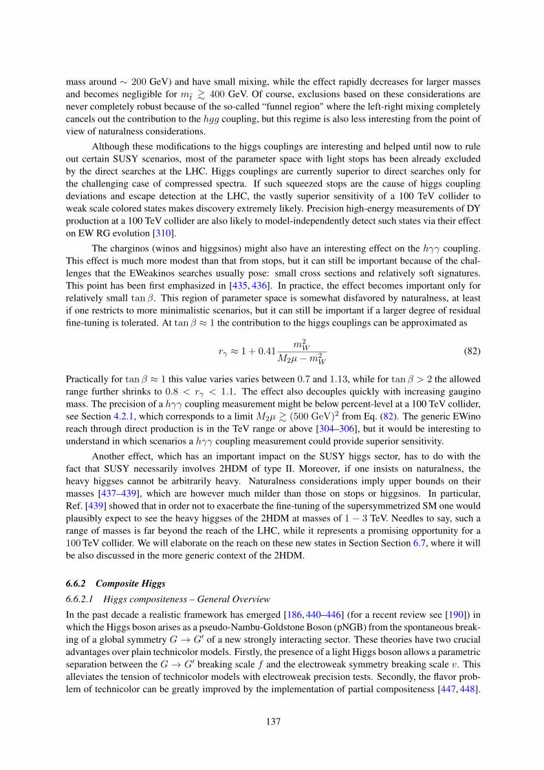
mass around ∼ 200 GeV) and have small mixing, while the effect rapidly decreases for larger massesand becomes negligible for mt & 400 GeV. Of course, exclusions based on these considerations arenever completely robust because of the so-called “funnel region" where the left-right mixing completelycancels out the contribution to the hgg coupling, but this regime is also less interesting from the point ofview of naturalness considerations.

Although these modifications to the higgs couplings are interesting and helped until now to ruleout certain SUSY scenarios, most of the parameter space with light stops has been already excludedby the direct searches at the LHC. Higgs couplings are currently superior to direct searches only forthe challenging case of compressed spectra. If such squeezed stops are the cause of higgs couplingdeviations and escape detection at the LHC, the vastly superior sensitivity of a 100 TeV collider toweak scale colored states makes discovery extremely likely. Precision high-energy measurements of DYproduction at a 100 TeV collider are also likely to model-independently detect such states via their effecton EW RG evolution [310].

The charginos (winos and higgsinos) might also have an interesting effect on the hγγ coupling.This effect is much more modest than that from stops, but it can still be important because of the chal-lenges that the EWeakinos searches usually pose: small cross sections and relatively soft signatures.This point has been first emphasized in [435, 436]. In practice, the effect becomes important only forrelatively small tanβ. This region of parameter space is somewhat disfavored by naturalness, at leastif one restricts to more minimalistic scenarios, but it can still be important if a larger degree of residualfine-tuning is tolerated. At tanβ ≈ 1 the contribution to the higgs couplings can be approximated as

rγ ≈ 1 + 0.41m2W

M2µ−m2W

(82)

Practically for tanβ ≈ 1 this value varies varies between 0.7 and 1.13, while for tanβ > 2 the allowedrange further shrinks to 0.8 < rγ < 1.1. The effect also decouples quickly with increasing gauginomass. The precision of a hγγ coupling measurement might be below percent-level at a 100 TeV collider,see Section 4.2.1, which corresponds to a limit M2µ & (500 GeV)2 from Eq. (82). The generic EWinoreach through direct production is in the TeV range or above [304–306], but it would be interesting tounderstand in which scenarios a hγγ coupling measurement could provide superior sensitivity.

Another effect, which has an important impact on the SUSY higgs sector, has to do with thefact that SUSY necessarily involves 2HDM of type II. Moreover, if one insists on naturalness, theheavy higgses cannot be arbitrarily heavy. Naturalness considerations imply upper bounds on theirmasses [437–439], which are however much milder than those on stops or higgsinos. In particular,Ref. [439] showed that in order not to exacerbate the fine-tuning of the supersymmetrized SM one wouldplausibly expect to see the heavy higgses of the 2HDM at masses of 1 − 3 TeV. Needles to say, such arange of masses is far beyond the reach of the LHC, while it represents a promising opportunity for a100 TeV collider. We will elaborate on the reach on these new states in Section Section 6.7, where it willbe also discussed in the more generic context of the 2HDM.

6.6.2 Composite Higgs6.6.2.1 Higgs compositeness – General Overview

In the past decade a realistic framework has emerged [186, 440–446] (for a recent review see [190]) inwhich the Higgs boson arises as a pseudo-Nambu-Goldstone Boson (pNGB) from the spontaneous break-ing of a global symmetry G → G′ of a new strongly interacting sector. These theories have two crucialadvantages over plain technicolor models. Firstly, the presence of a light Higgs boson allows a parametricseparation between the G → G′ breaking scale f and the electroweak symmetry breaking scale v. Thisalleviates the tension of technicolor models with electroweak precision tests. Secondly, the flavor prob-lem of technicolor can be greatly improved by the implementation of partial compositeness [447, 448].

137

The simplest realistic realization of the composite Higgs idea is represented by G = SO(5)× U(1)Xand G′ = SO(4) × U(1)X and called the Minimal Composite Higgs Model (MCHM) [442, 443]. TheU(1)X factor is needed to obtain the correct hypercharge, Y ≡ T 3

R + X , for the SM fermions. Thisbreaking pattern satisfies the conditions of a viable model: the SM vector bosons gauge a subgroupSU(2)L × U(1)Y ⊂ G and G/G′ contains an SU(2)L doublet which can be identified with the Higgsdoublet. The coset space of the MCHM contains four NGBs transforming as a 4 of SO(4), three ofwhich are eaten by the SM gauge bosons while the fourth is the physical Higgs boson. Larger cosetsgive rise to more NGBs, including, for example, extra singlets and doublets [449–451]. Interestingly, anadditional singlet could be interpreted as a Dark Matter candidate [449, 451–456].

At low energy, below the mass scale of the heavy resonances of the strong dynamics, the theory isdescribed by an effective Lagrangian involving the composite Higgs doublet and the SM fields. Effectsinduced by the virtual exchange of the heavy modes are encoded by local operators whose relative im-portance can be estimated by assuming a power counting. For example, under the assumption that thenew strongly-coupled dynamics is described by a single mass scalem∗ and a single coupling strength g∗,the effective Lagrangian has the form [186]

Leff =m4∗

g2∗L(Dµ

m∗,g∗Hm∗

,λΨ

m3/2∗

). (83)

One naively expects a typical coupling strength among the bound states of order g . g∗ ≤ 4π, wherevalues g∗ < 4π allow a perturbative expansion in the effective theory. The mass scale of the heavyresonances, m∗, represents the cutoff of the effective theory and sets its range of validity. Equation (83)describes the low-energy dynamics of the light composite Higgs H with elementary SM fermions Ψ, asfirst discussed in Ref. [186]. The coupling λ controls the strength of the interaction between the elemen-tary and composite fermions, where the latter have been integrated out. If the Higgs is strongly coupled,a simple yet crucial observation is that any additional power of H costs a factor g∗/m∗ ≡ 1/f , 30 whileany additional derivative is suppressed by a factor 1/m∗. Note that extra powers of the gauge fields arealso suppressed by 1/m∗ as they can only appear through covariant derivatives in minimally coupledtheories. If the light Higgs interacts strongly with the new dynamics, g∗ 1, then the leading correc-tions to low-energy observables arise from operators with extra powers ofH rather than derivatives. Thisremark greatly simplifies the list of important operators.

Composite Higgs models predict various new physics effects that can be probed at current andfuture colliders. In particular, new heavy vectors and fermions (the top partners) are expected and canbe directly searched for. In addition, the composite nature of the pNGB Higgs implies deviations of theHiggs couplings from their SM value by an amount proportional to ξ = v2/f2, where v is the scale ofEWSB and f the decay constant of the pNGB. In the MCHM, and more in general in theories with cosetSO(5)/SO(4), the following prediction holds for the couplings of one and two Higgs bosons to gaugebosons:

gMCHMhV V

gSMhV V=√

1− ξ , gMCHMhhV V

gSMhhV V= 1− 2ξ , (84)

where gSMhV V and gSMhhV V represent the SM couplings, while gMCHMhV V and gMCHM

hhV V stand for the couplingsin the MCHM. At low energy, virtual effects of the heavy resonances can be parametrized in terms oflocal operators, which also lead to anomalous Higgs couplings (such as, for example, derivative inter-actions between the Higgs and gauge bosons). Precision measurements of the Higgs couplings thusconstraint the compositeness scale and indirectly probe the heavy resonances. In fact, direct and indi-rect measurements represent complementary strategies to test the parameter space of a composite Higgsmodels.

30Note that a weakly-coupled, elementary Higgs would cost a factor g/m∗.

138

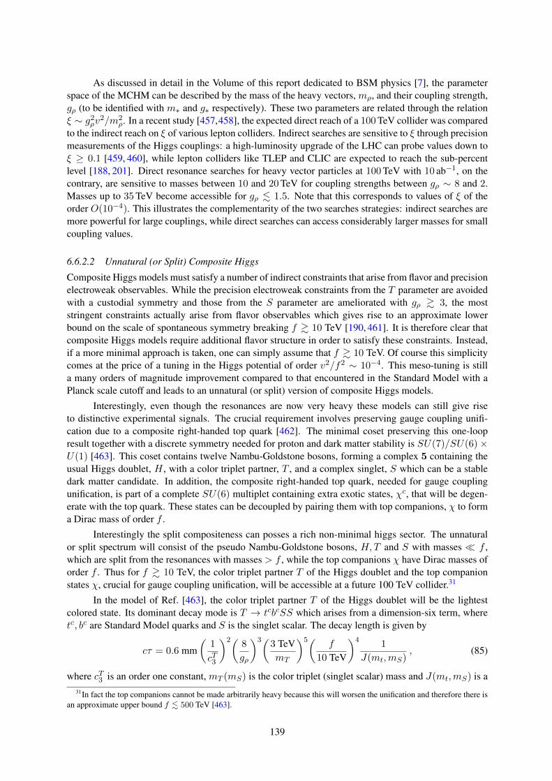
As discussed in detail in the Volume of this report dedicated to BSM physics [7], the parameterspace of the MCHM can be described by the mass of the heavy vectors, mρ, and their coupling strength,gρ (to be identified with m∗ and g∗ respectively). These two parameters are related through the relationξ ∼ g2

ρv2/m2

ρ. In a recent study [457,458], the expected direct reach of a 100 TeV collider was comparedto the indirect reach on ξ of various lepton colliders. Indirect searches are sensitive to ξ through precisionmeasurements of the Higgs couplings: a high-luminosity upgrade of the LHC can probe values down toξ ≥ 0.1 [459, 460], while lepton colliders like TLEP and CLIC are expected to reach the sub-percentlevel [188, 201]. Direct resonance searches for heavy vector particles at 100 TeV with 10 ab−1, on thecontrary, are sensitive to masses between 10 and 20 TeV for coupling strengths between gρ ∼ 8 and 2.Masses up to 35 TeV become accessible for gρ . 1.5. Note that this corresponds to values of ξ of theorder O(10−4). This illustrates the complementarity of the two searches strategies: indirect searches aremore powerful for large couplings, while direct searches can access considerably larger masses for smallcoupling values.

6.6.2.2 Unnatural (or Split) Composite Higgs

Composite Higgs models must satisfy a number of indirect constraints that arise from flavor and precisionelectroweak observables. While the precision electroweak constraints from the T parameter are avoidedwith a custodial symmetry and those from the S parameter are ameliorated with gρ & 3, the moststringent constraints actually arise from flavor observables which gives rise to an approximate lowerbound on the scale of spontaneous symmetry breaking f & 10 TeV [190, 461]. It is therefore clear thatcomposite Higgs models require additional flavor structure in order to satisfy these constraints. Instead,if a more minimal approach is taken, one can simply assume that f & 10 TeV. Of course this simplicitycomes at the price of a tuning in the Higgs potential of order v2/f2 ∼ 10−4. This meso-tuning is stilla many orders of magnitude improvement compared to that encountered in the Standard Model with aPlanck scale cutoff and leads to an unnatural (or split) version of composite Higgs models.

Interestingly, even though the resonances are now very heavy these models can still give riseto distinctive experimental signals. The crucial requirement involves preserving gauge coupling unifi-cation due to a composite right-handed top quark [462]. The minimal coset preserving this one-loopresult together with a discrete symmetry needed for proton and dark matter stability is SU(7)/SU(6)×U(1) [463]. This coset contains twelve Nambu-Goldstone bosons, forming a complex 5 containing theusual Higgs doublet, H , with a color triplet partner, T , and a complex singlet, S which can be a stabledark matter candidate. In addition, the composite right-handed top quark, needed for gauge couplingunification, is part of a complete SU(6) multiplet containing extra exotic states, χc, that will be degen-erate with the top quark. These states can be decoupled by pairing them with top companions, χ to forma Dirac mass of order f .

Interestingly the split compositeness can posses a rich non-minimal higgs sector. The unnaturalor split spectrum will consist of the pseudo Nambu-Goldstone bosons, H,T and S with masses f ,which are split from the resonances with masses > f , while the top companions χ have Dirac masses oforder f . Thus for f & 10 TeV, the color triplet partner T of the Higgs doublet and the top companionstates χ, crucial for gauge coupling unification, will be accessible at a future 100 TeV collider.31

In the model of Ref. [463], the color triplet partner T of the Higgs doublet will be the lightestcolored state. Its dominant decay mode is T → tcbcSS which arises from a dimension-six term, wheretc, bc are Standard Model quarks and S is the singlet scalar. The decay length is given by

cτ = 0.6 mm(

1

cT3

)2( 8

gρ

)3(3 TeVmT

)5( f

10 TeV

)4 1

J(mt,mS), (85)

where cT3 is an order one constant, mT (mS) is the color triplet (singlet scalar) mass and J(mt,mS) is a31In fact the top companions cannot be made arbitrarily heavy because this will worsen the unification and therefore there is

an approximate upper bound f . 500 TeV [463].

139

phase space factor (see Ref. [464] for details). Thus, since the scale f & 10 TeV, the color triplet is long-lived and can decay via displaced vertices or outside the detector. This signal at a 100 TeV collider wasanalyzed in Ref. [464]. When f = 10 TeV, displaced vertex and collider stable searches are sensitive totriplet masses in the range 3-10 TeV, while for heavier triplet masses, prompt decay searches are sensitiveto color triplet masses in the range 4-7 TeV. For f = 100 TeV there are no accessible prompt decays andthe displaced vertex and collider stable searches can now cover color triplet masses up to 10 TeV. Theseresults are depicted in Figure 84.

Fig. 84: Projections for a 100 TeV collider with 3 ab−1 of integrated luminosity as functions of the scalar massmS and triplet mass mT . The shaded regions show the 5σ discovery reach (95% CLs exclusion limit) for theR-hadron/displaced (prompt) searches. The dashed lines include an additional factor of two reduction in the signalefficiency for DV searches to account for the impact of more stringent experimental cuts. The left and right panelscorrespond to f = 10 and 100 TeV respectively. This figure is taken from Ref. [464].

The top companions are the next heaviest states and have SU(3) × SU(2) × U(1)Y quantumnumbers:

χ ≡ qc ⊕ e⊕ dc ⊕ l = (3,2)− 16⊕ (1,1)−1 ⊕ (3,1) 1

3⊕ (1,2)− 1

2(86)

These states are similar to excited Standard Model quarks and leptons and will decay promptly at a100 TeV collider. Assuming a scale f & 10 TeV the top companions will have masses in the 10−20 TeVrange. The colored top companions qc, dc will have unsuppressed decays to quarks and the color triplet T ,whereas the SU(2) singlet, e has a three-body decay into a bottom quark and two scalar triplets and theSU(2) doublet, l decays to a quark, a color triplet and a scalar singlet [463]. A further study of topcompanion mass limits from these decays at a 100 TeV collider will be useful.

In summary, at a 100 TeV collider color triplet scalars give rise to distinctive signals and togetherwith the top companions provide a smoking-gun signal for unnaturalness in composite Higgs models.

6.6.3 Neutral NaturalnessHere we briefly discuss the signatures of Neutral Naturalness, with emphasis on the Higgs-related mea-surements most suited for a 100 TeV collider. We anchor the discussion by referring to two concretebenchmark models, Folded SUSY (FSUSY) [281] which features EW-charged scalar top partners, andthe Twin Higgs [280] featuring SM-singlet fermionic top partners. However, some aspects of the phe-nomenology can also be derived more model-independently [303, 465]. The phenomenology of Neutral

140

Naturalness is rich, and includes potentially measurable Higgs coupling deviations, exotic Higgs decays,and direct production of partner states, additional Higgs states, or multi-TeV SM-charged states that arepart of the more complete protective symmetry that ultimately underlies the model.

6.6.3.1 Theory overview

In perturbative extensions of the SM, the hierarchy problem can be solved by introducing top partners.The coupling of these states to the Higgs is related to the top Yukawa by some symmetry (like supersym-metry, or a discrete symmetry in Little Higgs models [466–469]) such that the partner’s quadraticallydivergent one-loop Higgs mass contribution cancels that of the top quark. In most theories, this symme-try ensures that the top partners carry SM color charge, allowing copious production at hadron collidersas long as their mass is in the natural . TeV range.

It is possible to devise concrete models in which the symmetry which protects the Higgs includesa discrete group like Z2, and does not commute with SM color. This leads to the possibility of color-neutral top partners. Such theories of Neutral Naturalness feature very different phenomenology fromtheories like the MSSM.

We anchor our discussion by referring to two archetypical theory examples of Neutral Naturalness.The first is Folded SUSY (FSUSY) [281] which features a mirror sector of sparticles carrying SM EWquantum numbers. This mirror sector is charged under its own copy of QCD, which confines at a few –10 GeV. This leads to Hidden Valley phenomenology [385, 470–472]: since LEP limits forbid light EW-charged particles below ∼ 100 GeV, the lightest new particles are mirror glueballs. Because the onlyinteractions between the mirror sector and the SM proceed via the EW-scale particles, the lifetimes ofthe glueballs are necessarily suppressed by powers of Λ

EW , leading to the above mentioned hidden valleyscenarios. Top partner loops couple the Higgs to mirror gluons, allowing for mirror glueball productionin exotic Higgs decays, and displaced glueball decay via mixing with the SM-like Higgs.

Our second theory benchmark is the Twin Higgs [280], which features SM-singlet fermionic toppartners. These are part of a mirror sector containing copies of all SM particles and gauge forces.The original mirror Twin Higgs model has several cosmological problems due to an abundance of lightinvisible mirror states. One simple modification, which satisfies all cosmological constraints [473, 474],is the Fraternal Twin Higgs (FTH) [475], which only duplicates the third generation in the mirror sector.In that case, the hadrons of mirror QCD can be made up of mirror glueballs, mirror quarkonia, or amixture of both.

A common feature of these theories is the existence of a mirror QCD gauge group under which thetop partners (and other fields in the mirror sector) are charged. From a top-down perspective this mirrorQCD arises as a consequence of the discrete symmetry relating the SM and mirror sector. At some highscale, the mirror gBS and yBt are (almost) equal the SM gAS , y

At . From a bottom-up perspective [475],

the existence of a mirror QCD force is expected, since otherwise yBt would run very differently fromyAt , ruining the cancellation between the top loop and the top partner loop in the Higgs mass at a scaleof a few TeV. As we see below, this mirror QCD, and the associated low-energy hadron states, haveimportant phenomenological consequences. Of course, the discrete symmetry usually has to be brokenin some way (otherwise the two sectors would be identical), and it is possible to break mirror QCD aswell [476, 477]. In natural versions of these models, new SM-charged states appear at a few TeV, whichis in line with the above bottom-up expectation.

There are several features of Neutral Naturalness that are even more model-independent. Top part-ners, by their very nature, have to couple to the SM through the Higgs-portal, which leads to loop-leveldeviations in theZh production cross section that is potentially detectable at future lepton colliders [465].Other possibilities include tree-level Higgs coupling deviations can also arise due to mixing effects, mod-ifications of the Higgs cubic coupling due to top partner loops, electroweak precision observables [303],and direct top partner production via off-shell Higgs bosons [318, 326]. Crucially, it seems very chal-

141

lenging to construct a model of Neutral Naturalness which does not lead to detectable signatures at a100 TeV collider, lepton colliders, or both [303]. This lends additional motivation for Higgs-relatedmeasurements at a 100 TeV collider.

Models of Neutral Naturalness solve the Little Hierarchy problem via a one-loop cancellationbetween top and top partner Higgs mass contributions. This cancellation is not enforced at two-looporder, necessitating a full solution to the hierarchy problem to become apparent in a UV completion atscales of ∼ 5 − 10TeV [478–486]. In all known examples, these UV completions involve BSM statescarrying SM charges, allowing for direct production at a 100 TeV collider. This will not be our focushere, but since the UV completion scale is connected to the degree of tuning in the theory, the ability ofa 100 TeV collider to probe the full theory is complementary to Higgs-related measurements.

6.6.3.2 Higgs coupling deviations

In the minimal Folded SUSY model, the electroweak and Higgs sectors are identical to the MSSM.Realistically there is significant uncertainty as to the exact structure of the scalar sector: the MSSM itselffavors a light Higgs below 125 GeV, motivating extensions like non-decoupling D-terms [487], whileFolded SUSY needs some additional structure for viable electroweak symmetry breaking [488]. Even so,the required features of FSUSY imply the existence of additional Higgs bosons, leading to measurableHiggs coupling deviations if the decoupling limits is not satisfied. However, given that the naturalnesslimits, which are similar to the SUSY case, discussed in Sec. 6.6.1, the deviations might potentially betoo small not only for LHC, but also for the future leptonic collider.

The electroweak charge of the top partners in FSUSY implies loop-corrections to Br(h → γγ),which can be percent-level for top partner masses below 500 GeV [489]. This represents a significantopportunity for lepton colliders [188], but the LHC or a 100 TeV collider is more likely to produce theEW-charged top partners directly than to see deviations in the diphoton rate.

In all known Twin Higgs models, a soft mass which breaks the discrete symmetry between SM-and mirror-Higgs has to be balanced against f , the vev of the mirror Higgs (or, more generally, the scaleat which the higher symmetry which protects the light Higgs from quadratically divergent corrections isspontaneously broken) in order to achieve SM-like couplings of the 125 GeV Higgs to SM states. Thisleads to a tree-level tuning in the model, which is of order v2/f2, which is also the size of the mixingbetween the SM-like Higgs and the mirror Higgs. Therefore, in natural models where v2/f2 is not toosmall, there are detectable universal Higgs coupling deviations of the same order due to this tree-levelmixing effect. These deviations can be detected at the percent-level at future lepton colliders [188],which are the smoking gun of Twin Higgs theories. Such a deviation, if detected at lepton colliders,would greatly motivate 100 TeV searches for additional signals of the Twin Higgs, such as SM-chargedmulti-TeV states.

In principle, it is possible to imagine Neutral Naturalness scenarios from a bottom-up perspectivewithout measurable Higgs coupling deviations [303]. However, avoiding this smoking-gun-signature atlepton colliders comes at the cost of larger couplings in the hidden sector, reducing the required scaleof the UV completion in the absence of strong tuning. The 100 TeV collider would then be able toproduce the states of the UV completion directly, assuming they carry SM charge. This is the strongestdemonstration of the important complementarity between the two types of possible future colliders.

6.6.3.3 Exotic Higgs decays

Exotic Higgs decays are one of the best-motivated signatures of Neutral Naturalness. As outlined above,most theories of Neutral Naturalness feature a mirror-QCD gauge symmetry under which the top part-ners are charged. The Higgs therefore couples to mirror-gluons via a top partner loop in analogy to itscoupling to SM-gluons through the top loop. This means the Higgs can decay to mirror gluons, andtherefore into light states in the mirror sector. The size of the exotic branching fraction is related to the

142

top mass, and therefore to the naturalness of the theory itself, with less tuned scenarios giving higherexotic decay rates. The specific phenomenology of these exotic Higgs decays depends on the structureof the mirror QCD sector.

The mirror QCD sector could be SM-like, with quarks that are light compared to the confinementscale. This would allow the Higgs to decay to hidden pions and other hadrons, making it a classicalHidden Valley scenario [385, 470–472], realized for example by the original mirror Twin Higgs. If theexotic Higgs decays proceed through Yukawa couplings comparable to yb ∼ 0.02, exotic branchingratios could easily be as large as 10%, which is detectable at the LHC and future colliders even if thedecay products are detector-stable and hence invisible. On the other hand, if the decay proceeds througha top loop to mirror gluons only, the exotic branching fraction is of order . 10−3 (see below). A high-luminosity lepton collider like TLEP/FCC-ee [10] is sensitive to exotic Higgs decays with branchingfractions∼ 10−5 (10−3) if the decay products are very conspicuous with very little background (invisibleor inconspicuous with sizable backgrounds). Therefore, depending on the detailed final state, discoveringsuch a decay may be challenging even at lepton colliders.

In studying exotic Higgs decays, the clean environment of lepton colliders makes them superiorif the final states are not very distinctive, e.g. bb + MET or only MET. On the other hand, the hugeHiggs production rates make the LHC and the 100 TeV collider vastly superior to lepton colliders whenstudying exotic Higgs decays with highly distinctive final states, allowing access to much lower branchingfractions. Few final states are more distinctive than long-lived particles that decay within the detectorwith measurable displacement from the interaction point. Neutral Naturalness strongly motivates exoticHiggs decays to displaced final states.

The simplest scenario is a mirror sector without any light matter charged under mirror QCD. Thisis guaranteed in FSUSY, where LEP limits constrain the mass of the EW-charged mirror sector. It canoccur in Fraternal Twin Higgs scenarios, if the mirror b-quark is not too light. In that case, the mirrorhadrons are glueballs. There are ∼ 12 stable glueball states in pure SU(3) gauge theory [490], withmasses ranging from m0 ≈ 7ΛBQCD for the lightest G0 ≡ 0++ state, to ∼ 2.7m0 for the heaviest state.In the presence of top partners much heavier than ΛBQCD, some of these states can decay via a top partnerloop to SM particles via an off-shell Higgs boson [491]. We concentrate on the 0++ state, since it hasone of the shortest lifetimes and, as the lightest glueball, presumably produced commonly by mirror-hadronization.32 For m0 & 2mb (in the FTH case) and top partner mass mT , the decay length of G0 isapproximately

cτ ≈( mT

400GeV

)4(

20GeV

m0

)7

×

(35cm) [FSUSY](8.8cm) [FTH]

(87)

where we assume mT mt/2 for FTH and degenerate unmixed stops for FSUSY. For natural theories,these decay lengths are in the µm - km decay range. This leads to displaced signals at hadron colliders,with some glueballs decaying dominantly to 3rd generation SM fermion pairs.

RG arguments favor masses for G0 in the ∼ 10− 60GeV range (though model-dependent effectscan easily shift that range) [309]. The same top partner loop which allows glueballs to decay also allowsthe Higgs boson to decay to mirror gluons, which then hadronize to yield mirror glueballs, see Fig. 85.The rate for inclusive production of mirror glueballs from exotic Higgs decays can be estimated byrescaling Br(h→ gluons) ∼ 8% in the SM:

Br(h→ mirror glue) ≈ 10−3

(400GeV

mT

)4

×

1 [FSUSY]4 [FTH]

(88)

Non-perturbative or RG effects on the mirror QCD coupling can change this by an order 1 factor [309,475]. The exclusive branching fraction to the unstable 0++ glueballs can be parameterized as the above

32Thermal estimates [492] suggest that roughly half of all produced glueballs are in the 0++ state, but given our ignoranceabout pure-gauge hadronization, this estimate is highly uncertain.

143

Fig. 85: Production of mirror hadrons in exotic Higgs decays, and their decay back to the SM, in the FraternalTwin Higgs model. Figure from [475].

0 10 20 30 40 50 60

500

1000

1500

500

1000

1500

2000

m0 (GeV)

mt∼(GeV

)[FoldedSUSY]

mT(GeV

)[TwinHiggs

]

s = 14 TeV, 3000fb-1

(MS)x(MS or IT)

(VBF h→bb) x (IT, r > 4cm)

(single lepton) x (IT, r > 50μm)

TLEP Br(h→invisible)

0 10 20 30 40 50 60

500

1000

1500

2000

2500

3000

500

1000

1500

2000

2500

3000

3500

4000

m0 (GeV)

mt∼(GeV

)[FoldedSUSY]

mT(GeV

)[TwinHiggs

]

s = 100 TeV, 3000fb-1

(MS)x(MS or IT)

(VBF h→bb) x (IT, r > 4cm)

(single lepton) x (IT, r > 50μm)

TLEP Br(h→invisible)

Fig. 86: Summary of discovery potential for the simplified model of Neutral Naturalness with light mirror glue-balls at LHC14 and 100 TeV collider with 3000 fb−1, from looking for (i) one DV in the muon system (MS) andone additional DV in either the MS or the inner tracker (IT), (ii) one DV at least 4 cm from beam line and VBF jets(blue) and (iii) one DV with at least 50µm from beam line and a single lepton (orange). Assuming negligible back-grounds and 10 events for discovery. See [309] for details. Note different scaling of vertical axes. For comparison,the inclusive TLEP h → invisible limit, as applied to the perturbative prediction for Br(h → all glueballs), isshown for future searches as well, which serves as a pessimistic estimate of TLEP sensitivity. Lighter and darkershading correspond to the optimistic (pessimistic) estimates of exclusive 0++ yield, under the assumption that hdecays dominantly to two glueballs. Effect of glueball lifetime uncertainty is small and not shown. m0 is the massof the lightest glueball G0; the vertical axes correspond to mirror stop mass in FSUSY and mirror top mass inFTH and Quirky Little Higgs. Vertical solid (dashed) lines show where κ might be enhanced (suppressed) due tonon-perturbative mixing effects [475].

144

inclusive branching fraction multiplied by a nuisance factor κ which ranges from ∼ 0.1− 1 when thereis phase space available to produce heavier glueballs. This simple approach was used by the authorsof [309], who estimated the reach of various displaced searches at the LHC using ATLAS reconstructionefficiencies for displaced vertices (DV). A very conservative estimate of 100 TeV reach was derived bysimply repeating the analysis for higher energy. Top partner mass reach, which is ∼ 1.5TeV for THtop partners at the HL-LHC and ∼ 3TeV at the 100 TeV collider with 3ab−1 of luminosity, is shown inFig. 86 as a function of glueball mass. Light shading indicates estimated uncertainties due to unknowndetails of mirror hadronization. Different search strategies are required to cover the entire range ofglueball masses and lifetimes, most importantly searches for single displaced vertices together with VBFjets of leptons from Higgs production (see [309] for details, and [493] for other possibilities involvingdisplaced triggers). This sensitivity projection is highly conservative, since the exotic Higgs decay wasassumed to be 2-body, which underestimates the displaced vertex signal yield for light glueballs. Evenso, the reach is impressive and provides good coverage for the natural regime of these theories. It alsounderlines that the detector of a 100 TeV collider needs to be able to reconstruct soft and displacedobjects stemming from Higgs decays to maximize its potential for new physics discoveries. The reachcould also be dramatically improved if a future detector could trigger on displaced decays, or indeedoperate without a trigger.

Another possible scenario is a mirror QCD sector containing only light mirror bottom quarks B.This is one possible outcome of the Fraternal Twin Higgs (see [475] for a detailed discussion). If themirror bottom quark mass satisfies m0 . mB < mh/2, then the Higgs can decay to BB, which forms amirror bottomonium state and annihilates into mirror glueballs. This enhances the inclusive twin glueballrate to

Br(h→ mirror glue) ≈ Br(h→ BB) ≈ 0.15( mB

12GeV

)2(

400GeV

mT

)4

, (mB < mh/2) . (89)

which can be as large as ∼ 10%.

Alternatively, in the FTH, exotic Higgs decays can produce long-lived mirror bottomonium statesif they are the lightest mirror hadrons. The rate is equal to that shown in Eq. (89). The bottomoniumspectrum also contains an unstable 0++ state that decays via the top partner loop. The lifetime of thisstate is

Γχ→Y Y ∼ 2× 10−3

(v

f

)4 m11/3χ m

10/30

v2mh(m2h −m2

χ)2Γh→Y Y (mh) , (90)

assuming there are no light twin neutrinos which could short-curcuit this decay mode. This leads tosimilar phenomenology as the pure glueball scenario described above, however in this case the lifetimecan depend very differently on the 0++ mass, which motivates the search for relatively short decaylengths ∼ 10µm even for unstable particle masses near 15 GeV.

Finally, it is important to point out that in all of the above scenarios, the lifetime can be shorterthan ∼ 10 µm (for very heavy glueballs with light top partners, or for bottomonia), which motivatessearches for non-displaced b-rich final states of exotic Higgs decays.

6.6.3.4 Direct production of top partners

The Higgs portal guarantees that neutral top partners can be produced at the 100 TeV colliders via anintermediate off-shell Higgs boson. Measurement of the top partner masses or couplings via directproduction could serve as a powerful diagnostic of Neutral Naturalness to distinguish it from genericHidden Valleys, which can also lead to displaced exotic Higgs decays.

Let us first consider the FTH scenario. In that case, any produced top partner pair will quicklymirror-beta-decay to mirror-bottoms, which then either decay to light glueballs or bottomonia, leading to

145

displaced vertices in the detector. Higgs portal direct production, however, has a very low cross section,making direct production measurements unfeasible at the LHC for top partners heavier than a few 100GeV [494]. The 100 TeV collider with 3ab−1, on the other hand, will produce hundreds of top partnerpairs with potentially multiple displaced vertices, even if mT = 1TeV [303].

Top partner direct production is most spectacular for EW-charged partners, as for FSUSY. In thatcase, DY-like pair production leads to large signal rates. Since there is no light mirror-QCD-chargedmatter, the top partner pairs form a quirky bound state which de-excites via soft glueball and photonemission [495–498] before annihilating dominantly into mirror gluon jets, which hadronize to mirrorglueballs [494]. This can lead to spectacular “emerging jet” [386] type signatures with many displacedvertices for top partner masses in the TeV range at the LHC and multi-TeV range at the 100 TeV col-lider. This has been recently studied in [494], which also addresses how to parameterize the unknownhadronization of the pure-glue mirror sector. It is shown that exotic Higgs decays and direct top partnerpair production have complementary sensitivity to EW-charged partners in different regions of parameterspace. At a 100 TeV collider, the mass reach provided by both channels extends to several TeV or more.

The most challenging scenario is a scenario with neutral top partners but without mirror QCD.In that case, top partner production proceeds through the Higgs portal but without producing displacedvertices in the final state. This has been studied by [318, 326], which found that jj + MET searches forVBF h∗ → T T production was the most promising channel. Even so, the production rate is so low thatnow meaningful bounds are derived at the LHC. A 100 TeV collider is necessary to achieve sensitivityto top partner masses of a few 100 GeV, which is the naturally preferred range.

In all of the above cases, direct production of neutral top partners is complementary to directproduction of SM-charged BSM states at the 5-10 TeV scale, which are expected in the UV completionof Neutral Naturalness theories. The latter was recently explored in [499], which found reach for massesup to about 10 TeV. Both direct production measurements generally require a 100 TeV collider (especiallyfor the Twin Higgs) and would provide valuable information on the structure of the theory.

6.7 BSM Higgs SectorsIn this section we will overview the direct reach for the new BSM higgs states at 100 TeV machine. Wefirst review the two-Higgs doublet model (2HDM), which is relevant both as a standalone scenario andas an integral part of SUSY, models that explain the neutrino mass, etc. There have been a variety ofstudies studying the mass reach of a 100 TeV colliders to probe these new states by direct production.Singlet extensions are another highly relevant scenario, which occur in models of Neutral Naturalness,electroweak baryogenesis, and supersymmetry as the NMSSM and its derivatives, and we summarizerecent work on the reach of future colliders for these states. Of course, this exploration of possibilitiesfor BSM scalar sectors is not exhaustive, covering two of the most representative classes of scenarios.Particular examples of higgs triplet models are studied in the context of generating the neutrino mass inSection 6.5, and more work on general extensions at 100 TeV is needed.

6.7.1 Two-Higgs Doublet Models6.7.1.1 Higgs couplings

Two-doublet models are one of the most common extensions of the SM Higgs sector and are naturallyrealised in supersymmetry. Besides the ordinary Goldstones eaten by the gauge bosons, such modelsdescribe two CP-even (h0 and H0), one CP-odd (A0) and one charged (H±) physical states. Let usconsider, for simplicity, the type-II structure that arises in supersymmetry.

The physical content of the models can be described in terms of two angles. The angle β, whichdefines the direction of the Higgs vev in the plane of the two neutral CP-even current eigenstates (usuallydenoted by H0

d and H0u). And the angle α, which defines the direction of the lightest CP-even state (h0)

in the same plane. Following the usual convention for the definition of these angles, the directions of the

146

Higgs vev and h0 coincide when β − α = π/2. In the literature, the condition that these two directionscoincide is usually referred to as alignment. When alignment holds, h0 behaves as the SM Higgs and theorthogonal state does not participate in the process of EW breaking.

Present LHC measurements tell us that the observed Higgs boson is SM-like at the level of about20–30% while the full LHC program will be able to make tests in the range between a few to 10%.Assuming that no deviation is observed, it is a good starting point to take the Higgs as approximatelySM-like. This situation is automatically obtained in the limit in which we take all new states (H0, A0,H±) much heavier than h0, which corresponds to mA → ∞ and which is usually referred to as thedecoupling limit.

Since the Higgs couplings can be written in terms of the angles α and β, we can easily obtain theirexpression in the decoupling limit (mA →∞)

ghV V = sin(β − α) ≈ 1− 2 (1− t−2)2

t2 (1 + t−2)4

(mZ

mA

)4

(91)

ghtt =cosα

sinβ≈ 1− 2 (1− t−2)

t2 (1 + t−2)2

(mZ

mA

)2

(92)

ghbb = − sinα

cosβ≈ 1 +

2 (1− t−2)

(1 + t−2)2

(mZ

mA

)2

, (93)

where t ≡ tanβ and ghXX denote the couplings of the SM-like Higgs to weak gauge bosons (X = V ),top (X = t), and bottom (X = b), in units of the corresponding SM couplings. Equations (91)–(93)show explicitly how h behaves exactly as the SM Higgs in the decoupling limit. Note that the h couplingto gauge bosons becomes SM-like very rapidly, since deviations scale as (mZ/mA)4. The convergencebecomes even more rapid for large tanβ, since deviations scale as 1/t2.

To summarise: decoupling implies alignment, since mA →∞ implies β − α → π/2. Moreover,decoupling implies a special pattern of deviations from the SM predictions

δghV V ≈ 0.02%

(10

t

)2(300 GeV

mA

)4

(94)

δghtt ≈ 0.2%

(10

t

)2(300 GeV

mA

)2

(95)

δghbb ≈ 18%

(300 GeV

mA

)2

. (96)

In the decoupling limit, the couplings of the heavy states are also simply determined. For instance,for the heavy CP-even state H0, one finds

gHV V = cos(β − α) ≈ −2

t

(mZ

mA

)2

, gHtt ≈ −1

t, gHbb ≈ t . (97)

This means that the coupling of a single heavy Higgs to gauge bosons vanishes in the decoupling limit.Moreover, at large tanβ, the coupling to bottom quarks is enhanced. The production of heavy Higgsesis dominated by gg → H0/A0 via loops of top or bottom quarks, bb→ H0/A0, or associated productionwith H0/A0 emitted from a top or bottom quark line.

If the observed Higgs boson is confirmed to be nearly SM-like, we must conclude that thealignment condition is approximately satisfied. We have shown that decoupling implies alignment.So one may now wonder: does alignment imply decoupling? The answer is no. In a general two-Higgs doublet model it is possible to satisfy β − α ≈ π/2, while still keeping light the new Higgsstates [415, 417, 500, 501]. Although this cannot be achieved in the most minimal version of supersym-metric models, alignment without decoupling can occur in supersymmetry with new singlet or tripletstates [502] or for extreme values of radiative corrections [416].

147

As in the case of decoupling, also alignment without decoupling predicts a well-defined pattern ofHiggs couplings. Using ε ≡ cos(β − α) tanβ as expansion parameter, one finds

ghV V ≈ 1− ε2

2t2, ghtt ≈ 1 +

ε

t2, ghbb ≈ 1− ε , (98)

gHV V ≈ε

t, gHtt ≈ −

1

t(1− ε) , gHbb ≈ t

(1 +

ε

t2

). (99)

Comparing this result with eqs. (91)–(93) and (97), one finds the same result as decoupling once weidentify ε → −2(mZ/mA)2. Yet, the two cases do not lead to the same phenomenological predictions,since in alignment without decoupling ε can take either sign.

To summarise, there are two cases in which a two-Higgs doublet model can predict a nearly SM-like Higgs boson, such that Higgs coupling measurements can be satisfied to an arbitrary degree ofprecision. The two cases are decoupling and alignment without decoupling. Each case leads to a well-defined pattern for the couplings of the light and heavy Higgses, which can be expressed in terms of twoparameters: mA and tanβ for decoupling, or cos(β − α) and tanβ for alignment without decoupling.The important difference, from the phenomenological point of view, is that the new Higgs bosons mustbe heavy for decoupling, but can be arbitrarily light for alignment without decoupling. Furthermore,while standard decay channels of heavy Higgs bosons, like H/A → WW,ZZ, A → Zh, H → hh,H± → Wh are important in the decoupling limit, they become strongly suppressed in the alignmentlimit, where decays to SM fermions or photons become dominant [503]. This significantly affects thestrategy of direct searches, as discussed below.

6.7.1.2 Direct Searches for Heavy Higgs Bosons in 2HDM

At the 100 TeV pp collider the heavy Higgses of the 2HDM are dominantly produced via gluon fusiongg → H0/A, with dominant top and bottom (for large tanβ) loops, as well as bbH0/A associatedproduction. ttH0/A associated production could be important as well. The dominant production processfor the charged Higgses is tbH± associated production. In Fig. 87 we show the production cross sectionsforA,H0 andH± at 100 TeV pp collider in the Type II 2HDM with cos(β−α) = 0. For neutral Higgses,gluon fusion production dominates at low tanβ while bbH0/A associated production dominates at largetanβ. The tbH± production cross section gets enhanced at both small and large tanβ.

Comparing to the 14 TeV LHC, the production rates can be enhanced by about a factor of 30− 50for gluon fusion and bb associated production, and about a factor of 90 for the charged Higgs for Higgsmass of about 500 GeV, and even more for heavier Higgses, resulting in great discovery potential forheavy Higgses at a 100 TeV pp colliders.

At the LHC, most of the current searches for non-SM neutral Higgs bosons focus on the conven-tional Higgs search channels with aWW , ZZ, γγ, ττ and bb final state [509–515]. These decays modesare characteristic to the 2HDM in the decoupling limit, where we in general do not expect big splittingsbetween the various heavy Higgses. Typically, the production rate of the extra Higgses is suppressed,compared to that of the SM Higgs, either due to its larger mass or its suppressed couplings to the SMparticles. The decay of the heavy neutral Higgses to the WW and ZZ final states, which provided alarge sensitivity for SM Higgs searches, is absent for the CP-odd Higgs, and could be highly suppressedfor the non-SM like CP-even Higgs, especially in the alignment limit [503], in which case SM fermionand photon final states become more important. The decay modes into ττ or bb suffer from either sup-pressed branching fraction once the top pair mode opens up or large SM backgrounds, and are thereforeonly relevant for regions of the parameter space with an enhanced bb or ττ coupling. If the non-SMneutral Higgs is heavy enough, the decay mode into top pairs becomes important. However, when theHiggs is produced in gluon fusion, such decay suffers from large tt background and a possible destruc-tive interference with the SM background [503,516]. Direct searches for charged Higgs bosons are evenmore difficult at the LHC. For mH± > mt, the cross section for the dominant production channel of

148

Fig. 87: Dominant production cross sections for non-SM like Higgses in the Type II 2HDM at the 100 TeV pp

collider: NNLO cross section for gg → H0 or A (top left and top right panel, calculated using HIGLU [504]with the NNPDF2.3 parton distribution functions [125]), NNLO cross section for bottom-associated productionbbH0/A (lower left panel, calculated using SusHi [407,505,506]. bbH0 and bbA cross sections are the same in thealignment limit), NLO cross section for tbH± (lower right panel, calculated in Prospino [507, 508]).

tbH± is typically small. The dominant decay mode H± → tb is hard to identify given the large tt andttbb background, while the subdominant decay of H± → τν has suppressed branching fraction. In theMSSM, even at the end of the LHC running, there is a “wedge region” [188] in the mA− tanβ plane fortanβ ∼ 7 and mA & 300 GeV in which only a SM-like Higgs can be discovered at the LHC. Similarly,the reach for the non-SM Higgses in other models with an extended Higgs sector is limited as well.

The situation is very different at a 100 TeV collider. Two recent studies [296, 517] estimated thereach of Higgs production searches in the MSSM at 100 TeV, where the heavy bosons are produced inassociation with and decay into SM fermions. The reach, shown in Fig. 88, is impressive. Heavy Higgsmasses up to 5-10 TeV will be probed with 3 ab−1 for all values of tanβ. This also shows that the thewedge region could be covered by making use of new kinematic features of such signal events at a 100TeV pp collider, in this case top tagging in the boosted region. At low tanβ, the greatest sensitivity toneutral Higgs bosons is achieved with a same-sign dilepton search for Higgses produced in associationwith one or two top quarks, which subsequently decay to tt. The associated production channel avoidsthe difficult interference issues of a pp→ H0 → tt search.

149

0.5 1. 2. 5. 10. 20.

1.

2.

5.

10.

20.

50.

mA [TeV ]

tanβ

Fig. 88: 95% C.L. exclusion bounds for neutral (left panel, from [517]) and charged (right panel, from [296])Higgses of the MSSM at a 100 TeV collider. The blue and orange regions are probed by the channels pp →bbH0/A→ bbττ and pp→ bbH0/A→ bbtt for the neutral Higgses and pp→ tbH± → tbτν pp→ tbH± → tbtb

for the charged Higgses, respectively. The red region is probed by heavy Higgs production in association with oneor two top quarks, with subsequent decay to tt, yielding a same-sign dilepton signature. Given the same channelor the same color, the two different opacities indicate the sensitivities w.r.t. a luminosity of 3 ab−1 and 30 ab−1 ata 100 TeV pp collider, respectively. The cross-hatched and diagonally hatched regions are the predicted exclusioncontours for associated Higgs production at the LHC for 0.3 ab−1, and 3 ab−1, respectively.

Parent Higgs Decay Possible Final States Channels in 2HDMHH type (bb/ττ/WW/ZZ/γγ)(bb/ττ/WW/ZZ/γγ) H0 → AA, h0h0

Neutral Higgs HZ type (``/qq/νν)(bb/ττ/WW/ZZ/γγ) H0 → AZ,A→ H0Z, h0ZH0, A H+H− type (tb/τν/cs)(tb/τν/cs) H0 → H+H−

H±W∓ type (`ν/qq′)(tb/τν/cs) H0/A→ H±W∓

Charged Higgs HW± type (`ν/qq′)(bb/ττ/WW/ZZ/γγ) H± → h0W,H0W,AW

Table 44: Summary of exotic decay modes for non-SM Higgs bosons. For each type of exotic decays (secondcolumn), we present possible final states (third column) and relevant channels in 2HDM. Note that H in columntwo refers to any of the neutral Higgs, e.g. h0, H0 or A in 2HDM.

In addition to their decays to the SM particles, non-SM Higgses can decay via exotic modes, i.e.,heavier Higgs decays into two light Higgses, or one light Higgs plus one SM gauge boson. Clearly thishappens in the case when the splitting between the various heavy higgses is not small. This can happenin the alignment limit of the 2HDM without decoupling. As outlined above, this limit is less generic thanthe decoupling limit, but still worth a detail study.

Five main exotic decay categories for Higgses of the 2HDM are shown in Table 44. Once thesedecay modes are kinematically open, they typically dominate over the conventional decay channels.Recent studies on exotic decays of heavy Higgs bosons can be found in Refs. [518–529].

Theoretical and experimental constraints restrict possible mass hierarchies in 2HDM. At highHiggs mass and close to the alignment limit, unitarity imposes a relation between the soft Z2-breakingterm and the heavy CP-even neutral Higgs mass m2

12 = m2H0sβcβ

33. In this limit, the decay branchingfraction H0 → h0h0, AA,H+H− vanishes and vacuum stability further requires the CP-even non-SM

33Note that this is automatically fulfilled in the MSSM.

150

HiggsH0 to be the lightest non-SM like Higgs. In addition, electroweak precision measurements requirethe charge Higgs mass to be close to either of the neutral non-SM Higgs masses. This leaves us with onlytwo possible mass hierarchies permitting exotic Higgs decays: mH0 ≈ mH+ < mA and mH0 < mA ≈mH+ . At high Higgs masses, unitarity further requires the mass splitting between the non-SM Higgses tobe small and therefore imposes an upper bound on the Higgs mass permitting exotic Higgs decays aroundmH ∼ 1.5−2 TeV. These restrictions can be significantly relaxed at lower Higgs mass, allowing a largerspectrum of mass hierarchies including those permitting the decays H0 → AA,H+H−. Consideringthe limited reach of the LHC around the “wedge region”, extotic Higgs decay channels in the low Higgsmass region,mH0 <∼ 500 GeV, might still provide discovery potential at a 100 TeV pp collider. In Fig. 89we show the branching fraction of non-SM Higgs bosons in Type II 2HDM for sin(β − α) = 1 and amass hierarchy containing a 1 TeV parent Higgs and a 850 GeV daughter Higgs.

βtan1 10

BR

(A)

4−10

3−10

2−10

1−10

1 ±

W±H

HZ

tt

bb

ττ

=850GeVHm=1000GeVAm=850GeV+Hm

βtan1 10

BR

(A)

4−10

3−10

2−10

1−10

1HZ

tt

bb

ττ


βtan1 10

)+B

R(H

4−10

3−10

2−10

1−10

1+HW

tb

ντ


Fig. 89: Branching fractions for A (left and center panel) and H+ (right panel) in the Type II 2HDM with sin(β−α) = 1 and m2

12 = m2H0sβcβ . We show the two allowed mass hierarchies mH0 = mH+ < mA (left panel) and

mH0 < mA = mH+ (center and right panel). The parent and daughter Higgs masses are chosen to be 1 TeVand 850 GeV, respectively. Dashed curves are the branching fractions when exotic decay modes are kinematicallyforbidden. All decay branching fractions are calculated using the program 2HDMC [530].

Note that most of the current experimental searches for the non-SM Higgs assume the absence ofexotic decay modes. Once there are light Higgs states such that these exotic modes are kinematicallyopen, the current search bounds can be greatly relaxed given the suppressed decay branching fractionsinto SM final states [519, 521, 523]. Furthermore, exotic Higgs decays to final states with two lightHiggses or one Higgs plus one SM gauge boson provide complementary search channels. Here, we listsuch exotic Higgs decays and consider potential search strategies.

– H0 → AA or H0 → h0h0

With the final state Higgs decaying via bb, γγ, ττ , WW ∗, final states of bbbb, bbττ , bbγγ and γγWW ∗

can be used to search for resonant Higgs decay to two light neutral Higgses. Current searches at the LHC8 TeV with about 20 fb−1 luminosity gave observed limits of 2.1 pb at 260 GeV and about 0.018 pb at1000 GeV [531]. While bbγγ and bbττ have comparable sensitivities at low mass, bbbb mode dominatesat high mass.

– H0 → AZ or A→ H0Z

With Z → `` and H0/A → bb, ττ , the final states of bb``, ττ`` can be obtained with gluon fusionproduction, or in the bb associated production with two additional b jets [518–520]. Recent searchesfrom ATLAS and CMS have shown certain sensitivity in this channel [532–535]. In parameter regionswhere Br(A → H0Z) × Br(H0 → ZZ) is not completely suppressed, ZZZ final states with two Zdecaying leptonically and one Z decaying hadronically can also be useful [519]. Other channels withtop final states could be explored as well.

151

Note that the decay A→ ZH0 has been identified as a particular signature of a SFOEWPT in the2HDM [327]. As discussed below, the prospects for observing this channel in the ``bb and ``W+W−

model have been analyzed in Ref. [328].

– H0 → H+H−

With both H± decaying via τν final states, the signal of ττνν can be separated from the SM W+W−

background since the charged tau decay product in the signal typically has a hard spectrum compared tothat of the background [523].

– H0/A→ H±W∓

Similar to the H+H− case, H± → τν, tb and W → `ν with `τνν or tb`ν could be used to searchfor H0/A→ H±W∓. Note that for the CP-even Higgs H0, the branching fraction of H0 → H±W∓ ismostly suppressed comparing to H0 → H+H− as long as the latter process is kinematically open andnot accidentally suppressed [523]. However, for the CP-odd Higgs A, this is the only decay channel witha charged Higgs in the decay products.

– H± → H0W,AW

This is the only exotic decay channel for the charged Higgs in the 2HDM. Given the associated produc-tion of tbH±, and the decay of H0, A into the bb or ττ channel, ττbbWW or bbbbWW can be usedto probe this channel [521]. H0/A → tt could also be used given the boosted top in the high energyenvironment.

Note that while H± → WZ is absent in 2HDM type extension of the SM Higgs sector, it couldappear, however, in the real triplet models extension of the SM once the triplet obtains a vev [352].

6.7.2 Singlet Extensions of the Higgs Sector34

The simplest example of an extended Higgs sector consists in the addition of a real scalar field, sin-glet under all the gauge groups, to the SM. Despite its great simplicity, this scenario arises in many ofthe most natural extensions of the SM – e.g. the Next-to-Minimal Supersymmetric SM (NMSSM, seeSection 6.7.2.1), Twin Higgs (see Section 6.7.2.2), some Composite Higgs models – and is therefore ofconsiderable physical interest.

In general, a CP-even scalar singlet will mix with the Higgs boson at a renormalizable level. Asa consequence, both physical scalar states can be produced at colliders through their couplings to SMparticles, and be observed by means of their visible decays.

Let us denote by h and φ the physical mass eigenstates, and by γ the mixing angle. In a weaklyinteracting theory, the couplings of h and φ are just the ones of a SM Higgs, rescaled by a universalfactor of cos γ or sin γ, respectively. Hence, assuming no invisible decays, the signal strengths µh,φ intoSM particles are

µh = µSM(mh)× c2γ , (100)

µφ→V V,ff = µSM(mφ)× s2γ × (1− BRφ→hh) , (101)

µφ→hh = σSM(mφ)× s2γ × BRφ→hh, (102)

where µSM(m) is the corresponding signal strength of a standard Higgs with mass m, and BRφ→hh isthe branching ratio of φ into two Higgses – an independent parameter at this level. The phenomenology

34Contribution by Dario Buttazzo, Filippo Sala and Andrea Tesi

152

ϕ []

[

]

ϕ → ϕ → ()

=

ϕ []

[

]

ϕ →

ϕ → ()

= -

Fig. 90: Reach of direct searches for generic singlet extensions of the SM in the mφ–Mhh plane, see Eq. (103).The singlet vev is vs = 250 GeV (left) and vs = −75 GeV (right). Searches using the V V and hh final state areshown in red and purple. The solid colored regions are excluded at 95% CL by the 8 TeV LHC. Lines representthe expected bounds for FCC-hh (dotted), high-luminosity LHC (dashed), and high-energy LHC (dot-dashed), allwith a luminosity of 3 ab−1. Taken from ref. [536].

of the Higgs sector is therefore completely described by three parameters: mφ, sγ , and BRφ→hh. Thesecond state φ behaves like a heavy SM Higgs boson, with reduced couplings and an additional decaywidth into hh.

The mixing angle γ and mφ are not independent quantities, but are related via

sin2 γ =M2hh −m2

h

m2φ −m2

h

, (103)

where M2hh ∝ v2 is the first diagonal entry of the Higgs squared mass matrix, in the gauge eigenstate

basis. In the following we will often useMhh as a parameter, instead of γ, to avoid considering unnaturalregions of the parameter space with high mass and large mixing angle.

Given the singlet nature of φ, its main decay channels are into pairs of W , Z, and Higgs bosons.In the large-mφ limit, the equivalence theorem implies that

BRφ→hh = BRφ→ZZ =1

2BRφ→WW . (104)

The leading corrections to this relation35 for finite masses depend only on the vacuum expectation valueof the singlet, vs [536]. Therefore, to a good approximation mφ, Mhh, and vs constitute a set of inde-pendent parameters that describe the phenomenology.

The FCC reach for a generic resonance in these channels has been discussed in Ref. [536], whereit has been obtained through a parton luminosity rescaling from the 8 TeV LHC results [457]. Figure 90shows the combined reach from all the V V final states, compared with the one in the hh channel fromthe 4b final state, again for two different values of vs. The reach of the high-luminosity (14 TeV, 3 ab−1)and high-energy (33 TeV, 3 ab−1) upgrades of the LHC are also shown for comparison. It can be seen

35The exact expressions for the triple couplings gφhh and ghhh depend on the details of the scalar potential, and can be foundin ref. [536].

153

ϕ []

[

]

Δμ/μϕ →

[ϕ→] =

ϕ []

[

]

Δμ/μϕ →

[ϕ→] =

Fig. 91: Comparison between direct and indirect searches in the singlet model, and for BRφ→hh = 0.25. Left:region relevant for the LHC (thin lines: 13 TeV, thick lines: 14 TeV, dashed: high luminosity). Right: projectionsfor future colliders (dot-dashed: 33 TeV LHC, dotted: FCC-hh with 3 ab−1). Coloured isolines of s2

γ . The coloredregion is excluded at 95% CL. Taken from ref. [536].

that the V V searches are always dominant at FCC. Moreover, the detection of a hh resonance in themulti-TeV range is possible only for values of vs related also to very large modifications (a factor of twoor even larger) in the triple Higgs coupling ghhh. Moderate to large deviations in such a coupling are ageneric prediction of a singlet mixed with the Higgs, contrarily for example to the case of 2HDM, andthe very high energy of the FCC-hh appear to provide a unique opportunity to test this possibility.

Finally, Fig. 91 compares the reach of direct and indirect searches, for fixed BRφ→hh = 0.25, andfor two regions relevant for the LHC and for FCC, respectively. The deviation in Higgs signal strengths,shown as colored isolines, are proportional to s2

γ . Given the universal rescaling of all the couplings, thepower of Higgs coupling measurements in the singlet case is rather limited, as compared e.g. to a 2HDM(see Section 6.7.1). It is interesting to note that direct searches at FCC-hh are more powerful than indirectmeasurements at FCC-ee for resonance masses below about 1 TeV.

The results of the simple scenario presented in this Section apply in general to any singlet scalar,and can easily be applied to more concrete cases, as we discuss below for the NMSSM and the TwinHiggs.

6.7.2.1 NMSSM

The NMSSM constitutes a particularly interesting physics case for several reasons. In particular, sincethe extra Higgs bosons could be the first new degrees of freedom to be detected, it is important to quantifythe reach of LHC and future colliders for scalar states in this scenario.

The NMSSM consists in the MSSM with the addition of an extra gauge singlet S, so that thesuperpotential reads

WNMSSM = WMSSM + λSHuHd + V (S), (105)

where V is a polynomial up to order three in the new field S. This addition is relevant form the point ofview of naturalness for large enough λ, since the different dependence of the weak scale v in the highenergy parameters allows, for a given amount of tuning, to raise the stop and gluino masses by a factor∼ λ/g with respect to the MSSM. The Higgs mass value mh is also less constraining in the NMSSM

154

than in the MSSM, thanks to the extra SUSY-preserving contribution of the form sin2 2β λ v2/2. Thedrawback of this last feature is that, for a too large λ, a tuning is reintroduced to lower the Higgs massto 125 GeV. These considerations have been made precise in the analysis of ref. [537], that identifiedλ ∼ 1 as a region of minimal tuning, capable of accommodating stops and gluinos as heavy as 1.2 and2.5 TeV respectively. The loss of perturbativity before the GUT scale, implied by a value of λ & 0.75, isavoidable without spoiling unification, see e.g. the model proposed in [538] and references therein.

The Higgs sector of the NMSSM consists of six particles: three CP-even ones, h, H and φ, twoCP-odd ones A and As, and a charged state H±. We mostly concentrate on the CP-even ones, andidentify h with the 125 GeV state discovered at the LHC, H with the mostly doublet mass eigenstate,and φ with the mostly singlet one. Three mixing angles, to be called δ, γ, and σ, control the rotationbetween the mass eigenstates and the gauge eigenstates where one doublet takes all the vev.

It has been shown in ref. [538] that the phenomenology of the three CP-even states, with theexception of the trilinear couplings among the Higgses, can be described in terms of only six parameters,which we find convenient to choose as:

m2φ, m2

H , m2H± , tanβ, λ, ∆2, (106)

where with ∆2 we denote all the radiative contributions to the Higgs mass, which sums up the contribu-tions from the rest of the superpartner spectrum.36 Radiative corrections to other elements of the scalarmass matrix are assumed to be small. The mixings angles can be expressed in terms of the parameters in(106), see Refs. [538, 539] for the full analytical formulae.

Deviations in the Higgs couplings,

ghuugSMhuu

= cγ(cδ +sδ

tanβ),

ghddgSMhdd

= cγ(cδ − sδ tanβ),ghV VgSMhV V

= cγcδ , (107)

(where sθ, cθ = sin θ, cos θ) constrain only the two mixing angles δ and γ that involve h. While a fit tothe Higgs couplings leaves space for a sizable mixing γ, at the level of sin γ ∼ 0.45, it leaves little spacefor two mixed doublets. Perhaps more important than that, the LHC14 with 300 fb−1 is not expected toprobe substantially the h-S mixing γ, while the opposite is true for δ, which will be constrained to thefew percent level [539].

Since the purpose of this document is to set a general strategy for searching for BSM Higgses, forconvenience we now summarize the phenomenology in two limiting cases, identified by their relevantdegrees of freedom37.

h and a singlet-like state φ in the low-energy spectrum, with H decoupled and δ = 0. The genericparameter Mhh of Section 6.7.2 is now identified with the upper bound on the Higgs boson mass

M2hh = c2

2βm2Z + s2

2βλ2v2/2 + ∆2, (108)

and the total number of free parameters decreases from six to four, mφ, λ, tanβ and ∆. Since ∆has little impact on the phenomenology of the model (unless it is very large), it is convenient to fixit to some reference value, typical of stops in the TeV range. h and a second doublet H in the low-energy spectrum, with φ decoupled and γ = 0. The Higgs

sector now realizes a particular type-II 2HDM. Here the total number of free parameters is three,mH , tanβ and ∆, and also the charged scalar H± is predicted with a mass close to that of theCP-even one H . The MSSM is a particular realization of this case, where λ = 0 and ∆ is fixed toreproduce the correct value of the Higgs mass. However, for generic values of ∆, λ 6= 0 and therealized 2HDM will be different from the MSSM.

36We will choose values representative of TeV-scale stops, but the phenomenology does not sensitively depend on ∆2 unlessthe value is much larger than what we assume.

37For a discussion with the same logic and more details, we refer the reader to the short review [540].

155

ϕ []

β

Δμ/μ

ϕ →

λ =

ϕ []

β

Δμ/μ

ϕ →

λ =

Fig. 92: Parameter space of the NMSSM scenario in the limit of decoupled heavy doublet H . Shaded areas: 95%CL exclusions from Higgs signal strengths (pink) and direct searches for φ→ SM (red) at LHC8. Lines: contoursof s2

γ (pink), expected reach of direct searches at HL-LHC (dashed), HE-LHC (dot-dashed), and FCC-hh with3 ab−1 (dotted). Grey: unphysical regions. BRφ→hh fixed to its asymptotic value 1/4. Left: ∆ = 70 GeV andλ = 1.2; right: ∆ = 80 GeV and λ = 0.7. Taken from ref. [536].

Let us summarize the phenomenology of these two cases. In the h-singlet mixing scenario, Higgscoupling measurements will leave much of the parameter space unexplored, unless a per-mille precisionis reached, as expected at the FCC-ee (or CEPC). Direct searches for the extra Higgs is therefore themost powerful probe of the Higgs sector in this case. The impact of current and future searches is shownin Figure 92, for the values of λ = 1.2 and 0.7, respectively. For simplicity we have fixed BR(φ→ hh)to its asymptotic value of 1/4 , a case where V V searches dominate over hh ones38. From Figure 92one reads that direct searches are expected to dominate the reach in the parameter space of the model.At a 100 TeV pp collider they will be complementary with Higgs coupling measurements of a leptoniccollider like the FCC-ee or the CEPC. No matter how we look for BSM in the Higgs sector, the region ofsmaller λ will be more difficult to probe than that of a larger one, giving more importance to other SUSYsearches (like stop and gluino ones). In each scenario, singlet scalar masses in excess of a TeV can beprobed, depending on the value of tanβ.

We now move to the second case, where the relevant degrees of freedom are h and the doublet-likestate H . This scenario is best probed via measurements of the Higgs signal strengths into SM particles,as evident from Figure 93. A region of “alignment without decoupling” of the state H survives forλ ' 0.65 and tanβ ' 2.5, corresponding to a zero of the mixing angle δ. That region – which is alreadyconstrained by the bounds on mH± coming from flavour measurements like BR(B → Xsγ) – needsdirect searches for the new states in order to be probed. The discussion follows that of two Higgs doubletmodels of section 6.7.1. We recall here the main features for convenience, following the recent study ofref. [503]: exact alignment δ = 0 implies BRH→hh = BRH→V V = BRA→Zh = BRH±→W±h = 0, butcontrary to the h-φ singlet case some couplings to SM fermions survive, allowing to probe the existenceof H in resonant searches in tt, bb, `+`− and γγ. For larger values of mH , the tt channel opens anddominates the branching ratio. The 100 TeV studies of heavy Higgs production in association with SM

38“Small” values of vs can make resonant di-Higgs production more important, a case which we do not discuss here.

156

0.6 0.8 0.9 1 1.1 1.2 1.4 1.6

300

400

0.7

200

1.8

2 4 6 8 10150

200

250

300

350

400

450

500

tan Β

mH

@GeV

D

-0.2 0.0 0.2 0.4 0.6

2

4

6

8

10

12

14

sin ∆

tan

ΒFig. 93: Left: parameter space of the NMSSM scenario with a decoupled scalar S, with radiative corrections tothe Higgs mass fixed at ∆ = 75 GeV. Isolines of λ (solid black), and of mH± (dashed black). 95% CL exclusionsfrom Higgs coupling measurements at LHC8 (shaded pink), expected reach at LHC14 with 300 fb−1 (pink dashed).Blue: unphysical regions. The entire shown parameter space is likely to be excluded by direct searches for heavyHiggs doublets at 100 TeV, see Fig. 88. Right: Higgs couplings fit (95% CL allowed regions) for sin2 γ = 0

(green) and sin2 γ = 0.15 (grey) from the LHC run 1, and projection for LHC14 (dashed, γ = 0). Taken fromref. [541].

fermions [296, 517] indicates that 5-10 TeV masses can be probed, which likely applies to this NMSSMscenario as well, see Fig. 88.

Going back to a fully mixed situation, where all the states h, H and φ are kept in the spectrum,demands to work with more parameters. Numerical scans are usually employed for this purpose, and theyallow to interconnect the phenomenology of the Higgs scalar sector with that of other SUSY particles.We do not explore this case further, and refer the reader to the recent studies [542, 543] for a discussion.Also, in case some signal is observed, it will be important to explain it in a fully mixed situation. Forthis purpose, analytical relations such as the ones presented in refs [538, 539] would provide a usefulguidance.

Finally, we mention that the case of an extra Higgs lighter than 125 GeV is motivated and stillpartially unexplored. This is true especially for a singlet like state φ, since flavour bounds on mH± poseserious challenges to having mH < 125 GeV.

6.7.2.2 Twin Higgs

Another motivated scenario where we expect a scalar singlet at accessible energies is the Twin Higgsmodel (TH). As discussed in Section 6.6.3, the TH is a well-motivated solution to the Hierarchy problemwith uncolored top partners and many possible discovery channels. Here we discuss how the extendedHiggs sector may be directly probed.

Amongst the twin states the mirror Higgs, which is a SM singlet, can be singly produced via itsmixing with the SM Higgs, and accessible at present and future colliders. In order to describe the mainphenomenology, we focus on the linearised TH model [475], where the scalar potential consists of onlytwo degrees of freedom, the 125 GeV Higgs and the mirror Higgs σ. Notice that the presence of thisextra singlet is a feature of any TH construction, and therefore it constitutes a natural signature. Using

157

the label A for our SM sector and B for the twin sector, we have

V (HA, HB) = κ(|HA|4 + |HB|4

)+m2

(|HA|2 − |HB|2

)+ λ∗

(|HA|2 + |HB|2 −

f20

2

)2. (109)

The first term in the potential breaks the SU(4) global symmetry but leaves Z2 intact, the second termsoftly breaks Z2 as needed to achieve a separation between the two VEVs. The last one parametrises aspontaneous symmetry breaking SU(4)/SU(3). It is a combination of the spontaneous symmetry breakingand the soft breaking of the Z2 symmetry that realises the TH mechanism.

From a phenomenological point of view, the relevant parameters are λ∗ and f0, where the size ofλ∗ is required to be small, or the mirror Higgs will get a mass (mσ ∼

√λ∗f0) of the order of the cut-off

of the model invalidating our phenomenological picture. The particle σ is often called the radial-modeof the corresponding symmetry breaking pattern.

The two Higgs doublets HA and HB are charged under the SM and twin weak interactions, re-spectively. Therefore, in the unitary gauge, six Goldstone bosons are eaten by the gauge bosons of thetwo sectors, leaving only two scalar degrees of freedom the SM Higgs, h, and σ. In the interaction basisthey have a mass mixing. Trading two of the four parameters for the electro-weak VEV and Higgs mass,one can compute the mixing parameter between the two states

sin2 γ =v2

f2− m2

h

m2σ −m2

h

(1− 2

v2

f2

), (110)

where mh and mσ are the physical masses, while in terms of the parameters in eq. (109), v2 =κλ∗ f20−(κ+2λ∗)m2

κ(κ+2λ∗), f2 = f2

02λ∗

2λ∗+κ.

This is very similar to the spectrum of a simple singlet-extension of the SM, given that the mixingangle enters the σ signal strengths, and it also controls the leading and model independent contributionsto the electro-weak S and T parameters. Differently from the NMSSM or other weakly coupled exten-sions, however, in this case the mixing angle does not vanish in the large-mσ regime, but it approaches aconstant proportional to v2/f2. This is reminiscent of the pNGB nature of the Higgs in the Twin Higgsmodel. This simple scenario can be meaningfully constrained by means of indirect and direct measure-ment. While precision Higgs measurements are only sensitive to sin γ in (110), the direct searches of σdepend also on the branching ratios in its possible decay channels.

We now discuss direct searches for the radial mode σ. Through the mixing (110), σ inherits allthe decay mode of a SM Higgs with mass mσ. However, σ has model independent couplings to the twinelectro-weak gauge bosons. We expect σ to have a mass that scales with the parameter f , therefore inthe O(500 − 1000 GeV) range, where all the decay channels are practically open. It mostly decays tovector bosons of the SM and twin sector, the latter contribute to the invisible decay width. In the largemass limit, the branching ratios of σ are fixed by the equivalence theorem to be

BRtwin−V V '3

7, BRhh ' BRZZ '

1

2BRWW '

1

7. (111)

The above equation has two immediate consequences: i) the dominant decay channel is diboson (includ-ing double Higgs), as expected for an electro-weak singlet in the TeV region; ii) the additional invisibledecay channel to twin dibosons dilutes the branching fractions for the visible channels, and contributesto the widening of the width (especially in the large mass limit). i) and ii), together with the scalingof mσ, then suggest that the largest impact of direct searches is expected for weakly coupled scenarios,with mσ ∼ f , in a region of moderate f .

These considerations are reflected in Figure 94, where, in the plane of the only two free parameters,(f,mσ), we show the impact of Higgs coupling determination and recast of direct searches in the dibosonchannel. For reference, we fix the invisible branching ratio to its asymptotic value of 3/7. As expected,

158

0.05

0.1

0.15

0.23

500 1000 1500 2000400

600

800

1000

1200

mΣ @GeVD

f@G

eVD

BRΣ®inv. = 37Σ ® SMDΜΜSM

0.05

0.01

0.002

1000 2000 3000 4000 5000 6000

1000

2000

3000

4000

5000

6000

mΣ @GeVDf

@GeV

D

BRΣ®inv. = 37Σ ® SMDΜΜSM

Fig. 94: Parameter space of the scalar singlet in Twin Higgs scenarios in the plane of the mass of the radial modemσ and the mirror Higgs vev f . Pink lines: contours of s2

γ . A lepton collider like ILC250 (TLEP) will likelybe able to exclude s2

γ at the 0.05 (0.008) level [10, 188]. Red lines: expected reach of the LHC13 (continuousthin), LHC14 (continuous), HL-LHC (dashed), HE-LHC (dot-dashed), and FCC-hh with 3 ab−1 (dotted). Shadedregions: excluded at 95% C.L. by direct searches (red), excluded by Higgs couplings (pink), Γσ > mσ (blue),unphysical parameters (grey). BRφ→hh fixed to its asymptotic value 3/7 for reference. Figure taken from ref. [536].

direct searches will provide a strong probe of the scenario considered formσ ∼ f , while for much highervalues indirect constraints are expected to dominate39. This is an important example of complementaritybetween proposed future lepton and hadron colliders, which together will be able to probe the naturalTwin Higgs parameter space with TeV-scale mirror Higgs vevs and masses.

39In this Twin Higgs model, the trilinear Higgs coupling ghhh is fixed in terms of mσ and f , and does not substantiallydeviate from its SM value.

159

AcknowledgementsThe research of D.Buttazzo was supported in part by the Swiss National Science Foundation (SNF) undercontract 200021-159720. The work of C.-Y.C is supported by NSERC, Canada. Research at the Perime-ter Institute is supported in part by the Government of Canada through NSERC and by the Province ofOntario through MEDT. D.C. is supported by National Science Foundation grant No. PHY-1315155 andthe Maryland Center for Fundamental Physics. The work of Q-H.C. is supported in part by the NationalScience Foundation of China under Grand No. 11175069, No. 11275009 and No. 11422545. NG wassupported by the Swiss National Science Foundation under contract PZ00P2_154829. TG is supportedby the DOE grant DE-SC0011842 at the University of Minnesota. AK is supported by the British Sci-ence and Technology Facilities Council and by the Buckee Scholarship at Merton College. The work ofM.L.M. is supported by the European Research Council advanced grant 291377 “LHCtheory”: Theo-retical predictions and analyses of LHC physics: advancing the precision frontier. The work of R.N.M.is supported in part by the US National Science Foundation Grant No. PHY-1315155. F.P. is supportedby the U.S. DOE grants DE-FG02-91ER40684 and DE-AC02-06CH11357. MP is supported by theU.S. National Science Foundation grant PHY-1316222. M.J.R-M. was supported in part under U.S.Department of Energy contract DE-SC0011095. F.S. is supported by the European Research Council(ERC) under the EU Seventh Framework Programme (FP7/2007-2013)/ERC Starting Grant (agreementn. 278234 — ‘NEWDARK’ project). The work of M.S. is supported by the National Fund for ScientificResearch (F.R.S.-FNRS Belgium), by the IISN “MadGraph” convention 4.4511.10, by the IISN “Fun-damental interactions” convention 4.4517.08, and in part by the Belgian Federal Science Policy Officethrough the Interuniversity Attraction Pole P7/37. The work of P.T. has received funding from the Eu-ropean Union Seventh Framework programme for research and innovation under the Marie Curie grantagreement N. 609402-2020 researchers: Train to Move (T2M). The work of TMPT is supported in partby NSF Grant No. PHY-1316792 The work of P.S.B.D. was supported by the DFG with grant RO 2516/5-1. Y.C.Z. would like to thank the IISN and Belgian Science Policy (IAP VII/37) for support. The workof G.B., J.C., J.G., T.J., T.S., R.S. is supported by Department of Science & Technology, Governmentof INDIA under the Grant Agreement number IFA12-PH-34 (INSPIRE Faculty Award), Polish NationalCenter of Science (NCN) under the Grant Agreement number DEC-2013/11/B/ST2/04023 and Scienceand Engineering Research Canada (NSERC). The work of S-F.S. and F.K. was supported by US Depart-ment of Energy under Grant DE-FG02-04ER-41298. F.K. also acknowledges support from the FermilabGraduate Student Research Program in Theoretical Physics operated by Fermi Research Alliance, LLCunder Contract No. DE-AC02-07CH11359 with the United States Department of Energy. The work ofJ.K.B. is supported by a Rhodes Scholarship. D.B., J.A.F. and C.I. are supported by the STFC. J.Rojoand N. H. are supported by an European Research Council Starting Grant “PDF4BSM”. J.Rojo is sup-ported by an STFC Rutherford Fellowship and Grant ST/K005227/1 and ST/M003787/1. The researchof WA, WB, and GZ is supported by the ERC consolidator grant 614577 “HICCUP: High Impact CrossSection Calculations for Ultimate Precision”. For part of this research the computing resources from theRechenzentrum Garching were used.

References[1] M. Benedikt, “FCC study overview and status”, talk at the FCC week 2016, Rome, 11-15 April

2016, http://indico.cern.ch/event/438866/contributions/1085016/.[2] CEPC project website. http://cepc.ihep.ac.cn.[3] N. Arkani-Hamed, T. Han, M. Mangano, and L.-T. Wang, Physics Opportunities of a 100 TeV

Proton-Proton Collider, arXiv:1511.06495 [hep-ph].[4] E. Eichten, I. Hinchliffe, K. D. Lane, and C. Quigg, Super Collider Physics, Rev. Mod. Phys. 56

(1984) 579–707. [Addendum: Rev. Mod. Phys.58,1065(1986)].[5] I. Hinchliffe, A. Kotwal, M. L. Mangano, C. Quigg, and L.-T. Wang, Luminosity goals for a

100-TeV pp collider, Int. J. Mod. Phys. A30 (2015) no. 23, 1544002, arXiv:1504.06108

160

http://indico.cern.ch/event/438866/contributions/1085016/

http://cepc.ihep.ac.cn

http://arxiv.org/abs/1511.06495

http://dx.doi.org/10.1103/RevModPhys.56.579, 10.1103/RevModPhys.58.1065

http://dx.doi.org/10.1103/RevModPhys.56.579, 10.1103/RevModPhys.58.1065

http://dx.doi.org/10.1142/S0217751X15440029



[hep-ph].[6] M. Mangano, G. Zanderighi, et al., Physics at a 100 TeV pp collider: Standard Model processes,

CERN-TH-2016-112, 2016.[7] T. Golling et al., Physics at a 100 TeV pp collider: beyond the Standard Model phenomena,

arXiv:1606.00947 [hep-ph].[8] A. Dainese et al., Heavy ions at the Future Circular Collider, arXiv:1605.01389 [hep-ph].[9] B. Goddard, G. Isidori, F. Teubert, et al., Physics opportunities with the FCC-hh injectors, to

appear, 2016.[10] TLEP Design Study Working Group Collaboration, M. Bicer et al., First Look at the Physics

Case of TLEP, JHEP 01 (2014) 164, arXiv:1308.6176 [hep-ex].[11] LHeC Study Group Collaboration, J. L. Abelleira Fernandez et al., A Large Hadron Electron

Collider at CERN: Report on the Physics and Design Concepts for Machine and Detector, J.Phys. G39 (2012) 075001, arXiv:1206.2913 [physics.acc-ph].

[12] ATLAS Collaboration, G. Aad et al., Observation of a new particle in the search for the StandardModel Higgs boson with the ATLAS detector at the LHC, Phys. Lett. B716 (2012) 1–29,arXiv:1207.7214 [hep-ex].

[13] CMS Collaboration, S. Chatrchyan et al., Observation of a new boson at a mass of 125 GeV withthe CMS experiment at the LHC, Phys. Lett. B716 (2012) 30–61, arXiv:1207.7235 [hep-ex].

[14] F. Englert and R. Brout, Broken Symmetry and the Mass of Gauge Vector Mesons, Phys. Rev.Lett. 13 (1964) 321–323.

[15] P. W. Higgs, Broken symmetries, massless particles and gauge fields, Phys. Lett. 12 (1964)132–133.

[16] P. W. Higgs, Broken Symmetries and the Masses of Gauge Bosons, Phys. Rev. Lett. 13 (1964)508–509.

[17] G. S. Guralnik, C. R. Hagen, and T. W. B. Kibble, Global Conservation Laws and MasslessParticles, Phys. Rev. Lett. 13 (1964) 585–587.

[18] P. W. Higgs, Spontaneous Symmetry Breakdown without Massless Bosons, Phys. Rev. 145 (1966)1156–1163.

[19] T. W. B. Kibble, Symmetry breaking in nonAbelian gauge theories, Phys. Rev. 155 (1967)1554–1561.

[20] V. F. Weisskopf, On the Self-Energy and the Electromagnetic Field of the Electron, Phys. Rev. 56(1939) 72–85.

[21] LHC Higgs Cross Section Working Group Collaboration, S. Dittmaier et al., Handbook of LHCHiggs Cross Sections: 1. Inclusive Observables, arXiv:1101.0593 [hep-ph].

[22] S. Dittmaier et al., Handbook of LHC Higgs Cross Sections: 2. Differential Distributions,arXiv:1201.3084 [hep-ph].

[23] LHC Higgs Cross Section Working Group Collaboration, J. R. Andersen et al., Handbook ofLHC Higgs Cross Sections: 3. Higgs Properties, arXiv:1307.1347 [hep-ph].

[24] R. Gröber and M. Mühlleitner, Composite Higgs Boson Pair Production at the LHC, JHEP 06(2011) 020, arXiv:1012.1562 [hep-ph].

[25] R. Contino, M. Ghezzi, M. Moretti, G. Panico, F. Piccinini, and A. Wulzer, AnomalousCouplings in Double Higgs Production, JHEP 08 (2012) 154, arXiv:1205.5444 [hep-ph].

[26] M. Trodden, Electroweak baryogenesis, Rev.Mod.Phys. 71 (1999) 1463–1500,arXiv:hep-ph/9803479 [hep-ph].

[27] G. Degrassi, S. Di Vita, J. Elias-Miro, J. R. Espinosa, G. F. Giudice, G. Isidori, and A. Strumia,Higgs mass and vacuum stability in the Standard Model at NNLO, JHEP 08 (2012) 098,arXiv:1205.6497 [hep-ph].

161





http://dx.doi.org/10.1007/JHEP01(2014)164


http://dx.doi.org/10.1088/0954-3899/39/7/075001

http://dx.doi.org/10.1088/0954-3899/39/7/075001


http://dx.doi.org/10.1016/j.physletb.2012.08.020




http://dx.doi.org/10.1103/PhysRevLett.13.321


http://dx.doi.org/10.1016/0031-9163(64)91136-9

http://dx.doi.org/10.1016/0031-9163(64)91136-9




http://dx.doi.org/10.1103/PhysRev.145.1156














http://dx.doi.org/10.1103/RevModPhys.71.1463

http://arxiv.org/abs/hep-ph/9803479



[28] J. Baglio, A. Djouadi, and J. Quevillon, Prospects for Higgs physics at energies up to 100 TeV ,arXiv:1511.07853 [hep-ph].

[29] Higgs Cross Section Working Group,https://cern.ch/twiki/bin/view/LHCPhysics/LHCHXSWG.

[30] H. M. Georgi, S. L. Glashow, M. E. Machacek, and D. V. Nanopoulos, Higgs Bosons fromTwo-Gluon Annihilation in Proton-Proton Collisions, Physical Review Letters 40 (1978) no. 11,692–694. http://inspirehep.net/record/122052.

[31] F. Wilczek, Decays of Heavy Vector Mesons into Higgs Particles, Physical Review Letters 39(1977) no. 21, 1304–1306.

[32] M. Shifman, A. Vainshtein, and V. Zakharov, Remarks on Higgs-boson interactions withnucleons, Physics Letters B 78 (1978) no. 4, 443–446.

[33] Effective Gauge Theory and the Effect of Heavy Quarks, Zeitschrift für Physik C 18 (1983) 69.[34] V. P. Spiridonov and K. G. Chetyrkin, Nonleading mass corrections and renormalization of the

operators mψψ and GµνGµν , Sov. J. Nucl. Phys. 47 (1988) 522–527.http://inspirehep.net/record/275481.

[35] K. G. Chetyrkin, B. A. Kniehl, and M. Steinhauser, Decoupling Relations to O(α3s) and their

Connection to Low-Energy Theorems, Nucl. Phys. B510 (1998) 61–87,arXiv:hep-ph/9708255 [hep-ph].

[36] K. Chetyrkin, J. Kühn, and C. Sturm, QCD decoupling at four loops, Nuclear Physics B 744(2006) no. 1-2, 121–135. http://inspirehep.net/record/699609.

[37] Y. Schröder and M. Steinhauser, Four-loop decoupling relations for the strong coupling, Journalof High Energy Physics 2006 (jan, 2006) 051–051. http://inspirehep.net/record/699607.

[38] S. Dawson, Radiative corrections to Higgs boson production, Nuclear Physics B 359 (1991)no. 2-3, 283–300. http://inspirehep.net/record/302911.

[39] R. V. Harlander and W. B. Kilgore, Next-to-next-to-leading order Higgs production at HadronColliders., Physical review letters 88 (may, 2002) 201801.http://inspirehep.net/record/582006.

[40] V. Ravindran, J. Smith, and W. van Neerven, NNLO corrections to the total cross section forHiggs boson production in hadron-hadron collisions, Nuclear Physics B 665 (aug, 2003)325–366. http://inspirehep.net/record/613462.

[41] C. Anastasiou and K. Melnikov, Higgs boson production at hadron colliders in NNLO QCD,Nuclear Physics B 646 (dec, 2002) 220–256, arXiv:0207004 [hep-ph].http://arxiv.org/abs/hep-ph/0207004.

[42] C. Anastasiou, C. Duhr, F. Dulat, F. Herzog, and B. Mistlberger, Higgs boson gluon-fusionproduction in QCD at three loops., Physical review letters 114 (may, 2015) 212001,arXiv:1503.06056. http://arxiv.org/abs/1503.06056.

[43] U. Aglietti, R. Bonciani, G. Degrassi, and A. Vicini, Analytic results for virtual QCD correctionsto Higgs production and decay, Journal of High Energy Physics 2007 (jan, 2007) 021–021.http://inspirehep.net/record/732276.

[44] M. Spira, a. Djouadi, D. Graudenz, and P. M. Zerwas, Higgs boson production at the LHC,Nuclear Physics B 453 (1995) no. February, 17, arXiv:9504378 [hep-ph].

[45] R. V. Harlander and P. Kant, Higgs production and decay: analytic results at next-to-leadingorder QCD, Journal of High Energy Physics 2005 (2005) no. 12, 15, arXiv:0509189[hep-ph].

[46] C. Anastasiou, S. Bucherer, and Z. Kunszt, HPro: A NLO Monte-Carlo for Higgs production viagluon fusion with finite heavy quark masses, Journal of High Energy Physics 2009 (oct, 2009)068–068. http://inspirehep.net/record/825632.

162


https://cern.ch/twiki/bin/view/LHCPhysics/LHCHXSWG



http://inspirehep.net/record/122052



http://dx.doi.org/10.1016/0370-2693(78)90481-1

http://dx.doi.org/10.1007/BF01571710


http://dx.doi.org/10.1016/S0550-3213(98)81004-3, 10.1016/S0550-3213(97)00649-4


http://dx.doi.org/10.1016/j.nuclphysb.2006.03.020



http://dx.doi.org/10.1088/1126-6708/2006/01/051

http://dx.doi.org/10.1088/1126-6708/2006/01/051


http://dx.doi.org/10.1016/0550-3213(91)90061-2

http://dx.doi.org/10.1016/0550-3213(91)90061-2





http://dx.doi.org/10.1016/S0550-3213(03)00457-7

http://dx.doi.org/10.1016/S0550-3213(03)00457-7

http://dx.doi.org/10.1016/S0550-3213(03)00457-7


http://dx.doi.org/10.1016/S0550-3213(02)00837-4

http://dx.doi.org/10.1016/S0550-3213(02)00837-4

http://arxiv.org/abs/0207004






http://dx.doi.org/10.1088/1126-6708/2007/01/021

http://dx.doi.org/10.1088/1126-6708/2007/01/021


http://dx.doi.org/10.1016/0550-3213(95)00379-7


http://dx.doi.org/10.1088/1126-6708/2007/01/021



http://dx.doi.org/10.1088/1126-6708/2009/10/068

http://dx.doi.org/10.1088/1126-6708/2009/10/068

http://dx.doi.org/10.1088/1126-6708/2009/10/068


[47] A. Djouadi, M. Spira, and P. Zerwas, Production of Higgs bosons in proton colliders. QCDcorrections, Physics Letters B 264 (1991) no. 3-4, 440–446.http://inspirehep.net/record/315069.

[48] D. Graudenz, M. Spira, and P. M. Zerwas, QCD corrections to Higgs boson production at protonproton colliders, Phys. Rev. Lett. 70 (1993) no. 10, 1372–1375.http://link.aps.org/abstract/PRL/v70/p1372.

[49] R. Bonciani, G. Degrassi, and A. Vicini, Scalar Particle Contribution to Higgs Production viaGluon Fusion at NLO, Journal of High Energy Physics 2002 (2007) no. 11, 20,arXiv:0709.4227 [hep-ph]. http://arxiv.org/abs/0709.4227.

[50] C. Anastasiou, S. Beerli, S. Bucherer, A. Daleo, and Z. Kunszt, Two-loop amplitudes and masterintegrals for the production of a Higgs boson via a massive quark and a scalar-quark loop,Journal of High Energy Physics 2007 (jan, 2007) 082–082.http://inspirehep.net/record/732077.

[51] R. V. Harlander, H. Mantler, S. Marzani, and K. J. Ozeren, Higgs production in gluon fusion atnext-to-next-to-leading order QCD for finite top mass, The European Physical Journal C 66(2010) no. 3-4, 359–372, arXiv:0912.2104.

[52] A. Pak, M. Rogal, and M. Steinhauser, Finite top quark mass effects in NNLO Higgs bosonproduction at LHC, Journal of High Energy Physics 2010 (feb, 2010) 25.http://inspirehep.net/record/837783.

[53] R. V. Harlander and K. J. Ozeren, Finite top mass effects for hadronic Higgs production atnext-to-next-to-leading order, Journal of High Energy Physics 2009 (nov, 2009) 088–088.http://inspirehep.net/record/831613.

[54] S. Actis, G. Passarino, C. Sturm, and S. Uccirati, NLO Electroweak Corrections to Higgs BosonProduction at Hadron Colliders, eprint arXiv 0809 (2008) 1301, arXiv:0809.1301.

[55] U. Aglietti, R. Bonciani, G. Degrassi, and A. Vicini, Two-loop light fermion contribution toHiggs production and decays, Phys. Lett. B 595 (2004) no. 1-4, 432–441, arXiv:0404071[hep-ph]. http://inspirehep.net/record/647789.

[56] C. Anastasiou, R. Boughezal, and F. J. Petriello, Mixed qcd-electroweak corrections to Higgsboson production in gluon fusion, jhep 0904 (2009) no. 04, 003, arXiv:0811.3458.http://inspirehep.net/record/803217.

[57] C. Anastasiou, S. Buehler, F. Herzog, and A. Lazopoulos, Total cross-section for Higgs bosonhadroproduction with anomalous Standard-Model interactions, Journal of High Energy Physics2011 (2011) no. 12, 44, arXiv:1107.0683. http://arxiv.org/abs/1107.0683.

[58] C. Anastasiou, S. Buehler, F. Herzog, and A. Lazopoulos, Inclusive Higgs boson cross-sectionfor the LHC at 8 TeV , arXiv.org hep-ph (2012) , arXiv:1202.3638.

[59] J. Rojo, A. Accardi, R. D. Ball, A. Cooper-Sarkar, A. de Roeck, S. Farry, J. Ferrando, S. Forte,J. Gao, L. Harland-Lang, J. Huston, A. Glazov, M. Gouzevitch, C. Gwenlan, K. Lipka,M. Lisovyi, M. Mangano, P. Nadolsky, L. Perrozzi, R. Placakyte, V. Radescu, G. P. Salam, andR. Thorne, The PDF4LHC report on PDFs and LHC data: Results from Run I and preparationfor Run II, arXiv:1507.0556.

[60] C. Anastasiou, C. Duhr, F. Dulat, E. Furlan, T. Gehrmann, F. Herzog, A. Lazopoulos, andB. Mistlberger, High precision determination of the gluon fusion Higgs boson cross-section atthe LHC, arXiv:1602.00695 [hep-ph].

[61] W.-Y. Keung and F. J. Petriello, Electroweak and finite quark-mass effects on the Higgs bosontransverse momentum distribution, Physical Review D 80 (jul, 2009) 013007.http://inspirehep.net/record/820705.

[62] S. Alekhin, J. Blümlein, and S. Moch, The ABM parton distributions tuned to LHC data,Physical Review D 89 (mar, 2014) 054028. http://inspirehep.net/record/1258127.

163

http://dx.doi.org/10.1016/0370-2693(91)90375-Z



http://link.aps.org/abstract/PRL/v70/p1372

http://dx.doi.org/10.1088/1126-6708/2007/11/095



http://dx.doi.org/10.1088/1126-6708/2007/01/082

http://dx.doi.org/10.1088/1126-6708/2007/01/082

http://dx.doi.org/10.1088/1126-6708/2007/01/082


http://dx.doi.org/10.1140/epjc/s10052-010-1258-x






http://dx.doi.org/10.1088/1126-6708/2009/11/088

http://dx.doi.org/10.1088/1126-6708/2009/11/088








http://dx.doi.org/10.1088/1126-6708/2009/04/003










http://dx.doi.org/10.1103/PhysRevD.80.013007






[63] S. Alekhin, J. Blümlein, and S. Moch, Parton distribution functions and benchmark crosssections at next-to-next-to-leading order, Physical Review D 86 (sep, 2012) 054009.http://inspirehep.net/record/1088724.

[64] J. M. Campbell and R. K. Ellis, MCFM for the Tevatron and the LHC, Nucl. Phys. Proc. Suppl.205-206 (2010) 10–15, arXiv:1007.3492 [hep-ph].

[65] F. Caola, K. Melnikov, and M. Schulze, Fiducial cross sections for Higgs boson production inassociation with a jet at next-to-next-to-leading order in QCD, Phys. Rev. D92 (2015) no. 7,074032, arXiv:1508.02684 [hep-ph].

[66] A. Banfi, F. Caola, F. A. Dreyer, P. F. Monni, G. P. Salam, G. Zanderighi, and F. Dulat, Jet-vetoedHiggs cross section in gluon fusion at N3LO+NNLL with small-R resummation,arXiv:1511.02886 [hep-ph].

[67] R. Boughezal, F. Caola, K. Melnikov, F. Petriello, and M. Schulze, Higgs boson production inassociation with a jet at next-to-next-to-leading order, Phys. Rev. Lett. 115 (2015) no. 8, 082003,arXiv:1504.07922 [hep-ph].

[68] R. Boughezal, C. Focke, W. Giele, X. Liu, and F. Petriello, Higgs boson production inassociation with a jet at NNLO using jettiness subtraction, Phys. Lett. B748 (2015) 5–8,arXiv:1505.03893 [hep-ph].

[69] X. Chen, T. Gehrmann, E. W. N. Glover, and M. Jaquier, Precise QCD predictions for theproduction of Higgs + jet final states, Phys. Lett. B740 (2015) 147–150, arXiv:1408.5325[hep-ph].

[70] X. Chen, T. Gehrmann, N. Glover, and M. Jaquier, Higgs plus one jet production at NNLO, inProceedings, 12th International Symposium on Radiative Corrections (Radcor 2015) andLoopFest XIV (Radiative Corrections for the LHC and Future Colliders). 2016.arXiv:1604.04085 [hep-ph].http://inspirehep.net/record/1446990/files/arXiv:1604.04085.pdf.

[71] C. Arnesen, I. Z. Rothstein, and J. Zupan, Smoking Guns for On-Shell New Physics at the LHC,Phys. Rev. Lett. 103 (2009) 151801, arXiv:0809.1429 [hep-ph].

[72] C. Grojean, E. Salvioni, M. Schlaffer, and A. Weiler, Very boosted Higgs in gluon fusion, JHEP05 (2014) 022, arXiv:1312.3317 [hep-ph].

[73] N. Greiner, S. Hoeche, G. Luisoni, M. Schoenherr, J.-C. Winter, and V. Yundin,Phenomenological analysis of Higgs boson production through gluon fusion in association withjets, JHEP 01 (2016) 169, arXiv:1506.01016 [hep-ph].

[74] G. Cullen, N. Greiner, G. Heinrich, G. Luisoni, P. Mastrolia, et al., Automated One-LoopCalculations with GoSam, Eur.Phys.J. C72 (2012) 1889, arXiv:1111.2034 [hep-ph].

[75] G. Cullen et al., GOSAM -2.0: a tool for automated one-loop calculations within the StandardModel and beyond, Eur. Phys. J. C74 (2014) no. 8, 3001, arXiv:1404.7096 [hep-ph].

[76] T. Gleisberg, S. Hoeche, F. Krauss, M. Schonherr, S. Schumann, F. Siegert, and J. Winter, Eventgeneration with SHERPA 1.1, JHEP 02 (2009) 007, arXiv:0811.4622 [hep-ph].

[77] T. Binoth, F. Boudjema, G. Dissertori, A. Lazopoulos, A. Denner, et al., A Proposal for astandard interface between Monte Carlo tools and one-loop programs, Comput.Phys.Commun.181 (2010) 1612–1622, arXiv:1001.1307 [hep-ph].

[78] S. Alioli, S. Badger, J. Bellm, B. Biedermann, F. Boudjema, et al., Update of the Binoth LesHouches Accord for a standard interface between Monte Carlo tools and one-loop programs,Comput.Phys.Commun. 185 (2014) 560–571, arXiv:1308.3462 [hep-ph].

[79] P. Nogueira, Automatic Feynman graph generation, J.Comput.Phys. 105 (1993) 279–289.[80] J. A. M. Vermaseren, New features of FORM, math-ph/0010025.[81] J. Kuipers, T. Ueda, J. Vermaseren, and J. Vollinga, FORM version 4.0, Comput.Phys.Commun.

164




http://dx.doi.org/10.1016/j.nuclphysbps.2010.08.011

http://dx.doi.org/10.1016/j.nuclphysbps.2010.08.011














http://inspirehep.net/record/1446990/files/arXiv:1604.04085.pdf








http://dx.doi.org/10.1140/epjc/s10052-012-1889-1




http://dx.doi.org/10.1088/1126-6708/2009/02/007


http://dx.doi.org/10.1016/j.cpc.2010.05.016





http://dx.doi.org/10.1006/jcph.1993.1074

http://arxiv.org/abs/math-ph/0010025



184 (2013) 1453–1467, arXiv:1203.6543 [cs.SC].[82] G. Cullen, M. Koch-Janusz, and T. Reiter, Spinney: A Form Library for Helicity Spinors,

Comput.Phys.Commun. 182 (2011) 2368–2387, arXiv:1008.0803 [hep-ph].[83] H. van Deurzen, G. Luisoni, P. Mastrolia, E. Mirabella, G. Ossola, et al., Multi-leg One-loop

Massive Amplitudes from Integrand Reduction via Laurent Expansion, JHEP 1403 (2014) 115,arXiv:1312.6678 [hep-ph].

[84] T. Peraro, Ninja: Automated Integrand Reduction via Laurent Expansion for One-LoopAmplitudes, Comput.Phys.Commun. 185 (2014) 2771–2797, arXiv:1403.1229 [hep-ph].

[85] P. Mastrolia, E. Mirabella, and T. Peraro, Integrand reduction of one-loop scattering amplitudesthrough Laurent series expansion, JHEP 1206 (2012) 095, arXiv:1203.0291 [hep-ph].

[86] A. van Hameren, OneLOop: For the evaluation of one-loop scalar functions,Comput.Phys.Commun. 182 (2011) 2427–2438, arXiv:1007.4716 [hep-ph].

[87] G. Heinrich, G. Ossola, T. Reiter, and F. Tramontano, Tensorial Reconstruction at the IntegrandLevel, JHEP 10 (2010) 105, arXiv:1008.2441 [hep-ph].

[88] T. Binoth, J. P. Guillet, G. Heinrich, E. Pilon, and T. Reiter, Golem95: A Numerical program tocalculate one-loop tensor integrals with up to six external legs, Comput. Phys. Commun. 180(2009) 2317–2330, arXiv:0810.0992 [hep-ph].

[89] G. Cullen, J. P. Guillet, G. Heinrich, T. Kleinschmidt, E. Pilon, et al., Golem95C: A library forone-loop integrals with complex masses, Comput.Phys.Commun. 182 (2011) 2276–2284,arXiv:1101.5595 [hep-ph].

[90] S. Catani and M. H. Seymour, A general algorithm for calculating jet cross sections in NLOQCD, Nucl. Phys. B485 (1997) 291–419, arXiv:hep-ph/9605323.

[91] T. Gleisberg and S. Hoeche, Comix, a new matrix element generator, JHEP 12 (2008) 039,arXiv:0808.3674 [hep-ph].

[92] Z. Bern, L. J. Dixon, F. Febres Cordero, S. Hoeche, H. Ita, D. A. Kosower, and D. Maitre,Ntuples for NLO Events at Hadron Colliders, Comput. Phys. Commun. 185 (2014) 1443–1460,arXiv:1310.7439 [hep-ph].

[93] M. Cacciari and G. P. Salam, Dispelling the N3 myth for the kt jet-finder, Phys. Lett. B641(2006) 57–61, arXiv:hep-ph/0512210 [hep-ph].

[94] M. Cacciari, G. P. Salam, and G. Soyez, The Anti-k(t) jet clustering algorithm, JHEP 04 (2008)063, arXiv:0802.1189 [hep-ph].

[95] M. Cacciari, G. P. Salam, and G. Soyez, FastJet User Manual, Eur. Phys. J. C72 (2012) 1896,arXiv:1111.6097 [hep-ph].

[96] S. Dulat, T. J. Hou, J. Gao, M. Guzzi, J. Huston, P. Nadolsky, J. Pumplin, C. Schmidt, D. Stump,and C. P. Yuan, The CT14 Global Analysis of Quantum Chromodynamics, arXiv:1506.07443[hep-ph].

[97] O. Brein, R. V. Harlander, and T. J. Zirke, vh@nnlo - Higgs Strahlung at hadron colliders,arXiv:1210.5347 [hep-ph].

[98] R. V. Harlander, S. Liebler, and T. Zirke, Higgs Strahlung at the Large Hadron Collider in the2-Higgs-Doublet Model, JHEP 02 (2014) 023, arXiv:1307.8122 [hep-ph].

[99] O. Brein, R. Harlander, M. Wiesemann, and T. Zirke, Top-Quark Mediated Effects in HadronicHiggs-Strahlung, Eur. Phys. J. C72 (2012) 1868, arXiv:1111.0761 [hep-ph].

[100] G. Ferrera, M. Grazzini, and F. Tramontano, Associated WH production at hadron colliders: afully exclusive QCD calculation at NNLO, Phys. Rev. Lett. 107 (2011) 152003,arXiv:1107.1164 [hep-ph].

[101] G. Ferrera, M. Grazzini, and F. Tramontano, Higher-order QCD effects for associated WHproduction and decay at the LHC, JHEP 04 (2014) 039, arXiv:1312.1669 [hep-ph].

165










http://dx.doi.org/10.1007/JHEP11(2012)128, 10.1007/JHEP06(2012)095











http://dx.doi.org/10.1016/S0550-3213(96)00589-5


http://dx.doi.org/10.1088/1126-6708/2008/12/039







http://dx.doi.org/10.1088/1126-6708/2008/04/063

http://dx.doi.org/10.1088/1126-6708/2008/04/063















[102] G. Ferrera, M. Grazzini, and F. Tramontano, Associated ZH production at hadron colliders: thefully differential NNLO QCD calculation, Phys. Lett. B740 (2015) 51–55, arXiv:1407.4747[hep-ph].

[103] J. M. Campbell, R. K. Ellis, and C. Williams, Associated production of a Higgs boson at NNLO,arXiv:1601.00658 [hep-ph].

[104] A. Denner, S. Dittmaier, S. Kallweit, and A. Mück, HAWK 2.0: A Monte Carlo program forHiggs production in vector-boson fusion and Higgs strahlung at hadron colliders, Comput. Phys.Commun. 195 (2015) 161–171, arXiv:1412.5390 [hep-ph].

[105] A. Denner, S. Dittmaier, S. Kallweit, and A. Muck, Electroweak corrections to Higgs-strahlungoff W/Z bosons at the Tevatron and the LHC with HAWK, JHEP 03 (2012) 075,arXiv:1112.5142 [hep-ph].

[106] G. Luisoni, P. Nason, C. Oleari, and F. Tramontano, HW±/HZ + 0 and 1 jet at NLO with thePOWHEG BOX interfaced to GoSam and their merging within MiNLO, JHEP 1310 (2013) 083,arXiv:1306.2542 [hep-ph].

[107] R. Frederix and S. Frixione, Merging meets matching in MC@NLO, JHEP 12 (2012) 061,arXiv:1209.6215 [hep-ph].

[108] B. Hespel, F. Maltoni, and E. Vryonidou, Higgs and Z boson associated production via gluonfusion in the SM and the 2HDM, JHEP 06 (2015) 065, arXiv:1503.01656 [hep-ph].

[109] W. Astill, W. Bizon, E. Re, and G. Zanderighi, NNLOPS accurate associated HW production,arXiv:1603.01620 [hep-ph].

[110] K. Hamilton, P. Nason, E. Re, and G. Zanderighi, NNLOPS simulation of Higgs bosonproduction, JHEP 10 (2013) 222, arXiv:1309.0017 [hep-ph].

[111] NNPDF Collaboration, R. D. Ball et al., Parton distributions for the LHC Run II, JHEP 04(2015) 040, arXiv:1410.8849 [hep-ph].

[112] M. Cacciari, F. A. Dreyer, A. Karlberg, G. P. Salam, and G. Zanderighi, Fully DifferentialVector-Boson-Fusion Higgs Production at Next-to-Next-to-Leading Order, Phys. Rev. Lett. 115(2015) no. 8, 082002, arXiv:1506.02660 [hep-ph].

[113] T. Figy, V. Hankele, and D. Zeppenfeld, Next-to-leading order QCD corrections to Higgs plusthree jet production in vector-boson fusion, JHEP 02 (2008) 076, arXiv:0710.5621 [hep-ph].

[114] B. Jäger, F. Schissler, and D. Zeppenfeld, Parton-shower effects on Higgs boson production viavector-boson fusion in association with three jets, JHEP 07 (2014) 125, arXiv:1405.6950[hep-ph].

[115] P. Bolzoni, F. Maltoni, S.-O. Moch, and M. Zaro, Higgs production via vector-boson fusion atNNLO in QCD, Phys. Rev. Lett. 105 (2010) 011801, arXiv:1003.4451 [hep-ph].

[116] M. Ciccolini, A. Denner, and S. Dittmaier, Electroweak and QCD corrections to Higgsproduction via vector-boson fusion at the LHC, Phys. Rev. D77 (2008) 013002,arXiv:0710.4749 [hep-ph].

[117] P. Nason and C. Oleari, NLO Higgs boson production via vector-boson fusion matched withshower in POWHEG, JHEP 02 (2010) 037, arXiv:0911.5299 [hep-ph].

[118] P. Nason, A New method for combining NLO QCD with shower Monte Carlo algorithms, JHEP11 (2004) 040, arXiv:hep-ph/0409146 [hep-ph].

[119] S. Frixione, P. Nason, and C. Oleari, Matching NLO QCD computations with Parton Showersimulations: the POWHEG method, JHEP 11 (2007) 070, arXiv:0709.2092 [hep-ph].

[120] S. Alioli, P. Nason, C. Oleari, and E. Re, A general framework for implementing NLOcalculations in shower Monte Carlo programs: the POWHEG BOX, JHEP 06 (2010) 043,arXiv:1002.2581 [hep-ph].

[121] T. Sjostrand, S. Mrenna, and P. Z. Skands, PYTHIA 6.4 Physics and Manual, JHEP 0605 (2006)

166

























http://dx.doi.org/10.1088/1126-6708/2008/02/076











http://dx.doi.org/10.1088/1126-6708/2004/11/040

http://dx.doi.org/10.1088/1126-6708/2004/11/040


http://dx.doi.org/10.1088/1126-6708/2007/11/070




http://dx.doi.org/10.1088/1126-6708/2006/05/026

http://dx.doi.org/10.1088/1126-6708/2006/05/026

026, arXiv:hep-ph/0603175 [hep-ph].[122] P. Z. Skands, Tuning Monte Carlo Generators: The Perugia Tunes, Phys. Rev. D82 (2010)

074018, arXiv:1005.3457 [hep-ph].[123] L. A. Harland-Lang, A. D. Martin, P. Motylinski, and R. S. Thorne, Parton distributions in the

LHC era: MMHT 2014 PDFs, Eur. Phys. J. C75 (2015) no. 5, 204, arXiv:1412.3989[hep-ph].

[124] A. Buckley, J. Ferrando, S. Lloyd, K. Nordström, B. Page, M. Rüfenacht, M. Schönherr, andG. Watt, LHAPDF6: parton density access in the LHC precision era, Eur. Phys. J. C75 (2015)132, arXiv:1412.7420 [hep-ph].

[125] R. D. Ball, V. Bertone, S. Carrazza, C. S. Deans, L. Del Debbio, et al., Parton distributions withLHC data, Nucl.Phys. B867 (2013) 244–289, arXiv:1207.1303 [hep-ph].

[126] T. Han, G. Valencia, and S. Willenbrock, Structure function approach to vector boson scatteringin p p collisions, Phys. Rev. Lett. 69 (1992) 3274–3277, arXiv:hep-ph/9206246 [hep-ph].

[127] P. Bolzoni, F. Maltoni, S.-O. Moch, and M. Zaro, Vector boson fusion at NNLO in QCD: SMHiggs and beyond, Phys. Rev. D85 (2012) 035002, arXiv:1109.3717 [hep-ph].

[128] J. R. Andersen, T. Binoth, G. Heinrich, and J. M. Smillie, Loop induced interference effects inHiggs Boson plus two jet production at the LHC, JHEP 02 (2008) 057, arXiv:0709.3513[hep-ph].

[129] W. Beenakker, S. Dittmaier, M. Kramer, B. Plumper, M. Spira, and P. M. Zerwas, NLO QCDcorrections to t anti-t H production in hadron collisions, Nucl. Phys. B653 (2003) 151–203,arXiv:hep-ph/0211352 [hep-ph].

[130] S. Dawson, C. Jackson, L. H. Orr, L. Reina, and D. Wackeroth, Associated Higgs production withtop quarks at the large hadron collider: NLO QCD corrections, Phys. Rev. D68 (2003) 034022,arXiv:hep-ph/0305087 [hep-ph].

[131] S. Frixione, V. Hirschi, D. Pagani, H. S. Shao, and M. Zaro, Weak corrections to Higgshadroproduction in association with a top-quark pair, JHEP 09 (2014) 065, arXiv:1407.0823[hep-ph].

[132] A. Denner and R. Feger, NLO QCD corrections to off-shell top-antitop production with leptonicdecays in association with a Higgs boson at the LHC, JHEP 11 (2015) 209, arXiv:1506.07448[hep-ph].

[133] M. Mangano, T. Plehn, P. Reimitz, T. Schell, and H.-S. Shao, Measuring the Top YukawaCoupling at 100 TeV , arXiv:1507.08169 [hep-ph].

[134] J. Alwall, R. Frederix, S. Frixione, V. Hirschi, F. Maltoni, et al., The automated computation oftree-level and next-to-leading order differential cross sections, and their matching to partonshower simulations, JHEP 1407 (2014) 079, arXiv:1405.0301 [hep-ph].

[135] A. D. Martin, W. J. Stirling, R. S. Thorne, and G. Watt, Parton distributions for the LHC, Eur.Phys. J. C63 (2009) 189–285, arXiv:0901.0002 [hep-ph].

[136] J. Butterworth et al., PDF4LHC recommendations for LHC Run II, J. Phys. G43 (2016) 023001,arXiv:1510.03865 [hep-ph].

[137] ATLAS, CMS Collaboration, G. Aad et al., Combined Measurement of the Higgs Boson Mass inpp Collisions at

√s = 7 and 8 TeV with the ATLAS and CMS Experiments, Phys. Rev. Lett. 114

(2015) 191803, arXiv:1503.07589 [hep-ex].[138] P. Torrielli, Rare Standard Model processes for present and future hadronic colliders,

arXiv:1407.1623 [hep-ph].[139] M. Farina, C. Grojean, F. Maltoni, E. Salvioni, and A. Thamm, Lifting degeneracies in Higgs

couplings using single top production in association with a Higgs boson, JHEP 05 (2013) 022,arXiv:1211.3736 [hep-ph].

167

http://dx.doi.org/10.1088/1126-6708/2006/05/026

http://dx.doi.org/10.1088/1126-6708/2006/05/026

















http://dx.doi.org/10.1088/1126-6708/2008/02/057



http://dx.doi.org/10.1016/S0550-3213(03)00044-0
















http://dx.doi.org/10.1088/0954-3899/43/2/023001








[140] J. Chang, K. Cheung, J. S. Lee, and C.-T. Lu, Probing the Top-Yukawa Coupling in AssociatedHiggs production with a Single Top Quark, JHEP 05 (2014) 062, arXiv:1403.2053 [hep-ph].

[141] J. Baglio, Next-To-Leading Order QCD Corrections to Associated Production of a SM HiggsBoson with a Pair of Weak Bosons in the POWHEG-BOX, arXiv:1512.05787 [hep-ph].

[142] T. Corbett, O. J. P. Éboli, J. Gonzalez-Fraile, and M. C. Gonzalez-Garcia, Determining TripleGauge Boson Couplings from Higgs Data, Phys. Rev. Lett. 111 (2013) 011801,arXiv:1304.1151 [hep-ph].

[143] N. Liu, J. Ren, and B. Yang, Next-to-leading order QCD corrections to HZW± production at 14TeV LHC, Phys. Lett. B731 (2014) 70–73, arXiv:1310.6192 [hep-ph].

[144] E. Gabrielli, M. Heikinheimo, L. Marzola, B. Mele, C. Spethmann, and H. Veermae, AnomalousHiggs-boson coupling effects in HW+WâLŠ production at the LHC, Phys. Rev. D89 (2014) no. 5,053012, arXiv:1312.4956 [hep-ph].

[145] ATLAS Collaboration, G. Aad et al., Fiducial and differential cross sections of Higgs bosonproduction measured in the four-lepton decay channel in pp collisions at

√s=8 TeV with the

ATLAS detector, Phys. Lett. B738 (2014) 234–253, arXiv:1408.3226 [hep-ex].[146] CMS Collaboration, V. Khachatryan et al., Measurement of differential and integrated fiducial

cross sections for Higgs boson production in the four-lepton decay channel in pp collisions at√s = 7 and 8 TeV , arXiv:1512.08377 [hep-ex].

[147] ATLAS Collaboration, G. Aad et al., Observation and measurement of Higgs boson decays toWW∗ with the ATLAS detector, Phys. Rev. D92 (2015) no. 1, 012006, arXiv:1412.2641[hep-ex].

[148] CMS Collaboration, Measurement of the transverse momentum spectrum of the Higgs bosonproduced in pp collisions at

√s = 8 TeV using the H→WW decays, CMS-PAS-HIG-15-010,

CERN, Geneva, 2015. https://cds.cern.ch/record/2116452.[149] ATLAS Collaboration, G. Aad et al., Search for the Standard Model Higgs boson decay to µ+µ−

with the ATLAS detector, Phys. Lett. B738 (2014) 68–86, arXiv:1406.7663 [hep-ex].[150] CMS Collaboration, V. Khachatryan et al., Search for a standard model-like Higgs boson in the

µ+µ and e+e decay channels at the LHC, Phys. Lett. B744 (2015) 184–207, arXiv:1410.6679[hep-ex].

[151] J. M. Butterworth, A. R. Davison, M. Rubin, and G. P. Salam, Jet substructure as a new Higgssearch channel at the LHC, Phys. Rev. Lett. 100 (2008) 242001, arXiv:0802.2470 [hep-ph].

[152] T. Plehn, G. P. Salam, and M. Spannowsky, Fat Jets for a Light Higgs, Phys. Rev. Lett. 104(2010) 111801, arXiv:0910.5472 [hep-ph].

[153] G. Kasieczka, T. Plehn, T. Schell, T. Strebler, and G. P. Salam, Resonance Searches with anUpdated Top Tagger, JHEP 06 (2015) 203, arXiv:1503.05921 [hep-ph].

[154] J. Alwall, M. Herquet, F. Maltoni, O. Mattelaer, and T. Stelzer, MadGraph 5 : Going Beyond,JHEP 1106 (2011) 128, arXiv:1106.0522 [hep-ph].

[155] NNPDF Collaboration, R. D. Ball, V. Bertone, S. Carrazza, L. Del Debbio, S. Forte, A. Guffanti,N. P. Hartland, and J. Rojo, Parton distributions with QED corrections, Nucl. Phys. B877 (2013)290–320, arXiv:1308.0598 [hep-ph].

[156] T. Sjostrand, S. Ask, J. R. Christiansen, R. Corke, N. Desai, P. Ilten, S. Mrenna, S. Prestel, C. O.Rasmussen, and P. Z. Skands, An Introduction to PYTHIA 8.2, Comput. Phys. Commun. 191(2015) 159–177, arXiv:1410.3012 [hep-ph].

[157] DELPHES 3 Collaboration, J. de Favereau et al., DELPHES 3, A modular framework for fastsimulation of a generic collider experiment, JHEP 1402 (2014) 057, arXiv:1307.6346[hep-ex].

[158] J. Anderson, A. Avetisyan, R. Brock, S. Chekanov, T. Cohen, et al., Snowmass Energy Frontier

168

















https://cds.cern.ch/record/2116452
























Simulations, arXiv:1309.1057 [hep-ex].[159] Q.-H. Cao, S.-L. Chen, and Y. Liu, Probing Higgs Width and Top Quark Yukawa Coupling from

ttH and tttt Productions, arXiv:1602.01934 [hep-ph].[160] V. D. Barger, A. L. Stange, and R. J. N. Phillips, Four heavy quark hadroproduction, Phys. Rev.

D44 (1991) 1987–1996.[161] J. Alwall, P. Demin, S. de Visscher, R. Frederix, M. Herquet, F. Maltoni, T. Plehn, D. L.

Rainwater, and T. Stelzer, MadGraph/MadEvent v4: The New Web Generation, JHEP 09 (2007)028, arXiv:0706.2334 [hep-ph].

[162] A. Belyaev, N. D. Christensen, and A. Pukhov, CalcHEP 3.4 for collider physics within andbeyond the Standard Model, Comput. Phys. Commun. 184 (2013) 1729–1769,arXiv:1207.6082 [hep-ph].

[163] F. Maltoni, D. Pagani, and I. Tsinikos, Associated production of a top-quark pair with vectorbosons at NLO in QCD: impact on ttH searches at the LHC, arXiv:1507.05640 [hep-ph].

[164] ATLAS Collaboration, Search for strongly produced superpartners in final states with two samesign leptons with the ATLAS detector using 21 fb-1 of proton-proton collisions at sqrt(s)=8 TeV.,ATLAS-CONF-2013-007, CERN, Geneva, Mar, 2013.https://cds.cern.ch/record/1522430.

[165] CMS Collaboration, S. Chatrchyan et al., Search for new physics in events with same-signdileptons and jets in pp collisions at

√s = 8 TeV , JHEP 01 (2014) 163, arXiv:1311.6736.

[Erratum: JHEP01,014(2015)].[166] ATLAS Collaboration, Search for Supersymmetry in final states with two same-sign leptons, jets

and missing transverse momentum with the ATLAS detector in pp collisions at sqrts=8 TeV ,ATLAS-CONF-2012-105, CERN, Geneva, Aug, 2012.https://cds.cern.ch/record/1472674.

[167] J. Gallicchio and M. D. Schwartz, Seeing in Color: Jet Superstructure, Phys. Rev. Lett. 105(2010) 022001, arXiv:1001.5027 [hep-ph].

[168] G. Perez, Y. Soreq, E. Stamou, and K. Tobioka, Prospects for measuring the Higgs bosoncoupling to light quarks, Phys. Rev. D93 (2016) no. 1, 013001, arXiv:1505.06689 [hep-ph].

[169] G. T. Bodwin, F. Petriello, S. Stoynev, and M. Velasco, Higgs boson decays to quarkonia and theHcc coupling, Phys. Rev. D88 (2013) no. 5, 053003, arXiv:1306.5770 [hep-ph].

[170] A. L. Kagan, G. Perez, F. Petriello, Y. Soreq, S. Stoynev, and J. Zupan, Exclusive Window ontoHiggs Yukawa Couplings, Phys. Rev. Lett. 114 (2015) no. 10, 101802, arXiv:1406.1722[hep-ph].

[171] G. T. Bodwin, H. S. Chung, J.-H. Ee, J. Lee, and F. Petriello, Relativistic corrections to Higgsboson decays to quarkonia, Phys. Rev. D90 (2014) no. 11, 113010, arXiv:1407.6695[hep-ph].

[172] Y. Grossman, M. König, and M. Neubert, Exclusive Radiative Decays of W and Z Bosons inQCD Factorization, JHEP 04 (2015) 101, arXiv:1501.06569 [hep-ph].

[173] M. König and M. Neubert, Exclusive Radiative Higgs Decays as Probes of Light-Quark YukawaCouplings, JHEP 08 (2015) 012, arXiv:1505.03870 [hep-ph].

[174] R. Harnik, J. Kopp, and J. Zupan, Flavor Violating Higgs Decays, JHEP 03 (2013) 026,arXiv:1209.1397 [hep-ph].

[175] G. Degrassi and F. Maltoni, Two-loop electroweak corrections to the Higgs-boson decay H —>gamma gamma, Nucl. Phys. B724 (2005) 183–196, arXiv:hep-ph/0504137 [hep-ph].

[176] G. P. Lepage and S. J. Brodsky, Exclusive Processes in Perturbative Quantum Chromodynamics,Phys. Rev. D22 (1980) 2157.

[177] A. V. Efremov and A. V. Radyushkin, Factorization and Asymptotical Behavior of Pion

169





http://dx.doi.org/10.1088/1126-6708/2007/09/028

http://dx.doi.org/10.1088/1126-6708/2007/09/028































Form-Factor in QCD, Phys. Lett. B94 (1980) 245–250.[178] G. T. Bodwin, E. Braaten, and G. P. Lepage, Rigorous QCD analysis of inclusive annihilation

and production of heavy quarkonium, Phys. Rev. D51 (1995) 1125–1171,arXiv:hep-ph/9407339 [hep-ph]. [Erratum: Phys. Rev.D55,5853(1997)].

[179] M. Mangano and T. Melia, Rare exclusive hadronic W decays in a tt environment, Eur. Phys. J.C75 (2015) no. 6, 258, arXiv:1410.7475 [hep-ph].

[180] T.-C. Huang and F. Petriello, Rare exclusive decays of the Z-boson revisited, Phys. Rev. D92(2015) no. 1, 014007, arXiv:1411.5924 [hep-ph].

[181] ATLAS Collaboration, G. Aad et al., Search for Higgs and Z Boson Decays to J/ψγ andΥ(nS)γ with the ATLAS Detector, Phys. Rev. Lett. 114 (2015) no. 12, 121801,arXiv:1501.03276 [hep-ex].

[182] CMS Collaboration, V. Khachatryan et al., Search for a Higgs boson decaying into γ∗γ → ``γwith low dilepton mass in pp collisions at

√s = 8 TeV , Phys. Lett. B753 (2016) 341–362,

arXiv:1507.03031 [hep-ex].[183] Search for the Standard Model Higgs and Z Boson decays to J/ψ γ: HL-LHC projections,

ATL-PHYS-PUB-2015-043, CERN, Geneva, Sep, 2015.http://cds.cern.ch/record/2054550.

[184] A. Chisholm and K. Nikolopoulos. Generator level study of the H → φγ, H → ργ and H → ωγdecays.

[185] W. Buchmuller and D. Wyler, Effective Lagrangian Analysis of New Interactions and FlavorConservation, Nucl. Phys. B268 (1986) 621–653.

[186] G. F. Giudice, C. Grojean, A. Pomarol, and R. Rattazzi, The Strongly-Interacting Light Higgs,JHEP 06 (2007) 045, arXiv:hep-ph/0703164 [hep-ph].

[187] B. Grzadkowski, M. Iskrzynski, M. Misiak, and J. Rosiek, Dimension-Six Terms in the StandardModel Lagrangian, JHEP 10 (2010) 085, arXiv:1008.4884 [hep-ph].

[188] S. Dawson et al., Working Group Report: Higgs Boson, in Community Summer Study 2013:Snowmass on the Mississippi (CSS2013) Minneapolis, MN, USA, July 29-August 6, 2013. 2013.arXiv:1310.8361 [hep-ex].

[189] A. Azatov, R. Contino, G. Panico, and M. Son, Effective field theory analysis of double Higgsboson production via gluon fusion, Phys. Rev. D92 (2015) no. 3, 035001, arXiv:1502.00539[hep-ph].

[190] G. Panico and A. Wulzer, The Composite Nambu-Goldstone Higgs, Lect. Notes Phys. 913 (2016)pp.1–316, arXiv:1506.01961 [hep-ph].

[191] CMS Collaboration, V. Khachatryan et al., Search for resonant pair production of Higgs bosonsdecaying to two bottom quark-antiquark pairs in proton-proton collisions at 8 TeV , Phys. Lett.B749 (2015) 560–582, arXiv:1503.04114 [hep-ex].

[192] CMS Collaboration, Search for resonant pair production of Higgs bosons decaying to bb andτ+τ− in proton-proton collisions at

√s = 8 TeV , CMS-PAS-EXO-15-008, CERN, Geneva,

2015. https://cds.cern.ch/record/2125293.[193] A search for resonant Higgs-pair production in the bbbb final state in pp collisions at

√s = 8

TeV , ATLAS-CONF-2014-005, CERN, Geneva, Mar, 2014.https://cds.cern.ch/record/1666518.

[194] R. Contino, M. Ghezzi, C. Grojean, M. Mühlleitner, and M. Spira, Effective Lagrangian for alight Higgs-like scalar, JHEP 07 (2013) 035, arXiv:1303.3876 [hep-ph].

[195] G. Panico, Prospects for double Higgs production, in Physics Prospects for Linear and otherFuture Colliders after the Discovery of the Higgs (LFC15) Trento, Italy, September 7-11, 2015.2015. arXiv:1512.04316 [hep-ph].

170

http://dx.doi.org/10.1016/0370-2693(80)90869-2

http://dx.doi.org/10.1103/PhysRevD.55.5853, 10.1103/PhysRevD.51.1125












http://cds.cern.ch/record/2054550

http://dx.doi.org/10.1016/0550-3213(86)90262-2

http://dx.doi.org/10.1088/1126-6708/2007/06/045








http://dx.doi.org/10.1007/978-3-319-22617-0

http://dx.doi.org/10.1007/978-3-319-22617-0










[196] R. Frederix, S. Frixione, V. Hirschi, F. Maltoni, O. Mattelaer, P. Torrielli, E. Vryonidou, andM. Zaro, Higgs pair production at the LHC with NLO and parton-shower effects, Phys. Lett.B732 (2014) 142–149, arXiv:1401.7340 [hep-ph].

[197] J. Tian, Study of Higgs self-coupling at the ILC based on the full detector simulation at√s = 500 GeV and

√s = 1 TeV , 2013.

http://www-flc.desy.de/lcnotes/notes/LC-REP-2013-003.pdf.[198] M. Kurata et al., The Higgs Self Coupling Analysis Using the Events Containing H →WW ∗

Decay, 2013. http://www-flc.desy.de/lcnotes/notes/LC-REP-2013-025.pdf.[199] K. Fujii et al., Physics Case for the International Linear Collider, arXiv:1506.05992

[hep-ex].[200] L. Linssen, CLIC: physics and detectors at a future TeV-scale e+e- linear collider,

https://edms.cern.ch/file/1465497/1/Linssen_CLIC_Ghent_seminar_Jan2015_compressed.pdf, 2015. Seminar at Ghent University (on behalf of the CLICdp collaboration).

[201] CLIC Detector and Physics Study Collaborations, H. Abramowicz et al., Physics at the CLICe+e- Linear Collider – Input to the Snowmass process 2013, in Community Summer Study 2013:Snowmass on the Mississippi (CSS2013) Minneapolis, MN, USA, July 29-August 6, 2013. 2013.arXiv:1307.5288 [hep-ex].

[202] D. de Florian and J. Mazzitelli, Higgs pair production at next-to-next-to-leading logarithmicaccuracy at the LHC, JHEP 09 (2015) 053, arXiv:1505.07122 [hep-ph].

[203] E. W. N. Glover and J. J. van der Bij, Higgs boson pair production via gluon fusion, Nucl. Phys.B309 (1988) 282.

[204] O. J. P. Eboli, G. C. Marques, S. F. Novaes, and A. A. Natale, Twin Higgs boson production,Phys. Lett. B197 (1987) 269.

[205] T. Plehn, M. Spira, and P. Zerwas, Pair production of neutral Higgs particles in gluon-gluoncollisions, Nucl.Phys. B479 (1996) 46–64, arXiv:hep-ph/9603205 [hep-ph].

[206] S. Dawson, S. Dittmaier, and M. Spira, Neutral Higgs boson pair production at hadron colliders:QCD corrections, Phys. Rev. D58 (1998) 115012, arXiv:hep-ph/9805244 [hep-ph].

[207] D. de Florian and J. Mazzitelli, Higgs Boson Pair Production at Next-to-Next-to-Leading Orderin QCD, Phys. Rev. Lett. 111 (2013) 201801, arXiv:1309.6594 [hep-ph].

[208] D. Y. Shao, C. S. Li, H. T. Li, and J. Wang, Threshold resummation effects in Higgs boson pairproduction at the LHC, JHEP 07 (2013) 169, arXiv:1301.1245 [hep-ph].

[209] J. Grigo, J. Hoff, K. Melnikov, and M. Steinhauser, On the Higgs boson pair production at theLHC, Nucl. Phys. B875 (2013) 1–17, arXiv:1305.7340 [hep-ph].

[210] J. Grigo, J. Hoff, and M. Steinhauser, Higgs boson pair production: top quark mass effects atNLO and NNLO, Nucl. Phys. B900 (2015) 412–430, arXiv:1508.00909 [hep-ph].

[211] F. Maltoni, E. Vryonidou, and M. Zaro, Top-quark mass effects in double and triple Higgsproduction in gluon-gluon fusion at NLO, JHEP 11 (2014) 079, arXiv:1408.6542 [hep-ph].

[212] S. Borowka, N. Greiner, G. Heinrich, S. P. Jones, M. Kerner, J. Schlenk, U. Schubert, andT. Zirke, Higgs boson pair production in gluon fusion at NLO with full top-quark massdependence, arXiv:1604.06447 [hep-ph].

[213] W. Yao, Studies of measuring Higgs self-coupling with HH → bbγγ at the future hadroncolliders, arXiv:1308.6302 [hep-ph].

[214] A. J. Barr, M. J. Dolan, C. Englert, D. E. Ferreira de Lima, and M. Spannowsky, HiggsSelf-Coupling Measurements at a 100 TeV Hadron Collider, JHEP 1502 (2015) 016,arXiv:1412.7154 [hep-ph].

[215] H.-J. He, J. Ren, and W. Yao, Probing New Physics of Cubic Higgs Interaction via Higgs PairProduction at Hadron Colliders, arXiv:1506.03302 [hep-ph].

171




http://www-flc.desy.de/lcnotes/notes/LC-REP-2013-003.pdf

http://www-flc.desy.de/lcnotes/notes/LC-REP-2013-025.pdf



https://edms.cern.ch/file/1465497/1/Linssen_CLIC_Ghent_seminar_Jan2015_compressed.pdf

https://edms.cern.ch/file/1465497/1/Linssen_CLIC_Ghent_seminar_Jan2015_compressed.pdf




http://dx.doi.org/10.1016/0550-3213(88)90083-1

http://dx.doi.org/10.1016/0550-3213(88)90083-1

http://dx.doi.org/10.1016/0370-2693(87)90381-9

http://dx.doi.org/10.1016/0550-3213(96)00418-X



















[216] R. Contino, C. Englert, R. Jing, G. Panico, A. Papaefstathiou, M. Selvaggi, M. Son,M. Spannowsky, and W.-M. Yao, in preparation, .

[217] D. Stump, J. Huston, J. Pumplin, W.-K. Tung, H. L. Lai, S. Kuhlmann, and J. F. Owens, Inclusivejet production, parton distributions, and the search for new physics, JHEP 10 (2003) 046,arXiv:hep-ph/0303013 [hep-ph].

[218] J. K. Behr, D. Bortoletto, J. A. Frost, N. P. Hartland, C. Issever, and J. Rojo, Boosting Higgs pairproduction in the bbbb final state with multivariate techniques, arXiv:1512.08928 [hep-ph].

[219] D. Wardrope, E. Jansen, N. Konstantinidis, B. Cooper, R. Falla, and N. Norjoharuddeen,Non-resonant Higgs-pair production in the bb bb final state at the LHC, Eur. Phys. J. C75 (2015)no. 5, 219, arXiv:1410.2794 [hep-ph].

[220] D. E. Ferreira de Lima, A. Papaefstathiou, and M. Spannowsky, Standard model Higgs bosonpair production in the ( bb )( bb ) final state, JHEP 08 (2014) 030, arXiv:1404.7139 [hep-ph].

[221] V. Hirschi and O. Mattelaer, Automated event generation for loop-induced processes, JHEP 10(2015) 146, arXiv:1507.00020 [hep-ph].

[222] T. Sjostrand, S. Mrenna, and P. Z. Skands, A Brief Introduction to PYTHIA 8.1,Comput.Phys.Commun. 178 (2008) 852–867, arXiv:0710.3820 [hep-ph].

[223] P. Skands, S. Carrazza, and J. Rojo, Tuning PYTHIA 8.1: the Monash 2013 Tune, Eur. Phys. J.C74 (2014) no. 8, 3024, arXiv:1404.5630 [hep-ph].

[224] ATLAS Collaboration, G. Aad et al., Search for Higgs boson pair production in the bbbb finalstate from pp collisions at

√s = 8 TeV with the ATLAS detector, arXiv:1506.00285

[hep-ex].[225] G. P. Salam, Towards Jetography, Eur. Phys. J. C67 (2010) 637–686, arXiv:0906.1833

[hep-ph].[226] ATLAS Collaboration, G. Aad et al., Performance of jet substructure techniques for large-R jets

in proton-proton collisions at√s = 7 TeV using the ATLAS detector, JHEP 09 (2013) 076,

arXiv:1306.4945 [hep-ex].[227] J. M. Butterworth, B. E. Cox, and J. R. Forshaw, WW scattering at the CERN LHC, Phys. Rev.

D65 (2002) 096014, arXiv:hep-ph/0201098 [hep-ph].[228] J. Thaler and K. Van Tilburg, Identifying Boosted Objects with N-subjettiness, JHEP 03 (2011)

015, arXiv:1011.2268 [hep-ph].[229] J. Thaler and K. Van Tilburg, Maximizing Boosted Top Identification by Minimizing

N-subjettiness, JHEP 02 (2012) 093, arXiv:1108.2701 [hep-ph].[230] A. J. Larkoski, G. P. Salam, and J. Thaler, Energy Correlation Functions for Jet Substructure,

JHEP 06 (2013) 108, arXiv:1305.0007 [hep-ph].[231] A. J. Larkoski, I. Moult, and D. Neill, Power Counting to Better Jet Observables, JHEP 12

(2014) 009, arXiv:1409.6298 [hep-ph].[232] ATLAS Collaboration, G. Aad et al., Performance of b-Jet Identification in the ATLAS

Experiment, arXiv:1512.01094 [hep-ex].[233] M. Cacciari and G. P. Salam, Pileup subtraction using jet areas, Phys. Lett. B659 (2008)

119–126, arXiv:0707.1378 [hep-ph].[234] Calibration of b-tagging using dileptonic top pair events in a combinatorial likelihood approach

with the ATLAS experiment, ATLAS-CONF-2014-004, CERN, Geneva, Feb, 2014.https://cds.cern.ch/record/1664335.

[235] M. Gouzevitch, A. Oliveira, J. Rojo, R. Rosenfeld, G. P. Salam, and V. Sanz, Scale-invariantresonance tagging in multijet events and new physics in Higgs pair production, JHEP 07 (2013)148, arXiv:1303.6636 [hep-ph].

[236] A. Papaefstathiou, Discovering Higgs boson pair production through rare final states at a 100

172

http://dx.doi.org/10.1088/1126-6708/2003/10/046













http://dx.doi.org/10.1140/epjc/s10052-014-3024-y

http://dx.doi.org/10.1140/epjc/s10052-014-3024-y






























TeV collider, Phys. Rev. D91 (2015) no. 11, 113016, arXiv:1504.04621 [hep-ph].[237] M. Bahr et al., Herwig++ Physics and Manual, Eur. Phys. J. C58 (2008) 639–707,

arXiv:0803.0883 [hep-ph].[238] J. Bellm et al., Herwig 7.0 / Herwig++ 3.0 Release Note, arXiv:1512.01178 [hep-ph].[239] F. Cascioli, P. Maierhofer, and S. Pozzorini, Scattering Amplitudes with Open Loops, Phys. Rev.

Lett. 108 (2012) 111601, arXiv:1111.5206 [hep-ph].[240] Maierhöfer, Philipp and Papaefstathiou, Andreas, Higgs Boson pair production merged to one

jet, JHEP 03 (2014) 126, arXiv:1401.0007 [hep-ph].[241] S. Frixione, F. Stoeckli, P. Torrielli, and B. R. Webber, NLO QCD corrections in Herwig++ with

MC@NLO, JHEP 01 (2011) 053, arXiv:1010.0568 [hep-ph].[242] R. Frederix, S. Frixione, V. Hirschi, F. Maltoni, R. Pittau, and P. Torrielli, Scalar and

pseudoscalar Higgs production in association with a top?antitop pair, Phys. Lett. B701 (2011)427–433, arXiv:1104.5613 [hep-ph].

[243] H.-L. Lai, M. Guzzi, J. Huston, Z. Li, P. M. Nadolsky, J. Pumplin, and C. P. Yuan, New partondistributions for collider physics, Phys. Rev. D82 (2010) 074024, arXiv:1007.2241 [hep-ph].

[244] Performance assumptions based on full simulation for an upgraded ATLAS detector at aHigh-Luminosity LHC, ATL-PHYS-PUB-2013-009, CERN, Geneva, Sep, 2013.http://cds.cern.ch/record/1604420.

[245] Performance assumptions for an upgraded ATLAS detector at a High-Luminosity LHC,ATL-PHYS-PUB-2013-004, CERN, Geneva, Mar, 2013.http://cds.cern.ch/record/1527529.

[246] A. Djouadi, W. Kilian, M. Mühlleitner, and P. M. Zerwas, Testing Higgs selfcouplings at e+ e-linear colliders, Eur. Phys. J. C10 (1999) 27–43, arXiv:hep-ph/9903229 [hep-ph].

[247] D. A. Dicus, C. Kao, and W. W. Repko, Self Coupling of the Higgs boson in the processesp p → ZHHH +X and p p → WHHH +X , arXiv:1602.05849 [hep-ph].

[248] T. Plehn and M. Rauch, The quartic higgs coupling at hadron colliders, Phys. Rev. D72 (2005)053008, arXiv:hep-ph/0507321 [hep-ph].

[249] T. Binoth, S. Karg, N. Kauer, and R. Ruckl, Multi-Higgs boson production in the Standard Modeland beyond, Phys. Rev. D74 (2006) 113008, arXiv:hep-ph/0608057 [hep-ph].

[250] C.-Y. Chen, Q.-S. Yan, X. Zhao, Y.-M. Zhong, and Z. Zhao, Probing triple-Higgs productions via4b2γ decay channel at a 100 TeV hadron collider, Phys. Rev. D93 (2016) no. 1, 013007,arXiv:1510.04013 [hep-ph].

[251] A. Papaefstathiou and K. Sakurai, Triple Higgs boson production at a 100 TeV proton-protoncollider, arXiv:1508.06524 [hep-ph].

[252] B. Fuks, J. H. Kim, and S. J. Lee, Probing Higgs self-interactions in proton-proton collisions at acenter-of-mass energy of 100 TeV , arXiv:1510.07697 [hep-ph].

[253] V. Hirschi, R. Frederix, S. Frixione, M. V. Garzelli, F. Maltoni, et al., Automation of one-loopQCD corrections, JHEP 1105 (2011) 044, arXiv:1103.0621 [hep-ph].

[254] S. Ovyn, X. Rouby, and V. Lemaitre, DELPHES, a framework for fast simulation of a genericcollider experiment, arXiv:0903.2225 [hep-ph].

[255] J. Pumplin, D. Stump, J. Huston, H. Lai, P. M. Nadolsky, et al., New generation of partondistributions with uncertainties from global QCD analysis, JHEP 0207 (2002) 012,arXiv:hep-ph/0201195 [hep-ph].

[256] S. Yang and Q.-S. Yan, Searching for Heavy Charged Higgs Boson with Jet Substructure at theLHC, JHEP 02 (2012) 074, arXiv:1111.4530 [hep-ph].

[257] ATLAS Collaboration, G. Aad et al., Electron and photon energy calibration with the ATLASdetector using LHC Run 1 data, Eur. Phys. J. C74 (2014) no. 10, 3071, arXiv:1407.5063

173




















http://dx.doi.org/10.1007/s100529900082















http://dx.doi.org/10.1088/1126-6708/2002/07/012







[hep-ex].[258] b-tagging in dense environments, ATL-PHYS-PUB-2014-014, CERN, Geneva, Aug, 2014.

https://cds.cern.ch/record/1750682.[259] Centrality, rapidity and pT dependence of isolated prompt photon production in lead-lead

collisions at√sNN = 2.76 TeV with the ATLAS detector at the LHC, ATLAS-CONF-2014-026,

CERN, Geneva, May, 2014. https://cds.cern.ch/record/1702992.[260] S. Gieseke et al., Herwig++ 2.5 Release Note, arXiv:1102.1672 [hep-ph].[261] K. Arnold et al., Herwig++ 2.6 Release Note, arXiv:1205.4902 [hep-ph].[262] J. Bellm, S. Gieseke, D. Grellscheid, A. Papaefstathiou, S. Platzer, et al., Herwig++ 2.7 Release

Note, arXiv:1310.6877 [hep-ph].[263] CMS Collaboration, S. Chatrchyan et al., Search for the standard model Higgs boson decaying

into two photons in pp collisions at√s = 7 TeV , Phys. Lett. B710 (2012) 403–425,

arXiv:1202.1487 [hep-ex].[264] ATLAS Collaboration, G. Aad et al., Measurement of Higgs boson production in the diphoton

decay channel in pp collisions at center-of-mass energies of 7 and 8 TeV with the ATLASdetector, Phys. Rev. D90 (2014) no. 11, 112015, arXiv:1408.7084 [hep-ex].

[265] K. Assamagan et al., The Higgs Portal and Cosmology, 2016. arXiv:1604.05324 [hep-ph].http://inspirehep.net/record/1449094/files/arXiv:1604.05324.pdf.

[266] ACFI Workshop Probing the Electroweak Phase Transition with a Next Generation PP Collider,http://www.physics.umass.edu/acfi/seminars-and-workshops/probing-the-electroweak-phase-transition-with-a-next-generation-pp-collider.September 2015.

[267] Planck Collaboration, P. Ade et al., Planck 2013 results. XVI. Cosmological parameters,Astron.Astrophys. (2014) , arXiv:1303.5076 [astro-ph.CO].

[268] A. Sakharov, Violation of CP Invariance, c Asymmetry, and Baryon Asymmetry of the Universe,Pisma Zh.Eksp.Teor.Fiz. 5 (1967) 32–35.

[269] D. E. Morrissey and M. J. Ramsey-Musolf, Electroweak baryogenesis, New J.Phys. 14 (2012)125003, arXiv:1206.2942 [hep-ph].

[270] D. Curtin, P. Jaiswal, and P. Meade, Excluding Electroweak Baryogenesis in the MSSM, JHEP 08(2012) 005, arXiv:1203.2932 [hep-ph].

[271] T. Cohen, D. E. Morrissey, and A. Pierce, Electroweak Baryogenesis and Higgs Signatures, Phys.Rev. D86 (2012) 013009, arXiv:1203.2924 [hep-ph].

[272] A. Katz, M. Perelstein, M. J. Ramsey-Musolf, and P. Winslow, Stop-Catalyzed BaryogenesisBeyond the MSSM, arXiv:1509.02934 [hep-ph].

[273] Y. Cui, L. Randall, and B. Shuve, A WIMPy Baryogenesis Miracle, JHEP 04 (2012) 075,arXiv:1112.2704 [hep-ph].

[274] C. Caprini et al., Science with the space-based interferometer eLISA. II: Gravitational wavesfrom cosmological phase transitions, arXiv:1512.06239 [astro-ph.CO].

[275] R. Barbieri, L. J. Hall, and V. S. Rychkov, Improved naturalness with a heavy Higgs: AnAlternative road to LHC physics, Phys.Rev. D74 (2006) 015007, arXiv:hep-ph/0603188[hep-ph].

[276] P. Harris, V. V. Khoze, M. Spannowsky, and C. Williams, Closing up on Dark Sectors atColliders: from 14 to 100 TeV , Phys. Rev. D93 (2016) no. 5, 054030, arXiv:1509.02904[hep-ph].

[277] V. V. Khoze, G. Ro, and M. Spannowsky, Spectroscopy of scalar mediators to dark matter at theLHC and at 100 TeV , Phys. Rev. D92 (2015) no. 7, 075006, arXiv:1505.03019 [hep-ph].

[278] P. Fileviez Perez, New Paradigm for Baryon and Lepton Number Violation, Phys. Rept. 597

174














http://www.physics.umass.edu/acfi/seminars-and-workshops/probing-the-electroweak-phase-transition-with-a-next-generation-pp-collider

http://www.physics.umass.edu/acfi/seminars-and-workshops/probing-the-electroweak-phase-transition-with-a-next-generation-pp-collider

http://dx.doi.org/10.1051/0004-6361/201321591


http://dx.doi.org/10.1070/PU1991v034n05ABEH002497

http://dx.doi.org/10.1088/1367-2630/14/12/125003

http://dx.doi.org/10.1088/1367-2630/14/12/125003




















http://dx.doi.org/10.1016/j.physrep.2015.09.001


(2015) 1–30, arXiv:1501.01886 [hep-ph].[279] P. W. Graham, D. E. Kaplan, and S. Rajendran, Cosmological Relaxation of the Electroweak

Scale, arXiv:1504.07551 [hep-ph].[280] Z. Chacko, H.-S. Goh, and R. Harnik, The Twin Higgs: Natural electroweak breaking from

mirror symmetry, Phys. Rev. Lett. 96 (2006) 231802, arXiv:hep-ph/0506256 [hep-ph].[281] G. Burdman, Z. Chacko, H.-S. Goh, and R. Harnik, Folded supersymmetry and the LEP paradox,

JHEP 02 (2007) 009, arXiv:hep-ph/0609152 [hep-ph].[282] S. Weinberg, Using quark and lepton masses to guess the scalar spectrum, in In *Islamabad

1990, Proceedings, High energy physics and cosmology* 1-12. 1991.http://alice.cern.ch/format/showfull?sysnb=0132168.

[283] B. Grinstein, M. Redi, and G. Villadoro, Low Scale Flavor Gauge Symmetries, JHEP 11 (2010)067, arXiv:1009.2049 [hep-ph].

[284] C. D. Froggatt and H. B. Nielsen, Hierarchy of Quark Masses, Cabibbo Angles and CPViolation, Nucl. Phys. B147 (1979) 277.

[285] K. S. Babu and S. Nandi, Natural fermion mass hierarchy and new signals for the Higgs boson,Phys. Rev. D62 (2000) 033002, arXiv:hep-ph/9907213 [hep-ph].

[286] G. F. Giudice and O. Lebedev, Higgs-dependent Yukawa couplings, Phys. Lett. B665 (2008)79–85, arXiv:0804.1753 [hep-ph].

[287] D. Buttazzo, G. Degrassi, P. P. Giardino, G. F. Giudice, F. Sala, et al., Investigating thenear-criticality of the Higgs boson, JHEP 1312 (2013) 089, arXiv:1307.3536.

[288] A. V. Bednyakov, B. A. Kniehl, A. F. Pikelner, and O. L. Veretin, Stability of the ElectroweakVacuum: Gauge Independence and Advanced Precision, Phys. Rev. Lett. 115 (2015) no. 20,201802, arXiv:1507.08833 [hep-ph].

[289] M. Gonderinger, Y. Li, H. Patel, and M. J. Ramsey-Musolf, Vacuum Stability, Perturbativity, andScalar Singlet Dark Matter, JHEP 01 (2010) 053, arXiv:0910.3167 [hep-ph].

[290] M. Gonderinger, H. Lim, and M. J. Ramsey-Musolf, Complex Scalar Singlet Dark Matter:Vacuum Stability and Phenomenology, Phys.Rev. D86 (2012) 043511, arXiv:1202.1316[hep-ph].

[291] O. Lebedev, On Stability of the Electroweak Vacuum and the Higgs Portal, Eur. Phys. J. C72(2012) 2058, arXiv:1203.0156 [hep-ph].

[292] J. Elias-Miro, J. R. Espinosa, G. F. Giudice, H. M. Lee, and A. Strumia, Stabilization of theElectroweak Vacuum by a Scalar Threshold Effect, JHEP 06 (2012) 031, arXiv:1203.0237[hep-ph].

[293] W. Chao, M. Gonderinger, and M. J. Ramsey-Musolf, Higgs Vacuum Stability, Neutrino Mass,and Dark Matter, Phys. Rev. D86 (2012) 113017, arXiv:1210.0491 [hep-ph].

[294] C. Cheung, M. Papucci, and K. M. Zurek, Higgs and Dark Matter Hints of an Oasis in theDesert, JHEP 07 (2012) 105, arXiv:1203.5106 [hep-ph].

[295] P. Ferreira, H. E. Haber, and E. Santos, Preserving the validity of the Two-Higgs Doublet Modelup to the Planck scale, Phys. Rev. D92 (2015) 033003, arXiv:1505.04001 [hep-ph].

[296] J. Hajer, Y.-Y. Li, T. Liu, and J. F. H. Shiu, Heavy Higgs Bosons at 14 TeV and 100 TeV , JHEP 11(2015) 124, arXiv:1504.07617 [hep-ph].

[297] Prospects for measuring Higgs pair production in the channel H(→ γγ)H(→ bb) using theATLAS detector at the HL-LHC, ATL-PHYS-PUB-2014-019, CERN, Geneva, Oct, 2014.http://cds.cern.ch/record/1956733.

[298] Higgs Pair Production in the H(→ ττ)H(→ bb) channel at the High-Luminosity LHC,ATL-PHYS-PUB-2015-046, CERN, Geneva, Nov, 2015.http://cds.cern.ch/record/2065974.

175







http://dx.doi.org/10.1088/1126-6708/2007/02/009


http://alice.cern.ch/format/showfull?sysnb=0132168




http://dx.doi.org/10.1016/0550-3213(79)90316-X

































[299] CMS Collaboration, Higgs pair production at the High Luminosity LHC,CMS-PAS-FTR-15-002, 2015. http://cms-results.web.cern.ch/cms-results/public-results/preliminary-results/FTR-15-002/.

[300] A. J. Barr, M. J. Dolan, C. Englert, and M. Spannowsky, Di-Higgs final states augMT2ed –selecting hh events at the high luminosity LHC, Phys. Lett. B728 (2014) 308–313,arXiv:1309.6318 [hep-ph].

[301] F. Goertz, A. Papaefstathiou, L. L. Yang, and J. Zurita, Higgs Boson self-coupling measurementsusing ratios of cross sections, JHEP 1306 (2013) 016, arXiv:1301.3492 [hep-ph].

[302] H. Baer, T. Barklow, K. Fujii, Y. Gao, A. Hoang, S. Kanemura, J. List, H. E. Logan,A. Nomerotski, M. Perelstein, et al., The International Linear Collider Technical Design Report -Volume 2: Physics, arXiv:1306.6352 [hep-ph].

[303] D. Curtin and P. Saraswat, Towards a No-Lose Theorem for Naturalness, arXiv:1509.04284[hep-ph].

[304] M. Low and L.-T. Wang, Neutralino Dark Matter at 100 TeV , arXiv:1404.0682 [hep-ph].[305] S. Gori, S. Jung, L.-T. Wang, and J. D. Wells, Prospects for Electroweakino Discovery at a 100

TeV Hadron Collider, JHEP 12 (2014) 108, arXiv:1410.6287 [hep-ph].[306] J. Bramante, P. J. Fox, A. Martin, B. Ostdiek, T. Plehn, T. Schell, and M. Takeuchi, Relic

neutralino surface at a 100 TeV collider, Phys. Rev. D91 (2015) 054015, arXiv:1412.4789[hep-ph].

[307] D. Curtin et al., Exotic decays of the 125 GeV Higgs boson, Phys. Rev. D90 (2014) no. 7,075004, arXiv:1312.4992 [hep-ph].

[308] D. Curtin, R. Essig, S. Gori, and J. Shelton, Illuminating Dark Photons with High-EnergyColliders, JHEP 1502 (2015) 157, arXiv:1412.0018 [hep-ph].

[309] D. Curtin and C. B. Verhaaren, Discovering Uncolored Naturalness in Exotic Higgs Decays,arXiv:1506.06141 [hep-ph].

[310] D. S. M. Alves, J. Galloway, J. T. Ruderman, and J. R. Walsh, Running Electroweak Couplingsas a Probe of New Physics, JHEP 02 (2015) 007, arXiv:1410.6810 [hep-ph].

[311] M. Gurtler, E.-M. Ilgenfritz, and A. Schiller, Where the electroweak phase transition ends, Phys.Rev. D56 (1997) 3888–3895, arXiv:hep-lat/9704013 [hep-lat].

[312] M. Laine and K. Rummukainen, What’s new with the electroweak phase transition?, Nucl. Phys.Proc. Suppl. 73 (1999) 180–185, arXiv:hep-lat/9809045 [hep-lat].

[313] F. Csikor, Z. Fodor, and J. Heitger, Endpoint of the hot electroweak phase transition, Phys. Rev.Lett. 82 (1999) 21–24, arXiv:hep-ph/9809291 [hep-ph].

[314] M. S. Carena, M. Quiros, and C. Wagner, Electroweak baryogenesis and Higgs and stop searchesat LEP and the Tevatron, Nucl.Phys. B524 (1998) 3–22, arXiv:hep-ph/9710401 [hep-ph].

[315] M. Carena, G. Nardini, M. Quiros, and C. E. Wagner, The Effective Theory of the Light StopScenario, JHEP 0810 (2008) 062, arXiv:0806.4297 [hep-ph].

[316] A. Katz and M. Perelstein, Higgs Couplings and Electroweak Phase Transition, JHEP 1407(2014) 108, arXiv:1401.1827 [hep-ph].

[317] A. Noble and M. Perelstein, Higgs self-coupling as a probe of electroweak phase transition,Phys.Rev. D78 (2008) 063518, arXiv:0711.3018 [hep-ph].

[318] D. Curtin, P. Meade, and C.-T. Yu, Testing Electroweak Baryogenesis with Future Colliders,JHEP 1411 (2014) 127, arXiv:1409.0005 [hep-ph].

[319] S. Profumo, M. J. Ramsey-Musolf, and G. Shaughnessy, Singlet Higgs Phenomenology and theElectroweak Phase Transition, JHEP 0708 (2007) 010, arXiv:0705.2425 [hep-ph].

[320] M. Jiang, L. Bian, W. Huang, and J. Shu, Impact of a complex singlet: From dark matter tobaryogenesis, arXiv:1502.07574 [hep-ph].

176

http://cms-results.web.cern.ch/cms-results/public-results/preliminary-results/FTR-15-002/

http://cms-results.web.cern.ch/cms-results/public-results/preliminary-results/FTR-15-002/
























http://arxiv.org/abs/hep-lat/9704013

http://dx.doi.org/10.1016/S0920-5632(99)85017-8

http://dx.doi.org/10.1016/S0920-5632(99)85017-8





http://dx.doi.org/10.1016/S0550-3213(98)00187-4


http://dx.doi.org/10.1088/1126-6708/2008/10/062









http://dx.doi.org/10.1088/1126-6708/2007/08/010



[321] H. H. Patel and M. J. Ramsey-Musolf, Stepping Into Electroweak Symmetry Breaking: PhaseTransitions and Higgs Phenomenology, Phys.Rev. D88 (2013) 035013, arXiv:1212.5652[hep-ph].

[322] N. Blinov, J. Kozaczuk, D. E. Morrissey, and C. Tamarit, Electroweak Baryogenesis from ExoticElectroweak Symmetry Breaking, Phys. Rev. D92 (2015) no. 3, 035012, arXiv:1504.05195[hep-ph].

[323] S. Inoue, G. Ovanesyan, and M. J. Ramsey-Musolf, Two-Step Electroweak Baryogenesis,arXiv:1508.05404 [hep-ph].

[324] S. Profumo, M. J. Ramsey-Musolf, C. L. Wainwright, and P. Winslow, Singlet-CatalyzedElectroweak Phase Transitions and Precision Higgs Studies, arXiv:1407.5342 [hep-ph].

[325] B. Henning, X. Lu, and H. Murayama, What do precision Higgs measurements buy us?,arXiv:1404.1058 [hep-ph].

[326] N. Craig, H. K. Lou, M. McCullough, and A. Thalapillil, The Higgs Portal Above Threshold,JHEP 02 (2016) 127, arXiv:1412.0258 [hep-ph].

[327] G. Dorsch, S. Huber, and J. No, A strong electroweak phase transition in the 2HDM after LHC8,JHEP 1310 (2013) 029, arXiv:1305.6610 [hep-ph].

[328] G. Dorsch, S. Huber, K. Mimasu, and J. No, Echoes of the Electroweak Phase Transition:Discovering a second Higgs doublet through A0 → H0Z, arXiv:1405.5537 [hep-ph].

[329] M. E. Peskin, Comparison of LHC and ILC Capabilities for Higgs Boson CouplingMeasurements, arXiv:1207.2516 [hep-ph].

[330] A. Blondel, M. Koratzinos, R. Assmann, A. Butterworth, P. Janot, et al., LEP3: A HighLuminosity e+e− Collider to study the Higgs Boson, arXiv:1208.0504 [physics.acc-ph].

[331] M. Klute, R. Lafaye, T. Plehn, M. Rauch, and D. Zerwas, Measuring Higgs Couplings at aLinear Collider, Europhys.Lett. 101 (2013) 51001, arXiv:1301.1322 [hep-ph].

[332] J. M. Cline, K. Kainulainen, P. Scott, and C. Weniger, Update on scalar singlet dark matter,Phys. Rev. D88 (2013) 055025, arXiv:1306.4710 [hep-ph]. [Erratum: Phys.Rev.D92,no.3,039906(2015)].

[333] M. J. Dolan, C. Englert, and M. Spannowsky, New Physics in LHC Higgs boson pair production,Phys. Rev. D87 (2013) no. 5, 055002, arXiv:1210.8166 [hep-ph].

[334] J. M. No and M. Ramsey-Musolf, Probing the Higgs Portal at the LHC Through Resonantdi-Higgs Production, Phys.Rev. D89 (2014) 095031, arXiv:1310.6035 [hep-ph].

[335] C.-Y. Chen, S. Dawson, and I. M. Lewis, Exploring resonant di-Higgs boson production in theHiggs singlet model, Phys. Rev. D91 (2015) no. 3, 035015, arXiv:1410.5488 [hep-ph].

[336] V. Barger, L. L. Everett, C. B. Jackson, A. D. Peterson, and G. Shaughnessy, New physics inresonant production of Higgs boson pairs, Phys. Rev. Lett. 114 (2015) no. 1, 011801,arXiv:1408.0003 [hep-ph].

[337] A. V. Kotwal, M. J. Ramsey-Musolf, J. M. No, and P. Winslow, Singlet-Catalyzed ElectroweakPhase Transitions in the 100 TeV Frontier, arXiv:1605.06123 [hep-ph].

[338] H. H. Patel and M. J. Ramsey-Musolf, Baryon Washout, Electroweak Phase Transition, andPerturbation Theory, JHEP 1107 (2011) 029, arXiv:1101.4665 [hep-ph].

[339] L. G. Almeida, S. J. Lee, S. Pokorski, and J. D. Wells, Study of the standard model Higgs bosonpartial widths and branching fractions, Phys. Rev. D89 (2014) no. 3, 033006,arXiv:1311.6721 [hep-ph].

[340] A. Djouadi, J. Quevillon, and R. Vega-Morales, Into the multi-TeV scale with a Higgs goldenratio, arXiv:1509.03913 [hep-ph].

[341] M. Beltran, D. Hooper, E. W. Kolb, and Z. C. Krusberg, Deducing the nature of dark matter fromdirect and indirect detection experiments in the absence of collider signatures of new physics,

177

















http://dx.doi.org/10.1209/0295-5075/101/51001


















Phys. Rev. D80 (2009) 043509, arXiv:0808.3384 [hep-ph].[342] Q.-H. Cao, C.-R. Chen, C. S. Li, and H. Zhang, Effective Dark Matter Model: Relic density,

CDMS II, Fermi LAT and LHC, JHEP 08 (2011) 018, arXiv:0912.4511 [hep-ph].[343] M. Beltran, D. Hooper, E. W. Kolb, Z. A. C. Krusberg, and T. M. P. Tait, Maverick dark matter at

colliders, JHEP 09 (2010) 037, arXiv:1002.4137 [hep-ph].[344] J. Goodman, M. Ibe, A. Rajaraman, W. Shepherd, T. M. P. Tait, and H.-B. Yu, Constraints on

Dark Matter from Colliders, Phys. Rev. D82 (2010) 116010, arXiv:1008.1783 [hep-ph].[345] Y. Bai, P. J. Fox, and R. Harnik, The Tevatron at the Frontier of Dark Matter Direct Detection,

JHEP 12 (2010) 048, arXiv:1005.3797 [hep-ph].[346] J. Goodman, M. Ibe, A. Rajaraman, W. Shepherd, T. M. P. Tait, and H.-B. Yu, Constraints on

Light Majorana dark Matter from Colliders, Phys. Lett. B695 (2011) 185–188,arXiv:1005.1286 [hep-ph].

[347] J. Abdallah et al., Simplified Models for Dark Matter and Missing Energy Searches at the LHC,arXiv:1409.2893 [hep-ph].

[348] S. A. Malik et al., Interplay and Characterization of Dark Matter Searches at Colliders and inDirect Detection Experiments, Phys. Dark Univ. 9-10 (2015) 51–58, arXiv:1409.4075[hep-ex].

[349] G. Busoni et al., Recommendations on presenting LHC searches for missing transverse energysignals using simplified s-channel models of dark matter, arXiv:1603.04156 [hep-ex].

[350] C. P. Burgess, M. Pospelov, and T. ter Veldhuis, The Minimal model of nonbaryonic dark matter:A Singlet scalar, Nucl. Phys. B619 (2001) 709–728, arXiv:hep-ph/0011335 [hep-ph].

[351] M. Cirelli, N. Fornengo, and A. Strumia, Minimal dark matter, Nucl. Phys. B753 (2006)178–194, arXiv:hep-ph/0512090 [hep-ph].

[352] P. Fileviez Perez, H. H. Patel, M. Ramsey-Musolf, and K. Wang, Triplet Scalars and Dark Matterat the LHC, Phys.Rev. D79 (2009) 055024, arXiv:0811.3957 [hep-ph].

[353] T. Hambye, F. S. Ling, L. Lopez Honorez, and J. Rocher, Scalar Multiplet Dark Matter, JHEP 07(2009) 090, arXiv:0903.4010 [hep-ph]. [Erratum: JHEP05,066(2010)].

[354] V. Barger, P. Langacker, M. McCaskey, M. J. Ramsey-Musolf, and G. Shaughnessy, LHCPhenomenology of an Extended Standard Model with a Real Scalar Singlet, Phys. Rev. D77(2008) 035005, arXiv:0706.4311 [hep-ph].

[355] X.-G. He, T. Li, X.-Q. Li, J. Tandean, and H.-C. Tsai, Constraints on Scalar Dark Matter fromDirect Experimental Searches, Phys. Rev. D79 (2009) 023521, arXiv:0811.0658 [hep-ph].

[356] V. Barger, P. Langacker, M. McCaskey, M. Ramsey-Musolf, and G. Shaughnessy, ComplexSinglet Extension of the Standard Model, Phys.Rev. D79 (2009) 015018, arXiv:0811.0393[hep-ph].

[357] X.-G. He and J. Tandean, Low-Mass Dark-Matter Hint from CDMS II, Higgs Boson at the LHC,and Darkon Models, Phys. Rev. D88 (2013) 013020, arXiv:1304.6058 [hep-ph].

[358] L. Feng, S. Profumo, and L. Ubaldi, Closing in on singlet scalar dark matter: LUX, invisibleHiggs decays and gamma-ray lines, JHEP 03 (2015) 045, arXiv:1412.1105 [hep-ph].

[359] F. Kahlhoefer and J. McDonald, WIMP Dark Matter and Unitarity-Conserving Inflation via aGauge Singlet Scalar, JCAP 1511 (2015) no. 11, 015, arXiv:1507.03600 [astro-ph.CO].

[360] A. Drozd, B. Grzadkowski, J. F. Gunion, and Y. Jiang, Extending two-Higgs-doublet models by asinglet scalar field - the Case for Dark Matter, JHEP 11 (2014) 105, arXiv:1408.2106[hep-ph].

[361] M. R. Buckley, D. Feld, and D. Goncalves, Scalar Simplified Models for Dark Matter, Phys. Rev.D91 (2015) 015017, arXiv:1410.6497 [hep-ph].

[362] S. Baek, P. Ko, M. Park, W.-I. Park, and C. Yu, Beyond the Dark matter effective field theory and

178














http://dx.doi.org/10.1016/j.dark.2015.03.003




http://dx.doi.org/10.1016/S0550-3213(01)00513-2







http://dx.doi.org/10.1007/JHEP05(2010)066, 10.1088/1126-6708/2009/07/090

http://dx.doi.org/10.1007/JHEP05(2010)066, 10.1088/1126-6708/2009/07/090














http://dx.doi.org/10.1088/1475-7516/2015/11/015








a simplified model approach at colliders, Phys. Lett. B756 (2016) 289–294, arXiv:1506.06556[hep-ph].

[363] R. Foot, A. Kobakhidze, K. L. McDonald, and R. R. Volkas, A Solution to the hierarchy problemfrom an almost decoupled hidden sector within a classically scale invariant theory, Phys. Rev.D77 (2008) 035006, arXiv:0709.2750 [hep-ph].

[364] C. Englert, J. Jaeckel, V. V. Khoze, and M. Spannowsky, Emergence of the Electroweak Scalethrough the Higgs Portal, JHEP 04 (2013) 060, arXiv:1301.4224 [hep-ph].

[365] T. Cohen, J. Kearney, A. Pierce, and D. Tucker-Smith, Singlet-Doublet Dark Matter, Phys. Rev.D85 (2012) 075003, arXiv:1109.2604 [hep-ph].

[366] L. Calibbi, A. Mariotti, and P. Tziveloglou, Singlet-Doublet Model: Dark matter searches andLHC constraints, JHEP 10 (2015) 116, arXiv:1505.03867 [hep-ph].

[367] S. Banerjee, S. Matsumoto, K. Mukaida, and Y.-L. S. Tsai, WIMP Dark Matter in aWell-Tempered Regime: A case study on Singlet-Doublets Fermionic WIMP, arXiv:1603.07387[hep-ph].

[368] A. Dedes and D. Karamitros, Doublet-Triplet Fermionic Dark Matter, Phys. Rev. D89 (2014)no. 11, 115002, arXiv:1403.7744 [hep-ph].

[369] T. M. P. Tait and Z.-H. Yu, Triplet-Quadruplet Dark Matter, JHEP 03 (2016) 204,arXiv:1601.01354 [hep-ph].

[370] N. Zhou, D. Berge, L. Wang, D. Whiteson, and T. Tait, Sensitivity of future collider facilities toWIMP pair production via effective operators and light mediators, arXiv:1307.5327[hep-ex].

[371] A. Djouadi, O. Lebedev, Y. Mambrini, and J. Quevillon, Implications of LHC searches forHiggs–portal dark matter, Phys. Lett. B709 (2012) 65–69, arXiv:1112.3299 [hep-ph].

[372] CMS Collaboration, S. Chatrchyan et al., Search for invisible decays of Higgs bosons in thevector boson fusion and associated ZH production modes, Eur. Phys. J. C74 (2014) 2980,arXiv:1404.1344 [hep-ex].

[373] ATLAS Collaboration, G. Aad et al., Constraints on new phenomena via Higgs boson couplingsand invisible decays with the ATLAS detector, JHEP 11 (2015) 206, arXiv:1509.00672[hep-ex].

[374] CMS Collaboration, Search for invisible decays of a Higgs boson produced via vector bosonfusion at

√s = 13 TeV., CMS-PAS-HIG-16-009, CERN, Geneva, 2016.

https://cds.cern.ch/record/2142460.[375] J. Brooke, M. R. Buckley, P. Dunne, B. Penning, J. Tamanas, and M. Zgubic, Vector Boson

Fusion Searches for Dark Matter at the LHC, arXiv:1603.07739 [hep-ph].[376] F. Caola and K. Melnikov, Constraining the Higgs boson width with ZZ production at the LHC,

Phys. Rev. D88 (2013) 054024, arXiv:1307.4935 [hep-ph].[377] C. Englert and M. Spannowsky, Limitations and Opportunities of Off-Shell Coupling

Measurements, Phys. Rev. D90 (2014) 053003, arXiv:1405.0285 [hep-ph].[378] C. Englert, Y. Soreq, and M. Spannowsky, Off-Shell Higgs Coupling Measurements in BSM

scenarios, JHEP 05 (2015) 145, arXiv:1410.5440 [hep-ph].[379] M. Endo and Y. Takaesu, Heavy WIMP through Higgs portal at the LHC, Phys. Lett. B743

(2015) 228–234, arXiv:1407.6882 [hep-ph].[380] M. McCullough, Talk given at FERMILAB: Higgs Portal at 100 TeV , , Fermilab, 2015.[381] D. Lopez-Val, T. Plehn, and M. Rauch, Measuring extended Higgs sectors as a consistent free

couplings model, JHEP 10 (2013) 134, arXiv:1308.1979 [hep-ph].[382] G. M. Pruna and T. Robens, Higgs singlet extension parameter space in the light of the LHC

discovery, Phys. Rev. D88 (2013) no. 11, 115012, arXiv:1303.1150 [hep-ph].

179













































[383] P. Cushman et al., Working Group Report: WIMP Dark Matter Direct Detection, in CommunitySummer Study 2013: Snowmass on the Mississippi (CSS2013) Minneapolis, MN, USA, July29-August 6, 2013. 2013. arXiv:1310.8327 [hep-ex].https://inspirehep.net/record/1262767/files/arXiv:1310.8327.pdf.

[384] Fermi-LAT Collaboration, M. Ackermann et al., Constraining Dark Matter Models from aCombined Analysis of Milky Way Satellites with the Fermi Large Area Telescope, Phys. Rev. Lett.107 (2011) 241302, arXiv:1108.3546 [astro-ph.HE].

[385] M. J. Strassler and K. M. Zurek, Discovering the Higgs through highly-displaced vertices, Phys.Lett. B661 (2008) 263–267, arXiv:hep-ph/0605193 [hep-ph].

[386] P. Schwaller, D. Stolarski, and A. Weiler, Emerging Jets, JHEP 05 (2015) 059,arXiv:1502.05409 [hep-ph].

[387] P. Minkowski, µ→ eγ at a Rate of One Out of 109 Muon Decays?, Phys. Lett. B67 (1977)421–428.

[388] R. N. Mohapatra and G. Senjanovic, Neutrino Mass and Spontaneous Parity Violation, Phys.Rev. Lett. 44 (1980) 912.

[389] M. Gell-Mann, P. Ramond, and R. Slansky, Complex Spinors and Unified Theories, Conf. Proc.C790927 (1979) 315–321, arXiv:1306.4669 [hep-th].

[390] T. Yanagida, Horizontal symmetry and masses of neutrinos, Conf. Proc. C7902131 (1979)95–99. [Conf. Proc.C7902131,95(1979)].

[391] R. N. Mohapatra and J. C. Pati, Left-Right Gauge Symmetry and an Isoconjugate Model of CPViolation, Phys. Rev. D11 (1975) 566–571.

[392] R. N. Mohapatra and J. C. Pati, A Natural Left-Right Symmetry, Phys. Rev. D11 (1975) 2558.[393] G. Senjanovic and R. N. Mohapatra, Exact Left-Right Symmetry and Spontaneous Violation of

Parity, Phys. Rev. D12 (1975) 1502.[394] D. Chang, R. N. Mohapatra, and M. K. Parida, Decoupling Parity and SU(2)-R Breaking Scales:

A New Approach to Left-Right Symmetric Models, Phys. Rev. Lett. 52 (1984) 1072.[395] J. Heeck and S. Patra, Minimal Left-Right Symmetric Dark Matter, Phys. Rev. Lett. 115 (2015)

no. 12, 121804, arXiv:1507.01584 [hep-ph].[396] P. Ko and T. Nomura, SU(2)L×SU(2)R minimal dark matter with 2 TeV W ′, Phys. Lett. B753

(2016) 612–618, arXiv:1510.07872 [hep-ph].[397] C. Garcia-Cely and J. Heeck, Phenomenology of left-right symmetric dark matter,

arXiv:1512.03332 [hep-ph].[398] N. Nagata, K. A. Olive, and J. Zheng, Weakly-Interacting Massive Particles in

Non-supersymmetric SO(10) Grand Unified Models, JHEP 10 (2015) 193, arXiv:1509.00809[hep-ph].

[399] J. F. Gunion, B. Kayser, R. N. Mohapatra, N. G. Deshpande, J. Grifols, A. Mendez, F. I. Olness,and P. B. Pal, Production and detection at ssc of higgs bosons in left-right symmetric theories, inPhysics of the Superconducting Supercollider: Proceedings, 1986 Summer Study, June 23 - July11, 1986, Snowmass, Colorado. 1986.http://lss.fnal.gov/cgi-bin/find_paper.pl?other/PRINT-86-1324.pdf.

[400] J. F. Gunion, J. Grifols, A. Mendez, B. Kayser, and F. I. Olness, Higgs Bosons in Left-RightSymmetric Models, Phys. Rev. D40 (1989) 1546.

[401] P. S. B. Dev, R. N. Mohapatra, and Y. Zhang, Probing the Higgs Sector of the Minimal Left-RightSymmetric Model at Future Hadron Colliders, arXiv:1602.05947 [hep-ph].

[402] G. Beall, M. Bander, and A. Soni, Constraint on the Mass Scale of a Left-Right SymmetricElectroweak Theory from the K(L) K(S) Mass Difference, Phys. Rev. Lett. 48 (1982) 848.

[403] Y. Zhang, H. An, X. Ji, and R. N. Mohapatra, General CP Violation in Minimal Left-Right

180


https://inspirehep.net/record/1262767/files/arXiv:1310.8327.pdf









http://dx.doi.org/10.1016/0370-2693(77)90435-X

http://dx.doi.org/10.1016/0370-2693(77)90435-X


















http://lss.fnal.gov/cgi-bin/find_paper.pl?other/PRINT-86-1324.pdf




Symmetric Model and Constraints on the Right-Handed Scale, Nucl. Phys. B 802 (2008)247–279, arXiv:0712.4218 [hep-ph].

[404] A. Maiezza, M. Nemevsek, F. Nesti, and G. Senjanovic, Left-Right Symmetry at LHC, Phys. Rev.D82 (2010) 055022, arXiv:1005.5160 [hep-ph].

[405] S. Bertolini, A. Maiezza, and F. Nesti, Present and Future K and B Meson Mixing Constraints onTeV Scale Left-Right Symmetry, Phys. Rev. D89 (2014) no. 9, 095028, arXiv:1403.7112[hep-ph].

[406] ATLAS Collaboration, G. Aad et al., Search for anomalous production of prompt same-signlepton pairs and pair-produced doubly charged Higgs bosons with

√s = 8 TeV pp collisions

using the ATLAS detector, JHEP 03 (2015) 041, arXiv:1412.0237 [hep-ex].[407] R. V. Harlander, S. Liebler, and H. Mantler, SusHi: A program for the calculation of Higgs

production in gluon fusion and bottom-quark annihilation in the Standard Model and the MSSM,Comput.Phys.Commun. 184 (2013) 1605–1617, arXiv:1212.3249 [hep-ph].

[408] A. Maiezza, M. Nemevsek, and F. Nesti, Lepton Number Violation in Higgs Decay at LHC, Phys.Rev. Lett. 115 (2015) 081802, arXiv:1503.06834 [hep-ph].

[409] D. Rathlev, Vector pair cross sections at 100 TeV , 2015. https://indico.cern.ch/event/437912/session/1/contribution/6/attachments/1166328/1681749/talk.pdf (2015) .

[410] G. Bambhaniya, J. Chakrabortty, J. Gluza, T. Jelinski, and R. Szafron, Search for doubly chargedHiggs bosons through vector boson fusion at the LHC and beyond, Phys. Rev. D92 (2015) no. 1,015016, arXiv:1504.03999 [hep-ph].

[411] G. Bambhaniya, J. Chakrabortty, J. Gluza, M. Kordiaczynska, and R. Szafron, Left-RightSymmetry and the Charged Higgs Bosons at the LHC, JHEP 05 (2014) 033, arXiv:1311.4144[hep-ph].

[412] G. Bambhaniya, J. Chakrabortty, J. Gluza, T. Jelinski, and M. Kordiaczynska, Lowest limits onthe doubly charged Higgs boson masses in the minimal left-right symmetric model, Phys. Rev.D90 (2014) no. 9, 095003, arXiv:1408.0774 [hep-ph].

[413] C. Degrande, C. Duhr, B. Fuks, D. Grellscheid, O. Mattelaer, and T. Reiter, UFO - The UniversalFeynRules Output, Comput. Phys. Commun. 183 (2012) 1201–1214, arXiv:1108.2040[hep-ph].

[414] B. Dutta, R. Eusebi, Y. Gao, T. Ghosh, and T. Kamon, Exploring the doubly charged Higgs bosonof the left-right symmetric model using vector boson fusionlike events at the LHC, Phys. Rev.D90 (2014) 055015, arXiv:1404.0685 [hep-ph].

[415] J. F. Gunion and H. E. Haber, The CP conserving two Higgs doublet model: The Approach to thedecoupling limit, Phys. Rev. D67 (2003) 075019, arXiv:hep-ph/0207010 [hep-ph].

[416] M. Carena, I. Low, N. R. Shah, and C. E. M. Wagner, Impersonating the Standard Model HiggsBoson: Alignment without Decoupling, JHEP 04 (2014) 015, arXiv:1310.2248 [hep-ph].

[417] P. S. Bhupal Dev and A. Pilaftsis, Maximally Symmetric Two Higgs Doublet Model with NaturalStandard Model Alignment, JHEP 12 (2014) 024, arXiv:1408.3405 [hep-ph]. [Erratum:JHEP11,147(2015)].

[418] T. Han, I. Lewis, R. Ruiz, and Z.-g. Si, Lepton Number Violation and W ′ Chiral Couplings at theLHC, Phys. Rev. D87 (2013) no. 3, 035011, arXiv:1211.6447 [hep-ph]. [Erratum: Phys.Rev.D87,no.3,039906(2013)].

[419] C.-Y. Chen, P. S. B. Dev, and R. N. Mohapatra, Probing Heavy-Light Neutrino Mixing inLeft-Right Seesaw Models at the LHC, Phys. Rev. D88 (2013) 033014, arXiv:1306.2342[hep-ph].

[420] P. S. B. Dev, D. Kim, and R. N. Mohapatra, Disambiguating Seesaw Models using InvariantMass Variables at Hadron Colliders, arXiv:1510.04328 [hep-ph].

181

















https://indico.cern.ch/event/437912/session/1/contribution/6/attachments/1166328/1681749/talk.pdf

https://indico.cern.ch/event/437912/session/1/contribution/6/attachments/1166328/1681749/talk.pdf




























[421] J.-M. Frere, T. Hambye, and G. Vertongen, Is leptogenesis falsifiable at LHC?, JHEP 01 (2009)051, arXiv:0806.0841 [hep-ph].

[422] F. F. Deppisch, J. Harz, and M. Hirsch, Falsifying High-Scale Leptogenesis at the LHC, Phys.Rev. Lett. 112 (2014) 221601, arXiv:1312.4447 [hep-ph].

[423] P. S. B. Dev, C.-H. Lee, and R. N. Mohapatra, Leptogenesis Constraints on the Mass ofRight-handed Gauge Bosons, Phys. Rev. D90 (2014) no. 9, 095012, arXiv:1408.2820[hep-ph].

[424] P. S. B. Dev, C.-H. Lee, and R. N. Mohapatra, TeV Scale Lepton Number Violation andBaryogenesis, J. Phys. Conf. Ser. 631 (2015) no. 1, 012007, arXiv:1503.04970 [hep-ph].

[425] M. Dhuria, C. Hati, R. Rangarajan, and U. Sarkar, Falsifying leptogenesis for a TeV scale W±R atthe LHC, Phys. Rev. D92 (2015) no. 3, 031701, arXiv:1503.07198 [hep-ph].

[426] R. N. Mohapatra, Limits on the Mass of the Right-handed Majorana Neutrino, Phys. Rev. D34(1986) 909.

[427] A. Maiezza, M. Nemevsek, and F. Nesti, Perturbativity and mass scales of Left-Right Higgsbosons, arXiv:1603.00360 [hep-ph].

[428] S. Dimopoulos and G. Giudice, Naturalness constraints in supersymmetric theories withnonuniversal soft terms, Phys.Lett. B357 (1995) 573–578, arXiv:hep-ph/9507282 [hep-ph].

[429] A. G. Cohen, D. B. Kaplan, and A. E. Nelson, The More minimal supersymmetric standardmodel, Phys. Lett. B388 (1996) 588–598, arXiv:hep-ph/9607394 [hep-ph].

[430] M. Papucci, J. T. Ruderman, and A. Weiler, Natural SUSY Endures, JHEP 09 (2012) 035,arXiv:1110.6926 [hep-ph].

[431] C. Brust, A. Katz, S. Lawrence, and R. Sundrum, SUSY, the Third Generation and the LHC,JHEP 03 (2012) 103, arXiv:1110.6670 [hep-ph].

[432] N. Craig, The State of Supersymmetry after Run I of the LHC, in Beyond the Standard Model afterthe first run of the LHC Arcetri, Florence, Italy, May 20-July 12, 2013. 2013. arXiv:1309.0528[hep-ph]. http://inspirehep.net/record/1252552/files/arXiv:1309.0528.pdf.

[433] K. Blum, R. T. D’Agnolo, and J. Fan, Natural SUSY Predicts: Higgs Couplings, JHEP 01 (2013)057, arXiv:1206.5303 [hep-ph].

[434] J. R. Espinosa, C. Grojean, V. Sanz, and M. Trott, NSUSY fits, JHEP 12 (2012) 077,arXiv:1207.7355 [hep-ph].

[435] A. Djouadi, V. Driesen, W. Hollik, and J. I. Illana, The Coupling of the lightest SUSY Higgsboson to two photons in the decoupling regime, Eur. Phys. J. C1 (1998) 149–162,arXiv:hep-ph/9612362 [hep-ph].

[436] M. A. Diaz and P. Fileviez Perez, Can we distinguish between h(SM) and h0 in splitsupersymmetry?, J. Phys. G31 (2005) 563–569, arXiv:hep-ph/0412066 [hep-ph].

[437] L. J. Hall, D. Pinner, and J. T. Ruderman, A Natural SUSY Higgs Near 126 GeV , JHEP 04 (2012)131, arXiv:1112.2703 [hep-ph].

[438] T. Gherghetta, B. von Harling, A. D. Medina, and M. A. Schmidt, The price of being SM-like inSUSY , JHEP 04 (2014) 180, arXiv:1401.8291 [hep-ph].

[439] A. Katz, M. Reece, and A. Sajjad, Naturalness, b→ sγ, and SUSY heavy Higgses, JHEP 10(2014) 102, arXiv:1406.1172 [hep-ph].

[440] R. Contino, Y. Nomura, and A. Pomarol, Higgs as a holographic pseudoGoldstone boson,Nucl.Phys. B671 (2003) 148–174, arXiv:hep-ph/0306259 [hep-ph].

[441] K. Agashe, R. Contino, and A. Pomarol, The Minimal composite Higgs model, Nucl.Phys. B719(2005) 165–187, arXiv:hep-ph/0412089 [hep-ph].

[442] K. Agashe and R. Contino, The Minimal composite Higgs model and electroweak precision tests,Nucl. Phys. B742 (2006) 59–85, arXiv:hep-ph/0510164 [hep-ph].

182

http://dx.doi.org/10.1088/1126-6708/2009/01/051

http://dx.doi.org/10.1088/1126-6708/2009/01/051








http://dx.doi.org/10.1088/1742-6596/631/1/012007







http://dx.doi.org/10.1016/0370-2693(95)00961-J


http://dx.doi.org/10.1016/S0370-2693(96)01183-5














http://dx.doi.org/10.1007/BF01245805


http://dx.doi.org/10.1088/0954-3899/31/7/003

















[443] R. Contino, L. Da Rold, and A. Pomarol, Light custodians in natural composite Higgs models,Phys.Rev. D75 (2007) 055014, arXiv:hep-ph/0612048 [hep-ph].

[444] G. Panico, M. Serone, and A. Wulzer, A Model of electroweak symmetry breaking from a fifthdimension, Nucl. Phys. B739 (2006) 186–207, arXiv:hep-ph/0510373 [hep-ph].

[445] R. Barbieri, B. Bellazzini, V. S. Rychkov, and A. Varagnolo, The Higgs boson from an extendedsymmetry, Phys. Rev. D76 (2007) 115008, arXiv:0706.0432 [hep-ph].

[446] R. Contino, The Higgs as a Composite Nambu-Goldstone Boson, in Physics of the large and thesmall, TASI 09, proceedings of the Theoretical Advanced Study Institute in Elementary ParticlePhysics, Boulder, Colorado, USA, 1-26 June 2009, pp. 235–306. 2011. arXiv:1005.4269[hep-ph]. http://inspirehep.net/record/856065/files/arXiv:1005.4269.pdf.

[447] D. B. Kaplan, Flavor at SSC energies: A New mechanism for dynamically generated fermionmasses, Nucl. Phys. B365 (1991) 259–278.

[448] R. Contino, T. Kramer, M. Son, and R. Sundrum, Warped/composite phenomenology simplified,JHEP 05 (2007) 074, arXiv:hep-ph/0612180 [hep-ph].

[449] B. Gripaios, A. Pomarol, F. Riva, and J. Serra, Beyond the Minimal Composite Higgs Model,JHEP 04 (2009) 070, arXiv:0902.1483 [hep-ph].

[450] J. Mrazek, A. Pomarol, R. Rattazzi, M. Redi, J. Serra, and A. Wulzer, The Other Natural TwoHiggs Doublet Model, Nucl. Phys. B853 (2011) 1–48, arXiv:1105.5403 [hep-ph].

[451] M. Chala, h→ γγ excess and Dark Matter from Composite Higgs Models, JHEP 01 (2013) 122,arXiv:1210.6208 [hep-ph].

[452] M. Frigerio, A. Pomarol, F. Riva, and A. Urbano, Composite Scalar Dark Matter, JHEP 07(2012) 015, arXiv:1204.2808 [hep-ph].

[453] D. Marzocca and A. Urbano, Composite Dark Matter and LHC Interplay, JHEP 07 (2014) 107,arXiv:1404.7419 [hep-ph].

[454] N. Fonseca, R. Z. Funchal, A. Lessa, and L. Lopez-Honorez, Dark Matter Constraints onComposite Higgs Models, JHEP 06 (2015) 154, arXiv:1501.05957 [hep-ph].

[455] A. Carmona and M. Chala, Composite Dark Sectors, JHEP 06 (2015) 105, arXiv:1504.00332[hep-ph].

[456] M. Kim, S. J. Lee, and A. Parolini, WIMP Dark Matter in Composite Higgs Models and theDilaton Portal, arXiv:1602.05590 [hep-ph].

[457] A. Thamm, R. Torre, and A. Wulzer, Future tests of Higgs compositeness: direct vs indirect,JHEP 07 (2015) 100, arXiv:1502.01701 [hep-ph].

[458] A. Andreazza et al., What Next: White Paper of the INFN-CSN1, Frascati Phys. Ser. 60 (2015)1–302. [Inspire].

[459] CMS Collaboration, CMS at the High-Energy Frontier. Contribution to the Update of theEuropean Strategy for Particle Physics, CMS-NOTE-2012-006. CERN-CMS-NOTE-2012-006,CERN, Geneva, Oct, 2012. https://cds.cern.ch/record/1494600.

[460] Projections for measurements of Higgs boson signal strengths and coupling parameters with theATLAS detector at a HL-LHC, ATL-PHYS-PUB-2014-016, CERN, Geneva, Oct, 2014.http://cds.cern.ch/record/1956710.

[461] B. Bellazzini, C. Csaki, and J. Serra, Composite Higgses, Eur. Phys. J. C74 (2014) no. 5, 2766,arXiv:1401.2457 [hep-ph].

[462] K. Agashe, R. Contino, and R. Sundrum, Top compositeness and precision unification, Phys.Rev. Lett. 95 (2005) 171804, arXiv:hep-ph/0502222 [hep-ph].

[463] J. Barnard, T. Gherghetta, T. S. Ray, and A. Spray, The Unnatural Composite Higgs, JHEP 01(2015) 067, arXiv:1409.7391 [hep-ph].

[464] J. Barnard, P. Cox, T. Gherghetta, and A. Spray, Long-Lived, Colour-Triplet Scalars from

183







http://dx.doi.org/10.1142/9789814327183_0005




http://dx.doi.org/10.1016/S0550-3213(05)80021-5

http://dx.doi.org/10.1088/1126-6708/2007/05/074


http://dx.doi.org/10.1088/1126-6708/2009/04/070






























Unnaturalness, arXiv:1510.06405 [hep-ph].[465] N. Craig, C. Englert, and M. McCullough, New Probe of Naturalness, Phys. Rev. Lett. 111

(2013) no. 12, 121803, arXiv:1305.5251 [hep-ph].[466] N. Arkani-Hamed, A. G. Cohen, and H. Georgi, Electroweak symmetry breaking from

dimensional deconstruction, Phys.Lett. B513 (2001) 232–240, arXiv:hep-ph/0105239[hep-ph].

[467] N. Arkani-Hamed, A. G. Cohen, T. Gregoire, and J. G. Wacker, Phenomenology of electroweaksymmetry breaking from theory space, JHEP 08 (2002) 020, arXiv:hep-ph/0202089[hep-ph].

[468] N. Arkani-Hamed, A. Cohen, E. Katz, A. Nelson, T. Gregoire, et al., The Minimal moose for alittle Higgs, JHEP 0208 (2002) 021, arXiv:hep-ph/0206020 [hep-ph].

[469] M. Schmaltz and D. Tucker-Smith, Little Higgs review, Ann.Rev.Nucl.Part.Sci. 55 (2005)229–270, arXiv:hep-ph/0502182 [hep-ph].

[470] M. J. Strassler and K. M. Zurek, Echoes of a hidden valley at hadron colliders, Phys.Lett. B651(2007) 374–379, arXiv:hep-ph/0604261 [hep-ph].

[471] M. J. Strassler, Possible effects of a hidden valley on supersymmetric phenomenology,arXiv:hep-ph/0607160 [hep-ph].

[472] T. Han, Z. Si, K. M. Zurek, and M. J. Strassler, Phenomenology of hidden valleys at hadroncolliders, JHEP 0807 (2008) 008, arXiv:0712.2041 [hep-ph].

[473] I. G. Garcï£¡a, R. Lasenby, and J. March-Russell, Twin Higgs WIMP Dark Matter,arXiv:1505.07109 [hep-ph].

[474] N. Craig and A. Katz, The Fraternal WIMP Miracle, arXiv:1505.07113 [hep-ph].[475] N. Craig, A. Katz, M. Strassler, and R. Sundrum, Naturalness in the Dark at the LHC,

arXiv:1501.05310 [hep-ph].[476] D. Poland and J. Thaler, The Dark Top, JHEP 11 (2008) 083, arXiv:0808.1290 [hep-ph].[477] B. Batell and M. McCullough, Neutrino Masses from Neutral Top Partners, arXiv:1504.04016

[hep-ph].[478] P. Batra and Z. Chacko, A Composite Twin Higgs Model, Phys.Rev. D79 (2009) 095012,

arXiv:0811.0394 [hep-ph].[479] R. Barbieri, D. Greco, R. Rattazzi, and A. Wulzer, The Composite Twin Higgs scenario,

arXiv:1501.07803 [hep-ph].[480] M. Low, A. Tesi, and L.-T. Wang, Twin Higgs mechanism and a composite Higgs boson,

Phys.Rev. D91 (2015) no. 9, 095012, arXiv:1501.07890 [hep-ph].[481] M. Geller and O. Telem, A Holographic Twin Higgs Model, Phys.Rev.Lett. 114 (2015) no. 19,

191801, arXiv:1411.2974 [hep-ph].[482] N. Craig and K. Howe, Doubling down on naturalness with a supersymmetric twin Higgs, JHEP

1403 (2014) 140, arXiv:1312.1341 [hep-ph].[483] N. Craig and H. K. Lou, Scherk-Schwarz Supersymmetry Breaking in 4D, JHEP 1412 (2014)

184, arXiv:1406.4880 [hep-ph].[484] S. Chang, L. J. Hall, and N. Weiner, A Supersymmetric twin Higgs, Phys. Rev. D75 (2007)

035009, arXiv:hep-ph/0604076 [hep-ph].[485] N. Craig, S. Knapen, P. Longhi, and M. Strassler, The Vector-like Twin Higgs,

arXiv:1601.07181 [hep-ph].[486] R. Harnik, K. Howe, and J. Kearney, Tadpole-Induced Electroweak Symmetry Breaking and

pNGB Higgs Models, arXiv:1603.03772 [hep-ph].[487] P. Batra, A. Delgado, D. E. Kaplan, and T. M. P. Tait, The Higgs mass bound in gauge extensions

of the minimal supersymmetric standard model, JHEP 02 (2004) 043, arXiv:hep-ph/0309149

184





http://dx.doi.org/10.1016/S0370-2693(01)00741-9





http://dx.doi.org/10.1088/1126-6708/2002/08/021


http://dx.doi.org/10.1146/annurev.nucl.55.090704.151502

http://dx.doi.org/10.1146/annurev.nucl.55.090704.151502






http://dx.doi.org/10.1088/1126-6708/2008/07/008





http://dx.doi.org/10.1088/1126-6708/2008/11/083























http://dx.doi.org/10.1088/1126-6708/2004/02/043



[hep-ph].[488] T. Cohen, N. Craig, H. K. Lou, and D. Pinner, Folded Supersymmetry with a Twist,

arXiv:1508.05396 [hep-ph].[489] G. Burdman, Z. Chacko, R. Harnik, L. de Lima, and C. B. Verhaaren, Colorless Top Partners, a

125 GeV Higgs, and the Limits on Naturalness, Phys.Rev. D91 (2015) 055007,arXiv:1411.3310 [hep-ph].

[490] C. J. Morningstar and M. J. Peardon, The Glueball spectrum from an anisotropic lattice study,Phys.Rev. D60 (1999) 034509, arXiv:hep-lat/9901004 [hep-lat].

[491] J. E. Juknevich, Pure-glue hidden valleys through the Higgs portal, JHEP 1008 (2010) 121,arXiv:0911.5616 [hep-ph].

[492] J. Juknevich, Phenomenology of pure-gauge hidden valleys at Hadron colliders. PhD thesis,Rutgers U., Piscataway. https://rucore.libraries.rutgers.edu/rutgers-lib/30125/.

[493] C. Csaki, E. Kuflik, S. Lombardo, and O. Slone, Searching for displaced Higgs boson decays,Phys. Rev. D92 (2015) no. 7, 073008, arXiv:1508.01522 [hep-ph].

[494] Z. Chacko, D. Curtin, and C. B. Verhaaren, A Quirky Probe of Neutral Naturalness,arXiv:1512.05782 [hep-ph].

[495] J. Kang and M. A. Luty, Macroscopic Strings and ’Quirks’ at Colliders, JHEP 0911 (2009) 065,arXiv:0805.4642 [hep-ph].

[496] G. Burdman, Z. Chacko, H.-S. Goh, R. Harnik, and C. A. Krenke, The Quirky Collider Signals ofFolded Supersymmetry, Phys.Rev. D78 (2008) 075028, arXiv:0805.4667 [hep-ph].

[497] R. Harnik and T. Wizansky, Signals of New Physics in the Underlying Event, Phys.Rev. D80(2009) 075015, arXiv:0810.3948 [hep-ph].

[498] R. Harnik, G. D. Kribs, and A. Martin, Quirks at the Tevatron and Beyond, Phys.Rev. D84 (2011)035029, arXiv:1106.2569 [hep-ph].

[499] H.-C. Cheng, S. Jung, E. Salvioni, and Y. Tsai, Exotic Quarks in Twin Higgs Models, JHEP 03(2016) 074, arXiv:1512.02647 [hep-ph].

[500] I. F. Ginzburg and M. Krawczyk, Symmetries of two Higgs doublet model and CP violation,Phys. Rev. D72 (2005) 115013, arXiv:hep-ph/0408011 [hep-ph].

[501] N. Craig, J. Galloway, and S. Thomas, Searching for Signs of the Second Higgs Doublet,arXiv:1305.2424 [hep-ph].

[502] A. Delgado, G. Nardini, and M. Quiros, A Light Supersymmetric Higgs Sector Hidden by aStandard Model-like Higgs, JHEP 07 (2013) 054, arXiv:1303.0800 [hep-ph].

[503] N. Craig, F. D’Eramo, P. Draper, S. Thomas, and H. Zhang, The Hunt for the Rest of the HiggsBosons, JHEP 06 (2015) 137, arXiv:1504.04630 [hep-ph].

[504] M. Spira, HIGLU: A program for the calculation of the total Higgs production cross-section athadron colliders via gluon fusion including QCD corrections, arXiv:hep-ph/9510347[hep-ph].

[505] R. V. Harlander and W. B. Kilgore, Higgs boson production in bottom quark fusion atnext-to-next-to leading order, Phys.Rev. D68 (2003) 013001, arXiv:hep-ph/0304035[hep-ph].

[506] R. V. Harlander and W. B. Kilgore, Next-to-next-to-leading order Higgs production at hadroncolliders, Phys.Rev.Lett. 88 (2002) 201801, arXiv:hep-ph/0201206 [hep-ph].

[507] T. Plehn, Charged Higgs boson production in bottom gluon fusion, Phys.Rev. D67 (2003)014018, arXiv:hep-ph/0206121 [hep-ph].

[508] W. Beenakker, R. Hopker, and M. Spira, PROSPINO: A Program for the production ofsupersymmetric particles in next-to-leading order QCD, arXiv:hep-ph/9611232 [hep-ph].

[509] ATLAS Collaboration, G. Aad et al., Search for neutral Higgs bosons of the minimal

185










http://dx.doi.org/10.7282/T34F1QHM

https://rucore.libraries.rutgers.edu/rutgers-lib/30125/




http://dx.doi.org/10.1088/1126-6708/2009/11/065































supersymmetric standard model in pp collisions at√s = 8 TeV with the ATLAS detector, JHEP

1411 (2014) 056, arXiv:1409.6064 [hep-ex].[510] CMS Collaboration, Search for charged Higgs bosons with the H+ to tau nu decay channel in the

fully hadronic final state at sqrt s = 8 TeV , CMS-PAS-HIG-14-020, CERN, Geneva, 2014.https://cds.cern.ch/record/1950346.

[511] CMS Collaboration, S. Chatrchyan et al., Search for a Higgs boson decaying into a b-quark pairand produced in association with b quarks in proton-proton collisions at 7 TeV , Phys.Lett. B722(2013) 207–232, arXiv:1302.2892 [hep-ex].

[512] ATLAS Collaboration, G. Aad et al., Search for Higgs bosons in Two-Higgs-Doublet models inthe H →WW → eνµν channel with the ATLAS detector, ATLAS-CONF-2013-027, CERN,Geneva, Mar, 2013.

[513] CMS Collaboration, V. Khachatryan et al., Searches for heavy Higgs bosons intwo-Higgs-doublet models and for t to ch decay using multilepton and diphoton final states in ppcollisions at 8 TeV , Phys.Rev. D90 (2014) no. 11, 112013, arXiv:1410.2751 [hep-ex].

[514] G. Aad et al., Search for charged Higgs bosons in the τ+jets final state with pp collision datarecorded at

√s = 8 TeV with the ATLAS experiment, ATLAS-CONF-2013-090, CERN, Geneva,

Aug, 2013.[515] CMS Collaboration, S. Chatrchyan et al., Higgs to tau tau (MSSM), CMS-PAS-HIG-13-021,

CERN, Geneva, 2013.[516] D. Dicus, A. Stange, and S. Willenbrock, Higgs decay to top quarks at hadron colliders, Phys.

Lett. B333 (1994) 126–131, arXiv:hep-ph/9404359 [hep-ph].[517] N. Craig, J. Hajer, Y.-Y. Li, T. Liu, and H. Zhang, Heavy Higgs Bosons at Low tanβ: from the

LHC to 100 TeV , arXiv:1605.08744 [hep-ph].[518] B. Coleppa, F. Kling, and S. Su, Exotic Higgs Decay via AZ/HZ Channel: a Snowmass

Whitepaper, arXiv:1308.6201 [hep-ph].[519] B. Coleppa, F. Kling, and S. Su, Exotic Decays Of A Heavy Neutral Higgs Through HZ/AZ

Channel, JHEP 1409 (2014) 161, arXiv:1404.1922 [hep-ph].[520] E. Brownson, N. Craig, U. Heintz, G. Kukartsev, M. Narain, et al., Heavy Higgs Scalars at

Future Hadron Colliders (A Snowmass Whitepaper), arXiv:1308.6334 [hep-ex].[521] B. Coleppa, F. Kling, and S. Su, Charged Higgs search via AW±/HW± channel, JHEP 1412

(2014) 148, arXiv:1408.4119 [hep-ph].[522] F. Kling, A. Pyarelal, and S. Su, Light Charged Higgs Bosons to AW/HW via Top Decay, JHEP

11 (2015) 051, arXiv:1504.06624 [hep-ph].[523] T. Li and S. Su, Exotic Higgs Decay via Charged Higgs, JHEP 11 (2015) 068,

arXiv:1504.04381 [hep-ph].[524] U. Maitra, B. Mukhopadhyaya, S. Nandi, S. K. Rai, and A. Shivaji, Searching for an elusive

charged Higgs boson at the Large Hadron Collider, Phys.Rev. D89 (2014) no. 5, 055024,arXiv:1401.1775 [hep-ph].

[525] L. Basso, A. Lipniacka, F. Mahmoudi, S. Moretti, P. Osland, et al., Probing the charged Higgsboson at the LHC in the CP-violating type-II 2HDM, JHEP 1211 (2012) 011, arXiv:1205.6569[hep-ph].

[526] R. Dermisek, J. P. Hall, E. Lunghi, and S. Shin, A New Avenue to Charged Higgs Discovery inMulti-Higgs Models, JHEP 1404 (2014) 140, arXiv:1311.7208 [hep-ph].

[527] B. Mohn, N. Gollub, and K. A. Assamagan, The ATLAS discovery potential for a heavy ChargedHiggs boson in a large mass splitting MSSM scenario, ATL-PHYS-PUB-2005-017.ATL-COM-PHYS-2005-021. CERN-ATL-COM-PHYS-2005-021, CERN, Geneva, 2005.

[528] K. Assamagan, Signature of the charged Higgs decay H+- to W h0 with the ATLAS detector,

186










http://dx.doi.org/10.1016/0370-2693(94)91017-0

http://dx.doi.org/10.1016/0370-2693(94)91017-0






















Acta Phys.Polon. B31 (2000) 881–893.[529] K. A. Assamagan, Y. Coadou, and A. Deandrea, ATLAS discovery potential for a heavy charged

Higgs boson, Eur.Phys.J.direct C4 (2002) 9, arXiv:hep-ph/0203121 [hep-ph].[530] D. Eriksson, J. Rathsman, and O. Stal, 2HDMC: Two-Higgs-Doublet Model Calculator Physics

and Manual, Comput.Phys.Commun. 181 (2010) 189–205, arXiv:0902.0851 [hep-ph].[531] ATLAS Collaboration, G. Aad et al., Searches for Higgs boson pair production in the

hh→ bbττ, γγWW∗, γγbb, bbbb channels with the ATLAS detector, arXiv:1509.04670[hep-ex].

[532] CMS Collaboration, Search for a pseudoscalar boson A decaying into a Z and an h boson in thellbb final state, CMS-PAS-HIG-14-011, CERN, Geneva, 2014.https://cds.cern.ch/record/1969698.

[533] CMS Collaboration, 2HDM scenario, H to hh and A to Zh, CMS-PAS-HIG-13-025, CERN,Geneva, 2013. https://cds.cern.ch/record/1637776.

[534] ATLAS Collaboration, G. Aad et al., Search for a CP-odd Higgs boson decaying to Zh in ppcollisions at

√s = 8 TeV with the ATLAS detector, Phys.Lett. B744 (2015) 163–183,

arXiv:1502.04478 [hep-ex].[535] CMS Collaboration, Search for H/A decaying into Z+A/H, with Z to ll and A/H to fermion pair,

CMS-PAS-HIG-15-001, CERN, Geneva, 2015. https://cds.cern.ch/record/2014119.[536] D. Buttazzo, F. Sala, and A. Tesi, Singlet-like Higgs bosons at present and future colliders, JHEP

11 (2015) 158, arXiv:1505.05488 [hep-ph].[537] T. Gherghetta, B. von Harling, A. D. Medina, and M. A. Schmidt, The Scale-Invariant NMSSM

and the 126 GeV Higgs Boson, JHEP 02 (2013) 032, arXiv:1212.5243 [hep-ph].[538] R. Barbieri, D. Buttazzo, K. Kannike, F. Sala, and A. Tesi, Exploring the Higgs sector of a most

natural NMSSM, Phys. Rev. D87 (2013) no. 11, 115018, arXiv:1304.3670 [hep-ph].[539] R. Barbieri, D. Buttazzo, K. Kannike, F. Sala, and A. Tesi, One or more Higgs bosons?, Phys.

Rev. D88 (2013) 055011, arXiv:1307.4937 [hep-ph].[540] F. Sala, Higgs and flavour as doors to new physics, arXiv:1509.08655 [hep-ph].[541] D. Buttazzo, Natural scalars in the NMSSM, in Proceedings, 49th Rencontres de Moriond on

Electroweak Interactions and Unified Theories, pp. 369–374. 2014. arXiv:1405.3321[hep-ph]. http://inspirehep.net/record/1296087/files/arXiv:1405.3321.pdf.

[542] S. F. King, M. Mühlleitner, R. Nevzorov, and K. Walz, Discovery Prospects for NMSSM HiggsBosons at the High-Energy Large Hadron Collider, Phys. Rev. D90 (2014) no. 9, 095014,arXiv:1408.1120 [hep-ph].

[543] M. Carena, H. E. Haber, I. Low, N. R. Shah, and C. E. M. Wagner, On the Alignment Limit of theNMSSM Higgs Sector, arXiv:1510.09137 [hep-ph].

187

http://dx.doi.org/10.1007/s1010502c0009




























UC Irvine - eScholarship

Documents

Transcript of UC Irvine - eScholarship