UC DavisRecent Work

TitleElectric and Gasoline Vehicle Lifecycle Cost and Energy-Use Model

Permalinkhttps://escholarship.org/uc/item/1np1h2zp

AuthorsDelucchi, MarkBurke, AndyLipman, Timothyet al.

Publication Date2000-04-01

eScholarship.org Powered by the California Digital LibraryUniversity of California

Electric and Gasoline Vehicle Lifecycle Cost and Energy-Use Model

Report for the California Air Resources Board

FINAL REPORT

UCD-ITS-RR-99-4

April 2000

Mark A. Delucchimadelucchi@ucdavis.edu

with (listed alphabetically):

Andy BurkeTim Lipman

Marshall Miller

Institute of Transportation StudiesUniversity of CaliforniaDavis, California 95616

i

TABLE OF CONTENTS

TABLE OF CONTENTS ............................................................................................................... iACKNOWLEDGMENTS ...........................................................................................................vi

OVERVIEW OF THE DESIGN AND LIFECYCLE COST MODEL FOR FUEL-CELL, BATTERY, GASOLINE, AND ALTERNATIVE -FUEL VEHICLES................................................................................................................................ 1

INTRODUCTION .................................................................................................................. 1Overview of the documentation ........................................................................ 1

WHAT THE MODEL DOES................................................................................................... 2Types of vehicles in the model ........................................................................... 2Output of the model............................................................................................. 2

DISCUSSION OF MODELING INPUTS AND METHODS........................................................ 4Vehicle manufacturing and retail cost .............................................................. 4The battery............................................................................................................. 5Energy use: overview .......................................................................................... 6Energy use: vehicle efficiency............................................................................. 7Energy use: vehicle performance ....................................................................... 7Other ownership and operating costs ............................................................... 8Financial parameters for vehicle purchase ..................................................... 10

AN EXAMPLE OF THE WORKING OF THE MODEL............................................................ 10

MODEL OF VEHICLE WEIGHT AND COST .................................................................... 12OVERVIEW OF THE ANALYSIS.......................................................................................... 12WEIGHT AND MANUFACTURING COST OF ESCORT AND TAURUS ICEV

AND EV (EXCEPT EV DRIVETRAIN AND BATTERIES) ............................................. 13Parts groups in the 1989 model-year manufacturing-cost and

weight analysis ......................................................................................... 13Total weight and total manufacturing cost .................................................... 16Manufacturing cost by parts group................................................................. 17Adjustments to the 1989 weight and cost baseline........................................ 19

WEIGHT AND COST OF EV DRIVETRAIN AND BATTERY................................................ 26Weight of the EV drivetrain.............................................................................. 26Weight of the EV traction battery .................................................................... 27Cost of the electric drivetrain ........................................................................... 33Cost of the traction battery, auxiliaries, and electricity ................................ 36

DIVISION COSTS, CORPORATE COSTS, CORPORATE PROFIT, DEALER COST, AND FINAL RETAIL COST ............................................................................... 42

Overview ............................................................................................................. 42Division costs (engineering, testing, advertising, etc.) ................................. 42Corporate costs (executives, capital, research and

development, the cost of money, and true profit)............................... 44

ii

Factory invoice (price to dealer)....................................................................... 45Dealer costs.......................................................................................................... 46Total retail costs.................................................................................................. 48

LIFE AND SALVAGE VALUE OF VEHICLES AND VEHICLE SUBSYSTEMS ........................ 49Lifetime of vehicles, from purchase to disposal (miles) ............................... 49Lifetime of vehicles, from purchase to disposal (years) ............................... 52Lifetime of EV components except battery, from purchase to

disposal...................................................................................................... 53Battery lifecycle model ...................................................................................... 54Salvage value at the end of the life of the vehicle.......................................... 61

MODEL OF VEHICLE ENERGY USE .................................................................................. 63 OVERVIEW......................................................................................................................... 63

Description of the drivecycle energy consumption model .......................... 63The base case drivecycle.................................................................................... 64Vehicle energy consumption: calculated results for the

drivecycle .................................................................................................. 64CALCULATION OF PARAMETER VALUES IN THE DRIVECYCLE ENERGY

CONSUMPTION MODEL............................................................................................. 68Indicated thermal efficiency ............................................................................. 68Total net energy required for each segment of drivecycle (kJ

at engine piston head or fuel -cell terminals)....................................... 71Energy capacity of the battery.......................................................................... 72Power at engine crankshaft or fuel-cell or battery terminals....................... 74Total resistive energy at the wheels................................................................. 75Translational and rotational inertial energy................................................... 76Air resistance....................................................................................................... 79Rolling friction .................................................................................................... 82Grade work ......................................................................................................... 84Engine friction..................................................................................................... 85Revolutions of the engine or motor ................................................................. 89Air-conditioning energy.................................................................................... 91Average electrical power for auxiliaries and accessories,

excluding air conditioning...................................................................... 93Battery heating.................................................................................................... 94Once - through efficiency from the battery (or other energy-

storage system) or fuel - cell to the wheels (excluding storage device itself) ................................................................................ 96

Acceleration and distance ................................................................................. 96MODEL OF VEHICLE PERFORMANCE............................................................................... 97

Overview ............................................................................................................. 97The performance calculation ............................................................................ 98Estimation of the average available power over the

performance test, given the maximum power..................................... 99

iii

Calculated fuel-cell or battery or engine power required to deliver the acceleration of gasoline vehicle........................................ 101

Calculated average velocity in performance test......................................... 102

PERIODIC OWNERSHIP AND OPERATING COSTS .................................................. 103MAINTENANCE AND REPAIR COSTS ............................................................................. 103

Introduction ...................................................................................................... 103What we count as maintenance and repair costs for light-

duty vehicles (LDVs) ............................................................................. 103Maintenance and repair costs for light-duty gasoline ICEVs

in 1992 ...................................................................................................... 105Comparison with other estimates.................................................................. 113[Other] methodological issues........................................................................ 116Constructing a year-by-year maintenance and repair cost

schedule................................................................................................... 117Maintenance and repair costs for electric vehicles ...................................... 118Our assumptions for maintenance and repair ............................................. 119Do consumers recognize and evaluate maintenance and

repair costs? ............................................................................................ 121INSURANCE .................................................................................................................... 122

Overview ........................................................................................................... 122Data on insurance premiums.......................................................................... 122Monthly premiums for EVs and ICEVs ........................................................ 124Deductible and other ....................................................................................... 128The cost per mile of insurance........................................................................ 128

OTHER PERIODIC COSTS AND PARAMETERS ................................................................ 129Fuel and electricity ........................................................................................... 129The lifecycle cost of home recharging: offboard charger and

dedicated high-power circuit ............................................................... 131Replacement tires ............................................................................................. 134Vehicle registration .......................................................................................... 136Vehicle inspection fee ...................................................................................... 137Oil...... ................................................................................................................. 137Parking, tolls, fines, and accessories.............................................................. 138Federal, state, and local excise taxes.............................................................. 138The mileage accumulation schedule.............................................................. 138

FINANCIAL PARAMETERS.............................................................................................. 139Overview ........................................................................................................... 139Down-payment on the car (fraction of full vehicle selling

price) ........................................................................................................ 140Calculated length of financing period for cars bought on

loan (months).......................................................................................... 140Calculated fraction of new car buyers who take out a loan to

buy a new vehicle................................................................................... 140

iv

Calculated real annual interest rate on loans for buying a new car, before taxes ............................................................................. 141

Real annual interest rate that would have been earned on the money used for transportation expenditures, before taxes.......................................................................................................... 142

Effective (average) income tax on interest, after deductions..................... 142Real annual interest rate that would have been earned on

cash used for transportation expenditures, after taxes .................... 143CALCULATING THE COST PER MILE.............................................................................. 143

RESULTS .................................................................................................................................. 146PRESENTATION OF RESULTS.......................................................................................... 146DISCUSSION.................................................................................................................... 147

Initial cost: base-case results ........................................................................... 147Lifecycle cost (break-even gasoline price): base-case results ..................... 147Scenario analyses.............................................................................................. 148

CONCLUSIONS................................................................................................................ 151

REFERENCES .......................................................................................................................... 152

TABLE 1. MANUFACTURING COST OF THE BASELINE ICEVS ................................................ 167TABLE 2. THE COST OF MEETING EMISSION STANDARDS ....................................................... 170

A. PROJECTED COST OF MEETING CALIFORNIA EMISSION STANDARDS....................... 170B. EMISSION STANDARDS FOR LIGHT-DUTY MOTOR VEHICLES..................................... 170

TABLE 3. THE INCREMENTAL MSRP OF FUEL-ECONOMY IMPROVING TECHNOLOGIES FOR THE FORD TAURUS (1990$)................................................. 171

TABLE 4. ESTIMATES OF MANUFACTURING-COST MARK UPS ............................................... 172TABLE 5. MODELING OF CUMULATIVE VMT AS A FUNCTION OF YEARS OF

LIFE .......................................................................................................................... 174TABLE 6. THE AGGREGATED FUDS. ........................................................................................ 176TABLE 7. FUEL USE AT IDLE....................................................................................................... 179TABLE 8. ESTIMATES OF YEAR-BY-YEAR SCHEDULED AND UNSCHEDULED

MAINTENANCE COSTS FOR THREE VEHICLE TYPES, BASED ON FHWA (1984) ......................................................................................................... 181

A. ORIGINAL FHWA (1984) ESTIMATES (1984 $) .......................................................... 181B. FHWA (1984) TRANSFORMED TO ENTIRE U. S. IN 1997. .......................................... 182

TABLE 9. U. S. AVERAGE ANNUAL EXPENDITURES PER VEHICLE, FROM CONSUMER EXPENDITURE SURVEYS,1984-1997 ................................................... 183

TABLE 10. ESTIMATED AND ASSUMED MAINTENANCE AND REPAIR COSTS FOR ICEVS AND BATTERY-POWERED EVS, AS A FUNCTION OF VEHICLE VMT (1997) ............................................................................................. 185

FIGURE 1. MODELING OF ENERGY FLOWS IN THE BATTERY ................................................... 186

v

APPENDIX A: MODELING BATTERY AND DRIVETRAIN PARAMETERS .................................................................................................................... 187

INTRODUCTION.............................................................................................................. 187BATTERY MODELS........................................................................................................... 187

Battery efficiency .............................................................................................. 187Battery design trade-offs ................................................................................. 192

BATTERY DATA............................................................................................................... 193Pb/acid battery................................................................................................. 193Nickel metal-hydride “Gen2” battery ........................................................... 194Nickel metal-hydride “Gen4” battery ........................................................... 196Li-Ion battery .................................................................................................... 196Li-Al/Fe-S battery ............................................................................................ 198

VEHICLE DRIVETRAIN ................................................................................................... 198Motor, inverter, and transmission efficiency maps..................................... 198Idle and deceleration fuel consumption ....................................................... 199

TABLE A-1. SPECIFIC ENERGY (WH/KG) AS A FUNCTION OF SPECIFIC POWER (W/KG).................................................................................................................... 202

TABLE A-2. BATTERY COST PER KG AS A FUNCTION OF THE SPECIFIC ENERGY ($/KG)...................................................................................................................... 203

TABLE A-3. FUEL USAGE DURING IDLE CONDITIONS. ........................................................... 204TABLE A-4. FUEL USAGE DURING DECELERATION CONDITIONS.......................................... 205

EFFICIENCY MAPS FOR FIVE MOTOR AND CONTROLLER SETS.................................................. 206ETX-I GE AC INDUCTION MOTOR............................................................................................ 207ETX-I INVERTER......................................................................................................................... 207ETX-II GE PERMANENT MAGNET MOTOR .............................................................................. 208ETX-II INVERTER ....................................................................................................................... 208HUGHES G50 AC INDUCTION MOTOR...................................................................................... 209HUGHES G50 AC INVERTER ...................................................................................................... 209TB-1 EATON AC INDUCTION MOTOR ....................................................................................... 210TB-1 INVERTER........................................................................................................................... 210GE MEV 75-HP AC INDUCTION MOTOR .................................................................................. 211GE MEV 75-HP INVERTER......................................................................................................... 211

TABLES OF RESULTS ........................................................................................................... 212

PB/ACID BATTERY ............................................................................................................... 213Ford Taurus........................................................................................................................... 213Ford Escort ............................................................................................................................ 217

NIMH GEN2 BATTERY ........................................................................................................ 221Ford Taurus........................................................................................................................... 221

vi

Ford Escort ............................................................................................................................ 225LI/ION BATTERY ................................................................................................................... 229

Ford Taurus........................................................................................................................... 229Ford Escort ............................................................................................................................ 233

NIMH GEN4 BATTERY ........................................................................................................ 237Ford Taurus........................................................................................................................... 237Ford Escort ............................................................................................................................ 241

vii

ACKNOWLEDGMENTS

The California Air Resouces Board (CARB) funded our research. However, CARB does not necessarily endorse any of our methods or findings. We are solely responsible for the material herein.

1

OVERVIEW OF THE DESIGN AND LIFECYCLE COST MODEL FOR FUEL-CELL, BATTERY, GASOLINE, AND ALTERNATIVE-FUEL

VEHICLES

INTRODUCTION

The design and lifecycle cost model designs a motor vehicle to meet range and performance requirements specified by the modeler, and then calculates the initial retail cost and total lifecycle cost of the designed vehicle. The model can be used to investigate the relationship between the lifecycle cost -- the total cost of vehicle ownership and operation over the life of the vehicle -- and important parameters in the design and use of the vehicle.

Overview of the documentationAfter this major overview section, there are three other major parts to the

documentation of our motor-vehicle lifecycle cost and energy-use model:

• the model of vehicle cost and weight• the model of vehicle energy use• periodic ownership and operating costs.

The model of vehicle cost and weight consists of a model of manufacturing cost and weight, and a model of all of the other costs -- division costs, corporate costs, and dealer costs -- that compose the total retail cost. The manufacturing cost is the materials and labor cost of making the vehicle. In our analysis, material and labor cost is estimated for all of the nearly 40 subsystems that make up a complete vehicle. We also perform detailed analyses of the manufacturing cost of the key unique components of electric vehicles: batteries, fuel cells, fuel-storage systems, and electric drivetrains.

The model of vehicle energy use is a second-by-second simulation of all of the forces acting on a vehicle over a specified drive cycle. The purpose of this model is to accurately determine the amount of energy required to move a vehicle of particular characteristics over a specified drivecycle, with the ultimate objective of calculating the size of the battery or fuel-cell system necessary to satisfy the user-specified range and performance requirements. (The cost of the battery or fuel-cell system is directly related to its size; hence the importance of an accurate energy-use analysis within a lifecycle cost analysis.) The energy-use simulation is the standard textbook application of the physics of work, with a variety of empirical approximations, to the movement of motor vehicles.

Periodic ownership and operating costs, such as insurance, maintenance and repair, and energy, are in toto about the same magnitude as the amortized initial cost, and hence an important component of the total lifecycle cost of ownership and use. Because of this, and because these costs can vary with the vehicle technology, it is

2

helpful to estimate them accurately. We develop detailed estimates of the most important of these costs, maintenance and repair, and insurance.

An earlier and substantially different version of this model is partially documented in M. A. DeLuchi, Hydrogen Fuel-Cell Vehicles (1992).

WHAT THE MODEL DOES

Types of vehicles in the modelThe model calculates the performance and cost of twelve kinds of light-duty

motor vehicles: gasoline internal-combustion-engine vehicles (ICEVs); methanol ICEVs; ethanol ICEVs; compressed natural-gas (CNG) ICEVs; liquefied natural-gas (LNG) ICEVs; liquefied-petroleum -gas (LPG) ICEVs; liquefied-hydrogen (LH2) ICEVs; hydride-hydrogen ICEVs; compressed-hydrogen (CH2) ICEVs; battery-powered electric vehicles (BPEVs); hydrogen fuel-cell-powered electric vehicles (FCEVs); and methanol FCEVs . The model has over 1000 input variables (not counting “low-case” inputs separate from “high-case” inputs, and not counting optional multiple inputs of the same variable [e.g., for fuel-cell optimization]). It occupies about 3 megabytes of storage space, and takes a couple minutes to run on a personal computer. The model is detailed and integrated: all vehicle components are linked analytically to vehicle weight, power, cost, and energy use, and the resulting computational circularity is solved by iterative calculations. The overall performance of the fuel-cell and the battery are calculated from second-by-second simulations that are the equivalent of simplified engine maps for ICEVs.

We emphasize that the model is a vehicle-design and vehicle lifecycle-cost model: it designs vehicles that satisfy range and performance requirements over a particular drive-cycle, specified by the user, and then calculates the initial and lifecycle cost of that vehicle over the specified drive cycle.

Output of the modelThe model calculates the following outputs:

• Vehicle characteristics:

-- the peak power of the electric vehicle (EV) and the baseline ICEV

-- the acceleration performance of the EVs and the baseline ICEV (the user specifies the starting and ending speed, grade, and wind speed in the test

-- the weight of all of the vehicles types; the volume of the fuel-storage system and/or battery (EVs and baseline ICEVs only)

-- the gasoline-equivalent fuel economy of all of the vehicle types (in miles/gallon, mi/kWh, and liters/100 km)

-- the life of all of the vehicle types, in kilometers

3

-- the gross peak power of the fuel cell (a key user-input design variable)

-- battery cycle life, energy density, and retail-equivalent cost

-- and the coefficient of drag for all of the vehicle types.

• Vehicle and subsystem manufacturing cost and weight: the variable manufacturing cost, division cost, corporate cost, profit, dealer cost, and shipping cost; and the curb weight and loaded in-use weight, of the complete vehicle. The model also summarizes the cost, the weight, and (in some cases) the volume of the following vehicle subsystems: the chassis, body, and interior; the powertrain and emission control system; the traction battery, tray, and auxiliaries, if any; the fuel storage system, including valves, regulators, & fuel lines; and the fuel cell stack and associated auxiliaries, if any; and the methanol reformer and associated auxiliaries, if any. These detailed results are displayed for the baseline ICEV and the EVs; they are not produced for the eight alternative-fuel ICEVs (AFICEVs). All subsystems of the vehicle are sized to meet the requirements of any drive-cycle and performance specified by the user.

We emphasize that we estimate the full production and retail cost of the vehicle, which will not necessarily be the same as the actual selling price of the vehicle.

Costs are estimated for low (typically less than 10,000 units/year), medium, and high (generally 100,000 units/year or more) production runs of electric drivetrains and batteries. We also estimate maintenance and repair costs as a function of the drivetrain production volume.

• Fuel cost: the gasoline-equivalent cost of the fuel (in $/gallon-gasoline equivalent). The cost of gasoline, hydrogen and methanol is broken down by: feedstock cost, fuel-production cost; fuel-storage and distribution costs; and retail-level costs. We also estimate the cost of fuel used to heat battery EVs.

• The lifecycle cost per-mile (or per km): the levelized present-value cost per mile. The levelized present value, which is the conceptually correct expression of the lifecycle cost per mile, is calculated in three steps. First, the model calculates the present value (at specified interest rates) of every cost stream. Then, this present value is annualized (or levelized) over the life of the cost stream. Finally, the annualized present value is divided by the calculated annual average mileage.

The lifecycle cost is shown for all vehicle types, and is broken down into the following components:

-- Purchased electricity (accounts for regenerative braking from fuel cell, and energy to heat battery)

-- Vehicle, excluding battery, fuel cell, and hydrogen storage

-- Battery and tray and auxiliaries (Li/ion battery)

-- Space heating fuel for EVs

-- Motor fuel, excluding excise taxes

-- Fuel-storage system

-- Fuel-cell system, including reformer, if any

4

-- Home battery-recharging station

-- Insurance (calculated as a function of VMT and vehicle value)

-- Maintenance and repair, excluding oil, inspection, cleaning, towing

-- Oil

-- Replacement tires (calculated as a function of VMT and vehicle weight)

-- Parking, tolls, and fines (assumed to be the same for all vehicles)

-- Registration fee (calculated as a function of vehicle weight)

-- Vehicle safety and emissions inspection fee

-- Federal, state, and local fuel excise taxes

-- Accessories (assumed to be the same for all vehicles)

-- Dollar value of air pollution

The model can display the cost-per-mile results for six different EV designs (or “missions”) at once. For example, the model can show the results for three different driving ranges for each of the two kinds of EVs (two different kinds of BPEVs or FCEVs, or an FCEV and a BPEV), or for six different driving ranges for one kind of EV. (Of course, you actually can analyze an unlimited number of cases; if you want to do more than six cases, you must write down the results or copy them to another file. The point is that model will show six EV cases at any one time.) The model displays one case only for the baseline ICEV and each of the AFICEVs.

• The break-even price of gasoline: that price of gasoline, including all excise taxes, at which the lifecycle cost-per-mile of the alternative-fuel or electric vehicle equals the lifecycle cost-per-mile of the baseline gasoline vehicle. This statistic is produced along with the lifecycle cost statistic, and is shown in the same six output columns for EVs and individual output columns for the ICEVs.

• Cost summary: the gasoline-equivalent fuel retail price, excluding excise taxes ($/equivalent gallon); the full retail price of the vehicle, including dealer costs, shipping cost, and sales taxes ($); levelized annual maintenance cost ($/year); the total lifecycle cost (cents/km); the difference between the present value of the EV lifecycle cost and the present value of the gasoline-vehicle lifecycle cost; and the break-even gasoline price ($/gallon). This is shown for all vehicle types.

Note that this report addresses only BPEVs and gasoline ICEVs; it does not present data and results for FCEVs or alternative-fuel ICEVs.

DISCUSSION OF MODELING INPUTS AND METHODS

This section summarizes the cost parameters and methods used in the model. Subsequently, we give an example of how the model works.

Vehicle manufacturing and retail cost

5

The initial cost of the EVs and gasoline ICEV is calculated by a vehicle-manufacturing sub-model. This sub-model breaks a complete vehicle into nearly 40 parts, according to the “Uniform Parts Grouping” system used by the automobile industry. The major groups (or divisions) in this system are the body, the engine, the transmission, and the chassis. For each the part groups, the model-user enters the weight of the material user, the cost per pound of the material, the amount of assembly labor time required, the wage rate for labor, and the overhead on labor.

The material costs plus the burdened labor costs equal the total variable manufacturing cost. To this variable manufacturing cost are added fixed costs at the division and the corporate level: buildings, major equipment, executives, engineers, accountants, corporate advertising, design and testing, legal, and so on. Finally, corporate profit, dealer costs, and shipping costs are added to produce the Manufacturers’ Suggested Retail Price (MSRP).

The data for the baseline gasoline ICEVs (a Ford Taurus and a Ford Escort) are from cost analyses done by experienced automotive consultants. The baseline weight and cost data for the approximately 40 subparts sum up to the actual weight and MSRP of the Taurus and the Escort. For the EVs and the AFICEVs, the cost and weight of each sub-group is modified as appropriate. For, example, in the EV sub-model, the cost and weight of the emission-control system and of the exhaust system are zero, but the frame and suspension are heavier and costlier in order to support the heavy battery (the extra reinforcement is calculated by a weight-compounding factor). The manufacturing cost of an electric motor is calculated in the “engine” category, and the manufacturing cost of a motor-controller and inverter is calculated in the “engine electrical” category. We develop cost functions for the motor and controller, on the basis of a detailed review and analysis of available information. For the EVs, we include a complete heating and cooling system, an onboard charger (with offboard charging equipment accounted separately), regenerative braking, and battery thermal management.

The manufacturing cost of the battery, the fuel cell, and the methanol or hydrogen fuel-storage system (for FCEVs) are calculated separately elsewhere in the lifecycle cost model (and discussed elsewhere in this overview), and then added as an additional subsystem to the manufacturing cost of the vehicle.

The division cost is equal to a fixed cost plus an additional cost assumed to be proportional to the manufacturing cost. The corporate cost is equal to a fixed cost, plus an additional cost assumed to be proportional to the manufacturing-plus-divisions cost, plus the opportunity cost of money invested in manufacturing. The corporate profit is taken as a percentage of the factory invoice. The dealer cost is equal to a fixed cost plus, plus an additional cost assumed to be proportional to the factor invoice to the dealer, plus the cost of money to the dealer. The shipping cost is assumed to be proportional to vehicle weight.

The initial cost of the AFICEVs is calculated as the cost of the baseline gasoline vehicle, plus any cost differences between the AFICEV and the baseline gasoline vehicle in the following areas: fuel storage (e.g., CNG tankage); powertrain; emission control; fuel economy improvements; chassis support; and vehicle body and interior.

6

The battery The lifecycle cost of the battery is calculated from the following parameters,

several of which, as mentioned parenthetically in the following, are calculated from other parameters:

-- The $/kg manufacturing cost, estimated as a function of the Wh/kg specific energy of the battery (see discussions below). The specific energy of the battery is estimated on the basis of a function that relates specific energy to specific power. The specific power is estimated on the basis of the maximum power required over the drive cycle. These functions ($/kg vs. Wh/kg, and Wh/kg vs. W/kg) represent real tradeoffs in battery design and manufacturing, and allow us to optimize the battery for the specified range and performance requirements.

-- the weight of the battery, estimated as a function of the specific energy, the driving range, and the vehicle efficiency.

-- A recycling cost coefficient ($/kWh).

-- The life of the battery, estimated as the shorter of the calendar life and the cycle life. The cycle life is estimated as a function of the depth of discharge, and the capacity of the battery when it is discarded. The average daily depth of discharge is estimated as a function of the driving range of the BPEV.

-- The efficiency of the battery, estimated second-by-second over the specified drive cycle as a function of the battery resistance, voltage, and power.

-- the weight and size of the battery tray, tie downs,electrical auxiliaries (such as bus bars), thermal management system, and on-board charger. These are estimated as a function of battery parameters, temperature, and other factors.

The battery is designed in the model to be as light as possible for the user-specified range and performance mission. First, the battery is required to have the amount of power necessary to exactly meet the performance requirement -- and no more. Given the required power, the power density is calculated. With the calculated power density, the corresponding energy density is calculated, from functions that characterize the tradeoff between power density and energy density in design. The lower the required power density, the higher the energy density; hence, by having only as much power as is required by the performance standard, the energy density of the battery and hence the efficiency of the vehicle is maximized.

The model calculates the amount of heat loss from a high-temperature battery and the amount of energy required to heat the battery to maintain its operating temperature when it is not in use. The user can specify that the electrical resistive heating energy come either from the wall outlet or, if the vehicle has a fuel cell, from the fuel cell. If the user specifies that the fuel-cell system is used to maintain the

7

temperature of a high-temperature battery, the model re-sizes the fuel tank so that the vehicle can store enough energy to heat the battery and still satisfy the range requirement. The re-sizing of the fuel tank circularly and iteratively affects vehicle weight, efficiency, and power. Thus, whether one heats a battery from the fuel cell ultimately affects such thing as the cost of structural support material in the rest of the vehicle, because all vehicle components are linked in design via the performance, weight, and energy consumption of the vehicle.

The user also specifies the upper limit on the power density (W/kg) for the particular technology chosen. If the performance and range demanded of the vehicle necessitate a peak power density in excess of the maximum allowable, a warning statement appears.

The model does not account for the loss of battery energy and power capacity with age, or any loss of interior storage capacity due to the bulk of the battery.

Energy use: overview Energy use is a central variable in economic, environmental, and engineering

analyses of motor vehicles. The energy use of a vehicle directly determines energy cost, driving range, and emissions of greenhouse gases, and indirectly determines initial cost and performance. It therefore is important to estimate energy use as accurately as possible.

The drivecycle energy-use submodel calculates the energy consumption of EVs and ICEVs over a particular trip, or drivecycle. The energy consumption of a vehicle is a function of trip parameters, such as vehicle speed, road grade, and trip duration, and of vehicle parameters, such as vehicle weight and engine efficiency. Given trip parameters and vehicle parameters, energy use can be calculated from first principles (the physics of work) and empirical approximations.

In the energy-use submodel, the drivecycle followed by the EVs and ICEVs consists of up to 100 linked segments, defined by the user. For each segment, the user specifies the vehicle speed at the beginning, the speed at the end, the wind speed, the grade of the road, and the duration in seconds. Given these data for each segment of the drivecycle, and calculated or user-input vehicle parameters (total weight, coefficient of drag, frontal area, coefficient of rolling resistance, engine thermal efficiency, and transmission efficiency), the model uses the physics equations of work and empirical approximations to calculate the actual energy use and power requirements of the vehicle for each segment of the drivecycle. The equations can be found in physics and engineering textbooks, books on vehicle dynamics, and papers on estimating the fuel consumption of motor vehicles.

Given this drive cycle, and total vehicle range and a maximum fuel-cell net power output, the model calculates the total amount of propulsion energy consumed when the required power is less than the fuel-cell maximum power, and the amount consumed when the required drive power exceeds the fuel-cell maximum. These calculated energy data are used to size the peak-power device and the fuel-storage system. (The size of these is important because lifecycle cost is directly and indirectly a function of component size.)

8

Energy use: vehicle efficiency The vehicle efficiency is calculated from the efficiency or energy consumption of

individual components (the battery, the fuel-cell and reformer system, the engine, the transmission, the motor controller, and vehicle auxiliaries), the characteristics of the drive cycle (see discussion above), the characteristics of the vehicle (see above), the requirements of battery thermal management, and the requirements of cabin heating or cooling (in the base case, we assume year-round “average” heating and cooling needs). The model properly calculates the extra energy made available by regenerative braking. The efficiency of the battery, fuel cell, electric motor, motor controller, and transmission are not input as single values over the entire drive cycle, but rather are calculated second by second. Vehicle efficiency is circularly related to many components and parameters via weight: for example, if the driving range is increased, the amount of battery needed increases, which in turn increases the amount of structural support. The extra battery and structure make the vehicle heavier and less efficient, so that even more battery is needed to attain a given range, and so on, iteratively. The model resolves these circularities and converges on mutually consistent set of values through iterative calculations. An example of the circular involvement of vehicle efficiency in many areas of the lifecycle cost calculation is given below.

Energy use: vehicle performance The model designs the EVs to satisfy performance requirements specified by the

user. The user specifies the desired amount of time for the EV to accelerate from any starting speed to any ending speed, over any grade, and the model then calculates the required motor power (using calculated or input data on vehicle weight, component efficiency, drag, air density, rolling resistance, and so on). As an option, the user can specify that the EV have the same acceleration time, for any particular starting and ending speed and grade, as has the baseline gasoline ICEV. (The peak horsepower of the baseline gasoline ICEV is an input variable -- the peak horsepower for the chosen baseline vehicle. Given this input power, and other vehicle and drive-cycle characteristics, the model can calculate the acceleration time for the baseline gasoline vehicle.) The formulas used in the performance design calculation are the same as those used in the drive-cycle energy-use calculations.

In the model, the maximum power of the EV is, appropriately, circularly related to every component that (in vehicle design) really is related to vehicle performance. Thus, the model captures effects that one might overlook but which really do relate to performance. For example, if (in vehicle design) one changes the expected storage pressure of hydrogen in an FCEV, then the strength and hence the weight of the container needed to attain a given range will change. When the weight of the vehicle thus changes, the amount of power required to attain a given performance relative to the gasoline ICEV changes. This in turn changes the size and weight of the motor and battery. These changes in weight change the vehicle efficiency, which in turn changes the amount of battery and fuel-storage required to attain a given range. The change in weight again affects the amount of power required, and so on. The circularities are

9

resolved by iterative calculations. (Note that the peak power is calculated in this way for the EVs only; the AFICEVs are assumed to have the same performance as the baseline gasoline ICEV.)

Other ownership and operating costsInsurance. Our lifecycle cost model handles insurance payments in some detail.

We begin with an estimate of the monthly premium for comprehensive physical-damage insurance and liability insurance for a reference vehicle. Then, we formulate a relationship between the liability and physical-damage insurance premiums, and the value and annual travel of a vehicle. Generally, we assume that premiums are nearly proportional to VMT and vehicle value. With this relationship, and an estimate of the value of the modeled vehicle relative to the value of the reference vehicle, and of the VMT of the modeled vehicle relative to the VMT of the reference vehicle, we calculate the insurance premiums for the modeled vehicle relative to the estimated premiums for the reference vehicle.

We also specify the number of years that physical-damage insurance is carried, in order to accurately calculate the lifecycle cost.

Home recharging. The cost of home recharging is estimated as a function of the initial cost of a home recharging system (high-power circuit, and charger box), the interest rate, and the amortization period of the investment. The model calculates the length of time required to fully recharge the battery given a voltage and current input by the user, and the size of the battery required to satisfy the input vehicle range and power. If the user specifies that the battery in an FCEV be recharged by the outlet, the model deducts from the total recharging requirement the amount of energy returned to the battery by regenerative braking over the specified drive cycle, when the vehicle is operating on the fuel cell. If the user specifies that the battery in the FCEV be recharged by the fuel-cell instead of by the outlet, then the home recharging cost is assumed to be zero.

The retail cost of fuel or electricity. The model calculates the cost of gasoline, methanol, and hydrogen on the basis of user-specified feedstock costs, fuel-production costs, distribution costs, and retail costs. The cost of a hydrogen refueling station is calculated in detail, as discussed below. The cost of electricity is entered directly as an input variable. Federal and state fuel excise taxes are handled separately (see below).

Maintenance and repair. The cost of maintaining and repairing a motor vehicle is one of the largest costs of operating a motor vehicle, on a par with the cost of fuel and the cost of insurance. Because the maintenance and repair (m & r) cost is relatively large, and is different for EVs than for ICEVs, it is important to estimate it accurately.

We define a relevant set of m & r costs, estimate a year-by-year m & r schedule for the baseline gasoline light-duty ICEV, and then estimate m & r costs for the EV relative to the estimated m & r costs for the baseline gasoline ICEV. We define m & r costs with the objective of identifying the kinds of costs that probably are different for EVs than for ICEVs. The costs that we think are the same for ICEVs and EVs we put into a separate category.

10

Our analysis is based mainly on the comprehensive data on sales of motor-vehicle services and parts reported in the Bureau of the Census’ quinquennial Census of Service Industries and Census of Retail Trade. We use the Census’ data to estimate m & r costs per LDV per year, and then compare the results with estimates based on other independent data. We then consider estimates by FHWA to transform the Census’ estimates into a year-by-year m & r cost schedule.

The adjusted year-by-year maintenance and repair cost data series are converted to a net present value, which is then levelized to produce an equivalent uniform annual cost series over the life of the vehicle.

Replacement tires. The cost per mile of tires is calculated as a function of the initial cost of the tires, the life of the tires and the interest rate. The life of the tires on the gasoline ICEV is specified in miles, and is calculated by the model for the other vehicle types on the basis of the weight of the other vehicle type relative to the weight of the gasoline vehicle. Thus, if an EV weighs more than the baseline ICEV, then its tires will be replaced sooner and hence will have a higher lifecycle cost. The model does not replace the tires if the last replacement interval is near the end of life of the vehicle.

Vehicle registration. The model replicates the practice in most states and calculates the registration fee as a function of vehicle weight (heavier vehicles pay a higher fee).

Safety- and emissions-inspection fee. The user enters the annual fee for the baseline gasoline vehicle, and the fee for the other vehicle types relative to the gasoline vehicle fee. (For example, EVs would be subject to a safety-inspection only, not an emissions inspection, and so would have a lower fee.)

Parking, tolls, fines, and accessories. These are input by the user, and are assumed to be the same for all vehicles.

Federal, state, and local excise taxes. The model calculates the cost per mile of the current government excise taxes on gasoline, and then calculates the cost-per-mile for the other vehicles relative to this by using a scaling factor (0.0 to 1.0) specified by the user. In the base case, we assume that all vehicles pay the same tax per mile, so that government revenues from highway users (for the highways) would be the same regardless of the type of vehicle or fuel.

The dollar value of air pollution. The model calculates the cost-per-mile of pollution from user-specified emission rates of tailpipe VOCs, evaporative VOCs, CO, NOx, SOx, PM, benzene, formaldehyde, 1,3-butadiene, and acetaldehyde, and fuel-cycle greenhouse-gas emissions (in grams/mile), and user-specified emission values (in $/kg). The results are calculated for all EV and AFICEV vehicle types. (These results can be zeroed out.)

The model does not include any other nonmonetary environmental or consumer benefits or disbenefits (such as the disadvantage of low range, or the convenience of home recharging).

Year-by-year mileage schedule. The model requires as inputs a year-by-year mileage accumulation schedule for the ICEVs and AFICEVs, and a separate schedule for the EVs. This schedule is created from a continuous function that relates age to mileage; the user specifies the value of the coefficients in this function in order to

11

produce the desired mileage schedule. The model has two functions specified: one replicates a mileage-accumulation schedule derived from the Residential Transportation Energy Consumption Survey of the U.S. Department of Energy, and the second produces a schedule of more intensive use, in which more miles are driven in the early years of the a vehicle’s life.

Financial parameters for vehicle purchase The model characterizes a “weighted-average” or “typical” vehicle purchase by

calculating or taking as input a detailed set of financial parameters: the fraction of new car buyers who take out a loan to buy a new vehicle; the amount of the average downpayment on the car (input as a f fraction of full vehicle selling price); the length of financing period for cars bought on loan (in months); the real annual interest rate on loans taken out to buy a new car, before taxes; the real annual interest rate foregone on cash used for transportation expenditures, before taxes (the opportunity cost of cash used for downpayment or outright purchase); the effective (average) income tax paid on banking interest earned, after deductions; the annual discount rate to apply to yearly mileage (see discussion below) the annual rate of inflation (assumed to be zero in the present configuration); the base year and the target year for the inflation analysis (if inflation is not zero); and whether or not interest payments be deducted from taxableincome. The model treats loan payments as an ordinary cost, to be discounted by the personal opportunity cost of money.

As noted above, the user can specify a “discount rate” to be applied to the annual mileage. This allows the user to perform a quasi cost-benefit analysis, in which miles of travel are the “benefit” of travel, and are be discounted (or annualized) in the same way that the costs are. (It turns out that if one assumes different mileage schedules for different vehicles, then whether or not one treats VMT as a benefit and applies a discount rate can make a large difference in the overall cost-per-mile results.)

The financial-cost sub-model also performs a highly simplified macro-economic simulation: it assumes that the interest rate, the fraction of new car buyers who take out a loan, and the length of the financing period are a nonlinear function of the value of the vehicle.

AN EXAMPLE OF THE WORKING OF THE MODEL

Here is an illustration of the level of detail and integration of the model. As mentioned above, the user specifies characteristics of the drive cycle. The following illustrates what happens if the user changes one parameter that affects the drive cycle --say, the grade or wind speed or road roughness.

The battery. The new drive cycle and (if pertinent) fuel-cell power profile change the amount of energy that the peak-power device (say, a high-power battery) or traction battery must provide. The change in the required energy storage capacity of the battery changes the weight of the battery. This change in weight, combined with the changes in the weight of the fuel cell, fuel-storage system, and vehicle, change the amount of

12

maximum power needed to achieve a given performance (see discussion of performance above). The change in peak power and the change in weight change the power/weight ratio of the battery, which, via the battery design function in the model, changes the Wh/kg energy density of the battery. The changed Wh/kg changes the amount of battery required to supply the [new] amount of drive energy not supplied by the fuel-cell system; this change in weight feeds back to power and weight and W/kg and Wh/kg, and so on, until the model converges iteratively. The change in battery weight also affects vehicle efficiency and the weight of other components; these effects come back around to affect the amount of battery needed to supply the driving energy not covered by the fuel cell.

The change in the power profile of the fuel cell (if pertinent) changes the power profile of the battery. The model calculates the change in the battery power profile second by second, recalculating battery efficiency at each point (based on voltaic efficiency point by point, and overall coulombic efficiency). The new overall calculated battery efficiency changes vehicle efficiency, which changes the amount of battery, fuel-storage, etc. needed to attain the given range, which changes the amount of peak power needed, and so on, as above.

Ultimately, the changes in battery weight and power change the initial cost of the battery, according to the battery cost equation (see discussion of battery cost above). There actually are two effects: the change in Wh/kg changes the $/kg coefficient itself, and the change in total kg changes the total amount of battery to be paid for. The change in battey power and weight also change the initial cost of the EV motor and controllers, which are input as a function the peak power (kWpeak).

The change in vehicle efficiency and battery characteristics change the calendar lifetime of the battery, which in turn affects the annualized cost per mile of the battery. The change in vehicle efficiency (due to the changes in the battery and fuel cell profiles, and to the changes in weight) of course directly affects the cost per mile of fuel and electricity consumption.

If the battery is recharged and heated (if necessary) by the fuel cell, rather than from grid electricity from the outlet (-- the user can specify how the battery is heated and recharged--), then a change in the size of the battery changes the heat loss rate and amount of stored energy, which in turn change the amount of fuel needed on board for heating and recharging, which changes the amount of fuel-storage equipment, which changes the weight of the vehicle, which changes the efficiency and the power requirement, which then feedback to the size of the battery and fuel-storage system.

Other systems. Returning again to the original change in the drive cycle: this changes the cycle-average efficiency of the electric drivetrain, which is characterized by efficiency at different power points. The change in efficiency changes overall vehicle efficiency, weight, and required power. The change in the required power of the motor changes the drivetrain efficiency with respect to the drive cycle, and so on.

The changes in weight affect the rate at which tires wear out, which affects the tire replacement interval, which affects the annualized tire cost. The changes in the cost of the fuel-cell, fuel-storage system, battery, motor, vehicle, etc., change the value of the

13

vehicle, which in turn changes the cost of physical-damage insurance. The change in vehicle weight changes the annual registration fee.

Finally, the changes in the value of the vehicle (due to changes in the amount and cost of fuel-storage, battery, vehicle material, etc.) actually change the financial terms of vehicle purchase. In the model, as vehicles get more expensive, more people take at loans to buy them, and the cost of borrowing money goes up. These changes are calculated in the model, and affect the amortized initial cost of the vehicle.

14

MODEL OF VEHICLE WEIGHT AND COST

OVERVIEW OF THE ANALYSIS

The model of vehicle cost and weight consists of a model of manufacturing cost and weight, and a model of all of the other costs -- division costs, corporate costs, and dealer costs -- that compose the total retail cost. With these tools, we estimate the weight and total retail cost (in 1997 $) of a conventional and an electric drive Ford Escort and Ford Taurus. Costs are estimated for low (typically less than 10,000 units/year), medium, and high (generally 100,000 units/year or more) production runs of electric drivetrains and batteries1.

We use a manufacturing-cost framework developed by L. Lindgren (American Council for an Energy-Efficient Economy [ACEEE], 1990), with some new data from Energy and Environmental Analysis (EEA, 1998) and other sources, to calculate the weight and cost of nearly 40 subsystems (or parts groups) and operations in the manufacture of the Ford Escort and a Ford Taurus. The cost and weight of the subsystems sum to the manufacturing cost and weight of the complete Taurus or Escort.

The basis of Lindgren’s (ACEEE, 1990) analysis is the 1989 model-year ICE Escort and Taurus (Table 1). Starting from this basis, we wish to estimate:

• the cost of a present/near future ICE Escort and Taurus, and• the cost of a present/near future EV version of the Escort and the Taurus.

We begin with a description of the part groups in the 1989 model-year manufacturing cost and weight analysis. Next, we present, the overall manufacturing cost and weight equations. Then, we go through the parts groups and explain the changes we make to get from the 1989 baseline to the current ICEV and EV Taurus andEscort.

We use EEA’s (1998) analysis (which appears to be based a 1996 or 1997 model year), and other sources, to update Lindgren’s (ACEEE, 1990) estimates of ICEV costs.

To estimate the present/near future EVs, we must go through the entire parts grouping and remove those parts groups that are not used in EVs, and add parts groups, such as the electric drivetrain, the traction battery, the fuel cell, and the hydrogen or methanol storage system, that are in EVs but not ICEVs. Our estimates of the cost and weight of the EV traction battery and drivetrain, which are based on Lipman’s (1999b, 1999d) detailed analyses, are presented in a separate major section.

1In this report, the “low”, “medium,” and “high” production levels vary from component to component, but this variation is arbitrary inasmuch as it is not the result of an analysis of the actual potential supplier markets for different components. Ideally, one would model demand and supply from the level of final vehicle sales back through the various supplier industries, and estimate the production-volume scenarios accordingly. This, however, is beyond our scope. We assume that the resultant implicit inconsistencies between production-volume scenarios is relatively unimportant.

15

Once we have the manufacturing cost, we estimate and add the costs that make up the difference between the final retail cost and the manufacturing cost: division cost, corporate cost, corporate profit, dealer cost, shipping cost, and sales tax. We also present our analysis of vehicle life and salvage value, which are important parameters in the analysis of lifecycle cost.

WEIGHT AND MANUFACTURING COST OF ESCORT AND TAURUS ICEV AND EV (EXCEPT EV DRIVETRAIN AND BATTERIES)

Parts groups in the 1989 model-year manufacturing-cost and weight analysisAs mentioned above, we start with Lindgren’s detailed manufacturing model for

the 1989 Ford Escort and 1989 Taurus. Lindgren’s analysis, done for the American Council for an Energy-Efficient Economy (ACEEE, 1990), classifies parts and subsystems of a vehicle in a “Uniform Parts Grouping” (UPG). Lindgren estimates the weight of material used, the cost of the material, hours of labor to assemble the part, the labor wage rate, and the overhead charged on labor to account for benefits and other costs of the manufacturing plant (see Table 1). As we explain later, we have updated Lindgren’s costs to 1997$, and where available have substituted more recent data developed by Energy and Environmental Analysis (EEA, 1998).

Lindgren did not provide a detailed description of the his UPGs. However, we have Chryslers’ detailed UPGs for the 1988 model year (Chrysler, 1986). Their groupings are very similar but not quite identical to Lindgren’s groupings. In the following descriptions the UPG numbers and corresponding general titles are Lindgren’s (ACEEE, 1990); the detailed descriptions are from Chrysler’s UPG guide (Chrysler, 1986).

11A − 11B: Body in whiteUnderbody, windshield, dash board, running board, side panels, roof panels,

doors, tailgate, hood, fender, grille, hinges, seals and weatherstipping.

12A − EGA: HardwareHandles, strikers, latches, power lifters, convertible-top mechanism.

12F − 13, 79: Electrical componentsWindshield wipers, locks and keys, ventilation components and controls, interior

lamps, switches and knobs, instruments, fuses, cables, lighter, air conditioning controls, speedometer cable, warning units, electric controls, wiring and wiring clips

14, 20: Molding & ornamentsExterior and interior molding and finish panels and ornaments, finish grilles,

exterior lamps, reflectors, stripes.

16

15, 17, 21: Trim & insulationTrim panels, floor coverings, weathercord, convertible top excluding mechanism,

felts and liners, rubber parts, insulation, lubricants, cements, anti-corrosives, instrument panel, glove box, console excluding electrical

16: SeatsComplete seats: frame, springs, pads, supports, trim, tacks, covers.

18: GlassAll windows.

19: Convenience itemsSun shades, mirrors, ash trays, assist straps, luggage racks, arm rests, head rests,

air deflectors, spoilers, vehicle data (labels, plates, decals).

22: Paint and coatingsExterior and interior paint, solvents, cleaners, and primers.

30A: Base engine Cylinder block, crankshaft and balance shafts, pistons and rods, camshaft,

cylinder head and cover, valve train, water pump, oil pump and lubrication system, turbocharger, manifolds, engine supports, gasoline or diesel fuel-injection equipment. (Here we will include the electric motor in the EV.)

30B: Other engine componentsCarburetor and throttle bodies, air cleaner, gasoline fuel pump, radiator and

hoses and coolant reserve, radiator fan, throttle controls, power steering pump, air pump, engine brackets, oil filter, fuel tubes, vehicle data plates and other labels, exhaust- gas recirculation system, vacuum pump system, carburetor cold-air intake, miscellaneous parts. (Here we include a few miscellaneous components of the EV drivetrain., such as a small motor for power steering and power brakes. Also, we explicitly calculate the energy consumption of the power steering and power brakes, and other accessories.)

36C: Clutch & controlsClutch housing and flywheel, clutch pedal and linkage.

36E G: TransmissionTransfer case, power take-off, oil cooler and lines, speedometer, transmission

electrical, torque converter, gearshift controls.

30C except C10: Engine (or motor) electricalCranking system, alternator and voltage regulator, ignition distributor, ignition

coil, ignition cables, spark plugs, throttle stops, alternator brackets, low-temperature

17

starting aids, electronic engine controls, engine system sensors, electric fan and motor, engine system actuator and relays, distributor-less ignition system. (Here we will include the inverter, motor controller, and dc-dc converter in the EV.)

30C10: Engine emission controlsControls for spark advance, electric choke, deceleration throttle, exhaust gas

recirculation.

31: Final drivePropeller shaft, rear axle, and front axle.

32: FrameFrame assembly, front rails and underbody extensions, cab and body brackets.

(We will account for the effect of the EV weighing more or less than the ICEV version.)

33: SuspensionFront suspension, rear suspension, shock absorbers. (We will account for the

effect of the EV weighing more or less than the ICEV version.)

34: SteeringSteering gear, steering linkage, steering column.

35 35D: BrakesService brakes, brake drum and rotor, power brake booster and master cylinder,

brake pedal and bracket, parking brakes, brake tubes and valves and hoses, air brake system, vacuum tanks and lines. (Here we will include regenerative braking for the EV.)

36A 36C: Wheels, tires, and toolsWheels, tires, tools, jacks.

36E: Exhaust systemPipes, muffler and tailpipe, oxygen sensors, supports.

36O: Catalytic converterCatalytic converter and environmental shields.

36F: Fuel tank and fuel linesFuel tank and filler tube, fuel supply.

36G, H: Fenders and bumpersFenders, battery tray, front bumpers, rear bumpers, license plate frames and

brackets, bumper supports.

36K: Chassis electrical except battery

18

Signals, switches, horn, wiring.f

36K01: Battery12-V chassis battery. (The EV also has a 12-V battery, to run electrical-system

accessories, which are designed to run on 12 V.)

37A, C, D: Paint, cleaners, sealants, etc.Paint, cleaners, rust preventatives, phosphates, sealers, adhesives.

37B part: Oil and greaseOil and grease.

37B part: FuelGasoline, for the conventional ICEVs. In our accounting of manufacturing cost

and weight we count the weight but not the cost of the fuel, because the cost of all fuel is accounted separately as a running cost per mile.

80A, B: Air-conditioning systemAir conditioner, including installation.

80 H, J: Heating systemHeating system, including installation.

80K, M, C: Other climate controlPackaged cooling unit, rear-window defogger, blower motor components.

81: Safety equipmentInflatable restraints, seat belts.

85: Accessories equipmentAutomatic controls locks, automatic speed control, radio and speakers, electronic

information units, window washer.

Total weight and total manufacturing costOur ultimate objective here is to estimate the total weight and total

manufacturing cost of the ICEVs and EVs. The total weight is used in the energy-use model, and the total manufacturing cost of course a component of the total retail cost.

The total weight and manufacturing cost is the sum of the estimated weight and cost of each subsystem (or parts group) of the vehicle:

19

CWV = WMGG∑

MCV = MCGG∑ + CA

where:

subscript G = the parts or subsystem groups, described above and shown in Table 1.

CWV = the curb weight of the vehicle (lbs). The curb weight includes a full fuel tank, but excludes any passengers or payload.

WMG = the weight of material used to make subgroup G (lbs). Table 1 shows the weights for the 1989 ICEVs analyzed by Lindgren (ACEEE, 1990). As documented below, we make various adjustments to this baseline to model current/near future ICEVs and EVs.

MCV = the manufacturing cost of the vehicle.MCG = manufacturing cost of UPG subgroup G. This is discussed below.CA = assembly costs. These are discussed below.

In the calculation of the vehicle’s energy consumption over a specified drivecycle, we use the actual in-use weight of the vehicle, which differs slightly from the curb weight: i is equal to the curb weight, plus the weight of any passengers and payload, less (in the case of the ICEV) the weight of the average amount of fuel consumed:

WIU = CW − 1− Fl( )⋅FW + PW

where:

WIU = the in-use weight of the vehicle (lbs)CW = the curb weight (lbs). Fl = the average fuel level in the tank (fraction of capacity). For the purpose of

calculating the energy efficienc of the vehicle (wihch of course depends on the weight of the vehicle), we assume that tanks are 40% full on average.

FW = the weight of the full amount of fuel. The weight is equal to the volume (gallons) or energy (kJ) capacity of the fuel tank, multiplied by the volumetric (lb/gallon) or energy (lb/kJ) density of the fuel. In the gasoline Taurus and the gasoline Escort, the volume of fuel is the actual capacity of the fuel tank (16.0 gallons in the Taurus, 12.7 in the Escort [Edmunds, 1999]). For the FCEVs, and the alternative-fuel ICEVs, the fuel-energy capacity is the amount needed to supply the desired range, at the calculated rate of fuel use per mile. The fuel-use rate is estimated, in the

20

section“Vehicle energy consumption: calculated results for the drivecycle”. In a BPEV of course the fuel weight is zero.

PW = the weight of passengers and cargo (lbs). We assume one 165-lb passenger, and 15 lbs of cargo.

Manufacturing cost by parts groupThe manufacturing cost is the direct variable cost of building a motor vehicle. It

includes all costs incurred in the manufacturing plant: the cost of material, the cost of labor, and overhead on labor, which includes benefits for plant workers, maintenance and utility costs of the production plant, supervisor salaries, janitorial services, and perishable tools. As explained above, we use data and methods from L. Lindgren’s (ACEEE, 1990) (Table 1) with some updating from EEA (1998), to calculate the manufacturing cost of each of the nearly 40 subsystems that make up the vehicles.

The manufacturing cost of each parts group. The total manufacturing cost (MCG) of each part in the UPG is calculated as:

MCG =WMG ⋅CMG ⋅LTG ⋅ LWG ⋅ 1+OHG

100

where:

subscript G = UPG part G (see above).MCG = manufacturing cost of UPG part G. WMG = the weight of material used to make part G (lbs). Where appropriate, we

use EEA (1998) to update ACEEE (1990) estimates (Table 1) for the ICEVs.CMG = the cost of the material used to make part G ($/lb.) Table 1 shows the

cost parameters for the 1989 ICEVs modeled by Lindgren (ACEEE, 1990). We update ACEEE’s (1990) estimate, as explained below.

LTG = the labor time required to make part G (hours). For the ICEV Taurus and Escort, we use the estimates by ACEEE (1990) (Table 1), except as noted below.

LWG = the labor wage rate for making part G ($/hour). This is the gross wage rate, exclusive of benefits. We update ACEEE’s (1990) estimate, as explained below.

OHG = the overhead rate on labor (%). Overhead includes: all employee benefits, such as health benefits and paid vacations; the full salary-plus-benefits of working supervisors and custodians in the plant; the base-salary of plant managers (but not their benefits); all perishable tools used in the plants; and operating and maintenance costs of the plant, including utilities. We use ACEEE’s (1990) estimates (Table 1).

Assembly cost. We follow Lindgren (ACEEE, 1990), and estimate the cost of engine assembly, transmission assembly, and vehicle assembly, as:

21

CA = LTA ⋅ LWA ⋅ 1 +OH A

100

where:

CA = the cost of assembly ($)LTA = the labor time for time (hours). For ICEVs, we use the estimates of Table 1.

Our estimates for the assembly of the EV motor, transmission, and battery are discussed in the major section on EV drivetrain and battery costs. We assume that final “vehicle assembly” of an EV, excluding assembly into the vehicle of batteries, fuel cell systems, and fuel-storage systems (which as just mentioned are accounted separately), takes 15% less time than ICE “vehicle assembly,” on account of the fewer [remaining] systems in the EV.

LWA = the labor rate for assembly ($/hour). We assume that this is the labor rate for subsystem assembly, LWG, discussed in this section.

OHA = the overhead rate on the assembly labor wage (%). We use ACEEE’s (1990) estimate of 250% (Table 1).

Updating materials prices. Lindgren’s (ACEEE, 1990) materials prices are in 1989$. We assume that prices increased 2.0%/year through 1997, on the basis of the following changes in the producer price index from 1985 to 1990 (Bureau of the Census, Statistical Abstract, 1992):

Intermediate steel-mill products: 1.4%/yearInternal combustion engines: 3.2%/yearIntermediate motor-vehicle parts: 1.6%/yearFinished motor-vehicle bodies: 2.3%/yearAutomotive stampings: 0.4 %/year

Updating wage rates in the automotive industry. Lindgren’s (ACEEE, 1990) estimate of the 1989 MSRP (manufacturer’s suggested retail price) of the Ford Taurus, Ford Escort, and General Motors Caprice assumed a wage rate of $9.50/hour for labor, and an “overhead” rate, which accounts for manufacturing plant variable costs as well as employee benefits, ranging from 100% to 250% (Table 1). We assume that his estimate refers to wage rates in 1988 and 1989, when the model year 1989 vehicles were being manufactured. EEA (1998) uses a base wage rate of $18.65, and a total compensation rate, including benefits but not other manufacturing plant overhead, of $51.00/hour, presumably for 1996 or 1997.

However, the Bureau of Labor Statistics (BLS), in its “Employer Costs for Employee Compensation (1998), reports lower $/hour compensation rates for employees in the “Transportation Equipment” industry:

22

blue collar service white collar allwages 17.02 18.45 25.95 20.23total compensation 29.22 34.69 37.68 32.34

The BLS series also includes the average hourly wages and salaries of the occupational group “machine operators, assemblers, and inspectors” in manufacturing industries. (The hourly wages for this group also can be estimated by dividing mean weekly earnings by this group, as shown in unpublished tabulations from the BLS’ Current Population Survey [CPS], by 39 hours per week. The CPS wage data published in the BLS’ Employment and Earnings [1993] are median not mean, weekly earnings.) In March 1998, “machine operators, assemblers, and inspectors” in manufacturing industries earned $11.42/hour, and received total compensation of $17.27/hour.

The lower figures seem more consistent with Lindgren’s accounting system. We assume a labor wage rate of $14/hour, and then assume that overhead on labor, as a percentage of salary, is defined the same as, and is the same magnitude as, in Lindgren’s (ACEEE, 1990) analysis for 1988-89.

Adjustments to the 1989 weight and cost baselineOur current/near-future Escort and Taurus is, or will be, safer, less polluting,

and presumably more efficient than the 1989 versions costed by Lindgren (ACEEE, 1990). We adjust the 1989 weight and cost baseline to account for these actual or anticipated (or assumed) changes, for EVs as well as ICEVs. Unless otherwise noted, we assume that the equipment in the Escort costs and weighs 80% as much as the equipment in the Taurus.

In the following, we discuss all of the vehicle systems, parts, or parameters which we adjusted in order to create current EV and ICEV versions of the original 1989 ICEV baseline.

Total vehicle weight. We assume that since 1989, the weight of the Taurus and Escort has been, or can be, reduced economically.

Ledbetter and Ross (1990) note that greater use of aluminum and reinforced plastics could reduce the weight of an ICEV by 10% by the year 2000, at a cost to the consumer of $250. EEA (1990) also notes that the use of plastic/composite materials in the body, chassis, and bumpers of vehicles could reduce the weight of the vehicle by more than 10%. EEA’s (1998) more recent analysis finds that an aluminum space frame weighs 250 lbs less and costs $140 more (manufacturing cost) than a steel unibody, in high production2. This result is consistent with that of Ledbetter and Ross (1990)3.

2In the EEA (1998) analysis, the aluminum unibody cost much more than the space-frame, but weighed the same, and the composite cost more and weighed more than the aluminum space frame. Thus, the aluminum space-frame was the clear winner, at high-volume production.

3However, Lindgren's analysis (ACEEE, 1990) indicates that more extensive use of plastic/composite material in the Ford Taurus actually would reduce the retail price of the vehicle by $300, as well as reduce the weight. Similarly, EEA (1990) cites a GM estimate that a plastic/composite bumper would cost less than the standard bumper.

23

We assume a reduction in vehicle weight of 250 lbs, at an incremental manufacturing cost of $140 (1997 $) for the ICEV Taurus, and 250 lbs plus an additional 4% of the curb weight, at a cost of $200, for the EV Taurus. We assume a greater reduction in weight for the EV because of the greater importance of improving the efficiency of the EV, in order to minimize the amount of costly battery needed to attain a given range. (Honda’s “Insight”, a hydrid EV, uses an aluminum frame to reduce weight and energy consumption [Knight, 1999].)

Vehicle aerodynamic drag. The 1991 Ford Taurus and the 1991 Ford Escort have a Cd of 0.34 (Allison Gas Turbine Division, 1994). According to Ross (1997), the 1995 Taurus has a Cd of 0.33. We assume that the Cd of the Escort and Taurus ICEV is reduced, economically, to 0.30. We assume that the Cd of the EVs will be reduced further to 0.24, because of the greater importance of conserving energy in an EV than in ICEV. (The Honda “Insight,” a motor-assist hybrid electric vehicle, has a Cd of 0.25 [Knight, 1999].)

Ledbetter and Ross (1990) estimate that reducing the Cd from 0.37 to 0.30 would add $83 to the price of the vehicle (1990$). OTA (1991) estimates that going from 0.33 to 0.30 would add only $17 to the price of a vehicle. We assume that reducing the Cd from 0.33 to 0.30 would add about $20 (1997 $) to the manufacturing cost of the vehicle.

Because we assume that the EVs have much lower Cds than do the ICEVs, we assume that cost of drag reduction for the EVs is about twice the cost for the gasoline ICEV.

We assume that drag reduction measures do not affect the weight of the vehicle.The body: improved safety. In 1991, OTA estimated that then-future side-impact

requirements and other then-forthcoming safety requirements would add $200 to the price of the vehicle by the year 2000 (1990$). This figure appears to be in line with the cost of safety requirements during the 1980s (MVMA, 1990). ACG News (1992) claimed that new Federal Safety regulations would cost consumers $750. We assume an increment of $100 (manufacturing cost, 1997 $) and 40 lbs for the Taurus.

The ICEV engine and transmission. We assume that since 1989, the engine and transmission has been, or can be, made lighter and more efficient.

In its assessment of the potential to improve the fuel economy of LDVs, OTA (1991) hypothetically redesigned the Ford Taurus for high efficiency in the year 2000. We follow some of their analysis, and assume that the Taurus has a 4-valve, overhead-cam aluminum engine with electronic valve control (they also assume a 2.0 liter, 4-cylinder engine, but we assume the standard for 3.0 liter 6-cylinder Taurus engine), with a compression ratio of 9.7 (they assume 10), and advanced engine friction reduction. (They assume a 5-speed manual transmission, but we assume the standard 4-speed automatic.) Cost estimates for some of these changes are shown in Table 3.

Unfortunately, the estimates of Table 3 are not consistent. The discrepancies are due to different baselines, different cost-estimation methods (e.g. top down vs. bottom up), different technologies included under generic headings (e.g., “friction reduction”), and other factors. We are unable to fully reconcile all the differences. We assume that on

24

balance, the net increase in the manufacturing cost would be about $200 (1997 $). We assume that the weight of the engine is reduced by 80 lbs in the Taurus.

The EV engine and transmission. See the separate major sections on the weight and cost of the EV drivetrain.

Improved emission control systems. The 1990 amendments to the Clean Air Act require significant reductions in tailpipe and evaporative emissions from motor vehicles of model year 1990 and earlier (EPA, 1990). To meet the “Tier I” standards of the amended Clean Air Act (Table 2) vehicles have been or are being redesigned to have improved fuel metering and ignition, a larger or additional or close-coupled catalytic converter, and a larger evaporative-emissions canister.

Not surprisingly, there was some disagreement about how much these changes would or did cost. The EPA estimated that the Clean Air Act Amendments would add $150 (Walsh, 1992) to $200 (Schaefer, 1991) to the price of a new vehicle. Sierra Research (1994) analyzed cost data provided by auto manufactures and concluded that the Tier 1 standards would add $144 to the price of a vehicle (sales-weighted average of estimates for cars and light trucks). The auto manufacturers themselves estimated that Tier 1 would cost $273/vehicle (sales-weighted average of estimates for cars and light trucks) (Sierra Research, 1994). The Automotive Consulting group (ACG) stated that “the Clean Air Act alone is expected to cost consumers an additional $1,000 per vehicle in emissions controls” (ACG News, 1992, p. 3). Similarly, in its lifecycle cost analysis of EVs and ICEVs, the U. S. Department of Energy (DOE) (1995) adds $1,000 to the price of a 1994 Ford Aerostar ICEV to account for new advanced emission controls.

It will cost even more to reduce emissions from gasoline vehicles further, beyond what is required by Tier I of the Clean Air Act Amendments. Sierra Research (1994) estimates that the stricter Tier 2 standards (which are half of the Tier-1 standards, and will be implemented only if the EPA deems them necessary) will cost $634 per vehicle (sales-weighted average of estimates for cars and light trucks, relative to 1993 Federal vehicle), but the auto manufacturers themselves estimate that Tier 2 will cost $1,013/vehicle (sales-weighted average of estimates for cars and light trucks, relative to 1993 Federal vehicle) (Sierra Research, 1994).

There also has been some uncertainty concerning the cost of meeting California’s “Low-Emission Vehicle” standards. Table 2 compares estimates by the California Air Resources Board, Sierra Research, and automobile manufacturers, of the cost of going beyond Federal Tier-1 standards and meeting CARB’s LEV standards.

CARB (1994) assumes that to meet ULEV standards, gasoline vehicles will have to use dual oxygen sensors, adaptive transient control, sequential fuel injection, improved fuel preparation, improved washcoats on catalytic converters, more catalyst material (mainly palladium), double-wall exhaust pipes, air injection, and electrically heated catalysts. (Some of these items will be used in vehicles meeting the Tier-I standards, and some of them will cost little or nothing extra.) Generally, Sierra Research and the auto manufacturers assumed that vehicles would need more modifications and equipment than CARB assumed, and that these would be more expensive than CARB estimated.

25

With these considerations, we assume that our baseline ICEV Taurus has an extra $150 (manufacturing cost, 1997 $; about $300 retail level cost) and 15 lbs worth of improved emission control equipment, compared to the 1989 Taurus.

Of course, the EVs do not have an emission control system.Tires. We assume improve tires, compared with the 1989 version. OTA (1991)

and Ledbetter and Ross (1990) estimate that improved tires would add $30 to $40 to the retail price. Lindgren's analysis (ACEEE, 1990) indicates that advanced tires could cost several hundred dollars more than current tires, but we assume that at such high prices the tires would not improve fuel economy cost-effectively and would not be bought.

Ledbetter and Ross (1990) and OTA (1991) indicate that improvements in the efficiency of accessories would add about $20 to the price of the vehicle, but according to Lindgren, some improvements actually would save money. We ignore them here.

Structure (frame and suspension). The frame and suspension of a vehicle must be sized to handle the weight of the vehicle and its payload. We use a weight compounding factor to adjust the weight of the frame and suspension in the 1989 baseline to account for differences in vehicle weight between the 1989 baseline and the current/near-future vehicles.

The compounding factor is expressed as lbs of extra frame or suspension weight (relative to the weight in the 1989 baseline [Table 1]) per lb of extra vehicle curb weight (relative to the weight of the 1989 baseline [Table 1]). With this compounding factor, we estimate the weight of the frame and suspension in the vehicles we model:

WMS,V =WMS,V * ⋅ CWV − CWV*( )⋅WCF

where:

WMS,V = the weight of structural support group S (frame, suspension) in modeled vehicle V

WMS,V* = the weight of structural support group S (frame, suspension) in reference vehicle V (Table 1)

CWV = the curb weight of modeled vehicle V (calculated by the model)CWV* = the curb weight of reference vehicle V (Table 1)WCF = the weight compounding factor (lb-extra structural weight/lb-extra

vehicle weight) (discussed below)

Estimates of the compounding factor have ranged from 0.07 to 0.11. For example, the ETX-I had 83 lbs of extra body structure for a battery and tray that weighed 1237 lbs (Ford and GE, 1987), or 0.067-lbs extra structure/extra lb. EEA (1998) states that “a good rule of thumb is that the structural weight will increase by 10% for every 100 kg of battery weight” (p. 5-1). Using the EEA rule of thumb, if the baseline structural weight is 250 lbs, then an extra 100 kg (221 lbs) will result in an additional 25 lbs of structure, or about 0.11 lbs extra structure/extra vehicle lb.

26

Berry and Aceves (1998) assume 0.30, and Maclean and Lave (1998) assume 0.50, but I believe that these are too high. We settle on 0.10.We also assume that the labor hours required are proportional to the weight of the material.

Note that our compounding factor does not reflect an increase in the total volume of the vehicle in order to accomodate the battery. We assume that the total volume of the EV is the same as the volume of the comparable ICEV, and do not analyzes differences in usable interior volume.

Brakes. We assume that the material weight and labor time for brakes are proportional to the weight of the vehicle, and adjust the baseline 1989 values (Table 1) accordingly. We assume that the total cost/lb of brakes in the EV is slightly higher than the cost/lb of brakes in the EV on account of the additional cost of a regenerative braking control system.

Fuel. The total vehicle weight and manufacturing cost includes the weight and cost of a full tank of fuel (Table 1). We estimate this assuming a 16.0 gallon capacity for the Taurus, and a 12.7-gallon capacity for the Escort (Edmund’s, 1999), 2790 grams/gallon, and the price of gasoline estimated in this analysis (in the section “Fuel and electricity”). For the AFICEVs, and FCEVs, fuel costs are analyzed separately. For the BPEVs, the fuel cost is zero.

Optional or upgraded equipment. We assume that the 1989 baseline vehicles have hydraulic power steering, which is included in Lindgren’s (ACEEE, 1990) analysis, rather than the more expensive electric power steering.

Anti-lock brakes are not included in the 1989 vehicles, and remain options in the 1999 model year vehicles (Edmund’s, 1999). We assume that they are not used.

The baseline vehicle in Lindgren’s analysis apparently does not have an stereo cassette system: the total manufacturing cost under the “accessories” line is on the order of only $10. EEA (1998) estimates that an AM/FM cassette system and speakers weighs 13 lbs and costs $104 from the supplier ($8/lb in 1997 $). We have added these amounts.

It appears that the baseline vehicle in Lindgren’s analysis does not include air bags. EEA (1998) estimates that air bags and air bag controls weigh 33 lbs and cost $348 from the supplier ($10.54/lb). We have included these amounts under the “safety equipment” line, along with a nominal labor charge for installation.

Air conditioning and heating. ICEVs. In our vehicle cost and weight accounting system, we have a line for the air conditioning system, and a line for the heating system (Table 1). From Lindgren’s estimates we are able to extract data for the ICEV heating system (see notes to Table 1). However, the 1989 baseline vehicles in our analysis do not include air conditioning, so in Table 1 we enter zeros for the weight parameters of the air conditioning system. Then, we estimate the cost and weight of the ICEV air conditioning system in this section, as an adjustment to the 1989 baseline4.

According to the 1991 Market Data Book (1991), air conditioning on the Taurus costs $800 at the retail level. This implies about $370 (in 1990 $) at what we define to be the manufacturing cost level, or probably $400 in 1997 $. (The price of motor-vehicle

4About 95% of current model-year vehicles are equipped with air conditioning (Koupal, 1998).

27

parts and equipment has not changed appreciably in the 1990s [BLS, CPI data extracted from web site, 1999].) We assume that the air conditioning system in the ICEV weighs 70 lbs. We assume that the air conditioning system in the Escort weighs and costs the same as the system in the Taurus. These cost and weight figures include manufacturer installation, coolant, and miscellaneous hoses, wiring, and brackets.

EVs. Because the EV drivetrain does not produce enough waste heat to warm the interior cabin, we assume that EVs will not have a heat recovery and delivery system of the sort in ICEVs. Thus, in our accounting model, we zero out the parameters in the 80H,J line for the ICEV-like-heating system. Then, we estimate in this section a special EV-heating system, along with an EV cooling system, as an adjustment to the baseline for EVs.

A company called Glacier Bay provided cost and weight data for a heating and cooling system designed specifically for EVs. The system includes the following major components (Glacier Bay, 1998a):

• 100% hermetically sealed rolling-piston compressor; • 12-pole brushless DC compressor motor; • condenser and evaporator heat exchanger and fans, powered and controlled by

variable frequency inverters; • heating unit, incorporating a heat exchanger and ten-jet burner, and capable of

using propane or natural gas5; • system controller.

The heat pump weighs 60.8 lbs, and the heating unit weighs 36 lbs. (Dieckmann and Mallory [1993] describe a variable speed, non-ozone-depleting air conditioning for the ETX-II that weighs 67 lbs.) According to Glacier Bay (1998b), their selling price to an auto manufacturer would depend on the number of units sold:

20,000 units/yr. 100,000 units/yr.

cost to auto manufacturer ($/unit) $1,100 $760

The figure of $760 for a complete cooling and heating system seems consistent with our estimate of $400 for an ICEV air conditioning (cooling) system alone.

A complete EV heating and cooling system will have five elements not included in the system described and priced by Glacier Bay. We assume the cost and weight of these to be as follows (at 20,000 units/yr.):

5An alternative to a fossil-fuel heater is a combination of reverse heat-pump operation, and electric resistance heating from the battery (Dieckmann and Mallory, 1991). However, electric resistance heating is inefficient and expensive, and reduces the range of the vehicle appreciably -- by at least 20% for short-trip driving in cold climates (Dieckmann and Mallory, 1991). Nevertheless, it is possible in our model to specify an electric heating system: the model includes parameter values and calculations for electricity consumption for heating, as well as for fossil-fuel-consumption for heating. If one specifies an electric system, one must modify the capital cost and weight estimates here accordingly.

28

Additional items for EV heating and cooling system Cost ($) Wt. (lbs)

manufacturer installation 50 0

initial coolant charge 20 5

hoses, coolant lines, brackets, wiring, etc. 50 5

propane tank 50 20

addiional thermal management measures in vehicle 0 0

The manufacturer installation cost is the assembly cost only; that is, it does not include manufacturer overhead, which we treat separately for both the EV and the ICEV. Regarding the last item in the table above, we assume that because it is so important to minimize energy consumption in an EV ( in order to minimize the amount of battery required to provide a desired range), it will be worthwhile to invest a bit more in measures that reduce heat loss (or gain) in the vehicle, to reduce the amount of cooling or heating energy needed to maintain a comfortable temperature. However, these extra measures also will allow a lower-capacity heating and cooling system. We assume that the cost and weight savings of having a system of lower capacity than that described by Glacier Bay cancel the cost and weight of any extra heat-management measures (such as better vehicle insulation).

Thus, our final assumptions regarding the full capital and installation cost and weight of a complete heating and cooling system for an EV:

2,000/year 20,000/year 100,000/year

OEM manufacturing cost ($) $2,300 $1,270 $850

weight (lbs) 127 127 110

Glacier Bay (1998b) told us that the system for a mid-size car would be the same as the system for a small car. We assume so here.

The energy consumption of the air conditioning and heating system are discussed in the sections “Air-conditioning energy” and “Fuel and electricity”.

Part groups not included in the EV. With respect to Table 1, we assume that the following groups are not included in the EV:

36C Clutch & controls (we estimate the cost of the simple EV transmission separately)

30C10 Engine emission & electrical controls36E Exhaust system360 Catalytic converter36F Fuel tank and fuel lines (for FCEVs, the fuel tank cost is estimated

separately)37B part Fuel (for FCEVs, fuel cost is estimated separately)

29

37B part Oil and grease -- we assume that the “oil” component is half of the total shown in Table 1, and zero it out for EVs

Finally, recall that the in the following engine and related parts groups, EV components are substituted for ICEV components:

30A Base engine: substitute electric motor30B Other engine components: substitute EV cables, brackets, auxiliary

motor30C Engine electrical: substitute EV motor controller and other EV

electrical80A,B,H,J Heating and cooling systems: substitute EV systems

WEIGHT AND COST OF EV DRIVETRAIN AND BATTERY

Weight of the EV drivetrainThe lifecycle cost model has five different motor and controller sets: the ETX-1

GE ac induction set; the ETX-II GE permanent-magnet set; the TB-1 Eaton ac induction set; the Hughes G50 ac induction set; and the GE MEV ac induction set. Each set has a motor efficiency map and a controller efficiency map (see Appendix A). However, with respect to the estimation of weight and cost, we distinguish only between ac induction and permanent-magnet sets in general; we do not distinguish the different kinds of ac induction sets.

Motor and controller. Lipman (1999c) reviews and analyzes estimates of the cost and weight of electric motors, controllers, and transaxles. He proposes the following function, which he calls “conservative,” in the sense that further optimization is likely:

AC induction system weight (kg) = 5 + 1 ∞ kWmotor-peak

BPM system weight (kg) = 350/kW(peak) + 1 ∞ kWmotor-peak(note: not reliable for systems with >100 kW peak power)

The data cited by Lipman (1999c) indicate that there is no consistent difference between an ac induction system and a BPM system (note that at 70 kW -- a typical motor peak output -- the BPM formula is the same as the ac induction formula). Therefore, we start with the formula:

motor+controller weight (kg) = 5 + 1 ∞ kWmotor-peak.

We assume that it applies in our “low-volume” production scenario, and that at higher volumes (in the long run), system weights will be slightly lower. (Lipman [1999c] cites some very recent estimates that indicate slightly lighter system weights than estimated by the formula above.) We distribute the total system weight separately to

30

the motor and controller, on the assumption that most of the fixed or power-independent weight is in the controller.

Transmission. Lipman (1999c) cites data that indicate a weight of nearly 1 kg/kWmotor-peak DeLuchi (1992) cites estimates that imply lower values. We assume 0.8 kg/kWmotor-peak in the “low-volume” production scenarios, declining to 0.4 kg/kWmotor-peak at high volumes.

Integrated on-board battery recharging charging system. The current needed to recharge EV batteries can be transferred from the electric grid to the vehicle conductively or inductively. In conductive charging, the electrons are transferred directly through the conducting metal media of the cables and plugs. In inductive charging, the current in a thin paddle that is inserted into the vehicle generates a magnetic field that in turn induces a current in the pick-up on the vehicle. The inductive system requires a charger located off-board the vehicle; the conductive system can have the charger off-board, or integrated with the vehicle powertrain.

We assume an integrated, on-board conductive charging system, rather than an inductive system, or a conductive system with an off-board charger, because the integration with the EV powertrain -- which cannot be accomplished with inductive systems -- reduces cost and allows for high power levels (New Fuels and Vehicles Report,1999; Oros, 1999a, 1999b; AC Propulsion, 1999; Gage, 2000a). According to AC Propulsion, a manufacturing of advanced EV powertrains, the extra components required for an integrated on-board charging system -- a charge port, communication module, battery monitor computer, and integrated charger (Gage, 2000a) -- would weigh less than 10 lbs (AC Propulsion, 1999).

Other drivetrain components. The electric drive also comprises miscellaneous cabling and brackets, a small auxiliary motor used to drive compressors for the steering and brake systems, and extra components for regenerative braking. (The ICEV versions of these components are in parts group 30B. The brake component group, 35D, which is the same for the EV and the ICEV, does not include the power source for power-assist braking.)

We assume that in an advanced EV, these miscellaneous cabling and brackets, and the small auxiliary motor, would not weigh more than 20 lbs. For these, we assume 0.5 (low volume), 0.4 (medium volume) and 0.3 (high volume) lbs/kWmotor-peak. As regards the brakes, we assume that the weight of the friction brake system is proportional to the weight of the vehicle, and then assume that the extra components required for regenerative braking add 10% more weight.

Note that the part of the electrical system that is more or less the same in EV and an ICEV is included for all vehicles under the “chassis electrical system” group (see the discussion above).

Representation of driveline weight. Finally, note that all driveline weights are expressed with respect to the peak power from the motor. The peak motor power is estimated on the basis of the peak power from the battery or fuel cell, which is the user-input variable, and the efficiency of the motor controller and motor under maximum power conditions:

KW motor−peak = Mem ⋅Cem

31

where:

Mem and Cem are the efficiency of the motor, controller, and EV transmission under maximum power. This maximum-power efficiency is looked up from a map of efficiency as a function of torque and rpm (see the discussion, in Appendix A, of efficiency maps).

Weight of the EV traction batteryAs explained in the overview of the model, the battery is designed to provide

exactly the amount of energy and power to meet the range and performance requirements -- and no more. The battery is sized on the basis of a design trade-off relationship between specific power and specific weight.

The model has four kinds of batteries: advanced, sealed lead/acid (Pb/acid); nickel-metal hydride (NiMH; we consider a current-technology case, “Gen2,”and a speculative advanced-technology case, “Gen4”); lithium-ion (Li-ion), and a high temperature lithium-aluminum/iron-sulfide battery (Li-Al/Fe-S). (We emphasize that many of the parameters for NiMH Gen4 and Li-ion are speculative.) For each battery we develop weight, cost, and performance parameters.

Traction battery. The weight of the traction battery system is equal to the weight of the battery modules plus the weight of the system auxiliaries (tray, harness, straps, and thermal management system). The weight of the modules is calculated on the basis of the nominal discarge capacity and the specific energy of a new battery. Formally:

WTB = 2.205 ⋅ WTBM ⋅ 1+ TRAY + TMS( )+ BEL ⋅Pmax*( )

WTBM = ESTBC/ 3 ⋅1000

EDTBC/3

ESTBC/ 3 = EI ⋅BDCHC/ 3

where:

WTB = the weight of the traction battery system (modules and tray and all auxliaries) (lbs)

WTBM = the weight of the traction battery modules only (kg)2.205 = lbs/kgESTBC/3 = the nominal total energy discharge capacity of the new traction battery,

measured at the C/3 discharge rate (kWh). Calculated as the amount of energy (measured outgoing at the battery terminals) required to provide the desired driving range over the specified driving cycle, given the characteristics of the vehicle.

1000 = Wh/kWh

32

EDTBC/3 = the gravimetric energy density of the new traction battery modules (Wh/kg-battery-module [i.e., not including battery tray and auxiliaries, in the weight), measured at the C/3 discharge rate; based on a battery design function, discussed in this section)

TRAY = the weight of the battery tray and straps (kg/kg-battery-module) (discussed below)

TMS = the weight of the thermal management system (kg/kg-battery-module) (discussed below)

BEL = the weight of the battery bus bars, harness, and termainal interconnects (kg/kW-battery) (discussed below)

Pmax* = the maximum power required from the battery terminals (kW; see the section on performance)

EI = what we will designate as the “interior” capacity of the battery, or the potential at the electrodes, required to provide the desired driving range over the actual drivecycle selected (kWh). It is an arbitrary construct, equal in essence to the net energy outgoing at the terminals divided by the discharge efficiency. This is discussed below.

BDCHC/3 = the efficiency of a C/3 discharge of the new battery (as opposed to the efficiency of the actual discharge of the battery over the selected drivecycle). We use this to express the energy storage capacity of the battery on a C/3 discharge basis, which is the basis of the gravimetric energy density (wh/kg) and cost data ($/kWh) figures we use. The C/3 discharge rate is discussed in Appendix A.

The gravimetric energy density is calculated from a battery-design function in which energy density is related to power density (Burke, 1995, 1999; Lipman, 1999b). We emphasize that these functions expresses the power/energy tradeoff in battery design; they are not Ragone functions, which express the relationship between power and energy during the discharge of any particular battery. A battery can be designed to have a relatively high power density (over some discharge pattern), and a relatively low energy density, or vice versa; once designed and built, any battery when it is discharged will exhibit the Ragone relationship, in which a high-power discharge reduces the available energy.

The purpose of this is to design the battery to be as light as possible for the range and performance mission specified. First, the battery is required to have the amount of power necessary to exactly meet the performance requirement -- and no more. Given the required power, the power density is calculated. With the calculated power density, the corresponding energy density is calculated, from the functions that characterize the tradeoff between power density and energy density in design. The lower the requiredpower density, the higher the energy density; hence, by having only as much power as is required by the performance standard, the energy density of the battery and hence the efficiency of the vehicle is maximized.

The functional form of the design tradeoff between energy and power density is:

33

EDTBC/3 =EDTBC/3 *

1+ b ⋅PDTB

PDTBC/ 3 *− 1

PDTB =P max* ⋅1000

WTBM

check:

PDTB ≤ PDTB#

where:

EDTBC/3 = the gravimetric energy density of the new traction battery modules (Wh/kg-battery-module; not including battery tray and auxiliaries)6.

PDTB = the gravimetric power density of the new traction battery modules (W/kg-battery-module, at the C/3 dishcarge rate; not includng battery tray and auxiliaries)

EDTBC/3* = the gravimetric energy density of a new reference traction battery module (Wh/kg; see discussion below)

PDTB* = the gravimetric power density of a new reference traction battery module(W/kg; see discussion below).

b = relational parameter (see discussion below). Pmax* = the maximum power required from the battery terminals (kW; see the

section on performance)WTBM = the calculated weight of the traction battery modules (kg; see above)2.205 = lbs/kg1000 = W/kWPDTB# = the maximum allowable power density of any design (W/kg-battery-

module)

Again, note the circularity: energy density is a function of power density, power density is a function of weight, and weight is a function of energy density.

We estimate the volumetric energy density, in Wh/l, analogously:

6DeLuchi (1992) fits the data of Nelson and Kaun (1991) to a different functional form:

EDTBC/3 = A2+ B2 ⋅PDTBF2( )1

F1

where:

A2 = 1426.96, B2 = -947.4, F1 = 1.02, F2 = 0.05

34

VDTBC/3 =VDTBC/ 3 *

1+ b ⋅PDTB

PDTBC/ 3 *− 1

where:

VDTBC/3 = the volumetric energy density of the new traction battery modules (Wh/l-battery-module).

VDTBC/3* = the volumetric energy density of a new reference traction battery module (Wh/l-battery-module; see discussion below)

The parameter values are:

Pb/acid NiMH Gen2 Li-ion Li-Al/Fe-S NiMH Gen4

EDTBC/3* (Wh/kg) 42 80 150 180 120

VDTBC/3* (Wh/L) 90 200 250 300 300

PDTBC/3* (W/kg) 130 250 300 400 300

b value 0.20 0.20 0.30 0.30 0.20

PDTB# (W/kg max.) 450 500 600 600 600

35

These were estimated as follows.

Pb/acid7 NiMH Gen2 Li-ion8 Li-Al/Fe-S NiMH Gen4

EDTBC/3* (Wh/kg)

Burke (1999, 1998), for this project, but

increased by 10% to account

for improvements since the base

year of Burke’s modeling

Burke (1999, 1998), for this

project

Kalhammer et al. (1995);

Rivers (1999); Kalhammer (1999); U. S. Advanced

Battery Consortium

goal

Nelson and Kaun (1991)

Lipman (1999b);

Kalhammer et al. (1995)

Wh/l reference

Kalhammer et al. (1995);

Electrosource (2000)

Kalhammer et al. (1995);

Kalhammer (1999)

Kalhammer et al. (1995);

Rivers (1999); Kalhammer

(1999)

Nelson and Kaun (1991)

Kalhammer et al. (1995)

PDTBC/3* (W/kg)

Burke (1999, 1998), for this project, but

increased by 50% to be more

in line with Kalhammer et al. (1995), Vyas

et al. (1997), and

Electrosource (2000)

Burke (1999, 1998), for this project, but decreased

somewhat to be consistent with

actual data, Kalhammer et

al (1995), Kalhammer (1999), and Vyas et al.

(1997)

Kalhammer et al. (1995);

Kalhammer (1999)

Nelson and Kaun (1991)

Burke (1999, 1998); Vyas et

al. (1999b) Kalhammer et

al. (1995)

b value our judgment; with ref. to

Burke (1999)

our judgment; with ref. to

Burke (1999)

our judgment our judgment; Nelson and Kaun (1991)

our judgment

PDTB# our judgement our judgment our judgment our judgment our judgment

The b values were picked to produce what appeared to us be reasonable relationships between specific power and specific energy. A higher value produces a greater a wider range of Wh/kg values for a given range of W/kg values. Table A-1 in Appendix A shows Wh/kg as a function of W/kg for the five batteries, given the values of “b” assumed above.

7The Horizon pb/acid battery available today from Electrosource (2000) has 39 Wh/kg, about 300 W/kg, 85 Wh/L, and a cycle life of 700.

8 By comparison, the Li-ion batteries in 1998 MY Nissan EVs provide 300-350 W/kg but only 90 Wh/kg (Miyamoto, 1999).

36

Degradation of battery performance with age. Note that we design the battery to meet the desired range and performance targets on the basis of the performance of a new battery. As the battery is cycled and ages, changes in its internal chemistry change its energy and power capacity. The capacity actually may increase slightly at first, then decrease very slowly on account of irreversible losses with age and cycling, then decrease rapidly as the battery breaks down (Burke, 2000). As a result, a system designed to meet range and performance targets when the battery is new will fall short of those targets when the battery is near the end of its life. We do not account for this here.

Battery auxiliaries. A complete battery “system” includes battery modules (analyzed above), a support tray, terminal interconnects, a battery electrical harness, a bus bar, various straps or tie downs, and thermal management systems. We assume that for all batteries, the tray and straps weigh 0.04 kg/kgbattery(modules), and that the terminal interconnects, bus bars, and electrical harness weigh 0.14 kg/kWbattery9. The thermal management system will depend on the type of battery.

Pb/acid batteries lose capacity in cold weather. Ellis (1994) reports that the capacity of the Pb/acid battery in the GM Impact EV is about 15% lower at 30o F than at 70oF. Burke (1994) uses the SIMPLEV model to simulate the effects of battery temperature on the range of a Ford Ecostar with pb-acid batteries, and finds that the range is 6% lower at 41oF, 19% lower at 14oF, and 34-42% less at -4oF, than at 77oF. He also finds a significant increase in acceleration time with decreasing temperature.

Garabedian (1999), Jelinski (1996), and Burke (1993) show that one can avoid these losses by insulating the battery and if necessary heating it with a resistance heater that draws power from the grid. Burke (1993) concludes that insulation can maintain acceptable battery temperature even at ambient temperatures of 15oF. However, in the summer the battery would have to be cooled, so that it does not overheat.

With Ni-MH batteries, the main concern is to prevent overheating. This apparently can be accomplished with a fan and ventilation system. However, Garabedian (1998) notes that in cold weather, the voltage in Ni-MH batteries can drop, and vary substantially from cell to cell. Garabedian reports that this can be mitigated by managing the ventilation system so as to retain instead of dissipate heat.

We assume that all batteries have some sort of cooling and ventilation system, which is more complex for NiMH batteries. . In our base case, we assume that EVs are operated in a relatively warm climate, and so do not need insulation and a resistance heater (except in the case of the Li-Al/Fe-S battery). However, we consider a scenario in which EVs are operated in cold weather, and have insulation and a simple resistance heating system.

Of course, high-temperature batteries, such as Na-S and Li-Al/Fe-S, must be heated to and maintained at their proper operating temperature. In the analysis of Nelson and Kaun (1991), the insulation and thermal management system for the high-temperature Li-Al/Fe-S battery are 23% of the weight of the modules.

9The bus bar for the Li-Al/Fe-S battery described in Nelson and Kaun (1991) weighs 0.12 kg/kW.

37

With these considerations, our weight assumptions are as follows(kg-system/kg-battery-module, except as noted):

Pb/acid NiMH 2 Li-ion Li-Al/Fe-S

NiMH 4

trays and straps 0.04 0.04 0.04 0.04 0.04harness, bus bar...(kg/kW) 0.14 0.14 0.14 0.14 0.14heating system 0.040 w/cooling w/cooling 0.230 w/coolingcooling/ventilation system 0.010 0.020 0.020 w/heatin

g0.020

Chassis battery for electrical system. The EV is assumed to have a 12-volt battery to run the chassis electrical system and the accessories, which are designed for 12 volts. The weight and cost of this chassis battery is included in the “battery” parts group line, for both the EV and the ICEV.

Cost of the electric drivetrainThe lifecycle cost model has five different motor and controller sets: the ETX-1

GE ac induction set; the ETX-II GE permanent-magnet set; the TB-1 Eaton ac induction set; the Hughes G50 ac induction set; and the GE MEV ac induction set. Each set has a motor efficiency map and a controller efficiency map (see Appendix A). However, with respect to the estimation of weight and cost, we distinguish only between ac induction and permanent-magnet sets in general; we do not distinguish the different kinds of ac induction sets.

Electric motor. Lipman (1999c) provides a comprehensive review and analysis of the cost of EV drivetrains. He derives the following cost functions for electric motors for EVs:

brushless permanent magnet (BPM) motors:OEM price = 1.18 ∞ ((10.16 ∞ kWmotor-peak) + (660 + (15 ∞ kWmotor-peak))) 2,000/yearOEM price = 1.18 ∞ ((10.16 ∞ kWmotor-peak) + (75 + (1.8 ∞ kWmotor-peak))) 20,000/yearOEM price = 1.18 ∞ ((9.4 ∞ kWmotor-peak) + (1.2 ∞ kWmotor-peak)) 200,000/year

where:

OEM price = the selling price to the auto manufacturer ($)kWmotor-peak = peak power from the motor (kW)1.18 = manufacturing cost + 18% supplier profit10.16 (or 9.4) ∞ kWmotor-peak = materials cost ($)Additional term = cost of adding value to materials ($)

38

AC induction motors:OEM price = (kWmotor-peak / 50) ∞ (470 + (1.4 ∞ 50)) all volumes

where:

OEM price = the selling price to the auto manufacturerkWmotor-peak / 50 = peak power scaling factor470 = selling price of 50 kW core motor1.4 ∞ 50 = extra parts plus 40% overhead on parts, for the core motor

These functions simplify to:

BPM motors:OEM price = 778.80 + 29.69 ∞ kWmotor-peak 2,000/yearOEM price = 88.50 + 14.11 ∞ kWmotor-peak 20,000/yearOEM price = 12.51 ∞ kWpk 200,000/year

AC induction motors:OEM price = 10.80 ∞ kWmotor-peak all volumes

We assume that the figures are 1997 $. In the manufacturing cost and lifecycle cost model, the user specifies the type of

drivetrain, including whether it is ac induction or BPM, and the production volume scenario, and the model reads in the appropriate cost coefficients.

Motor controller. Lipman (1999c) also reviews and analyzes estimates of the cost of EV motor controller/inverters. He estimates the following near-term cost functions for BPM and ac induction motor controllers:

OEM price = 1.18 ∞ (1400 + 1.8 ∞ (775+ CE1 ∞ kWmotor-peak)) 2,000/yearOEM price = 1.18 ∞ (70 + 1.4 ∞ (775+ CE2 ∞ kWmotor-peak)) 20,000/yearOEM price = 1.18 ∞ (25 + 1.2 ∞ (620+ CE3 ∞ kWmotor-peak)) 200,000/year

where CE1, CE2, and CE3 are 4.3, 4.3, and 3.4 for ac motors, and 2.9, 2.9, and 2.3 for BPM induction motors. These functions simplify to:

OEM price = 3298 + 2.12 ∞ CE1 ∞ kWmotor-peak 2,000/yearOEM price = 1363 + 1.65 ∞ CE2 ∞ kWmotor-peak 20,000/yearOEM price = 907 + 1.42 ∞ CE3 ∞ kWmotor-peak 200,000/year

Lipman (1999c) also estimates “long-term” cost functions, on the basis of cost targets from SatCon Technology Corporation’s Automotive Integrated Power Module program. These functions have much lower fixed costs:

39

ac controllers:OEM price = 418 + 10.76 ∞ kWmotor-peak 20,000/yearOEM price = 312 + 7.60∞ kWmotor-peak 200,000/year

BPM controllers:OEM price = 392 + 9.44 ∞ kWmotor-peak 20,000/yearOEM price = 262 + 6.94 ∞ kWmotor-peak 200,000/year

Considering these estimates, our assumptions are as follows:

ac controllers:OEM price = 3200 + 9.1 ∞ kWmotor-peak 2,000/yearOEM price = 1000 + 7.1 ∞ kWmotor-peak 20,000/yearOEM price = 312 + 7.6 ∞ kWmotor-peak 200,000/year

BPM controllers:OEM price = 3000 + 6.1 ∞ kWmotor-peak 2,000/yearOEM price = 800 + 4.8 ∞ kWmotor-peak 20,000/yearOEM price = 262 + 6.9 ∞ kWmotor-peak 200,000/year

We treat the motor and controller as materials cost to the auto maker, and hence enter the calculated cost as a material cost per lb, on the “base engine or motor” and “engine electrical” lines. The cost per lb. is just the total cost to the car manufacturer divided by the total weight. The car manufacturer’s associated labor time, apart from assembly into the vehicle, is assumed to be zero.

Transmission. Lipman (1999c) reports the following for the single-speed transaxle of Unique Mobility, which can be used with a 50-kWmotor-peak motor:

2,000 20,000 200,000$1,800 $36/kW $806 16/kW $469 $9.4/kW

We use the cost per peak-kW from the motor, but reduce them by 30%, in expectation of long-run improvements, and in consideration of data reported in DeLuchi (1992).

Integrated on-board battery recharging charging system. AC propulsion has provided us with an estimate of the OEM cost (to the automanufacturer) of theadditional on-board components of an integrated conductive recharging system, at 5,000-10,000 units per year (Gage, 2000a):

charge port $200communication module $100

40

battery monitor computer $200integrated charger $300Total 800

The New Fuels and Vehicles Report (1999) cites an estimate, probably based ultimately on that of AC Propulsion, of a “few hundred dollars” for the extra components of an on-board integrated charging system. We use the AC Propulsion estimates as our basis, and assume that costs are independent o the maximum power of the drivetrain. Our assumptions:

low-volume production (2,000 vehicles/year) $1200medium-volume production (20,000 vehicles/year) $600high-volume production (200,000 vehicles/year) $400

Other drivetrain components. As indicated above, these comprise: miscellaneous cabling and brackets, a small auxiliary motor used to drive compressors for the steering and brake systems; and extra components required for regenerative braking.

Lipman (1999c) estimates that a small auxiliary motor used to drive compressors for steering and brake systems will cost $45 (200,000/yr), $50 (20,000/yr), or $100 (2,000/yr), or roughly $0.5 - 2/kWmotor-peak. Miscellaneous cabling, brackets, and so on also should be added. The total might be on the order of $150 to $250 for a “typical” vehicle. We estimate these costs relative to the peak power of the motor, and assume $2/kWmotor-peak (200,000/yr), $3/kWmotor-peak (20,000/yr), and $5/kWmotor-peak

(2,000/yr).We assume that the components required for regenerative braking cost more per

lb than do the rest of the brake-system components, and that as a result the $/lb cost of the entire EV brake system is 5% higher than the $/lb cost of the entire ICEV brake system.

Motor and transmission assembly at the auto manufacturing plant. In Lindgren’s accounting system, there are three labor or “assembly” steps as regards the ICEV drivetrain: labor associated with making the components of the engine or transmission (“labor hours” in Table 1), labor associated with assembling the components into a complete engine or transmission (“engine assembly” or “transmission assembly” in Table 1), and labor associated with putting the engine or transmission into the vehicle (“vehicle assembly” in Table 1). Now, our estimates, presented above, of the manufacturing cost of the EV motor, controller, and transaxle, include all of the labor cost of making the components of the motor, controller, and transaxle (Lindgren’s “labor hours” category, Table 1), and none of the vehicle assembly cost. It is not clear, though, how much additional motor, controller, or transaxle “assembly” will be required at the auto- manufacturing plant, apart from the actual assembly into the vehicle (which we account for separately). We assume that the EV drivetrain systems arrive at the auto manufacturing plant almost completely assembled, so that the subsystem assembly time (“engine assembly” or “transmission” assembly) is only 33% of that for the ICEV engine and transmission.

41

Cost of the traction battery, auxiliaries, and electricityThe model has four kinds of batteries: advanced, sealed lead/acid (Pb/acid);

nickel-metal hydride (NiMH; we consider a current-technology case, “Gen2,” and an advanced-technology case, “Gen4”); lithium-ion (Li-ion), and a high temperature lithium-aluminum/iron-sulfide battery (Li-Al/Fe-S). For each battery we develop weight, cost, and performance parameters.

In most if not virtually all other cost analyses, the battery cost is estimated as the product of the cost per kWh and the total number of kWh. This method assumes that the cost per kWh does not vary with the design of the battery. However, because the cost does vary with design, it is better is to estimate cost as a function of battery-design parameters. In this analysis, we estimate the cost per kg (rather than the cost per kWh) as a function of the battery specific energy (Wh/kg), which in turn is a function of the battery specific power, a key battery-design parameter in our model. Thus, we have an internally consistent and valid model of battery performance and cost. We add the cost of battery-related auxiliaries to get the total battery cost. Formally:

MCTB =max MCC, MCCMIN{ }⋅WTBM2.205

+ BAUX

MCC = MCC * −EDTBC/3 − EDTBC/3 *

KBM⋅ ln ESTBC/ 3[ ]

where:

MCTB = the manufacturing cost of the battery ($; selling price from the battery OEM to the automaker, including distribution charges)

MCC = the estimated OEM manufacturing cost (selling price) per kg ($/kg)MCCMIN = the minimum allowable manufacturing cost, as a bound on the MCC

function ($/kg; see Appendix A)WTMB = the weight of the traction battery modules (lb; discussed in the section

“Weight of the EV traction battery”)2.205 = lbs/kgBAUX = the cost of the battery auxiliaries: tray, straps, bus bar, electrical harness,

and thermal management system (discussed below)MCC* = the reference OEM manufacturing cost (selling price) per kg, for

batteries of the reference specific energy ($/kg; discussed below)EDTBC/3 = the specific energy of the new battery (Wh/kg; discussed in the

section “Weight of the EV traction battery”)EDTBC/3* = the reference specific energy of the new battery (Wh/kg; discussed

in the section “Weight of the EV traction battery”)KBM = coefficient (discussed below)

42

With this formulation, our main task is to estimate the reference unit cost at the reference specific energy, for each battery type.

Battery cost per kg. We assume the following values for the battery cost parameters, at low, medium, and high volumes of production:

Pb/acid NiMH Gen2 Li-ion Li-Al/Fe-S NiMH Gen4

MCC* ($/kg) -- low 5.50 35.00 71.70 90.00 35.00

MCC* ($/kg) -- med. 4.30 21.64 40.00 50.00 21.23

MCC* ($/kg) -- high 3.90 18.76 22.90 30.40 17.69

KBM -- all volumes 30 15 20 35 15

These estimates are derived as follows: Pb/acid: Lipman (1999b) has published the most detailed and complete analysis

of the OEM cost of manufacturing pb-acid batteries. He estimates a cost of $4.12/kg ($108/kWh) at 120,000 modules per year, and $3.91/kg ($102/kWh) at 480,000 modules per year, excluding the cost of recycling. These costs are considerably lower than those projected in Vyas et al. (1997) and Kalhammer et al. (1995) (see below). Our estimates here are based on Lipman’s (1999b).

NiMH Gen2 and Gen4: Lipman’s (1999b) report also includes the most detailed and complete published analysis of the OEM cost of manufacturing NiMH batteries. He estimates low and high OEM selling prices for four generations of battery technology produced in different cell sizes at 350 packs/year, 7700 packs/year, 20000 packs/year, and 100000 packs/year. We use the average of his low and high estimates for 100-Ah cells in 20,000 packs/year as our “medium-volume” case, and the average of his low and high estimates for 100-Ah cells in 100,000 packs/year as our “high-volume” case. For our low volume case, we assume values slightly higher than the average of Lipman’s low and high estimates for 7,700 packs/year.

Li-ion: Gaines and Cuenca (1999) perform a detailed analysis of the cost of materials in Li-ion batteries, and estimate the following total cost of materials per cell ($/kg):

current costs optimistic costshigh-energy cells $46.40 $17.60high-power cells $42.50 $15.60

Gaines and Cuenca (1999) estimate that the in the current-cost case, the total manufacturing cost (materials+capital+labor) is 1.04 times (high-energy cells) to 1.20 times (high-power cells) the materials cost, and that the total manufacturing selling price (manufacturing cost+corporate overhead+marketing+transportation+[etc.]) is 1.35 times the manufacturing cost. They suggest that the selling price could decline to 1.25 times the manufacturing cost. Apparently, none of these estimates include the costs of

43

packaging cells into modules. With these considerations, we assume the parameter values indicated above10.

Li-Al/Fe-S: In support of the Jet Propulsion Laboratory's Advanced Vehicle Assessment (AVA), a battery review board projected that lithium/iron-sulfide batteries would cost $70/kWh, $10/kW, and $750 fixed cost per battery (1982$) to manufacture in the early 1990s (Hardy and Kirk, 1985)11. However, experts surveyed by Argonne National Laboratory (ANL) predicted much, much higher costs -- over $600/kWh. If one inflates the AVA’s 1982-$ estimates by 60% to 1997 $ (based on GNP price deflators), assumes 45 kWh, 85 kW, and 180 Wh/kg-module, then the unit cost is $30.40/kg, which does not seem unreasonable for long-term, high-volume production. (We assume that this cost does not include battery auxiliaries and thermal management systems.) Therefore, we use this for our high-volume case, and work from there to estimates for our medium-volume and low-volume cases.

Note that none of these estimates include costs related to recycling, which we analyze separately.

For overall comparison, the ANL Delphi study predicted the following mean battery characteristics in 2020 (Vyas et al., 1997):

Wh/kg W/kg Life cycles $/kWh $/kg

Pb/acid 48 214 872 184 8.83

NiMH 89 203 1312 180 16.02

Li-polymer 172 193 1185 296 50.91

The so-called “Battery Panel” sponsored by the California Air Resources Board estimated the following battery characteristics for the 1998 -2005 time frame (Kalhammer et al., 1995):

10Our assumptions are based on the “high-energy” cells in Gaines and Cuenca (1999). Assumptions based on the “high-power” cells would be: $75.70/kg at low volume, $42.00/kg at medium volume, and $23.40/kg at high volume.

11DeLuchi (1992) uses these estimates in a different cost function:

MCTB = MCK + MCBE ⋅ESTBC/ 3 + MCBP ⋅PPTBwhere:

MCTB = the manufacturing cost of the traction battery and tray ($)MCK = a manufacturing cost constantMCBE = the manufacturing cost per unit of energy ($/kWh)ESTB = the nominal total energy discharge capacity of the traction battery (kWh)MCBP = the manufacturing cost per unit of power of the battery ($/kW)PPTB = the peak power of the traction battery (kW).

44

Wh/kg W/kg Life cycles $/kWh $/kg

Pb/acid 50 400-500 1000 120-150 6.00 - 7.50

NiMH 90-120 300 2000 150-250 13.50 - 30.00

Li-ion 120-140 200-300 1200 150-200 18.00 - 28.00

Kalhammer (1999) updated the Battery Panel estimates with the following apparently near-term projections:

Wh/kg W/kg Wh/l Life cycles $/kWh

NiMH (Ovonic) 60-80 230 200 800-1000 200

Li-ion (Saft) 150 300 n.r. >1000 150 (goal)

The “K” coefficient. The “K”coefficient in the battery-cost equation determines the “spread” of the $/kg values for a given range of Wh/kg battery designs. The smaller the coefficient, the wider the spread of $/kg values for a given range of Wh/kg battery designs. The equation results in $/kg decreasing with increasing Wh/kg; the rationale for this is that as the specific energy increases, the specific power decreases, and high-power cells are more costly, per unit of weight, than are low-power cells, over the relevant range of specific energy and specifc power (Lipman, 1999b).

Lipman (1999b) provides data which we can use to calculate $/kg and Wh/kg for NiMH “Gen4”technology, at 20,000 and 100,000 packs per year:

Wh/kg $/kg (20k/yr) $/kg (100k/yr)100 26.99 22.58104 26.49 22.17107 21.23 17.69113 19.66 16.28

We use these relationships as a basis for estimating the K parameter. (We are not actually to reproduce this degree of variation in $/kg over such a small range of Wh/kg.) Table A-2 in Appendix A shows $/kg estimated as a function of Wh/kg for the base-case parameter values.

Cost of tray, harness, straps, and thermal management systems. See the dicsussion in regards to estimating weight. For costs, we make the following assumptions ($/lb)

45

Pb/acid NiMH 2 Li-ion Li-Al/Fe-S

NiMH 4

trays and straps 1.10 1.10 1.10 1.10 1.10harness, bus bar, terminal 1.10 1.10 1.10 1.10 1.10heating system 1.50 1.50 1.50 2.50 1.50cooling/ventilation system 1.50 1.50 1.50 2.50 1.50

End-of-life disposal: recycling cost, or market value. Batteries gradually lose capacity, as individual cells fail or lose capacity due to irreversible reactions. In life-cycle testing of batteries, the battery is deemed to have reached the end of its life when it loses 20% of its initial capacity. This, however, is just a convention; in the real world, some consumers might choose to get rid of a battery that has lost only 15% of its initial capacity, and others might choose to keep a battery that has lost 50% or more of its initial capacity. As explained in the section “Battery lifecycle model”, we assume that the battery is discarded when it has lost 40% of its original capacity.

An old EV battery either can be recycled, and some of its original materials salvaged, or else re-used in other less demanding applications, such as load-leveling or back-up for electric utilities. If the battery is recycled, there is a cost for the collection and actual recycling, but a value for the salvaged components; and if the salvage value exceeds the recycling cost, the battery will have a positive market value at the end of its life. If the battery is re-used, it definitely will have a positive market value12. Thus, we estimate the cost of recycling net of any market value. If the market value exceeds the recycling cost, the net cost is negative -- a payment to the consumer. The present value of the recycling cost or payment (i.e., the cost discounted at the relevant interest rate over the life of the battery in years) is added to the initial cost of the battery.

Although it has been suggeested that electric utilities will want ot use old EV batteries13, we doubt that there will be much of a market for vehicle batteries that have lost 40% of their capacity, especially given that the remaining 60% will be lost very quickly. Therefore, in our base case, we assume that discarded EV batteries must be recycled. However, in a scenario analysis, we examine the impact of assuming a market for discarded EV batteries.

Estimates of the cost. Patil et al. (1991) believe that initially, battery recycling will cost $30 to $50 per kWh, but that the cost eventually will decline to $10 to $20 per kWh,

12If the vehicle dies long before the last battery does, then presumably the last battery will be salvaged and re-used as a motor-vehicle traction battery. We discuss our estimation of this in a separate section on salvage value of vehicles and vehicle subsystems.

13According to Taylor (1999), battery experts at Southern California Edison believe that NiMH batteries retired from vehicle use would be at least as good for load-leveling, back-up, and other utility applications as would new pb/acid packs. If this was true, then NiMH batteries retired from vehicles would have a market value approximately equal to the cost of new pb/acid batteries, at least until the supply of retired batteries saturated the “secondary use’ market and drove down prices.

46

and perhaps lower. We assume that this cost includes any credit for salvage value. ForPb/acid, Lipman (1999b) assumes a cost $5/kWh, on the basis of conversations with battery manufacturers. We assume $15, $10, and $5/kWh for the low, medium, and high-volume scenarios.

Lipman (1999b) estimates that NiMH batteries will have a net recycling cost of about -$20/kWh, on account of the high value of the nickel. This, though, seems likely to occur at high volumes of production. We assume that at low volumes, there is a small positive recycling cost, and at medium volumes, there is a small net salvage value.

For Li-ion and Li-Al/Fe-S, we assume no net recycling cost at high volumes. Gaines and Cuenca (1999) remark that a “high” recycling cost for Li-ion batteries would be about $0.50/kg, but note that Sony expects to its Li-ion recycling operation to be profitable with no with no charge to the disposer, and that eventually, some recyclers might pay to take to batteries.

Final assembly, into the vehicle, of the battery, fuel cell, and hydrogen or methanol fuel-storage tank into vehicle. Because the battery, fuel-cell system, and fuel-storage system are major, unique components in an EV, we account separately for their assembly into the vehicle. The cost of assembling the battery, fuel cell, and hydrogen or methanol fuel-storage tank into the vehicle is calculated as:

CAE = LTTB + LTFC + LTR + LTM + LTH( )⋅LW A ⋅ 1 +OHA

100

where:

CAE = the cost of final assembly, into the vehicle, of the battery, fuel cell, and hydrogen or methanol fuel tank ($)

LTTB = time required to assemble the traction battery and tray into the vehicle (hours). We assume that it takes 1.5 hours. As a point of reference, total final vehicle assembly of an ICEV takes 30-35 hours, and assembly of the engine subsystem takes 4-6 hours (Table 1).

LTFC = time required to assemble the fuel cell into the vehicle (hours) . We assume that it takes 1.5 hours.

LTR = time required to assemble the reformer into the vehicle (hours). We assume that it takes 0.5 hours.

LTM = time required to assemble the methanol tank into the vehicle (hours). We assume that it takes 0.3 hours.

LTH = time required to assemble the hydrogen tank into the vehicle (hours). We assume 0.6 hours -- twice as long as it takes to install a simple liquid-fuel storage tank.

LWA = the labor rate for final assembly ($/hour). We assume that this rate is the same as the labor wage rate for parts-group assembly, LWG, discussed above)

47

OHA = the overhead rate on the assembly labor wage (%). Lindgren uses 250% for all assembly operations (Table 1), and so do we.

Of course, LT TB is zero if there is no battery, LTFC is zero if there is no fuel cell, and so on.

DIVISION COSTS, CORPORATE COSTS, CORPORATE PROFIT, DEALER COST, AND FINAL RETAIL COST

OverviewThe next major steps in the cost analysis are to estimate and add the costs that

make up the difference between the final retail cost and the manufacturing cost: division cost, corporate cost, corporate profit, dealer cost, shipping cost, and sales tax. Interestingly, it turns out that the variable manufacturing cost, or plant cost, is only about half of the final retail cost of a vehicle. The combined costs of the division, the corporation, and the dealer constitute the other half of the cost of a vehicle.

We emphasize that we are attempting to estimate the allocated full production cost and not necessarily the actual selling price of the vehicle. The market price will depend on a number of factors, and might or might not equal the fully allocated production cost14.

In estimating the full production cost, the problem lies not in determining what in principle is a cost, but rather in interpreting the available cost data. It is clear that we must include all capital, labor, materials, and operating costs, where “capital” includes all investment costs, with a normal rate of return, “labor” includes every individual employed in any capacity with the corporation, a normal profit is allowed, and all costs from the beginning to the end of the product life are included. However, automobile corporations produce multiple products, and have costs, called joint costs, that are common to all products. These joint costs must be allocated to the various products. Ideally, one would do this in a way such that the per-vehicle allocated cost is the same as it would be if the corporation produced only the vehicle line in question. (If auto manufacturers -- or at least the ones for which we could get data -- produced only one product, then it would be easy to determine the cost per vehicle: we would estimate the full, annualized cost of the corporation, and divide by the total annual production.) Thus, we must hope that, in the allocated-cost data that we use, the costs were allocated in the way that we would like15.

Division costs (engineering, testing, advertising, etc.)

14For a discussion of EV pricing vs. costing, see Green Car Media (1998) or Dixon and Garber (1996).

15For further discussion of manufacturer cost accounting, see Cuenca and Gaines (1996) and OTA (1995).

48

A division is just that -- a division of the motor-vehicle corporation. For example, Pontiac and Chevrolet are divisions of General Motors. Division costs include all costs associated with these corporate divisions, except costs in the manufacturing plants (which already have been counted in the preceding manufacturing-cost analysis): full salary-plus-benefits of engineers, vehicle testers, managers, administrators, division executives, and everyone else who works in the division but not in a manufacturing plant; the operating and maintenance costs of division facilities (except manufacturing plants); and advertising for division products. The division cost does not include major capital costs, for equipment or facilities.

We will estimate the division costs as some function of the manufacturing-level cost (estimated above), starting with Lindgren’s (ACEEE, 1990) estimates of the division cost for the 1989 Ford Escort, 1989 Ford Taurus, and 1989 Chevrolet Caprice. We have four reasons for using Lindgren’s estimates: 1) he is a recognized expert on motor-vehicle production costs, and has produced a detailed cost model; 2) we use his cost model for all of the other cost categories; 3) his estimates of cost in each category sum to the actual MSRP of the 1989 Ford Taurus; and 4) his estimates of the division and factory costs are consistent with some of the other estimates shown in Table 4.

We begin with Lindgren’s estimates for the baseline 1989 vehicles in his cost analysis, in 1989$ (ACEEE, 1990):

Escort Taurus CapriceManufacturing costs 3,472 5,530 7,258Division-level costs 2,430 3,041 2,686Gross profit (corporate-level costs) 1,878 2,043 2,458Factory invoice (price to dealer) 7,780 10,614 12,402Dealer margin 1,520 2,330 2,723Manufacturers' suggested retail price 9,300 12,944 15,125Disaggregate corporate cost:Corporate profit 311 425 496Interest money-holding cost 146 200 234Other corporate costs 1,420 1,419 1,728

Next, we update these estimates to 1997$, assuming that prices at the division level and corporate level have increased 30% since mid 1989. (The average increase in manufacturing prices -- the weighted average of the increasing in wages plus increase in materials prices -- is about 30%.)

Given this updated estimate of the division cost of the baseline gasoline ICE Ford Escort or Taurus, the next step is to estimate the division cost of any version of these vehicles with a different manufacturing cost. That is, given the division cost of the baseline 1989 ICEV, we need to estimate the division cost of the current-year ICEV, with all of the adjustments to the manufacturing cost baseline (see the discussion above), and the division cost of the current-year EV version of the vehicle.

49

We assume that the division cost is related to, but not strictly proportional to, the manufacturing cost:

DVCV =DVCV* ⋅ 1+ Rc ⋅MCV

MCV *− 1

where:

DVCV = the division cost of the vehicle being modeledDVCV* = the division cost of a reference or baseline ICEV Rd = the % increase in division costs per 1% increase in manufacturing cost. This

is discussed in this section. MCV = the manufacturing cost of the vehicle being modeled. This is estimated in

the section “Total weight and manufacturing cost”.MCV* = the manufacturing cost of the reference vehicle.

In estimating the division cost of the ICEVs, we assume that the reference vehicle is the 1989 Taurus or Escort costed by Lindgren (ACEEE, 1990) (Table 1). In estimating the division cost of the EV, we assume that the reference vehicle is the ICEV whose division cost is estimated with respect to the 1989 ICEV.

Our formula presumes that the division cost of the EV has a first-order relationship to the division cost of the ICEV. The relational factor in the equation is Rd, the percentage change in division cost per 1% change in the manufacturing cost. Rd is zero if the division cost is fixed and completely independent of the manufacturing cost, and is 1.0 if the division cost is strictly proportional to the manufacturing cost. Lindgren’s (ACEEE, 1990) estimates of the manufacturing cost and division costs of the Taurus and the Escort imply that Rd is about 0.40, but a comparison between the Escort or Taurus and Caprice imply that Rd is closer to 0.0. (However, perhaps one should not compare either of the Ford’s with the Chevrolet, because Lindgren might have used different accounting conventions for the two companies.)

We assume an Rd of 0.30, which implies that a large fraction of the division cost is fixed, and independent of the manufacturing cost, but also that some nontrivial fraction is related to the manufacturing cost. This seems reasonable. For example, it might cost slightly more to market a vehicle with a $10,000 battery than a vehicle with a $5,000 battery, but it the marketing expense surely will not increase in proportion to the increase in the total vehicle cost. Similarly, even though it may cost more to design and test the vehicle with the more costly battery, especially if the more costly battery is more complex, it probably will not cost twice as much.

Corporate costs (executives, capital, research and development, the cost of money, and true profit)

The remainder of the total factory cost of a producing a vehicle -- the costs “above” the division level -- are assigned to the corporation: full salary- plus-benefits

50

(compensation) of corporate executives, research and development (r & d), the cost of money, capital equipment (including facilities), corporate advertising, and corporate profit (as distinct from the cost of money). We will discuss and estimate three separate components of the corporate cost: the cost of money, the corporate profit, and all other corporate costs (compensation, r & d, capital equipment, and advertising, and so on). We distinguish these three types of costs because they are estimated differently: the cost of money is a function of the level and time of investment; the corporate profit is a fraction of total costs, and other corporate costs can be estimates as some function of division and manufacturing costs.

Corporate costs other than money costs and profit. We treat these costs (for r & d, capital and facilities, advertising, executives, and the like) analogously to division costs: we assume that they are related to, but not strictly proportional to, the sum of division plus manufacturing costs:

CCOV = CCOV* ⋅ 1+ Rc ⋅DVCV + MCV

DVCV * + MCV*− 1

where:

CCOV = the “other” corporate cost of the vehicle being modeled (i. e., corporate cost other than the cost of money and true profit)

CCOV* = the “other” corporate cost of a reference or baseline ICEV Rc = the % increase in other corporate costs per 1% increase in manufacturing

plus division cost. As explained in this section, we assume 0.15. Other terms are defined above.

In estimating the other corporate cost of the ICEVs, we assume that the reference vehicle is the 1989 Taurus or Escort costed by Lindgren (ACEEE, 1990) (Table 1). In estimating the other corporate cost of the EV, we assume that the reference vehicle is the ICEV whose corporate cost is estimated with respect to the 1989 baseline.

The relational factor in the corporate-cost equation is analogous to the relational factor in the division-cost formula. Rc is zero if the other corporate cost is fixed and completely independent of the manufacturing-plus-division cost, and is 1.0 if the other corporate cost is strictly proportional to the manufacturing-plus-division cost. Lindgren’s (ACEEE, 1990) estimates of the costs of the Taurus and the Escort imply that Rc is about 0.0, but a comparison between the Escort or Taurus and Caprice imply that Rd is at least 0.40. (However, perhaps one should not compare either of the Ford’s with the Chevrolet, because Lindgren might have used different accounting conventions for the two companies.) We assume a value of 0.15, on the grounds that most corporate costs (other than the cost of money and true profit) are not likely to be sensitive to expenditures at the plant and division level.

The cost of money. The corporate cost of money obviously is a function of the amount of money invested or borrowed, which in turn is related to the average cost of

51

manufacturing a vehicle. A more costly vehicle has a higher cost of money because more money is invested in the vehicle. We estimate the cost of money simply as:

CCM = MC +DVC +CCO( )⋅ imtm/12 −1( )where:

CCM = the corporate cost of moneyim = the cost of money to the auto manufacturer, as an annual fraction of the

investment, plus one. We assume a rate of 1.06. tm = the number of months that the investment is “held,” i.e., the length of time

between incurring costs to make a vehicle and recovering those costs in factory sales (months). We assume 3 months.

Corporate profit. The true corporate profit (above the cost of money) is taken as a fraction of the factory invoice (including corporate profit), rather than as a fixed amount per vehicle, because money is invested according to yield or profit per dollar invested, not according to yield per unit of output. Presumably, auto manufacturers will expect the same profit rate on EVs as ICEVs, regardless of how much more or less it costs to produce an EV than an ICEV. Lindgren (1991) assumes that corporate profit is 5-6% of the factory invoice price, but Cuenca and Gaines (1996) assume that the true profit is 2.5% of the factor invoice price (which includes the corporate profit). We assume 3%.

Factory invoice (price to dealer)The factory-invoice cost -- the price to the dealer -- is equal to the manufacturing

cost plus the division cost plus the corporate cost plus the corporate profit:

FC = MC + DVC + CC + CP

where:

FC = the factory cost ($).MC = the manufacturing cost ($).DVC = the division costs ($).CC = the corporate cost ($).CP = the corporate profit ($).

Dealer costsDealer costs include dealer staff salaries, cost of buildings and operation and

maintenance, dealer advertising, warranty work, and dealer preparation and license. They do not include state sales tax, or shipping (also known as “destination charges”).

Dealer costs for ICEVs. For the gasoline ICEV, we estimate the dealer cost as a fraction of the factory invoice paid by the dealer, because that typically is how dealers take their margin. Table 4 summarizes several estimates of the dealer margin, expressed

52

as the ratio of the Manufacturer’s Suggested Retail Price (MSRP) to the factor cost to the dealer (FC).

Most of the estimates cited in Table 4 are that the dealer margin is 15 to 22% of the cost to the dealer, or 14% to 18% of the retail price. According to the Bureau of Economic Analysis (cited in Motor Vehicle Manufacturers Association, 1993), in 1992 the average transaction price for an automobile was about $17,068 including sales taxes. About 3 % of this was sales taxes (Delucchi, 1999b). Thus, in 1992 the average dealer margin was $2,000 to $3,000 per car.

According to Edmunds (1999), the difference between the factory invoice and the MSRP is 13% of the factory invoice for the 1999 Ford Taurus and 10% of the factory invoice for the 1999 Ford Escort. However, Cuenca and Gaines (1996) note that even though the reported difference between MSRP and factory invoice has declined, as indicated by the data just cited for the Taurus and the Escort, the “total cost of selling” still is more than 20% of the MSRP, or on the order of 30% of the factory invoice. Apparently, the prices reported by Edmunds do not reflect all of the post-factory costs, perhaps because certain dealer costs are paid by the manufacturer in the form of dealer rebates and incentives.

Note that the estimates from the U.S. Census are derived from a sample survey of retail businesses. The Census figure of 21% (Table 4) agrees nicely with Lindgren’s estimates of 20 to 22% (ACEEE, 1990). Because of this agreement, and because we have been relying on Lindgren’s estimates throughout, we use them here.

Note that the dealer cost includes the dealer cost of maintenance and repair (m & r) work done under warranty. Because we count this work done under warranty as a cost of m & r (see the section on maintenance and repair), we must deduct it here, to avoid double counting. As explained in the section on m & r, it appears that warranty work costs on the order of $300/vehicle. We adopt this figure here.

Dealer cost for EVs. We assume that the dealer cost for EVs comprises two components: i) the opportunity or interest cost of holding the EV; and ii) all other dealer costs:

DLCEV = DHCEV +DLC EV

where:

DLCEV = the dealer cost for the EVDHCEV = the dealer cost holding cost for the EVDLC^EV = the dealer cost for the EV, other than holding costs

The difference in the holding cost is straightforward. If there is a lapse between the time that the dealer buys the vehicle from the factory, and the time that she sells it, then she will pay an interest cost on the factory invoice, until she collects from the final buyer. The higher the factory invoice and the longer the lapse, the higher the interest cost. Formally:

53

DHCEV = FCEV ⋅ idtd/12 − 1( )where:

FCEV = factory-invoice cost of the EV. This is calculated above.id = the cost of money to the dealer, as an annual fraction of the investment, plus

one. We assume a rate of 1.06.td = the number of months that dealer holds the vehicle, from the time he pays

the factory to the time he is paid by the customer. According to Edmunds (1999), most vehicles remain “on the lot” for less than 90 days. We thus assume that on average the dealer holds his investment for 3 months.

EV dealer costs other than the holding cost can be estimated relative to ICEV dealer costs other than holding costs, using the same sort of relational factor used to estimate division and corporate costs:

DLC^EV =DLC^ICEV ⋅ 1 + Rdl ⋅FCEV

FCICEV− 1

DLC^ICEV = DLCICEV − FCICEV ⋅ idtd/12 −1( )where:

DLC^EV, FCEV, id, and td are as defined above (and id and td for ICEVs are assumed to be the same as for EVs).

DLC^ICEV = dealer costs for the ICEV, other than holding costs. Rdl = the % increase in other dealer costs per 1% increase in factor cost. This is

discussed below.DLCICEV = dealer costs for the ICEV. Our assumptions are explained above. FCICEV = factory-invoice cost of the ICEV. This is calculated above.

Once again, the analysis hinges on the value of the relational parameter, in this case Rdl. If it is 1.0, then other dealer costs are proportional to the factory cost. If it is 0.0, then other dealer costs are independent of the factory cost.

Data on the published MSRP and factory invoice for a variety of vehicles (Edmunds, 1999) indicates that the dealer margin, as a percentage of the factory invoice, either is fixed, or else actually increase slightly with increasing factory invoice. This implies that Rdl is at least 1.0. However, even though this might represent how pricesvary with the factory invoice, it does not necessarily represent how costs vary with the factory invoice. Indeed, it is a bit difficult to see what dealer costs, apart from the holding cost, actually increase in proportion with the factory invoice. One possibility is that the rate of return is expected to be a fixed percentage of costs (apart from the cost of

54

money); with the result that if costs rise, the absolute rate of return per owner or investor rises.

In any event, the price data strongly suggest that, Rdl (for dealer costs) must be significantly greater than zero. We assume a value of 0.50.

Total retail costsManufacturers' suggested retail price (MSRP). The MSRP is equal to the factory

invoice cost plus the dealer cost:

MSRP = FC +DLC

Shipping cost ($). The shipping cost can reasonably be assumed to be a function of weight and distance. Assuming that the distance is the same for ICEVs, AFICEVs, and EVs, the shipping cost is a function of the weight only.

Edmund’s (1999) reports that the destination charge is $415 for the 2468-lbEscort, and $550 for the 3329-lb Taurus -- about 0.16 $/lb, in 1997 $. Thus:

SHCV = CWV ⋅SHPwhere:

SHCV = the shipping cost of the vehicle ($)SHPICEV = the shipping cost per lb ($0.16/lb, as explained above)CWV = the curb weight of the vehicle

Retail cost to consumer; MSRP + shipping + sales tax. The final retail cost to the consumer is equal to the MSRP plus the shipping cost, multiplied by the average sales tax rate:

RCV = MSRP + SHC( )⋅ST

where:

RCV = the retail cost of the vehicle to the consumer ($), including shipping cost and sales tax

MSRP = the manufacturer’s suggested retail price ($). .SHC = the shipping cost ($). ST = the sales tax rate. Delucchi (1999b) calculates that from 1982 to 1991 the

average sales tax paid on motor-vehicle purchases in the U.S. was about 3% of pre-tax sales. Their 3% estimate includes all state and local sales taxes, and is based on a detailed analysis of actual sales tax payments by motor-vehicle dealers. We assume that this fraction remains the same in the near term. Of course, the sales tax rate is the same for EVs as for ICEVs. Thus, we assume a rate of 1.03.

55

LIFE AND SALVAGE VALUE OF VEHICLES AND VEHICLE SUBSYSTEMS

Lifetime of vehicles, from purchase to disposal (miles)The vehicle lifetime is an important parameter in the estimation of lifecycle cost

per mile, because the initial cost is annualized over the life over the life of the vehicle. The longer the life, the lower the annualized cost and the lower the cost per mile.

The life of the vehicle (LVM) in miles is assumed to be:

LVMICEV = 150,000 milesLVMEV = 165,000 miles

Davis (1998) presents data that indicate that lifetime of vehicles has increased steadily since 1970, and now is over 140,000 miles. Delucchi (1999a) uses this and other data to estimate an mean vehicle life of on the order of 150,000 miles.

The EV body and chassis is assumed to last 10% longer than the ICEV’s, on account of the longer life of the EV drivetrain. The basis for this assumption is discussed in DeLuchi (1992), and is expanded here.

The lifetime of an EV. Electric motors are not subject to such extremes of heat, pressure, vibration, and mechanical movement as are engines, and as a consequence last many times longer than engines used in the same applications. This longer life has been demonstrated in both stationary and mobile applications. Hamilton (1988) reports that the mean time between failures for motors and controllers in industrial forklifts exceeds 20,000 hours, which is about 4 times the life of most ICEs. Hamilton (1988) also states that:

...the Dairy Trade Federation reported in 1980 that EVs used to deliver milk door-to-door outlast comparable diesel vehicles...15 years vs. 5 years. These vehicles...are designed for and operated in grueling start-and-stop service seven days a week...[and] they constitute the only large fleet of on-road electric vehicles in the world (over 30,000 in 1980). Moreover, they represent the only sizable on-road application where electric and ICE propulsion compete on reasonably equal footing, i.e., with comparable production volumes and mature technology. (p. 19)

Hamilton’s (1988) analysis for the U. S. Department of Energy (1990b) assumes that an EV would last 25% longer than an ICEV.

George Steele, manager of the 74-vehicle (as of 1984) electric fleet of the Southern Electricity Board in the United Kingdom, stated in 1984 that:

It is generally recognized that electric vehicles should perform economically and efficiently in fleet service much longer than their conventional counter-parts, but only if due provision is made to ensure that the onset of rust or other premature decay does not preclude these considerable savings from accruing to the electric vehicle fleet operator.

These benefits can be obtained by careful attention to such items as paint specification and the use of high-quality bodywork materials e.g. by ensuring special rust preventative treatment is used on all vulnerable areas and that full use is made of long-lasting materials such as glass re-inforced plastics. (p. 3)

56

Steele (1984) summarized the performance of his own EV fleet as follows:

“The longer vehicle lives predicted for electric vehicles -- so necessary for equating whole-life cost comparisons -- seem to be fully justified so far”.

Based on these experiences with vehicles, and on widespread experience with electric motors, we think that is reasonable to assume that: a) electric motors will last much longer than the ICEs that they will replace, in essentially any kind of vehicle and any kind of application; and b) in at least some kinds of commercial fleets, EVs will outlast their ICE counterparts. Turrentine and Kurani (1998) agree:

In theory, EV drive systems could have longer lives because of their relatively few moving parts. Electric motors and some electrical parts have very long expected life, having fewer moving parts and no combustion heat. The smooth underbody of EVs may also allow manufacturers to protect the underbody from water and chemicals on roads that rust the frame. (p. 3-48)

However, to generalize from all kinds of motors and some kinds of fleet vehicles to all kinds of passenger vehicles, we must address at least these four issues:

i). There is no significant on-road experience with advanced electronics packages (inverter/on-board charger and motor controller packages). The electronics in future passenger vehicles will be different from, and used differently than, the electronics in the forklifts and commercial vehicles mentioned above. These electronics will have to be designed to handle sustained high voltages and currents, extreme fluctuations in power, complex power flows, and considerable vibration and shocks, under a wide range of weather conditions -- and without requiring sophisticated routine maintenance. Although advanced electronics generally can be made to be very robust, we are reluctant to simply assume that the life of the vehicle electronics routinely will match the life of the electric motor itself. We do expect, though, that electronics packages will last at least as long as any of the major components of the ICE system. In any case, there will be at least one tradeoff between life and cost: the lower the maximum voltage the lower cost, but also the shorter the life, because the system will be operating closer to its capacity more often.

ii). It is not clear how the life of the vehicle relates to the life of the motor. Certainly, the life of the motor is not the sole or even primary determinant of the life of an automobile. Econometricians usually assume that a vehicle is scrapped when needed repairs cost more than the present value of expected remaining services of the vehicle (Manski and Goldin, 1983; Weber, 1981). If the motor on an old car fails, it is likely to be costly to fix, and, in the eyes of the consumer, probably not worth it. In these instances, a longer-lasting motor would have prolonged the life of the vehicle. But vehicles are scrapped for many reasons, such as major body or frame damage, failure of the steering or the suspension, or just overall deterioration. In fact, the only empirical study that we were able to find suggests that most cars are scrapped because they are old and worn out, not because the motor failed. In a study of scrappage in the Netherlands, Ghering et al. (1989) found that 7% of the cars were scrapped because of mechanical defects only, 14% because of mechanical defects and bodywork defects both, 39% because of

57

bodywork defects only, 22% because of a collision, 5% because of the wish for a better car, and 12% because of other or unknown reasons. In this breakdown, motor failure -- a subset of mechanical failure -- clearly is a minor factor. Ghering et al. (1989) conclude that “car life depends mainly on the passage of time and its effect on bodywork, which is to a large extent independent of the quality of the car and its usage” (p. 212). This finding lead us to believe that a very large increase in the expected life of the motor will only slightly increase the expected life of the whole vehicle.

We do note, though, that rust should not be a major determinant of vehicle life. We agree with Steele’s (1984) remarks quoted above: vehicles can be made to be rust proof, at low cost, either by rust-proofing metal, or by using non-metallic parts.

iii). It is possible that even if EVs last considerably longer than ICEVs, consumers will not value the extra life as much as they “should,” according to a rational cost accounting. Whereas many commercial and institutional buyers perform lifecycle cost calculations that explicitly account for the expected life of the vehicle, nearly all other buyers consider reliability and reputation for longevity only qualitatively.Moreover, individuals are more concerned than are commercial and institutional buyers with style and newness per se, and these aesthetic attributes will deteriorate as rapidly in an EV as in an ICEV. It therefore is probable that EVs will depreciate faster in the private-vehicle market than in a fleet-manager’s lifecycle cost accounting.

Nevertheless, consumers do consider and value vehicle longevity. For example, there is evidence that many people who buy diesel vehicles value the longer life and lower maintenance costs (see the section “Maintenance and repair costs”). Turrentine and Kurani (1998) note that some consumers will pay extra for long life, and that long-life brings higher resale value.

iv). There is a remote possibility that, in order to prevent customers from hanging on to cars longer and buying new vehicles less frequently, automakers will collude and all agree to design EVs somehow to have the same life as ICEVs. It is important to note that for this to happen, automakers must actually collude : any individual auto manufacturer that decided unilaterally to make short-lived EVs, in order to maintainannual vehicle sales, would find itself without customers, because buyers obviously would prefer the longer-lived EVs (all else equal). In fact, in the absence of collusion, the incentive actually works in the other direction: if buyers appreciate the longer life, then the companies with the reputation for building the longer-lived vehicles will sell more vehicles, all else equal. (Mercedes Benz does not appear to be upset that it has a reputation for building long-lasting automobiles.)

Collusion of this sort is very unlikely, for several reasons. First, it is very difficult to arrange and enforce. Second, it is illegal and therefore risky. Third, and most importantly, automakers really don’t have any reason to collude in the first place, because they are more interested in total dollar sales than in the number of units sold. EVs will retail for more than ICEVs, so that even if fewer of them than ICEVs are sold, total dollar sales will not necessarily be lower.

58

Based on this analysis, we assume that household EVs will last 10% longer than ICEVs, on average16. For consistency, we estimate a maintenance schedule for EVs that explicitly assumes that very old EVs occasionally will require additional expenditures to maintain the parts it will have in common with ICEVs (the body, interior, chassis, brakes, etc.).

Lifetime of vehicles, from purchase to disposal (years)The lifetime of the vehicles in years is calculated from a nonlinear function that

relates years to miles:

LVY =ln LVM − K1

K2

K3

This function can be solved for LVM instead:

LVM = K2 ⋅ eLVY⋅K3 + K1

where:

LVY = vehicle lifetime in yearsln = the natural log functionLVM = vehicle lifetime in miles. This is discussed in the section “Lifetime of

vehicles, from purchase to disposal (miles)”.K1, K2, and K3 are coefficients derived from a regression fit of cumulative

mileage data estimated from the Residential Transportation Energy Consumption Survey (RTECS):

K1 K2 K3Gas ICEV 266799 -270021 -0.0563AFVs 266799 -270021 -0.0563EVs 266799 -270021 -0.0563

The function for LVY is valid for values of LVM of up to about 210,000 miles. Above 210,000 miles, the years start to run away, so we assume that LVY = 30 years for any value of LVM over 210,000 miles.

As shown, in the base case we have used the same coefficients, and hence the same mileage accumulation rate, for all vehicle types. Although it is unlikely that EVs will have the exactly the same annual mileage schedule as would have had the vehicles

16In its analysis of the lifecycle costs of EVs and ICEVs, the U. S. DOE (1995) assumes the same life for EVs and ICEVs.

59

they replace, it is not clear just how the annual usage of EVs might differ. On the one hand, EVs cannot be used for very long trips. On the other hand, the low running costs and good around-town performance of EVs makes them more attractive for the trips they can make. Without actual long-term evidence regarding usage patterns, we think it is most reasonable to assume the mileage accumulation schedule for EVs and ICEVs17.

Table 5 compares the predictions of the function with the original estimated RTECS data from which the function was derived. For all but years 1 and 2, the model fits the data to within about 1%.

Lifetime of EV components except battery, from purchase to disposalLifetime of components, in miles. We assume that the motor will last 200,000

miles. As discussed above, electric motors are very robust and can last a long time under a wide range of conditions.

We assume that the controller will last as long as will the vehicle, but not longer (and therefore not as long as the motor will last). There are few data on the lifetime of advanced power electronics in automotive use. Power electronics in vehicles will have to be designed to tolerate repeated cycling, a wide range of temperature and moisture conditions, and constant vibration. Lesster (1993) remarks that a properly cooled electronic system can provide full performance over a wide range of temperatures (-40o

C to 49o C) for 5,000 hours, which probably is slightly longer than most vehicles operate (about 4,000 hours). However, there is no evidence yet that controllers will be designed and built to last as long as will electric motors.

We assume that the hydrogen-storage system will last 300,000 miles, or a bit more than two vehicle lifetimes.

The life in miles of the fuel-cell and reformer is calculated from the assumed life in years:

LCMF = K2 ⋅e LCYF ⋅K3( ) +K1where:

LCMF = the life of the fuel cell in miles. LCYF = the life in years (input assumption). K1, K2, K3 are coefficients, derived in the section “Lifetime of vehicles, from

purchase to disposal (years)”.

17Moreover, the correct way in principle to analyze the lifecycle cost of owning and using an EV is in the context of a household’s total annual travel and travel costs. Because the monetary and non-monetary costs of EV ownership and usage are different from the costs of ICEV ownership and usage, the purchase and use of an EV will make a household’s total travel and vehicle usage patterns differ from what they would have been had an ICEV been purchased and used instead. Technically, then, one should compare total household travel and travel costs in the EV-ownership-and-use case with travel and costs in the ICEV-ownership-and-use case. Our analysis presumes that the ownership and use of EVs changes neither total household travel nor vehicle usage patterns.

60

This function for LCM is derived from the function LCY = ln[(LCM − K1)/K2]/K3, which in turn is the same as the function for LVY (explained in the section “Lifetime of vehicles, from purchase to disposal (years)”) except with components (c) substituted for vehicles (v). The function for LCM is valid for values of LCY up to 27.7 years.

Lifetime of components, in years. The lifetime of the motor, controller, and hydrogen storage system in years (LCY) is calculated with component analog of the vehicle lifetime (LVY) function:

LCY =ln LCM −K1

K2

K3

The fuel cell and reformer system are assumed to last as long as the vehicle.

Battery lifecycle modelThe annualized cost of the battery, in cents/mile, is the second largest

component of a the total lifecycle of an EV. (The largest is the annualized cost of the rest of the vehicle.) The battery’s lifecycle cost is determined primarily by two parameters: the selling price of the battery, and its lifetime. The lifetime of the battery thus turns out to be an extremely important parameter in the estimation of the total lifecycle cost of the EV.

In our model, the number of years that the battery lasts is calculated from a function that relates years to accumulated mileage. The battery lifetime in miles, in turn, is calculated from a cycle-life function, which specifies the life number of cycles as a function of the average depth of discharge and other factors. This cycle-life function thus plays a critical role in the estimation of the EV’s total lifecycle cost.

In this section, we present the lifetime mileage function first, and then discuss the cycle-life model in detail.

Lifetime of the battery, in miles. The life of the battery in miles is calculated as a function of the cycle life, depth of discharge, and driving range:

LMB = CLAVE,EOL ⋅DoDAVE ⋅RMB

where:

LMB = the lifetime of the battery, in miles.CLAVE,EOL = the number of cycles, at the average depth of discharge (DoD) to the

end-of-life (EOL) capacity (discussed below)DoDAVE = the average depth of discharge throughout the battery’s life (discussed

below)RM = the driving range of the vehicle, to 100% depth-of-discharge of the battery.

This is a user-specified input (vehicle-design) variable.

61

The average depth of discharge can be presumed to be related to the range of the vehicle. Presumably, the average DoD will increase as the vehicle range increases, because the required reserve “buffer” does not increase with vehicle range. We estimate the following relationship:

DoDAVE = C0 +C1 ⋅RMBE1 +C2 ⋅RMB

E2 +C3 ⋅RMBE3 +C4 ⋅RMB

E4

C0 C1 C2 C3 C4 E1 E2 E3 E40.3876 0.0005

4-0.00 -2 0 1 2 -1 -1

This function and the parameter values are a fit of this assumed driving

behavior:

Range (mi) Driven (mi) DoDAVE

25 8 0.32030 10 0.33335 12 0.34340 14 0.35045 16 0.35650 19 0.38055 21 0.38260 23 0.38370 27 0.38680 32 0.40090 37 0.411100 42 0.420110 47 0.427120 53 0.442140 64 0.457160 74 0.463180 85 0.472200 96 0.480225 110 0.489250 130 0.520300 160 0.533350 200 0.571

62

The battery cycle life. Overtime, irreversible chemical reactions occur inside the battery and reduce its energy-storage capacity. Some of these irreversible reactions are related to the charge/discharge cycling of the battery, and some are just a function of time, independent of battery cycling. At some point, the battery loses so much of its initial capacity that the EV owner decides to scrap the battery and buy a new one.

An ideal model of battery cycle life would represent the loss of a capacity as a function of time and cycling. Although our model does not do this in formal detail, it nevertheless does consider the loss of capacity due to cycling, the loss of capacity due to “standing” independent of cycling (the so-called “shelf life” or “calendar life”), and the point at which the battery life is deemed to be over. The loss of capacity due to cycling, in turn, is a function of the average depth of discharge.

What is the end of life for the battery? The first issue we address is: what is the end of life for the battery? In the context of a lifecycle cost analysis, this question can be framed more precisely as: how much capacity loss will drivers tolerate before they decide that it is worth paying for a new battery? There apparently are no data that bear on this question. Neither, unfortunately, do theoretical considerations provide a clear answer: on the one hand, batteries are very expensive, and hence very costly to replace; on the other hand, batteries have only a relatively limited energy capacity to begin with, and hence my become practically crippling after losing only a small amount of that already-small capacity.

In the standard laboratory tests of battery lifetime, a battery is cycled continuously to 80% DoD until it has lost 20% of its initial capacity. Although this 20% figure is arbitrary in the sense that it is not based on data on consumer behavior, it does have some technical basis: once the capacity of a battery starts to decrease, it decreases rapidly with additional cycles, such that there is not much difference between cycles to 20% loss of capacity and cycles to 80% loss of capacity (Ovshinsky et al. [1992] for Ovonic NiMH cells; Electrosource [1993] for Horizon Pb/acid batteries; Burke [2000] for Pb/acid batteries). The deterioration accelerates in part because the initial failure of one module puts additional demands on the others, and hence accelerates their failure.

Lacking solid data or theoretical guidance, we simply assume that batteries will be scrapped when they have lost 40% of their initial capacity. Also, we assume that if the last battery replacement happens so close to the end of the life of the vehicle that the user would get less than 15% of the life of the battery before the vehicle dies, that the user foregoes the last battery replacement, and simply runs down the old battery more than would be usual.

Shelf life (or calendar life) versus cycling life. Next, we introduce the condition that the battery may reach its end-of-life capacity either as a result of losses due to “standing,” or losses due to cycling. The actual life of the battery is the lesser of shelf or calendar life (converted to cycles) and the cycle life independent of standing losses (Vyas et al., 1998):

CLAVE,EOL = lesser CLAVE,EOL*, CLS,EOL[ ]

where:

63

CLAVE,EOL = the number of cycles, at the average depth of discharge (DoD) to the end-of-life (EOL) capacity

CLAVE,EOL* = the number of cycles, at the average depth of discharge (DoD) to the end-of-life (EOL) capacity, due to cycling per se (i.e., not accounting for the “standing” losses that determine the shelf life) (discussed below)

CLS,EOL = the number of cycles to the end-of-life (EOL) capacity, due to standing losses, independent of cycling (discussed below)

Shelf life. The number of cycles to EOL, due to irreversible losses from standing, is calculated ultimately from the assumed shelf life of the battery18:

CLS,EOL =LYB,S ⋅AVMT

DoDAVE ⋅RMB

where:

LYB,S = the assumed shelf life of the battery, to end of life; assumed to be (years):

Pb/acid NiMH Gen2

Li/ion Li/Fe-S NiMH Gen4

6.5 8.0 10.0 12.0 15.0

AVMT = average annual vehicle miles of travel (equal to lifetime miles divided by lifetime years)

other parameters defined above in this section

There are no good data on the shelf life of batteries in actual use19. Argonne National Laboratory (Vyas et al., 1997) reports experts’ opinions regarding shelf life, but it is not clear what the end of life is assumed to be, or how shelf life has been disentangled from cycle life. Kalhammer (1999) reports current and projected calendar

18Note that we relate cycles to shelf life on the basis of the average annual vehicle milesof travel (AVMT). Technically, we should do this using the actual mileage accumulation function (Table 5). In the early years, when the vehicle is driven more than the AVMT, the shelf life corresponds to more cycles than is estimated on the basis of AVMT. In the out years, when the vehicle is driven less than the AVMT, the same shelf life corresponds to fewer cycles than is estimated on the basis of AVMT. The battery replacement pattern that results from estimating the shelf cycle life with respect to the actual mileage accumulation schedule might differ from the shelf cycle life estimated with respect to AVMT.

19There are short-term data, but these tell us nothing about long-term calendar life. For example, the Horizon Pb/acid battery loses its all of its charge after standing for about 150 days, but regains 100% of its initial capacity once it is charged and discharged again (Electrosource, 1993). The Ovonic NiMH battery loses about 15% of its capacity after standing for 30 days (Ovshinsky et al, 1993), but it is not clear how much of this is regained upon charging and discharging again

64

life for NiMH and Li-ion technologies (in most cases, he reports > 5 years or > 10 years). Our assumptions, shown immediaely above, are based partly on the Vyas et al. (1997) and Kalhammer (1999), and partly on our judgment

Cycling life. The cycle life of the battery due to cycling per se is a function of the average depth of discharge (Burke, 1995; Kalhammer et al., 1995), and the capacity point at which the battery life is assumed to be over. The number of charge-discharge cycles over the useful life of the battery depends crucially on the energy discharged from the battery before recharging. If a battery is discharged completely before recharging, the cycle life will be shorter than if the battery is only partly discharged before recharging.

We assume the following nonlinear relationship between DoD and cycle life (based on Burke, 1995):

CLAVE,EOL* = CL0.8,EOL ⋅DoDAVE

0.8⋅ e

K ⋅ 1−DoDAVE

0.8

where:

CL0.8,EOL = the number of cycles, at 80% (0.8) DoD, to the designated end of life (EOL) capacity point (discussed below in this section)

0.8 = coefficient to normalize to 80% DoD referenceK = shape parameter (3.2; discussed next)other parameters defined above

The shape parameter K determines the shape of the relationship between DoD and cycle life. Burke (1995) assumes that K = 3.0; on the basis of the data and results summarized next, we find that K = 3.1 produces slightly more agreeable results.

Corrigan (1998) provided data on cycle life vs. DoD for the Ovonic NiMH 90 Amp-hr battery. We compare the measured data with our modeled results20 for four different values of K:

DoD Measured

cycles Modeled

cycles K=2.5

Modeled cycles K=3.0

Modeled cycles K=3.1

Modeled cycles K=3.5

20A different model actually fits the Ovonic data best: CLAVE,EOL* = −421.45+932.62

DoDAVE gives the

following results:

DoD Measured Modeled 0.3860 2000 19950.5375 1310 13140.8210 690 7151.000 534 511

65

0.3860 2000 1,284 1,664 1,752 2,1550.5375 1310 1,114 1,313 1,356 1,5470.8210 690 702 692 691 6831.0000 534 488 431 420 380

We do the same with data presented by Fujioka (1998) for the Panasonic NiMH battery:

DoD Measured

cycles Modeled

cycles K=2.5

Modeled cycles K=3.0

Modeled cycles K=3.1

Modeled cycles K=3.5

0.60 1500-1900 1,892 2,143 2,198 2,4290.80 1200-1500 1,350 1,350 1,350 1,3501.00 750-950 903 797 777 703

The nonlinearity of the cycle life/DoD function can be illustrated by showing the ratio of cycles predicted by the function to cycles that would obtain if cycle life were proportional to DoD (such that one obtained 8 times as many cycles at 0.10 DoD as at 0.80 DoD):

Ratio of modeled cycles to proportional: DoD K=2.5 K=3.0 K=3.1 K=3.50.05 0.05 0.09 0.10 0.160.10 0.17 0.29 0.33 0.510.15 0.32 0.55 0.61 0.930.20 0.49 0.80 0.89 1.320.25 0.65 1.04 1.14 1.660.30 0.80 1.24 1.36 1.920.35 0.93 1.40 1.52 2.100.40 1.04 1.52 1.64 2.210.45 1.13 1.59 1.71 2.250.50 1.19 1.63 1.74 2.230.55 1.23 1.64 1.73 2.170.60 1.26 1.61 1.70 2.070.65 1.26 1.57 1.64 1.950.70 1.25 1.51 1.57 1.820.75 1.23 1.44 1.48 1.680.80 1.20 1.35 1.39 1.540.85 1.15 1.27 1.29 1.390.90 1.11 1.18 1.19 1.250.95 1.06 1.09 1.10 1.121.00 1.00 1.00 1.00 1.00

These ratios also tell us the total amount of energy available from the battery over its life, normalized to the amount available from cycling at 100% DoD. We see that

66

for K=3.1, the maximum amount of energy is recovered by cycling at 50% DoD, which appears reasonable. Very “short” cycling, to 10% DoD or less, greatly reduces the amount of energy available from the battery over its life.

With these considerations, we assume K=3.1, for all battery types. In the final part of the battery lifecycle model, we estimate the number of cycles

to the assumed end-of life relative to the number of cycles to the 20% loss-of-capacity point (at 80% DoD), which is mentioned above is the usual termination point in the battery lifecycle tests:

CL0.8,EOL = CL0.8,0.2 ⋅EOL0.2

KL

where:

CL0.8,EOL = the number of cycles, at 80% (0.8) DoD, to the designated end of life (EOL) capacity point

CL0.8,0.2 = the number of cycles, at 80% (0.8) DoD, to the point that the battery has lost 20% (0.2) of its initial capacity; assumed as follows (Vyas et al., 1997; Kalhammer et al., 1995; Kalhammer, 1999; Madery and Liska, 1998; Fujii, 1999; Electrosource, 2000)21:

Pb/acid NiMH Gen2

Li/ion Li/Fe-S NiMH Gen4

700 600 1,000 800 1,200

EOL = the battery end-of-life capacity point (fraction of initial capacity lost) (as discussed above, assumed to be0.4)

KL = exponent that determines the shape of the cycle life function; a lower exponent results in a steeper loss of capacity with additional cycles past the reference capacity loss of 20%. We assume KL = 0.15, on the basis of the results in the following table, which show CL0.8,EOL for different values of KL and EOL (CL0.8,0.2 = 650 in this example):

21Saft has tested a Ni-MH module for 900 cycles with only a 5% loss of capacity (Madery and Liska, 1998). The module has 66 Wh/kg and 150 W/kg. Fujii (1999) reports that Panasonic’s prismatic NiMH battery lasts more than 100,000 km in a Toyota RAV4 over in EV driving test in Japan, with “normal” charging. Panasonic believes that with an “economy” charging procedure, and other improvements, the NiMH battery could last 200,00 km, over 1000 cycles, and 5-10 years. Earlier, Panasonic reported that it tested a pack of 24 modules, in simulated city, hill-climbing, and highway driving, and found a about a 5% decrease in battery capacity after 40,000 km (Fujioka, 1998). Single modules of 65 Wh/kg and 200 W/kg have been tested to over 1400 cycles with less than 20% loss of capacity (Fujioka, 1998). However, the Ovonic NiMH battery, upon which we base our estimates, has a lower cycle life but higher specific energy and specific power than do the Saft and Panasonic NiMH batteries (Kalhammer, 1999).

67

¬EOL KL∅

0.10 0.15 0.3 0.5

0.01 482 415 265 1450.05 566 528 429 3250.10 606 586 528 4600.20 632 623 596 5630.40 650 650 650 6500.60 665 672 695 7270.80 677 691 734 7961.00 687 707 769 860

Plots of energy capacity vs. cycles for pb-acid batteries (Burke, 2000) appear to correspond roughly to the pattern indicated by KL=0.15 in the table above.

Lifetime of battery, in years. Given an estimate of the battery lifetime in miles, the lifetime in years is calculated with the same equation, shown above, used to calculate the lifetime in years of other components.

Salvage value at the end of the life of the vehicleAt the end of the life of the vehicle, the vehicle and some of its major components

may have a small positive value. In the lifecycle cost analysis (presented below), the present value of this salvage value is subtracted from the initial cost.

We treat differently the vehicle itself, the traction battery, and the other major EV components: motor, controller, fuel-cell system, or hydrogen-storage system).

The vehicle. At the end of its life, the entire gasoline ICEV, and the EV (or AFICEV) exclusive of its motor, controller, battery, fuel−cell system, or hydrogen-storage system, is assumed to be worth about 0.3% of its new retail cost. (This results in a SV of about $50.) The retail cost of the EV exclusive of its motor, controller, battery, fuel-cell system, or hydrogen-storage system is equal to the total retail cost of the EV less the new retail-level cost of these components.

EV components other than the battery. The salvage value of a major EV component is calculated as a function of its manufacturing cost:

SVG = REPG ⋅VelG

REPG = MCG

MCV⋅RCV ⋅REPRG

where:

subscript G = vehicle components except the battery (motor, controller, fuel-cell system, or hydrogen-storage system)

68

SVG = the salvage value of vehicle component G ($).REPG = the replacement value of a new component G ($). VelG = the value of component G at the end of the life of the vehicle, expressed as

a fraction of the replacement value of a new component. This is discussed next.

MCG = manufacturing cost of component G, excluding assembly cost ($). This is estimated in the section “Total weight and total manufacturing cost”.

MCV = the manufacturing cost of the vehicle, including all assembly ($). This is estimated in the section “Total weight and total manufacturing cost”.

RCV = the retail cost of the complete vehicle to the consumer ($), including shipping cost and sales. This is estimated in the section “Total retail costs”.

REPRG = for component G, the ratio of the replacement value to the fully

burdened initial retail cost equivalent (the term MCG

MCV⋅RCV ). This is

discussed next.

Fractional value at end of life. The Vel of the motor, controller, fuel−cell system, or hydrogen-storage system is assumed to be related to the fraction of the total life of the component remaining at the end of the life of the vehicle. We define a function so that if the life of the motor is within 10% of the life of the vehicle, the salvage value is a fixed 2% of the retail-level value of the component; otherwise, the salvage value as, a fraction of the retail-level value, is 65% of the remaining life as a fraction of the total expected life. The 10% cutoff accounts for the likelihood that the component will not be recovered and re-used if there is so little life remaining; the 65% factor reflects the likelihood that the salvage value will be “less” than proportional to the remaining life because consumers probably consider used parts to be less reliable than new parts, even after allowing for the years of prior use. Formally:

VelG = 0.01 if absolute value of LCMG/LVM− 1 < 0.1;

otherwise:

VelG =LCMG − LVM

LCMG⋅K

where:

LCMG = the life of component G (miles). LVM = the life of the vehicle (miles). K = salvage-value reduction factor (assumed to be 0.65)

Replacement value relative to initial value. Finally, note that we calculate the replacement value of a new system, which is the appropriate basis for estimating the salvage value of an old system, as some multiple (or fraction) of what we will call the

69

fully burdened initial retail cost equivalent -- the term MCG/MCV ∞ RCV. As is evident from its expression, the fully burdened initial retail cost equivalent assigns full auto-manufacturer overhead and profit, plus dealer costs, to the manufacturing cost of the system in question. But there is no reason for the actual retail cost of a replacement system to be equal to the fully burdened initial retail cost equivalent so calculated. In some cases, the replacement cost will be lower; in other cases, it will be higher. However, for all components except the battery, we assume that it is the same, so that REPR = 1.0.

Salvage value of the traction battery. If the vehicle dies well before the battery does, the battery presumably will be salvaged and re-used as a motor-vehicle battery. Our treatment of the salvage value of the battery in this case is similar to our treatment of the salvage value of other major components, except:

i) we assume that if the battery has less than 10% of its expected remaining life when the vehicle dies, that it won’t be salvaged at all, but rather recycled, at the normal end-of-life recycling cost (which, as discussed in the section on battery recycling, can be negative)

ii) the replacement cost is assumed to be 80% of the fully burdened initial retail cost. We believe that replacement batteries will not be burdened with all of the auto manufacturer overhead costs that burden the initial battery (Cuenca and Gaines [1995] apparently agree).

iii) the salvage value of a battery, as a fraction of the replacement value, is 70% of the fraction of life remaining.

70

MODEL OF VEHICLE ENERGY USE

OVERVIEW

Description of the drivecycle energy consumption modelEnergy use is a central variable in economic, environmental, and engineering

analyses of motor vehicles. The energy use of a vehicle directly determines energy cost, driving range, and emissions of greenhouse gases, and indirectly determines initial cost and performance. It therefore is important to estimate energy use as accurately as possible.

This submodel calculates the energy consumption of EVs and ICEVs over a particular trip, or drivecycle. The energy consumption of a vehicle is a function of trip parameters, such as vehicle speed, road grade, and trip duration, and of vehicle parameters, such as vehicle weight and engine efficiency. Given trip parameters and vehicle parameters, energy use can be calculated from first principles (the physics of work) and empirical approximations.

In this submodel, the drivecycle followed by the EVs and ICEVs consists of up to 100 linked segments, defined by the user. For each segment, the user specifies the vehicle speed at the beginning, the speed at the end, the wind speed, the grade of the road, and the duration in seconds. Given these data for each segment of the drivecycle, and calculated or user-input vehicle parameters (total weight, coefficient of drag, frontal area, coefficient of rolling resistance, engine thermal efficiency, and transmission efficiency), the model uses the physics equations of work and empirical approximations to calculate the actual energy use and power requirements of the vehicle for each segment of the drivecycle22. The equations can be found in physics and engineering textbooks, books on vehicle dynamics (e.g., Gillespie, 1992), and papers on estimating the fuel consumption of motor vehicles (e.g., Thomas and Ross, 1997; Ross, 1997; Mendler, 1993).

The calculations are reasonably detailed and realistic. For example, the rolling resistance of the vehicle is not input as a constant, but rather is calculated as a function of vehicle speed and type of road. The air density (which affects the aerodynamic resistance) is calculated as a function of the ambient temperature and the elevation. The model accounts for the rotational inertia of the tires (on the assumption that the tires are homogenous disks), and approximates the rotational inertia of the drivetrain as a

22This “segment” characterization of the drive cycle is partly based on but more accurate than the aggregated approach developed by An and Ross (1993) (whereby the user specifies average speed, peak speed, time spent stopped, and time spent decelerating), because in principle it can better represent all accelerations, decelerations, stops, and so on (the user creates a new segment for any change in the driving profile). Also, it allows for accurate “real-time” treatment of regenerative braking, which the An and Ross (1993; Ross, 1994) approach does not. It is intuitively appealing because it represents phases of the drive cycle as they occur. Also, a segment-by-segment characterization of the U. S. Federal Urban Drive Schedule is available.

71

function of engine speed. It allows the user to specify the length of time it takes an ICEV to warm up from a cold start, and the extra fuel-consumed by the vehicle during the warm-up period.

The model properly calculates the extra energy made available by regenerative braking: it calculates the amount of energy applied to the brakes, then cycles a portion of that available energy back through the powertrain to the energy-storage device (e.g., a battery) and through the energy-storage device to its outgoing terminals. The model restricts regenerative power to be less than or equal to a user-specified maximum, and restricts regenerative energy to be less than or equal to the available capacity of the energy-storage device.

The model uses an empirical formula to calculate the amount of frictional work within an engine. Friction work is equal to kJ of friction work per liter of displacement per revolution of the engine, multiplied by the displacement in liters (an input variable) and the number of engine revolutions. The parameter [kJ of friction work per liter of displacement per revolution of the engine] is itself a function of the rpm and power output of the engine. The model calculates the exact number of engine revolutions over each segment, given a user-defined shift schedule, user-input gear ratios, and starting and ending speeds. The model properly accounts for any number of gear shifts within a segment, at any point within the segment.

The model also calculates the thermal efficiency of combustion second by second, as a function of engine characteristics such as rpm and liters per cylinder.

The next sections presents the base case drivecycle. The section after that presents the calculated overall energy-consumption results. The final section documents all of the calculations in the energy-use submodel. Base case values are given for our baseline Ford Escort and Ford Taurus, which as explained earlier are slightly “advanced”, year 2000+ versions of the present vehicles.

The base case drivecycleWe assume that most EVs will be used mainly in local or “city” driving.

Accordingly, our base-case drive cycle is a condensation of the official U. S. city-driving test cycle, the Federal Urban Drive Schedule (FUDS). The FUDS is a relatively low-speed, low-power drivecycle: it covers 7.4 miles in 22.9 minutes, and thus results in an average speed of 19.5 mph. The maximum speed is 56.6 mph.

We condensed the 1372 seconds of the actual FUDS into 153 segments of approximately constant acceleration (Table 6): we graphed the actual velocity versus time over the FUDS, and then defined as a segment in our condensed drivecycle any more-or-less straight line segment of the graph. The segments thus are represented by a beginning velocity, an ending velocity, and a total time. The condensed schedule is shown in Table 6.

Vehicle energy consumption: calculated results for the drivecycleVehicle energy use: BTUs/mile. The energy use by the vehicle over the

drivecycle is calculated by adding up the amount of energy consumed during each “step” of the cycle, and dividing by the sum of the distances for each step. In the case of

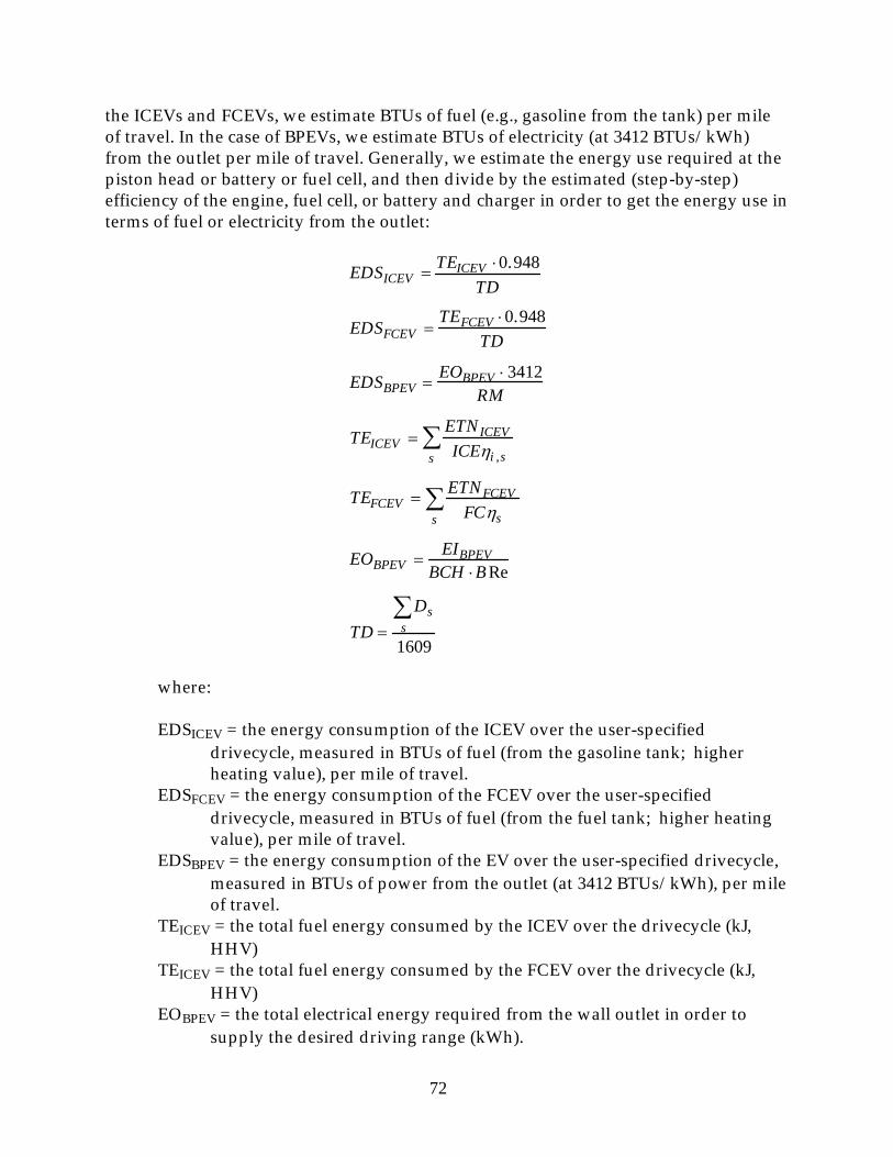
72

the ICEVs and FCEVs, we estimate BTUs of fuel (e.g., gasoline from the tank) per mile of travel. In the case of BPEVs, we estimate BTUs of electricity (at 3412 BTUs/kWh) from the outlet per mile of travel. Generally, we estimate the energy use required at the piston head or battery or fuel cell, and then divide by the estimated (step-by-step) efficiency of the engine, fuel cell, or battery and charger in order to get the energy use in terms of fuel or electricity from the outlet:

EDSICEV = TEICEV ⋅0.948TD

EDSFCEV =TEFCEV ⋅0.948

TD

EDSBPEV = EOBPEV ⋅ 3412RM

TEICEV =ETNICEV

ICEηi ,ss∑

TEFCEV = ETNFCEV

FCηss∑

EOBPEV = EIBPEVBCH ⋅B Re

TD =Ds

s∑1609

where:

EDSICEV = the energy consumption of the ICEV over the user-specified drivecycle, measured in BTUs of fuel (from the gasoline tank; higher heating value), per mile of travel.

EDSFCEV = the energy consumption of the FCEV over the user-specified drivecycle, measured in BTUs of fuel (from the fuel tank; higher heating value), per mile of travel.

EDSBPEV = the energy consumption of the EV over the user-specified drivecycle, measured in BTUs of power from the outlet (at 3412 BTUs/kWh), per mile of travel.

TEICEV = the total fuel energy consumed by the ICEV over the drivecycle (kJ, HHV)

TEICEV = the total fuel energy consumed by the FCEV over the drivecycle (kJ, HHV)

EOBPEV = the total electrical energy required from the wall outlet in order to supply the desired driving range (kWh).

73

TD = the total distance of the drivecycle (miles)RM = the total required driving range of the EV (miles) (a user input variable).3412 = BTUs/kWh.0.948 = BTU/kJ. ETNICEV,s = net energy at the piston head in the ICEV, required for each segment

S of the drivecycle (kJ). This is calculated below. ETNFCEV,s = net energy at the outgoing terminals of the fuel cell in the EV,

required for each segment S of the drivecycle (kJ). This is calculated below.

ICEηi.s = the indicated energy conversion efficiency of the engine, also known as the thermal efficiency (BTUs-work on the piston head/BTU-fuel consumed [higher heating value]), in each segment S of the drive cycle. This is calculated below.

FCηs = the net energy conversion efficiency of the complete fuel-cell system, including any reformer (BTUs-electric at fuel-cell terminal [net of fuel cell auxiliaries]/BTUs-fuel-from tank [HHV]), in each segment S of the drive cycle. This efficiency is calculated in a detailed fuel-cell energy-use submodel, which includes a polarity plot for the fuel cell.

EIBPEV = what we will designate as the “interior” capacity of the battery, or the potential at the electrodes, required to provide the desired driving range over the actual drivecycle selected(kWh). It is an arbitrary construct, equal in essence to the net energy outgoing at the terminals divided by the discharge efficiency. This is discussed below.

BRe = the efficiency of the battery recharger (energy into battery/energy from outlet). Data reviewed in DeLuchi (1992) indicate that conductive charging in general is about 90% efficient. Gage (2000b) confirms that integrated on-board conductive chargers also are about 90% efficient.

BCH = the efficiency of battery charging (see Appendix A).Ds = the distance of the segment S of the drivecycle (meters). This is calculated

from the user-input velocity and time for the segment. 1609 = meters/mile.

Σs = summation over all segments of the drivecycle.

Vehicular fuel economy. Given the energy consumption in BTUs/mi, it is a straightforward matter to calculate the fuel economy in either mi/106 BTU or miles per gasoline-equivalent gallon:

FE=1000000

EDS

MPGeq = FE ⋅ECG

where:

74

EDS is defined above FE = the fuel economy ( mi/106 BTU)1000000 = BTUs/106 BTU. MPGeq = miles per gasoline-equivalent gallon fuel economyECG = the energy content of conventional gasoline (0.125.106 BTU/gallon-

gasoline)

The efficiency of the EV powertrain relative to the efficiency of the ICEV powertrain. The efficiency of the EV powertrain relative to the efficiency of the ICEV powertrain is an overall result that can be used in energy, economic, and environmental comparisons of EVs and ICEVs. For example, the relative powertrain efficiency is input into the greenhouse-gas emissions model of DeLuchi (1991). Note that the relative efficiency does not account for the efficiency of the battery, battery charger or fuel cell (these are accounted for separately in DeLuchi [1991] and here as well), but does account for the thermal efficiency of the ICEV. The objective of the relative powertrain efficiency measure is to relate the efficiency of the electric driveline to the known overall fuel economy of the ICEV, with the efficiency of the battery and fuel cell then being estimated separately.

The relative powertrain efficiency is calculated as:

Re p =FEPEV

FEICEV

FEPBPEV = FEBPEVBRe⋅BCH ⋅BDCH

FEPFCEV =FEFCEV

FCη

BDCH =∆EIBPEV ,s ⋅BDCHs

s∑

∆EIBPEV ,ss∑

∆EIBPEV,s = EIBPEV ,s−1 − EIBPEV ,s

where:

Rep = the BTU/mile energy consumption of the EV powertrain relative to the BTU/mile energy consumption of the gasoline ICEV powertrain, over the user-specified drivecycle. Note that EV powertrain does not include the battery, fuel-cell, or battery charger.

75

FEP = the fuel economy of the powertrain (mi/106-BTU from the battery or fuel terminals, in the case of the BPEV or FCEV, and mi/106-BTU fuel in the case of the ICEV).

BDCH = the overall battery discharge efficiency.FCη = the overall (drive-cycle average) net energy conversion efficiency of the

complete fuel-cell system, including any reformer (BTUs-electric at fuel-cell terminal [net of fuel cell auxiliaries]/BTUs-fuel-from tank [HHV]). This is equal to net energy from the fuel cell system divided by total fuel energy input, over the entire drivecycle.

BDCHs = the battery discharge efficiency during segment S of the drivecycle. This is calculated on the basis of the battery resistance and voltage, which in turn are a function of the depth of discharge. See Appendix A.

•EIBPEV,S = the change in what we have designated the “interior” capacity of the battery (see above).

FE, BRe, BCH, and EIBPEV are as defined above.

The model presently estimates an Rep of about 8. Note that the Rep here is not quite the same as the relative powertrain efficiency

used in DeLuchi (1991). In that report, the relative efficiency was exclusive of the effect of any difference in weight between the EV and the ICEV. Here, Rep is inclusive of the effect of all vehicle attributes: weight, drag, rolling resistance, and so on.

Average and maximum speed (miles/hour) over the drivecycle. The calculated average speed (including stop time) for the base-case drivecycle is about 20 mph, and the maximum speed is 57 mph.

Vehicle weight. The results tables show the estimated weights of the Ford Taurus and Ford Escort. The curb weight is the weight of the empty vehicle, but with a full fuel tank in the ICEV or fuel-cell EV. The in-use weight includes 180 pounds of people and cargo, but only a 40% full fuel tank. For reference, the 1991 Escort has a curb weight of 2364 lbs, and the 1991 Taurus a curb weight of 2991 lbs (Allison Gas Turbine Division, 1994).

CALCULATION OF PARAMETER VALUES IN THE D RIVECYCLE ENERGY CONSUMPTION MODEL

Indicated thermal efficiencyThe indicated thermal efficiency is the ratio of the work on the piston head to the

energy content (higher heating value, in our analysis) of the fuel input. Wu and Ross (1999) have provided a useful, simple model of the indicated thermal efficiency as a function of engine parameters that we can specify.

The thermal efficiency depends on a number of parameters, including:

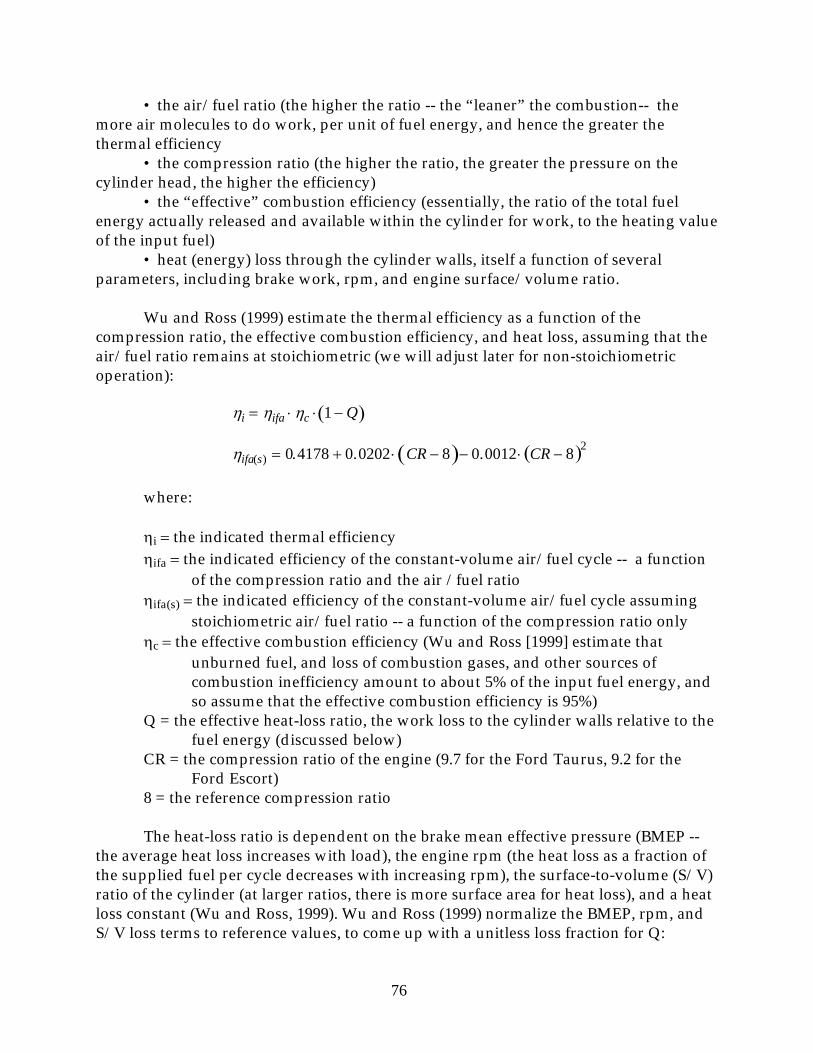
76

• the air/fuel ratio (the higher the ratio -- the “leaner” the combustion -- the more air molecules to do work, per unit of fuel energy, and hence the greater the thermal efficiency

• the compression ratio (the higher the ratio, the greater the pressure on the cylinder head, the higher the efficiency)

• the “effective” combustion efficiency (essentially, the ratio of the total fuel energy actually released and available within the cylinder for work, to the heating value of the input fuel)

• heat (energy) loss through the cylinder walls, itself a function of several parameters, including brake work, rpm, and engine surface/volume ratio.

Wu and Ross (1999) estimate the thermal efficiency as a function of the compression ratio, the effective combustion efficiency, and heat loss, assuming that the air/fuel ratio remains at stoichiometric (we will adjust later for non-stoichiometric operation):

ηi = ηifa ⋅ ηc ⋅ 1−Q( )

ηifa(s) = 0.4178 + 0.0202 ⋅ CR − 8( )− 0.0012 ⋅ CR − 8( )2

where:

ηi = the indicated thermal efficiencyηifa = the indicated efficiency of the constant-volume air/fuel cycle -- a function

of the compression ratio and the air /fuel ratioηifa(s) = the indicated efficiency of the constant-volume air/fuel cycle assuming

stoichiometric air/fuel ratio -- a function of the compression ratio onlyηc = the effective combustion efficiency (Wu and Ross [1999] estimate that

unburned fuel, and loss of combustion gases, and other sources of combustion inefficiency amount to about 5% of the input fuel energy, and so assume that the effective combustion efficiency is 95%)

Q = the effective heat-loss ratio, the work loss to the cylinder walls relative to the fuel energy (discussed below)

CR = the compression ratio of the engine (9.7 for the Ford Taurus, 9.2 for the Ford Escort)

8 = the reference compression ratio

The heat-loss ratio is dependent on the brake mean effective pressure (BMEP --the average heat loss increases with load), the engine rpm (the heat loss as a fraction of the supplied fuel per cycle decreases with increasing rpm), the surface-to-volume (S/V) ratio of the cylinder (at larger ratios, there is more surface area for heat loss), and a heat loss constant (Wu and Ross, 1999). Wu and Ross (1999) normalize the BMEP, rpm, and S/V loss terms to reference values, to come up with a unitless loss fraction for Q:

77

Q = 0.13 ⋅350

150 + BMEP

β⋅

1800RPM

α⋅

SVRTDC

2.5

γ

where:

0.13 = the heat loss constant350 = typical (reference) indicated mean effective pressure (kPa)BMEP = brake mean effective pressure (kPa)1800 = reference rpmRPM = actual rpm of the engineSVRTDC = the surface-to-volume ratio of the engine at top-dead-center2.5 = the reference S/V, corresponding to that of engine with 2 cylinders per liter

displacement

Wu and Ross (1999) find that the best fits to test data are achieved with β = 0.2, α= 0.5, and γ = 1.0. We adopt those values here. However, in place of the ratio of S/V (which we don’t know) to the reference S/V of 2.5, we use the ratio of the cylinder per liter (CPL) displacement (which we do know) to the reference value of 2 CPL. As regards the BMEP, we assume that at the “typical” drivecycle-value of 200 kPa (Wu and Ross, 1999), the brake power is 10 kW. Thus, we assume that SVR/2.5 = CPL/2, and that BMEP = 200.brake power/10:

Q = 0.13 ⋅350

150 +20010

⋅Pc

0.2

⋅1800RPM

0.5

⋅CPL

2

where:

abs[Pc] = the absolute value of the power at the crankshaft (kW; estimated in the section “Power at engine crankshaft or fuel-cell or battery terminals”)

CPL = cylinders per liter (2.0 for the Taurus, 2.0 for the Escort)

Note that Wu and Ross (1999) estimate the efficiency with respect to the lower heating value; we divide by 1.093 to get the efficiency with respect to the higher heating value.

Adjustment for lean or rich combustion. As noted above, the Wu and Ross (1999) model applies to stoichiometric air-fuel ratios. Modern vehicles are designed to operate at stoichiometry almost all of the time, because the 3-way catalytic converter does not function properly if there is too little or too much air in the exhaust gas. However, under hard accelerations, the engine controller “commands” enrichment of the fuel/air ratio, in order to provide extra power. This enriched fuel/air mixture reduces the thermal efficiency of the engine and increases emissions of unburned fuel.

78

Ross (1997) says that to a “fairly good approximation,” the ratio of ηifa at the actual instantaneous equivalence ratio Φ to ηifa at stoichiometry (Φ =1.0; ηifa(s)) is:

ηifa

ηifa(s)= 4 − Φ

3

Hence:

ηifa =4 − Φ

3⋅ ηifa(s)

We need, finally, to determine the air/fuel ratio as a function of some parameter that we measure second-by-second. Thomas and Ross (1997) cite an analysis of second-by-second fuel use and emissions data from the FTP revision project which concludes that:

Φ = 1 for FR < 2.7 g/ s

Φ = 1+ 0.036 ⋅ FR for FR ≥ 2.7 g/ s

where FR is the fuel rate in grams/sec. In our model, the fuel rate can be calculated from the power required at the piston head, in kJ/sec:

FR =ETNICEV /Ts

0.34 ⋅ kJg

where:

ETNICEV = total net energy at the piston head, required for each segment of the drivecycle (kJ) (discussed below).

Ts = the duration of the segment (seconds).0.34 = the assumed indicated efficiency (HHV basis) for the purpose of

calculating the fuel rate (ratio of work energy to fuel energy).kJg = the energy content of the fuel (kJ/g) (about 46).

We calculate the indicated efficiency for each segment of the drive cycle.

Total net energy required for each segment of drivecycle (kJ at engine piston head or fuel -cell terminals)

For each segment of the drive cycle, we calculate the indicated energy from the ICE piston heads, or the energy from the fuel cell terminals (omitting the subscript S for convenience):

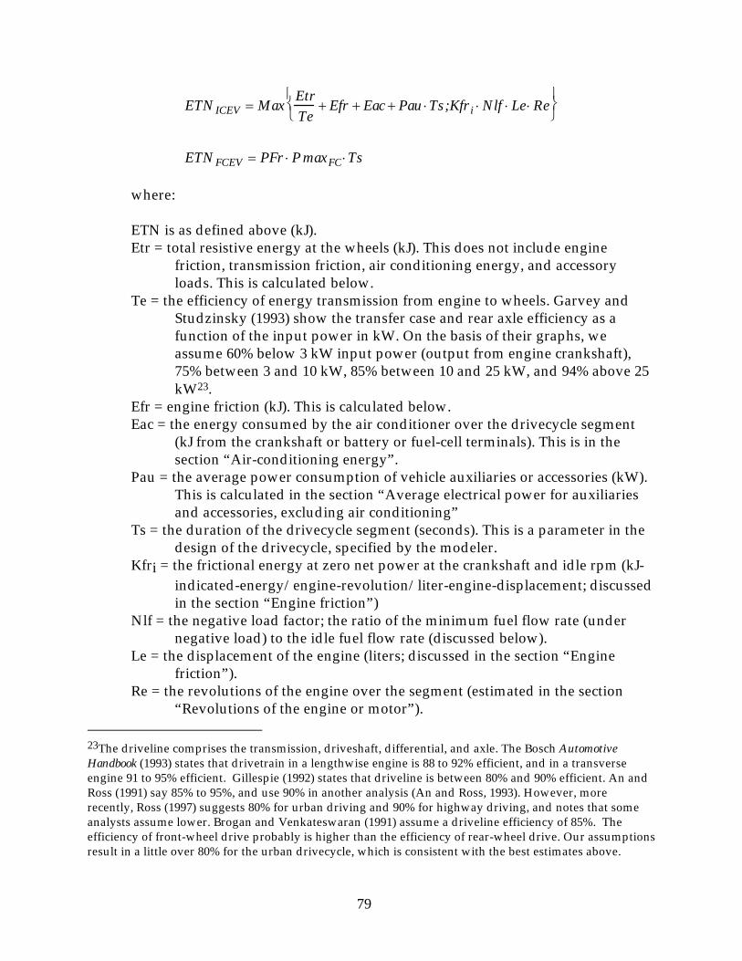
79

ETNICEV = MaxEtrTe

+ Efr + Eac + Pau ⋅Ts;Kfri ⋅Nlf ⋅ Le ⋅Re

ETNFCEV = PFr ⋅P maxFC ⋅Ts

where:

ETN is as defined above (kJ). Etr = total resistive energy at the wheels (kJ). This does not include engine

friction, transmission friction, air conditioning energy, and accessory loads. This is calculated below.

Te = the efficiency of energy transmission from engine to wheels. Garvey and Studzinsky (1993) show the transfer case and rear axle efficiency as a function of the input power in kW. On the basis of their graphs, we assume 60% below 3 kW input power (output from engine crankshaft), 75% between 3 and 10 kW, 85% between 10 and 25 kW, and 94% above 25 kW23.

Efr = engine friction (kJ). This is calculated below. Eac = the energy consumed by the air conditioner over the drivecycle segment

(kJ from the crankshaft or battery or fuel-cell terminals). This is in the section “Air-conditioning energy”.

Pau = the average power consumption of vehicle auxiliaries or accessories (kW). This is calculated in the section “Average electrical power for auxiliaries and accessories, excluding air conditioning”

Ts = the duration of the drivecycle segment (seconds). This is a parameter in the design of the drivecycle, specified by the modeler.

Kfri = the frictional energy at zero net power at the crankshaft and idle rpm (kJ-indicated-energy/engine-revolution/liter-engine-displacement; discussed in the section “Engine friction”)

Nlf = the negative load factor; the ratio of the minimum fuel flow rate (under negative load) to the idle fuel flow rate (discussed below).

Le = the displacement of the engine (liters; discussed in the section “Engine friction”).

Re = the revolutions of the engine over the segment (estimated in the section “Revolutions of the engine or motor”).

23The driveline comprises the transmission, driveshaft, differential, and axle. The Bosch Automotive Handbook (1993) states that drivetrain in a lengthwise engine is 88 to 92% efficient, and in a transverse engine 91 to 95% efficient. Gillespie (1992) states that driveline is between 80% and 90% efficient. An and Ross (1991) say 85% to 95%, and use 90% in another analysis (An and Ross, 1993). However, more recently, Ross (1997) suggests 80% for urban driving and 90% for highway driving, and notes that some analysts assume lower. Brogan and Venkateswaran (1991) assume a driveline efficiency of 85%. The efficiency of front-wheel drive probably is higher than the efficiency of rear-wheel drive. Our assumptions result in a little over 80% for the urban drivecycle, which is consistent with the best estimates above.

80

PFr = the net power required from the fuel cell, as a fraction of the maximum gross power (discussed below).

PmaxFC = the maximum gross power of the fuel cell (kW). This is input by the user, or calculated readily from user inputs.

The term Etr, the load at the wheels, can be negative. When it is, energy is potentially available to do useful work, or for storage. In the case of the ICEV, this negative energy at the wheels can drive the crankshaft and thereby power the alternator and overcome engine friction24. However, we assume that in the ICEV, this energy cannot be stored, which means that if the available [negative] energy at the wheels exceeds the work to be done by powering the alternator or overcoming engine friction, the excess is dissipated uselessly in the brakes. In the model, this condition is created by requiring that the indicated energy at the piston head not be less than the minimum fuel flow rate (the second term in the “maximum” quantities in the brackets { } ).

If an EV has an energy storage device, it can recapture the regenerative braking energy. We discuss this more shortly.

Energy capacity of the batteryIn the case of the BPEV, as noted above, we calculate the C/3 discharge capacity

of the battery on the basis of the “interior” energy capacity of the battery, and the C/3 discharge efficiency:

ESTBC/ 3 = EI ⋅BDCHC/ 3

where:

ESTBC/3 = the nominal total energy discharge capacity of the new traction battery, measured at the C/3 discharge rate (kWh).

EI = what we will designate as the “interior” capacity of the new battery, based on the actual drivecycle specified (discussed in this section).

BDCHC/3 = the efficiency of a C/3 discharge of the new battery (as opposed to the efficiency of the actual discharge of the battery over the selected drivecycle). This is discussed in Appendix A.

This procedure is necessary because the new battery must be sized to meet the actual loads of the specified drivecycle, which in general will differ from a C/3 load. However, because the “Wh” in the gravimetric energy density (Wh/kg) that we derive as a function of the power density (see discussion above), and the “kWh” in the energy cost figure ($/kWh) that we estimate, both are based on a C/3 discharge, we must

24In a car with a manual transmission, the driver can put in the clutch and de-couple the engine from the wheels, so that the braking energy is not available to do useful work.

81

calculate, for the purpose of using our Wh/kg and $/kWh figures, what the discharge capacity of the battery would be at the C/3 rate.

The “interior” capacity of the battery can be understood as the amount of energy required to meet all of the loads on the vehicle, after accounting for regenerative energy made available, and the actual discharge (but not charging) efficiency of the battery. Put another way, it is equal to the net energy required at the battery terminals for load divided by the actual average discharge efficiency over the test.

Figure 1 shows battery energy flows graphically. Formally, we calculate EI as follows:

EI = abs EIs− final[ ]⋅RMTD

+ abs mins EIs( )− abs EIs− final[ ][ ]where:

EI is defined above“abs” means “absolute value of”EIS-final = the value of EI after the last segment of the trip simulated in the

drivecycle (kJ)RM = the desired total driving range (miles) (input by the user)TD = the trip distance (miles) (estimated in the section “Vehicle energy

consumption: calculated results for the drivecycle”)EIs = the value of EI at segment S (kJ)

This equation is interpreted as follows. First, we multiply the value of EI at the end of the last trip segment by the number of trips that can be taken within the driving range of the vehicle. Now, if there were no regenerative braking, then the resultant EI (the trip EI multiplied by the number of trips per driving range) would be the final EI we wish to calculate. However, because there is regenerative braking, it is possible that, towards the end of the last trip made before the battery is completely exhausted, the battery capacity will be drawn down to a level lower than it is after the last segment of the trip, because of energy returned to the battery during the last braking. To account for this, we add to the trip-scaled EI the difference between the lowest EI in the drivecycle (mins(EIs)) and the EI after the last segment of the drivecycle (abs[EIS-final]).

Next we must calculate EIs, the battery “interior” capacity at each trip segment:

EIs =EIs−1 − Pt ⋅TsBDCHs ⋅ 3600

for power Pt > 0 (under load)

EIs = min 0,EIs−1 − Pt ⋅Ts ⋅BDCHs

3600

for power Pt ≤ 0 (braking)

where:

82

Pt = the power required at the battery terminals (kW) (discussed below).Ts = the duration of the drivecycle segment S (seconds). BDCHs = the battery discharge efficiency during segment S (Appendix A).3600 = seconds per hour.

The “min” [ ] function ensures that the amount of regenerative energy returned to the battery does not exceed the available capacity of the battery.

Power at engine crankshaft or fuel-cell or battery terminalsFor EVs under load, the power required at the fuel cell or battery terminal is

calculated simply as the load on the wheels divided by the powertrain efficiency, plus the accessory and air conditioning power demand. For EVs braking, the regenerative power available at the battery terminals is some fraction of the negative load at the wheels (the fraction depending on the load), reduced by the powertrain efficiency and the accessory and air conditioning power demand:

Pt =Etr

Pe ⋅Ts+ Pac for Etr ε 0 (under load)

Pt =Etr ⋅Pe

Ts⋅ 1+

max −Pco, Etr ⋅PeTs

Pco

+ Pac for Etr < 0 (braking)

Pac =EacTs

+ Pau

where:

Pt = the power required at the battery terminals or fuel-cell terminals (kW)Etr = total resistive energy at the wheels (kJ). This is calculated in the section

“Total resistive energy at the wheels”.Pe = the efficiency of energy transmission from battery or fuel-cell terminals to

wheels. This is calculated in the section “Once − through efficiency from the battery (or other energy-storage system) or fuel − cell to the wheels (excluding storage device itself)”

Ts = the duration of the segment (seconds). This is a parameter in the design of the drivecycle, and so is specified by the modeler.

Pac = the power demand of the accessories and the air conditioner, at the engine crankshaft, or the battery or fuel cell terminals (kW)

83

Eac = the energy required by the air conditioning system over the drivecycle segment (kJ from the crankshaft or battery or fuel-cell terminals). This is calculated in the section “Air-conditioning energy”

Pau = the average power consumption of vehicle auxiliaries or accessories (kW). This is calculated in the section “Average electrical power for auxiliaries and accessories, excluding air conditioning”

Pco = maximum regenerative braking power into energy storage device (kW) (assumed to be 85% of the maximum output power of the battery)

The “max” [ ] term limits the recoverable braking power to the maximum that can be input to the energy storage device.

The treatment of regenerative braking requires some explanation. First, we do not assume that the entire negative load at the wheels drives the electric motor as a generator; rather, we assume only that some fraction does, and that the remainder of the negative load is dissipated in the friction brakes. This is due partly to the need to brake any non-driven wheels, which, on account of their not being connected to the electric motor, must be braked exclusively by friction.

In reality, and in our model, the fraction of the negative load that drives the electric motor as a generator decreases with the braking power. This fraction is given by the “1+” term in parentheses. As the negative load (the term Etr . Pe/Ts) increases, the ratio with Pco increases, and the “1+” term decreases (because the ratio is negative). As the negative load approaches the maximum allowable regenerative power, the fraction of the load that is used to drive the motor as a generator approaches zero. The “max” [ ] term limits the ratio to being no less than -1, and hence limits the “(1+..)” term to no less than zero.

Our treatment of regenerative braking thus is realistic in several respects:

i) the regenerative energy available from the brakes, as a fraction of the braking power, decreases with the braking power;

ii) there is a maximum regenerative braking power, set at some fraction of the maximum battery power;

iii) the regenerative braking energy returned to the battery cannot exceed the available capacity of the battery;

iv) all transfer losses -- transmission, motor, controller, battery discharge (twice) are accounted for by using the actual second-by-second component efficiencies; and

v) the regenerative energy is used to meet the accessory and air conditioning power demand first, before being charged into the battery (this is the most efficient method)25.

25If the accessory and air conditioning power demand exceeds the regenerative power available, and if the vehicle has a fuel cell, we assume that the fuel cell, not the battery, supplies the unmet power demand.

84

For ICEVs, the calculation of the power at the crankshaft (Pc) is essentially the same as for EVs, except that the transmission efficiency substitutes for the powertrain efficiency, and the maximum regenerative braking power is assumed to be zero, because there is no energy storage device.

Total resistive energy at the wheelsThis is simply the sum of the inertial, air-resistance, rolling-resistance, and grade

work terms:

Etr = Ei + Ead + Er+ Egr

where:

Etr = total resistive energy at the wheels (kJ). This does not include engine friction, transmission friction, air conditioning energy, and accessory loads.

Ei = total inertial energy (kJ). This is calculated in the section “Translational and rotational inertial energy”.

Ead = energy required to overcome air resistance (kJ). This is calculated in the section “Air resistance”.

Er = energy required to overcome rolling friction (kJ). This is calculated in the section “Rolling friction”.

Egr = energy required for grade work (kJ). This is calculated in the section “Grade work”.

Translational and rotational inertial energyThe total inertial energy that must be overcome over each segment of the

drivecycle is equal to the translational inertial energy of the vehicle plus the rotational inertial energy of the wheels plus the rotational inertial energy of each of the rotating parts in the motor and transmission:

Ei = Eit +Nw ⋅Eirw+ Eirm

where:

Ei = the total inertial energy over the drivecycle (kJ).Eit = the translational inertial energy over the drivecycle (kJ).Eirw = the rotational inertial energy of one wheel over the drivecycle (kJ). Nw = the number of wheels. We assume four. Eirm = the rotational inertial energy of the motor and transmission over the

drivecycle (kJ).

In this analysis we will treat all of the individual rotating parts of the motor and transmission as a single rotating mass.

85

The translational inertial energy from zero velocity to velocity V is given simply by:

Eit =WIU ⋅V2

2 ⋅1000

where:

Eit = the translational inertial energy over the drivecycle segment (kJ).WIU = the in-use weight of the vehicle, including the wheels and the passenger

and payload (kg). This is calculated in the section “Total weight and manufacturing cost”.

V = the velocity of the vehicle (m/s). This term eventually will drop out of the formula.

1000 = J/kJ (a Joule is a Newton-meter, or 1 kg m2 s-2).

The rotational inertial energy of a wheel (Eirw) is derived as follows.

Eirw = I ⋅ω2

2 ⋅ 1000

I = Mw ⋅Rt2

2(for a solid cylinder of uniform density)

ω =VRt

and thus:

Eirw = Mw ⋅V 2

4 ⋅1000

where:

Eirw = the rotational inertial energy of one wheel over the drivecycle (kJ). 1000 = J/kJ.I = the rotational inertia of the wheel.ω = the angular velocity of the wheel.Mw = the mass of one wheel (kg)V = the translational velocity of the vehicle (m/s). Rt = the radius of the wheel-plus-tire (discussed in the section “Revolutions of

the engine or motor”)

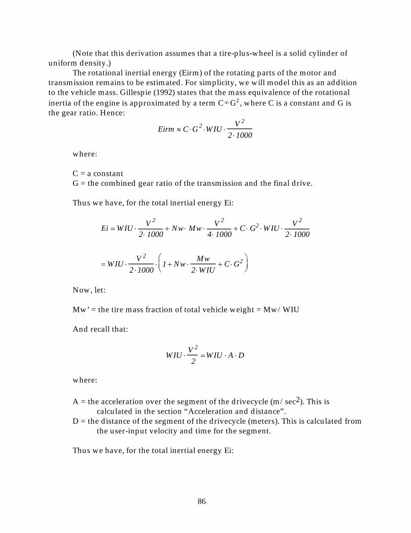
86

(Note that this derivation assumes that a tire-plus-wheel is a solid cylinder of uniform density.)

The rotational inertial energy (Eirm) of the rotating parts of the motor and transmission remains to be estimated. For simplicity, we will model this as an addition to the vehicle mass. Gillespie (1992) states that the mass equivalence of the rotational inertia of the engine is approximated by a term C ∞ G2 , where C is a constant and G is the gear ratio. Hence:

Eirm ≈C ⋅G 2 ⋅WIU ⋅V 2

2 ⋅1000

where:

C = a constantG = the combined gear ratio of the transmission and the final drive.

Thus we have, for the total inertial energy Ei:

Ei =WIU ⋅ V 2

2 ⋅ 1000+ Nw ⋅ Mw ⋅ V 2

4 ⋅ 1000+ C ⋅G2 ⋅WIU ⋅ V2

2 ⋅ 1000

=WIU ⋅V2

2 ⋅1000⋅ 1+Nw ⋅

Mw2 ⋅WIU

+ C ⋅G2

Now, let:

Mw’ = the tire mass fraction of total vehicle weight = Mw/WIU

And recall that:

WIU ⋅V2

2=WIU ⋅A ⋅D

where:

A = the acceleration over the segment of the drivecycle (m/sec2). This is calculated in the section “Acceleration and distance”.

D = the distance of the segment of the drivecycle (meters). This is calculated from the user-input velocity and time for the segment.

Thus we have, for the total inertial energy Ei:

87

Ei =WIU ⋅A ⋅D1000

⋅ 1+Nw ⋅Mw'

2+ C ⋅G2

where:

Ei = total inertial energy over the segment of the drivecycle (kJ)WIU = the in-use weight of the vehicle (kg). This is calculated in the section

“Total weight and manufacturing cost”. A = the acceleration over the segment of the drivecycle (m/sec2). This is

calculated below. D = the distance driven over the segment of the drivecycle (meters). Nw = the number of wheels. We assume four.Mw’ = the ratio of the weight of one wheel to the in-use weight of the vehicle.

We assume that each tire on the ICEV Taurus weighs 38 lbs (ACEEE, 1990), that each tire on the ICEV Escort weighs 36 lbs (ACEEE, 1990), and that the tires on the EVs weigh 10% less than the tires on the gasoline ICEV.

C = constant: the mass factor for rotating engine and transmission parts. This is discussed next.

G = the combined ratio of the transmission and the final gear. This is calculated from a look-up table that has the total gear ratio in each gear and a gear-shifting schedule as a function of vehicle speed. See the discussion in the section “Revolutions of the engine or motor”.

Mass factor for rotating motor and transmission parts (rotational inertia). Rather than calculate the actual rotational inertia of all of the rotating parts of an ICEV, we approximate the rotational inertia with an equivalent “mass factor”, which is multiplied by the total gear ratio and then added to the actual vehicle mass term in the calculation of total inertia. (In essence, we scale up vehicle mass by a small fraction in order to account for rotational inertia.) According to a 1972 source cited by Gillespie (1992), a typical mass factor is 0.0025. We assume that the factor for present and near-future vehicles is slightly lower, 0.0020.

The total rotational inertia, and hence the total equivalent mass factor, depends on the number and mass of rotating parts. An electric vehicle has far fewer rotating parts than does an ICEV, and hence a much lower rotational inertia. Lesster et al. (1993) remark that “the electric powertrain with its single speed reducer has a much lower inertia compared with the internal combustion engine running in its low gears” (p. 171). (The only significant rotating parts in an EV are the electric motor itself, the transmission gears, and the drive axles.) Consequently, we assume that the mass factor that represents the rotational inertia of an EV is 1/4th of the factor for an ICEV, or 0.0005.

88

Air resistanceThe air resistance work is a function of the air density, vehicle velocity, and

vehicle frontal area and drag:

Ead = 0.5 ⋅ ρair ,Y ⋅Cd ⋅Fa ⋅D ⋅Vb +Vw( )⋅ abs Vb +Vw[ ]+ Ve +Vw( )⋅ abs Ve +Vw[ ]

2 ⋅ 1000

where:

Ead = the energy required to overcome the resistance of the air (kJ). ρair,Y = the density of dry air at pressure PY (at elevation Y) and temperature

TEair (grams/liter or kg/m3). This is calculated below.Cd = coefficient of drag (dimensionless). The 1991 Ford Taurus and the 1991 Ford

Escort have a Cd of 0.34 (Allison Gas Turbine Division, 1994). According to Ross (1997), the 1995 Taurus has a Cd of 0.33. We assume that these values can be reduced economically. We assume that the Cd of the EV versions will be reduced even further, because of the greater importance of conserving energy in an EV than in ICEV. Our assumptions are shown below. As discussed in the section “Adjustments to the 1989 weight and cost baseline”, we also assume slightly higher cost for the lower Cd.

Fa = vehicle frontal area (meters2). The 1991 Ford Taurus has a frontal area of 1.99 m2, and the 1991 Ford Escort has a frontal area of 1.86 m2 (Allison Gas Turbine Division, 1994). According to Ross (1997), the 1995 Taurus has a frontal area of 2.12 m2. Our assumptions our shown below. We assume slightly lower values for the EVs, again because of the great importance of energy conservation in EVs26.

Taurus Escort

ICEV EV ICEV EV

Drag (Cd) 0.30 0.24 0.30 0.24

Frontal area (Fa) 2.00 1.95 1.85 1.80

D = the distance of the segment of the drivecycle (meters). This is calculated from the user-input velocity and time for the segment.

Vb = the velocity at the beginning of the segment of the drivecycle (m/sec). This is a parameter in the design of the drivecycle, and is specified by the modeler.

26We presume that the battery pack is placed so that the vehicle frontal area does not have to be increased to accommodate the pack.

89

Vw = the velocity of the wind during the trip segment, along the direction of vehicle travel (m/sec). This is a parameter in the design of the drivecycle, and is specified by the modeler. A tailwind is entered as a negative value (i.e., is equivalent to a decrease in vehicle speed), and a headwind is entered as a positive value (i.e., is equivalent to an increase in vehicle speed).

Ve = the velocity at the ending of the segment of the drivecycle (m/sec). This is a parameter in the design of the drivecycle, and is specified by the modeler.

abs = absolute value1000 = J/kJ

Calculated density of air (kg/m3). The density of the air depends on the temperature and the pressure, which in turn depends on the elevation. In this section we will derive an expression for air density as a function of temperature and elevation. We begin with the definition of density (ρ)

ρ ≡MV

where:

M = the mass of the air (g or kg)V = the volume of the air (liters or m3)

Ambient air is close to an ideal gas, so we can use the ideal gas law to find the ratio M/V:

PY ⋅V = n ⋅R ⋅TEair

n =M

MW air

where:

PY = the air pressure, a function of altitude Y (atmospheres). M = the mass of the air (g)V= the volume of the sample of air (liters).n = the number of moles in the sample of air. R = the gas constant (0.08206 liter-atm/mole- K).TEair = the ambient air temperature (oK). In our base case we will assume 68o F.M = the mass of the sample of air (grams). MWair = the molecular weight of air (grams/mole).

90

Thus we have:

PY ⋅V = MMW air

⋅ 0.08206 ⋅TEair

PY ⋅MW air

0.08206 ⋅TEair=

MV

≡ ρair,Y

The average molecular weight of air can be calculated from the composition of air and molecular weight of the constituents:

MW air = 0.7808 ⋅ 28.02 + 0.2095 ⋅ 32.00+ 0.0093 ⋅ 39.95 = 28.95 g / mole

where:

0.7808 = the nitrogen molar fraction of dry air. 28.02 = the molecular weight of N2.0.2095 = the oxygen molar fraction of dry air.32.00 = the molecular weight of O2.0.0093 = the argon molar fraction of dry air.39.95 = the molecular weight of argon.

With this, and assuming that the temperature will be input in degrees Fahrenheit (oF) (and converted in the model to degrees Kelvin) we have:

ρair,Y =PY ⋅ 28.95

0.08206 ⋅TEair

oF( )+ 459.67

1.8

What remains is to find an expression for pressure, PY, in terms of the standard atmosphere at sea level, and the elevation Y above sea level. Assuming that the density of air is proportional to the pressure, and that the gravitational acceleration does not vary with altitude (at least, not up to altitudes that cars can reach), then from the physics of air pressure one can derive the following (see any physics textbook):

PY = P0 ⋅ e−g⋅

ρair ,0

P0

⋅Y

where:

PY = pressure of air at elevation Y meters above sea level (atmospheres).

91

Po = U.S. standard atmosphere at sea level (1 atmosphere or 1.01325 ∞ 105

Pascals). g = the gravitational constant (9.807 m/sec2). ρair,0 = the density of air at the conditions of the standard atmosphere, Po

(kg/m3). According to Lutgens and Tarbuck (1995), the standard atmosphere at sea level is defined at 15oC (59oF). We input this temperature (59oF) and a pressure of 1 atmosphere into the equation for density, above (derived from the ideal gas law), and calculate that the density of dry air at sea level and 15oC is 1.2245 kg/m3.

Y = the elevation (m). In our base case we assume 60m (about 200 ft.).

The term in the exponent, −g ⋅ρair ,0

P0

, reduces to 0.0001185 meters-1 (for Po =

1.01325 ∞ 105 Pascals, the unit that must be used in the exponent). With this reduction, and given that Po in atmospheres is equal to 1.0 atm, and inputting the height Y in feet rather than meters, we have:

PY = e−0.0001185⋅Y ft⋅0.3048( )

where:

0.3048 = meters/foot.

And finally:

ρair,Y =e−0.0001185⋅Y ft⋅0.3048( ) ⋅ 28.95

0.08206 ⋅TEair

oF( )+ 459.67

1.8

Rolling frictionThe rolling resistance work is the vector product of the frictional force and the

distance over which the force operates. The frictional force is a function of the mass, the gravitational acceleration, the grade (i.e., the angle of the road with respect to the gravity vector), the coefficient of friction between the tires and the road, the temperature, and other factors. Formally:

Er =WIU ⋅ 9.81 ⋅ cos Gd ⋅0.01745[ ]⋅D ⋅Cr

1000

where:

92

Er = the energy required to overcome the rolling friction (kJ). WIU = the in-use weight of the vehicle (kg). This is calculated in the section

“Total weight and total manufacturing cost”.9.81 = gravitational acceleration (m/sec2). We assume that this is the same

everywhere on the earth. Gd = the slope of the grade (degrees). This is a parameter in the design of the

drivecycle, and so is specified by the modeler. 0.01745 = radians/degree. D = the distance of the segment of the drivecycle (meters). This is calculated from

the user-input velocity and time for the segment. 1000 = joules/kJ. Cr = the coefficient of rolling friction (dimensionless; discussed next).

Coefficient of rolling friction. The coefficient of friction is a function of the tire characteristics, vehicle speed, road characteristics, and temperature. On the basis of Gillespie (1992), we estimate the following equation for Cr:

Cr = Crf + Crv ⋅ 3.24 ⋅

Vb100

2.5

+ Ve100

2.5

2

⋅CrROAD ⋅CrTEMP

where:

Crf = the speed-independent (or fixed) rolling-resistance coefficient. (See discussion of Crv.)

Crv = the speed-dependent rolling-resistance coefficient. Gillespie (1992) presents a graph that shows Crf and Crv as a function of tire pressure. We estimated the coefficients at an inflation pressure of 36 psi, then reduced them by 15% to account for modest improvements ICEVs. We assume that coefficients for EVs are almost 10% lower than the [reduced] coefficients for ICEVs. The results of this estimation are:

ICEVs EVs

Crf 0.0075 0.0070

Crv 0.0025 0.0023

By comparison, Ross (1997) estimates that an overall Crf for the 1995 Ford Taurus is 0.009.

Ve = the velocity at the end of the segment (mph). This is a parameter in the design of the drivecycle, and so is specified by the modeler.

93

Vb = the velocity at the beginning of the segment (mph). This is a parameter in the design of the drivecycle, and so is specified by the modeler.

CrROAD = the ratio of the average road friction on the surface of interest to the average road friction on a concrete surface. The original equation in Gillespie (1992) applies to concrete surfaces; we have added the variable CrROAD, the road-surface coefficient, to be able to estimate Cr for any surface. (CrROAD of course is 1.0 for concrete surfaces.) According to Gillespie (1992), the friction of a worn concrete, brick, or cold asphalt road is 20% higher than the friction of a smooth concrete road, and the friction of a hot asphalt road 50% higher. In our base case, we assume a surface with 35% greater friction than has concrete, so that CrROAD = 1.35.

CrTEMP = temperature adjustment to the coefficient of rolling resistance (discussed next).

Effect of temperature on rolling resistance. Gillespie (1992) and Ellis (1994) show that the rolling resistance of tires increases substantially with decreasing temperature. Gillespie (1992) shows a graph in which the rolling resistance drops by about 15% as the tire warms by about 40o F, and remarks that because of this, “it is therefore common to warm up the tire for 20 minutes or more before taking measurements..” (p. 112). Ellis (1994) shows a graph of the source of energy loss in the GM Impact EV, as a function of the ambient temperature, at a speed of 55 mph. The energy losses attributable to tires at an ambient temperature of 20o F are about twice the losses at 70o F. (Presumably, the effect of temperature is less at lower speeds.)

On the basis of the Gillespie’s (1992) remark, quoted above, we assume first that all of the parameters in the rolling-resistance equation pertain to 80oF, and then adjust the calculated rolling resistance according to the difference between the assumed ambient temperature and 80oF. The following functional form gives reasonable adjustment factors for ambient temperatures from -20o F to 120oF.

CrTemp =80+ 100

TEair + 100

where:

80 = the reference air temperature (o F), pertaining, we assume, to the parameter values in our rolling-resistance equation

TEair = the assumed ambient air temperature (68o F in our base case)

Grade workThe amount of energy required to lift a vehicle up a grade depends of course on

the angle and length of the grade and the weight of the vehicle:

94

Egr =WIU ⋅ 9.81 ⋅ sin Gd ⋅0.01745[ ]⋅D

1000

where:

Egr = the energy required to lift the vehicle up the grade (kJ)WIU = the in-use weight of the vehicle (kg). This is calculated in the section

“Total weight and total manufacturing cost”.9.81 = gravitational acceleration (m/sec2). We assume that this is the same

everywhere on the earth. Gd = the slope of the grade (degrees). This is a parameter in the design of the

drivecycle, and so is specified by the modeler. 0.01745 = radians/degree.D = the distance of the segment of the drivecycle (meters). This is calculated from

the user-input velocity and time for the segment. 1000 = joules/kJ.

Engine frictionIt is convenient analytically to define three kinds of “sinks” of fuel energy in an

ICEV. In temporal order, the first is combustion heat lost to non-working parts of the engine and eventually to the atmosphere27. This is the difference between the higher heating value28 of the fuel, and the work (called “indicated” work) done on the piston head. Next is energy lost to engine friction. This is the difference between indicated work at the piston head, and brake work as measured at the crankshaft. Finally, energy at the crankshaft applies to inertial and frictional loads on the vehicle. In the composite U. S. driving cycle, the combustion loss is the largest, and the friction loss the second largest (Ross, 1997).

In this section we explain how we estimate the second component, the engine friction loss. The engine friction depends on many factors (Wu and Ross, 1999; Patton et al., 1989), including several, such as intake manifold pressure, that we cannot model easily. We adopt the simple models of Ross (1999, 1997, 1994b) and Thomas and Ross (1997), in which engine friction is a function of the displacement of the engine, the temperature of the engine, the load, and the rpm:

27A minor amount of fuel evaporates from the fuel tank , fuel lines, and engine, and a minor amount is not completely burned in the engine and is emitted as unburned fuel. These losses, however, are only about 1% of the total fuel energy put into the gasoline tank.

28It matters not whether the higher or the lower heating value is used, so long as the choice is maintained throughout the analysis. (The higher heating value includes the latent heat released upon the condensation of the water-vapor product of combustion. The lower heating value does not.).

95

Efr = Le ⋅Re⋅Kfr

Kfr = Kfro ⋅Cfr ⋅Rfr ⋅Lfr

Cfr = 1+W 1

Rfr = 1 + α ⋅RPM

60− 20

2

Lfr = 1 +Kfr 'Kfro

⋅Pc ⋅Ts

Re⋅ Le

α = 0.01 if RPM < 1200

α = 0.0001 if RPM > 1200

where:

Efr = the engine friction loss, at the piston head (kJ-indicated-energy) Le = the displacement of the engine (liters). The Taurus has a displacement of 3. 0

liters; the recent model-year Escort, 2.0 liters. Re = the revolutions of the engine. This is estimated in the section “Revolutions

of the engine or motor”.Kfr = the frictional loss per liter displacement per revolution (kJ-indicated-

energy/engine-revolution/liter-engine-displacement)Kfro = the frictional loss per liter per revolution at a reference rpm (1200),

temperature (“warmed up”), and engine load (zero). As explained below, we assume 0.074 kJ-indicated energy/rev/l.

Cfr = the adjustment factor for cold enginesRfr = the adjustment factor for the difference between the actual rpm and the

reference value of 1200Lfr = the adjustment factor for the difference between the actual load and the

reference value of zeroW1 = fractional increase in friction when engine is cold. We follow Ross (1997)

and assume that when the engine is cold, the frictional loss is 7% greater than when the engine is warmed up. We assume that the engine takes 3 minutes to warm up. Thus, for the first 180 seconds, W1 = 0.07; thereafter, W1 = 0.0.

RPM = engine revolutions per minute (calculated by dividing the number of revolutions over a segment by the duration of the segment in minutes)

Kfr’ = the change in frictional energy per change in power output at crankshaft power. (kJ-indicated-energy/kJ-crankshaft). As explained below, we assume 0.057 kJ-indicated energy/kJ-crankshaft.

Pc = the power required at the crankshaft (kW [kJ/s]). This is estimated in the section “Power at engine crankshaft or fuel-cell or battery terminals”.

96

Ts = the time of the segment (seconds). This is a parameter in the design of the drivecycle, and so is specified by the modeler.

In this model, the engine friction tends to increase with any change in rpm away from 1200, and tends to decrease with any increase in brake power, on account of the reduction in air “pumping” friction. The RPM-dependence terms are from Thomas and Ross (1997), and the load-dependence terms, discussed next, are from Ross’s (1994ab analysis of Patton et al. (1989).

Frictional loss per liter per revolution, reference value. Thomas and Ross (1997) assume that Kfro, based on the fuel energy, rather than the indicated energy at the piston head, is 0.24 kJ-fuel [LHV]/rev/l. Ross (1994b) analyzes data from Patton et al. (1989) and assumes a value of 0.22. Ross (1999) states that fits to data from tests on over 300 1990s vehicles indicate that Kfro, in kJ-fuel [LHV]/rev/l, ranges from 0.18 to 0.25. We start here with a value of 0.20, which is within the range reported by Ross (1999), but on the low side, on the assumption that the vehicles that we are modeling have slightly less friction than has the average vehicle.

We must convert from Ross’ units of kJ of fuel energy (lower heating value, LHV) per revolution per liter, to our units of kJ of indicated energy per revolution per liter. According to Ross (1997), the “best” indicated efficiency for conventional engines is 38%. The model of Wu an Ross (1999) produces a range of 34% to 39%, depending on RPM and power, with values typical of most driving falling between 36% and 38% (LHV). We therefore assume that, for the purpose of converting from Ross’ units of kJ-fuel [LHV]/rev/l to our units of kJ-indicated energy/rev/l, the indicated efficiency is 37% (LHV basis). Thus, 0.20 x 0.37 = 0.074 kJ-indicated energy/rev/liter.

Frictional loss as a function of brake power (as a proxy for throttling losses). Ross (1994b) uses data and models from Patton et al. (1989) to graph the relationship between: i) the amount of fuel used to overcome engine friction (in kJ-fuel [LHV]/revolution/liter), and ii) the specific brake power output of the engine (in kJ/revolution/liter). Patton et al. (1989) define friction energy as we do: as the difference between indicated energy at the piston head, and brake energy as measured at the crankshaft. The total engine friction declines with increasing power because the pumping-loss component of the total friction loss decreases as the throttle opens (as power increases) and de-constricts the flow of air (Ross, 1994b; Patton et al., 1989). Ross (1994b) does not present the formula or data points that he derived from Patton et al. (1989) and used to construct his graph. Ross’ graph looks like a straight line; we assume that it is, and estimate the slope (-0.15 kJ-fuel [LHV]/kJ-brake-energy) from his graph. (Although we have the Patton et al. [1989] paper, it is simpler for us to use Ross’s [1994b] analysis of it than to re-do Ross’ [1994b] analysis.)

It appears, however, that the relationship depicted in Ross (1994b) graph combines the effect of changes in rpm (as discussed above) with the effect of changes in pumping loss. Since we have accounted separately for the relationship between changes in rpm and engine friction, we wish here to isolate the relationship between changes in pumping loss (for which change in brake power is our proxy) and engine friction. Given that any change in rpm away from the reference value of 1200 increases the engine

97

friction, we can assume that, in Ross (1994b) graph of brake power vs. friction, the embedded effect of rpm is working to dampen the decrease in friction with increasing power due to reduced pumping loss. Thus, a graph of the relationship between engine friction and brake power at effectively constant rpm presumably would have a steeper slope than does the graph in which the rpm effect works against the pumping-loss effect. We assume a slope of -0.20 kJ-fuel [LHV]/kJ-brake-energy, and multiply this by the indicated efficiency [LHV] of 0.37 to obtain -0.074 kJ-indicated-energy/kJ-brake.

Patton et al. (1989) state that their measurements of engine friction include friction due to the oil pump, the water pump, and the alternator when it is not charging. This implies that our simple linear formulation of engine friction as a function of engine power (from Patton et al. via Ross) does not include work to meet any electrical load at all. Consequently, when calculating energy consumption, we must add to the engine friction the energy required to charge the battery (via the alternator) to meet all electrical loads.

We assume that the engine friction loss equations and parameter values are independent of the type of fuel used in an ICEV.

Comparison of Kfro with idle fuel flow rates. The value of Kfr at zero power and idle rpm can be compared with actual measurements of the fuel flow rate at idle. In Table 7 we show the measured fuel flow rate at idle for several vehicles, and convert the rate to kJ-fuel [LHV]/rev/l for comparison with our estimated Kfr. At zero power and an idle rpm of 750, and with some allowance for the engine being cold during the first few idling intervals, we estimate that Kfr is about 0.33 (corresponding to Kfro = 0.20). This can be compared with the values in Table 7.

McGill (1985) measured the idle fuel consumption rate, in milliliters/second, of 15 1981 to 1984 model-year cars and light trucks. The vehicles were chosen to represent “64% of the 1980-1992 population” (p. 1). The average engine displacement was 3.1 liters, which is close to the fleet-average displacement of light-duty vehicles in the early 1980s (Murrell et al., 1993). More recently, Haskew et al. (1996) reported g/sec emissions of CO, HC, and CO2 from a Ford Escort, a Ford Mustang, and a Ford Taurus, as part of the FTP revision data collection tests. Assuming that the reformulated gasoline contained 86.6% carbon by weight, one can calculate the fuel flow rate, in g/sec, which in turn can be converted easily to ml/sec (see Appendix A).

Given measurements (or assumptions) of ml/sec, rpm, and liter displacement, one can calculate a Kfr fuel-use term with the following formula:

kJ-fuel [LHV]/revolution/liter-displacement = (ml/sec) ∞ (60 sec/min)/(rpm)/(liter-displacement)/(3785.4 ml/gal) ∞ (115,400 BTUs [LHV]/gallon) ∞ (1.0548

Joules/BTU)

The data and calculated fuel-use for each vehicle are shown in Table 7. The calculated kJ/rev/l fuel-use spans a very wide range, from 0.17 to 1.12 -- a factor of more than 5. However, most of the values of Table 7-- especially those for the more recent vehicles -- tend to fall between 0.3 and 0.6, or perhaps a bit less if one adjusts the

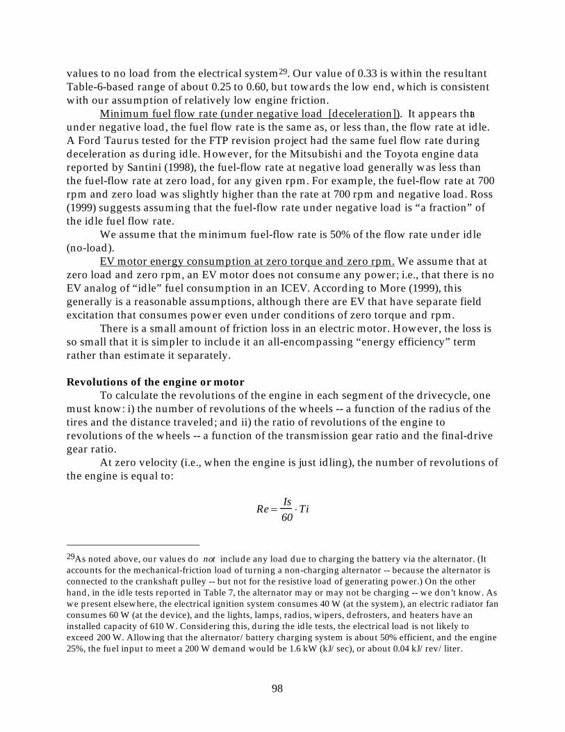
98

values to no load from the electrical system29. Our value of 0.33 is within the resultant Table-6-based range of about 0.25 to 0.60, but towards the low end, which is consistent with our assumption of relatively low engine friction.

Minimum fuel flow rate (under negative load [deceleration]). It appears that under negative load, the fuel flow rate is the same as, or less than, the flow rate at idle. A Ford Taurus tested for the FTP revision project had the same fuel flow rate during deceleration as during idle. However, for the Mitsubishi and the Toyota engine data reported by Santini (1998), the fuel-flow rate at negative load generally was less than the fuel-flow rate at zero load, for any given rpm. For example, the fuel-flow rate at 700 rpm and zero load was slightly higher than the rate at 700 rpm and negative load. Ross (1999) suggests assuming that the fuel-flow rate under negative load is “a fraction” of the idle fuel flow rate.

We assume that the minimum fuel-flow rate is 50% of the flow rate under idle (no-load).

EV motor energy consumption at zero torque and zero rpm. We assume that at zero load and zero rpm, an EV motor does not consume any power; i.e., that there is no EV analog of “idle” fuel consumption in an ICEV. According to More (1999), this generally is a reasonable assumptions, although there are EV that have separate field excitation that consumes power even under conditions of zero torque and rpm.

There is a small amount of friction loss in an electric motor. However, the loss is so small that it is simpler to include it an all-encompassing “energy efficiency” term rather than estimate it separately.

Revolutions of the engine or motorTo calculate the revolutions of the engine in each segment of the drivecycle, one

must know: i) the number of revolutions of the wheels -- a function of the radius of the tires and the distance traveled; and ii) the ratio of revolutions of the engine to revolutions of the wheels -- a function of the transmission gear ratio and the final-drive gear ratio.

At zero velocity (i.e., when the engine is just idling), the number of revolutions of the engine is equal to:

Re =Is60

⋅Ti

29As noted above, our values do not include any load due to charging the battery via the alternator. (It accounts for the mechanical-friction load of turning a non-charging alternator -- because the alternator is connected to the crankshaft pulley -- but not for the resistive load of generating power.) On the other hand, in the idle tests reported in Table 7, the alternator may or may not be charging -- we don’t know. As we present elsewhere, the electrical ignition system consumes 40 W (at the system), an electric radiator fan consumes 60 W (at the device), and the lights, lamps, radios, wipers, defrosters, and heaters have an installed capacity of 610 W. Considering this, during the idle tests, the electrical load is not likely to exceed 200 W. Allowing that the alternator/battery charging system is about 50% efficient, and the engine 25%, the fuel input to meet a 200 W demand would be 1.6 kW (kJ/sec), or about 0.04 kJ/rev/liter.

99

Re = revolutions of the engine. Is = the idling rate of the engine (revolutions per minute). We assume 700 rpm

for the Taurus, and 750 rpm for the Escort. 60 = seconds/minute. Ti = the time spend idling (seconds). This is a parameter in the design of the

drivecycle, and is specified by the modeler.

At constant velocity V1 (zero acceleration), the number of revolutions of the engine is equal to:

Re = D ⋅Gv1

2 ⋅ π ⋅Rt ⋅ 0.0254

where:

Re = revolutions of the engine. D = the distance of the segment of the drivecycle (meters). This is calculated from

the user-input velocity and time for the segment. Gv1 = the total gear ratio at velocity V1 (revolutions of engine/revolutions of

wheel). This is discussed below. Rt = the rolling radius of the tires (inches). The Allison Gas Turbine Division

(1994) gives the width of the tire, the ratio of the height to the width (called the “aspect ratio”), and the diameter of the rim, for the 1991 Taurus and the 1991 Escort. From these data, we calculate a radius of 12.25 inches for the Taurus, and 11.4 inches for the Escort.

0.0254 = meters/inch

When the vehicle is accelerating or decelerating, the number of revolutions is calculated as:

Re =Ve 2 ⋅Gve + SGve −Vb2 ⋅Gvb − SGvb

2 ⋅π ⋅Rt ⋅ 0.0254 ⋅ 2 ⋅A

where:

Re = revolutions of the engine.Ve = the velocity at the ending of the segment of the drivecycle (m/sec). This is a

parameter in the design of the drivecycle, and is specified by the modeler. Gve = the total gear ratio at the ending velocity (revolutions of

engine/revolutions of wheel). This is discussed below. SGve = the speed-gear result of the ending velocity. This is discussed below. Vb = the velocity at the beginning of the segment of the drivecycle (m/sec). This

is a parameter in the design of the drivecycle, and is specified by the modeler.

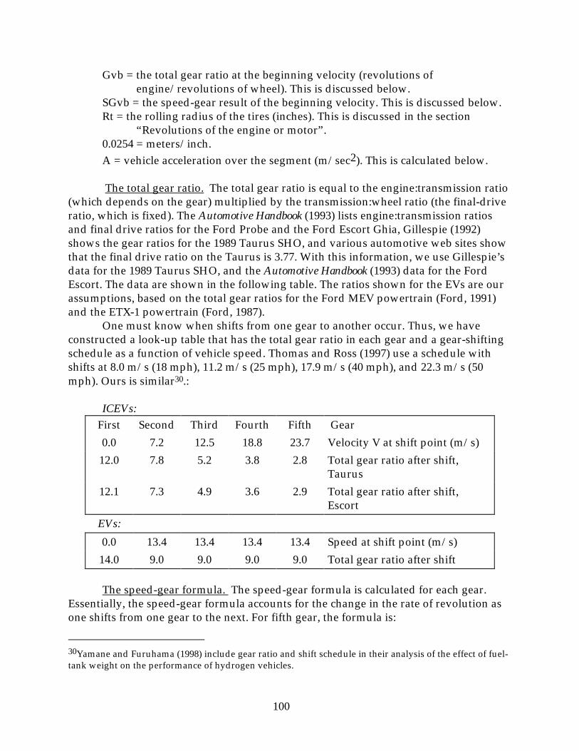
100

Gvb = the total gear ratio at the beginning velocity (revolutions of engine/revolutions of wheel). This is discussed below.

SGvb = the speed-gear result of the beginning velocity. This is discussed below. Rt = the rolling radius of the tires (inches). This is discussed in the section

“Revolutions of the engine or motor”.0.0254 = meters/inch.A = vehicle acceleration over the segment (m/sec2). This is calculated below.

The total gear ratio. The total gear ratio is equal to the engine:transmission ratio (which depends on the gear) multiplied by the transmission:wheel ratio (the final-drive ratio, which is fixed). The Automotive Handbook (1993) lists engine:transmission ratios and final drive ratios for the Ford Probe and the Ford Escort Ghia, Gillespie (1992) shows the gear ratios for the 1989 Taurus SHO, and various automotive web sites show that the final drive ratio on the Taurus is 3.77. With this information, we use Gillespie’s data for the 1989 Taurus SHO, and the Automotive Handbook (1993) data for the Ford Escort. The data are shown in the following table. The ratios shown for the EVs are our assumptions, based on the total gear ratios for the Ford MEV powertrain (Ford, 1991) and the ETX-1 powertrain (Ford, 1987).

One must know when shifts from one gear to another occur. Thus, we have constructed a look-up table that has the total gear ratio in each gear and a gear-shifting schedule as a function of vehicle speed. Thomas and Ross (1997) use a schedule with shifts at 8.0 m/s (18 mph), 11.2 m/s (25 mph), 17.9 m/s (40 mph), and 22.3 m/s (50 mph). Ours is similar30.:

ICEVs: First Second Third Fourth Fifth Gear

0.0 7.2 12.5 18.8 23.7 Velocity V at shift point (m/s)

12.0 7.8 5.2 3.8 2.8 Total gear ratio after shift, Taurus

12.1 7.3 4.9 3.6 2.9 Total gear ratio after shift, Escort

EVs:

0.0 13.4 13.4 13.4 13.4 Speed at shift point (m/s)

14.0 9.0 9.0 9.0 9.0 Total gear ratio after shift

The speed-gear formula. The speed-gear formula is calculated for each gear. Essentially, the speed-gear formula accounts for the change in the rate of revolution as one shifts from one gear to the next. For fifth gear, the formula is:

30Yamane and Furuhama (1998) include gear ratio and shift schedule in their analysis of the effect of fuel-tank weight on the performance of hydrogen vehicles.

101

SG5 =VG22 ⋅G1 + VG3

2 −VG22( )⋅G2+ VG4

2 −VG32( )⋅G3 + VG5

2 −VG 42( )⋅G4 −VG 5

2 ⋅G5

where:

SG5 = the speed-gear result for fifth fear.VGi = the velocity at the point of shift into gear (G) i. This is shown in the table

above. Gi = Ratio in gear i (revolutions of engine/revolutions of wheel). This is shown

in the table above. i = 1st, 2nd, 3rd, 4th, or 5th gear.

The speed-gear formulae for the other gears are similar, except that the terms for the numerically higher gears are omitted.

Air- conditioning energyThe amount of energy used by air conditioning during each segment of the

drivecycle is calculated simply as:

Eac =Fac ⋅Pac ⋅Ts

Eca[ICEVs]

Eac =Fac ⋅Pac ⋅Ts

Eba[EVs]

102

where:

Eac = the energy demand of the air conditioning system, over the drivecycle segment, measured at the engine crank or battery or fuel-cell terminals (kJ)

Fac = of total miles of travel, the fraction driven with the a/c in use (we assume it that it runs 1/3 of the time in the June through September, or for 11% of total annual driving)

Pac = the average input power to the a/c system during the cooling season (kW; note that this includes “internal” or “parasitic” losses by motor, compressors, controllers, fans, etc.) (discussed below)

Ts = the time of the segment (seconds). This is a parameter in the design of the drivecycle, and so is specified by the modeler.

Eca = the efficiency of the energy transfer from the crankshaft to the air-conditioner motor. We assume that the transfer is 98% efficient, because the air-conditioner compressor in an ICEV runs directly off the crankshaft, with essentially no energy loss.

Eba = the efficiency of the energy transfer from the battery or fuel-cell terminals to the a/c system (assume 0.98). We assume that the a/c system includes its own controller or inverter, so that there is only a small resistance loss from the power source to the a/c system. (Note that this assumption requires that our measure of the operating power of the a/c include all “internal” losses for the motor, controller, compressor, fans, and so on. These losses may be on the order of 20% of the total input power to the system [Dieckmann and Mallory, 1993].)

Power input to a/c system. According to Glacier Bay (1998b), the power necessary to cool a mid-size vehicle on a warm California day while driving at roughly 30 mph is 586 W. (This apparently does not include any “internal” or “parasitic” losses.) This power produces 6000 BTU/hr from the heat pump. Dieckmann and Mallory (1993) tested variable-speed air-conditioning systems in the G-Van, TE-Van, and the ETX-II, traveling at 30 mph with a full solar load, and found that the total steady-state input energy requirement was about 900 W at 90o F and 50% relative humidity, and 2000-3000 W at 110oF and 40% RH. (These figures include “parasitic” consumption of around 300 W.) The energy consumption of the a/c system reduced the range of the vehicle by about 10% at 90oF, and by more than 20% at 110oF (Dieckmann and Mallory, 1993; see also Gris, 1994).

Assuming that the EV is relatively well insulated, and equipped with a relatively efficient a/c system, but allowing for the extra “transient” load of the initial cooling, we assume that the a/c system in our baseline EVs consumes on average 1000 W, to cool a mid-size vehicle in the summer in California. (One also can argue that EV users will be inclined to trade off a little comfort for extended range, but we do not assume so here.)

This minor use of air conditioning turns out to have a relatively small effect on vehicle efficiency and lifecycle cost: it reduces vehicle efficiency by about 4%, increases

103

battery weight by about 10 k, or 3%, and increases the break-even gasoline price by about $0.10/gallon.

Average electrical power for auxiliaries and accessories, excluding air conditioningMany devices in a motor vehicle draw a small amount of electrical power, which

ultimately must be supplied by the energy in the fuel or the battery. Unless specifically stated otherwise, we assume that the power consumption of auxiliaries and accessories in an EV is the same as that in an ICEV.

The trip-average electrical power for auxiliaries and accessories (in kW of power from the battery or fuel cell terminals, or engine shaft), excluding air conditioning in all vehicles, and fossil-fuel heating in EVs (which are modeled separately), is calculated as:

Pau =Pig + Po + Ppb +

PpsVave

+ Pl ⋅Fl + Ph ⋅Fh ⋅ Fhp

Ace

where:

Pau = the average electrical power over the whole trip, excluding air conditioning (kW). from the battery or fuel cell terminals or engine crankshaft).

Pig = the power consumption of the electrical ignition (kW). The Bosch Automotive Handbook (1993) reports that electrical ignition consumes 0.04 kW. We use this estimate for ICEVs, and of course assume 0.0 kW for EVs.

Po = the power consumption of other electrical motor or engine auxiliaries at the device (kW). The Bosch Automotive Handbook (1993) reports that an electric radiator fan consumes 0.06kW. We use this estimate for ICEVs, and assume that the motor and controller auxiliary equipment in an EV (fans, switches, etc.) consume 0.22 kW of power.

Ppb = the average “base” power consumption of power steering and power brakes (kW). We assume an average of 0.04 kW for EVs and ICEVs.

Pps = the average-speed-dependent power consumption of power steering and power brakes (kW-mph). We assume 0.40 kW-mph for EVs and ICEVs.

Vave = the average speed over the drive cycle (total miles divided by total hours)Pl = the installed power capacity of lights, lamps, radio, windshield wipers, and

defroster (kW). The Bosch Automotive Handbook (1993) reports that these have an installed capacity of 0.49 kW. We use this estimate for both the EVs and the ICEVs.

Fl = the fraction of total trip time that the lights, lamps, radio, windshield wipers, ad defrost operate at full power. We assume that these operate 25% of the total driving time. The Bosch Automotive Handbook (1993) appears to assume that these operate about 50%.

104

Ph = the installed power capacity of the electrical heating system (kW). The Bosch Automotive Handbook (1993) reports that the heating system in an ICEV consumes 0.12 kW. We use this estimate for the ICEVs. In our base case, in which the EV uses a propane-fueled heater, this parameter is 0.0 for the EVs. However, the parameter is “active” in the model, so that if the user wishes to specify an electrical heating system for the EV, he can enter a value here (we assume 0.30 kW).

Fh = the fraction of miles and trips in the (equivalent of the) design ambient temperature (assume 0.20 for the base case; see also the section on the use fossil fuel for heating).

Fhp = the fraction of the maximum electrical heater power used, on average. We assume that when the heating system in the ICEV is on, that it operates at 50% of its maximum power on average. In our base case, in which the EV uses a propane-fueled heater, this parameter is 0.0 for the EVs. However, the parameter is “active” in the model for EVs, in case the user wishes to characterize an electrical heating system for the EV.

Ace = the efficiency of electricity supply to the accessories, from the alternator in ICEVs, and from the fuel cell or battery terminals in EVs. This is discussed below.

Note that because our base-case EVs have a fossil-fuel heater, rather than an electrical heat-pump and resistance-heat system, the parameters Ph and Fhp are 0.0 in the EV base case. (The parameters for consumption of fossil-fuel for heating are discussed in the section “Fuel and electricity”. There is a switch in the model which specifies either a fossil-fuel or electric heating system.)

Efficiency of the accessory electrical system. In an ICEV, some electrical systems are run off the alternator directly, and some are run off the 12-V chassis battery, which is charged by the alternator. Alternators are about 50-60% efficient at converting mechanical energy from the crankshaft into electrical energy to the battery (Bosch Automotive Handbook , 1993), and 12-V Pb/acid batteries are about 75% efficient. We assume that half of the electrical systems run off of the alternator directly, and half run off the 12-V battery/alternator system, which results in an overall average electrical efficiency of: 0.5 ∞ 0.55 + 0.5 ∞ 0.55 ∞ 0.75 = 0.48. In an EV, the low-power electrical systems will run off of a 12-V chassis battery, which will be charged by the main traction battery via a dc-dc converter that will reduce the voltage. A chassis battery is about 75%efficient, and a dc-dc converter about 85% efficient. Note, again, that we assume that the air conditioner, because of its relatively high power, is run directly off of the battery, the fuel cell, or the engine.

All of the estimates of electrical power consumption from the Bosch Automotive Handbook (1993) are estimates of “absolute” or installed capacity. The installed capacity of course does not account for the fraction of time that an accessory (such as the lights) are used.

105

Finally, note that we have estimated the consumption of power brakes and power steering as a function of the average speed, on the assumption that the higher the average speed, the less the brakes and the steering are used.

Battery heatingAs discussed elsewhere in this report, Pb/acid batteries lose an appreciable

amount of capacity at temperatures below about 40o F. To avoid this loss of capacity, batteries used in very cold climates should be insulated, and if necessary heated. NiMH batteries probably can be kept warm enough by managing the ventilation system to retain heat.

In our base case, we assume that EVs are used in comparatively warm climates, and hence do not require battery heating systems. However, in a scenario analysis, we consider the total initial and operating cost of installing and using a battery insulation and heating system.

The cost and weight of the heating system are discussed in the section “Adjustments to the 1989 weight and cost baseline in this report”; here, we discuss the energy requirements of heating. Garabedian (2000) reports the energy consumption of battery heaters on Solectria-Force EVs operated in the Northeastern U. S., as a function of the ambient temperature: about 2-3 kWh/d at -10.4 oC, 1.5-2.5 kWh/d at -4.4 oC, 1.5 to 2.0 kWh/d at -1.6 oC, and about 0.5 kWh/day at 4.6 oC. Jelinski (1996) reports that a Nissan EV equipped with an insulated battery box and four 50W battery blankets consumed 1-2 kWh per night when the ambient temperature was less than -5 o C. The energy consumption probably depends also on the size and design of the battery, but not in an obvious way, because a smaller battery takes less energy to heat than a larger battery, but also retains less heat. We therefore assume that the daily electricity consumption is a function only of the ambient temperature, and on the basis of the data in Garabedian (2000) and Jelinski (1996) estimate the following:

BHEm =Dbh ⋅ 3.30− 0.074 ⋅TEair( )

AVMT

BHEm ≥ 0

where:

BHEm = the average electricity consumption of the battery heater over the course of the year (kWh-ac/mi)

Dbh = the number of days per year that the battery heater is needed (assume 50 for the battery-heating scenario analysis)

AVMT = the annual average number of miles driven by the vehicle over its life (equal to lifetime miles divided by lifetime years)

TEair = the average ambient air temperature on days when the battery heater is

used (oF; assume 20o F for the battery-heating scenario)

106

The annual cost of electricity used for battery heating, plus the annualized cost of the heating system, add only 0.05 to 0.10 cents/mile to the lifecycle cost of EVs.

A high-temperature battery, such as Li-Al/Fe-S, or Na-S., must be heated to be maintained at its operating temperature. In the model, the average energy requirement for maintaining the temperature of the Li-Al/Fe-S battery is calculated as a simple function of the thermal loss per unit of battery, the size of the battery, and the stand time:

BHEm* =TLB ⋅ESTBC/3 ⋅ HLT

TVMT ⋅EFFRE

where:

BHEm* = the average electricity consumption required to maintain the temperature of a high-temperature battery (kWh-ac/mi)

TLB = the thermal loss of the battery (kWh-lost/kWh-battery; we assume 0.0030 [the U. S. Advanced Battery Consortium goal is 0.0032])

ESTBC/3 = the nominal total energy discharge capacity of the new traction battery, measured at the C/3 discharge rate (kWh; discussed in the section “weight of the EV traction battery”)

HLT = average hours of heat loss prior to average trip, after reaching lowest allowable temperature (we assume 3 in the base case)

TVMT = average vehicle miles per trip (in the FUDS, which is our base-case drive-cycle, the trip is 7.4 miles)

EFFRE = the efficiency of resistance heating (kWh-heat-to-battery/kWh-ac; assume 95%)

Once − − − − through efficiency from the battery (or other energy-storage system) or fuel − − − − cell to the wheels (excluding storage device itself)

The energy efficiency of the EV powertrain, from the battery or fuel-cell terminals to the wheels -- i.e., the efficiency of the motor controller, the motor, and the transmission -- is calculated as the product of the efficiency of the controller, motor, and transaxle:

Pe = Ce ⋅Me ⋅Te

where:

Pe = the efficiency of energy transmission from battery or fuel cell terminals to wheels.

107

Ce = the efficiency of the electric-motor controller. This is calculated second by second from maps of inverter efficiency as a function of torque and rpm. See Appendix A.

Me = the efficiency of the electric motor. This is calculated second by second from maps of motor efficiency as a function of torque and rpm. See Appendix A.

Te = the efficiency of energy transmission from motor to wheels. This is calculated second by second on the basis of the map of the Ford MEV transaxle efficiency as a function of motor output torque and rpm. See Appendix A.

Acceleration and distanceAcceleration. The acceleration over each segment of the drivecycle is simply:

A =Ve −Vb

Tswhere:

A = the acceleration over the drive-cycle segment (m/sec2).Ve = the velocity at the end of the segment (m/sec). This is a parameter in the

design of the drivecycle, and so is specified by the modeler. Vb = the velocity at the beginning of the segment (m/sec). This is a parameter in

the design of the drivecycle, and so is specified by the modeler. Ts = the time of the segment (seconds). This is a parameter in the design of the

drivecycle, and so is specified by the modeler.

Note that this calculation assumes that the acceleration is constant over each segment of the drivecycle. Or, put another way, the modeler is supposed to describe segments of constant acceleration.

Distance traveled. The distance traveled over each segment of the drivecycle is:

D =Ve +Vb

2⋅Ts

where:

D = the distance driven over the segment (meters)Ve = the velocity at the end of the segment (m/sec). This is a parameter in the

design of the drivecycle, and so is specified by the modeler. Vb = the velocity at the beginning of the segment (m/sec). This is a parameter in

the design of the drivecycle, and so is specified by the modeler. Ts = the time of the segment (seconds). This is a parameter in the design of the

drivecycle, and so is specified by the modeler.

108

Note that this calculation assumes that the acceleration is constant over each segment of the drivecycle.

MODEL OF VEHICLE PERFORMANCE

OverviewThe performance of the vehicle is measured as the amount of time that the

vehicle takes to accelerate from any beginning speed to any ending speed, over any grade. This time is calculated for the baseline gasoline ICEV, the AF ICEV, and the EVs. The purpose of this is to show the performance of the vehicle given the maximum power specified by the user.

The maximum power of the vehicle -- the maximum horsepower at the engine crankshaft in the ICEVs, and the maximum kW at the battery or fuel-cell terminals in the EVs -- is an input or design variable. Given this maximum power output, and the average velocity over the performance test, the model estimates (crudely) the average power over the performance test. With an estimate of the average power, and other calculated or input vehicle characteristics (such as vehicle weight and drag), the model calculates the time over the performance test. The user then can compare the performance time of the EVs or AFICEV with the performance time of the gasoline ICEV. If the relative performance is higher or lower than is desired, the user can re-specify the maximum power of the EV or AFICEV to produce the desired relative performance. Alternatively, the user can specify that the EVs have whatever maximum power is needed to result in the same acceleration (performance time) as the baseline ICEV.

The performance calculationTime. The measure of the performance of the vehicle is the time required to

accelerate from a beginning velocity Vb to an ending velocity Ve:

Tp =Ve −Vb

Ap

where:

Tp = the time required for acceleration in the performance test (seconds)Ve = the velocity at the end of the test (m/s). This is specified by the modeler.Vb = the velocity at the beginning of the test (m/s). This is specified by the

modeler. Ap = the acceleration over the performance test (m/sec2). This is presented next.

Acceleration. The acceleration over the performance test is calculated on the basis of the average available power, and the loads on the vehicle:

109

Ap =

Pavep ⋅ 0.746 ⋅TepVap

− Fad − Fr − Fgr

Mit[ICEVs]

Tep = 0.80 + P max− adj ⋅ TemICEV − 0.80( )

Ap =

Pavep ⋅Paup ⋅PepVap

− Fad − Fr − Fgr

Mit[EVs]

Paup =PoAce

Pep = 0.65 + P max− adj ⋅ Pem − 0.65( )

Pem = Mem ⋅Cem ⋅TemEV

where:

Pavep = the average power available over the performance test (discussed below) (hp for the ICEVs, kW for the EVs)

0.746 = kW/hp.Paup = in an EV, the power requirement of electric motor auxiliaries that must

operate during the performance test (kW). According to the BoschAutomotive Handbook (1993), performance is measured with only necessary accessories operating, which means that the lights, defrost, radio, wipers, and the like are not on. (In ICEVs Paup = 0, because engine brake power is measured net of obligatory accessories.)

Tep = the average efficiency of the ICEV transmission, over the performance test. We assume that this is related to the efficiency at the maximum power (see discussion below).

Pep = the average efficiency of the EV powertrain, over the performance test. We assume that this is related to the efficiency at the maximum power (see discussion below).

Vap = the average velocity over the performance test (m/s)Fad = the air-resistance force (kiloNewtons). Fad is calculated using the equation

for Ead (energy), without the distance term D, because Fad = Ead/D. Fr = the rolling-resistance force (kiloNewtons). Fr is calculated using the

equation for Er (energy), without the distance term D, because Fr = Er/D.

110

Fgr = the grade force (kiloNewtons). Fgr is calculated using the equation for Egr (energy), without the distance term D, because Fgr = Egr/D.

Mit = the total effective inertial mass of the vehicle (accounting for rotational inertia of tires, and rotational inertia of the engine) (kg). The inertial mass can be derived from the inertial energy, which is given elsewhere in this

report: Mit =Ei

A ⋅D=WIU ⋅ 1+ Nw ⋅

Mw'2

+ C ⋅G2

Po = the power consumption of the motor and controller auxiliary equipment in an EV (fans, switches, etc.). This is estimated in the section “Average electrical power for auxiliaries and accessories, excluding air conditioning”.

Ace = the efficiency of the electricity supply to the auxiliaries from the fuel cell or battery terminals in EVs. This is estimated in the section “Average electrical power for auxiliaries and accessories, excluding air conditioning.

Pmax-adj = the maximum-power adjustment factor. As explained below, this factor is a crude estimate of the ratio of the actual average available power from the engine or motor, over the performance test, to the maximum power of the engine or motor.

Pem = the efficiency of the EV powertrain, from battery or fuel cell terminals to wheels, under maximum power.

Mem, Cem and TemEV, are the efficiency of the motor, controller, and EV transmission under maximum power. This maximum-power efficiency is looked up from a map of efficiency as a function of torque and rpm (see the discussion, in Appendix A, of efficiency maps).

TemICEV = the ICEV transmission efficiency at maximum power. On the basis of data in Garvey and Studzinsky (1993), we assume a value of 95%.

Estimation of the average available power over the performance test, given the maximum power

If the maximum power of a motor or engine were available instantaneously at all vehicle speeds, then, in the calculation of the acceleration in the performance test, one simply would use the maximum power. However, the maximum engine or motor power is not available instantaneously at all vehicle speeds, but rather is available only at a particular torque-rpm point (in the case of ICEVs), or within a certain torque-rpm band (in the case of EVs). This means that either one must calculate the available power second-by-second over the performance test, or use some approximation of the average available power over the test as a function of the maximum power. We choose the latter.

A plot of maximum power versus vehicle speed, during a constant full-power acceleration, looks quite different for EVs than for ICEVs, on account of the different torque characteristics of electric motors versus ICEs. The maximum torque of an electric motor is available from zero rpm to moderate rpm (about 3,000 to 4,000 rpm); beyond this moderate rpm, the available torque is less than the maximum available at the lower

111

rpm (Appendix A tables; Lesster et al., 1993). By contrast, the available torque of an ICE increases with rpm, beginning at zero rpm, until the maximum torque is reached at moderately high rpm; at still higher rpm, the available torque is less than this maximum (Bosch Automotive Handbook, 1993).

As a result of these torque characteristics, the speed at which an EV reaches it maximum power is lower than the speed at which an ICEV reaches it maximum power. In the case of EVs, the maximum power apparently is reached at 1/3 to 1/2 of the top-end speed (see Appendix A tables), whereas in the case of ICEVs, the maximum power is reached at speeds much closer to the top-end speed. This, in turn, means that, given an EV and ICE drivetrain of equal maximum power, the EV will outperform the ICE, especially at lower speeds. Thus, according to Lesster et al. (1993, p. 171), “a 100-hp induction motor drive can give performance similar to a 150-hp ICE as it accelerates.” The graph in Lesster et al. (1993) actually shows that a 100 hp electric motor will out-accelerate a 165-hp ICE from zero to any speed up to 45 mph. The nominally much-higher powered ICE is faster accelerating to speeds above 45 mph. This is what one would expect on the basis of the torque curves.

If we do not calculate the acceleration second-by-second, on the basis of the available torque, then we must calculate the acceleration over the entire test on the basis of the average power over the test. To do this, we need to find a relationship between the maximum power point, which we pick, and the average power, as a function of some parameters of the test. This relationship will be different for EVs and ICEVs.

We therefore assume that the average power is equal to the maximum power multiplied a maximum-power point by an adjustment factor, which factor is a function of the average speed over the performance test:

Pavep = P max⋅P max− adj

P max − adj = minVapE1

, 1

E2

where:

Pmax = the maximum horsepower (hp) at the engine crankshaft in the ICEVs, and the maximum kW at the battery or fuel-cell terminals in the EVs. This is chosen by the modeler so as to give the desired performance.

the “min [ ]” function ensures that the adjustment factor is not greater than 1.0 .

ICEV EV

E1 30 20

E2 0.55 0.20

other terms are defined above

112

With these functions, the higher the average velocity, the higher the adjustment factor. The lower denominator and exponent in the EV function results in a higher adjustment factor for the EV. The advantage of the EV increases as the average velocity, Vap, decreases.

These adjustment factors are reasonably faithful to the differences, discussed above, between ICEVs and EVs, and also result in a 0-60 level-ground acceleration time consistent with published values for the Escort and Taurus (Edmunds, 1999). Nevertheless, the adjustments are crude, and the reader should keep in mind that our performance calculations do not actually simulate the second-by-second available power.

We make a similar adjustment (shown elsewhere in this section) to estimate the average drivetrain or transmission efficiency as a function of the efficiency under maximum power.

As discussed in the section “Weight of the EV traction battery,” the battery is designed to satisfy the performance targets on the basis of the performance of a newbattery. Near the end of its life, the battery may have a noticeably lower peak power. We do not account for this here.

Calculated fuel-cell or battery or engine power required to deliver the acceleration of gasoline vehicle

The preceding calculations tell us the vehicle performance given an assumed maximum power output. It also is interesting to determine the maximum power output that the AF ICEV or the EVs must have in order to have the same performance as the baseline gasoline ICEV. The power required for equal performance by the EV is calculated as:

P max* =

Fad + Fr + Fgr + Mit ⋅ApICEV( )⋅Vap

Pem+ Paup

P max− adj

where:

Pmax* = the maximum power required from the fuel-cell or battery in the EV or the engine in the ICEV to deliver the acceleration of the baseline gasoline ICEV (assuming constant vehicle weight) (kW).

ApICEV = the acceleration of the ICEV over the performance test (m/sec2)all other terms are defined above.

Calculated average velocity in performance testThe average speed over the performance test is a term in two of the equations in

the performance analysis, and so is calculated separately here:

Vap =Ve +Vb

2

113

where all terms are defined above.

Note that this calculation assumes constant acceleration.

114

PERIODIC OWNERSHIP AND OPERATING COSTS

The “periodic” or non-investment costs of a motor vehicle -- maintenance and repairs, insurance, fuel and oil, tires, parking, tolls, fees, fines, and taxes -- account for roughly half of the total lifecycle cost per mile. Most of these non-investment costs are different for EVs than for ICEVs. Consequently, to properly compare the lifecycle costs of EVs and ICEVs, one must consider the periodic costs as well as the initial investment costs.

There actually are few comprehensive, recent studies of the full lifecycle costs of EVs vs. ICEVs. Lipman (1999a) reviews the studies from the mid 1990s, and finds that most of the analyses of periodic costs are fairly simple, and based mainly on literature reviews. For example, in 1995, the U. S. DOE (1995) published a lifecycle cost analysis similar in outline but much less detailed than the one presented here. Cardullo (1993) describes a lifecycle cost model that might be similar in outline to the one described here. The best of the recently published lifecycle cost analyses is that by Argonne National Laboratory (Vyas et al, 1998).

In light of this, there is a need for a detailed, original analysis of periodic costs. We have attempted such an analysis here.

MAINTENANCE AND REPAIR COSTS

IntroductionThe cost of maintaining and repairing a motor vehicle is one of the largest costs

of operating a motor vehicle, on a par with the cost of fuel and the cost of insurance. Because the maintenance and repair (m & r) cost is relatively large, and is different for EVs than for ICEVs, it is important to estimate it accurately.

In this section, we define a relevant set of m & r costs, estimate a year-by-year m & r schedule for the baseline gasoline light-duty ICEV, and then estimate m & r costs for the EV relative to the estimated m & r costs for the baseline gasoline ICEV. We define m & r costs with the objective of identifying the kinds of costs that probably are different for EVs than for ICEVs. The costs that we think are the same for ICEVs and EVs we put into separate categories.

There are several sources of ultimately original data on m & r expenditures for motor vehicles, but by far the most comprehensive, detailed, and accurate source is the Bureau of the Census’ quinquennial Census of Service Industries and Census of Retail Trade. We use the Census’ data to estimate m & r costs per LDV per year, and then compare the results with estimates based on other independent data. We then consider estimates by FHWA (1984) to transform the Census’ estimates into a year-by-year m & r cost schedule.

115

What we count as maintenance and repair costs for light-duty vehicles (LDVs)In the Bureau of the Census classification system, there are two major industry

groups that provide automotive parts and services: service-sector SIC (Standard Industrial Classification) 75, “Automotive Repair, Services, and Parking”, and retail-sector SIC 55, “Automotive Dealers and Gasoline Service Stations”. These are further broken out as follows (Office of Management and Budget [OMB] 1987):

7513 Truck rental and leasing, without drivers7514 Passenger car rental7515 Passenger car leasing7519 Utility trailer and recreational vehicle rental7521 Automobile parking7532 Top, body, and upholstery repair shops and paint shops7533 Automotive exhaust system repair shops7534 Tire retreading and repair shops7536 Automotive glass replacement shops7537 Automotive transmission repair shops7538 General automotive repair shops (including repair of diesel trucks)7539 Automotive repair shops, not elsewhere classified7542 Car washes7549 Automotive services, except repair and car washes (includes emissions testing

and repair, diagnostic centers, inspection services, lubricating services, road service, towing, rust-proofing, window tinting, and undercoating.

551 Motor vehicle dealers (new and used)552 Motor vehicle dealers (used only)553 Auto and home supply stores554 Gasoline service stations555 Boat dealers556 Recreational vehicle dealers557 Motorcycle dealers559 Automotive dealers, not elsewhere classified

The task here is to identify or estimate, within each of the SICs above, those costs (reported as receipts to the industry), for motor vehicle services, repair, and parts, that per vehicle are:

• the same for EVs and ICEVs; • unique to ICEVs; • common to but not the same for EVs and ICEVs

116

Note that, in the case of the retail SICs (551 to 559), we are interested only in receipts for services or parts; we are not interested here in receipts for sales of vehicles or fuels.

Note, too, that there are some minor relevant receipts in the wholesale sector (for used motor vehicle parts), and probably in other sectors as well. We address these later. Also, we deduct costs covered by motor-vehicle insurance, because in our analysis, those costs show up to the vehicle owner as insurance payments, not m & r costs.

Once we have estimated costs that are the same for EVs and ICEVs, costs that are unique to ICEVs, and costs that are common to but not the same for EVs and ICEVs, we estimate the cost per vehicle in 1992, by dividing by the number of LDVs for which the services and parts were bought. We scale the results to 1997, and compare the resultant per-vehicle costs with estimates from other sources. Then, we develop a year-by-year m & r cost schedule, on the basis of estimates by the FHWA. Finally, we estimate the EV costs relative to the ICEV costs for those costs that are common to but not the same for EVs and ICEVs.

Maintenance and repair costs for light-duty gasoline ICEVs in 1992SIC 75 Automotive services. The Census of Service Industries, Sources of Receipts or

Revenue (1996) reports sources of receipts, by type of service or merchandise, for all of the motor-vehicle service industries listed above. With this report, we can classify costs, within each SIC, that are not related to motor-vehicle m & r, the same for EVs and ICEVs, unique to ICEVs, or common to but not the same for EVs and ICEVs. In the following, actual Census cost (revenue) lines are shown in quotes. Unless otherwise noted, the data in this subsection for SIC 75 are from the Census Sources of Receipts or Revenue report.

751 Automotive rental and leasing, without drivers. Because we are interested here in the lifecycle cost owning an LDV, we do not count any costs of renting or leasing cars or trucks. It is conceivable that rental and leasing facilities sell a tiny amount of parts and services to private vehicle owners, but if the amount is not zero it surely is insignificant.

7521 Automobile parking. These costs likely are the same for EVs and ICEVs. We assume that they are, and count them in a category entirely separate from m & r, “parking, fines, and tolls” (discussed below).

7532 Top, body, and upholstery repair shops and paint shops. We assume that expenditures body, upholstery, or paint will be the same for EVs and ICEVs. Hence:

117

Total receipts in SIC (109 $)

Not motor-vehicle m & r

Same for EVs and ICEVs

Unique to ICEVs

Common to EVs and ICEVs

other (non-motor-vehicle) receipts, rental

and leasing

all other receipts

none none

12.263 0.283 11.980 0.000 0.000

The detailed breakdown of sources of revenue at these establishments does not reveal any kinds of receipts that are likely to be unrelated to body, upholstery, or paint work.

7533 Automotive exhaust system repair shops. We assume that service identified specifically for the exhaust system is unique to ICEVs. Hence:

Total receipts in SIC (109 $)

Not motor-vehicle m & r

Same for EVs and ICEVs

Unique to ICEVs

Common to EVs and ICEVs

“other receipts from

customers” and “all other receipts”

none “repair and maintenance” and “sales of merchandise”

“all other motor vehicle

services"

1.953 0.010 0.000 1.936 0.006

The Census accounting is such that “all other motor vehicle services” are those not related to the main repair and sales activity of the industry.

7534 Tire retreading and repair shops. The Census’ breakdown of receipts by kind indicates that all receipts in SIC 7534 are either for tires, or else are unrelated to motor-vehicle use. Because we count costs related to tires separately, we do not count any of the SIC 7534 costs as m & r costs here.

7536 Automotive glass replacement shops. The Census’ breakdown of receipts by kind indicates that virtually all receipts in SIC 7536 are for automotive glass. Assuming that expenditures related to automotive glass are the same for EVs and ICEVs, we have:

118

Total receipts in SIC (109 $)

Not motor-vehicle m & r

Same for EVs and ICEVs

Unique to ICEVs

Common to EVs and ICEVs

“other receipts from

customers” and “all other receipts”

all the rest none, apparently

assume none (assume all related to

automotive glass)

1.889 0.086 1.803 0.000 0.000

7537 Automotive transmission repair shops. The Census’ breakdown of receipts by kind indicates that virtually all receipts in SIC 7537 are for automotive transmission repair, which is a cost common to EVs and ICEVs:

Total receipts in SIC (109 $)

Not motor-vehicle m & r

Same for EVs and ICEVs

Unique to ICEVs

Common to EVs and ICEVs

“other receipts from

customers” and “all other receipts”

none none, apparently

assume none (assume all related to

automotive glass)

1.660 0.006 0.000 0.000 1.654

7538 General automotive repair shops (including repair of diesel trucks). The Census reports receipts for diesel repair shops separately ($2.5 billion in 1992). Since most diesel vehicles are heavy-duty (Delucchi [1996] estimates that in 1991, heavy-duty diesel vehicles accounted for 83% of total VMT by all diesel vehicles, and 93% of total expenditures on m & r for all diesel vehicles), and we are interested here in LDVs only, we exclude 93% of receipts at diesel repair shops. Thus:

Total receipts in SIC (109 $)

Not LDV m & r

Same for EVs and ICEVs

Unique to ICEVs

Common to EVs and ICEVs

other (non-motor-vehicle) receipts, rental

and leasing, tires, 93% of diesel repair

“carwash receipts”

none specifically

shown

all the other receipts

17.773 2.638 0.007 0.000 15.128

7539 Automotive repair shops, not elsewhere classified. The Census’ 1992 Census of Service Industries, United States (1994) breaks out data for radiator repair shops

119

and carburetor repair shops. We assume that 98% of the receipts at these shops are for work unique to an ICEV (because EV’s don’t have radiators or carburetors or their analogs.) With this assumption, and other data from the Sources of Receipts or Revenuereport, we have:

Total receipts in SIC (109 $)

Not motor-vehicle m & r

Same for EVs and ICEVs

Unique to ICEVs

Common to EVs and ICEVs

other (non-motor-vehicle)

receipts, tire repair

none 98% of carburetor and radiator repair shop receipts

all the other receipts

2.892 0.020 0.000 0.954 1.918

7542 Carwashes. Presumably EV owners spend as much on car washes as do owners of ICEVs. Hence:

Total receipts in SIC (109 $)

Not motor-vehicle m & r

Same for EVs and ICEVs

Unique to ICEVs

Common to EVs and ICEVs

“other receipts from

customers” and “all other receipts”

“carwash receipts”

none motor vehicle m & r and parts

2.644 0.056 2.315 0.000 0.273

7549 Automotive services, except repair and carwashes. The Census shows receipts for repair and maintenance, merchandise, and all other motor-vehicle services, at lubrication shops. We assume that 95% of the “repair and maintenance” pertains to the engine lubrication system, which is unique to ICEVs. We assume that “all other motor-vehicle services” at lubrication shops are common to EVs and ICEVs. We exclude what we estimate to be the cost of oil (80% of “sales of merchandise), because we make a separate estimate (in a separate cost category) of the total cost of lubricating oil.

Although this SIC includes establishments that do emissions testing (which is unique to ICEVs), we do not attempt to separate emissions testing from this SIC only, but rather make a separate estimate of the total cost of emission testing, and then deduct that en masse from estimated m & r expenditures.

Hence:

120

Total receipts in SIC (109 $)

Not motor-vehicle m & r

Same for EVs and ICEVs

Unique to ICEVs

Common to EVs and ICEVs

other receipts, rental and leasing, oil

“carwash receipts”

assume 95% of motor vehicle

services at lube shops

all other motor vehicle m & r

and parts

3.403 0.124 0.014 0.765 2.500

SIC 75 total. Adding up the amounts estimated for the individual SICs, and counting amounts for SIC 751 (renting and leasing) and SIC 7521 (parking) as “not motor-vehicle m & r,” we have, for 1992 m & r costs (109 $):

Total receipts in SIC (109 $)

Not motor-vehicle m & r

Same for EVs and ICEVs

Unique to ICEVs

Common to EVs and ICEVs

70.034 28.780 16.119 3.654 21.481

The amount unique to ICEVs is for the exhaust system, radiator, carburetor, and engine-oil lubrication. The amount that is the same for EVs and ICEVs is for body and upholstery, automotive glass, and carwashes.

Adjustments to the SIC 75 totals. We wish to remove from the foregoing totals receipts for heavy-duty vehicle (HDV) m & r (because we are interested in LDVs only), receipts for vehicle inspection and testing, which we estimate separately. We also must address costs not included in the Census data: sales taxes, work done by private contractors who do not have a payroll, or maintenance and repair work done “in house” by government or businesses that do not have separately identified service establishments. Finally, we deduct costs covered by motor-vehicle insurance, because in our analysis, those costs show up to the vehicle owner as insurance payments, not m & r costs.

1). First, we deduct receipts for m & r of HDVs. Given that we already have excluded 93% of receipts at diesel repair shops, the task here is to estimate the m & r receipts for work on HDVs in other SICs. Delucchi (1996) estimates m & r expenditures of $19 billion for HDVs in 1991, but this includes expenditures “in house” at fleet sites, as well as expenditures on services in SIC 75. We assume that of the $19 billion total, $2.3 billion is repair work at diesel repair shops (already excluded, above), $9 billion is m & r expenditure in SIC 75 except diesel repair shops, and the remainder is in-house m & r expenditure that does not show up in the SIC 75 receipts. We deduct $4 billion from the category “same for EVs and ICEVs,” $1 billion from the category “unique to ICEVs”, and $4 billion from “common to EVs and ICEVs”.

3). Second, we must deduct what we estimate to be the receipts for vehicle inspection services, because we estimate the cost of inspection separately. (We could not deduct inspection costs from each 4-digit SIC area, as we did with tire costs, because inspection costs are not specifically identified). We assume that in SIC 75, businesses received $1.5 billion for motor vehicle inspections. This amounts to roughly

121

$10/veh/year -- less than what we assume below for actual inspection costs per vehicle per year. This discrepancy is acceptable because not all vehicles are subject to inspections (in the Census data), but we are estimating costs for vehicles that do undergo inspection. We deduct this amount from the category “Common to EVs and ICEVs”.

4). We wish to include sales taxes, because they are part of the consumer lifecycle cost, and also included other data series with which we will compare our Census estimates. Every five years, the Bureau of the Census Service Annual Survey asks service establishments to report the amount of “sales taxes and other taxes (i.e., amusement, occupancy, use, etc.) collected from customers and forwarded directly to taxing authorities” (The Bureau of the Census Service Annual Survey: 1992 , 1994, p. D-22). In 1992, these sales and “other taxes” were 3.4% of total receipts in SIC 75, Automotive Services (Bureau of the Census Service Annual Survey: 1992, 1994). Thus, we multiply our receipts in SIC 75 by 1.034.

5). We do not have data on work done by private contractors who do not have a payroll, but presume that the amount is insignificant relative to the totals for SIC 75.

6). Assuming that m & r work done “in house” at businesses or government agencies is for business or government vehicles, and not private household vehicles, we can properly ignore these “in-house” costs if we make sure that we exclude from our vehicle count (when we estimate m & r costs per vehicle) those vehicles that benefit from in-house services. In other words, either we include in-house m & r costs in the numerator, and divide by all LDVs, or exclude in-house m & r from the numerator, and vehicles that use in-house services from the denominator. Given that later, when we deduct m & r costs covered by insurance, we exclude vehicles that used in-house m & r services, we do the same here.

Automotive services provided in SIC 55. Some retail firms, in SIC 55, also provide automotive services. In 1992, firms in SICs 551, 552, 553, and 554 received $23.9 billion for automotive services (“labor charges for work by this establishment,” and “value of service contracts”) (Bureau of the Census, Merchandise Line Sales, 1995). We exclude receipts in SICs 556-559 because those establishments do not serve light-duty motor vehicles. We count parts installed in repair separately, in the next section. We assume that retail establishments outside of SIC 55 did not perform any automotive services.

We assume that 95% of the total $23.9 billion was for service performed on LDVs.In 1992, sales taxes in SIC 551 were 2.7% of sales (Key, 1997). We assume this

percentage here. Note that we have included “the value of service contracts” at auto dealers -- at

least $2 billion in 1992 (Bureau of the Census, Merchandise Line Sales, 1995). The sample Census reporting form directs respondents to include the “total value of service contracts -- include service contracts made on its own behalf of a the agent for others (e.g., selling service contracts for the manufacturer).” This suggests to us that the value of repair work performed under warranty is included in the receipts reported to the Census. However, the customer with a warranty does not pay for these m & r costs directly, as they are incurred, but rather indirectly in the form of a higher vehicle price

122

with the costs of the warranty embedded (FHWA, 1984). Thus, if we count these warranty-covered costs here, we should make sure that our estimated MSRP of the vehicle does not double count the warranty-covered costs.

Assuming at least $2 billion for warranty-covered m & r, the cost per vehicle per year would be at least $11, or about $150 per vehicle (assuming a 14-year life). However, the total cost could be a good deal higher than this, because the Census does not explicitly identify all “value of service contract” receipts. Cuenca and Gaines (1996) state that warranty costs are 5% of MSRP, which implies nearly $900. This, though, may be for an extended warranty, which might not be included in the dealer cost estimates that we use here. We assume a value of $300.

Automobile parts sold or installed in repair in the retail sector. The Census, Merchandise Line Sales (1995) reports total retail sales of new and rebuilt automobile parts and accessories, including tires and tubes, and parts installed in repair: $62.9 billion in 1992. From this we must deduct receipts for tires and tubes, which we treat as a separate cost item. Here we run into a bit of a problem. There is a general merchandise line, ML 740, which consists of automobile parts, tires, tubes, accessories, storage batteries, etc. The Census reports total sales of $45 billion of ML 740, but does not give a complete breakdown of the sales by the component merchandise lines. A partial breakdown shows about $9 billion in sales of ML 745, “tires and tubes,” (Bureau of the Census, Merchandise Line Sales, 1995), but some unknown portion of the remaining $36 billion in ML 740 is also for ML 745 specifically.

At the wholesale level, sales of tires and tubes, for passenger cars and commercial vehicles (commodity line 300), were $21 billion in 1992 (Bureau of the Census, 1992 Census of Wholesale Trade, Subject Series, Commodity Line Sales, United States, 1995). This figure seems quite high compared to the $45 billion in total retail sales of all automotive parts, tires, batteries, and accessories (merchandise line 740) (Bureau of the Census, Merchandise Line Sales, 1995). It may be, though, that a large fraction of the $21 billion is for heavy vehicles and off-road vehicles.

In light of the foregoing, we assume that sales of tires and tubes for light-duty motor vehicles were $12 billion in 1992.

We assume that 95% of the resultant $50.9 billion total was for service performed on LDVs.

In 1992,the sales tax in SIC 553 was 4.1% of sales. We assume this percentage here.

M & r costs covered by insurance. We should deduct from the total m & r receipts amounts that are paid by insurance companies, because in our accounting such costs are covered by, and classified as, payments for insurance31.

In 1992, automobile insurers paid out the following amounts to cover losses incurred by insured (A. M. Best, 1997) (109 dollars):

31It is appropriate to deduct the insurance-covered m & r receipts here, rather than from the final year-by-year m & r schedule, because the FHWA (1984) estimates that we use as the basis of our year-by-year schedule already exclude m & r costs covered by insurance.

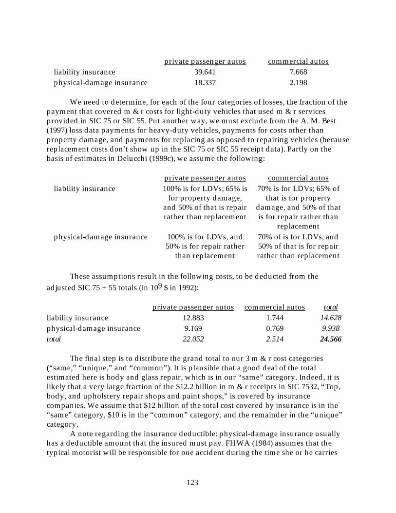
123

private passenger autos commercial autosliability insurance 39.641 7.668physical-damage insurance 18.337 2.198

We need to determine, for each of the four categories of losses, the fraction of the payment that covered m & r costs for light-duty vehicles that used m & r services provided in SIC 75 or SIC 55. Put another way, we must exclude from the A. M. Best (1997) loss data payments for heavy-duty vehicles, payments for costs other than property damage, and payments for replacing as opposed to repairing vehicles (because replacement costs don’t show up in the SIC 75 or SIC 55 receipt data). Partly on the basis of estimates in Delucchi (1999c), we assume the following:

private passenger autos commercial autosliability insurance 100% is for LDVs; 65% is

for property damage, and 50% of that is repair rather than replacement

70% is for LDVs; 65% of that is for property

damage, and 50% of that is for repair rather than

replacementphysical-damage insurance 100% is for LDVs, and

50% is for repair rather than replacement

70% of is for LDVs, and 50% of that is for repair rather than replacement

These assumptions result in the following costs, to be deducted from the adjusted SIC 75 + 55 totals (in 109 $ in 1992):

private passenger autos commercial autos totalliability insurance 12.883 1.744 14.628physical-damage insurance 9.169 0.769 9.938total 22.052 2.514 24.566

The final step is to distribute the grand total to our 3 m & r cost categories (“same,” “unique,” and “common”). It is plausible that a good deal of the total estimated here is body and glass repair, which is in our “same” category. Indeed, it is likely that a very large fraction of the $12.2 billion in m & r receipts in SIC 7532, “Top, body, and upholstery repair shops and paint shops,” is covered by insurance companies. We assume that $12 billion of the total cost covered by insurance is in the “same” category, $10 is in the “common” category, and the remainder in the “unique” category.

A note regarding the insurance deductible: physical-damage insurance usually has a deductible amount that the insured must pay. FHWA (1984) assumes that the typical motorist will be responsible for one accident during the time she or he carries

124

physical-damage insurance, and hence will have to pay, once, the deductible portion of the insurance, which FHWA (1991) assumes to be $250. However, any insurance deductible amount paid towards m & r shows up in the Census’ data on receipts for automotive maintenance and repair services. Hence, payments of the deductible already are included in the m & r data we use here, and no additional analysis or estimation is required32.

Used motor vehicle parts. According to the OMB’s Standard Industrial Classification Manual (1987), the auto and home supply stores of SIC 553 sell new and rebuilt -- but not used -- automobile parts and accessories. In support of this, the Census Merchandise Line Sales (Bureau of the Census, 1995), shows $11.5 billion in sales of new and rebuilt parts in SIC 55, and only $68 million in sales of used parts. In the Census system, sales of used parts are classified as “wholesale,” and occur mainly in SIC 5015, “motor vehicle parts, used”. In 1992, sales of “used automotive parts, accessories, and equipment” (commodity line 0240) were $3.571 billion (Bureau of the Census, 1992 Census of Wholesale Trade, Subject Series, Commodity Line Sales, United States, 1995).

We assume that 95% of the total $3.6 billion was for parts for LDVs.In 1992, sales taxes were 0.5% of sales in all of SIC 501 (Key, 1997). However, they

likely were a higher percentage of sales of used parts. We assume 3%.Parts and services classified elsewhere. Finally, we account for expenditures on

items, such as all-purpose tools, that are used for motor vehicles but not sold in automotive stores or classified as automotive merchandise. We assume that expenditures on such items are 1% of the total expenditures estimated above.

Total m & r costs for LDVs in 1992. We distribute the costs estimated for retail and wholesale sector m & r to the three categories (same for EVs and ICEVs, unique to ICEVs, and common to EVs and ICEVs) according to the proportions estimated for m & r costs in SIC 75. Thus we end up with:

Total m & r costs (109 $)

Same for EVs and ICEVs

Unique to ICEVs

Common to EVs and ICEVs

85.21 31.24 6.90 47.07

Cost per vehicle. To obtain the cost per vehicle -- initially, for 1992 -- we divide the total m & r costs by the relevant number of vehicles. As noted above, our estimates of m & r costs do not include costs for HDVs or costs of in-house government or business m & r. Therefore, the relevant vehicle population is all light-duty vehicles that used m & r services from SICs 75 and 55, which is all LDVs less those that were serviced at “in-house” shops.

In 1992, FHWA reported 190 million vehicles in use, and Polk reported 182 million (Davis, 1998). The Polk figures probably are a bit more accurate, so we assume

32One perhaps could remove the deductible from the m & r category, and add it in as an “insurance” expense, but we seen no reason for this account shifting, especially because the deductible is not an insurance payment, but rather a payment not covered by insurance.

125

185 million. From this we deduct the 4 million non-light duty trucks in use in 1992 (Bureau of the Census, Truck Inventory and Use Survey,, 1995). Next, we note that there were on the order of 8 million LDVs in relatively large fleets (Davis, 1998; Key, 1994). We assume that half of those were serviced “in house”. The result is 177 million LDVs33.

To get the cost per vehicle in 1997, we multiply the 1992 per-vehicle costs by our estimate of the 1997/1992 ratio of per vehicle costs. Table 9 shows expenditures on maintenance, repair, and parts, per vehicle, as reported in the BLS’ Consumer Expenditure Survey (CES) (BLS, 1999).The current-dollar expenditure series accounts for changes in the “quantity” of m & r consumed, as well as changes in the price, which is what we want. As shown, m & r expenditures per vehicle increased by 6% from 1992 to 1997. We therefore end up with the following m & r cost per vehicle per year, in 1997 $:

Total m & r costs ($/veh)

Same for EVs and ICEVs

Unique to ICEVs

Common to EVs and ICEVs

509.66 186.82 41.30 281.54

The total here includes car washes, tune ups, and accessories (and sales taxes on all of them), but excludes tires and tubes, emissions and diagnostic testing, oil, parking, tolls, and renting and leasing34.

Comparison with other estimates There are at least four other independent estimates or data on m & r

expenditures for motor vehicles. FHWA (1984). The FHWA has estimated year-by-year m & r costs for large,

intermediate, compact, and subcompact automobiles, and for passenger vans, for the Baltimore area, in 1984 (Table 8). The FHWA definition of m & r is reasonably close to the definition used here, the main difference being that they include safety checks, and we don’t:

33This is not the same as the number of personal-use household vehicles, because that number excludes certain business and government-owned vehicles. The 1990 Nationwide Personal Transportation Survey (Hu and Young, 1993), on the basis of 22,000 interviews, estimates about 160 million vehicles “owned by or available on a regular basis” to households in 1990, excluding heavy trucks, recreational vehicles, and motor cycles, but including business vehicles if used regularly by the household. The EIA report Household Vehicles Energy Consumption 1991 (EIA, 1993) estimates about 150 million household vehicles in 1991, excluding heavy trucks, recreational vehicles, and motor cycles, but including business vehicles if used regularly by the household for personal trips. Finally, the Bureau of Economic Analysis, in making its estimates of “personal consumption expenditures” for the National Income Product Accounts of the United States, estimates about 140 million personal-use cars and trucks in the U. S. in 1992 -- or about 147 million if household/business autos are included) (Key, 1994)

34Keep in mind that these are estimates of national-average expenditures. Expenditures vary regionally with variations in labor costs, parts costs, weather (in places where roads are salted to melt snow, vehicles may rust more quickly), and other factors.

126

included in FHWA: all repairs and parts and servicesoil changes (but not the oil itself)tune upssafety checksaccessory items such as lights and wiperswashing and waxing

excluded:tiresoiloptional “add ons” such as seat covers and cup holderscosts covered by insurance (but, not clear)35

They distinguish between “scheduled” and “unscheduled” costs: “scheduled” costs are the cost of services explicitly suggested or required by the owners manual (e.g., checking the emission control system, changing the oil, tuning up the vehicle, checking the brakes). Costs contingent upon the outcome of an recommended inspection, and all other m & r costs, are considered “unscheduled”. For example, if the manual recommends periodic brake checks, and states the conditions under which brakes should be replaced, but does not explicitly establish a replacement interval, then the cost of the inspection is considered scheduled maintenance, but the cost of the replacement is considered unscheduled (because the replacement per se is not explicitly scheduled in the manual).

To estimate m & r costs, FHWA consulted repair manuals, service managers of major dealers, personnel in the automotive industry, and published statistics. They assumed that all labor was done by a professional mechanic, at $26/hour (in 1984). They used retail prices for parts. However, they excluded labor and parts costs for those repairs covered by a normal vehicle manufacturer's warranty (but not an extended, 5-year/50,000-mile warranty)36.

For comparison with our estimates, the FHWA estimates must be adjusted from Baltimore in 1984 to the U. S. in 1997.

35Presumably, FHWA (1984) does not count costs that are reimbursed by insurance, since such costs already are counted as part of insurance payments. The later FHWA (1991) report states that it excludes costs or repairs of collision damage.

36The FHWA did update the cost report in 1991 (FHWA, 1992), but changed the method of estimating maintenance and repair costs. Rather than build original estimates, in the way that they did in 1984, they simply started with the maintenance and repair expenditures reported in the BLS’ Consumer Expenditure Survey (CES). We examine the CES independently, and hence do not need to review the FHWA’s (1992) more recent estimate.

127

1). Generalizing from the Baltimore area to the whole U. S., in 1984. The FHWA estimates are based on prices in the Baltimore area in 1984. The first step, then, is to generalize these estimates to the nation as a whole. In 1984-85, households in the Baltimore area had 1.7 vehicles and spent $515/year on maintenance and repairs, or $303/vehicle (BLS, 1989a) (note that the definition of m & r is not very important here, since we are interested in relative costs). In 1984 and 1985, all urban households in the U. S. owned 1.9 vehicles, and spent about $480/year, or $250/vehicle (BLS, 1989a). This suggests that the Baltimore- area estimates should be multiplied by 250/303 = 0.83, to yield nationwide average estimates.

2). Updating to 1997. Since 1984, both the price and average “quantity” of m & r have changed. These two effects can be estimated separately, or together. First we estimate the price and quantity effects separately.

The Consumer Price Index has an index for “motor vehicle maintenance and repair,” but their definition of “maintenance and repair” does not include everything that we include. The expenditures that we count as m & r but that the CPI does not apparently are in another CPI category, now called “vehicle parts and equipment other than tires,” formerly called “other parts and equipment”. To combine the relevant parts of these two indices into a single index for m & r as we define it, the rate for each CPI category must be weighted by the portion of the total m & r expenditure (as we define it) that it accounts for.

The CPI shows that consumers spent 2.2 times more on m & r (as defined in the CPI) than on “other private transportation commodities,” which is the category that contains “other parts and equipment”. Assuming that expenditures on “other parts and equipment” were 40-50% of expenditures on “other private transportation commodities,” then expenditures on m & r (as defined by the CPI) were about 5 times expenditures on “other parts and equipment.”

For “motor vehicle maintenance and repair,” the ratio of the 1997 to the 1984 CPI is 1.57, and for “vehicle parts and equipment other than tires”, the ratio is 1.08 (BLS, 1999). Assuming five times as much expenditure on “motor vehicle maintenance and repair,” as on “vehicle parts and equipment other than tires,” the weighted-average price of m & r as we define it is equal to 0.833 x 1.57 + 0.166 x 1.08 = 1.49.

To the adjust the quantity of m & r consumed from 1984 to 1997, we can look at total household expenditures on m & r, per vehicle, in 1984 versus 1997, in constant dollars, as reported in the BLS’ CES (Table 9). Table 9 shows that from 1984 to 1997, reported direct m & r expenditures per vehicle remained relatively constant, in 1997$. Expenditures per vehicle in 1984 were about 5% higher than expenditures per vehicle in 1997, in 1997 $. Thus, the quantity consumed apparently declined by 5%. Thus, the overall 1997/1984 scaling factor is 1.49 [price] divided by 1.05 (quantity) = 1.42.

This can be compared with the ratio expenditures in 1997 with expenditures in 1984, in current dollars -- which ratio captures both price and quantity effects. As shown in Table 9 this ratio is 1.34, somewhat lower than the 1.42 calculated above. We use a value of 1.40.

3) Other adjustments. The FHWA estimates exclude m & r costs covered by a “normal” manufacturers warranty (as opposed to an extended, 5-year or 50,000-mile

128

warranty), because consumers do not pay these covered m & r costs when they incur them. As noted above, we count these warranty-covered costs as m & r expenditures. We would like to add warranty-covered costs to the FHWA’s estimates, but unfortunately, FHWA’s analysis does not specify the warranty or its implicit price, or the cost of the m & r it covers. On the other hand, the FHWA (1984) includes inspection costs, which we do not. We will assume that the omission of warranty costs cancels the inclusion of inspection costs.

4). Summary and comparison. The FHWA data, transformed from Baltimore in 1984 to the U. S. in 1997 (Table 8) result in annual average m & r expenditures of $525 for a mid-size, $456 for a compact, and $521 for a subcompact. Assuming that FHWA would have estimated higher m & r costs for large cars, luxury cars, sports cars, and light-duty trucks and vans, the FHWA estimates imply a national average m & r expenditure of on the order of $530 for all LDVs. This is very close to our figure of $510, derived above.

BLS CES. As shown in Table 9, consumers reported spending only $341/vehicle/year on m & r, including batteries, tires, transmission fluids, oil changes, exhaust system repairs, brake work, auto repair policies, and much more. This is much less than our estimate based on the Census data.

Some of this discrepancy is related to the number of vehicles over which costs are distributed. In the BLS survey, there were 105.6 million consumer units, 211 million vehicles, and $72 billion in total m & r expenditures. The total number of “household” vehicles seems anomolously high, since in 1997 there were fewer than 210 million registered vehicles of all kinds, including heavy trucks, commercial vehicles, government vehicles, and business vehicles. If we distributed our total over 211 vehicles rather than 177 million vehicles, our cost per vehicle would be $428 rather than $510.

We cannot readily explain the rest of the discrepancy of about $90/veh/year. Either the establishments surveyed by the Census get an unexpectedly large share of their m & r revenue from commercial vehicles, or the consumers in the CES significantly under-report their expenses, or embedded warranty costs (which we count as an m & r expense, but consumers in the CES would not) are much higher than we estimate. We suspect that consumers under-report their m & r expenses in the CES.

The U. S. Government Accounting Office (GAO, 1991). The GAO reports that the fleet of vehicles operated by the General Services Administration has a m & r cost of 5 cents per mile. Assuming 12,000 mi/year, and updating to 1997, this results in about $700/year -- considerably higher than our estimate based on the Census data. This, however, may include collision repair costs, which we have removed from our estimates.

Runzheimer International (1992, 1989). Runzheimer surveys and estimates the maintenance and repair and tire costs of vehicles in business fleet. Assuming 12,000 mi/year, and updating to 1997, their estimates result in $400 to $650/year, depending on the type of the car, usage, and location (scaled to 12,000 miles per year). This range is consistent with our estimate.

[Other] methodological issues

129

The cost of personal time related to vehicle maintenance and repair. Many consumers do minor servicing, such as tuning the car and changing the oil, themselves. Presumably, these consumers feel that what they pay for parts and tools, plus the total value of their time, is less than what they would pay a professional for the same service (plus the time cost of having a car serviced professionally). The time cost of these do-it-yourselfers is not included in the Census data on receipts for m & r at commercial, tax-paying establishments with payroll.

The Census estimates do not include several other time or psychological “costs”: the psychological cost of discovering and having to deal with an automotive problem; the value of the time required to take a car to and from a mechanic; and the value of the inconvenience of being without the car (if one does not get a replacement from the shop).

Although we do not estimate these costs (because in this analysis, we include only monetary costs), we note that they probably are substantial. Delucchi (1998a) cites estimates of the time spent repairing and maintaining vehicles and buying gasoline, and concludes that the time cost is on the order of $50-$100 billion per year (in 1991 $, for the entire U. S.), with the bulk of the cost being due to m & r rather than buying gasoline. This (which does not include inconvenience or aggravation costs) is the same order of magnitude as actual expenditures on m & r. If EVs reduce these personal costs, the nonmonetary social benefit could be significant. Thus, by omitting these personal costs, we fail to count some of the potential social benefits of reduced m & r requirements of EVs.

Future maintenance and repair costs. Ideally, one should compare the m & r costs of EVs with the m & r costs of ICEVs in some future periods. One might do this by projecting future m & r costs for ICEVs, based on historical trends in real m & r costs, and anticipated new forces in the future.

Table 9 shows that from 1984 to 1997, reported direct m & r expenditures per vehicle remained relatively constant, in 1997$. Although it is possible that totalexpenditures (direct cash expenditures, plus do-it-yourself costs, plus the actual or implicit price of warranties) did change appreciably, because of a systematic bias in reporting, or because warranties covered increasingly more or less repair work, or because consumers were doing more or less work themselves, we do not have reliable evidence of such effects. We therefore reasonably can assume that real total expenditures on m & r have been relatively constant in the recent past.

It is possible that the cost of maintaining and repairing increasingly stringent and sophisticated emission control equipment will raise overall m & r costs over the next decade. However, any such trend is likely to be dampened somewhat by the use of on-board emission control diagnostic systems, which will help keep the systems operating properly.

This brief analysis suggests that there is little ground for projecting a radical change in real m & r costs in the future. Therefore, we use assume that m & r costs remain level in constant dollars.

Constructing a year-by-year maintenance and repair cost schedule

130

Our final objective is to estimate m & r costs for each vehicle type in each year of life. We then will take the present value of each year’s expenditure, sum the present values, and annualize the sum over the life of the vehicle, with the ultimate aim of arriving at a cost/mile figure.

As shown in Table 8, the FHWA (1984) provides estimates the m & r cost in every year, over the twelve-year life of the vehicle. The average of the FHWA series (transformed to a 1997 basis) is close to the m & r expenditure per vehicle per year that we estimate from the Census data. To estimate a year-by-year m & r schedule consistent with the Census data, we scale the FHWA estimate (scheduled plus unscheduled m & r) by a factor to make them consistent with the average m & r cost per vehicle estimated from the Census data (it turns out that the factor is about 1.0), and then distribute the scaled FHWA total to the categories “same for EVs and ICEVs,” unique to ICEVs,” and “common to EVs and ICEVs”, according to the proportions estimated from the Census data (see above).

Finally, because the net present value is a function of time, but the m & r expenditures actually are a function of cumulative mileage, we have to map the FHWA’s yearly maintenance schedule onto our own schedule of VMT/year, which is different from FHWA’s. We do this by making FHWA’s m & r schedule a function of their assumed accumulated mileage, rather than of time, and then calculating the age that corresponds to each cumulative mileage point, using our own VMT/age function (see discussion in section “Lifetime of vehicles, from purchase to disposal (years)”).

Maintenance and repair after 120,000 miles. The FHWA estimates m & r costs over what they assume to be the typical 12-year, 120,000-mile average life of the gasoline ICEV. However, because EVs and perhaps some alternative-fuel ICEVs will last longer than gasoline ICEVs, and because we are estimating m & r costs for the alternatives relative to m & r costs for the baseline gasoline ICEV, we need to extend the m & r series for the baseline gasoline ICEV beyond 120,000 miles. Although the FWHA (1984) estimated relatively minor m & r expenditures in the last few years of a 12-year life, perhaps under the assumption that a car owner would not spend a lot of money fixing up a car that he or she was planning to scrap soon, we assume that this trend would not continue: presumably, if the owner was planning to keep the car much beyond 120,000 miles, he or she would spend relatively large sums periodically in order to repair major systems and parts as they aged and failed. With this in mind, we have estimated a m & r expenditure series beyond 120,000 miles (Table 10).

Maintenance and repair costs for electric vehiclesEventually, when EVs are produced and serviced and maintained in large

numbers, they may have lower m & r costs (excluding tires and oil) than ICEVs, because electric drivetrains are simpler, more robust, and cleaner than ICE drivetrains. Turrentine and Kurani (1998) write:

Hypothetically, EVs should have fewer maintenance and service needs. Electric drive systems have fewer moving parts; produce no combustion products; operate at lower temperatures, which should reduce lubricant and seal breakdown;have no air intake or fuel filters; and, of course no

131

smog checks. Climate control systems in EVs will probably not have air filters because such filters increase energy demands. (p. 3-49)

They also suggest that EVs with regenerative braking might have less brake wear, although this might be offset by higher inertial mass.

A recent survey of “experts” on the state of EV technology gives more nuanced results. The experts believe that early EVs (year 2000) will have about 20% higher fuel and maintenance costs than ICEVs, but that by the year 2020, the EVs will have about 15% lower fuel and maintenance costs (Vyas et al., 1997). Dixon and Garber (1996) take a similar view, arguing that is unlikely that EVs will have lower maintenance costs in the early years of deployment. We agree that any maintenance cost advantage is not likely to be realized until there is a lot of experience with a lot of vehicles.

Many cost analysts have assumed that the m & r costs for EVs will be about half the costs for comparable ICEVs (GM, n.d.; Solar Energy Research Institute, 1981; Asbury et al., 1984; Edwards, 1984; Cohen, 1986; Humphreys and Brown, 1990; Morcheoine and Chaumain, 1992; U. S. DOE, 1995). For example, in an analysis done in support of the introduction of 300 commercial EVs in Britain, Edwards (1984) assumes that EVs will have 50% lower m & r costs than comparable ICEVs. Similarly, a cost model developed by the Jet Propulsion Laboratory for the USDOE assumes that total maintenance costs per mile for a Pb/acid-battery EV will be 40% lower than the costs for an ICEV (Humphreys and Brown, 1990). General Motors (n.d.) asserted that “G-Van owners could save up to 50% on normal maintenance operations” (p. 2). In its lifecycle cost analysis of EVs and ICEVs, the U. S. Department of Energy (DOE) (1995) assumes that EVs have 50% of the scheduled and unscheduled maintenance costs of ICEVs. Dixon and Garber (1996) are skeptical of 50% reductions, and assume instead 0% to 33% lower m & r costs.

There is a fair amount of evidence of the potential for lower m & r costs. Kocis' (1979) survey of consumer experience with EVs found that EV operators considered maintenance and operating costs to be substantially lower than for ICEVs. The electric milk delivery fleet in England was reported to have 35% lower m & r costs than the comparable ICEV fleet (Hamilton, 1984). A utility in the U. K. reports that EVs have 60% lower unscheduled maintenance costs than comparable diesel-powered vans Marfisi et al. (1978), using data compiled by Hamilton (1974) on the percentage of engine-related business at auto repair shops and parts stores, estimated that per-mile maintenance costs for the EV would be 66% lower than those for comparable ICEVs (they excluded tires, as we do, but included oil).

A comparison of the Griffon electric van with conventional ICE vans showed that the Griffon had only a 25% lower maintenance cost-per-mile than the ICEVs, excluding battery watering and oil, but including tire cost (Brunner et al., 1987a, 1987b). Further analysis showed that costs related to the engine were only about 24% of total maintenance costs for ICEVs, a figure sharply lower than that estimated in Hamilton et al. (1974) and Marfisi et al. (1978). Part of this relatively high m & r cost for the Griffon vans was attributable to unfamiliarity with EVs. More importantly, however, the authors note that the ICE vans were withdrawn from service and sold before accumulating 60,000 miles, which was about when major transmission and engine

132

repairs were expected. This suggests that the electric Griffon’s m & r advantage was greater over the second 60,000 miles of both vehicle's lives, and that it averaged better than 25% lower m & r costs over the whole of both vehicles’ lives.

In sum, both engineering analyses and operational data show that EVs can have lower m & r costs than ICEVs. We will estimate this advantage with respect to the costs that we have identified as “common to EVs and ICEVs”.

Our assumptions for maintenance and repair Based on the preceding analysis, we assume that BPEVs in high production

volumes have 30% lower common m & r costs than comparable ICEVs, over the entire life of the EV -- but without (for the moment) accounting for any batter-related costs. Of course, we assume that the costs that are “unique to ICEVs” are zero for EVs, and that the costs that are the “same for EVs and ICEVs” are, well, the same. (Recall from above that the costs that are the same are a little less than the costs that are common). The overall result (including battery maintenance, discussed below) is that the EV has about 25% lower m & r cost per mile than does the ICEV.

This result is less of a reduction than is typically assumed in the literature. However, we feel that because it is calculated more carefully, with respect to different kinds of m & r costs, it is more accurate.

For EVs in low-volume production, we assume no reduction in common m & r costs, on the grounds that the cost of unfamiliarity with EVs, due to their being few of them, cancels the “inherently” lower m & r costs.

The battery, fuel cell, and fuel storage system. Advanced Pb/acid, NiMH, and Li-polymer batteries are designed to be maintenance free, and hence, if they work as designed, they will have no m & r costs. But nothing works as intended 100% of the time, and we must allow for periodic repair and maintenance of even “maintenance-free” batteries. We assume an “unscheduled” battery m & r expenditure of $250 once over the life of the vehicle, in year 6 of vehicle operation.

Given how we have calculated the lifecycle cost of the battery, the actual servicing cost of replacing the battery is included in the battery initial cost. This is because we have calculated a “fully loaded” battery retail price: the OEM cost (including profit) of manufacturing the battery, plus the cost of shipping the battery to the auto manufacturer, plus all of the auto manufacturer costs associated with the battery: assembly, design, testing, marketing, shipping, profit -- everything. Since we assume that the consumer cost of a replacement battery is the similar to the just-explained “fully loaded” implicit retail price of the initial battery, the price of the replacement battery can be assumed to include most if not all of the costs associated with the initial battery, including shipping, marketing, and installation. Hence, we do not need to add an additional cost for the service of replacing a battery; that service is covered in the retail or replacement cost.

However, we do no need to consider the cost of removing and disposing of the old battery. This cost (or salvage value, if the old battery can be profitably recycled) is handled by an explicit term in our calculation of the battery cost: the model takes the

133

present value of the final disposal cost (or value) when it occurs, and adds that to the actual initial cost of the battery.

Compared with BPEVs, FCEVs will have two additional large and expensive components: a fuel cell, and a fuel storage/processing system. To estimate the relative m & r costs of FCEVs, or of BPEVs or FCEVs with a longer life than ICEVs, additional assumptions are necessary:

i) FCEVs will have two kinds of additional m & r costs: those associated with the fuel cell stack, and those associated with the fuel storage or processing system (the hydrogen storage system or the methanol reformer). We assume that these costs will be related to the complexity of the system, and express them as a fraction of the annual m & r cost of the BPEV. We estimate that it will cost less than $40/year to maintain PEM fuel cells, and very little to maintain high-pressure hydrogen storage tanks, which are simple and durable. (Hydrogen tanks might need to be leak-tested occasionally.)

ii) We assume that the ratio of EV m & r expenditures to ICEV m & r expenditures is the same for the “out-years” of life (beyond 120,000 miles) as it is for the first 120,000 miles. (This is an assumption, or an extension of the available data, rather than an interpretation of available data, because the published comparisons of EV m & r expenditures with ICEV m & r expenditures do not extend beyond the life of a typical ICEV.) Although the electric motor probably will continue to function reliably in the out years of life, the parts that an EV will have in common with an ICEV -- the suspension, body, interior, brakes, frame, and more -- will continue to deteriorate and fail. The owner of an old EV either will have to pay a large amount of money occasionally to maintain and repair these parts, or else scrap the vehicle. In the absence of actual data on EV m & r expenditure in the out years of life, we estimate them relative to ICEV m & r expenditures, the same way that we estimate m & r expenditures over the first 120,000 miles. The resultant m & r expenditure schedule shown in Table 10. (Note that we have, in fact, tried to make the assumption about vehicle life consistent with the m & r cost schedule, by accounting for the inevitable deterioration of the parts that EVs will have in common with ICEVs.)

The final assumed and calculated m & r costs, for BPEVs, are shown in Table 9. (Increments for fuel cells or fuel storage systems are not shown here.)

Warranty costs. As noted above, our estimates of m & r costs include the value of work done under a warranty. However, the cost of this work is not charged directly to the customer, but rather is embedded in the dealer cost portion of the price of the vehicle. This gives rise to a question: if EVs have lower m & r costs, will this be reflected in a lower implicit warranty cost, in the vehicle purchase price? Our analysis in essence assumes so, because we treat the m & r warranty costs explicitly , and assume that they will be a little lower with an EV. It is difficult to say whether or not any lower m & r costs will be translated into a reduction in the vehicle price: on the one hand, normal competitive pressures will tend to push prices down to cost; on the other hand, the cost-reduction “signal” might not be clear enough or large enough to warrant price differentiation.

134

Do consumers recognize and evaluate maintenance and repair costs?We have argued here that electric-drive vehicles will have lower m & r costs than

ICEVs, and that this cost reduction will partially offset the higher initial cost, from a life-cycle-cost point of view. Now, it is widely accepted that many fleet operators calculate life-cycle costs explicitly, and so can be expected to account for the m & r cost reduction of EVs in the way we have here. Unfortunately, though, the fleet-vehicle market is tiny compared to the household-vehicle market, and most households apparently do not do calculate life-cycle costs explicitly. (For example, Patil and Huff [1987] argue that "life cycle costs are not usually used to determine economic feasibility in passenger car applications" [p. 998]). If households do not even qualitatively weigh running costs against initial costs, then either the maintenance cost reduction of EVs will not be realized, or else it will have to be translated into a purchase incentive. It is of some interest, then, from both an analytical and a policy-making standpoint, to determine if consumers are likely to weigh lower m & r costs against higher a initial cost.

To address this question econometrically, one would need to know, for a large set of vehicles, the selling price and all attributes of the vehicles, including m & r costs, that determine consumer utility. There would have to be reasonable variation in the expected m & r costs, and one would have to believe that buyers were aware of differences in m & r costs. Unfortunately, it is not likely that most buyers choosing among spark-ignition vehicles consider m & r costs, because m & r costs are not posted on the vehicle, are not evident by inspection, and generally are not well known. However, diesel vehicles do have appreciably lower m & r costs than gasoline vehicles (Redsell et al., 1988), and buyers choosing between spark-ignition (gasoline) and compression-ignition (diesel) vehicles apparently are aware of this (Kurani and Sperling, 1989).

It might be worthwhile, then, to try to find the implicit price of lower maintenance costs and longer vehicle life, by comparing purchases of diesel vehicles and gasoline vehicles. For our purpose, though, it is sufficient to note that car buyers do indeed take account of reduced m & r costs. The case of diesel vehicles is enlightening. Light-duty diesel vehicles are harder to start, noisier, dirtier, and up to $1000 more expensive than their gasoline counterparts, but have lower fuel and m & r costs (Kurani and Sperling, 1989). Buyers of light-duty diesel-fuel vehicles expect the lower fuel and m & r costs to compensate for the disadvantages, including the higher initial cost (Kurani and Sperling, 1989). Kurani and Sperling's (1989) survey of diesel-car buyers shows clearly that people who chose diesels over gasoline vehicles did so in part because of the lower maintenance costs of the diesel.

Of course, one could argue that the people who choose diesels probably are unusually concerned about maintenance (and fuel) costs. This probably is true. However, EVs are likely to have lower m & r costs than even diesels, and so will appeal to people who are less concerned with m & r costs. Interviews of participants in a recent EV test-drive clinic do suggest that consumers will recognize the lower m & r costs of EVs. Turrentine et al. (1991) write:

The initial inspection of EVs convinced some participants that the motor was so simple there would be little to repair...When asked to reflect upon maintenance costs of EVs, many thought

135

about electric appliances such as their refrigerator and commented that there was little that could go wrong (p. 30).

Similarly, Turrentine and Kurani (1998) cite an article by Cambridge Reports that states that 80% of survey respondents say that they are more interested in EVs after learning that their maintenance costs are lower. Turrentine and Kurani (1998) also note that “car makers have been keen to reduce maintenance for conventional vehicles, aware of the cost and hassle to consumers” (p. 3-49).

It appears, then, that consumers likely will account for the lower m & r costs of EVs. (Whether they do so explicitly, using the rate of interest used here, is another question, which we do not address.)

INSURANCE

Overview Our lifecycle cost model handles insurance payments in some detail. We begin

with an estimate of the monthly premium for comprehensive physical-damage insurance and liability insurance for a reference vehicle. Then, we formulate a relationship between the liability and physical-damage insurance premiums, and the value and annual travel of a vehicle. Generally, we assume that premiums are nearly proportional to VMT and vehicle value. With this relationship, and an estimate of the value of the modeled vehicle relative to the value of the reference vehicle, and of the VMT of the modeled vehicle relative to the VMT of the reference vehicle, we calculate the insurance premiums for the modeled vehicle relative to the estimated premiums for the reference vehicle.

We also specify the number of years that physical-damage insurance is carried, in order to accurately calculate the lifecycle cost.

Data on insurance premiums There are several independent sources of data on insurance payments for motor

vehicles. However, the most comprehensive, primary source of data on premiums and expenses in the insurance industry is A. M. Best’s Aggregates and Averages, Property-Casualty (1997). (These data are comprehensive enough that the Bureau of Economic Analysis uses them in its National Income Product Accounts for the U. S.) A. M. Best (1997) reports premiums earned, and losses incurred, by companies writing auto liability insurance and physical-damage insurance for private passenger vehicles and commercial vehicles. (“Physical damage” includes collision, vandalism, fire, and theft insurance; and “liability” includes uninsured motorist coverage.) The following shows A. M. Best’s (1997) estimates of billions of dollars of net premiums earned for automobile insurance in 1996, from which we calculate $/vehicle assuming 170 million private passenger vehicles (including uninsured vehicles):

136

109 $ (1996) $/veh/yr. $/veh/mo.physical damage 38.76 228.00 19.00liability 67.15 395.00 32.92total 105.91 623.00 51.92

For the purpose of comparing the A. M. Best estimates with other estimates, and of developing our own $/insured-vehicle/month figures, we derive from the above an estimate of the average insurance premiums per insured vehicle, in 1997. First, we update from 1996 to 1997, by multiplying by 1997/1996 motor-vehicle-insurance CPI ratio of 1.03 (BLS, 1999). Next, we remove uninsured vehicles from the number of vehicles over which we divide the aggregate premiums reported by Best. Marowitz (1991) estimated that in California in 1990, about 20% of the vehicles were uninsured. Today the percentage probably is lower, as a result of laws that require proof of insurance when a person registers a vehicle or is pulled over by the highway patrol. We assume a national rate of 12%. Next, we assume that at any time, only half of the vehicles that do have liability insurance also carry physical-damage insurance. (We assume that nobody has physical damage insurance, but not liability insurance.) With these assumptions, we estimate the following:

109 $ (1996) 109 $ (1997) $-insured-

veh/yr. $-insured-veh/mo.

physical damage 38.76 39.92 533.73 44.48liability 67.15 69.16 462.33 38.53total 105.91 39.92 996.06 83.00

These are national average figures for all insured private passenger vehicles. Later, we will use these to develop estimates of the monthly insurance premiums for the Taurus and Escort ICEVs and EVs, on the assumptions that the averages above apply to the average price vehicle, and insurance premiums are a function of vehicle value. First, though, we will compare the A. M. Best (1997)-derived estimates with other estimates of insurance costs.

The FHWA (1984) estimated that in 1984, insurance against liability, property damage, personal injury, and uninsured motorists cost $36/month for the mid-size car and $33/month for the subcompact. Collision-damage insurance, held only for the first five years, cost $25/month for a mid-size car and $20/month for a subcompact car. In 1991, they updated their estimates (FHWA, 1991). Multiplying the FHWA estimates by the 1997/1984 and 1997/1991 CPI for insurance (factors of 2.33 and 1.32 -- the price of insurance doubled between 1984 and 1993) results in the following monthly premiums

137

FHWA (1984) (1997 $/mo.) FHWA (1991) (1997 $/mo.)subcompact midsize subcompact midsize

physical damage 47 58 30 30liability 77 84 70 70total 124 142 100 100

According to Runzheimer International’s Survey & Analysis of Business Car Policies & Costs 1991-1992 (1992), business fleets paid a median value of $650/year for insurance in 1991 ($860 at 1997 prices). Similarly, the MVMA (1990) cited estimates by the American Automobile Association (which in turn got its data from Runzheimer International) that in 1990 property-damage and liability insurance cost $26.50/month, and physical-damage insurance cost $30.74/month ($21.58/month for collision-damage and $9.16/month for fire and theft insurance), for a total of $57.24/month or $686/year ($970 at 1997 prices).

The Runzheimer (1992) and MVMA (1990) estimates are consistent with the A. M. Best (1992) data, but the FHWA estimates of liability insurance are quite high, perhaps because of high insurance prices in the Baltimore area, where the data were collected.

A final source of data is the Consumer Expenditure Survey administered by the Bureau of Labor Statistics (BLS) of the U. S. Department of Labor. According to these surveys of actual consumer expenditures, households in 1997 spent $750 on insurance for 2.0 vehicles, or $375 per vehicle ($31/month/vehicle) (BLS, 1999). This is considerably lower than the average per-vehicle premium (including uninsured vehicles) of about $630, as shown above. This suggests that consumers seriously under-report their insurance expenditures, just as, we believe, they under-report their expenditures on vehicular maintenance and repair (see above).

Monthly premiums for EVs and ICEVs Given the average insurance premium per insured vehicle estimated from above

from the A. M. Best data, we wish to estimate the premiums for the Taurus and Escort ICEVs and EVs modeled here.

Insurance premiums are a function of many factors, including the amount and kind of protection, the value of the vehicle, the characteristics of the drivers and the area where the vehicle is driven, and the amount and kind of driving. However, we think it reasonable to assume that the vehicles that we model here are driven the same way, in the same sorts of places, as is the “average” vehicle to which the A. M. -Best (1997)-derived averages apply. But the vehicles that we model in general will not be worth the same, and might not be driven the same distance annually, as the “average” vehicle. Hence, we can estimate the insurance premiums, for the vehicles that we model, on the basis of the value and annual VMT of the modeled vehicles relative to the value and annual VMT of the “average” vehicle with the estimated average insurance premiums.

Our formal model assumes a simple nonlinear relationship between relative insurance premiums and relative vehicle value and annual VMT:

138

PDPV = PDPV * ⋅RCV

RCV *

PV

⋅AVMT 'VAVMT 'V*

PE

LPV = LPV* ⋅RCV

RCV *

LV

⋅AVMTV

AVMTV*

LE

AVMT =LVMLVY

where:

PDPV = the physical-damage insurance premium for the vehicle being modeled ($/month)

PDPV* = the physical-damage insurance premium for the reference vehicle ($/month) (the average calculated above, from the A. M. Best [1997] data)

RCV = The retail cost of the vehicle being modeled ($) (calculated above)RCV* = The retail cost of the reference vehicle ($). The BEA (Morris, 1998) reports

that the average expenditure per new model-year 1997 car was $20,273, and the average expenditure per new model-year 1998 car was $20,787. (“Expenditure” includes everything: taxes, options, shipping, dealer preparation, etc., and so is equivalent to our “RC” parameter.) We weight the 1997 model year by 0.75, and the 1998 model year by 0.25, to come up with a 1997 calendar-year figure of $20,400.

PV = exponent that determines the relationship between the relative vehicle value and the relative physical-damage insurance premium (discussed below)

AVMT’V = average annual vehicle miles of travel by the vehicle being modeled, over the life that physical-damage insurance is held37

AVMT’V* = average annual vehicle miles of travel by the reference vehicle, overthe life that physical-damage insurance is held (assumed to be the same as that estimated for the ICEV in this analysis)

PE = exponent that determines the relationship between the relative vehicle travel and the relative physical-damage insurance premium (discussed below)

LPV = the liability insurance premium for the vehicle being modeled ($/month)LPV* = the liability insurance premium for the reference vehicle ($/month) (the

average calculated above, from the A. M. Best [1997] data)

37We distinguish AVMT from AVMT’ because EV/ICEV ratio of AVMT can be different from the EV/ICEV ratio of AVMT’, on account of different annual mileage accumulation schedules.

139

LV = exponent that determines the relationship between the relative vehicle value and the relative liability insurance premium (discussed below)

AVMTV = average annual vehicle miles of travel by the vehicle being modeled, over its life

AVMTV* = average annual vehicle miles of travel by the reference vehicle, over its life (assumed to be the same as that estimated for the ICEV in this analysis)

LE = exponent that determines the relationship between the relative vehicle travel and the relative liability insurance premium (discussed below)

LVM = the life of the vehicle in miles (input by the user)LVY = the life of the vehicle in years (calculated from a function of mile

accumulation v. time; see discussion in section “Lifetime of vehicles, from purchase to disposal (years)”)

Given assumptions or model-calculated results for vehicle value and annual VMT, and assuming that AVMTV* = AVMTICEV, then the key remaining parameters in these functions are the exponents PV, PE, LV, and LE. If they are zero, then differences in vehicle value or VMT have no affect on insurance premiums, and the premiums for the modeled vehicles are equal to the average premiums. If the exponents are equal to 1.0, then insurance premiums are proportional to vehicle value and VMT.

The relationship between insurance premiums and annual travel. Most if not all auto insurance premiums are some function of annual VMT. In some cases the premium is set by VMT category (“second-car,” “less than 5,000 mi/yr.,” etc.); in others, the premium is charged per mile of travel, and hence is proportional to VMT.

An insurance premium can be analyzed in two parts: a payment that covers expected losses, and a payment that covers the insurance company’s management and administration cost, and profit. The expected losses are a function of the probability and cost of losses (theft, accident, etc.), and are equal to •i Pi . Ci, where Pi is the probability of loss type i and Ci is the cost of loss type i. The management and administration cost, and profit, may also be a function of the expected losses.

It might seem reasonable to suppose that the probability of an accident per year is proportional to the amount of travel per year, but there can be important “feedback” effects that undermine this proportionality. For example, there is evidence that as total VMT increases and streets become more crowded, drivers exercise more care, and hence “compensate” for the increased exposure by reducing the accident rate per mile (Simonet and Wilde, 1997; Blomquist, 1986; Evans, 1985). Moreover, an increase in VMT might reduce average speed, which in turn might reduce the average severity -- and cost, Ci -- of accidents.

Turning now to the relationship between physical-damage insurance and VMT, we do not know how the likelihood of theft -- one of the losses covered by comprehensive physical-damage insurance -- is related to VMT. We suspect, though, that the relationship is not one of proportionality, because vehicles are stolen when they

140

are parked, not when they are being driven, and they might be just as likely to be stolen when parked at home as when parked away from home.

Finally, as regards the relationship between VMT and the administration and management cost, and profit, it is possible that profit is a fixed percentage of the premium, rather than a fixed absolute amount.

With these considerations, we assume that all expected losses except theft are virtually proportional to VMT; that theft loss is only weakly related to VMT; and that profit is nearly a fixed percentage of the premium. Qualitatively, we judge that the exponent PE, which relates the relative annual VMT to the relative physical-damage premium, is 0.75, and that the exponent LE, which relates the relative annual VMT to the liability premium, is 0.90. (Recall from above that a value of 1.0 makes the premium proportional to VMT, whereas a value of 0.0 makes the premium completely independent of VMT.)

The relationship between insurance premiums and vehicle value. The task here is to quantify the relationship between vehicle value and insurance premiums. The issue may be put as follows: if EVs, with their expensive batteries, fuel cells, and hydrogen storage equipment, cost, say 40% more than ICEVs, will their physical-damage premiums, or even liability premiums, be 40% higher? What is the relationship between the relative vehicle value, and the relative insurance premium? (In our formal model, we embody this relationship in the PV and LV parameters shown above.)

To answer this, we may distinguish three kinds of insurance, related to theft, property damage, and injury.

Since theft insurance premiums presumably are equal to expected losses plus insurers’ administration and management cost and profit, and the expected losses are equal to the value of lost vehicles multiplied by the number of lost vehicles, then, for a given probability of loss, the theft insurance premium is proportional to the vehicle value. If we assume that the probability of theft is independent of the type of drivetrain or fuel used by a vehicle, then the theft component of the EV insurance premium is equal to the component for some reference vehicle multiplied by the ratio of the value of the EV to the value of the reference vehicle38.

Similarly, property-damage insurance premiums are equal to expected payments for damages plus insurers’ administration management cost and profit. As noted above, expected payments for damages can be represented as •i Pi . Ci, where Pi is the probability of loss type i and Ci is the cost of loss type i. Assuming that the Pi are unaffected by the value of the vehicle39, the question becomes: what is the relationship between changes in the value of the vehicle, and changes in the average damage per

38One could argue that the probability of theft increases with vehicle value; if so, and assuming that the loss is proportional to vehicle value, then this component of the exponent PV would be greater than 1.0. However, it is not clear to us that the extra cost of an EV or AFICEV is especially valuable to would-be thieves.

39This of course might not be right: perhaps as the value of a vehicle increases, the owner drives more carefully.

141

incident? To answer this question, let us first define the “value ratio,” as the ratio of the value of vehicle X to the value of vehicle Y, or the ratio of the value of component P of vehicle X to the value of component P of vehicle Y. With this, we may say that if damage tends to occur disproportionately to components whose value ratio is significantly different from the vehicle value ratio, then the average damage per incident will not be proportional to the vehicle value.

An example will help. Suppose that the only difference between vehicle X and vehicle Y is the fuel storage system, which costs $C in vehicle X, and $10.C in vehicle Y, with the result that value of vehicle Y is 1.1 times the value of vehicle X. If all accidents involve components other than the vehicle storage system, then the average damage per incident will be the same for X and Y, and hence will be independent of the vehicle value. Conversely, if all accidents involve only the fuel storage system, then the average damage per incident will be 10 times higher for vehicle Y than for vehicle X -- much more than the 1.1 ratio of vehicle values. If, however, the fuel storage system is damaged 50% of the time, then the average damage per incident for vehicle Y will be 1.1 times that of vehicle X -- the same as the vehicle value ratio.

Because we have no reason to assume that damage tends to occur disproportionately to components whose value ratio is significantly different from the value ratio, we assume that property damage is proportional to vehicle value.

Finally, as regards injuries and related costs, there is no obvious relationship between the value of vehicles and the probability and severity of injury-accidents, so we assume that the personal-injury portion of the liability premium is independent of vehicle value. In order to separate this “value-independent” portion of the premium, we assume that the portion of the liability premium that covers costs related to injury is twice the portion that covers costs related to property damage (based in part on Miller et al., 1991, and Blincoe, 1996). We further assume that the insurance administration and management cost and profit is 20% of the total premium (based in part on A. M. Best, 1997).

With these considerations, we assume that all theft loss, and all property damage whether under physical-damage insurance or liability insurance40, is virtually proportional to vehicle value; that liability insurance for personal injury is independent of vehicle value; and that profit is nearly a fixed percentage of the premium. Qualitatively, we judge that the exponent PV, which relates the relative vehicle value to the relative physical-damage premium, is 0.90, and that the exponent LV, which relates the relative vehicle value to the liability premium, is 0.45. (Recall from above that a value of 1.0 makes the premium proportional to VMT, whereas a value of 0.0 makes the premium completely independent of VMT.)

40The use of a more valuable vehicle does not affect the liability premium of the user of the more valuable vehicle, but it does affect the property-damage portion of the liability premium of all other drivers, because everyone else now has to insure against damaging a more valuable vehicle. We assign this increase in the damage premium to the insurance of the more valuable vehicle.

142

Deductible and otherDeductible. As mentioned above, we treat any payments of the insurance

deductible, which typically is around $25041, as an expenditure on m & r. Since any such payment is included in the Census data on receipts for automotive maintenance and repair services, the payments of the deductible, if for m & r, already are included in our “maintenance and repair” category. We leave the matter this way.

Note that, since we do we count insurance payments as such (i.e., in the “insurance category), we make sure that any m & r costs that are covered by insurance are not counted (a second time) in the “maintenance and repair” category. We do this by removing from the grand total m & r receipts the amount that we estimate is paid by automobile insurance.

Length of time carrying physical-damage insurance. We assume that the length of time that physical-damage insurance is carried is related to the initial value of the vehicle, and estimate the time relative to that for the reference vehicle, based on the relative vehicle values:

CDTV = CDTV* ⋅RCV

RCV*

0.5

where:

CDTV = the number of years that the owner of the modeled vehicle carries physical-damage insurance

CDTV* = the number of years that the owner of the reference vehicle carries physical-damage insurance (we assume 5.5)

RCV, RCV* are defined aboveK = dampening exponent (0 eliminates the effect of differences in vehicle price; 1

makes CDT proportional to the price ratio; we assume 0.5)

The cost per mile of insuranceThe cost per mile of insurance is calculated in three steps:

1) sum the present value of two payment series: i) monthly liability insurance premium over the life of the vehicle, andii) monthly physical-damage insurance premium, over the time that it is

paid;

41 In its analysis of the cost of owning and operating cars and trucks, FHWA (1984) assumed that the deductible amount from insurance coverage “usually” was $100. However, Runzheimer International (1992) reports that among business fleets surveyed the median deductible in 1991 was $250, and the MVMA (1990) cites estimates by the American Automobile Association (which in turn got its data from Runzheimer International) that the deductible from physical-damage insurance was $250 from 1978 to 1990.

143

2) annualize this summed present value over the life of the vehicle;

3) divide by miles of travel.

The present-value and annualization formulae are the standard ones, and are presented in the section on the lifecycle cost per mile (see also the lifecycle cost per mile of the tires, which cost is calculated in a manner similar to that for insurance). The relevant interest rate for the present value and annualization calculations is the real annual or monthly interest rate foregone on cash used for transportation expenditures, after taxes (see the discussion in the section on financial parameters).

As shown in the tables of results, the EVs, because of their appreciably higher total value, have a considerably higher insurance cost per mile.

OTHER PERIODIC COSTS AND PARAMETERS

Fuel and electricityGasoline. The Energy Information Administration (EIA) (1998) projects that oil

will cost about $20/bbl, and gasoline will retail for $1.20- $1.30/gallon, including Federal and State but not local taxes (1997 $) from about 2005 onwards. In the model, we specify a $20/bbl oil cost (and assume that gasoline is 90% crude oil), a $0.30/gallon refining cost, a $0.17 distribution and retailing cost, and $0.38 in taxes (see DeLuchi, 1992, for data on refining, distribution, and retail costs), for a total selling price of $1.31/gallon.

Electricity. It is likely that if electric vehicles become widespread, utilities will offer low off–peak rates, to encourage consumers to recharge when capacity is available. In California, all five major utilities -- Southern California Edison, Pacific Gas and Electric, Los Angeles Department of Water and Power, Sacramento Municipal Utility District, and San Diego Gas and Electric -- have proposed or adopted time-of-use rates that will encourage EV owners to charge during off-peak hours (California Energy Commission, 1994). All five utilities charge or have proposed to charge from 3 to 5 cents/kWh from midnight until 6:00 am. Rates go as high as 36 cents/kWh in the afternoon in summertime (California Energy Commission, 1994).

In any event, the EIA projects that average electricity price nationwide will not be much higher than the off-peak rates in California: about a 8.0 cents/kWh (1997 $) to the residential sector through the year 2020 (EIA, 1998).

With these considerations, we assume an average rate of $0.06/kWh.Fuel for the EV heater. As discussed above, we assume in our base case that the

EV has a propane heater, because the EV drivetrain does not produce enough waste heat to warm the interior cabin, and it is more efficient (Garabedian, 1999) and cost-effective to use a fuel heater rather than a resistance heater in the vehicle cabin. The cost of the heater itself is included in our of the cost of heating and cooling system. The cost-per-mile of the heating fuel (we assume propane) is a function of the steady-state heat requirement per hour, the initial (transient) heating requirement, the average speed, the

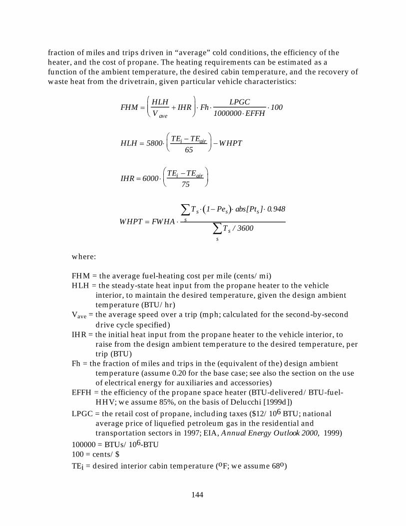
144

fraction of miles and trips driven in “average” cold conditions, the efficiency of the heater, and the cost of propane. The heating requirements can be estimated as a function of the ambient temperature, the desired cabin temperature, and the recovery of waste heat from the drivetrain, given particular vehicle characteristics:

FHM =HLHVave

+ IHR

⋅ Fh ⋅

LPGC1000000 ⋅EFFH

⋅100

HLH = 5800 ⋅ TEi − TEair

65

−WHPT

IHR = 6000 ⋅TEi −TEair

75

WHPT = FWHA ⋅

Ts ⋅ 1− Pes( )⋅ abs[Pts ] ⋅ 0.948s∑

Ts / 3600s∑

where:

FHM = the average fuel-heating cost per mile (cents/mi)HLH = the steady-state heat input from the propane heater to the vehicle

interior, to maintain the desired temperature, given the design ambient temperature (BTU/hr)

Vave = the average speed over a trip (mph; calculated for the second-by-second drive cycle specified)

IHR = the initial heat input from the propane heater to the vehicle interior, to raise from the design ambient temperature to the desired temperature, per trip (BTU)

Fh = the fraction of miles and trips in the (equivalent of the) design ambient temperature (assume 0.20 for the base case; see also the section on the use of electrical energy for auxiliaries and accessories)

EFFH = the efficiency of the propane space heater (BTU-delivered/BTU-fuel-HHV; we assume 85%, on the basis of Delucchi [1999d])

LPGC = the retail cost of propane, including taxes ($12/106 BTU; national average price of liquefied petroleum gas in the residential and transportation sectors in 1997; EIA, Annual Energy Outlook 2000, 1999)

100000 = BTUs/106-BTU100 = cents/$TEi = desired interior cabin temperature (oF; we assume 68o)

145

TEair = design ambient temperature (oF; we assume 45o)WHPT = the powertrain waste heat actually delivered to the vehicle interior, in

steady state (we follow Dieckmann and Mallory [1991] and assume that the powertrain cannot supply any of the “transient” heat at the start of a trip, because it hasn’t warmed up enough) (BTU/hr)

FHWA = of the powertrain waste heat generated theoretically, the fraction that actually is delivered to the vehicle interior (0.20; see discussion below)

subscript s = segment of the drivecycle. Ts = the duration of segment s of the drive cycle (seconds)Pes = the efficiency of energy transmission from battery or fuel-cell terminals to

wheels, for segment s of the drivecycle. This is calculated in the section “Once − through efficiency from the battery (or other energy-storage system) or fuel − cell to the wheels (excluding storage device itself)”

abs[Pts] = the absolute value of the power through the drivetrain during segment s of the drivecycle (kW; this is discussed in the section “Power at engine crankshaft or fuel-cell or battery terminals”)

0.9480=BTUs/kJ3600 = sec/hr

The equation for the steady-state heat loss, HLH, and the initial heat input, IHR, are based in part on graphs that show the steady-state and transient heating requirements as a function of the ambient temperature, for a minivan (Dieckmann and Mallory, 1991). We assume that our baseline EV has a smaller cabin and better insulation than has the minivan in the Dieckmann and Mallory (1991) analysis, and so reduce the heating requirements in Dieckmann and Mallory (1991) by about 20%.

Dieckmann and Mallory (1991) note that the waste heat from the EV drivetrain, though much less than the waste heat from the ICEV drivetrain, can, if completely recovered, supply a substantial fraction of the steady-state heating needs. Using the actual second-by-second data on the energy rate and efficiency of the powertrain, we can calculate fairly accurately the amount of waste heat generated theoretically by the drive train (see the equations above). However, the difficult question is: what fraction of this theoretically available waste heat is economically recoverable? Without any analysis, we assume that 20% of the available heat actually is delivered to the interior of the vehicle, at essentially no capital cost.

As shown in the tables of cents-per-mile results, these assumptions, which are relatively moderate (e.g., the EV is operated 20% of the time in 45o F ambient temperature), still result in a non-trivial cost per mile for propane fuel for heating. Indeed, in our base case, the heating fuel cost per mile is about the same as the tire replacement cost per mile, or the registration cost per mile. And in very cold conditions -- say, 35% of the time in 30o weather -- the cost of heating fuel is the same as the cost of electricity to power the vehicle!

Note that in ICEVs, the heat for the interior cabin is essentially free.

146

It is possible in this model to specify an electrical heating system (a heat pump and a resistance heater) instead of a fossil-fuel system. The parameter values for the electric heating system are presented in the section “. There is a switch in the model which specifies either a fossil-fuel or electric heating system.

The lifecycle cost of home recharging: offboard charger and dedicated high-power circuit

We assume that battery EVs will use an integrated conductive charging system, which promises to deliver high recharging power at comparatively low cost (New Fuels and Vehicles Report, 1999; AC Propulsion, 1999; Gage, 2000a; Oros, 1999a). This system may be analyzed in three parts:

1). A dedicated high-power circuit in the house. EV owners presumably will want a separate 220-V, 30-to-50-amp circuit for recharging EVs. As DeLuchi (1992) shows, a standard120-V/30-A circuit in many cases will not provide enough power to charge an EV overnight. Although some owners also may want a separate electricity meter for their EV circuit, we do not include this in our cost analysis.

2). Offboard outlet or charger. The off-board charger transfers power from the external high-power circuit to the vehicle. The box, or charger, is wired into the home circuit at one side, and has a cable and vehicle connector at the other. If it is relatively sophisticated, it does handshake and safety checks, and can be programmed by the user.

3). Integrated on-board charging components. On board the vehicle are the components that convert the ac power from the offboard charge to dc, monitor the battery voltage, and control the current flow and charge termination. Gage (2000a) lists four components: a charge port, a communication module, a battery monitor computer, and an integrated charger. These components are integrated with the motor controller/inverter in the EV drivetrain, to avoid duplication and thus reduce costs.

We estimate the cost of the on-board components (number 3 above) in the section “Cost of the electric drivetrain”. In this section, we estimate the cost of the high-power circuit and off-board charger.

The lifecycle cost of the circuit and off-board charger is estimated as a function of the initial cost, the interest rate, and the amortization period of the investment. The model calculates the length of time required to fully recharge the battery given a voltage and current input by the user, and the size of the battery required to satisfy the input vehicle range and power. If the user specifies that the battery in an FCEV be recharged by the outlet, the model deducts from the total recharging requirement the amount of energy returned to the battery by regenerative braking over the specified drive cycle, when the vehicle is operating on the fuel cell. If the user specifies that the battery in the FCEV be recharged by the fuel-cell instead of by the outlet, then the home recharging cost is assumed to be zero.

Formally, the cost per mile of the dedicated high-power circuit and the off-board charger is calculated as:

147

HRCM = AHRCAVMT

AHRC = IHRC ⋅iA

1 − 1 + iA( )−LHRY

where:

HRCM = the cost per mile of the home recharging system (circuit and charger) ($/mi)

AHRC = the annualized cost of the home recharging system ($/per year)IHRC = the initial cost of the home recharging system ($; discussed below)LHRY = the life of the home recharging system (assumed to be 30 years, the same

as the usual “life” of a home)iA = the relevant annual interest rate (for consumer expenditures related to

transportation; see section on financial parameters)AVMT = annual vehicle miles of travel (equal to lifetime miles divided by

lifetime years)

The key parameter in this calculation, of course, is the initial cost of adding a dedicated, high-power “smart” EV home recharging system (circuit and charger).

The dedicated high-power circuit. The cost of adding an EV recharging circuit toa home depends on several factors: whether one puts the circuit in a newly constructed home or retrofits an existing home; if one retrofits, whether or not the existing panel has adequate capacity; the length of the run from the panel to the outlet; local wage rates; and details of home construction..

It does not cost much to add an extra 220-volt circuit and install a slightly larger panel (than one would otherwise) at the time of construction, but it costs quite a bit more to remove an existing panel, put in a larger panel (perhaps in a different place), and run wires through existing walls. In a new installation, one pays only for the extra cost of the larger panel, and for the extra labor and materials to add the extra circuit. (The installation of the panel is free, because one must do it anyway.) In a retrofit, however, in the worst case one must pay to remove the old panel, pay for all of a new larger panel, pay to relocate and install the new panel, pay to relocate the existing wiring as necessary, and pay to install wiring in existing construction (which always is more costly than installing in new construction).

DeLuchi (1992) presents cost estimates from the literature, and from conversations with electricians and building inspectors across the United States. These estimates indicate that retrofitting an existing house with a 240-volt EV-recharging circuit would cost at least $200 if the installation was relatively simple, and $700-$800 if the installation was complex. Building a recharging circuit into a new home at the time of construction would add at least $100 to the price of the home.

Since the publication of DeLuchi’s (1992) estimates, a more recent, detailed analysis of customer costs has confirmed the high end of the range cited above.

148

According to Keeping Current (1993), Associated Utility Services (AUS) surveyed 314 customers of three major utilities in California, estimated the customer’s load, examined the existing wiring, and calculated the cost for installing an EV charging circuit to the garage or the parking area. They estimated that the EV charging circuitry and plug would cost an average of $709 in the Southern California Edison service area, $830 in the Los Angeles Department of Water and Power service area, and $874 in the Pacific Gas and Electric service area. These estimates include a plug, but not an off-board charger, load-management device, or separate meter. They found that it cost much less than the average to retrofit homes that have an attached garage and an adequate panel, and much more than the average to retrofit homes that had a detached garage and needed a new service panel.

The off-board charger. Off board chargers probably will cost from $200 to $500, depending on their design and power rating. Recently, Ford Motor Company and a supplier company (Avcon) have announced that they will offer a conductive charging box for as little as $295 (retail price to consumer). This does not include a state-of-charge indicator, or a separate meter (New Fuels & Vehicle Report, 1998), but apparently does include a recharging cord (Gage, 2000b). Electric Vehicle Infrastructure Inc., a major supplier of off-board conductive charging equipment, projects a cost of at least $300 for a programmable off-board charger with a state-of-charge indicator (Oros, 1999b).

AC propulsion (Gage, 2000a) estimates that the simplest low-power (1-10 kW) recharging box, such as is used to supply power to parked recreational vehicles, costs $170, not including the cost of a separate cord, which they estimate will cost an additional $200! (Gage [2000b] believes that the $295 Avcon “Power Pak” mentioned above includes a cord.) AC propulsion (Gage, 2000a) estimates that a higher-power version of the Avcon charging box (5-20 kW rather than 7 kW) will cost $450.

It thus seems reasonable to assume that the off-board charger (and cord) will cost as little as $300 at what we assume are modest volumes of production.

“Smart” meters. Some EV owners (and utilities) may want separate meters and load-management devices that communicate between the utility and each individual charging station to minimize cost and maximize the reliability and performance of the grid. Presently, a second ordinary mechanical meter dedicated to an EV costs $0.12/day from Southern California Edison (Gonzalez, 1994), equivalent to an up-front cost of around $200 to $400. Smart” electronic meters and load-management/meter devices probably will cost less than these additional mechanical meters. However, we don’t include these in our cost analysis.

Our assumptions. It probably is reasonable to assume that in the short term, costs will be relatively high. In the long run, if EVs are made in high volume, and new houses are built to accommodate EV charging, costs could be relatively low. With these considerations, we assume that, in the long run (at high production volume for EVs), there is an incremental consumer cost of $150 for a high-power circuit instead of an ordinary circuit, and an incremental consumer cost of $250 for a relatively simple offboard charger and cord set produced in high volume. In the short run (at low EV production volumes), we assume that houses have to be retrofitted, and that the total cost of the home recharging system is three times higher ($1,200).

149

Replacement tiresThe cost per mile of tires is calculated as a function of the initial cost of the tires,

the life of the tires and the interest rate. The life of the tires on the gasoline ICEV is specified in miles, and is calculated by the model for the other vehicle types on the basis of the weight of the other vehicle type relative to the weight of the gasoline vehicle. Thus, if an EV weighs more than the baseline ICEV, then its tires will be replaced sooner and hence will have a higher lifecycle cost. The model does not replace the tires if the last replacement interval is near the end of life of the vehicle.

In more detail, the calculation proceeds as follows. First, the model calculates the number of tire replacements by dividing the life of the vehicle by the life of the tires. If the last replacement is scheduled to fall such that the owner would get only 20% or less of the full use of the tires before the vehicle is scrapped at the end of its life, the replacement is assumed not to take place, and the final set of tires worn beyond the normal period until the vehicle is scrapped. The lifetime, again, is assumed to be proportional to the weight of the vehicle, on the assumption that tire wear is linear with vehicle weight42. (This assumption is reasonable because the force of friction is equal to the vehicle weight multiplied by the coefficient of friction, which depends on the characteristics of the two contacting surfaces.) Formally:

TR = Integer LVMEVTL

− 0.2

TLEV = TLICEV ⋅WIUEV

WIUICEV

where:

TR = the number of tire replacements“Integer” returns the integer portion of the quantity in the brackets [ ].0.2 = factor to prevent replacement if user would get less than 20% of use of the

final set of tiresLVMEV = the life of the vehicle in miles (input).TL = life of tires (miles).TLEV = the life of the tires for the EV.TLICEV = the life of the tires for the baseline ICEV (assumed to be 45,000).WIUEV = the in-use weight of the EV (calculated in the section “Total weight and

total manufacturing cost”).

42In its analysis of the lifecycle costs of EVs and ICEVs, the U. S. DOE (1995) simply assumes that tires on EVs last half as long as tires on ICEVs, on account of the extra weight. It is more reasonable to make the tire life proportional to weight.

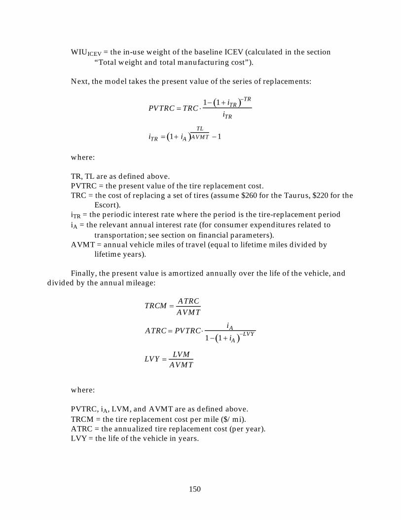
150

WIUICEV = the in-use weight of the baseline ICEV (calculated in the section “Total weight and total manufacturing cost”).

Next, the model takes the present value of the series of replacements:

PVTRC = TRC ⋅1− 1 + iTR( )−TR

iTR

iTR = 1+ iA( )TL

AVMT −1

where:

TR, TL are as defined above.PVTRC = the present value of the tire replacement cost.TRC = the cost of replacing a set of tires (assume $260 for the Taurus, $220 for the

Escort).iTR = the periodic interest rate where the period is the tire-replacement periodiA = the relevant annual interest rate (for consumer expenditures related to

transportation; see section on financial parameters).AVMT = annual vehicle miles of travel (equal to lifetime miles divided by

lifetime years).

Finally, the present value is amortized annually over the life of the vehicle, and divided by the annual mileage:

TRCM = ATRCAVMT

ATRC = PVTRC ⋅iA

1 − 1 + iA( )−LVY

LVY = LVMAVMT

where:

PVTRC, iA, LVM, and AVMT are as defined above.TRCM = the tire replacement cost per mile ($/mi).ATRC = the annualized tire replacement cost (per year).LVY = the life of the vehicle in years.

151

Vehicle registrationRegistration fees vary from state to state. Many states have either a flat fee or a

weight-based fee for passenger vehicles; a few states have a value-based or an age-based fee (FHWA, 1995). Some of the weight-based fees are graduated per ton, some distinguish only a few weight classes (e.g., under 14,000 lbs or over 14,000 lbs), and some have several classes.

Most fees range between about $20 and $100, with $50 appearing to be a rough average (FHWA, 1995). This is consistent with $8 billion in registration fees collected in 1997 (FWHA, 1998), which implies roughly $50 per passenger vehicle. Also consistent with this, households surveyed for the CES, reported spending about $35 to register a vehicle in 1990 (Division of CES, 1993). Data on total revenues from automobile registrations, and total automobile registrations, indicate about $42/vehicle in 1990 (FHWA, 1991a).

Given this data background, the model replicates the practice in most states and calculates the registration fee as a function of vehicle weight (heavier vehicles pay a higher fee). We use a weight-based fee because it is common and has a solid rationale, inasmuch as road damage is proportional to vehicle weight. The cost program assumes a $50 dollar yearly fee for the baseline passenger ICEV, and increases the EV registration fee, compared to the ICEV registration fee, in proportion to the extra weight of the EV:

VRCM =AVRCAVMT

AVRCEV = AVRCICEV ⋅WIUEV

WIU ICEV

where:

VRCM = the vehicle registration cost per mile.AVRC = the annual vehicle registration cost.AVMT = average annual vehicle miles of travel (calculated on the basis of a

mileage accumulation schedule).AVRCEV = the annual vehicle registration cost for the EV.AVRCICEV = the annual vehicle registration cost for the baseline ICEV (assumed

to be $50).WIUEV = the in-use weight of the EV (calculated in the section “Total weight and

total manufacturing cost”).WIUICEV = the in-use weight of the baseline ICEV (calculated in the section

“Total weight and total manufacturing cost”).

152

Vehicle inspection fee Presently, some states require safety inspections and inspections of the emission-

control systems. The Clean Air Act Amendments of 1990 require inspection and maintenance in ozone non-attainment areas; the further from attainment, the more stringent the I&M requirement (EPA, 1990). In California the inspection is every two years, and costs about $35 if the car passes the first time. If the vehicle fails and has to be fixed, but has not been tampered with, the owner is required to spend several hundred dollars to repair it. If the pollution control equipment has been tampered with, the owner must pay all repair costs.

In 1991, households surveyed for the CES reported spending about $4/vehicle for vehicle inspection (Division of Consumer Expenditure Surveys, 1993). In 1992, dedicated automotive inspection facilities received on the order of $2/vehicle (Bureau of the Census, Census of Service Industries, Sources of Receipts or Revenue, 1996). Since 1991/1992, the amount spent on inspection almost certainly has increased, in part because of the Clean Air Act Amendments mentioned above.

We assume that most vehicles undergo a biennial safety and emission inspection and test. We assume that the safety inspection costs $20 (every two years), and that the emissions inspection and test, which requires more sophisticated equipment, costs $40 (every two years). These assumptions result in a total cost of $60 every two years, or $30/year/vehicle, of which $10/year is the cost of the safety inspection. (Note that the cost of any required repair already is accounted for in m & r expenditures.)

EVs do not have any pollution control equipment, and hence are not subject to inspection and maintenance of emission controls. They are subject to safety inspections, however. Thus, we distinguish between fees for safety inspection and fees for inspection of the emission control system. The user enters the annual fee for the baseline gasoline vehicle, and the fee for the other vehicle types relative to the gasoline vehicle fee. (For example, EVs would be subject to a safety-inspection only, not an emissions inspection, and so would have a lower fee.)

OilThere are three ways to calculate the ICEV oil cost per mile, and they give

reasonably similar results. First, in 1992, retail stores sold $3.5 billion worth of automotive lubricants (Bureau of the Census, 1992 Census of Retail Trade, Merchandise Line Sales, 1995). Allowing for sales of another $0.5 billion in the service industries, and dividing by about 2 trillion VMT results in $0.0020/mile. Second, Delucchi (1999a) estimates 1.35 g-lube-oil/mi-travel, or 0.0016 quarts/mi, which at $1.30/quart is$0.0020/mi. Third, if one assumes 1 quart per 1000 miles, the result is $0.0013/mi. We assume one quart per 1000 miles for the Escort, and one quart per 750 miles for the Taurus, at $1.30/quart.

The cost of oil changes, apart from the cost of oil per se, already has been estimated separately as a m & r cost unique to ICEVs. (Note that the cost of the oil was deducted from the m & r costs.)

EVs do not consume lubricating oil.

153

Parking, tolls, fines, and accessoriesWe assume that these costs, per mile of vehicle travel, are the same for all LDVs. Delucchi (1999c) estimates that in 1991, all parking establishments in the U. S.

received about $8 billion in revenues, including parking taxes. From 1991 to 1997, revenues received in SIC 752 increased by 29% (Bureau of the Census, Service Annual Survey: 1997, 1998). Hence, we assume $10.3 billion in payments for parking in 1997. In addition, FHWA (1998) reports $4.4 billion in toll receipts by all levels of government in 1997. Delucchi (1999b) estimates about $5 billion in traffic and parking fines in 1991; we assume $6.5 billion in 1997. The total thus far is $21.2 billion. Dividing this by 200 million vehicles yields $106/vehicle/year, or $8.83/month.

The FHWA (1984) estimated that in 1984 owners of mid-size automobiles spent $16.50/year on vehicle accessories. We assume $30/year in 1997.

The yearly or monthly costs are divided by yearly or monthly VMT to obtain the cost per mile.

Federal, state, and local excise taxes The model calculates the cost per mile of the current government excise taxes on

gasoline, and then calculates the cost-per-mile for the other vehicles relative to this by using a scaling factor (0.0 to 1.0) specified by the user. In the base case, we assume that all vehicles pay the same tax per mile, so that government revenues from highway users (for the highways) would be the same regardless of the type of vehicle or fuel.

In 1997, the Federal excise tax on gasoline was $0.184/gallon, and the weighted-average of state excise taxes was $0.191/gallon (FWHA, 1998), for a total of $0.375/gallon. In addition, a few states and localities (most notably California and New York) charge sales tax on gasoline (FHWA, 1995): in the past, the total sales tax on gasoline nationally has been about 2% of pre-tax sales. With this, the total tax on gasoline becomes $0.383/gallon.

The mileage accumulation scheduleAs shown throughout this analysis, the lifecycle cost per mile is equal to an

annual cost divided by the average annual VMT. The average annual VMT is calculated from year-by-year mileage accumulation schedule for the ICEVs and AFICEVs, and a continuous function that relates age to mileage; the user specifies the value of the coefficients in this function in order to produce the desired mileage schedule. (See the discussion related to Table 5) A continuous function is used to avoid having to interpolate between years to get exact mileage (or vice versa) in those calculations where one must calculate mileage or age given the other. The model has two functions specified: one replicates a mileage-accumulation schedule derived from the Residential Transportation Energy Consumption Survey of the U.S. Department of Energy, and the second produces a schedule of more intensive use, in which more miles are driven in the early years of the a vehicle’s life.

154

FINANCIAL PARAMETERS

OverviewThe model characterizes a typical, “weighted-average” vehicle purchase by

calculating or taking as input a detailed set of financial parameters: the fraction of new car buyers who take out a loan to buy a new vehicle; the amount of the average down-payment on the car (input as a fraction of full vehicle selling price); the length of financing period for cars bought on loan (in months); the real annual interest rate on loans taken out to buy a new car, before taxes; the real annual interest rate foregone on cash used for transportation expenditures, before taxes (the opportunity cost of cash used for down-payment or outright purchase); the effective (average) income tax paid on banking interest earned, after deductions; the annual discount rate to apply to yearly mileage (see discussion below) the annual rate of inflation (assumed to be zero in our analysis here); the base year and the target year for the inflation analysis (if inflation is not zero); and whether or not interest payments be deducted from taxable income.

We distinguish between paying cash and financing because the proper opportunity-cost accounting for a cash payment is different from that for a loan. For a cash payment, the opportunity cost is the alternative use of the money, which is best represented by an interest rate for ordinary cash investment. An initial cash payment, then, is simply annualized at the interest rate foregone on alternative personal uses of the money. But in the case of a loan, the actual cost to the consumer is not the initial price, but the loan payment. Hence, one first must calculate the actual loan payments, which of course depend on the amount of the loan, the life of the loan, and the interest rate on the loan. The resulting loan payment series is treated as an ordinary cost (annuity): one finds the present value of the loan payment series, on the basis now of the interest rate for ordinary cash investment (the personal opportunity cost of money). Finally, the present value is annualized over the entire life of the vehicle, again on the basis of the personal opportunity cost of money. (The formulae for present value and annualization calculations are shown in the section on cost per mile.)

This three step procedure -- calculate the loan payment, calculate the present value of the loan payment series, and annualize the present value -- is necessary because the interest rate that pertains to loans is different from the interest rate that expresses the consumers opportunity cost of money, and because the life of the loan is different from the life of the vehicle financed with the loan.

The model user can specify a “discount rate” to be applied to the annual mileage. This allows the user to perform a quasi cost-benefit analysis, in which miles of travel are the “benefit” of travel, and are be discounted (or annualized) in the same way that the costs are. (It turns out that if one assumes different mileage schedules for different vehicles, then whether or not one treats VMT as a benefit and applies a discount rate can make a large difference in the overall cost-per-mile results.)

The financial-cost sub-model also performs a highly simplified macro-economic simulation: it assumes that the interest rate, the fraction of new car buyers who take out a loan, and the length of the financing period are a nonlinear function of the value of the vehicle. Thus, the more costly the vehicle, the greater the number of people who take

155

out a loan to buy it, the longer the financing period, and the higher the interest rate (because of the greater demand for money). Of course, the higher interest rate increases the amortized (per-mile) initial cost.

Down-payment on the car (fraction of full vehicle selling price) From 1972 through 1998 the loan-to-value ratio for new cars ranged between 0.85

and 0.94, and averaged about 0.89 (Federal Reserve Statistical Release, 1999). One would expect this ratio to be a function of the interest rate on the loan, the interest rate available on saved money, the availability of money, the cost of new cars, the length of time of the loan, and probably other factors. However, we simply assume the 10-year average of 0.89, which means that 11% of the value of the car must be a down-payment. We assume this percentage for all vehicle types.

Calculated length of financing period for cars bought on loan (months)The loan period for new cars rose steadily from around 35 months in 1970, to 45

months in 1980, to 55 months in 1990. However, in the 1990s, the period has remained relatively constant, at around 55 months (Federal Reserve Statistical Release, 1999). On the basis of this trend, we assume that the average loan period for new gasoline ICEVs is 55 months.

We expect that over time, the average loan period is a function of the average cost of motor vehicles, personal income, demand for motor vehicles, the money supply, and other factors. We therefore assume that the loan period for EVs, relative to the period for ICEVs, is a function of the cost of EVs relative to the cost of ICEVs. However, because the loan period undoubtedly is a function of other factors besides the cost of the car, it cannot be strictly proportional to the cost of a car. Given a loan period for the baseline gasoline vehicle, we calculate the loan period for the EV as:

LPEV = LPICEV ⋅MSRPEV

MSRPICEV

K1

where:

LPEV = loan period for the EV (months)LPICEV = loan period for the baseline ICEV (months; see discussion in text)MSRPEV = Manufacturers Suggested Retail Price of the EV ($)MSRPICEV = Manufacturers Suggested Retail Price of the baseline ICEV ($)K1 = price exponent (see discussion in the text)

The price exponent determines the relationship between the retail price ratio and the loan period ratio. A value of 0 eliminates the effect of price differences, and a value of 1.0 makes the loan period ratio equal to the price ratio. We assume a value of 0.3

156

Calculated fraction of new car buyers who take out a loan to buy a new vehicle In 1988, 70% of car buyers financed their purchase (Motor Vehicle

Manufacturer’s Association, 1990). In 1990, the figure was 62% (Motor Vehicle Manufacturer’s Association, 1992). We assume 68% for the baseline ICEV.

The fraction of buyers who finance must be related to the average price of vehicles (at constant household income). Given our assumption regarding the fraction of buyers who would finance the purchase of a gasoline ICEV, we calculate the fraction who would finance the purchase of an FCEV or BPEV as:

FLEV = FLICEV ⋅MSRPEV

MSRPICEV

K2

where:

FLEV = fraction of people who would take out a loan to buy an EVFLICEV = fraction of people who would take out a loan to buy the baseline ICEV

(discussed in the text)MSRPEV = Manufacturers Suggested Retail Price of the EV ($)MSRPICEV = Manufacturers Suggested Retail Price of the baseline ICEV ($)K2 = price exponent (analogous to K1 in the equation for LPEV; we assume 0.40)

If the value of FLEV calculated by this equation is greater than 1.00, 1.00 is used.

Calculated real annual interest rate on loans for buying a new car, before taxes From 1980 through 1990 automobile finance companies charged an average

nominal interest rate of 13.1% for loans for new cars, and 17.4% for loans for used cars, and commercial banks charged an average of 13.2% for loans for new cars (Federal Reserve Statistical Release, 1999). However, since 1992 the new-car rate at commercial banks has been around 9%, and in the past couple years, the new-car rate at auto finance companies has dropped to 6% (Federal Reserve Statistical Release, 1999). As of 1998, commercial banks held 35% of the consumer credit outstanding for automobile loans, automobile finance companies held 23%, credit unions held 22%, savings institutions held 4%, and pools of securitized assets held 16% (Federal Reserve Statistical Release, 1999).

Given these statistics, we assume a nominal interest rate of 10% for the gasoline ICEV base case.

To derive a real interest rate from this, the effect of inflation must be netted out. From 1980 through 1990, inflation, as reflected in the GNP implicit price deflators, averaged 4.8% per year (Survey of Current Business, 1991; Bureau of the Census, Statistical Abstract of the United States, 1990). There has been a similar change in the Consumer Price Index. (While this average does reflect the unusually high inflation of the early 1980s, so does the average of the nominal-interest-rate series over the same period.) In the 1990s, though, inflation has been at around 3% or lower (BLS, CPI data

157

extracted from BLS web site, 1999). Assuming a value of 3%, we calculate an 7% real rate of interest on loans for new gasoline ICEVs.

It seems reasonable to assume that interest rates for loans are a function of the total amount of money borrowed. If the introduction of electric vehicles increases the total demand for loaned money for automobiles, because of the higher initial cost of EVs, it is likely that interest rates will be higher than they otherwise would be43. Given an interest rate on loans for the baseline gasoline vehicle, we calculate the interest rate on loans for the fuel cell vehicle as:

RIEV = RIICEV ⋅FLEV ⋅MSRPEV ⋅ 1 −DPFEV( )

FLICEV ⋅ MSRPICEV ⋅ 1−DPFICEV( )

K3

where:

FLEV, FLICEV, MSRPEV, MSRPICEV are as defined aboveRIEV = real interest rate on loans for new EVsRIICEV = real interest rate on loans for new ICEVs DPFEV = fraction of selling price that is a down-payment, for EVs (see discussion

in the section “Down-payment on the car (fraction of full vehicle selling price)”)

DPFICEV = fraction of selling price that is a down-payment, for ICEVs (see discussion in the section “Down-payment on the car (fraction of full vehicle selling price)”)

K3 = price exponent (analogous to K1 in the equation for LPEV; we assume 0.15, to greatly dampen the effect of price differences)

Note that because FLEV and FLICEV cannot be greater than 1.00, and FLEV is greater than or equal to FLICEV if MSRPEV > MSRPICEV, as soon as FLEV reaches 1.00, an increase in FLICEV results in no change in FLEV , and hence in a decrease in RIEV.

43Arguably, a change in the average cash outlay, apart from a change in the average loan payment, could affect savings rates. We do not account for this.

158

Real annual interest rate that would have been earned on the money used for transportation expenditures, before taxes

We assume that the interest opportunity cost of money spent on a new car is the rate the money would have earned in a reasonably liquid but also reasonably high-yielding investment, were it not spent on a new car. In the late 1980s, the nominal interest rates on various kinds of money-market funds and deposits ranged between 7% and 9% (Federal Reserve Bulletin, 1991). The nominal rates on U. S. Treasury bonds of various maturities were between 8% and 9%; the nominal rates on state and local bonds were between 7% and 8%, and the nominal rates on corporate bonds were between 9 and 10%. The rates on ordinary savings accounts typically are lower, and sometimes considerably lower than rates on bonds. Recently, rates have been relatively low (Federal Reserve Statistical Release, 1999). Considering these data, we assume that the nominal opportunity interest cost of money spent on transportation is 7%. Given an inflation rate of 3% (discussed above), the real before-tax opportunity interest rate becomes 1.07/1.03 = 1.039 = 3.9%. The after-tax rate, of course, will be even lower.

Effective (average) income tax on interest, after deductionsTo calculate the after-tax real rate of interest, we must know the marginal state

and Federal interest-income tax. The marginal Federal tax rate for a married couple with 2 children and income up to about $35,000/year is 15%; at higher incomes, the rate is 28%. State income taxes are between 2 and 10% (The Book of the States, 1990). We assume a combined marginal rate of 20%. Interest income is not charged the FICA tax. We ignore the fact that some forms of interest are tax-free.

One perhaps could argue (although we think not convincingly) that the effective average tax rate, equal to tax liability divided by stated personal income, and not the marginal tax rate, should be used. In 1989, the effective average Federal income tax rate was 7.1% for a 4-person household with a total income of $25,000/year, 9.3% for a 4-person household earning $35,000/year, and 12.6% for a $50,000/year household (Bureau of the Census, Statistical Abstract of the United States, 1990). In 1986, state taxes paid were 27.5% of Federal taxes paid (which is consistent with the marginal tax-rate data cited above). This indicates a total effective average tax rate of 11.9% for a $35,000/year household.

The model has an option to allow interest payments to be deducted from taxable income. However, presently, interest payments cannot be deducted from taxable income.

Real annual interest rate that would have been earned on cash used for transportation expenditures, after taxes

In order to arrive at a total lifetime levelized monthly cost for the purchase of an automobile, we must apply, to all payments for the automobile -- to the loan payments as well as to the down-payment -- the real annual interest rate that would have been earned on cash used for transportation expenditures, after taxes. We proceed as follows. First, the monthly loan payments are calculated using the loan rate, loan period, and amount of the loan. The present value of these payments is calculated, using the real

159

annual interest rate that would have been earned on cash expenditures, and added to the actual down-payment. This total (down-payment plus present value of loan series) is then levelized over the life of the car (not the loan period, but the life of the car), using, again, the foregone real interest rate on cash. Note that the loan payment is simply a monthly bill, which must be handled using the foregone real annual interest rate on cash expenditures. The loan rate does not represent the consumer’s opportunity cost of money; the foregone interest rate on cash does.

CALCULATING THE COST PER MILE

The levelized (or annualized) present value, which is the conceptually correct expression of the lifecycle cost per mile, is calculated in three steps. First, the model calculates the present value (at specified interest rates) of every cost stream. For initial or investment costs, such as a battery or vehicle, the present value is equal to the initial cost, less the present value of any salvage value at the end of the life of the investment:

PVCI = CI + ⋅REPI ⋅Vel

1+ iA( )LIY

where:

PVCI = the present value of the initial investment ($)CI = the initial investment, in year 0 of the analysis ($)REPI = the replacement cost of the capital investmentVel = the salvage value of the capital at the end of its life, as a fraction of the full

replacement costiA = the annual interest rateLIY = the life of the investment in years

For regular (periodic) cost streams (e.g., tires) the present value is the present value of a periodic payment:

PVCP = CP ⋅1− 1+ iP( )−TP

iP

where:

PVCP = the present value of the periodic cost streamCP = the periodic cost ($/period)iP = the periodic interest rate (fractional interest per period)TP = the total number of periods (that fall within the life of the vehicle)

160

In general, any periodic interest rate iP must be calculated on the basis of the known annual interest rate iA :

iP = 1 + iA( )−TPY − 1

TPY = the total number of periods of interest, in years

For irregular cost streams (e.g., maintenance and repair), the model calculates the present value of each period’s cost, and sums all of the present values, for all of the cost occurrences that fall within the life of the vehicle:

PVCT =CT

1+ iP( )TT∑

where:

PVCT = the present value of a cost incurred at time TCT = the cost incurred at time T ($)iP = the periodic interest rate (fractional interest per period, where the period is

the unit of T (e.g., years, months)T = the time when cost CT is incurred

By convention, all initial and present-value costs are annualized over the life of the vehicle. The present value any regular or irregular cost stream is annualized over the life of the vehicle, because, by convention, for any particular kind of cost (e.g., maintenance and repair), all costs that occur over the life of the vehicle are included in the present value calculation. The formula is:

APVC = PVC ⋅iA

1 − 1+ iA( )−LVY

where:

APVC = the annualized present-value cost ($/year)PVC = the present value cost ($)iA = the annual interest rateLVY = the life of the cost

Finally, the annualized present value is divided by the calculated annual average mileage:

161

CM =APVCAVMT

AVMT = f MPY , iM( )

where:

CM = the cost per mile ($/mi)AVMT = average annual vehicle miles of travel (lifetime miles divided by

lifetime years)MPY = the mileage-per-year schedule (see discussion related to Table 5)iM = the discount rate pertaining to miles of travel (assumed to be zero here)

Of course, if the period of the regular payment (P) is a year, and the total number of periods (TP) is the same as the life of the vehicle LVY, then the annualized present-value cost, APVC, is just the annual payment, CP. This is the case for annual registration fees, parking, tolls, gas taxes, and a few other cost items. But for several important periodic costs, one or the other condition (P = year; TP = LVY) does not hold. For example, physical-damage insurance is a periodic payment, but is made for a total number of years (TP) less than the life of the vehicle (LVY). Hence, to annualize the physical-damage cost over the life of the vehicle, the procedure above must be used. On the other hand, tire replacement costs are incurred over the life of the vehicle, but an interval of many years, not yearly.

162

RESULTS

PRESENTATION OF RESULTS

In this section, we present and discuss the results of the analysis. In the table below we summarize our estimates of the retail cost and the break-even gasoline price, for the base case (high-volume production, FUDS, etc.), and for several scenarios (low-volume production, highway cycle, and so on). The break-even price is the full retailprice of gasoline, including all sales and excise taxes, at which the total lifecycle ownership and operating cost of the gasoline vehicle (in cents/mile) is equal to the total lifecycle ownership and operating cost of the EV. The summary table here shows results for two different driving ranges for each battery technology.

Pb/acid NiMH Gen2 Li-ion NiMH Gen4Retail cost, Taurus ($) 65 mi 110 mi 90 mi 165 mi 140 mi 260 mi 100 mi 190 mi

Base case 24,553 29,422 28,034 35,759 27,678 32,448 25,487 29,692

Highway cycle 24,623 28,276 27,706 34,422 27,485 31,879 25,346 29,215

Low-volume production 36,566 44,955 44,920 61,801 52,942 72,819 40,357 50,563

10% less power 23,789 28,039 27,116 34,208 26,648 30,894 24,716 28,542

Retail cost, Escort ($)Base case 19,784 23,384 22,725 28,822 22,280 25,948 20,623 23,904

Highway cycle 19,566 22,574 22,518 27,893 22,179 25,563 20,540 23,571

Low-volume production 30,726 36,782 37,826 50,921 44,369 60,053 34,117 42,157

10% less power 19,218 22,434 22,038 27,659 21,517 24,785 20,055 23,075

Break-even, Taurus ($/gal)Base case 2.64 4.14 4.19 6.66 2.77 4.33 1.83 2.91

Highway cycle 3.71 5.63 6.26 9.60 4.11 6.40 2.59 4.20

Low-volume production 6.01 8.69 9.96 15.65 10.49 17.09 5.80 8.60

Same vehicle life 2.92 4.40 4.53 6.36 2.97 4.57 2.09 2.87

20% longer vehicle life 2.44 3.68 3.51 6.62 2.17 3.56 1.65 2.83

No limit on shelf life 2.63 3.59 4.19 5.33 1.37 2.71 1.82 2.27

10% less power 2.33 3.67 3.85 6.10 2.46 3.85 1.60 2.60

Break-even, Escort ($/gal)Base case 3.27 4.84 5.04 7.73 3.38 5.06 2.40 3.59

Highway cycle 4.50 6.37 7.20 10.64 4.83 7.15 3.36 4.99

Low-volume production 7.41 10.12 11.95 17.96 12.47 19.61 7.33 10.33

Same vehicle life 3.62 5.11 5.42 7.35 3.66 5.32 2.73 3.53

20% longer vehicle life 3.06 4.34 4.32 7.68 2.74 4.20 2.20 3.46

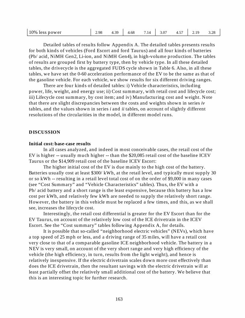
163

10% less power 2.98 4.39 4.68 7.14 3.07 4.57 2.19 3.28

Detailed tables of results follow Appendix A. The detailed tables presents results for both kinds of vehicles (Ford Escort and ford Taurus) and all four kinds of batteries (Pb/acid, NiMH Gen2, Li-ion, and NiMH Gen4), in high-volume production. The tables of results are grouped first by battery type, then by vehicle type. In all these detailed tables, the drivecycle is the aggregated FUDS cycle shown in Table 6. Also, in all these tables, we have set the 0-60 acceleration performance of the EV to be the same as that of the gasoline vehicle. For each vehicle, we show results for six different driving ranges.

There are four kinds of detailed tables: i) Vehicle characteristics, including power, life, weight, and energy use; ii) Cost summary, with retail cost and lifecycle cost; iii) Lifecycle cost summary, by cost item; and iv) Manufacturing cost and weight. Note that there are slight discrepancies between the costs and weights shown in series ivtables, and the values shown in series i and ii tables, on account of slightly different resolutions of the circularities in the model, in different model runs.

DISCUSSION

Initial cost: base-case resultsIn all cases analyzed, and indeed in most conceivable cases, the retail cost of the

EV is higher -- usually much higher -- than the $20,085 retail cost of the baseline ICEV Taurus or the $14,909 retail cost of the baseline ICEV Escort:

The higher initial cost of the EV is due mainly to the high cost of the battery. Batteries usually cost at least $300/kWh, at the retail level, and typically must supply 30 or so kWh -- resulting in a retail level total cost of on the order of $9,000 in many cases (see “Cost Summary” and “Vehicle Characteristics” tables). Thus, the EV with a Pb/acid battery and a short range is the least expensive, because this battery has a low cost per kWh, and relatively few kWh are needed to supply the relatively short range. However, the battery in this vehicle must be replaced a few times, and this, as we shall see, increases the lifecycle cost.

Interestingly, the retail cost differential is greater for the EV Escort than for the EV Taurus, on account of the relatively low cost of the ICE drivetrain in the ICEV Escort. See the “Cost summary” tables following Appendix A, for details.

It is possible that so-called “neighborhood electric vehicles” (NEVs), which have a top speed of 25 mph or less, and a driving range of 35 miles, will have a retail cost very close to that of a comparable gasoline ICE neighborhood vehicle. The battery in a NEV is very small, on account of the very short range and very high efficiency of the vehicle (the high efficiency, in turn, results from the light weight), and hence is relatively inexpensive. If the electric drivetrain scales down more cost effectively than does the ICE drivetrain, then the resultant savings with the electric drivetrain will at least partially offset the relatively small additional cost of the battery. We believe that this is an interesting topic for further research.

164

Lifecycle-cost (break-even gasoline price): base-case resultsThe lifecycle cost is expressed here the break-even price of gasoline, in 1997

$/gal. including taxes. This break-even price, shown in the summary table above, and in the detailed tables following Appendix A, can be compared with the EIA’s (1999) most recent projection that the price of gasoline, including Federal and State but not local taxes, will hold steady at $1.29/gallon between 2005 and 2020 (in 1997 $). Local taxes would add about $0.01/gallon. (The EIA’s projections were made before the recent run-up in gasoline prices.)

We observe that in the base case, there is only combination of vehicle type, battery type, production scenario, and driving range that results in a remotely reasonable break-even gasoline price (i.e., under $2/gallon): the NiMH Gen4 battery, in a Ford Taurus with a relatively short driving range. In all other cases, the high lifecycle cost per mile of the battery dominates all other lifecycle cost differences between the EV and ICEV, and causes the EV to have a comparatively high lifecycle cost and break-even price (see “Lifecycle cost summary” detailed tables). We remind the reader, though, that our characterization of the NiMH-Gen4 (and the Li-ion battery, for that matter) is much more speculative than is our characterization of the Pb/acid and NiMH Gen2 batteries. The NiMH Gen4 case should be viewed as something akin to a “best battery” scenario.

As shown in the detailed tables following Appendix A, the EVs have somewhat lower m & r, oil, and inspection costs, and, if they use off-peak power, lower energy costs as well. However, most or all of this lower cost per mile is offset by higher insurance costs per mile, due to the higher value of the EV (due, in turn, to the high cost of the battery), plus the modest additional cost of the home recharging station, plus the cost of propane for cabin heating, plus in some cases slightly higher registration costs. Thus, overall, differences in vehicle operating costs per mile do not figure prominently in the final lifecycle cost results (see “Lifecycle cost summary” detailed tables). The lifecycle cost comparison comes down to the lifecycle cost of the battery.

The one case shown above in which the break-even gasoline price is less than $2/gallon nicely illustrates the working of the model and the importance of cost parameters related to the battery. The Ford Taurus with a 100-mile range on a NiMH Gen4 battery has a relatively low lifecycle cost because the cost-per-mile of the battery is considerably lower than in other cases. The battery cost per mile is low in part because the vehicle has a short range and the battery has relatively high specific energy and relatively low manufacturing cost, but also because the battery lasts for more than half the life of the vehicle. Furthermore, the relatively low weight of the battery reduces the weight of the vehicle and thereby reduces fuel, tire, and (in our analysis) registration costs. And the relatively low cost (and hence replacement value) of the battery reduces the cost of insurance. It takes all of these favorable interactions in order to produce a break-even gasoline price under $2/gallon.

Scenario analysesIn this section, we examine the impact on cost of varying some key parameters

away from their base-case values.

165

Highway cycle. First, we consider the impact of designing the EVs to satisfy the range requirement over the highway cycle rather than the FUDS. In almost all cases, the initial cost of the EV designed to the highway cycle is lower than for the EV designed to the FUDS. This is because EVs are about 10% more efficient in highway than in city driving, because in highway driving the drivetrain operates less often at low torque and low rpm, which is a relatively inefficient combination (see the torque vs. rpm efficiency maps after Appendix A).The increase in efficiency decreases the amount of battery-storage energy -- and hence battery cost -- required to supply the desired range.

However, even though the difference in cents/mile lifecycle cost decreases slightly over the highway cycle than over the FUDS, the break-even gasoline price increases substantially compared to that over the FUDS, . This is because the fuel economy of the gasoline Taurus is much higher in the highway than in the city cycle (32 mpg vs. 20 mpg), and a higher ICEV fuel economy requires a higher break-even gasoline price to cover any given cents/mile difference between the EV and ICEV. In the calculation of the break-even price, the effect of the increase in ICEV fuel economy effect outweighs the slight reduction in lifecycle cents/mile.

Production level. Obviously, the initial and lifecycle costs of low-volume production are much higher than those for high-volume production. As shown in the summary table above, break-even gasoline prices at least double, and initial retail costs increase by ten thousand dollars or more:

Battery calendar (‘shelf”) life and salvage value. The shelf life, or calendar life, turns out to be a critical parameter, because in many cases the battery reaches the end of its calendar life before it reaches the end of its cycle life. If the calendar life limit is relaxed, so that the cycle life is the determining factor, the break-even gasoline prices are substantially reduced in all of the higher range cases (cf. base-case results).

The calendar life is up before the cycle life in the higher range cases because of the greater time between cycles, due to the longer driving distance between cycles. In the case of Li/ion, the relaxation of calendar life greatly reduces the break-even price, because of the very high projected cycle life (which now becomes the determinative parameter). Thus, if Li/ion batteries can be designed to last at least the life of the motor vehicle, with the cost and performance characteristics assumed here, then EVs that use them will have a lifecycle cost competitive with that of gasoline ICEVs.

In the text, we mention, but are not convinced of, arguments that NiMH batteries salvaged from motor-vehicles might have a relatively high value in stationary applications. (We doubt this, because in our analysis, the battery is scrapped when it has lost 40% of its capacity, and is losing remaining capacity quickly.) If in fact the NiMH battery has a salvage value of, say, $100/kWh. then the break-even gasoline price declines by about $0.10/gallon.

Vehicle lifetime. Relatively small changes in the assumed lifetime VMT of the EV (exclusive of the lifetime of the battery, drivetrain, and fuel cell, which are treated separately) can be important to the lifecycle cost. In the base case, the EV has a 10% longer VMT lifetime than does the ICEV. If this advantage is eliminated, so that the lifetime of the ICEV is the same as the lifetime of the ICEV, the break-even price in most cases increases by 5-10%. However, in a few cases, the shorter lifetime actually

166

decreases the break-even gasoline price, most likely because in some cases shortening the vehicle life forestalls a relatively costly battery replacement44. Conversely, a further increase in the life of the EV, to 20% longer than that of the ICEV, generally decreases the break-even price. In a few cases, however, the longer life results in a higher break-even price, because the vehicle owner must make an additional battery purchase.

Drivetrain efficiency and power. Parameters that effect the energy use of the EV have a significant effect on the retail cost and break-even gasoline price, because the energy use determines the amount of battery needed to supply a given range.

In our analysis, we have torque/rpm efficiency maps for five different motor/controller sets. The differences in these maps result in significant differences in the overall energy consumption of the vehicle, as shown below. These differences in energy consumption translate directly into significant differences in the cost of the battery, and hence the retail cost of the vehicle and the lifecycle break-even gasoline price (Ford Taurus, FUDS, NiMH Gen4):

Motor/controller sets ETX-I ETX-II Hughes G50 TB-1 Eaton GE MEV100 190 100 190 100 190 100 190 100 190

Retail cost 27,058 33,465 25,837 30,449 26,063 30,906 27,111 33,885 25,452 29,699

Break-even price 2.39 4.12 1.95 3.14 2.03 3.28 2.42 4.27 1.82 2.91

mi/kWh 2.47 2.02 3.05 2.65 3.02 2.60 2.34 1.87 3.28 2.86

The base-case motor/controller set, the GE MEV, is the most efficient, and produces the lowest initial and lifecycle costs. (Recall that we assume that the cost/kg is the same for all ac induction motors.) With the GE MEV set rather than the least efficient set (the TB-1 Eaton), the EV is much more efficient, costs several thousand dollars less, and has a much lower break-even gasoline price.

In our base case, the EV has the same performance as the ICEV. If one relaxes the performance requirement a bit, so that the EV has 90% of the maximum power of the ICEV, then the battery and drivetrain can have a lower maximum power. The reduction in the maximum power allows the battery to be designed for a higher specific energy, which ultimately reduces the weight and cost of the battery. This reduction, combined with the reduction in the cost of the powertrain, results in a significant decrease in the initial and lifecycle cost:

Air conditioning and heating. The minor use of air conditioning assumed in our base case turns out to have a relatively small effect on vehicle efficiency and lifecycle cost: it reduces vehicle efficiency by about 4%, increases battery weight by about 3%, and increases the break-even gasoline price by about $0.10/gallon.

44Because the salvage value of a used battery is relatively low, it is more cost effective for the last battery to die about when the vehicle dies than to have to salvage a relatively good battery from a scrapped vehicle. If the increase in vehicle life forces a last-minute battery replacement, the lifecycle cost will increase, because that expensive additional battery will be used for only a few thousand miles before it is salvaged, when the vehicle finally dies, at a relatively low value.

167

As shown in the “Lifecycle cost summary” tables , our assumptions regarding EV heating (e.g., the EV is operated 20% of the time in 45o F ambient temperature), result in a non-trivial cost per mile for propane fuel for heating. Indeed, in our base case, the cost-per-mile of heating fuel is about the same as the tire replacement cost per mile, or the registration cost per mile. And in very cold conditions -- say, 35% of the time in 30oweather -- the cost of heating fuel is the same as the cost of electricity to power the vehicle!

The cost of heating a battery in cold weather is trivial -- it adds only a penny or two to the break-even gasoline price.

Electricity price. In the base case, we assume a relatively low price of electricity, $0.06/kWh. At the national average residential price of about $0.08/kWh (EIA, 1999), the break-even price increases by about $0.16/gal, and at $0.10/kWh, the break-even price increases by about $0.34/gal, for the Ford Taurus. On the other hand, if the damage cost of pollutant emissions (based on $/kg damage values estimated in Delucchi [1998b] is included, the break-even price decreases by $0.24/gallon.

CONCLUSIONS

As we expected, battery manufacturing costs, and the parameters that affect battery lifecycle cost, such as the battery calendar life and cycle life (which in our model is related to driving and recharging patterns), are the most important parameters in the cost analysis. The high cost of the battery increases the initial cost of the vehicle, and also increases the insurance and even registration costs.

Our analysis suggests that in order for BPEVs to be cost-competitive with gasoline ICEVs, batteries will have to better than the best batteries analyzed here: they will have to have a lower manufacturing cost, and a longer life, then the Li/ion and NiMH batteries we modeled. We believe that it is most important to reduce the manufacturing cost to $100/kWh or less (this will result in a retail- level cost of under $200/kWh45), attain a cycle life of 1200 or more and a calendar life of 12 years or more, and aim for a specific energy of around 100 Wh/kg. These cost and life targets are the same as the long-term cost and life goals of the U. S. Advanced Battery Consortium (USABC), but our specific energy target actually is much less than the USABC long-term goal of 200 Wh/kg and commercialization goal of 150 Wh/kg. Because at the moment there are no prospects for achieving such high energy densities at low cost, we think it is a mistake to continue to focus efforts on attaining very high specific energy in order to supply a long driving range. We think it is better to aim for a modest range of around 100 miles, and focus then on reducing the manufacturing cost and improving the cycle life of the battery technologies that can offer this range. The data and

45If the ratio of the retail to the manufacturing cost is less than we have estimated here, then the competitive battery manufacturing cost is greater than $100/kWh. This ratio is an important uncertainty in our analysis.

168

projections available today suggest that an EV with a 200+ mile range will have a much higher lifecycle cost than will a comparable gasoline ICEV, at gasoline prices expected to prevail for at least two decades, and that it will be difficult, but not necessarily impossible, for an EV with a 100-mile range to have a lifecycle cost close to that of a gasoline ICEV.

169

REFERENCES

AC Propulsion, “AC Propulsion’s Reductive Charger -- Integrated Charging for the Electric Vehicle,” available from www.acpropulsion.com/products/Reductive_Charging.htm, AC Propulsion, San Dimas, California (1999).

AC Propulsion, “EV User Alert: EV Charging Standards Will Cost You Money and Complicate Your Life,” AC Propulsion, San Dimas, California, September 2 (1998).

ACG News, “Economic Environmentalism,” The Automotive Consulting Group, Ann Arbor, Michigan, July, p 3 (1992).

Allison Gas Turbine Division, General Motors Corporation, Research and Development of Proton-Exchange Membrane (PEM) Fuel Cell System for Transportation Applications: Initial Conceptual Design Report, DOE/CH/10435-01, prepared for the U. S. Department of Energy, Office of Transportation Technologies, Washington, D. C., February (1994).

ACEEE (American Council for an Energy Efficient Economy), Development of Cost Estimates for Fuel Economy Technologies, manufacturing-cost estimates prepared by L. H. Lindgren for M. Ledbetter, ACEEE, Washington, D. C. (1990).

F. An and M. Ross, “A Model of Fuel Economy and Driving Patterns,” SAE Technical Paper Series #930328, Society of Automotive Engineers, Warrendale, Pennsylvania, March (1993).

F. An and M. Ross, Automobile Energy Efficiency at Part-Load: The Opportunity for Improvement, draft paper, Physics Department, University of Michigan, Ann Arbor, June 4 (1991).

J. G. Asbury, J. G. Seay, and W. J. Walsh, The Role of Electric Vehicles in the Nation's Energy Future, DE86-003295, Argonne National Laboratory, Illinois, November (1984).

Auto industry 1, a personal communication from a cost analyst with a major auto company, who spoke on condition of anonymity, January (1992).

Auto industry 2, a personal communication from a cost analyst with a major auto company, who spoke on condition of anonymity, January (1992).

Automotive Handbook, third edition, Robert Bosch GmbH, Stuttgart, Germany (1993).

G. D. Berry and S. M. Aceves, “Onboard Storage Alternatives for Hydrogen Vehicles,” Energy & Fuels 12: 49-55 (1998).

170

A. M. Best Company, Best’s Aggregates & Averages, Property-Casualty, 1997 edition, A. M. Best Company, Oldwick, New Jersey (1997).

L. J. Blincoe, The Economic Cost of Motor Vehicle Crashes, 1994, DOT-HS-808-425, National Highway Traffic Safety Administration, U. S. Department of Transportation, Washington, D. C., July (1996).

G. Blomquist, “A Utility Maximization Model of Driver Traffic Safety Behavior,” Accident Analysis and Prevention 18: 371-375 (1986).

J. J. Brogan and S. R. Venkateswaran, The Vehicle Propulsion R&D program, U. S. Department of Energy, Office of Propulsion Systems, U. S. Department of Energy, Washington, D. C. (1991).

J. W. Brunner, W. Hamilton, and O. Bevilacqua, Estimated Life-Cycle Costs for Electric and Conventional Vans, Electric Vehicle Development Corporation, Cupertino, California, for the U. S. Department of Energy, July 15 (1987a).

The Book of the States, 1990-91 Edition, The Council of the State Governments, Lexington, Kentucky (1990).

J. W. Brunner, O. Bevilacqua, and W. Hamilton, A Life-Cycle Cost Model for Electric and Conventional Vans, Electric Vehicle Development Corporation, Cupertino, California, for the U. S. Department of Energy, July 17 (1987b)

Bureau of the Census, 1992 Census of Retail Trade, Subject Series, Merchandise Line Sales, United States, RC92-S- 3RV, U.S. Department of Commerce, Washington, D. C., September (1995).

Bureau of the Census, 1992 Census of Service Industries, Geographic Area Series, United States, SC92-A-52, U.S. Department of Commerce, Washington, D. C., December (1994).

Bureau of the Census, 1992 Census of Service Industries, Subject Series, Sources of Receipts or Revenue, SC92-S-4, U.S. Department of Commerce, Washington, D. C., October (1996).

Bureau of the Census, 1992 Census of Transportation, Truck Inventory and Use Survey, United States, TC92-T-52, U.S. Department of Commerce, Washington, D. C., May (1995).

Bureau of the Census, 1992 Census of Wholesale Trade, Subject Series, Commodity Line Sales, United States, WC92-S-3, U.S. Department of Commerce, Washington, D. C., August (1995).

171

Bureau of the Census, Combined Annual and Revised Monthly Retail Trade, January 1984 Through December 1993, BR/93-RV, Current Business Reports, U.S. Department of Commerce, Washington, D. C., April (1994).

Bureau of the Census, Service Annual Survey: 1997, BS/97, U.S. Department of Commerce, Washington, D. C., December (1998). Available from the U. S. Census web site, www.census.gov.

Bureau of the Census, Service Annual Survey: 1992, BS/92, U.S. Department of Commerce, Washington, D. C., April (1994).

Bureau of the Census, Statistical Abstract of the United States 1992, U. S. Department of Commerce, Washington, D. C. (1992).

Bureau of the Census, Statistical Abstract of the United States 1990, U. S. Department of Commerce, Washington, D. C. (1990).

Bureau of Labor Statistics, CPI data extracted from “selective access” data page on BLS web site, www.bls.gov/text_only/sahome_txt.htm, accessed February (1999).

Bureau of Labor Statistics, Average annual expenditures and characteristics of all consumer units, from the Consumer Expenditure Survey, 1984-1997, data extracted from BLS web site, consumer expenditure survey home page, http://stats.bls.gov/csxhome.htm, accessed February (1999).

Bureau of Labor Statistics, CPI Detailed Report, January 1991, U. S. Department of Labor, Washington, D. C., March (1991).

Bureau of Labor Statistics, “Employer Costs for Employee Compensation -- March 1998,” News, USDL: 98-285, U.S. Department of Labor, Washington, D. C., July 9 (1998).

Bureau of Labor Statistics, Employment and Earnings, U.S Department of Labor, Washington, D. C., January (1993).

Bureau of Labor Statistics, Employment and Earnings, U.S Department of Labor, Washington, D. C., October (1992).

Bureau of Labor Statistics, Consumer Expenditure Survey: Integrated Survey Data, 1984-1986, Bulletin 2333, U. S. Department of Labor, Washington, D. C., August (1989a).

A. F. Burke, Institute of Transportation Studies, University of California, Davis, fax transmittal of battery cycle life data, January 3 (2000).

172

A. F. Burke, A Method for the Analysis of High Power Battery Designs, UCD-ITS-RR-99-6, Institute of Transportation Studies, University of California, Davis, February (1999).

A. F. Burke, Institute of Transportation Studies, University of California, Davis, personal communication, October (1998).

A. F. Burke, “Cycle Life Considerations for Batteries in Electric and Hybrid Vehicles,” SAE Technical Paper Series #951951, Society of Automotive Engineers, Warrendale, Pennsylvania (1995).

A. F. Burke, “Batteries and Capacitors for Cold Weather Operation in Electric Vehicles,” presented at the S/EV94 Sustainable Transportation Conference, Providence, Rhode Island, October 3-5 (1994).

A. F. Burke, “Operation of Electric Vehicles in Cold Weather Using Sealed Lead-Acid Batteries,” presented at Sustainable Transportation S/EV93 Symposium, Boston, Massachusetts, October 21-23 (1993).

California Air Resources Board (CARB), Mobile Source Division, Draft Discussion Paper for the Low-Emission Vehicle and Zero-Emission Vehicle Workshop on March 25, 1994; Low-Emission Vehicle Program Costs, Mail-out #94-11, El Monte, California, March 2 (1994).

California Energy Commission, Calfuels Plan, Developing an Infrastructure Plan for Alternative Fuel Vehicles, Draft Committee Report, P500-94-002, Sacramento, California, September (1994).

J. Carcone, “Current Status of Sanyo's Lithium-ion Battery Development”, The Eleventh International Seminar on Primary and Secondary Battery Technology and Applications, Boca Raton, Florida, March (1994).

M. W. Cardullo, “Total Life-Cycle Cost Analysis of Conventional Alternative Fueled Vehicles,” Proceedings of the I993 Intersociety Energy Conversion Engineering Conference(San Diego, CA) American Chemical Society, pp. 2-75 to 2-80 (1993).

Chrysler Motors Inc., Engineering Standards, 1988 Model Year Uniform Parts Grouping, November (1986).

J. Cohen, "Fleet Vans Lead the Way for Electric Vehicles," EPRI Journal, July-August, 22-29 (1986).

D. Corrigan, private communication, Ovonic Battery Corp. (1998).

173

R. M. Cuenca and L. L. Gaines, Estimate of Electric Vehicle Production Cost, Center for Transportation Research, Energy Systems Division, Argonne National Laboratory, Argonne, Illinois, June (1996).

S. D. Davis, Transportation Energy Data Book, edition 13, ORNL-6941, Oak Ridge National Laboratory, Oak Ridge, Tennessee, September (1998).

S. C. Davis, Oak Ridge National Laboratory, special compilation of data from the computer tapes of the Residential Transportation Energy Consumption Survey of 1988, May 19 (1992).

S. C. Davis and S. G. Strang, Transportation Energy Data Book: Edition 13, ORNL- 6743 (Edition 13 of ORNL-5198), Oak Ridge National Laboratory, Oak Ridge, Tennessee, March (1993).

M. A. DeLuchi, Hydrogen Fuel Cell Vehicles, UCD-ITS-RR-92-14, Institute of Transportation Studies, University of California, Davis, September (1992).

M. A. DeLuchi, Emissions of Greenhouse Gases from the Use of Transportation Fuels and Electricity, ANL/ESD/TM-22, Argonne National Laboratory, Argonne, Illinois, November (1991).

M. A. Delucchi, Lifecycle Energy Use, Greenhouse-Gas Emissions, and Air Pollution from the Use of Transportation Fuels and Electricity, Institute of Transportation Studies, University of California, Davis, February (1999a).

M. A. Delucchi, Tax and Fee Payments by Motor Vehicle Users for the Use of Highways, Fuels, and Vehicles, UCD-ITS-RR-96-3 (17), Institute of Transportation Studies, University of California, Davis (1999b).

M. A. Delucchi, Motor Vehicle Goods and Services Priced in the Private Sector, UCD-ITS-RR-96-3 (5), Institute of Transportation Studies, University of California, Davis (1999c).

M. A. Delucchi, LPG for Space Heating and Water Heating: A Fuelcycle Analysis of Emissions of Urban Air Pollutants and Greenhouse-Gases, prepared for the Propane Education and Research Council, Washington, D. C. (1999d).

M. A. Delucchi, Personal Nonmonetary Costs of Motor-Vehicle Use, UCD-ITS-RR-96-3 (4), Institute of Transportation Studies, University of California, Davis, September (1998a).

M. A. Delucchi, The Allocation of the Social Cost of Motor-Vehicle Use to Six Classes of Motor Vehicles, UCD-ITS-RR-96-3 (10), Institute of Transportation Studies, University of California, Davis, December (1996).

174

M. A. Delucchi, Summary of the Nonmonetary Externalities of Motor-Vehicle Use, UCD-ITS-RR-96-3 (9), Institute of Transportation Studies, University of California, Davis, September (1998b).

J. T. Dieckmann and D. Mallory (Arthur D. Little), Air Conditioning Systems for Electric Vehicles, Final Report, EPRI TR-102657, Electric Power Research Institute, Palo Alto, California, September (1993).

J. Dieckmann and D. Mallory, “Climate Control for Electric Vehicles,” SAE Technical Paper Series #912050, Society of Automotive Engineers, Warrendale, Pennsylvania (1991).

Division of Consumer Expenditure Surveys, Bureau of Labor Statistics, U. S. Department of Labor, Washington, D. C., detailed expenditures from the Consumer Expenditure Survey, 1984 to 1991, personal communication, February 1 (1993).

L S. Dixon and S. Garber, California's Ozone-Reduction Strategy for Light-Duty Vehicles, ISBN: 0-8330-2392-6, Rand Institute for Civil Justice, Santa Monica, (1996).

Edmund’s Publications, www.edmunds.com/edweb, information extracted March (1999).

B. D. Edwards, “Battery Electric Vehicles -- The Transition from Demonstration to Production,” 19th Intersociety Energy Conversion Engineering Conference, Vol. 2, The American Nuclear Society, New York, 752-760 (1984).

J. M. Ellis, “Cold Weather Experience with GM Impact,” presented at the Sustainable transportation Conference, S/EV 94, Northeast Sustainable Energy Association, October 3-5 (1994).

Electrosource, Inc., Appendix D of Horizon Battery Manual, available at www.electrosource.com/batt_mnl, January (2000).

Electrosource, Inc., technical data sheets for the Horizon Pb/acid battery (1993).

Energy and Environmental Analysis, Inc., Assessment of Costs of Body-in-White and Interior Components for an Electric Vehicle, prepared for the California Air Resources Board, Energy and Environmental Analysis, Inc., Arlington, Virginia, March (1998).

Energy and Environmental Analysis, Analysis of the Fuel Economy Boundary for 2010 and Comparison to Prototypes, prepared for Martin Marietta Energy Systems, Oak Ridge, Tennessee, November (1990).

175

Energy Information Administration, Annual Energy Outlook 2000, DOE/EIA-0383 (2000), U. S. Department of Energy, Washington, D. C., December (1999).

Energy Information Administration, Annual Energy Outlook 1999, DOE/EIA-0383 (99), U. S. Department of Energy, Washington, D. C., December (1998).

Energy Information Administration, Household Vehicles Energy Consumption, 1991, DOE/EIA-0464 (91), U. S. Department of Energy, Washington, D. C., December (1993).

Energy Information Administration, Household Vehicles Energy Consumption, 1988, DOE/EIA-0464 (88), U. S. Department of Energy, Washington, D. C., February (1990).

Environmental Protection Agency, Office of Air and Radiation, Clean Air Act Amendments of 1990, Detailed Summary of Titles, Washington, D. C., November 30 (1990).

L. Evans, “Human Behavior Feedback and Traffic Safety,” Human Factors 27: 555-576 (1985).

Federal Highway Administration, Cost of Owning and Operating Automobiles, Vans, and Light Trucks 1991, FHWA-PL-92-019, U. S. Department of Transportation, Washington, D. C., April (1992).

Federal Highway Administration, Cost of Owning and Operating Automobiles and Vans, 1984, U. S. Department of Transportation, Washington, D. C. (1984).

Federal Highway Administration, Highway Statistics 1997, FHWA- PL-98-020, U.S. Department of Transportation, Washington, D. C., November (1998).

Federal Highway Administration, Highway Taxes and Fees: How they Are Collected and Distributed 1995 FHWA- PL-95-036, U.S. Department of Transportation, Washington, D. C. (1995).

Federal Reserve Statistical Release, data extracted from web sites (www.federalreserve.gov/releases/g20/hist/fc_hist_tc.html; www.federalreserve.gov/releases/g19/hist/cc_hist_tc.html; www.federalreserve.gov/releases/g19/hist/cc_hist_a.html; www.federalreserve.gov/releases/g13), February (1999). Data also are published in the Federal Reserve Bulletin, and in the Annual Statistical Digest published by the Federal Reserve.

Federal Reserve Bulletin, Vol. 77, No. 4, Board of Governors of the Federal Reserve System, Washington, D. C., April (1992).

F. Fields, MIT Materials Laboratory, Massachusetts Institute of Technology, Cambridge, Massachusetts, personal communication, February (1992).

176

Ford Motor Company, Modular Electric Vehicle Program (MEVP), Phase I Technical Report, DOE Contract No. DE-AC07- 90ID13019, prepared for the U. S. Department of Energy, March (1991).

Ford Motor Company, Single Shaft Electric Propulsion System Technology Development Program - ETX-II, Final Report, Contract DE- AC07- 85NV10418, prepared for the U. S. Department of Energy, October (1990).

Ford Motor Company and General Electric Company, Single-Shaft Electric Propulsion System Technology Development Program -- ETX-II, Phase II Technical Report, DOE Contract ACX07-85NV10418, prepared for the U.S. Department of Energy, April (1989).

Ford Motor Company and General Electric Company, ETX-1: First-Generation Single-Shaft Electric Power Propulsion System Program, Vol. I, Final Report, DOE/NV/10308-H1, prepared for the U.S. Department of Energy, February (1987).

Y. Fujii, “Battery Production and Cost Issues: Nickel Metal Hydride,” in Ultra-Clean Vehicles: Technology Advances, Relative Marketability, and Policy Implications, UCD-ITS-RR-99-19, Institute of Transportation Studies, University of California, Davis, December (1999).

N. Fujioka, “Nickel-Metal Hydride Batteries for Pure Electric Vehicle,” presented at 15th Electric Vehicle Symposium and Exhibition, Brussels, Belgium, September 30-October 3 (1998).

T. F. Fwa and B. W. Ang, “Estimating Automobile Fuel Consumption in Urban Traffic,” paper #920040, presented at the Transportation Research Board 71st Annual Meeting, Washington, D. C., January 12-16 (1992).

T. Gage, AC Propulsion, San Dimas, California, fax transmittal of cost estimates, January 12 (2000a).

T. Gage, AC Propulsion, San Dimas, California, personal communication, January 25 (2000b).

L. Gaines and R. Cuenca, Lithium-Ion Battery Costs, draft report, Center for Transportation Research, Argonne National Laboratory, Illinois, November 24 (1999).

H. Garabedian, Vermont Agency of Natural Resources, data transmittal by e-mail, January 31 (2000).

H. Garabedian, “User Experience with EVs: Operating EVs in an Area with Cold Climate, Hilly Terrain, and Rural Settlement Patterns,” in Ultra-Clean Vehicles:

177

Technology Advances, Relative Marketability, and Policy Implications, UCD-ITS-RR-99-19, Institute of Transportation Studies, University of California, Davis, December (1999).

H. Garabedian and A. Heafitz, “Improved Performance of a Nickel Metal Hydride Powered EV Operating in Vermont,” presented at 15th Electric Vehicle Symposium and Exhibition, Brussels, Belgium, September 30-October 3 (1998).

M. Garvey and A. Studzinski, “Powertrain Component Efficiency Testing,” Automotive Engineering, pp. 9-10, March (1993).

General Motors Corporation, Truck Division, “Electric G-Van” (n.d.) .

M. Ghering, C. Teuling, and J. S. Cramer, “A Sample Survey of Car Scrappage,” Proceedings of Seminar C held at the PTRC Transport and Planning Summer Annual Meeting(University of Sussex, England, September 11-15), Volume P318, PTRC Education and Research Services Ltd., 205-217 (1989).

T. D. Gillespie, Fundamentals of Vehicle Dynamics, Society of Automotive Engineers, Warrendale, Pennsylvania (1992).

Glacier Bay, Environmental Control System for Electric and Hybrid Vehicles (ECS), Final report to Calstart/DARPA, Oakland, California, April 10 (1998a). Available from http://www.glacierbay.com/Darphtm.htm

Glacier Bay, Inc. Private conversation with Kevin Alstan, Glacier Bay, Inc., San Mateo, California (1998b).

R. Gladstone, M. R. Harvey, and J. Lesczhik, Weight and Consumer Price Components of the 1980 General Motors Chevrolet Citation and the 1981 Chrysler Plymouth Reliant, Volume: 1, DOT HS-806 295, U . S. Department of Transportation, National Highway Traffic Safety Administration, Washington, D. C., April (1982).

Gonzalez, Southern California Edison, personal communication (1994).

U. S. Government Accounting Office, Alternative Fuels, Increasing Federal Procurement of Alternative-Fueled Vehicles, GAO/RCED-91-169, Washington, D. C., May (1991).

Green Car Media, Pricing for Success: Using Auto Industry Models to Review Electric Vehicle Costing and Pricing, Final Report, EPRI-TR-107094 4682, Electric Power Research Institute, Palo Alto, California, October (1996).

A. E. Gris, Evaluation of Potential Hybrid Electric Vehicle Applications, Volume 1, PATH Research Report UCB-ITS-PRR-91-4, Program on Advanced Technology for the

178

Highway, Institute of Transportation Studies, University of California, Berkeley (1994).

W. Hamilton, Electric and Hybrid Vehicles, Technical Background Report for the DOE Flexible and Alternative Fuels Study, for the U. S. Department of Energy, Office of Planning, Policy, and Analysis, May (1988).

W. Hamilton, Impact of Future Use of Electric Cars in the Los Angeles Region, EPA-460/3-74-020, prepared for the U.S. EPA, October (1974).

K. Hardy and R. S. Kirk, “Advanced Terrestrial Vehicle Electric Propulsion Systems Assessment,” Proceedings of the 20th Intersociety Energy Conversion Engineering Conference, Society of Automotive Engineers, Warrendale, Pennsylvania, 1.705-1.711 (1985).

H. M. Haskew, et. al., “The Execution of a Cooperative Industry/Government Exhaust Emission Test Program”, SAE Technical Paper 94C016, Society of Automotive Engineers, Warrendale, Pennsylvania (1994). Data available on CD ROM “FTP Revision Program Emissions Database,” Cooperative Program Between EPA, CARB, AWMA, AIAM, January 1995, EDS Corporation.

P. S. Hu and J. Young, Nationwide Personal Transportation Survey, 1990 NPTS Databook, Volume I, FHWA- PL-94-010A, Office of Highway Information and Management, Federal Highway Administration, U. S. Department of Transportation, Washington, D. C., November (1993).

K. K. Humphries and D. R. Brown, Life-Cycle Cost Comparisons of Advanced Storage Batteries and Fuel Cells for Utility, Stand-Alone, and Electric Vehicle Applications, PNL-7203, Pacific Northwest Laboratory, Richland, Washington, January (1990).

E. Jelinksi, “Cold Weather Operating Experience with an Electric Vehicle,” presented at the North East Sustainable Energy Association (NESEA) Sustainable Transportation Symposium, New York, September 16-18 (1996).

F.R. Kalhammer, Batteries for Electric and Hybrid Vehicles: Recent DevelopmentProgress, California Air Resources Board, Sacramento, California, November (1999).

F. R. Kalhammer, A. Kozawa, C. B. Moyer, and B. B. Owens, Performance and Availability of Batteries for Electric Vehicles: A Report of the Battery Technical Advisory Panel, prepared for the California Air Resources Board, El Monte, California, December 11 (1995).

Keeping Current (Southern California Edison Company, Electric Transportation Department, Rosemead, California), Volume 2, Number 3, “Utility Surveys Determine Costs for Getting Homes EV-Ready,” p. 5, December (1993).

179

W. Kelledes, "DSEP ac Electric Van First Vehicle Test Results," Proceedings of the 9th International Electric Vehicle Symposium, EVS88-040, Kerwill Publications, Mississauga, Canada (1988).

G. Key, Consumption Branch, National Income and Wealth Division, Bureau of Economic Analysis, U. S. Department of Commerce, Washington, D. C., personal communication, tax data and tax worksheets derived from unpublished data from the U. S. Bureau of the Census, February 13 (1997).

G. Key, National Income and Wealth Division, Bureau of Economic Analysis, U. S. Department of Commerce, Washington, D. C., personal communication, August 30 (1994).

B. Knight, “Insight: A Motor-Assist Hybrid,” in Ultra-Clean Vehicles: Technology Advances, Relative Marketability, and Policy Implications, UCD-ITS-RR-99-19, Institute of Transportation Studies, University of California, Davis, December (1999).

J. Koupal, Air Conditioning Activity Effects in MOBILE6, Report M6.ACE.001, Assessment and Modeling Division, Office of Mobile Sources, U. S. Environmental Protection Agency, January 26 (1998).

K. S. Kurani and D. Sperling, "Rise and Fall of Diesel Cars: A Consumer Choice Analysis," Transportation Research Record 1175: 23-32 (1989).

M. Ledbetter and M. Ross, “A Supply Curve of Conserved Energy for Automobiles,” Proceedings of the 25th Intersociety Energy Conversion Engineering Conference, Vol. 4, ed. P. A. Nelson, W. W. Schertz, and R. H. Till, American Institute of Chemical Engineers, New York, 426-431 (1990).

L. E. Lesster, “Session Report: Electric Propulsion Systems,” Advanced Components for Electric and Hybrid Electric Vehicles (Workshop Proceedings, October 27-28, 1993, Gaithersburg, Maryland), NIST Special Publication 860, National Institute of Standards and Technology, U. S. Department of Commerce, Washington, D. C., pp. 164-169 (1993).

L. E. Lesster, F. A. Lindberg, R. M. Young, and W. B. Hall, “An Induction Motor Power Trains for EVs -- The Right Power at the Right Price,” Advanced Components for Electric and Hybrid Electric Vehicles (Workshop Proceedings, October 27-28, 1993, Gaithersburg, Maryland), NIST Special Publication 860, National Institute of Standards and Technology, U. S. Department of Commerce, Washington, D. C., pp. 170-173 (1993).

L. H. Lindgren, Rath and Strong Inc., Lexington, Massachusetts, personal communication, June (1991).

180

T. E. Lipman, A Review of Electric Vehicle Cost Studies: Assumptions, Methodologies, and Results, UCD-ITS-RR-99-8, Institute of Transportation Studies, University of California, Davis, May (1999a).

T. E. Lipman, The Cost of Manufacturing Electric Vehicle Batteries, UCD-ITS-RR-99-5, Institute of Transportation Studies, University of California, Davis, February (1999b).

T. E. Lipman, personal communication, Institute of Transportation Studies, University of California, Davis, March 19 (1999c).

T. E. Lipman, The Cost of Manufacturing Electric Vehicle Drivetrains, UCD-ITS-RR-99-7,Institute of Transportation Studies, University of California, Davis, May (1999d).

F. K. Lutgens and E. J. Tarbuck, The Atmosphere, Prentice Hall, New Jersey (1995).

H. L. MacLean and L. B. Lave, “Environmental Implications of Alternative-Fueled Automobiles: Air Quality and Greenhouse-Gas Tradeoffs,” Environmental Science and Technology 34 (2): 225-231 (2000).

C. Madery and J.-L. Liska, “Saft Nickel-Metal Hydride (Ni-Mh) Battery in Production,” presented at 15th Electric Vehicle Symposium and Exhibition, Brussels, Belgium, September 30-October 3 (1998).

C. F. Manski and E. Goldin, “An Econometric Analysis of Automobile Scrappage,” Transportation Science 4: 365-375 (1983).

E. P. Marfisi et al., The Impact of Electric Passenger Automobiles on Utility System Loads 1985-2000, EPRI EA-623, Electric Power Research Institute, Palo Alto, California, July (1979).

1991 Market Data Book, Automotive News, Crain Publications, Detroit, Michigan (1991).

L. Marowitz, Uninsured Motorists: Their Rate and Cost to Insured Motorists, CAL-DMV-RSS-91-131, California Department of Motor Vehicles, Sacramento, California, December (1991).

W. W. Marr, W. J. Walsh, and P. C. Symons, User’s Guide to DIANE Version 2.1: A Microcomputer Software Package for Modeling Battery Performance in Electric Vehicle Applications, ANL/ESD-8, Energy Systems Division, Argonne National Laboratory, Argonne, Illinois, June (1990).

C. Mendler, “Equations for Estimating and Optimizing the Fuel Economy of Future Automobiles,” SAE Technical Paper Series #932877, Society of Automotive Engineers, Warrendale, Pennsylvania (1993).

181

T. R. Miller, J. Viner, S. Rossman, N. Pindus, W. Gellert, J. Douglass, A. Dillingham, and G. Blomquist, The Costs of Highway Crashes, FHWA-RD-91-055, Office of Safety and Traffic Operations R & D, Federal Highway Administration, U. S. Department of Transportation, October (1991).

T. Miyamoto, “Lithium-Ion Batteries for EV & HEV Applications,” in Ultra-Clean Vehicles: Technology Advances, Relative Marketability, and Policy Implications, UCD-ITS-RR-99-19, Institute of Transportation Studies, University of California, Davis, December (1999).

A. Morcheoine and G. Chaumain, “Energy Efficiency, Emissions and Costs -- What Are the Advantages of Electric Vehicles?,” The Urban Electric Vehicle Conference, Stockholm, Sweden, May 25-27 (1992).

B. More, Institute of Transportation Studies, University of California, Davis, personal communication, January (1999).

R. W. Morris, “Motor Vehicles, Model Year 1998,” Survey of Current Business 78:(November): 6-11 (1998).

Motor Vehicle Manufacturer's Association, MVMA Motor Vehicles Facts and Figures '93, Detroit, Michigan (1993).

Motor Vehicle Manufacturer's Association, MVMA Motor Vehicles Facts and Figures '90, Detroit, Michigan (1990).

J. D. Murrell, K. H. Hellman, and R. M. Heavenrich, Light-Duty Automotive Technology and Fuel Economy Trends Through 1993, EPA/AA/TDG/93-01, Office of Mobile Sources, U. S. Environmental Protection Agency, Ann Arbor, Michigan, May (1993).

P. A. Nelson and T. D. Kaun, “Modeling of Lithium/Sulfide Batteries for Electric and Hybrid Vehicles,” Proceedings of the 26th Intersociety Energy Conversion Engineering Conference, Vol. 3, American Nuclear Society, La Grange, Illinois, 423-428 (1991).

New Fuels & Vehicle Report, “EV-Ownership Obstacle Removed: $295 Conductive Charger Offered”, Volume 19, Number 29, p. 9, December 18 (1998).

New Fuels & Vehicle Report, “Technological Advances in Recharging Expected to Reduce Costs”, Volume 20, Number 25, p. 1, December 9 (1999).

Office of Management and Budget, Standard Industrial Classification Manual 1987, Executive Office of the President, Washington, D. C. (1987).

182

Office of Technology Assessment (OTA), U. S. Congress, Advanced Automotive Technology, Visions of a Super-Efficient Family Car, OTA- ETI-638, U. S. Government Printing Office, Washington, D. C., September (1995).

Office of Technology Assessment (OTA), U. S. Congress, Improving Automobile Fuel Economy: New Standards, New Approaches, OTA-E- 504, U. S. Government Printing Office, Washington, D. C., October (1991).

J. Oros, “EV Charging Infrastructure,” in Ultra-Clean Vehicles: Technology Advances, Relative Marketability, and Policy Implications, UCD-ITS-RR-99-19, Institute of Transportation Studies, University of California, Davis, December (1999a).

J. Oros, President, Electric Vehicle Infrastructure, Inc., Auburn, California, personal communication, December 22 (1999b).

S. Ovshinsky, P. Gifford, S. Venkatesan, M. Fetcenko, D. Corrigan, and S. Dhar, “Advancements in Ovonic Nickel Metal Hydride Batteries for Portable EV Applications,” presented at the Tenth International Seminar on Primary and Secondary Battery Technology and Application, Deerfield Beach, Florida, March (1993).

S. R. Ovshinsky, S. K. Dhar, S. Venkatesan, M. A. Fetcenko, P. R. Gifford, and D. A. Corrigan, “Performance Advances in Ovonic Nickel-Metal Hydride Batteries for Electric Vehicles,” presented at the 11th International Electric Vehicle Symposium, Florence, Italy, September (1992).

Y. Fujii, Panasonic EV Energy Company, Ltd., “Battery Production and Cost Issues: Nickel Metal Hydride,” in Ultra-Clean Vehicles: Technology Advances, Relative Marketability, and Policy Implications, UCD-ITS-RR-99-19, Institute of Transportation Studies, University of California, Davis, December (1999).

P. Patil, G. L. Henriksen, D. R. Vissers, C. and Christianson, “Shipping, Use, and Disposal/Recycle Considerations for Sodium/Beta Batteries in EV Applications,” in Proceedings: DOE/EPRI Beta (Sodium Sulfur) Battery Workshop VIII), EPRI GS-7163, Electric Power Research Institute, Palo Alto, California, 38-1 to 38-24 (1991).

P. G. Patil and J. Huff, “Fuel Cell/Battery Hybrid Power Source for Vehicles,” Proceedings of the 22nd Intersociety Energy Conversion Engineering Conference, paper #879083, American Institute of Aeronautics and Astronautics, New York, 993-998 (1987).

K. J. Patton, R. G. Nitschke, and J. B. Heywood, “Development and Evaluation of a Friction Model for Spark-Ignition Engines,” SAE Technical Paper Series # 890836, Society of Automotive Engineers, Warrendale, Pennsylvania (1989).

183

M. Redsell, G. G. Lucas, and N. U. Ashford, Comparison of on-Road Fuel Consumption for Diesel and Petrol Cars, Contractor Report 79, Transport and Road Research Laboratory, Berkshire, England (1988).

D. D. Rivers, “Advanced Plastic Lithium-Ion HEV Battery Technology,” in Ultra-Clean Vehicles: Technology Advances, Relative Marketability, and Policy Implications, UCD-ITS-RR-99-19, Institute of Transportation Studies, University of California, Davis, December (1999).

M. Ross, Physics Department, University of Michigan, Ann Arbor, Michigan, personal communication via e-mail, February 23 (1999).

M. Ross, “Fuel Efficiency and the Physics of Automobiles,” Contemporary Physics 38:381-394 (1997).

M. Ross, “Purchases, by AMIGA Sector, in the Manufacture of Advanced Vehicles (Technical Characterization),” draft, University of Michigan, May 16 (1994a).

M. Ross, “Automobile Fuel Consumption and Emissions: Effects of Vehicle and Driving Characteristics,” Annual Review of Energy 19: 75-112 (1994b).

Runzheimer International, Survey & Analysis of Business Car Policies & Costs 1991-1992, Northbrook, Illinois (1992).

Runzheimer International, The Runzheimer Guide to Fleet Management, Northbrook, Illinois (1989).

D. Santini, Center for Transportation Research, Argonne National Laboratory, Argonne Illinois, e-mail data transmission, September (1998).

R. M. Schaefer, "Federal Clean Air Act Amendments of 1990," presented at Fuel Cells for Transportation, TOPTEC workshop sponsored by the Society of Automotive Engineers, Arlington, Virginia, November 4-5 (1991).

Sierra Research, Inc., and Charles Rives Associates, The Cost-Effectiveness of Further Regulating Mobile Source Emissions, Report No. SR94-02-04, Sacramento, California, February 28 (1994).

S. Simonet and G. J. S. Wilde, “Risk: Perception, Acceptance and Homeostasis,” Applied Psychology-an International Review-Psychologie Appliquee-Revue 46: 235-252 (1997).

Solar Energy Research Institute, A New Prosperity: Building a Sustainable Energy Future, Brick House Publishing, Andover, Massachusetts (1981).

184

G. Steele, paper presented at the 7th International Electric Vehicle Symposium (1984).

Survey of Current Business 71, No. 7, Bureau of Economic Analysis, U. S. Department of Commerce, Washington, D. C. (1991).

D. Taylor, Southern California Edison, e-mail communication, December 10 (1999).

M. Thomas and M. Ross, “Development of Second-by-Second Fuel Use and Emissions Models Based on an early 1990s Composite Car,” Society of Automotive Engineers Technical Paper Series #971010, Society of Automotive Engineers, Warrendale, Pennsylvania (1997).

T. Turrentine, D. Sperling, and K. Kurani, Market Potential of Electric and Natural Gas Vehicles, Draft Final Report for Year One, Institute of Transportation Studies, University of California, Davis, December (1991).

T. S. Turrentine and K. Kurani, Consumer Benefits of EVs and Plug-in HEVs, EPRI Final Report TR-110780, Electric Power Research Institute, Palo Alto, California, June (1998).

U. S. Department of Energy, Office of Transportation Technologies, Encouraging the Purchase and Use of Electric Motor Vehicles, prepared in response to Section 615 (b) of the Energy policy Act of 1992 (Public Law 102-486), U. S. Department of Energy, Washington, D. C., May (1995).

U. S. Department of Energy, Office of Policy, Planning, and Analysis, Assessment of Costs and Benefits of Flexible and Alternative Fuel Use in the U. S. Transportation Sector, Technical Report Four: Vehicle and Fuel Distribution Requirements, DOE/EP-0095P, Washington, D. C., August (1990).

A. D. Vyas, H. K. Ng, D. J. Santini, and J. L. Anderson, Electric and Hybrid Electric Vehicles: A Technology Assessment Based on a Two-Stage Delphi Study, ANL/ESD-36, Center for Transportation Research, Argonne National Laboratory, Argonne, Illinois, December (1997).

A. Vyas et al., “An Assessment of Electric Vehicle Life Cycle Costs to Consumers,” SAE Technical Paper Series #982182, Society of Automotive Engineers, Warrendale, Pennsylvania (1998).

M. P. Walsh, Car Lines, 1991: The Year in Review, International Regulatory Developments, Volume 9, Number 1, Arlington, Virginia, January (1992).

E. A. Weber, Automobile Scrappage as an Economically Motivated Event, Ph.D. Dissertation, Michigan State University (1981).

185

J. P. Womack, D. T. Jones, and P. Roos, The Machine that Changed the World, Rawson Associates, New York (1990).

W. Wu and M. Ross, “Spark-Ignition Engine Fuel Consumption,” SAE Technical Paper Series #1999-01-0554, Society of Automotive Engineers, Warrendale, Pennsylvania (1999).

K. Yamane and S. Furuhama, “A Study on the Effect of the Total Weight of Fuel and Fuel Tank on the Driving Performance of Cars,” International Journal of Hydrogen Energy23: 825-831 (1998).

186

TABLE 1. MANUFACTURING COST OF THE BASELINE ICEVS

Finished weight (lbs)

Material used (lbs)

Material cost ($/lb)a

Labor time (hrs.)

Over-head %

UPG Subsystem Escort Taurus Escort Taurus Escort Taurus Escort Taurus

11A-11B Body in white 575 826 660 926 0.40 0.40 5.42 10.84 250

12A-EGA

Hardware 23 33 23 33 0.60 0.42 0.33 0.59 100

12F-13, 79

Electrical components

19 23 19 23 0.78 0.78 0.40 0.52 100

14, 20 Molding & ornaments

15 30 15 33 1.10 1.10 0.25 0.37 150

15, 17, 21 Trim & insulation 126 207 130 210 1.00 1.00 1.93 4.03 150

16 Seats 76 107 80 110 1.10 1.10 1.05 1.73 150

18 Glass 59 81 59 81 1.10 1.10 1.04 1.37 200

19 Convenience itemsb 15 21 15 21 1.30 1.00 0.38 0.55 100

22 Paint & coatings 7 10 7 10 0.50 0.50 0.06 0.07 200

Total Body 915 1,338 1,008 1,447 n.e. n.e. 10.86 20.07 n.e.

30A Base engine 225 444 230 464 0.60 0.60 2.41 13.11 250

30B Other engine componentsc

60 140 65 158 0.40 0.40 0.87 2.20 150

30T Engine assembly n.a. n.a. n.a. n.a. n.a. n.a. 4.00 6.00 250

Total engine 285 584 295 622 n.e. n.e. 7.28 21.31 n.e.

36C Clutch & controls 33 7 36 8 0.40 0.40 0.29 0.05 150

36E, G Transmission 50 134 53 140 0.40 0.40 0.48 4.30 150

30T Transmission assembly

n.a. n.a. n.a. n.a. n.a. n.a. 2.87 3.47 250

Total transmission 83 141 89 148 n.e. n.e. 3.64 7.82 n.e.

Table continued on next page.

187

TABLE 1, CONTINUED.

Finished weight (lbs)

Material used (lbs)

Material cost ($/lb)a

Labor time (hrs.)

Over-head %

UPG Subsystem Escort Taurus Escort Taurus Escort Taurus Escort Taurus

30C Engine electrical 31 38 31 38 0.75 0.75 0.41 0.53 100

30C10 Engine emission & elect. controls

19 30 20 32 3.00 3.00 0.38 0.70 100

31 Final drive 89 110 90 115 0.40 0.40 0.78 1.52 150

32 Frame 106 99 110 110 0.32 0.32 0.84 1.30 150

33 Suspension 96 153 90 160 1.40 1.40 0.77 2.00 150

34 Steering 29 60 31 65 0.40 0.40 0.30 1.17 150

35, 35D Brakes 103 154 110 160 0.55 0.55 0.90 3.20 150

36A, 36C Wheels tires tools 172 181 190 190 0.50 0.55 4.59 6.40 200

36E Exhaust system 46 33 50 35 0.50 0.60 0.49 1.40 100

360 Catalytic converter 25 30 27 33 3.00 3.00 0.30 0.60 250

36F Fuel tank & fuel lines

31 24 33 27 0.30 0.30 0.28 0.50 150

36GH Fenders & bumpers 74 90 76 93 0.90 0.90 0.87 1.80 150

36K Chassis electrical exc. batteryd

9 10 10 10 0.30 0.30 0.50 1.60 100

36K01 Batteryd 30 31 30 31 0.30 0.30 0.05 0.16 100

37A, C, D

Paint, cleaners, sealants, etc.e

5 8 5 8 4.00 4.00 0.29 2.00 150

37B part Oil and greasee 6 7 6 7 0.80 0.80 0.03 0.60 150

37B part Fuele 60 100 60 100 0.00 0.00 0.00 0.00 150

80A, B Air conditioningc 0 0 0 0 0.60 0.60 0.00 0.00 150

80H, J Heating systemc 10 15 11 16 0.40 0.40 0.07 0.15 150

80K, M, C

Other climate controlc

4 5 4 22 0.60 0.60 0.03 0.05 150

85 Accessories equipment

2 4 2 4 1.10 1.10 0.06 0.10 150

Total chassis 947 1182 986 1240 n.e. n.e. 11.96 25.88 n.e.

29T Vehicle assembly n.a. n.a. n.a. n.a. n.a. n.a. 30.00 35.00 250

TOTAL VEHICLE 2,230 3,245 2,378 3,457 n.e. n.e. 63.74 110.08 n.e.

From Lindgren (ACEEE, 1990), except as noted. The Escort is a 1989, 1.9 L, fuel injected, 4-speed front-wheel drive vehicle. The Taurus is a 1989, 3.0 L, fuel-injected, 4-speed automatic fuel-

188

injected front-wheel drive. n.a. = not applicable; n. e. = not estimated. These are Lindgren’s original estimates, and do not reflect any of the updates or adjustments we discuss in the text.

aIn the original 1989 $.

bLindgren (ACEEE, 1990) calls this “safety equipment”.

cLindgren’s (ACEEE, 1990) had one line for groups 30B and 80, called “engine components and accessories”. We separated his combined group into separate lines for 30B (other engine components), 80A,B (air conditioning), 80H,J (heating system), and 80K,M (other climate control. We assigned zero cost and weight to 80A,B, because the vehicles in Lindgren’s analysis did not have air conditioning, and so therefore the total between 30B, 80H,J, and 80K,M. The amount assigned to 80K,M (other climate control) is included in the baseline EV configuration. However, in the baseline EV configuration the lines for air conditioning (80A,B) and heating (80H,J) are zeroed, because the complete EV heating and cooling system is estimated as a separate add-on (see the text for details).

dLindgren (ACEEE, 1990) had one line, group 36K, for the chassis battery and electrical system. We used our judgment to split this into the battery and the electrical system.

eLindgren (ACEEE, 1990) had one line, group 37, for all fluids. We used our judgment to split this into the three parts shown. We assign zero cost to fuel here in the analysis of manufacturing cost and weight because we account separately for the cost of fuel as a running cost per mile.

189

TABLE 2. THE COST OF MEETING EMISSION STANDARDS

A. PROJECTED COST OF MEETING CALIFORNIA EMISSION STANDARDS

Cost to go from Federal Tier 1 to:

TLEV LEV ULEV

California Air Resources Board (1994) $34.61 MC

$56.13 RPE

$84.96 MC

$112.10 RPE

$165.54 MC

$203.49 RPE

Sierra Research (1994) $346 RPE $906 RPE $1331 RPE

Auto makers (Sierra Research, 1994) $599 RPE $1479 RPE $2230 RPE

The projections are of the average increase in retail price equivalent (RPE) of manufacturing cost (MC) , per vehicle, to go beyond the Tier-1 Clean Air Act Standards, to meet the indicated California standards. The standards are shown below.

B. EMISSION STANDARDS FOR LIGHT-DUTY MOTOR VEHICLES.

Federal

1993 standards

Federal CAAA

Tier 1 1994 MY

Federal CAAA

Tier 2 (if needed)

CARB TLEV

1994 MY

CARB LEV

1997 MY

CARB ULEV

1997 MY

HC 0.41 0.25 0.125 0.125 0.075 0.040

CO 3.40 3.40 1.70 3.40 3.40 1.70

NOx 1.00 0.40 0.20 0.40 0.20 0.20

Source: Davis and Strang (1993); Sierra Research (1994).

HC = hydrocarbons (California regulates nonmethane organic gases, not hydrocarbons); CO = carbon monoxide; NOx = nitrogen oxides; TLEV = transitional low-emission vehicle; LEV = low-emission vehicle; ULEV = ultra-low emission vehicle; CAAA = Clean Air Act Amendments of 1990; CARB = California Air Resources Board; MY = model year.

190

TABLE 3. THE INCREMENTAL MSRP OF FUEL-ECONOMY IMPROVING TECHNOLOGIES FOR THE FORD TAURUS (1990$)

Estimate by:a Lindgren EEA ACEEE

Technology

4-valve, DOHC, RCF, intake valve control replaces 2-valve, cam

630 440 285

5-speed auto. trans. w/lock-up, elect. control, replaces 4-speed auto. trans. w/lock-up

648 134 219

advanced friction reduction 24+ 33 83

compression ratio from 9.3 to 9.7 n.e. n.e. n.e.

aluminum engine ~75c n.e. n.e.

4 cylinder replaces 6 cylinder ~(400)c n.e. n.e.

MSRP = manufacturer’s suggested retail price; DOHC = direct-overhead-cam engine. RCF = roller-cam followers. n.e. = not estimated. EEA = Energy and Environmental Analysis. ACEEE = American Council for an Energy-Efficient Economy.

aLindgren is ACEEE (1990); EEA is Energy and Environmental Analysis (1990) ACEEE is Ledbetter and Ross (1990). We have updated Ledbetter and Ross (1990) and Lindgren (ACEEE, 1990) estimates from 1989$, and EEA estimates from 1988$, to 1990$ using the GNP implicit price deflator. Ledbetter and Ross estimates are based on earlier estimates by EEA, and by the estimates provided by Lindgren. Some EEA estimates may be based on Lindgren's work.

cOur estimate based on data in Lindgren.

191

TABLE 4. ESTIMATES OF MANUFACTURING-COST MARK UPS

Source of estimate Type of vehicle FC/MC MSRP/ FC

MSRP/ MC

Gladstone et al. (1982) GM Citation 1.33 1.14 1.51

Gladstone et al. (1982) Plymouth Reliant 1.33 1.14 1.51

Lindgren (ACEEE, 1990) Ford Escort 2.24 1.20 2.69

Lindgren (ACEEE, 1990) Ford Taurus 1.92 1.22 2.34

Lindgren (ACEEE, 1990) GM Caprice 1.71 1.22 2.10

Humphreys & Brown (1990) electric cars n.e. n.e. 1.50

U. S. DOE (1990) EV batteries n.e. n.e. 1.50

Auto industry 1 (1992)a (generic) n.e. n.e. 1.40-1.67

Auto industry 2 (1992) (generic) n.e. n.e. 1.8

F. Fields (1992) (generic) 1.5-2.0 1.15-1.20 1.73-2.40

Womack et al. (1991)b (generic) n.e. 1.15 n.e.

Ross (1994a) average 1987 car 1.88/2.44c 1.22 2.29/2.98

Bureau of the Census (1994)d all, at all dealers n.e. 1.21 n.e.

OTA (1995) (generic) e 1.25 n.e.

Cuenca and Gaines (1996)f (generic) 1.53 1.31 2.00

Edmunds (1999)g various n.e. 1.10-1.17 n.e.

FC = factory cost. MC = manufacturing cost. MSRP = Manufacturers Suggested Retail Price. n.e. = not estimated.

aThe first auto industry source said that 79% of the MSRP of a car was variable (materials plus direct and indirect labor, but also including engineers, designers, and some higher level costs), and 21% was profit (plant amortization, cost of money, corporate and division costs, and dealer costs and profit). When asked to estimate the breakdown using the definitions of manufacturing cost and factory cost used here, the source estimated that it would be about 69%/31%, but said that there was some uncertainty in the estimate, and indicated that a range of 60% to 72% would be reasonable.

bWomack et al. (1990) write that “most analysts estimate that 15% of the buyers' total cost is incurred after the factory gate, when the new car is turned over to the assembler's selling division before being sent on to the dealer” (p. 174). The costs include manufacturer and dealer advertising, warranty work, staff, overhead, and shipping. If shipping is 2% of the total cost, then dealer mark-up, as defined here, is 0.98/0.85 = 1.15.

192

cFor both figures, the factory cost is the retail transaction price less delivery and retail costs. In the case of the 1.88 figure, the manufacturing cost is the delivered cost of parts from producers plants. In the case of the 2.44 figure, the manufacturing cost is the cost of materials plus labor plus overhead on labor including tooling and short term labor. This latter manufacturing cost appears to correspond more closely with the definition that we use.

dAccording to the Census’ Combined Annual and Revised Monthly Retail Trade (1994), from 1984 to 1992 the gross margin on retail sales of motor vehicles (SICs 551,2,5,6,7,9) averaged 17.0% of the value of sales, or 20.5% of the cost to dealers. The “gross margin” is equal to total sales less the cost of goods sold. Sales are net of refunds and allowances, and include services incidental to the sale of merchandise and excise taxes paid by manufacturers and passed along to the retailer, but exclude retail sales and excise taxes. The cost of goods sold is equal to the value of inventory at the beginning of the year plus purchases of goods (for resale) during the year less the value of inventory at the end of the year. Purchases includes the cost value of intercompany transfers from the wholesale level to the retail level.

I assume that shipping cost, which is about 2% of the retail price, is included in both the total sales and the cost of goods sold. Thus, the gross margin is 17.0/0.98 = 17.4% of the value of sales-ex-shipping, or 21.0% of the dealer cost-ex-shipping.

eOTA (1995) does not estimate this, but does assume that the manufacturer overhead and profit is 40% of what we call the manufacturing cost. This 40% does not include what we would call the division cost. It would appear, though, that OTA’s (1995) assumptions are broadly consistent with Lindgren’s (ACEEE, 1990).

fThe cost of manufacturing includes materials, labor, and plant overhead (utilities, maintenance, etc.). Here, the MSRP/FC ratio accounts for the cost of distribution, and the cost of advertising and dealer support, and hence may be broader than the ratio as defined by others. We include their warranty costs (5% of MSRP) in the corporate or division costs.

gWe have added to the dealer cost (the difference between the MSRP and the factory invoice) the so-called “dealer holdback,” typically 2-3%. This is the part of the dealer’s inventory-holding cost covered by the manufacturer. However, we have not accounted for any other dealer incentives or rebates.

193

TABLE 5. MODELING OF CUMULATIVE VMT AS A FUNCTION OF YEARS OF LIFE

End of year of life

Cumulative VMT predicted by equation for

LVYa

Cumulative VMT estimated from RTECS

datab

1 11,561 12,780

2 25,534 26,415

3 38,742 38,692

4 51,227 50,889

5 63,028 62,099

6 74,183 72,711

7 84,728 83,769

8 94,696 93,931

9 104,117 103,545

10 113,023 112,712

11 121,442 121,432

12 129,399 129,823

13 136,921 137,884

14 144,031 145,144

15 150,752 151,604

16 157,105 158,064

17 163,110 163,801

18 168,787 169,217

19 174,152 174,331

20 179,224 179,160

21 184,018 183,719

22 188,550 188,024

23 192,834 192,181

24 196,883 196,338

25 200,711 200,495

VMT = vehicle miles traveled. RTECS data are for household passenger vehicles.

194

aSee the equation given in the text.

bThe data shown in the “RTECS” column are our estimates; they are not published anywhere in this form. Oak Ridge National Laboratory (Davis, 1992) provided us with data on the fraction of total vehicles and total VMT in each vehicle age class (new, 1-year old, 2-years old, and so on), for household vehicles, from the computer tapes that contain the raw data of the 1988 RTECS. We used these data, and data from the published RTECS (EIA, Household Vehicles Energy Consumption, 1988, 1990), to estimate cumulative VMT at each year.

195

TABLE 6. THE AGGREGATED FUDS.

Seg-ment S

Duration Ts (seconds)

Beginning velocity Vb

(mph)

Ending velocity Ve

(mph)

Seg-ment S

Duration Ts (seconds)

Beginning velocity Vb

(mph)

Ending velocity Ve

(mph)

1 20.0 0.0 0.0 41 6.0 30.0 34.52 6.0 0.0 16.9 42 15.0 34.5 36.53 6.0 16.9 22.5 43 5.0 36.5 33.54 5.0 22.5 19.8 44 12.0 33.5 0.05 2.0 19.8 14.9 45 5.0 0.0 0.06 5.0 14.9 17.1 46 8.0 0.0 25.07 3.0 17.1 22.7 47 4.0 25.0 30.08 3.0 22.7 22.6 48 6.0 30.0 28.09 4.0 22.6 15.8 49 9.0 28.0 0.0

10 5.0 15.8 23.2 50 18.0 0.0 0.011 36.0 23.2 30.8 51 8.0 0.0 26.412 3.0 30.8 29.5 52 6.0 26.4 34.813 6.0 29.5 30.9 53 3.0 34.8 36.114 2.0 30.9 29.8 54 27.0 36.1 34.515 7.0 29.8 32.4 55 4.0 34.5 28.016 2.0 32.4 31.7 56 10.0 28.0 0.017 10.0 31.7 0.0 57 5.0 0.0 0.018 38.0 0.0 0.0 58 11.0 0.0 17.719 6.0 0.0 19.8 59 8.0 17.7 24.920 4.0 19.8 26.4 60 15.0 24.9 24.421 3.0 26.4 24.7 61 8.0 24.4 0.022 6.0 24.7 26.5 62 16.0 0.0 0.023 5.0 26.5 17.2 63 4.0 0.0 13.024 3.0 17.2 20.0 64 3.0 13.0 17.025 6.0 20.0 36.2 65 17.0 17.0 17.026 9.0 36.2 47.5 66 5.0 17.0 21.027 10.0 47.5 47.4 67 9.0 21.0 22.728 14.0 47.4 55.0 68 5.0 22.7 27.029 18.0 55.0 56.5 69 9.0 27.0 0.030 25.0 56.5 51.5 70 25.0 0.0 0.031 10.0 51.5 56.0 71 5.0 0.0 12.532 10.0 56.0 50.1 72 9.0 12.5 25.333 10.0 50.1 48.1 73 10.0 25.3 25.534 18.0 48.1 27.5 74 11.0 25.5 0.035 2.0 27.5 21.5 75 13.0 0.0 0.036 5.0 21.5 15.5 76 9.0 0.0 16.437 6.0 15.5 0.0 77 13.0 16.4 23.538 13.0 0.0 0.0 78 3.0 23.5 20.539 8.0 0.0 22.5 79 5.0 20.5 6.240 5.0 22.5 30.0 80 5.0 6.2 0.5

196

TABLE 6, CONTINUED.

Seg-ment S

Duration Ts (seconds)

Beginning velocity Vb

(mph)

Ending velocity Ve

(mph)

Seg-ment S

Duration Ts (seconds)

Beginning velocity Vb

(mph)

Ending velocity Ve

(mph)

81 8.0 0.5 19.6 121 14.0 14.0 25.082 10.0 19.6 28.6 122 17.0 25.0 26.483 5.0 28.6 27.5 123 9.0 26.4 14.084 7.0 27.5 14.9 124 5.0 14.0 0.085 4.0 14.9 3.0 125 15.0 0.0 0.086 4.0 3.0 0.0 126 6.0 0.0 18.687 6.0 0.0 17.5 127 3.0 18.6 23.588 11.0 17.5 28.9 128 2.0 23.5 22.589 18.0 28.9 28.5 129 8.0 22.5 0.090 8.0 28.5 34.3 130 9.0 0.0 0.091 26.0 34.3 27.0 131 3.0 0.0 3.592 5.0 27.0 19.2 132 3.0 3.5 12.093 21.0 19.2 29.1 133 6.0 12.0 13.194 7.0 29.1 24.5 134 6.0 13.1 21.095 11.0 24.5 29.2 135 13.0 21.0 21.496 10.0 29.2 26.6 136 7.0 21.4 19.597 4.0 26.6 28.0 137 10.0 1 9.5 0.098 20.0 28.0 25.5 138 11.0 0.0 0.099 4.0 25.5 21.6 139 9.0 0.0 10.5100 12.0 21.6 25.5 140 3.0 10.5 7.6101 19.0 25.5 24.0 141 6.0 7.6 21.0102 9.0 24.0 0.0 142 26.0 21.0 28.8103 2.0 0.0 0.0 143 1.0 28.8 27.3104 5.0 0.0 15.2 144 1.0 27.3 29.0105 9.0 15.2 27.5 145 3.0 29.0 28.0106 5.0 27.5 28.5 146 9.0 28.0 0.0107 8.0 28.5 25.2 147 24.0 0.0 0.0108 2.0 25.2 22.0 148 4.0 0.0 11.1109 19.0 22.0 25.5 149 9.0 11.1 22.9110 9.0 25.5 20.5 150 12.0 22.9 14.0111 7.0 20.5 0.0 151 5.0 14.0 0.0112 29.0 0.0 0.0 152 5.0 0.0 0.0113 6.0 0.0 17.0 153 0.0 0.0 0.0114 12.0 17.0 28.3115 9.0 28.3 20.6116 3.0 20.6 12.3117 11.0 12.3 8.6118 7.0 8.6 0.0119 4.0 0.0 3.6120 4.0 3.6 14.0

197

Source: we condensed the actual second-by-second FUDS from 1372 segments of one second each to 153 segments of constant acceleration.

198

TABLE 7. FUEL USE AT IDLE

Fuel Fuel Engine Idle Idle fuel use

system (liters) (rpm)a (ml/s)b (kJ[LHV]/

rev/l)c

McGill (1985):

1982 Ford Fairmont G C 2.30 700 0.80 0.96

1982 Chevrolet Citation G TBI 2.50 700 0.83 0.92

1982 Ford Futura G C 3.30 650 0.65 0.58

1983 Plymouth Reliant G C 2.60 700 0.67 0.71

1982 Toyota Corolla G C 1.80 800 0.27 0.36

1983 Ford Escort G C 1.60 800 0.40 0.60

1983 Pontiac Firebird G C 2.80 625 0.79 0.87

1983 Chevrolet Monte Carlo G C 3.75 600 0.50 0.43

1982 Chevrolet Chevette D I 1.80 800 0.16 0.21

1981 Chevrolet Caprice D I 5.70 500 0.63 0.43

1983 Chevrolet Silverado Pickup D I 6.20 450 0.51 0.35

1982 Datsun 210 G C 1.50 850 0.11 0.17

1982 Chevrolet Caprice Wagon G C 5.00 500 0.49 0.38

1981 Buick Century G C 3.80 600 0.55 0.47

1984 Chevrolet S-10 Pickup G C 2.00 800 0.37 0.45

Average of McGill (1985) tests 3.11 672 0.52 0.53

FTP revision data based

1993 Ford Mustang G I 5.00 800 0.56 0.27

1993 Ford Taurus G I 3.00 700 0.53 0.49

1993 Ford Escort G I 1.90 700 0.38 0.55

Santini (1998)e

Recent MY Japanese vehicles G? I ~ 2.0 ~800 ~0.51 ~0.61

Automotive consultantf

modern automobiles G I -- -- -- 0.51

199

From McGill (1985), except as noted. G = gasoline; D = diesel fuel; C = carburetor; TBI = throttle-body injection; I = injector; rpm = revolutions per minute; ml/s = milliliters per second; kJ/rev/l = 103 Joules of gasoline per revolution per liter displacement; BTUs = British Thermal Units; LHV = lower heating value.

aOur assumptions, except in the case of 1993 Mustang and 1993 Escort, which were measured. We assume that large engines idle more slowly than do small engines. Thomas and Ross (1997) suggest 600 rpm for 8-cylinder engines, 700 rpm for 6-cylinder, and 800 rpm for 4-cylinder engines.

bThese values are consistent with the 12 estimates ranging from 0.27 ml/sec to 1.05 ml/sec cited by Fwa and Ang (1992).

cCalculated using the formula in the text.

dThe FTP data reported gm/sec. We converted to ml/sec assuming 2749 grams/gallon for reformulated gasoline. See Appendix A.

eData provided by Santini (1998) show 2.0 lbs/hr at low rpm for a Toyota 3.0 L engine, a Honda 1.5 L engine, and a Mitsubishi 1.8 L engine. The Mitsubishi 1.8 L and the Toyota 3.0 L engine had a fuel flow rate of 0.3 to 0.45 g/sec (2.4 to 3.6 lbs/hr) at zero torque and 700 to 900 rpm.

fAccording to auto industry sources, most modern engines consume 1.0 lb. per hour per liter of displacement at 700 rpm, or 0.13 g/sec/l, which corresponds to 0.51 kJ[LHV]/rev/liter. Ross (1999) gives a similar value of 0.10 g/sec/l.

200

TABLE 8. ESTIMATES OF YEAR-BY-YEAR SCHEDULED AND UNSCHEDULED MAINTENANCE COSTS FOR THREE VEHICLE TYPES, BASED ON FHWA (1984)

A. ORIGINAL FHWA (1984) ESTIMATES (1984 $)

Age (years)

Annual VMT

Cumul.VMT

Midsize ($/yr.)

Compact ($/yr.)

Subcompact ($/yr.)

sched. unsched. sched. unsched. sched. unsched.

1 14,500 14,500 65.25 11.60 34.80 10.15 27.55 8.70

2 13,700 28,200 108.23 47.95 109.60 45.21 73.98 39.73

3 12,500 40,700 111.25 363.75 92.50 217.50 111.25 318.75

4 11,400 52,100 108.30 305.52 82.08 225.72 55.86 324.90

5 10,300 62,400 65.92 897.13 50.47 509.85 64.89 683.92

6 9,700 72,100 231.83 733.32 168.78 613.04 187.21 1,035.96

7 9,200 81,300 66.24 1,101.24 34.96 1,460.96 56.12 1,288.92

8 8,700 90,000 108.75 515.91 108.75 561.15 53.94 518.52

9 8,200 98,200 110.70 239.44 81.18 122.18 107.42 198.44

10 7,800 106,000 144.30 14.82 82.68 10.14 135.72 9.36

11 7,300 113,300 24.09 10.95 35.04 6.57 51.10 5.84

12 6,700 120,000 24.12 11.39 34.84 6.70 17.42 6.03

Notes:

The midsize vehicle weighs less than 3500 lbs, the compact less than 3000 lbs, and the subcompact less than 2500 lbs. The estimates are based on parts prices and labor rates (26.33/hour) in Baltimore, Maryland, in 1984. VMT = vehicle miles traveled; cumul. = cumulative; sched. = scheduled maintenance; unsched. = unscheduled maintenance. These are the original FHWA estimates; none of the adjustments discussed in the text have been made.

201

B. FHWA (1984) TRANSFORMED TO ENTIRE U. S. IN 1997.

Age (years)

Annual VMT

Cumul. VMT

Midsize ($/yr.)

Compact ($/yr.)

Subcompact ($/yr.)

sched. unsched. sched. unsched. sched. unsched.

1 14,500 14,500 75.82 13.48 40.44 11.79 32.01 10.11

2 13,700 28,200 125.76 55.72 127.36 52.53 85.96 46.17

3 12,500 40,700 129.27 422.68 107.49 252.74 129.27 370.39

4 11,400 52,100 125.84 255.01 95.38 162.29 64.91 277.53

5 10,300 62,400 76.60 1,042.47 58.65 592.45 75.40 794.72

6 9,700 72,100 269.39 852.12 196.12 712.35 217.54 1,203.79

7 9,200 81,300 76.97 1,279.64 40.62 1,697.64 65.21 1,497.73

8 8,700 90,000 126.37 599.49 126.37 652.06 62.68 602.52

9 8,200 98,200 128.63 278.23 94.33 141.97 124.82 230.59

10 7,800 106,000 167.68 17.22 96.07 11.78 157.71 10.88

11 7,300 113,300 27.99 12.72 40.72 7.63 59.38 6.79

12 6,700 120,000 28.03 13.24 40.48 7.79 20.24 7.01

Notes: see the text for an explanation of the transformation. We use the FHWA series only to turn our estimate of annual average m & r costs, which as explained in the text is based on data from the Census, into a year-by-year m & r schedule.

202

TABLE 9. U. S. AVERAGE ANNUAL EXPENDITURES PER VEHICLE, FROM CONSUMER EXPENDITURE SURVEYS,1984-1997

Year Maintenance & repaira Insurance Other feesb

current 1997 $c current 1997 $d current 1997 $

1984 253 359 184 427 71 n.e.

1985 249 346 196 414 75 n.e.

1986 246 334 210 391 81 n.e.

1987 257 339 231 398 80 n.e.

1988 267 339 254 408 89 n.e.

1989 281 344 288 434 94 n.e.

1990 295 350 282 398 95 n.e.

1991 307 352 307 403 116 n.e.

1992 322 358 331 405 147 n.e.

1993 326 355 357 414 158 n.e.

1994 358 381 363 406 183 n.e.

1995 344 358 375 402 205 n.e.

1996 339 346 367 379 232 n.e.

1997 341 341 378 378 251 n.e.

Data on current expenditures and vehicles per consumer unit from the Bureau of Labor Statistics web site (1999). n. e. = not estimated.

aExpenditures on all maintenance, repairs, and parts, including batteries, tires, transmission fluids, oil changes, exhaust system repairs, brake work, auto repair policies, and much more.

bExpenditures on leased and rented vehicles (including trucks), inspection fees, state and local registration fees, driver's license fees, parking fees, towing charges, and tolls.

cWe adjust the “m & r” current-$ expenditures reported in the expenditure survey to 1997$ by applying price indices from the CPI category that most closely matches the “m & r” category in the expenditure surveys. The CPI has a price category called “motor vehicle maintenance and repairs,” and a category called “motor vehicle parts and equipment,” which apparently formerly was called “other private transportation commodities.” The old “other private transportation commodities” included tires, oil, coolant, and other parts, products, and equipment; presumably the new “motor vehicle parts and equipment” includes the same. These two CPI categories -- motor vehicle maintenance and repair, and motor vehicle parts and equipment-- appear to correspond to the single "maintenance and repair” category in the

203

CESs. Hence, the two CPI indices that cover the m & r category of the expenditure surveys must be combined into a single index, by weighting each CPI-index category by its relative importance. The relative importance of each of these two categories of the CPI is defined as: expenditures in each category divided by the sum of expenditures in both categories. According to the CPI “relative importance” index, in 1990 consumers spent 2.18 times as much on maintenance and repairs (as defined by the CPI) as on "other private transportation commodities" (BLS, CPI Detailed Report, 1991). Hence, we multiply the maintenance and repair CPI by 0.685, and the motor vehicles parts and equipment CPI by 0.315, and sum, to get a weighted CPI to apply to the m & r category defined in the BLS consumer - expenditure survey. (The CPI indices are from the BLS web site [1999].)

dAdjusted to 1997$ using the CPI for motor vehicle insurance (BLS web site, 1999).

204

TABLE 10. ESTIMATED AND ASSUMED MAINTENANCE AND REPAIR COSTS FOR ICEVS AND BATTERY-POWERED EVS, AS A FUNCTION OF VEHICLE VMT (1997)

Ann. VMT Cum. VMT ICEV ($/yr.) BPEV

Same Unique Common All

14,500 14,500 34.16 7.48 45.04 65.69

13,700 28,200 69.42 15.20 91.54 133.50

12,500 40,700 211.13 46.24 278.41 406.02

11,400 52,100 183.94 40.29 242.55 353.73

10,300 62,400 428.07 93.75 564.48 823.20

9,700 72,100 429.00 93.96 565.71 825.00

9,200 81,300 518.93 113.66 684.30 1,247.94

8,700 90,000 277.66 60.81 366.14 533.95

8,200 98,200 155.63 34.09 205.23 299.29

7,800 106,000 70.73 15.49 93.27 136.01

7,300 113,300 15.57 3.41 20.54 29.95

6,700 120,000 15.78 3.46 20.81 30.35

6,200 126,200 38.25 8.38 50.44 73.56

5,800 132,000 22.95 5.03 30.27 44.14

5,500 137,500 57.38 12.57 75.66 110.34

5,200 142,700 229.51 50.27 302.65 441.37

5,000 147,700 47.82 10.47 63.05 91.95

5,000 152,700 13.39 2.93 17.65 25.75

5,000 157,700 38.25 8.38 50.44 73.56

5,000 162,700 38.25 8.38 50.44 73.56

5,000 167,700 229.51 50.27 302.65 441.37

5,000 172,700 76.50 16.76 100.88 147.12

5,000 177,700 28.69 6.28 37.83 55.17

5,000 182,700 13.39 2.93 17.65 25.75

5,000 187,700 38.25 8.38 50.44 73.56

205

Source: See the text for an explanation of the methods and data sources used. Ann. VMT = annual VMT; Cum. VMT = cumulative VMT; “same = costs that are the same for the ICEV and EV; “Unique = costs unique to the ICEV; Common = costs common to the EV and ICEV.

206

FIGURE 1. MODELING OF ENERGY FLOWS IN THE BATTERY

Battery energy flows

+10 kWh82% charging efficiency

8.2 kWh

regeneration90% discharge efficiency

90% discharge efficiency

+1.8 kWh

-10.0 kWh

from charger

"interior capacity" (EI)

drivetrain load

Notes:

Quantities shown are illustrative, and not necessarily indicative of modeled or measured values. We model charging from regenerative braking using the “discharge” rather than “charge” equations of Appendix A.

207

APPENDIX A: MODELING BATTERY AND DRIVETRAIN PARAMETERS

Mark A. DelucchiMarshal Miller

Institute of Transportation StudiesUniversity of California

Davis, California

INTRODUCTION

As part of the calculation of the lifecycle cost, the energy-use model calculates energy use second-by- second over a particular drive cycle. These calculations use a dynamic vehicle model and input parameters for the vehicle platform, drivetrain, and battery. To properly determine energy usage and range of an electric vehicle, the battery efficiency and drivetrain efficiency must be calculated for each step in the drive cycle. This appendix describes the battery and drivetrain efficiency models used in the spreadsheet.

BATTERY MODELS

Battery efficiencyThe efficiency of the battery, expressed as the ratio of energy outgoing from the

battery terminals (to the drivetrain) to the energy input from the battery charger, comprises two terms: the efficiency of charging (putting energy into) the battery, and the efficiency of discharging (taking energy out of) the battery. The charging efficiency depends on the algorithm used to charge the battery, and the depth of discharge just prior to recharging. The depth of discharge matters because the final “topping off” charge is relatively in efficient, on account of the use of over-voltage; hence, the larger the topping-off phase in relation to the total charge, the more inefficient the total charge. Charging from a low depth of discharge, then, will be relatively inefficient.

The discharge efficiency depends on the total resistive loss, which depends on the battery resistance and the current, which in turn depend on the open-circuit voltage and the required power. The open circuit voltage and the resistance can be modeled as a function of the battery depth of discharge, which, along with the required power, can be calculated for each segment of the drive cycle. Thus, in order to calculate the discharge efficiency accurately for each segment of the drivecycle, we must calculate the depth of discharge and the power at each segment.

Formally:

208

Charging efficiency. The DC charge efficiency is modeled simply by a third-order polynomial:

BCH = AC + BC ⋅DoD + CC ⋅DoD2 +DC ⋅DoD3

where:

BCH = the efficiency of battery chargingDoD = the depth of discharge when the battery is rechargedAC, BC, CC, and DC are battery-specific constants (see the Data section).

Note that this expression:

a) does not include the efficiency of the battery charger (which we discuss in the main text); and

b) is valid only for low-power charging from an external power source when the vehicle is idle.

We fit this function to actual charging data for Pb/acid, NiMH Gen2, and Li-ion. For Li-Al/Fe-S, and NiMH Gen4, we use our judgment.

Recharging via regenerative braking, at high voltage and current, can be treated as simply the reverse of discharging, and hence modeled as we model the discharge efficiency, discussed next.

Discharge efficiency. In general, the energy loss during battery discharge can be analyzed as two terms: the loss of energy per charge (joules per coulomb, or voltage), and the loss of charge (coulombs). Expressing these as the voltaic efficiency (VE) and the coloumbic efficiency (CE):

BDCH =VE ⋅CE

where:

BDCH = the efficiency of battery discharge (ratio of energy available at the battery terminals, outgoing, to energy available “in” the battery)

VE = the voltaic efficiency (the efficiency related to the loss of energy per charge)CE = the coloumbic efficiency (the efficiency related to the loss of charge from the

useful [work-producing] circuit).

The coloumbic efficiency generally is quite high, near 1.0, unless the battery short-circuits, because the only normal source of charge loss, unproductive side reactions, is quite minor. We assume a value of 0.99 for all battery types. Rivers (1999) reports a value of about 100% for plastic Li-ion values.

209

The voltaic efficiency is the ratio of the actual voltage, after voltaic losses, to the open circuit (no-loss) voltage. The voltaic loss is the energy dissipated in internal battery resistance, and is given by the product I . R loss. Hence the voltaic efficiency is:

VE =VOC − I ⋅R

VOCwhere:

VOC = the open circuit voltage (volts) (which we will estimate as function of DoD)

R = the battery resistance (ohms) which we will estimate as a function of DoD)I = the current (amps)

Given that we will estimate VOC and R as a function only of the DoD, which we can calculate, it remains for us to find an expression for I in terms of estimable parameters. We do this by solving the following 2 simultaneous equations for I:

P = I ⋅V

V =VOC − I ⋅R

where:

P = the power (W) (see the discussion below)V = the actual voltage

Substituting P/I for V, we get:

PI=VOC − I ⋅R

R ⋅ I 2 −VOC ⋅ I + P = 0

which can be solved by the quadratic formula:

I =VOC − VOC

2 − 4RP( )0.5

2R

Substituting the expression for I gives us the final efficiency expression in terms of the estimated parameters R(DoD), VOC,(DoD) and P:

210

BDCH =VOC −

VOC − VOC2 − 4RP( )0.5

2VOC

⋅CE

= 0.5 +VOC

2 − 4RP( )0.5

2 ⋅VOC⋅CE

= 0.5 +

VOC2 ⋅ 1 −

4RP

VOC2

0.5

2 ⋅VOC⋅CE

=

1+ 1− 4RPVOC

2

0.5

2⋅CE

We have one more expression to derive. Note, first, that the discharge capacity of any particular battery (the energy measured outgoing at the battery terminals), and hence the gravimetric energy density, depends on the discharge rate. Now, as we explain in the text, when we size the “interior” capacity of the battery to exactly satisfy the drivecycle, we must do so on the basis of the actual discharge efficiency of thebattery over the specified drivecycle. However, the “Wh” in the gravimetric energy density (Wh/kg) that we derive as a function of the power density, and the “kWh” in the energy cost figure ($/kWh) that we estimate, are based on a C/3 discharge. Hence, given our estimate of the “interior” capacity of the battery required to exactly satisfied the drivecycle, at the actual discharge efficiencies of the drive cycle, we must calculate, for the purpose of using the Wh/kg and $/kWh figures, what the discharge capacity of the battery would be at the C/3 discharge rate. We do this by multiplying the actual “interior” capacity of the battery (the capacity of the battery “at the electrodes” needed to exactly satisfy the selected drivecycle) by the C/3 discharge efficiency.

To determine the C/3 discharge efficiency, we simply specify BDCH equation for the conditions of the C/3 discharge test: we calculate the P corresponding to C/3 discharge, and estimate the “average” R and VOC over the C/3 discharge. We will assume that the average R and VOC occur at 50% DoD, as shown in the battery test data reported below. The cell-level P corresponding to C/3 is equal to the Ah capacity of the module (given below), multiplied by the voltage of the module (given below), divided by the number of cells per module (given below), divided by the 3 (the definition of C/3). But since the module voltage is equal to the cell voltage multiplied by the number of cells, the expression reduces to Ah . VCELL/3. Thus we have:

211

BDCHC/3 =

1 + 1 −4RC/3PC/3

VOC−C/32

0.5

2⋅CE

=

1+ 1−4RC/3Ah/ 3 ⋅VC/3

VOC−C/32

0.5

2⋅CE

assuming:

VC/3 =VOC−C/3 (acceptable approximation for this purpose)

RC/3 = R50DoD

VOC−C/3 =VOC−50DoD

then:

BDCHC/3 ≈1+ 1−

4R50DoDAh / 3VOC−50DoD

0.5

2⋅CE

where:

BDCHC/3 = the efficiency of a C/3 discharge of the batteryRC/3 = the average resistance over the C/3 dischargePC/3 = the average power over the C/3 dischargeVOC-C/3 = the average open-circuit voltage over the C/3 dischargeAh = the Amp-hour capacity of the module (see battery data section)R50DoD = the resistance at 50% DoD (see battery data section; assumed to be the

average resistance over the C/3 discharge)V50DoD = the open-circuit voltage at 50% DoD (see battery data section; assumed

to be the average open-circuit voltage over the C/3 discharge)

Open-circuit voltage. The open-circuit voltage of a battery cell is modeled by a 3rd order polynomial function of the depth of discharge:

Voc = Av + Bv ⋅DoD + Cv ⋅DoD2 +Dv ⋅DoD3

212

where:

Voc = the open circuit voltage of the battery DoD = the battery depth of dischargethe parameters AV, BV, CV, and DV are constants for a given battery technology

(Pb/acid, Nickel Metal Hydride, and Lithium Ion; see Data section below)

The function models the data to better than 0.5% (see Data section below).

Resistance. The resistance of a battery cell is modeled by a 6th order polynomial function of the depth of discharge:

R = AR + BR ⋅DoD + CR ⋅DoD2 + DR ⋅DoD3 + ER ⋅DoD4 + FR ⋅DoD5 +GR ⋅DoD6

where:

R = the battery resistancethe parameters AR, BR, CR, DR, ER, and FR are constants for a given battery

technology (see Data section below)

The function models the data to better than 2.1% (see Data section below).

Power of the cell. Note that VOC, R, and P here are per cell. Now, we have just estimated VOC and R, at the cell level, as a function of DoD. However, the energy-use model, described in the text, produces total power required of the whole battery. To get the power per cell, we must divide the required power by the number of cells in the battery. The number of cells in the battery is obtained by dividing the desired maximum system voltage, at some reference DoD, by the open-circuit voltage per cell at the reference DoD. We assume higher system voltages with the batteries that have a higher cell voltage:

Pb/acid NiMH Li-ion Li-Al/Fe-SDesired system V at ref. DoD 312 288 420 360V/cell at ref. DoD 2.0 1.2 3.5 3.0# cells 156 240 120 120

Note on DoD. Finally, note that the second-by-second DoD of the cells over a particular driving cycle depends on the depletion of the battery at the start of the cycle. For the purpose of calculating the average second-by-second DoD over the drive cycle, we assume that the average DoD at the start of a trip is half of the average depth of discharge to recharging.

Battery design trade-offs

213

As discussed in the text, the specific energy of the battery is calculated as a function of the specific power, which in turn is calculated simply as the maximum power of the battery divided by its weight. Table A-1 shows the specific energy (Wh/kg) estimated as a function of the specific power (W/kg) for the five batteries, given the base-case parameter values presented in the main text.

The “K” coefficient in the battery-cost equation determines the “spread” of the $/kg values for a given range of Wh/kg battery designs. The smaller the coefficient, the wider the spread of $/kg values for a given range of Wh/kg battery designs. Table A-2 shows $/kg estimated as a function of Wh/kg for all battery types.

BATTERY DATA

This section supplies the data used for the battery and power electronics.

Pb/acid batteryThe data were taken at the University of California, Davis in the Electric Vehicle

Propulsion Systems laboratory using the Horizon Pb/acid battery. The weight and capacity of modules used in the simulation are:

26.3 kg / module90 Ah6 cells / module

The voltage constants per cell are:

AV = 2.1226BV = -.21502CV = .15367DV = -.16803

A comparison between the data and the model as a function of DoD is shown below.

DoD Data Data minus model 0 2.12 -.002567 .1 2.105 .002566 .2 2.087 .002634 .3 2.067 -.0003555 .4 2.05 -.0003941 .5 2.03 -.002473 .6 2.01 -.002585 .7 1.99 .0002785 .8 1.965 .002126

214

.9 1.935 .003965 1 1.89 -.003196

The resistance constants per cell are:

AR = .0006234BR = 4.8353E-04CR = -.0098311DR = .040234ER = -.072424FR = .060911GR = -.018995

A comparison between the data and the model as a function of DoD is shown below.

DoD Data Data minus model 0 .000625 1.596E-06 .1 .0006 -7.027E-06 .2 .00056 8.868E-06 .3 .00052 2.495E-06 .4 .0005 -1.067E-05 .5 .000515 -1.786E-06 .6 .00054 1.111E-05 .7 .00056 1.585E-06 .8 .00062 -1.311E-05 .9 .00079 8.809E-06 1 .001 -1.888E-06

The charging constants per cell are:

AC = .356BC = 1.65CC = -2.0625DC = .9375

A comparison between the data and the model as a function of DoD is shown below.

DoD Data Data minus model .2 .61 -.001

215

.4 .75 .004 .6 .8 .006 .8 .84 .004 1 .88 .001

Nickel metal-hydride “Gen2” batteryThe data were taken at the University of California, Davis in the Electric Vehicle

Propulsion Systems laboratory using the Ovonic nickel metal hydride battery. The weight and capacity of modules used in the simulation are:

17 kg / module88.9 Ah 11 cells / module

The voltage constants per cell are:

AV = 1.3711 BV = -.70027 CV = 1.6023 DV = -1.2549

A comparison between the data and the model as a function of DoD is shown below.

DoD VOC Data minus model 0 1.365 -.006141 .084 1.325 .00212 .197 1.295 .009225 .309 1.275 .004284 .394 1.267 -.0002052 .506 1.258 -.006455 .59 1.248 -.009986 .7 1.227 -.008609 .788 1.204 .003813 .9 1.154 .03013 1 1 -.01818

216

The resistance constants per cell are:

AR = .0010502 BR = -.0001869 CR = -.0012148 DR = .0069915 ER = -.015541 FR = .015821 GR = -.0058706

A comparison between the data and the model as a function of DoD is shown below.

DoD Resistance Data minus model 0 .00105 -1.997E-07.084 .00103 6.373E-07 .197 .001 -6.323E-07 .309 .00098 -5.1E-07 .394 .00097 6.506E-07 .506 .00096 2.136E-06 .59 .00095 -3.291E-06 .7 .00096 7.583E-07 .788 .00098 1.106E-06 .9 .00102 -8.56E-07 1 .00105 2.024E-07

The charging constants are:

AC = .3700BC = .67381CC = -.15179DC = -.10417

A comparison between the data and the model as a function of DoD is shown below.

DoD Data Data minus model .2 .50 .002143 .4 .60 -.008571 .6 .71 .01286 .8 .75 -.008571 1 .79 .002143

217

Note that charging is very inefficient at low depths of discharge. This affects the energy cost of the battery.

Nickel metal-hydride “Gen4” batteryWe assume that the voltage and resistance constants for a future Gen4 battery

would be the same as those measured and reported above for the Gen2 battery. However, because the charging efficiency of the Gen2 battery is so low, we assume that there is considerable improvement in charging efficiency by Gen4 technology.

We assume that the charging constants are:

AC = .6000BC = .5000CC = -.1300DC = -.0900

These result in the following charging efficiencies, as a function of DoD:

DoD Efficiency0.1 0.650.2 0.690.3 0.740.4 0.770.5 0.810.6 0.830.7 0.860.8 0.870.9 0.881.0 0.88

Li-Ion batteryThe data used comes from a Saft D size cell (Carcone, 1994). The data are scaled

to produce 100 Ah cells. The D cell contains 3.76 Ah. The weight was multiplied by 100/3.76. The resistance was divided by 100/3.76. The weight and capacity of modules used in the simulation are:

9.18 kg / module100 Ah 3 cell / module

The voltage constants per cell are:

AV = 3.9942BV = -1.1917

218

CV = 1.4965DV = -.93183

A comparison between the data and the model as a function of DoD is shown below.

DoD VOC Data minus model 0 4 .005813 .16 3.82 -.018 .33 3.75 .01961 .49 3.65 -.009912 .66 3.6 .008389 .82 3.5 -.009417 .98 3.39 .003523

The resistance constants per cell are:

AR = .004268 BR = -.015915 CR = .10247 DR = -.3285 ER = .53818 FR = .42989 GR = .13306

A comparison between the data and the model as a function of DoD is shown below.

DoD Resistance Data minus model 0 .004268 0 .16 .003309 2.328E-10 .33 .003241 2.328E-10 .49 .003147 6.985E-10 .66 .003234 2.561E-09 .82 .003384 7.683E-09 .98 .003572 1.863E-08

The charging constants are:

AC = .966BC = .035714CC = -.071428DC = 0

219

A comparison between the data and the model as a function of DoD is shown below.

DoD Data Data minus model .2 .97 -.0002857 .4 .97 .001143 .6 .96 -.001714 .8 .95 .001143 1 .93 -.0002857

Li-Al/Fe-S batteryWe were not able to test a Li-Al/Fe-S battery. We assume that the voltage,

resistance, and charging coefficients for this batter are the same as those for the Li-ion battery.

VEHICLE DRIVETRAIN

The vehicle drivetrain consists of the power electronics, motor, and transmission. These components are modeled using efficiency maps. The maps give the efficiency as a function of the component torque and rotational speed. The power electronics are designed to match the motor. The efficiency maps used in the spreadsheet are shown below.

Motor, inverter, and transmission efficiency mapsThe maps of efficiency as a function of rpm and torque, for five motor and

controller sets, and one transaxle, are presented at the end of this report. Data for the GE MEV motor, controller, and transaxle are from Ford (1991). Data for the ETX-1 are from Ford and GE (1987), and data for the ETX-II are from Ford and GE (1989). Kelledes (1988) also shows data for the TB-1.

Note that in several instances, efficiency points were provided at 0 rpm and 1000 rpm, but not in between. For these, we interpolated at several points in between.

The model looks up the user-specified motor and controller, and reads all of the values into an active table set. For each segment of the drive cycle model, the model looks up the efficiency in the active table corresponding to the torque fraction and rpm of the segment. The model averages between the four efficiency points that correspond to the torque-rpm cells that bound the actual torque fraction and rpm of the segment. (As explained below, the torque fraction is the fraction of the torque at maximum power.)

Because we do not have transmission efficiency maps for all of the five motor and controller sets, we use the Ford MEV transaxle efficiency map for all cases. The transaxle has a gear ratio of 12.18:1.

220

Adjustment for different maximum power. The EV motors sized within our model to satisfy the user-specified performance test have a different (usually higher) maximum power than that of any of the five motor-controller sets for which we have torque/rpm map efficiency data. Hence, we need to scale the efficiency points in the maps that we have to the levels that would correspond to a motor with the maximum power required in our analysis. We assume that for any particular type of motor, the efficiency is a function not of the absolute torque, but of the torque as a fraction of the torque at maximum power. This means, generally, that the more powerful the motor, the less efficient it is at any absolute torque value, because as the maximum power increases, the absolute torque becomes a smaller fraction of torque at the maximum power (which typically is reached between 5000 and 7000 rpm.)

Thus, we replace the absolute torque value with the torque as a fraction of the torque at maximum power. Specifically, in the efficiency map tables, we replace the torque values, shown as the column headings, with the ratio of the torque to the torque at the maximum calculated power, where the maximum power of course is just the maximum of the set of products of rpm and maximum torque at that rpm. (The maximum torque at each rpm is shown in the motor map tables). Then, in the segment-by-segment drivecycle energy analysis, we calculate the torque as a fraction of the torque at the maximum power output of the motor, where the torque at the maximum power is calculated with respect to the rpm at the maximum power point:

TQFS =TQMS

TQMmax= PMS / RPMS

PMmax / RPMmax−power

PMmax = PBmax ⋅EFFC@max ⋅EFFM@ max

RPMmax−power → RPM@max TQM ⋅RPM[ ]

where:

TQFS = the torque, as a fraction of the torque at the maximum power, for segment of the drive cycle S -- the value used to “look up” efficiency in the torque/rpm efficiency maps

TQMS = the absolute torque from the motor during segment STQMmax = the torque at the maximum power output from the motorPMS = the power required from the motor during segment S (kW)RPMS = the revolutions per minute of the motor during segment S PMmax = the maximum continuous power from the motor (kW)RPMmax = the rpm at the maximum power from the motor (the rpm

corresponding to the maximum of the torque-rpm products for the particular motor; see the motor map data)

PBmax = the maximum power output from the batter (kW; a user input variable, selected to provide what the user considers to be “acceptable” performance over a specified performance test)

221

EFFC@max = the efficiency of the controller at the maximum power point (efficiency at RPMmax and TQF = 1.0, looked up in the torque-fraction/RPM efficiency map)

EFFM@max = the efficiency of the motor at the maximum power point (efficiency at RPMmax and TQF = 1.0, looked up in the torque-fraction/RPM efficiency map)

For each segment, the calculated torque fraction is used to look up the component efficiency in the torque-fraction/rpm efficiency tables.

Idle and deceleration fuel consumptionTo determine fuel consumption in an ICE during idle and vehicle deceleration,

data from dynamic vehicle tests were used. These tests measured emissions from the vehicles over a variety of drive cycles on a second by second basis (Haskew et al., 1994). The second by second data for 3 vehicle types - Ford Mustang, Ford Taurus, and Ford Escort - were analyzed to determine fuel consumption during periods of engine idle and vehicle deceleration. All 3 vehicles were model year 1993, and the vehicles used gasoline as fuel. The engine displacements are shown below.

Vehicle Engine Displacement (liters)Escort 1.9Taurus 3.0Mustang 5.0

The data files contained the second by second emissions of CO, CO2, NOx, and HC from the tailpipe. To determine the fuel usage, the grams of carbon per second were calculated for each emission gas:

gm(C)/sec (CO) = gm/sec (CO) ∞ gm(C)/gm(CO)

gm(C)/sec (CO2) = gm/sec (CO2) ∞ gm(C)/gm(CO2)

gm(C)/sec (HC) = gm/sec (HC) ∞ gm(C)/gm(HC)

where:

gm(C)/gm(CO) = 0.43gm(C)/gm(CO2) = 0.27gm(C)/gm(HC) = 0.85

Finally, the fuel usage was calculated using:

gm/sec (FUEL) = [gm(C)/sec (CO) + gm(C)/sec (CO2) + gm(C)/sec (HC)]/gm(C)/gm(FUEL)

where:

222

gm(C)/gm(FUEL) = 0.866.

To assure that the vehicle was operating in idle mode at time t, the following condition was required:

v(t-1) = v(t) = v(t+1) = 0

where time intervals were 1 second long. To assure that the vehicle was operating in deceleration mode at time t, the

following condition was required:

v(t-1) > v(t) > v(t+1).

Table A-3 shows idle results for various different runs for the 3 vehicles. For each run the average is given for rpm, gm/sec (FUEL), and the gm/(sec ∞ vol ∞ rev). The last number is the gm/sec (FUEL) normalized by the engine volume and the engine revolutions per second. The first 3 digits of the run designation indicate the vehicle type (201 = Escort, 202 = Taurus, 203 = Mustang). The other letters and numbers indicate various run conditions including the drive cycle. Although the rpm and gm/(sec ∞ vol ∞ rev) were not constant for each vehicle, the gm/sec (FUEL) was fairly constant during all idle portions of the drive cycles.

Table A-4 shows deceleration results for the Ford Taurus. The Taurus data did not include engine rpm values so both the rpm and gm/(sec*vol*rev) are unavailable.

223

TABLE A-1. SPECIFIC ENERGY (WH/KG) AS A FUNCTION OF SPECIFIC POWER (W/KG)

W/kg Wh/kgPb/acid NiMH Gen2 Li/ion46 Li/Fe-S NiMH Gen4

75 46 94 194 238 141100 44 92 188 232 138150 41 88 176 222 133200 38 85 167 212 129250 35 81 158 203 124300 33 79 150 195 120350 31 76 143 187 116400 30 73 136 180 112450 28 71 130 173 109500 27 69 125 167 106

Calculated using the equation EDTBC/3 =EDTBC/3 *

1+ b ⋅PDTB

PDTBC/ 3 *− 1

documented in the text.

46Miyamoto (1999) reports that a Li-ion battery designed for high-power output in a hybrid vehicle has a power density of 800 W/kg and an energy density of only 31 Wh/kg, which implies a value for the “b” parameter of more than 0.30. Nonetheless, we assume 0.30.

224

TABLE A-2. BATTERY COST PER KG AS A FUNCTION OF THE SPECIFIC ENERGY ($/KG)

Wh/kg Pb/acid NiMH Gen2 Li/ion Li/Fe-S NiMH Gen4

20 6.10 30.74 42.37 44.09 37.6625 5.72 30.56 43.02 44.66 38.0830 5.26 30.10 43.31 44.98 38.1035 4.73 29.43 43.34 45.13 37.8440 4.15 28.60 43.19 45.16 37.3645 3.52 27.64 42.88 45.08 36.7250 3.40 26.58 42.46 44.93 35.9560 3.40 24.22 41.32 44.44 34.0770 3.40 21.59 39.89 43.75 31.8580 3.40 18.76 38.24 42.92 29.3890 3.40 15.76 36.40 41.97 26.69100 3.40 15.00 34.41 40.93 23.83110 3.40 15.00 32.30 39.80 20.82120 3.40 15.00 30.08 38.61 17.69140 3.40 15.00 25.37 36.05 14.00160 3.40 15.00 20.36 33.30 14.00180 3.40 15.00 16.00 30.40 14.00200 3.40 15.00 16.00 27.37 14.00220 3.40 15.00 16.00 24.24 14.00

Calculated using the equation max MCCMIN , MCC * −EDTBC/ 3 − EDTBC/ 3 *

KBM⋅ln ESTBC/ 3[ ]

documented in the text. The minimum allowable manufacturing costs (MCCMIN) are:

Production volume Pb/acid NiMH Gen2 Li/ion Li/Fe-S NiMH Gen4low 5.00 30.00 65.00 78.00 30.00medium 3.80 17.00 33.00 40.00 16.00high 3.40 15.00 16.00 23.00 14.00

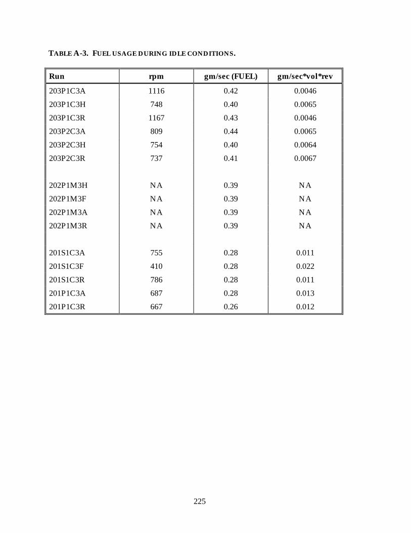
225

TABLE A-3. FUEL USAGE DURING IDLE CONDITIONS.

Run rpm gm/sec (FUEL) gm/sec*vol*rev

203P1C3A 1116 0.42 0.0046

203P1C3H 748 0.40 0.0065

203P1C3R 1167 0.43 0.0046

203P2C3A 809 0.44 0.0065

203P2C3H 754 0.40 0.0064

203P2C3R 737 0.41 0.0067

202P1M3H NA 0.39 NA

202P1M3F NA 0.39 NA

202P1M3A NA 0.39 NA

202P1M3R NA 0.39 NA

201S1C3A 755 0.28 0.011

201S1C3F 410 0.28 0.022

201S1C3R 786 0.28 0.011

201P1C3A 687 0.28 0.013

201P1C3R 667 0.26 0.012

226

TABLE A-4. FUEL USAGE DURING DECELERATION CONDITIONS.

Run rpm gm/sec (FUEL) gm/sec*vol*rev

202P1M3A NA 0.40 NA

202P1M3H NA 0.41 NA

202P1M3F NA 0.40 NA

NA = not available.

227

EFFICIENCY MAPS FOR FIVE MOTOR AND CONTROLLER SETS

228

ETX-I GE AC INDUCTION MOTOR

Torque (foot-lbs/radian) Max. at rpm

rpm 0 10 20 30 40 50 60 70 ft-lb kW

0 0.000 0.000 0.000 0.000 0.000 0.000 0.000 0.000 64.4 0.0

100 0.078 0.110 0.147 0.177 0.182 0.167 0.158 0.156 64.4 0.9

250 0.175 0.236 0.302 0.350 0.357 0.333 0.319 0.316 64.4 2.3

500 0.300 0.382 0.464 0.518 0.527 0.500 0.484 0.480 64.4 4.6

750 0.389 0.481 0.565 0.617 0.625 0.600 0.584 0.581 64.4 6.9

1000 0.485 0.553 0.621 0.688 0.712 0.693 0.674 0.664 64.4 9.1

2000 0.603 0.683 0.746 0.786 0.794 0.777 0.778 0.787 64.9 18.4

3000 0.721 0.813 0.871 0.883 0.876 0.861 0.846 0.839 64.8 27.6

4000 0.785 0.859 0.899 0.897 0.882 0.873 0.872 0.839 61.3 34.8

5000 0.850 0.904 0.928 0.911 0.888 0.867 0.872 0.839 49.6 35.2

6000 0.901 0.921 0.922 0.905 0.894 0.867 0.872 0.839 37.9 32.3

7000 0.950 0.938 0.916 0.886 0.882 0.867 0.872 0.839 31.4 31.2

8000 0.968 0.942 0.917 0.907 0.882 0.867 0.872 0.839 25.0 28.4

9000 0.989 0.945 0.906 0.898 0.882 0.867 0.872 0.839 22.1 28.2

Note: data for 100-750 rpm are calculated

ETX-I INVERTER

Torque (foot-lbs/radian)

rpm 0 10 20 30 40 50 60 70

0 0.834 0.824 0.821 0.821 0.837 0.863 0.887 0.899

100 0.836 0.828 0.825 0.825 0.841 0.866 0.890 0.901

250 0.840 0.833 0.831 0.832 0.846 0.871 0.894 0.905

500 0.846 0.842 0.841 0.842 0.855 0.878 0.900 0.911

750 0.852 0.851 0.851 0.853 0.864 0.886 0.907 0.917

1000 0.858 0.860 0.861 0.863 0.873 0.893 0.913 0.923

2000 0.884 0.894 0.901 0.903 0.911 0.924 0.940 0.949

3000 0.911 0.929 0.941 0.944 0.948 0.955 0.962 0.965

4000 0.929 0.943 0.952 0.956 0.957 0.955 0.950 0.965

5000 0.946 0.956 0.962 0.967 0.966 0.957 0.950 0.965

6000 0.937 0.955 0.964 0.953 0.937 0.957 0.950 0.965

7000 0.926 0.954 0.965 0.960 0.959 0.957 0.950 0.965

8000 0.925 0.951 0.952 0.939 0.959 0.957 0.950 0.965

9000 0.922 0.948 0.955 0.953 0.959 0.957 0.950 0.965

Note: data for 100-750 rpm are calculated

229

ETX-II GE PERMANENT MAGNET MOTOR

Torque (foot-lbs/radian) Max. at rpm

rpm 0 10 20 30 40 50 60 70 80 ft-lb kW

0 0.000 0.000 0.000 0.000 0.000 0.000 0.000 0.000 0.000 86.5 0.0

100 0.247 0.380 0.471 0.490 0.481 0.465 0.447 0.426 0.407 86.5 1.2

250 0.450 0.606 0.690 0.706 0.698 0.685 0.669 0.650 0.632 86.5 3.1

500 0.620 0.754 0.817 0.828 0.822 0.813 0.802 0.788 0.774 86.5 6.1

750 0.710 0.822 0.870 0.878 0.874 0.867 0.858 0.848 0.837 86.5 9.2

1000 0.814 0.914 0.931 0.928 0.920 0.911 0.902 0.893 0.883 86.2 12.2

2000 0.804 0.918 0.943 0.948 0.947 0.944 0.940 0.935 0.930 86.1 24.4

3000 0.833 0.933 0.955 0.960 0.960 0.959 0.957 0.954 0.951 86.0 36.6

4000 0.879 0.951 0.967 0.972 0.971 0.968 0.966 0.963 0.959 85.8 48.7

5000 0.894 0.956 0.969 0.971 0.970 0.967 0.964 0.959 0.959 74.1 52.6

6000 0.848 0.938 0.959 0.964 0.963 0.961 0.957 0.957 0.957 63.5 54.1

7000 0.798 0.918 0.948 0.955 0.956 0.954 0.954 0.954 0.954 54.9 54.6

8000 0.754 0.900 0.938 0.947 0.949 0.949 0.949 0.949 0.949 47.9 54.4

9000 0.716 0.884 0.928 0.940 0.941 0.941 0.941 0.941 0.941 42.0 53.7

10000 0.685 0.869 0.919 0.932 0.932 0.932 0.932 0.932 0.932 37.7 53.5

11000 0.658 0.856 0.911 0.925 0.925 0.925 0.925 0.925 0.925 33.2 51.9

Note: data for100-750 rpm are calculated

ETX-II INVERTER

Torque (foot-lbs/radian)

rpm 0 10 20 30 40 50 60 70 80 90

0 0.329 0.466 0.564 0.603 0.620 0.630 0.633 0.636 0.633 0.474

100 0.361 0.494 0.587 0.624 0.641 0.650 0.653 0.656 0.653 0.474

250 0.409 0.535 0.623 0.657 0.672 0.680 0.683 0.685 0.683 0.474

500 0.489 0.604 0.681 0.710 0.723 0.730 0.733 0.734 0.732 0.474

750 0.569 0.673 0.740 0.763 0.775 0.780 0.782 0.783 0.782 0.474

1000 0.649 0.742 0.798 0.817 0.826 0.830 0.832 0.832 0.831 0.474

2000 0.780 0.844 0.880 0.892 0.898 0.901 0.902 0.903 0.903 0.474

3000 0.842 0.891 0.918 0.927 0.932 0.935 0.938 0.940 0.941 0.605

4000 0.881 0.921 0.943 0.958 0.961 0.963 0.964 0.964 0.964 0.790

5000 0.900 0.939 0.958 0.964 0.967 0.968 0.968 0.968 0.968 0.974

6000 0.860 0.923 0.954 0.963 0.967 0.968 0.969 0.969 0.969 0.987

7000 0.842 0.913 0.951 0.962 0.967 0.969 0.969 0.969 0.969 1.000

8000 0.834 0.910 0.950 0.962 0.967 0.967 0.967 0.967 0.967 0.987

9000 0.832 0.909 0.950 0.963 0.968 0.968 0.968 0.968 0.968 0.974

10000 0.833 0.909 0.951 0.963 0.963 0.963 0.963 0.963 0.963 0.947

11000 0.835 0.911 0.952 0.964 0.964 0.964 0.964 0.964 0.964 0.921

Note: data for100-750 rpm are calculated

230

HUGHES G50 AC INDUCTION MOTOR

Torque (foot-lbs/radian) Max. at rpm

rpm 0.0 8.8 17.7 26.5 35.3 44.1 52.9 61.8 70.6 79.4 88.2 97.1 ft-lb kW

0 0.000 0.000 0.000 0.000 0.000 0.000 0.000 0.000 0.000 0.000 0.000 0.000 99.3 0.0

100 0.290 0.440 0.430 0.410 0.370 0.340 0.300 0.260 0.250 0.250 0.240 0.240 99.3 1.4

300 0.550 0.700 0.700 0.680 0.640 0.600 0.560 0.520 0.500 0.490 0.490 0.490 99.3 4.2

600 0.820 0.900 0.880 0.850 0.820 0.810 0.790 0.720 0.710 0.700 0.700 0.700 99.3 8.5

1200 0.820 0.900 0.900 0.890 0.870 0.840 0.830 0.810 0.800 0.790 0.790 0.790 99.3 16.9

1800 0.840 0.910 0.910 0.910 0.900 0.890 0.860 0.850 0.840 0.840 0.830 0.830 99.3 25.4

2400 0.840 0.910 0.920 0.920 0.910 0.900 0.900 0.890 0.870 0.860 0.850 0.850 99.3 33.8

3000 0.850 0.910 0.920 0.920 0.910 0.910 0.900 0.900 0.900 0.900 0.890 0.880 99.3 42.3

3600 0.850 0.920 0.920 0.920 0.920 0.910 0.910 0.900 0.900 0.900 0.900 0.870 99.3 50.7

4200 0.850 0.920 0.920 0.920 0.920 0.910 0.910 0.900 0.900 0.900 0.880 0.860 88.2 52.6

4800 0.850 0.920 0.920 0.930 0.920 0.910 0.910 0.900 0.900 0.880 0.870 0.850 76.5 52.1

5400 0.850 0.920 0.920 0.920 0.920 0.910 0.900 0.880 0.880 0.870 0.860 0.840 64.7 49.6

6000 0.850 0.920 0.920 0.920 0.910 0.900 0.880 0.870 0.870 0.860 0.850 0.830 52.9 45.1

6600 0.850 0.920 0.920 0.910 0.900 0.880 0.870 0.860 0.860 0.850 0.840 0.820 41.9 39.3

7200 0.840 0.910 0.910 0.900 0.880 0.870 0.870 0.850 0.850 0.840 0.830 0.810 30.9 31.6

Note: data for100-300 rpm are calculated

HUGHES G50 AC INVERTER

Torque (foot-lbs/radian)

rpm 0.0 8.8 17.7 26.5 35.3 44.1 52.9 61.8 70.6 79.4 88.2 97.1

0 0.710 0.710 0.710 0.720 0.720 0.730 0.730 0.730 0.730 0.730 0.720 0.700

100 0.717 0.728 0.728 0.738 0.738 0.748 0.748 0.748 0.748 0.748 0.730 0.710

300 0.730 0.765 0.765 0.775 0.775 0.785 0.785 0.785 0.785 0.785 0.750 0.730

600 0.750 0.820 0.820 0.830 0.830 0.840 0.840 0.840 0.840 0.840 0.780 0.760

1200 0.760 0.840 0.860 0.900 0.900 0.900 0.900 0.900 0.910 0.910 0.840 0.780

1800 0.800 0.900 0.910 0.910 0.920 0.920 0.920 0.920 0.920 0.930 0.930 0.800

2400 0.810 0.910 0.920 0.930 0.940 0.940 0.940 0.940 0.940 0.940 0.940 0.820

3000 0.820 0.930 0.940 0.950 0.950 0.950 0.950 0.950 0.950 0.950 0.950 0.840

3600 0.830 0.950 0.950 0.950 0.950 0.950 0.950 0.950 0.950 0.950 0.950 0.840

4200 0.830 0.950 0.960 0.960 0.960 0.950 0.950 0.950 0.950 0.950 0.950 0.950

4800 0.840 0.960 0.970 0.970 0.960 0.960 0.950 0.950 0.950 0.950 0.950 0.950

5400 0.840 0.960 0.970 0.970 0.960 0.960 0.960 0.950 0.940 0.940 0.940 0.940

6000 0.840 0.960 0.970 0.970 0.960 0.960 0.960 0.950 0.940 0.940 0.940 0.940

6600 0.850 0.970 0.970 0.970 0.960 0.960 0.960 0.940 0.930 0.930 0.930 0.930

7200 0.850 0.970 0.970 0.970 0.960 0.960 0.960 0.940 0.930 0.930 0.930 0.930

Note: data for100-300 rpm are calculated

231

TB-1 EATON AC INDUCTION MOTOR

Torque (foot-lbs/radian) Max. at rpm

rpm 0.0 10 20 30 40 50 60 ft-lb kW

0 0.000 0.000 0.000 0.000 0.000 0.000 0.000 52.5 0.0

100 0.139 0.184 0.256 0.278 0.268 0.273 0.273 52.5 0.7

250 0.288 0.360 0.462 0.490 0.478 0.485 0.485 52.5 1.9

500 0.447 0.530 0.632 0.658 0.647 0.653 0.653 52.5 3.7

750 0.548 0.628 0.721 0.742 0.733 0.738 0.738 52.5 5.6

1000 0.654 0.704 0.755 0.766 0.761 0.761 0.761 53.5 7.6

2000 0.767 0.827 0.887 0.898 0.889 0.894 0.894 54.5 15.5

3000 0.807 0.859 0.911 0.924 0.922 0.924 0.924 55.5 23.6

4000 0.824 0.875 0.925 0.933 0.936 0.942 0.942 57.5 32.7

5000 0.825 0.878 0.932 0.917 0.936 0.944 0.944 59.2 42.0

6000 0.830 0.884 0.937 0.936 0.936 0.944 0.944 58.0 49.4

7000 0.836 0.882 0.928 0.936 0.936 0.944 0.944 50.5 50.2

8000 0.843 0.883 0.923 0.936 0.936 0.944 0.944 43.3 49.2

9000 0.910 0.924 0.939 0.936 0.936 0.944 0.944 37.5 47.9

10000 0.935 0.933 0.932 0.936 0.936 0.944 0.944 33.5 47.6

11000 0.919 0.929 0.940 0.936 0.936 0.944 0.944 29.2 45.6

12000 0.903 0.924 0.945 0.936 0.936 0.944 0.944 25.0 42.6

Note: data for 100-750 rpm are calculated Data for 60 ft-lbs/rad assumed to be same as for 50 ft-lbs/rad

TB-1 INVERTER

Torque (foot-lbs/radian)

rpm 0.0 10 20 30 40 50 60

0 0.569 0.616 0.663 0.753 0.766 0.791 0.757

100 0.573 0.620 0.667 0.756 0.770 0.795 0.762

250 0.580 0.627 0.674 0.761 0.775 0.800 0.769

500 0.591 0.638 0.685 0.770 0.785 0.809 0.782

750 0.602 0.648 0.695 0.778 0.794 0.817 0.794

1000 0.613 0.659 0.706 0.786 0.803 0.826 0.806

2000 0.657 0.703 0.749 0.820 0.841 0.860 0.855

3000 0.699 0.743 0.787 0.857 0.882 0.895 0.893

4000 0.756 0.794 0.831 0.894 0.918 0.928 0.921

5000 0.832 0.857 0.882 0.921 0.957 0.957 0.928

6000 0.890 0.903 0.917 0.939 0.954 0.954 0.928

7000 0.867 0.891 0.915 0.945 0.954 0.949 0.928

8000 0.899 0.913 0.926 0.946 0.944 0.949 0.928

9000 0.895 0.910 0.925 0.947 0.944 0.949 0.928

10000 0.923 0.929 0.935 0.952 0.944 0.949 0.928

11000 0.922 0.929 0.937 0.931 0.944 0.949 0.928

12000 0.915 0.926 0.937 0.923 0.944 0.949 0.928

Note: data for 100-750 rpm are calculated

232

GE MEV 75-HP AC INDUCTION MOTOR

Torque (foot-lbs/radian) Max. at rpm

rpm 0 10 20 30 40 50 60 70 80 90 100 110 130 ft-lb kW

0 0.416 0.520 0.625 0.623 0.682 0.721 0.744 0.757 0.763 0.764 0.763 0.752 0.747 143.8 0.0

100 0.457 0.553 0.650 0.649 0.702 0.737 0.757 0.768 0.772 0.772 0.770 0.759 0.752 143.6 2.0

400 0.578 0.652 0.725 0.727 0.763 0.785 0.796 0.800 0.799 0.796 0.791 0.780 0.769 143.2 8.1

700 0.700 0.750 0.801 0.805 0.824 0.832 0.834 0.832 0.827 0.819 0.812 0.800 0.785 142.5 14.2

1000 0.821 0.849 0.876 0.883 0.885 0.880 0.873 0.864 0.854 0.843 0.833 0.821 0.801 142.0 20.2

2000 0.874 0.897 0.920 0.924 0.928 0.927 0.924 0.919 0.914 0.908 0.902 0.896 0.883 141.3 40.1

3000 0.895 0.916 0.937 0.941 0.945 0.945 0.943 0.940 0.937 0.933 0.928 0.924 0.914 131.4 56.0

4000 0.907 0.927 0.947 0.952 0.955 0.956 0.954 0.952 0.949 0.937 0.925 0.912 0.914 100.3 57.0

5000 0.916 0.936 0.956 0.942 0.948 0.950 0.949 0.947 0.943 0.940 0.925 0.912 0.914 83.4 59.2

6000 0.937 0.943 0.950 0.955 0.955 0.953 0.948 0.942 0.943 0.940 0.925 0.912 0.914 69.8 59.5

7000 0.946 0.951 0.956 0.958 0.953 0.949 0.941 0.942 0.943 0.940 0.925 0.912 0.914 59.7 59.3

8000 0.935 0.948 0.960 0.958 0.951 0.941 0.931 0.942 0.943 0.940 0.925 0.912 0.914 51.8 58.8

9000 0.948 0.955 0.961 0.955 0.944 0.933 0.931 0.942 0.943 0.940 0.925 0.912 0.914 45.5 58.1

10000 0.959 0.959 0.960 0.949 0.933 0.918 0.931 0.942 0.943 0.940 0.925 0.912 0.914 40.4 57.4

11000 0.943 0.962 0.981 0.971 0.962 0.918 0.931 0.942 0.943 0.940 0.925 0.912 0.914 36.1 56.4

12000 0.973 0.963 0.954 0.932 0.910 0.918 0.931 0.942 0.943 0.940 0.925 0.912 0.914 32.5 55.4

13000 0.978 0.963 0.949 0.920 0.910 0.918 0.931 0.942 0.943 0.940 0.925 0.912 0.914 29.3 54.1

Note: data for100-700 rpm are calculated; max torque 100-600 data my estimates. Data for "out of bounds" torque values estimated.

GE MEV 75-HP INVERTER

Torque (foot-lbs/radian)

rpm 0 10 20 30 40 50 60 70 80 90 100 110 130

0 0.698 0.670 0.641 0.594 0.598 0.602 0.607 0.613 0.619 0.626 0.634 0.639 0.656

100 0.706 0.686 0.664 0.623 0.628 0.632 0.637 0.643 0.648 0.654 0.662 0.666 0.681

400 0.731 0.732 0.733 0.711 0.718 0.723 0.727 0.731 0.735 0.740 0.744 0.747 0.756

700 0.755 0.779 0.802 0.798 0.808 0.813 0.817 0.820 0.823 0.825 0.827 0.827 0.832

1000 0.780 0.825 0.871 0.886 0.898 0.904 0.907 0.909 0.910 0.910 0.909 0.908 0.907

2000 0.865 0.893 0.920 0.931 0.938 0.942 0.945 0.946 0.947 0.947 0.947 0.947 0.946

3000 0.898 0.920 0.942 0.953 0.959 0.962 0.964 0.965 0.965 0.966 0.966 0.966 0.966

4000 0.918 0.937 0.957 0.970 0.974 0.977 0.978 0.979 0.979 0.986 0.993 0.999 0.966

5000 0.931 0.950 0.969 0.984 0.986 0.987 0.987 0.988 0.988 0.988 0.993 0.999 0.966

6000 0.938 0.960 0.983 0.986 0.987 0.988 0.988 0.988 0.988 0.988 0.993 0.999 0.966

7000 0.954 0.969 0.985 0.987 0.988 0.988 0.989 0.988 0.988 0.988 0.993 0.999 0.966

8000 0.972 0.979 0.986 0.988 0.988 0.989 0.989 0.988 0.988 0.988 0.993 0.999 0.966

9000 0.974 0.980 0.986 0.988 0.988 0.989 0.989 0.988 0.988 0.988 0.993 0.999 0.966

10000 0.976 0.981 0.987 0.988 0.988 0.988 0.989 0.988 0.988 0.988 0.993 0.999 0.966

11000 0.974 0.982 0.991 0.991 0.991 0.988 0.989 0.988 0.988 0.988 0.993 0.999 0.966

12000 0.979 0.983 0.987 0.988 0.988 0.988 0.989 0.988 0.988 0.988 0.993 0.999 0.966

13000 0.980 0.984 0.987 0.987 0.988 0.988 0.989 0.988 0.988 0.988 0.993 0.999 0.966

Note: data for100-700 rpm are calculated; max torque 100-600 data my estimates. Data for "out of bounds" torque values estimated.

233

TABLES OF RESULTS

PB/ACID BATTERYFord Taurus

Vehicle characteristicsCost summaryLifecycle costManufacturing cost and weight

Ford EscortVehicle characteristicsCost summaryLifecycle costManufacturing cost and weight

NIMH GEN2 BATTERYFord Taurus

Vehicle characteristicsCost summaryLifecycle costManufacturing cost and weight

Ford EscortVehicle characteristicsCost summaryLifecycle costManufacturing cost and weight

LI/ION BATTERYFord Taurus

Vehicle characteristicsCost summaryLifecycle costManufacturing cost and weight

Ford EscortVehicle characteristicsCost summaryLifecycle costManufacturing cost and weight

NIMH GEN4 BATTERYFord Taurus

Vehicle characteristicsCost summaryLifecycle costManufacturing cost and weight

234

Ford EscortVehicle characteristicsCost summaryLifecycle costManufacturing cost and weight

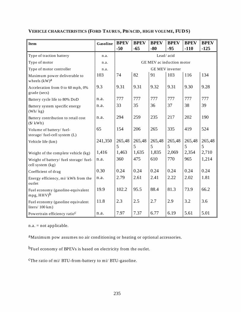
235

VEHICLE CHARACTERISTICS (FORD TAURUS, PB/ACID, HIGH VOLUME, FUDS)

Item Gasoline BPEV-50

BPEV-65

BPEV-80

BPEV-95

BPEV-110

BPEV-125

Type of traction battery n.a. Lead/acid

Type of motor n.a. GE MEV ac induction motor

Type of motor controller n.a. GE MEV inverter

Maximum power deliverable to wheels (kW)a

103 74 82 91 103 116 134

Acceleration from 0 to 60 mph, 0% grade (secs)

9.3 9.31 9.31 9.32 9.31 9.30 9.28

Battery cycle life to 80% DoD n.a. 777 777 777 777 777 777

Battery system specific energy (Wh/kg)

n.a. 33 35 36 37 38 39

Battery contribution to retail cost ($/kWh)

n.a. 294 259 235 217 202 190

Volume of battery/fuel-storage/fuel-cell system (L)

65 154 206 265 335 419 524

Vehicle life (km) 241,350 265,485

265,485

265,485

265,485

265,485

265,485

Weight of the complete vehicle (kg) 1,416 1,463 1,635 1,835 2,069 2,354 2,710

Weight of battery/fuel- storage/fuel-cell system (kg)

n.a. 360 475 610 770 965 1,214

Coefficient of drag 0.30 0.24 0.24 0.24 0.24 0.24 0.24

Energy efficiency, mi/kWh from the outlet

n.a. 2.79 2.61 2.41 2.22 2.02 1.81

Fuel economy (gasoline-equivalent mpg, HHV)b

19.9 102.2 95.5 88.4 81.3 73.9 66.2

Fuel economy (gasoline equivalent liters/100 km)

11.8 2.3 2.5 2.7 2.9 3.2 3.6

Powertrain efficiency ratioc n.a. 7.97 7.37 6.77 6.19 5.61 5.01

n.a. = not applicable.

aMaximum pow assumes no air conditioning or heating or optional accessories.

bFuel economy of BPEVs is based on electricity from the outlet.

cThe ratio of mi/BTU-from-battery to mi/BTU-gasoline.

236

COST SUMMARY (FORD TAURUS, PB/ACID, HIGH VOLUME, FUDS)

Item Gasoline BPEV-50

BPEV-65

BPEV-80

BPEV-95

BPEV-110

BPEV-125

Fuel retail cost, excluding taxes ($/gasoline-equivalent gallon)

0.90 2.20 2.20 2.20 2.20 2.20 2.20

Full retail cost of vehicle, incl. taxes ($)

20,085 23,363 24,553 25,918 27,510 29,422 31,814

Battery contribution to retail cost ($) n.a. 3,447 4,276 5,190 6,231 7,447 8,940

Levelized maintenance cost ($/yr) 492 355 355 355 355 355 355

Total lifecycle cost (cents/mile) 38.71 44.77 45.55 46.39 49.37 53.11 57.92

Present value of lifecycle cost vs. gasoline ($)a

45,892 10,516 11,495 12,556 16,305 21,018 27,072

Breakeven gasoline price ($/gal) n.a. 2.48 2.64 2.80 3.40 4.14 5.09

n.a. = not applicable.

aFor gasoline, the present value is shown. For the EVs, the difference between the present value for the EV and the present value for gasoline is shown.

237

LIFECYCLE COST SUMMARY (FORD TAURUS, PB/ACID, HIGH VOLUME, FUDS) (U.S. CENTS/MILE)

Cost item Gasoline BPEV-50

BPEV-65

BPEV-80

BPEV-95

BPEV-110

BPEV-125

Independently calculated cost of fast recharging

n.a. 0.00 0.00 0.00 0.00 0.00 0.00

Purchased electricity (including battery heating, if any)

n.a. 2.15 2.30 2.49 2.70 2.97 3.32

Vehicle, excluding batterya 17.55 16.38 16.73 17.15 17.67 18.33 19.19

Battery and tray and auxiliariesa n.a. 10.03 9.84 9.66 11.30 13.53 16.29

Space heating fuel for EVs 0.00 0.53 0.53 0.53 0.53 0.52 0.52

Motor fuel, excluding excise taxes and electricity

4.52 0.00 0.00 0.00 0.00 0.00 0.00

Home battery-recharging station n.a. 0.22 0.22 0.22 0.22 0.22 0.22

Insurance (calculated as a function of VMT and vehicle value)

6.75 7.26 7.54 7.86 8.24 8.68 9.24

Maintenance and repair, excluding oil, inspection, cleaning, towing

4.88 3.72 3.72 3.72 3.72 3.72 3.72

Engine oil 0.17 0.00 0.00 0.00 0.00 0.00 0.00

Replacement tires (calculated as a function of VMT and vehicle wt.)

0.50 0.46 0.60 0.62 0.76 0.79 0.94

Parking, tolls, and fines (assumed to be the same for all vehicles)

1.05 1.05 1.05 1.05 1.05 1.05 1.05

Registration fee (calculated as a function of vehicle weight)

0.50 0.54 0.61 0.68 0.77 0.87 1.00

Vehicle safety and emissions inspection fee

0.60 0.21 0.21 0.21 0.21 0.21 0.21

Federal, state, and local fuel (energy) excise taxes

1.90 1.90 1.90 1.90 1.90 1.90 1.90

Accessories (assumed to be the same for all vehicles)

0.30 0.30 0.30 0.30 0.30 0.30 0.30

Total lifecycle cost (cents/mile) 38.71 44.77 45.55 46.39 49.37 53.11 57.92

The breakeven price of gasoline, including taxes

n.a. 2.48 2.64 2.80 3.40 4.14 5.09

n.a.= not applicable

aRetail-cost equivalent.

238

MANUFACTURING COST & WEIGHT (FORD TAURUS, PB/ACID, HIGH VOLUME, FUDS)

Manufacturing costs ($) Weight (lbs)

Baseline vehicle components ICEV BPEV-65

BPEV-110

ICEV BPEV-65

BPEV-110

Body, chassis, interior, electrical, steering, etc. 3,621 3,752 4,240 2,080 2,165 2,483

Powertrain, emission control, brakes, fluidsa 2,468 3,432 4,523 1,141 448 643

Vehicle assembly (excl. battery, fuel tank) 1,715 1,458 1,458 n.a. n.a. n.a.

Traction battery 0 1,960 3,622 0 972 1,987

Traction battery auxiliaries 0 89 162 0 77 140

Final assembly of battery and fuel tanks 0 74 74 n.a. n.a. n.a.

Adjustments to baseline (v. 1989)*

Air conditioning, EV heater, thermal management (incl. assembly)

400 850 850 70 110 110

Improved emission control system 150 0 0 15 0 0

New safety features (except air bags) 100 100 100 40 40 40

Engine and transmission improvements 200 0 0 (80) 0 0

Body weight-reduction measures 140 200 200 (250) (371) (371)

Drag-reduction measures 20 50 50 0 0 0

Subtotal manufacturing costs 8,814 11,964 15,278 n.a n.a. n.a.

Division costs (engineers, testing, advertising) 4,162 4,608 5,078 n.a. n.a. n.a.

Corporate costs (executives, capital, research and development)

2,166 2,256 2,351 n.a. n.a. n.a.

Corporate cost of money 222 276 333 n.a. n.a. n.a.

Corporate true profit (taken as fraction of factory invoice)

475 591 712 n.a. n.a. n.a.

Factory invoice (price to dealer) 15,840 19,691 23,737 n.a. n.a. n.a.

Dealer costs 3,177 3,592 4,027 n.a. n.a. n.a.

Manufacturers' suggested retail price (MSRP) 19,017 23,283 27,764 n.a. n.a. n.a.

Shipping cost 483 551 805 n.a. n.a. n.a.

Other costs 0 0 0 n.a. n.a. n.a.

Final retail cost and weight

Consumer cost = MSRP+shipping+ tax ($)b 20,085 24,548 29,426 n.a. n.a. n.a.

Curb weight (no payload, full fuel)(lbs) n.a. n.a. n.a. 3,016 3,441 5,030

Actual in-use weight (lbs) n.a. n.a. n.a. 3,122 3,605 5,191

aThe fuel tank is 40% full in the weight and energy-use analysis, empty in the cost analysis.

bRetail price includes licence fees and all mark-ups and taxes.

239

VEHICLE CHARACTERISTICS (FORD ESCORT, PB/ACID, HIGH VOLUME, FUDS)

Item Gasoline BPEV-50

BPEV-65

BPEV-80

BPEV-95

BPEV-110

BPEV-125

Type of traction battery n.a. Lead/acid

Type of motor n.a. GE MEV ac induction motor

Type of motor controller n.a. GE MEV inverter

Maximum power deliverable to wheels (kW)a

67 54 59 66 74 84 95

Acceleration from 0 to 60 mph, 0%grade (secs)

10.3 10.26 10.28 10.27 10.28 10.28 10.27

Battery cycle life to 80% DoD n.a. 777 777 777 777 777 777

Battery system specific energy (Wh/kg)

n.a. 34 36 37 38 39 40

Battery contribution to retail cost ($/kWh)

n.a. 288 253 231 213 200 188

Volume of battery/fuel-storage/fuel-cell system (L)

52 124 167 213 269 335 415

Vehicle life (km) 241,350 265,485 265,485 265,485 265,485 265,485 265,485

Weight of the complete vehicle (kg) 1,007 1,160 1,298 1,454 1,639 1,856 2,121

Weight of battery/fuel- storage/fuel-cell system (kg)

n.a. 290 383 491 616 766 949

Coefficient of drag 0.30 0.24 0.24 0.24 0.24 0.24 0.24

Energy efficiency, mi/kWh from the outlet

n.a. 3.35 3.13 2.92 2.70 2.48 2.25

Fuel economy (gasoline-equivalent mpg, HHV)b

26.9 122.6 114.6 107.1 98.8 90.7 82.2

Fuel economy (gasoline equivalent liters/100 km)

8.7 1.9 2.1 2.2 2.4 2.6 2.9

Powertrain efficiency ratioc n.a. 7.04 6.50 6.03 5.53 5.06 4.57

n.a. = not applicable.

aMaximum pow assumes no air conditioning or heating or optional accessories.

bFuel economy of BPEVs is based on electricity from the outlet.

cThe ratio of mi/BTU-from-battery to mi/BTU-gasoline.

240

COST SUMMARY (FORD ESCORT, PB/ACID, HIGH VOLUME, FUDS)

Item Gasoline BPEV-50

BPEV-65

BPEV-80

BPEV-95

BPEV-110

BPEV-125

Fuel retail cost, excluding taxes ($/gasoline-equivalent gallon)

0.90 2.20 2.20 2.20 2.20 2.20 2.20

Full retail cost of vehicle, incl. taxes ($)

14,909 18,869 19,784 20,796 21,991 23,384 25,084

Battery contribution to retail cost ($) n.a. 2,808 3,482 4,224 5,052 6,003 7,128

Levelized maintenance cost ($/yr) 483 348 348 348 348 348 348

Total lifecycle cost (cents/mile) 30.90 37.81 38.31 38.98 41.19 44.12 47.66

Present value of lifecycle cost vs. gasoline ($)a

36,632 11,009 11,632 12,482 15,267 18,955 23,411

Breakeven gasoline price ($/gal) n.a. 3.14 3.27 3.45 4.05 4.84 5.79

n.a. = not applicable.

aFor gasoline, the present value is shown. For the EVs, the difference between the present value for the EV and the present value for gasoline is shown.

241

LIFECYCLE COST SUMMARY (FORD ESCORT, PB/ACID, HIGH VOLUME, FUDS) (U.S. CENTS/MILE)

Cost item Gasoline BPEV-50

BPEV-65

BPEV-80

BPEV-95

BPEV-110

BPEV-125

Independently calculated cost of fast recharging

n.a. 0.00 0.00 0.00 0.00 0.00 0.00

Purchased electricity (including battery heating, if any)

n.a. 1.79 1.92 2.05 2.22 2.42 2.67

Vehicle, excluding batterya 13.03 13.29 13.53 13.79 14.15 14.59 15.15

Battery and tray and auxiliariesa n.a. 8.19 8.03 7.88 9.18 10.94 13.02

Space heating fuel for EVs 0.00 0.54 0.54 0.53 0.53 0.53 0.53

Motor fuel, excluding excise taxes and electricity

3.34 0.00 0.00 0.00 0.00 0.00 0.00

Home battery-recharging station n.a. 0.22 0.22 0.22 0.22 0.22 0.22

Insurance (calculated as a function of VMT and vehicle value)

5.45 6.18 6.40 6.64 6.92 7.24 7.64

Maintenance and repair, excluding oil, inspection, cleaning, towing

4.80 3.66 3.66 3.66 3.66 3.66 3.66

Engine oil 0.13 0.00 0.00 0.00 0.00 0.00 0.00

Replacement tires (calculated as a function of VMT and vehicle wt.)

0.42 0.51 0.52 0.64 0.66 0.79 0.92

Parking, tolls, and fines (assumed to be the same for all vehicles)

1.05 1.05 1.05 1.05 1.05 1.05 1.05

Registration fee (calculated as a function of vehicle weight)

0.40 0.48 0.54 0.61 0.68 0.77 0.89

Vehicle safety and emissions inspection fee

0.60 0.21 0.21 0.21 0.21 0.21 0.21

Federal, state, and local fuel (energy) excise taxes

1.40 1.40 1.40 1.40 1.40 1.40 1.40

Accessories (assumed to be the same for all vehicles)

0.30 0.30 0.30 0.30 0.30 0.30 0.30

Total lifecycle cost (cents/mile) 30.90 37.81 38.31 38.98 41.19 44.12 47.66

The breakeven price of gasoline, including taxes

n.a. 3.14 3.27 3.45 4.05 4.84 5.79

n.a.= not applicable

aRetail-cost equivalent.

242

MANUFACTURING COST & WEIGHT (FORD ESCORT, PB/ACID, HIGH VOLUME, FUDS)

Manufacturing costs ($) Weight (lbs)

Baseline vehicle components ICEV BPEV-65

BPEV-110

ICEV BPEV-65

BPEV-110

Body, chassis, interior, electrical, steering, etc. 2,434 2,584 2,891 1,542 1,662 1,907

Powertrain, emission control, brakes, fluidsa 1,154 2,645 3,393 709 333 472

Vehicle assembly (excl. battery, fuel tank) 1,470 1,250 1,250 n.a. n.a. n.a.

Traction battery 0 1,544 2,804 0 789 1,580

Traction battery auxiliaries 0 69 125 0 60 108

Final assembly of battery and fuel tanks 0 74 74 n.a. n.a. n.a.

Adjustments to baseline (v. 1989)*

Air conditioning, EV heater, thermal management (incl. assembly)

400 850 850 70 110 110

Improved emission control system 120 0 0 12 0 0

New safety features (except air bags) 80 80 80 32 32 32

Engine and transmission improvements 160 0 0 (64) 0 0

Body weight-reduction measures 112 160 160 (200) (284) (284)

Drag-reduction measures 16 40 40 0 0 0

Subtotal manufacturing costs 5,946 9,296 11,666 n.a n.a. n.a.

Division costs (engineers, testing, advertising) 3,416 3,994 4,402 n.a. n.a. n.a.

Corporate costs (executives, capital, research and development)

2,184 2,322 2,419 n.a. n.a. n.a.

Corporate cost of money 169 229 271 n.a. n.a. n.a.

Corporate true profit (taken as fraction of factory invoice)

362 489 580 n.a. n.a. n.a.

Factory invoice (price to dealer) 12,079 16,309 19,346 n.a. n.a. n.a.

Dealer costs 2,060 2,452 2,733 n.a. n.a. n.a.

Manufacturers' suggested retail price (MSRP) 14,139 18,760 22,079 n.a. n.a. n.a.

Shipping cost 336 432 628 n.a. n.a. n.a.

Other costs 0 0 0 n.a. n.a. n.a.

Final retail cost and weight

Consumer cost = MSRP+shipping+ tax ($)b 14,909 19,768 23,388 n.a. n.a. n.a.

Curb weight (no payload, full fuel)(lbs) n.a. n.a. n.a. 2,101 2,700 3,926

Actual in-use weight (lbs) n.a. n.a. n.a. 2,219 2,858 4,093

aThe fuel tank is 40% full in the weight and energy-use analysis, empty in the cost analysis.

bRetail price includes licence fees and all mark-ups and taxes.

243

VEHICLE CHARACTERISTICS (FORD TAURUS, NIMH GEN2, HIGH VOLUME, FUDS)

Item Gasoline BPEV-65

BPEV-90

BPEV-115

BPEV-140

BPEV-165

BPEV-190

Type of traction battery n.a. Nickel metal hydride, generation 2

Type of motor n.a. GE MEV ac induction motor

Type of motor controller n.a. GE MEV inverter

Maximum power deliverable to wheels (kW)a

103 63 69 75 82 90 100

Acceleration from 0 to 60 mph, 0% grade (secs)

9.3 9.34 9.32 9.29 9.30 9.29 9.29

Battery cycle life to 80% DoD n.a. 666 666 666 666 666 666

Battery system specific energy (Wh/kg)

n.a. 67 71 73 75 77 79

Battery contribution to retail cost ($/kWh)

n.a. 551 475 428 389 361 338

Volume of battery/fuel-storage/fuel-cell system (L)

65 77 105 137 175 218 269

Vehicle life (km) 241,350 265,485 265,485 265,485 265,485 265,485 265,485

Weight of the complete vehicle (kg) 1,416 1,246 1,361 1,489 1,638 1,809 2,011

Weight of battery/fuel- storage/fuel-cell system (kg)

n.a. 208 288 380 479 597 734

Coefficient of drag 0.30 0.24 0.24 0.24 0.24 0.24 0.24

Energy efficiency, mi/kWh from the outlet

n.a. 2.48 2.39 2.28 2.15 2.02 1.87

Fuel economy (gasoline-equivalent mpg, HHV)b

19.9 91.0 87.5 83.6 78.8 73.9 68.5

Fuel economy (gasoline equivalent liters/100 km)

11.8 2.6 2.7 2.8 3.0 3.2 3.4

Powertrain efficiency ratioc n.a. 8.78 8.31 7.86 7.33 6.83 6.30

n.a. = not applicable.

aMaximum pow assumes no air conditioning or heating or optional accessories.

bFuel economy of BPEVs is based on electricity from the outlet.

cThe ratio of mi/BTU-from-battery to mi/BTU-gasoline.

244

COST SUMMARY (FORD TAURUS, NIMH GEN2, HIGH VOLUME, FUDS)

Item Gasoline BPEV-65

BPEV-90

BPEV-115

BPEV-140

BPEV-165

BPEV-190

Fuel retail cost, excluding taxes ($/gasoline-equivalent gallon)

0.90 2.20 2.20 2.20 2.20 2.20 2.20

Full retail cost of vehicle, incl. taxes ($)

20,085 25,984 28,034 30,261 32,834 35,759 39,223

Battery contribution to retail cost ($) n.a. 7,651 9,675 11,809 14,063 16,603 19,488

Levelized maintenance cost ($/yr) 492 355 355 355 355 355 355

Total lifecycle cost (cents/mile) 38.71 51.49 53.39 55.36 60.14 65.77 72.53

Present value of lifecycle cost vs. gasoline ($)a

45,892 18,982 21,369 23,858 29,878 36,974 45,484

Breakeven gasoline price ($/gal) n.a. 3.82 4.19 4.59 5.54 6.66 8.00

n.a. = not applicable.

aFor gasoline, the present value is shown. For the EVs, the difference between the present value for the EV and the present value for gasoline is shown.

245

LIFECYCLE COST SUMMARY (FORD TAURUS, NIMH GEN2, HIGH VOLUME, FUDS) (U.S. CENTS/MILE)

Cost item Gasoline BPEV-65

BPEV-90

BPEV-115

BPEV-140

BPEV-165

BPEV-190

Independently calculated cost of fast recharging

n.a. 0.00 0.00 0.00 0.00 0.00 0.00

Purchased electricity (including battery heating, if any)

n.a. 2.42 2.51 2.63 2.79 2.97 3.21

Vehicle, excluding batterya 17.55 15.20 15.30 15.46 15.83 16.28 16.91

Battery and tray and auxiliariesa n.a. 17.16 18.32 19.44 22.90 27.15 32.02

Space heating fuel for EVs 0.00 0.54 0.53 0.53 0.53 0.53 0.53

Motor fuel, excluding excise taxes and electricity

4.52 0.00 0.00 0.00 0.00 0.00 0.00

Home battery-recharging station n.a. 0.22 0.22 0.22 0.22 0.22 0.22

Insurance (calculated as a function of VMT and vehicle value)

6.75 7.88 8.36 8.88 9.47 10.15 10.96

Maintenance and repair, excluding oil, inspection, cleaning, towing

4.88 3.72 3.72 3.72 3.72 3.72 3.72

Engine oil 0.17 0.00 0.00 0.00 0.00 0.00 0.00

Replacement tires (calculated as a function of VMT and vehicle wt.)

0.50 0.44 0.45 0.47 0.60 0.62 0.76

Parking, tolls, and fines (assumed to be the same for all vehicles)

1.05 1.05 1.05 1.05 1.05 1.05 1.05

Registration fee (calculated as a function of vehicle weight)

0.50 0.46 0.50 0.55 0.61 0.67 0.75

Vehicle safety and emissions inspection fee

0.60 0.21 0.21 0.21 0.21 0.21 0.21

Federal, state, and local fuel (energy) excise taxes

1.90 1.90 1.90 1.90 1.90 1.90 1.90

Accessories (assumed to be the same for all vehicles)

0.30 0.30 0.30 0.30 0.30 0.30 0.30

Total lifecycle cost (cents/mile) 38.71 51.49 53.39 55.36 60.14 65.77 72.53

The breakeven price of gasoline, including taxes

n.a. 3.82 4.19 4.59 5.54 6.66 8.00

n.a.= not applicable

aRetail-cost equivalent.

246

MANUFACTURING COST & WEIGHT (FORD TAURUS, NIMH GEN2, HIGH VOLUME, FUDS)

Manufacturing costs ($) Weight (lbs)

Baseline vehicle components ICEV BPEV-90

BPEV-165

ICEV BPEV-90

BPEV-165

Body, chassis, interior, electrical, steering, etc. 3,621 3,566 3,872 2,080 2,044 2,243

Powertrain, emission control, brakes, fluidsa 2,468 3,016 3,700 1,141 374 496

Vehicle assembly (excl. battery, fuel tank) 1,715 1,458 1,458 n.a. n.a. n.a.

Traction battery 0 5,132 9,589 0 579 1,211

Traction battery auxiliaries 0 69 124 0 59 104

Final assembly of battery and fuel tanks 0 74 74 n.a. n.a. n.a.

Adjustments to baseline (v. 1989)*

Air conditioning, EV heater, thermal management (incl. assembly)

400 850 850 70 110 110

Improved emission control system 150 0 0 15 0 0

New safety features (except air bags) 100 100 100 40 40 40

Engine and transmission improvements 200 0 0 (80) 0 0

Body weight-reduction measures 140 200 200 (250) (371) (371)

Drag-reduction measures 20 50 50 0 0 0

Subtotal manufacturing costs 8,814 14,515 20,016 n.a n.a. n.a.

Division costs (engineers, testing, advertising) 4,162 4,969 5,749 n.a. n.a. n.a.

Corporate costs (executives, capital, research and development)

2,166 2,329 2,487 n.a. n.a. n.a.

Corporate cost of money 222 320 415 n.a. n.a. n.a.

Corporate true profit (taken as fraction of factory invoice)

475 684 884 n.a. n.a. n.a.

Factory invoice (price to dealer) 15,840 22,815 29,479 n.a. n.a. n.a.

Dealer costs 3,177 3,928 4,645 n.a. n.a. n.a.

Manufacturers' suggested retail price (MSRP) 19,017 26,743 34,124 n.a. n.a. n.a.

Shipping cost 483 454 613 n.a. n.a. n.a.

Other costs 0 0 0 n.a. n.a. n.a.

Final retail cost and weight

Consumer cost = MSRP+shipping+ tax ($)b 20,085 28,013 35,780 n.a. n.a. n.a.

Curb weight (no payload, full fuel)(lbs) n.a. n.a. n.a. 3,016 2,835 3,831

Actual in-use weight (lbs) n.a. n.a. n.a. 3,122 3,000 3,990

aThe fuel tank is 40% full in the weight and energy-use analysis, empty in the cost analysis.

bRetail price includes licence fees and all mark-ups and taxes.

247

VEHICLE CHARACTERISTICS (FORD ESCORT, NIMH GEN2, HIGH VOLUME, FUDS)

Item Gasoline BPEV-65

BPEV-90

BPEV-115

BPEV-140

BPEV-165

BPEV-190

Type of traction battery n.a. Nickel metal hydride, generation 2

Type of motor n.a. GE MEV ac induction motor

Type of motor controller n.a. GE MEV inverter

Maximum power deliverable to wheels (kW)a

67 46 50 55 60 66 72

Acceleration from 0 to 60 mph, 0% grade (secs)

10.3 10.29 10.29 10.28 10.27 10.27 10.28

Battery cycle life to 80% DoD n.a. 666 666 666 666 666 666

Battery system specific energy (Wh/kg)

n.a. 68 73 75 77 79 81

Battery contribution to retail cost ($/kWh)

n.a. 542 465 418 384 357 335

Volume of battery/fuel-storage/fuel-cell system (L)

52 62 86 112 142 177 217

Vehicle life (km) 241,350 265,485 265,485 265,485 265,485 265,485 265,485

Weight of the complete vehicle (kg) 1,007 988 1,082 1,185 1,303 1,437 1,595

Weight of battery/fuel- storage/fuel-cell system (kg)

n.a. 170 234 306 387 479 586

Coefficient of drag 0.30 0.24 0.24 0.24 0.24 0.24 0.24

Energy efficiency, mi/kWh from the outlet

n.a. 2.98 2.86 2.74 2.60 2.45 2.28

Fuel economy (gasoline-equivalent mpg, HHV)b

26.9 109.2 104.7 100.3 95.1 89.7 83.7

Fuel economy (gasoline equivalent liters/100 km)

8.7 2.2 2.2 2.3 2.5 2.6 2.8

Powertrain efficiency ratioc n.a. 7.73 7.29 6.90 6.48 6.06 5.61

n.a. = not applicable.

aMaximum pow assumes no air conditioning or heating or optional accessories.

bFuel economy of BPEVs is based on electricity from the outlet.

cThe ratio of mi/BTU-from-battery to mi/BTU-gasoline.

248

COST SUMMARY (FORD ESCORT, NIMH GEN2, HIGH VOLUME, FUDS)

Item Gasoline BPEV-65

BPEV-90

BPEV-115

BPEV-140

BPEV-165

BPEV-190

Fuel retail cost, excluding taxes ($/gasoline-equivalent gallon)

0.90 2.20 2.20 2.20 2.20 2.20 2.20

Full retail cost of vehicle, incl. taxes ($)

14,909 21,056 22,725 24,510 26,532 28,822 31,515

Battery contribution to retail cost ($) n.a. 6,263 7,907 9,629 11,488 13,508 15,815

Levelized maintenance cost ($/yr) 483 348 348 348 348 348 348

Total lifecycle cost (cents/mile) 30.90 43.31 44.87 46.55 50.30 54.87 60.12

Present value of lifecycle cost vs. gasoline ($)a

36,632 17,929 19,893 22,016 26,738 32,494 39,110

Breakeven gasoline price ($/gal) n.a. 4.62 5.04 5.49 6.50 7.73 9.15

n.a. = not applicable.

aFor gasoline, the present value is shown. For the EVs, the difference between the present value for the EV and the present value for gasoline is shown.

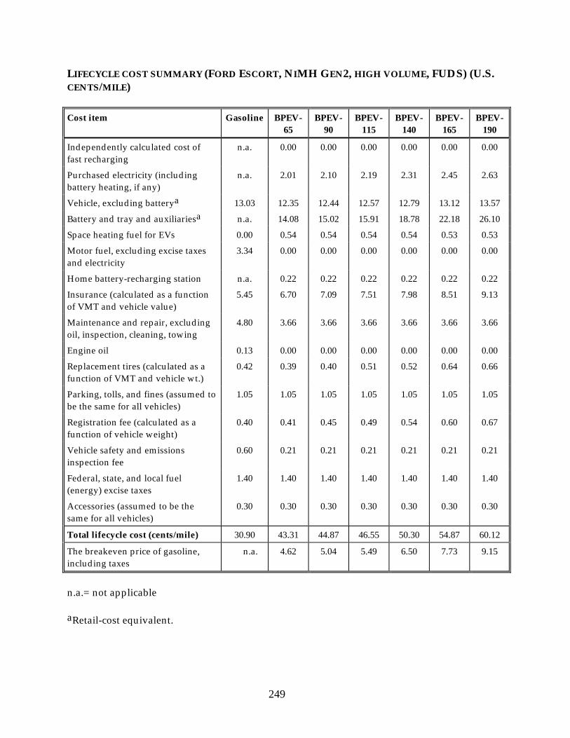
249

LIFECYCLE COST SUMMARY (FORD ESCORT, NIMH GEN2, HIGH VOLUME, FUDS) (U.S. CENTS/MILE)

Cost item Gasoline BPEV-65

BPEV-90

BPEV-115

BPEV-140

BPEV-165

BPEV-190

Independently calculated cost of fast recharging

n.a. 0.00 0.00 0.00 0.00 0.00 0.00

Purchased electricity (including battery heating, if any)

n.a. 2.01 2.10 2.19 2.31 2.45 2.63

Vehicle, excluding batterya 13.03 12.35 12.44 12.57 12.79 13.12 13.57

Battery and tray and auxiliariesa n.a. 14.08 15.02 15.91 18.78 22.18 26.10

Space heating fuel for EVs 0.00 0.54 0.54 0.54 0.54 0.53 0.53

Motor fuel, excluding excise taxes and electricity

3.34 0.00 0.00 0.00 0.00 0.00 0.00

Home battery-recharging station n.a. 0.22 0.22 0.22 0.22 0.22 0.22

Insurance (calculated as a function of VMT and vehicle value)

5.45 6.70 7.09 7.51 7.98 8.51 9.13

Maintenance and repair, excluding oil, inspection, cleaning, towing

4.80 3.66 3.66 3.66 3.66 3.66 3.66

Engine oil 0.13 0.00 0.00 0.00 0.00 0.00 0.00

Replacement tires (calculated as a function of VMT and vehicle wt.)

0.42 0.39 0.40 0.51 0.52 0.64 0.66

Parking, tolls, and fines (assumed to be the same for all vehicles)

1.05 1.05 1.05 1.05 1.05 1.05 1.05

Registration fee (calculated as a function of vehicle weight)

0.40 0.41 0.45 0.49 0.54 0.60 0.67

Vehicle safety and emissions inspection fee

0.60 0.21 0.21 0.21 0.21 0.21 0.21

Federal, state, and local fuel (energy) excise taxes

1.40 1.40 1.40 1.40 1.40 1.40 1.40

Accessories (assumed to be the same for all vehicles)

0.30 0.30 0.30 0.30 0.30 0.30 0.30

Total lifecycle cost (cents/mile) 30.90 43.31 44.87 46.55 50.30 54.87 60.12

The breakeven price of gasoline, including taxes

n.a. 4.62 5.04 5.49 6.50 7.73 9.15

n.a.= not applicable

aRetail-cost equivalent.

250

MANUFACTURING COST & WEIGHT (FORD ESCORT, NIMH GEN2, HIGH VOLUME, FUDS)

Manufacturing costs ($) Weight (lbs)

Baseline vehicle components ICEV BPEV-90

BPEV-165

ICEV BPEV-90

BPEV-165

Body, chassis, interior, electrical, steering, etc. 2,434 2,464 2,660 1,542 1,566 1,722

Powertrain, emission control, brakes, fluidsa 1,154 2,352 2,830 709 278 367

Vehicle assembly (excl. battery, fuel tank) 1,470 1,250 1,250 n.a. n.a. n.a.

Traction battery 0 4,066 7,541 0 472 974

Traction battery auxiliaries 0 54 97 0 46 81

Final assembly of battery and fuel tanks 0 74 74 n.a. n.a. n.a.

Adjustments to baseline (v. 1989)*

Air conditioning, EV heater, thermal management (incl. assembly)

400 850 850 70 110 110

Improved emission control system 120 0 0 12 0 0

New safety features (except air bags) 80 80 80 32 32 32

Engine and transmission improvements 160 0 0 (64) 0 0

Body weight-reduction measures 112 160 160 (200) (284) (284)

Drag-reduction measures 16 40 40 0 0 0

Subtotal manufacturing costs 5,946 11,389 15,581 n.a n.a. n.a.

Division costs (engineers, testing, advertising) 3,416 4,355 5,077 n.a. n.a. n.a.

Corporate costs (executives, capital, research and development)

2,184 2,408 2,580 n.a. n.a. n.a.

Corporate cost of money 169 266 341 n.a. n.a. n.a.

Corporate true profit (taken as fraction of factory invoice)

362 570 730 n.a. n.a. n.a.

Factory invoice (price to dealer) 12,079 18,987 24,320 n.a. n.a. n.a.

Dealer costs 2,060 2,700 3,193 n.a. n.a. n.a.

Manufacturers' suggested retail price (MSRP) 14,139 21,686 27,513 n.a. n.a. n.a.

Shipping cost 336 355 480 n.a. n.a. n.a.

Other costs 0 0 0 n.a. n.a. n.a.

Final retail cost and weight

Consumer cost = MSRP+shipping+ tax ($)b 14,909 22,703 28,833 n.a. n.a. n.a.

Curb weight (no payload, full fuel)(lbs) n.a. n.a. n.a. 2,101 2,219 3,003

Actual in-use weight (lbs) n.a. n.a. n.a. 2,219 2,384 3,169

aThe fuel tank is 40% full in the weight and energy -use analysis, empty in the cost analysis.

bRetail price includes licence fees and all mark-ups and taxes.

251

VEHICLE CHARACTERISTICS (FORD TAURUS, LI/ION, HIGH VOLUME, FUDS)

Item Gasoline BPEV-100

BPEV-140

BPEV-180

BPEV-220

BPEV-260

BPEV-300

Type of traction battery n.a. Lithium/ion

Type of motor n.a. GE MEV ac induction motor

Type of motor controller n.a. GE MEV inverter

Maximum power deliverable to wheels (kW)a

103 60 64 69 73 79 84

Acceleration from 0 to 60 mph, 0% grade (secs)

9.3 9.32 9.32 9.29 9.30 9.29 9.30

Battery cycle life to 80% DoD n.a. 1,110 1,110 1,110 1,110 1,110 1,110

Battery system specific energy (Wh/kg)

n.a. 118 129 136 143 147 152

Battery contribution to retail cost ($/kWh)

n.a. 416 337 289 253 228 207

Volume of battery/fuel-storage/fuel-cell system (L)

65 93 125 158 196 235 281

Vehicle life (km) 241,350 265,485 265,485 265,485 265,485 265,485 265,485

Weight of the complete vehicle (kg) 1,416 1,189 1,273 1,362 1,462 1,567 1,686

Weight of battery/fuel- storage/fuel-cell system (kg)

n.a. 172 229 294 359 432 512

Coefficient of drag 0.30 0.24 0.24 0.24 0.24 0.24 0.24

Energy efficiency, mi/kWh from the outlet

n.a. 4.17 3.99 3.82 3.62 3.44 3.25

Fuel economy (gasoline-equivalent mpg, HHV)b

19.9 152.8 146.0 139.9 132.4 125.9 119.0

Fuel economy (gasoline equivalent liters/100 km)

11.8 1.5 1.6 1.7 1.8 1.9 2.0

Powertrain efficiency ratioc n.a. 9.11 8.73 8.39 7.96 7.59 7.19

n.a. = not applicable.

aMaximum pow assumes no air conditioning or heating or optional accessories.

bFuel economy of BPEVs is based on electricity from the outlet.

cThe ratio of mi/BTU-from-battery to mi/BTU-gasoline.

252

COST SUMMARY (FORD TAURUS, LI/ION, HIGH VOLUME, FUDS)

Item Gasoline BPEV-100

BPEV-140

BPEV-180

BPEV-220

BPEV-260

BPEV-300

Fuel retail cost, excluding taxes ($/gasoline-equivalent gallon)

0.90 2.20 2.20 2.20 2.20 2.20 2.20

Full retail cost of vehicle, incl. taxes ($)

20,085 26,135 27,678 29,174 30,791 32,448 34,268

Battery contribution to retail cost ($) n.a. 8,430 10,000 11,513 12,993 14,516 16,121

Levelized maintenance cost ($/yr) 492 355 355 355 355 355 355

Total lifecycle cost (cents/mile) 38.71 43.55 46.22 48.70 51.34 54.06 57.16

Present value of lifecycle cost vs. gasoline ($)a

45,892 8,974 12,339 15,463 18,791 22,210 26,115

Breakeven gasoline price ($/gal) n.a. 2.24 2.77 3.26 3.79 4.33 4.94

n.a. = not applicable.

aFor gasoline, the present value is shown. For the EVs, the difference between the present value for the EV and the present value for gasoline is shown.

253

LIFECYCLE COST SUMMARY (FORD TAURUS, LI/ION, HIGH VOLUME, FUDS) (U.S. CENTS/MILE)

Cost item Gasoline BPEV-100

BPEV-140

BPEV-180

BPEV-220

BPEV-260

BPEV-300

Independently calculated cost of fast recharging

n.a. 0.00 0.00 0.00 0.00 0.00 0.00

Purchased electricity (including battery heating, if any)

n.a. 1.44 1.51 1.57 1.66 1.74 1.85

Vehicle, excluding batterya 17.55 14.68 14.72 14.76 14.93 15.11 15.36

Battery and tray and auxiliariesa n.a. 10.82 12.87 14.85 16.81 18.83 20.98

Space heating fuel for EVs 0.00 0.54 0.53 0.53 0.53 0.53 0.53

Motor fuel, excluding excise taxes and electricity

4.52 0.00 0.00 0.00 0.00 0.00 0.00

Home battery-recharging station n.a. 0.22 0.22 0.22 0.22 0.22 0.22

Insurance (calculated as a function of VMT and vehicle value)

6.75 7.91 8.27 8.62 9.00 9.38 9.81

Maintenance and repair, excluding oil, inspection, cleaning, towing

4.88 3.72 3.72 3.72 3.72 3.72 3.72

Engine oil 0.17 0.00 0.00 0.00 0.00 0.00 0.00

Replacement tires (calculated as a function of VMT and vehicle wt.)

0.50 0.32 0.45 0.45 0.46 0.47 0.61

Parking, tolls, and fines (assumed to be the same for all vehicles)

1.05 1.05 1.05 1.05 1.05 1.05 1.05

Registration fee (calculated as a function of vehicle weight)

0.50 0.44 0.47 0.51 0.54 0.58 0.63

Vehicle safety and emissions inspection fee

0.60 0.21 0.21 0.21 0.21 0.21 0.21

Federal, state, and local fuel (energy) excise taxes

1.90 1.90 1.90 1.90 1.90 1.90 1.90

Accessories (assumed to be the same for all vehicles)

0.30 0.30 0.30 0.30 0.30 0.30 0.30

Total lifecycle cost (cents/mile) 38.71 43.55 46.22 48.70 51.34 54.06 57.16

The breakeven price of gasoline, including taxes

n.a. 2.24 2.77 3.26 3.79 4.33 4.94

n.a.= not applicable

aRetail-cost equivalent.

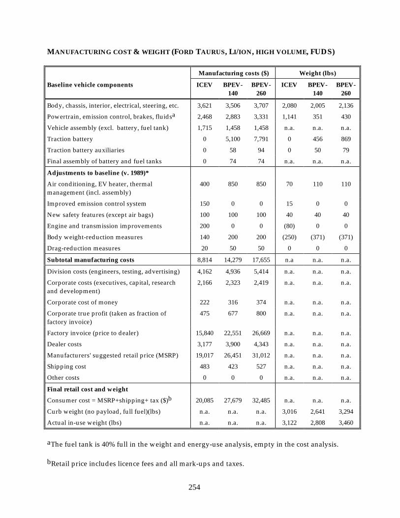
254

MANUFACTURING COST & WEIGHT (FORD TAURUS, LI/ION, HIGH VOLUME, FUDS)

Manufacturing costs ($) Weight (lbs)

Baseline vehicle components ICEV BPEV-140

BPEV-260

ICEV BPEV-140

BPEV-260

Body, chassis, interior, electrical, steering, etc. 3,621 3,506 3,707 2,080 2,005 2,136

Powertrain, emission control, brakes, fluidsa 2,468 2,883 3,331 1,141 351 430

Vehicle assembly (excl. battery, fuel tank) 1,715 1,458 1,458 n.a. n.a. n.a.

Traction battery 0 5,100 7,791 0 456 869

Traction battery auxiliaries 0 58 94 0 50 79

Final assembly of battery and fuel tanks 0 74 74 n.a. n.a. n.a.

Adjustments to baseline (v. 1989)*

Air conditioning, EV heater, thermal management (incl. assembly)

400 850 850 70 110 110

Improved emission control system 150 0 0 15 0 0

New safety features (except air bags) 100 100 100 40 40 40

Engine and transmission improvements 200 0 0 (80) 0 0

Body weight-reduction measures 140 200 200 (250) (371) (371)

Drag-reduction measures 20 50 50 0 0 0

Subtotal manufacturing costs 8,814 14,279 17,655 n.a n.a. n.a.

Division costs (engineers, testing, advertising) 4,162 4,936 5,414 n.a. n.a. n.a.

Corporate costs (executives, capital, research and development)

2,166 2,323 2,419 n.a. n.a. n.a.

Corporate cost of money 222 316 374 n.a. n.a. n.a.

Corporate true profit (taken as fraction of factory invoice)

475 677 800 n.a. n.a. n.a.

Factory invoice (price to dealer) 15,840 22,551 26,669 n.a. n.a. n.a.

Dealer costs 3,177 3,900 4,343 n.a. n.a. n.a.

Manufacturers' suggested retail price (MSRP) 19,017 26,451 31,012 n.a. n.a. n.a.

Shipping cost 483 423 527 n.a. n.a. n.a.

Other costs 0 0 0 n.a. n.a. n.a.

Final retail cost and weight

Consumer cost = MSRP+shipping+ tax ($)b 20,085 27,679 32,485 n.a. n.a. n.a.

Curb weight (no payload, full fuel)(lbs) n.a. n.a. n.a. 3,016 2,641 3,294

Actual in-use weight (lbs) n.a. n.a. n.a. 3,122 2,808 3,460

aThe fuel tank is 40% full in the weight and energy-use analysis, empty in the cost analysis.

bRetail price includes licence fees and all mark-ups and taxes.

255

VEHICLE CHARACTERISTICS (FORD ESCORT, LI/ION, HIGH VOLUME, FUDS)

Item Gasoline BPEV-100

BPEV-140

BPEV-180

BPEV-220

BPEV-260

BPEV-300

Type of traction battery n.a. Lithium/ion

Type of motor n.a. GE MEV ac induction motor

Type of motor controller n.a. GE MEV inverter

Maximum power deliverable to wheels (kW)a

67 44 47 50 53 57 61

Acceleration from 0 to 60 mph, 0% grade (secs)

10.3 10.29 10.28 10.27 10.28 10.27 10.28

Battery cycle life to 80% DoD n.a. 1,110 1,110 1,110 1,110 1,110 1,110

Battery system specific energy (Wh/kg)

n.a. 124 134 142 148 153 157

Battery contribution to retail cost ($/kWh)

n.a. 394 321 274 241 217 198

Volume of battery/fuel-storage/fuel-cell system (L)

52 75 101 129 159 191 227

Vehicle life (km) 241,350 265,485 265,485 265,485 265,485 265,485 265,485

Weight of the complete vehicle (kg) 1,007 942 1,009 1,082 1,160 1,244 1,338

Weight of battery/fuel- storage/fuel-cell system (kg)

n.a. 138 185 236 289 347 411

Coefficient of drag 0.30 0.24 0.24 0.24 0.24 0.24 0.24

Energy efficiency, mi/kWh from the outlet

n.a. 4.95 4.77 4.55 4.34 4.14 3.92

Fuel economy (gasoline-equivalent mpg, HHV)b

26.9 181.4 174.5 166.6 158.9 151.5 143.6

Fuel economy (gasoline equivalent liters/100 km)

8.7 1.3 1.3 1.4 1.5 1.6 1.6

Powertrain efficiency ratioc n.a. 7.95 7.66 7.33 7.01 6.70 6.36

n.a. = not applicable.

aMaximum pow assumes no air conditioning or heating or optional accessories.

bFuel economy of BPEVs is based on electricity from the outlet.

cThe ratio of mi/BTU-from-battery to mi/BTU-gasoline.

256

COST SUMMARY (FORD ESCORT, LI/ION, HIGH VOLUME, FUDS)

Item Gasoline BPEV-100

BPEV-140

BPEV-180

BPEV-220

BPEV-260

BPEV-300

Fuel retail cost, excluding taxes ($/gasoline-equivalent gallon)

0.90 2.20 2.20 2.20 2.20 2.20 2.20

Full retail cost of vehicle, incl. taxes ($)

14,909 21,110 22,280 23,462 24,677 25,948 27,335

Battery contribution to retail cost ($) n.a. 6,729 7,978 9,159 10,318 11,513 12,776

Levelized maintenance cost ($/yr) 483 348 348 348 348 348 348

Total lifecycle cost (cents/mile) 30.90 36.75 38.72 40.70 42.82 44.94 47.26

Present value of lifecycle cost vs. gasoline ($)a

36,632 9,662 12,150 14,643 17,320 19,991 22,904

Breakeven gasoline price ($/gal) n.a. 2.85 3.38 3.92 4.49 5.06 5.68

n.a. = not applicable.

aFor gasoline, the present value is shown. For the EVs, the difference between the present value for the EV and the present value for gasoline is shown.

257

LIFECYCLE COST SUMMARY (FORD ESCORT, LI/ION, HIGH VOLUME, FUDS) (U.S. CENTS/MILE)

Cost item Gasoline BPEV-100

BPEV-140

BPEV-180

BPEV-220

BPEV-260

BPEV-300

Independently calculated cost of fast recharging

n.a. 0.00 0.00 0.00 0.00 0.00 0.00

Purchased electricity (including battery heating, if any)

n.a. 1.21 1.26 1.32 1.38 1.45 1.53

Vehicle, excluding batterya 13.03 12.00 11.99 12.03 12.13 12.25 12.41

Battery and tray and auxiliariesa n.a. 8.67 10.31 11.86 13.40 15.00 16.70

Space heating fuel for EVs 0.00 0.54 0.54 0.54 0.54 0.54 0.53

Motor fuel, excluding excise taxes and electricity

3.34 0.00 0.00 0.00 0.00 0.00 0.00

Home battery-recharging station n.a. 0.22 0.22 0.22 0.22 0.22 0.22

Insurance (calculated as a function of VMT and vehicle value)

5.45 6.71 6.98 7.26 7.54 7.84 8.16

Maintenance and repair, excluding oil, inspection, cleaning, towing

4.80 3.66 3.66 3.66 3.66 3.66 3.66

Engine oil 0.13 0.00 0.00 0.00 0.00 0.00 0.00

Replacement tires (calculated as a function of VMT and vehicle wt.)

0.42 0.38 0.39 0.40 0.51 0.52 0.53

Parking, tolls, and fines (assumed to be the same for all vehicles)

1.05 1.05 1.05 1.05 1.05 1.05 1.05

Registration fee (calculated as a function of vehicle weight)

0.40 0.39 0.42 0.45 0.48 0.52 0.56

Vehicle safety and emissions inspection fee

0.60 0.21 0.21 0.21 0.21 0.21 0.21

Federal, state, and local fuel (energy) excise taxes

1.40 1.40 1.40 1.40 1.40 1.40 1.40

Accessories (assumed to be the same for all vehicles)

0.30 0.30 0.30 0.30 0.30 0.30 0.30

Total lifecycle cost (cents/mile) 30.90 36.75 38.72 40.70 42.82 44.94 47.26

The breakeven price of gasoline, including taxes

n.a. 2.85 3.38 3.92 4.49 5.06 5.68

n.a.= not applicable

aRetail-cost equivalent.

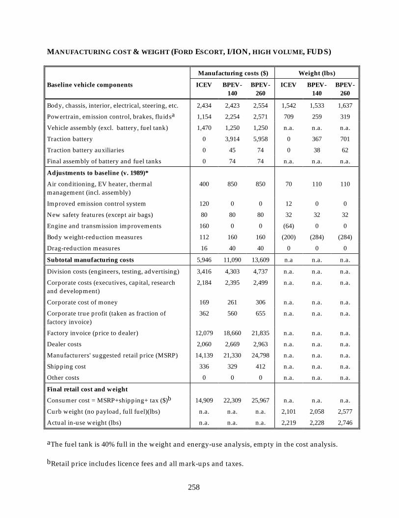
258

MANUFACTURING COST & WEIGHT (FORD ESCORT, I/ION, HIGH VOLUME, FUDS)

Manufacturing costs ($) Weight (lbs)

Baseline vehicle components ICEV BPEV-140

BPEV-260

ICEV BPEV-140

BPEV-260

Body, chassis, interior, electrical, steering, etc. 2,434 2,423 2,554 1,542 1,533 1,637

Powertrain, emission control, brakes, fluidsa 1,154 2,254 2,571 709 259 319

Vehicle assembly (excl. battery, fuel tank) 1,470 1,250 1,250 n.a. n.a. n.a.

Traction battery 0 3,914 5,958 0 367 701

Traction battery auxiliaries 0 45 74 0 38 62

Final assembly of battery and fuel tanks 0 74 74 n.a. n.a. n.a.

Adjustments to baseline (v. 1989)*

Air conditioning, EV heater, thermal management (incl. assembly)

400 850 850 70 110 110

Improved emission control system 120 0 0 12 0 0

New safety features (except air bags) 80 80 80 32 32 32

Engine and transmission improvements 160 0 0 (64) 0 0

Body weight-reduction measures 112 160 160 (200) (284) (284)

Drag-reduction measures 16 40 40 0 0 0

Subtotal manufacturing costs 5,946 11,090 13,609 n.a n.a. n.a.

Division costs (engineers, testing, advertising) 3,416 4,303 4,737 n.a. n.a. n.a.

Corporate costs (executives, capital, research and development)

2,184 2,395 2,499 n.a. n.a. n.a.

Corporate cost of money 169 261 306 n.a. n.a. n.a.

Corporate true profit (taken as fraction of factory invoice)

362 560 655 n.a. n.a. n.a.

Factory invoice (price to dealer) 12,079 18,660 21,835 n.a. n.a. n.a.

Dealer costs 2,060 2,669 2,963 n.a. n.a. n.a.

Manufacturers' suggested retail price (MSRP) 14,139 21,330 24,798 n.a. n.a. n.a.

Shipping cost 336 329 412 n.a. n.a. n.a.

Other costs 0 0 0 n.a. n.a. n.a.

Final retail cost and weight

Consumer cost = MSRP+shipping+ tax ($)b 14,909 22,309 25,967 n.a. n.a. n.a.

Curb weight (no payload, full fuel)(lbs) n.a. n.a. n.a. 2,101 2,058 2,577

Actual in-use weight (lbs) n.a. n.a. n.a. 2,219 2,228 2,746

aThe fuel tank is 40% full in the weight and energy-use analysis, empty in the cost analysis.

bRetail price includes licence fees and all mark-ups and taxes.

259

VEHICLE CHARACTERISTICS (FORD TAURUS, NIMH GEN4, HIGH VOLUME, FUDS)

Item Gasoline BPEV-70

BPEV-100

BPEV-130

BPEV-160

BPEV-190

BPEV-220

Type of traction battery n.a. Nickel metal hydride, generation 4

Type of motor n.a. GE MEV ac induction motor

Type of motor controller n.a. GE MEV inverter

Maximum power deliverable to

wheels (kW)a103 59 63 67 72 77 83

Acceleration from 0 to 60 mph, 0% grade (secs)

9.3 9.32 9.31 9.29 9.29 9.29 9.29

Battery cycle life to 80% DoD n.a. 1,331 1,331 1,331 1,331 1,331 1,331

Battery system specific energy (Wh/kg)

n.a. 95 103 106 111 114 116

Battery contribution to retail cost ($/kWh)

n.a. 413 336 290 256 231 212

Volume of battery/fuel-storage/fuel-cell system (L)

65 53 74 96 121 148 178

Vehicle life (km) 241,350 265,485 265,485 265,485 265,485 265,485 265,485

Weight of the complete vehicle (kg) 1,416 1,156 1,238 1,326 1,425 1,533 1,653

Weight of battery/fuel- storage/fuel-cell system (kg)

n.a. 149 206 269 335 409 491

Coefficient of drag 0.30 0.24 0.24 0.24 0.24 0.24 0.24

Energy efficiency, mi/kWh from the outlet

n.a. 3.36 3.25 3.15 3.00 2.87 2.73

Fuel economy (gasoline-equivalent

mpg, HHV)b19.9 123.0 119.1 115.2 109.9 105.0 99.9

Fuel economy (gasoline equivalent liters/100 km)

11.8 1.9 2.0 2.0 2.1 2.2 2.4

Powertrain efficiency ratioc n.a. 9.25 8.87 8.52 8.09 7.69 7.29

n.a. = not applicable.

aMaximum pow assumes no air conditioning or heating or optional accessories.

bFuel economy of BPEVs is based on electricity from the outlet.

cThe ratio of mi/BTU-from-battery to mi/BTU-gasoline.

260

COST SUMMARY (FORD TAURUS, NIMH GEN4, HIGH VOLUME, FUDS)

Item Gasoline BPEV-70

BPEV-100

BPEV-130

BPEV-160

BPEV-190

BPEV-220

Fuel retail cost, excluding taxes ($/gasoline-equivalent gallon)

0.90 2.20 2.20 2.20 2.20 2.20 2.20

Full retail cost of vehicle, incl. taxes ($)

20,085 24,208 25,487 26,771 28,184 29,692 31,348

Battery contribution to retail cost ($) n.a. 5,838 7,083 8,306 9,508 10,759 12,097

Levelized maintenance cost ($/yr) 492 355 355 355 355 355 355

Total lifecycle cost (cents/mile) 38.70 40.88 41.50 42.84 44.82 46.93 49.38

Present value of lifecycle cost vs.

gasoline ($)a45,881 5,625 6,404 8,093 10,586 13,247 16,331

Breakeven gasoline price ($/gal) n.a. 1.71 1.83 2.10 2.49 2.91 3.40

n.a. = not applicable.

aFor gasoline, the present value is shown. For the EVs, the difference between the present value for the EV and the present value for gasoline is shown.

261

LIFECYCLE COST SUMMARY (FORD TAURUS, NIMH GEN4, HIGH VOLUME, FUDS) (U.S. CENTS/MILE)

Cost item Gasoline BPEV-70

BPEV-100

BPEV-130

BPEV-160

BPEV-190

BPEV-220

Independently calculated cost of fast recharging

n.a. 0.00 0.00 0.00 0.00 0.00 0.00

Purchased electricity (including battery heating, if any)

n.a. 1.79 1.85 1.91 2.00 2.09 2.20

Vehicle, excluding batterya 17.55 15.16 15.24 15.34 15.57 15.84 16.17

Battery and tray and auxiliariesa n.a. 7.79 7.82 8.66 9.94 11.28 12.73

Space heating fuel for EVs 0.00 0.54 0.54 0.53 0.53 0.53 0.53

Motor fuel, excluding excise taxes and electricity

4.51 0.00 0.00 0.00 0.00 0.00 0.00

Home battery-recharging station n.a. 0.22 0.22 0.22 0.22 0.22 0.22

Insurance (calculated as a function of VMT and vehicle value)

6.75 7.46 7.76 8.06 8.39 8.74 9.13

Maintenance and repair, excluding oil, inspection, cleaning, towing

4.88 3.72 3.72 3.72 3.72 3.72 3.72

Engine oil 0.17 0.00 0.00 0.00 0.00 0.00 0.00

Replacement tires (calculated as a function of VMT and vehicle wt.)

0.50 0.31 0.44 0.45 0.46 0.47 0.60

Parking, tolls, and fines (assumed to be the same for all vehicles)

1.05 1.05 1.05 1.05 1.05 1.05 1.05

Registration fee (calculated as a function of vehicle weight)

0.50 0.43 0.46 0.49 0.53 0.57 0.61

Vehicle safety and emissions inspection fee

0.60 0.21 0.21 0.21 0.21 0.21 0.21

Federal, state, and local fuel (energy) excise taxes

1.90 1.90 1.90 1.90 1.90 1.90 1.90

Accessories (assumed to be the same for all vehicles)

0.30 0.30 0.30 0.30 0.30 0.30 0.30

Total lifecycle cost (cents/mile) 38.70 40.88 41.50 42.84 44.82 46.93 49.38

The breakeven price of gasoline, including taxes

n.a. 1.71 1.83 2.10 2.49 2.91 3.40

n.a.= not applicable

aRetail-cost equivalent.

262

263

MANUFACTURING COST & WEIGHT (FORD TAURUS, NIMH GEN4, HIGH VOLUME, FUDS)

Manufacturing costs ($) Weight (lbs)

Baseline vehicle components ICEV BPEV-100

BPEV-190

ICEV BPEV-100

BPEV-190

Body, chassis, interior, electrical, steering, etc. 3,621 3,482 3,684 2,080 1,990 2,121

Powertrain, emission control, brakes, fluidsa 2,468 2,830 3,279 1,141 341 421

Vehicle assembly (excl. battery, fuel tank) 1,715 1,458 1,458 n.a. n.a. n.a.

Traction battery 0 3,624 5,911 0 406 822

Traction battery auxiliaries 0 54 90 0 46 76

Final assembly of battery and fuel tanks 0 74 74 n.a. n.a. n.a.

Adjustments to baseline (v. 1989)*

Air conditioning, EV heater, thermal management (incl. assembly)

400 850 850 70 110 110

Improved emission control system 150 0 0 15 0 0

New safety features (except air bags) 100 100 100 40 40 40

Engine and transmission improvements 200 0 0 (80) 0 0

Body weight-reduction measures 140 200 200 (250) (371) (371)

Drag-reduction measures 20 50 50 0 0 0

Subtotal manufacturing costs 8,814 12,721 15,695 n.a n.a. n.a.

Division costs (engineers, testing, advertising) 4,162 4,715 5,137 n.a. n.a. n.a.

Corporate costs (executives, capital, research and development)

2,166 2,278 2,363 n.a. n.a. n.a.

Corporate cost of money 222 289 340 n.a. n.a. n.a.

Corporate true profit (taken as fraction of factory invoice)

475 619 728 n.a. n.a. n.a.

Factory invoice (price to dealer) 15,840 20,648 24,252 n.a. n.a. n.a.

Dealer costs 3,177 3,695 4,083 n.a. n.a. n.a.

Manufacturers' suggested retail price (MSRP) 19,017 24,343 28,335 n.a. n.a. n.a.

Shipping cost 483 410 515 n.a. n.a. n.a.

Other costs 0 0 0 n.a. n.a. n.a.

Final retail cost and weight

Consumer cost = MSRP+shipping+ tax ($)b 20,085 25,496 29,716 n.a. n.a. n.a.

Curb weight (no payload, full fuel)(lbs) n.a. n.a. n.a. 3,016 2,563 3,219

Actual in-use weight (lbs) n.a. n.a. n.a. 3,122 2,731 3,382

aThe fuel tank is 40% full in the weight and energy-use analysis, empty in the cost analysis.

bRetail price includes licence fees and all mark-ups and taxes.

264

VEHICLE CHARACTERISTICS (FORD ESCORT, NIMH GEN4, HIGH VOLUME, FUDS)

Item Gasoline BPEV-70

BPEV-100

BPEV-130

BPEV-160

BPEV-190

BPEV-220

Type of traction battery n.a. Nickel metal hydride, generation 4

Type of motor n.a. GE MEV ac induction motor

Type of motor controller n.a. GE MEV inverter

Maximum power deliverable to wheels (kW)a

67 43 46 49 52 56 60

Acceleration from 0 to 60 mph, 0% grade (secs)

10.3 10.28 10.28 10.27 10.28 10.26 10.27

Battery cycle life to 80% DoD n.a. 1,331 1,331 1,331 1,331 1,331 1,331

Battery system specific energy (Wh/kg)

n.a. 98 106 110 115 117 119

Battery contribution to retail cost ($/kWh)

n.a. 395 321 277 246 224 205

Volume of battery/fuel-storage/fuel-cell system (L)

52 43 61 79 99 121 146

Vehicle life (km) 241,350 265,485 265,485 265,485 265,485 265,485 265,485

Weight of the complete vehicle (kg) 1,007 916 984 1,056 1,134 1,220 1,317

Weight of battery/fuel- storage/fuel-cell system (kg)

n.a. 121 167 218 271 332 397

Coefficient of drag 0.30 0.24 0.24 0.24 0.24 0.24 0.24

Energy efficiency, mi/kWh from the outlet

n.a. 4.01 3.87 3.74 3.59 3.45 3.28

Fuel economy (gasoline-equivalent mpg, HHV)b

26.9 146.7 141.8 136.9 131.6 126.4 120.2

Fuel economy (gasoline equivalent liters/100 km)

8.7 1.6 1.7 1.7 1.8 1.9 2.0

Powertrain efficiency ratioc n.a. 8.11 7.76 7.44 7.10 6.79 6.43

n.a. = not applicable.

aMaximum pow assumes no air conditioning or heating or optional accessories.

bFuel economy of BPEVs is based on electricity from the outlet.

cThe ratio of mi/BTU-from-battery to mi/BTU-gasoline.

265

COST SUMMARY (FORD ESCORT, NIMH GEN4, HIGH VOLUME, FUDS)

Item Gasoline BPEV-70

BPEV-100

BPEV-130

BPEV-160

BPEV-190

BPEV-220

Fuel retail cost, excluding taxes ($/gasoline-equivalent gallon)

0.90 2.20 2.20 2.20 2.20 2.20 2.20

Full retail cost of vehicle, incl. taxes ($)

14,909 19,610 20,623 21,650 22,744 23,904 25,216

Battery contribution to retail cost ($) n.a. 4,688 5,692 6,675 7,639 8,654 9,733

Levelized maintenance cost ($/yr) 483 348 348 348 348 348 348

Total lifecycle cost (cents/mile) 30.90 34.67 35.07 36.16 37.72 39.47 41.35

Present value of lifecycle cost vs. gasoline ($)a

36,632 7,042 7,553 8,929 10,884 13,096 15,460

Breakeven gasoline price ($/gal) n.a. 2.29 2.40 2.69 3.11 3.59 4.09

n.a. = not applicable.

aFor gasoline, the present value is shown. For the EVs, the difference between the present value for the EV and the present value for gasoline is shown.

266

LIFECYCLE COST SUMMARY (FORD ESCORT, NIMH GEN4, HIGH VOLUME, FUDS) (U.S. CENTS/MILE)

Cost item Gasoline BPEV-70

BPEV-100

BPEV-130

BPEV-160

BPEV-190

BPEV-220

Independently calculated cost of fast recharging

n.a. 0.00 0.00 0.00 0.00 0.00 0.00

Purchased electricity (including battery heating, if any)

n.a. 1.50 1.55 1.60 1.67 1.74 1.83

Vehicle, excluding batterya 13.03 12.39 12.44 12.52 12.68 12.85 13.10

Battery and tray and auxiliariesa n.a. 6.28 6.31 6.99 8.03 9.12 10.30

Space heating fuel for EVs 0.00 0.54 0.54 0.54 0.54 0.54 0.54

Motor fuel, excluding excise taxes and electricity

3.34 0.00 0.00 0.00 0.00 0.00 0.00

Home battery-recharging station n.a. 0.22 0.22 0.22 0.22 0.22 0.22

Insurance (calculated as a function of VMT and vehicle value)

5.45 6.36 6.60 6.84 7.09 7.36 7.67

Maintenance and repair, excluding oil, inspection, cleaning, towing

4.80 3.66 3.66 3.66 3.66 3.66 3.66

Engine oil 0.13 0.00 0.00 0.00 0.00 0.00 0.00

Replacement tires (calculated as a function of VMT and vehicle wt.)

0.42 0.38 0.39 0.39 0.40 0.52 0.53

Parking, tolls, and fines (assumed to be the same for all vehicles)

1.05 1.05 1.05 1.05 1.05 1.05 1.05

Registration fee (calculated as a function of vehicle weight)

0.40 0.38 0.41 0.44 0.47 0.51 0.55

Vehicle safety and emissions inspection fee

0.60 0.21 0.21 0.21 0.21 0.21 0.21

Federal, state, and local fuel (energy) excise taxes

1.40 1.40 1.40 1.40 1.40 1.40 1.40

Accessories (assumed to be the same for all vehicles)

0.30 0.30 0.30 0.30 0.30 0.30 0.30

Total lifecycle cost (cents/mile) 30.90 34.67 35.07 36.16 37.72 39.47 41.35

The breakeven price of gasoline, including taxes

n.a. 2.29 2.40 2.69 3.11 3.59 4.09

n.a.= not applicable

aRetail-cost equivalent.

267

MANUFACTURING COST & WEIGHT (FORD ESCORT, NIMH GEN4, HIGH VOLUME, FUDS)

Manufacturing costs ($) Weight (lbs)

Baseline vehicle components ICEV BPEV-100

BPEV-190

ICEV BPEV-100

BPEV-190

Body, chassis, interior, electrical, steering, etc. 2,434 2,409 2,541 1,542 1,522 1,627

Powertrain, emission control, brakes, fluidsa 1,154 2,219 2,539 709 253 313

Vehicle assembly (excl. battery, fuel tank) 1,470 1,250 1,250 n.a. n.a. n.a.

Traction battery 0 2,814 4,594 0 331 668

Traction battery auxiliaries 0 42 71 0 36 60

Final assembly of battery and fuel tanks 0 74 74 n.a. n.a. n.a.

Adjustments to baseline (v. 1989)*

Air conditioning, EV heater, thermal management (incl. assembly)

400 850 850 70 110 110

Improved emission control system 120 0 0 12 0 0

New safety features (except air bags) 80 80 80 32 32 32

Engine and transmission improvements 160 0 0 (64) 0 0

Body weight-reduction measures 112 160 160 (200) (284) (284)

Drag-reduction measures 16 40 40 0 0 0

Subtotal manufacturing costs 5,946 9,937 12,198 n.a n.a. n.a.

Division costs (engineers, testing, advertising) 3,416 4,104 4,494 n.a. n.a. n.a.

Corporate costs (executives, capital, research and development)

2,184 2,348 2,441 n.a. n.a. n.a.

Corporate cost of money 169 240 281 n.a. n.a. n.a.

Corporate true profit (taken as fraction of factory invoice)

362 515 601 n.a. n.a. n.a.

Factory invoice (price to dealer) 12,079 17,182 20,032 n.a. n.a. n.a.

Dealer costs 2,060 2,532 2,796 n.a. n.a. n.a.

Manufacturers' suggested retail price (MSRP) 14,139 19,715 22,829 n.a. n.a. n.a.

Shipping cost 336 320 404 n.a. n.a. n.a.

Other costs 0 0 0 n.a. n.a. n.a.

Final retail cost and weight

Consumer cost = MSRP+shipping+ tax ($)b 14,909 20,636 23,930 n.a. n.a. n.a.

Curb weight (no payload, full fuel)(lbs) n.a. n.a. n.a. 2,101 2,001 2,526

Actual in-use weight (lbs) n.a. n.a. n.a. 2,219 2,170 2,693

aThe fuel tank is 40% full in the weight and energy-use analysis, empty in the cost analysis.

bRetail price includes licence fees and all mark-ups and taxes.

268