Oscillation of nonlinear neutral delay differential Equations

Model Theory, Algebra and
Differential Equations
Joel Chris Ronnie Nagloo
Submitted in accordance with the requirements
for the degree of Doctor of Philosophy
The University of Leeds
School of Mathematics
May 2014

The candidate confirms that the work submitted is his own, except where
work which has formed part of jointly-authored publications has been in-
cluded. The contribution of the candidate and the other authors to this
work has been explicitly indicated below. The candidate confirms that ap-
propriate credit has been given within the thesis where reference has been
made to the work of others.
Work from the following jointly-authored publications is included in this
thesis:
• Paper 1: J. Nagloo and A. Pillay, On algebraic relations between
solutions of a generic Painleve equation, accepted in J. Reine Angew.
Math.
• Paper 2: J. Nagloo and A. Pillay, On the algebraic independence of
generic Painleve transcendents, Compositio Mathematica, doi:10.1112/
S0010437X13007525.
Chapters 3 and 4 are based on Paper 1, and Chapter 6 is based on Paper 2.
The contribution of authors to the papers listed above consists of:
• Paper 1: A. Pillay provided a method that could be used to prove
geometric triviality of the generic Painleve equations and sketched such
a proof for the second equation. J. Nagloo did the detailed investigation
of the other Painleve equations and use that method to prove geometric
triviality of all the generic Painleve equations. Other concepts were
developed in discussions.
• Paper 2: J. Nagloo came up with a method that could be used to
prove algebraic independence of the generic second Painleve equations.
A. Pillay noticed that this method could be adapted for the other equa-
tions. J. Nagloo investigated further and was able to prove algebraic in-
dependence (ω-categoricity in some cases) of the other generic Painleve
equations.
This copy has been supplied on the understanding that it is copyright mate-
rial and that no quotation from the thesis may be published without proper
acknowledgement.
c© 2014 The University of Leeds and Joel Chris Ronnie Nagloo

iii Acknowledgements
Firstly, I would like to thank my supervisor Prof. Anand Pillay for his help,
encouragement and support. He has been a constant source of ideas and
inspiration and this thesis would not have been possible without him. It is
fair to say that I feel extremely lucky to have been his student.
I am also indebted to Prof. Frank Nijhoff who on Anand’s departure took
the role of supervisor very seriously and enthusiastically.
I am grateful to Prof. Dugald Macpherson and Jaynee for having taken
care of me and my wife, Sharonne, during the last two Christmases, and to
many of the PhD students at Leeds for making my time here memorable.
In particular, I would like to thank Davide, Robert, Vijay, Ahmet, Andres,
Pedro, Lovkush and Daniel for being much more than just familiar faces.
My gratitude also goes to David Marker, Zoe Chatzidakis, Rahim Moosa,
James Freitag and the many model theorists I have met along the way and
who have been very supportive of my work. Omar Leon Sanchez and Sil-
vain Rideau deserve a special mention for I have also found in them close
friendships.
I am grateful to the UK Engineering and Physical Sciences Research Council
(EPSRC) and to the School of Mathematics for funding my research.
Words cannot express my gratitude to Sharonne and our families for their
unlimited support and love. Without them this entire enterprise would not
have been possible.
Last but not least, I would like to thank God for allowing this one dream to
come true but also for giving me the strength and courage to persist in all
my endeavours.

kn
This thesis is dedicated to Sharonne and to my parents for their
love and continuous support.

iii Abstract
In this thesis, we applied ideas and techniques from model theory, to study
the structure of the sets of solutions XI − XV I , in a differentially closed
field, of the Painleve equations. First we show that the generic XII −XV I ,
that is those with parameters in general positions, are strongly minimal and
geometrically trivial. Then, we prove that the generic XII , XIV and XV are
strictly disintegrated and that the generic XIII and XV I are ω-categorical.
These results, already known for XI , are the culmination of the work started
by P. Painleve (over 100 years ago), the Japanese school and many others on
transcendence and the Painleve equations. We also look at the non generic
second Painleve equations and show that all the strongly minimal ones are
geometrically trivial.

Contents
1 Introduction 3
2 Preliminaries 7
2.1 Stability theory . . . . . . . . . . . . . . . . . . . . . . . . . . 7
2.1.1 Forking and Independence . . . . . . . . . . . . . . . . 8
2.1.2 Strongly minimal sets . . . . . . . . . . . . . . . . . . . 11
2.2 Differentially closed fields . . . . . . . . . . . . . . . . . . . . 15
2.2.1 Basic definitions and properties . . . . . . . . . . . . . 15
2.2.2 Finite Dimensional definable sets . . . . . . . . . . . . 19
2.3 Strongly minimal sets in DCF0 . . . . . . . . . . . . . . . . . 23
2.3.1 The dichotomy theorem . . . . . . . . . . . . . . . . . 23
2.3.2 The Classification of strongly minimal sets. . . . . . . . 26
3 Irreducibility and Analysability 30
3.1 Irreducibility . . . . . . . . . . . . . . . . . . . . . . . . . . . 30
3.1.1 The Painleve transcendents . . . . . . . . . . . . . . . 30
3.1.2 Classical functions and Irreducibility . . . . . . . . . . 33
3.2 Analysability . . . . . . . . . . . . . . . . . . . . . . . . . . . 35
3.2.1 Differential Galois theory . . . . . . . . . . . . . . . . . 36
3.2.2 Internality and Analysability . . . . . . . . . . . . . . . 39
4 Geometric triviality: The Generic cases 43
4.1 Condition (J) and strong minimality . . . . . . . . . . . . . . 43
4.2 Definability of the A→ A] functor . . . . . . . . . . . . . . . 45
4.3 Strong minimality and geometric triviality . . . . . . . . . . . 47
4.3.1 The equation PI . . . . . . . . . . . . . . . . . . . . . . 48
4.3.2 The family PII . . . . . . . . . . . . . . . . . . . . . . . 48
1

CONTENTS
4.3.3 The family PIII . . . . . . . . . . . . . . . . . . . . . . . 51
4.3.4 The family PIV . . . . . . . . . . . . . . . . . . . . . . . 53
4.3.5 The family PV . . . . . . . . . . . . . . . . . . . . . . . 54
4.3.6 The family PV I . . . . . . . . . . . . . . . . . . . . . . 56
4.3.7 Further Remarks . . . . . . . . . . . . . . . . . . . . . 59
5 Geometric triviality: Non Generic PII 61
5.1 Correspondences on A] . . . . . . . . . . . . . . . . . . . . . . 61
5.2 Geometric triviality and the second Painleve equations . . . . 64
5.3 Further comments . . . . . . . . . . . . . . . . . . . . . . . . . 68
6 Algebraic independence: The generic cases 69
6.1 A few remarks . . . . . . . . . . . . . . . . . . . . . . . . . . . 69
6.2 Generic Painleve equations PII , PIV and PV . . . . . . . . . . 70
6.2.1 The family PII . . . . . . . . . . . . . . . . . . . . . . 71
6.2.2 The family PIV . . . . . . . . . . . . . . . . . . . . . . 72
6.2.3 The family PV . . . . . . . . . . . . . . . . . . . . . . . 73
6.3 Generic PIII and PV I . . . . . . . . . . . . . . . . . . . . . . . 74
6.3.1 The family PIII . . . . . . . . . . . . . . . . . . . . . . 74
6.3.2 The family PV I . . . . . . . . . . . . . . . . . . . . . . 76
7 On Transformations in the Painleve Family 79
7.1 A remark on weak orthogonality . . . . . . . . . . . . . . . . . 79
7.2 The special case of PI . . . . . . . . . . . . . . . . . . . . . . 80
7.3 Orthogonality in the remaining cases . . . . . . . . . . . . . . 82
Bibliography 86
2

Chapter 1
Introduction
Les mathematiques constituent un continent solidment agence, dont tous
les pays sont bien relies les uns aux autres; l’oeuvre de Paul Painleve est
une ile originale et splendide dans l’ocean voisin.
– Henri Poincare
The Painleve equations are second order ordinary differential equations
and come in six families PI − PV I , where PI consists of the single equation
y′′ = 6y2 + t, and PII − PV I come with some complex parameters:
PII(α) : y′′ = 2y3 + ty + α
PIII(α, β, γ, δ) : y′′ =1
y(y′)2 − 1
ty′ +
1
t(αy2 + β) + γy3 +
δ
y
PIV (α, β) : y′′ =1
2y(y′)2 +
3
2y3 + 4ty2 + 2(t2 − α)y +
β
y
PV (α, β, γ, δ) : y′′ =
(1
2y+
1
y − 1
)(y′)2 − 1
ty′ +
(y − 1)2
t2
(αy +
β
y
)+ γ
y
t
+ δy(y + 1)
y − 1
PV I(α, β, γ, δ) : y′′ =1
2
(1
y+
1
y − 1+
1
y − t
)(y′)2 −
(1
t+
1
t− 1+
1
y − t
)y′
+y(y − 1)(y − t)t2(t− 1)2
(α + β
t
y2+ γ
t− 1
(y − 1)2+ δ
t(t− 1)
(y − t)2
)They were isolated in the early part of the 20th century, by Painleve, with
refinements by Gambier and Fuchs, as those ODE’s of the form y′′ = f(y, y′, t)
(where f is rational over C) which have the Painleve property: any local
analytic solution extends to a meromorphic solution on the universal cover
3

of P 1(C)\S, where S is the finite set of singularities of the equation (including
the point at infinity if necessary).
Painleve also believed that the solutions of the equations, at least for
general values of the parameters, defined “new” special functions. He gave a
definition of “known” functions and claimed to have proved that no solution
of the first Painleve equation is “known”, that is the equation is “irreducible”
(cf. [33]). Unfortunately, his definition lacked a bit of rigour and it took the
work of Nishioka ([26]) and Umemura ([46]), after about 80 years, to clarify
his notion of irreducibility. Of course, this special notion should not be con-
fused with the usual notions of irreducibility of an algebraic (or differential
algebraic) variety. In any case, in a series of papers by Okamoto, Nishioka,
Noumi, Umemura, Watanabe, and others, the irreducibility of PI −PV I out-
side special values of the complex parameters was established.
It turns out that what was actually proved by the Japanese school, is
that, except for some special values of the parameters, the set of solutions of
any of the Painleve equations, considered as a differential algebraic variety
or definable set in an ambient differentially closed field is strongly minimal
in the sense of model theory. This is where the work in this thesis begins.
Strong minimality is a fundamental notion in model theory. A definable set
is said to be minimal if every definable subset is finite or cofinite and strongly
minimal if it is minimal in every elementary extension. In differentially closed
fields strongly minimal sets determine, in a precise manner, the structure of
“finite rank” definable sets. It is no surprise then that a considerable amount
of work had been devoted to further our understanding of them.
The deepest result in that direction, due to Hrushovski and Sokolovic [13],
concerns the classification of strongly minimal sets. This classification, called
the trichotomy theorem, asserts that there are only three types of strongly
minimal sets: Type (i): those nonorthogonal to the constants; a version of
algebraic integrability after base change. Type (ii): those closely related to
the solution set A] of a very special kind of ODE on a simple abelian variety
A (of which PV I(0, 0, 0, 1/2) is an example). Type (iii): those geometrically
trivial: for equations of the form y′′ = f(y, y′, t) (where f is rational over
C), geometric triviality means that for any distinct solutions y1, . . . , yn, if
y1, y′1, . . . , yn, y
′n are algebraically dependent over C(t), then already for some
1 ≤ i < j ≤ n, yi, y′i, yj, y
′j are algebraically dependent over C(t).
4

So the first natural question to ask is: “Where do the strongly minimal
Painleve equations fit in the Hrushovski and Sokolovic classification?”. This
brings us to our first result (Propositions 4.3.6, 4.3.9, 4.3.12, 4.3.15 and
4.3.20):
Result A. The generic Painleve equations (that is those in the families
PII − PV I with algebraically independent complex parameters α, β, ..), are
geometrically trivial
These equations give the first examples of geometrically trivial sets of
order > 1. For the proof, we use the above-mentioned results of the Japanese
school, together with additional techniques that allows us to rule out Type (i)
and Type (ii) in the classification. One of the crucial ingredients is that for
each of the Painleve families PII − PV I , the set of complex tuples (α, β, . . .)
for which the corresponding equation is not strongly minimal has “infinitely
many components”.
Although the technique used in the proof of Result A is quite general
and uniform, in the sense that it works for all the generic equations, it fails
quite miserably for non generic parameters. Moreover, by adapting some
techniques of Nishioka [27] in his study of PI , we have been able to extend
Result A for PII to the non generic case (Propsition 5.2.2).
Result B. The strongly minimal second Painleve equations (i.e. whenever
α 6∈ 1/2 + Z) are geometrically trivial
Quite remarkably, using Result A and building on the ideas of its proof,
we have also been able to prove what has been an old belief in the Painleve
theory (Propositions 6.2,2, 6.2.4, 6.2.7, 6.3.2 and 6.3.3):
Result C. (i) Suppose y1, . . . , yn are distinct solutions of any generic PII ,
PIV or PV . Then tr.deg (C(t)(y1, y′1, . . . , yn, y
′n)/C(t)) = 2n.
(ii) Suppose y1, . . . , yk are distinct solutions of any generic PIII (repectively
PV I) such that tr.deg(C(t)(y1, y′1, . . . , yk, y
′k)/C(t)) = 2k. Then for all other
solutions y, except for at most k (respectively 11k), tr.deg(C(t)(y1, y′1, . . . ,
yk, y′k, y, y
′)/C(t)) = 2(k + 1).
5
Result C (i) means that the solution set (in a differentially closed field)
of a generic PII , PIV or PV is strictly disintegrated over C(t), while Result C
(ii) means that the solution set of any generic PIII or PV I is ω-categorical.
It is worth mentioning that Result C is the culmination of the work started
by P. Painleve (over 100 years ago), the Japanese school and many others on
transcendence and the Painleve equations.
Let us finish by mentioning the structure of the thesis: In Chapter 2
we recall the necessary background in (ω-)stability theory and the model
theory of differentially closed fields. We also give a detailed account of the
proof of the trichotomy theorem mentioned above. In Chapter 3 we look at
Umemura’s irreducibility notion and explain how it translates to the model
theoretic notion “analysability” and in particular point out its relation to
strong minimality. Chapter 4, 5 and 6 are where the main results (A, B and
C respectively) are proved. Finally in Chapter 7 we show how one can use
the same techniques as in the proof of Result A (or C) to answer negatively,
in most cases, the following question of P. Boalch: “Given any two generic
Painleve equations from any of the families PI − PV I , are there differential
transformations between them?”
6

Chapter 2
Preliminaries
It is at first surprising that such a preliminary model-theoretic investi-
gation of the basic geography of algebraic differential equations should
discover Abelian varieties in a special role.
– Ehud Hrushovski
In this chapter we provide a summary of the model theoretic and differ-
ential algebraic notions that play an important role in the thesis. Our aim is
to give an account of one of the most important results in the area, namely,
the trichotomy for strongly minimal sets. This powerful result is at the heart
of our work. We will assume that the reader has a working knowledge of
the fundamentals of model theory and some understanding of the basics of
algebraic geometry.
2.1 Stability theory
This section gives an overview of the basic machinery of ω-stability theory.
Good references in this case are the book of Marker [19] and the online
lecture notes of Pillay [41]. One can also find a more general treatment
of stability theory in Pillay’s book [35]. Examples to illustrate the various
notions introduced here will only appear in the next section when we look at
DCF0.
Throughout L will be a countable language and T a complete L-theory.
We also assume that T has elimination of imaginaries. Recall that this means
7

2.1 Stability theory
that for any ∅-definable set Y , if E is a ∅-definable equivalence relation on Y ,
then there is a ∅-definable map fE : Y → Um, for some m, such that xEy if
and only if fE(x) = fE(y). In other words we can view Y/E as the definable
set fE(Y ).
2.1.1 Forking and Independence
Let U , for now, be a κ-saturated, κ-strongly homogeneous model of T for a
sufficiently big κ > |T |.
Definition 2.1.1. Let Y ⊆ Un be a nonempty definable set
(i) The Morley rank of Y is defined inductively as follows:
• RM(Y ) ≥ 0;
• RM(Y ) ≥ α + 1 if and only if there are definable subsets Yi of Y
for i < ω which are pairwise disjoint and such that RM(Yi) ≥ α;
• For β a limit ordinal, RM(Y ) ≥ β if and only if RM(Y ) ≥ α for
all α < β.
Then RM(Y ) = α if RM(Y ) ≥ α and RM(Y ) 6≥ α + 1. We also write
RM(Y ) =∞ if RM(Y ) ≥ α for all α.
(ii) If RM(Y ) = α <∞ then the Morley degree of Y , dM(Y ), is the largest
number d so that there are pairwise disjoint definable subsets Yi of Y ,
with RM(Yi) = α for i = 1, . . . , d.
For a complete type p, the Morley rank and Morley degree are respectively
defined as RM(p) := inf{RM(φ(U)) : φ ∈ p} and dM(p) = inf{dM(φ(U)) :
φ ∈ p,RM(φ(U)) = RM(p)} and if dM(p) = 1, p is said to be stationary.
Remark 2.1.2. Given a tuple a from U , RM(a/B) (resp. dM(a/B)) denotes
the Morley rank (resp. Morley degree) of the type of a over B.
The Morley rank will allow us to define a good notion of independence
and dimension. However, given an arbitrary T , it is not necessarily true that
every definable set has ordinal valued Morley rank. This property is reserved
for a special class of theories:
8

2.1 Stability theory
Definition 2.1.3. T is said to be totally transcendental if for every definable
set Y , RM(Y ) <∞.
When working in a countable language, one can characterise totally tran-
scendental theories in terms of counting types. We first need the following
definition.
Definition 2.1.4. Let κ be an infinite cardinal.
(i) T is said to be κ-stable if for every A of cardinality at most κ, |Sn(A)| ≤
κ. One usually says ω-stable instead of ℵ0-stable.
(ii) T is said to be stable if it is κ-stable for some κ.
Theorem 2.1.5 ([19], Theorem 4.2.18 and 6.2.14). The following are
equivalent:
(i) T is ω-stable.
(ii) T is totally transcendental.
(iii) T is κ-stable for all infinite κ.
As we shall see in the next section, it is easier to check whether or not
a given theory is totally transcendental using the above characterisation. It
turns out that the ω-stable theories are among the nicest in the class of stable
theories. For example one has the following
Fact 2.1.6 ([19], Theorem 4.2.20 and 6.5.4). Assume that T is ω-stable.
Then
(i) T has saturated models of size κ for each cardinal κ > ℵ0.
(ii) T has prime models over any parameter set.
(iii) Any complete type p(x) ∈ S(A) is definable: for any formula ϕ(x, y),
there is a formula dϕ(y) ∈ LA such that for any a ∈ A, ϕ(x, a) ∈ p if
and only if |= dϕ(a).
9

2.1 Stability theory
The first assertion means that we can choose the size of U to be κ. The
second assertion means that for any A ⊂ U , there is M0 |= T , with A ⊂M0,
such that whenever M |= T and f : A → M is partial elementary, there is
an elementary f : M0 → M extending f . In ω-stable theories such an M0 is
unique up to isomorphisms fixing A.
Remark 2.1.7. The theory T is stable if and only if any complete type is
definable.
From now on we assume that T is ω-stable and we fix a sufficiently satu-
rated model U of T . The promised notion of independence is the following:
Definition 2.1.8. Suppose A ⊆ B ⊂ U , p ∈ Sn(A), q ∈ Sn(B), and p ⊆ q.
We say that q is a nonforking extension of p if RM(q) = RM(p). If a is
a tuple from U then we say that a is independent from B over A, written
a^A
| B, if tp(a/B) is a nonforking extension of tp(a/A); that is, if RM(a/B) =
RM(a/A).
Theorem 2.1.9 ([19], Section 6.3). Let a be a tuple and let A ⊆ B
(i) There is b such that tp(a/A) = tp(b/A) and b^A
| B.
(ii) If C ⊇ B, then we have a^A
| C if and only if a^A
| B and a^B
| C.
(iii) For another tuple b, a^A
| b if and only if b^A
| a.
(iv) a^A
| B if and only if for all finite B′ ⊆ B, a^A
| B′.
For obvious reasons (i), (ii), (iii) and (iv) are usually referred to as ex-
istence, transitivity, symmetry and finite character respectively. Also, for a
type p ∈ S(A), being stationary is equivalent to p having a unique nonforking
extension to any B ⊇ A.
Definition 2.1.10. Let Y ⊆ Un be definable. We say that e is a canonical
parameter of Y if for all σ ∈ Aut(U), σ fixes Y setwise if and only if σ fixes
e pointwise.
10

2.1 Stability theory
As we assume that T has elimination of imaginaries, we have that any
definable set has a canonical parameter in U . Indeed, if Y is defined by ϕ(x, a)
we can let E be the equivalence relation aEb⇔ ∀x(ϕ(x, a)↔ ϕ(x, b)
). Then
e = fE(a/E) is a canonical parameter for Y . It is not hard to see that a
canonical parameter is determined up to interdefinability. Now consider a
stationary type p ∈ S(A). A canonical base for p is a tuple fixed pointwise
by the automorphisms of U that fix the global nonforking extension of p. As
before, by elimination of imaginaries, a canonical base of p exists in U and
is unique up to interdefinability. One usually writes Cb(p) for the definable
closure of any canonical base of p.
Lemma 2.1.11 ([41], Lemma 2.38). Let p ∈ S(A) be a stationary type.
Then
(i) Cb(p) ⊆ dcl(A).
(ii) For any B ⊆ A, p does not fork over B if and only if Cb(p) ⊆ acl(B).
(iii) Cb(p) is interdefinable with a finite tuple.
Many of the properties discussed above hold for stable theories (cf. [35])
but we will not talk about this here.
2.1.2 Strongly minimal sets
We continue in similar settings as the previous section. So T is a countable
complete ω-stable theory which eliminates imaginaries and U a sufficiently
saturated model of T .
Definition 2.1.12. An infinite definable set Y in U is said to be strongly
minimal if for every definable subset Z ⊆ Y , either Z or Y \ Z is finite.
Equivalently, Y is strongly minimal if and only if RM(Y ) = dM(Y ) = 1.
For a strongly minimal set Y ⊆ U , if we let aclY (A) = acl(A) ∩ Y , we
have that (Y, aclY ) forms a pregeometry, namely for any A ⊆ Y , the following
holds (c.f [35]):
(i) A ⊆ aclY (A) and aclY (aclY (A)) = aclY (A).
11

2.1 Stability theory
(ii) If a ∈ aclY (A ∪ {b}) \ aclY (A), then b ∈ aclY (A ∪ {a}).
(iii) If a ∈ aclY (A), then there is some finite A0 ⊆ A such that a ∈ aclY (A0).
Property (iii) is known as the exchange property. Now, for any A ⊆ Y
and B ⊂ U , we say that A is independent over B if for all a ∈ A, a 6∈aclY ((A \ {a}) ∪ B). Furthermore, A0 ⊆ A is a basis for A over B if A0
is independent over B and A ⊆ aclY (A0 ∪ B). It turns out that any two
basis have the same cardinality and one writes dim(A/B) = |A0| for any
basis A0 of A over B. The upshot is that, if Y is a strongly minimal set
defined over some B, then for any finite tuple a from Y and any C ⊇ B,
RM(a/C) = dim(a/C).
Definition 2.1.13. A pregeometry (Y, cl) is said to be
(i) Modular: if for all b, c ∈ Y and A ⊆ Y , if c ∈ cl(A, b), then there is an
a ∈ acl(A) such that c ∈ cl(a, b);
(ii) Locally modular: if there is some a ∈ Y such that (Y, cl(a)) is modular.
(iii) Geometrically trivial: if cl(A) = ∪a∈Acl({a}) for all A ⊆ Y ;
Here (Y, cl(a)) is the pregeometry obtained after localising at a, that is
for B ⊂ U , cl(a)(B) = cl({a} ∪ B). Also it is not hard to see that geometric
triviality implies modularity.
One can use the canonical base to give a different characterisation of
modularity. We first need another definition
Definition 2.1.14. Let Y be an A-definable set. Then Y is said to be one-
based if for every tuple a from Y and B ⊇ A, Cb(tp(a/acl(B))) ⊆ acl(Aa)
Fact 2.1.15 ([41], Lemma 3.32 and Theorem 3.35). Let Y be a strongly
minimal set. Then
(i) If Y is modular, then Y is one-based.
(ii) Y is locally modular if and only if Y is one-based
12

2.1 Stability theory
The three typical examples of nonmodular, nontrivial modular and geo-
metrically trivial strongly minimal sets are respectively algebraically closed
fields, vector spaces and infinite sets with no structure. Zilber conjectured
that these are “essentially” all there is.
Definition 2.1.16. Let Y and Z be strongly minimal sets defined over A
and B respectively and denote by π1 : Y × Z → Y and π2 : Y × Z → Z the
projections to Y and Z respectively. We say that Y and Z are nonorthogonal
if there is some infinite definable relation R ⊂ Y ×Z such that π1�R and π2�R
are finite-to-one functions. We usually write Y 6⊥ Z.
It is not hard to see that nonorthogonality is an equivalence relation for
strongly minimal sets.
Zilber’s Principle. If Y is a non locally modular strongly minimal, then
there is a strongly minimal algebraically closed field F , definable in U , such
that Y is nonorthogonal to F .
Although the principle holds in many “important” examples, Hrushovski
proved that it is false in general. It will nevertheless be true in the theory of
differential closed fields of characteristic zero and this is crucial for the results
in this thesis. On the other hand, note that for one-based groups and locally
modular strongly minimal sets one has the following very general results.
Fact 2.1.17 ([35], Corollary 4.4.8 and Theorem 5.1.1). kj
(i) if G is a one-based group definable in U and Y ⊆ Gn is definable,
then Y is a finite Boolean combination of cosets of definable subgroups
H ≤ Gn.
(ii) Suppose X ⊆ Un is a non geometrically trivial locally modular strongly
minimal set. Then X is nonorthogonal to a definable modular strongly
minimal group.
We finish this section by mentioning ω-categoricity, a property that is
related to the “finer” structure of pregeometries. Recall that an infinite
structure M in a countable language L is said to be ω-categorical if for each
13

2.1 Stability theory
n there are only finitely many ∅-definable subsets of Mn. The reason for the
nomenclature is that M is ω-categorical if and only if Th(M) has exactly
one countable model, up to isomorphism. We want an analogous notion for
definable sets.
Definition 2.1.18. Suppose Y ⊂ Un is definable over some parameter set
A. We say that Y is ω-categorical in U over A if there are finitely many
subsets of Y n which are definable over A, for each n.
As we are in the ω-stable context, this notion does not depend on the
choice the parameter set A:
Lemma 2.1.19. Suppose Y ⊂ Un is definable, and let b, c be finite tuples
from U over which Y is definable. Then Y is ω-categorical in U over b iff Y
is ω-categorical in U over c. Therefore we just say that Y is ω-categorical in
U .
Proof. It is enough (by adding parameters) to prove that if Y is ∅-definable,
and ω-categorical over ∅ and b is any finite tuple from U then Y is ω-
categorical over b. Now by Fact 2.1.6, tp(b/Y ) is definable over a tuple e
of elements of Y . As ω-categoricity is preserved after naming a finite tu-
ple from Y , we see that Y is ω-categorical over e, so also over b (as every
b-definable subset of Y m is e-definable).
For strongly minimal sets one can do better.
Lemma 2.1.20. Let Y ⊂ Un be a strongly minimal definable set. Then Y
is ω-categorical if and only if for any finite tuple b from U over which Y is
defined acl(b) ∩ Y is finite.
Proof. If M is any structure then it is clear that M is ω-categorical just if for
any finite tuple a from M , there are only finitely many a-definable subsets
of M . If M is also strongly minimal and a is a finite tuple from M , then
as any a-definable subset of M is finite or cofinite, there are only finitely
many a-definable subsets of M iff acl(a) is finite. So the Lemma holds for a
14

2.2 Differentially closed fields
structure M in place of Y . The full statement follows as in the proof of the
previous Lemma.
Remark 2.1.21. If Y and Z are nonorthogonal strongly minimal sets in U ,
then Y is ω-categorical iff Z is ω-categorical.
Finally one has the following general result of Zilber:
Theorem 2.1.22 ([35], Theorem 2.4.17). If X ⊂ Un is a definable,
strongly minimal ω-categorical set, then X is modular.
2.2 Differentially closed fields
The goal of this section is twofold. First, we will try to explain how all the
abstract notions introduced in the previous section give rise to meaningful
tools when applied to the concrete context of differential algebra. Secondly,
we aim to give an account of the proof that Zilber’s principle and the tri-
chotomy theorem (Theorem 2.3.11) are true in DCF0. As mentioned several
times already, this will play an important role in our work.
2.2.1 Basic definitions and properties
Definition 2.2.1. A differential field (K, δ) is a field K equipped with a
derivation δ : K → K, i.e. an additive group homomorphism satisfying the
Leibniz rule
δ(xy) = xδ(y) + yδ(x).
The field of constants CK of K is defined set theoretically as {x ∈ K :
δ(x) = 0}. We usually write x′ for δ(x) and x(n) for δ . . . δδ︸ ︷︷ ︸n
(x).
Example 2.2.2. (C(t), d/dt) the field of rational functions over C in a single
indeterminate, where in this case, the field of constants is C.
For each m ∈ N>0, associated with a differential field (K, δ), is the differential
polynomial ring in m differential variables, K{X} = K[X,X′, . . . , X
(n), . . .],
where X = (X1, . . . , Xm) and X(n)
= (X(n)1 , . . . , X
(n)m ). If f ∈ K{X} is a
differential polynomial, then the order of f , denoted ord(f), is the largest n
such that for some i, X(n)i occurs in f .
15

2.2 Differentially closed fields
Example 2.2.3. f(X) = (X ′)2 − 4X3 − tX is an example of a differential
polynomial in C(t){X} and ord(f) = 1.
The analogue of algebraically closed fields in the differential context is
defined as follows
Definition 2.2.4. A differential field (K, δ) is said to be differentially closed
if for every f, g ∈ K{X} such that ord(f) > ord(g), there is a ∈ K such that
f(a) = 0 and g(a) 6= 0.
We will later see an equivalent definition of a more geometric nature due
to Pierce and Pillay. The one given above is due to Blum [1]. As a con-
sequence of the definition, a differentially closed field is also algebraically
closed. Differentially closed fields are the natural places for studying differ-
ential equations from an algebraic/geometric perspective and we shall say a
little bit more about this now.
A differential ideal I in K{X} is an ideal which is closed under the deriva-
tion, that is δ(f) ∈ I for all f ∈ I. As with classical algebraic geometry, if
S ⊆ K{X}, by choosing Vδ(S) = {x ∈ Kn : f(x) = 0 ∀ f ∈ S} as basic
closed sets, we obtain a topology on Kn called the Kolchin topology. The
Kolchin topology is Noetherian (cf. [18] Theorem 1.16 and 1.19):
Theorem 2.2.5 (Ritt-Raudenbush Basis Theorem). Suppose (K, δ) is
a differential field. Then
(i) There are no infinite ascending chains of radical differential ideals in
K{X}. Equivalently, every radical differential ideal is finitely gener-
ated.
(ii) If I ⊂ K{X} is a radical differential ideal, there are distinct prime
differential ideals P1, ..., Pr (unique up to permutation) such that I =⋂ri=1 Pi.
One also has the analogue of Hilbert’s Nullstellensatz (cf. [18] Corollary
2.6):
16

2.2 Differentially closed fields
Theorem 2.2.6 (Seidenberg’s Differential Nullstellensatz). Let K be a
differentially closed field. The map I → Vδ(I) is a one to one correspondence
between radical differential ideals and Kolchin closed sets.
In many ways the point of view of Kolchin’s differential algebraic geome-
try, which aims to study the solution sets of systems of differential algebraic
equations, coincides with that of the model theory of differentially closed
fields. The latter is of course the point of view we take in this thesis. So let
us bring in model theory.
Our language is Lδ = (+,−, ·, δ, 0, 1), the language of differential rings and
we denote by DF0 the theory of differential fields of characteristic zero. The
axioms of DF0 consist of the axioms for fields and the axioms for the deriva-
tion (expressed using δ). This theory can be quite wild: (Q,+,−, ·, 0, 1, δ =
0) is an example of a differential field and so one gets non-computable defin-
able sets.
Now, for each n, d1 and d2 ∈ N, one can write down an Lδ-sentence
that asserts that if f is a differential polynomial of order n and degree at
most d1 and g is a nonzero differential polynomial of order less than n and
degree at most d2, then there is a solution to f(X) = 0 and g(X) 6= 0. The
theory obtain by adding to DF0 all these Lδ-sentences is called the theory
of differentially closed fields of characteristic 0, DCF0. This theory is the
model companion of DF0, that is to say that any differential field embeds
in a model of DCF0 and DCF0 is model complete. Moreover, we have the
following:
Fact 2.2.7. DCF0 is complete, eliminates quantifiers and imaginaries and
is ω-stable.
Proof. The proof of completeness and quantifier elimination follows from a
back-and-forth argument in two saturated models of DCF0 (see [37] The-
orem 1.8(b)). The proof of elimination of imaginaries can be found in [18]
(Theorem 3.7). Finally to see that DCF0 is ω-stable, one just need to use the
fact that there is a bijection between Sn(K) and spec(K{X1, . . . , Xn}), the
space of prime differential ideals of K{X}, and (using the Ritt-Raudenbush
Basis Theorem) that |spec(K{X})| = |K{X}| = |K|.
17
2.2 Differentially closed fields
Quantifier elimination means that any definable set Y ⊆ Un, definable
over a differential subfield K of U |= DCF0, is a finite boolean combination
of Kolchin closed sets (over K). On the other hand as we have seen in the
first section, ω-stability means that
1. Prime models exists: Let K be differential field. Then there exist a
differentially closed field extension Kdiff of K, called the differential
closure of K, which embeds over K into any differentially closed exten-
sion of K and which is unique up to isomorphisms over K.
2. Saturated Models exists: We can work in a κ-saturated model of DCF0
of cardinality κ (for some large cardinal κ) which will act as a universal
domain for differential algebraic geometry in the sense of Kolchin. In
particular, if U is such a saturated model and if K is a differential
subfield of U of cardinality < κ and L is a differential field extension of
K of cardinality < κ, then there is an embedding of L into U over K.
3. Morley rank is well defined: To any definable set, one can associate a
well-defined ordinal-valued dimension. Furthermore, if we let U be a
saturated model of DCF0 as described above, in DCF0 the indepen-
dence relation translates to: a is independent from B over A if 〈A, a〉 is
algebraically disjoint from 〈A,B〉 over 〈A〉, where 〈A〉 denotes the dif-
ferential field generated by A, that is 〈A〉 = Q({a, a′, a′′, . . . : a ∈ A}).
Remark 2.2.8. For a ∈ Un and K < U , we define ord(a/K) to be the
transcendence degree of K 〈a〉 = K(a, a′, a(2), . . .) over K. And if Y ⊆ Un is
definable over K, we define the ord(Y ) = sup{ord(a/K) : a ∈ Y }. One can
show that for Y as above, RM(Y ) ≤ ord(Y ) and furthermore, RM(Y ) < ω
if and only if ord(Y ) < ω.
We say a few words about the field of constants of a differentially closed field
as it will play an important role in later sections and chapters.
Fact 2.2.9. Let K be a differential field. Then CK is relatively algebraically
closed in K. Consequently, if K is algebraically closed as a field, so is CK .
Proof. Suppose a ∈ K is algebraic over CK . Let f(x) =∑n
i=0 kixi (in CK [x])
be the minimum polynomial of a over CK . So f(a) = 0. Since K has
18

2.2 Differentially closed fields
characteristic zero we have δ(f(a)) = (∑n−1
i=0 (i+ 1)ki+1ai) · δ(a) = 0. As f(x)
is the minimal polynomial of a we must have that δ(a) = 0.
So in particular if K is a differentially closed field, then CK is algebraically
closed as a field. More is true:
Theorem 2.2.10 ([37], Lemma 1.11). Let K be a differentially closed
field. Then CK has no additional structure other than being an algebraically
closed field. That is, a subset of CnK is definable over K if and only if it is
definable (in the language of rings) over CK.
We finish this section by giving the algebraic characterisations of the
model theoretic definable and algebraic closures.
Fact 2.2.11 ([37], Lemma 1.10). Let K |= DCF0 and let A be a subset
of K. Then
(i) dcl(A) is the differential subfield of K generated by A, that is dcl(A) =
〈A〉.
(ii) acl(A) is dcl(A)alg, the field-theoretic algebraic closure of dcl(A).
2.2.2 Finite Dimensional definable sets
We will now specialise to finite dimensional definable sets. We aim to intro-
duce the category of algebraic δ-varieties and they turn out to be birationally
equivalent to the category of finite dimensional Kolchin closed sets (see [10]).
This in particular means that, every finite dimensional definable set can be
expressed in terms of algebraic δ-varieties and this give a characterisation
closer to geometry. We fix (U , δ), a sufficiently saturated differentially closed
field which we think of as a universal domain for differential fields as ex-
plained above.
Definition 2.2.12. A definable set Y ⊆ Un is said to be finite dimensional
if it has finite order, i.e. ord(Y ) < ω. Equivalently, Y is finite dimensional if
RM(Y ) < ω.
19
2.2 Differentially closed fields
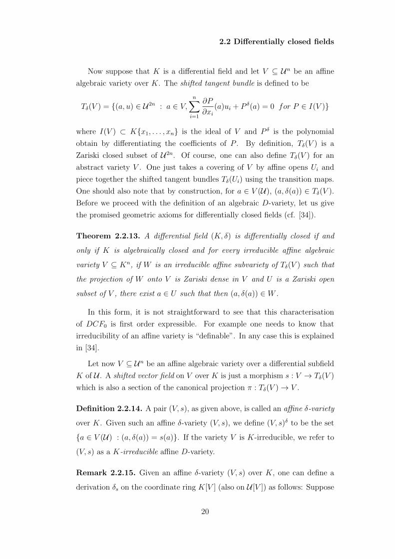
Now suppose that K is a differential field and let V ⊆ Un be an affine
algebraic variety over K. The shifted tangent bundle is defined to be
Tδ(V ) = {(a, u) ∈ U2n : a ∈ V,n∑i=1
∂P
∂xi(a)ui + P δ(a) = 0 for P ∈ I(V )}
where I(V ) ⊂ K{x1, . . . , xn} is the ideal of V and P δ is the polynomial
obtain by differentiating the coefficients of P . By definition, Tδ(V ) is a
Zariski closed subset of U2n. Of course, one can also define Tδ(V ) for an
abstract variety V . One just takes a covering of V by affine opens Ui and
piece together the shifted tangent bundles Tδ(Ui) using the transition maps.
One should also note that by construction, for a ∈ V (U), (a, δ(a)) ∈ Tδ(V ).
Before we proceed with the definition of an algebraic D-variety, let us give
the promised geometric axioms for differentially closed fields (cf. [34]).
Theorem 2.2.13. A differential field (K, δ) is differentially closed if and
only if K is algebraically closed and for every irreducible affine algebraic
variety V ⊆ Kn, if W is an irreducible affine subvariety of Tδ(V ) such that
the projection of W onto V is Zariski dense in V and U is a Zariski open
subset of V , there exist a ∈ U such that then (a, δ(a)) ∈ W .
In this form, it is not straightforward to see that this characterisation
of DCF0 is first order expressible. For example one needs to know that
irreducibility of an affine variety is “definable”. In any case this is explained
in [34].
Let now V ⊆ Un be an affine algebraic variety over a differential subfield
K of U . A shifted vector field on V over K is just a morphism s : V → Tδ(V )
which is also a section of the canonical projection π : Tδ(V )→ V .
Definition 2.2.14. A pair (V, s), as given above, is called an affine δ-variety
over K. Given such an affine δ-variety (V, s), we define (V, s)δ to be the set
{a ∈ V (U) : (a, δ(a)) = s(a)}. If the variety V is K-irreducible, we refer to
(V, s) as a K-irreducible affine D-variety.
Remark 2.2.15. Given an affine δ-variety (V, s) over K, one can define a
derivation δs on the coordinate ring K[V ] (also on U [V ]) as follows: Suppose
20

2.2 Differentially closed fields
s(x) = (x, s1(x), . . . , sn(x)) where x = (x1, . . . , xn). Then for f ∈ K[V ]
define δs(f) as
δs(f) = f δ(x) +n∑i=1
si(x)∂f
∂xi(x).
It is not hard to check that δs is indeed a derivation on K[V ]. Sometimes we
will write (V, δs) instead of (V, s).
Clearly, (V, s)δ is definable in Un. Furthermore one has the following:
Proposition 2.2.16. Let K be a differential subfield of U . Then
(i) If (V, s) is an irreducible affine δ-variety, then (V, s)δ is Zariski-dense
in V (U).
(ii) Any K-definable subset Y of Un of finite Morley rank and Morley degree
1, is generically and up to definable bijection, of the form (V, s)δ for
some K-irreducible affine δ-variety (V, s).
(iii) Let (V, δs) = (V, s) be an algebraic δ-variety, and a ∈ (V, s)δ. Let MV,a
be the maximal ideal of U [V ] at a. Then for each r ≥ 0, (MV,a)r is a
differential ideal of the differential ring (U [V ], δs), namely (MV,a)r is
closed under δs.
Proof. The proof is folklore and we include it for completeness.
(i) We have that {s(b) : b ∈ V } is closed and irreducible subvariety of TδV
and projects onto V . Hence by Theorem 2.2.13, for any Zariski open subset
U of V there is a ∈ U such that s(a) = (a, δ(a)) which is exactly what we
had to prove.
(ii) Suppose RM(Y ) = l and let p(x) be the unique generic type of Y over
K (this is the type which contains Y and has Morley rank l). Let a ∈ Un be
a realization of p so that in particular tr.degKK(a, a′, . . .) is finite. We can
hence suppose that K 〈a〉 = K(a, a′, . . . , a(r)) for some integer r and after
renaming, we rewrite K(a, a′, . . . , a(r)) as K(a1, . . . , am) where m = (r+ 1)n.
21

2.2 Differentially closed fields
Now, by construction we have that for each i = 1, . . .m, δ(ai) ∈ K(a), so
that δ(ai) = hi(a)gi(a)
, with gi(a) 6= 0. We can then write g(x) =∏m
i=1 gi(x) and
fi(x) = hi∏
j 6=i gj(x) to see that for each i = 1, . . .m, δ(ai) = fi(a)g(a)
, g(a) 6= 0.
Let now b = (b1, . . . , bm+1) be a renaming of (a1, . . . , am,1
g(a)) so that a and
b are interdefinable over K (i.e. K(a) = K(b)). Then for each i = 1, . . .m,
δ(bi) = si(b) for some polynomial si ∈ K[x1, . . . , xm+1]. For example for
i = 1, . . . ,m, we take si(x1, . . . , xm+1) = xm+1 · fi(x1, . . . , xm).
Writing s(x) = (x, s1(x), . . . , sm+1(x)), we let V be the K-irreducible
affine variety whose generic point (over K) is b. So s(b) ∈ Tδ(V ) and we see
that s is a section of Tδ(V ) → V . Hence (V, s) is a K-irreducible affine D-
variety and after removing from Y and (V, s)δ definable sets of Morley rank
< l (for example where s(x) 6= δ(x) on V ), (V, s)δ is in definable bijection
with Y . And we are done.
(iii) Keeping Remark 2.2.15 in mind, we see that for a ∈ (V, s)δ, (δsf)(a) =
δ(f(a)). So if f ∈ MV,a, then as f(a) = 0 we have that (δsf)(a) = 0. So
(δsf) ∈ MV,a and MV,a is closed under δs. A similar proof works for each
(MV,a)r.
Remark 2.2.17. jk
(i) From the proof of (ii) we see that ord(Y ) = dim(V ).
(ii) From (iii) we get that δs equips each U -vector space Vr =MV,a/(MV,a)r
with a δ-module structure (over (U , δ)): that is on Vr there is an additive
homomorphism δs : Vr → Vr satisfying δs(λv) = δ(λ)v + λδs(v) for all
λ ∈ U and v ∈ V .
Finally, let us say a few words about the δ-subvarieties of a K-irreducible
affine δ-variety (V, s).
Definition 2.2.18. By an algebraic δ-subvariety W of (V, s) we mean a
subvariety W of V (defined over some L > K) such that s�W is a section of
Tδ(W )→ W .
22

2.3 Strongly minimal sets in DCF0
The following holds (cf. [10], Proposition 1.1)
Fact 2.2.19. Let (V, s) be an affine δ-variety. Then
(i) The map taking a Kolchin closed subset X of (V, s)δ to its Zariski
closure, establishes a bijection between the Kolchin closed subsets of
(V, s)δ and the algebraic δ-subvarieties of (V, s).
(ii) X is irreducible as a Kolchin closed set iff its Zariski closure is irre-
ducible as a Zariski closed set.
Remark 2.2.20. j
(i) The inverse of the above bijection takes an algebraic δ-subvariety Y of
(V, s) to Y ∩ (V, s)δ.
(ii) Fact 2.2.19(i) in particular means that a Kolchin closed subset Y of
(V, s)δ is of the form W ∩ (V, s)δ = (W, s�W )δ, where W = Y zar ⊆ V .
2.3 Strongly minimal sets in DCF0
In this section, we look at strongly minimal sets in DCF0. We explain how to
show that Zilber’s Principle and the trichotomy theorem hold in the theory.
Throughout we assume that U is a sufficiently saturated differentially closed
field.
2.3.1 The dichotomy theorem
Let us start by characterising strongly minimal sets in the special case of
δ-varieties.
Fact 2.3.1. Let (V, s) be an affine δ-variety. Then (V, s)δ is strongly minimal
if and only if V is positive-dimensional and (V, s) has no proper (irreducible)
positive-dimensional algebraic δ-subvarieties.
23

2.3 Strongly minimal sets in DCF0
Proof. This follows from Fact 2.2.19 and quantifier elimination for DCF0.
For example assuming the right hand side, Fact 2.2.19 implies that (V, s)δ
is infinite and has no proper infinite Kolchin closed sets. As any definable
subset of (V, s)δ is a finite Boolean combination of Kolchin closed sets we
deduce strong minimality. Clearly it only suffices to consider irreducible
Kolchin closed sets.
Example 2.3.2. The field of constants CU is strongly minimal.
Example 2.3.3. If f is an absolutely irreducible polynomial over U in 2
variables then the subset Y of U defined by f(y, y′) = 0 is strongly minimal,
of order 1.
Example 2.3.4. The subset of U defined by {yy′′ = y′, y′ 6= 0} is strongly
minimal, of order 2. (See 5.17 of [18].)
Remark 2.3.5. Suppose Y1 and Y2 are nonorthogonal strongly minimal sets
and that the relation R ⊂ Y1 × Y2 is defined over some field K. Then by
definition, for any generic y ∈ Y1 there exist z ∈ Y2 generic such that (y, z) ∈
R and in that case K 〈y〉alg = K 〈z〉alg. So if Y1 and Y2 are nonorthogonal
strongly minimal sets then ord(Y1) = ord(Y2).
The field of constants, CU , is nonmodular. Indeed, if one consider alge-
braically independent points a, b, c ∈ CU and let d = ac + b, then one has
that d ∈ acl(a, b, c) but there is no b1 ∈ acl(a, b) such that d ∈ acl(b1, c). It
turns out that any nonmodular strongly minimal set is closely related to CU .
Theorem 2.3.6 (Zilber’s Principle). Suppose Y is strongly minimal. Then
either Y is locally modular or Y is nonorthogonal to CU (and not both).
The first proof was found by Hrushovski and Sokolovic in [13] where they
used the deep and difficult theorem on Zariski geometries from [14]. More
recently, using the theory of (differential) jet spaces, Pillay and Ziegler in
[42] found an alternative route that avoids Zariski geometries. We say a few
words about the Pillay-Ziegler proof. To begin with, they show that DCF0
has the canonical base property (CBP).
24

2.3 Strongly minimal sets in DCF0
So what do canonical bases look like in DCF0? As we have elimination
of imaginaries, if Y is Kolchin closed, then Y has a canonical parameter in
U . If K is an algebraically closed differential subfield of U and a ∈ Un we
want to understand Cb(tp(a/K)), the canonical base of the type of a over
K. We let Vδ(a) ∈ Un be the differential locus of a over K. That is
Vδ(a) ={b ∈ Un : P (b) = 0 for all P ∈ K{X} such that P (a) = 0
}.
Then Cb(tp(a/K)) is a canonical parameter for Vδ(a). More generally, for
B ⊂ U , if p ∈ Sn(B) is a stationary type, we define Cb(p) as follows: We let
a ∈ U be a realisation of p and let Vδ(a) ∈ Un be the differential locus of a
over 〈B〉. Then again, Cb(p) is a canonical parameter for Vδ(a).
Remark 2.3.7. If Y is Kolchin closed, then the differential field K = 〈e〉
generated by a canonical parameter e of Y is often called the smallest differ-
ential field of definition of Y . Namely, K is the smallest differential subfield
of U , such that Y can be defined by differential polynomials with coefficients
from K.
Theorem 2.3.8 (Canonical base property, [42]). Let Y be a finite-
dimensional definable set, defined over an algebraically closed differential sub-
field K of U . Let a ∈ Y and let L be a algebraically closed differential subfield
containing K. Let b = Cb(tp(a/L)). Then there are finite tuples c in CU and
d in U such that b is independent from d over K 〈a〉 and b ∈ dcl(K, a, c, d).
Sketch of the proof of Theorem 2.3.8 We may assume that a is the generic
point over K of (V, s)δ for some affine δ-variety (V, s) over K (by applying
the proof of Propostion 2.2.16(ii)). Let W be the algebraic-geometric locus
of a over L. Then (W, s�W ) is an algebraic δ-variety and a is a (differential)
generic point over L of (W, s�W )δ. It follows that b = Cb(tp(a/L)) is inter-
definable over K with the canonical parameter of W . More is true, if we
let fr be the map MV,a/(MV,a)r+1 → MW,a/(MW,a)
r+1, then b is interde-
finable over K 〈a〉 with the canonical parameter of ker(fr) for large enough
r. But ker(fr) is a δ-submodule (see Remark 2.2.17(ii)) of MV,a/(MV,a)r+1
and using the theory of δ-modules one gets that after naming a “suitable”
basis of MV,a/(MV,a)r+1 (say er), the canonical parameter of ker(fr) is in
dcl(K, a, er, c) for some tuple of constants c.
25

2.3 Strongly minimal sets in DCF0
Proof of Theorem 2.3.6 We assume that Y is defined without parameters.
If Y is nonmodular there are tuples a from Y and B ⊂ U such that b =
Cb(tp(a/acl(B))) is not contained in acl(a). By the CBP, there are finite
tuples c in CU and d in U such that b is independent from d over a and
b ∈ dcl(a, c, d). As b is essentially a tuple from Y (b ∈ acl(a1, . . . , ar) for
some independent realisations of tp(a/acl(B))), this yields some nontrivial
relation between Y and CU giving nonorthogonality.
2.3.2 The Classification of strongly minimal sets.
In the previous section we saw a neat characterisation of the non modular
strongly minimal sets. What about the locally modular ones? As we will
now see, the non trivial ones can also be classified up to nonorthogonality.
From Fact 2.1.17(ii) we know that to understand/classify non trivial locally
modular strongly minimal sets, one needs to identify and understand defin-
able modular strongly minimal groups. Essentially everything is contained
in the following (see [3] and [13]):
Fact 2.3.9. Let A be an abelian variety over U . We identify A with its set
A(U) of U -points. Then
(i) A has a (unique) smallest Zariski-dense definable subgroup, which we
denote by A] and called the Manin kernel of A.
(ii) A] is finite-dimensional, dim(A) ≤ order(A]) ≤ 2dim(A) and moreover
dim(A) = order(A]) if and only if A descends to CU (in which case
A] = A(CU)).
(iii) If A is a simple abelian variety with CU -trace 0, then A] is strongly
minimal and modular (non trivial).
(iv) If A is an elliptic curve then A] is strongly minimal, whether or not A
is of CU -trace 0.
Remark 2.3.10. By an abelian variety A with CU -trace 0, we mean that
A admits no non-zero algebraic homomorphisms to abelian varieties defined
over CU .
26

2.3 Strongly minimal sets in DCF0
Proof of Fact 2.3.9 The proof of (i) and (ii) can be found in the very good
note [21]. We will only later give a geometric account of the construction of
A] as this is not required here.
We say a few words about (iii). So let A be a simple abelian variety over Uwhich does not descend to CU . We want to see that A] is strongly minimal
and modular. Simplicity of A and (i) imply that A] has no proper definable
infinite subgroup, that is A] is minimal . Let X be a strongly minimal defin-
able subset of A]. We aim to understand A] by studying the possible nature
of X. If X were nonmodular then the dichotomy theorem together with some
additional arguments (see [36]) yield that A descends to CU , contradiction.
So X is modular. The minimality of A] implies that A] is contained in acl(X)
(together with finitely many additional parameters) and the modularity of
X yields that A] is a 1-based group and so (by Fact 2.1.17(i)) in particular
up to finite Boolean combination any definable subset of A] is a translate of
a subgroup. Finally, again using the fact that A] is minimal we have that
A] has no infinite co-infinite definable subset, so is strongly minimal, and of
course modular.
We can now state the most important result of this section.
Theorem 2.3.11 (The trichotomy theorem, [13]). If Y ∈ Un is strongly
minimal, then exactly one of the following hold
(i) Y is geometrically trivial, or
(ii) Y is non-orthogonal to the Manin kernel A] of some simple abelian
variety A of CU -trace zero, or
(iii) Y is non-orthogonal to the field of constants CU .
Proof. The arguments are given in [36], in the paragraphs leading up to
Proposition 4.10 there, and we repeat/summarize them here. Firstly for a
locally modular strongly minimal set Y in any structure, either Y is geomet-
rically trivial or by Fact 2.1.17 Y is nonorthogonal to a definable modular
strongly minimal group. So we may assume Y to be a strongly minimal mod-
ular group G (which has to be commutative, either by strong minimality or
27

2.3 Strongly minimal sets in DCF0
modularity). As discussed in [36] G definably embeds in a connected com-
mutative algebraic group A without proper connected positive dimensional
algebraic subgroups. So A is either the additive group, the multiplicative
group, or a simple abelian variety. In the first two cases G is nonorthogo-
nal to CU , contradiction, so A must be a simple abelian variety. From Fact
2.3.9(i), strong minimality of G forces G to be A] and by Fact 2.3.9(ii) A
does not descend to CU (for then A] = A(C) and G is nonorthogonal to CU ,
contradiction again).
By definition modularity of A] implies that (ii) and (iii) are mutually exclu-
sive. On the other hand if G is a strongly minimal group defined over K,
and a, b are mutually generic elements of G, then putting c = a · b, the triple
{a, b, c} is a counterexample to the geometric triviality of G. So we see that
(i) and (ii) are also mutually exclusive.
Proposition 2.3.12 ([36], Proposition 4.10). If A and B are two simple
abelian varieties of CU -trace zero, then A] and B] are non-orthogonal if and
only if A and B are isogenous.
Of course one should note here that we do not have any general classifica-
tion for geometrically trivial strongly minimal sets. Indeed, this issue can be
seen as one of the motivating factor for the work on the Painleve equations.
For a while it was conjectured that ω-categoricity could be a characteristic
feature of trivial sets. First note that one has the following
Lemma 2.3.13. If X ⊂ Un is a definable, strongly minimal ω-categorical
set, then X is geometrically trivial.
Proof. By Theorem 2.1.22 we know that X is modular. By Fact 2.1.17(ii),
if X is not geometrically trivial, X is nonorthogonal to a strongly minimal
group G which is also ω-categorical by Remark 2.1.21 as well as commutative.
ButG definably embeds in an algebraic groupH hence (as characteristic is 0),
G has only finitely many elements of any given finite order. This contradicts
ω-categoricity.
28

2.3 Strongly minimal sets in DCF0
A beautiful result of Hrushovski [11] is that the converse holds for order
1 strongly minimal sets:
Fact 2.3.14 ([37], Corollary 1.82). Let Y ⊂ Un be an order 1 strongly
minimal set and assume it is orthogonal to the constants (and so geometically
trivial). Then Y is ω-categorical.
This result of Hrushovski had given rise to a conjecture about geometri-
cally trivial strongly minimal sets of arbitrary order (cf. [20]):
Conjecture 2.3.15. In any differentially closed field, every geometrically
trivial strongly minimal set is ω-categorical.
It would seem however that Freitag and Scanlon [6] have recently found
a counterexample by studying the differential equation satisfied by the j-
function. In any case we shall later ask a related question that might still
hold of trivial sets (see the end of Chapter 5).
29

Chapter 3
Irreducibility and Analysability
..., j’ai ete conduit a une definition precise de l’irreductibilite, definition
plus restreinte que celle qu’il faudrait adopter dans d’autres recherches,
mais qui s’imposait ici.
– Paul Painleve
3.1 Irreducibility
In this section, we look at Painleve/Umemura’s notion of classical func-
tions and irreducibility. This also gives us the opportunity to introduce
the Painleve equations. Indeed Painleve had them in mind when giving his
definition.
3.1.1 The Painleve transcendents
Consider the following algebraic differential equation
F
(t, x,
dx
dt,d2x
dt2, . . . ,
dnx
dtn
)= 0 (3.1.1)
where F is in the differential polynomial ring, C(t){x}, of (C(t), d/dt). In
what follows we also let S denote the finite set of singularities of 3.1.1, that
is the set of elements t ∈ C where the equation is not defined.
For c = (c0, . . . , cn) ∈ Cn+1 and t0 ∈ D (a domain in C) such that
F (t, c0, . . . , cn) = 0, one can find a local analytic solution ϕ(t) = ϕ(t, t0, c) to
30

3.1 Irreducibility
the initial value problem
diϕ
dti(t0) = ci (i = 0, . . . , n).
The Painleve property is a condition that guarantees the tame behaviour,
under analytic (or meromorphic) continuation, of local solutions and is often
used as criterion of “integrability” of differential equations:
Definition 3.1.1. The equation 3.1.1 is said to have the Painleve property if
any local analytic solution in a neighbourhood of any point t0 ∈ C\S can be
analytically continued as a meromorphic function, along any path γ ⊂ C \ S
starting at t0.
One of the ongoing problems is to find all the algebraic differential equa-
tions which have the Painleve property. In the case where n = 1 in 3.1.1, the
work of Fuchs, Poincare and Painleve (cf. [33] and [43]) gives a full answer:
Fact 3.1.2. For n = 1, equation 3.1.1 has the Painleve property if and only
if it can be transformed, by a holomorphic change of the variable t and by a
homographic change of the variable x with coefficients in O(D) (see Remark
3.1.3 below), into one of the following equations:
(i) The Riccati equation x′ = a(t)x2 + b(t)x + c(t), where a(t), b(t), c(t) ∈
O(D); or
(ii) The equation of the Weierstrass ℘ function (x′)2 = 4x3−g2x−g3, where
g2, g3 ∈ C
where O(D) denotes the ring of holomorphic functions on D.
Remark 3.1.3. The change of variables (t, x) 7→ (T,X) mentioned above is
simply given by
X(t) =α(t)x(t) + β(t)
γ(t)x(t) + δ(t)and T = θ(t)
where αδ − βγ 6= 0 and α(t), β(t), γ(t), δ(t), θ(t) ∈ O(D)
31

3.1 Irreducibility
The case n = 2 was initiated by P. Painleve with some refinements from
his former student R. Gambier. For equations of the form y′′ = f(t, y, y′), f ∈C(t){y}, they came up with six equivalence classes under the transformations
(as in Remark 3.1.3) of ODE which do not reduce to a first order or linear
equation. The well-known representatives of these six classes are given in the
following lists (where α, β, γ, δ ∈ C):
PI : y′′ = 6y2 + t
PII(α) : y′′ = 2y3 + ty + α
PIII(α, β, γ, δ) : y′′ =1
y(y′)2 − 1
ty′ +
1
t(αy2 + β) + γy3 +
δ
y
PIV (α, β) : y′′ =1
2y(y′)2 +
3
2y3 + 4ty2 + 2(t2 − α)y +
β
y
PV (α, β, γ, δ) : y′′ =
(1
2y+
1
y − 1
)(y′)2 − 1
ty′ +
(y − 1)2
t2
(αy +
β
y
)+ γ
y
t
+ δy(y + 1)
y − 1
PV I(α, β, γ, δ) : y′′ =1
2
(1
y+
1
y − 1+
1
y − t
)(y′)2 −
(1
t+
1
t− 1+
1
y − t
)y′
+y(y − 1)(y − t)t2(t− 1)2
(α + β
t
y2+ γ
t− 1
(y − 1)2+ δ
t(t− 1)
(y − t)2
)and are called the Painleve equations.
One should note that R. Fuchs also independently discovered the sixth
Painleve equation, PV I(α, β, γ, δ), based on the notion of isomonodromic
deformation.
The cases of second order higher degree and more general higher order
equations are still open although there are partial results due to Chazy,
Bureau and Cosgrove to name a few. We recommend the appendix of [4]
for a very good survey.
The Painleve equations are nowadays among the most studied algebraic
differential equations. They have arisen in a variety of important physical
applications including for example statistical mechanics, general relativity
and fibre optics. However, from a differential algebraic perspective, it was
Painleve himself who made a claim that paved the way for the work in this
thesis. Indeed, he gave a definition of “known” (or classical) functions and
claimed that he proved the irreducibility of the first Painleve equation with
respect to known functions.
32

3.1 Irreducibility
3.1.2 Classical functions and Irreducibility
Painleve was aiming to show that the solutions to the Painleve equations were
really “new” special functions. It turned out though that Painleve’s definition
lacked some rigour and this was taken up again the 1980s by Umemura and
others who tried to give clear definitions of a “classical function” and an
“irreducible ODE”.
In this section, we aim to describe this theory of irreducibility as in [46].
This special notion of irreducibility should not be confused with the usual
notions of irreducibility of a differential algebraic variety.
Let D be a domain in C and F(D) denote the differential field of mero-
morphic functions on D, equipped with the derivation d/dt. Note that C(t)
is a differential subfield. We will consider only functions in F(D) where D
may vary. We also may identify a function f ∈ F(D) with its restriction to
a smaller domain D′. We will need the notion of the logarithmic derivative
∂lnG corresponding to a connected complex algebraic group G:
Let TG be the tangent bundle of G. Then TG is also a connected complex
algebraic group and is indeed a semidirect product of G with LG the Lie
algebra of G. Note that the underlying vector space of LG is Cn (for some
n ∈ N). Let F : D → G be holomorphic. Then for t ∈ G, F ′(t) = dF/dt can
be identified with a point in TG in the fibre above F (t) and then F ′(t)F (t)−1
(multiplication in the sense of TG) lies in LG, and we define δlnG(F ) to be the
holomorphic function from D to LG whose value at t is precisely F ′(t)F (t)−1.
Likewise if F : D → G is meromorphic δlnG(F ) : D → LG is meromorphic.
As we shall later see, the logarithmic derivative δlnG can also be defined in
any differential field.
Let us denote by K our base differential field C(t).
Definition 3.1.4. (a) Following Umemura [46] we give an inductive defini-
tion of a classical function.
(i) any f ∈ K is classical.
(ii) Suppose that f1, .., fn ∈ F(D) are classical, and f ∈ F(D′) (for
some appropriate D′ ⊆ D) is in the algebraic closure of the differ-
ential field generated by C(t)(f1, .., fn), then f is classical.
33

3.1 Irreducibility
(iii) Let G be a connected complex algebraic group with LG = Cn.
Suppose f1, .., fn ∈ F(D) are classical, and for some D′ ⊆ D, f :
D′ → G is a meromorphic function such that ∂lnG(f) = (f1, .., fn).
Then the coordinate functions of f are classical.
(b) An equation f(y, y′, ...y(n)) = 0 (with coefficients from K) is then said to
be irreducible with respect to classical functions if no solution is classical
and so in particular there are no algebraic solutions.
In this form, it is not clear why any f ∈ F(D) satisfying the Definition
3.1.4(a) is a “known” function. So let us give some examples (we still write
(C(t), d/dt) as (K, δ)):
Example 3.1.5. et is classical as it is a solution to δyy
= 1 and y 7→ δyy
is the
logarithmic derivative on (K,+)
Example 3.1.6. The Weierstrass ℘ function is classical. It is the solution
to δxy
= 1, where y2 = 4x3 − g2x − g3 and g2, g3 ∈ C. As is well known the
map (x, y) 7→ δxy
is the logarithmic derivative on the elliptic curve with affine
part given by y2 = 4x3 − g2x− g3.
Example 3.1.7. Solutions of linear differential equations with classical coef-
ficients are classical. To see this, recall that in matrix form, a linear differen-
tial equation (over K say) is given by δY = AY (or δ(Y )Y −1 = A) on GLn,
where A is an n × n matrix over K and Y is a n × n matrix of unknowns
ranging over GLn. The map Y → δ(Y )Y −1 is the logarithmic derivative on
GLn.
Consider now PII(−12), the second Painleve equation with parameter α =
−12, that is the equation y′′ = 2y3 + ty − 1
2. It is not hard to see that any
solution of the first order equation y′ = −y2− t2
is also a solution of PII(−12).
It should not matter whether or not PII(−12) is irreducible with respect to
classical functions as defined above: it satisfies a property that we would not
like an irreducible equation to enjoy.
So, when considering nonlinear second (or higher) order equations, one
needs to modify or extend the inductive Definition 3.1.4. This is exactly
34

3.2 Analysability
what Umemura did in [46]. We again consider functions in F(D) for varying
D.
Definition 3.1.8. (a) We give an inductive definition of a 1-classical func-
tion:
(i) any f ∈ K is 1-classical.
(ii) Suppose that f1, .., fn ∈ F(D) are classical, and f ∈ F(D′) (for
some appropriate D′ ⊆ D) is in the algebraic closure of the differ-
ential field generated by C(t)(f1, .., fn), then f is 1-classical.
(iii) Let G be a connected complex algebraic group with LG = Cn.
Suppose f1, .., fn ∈ F(D) are classical, and for some D′ ⊆ D, f :
D′ → G is a meromorphic function such that ∂lnG(f) = (f1, .., fn).
Then the coordinate functions of f are 1-classical.
(iv) Suppose f1, .., fn ∈ F(D) are 1-classical, and f ∈ F(D) is a solution
of an ODE g(y, y′) = 0 where g has coefficients from K(f1, .., fn).
Then f is 1-classical.
(b) An ODE over K is said to be irreducible with respect to 1-classical func-
tions if it has no 1-classical solutions.
Remark 3.1.9. The ‘1’ in 1-classical corresponds to the fact that we in-
clude solutions of ODEs of order 1 in the definition of a 1-classical function
(compare with Definition 3.1.4).
Of course one can define in a similar fashion irreducibility with respect
to n-classical functions (n ∈ N), but we will not need this here.
3.2 Analysability
In this section, we explain how to translate the above irreducibility notion
into a more model theoretic language. We will of course use DCF0 but also
some differential Galois theory. Perhaps a natural question at this point is
35

3.2 Analysability
“How do we move from thinking in term of functions to thinking in terms of
points in a differential field?”. This is how we will do so:
When required, we will fix a saturated model (U , δ) of DCF0 and assume
that its cardinality is the continuum. Then the field of constants CU of Ucan be identified with the field of complex numbers C. If we let t denote
an element of U such that δt = 1 then the differential field (C(t), d/dt) is
a differential subfield of U . Recall that the collection of all meromorphic
functions on some open connected set D ⊆ C, F(D) (equipped with d/dt),
is a differential field containing C(t). It is true that F(D) has cardinality
greater than the continuum so cannot be embedded in U , but if K is any
differential subfield of F(D) containing and countably generated over C(t) it
will be embeddable in U over C(t). Hence any f ∈ F(D) can be assumed to
be an element of U .
3.2.1 Differential Galois theory
For the moment, as in the previous chapter, U will denote an arbitrary suf-
ficiently saturated model of DCF0. We begin by giving a more abstract
definition of the logarithmic derivative. This can be found in many places
but we recommend [37] which we follow. We fix (K, δ) a differential subfield
of U .
Let G be an algebraic group defined over CK . The tangent bundle TG
is also an algebraic group over CK and we have the canonical projection
π : TG → G. As usual, we identify TeG with the Lie algebra LG of G. We
then also have the map π1 : TG → LG taking (g, v) 7→ d(ρg−1
)g(v), where
for g ∈ G, ρg denotes the right multiplication by g.
TgGd(ρg
−1)g // TeG
g
OO
ρg−1
// e
OO
(π, π1) defines an isomorphism between TG and LGoG. On the other hand,
using the homomorphism δ : G(U)→ TG(U), a 7→ (a, δ(a)) we have
Definition 3.2.1. The (Kolchin) logarithmic derivative is the map
δlnG : G(U) → LG(U)
a 7→ π1(a, δ(a))
36

3.2 Analysability
Remark 3.2.2. The fact that G is defined over the constants plays an im-
portant role in the above definition. If G was defined over an arbitrary
differential field, δ is a map from G(U) to the shifted tangent bundle TδG(U)
rather than TG(U). One then needs the notion of algebraic δ-group to be
able to define the logarithmic derivative [38].
Fact 3.2.3. Suppose G is as above. Then
(i) δlnG is surjective
(ii) Ker(δlnG) is precisely G(C)
Proof. (ii) g ∈ Ker(δlnG) iff d(ρg−1
)g(δ(g)) = 0 iff δg = 0 iff g ∈ G(C).
The logarithmic derivative plays a crucial role in Kolchin’s and more gen-
eral treatments of differential Galois theory. Indeed in some way logarithmic
differential equations are equations with good Galois theory. We will recall
a few things that we need. (K, δ) denotes a fixed differential field.
Definition 3.2.4. A differential field extension L of K is said to be strongly
normal if
(i) CL = CK is algebraically closed;
(ii) L is finitely generated over K;
(iii) If σ : U → U is an automorphism fixing K, then 〈L,CU〉 = 〈σL,CU〉.
The following holds (see [16]).
Proposition 3.2.5. kj
(i) Suppose CK is algebraically closed, G is a connected algebraic group over
CK and b ∈ LG(K). Then there is a solution α ∈ G(U) of δlnG(−) = b
such that L = K(α) is a strongly normal extension of K.
(ii) Conversely, if L is a strongly normal extension of K and K is alge-
braically closed, then there is a connected algebraic group G over CK
and b ∈ LG(K) such that L is generated by a solution of δlnG(−) = b.
37

3.2 Analysability
It turns out that strongly normal extensions are examples of Galois exten-
sions in the differential setting. Although not required for our work, we give
here for completeness a summary of the fundamental theorem of differential
Galois theory.
Definition 3.2.6. Let L be a strongly normal extension of K. We define
the (full) differential Galois group of L over K, Gal(L/K), to be the group
of differential automorphisms of 〈L,CU〉 which fix 〈K,CU〉 pointwise, that is
the group Autδ(〈L,CU〉 / 〈K,CU〉).
The proof of the following theorem can be found in [18].
Theorem 3.2.7. Suppose L is a strongly normal extension of K and suppose
K is algebraically closed. Then Gal(L/K) is isomorphic to the group of CU -
rational points of an algebraic group defined over CK.
The fundamental theorem of Kolchin is then the following (see [16] or the
more general proof found in [39]):
Theorem 3.2.8. Suppose L is a strongly normal extension of K and let H
be the algebraic group over CK given to us in Theorem 3.2.7. Let F be an
intermediate differential field (K ⊆ F ⊆ L) and HF = {g ∈ H(CU) : g(c) =
c for all c ∈ F}. Then
(i) L is a strongly normal extension of F and HF is the group of CU -
rational points of an algebraic subgroup of H over CK and is isomorphic
to Gal(L/F );
(ii) The correspondence F to HF gives a 1 to 1 correspondence between the
intermediate fields and the algebraic subgroups of H over CK;
(iii) F is a strongly normal extension of K if and only if HF is a normal
subgroup of H ((H/HF )(CU) is then isomorphic to Gal(F/K)).
Much of the theory described above has been generalised by A. Pillay
where he replaces groups over the constants with algebraic δ-groups over
differential fields. However we do not need this here.
38

3.2 Analysability
At this point one can certainly give a characterisation of classical func-
tions in terms of strongly normal extensions. This is already done in [46] and
follows from the definitions. So we now assume U is a saturated model of
DCF0 of cardinality continuum.
Proposition 3.2.9. g ∈ F(D) is classical if and only if g is contained in a
differential field L which can be decomposed into a tower of differential field
extensions
K0 = C(t) ⊆ K1 ⊆ · · · ⊆ Kn = L
where for each i either (i) Ki is finitely generated and algebraic over Ki−1 or
(ii) Ki is a strongly normal extension of Ki−1.
Remark 3.2.10. jd
(i) TheKi’s are taken to be differential subfields of the field of meromorphic
functions over a domain D′ ⊆ D.
(ii) Nishioka [28] calls a field L, with such a decomposition, a Painleve-
Umemura extension of C(t).
3.2.2 Internality and Analysability
We will now look at the very well known connection between differential
Galois theory and the model theoretic notion internality. We start with
some generalities and throughout K will denote a differential field with al-
gebraically closed field of constants CK . We also for the moment impose no
condition on the cardinality of the saturated model U
Definition 3.2.11. A partial type π(x) over K is said to be internal to
CU if for some set B of parameters π(U) is contained in dcl(K,B,CU), that
is for every realisation a of π(x) there is a tuple c from CU such that a ∈
dcl(K,B, c).
The proof of the following can be found in [45].
39

3.2 Analysability
Proposition 3.2.12. jk
(i) A type p ∈ S(K) is internal to CU if and only if there is some set of
parameters B and some realisation e of p such that e ∈ dcl(CU , B) and
e is independent over K from 〈K,B〉.
(ii) A consistent formula ϕ(x) is internal to CU if and only if there is a
definable surjection from CnU (for some n ∈ N) onto ϕ(U).
We usually denote the definable surjection by f(−,−, b) to show that
b ∈ U are the parameters needed to witness CU -internality of ϕ(x). The
tuple b is called a fundamental system of solutions.
Proposition 3.2.13. Suppose ϕ(x) is internal to CU . Then, the fundamental
system of solutions can always be chosen as a tuple from ϕ(Kdiff ).
Proof. Let Γ ⊆ CnU × ϕ(U) denote the graph of the definable surjection
CnU → ϕ(U). So Γ is defined by f(x, y, b) with b ∈ U a fundamental system
of solutions.
Let N be the differential field generated by K, CU and ϕ(U). By ω-
stability, tp(b/N) is definable with parameters from N . So (c, a) ∈ Γ if and
only if f(c, a,−) ∈ tp(b/N) if and only if |= φf (c, a, d, e) where d and e are
tuples from CU and ϕ(U) respectively and φf is an LK formula.
Finally as
U |= ∃d∃e
(∧i
d′i = 0 ∧∧j
ϕ(ej) ∧(∀a∃c(φf (c, a, d, e)
)),
by model completeness
Kdiff |= ∃d∃e
(∧i
d′i = 0 ∧∧j
ϕ(ej) ∧(∀a∃c(φf (c, a, d, e)
)).
Let d0 and e0 be tuples from CKdiff = CK and ϕ(Kdiff ) witnessing the
above. Then φf (x, y, d0, z) is an LK-formula such that φf (x, y, d0, e0) defines
the graph of a surjection CnU → ϕ(U) and so witnesses CU -internality of ϕ(x)
with fundamental system of solutions e0.
40

3.2 Analysability
The connection between internality and differential Galois theory is strik-
ing but well known (see Section 18.3 of [44].):
Proposition 3.2.14. Let a be a tuple from U . Then tp(a/K) is isolated and
internal to CU if and only if a is contained in some strongly normal extension
L of K.
To find the link between model theory and classical functions one requires
however the notion analysability. From now on, we assume that U is of
cardinality continuum and K = C(t).
Definition 3.2.15. Let f be an element of U and let K be a differential
subfield. tp(f/K) is said to be analysable in the constants if (possibly passing
to a larger universal differentially closed field U1), there are a0, a1, .., an such
that f ∈ K 〈a0, a1, .., an〉alg and for each i, either ai ∈ K 〈a0, .., ai−1〉alg or
tp(ai/K 〈a0, .., ai−1〉) is stationary and internal to the constants.
Remark 3.2.16. jk
(i) Suppose a0, .., an witness that tp(f/K) is analysable in the constants.
Then we may choose them (maybe enlarging the sequence) to be in
dcl(K, f)
(ii) Analysability of tp(a/K) in the constants is equivalent to every exten-
sion of this type being nonorthogonal to the constants.
Of course the connection between analysability and classical functions is
now evident
Proposition 3.2.17. A function f ∈ F(D) is classical if and only if in the
structure U , tp(f/C(t)) is isolated and analysable in the constants CU = C.
Proof. This follows by just putting together Proposition 3.2.9 and Proposi-
tion 3.2.14.
As far as irreducibility is concerned:
41

3.2 Analysability
Proposition 3.2.18. Let f(y, y′, .., y(n)) = 0 (with n ≥ 2) be an ODE over
K = C(t), which has no algebraic (over K) solutions and whose solution set
in U is strongly minimal. Then f(y, y′, .., y(n)) = 0 is irreducible with respect
to classical functions.
Proof. Let Y be the set of solution, in U , of the equation f(y, y′, .., y(n)) = 0.
As the ord(Y ) ≥ 2, using Remark 2.3.5 we have that Y is orthogonal to
the constants. Hence since there are no K-algebraic solutions we obtain
irreducibility.
Of course instead of classical functions, one can also translate Umemura’s
1-classical notion into model theoretic terminology and this is exactly what
we need for the Painleve equations.
Proposition 3.2.19. A function f ∈ F(D) is 1-classical if and only if
tp(f/K) is isolated and analysable in the constants together with the fam-
ily of all order 1 equations g(y, y′) = 0 (with coefficients from U).
Proposition 3.2.20. An ODE y′′ = f(y, y′) over K is irreducible with
respect to 1-classical functions if and only if it has no K-algebraic solutions
and its solution set is strongly minimal.
Proof. Let Y be the set of solution of the equation y′′ = f(y, y′). As with
the proof of Proposition 3.2.18, if we assume that Y is strongly minimal
(and since ord(Y ) = 2), Remark 2.3.5 gives that Y is orthogonal to the
constants and to all order 1 equations. So if furthermore there are no alge-
braic solutions, one gets irreducibility with respect to 1-classical functions.
Left-to-right follows as a consequence of the definitions.
42
Chapter 4
Geometric triviality: The
Generic cases
In the previous chapter we have seen Umemura’s definition of a classical
function. We have also shown how equipped with the notion analysability,
one can give a model theoretic description of irreducibility. In this chapter
we look at the work of the “Japanese school” on irreducibility and explain
how they show that the Painleve equations, except for some special sets
of parameters, are strongly minimal. We then prove that the pregeometry
attached to any generic member of the Painleve family is geometrically trivial.
Throughout, (U , δ) will be a saturated model of DCF0 of cardinality the
continuum (so CU = C). We let t denote an element of U such that δt = 1
then the differential field (C(t), d/dt) is a differential subfield of U .
4.1 Condition (J) and strong minimality
We ended the previous chapter by showing that one of the requirements
for the Painleve equations to be irreducible is that their solutions sets in
U are strongly minimal. We give here a different characterisation of strong
minimality in terms of the so called condition (J) of Umemura.
Let us begin by pointing out the Hamiltonian nature of the algebraic ∂-
variety attached to PI . Rewrite PI as the system y′ = x, x′ = 6y2 + t in
indeterminates y, x. Choosing H(y, x, t) to be 12x2−2y3 + ty, we see that the
43

4.1 Condition (J) and strong minimality
system can be written in Hamiltonian form as
y′ =∂H
∂x
x′ = −∂H∂y
(4.1.1)
So we obtain the algebraic δ-variety (A2, s) where s(y, x) = (x, 6y2+t). Writ-
ing the vector field s as a derivation δs on K[y, x] (for some/any differential
field (K, δ) ≥ (C(t), d/dt)) extending δ, we have that
δs = δ + x∂
∂y+ (6y2 + t)
∂
∂x.
where for P ∈ K[y, x], δ(P ) is the result of applying δ to the coefficients of
P . δs is sometimes called a “Hamiltonian vector field”. The solution set of
PI in U can be identified with (A2, δs)δ.
Such a Hamiltonian δ-variety structure exists for all the Painleve equa-
tions. As such, it will be a good idea to characterise strong minimality in
the situation where (V, δs) is an algebraic δ-variety over K, where V is A2,
affine 2-space and (K, δ) is any differential field extension of (C(t), d/dt)).
As explained before, δs is simply a derivation of the polynomial ring K[x, y]
extending δ, and for any L > K, δs ⊗δ L is the unique extension of δs to
a derivation of L[x, y] which extends δ. We may often notationally identify
δs ⊗δ L with δs.
Corollary 4.1.1. kj
(i) In the above situation (V = A2) (V, δs)δ is strongly minimal if and only
if there is no L ≥ K and nonconstant polynomial P (x, y) over L such
that δs(P ) = GP for some polynomial G(x, y) over L.
(ii) Moreover these conditions are also equivalent to each of
- (V, δs) has no 1-dimensional algebraic δ-subvariety,
- (V, δs)δ has no order 1 definable subset.
Proof. (i) Suppose first there is nonconstant P (x, y) over L > K such that
δs(P ) = GP for some G. Let I ⊆ L[x, y] be the ideal generated by P . It
follows that I is δs-invariant. So the radical√I of I is also δs-invariant (see
44

4.2 Definability of the A→ A] functor
Lemma 1.15 of [18]). So√I is the ideal of an algebraic δ-subvariety W of V
which has to be a curve. By Fact 2.3.1, (V,DV )∂ is not strongly minimal.
Conversely if (V, δs)δ is not strongly minimal, then by Fact 2.3.1 (V, δs)
has a proper positive-dimensional δ-subvariety, which can be assumed to
be irreducible (see above) hence is an irreducible plane curve W defined
over L > K say. Then the ideal I = IL(W ) is principal, generated by
an irreducible polynomial P (x, y) say. As I is δs-invariant it follows that
δs(P ) = GP for some G.
(ii) is clear.
Definition 4.1.2. The δ-variety (V, δs) is said to satisfy (Umemura’s) con-
dition (J) if the right hand side of Corollary 4.1.1(i) holds.
The reader is directed to [46] for more about this property. In any case in
a series of papers, the Japanese school showed that except for special sets of
parameters, the (Hamiltonian) δ-varieties attached to the Painleve equations
satisfy condition (J) (and so are strongly minimal).
4.2 Definability of the A→ A] functor
For the proof of our main result, we will need the following statement:
Lemma 4.2.1. Let φ(x, y) be a formula in the language of rings (+,−, ·, 0, 1),
such that for each b, φ(x, b), if consistent, defines an abelian variety Ab. Then
there is a formula ψ(x, y) in our language L of differential rings, such that
for each b, ψ(x, b) defines A]b.
So here x, y are tuples of variables, and strictly speaking φ(x, y) is a pair
of formulas, one for the underlying set (subset of a suitable projective space
for example), and one for the graph of the group operation. The above result
is implicit in Section 3.2 of [10], and may even be needed for key results in
that paper, but as there is neither an explicit statement nor proof of Lemma
2.25 in [10] we take the opportunity to give a proof here.
The first ingredient is a “geometric” account of the construction of A],
appearing in many places including [10] and [21] (but possibly originating
45

4.2 Definability of the A→ A] functor
with Buium). We summarise the situation. Let A be an abelian variety over
U . Then A has a “universal vectorial extension” π : A → A, that is A is a
commutative algebraic group which is an extension of A by a vector group
(power of the additive group) and for any other such extension f : B → A,
there is a unique homomorphism g : A→ B such that everything commutes.
(Here we work in the category of algebraic groups.) By functoriality of Tδ(−),
for any algebraic group G over U , Tδ(G)→ G is a surjective homomorphism
of algebraic groups with kernel a vector group, and moreover if h : H → G
is a homomorphism of algebraic groups we obtain Tδ(h) : Tδ(H) → Tδ(G).
In particular, taking B to be Tδ(A), and f : B → A the composition of
Tδ(A)→ A with Tδ(π) : Tδ(A)→ Tδ(A), we obtain a regular homomorphism
g : A → Tδ(A) which has to be a section of the canonical Tδ(A) → A. We
note that:
Fact 4.2.2. kj
(i) g : A→ Tδ(A) is the unique regular homomorphic section of Tδ(A)→ A,
and, just for the record
(ii) (A, g) is an algebraic δ-group, in the obvious sense.
From Fact 4.2.2(ii), we obtain (A, g)δ which is now a finite-dimensional
differential algebraic group, and the main point is:
Fact 4.2.3. A] = π((A, g)δ).
The second ingredient is Lemma 3.8 of [10], which we interpret as:
Fact 4.2.4. The map which takes A→ A is definable in ACF0. Namely let
φ(x, y), θ(y) be formulas in the language of rings such that for all b satisfying
θ(y) (in some ambient algebraically closed field of characteristic 0), φ(x, b)
defines an abelian variety Ab. Then there is a formula χ(z, y) in the language
of rings such that for all b satisfying θ, χ(z, b) defines Ab (and its canonical
surjection πb to Ab).
Proof of Lemma 4.2.1
We prove the equivalent statement:
(*) For any formula φ(x, y) in the language of rings and formula θ(y) in the
46

4.3 Strong minimality and geometric triviality
language of differential rings such that for each b ∈ U satisfying θ(y), φ(x, b)
defines an abelian variety Ab, then there is a formula ψ(x, y) in the language
of differential rings such that for each b satisfying θ(y), ψ(x, b) defines (Ab)].
First let χ(z, y) be as in Fact 4.2.1. We prove (*) by induction on the Morley
rank of θ(y). Suppose RM(θ(y)) = α. We may assume θ has Morley degree 1.
Let b be a “generic point” of θ(y) over ∅, namely |= ¬ν(b) for any formula ν(y)
without parameters, of Morley rank < α. Then χ(z, b) defines Ab and πb :
Ab → Ab. Note that Tδ(Ay) and the canonical surjection λy : Tδ(Ay) → Ay
are also uniformly definable in y in the differentially closed field: by formula
η(w, y) say (in the language of differential rings). Let s : Ab → Tδ(Ab) be the
unique regular homomorphic section of λb given by Fact 4.2.2. By uniqueness
s = sb is definable (in the language of rings) over b, by a formula γ(z, w, b)
say.
Now consider the formula θ′(y) which expresses: θ(y) + “γ(z, w, y) defines a
homomorphic section of the map λy : Tδ(Ay)→ Ay”.
Note that |= θ′(b). Moreover whenever |= θ′(c), then γ(z, w, c) defines the
unique regular homomorphic section, say sc : Ac → Tδ(Ac). Hence by Fact
4.2.3, (Ac)] = πc((Ac, sc)
δ), and so is defined by a formula ψ(x, c), where
ψ(x, y) does not depend on c. Hence (*) holds for θ′(y) in place of θ(y), but
as θ′(y) is true of b, and b is “generic” for the Morley degree 1 formula θ(y),
the formula θ(y) ∧ ¬θ′(y) has Morley rank < α, and we can use induction.
This completes the proof of (*) and Lemma 4.2.1 .
4.3 Strong minimality and geometric trivial-
ity
For each of the six families of Painleve equations we will prove strong mini-
mality and geometric triviality for an equation with generic parameters. We
will say that an equation in one of these families is “generic” if the corre-
sponding tuple of complex numbers is a tuple of algebraically independent
transcendental complex numbers. For each of the families we will have to
describe briefly relevant results by the “Japanese school”.
47

4.3 Strong minimality and geometric triviality
4.3.1 The equation PI.
As we have seen several times now, the first Painleve equations PI is given
by y′′ = 6y2 + t. Prior to the work in this thesis, pretty much everything was
already known for PI :
Proposition 4.3.1. The solution set of PI is strongly minimal and ω-categorical.
Strong minimality is given (using Corollary 4.1.1) by the following:
Fact 4.3.2. Let K < L be differential fields containing C(t). Let y ∈ L be
a solution of y′′ = 6y2 + t. Then either y ∈ Kalg or tr.deg.(K〈y〉/K) = 2.
Fact 4.3.2 is attributed to Kolchin in [18] (Theorem 5.18) and to Kolchin-
Kovacic in [46] (Lemma 0). It was also rediscovered by Nishioka [26]. In any
case [46] gives a complete proof.
Painleve proved that PI has no solution algebraic over C(t) and again
a complete proof appears in [46] (Lemma 0.8). Nishioka [27] (Theorem 1)
proves:
Fact 4.3.3. If K < L are differential fields containing C(t) and y1, .., yn are
distinct solutions of PI in L each of which is not in Kalg, then y1, y′1, ....yn, y
′n
are algebraically independent over K.
This gives ω-categoricity and geometric triviality of PI .
4.3.2 The family PII.
For α ∈ C, PII(α) is the following equation
y′′ = 2y3 + ty + α.
Defining x to be y′+ y2 + t/2, we obtain the following equivalent (Hamil-
tonian) system:
SII(α)
{y′ = x− y2 − t
2
x′ = 2xy + α + 12.
We write δ(α) for the corresponding vector field (as a derivation)
δ + (x− y2 − t
2)∂
∂y+ (2xy + α +
1
2)∂
∂x.
48

4.3 Strong minimality and geometric triviality
As mentioned before the solution set of PII(−1/2) is not strongly minimal:
the ODE y′ = −y2 − t/2 defines a proper infinite differential algebraic sub-
variety. Equivalently the curve defined by x = 0 is an algebraic δ-subvariety
of (A2, δ(−1/2)).
In general there are “Backlund transformations” which take solutions of
SII(α) to solutions of SII(−1− α), SII(α− 1) and SII(α+ 1). From (I) and
(II) on p.160 of [47] we see:
Fact 4.3.4. For α ∈ C, δ(α) satisfies condition (J) if and only if α /∈ 12
+ Z.
So from Corollary 4.1.1, we see:
Corollary 4.3.5. For α ∈ C, the solution set (in U) of PII(α) is strongly
minimal if and only if α 6∈ 12
+ Z. Moreover if α ∈ 12
+ Z then the solution
set of PII(α) contains a definable subset of order 1.
We now give the main result in the case of PII . Its proof is the model for
all subsequent proofs of the main result for PIII − PV I ,
Proposition 4.3.6. Let α ∈ C be transcendental. Then (the solution set of)
PII(α) is strongly minimal and geometrically trivial.
Proof. Let α be transcendental and let Y (α) denote the solution set of PII(α).
By Corollary 4.3.5, Y (α) is strongly minimal. As ord(Y (α)) = 2, Y (α) is
orthogonal to the differential algebraic variety C (see Remark 2.3.5). So if
Y (α) is not geometrically trivial, then by the trichotomy theorem Theorem
2.3.11, Y (α) has to be nonorthogonal to A] for some simple abelian variety
A with C-trace 0.
Claim I. A is an elliptic curve.
Proof. By Remark 2.3.5 ord(A]) = 2. So by Fact 2.3.9(ii), dim(A) ≤ 2. If
dim(A) = 2 then by Fact 2.3.9(ii) again A descends to C, a contradiction, so
dim(A) = 1 and A is an elliptic curve.
So A is the solution set of y2 = x(x− 1)(x− a) for some a ∈ U \ C (in fact
we could choose a ∈ C(t)alg but this does not simplify the argument). Let
49

4.3 Strong minimality and geometric triviality
us rewrite A as Ea. Applying Lemma 4.2.1 to the family of elliptic curves in
Legendre form: {Eb : y2 = x(x − 1)(x − b) : b 6= 0, 1}, we obtain a formula
ψ(x, y, z) (in the language of differential rings) such that ψ(x, y, b) defines
E]b (for b 6= 0, 1). Now the nonorthogonality of Y (α) and E]
a is witnessed by
some definable set Z ⊂ Y (α)×E]a which, without loss of generality projects
onto each of Y (α), E]a and moreover such that each of these projections has
fibres of cardinality ≤ k for some fixed k. Now Z is defined by some formula
χ(−,−, c) where we witness the parameters in the formula by c.
Claim II. There is an L-formula ρ(w, u, v) with additional parameter t (where
u is possibly a tuple of variables) such that for any α1, c1, a1 from U , U |=
ρ(α1, c1, a1) if and only α1 is a constant, a1 is not a constant, and χ(−,−, c1)
defines a subset of Y (α1)×E]a1
which projects onto each of Y (α1), E]a1
, and
with all fibres of cardinality at most k.
Proof. This follows from the existence of the formula ψ(x, y, z), i.e. uniform
definability of E]b as b varies. (The additional parameter t in ρ is there
because PII(α) has parameter t in addition to α.)
So by Claim II, we have that U |= ρ(α, a, c), in particular taking η(w) to be
the formula ∃u, v(ρ(w, u, v)), we have that U |= η(α).
Claim III. |= η(α1) for all but finitely many α1 ∈ C.
Proof. This is because η(w) is over t, α is independent from t over ∅ and
C is strongly minimal. A little more slowly: By strong minimality of the
field CU = C of constants, η(w) defines either a finite or cofinite subset of C.
Suppose for the sake of contradiction that it defines a finite subset. Then as
|= η(α), we would conclude that α ∈ acl(t) in U . But acl(t) is simply the
field-theoretic algebraic closure of the differential field Q(t) generated by t,
which clearly does not contain the transcendental element α ∈ C. So η(w)
defines a cofinite subset of C as required.
By Claim III we conclude that |= η(α1) for some α1 ∈ 1/2 +Z. Hence by the
definition of η(w) there is a1 /∈ C and some finite-to-finite definable relation
50
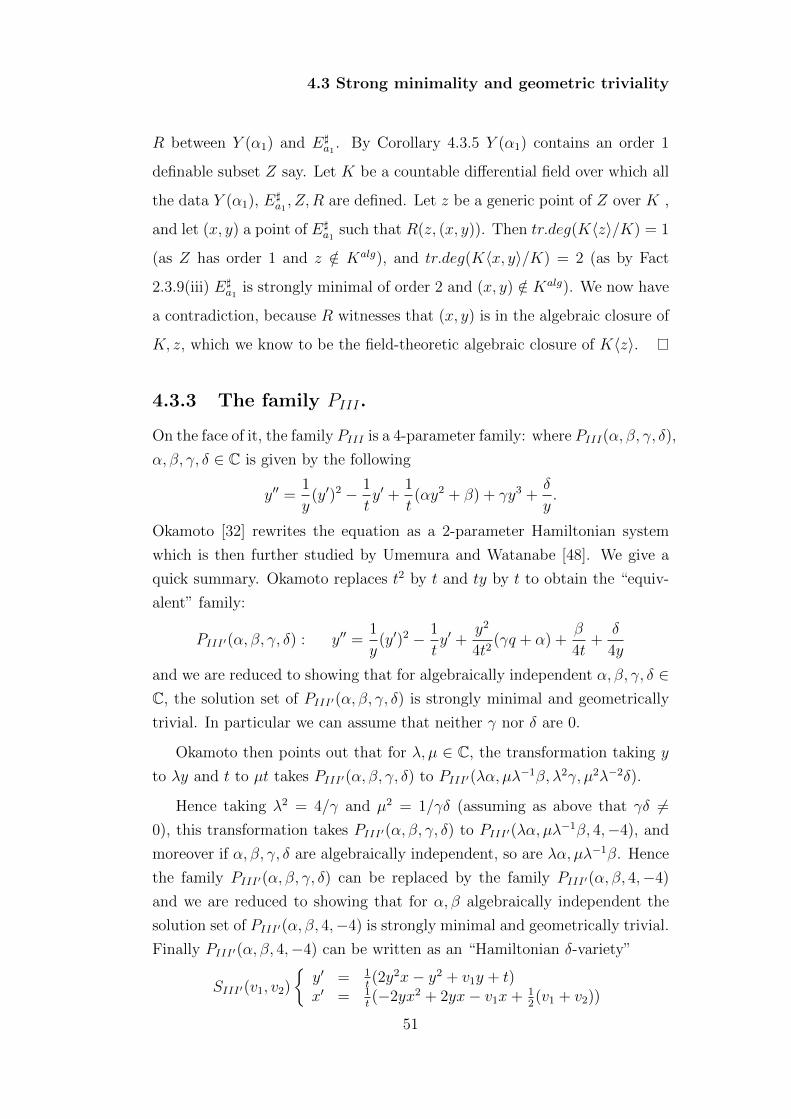
4.3 Strong minimality and geometric triviality
R between Y (α1) and E]a1
. By Corollary 4.3.5 Y (α1) contains an order 1
definable subset Z say. Let K be a countable differential field over which all
the data Y (α1), E]a1, Z,R are defined. Let z be a generic point of Z over K ,
and let (x, y) a point of E]a1
such that R(z, (x, y)). Then tr.deg(K〈z〉/K) = 1
(as Z has order 1 and z /∈ Kalg), and tr.deg(K〈x, y〉/K) = 2 (as by Fact
2.3.9(iii) E]a1
is strongly minimal of order 2 and (x, y) /∈ Kalg). We now have
a contradiction, because R witnesses that (x, y) is in the algebraic closure of
K, z, which we know to be the field-theoretic algebraic closure of K〈z〉.
4.3.3 The family PIII.
On the face of it, the family PIII is a 4-parameter family: where PIII(α, β, γ, δ),
α, β, γ, δ ∈ C is given by the following
y′′ =1
y(y′)2 − 1
ty′ +
1
t(αy2 + β) + γy3 +
δ
y.
Okamoto [32] rewrites the equation as a 2-parameter Hamiltonian system
which is then further studied by Umemura and Watanabe [48]. We give a
quick summary. Okamoto replaces t2 by t and ty by t to obtain the “equiv-
alent” family:
PIII′(α, β, γ, δ) : y′′ =1
y(y′)2 − 1
ty′ +
y2
4t2(γq + α) +
β
4t+
δ
4y
and we are reduced to showing that for algebraically independent α, β, γ, δ ∈C, the solution set of PIII′(α, β, γ, δ) is strongly minimal and geometrically
trivial. In particular we can assume that neither γ nor δ are 0.
Okamoto then points out that for λ, µ ∈ C, the transformation taking y
to λy and t to µt takes PIII′(α, β, γ, δ) to PIII′(λα, µλ−1β, λ2γ, µ2λ−2δ).
Hence taking λ2 = 4/γ and µ2 = 1/γδ (assuming as above that γδ 6=0), this transformation takes PIII′(α, β, γ, δ) to PIII′(λα, µλ
−1β, 4,−4), and
moreover if α, β, γ, δ are algebraically independent, so are λα, µλ−1β. Hence
the family PIII′(α, β, γ, δ) can be replaced by the family PIII′(α, β, 4,−4)
and we are reduced to showing that for α, β algebraically independent the
solution set of PIII′(α, β, 4,−4) is strongly minimal and geometrically trivial.
Finally PIII′(α, β, 4,−4) can be written as an “Hamiltonian δ-variety”
SIII′(v1, v2)
{y′ = 1
t(2y2x− y2 + v1y + t)
x′ = 1t(−2yx2 + 2yx− v1x+ 1
2(v1 + v2))
51

4.3 Strong minimality and geometric triviality
where α = 4v2 and β = −4(v1 − 1).
(Note that α and β are algebraically independent if and only if v1 and v2
are.)
The Hamiltonian is here:
H(v1, v2) =1
t
[y2x2 −
(y2 − v1y − t
)x− 1
2(v1 + v2)y
]and the Hamiltonian vector field on A2 is:
δ(v1, v2) = δ+1
t(2y2x−y2 +v1y+t)
∂
∂y+
1
t(−2yx2 +2yx−v1x+
1
2(v1 +v2))
∂
∂x
From [48] one now extracts:
Fact 4.3.7. δ(v1, v2) satisfies condition (J) if and only if v1 + v2 /∈ 2Z and
v1 − v2 /∈ 2Z.
Commentary. This is contained in the statements of Theorem 1.2(i) and
(ii), Proposition 2.1 and Corollary 2.5 of [48]: 1.2(i) and (ii) say that if either
v1 +v2 or v1−v2 are in 2Z then the solution set of the system SIII′(v1, v2) has
(many) proper differential algebraic subvarieties (hence by Corollary 4.1.1)
δ(v1, v2) does not satisfy condition (J). On the other hand Proposition 2.1
says that if δ(v1, v2) satisfies condition (J), then for some integers i, j, h ≥ 0,
such that not both i, j = 0 we have i(v1 + v2) + j(v1 − v2) + 2h(1− v1) = 0.
Strictly speaking this Proposition 2.1 studies the “Hamiltonian vector field”
corresponding to a different δ-variety structure on A2, namely{δ1(y) = 2y2x− y2 + v1y + tδ1(x) = −2yx2 + 2yx− v1x+ 1
2(v1 + v2)
where δ1 is the derivation tδ (or “t ddt
) on U with respect to which U is also
saturated, differentially closed, but it is clear that δ-subvarieties with respect
to the original δ-structure correspond to δ1-subvarieties with the new δ1-
structure.
Corollary 4.3.8. The solution set of SIII′(v1, v2) is strongly minimal if and
only if v1 + v2 /∈ 2Z and v1 − v2 /∈ 2Z.
We conclude our main result for PIII :
52

4.3 Strong minimality and geometric triviality
Proposition 4.3.9. Let v1, v2 be algebraically independent. Then (the solu-
tion set of) SIII′(v1, v2) is strongly minimal and geometrically trivial.
Proof. Let Y (v1, v2) denote the solution set of SIII′(v1, v2). Strong minimal-
ity is by Corollary 4.3.8. Suppose that geometric triviality fails. We copy
the proof of Proposition 4.3.6. So Y (v1, v2) is nonorthogonal to E]a for an
elliptic curve Ea : y2 = x(x− 1)(x− a) with a /∈ C. Using definability of the
family E]b, we express nonorthogonality of Y (v1, v2) to some E]
b by a formula
θ(v1, v2, t). As v2 is independent from v1, t, there are cofinitely many v ∈ C
such that θ(v1, v, t) holds. In particular we can find such v ∈ v1 + 2Z, and
we have a contradiction as in Proposition 4.3.6 (using now Fact 4.3.7)
4.3.4 The family PIV .
PIV (α, β), α, β ∈ C is given by the following equation
y′′ =1
2y(y′)2 +
3
2y3 + 4ty2 + 2(t2 − α)y +
β
y
Following [31] and [47] the equations can be rewritten in the form
SIV (v1, v2, v3)
{y′ = 2xy − y2 − 2ty + 2(v1 − v2)x′ = 2xy − x2 + 2tx+ 2(v1 − v3)
where v1, v2, v3 are complex numbers satisfying v1 + v2 + v3 = 0.
(*) Here α = 3v3 + 1 and β = −2(v2 − v1)2.
Let V be the plane defined by v1 + v2 + v3=0 and throughout let v de-
note a tuple (v1, v2, v3) from V . So the algebraic independence of α and
β means that the corresponding v is a generic point on V . Let δ(v) be
the derivation (Hamiltonian vector field) corresponding to SIV (v). Let W =
{v ∈ V : v1 − v2 ∈ Z}∪{v ∈ V : v2 − v3 ∈ Z}∪{v ∈ V : v3 − v1 ∈ Z}. Then
the analysis in [47], specifically Theorem 3.2, Proposition 3.5, and Corollary
3.9 yields
Fact 4.3.10. For v ∈ V , δ(v) satisfies condition (J) if and only if v /∈ W .
Corollary 4.3.11. For v ∈ V, the solution set of PIV (v) is strongly minimal
if and only if v 6∈ W.
53

4.3 Strong minimality and geometric triviality
Proposition 4.3.12. Let Y (α, β) denote the solution set of PIV (α, β). Sup-
pose α, β ∈ C are algebraically independent. Then Y (α, β) is strongly mini-
mal and geometrically trivial.
Proof. Let (v1, v2, v3) ∈ V correspond to (α, β) as in (*) above. So v1 and
v2 are algebraically independent and v3 = −v1 − v2. It suffices to work with
the solution set Y (v) of SIV (v). Strong minimality is by Corollary 4.3.11.
Again if geometric triviality fails this is witnessed by the truth of a formula
θ(v1, v2, t), where θ(u,w, t) expresses the existence of a differential algebraic
correspondence between Y (u,w,−u − w) and some E]b with b /∈ C. The
independence of v2 over v1, t implies that |= θ(v1, w, t) for all but finitely
many w ∈ C. So we can find such w ∈ v1 + Z giving a contradiction to
Corollary 4.3.11.
4.3.5 The family PV
We recall that PV (α, β, γ, δ), α, β, γ, δ ∈ C, is given by the following equation
y′′ =
(1
2y+
1
y − 1
)(y′)2 − 1
ty′ +
(y − 1)2
t2
(αy +
β
y
)+ γ
y
t+ δ
y(y + 1)
y − 1
The situation is similar to the case of PIII above, in that, in the light of certain
transformations preserving the equation, PV can be written as a 3-parameter
family. The analysis is carried out by Okamoto[30] and then Watanabe [49]
and again we give a summary:
First PV (α, β, γ, δ) can be rewritten as the Hamiltonian system
y′ =∂H
∂x, x′ = −∂H
∂y
where the Hamiltonian polynomial is
HV (κ0, κ1, θ, η) =1
t
[y(y − 1)2x2 −
(κ0(y − 1)2 + θy(y − 1) + ηty
)x+ κ(y − 1)
]and
α =1
2κ2
1, β = −1
2κ2
0, γ = −η(θ+ 1), δ = −1
2η2, κ =
1
4(κ0 + θ)2− 1
4κ2
1.
Okamoto points out that the transformation (y, x,H, t) → (y, x, λH, λ−1t)
and η → λ−1η “preserves the system” for any nonzero λ. As we may assume
54

4.3 Strong minimality and geometric triviality
δ 6= 0 (so also η 6= 0) we may choose λ = η, and hence the transforma-
tion takes δ to −1/2 (and η to 1). Hence we need only consider the system
PV (α, β, γ,−12), and prove that for α, β, γ algebraically independent, the so-
lution set of PV (α, β, γ,−12) is strongly minimal and geometrically trivial.
Let us now define:
v1 = −1
4(2κ0 + θ), v2 =
1
4(2κ0− θ), v3 =
1
4(2κ1 + θ), v4 = −1
4(2κ1− θ),
then the vector v = (v1, v2, v3, v4) is on the complex hyperplane V in C4
defined by v1 + v2 + v3 + v4 = 0. So our family is now parameterised by V .
Secondly make the following substitution: replace y(y − 1)−1 by y, and
−y(y − 1)2x+ (v3 − v1)(y − 1) by x.
Then our system can be written as:
SV (v)
{y′ = 1
t(2y2x− 2yx+ ty2 − ty + (v1 − v2 − v3 + v4)y + v2 − v1)
x′ = 1t(−2yx2 + x2 − 2txy + tx− (v1 − v2 − v3 + v4)x+ (v3 − v1)t)
and note that α = 12(v3 − v4)2, β = −1
2(v2 − v1)2 and γ = 2v1 + 2v2 − 1.
Let δ(v) be the corresponding (Hamiltonian) vector field δ(v) = δ+(1t(2x2x−
2yx+ ty2 − ty + (v1 − v2 − v3 + v4)y + v2 − v1)) ∂∂y
+ (1t(−2yx2 + x2 − 2txy +
tx− (v1 − v2 − v3 + v4)x+ (v3 − v1)t) ∂∂x
.
Hence we want to prove that for generic v ∈ V , SV (v) is strongly minimal
and geometrically trivial.
Consider the union of lines in V given by
W = {v ∈ V : v1 − v2 ∈ Z} ∪ {v ∈ V : v1 − v3 ∈ Z} ∪ {v ∈ V : v1 − v4 ∈ Z}
∪ {v ∈ V : v1 − v3 ∈ Z} ∪ {v ∈ V : v2 − v4 ∈ Z} ∪ {v ∈ V : v3 − v4 ∈ Z} ,
The following is proved in [49] (Theorem 1.2, Proposition 2.1, and Corollary
2.6):
Fact 4.3.13. For v ∈ V , δ(v) satisfies condition (J) if and only if v /∈ W .
Commentary. Strictly speaking Watanabe considers rather the vector
field corresponding to the δ1-variety structure on A2:{δ1(y) = 2x2x− 2yx+ ty2 − ty + (v1 − v2 − v3 + v4)y + v2 − v1)δ1(x) = −2yx2 + x2 − 2txy + tx− (v1 − v2 − v3 + v4)x+ (v3 − v1)t)
where δ1 = tδ.
But as in the case of PIII above, this suffices.
55

4.3 Strong minimality and geometric triviality
Corollary 4.3.14. For v ∈ V, the solution set of SV (v) is strongly minimal
if and only if v 6∈ W.
We conclude, as previously:
Proposition 4.3.15. For v1, v2, v3 ∈ C algebraically independent, the solu-
tion set of SV (v) is strongly minimal and geometrically trivial. Hence by the
reductions above, for algebraically independent α, β, γ, δ ∈ C the solution set
of PV (α, β, γ, δ) is strongly minimal and geometrically trivial.
4.3.6 The family PV I
Recall that PV I(α, β, γ, δ), α, β, γ, δ ∈ C, is given by the following equation
y′′ =1
2
(1
y+
1
y − 1+
1
y − t
)(y′)2 −
(1
t+
1
t− 1+
1
y − t
)y′
+y(y − 1)(y − t)t2(t− 1)2
(α + β
t
y2+ γ
t− 1
(y − 1)2+ δ
t(t− 1)
(y − t)2
)The equation is studied by Okamoto [29] followed by Watanabe [50]. Again
we summarise what we need.
Given α, β, γ, δ ∈ C, let α0, α1, α3, α4 be complex numbers such that
α = 12α2
1, β = −12α2
4, γ = 12α2
3 and δ = 12(1− α2
0). In what follows we also let
α be the tuple (α0, α1, α3, α4).
Then the equation PV I(α, β, γ, δ) can be written as the (Hamiltonian)
system:
SV I(α)
y′ = 1
t(t−1)(2xy(y − 1)(y − t)− {α4(y − 1)(y − t) + α3y(y − t)
+(α0 − 1)y(y − 1)})x′ = 1
t(t−1)(−x2(3y2 − 2(1 + t)y + t) + x{2(α0 + α3 + α4 − 1)y
−α4(1 + t)− α3t− α0 + 1} − α2(α1 + α2))
where α0 +α1 +2α2 +α3 +α4 = 1 and where δ(α) = ∂+( 1t(t−1)
(2xy(y−1)(y−t)−{α4(y−1)(y− t) +α3y(y− t) + (α0−1)y(y−1)})) ∂
∂y+ ( 1
t(t−1)(−x2(3y2−
2(1+t)y+t)+x{2(α0+α3+α4−1)y−α4(1+t)−α3t−α0+1}−α2(α1+α2))) ∂∂x
is the derivation giving the corresponding δ-variety structure on A2.
Let us note that any solution y of PV I(α, β, γ, δ) yields a unique solution
(y, x) of SV I(α). The only possible solutions (y, x) of SV I(α) not of this form
56

4.3 Strong minimality and geometric triviality
are when y = 0, 1, t and such solutions will exhibit non strong minimality of
SV I(α) (even though PV I(α, β, γ, δ) may be strongly minimal).
As before, we take a close look at the work of Watanabe on PV I . First,
note that the relation between the parameters α above and the parameters
(a1, a2, a3, a4) in Watanabe’s Hamiltonian vector field for PV I (beginning of
section 3 of [49]) is: α4 = a3 + a4, α3 = a3 − a4, α0 = 1 − a1 − a2, and
α1 = a1 − a2. However in [49], instead of only working with δ(α) and
the δ-variety structure on A2, Watanabe works with the so called Okamoto
space of initial conditions. This roughly corresponds to patching six copies
Ui = {(yi, xi)}, i = 0, 1, 2, 3, 4,∞, of A2 with some specified patching rule
(for example on U0∩U∞: y0y∞ = 1 and y0x0 +y∞x∞ = −α2 ). On each Ui is
also defined a derivation δi(α). These derivations respect the patching rule
and Watanabe looks for condition (J) for this entire “system”. But we only
work with δ0 = δ here and hence we shall only focus on what we need. So let
α0 α1 α2 α3 α4 y x
s0 −α0 α1 α2 + α0 α3 α4 y x− α0
y−t
s1 α0 −α1 α2 + α1 α3 α4 y x
s2 α0 + α2 α1 + α2 −α2 α3 + α2 α4 + α2 y + α2
xx
s3 α0 α1 α2 + α3 −α3 α4 y x− α3
y−1
s4 α0 α1 α2 + α4 α3 −α4 y x− α4
y
Table 4.1: Some Backlund Transformations for SV I
us start by describing some “Backlund transformations” for SV I(α). These
map solutions of a given SV I equation to solutions of the same equation with
different values of parameters α, but clearly may be undefined at certain
solutions. The list of the Backlund transformations we are interested in
are given in Table 4.1. The five transformations s0, s1, s2, s3, s4 generate
a group W which is isomorphic to the affine Weyl group of type D4 and
which is sometimes referred to as Okamoto’s affine D4 symmetry group. By
definition, the reflecting hyperplanes of Okamoto’s affine D4 action are given
by the affine linear relations
αi = n for i = 0, 1, 3, 4 and n ∈ Z,
as well as
α0 ± α1 ± α3 ± α4 = 2n+ 1 for n ∈ Z.
57
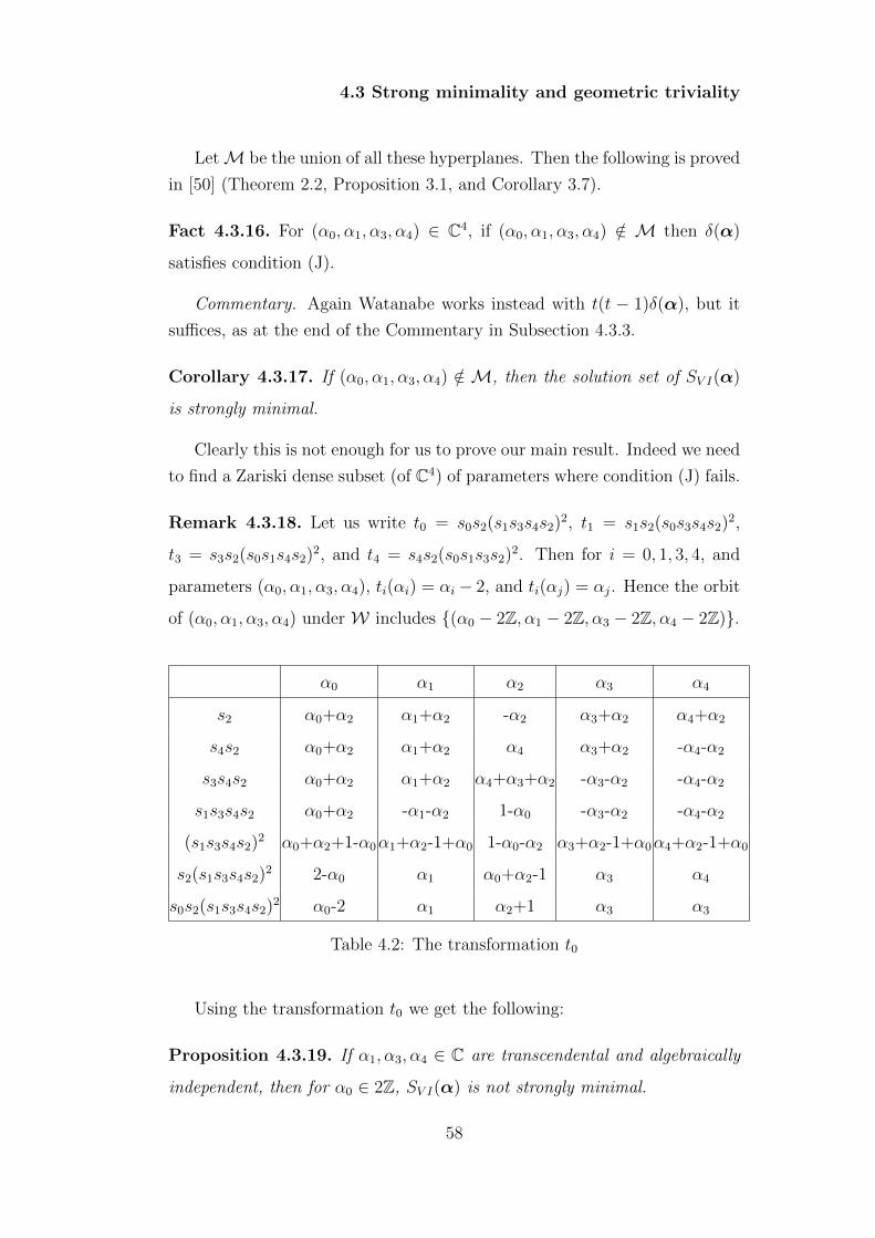
4.3 Strong minimality and geometric triviality
LetM be the union of all these hyperplanes. Then the following is proved
in [50] (Theorem 2.2, Proposition 3.1, and Corollary 3.7).
Fact 4.3.16. For (α0, α1, α3, α4) ∈ C4, if (α0, α1, α3, α4) /∈ M then δ(α)
satisfies condition (J).
Commentary. Again Watanabe works instead with t(t − 1)δ(α), but it
suffices, as at the end of the Commentary in Subsection 4.3.3.
Corollary 4.3.17. If (α0, α1, α3, α4) /∈ M, then the solution set of SV I(α)
is strongly minimal.
Clearly this is not enough for us to prove our main result. Indeed we need
to find a Zariski dense subset (of C4) of parameters where condition (J) fails.
Remark 4.3.18. Let us write t0 = s0s2(s1s3s4s2)2, t1 = s1s2(s0s3s4s2)2,
t3 = s3s2(s0s1s4s2)2, and t4 = s4s2(s0s1s3s2)2. Then for i = 0, 1, 3, 4, and
parameters (α0, α1, α3, α4), ti(αi) = αi − 2, and ti(αj) = αj. Hence the orbit
of (α0, α1, α3, α4) under W includes {(α0 − 2Z, α1 − 2Z, α3 − 2Z, α4 − 2Z)}.
α0 α1 α2 α3 α4
s2 α0+α2 α1+α2 -α2 α3+α2 α4+α2
s4s2 α0+α2 α1+α2 α4 α3+α2 -α4-α2
s3s4s2 α0+α2 α1+α2 α4+α3+α2 -α3-α2 -α4-α2
s1s3s4s2 α0+α2 -α1-α2 1-α0 -α3-α2 -α4-α2
(s1s3s4s2)2 α0+α2+1-α0α1+α2-1+α0 1-α0-α2 α3+α2-1+α0α4+α2-1+α0
s2(s1s3s4s2)2 2-α0 α1 α0+α2-1 α3 α4
s0s2(s1s3s4s2)2 α0-2 α1 α2+1 α3 α3
Table 4.2: The transformation t0
Using the transformation t0 we get the following:
Proposition 4.3.19. If α1, α3, α4 ∈ C are transcendental and algebraically
independent, then for α0 ∈ 2Z, SV I(α) is not strongly minimal.
58

4.3 Strong minimality and geometric triviality
Proof. Let α1, α3, α4 be transcendental and algebraically independent. Note
that then α2 is also transcendental. One can easily check that SV I(0, α1, α2, α3,α4)
is not strongly minimal; the curve defined by y = t is an algebraic ∂-
subvariety of (A2, D(0, α1, α2, α3, α4)).
As a consequence s0 : x → x − α0
y−t is undefined on these solutions.
However all the other si’s, as well as t0, are well defined. We want to worry
now about successively applying t0. But note that the occurrence of y = 0,
y = 1, y = t and x = 0 (where the si’s are not well defined) implies that
α4 = 0, α3 = 0, α0 = 0, and α2 = 0 respectively. Looking at Table 4.2, we
see that this cannot happen on successively applying t0, as α1, α2, α3, α4 are
transcendental and we are done.
Proposition 4.3.20. If α, β, γ, δ ∈ C are algebraically independent (and
transcendental), then the solution set of PV I(α, β, γ, δ) is strongly minimal
and geometrically trivial.
Proof. It is enough to work with the solution set of the system SV I(α) and
note that α0, α1, α3, α4 are algebraically independent, so by Corollary 4.3.17
its solution set Y (α0, α1, α3, α4) is strongly minimal. If it is not geometrically
trivial, then by independence of α0, α1, α3, α4, t in DCF0, for all but finitely
many c ∈ C, Y (c, α1, α3, α4) is in finite-to-finite relation with some E]b with
b /∈ C. Choosing such c ∈ 2Z gives a contradiction to Proposition 4.3.19
4.3.7 Further Remarks
First note that the methods above show that for the families PIII , PV and
PV I , the solution set of an equation is (strongly minimal and) geometrically
trivial as long as the transcendence degree of the tuple α, β, γ, δ is at least 2.
We would also guess that in fact the solution set of any of the Painleve
equations PII − PV is geometrically trivial whenever it is strongly minimal,
but this is not given by our methods (we have only succeeded to prove it for
the second Painleve equation using a different idea).
Note that the model-theoretic content of our methods is:
59

4.3 Strong minimality and geometric triviality
Proposition 4.3.21. Let y′′ = f(y, y′, b1, .., bn) where f(−,−,−..) is a ra-
tional function (over Q) and b1, .., bn ∈ U . Suppose that the solution set of
the equation is strongly minimal and not geometrically trivial. Then there
is a formula θ(y1, .., yn)(without parameters) true of b1, .., bn such that for
any c1, .., cn satisfying θ the solution set of y′′ = f(y, y′, c1, .., cn) is strongly
minimal (and nontrivial).
Likewise if X(b) is a strongly minimal set of order 2 which is defined over
b and is not geometrically trivial, then there will be a formula θ(y) true of b
such that for any c satisfying θ, X(c) is strongly minimal.
The next remark concerns “downward semi-definability of Morley rank”,
as discussed in [12]. The point is that each of the Painleve families witnesses
non downward semi-definability of Morley rank. For example for PII(α) the
analysis of [47] that we cite also gives that for α ∈ 1/2 + Z, the solution
set of PII(α) contains infinitely many (in fact a definable family of) order 1
definable sets, hence has Morley rank 2. So:
Fact 4.3.22. For α ∈ C transcendental, the solution set Y (α) of PII(α) has
Morley rank 1, but for every formula θ(x) true of α there is α1 satisfying
θ(x) such that Yα1 has Morley rank > 1,
This fact, together with the proof of Lemma 1.1 in [12], shows that there
is a ∅-definable set X of order 3 in DCF0 with Morley rank different from
Lascar rank. This answers (in a negative sense) Question 2.9 of [12].
Finally one might wonder whether our soft proofs of geometric triviality
of certain order 2 equations might apply to higher order equations. But an
obstacle is precisely non downward semi-definability of Morley rank for more
general families A], as given in [12]: There is a definable (in DCF0) family
(Ab : b ∈ B) (with B of finite Morley rank) family of 2-dimensional abelian
varieties such for generic b ∈ B, Ab is simple (hence A]b is strongly minimal),
but for every ∅-definable subset B′ ⊂ B there is b′ ∈ B′ such that Ab′ is not
simple (hence A]b′ has Morley rank 2).
60
Chapter 5
Geometric triviality: Non
Generic PII
In this Chapter, we extend the result in Chapter 4 for PII(α) to the non
generic strongly minimal case. That is we show that for α 6∈ 1/2 +Z, PII(α)
is geometrically trivial. Our proof is a uniform one, in the sense that it works
for all α 6∈ 1/2 +Z (so including the generic case). For the proof of the main
result, we give a new criteria for deciding whether strongly minimal sets in
DCF0 are geometrically trivial.
5.1 Correspondences on A]
We will in this section make use of the notion of multiplicity of a type, so
we say a few words in the strongly minimal setting. Suppose Y is a strongly
minimal set in U and K is any differential field over which Y is defined. If two
elements y and z of Y are such that y ∈ K 〈z〉alg (and so z ∈ K 〈y〉alg), then
mult(y/K 〈z〉) will denote the finite number of elements of Y that realise
tp(y/K 〈z〉). In other words, mult(y/K 〈z〉) is the degree of the minimal
polynomial of y over K 〈z〉.
It is well known that finite-to-finite correspondences (indeed finite-to-one)
exist for the Manin kernels: Let A be a simple abelian variety and let Y = A]
be its Manin kernel. For each n ∈ N, we have the multiplication-by-n map,
n : A→ A. This map is surjective and n2d-to-1 (where d is the dimension of
61
5.1 Correspondences on A]
A). So for any generic point a ∈ Y , mult(n ·a/a) = 1 while mult(a/n ·a) > 1
(as long as n > 1).
The same is true for any non-trivial locally modular strongly minimal set:
Proposition 5.1.1. Suppose that Y is a non-trivial locally modular strongly
minimal set in U . Then there exists a differential field K such that for any
generic point y of Y over K, there exist z ∈ Y generic over K, such that
z ∈ K 〈y〉alg and z 6∈ K 〈y〉.
Proof. Assume for contradiction that the conclusion of the proposition does
not hold. Now as Y is non-trivial locally modular, from Theorem 2.3.11,
there exist a simple Abelian variety A not defined over C such that Y is
nonorthogonal to X = A]. We work throughout over the differential field K
over which nonorthogonality occurs. Also, in what follows Ygen will be the
set of generic points of Y (same for Xgen).
Let y ∈ Ygen and let Z = acl(y)∩(Ygen∪Xgen). Note that as Y and X are
nonorthogonal, Z ∩X is non empty. Also if e ∈ Z ∩X, then for any n ∈ N>1
we have that n · e ∈ Z ∩X (since n · e ∈ acl(e) = acl(y)). We show that if
d, e ∈ Z ∩X, then mult(e/d) = mult(d/e). This contradicts the case when
d = n · e as discussed above and we are done. We prove this using several
claims.
Let a ∈ Z ∩ Y and d, e ∈ Z ∩X.
Claim 1: mult(e/a) = mult(d/a) and mult(a/e) = mult(a/d). Indeed
mult(d/a) and mult(a/d) does not depend on the choice of a or d.
Proof: First note that by construction (and nonorthogonality) a,d and e are
all interalgebraic. Indeed any two elements of Z are.
We first prove thatmult(e/a) = mult(d/a). So supposeD = {d = d1, . . . , dk}
is the set of realisations of tp(d/a), i.e mult(d/a) = k. Now as tp(e) = tp(d),
it is not hard to see that there is b ∈ Ygen and E = {e = e1, . . . , ek} ⊆ Xgen
such that E is the set of realisations of tp(e/b). But then K 〈a〉alg = K 〈b〉alg
and hence by assumption K 〈a〉 = K 〈b〉. So for any σ ∈ Aut(U/a), σ(b) = b
62
5.1 Correspondences on A]
and hence σ(E) = E. In particular E is definable over a and we have that
E is the set of realisations of tp(e/a), i.e mult(e/a) = k.
We now prove that mult(a/e) = mult(a/d). Suppose mult(a/d) = l and
that φ(x, d) isolates tp(a/d), i.e |= ∃=lyφ(y, d). As tp(e) = tp(d), we have that
|= ∃=lyφ(y, e). Choose c ∈ Ygen such that |= φ(c, e). Then K 〈a〉alg = K 〈c〉alg
and hence by assumption K 〈a〉 = K 〈c〉, that is there is a L∂-formula θ(x, y)
such that |= θ(a, c)∧∃=1xθ(x, c)∧∃=1yθ(a, y). Let ψ(x, e) be the L∂-formula
∃yφ(y, e)∧ θ(x, y). By construction |= ∃=lxψ(x, e) and it follows that ψ(x, e)
isolates tp(a/e), i.e mult(a/e) = l.
Claim 2: mult(d/a, e) = mult(e/a, d).
Proof: Since
mult(de/a) = mult(e/a) ·mult(d/a, e)
= mult(d/a) ·mult(e/a, d),
using Claim 1 we are done.
Claim 3: mult(da/e) = mult(ea/d).
Proof: As before, since
mult(da/e) = mult(a/e) ·mult(d/e, a)
mult(ea/d) = mult(a/d) ·mult(e/a, d),
using both Claim 1 and Claim 2 we are done.
Finally
Claim 4: mult(d/e) = mult(e/d).
Proof: This time we use
mult(da/e) = mult(d/e) ·mult(a/d, e)
mult(ea/d) = mult(e/d) ·mult(a/d, e).
So from Claim 3 the result follows
So if Y is a non-trivial locally modular strongly minimal set, over some
differential field K, there exist generic definable finite-to-finite correspon-
dences Y → Y that are not generic definable permutations of Y . The aim
63
5.2 Geometric triviality and the second Painleve equations
of the next section will hence be to show that such is not the case for the
strongly minimal second Painleve equations.
5.2 Geometric triviality and the second Painleve
equations
In this section we look at the second Painleve equation, y′′ = 2y3 + ty + α,
α ∈ C and denote by Y (α) ⊆ U its solution set. As we have seen in the
previous chapter the following is true (Corollary 4.3.5 and Proposition 4.3.6):
Fact 5.2.1. kj
(i) Y (α) is strongly minimal if and only if α 6∈ 12
+ Z.
(ii) For α 6∈ Qalg, Y (α) is geometrically trivial.
We now aim to extend Fact 5.2.1(ii) to all α 6∈ 12
+ Z. Before we proceed
recall that for a field K, K ((X)) denotes the field of formal Laurent series
in variable X, while K 〈〈X〉〉 denotes the field of formal Puiseux series, i.e.
the field⋃d∈NK
((X1/d
)). It is well known that if K is algebraically closed
of characteristic 0 then so is K 〈〈X〉〉 - it is the algebraic closure of K ((X))
(cf. [5] Corollary 13.15).
Proposition 5.2.2. For α 6∈ 12
+ Z, Y (α) is geometrically trivial.
Proof. We fix α 6∈ 12+Z. First note that by Remark 2.3.5, Y (α) is orthogonal
to C. So from Proposition 5.1.1 we only have to prove that for any differential
field K over which Y (α) is defined, if y and z are two generic elements (over
K) of Y (α), then if K(y, y′)alg = K(z, z′)alg, then K(y, y′) = K(z, z′).
So let K be any differential field containing C(t) and let y, z ∈ Y (α)
(generic) be such that z ∈ K(y, y′)alg. LettingK1 denote the algebraic closure
of K(y′) in U , we regard z as algebraic over K1(y) and we first aim to show
that z ∈ K1(y). As z ∈ K1(y)alg for any β ∈ K1, z can be seen as an element
of K1 〈〈y − β〉〉, so that there exists e ∈ N such that z ∈ K1
(((y − β)1/e
)). A
64

5.2 Geometric triviality and the second Painleve equations
simpler way of saying the above (a-la-Nishioka) is that we look at expansions
in a local parameter τ at β ∈ K1 given by
y = β + τ e z =∞∑i=r
aiτi (ar 6= 0)
with e the ramification exponent. Of course our intention is to show that for
every choice of β ∈ K1, we have that e = 1 and we are done.
Differentiating we have
eτ e−1τ ′ = y′ − β′
= y′ − β∗ − βy′(2y3 + ty + α)
= y′ − β∗ − βy′(2β3 + tβ + α) +
+(6β2 + t)βy′τe + 6ββy′τ
2e + βy′τ3e (5.2.1)
where “∗” indicates the extension on K1 of the derivation on K[y′] given by
(∑ciy′i)∗ =
∑c′iy′i and βy′ = ∂β
∂y′.
Letting γ = y′ − β∗ − βy′(2β3 + tβ + α), we have
Claim 1: γ 6= 0
Proof: For contradiction, suppose that γ = 0, that is
y′ − β∗ = βy′(2β3 + tβ + α) (5.2.2)
Let F ∈ K[y, y′] be an irreducible polynomial such that F (β, y′) = 0. Then
(F (β, y′))∗ = F ∗(β, y′) + β∗Fy(β, y′) = 0 (5.2.3)
∂
∂y′(F (β, y′)) = Fy′(β, y
′) + βy′Fy(β, y′) = 0. (5.2.4)
If we multiply 5.2.4 by 2β3 + tβ + α and use 5.2.2, we have
(2β3 + tβ + α)Fy′(β, y′) + (y′ − β∗)Fy(β, y′) = 0.
So, together with 5.2.4 we get
F ∗(β, y′) + y′Fy(β, y′) + (2β3 + tβ + α)Fy′(β, y
′) = 0.
65
5.2 Geometric triviality and the second Painleve equations
In other words (δF )(β, y′) = 0, so that F divides its derivative δF (i.e δF =
GF for some G ∈ K[y, y′]). This contradicts condition (J) and hence strong
minimality of Y (α) as per Corollary 4.1.1 and the claim is proved.
Hence from equation 5.2.1, γ 6= 0 implies that τ ′ = e−1γτ 1−e + A where
A = e−1τ 1−e ((6β2 + t)βy′τe + 6ββy′τ
2e + βy′τ3e)
and from this we get that
(τ i)′ = iτ i−1τ ′
= iτ i−1e−1γτ 1−e + A′
=iγ
eτ i−e + A′
and similarly
(τ i)′′ =i(i− e)e2
γ2τ i−2e + A′′.
Now from
z′′ = 2z3 + tz + α and z =∞∑i=r
aiτi
we have∞∑i=r
aii(i− e)e2
γ2τ i−2e + · · · = 2∑i,j,k
aiajakτi+j+k + · · · . (5.2.5)
Using this we prove a couple of claims. One should of course notice that the
“ignored” part does no play a role in our calculations below.
Claim 2: If e > 1 then r < 0.
Proof: Let e > 1 and assume r ≥ 0. If for all l ∈ {r, r + 1, . . .} we have that
e | l, then it is not hard to see that the ramification exponent must be one
(i.e e = 1), a contradiction. So choose l ∈ {r, r + 1, . . .} least such that e - l
and al 6= 0. First, note that since l − 2e < l and e - l − 2e, we have that
al−2e = 0 (same for al−e = 0) or else this contradicts that l is least such. So
in what follows one does not need to worry about the other coefficients in
5.2.5.
So if we look at the coefficient of τ l−2e on the LHS of 5.2.5, we see that
all(l − e)e2
γ2 6= 0.
66

5.2 Geometric triviality and the second Painleve equations
This implies that the coefficient on the RHS of τ i+j+k for some i, j, k ≥ r with
i+ j+k = l− 2e must be non-zero. However for any such, since i+ j+k < l
and e - i+ j + k, we have that e does not divide at least one them, say i < l.
But then ai = 0 (as l was chosen to be the least with this property) and so
aiajak = 0, a contradiction.
Claim 3: The case e > 1 and r < 0 leads to a contradiction.
Proof: So this time suppose e > 1 and r < 0. From the least powers of τ in
5.2.5 (which is 3r on the R.H.S) we have r − 2e = 3r, that is r = −e, and
from the coefficients of τ r−2e we get
arr(r − e)e2
γ2 = 2a3r
so that ar = ±γ, since ar 6= 0.
So again choose l ∈ {r, r + 1, . . .} least such that e - l and al 6= 0. The
coefficient of τ l−2e = τ l+2r on the LHS of 5.2.5 is
all(l − e)e2
γ2 6= 0.
On the RHS we see that the coefficient of τ l−2e = τ l+2r should be 6a2ral.
(Indeed, e - i+ j + k means that e does not divide at least one of them, say
i. Then e - i, ai 6= 0 means either i = l or i > l. But i > l implies that
j + k < 2r a contradiction. So i = l and hence j = k = r).
Hence
all(l − e)e2
γ2 = 6a2ral = 6γ2al
and we see that either l = −2e or l = 3e, contradicting e - l and we are done
Hence e = 1, and since β was arbitrary, the ramification exponent at
every β ∈ K1 is 1. So z ∈ K1(y).
Finally, letting K0 denote the algebraic closure of K(y) in U , one can show
similarly that z ∈ K0(y′). Indeed the calculation above seems to work for any
strongly minimal equation y′′ = f(y, y′, t), with f polynomial with coefficient
in C. Since K1(y) ∩K0(y′) = K(y, y′), we have shown that z ∈ K(y, y′).
Changing the role of y and z, we also have y ∈ K(z, z′) and hence
K(y, y′) = K(z, z′).
67

5.3 Further comments
5.3 Further comments
Recall that a strongly minimal set Y in U is said to be unimodular if for any n
and any differential field K over which Y is defined, if y1, . . . , yn,x1, . . . , xn ∈Y are such that y and x are interalgebraic over K (i.e K 〈y〉alg = K 〈x〉alg),and RM(y/K) = RM(x/K) = n, then mult(y/K 〈x〉) = mult(x/K 〈y〉).Here RM(y/K) = n means that y1, .., yn together with all their derivatives
y(j)i are algebraically independent over K.
Remark 5.3.1. jh
(i) This notion, unimodularity, is not restricted to DCF0 and indeed makes
sense for any strongly minimal set in any complete theory T (see for
example Definition 2.4.2 in [35]).
(ii) Any ω-categorical strongly minimal set in DCF0 (or in any stable the-
ory) is unimodular (cf. [35] Remark 2.4.2).
It is not hard to check that for α 6∈ 1/2+Z, since generic correspondences
of XII(α) are generic permutations, XII(α) is unimodular. On the other
hand, we have seen that the Manin kernels are not unimodular. Hrushovski
([8]) pointed out that for strongly minimal sets, unimodularity is preserved
under nonorthogonality (and the proof of Proposition 5.1.1 is basically a
special case). So we could have also deduced in that way that XII(α), α 6∈1/2 + Z, is geometrically trivial. More importantly though, we have that
in DCF0 any unimodular strongly minimal set is geometrically trivial. We
conjecture that the converse, a weakening of Conjecture 2.3.15, is also true:
Conjecture 5.3.2. In any differentially closed field, every geometrically triv-
ial strongly minimal set is unimodular.
68

Chapter 6
Algebraic independence: The
generic cases
In this chapter we show that that if y′′ = f(y, y′, t, α, β, . . .) is a generic
Painleve equation from among the classes II, IV and V , and if y1, . . . , yn
are distinct solutions, then tr.deg (C(t)(y1, y′1, . . . , yn, y
′n)/C(t)) = 2n. For
generic Painleve III and VI, we show that their solution sets are ω-categorical
The results confirm old beliefs about the Painleve transcendents and is a
culmination of the work started by Painleve over 100 years ago.
6.1 A few remarks
As in the previous chapters (U , δ) will be a saturated differentially closed
field of cardinality continuum with field of constants C and t will denote
an element of U with δ(t) = 1. Throughout F0 will be a finitely generated
subfield of C, K0 will denote the differential field F0(t) and K will usually
denote the field C(t). Note that when working with one of the Painleve
equation y′′ = f(y, y′, t, α, β, γ, δ), F0 will be the subfield of C generated over
Q by the α, β, γ, δ.
Remark 6.1.1. Suppose that Y is the solution set of one of the generic
Painleve equations. If y1, .., yn ∈ Y are mutually generic over K0, that is
tr.deg (K0(y1, y′1, . . . , yn, y
′n)/K0) = 2n, then they are also mutually generic
over K. In particular if y ∈ Y is in Kalg then it is already in Kalg0 .
69

6.2 Generic Painleve equations PII, PIV and PV
This is because Y , as we have seen in the Chapter 4, is strongly minimal
and of order 2 and so, by Theorem 2.3.11 and Remark 2.3.5, is orthogonal
to the constants C.
Definition 6.1.2. Let Y be a K0-definable set and let L > K0. We say that
Y is strictly disintegrated over L, if whenever y1, .., yn ∈ Y are distinct, then
they are mutually generic over L.
So in particular we want to show that the solution sets of generic Painleve
equations from among the classes II, IV and V are strictly disintegrated
over K. Note that Fact 4.3.3 shows that PI is strictly disintegrated over any
differential field K containing C(t)
Remark 6.1.3. kj
(i) Strict disintegratedness over L of Y implies strong minimality of Y . It
also implies that no solution is in Lalg.
(ii) As in the previous remark, if Y is the solution set of one of the generic
Painleve equations, we have that Y is strictly distintegrated over K0 if
and only if it is strictly disintegrated over K.
(iii) Strict disintegratedness of Y over L implies that any permutation of
Y extends to an automorphism of the differential field U which fixes L
pointwise.
6.2 Generic Painleve equations PII, PIV and
PV
In this section we prove that the solution set of each of the generic Painleve
equations PII , PIV and PV is strictly disintegrated over C(t): if y1, ..., yn
are distinct solutions, then y1, y′1, ..., yn, y
′n are algebraically independent over
C(t).
For each of the families we will first describe the results on the classifica-
tion of algebraic solutions and then make use of those results to prove strict
70

6.2 Generic Painleve equations PII, PIV and PV
disintegratedness. There is essentially just one common argument; using the
information that in each of the families, there is a Zariski-dense subset of the
parameter space for which the corresponding equation has a unique algebraic
(over C(t)) solution. We will go through the details in the case of PII , giving
sketches in the remaining cases.
6.2.1 The family PII
For α ∈ C, PII(α) is given by the following equation
y′′ = 2y3 + ty + α.
or by the equivalent Hamiltonian system:
SII(α)
{y′ = x− y2 − t
2
x′ = 2xy + α + 12.
It is not difficult to see that (y, x) = (0, t/2) is a rational solution of SII(0).
The work of Murata in [22] shows that this is the only algebraic solution.
However we also have “Backlund transformations” that send solutions of
SII(α) to those of SII(−1 − α), SII(α − 1) and SII(α + 1). We have from
[22] and [47]:
Fact 6.2.1. PII(α) has an algebraic over C(t) solution iff α ∈ Z. Further-
more, this solution is unique.
We can now prove our main result:
Proposition 6.2.2. Let α ∈ C be generic (i.e. transcendental). Then the
solution set X(α) of PII(α) is strictly disintegrated over K = C(t).
Proof. By Proposition 4.3.6 and Remark 6.1.1 it suffices to prove that any
two elements of X(α) are mutually generic over K0 = Q(α, t). Let y ∈ X(α)
(so generic over K0). We want to show that aclX(α)(K0, y) = {y}. For
a contradiction suppose there is z ∈ aclX(α)(K0, y), with z 6= y. Let the
formula φ(α, t, u, v) witness this, i.e. U |= φ(α, t, y, z) and for any α1, y1, z1
such that U |= φ(α1, t, y1, z1) we have that z1 ∈ acl(Q(α1, t, y1)). Now as
all elements of X(α) are generic over K0, strongly minimality means that in
71
6.2 Generic Painleve equations PII, PIV and PV
particular they all satisfy the same formulas as y over K0.
Hence: U |= σ(α, t) where σ(α, t) is
∀u (u ∈ X(α))→ ∃v(u 6= v ∧ v ∈ X(α) ∧ φ(α, t, u, v)))
As explained in Chapter 4, U |= σ(α1, t) for all but finitely many α1 ∈ C. So
for some n ∈ Z, σ(n, t) is true in U ; that is
∀u (u ∈ X(n))→ ∃v(u 6= v ∧ v ∈ X(n) ∧ φ(n, t, u, v))) .
However, choosing u to be the unique algebraic (over C(t)) element of X(n)
(from Fact 6.2.1), we obtain another distinct algebraic (over C(t)) element
of X(n), a contradiction.
6.2.2 The family PIV
For α, β ∈ C, the fourth Painleve equation is
y′′ =1
2y(y′)2 +
3
2y3 + 4ty2 + 2(t2 − α)y +
β
y.
From the work of Murata [22] (see also [7]) we have the following:
Fact 6.2.3. PIV has algebraic solutions if and only if α, β satisfy one of the
following conditions:
(i) α = n1 and β = −2(1 + 2n2 − n1)2, where n1, n2 ∈ Z;
(ii) α = n1, β = −29(6n2 − 3n1 + 1)2, where n1, n2 ∈ Z.
Furthermore the algebraic solutions for these parameters are unique.
Proposition 6.2.4. The solution set X(α, β) of PIV (α, β), α, β ∈ C alge-
braically independent, is strictly disintegrated over C(t).
Proof. Again it suffices to work over K0 = Q(t, α, β). Let y ∈ X(α, β). We
want to show that aclX(α,β)(K0, y) = {y}. Suppose for a contradiction there
is z ∈ aclX(α,β)(K, y), with z 6= y. As before this is witnessed by a formula
72

6.2 Generic Painleve equations PII, PIV and PV
φ(α, β, t, u, v), and again as all solutions of X(α, β) are generic over K0, the
following sentence σ(t, α, β) is true in U :
∀u (u ∈ X(α, β))→ ∃v(u 6= v ∧ v ∈ X(α, β) ∧ φ(α, β, t, u, v))) .
Since α and β are mutually generic (and by Fact 6.2.3(i)) we can first choose
n1 ∈ Z, then n2 ∈ Z such that σ(t, n1,−2(1 + 2n2 − n1)2) is true in U and
X(n1,−2(1 + 2n2−n1)2) has a unique algebraic (over C(t)) point. As in the
PII case we get a contradiction.
6.2.3 The family PV
The fifth Painleve equation PV (α, β, γ, δ) is given by
y′′ =
(1
2y+
1
y − 1
)(y′)2 − 1
ty′ +
(y − 1)2
t2
(αy +
β
y
)+ γ
y
t+ δ
y(y + 1)
y − 1,
where α, β, γ, δ ∈ C.
For our purposes it is enough to restrict to the case when δ 6= 0, in which
case all algebraic (over C(t)) solutions are rational (see [15] and [7]). We let
λ0 = (−2δ)−1/2, fixing −π < arg(λ0) < π, and with the same references we
have:
Fact 6.2.5. PV with δ 6= 0 has an algebraic solution if and only if for some
branch of λ0, one of the following holds with m,n ∈ Z:
(i) α = 12(m+ λ0γ)2 and β = −1
2n2 where n > 0, m+ n is odd, and α 6= 0
when |m| < n;
(ii) α = 12n2 and β = −1
2(m+ λ0γ)2 where n > 0, m+ n is odd, and β 6= 0
when |m| < n;
(iii) α = 12a2, β = −1
2(a + n)2 and λ0γ = m, where m + n is even and a
arbitrary;
(iv) α = 18(2m+ 1)2, β = −1
8(2n+ 1)2 and λ0γ 6∈ Z.
73

6.3 Generic PIII and PV I .
Remark 6.2.6. kj
(i) In case (iv) the algebraic solution is unique. This is also true for most
of the other cases (see [15]) except for:
(ii) In case (i) or (ii), if λ0γ ∈ Z then there are at most two algebraic
solutions. Specifically, if αβ 6= 0, there are exactly two; otherwise there
is only one.
Proposition 6.2.7. The solution set X(α, β, γ, δ) of PV (α, β, γ, δ), α, β, γ, δ ∈
C algebraically independent, is strictly disintegrated over C(t).
Proof. Assuming not, as in the earlier cases we find a sentence σ(t, α, β, γ, δ)
expressing that for any solution u ofX(α, β, γ, δ) there is another solution v 6=
u which is algebraic over Q(t, α, β, γ, δ, u). By Fact 4.11 (applied twice), we
first find r = 18(2m+1)2 for some m ∈ Z, and then s = −1
8(2n+1)2 for some
n ∈ Z such that U |= σ(t, r, s, γ, δ), and obtain (since γ and δ are algebraically
independent) a contradiction to Fact 6.2.5 and Remark 6.2.6(i).
6.3 Generic PIII and PV I.
We do not, currently, have any reason to believe that the results for generic
PII , PIV and PV do not hold for generic PIII and PV I . But our methods,
involving the description of algebraic solutions, as parameters vary, yield a
weaker statement: the solution sets of generic PIII and PV I are ω-categorical,
as in Definition 2.1.18.
6.3.1 The family PIII
As discussed in Chapter 4, on the face of it, the family PIII is a 4-parameter
family: where PIII(α, β, γ, δ), α, β, γ, δ ∈ C is given by the following
y′′ =1
y(y′)2 − 1
ty′ +
1
t(αy2 + β) + γy3 +
δ
y.
However Okamoto [32] (see also [23]) shows that for the case γδ 6= 0, it is
enough to rewrite the equation as a 2-parameter family. Indeed it is not
74

6.3 Generic PIII and PV I .
difficult to check that that for λ, µ ∈ C, the transformation taking y to λy
and t to µt takes PIII(α, β, γ, δ) to PIII(λµα, µλ−1β, λ2µ2γ, µ2λ−2δ).
Hence taking µ4 = −16/γδ and λ2 = 4/γµ2 (assuming as above that γδ 6=0), this transformation takes PIII(α, β, γ, δ) to PIII(λµα, µλ
−1β, 4,−4), and
moreover if α, β, γ, δ are algebraically independent, so are λµα, µλ−1β. Hence
the family PIII(α, β, γ, δ) can be replaced by the family PIII(α, β, 4,−4) and
we are reduced to showing that for α, β algebraically independent the solution
set of PIII(α, β, 4,−4) is ω-categorical. Finally, in the study of algebraic
solutions one also replaces α, β by new parameters v1, v2, with α = −4v2 and
β = 4(v1 + 1) and α, β are algebraically independent if and only if v1, v2 are.
Murata in [23] gives a classification of all the algebraic solutions of PIII(v1, v2):
Fact 6.3.1. kj
(i) PIII(v1, v2) has algebraic solutions if and only if there exists an integer
n such that v2 − v1 − 1 = 2n or v2 + v1 + 1 = 2n.
(ii) If PIII(v1, v2) has algebraic solutions, then the number of algebraic so-
lutions is two or four. PIII(v1, v2) has four algebraic solutions if and
only if there exist two integers n and m such that v2− v1− 1 = 2n and
v2 + v1 + 1 = 2m.
He also shows that all the algebraic solutions are rational and gives an
explicit description of the solutions (see Proposition 3.11 of [23]). From this
we easily get:
Proposition 6.3.2. Let X be the solution set of PIII(α, β, γ, δ), where α, β,
γ, δ ∈ C are algebraically independent (and transcendental). Then for any
y ∈ X, aclX(K, y) is finite, where K = C(t). Consequently as X is geomet-
rically trivial, X is ω-categorical.
Proof. We only need to work with X(v1, v2) the solution set of PIII(v1, v2),
v1, v2 in C algebraically independent. By Remark 6.1.1 again, it is enough
to prove the result over K0 = Q(t, v1, v2).
Let y ∈ X(v1, v2). We claim that aclX(v1,v2)(K0, y) has cardinality at most 2
75

6.3 Generic PIII and PV I .
(including y itself). If not, as before we have a formula σ(v1, v2, t) expressing
that for any solution y ∈ X(v1, v2), there are at least 2 other solutions in the
algebraic closure of K0(y, y′). Then U |= σ(v1, c, t) is true for all but finitely
many c ∈ C.
So we can find such c with c+v1 +1 ∈ 2Z. By Fact 6.3.1 and the fact that v1
is transcendental, X(v1, c) has only two algebraic (over C(t)) solutions. As
before, this gives a contradiction.
6.3.2 The family PV I
PV I(α, β, γ, δ), α, β, γ, δ ∈ C, is given by the following equation
y′′ =1
2
(1
y+
1
y + 1+
1
y − t
)(y′)2 −
(1
t+
1
t− 1+
1
y − t
)y′
+y(y − 1)(y − t)t2(t− 1)2
(α + β
t
y2+ γ
t− 1
(y − 1)2+ δ
t(t− 1)
(y − t)2
)As for PIII , our result is the following:
Proposition 6.3.3. Let X = X(α, β, δ, γ) be the solution set of PV I(α, β, δ, γ),
where α, β, δ, γ are algebraically independent, transcendental complex num-
bers. Then for any y ∈ X, aclX(K, y) is finite, where K = C(t). Conse-
quently as X is geometrically trivial, X is ω-categorical.
We will prove the proposition by again making use of part of the classi-
fication of algebraic solutions of PV I (see [17]). However to state the result
we need, we first recall a few facts about PV I .
Recall from Chapter 4 that in its hamiltonian form, PV I is given by
SV I(α)
{∂y = dH/dx∂x = −dH/dy
where H(α) = 1t(t−1)
(y(y − 1)(y − t)x2 − x{α4(y − 1)(y − t) + α3y(y − t) +
(α0 − 1)y(y − 1) + α2(α2 + α1)(y − t)) and α0 + α1 + 2α2 + α3 + α4 = 1.
The parameters α, β, δ, γ of PV I are related to the α as follows: α = 12α2
1,
β = −12α2
4, γ = 12α2
3 and δ = 12(1− α2
0).
Let us note that any solution y of PV I(α, β, γ, δ) yields a unique solution
(y, x) of SV I(α). The only possible solutions (y, x) of SV I(α) not of this form
76

6.3 Generic PIII and PV I .
are when y = 0, 1, t and such solutions will exhibit non strong minimality of
SV I(α) (even though PV I(α, β, γ, δ) may be strongly minimal).
Let M and W be as defined in Chapter 4 Section 3.6. As proven in
[49] by Watanabe (see Theorem 2.1(v)), and discussed in Chapter 4, if
(α0, α1, α3, α4) 6∈ M then the solution set of SV I(α) is strongly minimal
(equivalently Umemura’s condition (J) holds). We have already described
some “Backlund transformations” for SV I(α) in Chapter 4 (see Remark 4.3.18
in particular). Here are a few more properties of these transformations:
Remark 6.3.4. kj
(i) If (α0, α1, α3, α4) /∈M then its orbit under W also avoids M.
(ii) If α = (α0, α1, α3, α4) /∈ M, then each si, i = 0, 1, 2, 3, 4 establishes a
bijection between the solutions of SV I(α) and SV I(si(α)).
Proof. (ii) This is because the solution sets of both SV I(α) and SV I(si(α))
are strongly minimal, hence neither has a solution of form (y, x) with y = 0, 1
or t, or x = 0. So si is defined on all solutions. Using the fact that s2i is the
identity for each i we obtain the desired conclusion.
The key result is Boalch’s “generic icosahedral solution”: see Section 6 of
[2].
Fact 6.3.5. The equation SV I(1/2,−1/5, 1/3, 2/5) has exactly 12 algebraic
solutions (of course all in Q(t)alg). Moreover (1/2, 4/5, 1/3, 2/5) /∈M.
By Remark 6.3.4 we conclude:
Corollary 6.3.6. Let α ∈ {(1/2−2Z,−1/5−2Z, 1/3−2Z, 2/5−2Z). Then
SV I(α) has precisely 12 algebraic solutions (again necessarily in Q(t)alg).
This is enough for us to prove our result:
Proof of Proposition 6.3.3. Let α, β, γ, δ be algebraically independent and
transcendental constants. The solutions of PV I(α, β, γ, δ) are in bijection
with those of the SV I(α0, α1, α3, α4) (where the αi are related to α, β, γ, δ as
stated above) via y → (y, x). (Because α0, α1, α3, α4 are also algebraically
77
6.3 Generic PIII and PV I .
independent, so α /∈M and SV I(α) is strongly minimal.) Without ambiguity
we denote a solution of a system SV I(−) by y. Let now X(α) denote the
solution set of SV I(α) (likewise for other parameters). Let y ∈ X(α). As
before (using Remark 6.1.1), it is enough to work over K0 = Q(α, t). We
know y (like all elements of X(α)) is generic over K0.
Claim. aclX(α)(K0, y) has cardinality at most 12 (including y itself).
Proof. The same argument as before: if not then we find a true sentence
σ(α0, α1, α3, α4, t) expressing that for any solution y of SV I(α), there are
at least 12 other solutions in the algebraic closure of Q(α, t, y, y′) (i.e. in
(Q(α, t, y, y′)alg). We hence can choose (one by one), (r0, r1, r3, r4) ∈ {(1/2−
2Z,−1/5 − 2Z, 1/3 − 2Z, 2/5 − 2Z)} such that U |= σ(r0, r1, r3, r4, t). But
then choosing y to be one of the algebraic solutions of SV I(r0, r1, r3, r4) we
obtain at least 12 other algebraic solutions, contradicting Corollary 6.3.6.
This proves the claim and the Proposition.
Let us finish by pointing out how Result C (ii) in Chapter 1 relates to
Proposition 6.3.2 and Proposition 6.3.3. We give the argument for PIII and
the same will work for PV I : Let X be the solution set of PIII(α, β, γ, δ),
where α, β, γ, δ ∈ C are algebraically independent (and transcendental) and
let y ∈ X. The proof of Proposition 6.3.2 shows that the cardinality of
aclX(C(t), y) is at most 2 (including y itself). Hence for all other points
z ∈ X, except for at most 1, y, y′, z, z′ are algebraically independent over
C(t). The full statement of Result C (ii) for PIII then follows from geometric
triviality of X.
78

Chapter 7
On Transformations in the
Painleve Family
In this chapter we look at other natural and related questions concerning
algebraic relations between solutions of generic Paineleve equations from dif-
ferent families. The techniques we use are very similar to those employed in
Chapter 4 and 6. Throughout we assume that (U , δ) is a saturated model of
DCF0 of cardinality the continuum and t is an element of U satisfying δt = 1
7.1 A remark on weak orthogonality
As we have seen in the previous chapters, an important feature of the Painleve
family is the existence of Backlund transformations. For example for YII(α),
the solution set of PII(α), we have a bijection T+ : YII(α) → YII(α + 1),
where
T+(y) = −y +α− 1/2
y′ + x2 + t/2
Clearly, the existence of T+ means that for generic α, YII(α) is nonorthogonal
to YII(α+1). However, they are nonorthogonal in a very special way, namely
one does not require extra parameters (other that α and t) to witness that
they are nonorthogonal. It turns out that this is no coincidence but first we
need a definition.
Definition 7.1.1. Two strongly minimal sets Y1 and Y2 (both defined over ∅)
are said to be non weakly orthogonal if they are nonorthogonal, that is there
79
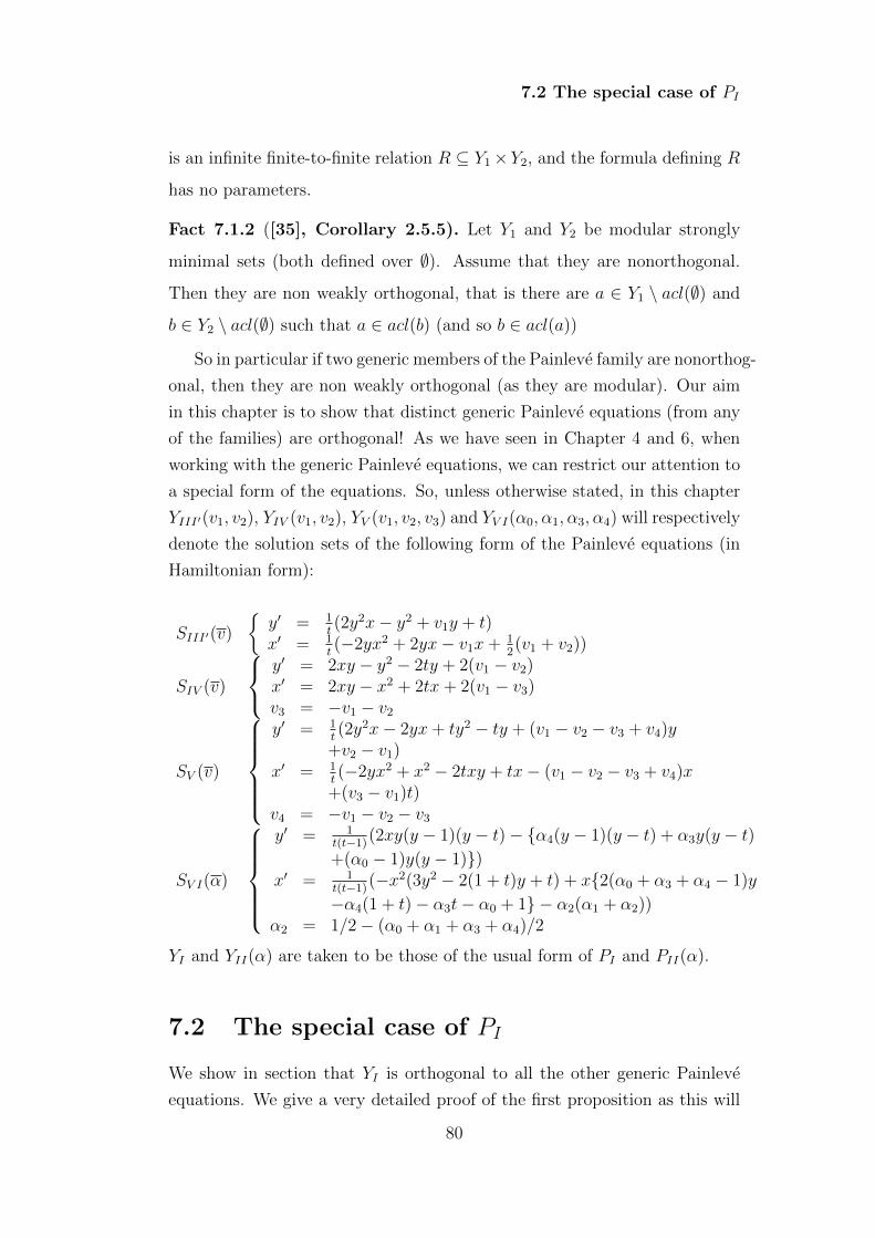
7.2 The special case of PI
is an infinite finite-to-finite relation R ⊆ Y1×Y2, and the formula defining R
has no parameters.
Fact 7.1.2 ([35], Corollary 2.5.5). Let Y1 and Y2 be modular strongly
minimal sets (both defined over ∅). Assume that they are nonorthogonal.
Then they are non weakly orthogonal, that is there are a ∈ Y1 \ acl(∅) and
b ∈ Y2 \ acl(∅) such that a ∈ acl(b) (and so b ∈ acl(a))
So in particular if two generic members of the Painleve family are nonorthog-
onal, then they are non weakly orthogonal (as they are modular). Our aim
in this chapter is to show that distinct generic Painleve equations (from any
of the families) are orthogonal! As we have seen in Chapter 4 and 6, when
working with the generic Painleve equations, we can restrict our attention to
a special form of the equations. So, unless otherwise stated, in this chapter
YIII′(v1, v2), YIV (v1, v2), YV (v1, v2, v3) and YV I(α0, α1, α3, α4) will respectively
denote the solution sets of the following form of the Painleve equations (in
Hamiltonian form):
SIII′(v)
{y′ = 1
t(2y2x− y2 + v1y + t)
x′ = 1t(−2yx2 + 2yx− v1x+ 1
2(v1 + v2))
SIV (v)
y′ = 2xy − y2 − 2ty + 2(v1 − v2)x′ = 2xy − x2 + 2tx+ 2(v1 − v3)v3 = −v1 − v2
SV (v)
y′ = 1
t(2y2x− 2yx+ ty2 − ty + (v1 − v2 − v3 + v4)y
+v2 − v1)x′ = 1
t(−2yx2 + x2 − 2txy + tx− (v1 − v2 − v3 + v4)x
+(v3 − v1)t)v4 = −v1 − v2 − v3
SV I(α)
y′ = 1
t(t−1)(2xy(y − 1)(y − t)− {α4(y − 1)(y − t) + α3y(y − t)
+(α0 − 1)y(y − 1)})x′ = 1
t(t−1)(−x2(3y2 − 2(1 + t)y + t) + x{2(α0 + α3 + α4 − 1)y
−α4(1 + t)− α3t− α0 + 1} − α2(α1 + α2))α2 = 1/2− (α0 + α1 + α3 + α4)/2
YI and YII(α) are taken to be those of the usual form of PI and PII(α).
7.2 The special case of PI
We show in section that YI is orthogonal to all the other generic Painleve
equations. We give a very detailed proof of the first proposition as this will
80

7.2 The special case of PI
be a model for many of the other cases.
Proposition 7.2.1. YI is orthogonal to any generic YII(α).
Proof. Let α ∈ C be generic and for contradiction, suppose that YI is non
weakly orthogonal to YII(α) (this suffices by Fact 7.1.2). By definition, this
means that there exists a finite-to-finite definable relation R ⊆ YI × YII(α)
and that R is defined over Q(α, t)alg. Since both YI and YII(α) are strictly
disintegrated (by Fact 4.3.3 and Proposition 6.2.2) and they have no elements
in C(t)alg, it is not hard to see however that R is the graph of a bijection
between YI and YII(α). Let us suppose that R is defined by ϕ(x, y, α, t) and
let σ(u, v) be the Lδ formula ∀x∃=1yϕ(x, y, u, v) ∧ ∀y∃=1xϕ(x, y, u, v). So
U |= σ(α, t) and by construction, U |= σ(α, t) implies that α ∈ C and YI is
in bijection with YII(α).
As C is strongly minimal and α generic, as argued before, σ(α, t) is true
for all but finitely many α ∈ C. In particular for some α0 ∈ 1/2 +Z, we have
that U |= σ(α0, t) and hence YI is in bijection with YII(α0) (and YII(α0) is
not strongly minimal by Corollary 4.3.5). By the same argument as in the
final paragraph of the proof of Corollary 4.3.6 we get a contradiction.
Similarly one has the following
Proposition 7.2.2. YI is orthogonal to the generic YIII′(v1, v2), YIV (v1, v2),
YV (v1, v2, v3) and YV I(α0, α1, α3, α4).
Proof. In the case of the generic YIV (v1, v2) and YV (v1, v2, v3) the same proof
as the one given above works. One only need to replace 1/2 + Z by the
appropriate exceptional sets. For YIV (v1, v2) and YV I(α0, α1, α3, α4) the only
other slight modification is to replace the definable bijection R by one-to-
finite maps (as the sets are only ω-categorical). But this does not pose any
real problems.
81

7.3 Orthogonality in the remaining cases
7.3 Orthogonality in the remaining cases
Although the idea of the proofs are the same, when trying to prove for
example that generic YII(α) is orthogonal to generic YIII(v1, v2) one needs to
be more careful as the parameters are not necessarily assumed to be mutually
generic. We start again with an easy case.
Proposition 7.3.1. The generic YII(α) is orthogonal to the generic YV (v1, v2,
v3) and YV I(α0, α1, α3, α4).
Proof. We look at the case of generic YV (v1, v2, v3) and the same will work
for YV I (although below we will see a different method of proof).
Case (i): α, v1 v2 and v3 are mutually generic. Then one uses the same
proof as that of Proposition 7.2.1.
Case (ii): α ∈ Q(v1, v2, v3)alg. For contradiction, suppose that YII(α) is
non weakly orthogonal to YV (v1, v2, v3). So we have as before a formula
σ(u,w1, w2, w3, x) such that U |= σ(α, v1, v2, v3, t) and this expresses that
YII(α) is in bijection with YV (v1, v2, v3). We then have to consider three sub-
cases:
Sub-case (i): α 6∈ Q(vi, vj)alg for any i 6= j. All we have to do is quantify
over v3 say, that is we use the fact that U |= ∃v3σ(α, v1, v2, v3, t). As α 6∈
Q(v1, v2)alg and C is strongly minimal we can as before find v1 ∈ v2 +Z such
that U |= ∃v3σ(α, v1, v2, v3, t). Choosing any v3 ∈ C witnessing this, we get
a bijection between YII(α) and YV (v1, v2, v3) (but again YV (v1, v2, v3) is not
strongly minimal by Corollary 4.3.14). This gives our desired contradiction.
Sub-case (ii): α ∈ Q(v1, v2)alg say but not in Q(v1)alg and Q(v2)alg. First
note that as v1, v2 and v3 are mutually generic we have that α is not in
Q(v3)alg, Q(v1, v3)alg or Q(v2, v3)alg. So this time we quantify over v2 say and
look at U |= ∃v2σ(α, v1, v2, v3, t). This allows us again to find v1 ∈ v3 + Z
such that U |= ∃v2σ(α, v1, v2, v3, t). Finally any v2 ∈ C making this true
leads us to our contradiction.
Sub-case (iii): α ∈ Q(v1)alg say. This time all we have to do is to quantify
over v1 and the same argument works.
82

7.3 Orthogonality in the remaining cases
For the other cases, we need to change a little bit our strategy. We will
this time use the results on algebraic solutions of the Painleve equations.
Proposition 7.3.2. The generic YII(α) is orthogonal to the generic YIII′(v1, v2).
Proof. We will work instead with YIII(v1, v2), the solution set of PIII given
in the form
y′′ =1
y(y′)2 − 1
ty′ +
4
t(v1 + 1− v2y
2) + 4y3 − 4
y.
For contradiction, suppose that YII(α) is non weakly orthogonal to YIII(v1, v2).
As before, we get a formula σ(u,w1, w2, x) such that U |= σ(α, v1, v2, t) and
this expresses that there is a “1 to ≤2” map between YII(α) and YIII(v1, v2).
This follows from strict disintegratedness of YII(α) and ω-categoricity of
YIII(v1, v2) (more precisely the proof of Proposition 6.3.2 gives that for any
y ∈ YIII(v1, v2) the cardinality of acl(C(t), y) ∩ YIII(v1, v2) is at most 2).
We then quantify over α, that is use that U |= ∃ασ(α, v1, v2, t). As v1
and v2 are mutually generic, we can first choose v1 ∈ (v2− 1) + 2Z (and have
U |= ∃ασ(α, v1, v2, t)) and then v2 ∈ Z so that U |= ∃ασ(α, v1, v2, t) where
v1 = v2 − 1 + 2m for some m ∈ Z. Choosing any α ∈ C witnessing this, we
have that there is a “1 to ≤2” map between YII(α) and YIII(v1, v2). By Fact
6.2.1, YII(α) contain at most 1 algebraic solution whereas by Fact 6.3.1(ii),
YIII(v1, v2) has exactly 4 algebraic solutions. So we get a contradiction.
Similarly one has the following
Proposition 7.3.3. dF
(i) The generic YIII′(v1, v2) is orthogonal to the generic YIV (w1, w2).
(ii) The generic YIV (w1, w2) is orthogonal to the generic YV (v1, v2, v3).
Proof. For (i) the exact same proof as Proposition 7.3.2, where one just needs
to quantify over w1 and w2, works.
For (ii), as mentioned in Section 4.3.5 of Chapter 4, one can instead work
83

7.3 Orthogonality in the remaining cases
with XV (α, β, γ) the solution set of PV (α, β, γ,−1/2). Arguing by contra-
diction, we have U |= σ(w1, w2, α, β, γ, t) witnessing that there is a bijection
between YIV (w1, w2) and XV (α, β, γ). Again by quantifying over w1 and w2
and moving α, β and γ into an appropriate set where XV has 2 algebraic
solutions (as given to us by 6.2.6(ii)), we are done as YIV (w1, w2) can only
have at most 1 algebraic solution.
Finally we look at orthogonality to the sixth Painleve equation. We will
need results about algebraic solutions (over C(t)) of YV I .
It is well known that for α0 = α1 = α3 = α4 = 0, YV I has infinitely many
algebraic solutions over C(t). Indeed, YV I(0, 0, 0, 0) can be identified with
the Manin kernel E]t of the elliptic curve Et : y2 = x(x−1)(x− t). Algebraic
solutions then corresponds to torsion points Etort . Furthermore, by applying
Backlund transformations (see [29]) one has the following:
Fact 7.3.4. For α0, α1, α3, α4 ∈ 1/2 + Z, YV I(α0, α1, α3, α4) has infinitely
many algebraic solutions over C(t).
Remark 7.3.5. Similarly, if αi ∈ Z and α0 + α1 + α3 + α4 ∈ 2Z there are
infinitely many algebraic solutions.
From this we easily get
Proposition 7.3.6. The generic YV I(α0, α1, α3, α4) is orthogonal to the generic
YIII′(v1, v2), YIV (v1, v2) and YV (v1, v2, v3).
Proof. One just uses the same trick as the proof of Proposition 7.3.2: We
want to prove that the generic YV I(α0, α1, α3, α4) is orthogonal to Y (v), where
Y (v) is any of the above generic sets.
Arguing by contradiction we get U |= σ(v, α0, α1, α3, α4, t) witnessing that
there is a finite-to-finite map between YV I(α0, α1, α3, α4) and Y (v). Quan-
tifying over v, we can move α0, α1, α3 and α4 one by one into the set of
half integers. On one side we then have infinitely many algebraic solutions
whereas on the other side Y (ν) (for any ν) can only have finitely many. A
contradiction.
84

7.3 Orthogonality in the remaining cases
Note that it would seem that none of the above arguments can be use to
prove that generic YII(α) are orthogonal to generic YIV (v1, v2) and similarly
that generic YIII′(v1, v2) are orthogonal to generic YV (v1, v2, v3).
85

Bibliography
[1] L. Blum, Generalized Algebraic Structures, PhD Dissertation, MIT,
1968.
[2] P. Boalch, The fifty-two icosahedral solutions to Painleve VI, J. Reine
Angew. Math. 596, (2006), 183214.
[3] A. Buium, Differential Algebraic Groups of Finite Dimension, Lecture
Notes in Mathematics 1506, Springer 1992.
[4] R. Conte and M. Musette, The Painleve Handbook, Springer, 2008.
[5] D. Eisenbud, Commutative Algebra with a View Toward Algebraic Ge-
ometry, Graduate Texts in Mathematics 150. Springer-Verlag, 1995.
[6] J. Freitag and T. Scanlon, Strong minimality of the j-function, preprint
2014.
[7] V. Gromak, I. Laine and S. Shimomura, Painleve differential equations
in the complex plane, De Gruyter studies in mathematics ; 28 (2002)
[8] E. Hrushovski, Private communications, (2012)
[9] E. Hrushovski, Locally modular regular types, in Classification The-
ory, Proceedings, Chicago 1985 (ed. J. Baldwin), Springer, 1987.
[10] E. Hrushovski and M. Itai, On model complete differential fields, Trans.
Amer. Math. Soc., vol 355(11) (2003), 4267-4296.
[11] E. Hrushovski, ODEs of order 1 and a generalization of a theorem of
Jouanalou, unpublished manuscript, 1995.
86
BIBLIOGRAPHY
[12] E. Hrushovski and T. Scanlon, Lascar and Morley Ranks Differ in Dif-
ferentially Closed Fields, Journal of Symbolic Logic, vol. 64 (1999), 1280-
1284.
[13] E. Hrushovski E. and Z. Sokolovic, Strongly minimal sets in differentially
closed fields, unpublished manuscript, 1994.
[14] E. Hrushovski and B. Zilber, Zariski geometries, Journal AMS, 9 (1996),
1 - 56
[15] A. Kitaev, C. Law and J. McLeod, Rational solutions of the fifth Painleve
equation, Differential Integral Equations 7 (1994), 9671000.
[16] E. Kolchin, Differential Algebra and Algebraic Groups, Academic Press,
1973.
[17] O. Lisovyy, Y. Tykhyy, Algebraic solutions of the sixth Painleve equa-
tion, preprint 2008.
[18] D. Marker, Model theory of differential fields, in Model theory of
fields, second edition, (Marker, Messmer, Pillay) Lecture Notes in Logic
5, ASL-CUP, 2006.
[19] D. Marker, Model theory: an introduction, Graduate texts in Mathe-
matics; Springer 217, 2002.
[20] D. Marker, The Number of Countable Differentially closed fields, Notre
Dame Journal of Formal Logic, vol. 48, Number 1 (2007), 99-113.
[21] D. Marker, Manin kernels, in Connections between Model Theory
and Algebraic and Analytic Geometry, edited by A. Macintyre,
Quaderni Matematica vol. 6, Naples II, 2000.
[22] Y. Murata, Rational solutions of the second and fourth Painleve equa-
tions, Funkcialaj Ekvacioj, 28 (1985), 1-32.
[23] Y. Murata, Classical solutions of the third Painleve equation, Nagoya
Math, 139 (1995), 37-65.
[24] J. Nagloo and A. Pillay, On Algebraic relations between solutions of a
generic Painleve equation, preprint 2011.
87

BIBLIOGRAPHY
[25] J. Nagloo and A. Pillay, On the algebraic independence of
generic Painleve transcendents, Compositio Mathematica, doi:10.1112/
S0010437X13007525.
[26] K. Nishioka, A note on the transcendency of Painleve first transcendent,
Nagoya Maths.J 109 (1988), 63-67.
[27] K. Nishioka, Algebraic independence of Painleve first transcendents,
Funkcialaj Ekvacioj, 47 (2004), 351-360.
[28] K. Nishioka, Painleve-Umemura extensions, Funkcialaj Ekvacioj, 37
(1994), 59-64.
[29] K. Okamoto, Studies on the Painleve equations, I, Sixth Painleve equa-
tion PV I , Ann. Mat. Pura Appl. 146 (1987) 337381.
[30] K. Okamoto, Studies on the Painleve equations, II, Fifth Painleve equa-
tion PV , Japan. J. Math., 13 (1987), 4776.
[31] K. Okamoto, Studies on the Painleve equations III, second and fourth
Painleve equations, PII and PIV , Math. Ann., 275 (1986),221-255.
[32] K. Okamoto, Studies on the Painleve equations IV, third Painleve equa-
tion, PIII , Funkcialaj Ekvacioj, 30 (1987), 305-332.
[33] P. Painleve, Lecons sur la Theorie Analytique des Equations
Differentielles, Professees a Stockholm, Hermann, Paris 1895.
(Reprinted, Oeuvres de Paul Painleve vol. 1, Editions du CNRS, Paris
1973.)
[34] D. Pierce and A. Pillay, A note on the axioms for differentially closed
fields of characteristic zero, J. Algebra 204:1 1998, 108-115.
[35] A. Pillay, Geometric Stability Theory, Oxford University Press, 1996.
[36] A. Pillay, Differential algebraic groups and the number of countable dif-
ferentially closed fields, in Model Theory of Fields, second edition,
(Marker, Messmer, Pillay) Lecture Notes in Logic 5, ASL-CUP, 2006.
[37] A. Pillay, Differential Fields, in Lecture Notes in Algebraic Model
Theory (ed. Hart, Valeriote), Fields Inst. Monograph 15, AMS (2002),
3-48.
88

BIBLIOGRAPHY
[38] A. Pillay, Algebraic D-groups and Differential Galois theory, Pacific
Journal of Mathematics, Vol. 216 No. 2 (2004), 343-360.
[39] A. Pillay, Differential Galois theory I, Illinois J. Math. Vol. 42, Issue 4
(1998), 678-69.
[40] A. Pillay, Two remarks on differential fields, in Model Theory and
Applications, Quaderni Matematica vol. 11, Naples II, 2003.
[41] A. Pillay, Stability theory, Lecture notes available at
http://www1.maths.leeds.ac.uk/ pillay/
[42] A. Pillay and M. Ziegler, Jet spaces of varieties over differential and
difference fields, Selecta Math. New series, 9 (2003), 579-599.
[43] H. Poincare, Sur un theoreme de M. Fuchs, Acta Math. 7 (1885), no. 1,
1-32.
[44] B. Poizat, A Course in Model Theory, translated into English by M.
Klein, Springer, 2000.
[45] K. Tent and M. Ziegler, A course in model theory, Lecture Notes in
Logic, vol. 40, ASL, 2012.
[46] H. Umemura, On the irreducibility of the first differential equation of
Painleve, Algebraic Geometry and Commutative Algebra in honor of
Masayoshi NAGATA, Kinokuniya, Tokoyo,(1988),771-789.
[47] H. Umemura and H. Watanabe, Solutions of the second and fourth
Painleve equations I, Nagoya Maths., J 148 (1997), 151-198.
[48] H. Umemura H. and H. Watanabe, Solutions of the third Painleve equa-
tion I, Nagoya Maths., J 151 (1998), 1-24.
[49] H. Watanabe, Solutions of the fifth Painleve equation I, Hokkaido Math-
ematical Journal, 24 (2) (1995) 231-267.
[50] H. Watanabe, Birational canonical transformations and classical solu-
tions of the sixth Painleve equation, Ann. Scuola Norm. Sup. Pisa Cl.
Sci.(4) Vol XXVII (1998) 379-425.
89
Copyright © 2022 FDOKUMEN