THE JOURNAL OF CHEMICAL PHYSICS 140, 074503 (2014)

Quadrupole terms in the Maxwell equations: Born energy, partial molarvolume, and entropy of ions

Radomir I. Slavchov1,a) and Tzanko I. Ivanov2

1Department of Physical Chemistry, Faculty of Chemistry and Pharmacy, Sofia University,1164 Sofia, Bulgaria2Theoretical Physics Department, Faculty of Physics, Sofia University, 1164 Sofia, Bulgaria

(Received 20 November 2013; accepted 4 February 2014; published online 21 February 2014)

A new equation of state relating the macroscopic quadrupole moment density Q to the gradient ofthe field ∇E in an isotropic fluid is derived: Q = αQ(∇E − U∇ · E/3), where the quadrupolarizabil-ity αQ is proportional to the squared molecular quadrupole moment. Using this equation of state, ageneralized expression for the Born energy of an ion dissolved in quadrupolar solvent is obtained.It turns out that the potential and the energy of a point charge in a quadrupolar medium are finite.From the obtained Born energy, the partial molar volume and the partial molar entropy of a dis-solved ion follow. Both are compared to experimental data for a large number of simple ions inaqueous solutions. From the comparison the value of the quadrupolar length LQ is determined, LQ

= (αQ/3ε)1/2 = 1-4 Å. Data for ion transfer from aqueous to polar oil solution are analyzed, whichallowed for the determination of the quadrupolarizability of nitrobenzene. © 2014 AIP PublishingLLC. [http://dx.doi.org/10.1063/1.4865878]

I. INTRODUCTION

The macroscopic Poisson equation of electrostatics com-bines the static macroscopic Coulomb and Ampere laws,

∇ · D = ρ(φ), (1)

E = −∇φ, (2)

with a linear dependence of the electric displacement field Don the electric field intensity E:

D ≡ ε0 E + P = ε0 E + αP E = εE. (3)

Here, ρ is the free charge number density; φ is the elec-trostatic potential; ε ≡ ε0 + αP = ε0εr is the absolute di-electric permittivity, ε0 is the vacuum permittivity, εr is therelative permittivity of the medium, αP is the macroscopicpolarizability of the medium. For a homogeneous medium(∇ε = 0) the Poisson equation for φ follows fromEqs (1)–(3):

− ε∇2φ = ρ(φ). (4)

For conducting media, one must provide also an equation ofstate for the dependence ρ(φ). A common assumption is thatthe charges are distributed according to the Boltzmann distri-bution

ρ(φ) =∑

eiCi exp(−eiφ/kBT ), (5)

where ei = eZi is the absolute charge of the ith ion, e is theelectron charge, Zi is the relative ionic charge, Ci = ν iCel isthe local concentration of the ith ion, ν i stands for its stoi-chiometric number, Cel is the electrolyte concentration, T isthe temperature, and kB is the Boltzmann constant. Insert-

a)E-mail: fhri@chem.uni-sofia.bg

ing Eq. (5) into Eq. (4), one obtains the Poisson-Boltzmannequation, widely used in physical chemistry and colloid sci-ence. Numerous basic concepts such as Debye-Hückel dou-ble layer,1, 2 Gouy model for charged interface,3, 4 Daviesadsorption model for ionic surfactant adsorption,5, 6 theelectrostatic disjoining pressure in DLVO theory,7–9 elec-trokinetic ζ -potential,10 etc., are merely a consequence ofEqs. (4) and (5).

It has been early recognized that both Poisson andBoltzmann equations (4) and (5) have severe limitations.The derivation of Eq. (4) involves a multipole expansionof the local potential up to dipole terms, i.e., it neglectsthe quadrupole moment density.11–13 Equation (3) is strictlyvalid for linear media.14 The Boltzmann distribution (5) isonly a first approximation valid for quasi-ideal solution;15–17

other “external” potentials except eiφ often arise.18–20 In or-der to make Eqs. (3)–(5) applicable to real systems, numer-ous corrections have been proposed, to point a few: (i) Cor-rections to the Boltzmann distribution (5) by introductionof various additional interaction potentials, either for ion-ion non-electrostatic interaction15, 16 or various ion-surfaceinteractions;18–20 (ii) corrections for the macroscopic natureof the equation, involving explicit molecular treatment ofthe first neighbor interactions21,14,22 or other discretenesseffects;23, 24 (iii) correction for the dielectric saturation, i.e.,the dependence of ε on the electric field intensity;25, 26,14 (iv)corrections related to the inhomogeneity of the medium (∇ε

�= 0; e.g., Refs. 27 and 28); (v) correlation effects2, 17 and non-local electrostatic effects,29–32 etc. Every major correction ofEqs. (4) and (5) has been an impetus for reconsideration of thebasic concepts following from the Poisson-Boltzmann equa-tion.

While most studies in physical chemistry criticizedmainly the Boltzmann part of Poisson-Boltzmann equation,

0021-9606/2014/140(7)/074503/15/$30.00 © 2014 AIP Publishing LLC140, 074503-1

074503-2 R. I. Slavchov and T. I. Ivanov J. Chem. Phys. 140, 074503 (2014)

several studies of optical phenomena33–36 attacked the Pois-son part of it. It was demonstrated that the quadrupolar termsin the macroscopic Coulomb law (1) become quite signifi-cant in cases where high gradients of E are present. In suchcases, quadrupolar term in the displacement field D need tobe introduced:36

D = ε0 E + P − 1

2∇ · Q. (6)

Here, Q is the macroscopic density of the quadrupole momenttensor. Note that the numerical coefficient in front of ∇ · Q de-pends on the choice of definition of quadrupole moment (forconvenience, a derivation of Eq. (6) and the definitions of theinvolved quantities are given in supplementary material A).66

The substitution of Eq. (6) into Eq. (1) yields a generalizationof the Poisson equation (4):

∇ ·(

εE − 1

2∇ · Q

)= ρ, (7)

which opens a vast field for analysis of the effect of thequadrupole moments of the molecules composing a mediumon the properties of charged particles in such medium. It hasbeen recently demonstrated that quadrupole terms in D canplay a role in solvent-solute interaction.12, 13 The correctionfor Q will be important if the solvent molecules possess largequadrupole moment – such is the case of water37 and manyothers, including “non-polar” media of low dipole momentbut high quadrupole moment such as liquid CO2, fluorocar-bons, etc.13, 38

The purpose of our study is to analyze the consequencesof the new term in Maxwell equation for several basic prob-lems of physical chemistry of electrolyte solutions and col-loid chemistry. Equation (7) is largely unknown to physicalchemists and virtually has never been used in colloid science.There are three reasons for this negligence. First, Eq. (7) isuseless without an equation of state for Q. There are severalexisting studies of this constitutive relation39–42,12, 13, 36 but allare scarcely analyzed. Therefore, in Sec. II, we will derive anew equation of state as simple as possible, showing that Qis a linear function of ∇E − U∇ · E/3, with a scalar coeffi-cient of proportionality – the quadrupolarizability33 αQ (hereU is the unit tensor). The second reason for Eq. (7) to be un-known in the colloid field is that it is a fourth-order equationwith respect to φ, and requires the use of new boundary con-ditions. Seemingly, these new conditions have been derivedonly recently.39, 40 We will review this problem in Sec. III. Fi-nally, the third obstacle to use Eq. (7) is that it involves a newparameter of unknown value – αQ. We will give in this paperboth theoretical estimation and values determined from 3 in-dependent sets of experimental data for ions in water; we willconsider also ions in polar oil solutions.

In Sec. IV, Eq. (7) is used to reinvestigate one basic con-cept in the physical chemistry of electrolyte solutions – Bornenergy. It will be shown that the “correction” Q in Eq. (7) infact leads to results which have no counterpart in the frameof Poisson equation (4), notably, finite electrostatic potentialand energy of a point charge in quadrupolarizable medium(similar result was obtained in Ref. 12). In Sec. IV, we com-pare our results for the Born energy in quadrupolar media to

experimental data, which allows us to determine the value ofquadrupolarizability αQ of water and nitrobenzene.

II. EQUATIONS OF STATE FOR THE QUADRUPOLEMOMENT DENSITY

The problem for the constitutive relation between Qand the field gradient ∇E has been addressed severaltimes.33, 36, 39–42,12, 13 Using as a starting point the approach ofJeon and Kim,13 we will be able to obtain a new simple equa-tion of state which relates Q to the field gradient ∇E and themolecular properties of the solvent.

Consider an ideal gas consisting of molecules possess-ing a solid quadrupole moment tensor q0 (for the sake ofsimplicity, the molecule is assumed non-polarizable and withno dipole moment). Since q0 is symmetrical and traceless,by a suitable choice of the coordinate system it can bediagonalized43 and in the general case, its diagonal form is

q0 =⎛⎝qxx 0 0

0 qyy 00 0 qzz

⎞⎠ − qxx + qyy + qzz

3U. (8)

The term (qxx + qyy + qzz)/3U ensures that the trace of q0 is 0and can be added because the field created by a quadrupole invacuum is invariant with respect to the operation of exchang-ing the quadrupole strength q0 with q0 + XU, where X is anyscalar.11, 44 The molecule is constantly rotating. An arbitraryrotation changes the quadrupole moment tensor from q0 to q.For a rotation at arbitrary Eulerian angles φ, ψ , and θ , theEuler matrix E φψθ is given by

E ϕψθ

=

⎛⎜⎜⎜⎜⎜⎜⎜⎜⎝

cos ϕ cos ψ−− sin ϕ sin ψ cos θ

sin ϕ cos ψ++ cos ϕ sin ψ cos θ

sinψ sin θ

− cos ϕ sin ψ−− sin ϕ cos ψ cos θ

− sin ϕ sin ψ++ cos ϕ cos ψ cos θ

cos ψ sin θ

sin ϕ sin θ − cos ϕ sin θ cos θ

⎞⎟⎟⎟⎟⎟⎟⎟⎟⎠

.

(9)

The relation between the tensor q for a randomly orientedmolecule and the tensor q0 is

qij (ϕ,ψ, θ ) = Eϕψθ

ik Eϕψθ

jl q0kl . (10)

In the absence of a gradient of the electric field the averagevalue of q is 0. In an external electric field gradient ∇E, themolecule tends to orientate itself in order to minimize its elec-tric energy, given by the expression (Eq 4.22 of Jackson, 3rdedition11):

uel = −1

2q : ∇ E. (11)

Here, the double dot product symbol “:” denotes the operationq:∇E = ��qij∂Ei/∂xj. The orientation of the molecule mustfollow the Boltzmann distribution which can be linearized inthe case of uel/kBT � 1:

ρφψθ = cn exp(−uel/kBT ) ≈ cn(1 − uel/kBT ). (12)

074503-3 R. I. Slavchov and T. I. Ivanov J. Chem. Phys. 140, 074503 (2014)

Here, cn is a normalizing coefficient calculated as

cn = 1/

2π∫0

2π∫0

π∫0

(1 − uel/kBT ) sin θdθdϕdψ = 1/8π2.

(13)The average quadrupole moment q of a molecule can be cal-culated directly using Eqs. (8)–(13):

q =2π∫

0

2π∫0

π∫0

qρφψθ sin θdθdϕdψ = αq(∇ E − U∇ · E/3).

(14)Here, the molecular quadrupolarizability αq was introduced,related to the diagonal components of q0 as follows:

αq = q0 : q0/10kBT

= (q2

xx +q2yy +q2

zz − qxxqyy − qxxqzz − qyyqzz

)/15kBT .

(15)

Equation (15) was obtained, e.g., in Ref. 13.The macroscopic density Q of the quadrupole moment in

a gas acted upon by a field gradient ∇E is the gas concentra-tion C times q, Eq. (14):

Q = αQ(∇ E − U∇ · E/3). (16)

Here, the macroscopic quadrupolarizability αQ is given by

αQ = Cαq = Cq0 : q0/10kBT . (17)

Our constitutive relation (16) is a direct consequence ofthe general form (8) of the molecular solid quadrupole and thelinearized Boltzmann distribution (12). Note that according toEq. (16) Q is traceless,11 in contrast to Eq. 2.25 of Jeon andKim.13 References 42 and 45 contain some discussion in favorof their choice. However, in the supplementary material A,66

we present arguments that the use of tensor Q with non-zerotrace is incompatible with Eqs. (6) and (7). Equation 2.4 ofChitanvis12 postulates an equation of state in which only theU∇ · E term of our Eq. (16) is present, i.e., according to him,Q has only diagonal elements and a non-zero trace.

In general, Q depends not only on the field gradient butalso on the field E itself, and, on the other hand, electric fieldgradient ∇E can induce non-zero dipole moment.39,36 For anideal gas of solid dipoles within the linear approximation forρφψθ , this is not the case. This can be shown by a direct calcu-lation analogous to the derivation of Eq. (16): if the moleculehas dipole moment p0 and quadrupole moment q0, then in ex-ternal field E and field gradient ∇E its energy is11

uel = − p · E − 1

2q : ∇ E. (18)

Using this expression instead of Eq. (11), one can calculatethe average dipole and quadrupole moments. This calculationyields for Q again Eq. (16), because the terms proportional toE cancel each other. Calculation of the macroscopic polariza-tion P gives the classical result:14

P = αP E, αP = Cαp = Cp20/3kBT , (19)

where αp and αP are the molecular and the macroscopic po-larizabilities.

The derivation above is strictly valid for a gas of solidmultipoles. It can be readily generalized to include molec-ular polarizabilities and quadrupolarizabilities.13 This yieldsinstead of Eq. (17) the expression

αq = αq0 + q0 : q0/10kBT , (20)

where αq0 is the average intrinsic (atomic + electronic)molecular quadrupolarizability (Eq. 4.5 of Jeon and Kim13).Equation (20) can be compared to the well-known formula forthe polarizability14

αp = αp0 + p20/3kBT , (21)

where αp0 is the average intrinsic molecular polarizability. Inaddition, in the case of liquids one can introduce a Clausius-Mossotti type of relation for the local gradient ∇E to themacroscopic quadrupole moment density Q and a reactionfield (similar to the relation between local field and averagemacroscopic polarization14 P). The local field is investigatedin Refs. 12 and 13. We shall not attempt such a generalizationin our study and in what follows we will assume that the equa-tion of state (16) is valid for isotropic fluids, provided that Eand ∇E are not too large (in order Eq. (12) to be applicable).For dense fluids, Eq. (17) for αQ will be invalid but it stillshould give the correct order of magnitude of the quadrupo-larizability.

Using the values of the quadrupole moment of water fromRef. 37: qxx = +5.85 × 10−40 Cm2, qyy = −5.56 × 10−40

Cm2, and qzz = −0.29 × 10−40 Cm2 (a factor of 2/3 for thedifferent definitions of q0 used here and in Ref. 37 must beaccounted for), we can calculate the value αQ = 1 × 10−30

Fm from Eq. (17). Both αq0 and the Clausius-Mossotti effectincrease αQ. For comparison, the experimental value for thepolarizability of water is αP = ε – ε0 = 6.8 × 10−10 F/m,which is about 3 times higher than the one calculated throughthe estimation αP = Cp2

0/3kBT . By analogy, we can assumethat αQ is several times larger than the value following fromEq. (17).

Let us now estimate the pressure and temperature deriva-tives of αQ. Assuming that the molecular quadrupolarizabilityαq is independent on p, from Eq. (17) it follows that

1

αQ

(∂αQ

∂p

)T

≈ 1

C

(∂C

∂p

)T

= βT , (22)

where βT is the isothermal compressibility. Since Eq. (17) isapproximate, the resulting equation (22) also gives only an es-timate of ∂αQ/∂p. For the temperature derivative of αQ (suit-ably made dimensionless by a factor of T/αQ), we use Eq. (20)for the dependence of the molecular quadrupolarizability ontemperature and the relation αQ = Cαq to obtain

T

αQ

(∂αQ

∂T

)p

= T

C

(∂C

∂T

)p

+ T

αq

(∂αq

∂T

)p

= −T αvp − q0 : q0/10kBT

αq0 + q0 : q0/10kBT. (23)

Here, αpv = −C−1(∂C/∂T)p is the coefficient of thermal ex-

pansion. For water,46 Tαpv = 0.0763. To estimate the second

term, we assume that αq0 � q0 : q0/10kBT (water has highquadrupole moment q0 and it is a “hard” molecule of low

074503-4 R. I. Slavchov and T. I. Ivanov J. Chem. Phys. 140, 074503 (2014)

intrinsic polarizability αp0 and perhaps low αq0). In this limit,the second term in Eq. (23) is about −1, much larger in abso-lute value than T αv

p. Therefore, we can write approximatelythat

T

αQ

∂αQ

∂T= −1. (24)

III. BOUNDARY CONDITIONS FOR THEGENERALIZED POISSON EQUATION

Within the quadrupolar approximation, the Coulomb-Ampere law (7) is of fourth order with respect to φ since uponsubstituting Eq. (16) in Eq. (7), one obtains

∇ ·[εE − 1

2∇ · αQ(∇ E − U∇ · E/3)

]= ρ(φ). (25)

In a homogeneous medium, this equation simplifies to

∇ · E − αQ

3ε∇2∇ · E = −∇2φ + L2

Q∇4φ = ρ(φ)

ε. (26)

Here, we have introduced the quadrupolar length LQ definedwith the relation

L2Q = αQ/3ε. (27)

From the estimation of αQ in the end of Sec. II, we can saythat LQ = (αQ/3ε)1/2 > 0.2 Å, perhaps several times larger.Equations. (26) and (27) are of the same form as those ofChitanvis,12 with the only difference of the obtained differentnumerical coefficient in Eq. (27). We are mainly concernedwith spherical symmetry in this study, where Eq. (26) reads

1

r2

dr2Er

dr− L2

Q

r2

d

drr2 d

dr

1

r2

dr2Er

dr= ρ(r)

ε. (28)

We will need an explicit expression for Q and ∇ · Q; the gradi-ent and the divergence of E in spherical coordinates are givenby

∇ E =⎛⎝ dEr/dr 0 0

0 Er/r 00 0 Er/r

⎞⎠ ; ∇ · E = dEr

dr+ 2Er

r.

(29)

Then from Eq. (16), one obtains

Q = αQ

3

(dEr

dr− Er

r

)⎛⎝2 0 0

0 −1 00 0 −1

⎞⎠ ,

(30)

∇ · Q = 2αQ

3

(d2Er

dr2+ 2

r

dEr

dr− 2Er

r2

)er ,

where er is a unit vector, collinear with the radius-vector.The boundary conditions of Eq. (7) have been derived re-

cently by Graham and Raab,39 using the singular distributionsapproach of Bedeaux et al.47, 48 in the case of a flat boundarysurface of an anisotropic medium with arbitrary equation ofstate; alternative derivation, again for flat boundary, was givenin Ref. 40. Following the approach of Graham and Raab, wewill deduce here the boundary conditions of Eq. (7) at a spher-ical surface dividing two isotropic phases. First, we write thesingular distributions of εE, Q, and ρ:

εE = η+ε+ E+ + η−ε− E−,

Q = η+Q+ + η−Q−,

ρ = η+ρ+ + η−ρ− + δρS. (31)

Here, X+ and X− denote the corresponding physical quantitiesfor the phase situated at r > R and r < R, respectively; ρS isthe surface charge density; the notations η± and δ stand forthe Heaviside function η and the Dirac δ-function:

η+ = η(r − R); η− = η(R − r); δ = δ(r − R). (32)

To obtain the necessary boundary conditions, we insertEq. (31) into Eq. (7) and use the irreducibility of η±, δ andits derivative δ1 = dδ/dr. We need first to calculate ∇ · εE and∇∇:Q, where εE and Q are given by Eq. (31):

∇ · εE = η+∇ · ε+ E++η−∇ · ε− E−+δ(ε+E+

r − ε−E−r

),

∇∇ : Q = η+∇∇ : Q+ + δer · (∇ · Q+)

+δ∇ · (er · Q+) + δ1Q+rr (r)

+η−∇∇ : Q− − δer · (∇ · Q−) − δ∇ · (er · Q−)

−δ1Q−rr (r). (33)

Using Eqs. (33), we can write Eq. (7) in the form

η+[∇ ·

(ε+ E+ − 1

2∇ · Q+

)− ρ+

]

+ η−[∇ ·

(ε− E− − 1

2∇ · Q−

)− ρ−

]

− δ

⎧⎪⎪⎪⎪⎨⎪⎪⎪⎪⎩

ρS −[ε+E+

r − 1

2er · (∇ · Q+) − 1

2∇ · (er · Q+) + 1

2

dQ+rr

dr

]

+[ε−E−

r − 1

2er · (∇ · Q−) − 1

2∇ · (er · Q−) + 1

2

dQ−rr

dr

]⎫⎪⎪⎪⎪⎬⎪⎪⎪⎪⎭

r=R

− δ11

2

(Q+

rr (R) − Q−rr (R)

) = 0. (34)

074503-5 R. I. Slavchov and T. I. Ivanov J. Chem. Phys. 140, 074503 (2014)

For the derivation of Eqs. (33) and (34), we have usedthe properties of the singular functions: ∇η+ = erδ; ∇η−

= –erδ; ∇δ = erδ1; δ1Qrr(r) = δ1Qrr(R) – δdQrr/dr|r= R. Decomposition of Eq. (34) yields, first, the bulkequations for the two phases (the coefficients of η± inEq. (34)):

∇ ·(

ε+ E± − 1

2∇ · Q±

)= ρ±. (35)

Setting the factor multiplying δ in Eq. (34) to 0, we ob-tain a generalization of the Gauss law for the quadrupolarmedia:

[ε+E+

r − 1

2er · (∇ · Q+) − 1

2∇ · (er · Q+) + 1

2

dQ+rr

dr

]r=R

−[ε−E−

r − 1

2er · (∇ · Q−)− 1

2∇ · (er · Q−)+ 1

2

dQ−rr

dr

]r=R

= ρS. (36)

The last term of Eq. (34), proportional to δ1, results in a newboundary condition, which balances the quadrupole momentdensities on the two sides of the spherical surface:

Q+rr (R) − Q−

rr (R) = 0. (37)

We now substitute Eqs. (30) into Eqs. (36) and (37) to obtainthe explicit form of the boundary conditions. Equation (36)reads

ρS =[ε+E+

r − α+Q

3

(d2E+

r

dr2+ 2

r

dE+r

dr− 2E+

r

r2

)− α+

Q

3

2

r

(dE+

r

dr− E+

r

r

)]r=R

−[ε−E−

r − α−Q

3

(d2E−

r

dr2+ 2

r

dE−r

dr− 2E−

r

r2

)− α−

Q

3

2

r

(dE−

r

dr− E−

r

r

)]r=R

. (38)

The explicit form of the new boundary condition (37) is

α+Q

(dE+

r

dr− E+

r

r

)r=R

− α−Q

(dE−

r

dr− E−

r

r

)r=R

= 0. (39)

Subtracting Eq. (38) and Eq. (39), we obtain the relation

D+r (R) − D−

r (R) = ρS, (40)

which is formally equivalent to the classical Gauss law, butone must keep in mind that D involves higher derivatives ofthe field E, cf. Eq. (6).

IV. EFFECT OF THE QUADRUPOLARIZABILITY OF AMEDIUM ON THE BORN ENERGIES, PARTIAL MOLARVOLUMES, AND ENTROPIES OF DISSOLVED IONS

In this part of our study the general equation (28) of elec-trostatics in quadrupolar media at spherical symmetry and itsboundary conditions (38) and (39) derived in Secs. I–III willbe used to solve several basic electrostatic problems of highsignificance to the physical chemistry of electrolyte solutions.

A. Point charge in an insulator

We solve Eq. (28) with ρ = eiδ(r). The general solutionof the equation is

E = 1

r2

[k1 + k2

(1 + r

LQ

)exp

(− r

LQ

)

+k3

(1 − r

LQ

)exp

(r

LQ

)]. (41)

In order to determine the three integration constants k1,k2, and k3, we need to impose three conditions on E. The firstone is to require E to tend to a finite value as r → ∞ (this givesk3 = 0). The second condition is that the asymptotic behaviorof E at r → ∞ is unaffected by the presence of quadrupoles,that is, the field of a point charge at r → ∞ tends to ei/4πεr2.This condition yields k1 = ei/4πε (the same result can be ob-tained by the Gauss law). There is one final condition neededto determine k2. Our assumption is to require that E tends tosomething finite as r → 0, i.e., there is no singularity of E at r→ 0, which yields k2 = –k1. Equation (28) has, thus, a finitesolution, which is

E = ei

4πε

1

r2

[1 −

(1 + r

LQ

)exp

(− r

LQ

)]. (42)

Integration of this result gives the following formula for theelectrostatic potential:

φ = ei

4πε

1 − exp(−r/LQ)

r. (43)

The potential in r = 0 is also finite, and its value at r = 0 isφ0 = ei/4πεLQ. The ion has, therefore, a finite energy:

uel = eiφ0/2 = e2i /8πεLQ. (44)

This is in marked contrast to the case of ion in vacuum wherethe potential is diverging as 1/r and the electrostatic self-energy of a point charge is infinite (Fig. 1). For a point chargein water at T = 25 ◦C, if LQ = 2 Å, we obtain φ0 = 92 mVand uel = 3.6 × kBT. Equation 2.8 of Chitanvis12 has the sameform as Eq. (43) (but his relation between LQ and αQ is dif-ferent). Equation (43) can be compared also to Eq. 2.48 of

074503-6 R. I. Slavchov and T. I. Ivanov J. Chem. Phys. 140, 074503 (2014)

FIG. 1. Electrostatic potential φ of a point charge in a quadrupolar mediumvs. the distance r from the point charge e in water, Eq. (43), for variousquadrupolar lengths LQ. In a quadrupolar medium, the point charge has finitepotential at r = 0. Solid line: LQ = 2 Å; dashed line: LQ = 1 Å; dashed-dottedline: LQ = 0 (the classical solution).

Jeon and Kim,13 who obtained a divergent potential since theyused another constitutive relation for Q and implied differentconditions on their solutions to determine the integration con-stants. In order to corroborate our non-classical choice for thefinite field condition, a different approach will be presented inSec. IV B to derive the same result (43), by placing the chargeinto a spherical cavity of radius R (at r = R the boundary con-ditions derived in Sec. III will be applied) and then taking thelimit R → 0 of the resulting potential.

B. Ion of finite size in an insulator

There are various models of an ion of finite size ina solution, which yield the same expression for the Bornenergy.49,28, 40 The simplest model assumes that the ion is apoint charge ei situated into a cavity, i.e., in an empty sphereof permittivity ε0 and radius Rcav; the empty sphere is locatedin a medium of dielectric permittivity ε. This model neglectsthe detailed charge distribution in the ion and can be gener-alized in various ways.12, 13, 17, 21, 22, 27–32, 50–52 Here, in order tokeep the picture simple, we will hold on to the empty spheremodel, only adding into account the quadrupolarizability αQ

of the medium. Similar problem (an entity of certain chargedistribution placed into a cavity in a medium with intrinsicquadrupolarizability) was considered by Chitanvis12 and Jeonand Kim13 using different equations of state and a differentset of boundary conditions.

We formulate the problem with the following equations:

(i) Inside the sphere (superscript “i”), at r < Rcav, there areno charges, bound or free, apart from the central ion ofcharge ei:

ε0∇ · Ei = eiδ(r). (45)

(ii) Outside the sphere (no superscript), at r > Rcav, Eq. (28)is valid with ρ = 0:

1

r2

dr2Er

dr− L2

Q

r2

d

drr2 d

dr

1

r2

dr2Er

dr= 0. (46)

(iii) The boundary conditions at r = Rcav are given byEqs. (38) and (39):

Er − ε0

εEi

r − L2Q

(d2Er

dr2+ 2

r

dEr

dr− 2Er

r2

)∣∣∣∣r=Rcav

= 0,

(47)(dEr

dr− Er

r

)r=Rcav

= 0. (48)

The solution of Eqs. (45)–(48) in terms of the electrostaticpotential is

φi = ei

4πε0

1

r− ei

4πRcav

×(

1

ε0− 1

ε

1 + 3LQ/Rcav

1 + 3LQ/Rcav + 3L2Q/R2

cav

)at r < Rcav,

(49)

φ = ei

4πε

1

r

×{

1− 3L2Q exp[−(r−Rcav)/LQ]

R2cav

(1+3LQ/Rcav+3L2

Q/R2cav

)}

at r > Rcav,

(50)

we used also the condition φ = φi at r = Rcav. As Rcav

→ 0, Eq. (50) for φ simplifies to Eq. (43) for a pointcharge, which justifies the assumption for finite E and φ atr → 0 which was used in Sec. IV A to derive Eq. (43) – thatis, the results obtained in Sec. IV A can be obtained alterna-tively by taking the limit from Eq. (50) without making use ofsuch a non-classical condition.

The self-energy uel of the ion is determined by the po-tential �φi = φi – ei/4πε0r, created by the polarized mediumand acting upon the ion. It is obtained from Eq. (49) as

uel = 1

2ei�φi

= − e2i

8πRcav

(1

ε0− 1

ε

1 + 3LQ/Rcav

1 + 3LQ/Rcav + 3L2Q/R2

cav

).

(51)

It can be compared to Eq. 3.1 of Chitanvis,12 who used insteadof our equation (48) a condition for continuity of dEr/dr atr = Rcav, without discussion. Jeon and Kim13 used anothercondition – for non-oscillatory solution, also with no goodjustification. When LQ → 0, Eq. (51) simplifies to the familiarexpression for the Born energy:49, 50

uBorn = − e2i

8πRcav

(1

ε0− 1

ε

). (52)

074503-7 R. I. Slavchov and T. I. Ivanov J. Chem. Phys. 140, 074503 (2014)

FIG. 2. Correction factor for the effect of the quadrupolarizability in themodified Born Eq. (51) as a function of LQ/Rcav.

It can be shown that any other charge distribution of sphericalsymmetry and total charge ei placed into the cavity will havethe same Born energy (51) provided that this charge distribu-tion is fixed (independent of the medium).40 In supplementarymaterial B,66 we demonstrate this with another common Bornmodel, where the ion is assumed to be a metal sphere of sur-face charge density ρS = ei/4πRi

2.It follows from Eq. (51) that the Born energy of small

ions is more strongly affected from the quadrupolarizabilityof the medium – this is illustrated in Fig. 2, where the factormultiplying 1/ε in Eq. (51) is plotted as a function of LQ/Rcav.However, the effect of quadrupolarizability on the Born en-ergy itself is negligibly small, at least for aqueous solutions:the 1/ε0 term is by far larger than the second term in the brack-ets of Eq. (51), which involves LQ. For this reason, the ob-tained result (51) for the effect of LQ on the self-energy uel

is not easy to test directly. In order to show the significanceof the LQ term in Eq. (51), we will eliminate the large term1/ε0 using two different approaches: (i) By differentiating uel

either with respect to p or T in Secs. IV D and IV E, andcomparing the results with experimental data for ionic partialmolar volumes and entropies; (ii) By investigating in Sec. IVG the transfer energy of an ion from aqueous to polar oil solu-tion (in this transfer energy, the 1/ε0 term cancels). This willallow us to give an estimate for the quadrupolar length LQ andthe quadrupolarizability αQ of water and the polar oil. How-ever, the correct assessment of LQ requires the knowledge ofthe relation between the cavity radius Rcav and the crystallo-graphic radius of the ion, Ri; this problem will be investigatedin Sec. IV C.

C. Ion free energy of hydration

The standard molarity-based chemical potential μ0i (cor-responding to a standard concentration C0 = 1 M) reflects the

state of a single ion in the solution, including the effect of theion’s field on the molecules of the solvent in the vicinity ofthe ion. For this energy one can write2, 17, 22, 53

μ0i = μintra(T ) + uel + pv0 + kBT ln C0. (53)

The first term in Eq. (53), μintra, is related to the intramolec-ular state of the ion itself. For simple ions, it is a commonapproximation that this term is the same in gaseous state andin any solvent. The second term, uel, stands for the electro-static ion-water interaction; we will use for uel the general-ized expression for the Born energy of the ion, Eq. (51), in-volving the quadrupolar length LQ. The third term, pv0, isthe mechanic work for introducing an ion of radius Ri intoa medium at pressure p. The fourth term, kBTlnC0, origi-nates from the choice of the standard state. The electrostaticterm uel is several orders of magnitude larger than the othersin Eq. (53); however, we will see in Secs. IV D–IV E thatthe derivatives of μ0i have non-negligible contributions frompv0 and kBTlnC0. Other contributions to the hydration energy,such as the energy for cavity formation53 and various spe-cific interactions,51, 52 are here neglected for simplicity. Thismakes Eq. (53) and its derivatives inapplicable to large ions.Since the quadrupolar electrostatic effects we are investigat-ing are significant for small ions only, this is not a drawback,but all data for molar hydration energies and partial molar vol-umes for ions larger than 3.2 Å will be neglected below. Hy-drophobic effect is especially important for the partial molarentropy,54 therefore, only entropy data for ions smaller than2.3 Å will be taken into account. The full list of data-points isgiven in the supplementary material D.66

The standard free energy of hydration of an ion �μ0i

= μ0i – μ0iG is the energy for transfer of an ion from a hy-

pothetical ideal gas at standard pressure p0 to a hypotheticalideal 1M solution.55 Neglecting the small contribution frompv0, we can write

�μ0i = kBT lnkBT C0

p0− Z2

i e2

8πRcav

×(

1

ε0− 1

ε

1 + 3LQ/Rcav

1 + 3LQ/Rcav + 3L2Q/R2

cav

). (54)

The first term stands for the choice of standard states inthe aqueous solution (hypothetical ideal solution with concen-tration C0 = 1M = 1000 × NA m−3, NA – Avogadro’s num-ber) and in the gas state (ideal gas of ions at standard pres-sure p0 = 101325 Pa). Its value is rather small (7.9 kJ/mol)but still of the order of the contribution of the 1/ε term in theBorn energy. The electrostatic energy in the gas (the 1/ε0 termin the brackets) is about 100 times larger than the respectiveenergy in the solution (the term proportional to 1/ε). There-fore, our expression (54) for �μ0i yields essentially the sameresults for the value of �μ0i as the one of Born who did notaccount for LQ, i.e., the quadrupolarizability of the mediumhas virtually no effect on the hydration energy itself. We willdiscuss �μ0i here only in relation to our choice of model forthe dielectric cavity radius Rcav in Eq. (51) and its relationto the crystallographic radius Ri of the ion. Latimer et al.50

found that the experimental data for �μ0i agree well with the

074503-8 R. I. Slavchov and T. I. Ivanov J. Chem. Phys. 140, 074503 (2014)

FIG. 3. Scheme of hydrated anion and cation. The lengths La and Lc reflectthe distance between the ion and the precise position of the partial chargesin the water molecule (water’s hydrogen atom in the anion hydration shell orwater’s electron pair in the cation shell). The grey hexagons circumscribingthe ions mark their partial molar volume v0 in the absence of electrostriction(the difference between v0 and 4/3 πRi

3 is accounted for by the packingfactor gV, cf. Eq. (60)). The outer hexagons mark the volume vcav of the“dielectric” cavity.

assumption that

Rcav,c = Ri + Lc and Rcav,a = Ri + La (55)

for cations and anions, respectively. Latimer et al. obtained Lc

= 0.85 Å and La = 0.1 Å, using data for the free energies forhydration �μ0i of several monovalent ions. Their interpreta-tion of these values was that La reflects the distance betweenthe anion and a proton from H2O in its hydration shell, whileLc is the distance between a cation and the electron pair of anoxygen atom, cf. Fig. 3. Rashin and Honig56 argued that Ri

+ Lc is, in fact, the covalent radius of the cation. Blum andFawcett57, 58 related La and Lc to the dielectric constant of wa-ter using an estimation based on the so-called Wertheim equa-tion. The length Lc was found to be the same for all cations,and La is the same for all anions.50, 56, 58

We assume a slightly different model of the cavitysize which accounts for the packing factor gV of the watermolecules in the first hydration shell of the ion††. This pack-ing factor is standing for the fact that the real volume occu-pied by the ion is not a sphere (of volume 4/3 πRi

3) but rathera polyhedron (cf. Fig. 3). The water molecules in the pure liq-uid have a packing factor of gV,w = 2.7 (the molecular volumevw = 29.9 Å3 following from the density of liquid water di-vided by the volume 11.2 Å3 of a single H2O molecule withradius Rw = 1.39 Å); this is close to the packing factor of adiamond crystal structure, due to the tetrahedral structure ofthe first neighbors shell in both cases. It can be expected thatthe molecules in the hydration shell of an ion will be packedmore densely, so that gV will be of the order of the packingfactor corresponding to hexagonal lattice, gV = 1.35, or body-centered cubic, 1.47. The packing factor probably decreaseswith the ion radius, but we will assume for simplicity that gV

is approximately independent of Ri and it has the same valueof about 1.35 for all ions studied. The volume of the cavityaround an ion, instead of being vcav,c = 4/3π (Ri + Lc)3 andvcav,a = 4/3π (Ri + La)3 as in the model of Latimer-Pitzer-Slansky, must be corrected for the packing factor:

vcav,c =4/3πgV (Ri +Lc)3 and vcav,a = 4/3πgV (Ri + La)3

(56)

(outer hexagons in Fig. 3). These values of vcav correspond tothe following effective radii of a sphere of the same volume:

Rcav,c = g1/3V (Ri + Lc) and Rcav,a = g

1/3V (Ri + La)

(57)for anions and cations, respectively. Equations (57) yieldslightly better agreement with the experiment than Eqs. (55),and more importantly, they allow the cavity radius to havecertain compressibility through gV, cf. Sec. IV D.

We tested both Latimer et al.’s model, Eq. (55), andour equation (57) by fitting the data for �μ0i taken fromRefs. 55 and 53. We were, thus, able to determine the valuesof Lc and La. Data-points for large ions as well as certain ionsof high polarizability or dipole moments were neglected (cf.supplementary material D66 for the list). The merit function,measuring the mean square difference between the theoreticaland experimental hydration energies, is defined as

σ 2�μ(Lc, La)

=

4∑Z=1

∑i

[�μ0i,th(Z, Ri ; Lc, La) − �μ0i,exp(Z, Ri)]2

N − f,

(58)

where �μ0i,th is the predicted value according to Eq. (54) ofan ion of valence Z and bare radius Ri; �μ0i,exp is the respec-tive experimental value; N = 86 is the number of data points,and f is the number of free parameters used in the optimiza-tion procedure. For Rcav we used either Eq. (55) or (57); in thesecond case, we assumed that gV = 1.35 (as a first approx-imation; cf. Sec. IV F for a direct determination of gV) andLQ = 1 Å. The merit function is almost independent on LQ, sothe second value is unimportant for the result for Lc and La.

The results from the minimization of σ�μ with respectto Lc, La are given in Table I. There, the performance of La-timer et al. formula (55) (row a) is compared with our equa-tion (57) accounting for the packing factor (row b). The twomodels have almost identical deviations from the experimen-tal hydration energies (151.0 vs. 149.6 kJ/mol). The use ofthe new Eq. (57) leads to smaller values of Lc and La. The ob-tained value of Lc in row b compares well with the distancebetween a cation and an electron pair of the oxygen atom (cf.Fig. 3): using Rw = 1.39 Å for the effective radius of a wa-ter molecule and 0.7 Å for the distance between the oxygenatom in the water molecule and its electron pair (accordingto the TIP5P model59), one obtains Lc = 0.69 Å, coincidingwith the value Lc = 0.69 ± 0.05 Å obtained from the fit withour model for Rcav,c. The value of La that follows from TIP5Pmodel of water is La = 1.39–0.96 = 0.43 Å (where 0.96 Åis the length of the OH bond59), while the fit with both mod-els suggests that La is zero, within the error (±0.15 Å). Mostprobably, this difference is due to the neglected contributionof van der Waals energy to �μ0i: anions have higher polariz-abilities and the dispersion ion-solvent interactions lead to asignificant decrease of their free energy in water,51, 52 whichis partly compensated in the model we use by the lower valueof La.

The comparison between the experimental data and thepredictions of Eq. (54) with Rcav obtained from Eq. (57) is

074503-9 R. I. Slavchov and T. I. Ivanov J. Chem. Phys. 140, 074503 (2014)

TABLE I. Values of Lc, La, LQ, gV, ∂gV/∂p, and ∂gV/∂T obtained from the fit of the experimental data for the hydration energies, partial molar volumes, andthe hydration entropies of various ions with the theoretical expressions, Eqs. (54), (64) and (68).

(a) Standard molar hydration energies, model of Latimer, Pitzer, and Slansky, Eqs. (54) and (55)f Lc (Å) La (Å) LQ (Å) σ�μ (kJ/mol)2 0.83 0.14 0a 151.0

(b) Standard molar hydration energies, Rcav corrected for the packing factor gV, Eqs. (54) and (57)f Lc (Å) La (Å) LQ (Å) gV σ�μ (kJ/mol)2 0.69 ∼0 1a 1.35a 149.6

(c) Ionic partial molar volumes at infinite dilution, Eq. (64)f Lc (Å) La (Å) LQ (Å) gV 1/gV × ∂gV/∂ p (1/Pa)×1010 σ v (ml/mol)2 0.69* 0a 1.8 1.35a −0.37 12.5

(d) Standard molar hydration entropies, Eq. (72)f Lc (Å) La (Å) LQ (Å) gV T/gV × ∂gV/∂T σ s (J/Kmol)2 0.69a 0a 1.3 1.35a 0.082 53.1

(e) Simultaneous minimization of σμ, σ v, and σ s, Eq. (75)f Lc (Å) La (Å) LQ (Å) gV 1/gV × ∂gV/∂p (1/Pa) × 1010 T/gV × ∂gV/∂T

6 0.68 ∼0 2.5 1.39 −0.40 0.092σ�μ = 150.4 kJ/mol, σ v = 12.3 ml/mol, σ s = 53.2 J/Kmol

(f) Ion transfer energies from nitrobenzene to waterf Lc

O (Å) LaO (Å) LQ

O (Å) gVO σ�μ (kJ/mol)

4 0.71 0.08 3.8 1.54 8.8

aFixed value (not used as an adjustable parameter in the optimization procedure).

illustrated in Fig. 4. The accuracy of Eq. (54) ranges from±15% for monovalent ions to ±3% for tri- and tetravalent.Data for ions of large charge follow the theoretical predictionsbetter, most probably because the neglected non-electrostatic

FIG. 4. Molar hydration energy –�μ0i vs. bare ion radii Ri. Data for cations(blue) and anions (red) of various valence (circles – monovalent, crosses –divalent, stars – trivalent, squares – tetravalent). The lines are drawn accord-ing to the theoretical prediction from Eqs. (54) and (57), with Lc = 0.69 Åand La = 0 Å, as obtained from the minimization of σ�μ, Eq. (58), at fixedvalues of gV and LQ (gV = 1.35, LQ = 1 Å).

contributions to �μ0i become less important compared to uel

∝ Zi2. The good coincidence observed in Fig. 4 confirms the

assumption of Latimer et al. that the lengths Lc and La are in-dependent of the ion size, and also proves their independenceof the ion valence as well.

Although Eq. (54) is in satisfactory agreement with theexperimental data, one must keep in mind it is an oversimpli-fied model of an ion in a medium. The strongest assumptionused in its derivation is that the continual model neglects thediscrete nature of the solvent-ion interactions. The expressionfor the Born energy was corrected by many authors in orderto take an explicit account for the discrete structure of matter(cf. Chapter 5.7 of Ref. 17 for a summary). The homogene-ity condition ∇ε = 0 has been criticized, e.g., by Abe;28 theeffect of dielectric saturation has been analyzed by Laidlerand Pegis.26 Nonlocal electrostatic theory was applied to theself-energy problem by Basilevsky and Parsons31, 32 (note thatthe presence of Q ∝ ∇E in definition (6) of the displacementfield D makes the electrostatic problems in quadrupolar me-dia nonlocal13). Duignan, Parsons, and Ninham51, 52 demon-strated the significance of the specific van der Waals ion-solvent interactions. All these effects contribute to the valueof μ0i, but are neglected in our calculations. In addition, thevalidity of Eq. (16) for liquids is a hypothesis only. Therefore,the comparison of Eq. (53) and its derivatives (Eqs. (64) and(68) below) with the experimental data should be consideredwith caution.

D. Ion partial molecular volume

The models for the partial molecular volume vi of ionsare reviewed in Ref. 60. We will consider only the values ofvi at infinite dilutions. The partial molecular volume of theion in aqueous solution is calculated by taking the deriva-tive of the chemical potential μi = μ0i + kBTln(Ci/C0), cf.

074503-10 R. I. Slavchov and T. I. Ivanov J. Chem. Phys. 140, 074503 (2014)

Eq. (53), with respect to p:

vi = ∂μi

∂p= v0

(1 + p

gV

∂gV

∂p

)+ kBTβT + Z2

i e2

8πε0R2cav

∂Rcav

∂p

− Z2i e

2

8πε2Rcav

1 + 3LQ/Rcav

1 + 3LQ/Rcav + 3L2Q/R2

cav

∂ε

∂p

−Z2i e

2

8πε

3LQ

R3cav

2 + 3LQ/Rcav(1 + 3LQ/Rcav + 3L2

Q/R2cav

)2

∂LQ

∂p. (59)

Here, the first term accounts for the volume of the ion and thepacking factor gV (the grey hexagon in Fig. 3):

v0 = 4/3gV πR3i . (60)

Note that v0 is smaller than the “dielectric” volume vcav,which involves the distances Lc and La, cf. Eq. (56). The con-tribution of v0p/gV × ∂gV/∂p is negligible and will be omittedbelow. In the second term of Eq. (59), βT = −1/vw × ∂vw/∂pis the compressibility of water; vw is water’s molar volume.The term kBTβT has a relatively small but measurable contri-bution to vi, 1.1 ml/mol. In the third term in Eq. (59) propor-tional to ∂Rcav/∂p, we neglected 1/ε in comparison with 1/ε0.To calculate ∂Rcav/∂p, we assume that Lc, La, and Ri are in-dependent of pressure, therefore, from Eq. (57) it follows that

∂Rcav

∂p= Rcav

3gV

∂gV

∂p. (61)

The fourth term in Eq. (59) (proportional to ∂ε/∂p) reflectsthe main electrostriction effect on vi due to the electric field,while the fifth term (proportional to ∂LQ/∂p) corresponds toelectrostriction due to the electric field gradient. The depen-dence ε(p) was determined by direct measurements61 andallows for the calculation of ∂ε/∂p; we use the followingvalue:60

1

ε

∂ε

∂p= 4.76 × 10−10Pa−1. (62)

The values of 1/ε × ∂ε/∂p and the compressibility60

βT = 4.57 × 10−10 Pa−1 are very close to each other since ε

is almost linear function of the water concentration – compareto Eq. (22) for αQ. Using Eqs. (22) and (62) we can estimate∂LQ/∂p:

1

LQ

∂LQ

∂p= 1

2αQ

∂αQ

∂p− 1

2ε

∂ε

∂p≈ −0.095 × 10−10Pa−1.

(63)It turns out that this value is quite small for aqueous solutionand, therefore, we can neglect the ∂LQ/∂p term in the expres-sion for vi.

Leaving only the significant terms in Eq. (59), we obtain

vi = 4

3πR3

i gV + kBTβT + Z2i e

2

24πε0Rcav

1

gV

∂gV

∂p

− Z2i e

2

8πε2Rcav

1 + 3LQ/Rcav

1 + 3LQ/Rcav + 3L2Q/R2

cav

∂ε

∂p. (64)

If LQ = 0, our expression (64) simplifies to the familiarformula60 for the partial molar volume vi following from the

Born energy equation (52):

vi = 4

3πR3

i gV + kBTβT + Z2i e

2

8πε0R2cav

∂Rcav

∂p− Z2

i e2

8πε2Rcav

∂ε

∂p.

(65)The expression (64) predicts the limiting partial molec-

ular volume of an ion at infinite dilutions as a function of itscrystallographic radius Ri. While the hydration energy �μ0i isvirtually independent of LQ, the partial molar volume is sen-sitive (although relatively weakly) to the value of LQ, whichallows us to use Eq. (64) to determine LQ from the experi-mental data. We use the data for cations and anions of variousvalence assembled by Marcus,55 neglecting ions of complexstructure and large Ri, cf. supplementary material D.66 Themerit function of the optimization procedure is defined as

σ 2v

(∂gV

∂p,LQ

)

=

4∑Z=1

∑i

[vi,th

(Z, Ri ;

∂gV

∂p, LQ

)− vi,exp(Z, Ri)

]2

N − f, (66)

the total number of data-points used in the optimization isN = 97. We used the values Lc = 0.69 Å, La = 0 Å, andgV = 1.35 obtained in Sec. IV C from �μ0i data, cf. Table I,when calculating Rcav,c = gV

1/3(Ri + Lc) and Rcav,a = gV1/3(Ri

+ La).The comparison between Eq. (64) and the experimental

data is illustrated in Fig. 5 (parameters from row c in Table I).The results from the optimization are:

FIG. 5. Partial molar volumes vi of ions of various valencies in infinitelydiluted aqueous solutions as functions of the ionic crystallographic radiiRi. Solid circles: monovalent ions; crosses: divalent; stars: trivalent; boxes:tetravalent; blue and red – cations and anions. Data assembled by Marcus.55

Lines: Eq. (64) with Z = 1, 2, 3, 4 and Rcav = gV1/3(Ri + Lc) or gV

1/3(Ri

+ La). The values for the parameters were obtained from the optimizationof σ v, Eq. (66). Two fitting parameters were used, LQ = 1.8 Å and 1/gV ×∂gV/∂p = −0.37, for all 8 curves.

074503-11 R. I. Slavchov and T. I. Ivanov J. Chem. Phys. 140, 074503 (2014)

(i) σ v has a shallow minimum and the uncertainty of the val-ues of the fitting parameters is high. This is illustrated inFig. S1 in the supplementary material C.66

(ii) The derivative 1/gV × ∂gV/∂p is found to be negative andhas the value of −0.37 × 10−10 Pa−1. This value canbe compared to the compressibility of water; since vw ∝gV,w,

− βT = 1

vw

∂vw

∂p= 1

gV,w

∂gV,w

∂p= −4.57 × 10−10Pa−1.

(67)

Thus, 1/gV,w × ∂gV,w/∂p for water is one order of mag-nitude larger than 1/gV × ∂gV/∂p for the ion’s hydrationshell, which suggests that the structure of the hydrationshell is far more incompressible than the structure of wa-ter itself. This effect is long known and the assumptionfor negligible compressibility of the hydration shell wasused to calculate hydration numbers from compressibil-ity data long ago.62, 63 The value of the hydration shellcompressibility obtained by us can be used to correct theso-obtained hydration numbers, but this falls outside thescope of our paper (an increase of about 10% in the finalvalues of the hydration numbers will arise due to 1/gV

× ∂gV/∂p �= 0).(iii) The value obtained for LQ is 1.8 Å. The quadrupolar

length LQ affects the data for the smallest ions only (Li+,Be2+, Al3+) and it explains why their partial molar vol-umes are more positive than the ones predicted from theclassical model with LQ = 0. For example, the partialmolar volume calculated for Al3+ (Ri = 0.53 Å) with theparameters from row c in Table I is −69 ml/mol, andif one sets LQ = 0, the result will be −84 ml/mol. Theexperimental value is55 −59 ml/mol. From the theoreti-cal estimation of αQ in Sec. II, we can predict that LQ isseveral times larger than 0.2 Å. Still, a difference of oneorder of magnitude between the value of LQ estimatedfrom Eqs. (17) and (27) and the experimental one is puz-zling. We will obtain a similar value of LQ from indepen-dent data for the partial molar entropy of various ions inSec. IV E and from activity coefficient data in a follow-ing paper, which suggest that the ideal gas formula (17)underrates αQ significantly (10–100 times).

E. Standard entropy of hydration

The partial molar entropy si of the ion in water can be cal-culated by taking minus the derivative of μ0i + kBTlnCi/C0,cf. Eq. (53), with respect to T. The molar entropy for hydra-tion, �si, is calculated analogously as −∂(�μ0i + kBTlnCi/C0

− kBTlnp/p0)/∂T, cf. Eq. (54) for �μ0i. The standard molarentropy for hydration �s0i is obtained2, 55 by setting p = p0

and Ci = C0 in �si. Using Eq. (53), one finds the followingexpression for �s0i (in units J/K):

�s0i = −kB lnkBT C0

p0+ kB(T αv

p − 1)

−pv0

gV

∂gV

∂T− e2

i

8πR2cav

1

ε0

∂Rcav

∂T

+ e2i

8πε2Rcav

1 + 3LQ/Rcav

1 + 3LQ/Rcav + 3L2Q/R2

cav

∂ε

∂T

+ e2i

8πεR2cav

3(2LQ/Rcav + 3L2

Q/R2cav

)(1 + 3LQ/Rcav + 3L2

Q/R2cav

)2

∂LQ

∂T. (68)

The first two terms in this equation arise from the choiceof standard state. Their contribution to �s0i is significant,−34.3 J/Kmol (for the coefficient of thermal expansion,we take46 Tαp

v = 0.0763). The mechanistic term pv0/gV

× ∂gV/∂T is very small and will be neglected below. In thefourth term in Eq. (68) proportional to ∂Rcav/∂T, we neglected1/ε in comparison with 1/ε0. The derivative ∂Rcav/∂T is calcu-lated by assuming that Lc, La, and Ri are independent of tem-perature – in that case, from Eq. (57) it follows the relation

∂Rcav

∂T= Rcav

3gV

∂gV

∂T, (69)

compared to Eq. (61). According to Eq. (69), the thermal ex-pansion of the hydration shell is proportional to Rcav (com-pare, e.g., to Eqs. 13 and 14 in Ref. 58, which predict thatdRcav/dT is the same for all ions). For the temperature de-pendence of ε, we use the experimental data for ε(T) fromRefs. 2 and 46, from which it follows that

T

ε

∂ε

∂T= −1.35. (70)

We can also estimate ∂LQ/∂T from Eqs. (27), (24), and (70),

T

LQ

∂LQ

∂T= T

2αQ

∂αQ

∂T− T

2ε

∂ε

∂T≈ 0.18. (71)

Since this value is quite small, the term proportional to∂LQ/∂T has insignificant contribution to the value of �s0i.Leaving only the significant terms in Eq. (68), we obtain

�s0i =−kB lnkBT C0

p0+ kB

(T αv

p − 1) − e2

i

24πε0Rcav

1

gV

∂gV

∂T

+ e2i

8πε2Rcav

1 + 3LQ/Rcav

1 + 3LQ/Rcav + 3L2Q/R2

cav

∂ε

∂T. (72)

The hydration entropy �s0i is known with reasonable ac-curacy for a large number of ions.55 The experimental dataassembled by Marcus55 can be used to obtain a second es-timation of LQ from an independent set of data (besides thepartial volumes), by comparing Eq. (72) to them. To do so,we define the merit function:

σ 2s (∂gV /∂T , LQ)

=

4∑Z=1

∑i

[�s0i,th(Z, Ri ; ∂gV /∂T , LQ) − �s0i,exp(Z, Ri)]2

N − f,

(73)

where �s0i,th is given by Eq. (72) and �s0i,exp is the experi-mental value. Data for N = 68 ions of valence Z = 1÷4 areanalyzed (cf. supplementary material D).66

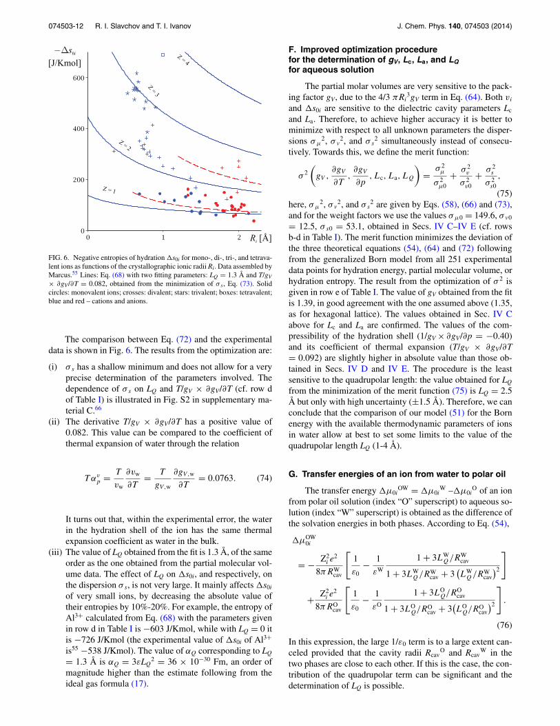
074503-12 R. I. Slavchov and T. I. Ivanov J. Chem. Phys. 140, 074503 (2014)

FIG. 6. Negative entropies of hydration �s0i for mono-, di-, tri-, and tetrava-lent ions as functions of the crystallographic ionic radii Ri. Data assembled byMarcus.55 Lines: Eq. (68) with two fitting parameters: LQ = 1.3 Å and T/gV

× ∂gV/∂T = 0.082, obtained from the minimization of σ s, Eq. (73). Solidcircles: monovalent ions; crosses: divalent; stars: trivalent; boxes: tetravalent;blue and red – cations and anions.

The comparison between Eq. (72) and the experimentaldata is shown in Fig. 6. The results from the optimization are:

(i) σ s has a shallow minimum and does not allow for a veryprecise determination of the parameters involved. Thedependence of σ s on LQ and T/gV × ∂gV/∂T (cf. row dof Table I) is illustrated in Fig. S2 in supplementary ma-terial C.66

(ii) The derivative T/gV × ∂gV/∂T has a positive value of0.082. This value can be compared to the coefficient ofthermal expansion of water through the relation

T αvp = T

vw

∂vw

∂T= T

gV,w

∂gV,w

∂T= 0.0763. (74)

It turns out that, within the experimental error, the waterin the hydration shell of the ion has the same thermalexpansion coefficient as water in the bulk.

(iii) The value of LQ obtained from the fit is 1.3 Å, of the sameorder as the one obtained from the partial molecular vol-ume data. The effect of LQ on �s0i, and respectively, onthe dispersion σ s, is not very large. It mainly affects �s0i

of very small ions, by decreasing the absolute value oftheir entropies by 10%-20%. For example, the entropy ofAl3+ calculated from Eq. (68) with the parameters givenin row d in Table I is −603 J/Kmol, while with LQ = 0 itis −726 J/Kmol (the experimental value of �s0i of Al3+

is55 −538 J/Kmol). The value of αQ corresponding to LQ

= 1.3 Å is αQ = 3εLQ2 = 36 × 10−30 Fm, an order of

magnitude higher than the estimate following from theideal gas formula (17).

F. Improved optimization procedurefor the determination of gV, Lc, La, and LQfor aqueous solution

The partial molar volumes are very sensitive to the pack-ing factor gV, due to the 4/3 πRi

3gV term in Eq. (64). Both vi

and �s0i are sensitive to the dielectric cavity parameters Lc

and La. Therefore, to achieve higher accuracy it is better tominimize with respect to all unknown parameters the disper-sions σμ

2, σ v2, and σ s

2 simultaneously instead of consecu-tively. Towards this, we define the merit function:

σ 2

(gV ,

∂gV

∂T,∂gV

∂p,Lc, La, LQ

)= σ 2

μ

σ 2μ0

+ σ 2v

σ 2v0

+ σ 2s

σ 2s0

,

(75)here, σμ

2, σ v2, and σ s

2 are given by Eqs. (58), (66) and (73),and for the weight factors we use the values σμ0 = 149.6, σ v0

= 12.5, σ s0 = 53.1, obtained in Secs. IV C–IV E (cf. rowsb-d in Table I). The merit function minimizes the deviation ofthe three theoretical equations (54), (64) and (72) followingfrom the generalized Born model from all 251 experimentaldata points for hydration energy, partial molecular volume, orhydration entropy. The result from the optimization of σ 2 isgiven in row e of Table I. The value of gV obtained from the fitis 1.39, in good agreement with the one assumed above (1.35,as for hexagonal lattice). The values obtained in Sec. IV Cabove for Lc and La are confirmed. The values of the com-pressibility of the hydration shell (1/gV × ∂gV/∂p = −0.40)and its coefficient of thermal expansion (T/gV × ∂gV/∂T= 0.092) are slightly higher in absolute value than those ob-tained in Secs. IV D and IV E. The procedure is the leastsensitive to the quadrupolar length: the value obtained for LQ

from the minimization of the merit function (75) is LQ = 2.5Å but only with high uncertainty (±1.5 Å). Therefore, we canconclude that the comparison of our model (51) for the Bornenergy with the available thermodynamic parameters of ionsin water allow at best to set some limits to the value of thequadrupolar length LQ (1-4 Å).

G. Transfer energies of an ion from water to polar oil

The transfer energy �μ0iOW = �μ0i

W –�μ0iO of an ion

from polar oil solution (index “O” superscript) to aqueous so-lution (index “W” superscript) is obtained as the difference ofthe solvation energies in both phases. According to Eq. (54),

�μOW0i

= − Z2i e

2

8πRWcav

[1

ε0− 1

εW

1 + 3LWQ/RW

cav

1 + 3LWQ/RW

cav + 3(LW

Q/RWcav

)2

]

+ Z2i e

2

8πROcav

[1

ε0− 1

εO

1 + 3LOQ/RO

cav

1 + 3LOQ/RO

cav + 3(LO

Q/ROcav

)2

].

(76)

In this expression, the large 1/ε0 term is to a large extent can-celed provided that the cavity radii Rcav

O and RcavW in the

two phases are close to each other. If this is the case, the con-tribution of the quadrupolar term can be significant and thedetermination of LQ is possible.

074503-13 R. I. Slavchov and T. I. Ivanov J. Chem. Phys. 140, 074503 (2014)

FIG. 7. Negative standard free energies for transfer of an ion from nitroben-zene to water �μ0i

OW [J/Kmol] for mono- and divalent ions as functions ofthe crystallographic ionic radii Ri [Å]. Experimental data from Refs. 64 and65. Lines: Eq. (76) with four fitting parameters: Lc

O = 0.71 Å, LaO = 0.08 Å,

LQO = 3.8 Å, and gV

O = 1.54. Solid circles: monovalent ions; crosses: diva-lent; blue and red – cations and anions.

Transfer energy data for nitrobenzene are available.64, 65

We compared Eq. (76) to the data for �μ0iOW of 13 ions, cf.

supplementary material D66 for the list. We minimized a meritfunction similar to Eq. (58) with respect to four parameters:gV

O, LcO, La

O, and LQO. The respective parameters for water

are taken as obtained from the optimization of Eq. (75) (cf.row e of Table I). For the dielectric permittivity of nitroben-zene we used the value εO = 34.8 × ε0 F/m.

The comparison between Eq. (76) and the measuredtransfer energies is shown in Fig. 7, and the obtained valuesof the fitting parameters are given in row f of Table I. In sum-mary:

(i) The standard deviation for the transfer energies �μ0iOW

is σμ = 8.8 kJ/mol; the deviation is highest for monova-lent cations.

(ii) The value obtained for gV, 1.54, suggests that the sol-vation shell of the ions in nitrobenzene is less denselypacked than in water, due to the large size of the nitroben-zene molecules.

(iii) According to Latimer-Pitzer-Slansky hypothesis, thevalue of Lc

O for a cation in nitrobenzene must correspondto the distance between the electron pair of an oxygenatom in the nitrogroup and the cation (compare to Fig. 3).Not surprisingly, within the error, the value obtained forthis distance (Lc

O = 0.71 Å) is the same as for a cation inwater. The positive charge of the nitrobenzene moleculeis delocalized towards benzene ring (-NO2 has negativemesomeric effect), and La

O is not easy to interpret. Weobtained the value La

O = 0.1 Å.(iv) For the quadrupolar length of liquid nitrobenzene we ob-

tained the value LQO = 3.8 Å. The respective quadrupo-

larizability follows from Eq. (27): αQO = 3εO(LQ

O)2

= 130 × 10−30 Fm. This can be compared to thequadrupolarizability of water: for LQ

W = 2.5 Å, αQW

= 3εW(LQW)2 = 130 × 10−30 Fm, i.e., both solvents have

similar quadrupolarizabilities. In nitrobenzene, however,the effect from the quadrupoles will be more pronouncedcompared to water due to the higher dielectric permittiv-ity of the latter. The effect of the quadrupolar lengths isto decrease the absolute values of the transfer energies ofthe small ions. For example, the transfer energy of Ca2+,according to Eq. (76) is −78 kJ/mol, while if LQ

W andLQ

O are set to 0, one obtains −93 kJ/mol (compare to theexperimental value: −68.3 kJ/mol).

V. CONCLUSIONS

Our work investigates the effects of the quadrupole mo-ment of the molecules in a medium on the properties ofcharged particles dissolved in this medium, using a macro-scopic approach based on the quadrupolar Coulomb-Amperelaw (26), generalizing the classical Poisson equation of elec-trostatics.

(i) We derived a new equation of state, Eq. (16), relatingthe macroscopic density of quadrupole moment Q andthe field gradient ∇E in gas of quadrupoles. The tensorQ has zero trace, unlike the one used in Refs. 12 and 13.Our constitutive relation involves a single scalar coeffi-cient, the quadrupolarizability αQ, which was estimatedto be αQ = 1 × 10−30 Fm or several times larger forwater.

(ii) We derived the boundary conditions needed for thefourth-order quadrupolar Coulomb-Ampere law (26) ata spherical surface between two media of differentdielectric permittivity ε and quadrupolarizability αQ,Eqs. (38) and (39).

(iii) The potential of a point charge in quadrupolar mediumis finite even at r = 0, cf. Eq. (43). This unexpected re-sult was obtained previously by Chitanvis12 with anotherconstitutive relation for Q.

As an illustration of the approach, we further inves-tigated the effect of quadrupolarizability on the Born en-ergy of an ion in solution. The classical model for a dis-solved ion as a charge in a cavity was generalized forthe case of quadrupolar medium. We had no intentionsto provide a complete theory of ion solvation, but ratherwe wanted to analyze the limits of the standard Poissonequation (4) and to search for cases where observabledeviations from the observations will occur due to theneglected multipole terms. This resulted in the follow-ing conclusions:

(iv) It was shown that the hydration energies �μ0i of all ionsare insensitive to the quadrupolar correction of Poissonequation. In contrast, the quadrupolarizability of wateraffects measurably (up to 10%-20%) the derivatives of�μ0i – partial molar volume vi and entropy for hydra-tion �s0i – of small ions in aqueous solution. From thiseffect and the experimental thermodynamic data for vi

and �s0i from Ref. 55, the value of the quadrupolarlength, LQ = (αQ/3ε)1/2 = 2.5 ± 1.5 Å, could be esti-mated.

074503-14 R. I. Slavchov and T. I. Ivanov J. Chem. Phys. 140, 074503 (2014)

(v) The transfer energies �μ0iOW of an ion from polar

oil to water have also been shown to depend on thequadrupolar lengths in both phases. Data for �μ0i

OW

in nitrobenzene were analyzed and they yield for LQ ofthis solvent the value 3.8 Å.

(vi) The order of magnitude of αQ and LQ obtained fromthese 3 sets of experimental data (vi, �s0i, and �μ0i

OW)compares well with the order predicted by otherauthors12,13 for other liquids.

(vii) The pressure and temperature derivatives of αQ were es-timated theoretically, cf. Eqs. (22) and (23). The esti-mated values of ∂αQ/∂p and ∂αQ/∂T show that the effectfrom these derivatives on the partial molar volume andentropy, Eqs. (64) and (68), of the dissolved ion is neg-ligible.

(viii) The pressure and temperature derivatives of the radius ofthe dielectric cavity Rcav around an ion were determinedfrom experimental data (Table I). From their values itcan be concluded that the structure of the hydration shellof an ion is about 10 times less compressible than thestructure of water. The thermal expansion coefficient isabout the same for the hydration shell and for pure water.

Although the results obtained here are encouraging, onemust not forget that our approach uses some strong approx-imations. First, the constitutive relation (16) is strictly validfor ideal gas only. The assumption that the equation of statekeeps the same form in dense liquid needs additional justi-fication. Also, our model for the dissolved ion (point chargein a cavity) is clearly an oversimplification, as discussed inSec. IV B. Nevertheless, we obtain self-consistent results andwe have enough proof to assert that quadrupolarizability hasmeasurable effect on many thermodynamic characteristics ofthe dissolved ions (vi, �s0i, and �μ0i

WO).The results obtained here for the equation of state for Q,

the boundary condition for the generalized Maxwell equationsof electrostatics, and the value of the quadrupolarizability αQ

of water will be used in the following study of this series forthe extension of the Debye-Hückel model for the activity co-efficient to quadrupolar media. It is also an interesting prob-lem to analyze both the interaction of the multipole moments(dipole, quadrupole, etc.) of the dissolved particle with thequadrupolar moment of the solvent,12, 13 on the one hand, andthe octupole moment of the solvent with the charge distribu-tion of the dissolved particle.36

ACKNOWLEDGMENTS

This work was funded by the Bulgarian National Sci-ence Fund Grant No. DDVU 02/12 from 2010. R. Slavchov isgrateful to the FP7 project BeyondEverest. Consultations withProfessor Alia Tadjer are gratefully acknowledged. A refereeof this paper contributed to certain extent to the model of thecavity used by us.

1P. Debye and E. Hückel, Phys. Z. 24, 185 (1923).2R. A. Robinson and R. H. Stokes, Electrolyte Solutions (Butterworth Sci-entific Publications, London, 1959).

3L. G. Gouy, J. Phys. (Paris) 9, 457 (1910).4H. Ohshima, Theory of Colloid And Interfacial Electric Phenomena (Else-vier, 2006).

5J. T. Davies, Proc. R. Soc. London, Ser. A 245, 417 (1958).6J. T. Davies and E. Rideal, Interfacial Phenomena (Academic, New York,1963).

7I. Langmuir, J. Chem. Phys. 6, 873 (1938).8B. V. Derjaguin and L. D. Landau, Acta Physicochim. URSS 14, 633(1941).

9E. J. W. Verwey and J. T. G. Overbeek, Theory of the Stability of LyophobicColloids (Elsevier, Amsterdam, 1948).

10M. von Smoluchowski, Bull. Int. Acad. Sci. Cracovie 1903, 184.11J. D. Jackson, Classical Electrodynamics, 1st ed. (John Wiley & Sons, Inc.,

New York, 1962); 3rd ed. (John Wiley & Sons, Inc., New York, 1962).12S. M. Chitanvis, J. Chem. Phys. 104, 9065 (1996).13J. Jeon and H. J. Kim, J. Chem. Phys. 119, 8606 (2003).14H. Fröhlich, Theory of Dielectrics (Clarendon, Oxford, 1958).15J. J. Bikerman, Philos. Magn. 33, 384 (1942).16D. Ben-Yaakov, D. Andelman, D. Harries, and R. Podgornik, J. Phys.: Con-

dens. Matter 21, 424106 (2009).17J. M. G. Barthel, H. Krienke, and W. Kunz, Physical Chemistry of

Electrolyte Solutions – Modern Aspects, edited by Deutsche Bunsen-Gesellschaft für Physicalische Chemie e.V. (Steinkopff, Darmstadt, 1998).

18B. W. Ninham and V. Yaminsky, Langmuir 13, 2097 (1997).19I. B. Ivanov, R. I. Slavchov, E. S. Basheva, D. Sidzhakova, and S. I. Karaka-

shev, Adv. Colloid Interface Sci. 168, 93 (2011).20D. Frydel, J. Chem. Phys. 134, 234704 (2011).21D. D. Eley and M. G. Evans, Trans. Faraday Soc. 34, 1093 (1938).22J. N. Israelachvili, Intermolecular and Surface Forces, 3rd ed. (Elsevier,

2011).23S. Levine, K. Robinson, G. M. Bell, and J. Mingins, J. Electroanal. Chem.

38, 253 (1972).24A. Levy, D. Andelman, and H. Orland, Phys. Rev. Lett. 108, 227801

(2012).25V. N. Paunov, R. I. Dimova, P. A. Kralchevsky, G. Broze, and A.

Mehreteab, J. Colloid Interface Sci. 182, 239 (1996).26K. J. Laidler and C. Pegis, Proc. R. Soc. London, Ser. A 241, 80

(1957).27P. J. Stiles, Aust. J. Chem. 33, 1389 (1980).28T. Abe, J. Phys. Chem. 90, 713 (1986).29R. R. Dogonadze and A. A. Kornyshev, J. Chem. Soc., Faraday Trans. 2

70, 1121 (1974).30S. Buyukdagli and T. Ala-Nissila, Phys. Rev. E 87, 063201 (2013).31M. V. Basilevsky and D. F. Parsons, J. Chem. Phys. 108, 9107 (1998).32M. V. Basilevsky and D. F. Parsons, J. Chem. Phys. 108, 9114 (1998).33R. A. Satten, J. Chem. Phys. 26, 766 (1957).34D. Adu-Gyamfi and B. U. Felderhof, Physica A 81, 295 (1975).35E. B. Graham and R. E. Raab, Proc. R. Soc. London, Ser. A 390, 73

(1983).36R. E. Raab and O. L. de Lange, Multipole Theory in Electromagnetism

(Clarendon, Oxford, 2005).37E. R. Batista, S. S. Xantheas, and H. Jonsson, J. Chem. Phys. 109, 4546

(1998).38A. D. Buckingham, Q. Rev. Chem. Soc. 13, 183 (1959).39E. B. Graham and R. E. Raab, Proc. R. Soc. London, Ser. A 456, 1193

(2000).40V. V. Batygin and I. N. Toptygin, Sbornik Zadach po Elektrodinamike i

Spetzialnoy Teorii Otnositelnosti, 4th ed. (Lan, 2010), p. 283 (in Russian).41D. Adu-Gyamfi, Physica A 108, 205 (1981).42D. E. Logan, Mol. Phys. 46, 271 (1982).43A. D. McLean and M. Yoshimine, J. Chem. Phys. 47, 1927 (1967).44L. D. Landau and E. M. Lifshitz, The Classical Theory of Fields, 7th ed.

(Nauka, Moscow, 1988) (in Russian); Chap. 5 (Butterworth-Heinemann,1980) (in English).

45O. L. de Lange and R. E. Raab, Phys. Rev. E 71, 036620 (2005).46C R C Handbook of Chemistry and Physics, edited by W. M. Haynes (CRC,

New York, 2011).47D. Bedeaux and J. Vlieger, Optical Properties of Surfaces (Imperial Col-

lege, London, 2002), 2nd ed.48A. M. Albano, D. Bedeaux, and J. Vlieger, Physica A 102, 105 (1980).49M. Born, Z. Phys. 1, 45 (1920).50W. M. Latimer, K. S. Pitzer, and C. M. Slansky, J. Chem. Phys. 7, 108

(1939).51T. T. Duignan, D. F. Parsons, and B. W. Ninham, J. Phys. Chem. B 117,

9412 (2013).52T. T. Duignan, D. F. Parsons, and B. W. Ninham, J. Phys. Chem. B 117,

9421 (2013).

074503-15 R. I. Slavchov and T. I. Ivanov J. Chem. Phys. 140, 074503 (2014)

53M. H. Abraham and J. Liszi, J. Chem. Soc., Faraday Trans. I 74, 1604(1978).

54M. H. Abraham and J. Liszi, J. Chem. Soc., Faraday Trans. I 74, 2858(1978).

55Y. Marcus, Ion Properties (Marcel Dekker, New York, 1997).56A. A. Rashin and B. Honig, J. Phys. Chem. 89, 5588 (1985).57L. Blum and W. R. Fawcett, J. Phys. Chem. 96, 408 (1992).58W. R. Fawcett, J. Phys. Chem. B 103, 11181 (1999).59M. W. Mahoney and W. L. Jorgensen, J. Chem. Phys. 112, 8910

(2000).60Y. Marcus, Chem. Rev. 111, 2761 (2011).61D. G. Archer and P. Wang, J. Phys. Chem. Ref. Data 19, 371 (1990).62A. Passinsky, Acta Physicochim. URSS 8, 385 (1938).63J. Padova, J. Chem. Phys. 40, 691 (1964).

64J. Koryta, J. Dvorak, and L. Kavan, Principles Of Electrochemistry, 2nd ed.(John Wiley & Sons, Chichester, 1993).

65F. Scholz, R. Gulaboski, and K. Caban, Electrochem. Commun. 5, 929(2003).

66See supplementary material at http://dx.doi.org/10.1063/1.4865878 for (A)derivation of the macroscopic Maxwell equations of electrostatics with ac-count for the quadrupole moment. (B) Born energy of an ion modeled as aconducting sphere placed into a cavity. (C) Analysis of the merit function ofthe optimization problems for the partial molecular volumes and entropiesof ions in aqueous solution. (D) Data-table of the crystallographic radii, thehydration free energies, the partial molar volumes, the hydration entropiesused for the determination of LQ in water (from Refs. 55 and 53), andthe transfer energies of an ion from nitrobenzene to water (from Refs. 64and 65).