
Maxwell-Stefan diffusion asymptotics for gas mixtures in non ...
14
MAXWELL-STEFAN DIFFUSION ASYMPTOTICS FOR GAS MIXTURES IN NON-ISOTHERMAL SETTING HARSHA HUTRIDURGA AND FRANCESCO SALVARANI Abstract. A mathematical model is proposed where the classical Maxwell-Stefan diffusion model for gas mixtures is coupled to an advection-type equation for the temperature of the physical system. This coupled system is derived from first principles in the sense that the starting point of our analysis is a system of Boltzmann equations for gaseous mixtures. We perform an asymptotic analysis on the Boltzmann model under diffuse scaling to arrive at the proposed coupled system. 1. Introduction The Maxwell-Stefan theory [23, 27] has been the most successful approach for describing diffusive phenomena in gaseous mixtures, and it is now the reference model for studying multicomponent diffusion. The Maxwell-Stefan system is a coupled system of cross-diffusion equations and it is commonly used in many scientific fields, for e.g., in engineering [22] and in medical sciences [7, 28]. Despite its current utility, the mathematical studies on the subject are however quite recent (see [17, 15, 16, 18]). In particular, existence and uniqueness issues, as well as the long-time behaviour, have been considered in [6, 10, 21, 13], whereas [24] deals with the numerical study of the Maxwell-Stefan equations. In [11], the authors provide the formal derivation of the Maxwell-Stefan diffusion equations starting from the non-reactive elastic Boltzmann system for monatomic gaseous mixtures [12, 14, 9]. They show that the zeroth and first order moments of appropriate solutions of the Boltzmann system, in the diffusive scaling and for vanishing Mach and Knudsen numbers limit, formally converge to the solution of the Maxwell-Stefan equations. This result, which lies in the research line introduced by Bardos, Golse and Levermore in [1, 2, 3], has been obtained in the framework of Maxwellian cross sections. Subsequently, the approach of [11] has been generalized in [8], where the Maxwell-Stefan diffusion coefficients have been written in terms of explicit formulas with respect to the cross-sections, and in [20] where the explicit dependence of the Maxwell-Stefan binary diffusion coefficients with respect to the temperature of the mixture has been obtained for general analytical cross sections satisfying Grad’s cutoff assumption [19]. All the previous results have been obtained in the isothermal case. However, as pointed out by Krishna and Wesselingh, “perfectly isothermal systems are rare in chemical engineering practice and many processes such as distillation, absorption, condensation, evaporation and drying involve the simultaneous transfer of mass and energy across phase interfaces” [22, p.876]. For this reason, it is natural to extend the strategy of [11] to the non-isothermal case, and this is the purpose of the present article: we provide here the asymptotics of the Boltzmann system for monatomic mixtures that leads to a non-isothermal form of the Maxwell-Stefan equations, and thus we can take into account the thermal diffusion contribution to the molar fluxes (thermophoresis). We postulate that the solution of the Boltzmann system keeps the structure of a local Maxwellian and then we deduce, in the standard diffusive limit, the coupled relationships satisfied by the 1
-
Upload
khangminh22 -
Category
Documents
-
view
0 -
download
0
Transcript of Maxwell-Stefan diffusion asymptotics for gas mixtures in non ...

MAXWELL-STEFAN DIFFUSION ASYMPTOTICS FOR GAS MIXTURESIN NON-ISOTHERMAL SETTING
HARSHA HUTRIDURGA AND FRANCESCO SALVARANI
Abstract. A mathematical model is proposed where the classical Maxwell-Stefan diffusion modelfor gas mixtures is coupled to an advection-type equation for the temperature of the physicalsystem. This coupled system is derived from first principles in the sense that the starting point ofour analysis is a system of Boltzmann equations for gaseous mixtures. We perform an asymptoticanalysis on the Boltzmann model under diffuse scaling to arrive at the proposed coupled system.
1. Introduction
The Maxwell-Stefan theory [23, 27] has been the most successful approach for describing diffusivephenomena in gaseous mixtures, and it is now the reference model for studying multicomponentdiffusion. The Maxwell-Stefan system is a coupled system of cross-diffusion equations and it iscommonly used in many scientific fields, for e.g., in engineering [22] and in medical sciences [7, 28].
Despite its current utility, the mathematical studies on the subject are however quite recent(see [17, 15, 16, 18]). In particular, existence and uniqueness issues, as well as the long-timebehaviour, have been considered in [6, 10, 21, 13], whereas [24] deals with the numerical study ofthe Maxwell-Stefan equations.
In [11], the authors provide the formal derivation of the Maxwell-Stefan diffusion equationsstarting from the non-reactive elastic Boltzmann system for monatomic gaseous mixtures [12, 14, 9].They show that the zeroth and first order moments of appropriate solutions of the Boltzmannsystem, in the diffusive scaling and for vanishing Mach and Knudsen numbers limit, formallyconverge to the solution of the Maxwell-Stefan equations. This result, which lies in the researchline introduced by Bardos, Golse and Levermore in [1, 2, 3], has been obtained in the framework ofMaxwellian cross sections. Subsequently, the approach of [11] has been generalized in [8], where theMaxwell-Stefan diffusion coefficients have been written in terms of explicit formulas with respect tothe cross-sections, and in [20] where the explicit dependence of the Maxwell-Stefan binary diffusioncoefficients with respect to the temperature of the mixture has been obtained for general analyticalcross sections satisfying Grad’s cutoff assumption [19].
All the previous results have been obtained in the isothermal case. However, as pointed out byKrishna and Wesselingh, “perfectly isothermal systems are rare in chemical engineering practiceand many processes such as distillation, absorption, condensation, evaporation and drying involvethe simultaneous transfer of mass and energy across phase interfaces” [22, p.876].
For this reason, it is natural to extend the strategy of [11] to the non-isothermal case, and thisis the purpose of the present article: we provide here the asymptotics of the Boltzmann system formonatomic mixtures that leads to a non-isothermal form of the Maxwell-Stefan equations, and thuswe can take into account the thermal diffusion contribution to the molar fluxes (thermophoresis).We postulate that the solution of the Boltzmann system keeps the structure of a local Maxwellianand then we deduce, in the standard diffusive limit, the coupled relationships satisfied by the
1

2 HARSHA HUTRIDURGA AND FRANCESCO SALVARANI
densities, the fluxes and the temperature at the macroscopic level which guarantee that the localMaxwellian structure is preserved by the time evolution of the system.
A major question is posed by the closure relationship. Indeed, as in the case of the Maxwell-Stefan system, the resulting equations for the densities, the fluxes and the temperature are, in thediffusive limit, linearly dependent and an additional equation between the unknowns is necessaryin order to close it. As it is well known, in the isothermal Maxwell-Stefan system, the closurerelationship consists in supposing that the sum of all molar fluxes J
i
is locally identically zero.This supplementary equation could be incompatible with some experimental behaviours in the non-isothermal setting: as pointed out in [22], indeed, in chemical vapour deposition (CVD) processes,thermal diffusion causes large, heavy gas molecules (for e.g., WF
6
) to concentrate in cold regionswhereas small, light molecules (such as H
2
) to concentrate in hot regions. Hence, non-isothermalsystems could require new closure relationships which, of course, relax to the isothermal one whenthe temperature is uniform in time and constant in space.
The closure relation that we suggest is the following: sum of the molar fluxes J
i
is locallyproportional to the gradient of the total molar concentration, i.e.,
nX
i=1
J
i
= �↵rc
tot
.
With respect to the above mentioned closure relation, we characterize the total molar concentrationc
tot
and the temperature field T (t, x) as solutions to a coupled system of evolution equations.Furthermore, the temperature-dependent flux-gradient relations derived in this paper – see secondline of (24) – implies that the product c
tot
T is space-independent. Hence the above mentionedclosure relation postulated in this paper recovers the standard closure relation – sum of the molarfluxes J
i
being locally identically zero – in the isothermal case.The outline of the paper is as follows: In subsection 2.1, we introduce the kinetic model – system
of Boltzmann equations for gas mixtures – and present the assumptions made on the Boltzmanncollision kernels (Maxwellian molecules). Subsection 2.2 deals with the scaling considered in thiswork and the main assumption made on the solutions to the scaled mesoscopic kinetic model.In subsection 2.3 we derive the balance laws (mass, momentum and energy) – see Proposition 1.Emphasis is given on computing the coefficients in the balance laws – given in terms of the velocityaverages of certain statistical quantities. A formal asymptotic analysis (in the mean free path goingto zero limit) is performed in subsection 2.4 which culminates in Theorem 2. Subsection 2.5 dealswith the closure relation. Finally, in subsection 2.6, we derive some qualitative properties on thetotal concentration c
tot
(t, x) and the temperature field T (t, x).
2. Kinetic model and asymptotics
2.1. Kinetic model. The starting point of our analysis is a system of Boltzmann-type equationsthat models the evolution of a mixture of ideal monatomic inert gases A
i
, i = 1, . . . , n withn � 2, subject to elastic mechanical collisions between each other. More precisely, for the unknownprobability density functions f
i
(t, x, v) � 0, we consider the Cauchy problem
@
t
f
i
+ v ·rx
f
i
=
nX
j=1
Q
ij
(f
i
, f
j
) for (t, x, v) 2 (0,1)⇥ R3 ⇥ R3
,(1)
f
i
(0, x, v) = f
in
i
(x, v) for (x, v) 2 R3 ⇥ R3
,(2)

MAXWELL-STEFAN MODEL IN NON-ISOTHERMAL SETTING 3
for each i = 1, . . . , n where Q
ij
(·, ·) denotes the bilinear integral operator describing the collisionsof molecules of species A
i
with molecules of species Aj
. In the above model, we have supposed thatthere are no external forces acting on the gas mixture. Hence any given particle travels in a straightline (ballistic motion) until it encounters another particle resulting in a mechanical collision whichis assumed here to be elastic. To facilitate the definition of the collision operator Q
ij
(·, ·), considertwo particles belonging to the species A
i
and Aj
, 1 i, j n, with masses m
i
, m
j
, and pre-collisional velocities v0, v0⇤. A microscopic collision is an instantaneous phenomenon which modifiesthe velocities of the particles, which become v and v⇤, obtained by imposing the conservation ofboth momentum and kinetic energy:
(3) m
i
v
0+m
j
v
0⇤ = m
i
v +m
j
v⇤,1
2
m
i
|v0|2 + 1
2
m
j
|v0⇤|2 =1
2
m
i
|v|2 + 1
2
m
j
|v⇤|2.
The previous equations allow us to write v
0 and v
0⇤ in terms of v and v⇤:
(4) v
0=
1
m
i
+m
j
(m
i
v +m
j
v⇤ +m
j
|v � v⇤|�), v
0⇤ =
1
m
i
+m
j
(m
i
v +m
j
v⇤ �m
i
|v � v⇤|�),
where � 2 S2 describes the two degrees of freedom in (3).If f and g are nonnegative functions, the operator describing the collisions between molecules of
species Ai
and molecules of species Aj
is defined by
(5) Q
ij
(f, g)(v) :=
ZZ
R3⇥S2
B
ij
(v, v⇤,�)hf(v
0)g(v
0⇤)� f(v)g(v⇤)
id� dv⇤
where v0 and v
0⇤, are given by the relation (4), and the cross sections B
ij
satisfy the microreversibilityassumptions: B
ij
(v, v⇤,�) = B
ji
(v⇤, v,�) and B
ij
(v, v⇤,�) = B
ij
(v
0, v
0⇤,�).
The operators Q
ij
can be written in weak form. For example, by using the changes of variables(v, v⇤) 7! (v⇤, v) and (v, v⇤) 7! (v
0, v
0⇤), we have
(6)Z
R3
Q
ij
(f, g)(v) (v) dv
= �1
2
ZZZ
R6⇥S2
B
ij
(v, v⇤,�)hf(v
0)g(v
0⇤)� f(v)g(v⇤)
ih (v
0)� (v)
id� dv dv⇤
=
ZZZ
R6⇥S2
B
ij
(v, v⇤,�) f(v)g(v⇤)h (v
0)� (v)
id� dv dv⇤,
or
(7)Z
R3
Q
ij
(f, g)(v) (v) dv +
Z
R3
Q
ji
(g, f)(v)�(v) dv
= �1
2
ZZZ
R6⇥S2
B
ij
(v, v⇤,�)hf(v
0)g(v
0⇤)� f(v)g(v⇤)
ih (v
0) + �(v
0⇤)� (v)� �(v⇤)
id� dv dv⇤,
for any , � : R3 ! R such that the integrals on the left hand sides of (6) and (7) are well defined.

4 HARSHA HUTRIDURGA AND FRANCESCO SALVARANI
The collision kernels B
ij
only depend on the modulus of the relative velocity and on the cosineof the deviation angle, i.e.,
B
ij
(v, v⇤,�) = B
ij
(|v � v⇤|, cos ✓) with cos ✓ =
v � v⇤|v � v⇤| · �.
In order to ease the presentation and also to ensure that the resulting mathematical model for themolar concentrations be simple, throughout this work we stick to the case of Maxwellian molecules.More specifically, we shall work with collision kernels that are independent of the relative velocity,i.e., they are of the form
B
ij
(v, v⇤,�) = b
ij
(cos ✓),(8)
where we assume that the angular collision kernels b
ij
2 L
1
(�1,+1) and are even. Observe that,because of the microreversibility assumption on the collision kernels, we have
B
ij
(v, v⇤,�) = B
ji
(v⇤, v,�) =) b
ij
✓v � v⇤|v � v⇤| · �
◆= b
ji
✓v⇤ � v
|v � v⇤| · �◆,
and that, by parity, bij
(cos ✓) = b
ji
(cos ✓).
Remark 1. Taking (v) = 1 in the weak form (6), yields
(9)Z
R3
Q
ij
(f, g)(v) dv = 0 for all i, j = 1, . . . , n
which helps us deduce the conservation of the total number of molecules of species Ai
. Moreoverin (7), if (v) = m
i
v and �(v⇤) = m
j
v⇤, and then if (v) = m
i
|v|2/2 and �(v) = m
j
|v⇤|2/2, werecover the conservation of the total momentum and of the total kinetic energy during the collisionbetween a particle of species A
i
and a particle of species Aj
:Z
R3
Q
ij
(f, g)(v)
✓m
i
v
m
i
|v|2/2◆
dv +
Z
R3
Q
ji
(g, f)(v)
✓m
j
v
m
j
|v|2/2◆
dv = 0.
2.2. Diffuse scaling and main assumptions. In order to arrive at the diffusive limit, we intro-duce a scaling parameter 0 < "⌧ 1 which represents the mean free path. The space-time variablesare scaled as (t, x) 7! ("
2
t, "x). Note that the velocity variable is not scaled. The unknown dis-tribution functions in the transformed variables are denoted by f
"
i
. Each distribution function f
"
i
solves the following scaled version of (1)-(2):
" @
t
f
"
i
+ v ·rx
f
"
i
=
1
"
nX
j=1
Q
ij
(f
"
i
, f
"
j
) for (t, x, v) 2 (0,1)⇥ R3 ⇥ R3
,(10)
f
"
i
(0, x, v) =
�f
in
i
�"
(x, v) for (x, v) 2 R3 ⇥ R3
.(11)
The initial data are assumed to be such that the associated local macroscopic velocities are of O("),i.e., Z
R3
v
�f
in
i
�"
(x, v) dv = " c
in
i
(x)u
in
i
(x)
for some c
in
i
: R3 ! [0,1) and u
in
i
: R3 ! R3.The main assumption in our work is that the evolution following (10) keeps the distribution
functions f "
i
(t, x, v) in local Maxwellian states. We hence suppose that there exist the local densities

MAXWELL-STEFAN MODEL IN NON-ISOTHERMAL SETTING 5
c
"
i
: [0,1) ⇥ R3 ! [0,1), the local macroscopic velocities u
"
i
: [0,1) ⇥ R3 ! R3 and the localtemperatures T "
i
: [0,1)⇥R3 ! [0,1) such that the solution to the scaled Boltzmann system (10)has the following Maxwellian structure:
f
"
i
(t, x, v) = c
"
i
(t, x)
✓m
i
2⇡kT
"
i
(t, x)
◆3/2
e
�m
i
|v�"u
"
i
(t,x)|2/2kT "
i
(t,x)(12)
where k is the Boltzmann constant. We record the zeroth, first and second moments for the aboveMaxwellian states:Z
R3
f
"
i
(t, x, v)
0
@1
v
|v|2
1
Adv =
0
B@c
"
i
(t, x)
" c
"
i
(t, x)u
"
i
(t, x)
3k
m
i
c
"
i
(t, x)T
"
i
(t, x) + "
2
c
"
i
(t, x)|u"i
(t, x)|2
1
CA .(13)
notation: For ` 2 {1, 2, 3}, we denote by w
(`)
the `-th component of any vector w 2 R3.Note that we postulate the ansatz (12) for the distribution functions. This line of attack to addressdiffusion limit procedures in the context of Boltzmann models is borrowed from [11, 20]. Also, notethat the choice of O(") local macroscopic velocities in the ansatz (12) results in the first moment ofthe distribution functions to be of O(") since we are only interested in the pure diffusive dynamics.
2.3. Balance laws. To derive a macroscopic description out of the mesoscopic dynamics of theBoltzmann-type equations such as (10), we need to arrive at balance equations obtained by in-tegrating the transport model (10) with respect to the velocity variable v only. The next resultrecords various macroscopic equations associated with the scaled Boltzmann-like system (10)-(11).
Proposition 1. Suppose that the evolution according to (10) keeps the distribution functionsf
"
i
(t, x, v) in the local Maxwellian states (12) for all time t > 0. Then, the local macroscopicobservables (c
"
i
, u
"
i
, T
"
) solve the following equations. We have the mass balance equations:
@
t
c
"
i
+rx
· (c"i
u
"
i
) = 0 for (t, x) 2 (0,1)⇥ R3
,(14)
for each 1 i n. We further have the momentum balance:
"
2
⇣@
t
(c
"
i
u
"
i
) +rx
· (c"i
u
"
i
⌦ u
"
i
)
⌘+
k
m
i
rx
(c
"
i
T
"
i
) = ⇥
"
i
for (t, x) 2 (0,1)⇥ R3
,(15)
for each 1 i n, where the right hand side of (15) reads
⇥
"
i
(t, x) =
X
j 6=i
2⇡kbij
kL
1
m
j
m
i
+m
j
⇣c
"
i
c
"
j
u
"
j
� c
"
j
c
"
i
u
"
i
⌘+O(").(16)
Furthermore, the energy balance reads
"
✓3k
m
i
@
t
(c
"
i
T
"
i
) +
5k
m
i
rx
· (c"i
T
"
i
u
"
i
)
◆+ "
3
✓@
t
�c
"
i
|u"i
|2�+ 3k
m
i
rx
· �c"i
T
"
i
|u"i
|2u"i
�◆= ⌅
"
i
(17)
for (t, x) 2 (0,1)⇥ R3 and for each 1 i n, where the right hand side of (17) reads
(18)
⌅
"
i
(t, x) =
1
"
X
j 6=i
kbij
kL
1
m
j
(m
i
+m
j
)
2
c
"
i
c
"
j
�T
"
i
� T
"
j
�
+ "
X
j 6=i
2kbij
kL
1c
"
i
c
"
j
m
j
✓(m
j
u
"
j
+m
i
u
"
i
) · (u"j
� u
"
i
)
(m
i
+m
j
)
2
◆.

6 HARSHA HUTRIDURGA AND FRANCESCO SALVARANI
Proof. To arrive at the balance equations (14)-(15)-(17), multiply the scaled equation (10) by(1, v
(`)
, |v|2) and integrate over all possible velocities in R3 yielding
" @
t
Z
R3
f
"
i
(t, x, v)
0
@1
v
(`)
|v|2
1
Adv +r
x
·Z
R3
vf
"
i
(t, x, v)
0
@1
v
(`)
|v|2
1
Adv =
1
"
nX
j=1
Z
R3
Q
ij
(f
"
i
, f
"
j
)
0
@1
v
(`)
|v|2
1
Adv.
(19)
The assumption of Maxwellian structure (12) on the solution f
"
i
(t, x, v) helps us compute thedivergence term in the second line on the left hand side of the above equation:
(20)
rx
·0
@Z
R3
v
(`)
f
"
i
(t, x, v)v dv
1
A
=
k
m
i
@
@x
(`)
⇣c
"
i
(t, x)T
"
i
(t, x)
⌘+ "
2
3X
k=1
@
@x
(k)
⇣c
"
i
(t, x) (u
"
i
)
(k)
(t, x) (u
"
i
)
(`)
(t, x)
⌘.
Next, we have for the divergence term in the third line on the left hand side of (19):
rx
·0
@Z
R3
|v|2vf "
i
(v) dv
1
A=
3X
k=1
@
@x
(k)
Z
R3
�|v(1)
|2 + |v(2)
|2 + |v(3)
|2� v(k)
f
"
i
(v) dv
=
3X
k=1
@
@x
(k)
Z
R3
⇣|v
(1)
+ " (u
"
i
)
(1)
|2 + |v(2)
+ " (u
"
i
)
(2)
|2 + |v(3)
+ " (u
"
i
)
(3)
|2⌘⇥
⇣v
(k)
+ " (u
"
i
)
(k)
⌘c
"
i
(t, x)
✓m
i
2⇡kT
"
i
(t, x)
◆3/2
e
�m
i
|v|22kT
"
i
(t,x)
dv.
Therefore, we have:
rx
·0
@Z
R3
|v|2vf "
i
(v) dv
1
A= "
5k
m
i
rx
· (c"i
T
"
i
u
"
i
) + "
3
3k
m
i
rx
· �c"i
T
"
i
|u"i
|2u"i
�.(21)
Observation (9) in Remark 1 implies that the first line on the right hand side of (19) vanishes.Under the Maxwellian molecules assumption (8) and under the local Maxwellian states assumption(12) on the solution f
"
i
(t, x, v), the second line on the right hand side of (19) has already beencomputed by L. Boudin, B. Grec and F. Salvarani [11, Section 4]. We will simply borrow the endresult of their computation below:
1
"
nX
j=1
Z
R3
v
(`)
Q
ij
(f
"
i
, f
"
j
)(v) dv =
X
j 6=i
2⇡m
j
kbij
kL
1
m
i
+m
j
⇣c
"
i
c
"
j
�u
"
j
�(`)
� c
"
j
c
"
i
(u
"
i
)
(`)
⌘+O(").(22)

MAXWELL-STEFAN MODEL IN NON-ISOTHERMAL SETTING 7
On the other hand to arrive at the expression (18), let us consider the right hand side of the thirdline in (19):1
"
X
j 6=i
Z
R3
|v|2Qij
(f
"
i
, f
"
j
) dv =
1
"
X
j 6=i
ZZZ
R6⇥S2
B
ij
(v, v⇤,�)f"
i
(v)f
"
j
(v⇤)�|v0|2 � |v|2� d� dv dv⇤
=
1
"
X
j 6=i
3X
`=1
ZZZ
R6⇥S2
B
ij
(v, v⇤,�)f"
i
(v)f
"
j
(v⇤)⇣|v0
(`)
|2 � |v(`)
|2⌘d� dv dv⇤
where we have used the weak form (6) with (v) = |v|2. Next, using the relation (4), the aboveexpression can be further simplified as
1
"
X
j 6=i
Z
R3
|v|2Qij
(f
"
i
, f
"
j
) dv =
1
"
X
j 6=i
3X
`=1
kbij
kL
1
✓m
2
i
(m
i
+m
j
)
2
� 1
◆ZZ
R6
f
"
i
(v)f
"
j
(v⇤)|v(`)
|2 dv dv⇤
+
1
"
X
j 6=i
3X
`=1
kbij
kL
1
m
2
j
(m
i
+m
j
)
2
ZZ
R6
f
"
i
(v)f
"
j
(v⇤)|v⇤(`)|2 dv dv⇤
+
1
"
X
j 6=i
3X
`=1
kbij
kL
1
2m
i
m
j
(m
i
+m
j
)
2
ZZ
R6
f
"
i
(v)f
"
j
(v⇤)v(`)
v⇤(`) dv dv⇤
+
1
"
X
j 6=i
3X
`=1
2
(m
i
+m
j
)
2
ZZZ
R6⇥S2
B
ij
(v, v⇤,�)f"
i
(v)f
"
j
(v⇤)⇥
�m
i
m
j
|v � v⇤|v(`)
+m
2
j
|v � v⇤|v⇤(`)��
(`)
d� dv dv⇤
+
1
"
X
j 6=i
3X
`=1
m
2
j
(m
i
+m
j
)
2
ZZZ
R6⇥S2
B
ij
(v, v⇤,�)f"
i
(v)f
"
j
(v⇤)|v � v⇤|2|�(`)
|2 d� dv dv⇤
=: I1
+ I2
+ I3
+ I4
+ I5
.
Substituting the local Maxwellian structure (12) for the distribution function f
"
i
(t, x, v) in the aboveintegrals and computing the thus obtained Gaussian integrals yield
I1
=
1
"
X
j 6=i
✓kb
ij
kL
1
✓m
2
i
(m
i
+m
j
)
2
� 1
◆c
"
i
c
"
j
3kT
"
i
m
i
+ "
2kbij
kL
1
✓m
2
i
(m
i
+m
j
)
2
� 1
◆c
"
i
c
"
j
|u"i
|2◆,
I2
=
1
"
X
j 6=i
kb
ij
kL
1
m
2
j
(m
i
+m
j
)
2
c
"
i
c
"
j
3kT
"
j
m
j
+ "
2kbij
kL
1
m
2
j
(m
i
+m
j
)
2
c
"
i
c
"
j
|u"j
|2!,
I3
=
1
"
X
j 6=i
✓"
2kbij
kL
1
2m
i
m
j
(m
i
+m
j
)
2
c
"
i
c
"
j
�u
"
i
· u"j
�◆.
Now, to treat the integral I4
, let us introduce the polar variable ' 2 [0, 2⇡] so that we can find therelationships between the Euclidean coordinates of � and the spherical ones, namely
�
(1)
= sin ✓ cos', �
(2)
= sin ✓ sin', �
(3)
= cos ✓.

8 HARSHA HUTRIDURGA AND FRANCESCO SALVARANI
In the integral I4
, note that the terms for ` = 1 or 2 in the sum are zero because
2⇡Z
0
sin' d' =
2⇡Z
0
cos' d' = 0,
and for ` = 3, because b
ij
is even, one has
Z
S2
b
ij
✓v � v⇤|v � v⇤| · �
◆�
(3)
d� = 2⇡
⇡Z
0
sin ✓ cos ✓ b
ij
(cos ✓) d✓ = 2⇡
1Z
�1
⌘ b
ij
(⌘) d⌘ = 0.
Hence the integral I4
vanishes. Next, we get to the computation of the integral I5
. Before we gofurther, we make the following observation:
3X
`=1
Z
S2
B
ij
(v, v⇤,�)|�(`)
|2 d� =
Z
S2
B
ij
(v, v⇤,�) d� = kbij
kL
1
because |�|2 = 1. Hence the integral I5
reduces to
I5
=
1
"
X
j 6=i
kbij
kL
1
m
2
j
(m
i
+m
j
)
2
ZZ
R6
f
"
i
(v)f
"
j
(v⇤)|v � v⇤|2 dv dv⇤.
Substituting the local Maxwellian structures (12) for the distribution functions f
"
i
and performingthe change of variables: (v, v⇤) 7! (v + "u
"
i
, v⇤ + "u
"
j
) yields
I5
=
1
"
X
j 6=i
kbij
kL
1
m
2
j
(m
i
+m
j
)
2
c
"
i
c
"
j
✓m
i
2⇡kT
"
i
◆3/2
m
j
2⇡kT
"
j
!3/2
⇥ZZ
R6
��v + "u
"
i
� v⇤ � "u
"
j
��2e
�m
i
|v|2/2kT "
i
e
�m
j
|v⇤|2/2kT "
j
dv dv⇤
=
1
"
X
j 6=i
kbij
kL
1
m
2
j
(m
i
+m
j
)
2
c
"
i
c
"
j
✓m
i
2⇡kT
"
i
◆3/2
m
j
2⇡kT
"
j
!3/2
⇥
3X
`=1
ZZ
R6
⇣|v
(`)
|2 + "
2| (u"i
)
(`)
|2 + 2"v
(`)
(u
"
i
)
(`)
+ |v⇤(`)|2 + "
2| �u"j
�(`)
|2 + 2"v⇤(`)�u
"
j
�(`)
� 2v
(`)
v⇤(`) � 2"v
(`)
�u
"
j
�(`)
� 2"v⇤(`) (u"
i
)
(`)
� 2"
2
(u
"
i
)
(`)
�u
"
j
�(`)
⌘e
�m
i
|v|2/2kT "
i
e
�m
j
|v⇤|2/2kT "
j
dv dv⇤.
MAXWELL-STEFAN MODEL IN NON-ISOTHERMAL SETTING 9
Note that some of the Gaussian integrals in the above sum vanish. Thus, the integral I5
simplifiesas follows:
I5
=
1
"
X
j 6=i
kbij
kL
1
m
2
j
(m
i
+m
j
)
2
c
"
i
c
"
j
✓m
i
2⇡kT
"
i
◆3/2
m
j
2⇡kT
"
j
!3/2
3X
`=1
ZZ
R6
⇣|v
(`)
|2 + |v⇤(`)|2
+ "
2| (u"i
)
(`)
|2 + "
2| �u"j
�(`)
|2 � 2"
2
(u
"
i
)
(`)
�u
"
j
�(`)
⌘e
�m
i
|v|2/2kT "
i
e
�m
j
|v⇤|2/2kT "
j
dv dv⇤
=
1
"
X
j 6=i
kbij
kL
1
m
2
j
(m
i
+m
j
)
2
c
"
i
c
"
j
✓3kT
"
i
m
i
+
3kT
"
j
m
j
+ "
2|u"i
|2 + "
2|u"j
|2 � 2"
2
u
"
i
· u"j
◆.
Summing all the above integral computations together, i.e., I1
through I5
, we have
(23)
1
"
X
j 6=i
Z
R3
|v|2Qij
(f
"
i
, f
"
j
) dv =
1
"
X
j 6=i
kbij
kL
1
m
j
(m
i
+m
j
)
2
c
"
i
c
"
j
�T
"
i
� T
"
j
�
+ "
X
j 6=i
2kbij
kL
1c
"
i
c
"
j
m
j
✓(m
j
u
"
j
+m
i
u
"
i
) · (u"j
� u
"
i
)
(m
i
+m
j
)
2
◆.
Finally, using the moments’ computations (13), the divergence terms (20)-(21) and the right handside terms (22)-(23) in the balance equation (19), we have arrived at the result. ⇤
In this article, we suppose that the cross sections are of Maxwellian type. Of course, it is possibleto consider the problem under more general assumptions on the cross sections. For example, in[20] the authors considered collision kernels of the form
B
ij
(v, v⇤,�) = b
ij
(cos(✓))�(|v � v⇤|)with the kinetic collision kernel having the structure (see [20, section 4] for precise details)
�(|v � v⇤|) =X
n2N⇤
a
n
|v � v⇤|2n .
It would be clearly feasible to handle such cross sections in the computations for ⌅
i
above – see(18). However an inspection of the computations in the proof of Proposition 1 suggests that anysuch consideration of a general cross section would only complicate the computations, withoutgiving a reasonable added value about the structure of the equation. For this reason, we have notconsidered here this possibility.
2.4. Asymptotic analysis. We are now ready to consider, at the formal level the " ! 0 limit ofthe system (14)-(15)-(17).
In the following, let us set the fluxes for i = 1, . . . , n:
J
"
i
(t, x) :=
1
"
Z
R3
v f
"
i
(t, x, v) dv = c
"
i
(t, x)u
"
i
(t, x) for (t, x) 2 (0,1)⇥ R3
,
and denote, for any t � 0 and x 2 R3,
c
i
(t, x) := lim
"!0
+
c
"
i
(t, x); J
i
(t, x) := lim
"!0
+
J
"
i
(t, x);
T
i
(t, x) := lim
"!0
+
T
"
i
(t, x); c
tot
(t, x) := lim
"!0
+
c
"
tot
(t, x),

10 HARSHA HUTRIDURGA AND FRANCESCO SALVARANI
where
c
"
tot
(t, x) :=
nX
i=1
c
"
i
(t, x).
We first note that, at the leading order, all the kinetic temperatures of the components of themixture converge to the same limit.
Lemma 1. Suppose that the distribution functions f "
i
(t, x, v) preserve the local Maxwellian structure(12) for all time t > 0. Then, we have
T
"
i
(t, x)� T
"
j
(t, x) = O("
2
) for (t, x) 2 (0,1)⇥ R3
, i, j = 1, . . . , n.
Consequently,lim
"!0
+
T
"
i
(t, x) = T (t, x)
for all i = 1, . . . , n.
Proof. By considering the leading order terms in the energy balance (17)-(18) we have:X
j 6=i
kbij
kL
1
m
j
(m
i
+m
j
)
2
c
"
i
c
"
j
�T
"
i
� T
"
j
�= O("
2
) for each i = 1, . . . , n.
In the limit, the above relations are linearly dependent. Hence we deduce that
T
i
(t, x) = T
j
(t, x) ⌘ T (t, x) for (t, x) 2 (0,1)⇥ R3
for each i, j = 1, . . . , n.⇤
Then, the following theorem holds.
Theorem 2. Let (ci
, J
i
, T ) be the limit, as "! 0
+ of the quantities (c
"
i
, J
"
i
, T
"
i
). Then the macro-scopic observables (c
i
, J
i
, T ) solve the system
(24)
8>>>>>>>>><
>>>>>>>>>:
@
t
c
i
+rx
· Ji
= 0 on (0,1)⇥ R3
, i = 1, . . . , n
rx
(c
i
T ) = �X
j 6=i
c
j
J
i
� c
i
J
j
Ðij
on (0,1)⇥ R3
, i = 1, . . . , n
@
t
(c
tot
T ) +
5
3
rx
· T
nX
i=1
J
i
!= 0 on (0,1)⇥ R3
,
where c
tot
(t, x) :=
nX
i=1
c
i
(t, x) is the total concentration and the binary diffusion coefficients Ðij
are
given by
Ðij
=
k
2⇡kbij
kL
1
(m
i
+m
j
)
m
i
m
j
i 6= j, i, j = 1, . . . , n.
Furthermore, the sumnX
i=1
c
i
(t, x)T (t, x) is space-independent.

MAXWELL-STEFAN MODEL IN NON-ISOTHERMAL SETTING 11
Proof. The first equation of (24) can be straightforwardly obtained by performing the formal limit,as " ! 0, of Equation (14). Deducing the flux-gradient relations is straightforward: equate theO(1) terms in the momentum balance equations (15)-(16) and pass to the limit as "! 0. Observethat the binary diffusion coefficients Ð
ij
= Ðji
, thanks to our earlier observation that b
ij
= b
ji
for i, j = 1, . . . , n on the angular collision kernels. To show that the sumP
n
i=1
c
i
T is space-independent, consider the flux-gradient relations on the second line of Equation (24), sum over theindex 1 i n and pass to the limit. The result is
(25) r
nX
i=1
c
i
T
!= r(c
tot
T ) = 0
which in turn implies thatnX
i=1
c
i
(t, x)T (t, x) = g(t) for (t, x) 2 (0,1)⇥ R3
,
for some function g(t). At the next order in the energy balance, by summing Equations (17)-(18)over the index 1 i n, we have that the right-hand side is identically zero by symmetry andhence, at the leading order in ", we obtain the transport equation:
@
t
(c
tot
T ) +
5
3
rx
· T
nX
i=1
J
i
!= 0.
⇤Remark 2. In our setting, all the kinetic temperatures of the species tend to the same limit T .In the literature, some authors considered limit procedures leading to multi-temperature and multi-velocity fluid-dynamic models, starting from the rescaled system
@
t
f
"
i
+ v ·rf
"
i
=
1
"
Q
ii
(f
"
i
, f
"
i
) +
X
j 6=i
Q
ij
(f
"
i
, f
"
j
)
for i 2 {1, . . . , n}, which can be interpreted to be under the hyperbolic time-space scaling, i.e.,(t, x) 7! ("t, "x). More details can be found in [4, 5, 25, 26].
2.5. Closure relation. Note that the flux-gradient relations, i.e., the second line of equations in(24) are linearly dependent. So, we have 2n independent equations for 2n+1 unknowns (c
i
, J
i
, T ).This necessitates an additional equation – a closure relation. Of course, the correct closure dependson the physical setting and on the observed physical phenomena. We propose here, as an example,a possible closure relation, which basically imposes that, as a whole, the total concentration followsa Fickian behaviour, and analyse its consequences.
We hence suppose that the sum of the molar fluxes is locally proportional to the gradient of thetotal molar concentration, i.e.,
nX
i=1
J
i
= �↵rc
tot
= ↵c
tot
rT
T
(26)
for some proportionality constant ↵ > 0, where the last equality comes from Equation (25). Thenegative sign guarantees that the mass flows locally in the opposite direction of the total concen-tration gradient. We name this closure the decoupling closure relation, as this leads to decoupledequations for the total concentration c
tot
and the temperature field T .
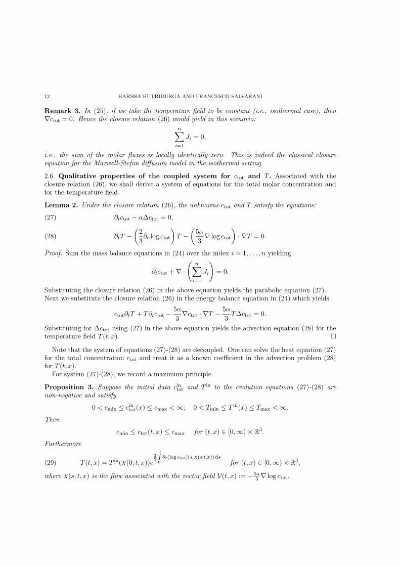
12 HARSHA HUTRIDURGA AND FRANCESCO SALVARANI
Remark 3. In (25), if we take the temperature field to be constant (i.e., isothermal case), thenrc
tot
= 0. Hence the closure relation (26) would yield in this scenario:nX
i=1
J
i
= 0,
i.e., the sum of the molar fluxes is locally identically zero. This is indeed the classical closureequation for the Maxwell-Stefan diffusion model in the isothermal setting.
2.6. Qualitative properties of the coupled system for c
tot
and T . Associated with theclosure relation (26), we shall derive a system of equations for the total molar concentration andfor the temperature field.
Lemma 2. Under the closure relation (26), the unknowns c
tot
and T satisfy the equations:
@
t
c
tot
� ↵�c
tot
= 0,(27)
@
t
T �✓2
3
@
t
log c
tot
◆T �
✓5↵
3
r log c
tot
◆·rT = 0.(28)
Proof. Sum the mass balance equations in (24) over the index i = 1, . . . , n yielding
@
t
c
tot
+r ·
nX
i=1
J
i
!= 0.
Substituting the closure relation (26) in the above equation yields the parabolic equation (27).Next we substitute the closure relation (26) in the energy balance equation in (24) which yields
c
tot
@
t
T + T@
t
c
tot
� 5↵
3
rc
tot
·rT � 5↵
3
T�c
tot
= 0.
Substituting for �c
tot
using (27) in the above equation yields the advection equation (28) for thetemperature field T (t, x). ⇤
Note that the system of equations (27)-(28) are decoupled. One can solve the heat equation (27)for the total concentration c
tot
and treat it as a known coefficient in the advection problem (28)for T (t, x).
For system (27)-(28), we record a maximum principle.
Proposition 3. Suppose the initial data c
in
tot
and T
in to the evolution equations (27)-(28) arenon-negative and satisfy
0 < c
min
c
in
tot
(x) c
max
< 1; 0 < T
min
T
in
(x) T
max
< 1.
Then
c
min
c
tot
(t, x) c
max
for (t, x) 2 [0,1)⇥ R3
.
Furthermore
T (t, x) = T
in
(X(0; t, x))e
2
3
tR
0
@
t
(log c
tot
)(s,X(s;t,x)) ds
for (t, x) 2 [0,1)⇥ R3
,(29)
where X(s; t, x) is the flow associated with the vector field V(t, x) := �5↵
3
r log c
tot
.

MAXWELL-STEFAN MODEL IN NON-ISOTHERMAL SETTING 13
Proof. Standard maximum principles on the heat equation implies that the solution to (27) staysnon-negative and is bounded both from above and below, the same as the initial data.To solve for the temperature field T (t, x) in the evolution equation (28), consider the solutionX(s; t, x) to the differential equation
dX
ds
(s; t.x) = V(s,X(s; t, x))X(t; t.x) = x.
Equipped with the flow X(s; t.x), the solution T (t, x) as given by (29) follows. ⇤
This article concerns a formal derivation of the diffusion limit for the gas mixtures in a non-isothermal setting. Proving an existence-uniqueness result for the proposed system is out of thescope of this present article. The authors are currently working on this problem and expect to havea publication in the near future.
Acknowledgments: This work was partially funded by the projects Kimega (ANR-14-ACHN-0030-01) and Kibord (ANR-13-BS01-0004). H.H. acknowledges the support of the ERC grantMATKIT and the EPSRC programme grant “Mathematical fundamentals of Metamaterials formultiscale Physics and Mechanic” (EP/L024926/1).
References
[1] C. Bardos, F. Golse, and C. D. Levermore. Sur les limites asymptotiques de la théorie cinétique conduisant à ladynamique des fluides incompressibles. C. R. Acad. Sci. Paris Sér. I Math., 309(11):727–732, 1989.
[2] C. Bardos, F. Golse, and C. D. Levermore. Fluid dynamic limits of kinetic equations. I. Formal derivations. J.Statist. Phys., 63(1-2):323–344, 1991.
[3] C. Bardos, F. Golse, and C. D. Levermore. Fluid dynamic limits of kinetic equations. II. Convergence proofs forthe Boltzmann equation. Comm. Pure Appl. Math., 46(5):667–753, 1993.
[4] M. Bisi and G. Martalò and G. Spiga. Multi-temperature Euler hydrodynamics for a reacting gas from a kineticapproach to rarefied mixtures with resonant collisions. EPL (Europhysics Letters), 95(5):55002, 2011.
[5] M. Bisi and G. Martalò and G. Spiga. Multi-temperature Hydrodynamic Limit from Kinetic Theory in a Mixtureof Rarefied Gases. Acta. Appl. Math., 122(1):37–51, 2012.
[6] D. Bothe. On the Maxwell-Stefan approach to multicomponent diffusion. In Parabolic problems, volume 80 ofProgr. Nonlinear Differential Equations Appl., pages 81–93. Birkhäuser/Springer Basel AG, Basel, 2011.
[7] L. Boudin, D. Götz, and B. Grec. Diffusive models for the air in the acinus. ESAIM: Proc., 30:90–103, 2010.[8] L. Boudin, B. Grec, and V. Pavan. The Maxwell-Stefan diffusion limit for a kinetic model of mixtures with
general cross sections. This issue.[9] L. Boudin, B. Grec, M. Pavić, and F. Salvarani. Diffusion asymptotics of a kinetic model for gaseous mixtures.
Kinet. Relat. Models, 6(1):137–157, 2013.[10] L. Boudin, B. Grec, and F. Salvarani. A mathematical and numerical analysis of the Maxwell-Stefan diffusion
equations. Discrete Contin. Dyn. Syst. Ser. B, 17(5):1427–1440, 2012.[11] L. Boudin, B. Grec, and F. Salvarani. The Maxwell-Stefan diffusion limit for a kinetic model of mixtures. Acta
Appl. Math., 136:79–90, 2015.[12] J.-F. Bourgat, L. Desvillettes, P. Le Tallec, and B. Perthame. Microreversible collisions for polyatomic gases
and boltzmann’s theorem. European journal of mechanics. B, Fluids, 13(2):237–254, 1994.[13] X. Chen and A. Jüngel. Analysis of an Incompressible Navier–Stokes–Maxwell–Stefan System. Comm. Math.
Phys., 340(2):471–497, 2015.[14] L. Desvillettes, R. Monaco, and F. Salvarani. A kinetic model allowing to obtain the energy law of polytropic
gases in the presence of chemical reactions. Eur. J. Mech. B Fluids, 24(2):219–236, 2005.[15] A. Ern and V. Giovangigli. Multicomponent transport algorithms, volume 24 of Lecture Notes in Physics. New
Series M: Monographs. Springer-Verlag, Berlin, 1994.

14 HARSHA HUTRIDURGA AND FRANCESCO SALVARANI
[16] A. Ern and V. Giovangigli. Projected iterative algorithms with application to multicomponent transport. LinearAlgebra Appl., 250:289–315, 1997.
[17] V. Giovangigli. Convergent iterative methods for multicomponent diffusion. Impact Comput. Sci. Engrg.,3(3):244–276, 1991.
[18] V. Giovangigli. Multicomponent flow modeling. Modeling and Simulation in Science, Engineering and Technology.Birkhäuser Boston Inc., Boston, MA, 1999.
[19] H. Grad. Principles of the kinetic theory of gases. In Handbuch der Physik (herausgegeben von S. Flügge), Bd.12, Thermodynamik der Gase, pages 205–294. Springer-Verlag, Berlin-Göttingen-Heidelberg, 1958.
[20] H. Hutridurga, and F. Salvarani. On the Maxwell-Stefan diffusion limit for a mixture of monatomic gases. Math.Meth. Appl. Sci., 40(3):803–813, 2017.
[21] A. Jüngel and I. V. Stelzer. Existence analysis of Maxwell-Stefan systems for multicomponent mixtures. SIAMJ. Math. Anal., 45(4):2421–2440, 2013.
[22] R. Krishna and J. A. Wesselingh. The Maxwell-Stefan approach to mass transfer. Chem. Eng. Sci., 52(6):861–911, 1997.
[23] J. C. Maxwell. On the dynamical theory of gases. Phil. Trans. R. Soc., 157:49–88, 1866.[24] M. McLeod and Y. Bourgault. Mixed finite element methods for addressing multi-species diffusion using the
Maxwell-Stefan equations. Comput. Methods Appl. Mech. Engrg., 279:515–535, 2014.[25] M. Pavić. Mathematical modelling and analysis of polyatomic gases and mixtures in the context of kinetic
theory of gases and fluid mechanics. École Normale Supérieure de Cachan, PhD Thesis, 2014.[26] S. Simić, M. Pavić-Čolić and D. Madjarević. Non-equilibrium mixtures of gases: modelling and computation.
Riv. Mat. Univ. Parma, 6(1):135–214, 2015.[27] J. Stefan. Ueber das Gleichgewicht und die Bewegung insbesondere die Diffusion von Gasgemengen. Akad. Wiss.
Wien, 63:63–124, 1871.[28] M. Thiriet. Anatomy and Physiology of the Circulatory and Ventilatory Systems. . Springer, New York, 2014.
H.H.: Department of Mathematics, Imperial College London, London, SW7 2AZ, United Kingdom.E-mail address: [email protected]
F.S.: Université Paris-Dauphine, Ceremade, UMR CNRS 7534, F-75775 Paris Cedex 16, France &Università degli Studi di Pavia, Dipartimento di Matematica, I-27100 Pavia, Italy
E-mail address: [email protected]