Citation: Zhou, D.; Babaei, A.;

Banihashemi, S.; Jafari, H.; Alzabut, J.;

Moshokoa, S.P. A Chebyshev

Collocation Approach to Solve

Fractional Fisher–Kolmogorov–

Petrovskii–Piskunov Equation with

Nonlocal Condition. Fractal Fract.

2022, 6, 160. https://doi.org/

10.3390/fractalfract6030160

Academic Editor: Hijaz Ahmad

Received: 10 January 2022

Accepted: 10 February 2022

Published: 15 March 2022

Publisher’s Note: MDPI stays neutral

with regard to jurisdictional claims in

published maps and institutional affil-

iations.

Copyright: © 2022 by the authors.

Licensee MDPI, Basel, Switzerland.

This article is an open access article

distributed under the terms and

conditions of the Creative Commons

Attribution (CC BY) license (https://

creativecommons.org/licenses/by/

4.0/).

fractal and fractional

Article

A Chebyshev Collocation Approach to Solve FractionalFisher–Kolmogorov–Petrovskii–Piskunov Equation withNonlocal ConditionDapeng Zhou 1, Afshin Babaei 2 , Seddigheh Banihashemi 2, Hossein Jafari 2,3,4,* , Jehad Alzabut 5,6 andSeithuti P. Moshokoa 7

1 School of Mathematics and Quantitative Economics, Shandong University of Finance and Economics,Jinan 250014, China; dapengzhou225@outlook.com

2 Department of Applied Mathematics, University of Mazandaran, Babolsar 4741613534, Iran;babaei@umz.ac.ir (A.B.); s.banihashemi@stu.umz.ac.ir (S.B.)

3 Department of Mathematical Sciences, University of South Africa (UNISA), Pretoria 0003, South Africa4 Department of Medical Research, China Medical University Hospital, China Medical University,

Taichung 110122, Taiwan5 Department of Mathematics and Sciences, Prince Sultan University, Riyadh 11586, Saudi Arabia;

jalzabut@psu.edu.sa6 Department of Industrial Engineering, OSTIM Technical University, Ankara 06374, Turkey7 Department of Mathematics and Statistics, Tshwane University of Technology, Pretoria 0008, South Africa;

moshokoasp@tut.ac.za* Correspondence: jafari.usern@gmail.com

Abstract: We provide a detailed description of a numerical approach that makes use of the shiftedChebyshev polynomials of the sixth kind to approximate the solution of some fractional orderdifferential equations. Specifically, we choose the fractional Fisher–Kolmogorov–Petrovskii–Piskunovequation (FFKPPE) to describe this method. We write our approximate solution in the productform, which consists of unknown coefficients and shifted Chebyshev polynomials. To compute thenumerical values of coefficients, we use the initial and boundary conditions and the collocationtechnique to create a system of equations whose number matches the unknowns. We test theapplicability and accuracy of this numerical approach using two examples.

Keywords: fractional Fisher–Kolmogorov–Petrovskii–Piskunov equation; collocation scheme; sixth-kind Chebyshev polynomials; convergence analysis

1. Introduction

A study of generalized derivatives and integrals has gained considerable popularity inthe last few years, mainly due to its attractive applications in numerous diverse fields suchas fluid flow [1], finance [2] and physics [3]. These generalized derivatives and integrals arecalled fractional derivatives and integrals, respectively [4–6]. They are more flexible for real-world applications since they can have both integer and noninteger operators. Fractionalderivatives are well-known for their utility in describing the memory and heredity featuresof a variety of materials and processes [7–10]. Nikan et al. [11] considered the fractionalnonlinear sine-Gordon and Klein–Gordon models arising in relativistic quantum mechanics.Babaei et al. [12] introduced a class of time-fractional stochastic heat equations drivenby Brownian motion. Numerical solution of time fractional convection–diffusion-waveequation based on RBF method is described in [13,14]. Zaky et al. [15] applied somepseudospectral methods for solving the Riesz space-fractional Schrödinger equation. Lately,countless researchers are contributing to new models based on fractional equations. Amongwhich, the generalized Fisher–Kolmogorov–Petrovskii–Piskunov equation has substantialattention [16–19].

Fractal Fract. 2022, 6, 160. https://doi.org/10.3390/fractalfract6030160 https://www.mdpi.com/journal/fractalfract

Fractal Fract. 2022, 6, 160 2 of 13

In this paper, we introduce the FFKPPE in the form

0Dηt u(x, t) = µ∆u(x, t) + β∇u(x, t) +

κ

ζ

∫ t

0e−

t−sζ ∆u(x, s)ds +F (x, t, u), (1)

where (x, t) ∈ ΩL ×ΩT, with the following initial and boundary conditions

u(x, 0) = u0(x), x ∈ ΩL, (2)

g(u(0, t)) = ρ0(t), t ∈ ΩT, (3)

θu(L, t) + δux(L, t) = ρL(t), t ∈ ΩT, (4)

where ∆ := ∂2

∂x2 is the Laplace operator and ∇ := ∂∂x . Further, µ, β, κ, ζ 6= 0, θ and δ

are given real constants. Moreover, ΩL := [0, L], ΩT := [0, T], the nonlinear source termF (x, t, u) ∈ C1(ΩL ×ΩT ×R) fulfills the Lipschitz condition in terms of u and u0(x), ρ0(t)and ρL(t) are regarded as known continuous functions. In addition, the nonlinear functiong of u(0, t) is given and the operator 0D

ηt [·] denotes the Caputo fractional derivative of

order η ∈ (0, 1) defined as [20]:

0Dηt u(x, t) =

1Γ(1− η)

∫ t

0(t− s)−ηus(x, s)ds, (5)

in which Γ(·) denotes the Gamma function. The generalized FFKPPE (1), belongs to theclass of reaction–diffusion equations. It is commonly used to represent practical situationsthat often arise in physics, chemistry and biology [18,19,21]. A more specific example is inthe modeling of genetic behavior in the growth of micro-organisms [22].

In the literature, the problem (1)–(4) has been considered analytically and numerically.For instance, Araújo et al. [23] investigated the stability of the model represented by (1),while also investigating the qualitative features of its solutions obtained under Dirichletboundary conditions. Splitting methods were created for purposes of numerically studyingthe qualitative nature of the solutions. A list of numerical approaches has been proposedand studied for different cases of the Equation (1). Branco et al. [16] studied the approachof method of lines for the numerical solution to integro-differential equation of type (1).In their work, Araújo et al. [24] developed the famous Fisher equation by investigatingthe qualitative features of the numerical traveling wave solutions of integro-differentialequations. The hyperbolic equation equivalence was used to replace the integro-differentialequation, allowing for the numerical quantification of the velocity of traveling wavesolutions. While studying the effects on memory factors in phenomena of diffusion [25]developed approximation methods for computing integro-differential equations. Barbeiroand Ferreira [26] provided mathematical models to describe medication absorption throughthe skin. The development of these models involved extending the traditional Fick’slaw by incorporating a memory term. This replaces the classical models of advection–diffusion equations with integro-differential equations. The well-posedness of model wasinvestigated using Neumann, Dirichlet and natural boundary conditions. The methods forcomputing numerical solutions were proposed. In addition, their stability and convergencewere studied, while including a presentation of numerical simulations to illustrate thebehavior of the model. Khuri and Sayfy proposed a numerical scheme to solve a generalizedFisher integro-differential equation using finite differences and spline collocation in [17].To manage the numerical integration, a composite weighted trapezoidal rule was used,resulting in a closed-form difference scheme. To assess the method’s accuracy, multiple testexamples were solved. The scheme’s convergence and stability were also explored. Babaeiet al. sets up a numerical technique that makes use of the Chebyshev polynomials of thesixth kind with the main purpose of approximating the solutions of integro-differentialequations of variable order [27]. The sixth-kind Chebyshev polynomials are a special caseof the general nonsymmetric class mentioned in [28,29].

Fractal Fract. 2022, 6, 160 3 of 13

We subdivide our research under different headings as follows. In the next section,we focus on fundamental mathematical concepts that lay important groundwork for thesubsequent sections. Section 3 outlines the methodology that we use to conduct our researchand in the fourth section we study the convergence of this methodology. In Section 5, weapply the methodology to specific examples. We mention our findings and give suggestionsin the last section of this manuscript.

2. Preliminaries

For use in sequel, this section presents the basic properties of the sixth-kind Chebyshevpolynomials and related necessary definitions.

Definition 1. We define the Riemann–Liouville fractional integral with order η ∈ (0, 1) as [20]

Iηt u(x, t) =

1Γ(η)

∫ t

0u(x, s)(t− s)η−1ds.

Definition 2 ([12]). The following recurrence relation is used to obtain the sixth-kind Chebyshevpolynomials φq(t)

φ0(t) = 1, φ1(t) = t,

φq+1(t) = t φq(t) + $qφq−1(t), q = 2, 3, . . .,

where

$q :=−(q + 1− (−1)q)(q + 2− (−1)q)

4(q + 1)(q + 2).

Definition 3 ([29]). Considering the interval [0, T], then the shifted sixth-kind Chebyshev polyno-mials are written as

φq(t) = φq((2/T)t− 1), q = 0, 1, 2, . . .

In analytical format, these polynomials are presented as [29]

φq(t) =q

∑k=0

Lk,qtk, (6)

where

Lk,q =

22k−q

(2k+1)!Tk

q2∑

p=b k+12 c

(−1)q2+p+k(2p + k + 1)!(2p− k)!

, q even,

22k−q+1

(2k+1)!(q+1)Tk

q−12∑

p=b k2 c

(−1)q+1

2 +p+k(p + 1)(2p + k + 2)!(2p− k + 1)!

, q odd.

Let L2v(ΩL ×ΩT) represent a space that consists of square integrable functions having

variables (x, t) and the weight function v(x, t) = w(x)w(t) with w(x) =√

x− x2(2x− 1)2.

Theorem 1. We assume that f (x, t) ∈ L2v(ΩL ×ΩT) satisfies the expansion [12]

f (x, t) =∞

∑p=0

∞

∑q=0

cp,qφp(x)φq(t).

Suppose∥∥∥ ∂6 f (x,t)

∂x3∂t3

∥∥∥2≤ c and c > 0. The inequality |cp,q| < c

p3q3 for all p, q > 3, is satisfiedfor the expansion coefficients. Further, if

f (x, t) ' fn,m(x, t) =n

∑p=0

m

∑q=0

cp,qφp(x)φq(t), (7)

Fractal Fract. 2022, 6, 160 4 of 13

is an estimate for f (x, t), then

| f (x, t)− fn,m(x, t)| < c2n+m ,

∣∣∣∇ f (x, t)−∇ fn,m(x, t)∣∣∣ < σ

n2n+m−2 ,∣∣∣∆ f (x, t)− ∆ fn,m(x, t)

∣∣∣ < σn3

2n+m−8 ,

where σ, σ > 0.

Definition 4. Suppose Pp+1(t) is Legendre polynomial of order p + 1 on [−1, 1]. The Legendre–Gauss quadrature formula for g(t) ∈ C[a, b] is defines as:

∫ b

ag(t)dt =

b− a2

M

∑r=0

wr g(b− a

2ςr +

b + a2

),

in which distinct nodes ςrMr=0 are the zeros of PM+1(t) and wrM

r=0 are the correspondingweights [30]

wr =2

(1− ς2r)(P′M+1(ςr))2 .

3. Numerical Method

In this section, we describe numerical technique for solving (1)–(4) on the basis ofthe shifted sixth-kind Chebyshev polynomials. We obtain the numerical approximation ofEquation (1) by considering an approximation of the fractional derivative of the unknownfunction as:

0Dηt u(x, t) ' 0D

ηt un,m(x, t) =

n

∑p=0

m

∑q=0

cp,qφp(x)φq(t) = Φ(x)TCΦ(t), (8)

in which

Φ(x) = [φ0(x), φ1(x), . . ., φn(x)]T, (9)

Φ(t) = [φ0(t), φ1(t), . . ., φm(t)]T, (10)

andC =

[cp,q

](n+1)×(m+1)

, p = 0, . . ., n, q = 0, . . ., m,

represent a matrix with unknown entries whose numerical values are to be computed.According to Definition 1 and the initial condition (2)

u(x, t) ' Iηt

(Φ(x)TCΦ(t)

)+ u0(x) = Φ(x)TC Iη

t Φ(t) + u0(x).

By applying Definition 1 and shifted SKCPs (6), for q = 0, . . ., m

Ληq (t) := Iη

t φq(t) =q

∑k=0

Lk,qIηt (t

k) =q

∑k=0

Lη

k,qtk+η ,

where Lη

k,q := Lk,qΓ(k+1)

Γ(k+1+η), thus, we let

u(x, t) ' un,m(x, t) = Φ(x)TCΦηt (t) + u0(x), (11)

Fractal Fract. 2022, 6, 160 5 of 13

such that

Φηt (t) :=

[Λη

0(t), Λη1(t), . . ., Λη

m(t)]T

. (12)

According to (1) and (11)

R(x, t) := Φ(x)TCΦ(t)− µ(

Φxx(x)TCΦηt (t) + u′′0 (x)

)− β

(Φx(x)TCΦη

t (t) + u′0(x))

− κ

ζ

∫ t

0e−

t−sζ

(Φxx(x)TCΦη

s (s) + u′′0 (x))

ds

−F(

x, t, Φ(x)TCΦηt (t) + u0(x)

), (13)

with

Φx(x) =[φ′0(x), φ′1(x), . . ., φ′n(x)

]T, (14)

Φxx(x) =[φ′′0 (x), φ′′1 (x), . . ., φ′′n (x)

]T. (15)

In addition, from Equation (11) and the initial and boundary conditions (2)–(4),we define

Ψ(x) := Φ(x)TCΦηt (0) + u0(x), (16)

Π1(t) := g(

Φ(0)TCΦηt (t) + u0(0)

)− ρ0(t), (17)

Π2(t) := θ(

Φ(L)TCΦηt (t) + u0(L)

)+ δ(

Φx(L)TCΦηt (t) + u′0(L)

)− ρL(t). (18)

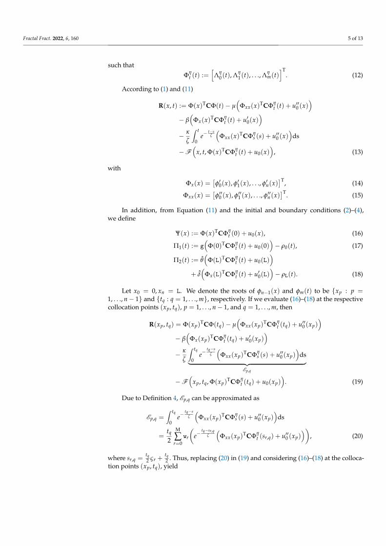
Let x0 = 0, xn = L. We denote the roots of φn−1(x) and φm(t) to be xp : p =1, . . ., n− 1 and tq : q = 1, . . ., m, respectively. If we evaluate (16)–(18) at the respectivecollocation points (xp, tq), p = 1, . . ., n− 1, and q = 1, . . ., m, then

R(xp, tq) = Φ(xp)TCΦ(tq)− µ

(Φxx(xp)

TCΦηt (tq) + u′′0 (xp)

)− β

(Φx(xp)

TCΦηt (tq) + u′0(xp)

)− κ

ζ

∫ tq

0e−

tq−sζ

(Φxx(xp)

TCΦηs (s) + u′′0 (xp)

)ds︸ ︷︷ ︸

Ep,q

−F(

xp, tq, Φ(xp)TCΦη

t (tq) + u0(xp))

. (19)

Due to Definition 4, Ep,q can be approximated as

Ep,q =∫ tq

0e−

tq−sζ

(Φxx(xp)

TCΦηs (s) + u′′0 (xp)

)ds

=tq

2

M

∑r=0

wr

(e−

tq−sr,qζ

(Φxx(xp)

TCΦηt (sr,q) + u′′0 (xp)

)), (20)

where sr,q =tq2 ςr +

tq2 . Thus, replacing (20) in (19) and considering (16)–(18) at the colloca-

tion points (xp, tq), yield

Fractal Fract. 2022, 6, 160 6 of 13

R(xp, tq) = 0, p = 1, . . ., n− 1, q = 1, . . ., m, (21)

Π1(tq) = 0, q = 1, . . ., m, (22)

Π2(tq) = 0, q = 1, . . ., m, (23)

Ψ(xp) = 0, p = 0, . . ., n. (24)

The relations (21)–(24) imply that we deduce an (n + 1)× (m + 1) system of nonlinearequations that can be solved through a numerical approach, such as the Newton iterationtechnique, to achieve the numerical values of cp,q, p = 0, 1, . . ., n, q = 0, . . ., m. The givenmethod in this section is listed as Algorithm 1.

Algorithm 1: Algorithm of presented method in Section 3

Input: L, T, µ, β, κ, ζ, θ, δ and n, m, M ∈ Z+, η ∈ (0, 1) and functions F, g, u0, ρ0 andρL.

Step 1: Compute the shifted sixth-kind Chebyshev polynomials φi(x) on theinterval [0, L] and φj(t) on the interval [0, T].

Step 2: Compute the vector of shifted sixth-kind Chebyshev polynomials Φ(x)and Φ(t) from Equations (9) and (10).

Step 3: Compute the vectors Φηt (t) from (12) and Φx(x), Φxx(x) from Equations

(14) and (15).Step 4: Compute the collocation points xp and tq.Step 5: Compute the collocation points sr,p and wr.Step 10: Solve the nonlinear system (21)–(24) and obtain the unknown vector C.Step 12.4: Let un,m(x, t) = Φ(x)TCΦη

t (t) + u0(x).Step 13: Post-processing the results.

Output: The approximate solution: u(x, t) ' un,m(x, t).

4. Convergence Analysis

To further explore the behavior of the obtained numerical solution, this section presentsa discussion of how the numerical solution un,m(x, t) converges towards the exact solutionu(x, t).

Theorem 2. Let un,m(x, t) be the approximate solution of (1), u(x, t) be its exact solution andRn,m(x, t) be the residual error. Then,

sup(x,t)∈ΩL×ΩT

|Rn,m(x, t)| ≤ ρn3 + n + m + 1

2n+m−8 ,

where ρ is a positive constant.

Proof. Since un,m(x, t) is the numerical solution of (1), thus

0Dηt un,m(x, t) = µ∆un,m(x, t) + β∇un,m(x, t) +F (x, t, un,m(x, t))

+κ

ζ

∫ t

0e−

t−sζ ∆un,m(x, s)ds +Rn,m(x, t). (25)

With reference to Equations (1) and (25), we have

|Rn,m(x, t)| ≤ |0Dηt en,m(x, t)|+ |µ||∆en,m(x, t)|+ |β||∇en,m(x, t)|

+∣∣∣F (x, t, u(x, t))−F (x, t, Un,m(x, t))

∣∣∣+ |κ

ζ|∣∣∣ ∫ t

0e−

t−sζ ∆en,m(x, s)ds

∣∣∣ (26)

where en,m(x, t) := u(x, t)− un,m(x, t). Using (5) and Theorem 1, results

Fractal Fract. 2022, 6, 160 7 of 13

|0Dηt en,m(x, t)| ≤ 1

Γ(1− η)

∫ t

0|(t− s)−η |

∣∣∣∂en,m

∂s(x, s)

∣∣∣ds

≤ b1

Γ(1− η)

∫ t

0sup

(x,t)∈ΩL×ΩT

∣∣∣∂en,m

∂t(x, t)

∣∣∣ds

≤ λm

2n+m−2 , (27)

where λ = σb1TΓ(1−η)

and b1 is a positive constant depended on η and T. The function F

fulfills the Lipschitz condition in terms of u, hence∣∣∣F (x, t, u(x, t))−F (x, t, un,m(x, t))∣∣∣ ≤ ξF|en,m(x, t)|,

where ξF > 0. From Theorem 1∣∣∣F (x, t, u(x, t))−F (x, t, un,m(x, t))∣∣∣ < c ξF

2n+m . (28)

Moreover, ∣∣∣ ∫ t

0e−

t−sζ ∆en,m(x, s)ds

∣∣∣ ≤ ∫ t

0

∣∣∣e− t−sζ

∣∣∣|∆en,m(x, s)|ds

≤ b2

∫ t

0sup

(x,t)∈ΩL×ΩT

|∆en,m(x, s)|ds

≤ b2Tσn3

2n+m−8 , (29)

where b2 is a positive constant depended on T. Thus, from relations (26)–(29) and Theorem 1,we obtain

|Rn,m(x, t)| ≤ λm + |β|σn2n+m−2 + (|µ|σ + |κ

ζ|b2Tσ)

n3

2n+m−8 +c ξF

2n+m

≤ λm + |β|σn2n+m−8 + (|µ|σ + |κ

ζ|b2Tσ)

n3

2n+m−8 +c ξF

2n+m−8

≤ ρn3 + n + m + 1

2n+m−8 ,

in which ρ = maxλ, |β|σ, |µ|σ + | κζ |b2Tσ, c ξF. As a result

sup(x,t)∈ΩL×ΩT

|Rn,m(x, t)| ≤ ρn3 + n + m + 1

2n+m−8 .

5. Numerical Example

Herein, we implement the described method for solving some numerical examples toinvestigate the applicability and practical computational efficiency. To assess the accuracyof the scheme, let n = m, and the l∞-norm error be given as

‖E n‖∞ = max(νp ,τq)

∣∣∣u(νp, τq)− un(νp, τq)∣∣∣, (30)

where un(νp, τq) is an approximate solution of u(x, t) at the designated collocation nodesx = νp, t = τq and p, q = 1, . . ., n. In which case, convergence order (CO) with respect to thel∞-norm is as given by

Fractal Fract. 2022, 6, 160 8 of 13

CO = log n1n2

‖E n1‖∞

‖E n2‖∞. (31)

For numerical computations, a personal computer with a 1.70 GHz processor wasused. In addition the computational software of choice was MatLab.

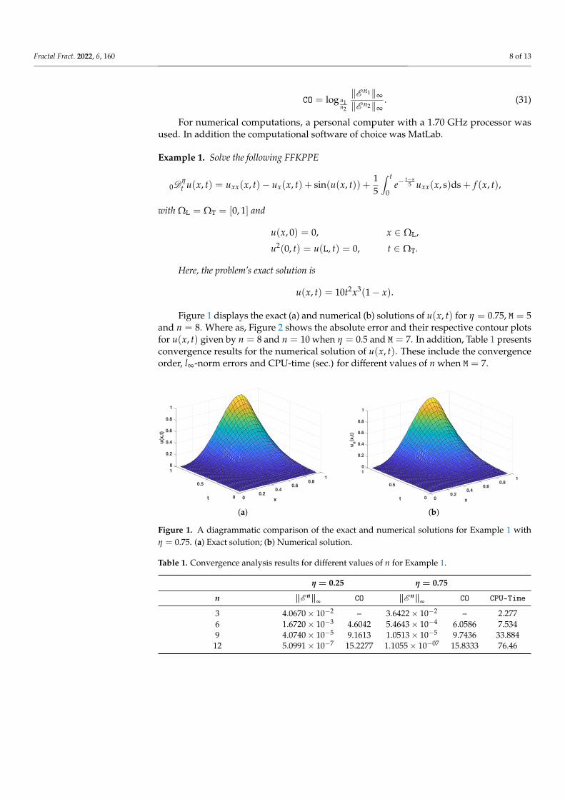
Example 1. Solve the following FFKPPE

0Dηt u(x, t) = uxx(x, t)− ux(x, t) + sin(u(x, t)) +

15

∫ t

0e−

t−s5 uxx(x, s)ds + f (x, t),

with ΩL = ΩT = [0, 1] and

u(x, 0) = 0, x ∈ ΩL,

u2(0, t) = u(L, t) = 0, t ∈ ΩT.

Here, the problem’s exact solution is

u(x, t) = 10t2x3(1− x).

Figure 1 displays the exact (a) and numerical (b) solutions of u(x, t) for η = 0.75, M = 5and n = 8. Where as, Figure 2 shows the absolute error and their respective contour plotsfor u(x, t) given by n = 8 and n = 10 when η = 0.5 and M = 7. In addition, Table 1 presentsconvergence results for the numerical solution of u(x, t). These include the convergenceorder, l∞-norm errors and CPU-time (sec.) for different values of n when M = 7.

0

1

0.2

0.4

1

u(x

,t) 0.6

0.8

t

0.8

0.5 0.6

x

1

0.40.2

0 0

(a)

0

1

0.2

0.4

1

un(x

,t) 0.6

0.8

t

0.8

0.5 0.6

x

1

0.40.2

0 0

(b)

Figure 1. A diagrammatic comparison of the exact and numerical solutions for Example 1 withη = 0.75. (a) Exact solution; (b) Numerical solution.

Table 1. Convergence analysis results for different values of n for Example 1.

η = 0.25 η = 0.75

n ‖E n‖∞ CO ‖E n‖∞ CO CPU-Time

3 4.0670× 10−2 – 3.6422× 10−2 – 2.2776 1.6720× 10−3 4.6042 5.4643× 10−4 6.0586 7.5349 4.0740× 10−5 9.1613 1.0513× 10−5 9.7436 33.88412 5.0991× 10−7 15.2277 1.1055× 10−07 15.8333 76.46

Fractal Fract. 2022, 6, 160 9 of 13

0

1

1

2

1

10-5

3

Absolute error

t

4

0.5

x

5

0.5

0 0

0.5

1

1.5

2

2.5

3

3.5

4

10-5

(a)

0.1 0.2 0.3 0.4 0.5 0.6 0.7 0.8 0.9

x

0.1

0.2

0.3

0.4

0.5

0.6

0.7

0.8

0.9

t

0.5

1

1.5

2

2.5

3

3.5

4

10-5

(b)

0

1

0.8

2

10-8

0.80.6

Absolute error

3

t

0.6

x

0.40.4

0.2 0.2

0.5

1

1.5

2

2.5

3

3.5

10-8

(c)

0.1 0.2 0.3 0.4 0.5 0.6 0.7 0.8 0.9

x

0.1

0.2

0.3

0.4

0.5

0.6

0.7

0.8

0.9

t

0.5

1

1.5

2

2.5

3

3.5

10-8

(d)

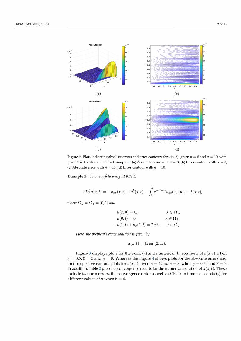
Figure 2. Plots indicating absolute errors and error contours for u(x, t), given n = 8 and n = 10, withη = 0.5 in the domain Ω for Example 1. (a) Absolute error with n = 8; (b) Error contour with n = 8;(c) Absolute error with n = 10; (d) Error contour with n = 10.

Example 2. Solve the following FFKPPE

0Dηt u(x, t) = −uxx(x, t) + u2(x, t) +

∫ t

0e−(t−s)uxx(x, s)ds + f (x, t),

where ΩL = ΩT = [0, 1] and

u(x, 0) = 0, x ∈ ΩL,

u(0, t) = 0, x ∈ ΩT,

−u(1, t) + ux(1, t) = 2πt, t ∈ ΩT.

Here, the problem’s exact solution is given by

u(x, t) = tx sin(2πx).

Figure 3 displays plots for the exact (a) and numerical (b) solutions of u(x, t) whenη = 0.5, M = 5 and n = 8. Whereas the Figure 4 shows plots for the absolute errors andtheir respective contour plots for u(x, t) given n = 4 and n = 8, when η = 0.65 and M = 7.In addition, Table 2 presents convergence results for the numerical solution of u(x, t). Theseinclude l∞-norm errors, the convergence order as well as CPU run time in seconds (s) fordifferent values of n when M = 6.

Fractal Fract. 2022, 6, 160 10 of 13

-0.8

-0.6

-0.4

-0.2

0.8

u(x

,t)

0

0.2

0.80.6

t

0.6

x

0.4 0.40.2 0.2

(a)

-0.8

-0.6

-0.4

-0.2

0.8

un(x

,t)

0

0.2

0.80.6

t

0.6

x

0.4 0.40.2 0.2

(b)

Figure 3. A diagrammatic comparison of the exact and numerical solutions for Example 2 withη = 0.5. (a) Exact solution; (b) Numerical solution.

0

1

0.5

1

10-5

1

Absolute error

t

0.5

x

1.5

0.5

0 0

2

4

6

8

10

12

10-6

(a)

0.1 0.2 0.3 0.4 0.5 0.6 0.7 0.8 0.9

x

0.1

0.2

0.3

0.4

0.5

0.6

0.7

0.8

0.9

t

2

4

6

8

10

12

10-6

(b)

0

0.5

0.8

1

10-7

1.5

0.80.6

Absolute error

t

2

0.6

x

0.40.4

0.2 0.2

0.2

0.4

0.6

0.8

1

1.2

1.4

1.6

1.8

2

2.2

10-7

(c)

0.1 0.2 0.3 0.4 0.5 0.6 0.7 0.8 0.9

x

0.1

0.2

0.3

0.4

0.5

0.6

0.7

0.8

0.9

t

0.2

0.4

0.6

0.8

1

1.2

1.4

1.6

1.8

2

2.2

10-7

(d)

Figure 4. Plots indicating absolute errors and error contours for u(x, t) with n = 12 and n = 15when η = 0.65 in Ω for Example 2. (a) Absolute error with n = 12; (b) Error contour with n = 12;(c) Absolute error with n = 15; (d) Error contour with n = 15.

Table 2. Convergence analysis results for different values of n for Example 2.

η = 0.25 η = 0.75

n ‖En‖∞ CO ‖En‖∞ CO CPU-Time

3 6.3855× 10−1 − 3.7469× 10−1 − 2.346 3.4551× 10−2 4.2080 8.2972× 10−2 5.4969 4.2159 2.5097× 10−3 6.4673 1.8042× 10−4 9.4419 15.11612 7.2113× 10−5 12.3389 5.2019× 10−6 12.3271 70.638

Example 3. Solve the following generalized Fisher–Kolmogorov–Petrovskii–Piskunov [17]

ut(x, t) = − 12π2 uxx(x, t) + u2(x, t) +

∫ t

0e−

(t−s)2 uxx(x, s)ds + f (x, t),

Fractal Fract. 2022, 6, 160 11 of 13

where (x, t) ∈ (0, 1)× (0, 1] and

u(x, 0) = sin(πx), x ∈ [0, 1],

u(0, t) + ux(0, t) = πe−t/2, t ∈ (0, 1],

u(1, t) + ux(1, t) = −πe−t/2, t ∈ (0, 1].

Here, the problem’s exact solution is given by

u(x, t) = e−t/2 sin(πx).

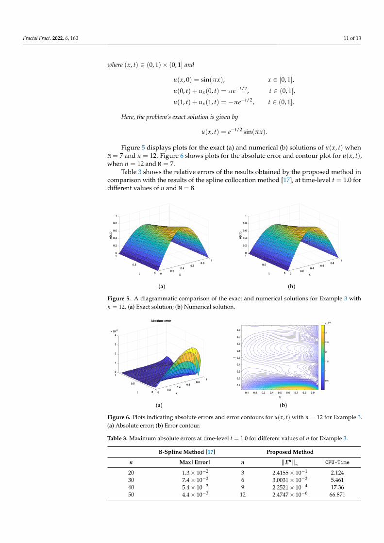
Figure 5 displays plots for the exact (a) and numerical (b) solutions of u(x, t) whenM = 7 and n = 12. Figure 6 shows plots for the absolute error and contour plot for u(x, t),when n = 12 and M = 7.

Table 3 shows the relative errors of the results obtained by the proposed method incomparison with the results of the spline collocation method [17], at time-level t = 1.0 fordifferent values of n and M = 8.

0

1

0.2

0.4

1

u(x

,t) 0.6

0.8

t

0.8

0.5 0.6

x

1

0.40.2

0 0

(a)

0

1

0.2

0.4

1

u(x

,t) 0.6

0.8

t

0.8

0.5 0.6

x

1

0.40.2

0 0

(b)

Figure 5. A diagrammatic comparison of the exact and numerical solutions for Example 3 withn = 12. (a) Exact solution; (b) Numerical solution.

0

1

1

1

2

10-5

0.8

Absolute error

3

t

0.50.6

x

4

0.4

0.20 0

(a)

0.1 0.2 0.3 0.4 0.5 0.6 0.7 0.8 0.9

x

0.1

0.2

0.3

0.4

0.5

0.6

0.7

0.8

0.9

t

0.5

1

1.5

2

2.5

3

10-5

(b)

Figure 6. Plots indicating absolute errors and error contours for u(x, t) with n = 12 for Example 3.(a) Absolute error; (b) Error contour.

Table 3. Maximum absolute errors at time-level t = 1.0 for different values of n for Example 3.

B-Spline Method [17] Proposed Method

n Max|Error| n ‖En‖∞ CPU-Time

20 1.3× 10−2 3 2.4155× 10−1 2.12430 7.4× 10−3 6 3.0031× 10−3 5.46140 5.4× 10−3 9 2.2521× 10−4 17.3650 4.4× 10−3 12 2.4747× 10−6 66.871

Fractal Fract. 2022, 6, 160 12 of 13

6. Conclusions

Shifted Chebyshev polynomials of the sixth-kind form the backbone of the numericalscheme that we have discussed in this research. Through these polynomials, we were ableto construct a differential matrix and write an equation that approximates the solution ofa differential equation with fractional order. The role of the collocation technique in oursolution procedure is to augment the number of equations created from the initial andboundary conditions. Graphical comparisons of the results attained from this numericalscheme and the known exact solutions indicate that this scheme has a high level of accuracy.We also note that, as we increase the number of polynomials used, the accuracy andconvergence rates also improve although this is accompanied by more intensive labor.Fortunately, it is clear from the results that we need a few polynomials to reach acceptedlevel of accuracy.

Author Contributions: Conceptualization, methodology and software, S.B. and D.Z.; formal analysis,A.B.; investigation, J.A. and S.P.M.; writing—original draft preparation, D.Z., A.B. and S.B.; writing—review and editing, H.J., J.A. and S.P.M.; supervision, A.B., S.B. and H.J. All authors have read andagreed to the published version of the manuscript.

Funding: This research received no external funding.

Acknowledgments: Jehad Alzabut is thankful to Prince Sultan University and OSTIM TechnicalUniversity for their endless support.

Conflicts of Interest: The authors declare no conflict of interest.

References1. Baeumer, B.; Benson, D.Z.; Meerschaert, M.M.; Wheatcraft, S.W. Subordinated advection-dispersion equation for contaminant

transport. Water Resour. Res. 2001, 37, 1543–1550. [CrossRef]2. Mainardi, F.; Raberto, M.; Gorenelo, R.; Scalas, E. Fractional calculus and continuous-time finance II: The waiting-time discribution.

Phys. A Stat. Mech. Its Appl. 2000, 287, 468–481. [CrossRef]3. Javidi, M.; Ahmad, B. Numerical solution of fractional partial differential equations by numerical Laplace inversion technique.

Adv. Differ. Equ. 2013, 2013, 375. [CrossRef]4. Oldham, K.; Spanier, J. The Fractional Calculus; Academic Press: New York, NY, USA, 1974.5. Srivastava, H.M. Some parametric and argument variations of the operators of fractional calculus and related special functions

and integral transformations. J. Nonlinear Convex Anal. 2021, 22, 1501–1520.6. Hosseini, V.R.; Shivanian, E.; Chen, W. Local integration of 2-D fractional telegraph equation via local radial point interpolant

approximation. Eur. Phys. J. Plus 2015, 130, 1–21. [CrossRef]7. Esmaeelzade Aghdam, Y.; Safdari, H.; Azari, Y.; Jafari, H.; Baleanu, D. Numerical investigation of space fractional order diffusion

equation by the Chebyshev collocation method of the fourth kind and compact finite difference scheme. Discret. Contin. Dyn.Syst.-S 2021, 14, 2025–2039.

8. Ali, I.; Haq, S.; Nisar, K.S.; Baleanu, D. An efficient numerical scheme based on Lucas polynomials for the study of multidimen-sional Burgers-type equations. Adv. Differ. Equ. 2021, 1, 1–24. [CrossRef]

9. Hosseini, V.R.; Yousefi, F.; Zou, W.N. The numerical solution of high dimensional variable-order time fractional diffusion equationvia the singular boundary method. J. Adv. Res. 2020, 32, 73–84. [CrossRef]

10. Abdelkawy, M.A.; Amin, A.Z.; Babatin, M.M.; Alnahdi, A.S.; Zaky, M.A.; Hafez, R.M. Jacobi spectral collocation technique fortime-fractional inverse heat equations. Fractal Fract. 2021, 5, 115.

11. Nikan, O.; Avazzadeh, Z.; Tenreiro Machado, J.A. Numerical investigation of fractional nonlinear sine-Gordon and Klein-Gordonmodels arising in relativistic quantum mechanics. Eng. Anal. Bound. Elem. 2020, 120, 223–237. [CrossRef]

12. Babaei, A.; Jafari, H.; Banihashemi, S. A Collocation Approach for Solving Time-Fractional Stochastic Heat Equation Driven by anAdditive Noise. Symmetry 2020, 12, 904. [CrossRef]

13. Zhang, X.; Yao, L. Numerical approximation of time-dependent fractional convection-diffusion-wave equation by RBF-FDmethod. Eng. Anal. Bound. Elem. 2021, 130, 1–9. [CrossRef]

14. Qiao, H.; Cheng, A. A fast finite difference/RBF meshless approach for time fractional convection-diffusion equation withnon-smooth solution. Eng. Anal. Bound. Elem. 2021, 125, 280–289. [CrossRef]

15. Zaky, M.A.; Abdelkawy, M.A.; Ezz-Eldien, S.S.; Doha, E.H. Pseudospectral methods for the Riesz space-fractional Schrödingerequation. In Fractional-Order Modeling of Dynamic Systems with Applications in Optimization; Signal Processing and Control;Academic Press: Cambridge, MA, USA, 2022; pp. 323–353.

16. Branco, J.R.; Ferreira, J.A.; de Oliveira, P. Numerical methods for the generalized Fisher-Kolomogrov-Petrovskii-Piskunovequation. Appl. Numer. Math. 2007, 57, 89–102. [CrossRef]

Fractal Fract. 2022, 6, 160 13 of 13

17. Khuri, S.A.; Sayfy, A. A numerical approach for solving an extended Fisher-Kolomogrov-Petrovskii-Piskunov equation. J. Comput.Appl. Math. 2010, 233, 2081–2089. [CrossRef]

18. Machado, J.A.; Babaei, A.; Moghaddam, B.P. Highly accurate scheme for the Cauchy problem of the generalized Burgers-Huxleyequation. Acta. Polytech. Hung. 2016, 13, 183–195.

19. Veeresha, P.; Prakasha, D.G.; Baleanu, D. An efficient numerical technique for the nonlinear fractional Kolmogorov-Petrovskii-Piskunov equation. Mathematics 2019, 7, 265. [CrossRef]

20. Podlubny, I. Fractional-order systems and PI/sup/spl lambda//D/sup/spl mull-Controllers. IEEE Trans. Autom. Control 1999,44, 208–214. [CrossRef]

21. Leclerc, Q.J.; Lindsay, J.A.; Knight, G.M. Mathematical modelling to study the horizontal transfer of antimicrobial resistancegenes in bacteria: Current state of the field and recommendations. J. R. Soc. Interface 2019, 16, 20190260. [CrossRef] [PubMed]

22. Khater, M.M.; Attia, R.A.; Abdel-Aty, A.H.; Alharbi, W.; Lu, D. Abundant analytical and numerical solutions of the fractionalmicrobiological densities model in bacteria cell as a result of diffusion mechanisms. Chaos Solitons Fractals 2020, 136, 109824.[CrossRef]

23. Araújo, A.; Branco, R.; Ferreira, J.A. On the stability of a class of splitting methods for integro-differential equations. Appl. Numer.Math. 2009, 59, 436–453. [CrossRef]

24. Araújo, A.; Ferreira, J.A.; de Oliveira, P. Qualitative solutions for reaction-diffusion equations with memory. Appl. Anal. 2005, 84,1231–1246. [CrossRef]

25. Araújo, A.; Ferreira, J.A.; de Oliveira, P. The effect of memory terms in diffusion phenomena. J. Comput. Math. 2006, 24, 91–102.26. Barbeiro, S.; Ferreira, J.A. Integro-differential models for percutaneous drug absortion. Int. J. Comput. Math. 2007, 84, 451–467.

[CrossRef]27. Babaei, A.; Jafari, H.; Banihashemi, S. Numerical solution of variable order fractional nonlinear quadratic integro-differential

equations based on the sixth-kind Chebyshev collocation method. J. Comput. Appl. Math. 2020, 377, 112908. [CrossRef]28. Abd-Elhameed, W.M.; Youssri, Y.H. Fifth-kind orthonormal Chebyshev polynomial solutions for fractional differential equations.

Comput. Appl. Math. 2018, 37, 2897–2921. [CrossRef]29. Abd-Elhameed, W.M.; Youssri, Y.H. Sixth-kind Chebyshev spectral approach for solving fractional differential equations. Int. J.

Nonlinear Sci. Numer. Simul. 2019, 20, 191–203. [CrossRef]30. Canuto, C.; Hussaini, M.Y.; Quarteroni, A.; Zang, T.A. Spectral Methods in Fluid Dynamics; Springer: New York, NY, USA, 1988.