MARINE ECOLOGY PROGRESS SERIESMar Ecol Prog Ser

Vol. 232: 29–44, 2002 Published May 3

INTRODUCTION

The ecological importance of space-time heterogene-ity in phytoplankton populations has been pointed out byseveral authors (e.g. Hutchinson 1961, Margalef 1967,Platt 1975) and widely investigated both in marine and

freshwater ecology (e.g. Platt 1972, Powell et al. 1975,Abbott et al. 1982, Weber et al. 1986, Denman & Abbott1994). However, in spite of the intensive investigationsconducted on the nutrient dependence of phytoplanktongrowth (Jickells 1998, McCarthy et al. 1998) that pro-vided direct evidence for nutrient control of photosyn-thesis in the ocean (Platt et al. 1992, Falkowski et al.1998), studies concerning the small-scale heterogeneityof nutrients are still scarce (Estrada & Wagensberg 1977,Steele & Henderson 1979).

© Inter-Research 2002 · www.int-res.com

*Present address: Ecosystem Complexity Research Group, Station Marine de Wimereux, UMR 8013 ELICO, Université des Sciences et Technologies de Lille, BP 80, 62930 Wimereux, France. E-mail: laurent.seuront@univ-lille1.fr

Small-scale nutrient patches in tidally mixedcoastal waters

Laurent Seuront1,*, Valérie Gentilhomme2, Yvan Lagadeuc3

1Department of Ocean Sciences, Tokyo University of Fisheries, 4-5-7 Konan, Minato-ku, Tokyo 108-8477, Japan2Ecosystem Complexity Research Group, Station Marine de Wimereux, UMR 8013 ELICO,

Université des Sciences et Technologies de Lille, BP 80, 62930 Wimereux, France3Université de Caen, Laboratoire de Biologie et Biotechnologies Marines, IUT Génie Biologique, Bd du Maréchal Juin,

14032 Caen cedex, France

ABSTRACT: In the eastern English Channel, characterized by its megatidal regime and the resultingvery high turbulence, phytoplankton biomass and purely passive scalars such as temperature andsalinity are basically regarded as homogenised by turbulent fluid motions. However, recent studieshave demonstrated — on the basis of innovative statistical analyses in marine ecology — that theseparameters were heterogeneously distributed at a small scale. We extend these concepts to high-resolution time series of dissolved nitrogen (NO2

–). We first demonstrate the validity of our samplingprocedure of continuously measuring nitrite concentration (3 s temporal resolution). Second, wedescribe how these time series recorded at different times of 4 tidal cycles can be characterized asheterogeneously distributed using fractal and multifractal parameters, and then can be described interms of small-scale patches. In addition, we show how multifractal parameters can be regarded asbeing both qualitatively and quantitatively more informative than a single fractal dimension. Theseparameters showed very specific temporal patterns revealing the absence of density-dependence ofnitrite distribution. In contrast, nitrite distributions clearly appeared to be less heterogeneously dis-tributed under higher turbulence, suggesting a physical control of small-scale nutrient patchiness.Nevertheless, taking into account the different structures of nitrite distributions under high and lowturbulence, we suggest that the observed small-scale nutrient patches could be the result of complexinteractions between hydrodynamic conditions, biological processes related to phytoplankton popu-lations, and the productive efficiency of bacterial populations. This hypothesis is supported by obser-vations that the structure of temperature and salinity — regarded as passive scalars under purelyphysical control of turbulent motions — recorded simultaneously to the nitrite data remained similarunder all hydrodynamic conditions.

KEY WORDS: Turbulence · Patchiness · Nitrite · Time series · Tidal forcing · Fractal and multifractalanalysis

Resale or republication not permitted without written consent of the publisher

Mar Ecol Prog Ser 232: 29–44, 2002

The small-scale distribution of nutrients in the sea isnevertheless a particular salient issue in marine ecol-ogy. Indeed, if small-scale heterogeneity in the dist-ribution of nutrients is really more prevalent thangenerally thought, for instance, new production byphytoplankton might have been biased in many envi-ronments, especially at the continental margins of theocean, where spatio-temporal variability of both phys-ical and biological processes is usually very developed(see e.g. Mackas et al. 1985, and references therein).Indeed, while some studies have been dedicated tospatio-temporal distributions of phyto- and zooplank-ton (Brylinski et al. 1984, 1988, Brunet et al. 1993, Seu-ront et al. 1996a,b, 1999, Seuront & Lagadeuc 1998),results concerning the spatio-temporal distribution ofnutrients are still scarce in this area (Bentley et al.1993, Gentilhomme & Lizon 1998), especially onsmaller scales.

In the eastern English Channel and the SouthernBight of the North Sea, characterized by their mega-tidal regime and the resulting very high turbulence,recent studies have shown that phytoplankton biomassis neither randomly nor homogeneously distributed butrather exhibits a very structured small-scale patchydistribution similar to that of purely passive scalarssuch as temperature and salinity (Seuront et al.1996a,b, 1999). The question is then to knowwhether dissolved nitrogen exhibits a struc-tured distribution driven purely by physicalforces (i.e. similar to that observed regardingtemperature and salinity) or another kind ofdistribution, suggesting another level of com-plexity in the structure of nutrient variability.

However, studies of small-scale distribu-tions are subject to both technical and statis-tical limitations. Small-scale patches withelevated nitrogen content cannot be ob-served with present-day techniques. Thefastest response nutrient analyser allows, toour knowledge, only a 2 min temporal reso-lution (Sakamoto et al. 1996) and is still insuf-ficient to work in the coastal ocean, wherespatio-temporal variability is high relative tothe open ocean (Mackas et al. 1985). Previ-ous statistical studies of plankton patchiness,mainly based on spectral analysis (see e.g.Platt & Denman 1975, Fasham 1978), haveallowed inferences on when biological pro-cesses contribute significantly to phytoplank-ton spatial structure, over spatial scales rang-ing from tens of meters to tens of kilometers.However, while able to quantify the varianceas a function of scales, these techniques,based on second order statistics and Gauss-ian hypotheses, were not able to reveal the

precise variability associated with those scales and themechanism of the physical-biological interactions, par-ticularly at small scales (i.e. meters and seconds). Thisis in the range where physical forces dominate biolog-ical processes (e.g. Seuront et al. 1996a,b, 1999).Herein, the goal of this paper is: (1) to demonstrate thevalidity of a high resolution (i.e. a 3 s temporal resolu-tion) dissolved nitrogen analysis technique; (2) to showhow high resolution nitrogen time series can be whollycharacterized in terms of structured variability in thepowerful framework of multifractal analyses in a moreefficient way than in a spectral framework; and (3) toreveal how the organization of this structured variabil-ity can be regarded as mainly dependent on hydrody-namic conditions.

MATERIALS AND METHODS

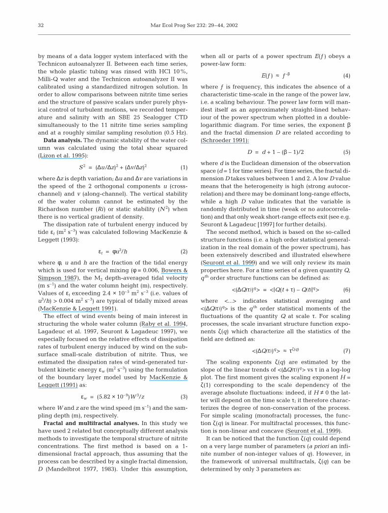
Sampling experiment. Sampling was conductedduring 48 h (ca 4 tidal cycles) in a period of spring tide,from 2 to 4 April 1996, at an anchor station (Fig. 1)located in the coastal waters (i.e. the ‘Coastal Flow’;Brylinski et al. 1991) of the eastern English Channel(50° 47’ 300’’ N, 1° 33’ 500’’ E). Measurements of physi-cal parameters (temperature and salinity) and in vivo

30

Fig. 1. Study area and location of the sampling station ( ) along the French coast of the eastern English Channel

Seuront et al.: Small-scale heterogeneity of nutrients

fluorescence were taken every hour from the surfaceto the bottom with an SBE 19 Sealogger CTD and a SeaTech fluorometer, respectively. Every 5 min, currentspeed and direction were measured at 3, 6 and 10 mwith Anderra current meters. Every hour, wind datawere collected with the on-board anemometer. Every 2h, water samples were taken at 2, 6, 10 and 16 m, usingNiskin bottles. Dissolved inorganic nitrogen concen-trations (5 ml frozen samples, analysed using a Techni-con autoanalyzer II; Treguer & Le Corre 1971) andchl a concentrations (1 l filtered frozen samples, ex-tracted with 90% acetone, assayed in a spectrophoto-meter and the chl a concentration calculated followingStrickland & Parsons 1972) were estimated for eachsampled depth.

High-resolution nitrogen sampling design. Wefocused on nitrite (NO2

–) rather than nitrate (NO3–) or

ammonium (NH4+) concentration for both conceptual

and technical reasons. Nitrite is indeed the most con-servative nutrient and can be expected to behave as apurely passive scalar. Therefore the observed variabil-ity will presumably be little or not biased by biologicalprocesses such as phytoplankton uptake and releaseas nitrate and ammonium can be. Moreover, nitriteallows a higher temporal resolution than nitrate — andthen more direct comparisons with the 0.5 s resolutionreached by Seuront et al. (1996a,b, 1999) — because ofthe substantial smoothing introduced by the reductionprocess associated with nitrate determination (seeTreguer & Le Corre 1971 for further details).

In order to continuously investigate the small-scaledistribution of nitrite (NO2

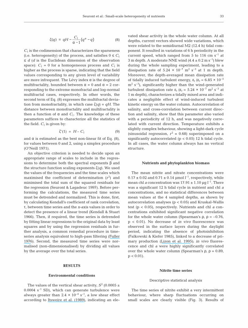
–), water was continuouslytaken from a depth of 0.25 m through a sea-waterintake mounted on a suspended hose at a distance of1 m away from the hull of the vessel, and directly pro-cessed in a Technicon autoanalyzer II (Treguer & LeCorre 1971) by means of a railwheel pump connectedto 1.5 mm diameter plastic tubing (Fig. 2) with anapproximate output of 0.80 ml min–1. The temporal res-olution (i.e. 3 s) was chosen as the minimum time inter-val allowed by the Technicon autoanalyzer II between2 nitrite quantity determinations. One may note herethat such an approach, while suggested by Treguer &Le Corre (1971) has, to our knowledge, never beenused in that way except by Estrada & Wagensberg(1977) with a lower temporal resolution (1 min) and aconsiderable smoothing of the output signal associatedwith the dimension of the pumping apparatus.

In more practical terms, the Reynolds number associ-ated with our pumping apparatus was low (i.e. Re ~18.75) and indicated that no turbulent processes oc-curred during the pumping in the plastic tubing. Wethen subsequently estimated the characteristic lengthscale, L, covered by the nitrite molecules because ofmolecular diffusion occurring in the plastic tubing dur-

ing pumping following L = 133(D × t)32 (Mann & Lazier1991), where D is the molecular diffusion (D = 10–9 m2

s–1) and t the diffusion time scale (i.e. the time taken bythe water to be brought through the Technicon autoan-alyzer II; t = 20 min). This led to a characteristic diffu-sion length scale L = 10–3 m which is about 5 orders ofmagnitude lower than the intersample bubbling usedby the Technicon autoanalyzer II. We can state that ourpumping apparatus cannot be responsible for any bias-ing associating with turbulent or molecular diffusion.

Finally, our sampling cannot be biased by the bound-ary layer occurring around the hull of the vesselbecause of the 1 m distance chosen for our seawaterintake. Indeed, the thickness of a boundary layer, δ,increases with increasing distance from the leadingedge according to δ = (xν/u)1/2 (Mann & Lazier 1991),where x (m) is the distance from the leading edge (i.e.the distance from the ship bow) where water has beencontinuously taken (i.e. x = 15 m), ν the kinematic vis-cosity (10–6 m2 s–1) and u (m s–1) the free-stream veloc-ity. We then estimated δ for the range of free-streamvelocities (i.e. 0.10 to 1.04 m s–1) experienced duringthe sea water pumping experiment as being in therange 0.38 to 1.22 cm. The potential influence of such aminute boundary layer thickness in the temporalpatterns on the nitrite measurements can then beneglected in the present case.

We then recorded 11 time series of nitrite concentra-tions of approximately 1 h duration at a sampling fre-quency of 0.33 Hz; data were directly recorded on a PC

31

Fig. 2. Side view schematic diagram of the experimental set-up used to continuously sample subsurface water

Mar Ecol Prog Ser 232: 29–44, 2002

by means of a data logger system interfaced with theTechnicon autoanalyzer II. Between each time series,the whole plastic tubing was rinsed with HCl 10%,Milli-Q water and the Technicon autoanalyzer II wascalibrated using a standardized nitrogen solution. Inorder to allow comparisons between nitrite time seriesand the structure of passive scalars under purely phys-ical control of turbulent motions, we recorded temper-ature and salinity with an SBE 25 Sealogger CTDsimultaneously to the 11 nitrite time series samplingand at a roughly similar sampling resolution (0.5 Hz).

Data analysis. The dynamic stability of the water col-umn was calculated using the total shear squared(Lizon et al. 1995):

S2 = (∆u/∆z)2 + (∆v/∆z)2 (1)

where ∆z is depth variation; ∆u and ∆v are variations inthe speed of the 2 orthogonal components u (cross-channel) and v (along-channel). The vertical stabilityof the water column cannot be estimated by theRichardson number (Ri) or static stability (N 2) whenthere is no vertical gradient of density.

The dissipation rate of turbulent energy induced bytide εt (m2 s–3) was calculated following MacKenzie &Leggett (1993):

εt = φu3/h (2)

where φ, u and h are the fraction of the tidal energywhich is used for vertical mixing (φ = 0.006, Bowers &Simpson 1987), the M2 depth-averaged tidal velocity(m s–1) and the water column height (m), respectively.Values of εt exceeding 2.4 × 10–5 m2 s–3 (i.e. values ofu3/h) > 0.004 m2 s–3) are typical of tidally mixed areas(MacKenzie & Leggett 1991).

The effect of wind events being of main interest instructuring the whole water column (Raby et al. 1994,Lagadeuc et al. 1997, Seuront & Lagadeuc 1997), weespecially focused on the relative effects of dissipationrates of turbulent energy induced by wind on the sub-surface small-scale distribution of nitrite. Thus, weestimated the dissipation rates of wind-generated tur-bulent kinetic energy εw (m2 s–3) using the formulationof the boundary layer model used by MacKenzie &Leggett (1991) as:

εw = (5.82 × 10–9)W 3/z (3)

where W and z are the wind speed (m s–1) and the sam-pling depth (m), respectively.

Fractal and multifractal analyses. In this study wehave used 2 related but conceptually different analysismethods to investigate the temporal structure of nitriteconcentrations. The first method is based on a 1-dimensional fractal approach, thus assuming that theprocess can be described by a single fractal dimension,D (Mandelbrot 1977, 1983). Under this assumption,

when all or parts of a power spectrum E(ƒ) obeys apower-law form:

E(ƒ) ≈ ƒ–β (4)

where ƒ is frequency, this indicates the absence of acharacteristic time-scale in the range of the power law,i.e. a scaling behaviour. The power law form will man-ifest itself as an approximately straight-lined behav-iour of the power spectrum when plotted in a double-logarithmic diagram. For time series, the exponent βand the fractal dimension D are related according to(Schroeder 1991):

D = d + 1 – (β – 1)/2 (5)

where d is the Euclidean dimension of the observationspace (d = 1 for time series). For time series, the fractal di-mension D takes values between 1 and 2. A low D valuemeans that the heterogeneity is high (strong autocor-relation) and there may be dominant long-range effects,while a high D value indicates that the variable israndomly distributed in time (weak or no autocorrela-tion) and that only weak short-range effects exit (see e.g.Seuront & Lagadeuc [1997] for further details).

The second method, which is based on the so-calledstructure functions (i.e. a high order statistical general-ization in the real domain of the power spectrum), hasbeen extensively described and illustrated elsewhere(Seuront et al. 1999) and we will only review its mainproperties here. For a time series of a given quantity Q,q th order structure functions can be defined as:

<(∆Q(τ))q> = <|Q(t + τ) – Q(t)|q> (6)

where <...> indicates statistical averaging and<(∆Q(τ))q> is the q th order statistical moments of thefluctuations of the quantity Q at scale τ. For scalingprocesses, the scale invariant structure function expo-nents ζ(q) which characterize all the statistics of thefield are defined as:

<(∆Q(τ))q> ≈ τζ(q) (7)

The scaling exponents ζ(q) are estimated by theslope of the linear trends of <(∆Q(τ))q> vs τ in a log-logplot. The first moment gives the scaling exponent H =ζ(1) corresponding to the scale dependency of theaverage absolute fluctuations: indeed, if H ≠ 0 the lat-ter will depend on the time scale τ; it therefore charac-terizes the degree of non-conservation of the process.For simple scaling (monofractal) processes, the func-tion ζ(q) is linear. For multifractal processes, this func-tion is non-linear and concave (Seuront et al. 1999).

It can be noticed that the function ζ(q) could dependon a very large number of parameters (a priori an infi-nite number of non-integer values of q). However, inthe framework of universal multifractals, ζ(q) can bedetermined by only 3 parameters as:

32

Seuront et al.: Small-scale heterogeneity of nutrients

(8)

C1 is the codimension that characterizes the sparseness(i.e. heterogeneity) of the process, and satisfies 0 ≤ C1

≤ d (d is the Euclidean dimension of the observationspace): C1 = 0 for a homogeneous process and C1 ishigher as the process is sparse, indicating that the fieldvalues corresponding to any given level of variabilityare more infrequent. The Lévy index α is the degree ofmultifractality, bounded between α = 0 and α = 2 cor-responding to the extreme monofractal and log-normalmultifractal cases, respectively. In other words, thesecond term of Eq. (8) expresses the multifractal devia-tion from monofractality, in which case ζ(q) = qH. Thedistance between monofractality and multifractality isthen a function of α and C1. The knowledge of theseparameters suffices to characterize all the statistics ofthe field. C1 is given by:

ζ’(1) = H – C1 (9)

and α is estimated as the best non-linear fit of Eq. (8),for values between 0 and 2, using a simplex procedure(O’Neill 1971).

An objective criterion is needed to decide upon anappropriate range of scales to include in the regres-sions to determine both the spectral exponents β andthe structure function scaling exponents ζ(q). We usedthe values of the frequencies and the time scales whichmaximised the coefficient of determination (r2) andminimised the total sum of the squared residuals forthe regression (Seuront & Lagadeuc 1997). Before per-forming the calculations, the measured time seriesmust be detrended and normalized. This is done, first,by calculating Kendall’s coefficient of rank correlation,τ, between time series and the x-axis values in order todetect the presence of a linear trend (Kendall & Stuart1966). Then, if required, the time series is detrendedby fitting linear regressions to the original data by leastsquares and by using the regression residuals in fur-ther analysis, a common remedial procedure in time-series analysis equivalent to high-pass filtering (Fuller1976). Second, the measured time series were nor-malised (non-dimensionalised) by dividing all valuesby the average over the total series.

RESULTS

Environmental conditions

The values of the vertical shear activity, S2 (0.0005 ±0.0004 s–1 SD), which can generate turbulence werealways greater than 2.4 × 10–4 s–1, a low shear effectaccording to Itsweire et al. (1989), indicating an ele-

vated shear activity in the whole water column. At alldepths, current vectors showed wide variations, whichwere related to the semidiurnal M2 (12.4 h) tidal com-ponent. It resulted in variations of 6 h periodicity in thecurrent speed, which ranged from 5 to 116 cm s–1 at3 m depth. A moderate NNE wind (4.4 ± 0.2 m s–1) blewduring the whole sampling experiment, leading to adissipation rate of 5.24 × 10–7 m2 s–3 at 1 m depth.Moreover, the depth-averaged mean dissipation rateof tidally induced turbulent energy, εt (εt = 6.85 × 10–5

m2 s–3), significantly higher than the wind-generatedturbulent dissipation rate εt (εt = 5.24 × 10–7 m2 s–3 at1 m depth), characterizes a tidally mixed area and indi-cates a negligible effect of wind-induced turbulentkinetic energy on the water column. Autocorrelation ofsalinity, and cross-correlation between current direc-tion and salinity, show that this parameter also variedwith a periodicity of 12 h, and was negatively corre-lated with current direction. Temperature exhibits aslightly complex behaviour, showing a light-dark cycle(sinusoidal regression, r 2 = 0.68) superimposed on asignificantly autocorrelated (p < 0.05) 12 h tidal cycle.In all cases, the water column always has no verticalstructure.

Nutrients and phytoplankton biomass

The mean nitrite and nitrate concentrations were0.17 ± 0.02 and 0.71 ± 0.14 µmol l–1, respectively, whilemean chl a concentration was 17.91 ± 1.10 µg l–1. Therewas a significant 12 h tidal cycle in nutrient and chl aconcentrations, and no statistical differences betweenmean values at the 4 sampled depths, as shown byautocorrelation analyses (p < 0.05) and Kruskal-Wallistest (p < 0.05), respectively. Nutrients and chl a con-centrations exhibited significant negative correlationfor the whole water column (Spearman’s ρ, ρ = –0.76,p < 0.01). No decrease of in vivo fluorescence wasobserved in the surface layers during the daylightperiod, indicating the absence of photoinhibition(Falkowski & Kiefer 1985), linked to a decrease of pri-mary production (Lizon et al. 1995); in vivo fluores-cence and chl a were highly significantly correlatedover the whole water column (Spearman’s ρ, ρ = 0.89,p < 0.01).

Nitrite time series

Descriptive statistical analysis

The time series of nitrite exhibit a very intermittentbehaviour, where sharp fluctuations occurring onsmall scales are clearly visible (Fig. 3). Results of

ζα

αq qHC

q q( ) = −−

−( )1

1

33

Mar Ecol Prog Ser 232: 29–44, 2002

descriptive analysis, including skewness and kurtosisestimates, for the 11 nitrite time series are presented inTable 1. The different time series of nitrite concentra-tions are not normally distributed (Kolmogorov-Smirnov test, p < 0.01; Lilliefors 1967) and their fre-quency distributions exhibit a skewed behaviour(Table 1), reflecting heterogeneous distributions with afew dense patches and a wide range of low-densitypatches.

In order to validate our continuous use of the Tech-nicon Autoanalyzer II, we computed the means ofeach time series and plotted them together with theevolution curves of the hourly estimates of nitrite con-centrations (Fig. 4). Thus, means of the continuouslyrecorded time series clearly appear to be very wellintegrated in the 12 h tidal cycle of the nitrite concen-trations corresponding to our discrete samplingscheme at 2 m depth. More precisely, means of the

34

Time series Nitrite concentration (µmol l–1)N T Mean Min Max SD Skewness Kurtosis

1 999 3 0.10 0.05 0.29 0.03 1.97 5.802 604 6 0.29 0.21 0.41 0.04 0.58 2.853 659 6 0.11 0.03 0.31 0.05 0.39 3.834 613 6 0.26 0.19 0.50 0.03 2.69 17.655 1454 3 0.27 0.21 0.42 0.03 1.94 8.526 1455 3 0.16 0.05 0.43 0.03 0.30 7.187 1167 3 0.20 0.09 0.77 0.07 2.57 11.528 1157 3 0.07 0.03 0.20 0.02 1.86 7.949 1207 3 0.20 0.14 0.27 0.02 0.10 4.8910 1241 3 0.20 0.13 0.45 0.02 16.19 45.9411 1579 3 0.11 0.04 0.50 0.05 0.17 6.58

Table 1. Descriptive analysis of the 11 nitrite concentration time series. T: temporal resolution (s); SD: standard deviation

Fig. 3. Samples of high-resolution (0.33 Hz) nitrite concentration time series recorded in the eastern English Channel in high (time series 5 and 8) and low (time series 6 and 11) current speed conditions

Seuront et al.: Small-scale heterogeneity of nutrients

different time series cannot statistically be regardedas being different from the closest discrete estimateof nitrite concentration (Binomial test, p < 0.05; Siegel& Castellan 1988), except in the case of the timeseries 4.

Fractal time series analysis

The double logarithmic power spectra for the nitritetime series together with their best fitting lines aregiven in Fig. 5. Log-log linearity of power spectra isvery strong for the whole range of scales considered,with coefficient of determination (r2) ranging from 0.76to 0.95. Those temporal scales can be associated withspatial scales using ‘Taylor’s hypothesis of frozen tur-bulence’ (Taylor 1938), which basically states that tem-poral and spatial averages t and l, respectively, can berelated by a constant velocity V, with l = V · t. Then,using the mean instantaneous tidal circulations

35

Fig. 4. Time series of nitrite concentrations (S) estimated froma 2 m depth sampling using Niskin bottles, shown togetherwith the means (d) and standard deviations (vertical bars) ofthe 11 high-resolution nitrite time series continuously re-

corded at 0.25 m depth. Time in local hours

Fig. 5. The power spectra E(ƒ) (ƒ is frequency) of the nitrite time series 5, 6, 8 and 11, shown together with their best-fitting lines in a log-log plot. The clear linearity of the power spectra indicates a scaling behaviour over the whole range of scales

Mar Ecol Prog Ser 232: 29–44, 2002

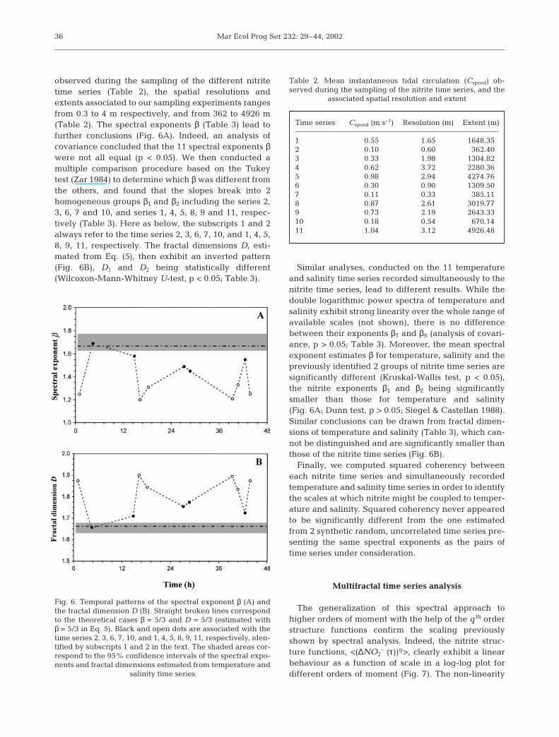
observed during the sampling of the different nitritetime series (Table 2), the spatial resolutions andextents associated to our sampling experiments rangesfrom 0.3 to 4 m respectively, and from 362 to 4926 m(Table 2). The spectral exponents β (Table 3) lead tofurther conclusions (Fig. 6A). Indeed, an analysis ofcovariance concluded that the 11 spectral exponents βwere not all equal (p < 0.05). We then conducted amultiple comparison procedure based on the Tukeytest (Zar 1984) to determine which β was different fromthe others, and found that the slopes break into 2homogeneous groups β1 and β2 including the series 2,3, 6, 7 and 10, and series 1, 4, 5, 8, 9 and 11, respec-tively (Table 3). Here as below, the subscripts 1 and 2always refer to the time series 2, 3, 6, 7, 10, and 1, 4, 5,8, 9, 11, respectively. The fractal dimensions D, esti-mated from Eq. (5), then exhibit an inverted pattern(Fig. 6B), D1 and D2 being statistically different(Wilcoxon-Mann-Whitney U-test, p < 0.05; Table 3).

Similar analyses, conducted on the 11 temperatureand salinity time series recorded simultaneously to thenitrite time series, lead to different results. While thedouble logarithmic power spectra of temperature andsalinity exhibit strong linearity over the whole range ofavailable scales (not shown), there is no differencebetween their exponents βΤ and βS (analysis of covari-ance, p > 0.05; Table 3). Moreover, the mean spectralexponent estimates β for temperature, salinity and thepreviously identified 2 groups of nitrite time series aresignificantly different (Kruskal-Wallis test, p < 0.05),the nitrite exponents β1 and β2 being significantlysmaller than those for temperature and salinity(Fig. 6A; Dunn test, p > 0.05; Siegel & Castellan 1988).Similar conclusions can be drawn from fractal dimen-sions of temperature and salinity (Table 3), which can-not be distinguished and are significantly smaller thanthose of the nitrite time series (Fig. 6B).

Finally, we computed squared coherency betweeneach nitrite time series and simultaneously recordedtemperature and salinity time series in order to identifythe scales at which nitrite might be coupled to temper-ature and salinity. Squared coherency never appearedto be significantly different from the one estimatedfrom 2 synthetic random, uncorrelated time series pre-senting the same spectral exponents as the pairs oftime series under consideration.

Multifractal time series analysis

The generalization of this spectral approach tohigher orders of moment with the help of the q th orderstructure functions confirm the scaling previouslyshown by spectral analysis. Indeed, the nitrite struc-ture functions, <(∆NO2

– (τ))q>, clearly exhibit a linearbehaviour as a function of scale in a log-log plot fordifferent orders of moment (Fig. 7). The non-linearity

36

Time series Cspeed (m s–1) Resolution (m) Extent (m)

1 0.55 1.65 1648.352 0.10 0.60 362.403 0.33 1.98 1304.824 0.62 3.72 2280.365 0.98 2.94 4274.766 0.30 0.90 1309.507 0.11 0.33 385.118 0.87 2.61 3019.779 0.73 2.19 2643.3310 0.18 0.54 670.1411 1.04 3.12 4926.48

Table 2. Mean instantaneous tidal circulation (Cspeed) ob-served during the sampling of the nitrite time series, and the

associated spatial resolution and extent

Fig. 6. Temporal patterns of the spectral exponent β (A) andthe fractal dimension D (B). Straight broken lines correspondto the theoretical cases β = 5/3 and D = 5/3 (estimated with β = 5/3 in Eq. 5). Black and open dots are associated with thetime series 2, 3, 6, 7, 10, and 1, 4, 5, 8, 9, 11, respectively, iden-tified by subscripts 1 and 2 in the text. The shaded areas cor-respond to the 95% confidence intervals of the spectral expo-nents and fractal dimensions estimated from temperature and

salinity time series

Seuront et al.: Small-scale heterogeneity of nutrients

of the exponents ζ(q) (not shown) indicates that thesmall-scale distributions of nitrite can be consideredas multifractals. More specifically, the scaling of thefirst moments ζ(1) = H leads to a behaviour very simi-

lar to the one observed in the case of the spectralexponents β (Fig. 8A); an analysis of covariance andan appropriate multiple comparison procedure alsolead to distinguish 2 groups of H values (Table 3). The

37

β D H C1 α

Temperature 1.70 (0.03) 1.64 (0.02) 0.40 (0.02) 0.060 (0.008) 1.91 (0.01)Salinity 1.69 (0.03) 1.65 (0.02) 0.39 (0.02) 0.062 (0.009) 1.90 (0.01)

Nitrite (1 & 2) 1.40 (0.05) 1.80 (0.02) 0.30 (0.04) 0.095 (0.01) 1.87 (0.01)Group 1 1.55 (0.04) 1.72 (0.02) 0.42 (0.02) 0.140 (0.01) 1.84 (0.02)Group 2 1.26 (0.02) 1.87 (0.01) 0.21 (0.01) 0.070 (0.01) 1.89 (0.01)

Table 3. Mean values of the spectral exponent β, the fractal dimension D, and the universal multifractal parameters H, C1, and αestimated for temperature, salinity time series, for the 11 nitrite time series (Nitrite 1 & 2) and the nitrite time series 2, 3, 6, 7, 10(Group 1) and 1, 4, 5, 8, 9, 11 (Group 2), recorded in high and low hydrodynamic conditions, respectively. Standard errors are

given in brackets

Fig. 7. The structure functions <(∆NO2–(τ))q> vs τ in log-log plots for q = 1, 2 and 3 (from top to bottom) for time series 5, 6, 8 and

11. As shown in the case of power spectral analysis, the data are scaling over the whole range of scales. The slopes of the straight dashed lines provide estimates of the first, second and third moment scaling exponents ζ(1) = H, ζ(2) and ζ(3)

Mar Ecol Prog Ser 232: 29–44, 2002

universal multifractal parameters C1 and α (Table 3)also exhibit a variable behaviour from one time seriesto another (Fig. 8B,C), suggesting a differential con-trol of the organization of the NO2

– variability overtime. Namely, C11

and C12, as well as α1 and α2, are

significantly different (Wilcoxon-Mann-Whitney U-test, p < 0.05).

Similar analyses of temperature and salinity indicatethat the first universal multifractal parameter H doesnot exhibit significant difference from one time seriesto another (p > 0.05) (Table 3) and are indistinguish-able from the first group of H values and significantlyhigher than the second group of H values estimated fornitrite time series (Table 3). Second, the parameters C1

shared by the temperature and salinity time series (p >0.05) are significantly smaller than the C1 values esti-mated for the first group of the nitrite time series, andnot significantly different from that for the secondgroup (Fig. 8B; Table 3). Finally, the parameters α esti-mated for the temperature and salinity time series(Table 3) are indistinguishable (p > 0.05), but appear tobe significantly higher than that estimated parametersfor the first group of the nitrite time series, and not sig-nificantly different from that for the second group(Dunn test, p < 0.05; Fig. 8C; Table 3).

Correlation analyses

In order to determine the factors influencing themagnitude of the differential structure levels of nitritetime series represented by the fractal dimension D,and the universal multifractal parameters H, C1 and α,we conducted correlation analyses between theseparameters, the integrals of the nitrite spectra (i.e. anestimate of the total variation in a given record; Bendat& Piersol 1986), the means of the nitrite time series andchl a concentrations estimated from 2 m depth watersamples during each time series recording, and thecurrent speed and direction, as an indicator of thephysical forcings (Table 4). These analyses showedthat the fractal and multifractal structures of nitritevariability were not correlated with the mean nitriteand chl a concentrations, nor with the integral of thenitrite spectra (Spearman’s ρ, 2-tailed, 90% level, p >0.05). Moreover, the absence of correlation betweenfractal and multifractal parameters and current direc-tion also indicates that the structure of nitrite variabil-ity cannot be related with the horizontal advection pro-cesses associated with the M2 tidal component.Instead, fractal and multifractal parameters were sig-nificantly correlated with current speed (Spearman’s ρ,2-tailed, p < 0.05 and p < 0.01; see Table 4), suggestinga differential hydrodynamic control of the structure ofnitrite variability.

38

Fig. 8. Temporal patterns of the universal multifractal para-meters H (A), C1 (B) and α (C). Black and open dots are asso-ciated with the time series 2, 3, 6, 7, 10, and 1, 4, 5, 8, 9, 11,respectively, identified by the subscript 1 and 2 in the text.The straight broken line in (A) corresponds to the theoreticalcase H = 1/3 expected for purely passive scalar in Obukhov-Corrsin homogeneous turbulence. The shaded areas cor-respond to the 95% confidence intervals of the universal multifractal parameters estimated from the temperature and

salinity time series

Seuront et al.: Small-scale heterogeneity of nutrients

DISCUSSION

Sampling small-scale nutrient patches

The differences observed between the values of themultifractal parameters H, C1 and α estimated fromnitrite time series, like the differences between theseparameters and those estimated from in vivo fluores-cence, temperature and salinity time series in previousstudies (Seuront et al. 1996a,b, 1999), cannot be associ-ated with the different spatial resolutions and extentsassociated with each nitrite time series (see Table 2),nor with the differences between nutrient and temper-ature, salinity and in vivo fluorescence sampling tech-niques. In the former case, we should have observed atransition between 2 different scaling regimes, both inpower spectra and structure function log-log plots.This is obviously not the case here (see Figs. 5 & 7,respectively). In the latter case, the temporal and spa-tial resolutions of previous studies (i.e. 0.5 to 1 s, and0.3 to 1 m, respectively), the small sizes and the minutetime scales of the response of the temperature, salinityand in vivo fluorescence sensors lead to sampling con-ditions very similar to those reached in the presentstudy.

On the other hand, we argue here that our samplingprocess cannot be regarded as affected by the motionof the ship, nor the characteristics of the sample pro-cessing chain including features of the electronicsinvolved. First, a contamination by the motion of theship (our pumping system did not move except withthe ship) would have been indicated by peaks at char-acteristic frequencies or time scales (Jenkins & Watts1968), which is clearly not the case in our data (seeFigs. 3, 5 & 7). Second, the linearity of the nitrite powerspectra over the whole range of available scales indi-cates the absence of any kind of noise contaminationby the electronics or the processing chain, in whichcase the high-frequency part of the spectra would haveshown a roll-off towards the noise level of the involvedelectronics. The absence of this characteristic signa-

ture of high-frequency noise demonstrates that oursampling frequency is well above the electronic noiselevel (Jenkins & Watts 1968).

Fractal versus multifractal analyses

The differences in the temporal patterns of variabil-ity exhibited by the fractal dimension D and the uni-versal multifractal parameters H, C1 and α estimatedfrom the nitrite time series clearly demonstrate theability of multifractal analysis to provide more com-plete information than the results obtained from fractalanalysis. Using only fractal dimensions D would haveled to viewing the local temporal patterns of nitritetime series as independent of physical processes: thespectral exponents β are significantly different fromthe theoretical value expected in the case of a purelypassive scalar, and the fractal dimensions estimatedfrom nitrite time series, and from temperature andsalinity time series are significantly different (cf.Fig. 6). The correlation observed between fractaldimension and current speed then only suggests anindirect control of nitrite fractal structure by hydrody-namic processes. In contrast, the universal multifractalparameters temporal distributions revealed couplingand uncoupling between nitrite distribution and phys-ical processes, as a function of tidal current intensity.Such observations then demonstrate that marine ecol-ogists should focus on the precise nature of the distrib-ution of patterns and processes in question in order toobtain more relevant information on the driving pro-cesses responsible for the observed variability.

Small-scale nutrient patches and hydrodynamicconditions

In well-mixed environments where turbulent pro-cesses are fully developed, previous empirical studieshave demonstrated that fluctuations of biological para-

39

NO2–mean NO2

–spectral sum D H C1 α Cspeed Cdirection

NO2–mean –1.000 – – – – – – –

NO2–spectral sum –0.150 –1.000 – – – – – –

D –0.347 –0.187 –1.000 – – – – –H –0.489 –0.169 –0.927** –1.000 – – – –C1 –0.177 –0.380 –0.805** –0.846** –1.000 – – –α –0.512 –0.097 –0.690* –0.648* –0.509 1.000 – –Cspeed –0.305 –0.191 –0.724* –0.815** –0.654* 0.610* 1.000 –Cdirection –0.509 –0.124 –0.184 –0.401 –0.370 0.234 0.014 1.000

Table 4. Correlation matrix of variables relative to the structure of nitrite time series. NO2–mean and NO2

–spectral sum: mean con-

centration of nitrite time series and sum of the nitrite power spectra; D: fractal dimension; H, C1, and α: universal multifractal parameters; Cspeed and Cdirection: current speed and direction. *5% significance level; **1% significance level

Mar Ecol Prog Ser 232: 29–44, 2002

meters (e.g. phytoplankton biomass) could follow aspectral power law behaviour marked by a characteris-tic exponent β (β = 5/3) over a wide range of scales (e.g.Seuront et al. 1996a,b, 1999), as theoretically expectedin the case of purely passive scalars (i.e. temperatureor salinity) advected by turbulent processes. However,except in the case of the time series 2, our estimates ofthe spectral exponent β are significantly different fromthe previously defined theoretical value (β = 5/3). Thisobservation indicates that the small-scale variability ofthe NO2

– time series cannot be regarded as beingpurely passively driven by turbulent fluid motion andthat there could exist an additional level of complexityin the origin of the structure of NO2

– variability. More-over, the high fractal dimensions associated withstrong current speeds characterize very complex pro-cesses where short-range, local variability is highlydeveloped and tends to obfuscate long-range trendsperceptible from lower fractal dimensions, associatedwith weak current speed; NO2

– is thus more evenlydistributed under high turbulence.

The negative correlation between H and the fractaldimensions D confirms the results of the monofractalanalysis. The first universal multifractal parameter Hcharacterizes the degree of non-conservation of theprocess. The lower H is, the more conservative is thecorresponding process, i.e. the mean of the fluctua-tions is less scale-dependent, indicating a reduced fluxof variance from large to smaller scales, and thus theprevalence of local variability.

Under low turbulence the higher values of C1 indi-cate the occurrence of few patches of high NO2

– con-centrations that are several orders of magnitude abovebackground levels. Under higher turbulence the lowerC1 indicates that NO2

– is more homogeneously distrib-uted (Fig. 3) and behaves as a passive scalar. Thishypothesis is supported by observations that the C1

values observed for nitrite time series under high tur-bulence cannot be distinguished from the C1 valuesestimated for temperature and salinity irrespective ofhydrodynamic conditions. Here the so-calledhomogenisation effect is mainly perceptible from thedisruption of these patches (see Fig. 3). NO2

– distribu-tion nevertheless remains heterogeneous (i.e. struc-tured) irrespective of the hydrodynamic conditions, asthe parameter C1 is significantly greater than 0 (p <0.05), in which case the nitrite would have been homo-geneously distributed.

Finally, the mean value of α indicates that NO2– can-

not be regarded as log-normally distributed, in whichcase α = 2. On the contrary, this value is typically in therange of α values estimated for phytoplankton bio-mass, temperature and salinity distribution over simi-lar ranges of scales (see Seuront et al. 1996a,b, 1999,present study). Nevertheless, our results indicate a dif-

ferential NO2– structure characterized by a greater

complexity in the hierarchy of its variability levelsunder high turbulence (Table 4).

Small-scale nutrient patches and phytoplanktonpatchiness

A comparison of the fractal and multifractal para-meters estimated for nitrite time series and those ofphytoplankton biomass warrants further comments.The fractal dimensions D are higher than those foundfor phytoplankton biomass distribution by Seuront &Lagadeuc (1998) and Seuront et al. (1996a) duringneap tide, and by Seuront et al. (1996b, 1999) duringspring tide; fractal dimensions were estimated usingthe β values reported by Seuront et al. (1996a,b, 1999)in Eq. (5). That indicates that the processes generat-ing the nitrite variability could be associated withsmaller-scale variability than the processes responsi-ble for the small-scale distribution of phytoplanktonbiomass, under all hydrodynamic conditions. Theseobservations are specified by the values of the firstand second universal multifractal parameters H andC1. The former and the latter, when estimated fornitrite time series recorded in strong and low turbu-lence (Table 3), are significantly smaller and largerthan the values reported by Seuront et al. (1996a,b,1999) for phytoplankton, temperature and salinity dis-tributions, and for temperature and salinity in the pre-sent study (Fig. 8A,B). In contrast, the third universalmultifractal parameter α values estimated from nitritetime series are significantly higher than the valuesestimated from phytoplankton biomass in the easternEnglish Channel and the Southern Bight of the NorthSea. These results, suggesting a very specific struc-ture of nitrite variability, irrespective of the externalphysical and/or biological forcings, thus show that thesmall-scale distribution of nitrite is (1) characterizedby the prevalence of a more local variability (low H)in comparison with phytoplankton biomass underhigh turbulence, (2) more heterogeneous (high C1)than phytoplankton biomass distribution over similarranges of scales in weak turbulence, and (3) lesscomplex than phytoplankton distributions under allhydrodynamic conditions.

Small-scale nutrient patchiness: towards amechanistic interpretation

The organization of NO2– variability cannot be

regarded as density-dependent, whereas Seuront &Lagadeuc (1998) found a strong density-dependenceof phytoplankton biomass structure (estimated on the

40

Seuront et al.: Small-scale heterogeneity of nutrients

basis of a monofractal analysis) in relation with boththe inshore-offshore gradient and the horizontaladvection processes characterizing the coastal watersof the eastern English Channel. However, a source ofNO2

– in marine waters being its release by phyto-plankton populations that are growing on nitrate(McCarthy et al. 1984), the observed heterogeneity inthe NO2

– distributions could be connected to the occur-rence of the prymnesiophyceae Phaeocystis sp., whichreached high concentrations during the samplingexperiment (Truffier et al. 1997). This species beingknown for its highly developed swarming capacitiesalong the English coast of the eastern English Channel(Tyler 1977, Lennox 1979), we could suggest 2 non-conflicting hypotheses for the observed nitrite hetero-geneous distributions:

(1) The aggregation properties of Phaeocystis andthe associated potential release of nitrite can beregarded as a direct source of heterogeneity for nitriteconcentrations.

(2) The presence of Phaeocystis aggregates couldprovide highly favourable microhabitats for micro-plankton populations (Mitchell et al. 1985, Mitchell &Fuhrman 1989) and thus lead to an indirect source ofpatchiness for nutrient distributions.

The observed heterogeneous distributions of nitriteconcentrations would on the one hand be a direct con-sequence of the heterogeneous distribution of Phaeo-cystis (NO2

– release), and on the other hand the result ofthe interactions between the heterogeneous distribu-tion of phytoplankton cells and the associated cluster-ing of bacteria. In that way, the degradation of Phaeo-cystis can also be regarded as a potential secondarysource of nutrient patchiness. Indeed, the degradationof phytoplankton cells has been widely shown to be asource of patchiness and taxonomic diversity for bacte-rioplankton populations (Wilcox Silver et al. 1978,Blight et al. 1995), and then a likely patchy nutrient re-source. In both cases, an increase in turbulence leads tothe disruption of Phaeocystis aggregates — as sug-gested by previous works on phytoplankton coagula-tion (e.g. Riebesell 1991a,b) — and/or the disruption ofthe bacterial clusters existing around phytoplanktoncells (Bowen et al. 1993). They could thus be regardedas a potential source of homogenisation, as shown fromthe values of the universal multifractal parameter C1

(see also Fig. 3). One may note the absence of any cir-cadian periodicity in the mean nitrite concentration andin the structure of nitrite variability. This lack of period-icity shows that during the sampling experiment nitrify-ing bacterial production was not photoinhibited — aspreviously demonstrated elsewhere (Gentilhomme1993, Gentilhomme & Raimbault 1995) — and is consis-tent with our second hypothesis (i.e. role of nitrifyingand/or denitrifying bacteria in the NO2

– structure).

The hypotheses related to the origin of the differen-tial temporal structure of nitrite variability neverthe-less need to be tested both in the field and by way ofnumerical experiments. Simultaneous measurementsof nitrite and phytoplankton concentration, bacterialabundance and activity under different hydrodynamicconditions — known to influence bacterial productionrates (e.g. Confer & Logan 1991, Logan & Kirchman1991) — could be helpful in determining the sources ofthe nutrient patches, especially at low flow speed. Onthe other hand, numerical simulations of the differen-tial aggregative properties of phytoplankton and bac-terial populations relative to the physical forcing of tur-bulent processes could lead to a better understandingof the small-scale patch formation and maintenance.Indeed, Blackburn et al. (1998) demonstrated thatspherical patches a few millimeters in diameter couldsustain swarms of bacteria for about 10 min, and Black-burn & Fenchel (1999) numerically showed that mod-erate shear does not significantly alter patch volumeswithin the time scales of several minutes. Such infor-mation is still not available in turbulent environments.

CONCLUSION

This study demonstrates the validity of our high res-olution (i.e. a 3 s temporal resolution) dissolved nitro-gen continuous sampling technique and its applicabil-ity to the distribution of nitrite in a highly dissipativeenvironment. On the basis of a unique dataset of 11temperature, salinity and nitrite time series simultane-ously recorded in the eastern English Channel, wedemonstrate that the distribution of nitrite is patchyunder all hydrodynamic conditions, that this patchi-ness can be very specific, different from the one exhib-ited by purely passive scalars such as temperature andsalinity, or phytoplankton cells, and can be thought ofas the result of complex interactions between hydro-dynamic conditions, biological processes related tophytoplankton populations, and bacterial activity.Additionally, while the applicability of fractal andmultifractal algorithms to marine studies is now widelyrecognized (e.g. Frontier 1987, Sugihara & May 1990,Pascual et al. 1995, Seuront et al. 1999), this studyclearly shows that a multifractal framework can gener-ate useful and unique information for an understand-ing of the spatio-temporal structure of marine systems.

The previously demonstrated small-scale hetero-geneity of nitrite distribution presents several implica-tions on the structure and the functioning of thepelagic food-web:

(1) In particular, the observed small-scale nutrientpatchiness is of prime interest in the estimates ofphytoplankton growth considering the importance of

41

Mar Ecol Prog Ser 232: 29–44, 2002

nutrient ‘surge uptake’ by phytoplankton in the pres-ence of ephemeral point sources of nutrients (e.g. Col-los 1983, Raimbault & Gentilhomme 1990). However,such estimates will still suffer from the lack of both anyadequate model of uptake under non-steady state con-ditions and any convergent empirical evidence of theeffect of a heterogeneous nutrient distribution onphytoplankton uptake and growth.

(2) Heterogeneous nutrient distribution or, moregenerally, small-scale heterogeneity of resources andconsumers in the ocean could provide a potential phe-nomenological explanation to the persistence of localhigh phytoplankton diversity in highly energetic areas(Hutchinson 1961) referred to as the ‘paradox of theplankton’. Indeed, heterogeneous distributions ofresources could be regarded as a source of patchinessfor higher and lower trophic levels, such as detritusand marine snow for microbial communities (Azam1998).

(3) The temporal differential structure of nutrientdistribution shown in the present work indicates thatthe size of the elemental structures of the observedpatterns was related to the available energy (the tidalcurrent velocity here), as proposed by Margalef (1979),but also to the biological response of micro-organismsto physical forcing (disruption of patches under ele-vated turbulence).

Further extensions of these ideas and observationsare still needed to achieve a more complete under-standing of the small-scale spatio-temporal couplingsbetween a heterogeneous nutrient supply and utiliza-tion of the different components of the oceanic nitro-gen cycling by phytoplankton populations.

Acknowledgements. We acknowledge the captain and thecrew of the NO ‘Côte d’Aquitaine’ for their cooperation, MsN. Esquerre for her help in the data processing and measur-ing out of nitrite and nitrate concentrations, Mr D. Hilde forthe extraction of chl a, as well as Ms N. Jobert and Mr B. Vig-nolle for excellent assistance during the cruise. We enjoyedour conversation with Dr F. Schmitt and acknowledge hishelpful advice on multifractals. The authors would like tothank Prof. H. Yamazaki and Dr J. G. Mitchell for stimulatingdiscussions, and 4 anonymous reviewers for constructive crit-icisms of an earlier version of this work. Ms V. Pasour kindlyimproved the language.

LITERATURE CITED

Abbott MA, Beltrami E, Richerson PJ (1982) The relationshipof environmental variability to the spatial patterns ofphytoplankton biomass in Lake Tahoe. J Plankton Res 4:927–941

Azam F (1998) Microbial control of oceanic carbon flux: theplot thickens. Science 280:694–696

Bendat JS, Piersol AG (1986) Random data: analysis and mea-surement procedures, 2nd edn. John Wiley, New York

Bentley D, Lafite R, Morley NH, James R, Statham PJ, GuaryJC (1993) Flux de nutriements entre la Manche et la Merdu Nord. Situation actuelle et évolution depuis dix ans.Oceanol Acta 16:599–606

Blackburn N, Fenchel T (1999) Influence of bacteria, diffusionand shear on micro-scale nutrient patches, and implica-tions for bacterial chemotaxis. Mar Ecol Prog Ser 189:1–7

Blackburn N, Fenchel T, Mitchell J (1998) Microscale nutrientpatches in planktonic habitats shown by chemotactic bac-teria. Science 282:2254–2256

Blight SP, Bentley TL, Lefevre D, Robinson C, Rodrigues R,Rowland J, Williams PJ (1995) Phasing of autotrophic andheterotrophic plankton metabolism in a temperate coastalecosystem. Mar Ecol Prog Ser 128:61–75

Bowen JD, Stolzenbach KD, Chisholm SW (1993) Simulatingbacterial clustering around phytoplankton cells in a turbu-lent ocean. Limnol Oceanogr 38:36–51

Bowers DG, Simpson JH (1987) Mean position of tidal frontsin Europen-shelf seas. Cont Shelf Res 7:35–44

Brunet C, Brylinski JM, Lemoine Y (1993) In situ variations ofthe xanthophylls dioxanthin and diadinoxanthin: photoad-aptation and relationships with a hydrodynamical system inthe eastern English Channel. Mar Ecol Prog Ser 102:69–77

Brylinski JM, Dupont J, Bentley D (1984) Conditionshydrologiques au large du cap Griz-Nez (France): pre-miers résultats. Oceanol Acta 7:315–322

Brylinski JM, Bentley D, Quisthoudt C (1988) Discontinuitéécologique et zooplancton (copépodes) en Manche orien-tale. J Plankton Res 10:503–513

Brylinski JM, Lagadeuc Y, Gentilhomme V, Dupont JP and7 others (1991) Le ‘fleuve côtier’: un phénomènehydrologique important en Manche orientale: exemple duPas-de-Calais. Oceanol Acta 11:197–203

Collos Y (1983) Transient situations in nitrate assimilation bymarine diatoms. 4. Non-linear phenomena and the estima-tion of the maximum uptake rate. J Plankton Res 5:677–691

Confer DR, Logan BE (1991) Increased bacterial uptake ofmacromolecular substrates with fluid shear. Appl EnvironMicrobiol 57:3093–3100

Denman KL, Abbott MR (1994) Time scales evolution fromcross-spectrum analysis of advanced very high resolutionradiometer and coastal zone color scanner imagery. J Geo-phys Res 99:7433–7442

Estrada M, Wagensberg M (1977) Spectral analysis of spatialseries of oceanographic variables. J Exp Mar Biol Ecol 30:147–164

Falkowski PG, Kiefer DA (1985) Chl a fluorescence in phyto-plankton: a comparative field study. J Mar Res 7:715–731

Falkowski PG, Barber RT, Smetacek V (1998) Biogeochemicalcontrols and feedbacks on ocean primary production.Science 281:200–206

Fasham MJR (1978) The statistical and mathematical analysisof plankton patchiness. Oceanogr Mar Biol Annu Rev 16:43–79

Frontier S (1987) Applications of fractal theory to ecology. In:Legendre P, Legendre L (eds) Developments in numericalecology. Springer-Verlag, Berlin, p 335–378

Fuller WA (1976) An introduction to statistical time series.John Wiley, New York

Gentilhomme V (1993) Quantification des flux d’absorption etde régénération de l’azote minéral (nitrate, nitrite etammonium) et organique (urée) dans la couche eupho-tique des océans oligotrophes. PhD thesis, University ofAix-Marseille II

42

Seuront et al.: Small-scale heterogeneity of nutrients

Gentilhomme V, Lizon F (1998) Seasonal cycle of nitrogen andphytoplankton biomass in a well-mixed coastal system(Eastern English Channel). Hydrobiologia 361:191–199

Gentilhomme V, Raimbault P (1995) Absorption et régénéra-tion de l’azote dans la zone frontale du courant Algérien(Méditerranée Occidentale): réévaluation de la produc-tion nouvelle. Oceanol Acta 17:555–562

Hutchinson GE (1961) The paradox of the plankton. Am Nat95:137–146

Itsweire EC, Osborn TR, Stanton TP (1989) Horizontal distrib-ution and characteristics of shear layers in the seasonalthermocline. J Phys Oceanogr 10:301–320

Jenkins G, Watts D (1968) Spectral analysis and its applica-tions. Holden-Day, San Francisco

Jickells TD (1998) Nutrient biogeochemistry of the coastalzone. Science 281:217–222

Kendall M, Stuart A (1966) The advanced theory of statistics.Hafner, New York

Lagadeuc Y, Brylinski JM, Aelbrecht D (1997) Temporal vari-ability of the vertical stratification of a front in a tidalRegion of Freshwater Influence (ROFI) system. J Mar Res12:147–155

Lennox A (1979) Studies of the ecology and physiology ofPhaeocystis. PhD thesis, University of Wales

Lilliefors HW (1967) On the Kolmogorov-Smirnov test for nor-mality with mean and variance unknown. J Am Stat Assoc64:387–389

Lizon F, Lagadeuc Y, Brunet C, Aelbrecht D, Bentley D (1995)Primary production and photoadaptation of phytoplank-ton in relation with tidal mixing in coastal waters. J Plank-ton Res 17:1039–1055

Logan BE, Kirchman DL (1991) Uptake of dissolved organicsby marine bacteria as a function of fluid motion. Mar Biol111:175–181

Mackas DL, Denman KL, Abbott MR (1985) Plankton patchi-ness: biology in the physical vernacular. Bull Mar Sci 37:652–674

MacKenzie BR, Leggett WC (1991) Quantifying the contribu-tion of small-scale turbulence to the encounter ratesbetween larval fish and their zooplankton prey: effects ofwind and tide. Mar Ecol Prog Ser 73:149–160

MacKenzie BR, Leggett WC (1993) Wind-based models forestimating the dissipation rates of turbulence energy inaquatic environments: empirical comparisons. Mar EcolProg Ser 94:207–216

Mandelbrot B (1977) Fractals. Form, chance and dimension.WH Freeman, London

Mandelbrot B (1983) The fractal geometry of nature. WHFreeman, New York

Mann KH, Lazier JRN (1991) Dynamics of marine ecosystems.Biological-Physical interactions in the oceans. Blackwell,Boston

Margalef R (1967) Some concepts relative to the organizationof plankton. Oceanogr Mar Biol Annu Rev 5:257–289

Margalef R (1979) The organization of space. Oikos 33:152–159McCarthy MD, Kaplan JJ, Nevins JL (1984) Chesapeake Bay

nutrient and plankton dynamics. 2. Sources and sinks ofnitrite. Limnol Oceanogr 29:84–98

McCarthy MD, Hedges JI, Benner R (1998) Major bacterialcontribution to marine dissolved organic nitrogen. Science281:231–234

Mitchell JG, Fuhrman JA (1989) Centimeter scale verticalheterogeneity in bacteria and chl a. Mar Ecol Prog Ser 54:141–148

Mitchell JG, Okubo A, Fuhrman JA (1985) Microzones sur-rounding phytoplankton form the basis for a stratifiedmarine microbial ecosystem. Nature 316:58–59

O’Neill R (1971) Function minimization using a simplex pro-cedure. Appl Stat 21:338–343

Pascual M, Ascioti FA, Caswell H (1995) Intermittency in theplankton: a multifractal analysis of zooplankton biomassvariability. J Plankton Res 17:1209–1232

Platt T (1972) Local phytoplankton abundance and turbu-lence. Deep-Sea Res 19:183–187

Platt T (1975) The physical environment and spatial structureof phytoplankton populations. Mém Soc R Sci Liège 7:9–17

Platt T, Denman KL (1975) Spectral analysis in ecology. AnnuRev Ecol Syst 6:189–210

Platt T, Sathyendranath S, Ulloa O, Harrison WG, HoepffnerN, Goes J (1992) Nutrient control of phytoplankton photo-synthesis in the Western North Atlantic. Nature 356:229–231

Powell TM, Richerson PG, Dillon TM, Agee BA, Dozier BJ,Godden DA, Myrup LO (1975) Spatial scales of currentspeed and phytoplankton biomass fluctuations in LakeTahoe. Science 189:1088–1089

Raby D, Lagadeuc Y, Dodson JJ, Mingelbier M (1994) Rela-tionship between feeding and vertical distribution ofbivalve larvae and mixed waters. Mar Ecol Prog Ser 130:275–284

Raimbault P, Gentilhomme V (1990) Short- and long-termresponses of the marine diatom Phaeodactylum tricornu-tum to spike additions of nitrate at nanomolar levels. J ExpMar Biol Ecol 135:161–176

Riebesell U (1991a) Particle aggregation during a diatombloom. I. Physical aspects. Mar Ecol Prog Ser 69:273–280

Riebesell U (1991b) Particle aggregation during a diatombloom. II. Biological aspects. Mar Ecol Prog Ser 69:281–291

Sakamoto CM, Friederich GE, Service SK, Chavez FP (1996)Development of automated surface seawater nitrate map-ping systems for use in open ocean and coastal waters.Deep-Sea Res Part I 43:1763–1775

Schroeder M (1991) Fractals, chaos, power laws. WH Free-man, New York

Seuront L, Lagadeuc Y (1997) Characterisation of space-timevariability in stratified and mixed coastal waters (Baie desChaleurs, Québec, Canada): application of fractal theory.Mar Ecol Prog Ser 159:81–95

Seuront L, Lagadeuc Y (1998) Spatio-temporal structure oftidally mixed coastal waters: variability and heterogene-ity. J Plankton Res 20:1387–1401

Seuront L, Schmitt F, Schertzer D, Lagadeuc Y, Lovejoy S(1996a) Multifractal intermittency of Eulerian andLagrangian turbulence of ocean temperature and plank-ton fields. Nonlinear Proc Geophys 3:236–246

Seuront L, Schmitt F, Lagadeuc Y, Schertzer D, Lovejoy S,Frontier S (1996b) Multifractal analysis of phytoplanktonbiomass and temperature in the ocean. Geophys Res Lett23:3591–3594

Seuront L, Schmitt F, Lagadeuc Y, Schertzer D, Lovejoy S(1999) Universal multifractal analysis as a tool to charac-terize multiscale intermittent patterns: example of phyto-plankton distribution in turbulent coastal waters. J Plank-ton Res 21:877–922

Siegel S, Castellan NJ (1988) Nonparametric stsistics.McGraw-Hill, New York

Steele JH, Henderson EW (1979) Spatial patterns in NorthSea plankton. Deep-Sea Res 26:955–963

Strickland JDH, Parsons TR (1972) A practical handbook ofseawater analysis. Bull Fish Res Board Can 167:1–311

Sugihara G, May RM (1990) Applications of fractals in ecol-ogy. TREE 5:79–86

Taylor GI (1938) The spectrum of turbulence. Proc R Soc LondSer A 20:1167–1170

43

Mar Ecol Prog Ser 232: 29–44, 2002

Treguer P, Le Corre P (1971) Manuel d’analyse des sels nutri-tifs dans l’eau de mer (utilisation de l’autoanalyseur IITechnicon). Université de Bretagne Occidentale

Truffier S, Hitier B, Olivesi R, Delesmont R, Morel M, LoquetN (1997) Suivi regional des nutriments sur le littoral Nord/Pas-de-Calais/Picardie. Rapport IFREMER, Boulogne/Mer

Tyler PJ (1977) Microbiological and chemical studies ofPhaeocystis. PhD thesis, University of Wales

Weber LH, El-Sayed SZ, Hampton I (1986) The variance spectraof phytoplankton, krill and water temperature in the Antarc-tic Ocean south of Africa. Deep-Sea Res 33:1327–1343

Wilcox Silver M, Shanks AL, Trent JD (1978) Marine snow:microplankton habitat and source of small-scale patchi-ness in pelagic populations. Science 201:371–373

Zar JH (1984) Biostatistical analysis. Prentice-Hall, Engle-wood Cliffs, NJ

44

Editorial responsibility: Otto Kinne (Editor),Oldendorf/Luhe, Germany

Submitted: February 28, 2000; Accepted: July 10, 2001Proofs received from author(s): April 11, 2002