Math. Model. Nat. Phenom.Vol. 3, No. 3, 2008, pp. 150-170

Dynamics of Nutrient-Phytoplankton Interactionin the Presence of Viral Infection and Periodic Nutrient Input

K. pada Das, S. Chatterjee, J. Chattopadhyay1

Agricultural and Ecological Research Unit, Indian Statistical Institute,203 B. T. Road Kolkata 700108, India

Abstract. Chattopadhyay et al. [Biosystems (2003), 68, pp. 5-17] proposed and analyzed anN − P model in the presence of viral infection on phytoplankton population. They studied thedynamics under the constant nutrient input. The present paper deals with the problem with seasonalvariability on nutrient input. We use a general periodic function for nutrient input. We observe thedynamics of the system by considering (i) the infected phytoplankton consumes nutrient and (ii)the infected phytoplankton is not in a state to consume nutrient. Conditions for the persistenceand extinction of populations are worked out. Our numerical experiments show that if the infectedphytoplankton does not take nutrient then susceptible phytoplankton coexists with the infectedones. But if the infected phytoplankton consumes nutrient then there is a chance for extinction ofsusceptible phytoplankton for high rate of infection. We also observe that periodic nutrient inputenforces the system to enter into chaotic region.

Keywords: nutrient-phytoplankton, periodic nutrient recycle, viral disease, chaosAMS subject classification: 92B05, 92D25.

1. IntroductionPhytoplanktons are the micro organism in aquatic system. They transform mineral nutrients intoprimitive biotic material using external energy, provided by the sun. The dynamical relationshipbetween the phytoplankton community and the nutrients has long been of great interest from bothexperimental and theoretical view point. The importance of nutrients on the growth of planktonleads to explicit incorporation of nutrients concentration in the plankton- herbivore models. Busen-berg et al. [29] analyzed the dynamics of plankton-nutrient interaction and observed that undercertain conditions the coexistence of phytoplankton and zooplankton occured in an orbitally stable

1Corresponding author. E-mail: joydev@isical.ac.in

150

K. pada Das et al. Nutrient-Phytoplankton Interaction

oscillatory mode. Ruan [31] considered plankton-nutrient interaction model with general nutrientuptake function and instantaneous nutrient recycling. Further he considered the plankton-nutrientinteraction model with a fluctuating nutrient input and with a periodic washout rate. He showedthat coexistence of the zooplankton and the phytoplankton might arise due to positive bifurcatingperiodic solutions. Many research papers related to nutrient-plankton model with constant andperiodic nutrient input have been published, for example see [12, 4, 3, 18]. In recent time, Huppertet al.[2] considered a nutrient-phytoplankton model, where they assumed the consumption rate tobe a function of time t. But they took the input rate of the nutrient to be a constant. They observedthe seasonal phytoplankton bloom and the dynamics of seasonally recurring algae blooms. Theirmodel displayed a wide spectrum of dynamical behaviours, from simple cyclical blooms whichtrigger annually, to irregular chaotic blooms in which both the time between outbreaks and theirmagnitudes were erratic. Viral infection is another factor, other than the nutrient availability, thatgovern the growth rate of the phytoplankton population. In marine ecosystem phytoplankton areinfected through virus entities that are the most abundant in the sea-nearshore and offshore, trop-ical to polar, sea surface to seafloor, and in sea ice and sediment pore water. The first evidenceof infective “phycoviruses” in sea water was provided by Mayer and Taylor [17]. Quite a goodnumber of studies [22, 27, 21, 6] showed the presence of pathogenic viruses in the phytoplanktoncommunities. Fuhrman [16] synthesized the accumulated evidence regarding the nature of marineviruses and their ecological as well as biogeological effects. Suttle et al. [6] showed by usingelectron microscopy that the viral disease could infect bacteria and even phytoplankton in coastalwater. Viral infections can cause various phenomenon such as phytoplankton cell lysis, the col-lapse of Emiliania huxleyi blooms in mesocosms [11] and in the North Sea [5] and the lysis ofChrysochromulina [7]. Due to strain-specific, viruses can increase genetic diversity [20]. Virusesmay be important agents in the mortality of marine micro-organism and in controlling their ge-netic compositions. Nevertheless, despite the increasing number of reports, the role viral infectionin phytoplankton population is still far from understood.

Recently, Chattopadhyay et al. [15] proposed a nutrient-phytoplankton model with viral infec-tion on phytoplankton population. They divided phytoplankton into two groups susceptible andinfected. They derived the conditions for the co-existence and extinction of the population. Theirresults indicated that the system will persist when the infected phytoplankton population was notable to consume nutrient.

The main aim of the present paper is to observe the effect of viral disease on the growth of phy-toplankton in the presence of periodic nutrient input. As far our knowledge goes, no such work hasbeen initiated in this direction. In this paper we modify the model of Chattopadhyay et al. [15] byintroducing periodic nutrient input. We first consider a phytoplankton-nutrient interaction modelwith general uptake functions and input nutrient is general periodic function of period ω. Later fornumerical simplicity we consider the functional response is of Holling-II. Then we compare oursystem numerically with the dynamics of the system where infected phytoplankton is incapable ofnutrient uptake and the system where input nutrient is of constant in nature.

The paper is organized as follows. In section 2, we outline the basic mathematical model withsome preliminary results. In section 3, we analyze our model with the assumption that the infectedphytoplankton population is incapable of nutrient consumption. We perform extensive numerical

151

K. pada Das et al. Nutrient-Phytoplankton Interaction

simulations in section 4. The article ends with a concluding remarks.

2. Model description and qualitative analysis

2.1. The mathematical modelWe modify the model of Chattopadhyay et al. [15] which studied the nutrient plankton interactionunder the influence of viral infection, by introducing periodic nutrient input N0(t), a nontrivialpositive ω periodic C0 function. Thus the mathematical model takes the following form,

dN

dt= D(N0(t)−N)− aSf0(N)− bIf1(N)

dS

dt= aSf0(N)− λ

SI

S + I−D1S (2.1)

dI

dt= bIf1(N) + λ

SI

S + I−D2I.

System (2.1) has to be analyzed with the following initial conditions :

N(0) = N0 > 0, S(0) > 0, I(0) > 0.

Here, N(t) is the concentration of the nutrient at time t. S(t) and I(t) be the concentration ofsusceptible phytoplankton population and infected phytoplankton respectively at time t. N0(t)bethe periodic input of nutrient concentration; D is the washout rate of the nutrient; D1 is the mor-tality rate of susceptible population ; D2 is the mortality rate of infected population and λ denotesthe infection rate. The maximal nutrient uptake rate for the susceptible population and maximalnutrient uptake rate for the infected population are a and b respectively.

A crucial part of all host-pathogen models is the term describing the way in which the pathogenis transmitted between hosts. In this connection we mention that all conventional host-pathogenmodels make the assumption that the rate of pathogen transmission follows the mass action lawηSI [i.e. the product of the number of susceptible hosts (S), the number of infectious units (I) andthe transmission coefficient, a constant which represents the chance of transmission of the infec-tious per contact between susceptible hosts and infectious units] [28, 25]. But Jong et al. [8]andBouma et al. [1] pointed out that there was some confusion between mass action incidence ηSIand standard incidence λSI

N(where N is total host population) on the description of disease trans-

mission. They also suggested that standard incidence λSIN

is more suitable term to describe thedisease transmission. Begon and his co-workers [23, 24] concluded that standard incidence is bet-ter descriptor of transmission dynamics than density dependent transmission for cowpox. In ourproposed model standard incidence has been assumed to transmit viral disease in phytoplanktonpopulations rather than a simple mass action ηSI . The comparison between standard incidence andmass action incidence shows λ = η(S+I) so that this form implicitly assumes that the contact rateλ increases linearly with the population size [14]. But for human disease the contact rate seems tobe only very weakly dependent on the population size [14]. Also there are animal population like

152

K. pada Das et al. Nutrient-Phytoplankton Interaction

mice in a mouse-room or animal in a herb [8], where the disease transmission primarily occurslocally from nearby animals. This is because in case of large population and slow movements ofindividual prevents it to make contact to a large numbers of individuals in a unit time like phyto-plankton. In this connection we mention that Beltrami and Carroll [9]assumed standard incidencein phytoplanktons so that infected phytoplanktons represent a small fraction of the total biomass.In fact, this assumed that the contact rate was not limited by the availability of phytoplankton cells,which was responsible in view of the typically high algal concentrations. The above theoreticaland experimental evidences motivate us to consider the transmission term as of standard incidence.

Here the functions f0(N) and f1(N) describe the nutrient uptake rates of susceptible and in-fected population respectively. Moreover we assume

(A1) N0(t) is a nontrivial positive ω-periodic C0 function.(A2)fi: R+ → [0 1], i = 0, 1, fi ∈ C1(R+, [0 1]), is increasing i.e.( ´fi(r) > 0 for r ≥ 0, i =

0, 1) and fi(0) = 0, fi(+∞) = 1.Suppose

l1 = minN0(t) : 0 ≤ t ≤ ω

, l2 = max

N0(t) : 0 ≤ t ≤ ω

andN =

1

ω

∫ ω

0

N0(t)dt.

Then clearly 0 < l1 < N < l2.

N = D(N0(t)−N). (2.2)

It is easy to verify that

N∗(t) =D

eDω − 1

∫ ω

0

eDrN0(t + r)dr

is the unique ω-periodic solution of (2.2) and moreover every solution of (2.2) can be written asN(t) = N∗(t) + ce−Dt with c = N(0)−N∗(0).

We also found that N(t) − N∗(t) → 0 as t → ∞ and thus N∗(t) is a globally exponentiallystable ω-periodic solution of (2.2).

Since l1 ≤ N0(t) ≤ l2, all solutions N(t) eventually enter the interval J = [l1 l2] and remainthere for all future time.

2.2. Some preliminary resultsThe following lemma describes the behaviour of N∗(t).

Lemma 1. (i) There exists b > 0 such that

l1 + b ≤ N∗(t) ≤ l2 − b

for all t ∈ R.

153

K. pada Das et al. Nutrient-Phytoplankton Interaction

(ii)1

ω

∫ ω

0

N∗(t)dt = N .

Proof.Since all solutions N(t) eventually enter the interval J = [l1 l2] and remain there for all future

time, l1 ≤ N∗(t) ≤ l2.Now if we take

l2 = maxN∗(t) : 0 ≤ t ≤ ω( or l1 = minN∗(t) : 0 ≤ t ≤ ω)then there exists t∗ ∈ (0, ω] such that N∗(t∗) = l2(or = l1). Now (2.2) has no constant solutionsince N0(t) is not constant, hence there exists t0 ∈ (0, t∗) such that N∗(t0) < l2(or > l1).Hence we can choose a solution N(t) with N∗(t0) < N(t0) < l2 ( or l1 < N(t0) < N∗(t0)).Then by the intermediate value theorem, there exists t1 ∈ (t0, t

∗] such that N(t1) = N∗(t1) sinceN(t0) > N∗(t0) (or N(t0) < N∗(t0)) while N(t∗) ≤ N∗(t∗) (or N(t∗) ≥ N∗(t∗)). This is acontradiction to the uniqueness of solutions of initial value problems. So there exists b > 0 suchthat

l1 + b ≤ N∗(t) ≤ l2 − b for all t ∈ R.

Now, we proof the second part of the theorem.(ii) By substituting N∗(t) into (2.2) and then integrating both side of (2.2) from 0 to ω we get

1

ω

∫ ω

0

N∗dt =1

ω

∫ ω

0

N0(t)dt = N .

Lemma 2. Suppose (A2) holds. Then each solution (N(t), S(t), I(t)) of (1) with its initialvalue in R3

+ will remain in R3+ for all t ≥ 0. Further if we denote u(t) = N∗(t) − N(t) for

solutions N(t), then the following are true:(i)

u(0)e−Dt ≤ u(t),

(ii) Either there exists t1 ≥ 0 such that u(t) ≥ 0 for all t ≥ t1 or u(t) < 0 ∀ t ≥ 0 in whichcase u(t), S(t), I(t) all tend to zero exponentially as t → +∞.

Proof.u(t) = N∗(t)−N(t).

˙u(t) = ˙N∗(t)− ˙N(t)

= D(N0(t)−N∗(t))−D(N0(t)−N(t)) + aSf0(N) + bIf1(N)

= −Du(t) + aSf0(N) + bIf1(N) (2.3)≥ −Du(t)

By standard comparison theory it follows that

u(0)e−Dt ≤ u(t).

154

K. pada Das et al. Nutrient-Phytoplankton Interaction

On the other hand, by variation of constant

u(t) = e−Dt(u(0) + F (t)), (2.4)

˙u(t) = −De−Dt(u(0) + F (t)) + e−Dt ˙F (t). (2.5)

From (2.3) and (2.5) we have

−De−Dt(u(0) + F (t)) + e−Dt ˙F (t) = −Du(t) + aSf0(N) + bIf1(N),

Thus from (2.4) we have

−De−Dt(u(0) + F (t)) + e−Dt ˙F (t) = −De−Dt(u(0) + F (t)) + aSf0(N) + bIf1(N).

Therefore

F (t) =

∫ t

0

eDr [aS(r)f0(N) + bI(r)f1(N)] dr,

is an increasing nonnegative function for t ≥ 0 since the integrand is positive.Therefore, the first case of (ii) occurs if u(0) ≥ 0. If u(0) < 0 then F (+∞) > −u(0),

otherwise u(t) < 0 ∀t ≥ 0.In the latter case, let

W (t) = S(t) + I(t)− u(t), (2.6)

˙W (t) = ˙S(t) + ˙I(t)− ˙u(t)

= aSf0(N)−D1S + bSf1(N)−D2I − ˙u(t)

= −D1S −D2I + Du(t)

≤ −δW (t), where δ = minD, D1, D2 > 0.

It follows thatW (t) ≤ W (0)e−δt → 0 as t → 0.

Since S(t), I(t) and −u(t) (since u(t) < 0 ∀t ≥ 0) are all nonnegative, this assertions (ii) is true.With the above lemmas, we can prove the following theorem, showing system (2.1) is dissipa-

tive. A system of ordinary differential equations

dy

dt= f(t, y)

defined in a domain Ω is dissipative if there exists a B such that all solutions y(t) with y(t) ∈ Ωfor all t satisfy

lim supt→∞

| y(t) |≤ B.

155

K. pada Das et al. Nutrient-Phytoplankton Interaction

Definition of dissipativeness is taken from V. A. Pliss, ’Nonlocal problems of the theory of oscil-lations’ [32].

Theorem 1. System (2.1) with (A2) is dissipative and all solutions initiating in R3+ satisfy

(i)0 ≤ lim inf u(t)

(ii)

lim sup[N(t) + S(t) + I(t)] ≤ Dl∗2δ

where δ is given in the proof of lemma 2.Proof. The first part of the proof is immediate from lemma 2.For second part, we note that

W ≤ −δW (t) + (D − δ)u(t)

≤ −δW (t) + (D − δ)l∗2, since u(t) ≤ N∗(t) ≤ l∗2 and D − δ ≥ 0.

By variation of constants,

W (t) ≤ e−δt

(W (0)− (D − δ)l∗2

δ

)+

(D − δ)l∗2δ

. (2.7)

On the other hand,

N(t) + S(t) + I(t) = W (t) + N∗(t). (2.8)

Combination of (2.7) and (2.8) proves (ii). Hence the system (2.1) is dissipative.

The following theorems describe extinction of the prey due to lack of nutrient. The conditionsgiven in these theorems describe an environment which provides insufficient nutrient for preysurvival and consequently they are washed away from the system.

Theorem 2. Suppose (A2) holds.i) If

σ0 =1

ω

∫ ω

0

[af0(N∗(t))−D1] dt < 0,

then S(t) tends to zero exponentially, andii) if

σ1 =1

ω

∫ ω

0

[bf1(N∗(t)) + λ−D2]dt < 0,

then I(t) tends to zero exponentially.Proof. The result (ii) of lemma 2 is sufficient to show the theorem is valid.So our assumption that u(t) ≥ 0 implies N∗(t) ≥ N(t) for t ≥ t1 ≥ 0.Since f0 is increasing, so

f0(N(t)) ≤ f0(N∗(t)) for t ≥ t1.

156

K. pada Das et al. Nutrient-Phytoplankton Interaction

dS

dt= aSf0(N)− λ

SI

S + I−D1S ≤ S(af0(N

∗)−D1) for t ≥ t1.

We have

0 ≤ S(t) ≤ S(0)eR t10 [af0(N∗(t))−D1]dte

R t1+nωt1

[af0(N∗(t))−D1]dt

= S(0)eR t10 [af0(N∗(t))−D1]dte

R nω0 [af0(N∗(t))−D1]dt (2.9)

for some n = n(t) > 0.If we take

σ0 < 0 i.e. ωσ0 =

∫ ω

0

[af0(N∗(t))−D1]dt < 0

then (2.9) implies that S(t) tends to zero exponentially. Similarly we can proof that I(t) tends tozero exponentially provided the conditions stated in the theorem is satisfied. Hence the theorem.

Remark 1. If σ0 < 0 and σ1 < 0 then for every solution (N(t), S(t), I(t)) of (2.1), S(t) andI(t) both tend to zero exponentially. If σ0 > 0 and σ1 > 0 then for every solution (N(t), S(t), I(t))of (1), S(t) and I(t) both co-exist.

Theorem 3. Let us suppose that a > D1 and b > D2, then (A2) implies that there exists uniqueλ0 and λ1 for which f0(λ0) = D1

aand f1(λ1) = D2−λ

b. Moreover we assume that the derivative f ′0

of f0 and f ′1 of f1 are strictly decreasing.i) If

λ0 ≥ N

then S(t) tends to zero exponentially as t →∞, andii) if

λ1 ≥ N

then I(t) tends to zero exponentially as t →∞.Proof. Denote

J+ = t ∈ [0, ω] : N∗(t) ≥ λ0 and J− = [0, ω] \ J+

is the compliment of J+ in [0, ω]. J− is a nonempty open set in [0, ω].By the mean value theorem,

f0(N∗(t))− f0(λ0) = f ′0(θ(t))(N

∗(t)− λ0),

where θ(t) lies between λ0 and N∗(t).Thus

f0(N∗(t))− f0(λ0) ≤ f ′0(λ0)(N

∗(t)− λ0). (2.10)

If t ∈ J+ and θ(t) ≥ λ0 then f ′0(θ(t)) ≤ f ′0(λ0) as f ′0 is strictly decreasing . But if t ∈ J− andθ(t) < λ0 then f ′0(θ(t)) > f ′0(λ0).

Hence in both cases the above inequality holds.

157

K. pada Das et al. Nutrient-Phytoplankton Interaction

From the inequality (2.10) and nonemptiness of J−, we get∫ ω

0

[f0(N∗(t))− f0(λ0)]dt < ωf ′0(λ0)(N − λ0).

Therefore, we have

σ0 =a

ω

∫ ω

0

(f0(N∗(t))− f0(λ0)]dt < af ′0(λ0)(N − λ0) ≤ 0, if N ≤ λ0.

This completes the first part (i) of the theorem. The second part of (ii) follows the similar proofand hence omitted.

Hence the theorem.

Remark 2. If we take f0(N) = Nk1+N

then f0(λ0) = D1

aimplies λ0 = k1D1

a−D1and condition

λ0 ≥ N takes the form k1D1

a−D1≥ N . If we take f1(N) = N

k2+Nthen f1(λ1) = D2−λ

bimplies

λ1 = k2(D2−λ)b−D2+λ

and condition λ1 ≥ N takes the form k2(D2−λ)b−D2+λ

≥ N .

We shall now summarize our analytical findings in a tabular form (Table 1).

Table 1: Table summarizing the analytical findings of system (2.1).

Threshold conditions Dynamical behaviourσ0 < 0 Extinction of susceptible phytoplanktonσ1 < 0 Extinction of infected phytoplankton

σ0 > 0 & σ1 > 0 Co-existing of both phytoplanktons

3. Infected population is incapable of nutrient consumptionThe study of Uhlig and Sahling [13] on the dinolagellate Noctiluca scintillans in the German Bightshowed that infected phytoplankton cells do not feed any more and are also not in a position toreproduce. Under this assumption the system (2.1) takes the following form:

dN

dt= D(N0(t)−N)− aSf0(N)

dS

dt= aSf0(N)− λ

SI

S + I−D1S (3.1)

dI

dt= λ

SI

S + I−D2I

The following theorem describes the extinction of both phytoplanktons due to lack of nutrient.

158

K. pada Das et al. Nutrient-Phytoplankton Interaction

Theorem 4. Suppose (A2) holds.i) If

σ0 =1

ω

∫ ω

0

[af0(N∗(t))−D1] dt < 0,

then S(t) tends to zero exponentially as t →∞, andii) if

σ∗1 = λ−D2 < 0,

then I(t) tends to zero exponentially as t →∞.Proof.Proof follows from the Theorem2 by putting b = 0

Remark 3. If σ0 < 0 and σ∗1 < 0 then for every solution (N(t), S(t), I(t)) of (3.1) S(t) andI(t) both tend to zero exponentially. If σ0 > 0 and σ∗1 > 0 then for every solution (N(t), S(t), I(t))of (3.1) S(t) and I(t) both coexist.

Theorem 5. Suppose (A2) holds and the derivative f ′0 of f0 is strictly decreasing. If λ0 ≥ Nthen S(t) tends to zero exponentially as t →∞.

Proof. Similar to theorem 3.Now, we summarize the results of system (3.1) in the following table (Table2)

Table 2: Table is summarizing the analytical findings of model (3.1).

Threshold conditions Dynamical behaviourσ0 < 0 Extinction of susceptible phytoplanktonσ∗1 < 0 Extinction of infected phytoplankton

σ0 > 0 & σ∗1 > 0 Co-existing of both phytoplanktons

4. Numerical SimulationsIn numerical experiment we consider the following forms for nutrient uptake f0(N) = N

k1+Nand

f1(N) = Nk2+N

with k1 and k2 are half-saturation constants. The general system (2.1) reduces to

dN

dt= D(N0(t)−N)− a

SN

k1 + N− b

IN

k2 + NdS

dt= a

SN

k1 + N− λ

SI

S + I−D1S (4.1)

dI

dt= b

IN

k2 + N+ λ

SI

S + I−D2I,

159

K. pada Das et al. Nutrient-Phytoplankton Interaction

whereN0(t) = 0.5 + A sin(ωt).

We perform our numerical experiments by considering the following three different situationof the system (4.1).

Case 0: Both phytoplanktons are able to consume nutrient (i.e. we consider in full system(4.1)).

Case I: The infected phytoplankton is not able to consume nutrient (i.e. the system (4.1) withb = 0).

Case II: Nutrient input is constant (i.e. the system (4.1) with N0 = const).For numerical simulations we use the following hypothetical parameter values and simulations

have been carried out with MATLAB.

D = 0.0012, D1 = 0.02, D2 = 0.05, a = 1.5, b = 0.3,

k1 = 0.1, k2 = 0.2, λ = 0.2, A = 0.5, ω = 0.19. (4.2)

Numerical simulations have been carried out with the help of MATLAB software.

Table 3: Table summarizing the analytical findings in light of numerical values given in (4.2) forthe system (2.1).

Threshold Variable Dynamicalconditions parameter behaviour Figure

λσ0 = −0.0158984 < 0 λ = 0.39 Extinction of susceptible Fig. 5

phytoplanktonσ1 = −0.00958928 < 0 λ = 0.04 Extinction of Fig. 1a

infected phytoplanktonσ0 = 0.4288 > 0 & σ1 = 0.302775 > 0 λ = 0.3 Co-existing of both

phytoplankton populations Fig. 5

In our simulation experiments we like to observe the effect of nutrient-concentration and dis-ease transmission factor in the dynamics of N − S − I systems described in Case 0–Case II of thesystem (4.1). Before that we present the following table (Table3) to verify the analytical findings inlight of numerical observations. Now we observe the following steps: (i) in system (4.1) we varythe force of infection λ (ii) in the subsequent stages, we compare the observations thus obtained forthe system (4.1) with b = 0 (i.e. Case I) and system (4.1) with N(t)=const (i.e. Case II) and (iii)finally we observe the rate of nutrient concentration in the dynamics of system (4.1) and system(4.1) with b = 0. The dynamics of the system (4.1) with three different cases (viz Case 0, Case Iand Case II) have observed by considering the force of infection λ as a bifurcation parameter.

The infected phytoplankton population does not persist below a minimum threshold of infec-tion (λ ≤ λmim = 0.04) in the system(4.1) and in Case II of system(4.1) (see Fig. 1a,c). But

160

K. pada Das et al. Nutrient-Phytoplankton Interaction

0 200 400 600 800 1000 1200 1400 1600 1800 20000

0.01

0.02

0.03

0.04

0.05

0.06

0.07

TIME

PO

PU

LA

TIO

N

infected phytoplankton

susceptible phytoplankton

0 500 1000 1500 2000 2500 3000 35000

0.01

0.02

0.03

0.04

0.05

0.06

0.07

TIME

PO

PU

LA

TIO

N

susceptible phytoplankton

infected phytoplankton

0 500 1000 15000

0.01

0.02

0.03

0.04

0.05

0.06

0.07

TIME

PO

PU

LA

TIO

N

susceptible phytoplankton

infected phytoplankton

Figure 1: Figures(a) and (c) show the extinction of infected phytoplankton for λ = 0.04 in Case 0and Case II of the system (4.1) respectively and (b) shows the extinction of infected phytoplanktonfor λ = 0.05 in Case I keeping other parameters fixed as given in (4.2).

0 500 1000 15000.006

0.008

0.01

0.012

0.014

0.016

0.018

0.02

time

susc

eptib

le ph

ytopla

nkto

n

0 500 1000 15007.5

8

8.5

9

9.5x 10

−3

time

infec

ted ph

ytopla

nkto

n

Figure 2: Figure shows that both phytoplanktons coexist in limit cycle oscillating position forλ = 0.05 in the system (4.1), keeping other parameters fixed as given in (4.2).

161

K. pada Das et al. Nutrient-Phytoplankton Interaction

Table 4: Table summarizing the analytical findings in light of numerical values given in (4.2) forthe system (3.1).

Threshold Variable Dynamicalconditions parameter behaviour Figure

λσ1 = −0.01 < 0 λ = 0.05 Extinction of Fig1b

infected phytoplanktonσ0 = 0.25572 > 0 & σ1 = 0.34 > 0 λ = 0.39 Co-existing of both

phytoplankton populations Fig6

0 500 1000 15000.008

0.01

0.012

0.014

0.016

0.018

0.02

time

susc

eptib

le ph

ytopla

nkto

n

0 500 1000 15006.8

7

7.2

7.4

7.6

7.8

8x 10

−3

time

infec

ted ph

ytopla

nkto

n

Figure 3: Figure shows that both phytoplanktons coexist in limit cycle oscillating position forλ = 0.06 in Case I of the system (4.1), keeping other parameters fixed as given in (4.2).

we also notice that the infected phytoplankton does not survive below a minimum threshold ofinfection (λ ≤ λmin = 0.05) in Case I of the system (4.1)(see Fig. 1b). We observe that bothsusceptible and infected phytoplanktons coexist in oscillatory (limit cycle) position for λ = 0.05in Case 0 and for λ = 0.06 in case I of the system (4.1) respectively (see Figs. 2 and 3). But incase II of the system (4.1) both phytoplanktons coexist in stable situation for λ = 0.05 (see Fig. 4).It is clearly found that both phytoplanktons coexist in limit cycle oscillation for 0.05 ≤ λ ≤ 0.22and both phytoplanktons coexist in chaotic position for 0.22 < λ < 0.39 in Case 0 but in Case Iboth phytoplanktons coexist in limit cycle oscillation for 0.06 ≤ λ ≤ 0.22 and chaotic position for0.22 < λ (see Figs. 2 and 3, and Figs. 5 and 6). It is also found that susceptible phytoplankton doesnot survive for λ ≥ 0.39 in Case 0 but both phytoplankton persist in chaotic position for λ ≥ 0.39in Case I (see Figs. 5 and 6).

It is noticed that as λ increases, the system (4.1) enters into a chaotic region from limit cycleoscillation and a further increase in the value of λ leads to the extinction of the susceptible phyto-plankton population, (see Fig. 5). On the other hand, when infected phytoplankton is not in a stateto consume nutrient (the dynamics presented in the Case I of the system (4.1)), both susceptibleand infected phytoplankton settle down into chaotic region from limit cycle oscillation and there is

162

K. pada Das et al. Nutrient-Phytoplankton Interaction

0 500 1000 15000

0.01

0.02

0.03

0.04

0.05

0.06

0.07

TIME

POP

ULAT

ION

susceptible phytoplankton

infected phytoplankton

Figure 4: Figure shows that both phytoplanktons coexist in steady stable position for λ = 0.05 inCase II of the system (4.1), keeping other parameters fixed as given in (4.2).

no chance of extinction of susceptible phytoplankton (see Fig. 6). It is clear from the above obser-vations that susceptible phytoplankton does not survive in Case 0 for higher values of λ whereasboth phytoplankton survive for higher values of λ for Case I. This result indicates that for theco-existence of the phytoplankton, incapability of nutrient consumption by infected phytoplank-ton play an important role. In this connection we like to mention the experimental observationsof Uhlig and Sahling [13] on dinoflagellate Noctiluca scintillans (milliaris). They observed thatNoctiluca scintillans in German Bight showed clear isolated bursts occured fairly regularly wheninfected Noctiluca scintillans did not feed anymore.

From Figs. 4 and 7 we observe that both phytoplankton coexist in stable position for 0.05 ≤λ ≤ 0.22 and limit cycle position for 0.22 < λ < 0.39 and susceptible phytoplankton wipes outfor λ ≥ 0.39 in Case II. For Case II we observe that both phytoplanktons persist in limit cycleoscillation for λ > 0.22 when infected phytoplankton is unable to consume nutrient (see Fig. 8).

It is observed for Case II of system (4.1), both susceptible and infected population enter intolimit cycle oscillation from steady state and ultimately the susceptible phytoplankton goes to ex-tinction for variation of λ (see Fig. 7). In such case, if the infected population does not consumenutrient, all population co-exist (see Fig. 8). Chattopadhyay et al. [15] also observed both phy-toplanktons do not persist when both phytoplanktons are able to consume nutrient whereas bothphytoplankton coexist if infected phytoplankton do not consume nutrient. Our analytical and nu-merical analysis suggest that inconsumption of nutrient by infected phytoplankton is a crucialfactor for coexistence of both phytoplanktons species.

To observe the role of seasonal forcing strength (A) and force of infection (λ) in the Case 0and Case I of equations (4.1) we plot 2-D parameter figure. We observe that when infected phyto-plankton consume nutrient there is a chance of extinction of susceptible phytoplankton for higher

163

K. pada Das et al. Nutrient-Phytoplankton Interaction

0.1 0.2 0.3 0.4 0.50

0.002

0.004

0.006

0.008

0.01

0.012

0.014

λ

Sm

ax &

Sm

in

0.1 0.2 0.3 0.4 0.50

0.005

0.01

0.015

0.02

0.025

0.03

0.035

λ I

ma

x &

Im

in

Figure 5: Figure shows that the bifurcation diagram for λ ∈ [0.1,0.5] and extinction of susceptiblephytoplankton for the system (4.1), keeping other parameters fixed as given in (4.2).

0.1 0.2 0.3 0.4 0.50

0.01

0.02

0.03

0.04

0.05

0.06

0.07

λ

Sm

ax &

Sm

in

0.1 0.2 0.3 0.4 0.50

0.01

0.02

0.03

0.04

0.05

λ

Im

ax &

Im

in

Figure 6: Figure shows the co-existing of all population for Case I of the system (4.1) (all the otherparameter values fixed as given in (4.2).

164

K. pada Das et al. Nutrient-Phytoplankton Interaction

0.1 0.2 0.3 0.4 0.50

0.002

0.004

0.006

0.008

0.01

0.012

λ

Sm

ax &

Sm

in

0.1 0.2 0.3 0.4 0.50

0.005

0.01

0.015

0.02

0.025

0.03

0.035

λ

Im

ax &

Im

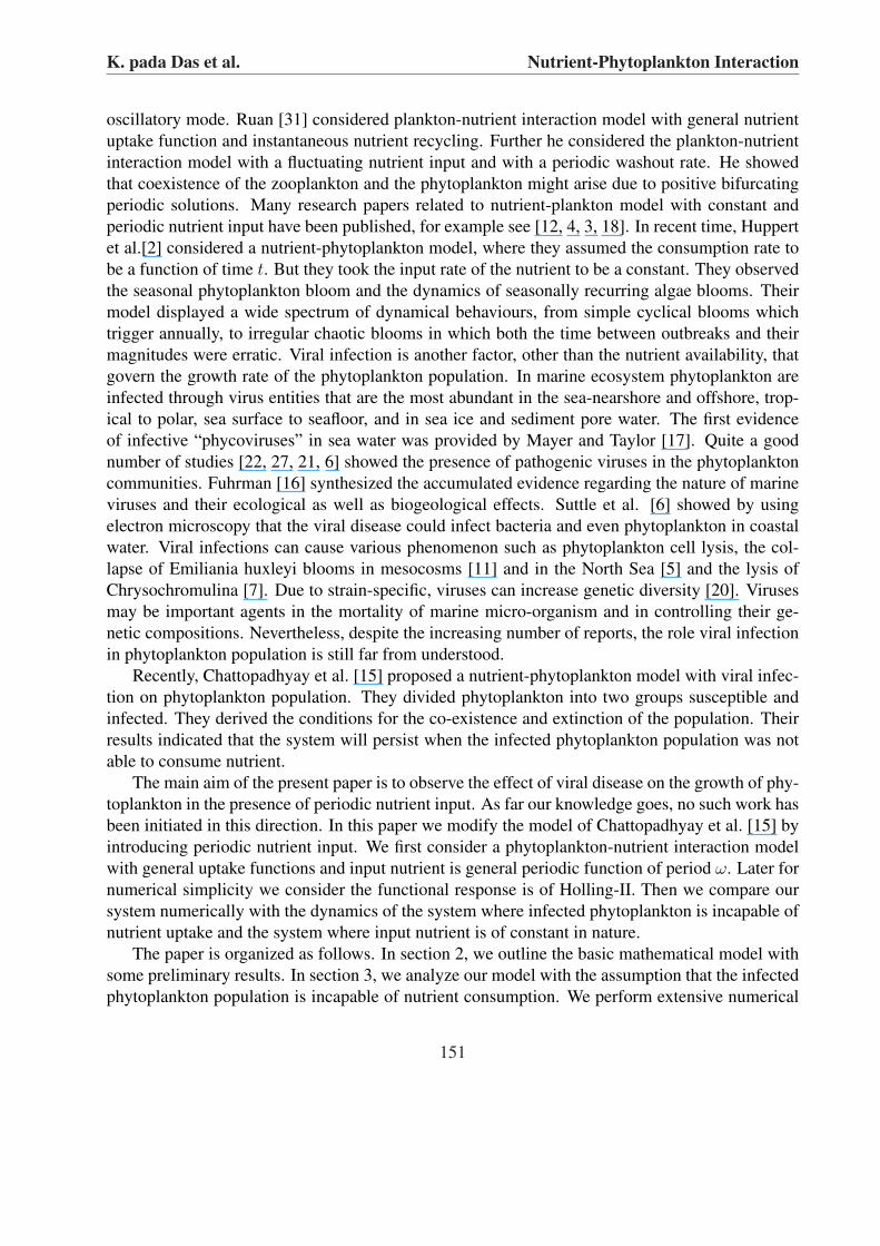
inFigure 7: Figure shows the bifurcation diagram for λ ∈ [0.1,0.5] and the extinction of susceptiblephytoplankton for Case II of the system (4.1) (all the other parameter values fixed as given in (4.2).

0.1 0.2 0.3 0.4 0.50

0.02

0.04

0.06

0.08

λ

Sm

ax &

Sm

in

0.1 0.2 0.3 0.4 0.50

0.01

0.02

0.03

0.04

0.05

0.06

λ

Im

ax &

Im

in

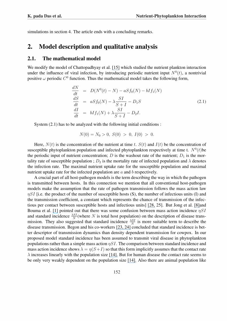
Figure 8: Figure shows co-existing of all species when infected population is not able to consumenutrient for Case II of the system (4.1) (all the other parameter values fixed as given in (4.2).)

165

K. pada Das et al. Nutrient-Phytoplankton Interaction

0.1 0.15 0.2 0.25 0.3 0.35 0.4 0.45 0.5 0.55 0.60.1

0.15

0.2

0.25

0.3

0.35

0.4

0.45

λ

A

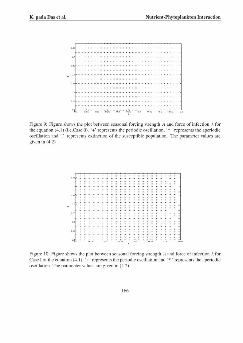
Figure 9: Figure shows the plot between seasonal forcing strength A and force of infection λ forthe equation (4.1) (i.e.Case 0). ‘+’ represents the periodic oscillation, ‘* ’ represents the aperiodicoscillation and ‘.’ represents extinction of the susceptible population. The parameter values aregiven in (4.2)

0.1 0.15 0.2 0.25 0.3 0.35 0.4 0.450.1

0.15

0.2

0.25

0.3

0.35

0.4

0.45

λ

A

Figure 10: Figure shows the plot between seasonal forcing strength A and force of infection λ forCase I of the equation (4.1). ‘+’ represents the periodic oscillation and ‘* ’ represents the aperiodicoscillation. The parameter values are given in (4.2).

166

K. pada Das et al. Nutrient-Phytoplankton Interaction

values of λ but when the infected phytoplankton do not consume nutrients, then the susceptiblephytoplankton will never be washed away from the system for higher values of λ. We observe forboth the system that when the values of λ and A is small the systems show periodic oscillation, see‘+’ in Figs. 9 and 10. But for higher values of λ or A we observe that the system shows aperiodicoscillation, see ‘* ’ in Figs. 9 and 10. Finally for large values of λ we observe that the susceptiblephytoplankton goes to extinction when the infected phytoplankton consume nutrients, see ‘.’ inFig. 9.

For convenience, we summarize the above findings in a tabular form (Table 5).

Table 5: Behaviour of system(4.1).

Variation of Case 0 Case I Case IIλ

Extinction of Extinction of Extinction ofλ ≤ 0.04 infected infected infected

phytoplankton phytoplankton phytoplankton

0.05 = λ Limit cycle Extinction of infected Both phytoplanktonsphytoplankton coexist in steady state

stable position

0.06 ≤ λ ≤ 0.22 Limit cycle Limit cycle Both phytoplanktonscoexist in steady state

stable position

0.22 < λ < 0.39 Chaotic oscillation Chaotic oscillation Limit cycle

Extinction of co-existing of both Extinction ofλ ≥ 0.39 susceptible phytoplanktons susceptible

phytoplankton phytoplankton

5. Concluding RemarksIn marine ecosystem two factors viz seasonality of nutrient and viral disease in phytoplanktoninfluence the dynamics of plankton. However, viral disease in phytoplankton affects significantlythe dynamics of nutrient-plankton model in the presence of periodic nutrient input. In this paper weconsider an NP model with periodic nutrient input and compare it with different cases arising due

167

K. pada Das et al. Nutrient-Phytoplankton Interaction

to constant nutrient input and non-consumption nutrient by infected phytoplankton. We begin witha general model where we took a general functional response and a general periodic function forthe nutrient input. The analytical results corresponding to the general model leads to two distinctthresholds σ0, and σ1. The existence of susceptible and infected phytoplankton, the endemicity ofthe system and disease freeness of the system have been determined by these thresholds. Whenboth phytoplankton uptake nutrient, the system is endemic for σ1 ≥ 0 and disease free for σ1 < 0and both plankton co-exist for σ0 > 0 and σ1 > 0. But endemicity of system is determined by σ∗1(it is obtained by putting b = 0 in σ1) and σ0 > 0 and σ∗1 > 0 implies the persistence of susceptibleand infected phytoplankton when infected phytoplankton is incapable of uptaking nutrient. Thenumerical simulations in our study demonstrates a number of interesting phenomena. With theincrease of the force of infection, the system with periodic nutrient input goes to chaotic regionfrom limit cycle while the system with constant nutrient goes to limit cycle from stable position.In this connection we like to mention the result of Inoue and Kamifukumoto [26] that externalforcing can induce oscillations in a simple prey-predator system. Ecological communities aregenerally embeded in periodically varying environments. It has been shown by Rinaldi et al. [30]that such periodic external forcing may lead to a classical prey-predator system into limit cycleoscillation, period doubling and chaos. We claim from the observations of our proposed modelwith periodic nutrient input and constant nutrient input that seasonal forcing is responsible forchaotic dynamics. In this connection we like to mention that Huppert et al. [2] extended the basicNP model by introducing periodic seasonal forcing which induced all kinds of complex dynamicsfrom limit-cycles to chaos. We also observe that when the force of infection is high, the susceptiblephytoplankton co-exist with infected phytoplankton only if infected phytoplankton is incapable ofuptaking nutrient. This observation is also supported by the experimental observation of Uhlig andSahling [13].

We finally observe from the 2-D parameter figure that for low values of λ and A the systemsshow periodic solution while for high values they show aperiodic solution, which may lead to theextinction of the phytoplankton population if the infected phytoplankton population consumes nu-trient.

Acknowledgement: The authors are grateful to the learned reviewers for their critical com-ments and suggestions on the earlier version of the paper.

References[1] A. Bouma, M.C.M. De Jong, T.G. Kimman. Transmission of pseudorabies virus within pig

populations is independent of the size of the population. Preventative Veterinary Medicine,23 (1995), 163-72.

[2] A. Huppert, B. Blasius, R. Olinky, L. Stone. A model for seasonal phytoplankton blooms. J.Theo. Biol. 236 (2005), 276-290.

168

K. pada Das et al. Nutrient-Phytoplankton Interaction

[3] A.J. Taylor. Characteristic properties of model for the vertical distribution of phytoplanktonunder stratification. Ecol. Model. 40 (1988), 175-199.

[4] B.W. Frost. Grazing control of phytoplankton stock in the open sub-arctic pacific Ocean: amodel assessing the of mesozooplankton, particularly the large calanoid copepod neocalanus.Mar. Ecol. Ser. 39 (1987), 49-68.

[5] C.P.D. Brussaard, R.S. Kempers, A.J. Kop, R. Tiegman, M. Heldel. Virus like particles in asummer bloom of Emiliania huxleyi in the North Sea. Aq. Microbial. Ecol. 10 (1996), 105-113.

[6] C. Suttle, A. Charm, M. Cottrell. Infection of phytoplankton by viruses and reduction of pri-mary productivity. Nature 347 (1990), 467-469.

[7] C.A. Suttle, A.M. Chan. Marine cyanophages infecting oceanic a nd coastal strains of Syne-chococcus: abundance, morphology, cross-infectivity and growth characteristics. Mar. Ecol.Prog. Ser. 92 (1993), 99-109.

[8] D.M.C.M. Jong, O. Diekmann, J.A.P. Heesterbeek. How does transmission depend on popu-lation size? in Human Infectious Disease, Epidemic Models, D.Mollisison, ed., CambridgeUniversity press, Cambridge, UK, (1995) 84-94.

[9] E. Beltrami and T.O. Carroll. Modeling the role of viral disease in recurrent phytoplanktonblooms. J. Math. Biol. 32 (1994), 857-863.

[10] G.J. Butler, P. Waltman. Persistence in dynamical systems. J. Diff. Equations 63 (1986), 255-263 .

[11] G. Bratbak, M. Leavasseur, S. Michand, G. Cantin, E. Fernandez, M. Heldel. Viral activityin relation to Emiliania huaxleyi blooms: a mechanism of DMSP release ? Mar. Ecol. Progr.Ser. 128 (1995), 133-142.

[12] G.T. Evans, J.S. Parslow. A model of annual plankton cycles. Bio. Oceanogr. 3 (1985), 327-427.

[13] G. Uhlig, G. Sahling. Long-term studies on Noctiluca scintillans in the German Bight. Neth.J. Sea Res. 25 (1992), 101-112.

[14] H.W. Hethcote. The mathematics of infectious disease. SIAM Rev., 42 (2000), 599-653.

[15] J. Chattopadhyay, R.R. Sarkar, S. Pal. Dynamics of nutrient-phytoplankton interaction in thepresence of viral infection. BioSystems, 68 (2003), 5-17 .

[16] J.A. Fuhrman. Marine viruses and their biogeochemical and ecological effects. Nature399 (1999), 541-548.

[17] J.A. Mayer and F.J.R. Taylor. A virus which lyses the marine nanoflagellate micromonaspusilla. Nature, 281 (1979), 299-301 .

169

K. pada Das et al. Nutrient-Phytoplankton Interaction

[18] J. S. Wroblewski, J. L. Sarmiento, G. R. Flierl. An ocean basin scale model of planktondynamics in the North Atlantic, 1, solutions for the climatological oceanographic condition inMay. Global Biogeochem. Cycles 2 (1988), 199-218.

[19] K.P. Hadeler, H.I. Freedman. Predator-prey population with parasitic infection. J. Math. Biol.27 (1989), 609-631.

[20] K. Nagasaki, M.Yamaguchi. Isolation of a virus infectious to the harmful bloom causingmicroalga Heterosigma akashiwo (Raphidophyceae). Aquat. Microbial. Ecol. 13 (1997), 135-140.

[21] K. Tarutani, K. Nagasaki, M.Yamaguchi. Viral impacts on total abundance and clonal com-position of the harmful bloom-forming phytoplankton Heterosigma akashiwo. Appl. Environ.Microbial. 66 (2000), No. 11, 4916-4920.

[22] K.E. Wommack, R.R. Colwell. Virioplankton: viruses in aquatic ecosystems. Microbial. Mol.Biol. Rev. 64 (2000), No. 1, 69-114.

[23] M. Begon et al. Population and transmission dynamics of cowpox in bank voles: testingfundamental assumptions. Ecol. 1 (1998), 82-86.

[24] M. Begon et al. Transmission dynamics of a zoonotic pathogen within and between wildlifehost species. Proc R. Soc. Lond. B,266 (1999), 1939-1945.

[25] M.E. Hochberg. The potential role of pathogens in pest control. Nature, 337 (1989), 262-265.

[26] M. Inoue, H. Kamifukumoto. Scenarios leading to chaos in a forced Lotka Volterra model.Prog. Theor. Phys. 71 (1984), 930-937.

[27] O. Bergh, K.Y. Borsheim, G.Bratbak, M. Heldal. High abundance of viruses found in aquaticenvironments. Nature 340 (1989), 467-468.

[28] R.M. Anderson. Theoretical basis for the use of pathogens as biological control agents ofpest species. Parasitology 84 (1982), 3-33.

[29] S. Busenberg, K.S. Kishore, P.Austin, G. Wake. The dynamics of a model of a plankton-nutrient interaction. J. Math. Biol. 52 (1990), 677-696.

[30] S. Rinaldi, S. Murtori, Y. Kuznetsov. Multiple attractors catastrophe and chaos in seasonallyperturbed predator-prey communities. Bull.Math.Biol. 55 (1993), 15-35.

[31] S. Ruan. Persistence and co-existence in zooplankton-phytoplankton-nutrient models withinstantaneous nutrient recycling. J. Math. Biol. 31 (1993), 633-654.

[32] V.A. Pliss. Nonlocal problems of the theory of oscillations., Academic Press, New York,1966.

170