arX

iv:0

805.

2316

v1 [

mat

h.ST

] 1

5 M

ay 2

008

IMS Collections

Beyond Parametrics in Interdisciplinary Research: Festschrift in Honor of Professor

Pranab K. Sen

Vol. 1 (2008) 197–210c© Institute of Mathematical Statistics, 2008DOI: 10.1214/193940307000000149

U-tests for variance components in

one-way random effects models∗

Juvencio S. Nobre1, Julio M. Singer2 and Mervyn J. Silvapulle3

Universidade Federal do Ceara, Universidade de Sao Paulo and Monash University

Abstract: We consider a test for the hypothesis that the within-treatmentvariance component in a one-way random effects model is null. This test isbased on a decomposition of a U -statistic. Its asymptotic null distributionis derived under the mild regularity condition that the second moment of therandom effects and the fourth moment of the within-treatment errors are finite.Under the additional assumption that the fourth moment of the random effectis finite, we also derive the distribution of the proposed U -test statistic under asequence of local alternative hypotheses. We report the results of a simulationstudy conducted to compare the performance of the U -test with that of theusual F -test. The main conclusions of the simulation study are that (i) undernormality or under moderate degrees of imbalance in the design, the F -testbehaves well when compared to the U -test, and (ii) when the distribution ofthe random effects and within-treatment errors are nonnormal, the U -test ispreferable even when the number of treatments is small.

1. Introduction

Consider the one-way random effects model

Yij = µ+ bi + eij , i = 1, . . . k, j = 1, . . . , ni (≥ 2)(1.1)

with bi and eij , i = 1, . . . , k, j = 1, . . . , ni, denoting independent random vari-ables with null means and variances σ2

b and σ2e , respectively. Thus, µ is the mean

response, bi represents the random effect of the i-th treatment, eij represents arandom measurement error associated with the j-th observation obtained underthe i-th treatment, and σ2

b and σ2e are between- and within-treatment variance

components, respectively.In general, data analysis based on such a model focuses on the estimation of µ

and on testing the one-sided hypothesis (of no treatment effects)

H0 : σ2b = 0 vs H1 : σ2

b > 0.(1.2)

Inference about variance components in random effects models, and more generallyin linear mixed models, has a long history in the statistical literature. In this con-text, Searle et al. [21] provides an excellent overview of estimation and prediction

∗Supported by Conselho Nacional de Desenvolvimento Cientıfico e Tecnologico (CNPq) andFundacao de Amparo a Pesquisa do Estado de Sao Paulo (FAPESP), Brazil.

1Departamento de Estatıstica e Matematica Aplicada, Universidade Federal do Ceara, Brazil,e-mail: juvencio@ufc.br

2Departamento de Estatıstica, Universidade de Sao Paulo, Brazil, e-mail: jmsinger@ime.usp.br3Department of Econometrics and Business Statistics, Monash University, P.O. Box 197,

Caulfield East, Australia 3145, e-mail: Mervyn.Silvapulle@buseco.monash.edu.auAMS 2000 subject classifications: Primary 62F03; secondary 62F05.Keywords and phrases: martingales, one-sided hypotheses, one-way random effects model, re-

peated measures, U -statistics, variance components.

197

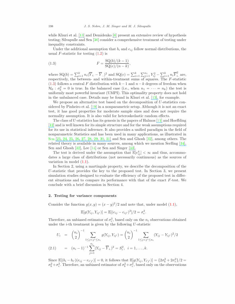
198 J. S. Nobre, J. M. Singer and M. J. Silvapulle

while Khuri et al. [13] and Demidenko [6] present an extensive review of hypothesistesting; Silvapulle and Sen [36] consider a comprehensive treatment of testing underinequality constraints.

Under the additional assumption that bi and eij follow normal distributions, theusual F -statistic for testing (1.2) is

F =SQ(b)/(k − 1)

SQ(e)/(n− k),(1.3)

where SQ(b) =∑k

i=1ni(Y i. − Y ..)

2 and SQ(e) =∑k

i=1

∑ni

j=1Y 2

ij −∑k

i=1niY

2

i. are,respectively, the between- and within-treatment sums of squares. The F -statistic(1.3) follows a central F distribution with k− 1 and n− k degrees of freedom whenH0 : σ2

b = 0 is true. In the balanced case (i.e., when n1 = · · · = nk) the test isuniformly most powerful invariant (UMPI). This optimality property does not holdin the unbalanced case. Details may be found in Khuri et al. [13], for example.

We propose an alternative test based on the decomposition of U -statistics con-sidered by Pinheiro et al. [19] in a nonparametric setup. Although it is not an exacttest, it has good properties for moderate sample sizes and does not require thenormality assumption. It is also valid for heteroskedastic random effects.

The class of U -statistics has its genesis in the papers of Halmos [11] and Hoeffding[12] and is well known for its simple structure and for the weak assumptions requiredfor its use in statistical inference. It also provides a unified paradigm in the field ofnonparametric Statistics and has been used in many applications, as illustrated inSen [23, 24, 25, 26, 27, 28, 29, 30, 31] and Sen and Ghosh [32], among others. Therelated theory is available in many sources, among which we mention Serfling [34],Sen and Ghosh [32], Lee [14] or Sen and Singer [33].

The test is derived under the assumption that E[e4ij ] < ∞ and thus, accommo-dates a large class of distributions (not necessarily continuous) as the sources ofvariation in model (1.1).

In Section 2, using a martingale property, we describe the decomposition of theU -statistic that provides the key to the proposed test. In Section 3, we presentsimulation studies designed to evaluate the efficiency of the proposed test in differ-ent situations and to compare its performance with that of the exact F -test. Weconclude with a brief discussion in Section 4.

2. Testing for variance components

Consider the function g(x, y) = (x− y)2/2 and note that, under model (1.1),

E[g(Yij , Yij′ )] = E[(eij − eij′ )2]/2 = σ2

e .

Therefore, an unbiased estimator of σ2e , based only on the ni observations obtained

under the i-th treatment is given by the following U -statistic

Ui =

(

ni

2

)−1∑

1≤j<j′≤ni

g(Yij , Yij′ ) =

(

ni

2

)−1∑

1≤j<j′≤ni

(Yij − Yij′ )2/2

= (ni − 1)−1

ni∑

j=1

(Yij − Y i.)2 = S2

i , i = 1, . . . , k.(2.1)

Since E[(bi − bi′)(eij − ei′j′)] = 0, it follows that E[g(Yij , Yi′j′)] = {2σ2b + 2σ2

e}/2 =σ2

b +σ2e . Therefore, an unbiased estimator of σ2

b +σ2e , based only on the observations

U-tests for variance components 199

obtained under treatments i and i′, is given by the following generalized U -statisticof order (1,1)

Uii′ = (nini′)−1

ni∑

j=1

ni′∑

j′=1

(Yij − Yi′j′)2

2, 1 ≤ i < i′ ≤ k.(2.2)

Letting n =∑k

i=1ni, the lexicographically ordered observations,

Y11, . . . , Y1n1, Y21, . . . , Y2n2

, . . . , Yk1, . . . , Yknk,

may be re-expressed as

Y1, . . . , Yn1, Yn1+1, . . . , Yn1+n2

, . . . , Yn1+···+nk−1+1, . . . , Yn,

where the first n1 observations relate to treatment 1, the next n2, to treatment 2and so on. The uniformly minimum variance unbiased estimator (UMVUE) of thevariance of the observations is given by the U -statistic

U0n =

(

n

2

)−1∑

1≤r<s≤n

1

2(Yr − Ys)

2,

which can be rewritten as

U0n =

(

n

2

)−1

k∑

i=1

(

ni

2

)

Ui +∑

1≤i<i′≤k

nini′Uii′

=k∑

i=1

ni(ni − 1)

n(n− 1)Ui + 2

∑

1≤i<i′≤k

nini′

n(n− 1)Uii′ ,(2.3)

highlighting its nature of a linear combination of generalized U -statistics. The firstand second terms in (2.3) correspond, respectively, to the within and between-treatments components. Since

ni(ni − 1)/{n(n− 1)} = {ni/n} − {ni(n− ni)}/{n(n− 1)},

and∑

i′ 6=i ni′ = n− ni, we can rewrite the first term in (2.3) as

k∑

i=1

ni(ni − 1)

n(n− 1)Ui =

k∑

i=1

ni

nUi −

k∑

i=1

ni(n− ni)

n(n− 1)Ui

=

k∑

i=1

ni

nUi −

∑

1≤i<i′≤k

nini′

n(n− 1)Ui −

∑

1≤i<i′≤k

nini′

n(n− 1)Ui′ ,

leading to the decomposition

(2.4) U0n = Wn +Bn

where

Wn =

k∑

i=1

ni

nUi and Bn =

∑

1≤i<i′≤k

nini′

n(n− 1){2Uii′ − Ui − Ui′} .

200 J. S. Nobre, J. M. Singer and M. J. Silvapulle

This includes the classical ANOVA decomposition as a special case. Now observethat

E[Bn] =∑

1≤i<i′≤k

nini′

n(n− 1)

{

2(σ2b + σ2

e) − 2σ2e

}

= 2σ2b

∑

1≤i<i′≤k

nini′

n(n− 1)

= σ2b

k∑

i=1

∑

i′ 6=i

nini′

n(n− 1)= σ2

b

k∑

i=1

ni(n− ni)

n(n− 1)= σ2

b

(

n2 −∑ki=1

n2i

n(n− 1)

)

≥ 0.

Therefore, E[Bn] = 0 if and only if σ2b = 0. These results allow us to construct a

test for (1.2) based on Bn (suitably standardized) as we show in the sequel.Firstly using the lexicographically ordered observations, we show that Bn may

be reexpressed as

Bn =

(

n

2

)−1∑

1≤r<s≤n

ηnrsψ(Yr , Ys),(2.5)

where ψ(x1, x2) = (x1 − µ)(x2 − µ) and

ηnrs =

(n− ni)/(ni − 1), if Yr and Ys are both observedunder the i-th treatment,

−1, otherwise.(2.6)

Thus, it follows that

∑

1≤r<s≤n

ηnrs = 0(2.7)

and

∑

1≤r<s≤n

η2nrs =

(

n

2

)

(k − 1)

{

1 +1

n

k∑

i=1

n− ni

(ni − 1)(k − 1)

}

.(2.8)

When k → ∞ and the ni’s are bounded, i.e., the maximum number of observationsper treatment does not increase with the number of treatments, it follows thatk = O(n); hence, by (2.8) we may conclude that Mn =

∑

1≤r<s≤n η2nrs = O(n3).

Under H0 : σ2b = 0, the random variables Y1, . . . , Yn are independent and iden-

tically distributed and ψ(x, y) is a first-order stationary kernel, centered at 0, con-stituting an orthogonal system in the sense adopted in Pinheiro et al. [19], thatis,

ψ1(Yr) = E[ψ(Yr , Ys)|Yr] = E[(Yr − µ)(Ys − µ)|Yr] = 0 a.s.(2.9)

E[ψ(Y1, Y2)ψ(Y1, Y3)] = 0.(2.10)

Now, observe that E[ψ2(Yr, Ys)] = Var[ψ(Yr , Ys)] = E[(Yr−µ)2(Ys−µ)2] = σ4e <∞.

Then, we may show (see Appendix), that under H0 : σ2b = 0,

Jn =

(

n2

)

Bn

Wn

√Mn

D−→N (0, 1)(2.11)

when k → ∞(⇒ n→ ∞). The key to the proof is the martingale property exhibitedby Bn, as pointed in Pinheiro et al. [19] in a different setup. Let limn→∞Mn/n

3 =

U-tests for variance components 201

λ, which is finite because Mn = O(n3); assume that the fourth moment of thedistribution of the random effects is finite and let δ denote a constant. Then, underthe sequence of local hypotheses

H1n : σ2b = δ2/

√n,(2.12)

it follows that

JnD−→N

(

δ2

2σ2e

√λ, 1

)

as k → ∞,(2.13)

Details are presented in the Appendix. Because the mean of this limiting normaldistribution is positive, we may use Jn as a test statistic for (1.2), rejecting the nullhypothesis H0 at significance level α when Jn ≥ zα, where zα is the (1 − α)100%percentile of the standard normal distribution. By (2.13), the power of this testis directly related to the magnitude of the intraclass correlation coefficient ρ =σ2

b/(σ2b + σ2

e); more specifically, the power is a monotone increasing function of ρ,as expected.

3. Simulation results

We summarize some simulation studies conducted with the objective of evaluatingthe behaviour of the proposed test. First, we examine the efficiency of the U -testin balanced studies under different distributions for the within-treatment errorseij and random effects bi. Then, we compare the efficiency of the proposed U -testwith that of the usual F -test under various settings. Additional results from thesimulation studies may be obtained from the authors.

3.1. Efficiency of the proposed test

To evaluate the behaviour of the proposed test for small and moderate samples weconsidered 10, 000 Monte-Carlo samples obtained under model (1.1) with µ = 2and σ2

e = 1, for different numbers of treatments (k = 10, 30 and 100) in balancedstudies. We assumed that eij ∼ N (0, 1) and bi ∼ t3 ×

√

σ2b/3, so that Var[bi] = σ2

b .The between-treatments variance, σ2

b , was set to 0 (to estimate the size of the test),0.2, 0.5 and 1. The empirical power of the test under each setting was evaluated fora significance level of α = 0.05.

The results, displayed in first half of Table 1, suggest that the U -test tends to beliberal when there are few observations for each treatment (ni ≤ 4). The differencebetween the empirical and nominal size of the test is acceptable when the numberof treatments is at least 30 and there are 5 or more observations per treatment.Furthermore, the power of the test increases with σ2

b , ni and k, as expected.

To illustrate the robustness of the U -test with respect to heavy-tailed within-treatment error distributions, we repeated the simulation study described previ-ously assuming that eij ∼ t5 ×

√

3/5 (so that Var[eij ] = 1). The results, summa-rized in the second half of Table 1, are not considerably different from the previousones; here, however, the empirical size of the test is closer to the nominal size andthe test also tends to be more powerful than when the within-treatment errors arenormal.

202 J. S. Nobre, J. M. Singer and M. J. Silvapulle

Table 1

Rejection rates (%) for the 5% level U-test in balanced designs with bi ∼ t3 ×√

σ2

b/3

k = 10 k = 30 k = 100

ni ni ni

σ2

b2 4 5 10 2 4 5 10 2 4 5 10

eij ∼ normal

0 14 8.8 7.6 6.2 8.3 7.1 6.3 6.1 7.2 6.1 5.9 5.40.2 26 36 41 64 33 59 69 93 54 92 97 1000.5 41 61 69 89 61 91 96 100 93 100 100 1001.0 57 82 88 98 85 99 100 100 100 100 100 100

eij ∼ t5 ×√

3/5

0 13 8.9 7.8 6.3 8.4 6.8 6.3 6.1 7.3 5.9 5.5 5.40.2 26 37 42 64 34 61 69 93 54 92 97 1000.5 41 62 71 89 63 91 95 100 92 100 100 1001.0 60 83 89 97 86 99 100 100 100 100 100 100

3.2. Comparison between the F - and U-tests

To compare the two tests, we first repeated the simulation study described previ-ously, using the same values for µ and σ2

e in the following situations:

(i) Balanced study under normality;(ii) Moderately unbalanced study under normality;(iii) Lightly unbalanced study with heavy-tailed distributions;(iv) Balanced study with heavy-tailed asymmetric distributions.

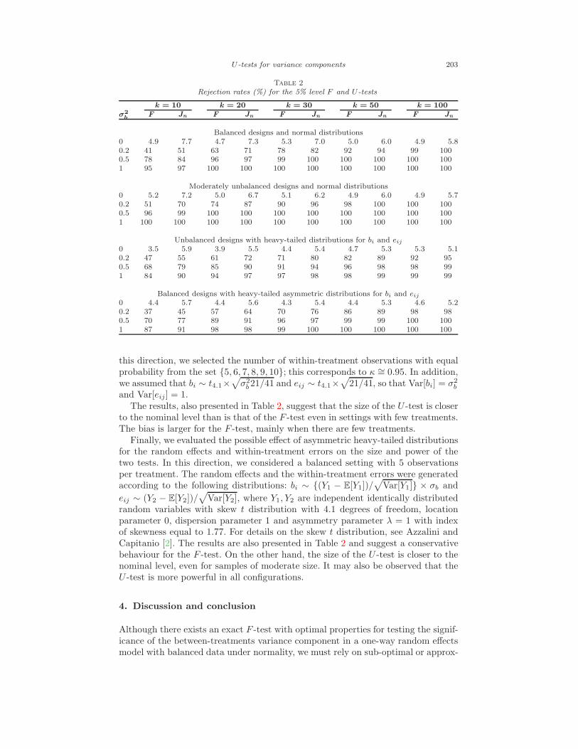
Firstly, we consider a balanced setting with 5 observations per treatment. Therandom effects and the within-treatment errors were generated according to: bi ∼N (0, σ2

b ) and eij ∼ N (0, 1). The results are presented in Table 2 and as in theprevious studies, they suggest that the U -test is liberal. However, the differencebetween the empirical and nominal size of the test decreases substantially whenthe number of treatments increases. This occurs mainly when there are few unitsper treatment. On the other hand, the proposed U -test is more powerful than theexact F -test, though we should recognize that this might be influenced by its liberalnature.

We also considered simulation studies to evaluate the effect of imbalance in thepower of the two tests under investigation. Khuri et al. [13], Donner and Koval [7]and Lee [15] discuss the performance of F -tests for different degrees of imbalance,defined as κ = 1/(1 + ψ2) where ψ denotes the coefficient of variation associatedwith the sample sizes n1, . . . , nk. By definition, 0 < κ ≤ 1 with κ = 1 only forbalanced studies. Smaller values of κ indicate larger degrees of imbalance.

We selected the number of within-treatment observations from a geometric dis-tribution (shifted to the right by 2) with parameter p = 0.15 and support {0, 1, . . .}.This corresponds to a moderate degree of imbalance (κ = 0.61). The random effectsbi and the within-treatment errors eij were respectively generated from N (0, σ2

b )and N (0, 1) distributions.

In spite of the moderate imbalance, the size of the F -test is closer to the nom-inal level than is that of the (more liberal) U -test, especially when the number oftreatments is small; however, the latter is more powerful than the F -test in mostsettings.

We also evaluated the simultaneous effects of a small degree of imbalance andheavier-tailed distributions for the random effects and within-treatment errors. In

U-tests for variance components 203

Table 2

Rejection rates (%) for the 5% level F and U-tests

k = 10 k = 20 k = 30 k = 50 k = 100

σ2

bF Jn F Jn F Jn F Jn F Jn

Balanced designs and normal distributions0 4.9 7.7 4.7 7.3 5.3 7.0 5.0 6.0 4.9 5.80.2 41 51 63 71 78 82 92 94 99 1000.5 78 84 96 97 99 100 100 100 100 1001 95 97 100 100 100 100 100 100 100 100

Moderately unbalanced designs and normal distributions0 5.2 7.2 5.0 6.7 5.1 6.2 4.9 6.0 4.9 5.70.2 51 70 74 87 90 96 98 100 100 1000.5 96 99 100 100 100 100 100 100 100 1001 100 100 100 100 100 100 100 100 100 100

Unbalanced designs with heavy-tailed distributions for bi and eij

0 3.5 5.9 3.9 5.5 4.4 5.4 4.7 5.3 5.3 5.10.2 47 55 61 72 71 80 82 89 92 950.5 68 79 85 90 91 94 96 98 98 991 84 90 94 97 97 98 98 99 99 99

Balanced designs with heavy-tailed asymmetric distributions for bi and eij

0 4.4 5.7 4.4 5.6 4.3 5.4 4.4 5.3 4.6 5.20.2 37 45 57 64 70 76 86 89 98 980.5 70 77 89 91 96 97 99 99 100 1001 87 91 98 98 99 100 100 100 100 100

this direction, we selected the number of within-treatment observations with equalprobability from the set {5, 6, 7, 8, 9, 10}; this corresponds to κ ∼= 0.95. In addition,we assumed that bi ∼ t4.1×

√

σ2b21/41 and eij ∼ t4.1×

√

21/41, so that Var[bi] = σ2b

and Var[eij ] = 1.The results, also presented in Table 2, suggest that the size of the U -test is closer

to the nominal level than is that of the F -test even in settings with few treatments.The bias is larger for the F -test, mainly when there are few treatments.

Finally, we evaluated the possible effect of asymmetric heavy-tailed distributionsfor the random effects and within-treatment errors on the size and power of thetwo tests. In this direction, we considered a balanced setting with 5 observationsper treatment. The random effects and the within-treatment errors were generatedaccording to the following distributions: bi ∼ {(Y1 − E[Y1])/

√

Var[Y1]} × σb and

eij ∼ (Y2 − E[Y2])/√

Var[Y2], where Y1, Y2 are independent identically distributedrandom variables with skew t distribution with 4.1 degrees of freedom, locationparameter 0, dispersion parameter 1 and asymmetry parameter λ = 1 with indexof skewness equal to 1.77. For details on the skew t distribution, see Azzalini andCapitanio [2]. The results are also presented in Table 2 and suggest a conservativebehaviour for the F -test. On the other hand, the size of the U -test is closer to thenominal level, even for samples of moderate size. It may also be observed that theU -test is more powerful in all configurations.

4. Discussion and conclusion

Although there exists an exact F -test with optimal properties for testing the signif-icance of the between-treatments variance component in a one-way random effectsmodel with balanced data under normality, we must rely on sub-optimal or approx-

204 J. S. Nobre, J. M. Singer and M. J. Silvapulle

imate tests in unbalanced or nonnormal settings. We derived an asymptotic U -testthat may be employed with unbalanced data and does not require a specified formfor the underlying probability distributions. Simulation studies suggest that it hasreasonable properties even for moderate and small samples.

In particular, we may conclude that the F -test is more affected by the lack ofnormality of the random effects and within-treatment errors than by imbalance.Furthermore, the U -test seems to be less sensitive to imbalance and to be morepowerful than the F -test in general. Such conclusions must be viewed with caution,given the liberal nature of the U -test, specially for small sample sizes. To bypass thisproblem, one could consider bootstrap methods to obtain the empirical distributionof the statistic Jn under H0 and use the fact that the null hypothesis should berejected for high values of Jn. For details on the use of bootstrap to constructconfidence regions or for hypothesis testing, see Davison and Hinkley [5] or Lehmannand Romano [16], Chapter 15, for example.

In summary, under normality or under moderate degrees of imbalance, the F -testbehaves well in terms of power when compared to U -test; however, in situationswhere the distribution of the random effects and within-treatment errors are non-normal, the U -test is preferable even when the number of treatments is small. In allsettings the U -test is more powerful than the F -test, mainly for small and moderatesamples.

The proposed U -test may also be used to test for simultaneous significance of allrandom components in models with more than one random effect, since it behaves as(2.11) under H0. The corresponding power computations, however, require furtherresearch.

Brownie and Boos [4] and Boos and Brownie [3] study the behaviour of F -testsand analogous rank tests in one-way random effects models when the number oftreatments is large. Akritas and Arnold [1] also study the asymptotics of ANOVAunder similar conditions but their results require more restrictive assumptions thanthose we considered; the proofs, however, are different for balanced and unbalancedstudies.

In the context under investigation, the derivation of tests for (1.2) may not fol-low the standard procedures since the null hypothesis defines a point (or region) onthe boundary of the parameter space and this brings in some technical difficulties.Asymptotic tests for (1.2) or, more generally, for testing the significance of variancecomponents under linear mixed models are available in the literature. Based onthe ideas of Silvapulle and Silvapulle [35], Verbeke and Molenberghs [38] obtainedscore-type tests under the assumption that the underlying probability distributionsare normal. Along the same lines, Savalli et al. [20] extended the results to accom-modate elliptical underlying distributions. In particular, for the one-way randomeffects models, the corresponding test statistic follows an asymptotic distributiongiven by a 50:50 mixture of χ2

0 and χ21 distributions. Tests based on generalized

likelihood methods (that are asymptotically equivalent to the score-type tests) areconsidered in Self and Liang [22], Stram and Lee [37] and Silvapulle and Sen [36],for example. The main disadvantage of such tests is the difficulty in verifying therequired regularity conditions as shown in Giampaoli and Singer [9]. The derivationof the proposed U -test is not affected by such difficulties and we envisage that itmay serve as a building block for more general setup as indicated in Nobre [18].

Other alternatives have been suggested in the literature. Using a Laplace expan-sion of the integrated log-likelihood, Lin [17] obtained a global score test for thehypothesis that all variance components are zero in the framework of generalizedlinear models with random effects. Along the same lines, Zhu and Fung [39] ob-

U-tests for variance components 205

tained a global score-type test for the hypothesis that all variance components arezero in a semiparametric mixed model, under the assumption of normality only ofthe conditional error vector. It is important to point out, that the tests are ob-tained without specifying the distribution of the random effects, though they arebased on a marginal approach under which the within-treatment covariances maybe negative. Hall and Præstgaard [10] consider such a constraint in the frameworkof generalized linear models with random effects, via a projected score test. In prac-tice, their results are difficult to apply when the dimension of the vector of randomeffects is large.

Appendix A: Proof of (2.11)

Note that under H0 : σ2b = 0,

Bn =

(

n

2

)−1∑

1≤r<s≤n

ηnrsψ(Yr, Ys)

is a sum of(

n2

)

uncorrelated terms such that E[ψ(Yr , Ys)] = 0 e Var[ψ(Yr, Ys)] =σ4

e <∞. Thus, it follows that

(A.1) E[Bn] = 0 and Var[Bn] = σ4eMn

(

n

2

)−2

.

Then, along the lines adopted in Pinheiro et al. [19], we explore the martingale struc-ture of Bn, and apply a martingale Central Limit Theorem as given in Dvoretzky[8] or Sen and Singer [33] to obtain the desired asymptotic distribution. Their proofrequires k fixed and ni → ∞; we consider ni bounded and let k → ∞, although thetest is also valid when both k → ∞ and ni → ∞.

Initially, consider the statistic

Tn =∑

1≤i<j≤n

ηnijφ(Xi, Xj)(A.2)

with φ satisfying

φ1(X1) = E[φ(X1, X2)|X1] = 0 a.s.,(A.3)

E[φ(X1, X2)φ(X1, X3)] = 0,(A.4)

E[φ2(X1, X2)] <∞,(A.5)

where X1, . . . , Xn represents a sequence of independent and identically distributedrandom variables and ηnij denotes weights such that

(A.6)∑

1≤i<j≤n

ηnij = 0 and∑

1≤i<j≤n

η2nij = M∗

n.

Defining, Znj =∑j−1

i=1ηnijφ(Xi, Xj), for j = 2, ...n and Tnu =

∑ul=2

Znl for 2 ≤u ≤ n, it follows that Tnn = Tn. Now, considering the nondecreasing sequence (inu) of σ-fields σnu = σ(Xi, i ≤ u) that corresponds to the σ-fields generated by therandom vector (X1, . . . , Xu)⊤, 2 ≤ u ≤ n we may apply the following result due toPinheiro et al. [19].

206 J. S. Nobre, J. M. Singer and M. J. Silvapulle

Theorem A.1. Under conditions (A.2)–(A.5), {Tnu, 2 ≤ u ≤ n} is a zero meanmartingale process adapted to the filter {σnu, 2 ≤ u ≤ n}.

Letting Dn denote a weakly consistent estimator of τ2 = E[φ2(Xi, Xj)] < ∞(i < j), it follows from (A.4) and (A.5) that Var[Tn] = E[T 2

n ] = τ2M∗n. Using

Slutsky’s theorem, we obtain

DnM∗n

E[T 2n ]

P−→1.(A.7)

Now, note that the statistic(

n2

)

Bn is of the form (A.2) with φ(x, y) = (x−µ)(y−µ)satisfying (A.3)–(A.5). Additionally, observe that τ2 = E[φ2(Xi, Xj)] = σ4

e <∞. Aconsistent estimator of τ2 may be obtained from the following result.Lemma A.1. Consider a linear combination of U -statistics of the form Wn =∑k

i=1

ni

n Ui =∑k

i=1wiUi. If

max1≤i≤k

ni∑k

i=1ni

→ 0,(A.8)

it follows that W 2n

P−→σ4e .

Proof. Condition (A.8) is valid when the ni’s are fixed and k → ∞. It also holdswhen ni → ∞, as for example, in a balanced study.

Noting that E[Wn] = σ2e , and using properties of U -statistics, it is possible to

show that Var[Ui] = E[e4ij ]/ni − (ni − 3)σ4e/{(ni − 1)ni}. Then, a direct application

of Chebyshev’s inequality leads to WnP−→σ2

e . Since x2 is a continuous function in

the support of Wn, we conclude that Dn = W 2n

P−→σ4e .

In the proof, E[e4ij ] < ∞ is used to guarantee the existence of Var[Ui]. In somesituations, as in the balanced case, this requirement may be relaxed and the resultfollows from Khintchine’s weak law of large numbers.

We now focus on the following lemma.Lemma A.2. Consider the weights defined in (2.6). When k → ∞ it follows that

∑

1≤i6=j<u≤n

η2niuη

2nju/M

2n → 0, and

∑

1≤i6=j≤n

η4nij/M

2n → 0.(A.9)

Proof. When k → ∞ and the ni’s are bounded, it follows that k = O(n). Then by(2.8), we obtain Mn =

∑

1≤r<s≤n η2nrs = O(n3). Now, the result follows from

∑

1≤i6=j≤n

η4nij = O(n5) and

∑

1≤i6=j<u≤n

η2niuη

2nju = O(n5).

The proof of the main result consists in verifying the two regularity conditionsof Theorem 3.3.7 in (Sen and Singer [33], page 120) and it is similar to the proofpresented in Pinheiro et al. [19].Theorem A.2. Suppose that E[φ4(X1, X2)] < ∞, (A.3)-(A.5) hold and, for n →∞, the weights ηnij satisfy

(A.10)∑

1≤i6=j<k≤n

η2nikη

2njk/(M

∗n)2 → 0 and

∑

1≤i6=j≤n

η4nij/(M

∗n)2 → 0.

U-tests for variance components 207

Then, for Tn in (A.2), we have that

(M∗nDn)−1/2Tn

D−→N (0, 1).(A.11)

Proof. For the weights defined in (2.6), we have M∗n = Mn. Then (2.11) follows

from Lemmas A.1 and A.2.

Appendix B: Proof of (2.13)

First observe that

Ui =

(

ni

2

)−1∑

1≤j<j′≤ni

(Yij − Yij′ )2

2=

(

ni

2

)−1∑

1≤j<j′≤ni

(eij − eij′)2

2

and Wn =

k∑

i=1

(ni/n)Ui, are functions only of the vector of within-treatment er-

rors e. Consequently, their distributions under H0 and H1n are the same. On theother hand, we have

Bn =∑

1≤i<i′≤k

nini′

n(n− 1){2Uii′ − Ui − Ui′}

=∑

1≤i<i′≤k

nini′

n(n− 1)

2

nini′

ni∑

j=1

ni′∑

j′=1

(Yij − Yi′j′)2

2− Ui − Ui′

= B0n + Cn,

where

B0n =

∑

1≤i<i′≤k

nini′

n(n− 1)

2

nini′

ni∑

j=1

ni′∑

j=1

(eij − ei′j′ )2

2− Ui − Ui′

,

Cn =∑

1≤i<i′≤k

nini′

n(n− 1)

(bi − bi′)2 +

2(bi − bi′)

nini′

ni∑

j=1

ni′∑

j′=1

(eij − ei′j′)

.

Also, under H0, Bn = B0n. Therefore,

J∗n =

(

n2

)

Bn

σ2eM

1/2n

=

(

n2

)

B0n

σ2eM

1/2n

+

(

n2

)

Cn

σ2eM

1/2n

= Jn0 +Qn,(B.1)

where Jn0 =(

n2

)

B0n/(σ

2eM

1/2n )

D−→N (0, 1) (by 2.11) and Qn =(

n2

)

Cn/(σ2eM

1/2n ).

The term Cn can be decomposed as Cn = Cn1 + Cn2 where

Cn1 =1

n(n− 1)

∑

1≤i≤i′≤k

nini′(bi − bi′)2

and

Cn2 =2

n(n− 1)

∑

1≤i≤i′≤k

(bi − bi′)

ni∑

j=1

ni′∑

j′=1

(eij − eij′).

208 J. S. Nobre, J. M. Singer and M. J. Silvapulle

Since E[Cn2] = 0, we have

E[Cn] = E[Cn1] =1

n(n− 1)

∑

1≤i≤i′≤k

nini′E[(bi − bi′)2]

=1

n(n− 1)

∑

1≤i≤i′≤k

nini′2σ2b = σ2

b

(

n2 −∑ki=1

n2i

n(n− 1)

)

= O(n−1/2).

The following result provides the asymptotic behaviour of Qn under the assumptionof the existence of the fourth moment of the random effects.Lemma B.1. Consider model (1.1) under H1n = σ2

b = δ2/√n. Assuming that

E[b4i ] <∞ and letting limn→∞Mn/n3 = λ, we have

(

n2

)

Cn√Mn

P−→ δ2

2√λ.

Proof. Given that E[b4i ] <∞, then by contiguity of the sequence of local alternativehypotheses H1n : σ2

b = δ2/√n, we have that E[b4i ] = o(1) under H1n. Defining

bij = (bi− bj)2, recalling that b1, . . . , bk are independent and identically distributedand that the ni’s are bounded, we have

Var[Cn1] =1

n2(n− 1)2

∑

1≤i<i′≤k

n2in

2i′Var[bii

′

] +∑

1≤i<t≤k

1≤i<w≤k

t6=w

n2intnwCov[bit, biw]

≤ max{Var[b12],Cov[b12, b13]}n2(n− 1)2

∑

1≤i<i′≤k

n2in

2i′ +

∑

1≤i<t≤k

1≤i<w≤k

t6=w

n2intnw

= o(1)O(n−1) = o(n−1),

since Var[b12a ] and Cov[b12a , b13a ] are of the same order as E[b4i ], namely, o(1). Sim-

ilarly, it is possible to show that Var[Cn2] = o(n−1). Here, observing that(

n2

)

/√Mn = O(

√n), we have

limn→∞

(

n2

)

E[Cn1]√Mn

= limn→∞

δ2(

n2 −∑ki=1

n2i

)

2√n√Mn

=δ2

2√λ,

and since O(n)Var[Cn1] = o(1) → 0, when n → ∞, it follows that(

n2

)

Cn1/√Mn

P−→ δ2/{2√λ}. Since E[Cn2] = 0 and Var[Cn2] = o(n−1), we have that

(

n2

)

Cn2/√Mn

P−→0. Therefore,

(

n

2

)

Cn/√

Mn =

(

n

2

)

(Cn1 + Cn2)/√

MnP−→δ2/{2

√λ}.

Now, recalling (B.1), Lemma B.1 observing that WnP−→σ2

e , and using Slutsky’stheorem, we obtain

Jn =

(

n2

)

Bn

Wn

√Mn

=

(

n2

)

B0n

σ2e

√Mn

σ2e

Wn+

(

n2

)

Cn

σ2e

√Mn

σ2e

Wn

D−→N(

δ2

2σ2e

√λ, 1

)

,

U-tests for variance components 209

implying that, under H1n : σ2b = δ2/

√n the center of the normal is shifted to the

right by δ2/(2σ2e

√λ).

Acknowledgments. We are grateful to Professor P. K. Sen and Drs. N. I. Tanakaand A. S. Pinheiro for constructive comments and suggestions. It is our pleasure tocontribute to this Festschrift in the honour of Professor Sen.

References

[1] Akritas, M. and Arnold, S. (2000). Asymptotics for analysis of variancewhen the number of levels is large. J. Amer. Statist. Assoc. 95 212–226.MR1803150

[2] Azzalini, A. and Capitanio, A. (2003). Distributions generated by pertur-bation of symmetry with emphasis on a multivariate skew t-distribution. J. R.Stat. Soc. Ser. B Stat. Methodol. 65 367–389. MR1983753

[3] Boos, D. D. and Brownie, C. (1995). ANOVA and rank tests when thenumber of treatments is large. Statist. Probab. Lett. 23 183–191. MR1341363

[4] Brownie, D. D. and Boos, D. D. (1994). Type I error robustness of ANOVAand ANOVA on ranks when the number of treatments is large. Biometrics 50542–549.

[5] Davison, A. C. and Hinkley, D. V. (1997). Bootstrap Methods and theirApplication. Cambridge Univ. Press. MR1478673

[6] Demidenko, E. (2004). Mixed Models: Theory and Applications. Wiley, Hobo-ken, NJ. MR2077875

[7] Donner, A. and Koval, J. J. (1989). The effect of imbalance on significance-testing in one-way model II analysis of variance. Comm. Statist. Theory Meth-ods 18 1239–1250. MR1010101

[8] Dvoretzky, A. (1972). Asymptotic normality for sums of dependent randomvariables. In Proceedings of the Sixth Berkeley Symposium on MathematicalStatistics and Probability (Univ. California, Berkeley, Calif., 1970/1971) II.Probability Theory 513–535. Univ. California Press, Berkeley. MR0415728

[9] Giampaoli, V. and Singer, J. M. (2007). Generalized likelihood ratio testsfor variance components in linear mixed models. Submitted.

[10] Hall, D. B. and Præstgaard, J. T. (2001). Order-restricted score testsfor homogeneity in generalised linear and nonlinear mixed models. Biometrika88 739–751. MR1859406

[11] Halmos, P. R. (1946). The theory of unbiased estimation. Ann. Math. Statist.17 34–43. MR0015746

[12] Hoeffding, W. (1948). A class of statistics with asymptotically normal dis-tribution. Ann. Math. Statist. 19 293–325. MR0026294

[13] Khuri, A. I., Mathew, T. and Sinha, B. K. (1998). Statistical Tests forMixed Linear Models. Wiley, New York. MR1601351

[14] Lee, A. J. (1990). U -Statistics: Theory and Practice. Dekker, New York.MR1075417

[15] Lee, J. (2003). The effect of design imbalance on the power of the F -test of avariance component in the one-way random model. Biometrical J. 45 238–248.MR1965947

[16] Lehmann, E. L. and Romano, J. P. (2005). Testing Statistical Hypotheses,3rd ed. Springer, New York. MR2135927

[17] Lin, X. (1997). Variance component testing in generalised linear models withrandom effects. Biometrika 84 309–326. MR1467049

210 J. S. Nobre, J. M. Singer and M. J. Silvapulle

[18] Nobre, J. S. (2007). Tests for variance components using U -statistics. Ph.D.thesis (in Portuguese), Dept. de Estatistica, Univ. de Sao Paulo, Brazil.

[19] Pinheiro, A. S., Sen, P. K. and Pinheiro, H. P. (2007). Decomposabilityof high-dimensional diversity measures: Quasi U -statistics, martingales andnonstandard asymptotics. Submitted.

[20] Savalli, C., Paula, G. A. and Cysneiros, F. J. A. (2006). Assessment ofvariance components in elliptical linear mixed models. Stat. Model. 6 59–76.MR2226785

[21] Searle, S. R., Casella, G. and McCulloch, C. E. (1992). VarianceComponents. Wiley, New York. MR1190470

[22] Self, S. G. and Liang, K.-Y. (1987). Asymptotic properties of maximumlikelihood estimators and likelihood ratio tests under nonstandard conditions.J. Amer. Statist. Assoc. 82 605–610. MR0898365

[23] Sen, P. K. (1960). On some convergence properties of U -statistics. CalcuttaStatist. Assoc. Bull. 10 1–18. MR0119286

[24] Sen, P. K. (1963). On the properties of U -statistics when the observationsare not independent. I. Estimation of non-serial parameters in some stationarystochastic process. Calcutta Statist. Assoc. Bull. 12 69–92. MR0161417

[25] Sen, P. K. (1965). On some permutation tests based on U -statistics. CalcuttaStatist. Assoc. Bull. 14 106–126. MR0202247

[26] Sen, P. K. (1967). On some multisample permutation tests based on a classof U -statistics. J. Amer. Statist. Assoc. 62 1201–1213. MR0221696

[27] Sen, P. K. (1969). On a robustness property of a class of nonparametric testsbased on U -statistics. Calcutta Statist. Assoc. Bull. 18 51–60. MR0256520

[28] Sen, P. K. (1974a). Almost sure behaviour of U -statistics and von Mises’differentiable statistical functions. Ann. Statist. 2 387–395. MR0362634

[29] Sen, P. K. (1974b). Weak convergence of generalized U -statistics. Ann.Probab. 2 90–102. MR0402844

[30] Sen, P. K. (1981). Sequential Nonparametrics: Invariance Principles and Sta-tistical Inference. Wiley, New York. MR0633884

[31] Sen, P. K. (1984). Invariance principles for U -statistics and von Mises’ func-tionals in the non-I.D. case. Sankhya Ser. A 46 416–425. MR0798047

[32] Sen, P. K. and Ghosh, M. (1981). Sequential point estimation of estimableparameters based on U -statistics. Sankhya Ser. A 43 331–344. MR0665875

[33] Sen, P. K. and Singer, J. M. (1993). Large Sample Methods in Statistics:An Introduction with Applications. Chapman and Hall, New York. MR1293125

[34] Serfling, R. J. (1980). Approximation Theorems of Mathematical Statistics.Wiley, New York. MR0595165

[35] Silvapulle, M. J. and Silvapulle, P. (1995). A score test against one-sidedalternatives. J. Amer. Statist. Assoc. 90 342–349. MR1325141

[36] Silvapulle, M. J. and Sen, P. K. (2005). Constrained Statistical Inference:Inequality, Order, and Shape Restrictions. Wiley, Hoboken, NJ. MR2099529

[37] Stram, D. O. and Lee, J. W. (1994). Variance components testing in thelongitudinal mixed effects model. Biometrics 50 1171–1177.

[38] Verbeke, G. and Molenberghs, G. (2003). The use of score tests forinference on variance components. Biometrics 59 254–262. MR1987392

[39] Zhu, Z. and Fung, W. K. (2004). Variance component testing in semipara-metric mixed models. J. Multivariate Anal. 91 107–118. MR2083907