Abstract An introduction to random-utility-based multiregional input–output models used for the purpose of

spatial economic and transport interaction modelling is provided. The main methodological

developments and important results of a dozen applications from the years 1996 to 2013 are described.

This is followed by an outlook of potential future directions. Further research is mainly needed in five

areas: a) overall validation of the method, perhaps through back-casting applications on infrastructure

plans with observed trade impacts; b) extensions of trade coefficient models to add realism and improve

accuracy; c) the use of multi-scale modelling to capture interdependencies between geographical scales

and to improve the representation of exports and imports; d) improvements in the representation of

price effects, as well as innovation and technological progress, by way of variable technical coefficients;

and e) a deeper investigation of the algorithm used to include elastic selling prices.

Keywords Input output model; Spatial economy; Trade flow patterns; Random utility; Land use transportation

models; Economic impact analysis; Trade coefficients.

2

1 Introduction

1.1 Background There is a two-way relationship between spatial economic and transport systems. The transportation

system can be viewed as a physical manifestation of the economy: individual activity patterns and

business operations create passenger and freight demands that result in car and truck movements.

Simultaneously, the performance of the transportation system affects the spatial organization of the

economy, for example through household and firm location choices, as well as trade and travel patterns.

Many modelling approaches are used to study the spatial economic and transport interaction (SETI)

process. The REMI model, for example, incorporates multiple modelling approaches such as input-

output, general equilibrium, econometric techniques, and economic geography (Regional Economic

Models, Inc., 2013). Kim, Ham, & Boyce (2002) and Ham, Kim, & Boyce (2005) use an optimization-based

commodity flow model to estimate the economic impacts from earthquakes or other natural disasters

damaging infrastructure. Many Land Use Transport Interaction (LUTI) models such as DELTA (Simmond,

1999) and TIGRIS XL (Zondag & de Jong, 2011) use a series of sub-models to simulate the SETI process

with a particular focus on land use at the urban scale. The focus of this paper is on random-utility-based

multi-regional input-output (RUBMRIO) models, which are generally used to study changes in

international or interregional trade patterns as a result of changes in the transport network or spatial

economy.

Since the seminal work of Professor Wassily Leontief in the mid-1930’s (Leontief, 1936, 1951), numerous

methods have been developed to extend input-output analysis to more than one region. The first spatial

extension was proposed by Isard (1951) and became known as the interregional input-output model

(IRIO). Chenery (1953) and Moses (1955) are both widely credited by the IO community with developing

the multiregional input-output model (MRIO). Unfortunately, the development of IRIO and MRIO

models relied on unchanging spatial relations between producers and suppliers. For example, they

assume that the cost of transporting a unit of a good between every pair of regions is fixed over time.

Moses (1955) writes in depth about this assumption, providing discussion of its reasonableness as well

as a sensitivity analysis of trade coefficients using his model.

To create changing spatial relations (i.e., elastic trade coefficients), de la Barra (1989) proposed the use

of random-utility-maximization (RUM) based models (e.g., multinomial logit (MNL) model) for trade

coefficients in a LUTI model. Cascetta, Di Gangi, & Conigliaro (1996) developed a National Economic

Transport Interaction (NETI) model for freight demand in Italy where trade coefficients were also

estimated through a MNL model. In both cases, changes to the transportation network or other

attributes affecting trade utility could influence trade coefficients (i.e., supply chains and trade

patterns). RUM models conveniently handle trade linkages because they: 1) are behaviourally based for

simulating choice behaviour; 2) result in trade shares that sum to the total imports of a region; and 3)

are familiar to transportation researchers and practitioners. These works mark the beginning of random-

utility-based multi-regional input-output (RUBMRIO) models.

3

Elastic trade coefficients are particularly important for transportation-related research because the

assumption of stable trading patterns is reasonable only in the very short-term. In the long-term, trade

coefficients are functions of transportation and economic variables. Therefore, changes in the

transportation network, including the increasing presence of congestion, affect trade. The trade

patterns in standard MRIO models with fixed trade coefficients are unrealistic because they do not

respond to these changes. Hence, elastic trade coefficients in RUBMRIO models consider transportation

level of service between regions, and do not merely reflect a fixed point in time. RUBMRIO models are

then well positioned to study the effect of transportation network changes on trade and travel

behaviour.

Although many LUTI models integrate both RUM and IO models, RUBMRIO models have a few defining

characteristics. First, RUBMRIO models are generally constructed at the regional or international scale,

rather than urban scale. Second, RUBMRIO models generally focus on changes in international or

interregional trade patterns, rather than land use changes, as a result of changes in the transport

network or spatial economy. Third, RUBMRIO models typical consist of only two components, namely a

standard MRIO model and a trade coefficient model, rather than a series of RUM models for various

purposes (e.g., housing markets, labour markets, etc.). However, a RUBMRIO model can incorporate

features of a LUTI model, thereby blurring the line between model types. There have been many reviews

of LUTI models including (Timmermans, 2003), (Wegener, 2004), (Miller, 2006), (Iacono, Levinson, & El-

Geneidy, 2008).

The various input-output models introduced above and their relations are visually summarized in Figure

1. The description of IO models above is brief due to space limitations; it is also far from exhaustive. For

example, Leontief (1953) also extended input-output analysis to consider many regions, creating a less

common approach often referred to as a “balanced regional model”. A suitable starting point for a more

in-depth background on input-output analysis is a textbook such as the one written by Miller & Blair

(2009).

4

Figure 1: A brief typology of input-output analysis

1.2 Research objective It has been over twenty years since de la Barra (1989) formulated the RUBMRIO algorithm and it has

since been widely applied for spatial economic and transport interaction modelling. Numerous

conference papers, journal articles, and book chapters have been published related to RUBMRIO

models. The objective of this research is to gather these resources and provide a comprehensive review

of this stream of input-output models. Therefore, this paper serves as the complete reference for

RUBMRIO research to date. By reviewing the current state of research, it is also then possible to identify

areas for further development.

On its own, this paper contributes to the transportation literature by conducting a review of RUBMRIO

models. On a broader scale, this paper contributes to the IO literature by complementing other review

papers that have focused on different areas of IO analysis. For example, Wiedmann (2009) provides a

review of recent MRIO models used for consumption-based emission and resource accounting. More

recently, Tukker & Dietzenbacher (2013) introduce a special issue of Economic Systems Research on the

topic of global multiregional input–output (GMRIO) tables, models, and analysis. These and other recent

IO review papers [e.g., (Wiedmann, Lenzen, Turner, & Barrett, 2007) and (Hoekstra, 2010)], contribute

to a complete review of the current state of IO research.

5

1.3 Paper structure The remainder of the paper is organized as follows. The next section provides a detailed review of the

motivation, origin, and method of RUBMRIO models. Section 3 then reviews by region and

chronologically the real-world applications of RUBMRIO models. Section 4 summarizes the findings of

section 3 and provides a comparison and discussion of the reviewed applications. Section 5 points to

areas for future research based on the preceding review, comparison and discussion.

2 An overview of RUBMRIO models

2.1 Motivation The motivation for RUBMRIO models stems from what is sometimes called the Spatial Economic

Transport Interaction (SETI) process (Russo & Musolino, 2009). A model of the spatial economy may

include activity generation, location and their interactions endogenously, whereas transportation

accessibility is an exogenous component (e.g., a typical MRIO model) (see Figure 2). Conversely, a model

of the transportation system considers travel demand, transport supply and their interactions

endogenously, while the level and spatial distribution of activities is given exogenously. Clearly though,

there is a two-way interaction between the two systems: the transport system determines accessibility

to locations in the spatial economy, and the spatial economy creates travel demand through activities.

Hence, RUBMRIO models emerged as a framework to capture these interactions.

Figure 2: SETI process: components and interaction, Figure 1 in (Russo & Musolino, 2012).

6

2.2 Origin There are essentially two origins of RUBMRIO models owing to the fact that the SETI process is occurring

on multiple scales. Russo & Musolino (2012) grouped the scales into two categories which will be

adopted here for consistency: national, from regional to intercontinental, and urban, from town to

megalopolis.

de la Barra (1989) first introduced a RUBMRIO algorithm at the urban scale for the purpose of LUTI

modelling. His MRIO model formulation included elastic trade coefficients through an MNL model and

an iterative algorithm to compute elastic prices. His work was operationalized in a modelling package

known as TRANUS. Other LUTI models such as MEPLAN [(Echenique et al., 1990), (Echenique, 2008),

(Echenique, 2011), (Abraham, 1998), (Abraham & Hunt, 1999), (Abraham & Hunt, 1999)] and PECAS

(Abraham & Hunt, 2003) also make extensive use of MRIO and RUM based models. Note that

Echenique, the creator of MEPLAN, was de la Barra’s Cambridge supervisor. Moreover, Hunt and

Abraham were working with MEPLAN before developing PECAS, which is a generalisation of the

approach used in MEPLAN and TRANUS.

Cascetta et al. (1996) first used a RUBMRIO model at the national scale for the simulation of freight

transport demand. Their NETI model formulation included elastic trade coefficients through an MNL

model but did not use an iterative algorithm to capture elastic prices. Nonetheless, the term RUBMRIO

is used more loosely in this paper to include any MRIO model that includes elastic trade coefficients

through a RUM-based model (i.e., not necessarily adopting de la Barra’s approach to include elastic

prices through an iterative algorithm). Many RUBMRIO models at the national scale later adopted elastic

prices by using the standard RUBMRIO iterative elastic prices algorithm (described in the next section).

Cascetta et al. (1996) seem to have been unaware of de la Barra’s model but also applied MNL models

for trade coefficients – similar to how Chenery and Moses almost simultaneously developed MRIO

models in the mid-1950’s!

2.3 Elastic Prices Algorithm The RUBMRIO elastic prices algorithm is described in various texts with varying degrees of specificity

[e.g., (de la Barra, 1989), (Cascetta, 2001), (Zhao & Kockelman, 2004), (Cascetta, Marzano, & Papola,

2008)]. The most commonly applied iterative RUBMRIO algorithm was formulated as a fixed-point

problem (i.e., the solution of the problem was given as a function of the parameters of the problem

itself) and was shown to always uniquely converge by Zhao & Kockelman (2004). A simple analytical

specification of this algorithm is summarized in Figure 3, with variables specified in Table 1. The

algorithm proceeds as follows and repeats until the solution converges according to a predefined

threshold (e.g., 1% relative error):

1. The utility of each region trading with each other region for each sector are calculated based on

selling prices at the origin region and transport costs between the regions. This is done using

Equation 1 in Figure 3, which is referred to as a trade coefficient model.

7

2. Total production in each region for each sector is calculated as the sum of the sector’s flows

leaving the region (including itself).

3. Total consumption in each region for each sector is calculated as the sum of the sector’s inter-

industry usage and final demand.

4. Total consumption in each region is divided among supplying regions based on the previously

calculated trade utilities.

5. The average cost of each sector in each region is updated based on the sector’s weighted

average of purchase prices and transportation prices to the region across all input regions.

6. Selling prices in each region for each sector are updated based on the previously determined

acquisition costs. Note that equation 6 in figure 3 can be modified to include profits or other

costs.

7.

Figure 3: Iterative RUBMRIO Algorithm

In this procedure, the final demands, technical coefficients, transport costs, and MNL model parameters

are given. It is then possible to solve for the flows between regions, acquisition costs, and selling prices;

hence this model has elastic trade coefficients and elastic prices. The initial values are normally set to

zero but can be set to any arbitrary number. The simple specification presented here is the basis for the

applications reviewed in the next section, though some RUBMRIO models do not include elastic prices

(e.g., Cascetta, Marzano, & Papola, 2012), but do include elastic trade coefficients through a RUM-based

model. An in-depth treatment of RUM models can be found in many textbook such as the one by Train

(2009).

8

2.4 RUBMRIO versus CGE Computable general equilibrium (CGE) analysis (sometimes called applied general equilibrium (AGE)

analysis) and spatial CGE (SCGE) are alternative methods to study the SETI process. Before comparing

the approaches, it is worthwhile to review some of the commonly cited limitations of traditional input-

output analysis:

1. There is a lack of flexibility due to fixed technical coefficients and fixed trade coefficients.

2. It is demand driven with no supply-side constraints (e.g., capacity limits from labour, land,

capital, and other factors of production).

3. It does not incorporate macroeconomic feedbacks, which tend to reduce the impact of

multipliers. For example, although producers adjust their output quantity to meet any changes

in final demand, prices are fixed. In reality, productive resources are in limited supply and firms’

competition for them will affect their prices. The increases in prices then reduce the final

demand, until a new set of prices is found at which supply and demand are theoretically again in

equilibrium.

4. It assumes linear proportionality between inputs and outputs, which can be inappropriate in

certain cases such as employment.

RUBMRIO models explicitly address the first limitation by making trade coefficients elastic. Having fixed

technical coefficients is a common modelling assumption, as even CGE models typically use a Leontief

demand function for intermediate inputs, and only allow substitution between factors of production

through another type of demand function (commonly a Constant Elasticity Substitution (CES) demand

function). The second limitation can be removed by incorporating methods from the LUTI literature (this

is the specific aim of Ruiz Juri & Kockelman (2004)). Prices in a RUBMRIO model can be updated to

reflect changing transport costs, but these new prices do not affect the final demand, only which region

supplies the demand (i.e., demand is fixed). Finally, RUBMRIO models are still subject to the fourth

limitation.

A CGE model is a system of representative supply and demand equations describing an economy where

consumers maximize their utility, producers minimize their cost, and the circular flow of money is

maintained. CGE models can address the limitations of input-output analysis described above but their

added complexity also introduces other drawbacks:

1. Parameter estimation is much more difficult due to the numerous elasticity parameters (e.g.,

demand elasticity) in the model. Many parameter assumptions are arbitrary, although this can

be mitigated through the use of sensitivity analysis.

2. The results can be sensitive to behavioural assumptions in the model (e.g., market conditions)

which are difficult to test empirically.

3. The results can also be sensitive to the format of the social accounting matrix (SAM) (e.g.,

location and distribution of taxes).

4. There are some practical limitations (mainly intense data demands) as noted by (Kockelman, Jin,

Zhao, & Ruiz Juri (2005), Ruiz Juri & Kockelman, (2006), and Huang & Kockelman (2007)).

9

[RUBMRIO models require relatively little data: an MRIO model and data on transport network

distances/costs to estimate a trade coefficient model.]

For the sake of brevity, the use of CGE in SETI modelling is not reviewed here. Relatively recent reviews

are provided by Bröcker (2008) and Bröcker & Mercenier (2011). An excellent introduction to CGE is

provided by Burfisher (2011). Rose (1995) discusses the history and relationship between IO and CGE

models, as well as their trade-offs.

CGE and RUBMRIO analyses are capable of capturing the SETI process within the varying restrictions and

assumptions listed above. With these considerations in mind, the choice between these alternative

methods may be driven by the desired application. A transport project or policy analyses may require a

CGE model if: a) it is price-oriented; b) it is expected to generate significant price effects; or c) its

measures of effectiveness (MOEs) are price sensitive. A transport project or policy analyses might forgo

the additional burdens of a CGE model and utilize a RUBMRIO model if: a) the policy is easy to translate

into representative changes in the transport network model (e.g., travel time savings); b) it is not

expected to generate significant price changes in the economy; and c) the MOEs are concerned with

trade and travel patterns. Therefore, measures of GDP might be better calculated from a CGE model

(where demand is price sensitive) than a RUBMRIO model (where demand is fixed). RUBMRIO models

can calculate GDP effects, but only to the extent that production has moved from one location to

another. These measures of GDP must then not be confused with the overall impact on GDP that may

result from the implementation of the policy or project, including the cost and benefit of the project or

policy itself (e.g., construction and its multipliers).

3 RUBMRIO model applications RUBMRIO models span the years 1996 to 2013 and include: Italy, Texas, Europe, Canada, United States,

and Spain. These studies are grouped geographically and reviewed chronologically below with their

novelties and findings highlighted. Table 2 summarizes the important attributes of the RUBMRIO

research to date including: researchers, year, area, regions, sectors, modes, and scenarios tested.

3.1 Italy Cascetta et al. (1996) develop a RUBMRIO model for simulating the level and distribution of freight

demand in Italy. Their model consists of the twenty administrative regions in Italy and considers 17

sectors of the economy (11 producing goods and 6 services). They use 5 groupings of the 11 goods

producing sectors to estimate MNL models for trade coefficients. They found that the coefficients for

generalised transport cost strongly depend on the nature of the sector: larger absolute values were

obtained for energy and chemical products implying greater elasticity to the generalised travel cost for

these groups as opposed to other groups (particularly agricultural and food). The complete modelling

system was used to obtain long term freight demand forecasts for ten different combinations of

exogenous variables (migration, natural birth-death rates, exports, etc.) over the period 1995-2025

subdivided into three periods (1995-1999; 2000-2009; 2010-2025), though the results are not reported.

10

Marzano & Papola (2004) build on the above work and specify and estimate a new trade coefficient

model for Italy. Their MNL model is estimated for each of the 11 goods producing sectors and includes:

selling prices (as in de la Barra’s model), transportation costs (log sum of a freight mode choice model),

regional exports, and total internal availability of goods. The presence of regional exports and total

internal availability of goods in the trade coefficient model introduces a new feedback between the

MRIO model and the trade coefficient model to capture agglomeration effects that is not present in the

typical RUBMRIO formulation. They used the model to analyse some short and long term scenarios. For

example, they found that even with travel time improvements, train and intermodal modes could only

be competitive with trucking for far distances. In terms of sectors, a greater elasticity of perishable

goods to changes in time attributes was observed. Long term analysis showed a strict connection

between variations in level of service attributes and changes in the mean distance of regional trades.

Additionally, a decrease in accessibility pushes regions with a high import level to decrease their level of

imports and increase production. Consequently, the production of main export regions tends to

decrease.

In addition to providing an overview of the theoretical and operational aspects of RUBMRIO models

(including the derivations for a taxonomy of MRIO models), the book chapter by Cascetta, Marzano, &

Papola (2008) presents an appraisal of infrastructural policies in Southern Italy. The model is used to

assess the impact of five different transportation corridor improvement scenarios on the national and

regional GDPs, as well as the productive structure of the economy. They compute a national GDP

increase of 0.325% under the overall scenario, where the cross-corridor, eastern corridor, and western

corridor are all improved in Southern Italy. They also show that production of perishable goods, non-

perishable goods, and services increases significantly in Southern Italian regions, concluding that the

accessibility to Northern Italy is mostly an opportunity rather than a threat for Southern Italy.

3.2 Texas Kockelman et al. (2005) developed a RUBMRIO model for Texas to estimate two kinds of flows:

interzonal trade flows and flows to export zones (i.e., they assume that the State economy is driven

purely by foreign export demand). Their model includes 16 industry sectors and 2 other sectors

(household and government), but only 10 trade coefficient model specifications due to data limitations.

They apply their model to study the effect of export demand for 12 sectors and calculate flow and value

added multipliers. The multiplier values for trade flows [change in trade flows ($)/change in a specific

commodity’s export ($)] range from $4.5 to $5.5 across export sectors, with agriculture and industrial

machinery and equipment exhibiting the greatest multipliers, suggesting these sectors are where losses

(or increases) could be most harmful (or beneficial) to the Texas economy. They also use their model to

simulate a 10% decrease/increase in transportation costs along Interstate Highway 35 (I-35), a key trade

corridor for the US and Texas. Their model predicts that changes in total production for the five most

affected counties range from $585 to $175 million more per year (in the case of I-35 cost reductions),

and from $91 to $409 million less per year (following I-35 cost increases). Overall, it was found that

travel-cost increases result in trade localization, while reductions lead to greater interaction, as could be

expected.

11

The Texas RUBMRIO model was extended in many ways by Ruiz Juri & Kockelman (2004). First, the

extended model incorporates domestic final demands by other U.S. states. Incorporation of domestic

demands (which are 55% of total final demand) increased the model’s predictions of intermediate trade

flows by $625 billion (106%). Second, vehicle trips (including commodity trips, work trips, and shopping

trips) resulting from monetary trades are estimated and distributed using a series of regression and logit

models respectively. A third extension was designed to capture the effects of network congestion on

trade and production decisions using an iterative feedback with TransCAD. More specifically, TransCAD

performed the traffic assignment, and computed new travel times; the ratios of these to the original

(free-flow) times are used as “updating factors”. All distances are scaled up by these factors, and the

RUBMRIO model is re-run with the “congested” distances. Fourth, their extended model compares

available land to production and local labour needs to recognize land use constraints on production (and

residence) and proportionally reduces all flows originating in the overloaded zones. In addition to

investigating location effects, they simulated the effect of a $1 increase in domestic demand for each

commodity group, finding total flow multipliers ranging from $4.20 to $5.30, with the greatest impacts

resulting from changes in demand of Agriculture, Industrial Machinery and Equipment, and Fabricated

Metal Products (consistent with their earlier work on export demands, above). Lastly, they simulated

possible improvements in production technologies by reducing all technical coefficients except for

labour by 20%; more specific scenarios targeting technology improvements only in specific industries

were also investigated. In general, trading falls as inputs become less necessary with improved

production technologies.

Further developments of the Texas RUBMRIO model are reported by Ruiz Juri & Kockelman (2006). Their

revised model makes monetary prices explicit for two markets: floor space and labour. They adjust

wages and floor space rents to achieve market equilibration (i.e., that demand equals supply) using a

series of relatively simple econometric equations. With this addition, their revised model has certain

elements from CGE theory (for land and labour markets), IO analysis (for inter-industry relations), and

RUM based models (for spatial distribution of trade). They use the complete model to test the proposal

of the Trans-Texas Corridor (TTC) that involves the construction of 6,400 centre line km of new tolled

roadways, accompanied by freight railways and pipelines, constructed over as many as 50 years. It is

difficult to summarize their findings succinctly because of the complexity of the model, project and its

impacts. However, the model was able to capture some unintended and unwanted consequences, such

as more pronounced regional disparities.

Most recently, Huang & Kockelman (2007) developed a short-term and long-term model structure, as

well as the dynamics between these structures, for the Texas RUBMRIO model. In the short-term model,

household demands are exogenous to the model, and essentially added to the final demands which

drive Texas’s economy. On the other hand, the long-term model creates an equilibrium state for inter-

county and inter-sector interactions, including an endogenous household/labour sector. Therefore, the

main distinction between the short- and long-term model structures is the treatment of the household

sector (i.e., an “open” versus “closed” model). In terms of model dynamics, households move in

proportion to the long-run/equilibrium and short-run labour supply-demand imbalances at each time

step, using a parameter that represents the change in labour as a fraction of the current excess supply

12

(or excess demand). The authors used this dynamic model to anticipate changes in Texas trade patterns

over 18 years from 2002 to 2020, with 1-year time steps. Most importantly, they found that the decision

to model household demand endogenously or exogenously plays a major role in prediction, as the

comparison between short-term and long-term model runs was quite dramatic.

3.3 Europe Marzano & Papola’s (2008) European model includes 59 sectors (29 tradable goods, 30 services) and 22

European Union (EU) countries. The model is used to assess the impact of the planned high-speed

railway link in the Lyon-Turin corridor. The proposed high speed link from Lyon to Turin would carry

both passenger and freight trains. However, freight trains are not expected to travel at high speeds.

Results show the highest percentage changes in trade coefficients are observed between Italy and

France (20% increase), Italy and Netherlands/Belgium (10% increase) and Italy and Spain (5% increase).

Additionally, the model predicts a GDP increase equal to 0.99% for Italy, 0.32% for France and 0.09% for

Spain.

More recently, Cascetta, Marzano, & Papola (2012) developed another European RUBMRIO model. This

model includes 59 sectors and 22 European Union countries. The authors estimate a new trade

coefficient model that includes: a mode choice log sum, the average observed selling prices (from real-

world data), the production of the sector and region pair, and a same zone dummy variable to capture

the tendency of intraregional trade. Since they are not using the standard RUBMRIO algorithm to

include elastic prices (in utility units), their model has fixed selling prices. They estimate this model for

30 of the 59 sectors, making it the most sector-specific trade coefficient model in the literature. Their

model also includes a multimodal transport supply model that includes: road, rail, inter water way, and

sea. Their paper discusses the challenges in modelling trade coefficients as a function of transport LOS

while trying to incorporate a multimodal freight system. For example, non-additive fares and times and

complex combinations of modes add complexity in modelling freight supply. They present two

applications of their model: 1) 10% increase in road costs (e.g., coming either from an increase of oil

price or from a reduction of public subsidies for trucks); and 2) 20% reduction of maritime fares (e.g., to

mimic a policy of public subsidies towards motorways of the sea within the EU). Overall, they found that

their model reveals macroeconomic impacts generated by changes in transport costs that are otherwise

very difficult to predict, since combinations of competitive advantages, transport costs, and accessibility,

result in complex interactions.

3.4 Canada Maoh, Kanaroglou, & Woudsma (2008) develop CLIMATE-C, a simulation tool for assessing the impact of

climate change on transportation and the economy in Canada. Transportation and the economy are

linked through a RUBMRIO model that predicts interregional trade flows by truck and rail for 76 regions

of Canada for 43 commodities. Weather and transportation system performance are linked by speed

reduction factors that account for the reduction in travel speeds because of changes in the frequencies

of various weather events. The simulation results for an increased number of weather events suggest a

mode shift from truck to rail, as their model assumes only extreme snow impedes rail speeds, while all

levels of rain and snow increase truck travel times.

13

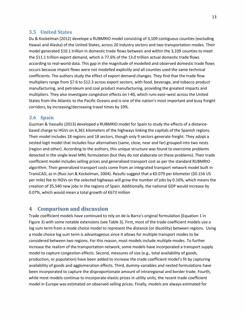
3.5 United States Du & Kockelman (2012) develope a RUBMRIO model consisting of 3,109 contiguous counties (excluding

Hawaii and Alaska) of the United States, across 20 industry sectors and two transportation modes. Their

model generated $10.1 trillion in domestic trade flows between and within the 3,109 counties to meet

the $11.1 trillion export demand, which is 77.6% of the 13.0 trillion actual domestic trade flows

according to real-world data. This gap in the magnitude of modelled and observed domestic trade flows

occurs because import flows were not modelled explicitly and all counties used the same technical

coefficients. The authors study the effect of export demand changes. They find that the trade flow

multipliers range from $7.6 to $12.3 across export sectors, with food, beverage, and tobacco product

manufacturing, and petroleum and coal product manufacturing, providing the greatest impacts and

multipliers. They also investigate congestion effects on I-40, which runs east–west across the United

States from the Atlantic to the Pacific Oceans and is one of the nation’s most important and busy freight

corridors, by increasing/decreasing travel times by 10%.

3.6 Spain Guzman & Vassallo (2013) developed a RUBMRIO model for Spain to study the effects of a distance-

based charge to HGVs on 6,361 kilometers of the highways linking the capitals of the Spanish regions.

Their model includes 18 regions and 18 sectors, though only 9 sectors generate freight. They adopt a

nested logit model that includes four alternatives (same, close, near and far) grouped into two nests

(region and other). According to the authors, this unique structure was found to overcome problems

detected in the single level MNL formulation (but they do not elaborate on these problems). Their trade

coefficient model includes selling prices and generalized transport cost as per the standard RUBMRIO

algorithm. Their generalized transport costs come from an integrated transport network model built in

TransCAD, as in (Ruiz Juri & Kockelman, 2004). Results suggest that a €0.079 per kilometer ($0.156 US

per mile) fee to HGVs on the selected highways will grow the number of jobs by 0.16%, which means the

creation of 35,540 new jobs in the regions of Spain. Additionally, the national GDP would increase by

0.07%, which would mean a total growth of €673 million

4 Comparison and discussion Trade coefficient models have continued to rely on de la Barra’s original formulation (Equation 1 in

Figure 3) with some notable extensions (see Table 3). First, most of the trade coefficient models use a

log sum term from a mode choice model to represent the distance (or disutility) between regions. Using

a mode choice log sum term is advantageous since it allows for multiple transport modes to be

considered between two regions. For this reason, most models include multiple modes. To further

increase the realism of the transportation network, some models have incorporated a transport supply

model to capture congestion effects. Second, measures of size (e.g., total availability of goods,

production, or population) have been added to increase the trade coefficient model’s fit by capturing

availability of goods and agglomeration effects. Third, dummy variables and nested formulations have

been incorporated to capture the disproportionate amount of intraregional and border trade. Fourth,

while most models continue to incorporate elastic prices in utility units, the recent trade coefficient

model in Europe was estimated on observed selling prices. Finally, models are always estimated for

14

different groups of commodities, allowing the sensitivity of transport costs to vary (e.g., higher for bulk

goods, etc.).

Transport costs that enter trade coefficient utility functions have been computed in various ways. The

simplest way to incorporate transport costs is to use shortest-path distances over the highway and/or

railway networks as proxy. Changes to the network are then incorporated by modifying these initial

distances. The most common way to incorporate transport costs is to use a log-sum term from a mode

choice model that includes transports costs and/or distances for various modes such as road and rail, in

which case the trade coefficient model becomes a nested logit model. The most sophisticated way of

incorporating transport costs is to simulate the travel time changes in a transport network model and

feed these travel times back into a mode choice model or the trade coefficient model directly. In this

last approach, dollar flows are converted to vehicle flows, and these vehicle flows are assigned to a

transport network model. The network returns updated travel times, which are either fed into a mode

choice model or the trade coefficient model directly. This process is done iteratively until the transport

network reaches user equilibrium and the trade flows in the RUBMRIO model reach transport cost

equilibrium. Two of the trade coefficient model extensions discussed above have created new feedbacks

in the original formulation as shown in Figure 4; a unique and convergent solution is expected but has

not been proven, as discussed in the next section.

15

Figure 4: Multiple equilibriums in RUBMRIO models

As shown in the third column of Table 3, a few different methods have been used to assess the trade

coefficient model fit. Statistical tests are often used to determine whether or not individual parameters

are significant. In most cases where these statistics are provided, the included parameters are significant

for most commodity groups, indicating they do indeed affect trade choices. Many researchers also

present a rho-squared value, although this statistic is better suited to compare between different model

specifications, than show overall level of fit. More appropriate, and perhaps most robust for this

application of RUM models, is an R-square measure computed based on observed versus predicted

trade flow shares. An R-square measure is only reported by Kockelman, Jin, Zhao, & Ruiz Juri (2005), and

values range from 0.0004 to 0.4499 for various commodity groups. These measures of overall fit suggest

that although the individual variables may significantly affect trade behaviour (as indicated by their test

statistics), they do not adequately explain it. Further extensions in RUM models are therefore required

to enhance their fit as discussed in the next section.

16

One particular issue with trade coefficient models is how elastic prices are calculated in the RUBMRIO

algorithm. Although there has been no discussion of this in the literature, elastic prices have actually

been handled in two different ways. In some instances, an initial set of prices are determined by

iteratively solving equations 5 and 6 in Figure 3 before model estimation, as described by Marzano &

Papola (2008). Then, the trade coefficient model is estimated with these prices; the resulting utility

function has a parameter attached to the price variable and prices are measured in the same units as

transport costs. In other instances, costs are calculated as the weighted input of the entire utility

function (i.e., replacing (bni +dn

ij) with their vnij in equation 5 of Figure 3). In these cases, an initial set of

prices cannot be determined because the utility function is not yet specified. Yet to estimate the model

requires the initial set of prices. To solve this problem, it is then assumed that prices are relatively

constant among competing regions and price is dropped during model estimation. The price variable is

later added into the utility function during application (where it is calculated endogenously) with no

parameter attached to it since it is measured in units of utility. An investigation, or even recognition, of

these two approaches has not been made in the literature and requires further research.

5 Future directions Input-output research is likely to continue in many directions, from basic economic modelling as

originally intended, to studying contemporary issues such as greenhouse gas emissions (Wiedmann,

2009), water footprints (Daniels, Lenzen, & Kenway, 2011), endangered species (Lenzen et al., 2012),

and terrorism attacks (Lee, Park, Gordon, Moore II, & Richardson, 2012). As far as studying the spatial

economic and transport interaction process is concerned, there are a few directions that should be

pursued. Future research directions are described below, presented in the order of importance from the

authors’ perspective.

First, the RUBMRIO method would benefit from a holistic validation effort. Uncoordinated partial

validation efforts have been pursued and deserve mention. The RUBMRIO base case model outputs can

be compared against the original MRIO dataset. With this aim, Marzano & Papola (2008) compare their

production, value added, and GDP, for each country and sector, and find a weighted mean absolute

percentage deviation of 20.3%, 17.3%, and 7.7%, respectively. For those models that capture congestive

feedbacks through a transport supply model, it is also possible to validate the model through

comparisons between predicted and observed flows on links. For example, Guzman & Vassallo (2013)

compare their generated flows per functional class and find Room Mean Squared Errors (RMSEs)

between 21.91% and 45.55%. Despite these approaches, however, no research to date has provided a

holistic validation of the complete RUBMRIO method by demonstrating that the model successfully

captured the impact of an infrastructure project that has already occurred. An effort of this nature

would validate the method, as opposed to validating sub-components or only the base case model.

Challenges to the recommended validation approach include: a) obtaining corresponding data spanning

a large time frame; b) isolating the effects of the infrastructure under study from effects of concurrent

changes; c) properly isolating the lead and lag times of the impacts.

Second, there is much work to be done in trade coefficient modelling, particularly to add realism and to

increase accuracy. Regional differences in goods production can be captured by including a region

17

specific dummy variable in the trade coefficient model; this is particularly relevant at the global scale

where large regional differences exist (e.g., German cars versus Asian cars). In the past, a same-zone

dummy variable (i.e., equal to 1 if i=j) has been used to handle the magnitude of the internal trade

coefficient relative to other trade coefficients and a common boundary dummy has been used if two

regions share a border. This notion can be extended to include unique linkages between regions such as

trade agreement specific dummies (i.e., equal to 1 if i and j have a specific commercial and/or trade

agreement). Finally, it would be useful and novel if elasticities created by the trade coefficient models

could be illustrated in terms of price elasticities, in order to contribute to the literature on price

elasticities of freight transport demand.

Third, the use of multi scale modelling should be considered to develop more comprehensive models. As

noted earlier, the models to date have focused on one regional scale. However, a more comprehensive

model could be developed by joining multiple scales. For example, the model of Italy captures regional

differences, but lacks integration with neighbouring countries. On the other hand, the model of Europe

captures the relationships between countries in the European Union, but lacks regional detail for

individual countries. By linking these two models, the impact of a European policy or infrastructure

project could be assessed at the regional level in Italy. Of course, the linking of multiple scales may be

challenging from a data (and modelling) point of view. Additionally, applications would no longer need

to rely on hypothetical export demand increases but could model real-world scenarios (e.g.,

development in a particular trade partner). One such example of a multi scale input-out analysis is

presented by Okamoto & Inomata (2011), where they use a Transnational Interregional Input-Output

(TIIO) model that combines a multinational scale with regional disaggregation of China and Japan.

Fourth, the inclusion of other variable technical coefficients could open up new possibilities for

RUBMRIO models. Existing work has made some efforts in this area. For example, Kockelman et al.

(2005) discuss the use of price-elastic technical coefficients, but provide no application. Ruiz Juri &

Kockelman (2004) simulate possible improvements in production technologies by reducing all technical

coefficients except for those on labour by 20%. Meanwhile, two book chapters by Cascetta and others

[(Cascetta, 2001); (Cascetta, Marzano, & Papola, 2008)] describe extensions on the dependence of price

through other key variables such as technical coefficients, imports, and final demand. Outside of the

RUBMRIO literature, the textbook by Miller & Blair (2009) discusses the process of projecting technical

coefficients into the future, finding that early attempts using trends and extrapolation did not prove to

be very successful. But they also describe alternative approaches involving marginal input coefficients

and “best practice” firms which may be better options. However, Marzano & Papola (2008) found the

temporal variability of trade coefficients and technical coefficients in Italy from 1995 to 2005 to be very

small, except for the energy producing sectors. Nevertheless, extensions along these lines would

develop a more comprehensive method capable of modelling more complex and realistic interactions.

Fifth, the RUBMRIO algorithm used to include elastic selling prices (section 2.3) requires deeper

investigation if it is to be used in the future. Marzano & Papola (2004) note that the equation used in

the RUBMRIO algorithm to update selling prices is approximate (Equation 6 in Figure 3) since it should

consider technical coefficients in physical quantity (i.e., weight, volume) rather than technical

coefficients in monetary value. They worry this assumption may create significant bias and recommend

18

a deep analysis of this issue be carried out. Cascetta et al. (2008) agree and further note that introducing

technical coefficients in quantity leads to theoretical and operational problems of the fixed-point

approach. Furthermore, extensions of the basic trade coefficient model, such as the one introduced by

Marzano & Papola (2004), include other attributes from IO tables, therefore introducing a new feedback

between the trade coefficient model and the MRIO model. An analysis of the solution existence and

uniqueness of this new fixed point problem is still required. Cascetta et al. (2008) found that trials on

synthetic and real data have always shown a fast convergence to a unique solution, which is an

encouraging finding. Additionally, others extended the RUBMRIO elastic prices algorithm to include a

transportation network model to capture congestion effects, but the uniqueness of the system solution

is still unproven. However, as pointed out by Zhao & Kockelman (2004), there are unique solutions to

the separate RUBMRIO algorithm and traffic assignment procedures, suggesting that an

overall/integrated unique solution exists. Finally, as discussed in the previous section, the basic elastic

selling prices algorithm has also been implemented in two different ways, which requires further

investigation.

Finally, there are a few other directions that have been brought to light by other authors that would

improve the realism of RUBMRIO models. First, Du & Kockelman (2012) observe that the RUBMRIO

method results in more low-value trade flows compared to real-world trade flows, since the logit model

distributes trade flows everywhere over space (i.e., every trading region has a non-zero trade flow).

They suggest that a potential solution is to use microsimulation (i.e., Monte Carlo simulation) and

randomized runs (rather than producing average or expected flow results), to represent real trade

agreements between individual market agents, and discretize flows. Second, Ruiz Juri & Kockelman

(2004) found that conversion from dollars to tons is rather straightforward but conversion from tonnage

to vehicle trips is not. They estimate a proportion of empty trips and the number of trips by type with

regression models. To capturing trip chaining or touring effects, future applications might also benefit

from linkage with a microsimulation model of the freight system. Third, modern economies in

developed countries are primarily service sector orientated. A trade coefficient model can be estimated

specifically for service sectors (or even for individual service sectors) to capture their unique sensitivity

(or lack thereof) to transport costs. However, given that service sectors generally rely on passenger trips,

the RUBMRIO model may need further extensions to adequately capture this interdependence.

Whether or not a RUBMRIO model can give an adequate representation of the impacts of transport

policy on the service sector of an economy requires further investigation. Finally, the quest for more

sector, product, and regional detail should continue, as in traditional IO models (Tukker &

Dietzenbacher, 2013).

19

6 References Abraham, J. E. (1998). A review of the MEPLAN modelling framework from a perspective of urban

economics. Calgary: University of Calgary Department of Civil Engineering.

Abraham, J. E., & Hunt, J. D. (1999). Firm location in the MEPLAN model of Sacramento. Transportation

Research Record: Journal of the Transportation Research Board, 1685, 187-198.

Abraham, J. E., & Hunt, J. D. (1999). Policy analysis using the Sacramento MEPLAN land use-

transportation interaction model. Transportation Research Record: Journal of the Transportation

Research Board, 1685, 199-208.

Abraham, J. E., & Hunt, J. D. (2003). Design and application of the PECAS land use modeling system.

Davis: Institute of Transportation Studies, University of California, Davis.

Bröcker, J. (2008). Computable general equilibrium analysis in transportation. In D. A. Hensher, K. J.

Button, K. E. Haynes, & P. R. Stopher, Handbook of Transport Geography and Spatial Systems

(pp. 269-289). Howard House, Wagon Lane, Bingley BD16 1WA, UK: Emerald Group Publishing

Limited.

Bröcker, J., & Mercenier, J. (2011). General equilibrium models for transportation economics. In A. de

Palma, R. Lindsey, E. Quinet, & R. Vickerman, Handbook in Transport Economics (pp. 21-45).

Massachusetts: Edward Elgar Publishing.

Burfisher, M. E. (2011). Introduction to computable general equilibrium models. Cambridge: Cambridge

University Press.

Cascetta, E. (2001). 4.6.1 Multiregional Input-Output (MRIO) models. In E. Cascetta, Transportation

Systems Engineering: Theory and Methods (pp. 232-243). Norwell, MA 02061, U.S.A.: Kluwer

Academic Publishers.

Cascetta, E., Di Gangi, M., & Conigliaro, G. (1996). A multi-regional input-output model with elastic trade

coefficients for the simulation of freight transport demand in Italy. Transportation Planning

Methods. Proceedings of Seminar E Held at the PTRC European Transport Forum. Brunel

University, England: PTRC Education and Research Services Limited.

Cascetta, E., Marzano, V., & Papola, A. (2008). Multi-regional input-output models for freight demand

simulation at a national level. In M. E. Ben-Akiva, H. Meersman, & E. Van der Voorde, Recent

Developments in Transport Modelling: Lessons for the Freight Sector (pp. 93-116). Howard

House, Wagon Lane, Bingley BD16 1WA, United Kingdom: Emerald Group Publishing Limited.

Cascetta, E., Marzano, V., & Papola, A. (2012). A multimodal elastic trade coefficients MRIO model for

freight demand in Europe. Proceedings of the Freight Transport Modeling Colloquium in memory

of Prof. Marvin L. Manheim. Antwerp: University of Antwerp - Department of Transport and

Regional Economics.

20

Chenery, H. (1953). Regional analysis. In H. B. Chenery, P. G. Clark, & V. Cao-Pinna, The Structure and

Growth of the Italian Economy (pp. 97–116). Rome: United States Mutual Security Agency.

Daniels, P. L., Lenzen, M., & Kenway, S. J. (2011). The ins and outs of water use – a review of multi-

region input–output analysis and water footprints for regional sustainability analysis and policy.

Economic Systems Research, 23(4), 353–370.

de la Barra, T. (1989). Integrated land use and transport modelling: Decision chains and hierarchies.

Cambridge: Cambridge University Press.

Du, X., & Kockelman, K. M. (2012). Tracking transportation and industrial production across a nation:

Applications of RUBMRIO model for U.S. trade patterns. Transportation Research Record:

Journal of the Transportation Research Board, 2269, 99-109.

Echenique, M. (2008). Econometric models of land use and transportation. In D. A. Hensher, K. J. Button,

K. E. Haynes, & P. R. Stopher, Handbook of transport geography and spatial systems (pp. 185-

202). Howard House, Wagon Lane, Bingley BD16 1WA, UK: Emerald Group Publishing Limited.

Echenique, M. (2011). Land use/transport models and economic assessment. Research in Transportation

Economics, 31(1), 45-54.

Echenique, M. H., Flowerdew, A. D., Hunt, J. D., Mayo, T. R., Skidmore, I. J., & Simmonds, D. C. (1990).

The MEPLAN models of Bilbao, Leeds and Dortmund. Transport Reviews: A Transnational

Transdisciplinary Journal, 10(4), 309-322.

Guzman, A. F., & Vassallo, J. M. (2013). A methodology for assessing regional economic impacts of

charging HGVs in Spain: an integrated approach through a Random Utility Based Multiregional

Input-Output and a Road Transportation Network Model. Proceedings of the 92nd Annual

Meeting of the Transportation Research Board. Washington: Transportation Research Board.

Ham, H., Kim, T. J., & Boyce, D. (2005). Implementation and estimation of a combined model of

interregional, multimodal commodity shipments and transportation network flows.

Transportation Research Part B: Methodlogical, 39, 65–79.

Hoekstra, R. (2010). (Towards) a complete database of peer-reviewed articles on environmentally

extended input-output analysis. 18th International Input–Output Conference. Sydney, Australia:

Statistics Netherlands.

Huang, T., & Kockelman, K. M. (2007). The introduction of dynamic features in a random-utility-based

multiregional input-output model of trade, production, and location choice. Proceedings of the

86th Annual Meeting of the Transportation Research Board. Washington: Transportation

Research Board.

Iacono, M., Levinson, D., & El-Geneidy, A. (2008). Models of transportation and land use change: A guide

to the territory. Journal of Planning Literature, 22(4), 323-340.

21

Isard, W. (1951). Interregional and regional input-output analysis: A model of a space-economy. The

Review of Economics and Statistics, 33(4), 318-328.

Keynes, J. M. (1936). The general theory of employment, interest, and money. London: Macmillan.

Kim, T. J., Ham, H., & Boyce, D. E. (2002). Economic impacts of transportation network changes:

Implementation of a combined transportation network and input-output model. Papers in

Regional Science, 81, 223-246.

Kockelman, K. M., Jin, L., Zhao, Y., & Ruiz Juri, N. (2005). Tracking land use, transport, and industrial

production using random-utility-based multiregional input–output models: Applications for

Texas trade. Journal of Transport Geography, 13, 275-286.

Lee, B., Park, J., Gordon, P., Moore II, J. E., & Richardson, H. W. (2012). Estimating the state-by-state

economic impacts of a foot-and-mouth disease attack. International Regional Science Review,

35(1), 26-47.

Lenzen, M., Moran, D., Kanemoto, K., Foran, B., Lobefaro, L., & Geschke, A. (2012). International trade

drives biodiversity threats in developing nations. Nature, 486, 109–112.

Leontief, W. W. (1936). Quantitative input and output relations in the economic systems of the United

States. The Review of Economics and Statistics, 18(3), 105-125.

Leontief, W. W. (1951). The structure of American economy, 2nd ed. New York: Oxford University Press.

Leontief, W. W. (1953). Studies in the structure of the American economy: Theoretical and empirical

explorations in input-output analysis. New York: Oxford University Press.

Maoh, H., Kanaroglou, P., & Woudsma, C. (2008). Simulation model for assessing the impact of climate

change on transportation and the economy in Canada. Transportation Research Record: Journal

of the Transportation Research Board, 2067, 84-92.

Marzano, V., & Papola, A. (2004). Modelling freight demand at a national level: Theoretical

developments and application to Italian demand. Proceedings of the 2004 Eurpean Transport

Conference. Association for European Transport.

Marzano, V., & Papola, A. (2008). A multi-regional input-output model for the appraisal of transport

investments in Europe. Proceedings of the 2008 Eurpean Transport Conference. Association for

European Transport.

Miller, E. J. (2006). Integrated urban models: Theoretical prospects. 11th International Conference on

Travel Behaviour Research. Kyoto, Japan.

Miller, R. E., & Blair, P. D. (2009). Input-output analysis: Foundations and extensions. Cambridge:

Cambridge University Press.

22

Moses, L. N. (1955). The stability of interregional trading patterns and input-output analysis. The

American Economic Review, 45(5), 803-826.

Okamoto, N., & Inomata, S. (2011). 6 To what extent will the shock be alleviated? The evaluation of

China's counter-crisis fiscal expansion. In S. Inomata, Asia beyond the global economic crisis: The

transmission mechanism of financial shocks. Cheltenham: Edward Elgar Publishing Limited.

Regional Economic Models, Inc. (2013). Regional Economic Models, Inc. Retrieved from The REMI Model:

http://www.remi.com/the-remi-model

Rose, A. (1995). Input-output economics and computable general equilibrium models. Structural Change

and Economic Dynamics, 6(3), 295-304.

Ruiz Juri, N., & Kockelman, K. M. (2004). Extending the random-utility-based multiregional input-output

model: Incorporating land-use constraints, domestic demand and network congestion in a

model of Texas trade. Proceedings of the 83rd Annual Meeting of the Transportation Research

Board. Washington: Transportation Research Board.

Ruiz Juri, N., & Kockelman, K. M. (2006). Evaluation of the trans-Texas corridor proposal: Application and

enhancements of the random-utility-based multiregional input–output model. Journal of

Transportation Engineering, 132(7), 531-539.

Russo, F., & Musolino, G. (2009). Multiple equilibria in spatial-economic transport interaction models.

Proceedings of the 2009 European Transport Conference. Association for European Transport.

Russo, F., & Musolino, G. (2012). A unifying modelling framework to simulate the spatial economic

transport interaction process at urban and national scales. Journal of Transport Geography, 24,

189–197.

Simmond, D. C. (1999). The design of the DELTA land-use modelling package. Environment and Planning

B: Planning and Design, 26(5), 665-684.

Timmermans, H. (2003). The saga of integrated land use-transport modeling: How many more dreams

before we wake up? 10th International Conference on Travel Behaviour Research. Lucerne,

Switzerland.

Train, K. (2009). Discrete choice methods with simulation. Cambridge: Cambridge University Press.

Tukker, A., & Dietzenbacher, E. (2013). Global multiregional input–output frameworks: An introduction

and outlook. Economic Systems Research, 25(1).

Wegener, M. (2008). Overview of land-use transport models. In D. A. Hensher, K. J. Button, K. E. Haynes,

& P. R. Stopher, Handbook of transport geography and spatial systems (pp. 127-146). Howard

House, Wagon Lane, Bingley BD16 1WA, UK: Emerald Group Publishing Limited.

23

Wiedmann, T. (2009). A review of recent multi-region input–output models used for consumption-based

emission and resource accounting. Ecological Economics, 69(2), 211–222.

Wiedmann, T., Lenzen, M., Turner, K., & Barrett, J. (2007). Examining the global environmental impact of

regional consumption activities - Part 2: Review of input-output models for the assessment of

environmental impacts embodied in trade. Ecological Economics, 61 (1), 15-26.

Zhao, Y., & Kockelman, K. M. (2004). The random-utility-based multiregional input–output model:

Solution existence and uniqueness. Transportation Research Part B: Methodological, 38, 789-

807.

Zondag, B., & de Jong, G. (2011). The development of the TIGRIS XL model: A bottom-up approach to

transport, land-use and the economy. Research in Transportation Economics, 31(1), 55–62.

24

Table 1: Variable Definitions

Variable Definition

𝑢𝑖𝑗𝑛 Utility of purchasing one unit of sector n’s goods from region i for use as input in region j

𝑏𝑖𝑛 Price of producing a unit of sector n in region i (in units of utility)

𝑑𝑖𝑗𝑛 Price of transporting a unit of sector n from i to j

𝜀𝑖𝑗𝑛 Random error term

𝑋𝑖𝑚 Total output of sector m in region i

𝑥𝑖𝑗𝑚 Flow of sector m from region i to j

𝐶𝑗𝑚 Total consumption of sector m in region j

𝑎𝑗𝑚𝑛 Technical coefficient representing the amount of sector m product required to produce one

dollar of sector n product in region j

𝑌𝑗𝑚 Final demand for sector m’s output in region j

𝑡𝑖𝑗𝑛 Percentage of sector n product used in zone j acquired from production zone i (elastic trade

coefficient)

𝜆𝑛 Dispersion parameter

𝑣𝑖𝑗𝑛 Systematic utility: 𝑣𝑖𝑗

𝑛 = −(𝑏𝑖𝑛 + 𝑑𝑖𝑗

𝑛 )

𝑐𝑗𝑛 Average cost of input n in region j

25

Table 2: Applications of RUBMRIO Models

Author Publication Year

Area Regions Industry Sectors Modes Scenarios

Cascetta, E., Di Gangi, M., & Conigliaro, G.

1996 Italy 20 Italian administrative regions 17 sectors (11 producing goods and 6 services)

Rail, Road

Freight demand forecasting

Kockelman, K. M., Jin, L., Zhao, Y., & Ruiz Juri, N.

2005 (First presented in 2003)

Texas 254 counties and 31 foreign-export zones

16 industry sectors and 2 other economic sectors (government and households)

Highway, Rail

1) Effects of export demand changes 2) Transport cost effects (transport costs were reduced 10% along Interstate Highway 35)

Ruiz Juri, N., & Kockelman, K. M.

2004 Texas 254 counties, 18 foreign export ports, and demand from the 50 U.S. states plus the District of Columbia (treated as ports)

16 industry sectors and 2 other economic sectors (government and households)

Highway, Rail

1) Effects of domestic demands changes (by both product and location) 2) Effects of variations in technical coefficients

Marzano, V., & Papola, A.

2004 Italy 20 regions 11 sectors producing goods

Train, Intermodal, Truck

1) Short term runs: base scenario; +10% truck time; -10% combined time; - 10% train time 2) Long term runs: base scenario; +10% truck time

Ruiz Juri, N., & Kockelman, K. M.

2006 Texas 254 zones (demands from 18 foreign export ports, and domestic demands by 50 United States states plus the District of Columbia)

21 economic sectors Highway, Rail

Evaluation of the The Trans-Texas Corridor (TTC) proposal (with/without comparative analysis)

Huang, T., & Kockelman, K. M.

2007 Texas 254 counties driven by exports to foreign and domestic purchasers (with exogenous household demands for short-term modelling )

16 industry sectors and 2 other economic sectors (government and households)

Highway, Rail

Estimate changes in Texas trade patterns over the next 20 years

Marzano, V., & Papola, A.

2008 Europe 22 European Union countries 59 CPA (statistical classification of products by activity) sectors

Train, Intermodal, Truck

Appraisal of the planned high-speed railway link on the Lyon-Turin corridor

Cascetta, E., 2008 Italy 20 regions 11 sectors producing Train, Assessment of strategic

26

Marzano, V., & Papola, A.

goods Intermodal, Truck

transport corridors in Southern Italy: 1) cross-corridors 2) eastern corridor 3) western corridor 4) western plus eastern corridors 5) overall improvement

Maoh, Kanaroglou, & Woudsma

2008 Canada 76 economic regions 43 commodities Highway, Railway

Increase in Proportion of Days with Extreme Weather Events

Du, X., & Kockelman, K. M.

2011 United States

3,109 contiguous counties 20 social-economic sectors

Highway, Railway

1) Forecast the effects of various export demands on the U.S. economy 2) Examination of congestion effects on I-40 (travel times were increased 10%) 3) Examine effects of transport costs (marginal average cost of trucking was raised and lowered 20%)

Cascetta, E., Marzano, V., & Papola, A.

2012 Europe 22 European Union Countries 59 CPA sectors (29 tradable goods, 30 services)

Road, Sea, Inland Waterways, Rail

1) 10% increase in road costs 2) 20% reduction of maritime fares

Guzman, A. F., & Vassallo, J. M.

2013 Spain 18 regions 18 (9 freight transport intensive, 9 non-freight transport intensive sectors)

Road Evaluate a distance-based charge of 0.079 €/kms for HGVs

27

Table 3: RUM-based Trade Coefficient Models

Trade Coefficient Model Utility Function (Replaces Equation 1 in Figure 3)

Model Variables Model Fit Assessment Applications

Virs = βi

1*costirs + βi

2*borderrs + βi

3*ln(Productionir)

Virs: systematic utility of the acquisition by region s of

good i in region r Costi

rs: generalised transportation cost of good i between regions r and s (logsum of a mode choice model) Borderrs: dummy variable expressing the neighbourhood of regions (1 if the region r is contiguous to region s, 0 otherwise) Productioni

r: total annual production of sector i in the region r

t Statistics for each parameter; Rho squared for estimated models

Cascetta, E., Di Gangi, M., & Conigliaro, G. (1996)

Vmij = pm

i + λmln[Σt exp(β0,t + βtdij,t)]

Vmij: disutility of acquiring commodity m from origin

zone i and consuming it in zone j pm

i: price of purchasing $1 of commodity m in zone i dij,t: is the network distance (or travel cost) between zones i and j by mode t

R-square for estimated models Kockelman, K. M., Jin, L., Zhao, Y., & Ruiz-Juri, N. (2005) Huang, T., & Kockelman, K. M. (2007) Ruiz Juri, N., & Kockelman, K. M. (2006) Ruiz Juri, N., & Kockelman, K. M. (2004)

Vmij = βm

1dmij + βm

2bmi + βm

3YmREG if i

≠ j Vm

ij = βm1dm

ii + βm2bm

i + βm3Am

i if i = j

dmij: transportation cost of the goods of sector m

between regions i and j (logsum of a mode choice model) bm

i: selling price of goods/service of sector m in region i Ym

REGi: demand for goods of sector m in region i by regional export Am

i: total internal availability of goods of sector m in region i

Only report statistically significant parameters (significance level not reported)

Marzano, V., & Papola, A. (2004) Marzano, V., & Papola, A. (2008) Cascetta, E., Marzano, V., & Papola, A. (2008)

Vnij = bn

i + β0i + β1tcnij +β2ln(Sn

i) +β3COMq (for goods) Vn

ij = bni + β0i +β2ln(Sn

i) +β3COMq (for services)

Vnij: disutility of purchasing of sector n’s goods from

subregion i for use as inputs in subregion j bn

i: price of producing a unit of n in region i tcn

ij: price of transporting a unit of n from i to j Sn

i: size of the market of n in subregion i

t Statistics for each parameter; Rho squared for estimated models

Maoh, Kanaroglou, & Woudsma (2008)

28

COMq: commodity dummies that are set equal to unity if the observation refers to commodity group q to which n belongs and 0 otherwise

Vmij = -pm

i + ϒmln(popi)+ λmln[Σt exp(βm

0,t + βm1timeij,t + βm

2costij,t)]

Vmij: disutility of acquiring commodity m from origin

zone i and consuming it in zone j pm

i: sales price of commodity m in county or zone i popi: population of zone i timeij,t: travel time between zones i and j by mode t costij,t: cost between zones i and j by mode t

Rho-square for estimated models Du, X., & Kockelman, K. M. (2011)

Vmij = βm

1Ymij + βm

2bmi + βm

3lnXmi + βm

4δSZ

Ymij: mode choice logsum for sector m between i and j

bmi: average observed selling prices for sector m in

zone i Xm

i: production for sector m in zone i δSZ: same zone dummy variable

Only report statistically significant parameters at 95% level

Cascetta, E., Marzano, V., & Papola, A. (2012)

umij = -pm

i + λmln[ΣR exp(βmGTCmij,R)]

pi

m: the price of goods/services of sector m in region i GTCm

ij: generalized transport cost of sector m goods from production or origin region i to consumer region j (linear function of time and distance costs)

Wald statistical significance test for each parameter; Likelihood ratio Index for estimated models

Guzman, A. F., & Vassallo, J. M. (2013)