A Critical Reexamination of Augmented & Open Input Output Systems

A Critical Reexamination of Augmented & Closed Input-Output Models: A Note on the Structure & Closure

Nikolaos Adamou1 & Gülay Günlük-Senesen2

XII International Conference of Input-Output Techniques New York University

May 18-22, 1988

Topic: Mathematical and Methodological Developments

Abstract: Open Input-Output models, closed with respect to household (or government), include the row vector of the household input coefficients, as well as the column vector of the household consumption coefficients as endogenous aspects of the model. In this way, the closure of the model is shifted, and household input and consumption coefficients are taken into account evaluating the interdependence of the sectors of the entire production system. As a result of the above formulation gross output evaluated by an open model is greater than the gross output given by the closed model. The reasoning behind this diversity is explained by Miller and Blair [1985] due to additional outputs needed to satisfy the anticipated increase in consumer spending reflected in the household consumption coefficients column, expected because of the increased household earnings due to increase outputs, hence increased wage payments. This paper provides a different critical interpretation to the above thesis based on the interdependence flows among the endogenous sectors of the open model.

Introduction

Open input-output models distribute gross output into two major categories, intermediate and final. Similarly the value of production is distinguished as value of intermediate inputs and value added. Thus processing inter-depended sectors are the providing intermediate output and requiring intermediate inputs . Closed models assume all sectors to be processing sectors. Frequently is observed in the literature a shift of a part of the exogenous final use and value added part of the model into processing sectors. Such change in the closure of the model was attempted in order to evaluate impact analysis assuming that household sector or government sectors behave as the other processing sectors. Thus, the value of final use and value added decline and the value of intermediate transactions increase. The augmented model then is used to provide impact analysis for new final use.

Methodological Considerations

This paper uses the same example with Miller & Blair. A 2x2 transaction matrix is 150 500200 100

with final demand

column 350 1700 , value added row 650 1400[ ], and gross output 1000 2000[ ]. This model used as an accounting model [I − A] provides the expected solution x . An estimated final demand ˆ y would provide an estimated gross output ˆ x treating the model as a forecasting one, like,

[ ]T

−1 y

I − A[ ]−1 ˆ y = ˆ x . (1)

Such estimated final demand of 600 1500[ ]T yield gross output 1248 1842[ ]T .

1 Aristotelian University of Thessaloniki, School of Law & Economics, Economics Department., Greece. 2 Istanbul Üniversitesi, Siyasal Bilgiler Fakültesi, Beyazit 34452 Istanbul - Turkey, Fax: +90 212 511 9095

Adamou & Günlük-Senesen XII International Conference of Input-Output Techniques 2

Closing the same example with respect to household according the example yields intermediate transaction matrix of

final demand column of 150 500 50

200 100 400300 500 50

300 1300 150[ ]T , value added row of 350 900 500[ ] and gross

output of [1000 2000 1000 . While the accounting model in this case solves as anticipates, the final demand vector [600 1500 0]T yields expected gross output of 1457 2339 1075[ ].

]T

The provided explanation is “The new (larger) values ... reflect the fact that additional outputs are necessary to satisfy the anticipated increase in consumer spending, as reflected in the household consumption coefficients column, expected because of the increase household earnings due to increase output s for sector 1 and 2 and hence increase wage payments”.

Before one accepts this provided explanation, a comparative look of the Leontief inverse of the open and the augmented models shows that the inverse of the augmented model has larger values than the inverse of the open model.

1.254 0.3300.264 1.122

1.365 0.425 0.2500.527 1.348 0.5950.569 0.489 1.288

This lead one to examine the reason of the variations between all elements of the inverse matrices, while the portion of the processing sectors of the open model is the same for the production matrices.

0.85 −0.25−0.20 0.95

0.85 −0.25 −0.05−0.20 0.95 −0.40−0.30 −0.25 0.95

An explanation is based on the nature of the augmented inverse

I − A*[ ]−1=

adj I − A*[ ]det I − A*[ ]

leads to the examination of the nature of the production matrix of the augmented model

I − A*[ ]=1− a11 −a21 −c13

−a21 1 − a22 −c23

−d31 −d32 1 − e33

,

its determinant det I − A*[ ] and its adjoint adj I − A*[ ]. The n+1 elements cij = Ci wj are the ratios of

private consumption to the wage of the sector, while the n+1 elements dij = wj xi are the ratios of wage to

gross output of each sector. Finally, the last diagonal element of the matrix I − A*[ ] has a meaning in the

case that a fourth quadrant of an input output transaction matrix exists, and other wise is one, e 0 .

Although is non a usual case. ij =

The respective determinant is:

A Critical Reexamination of Augmented & Closed Input-Output Models: A Note on the Structure & Closure 3

det I − A[ *]=1 − (a11 + a22 + e33) + (a11a22 + a11e33 + a22e33) − (a11a22e33)

(a12a21 + c13d31 + d32c32) − (a12c23d31 + a21c13d32 )+(a22c13d31 + a11c23d32 + e33a12a21)−

We have c which are cijdij ijdij =Cixj

. If i = j , we have c13d31 =C1x1

& c23d32 =C2x2

meaning the relationship

of private consumption relative to gross output of the sector.

The terms i ≠ j of the determinant, in particular c13d32 =C1w1

w2x2

& c23d31 =

C2w2

w1x1

have the follow meaning.

These terms give the private consumption of sector (i) relative to gross output of sector (j), Ci x j , weighted

by the relative wage bill of the two sectors, wj wi( ), and the wage bill (cost) per unit of output of a sector

wj x j( ), weighted by the relative private consumption to wages of another sector Ci wi( ).

( )

Since the determinant gives the net value of production, then the terms (a11a22 + a11e33 + a22e33) and (a22c13d31 + a11c23d32 + e33a12a21) contribute positively for a unit of final use, and the terms (a11 + a22 + e33),

, ((a11a22e33) a12a21 + c13d31 + d32c32), and (a12c23d31 + a21c13d32) negatively.

The terms are: a22c13d31 =X22x2

C1x1

w1x1

& a11c23d32 =X11x1

C2x2

w2x2

the intra-industry (diagonal) transactions of the

sector 2 (1) interacting to private consumption for sector 1 (2) relative to the interaction of the gross output of sectors

1 & 2. The last two terms are: a21c23d31 =X21x1

C2w2

w1x1

, and a21c13d32 =X21x1

C1w1

w2x2

. The first gives the requirements

of sector one from sector two as a percentage of the value of gross output of sector one, weighted by the relative private consumption to wage bill of sector two and the relative wage to gross output of the sector one. Analogous meaning for the second.

The adjoint of the production augmented approach is:

adj I − A[ *]1 − a22( )1 − e33( )− d32c23 1− e33( )a12 + c13d32 1 − a22( )c13 + a12c23

1 − e33( )a21 − d32c23 1 − e33( )1 − a11( )+ c13d31 1− a11( )c23 + a21c13

1 − a22( )d31 − d32a21 1− a11( )d32 + d31a12 1− a11( )1 − a22( )− a12a21

.

The terms c13d31 =C1x1

wx

1

1, c23d32 =

C2x2

w2x2

, c13d32 =C1x1

w2x2

,

d32a21 =w2x2

X21x1

, d31a12 =w1x1

X21x2

, and a12c23 =X12x2

C2x2

, a12c13 =X12x2

C1x1

Shift of closures in interindustry models imply that consumption expenditures and wages, (or government expenditure and indirect taxes) belong not to NET but to the INTERMEDIATE output. These are also the most important in terms of size and function part of final demand and value added. Such shifts of the closure, do not only reduce the net value part of gross output and increase by the same amount the value intermediate of gross output, but it alters the structure of the interdependent productive sectors. The question requiring an answered by the users of the altered augmented productive structure is if the augmented productive structure is realistic. The distinction of what part of gross output is exogenous or endogenous of the productive process is absolute or flexible? If it is flexible, then one may augment the open IO table, although such an alternation effects the productive structure. Is


the productive structure a matter of a choice? Do we close or open the interindustry system as needed, or accept the closure given by the commonly accepted national income and product theory?

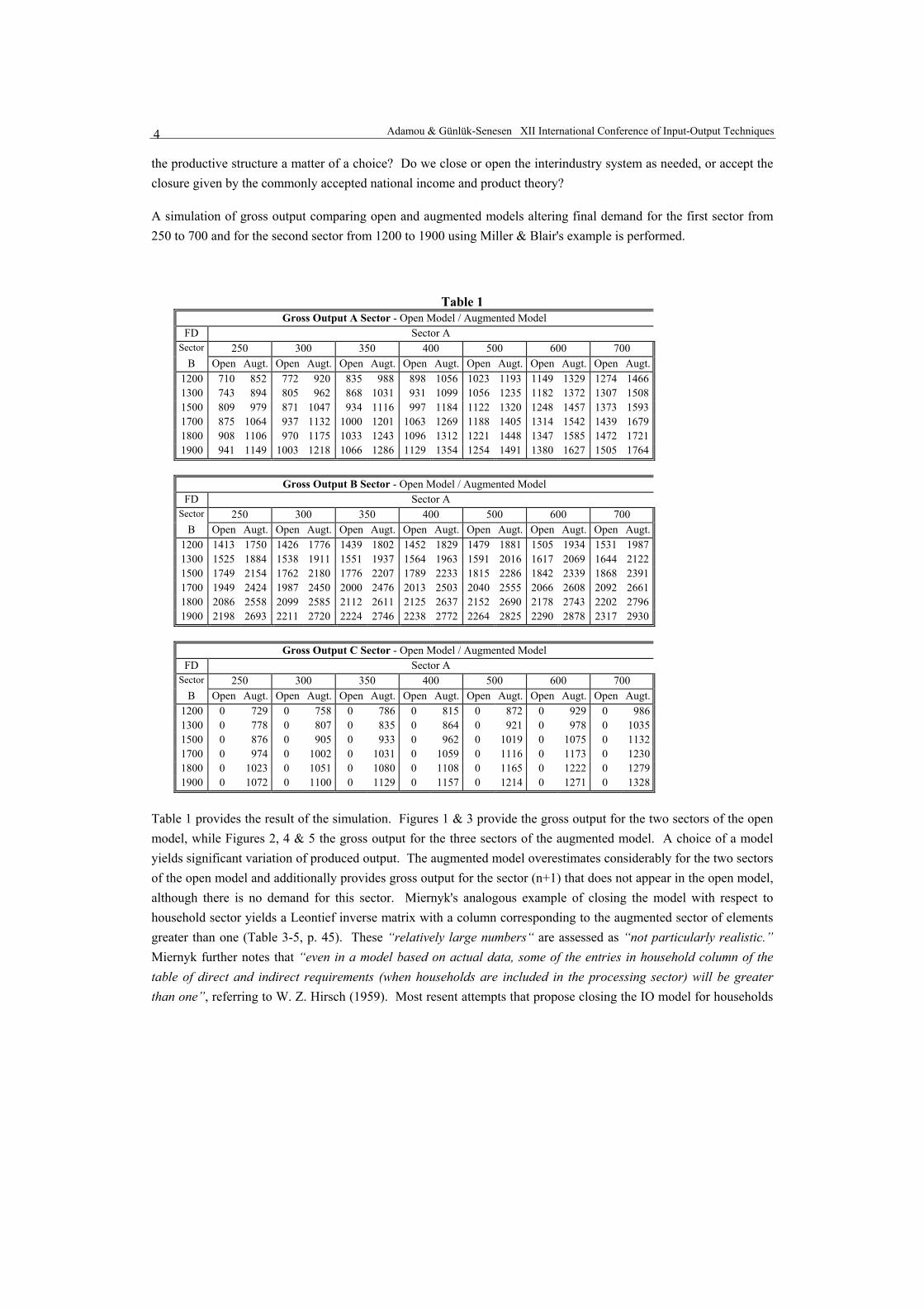
A simulation of gross output comparing open and augmented models altering final demand for the first sector from 250 to 700 and for the second sector from 1200 to 1900 using Miller & Blair's example is performed.

Table 1 Gross Output A Sector - Open Model / Augmented Model

FD Sector A Sector 250 300 350 400 500 600 700

B Open Augt. Open Augt. Open Augt. Open Augt. Open Augt. Open Augt. Open Augt.1200 710 852 772 920 835 988 898 1056 1023 1193 1149 1329 1274 14661300 743 894 805 962 868 1031 931 1099 1056 1235 1182 1372 1307 15081500 809 979 871 1047 934 1116 997 1184 1122 1320 1248 1457 1373 15931700 875 1064 937 1132 1000 1201 1063 1269 1188 1405 1314 1542 1439 16791800 908 1106 970 1175 1033 1243 1096 1312 1221 1448 1347 1585 1472 17211900 941 1149 1003 1218 1066 1286 1129 1354 1254 1491 1380 1627 1505 1764

Gross Output B Sector - Open Model / Augmented Model



Gross Output C Sector - Open Model / Augmented Model



Table 1 provides the result of the simulation. Figures 1 & 3 provide the gross output for the two sectors of the open model, while Figures 2, 4 & 5 the gross output for the three sectors of the augmented model. A choice of a model yields significant variation of produced output. The augmented model overestimates considerably for the two sectors of the open model and additionally provides gross output for the sector (n+1) that does not appear in the open model, although there is no demand for this sector. Miernyk's analogous example of closing the model with respect to household sector yields a Leontief inverse matrix with a column corresponding to the augmented sector of elements greater than one (Table 3-5, p. 45). These “relatively large numbers“ are assessed as “not particularly realistic.” Miernyk further notes that “even in a model based on actual data, some of the entries in household column of the table of direct and indirect requirements (when households are included in the processing sector) will be greater than one”, referring to W. Z. Hirsch (1959). Most resent attempts that propose closing the IO model for households


(Duchin, 1988) propose the knowledge of the household sector before the move towards theoretical closure of the IO model for household as a requirement for the empirical interest of the exercise, without a pose of any question to the theoretical exercise itself.

Gross Output A Sector Final D. Sector A - Open Model Sector A - Augmented Model Sector B 250 300 350 400 500 600 700 250 300 350 400 500 600 700

1200 710 772 835 898 1023 1149 1274 852 920 988 1056 1193 1329 14661300 743 805 868 931 1056 1182 1307 894 962 1031 1099 1235 1372 15081500 809 871 934 997 1122 1248 1373 979 1047 1116 1184 1320 1457 15931700 875 937 1000 1063 1188 1314 1439 1064 1132 1201 1269 1405 1542 16791800 908 970 1033 1096 1221 1347 1472 1106 1175 1243 1312 1448 1585 17211900 941 1003 1066 1129 1254 1380 1505 1149 1218 1286 1354 1491 1627 1764

Gross Output B Sector Final D. Sector A - Open Model Sector A - Augmented Model Sector B 250 300 350 400 500 600 700 250 300 350 400 500 600 700

1200 1413 1426 1439 1452 1479 1505 1531 1750 1776 1802 1829 1881 1934 19871300 1525 1538 1551 1564 1591 1617 1644 1884 1911 1937 1963 2016 2069 21221500 1749 1762 1776 1789 1815 1842 1868 2154 2180 2207 2233 2286 2339 23911700 1949 1987 2000 2013 2040 2066 2092 2424 2450 2476 2503 2555 2608 26611800 2086 2099 2112 2125 2152 2178 2202 2558 2585 2611 2637 2690 2743 27961900 2198 2211 2224 2238 2264 2290 2317 2693 2720 2746 2772 2825 2878 2930

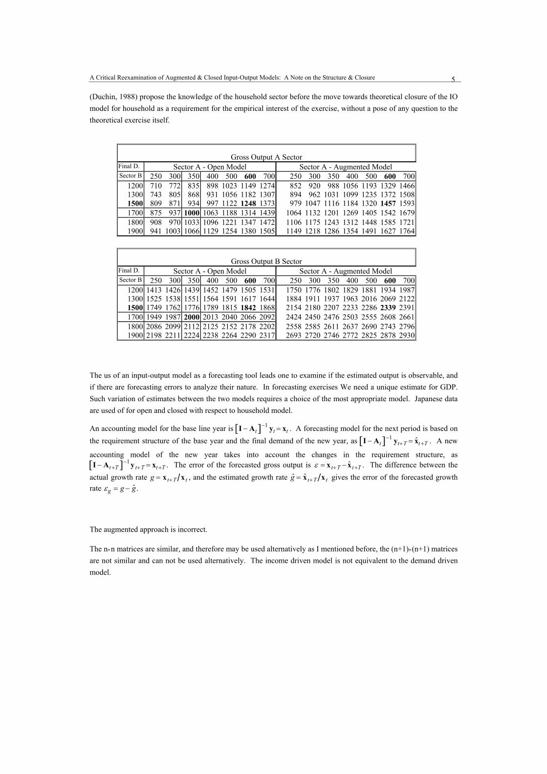
The us of an input-output model as a forecasting tool leads one to examine if the estimated output is observable, and if there are forecasting errors to analyze their nature. In forecasting exercises We need a unique estimate for GDP. Such variation of estimates between the two models requires a choice of the most appropriate model. Japanese data are used of for open and closed with respect to household model.

An accounting model for the base line year is I − At[ ]−1 yt = xt . A forecasting model for the next period is based on the requirement structure of the base year and the final demand of the new year, as I − At[ ] yt+T = ˆ x t +T . A new

accounting model of the new year takes into account the changes in the requirement structure, as . The error of the forecasted gross output is I − At +T[ ] y t+T = xt + ε = x t+T − ˆ x t +T . The difference between the

actual growth rate g = x t+T x t , and the estimated growth rate g ˆ = ˆ x t+T x t gives the error of the forecasted growth rate εg = g − ˆ g .

−1

−1T

The augmented approach is incorrect.

The n×n matrices are similar, and therefore may be used alternatively as I mentioned before, the (n+1)×(n+1) matrices are not similar and can not be used alternatively. The income driven model is not equivalent to the demand driven model.


Bibliography

Hirsch, Werner Z. (1959) “Interindustry Relations of a Metropolitan Area,” The Review of Economics and Statistics, XLI, November, p. 368.

Miernyk, William H. (1966) Input-Output Analysis, Random House Miller, R. E. & P. D. Blair (1985) Input-Output Analysis: Foundations and Extensions, Prentice Hall Duchin, Faye (1988) “Analysing structural change in the economy” in Ciaschini, M. (ed.) Input-Output Analysis:

Current Developments, Chapman & Hall, pp. 114-128

Appendix

Open model

Direct coefficients 3

201

41

5120

.15 .25

.20 .05

Production matrix 0.85 −0.25

−0.20 0.95

Total coefficients 0.95

0.75750.25

0.75750.20

0.75750.85

0.7575

1.254 0.3300.264 1.122

Augmented model

150 500 50200 100 400300 500 50

3001300150

100020001000

150 500 50200 100 400300 500 50

350 900 500[ ]1000 2000 1000[ ]

3001300150

100020001000

350 900 500[ ]1000 2000 1000[ ]

Direct coefficients

320

14

120

15

120

25

310

14

120

0.15 0.25 0.050.20 0.05 0.400.30 0.25 0.05

Production matrix 0.85 −0.25 −0.05

−0.20 0.95 −0.40−0.30 −0.25 0.95

1 − a11 −a12 −c13

−a21 1− a22 −c23

−d31 −d32 1− e33

Total coefficients 1

0.5878

0.95 −0.40−0.25 0.95

−−0.20 −0.40−0.30 0.95

−0.20 0.95−0.30 −0.25

−−0.25 −0.05−0.25 0.95

0.85 −0.05−0.30 0.95

−0.85 −0.25−0.30 −0.25

−0.25 −0.050.95 −0.40

−0.85 −0.05

−0.20 −0.400.85 −0.25

−0.20 0.95

T

=


1

0.5878

0.8025 0.3100 0.33500.2500 0.7925 0.28750.1475 0.3500 0.7575

T

=

10.5878

0.8025 0.2500 0.14750.3100 0.7925 0.35000.3350 0.2875 0.7575

=

1.365 0.425 0.2500.527 1.348 0.5950.569 0.489 1.288

Open model as an accounting model: 1.254 0.3300.264 1.122

x

3501700

= 10002000

Open model as a forecasting model: 1.254 0.3300.264 1.122

x

6001500

= 1247.521841.58

Augmented model as an accounting model: 1.365 0.425 0.2500.527 1.348 0.5950.569 0.489 1.288

x

3001300150

=

100020001000

Augmented model as a forecasting model: 1.365 0.425 0.2500.527 1.348 0.5950.569 0.489 1.288

x

6001500

0

=

1456.942338.511075.48

Det = +

1 + a11a22 ++a22c13d31 + a11c23d32 − a12c23d31 − a21c13d32 +

+a12a21e33 − a11a22e33 +

a11e33 + a22e33 −−a11 − a12a21 − a22

−c13d31 − d32c32 −

−e33


1 − a11 − a12a21 − a22 + a11a22 −

−c1d1 ++a22c1d1 − a12c2d1 − a21c1d2 −

−c2d2 ++a11c2 d2 −−e3 +

+a11e3 + a12a21e3 + a22e3 − a11a22e3

1 + a11a22 ++a22c13d31 + a11c23d32 − a12c23d31 − a21c13d32 +

+a12a21e33 − a11a22e33 +

+a11e33 + a22e33 −−a11 − a12a21 − a22

−c13d31 − d32c32 −

−e33

=

1 − a11 − a22 − e33 + a11a22 + a11e33 + a22e33 − a11a22e33

−a12a21 − c13d31 − d32c32 ++a22c13d31 + a11c23d32 + e33a12a21 −

−a12c23d31 − a21c13d32

adj I − A[ *] =

+1 − a22 −c2

−d2 1 − e3−

−a12 −c1

−d2 1 − e3+

−a12 −c1

1− a22 −c2

−−a21 −c2

−d1 1− e3+

1− a11 −c1

−d1 1 − e3−

1 − a11 −c1

−a21 −c2

+−a21 1− a22

−d1 −d2−

1 − a11 −a12

−d1 −d2+

1 − a11 −a12

−a21 1 − a22

=

1 − a22 − c23d32 − e33 + a22e33 a12 + c13d32 − a12e33 c13 − a22c13 + a12c23

a21 + c23d31 − a21e33 1− a11 − c13d31 − e33 + a11e33 a21c13 + c23 − a11c23

d31 − a22d31 + d32a21 a12d31 + d32 − a11d32 1− a11 − a12a21 − a22 + a11a22

adj I − A[ *] = 1 − a22( )1 − e33( )− c23d32 1− e33( )a12 + c13d32 1 − a22( )c13 + a12c23

1 − e33( )a21 − c23d32 1 − e33( )1 − a11( )+ d31c13 1− a11( )c23 + a21c13

1 − a22( )d31 − a21d32 1− a11( )d32 + d31a12 1− a11( )1 − a22( )− a12a21


Figure 1-A Figure 2-A

1200

1500

1800

600800

10001200140016001800

Final Demand A

Gross Output A - Open Model

1200

1500

1800

600800

10001200140016001800

Final Demand A

Gross Ouput A - Augmented Model

Figure 3-A Figure 3-B

1200

1500

1800

140016001800200022002400260028003000

Final Demand A

Gross Output B - Open Model

1200

1500

1800

140016001800200022002400260028003000

Final Demand A

Gross Output B - Augmented Model


Table A Japan

1951 (1) (2) (3) CONSUMP-

TION Other Final

Demand Total

Output AGRCULTURE (1) 55 706 140 883 -437 1,347 INDUSTRY (2) 179 3,016 857 1,011 1,425 6,488 SERVICES (3) 65 925 853 1,682 539 4,063 WAGES & SALARIES 1 68 136 OTHER VALUE ADDED 1,047 1,773 2,077 Total Output 1,347 6,488 4,063 11,899

1955 (1) (2) (3) CONSUMP-

TION Other Final

Demand Total

Output AGRCULTURE (1) 357 1,879 86 954 -775 2,500 INDUSTRY (2) 268 4,357 1,203 2,717 2,152 10,697 SERVICES (3) 192 1,380 1,302 3,585 662 7,120 WAGES & SALARIES 246 1,503 1,922 OTHER VALUE ADDED 1,437 1,578 2,607 Total Output 2,500 10,697 7,120 20,317

1960 (1) (2) (3) CONSUMP-

TION Other Final

Demand Total

Output AGRCULTURE (1) 474 2,447 87 556 -413 3,150INDUSTRY (2) 447 11,073 2,183 4,287 5,269 23,260SERVICES (3) 149 3,007 1,818 4,852 2,068 11,893WAGES & SALARIES 281 3,219 3,910 OTHER VALUE ADDED 1,800 3,513 3,895 Total Output 3,150 23,260 11,893 38,302

1965 (1) (2) (3) CONSUMP-

TION Other Final

Demand Total

Output AGRCULTURE (1) 551 3,665 225 1,108 -709 4,840 INDUSTRY (2) 780 19,244 4,019 7,690 10,490 42,222 SERVICES (3) 324 5,663 3,690 11,153 3,967 24,796 WAGES & SALARIES -5 671 842 OTHER VALUE ADDED 3,190 12,979 16,020 Total Output 4,840 42,222 24,796 71,859

1970 (1) (2) (3) CONSUMP-

TION Other Final

Demand Total

Output AGRCULTURE (1) 911 5,612 289 1,797 -1,495 7,114 INDUSTRY (2) 1,252 45,932 8,413 14,035 27,830 97,462 SERVICES (3) 434 13,311 9,420 25,064 8,853 57,082 WAGES & SALARIES -143 1,176 1,339 OTHER VALUE ADDED 4,659 31,431 37,621 Total Output 7,114 97,462 57,082 161,658

1975 (1) (2) (3) CONSUMP-

TION Other Final

Demand Total

Output AGRCULTURE (1) 1,394 10,000 916 3,212 -2,483 13,038 INDUSTRY (2) 2,544 81,035 22,599 27,198 45,463 178,838 SERVICES (3) 1,114 28,412 29,355 61,734 19,740 140,355 WAGES & SALARIES 1,057 31,932 46,261 OTHER VALUE ADDED 6,929 27,460 41,224 Total Output 13,038 178,838 140,355 332,231

1980 (1) (2) (3) CONSUMP-

TION Other Final

Demand Total

Output AGRCULTURE (1) 1,941 12,119 1,425 4,749 -2,861 17,373


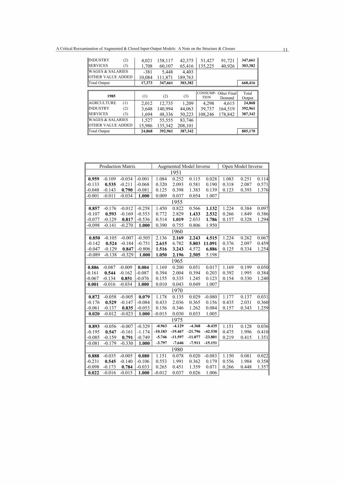
INDUSTRY (2) 4,021 158,117 42,375 51,427 91,721 347,661 SERVICES (3) 1,708 60,107 65,416 135,225 40,926 303,382 WAGES & SALARIES -381 5,448 4,403 OTHER VALUE ADDED 10,084 111,871 189,763 Total Output 17,373 347,661 303,382 668,416

1985 (1) (2) (3) CONSUMP-

TION Other Final

Demand Total

Output AGRCULTURE (1) 2,012 12,735 1,209 4,298 4,615 24,868 INDUSTRY (2) 3,648 140,994 44,063 39,737 164,519 392,961 SERVICES (3) 1,694 48,336 50,223 108,246 178,842 387,342 WAGES & SALARIES 1,527 55,555 83,746 OTHER VALUE ADDED 15,986 135,342 208,101 Total Output 24,868 392,961 387,342 805,170

Production Matrix Augmented Model Inverse Open Model Inverse 1951

0.959 -0.109 -0.034 -0.001 1.084 0.252 0.115 0.028 1.083 0.251 0.114-0.133 0.535 -0.211 -0.068 0.320 2.093 0.581 0.190 0.318 2.087 0.571-0.048 -0.143 0.790 -0.081 0.125 0.398 1.383 0.139 0.123 0.393 1.376-0.001 -0.011 -0.034 1.000 0.009 0.037 0.054 1.007

1955 0.857 -0.176 -0.012 -0.258 1.450 0.822 0.566 1.132 1.224 0.384 0.097

-0.107 0.593 -0.169 -0.553 0.772 2.829 1.433 2.532 0.266 1.849 0.386-0.077 -0.129 0.817 -0.536 0.514 1.019 2.033 1.786 0.157 0.328 1.294-0.098 -0.141 -0.270 1.000 0.390 0.755 0.806 1.950

1960 0.850 -0.105 -0.007 -0.505 2.136 2.169 2.243 4.515 1.224 0.262 0.067

-0.142 0.524 -0.184 -0.751 2.615 6.782 5.803 11.091 0.376 2.097 0.459-0.047 -0.129 0.847 -0.806 1.516 3.243 4.572 6.886 0.125 0.334 1.254-0.089 -0.138 -0.329 1.000 1.050 2.196 2.505 5.198

1965 0.886 -0.087 -0.009 0.004 1.169 0.200 0.051 0.017 1.169 0.199 0.050

-0.161 0.544 -0.162 -0.087 0.394 2.004 0.394 0.203 0.392 1.995 0.384-0.067 -0.134 0.851 -0.076 0.155 0.335 1.245 0.123 0.154 0.330 1.2400.001 -0.016 -0.034 1.000 0.010 0.043 0.049 1.007

1970 0.872 -0.058 -0.005 0.079 1.178 0.135 0.029 -0.080 1.177 0.137 0.031

-0.176 0.529 -0.147 -0.084 0.433 2.036 0.365 0.156 0.435 2.031 0.360-0.061 -0.137 0.835 -0.053 0.156 0.346 1.262 0.084 0.157 0.343 1.2590.020 -0.012 -0.023 1.000 -0.015 0.030 0.033 1.005

1975 0.893 -0.056 -0.007 -0.329 -0.963 -4.129 -4.368 -8.435 1.151 0.128 0.036

-0.195 0.547 -0.161 -1.174 -10.183 -19.467 -21.796 -42.530 0.475 1.996 0.410-0.085 -0.159 0.791 -0.749 -5.746 -11.597 -11.077 -23.801 0.219 0.415 1.351-0.081 -0.179 -0.330 1.000 -3.797 -7.646 -7.911 -15.151

1980 0.888 -0.035 -0.005 0.080 1.151 0.078 0.020 -0.083 1.150 0.081 0.022

-0.231 0.545 -0.140 -0.106 0.553 1.991 0.362 0.179 0.556 1.984 0.358-0.098 -0.173 0.784 -0.033 0.265 0.451 1.359 0.071 0.266 0.448 1.3570.022 -0.016 -0.015 1.000 -0.012 0.037 0.026 1.006


1985 0.919 -0.032 -0.003 -0.355 1.285 0.454 0.415 1.413 1.098 0.057 0.011

-0.147 0.641 -0.114 -1.398 1.260 3.708 2.338 7.441 0.274 1.615 0.213-0.068 -0.123 0.870 -0.774 0.627 1.299 2.263 3.790 0.125 0.233 1.180-0.061 -0.141 -0.216 1.000 0.391 0.831 0.844 2.954


Forecasted output by x ˆ t = I − At−1[ ]−1yx t = I − At

t evaluated output by [ ]−1yt and error is x ˆ t − xt .

Agriculture Industry Services forecasted evaluated error forecasted evaluated error forecasted evaluated error

1955 1,898 2,503 -605 12,640 10,692 1,948 7,778 7,121 657 1960 4,523 3,140 1,383 20,383 23,262 -2,878 12,115 11,887 228 1965 6,258 4,849 1,409 45,198 42,240 2,959 25,082 24,800 282 1970 10,402 7,152 3,251 96,683 97,392 -710 55,898 57,121 -1,223 1975 13,358 13,131 228 177,265 178,827 -1,562 127,634 140,359 -12,725 1980 26,957 17,557 9,401 358,942 348,111 10,831 297,742 303,692 -5,950 1985 32,978 24,656 8,322 512,961 393,224 119,737 483,499 387,508 95,991

Annual growth rate is g = xt +1 − xt( ) xt( )/ T

ˆ x t +1 − ˆ x t( ) ˆ x t

, where T is the time difference between t and t+1. Forecasted annual

growth rate is ˆ g = ( )/ T .

Errors in Annual Forecasted Growth Rates of the Open Model

23%

-3%

4%

-11%

14%

-4%

-11%

8%

-3%

0% 2%6%

-2% 0% -1% -3%

3%7%

-20%

-10%

0%

10%

20%

30%

60 / 55 65 / 60 70 / 65 75 / 70 80 / 85 85 / 80

Agriculture Industry Services


Figure 1-B Figure 2-B

250 300 350 400 500 600 7001200

1300

1500

1700

1800

1900

Final Demand A

Gross Output A - Open Model

250 300 350 400 500 600 7001200

1300

1500

1700

1800

1900

Final Demand A

Gross Output A - Augmented Model

Figure 4-A Figure 4-B

250 300 350 400 500 600 7001200

1300

1500

1700

1800

1900

Final Demand A

Gross Output B - Open Model

250 300 350 400 500 600 7001200

1300

1500

1700

1800

1900

Final Demand A

Gross Output B - Augmented Model

çç

A Critical Reexamination of Augmented & Open Input Output Systems

Documents

Transcript of A Critical Reexamination of Augmented & Open Input Output Systems