Systems 2014, 2, 661-686; doi:10.3390/systems2040661

systems ISSN 2079-8954

www.mdpi.com/journal/systems

Article

Beyond an Input/Output Paradigm for Systems: Design Systems

by Intrinsic Geometry

Germano Resconi 1 and Ignazio Licata 2,3,*

1 Department of Mathematics, Catholic University, via Trieste 17 Brescia, Italy;

E-Mail: resconi@speedyposta.it 2 ISEM, Institute for Scientific Methodology, 90146 Palermo, Italy 3 School of Advanced International Studies on Applied Theoretical and Non Linear Methodologies in

Physics, 70121 Bari, Italy

* Author to whom correspondence should be addressed; E-Mail: ilcomplex@tiscali.it.

External Editors: Gianfranco Minati and Eliano Pessa

Received: 22 July 2014; in revised form: 27 October 2014 / Accepted: 3 November 2014 /

Published: 14 November 2014

Abstract: Given a stress-free system as a perfect crystal with points or atoms ordered in a

three dimensional lattice in the Euclidean reference space, any defect, external force or

heterogeneous temperature change in the material connection that induces stress on a

previously stress-free configuration changes the equilibrium configuration. A material has

stress in a reference which does not agree with the intrinsic geometry of the material in the

stress-free state. By stress we mean forces between parts when we separate one part from

another (tailing the system), the stress collapses to zero for any part which assumes new

configurations. Now the problem is that all the new configurations of the parts are

incompatible with each other. This means that close loop in the earlier configuration now is

not closed and that the two paths previously joining the same two points now join different

points from the same initial point so the final point is path dependent. This phenomenon

is formally described by the commutators of derivatives in the new connection of the

stress-free parts of the system under the control of external currents. This means that we

lose the integrability property of the system and the possibility to generate global

coordinates. The incompatible system can be represented by many different local references

or Cartan moving Euclidean reference, one for any part of the system that is stress-free.

The material under stress when is free assumes an equilibrium configuration or manifold

that describes the intrinsic “shape” or geometry of the natural stress—the free state of the

OPEN ACCESS

Systems 2014, 2 662

material. Therefore, we outline a design system by geometric compensation as a prototypical

constructive operation.

Keywords: intrinsic geometry; holonomic constraints; nonholonomic systems; dissipative

systems; free stress material; Cartan moving reference; Maxwell-like Gauge approach;

generalized Gauge as compensation; non-conservative gravity; gravity with torsion;

physical theory as system; crystal defects; memristors

1. Introduction

Given the stress-free system in the Euclidean reference space, any field of forces between particles

due to gravity, electromagnetic, heterogeneous temperature, dissipation, or crystal defects will be

called stress field. The defects or the physical fluxes change the material connection that induce stress

on a previously stress-free configuration as in the holonomic system and as the equilibrium

configuration or geometry change. Now the problem is that all the new configurations of the parts are

incompatible with each other, with a geometry that differs from the intrinsic geometry of the system.

This incompatibility creates defects in the reference. The coordinates of non-intrinsic geometry are not

commutative and any loop cannot return to the initial value. This means that the integration operator is

not unique and the system is not conservative. A simple example of incompatible geometry is given by

rotation movement in the flat geometry. The geometry without curvature is not the intrinsic geometry

of the rotation so stress forces appear as centripetal and centrifugal forces to compute the movement.

When we use the intrinsic geometry for rotation as curvilinear coordinates, the reference is stress-free.

The incompatible system for the defects (singularity) cannot be represented by a global reference but

can be represented by many different references or Cartan moving references, one for any part of the

system that is stress-free or locally compatible. The material under stress when is free assumes an

equilibrium configuration or manifold that describes the intrinsic “shape” or geometry of the natural

stress-free state of the material. The article underlines that the appearance of non-conservative facets in

systems is a universal aspect which may be explained analyzing the structural links between quantum

mechanics and Maxwell’s equations, and also between gravitation and Maxwell's equations, thus

outlining a general theory of open and nonholonomic systems. All that generalizes “input” and “output”

concepts in Systems Theory (every “law” is a systemic connection among a series of input/output(s),

under specific boundary conditions) has already been overcome by Einstein geometry that radically

changes the old Newtonian concept of input (force) and output (acceleration).

The main examples of the intrinsic geometry for gravity force as a stress are the Einstein general

relativity with curvature (defects in rotations) without torsion and the example of Cartan moving

reference in gravity is the “Teleparallel” with torsion (defects in translation) without curvature. In this

paper, we use a Maxwellian-like generalized gauge approach to get the intrinsic geometry in different

systems. Here, we follow Caianello’s idea [1] that any description of a physical theory or model

represents a “system”—in formal and conceptual senses—and new possibilities of description emerge

when we introduce new hypotheses to modify the logical closeness of this system.

Systems 2014, 2 663

2. Local Intrinsic Geometry Used to Map Global Intrinsic Geometry

With a moving local reference it is possible to detect the geometric nature of the system.

Historically we remember the Galileo principle for which systems with constant velocity are all equal

by local reference that moves with the system (inertial movement). Any local reference cannot be

detected if the system moves and the velocity itself, too, cannot be detected. In this Galilean situation,

any local reference has the same geometry of the global reference, the topology of the system is always

the same (conservative system). In Figure 1, we show a transformation of the system that cannot

change the connection elements or geometry between one point and another point. The local geometry

is the intrinsic geometry of all the system.

Figure 1. The Cartesian reference has no defects and local geometry is the same of the

global geometry. After the transformation, we have another reference that has the same

properties of the original Cartesian coordinates (Definition: A system is compatible if the

local geometry is the same as the global geometry).

To know if a system has no defects or is compatible we take a local reference that we move to form

a loop. If, after the loop, we return to the same point and to the same states, the system is compatible

and conservative. We know that the Euclidean geometry in the Cartesian reference is a compatible

geometry without defect for which any derivative commutes one with the other in this way

2 2, ( ) 0

x y x y y x x y y xi j i j j i i j j i

(1)

We can see the compatible property by this categorical diagram

ai

where

b j

0a b b ai j j i

b j

ai

Systems 2014, 2 664

,a bi jx yi j

(2)

Given the rotation system, we know that the tangent vector in any point in the Cartesian reference is

given by the tangent vector

yv

x

(3)

The directional derivative is given by the scalar product of the vector

x x

y y

(4)

With v . So we have

( )

Ty x

D y xx x y

y

(5)

For

( ) 0y xx y

(6)

We have that 2 2 2x y R so circles with different radius are the new coordinates that design

the intrinsic geometry.

Figure 2. Intrinsic geometry of circles which derivative is ( )D y xx y

.

When we move on the intrinsic geometry circles (Figure 2), the derivative is equal to zero so we

have no stress or virtual forces. When we consider the Cartesian coordinates and we move on the circle

we have the relation between the partial derivatives for x and y

Systems 2014, 2 665

x

x y y

(7)

and

2 2

2 2 2 2

, ( ) ( )

( ( )) 0

x x

x y x y y x y y y y y y

x x x x

y y y y y y y y

(8)

The Cartesian coordinates and geometry are not the intrinsic geometry because include the (0,0)

point that is a singular point or defect. In this situation, the commutator is different from zero. Because

the direction derivative on the tangent vector to the circle is a derivative for polar coordinates that is the

intrinsic geometry, we have no particular problem to introduce the singular point. The derivative is denoted

as the Lie derivative. We remark that the Lie derivative can be obtained also by the differential form

0xdx ydy (9)

In fact, we have

0 ,

1( ) 0

0

dx dy dx y dyx y

dt dt dt x dt

but

d dx dy y dy dy dyy x

dt x dt y dt x dt x y dt x y x dt

and

dy x

x y dt

(10)

but

and

0 ,

1( ) 0

0

dx dy dx y dyx y

dt dt dt x dt

but

d dx dy y dy dy dyy x

dt x dt y dt x dt x y dt x y x dt

and

dy x

x y dt

where the invariant form for the intrinsic geometry is the circle 2 2 2x y R .

2.1. Change of Intrinsic Geometry by Moving Reference

In the Cartesian reference and geometry, the equation for inertial movement is

2 = 0

2

id x

dt (11)

We can see that no force appears so the system is in the stress-free state. Given the transformation

of the curvilinear coordinates q in the Cartesian coordinates x

( ) ( )i i ix x q x q

(12)

We have the change of the velocity

1 2( ) ( ) ( ) ( ) ( ) ( )......

1 2

( )

pi i i i i idx dx q x q dq x q dq x q dq x dq t dq tiepdt dt dt dt dt dt dtqqq q

ixi ie x q Jq

(13)

0 ,

1( ) 0

0

dx dy dx y dyx y

dt dt dt x dt

but

d dx dy y dy dy dyy x

dt x dt y dt x dt x y dt x y x dt

and

dy x

x y dt

Systems 2014, 2 666

In many cases this is true of only the local transformation of the derivative but, in general, it is

impossible to write a global expression. So, it is true of only the transformation

( )idx dq tiedt dt

(14)

The reference e (q(t))i

is the basis moving reference that is a function of the new coordinates q

changing in time as we can see in Figure 3.

Figure 3. The basis of the new reference is a function of the position q and time t in the

Euclidean space.

We remark that the new moving reference in a Cartesian space loses the commutative property

e (q(t)) e (q(t))0

i i

q q

(15)

In the new reference, the acceleration takes this form

2 2 e (q(t)) = ( e (q(t)) ) e (q(t)) + 0

2 2

2 e (q(t))= e (q(t)) + = 0

2

ii dd x d dq d q dqi i

dt dt dt dtdt dt

id q dq dqi

q dt dtdt

(16)

Because the basis is orthonormal and complete, as we can see in Figure 2; therefore, we have

1 0 ... 0

0 1 ... 0

... ... ... ...

0 0 ... 1

i

ie e

where

(17)

where

1 0 ... 0

0 1 ... 0

... ... ... ...

0 0 ... 1

i

ie e

where

So, we have

Systems 2014, 2 667

2 e (q(t))

e (q(t)) + = 0 2

2 e (q(t))e (q(t)) + = 0

2

and

2 2e (q(t))e (q(t)) e (q(t)) + e (q(t)) + e (q

2 2

can be written in this way

id q dq dqi

q dt dtdt

i p sd q dq dqi s

q dt dtdt p

i p sd q dq dq d qi si i iq dt dtdt dtp

that

e (q(t))(t))

2+ 0

2 ,

i p sdq dqs

q dt dtp

p sd q dq dq

p q dt dtdt

that can be written in this way

and

(18)

By the inertial movement of the basis, we compute the movement in a stress-free intrinsic geometry

whose geodesic equation computes the connection on the manifold where the basis moves, which

value is given by the variables ,p q

. Because the previous equation can be written in this way

2= -

2 ,

p sd q dq dqF

p q dt dtdt

(19)

The force F

is the stress force that we must use to compute the kinematic movement in the

Cartesian coordinates where the basis moves. In the Cartesian space, we have to treat stress as an

external element, i.e., “it breaks the system”, but when we use the intrinsic geometry with curve and

torsion, the kinematic movement is stress-free. This occurs, for example, when the basis moves on the

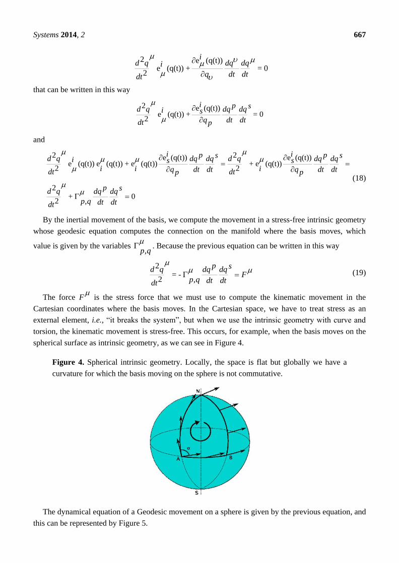
spherical surface as intrinsic geometry, as we can see in Figure 4.

Figure 4. Spherical intrinsic geometry. Locally, the space is flat but globally we have a

curvature for which the basis moving on the sphere is not commutative.

The dynamical equation of a Geodesic movement on a sphere is given by the previous equation, and

this can be represented by Figure 5.

2 e (q(t)) e (q(t)) + = 0

2

2 e (q(t))e (q(t)) + = 0

2

and

2 2e (q(t))e (q(t)) e (q(t)) + e (q(t)) + e (q

2 2

can be written in this way

id q dq dqi

q dt dtdt

i p sd q dq dqi s

q dt dtdt p

i p sd q dq dq d qi si i iq dt dtdt dtp

that

e (q(t))(t))

2+ 0

2 ,

i p sdq dqs

q dt dtp

p sd q dq dq

p q dt dtdt

(18)

2 e (q(t)) e (q(t)) + = 0

2

2 e (q(t))e (q(t)) + = 0

2

and

2 2e (q(t))e (q(t)) e (q(t)) + e (q(t)) + e (q

2 2

can be written in this way

id q dq dqi

q dt dtdt

i p sd q dq dqi s

q dt dtdt p

i p sd q dq dq d qi si i iq dt dtdt dtp

that

e (q(t))(t))

2+ 0

2 ,

i p sdq dqs

q dt dtp

p sd q dq dq

p q dt dtdt

(18)

Systems 2014, 2 668

Figure 5. Geodesic triangle and geodesic trajectories. On the surface of the intrinsic geometry

(spherical geometry), the geodesics are straight lines without curvature and so are stress-free.

Now, we have the problem to compute the derivative from the Cartesian coordinates to the general

moving basis e . We solve the previous problem by projecting the vector A on the moving basis so

we have the vector field i

iA A e (20)

The derivative is

(21)

we can write the term ei

x j

as the linear combination of the basis

,

e ki ei j kx j

(22)

We remark that if

0ee ji

x xj i

(23)

The connection terms ,ki j are not commutative in the index , ,

k ki j j i we have that ,

ki j are not

Christoffel symbols but are simple connections with torsion , , ,k k kTi j i j j i . Now, we have

,

, ,

( ) , ,

iA A i ke A ei i j kx xj j

but

k ie ei j ik k j

i iA Ak i k ie A e A ei i ik j k jx xj j

(24)

but

,

, ,

( ) , ,

iA A i ke A ei i j kx xj j

but

k ie ei j ik k j

i iA Ak i k ie A e A ei i ik j k jx xj j

(21)

i iA e eA A ii ie Aix x x xj j j j

Systems 2014, 2 669

Now, in index notation, the covariant derivative of iA is given by

( ),

iAi k iD A Aj k jx j

(25)

and

, ( )D D A D D D D A R A

(26)

where A

is a vector and R

is the Riemann tensor curvature.

If we have a point moving on a curve in time, we have

( )j j

x x t (27)

and the directional derivative to the tangent vector is

( ) ,

( ) ( ) , ,

i idx dx dxA edA A Aj j jk ii A eik jdt x dt x dt x dtj j j

i idx dx dxA dAj j jk i k iA e A ei ik j k jx dt dt dt dtj

(28)

In the geodesic line we have

0,

i dxdA jk iAk jdt dt

(29)

The derivative in the direction of the tangent vector is equal to zero. So, the geodesic is a line

without stress.

2.2. Electrical Circuit and Moving Reference

Given the electrical circuit inertial equation (free from stress) for the voltages

20

2

id v

dt (30)

When we change the reference from fixed and inertial movement for the voltage to the current

moving reference we know that we have the relation

0 and 0

i i idv R di e di

or

i i i idv R di dv e di

(31)

or

0 and 0

i i idv R di e di

or

i i i idv R di dv e di

The first equation is the phenomenological relation between currents and voltage by the resistor

tensor iR . The second is the geometry representation of the movement by the movie reference tensor

without stress ie . The previous relations can be written by the tangent vectors in this way

Systems 2014, 2 670

( ( )) ( ( ))

idv di dii idt e dt R dtdt dt dt

or

idv di dii ie i t R i tdt dt dt

(32)

or

( ( )) ( ( ))

idv di dii idt e dt R dtdt dt dt

or

idv di dii ie i t R i tdt dt dt

For the compatibility between the phenomenological equation and intrinsic geometry, we have

the identity

,

, ,

R ki Ri j kx j

and

R k k k ki R R Ri j i jkx j

(33)

and

,

, ,

R ki Ri j kx j

and

R k k k ki R R Ri j i jkx j

Given the connection term, we can design the resistor tensor in a way to have geodesic

transformation and covariant derivative in the wanted space of the currents. For example, given the

spherical geometry by the transformation

1

2

3

sin( )cos( )

sin( )sin( )

cos( )

x

x

x

(34)

The tangent vector is

1 1 11

2 2 2 2 ,

3 3 3 3

x x xdxdR

Rdt dtdx x x x d

dt R dt

dx dx x x

dtdt R

(35)

And the moving basis is

1 1 1

sin( )cos( ) cos( )cos( ) sin( )sin( )2 2 2 sin( )sin( ) cos( )sin( ) sin( )cos(

cos( ) sin( ) 0

3 3 3

x x x

R

x x xieR

x x x

R

(36)

For the phenomenological identity, we have the resistor matrix

(37)

sin( )cos( ) cos( )cos( ) sin( )sin( )

sin( )sin( ) cos( )sin( ) sin( )cos( (37)

cos( ) sin( ) 0

iR

Systems 2014, 2 671

And the electrical circuits with current-controlled voltage sources (CCVS) and resistors (Figure 6).

Figure 6. Moving reference on the sphere.

We know that the connection terms of the intrinsic geometry are

,

iR k iRji j

(38)

Now, we represent the circuit with current-controlled voltage source (CCVS) iR where i and

variable resistor for i .

In Figure 7, we have three circuits providing the derivative in time of the current. The big circle

represents the sources of the voltage that are constant or change proportionally to the time. The term

R is ordinary resistors, while the other is sources of voltages v controlled by current i in other

circuits by the proportional value R

Figure 7. Moving reference in the electrical circuit.

1di

dt

2di

dt

3di

dt

11

R 22

R 33

R

12

R

13

R

21

R

23

R

32

R

31

R

1E

2E

3E

Systems 2014, 2 672

To complete possible electrical circuits, we have another three derivative transformations

jdq dv dvj j

e Cdt dt dt

id di dii ie Ldt dt dt

kdq d dk ke Mdt dt dt

(39)

where jC ,

iL ,

kM are the capacitor tensor, the induct tensor and the memristor tensor [2,3]. The

variables , , ,i v q are the currents, the voltages, the charges and the magnetic fluxes.

2.3. Deformation and Displacement in Media with Defects for Rotation (Disclination) and Translation

(Dislocation)

Given a space where the general coordinates are 1 2, ,....., nq q q q , the bases are the vectors

se

q

where s is the displacement vector (Figure 8).

Figure 8. Angular displacement q = and mind control of initial and final positions.

With the basis vectors s

eq

we can compute the affine connection ,

in this way

,

ee

x

. Now, when

, , , we have curvature and metric , ( ) ( )Tg e e but

no torsion. When , ,

, we have the torsion

, , ,S (40)

Intrinsic geometry can have curvature and torsion that can be seen as an external element as we can

see in the Euler Lagrange equation with torsion

2

1

,

,

2

,

t

t

d L L LS v

dt v q v

dq dq dqL dt g v

dt dt dt

(41)

Systems 2014, 2 673

Examples of curvature and torsion (Figure 9):

Figure 9. Rotation and torsion geometry.

We provide that any deformation of the reference as a crystal totally ordered is given by the

transformation

( )i i iy x s x (42)

The difference of the distance L between points (atoms) before and after the deformation is given

by the expression

2 2 2jidL dL x xy x ij (43)

where ij is the strain tensor

1( )

2

ks ss sj i kij x x x xi j i j

(44)

In the work by Ruggero and Tartaglia [4], we find some important remarks. After the deformation,

we may have two different situations:

(1) The deformed elements fit perfectly or they do not. In the latter case, we must apply a further

deformation to re-compact the body. In the first case, we speak of a compatible deformation.

(2) In the second case, we have an incompatible deformation. Let us imagine that during the

deformation the coordinates are dragged with the medium. In the compatible deformation, the

internal or intrinsic observer cannot see any difference as the Galileo internal observer for

inertial system. In the incompatible deformation, the internal observer notices a change in the

number of particles along a cycle in the medium as excess of holes or particles. The internal

point of view is useful to find an incompatible deformation, due to the presence of defects.

Mathematically, an incompatible deformation corresponds to the non-integrability of the

differential form jds where js is the displacement. The non-integrability means that the

displacement field ( )js x is multivalued, and thus discontinuities or defects arise when passing

from one point to another. This fact is expressed by,

[ , ] 0j

k h

sx x

(45)

Systems 2014, 2 674

In this situation, intrinsic geometry will no longer be Euclidean. The intrinsic view suggests that

relations can be found between the geometric properties and the densities of defects that influence

them. From ideal crystal or ideal reference as Cartesian reference, after the deformation we have

Crystal incompatibility or disclination where there is deformation in the rotation and without torsion

(Figure 10).

Figure 10. Change of reference or crystal medium by curved system where the center is a

singularity or defect in the disclination.

With the scalar f there is the torsion connection [5]

, ( ),

D D f D D D D f T D f

(46)

Tensor ,

T

is the torsion tensor. The torsion is given by Figure 11.

Figure 11. Torsion as defects in translation.

The torsion is a defect in translation (dislocation) as we can see in Figure 12.

Figure 12. Defects in translation or crystal dislocation.

The defect or singularity is given by defect in the reference due to translation transformation.

Systems 2014, 2 675

3. Incompatible Condition for Commutators and Wave Field Control by Active Secondary Sources

For the wave equation, we have

2

2

2 2 0

2c

tj x j

iee

(47)

where is the field with noise and is the field without noise or incompatibility.

2 22 0

2 2

2 2( ) ( )

2 2

22( ) (

2

ie iee e

cj x tj

ie ie ie ie iee e ie e ie e ie ie e ie

x x x x x xj x xj j j j j jj j

ie ie ie ie iec e e ie e ie e ie ie e ie

t t t t t tt

20

2

2 2( ) ( )

2 2

2 22( ) ( 0

2 2

2 222 )

2 2

22( 2

2

t

ie ie ie ie iex x x x x xj x xj j j j j jj j

c ie ie ie ie iet t t t t tt t

ie e iex x x xj x xj j j jj j

ct

22 ) 0

2

2 0

ie e iet t t t t

D D c D Dt tj jj

(48)

where

,

,

D ieA D ietj jx tj

where Aj x tj

(49)

where

,

,

D ieA D ietj jx tj

where Aj x tj

When we use the space time reference ( , , , )

1 2 3y x x x ictj we have

2 2 242 02 2 21

cj kx t yj k

(50)

For ie

e

we have 2 2 24 42 02 2 21 1

c D Dk kj k kx t yj k

(51)

Systems 2014, 2 676

where

, CD ieC wherek k ky y

k k

where

, CD ieC wherek k ky y

k k

(52)

We remark that

[ , ] ( )( ) ( )( )

2 2( ) ( ) ( )

2 2( ) ( ) ( )

( )

D D ieC ieC ieC ieC

ie C ieC ieC e C C

ie C ieC ieC e C C

CCie ieW

x x

(53)

For the wave equation, the change of the wave function generates incompatible medium where there

are defects as we can see in Figure 13.

Figure 13. From compatible medium on the left, there is incompatible medium on the screen.

The new derivative does not commute but the wave equation does not change its form and the wave

sources are always the same. In fact, for

2 2 242 2 2 21

c Sj kx t yj k

(54)

We have 4

1D D S

k kk

(55)

In the Jessel book [6] we found the connection between sources and transformation of field

variable. Now, we use this method to explain better the meaning of the non-commutativity of the

derivates and the incompatibility.

In fact, the transformation ie

e

of the equation 2

2

2 2

2c S

tj x j

we have

Systems 2014, 2 677

2 2 2 22 22 )

2 2 2 2

2 22 2( 2 )

2 2

2 22

2 2

22 2(2 ) (2

2j

ie iee e

c ie e iex x x xj jx t x xj j j jj j j

c ie e ie St t t tt t

or

cj x tj

S ie e ie c ix x x x txj j j j j

22 ) *

2e e ie S S

t t t t

or

2 2 2 22 22 )

2 2 2 2

2 22 2( 2 )

2 2

2 22

2 2

22 2(2 ) (2

2j

ie iee e

c ie e iex x x xj jx t x xj j j jj j j

c ie e ie St t t tt t

or

cj x tj

S ie e ie c ix x x x txj j j j j

22 ) *

2e e ie S S

t t t t

(56)

In the transformation, the derivatives are those in the compatible medium but we must change the

source from S as the original sources of the wave to new artificial sources or secondary sources

2 22 2 2* (2 ) (2 )

2 2j

S ie e ie c ie e iex x x x t t t tx tj j j j j

That gives us the physical image of the incompatibility in the medium when we transform one field

to another. By the new sources we can generate the new field with the same derivatives. M. Jessel uses

the new sources to design a wanted field from the initial one. This is the beginning of a new

computation where we design a new intrinsic geometry in the field by artificial sources. This is an

example of field control by the active or secondary sources S* [7].

InVuksanovic and Nikolic [8] we have the multichannel active noise control (see Figure 14).

Figure 14. Active noise control (ANC) by the algorithm or DSP for S*.

The active noise control (ANC) is the process of reducing an unwanted or incompatible sound by

combining it with a sound of the same amplitude but of opposite phase. The proposed ANC system

uses an active sound barrier of secondary sources S* to cancel the unwanted sound or incompatibility

from the primary source at an array of error microphones. By cancelling the sound at the error

microphones distributed across the controlled region, the secondary sources create a zone of reduced

noise over this area as we can see in Figure 14 where the DSP algorithm uses the expression for S* to

generate a wanted field without noise.

Systems 2014, 2 678

4. Schrödinger and Maxwell Equations Commutators and Incompatible Equations

In the work by Russer [9], we can see that the Maxwell equation can be represented by exterior

differential forms. Now, in this chapter, because of a suggestion by Pessa [10], we show the invariance

of the Schrodinger equation for a given transformation of the wave function; therefore, we obtain the

Maxwell equations by commutators that are connected by the incompatibility of the medium. So, given

the celebrate Schrodinger equation, 21

22

i m Ut j x j

iee

(57)

When we substitute the new variable, we have

2 2

2 2

2 22 2

2 2

1( ) ( )

2

1( ) [ ( 2 ) ( ( ) )] ( )

2

j j j j j j j j j

j j j j j j

m ie ie ie ie ie Ux x x x x x x x

i m ie e ie U et x x x x x t

(58)

For

,j

j

Ax t

(59)

21 2 2( ) [ ( 2 ) ( ) )] ( )22

Aji m ieA e A ie U ej jt x xj x j jj

(60)

but

( )( )

22( ) ( ) ( )

2

22[ 2 ( ) ( ( ) )]

2

D D ieA ieAj j j jx xj j

Ajie ieA ieA e A Aj j j jx x xx j j jj

AjieA ie e A Aj j jx xx j jj

(61)

and

1

2j ji m D D

t j

where

U e

(62)

where

1

2j ji m D D

t j

where

U e

When

0, 0jx t

(63)

The phase is constant in space and time and we have the compatible condition

Systems 2014, 2 679

[ , ] [ ] 0D D (64)

We have no curvature and torsion and the medium has no defects. However, when

,Ajx tj

(65)

We have the incompatible condition

[ , ] ( )( ) ( )( )

2 2( ) ( ) ( )

2 2( ) ( ) ( )

( )

D D ieA ieA ieA ieA

ie A ieA ieA e A A

ie A ieA ieA e A A

AAie ieF

x x

(66)

For a reference with torsion, we obtain the incompatible equation

, ( )

, ,

, ,

D D f D D D D f T D f ieF

and

T D f ieF

(67)

and

, ( )

, ,

, ,

D D f D D D D f T D f ieF

and

T D f ieF

When we solve this equation, we can provide a new geometric representation of the electromagnetic

equation by torsion of the reference and defects in the medium. In crystal, there is a separation of the

charges and the reference for the electromagnetic field is deformed by a torsion as in the dislocation of

the crystal.

In the electromagnetic theory, we have that

[ ,[ , ] ([ , ] ) [ , ] [ ( ) ]

[( ) ] ( ) (68)

D D D D D D D D D ie D F F D

ie D F F D F D ie D F

where

,D F J v (69)

,J v are the currents of the defects or electrical particles.

Because we have

[ ,[ , ] [ ,[ , ] [ ,[ , ] 0D D D D D D D D Dv v (70)

We have the invariant property for the currents

0, , ,J J Jv v v (71)

Given the Maxwell equations in the tensor form

4

0

F Jc

F F F

(72)

Systems 2014, 2 680

where the contravariant four-vector which combines electric current density and electric charge density

Jv = (cp, Jx, Jy, Jz) is the four-current, the electromagnetic tensor is 𝐹???? = 𝑎? ??? 𝐴?? − 𝑎? ??? 𝐴?? that can

be connected with the commutators’ property and the incompatible condition that we have explained in

the prrevious chapters.

The Maxwell-like scheme for an incompatible system is given by the set of equations

( )

[ , ]

[ ,[ , ] ,

D kA xx

D D F

D D D J v

(73)

where the covariant derivative includes a connection term that is the potential, the commutator is the

compensatory field for the incompatible system and the second commutator is the density current of

the defects. The three equations can be used as models for all possible dynamical systems that include

defects or sources. In the next chapter, we use this new scheme to improve the Einstein gravitational

geometry.

5. Dynamic Equations with Torsion in Non-Conservative Gravity Maxwell-Like Equations

To introduce the new wave equation for gravity [11,12] and for the “constructive logic” of the

gauges theories [13], we remember that

, V R V

(74)

where the Riemann tensor is

R (75)

With the double commutator we have the dynamic equation

[ ,[ , ]] ( [ , ]) [ , ]( )

( ) ( )

K K K

R K R K

(76)

where 𝑅 is the Riemann tensor, a? ?𝑘 is the covariant derivative and 𝐾?? is the vacuum field. Now we

connect the commutator with the gravity current in this way

( ) ( )J K R K R K (77)

For the conservation of the current, after contractions, we have the equation

a? ??? [R????+? ? (T???? +1

2g????T)] K?? + R????(a? ??? K??) = 0 (78)

when a? ?𝑘 𝐾?? = 0 we have the Einstein equations.

Most applications of differential geometry, including General Relativity, assume that the connection

is “torsion free”: that is, vectors do not rotate during parallel transport. Because some extensions of GR

do include torsion, it is useful to see how torsion appears in a modern geometrical language. The

torsion corresponds intuitively to the condition that vectors must not be rotated by parallel transport.

Systems 2014, 2 681

Such a condition is natural to impose, the theory of General Relativity itself includes this assumption.

However, differential geometry is equally well.defined with torsion as well as without, and some

extensions of general relativity include torsion terms. The first of these was “Einstein-Cartan theory”,

as introduced by Cartan in 1922. We define the torsion tensor by the connection symbols in this way

T (79)

We now show in an explicit way that it is possible to present the previous dynamical equation by a

wave equation with a particular source where the variables include symmetric and anti-symmetric

connection symbols as well as torsion in one geometric picture. In Appendix A, we define the new

type of wave with an explicit computation of the commutator and of the double commutator.

6. Conclusions

Symmetry and its physical implications on conservation principles have a long history in physics.

The same importance, if not higher, is shown by the concepts of symmetry breaking and local gauge as

the constructive principle to characterize interactions as a “compensation mechanism”. In particular, this

was made possible by a unified geometrical vision of fundamental interactions in Gauge Theories [14].

The structural logics of these theories are not an exclusive prerogative of particle physics or relativistic

geometrodynamics. In this work, we delineated a parallel development of such ideas we called

“Compensative Geometry” which has old systemic roots. It is within such a context—at the crossroad

of Theoretical Physics, Cybernetics, Category and Group Theory and Logical System Theory—that the

constructive approach here introduced has been developed [3,7,11] (for some fundamental steps,

see [15–17]; for the consequences on the computation concept, see [18,19]). Such class of theories is

based on few principles related to different orders of commutators between covariant derivatives. Their

physical meaning is very simple, and lies in stating that the local transformations of a suitable substratum

(the space-time or a particular phase space) and the imposed constraints define a “compensative

mechanism” or the “interaction” we want to characterize.

We stress the mathematical aspects which make this approach a “theory to build geometric-based

unified theories”.

The conceptual core of the procedure can be expressed in a five-point nutshell:

(a) The description of a suitable substratum and its global and local properties on invariance;

(b) The field potentials are compensative fields defined by a gauge covariant derivative. They

share the global invariance properties with the substratum;

(c) The calculation of the commutators of the covariant derivatives in (b) provides the relations

between the field strength and the field potentials;

(d) The Jacobi identity applied to commutators provides the dynamic equations satisfied by the

field strength and the field potentials;

(e) The commutator between the covariant derivatives (b) and the commutator (c) (triple Jacobian

commutator) fixes the relations between field strength and field currents.

We chose an example connected to the recent developments of the extended gravity theories in

order to show the generality of the approach. Actually, the GR syntax seems to regenerate itself from

Systems 2014, 2 682

inside and to produce many schemes of classical coupling Raum–Zeit–Materie. This autopoietic

feature is a distinctive and propulsive of Theoretical Physics considered as a totality of structures that

fixes the conditions of thinkability for its entities and “beables”.

In conclusion, the geometrical approach here delineated has significant potential in relation to the

classical themes of systemics (system/environment; contextuality; computation; logical openness)

thanks to the strategy allowing, in a simple and general way, to recognise the gauging as cognitive

compensation between known and unknown domains.

Acknowledgments

The authors thank the Editors for their critical reading, and suggestions.

Author Contributions

The authors contributed in equal measure to the work.

Conflicts of Interest

The authors declare no conflict of interest.

References

1. Caianello, E. Quantum and other physics as systems theory. La Rivista del Nuovo Cimento 1992,

15, 1–65.

2. Kozma, R.; Pino, R.E.; Pazienza, G.E. Advances in Neuromorphic Memristor Science and

Applications; Springer: Berlin, Germany, 2012.

3. Resconi, G.; Licata, I. Geometry for a brain. Optimal control in a network of adaptive memristor.

Adv. Studies Theor. Phys. 2013, 7, 479–513.

4. Ruggero, M.L.; Tartaglia, A. Einstein—Cartan theory as a theory of defects in space-time. Am. J.

Phys. 2003, 71, 1303–1313.

5. Kleinert, H. Gauge Fields in Condensed Matter, Volume II: Stresses and Defects; World

Scientific: Singapore, 1989.

6. Jessel, M. Acoustique Theorique. Propagation et holophonie; Masson: Paris, France, 1973.

7. Jessel, M.; Resconi, G. A general system logical theory. Int. J. Gen. Syst. 1986, 12, 159–182.

8. Vuksanovic, B.; Nikolic, D. Multichannel Active Noise Control in Open Spaces. In Proceedings

of ICCC 2004, Zakopane, Poland, 25–28 May 2004.

9. Russer, P. The Geometric Representation of Electrodynamics by Exterior Differential Forms.

In Proceedings of the TELSIKS 2013, Nis, Serbia, 16–19 October 2013.

10. Mignani, R.; Pessa, E.; Resconi, G. Non-conservative gravitational equation. Gen. Relat. Gravit.

1997, 29, 1049–1073.

11. Mignani, R.; Pessa, E.; Resconi, G. Electromagnetic-like generation of unified-Gauge theories.

Phys. Essay 1999, 12, 62–79.

12. Hamani Daouda, M.; Rodrigues, M.E.; Houndjo, M.J.S. New black holes solutions in a Modified

Gravity. ISRN Astron. Astrophys. 2011, 2011, doi:10.5402/2011/341919.

Systems 2014, 2 683

13. Licata, I. Methexis, mimesis and self duality: Theoretical physics as formal systems. Versus 2014,

118, 119–140.

14. Aitchinson, I.J.R.; Hey, A.J.G. Gauge Theories in Particle Physics: A Practical Introduction,

4th ed.; CRC Press: Boca Raton, FL, USA, 2012.

15. Resconi, G.; Marcer, P.J. A novel representation of quantum cybernetics using Lie algebras.

Phys. Lett. A 1987, 125, 282–290.

16. Fatmi, H.A.; Marcer, P.J.; Jessel, M.; Resconi, G. Theory of cybernetic and intelligent machine

based on Lie commutators. Int. J. Gen. Syst. 1990, 16, 123–164.

17. Resconi, G. Geometry of Knowledge for Intelligent Systems; Springer: Berlin, Germany, 2013.

18. Licata, I.; Resconi, G. Information as Environment Changings. Classical and Quantum Morphic

Computation. Methods, Models, Simulation and Approaches. Toward A General Theory of Change;

Minati, G., Pessa, E., Abram, M., Eds.; World Scientific: Singapore, 2012; pp. 47–81.

19. Licata, I. Beyond turing: Hypercomputation and quantum morphogenesis. Asian Pacif. Math.

Newsl. 2012, 2, 20–24.

20. Kleinert, H. Nonabelian Bosonization as a nonholonomic transformations from Flat to Curved

field space. Ann. Phys. 1997, 253, 121–176.

21. De Witt, B.; Nicolai, H.; Samtleben, H. Gauged Supergravities, Tensor Hierarchies and M-theory.

2008. Available online: http://arxiv.org/pdf/0801.1294.pdf (accessed on 22 July 2014).

22. Mukhi, S. Unravelling the Novel Higgs Mechanism in (2+1)d Chern-Simons Theories. J. High

Energy Phys. 2011, 83, doi:10.1007/JHEP12(2011)083.

Appendix A

Given the general covariant derivative

VD V V

x

(1A)

where the connection terms are unknown variables that we define by the new gravitational equation

obtained by the first and second commutator. We remark that the connection terms are not Christoffel

elements but are a general connection which values will be defined by the new gravitational equations.

To know the connection terms we begin with the computation of the first commutator

, ( ) ( ),V V

F D D V D D V D D V D V D Vx x

(2A)

So we have

𝐹𝜇𝜈,𝛼 = [𝐷𝜇 , 𝐷𝜈]𝑉𝛼 = (𝜕𝐵𝜈,𝛼

𝜕𝑥𝜇− Γ𝜈,𝜇

𝜆 𝐵𝜈,𝜆 − Γ𝛼,𝜇𝜆 𝐵𝛼,𝜆) − (

𝜕𝐵𝜇,𝛼

𝜕𝑥𝜈− Γ𝜇,𝜈

𝜆 𝐵𝜇,𝜆 − Γ𝛼,𝜈𝜆 𝐵𝛼,𝜆) (3A)

with

𝐵𝜈,𝛼 = (𝜕𝑉𝛼

𝜕𝑥𝜈− Γ𝜈,𝛼

𝜆 𝑉𝜆)

𝐵𝜇,𝛼 = (𝜕𝑉𝛼

𝜕𝑥𝜇− Γ𝜇,𝛼

𝜆 𝑉𝜆)

and

Systems 2014, 2 684

𝐹𝜇𝜈,𝛼 = [𝐷𝜇 , 𝐷𝜈]𝑉𝛼 = −(𝑅𝛼𝜇𝜈𝜆 𝑉𝜆 + T𝜇𝜈

𝜆 𝐷𝜆𝑉𝛼)

where

𝑅𝛼𝜇𝜈𝜆 = (

𝜕Γ𝜈,𝛼𝜆

𝜕𝑥𝜇−

𝜕Γ𝜇,𝛼𝜆

𝜕𝑥𝜈+ Γ𝜇,𝑞

𝜆 Γ𝜈,𝛼𝑞

− Γ𝜇,𝛼𝑞

Γ𝜈,𝛼𝜆 )

In conclusion, we have

−𝐹𝜇𝜈,𝛼 = −[𝐷𝜇 , 𝐷𝜈]𝑉𝛼 = (𝜕Γ𝜈,𝛼

𝜆

𝜕𝑥𝜇−

𝜕Γ𝜇,𝛼𝜆

𝜕𝑥𝜈) 𝑉𝜆 + (Γ𝜇,𝑞

𝜆 Γ𝜈,𝛼𝑞

− Γ𝜇,𝛼𝑞

Γ𝜈,𝑞𝜆 )𝑉𝜆 + (Γ𝜇,𝜈

𝜆 − Γ𝜈,𝜇𝜆 )𝐷𝜆𝑉𝛼 = 𝐺𝜇𝜈,𝛼 + Ω𝜇𝜈,𝛼 (4A)

where

𝐺𝜇𝜈,𝛼 = (𝜕𝛤𝜈,𝛼

𝜆

𝜕𝑥𝜇−

𝜕𝛤𝜇,𝛼𝜆

𝜕𝑥𝜈) 𝑉𝜆

and

Ω𝜇𝜈,𝛼 = (𝛤𝜇,𝑞𝜆 𝛤𝜈,𝛼

𝑞− 𝛤𝜇,𝛼

𝑞𝛤𝜈,𝑞

𝜆 )𝑉𝜆 + (𝛤𝜇,𝜈𝜆 − 𝛤𝜈,𝜇

𝜆 )𝐷𝜆𝑉𝛼

Now, we have that

x

obtaining

2 2( ), ,G V G

x x x x x x

(5A)

So, we have that the field 𝐺 is invariant. Now, we impose the Lorenz-like gauge condition in this way

0x

(6A)

Now, we have

, , ,

, , , ,, ,( ) ( ) ( )

, , , ,, ,

G G Gx x x

vV V V

x x x x x x x x xv

v

x x x x x x x x x x x xv

0

(7A)

The Lagrangian gravitational density is

𝐿 = 𝐹𝜇𝜈,𝛼𝐹𝜇𝜈,𝛼 = (𝐺𝜇𝜈,𝛼 + Ω𝜇𝜈,𝛼)(𝐺𝜇𝜈,𝛼 + Ω𝜇𝜈,𝛼) = 𝐺𝜇𝜈,𝛼𝐺𝜇𝜈,𝛼 + Ω𝜇𝜈,𝛼Ω𝜇𝜈,𝛼 + 2𝐺𝜇𝜈,𝛼Ω𝜇𝜈,𝛼(8A)

where 𝐺𝜇𝜈,𝛼𝐺𝜇𝜈,𝛼 and Ω𝜇𝜈,𝛼Ω𝜇𝜈,𝛼 + 2𝐺𝜇𝜈,𝛼Ω𝜇𝜈,𝛼 are the Lagrangian density for the free gravitational

field and the reaction field of the vacuum. The interaction term 𝐺𝜇𝜈,𝛼Ω𝜇𝜈,𝛼 connects the gravitation

field with the field of the vacuum.

Systems 2014, 2 685

The dynamic equation for Non Conservative Gravity can be obtained in this way

[𝐷𝛽 , [𝐷𝜇 , 𝐷𝜈]] 𝑉𝛼 = 𝐷𝛽[𝐷𝜇, 𝐷𝜈]𝑉𝛼 − [𝐷𝜇 , 𝐷𝜈]𝐷𝛽𝑉𝛼 = 𝐷𝛽𝐹𝜇𝜈,𝛼 − [𝐷𝜇, 𝐷𝜈]𝐷𝛽𝑉𝛼 =

= −𝐷𝛽(𝐺𝜇𝜈,𝛼 + Ω𝜇𝜈,𝛼) − [𝐷𝜇, 𝐷𝜈]𝐷𝛽𝑉𝛼 = 𝐽𝜇𝜈,𝛼𝛽 (9A)

and

𝐷𝛽𝐺𝜇𝜈,𝛼 = −𝐽𝜇𝜈,𝛼𝛽 − 𝐷𝛽Ω𝜇𝜈,𝛼 − [𝐷𝜇, 𝐷𝜈]𝐷𝛽𝑉𝛼 (10A)

where

𝐷𝛽𝐺𝜇𝜈,𝛼 =𝜕𝐺𝜇𝜈,𝛼

𝜕𝑥𝛽− 𝐺𝑗𝜈,𝛼Γ𝜇𝛽

𝑗− 𝐺𝜇𝑗,𝛼Γ𝜈𝛽

𝑗− 𝐺𝜇𝜈,𝑗Γ𝛼𝛽

𝑗 (11A)

so

𝜕𝐺𝜇𝜈,𝛼

𝜕𝑥𝛽− 𝐺𝑗𝜈,𝛼Γ𝜇𝛽

𝑗− 𝐺𝜇𝑗,𝛼Γ𝜈𝛽

𝑗− 𝐺𝜇𝜈,𝑗Γ𝛼𝛽

𝑗= −𝐽𝜇𝜈,𝛼𝛽 − 𝐷𝛽Ω𝜇𝜈,𝛼 − [𝐷𝜇 , 𝐷𝜈]𝐷𝛽𝑉𝛼 (12A)

and

𝜕𝐺𝜇𝜈,𝛼

𝜕𝑥𝛽= 𝐺𝑗𝜈,𝛼Γ𝜇𝛽

𝑗+ 𝐺𝜇𝑗,𝛼Γ𝜈𝛽

𝑗+ 𝐺𝜇𝜈,𝑗Γ𝛼𝛽

𝑗− 𝐽𝜇𝜈,𝛼𝛽 − 𝐷𝛽Ω𝜇𝜈,𝛼 − [𝐷𝜇, 𝐷𝜈]𝐷𝛽𝑉𝛼 (13A)

,,

GJ

x

Now, we have

𝜕𝐺𝜇𝜈,𝛼

𝜕𝑥𝛽=

𝜕

𝜕𝑥𝛽(

𝜕𝛤𝜈,𝛼𝜆

𝜕𝑥𝜇−

𝜕𝛤𝜇,𝛼𝜆

𝜕𝑥𝜈) 𝑉𝜆 = (

𝜕2𝛤𝜈,𝛼𝜆

𝜕𝑥𝛽𝜕𝑥𝜇−

𝜕2𝛤𝜇,𝛼𝜆

𝜕𝑥𝛽𝜕𝑥𝜈) 𝑉𝜆 (14A)

For 𝑥?2 = 𝑥?? we have

𝜕𝐺𝜇𝜈,𝛼

𝜕𝑥𝜇= (

𝜕2𝛤𝜈,𝛼𝜆

𝜕2𝑥𝜇−

𝜕2𝛤𝜇,𝛼𝜆

𝜕𝑥𝜇𝜕𝑥𝜈) 𝑉𝜆 = (

𝜕2𝛤𝜈,𝛼𝜆

𝜕2𝑥𝜇−

𝜕2𝛤𝜇,𝛼𝜆

𝜕𝑥𝜈𝜕𝑥𝜇) 𝑉𝜆 (15A)

However, for the Lorentz-like gauge we have

𝜕2𝛤𝜇,𝛼𝜆

𝜕𝑥𝜈𝜕𝑥𝜇=

𝜕

𝜕𝑥𝜈(

𝜕𝛤𝜈,𝛼𝜆

𝜕𝑥𝜇) = 0 (16A)

and

𝜕𝐺𝜇𝜈,𝛼

𝜕𝑥𝜇=

𝜕2𝛤𝜈,𝛼𝜆

𝜕2𝑥𝜇𝑉𝜆 = (

𝜕2𝛤𝜈,𝛼𝜆

𝜕2𝑥− 𝑐2 𝜕2𝛤𝜈,𝛼

𝜆

𝜕2𝑡) 𝑉𝜆 = 𝐽𝜈𝛼 (17A)

When the currents are equal to zero we have that

𝜕𝐺𝜇𝜈,𝛼

𝜕𝑥𝜇=

𝜕2𝛤𝜈,𝛼𝜆

𝜕2𝑥𝜇𝑉𝜆 = (

𝜕2𝛤𝜈,𝛼𝜆

𝜕2𝑥− 𝑐2 𝜕2𝛤𝜈,𝛼

𝜆

𝜕2𝑡) 𝑉𝜆 = 0 (18A)

The variable 𝛤𝜈,𝛼𝜆 has a wave-like behaviour.

Now we look at the currents

𝐽𝜇𝜈,𝛼𝛽 = 𝐺𝑗𝜈,𝛼Γ𝜇𝛽𝑗

+ 𝐺𝜇𝑗,𝛼Γ𝜈𝛽𝑗

+ 𝐺𝜇𝜈,𝑗Γ𝛼𝛽𝑗

− 𝐽𝜇𝜈,𝛼𝛽 − 𝐷𝛽Ω𝜇𝜈,𝛼 + [𝐷𝜇 , 𝐷𝜈]𝐷𝛽𝑉𝛼 = 𝑅𝜇𝜈,𝛼𝛽 − 𝐽𝜇𝜈,𝛼𝛽 (19A)

where 𝑅 is a reaction of a virtual matter or medium (vacuum) and 𝐽 is the ordinary currents for the

ordinary matter represented by the energetic tensor. The non-linear reaction of the self-coherent system

Systems 2014, 2 686

produces a current that justifies the complexity of the gravitational field and non-linear properties of

the gravitational waves.

(𝜕2𝛤𝜈,𝛼

𝜆

𝜕2𝑥− 𝑐2 𝜕2𝛤𝜈,𝛼

𝜆

𝜕2𝑡) 𝑉𝜆 = 𝑅𝜈𝛼 − 𝐽𝜈𝛼 (20A)

In conclusion, we show that the non-conservative gravitational field is similar to a wave for

64 variables jv

in a non-linear material where we have complex non-linear phenomena inside the

virtual material that represents the vacuum. In the previous equations, in the free field of the medium

the Proca terms , the Chern-Simons terms ( ) and the Maxwell-like terms ( ) ( )

are present. So, we have the mass terms, the topologic terms and the electromagnetic-like field terms.

We can model the gravitational wave with torsion as a particle in a non-linear medium which gives the

mass of the particle, in a way that can be compared to usual SSB processes of the standard model, for

an orientation in extensive literature [20–22].

© 2014 by the authors; licensee MDPI, Basel, Switzerland. This article is an open access article

distributed under the terms and conditions of the Creative Commons Attribution license

(http://creativecommons.org/licenses/by/4.0/).