Where intrinsic job satisfaction fails to work: national moderators of intrinsic motivation
Upload
khangminh22Category
view
1download
0
Technical Protocol for Implementing Intrinsic Remediation with Long-Term Monitoring for Natural Attenuation of Fuel Contamination Dissolved in Groundwater
Volume I
By
Todd Wiedemeier Parsons Engineering Science, Inc. Denver, Colorado
TOB ET J| J
John T. Wilson and Donald H. Kampbell U.S. Environmental Protection Agency Robert S. Kerr Laboratory Ada, Oklahoma
Ross N. Miller and Jerry E. Hansen Air Force Center for Environmental Excellence Technology Transfer Division Brooks AFB, San Antonio, Texas
425 019 Air Force Center for Environmental Excellence Technology Transfer Division Brooks AFB, San Antonio, Texas
[DUO QUALITY INSPECTED S
TECHNICAL PROTOCOL FOR IMPLEMENTING INTRINSIC REMEDIATION WITH LONG-TERM MONITORING FOR NATURAL ATTENUATION OF FUEL CONTAMINATION
DISSOLVED IN GROUNDWATER
VOLUME I
by
Todd H. Wiedemeier Parsons Engineering Science, Inc.
Denver, Colorado
Dr. John T. Wilson and Dr. Donald H. Kampbell United States Environmental Protection Agency* National Risk Management Research Laboratory Subsurface Protection and Remediation Division
Ada, Oklahoma
Lt. Col. Ross N. Miller and Jerry E. Hansen Air Force Center for Environmental Excellence
Technology Transfer Division Brooks Air Force Base, Texas
for
Air Force Center for Environmental Excellence Technology Transfer Division
Brooks Air Force Base San Antonio, Texas *>TIO ®ßMJS7 mSPEGim 9
*Ttts United States Air Force guidance was developed in cooperation with United States Environmental Protection Agency (USEPA) researchers but
was not issued by the USEPA and does not represent USEPA guidance.

Revision 0
This report is a work prepared for the United States Air Force Center for Environmental Excellence (AFCEE) - Technology Transfer Division by Parsons Engineering Science, Inc. and representatives from AFCEE and the United States Environmental Protection Agency. In no event shall either the United States Government or Parsons Engineering Science, Inc. have any responsibility or liability for any consequences of any use, misuse, inability to use, or reliance upon the information contained herein, nor does either warrant or otherwise represent in any way the accuracy, adequacy, efficacy, or applicability of the contents hereof.
Revision 0
DOCUMENT ORGANIZATION
VOLUME I
Section 1: Introduction
Section 2: Protocol For Implementing Intrinsic Remediation
Section 3: References
Appendix A: Site Characterization in Support of Intrinsic Remediation Appendix B: Important Processes Affecting the Fate and Transport of Fuel Hydrocarbons in the
Subsurface Appendix C: Data Interpretation and Calculations Appendix D: Modeling the Fate and Transport of Fuel Hydrocarbons Dissolved in Groundwater
VOLUME n
Appendix E: Intrinsic Remediation Demonstration at Hill Air Force Base, Utah Appendix F: Intrinsic Remediation Demonstration at Patrick Air Force Base, Florida
Revision 0
VOLUME I
TABLE OF CONTENTS
1 INTRODUCTION 1-1
2 PROTOCOL FOR IMPLEMENTING INTRINSIC REMEDIATION 2-1
2.1 REVIEW AVAILABLE SITE DATA 2-3 2.2 DEVELOP PRELIMINARY CONCEPTUAL MODEL AND ASSESS
POTENTIAL FOR INTRINSIC REMEDIATION 2-4 2.3 PERFORM SITE CHARACTERIZATION IN SUPPORT OF INTRINSIC
REMEDIATION 2-6 2.3.1 Soil Characterization 2-7
2.3.1.1 Soil Sampling 2-7 2.3.1.2 Soil Analytical Protocol 2-8
2.3.1.2.1 Total Volatile and Extractable Hydrocarbons 2-8 2.3.1.2.2 Aromatic Hydrocarbons 2-8 2.3.1.2.3 Total Organic Carbon 2-8
2.3.2 Groundwater Characterization 2-14 2.3.2.1 Groundwater Sampling 2-14 2.3.2.2 Groundwater Analytical Protocol 2-14
2.3.2.2.1 Total Volatile and Extractable Hydrocarbons, Aromatic Hydrocarbons, and Polycyclic Aromatic Hydrocarbons 2-14
2.3.2.2.2 Dissolved Oxygen 2-15 2.3.2.2.3 Nitrate 2-17 2.3.2.2.4 Iron (II) 2-17 2.3.2.2.5 Sulfate 2-18 2.3.2.2.6 Methane 2-18 2.3.2.2.7 Alkalinity 2-18 2.3.2.2.8 Oxidation/Reduction Potential (Eh) 2-19 2.3.2.2.9 pH, Temperature, and Conductivity 2-21 2.3.2.2.10 Chloride 2-21
2.3.3 Aquifer Parameter Estimation 2-22 2.3.3.1 Hydraulic Conductivity 2-22
2.3.3.1.1 Pumping Tests 2-22 2.3.3.1.2 Slug Tests 2-23
2.3.3.2 Hydraulic Gradient 2-23 2.3.3.3 Processes Causing an Apparent Reduction in Total
Contaminant Mass 2-23 2.3.3.3.1 Dilution 2-24 2.3.3.3.2 Sorption (Retardation) 2-24 2.3.3.3.3 Hydrodynamic Dispersion 2-25

Revision 0
VOLUME I
TABLE OF CONTENTS - Continued
2.3.4 Optional Confirmation of Biological Activity 2-25 2.3.4.1 Field Dehydrogenase Test 2-25 2.3.4.2 Microcosm Studies 2-25 2.3.4.3 Volatile Fatty Acids 2-26
2.4 REFINE CONCEPTUAL MODEL, COMPLETE PRE-MODELING CALCULATIONS, AND DOCUMENT INDICATORS OF INTRINSIC REMEDIATION 2-27
2.4.1 Conceptual Model Refinement 2-27 2.4.1.1 Geologic Logs 2-27 2.4.1.2 Cone Penetrometer Logs 2-28 2.4.1.3 Hydrogeologie Sections 2-28 2.4.1.4 Potentiometric Surface or Water Table Map(s) 2-28 2.4.1.5 Contaminant Contour Maps 2-29 2.4.1.6 Electron Acceptor, Metabolic Byproduct, and Alkalinity
Contour Maps 2-29 2.4.1.6.1 Electron Acceptor Contour Maps 2-29 2.4.1.6.2 Metabolic Byproduct Contour Maps 2-30 2.4.1.6.3 Total Alkalinity Contour Map 2-30
2.4.2 Pre-Modeling Calculations 2-30 2.4.2.1 Analysis of Contaminant, Electron Acceptor, Metabolic
Byproduct, and Total Alkalinity Data 2-31 2.4.2.1.1 Electron Acceptor and BTEX Data 2-31 2.4.2.1.2 Metabolic Byproduct and BTEX Data 2-32 2.4.2.1.3 Total Alkalinity and BTEX Data 2-32
2.4.2.2 Sorption and Retardation Calculations 2-32 2.4.2.3 Fuel/Water Partitioning Calculations 2-32 2.4.2.4 Groundwater Flow Velocity Calculations 2-33 2.4.2.5 Biodegradation Rate-Constant Calculations 2-33
2.5 SIMULATE INTRINSIC REMEDIATION USING SOLUTE FATE AND TRANSPORT MODELS 2-33
2.6 CONDUCT AN EXPOSURE PATHWAYS ANALYSIS 2-34 2.7 PREPARE LONG-TERM MONITORING PLAN 2-35 2.8 CONDUCT REGULATORY NEGOTIATIONS 2-37
3 REFERENCES 3-1
m

Revision 0
VOLUME I
TABLE OF CONTENTS - Continued
Appendix A: Site Characterization in Support of Intrinsic Remediation Appendix B: Important Processes Affecting the Fate and Transport of Fuel Hydrocarbons in the
Subsurface Appendix C: Data Interpretation and Calculations Appendix D: Modeling the Fate and Transport of Fuel Hydrocarbons Dissolved in Groundwater
FIGURES
No. Title Page
2.1 Intrinsic Remediation Flow Chart 2-2
2.2 Diagram Showing the Suggested Procedure for Dissolved Oxygen and Oxidation-Reduction Potential Sampling 2-16
2.3 Redox Potentials for Various Electron Acceptors 2-20
2.4 Hypothetical Long-Term Monitoring Strategy 2-36
TABLES
No. Title Page
2.1 Soil and Groundwater Analytical Protocol 2-9
IV
Revision 0
ACKNOWLEDGMENTS
The authors would like to thank Mr. Doug Downey, Dr. Robert Edwards, Dr. Robert Taylor,
Dr. Guy Sewell, Dr. Mary Randolph, Mr. Randall Ross, Dr. Hanadi Rifai, and Ms. E. Kinzie
Gordon for their extensive and helpful reviews of this manuscript. Dr. Robert Edwards for his
contributions to the analytical protocol presented in Table 2.1. Mr. Matt Swanson for his
contribution to the sections on modeling. Kyle Cannon, R. Todd Herrington, Jeff Black, Dave
Moutoux, Bill Crawford, Peter Guest, Leigh Benson, Mark Vesseley, Jeff Fetkenhour, John
Hicks, Steve Ratzlafif, Michael Phelps, Don Malone, Tom Richardson, Saskia Hoffer, and Haiyan
Liu for their efforts at making this project a success!
Revision 0 11/11/95
SECTION 1
INTRODUCTION
The intent of this document is to present a technical protocol for data collection and analysis in
support of intrinsic remediation with long-term monitoring (LTM) for restoration of groundwater
contaminated with fuel hydrocarbons. Specifically, this protocol is designed to evaluate the fate
in groundwater of fuel hydrocarbons that have regulatory standards. Intrinsic remediation is an
innovative remedial approach that relies on natural attenuation to remediate contaminants in the
subsurface. In many cases, the use of this protocol should allow the proponent of intrinsic
remediation to show that natural degradation processes will reduce the concentrations of these
contaminants to below regulatory standards before potential receptor exposure pathways are
completed. The evaluation should include consideration of existing exposure pathways, as well as
exposure pathways arising from potential future use of the groundwater.
Based on experience at over 40 Air Force sites, the cost to fully implement this protocol ranges
from $100,000 to $175,000, depending on site conditions. This cost includes site characterization
(with monitoring well installation), chemical analyses, numerical modeling, report preparation
including comparative analysis of remedial options, and regulatory negotiations. The additional
chemical analyses required to implement this protocol typically increase analytical costs by 10 to
15 percent over the analytical costs of a conventional remedial investigation. This modest
investment has the potential to save significant taxpayer dollars in unnecessary cleanup activity.
The intended audience for this document is United States Air Force personnel and their
contractors, scientists, consultants, regulatory personnel, and others charged with remediating
groundwater contaminated with fuel hydrocarbons. This protocol is intended to be used within
the established regulatory framework. It is not the intent of this document to prescribe a course
of action, including site characterization, in support of all possible remedial technologies. Instead,
this protocol is another tool, similar to the Air Force Center for Environmental Excellence
(AFCEE) - Technology Transfer Division bioventing (Hinchee et al, 1992) or bioslurping
(Battelle, 1995) protocols that allows practitioners to adequately evaluate these alternatives in
1-1

Revision 0 11/11/95
subsequent feasibility studies. This protocol is not intended to support intrinsic remediation of
chlorinated solvent plumes, plumes that are mixtures of fuels and solvents, or groundwater
contaminated with metals. It is not the intent of this document to replace existing United States
Environmental Protection Agency (USEPA) or state-specific guidance on conducting remedial
investigations.
The AFCEE Remediation Matrix - Hierarchy of Preferred Alternatives has identified intrinsic
remediation as the first option to be evaluated for Air Force sites. This matrix implies only that
intrinsic remediation should be evaluated prior to proceeding (if necessary) to more costly
solutions (e.g., pump and treat), not that intrinsic remediation be selected "presumptively" in
every case. The USEPA has not identified intrinsic remediation as a presumptive remedy at the
time of this writing (September 1995).
Fuels are released into the subsurface as oily-phase liquids that are less dense than water. As
oils, they are commonly referred to as "light nonaqueous-phase liquids," or LNAPLs. The
greatest mass of contaminant hydrocarbons are associated with these LNAPL source areas, not
with groundwater. For typical spills, 90% of the benzene, 99% of the benzene, toluene,
ethylbenzene, and xylenes (BTEX), and 99.9% of total petroleum hydrocarbons (TPH) is
associated with the oily-phase hydrocarbons (Kennedy and Hutchins, 1992). As groundwater
moves through the LNAPL source • areas, soluble components partition into the moving
groundwater to generate the plume of dissolved contamination. After further releases have been
stopped, these LNAPL source areas tend to slowly weather away as the soluble components, such
as BTEX, are depleted. In cases where mobile LNAPL removal is feasible, it is desirable to
remove product and decrease the time required for complete remediation of the site. However, at
many sites mobile LNAPL removal is not feasible with available technology. In fact, the quantity
of LNAPL recovered by commonly used recovery techniques is a trivial fraction of the total
LNAPL available to contaminate groundwater. Frequently less than 10% of the total LNAPL
mass in a spill can be recovered by mobile LNAPL recovery (Battelle, 1995). At 10 Air Force
sites with LNAPL that were evaluated following a draft version of the intrinsic remediation
protocol, historical data on groundwater quality are available. The concentration, and total mass,
of contaminants in groundwater declined over time at these sites even though mobile LNAPL
removal was not successful.
Advantages of intrinsic remediation over conventional engineered remediation technologies
include: 1) during intrinsic remediation, contaminants are ultimately transformed to innocuous
1-2
Revision 0 11/11/95
byproducts (e.g., carbon dioxide and water), not just transferred to another phase or location
within the environment; 2) intrinsic remediation is nonintrusive and allows continuing use of
infrastructure during remediation; 3) engineered remedial technologies can pose greater risk to
potential receptors than intrinsic remediation because contaminants may be transferred into the
atmosphere during remediation activities; 4) intrinsic remediation is less costly than currently
available remedial technologies such as pump and treat; 5) intrinsic remediation is not subject to
limitations imposed by the use of mechanized remediation equipment (e.g., no equipment
downtime); and 6) those fuel compounds that are the most mobile and toxic are generally the
most susceptible to biodegradation.
Limitations of intrinsic remediation include: 1) intrinsic remediation is subject to natural and
institutionally induced changes in local hydrogeologic conditions, including changes in
groundwater gradients/velocity, pH, electron acceptor concentrations, or potential future releases;
2) aquifer heterogeneity may complicate site characterization, as it will with any remedial
technology; and 3) time frames for completion may be relatively long.
This document describes those processes that bring about intrinsic remediation, the site
characterization activities that may be performed to support the intrinsic remediation option,
intrinsic remediation modeling using analytical or numerical solute fate and transport models, and
the post-modeling activities that should be completed to ensure successful support and
verification of intrinsic remediation. The objective of the work described herein is to support
intrinsic remediation at sites where naturally occurring subsurface attenuation processes are
capable of reducing dissolved fuel hydrocarbon concentrations to acceptable levels. A recent
comment made by a member of the regulatory community summarizes what is required to
successfully implement intrinsic remediation:
A regulator looks for the data necessary to determine that a
proposed treatment technology, if properly installed and operated,
will reduce the contaminant concentrations in the soil and water to
legally mandated limits. In this sense the use of biological
treatment systems calls for the same level of investigation,
demonstration of effectiveness, and monitoring as any
conventional [remediation] system (National Research Council,
1993).
1-3

Revision 0 11/11/95
To support implementation of intrinsic remediation, the property owner must scientifically
demonstrate that degradation of site contaminants is occurring at rates sufficient to be protective
of human health and the environment. Three lines of evidence can be used to support intrinsic
remediation including:
1) Documented loss of contaminants at the field scale,
2) Contaminant and geochemical analytical data, and
3) Direct microbiological evidence.
The first line of evidence involves using statistically significant historical trends in contaminant
concentration or measured concentrations of biologically recalcitrant tracers found in fuels in
conjunction with aquifer hydrogeologic parameters such as seepage velocity and dilution to show
that a reduction in the total mass of contaminants is occurring at the site. The second line of
evidence involves the use of chemical analytical data in mass balance calculations to show that
decreases in contaminant and electron acceptor concentrations can be directly correlated to
increases in metabolic byproduct concentrations. This evidence can be used to show that electron
acceptor concentrations in groundwater are sufficient to facilitate degradation of dissolved
contaminants. Solute fate and transport models can be used to aid mass balance calculations and
to collate information on degradation. The third line of evidence, direct microbiological evidence,
can be used to show that indigenous biota are capable of degrading site contaminants.
This document presents a technical course of action that allows converging lines of evidence to
be used to scientifically document the occurrence, and to quantify rates, of intrinsic remediation.
Ideally, the first two lines of evidence listed above should be used in the intrinsic remediation
demonstration. To further document intrinsic remediation, direct microbiological evidence can be
used. Such a "weight-of-evidence" approach will greatly increase the likelihood of successfully
implementing intrinsic remediation at sites where natural processes are restoring the
environmental quality of groundwater contaminated with fuel hydrocarbons.
Collection of an adequate database during the iterative site characterization process is an
important step in the documentation of intrinsic remediation. Site characterization should provide
data on the location and extent of contaminant sources. Contaminant sources generally consist of
nonaqueous-phase liquid (NAPL) hydrocarbons present as mobile NAPL (NAPL occurring at
sufficiently high saturations to drain under the influence of gravity into a well) and residual NAPL
(NAPL occurring at immobile residual saturations that are unable to drain into a well by gravity).
1-4

Revision 0 11/11/95
Site characterization also should.provide information on the location, extent, and concentrations
of dissolved contamination; groundwater geochemical data; geologic information on the type and
distribution of subsurface materials; and hydrogeologic parameters such as hydraulic conductivity,
hydraulic gradients, and potential contaminant migration pathways to human or ecological
receptors. Methodologies for determining these parameters are discussed in Appendix A.
Intrinsic remediation results from the integration of several subsurface attenuation mechanisms
that are classified as either destructive or nondestructive. Biodegradation is the most important
destructive attenuation mechanism. Nondestructive attenuation mechanisms include sorption,
dispersion, dilution from recharge, and volatilization. Appendix B discusses both destructive and
nondestructive processes.
The data collected during site characterization can be used to simulate the fate and transport of
contaminants in the subsurface. Such simulation allows prediction of the future extent and
concentration of the dissolved plume. Several models can be used to simulate dissolved
contaminant transport and attenuation. The intrinsic remediation modeling effort has three
primary objectives: 1) to predict the future extent and concentrations of a dissolved contaminant
plume by simulating the combined effects of advection, dispersion, sorption, and biodegradation;
2) to assess the potential for downgradient receptors to be exposed to contaminant concentrations
that exceed regulatory levels intended to be protective of human health and the environment; and
3) to provide technical support for the intrinsic remediation option at post-modeling regulatory
negotiations. Appendix C discusses data interpretation and pre-modeling calculations. The use of
solute fate and transport models is discussed in Appendix D.
Upon completion of the fate and transport modeling effort, model predictions can be used in an
exposure pathways analysis. If intrinsic remediation is sufficiently active to mitigate risks to
potential receptors, the proponent of intrinsic remediation has a reasonable basis for negotiating
this option with regulators. The exposure pathways analysis allows the proponent to show that
potential exposure pathways to receptors will not be completed.
Intrinsic remediation is achieved when naturally occurring attenuation mechanisms, such as
biodegradation (aerobic and anaerobic), bring about a reduction in the total mass of a contaminant
dissolved in groundwater. In most cases, intrinsic remediation will reduce dissolved contaminant
concentrations to below regulatory standards such as maximum contaminant levels (MCLs)
before the contaminant plume reaches potential receptors. To date (September 1995), this
1-5
Revision 0 11/11/95
protocol has been fully or partially implemented at 40 Air Force sites at Hill Air Force Base
(AFB), UT; Eglin AFB, FL; Patrick AFB, FL; Dover AFB, DE; Plattsburgh AFB, NY; Elmendorf
AFB (two sites), AK; Boiling AFB, DC; Madison Air National Guard Base (ANGB), WI; Battle
Creek ANGB, MI; King Salmon AFB (two sites), AK; Eaker AFB, AR, Wurtsmith AFB (four
sites), MI; Beale AFB, CA; Pope AFB, NC; Fairchild AFB (two sites), WA; Griffis AFB, NY;
Langley AFB, VA; MacDill AFB (three sites), FL; Myrtle Beach AFB (two sites), SC; Offutt
AFB (two sites), NE; Rickenbacker AFB, OH; Seymour Johnson AFB, NC; Travis AFB, CA;
Westover AFRB (two sites), MA; Grissom AFB, IN; Tyndall AFB, FL; Carswell AFB, TX;
Ellsworth AFB, SD; and Kessler AFB, MS. In 28 out of 30 Air Force sites that have been fully
evaluated using this protocol (Parsons ES, 1994a through 1994d; Parsons ES 1995a through
1995q; Wiedemeier et al., 1995c), intrinsic remediation is expected to reduce concentrations of
contaminants to levels below regulatory standards prior to reaching potential receptors, and only
two of the 30 plumes have crossed or are projected to cross Air Force boundaries. At the 20 sites
where historical data are available, contaminant concentrations and mass have declined over time.
The material presented herein was prepared through the joint effort of the AFCEE Technology
Transfer Division; the Bioremediation Research Team at USEPA's National Risk Management
Research Laboratory in Ada, Oklahoma (NRMRL), Subsurface Protection and Remediation
Division; and Parsons Engineering Science, Inc. (Parsons ES) to facilitate implementation of
intrinsic remediation at fuel-hydrocarbon-contaminated sites owned by the United States Air
Force and other United States Department of Defense agencies, the United States Department of
Energy, and public interests. This document contains three sections, including this introduction,
and six appendices. Section 2 presents the protocol to be used to obtain scientific data to support
the intrinsic remediation option. Section 3 presents the references used in preparing this
document. Appendix A describes the collection of site characterization data necessary to support
intrinsic remediation, and provides soil and groundwater sampling procedures and analytical
protocols. Appendix B provides an in-depth discussion of the destructive and nondestructive
mechanisms of intrinsic remediation. Appendix C covers data interpretation and pre-modeling
calculations. Appendix D describes solute fate and transport modeling in support of intrinsic
remediation. Appendix D also describes the post-modeling monitoring and verification process.
Appendices E and F present case studies of site investigations and modeling efforts that were
conducted in support of intrinsic remediation using the methods described in this document.
1-6
Revision 0 11/11/95
SECTION 2
PROTOCOL FOR IMPLEMENTING INTRINSIC REMEDIATION
The primary objective of the intrinsic remediation investigation is to show that natural
processes of contaminant degradation will reduce contaminant concentrations in groundwater to
below regulatory standards before potential receptor exposure pathways are completed. Further,
intrinsic remediation should be evaluated to determine if it can meet all appropriate federal and
state remediation objectives for a given site. This requires that a projection of the potential extent
and concentration of the contaminant plume in time and space be made. This projection should be
based on historic variations in, and the current extent and concentrations of, the contaminant
plume, as well as the measured rates of contaminant attenuation. Because of the inherent
uncertainty associated with such predictions, it is the responsibility of the proponent of intrinsic
remediation to provide sufficient evidence to demonstrate that the mechanisms of intrinsic
remediation will reduce contaminant concentrations to acceptable levels before potential receptors
are reached. This requires the use of conservative input parameters and numerous sensitivity
analyses so that consideration is given to all plausible contaminant migration scenarios. When
possible, both historical data and modeling should be used to provide information that collectively
and consistently supports the natural reduction and removal of the dissolved contaminant plume.
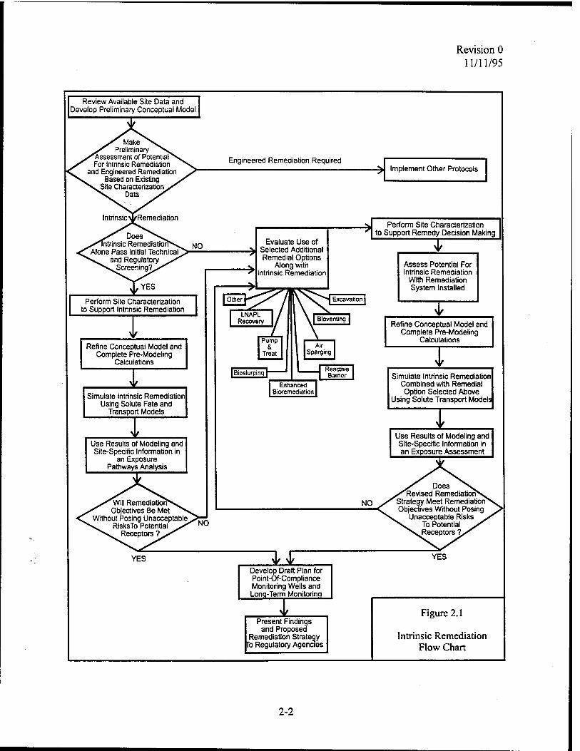
This section describes the steps that should be taken to gather the site-specific data necessary
to predict the future extent of a contaminant plume and to successfully support the intrinsic
remediation option. The flow chart presented in Figure 2.1 presents the information that must be
developed and the important regulatory decision points in the process of implementing intrinsic
remediation.
Predicting the future extent of a contaminant plume requires the quantification of groundwater
flow and solute transport and transformation processes, including rates of natural attenuation.
Quantification of contaminant migration and attenuation rates, and successful implementation
2-1
Revision 0 11/11/95
2-2
Revision 0 11/11/95
of the intrinsic remediation option, require completion of the following steps, each of which is
outlined in Figure 2.1 and discussed in the following sections:
1) Review available site data;
2) Develop preliminary conceptual model and assess potential for intrinsic remediation;
3) If intrinsic remediation is selected as potentially appropriate, perform site characterization in support of intrinsic remediation;
4) Refine conceptual model based on site characterization data, complete pre-modeling calculations, and document indicators of intrinsic remediation;
5) Simulate intrinsic remediation using analytical or numerical solute fate and transport models that allow incorporation of a biodegradation term, as necessary;
6) Conduct an exposure pathways analysis;
7) If intrinsic remediation alone is acceptable, prepare LTM plan; and
8) Present findings to regulatory agencies and obtain approval for the intrinsic remediation with LTM option.
2.1 REVIEW AVAILABLE SITE DATA
The first step in the intrinsic remediation investigation is to review available site-specific data
to determine if intrinsic remediation is a viable remedial option. A thorough review of these data
also allows development of a preliminary conceptual model. The preliminary conceptual model
will help identify any shortcomings in the data and will allow placement of additional data
collection points in the most scientifically advantageous and cost-effective manner possible.
When available, information to be obtained during data review includes:
• Nature, extent, and magnitude of contamination:
- Nature and history of the contaminant release: -Catastrophic or gradual release of LNAPL ? —More than one source area possible or present ? —Divergent or coalescing plumes ?
- Three-dimensional distribution of mobile and residual LNAPL and dissolved contaminants. The distribution of mobile and residual LNAPL will be used to define the dissolved plume source area.
- Groundwater and soil chemical data.
- Historical water quality data showing variations in contaminant concentrations through time.
2-3

Revision 0 11/11/95
- Chemical and physical characteristics of the contaminants.
- Potential for biodegradation of the contaminants.
• Geologic and hydrogeologic data (in three dimensions, if feasible):
- Lithology and stratigraphic relationships.
- Grain-size distribution (sand vs. silt vs. clay).
- Aquifer hydraulic conductivity.
- Groundwater flow gradients and potentiometric or water table surface maps (over several seasons, if possible).
- Preferential flow paths.
- Interactions between groundwater and surface water and rates of infiltration/recharge.
• Locations of potential receptors:
- Groundwater wells.
- Downgradient and crossgradient groundwater discharge points.
In some cases, few or no site-specific data are available. If this is the case, and if it can be
shown that intrinsic remediation is a potential remedial option (Section 2.2), all future site
characterization activities should include collecting the data necessary to support this remedial
alternative. The additional costs incurred by such an investigation are greatly outweighed by the
cost savings that will be realized if intrinsic remediation is selected. Even if not selected, most of
the data collected in support of intrinsic remediation can be used to design and support other
remedial measures.
2.2 DEVELOP PRELIMINARY CONCEPTUAL MODEL AND ASSESS POTENTIAL FOR INTRINSIC REMEDIATION
After reviewing existing site characterization data, a conceptual model should be developed,
and a preliminary assessment of the potential for intrinsic remediation should be made. The
conceptual model is a three-dimensional representation of the groundwater flow and solute
transport system based on available geological, biological, geochemical, hydrological,
climatological, and analytical data for the site. This type of conceptual model differs from the
conceptual site models commonly used by risk assessors that qualitatively consider the location of
contaminant sources, release mechanisms, transport pathways, exposure points, and receptors.
However, the groundwater system conceptual model facilitates identification of these risk-
assessment elements for the exposure pathways analysis. After development, the conceptual
2-4

Revision 0 11/11/95
model can be used to help determine optimal placement of additional data collection points as
necessary to aid in the intrinsic remediation investigation and to develop the solute fate and
transport model. Contracting and management controls must be flexible enough to allow for the
potential for revisions to the conceptual model and thus the data collection effort.
Successful conceptual model development involves:
• Definition of the problem to be solved (generally the unknown nature and extent of existing and future contamination).
• Integration and presentation of available data, including:
- Local geologic and topographic maps,
- Geologic data,
- Hydraulic data,
- Biological data,
- Geochemical data, and
- Contaminant concentration and distribution data.
• Determination of additional data requirements, including:
- Borehole locations and monitoring well spacing,
- An approved sampling and analysis plan, and
- Any data requirements listed in Section 2.1 that have not been adequately addressed.
After conceptual model development, an assessment of the potential for intrinsic remediation
must be made. As stated previously, existing data can be useful in determining if intrinsic
remediation will be sufficient to prevent a dissolved contaminant plume from completing exposure
pathways, or from reaching a predetermined point of compliance (POC), in concentrations above
applicable regulatory standards. Determining the likelihood of exposure pathway completion is an
important component of the intrinsic remediation investigation. This is achieved by estimating the
migration and future extent of the plume based on contaminant properties, including
biodegradability, aquifer properties, groundwater velocity, and the location of the plume and
contaminant source relative to potential receptors (i.e., the distance between the leading edge of
the plume and the potential receptors). Appendix B discusses the biodegradability of BTEX
under laboratory conditions and in the field.
2-5

Revision 0 11/11/95
If intrinsic remediation is determined to be a significant factor in contaminant reduction, site
characterization activities in support of this remedial option should be performed. If exposure
pathways have already been completed and contaminant concentrations exceed regulatory levels,
or if such completion is likely, other remedial measures should be considered. Even so, the
collection of data in support of the intrinsic remediation option can be integrated into a
comprehensive remedial plan and may help reduce the cost and duration of other remedial
measures such as intensive source removal operations or pump-and-treat technologies.
2.3 PERFORM SITE CHARACTERIZATION IN SUPPORT OF INTRINSIC REMEDIATION
Detailed site characterization is necessary to document the potential for intrinsic remediation.
As discussed in Section 2 A, review of existing site characterization data is particularly useful
before initiating site characterization activities. Such review should allow identification of data
gaps and guide the most effective placement of additional data collection points.
There are two goals during the site characterization phase of the intrinsic remediation
investigation. The first is to collect the data needed determine if natural mechanisms of
contaminant attenuation are occurring at rates sufficient to protect human health and the
environment. The second is to provide sufficient site-specific data to allow prediction of the
future extent and concentration of a contaminant plume through solute fate and transport
modeling. Because the burden of proof for intrinsic remediation is on the proponent, very
detailed site characterization is required to achieve these goals and to support this remedial
option. Adequate site characterization in support of intrinsic remediation requires that the
following site-specific parameters be determined:
• Extent and type of soil and groundwater contamination.
• Location and extent of contaminant source area(s) (i.e., areas containing mobile or residual NAPL).
• The potential for a continuing source due to leaking tanks or pipelines.
Aquifer geochemical parameters.
Regional hydrogeology, including:
- Drinking water aquifers, and
- Regional confining units.
2-6

Revision 0 11/11/95
• Local and site-specific hydrogeology, including:
- Local drinking water aquifers.
- Location of industrial, agricultural, and domestic water wells.
- Patterns of aquifer use (current and future).
- Lithology.
- Site stratigraphy, including identification of transmissive and nontransmissive units.
- Grain-size distribution (sand vs. silt vs. clay).
- Aquifer hydraulic conductivity.
- Groundwater hydraulic information.
- Preferential flow paths.
- Locations and types of surface water bodies.
- Areas of local groundwater recharge and discharge.
• Identification of potential exposure pathways and receptors.
The following sections describe the methodologies that should be implemented to allow
successful site characterization in support of intrinsic remediation.
2.3.1 Soil Characterization
In order to adequately define the subsurface hydrogeologic system and to determine the
amount and three-dimensional distribution of mobile and residual NAPL that can act as a
continuing source of groundwater contamination, extensive soil characterization must be
completed. Depending on the status of the site, this work may already have been completed
during previous remedial investigation work. The results of soils characterization will be used as
input into a solute fate and transport model to help define a contaminant source term and to
support the intrinsic remediation investigation.
2.3.1.1 Soil Sampling
The purpose of soil sampling is to determine the subsurface distribution of hydrostratigraphic
units and the distribution of mobile and residual NAPL. These objectives can be achieved through
the use of conventional soil borings or direct-push methods (e.g., Geoprobe or cone
penetrometer testing). All soil samples should be collected, described, analyzed, and disposed of
in accordance with local, state, and federal guidance. Appendix A contains suggested procedures
2-7
Revision 0 11/11/95
for soil sample collection. These procedures may require modification to comply with local, state,
and federal regulations.
2.3.1.2 Soil Analytical Protocol
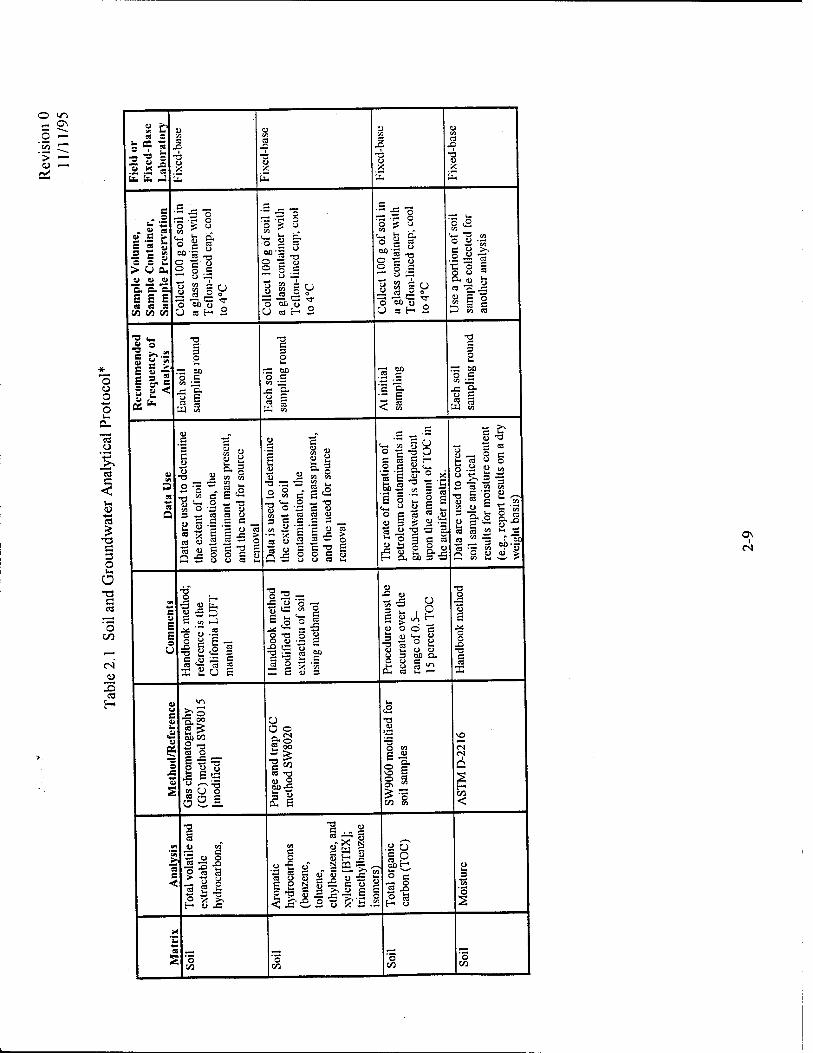
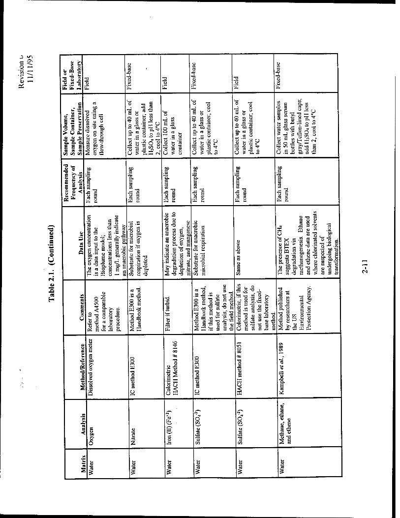
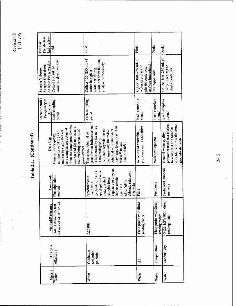
The analytical protocol to be used for soil sample analysis is presented in Table 2.1. This
analytical protocol includes all of the parameters necessary to document intrinsic remediation of
fuel hydrocarbons, including the effects of sorption and biodegradation (aerobic and anaerobic) of
fuel hydrocarbons. Each analyte is discussed separately below.
2.3.1.2.1 Total Volatile and Extractable Hydrocarbons
Knowledge of the location, distribution, concentration, and total mass of TPH sorbed to soils
or present as mobile NAPL is required to calculate contaminant partitioning from these phases
into groundwater. The presence or absence of TPH also is used to define the edge of the NAPL
plume. One of the greatest areas of uncertainty remaining in the conventional remedial
investigation process is delineation of NAPL in the subsurface. Knowledge of the location of the
leading edge of the NAPL plume is important in proper model implementation because it defines
the extent of the contaminant source area.
2.3.1.2.2 Aromatic Hydrocarbons
Knowledge of the location, distribution, concentration, and total mass of fuel-derived
hydrocarbons of regulatory concern (especially BTEX) sorbed to soils or present as mobile NAPL
is required to calculate contaminant partitioning from mobile and residual NAPL into
groundwater.
2.3.1.2.3 Total Organic Carbon
Knowledge of the total organic carbon (TOC) content of the aquifer matrix is important in
sorption and solute-retardation calculations. TOC samples should be collected from a
background location in the zone(s) where most contaminant transport is expected to occur.
2-8
o in C\
o ^~ ai •-" > — U ^— ai
fc so
to. U. J
O o o o UM
o
CO
■4-t
T3 C 3 O u
o T3 a
o
« c r E « £ |gg > 0 cü "Si's, e E E E a es es M to CO
«3 _ — .-3 -^ O o £ u v]
CJ ca
"3 n- 3 ? | S 5 E o ■= E 5. B 5 g <
§11
-Iso ™r o o s cj
.2 T3 „ a u
2 p .£
u
o c
J2 ea « o o "oo^ ^ U ea r- 2
■5 o ■? o
S o )■= u
.2 -a a u
o .£ CJ .S co B r ^ co 5 U
CJ 00 cj ca H
o £ co
O U a o o Ü *. "3 o o B. CJ CO *7^
co 5 t-J CO
~ OO o a
2 a CO CO CO i_
*P — o - e prt w a a —
io o \s e CJ a w ca ca cj
I 'i 'I o ca ca —
P
2 Q 5
C3 — o c "^ £ o c S cj ca t-H
1 H
E M _j
8 § e- I §1 I a cj ~a a ca tr? ca 2 K S U e
C
u •a ^
3 § CO w '- •/< ca u
u » i
e e "— — -o
_ a u a ca u a a a _ g'S (J s a a j; >
a a "o E o o a cj cj u ca u
O \3
2 e a a- a B
s oo o a CO "•^
J3 o. ca ca
CO
e _ •= - '» § y O -g -! O a S S H
■2.S c,<3
S 3 o a o 3 K O 3 =
oo a
a ca u
a & cj "O B «
— o a CO U O
- £ "
C3 OT «
E Z m
^- o 2 C3
E £ §■*
_ a oo-a^ .« co . aj o aj cj > CO Ui v^ >
2 £ 00 CO
2 T3 CO o ES^ O cj s .a s| co CJ O oSS.
•a — ■£ Si "o — u «3 CO o
^-2 O T3 O CJ
B " 5 2
o 3 a 53 3 55 •s a ä ?0 u. a
ca CJ CO*
'S cj o ■s s -e o ea a
s^ H cj ja
CJ O o
2 CO
ii ca »a u o
ft, E
co 53 Ä a u i P
U O Ö E b cj c„ cj
ty C- U u
ca u.
o
ON
E — o "^ vo a
S s CO co
s a ea CJ
s£ o -a
CJX § u H ^ s .aat-
CJ ai -a ^* c
X> o
S O E?b j= a
CO ^
H cj
o CO
o yn rm ON
o *« in
T
> ■•—•
SJ —
■o
3 _g S o U
Fie
ld o
r F
ixed
-Bas
e L
abor
ator
y
u en a
XI 1
•a cj
o en co
.c i
T3 CJ
o VI a
x> i T3 U
E
Sam
ple
Vol
ume,
Sa
mpl
e C
onta
iner
, Sa
mpl
e P
resc
nat
ion
1 o
8 1 2j ^ O CO = <N
?|ju .a i £ 8 o
rs — o o u y e— .S a
•§ o a o * rfi £• ° ^ K> ■_> .3 O aä £ — U CO
en . *-
a- > — 3 < T3 3
u s£ es a
5: a ° ° c "* 2 u o o t3 ü ^ r £ <N •a « o "p — U.S 8 x? ft
a — — o h ° « i-T * 2 <— .a O CO
HJ a _ o "^ u
Ü a o
U co 2
Rec
omm
ende
d F
requ
ency
of
Ana
lysi
s u
e a T3 .2 3 i_ U — '•3 © .3 a
flj w 3 3 C S TOO n y <u u
op
a 3
*■§
u £
XI
Ji s •3-2
£ ■= c« 2) < £
u
a a Q
i i >-X 5 » S n n O-SafViOk-3.3 0
cSPHcouj-c-g g CflOJ 2ä ° S 5
= 8 x? .2 Ü -s So w
•a - a ° _. •= a S
= 1 öla 1 § OÄ--S
Sl's-os-i'si'iS
^- JS o O -° l-
•SH^ " i^ =?^S 3
3 .§ S 1 S g E E 3 •? .§ -8 g .8 ■ J £? i a •2 <H »f o ? ä 3 ~ a .
Qju-.aS^aSaw^aaaoo« ^caaacsoBuuCAN o."0 ca
^ cj a <—• .t: w o o . u as
'S >» o 2 3 S 3 = a g c "3 -2 g .H 3 co g o § Q. Q. °0 'S ° n 2 s* r* cj co M CJ a s >> c -a £ £ Ü u Jl n u ,s s n o « „ e 'S T -a cö -2 ^ .2 S = g
ä .*.§•!• 3 11 S? ^3 o a a c c 5> a a o o a <— 0-« cs co cj a cj o
CM
c u E E Ö
% H
a a, j
sill C u x; s a "r? co « S 2 U E
= ca o :> 5 ■* E " «- a o T3 a a o M o "a w
a a; u — >> S 2 ^ o^ — 3 cj a "a
T3
■aj
u >- O u figs2 •s •€= 3 2 ™ > MS J' U ft
3 g<2 8
a u c o u
a
■S
s
in
O 00
CO ■o 2 ^ £ u u c E =3 ri ° O £.
U O o
f| ca —3 u 2 g? 5 3 u
cu E
ä i? o o. U cd o o " o?o
8.S sis &£ g 15 en tZ) <g .2 CO g T3 U U -a 3 g 0--3 O
<: =3 J= "3 5 t_) CJ 00 g* *> Ö E5= S
Ml
c
en
5 "2 o •e §s tS u 8
s| | g - TJ — a H x: > o
CJ a u
a S o x> £
■3 ca ^J1 ST" en
E £ ü y |
•3 itS-'S .1
.a Ji =« u • a 3 ~ g
£ ixTfee
es
s U *-» CO
U,
1 o o
o I
■5 yr\ a\
O m~
co ~~ > ^—
u r—m
fS
•a 3
e o U
Z es H
Fie
ld o
r F
ixed
-Bas
e L
abor
ator
y ■3
2* I'lx
cd-b
ase
2 "3
CO a
■3 Ü 2 13
y CO a Ä
1
U X
Sam
ple
Vol
ume,
Sa
mpl
e C
onta
iner
, Sa
mpl
e P
resc
nat
ion
a SO
- .£ O co — ^ = O o u o co r^ r* a « M
"O c 3 «J o S 3 a i « Uli
2 o cs
<— ^ C3 »^ — O :_*• w
2 -a a ~ o
3 2 S 2 2
1 ö I o 1
o
E a o °° 2 « v.
s Si u '" ■- Ji u 2
u ? 8
c_
O O -J O
ES" O w 0
2 -5)2 §• a g
g I .3 U 0 a a ^ u ? c.2
c_ 0 "3 j 0 B w. 0 _ 0 c
O OT O « C3 .S 2 «2 §• a g
a u
- -'S^r O ? &2
co eo" 2 E 5/8 2/5 3 0 y
a m ^ ü ~ T co co 3 a 0. U g X3 = 0 2 2 ^ ä = 2 — ? «j S c O 8
So st = «N
U .5 J3 00 a —
Rec
omm
ende
d F
requ
ency
of
Ana
lysi
s
DC
"a. a 3 _£-
CJ 5 es ä ,,, O
op
"a. 5 J=2 ,5 O i—. u
op
"3. E a
•a % U 3 a Ä
O0 B
a
-s 2
O0 _B
"3. B a
•B c 0 3
U-l b*
00 _B
"3- a
•B c cj § a 5 tu £
■■*>
« a Q
.2 c « "£ 2 ° ^ J3 1> — ;3 03
5 ~ „ w •;■* £
J= ^ Ü ~ — s
(5 « 3 £ er a
H .22 S3 8 — 5
a -2
f: § K ou o >. 'a X E o k. <—
«2 B
2 g 2 w •? .2
-3 « g.
0 2 '•§ u p 3 O
2 co c G S K u a a u ou of a 0 r? S a S ■& 2
3 § 2 c '■§ "3 S a. — "a w u >^ k- ^- a
2 "O TJ s
CJ
13 - S.s C3 C3 s *■* C3 'p,
c2 £i 3 ä
3 -B
0 > 0
a CO a u £ a
CO
2 T S 3 0 S a co ?" --
vj -S B 0 a SJ a u " .a y . a-g^ g" oX.2-|2ao3c
8 E - g -3 -c "8 3 -B Sea.sac-Sal! Si2ag2~o.SE
H5jT3Sa:Sa3.B
s cv
E E Ö
o S -2 f; CO
5 |-£>2 K 2 u 2 13 O U w. .O g
s* E c° « 3,
«"3 CO ^
O *>
3 •* ~ o "= S .a ~
1J
■a 13 3
CM
k* 2
CJ
•a | -s s ^ -g 0 y "2 t5 B -B 0 E 2 — 0 «
■3§Es.a2 = "2 -s -a i^«
^; — ~ 3 as
w 0
5 <2 ~° J, •'S T3 .2 S &
'C - "o u 2
11 2 8 S "g 0 * £ 3 tu ä
"3 1 3 3 a «a U E « S ä E
0 -B 2 j- a a co co *B u„ _ " a so 3 2 a < =* is 2 - - 1 § 3 _. CO £ ■ —
1 » ^ 2 y 1 ^ » c^ £ 2 JJ — w s-
a CJ e S a
c
s
u
E a Ü 00
g? o ■o u > 3 V)
'Q
o o m
T3 O
Ü £
,^- 00
-a 0
0 ä
'§0 "3 <
0 c en
1 ü
y
0 00 «: T3 O
Ü E
•-rt
Ö
Si
00 o\
"5
•8. E a
> "S s < u
oo X o
u a
5
' ^ 0
u c2 's
I •s 2" s C3 •-*
2 S
>
8
5 • 1 o a
u a
0 a
u a i5 1
cs
o in ^ C\ o —M
{*) ^ > «—* <u *•-* at
■o 3
a o U
CM CU
H
Fie
ld o
r F
ixed
-Bas
e L
abor
ator
y 2 ~5
2 "3
2 2 2
Sam
ple
Vol
ume,
Sa
mpl
e C
onta
iner
, Sa
mpl
e P
rese
rvat
ion JJ
'3
° § p w S CO O 5 O OS
— .s
"o ra U £
"3 s -! S >> S ?S 0 ,„ 2P .0 .2
5?J=il 0 00C ,C g
s ° y u u 5 a d X ^ •£ a a a a % s s 1
0
a w 0
0 ° i-" «
<N n .3 u
0 "- 5 0 ° 0 .5 - .S u 0
•3.M ^ g U & 0. 3
CS u
"S. 0. < 0 2
0
§ " ä <N es .3
2 a 0 a 0
" T u
000 0 & 0.
Rec
omm
ende
d F
requ
ency
of
Ana
lvsi
s
00 .g "5. B 3
•a c ,S o
00 _g ■3.
3
u 3 5 2
SO ,g "a.
a
1 = .?, 0
00 ,g "H. E CS
-a c y 3 ,S 0
00 g
■g.
3
u a w 2
a
H
Q
l-t u „ CS = ja j g O
>, en n -g -3 S >.
•3 --^ 2 £ a E <-> 2 — •= o o „ ta 3 —^ ^- o a. cr_ ,>. o on — a
!> 3 ■• u n -J .3 .H
* Ss &S §■§ |
-3 c u c a 3 <— .> 1- 3
° 1 5 §"8 1 g • - 3TS-^C3 O C S a C3 -^ — T3 .3 3 " Ü .3 -" Q t- . - u S co .*/
u"3 3-S E'-S CB "J. t £isc:o.2aBl-a1
«> 3 SB'S ? u >. —, s
F M.2 0 s u acoos
■0 s
« l-i-t S p. « ü
a a
es en
2 Sä
Ji 2
a u E D.
_o "03 > u
-a
i< "> E |«a 2 a. w
>. a g 0 S « 3 -3 a S c« m r- O
J-; 0) w C3 W
■33320 == Ö - .s g s "5 ^« -3 S § g => a 3 a ^ u 0 0 0.2 ö ä
V)
C o E £
g u
o o s ■=■
it
en « 53 0 •3 c 5° y
3 M« S § 0 "3 Ö 'S
u 0 UMSJü a^ -a u 2
2 0
M O O
J3 T3 a CB
w — OT O *T3
0 J S «
B- a
u s u
&
X i 5
w 6
;s <
< S ~ o 0
00
5
u u
'■3
s fc
a 2P
u cs
S £
U
'•3 ■3 "5 0 11 2 3 E S2
t3 u
'•5 0*
0 fc-
co a — SO
SI
"öS c s
■3 .id
<
1
•1.2 !s |u a
51s. *3.
I 2 a. £
3
C O U
9
5
1
• es
5 1 w Ü ffl
I cs

n iri C\
o f—•
C/l —,
> i—.
<U ^—■
~s
CU ■o
"w s o U
8 C a a c C/3
= CD -S C3
il! = i ■3 2
2 * s X u Ex. U. -i m a*
(-• u c a
■-" *C
o .5 J 2 s s § 2 ol
umc,
on
tain
c rc
scn'
a "3 ■d in
o "ob > u a. ■no.
— — — u h C3
E S E S co aas
<fl CO C« a.s "= fc- « o 00 CO
| S 5, E o —
££ s
"a. "H. s c
Rcc
om
Frc
qu
An:
5 o
a J2-S
<-> §
S »5 So."
>. e c <u
« .s i3 o
t3 ca -=-
S a 35 E oo.2 o a o CO M c 3 a O C o"_. — O
o IM
>-< o ■- E •a 2 ^
C C3 -* r- Cl
§ 1 §■§
3 B.IS
im u a
-a e
e a r2 s <- 8 , O C
| -2 'S 1 'S S.s^ i? "3 S H o
oo
•5 O ""> B-o o -a V)
C
E c Ü
g1«? 3 u
S ~ o o .2 E u "3
I '5 e w. .2
5GoE
■CJ ^4
c 1 {A
<J ±j M -L u
e£ ■a ° ^ OS 2 ° o
2 Cp
i 2
U oo
3 -2 b s 2 -3
ac — u u
ä ff
■■* U •u ■4 VI 5* i
c ft? Ji a o •< *c ■c S 3
*—» - "5 « 5 s-o u
'*> ( 'Z ■ t-l kn
: u u 0 i «<
5 :5
a i
1? 1
su ^
&0 >..
ts .^ ON t^ OS * —" '5 u c s .'U NO 3 «, 00 ""I ON
- 3 e io <o 0
"5 .0 .■^
0 T3 0
0 ■S? •a > u ^^ t; m
"5 ji
< .u •^ CU ^*4
"3 CO 2 ^ D
CU N ^ NS •• CD -r 3 05 00
1 5 <N 5^ £
0
^. CO ■3 u
30
S 5 l 00 ON
•*^ c SP s „ c. 0 >^ 0 T3 0 v -=5 2 0 c .2
O "55 0, c "3 3
"3. 00 m a: 0
g 90 0 0 3 ts 0 0
C o\ •* -s: ■Si — 31 0 U .*>
0
3
"S3
< w
"c 1
^5 CU
es: s:
r5 ■3 SO
IM
| CO s .0
3 "3
I .2 "S r? <i
5 •a u k-l
1 **• 'S?
tu CU <-*
^2
CU 1 t: c 3
^ 0
1 O
O
"2 3 "I
0
SB
U
0
SO
S5
1 3
go 2
.If CU 3 a *•—
*— C
u « 0 en O
C
re u
re O. B 5 U "0 re
u
0
1
"5 c
"5 u
3
5
■8
1 1 w
u
0
W til U
O
fi ON ON
2 "3
0
1 ES;
_cu
Ü
CU
-J re 'E 1-
<2 "re U u 0 u re
55 u
0 U 5 0
i>5
■5 t/3 y 0 0
CD W3 .a C-1 g
0 0 en
en
0 O IM - a en eS
O
H CO
e_»
OT
ES:
A
naly
ses
ot
<
en h-i a 0 u
en IM
"tn
"3 CJ O
s
it! O O
X> •O s re
cu CO
1 a
k X '< u. 0. ? CO < J
Z
en ■
tN
—. ts m •<• in NO r- 00

Revision 0 11/11/95
2.3.2 Groundwater Characterization
To adequately determine the amount and three-dimensional distribution of dissolved
contamination and to document the occurrence of intrinsic remediation, groundwater samples
must be collected and analyzed. Biodegradation of fuel hydrocarbons brings about measurable
changes in the chemistry of groundwater in the affected area. By measuring these changes, the
proponent of intrinsic remediation can document and quantitatively evaluate the importance of
intrinsic remediation at a site.
2.3.2.1 Groundwater Sampling
Groundwater sampling is conducted to determine the concentration and three-dimensional
distribution of contaminants and groundwater geochemical parameters. Groundwater samples
may be obtained from monitoring wells or point-source sampling devices such as a Geoprobe®,
Hydropunch®, or cone penetrometer. All groundwater samples should be collected in accordance
with local, state, and federal guidelines. Appendix A contains suggested procedures for
groundwater sample collection. These procedures may have to be modified to comply with local,
state, and federal regulations.
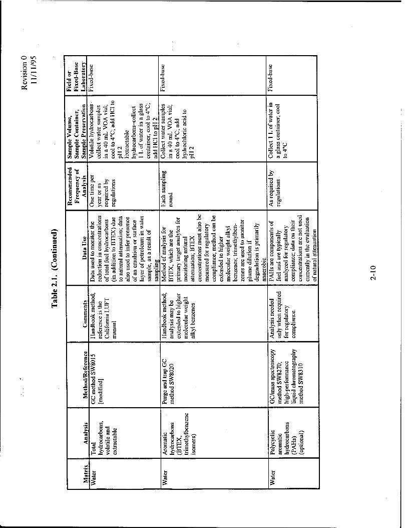
2.3.2.2 Groundwater Analytical Protocol
The analytical protocol to be used for groundwater sample analysis is presented in Table 2.1.
This analytical protocol includes all of the parameters necessary to document intrinsic remediation
of fuel hydrocarbons, including the effects of sorption and aerobic and anaerobic biodegradation.
Data obtained from the analysis of groundwater for these analytes is used to scientifically
document intrinsic remediation of fuel hydrocarbons and can be used as input into a solute fate
and transport model. The following paragraphs describe each groundwater analytical parameter
and the use of each analyte in the intrinsic remediation demonstration.
2.3.2.2.1 Total Volatile andExtractable Hydrocarbons, Aromatic Hydrocarbons, andPolycyclic Aromatic Hydrocarbons
These analytes are used to determine the type, concentration, and distribution of fuel
hydrocarbons in the aquifer. Of the compounds present in most gasolines and jet fuels, the BTEX
compounds generally represent the contaminants of regulatory interest. For this reason, these
2-14
Revision 0 11/11/95
compounds are generally of significant interest in the fate and transport analysis, as described
below and in the appendices. At a minimum, the aromatic hydrocarbon analysis (Method
SW8020) must include BTEX and the trimethylbenzene isomers. The combined dissolved
concentrations of BTEX and trimethylbenzenes should not be greater than about 30 milligrams
per liter (mg/L) for a JP-4 spill (Smith et ai, 1981). If these compounds are found in
concentrations greater than 30 mg/L, sampling errors such as emulsification of LNAPL in the
groundwater sample likely have occurred and should be investigated. The combined dissolved
concentrations of BTEX and trimethylbenzenes should not be greater than about 135 mg/L for a
gasoline spill (Cline et ai, 1991; American Petroleum Institute, 1985). If these compounds are
found in concentrations greater than 135 mg/L, then sampling errors such as emulsification of
LNAPL in the groundwater sample have likely occurred and should be investigated.
Polycyclic aromatic hydrocarbons (PAHs) are constituents of fuel that also may be of concern.
PAHs should be analyzed only if required for regulatory compliance.
2.3.2.2.2 Dissolved Oxygen
Dissolved oxygen is the most thermodynamically favored electron acceptor used in the
biodegradation of fuel hydrocarbons. Dissolved oxygen concentrations are used to estimate the
mass of contaminant that can be biodegraded by aerobic processes. Each 1.0 mg/L of dissolved
oxygen consumed by microbes will destroy approximately 0.32 mg/L of BTEX. During aerobic
biodegradation, dissolved oxygen concentrations decrease. Anaerobic bacteria (obligate
anaerobes) generally cannot function at dissolved oxygen concentrations greater than about
0.5 mg/L. The stoichiometry of BTEX biodegradation via aerobic respiration is given in
Appendix B.
Dissolved oxygen measurements should be taken during well purging and immediately before
and after sample acquisition using a direct-reading meter. Because most well purging techniques
can allow aeration of collected groundwater samples, it is important to minimize potential aeration
by taking the following precautions:
1) Use a peristaltic pump to purge the well when possible (depth to groundwater
less than approximately 25 feet). To prevent downhole aeration of the sample
in wells screened across the water table, well drawdown should not exceed
about 5 percent of the height of the standing column of water in the well. The
2-15

Revision 0 11/11/95
pump tubing should be immersed alongside the dissolved oxygen probe beneath
the water level in the sampling container (Figure 2.2). This will minimize
aeration and keep water flowing past the dissolved oxygen probe's sampling
membrane. If bubbles are observed in the tubing during purging, the flow rate
of the peristaltic pump must be slowed. If bubbles are still apparent, the tubing
should be checked for holes and replaced.
Tubing from Pump or Bailer
Dissolved Oxygen or Redox Potential Probe
J Erlenmeyer Flask or Flow-Through Cell
Figure 2.2
Diagram Showing the Suggested Procedure for Dissolved Oxygen
and Oxidation-Reduction Potential Sampling
2) When using a bailer, the bailer should be slowly immersed in the standing
column of water in the well to minimize aeration. After sample collection, the
water should be drained from the bottom of the bailer through tubing into the
sampling container. The tubing used for this operation should be immersed
alongside the dissolved oxygen probe beneath the water level in the sampling
2-16
Revision 0 11/11/95
container (Figure 2.2). This will minimize aeration and keep water flowing past
the dissolved oxygen probe's sampling membrane.
3) Downhole dissolved oxygen probes can be used for dissolved oxygen analyses,
but such probes must be thoroughly decontaminated between wells. In some
cases decontamination procedures can be harmful to the dissolved oxygen
probe.
2.3.2.2.3 Nitrate
After dissolved oxygen has been depleted in the microbiological treatment zone, nitrate may be
used as an electron acceptor for anaerobic biodegradation via denitrification. Nitrate
concentrations are used to estimate the mass of contaminant that can be biodegraded by
denitrification processes. By knowing the volume of contaminated groundwater, the background
nitrate concentration, and the concentration of nitrate measured in the contaminated area, it is
possible to estimate the mass of BTEX lost to biodegradation. Each 1.0 mg/L of ionic nitrate
consumed by microbes results in the destruction of approximately 0.21 mg/L of BTEX. The
stoichiometry of BTEX biodegradation via denitrification is given in Appendix B. Example
calculations are presented in Appendix C. Nitrate concentrations will be a direct input parameter
to the Bioplume III model currently under development by AFCEE.
2.3.2.2.4 Iron (II)
In some cases iron (III) is used as an electron acceptor during anaerobic biodegradation of
petroleum hydrocarbons. During this process, iron (III) is reduced to iron (II), which may be
soluble in water. Iron (II) concentrations can thus be used as an indicator of anaerobic
degradation of fuel compounds. By knowing the volume of contaminated groundwater, the
background iron (II) concentration, and the concentration of iron (II) measured in the
contaminated area, it is possible to estimate the mass of BTEX lost to biodegradation through
iron (III) reduction. The degradation of 1 mg/L of BTEX results in the production of
approximately 21.8 mg/L of iron (II) during iron (III) reduction. The stoichiometry of BTEX
biodegradation via iron reduction is given in Appendix B. Example calculations are presented in
Appendix C. Iron concentrations will be used as a direct input parameter to Bioplume III.
2-17

Revision 0 11/11/95
2.3.2.2.5 Sulfate
After dissolved oxygen, nitrate, and bioavailable iron (III) have been depleted in the
microbiological treatment zone, sulfate may be used as an electron acceptor for anaerobic
biodegradation. This process is termed sulfate reduction and results in the production of sulfide.
Sulfate concentrations are used as an indicator of anaerobic degradation of fuel compounds. By
knowing the volume of contaminated groundwater, the background sulfate concentration, and the
concentration of sulfate measured in the contaminated area, it is possible to estimate the mass of
BTEX lost to biodegradation through sulfate reduction. Each 1.0 mg/L of sulfate consumed by
microbes results in the destruction of approximately 0.21 mg/L of BTEX. The stoichiometry of
BTEX biodegradation via sulfate reduction is given in Appendix B. Example calculations are
presented in Appendix C. Sulfate concentrations will be used as a direct input parameter for the
Bioplume III model.
2.3.2.2.6 Methane
During methanogenesis (an anaerobic biodegradation process), carbon dioxide (or acetate) is
used as an electron acceptor, and methane is produced. Methanogenesis generally occurs after
oxygen, nitrate, bioavailable iron (III), and sulfate have been depleted in the treatment zone. The
presence of methane in groundwater is indicative of strongly reducing conditions. Because
methane is not present in fuel, the presence of methane in groundwater above background
concentrations in contact with fuels is indicative of microbial degradation of fuel hydrocarbons.
Methane concentrations can be used to estimate the amount of BTEX destroyed in an aquifer. By
knowing the volume of contaminated groundwater, the background methane concentration, and
the concentration of methane measured in the contaminated area, it is possible to estimate the
mass of BTEX lost to biodegradation via methanogenesis. The degradation of 1 mg/L of BTEX
results in the production of approximately 0.78 mg/L of methane during methanogenesis. The
stoichiometry of BTEX biodegradation via methanogenesis is given in Appendix B. Example
calculations are presented in Appendix C.
2.3.2.2.7 Alkalinity
The total alkalinity of a groundwater system is indicative of a water's capacity to neutralize
acid. Alkalinity is defined as the net concentration of strong base in excess of strong acid with a
pure COrwater system as the point of reference (Domenico and Schwartz, 1990). Alkalinity
results from the presence of hydroxides, carbonates, and bicarbonates of elements such as
2-18
Revision 0 11/11/95
calcium, magnesium, sodium, potassium, or ammonia. These species result from the dissolution
of rock (especially carbonate rocks), the transfer of CO2 from the atmosphere, and respiration of
microorganisms. Alkalinity is important in the maintenance of groundwater pH because it buffers
the groundwater system against acids generated during both aerobic and anaerobic
biodegradation.
In general, areas contaminated by fuel hydrocarbons exhibit a total alkalinity that is higher than
that seen in background areas. This is expected because the microbially-mediated reactions
causing biodegradation of fuel hydrocarbons cause an increase in the total alkalinity in the system,
as discussed in Appendix B. Changes in alkalinity are most pronounced during aerobic
respiration, denitrification, iron reduction, and sulfate reduction, and less pronounced during
methanogenesis (Morel and Hering, 1993). In addition, Willey et al. (1975) show that short-chain
aliphatic acid ions produced during biodegradation of fuel hydrocarbons can contribute to
alkalinity in groundwater.
Each 1.0mg/L of alkalinity produced by microbes results from the destruction of
approximately 0.13 mg/L of total BTEX. The stoichiometry of this reaction is given in
Appendix B. Example calculations are presented in Appendix C. The production of alkalinity can
be used to cross-check calculations of expressed assimilative capacity based on concentrations of
electron acceptors.
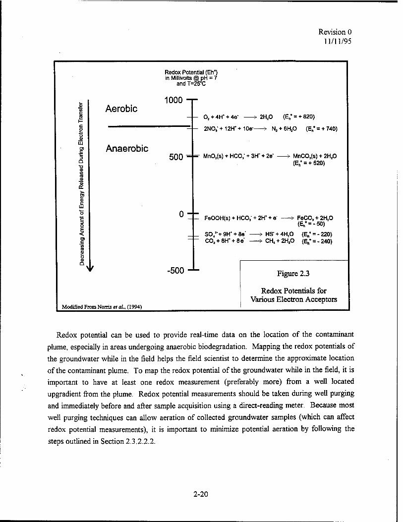
2.3.2.2.8 Oxidation/Reduction Potential (Eh)
The oxidation/reduction (redox) potential of groundwater (Eh) is a measure of electron activity
and is an indicator of the relative tendency of a solution to accept or transfer electrons. Redox
reactions in groundwater contaminated with petroleum hydrocarbons are usually biologically
mediated, and therefore, the redox potential of a groundwater system depends upon and
influences rates of biodegradation. Knowledge of the redox potential of groundwater also is
important because some biological processes operate only within a prescribed range of redox
conditions. The redox potential of groundwater generally ranges from -400 millivolts (mV) to
800 mV. Figure 2.3 shows the typical redox conditions for groundwater when different electron
acceptors are used.
2-19
Revision 0 11/11/95
c s u a Ui O) c •c 3 a •a a> to
a> K >. s> o c
LU
c 3
B) CO 0) b CD Q
Redox Potential (Eh°) in Millivolts @ pH = 7
and T=25X
Aerobic 1000 -r
Anaerobic 5Q0 - =- Mn02(s) + HCO; + 3H* + 2e'
o —
02 + 4H* + 4o' -» 2H20 (Eh* = + 820)
2NO,-+12H*+10e- > Nj + ßHjO (Eh° = + 740)
-> MnCO,(s) + 2H20 (E„- = + 520)
FeOOH(s) + HCO,-+ 2H* + e > FeCO, + 2H,0 (Eno = -50)
SO/-+9H* + 8e" ¥ HS+4H,0 (Eh° = -220) COj + 8H* + 8e > CH4 + 2H20 (Ei,* = -240)
-500
Modified From Norris et al, (1994)
Figure 2.3
Redox Potentials for Various Electron Acceptors
Redox potential can be used to provide real-time data on the location of the contaminant
plume, especially in areas undergoing anaerobic biodegradation. Mapping the redox potentials of
the groundwater while in the field helps the field scientist to determine the approximate location
of the contaminant plume. To map the redox potential of the groundwater while in the field, it is
important to have at least one redox measurement (preferably more) from a well located
upgradient from the plume. Redox potential measurements should be taken during well purging
and immediately before and after sample acquisition using a direct-reading meter. Because most
well purging techniques can allow aeration of collected groundwater samples (which can affect
redox potential measurements), it is important to minimize potential aeration by following the
steps outlined in Section 2.3.2.2.2.
2-20

Revision 0 11/11/95
2.3.2.2.9 pH, Temperature, and Conductivity
Because the pH, temperature, and conductivity of a groundwater sample can change
significantly within a short time following sample acquisition, these parameters must be measured
in the field in unfiltered, unpreserved, "fresh" water collected by the same technique as the
samples taken for dissolved oxygen and redox analyses. The measurements should be made in a
clean glass container separate from those intended for laboratory analysis, and the measured
values should be recorded in the groundwater sampling record.
The pH of groundwater has an effect on the presence and activity of microbial populations in
groundwater. This is especially true for methanogens. Microbes capable of degrading petroleum
hydrocarbon compounds generally prefer pH values varying from 6 to 8 standard units.
Groundwater temperature directly affects the solubility of oxygen and other geochemical
species. The solubility of dissolved oxygen is temperature dependent, being more soluble in cold
water than in warm water. Groundwater temperature also affects the metabolic activity of
bacteria. Rates of hydrocarbon biodegradation roughly double for every 10-degree Celsius (°C)
increase in temperature ("Q"io rule) over the temperature range between 5 and 25°C.
Groundwater temperatures less than about 5°C tend to inhibit biodegradation, and slow rates of
biodegradation are generally observed in such waters.
Conductivity is a measure of the ability of a solution to conduct electricity. The conductivity
of groundwater is directly related to the concentration of ions in solution; conductivity increases
as ion concentration increases. Conductivity measurements are used to ensure that groundwater
samples collected at a site are representative of the water comprising the saturated zone in which
the dissolved contamination is present. If the conductivities of samples taken from different
sampling points are radically different, the waters may be from different hydrogeologic zones.
2.3.2.2.10 Chloride
Chloride is measured to ensure that groundwater samples collected at a site are representative
of the water comprising the saturated zone in which the dissolved contamination is present (i.e.,
to ensure that all samples are from the same groundwater flow system). If the chloride
concentrations of samples taken from different sampling points are radically different, the waters
may be from different hydrogeologic zones.
2-21
Revision 0 11/11/95
2.3.3 Aquifer Parameter Estimation
2.3.3.1 Hydraulic Conductivity
Hydraulic conductivity is a measure of an aquifer's ability to transmit water, and is perhaps the
most important aquifer parameter governing fluid flow in the subsurface. The velocity of
groundwater and dissolved contamination is directly related to the hydraulic conductivity of the
saturated zone. In addition, subsurface variations in hydraulic conductivity directly influence
contaminant fate and transport by providing preferential paths for contaminant migration.
Estimates of hydraulic conductivity are used to determine residence times for contaminants and
tracers, and to determine the seepage velocity of groundwater.
The most common methods used to quantify hydraulic conductivity are aquifer pumping tests
and slug tests (Appendix A). Another method that may be used to determine hydraulic
conductivity is the borehole dilution test. One drawback to these methods is that they average
hydraulic properties over the screened interval. To help alleviate this potential problem, the
screened interval of the well should be selected after consideration is given to subsurface
stratigraphy. Information about subsurface stratigraphy should come from geologic logs created
from continuous cores. An alternate method to delineate zones with high hydraulic conductivity
is to use pressure dissipation data from cone penetrometer test logs.
2.3.3.1.1 Pumping Tests
Pumping tests generally give the most reliable information on hydraulic conductivity, but are
difficult to conduct in contaminated areas because the water produced during the test generally
must be contained and treated. In addition, a minimum 4-inch-diameter well is generally required
to complete pumping tests in highly transmissive aquifers because the 2-inch submersible pumps
available today are not capable of producing a flow rate large enough for meaningful pumping
tests. In areas with fairly uniform aquifer materials, pumping tests can be completed in
uncontaminated areas, and the results can be used to estimate hydraulic conductivity in the
contaminated area. Pumping tests should be conducted in wells that are screened in the most
transmissive zones in the aquifer.
2-22
Revision 0 11/11/95
2.3.3.1.2 Slug Tests
Slug tests are a commonly used alternative to pumping tests. One commonly cited drawback
to slug testing is that this method generally gives hydraulic conductivity information only for the
area immediately surrounding the monitoring well. Slug tests do, however, have two distinct
advantages over pumping tests: they can be conducted in 2-inch monitoring wells, and they
produce no water. If slug tests are going to be relied upon to provide information on the three-
dimensional distribution of hydraulic conductivity in an aquifer, multiple slug tests must be
performed. It is not advisable to rely on data from one slug test in one monitoring well. Because
of this, slug tests should be conducted at several monitoring wells at the site. Like pumping tests,
slug tests should be conducted in wells that are narrowly screened in the most transmissive zones
in the aquifer.
2.3.3.2 Hydraulic Gradient
The hydraulic gradient is the change in hydraulic head (feet of water) divided by the length of
groundwater flow. To accurately determine the hydraulic gradient, it is necessary to measure
groundwater levels in all monitoring wells and piezometers at a site. Because hydraulic gradients
can change over a short distance within an aquifer, it is essential to have as much site-specific
groundwater elevation information as possible so that accurate hydraulic gradient calculations can
be made. In addition, seasonal variations in groundwater flow direction can have a profound
influence on contaminant transport. Sites in upland areas are less likely to be affected by seasonal
variations in groundwater flow direction than sites situated near surface water bodies such as
rivers and lakes.
To determine the effect of seasonal variations in groundwater flow direction on contaminant
transport, quarterly groundwater level measurements should be taken over a period of at least 1
year. For many sites, these data may already exist. If hydraulic gradient data over a 1-year period
are not available, intrinsic remediation can still be implemented pending an analysis of seasonal
variation in groundwater flow direction.
2.3.3.3 Processes Causing an Apparent Reduction in Total Contaminant Mass
Several processes cause a reduction in contaminant concentrations and an apparent reduction
in the total mass of contaminant in a system. Processes causing an apparent reduction in
2-23

Revision 0 11/11/95
contaminant mass include dilution, sorption, and hydrodynamic dispersion. In order to determine
the mass of contaminant removed from the system it is necessary to correct observed
concentrations for the effects of these processes. This is done by incorporating independent
assessments of these processes into the comprehensive solute transport model. The following
sections give a brief overview of the processes that result.in apparent contaminant reduction.
Appendix B describes these processes in detail.
To accurately determine the mass of contaminant transformed to innocuous byproducts, it is
important to correct measured BTEX concentrations for those processes that cause an apparent
reduction in contaminant mass. This is accomplished by normalizing the measured concentration
of each of the BTEX compounds to the concentration of a tracer that is at least as sorptive as
BTEX, but that is biologically recalcitrant. Two potential chemicals found in fuel hydrocarbon
plumes are trimethylbenzene and tetramethylbenzene (Cozzarelli et ah, 1990; Cozzarelli et al.,
1994). These compounds are difficult to biologically degrade under anaerobic conditions, and
frequently persist in groundwater longer than BTEX. Depending on the composition of the fuel
that was released, other tracers are possible. Appendix C (Section C.3.3.4.2.1) contains an
example calculation of how to correct for the effects of dilution.
2.3.3.3.1 Dilution
Dilution results in a reduction in contaminant concentrations and an apparent reduction in the
total mass of contaminant in a system. The two most common causes of dilution are infiltration
and monitoring wells screened over large vertical intervals. Infiltration can cause an apparent
reduction in contaminant mass by mixing with the contaminant plume, thereby causing dilution.
Monitoring wells screened over large vertical distances may dilute groundwater samples by
mixing water from clean aquifer zones with contaminated water during sampling. This problem is
especially relevant for dissolved BTEX contamination, which may remain near the groundwater
table for some distance downgradient from the source. To avoid potential dilution, monitoring
wells should be screened over relatively small vertical intervals (less than 5 feet). Nested wells
should be used to define the vertical extent of contamination in the saturated zone.
2.3.3.3.2 Sorption (Retardation)
The retardation of organic solutes caused by sorption is an important consideration when
simulating intrinsic remediation. Sorption of a contaminant to the aquifer matrix results in an
2-24

Revision 0 11/11/95
apparent decrease in contaminant mass because dissolved contamination is removed from the
aqueous phase. Dissolved oxygen and other electron acceptors present in the groundwater are
not retarded by sorption. Any slowing of the solute relative to the advective transport velocity of
the groundwater allows replenishment of electron acceptors into upgradient areas of the plume.
The processes of contaminant sorption and retardation are discussed in Appendix B.
2.3.3.3.3 Hydrodynamic Dispersion
The dispersion of organic solutes in an aquifer is another important consideration when
simulating intrinsic remediation. The dispersion of a contaminant into relatively pristine portions
of the aquifer allows the solute plume to mix with uncontaminated groundwater containing higher
concentrations of electron acceptors. Dispersion occurs both downgradient and, more importantly, crossgradient from the direction of groundwater flow.
2.3.4 Optional Confirmation of Biological Activity
Extensive evidence showing that biodegradation of fuel hydrocarbons frequently occurs under
natural conditions can be found in the literature. Several of the many available references in
support of intrinsic remediation are listed in Section 3 and discussed in Appendix B. The
following sections describe three techniques that may be used if it is necessary to show that
microorganisms capable of degrading fuel hydrocarbons are present at a site.
2.3.4.1 Field Dehydrogenase Test
The field dehydrogenase test is a qualitative method used to determine if aerobic bacteria are
present in an aquifer in quantities capable of biodegrading fuel hydrocarbons. If the test gives a
positive result, a sufficient number of microorganisms capable of aerobic metabolism and/or
denitrification are present in the aquifer. A negative result for the dehydrogenase test gives no
indication of the relative abundance of anaerobic microorganisms capable of utilizing sulfate, iron (III), or carbon dioxide during biodegradation.
2.3.4.2 Microcosm Studies
If additional evidence supporting intrinsic remediation is required, a microcosm study using
site-specific aquifer materials and contaminants can be undertaken. Microcosm studies are used
2-25
Revision 0 11/11/95
to show that the microorganisms necessary for biodegradation are present and can be used as another line of evidence to support intrinsic remediation.
If properly designed, implemented, and interpreted, microcosm studies can provide very
convmcmg documentation of the occurrence of biodegradation. Such studies are the only "line of
evidence" that allows an unequivocal mass balance determination based on the biodegradation of
environmental contammants. If the microcosm study is properly designed, it will be easy for
decision makers with nontechnical backgrounds to interpret. The results of a microcosm study
are strongly influenced by the nature of the geological material submitted for study the physical
properties of the microcosm, the sampling strategy, and the duration of the study Because
microcosm stupes are time consuming and expensive, they should be undertaken only at sites
where there is considerable skepticism concerning the biodegradation of fuel hydrocarbons.
Biodegradation rate constants determined by microcosm studies often are much greater than
rates achieved in the field. Microcosms are most appropriate as indicators of the potential for
intrinsic bioremediation, and to prove that losses are biological, but it may be inappropriate to use
them to generate rate constants. The preferable method of fuel hydrocarbon biodegradation rate-
constant determination is by in situ field measurement. The collection of material for the
microcosm study, the procedures used to set up and analyze the microcosm, and the interpretation of the results of the microcosm study, are presented in Appendix C.
2.3.4.3 Volatile Fatty Acids
During biodegradation of BTEX compounds, volatile fatty acids (VFAs) are produced as
metabolic byproducts. The production of these VFAs is a direct indication that biodegradation of
BTEX has occurred. This test is a gas chromatography/mass spectrometry method wherein the
samples are compared to a standard mixture containing a total of 58 phenols, aliphatic acids and
aromatic acids. Volatile fatty acid analyses are necessary only when there is considerable
skepticism about the biodegradation of fuel hydrocarbons at a specific site.
2-26
Revision 0 11/11/95
2.4 REFINE CONCEPTUAL MODEL, COMPLETE PRE-MODELING CALCULATIONS, AND DOCUMENT ENDICATORS OF INTRINSIC REMEDIATION
Site investigation data should first be used to refine the conceptual model and quantify
groundwater flow, sorption, dilution, and biodegradation. The results of these calculations are
used to scientifically document the occurrence and rates of intrinsic remediation and to help
simulate intrinsic remediation over time. Because the burden of proof is on the proponent, all
available data must be integrated in such a way that the evidence is sufficient to support the
conclusion that intrinsic remediation is occurring.
2.4.1 Conceptual Model Refinement
Conceptual model refinement involves integrating newly gathered site characterization data to
refine the preliminary conceptual model that was developed based on previously existing site-
specific data. During conceptual model refinement, all available site-specific data should be
integrated to develop an accurate three-dimensional representation of the hydrogeologic and
contaminant transport system. This conceptual model can then be used for contaminant fate and
transport modeling. Conceptual model refinement consists of several steps, including preparation
of geologic logs, hydrogeologic sections, potentiometric surface/water table maps, contaminant
contour (isopleth) maps, and electron acceptor and metabolic byproduct contour (isopleth) maps.
2.4.1.1 Geologic Logs
Geologic logs of all subsurface materials encountered during the soil boring phase of the field
work should be constructed. Descriptions of the aquifer matrix should include relative density,
color, major textural constituents, minor constituents, porosity, relative moisture content,
plasticity of fines, cohesiveness, grain size, structure or stratification, relative permeability, and
any other significant observations such as visible fuel or fuel odor. It is also important to
correlate the results of volatiles screening using soil sample headspace vapor analysis with depth
intervals of geologic materials. The depth of lithologic contacts and/or significant textural
changes should be recorded to the nearest 0.1 foot. This resolution is necessary because
preferential flow and contaminant transport paths may be limited to thin stratigraphic units.
2-27
Revision 0 11/11/95
2.4.1.2 Cone Penetrometer Logs
Cone penetrometer logs express stratigraphic information as the ratio of sleeve friction to tip
pressure. Cone penetrometer logs also may contain fluid resistivity data and estimates of aquifer
hydraulic conductivity. To provide meaningful data, the cone penetrometer must be capable of
proving stratigraphic resolution on the order of 3 inches. To provide accurate stratigraphic
information, cone penetrometer logs must be correlated with continuous subsurface cores At a
minimum, there must be one correlation for every hydrostratigraphic unit found at the site Cone
penetrometer logs can be used to complete the hydrogeologic sections discussed in Section 2.4.1.3.
2.4.1.3 Hydrogeologic Sections
Hydrogeologic sections should be prepared from boring logs or CPT data. A minimum of two
hydrogeologic sections are required; one parallel to the direction of groundwater flow and one
perpendicular to the direction of groundwater flow. Hydraulic head data including potentiometric
surface and/or water table elevation data should be plotted on the hydrogeologic section These
sections are useful in locating potential preferential contaminant migration paths and in simulating contaminant transport using solute fate and transport models.
2.4.1.4 Potentiometric Surface or Water Table Map(s)
A potentiometric surface or water table map is a two-dimensional graphic representation of
equipotential lines shown in plan view. These maps should be prepared from water level
measurements and surveyor's data. Because groundwater flows from areas of high hydraulic
head to areas of low hydraulic head, such maps are used to estimate the probable direction of
plume migration and to calculate hydraulic gradients. These maps should be prepared using water
levels measured in wells screened in the same relative position within the same hydrogeologic
unit. To determine vertical hydraulic gradients, separate potentiometric maps should be
developed for different horizons in the aquifer to document vertical variations in groundwater
flow. Flow nets should also be constructed to document vertical variations in groundwater flow
To document seasonal variations in groundwater flow, separate potentiometric surface or water
table maps should be prepared for quarterly water level measurements taken over a period of at
least 1 year. In areas with mobile NAPL, a correction must be made for the water table deflection
2-28
Revision 0 11/11/95
caused by the NAPL. This correction and po.entiome.ric surface map preparation are discussed in Appendix C.
2.4.1.5 Contaminant Contour Maps
Contaminant contour maps should be prepared for each of the BTEX compounds present and
for total BTEX for each discrete sampling event. Such maps allow interpretation of data on the
distribution and the relative transport and degradation rates of contaminants in the subsurface In
addition, contaminant contour maps are necessary so that contaminant concentrations can be gndded and used for input into a numerical model.
If mobile and residual NAPLs are present at the site, a contour map showing the thickness and
vertical and horizontal distribution of each should be prepared. These maps will allow
interpretation of the distribution and the relative transport rate of NAPLs in the subsurface In
addition, these maps will aid in partitioning calculations and solute fate and transport model
development. It is important to note that, because of the differences between the magnitude of
capillary suction in the aquifer matrix and the different surface tension properties of fuel and
water, NAPL thickness observations made at monitoring points may not provide an accurate
estimate of the actual volume of mobile and residual NAPL in the aquifer. To accurately
determine the distribution of NAPLs, it is necessary to take continuous soil cores or to use CPT
testing coupled with laser-induced fluorescence. Appendix C discusses the relationship between actual and apparent NAPL thickness.
2.4.1.6 Electron Acceptor, Metabolic Byproduct, and Alkalinity Contour Maps
Contour maps should be prepared for electron acceptors consumed (dissolved oxygen, nitrate
and sulfate) and metabolic byproducts produced [iron (II) and methane] during biodegradation'
In addition, a contour map should be prepared for alkalinity. The electron acceptor, metabolic
byproduct, and alkalinity contour maps provide evidence of the occurrence of intrinsic remediation at a site.
2.4.1.6.1 Electron Acceptor Contour Maps
Contour maps should be prepared for the electron acceptors including dissolved oxygen
nitrate, and sulfate. During aerobic biodegradation, dissolved oxygen concentrations will
2-29

Revision 0 11/11/95
decrease to levels below background concentrations. Similarly, during anaerobic degradation, the
concentrations of nitrate and sulfate will be seen to decrease to levels below background. The
electron acceptor contour maps allow interpretation of data on the distribution of the electron
acceptors and the relative transport and degradation rates of contaminants in the subsurface.
Thus, electron acceptor contour maps provide visual evidence of biodegradation and a visual
indication of the relationship between the contaminant plume and the various electron acceptors.
In addition, the dissolved oxygen contour map is used to grid dissolved oxygen concentrations for
input into the solute fate and transport model. Bioplume III will allow direct input of all these parameters.
2.4.1.6.2 Metabolic Byproduct Contour Maps
Contour maps should be prepared for the metabolic byproducts iron (II) and methane. During
anaerobic degradation, the concentrations of these parameters will be seen to increase to levels
above background. These maps allow interpretation of data on the distribution of metabolic
byproducts resulting from the microbial degradation of fuel hydrocarbons and the relative
transport and degradation rates of contaminants in the subsurface. Thus, metabolic byproduct
contour maps provide visual evidence of biodegradation and a visual indication of the relationship between the contaminant plume and the various metabolic byproducts.
2.4.1.6.3 Total Alkalinity Contour Map
A contour map should be prepared for total alkalinity (as CaC03). Respiration of dissolved
oxygen, nitrate, iron (III), and sulfate tends to increase the total alkalinity of groundwater. Thus,
the total alkalinity inside the contaminant plume generally increases to levels above background.
This map will allow visual interpretation of alkalinity data by showing the relationship between the contaminant plume and alkalinity.
2.4.2 Pre-Modeling Calculations
Several calculations must be made prior to implementation of the solute fate and transport
model. These calculations include sorption and retardation calculations, fuel/water partitioning
calculations, groundwater flow velocity calculations, and biodegradation rate-constant
calculations. Each of these calculations is discussed in the following sections. The specifics of
each calculation are presented in the appendices referenced below.
2-30
Revision 0 11/11/95
2.4.2.1 Analysis of Contaminant, Electron Acceptor, Metabolic Byproduct, and Total Alkalinity Data
The extent and distribution (vertical and horizontal) of contamination and electron acceptor
and metabolic byproduct concentrations and distributions are of paramount importance in
documenting the occurrence of biodegradation of fuel hydrocarbons and in solute fate and
transport model implementation.
2.4.2.1.1 Electron Acceptor and BTEXData
Dissolved oxygen concentrations below background in an area with fuel hydrocarbon
contamination are indicative of aerobic hydrocarbon biodegradation. Similarly, nitrate and sulfate
concentrations below background in an area with fuel hydrocarbon contamination are indicative of
anaerobic hydrocarbon biodegradation. If these trends can be documented, it is possible to
quantify the relative importance of each biodegradation mechanism, as described in appendices B
and C. The contour maps described in Section 2.4.1 can be used to provide visual evidence of these relationships.
Microorganisms generally utilize dissolved oxygen and nitrate in areas with dissolved fuel-
hydrocarbon contamination at rates that are instantaneous relative to the average advective
transport velocity of groundwater. This results in the consumption of these compounds at a rate
approximately equal to the rate at which they are replenished by advective flow processes. For
this reason, the use of these compounds as electron acceptors in the biodegradation of dissolved
fuel-hydrocarbons is a mass-transport-limited process (Wilson et ed., 1985; Borden and Bedient,
1986). The use of models for simulating these processes is discussed in Appendix D.
Microorganisms generally utilize sulfate, iron (III), and carbon dioxide in areas with dissolved
fuel-hydrocarbon contamination at rates that are slow relative to rates of dissolved oxygen and
nitrate utilization. This results in the consumption of these compounds at a rate that could be
slower than the rate at which they are replenished by advective flow processes and plumes of
contamination can extend away from the source. The use of these compounds as electron
acceptors in the biodegradation of dissolved fuel-hydrocarbons may be a reaction-limited process
that is approximated by first-order kinetics. Determination of first-order biodegradation rate
constants is discussed in Appendix C.
2-31

Revision 0 11/11/95
2.4.2.1.2 Metabolie Byproduct andBTEXData
Elevated concentrations of the metabolic byproducts iron (II) and methane in areas with fuel
hydrocarbon contamination are indicative of hydrocarbon biodegradation. If these trends can be
documented, it is possible to quantify the relative importance of each biodegradation mechanism,
as described in appendices B and C. The contour maps described in Section 2.4.1 can be used to provide visual evidence of these relationships.
2.4.2.1.3 Total Alkalinity and BTEX Data
Elevated concentrations of total alkalinity (as CaC03) in areas with fuel hydrocarbon
contamination are indicative of hydrocarbon biodegradation via aerobic respiration,
denitrification, iron (III) reduction, and sulfate reduction. If this trend can be documented, it is
possible to estimate the assimilative capacity of the groundwater based on the increase (above
background) in total alkalinity in contaminated areas, as described in appendices B and C. The
contour maps described in Section 2.4.1 can be used to provide visual evidence of these relationships.
2.4.2.2 Sorption and Retardation Calculations
Contaminant sorption and retardation calculations should be made based on the TOC content
of the aquifer matrix and the organic carbon partitioning coefficient (K^) for each contaminant.
The average TOC concentration from the most transmissive zone in the aquifer should be used for
retardation calculations. A sensitivity analysis should also be performed during modeling using a
range of TOC concentrations, including the lowest TOC concentration measured at the site. At a
minimum, sorption and retardation calculations should be completed for BTEX and any tracers.
Sorption and retardation calculations are described in Appendix C.
2.4.2.3 Fuel/Water Partitioning Calculations
If NAPL remains at the site, fuel/water partitioning calculations should be made to account for
the partitioning from this phase into groundwater. Several models for fuel/water partitioning have
been proposed in recent years, including those by Hunt et al. (1988), Bruce et al. (1991), Cline et
al. (1991), and Johnson and Pankow (1992). Because the models presented by Cline et al. (1991)
and Bruce et al. (1991) represent equilibrium partitioning, they are the most conservative models.
2-32
Revision 0 11/11/95
Equilibrium partitioning is conservative because it predicts the maximum dissolved concentration
when LNAPL in contact with water is allowed to reach equilibrium. The results of these
equilibrium partitioning calculations can be used in a solute fate and transport model to simulate a
continuing source of contamination. The theory behind fuel/water partitioning calculations is
presented in Appendix B, and example calculations are presented in Appendix C.
2.4.2.4 Groundwater Flow Velocity Calculations
The average linear groundwater flow velocity of the most transmissive aquifer zone containing
contamination should be calculated to check the accuracy of the solute fate and transport model
and to allow calculation of first-order biodegradation rate constants. An example of a
groundwater flow velocity calculation is given in Appendix C.
2.4.2.5 Biodegradation Rate-Constant Calculations
Biodegradation rate constants are necessary to accurately simulate the fate and transport of
BTEX compounds dissolved in groundwater. In many cases, biodegradation of fuel hydrocarbons
can be approximated using first-order kinetics. In order to calculate first-order biodegradation
rate constants, the apparent degradation rate must be normalized for the effects of dilution and
volatilization. Two methods for determining first-order rate constants are described in
Appendix C. One method involves the use of a biologically recalcitrant compound found in the
dissolved BTEX plume that can be used as a conservative tracer. The other method, proposed by
Buscheck and Alcantar (1995) involves interpretation of a steady-state contaminant plume and is
based on the one-dimensional steady-state analytical solution to the advection-dispersion equation presented by Bear (1979).
2.5 SIMULATE INTRINSIC REMEDIATION USING SOLUTE FATE AND TRANSPORT MODELS
Simulating intrinsic remediation allows prediction of the migration and attenuation of the
contaminant plume through time. Intrinsic remediation modeling is a tool that allows site-specific
data to be used to predict the fate and transport of solutes under governing physical, chemical,
and biological processes. Hence, the results of the modeling effort are not in themselves sufficient
proof that intrinsic remediation is occurring at a given site. The results of the modeling effort are
only as good as the original data input into the model; therefore, an investment in thorough site
2-33

Revision 0 11/11/95
characterization will improve the validity of the modeling results. In some cases, straightforward
analytical models of contaminant attenuation are adequate to simulate intrinsic remediation.
Several well documented and widely accepted solute fate and transport models are available
for simulating the fate and transport of fuel hydrocarbons under the influence of advection,
dispersion, sorption, and biodegradation. One such model that is readily available
(nonproprietary) and that is well documented is Bioplume II. The use of solute fate and transport
modeling in the intrinsic remediation investigation is described in Appendix D.
The Bioplume II model is based upon the United States Geological Survey (USGS) two-
dimensional (2-D) solute transport model (method of characteristics) of Konikow and Bredehoeft
(1978). Bioplume II includes an aerobic biodegradation component that is activated by a
superimposed plume of dissolved oxygen (Rifai et al, 1988). The model solves the USGS 2-D
solute transport equation twice, once for hydrocarbon concentrations in the aquifer and once for a
dissolved oxygen plume. The two plumes are combined using superposition at every particle
move to simulate the biological reaction between hydrocarbons and oxygen. The model assumes
that the hydrocarbons are directly mineralized to carbon dioxide and water through an
instantaneous reaction. In recent years many studies have shown that Bioplume II can be used to
successfully support the intrinsic remediation option at fuel-hydrocarbon-contaminated sites
(Downey and Gier, 1991; Parsons ES, 1994a through 1994d; Parsons ES 1995a through 1995q;
Wiedemeiere/a/., 1993, 1994a, and 1994b).
2.6 CONDUCT AN EXPOSURE PATHWAYS ANALYSIS
After the rates of natural attenuation have been documented, and predictions of the future
extent and concentrations of the contaminant plume have been made using the appropriate solute
fate and transport model, the proponent of intrinsic remediation should combine all available data
and information to negotiate for implementation of this remedial option. Supporting the intrinsic
remediation option generally will involve performing an exposure pathways analysis. This analysis
includes identifying potential human and ecological receptors at points of exposure under current
and future land and groundwater use scenarios. The results of solute fate and transport modeling
are central to the exposure pathways analysis. If conservative model input parameters are used,
the solute fate and transport model should give conservative estimates of contaminant plume
migration. From this information, the potential for impacts on human health and the environment
from contamination present at the site can be estimated.
2-34
Revision 0 11/11/95
2.7 PREPARE LONG-TERM MONITORING PLAN
Groundwater flow rates at many Air Force sites studied to date are such that many years will
be required before contaminated groundwater could potentially reach the Base property
boundary. Thus, there frequently is time and space for intrinsic remediation to reduce
contaminant concentrations in groundwater to acceptable levels. Experience at 40 Air Force sites
studied by AFCEE to date (September 1995) using a draft of this document suggests that many
BTEX plumes are relatively stable, or are moving only very slowly with respect to groundwater
flow. These examples demonstrate the efficacy of LTM to track plume migration and to validate or refine modeling results.
The LTM plan consists of locating groundwater monitoring wells and developing a
groundwater sampling and analysis strategy. This plan is used to monitor plume migration over
time and to verify that intrinsic remediation is occurring at rates sufficient to protect potential
downgradient receptors. The LTM plan should be developed based on site characterization data,
the results of solute fate and transport modeling, and the results of the exposure pathways analysis.
The LTM plan includes two types of monitoring wells. Long-term monitoring wells are
intended to determine if the behavior of the plume is changing. Point-of-compliance wells are
intended to detect movements of the plume outside the negotiated perimeter of containment, and
to trigger an action to manage the risk associated with such expansion. Figure 2.4 depicts 1) an
upgradient well in unimpacted groundwater, 2) a well in the LNAPL source area, 3) a well
downgradient of the LNALP source area in a zone of anaerobic treatment, 4) a well in the zone of
aerobic treatment, along the periphery of the plume, 5) a well located downgradient from the
plume where concentrations of petroleum hydrocarbons are below regulatory acceptance levels
and soluble electron acceptors are depleted with respect to unimpacted groundwater, and 6) three POC wells.
Although the final number and placement of LTM and POC wells is determined through
regulatory negotiation, the following guidance is recommended. Location of LTM wells are
based on the behavior of the plume as revealed during the initial site characterization. The final
number and location of LTM wells will depend on regulatory considerations. POC wells are
placed a distance of 500 feet downgradient from the leading edge of the plume or the distance
traveled by the groundwater in 2 years, whichever is greater. If the property line is less than 500
2-35
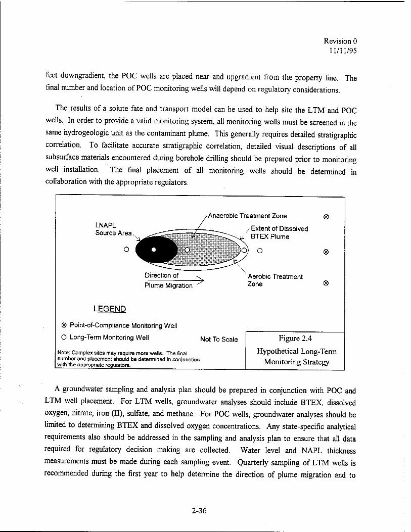
Revision 0 11/11/95
feet downgradient, the POC wells are placed near and upgradient from the property line. The
final number and location of POC monitoring wells will depend on regulatory considerations.
The results of a solute fate and transport model can be used to help site the LTM and POC
wells. In order to provide a valid monitoring system, all monitoring wells must be screened in the
same hydrogeologic unit as the contaminant plume. This generally requires detailed stratigraphic
correlation. To facilitate accurate stratigraphic correlation, detailed visual descriptions of all
subsurface materials encountered during borehole drilling should be prepared prior to monitoring
well installation. The final placement of all monitoring wells should be determined in
collaboration with the appropriate regulators.
LNAPL Source Area
Anaerobic Treatment Zone
/ Extent of Dissolved BTEX Plume
O
Plume Migration Aerobic Treatment Zone
LEGEND
® Point-of-Compliance Monitoring Well
O Long-Term Monitoring Well
Note: Complex sites may require more wells. The final number and placement should be determined in conjunction with the appropriate regulators.
Not To Scale Figure 2.4
Hypothetical Long-Term Monitoring Strategy
A groundwater sampling and analysis plan should be prepared in conjunction with POC and
LTM well placement. For LTM wells, groundwater analyses should include BTEX, dissolved
oxygen, nitrate, iron (II), sulfate, and methane. For POC wells, groundwater analyses should be
limited to determining BTEX and dissolved oxygen concentrations. Any state-specific analytical
requirements also should be addressed in the sampling and analysis plan to ensure that all data
required for regulatory decision making are collected. Water level and NAPL thickness
measurements must be made during each sampling event. Quarterly sampling of LTM wells is
recommended during the first year to help determine the direction of plume migration and to
2-36
Revision 0 11/11/95
determine baseline data. Based on the results of the first year's sampling, the sampling frequency
may be reduced to annual sampling in the quarter showing the greatest extent of the plume.
Sampling frequency is dependent on the final placement of the POC monitoring wells and
groundwater flow velocity. The final sampling frequency should be determined in collaboration with regulators.
2.8 CONDUCT REGULATORY NEGOTIATIONS
The purpose of regulatory negotiations is to provide scientific documentation that supports
intrinsic remediation as the most appropriate remedial option for a given site. All available site-
specific data and information developed during the site characterization, conceptual model
development, pre-modeling calculations, biodegradation rate calculation, groundwater modeling,
model documentation, and LTM plan preparation phases of the intrinsic remediation investigation
should be presented in a consistent and complementary manner at the regulatory negotiations. Of
particular interest to the regulators will be proof that intrinsic remediation is occurring at rates
sufficient meet regulatory compliance levels at the POC and to protect human health and the
environment. The regulators must be presented with a "weight-of-evidence" argument in support
of this remedial option. For this reason, all available evidence in support of intrinsic remediation must be presented at the regulatory negotiations.
A comprehensive LTM and contingency plan also should be presented to demonstrate a
commitment to proving the effectiveness of intrinsic remediation as a remedial option. Because
LTM and contingency plans are very site specific, they should be addressed in the individual
reports generated using this protocol. See Sections 6 and 7 of the two case studies presented in Appendices E and F for examples of such plans.
2-37
Revision 0 11/11/95
SECTION 3
REFERENCES
Abdul, AS., Kia S.F., and Gibson, T.L., 1989, Limitations of monitoring wells for the detection and quantification of petroleum products in soils and aquifers: Ground Water Monitoring Review, Spring, 1989, p. 90-99. ö
Alvarez P.J.J and Vogel, T.M., 1991, Substrate interactions of benzene, toluene and para- xylene during microbial degradation by pure cultures-and mixed culture aquifer slurries- Applied Environmental Microbiology, v. 57, p. 2981-2985.
American Petroleum Institute, 1985, Laboratory Study on Solubilities of Petroleum Hydrocarbons in Oroundwater: American Petroleum Institute, Publication Number 4395
Anderson, M.P., 1979, Using models to simulate the movement of contaminants through groundwater flow systems: CRC Critical Review in Environmental Control, no. 9, p. 97-
Anderson, MJ and Woessner, W.W., 1992, Applied Groundwater Modeling - Simulation of Mow and Advective Transport: Academic Press, New York, New York, 38lp.
Arthur D. Little, Inc., 1985, The Installation Restoration Program Toxicology Guide Volume 1 Prepared for Air Force Systems Command, Wright-Patterson Air Force Base Ohio October 1985
Arthur D. Little, Inc., 1987, The Installation Restoration Program Toxicology Guide Volume 3 Prepared for Air Force Systems Command, Wright-Patterson Air Force Base, Ohio, June 1987
Atlas, R. M., 1981, Microbial degradation of petroleum hydrocarbons - an Environmental Perspective; Microbiological Reviews, 45(1): 180-209.
Atlas, R.M, 1984, Petroleum Microbiology: Macmillan Publishing Co., New York.
Atlas, R.M., 1988, Microbiology - Fundamentals and Applications: Macmillan, New York.
Avon, L. and Bredehoeft, J.D., 1989, An analysis of trichloroethylene movement in groundwater at Castle Air Force Base, California: Journal of Hydrology, v. 110, p. 23-50.
Baedecker M.J Siegel, D.I., Bennett, P.C., and Cozzarelli, I.M., 1988, The fate and effects of crude oil in a shallow aquifer: I. The distribution of chemical species and geochemical facies, In, GE. Mallard, and S.E. Ragone, editors, U.S. Geological Survey Toxic Substances Hydrology Program, Proceedings of the Technical Meeting, Phoenix, Arizona,
3-1
Revision 0 11/11/95
September 26-30, 1988: U.S. Geological Survey Water-Resources Investigations Reoort 88-42320, p. 13-20. F
Bailey, G.W., and White, J.L., 1970, Factors influencing the adsorption, desorption, and movement of pesticides in soil, In Residue Reviews, FA. Günther and J.D. Günther editors: Springer Verlag, p. 29-92.
Ballestero, T.P., Fiedler, F.R., and Kinner, N.E., 1994, An investigation of the relationship between actual and apparent gasoline thickness in a uniform sand aquifer- Ground Water v. 32, no. 5, p. 708-718.
Barker, J.F., Patrick, G.C., and Major, D., 1987, Natural attenuation of aromatic hydrocarbons in a shallow sand aquifer: Ground Water Monitoring Review, Winter 1987, p. 64-71.
Barr, K.D., 1993, Enhanced groundwater remediation by bioventing and its simulation by biomodeling: In, R.N. Miller, editor, Proceedings of the Environmental Restoration Technology Transfer Symposium, January 26-27, 1993.
Bartha, R., 1986, Biotechnology of petroleum pollutant biodegradation: Microbial Ecoloev 12:155-172. Sy'
Battelle, 1995, Test Plan and Technical Protocol for Bioslurping, Rev. 2: US Air Force Center for Environmental Excellence, Brooks Air Force Base, Texas.
Bear, J., 1972, Dynamics of Fluids in Porous Media: Dover Publications, Inc., New York, 764 p.
Bear, J., 1979, Hydraulics of Groundwater: McGraw-Hill, Inc., New York, New York, 569.
Bedient, P.B., Rifai, H.S., and Newell, C.J., 1994, Groundwater Contamination - Transport and Remediation: PTR Prentice Hall, New Jersey, 541 p.
Beller, H.R., Reinhard, M., and Grbic-Galic, D., 1992, Metabolic byproducts of anaerobic toluene degradation by sulfate-reducing enrichment cultures: Appl. Environ Microbiol v 58 D 3192-3195. "' ' F'
Beller, H. R., D. Grbic-Galic, and M. Reinhard. 1992b. Microbial degradation of toluene under sulfate-reducing conditions and the influence of iron on the process Appl Environ Microbiol. 58:786-793
Blake, S.B., and Hall., R.A, 1984, Monitoring petroleum spills with wells - some problems and solutions: In, Proceedings of the Fourth National Symposium on Aquifer Restoration and Groundwater Monitoring: May 23-25, 1984, p. 305-310.
Borden, R.C. and Bedient, P.B., 1986, Transport of dissolved hydrocarbons influenced by oxygen limited biodegradation - theoretical development: Water Resources Research v 22 no 13, p. 1973-1982.
Borden, R. C, Gomez, CA., and Becker, M. T., 1994, Natural Bioremediation of a gasoline spill. In R.E. Hinchee, B.C. Alleman, R. E. Hoeppel and R. N. Miller (Eds.). Hydrocarbon Bioremediation. 290-295. Lewis Publishers.
Borden, R. C, Gomez, CA., and Becker, M. T., 1995, Geochemical indicators of natural bioremediation. Ground Water, (in press).
3-2
Revision 0 11/11/95
Bouwer, E.J., 1992, Bioremediation of Subsurface Contaminants, In R. Mitchell, editor, Environmental Microbiology: Wiley-Liss, New York, p. 287-318.
Bouwer, H., and Rice, R.C., 1976, A Slug Test for Determining Hydraulic Conductivity of Unconfined Aquifers With Completely or Partially Penetrating Wells: Water Resources Research, v. 12, no. 3, p. 423-428.
Bouwer, H., 1989, The Bouwer and Rice slug test - an update: Ground Water, v 27 no 3 p 304-309.
Bredehoeft, J.D., and Konikow, L.F., 1993, Ground-water models - validate or invalidate: Ground Water, v. 31, no. 2, p. 178-179.
Brown, D.S. and Flagg, E.W., 1981, Empirical prediction of organic pollutant sorption in natural sediments: Journal of Environmental Quality, v. 10, no. 3, p. 382-386.
Briggs, G.G., 1981, Theoretical and experimental relationships between soil adsorption, octanol- water partition coefficients, water solubilities, bioconcentration factors, and the parachor: Journal of Agriculture and Food Chemistry, v. 29, p. 1050-1059.
Bruce, L., Miller, T., and Hockman, B., 1991, Solubility versus equilibrium saturation of gasoline compounds - a method to estimate fuel/water partition coefficient using solubility or K^, In, A. Stanley, editor, NWWA/API Conference on Petroleum Hydrocarbons in Ground Water: NWWA/API, p. 571-582.
Buscheck, T.E. and Alcantar, CM., 1995, "Regression Techniques and Analytical Solutions to Demonstrate Intrinsic Bioremediation." In, Proceedings of the 1995 Battelle International Conference on In-Situ and On Site Bioreclamation, April 1995
Cerniglia, C. E. 1984. Microbial transformation of aromatic hydrocarbons, In Petroleum Microbiology. R. M. Atlas editor: Macmillan Publishing Co., New York., p. 99-128.
Chapelle, F.H., 1993, Ground-Water Microbiology and Geochemistry: John Wily & Sons, Inc., New York, 424 p.
Chiang, C.Y., Salanitro, J.P., Chai, E.Y., Colthart, J.D., and Klein, C.L., 1989, Aerobic biodegradation of benzene, toluene, and xylene in a sandy aquifer - data analysis and computer modeling, Ground Water, v. 27, no. 6, p. 823-834.
Chiou, CT., Porter, P.E., and Schmedding, D.W., 1983, Partition equilibria of nonionic organic compounds between soil organic matter and water: Environmental Science and Technology: v. 17, no. 4, p. 227-231.
Ciccioli, P., Cooper, W.T., Hammer, P.M., and Hayes, J.M., 1980, Organic solute-mineral surface interactions; a new method for the determination of ground water velocities: Water Resources Research, v. 16, no. 1, p. 217-223.
Cline, P. V., Delfino, J.J., and Rao, P.S.C, 1991, Partitioning of aromatic constituents into water from gasoline and other complex solvent mixtures: Environmental Science and Technology, v. 25, p. 914-920.
Concawe, 1979, Protection of groundwater from oil pollution; Den Haag, Report No. 3/79.
3-3
Revision 0 11/11/95
Cozzarelli, I. M Eganhouse, R.P., and Baedecker, M.J., 1990, Transformation of monoaromatic hydrocarbons to organic acids in anoxic groundwater environment: Environ. Geol. Water science, 16.
Cozzarelli I.M., Baedecker, M.J., Eganhouse, R.P., and Goerlitz, D.F., 1994 The geochemical evolution of low-molecular-weight organic acids derived from the degradation of Peto?!eo^COntaminantS in §roundwater: Geochimica et Cosmochimica Ada, v. 58 no 2 p. 863-877. ' '
CRC, 1956, Handbook of Chemistry and Physics: CRC Press
Cripps, R. E., and Watkinson, R.J., 1978, Polycyclic aromatic hydrocarbon metabolism and environmental aspects, In J. R. Watkinson, editor, Developments in Biodegradation of Hydrocarbons - 1, Applied Science Publishers, Ltd., London, p. 133-134.
Curtis C. D. 1985. Clay mineral precipitation and transformation during burial diagenesis Phil Trans. R. Soc. London.315: 91-105
Dalton' H- and Stirlin§> D.E., Co-metabolism: Philos Trans R Soc Lond 297 481-496
^UäÄ£^ 1979' C^0il ^tion by fungi: Canadian Journal of
Davis, R.K., Pederson, D.T., Blum, D.A., and Carr, J.D., 1993, Atrazine in a stream-aquifer w *~, estimatlon of acluifer Properties from atrazine concentration profiles- Ground Water Monitoring Review, Spring, 1993, p. 134-141
Davis, J.W. Klier, N.J., and Carpenter, 1994a, Natural biological attenuation of benzene in groundwater beneath a manufacturing facility: Ground Water, v. 32, no. 2, p. 215-226.
Davis, A Campbell J., Gilbert, C, Ruby, M.V., Bennett, M., and Tobin, S., 1994b, Attenuation and biodegradation of chlorophenols in groundwater at a former wood treating facility- Ground Water, v. 32, no. 2, p. 248-257.
Dawson K.J. and Istok J.D., 1991, Aquifer Testing - Design and analysis of pumping and slug tests: Lewis Publishers, Chelsa, Michigan, 344 p.
Dean, J. A., 1972, Lange's Handbook of Chemistry, 13th ed.: McGraw-Hill, New York
de Pastrovich T.L., Baradat, Y., Barthel, R., Chiarelli, A., and Fussell, D.R., 1979, Protection of groundwater from oil pollution: CONCAWE, The Hague, 61 p.
Devinny J.S. Everett L.G., Lu J.C.S. and Stellar R.L., 1990, Subsurface Migration of Hazardous Wastes: Van Nostrand Reinhold 387 p.
Domenico, P.A., 1987, An analytical model for multidimensional transport of a decaying contaminant species: Journal of Hydrology, 91, p. 49-58.
Domenico P.A. and Schwartz, F.W., 1990, Physical and Chemical Hydrogeology: John Wiley and Sons, New York, New York, 824 p.
Donaghue, N A., Griffin M., Norris, D.G, and Trudgill, P.W., 1976, The microbial metabolism of cyclohexane and related compounds, In J.M. Sharpley and A. M. Kaplan editors,
3-4

Revision 0 11/11/95
pÄ^d*;;r°nd Biodesradation symposium; A^iied s— Downey ac. and Gier, M.J., 1991, Supporting the no action alternative at a hydrocarbon snill
site: In Proceedings USAF Environmental Restoration Technology SymPos7m ts Mav San Antonio, Texas, Section U, p. 1-11. * oymPosmm' ' * May>
Dragun J„ 1988, The Soil Chemistry of Hazardous Materials: Hazardous Materials Control Research Institute, Silver Spring Maryland, 458 p.
Dunlap, W. I, J. F. McNabb, M. R. Scalf, and R. L. Cosby. 1977. Sampling for organic chemicals
Z^SST " *" ^^ EPA"600/2-77-176' vALonJZ^t Edwards, E.A., and Grbic-Galic, D., 1992, Complete mineralization of benzene by aquifer
^eS-lSr™ StriCtly anaer°biC COndid0nS: APPI Envir0a Microbiol., v. 58, p.
Edwards E. A., and D. Grbic-Galic. 1994. Anaerobic degradation of toluene and o-xylene by a methanogenic consortium. Appl. Environ. Microbiol. 60:313-322
Edwards E.A., Wells L.E Reinhard, M, and Grbic-Galic, D., 1992, Anaerobic degradation of toluene and xylene by aquifer microorganisms under sulfate-reducing conditions- Appl Environ. Microbiol., v. 58, p. 794-800. pp
^tE^An^f' "? Y<T5 ^V"18' DeSrad^ of toluene and m-xylene and v 57 FTAITASA Y mtnfymS enriChment CUltUreS: APPI Envir°n- ^ciobiol.,
EVanS'bvJa H^84,D'\' ^ KS; and Y°Ung' LY- 1991b' ^^ de8rad*ion of toluene by a demtnfying bacterium: Appl. Environ. Microbiol., v. 57, p. 1139-1145.
EVan\l!f °- J" Mfg' T* \ Y Y0Ung' 199L De§radati°n of toluene and m-xylene and transformation of o-xylene by denitrifying enrichment cultures. 57: 450-454
Farr, A.M., Houghtaler, R.J., and McWhorter, D.B., 1990, Volume estimation of light nonaqueous phase liquids in porous media: Ground Water, v. 28, no. 1, p. 48-56.
Fetter C.W., 1988, Applied Hydrogeology: Merril Publishing Company Columbus Ohio 592 p.
Fetter, C.W., 1993, Contaminant Hydrogeology: MacMillan, New York, New York, 458 p.
Franke CXL., Reilly TE., and Bennett, G.D., 1987, Definition of boundary and initial conditions in the analysis of saturated ground-water flow systems - an introduction: United States Geological Survey Techniques of Water-Resources Investigations Book 3 Chapter B5 15
FreeZe'je^y; 6aS4pCheny' JA" 1979' Gr0UndWater Prentice"HalI> mc- Englewood Cliffs, New
Gibbs, C R 1976. Characterization and application of ferrozine iron reagent as a ferrous iron indicator. Anal. Chem. 48:1197-1200
3-5
Revision 0 11/11/95
abSOnM?croLioS, lTlh99-^3r0bial ^^ * """* W™*™ «»ca. Rev,ews in
Godsy:l3^
Stotzky, editors, Soü Biochemistry: Marcel Dekker, Inc., New York, p in-Iss>
Hall, RAßlake S.B and Champlin, S.C. Jr., 1984, Determination of hydrocarbon thicknesses
Hassett, J.J., Means, J.C., Banwart WL anH WnnH c/- mon o
Protection Agency, Washington, D.C. environmental
^^'ornHnnT^' ^' ^ ^^ RA" 1983' Correlation of compound properties with
S:hrnaCWt,CFS °f n0Tiar C°mP0UndS by SOi,S and «-USS2 Br^BosI,^ AUerbaCh' edit0rS' Envi~ - Solid Wastes:
Hem' Udted9S8tLfrdy,and ^erpretation of the Chemical Characteristics of Natural Water- United States Geological Survey Water Supply Paper 2254, 264 p.
Her0nV?am Cr°Uf' A- C,M- B°Urg' ^ T- H- Christensen. 'l994. Speciation of Fe (II) and
T^Tl^lr^ Sedimem USln§ ChemiCal «"*» ^ta ££! £
3-6
Revision 0 11/11/95
Higgins, I.J., and Gilbert, P.D., 1978, The biodegradation of hydrocarbons, In, K.W.A. Chator and HJ. Somerville, editors, The Oil Industry and Microbial Ecosystems: Heyden and Sons, London, p. 80-114.
Hinchee, R.E., Ong, S.K., Miller, R.N., Downey, D.C., and Frandt, R., 1992, Test Plan and Technical Protocol for a Field Treatibility Test for Bioventing, Rev. 2: US Air Force Center for Environmental Excellence, Brooks Air Force Base, Texas.
Hopper, D. J., 1978, Incorporation of [180] water in the formation of p-hydroxybenzyl alcohol by the p-cresol methylhydroxylase from Pseudomonasputida: Biochem. J., 175:345-347.
Hubbert, M.K., 1940, The theory of groundwater motion: Journal of Geology v. 48 p. 785-944.
Hughes, J.P., Sullivan, C.R., and Zinner, R.E., 1988, Two techniques for determining the true hydrocarbon thickness in an unconfined sandy aquifer: In Proceedings of the Petroleum Hydrocarbons and Organic Chemicals in Ground Water: Prevention, Detection, and Restoration Conference: NWWA/API, p. 291 -314.
Hunt, J.R., Sitar, N., and Udell, K.S., 1988, Nonaqueous phase liquid transport and cleanup, 1. Analysis of mechanisms: Water Resources Research, v. 24, no. 8, p. 1247-1258.
Hunt, M.J., Beckman, M.A., Borlaz, M.A., and Borden, R.C., 1995, Anaerobic BTEX Biodegradation in Laboratory Microcosms and In-Situ Columns: Proceedings of the Third International Symposium on In Situ and On-Site Bioreclamation, April 24-27 1995 San Diego, CA.
Huntley, D., Hawk, R.N., and Corley, H.P., 1994a, Nonaqueous phase hydrocarbon in a fine- grained sandstone - 1. Comparison between measured and predicted saturations and mobility: Ground Water, v. 32, no. 4, p. 626-634.
Huntley, D., Wallace, J.W., and Hawk, R.N., 1994b, Nonaqueous phase hydrocarbon in a fine- grained sandstone - 2. Effect of local sediment variability on the estimation of hydrocarbon volumes: Ground Water, v. 32, no. 5, p. 778-783.
Hutchins, S.R., 1991, Biodegradation of monoaromatic hydrocarbons by aquifer microorganisms using oxygen, nitrate, or nitrous oxide as the terminal electron acceptor: Appl. Environ Microbiol., v. 57, p. 2403-2407.
Hutchins, S.R., Sewell, G.W., Sewell, D.A., Kovacs, DA., and Smith, G.A., 1991, Biodegradation of aromatic hydrocarbons by aquifer microorganisms under denitrifying conditions: Environmental Science and Technology, v. 25, p. 68-76.
Hvorslev M.J., 1951, Time lag and soil permeability in ground-water observations: United States Corps of Engineers Waterways Experiment Station Bulletin 36 Vicksburg Mississippi 50 p.
Jamison, V.W., Raymond, R.L., and Hudson, J.O. Jr., 1975, Biodegradation of high-octane gasoline in groundwater: Developments in Industrial Microbiology, v. 16.
Jeng, C.Y., Chen, D.H., and Yaws, C.L., 1992, Data compilation for soil sorption coefficient: Pollution Engineering, June 15, 1992
3-7

Revision 0 11/11/95
Jury, W.A., Gardner, W.R., and Gardner W H 1991 Snil Phvci™- T U «n o „ York, New York, 328 p. ' ' yS1CS- John Wlley & Sons> N™
Kampbell, D.H., Wilson, J.T and Vandeerift 9 A loeo n- i J
water by a GC headspace «5^^'^?Ä^5^^ p"
^lÄ^Ä^%-« P—• on
Kena^rTeÄacte^,rc™ sr***- pubfa,ion *» —
Klein, C, and S. C. Hnrlbn. Jr. 1985. Mannal of mineralogy. John Wiley & Sons, New York. 596
""* SS. SÄ^tÄJsTiiTSubsurface Transpon "4 Fa,e p™ '"täÄ'Är^ r* In Verifirati°" °f Mathematical and
York,7 87°93 * Engmeenng: American Society of Civil Engineers, New
Konikow L.F., and Bredehoeft, J.D., 1978, Computer model of two-dimensional solute tran™„ and dtsperston i„ groundwater: United States Geological Su^ TecMoues ofZ^ Resources Investigations of «he United States Geological Survey, ^0^^! 90
KmSeZ°^,P T, ^ '"'I'16'' NA - 1991' ^y** Md Eval^tion of Pumping Test Data Internauonal Insaute for Land Redaction and Improvement, The NedeXds 3 77 p
KUh,,• f£, Mlberf' PI' Sj'm00r' JL- Wamer' °- Zehnder. A.J.B., and Schwarzenbach RP 1985, Mtcrobtal transformattons of substituted benzenes during infiltration of riverwattto
Revision 0 11/11/95
groundwater: laboratory column studies: Environmental Science and Technology, v. 19, p.
KUb1, lP,\Z,eyKr' J" EiChe,r' P" and Schwarzenbach, R.P., 1988, Anaerobic degradation of alkylated benzenes in denitrifying laboratory aquifer columns: Applied and Environmental Microbiology, v. 54, p. 490-496. environmental
Kukor, J.J., and Olsen, R.H., 1989, Diversity of toluene degradation following lone-term exposure to BTEX in situ: Biotechnology and Biodegradation, Portfolio Publishing The Woodlands, Texas, p. 405-421. "«»mug, ine
Lallemand-Barres, P., and P. Peaudecerf. 1978. Recherche des relations entre la valeur de la dispersivite macroscopique d'un milieu aquifere, ses autres caracteristiques et les conditions
fecm3/4r27?-287bibli°SraPhiqUe ^^ BUr6aU ^ Recherches Geol<>giques et Minieres.
Langmuir a and Whittemore, D. O., 1971, Variations in the stability of precipitated ferric oxyhydroxides In J. D. Hem (ed.), Nonequilibrium Systems m Natural Water Chemistry Advances in Chemistry Series 106: Am. Chem. Soc, Washington, D.C..
Larson RA, and Weber, E.J., 1994, Reaction Mechanisms in Environmental Organic Chemistry- Lewis Publishers, Boca Raton, Florida, 433p.
Leahy, J. G, and Colewell, R.R., 1990, Microbial degradation of hydrocarbons in the environment: Microbiological Reviews, 53(3):305-315.
Lee, MD. 1988. Biorestoration of Aquifers Contaminated with Organic Compounds CRC Critical Reviews in Environmental Control, v. 18. p. 29-89.
Lenhard, R.J., and Parker, J.C., 1990, Estimation of free hydrocarbon volume from fluid levels in monitoring wells: Ground Water, v. 28, no. 1, p. 57-67.
Lovley D. R. 1987. Organic matter mineralization with the reduction of ferric iron- A review Geomicrobiol. J. 5:375-399
Lovley, D.R., 199^, Düsimilatoiy Fe(III) and Mn(IV) reduction: Microbiological Reviews, June
Lovley D. R, and E. J. P. Phillips. 1986. Availability of ferric iron for microbial reduction in
52t75T-75e7 ^ ^ freShWater ÜM Pot0mac ***«■ APPL Environ- Microbiol.
Lovley, D. R, and E. J. P. Phillips. 1987. Competitive mechanisms for inhibition of sulfate reduction and methane production in the zone of ferric iron reduction in sediments Appl Environ. Microbiol. 53:2636-2641. '
LOVley,i^'r,Ba!deCker',MJ-' LonerSan' DJ-> Cozzarelli, I.M., Phillips, E.J.P., and Siegel, D I lyay, Uxidation of aromatic contaminants coupled to microbial iron reduction- Nature v' 339, p. 297-299.
3-9

Revision 0 11/11/95
Lovley D.R., F.K Chapelle, and J.C. Woodward. 1994. Use of dissolved H2 concentrations to determine distribution of microbially catalyzed redox reactions in anoxic groundwater Environmental Science & Technology, v. 28, no. 7„ p. 1205-1210. "^waier.
Lovley D.R J.D. Coates, J.C. Woodward, and E.J.P. Phillips. 1995. Benzene oxidation coupled to sulfate reduction: Applied and Environmental Microbiology, v. 61, no. 3., p. 953-958
Lym™^LT\rKSOrPti?o C°effiCient f°r S°ilS and Sediment' In' W J- LVman " a!., editors Handbook of Chemical Property Estimation Methods: McGraw-Hill, New York, 4.1-4 33
Lyman W.J Reidy, P.J and Levy, B., 1992, Mobility and Degradation of Organic Contaminants in Subsurface Environments: C.K. Smoley, Inc., Chelsea, Michigan, 395 p.
MacIntyre^W.G., Boggs, M, Antworth, C.P., and Stauffer, T.B., 1993, Degradation kinetics of aromatic organic solutes introduced into a heterogeneous aquifer: Water Resources Research, v. 29, no. 12, p. 4045-4051. sources
Mackenzie F. T., R. M. Garrels, O. P. Bricker, and F. Bickley. 1967. Silica in sea-water: control by silica minerals. Science 155:1404-1405
Major, D.W Mayfield, C.I., and Barker, J.F., 1988, Biotransformation of benzene by denitrification m aquifer sand: Ground Water, v. 26, p. 8-14.
Malone, D.R. Kao, CM., and Borden, R.C., 1993, Dissolution and biorestoration of nonaqueous phase hydrocarbons - model development and laboratory evaluation: Water Resources Research, v. 29, no. 7, p. 2203-2213.
Martel 1987, Military Jet Fuels 1944-1987: AF Wright Aeronautical Laboratories, Wright- Patterson Air Force Base, Ohio. S
McCarty, PL., 1972, Energetics of organic matter degradation, In R. Mitchell, Water Pollution Microbiology: Wiley-Interscience, p. 91-118.
McCarty, PL., Reinhard, M., and Rittmann, B.E., 1981, Trace organics in groundwater- environmental Science and Technology, p. 40-51
McCall, P.J., Swann, R.L., and Laskowski, 1983, Partition models for equilibrium distribution of chemicals ,n environmental compartments, In, R.L. Swann and A. Eschenroder, editors fate ot Chemicals in the Environment: American Chemical Society, p. 105-123.
Mckenna, E J„ andKalHo, R.E., 1964, Hydrocarbon structure - its effect on bacterial utilization of alkanes In H. Heukelian and W.C Dondero editors: Principals and Applications in Aquatic Microbiology: John Wiley & Sons, Inc., New York, p. 1-14.
Means, J.C. Wood, S.G, Hasse«, J.J., and Banwart, W.L., 1980, Sorption of polynuclear aromatic hydrocarbons by sediments and soils: Environmental Science and Technology v 14, no., 12, p. 1524-1528. öy'
Mercer J.W. and Faust C.R., 1981, Ground-water modeling: National Water Well Association ÖU p. '
3-10

Revision 0 11/11/95
Mercer, J.W., and Cohen, R.M., 1990, A review of immiscible fluids in the subsurface - properties, models, characterization and remediation: Journal of Contaminant Hydrology, v.6, p. 107-163.
Miller, R.N. 1990, A Field-Scale Investigation of Enhanced Petroleum Hydrocarbon Biodegradation in the Vadose Zone at Tyndall Air Force Base, Florida, In Proceedings of the Petroleum Hydrocarbons and Organic Chemicals in Ground Water: Prevention, Detection, and Restoration Conference: NWWA/API, p. 339 -351.
Monod, J., 1942, Recherches sur la Croissance des Cultures Bacteriennes: Herman & Cie, Paris.
Morel, F.M.M. and Hering, JG., 1993, Principles and Applications of Aquatic Chemistry: John Wiley & Sons, Inc., New York
National Research Council, 1993, In Situ Bioremediation, When Does it Work?: National Academy Press, Washington, D.C., 207 p.
Naumov, G. B., Ryzhenko, B. N. and Khodakovsky, I. L., 1974, Handbook of Thermodynamic Data, (translated fin. the Russian): U.S. Geol. Survey, USGS-WRD-74-001.
Newman, W.A., and Kimball, G, 1991, Dissolved oxygen mapping; A powerful tool for site assessments and groundwater monitoring: Proceedings of the Fifth National Outdoor Action Conference on Aquifer Restoration, Groundwater Monitoring, and Geophysical Methods, Number 5, p. 103-117.
Norris, R.D., Hinchee, R.E., Brown, R., McCarty, P.L, Semprini, L., Wilson, J.T., Kampbell, D.H., Reinhard, M., Bouwer, E.J., Borden, R.C., Vogel, T.M., Thomas, J.M., and Ward, C.H., 1994, Handbook of Bioremediation: Lewis Publishers, Inc., 257 p.
Parker, J.C., and van Genuchten, 1984, Determining transport parameters from laboratory and field tracer experiments: Virginia Agricultural Experiment Station, Bulletin, 84-3.
Parsons ES, Inc., 1994a, Intrinsic Remediation Engineering Evaluation/Cost Analysis, Plattsburgh AFB, New York.
Parsons ES, Inc., 1994b, Draft Intrinsic Remediation Engineering Evaluation/Cost Analysis, Dover AFB, Delaware.
Parsons ES, Inc., 1994c, Draft Intrinsic Remediation Engineering Evaluation/Cost Analysis, Site ST-41, Elmendorf AFB, Alaska.
Parsons ES, Inc., 1994d, Intrinsic Remediation Treatibility Study for the Hangar 10 Site, Elmendorf AFB, Alaska.
Parsons ES, Inc., 1995a, Intrinsic Remediation Engineering Evaluation/Cost Analysis, Hill AFB, Utah.
Parsons ES, Inc., 1995b Intrinsic Remediation Treatibility Study, Patrick AFB, Florida.
Parsons ES, Inc., 1995c, Draft Intrinsic Remediation Treatibility Study, Eglin AFB, Florida.
Parsons ES, Inc., 1995d, Draft Intrinsic Remediation Engineering Evaluation/Cost Analysis, Boiling AFB, D.C.
3-11
Revision 0 11/11/95
Parsons ES, Inc., 1995c Draft Intrinsic Remediation Engineering Evaluation/Cost Analysis Madison ANGB, Wisconsin. ^KUVMS,
Parsons ES Incl995f, Draft Intrinsic Remediation Engineering Evaluation/Cost Analysis, Battle Creek ANGB, Michigan.
Parsons ES, Inc., 1995g, Draft Intrinsic Remediation Engineering Evaluation/Cost Analysis Upper Naknek Site, King Salmon APB, Alaska. Y
Parsons ES Incl995h Intrinsic Remediation Treatibility Study for the Gasoline Station, MacDill AFB, Florida.
Parsons ES Inc., 1995i, Draft Intrinsic Remediation Engineering Evaluation/Cost Analysis Myrtle Beach, South Carolina. '
ParSOnFTEnn]nnffl19^LDxf1.
IntrinSiC Remediation Engineering Evaluation/Cost Analysis for 11 -003, Offutt AFB, Nebraska.
Parsons ES Inc 1995k, Draft Intrinsic Remediation Engineering Evaluation/Cost Analysis for FT-001, Westover AFRES, Massachusetts.
ParS°n^Ennin?,; 19951' Draft Intrinsic Remediation Engineering Evaluation/Cost Analysis for FT-003, Westover AFRES, Massachusetts.
Parsons ES, Inc. 1995m, Draft Intrinsic Remediation Engineering Evaluation/Cost Analysis Seymour Johnson AFB, North Carolina.
Parsons ES, Inc., 1995n, Draft Intrinsic Remediation Engineering Evaluation/Cost Analysis Pope AFB, North Carolina. F
Parsons ES, Inc., 1995o, Intrinsic Remediation Treatibility Study for Site ST-57 MacDill AFB Florida.
Parsons ES, Inc., 1995p, Intrinsic Remediation Treatibility Study for Site OT-24 MacDill AFB Florida.
Parsons ES, Inc., 1995q, Intrinsic Remediation Treatibility Study, Langley AFB, Virginia.
Payne, W.I, 1981, The status of nitric oxide and nitrous oxide as intermediates in denitrification- Ini C.C. Delwiche, editor, Denitrification, Nitrification, and Atmospheric Nitrous Oxide Wiley-Interscience, New York, New York, p. 85-103.
Perry, J. J, 1984, Microbial metabolism of cyclic alkanes, In, Petroleum Microbiology R M Atlas, editor, Macmillan Publishing Co., New York, p. 61-67.
Postgate, J. R. 1984. The sulfate-reducing bacteria. Cambridge University Press, New York.
Rao, P.S.C., and Davidson, J.M., 1980, Estimation of pesticide retention and transformation parameters required in nonpoint source pollution models, In, M.R. Overcash and J M Davidson, editors, Environmental Impact of Nonpoint Source Pollution: Ann Arbor Science Publishers, Inc., Ann Arbor, Michigan, p. 23-67.
3-12

Revision 0 11/11/95
Reinhard, M., Goodman, N.L., and Barker, J.F., 1984, Occurrence and distribution of organic chemicals in two landfill leachate plumes: Environmental Science and Technology 18953- 961.
Rifai, H.S., Bedient, P.B., Wilson, J.T., Miller, K.M., and Armstrong, J.M., 1988, Biodegradation modeling at aviation fuel spill site: Journal of Environmental Engineering, v 114 no 5 p 1007-1029.
Riser-Roberts, E., 1992, Bioremediation of Petroleum Contaminated Sites: C.K. Smoley, Boca Raton, Florida, 461 p.
Roy, W.R., Krapac, LG., Chou, S.F.J., and Griffin, R.A., 1992, Batch-type procedures for estimating soil adsorption of chemicals: United States Environmental Protection Agency Technical Resource Document EPA/530-SW-87-006-F, 100 p.
Segol, 1994, Classic Groundwater Simulations:
Sellers, K.L., and Schreiber, R.P., 1992, Air sparging model for predicting groundwater clean up rate: Proceedings of the 1992 NGWA Petroleum Hydrocarbons and Organic Chemicals in Ground Water, Prevention, Detection, and Restoration Conference, November, 1992.
Shwarzenbach, R.P. and Westall, I, 1981, Transport of nonpolar organic compounds from surface water to groundwater. Laboratory sorption studies: Environmental Science and Technology, p. 1360-1367.
Shwarzenbach, R.P., W. Giger, E. Ffoehn, and J. K. Schneider. 1983. Behavior of organic compounds during infiltration of river water to groundwater. Field studies. Environmental Science and Technology, 17:472-479.
Shwarzenbach, R.P., and Westall, J., 1985, Sorption of hydrophobic trace organic compounds in groundwater systems: Water Science Technology, v. 17, p. 39-55.
Singer, M. E., and Finnerty, W.R., 1984, Microbial metabolism of straight-chain and branched alkanes, In, R.M. Atlas, editor, Petroleum Microbiology: Macmillan Publishing Co., New York, p. 1-59.
Smith, J.H., Harper, J.C., and Jaber, H, 1981, Analysis and environmental fate of Air Force distillate and high density fuels: Report No. ESL-TR-81-54, Tyndall Air Force Base, Florida, Engineering and Services Laboratory.
Smith, M. R, 1990, The biodegradation of aromatic hydrocarbons by bacteria: Biodegradation, 1:191-206.
Srinivasan, P., and Mercer, J.W., 1988, Simulation of biodegradation and sorption processes in groundwater: Ground Water, v. 26, no. 4, p. 475-487.
Starr, R.C. and Gillham, R.W., 1993, Denitrification and organic carbon availability in two aquifers: Ground Water, v. 31, no. 6, p. 934-947
Stauffer, T.B., T.B. Antworth, J.M. Boggs, and W.G. Maclntyre. 1994. "A Natural Gradient Tracer Experiment in a Heterogeneous Aquifer with Measured In Situ Biodegradation Rates: A Case for Natural Attenuation." In Proceedings of the Symposium on Intrinsic
3-13

Revision 0 11/11/95
^^^f^^^ August 30- Selber 1, 1994. US Environment,
St0tZlTl! 19H u Act^ecolo§y' and Population dynamics of microorganisms in soil In A
Laskin and H. Lechevaher editors, Microbial ecology: CRC Press, Cleveland, p. 57-131
Stookey, L. L. 1970. Ferrozine-A new spectrophotometric reagent for iron. Anal. Chem. 42:779-
Stucki, J. W, P. Komadel and H. T. Wilkinson. 1987. Microbial reduction of structural iron (III) in smetites. Soil Science Society of America Journal. 51: 1663-1665
Stucki, J w. P. F. Low, C. B. Roth, and D. C. Golden. 1984. Effects of oxidation state of octanedrahl iron on clay swelling. Clays and Clay Minerals. 32:357-362
Stumm, W., and Morgan, J. J„ 1981, Aquatic Chemistry: John Wiley & Sons, New York.
Sutton, C and Calder, JA., 1975, Solubility of higher-molecular weight n-paraffins in distilled water and seawater: J. Chem. Eng. Data, v. 20, p. 320-322.
Swindoll MC, Aelion CM, and Pfaender, F.K., 1988, Influence of inorganic and organic nutrients on aerobic biodegradation and on the adaptation response of subsurface microbial communities: Applied and Environmental Microbiology, 54(1):221-217.
Testa, S.M., and Paczkowski, M.T., 1989, Volume determination and recoverability of free hydrocarbon: Ground Water Monitoring Review, Winter, 1989, p. 120-128.
Thierri^ D^' ^ Ba?er' C' PatterS°n' B-M- Pribac' F- Power> TR> and Lambert M 1992, Natural degradation rates of BTEX compounds and naphthalene in a sulfate reducing groundwater environment, In, In-Situ Bioremediation Symposium "92" Niagara- on-the-Lake, Ontario, Canada, September 20-24, 1992: In Press. '
Trudgill P. W, 1984 Microbial degradation of the alicyclic ring: structural relationships and metabolic pathways n D.T. Gibson, editor, Microbial Degradation of Organic Compounds: Marcel Dekker, Inc. New York, p. 131-180.
US ^tX^^^^ 1987' A ComPendium of Superfund Field Methods. bl'A/540/P-87/001A. OS WER Directive 9355.0-14.
US Environmental Protection Agency, 1990, Groundwater - Volume 1: Groundwater and Contamination: EPA/625/6-90/016A.
US Environmental Protection Agency, 1991a, Handbook of Suggested Practices for the Design and Installation of Ground-Water Monitoring Wells: EPA/600/4-89/034, 221 pp.
US Environmental Protection Agency, 1992b. Contract Laboratory Program Statement of Work for Inorganics Analyses, Multi-Media, Multi-Concentration. Document Number JLM03 0
van Genuchten, M^ Th. and Alves, W.J., 1982, Analytical Solutions of the One-Dimensional Convective-Dispersive Solute Transport Equation: U.S. Department of Agriculture Technical Bulletin Number 1661, 151 p.
3-14

Revision 0 11/11/95
von Gunten, U., and Zobrist, J., 1993, Biogeochemical changes in groundwater-infiltration systems - Column Studies: Geochim. Cosmochim Acta, v.57, p. 3895-3906.
Vogel, T. M., and Grbic-Galic, D., 1986, Incorporation of Oxygen from Water into Toluene and Benzene During Anaerobic Fermentative Transformation: Applied and Environmental Microbiology, 52:200-202.
Vroblesky, D.A., and Chapelle, F.H., 1994, Temporal and spatial changes of terminal electron- accepting processes in a petroleum hydrocarbon-contaminated aquifer and the significance for contaminant biodegradation: Water Resources Research, v. 30, no. 5, p. 1561-1570
Walton, W.C., 1988, Practical Aspects of Groundwater Modeling: National Water Well Association, Worthington, Ohio, 587 p.
Walton, W.C., 1991, Principles of Groundwater Engineering: Lewis Publishers Chelsea Michigan, 546 p. '
Wexler, E.J. 1992. Analytical solutions for one-, two-, and three-dimensional solute transport in ground-water systems with uniform flow: United States Geological Survey, Techniques of Water-Resources Investigations of the United States Geological Survey, Book 3, Chapter B7, 190 p.
Wiedemeier, T.H., Guest, P.R., Henry,' R.L., and Keith, C.B., 1993, The use of Bioplume to support regulatory negotiations at a fuel spill site near Denver, Colorado, In Proceedings of the Petroleum Hydrocarbons and Organic Chemicals in Ground Water: Prevention Detection, and Restoration Conference: NWWA/API, p. 445 -459.
Wiedemeier, T.H., Miller, R.N., Wilson, J.T., and Kampbell, D.H., 1994a, Proposed Air Force guidelines for successfully supporting the intrinsic remediation (natural attenuation) option at fuel hydrocarbon contaminated sites: Accepted for presentation at the 1994 NWWA/API Outdoor Action Conference.
Wiedemeier, T.H., Blicker, B., and Guest, P.R., 1994b, Risk-based approach to bioremediation of fuel hydrocarbons at a major airport: Federal Environmental Restoration III & Waste Minimization Conference & Exhibition.
Wiedemeier, T.H., Swanson, M.A., Herrington, R.T., Wilson, J.T., Kampbell, D.H., Miller, R.N., and Hansen, J.E., 1995a, Comparison of two methods for determining biodegradation rate constants at the field scale: Submitted to Ground Water Monitoring and Remediation.
Wiedemeier, T.H., Swanson, M.A., Wilson, J.T., Kampbell, D.H., Miller, R.N., and Hansen, J.E., 1995b, Patterns of Intrinsic Bioremediation at Two United States Air Force Bases- In Proceedings of the 1995 Conference on Bioremediation
Wiedemeier, T.H., Wilson, J.T., and Miller, R.N., 1995c, Significance of Anaerobic Processes for the Intrinsic Bioremediation of Fuel Hydrocarbons: In Proceedings of the Petroleum Hydrocarbons and Organic Chemicals in Ground Water: Prevention, Detection and Restoration Conference: NWWA/API.
3-15

Revision 0 11/11/95
Willey, L.M, Kharaka, Y.K., Presser, T.S., Rapp, J.B., and Barnes, Ivan, 1975 Short chain aliphatic acid anions in oil field waters and their contribution to the measured alkalinity Geocnimica et Cosmochimica Acta, v. 39. p. 1707-1711.
Wilson, B H Smith G.B., and Rees, IF., 1986, B^transformations of selected alkylbenzenes and halogenated aliphatic hydrocarbons in methanogenic aquifer material - A microcosm study: Environmental Science and Technology, 20:997-1002.
Wilson, B.H., Bledsoe, B., and Kampbell, D., 1987, Biological processes occurring at an aviation gasoline spill site, In R. C Averett and D. M. Mcknight editors, Chemical Quality of Water and the Hydrologie Cycle: Lewis Publishers, Chelsea, Michigan, p. 125-137.
Wilson, B.H., Wilson, IT., Kampbell, D.H., Bledsoe, B.E., and Armstrong JM 1990 Biotransformation of monoaromatic and chlorinated hydrocarbons at an aviation gasoline spill site: Geomicrobiology Journal, v. 8, p. 225-240.
Wilson J.L., and Miller, PI, 1978, Two-dimensional plume in uniform ground-water flow American Society of Civil Engineers, Journal of Hydraulic Division, v. 104, no. HY4, p.
Wilson, J.T., McNabb, J.F., Cochran, J.W., Wang, T.H., Tomson, M.B., and Bedient P B 1985 Influence of microbial adaptation on the fate of organic pollutants in groundwater Environmental Toxicology and Chemistry, v. 4, p. 721-726.
Wilson, IT Leach, L.E., Henson, M., and Jones, J.N., 1986, In Situ biorestoration as a groundwater remediation technique: Ground Water Monitoring Review, Fall 1986 p. 56- 64. ' '
WÜSOn'JJ-^Pbe11' DH-' and Amstron8' J- 1993' Natural ^reclamation of alkylbenzenes (BIEX) from a gasoline spill in methanogenic groundwater: Proceedings of the Environmental Restoration Technology Transfer Symposium, San Antonio, Texas
Wilson, JT., Pfeffer, F.M., Weaver, J.W., Kampbell, D.H., Wiedemeier, T.H., Hansen JE and Miller, R.N., 1994, Intrinsic bioremediation of JP-4 jet fuel: United States Environmental Protection Agency, Symposium on Intrinsic Bioremediation of Groundwater EPA/540/R- 94/515, p. 60-72.
Wu, J., C. B. Roth, and P. F. Low. 1988. Biological reduction of structural iron in sodium- nontronite. Soil Science Society of America Journal. 52: 295-296
Young, L.Y., 1984, Anaerobic degradation of aromatic compounds, In, D.R. Gibson, editor Microbial Degradation of Aromatic Compounds: Marcel-Dekker, New York.
Zehnder, A. J. B., 1978, Ecology of Methane Formation, In, R. Mitchell editor, Water Pollution Microbiology: Wiley, New York, p. 349-376.
Zeyer, J., Kuhn, E.P., and Schwarzenbach, R.P., 1986, Rapid microbial mineralization of toluene and 1,3 dimethylbenzene in the absence of molecular oxygen: Applied & Environmental Microbiology, v. 52, p. 944-947.
3-16
Revision 0
APPENDIX A
SITE CHARACTERIZATION IN SUPPORT OF INTRINSIC REMEDIATION

Revision 0
TABLE OF CONTENTS - APPENDIX A
A-1 INTRODUCTION Al-1
A-2 PRELIMINARY CONCEPTUAL MODEL DEVELOPMENT AND LOCATION OF ADDITIONAL DATA POINTS A2-1
A-3 SOIL CHARACTERIZATION METHODOLOGIES A3-1 A.3.1 SOIL BORINGS A3-2
A3.1.1 Equipment Decontamination Procedures A3-2 A3.1.2 Drilling and Soil Sampling .A3-2 A3.1.3 Borehole Abandonment A3-5
A.3.2 CONE PENETROMETER TESTING A3-6 A.3.2.2 Soil Core Sampling and Analysis A3-7 A.3.2.3 CPT Hole Grouting Procedure A3-9 A.3.2.4 Decontamination Procedures A3-9
A.3.3 BORING AND CONE PENETROMETER TEST LOCATION SURVEY... A3-10 A.3.4 SOIL ANALYTICAL PROTOCOL A3-10
A-4 GROUNDWATER CHARACTERIZATION METHODOLOGIES A4-1 A.4.1 MONITORING WELL INSTALLATION AND SAMPLING A4-1
A4.1.1 Monitoring Well Installation A4-1 A.4.1.1.1 Well Materials Decontamination A4-2 A.4.1.1.2 Well Casing A4-2 A4.1.1.3 Well Screen A4-4 A.4.1.1.4 Sand Filter Pack A4-4 A4.1.1.5 Annular Sealant A4-4 A4.1.1.6 Protective Well Cover A4-5
A4.1.1.6.1 Above-Grade Cover A4-5 A.4.1.1.6.2 At-Grade Cover A4-5
A4.1.2 Well Development A4-6 A.4.1.3 Groundwater Monitoring Well Sampling A4-7
A.4.1.3.1 Preparation for Sampling A4-7 A.4.1.3.2 Equipment Cleaning and Calibration A4-7 A4.1.3.3 Water Level and Total Depth Measurements A4-9 A.4.1.3.4 Mobile LNAPL Thickness Measurements A4-9 A.4.1.3.5 Well Bore Purging A4-10 A4.1.3.6 Sample Extraction A4-11
A.4.2 MONITORINGPOINTINSTALLATION AND SAMPLING A4-11
A-i
Revision 0
A.4.2.1 Monitoring Point Locations and Completion Intervals A4-13 A.4.2.2 Monitoring Point Installation A4-13
A.4.2.2.1 Preplacement Activities A4-13 A.4.2.2.2 Monitoring Point Materials Decontamination A4-13 A.4.2.2.3 Monitoring Point Screen and Casing A4-14 A.4.2.2.4 Protective Cover A4-14
A.4.2.3 Monitoring Point Development A4-16 A4.2.4 Monitoring Point Location and Datum Survey A4-16 A.4.2.5 Monitoring Point Sampling A4-17
A.4.3 HYDROPUNCH® SAMPLING A4-17 A.4.3.1 Preparation for Sampling A4-18 A.4.3.2 Equipment Cleaning and Calibration A4-18 A.4.3.3 Water Level and Total Depth Measurements A4-18 A.4.3.4 Sample Acquisition A4-18
A.4.4 GEOPROBE® SAMPLING A4-19 A.4.4.1 Preparation for Sampling A4-20 A.4.4.2 Equipment Cleaning and Calibration A4-20 A4.4.3 Water Level and Total Depth Measurements A4-20 A.4.4.5 Purging A4-20 A.4.4.6 Sample Acquisition A4-21
A-5 SOIL AND GROUNDWATER SAMPLE HANDLING A5-1 A.5.1 SAMPLE PRESERVATION, CONTAINERS, AND LABELS A5-1 A.5.2 SAMPLE SHIPMENT A5-1 A.5.3 CHAIN-OF-CUSTODY CONTROL A5-2 A.5.4 SAMPLING RECORDS A5-3 A.5.5 GROUNDWATER AND SOIL ANALYTICAL PROTOCOL A5-3
A-6 AQUIFER CHARACTERIZATION METHODOLOGIES A6-1 A.6.1 HYDRAULIC CONDUCTIVITY A6-1
A.6.1.1 Definitions A6-1 A.6.1.2 Slug Tests A6-2
A.6.1.2.1 Equipment A6-2 A.6.1.2.2 General Test Methods A6-3 A.6.1.2.3 Falling Head Test A6-3 A.6.1.2.4 Rising Head Test A6-5
A.6.1.3 Pumping Tests A6-6 A.6.1.3.1 Equipment A6-6 A.6.1.3.2 Procedure A6-7
A-ü
Revision 0
A.6.1.3.2.1 Preparation for Testing A6-8 A.6.1.3.2.2 Conducting the Pumping Test A6-9
A.6.2 HYDPvAULIC GRADffiNT A6-11 A.6.2.1 Water Level Measurements A6-11 A.6.2.2 Well Location and Datum Survey A6-11
FIGURES
No. Title Page
A.3.1 Example Geologic Boring Log A3-4 A.3.2 Schematic of Fiber Optic Fluorometry Cone Penetrometer A3-8
A.4.1 Monitoring Well Installation Record A4-3 A.4.2 Monitoring Well/Point Development Record A4-8 A.4.3 Typical Monitoring Point Completion Diagram A4-12 A.4.4 Typical Monitoring Point Installation Record A4-15
A.5.1 Groundwater Sampling Record A5-4
A.6.1 Slug Test Data Form A6-4
A-iii
Revision 0
SECTION A-l
INTRODUCTION
Detailed site characterization is an important aspect of the intrinsic remediation demonstration.
A review of existing site characterization data is particularly useful before initiating supplemental
site characterization activities. Such a review allows development of a preliminary conceptual
hydrogeologic model and facilitates effective placement of additional data collection points.
Because the burden of proof for intrinsic remediation is on the proponent, very detailed site-
specific characterization is required to support this remedial option.
To help quantify rates of intrinsic remediation and to help successfully implement this remedial
option, the following site-specific physical and chemical hydrogeologic parameters should be
determined:
Physical hydrogeologic characteristics to be determined include:
• Depth from measurement datum to the groundwater surface (and to mobile light nonaqueous-phase liquid [LNAPL], if present).
• Depths from measurement datum to the top and base of the shallow saturated zone (where feasible).
• Hydraulic conductivity through slug or pumping tests, as required.
• Estimate of dispersivity (accepted literature values are generally used).
• Estimate of effective porosity (accepted literature values are generally used).
• Stratigraphic analysis of subsurface media.
• Interaction between groundwater and surface water and rates of infiltration/recharge.
• Preferential flow paths for contaminant transport.
• Patterns of aquifer use.
• Location of potential receptors, including groundwater recharge and discharge areas.
Al-1
Revision 0
- Groundwater well locations, including municipal supply wells and well fields, private domestic wells, agricultural supply wells, industrial production wells, and any other groundwater production wells
- Groundwater discharge points downgradient of site.
Chemical hydrogeologic characteristics to be determined include:
• Three-dimensional distribution of residual, mobile, and dissolved contaminants. The distribution of residual and mobile contaminants will be used to define the dissolved plume source area.
• Groundwater quality and geochemical data, including
- Alkalinity
- Aromatic hydrocarbons (including the trimethylbenzene isomers)
- Total petroleum hydrocarbons (total volatile hydrocarbons [TVH] and total extractable hydrocarbons [TEH])
- Dissolved oxygen
- Iron (II)
- Methane
- Nitrate
- Sulfate
- Temperature
- Chloride
- Conductivity
-pH
- Oxidation/reduction (redox) potential
- Any other analyses required for regulatory compliance
• Soil quality and geochemical data, including
- Total petroleum hydrocarbons
- Benzene, toluene, ethylbenzene, and xylenes (BTEX)
- Total organic carbon (TOC)
- Moisture
- Any other analyses required for regulatory compliance
• Chemical analysis of mobile LNAPL to determine mass fraction of BTEX.
Al-2
Revision 0
Several soil, groundwater, and LNAPL sampling techniques may be used to gather these data, including conventional soil borings, cone penetrometer testing (CPT), monitoring well installation and sampling, Geoprobe® or Hydropunch® sampling, and soil gas sampling. Regardless of the techniques used, groundwater, soil, and LNAPL samples must be obtained for laboratory
analyses. At sites where surface water bodies are affected (or potentially affected) by contamination, surface water and sediment sample collection and analysis may be useful. Laboratory analyses should be performed on as many soil and groundwater samples as is
necessary to define the horizontal and vertical extent of contamination. The final number and
locations of samples should be based on regulatory considerations. The analytical protocols to be used for soil and groundwater samples are discussed in Section 2 of the protocol document. If LNAPL is present at the site, a sample of it should be analyzed for mass fraction of BTEX so that
equilibrium dissolved concentrations can be determined.
This appendix consists of six sections, including this introduction. Section A-2 discusses
preliminary conceptual model development and selection of sites for additional data collection. Section A-3 discusses soil characterization methodologies. Section A-4 discusses groundwater characterization methodologies. Section A-5 discusses soil and groundwater handling procedures. Section A-6 discusses aquifer characterization methodologies.
Al-3

Revision 0
SECTION A-2
PRELIMINARY CONCEPTUAL MODEL DEVELOPMENT AND LOCATION OF ADDITIONAL DATA POINTS
After reviewing existing site characterization data, a preliminary conceptual model should be
developed and an assessment of the potential for intrinsic remediation made. Successful
conceptual model development involves integrating site-specific data into a coherent
representation of the groundwater flow and contaminant transport system. A conceptual model is
a three-dimensional representation of the groundwater flow and contaminant transport system
based on available geological, hydrological, climatological, and analytical data for the site. After
development, the preliminary conceptual model will be used to determine optimal placement of
additional data collection points and to help develop the numerical groundwater flow and
contaminant transport model for the site.
Successful conceptual model development involves:
• Definition of the problem to be solved (generally the unknown nature and extent of existing and future contamination).
• Integration of available data including:
- Local geologic and topographic maps
- Hydraulic data
- Biological data
- Geochemical data
- Site stratigraphy - Contaminant concentration and distribution data (isopleth maps).
• Determination of additional data requirements, including:
- Borehole locations and monitoring well spacing
- An approved sampling and analysis plan.
A2-1

Revision 0
Ancillary data that are necessary for conducting an exposure pathways analysis also should be
determined concurrently with development of the conceptual model. These data can include the
following:
• Determination of preferential groundwater flow pathways and points of groundwater
discharge at which receptors may be exposed.
• Research to compile sociocultural data (e.g., surrounding land uses and well surveys) to
establish potential receptors and receptor exposure points.
• Determination of applicable regulatory standards for groundwater, and soil if
appropriate.
• Determination of likely future land use scenarios.
These data will help establish regulatory point-of-compliance (POC) goals and aid in the selection of locations for POC wells to ensure that human health and the environment are not
adversely impacted by site-related contamination.
A2-2

Revision 0
SECTION A-3
SOIL CHARACTERIZATION METHODOLOGIES
Several techniques are available for collection of soil samples for lithologic description and
laboratory analysis. Regardless of the lithologic logging technique chosen, it is imperative that
continuous samples be collected so that stratigraphic relationships and the vertical extent of soil
contamination can be determined. Conventional soil borings are generally the most common
method used for soil sample collection. Newer technologies, such as CPT allow a much larger
area to be covered in a given time, but are somewhat limited in their ability to collect soil samples.
Lithologic logs and soil analytical results from previous investigations may be available to
supplement or eliminate soil characterization activities in support of intrinsic remediation.
Regardless of the source of information or the method chosen, sufficient soil samples must be
collected to adequately define the horizontal and vertical extent of contamination and those soil
characteristics that would affect the migration (transport) and distribution of contaminants.
In order to increase investigation efficiency, all necessary digging, drilling, and groundwater
monitoring well installation permits should be obtained prior to mobilizing to the field. In
addition, proposed drilling locations must be cleared for utilities and other infrastructure prior to
any drilling activities. Frequently, results obtained during field investigations indicate that an
alternate sampling strategy might provide more appropriate information than the one originally
proposed. Therefore, it is useful to have all utility lines located and marked prior to initiation of
field activities to allow for investigation flexibility.
In general, water to be used in drilling, equipment cleaning, or grouting should be obtained
from a potable water supply. Water use approval should be verified by contacting the appropriate
facility personnel. The field scientist should make the final determination of the suitability of the
water to be used for these activities.
A3-1
Revision 0
A.3.1 SOIL BORINGS
Soil boring locations should be selected to provide sufficient data for successful
implementation of the intrinsic remediation option. Soil boring data will be used to refine the
preliminary conceptual model and as input into a numerical model, such as Bioplume II®. The
biggest advantages of soil borings are that a large sample volume can be generated and US
Environmental Protection Agency (USEPA) approved monitoring wells can be installed in such
borings. Some disadvantages of soil borings are that they are time consuming and they generate
large volumes of potentially contaminated soil that must be properly managed.
A.3.1.1 Equipment Decontamination Procedures
In order to prevent sample cross contamination, equipment decontamination must be
performed. At a minimum, decontamination procedures should include the use of a high-pressure,
steam/hot water wash. Some projects, states, or USEPA Regions may require additional
decontamination procedures. Upon arrival at the site, and between each borehole, the augers,
drilling rods, bits, casing, samplers, tools, and other downhole equipment should be
decontaminated. The drill rig also should be decontaminated upon arrival at the site. Only water
from an approved source should be used for decontamination.
All sampling tools must be cleaned onsite, prior to use and between each sampling event, with
a clean water/phosphate-free detergent mix and a clean water rinse. Materials that cannot be
cleaned to the satisfaction of the field scientist should not be used. All decontamination activities
must be conducted in a manner so that the excess water will be controlled and not allowed to flow
into any open borehole. Some projects, states, or USEPA Regions may require containment of
the decontamination fluids
A.3.1.2 Drilling and Soil Sampling
Drilling in unconsolidated soils is generally accomplished using the hollow-stem auger method.
If subsurface conditions are such that the planned drilling technique does not produce acceptable
results (e.g., unstable borehole walls or poor soil sample recovery), another technique deemed
more appropriate for the type of soils present should be used. Any alternate soil sampling
procedure used must be approved by the field scientist and should be appropriate for the
subsurface lithologies present at the site.
A3-2

Revision 0
Continuous soil samples should be obtained using a CME® split-barrel, continuous sampling
device or another similar method judged acceptable by the field scientist. Samples must be
collected continuously over the full depth of the soil borehole. Direct collection of soil samples
into liners within the split-spoon sampler will better preserve volatile organic compounds (VOCs).
The soil samples should be split and removed from the continuous sampler. A portion of the
sample should immediately be transferred to sample vials for laboratory analysis. A representative
portion of the soil sample should be screened for VOCs using photoionization detector (PID)
headspace measurements. Soil samples collected for the headspace procedure should correlate
with samples placed in laboratory sample vials and should be quickly transferred to clean glass
jars, sealed with aluminum foil, and held for 15 minutes at an ambient temperature of 68 degrees
Fahrenheit (°F) or greater. The field scientist should record both the hold time and ambient
temperature in the field log book. Semiquantitative measurements of VOC concentrations are
made by puncturing the aluminum foil seal with the PID probe and reading the concentration of
the headspace gases. The PID relates the concentration of total VOCs in the sample to an
isobutylene calibration standard. Headspace measurements should be performed on all samples
collected during drilling operations. Soil samples with the highest PID readings should be
submitted to the laboratory for analysis. Actual sampling procedures should be in accordance
with local, state, and federal requirements.
The field scientist should observe all drilling and sample collection activities, maintain a
detailed descriptive log of subsurface materials recovered, photograph representative samples, and
properly label and store soil samples. An example of a geologic boring log form is presented in
Figure A3.1. This example should be adequate for most sites. If there is significant vertical
variability, the scale should be adjusted accordingly. The descriptive log must contain, at a
minimum:
• Sample interval (top and bottom depths);
• Sample recovery;
• Presence or absence of contamination (based on PID, visual, or olfactory evidence);
• Water level during drilling, the water level at the completion of drilling, and the overnight or 24-hour water level if the borehole remains open;
• Sediment or rock description, including relative density, color, major textural constituents, minor constituents, porosity, relative moisture content, plasticity of fines, cohesiveness, grain size, structure or stratification, relative permeability, and any other significant observations;
A3-3

GEOLOGIC BORING LOG Sheet 1 of 1
BORING NO.: CLIENT:
JOB NO.: LOCATION: GEOLOGIST:
COMENTS:
CONTRACTOR: RIG TYPE:
. DRLG METHOD:
. BORING DIA:
. DRLG FLUID:
DATE SPUD: DATE CMPL:
ELEVATION: TEMP: WEATHER:
Bev. , Depth (ft) ' (ft)
l
Profile uses Geologic Description Sample Sample Penet
Res
PID (ppm)
TLV TOTAL TPH (ppm)
No. Depth (ft) Type (ppm) (ppm)
! i
1
■ I ! i l
I
;
I
| i j
i ! ! i
i I i I i I
I ; I
I i
! i I
I I i
i
i I
I
j
— 30 - j
l
i !
— 35 - I Water Level During Drilling
Water Level @ Completion of Drilling
Water Level After 24 Hours (if borehole left open)_
NOTES
bgs - Below Ground Surface GS - Ground Surface
TOC - Top of Casing NS - Not Sampled
SAA - Same As Above
SAMPLE TYPE
D - DRIVE C- CORE G- GRAB
Figure A3.1
Example Geologic Boring Log
A3-4
Revision 0
• Unified soil classification system classification of sediments;
• Blow counts, and any additional drilling or soil sampler information (cable tool blows, Shelby tube time/pressure, etc.); and
• Lithologic contacts: the depth of lithologic contacts and/or significant textural changes should be measured and recorded to the nearest 0.1 foot (1 inch).
Soils exhibiting petroleum hydrocarbon contamination based on PID screening should be handled in accordance with local regulations. Upon completion of the drilling activities, samples
from the contaminated soils should be collected and analyzed by the appropriate USEPA- approved methods for waste disposal characterization. Some projects, states, or USEPA Regions
may require containment and sampling of all investigation-derived soils.
If contaminated soils are encountered during drilling (based on visual, olfactory, or PID indications), and the potential for cross-contamination is anticipated, drilling should be stopped, and modified drilling procedures should be implemented to prevent the transfer of contaminants to
deeper water-bearing strata.
Surface runoff such as miscellaneous spills and leaks, precipitation, and spilled drilling fluid must not be allowed to enter any borehole or well either during or after borehole drilling/well construction. To prevent this from happening, starter casing, recirculation tanks, berms around
the borehole, or surficial bentonite packs, as appropriate, should be used.
A.3.1.3 Borehole Abandonment
In general, any borehole should be completed as a monitoring well, bioventing well, or bioventing monitoring point. Completing all boreholes in this manner usually saves money in the long run. For example, if a borehole is completed in the unsaturated zone in a contaminated area, it is possible that bioventing may be required at a later date. If the borehole is abandoned, it may be necessary to install a bioventing well at a later date. If a bioventing well is initially installed in the borehole, such duplication of effort is not necessary. As another example, if a borehole is completed in the unsaturated zone in an uncontaminated area, it is possible that bioventing may be required in the area at a later date and this location can be used as a bioventing or background
monitoring point, thereby avoiding unnecessary duplication of effort.
If for some reason, a borehole is not completed as a monitoring well, bioventing well, or bioventing monitoring point, it must be abandoned according to state or federal protocol.
A3-5

Revision 0
Borehole abandonment is generally accomplished by backfilling the hole with bentonite chips or a Portland cement/sodium bentonite grout mixture to within approximately 3 feet of ground surface. If Portland cement/sodium bentonite grout is used, the bentonite content of the grout
generally should not exceed 5 percent by dry weight. If standing water is present in the boring,
the grout mixture should be placed using a tremie pipe inserted below the static water level near the bottom of the boring. The grout mixture should be pumped through the tremie pipe until
undiluted grout is present near ground surface in the boring.
Twenty-four hours after abandonment, the field scientist should check the abandoned site for
grout settlement and specify additional grout, or backfill the hole to ground surface with clean native soil, or concrete, as necessary. Boreholes drilled through asphalt or concrete paving should
be finished with a like material blended to the surrounding pavement.
A.3.2 CONE PENETROMETER TESTING
CPT is increasingly being used for successful site characterization. CPT is accomplished using a cone penetrometer truck, which consists of an instrumented probe that is forced into the ground using a hydraulic load frame mounted on a heavy truck, with the weight of the truck providing the necessary reaction mass. The penetrometer equipment is generally mounted inside an 18-foot van body attached to a 10-wheel truck chassis with a turbo-charged diesel engine. Ballast in the form of metal weights and a steel water tank that can hold approximately 5,000 pounds of water, are added to the truck to achieve an overall push capability of approximately 45,000 pounds. This push capacity may be limited in tight soils by the structural bending capacity of the 1.405-inch outside-diameter (OD) push rods, rather than by the weight of the truck. Penetration force is
supplied by a pair of large hydraulic cylinders bolted to the truck frame.
The penetrometer probe generally has a 1.405-inch-OD, 60-degree conical tip, and a 1.405- inch-OD by 5.27-inch-long friction sleeve. Inside the probe, two load cells independently measure the vertical resistance against the conical tip and the side friction along the sleeve. Each load cell is a cylinder of uniform cross section inside the probe which is instrumented with four strain gauges in a full-bridge circuit. Forces are sensed by the load cells, and the data are transmitted from the probe assembly via a cable running through the push tubes. The analog data are digitized, recorded, and plotted by computer in the penetrometer truck. Penetration, dissipation,
and resistivity data are used to determine site stratigraphy.
A3-6
Revision 0
In some cases, the CPT tool can be coupled with a laser-induced fluorescence (LIF) device
that is used to delineate the areal extent of a contaminant plume. The LIF/CPT probe is designed
to measure tip and sleeve stress, pore pressure, and LIF simultaneously. A fiber optic cable
connected to the laser spectrometer, and a 6-pair electrical conductor connected to the CPT data
acquisition system, are routed through the interior of the push tubes to the CPT probe. Two load
cells measure vertical resistance beneath the tip and frictional resistance on the side of the probe,
respectively. A pressure gauge located above the cone tip monitors the pore water pressure.
Figure A3.2 is a schematic of the CPT tip that incorporates LIF.
The basic laser system components of the LIF-CPT are a Nd:YAG® pump laser, two separate
and independent dye lasers, frequency-doubling crystals to convert the visible dye laser output to
ultraviolet, a fiber optic probe, a monochromator for wavelength resolution of the return
fluorescence, a photomultiplier tube to convert photons into an electrical signal, a digital
oscilloscope for waveform capture, and a control computer. The fiber optic probe for the cone
penetrometer consists of a delivery and a collection fiber, a protective sheath, a fiber optic mount
within the cone, and a sapphire window. The uphole portion of the system is adaptable to either
groundwater monitoring fiber optic probes or an optical cone penetrometer probe. Optimal
wavelengths to be used during a continuous CPT push are determined from initial data.
Wavelength is selected to give the strongest fluorescence signal, which can be attributed to the
presence of contamination. Past experience suggests that a short wavelength of less than 275
nanometers (nm) may be appropriate for the fluorescence of BTEX.
A.3.2.2 Soil Core Sampling and Analysis
The purpose of the soil corings is to verify/validate the LIF/CPT data. All necessary digging
permits should be obtained prior to mobilizing to the field. In addition, all utility lines should be
located and all proposed CPT locations cleared prior to any CPT pushing activities.
Soil cores collected for CPT confirmation/calibration can be collected using standard HSA
techniques, Geoprobe sampling apparatus, or in some cases, CPT sampling apparatus. Enough
cores must be collected to allow confirmation/calibration of the CPT readings. The actual number
of soil cores will depend on site conditions. The determination of the number of soil cores
required to confirm/calibrate the CPT data should be made by the field geologist in conjunction
with the CPT operator. Soil samples should be collected continuously over the full depth of the
CPT penetration. Procedures should be modified, as necessary, to ensure good sample recovery.
A3-7
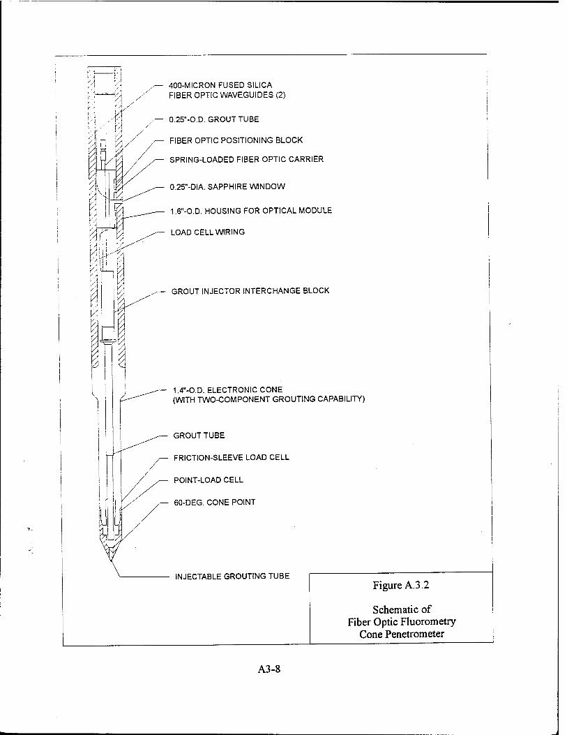
400-MICRON FUSED SILICA FIBER OPTIC WAVEGUIDES (2)
0.25"-O.D. GROUT TUBE
FIBER OPTIC POSITIONING BLOCK
SPRING-LOADED FIBER OPTIC CARRIER
0.25"-DIA. SAPPHIRE WINDOW
1.6"-O.D. HOUSING FOR OPTICAL MODULE
LOAD CELL WIRING
GROUT INJECTOR INTERCHANGE BLOCK
1.4"-O.D. ELECTRONIC CONE (WITH TWO-COMPONENT GROUTING CAPABILITY)
GROUT TUBE
FRICTION-SLEEVE LOAD CELL
POINT-LOAD CELL
60-DEG. CONE POINT
INJECTABLE GROUTING TUBE Figure A.3.2
Schematic of Fiber Optic Fluorometry
Cone Penetrometer
A3-8

Revision 0
Direct collection of soil samples into liners within the sampler will better preserve VOCs. The
soil samples should be split and removed from the continuous sampler. A portion of the sample
should immediately be transferred to sample vials for laboratory analysis. A representative
portion of the soil sample should be analyzed for VOCs using PID headspace measurements, as
described in Section A3.1.2.
The field scientist should observe all drilling and sample collection activities, maintain a
detailed descriptive log of subsurface materials recovered, photograph representative samples, and
properly label and store soil samples. An example of a geologic boring log form is presented in
Figure A3.1. This example should be adequate for most sites. If there is a large amount of
vertical variability then the scale should be adjusted accordingly. The contents of the descriptive
log are listed in Section A.3.1.2.
Although soil cuttings should be very minimal with the CPT technology, any soil cuttings
exhibiting petroleum hydrocarbon contamination based on PID screening should be handled in
accordance with local regulations.
A.3.2.3 CPT Hole Grouting Procedure
Cone penetrometer testing can create holes that may provide potential contamination pathways
into groundwater. To prevent cross contamination, the test holes should be grouted to seal the
hole and eliminate the contaminant migration pathway. The instrumented cone assembly and any
other retrievable portion of the assembly will be completely removed from the penetration hole.
Grout is generally prepared by mixing up to 5 percent (by dry weight) bentonite with Portland
cement. Some CPT trucks are capable of injecting grout into the hole as the pushrods are
removed.
A.3.2.4 Decontamination Procedures
Generally, the CPT push rods are cleaned with a steam-cleaning system as the rods are
withdrawn from the ground. Most cone penetrometer trucks have a vacuum system that recovers
nearly 100 percent of the steam-cleaning rinseate. Rinseate is generated only as the rods move
past the cleaner, thereby minimizing liquid waste generation. Care should be taken not to apply
the pressurized steam to the LIF module. Rinseate generally should be collected for proper
disposal.
A3-9

Revision 0
Potable water should be used for CPT equipment cleaning, decontamination, and grouting.
Precautions should be taken to .minimize any impact to the surrounding area that might result from decontamination operations. Fuel, lubricants, and other similar substances are to be handled
in a manner consistent with accepted safety procedures and standard operating practices.
A.3.3 BORING AND CONE PENETROMETER TEST LOCATION SURVEY
The horizontal location of all boring and CPT locations should be measured relative to established coordinates. Horizontal coordinates should be measured to the nearest 0.1 foot. The elevation of the ground surface and the measurement datum should be measured relative to mean sea level. The ground surface elevation should be measured to the nearest 0.1 foot, and the
measurement datum to the nearest 0.01 foot.
A.3.4 SOIL ANALYTICAL PROTOCOL
The analytical protocol to be used for soil sample analysis is presented in Table 2.1. This analytical protocol includes all of the parameters necessary to document intrinsic remediation of fuel hydrocarbons, including the effects of sorption and both aerobic and anaerobic biodegradation of fuel hydrocarbons. Section 2.3.1.2 of the protocol document describes each soil analytical parameter and the use of each analyte in the intrinsic remediation demonstration.
A3-10
Revision 0
SECTION A-4
GROUNDWATER CHARACTERIZATION METHODOLOGIES
This section describes the scope of work required to collect groundwater quality samples to support the intrinsic remediation demonstration. In order to maintain a high degree of quality control during groundwater sampling, the procedures described in the following sections should
be followed.
Groundwater sampling should be conducted only by qualified scientists and technicians trained in the conduct of well sampling, sampling documentation, and chain-of-custody procedures. In addition, sampling personnel should thoroughly review this protocol document and the site- specific work plan prior to sample acquisition and have a copy of the work plan available onsite for reference. Detailed groundwater sampling and sample handling procedures are presented in following sections. Samples should be collected in accordance with local, state, and federal
requirements.
Rapid and inexpensive survey techniques such as Geoprobe or CPT are appropriate for the initial site characterization and plume definition of the intrinsic remediation demonstration. Conventional monitoring wells will be required for long-term monitoring (LTM) and point-of-
compliance (POC) groundwater sampling.
A.4.1 MONITORING WELL INSTALLATION AND SAMPLING
A.4.1.1 Monitoring Well Installation
Groundwater monitoring wells should be located based on the distribution of contaminants in each plume. At a minimum, one monitoring well should be placed upgradient of the contaminant plume, two wells should be placed within the plume, and three wells should be placed various distances downgradient of the plume. The number of wells should be related to site conditions and the size of the spill. To define the three-dimensional extent of contamination and to determine the three-dimensional hydraulic relationships within the saturated zone, it is best to use nested wells with a maximum screened interval of 5 feet. Screening a larger area of the saturated
A4-1
Revision 0
zone will result in averaging of contaminant concentrations and hydraulic properties. To ensure
well integrity, nested well pairs generally should be completed in separate boreholes. Detailed
well installation procedures are described in the following paragraphs. Of course, local protocols,
regulations, and site conditions should dictate actual well completion details.
A.4.1.1.1 Well Materials Decontamination
Well completion materials should be inspected by the field scientist to ensure that they are
clean and acceptable for monitoring purposes prior to use. If not factory sealed, casing, screen,
and casing plugs and caps should be cleaned with a high-pressure, steam/hot-water cleaner using
approved water prior to use. Prepackaged sand, bentonite, and Portland cement should be used
in well construction, and the bags should be inspected for possible external contamination before
use. Materials that cannot be cleaned to the satisfaction of the field scientist should not be used.
A.4.1.1.2 Well Casing
Upon completion of drilling to the proper boring termination depth, the monitoring well casing
can be installed. Well construction details should be noted on a Monitoring Well Installation
Record form (Figure A.4.1). This information will become part of the permanent field record for
the site.
Blank well casing should be constructed of Schedule 40 polyvinyl chloride (PVC) with an
inside diameter (ED) of 2 inches when installing wells in boreholes, and Schedule 40 PVC with an
ID of 0.5 or 1.5 inches when installing wells in CPT holes. All well casing sections should be
flush-threaded; glued joints should not be used. The casing at each well should be fitted with a
threaded bottom plug and a top cap constructed of the same type of material as the well casing.
The top should be vented to maintain ambient atmospheric pressure within the well casing. Site
conditions and local, state, and federal requirements should ultimately dictate well completion
details and materials.
The field scientist should verify and record the boring depth, the lengths of all casing and
screen sections, and the depth to the top of all well completion materials placed in the annulus
between the casing and borehole wall. All lengths and depths should be measured to the nearest
0.1 foot.
A4-2
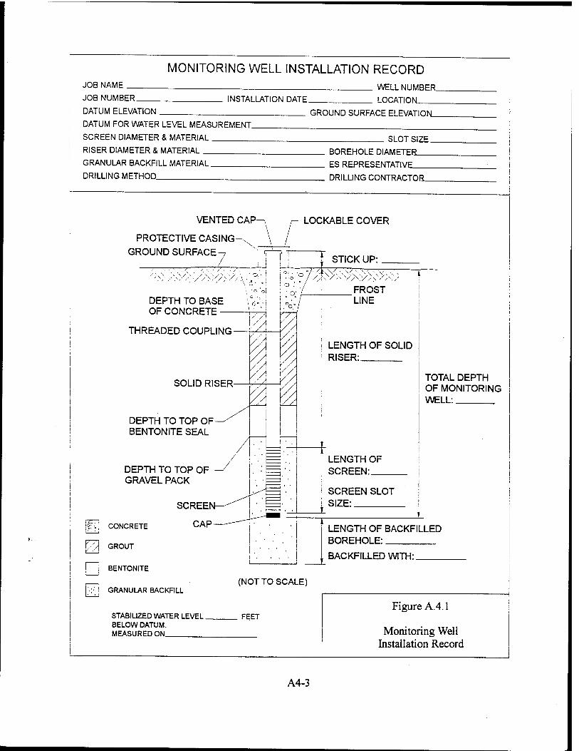
MONITORING WELL INSTALLATION RECORD JOB NAME
JOB NUMBER
DATUM ELEVATION
DATUM FOR WATER LEVEL MEASUREMENT.
SCREEN DIAMETER & MATERIAL
RISER DIAMETER & MATERIAI
GRANULAR BACKFILL MATERIAL
DRILLING METHOD
INSTALLATION DATE.
WELL NUMBER,
LOCATION
GROUND SURFACE ELEVATIONL
SLOT SIZE.
BOREHOLE DIAMETER
ES REPRESENTATIVE
DRILLING CONTRACTOR_
VENTED CAP-
PROTECTIVE CASING-X
GROUND SURFACE^
LOCKABLE COVER
y/y?</Ay/\-,
DEPTH TO BASE OF CONCRETE - \?\
THREADED COUPLING- //
SOLID RISER- ^ r.
DEPTH TO TOP OF- BENTONITE SEAL
DEPTH TO TOP OF GRAVEL PACK
!".:;; CONCRETE
F73 GROUT
I i BENTONITE
K-'i GRANULAR BACKFILL
STABILIZED WATER LEVEL. BELOW DATUM. MEASURED ON
(NOT TO SCALE)
FEET
STICK UP:
FROST LINE
LENGTH OF SOLID RISER:
LENGTH OF SCREEN:
SCREEN SLOT SIZE:
TOTAL DEPTH OF MONITORING WELL:
f
LENGTH OF BACKFILLED BOREHOLE:
BACKFILLED WITH:
Figure A.4.1
Monitoring Well Installation Record
A4-3
Revision 0
A.4.1.1.3 Well Screen
Well screens should be constructed of Schedule 40 PVC with an ID of 2 inches when installing wells in boreholes, and Schedule 40 PVC with an ID of 0.5 or 1.5 inches when installing wells in
CPT holes. The screens should be factory slotted with 0.010-inch openings. Wells generally
should be installed in nested pairs with a maximum 5-foot screened interval. Screening a larger section of the saturated zone will result in averaging of contaminant concentrations and hydraulic
properties. It is usually desirable to screen at least one well so that seasonal fluctuations of the water table can be measured. The positioning of well screens should be selected by the field scientist after consideration is given to the geometry and hydraulic characteristics of the stratum in which the well will be screened. Wells should be screened so that the vertical distribution of contaminants and hydraulic gradients can be delineated. To ensure well integrity, nested well pairs generally should be completed in separate boreholes. Site conditions and local, state, and federal requirements should ultimately dictate well completion details and materials.
A. 4.1.1.4 Sand Filter Pack
When monitoring wells are completed in boreholes, a graded sand filter should be placed around the screened interval and should extend approximately 2 feet above the top of the screen. Design of the sand filter should be based on the grain size distribution of the aquifer matrix as described in Harlan et al. (1989), but generally will consist of 10-20 silica sand. When monitoring points are completed in CPT holes, the annulus will generally be too small to allow filter pack construction. In such cases, native aquifer materials will be allowed to collapse around the well. Because of the absence of a filter pack, monitoring points in very silty or clayey materials may
yield water that is too turbid for analysis.
A.4.1.1.5 Annular Sealant
An annular seal of sodium bentonite pellets must be placed above the filter pack. The pellet seal should be a minimum of 2 feet thick. When installed above the water table, the bentonite seal should be hydrated in place in 6-inch lifts using potable water. The pellet seal must be overlain by a Portland cement/sodium bentonite grout that will extend from the top of the pellet seal to below the maximum frost line in the region. The Portland cement/sodium bentonite grout should consist of one 94-pound sack of cement and about 5 pounds of bentonite for each 7 gallons of water used. The bentonite content of the cement/bentonite mix should not exceed 5 percent by dry weight. The grout should be overlain by concrete extending to the ground surface. To reduce
A4-4
Revision 0
heaving of the newly installed monitoring well caused by freeze-thaw processes, it is imperative
that the uppermost concrete seal extend below the maximum frost line for the area. In some
cases, use of bentonite grout without cement can be used to minimize frost heave damage.
USEPA Region 4 has found that in some cases the potable water supply has been chemically
treated to the extent that water and soil analyses can be significantly altered. In these cases, an
alternate water supply should be used, especially for drilling fluid, water used to prepare grout, and bentonite hydration water.
A.4.1.I.6 Protective Well Cover
To provide protection for the PVC well casing, each monitoring well should be completed with
an above-grade or an at-grade protective cover. The choice of installing an above-grade
protective well cover versus an at-grade protective well cover will depend mainly on aesthetics
and logistical considerations. The facility point-of-contact should be consulted prior to work plan
development so the appropriate well cover can be specified. In general, above-grade well covers
are better because they are easily located and the problem of standing water in the annulus at the well head is minimized.
A. 4.1.1.6.1 Above-Grade Cover
In areas where pavement is present, the above-grade cover should be cemented in place using
concrete blended to the existing pavement. In areas where pavement is not already present, a 6-
inch-thick, 2-foot-diameter concrete pad should be constructed around the protective cover. In
either case, the concrete immediately surrounding the well cover should be sloped gently away
from the protective casing to facilitate runoff during precipitation events.
A.4.1.1.6.2 At-Grade Cover
In areas where pavement is present, the at-grade cover should be cemented in place using
concrete blended to the existing pavement. In areas where pavement is not already present, a 6-
inch-thick, 2-foot-diameter concrete pad will be constructed around the protective cover. In
either case, the concrete immediately surrounding the well cover should be sloped gently away
from the protective casing to facilitate runoff during precipitation events. The seal of the cap to the well should be water tight.
A4-5
Revision 0
A.4.1.2 Well Development
Before any new well can be used for monitoring water levels or taking water samples, it must
be developed. Development removes sediment from inside the well casing and flushes fines,
cuttings, and drilling fluids from the sand pack and the portion of the formation adjacent to the
well screen. The water samples are intended for analysis of soluble electron acceptors and
petroleum hydrocarbons. A small amount of turbidity does not interfere with these analyses.
Turbidity criteria for drinking water are not relevant. Well development should be accomplished
in a manner that is consistent with local, state, and federal requirements.
If the depth to water allows, well development can be accomplished using a bailer, peristaltic
pump with dedicated Teflon®-lined polyethylene tubing, or a submersible pump. The bailer or
pump must be regularly lowered to the bottom of the well so that fines that have accumulated in
the bottom are agitated and removed from the well in the development water.
Development should be continued until a minimum of 10 casing volumes of water have been
removed from the well and the water pH, temperature, specific conductivity, dissolved oxygen
concentration, and redox potential have stabilized (i.e., three readings are taken with less than 10
percent difference). If the development water is still turbid after removal of 10 casing volumes,
development should be continued until the water becomes clear or the turbidity of the water
produced is stable after the removal of several additional casing volumes.
The development procedure specifies that 10 casing volumes of water be removed from the
well. However, some wells completed in marginal aquifers will be evacuated dry during well
development prior to the recovery of 10 casing volumes. In these low-productivity wells,
development activity will have to be staged over a period of time to allow water to refill the well
bore. In the event that 10 casing volumes of water cannot be recovered, the water volume
recovered should be noted in the development records noting this deficiency.
Clean development waters should be discharged at the drilling site in a manner that will control
excessive ponding. Visibly or PID-indicated contaminated waters must be collected in contained
and transported to the facility storage area for storage or to the facility water treatment plant for
treatment and disposal. The facility point-of-contact should be consulted to determine the final
disposition of purge waters. Some projects, states, or USEPA Regions require the containment
of all development water produced at potentially contaminated sites.
A record of well development should be maintained for each well. The well development
record should be maintained in a bound field notebook or on monitoring well development forms
A4-6
Revision 0
by the field scientist. Figure A.4.2 is an example of a monitoring well/point development record.
A summary well development record form should be prepared for each well. Development
records must include:
• Well number;
• Date and time of development;
• Development method;
• Pre-development water level and well depth;
• Volume of water produced;
• Description of water produced;
• Post-development water level and well depth; and
• Field analytical measurements, including pH, temperature, dissolved oxygen concentration, redox potential, and specific conductivity.
A.4.1.3 Groundwater Monitoring Well Sampling
All equipment to be used for sampling should be assembled and properly cleaned and calibrated
(if required) prior to arriving in the field. In addition, all record-keeping materials should be
gathered prior to leaving the office.
A. 4.1.3.1 Preparation for Sampling
Prior to starting the sampling procedure, the area around the well should be cleared of foreign
materials, such as brush, rocks, and debris. These procedures will prevent sampling equipment
from inadvertently contacting debris around the monitoring well.
A. 4.1.3.2 Equipment Cleaning and Calibration
All portions of sampling and test equipment that will contact the sample matrix must be
thoroughly cleaned before use. This includes the water-level probe and cable, bailer (unless a
dedicated disposable bailer is used), bailer lifting line, test equipment for onsite use, and other
equipment or portions thereof that will contact the samples. Based on the types of sample
analyses to be conducted, a cleaning protocol similar to the following should be used:
A4-7
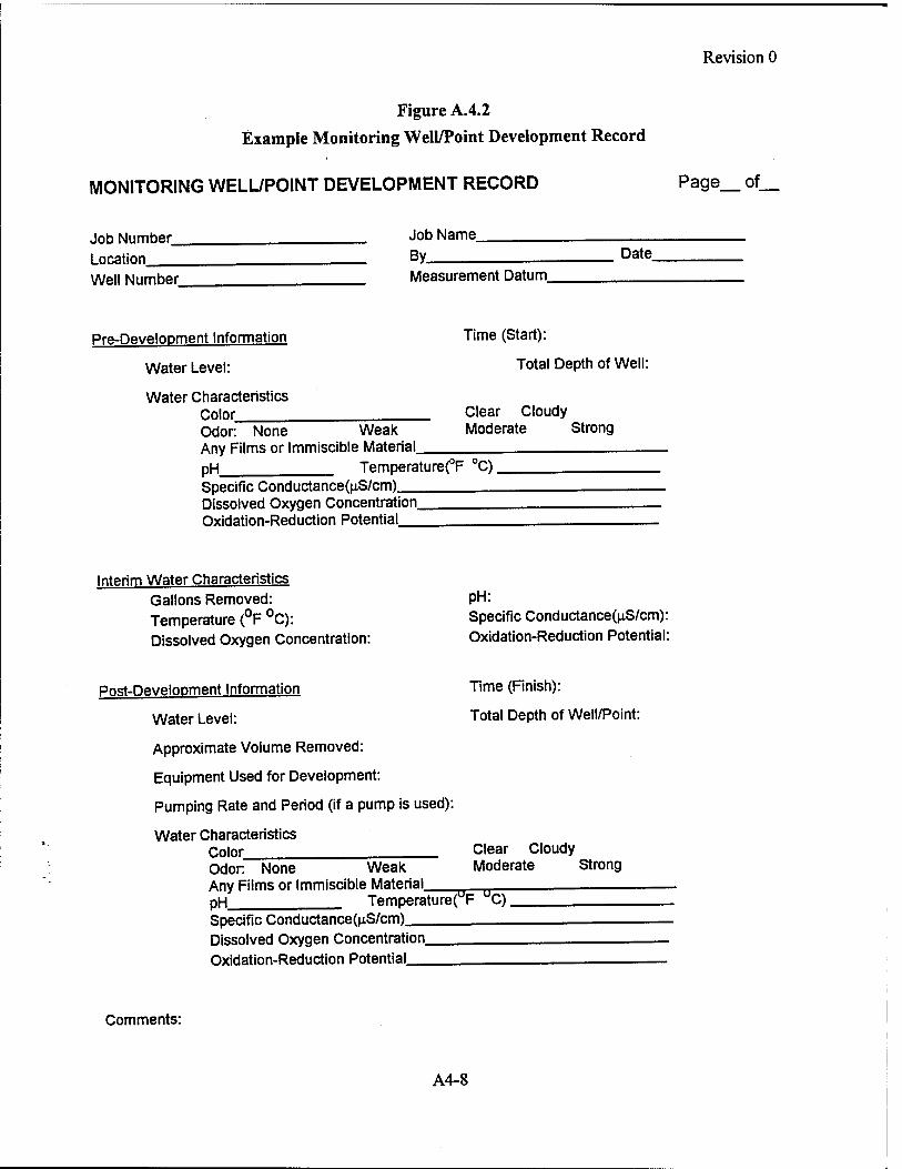
Revision 0
Figure A.4.2 Example Monitoring Well/Point Development Record
MONITORING WELL/POINT DEVELOPMENT RECORD Page of.
Job Number. Location Well Number
Job Name_ By Measurement Datum
Date
Pre-Develooment Information
Water Level:
Water Characteristics Color Odor None Weak Any Films or Immiscible Material pH Temperature(°F °C) Specific Conductance(nS/cm) Dissolved Oxygen Concentration Oxidation-Reduction Potential
Time (Start):
Total Depth of Well:
Clear Cloudy Moderate Strong
Interim Water Characteristics Gallons Removed: Temperature (°F °C): Dissolved Oxygen Concentration:
pH: Specific Conductance(n.S/cm): Oxidation-Reduction Potential:
Post-Development Information
Water Level:
Approximate Volume Removed:
Equipment Used for Development:
Pumping Rate and Period (if a pump is used):
Water Characteristics Color _^___
Time (Finish):
Total Depth of Well/Point:
Odor None Weak Any Films or Immiscible Material pH Temperature( F C) Specific Conductance(nS/cm) Dissolved Oxygen Concentration Oxidation-Reduction Potential_
Clear Cloudy Moderate Strong
Comments:
A4-8
Revision 0
• Clean with potable water and phosphate-free laboratory detergent such as Alconox®;
• Rinse with potable water;
• Rinse with distilled or deionized water;
• Rinse with reagent-grade methanol or similar;
• Rinse with distilled or deionized water;
• Air dry the equipment prior to use.
Final selection of cleaning procedures should be based on project, state, and USEPA Region
requirements and anticipated site contaminants. Any deviations from established cleaning
procedures should be documented in the field scientist's field notebook and on the groundwater
sampling form.
If pre-cleaned dedicated sampling equipment is used, the cleaning protocol specified above is
not required. Laboratory-supplied sample containers will be cleaned, sealed, and certified by the
laboratory, and therefore do not need to be cleaned in the field. The type of container provided
and the method of container decontamination will be documented in the permanent record of the
sampling event.
As required, field analytical equipment should be calibrated according to the manufacturer's
specifications immediately prior to use in the field. This applies to equipment used for onsite
measurements of pH, electrical conductivity, temperature, dissolved oxygen, and redox potential.
A. 4.1.3.3 Water Level and Total Depth Measurements
Prior to removing any water from the well the static water level should be measured. An
electric water level probe should be used to measure the depth to groundwater below the datum
to the nearest 0.01 foot. After measuring the static water level, the water level probe should be
slowly lowered to the bottom of the well, and the total well depth should be measured to the
nearest 0.01 foot. Based on these measurements the volume of water to be purged from the well
can be calculated. If mobile LNAPL is encountered, the LNAPL thickness should be determined,
and attempts should be made to sample both the groundwater below the LNAPL layer and the
fluid making up the LNAPL.
A.4.1.3.4 Mobile LNAPL Thickness Measurements
At sites where phase-separated hydrocarbons are present in the groundwater system, it is
important to accurately measure the thickness of floating hydrocarbons. Accurate measurement
A4-9

Revision 0
of hydrocarbon thickness allows for estimation of the amount and distribution of the hydrocarbon
and correction of measured groundwater elevations.
There are three methods that can be used to determine the thickness of mobile LNAPL in a
well, including use of an interface probe, a bailer, or tape and paste. Interface probes generally
operate on either tight refraction sensors or density float switches to detect hydrocarbons and the hydrocarbon/water interface. The depth to mobile LNAPL and depth to water should be measured to the nearest 0.01 foot. The thickness of phase-separated hydrocarbons should also be measured to the nearest 0.01 foot. Three consecutive measurements should be made to ensure the accuracy of the measuring instrument. A clear bailer can be slowly lowered into the well until
it intersects the fluid but is not totally immersed. The bailer is then retrieved, and the floating LNAPL can be visually observed and measured with an engineer's tape. The third method for
measurement of floating hydrocarbon thickness is hydrocarbon paste and an engineer's tape. The paste, when applied to the tape, changes color when it intersects the hydrocarbon and the hydrocarbon/water interface. Measurements of the mobile LNAPL thickness can be made directly from the engineer's tape. It is extremely important to remember to thoroughly decontaminate all equipment between well measurement events to prevent cross contamination of wells.
Measurements of mobile LNAPL thickness made in monitoring wells provide only an estimate of the actual thickness of NAPL at that location. Actual mobile and residual LNAPL thicknesses can only be obtained from continuous soil cores. Correcting apparent mobile LNAPL thickness as measured in monitoring wells to true thickness is discussed in Appendix C.
A. 4.1.3.5 Well Bore Purging
The volume of water contained within the well casing at the time of sampling should be calculated, and three times the calculated volume removed from the well prior to the collection of samples for analysis. All purge water should be placed in 55-gallon drums pending final disposition. To prevent cross contamination between wells, dedicated disposable bailers, or peristaltic pumps with dedicated Teflon®-lined polyethylene tubing should be used for well evacuation. Additional methods for well purging include use of bladder pumps, WaTerra® pumps, or down hole positive-displacement pumps such as the Grundfos® pump. All wells should be
purged in accordance with local, state, or federal requirements.
If a well is evacuated to a dry state during purging, the well should be allowed to recharge, and the sample should be collected as soon as sufficient water is present in the well to obtain the necessary sample quantity. Sample compositing, or sampling over a lengthy period by
A4-10
Revision 0
accumulating small volumes of water at different times to eventually obtain a sample of sufficient
volume, is not allowable.
A.4.1.3.6 Sample Extraction
Sample extraction should be done in accordance with local, state, and federal requirements. If
a peristaltic pump is used, the sample should be collected directly from the discharge end of the
tubing. If a dedicated, disposable, polyethylene bailer is used, it should be lowered into the water
gently to prevent splashing and extracted gently to prevent creation of an excessive vacuum in the
well. The sample should be transferred directly into the appropriate sample container. If a bailer
is used, the water sample must be transferred to the sample container by discharging the sample
from the bottom of the bailer. In any case, the water should be carefully poured down the inner
walls of the sample bottle to minimize aeration of the sample. Unless other instructions are given
by the analytical laboratory, sample containers should be completely filled so that no air space
remains in the container.
A.4.2 MONITORING POINT INSTALLATION AND SAMPLING
Groundwater monitoring points are similar to monitoring wells in that they consist of Schedule
40 PVC slotted screen and solid riser. Groundwater monitoring points differ from monitoring
wells in that they are completed in holes created using CPT (or Geoprobe®) equipment. Because
of the extremely small to nonexistent annular space between the PVC monitoring point
completion materials and the hole created using the CPT, common monitoring well completion
components including the gravel pack, bentonite seal, and Portland cement/sodium bentonite seal
are not used. Because these components are missing, groundwater monitoring points should be
installed only in shallow aquifers where installation of such devices will not result in the cross-
contamination of adjacent water-bearing strata. Groundwater monitoring points are best utilized
in shallow unconfined aquifers where such contamination is not a potential problem. Figure A.4.3
shows a typical monitoring point completion.
A4-11
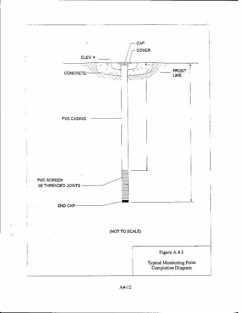
PVC SCREEN W/THREADED JOINTS
END CAP
(NOT TO SCALE)
Figure A.4.3
Typical Monitoring Point Completion Diagram
A4-12
Revision 0
A.4.2.1 Monitoring Point Locations and Completion Intervals
Groundwater monitoring points should be located based on the distribution of contaminants in
each plume. At a minimum, one monitoring point should be placed upgradient of the contaminant
plume, two points should be placed within the plume, and three points should be placed various
distances downgradient of the plume. The number of points should be related to site conditions
and the size of the spill. Each monitoring point should consist of a pair of nested monitoring
points: a shallow point intended to sample the shallow portion of the aquifer and a deep point
intended to sample the groundwater at some depth below the water table. The shallow screened
interval generally should extend from 1 foot above the water table to no more than 5 feet below
the water table. The deep screened interval should have between 3 and 6 feet of screen. The
deep points should be placed based on contaminant distribution. Such short screened intervals,
with between 3 and 6 feet of screen each, help mitigate the dilution of water samples from
potential vertical mixing of contaminated and uncontaminated groundwater in the monitoring
point casing In addition, short screened intervals used in nested pairs give important information
on the nature of vertical hydraulic gradients in the area.
A.4.2.2 Monitoring Point Installation
A.4.2.2.1 Preplacement Activities
All necessary digging, coring, drilling, and groundwater monitoring point installation permits
should be obtained prior to mobilizing to the field. In addition, all utility lines should be located
and proposed drilling locations cleared prior to any intrusive activities.
Water to be used in monitoring point installation and equipment cleaning should be obtained
from a potable water supply. The field hydrogeologist should make the final determination as to
the suitability of water for these activities. It is recommended that the source water utilized for
decontamination activities be tested for the same parameters as the analytical samples from the
specific site.
A.4.2.2.2 Monitoring Point Materials Decontamination
Monitoring point completion materials should be inspected by the field hydrogeologist and
determined to be clean and acceptable prior to use. If not factory sealed, casing, screen, and
casing plugs and caps should be cleaned with a high-pressure, steam/hot-water cleaner using
A4-13
Revision 0
approved water prior to use. Materials that cannot be cleaned to the satisfaction of the field
hydrogeologist should not be used.
A.4.2.2.3 Monitoring Point Screen and Casing
Groundwater monitoring points are installed by pushing 0.5-inch ID PVC through the inside of
the CPT pushrods. As the pushrod descends, new PVC casing is continuously attached until the
desired depth is reached and a fully cased monitoring point is created.
Monitoring point construction details should be noted on a Monitoring Point Installation
Record form (Figure A.4.4). This information becomes part of the permanent field record for the
site.
Monitoring point screens are constructed of flush-threaded, Schedule 40 PVC with an ID of
0.5 inch. The screens should be factory slotted with 0.01-inch openings. The positions of the
screens should be selected by the field hydrogeologist after consideration is given to the geometry
and hydraulic characteristics of the stratum in which the monitoring point will be screened.
Blank monitoring point casing should be constructed of Schedule 40 PVC with an ID of 0.5
inch. All monitoring point casing sections should be flush-threaded; glued joints should not be
used. The casing at each monitoring point should be fitted with a bottom cap and a top cap
constructed of PVC. The top cap should be vented to maintain ambient atmospheric pressure
within the monitoring point casing.
The field hydrogeologist should verify and record the total depth of the monitoring point, the
lengths of all casing sections, and the depth to the top of all monitoring point completion
materials. All lengths and depths are to be measured to the nearest 0.1 foot.
A.4.2.2.4 Protective Cover
To provide protection for the PVC well casing, each monitoring point will be completed with
either an at-grade, or an above-grade protective cover. In either case, the concrete immediately
surrounding the monitoring point will be sloped gently away from the protective casing to
facilitate runoff during precipitation events. Protective cover installation procedures are described
in Section A4.1.1.6.
A4-14
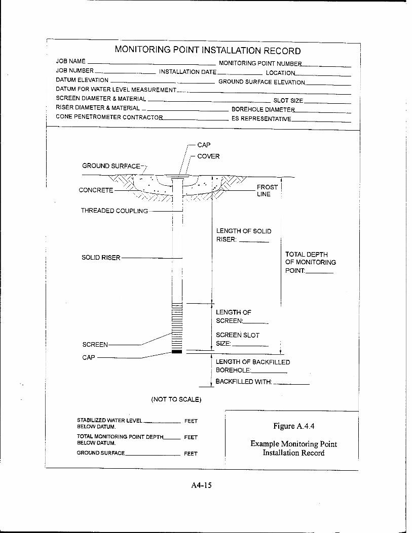
JOB NAME
JOB NUMBER.
MONITORING POINT INSTALLATION RECORD — MONITORING POINT NUMBEBL.
INSTALLATION DATE, LOCATION, DATUM ELEVATION
DATUM FOR WATER LEVEL MEASUREMENT.
SCREEN DIAMETER & MATERIAL
RISER DIAMETER & MATERIAI
GROUND SURFACE ELEVATION-
CONE PENETROMETER CONTRACTOR.
SLOT SIZE.
BOREHOLE DIAMETESL.
ES REPRESENTATIVE_
GROUND SURFACE-7
CONCRETE
THREADED COUPLING
SOLID RISER-
LENGTH OF SOLID RISER:
LENGTH OF SCREEN:
SCREEN SLOT SIZE:
TOTAL DEPTH OF MONITORING POINT:
i
LENGTH OF BACKFILLED BOREHOLE:
BACKFILLED WITH:
(NOT TO SCALE)
STABILIZED WATER LEVEL BELOW DATUM.
TOTAL MONITORING POINT DEPTH. BELOW DATUM.
GROUND SURFACE
FEET
FEET
FEET
Figure A.4.4
Example Monitoring Point Installation Record
A4-15
Revision 0
A.4.2.3 Monitoring Point Development
New monitoring points must be developed prior to sampling. Development removes sediment
from inside the monitoring point casing and flushes fines from the portion of the formation
adjacent to the monitoring point screen. Monitoring point development can be accomplished
using either a small, custom-made bailer or a peristaltic pump. The bailer or pump tubing should
be regularly lowered to the bottom of the monitoring point so that fines that have accumulated in
the bottom are agitated and removed from the monitoring point in the development water.
Development should be continued until a minimum of 10 casing volumes of water has been
removed from the monitoring point and until pH, temperature, specific conductivity, dissolved
oxygen concentration, and redox potential have stabilized. If the water remains turbid after
removing 10 casing volumes of water, monitoring point development should continue until the
turbidity of the water produced is constant.
A monitoring point development record shall be maintained for each point. The monitoring
point development record will be completed in the field by the field hydrogeologist. Figure A.4.2
is an example of the monitoring well/point development record. Development records will
include:
• Monitoring point number;
• Date and time of development;
• Development method;
• Pre-development water level and monitoring point depth;
• Volume of water produced;
• Description of water produced;
• Post-development water level and monitoring point depth; and
• Field analytical measurements, including pH, temperature, dissolved oxygen concentration, redox potential, and specific conductivity.
A.4.2.4 Monitoring Point Location and Datum Survey
The location and elevation of the new monitoring points should be surveyed soon after
completion. The horizontal location should be measured relative to established coordinates.
Horizontal coordinates are to be measured to the nearest 0.1 foot. The elevation of the ground
surface adjacent to the monitoring point casing and the measurement datum elevation (top of
PVC casing) is to be measured relative to a mean sea level datum. The ground surface elevation
A4-16
Revision 0
is to be measured to the nearest 0.1 foot, and the measurement datum, outer casing, and
surveyor's pin (if present) elevation should be measured to the nearest 0.01 foot.
A.4.2.5 Monitoring Point Sampling
Monitoring point sampling should be accomplished in accordance with the procedures described in Section A.4.1.3.
A.4.3 HYDROPUNCH® SAMPLING
The HydroPunch II® sampling device is designed to be pushed or driven to the desired sample
depth, either from the ground surface or from the bottom of a drilled borehole. The
HydroPunch® utilizes an air-tight and water-tight sealed intake screen and sample chamber that is
isolated from the surrounding environment as the tool is advanced. The surface of the
HydroPunch® is designed to prevent the downward transport of contamination as the tool is
advanced; it cleans itself as the soil particles are displaced to the side. The tight seal created as
the soil is displaced and compacted allows the collection of a discrete sample from a specific depth.
The HydroPunch® can be used to sample both groundwater and floating LNAPL.
Groundwater samples should be collected from the groundwater table to below visibly impacted
groundwater at 5-foot intervals using the HydroPunch® sampling apparatus. When performing a
groundwater investigation exclusively with the HydroPunch® sampling device, samples should be
taken in an upgradient (background) area, within the defined mobile LNAPL plume, in the area
immediately downgradient of the mobile LNAPL plume, within the dissolved BTEX plume, and
immediately downgradient of the dissolved BTEX plume. HydroPunch® provides up to 1.2 liters
of sample volume. This should be sufficient for the water quality analyses detailed in Table 2.1.
Should the sample volume prove to be insufficient, the analytical protocol should be modified based on sample yield at each depth interval.
All equipment to be used for sampling should be assembled and properly cleaned and calibrated
(if required) prior to arriving in the field. In addition, all record-keeping materials must be gathered prior to leaving the office.
A4-17
Revision 0
A.4.3.1 Preparation for Sampling
Prior to starting the sampling procedure, the area around the Hydropunch® sampling location
must be cleared of foreign materials, such as brush, rocks, and debris. These procedures will
prevent sampling equipment from inadvertently contacting surface debris.
A.4.3.2 Equipment Cleaning and Calibration
All portions of sampling and testing equipment that will contact the sample matrix must be
thoroughly cleaned before. This includes the HydroPunch® tool, water-level probe and cable,
lifting line, test equipment for onsite use, and other equipment or portions thereof that will contact
the samples. The cleaning protocol to be used is described in Section A4.1.3.2.
A.4.3.3 Water Level and Total Depth Measurements
Prior to removing any water from the HydroPunch® sampling device, the static water should
be measured. Hollow, high-density polyethylene (HDPE) tubing connected to a manometer will
be inserted into the hollow HydroPunch® until the manometer indicates that groundwater has been
reached. The HDPE attached to the manometer will then be marked at the level of the ground
surface and removed. The depth to water will be determined by placing a tape measure next to
the HDPE tubing and measuring the length from the base of the tubing to the ground level mark
to the nearest 0.01 foot. The sampling depth is measured (to the nearest 0.1 foot) by noting the depth to which the HydroPunch® tool was driven.
A.4.3.4 Sample Acquisition
Samples should be collected in accordance with local, state, and federal requirements. Special
care should be taken to prevent contamination of the groundwater and extracted samples. The
two primary ways that sample contamination can occur are through contact with improperly
cleaned equipment and by cross contamination through insufficient cleaning of equipment between
wells. To prevent such contamination, new HDPE tubing must be used for each water level
measurement. If the water level probe and cable are used to determine static water levels and well
total depths, they should be thoroughly cleaned between uses at different sampling locations. In
addition to the use of properly cleaned equipment, a clean pair of new, disposable nitrile gloves will be worn each time a different well is sampled.
The following paragraphs present the procedures to be followed for groundwater (or LNAPL)
sample collection from the HydroPunch®. These activities should be performed in the order
A4-18

Revision 0
presented below. Exceptions to this procedure should be noted in the field scientist's field notebook.
The sampling depth and interval generally should be specified prior to driving the
HydroPunch® into the ground. The field scientist should verify the sampling depth by measuring
the length of each HydroPunch® sampling rod prior to insertion into the ground. After insertion,
the drive rods or hammer are retracted to pull the cone out of the body of the HydroPunch®
device, permitting groundwater to enter. A minimum of 6 inches of the body of the device must
be in the driven hole to provide a good annular seal.
After allowing for adequate fill time, the HydroPunch® sampling device is pulled to the surface,
unthreaded from the upper subassembly, and replaced with the thread retainer. The sample is then
transferred directly into the analyte-appropriate sample container. The water should be carefully
poured down the inner walls of the sample bottle to minimize aeration of the sample. Unless
other instructions are given by the analytical laboratory, sample containers should be completely filled so that no air space remains in the container.
A.4.4 GEOPROBE® SAMPLING
This section describes the scope of work required for collecting groundwater quality samples
using the Geoprobe® sampling apparatus. In order to maintain a high degree of quality control
during the sampling event, the procedures described in the following sections should be followed.
The sampling depth and interval should be determined prior to driving the Geoprobe® sampling
rods into the ground. The field scientist should verify the sampling depth by measuring the length
of each Geoprobe® sampling rod prior to insertion into the ground. A disposable drive tip will be
placed at the tip of the Geoprobe® sampling rods. This tip is threaded on the uphole end to allow
attachment of dedicated 3/8-inch, HDPE tubing. After reaching the desired depth, the 3/8-inch
HDPE tubing is threaded through the center of the hollow Geoprobe® sampling rods and secured
to the drive point. The polyethylene tubing is perforated at the downhole end using a 1/16-inch
drill bit at 1/4-inch intervals alternately offset at 90-degree angles. The Geoprobe® sampling rods
are then pulled back approximately 1 foot to allow groundwater to enter the perforated end of the
polyethylene tubing. When the rod is pulled up, the sampling tip remains at the probe termination
depth, and the 1-foot perforated interval of the polyethylene tubing is exposed to groundwater.
The groundwater sample is then acquired using a peristaltic pump.
A4-19

Revision 0
Groundwater sampling will be conducted by qualified scientists and technicians trained in the
conduct of Geoprobe® sampling, records documentation, and chain-of-custody procedures In
addition, sampling personnel should thoroughly review this plan prior to sample acquisition and must have a copy of the plan available onsite for reference.
Detailed groundwater sampling and sample handling procedures are presented in following sections.
A.4.4.1 Preparation for Sampling
All equipment to be used for sampling is to be assembled and properly cleaned and calibrated
(if required) prior to arriving in the field. In addition, all record-keeping materials should be gathered prior to leaving the office.
A.4.4.2 Equipment Cleaning and Calibration
All portions of sampling and test equipment that will contact the sample must be thoroughly
cleaned before use. This includes water-level probe and cable, lifting line, test equipment for
onsite use, and other equipment or portions thereof that will contact the samples. A cleaning protocol similar to that described in Section A4.1.3.2 should be used.
A.4.4.3 Water Level and Total Depth Measurements
Prior to removing any water from the Geoprobe® sampling device, the static water should be
measured. Several commercially available water-level probes are capable of recording water
levels through the center of the hollow Geoprobe® rods. The depth to water should be
determined to the nearest 0.1 foot. The sampling depth also should be measured (to the nearest 0.1 foot) by noting the depth to which the Geoprobe® tool was driven.
A.4.4.5 Purging
The Geoprobe® sampling point should be purged prior to sample acquisition. Groundwater
should be pumped through the same dedicated Teflon®-lined polyethylene tubing that will be used
for sample acquisition. The sampling point should be purged until pH, temperature, specific
conductivity, dissolved oxygen, and redox potential readings have stabilized. Additional details on purging are specified in Section 4.1.3.5.
A4-20
Revision 0
A.4.4.6 Sample Acquisition
Samples should be collected in accordance with local, state, and federal requirements. Special care must be taken to prevent contamination of the groundwater and extracted samples. The two primary ways that sample contamination can occur are through contact with improperly cleaned
equipment and by cross contamination through insufficient cleaning of equipment between sampling locations. To prevent such contamination, the HDPE used to determine static water levels and sample depth should not be reused. In addition to the use of properly cleaned equipment, a clean pair of new, disposable nitrile gloves will be worn each time a different Geoprobe® location is sampled.
The following paragraphs present the procedures that comprise groundwater sample acquisition from the Geoprobe®. These activities should be performed in the order presented below. Exceptions to this procedure should be noted in the field scientist's field notebook.
A peristaltic pump should be used to extract groundwater samples from the Geoprobe® sampling point. Prior to sample collection, groundwater should be purged until dissolved oxygen, temperature, pH, specific conductivity, and redox readings have stabilized. The sample is collected at the discharge end of the HDPE tubing directly into the appropriate sample container. The water should be carefully directed down the inner walls of the sample bottle to minimize aeration of the sample.
Unless other instructions are given by the analytical laboratory, sample containers should be completely filled so that no air space remains in the container. Excess water collected during sampling should be handled in accordance with local regulations.
A4-21

Revision 0
SECTION A-5
SOIL AND GROUNDWATER SAMPLE HANDLING
This section describes the handling of soil and groundwater samples from the time of sampling
until the samples arrive at the laboratory.
A.5.1 SAMPLE PRESERVATION, CONTAINERS, AND LABELS
The analytical laboratory should add any necessary chemical preservatives prior to shipping the
containers to the site. Samples should be properly prepared for transportation to the analytical
laboratory by placing the samples in a cooler containing ice to maintain a shipping temperature of
approximately 4 degrees centigrade (°C).
Sample containers and appropriate container lids should be provided by the analytical
laboratory. The sample containers should be filled in accordance with accepted procedures for
the sample matrix and the type of analysis to be conducted. Container lids should be tightly
closed. The sample label should be firmly attached to the container side, and the following
information legibly and indelibly written on the label:
• Facility name; • Sample identification; • Sample type (groundwater, surface water, etc.); • Sampling date; • Sampling time; • Preservatives added; and • Sample collector's initials.
A.5.2 SAMPLE SHIPMENT
After the samples are sealed and labeled, they should be packaged for transport to the
analytical laboratory. The packaged samples should be delivered to the analytical laboratory
shortly after sample acquisition using an overnight delivery service. The following packaging and
labeling procedures are to be followed:
A5-1

Revision 0
• Abide by all US Department of Transportation (DOT) shipping regulations; • Package samples so that they will not leak, spill, or vaporize from their containers; • Label shipping container with
- Sample collector's name, address, and telephone number; - Laboratory's name, address, and telephone number; - Description of sample; - Quantity of sample; and - Date of shipment.
A.5.3 CHAIN-OF-CUSTODY CONTROL
After the samples are collected, chain-of-custody procedures must be followed to establish a
written record of sample handling and movement between the sampling site and the analytical
laboratory. Each shipping container should have a chain-of-custody form completed in triplicate
by the sampling personnel. One copy of this form should be kept by the sampling contractor after
sample delivery to the analytical laboratory; the other two copies should be retained at the
laboratory. One of the laboratory copies will become a part of the permanent record for the
sample and will be returned with the sample analytical results. The chain-of-custody form should contain the following information:
Unique sample identification number; Sample collector's printed name and signature; Date and time of collection; Sample location; Sample matrix; Sample size and container; Chemical preservatives added; Analyses requested; Signatures of individuals involved in the chain of possession; and Inclusive dates of possession.
The chain-of-custody documentation should be placed inside the shipping container so that it
will be immediately apparent to the laboratory personnel receiving the container, but cannot be
damaged or lost during transport. The shipping container is to be sealed so that it will be obvious if the seal has been tampered with or broken.
A5-2
Revision 0
A.5.4 SAMPLING RECORDS
In order to provide complete documentation of the sampling event, detailed records are to be
mamtained by the field scientist. Figure A.5.1 is an example groundwater sampling form At a minimum, these records must include the following information:
• Sample location (facility name); • Sample identification;
Sample location map or detailed sketch; Date and time of sampling; Sampling method; Field observations of - Sample appearance, - Sample odor;
Weather conditions; Water level prior to purging (groundwater samples); Total well depth (groundwater samples); Purge volume (groundwater samples); Water level after purging (groundwater samples); Well condition (groundwater samples); Sample depth; Sampler's identification;
Field measurements of pH, temperature, specific conductivity, dissolved oxygen concentration, and redox potential (groundwater samples); and 8
Any other relevant information.
A.5.5 GROUNDWATER AND SOIL ANALYTICAL PROTOCOL
Laboratory analyses should be performed on all soil and groundwater samples using the
analytical procedures listed in Table 2.1. Prior to sampling, arrangements should be made with
the analytical laboratory to provide a sufficient number of appropriate sample containers for the
samples to be collected. All containers, preservatives, and shipping requirements should be
consistent with the analytical protocol. The field scientist must specify the necessary quality
control samples and notify the laboratory so that they can prepare these bottles. For samples
requiring chemical preservation, preservatives should be added to containers by the laboratory
prior to shipping. Shipping containers, ice chests with adequate padding, and cooling media should be sent by the laboratory to the site.
A5-3

Revision 0
Figure A.5.1 Groundwater Sampling Record
SAMPLING LOCATION SAMPLING DATE(S) \
GROUNDWATER SAMPLING RECORD - MONITORING WELL/POINT (number)
REASON FOR SAMPLING: [ ] Regular Sampling; [ ] Special Sampling; DATE AND TIME OF SAMPLING: , 19 a.m./p.m. SAMPLE COLLECTED BY: of WEATHER: DATUM FOR WATER DEPTH MEASUREMENT (Describe):
MONITORING WELL CONDITION: [ ] LOCKED: [ ] UNLOCKED WELL NUMBER (IS - IS NOT) APPARENT STEEL CASING CONDITION IS: INNER PVC CASING CONDITION IS: WATER DEPTH MEASUREMENT DATUM (IS - IS NOT) APPARENT
[ ] DEFICIENCIES CORRECTED BY SAMPLE COLLECTOR [ ] MONITORING WELL REQUIRED REPAIR (describe):
Check-off 1 [ ] EQUIPMENT CLEANED BEFORE USE WITH.
Items Cleaned (List):
2 [ ] LNAPL DEPTH FT. BELOW DATUM Measured with:
WATER DEPTH : FT. BELOW DATUM Measured with:
3[ ] WATER-CONDITION BEFORE WELL EVACUATION (Describe): Appearance:_ Odor: Other Comments:
4[ ] WELL EVACUATION: Method: Volume Removed: Observations: Water (slightly - very) cloudy
Water level (rose - fell - no change) Water odors: Other comments:
A5-4

Figure A.5.1 (Continued)
5 [ ] SAMPLE EXTRACTION METHOD:
[ ] Bailer made of:_ [ ] Pump, type:_ [ ] Other, describe:.
6 [ ] ON-SITE MEASUREMENTS: Temp: ° Measured with pH: Measured with Conductivity: Measured with Dissolved Oxygen: Measured with Redox Potential: Measured with Salinity: Measured with Nitrate: Measured with Sulfate: Measured with Ferrous Iron: Measured with Other:
7 [ ] SAMPLE CONTAINERS (material, number, size):.
8 [ ] ON-SITE SAMPLE TREATMENT:
Revision 0
Sample obtained is [ ] GRAB; [ ] COMPOSITE SAMPLE
[ ] Filtration: Method. Method. Method
Containers: Containers:. Containers:
[ ] Preservatives added:
Method. Method. Method. Method
Containers:. Containers:. Containers:. Containers:
9 [ ] CONTAINER HANDLING:
[ ] [ ] [ 1
10 [ ] OTHER COMMENTS:.
Container Sides Labeled Container Lids Taped Containers Placed in Ice Chest
A5-5

Revision 0
SECTION A-6
AQUIFER CHARACTERIZATION METHODOLOGIES
Adequate characterization of the groundwater flow and contaminant transport system is an
important component of the intrinsic remediation demonstration. The following sections describe
the methodologies that should be used to characterize the hydrogeologic system.
A.6.1 HYDRAULIC CONDUCTIVITY
Hydraulic conductivity is perhaps the most important aquifer parameter governing
groundwater flow and contaminant transport in the subsurface. Typical methods for determining
hydraulic conductivity in the field include pumping tests and slug tests, both of which are
described below.
A.6.1.1 Definitions
• Hydraulic Conductivity (K). A quantitative measure of the ability of porous material to transmit water; defined as the volume of water that will flow through a unit cross-sectional area of porous or fractured material per unit time under a unit hydraulic gradient.
• Transmissivity (T). A quantitative measure of the ability of an aquifer to transmit water. It is the product of the hydraulic conductivity and the saturated thickness.
• Slug Test. Two types of testing are possible; a rising head or falling head test. A slug test consists of adding (or removing) a solid cylinder of known volume to (or from) the well to be tested and measuring the rate of recovery of the water level inside the well.
• Rising Head Test. A test used in an individual well within the saturated zone to estimate the hydraulic conductivity of the surrounding formation by lowering the water level in the well and measuring the rate of recovery of the water level. The water level is lowered by removing a submerged solid cylinder (slug) from the well.
• Falling Head Test. A test used in an individual well to estimate the hydraulic conductivity of the surrounding formation by raising the water level in the well by insertion of a slug, and then measuring the rate of drop in the water level.
A6-1
Revision 0
• Storage Coefficient (S). Volume of water that an aquifer releases from or takes into storage per unit area of aquifer, per unit of change in head. The storage coefficient is dimensionless.
• Specific Yield (Sy). The volume of water that a saturated soil will yield per unit volume of aquifer, under the influence of gravity.
• Specific Capacity (C,). Rate of yield per unit of drawdown in a pumping well.
• Drawdown (s). Difference between the elevation of the nonpumping potentiometric surface and the water level elevation, at some position during pumping.
• Discharges (Q). Volume of water removed per unit of time.
• Unconfined (Water Table) Aquifer. An aquifer in which the water table forms the upper boundary.
• Confined Aquifer. An aquifer confined between two low permeability layers where the water level in a well completed in the aquifer rises to some level (i.e., potentiometric surface) above the top of the aquifer.
A.6.1.2 Slug Tests
Slug tests should be conducted to estimate the hydraulic conductivity of the shallow saturated zone if it is not possible to conduct pumping tests. A slug test is a single-well hydraulic test used to determine the hydraulic conductivity of an aquifer in the immediate vicinity of the well. Slug tests can be used for both confined and unconfined aquifers that have a transmissivity of less than 7,000 square feet per day (fWday). Slug testing can be performed using either a rising head or a falling head test; in the method presented herein both methods are used in sequence. Slug tests should be conducted in all wells present at a site. The analysis of slug test data is discussed in Appendix C.
A. 6.1.2. J Equipment
The following equipment is needed to conduct a slug test:
• Teflon®, PVC , or metal slugs
• Nylon or polypropylene rope
• Electric water level indicator
• Pressure transducer/sensor
• Field logbook/forms • Automatic data recording instrument (such as the Hermit Environmental Data
Logger®, In-Situ, Inc. Model SE1000B or equal)
A6-2
Revision 0
A.6.1.2.2 General Test Methods
Slug tests are accomplished by removal of a solid slug (rising head) or introduction of a solid
slug (falling head), and then allowing the water level to stabilize while taking water level
measurements at closely spaced time intervals.
Prior to testing, the monitoring well must be thoroughly developed as described 'in
Section A.4.1.2, and water levels should be allowed to stabilize. Slug testing should proceed only
after water level measurements show that static water level equilibrium has been achieved.
During the slug test, the water level change should be influenced only by the introduction (or
subtraction) of the slug volume. Other factors, such as inadequate well development, extended
pumping, etc., may lead to inaccurate results. It is up to the field scientist to decide when static
equilibrium has been reached in the well. The pressure transducer, slugs, and any other down-
hole equipment must be decontaminated prior to and immediately after the performance of the
slug test.
A. 6.1.2.3 Falling Head Test
The falling head test is the first step in the two-step slug-testing procedure. The following
steps describe the procedure to be followed to perform the falling head test.
1. Decontaminate all downhole equipment prior to initiating the test.
2. Open the well. Where wells are located within a 100-year flood plain, and equipped with
water tight caps, the well should be unsealed at least 24 hours prior to testing to allow the
water level to stabilize. The protective casing will remain locked during this time to
prevent vandalism.
3. Prepare the Slug Test Data form (Figure A.6.1) with entries for:
Borehole/well number.
Project number.
Project name.
Aquifer testing team.
Climatic data.
Ground surface elevation.
Top of well casing elevation.
A6-3

Location Job No. Water Level
Figure A.6.1 Slug Test Data Form
Client:
Measuring Datum_ Weather Slug Dimensions and Volume Comments
Field Scientist Total Well Depth, Datum Elevation _ Temp
Well No.. Date
Beginning Time
Ending Time
Initial Head
Reading
Ending Head
Reading Test Type (Rise/Fall)
File Name Comments
c:\protocol\append-a\figa_6_ 1 .doc A6-4
Revision 0
• Identification of measuring equipment being used.
• Page number.
• Static water level.
• Date.
4. Measure the static water level in the well to the nearest 0.01 foot.
5. Lower the decontaminated pressure transducer into the well and allow the displaced water
to return to its static level. This can be determined by making periodic water level
measurements until the static water level in the well is within 0.01 foot of the original
static water level.
6. Lower the decontaminated slug into the well to just above the water level in the well.
7. Turn on the data logger and quickly lower the slug below the water table being careful not
to disturb the pressure transducer. Follow the owner's manual for proper operation of the
data logger.
8. Terminate data recording when the water level stabilizes in the well. Remove the slug
from the well and continue with the rising head test.
Hard copies of the data logger output (drawdown vs. time) should be printed on field printers
before transporting the logger back to the office.
A. 6.1.2.4 Rising Head Test
Immediately following completion of the falling head test, the rising head test is performed.
The following steps describe the rising head slug test procedure.
1. Measure the static water level in the well to the nearest 0.01 foot to ensure that it has
returned to the static water level.
2. Initiate data recording and quickly withdraw the slug from the well. Follow the owner's
manual for proper operation of the data logger.
3. Terminate data recording when the water level stabilizes in the well. Remove the pressure
transducer from the well and decontaminate it.
A6-5
Revision 0
A.6.1.3 Pumping Tests
This section outlines the methods for determining aquifer hydraulic characteristics from
pumping tests. For a more detailed discussion of how to conduct a pumping test, the reader is
referred to the work of Dawson and Istok (1991) and Kruseman and de Ridder (1991). The
methods described in this section may be used for both unconfined and confined aquifers. Values
obtained are representative of the conditions of the aquifer over a large area. The interpretation
of aquifer pumping test data is not unique. Similar sets of data can be obtained from various
combinations of geologic conditions. The interpretation of pumping test data is discussed in Appendix C of this protocol document.
The pumping test procedure consists of pumping a well at a constant rate for a specified length
of time, and measuring the rate of drawdown of the water table or potentiometric surface in the
surrounding aquifer. Periodic water level measurements are taken in both the pumped well and
any nearby observation wells. Field personnel must have a basic familiarity with pumping tests,
and should be trained to assist in conducting the test and gathering data.
A.6.1.3.1 Equipment
The equipment needed to perform
• Pumps
• Gate valve
• Electrical generator
• Flow meter with totalizer
• Water level indicators
• Pressure gauge
• Field logbook/forms
• Pressure transducers and data recorder
• Engineer's tape calibrated to 0.01 ft
• 5-gallonpail
aquifer tests includes:
• Conductivity meter, pH meter, and thermometer
• Barometer
• Semi-log and log-log graph paper
• Portable computer
• Field printer for data
• Type matching curves
• Meter and stopwatch for discharge measurement
• Hose or pipe for transfer of water
• Adequately sized tank for storing contaminated water
A6-6
Revision 0
A.6.J.3.2 Procedure
The location of an aquifer test is determined to a great extent by the size of the area, the
uniformity and homogeneity of the aquifer, and known or suspected recharge or barrier boundary
conditions. The hydrogeological conditions of the site should not change over short distances, and should be representative of the area under study.
As much information as possible should be collected and evaluated before performing an aquifer pumping test. Such data should include groundwater flow direction, hydraulic gradients, well characteristics, regional water level trends, the existence of other pumping wells in the vicinity of the test area, the anticipated groundwater quality and quantity of the discharge water
need to determine type/volume of storage container(s), and the expected specific capacity of the pumped well.
Pumping equipment should conform to the size of the well. Drilling logs, data associated with well construction, and performance characteristics of other wells in the area should be considered. Transmissivities may be estimated from the boring logs, laboratory permeability tests, and slug
tests. Any number of observation wells may be used. The number chosen is contingent upon both cost and the need to obtain the maximum amount of accurate and reliable data. If three or more observation wells are to be installed, and there is a known boundary condition, the wells should be placed along a radial line extending from the pumping well toward the boundary. One well should be placed perpendicular to the line of observation wells to determine whether radial anisotropy exists within the aquifer. If two observation wells are to be installed, they should be placed in a triangular pattern, non-equidistant from the pumping well. Observation wells should be located at distances and depths appropriate for the planned method for analysis of the aquifer test data. Observation well spacing should be determined based upon expected drawdown conditions that are the result of the geohydraulic properties studies, pumping test duration, and the pumping rate proposed. Preliminary pumping results should also be used (if available). Not all projects can afford the luxury of preliminary testing and pump testing.
If testing a confined aquifer that is relatively thin, the pumping well should be screened for the entire thickness of the aquifer. For a confined aquifer, the water level in the pumping well should not be allowed, if possible, to fall below the bottom of the upper confining stratum during a pumping test. For an unconfined aquifer, the wells should be screened in the bottom one-third or two-thirds of the saturated zone.
A6-7
Revision 0
A.6.1.3.2.1 Preparation for Testing
For at least 24 hours prior to performing a pumping test, water levels in the test well and
observation wells and barometric pressure should be measured hourly to determine whether there is a measurable fluctuation and trend in water levels. If pressure transducers and a data logger are used, water levels should be recorded hourly. If a trend is apparent, a curve of the change in depth versus time should be prepared and used to correct the water levels observed during the test.
Test wells should undergo preliminary pumping or step drawdown tests prior to the actual test. This will enable fines to be flushed from the adjacent formation near the well and a steady flow
rate to be established. The preliminary pumping should determine the maximum drawdown in the
well and the proper pumping rate should be determined by step drawdown testing. The aquifer
should then be given time to recover before the actual pumping test begins (as a rule-of-thumb, one day).
Barometric changes may affect water levels in wells, particularly in semiconfined and confined aquifers. A change in barometric pressure may cause a change in the water level. The field barometer should be calibrated prior to use. Any change in barometric pressure during the test should be recorded, to allow corrections in water level measurements taken during the pumping test.
A record should be maintained in the field logbook of the times of pumping and discharge of other wells in the area, and if their radii of influence intersect the cone of depression of the test well. All measurements and observations should be recorded in a field notebook or on an Aquifer Test Data Form. If data loggers with transducers are used, field measurements should be performed in case of data logger malfunction.
In areas of severe winter climates, where the frost line may extend to depths of several feet, pumping tests should be avoided during cold weather months where the water table is less than 12 feet from the surface. Under certain conditions, the frozen soil acts as a confining stratum, and combined with leaky aquifer and delayed storage characteristics, test results may be unreliable.
A6-8
Revision 0
A. 6.1.3.2.2 Conducting the Pumping Test
Immediately prior to starting the pump, the water levels should be measured in all wells to
determine the static water levels upon which all drawdowns will be based. These data and the
times of measurement should be recorded on the Aquifer Test Data Form. Data loggers should be reset for each well to a starting water level of 0.0 foot.
Water pumped from an unconfined aquifer during a pumping test should be disposed of in such
a manner as not to allow the aquifer to be recharged by infiltration during the test. This means
that the water must be piped well away from the well and associated observation wells. Recharge
could adversely affect the results obtained. Also, if contaminated water is pumped during the test,
the water must be stored and treated or disposed of according to the project work plan for the
study. The discharge water may be temporarily stored in drums, a lined, bermed area, or tanks. If
necessary, it should be transported and staged in a designated secure area.
The discharge rate should be measured frequently throughout the test and controlled to
maintain it as constant as possible, after the initial excess discharge has been stabilized. This can be achieved by using a control valve.
The pitch or rhythm of the pump engine or generators provides a check on performance. If
there is a sudden change in pitch, the discharge should be checked immediately and proper
adjustments to the control valve or the engine speed should be made, if necessary. Do not allow
the pump to break suction during the test. Allow for maximum drawdown of the well during the
step drawdown test. If done properly, the flow control valve can be pre-set for the test and will
not have to be adjusted during pumping. If the pump does shut down during the test, make necessary adjustments and restart the test after the weU has stabilized.
At least 10 measurements of drawdown for each log cycle of time should be made both in the
test well and the observation wells. Data loggers can be set to record in log time, which is very
useful for data analysis. A suggested schedule for recording water level measurements made by hand is as follows:
• 0 to 10 minutes - 0.5, 1.0, 2.5, 2.0, 2.5, 3.0, 4.5, 6.5, 8, and 10 minutes. It is important in the early part of the test to record with maximum accuracy the time at which readings are taken.
• 10 to 100 minutes -10, 15, 20, 25, 30, 40, 50, 65, 80 and 100 minutes.
A6-9

Revision 0
• Then, at 1-hour intervals from 100 minutes to 1,440 minutes (one day) and every 2 hours after 1 day completion.
Initially, there should be sufficient field personnel to station one person at each well used in the
pumping test (unless an automatic water-level recording system has been installed). After the first
2 hours of pumping, two people are usually sufficient to complete the test. A third person is
needed when treatment of the pumped water is required prior to discharge.
Field personnel should be aware that electronic equipment sometimes fails in the field. Some
field crews have experienced complete loss of data due to failure of a logger or transducer. It is a
good idea to record data in the field logbook or on a manual form as the data are produced. That way, the data are not lost should the equipment fail.
The discharge or pumping rate should be measured with a flow meter that also has a totalizer.
When the pumping is complete, the total gallons pumped are divided by the time of pumping to
obtain the average discharge rate for the test. Periodic checking and recording of the pumping rate during the test also should be performed.
The total pumping time for a test depends on the type of aquifer and degree of accuracy
desired. Economizing on the duration of pumping is not recommended. More reliable results are
obtained if pumping continues until the cone of depression achieves a stabilized condition. The
cone of depression will continue to expand at a slower rate until recharge of the aquifer equals the
pumping rate, and a steady-state condition is established. The time required for steady-state flow to occur may vary from a few hours to years.
Under normal conditions, it is a good practice to continue a pumping test in a confined aquifer
for at least 24 hours, and in an unconfined aquifer for a minimum of 72 hours. A longer duration
of pumping may reveal the presence of boundary conditions or delayed yield. Use of portable
computers allows time/drawdown plots to be made in the field. If data loggers are used to
monitor water levels, hard copies of the data printed on field printers should be obtained before transporting the logger back to the office for downloading.
A6-10
Revision 0
A.6.2 HYDRAULIC GRADIENT
In order to determine the hydraulic gradient and groundwater flow direction, it is necessary to take water level measurements. To adequately determine the flow direction of a solute plume, it is desirable to have a minimum of quarterly water level measurements over a period of 1 year.
A.6.2.1 Water Level Measurements
Water levels at all monitoring wells and piezometers should be measured within a short time interval so that the water level data are comparable. Water levels measured in wells should not be used for gradient calculations and potentiometric surface maps until the wells are developed and the water levels have stabilized. The depth to water below the measurement datum is made using an electric water level probe, and measurements should be made to the nearest 0.01 ft.
A.6.2.2 Well Location and Datum Survey
The location and elevation of all wells at the site should be surveyed by a registered surveyor. The horizontal location should be measured relative to established facility coordinates. Horizontal coordinates should be measured to the nearest 0.1 foot. Vertical location of the ground surface adjacent to the well casing, the measurement datum (top of the interior casing), and the top of the outer well casing should be measured relative to a mean sea level datum. The ground surface elevation should be measured to the nearest 0.1 foot, and the measurement datum, outer casing, and surveyor's pin (if present) elevations should be measured to the nearest 0.01 foot.
A6-11
APPENDIX B
IMPORTANT PROCESSES AFFECTING THE FATE AND TRANSPORT OF FUEL HYDROCARBONS IN THE
SUBSURFACE
C:\PROTOCOL\APPEND-B\TOC-B.DOC
TABLE OF CONTENTS - APPENDIX B
B-l INTRODUCTION Bl-1
B.l.l FATE AND TRANSPORT MECHANISMS Bl-1 B.1.2 MATHEMATICAL DESCRIPTION OF SOLUTE FATE AND
TRANSPORT Bl-3
B-2ADVECTION B2-1
B-3 HYDRODYNAMIC DISPERSION B3-1 B.3.1 HYDRODYNAMIC DISPERSION B3-1
B.3.1.1 Mechanical Dispersion B3-1 B.3.1.2 Molecular Diffusion B3-3 B.3.1.3 Equation of Hydrodynamic Dispersion B3-4
B.3.2 ONE-DIMENSIONAL ADVECTION-DISPERSION EQUATION B3-6
B-4 SORPTION B4-1
B.4.1 MECHANISMS OF SORPTION B4-1 B.4.2 SORPTION MODELS AND ISOTHERMS B4-2
B.4.2.1 Langmuir Sorption Model B4-3 B.4.2.2 Freundlich Sorption Model B4-4
B.4.3 DISTRIBUTION COEFFICIENT B4-5 B.4.4 COEFFICIENT OF RETARDATION B4-7
B.4.4.1 Determining the Coefficient of Retardation using K«. B4-8 B.4.4.2 Determining the Coefficient of Retardation using Laboratory Tests B4-10
B.4.5 ONE-DIMENSIONAL ADVECTION-DISPERSION EQUATION WITH RETARDATION B4-12
B-5 BIODEGRADATION B5-1
B.5.1 OVERVIEW OF BIODEGRADATION B5-2 B.5.2 AEROBIC BIODEGRADATION B5-15 B.5.3 ANAEROBIC BIODEGRADATION B5-18
B.5.3.1 Denitrification B5-21 B.5.3.2 Iron (HI) Reduction B5-23 B.5.3.3 Sulfate Reduction B5-25 B.5.3.4 Methanogenesis B5-26
B.5.4 NEUTRALIZATION OF BIOGENIC CARBON DIOXTOE B5-28 B.5.5 ONE-DIMENSIONAL ADVECTION-DISPERSION EQUATION WITH
RETARDATION AND BIODEGRADATION B5-29
B-6 VOLATILIZATION AND INFILTRATION B6-1 B.6.1 VOLATILIZATION B6-1 B.6.2 DNHTLTRATION B6-2
B-i
C:\PROTOCOL\APPENT>-B\TOC-B.DOC
FIGURES
No. Title Page
B.2.1 Breakthrough Curve in One Dimension Showing Plug Flow with Continuous Source Resulting from Advection Only B2-2
B.2.2 Breakthrough Curve in One Dimension Showing Plug Flow with Instantaneous Source Resulting from Advection Only B2-2
B.2.3 Plume Migration in Two Dimensions (Plan View) Showing Plume Migration Resulting from Advective Flow Only with Continuous and Instantaneous Source B2-2
B.3.1 Physical Processes Causing Mechanical Dispersion B3-2 B.3.2 Breakthrough Curve in One Dimension Showing Plug Flow with Instantaneous Source
Resulting from Advection Only and the Combined Processes of Advection and Hydrodynamic Dispersion B3-3
B.3.3 Breakthrough Curve in One Dimension Showing Plug Flow with Instantaneous Source Resulting from Advection Only and the Combined Processes of Advection and Hydrodynamic Dispersion B3-3
B.4.1 Breakthrough Curve in One Dimension Showing Plug Flow with Continuous Source Resulting from Advection Only; the Combined Processes of Advection and Hydrodynamic Dispersion; and the Combined Processes of Advection, Hydrodynamic Dispersion, and Sorption B4-2
B.4.2 Breakthrough Curve in One Dimension Showing Plug Flow with Instantaneous Source Resulting from Advection Only; the Combined Processes of Advection and Hydrodynamic Dispersion; and the Combined Processes of Advection, Hydrodynamic Dispersion, and Sorption B4-2
B.4.3 Characteristic Adsorption Isotherm Shapes B4-4 B.4.4 Plot of Sorbed Concentration versus Equilibrium Concentration B4-12
B.5.1 Breakthrough Curve in One Dimension Showing Plug Flow with Continuous Source Resulting from Advection Only; the Combined Processes of Advection and Hydrodynamic Dispersion; the Combined Processes of Advection, Hydrodynamic Dispersion, and Sorption; and the Combined Processes of Advection, Hydrodynamic Dispersion, Sorption, and Biodegradation B5-1
B.5.2 Breakthrough Curve in One Dimension Showing Plug Flow with Instantaneous Source Resulting from Advection Only; the Combined Processes of Advection and Hydrodynamic Dispersion; the Combined Processes of Advection, Hydrodynamic Dispersion, and Sorption; and the Combined Processes of Advection, Hydrodynamic Dispersion, Sorption, and Biodegradation B5-1
B.5.3 Expected Sequence of Microbially-Mediated Redox Reactions and Gibb's Free Energy of the Reaction B5-13
B-ü
C:\PROTOCOL\APPEND-B\TOC-B.DOC
B.5.4 Sequence of Microbially-Mediated Reactions Based on pE B5-14 B.5.5 Some Oxidized Intermediates Produced During Anaerobic Biodegradation B5-20
TABLES
No. Title Page
B. 1.1 Summary of Important Processes Acting on BTEX in the Subsurface B1 -2
B.3.1 Accepted Literature Values of Dispersivity for Alluvial Sediments B3-5
B.4.1 Values of Aqueous Solubility and K«; for the BTEX Compounds B4-9 B.4.2 Data from Hypothetical Batch Test Experiment B4-11
B.5.1 Some Microorganisms Capable of Degrading Various Hydrocarbons B5-2 B.5.2 Trends in Contaminant, Electron Acceptor, Metabolic Byproduct, and Total
Alkalinity Concentrations During Biodegradation B5-4 B.5.3 Electron Donor and Electron Acceptor Half Cell Reactions B5-6 B.5.4 Gibbs Free Energy of Formation for Species used in Half Cell Reactions
and Coupled Oxidation-Reduction Reactions B5-7 B.5.5 Coupled BTEX Oxidation-Reduction Reactions B5-8 B. 5.6 Mass Ratio of Electron Acceptors Removed or Metabolic Byproducts
Produced to Total BTEX Degraded B5-18 B. 5.7 Mass Ratio of Alkalinity (as CaC03) Produced to BTEX Degraded
During Aerobic Respiration, Denitrification, Iron (HI) Reduction, and Sulfate Reduction B5-29
B.6.1 Henry's Law Constants and Vapor Pressures for Common Fuel Hydrocarbon Compounds B6-2
B-iii
C:\PROTOCOL\APPEND-B\TOC-B.DOC

Revision 0
SECTION B-l
INTRODUCTION
B.1.1 FATE AND TRANSPORT MECHANISMS
This appendix presents an overview of the important processes affecting the fate and transport
of benzene, toluene, ethylbenzene, and xylene (BTEX) dissolved in groundwater. Processes
discussed include advection, hydrodynamic dispersion (mechanical dispersion and diffusion)
sorption, biodegradation, infiltration, and volatilization. Table B.1.1 summarizes these processes!
The environmental fate and transport of a contaminant is controlled by the compound's physical
and chemical properties and the nature of the subsurface media through which the compound is migrating. Important properties include:
• Soil/water distribution coefficient (K<i);
• Organic carbon/water partition coefficient (K«);
• Octanol/water partition coefficient (K„w);
• Water solubility;
• Vapor pressure;
• Henry's Law constant (air/water partition coefficient, H);
• Indigenous bacterial population;
• Hydraulic conductivity;
• Porosity;
• Total organic carbon content;
• Bulk density;
• Grain size distribution; and
• Ambient groundwater geochemistry.
Bl-1 c:\protocolvappend-b\appnd-b 1 .doc

Revision 0
Table B.1.1 Summary of Important Processes Acting on BTEX in the Subsurface
Process Description Dependencies Effect Advection Movement of solute by bulk
groundwater movement. Dependent on aquifer properties, mainly hydraulic conductivity and effective porosity, and hydraulic gradient. Independent of contaminant properties.
Main mechanism driving contaminant movement in the subsurface.
Dispersion Fluid mixing due to groundwater movement and aquifer heterogeneities.
Dependent on aquifer properties and scale of observation. Independent of contaminant.
Causes longitudinal, transverse, and vertical spreading of the plume. Reduces solute concentration.
Diffusion Spreading and dilution of contaminant due to molecular diffusion.
Dependent on contaminant properties and concentration gradients. Described by Fick's Laws.
Diffusion of contaminant from areas of relatively high concentration to areas of relatively low concentration. Generally unimportant at most groundwater flow velocities.
Sorption Reaction between aquifer matrix and solute whereby the relatively hydrophobic BTEX compounds become sorbed to organic carbon or clay minerals.
Dependent on aquifer matrix properties (organic carbon and clay mineral content, bulk density, specific surface area, and porosity) and contaminant properties (solubility, hydrophobicity, octanol-water partitioning coefficient).
Tends to reduce solute transport rate and remove solutes from the groundwater via sorption to the aquifer matrix.
Infiltration (Simple Dilution)
Infiltration of water from the surface into the subsurface.
Dependent on aquifer matrix properties, depth to groundwater and climate.
Causes dilution of the contaminant plume and replenishes electron acceptor concentrations, especially dissolved oxygen.
Volatilization Volatilization of BTEX from the aqueous phase in groundwater into the vapor phase in soil gas.
Dependent on the chemical's vapor pressure and Henry's Law constant.
Causes removal of BTEX from the groundwater.
Biodegradation Microbially mediated oxidation-reduction reactions that transform BTEX to carbon dioxide and water.
Dependent on groundwater geochemistry, microbial population and contaminant properties. BTEX is biodegradable under aerobic and anaerobic conditions.
Results in complete mineralization of BTEX to carbon dioxide and water. Most important process in contaminant mass reduction.
Partitioning from LNAPL Partitioning from LNAPL into groundwater. LNAPL plumes tend to act as a continuing source of groundwater contamination.
Dependent on aquifer matrix (relative permeability, capillary pressure, and residual saturation) and contaminant properties (solubility, mass fraction, volatility, density, interfacial tension).
Dissolution of BTEX from LNAPL represents the primary source of dissolved BTEX in groundwater.
c:\protocol\append-b\appnd-bl .doc
Bl-2
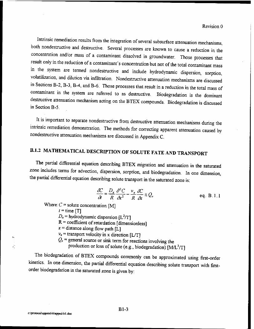
Revision 0
Intrinsic remediation results from the integration of several subsurface attenuation mechanisms
both nondestructive and destructive. Several processes are known to cause a reduction in the
concentration and/or mass of a contaminant dissolved in groundwater. Those processes that
result only in the reduction of a contaminant's concentration but not of the total contaminant mass
in the system are termed nondestructive and include hydrodynamic dispersion, sorption,
volatilization, and dilution via infiltration. Nondestructive attenuation mechanisms are discussed
in Sections B-2, B-3, B-4, and B-6. Those processes that result in a reduction in the total mass of
contaminant in the system are referred to as destructive. Biodegradation is the dominant
destructive attenuation mechanism acting on the BTEX compounds. Biodegradation is discussed in Section B-5.
It is important to separate nondestructive from destructive attenuation mechanisms during the
intrinsic remediation demonstration. The methods for correcting apparent attenuation caused by nondestructive attenuation mechanisms are discussed in Appendix C.
B.1.2 MATHEMATICAL DESCRIPTION OF SOLUTE FATE AND TRANSPORT
The partial differential equation describing BTEX migration and attenuation in the saturated
zone includes terms for advection, dispersion, sorption, and biodegradation. In one dimension,
the partial differential equation describing solute transport in the saturated zone is:
fc_Dxd1C vxcC,„
ä R ck\ ~R~fc±Q° eq.B.1.1
Where: C = solute concentration [M] / = time [T] Ac = hydrodynamic dispersion [L2/T] R = coefficient of retardation [dimensionless] x = distance along flow path [L] vx = transport velocity in x direction [L/T] Os = general source or sink term for reactions involving the
production or loss of solute (e.g., biodegradation) [M/L3/T]
The biodegradation of BTEX compounds commonly can be approximated using first-order
kinetics. In one dimension, the partial differential equation describing solute transport with first- order biodegradation in the saturated zone is given by:
Bl-3 c:\protocolVappcnd-b\appnd-bl .doc
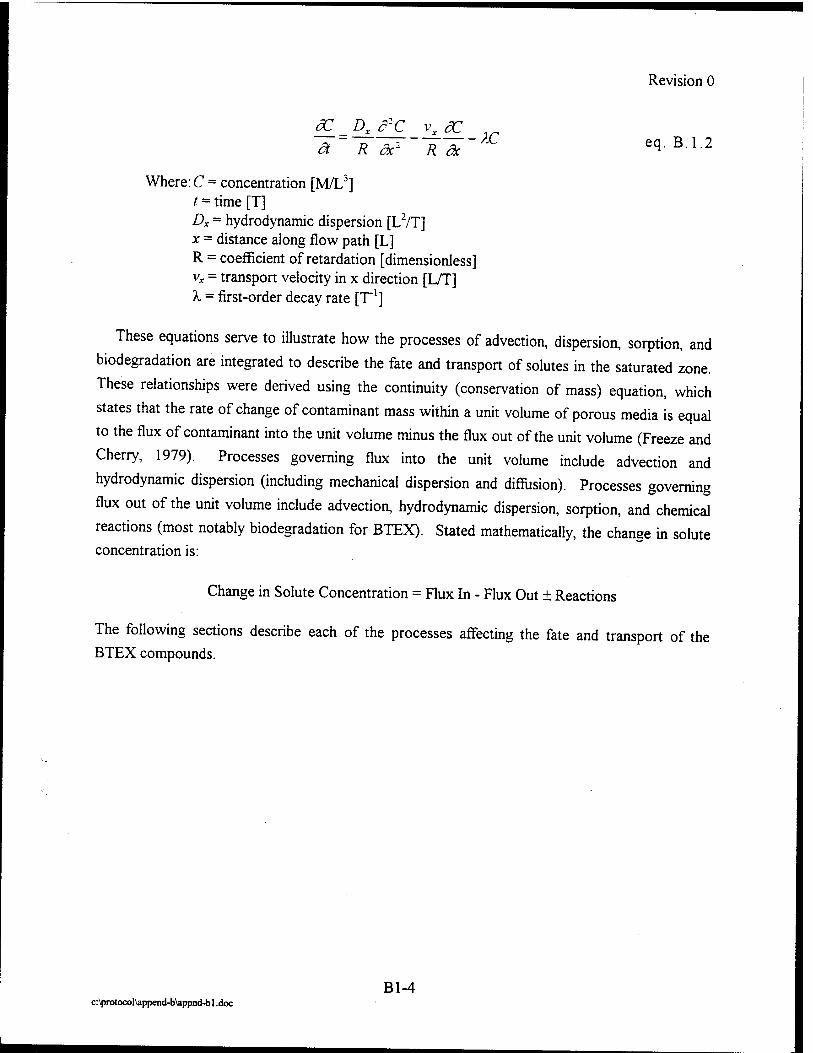
Revision 0
ac_Dx?c vxdc .r ä~ R &> R^~ÄC eq.B.1.2
Where: C = concentration [M/L3] t = time [T] Dx = hydrodynamic dispersion [L2/T] x = distance along flow path [L] R = coefficient of retardation [dimensionless] vx = transport velocity in x direction [L/T] X = first-order decay rate [T1]
These equations serve to illustrate how the processes of advection, dispersion, sorption, and
biodegradation are integrated to describe the fate and transport of solutes in the saturated zone.
These relationships were derived using the continuity (conservation of mass) equation, which
states that the rate of change of contaminant mass within a unit volume of porous media is equal
to the flux of contaminant into the unit volume minus the flux out of the unit volume (Freeze and
Cherry, 1979). Processes governing flux into the unit volume include advection and
hydrodynamic dispersion (including mechanical dispersion and diffusion). Processes governing
flux out of the unit volume include advection, hydrodynamic dispersion, sorption, and chemical
reactions (most notably biodegradation for BTEX). Stated mathematically, the change in solute concentration is:
Change in Solute Concentration = Flux In - Flux Out ± Reactions
The following sections describe each of the processes affecting the fate and transport of the BTEX compounds.
Bl-4 c:\protocol\append-b\appnd-bl.doc

Revision 0
SECTION B-2
ADVECTION
Advective transport is the transport of solutes by the bulk movement of groundwater.
Advection is the most important process driving contaminant migration in the subsurface. The
linear groundwater velocity in the direction parallel to groundwater flow caused by advection is given by:
KdH Vx=~VelE ec*B21
Where: v, = average linear velocity [L/T] K = hydraulic conductivity [L/T] ne = effective porosity [L3/L3] dH/dL = hydraulic gradient [L/L]
Solute transport by advection alone yields a sharp solute concentration front. Immediately
ahead of the front, the solute concentration is equal to the background concentration (generally
zero). Behind the advancing solute front, the concentration is equal to the initial contaminant
concentration at the point of release. This is referred to as plug flow and is illustrated in
Figures B.2.1, B.2.2, and B.2.3. In reality, the advancing front spreads out due to the processes
of dispersion and diffusion, as discussed in Section B-3, and is retarded by sorption and biodegradation, as discussed in Sections B-4 and B-5, respectively.
The one-dimensional advective transport component of the advection-dispersion equation is given by:
30 _ cC
Where: vx = average linear velocity [L/T] C = contaminant concentration [M/L3] t = time [T] x = distance along flow path [L]
B2-1 c:\protocoi\append-b\appnd-b2.doc

Revision 0
l.th
Contaminant front with advection only
U 'S g C/C0 0.5-j 'S <-> | — c I U O j
0.0-
Time or Distance from Source- ^>
Figure B.2.1 Breakthrough curve in one dimension showing plug flow with continuous source resulting from advection only.
« g o o
1.0-,
C/C„ 0.5
Contaminant front with advection only
0.0
Time or Distance from Source -5*-
Figure B.2.2 Breakthrough curve in one dimension showing plug flow with instantaneous source resulting from advection only.
This equation considers only advective transport of the solute. In some cases this may be a fair
approximation for simulating solute migration because advective transport is the main force
behind contaminant migration. However, because of dispersion, diffusion, sorption, and
biodegradation, this equation generally must be combined with the other components of the
modified advection-dispersion equation (equation B.l.l) to obtain an accurate mathematical
description of solute transport.
Groundwater Flow Direction
Source' «2
x,
Continuous Source
Instantaneous Source
Figure B.2.3 Plume migration in two dimensions (plan view) showing plume migration resulting from advective flow only with continuous and instantaneous sources.
B2-2 c:\protocol\append-b\appnd-b2.doc

Revision 0
SECTION B-3
HYDRODYNAMIC DISPERSION
Hydrodynamic dispersion, which includes mechanical dispersion and diffusion, is an important
process causing dilution of contaminants dissolved in groundwater. The following sections
describe these processes and how they are incorporated into the modified advection-dispersion
equation (Equation B. 1.1). Infiltration, another process that may cause dilution of contaminants, is discussed in Section B-6.
B.3.1 HYDRODYNAMIC DISPERSION
Hydrodynamic dispersion is the process whereby a contaminant plume spreads out in directions
that are longitudinal and transverse to the direction of plume migration. There are two
components of hydrodynamic dispersion; mechanical dispersion and molecular diffusion.
Hydrodynamic dispersion, D, is the sum of mechanical dispersion and molecular diffusion.
Mechanical dispersion is the dominant mechanism causing hydrodynamic dispersion at normal
groundwater velocities. At extremely low groundwater velocities, molecular diffusion can
become the dominant mechanism of hydrodynamic dispersion. Molecular diffusion is generally ignored for most groundwater studies.
B.3.1.1 Mechanical Dispersion
Three processes are responsible for mechanical dispersion (Figure B.3.1). The first process is
the variation in flow velocity through pores of various sizes. As groundwater flows through a
porous medium, it flows more slowly through large pores than through smaller pores. The
second cause of mechanical dispersion is tortuosity, or flow path length. As groundwater flows
through a porous medium, some of the groundwater follows less tortuous (shorter) paths, while
some of the groundwater takes more tortuous (longer) paths. The longer the flow path, the
slower the average linear velocity of the groundwater and the dissolved contaminant. The final
process causing mechanical dispersion is variable friction within an individual pore. Groundwater
traveling close to the center of a pore experiences less friction than groundwater traveling next to
B3-1 c:\protocol\append-b\appncUb3.doc
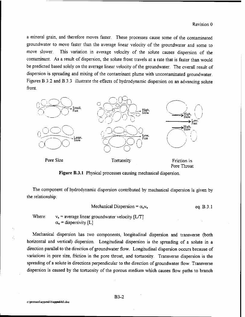
Revision 0
a mineral grain, and therefore moves faster. These processes cause some of the contaminated
groundwater to move faster than the average linear velocity of the groundwater and some to
move slower. This variation in average velocity of the solute causes dispersion of the
contaminant. As a result of dispersion, the solute front travels at a rate that is faster than would
be predicted based solely on the average linear velocity of the groundwater. The overall result of
dispersion is spreading and mixing of the contaminant plume with uncontaminated groundwater.
Figures B.3.2 and B.3.3 illustrate the effects of hydrodynamic dispersion on an advancing solute
front.
Qi \
. Small, Fast
0 i. i
Ö. ^ -\ -ksr-
Pore Size
Slow
/ \ I I
. Low, Fast
*&-.
u
Friction in Pore Throat
Figure B.3.1 Physical processes causing mechanical dispersion.
The component of hydrodynamic dispersion contributed by mechanical dispersion is given by
the relationship:
Mechanical Dispersion = axvx
Where: vx = average linear groundwater velocity [L/T] ax = dispersivity [L]
eq. B.3.1
Mechanical dispersion has two components, longitudinal dispersion and transverse (both
horizontal and vertical) dispersion. Longitudinal dispersion is the spreading of a solute in a
direction parallel to the direction of groundwater flow. Longitudinal dispersion occurs because of
variations in pore size, friction in the pore throat, and tortuosity. Transverse dispersion is the
spreading of a solute in directions perpendicular to the direction of groundwater flow. Transverse
dispersion is caused by the tortuosity of the porous medium which causes flow paths to branch
B3-2 c:\protocol\append-b\appnd-b3.doc
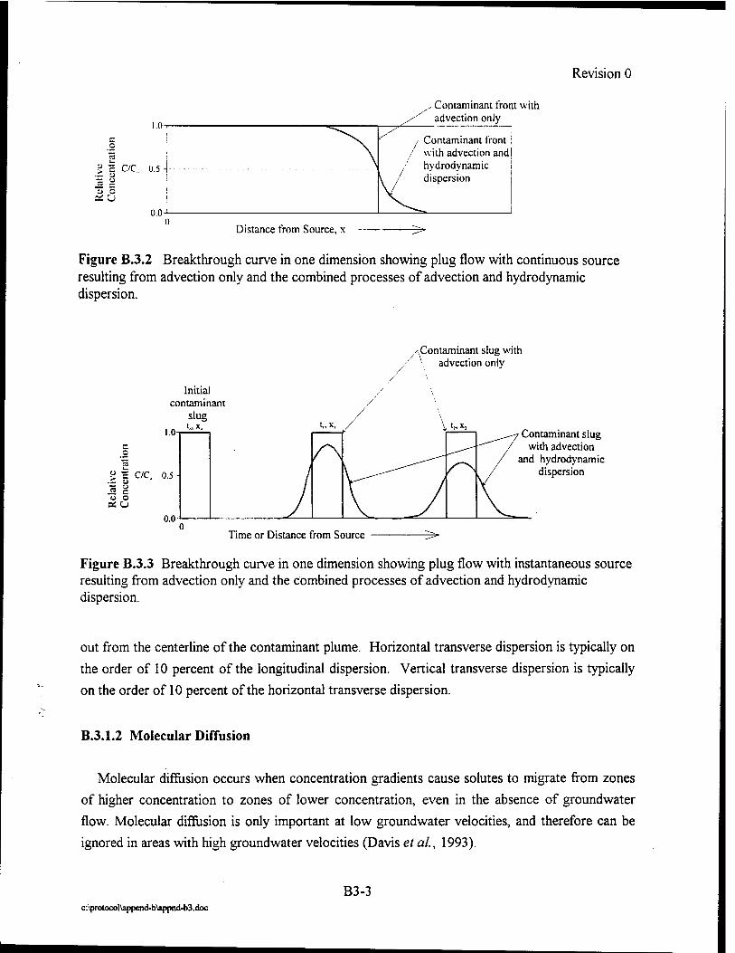
Revision 0
> =
U C as U
1.0
C7C. 0.5 -1
0.0-
„- Contaminant front with advection only
Contaminant front with advection and hydrodynamic dispersion
Distance from Source, x ^>
Figure B.3.2 Breakthrough curve in one dimension showing plug flow with continuous source resulting from advection only and the combined processes of advection and hydrodynamic dispersion.
/ \ Contaminant slug with
advection only
Initial contaminant
slug 1.0
t = C/C„
o o ai U
Contaminant slug with advection
and hydrodynamic dispersion
Time or Distance from Source
Figure B.3.3 Breakthrough curve in one dimension showing plug flow with instantaneous source resulting from advection only and the combined processes of advection and hydrodynamic dispersion.
out from the centerline of the contaminant plume. Horizontal transverse dispersion is typically on
the order of 10 percent of the longitudinal dispersion. Vertical transverse dispersion is typically
on the order of 10 percent of the horizontal transverse dispersion.
B.3.1.2 Molecular Diffusion
Molecular diffusion occurs when concentration gradients cause solutes to migrate from zones
of higher concentration to zones of lower concentration, even in the absence of groundwater
flow. Molecular diffusion is only important at low groundwater velocities, and therefore can be
ignored in areas with high groundwater velocities (Davis et ai, 1993).
B3-3 c:\protocol\append-b\appnd-b3.doc
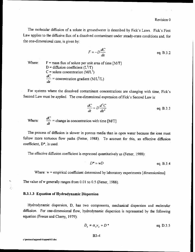
Revision 0
The molecular diffusion of a solute in groundwater is described by Fick's Laws. Fick's First
Law applies to the diffusive flux of a dissolved contaminant under steady-state conditions and, for
the one-dimensional case, is given by:
F = -D— eq. B.3.2 dx
Where: F = mass flux of solute per unit area of time [M/T] D = diffusion coefficient (L2/T) C = solute concentration (M/L3) dC , — = concentration gradient (M/L /L) dx
For systems where the dissolved contaminant concentrations are changing with time, Fick's
Second Law must be applied. The one-dimensional expression of Fick's Second Law is:
dC „d2C -*=»-& eq.B.3.3
Where: — = change in concentration with time [M/T]
The process of diffusion is slower in porous media than in open water because the ions must
follow more tortuous flow paths (Fetter, 1988). To account for this, an effective diffusion
coefficient, D*, is used.
The effective diffusion coefficient is expressed quantitatively as (Fetter, 1988):
D* = wD eq. B.3.4
Where: w = empirical coefficient determined by laboratory experiments [dimensionless]
The value of w generally ranges from 0.01 to 0.5 (Fetter, 1988).
B.3.1.3 Equation of Hydrodynamic Dispersion
Hydrodynamic dispersion, D, has two components, mechanical dispersion and molecular
diffusion. For one-dimensional flow, hydrodynamic dispersion is represented by the following
equation (Freeze and Cherry, 1979):
Dx=axvx+D* eq. D.3.5
B3-4 c:\protocol\append-b\appnd-b3.doc

Revision 0
Where: Dx = longitudinal coefficient of hydrodynamic dispersion in the x direction [L2/T] ax = longitudinal dispersivity [L] vx = average linear groundwater velocity [L/T] D* = effective molecular diffusion [L2/T]
Dispersivity is a parameter that is characteristic of the porous medium through which the
contaminant migrates. Dispersivity represents the spreading of a contaminant over a given length
of flow, and therefore has units of length. Several approaches can be used to estimate
longitudinal dispersivity, a*. One technique involves conducting a tracer test. Although this is
potentially the most reliable method, time and monetary constraints can be prohibitive. Another
method commonly used to estimate dispersivity when implementing a solute transport model is to
start with a longitudinal dispersivity of 0.1 times the plume length (Lallemand-Barres and
Peaudecerf, 1978). Some solute transport modelers will start with an accepted literature value for
the types of materials found in the aquifer matrix. After selecting an initial dispersivity, the
contaminant transport model is calibrated by adjusting the dispersivity within the range of
accepted literature values until the modeled and observed contaminant distribution patterns match
(Anderson, 1979). This is a two-step process. The first step is to calibrate the flow model to the
hydraulic conditions present at the site. After the groundwater flow model is calibrated to the
hydraulics of the system, the contaminant transport model is calibrated by trial and error using
various values for dispersivity. There is no unique solution because several parameters, including
hydraulic conductivity, effective porosity, and dispersivity, are variable within the flow system
(Anderson, 1979; Davis et al, 1993). Table B.3.1 presents commonly accepted literature values
for hydrodynamic dispersion.
The dispersion of organic solutes in an aquifer is an important consideration when modeling
intrinsic remediation because the dispersion of a contaminant into relatively pristine portions of
the aquifer allows the solute to admix with more electron acceptors crossgradient to the direction
of groundwater flow.
Table B.3.1 Accepted Literature Values of Dispersivity for Alluvial Sediments (From Walton, 1988)
Aquifer Matrix Method of Measurement
Longitudinal Dispersivity (m)
Transverse Dispersivity (m)
Alluvial Sediments Single Well Test 0.03 to 7 0.009 to 1 Alluvial Sediments Two Well Test 0.1 to 15 Alluvial Sediments Areal Model 12 to 61 4 to 30
c:\protocol\append-b\appnd-b3.doc
B3-5
Revision 0
B.3.2 ONE-DIMENSIONAL ADVECTION-DISPERSION EQUATION
The advection-dispersion equation is obtained by adding hydrodynamic dispersion to equation
B.2.2. In one dimension, the advection-dispersion equation is given by:
cC _. d2C dC ,, — = Dx —— ~ v —- eq. B.3.6 ä ax' ax
Where: vx = average linear velocity [L/T] C = contaminant concentration [M/L3] Dx = hydrodynamic dispersion [L2/T] t = time [T] x = distance along flow path [L]
This equation considers both advection and hydrodynamic dispersion. Because of sorption and
biodegradation, this equation generally must be combined with the other components of the
modified advection-dispersion equation presented as equation B.l.l to obtain an accurate
mathematical description of solute transport.
B3-6 c:\protocol\append-b\appnd-b3.doc
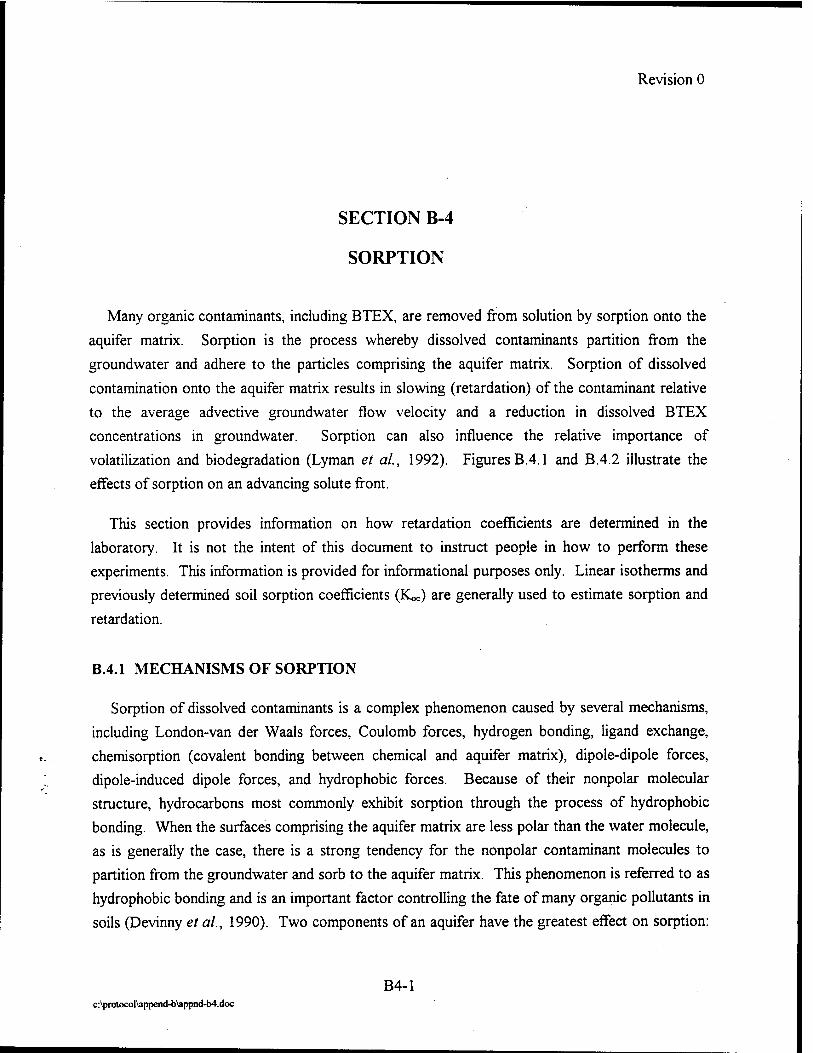
Revision 0
SECTION B-4
SORPTION
Many organic contaminants, including BTEX, are removed from solution by sorption onto the
aquifer matrix. Sorption is the process whereby dissolved contaminants partition from the
groundwater and adhere to the particles comprising the aquifer matrix. Sorption of dissolved
contamination onto the aquifer matrix results in slowing (retardation) of the contaminant relative
to the average advective groundwater flow velocity and a reduction in dissolved BTEX
concentrations in groundwater. Sorption can also influence the relative importance of
volatilization and biodegradation (Lyman et ai, 1992). Figures B.4.1 and B.4.2 illustrate the
effects of sorption on an advancing solute front.
This section provides information on how retardation coefficients are determined in the
laboratory. It is not the intent of this document to instruct people in how to perform these
experiments. This information is provided for informational purposes only. Linear isotherms and
previously determined soil sorption coefficients (K«) are generally used to estimate sorption and
retardation.
B.4.1 MECHANISMS OF SORPTION
Sorption of dissolved contaminants is a complex phenomenon caused by several mechanisms,
including London-van der Waals forces, Coulomb forces, hydrogen bonding, ligand exchange,
chemisorption (covalent bonding between chemical and aquifer matrix), dipole-dipole forces,
dipole-induced dipole forces, and hydrophobic forces. Because of their nonpolar molecular
structure, hydrocarbons most commonly exhibit sorption through the process of hydrophobic
bonding. When the surfaces comprising the aquifer matrix are less polar than the water molecule,
as is generally the case, there is a strong tendency for the nonpolar contaminant molecules to
partition from the groundwater and sorb to the aquifer matrix. This phenomenon is referred to as
hydrophobic bonding and is an important factor controlling the fate of many organic pollutants in
soils (Devinny et al., 1990). Two components of an aquifer have the greatest effect on sorption:
B4-1 o:\protocol\append-b\appnd-M.doc
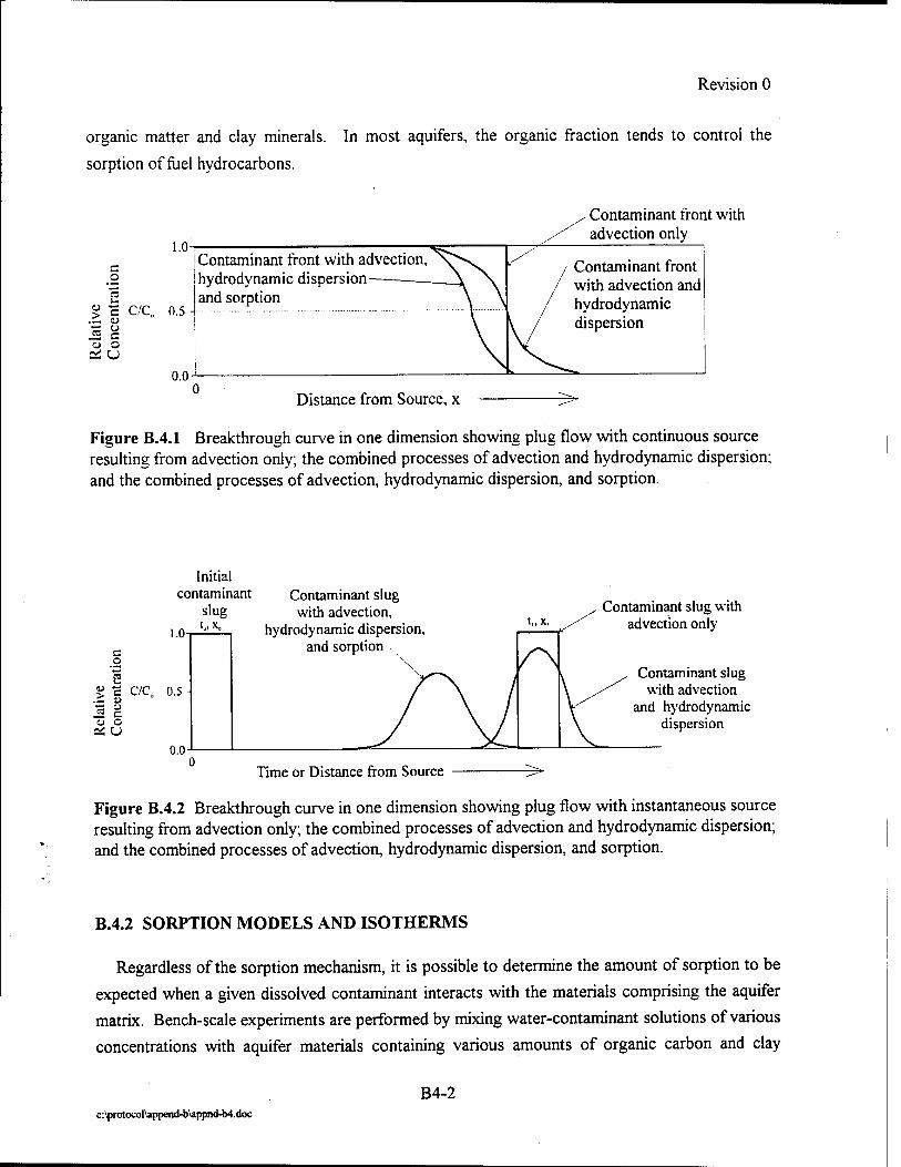
Revision 0
organic matter and clay minerals. In most aquifers, the organic fraction tends to control the
sorption of fuel hydrocarbons.
l.o-
Contaminant front with advection only
c o
C/C„ 0.5 -
Contaminant front with advection, hydrodynamic dispersion and sorption
0.0
Contaminant front / with advection and
hydrodynamic dispersion
Distance from Source, x
Figure B.4.1 Breakthrough curve in one dimension showing plug flow with continuous source resulting from advection only; the combined processes of advection and hydrodynamic dispersion; and the combined processes of advection, hydrodynamic dispersion, and sorption.
Initial contaminant
slug I .On
t„. x„
c .2 ■*—'
> c .z. u 1 c «J o Si U
C7C„ 0.5-
0.0
Contaminant slug with advection,
hydrodynamic dispersion and sorption
\
Contaminant slug with advection only
Contaminant slug with advection
and hydrodynamic dispersion
Time or Distance from Source
Figure B.4.2 Breakthrough curve in one dimension showing plug flow with instantaneous source resulting from advection only; the combined processes of advection and hydrodynamic dispersion; and the combined processes of advection, hydrodynamic dispersion, and sorption.
B.4.2 SORPTION MODELS AND ISOTHERMS
Regardless of the sorption mechanism, it is possible to determine the amount of sorption to be
expected when a given dissolved contaminant interacts with the materials comprising the aquifer
matrix. Bench-scale experiments are performed by mixing water-contaminant solutions of various
concentrations with aquifer materials containing various amounts of organic carbon and clay
B4-2 c:\protocol\append-b\appnd-b4.doc

Revision 0
minerals. The solutions are then sealed with no headspace and left until equilibrium between the
various phases is reached. The amount of contaminant left in solution is then measured.
Both environmental conservative isotherms (ECI) and constant soil to solution isotherms (CSI)
can be generated. The ECI study uses the same water concentration but changes the soil to water
ratio. In CSI isotherm studies the concentration of contaminant in water is varied while the
amount of water and sediment is constant. In some instances, actual contaminated water from the
site is added. Typically the samples are continually rotated and concentrations measured with
time to document equilibrium. True equilibrium may require hundreds of hours of incubation but
80 to 90 percent of equilibrium may be achieved in one or two days.
The results are commonly expressed as a plot of the concentration of chemical sorbed (ug/g)
versus the concentration remaining in solution (ug/L). The relationship between the
concentration of chemical sorbed (Ca) and the concentration remaining in solution (Q) at
equilibrium is referred to as the sorption isotherm because the experiments are performed at
constant temperature.
Sorption isotherms generally exhibit one of three characteristic shapes depending on the
sorption mechanism. These isotherms are referred to as the Langmuir isotherm, the Freundlich
isotherm, and the linear isotherm (a special case of the Freundlich isotherm). Each of these
sorption isotherms, and related equations, are discussed in the following sections.
B.4.2.1 Langmuir Sorption Model
The Langmuir model describes sorption in solute transport systems wherein the sorbed
concentration increases linearly with increasing solute concentration at low concentrations and
approaches a constant value at high concentrations. The sorbed concentration approaches a
constant value because there are a limited number of sites on the aquifer matrix available for
contaminant sorption. This relationship is illustrated in Figure B.4.3. The Langmuir equation is
described mathematically as (Devinney et ai, 1990):
_ KC.b -. . . ^ - '- eq. B.4.1
l + KC,
Where: Ca = sorbed contaminant concentration (mass contaminant/mass soil) K = equilibrium constant for the sorption reaction (ug/g) Q = dissolved contaminant concentration (ug/ml) b = number of sorption sites (maximum amount of sorbed contaminant)
B4-3 c:\protocol\append-b\appnd-b4.doc

Revision 0
The Langmuir model is appropriate for highly specific sorption mechanisms where there are a
limited number of sorption sites. This model predicts a rapid increase in the amount of sorbed
contaminant as contaminant concentrations increase in a previously pristine area. As sorption
sites become filled, the amount of sorbed contaminant reaches a maximum level equal to the
number of sorption sites, b.
to "a
u
e z> U "3
Langmuir
Dissolved Concentration C, (fig/ml)
Figure B.4.3 Characteristic adsorption isotherm shapes.
B.4.2.2 Freundlich Sorption Model
The Langmuir isotherm model can be modified if the number of sorption sites is large (assumed
infinite) relative to the number of contaminant molecules. This is generally a valid assumption for
dilute solutions (e.g., downgradient from a petroleum hydrocarbon spill in the dissolved BTEX
plume) where the number of unoccupied sorption sites is large relative to contaminant
concentrations. The Freundlich model is expressed mathematically as (Devinny et al, 1990):
Where: Kj- C a Q= n =
Ca = K,C, l/n eq. B.4.2
distribution coefficient sorbed contaminant concentration (mass contaminant/mass soil, u.g/g) dissolved concentration (mass contaminant/volume solution, (ug/ml) chemical-specific coefficient
B4-4 c:\protocol\append-b\appnd-b4.doc
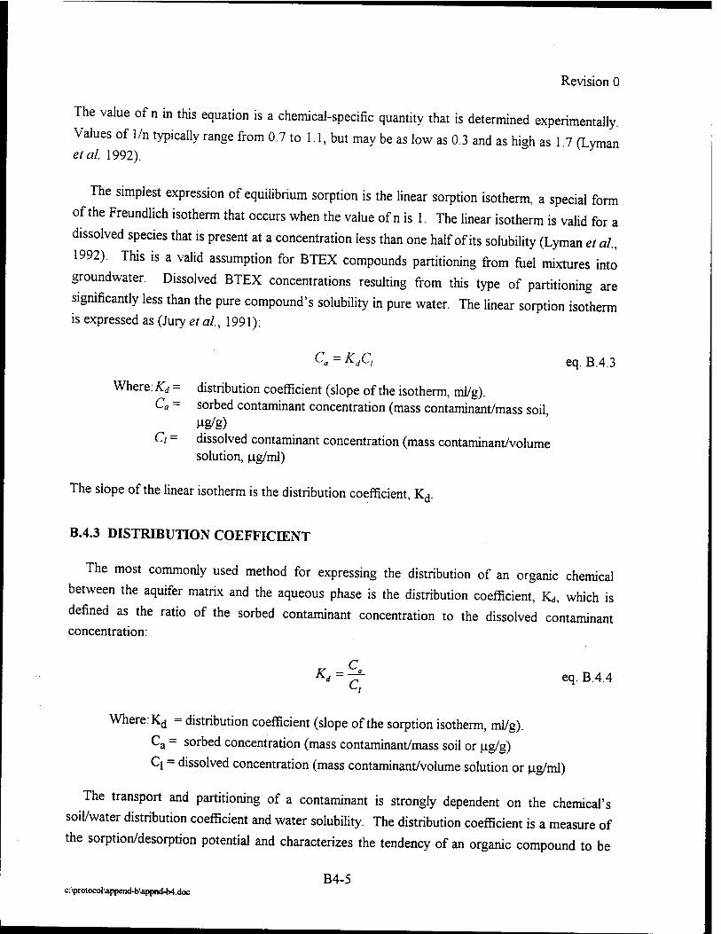
Revision 0
The value of n in this equation is a chemical-specific quantity that is determined experimentally.
Values of 1/n typically range from 0.7 to 1.1, but may be as low as 0.3 and as high as 1 7 (Lyman etal. 1992).
The simplest expression of equilibrium sorption is the linear sorption isotherm, a special form
of the Freundlich isotherm that occurs when the value of n is 1. The linear isotherm is valid for a
dissolved species that is present at a concentration less than one half of its solubility (Lyman et al,
1992). This is a valid assumption for BTEX compounds partitioning from fuel mixtures into
groundwater. Dissolved BTEX concentrations resulting from this type of partitioning are
significantly less than the pure compound's solubility in pure water. The linear sorption isotherm is expressed as (Jury et al., 1991):
Ca ~ KdC, eq B.4.3
Where: Kd = distribution coefficient (slope of the isotherm, ml/g). Ca = sorbed contaminant concentration (mass contaminant/mass soil,
ug/g) Ci = dissolved contaminant concentration (mass contaminant/volume
solution, u.g/ml)
The slope of the linear isotherm is the distribution coefficient, Kd.
B.4.3 DISTRIBUTION COEFFICIENT
The most commonly used method for expressing the distribution of an organic chemical
between the aquifer matrix and the aqueous phase is the distribution coefficient, Kd, which is
defined as the ratio of the sorbed contaminant concentration to the dissolved contaminant concentration:
C Kj = -f- eq. B.4.4
^/
Where: Kd = distribution coefficient (slope of the sorption isotherm, ml/g).
Ca = sorbed concentration (mass contaminant/mass soil or ug/g)
Ci = dissolved concentration (mass contaminant/volume solution or ug/ml)
The transport and partitioning of a contaminant is strongly dependent on the chemical's
soil/water distribution coefficient and water solubility. The distribution coefficient is a measure of
the sorption/desorption potential and characterizes the tendency of an organic compound to be
B4-5 c:\protocol\append-b\appnd-b4.doc
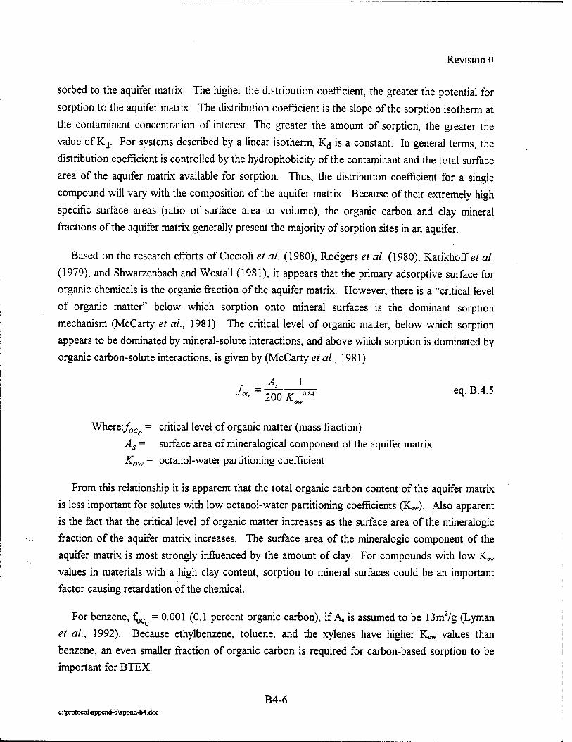
Revision 0
sorbed to the aquifer matrix. The higher the distribution coefficient, the greater the potential for
sorption to the aquifer matrix. The distribution coefficient is the slope of the sorption isotherm at
the contaminant concentration of interest. The greater the amount of sorption, the greater the
value of Kd. For systems described by a linear isotherm, Kd is a constant. In general terms, the
distribution coefficient is controlled by the hydrophobicity of the contaminant and the total surface
area of the aquifer matrix available for sorption. Thus, the distribution coefficient for a single
compound will vary with the composition of the aquifer matrix. Because of their extremely high
specific surface areas (ratio of surface area to volume), the organic carbon and clay mineral
fractions of the aquifer matrix generally present the majority of sorption sites in an aquifer.
Based on the research efforts of Ciccioli et al. (1980), Rodgers et al. (1980), Karikhoff et al.
(1979), and Shwarzenbach and Westall (1981), it appears that the primary adsorptive surface for
organic chemicals is the organic fraction of the aquifer matrix. However, there is a "critical level
of organic matter" below which sorption onto mineral surfaces is the dominant sorption
mechanism (McCarty et al, 1981). The critical level of organic matter, below which sorption
appears to be dominated by mineral-solute interactions, and above which sorption is dominated by
organic carbon-solute interactions, is given by (McCarty et al, 1981)
As 1 /oc< " 200 K °84 eq- BA5
ow
Where :foc = critical level of organic matter (mass fraction) 'C
As = surface area of mineralogical component of the aquifer matrix
Kow = octanol-water partitioning coefficient
From this relationship it is apparent that the total organic carbon content of the aquifer matrix
is less important for solutes with low octanol-water partitioning coefficients (KoW). Also apparent
is the fact that the critical level of organic matter increases as the surface area of the mineralogic
fraction of the aquifer matrix increases. The surface area of the mineralogic component of the
aquifer matrix is most strongly influenced by the amount of clay. For compounds with low K^
values in materials with a high clay content, sorption to mineral surfaces could be an important
factor causing retardation of the chemical.
For benzene, f^ = 0.001 (0.1 percent organic carbon), if A, is assumed to be 13m2/g (Lyman
et al., 1992). Because ethylbenzene, toluene, and the xylenes have higher Kow values than
benzene, an even smaller fraction of organic carbon is required for carbon-based sorption to be
important for BTEX.
B4-6 c:\protocoI\append-b\appnd-b4.doc

Revision 0
Several researchers have found that if the distribution coefficient is normalized relative to the
aquifer matrix total organic carbon content, much of the variation in observed K, values between
different soils is eliminated (Dragun, 1988). Distribution coefficients normalized to total organic
carbon content are expressed as K«. The following equation gives the expression relating K, to Koc.
K. =^- eq. B.4.6 f<
Where:Koc = soil sorption coefficient normalized for total organic carbon content Kd = distribution coefficient foe =. fraction total organic carbon (mg organic carbon/mg soil)
In areas with high clay concentrations and low total organic carbon concentrations, the clay
minerals become the dominant sorption sites. Under these conditions, the use of K« to compute
Kd might result in underestimating the importance of sorption in retardation calculations, a source
of error that will make retardation calculations based on the total organic carbon content of the
aquifer matrix more conservative. In fact, aquifers that have a high enough hydraulic conductivity
to spread hydrocarbon contamination generally have low clay content. In these cases, the
contribution of sorption to mineral surfaces is generally trivial.
Earlier investigations reported distribution coefficients normalized to total organic matter
content (K™). The relationship between fom and k is nearly constant and, assuming that the
organic matter contains approximately 58 percent carbon (Lyman et al, 1992):
Koc = \.12AKom eq.B.4.7
B.4.4 COEFFICIENT OF RETARDATION
As mentioned earlier, sorption tends to slow the transport velocity of contaminants dissolved in
groundwater. The coefficient of retardation, R is used to estimate the retarded contaminant
velocity. The coefficient of retardation for linear sorption is determined from the distribution coefficient using the relationship:
Ä = l+^ eq. B.4.8
Where: R = coefficient of retardation [dimensionless] pb = bulk density of aquifer [M/L3]
B4-7 c:\protocol\append-b\appnd-b4.doc
Revision 0
Kd = distribution coefficient [L^/M] n = porosity [IZ/IZ]
The retarded contaminant transport velocity, vc, is given by:
vc = ^- eq. B.4.9
Where: vc = retarded contaminant transport velocity [L/T] Vj = advective groundwater velocity [L/T] R = coefficient of retardation [dimensionless]
Two methods used to quantify the distribution coefficient and amount of sorption (and thus
retardation) for a given aquifer/contaminant system are presented below. The first method
involves estimating the distribution coefficient by using Koc for the contaminants and the fraction
of organic carbon comprising the aquifer matrix. The second method involves conducting batch
or column tests to determine the distribution coefficient. Because numerous authors have
conducted experiments to determine K« values for common contaminants, literature values are
reliable, and it generally is not necessary to conduct laboratory tests.
B.4.4.1 Determining the Coefficient of Retardation using K«
Batch and column tests have been performed for a wide range of contaminant types and
concentrations and aquifer conditions. Numerous studies have been performed using the results
of these tests to determine if relationships exist that are capable of predicting the sorption
characteristics of a chemical based on easily measured parameters. The results of these studies
indicate that the amount of sorption is strongly dependent on the amount of organic carbon
present in the aquifer matrix and the degree of hydrophobicity exhibited by the contaminant
(Bailey and White, 1970; Karickhoff <?/ al., 1979; Kenaga and Goring, 1980; Brown and Flagg,
1981; Schwarzenbach and Westall, 1981; Hassett et al., 1983; Chiou et al, 1983). These
researchers observed that the distribution coefficient, Kd, was proportional to the organic carbon
fraction of the aquifer times a proportionality constant. This proportionality constant, K«, is
defined as given by equation B.4.6. In effect, equation B.4.6 normalizes the distribution
coefficient to the amount of organic carbon in the aquifer matrix. Because it is normalized to
organic carbon, values of K« are dependent only on the properties of the compound (not on the
type of soil). Values of Koc have been determined for a wide range of chemicals. Table B.4.1 lists
Koc values for BTEX and trimethylbenzene.
B4-8 c:\protocol\append-b\appnd-b4.doc
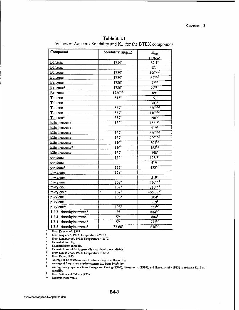
Revision 0
Table B.4.1 Values of Aqueous Solubility and KoC for the BTEX compounds
Compound Solubility (mg/L) Koc
Benzene 1750" 87. r Benzene 83" Benzene 1780° 190cd.f
Benzene 1780° 62c=.t
Benzene 1780h 72h"' Benzene* 1780h 79ho.-
Benzene 1780c,h 89k
Toluene 515a 151a
Toluene 303b
Toluene 537c 3g0cd,t
Toluene 537c 110c..i
Toluene* 537c 190^* Ethvlbenzene 152" 158.5a
Ethvlbenzene 519b
Ethylbenzene 167° 680cA1
Ethvlbenzene 167c 200cef
Ethvlbenzene 140h soi"-1
Ethylbenzene* 140h 468^ Ethvlbenzene 167c 398k
o-xvlene 152a 128.8" o-xvlene 519b
o-xylene* 152a 422"-" m-xylene 158a
m-xvlene 519b
m-xylene 162c 720Cl<u
m-xvlene 162c 210c,=.i
m-xylene* 162c 405.37k/
p-xylene 198a 204a
p-xylene 519b
p-xylene* 198a 357"-" 1.2,3 -trimethylbenzene* 75 884b'* 1,2,4-trimethylbenzene 591 884b
1,2,4-trimethylbenzene* 59' 772^" 1,3,5-trimethylbenzene* 72.60« 676*-* From Knox et ai, 1993 From Jeng et ai, 1992; Temperature = 20°C From Lyman et ai, 1992; Temperature = 25°C Estimated from Ko, Estimated from solubility Estimate from solubility generally considered more reliable From Lyman et ai, 1992; Temperature = 20°C From Fetter, 1993 Average of 12 equations used to estimate K« from K<,wor Kom Average of 5 equations used to estimate K« from Solubility Average using equations from Kanaga and Goring (1980), Means et al. (1980), and Hassett et al. (1983) to estimate IC* from solubility From Sutton and Calder (1975) Recommended value
c:\protocol\append-b\appnd-b4.doc
B4-9
Revision 0
By knowing the value of K« for a contaminant and the fraction of organic carbon present in
the aquifer, the distribution coefficient can be determined by using the relationship:
Kd = K-oJoc eq. B.4.10
When using the method presented in this section to predict sorption of the BTEX compounds,
total organic carbon concentrations obtained from the most transmissive aquifer zone should be
averaged and used for predicting sorption. This is because the majority of dissolved contaminant
transport occurs in the most transmissive portions of the aquifer. In addition, because the most
transmissive aquifer zones generally have the lowest total organic carbon concentrations, the use
of this value will give a conservative prediction of contaminant sorption and retardation. '
B.4.4.2 Determining the Coefficient of Retardation using Laboratory Tests
The distribution coefficient may be quantified in the laboratory using batch or column tests.
Batch tests are easier to perform than column tests. Although more difficult to perform, column
tests generally produce a more accurate representation of field conditions than batch tests because
continuous flow is involved. Knox et al. (1993) suggest using batch tests as a preliminary
screening tool, followed by column studies to confirm the results of batch testing. The authors of
this document feel that batch tests, if conducted properly, will yield sufficiently accurate results
for fate and transport modeling purposes provided that sensitivity analyses for retardation are conducted during the modeling.
Batch testing involves adding uncontaminated aquifer material to a number of vessels, adding
solutions prepared using uncontaminated groundwater from the site mixed with various amounts
of contaminants to produce varying solute concentrations, sealing the vessel and shaking it until
equilibrium is reached, analyzing the solute concentration remaining in solution, and calculating
the amount of contaminant sorbed to the aquifer matrix using mass balance calculations. A plot
of the concentration of contaminant sorbed versus dissolved equilibrium concentration is then
made using the data for each reaction vessel. The slope of the line formed by connecting each
data point is the distribution coefficient. The temperature should be held constant during the batch
test, and should approximate that of the aquifer system through which solute transport is taking place.
Table B.4.2 contains data from a hypothetical batch test. These data are plotted (Figure B.4.4)
to obtain an isotherm unique to the aquifer conditions at the site. A regression analysis can then
be performed on these data to determine the distribution coefficient. For linear isotherms, the
B4-10 c:\protocol\append-b\appnd-M.doc

Revision 0
distribution coefficient is simply the slope of the isotherm. In this example, Kd = 0.0146 L/g.
Batch-testing procedures are described in detail by Roy et al. (1992).
Initial Concentration (Hg/L)
Table B.4.2
Data from Hypothetical Batch Test Experiment
250 500 1000 1500 2000 3800
6000 9000
Equilibrium Concentration
77.3 150.57 297.04 510.1
603.05 1198.7 2300.5 3560.7
Weight of Solid Matrix (g)
20.42 20.42 20.42 20.42 20.42
20.42 20.42 20.42
Sorbed Concentration* (jig/g)
1.69 3.42 6.89 9.70 13.68 25.48 36.23 53.27
♦Adsorbed Concentration = ((Initial Concentration-Equilibrium Concentration)* Volume of Solution)/Weight of Solid Matrix
Column testing involves placing uncontaminated aquifer matrix material in a laboratory column
and passing solutions through the column. Solutions are prepared by mixing uncontaminated
groundwater from the site with the contaminants of interest and a conservative tracer. Flow rate
and time are accounted for and samples are periodically taken from the effluent end of the column
and analyzed to determine contaminant and tracer concentrations. Breakthrough curves are
prepared for the contaminants by plotting chemical concentration versus time (or relative
concentration versus number of pore volumes). The simplest way to determine the coefficient of
retardation (or the distribution coefficient) from the breakthrough curves is to determine the time
required for the effluent concentration to equal 0.5 of the influent concentration. This value can
be used to determine average velocity of the center of mass of the contaminant. The retardation
factor is determined by dividing the average flow velocity through the column by the velocity of
the center of mass of the contaminant. The value thus obtained is the retardation factor. The
coefficient of retardation also can be determined by curve fitting using the CXTFIT model of
Parker and van Genuchten (1984). Breakthrough curves also can be made for the conservative
tracer. These curves can be used to determine the coefficient of dispersion by curve fitting using the model of Parker and van Genuchten (1984).
When using the method presented in this section to predict sorption of the BTEX compounds,
aquifer samples should be obtained from the most transmissive aquifer zone. This is because the
majority of dissolved contaminant transport occurs in the most transmissive portions of the
aquifer. In addition, because the most transmissive aquifer zones generally have the lowest
B4-11 c:\protocol\append-b\appnd-b4.doc

Revision 0
organic carbon concentrations, the use of these materials will give a conservative prediction of contaminant sorption and retardation.
0 1000 2000 3000 4000 Equilibrium Concentration (ug/L)
Figure B.4.4 Plot of sorbed concentration vs. equilibrium concentration.
B.4.5 ONE-DIMENSIONAL ADVECTION-DISPERSION EQUATION WITH RETARDATION
The advection-dispersion equation is obtained by adding hydrodynamic dispersion to equation
B.2.2. In one dimension, the advection-dispersion equation is given by:
eq. B.4.11 udC d2C dC K— = ux —-— v —
ft cx~ x 3c
Where: vx = average linear velocity groundwater velocity [L/T] R = coefficient of retardation [dimensionless] C = contaminant concentration [M/L3] Dx = hydrodynamic dispersion [L2/T] / = time [T] x = distance along flow path [L]
This equation considers advection, hydrodynamic dispersion, and sorption (retardation).
Because of biodegradation, this equation generally must be combined with the other components
of the modified advection-dispersion equation, presented as equation B. 1.1, to obtain an accurate mathematical description of solute transport.
B4-12 c:\protocol\append-b\appnd-b4.doc
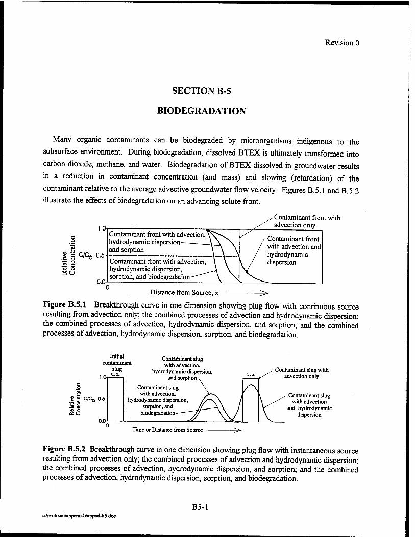
Revision 0
SECTION B-5
BIODEGRADATION
Many organic contaminants can be biodegraded by microorganisms indigenous to the
subsurface environment. During biodegradation, dissolved BTEX is ultimately transformed into
carbon dioxide, methane, and water. Biodegradation of BTEX dissolved in groundwater results
in a reduction in contaminant concentration (and mass) and slowing (retardation) of the
contaminant relative to the average advective groundwater flow velocity. Figures B.5.1 and B.5.2
illustrate the effects of biodegradation on an advancing solute front.
1.0 c o
g» c C/C0 0.5
u o
0.0
Contaminant front with advection, hydrodynamic dispersion and sorption
Contaminant front with advection, hydrodynamic dispersion, sorption, and biodegradation
- Contaminant front with advection only
Contaminant front with advection and hydrodynamic dispersion
Distance from Source, x -=>
Figure B.5.1 Breakthrough curve in one dimension showing plug flow with continuous source resulting from advection only; the combined processes of advection and hydrodynamic dispersion; the combined processes of advection, hydrodynamic dispersion, and sorption; and the combined processes of advection, hydrodynamic dispersion, sorption, and biodegradation.
Initial contaminant
slug 1.0
C/CQ 0.5-
u o « U
0.O
Contaminant slug with advection,
hydrodynamic dispersion, and sorption
Contaminant slug with advection,
hydrodynamic dispersion, sorption, and
biodegradation
Time or Distance from Source
Contaminant slug with advection only
Contaminant slug with advection
and hydrodynamic dispersion
-S>
Figure B.5.2 Breakthrough curve in one dimension showing plug flow with instantaneous source resulting from advection only; the combined processes of advection and hydrodynamic dispersion; the combined processes of advection, hydrodynamic dispersion, and sorption; and the combined processes of advection, hydrodynamic dispersion, sorption, and biodegradation.
B5-1 c:\protocol\append-b\appnd-b5.doc
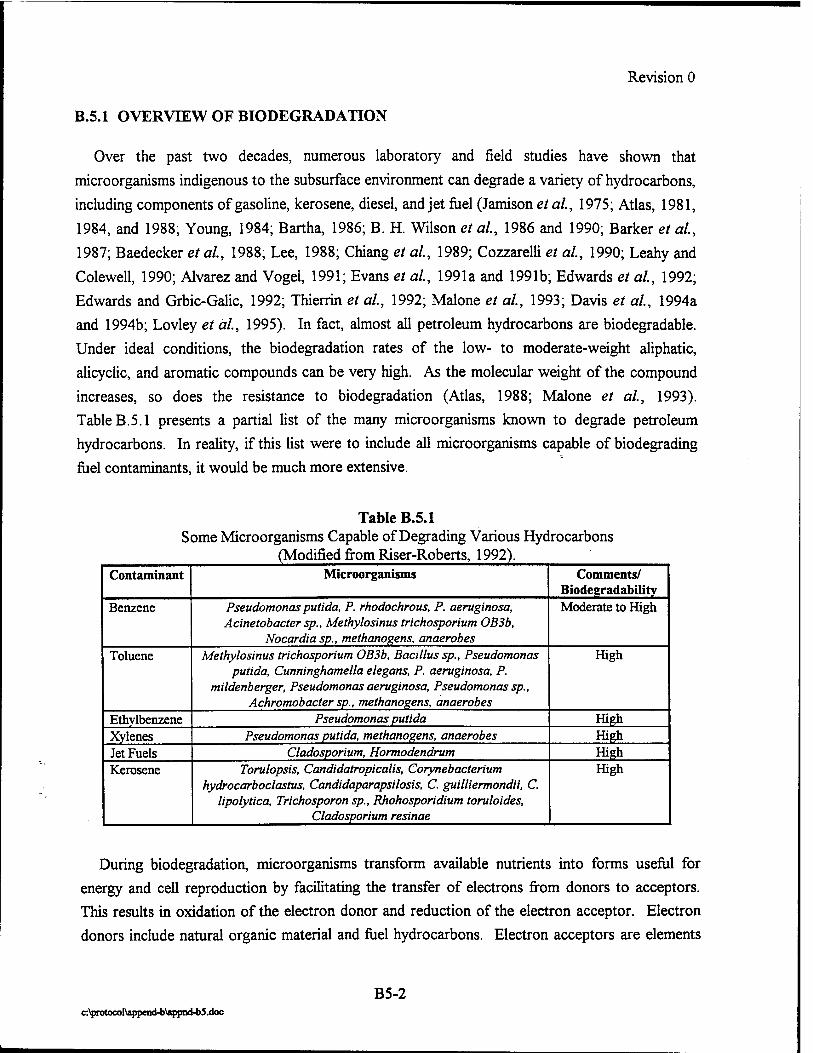
Revision 0
B.5.1 OVERVIEW OF BIODEGRADATION
Over the past two decades, numerous laboratory and field studies have shown that
microorganisms indigenous to the subsurface environment can degrade a variety of hydrocarbons, including components of gasoline, kerosene, diesel, and jet fuel (Jamison etal., 1975; Atlas, 1981, 1984, and 1988; Young, 1984; Bartha, 1986; B. H. Wilson et al, 1986 and 1990; Barker et al,
1987; Baedecker et al, 1988; Lee, 1988; Chiang et al, 1989; Cozzarelli et al, 1990; Leahy and
Colewell, 1990; Alvarez and Vogel, 1991; Evans et al, 1991a and 1991b; Edwards et al, 1992; Edwards and Grbic-Galic, 1992; Thierrin et al, 1992; Malone et al, 1993; Davis et al, 1994a and 1994b; Lovley et al, 1995). In fact, almost all petroleum hydrocarbons are biodegradable. Under ideal conditions, the biodegradation rates of the low- to moderate-weight aliphatic, alicyclic, and aromatic compounds can be very high. As the molecular weight of the compound increases, so does the resistance to biodegradation (Atlas, 1988; Malone et al, 1993). Table B.5.1 presents a partial list of the many microorganisms known to degrade petroleum hydrocarbons. In reality, if this list were to include all microorganisms capable of biodegrading fuel contaminants, it would be much more extensive.
Table B.5.1 Some Microorganisms Capable of Degrading Various Hydrocarbons
(Modified from Riser-Roberts, 1992). Contaminant Microorganisms Comments/
Biodegradability Benzene Pseudomonas putida, P. rhodochrous, P. aeruginosa,
Acinetobacter sp., Methylosinus trichosporium OB3b, Nocardia sp., methanogens, anaerobes
Moderate to High
Toluene Methylosinus trichosporium OB3b, Bacillus sp., Pseudomonas putida, Cunninghamella elegans, P. aeruginosa, P.
mildenberger, Pseudomonas aeruginosa, Pseudomonas sp., Achromobacter sp., methanogens, anaerobes
High
Ethvlbenzene Pseudomonas putida High Xylenes Pseudomonas putida, methanogens, anaerobes High Jet Fuels Cladosporium, Hormodendrum High Kerosene Torulopsis, Candidatropicalis, Corynebacterium
hydrocarboclastus, Candidaparapsilosis, C. guilliermondii, C. lipolytica, Trichosporon sp., Rhohosporidium toruloides,
Cladosporium resinae
High
During biodegradation, microorganisms transform available nutrients into forms useful for energy and cell reproduction by facilitating the transfer of electrons from donors to acceptors. This results in oxidation of the electron donor and reduction of the electron acceptor. Electron donors include natural organic material and fuel hydrocarbons. Electron acceptors are elements
B5-2 c:\protocol\append-b\appnd-bS.doc
Revision 0
or compounds that occur in relatively oxidized states. The more important electron acceptors in
groundwater include dissolved oxygen, nitrate, iron (III), sulfate, and carbon dioxide. In addition,
Manganese (IV) can act as an electron acceptor in some groundwater environments.
Biodegradation of organic pollutants occurs when microbially mediated redox reactions cause a
pollutant to be oxidized. The total number of electrons is conserved during a biochemical
reaction. When the metabolite has carbon atoms in a higher oxidation state because of loss of
electrons, the reaction product must be present in a reduced state with more electrons/carbon
atoms.
When fuel hydrocarbons are utilized as the primary electron donor for microbial metabolism,
they typically are completely degraded or detoxified (Bouwer, 1992). When fuel hydrocarbons
are not present in sufficient quantities to act as the primary metabolic substrate, they cannot
support microbial growth as the only electron donors. In this case, the fuel hydrocarbon can still
be degraded, but the microorganisms will obtain the majority of their energy from alternative
substrates in the aqueous environment. This type of metabolic degradation of fuel hydrocarbons
is referred to as secondary utilization because the fuel hydrocarbon contributes only a small
fraction of the energy and carbon needed for cell production and maintenance (Bouwer, 1992).
Subsurface bacteria typically are smaller than their terrestrial counterparts, giving rise to a larger
surface area to volume ratio. This allows them to efficiently utilize nutrients from dilute solutions
(Bouwer, 1992). Bacteria that degrade fuel hydrocarbons have been known to withstand fluid
pressures of hundreds of bars, pH conditions ranging from 1 to 10 standard units, temperatures
from 0 to 75 degrees Celsius, and salinities greater than those of normal sea water (Freeze and Cherry, 1979).
Biodegradation causes measurable changes in groundwater geochemistry. During aerobic
respiration, oxygen is reduced to water, and dissolved oxygen concentrations decrease. In
anaerobic systems where nitrate is the electron acceptor, the nitrate is reduced to N02", N20, NO,
NH4"1", or N2, and nitrate concentrations decrease. In anaerobic systems where iron (HI) is the
electron acceptor, it is reduced to iron (II), and iron (II) concentrations increase. In anaerobic
systems where sulfate is the electron acceptor, it is reduced to H2S, and sulfate concentrations
decrease. In anaerobic systems where C02 is used as an electron acceptor, it is reduced by
methanogenic bacteria, and CH4 is produced. During aerobic respiration, denitrification, iron (HI)
reduction, and sulfate reduction, total alkalinity will increase. If methanogenesis is the dominant
TEAP, alkalinity will remain fairly constant. Table B.5.2 summarizes these trends. Changes in
dissolved oxygen, nitrate, iron (II), sulfate, and methane concentrations can be used to ascertain
the dominant terminal electron-accepting process (TEAP). Lovley et al. (1994) suggest using
B5-3 c:\protocol\append-b\appnd-bS.doc

Revision 0
dihydrogen (H2) concentrations to determine the dominant TEAP. However, at this time
measurement of H2 concentrations in groundwater is not common practice.
Table B.5.2
Trends in Contaminant, Electron Acceptor, Metabolic Byproduct —and Total Alkalinity Concentrations During Biodegradation
Analyte BTEX
Terminal Electron Accepting Process
Dissolved Oxygen Nitrate Iron (II) Sulfate Methane Alkalinity
Aerobic Respiration Denitrification
Iron (III) Reduction Sulfate Reduction Methanogenesis
Aerobic Respiration, Denitrification, Iron (III) Reduction, and Sulfate
Reduction
Trend in Analyte Concentration During
Biodegradation Decreases
Decreases Decreases Increases Decreases Increases Increases
Fuel hydrocarbons biodegrade naturally when an indigenous population of hydrocarbon-
degrading microorganisms is present in the aquifer and sufficient concentrations of electron
acceptors and nutrients are available to these organisms. In most subsurface environments both
aerobic and anaerobic degradation of fuel hydrocarbons can occur, often simultaneously in
different parts of the plume. For thermodynamic reasons (as discussed later), microorganisms
preferentially utilize those electron acceptors that provide the greatest amount of free energy
during respiration (Bouwer, 1992). The rate of natural biodegradation generally is limited by a
lack of electron acceptors rather than by a lack of nutrients such as ammonia, nitrate or
phosphate. Studies at a jet-ruel-contaminated site noted little difference in biodegradation rates in
areas with or without nutrient additions (Miller, 1990). These researchers concluded that
nitrogen, phosphorus, and other trace nutrients were efficiently recycled by microorganisms at this site.
The driving force of BTEX degradation is the transfer of electrons from an electron donor
(BTEX) to an electron acceptor. The energy produced by these reactions is quantified by the
Gibb's free energy of the reaction (AGr). The AGr defines the maximum useful energy change for
a chemical reaction at a constant temperature and pressure. The state of a redox reaction relative
to equilibrium is defined by the sign of AG, Negative values indicate that the reaction is
exothermic (energy producing) and will proceed from left to right (i.e., reactants will be
transformed into products and energy will be produced). Positive values indicate that the reaction
c:\protocol\append-b\appnd-b5.doc B5-4

Revision 0
is endothermic and in order for the reaction to proceed from left to right, energy must be put into
the system. The value of AGr estimates how much free energy is consumed or can be yielded to the system during the reaction.
Like all living organisms, microorganisms are constrained by the laws of thermodynamics.
They can facilitate only those redox reactions that are thermodynamically possible (Chapelle, 1993). That is, microorganisms will facilitate only those redox reactions that will yield some energy (i.e., AGr < 0). Microorganisms will not invest more energy into the system than can be
released. Table B.5.3 presents electron acceptor and electron donor (BTEX) half-cell reactions. This table also gives the calculated AGr values for each of the half-cell reactions. Table B.5.4
gives the Gibbs free energy of formation (AGf) for species used in the half-cell reactions presented in Table B.5.3. The positive calculated AGr values for the oxidation of BTEX (electron donor half-cell reactions) presented in Table B.5.3 indicate that these oxidation reactions are endothermic (i.e., energy-consuming). The negative calculated AGr values for the reduction of the electron acceptors (electron acceptor half-cell reactions) presented in Table B.5.3 indicate that these reduction reactions are exothermic (i.e., energy-producing). In order to derive energy for cell maintenance and production from BTEX, the microorganisms must couple an endothermic reaction (electron donor oxidation) with an exothermic reaction (electron acceptor reduction). Most of the reactions involved in BTEX oxidation cannot proceed abiotically, even though they are thermodynamically favorable. These reactions require microorganisms to proceed. The microorganisms facilitate these redox reactions by providing the necessary activation energy. The requirement of this initial energy input is what prevents these redox reactions from spontaneously occurring in groundwater.
Microorganisms are able to utilize electron transport systems and chemiosmosis to combine energetically favorable and unfavorable reactions with the net result of producing energy for life processes. Table B.5.5 shows how microorganisms combine endothermic and exothermic reactions to release useful energy for cell maintenance and reproduction. By coupling the oxidation of BTEX to the reduction of electron acceptors, the overall reaction becomes energy- yielding, as indicated by the negative AGr values. For example, the oxidation of 1 mole of benzene via oxygen reduction produces 765.34 kilocalories of free energy that is available to the microorganisms. Thus, microorganisms derive a significant source of energy by facilitating this coupled reaction.
B5-5 c:\protocol\append-b\appnd-bS.doc
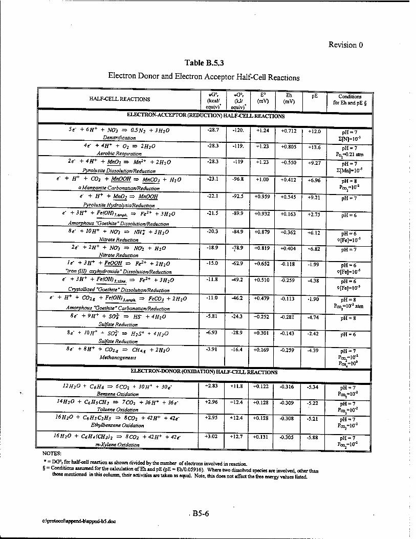
Revision 0
Table B.5.3
Electron Donor and Electron Acceptor Half-Cell Reactions
HALF-CELL REACTIONS *G°r
(kcatf equiv)
*G°r (kJ/^
equiv)'
E° (mV)
Eh (mV)
pE Conditions for Eh and pE §
FXECTRON-ACCEPTOR (REDUCTION) HALF-CELL REACTIONS
5e~ + 6H+ + NOS => 0.5N2 + 3H20 Denitrification
-28.7 -120. +1.24 +0.712 +12.0 pH = 7 E[N]=10-3
4e- + 4H+ + 02 => 2H20 Aerobic Respiration
-28.3 -119. +1.23 +0.805 +13.6 pH = 7 Po2=0.21 atm
2e- + 4H+ + MnOi => Mn2+ + 2H20
Pvrolusite Dissolution/Reduction
-28.3 -119 +1.23 +0.550 +9.27 pH = 7 £[Mn]=10-3
e' + H* + C02 + MnOOH => MnCO, + ff?0
aManganite Carbonation/Reduction
-23.1 -96.8 +1.00 +0.412 +6.96 pH = 8 Pco=10-2
e- + H+ + Mn02 => MnOOH
Pyrolusite Hydrolysis/Reduction
-22.1 -92.5 +0.959 +0.545 +9.21 pH = 7
e + 3H+ + Fe(OH)3amph =, Fe2+ + 3H20
Amorphous "Goethite " Dissolution/Reduction
-21.5 -89.9 +0.932 +0.163 +2.75 pH = 6
8f + 10H+ + NO-} => NHJ + 3H20
Nitrate Reduction
-20.3 -84.9 +0.879 +0.362 +6.12 pH = 6 <?[Fe]=10-5
2f + 2H+ + NCr3 => NCT2 + H2O
Nitrate Reduction -18.9 -78.9 +0.819 +0.404 +6.82 pH = 7
If + 3H+ + FeOOH => Fe*+ + 2H->0
"iron (III) oxyhydroxide"Dissolution/Reduction
-15.0 -62.9 +0.652 -0.118 -1.99 pH = 6 o[Fe]=103
e- + 3H+ + Fe(OH)3xlint => Fe2+ + 3H20
Crystallized "Goethite " Dissolution/Reduction
-11.8 -49.2 +0.510 -0.259 -4.38 pH = 6 9[Fe]=10-5
e- + H+ + C02.t + Fe(OH)}ampk => FeC03 + 2H20
Amorphous "Goethite"Carbonation/Reduction
-11.0 -46.2 +0.479 -0.113 -1.90 pH = 8 Poo2=10"2 aim
8f + 9H+ + SO2; => HS- + 4H20
Sulfate Reduction
-5.81 -24.3 +0.252 -0.281 -4.74 pH = 8
8e- + JOH* + SO2/ => H:S" + 4H20
Sulfate Reduction
-6.93 -28.9 +0.301 -0.143 -2.42 pH = 6
8e- + 8H+ + C02,g =■ CHU + 2H20
Methanogenesis
-3.91 -16.4 +0.169 -0.259 -4.39 pH = 7 Pco=10-2
PCH'=10°
ELECTRON-DONOR (OXID.A LTION)HAI JF-CELLI lEACnON S ^™
12H20 + C6Hs => 6CO2 + 30H* + 30e Benzene Oxidation
+2.83 +11.8 +0.122 -0.316 -5.34 pH = 7 Poo2=10-2
14H20 + C6HsCH3 => 7C02 + 36H+ + 36c Toluene Oxidation
+2.96 +12.4 +0.128 -0.309 -5.22 pH = 7 Pco2=10-J
16H20 + C6HsC2Hs => 8C02 + 42H+ + 42e' Ethylbenzene Oxidation
+2.95 +12.4 +0.128 -0.308 -5.21 pH = 7 Pco2=10-2
16H20 + C6H4<CH3)2 => 8C02 + 42H+ + 42e-
m-Xylene Oxidation
+3.02 +12.7 +0.131 -0.305 -5.88 pH = 7 Pco2=10"2
NOTES
* = DG°r for half-cell reaction as shown divided by the number of electrons involved in reaction. § - Conditions assumed for the calculation of Eh and pE (pE - Eh/0.05916). Where two dissolved species are involved, other than
those mentioned in this column, their activities are taken as equal. Note, this does not affect the free energy values listed.
B5-6 c:\DrotocoI\append-b\appnd-bS.doc
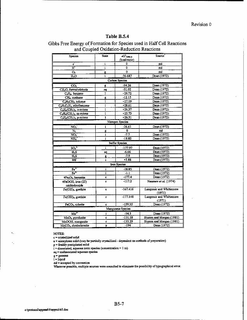
Revision 0
Table B.5.4 Gibbs Free Energy of Formation for Species used in Half Cell Reactions
and Coupled Oxidation-Reduction Reactions Species State *G°09H3
(kcal/mole) Source'
e' i 0 std IT i 0 std o, ß 0 std
H,0 1 -56.687 Dean(1972) Carbon Species
CO, g -94.26 Dean (1972) CH,0, formalydehyde aq -31.02 Dean (1972)
C«H«, benzene I +29.72 Dean(1972) CHj, methane 8 -12.15 Dean (1972)
CsHjCH,, toluene 1 +27.19 Dean (1972) CSHJCJHJ, ethvlbenzene 1 +28.61 Dean (1972) CA(CH,)i, o-xylene 1 +26.37 Dean (1972) C«H«(CH3)i, m-xylene 1 +25.73 Dean(1972) C«H4(CHJ)J, p-xylene i +26.31 Dean(1972)
Nitrogen Species
NO,- i -26.61 Dean(1972) N, g 0 std
NO," i -7.7 Dean(1972) NH4* i -18.82 Dean(1972)
Sulfur Species
SO42- i -177.97 Dean (1972) H,S aq -6.66 Dean (1972) H,S g -7.9 Dean (1972) HS- i +2.88 Dean(1972)
Iron Species
Fe1* i -18.85 Dean (1972) FeJ* i -1.1 Dean (1972)
9Fe,03, hematite c -177.4 Dean(1972)
9FeOOH, iron (III) oxyhydroxide
c -117.2 Naumov etaL (1974)
Fe(OH)j, goethhe a -167.416 Langmuir and Whittemore (1971)
Fe(OH)j, goethite c -177.148 Langmuir and Whittemore (1971)
FeCOj, siderite c -159.35 Dean (1972) Manganese Species
Mnlr i -54.5 Dean(1972) MnO,, pyrolusite c -111.18 Stumm and Morgan (1981)
MnOOH, manganite c -133.29 Stumm and Morgan (1981) MnCOj, rhodochroshe P -194 Dean (1972)
NOTES: c = crystallized solid a = amorphous solid (may be partially crystallized - dependent on methods of preparation) p = freshly precipitated solid i = dissociated, aqueous ionic species (concentration = 1 m) aq = undissociated aqueous species g = gaseous 1 = liquid std = accepted by convention Wherever possible, multiple sources were consulted to eliminate the possibility of typographical error.
B5-7 c:\protocol\append-b\appnd-b5.doc
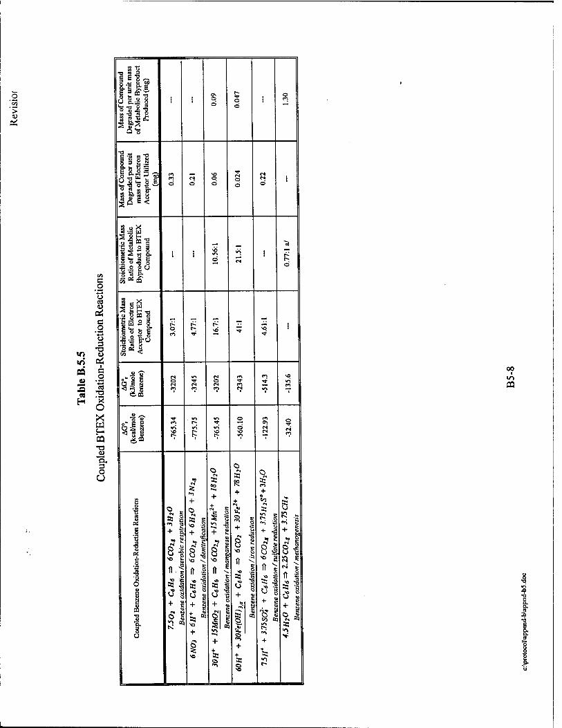
'S? >
C o o CO a & c o o 3
T3 U
i £0 S3 " O
- '5 ■ I
X w H PQ -a JD "5. 3 O U
8/3 £E E 3 m^
'a T> g 3 ■o -a 3 g
a1?
[Ill nil--
23 ^ I-6-
- — ttJ
•§.2 go 'SIS: -•? öS m
5 is 2 -R fe -o
o
o d
+ o
as
+ + a: +
Ö
^ ■§
S ! ft ^
c ■a O
+ as
aa
+ g
II c
'S - to as
as
00 I
in pa
5
« o O » c
Z s as
I
I ■a
I
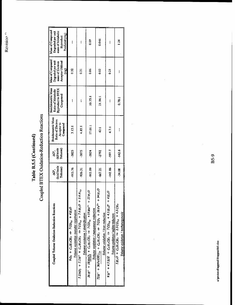
'35 >
u s c s o U
05 H
I« c
'-*-» o «i <u Pi a
o 3
T3 <U Pi
I e o '3 •o •3 O X w H CQ T3 _U o. 3 O U
O cd
s-1
E 8.2 60 E
"«■So Bb 3 ,„ u «
Si iff"?
C 5 u
8.4! S
5I m ö
•1.2 il &
CO
6
•g 8 r § «3 si §"8 8-f SI** o OS
.-■s a O E g
o"|I
"5
■8 'S. 3 O u
+
8
5!
+
+ O
K +
o a;
I 00
8 ts
5
+ + as ts
IN
as
+ o I 00
33
O ft
+
8
5 as
+
o a: +
as >' +
5 ■«a-'
+ ■3
8 ts
8
I
5 as
+
8
S3 ON
5 as «5 + o as
PQ
■o
I- "S 8

> et
T3 a 3 a B O U V) in
B O
'B Q u
c #o *-» 3 -a <u ■
B o
o X w « JU Q. 3 O U
J3 •O C a
1
,9 o
I

ES '> 1)
a*
"O <u •a s ~ s o U m IT)
n
«a H
en C o o ca
c o '•£* o 3
T3 <U
i C
-a •a o X w H m U
'S. 3 O
<w C 3 'S M
1 £.JJ -a -o
Q E
-sM ffl
g-s i- e h o s ° 3 S.JJ S <-*
I l-8'SSli
Si3
E « 2 a S ° iS •£ "S ° o K JJ &•*■
'•S I S IS OQ
Soul
jail •iji? io «2 JD —
E •o
us .a
ON
O Ö
o Ö o
Ö
ON
6
vo
I
m
8 1
a; o
t*.
9
8 «0
as
+
|
3
a:
o CM
aj
+
S3
SI
+
5 CM
+
s-s
ft •©
U +
s S3
a: «1
aj
B O
Q.
■s u E 60 c
•a o u 3
•a o
■S <u 5
I
JO
■o c a. a. 3 •6
i 8
I
Revision 0
Coupled redox reactions would be expected to occur in order of their thermodynamic energy
yield assuming that there are organisms capable of facilitating each reaction and that there is an
adequate supply of BTEX and electron acceptors (Stumm and Morgan, 1981; Chapelle 1993)
Figure B.5.3 illustrates the expected sequence of microbially mediated redox reactions In
general, reactions that yield the most energy tend to take precedence over those reactions that
yield less energy (Stumm and Morgan, 1981; Godsey, 1994). Although denitrification yields
slightly more energy than aerobic respiration, free dissolved oxygen is toxic to obligate anaerobic
bacteria in concentrations in excess of about 0.5 mg/L. Therefore, dissolved oxygen must be
removed from the groundwater before denitrification can occur. This being the case, aerobic
respiration is the first reaction to occur in an aerobic environment that contains microorganisms
capable of aerobic respiration (i.e., obligate aerobes or facultative anaerobes) (Bouwer 1992-
Chapelle, 1993). Once the available dissolved oxygen is depleted and anaerobic conditions
dominate the interior regions of the BTEX plume, facultative or obligate anaerobic
microorganisms can utilize other electron acceptors in the following order of preference- nitrate
manganese, iron (BO), sulfate, and finally carbon dioxide. As each electron acceptor being utilized
for biodegradation becomes depleted, the next most preferable electron acceptor is utilized. Each successive redox couple provides less energy to the microorganism.
The expected sequence of redox processes is also a function of the oxidizing potential of the
groundwater which is a measure of the relative tendency of a solution or chemical reaction to
accept or transfer electrons. As each subsequent electron acceptor is utilized, the groundwater
becomes more reducing and the redox potential of the water decreases. The main force driving
this change in redox potential is microbially mediated redox reactions. Redox potential can be
used as a crude indicator of which redox reactions may be operating at a site. The redox potential
determined in the field using a probe is termed Eh. Eh can be expressed as pE, which is the
hypothetical measure of the electron activity associated with a specific Eh. High pE means that
the solution or redox couple has a relatively high oxidizing potential. Figures 2.3 and B.5.4 show
the relationship between the dominant TEAP and the redox potential of the groundwater.
The reduction of highly oxidized species results in an overall decrease in the oxidizing potential
of the groundwater. As shown in Figures B.5.3 and B.5.4, the reduction of oxygen and nitrate
will reduce the oxidizing potential to levels at which iron (BT) reduction can occur. As each
chemical species that can be used to oxidize BTEX is exhausted, the microorganisms are forced
to use electron acceptors with a lower oxidizing capacity. When sufficiently negative pE levels
have been developed by these redox reactions, sulfate reduction and methane fermentation can occur.
B5-12 c:\protocol\append-b\appi*H>5.doc
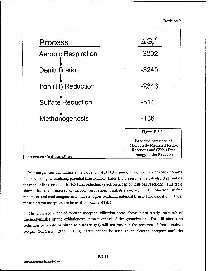
Revision 0
Process Aerobic Respiration
Denitrification
i Iron (III) Reduction
l Sulfate Reduction
i Methanogenesis
AGr0'
-3202
-3245
-2343
-514
-136
For Benzene Oxidation, kJ/mole
Figure B.5.3
Expected Sequence of Microbially Mediated Redox
Reactions and Gibb's Free Energy of the Reaction
Microorganisms can facilitate the oxidation of BTEX using only compounds or redox couples that have a higher oxidizing potential than BTEX. Table B.5.3 presents the calculated pE values for each of the oxidation (BTEX) and reduction (electron acceptor) half-cell reactions. This table shows that the processes of aerobic respiration, denitrification, iron (III) reduction, sulfate reduction, and methanogenesis all have a higher oxidizing potential than BTEX oxidation. Thus,
these electron acceptors can be used to oxidize BTEX.
The preferred order of electron acceptor utilization noted above is not purely the result of thermodynamics or the oxidation-reduction potential of the groundwater. Denitrification (the reduction of nitrate or nitrite to nitrogen gas) will not occur in the presence of free dissolved oxygen (McCarty, 1972). Thus, nitrate cannot be used as an electron acceptor until the
B5-13 c:\protocol\append-b\appnd-b5.doc

Revision 0
PE -10 -5 +5 -1-10 + 15
i AEROBIC RESPIRATION
DENITRIFICATION
MANGANESE REDUCTION
{ NURATE REDUCTION
{ IRON REDUCTION
<
SULFATE REDUCTION
METHANE FERMENTATION
NOTES
1. These reactions would be expected to occur in sequence if the system is moving toward equilibrium.
2. These redox processes occur in order of their energy-yielding potential (provided microorganisms are available to mediate a specific reaction). Reduction of a highly oxidized species decreases the pE of the system.
3. Redox sequence is paralleled by an ecological succession of biological mediators.
ADAPtED FROM STUMM AND MORGAN. 1981
Figure B.5.4
Sequence of Microbially Mediated Redox Reactions Based on pE
concentration of dissolved oxygen falls below about 0.5 mg/L. In addition, because oxygen and
nitrate (if present at high concentrations) are toxic to sulfate-reducing organisms, sulfate cannot
be used as an electron acceptor in the presence of either oxygen or high concentrations of nitrate
(McCarty, 1972). During anaerobic biodegradation, aerobic degradation can still be occurring
near the margins of the plume where dispersion helps spread the plume out into more oxygenated
regions of the aquifer. Because there is unequivocal evidence that microbial processes degrade
fuel hydrocarbons, the most important things to ascertain during the intrinsic remediation
B5-14 c:\protocol\append-b\appnd-b5.doc
Revision 0
demonstration are which mechanisms of biodegradation are most important and the rate at which
biodegradation is occurring. Biodegradation rates can be limited by substrate availability or by
the availability of electron acceptors.
B.5.2 AEROBIC BIODEGRADATION
Biodegradation of fuel hydrocarbons is often an aerobic process that occurs when indigenous populations of hydrocarbon-degrading microorganisms are supplied with the oxygen and nutrients
necessary to utilize fuel hydrocarbons as an energy source. Hydrocarbon-degrading microorganisms are ubiquitous, and as many as 28 hydrocarbon-degrading isolates (bacteria and
fungi) have been discovered in different subsurface environments (Davies and Westlake, 1977; Jones and Eddington, 1968). Because indigenous microorganisms are well adapted to the physical and chemical conditions of the subsurface environment in which they reside, they have a distinct advantage over microorganisms injected into the subsurface to enhance biodegradation. Therefore, attempts to enhance biodegradation have often met with less-than-anticipated success
(Goldsteine/ ai, 1985).
Almost all types of fuel hydrocarbons can be biodegraded under aerobic conditions (Borden at al, 1994). Mineralization of fuel hydrocarbons to carbon dioxide and water under aerobic conditions involves the use of oxygen as a cosubstrate during the initial stages of metabolism and as a terminal electron acceptor during the later stages of metabolism for energy production (Higgins and Gilbert, 1978; Gibson and Subramanian, 1984; Young, 1984). As shown earlier, the 02-H20 redox couple has a high oxidizing potential and, when coupled with endothermic
reactions involving BTEX, can be used by microorganisms to release a large amount of free energy (Tables B.5.3 and B.5.5). In fact, reduction of molecular oxygen is one of the most energetically favorable of the redox reactions involved in BTEX degradation.
An important consideration in evaluating long-term risks at a site is an accurate estimate of the potential for natural biodegradation BTEX in the groundwater. A reduction in dissolved oxygen concentrations within an existing BTEX plume is a strong indication that indigenous bacteria are already established and actively biodegrading fuel contamination via aerobic respiration. In general, dissolved oxygen concentrations will be lower than background levels in groundwater
that contains BTEX.
Aerobic attack on petroleum hydrocarbons requires the action of oxygenases and, therefore, the presence of free dissolved oxygen. Subsurface environments can quickly become devoid of oxygen, especially if high concentrations of organic contaminants are present. When this is the
B5-15 c:\protocol\append-b\appnd-bS.doc

Revision 0
case, the rate of aerobie biodegradation will typically be limrted by oxygen supply rather ,ha„ by
nutrtent concentrate (Borden and Bedien,. 1986). Although nutrients such as nitrogen and
Phosphorus are essential for biodegradarion of organic contaminants by bacteria, the influence of
morgamc and organic nutrients on ,„ .«,„ biodegradarion varies substantially, and in some cases
the addttton of nutnents into the subsurface environment has been shown to have little or no effect
on btodegradatton rates of hydrocarbons (Swindoll e, ai, .988; Miller, 1990) In any even,
btodegradation of flue! hydrocarbons occurs in most subsurface environments wtthottt the addition of supplemental nutrients.
Low-molecular-weight aromatic hydrocarbons such as BTEX are easily biodegraded in the
concentrations found Solved in groundwater. Aromatic biodegradation involves the formation
of a diol, followed by cleavage and formation of a diacid, followed by ortho- or ^-cleavage of
the nng structure (Cernigha. 1984; Smith, 1990). Extensa methyl substitution can inhibit initial
oxidation (Cnpps and Watkinson, 1978), and chain lengths longer than butyl groups will be
preferentially degraded before ortho- or meta- cleavage of the aromatic ring occurs.
N-alkanes between CIO and C22 are perceived as the most readily degradable hydrocarbon
constituents (Atlas, 1981). The common type of attack by microorganisms is through terminal or
subterminal attack of the saturated chain, causing formation of a primary or secondary alcohol
Oxidation then continues to aldehydes and fatty acids for primary attack, and ketones and esters
for secondary attack. Branched alkanes pose a problem for bacteria because methyl- or higher-
chained groups on subterminal carbons block the ß-oxidation pathway (Mckenna and Kallio
1964; Singer and Finnerty, 1984). Sufficiently branched isoalkanes are extremely biologically
recalcitrant, and the isoalkanes pnstane and phytane are commonly used as biomarkers in crude
oils. Cycloahphatic compounds are difficult to biodegrade because the oxidases required for
initial oxidation and subsequent ring cleavage are seldom found in the same bacteria (Donaghue et
al., 1976). There have been several reports of cycloahphatic oxidation through cometabolic
pathways (Perry, 1984; Trudgill, 1984). For instance, biodegradation of cyclohexane can proceed
by conversion to cyclohexanol by one bacterial species, followed by lactonization to hexanoic acid
by another. Alkylated cycloaliphatics are considered more easily biodegraded because ß-
oxidation of the methyl group gives bacteria leverage to break the rings by initial formation of
para-alcohols or para-ketones. Once the ring is broken, biodegradation proceeds through n-
alkane biodegradation mechanisms. Because of their low solubility in groundwater, however
these compounds generally are not very mobile in the subsurface environment, and therefore represent only a very localized problem.
c:\protocol\append-b\appnd-b5.doc B5-16
Revision 0
Petroleum hydrocarbons mixtures, such as JP-4 jet fuel, with its multitude of potential primary
substrates will undergo simultaneous degradation of the aliphatic, aromatic, and alicyclic
hydrocarbons. Mixed hydrocarbon-degrader populations often contain microorganisms that
produce enzymes with a broad specificity for substrates that can result in the degradation of
hydrocarbon mixtures through co-metabolic pathways (Perry, 1984). Early evidence of this was
presented by Jamison et al. (1975), who reported that individual hydrocarbon mineralization rates
were not the same as in hydrocarbon mixtures. Biodegradation rates for each of the constituents
may certainly vary however, depending on site-specific environmental and biological factors.
The detailed mineralization of aromatic hydrocarbons to carbon dioxide and water under
aerobic conditions involves the use of oxygen as a cosubstrate during the initial stages of
hydrocarbon metabolism, and the later use of oxygen as the terminal electron acceptor for energy
production (Young, 1984; Higgins and Gilbert, 1978; Gibson and Subramanian, 1984).
The following equations describe the overall stoichiometry of aromatic hydrocarbon
biodegradation. In the absence of microbial cell production, the oxidation (mineralization) of benzene to carbon dioxide and water is given by:
C6H6 + 7 502 -* 6C02 + 3H20
Therefore, 7.5 moles of oxygen are required to metabolize 1 mole of benzene. On a mass basis, the ratio of oxygen to benzene is given by:
Molecular weights: Benzene 6(12) + 6(1) = 78 gm Oxygen 7 5(32) = 240 gm
Mass Ratio of Oxygen to Benzene = 240:78 = 3.08:1
Therefore, in the absence of microbial cell production, 3.08 mg of oxygen are required to
completely metabolize 1 mg of benzene. Similar calculations can be made for toluene,
ethylbenzene, and xylene. The results of these calculations are shown in Table B.5.5. Table B.5.6
summarizes the mass of total BTEX degraded per mg of dissolved oxygen utilized. This table was prepared by averaging the values for BTEX presented in Table B.5.5.
Based on the stoichiometry presented in Table B.5.5, the ultimate metabolic byproducts of
aerobic respiration are carbon dioxide and water. However, this stoichiometry presents the final
products of aerobic respiration only. In reality, several intermediate products are produced from the BTEX before the end result is achieved.
B5-17 c:\protocol\append-b\appnd-b5.doc
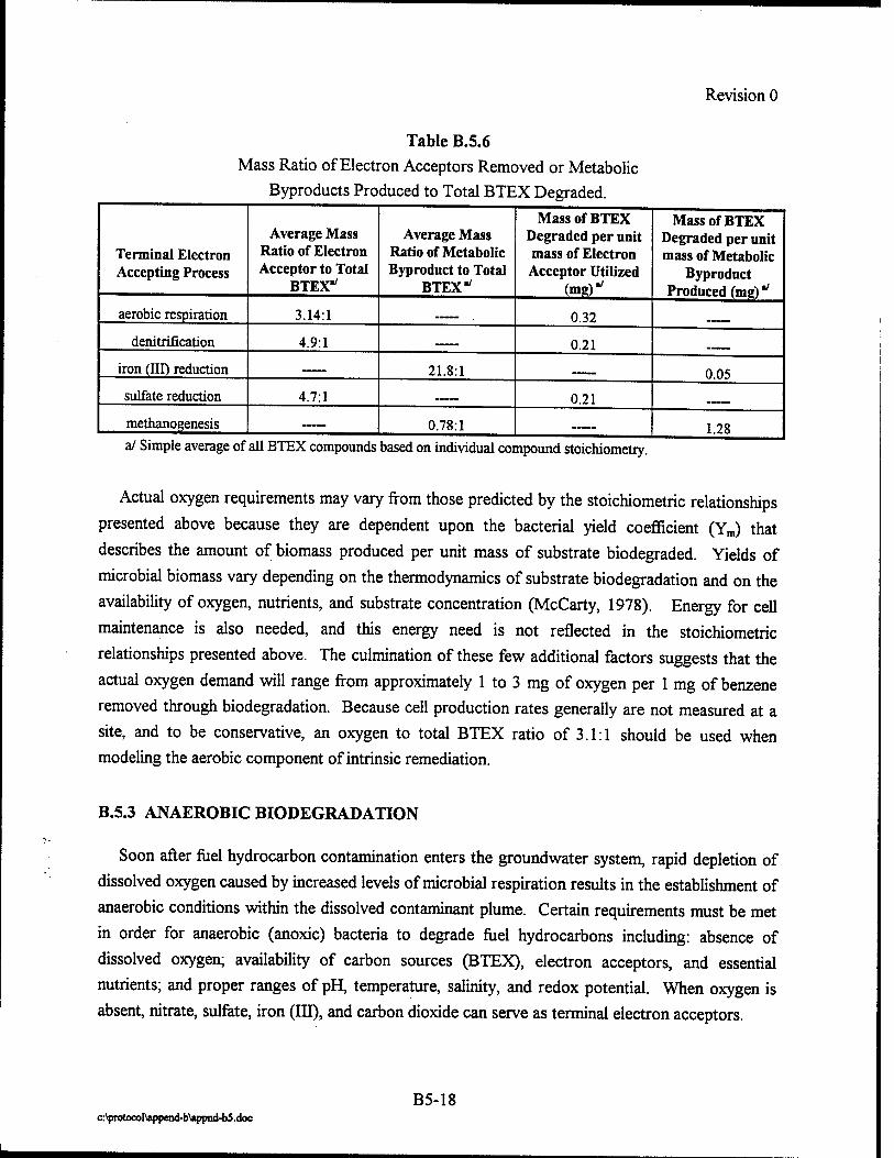
Revision 0
Table B.5.6 Mass Ratio of Electron Acceptors Removed or Metabolic
Byproducts Produced to Total BTEX Degraded.
Terminal Electron Accepting Process
Average Mass Ratio of Electron Acceptor to Total
BTEXm/
Average Mass Ratio of Metabolic Byproduct to Total
BTEX1"
MassofBTEX Degraded per unit mass of Electron Acceptor Utilized
(mg)"
MassofBTEX Degraded per unit mass of Metabolic
Byproduct Produced (me)"
aerobic respiration 3.14:1 .._. 0.32
denitrification 4.9:1 —— 0.21
iron (III) reduction 21.8:1 „„.._ 0.05 sulfate reduction 4.7:1 -._ 0.21
methanogenesis 0.78:1 1.28
Actual oxygen requirements may vary from those predicted by the stoichiometric relationships
presented above because they are dependent upon the bacterial yield coefficient (Ym) that
describes the amount of biomass produced per unit mass of substrate biodegraded. Yields of
microbial biomass vary depending on the thermodynamics of substrate biodegradation and on the
availability of oxygen, nutrients, and substrate concentration (McCarty, 1978). Energy for cell
maintenance is also needed, and this energy need is not reflected in the stoichiometric
relationships presented above. The culmination of these few additional factors suggests that the
actual oxygen demand will range from approximately 1 to 3 mg of oxygen per 1 mg of benzene
removed through biodegradation. Because cell production rates generally are not measured at a
site, and to be conservative, an oxygen to total BTEX ratio of 3.1:1 should be used when
modeling the aerobic component of intrinsic remediation.
B.5.3 ANAEROBIC BIODEGRADATION
Soon after fuel hydrocarbon contamination enters the groundwater system, rapid depletion of
dissolved oxygen caused by increased levels of microbial respiration results in the establishment of
anaerobic conditions within the dissolved contaminant plume. Certain requirements must be met
in order for anaerobic (anoxic) bacteria to degrade fuel hydrocarbons including: absence of
dissolved oxygen; availability of carbon sources (BTEX), electron acceptors, and essential
nutrients; and proper ranges of pH, temperature, salinity, and redox potential. When oxygen is
absent, nitrate, sulfate, iron (El), and carbon dioxide can serve as terminal electron acceptors.
B5-18 c:\protocol\append-b\appnd-bS.doc
Revision 0
It is now known with a high degree of certainty that aromatic organic compounds such as
BTEX, some of the simple polvnuclear aromatic compounds, and some nitrogen heterocyclic
organic compounds can be degraded in anaerobic groundwater (Grbic'-Galic' and Vogel, 1987;
Lovley et ai, 1989; Hutchins, 1991; Grbic'-Galic', 1990; Beller et ai, 1992a and 1992b;
Edwards etai, 1992; Edwards and Grbic'-Galic', 1992; Lovley etal, 1995).
During anaerobic degradation, the aromatic compounds are first oxidized to phenols or organic
acids, then transformed to long-chain volatile fatty acids that are finally metabolized to carbon
dioxide and possibly to methane. Destruction of the more hazardous compounds, such as BTEX,
is associated with accumulation of fatty acids, production of methane, solubilization of iron, and
reduction of nitrate and sulfate (Cozzarelli, et ai, 1990; Wilson et ai, 1990). Figure B.5.5 shows
some of these oxidized intermediates.
Depending on the type of electron acceptor present [nitrate, iron (III), sulfate, or carbon
dioxide], pH conditions, and redox potential, anaerobic biodegradation can occur by
denitrification, iron (III) reduction, sulfate reduction, or methanogenesis. Other, less common
anaerobic degradation mechanisms such as manganese reduction may dominate if the physical and
chemical conditions in the subsurface favor use of these electron acceptors. Environmental
conditions and microbial competition ultimately will determine which processes will dominate, but
in a typical aquifer denitrification typically occurs first, followed by iron (HI) reduction, sulfate
reduction, and finally by methanogenesis. Vroblesky and Chapelle (1994) show that the dominant
terminal electron accepting process can vary both temporally and spatially in an aquifer with fuel
hydrocarbon contamination. For example, a given area within an aquifer may switch among
iron (III) reduction, sulfate reduction, and methanogenesis depending on seasonal recharge of
dissolved oxygen and sulfate recharge.
Initial oxidation of petroleum hydrocarbons under anaerobic conditions largely depends on the
chemical structure of the compound. Cozzarelli et ai (1990) found that monoaromatic
compounds with alkyl substituents longer than an ethyl group were highly recalcitrant to
biodegradation under anaerobic conditions. Examples of such compounds include diethylbenzene,
methylpropylbenzene, and n-butyl-benzene. The actual pathways used by anaerobic bacteria to
biodegrade petroleum hydrocarbons is less understood than aerobic pathways. It is certain that
monoaromatics are susceptible to anaerobic biodegradation, and oxygen is derived from water
molecules under many circumstances. Vogel and Grbic-Galic (1986) used 180-labeled water to
show that water was the source of oxygen for toluene and benzene biodegradation under methane
fermentative conditions. In this case, 180-labeled p-cresol was the first intermediate detected. It
B5-19 c:\protocol\append-b\appnd-b5.doc

Revision 0
Parent Compound Oxidized Intermediates
Benzene phenol
Toluene (methyl benzene)
CH,
o-xylene
CH,
m-xylene
CH,
CH, p-xylene
cti,cii,
Q Ethylbenzene
Modified from Cozzarelli ct al. (1990)
benroic acid
COOH
- Q CH,
o-tnluic acid
coon
Q m-toluic acid
COOH
CH, p-lnluic acid
Figure B.5.5
Some Oxidized Intermediates Produced During Anaerobic Biodegradation
c:\protocol\append-b\appnd-b5.doc
B5-20

Revision 0
has been suggested that denitrifying bacteria also incorporate oxygen from water in the initial oxidation of aromatic compounds (Hopper, 1978), forming aromatic alcohols. As biodegradation proceeds, alicyclic and aromatic rings are cleaved by incorporation of oxygen, derived from water,
to form various aliphatic acids. Complete mineralization of BTEX during anaerobic biodegradation results in the formation of carbon dioxide, methane, and water.
B.5.3.1 Denitrification
After almost all free dissolved oxygen has been removed from the aquifer and anaerobic conditions prevail, nitrate can be used as an electron acceptor by facultative anaerobic
microorganisms to mineralize BTEX via denitrification. Denitrification ultimately results in the formation of carbon dioxide, water, and dinitrogen gas (N2). In areas where denitrification is occurring, there will be a strong correlation between areas with elevated dissolved BTEX concentrations and depleted nitrate concentrations relative to measured background concentrations. The absence of nitrate in contaminated groundwater suggests that nitrate may be functioning as an electron acceptor.
The oxidation of BTEX via denitrification is thermodynamically more favorable than aerobic respiration (Table B.5.5). However, nitrate can only function as an electron acceptor in microbially facilitated BTEX degradation reactions if the groundwater system has been depleted of dissolved oxygen (i.e., the groundwater must be functionally anaerobic). Oxygen is toxic to the enzyme systems used for electron transfer and energy production of nitrate-reducing microorganisms (McCarty, 1972). Many species of bacteria are capable of reducing nitrate to produce respirative energy (McCarty, 1972; Chapelle, 1993; Riser-Roberts, 1992). Denitrification occurs in the following sequence (Payne, 1981; von Gunten and Zobrist, 1993):
NO~ => NOi =>NO=> N20 => NH; => N2
Each reaction in this sequence is catalyzed by different microorganisms (Chapelle, 1993). Denitrification occurs only under anaerobic conditions; under aerobic conditions, the process is reversed and nitrification occurs (if the necessary conditions are met). Denitrification is favored under pH conditions ranging from 6.2 to 10.2 standard units and results in corresponding redox potentials (Eh) of 665 mV and -200 mV, respectively (Stotzky, 1974).
There are four requirements for denitrification (Starr and Gillham, 1993) including: 1) Nitrate in the aquifer, 2) Organic carbon, 3) Denitrifying bacteria, and 4) Reducing conditions (i.e., low to no dissolved oxygen).
B5-21 c:\protocol\append-b\appnd-b5.doc

Revision 0
The following equations describe the overall stoichiometry of denitrification caused by
anaerobic microbial biodegradation. In the absence of microbial cell production, the
mineralization of benzene to carbon dioxide and water is given by:
6NO3- + 6H~ + C6H6 -> 6C02(g) + 6H20 + 3N 2(g)
Therefore, 6 moles of nitrate are required to metabolize 1 mole of benzene. On a mass basis, the ratio of nitrate to benzene is given by:
Molecular weights: Benzene 6(12) + 6(1) = 78 gm Nitrate 6(62) = 372 gm
Mass ratio of nitrate to benzene = 372:78 = 4.77:1
Therefore, 4.77 mg of nitrate are required to completely metabolize 1 mg of benzene. Similar
calculations can be made for toluene, ethylbenzene, and xylene. The results of these calculations
are shown in Table B.5.5. Based on these calculations, the average ratio of nitrate consumed per
mole of BTEX degraded is 4.87:1. Table B.5.6 summarizes the mass of total BTEX degraded per
mg of nitrate utilized during denitrification.
Plumes of dissolved fuel hydrocarbons generally do not contain nitrate, indicating that
adaptation of the necessary bacterial populations is rapid, and ambient concentrations of nitrate
are quickly consumed. This is similar to the relationship observed between dissolved oxygen and
BTEX in contaminant plumes, and suggests that nitrate availability, and not microbial processes,
may be the limiting factor during denitrification. This is an important observation and is
consistent with observations at 40 Air Force sites studied to date.
Work conducted by several authors suggests that the biodegradation of BTEX under
denitrifying conditions occurs in the following order: toluene, p-xylene, m-xylene, ethylbenzene,
and finally o-xylene (Norris et al., 1994). The work by Kuhn et al. (1988), Evans et al. (1991a
and 1991b) and Hutchins et al. (1991b) suggests that benzene is biologically recalcitrant under
denitrifying conditions. However, Major et al. (1988) report degradation of benzene under
conditions thought to be denitrifying. Kukor and Olsen (1989) also note biodegradation of
benzene under denitrifying conditions.
Kuhn et al. (1985) used aquifer material taken from the water-sediment interface of a river in a
microcosm study of anaerobic, hydrocarbon biodegradation. The indigenous microorganisms
were supplied with nitrate. Biodegradation of /?-xylene and /w-xylene occurred after 3 months.
Biodegradation of o-xylene occurred only after removal of both /?-xylene and /«-xylene. The
B5-22 c:\protocol\append-b\appnd-b5.doc
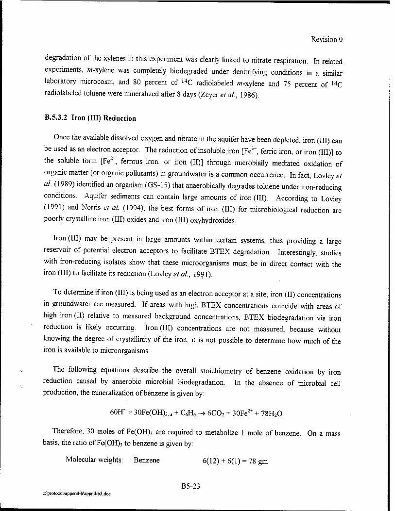
Revision 0
degradation of the xyienes in this experiment was clearly linked to nitrate respiration. In related
experiments, w-xylene was completely biodegraded under denitrifying conditions in a similar
laboratory microcosm, and 80 percent of 14C radiolabeled m-xylene and 75 percent of 14C
radiolabeled toluene were mineralized after 8 days (Zeyer et al., 1986).
B.5.3.2 Iron (HI) Reduction
Once the available dissolved oxygen and nitrate in the aquifer have been depleted, iron (III) can
be used as an electron acceptor. The reduction of insoluble iron [Fe3~, ferric iron, or iron (III)] to
the soluble form [Fe2\ ferrous iron, or iron (II)] through microbially mediated oxidation of
organic matter (or organic pollutants) in groundwater is a common occurrence. In fact, Lovley et
al. (1989) identified an organism (GS-15) that anaerobically degrades toluene under iron-reducing
conditions. Aquifer sediments can contain large amounts of iron (III). According to Lovley
(1991) and Norris et al. (1994), the best forms of iron (III) for microbiological reduction are poorly crystalline iron (III) oxides and iron (III) oxyhydroxides.
Iron (III) may be present in large amounts within certain systems, thus providing a large
reservoir of potential electron acceptors to facilitate BTEX degradation. Interestingly, studies
with iron-reducing isolates show that these microorganisms must be in direct contact with the iron (III) to facilitate its reduction (Lovley et al., 1991).
To determine if iron (III) is being used as an electron acceptor at a site, iron (II) concentrations
in groundwater are measured. If areas with high BTEX concentrations coincide with areas of
high iron (II) relative to measured background concentrations, BTEX biodegradation via iron
reduction is likely occurring. Iron (III) concentrations are not measured, because without
knowing the degree of crystallinity of the iron, it is not possible to determine how much of the iron is available to microorganisms.
The following equations describe the overall stoichiometry of benzene oxidation by iron
reduction caused by anaerobic microbial biodegradation. In the absence of microbial cell
production, the mineralization of benzene is given by:
60H* + 30Fe(OH)3,a + CsHg -» 6C02 + 30Fe2+ + 78H20
Therefore, 30 moles of Fe(OH)3 are required to metabolize 1 mole of benzene. On a mass
basis, the ratio of Fe(OH)3 to benzene is given by:
Molecular weights: Benzene 6(12) + 6(1) = 78 gm
B5-23 c:\protocol\append-b\appnd-b5.doc
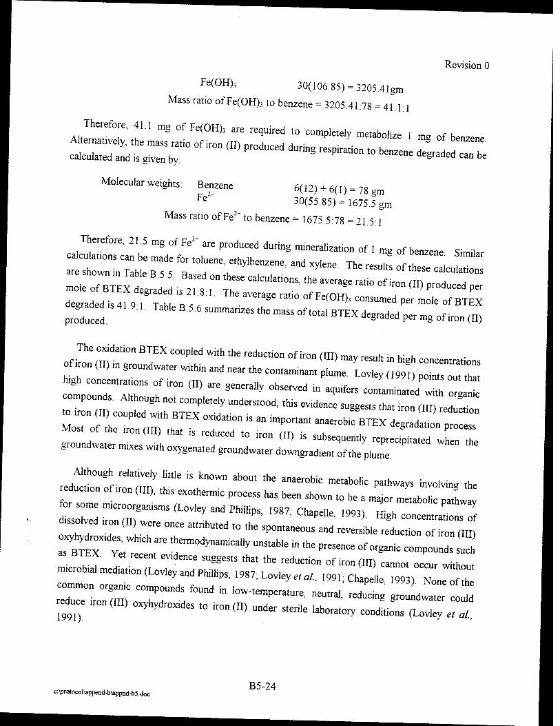
Revision 0
Fe(OH)3 30(106.85) = 3205.41gm
Mass ratio ofFe(OH)3 to benzene = 3205.41:78 = 41.\.i
A,teTrneatefT ^ "* * ^ "" " t0 C°« »***" ' -g of benzene
~ id:~°of iron (II) produced dunn§—»—«t:: Molecular weights: Benzene
Fe2~ 6(12)+ 6(1) = 78 gm 30(55.85)= 1675.5 gm
Mass ratio of Fe2~ to benzene = 1675.5:78 = 21 51
Therefore, 21.5 mg of Fe2T are produced during mineralization of 1 mg 0f benzene Simil, calculates can be made for toluene, ethylbenzene, and xylene The resuS o 1 are shown in Table R ss n A U , 'ne results of these calculations
mole of BTEXZI is 27s 7 T " "* """" ^ * ™ ^ ™ "» H J , ■ ! aVerage rano of Fe(°H>3 consumed per mole of RTF v dr«,s4f9.TableB56summari2esthema_
The „xidat,o„ BTEX coupled with ,he reduction of iron (,„) may resu„ In high concemrations of ■ on („) ,„ groundwater witWn Md near the contammam J J<2
colrncrrr :f iron (ii) are generauy °bse™d » >***> «ZLJJZZZZ compounds. Althongh no« completely understood, this evtdence suggests that iron rim 1 «o ,ron („) coupled w,,b BTEX oxidation , an tmportan, .«J^CC^T
Most of the ,ron(,ri) tha, is redueed to iron (II) is subsequently reprecLteJZZ
gronndwater mtxes wtth oxygenated groundwater downgradien, of the pile
^though relatively little is known about the anaerobic metaboiic pathways involving the reduce» of ,ron (HI), this exothermtc process has been shown to be a major mil*
dtssolved tron (II) were once atmbuted to the spontaneous and reverstble reduction of iron (III)
as BTEX Ye, recent evtdence suggests that the reduction of iron (III) cannot occur without
mtcrobtalmedtafon^ovlevandPninips, .987; Lovley e,a,„ 1991; Chapele, wfZ^Z
common organ, compounds found in low-temperature, neutral, reducmg grou dwlcll reduce lron (m) oxyhydroxides to ^ ^J^Z e7a
c:\protocol\append-b\appnd-b5.doc B5-24

Revision 0
B.5.3.3 Sulfate Reduction
Once the available oxygen and nitrate in the groundwater system have been depleted, sulfate-
reducing bacteria can begin degrading fuel hydrocarbons. Decreases in Eh, along with dissolved
oxygen and nitrate depletion, will favor sulfate-reducing bacteria at a redox potential of -200 mV
and a pH of 7 standard units (Postgate, 1984).
Sulfate is reduced to sulfide during the oxidation of BTEX. The presence of decreased
concentrations of sulfate and increased concentrations of sulfide relative to background
concentrations indicates that sulfate may be participating in BTEX oxidation reactions at a site.
In general, the extent and significance of BTEX biodegradation via sulfate reduction is not well
understood (Norris et al, 1994). Although oxidation of benzene by sulfate reduction is
thermodynamically favorable (see Table B.5.3), it is not as favorable as aerobic respiration,
denitrification, or iron reduction. Additionally, sulfate-reducing microorganisms typically are
sensitive to environmental conditions, including temperature, inorganic nutrients, and pH
(Zehnder, 1978). An imbalance in suitable environmental conditions could severely limit the
significance of BTEX degradation via sulfate reduction.
According to Hem (1985), low sulfate concentrations commonly result from the bacterial
reduction of sulfate. In waters containing dissolved BTEX, sulfate concentrations are further
reduced, and these microbes utilize BTEX as the oxidant. Lovley et al. (1995) show that under
sulfate-reducing conditions, benzene is mineralized to carbon dioxide and water with no
intermediate products such as phenol, benzoate, p-hydroxybenzoate, cyclohexane, and acetate.
Furthermore, the results of their work show that benzene can be biodegraded in the absence of
dissolved oxygen. Thierrin et al. (1992) described the biodegradation of a BTEX plume from a
gasoline spill in Perth, Western Australia, under sulfate-reducing conditions. Edwards et al.
(1992) give an example where toluene and the xylenes are degraded by indigenous
microorganisms under sulfate-reducing conditions. Beller et al. (1992a) describe the metabolic
byproducts of toluene biodegradation under sulfate-reducing conditions.
The following equations describe the overall stoichiometry of BTEX oxidation by sulfate
reduction caused by anaerobic microbial biodegradation. In the absence of microbial cell
production, the mineralization of benzene is given by:
7.5HT + 3.75S042' + C£k -* 6C02(g) + 3.75H2S° + 3H20
B5-25 c:\protocol\append-b\appnd-b5.doc
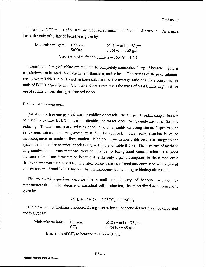
Revision 0
Therefore. 3.75 moles of sulfate are required to metabolize 1 mole of benzene. On a mass
basis, the ratio of sulfate to benzene is given by:
Molecular weights: Benzene 6(12) + 6(1) = 78 gm Sulfate 3.75(96) = 360 gm
Mass ratio of sulfate to benzene = 360:78 = 4.6:1
Therefore. 4.6 mg of sulfate are required to completely metabolize 1 mg of benzene. Similar
calculations can be made for toluene, ethylbenzene, and xylene. The results of these calculations
are shown in Table B.5.5. Based on these calculations, the average ratio of sulfate consumed per
mole of BTEX degraded is 4.7:1. Table B.5.6 summarizes the mass of total BTEX degraded per
mg of sulfate utilized during sulfate reduction.
B.5.3.4 Methanogenesis
Based on the free energy yield and the oxidizing potential, the C02-CH4 redox couple also can
be used to oxidize BTEX to carbon dioxide and water once the groundwater is sufficiently
reducing. To attain necessary reducing conditions, other highly oxidizing chemical species such
as oxygen, nitrate, and manganese must first be reduced. This redox reaction is called
methanogenesis or methane fermentation. Methane fermentation yields less free energy to the
system than the other chemical species (Figure B.5.3 and Table B.5.3). The presence of methane
in groundwater at concentrations elevated relative to background concentrations is a good
indicator of methane fermentation because it is the only organic compound in the carbon cycle
that is thermodynamically stable. Elevated concentrations of methane correlated with elevated
concentrations of total BTEX suggest that methanogenesis is working to biodegrade BTEX.
The following equations describe the overall stoichiometry of benzene oxidation by
methanogenesis. In the absence of microbial cell production, the mineralization of benzene is given by:
C6H6 + 4.5H20 -> 2.25C02 + 3.75CH4
The mass ratio of methane produced during respiration to benzene degraded can be calculated and is given by:
Molecular weights: Benzene 6( 12) + 6( 1) = 78 gm CH4 3.75(16) = 60 gm
Mass ratio of CH4 to benzene = 60:78 = 0.77:1
B5-26 c:\protocol\append-b\appnd-b5.doc

Revision 0
Therefore, 0.77 mg of CH4 are produced during mineralization of 1 mg of benzene. Similar
calculations can be made for toluene, ethylbenzene, and xylene. The results of these calculations
are shown in Table B.5.5. Based on these calculations, the average ratio of methane produced per mole of BTEX degraded is 0.78:1. Table B.5.6 summarizes the mass of total BTEX degraded per mg of methane produced.
This reaction is accomplished in at least four steps (Chapelle, 1993). In each step hydrogen
reacts with carbon. During the final step of methanogenesis, a methyl-coenzyme M methylreductase (C0M-CH3) complex is formed and the carbon is reduced to methane (Chapelle, 1993).
Because of the relatively small amounts of free energy produced by these reactions, methanogenesis is generally not the thermodynamically-favored reaction in the anaerobic environment but will proceed in environments that lack other electron acceptors or after these other electron acceptors (e.g., nitrate, sulfate) have been depleted. Methanogenic bacteria are active after sulfate reduction ceases and methanogenesis begins. Methanogenesis causes the redox potential to fall below -200 mV for a pH of 7 (Zehnder, 1978).
When the pH of groundwater is buffered by the presence of carbonate in the aquifer, the metabolic activity of the microorganisms becomes the rate-limiting step. The rate of reaction is controlled by the density of the active organisms and by the concentration of metabolizable compounds. B.H. Wilson et al. (1986) used a microcosm to show that BTEX was biodegraded under methanogenic conditions. Grbic'-Galic' and Vogel (1987) show the potential for the complete degradation of benzene and toluene to carbon dioxide and methane by methanogenic bacteria in laboratory studies. Wilson et al. (1987 and 1990) described the methanogenic degradation of benzene, toluene, and xylenes in groundwater contaminated by an aviation gasoline spill. Cozzarelli et al. (1990) reported the anaerobic biodegradation of alkylbenzenes in a contaminant plume originating from a spill of crude oil in Minnesota. The groundwater was actively methanogenic and accumulated long-chain volatile fatty acids. Wilson et al. (1993) studied biodegradation of aromatic hydrocarbons in a plume produced from a gasoline spill from a leaking underground storage tank. The water was methanogenic and accumulated acetate. The rates of anaerobic biodegradation in this plume were very similar to the rates in the crude oil spill studied by Cozzarelli et al. (1990) and the aviation gasoline spill studied by Wilson et al. (1990).
B5-27 c:\protocol\append-b\appnd-b5.doc
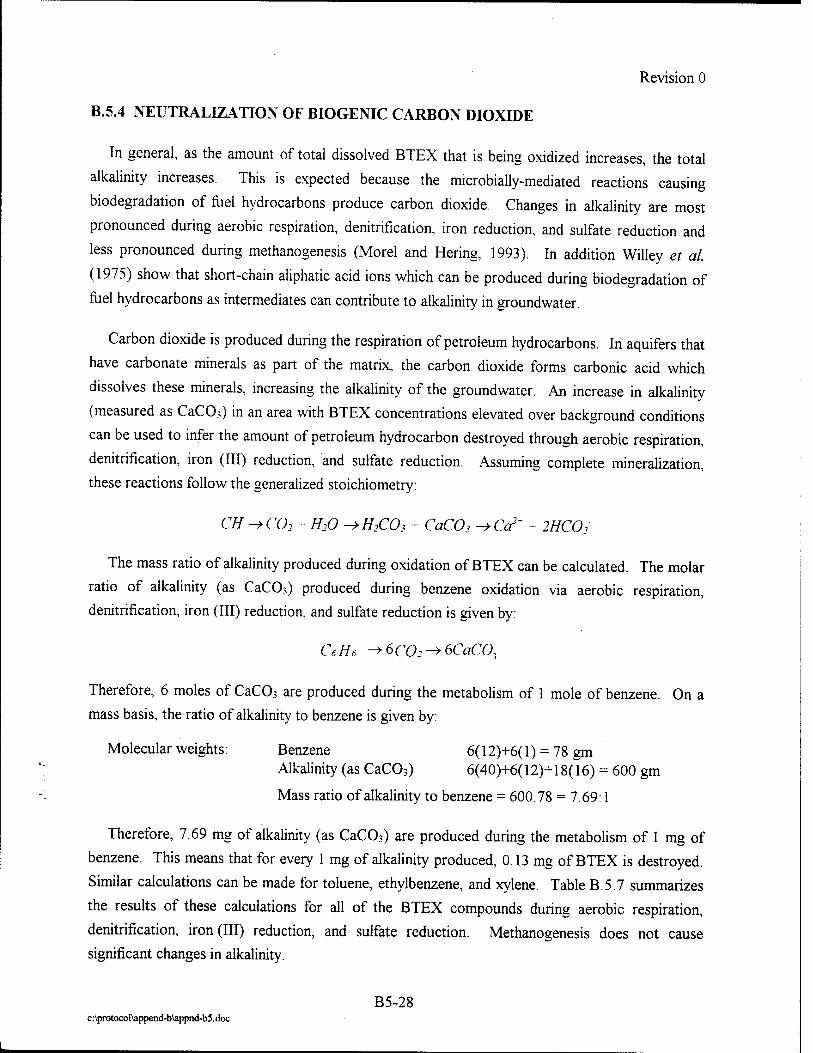
Revision 0
B.5.4 NEUTRALIZATION OF BIOGENIC CARBON DIOXIDE
In general, as the amount of total dissolved BTEX that is being oxidized increases, the total
alkalinity increases. This is expected because the microbially-mediated reactions causing
biodegradation of fuel hydrocarbons produce carbon dioxide. Changes in alkalinity are most
pronounced during aerobic respiration, denitrification, iron reduction, and sulfate reduction and
less pronounced during methanogenesis (Morel and Hering, 1993). In addition Willey et al.
(1975) show that short-chain aliphatic acid ions which can be produced during biodegradation of
fuel hydrocarbons as intermediates can contribute to alkalinity in groundwater.
Carbon dioxide is produced during the respiration of petroleum hydrocarbons. In aquifers that
have carbonate minerals as part of the matrix, the carbon dioxide forms carbonic acid which
dissolves these minerals, increasing the alkalinity of the groundwater. An increase in alkalinity
(measured as CaCO?) in an area with BTEX concentrations elevated over background conditions
can be used to infer the amount of petroleum hydrocarbon destroyed through aerobic respiration,
denitrification, iron (III) reduction, and sulfate reduction. Assuming complete mineralization,
these reactions follow the generalized stoichiometry:
CH-^C02 - H20 ^H2COs - CaC03 ->Cc?~ - 2HCO/
The mass ratio of alkalinity produced during oxidation of BTEX can be calculated. The molar
ratio of alkalinity (as CaC03) produced during benzene oxidation via aerobic respiration,
denitrification, iron (III) reduction, and sulfate reduction is given by:
CeH6 -+6C02^>6CaC03
Therefore, 6 moles of CaC03 are produced during the metabolism of 1 mole of benzene. On a
mass basis, the ratio of alkalinity to benzene is given by:
Molecular weights: Benzene 6(12)+6(1) = 78 gm Alkalinity (as CaC03) 6(40)+6(12)+18(16) = 600 gm
Mass ratio of alkalinity to benzene = 600:78 = 7.69:1
Therefore, 7.69 mg of alkalinity (as CaC03) are produced during the metabolism of 1 mg of
benzene. This means that for every 1 mg of alkalinity produced, 0.13 mg of BTEX is destroyed.
Similar calculations can be made for toluene, ethylbenzene, and xylene. Table B.5.7 summarizes
the results of these calculations for all of the BTEX compounds during aerobic respiration,
denitrification, iron (III) reduction, and sulfate reduction. Methanogenesis does not cause
significant changes in alkalinity.
B5-28 c:\protocol\append-b\appnd-b5.doc

Revision 0
Table B.5.7
Mass Ratio of Alkalinity (as CaC03) Produced to BTEX Degraded During Aerobic Respiration, Denitrification, Iron (III) Reduction, and Sulfate Reduction
Alkalinity Production Reaction Stoichiometric Mass Ratio of
Alkalinity Produced to BTEX Degraded
Mass of Compound Degraded (mg) per unit
mass of Alkalinity Produced (mg-)
CeHe ->6ca->6CaC03
Benzene Oxidation 600:78 0.13
CnHi -+7C02-*1CaC03
Toluene Oxidation 700:92 0.13
CsHio ->8C03->8CaCO3
Ethylbenzene Oxidation 800:104 0.13
CsHio ->8COa->8CaC03
Xylene Oxidation 800:104 0.13
B.5.5 ONE-DIMENSIONAL ADVECTION-DISPERSION EQUATION WITH RETARDATION AND BIODEGRADATION
The advection-dispersion equation is obtained by adding a biodegradation term to equation B.4.11. In one dimension, this is expressed as:
dC Dxd2C vxdC ,_
a^Ta3"*"*"*7 eqB51
Where: vx = average linear groundwater velocity [L/T] R = coefficient of retardation C = contaminant concentration [M/L3] Dx = hydrodynamic dispersion [L2/T] t = time [T] x = distance along flow path [L] X, = first-order biodegradation decay rate [T1]
This equation considers advection, hydrodynamic dispersion, sorption (retardation), and biodegradation. First-order rate constants are appropriate for iron (m)-reducing, sulfate- reducing, and methanogenic conditions. They are not appropriate under aerobic or denitrifying conditions.
B5-29 c:\protocol\append-b\appnd-b5.doc

DRAFT FINAL 10/1/95
SECTION B-6
VOLATILIZATION AND INFILTRATION
B.6.1 VOLATILIZATION
While not a destructive attenuation mechanism, volatilization does remove contaminants from
the groundwater system. Partitioning of a contaminant between the liquid phase and the gaseous
phase is governed by Henry's Law. Thus, the Henry's Law constant of a chemical determines the
tendency of a contaminant to volatilize from groundwater into the soil gas. Henry's Law states
that the concentration of a contaminant in the gaseous phase is directly proportional to the
compound's concentration in the liquid phase and is a constant characteristic of the compound.
Stated mathematically, Henry's Law is given by (Lyman et al, 1992):
Ca = HC,
Where: H = Henry's Law Constant (atm m3/mol)
Ca = concentration in air (atm)
Q = concentration in water (mol/m3)
Henry's Law constants for hydrocarbons range over three orders of magnitude, with the light
aromatics having the lowest volatility (e.g., BTEX). Henry's Law constants for the saturated
aliphatics range from 1 to 10 atm m3/mol @ 25°C, for the unsaturated and cyclo-aliphatics H
range from 0.1 to 1 atm m3/mol @ 25°C, and for the light aromatics H ranges from 0.007 to 0.02
atm m3/mol @ 25°C (Lyman et al, 1992). Values of Henry's Law constants for the BTEX
compounds are given in Table B.6.1. The solubility and relative volatility of the BTEX
compounds lead to a very strong enrichment of these compounds in the dissolved-phase in
groundwater relative to the other constituents of hydrocarbon fuels (Lyman et al, 1992).
B6-1 c:\protocol\append-b\appnd-b6.doc
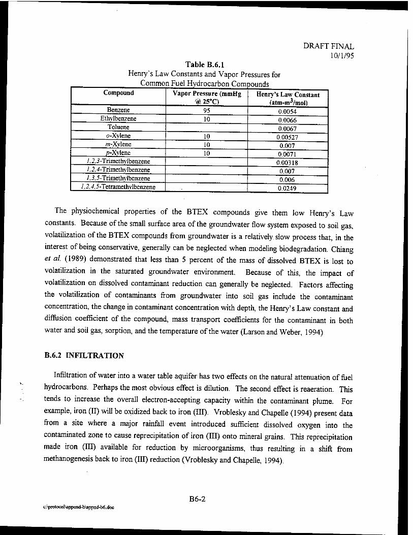
DRAFT FINAL 10/1/95
Table B.6.1 Henry's Law Constants and Vapor Pressures for
tommo n ruei riyarocaroon Lorn jounds Compound Vapor Pressure (mmHg
ra\ 25°C) Henry's Law Constant
(atm-m3/moI) Benzene 95 0.0054
Ethvlbenzene 10 0.0066 Toluene 0.0067 o-Xvlene 10 0.00527 w-Xvlene 10 0.007 p-Xvlene 10 0.0071
1,2,5-Trimethvlbenzene 0.00318 /, 2,4-Trimethvlbenzene 0.007 1,3,5-Trimethvlbenzene 0.006
1,2,4,5-Tetramethvlbenzene 0.0249
The physiochemical properties of the BTEX compounds give them low Henry's Law
constants. Because of the small surface area of the groundwater flow system exposed to soil gas,
volatilization of the BTEX compounds from groundwater is a relatively slow process that, in the
interest of being conservative, generally can be neglected when modeling biodegradation. Chiang
et al (1989) demonstrated that less than 5 percent of the mass of dissolved BTEX is lost to
volatilization in the saturated groundwater environment. Because of this, the impact of
volatilization on dissolved contaminant reduction can generally be neglected. Factors affecting
the volatilization of contaminants from groundwater into soil gas include the contaminant
concentration, the change in contaminant concentration with depth, the Henry's Law constant and
diffusion coefficient of the compound, mass transport coefficients for the contaminant in both
water and soil gas, sorption, and the temperature of the water (Larson and Weber, 1994)
B.6.2 INFILTRATION
Infiltration of water into a water table aquifer has two effects on the natural attenuation of fuel
hydrocarbons. Perhaps the most obvious effect is dilution. The second effect is reaeration. This
tends to increase the overall electron-accepting capacity within the contaminant plume. For
example, iron (II) will be oxidized back to iron (III). Vroblesky and Chapelle (1994) present data
from a site where a major rainfall event introduced sufficient dissolved oxygen into the
contaminated zone to cause reprecipitation of iron (III) onto mineral grains. This reprecipitation
made iron (III) available for reduction by microorganisms, thus resulting in a shift from
methanogenesis back to iron (III) reduction (Vroblesky and Chapelle, 1994).
B6-2 c:\protocol\append-b\appnd-b6.doc
Revision 0
APPENDIX C
DATA INTERPRETATION AND CALCULATIONS

Revision 0
TABLE OF CONTENTS - APPENDIX C
C-l INTRODUCTION C11
C-2 PREPARATION OF GEOLOGIC BORING LOGS, HYDROGEOLOGIC SECTIONS AND MAPS C2-1
C.2.2.1 Preparation of Lithologic Logs C2-1 C.2.2.2 Preparation of Hydrogeologie Sections C2_i C.2.2.3 Review of Topographic Maps and Preparation of Potentiometric Surface
Maps and Flow Nets C2-2 C.2.2.3.1 Review of Topographic Maps C2-2 C.2.2.3.2 Preparation of Potentiometric Surface Maps C2-4 C.2.2.3.3 Preparation of Flow Nets C2_5
C.2.2.4 Preparation of Contaminant Isopach Maps C2-7 C.2.2.4.1 Relationship Between Apparent and Actual LNAPL Thickness C2-7
C.2.2.4.1.1 Empirical Relationships C2-10 C.2.2.4.1.2 LNAPL Baildown Test ZZZZZZZZZZZZZZZZ C&13
C.2.2.5 Preparation of Contaminant Isopleth Maps C2-15 C.2.2.6 Preparation of Electron Acceptor, Metabolic Byproduct, and Alkalinity
Contour (Isopleth) Maps C2-15 C.2.2.6.1 Electron Acceptor Isopleth Maps C2-18 C.2.2.6.2 Metabolic Byproduct Isopleth Maps C2-19 C.2.2.6.3 Total Alkalinity Isopleth Map C2-19
C-3 INTRINSIC REMEDIATION CALCULATIONS C3A
C.3.1 CALCULATING HYDRAULIC PARAMETERS ZZZZZZZZZZZZZ C3-1 C.3.1.1 Hydraulic Conductivity C3_l
C.3.1.1.1 Hydraulic Conductivity from Pumping Tests C3-2 C.3.1.1.2 Hydraulic Conductivity from Slug Tests C3-3
C.3.1.2 Transmissivity C3_3 C.3.1.3 Hydraulic Head and Gradient C3.3 C.3.1.4 Total Porosity (n) and Effective Porosity (n.) C3-7 C.3.1.5 Linear Groundwater Flow Velocity (Seepage or Advective Velocity) C3-9 C.3.1.6 Coefficient of Retardation and Retarded Contaminant Transport
Velocity Q^-9
C.3.1.6.1 Bulk Density C3-11 C.3.1.6.2 Distribution Coefficient and Total Organic Carbon Content C3-12
C-i c:\protocol\append-c\toc-c.doc

Revision 0
C.3.2 CONTAMINANT SOURCE TERM CALCULATIONS C3-14 C.3.2.1 Direct Measurement of Dissolved Contaminant Concentrations in
Groundwater in Contact with NAPL C3-18 C.3.2.1.1 Collecting Groundwater Samples From Beneath the LNAPL C3-18 C.3.2.1.2 Collecting Mixed Groundwater/NAPL Samples C3-18
C.3.2.2 Partitioning Calculations C3-19 C.3.2.2.1 Equilibrium Partitioning of BTEX from Mobile LNAPL into
Groundwater C3-19
C.3.2.2.2 Nonequilibrium Partitioning of BTEX from Mobile LNAPL into Groundwater C3-22
C.3.2.3 Intrinsic Remediation of Contaminant Sources C3-24 C.3.3 CONFIRMING AND QUANTIFYING BIODEGRADATION C3-28
C.3.3.1 Isopleth maps C3-28 C.3.3.2 Conservative Tracer C3-29 C.3.3.3 Mass Balance Calculations C3-34
C.3.3.3.1 Dissolved Oxygen C3-35 C.3.3.3.2 Nitrate C3-35 C.3.3.3.3 Iron C3-36 C.3.3.3.4 Sulfate C3-36 C.3.3.3.5 Methane C3-37 C.3.3.3.6 Alkalinity C3-37
C.3.3.4 Calculating Rates of Biodegradation C3-38 C.3.3.4.1 Instantaneous Reaction C3-38 C.3.3.4.2 First-Order Decay C3-38
C.3.3.4.2.1 Use of Conservative Tracer C3-39 C.3.3.4.2.2 Method of Buscheck and Alcantar (1995) C3-46 C.3.3.4.2.3 Comparison of Conservative Tracer Method and Method
of Buscheck and Alcantar (1995) C3-47 C.3.4 DESIGN, IMPLEMENTATION, AND INTERPRETATION OF MICROCOSM STUDIES C3-50
C.3.4.1 Overview C3-50 C.3.4.2 Case Study on a Gasoline Spill at Arvida, North Carolina C3-52
C.3.4.2.1 Material and Methods C3-52 C.3.4.2.1.1 Sediment and Groundwater Collection C3-52 C.3.4.2.1.2 Microcosm Construction C3-54 C.3.4.2.1.3 Aqueous Sampling and Analyses C3-55 C.3.4.2.1.4 Results C3-55
C-ü c:\protocoI\append-cUoc-c.doc
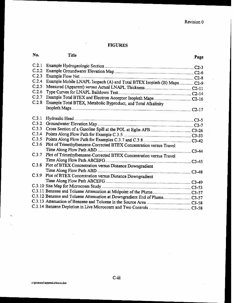
Revision 0
FIGURES
No.
C.2.1 C.2.2 C.2.3 C.2.4 C.2.5 C.2.6 C.2.7 C.2.8
C.3.1 C.3.2 C.3.3 C.3.4 C.3.5 C.3.6
C.3.7
C.3.8
C.3.9
C.3.10 C.3.11 C.3.12 C.3.13 C.3.14
Title Page
Example Hydrogeologie Section C2_3 Example Groundwater Elevation Map C2-6 Example Flow Net ^2-8 Example Mobile LNAPL Isopach (A) and Total BTEX Isopleth (B) Maps ... C2-9 Measured (Apparent) versus Actual LNAPL Thickness C2-11 Type Curves for LNAPL Baildown Test ""c2-14 Example Total BTEX and Electron Acceptor Isopleth Maps C2-16 Example Total BTEX, Metabolic Byproduct, and Total Alkalinity Isopleth Maps C2-17
Hydraulic Head C3_5 Groundwater Elevation Map C3.7 Cross Section of a Gasoline Spill at the POL at Eglin AFB ^C3-26 Points Along Flow Path for Example C.3.5 " C3-33 Points Along Flow Path for Examples C.3.7 and C.3.8 C3-42 Plot of Trimethylbenzene-Corrected BTEX Concentration versus Travel Time Along Flow Path ABD C3-44 Plot of Trimethylbenzene-Corrected BTEX Concentration versus Travel Time Along Flow Path ABCEFG C3-45 Plot of BTEX Concentration versus Distance Downgradient Time Along Flow Path ABD C3-48 Plot of BTEX Concentration versus Distance Downgradient Time Along Flow Path ABCEFG C3-49 Site Map for Microcosm Study C3-53 Benzene and Toluene Attenuation at Midpoint of the Plume C3-57 Benzene and Toluene Attenuation at Downgradient End of Plume C3-57 Attenuation of Benzene and Toluene in the Source Area C3-58 Benzene Depletion in Live Microcosm and Two Controls C3-58
C-iii c:\protocol\append-c\toc-c.doc

Revision 0
TABLES
No. Title Page
C.2.1 Typical values for hcaw\dr C2-12
C.2.2 Surface Tensions for Various Compounds C2-13 C.2.3 Results of Example Baildown Test C2-15
C.3.1 Representative Values of Hydraulic Conductivity for Various Sediments and Rocks C3-2
C.3.2 Representative Values of Dry Bulk Density, Total Porosity, and Effective Porosity for Common Aquifer Matrix Materials C3-8
C.3.3 Representative Values of Total Organic Carbon for Common Sediments C3-13
C.3.4 Example Retardation Calculations for the BTEX Compounds C3-14 C.3.5 Dissolved Concentrations (in Water) of Water-Soluble Components
Present in JP-4 C3"16
C.3.6 Weight Percent Water-Soluble Components in Gasoline and Their Concentrations in Water in Contact with Gasoline C3-17
C.3.7 Fuel-Water Partitioning Coefficients (Kf*) for Those Compounds Most Commonly found in the Aqueous Phase in Water in Contact with Jet Fuel or Gasoline C3-20
C.3.8 Relationships Relating Fuel-Water Partitioning Coefficients (Kf*) to Pure Aqueous-Phase Solubility C3-20
C.3.9 Density of Common Liquids C3-21 C.3.10 Solution to Example C.3.4 C3-22 C.3.11 Concentrations of TPH and BTEX in Core Material from a Gasoline Spill C3-27 C.3.12 Comparison of BTEX in Groundwater to Predictions Based on
the BTEX Content of the Weathered Residual Gasoline C3-28 C.3.13 Percent BTEX Lost to Biodegradation C3-31 C.3.14 Hypothetical Electron Acceptor and Metabolic Byproduct
Concentrations C3-34 C.3.15 Representative First-Order Rate Constants C3-39 C.3.16 BTEX and TMB Data for Examples C.3.7 and C.3.8 C3-41 C.3.17 7,3,5-Trimethylbenzene-CorrectedBenzene, Toluene, Ethylbenzene, and
Xylene Concentrations for Examples C.3.7 and C.3.8 C3-43 C.3.18 Results of Exponential Regression Analyses using Conservative Tracer C3-46 C.3.19 Results of Exponential Regression Analyses using Method of
Buscheck and Alcantar (1995) C3"50
C.3.20 Microcosm vs. Field BTEX Intrinsic Remediation Rates C3-59
C-iv c:\protocol\append-c\toc-c.doc
Revision 0
SECTION C-l
INTRODUCTION
Successful documentation of intrinsic remediation requires interpretation of site-specific data
to define the groundwater flow system, refine the conceptual model, quantify rates of contaminant
attenuation, and model the fate and transport of dissolved benzene, toluene, ethylbenzene, and
xylenes (BTEX). Tasks to be completed include preparation of lithologic logs, hydrogeologic
sections, potentiometric surface maps and flow nets, contaminant isopach and isopleth maps,
electron acceptor and metabolic byproduct isopleth maps, and calculation of hydraulic parameters,
retardation coefficients, and anaerobic degradation rate constants. The rate and amount of
partitioning of BTEX compounds from mobile and residual light nonaqueous-phase liquid
(LNAPL) into groundwater should also be determined to allow estimation of a source term.
Completion of these tasks permits refinement of the conceptual model and is necessary to
successfully support intrinsic remediation.
This appendix consists of three sections, including this introduction. Section C-2 discusses
preparation of geologic boring logs, hydrogeologic sections, and maps. Section C-3 covers
intrinsic remediation calculations, including hydraulic parameter calculations, contaminant source
term calculations, confirming and quantifying biodegradation, and designing, implementing, and
interpreting microcosm studies.
Cl-1 C:\PROTOCOL\APPENDC\APPND-C1 .DOC

Revision 0
SECTION C-2
PREPARATION OF GEOLOGIC BORING LOGS, HYDROGEOLOGIC SECTIONS, AND MAPS
The first step after completion of site characterization field activities is to prepare geologic
boring logs, hydrogeologic sections, water table elevation (or potentiometric surface) maps, flow
nets, and maps depicting contaminant concentrations, electron acceptor and metabolic byproduct
concentrations, and mobile LNAPL thickness. The construction of these items is discussed in the
following sections.
C.2.2.1 Preparation of Lithologic Logs
Lithologic logs should be prepared using field data. Whenever possible, these logs should
contain descriptions of the aquifer matrix, including relative density, color, major textural
constituents, minor constituents, porosity, relative moisture content, plasticity of fines,
cohesiveness, grain size, structure or stratification, relative permeability, and any significant
observations such as visible fuel or fuel odor. It is also important to correlate the results of
volatile organic compound (VOC) screening using headspace vapor analysis with depth intervals
of geologic materials. The depth of lithologic contacts and/or significant textural changes should
be recorded to the nearest 0.1 foot. This resolution is necessary because preferential flow and
contaminant transport pathways may be limited to stratigraphic units less than 6 inches thick.
C.2.2.2 Preparation of Hydrogeologic Sections
Lithologic logs should be used in conjunction with water level data to prepare a minimum of
two hydrogeologic sections for the site. One section should be oriented parallel to the direction
of groundwater flow, and one section should be oriented perpendicular to the direction of
groundwater flow. Both sections should be drawn to scale. Hydrogeologic sections are an
integral part of the conceptual model and are useful in identifying preferential contaminant
migration pathways and in modeling the site.
C2-1
c:\protocoI\append-c\appnd-c2.doc
Revision 0
At a minimum, hydrogeologic sections should contain information on the relationships between hydrostratigraphic units at the site, including the location and distribution of transmissive vs. non-
transmissive units, the location of the water table relative to these units, and the location(s) of the
contaminant source(s). Figure C.2.1 is an example of a completed hydrogeologic section.
C.2.2.3 Review of Topographic Maps and Preparation of Potentiometric Surface Maps and Flow Nets
Determining the direction of groundwater flow and the magnitude of hydraulic gradients is important because these parameters influence the direction and rate of contaminant migration. Groundwater flow directions are represented by a three-dimensional set of equipotential lines and orthogonal flow lines. If a plan view (potentiometric surface, or water table elevation, map) or a two-dimensional cross-section is drawn to represent a flow system, the resultant equipotential lines and flow lines constitute a flow net. A flow net can be used to determine the distribution of hydraulic head, the groundwater velocity distribution, groundwater and solute flow paths and flow rates, and the general flow pattern in a groundwater system.
C.2.2.3.1 Review of Topographic Maps
Groundwater flow is strongly influenced by the locations of groundwater divides and by recharge from and discharge to surface water bodies such as rivers, streams, lakes, and wetlands. Topographic highs generally represent divergent flow boundaries (divergent groundwater divide), and topographic lows such as valleys or drainage basins typically represent convergent flow boundaries (convergent groundwater divide). In addition, the configuration of the water table is typically a subtle reflection of the surface topography in the area. However, topography is not always indicative of subsurface flow patterns and should not be depended upon unless confirmed by head data. In order to place the local hydrogeologic flow system within the context of the regional hydrogeologic flow system, it is important to have an understanding of the local and regional topography. Included in this must be knowledge of the locations of natural and manmade surface water bodies. This information can generally be gained from topographic maps published by the United States Geological Survey.
C2-2
c:\protocoI\append-c\appnd-c2.doc

LU
<
CN-
Ü l_ 3 00
c _o o u
i ° X o « ao
TJ
a. < 2
o-1
«~ a>
«1 Si CO CO
2s a. </) a. a)
> -J -^ t_ CO
co ^
■a o>
CD S
►I
CO
o lO
«a-
a a o
o m lO «3-
a 2 HI a in
>* CO <u >> CO TJ
■a </> o-o
CO CO
2 <= TJ Ä CO C °w CO
><TJ >» — CO o-c o o CO
CLCO U
— TJ 5
CO >« CD
Si a TJ e CO
CO
JO a >«
co u CO
XI — u CO "7
>» y 03
CO '8
O ?!
D |8A9-| B9S Ue9|AJ SAOqV 199J
C2-3
Revision 0
C.2.2.3.2 Preparation of Potentiometric Surface Maps
A potentiometric surface map is a two-dimensional graphical representation of equipotential
lines shown in plan view. Water table elevation maps are potentiometric surface maps drawn for
water table (unconfined) aquifers. Potentiometric surface maps for water table aquifers show
where planes of equal potential intersect the water table. A potentiometric surface map should be
prepared from water level measurements and surveyor's data. These maps are used to estimate
the direction of plume migration and to calculate hydraulic gradients. To document seasonal
variations in groundwater flow, separate potentiometric surface maps should be prepared using quarterly water level measurements taken over a period of at least 1 year.
The data used to develop the potentiometric surface map should be water level elevation data
(elevation relative to mean sea level) from piezometers/wells screened in the same relative
position within the same hydrogeologic unit. For example, wells that are screened at the water
table can be used for the same potentiometric surface map. Wells screened in different
hydrogeologic units or at different relative positions within the same water table aquifer cannot be
used to prepare a potentiometric surface map. Where possible, a potentiometric surface map
should be prepared for each hydrogeologic unit at the site. In recharge areas, wells screened at
various elevations cannot all be used to prepare the same potentiometric surface map because of
strong downward vertical gradients. Likewise, wells screened at various elevations in discharge
areas such as near streams, lakes, or springs, should not all be used because of the strong upward vertical gradients.
When preparing a potentiometric surface map, the locations of system boundaries should be
kept in mind; particularly the site features that tend to offset the shape of the contours on the map.
Such features include topographic divides, surface water bodies, and pumping wells.
In addition to, and separately from, preparation of a potentiometric surface map, water level
measurements from wells screened at different depths can be used to determine any vertical
hydraulic gradients. It is important to have a good understanding of vertical hydraulic gradients
because they may have a profound influence on contaminant migration.
In areas with measurable mobile LNAPL, a correction must be made for the water table
deflection caused by the LNAPL. The following relationship, based on Archimedes' Principle,
provides a correction factor that allows the water table elevation to be adjusted for the effect of floating LNAPL.
C2-4
c:\protocol\append-c\appnd-c2.doc

Revision 0
CDTW=MDTW-^-{PT) eq C 2 1
Where: CDTW= corrected depth to water [L] MDTW- measured depth to water [L] Plnapl= density of the LNAPL [M/L3] pw = density of the water, generally 1.0 [M/L3] PT= measured LNAPL thickness [L]
Using the corrected depth to water, the corrected groundwater elevation, CGWE, is given by:
CGWE = Datum Elevation - CDTW eq. C.2.2
Corrected groundwater elevations should be used for potentiometric surface map preparation.
Figure C.2.2 is an example of a groundwater elevation map for an unconfined aquifer. Water
table elevation data used to prepare this map were taken from wells screened across the water
table.
C.2.2.3.3 Preparation of Flow Nets
Where an adequate three-dimensional database is available, flow nets can be constructed to
facilitate the interpretation of the total hydraulic head distribution in the aquifer. This will help
determine potential solute migration pathways. The simplest groundwater flow system is one that
is homogeneous and isotropic. This type of hydrogeologic setting serves as a simple basis for
describing the basic rules of flow net construction, despite the fact that homogeneous, isotropic
media rarely occur in nature. Regardless of the type of geologic media, the basic rules of flow net
construction must be applied, and necessary modifications must be made throughout the
procedure to account for aquifer heterogeneity or anisotropic conditions. Water level data for
flow net construction should come from multiple sets of nested wells (two or more wells at the
same location) at various depths in the aquifer. The fundamental rules of flow net construction
and the important properties of flow nets are summarized as follows:
• Flow lines and equipotential lines intersect at 90-degree angles if the permeability is isotropic;
• The geometric figures formed by the intersection of flow lines and equipotential lines must approximate squares or rectangles;
• Equipotential lines must meet impermeable boundaries at right angles (impermeable boundaries are flow lines); and
C2-5
c:\protocol\append-c\appnd-c2.doc
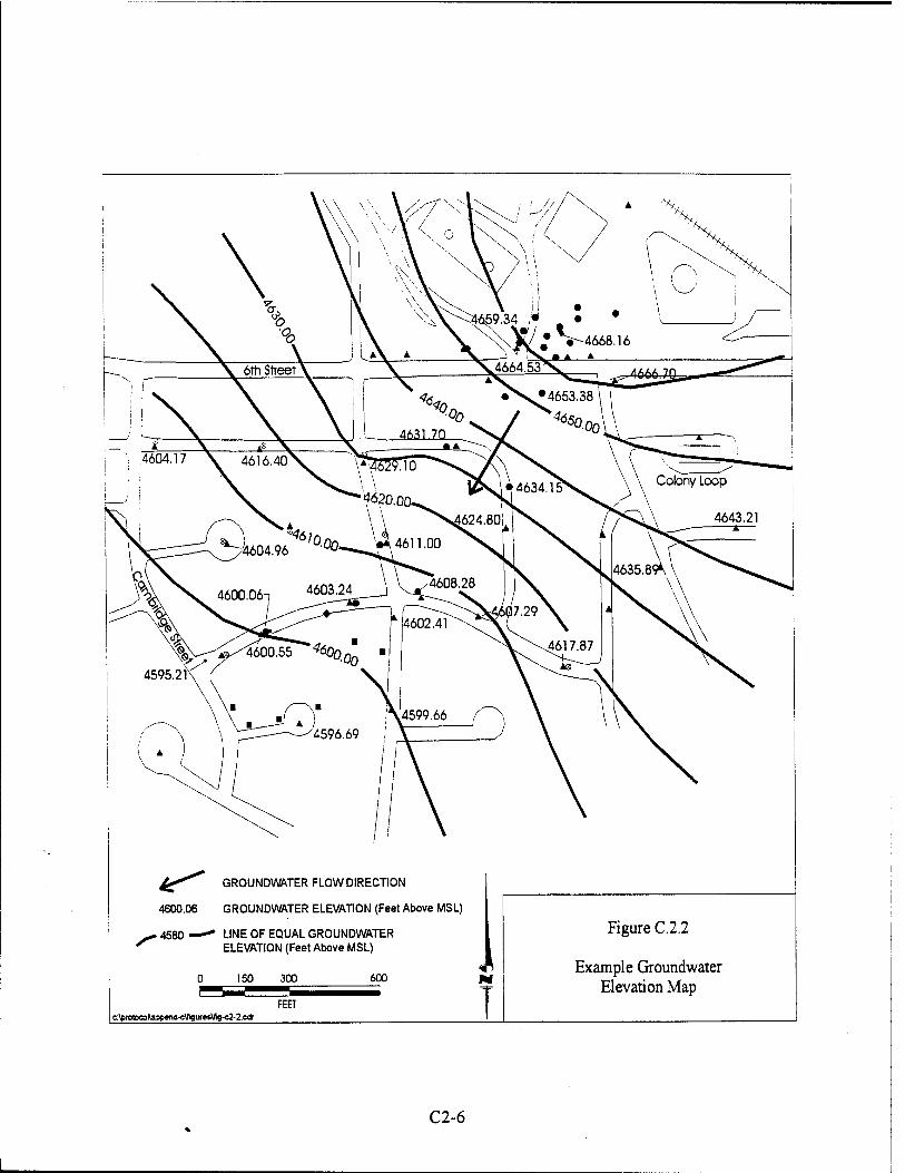
^^0> GROUNDWATER FLOW DIRECTION
4600.06 GROUNDWATER ELEVATION (Feet Above MSL)
4580 —* LINE OF EQUAL GROUNDWATER ELEVATION (Feet Above MSL)
150 300 600
FEET c:\ptotpcotappcnd-c\liguict\tig-c2-2-Cdt
Figure C.2.2
Example Groundwater Elevation Map
C2-6
Revision 0
• Equipotential lines must be parallel to constant-head boundaries (constant-head boundaries are equipotential lines).
Trial-and-error sketching is generally used to construct a flow net. Flow net sketching can be
sufficiently accurate if constructed according to the basic rules outlined above. A relatively small
number of flow lines (three to five) generally are sufficient to adequately characterize flow
conditions. Flow nets should be superimposed on the hydrogeologic sections. Figure C.2.3 is an
example of a completed flow net. This figure shows groundwater flow patterns in both recharge and discharge areas.
C.2.2.4 Preparation of Contaminant Isopach Maps
If LNAPL is present at the site, isopach maps showing the thickness and distribution of
LNAPL should be prepared. Two maps should be prepared: one for mobile LNAPL, and one for
residual LNAPL. Such isopach maps allow estimation of the distribution of LNAPL in the
subsurface and aid in fate and transport model development by identifying the boundary of the
LNAPL. Because of the differences between the magnitude of capillary suction in the aquifer
matrix and the different surface tension properties of fuel and water, LNAPL thickness
observations made in monitoring points are only an estimate of the actual volume of mobile
LNAPL in the aquifer. To determine the actual LNAPL thickness it is necessary to collect and
visually analyze soil samples. LNAPL thickness data also should be used to correct for water
table deflections caused by the mobile LNAPL. This process is described in Section C.2.2.3.2.
Isopach maps are prepared by first plotting the measured LNAPL thickness on a base map
prepared using surveyor's data. Lines of equal LNAPL thickness (isopachs) are then drawn and
labeled. Each data point must be honored during contouring. Figure C.2.4 is an example of a
completed isopach map. This figure also contains an example of an isopleth map.
C.2.2.4.1 Relationship Between Apparent and Actual LNAPL Thickness
It is well documented that LNAPL thickness measurements taken in groundwater monitoring
wells are not indicative of actual LNAPL thicknesses in the formation (de Pastrovich et al, 1979;
Blake and Hall, 1984; Hall et al, 1984; Hampton and Miller, 1988; Hughes et al, 1988; Abdul et
al, 1989; Testa and Paczkowski, 1989; Fair et al, 1990; Kemblowski and Chiang, 1990; Lehnard
and Parker, 1990; Mercer and Cohen, 1990; Ballestero et al, 1994; Huntley ei al, 1994a and
1994b). These authors note that the measured thickness of LNAPL in a monitoring well is
C2-7
c:\protocol\append-c\appnd-c2.doc

CN
Ü
3
z _o [x.
Qu
X
CD c
o
(1) c
CD
C CD O Q.
'D
U_ LU
"CD
E, ■o ca 0 X
&
o
■c
3 X E o
T3 O 5
C2-8
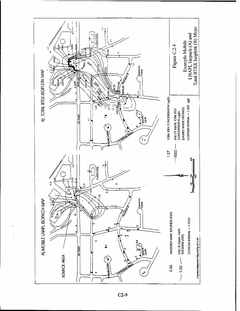
C2-9
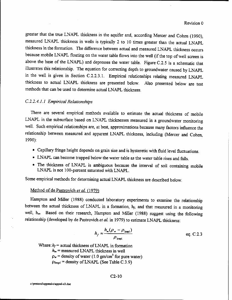
Revision 0
greater that the true LNAPL thickness in the aquifer and, according Mercer and Cohen (1990),
measured LNAPL thickness in wells is typically 2 to 10 times greater than the actual LNAPL
thickness in the formation. The difference between actual and measured LNAPL thickness occurs
because mobile LNAPL floating on the water table flows into the well (if the top of well screen is
above the base of the LNAPL) and depresses the water table. Figure C.2.5 is a schematic that
illustrates this relationship. The equation for correcting depth to groundwater caused by LNAPL
in the well is given in Section C.2.2.3.1. Empirical relationships relating measured LNAPL
thickness to actual LNAPL thickness are presented below. Also presented below are test
methods that can be used to determine actual LNAPL thickness.
C.2.2.4.1.1 Empirical Relationships
There are several empirical methods available to estimate the actual thickness of mobile
LNAPL in the subsurface based on LNAPL thicknesses measured in a groundwater monitoring
well. Such empirical relationships are, at best, approximations because many factors influence the
relationship between measured and apparent LNAPL thickness, including (Mercer and Cohen, 1990):
• Capillary fringe height depends on grain size and is hysteretic with fluid level fluctuations.
• LNAPL can become trapped below the water table as the water table rises and falls.
• The thickness of LNAPL is ambiguous because the interval of soil containing mobile LNAPL is not 100-percent saturated with LNAPL.
Some empirical methods for determining actual LNAPL thickness are described below.
Method of de Pastrovich et al. 0979)
Hampton and Miller (1988) conducted laboratory experiments to examine the relationship
between the actual thickness of LNAPL in a formation, h/, and that measured in a monitoring
well, hm. Based on their research, Hampton and Miller (1988) suggest using the following
relationship (developed by de Pastrovich et al. in 1979) to estimate LNAPL thickness:
*/* — eq. C.2.3
Where: hf= actual thickness of LNAPL in formation hm = measured LNAPL thickness in well Pw = density of water (1.0 gm/cm3 for pure water) Pinapi = density of LNAPL (See Table C.3.9)
C2-10
c:\protocol\appead-c\appnd-c2.doc
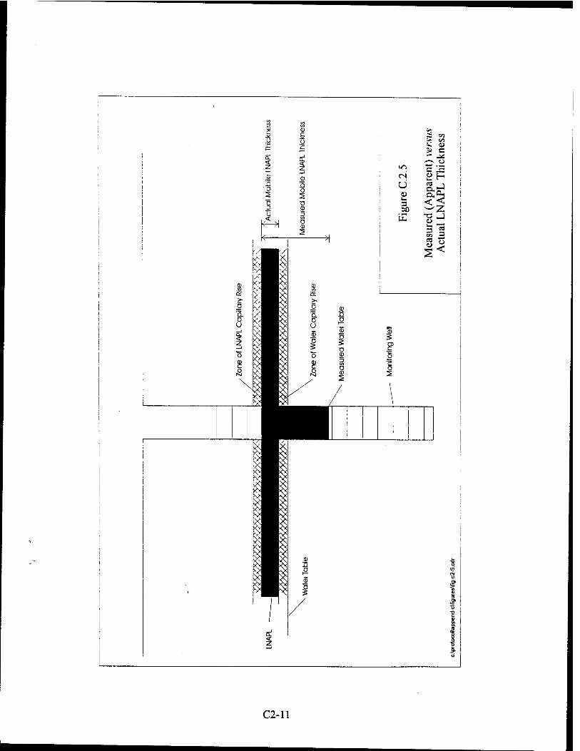
ü
■A
o *5 a m >3 cn s«. ü 5> C - .*
>—N ü u-> C JS CN £H u n J 4) 3 <5 50
w2 tu
5*
I
C2-11
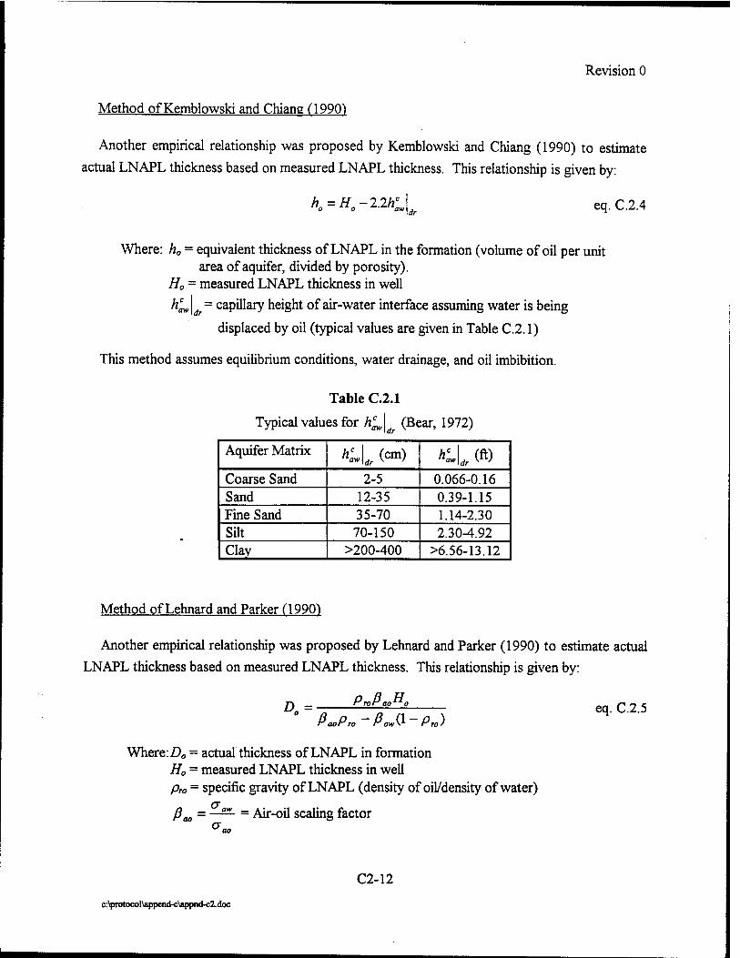
Revision 0
Method of Kemblowski and Chiang (1990')
Another empirical relationship was proposed by Kemblowski and Chiang (1990) to estimate
actual LNAPL thickness based on measured LNAPL thickness. This relationship is given by:
h=H-22h: dr
eq. C.2.4
Where: h0 = equivalent thickness of LNAPL in the formation (volume of oil per unit area of aquifer, divided by porosity).
H0 = measured LNAPL thickness in well
/zacw|^= capillary height of air-water interface assuming water is being
displaced by oil (typical values are given in Table C.2.1)
This method assumes equilibrium conditions, water drainage, and oil imbibition.
Table C.2.1
Typical values for he„\ (Bear, 1972)
Aquifer Matrix K» dr (cm) *• * (ft>
Coarse Sand 2-5 0.066-0.16 Sand 12-35 0.39-1.15 Fine Sand 35-70 1.14-2.30 Silt 70-150 2.30-4.92 Clay >200-400 >6.56-13.12
Method of Lehnard and Parker 09901
Another empirical relationship was proposed by Lehnard and Parker (1990) to estimate actual
LNAPL thickness based on measured LNAPL thickness. This relationship is given by:
£) - ProßaoHo
ßaoPro-ßo^-Pro)
Where: D0 = actual thickness of LNAPL in formation H0 = measured LNAPL thickness in well Pro = specific gravity of LNAPL (density of oil/density of water)
ßao = —— = Air-oil scaling factor
eq. C.2.5
C2-12
c:\protocol\append-c\appnd-c2.doc
Revision 0
ßow = —— = Oil-water scaling factor er ow
Go» = surface tension of uncontaminated water (72.75 dynes/cm @ 20°C) <jao = surface tension of LNAPL [25 dynes/cm @ 20°C for JP-4, Table C.2.2] cu = craw- <jao = interfacial tension between water and LNAPL (47.75dynes/cm @
20°C)
It is important to note that this method includes the capillary thickness of the hydrocarbon, and
is therefore likely to be an overestimate.
Table C.2.2
Surface Tensions for Various Compounds
Compound Surface Tension @ 20°C (dyne/cm)
JP-4 25" Gasoline 19-23 * Pure Water 72.75* a/Martel(1987). b/CRC Handbook (1956).
C.2.2.4.1.2 LNAPL Baildown Test
The LNAPL baildown test is applicable in areas where the hydrocarbon/water interface is
below the potentiometric surface, and the recharge rate of hydrocarbon into the well is slow
(Hughes et al, 1988).
Baildown Test Procedure (From Hughes et al., 1988):
1) Gauge the well and calculate the corrected potentiometric surface elevation using equations
C.2. land C.2.2.
2) Rapidly bail the hydrocarbon from the well.
3) Gauge the well again, and if the thickness of the hydrocarbon is acceptable (0.1 to 1 foot),
calculate the potentiometric surface elevation. The potentiometric surface elevation thus
calculated should be within 0.005 foot of the value calculated in step 1. If it is, then
continue to step 4; if it is not, repeat steps 2 and 3.
C2-13
c:\protocoI\append-c\appnd-c2.doc
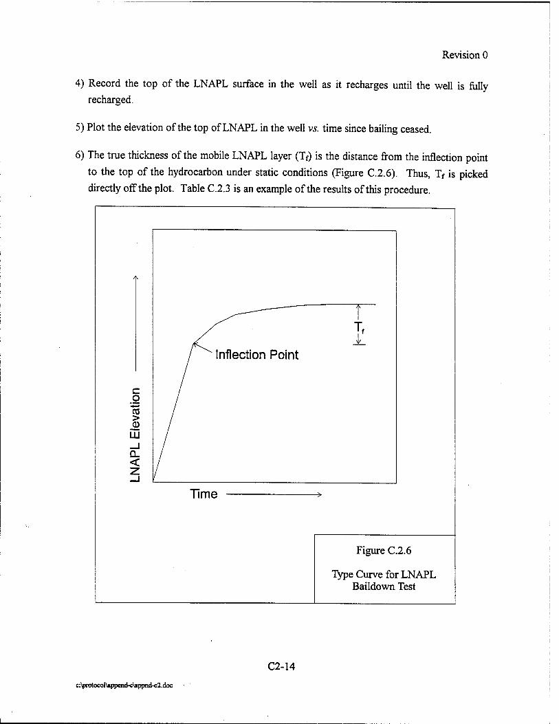
Revision 0
4) Record the top of the LNAPL surface in the well as it recharges until the well is fully recharged.
5) Plot the elevation of the top of LNAPL in the well vs. time since bailing ceased.
6) The true thickness of the mobile LNAPL layer (Tf) is the distance from the inflection point to the top of the hydrocarbon under static conditions (Figure C.2.6). Thus, Tf is picked directly off the plot. Table C.2.3 is an example of the results of this procedure.
/ v
/
f j '__
/ Inflection Point
c o 03 > CD
LU _1 GL <
Time -^
Figure C.2.6
Type Curve for LNAPL Baildown Test
C2-14
c:\protocol\append-c\appnd-c2.doc
Revision 0
Table C.2.3 Results of Example Baildown Test
(Modified from Hughes et al., 1988)
Well Tw(ft)" Tf(ft) Exaggeration (T,/Tf)
ROW-143 4.97 0.61 8.1:1 ROW-189 12.5 0.29 43.0:1 ROW-129 0.94 CO* N/A
a/ Tw = LNAPL thickness initially measured in the well b/ Capillary oil only
Hughes et al. (1988) also present a recharge method that involves pumping the mobile LNAPL
until steady-state conditions are achieved, and then letting the well fully recharge.
C.2.2.5 Preparation of Contaminant Isopleth Maps
Contaminant isopleth maps should be prepared for each of the BTEX compounds and for total
BTEX. Isopleth maps allow interpretation of data on the distribution and the relative transport
and degradation rates of contaminants in the subsurface. In addition, contaminant isopleth maps
allow contaminant concentrations to be gridded and used for input into a numerical model.
Isopleth maps are prepared by first plotting the concentration of the contaminant on a base
map prepared using surveyor's data. Lines of equal contaminant concentration (isopleths) are
then drawn and labeled. It is important to ensure that each data point is honored during
contouring, unless some data are suspect. Figures C.2.4, C.2.7, and C.2.8 contain examples of
total BTEX isopleth maps.
Dissolved BTEX concentrations are determined through groundwater sampling and laboratory
analysis. From these data, isopleth maps for each of the BTEX compounds and for total
dissolved BTEX should be made. Dissolved BTEX concentrations are transferred to the fate and
transport model grid cells by overlaying the isopleth map onto the model grid.
C.2.2.6 Preparation of Electron Acceptor, Metabolic Byproduct, and Alkalinity Contour (Isopleth) Maps
Isopleth maps should be prepared for dissolved oxygen, nitrate, sulfate, iron II, methane, and
total alkalinity. These maps are used to provide visible evidence that biodegradation is occurring.
C2-15
c:\protocol\append-c\appnd-c2.doc
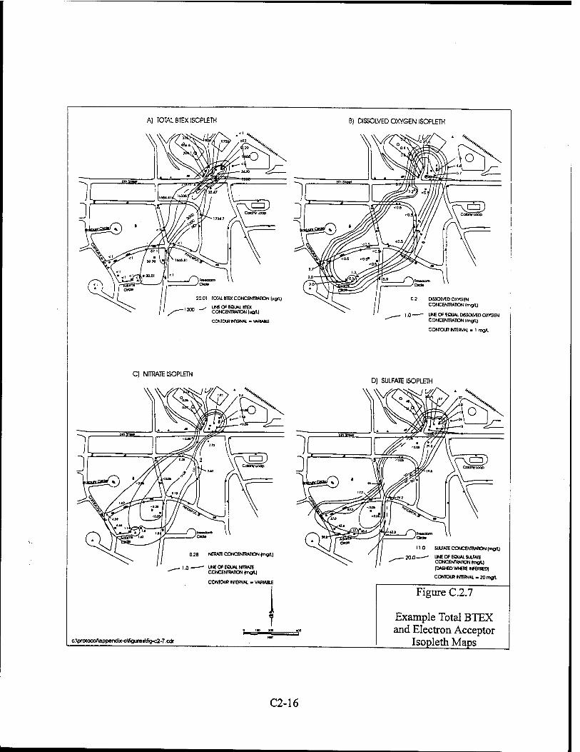
A) TOTAL BTEX ISOPLETH B) DISSOLVED OXYGEN ISOPLETH
V
CONTOUR INTEff/AL - VARIABLE
0.2 DISSOLVED OXYGEN CONCENTRATION Imq/L]
- UNE OF EQUAL DISSOLVED OWGEN CONCENTRATION |m£flj
CONTOUR NTERVAL - I mgfl
C) NITRATE ISOPLETH
w D) SULFATE ISOPLETH
. l o UNE OF EQUAL «IRATE CONCENTRATION |mgrL|
CONTOUR N1ERVAL - VARIABLE
0 1» 300
11.0 SULFATE CONCENTRATION (mtfl)
20.0 UNE OF EQUAL SULFATE CONCENTRATION (m#l| IDASWD WltRE NFERRED}
CONTOUR INTERVAL-30 m0l
c:\protocoAappendix-c\figures\fig-c2-7.cdr
Figure C.2.7
Example Total BTEX and Electron Acceptor
Isopleth Maps
C2-16

A) TOTAL BTEXISOPLETH
20.01 TOTAL BTEX CONCENTRATION ((igfL]
_^ LINE OF EQUAL BTEX CONCENTRATION (pgfl.]
CONTOUR INTERVAL - VARIABLE
■C) METHANE ISOPLETH
0.006 METHANE CONCENTRATION |mg/l|
005 UNEOf EQUAL METHANE CONCENTRATION (mgflj
CONTOUR INTERVAL - VARIABLE
B) IRON (II) ISOPLETH
V
5.22 IRON I«) CONCENTRATION (mod)
LINE OF EQUAL «ON («1 CONCENTRATION (mg/g
CONTOUR INTERVAL - VARIABLE
D) TOTAL ALKALINITY ISOPLETH
490 TOTAL ALKALINITY (AS CaOD3|(mg/l|
400—'' LINE OF EQUAL TOTAL ALKAUNTTY (mod)
CONTOUR NTERVAL - VARIABLE
•DATA FROM AUGUST 1993 (ONLYDAIA AVAILABLE FOR THE POM)
0 ISO ÄD
c:\pfOtocof\appencl-ctfi9um5tfi9-c2-fl.cdf
Figure C.2.8
Example Total BTEX, Metabolic Byproduct, and Total Alkalinity
Isopleth Maps
C2-17
Revision 0
The electron acceptor and metabolic byproduct isopleth maps can be used to determine the
relative importance of each of the terminal electron-accepting processes (TEAPs). The total
alkalinity map is used as a qualitative indicator of biodegradation via aerobic respiration, denitrification, and sulfate reduction.
Isopleth maps are prepared by first plotting the concentration of the electron acceptor,
metabolic byproduct, or total alkalinity on a base map prepared using surveyor's data. Lines of
equal concentration (isopleths) are then drawn and labeled. It is important to ensure that each
data point is honored during contouring, unless some data are suspect.
C.2.2.6.1 Electron Acceptor Isopleth Maps
The electron acceptor isopleth maps allow interpretation of data on the distribution of
dissolved oxygen, nitrate, and sulfate and the relative transport and degradation rates of
contaminants in the subsurface. These maps allow electron acceptor concentrations to be gridded
and used for input into the Bioplume model. Electron acceptor concentrations are transferred to
the model grid cells by overlaying the isopleth map on the model grid and transferring the
concentrations to the grid using interpolation where necessary.
Isopleth maps for dissolved oxygen, nitrate, and sulfate provide a visual indication of the
relationship between the contaminant plume and the electron acceptors and the relative
importance of each TEAP. Dissolved oxygen concentrations below background levels in areas
with BTEX contamination are indicative of aerobic respiration. Nitrate concentrations below
background in areas with BTEX contamination are indicative of denitrification. Sulfate
concentrations below background in areas with BTEX contamination are indicative of sulfate reduction.
Figure C.2.7 gives examples of completed electron acceptor isopleth maps for dissolved
oxygen, nitrate, and sulfate. This figure also contains the total BTEX isopleth map for the same
period. Comparison of the total BTEX isopleth map and the electron acceptor isopleth maps
shows that there is a strong correlation between areas with elevated BTEX and depleted electron
acceptor concentrations. The strong correlation indicates that the electron acceptor demand
exerted during the metabolism of BTEX has resulted in the depletion of soluble electron
acceptors. These relationships provide strong evidence that biodegradation is occurring via the
processes of aerobic respiration, denitrification, and sulfate reduction.
C2-18
c:\protocol\append-c\appnd-c2.doc
Revision 0
C.2.2.6.2 Metabolie Byproduct Isopleth Maps
Metabolie byproduct maps should be prepared for iron (II) and methane. The iron (II) map is
prepared in lieu of an electron acceptor isopleth map for iron (III) because the amount of
bioavailable amorphous or poorly crystalline iron (in) in an aquifer matrix is extremely hard to
quantify. Iron (II) concentrations above background levels in areas with BTEX contamination are
indicative of anaerobic iron (III) reduction. Methane concentrations above background levels in
areas with BTEX contamination are indicative of methanogenesis, another anaerobic process.
Figure C.2.8 gives examples of completed metabolic byproduct isopleth maps for iron (II) and
methane. This figure also contains the total BTEX isopleth map for the same period.
Comparison of the total BTEX isopleth map and the metabolic byproduct isopleth maps shows
that there is a strong correlation between areas with elevated BTEX and elevated metabolic
byproduct concentrations. The relationships between BTEX, iron (II), and methane provide
strong evidence that biodegradation is occurring via the processes of iron (III) reduction and methanogenesis.
C.2.2.6.3 Total Alkalinity Isopleth Map
Respiration of dissolved oxygen, nitrate, iron (El), and sulfate tends to increase the total
alkalinity (as CaC03) of groundwater. Thus, the total alkalinity inside the contaminant plume
generally increases to levels above background. This map will allow visual interpretation of
alkalinity data by showing the relationship between the contaminant plume and alkalinity.
Figure C.2.8 gives an example of a completed total alkalinity isopleth map. This figure also
contains the total BTEX isopleth map for the same period. Comparison of the total BTEX
isopleth map and the total alkalinity map shows that there is a strong correlation between areas
with elevated BTEX and elevated total alkalinity. The relationship between BTEX and total
alkalinity provides strong evidence that biodegradation is occurring via aerobic respiration, denitrification, iron (El) reduction, or sulfate reduction.
C2-19
c:\protocoI\append-c\appnd-c2.doc
Revision 0
SECTION C-3
INTRINSIC REMEDIATION CALCULATIONS
Several calculations using site-specific data must be made in order to document the occurrence of natural attenuation and successfully implement the intrinsic remediation alternative. The
following sections describe these calculations.
C.3.1 CALCULATING HYDRAULIC PARAMETERS
Hydraulic parameters necessary for adequate site characterization and model implementation include hydraulic conductivity, transmissivity, hydraulic gradient, linear groundwater flow velocity, hydrodynamic dispersion, and retarded solute transport velocity. Calculations for these parameters are discussed in the following sections.
C.3.1.1 Hydraulic Conductivity
Hydraulic conductivity, K, is a measure of an aquifer's ability to transmit water and is perhaps the most important variable governing fluid flow in the subsurface. Hydraulic conductivity has the units of length over time [L/T]. Observed values of hydraulic conductivity range over 12 orders of magnitude, from 3xl0"12 to 3 cm/sec (3xl0'9 to 3xl03 m/day) (Table C.3.1). In general terms, the hydraulic conductivity for unconsolidated sediments tends to increase with increasing grain size and sorting. The velocity of groundwater and dissolved contaminants is directly related to the hydraulic conductivity of the saturated zone. Subsurface variations in hydraulic conductivity directly influence contaminant fate and transport by providing preferential pathways for contaminant migration. The most common methods used to quantify hydraulic conductivity in the subsurface are aquifer pumping tests and slug tests. The quantitative analysis of pumping and slug test data is beyond the scope of this document. For information on the quantitative analysis of these data, the reader is referred to the works of Kruseman and de Ridder (1991) and Dawson
and Istok (1991).
C3-1
c:\protocol\append-c\appnd-c3 .doc
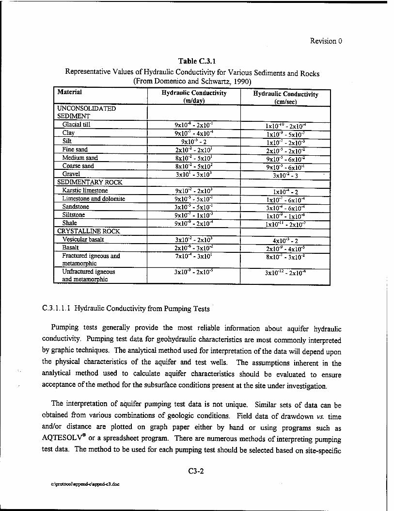
Revision 0
Table C.3.1 Representative Values of Hydraulic Conductivity for Various Sediments and Rocks
(From Domenico and Schwartz, 1990) Material Hydraulic Conductivity
(m/dav) Hydraulic Conductivity
(cm/sec) UNCONSOLIDATED SEDIMENT
Glacial till 9x10-* - 2xl0"' lxl0"iu - 2X10"4
Clav 9x10"' - 4X10⁻⁴ 1x10* - 5x10"'
Silt 9x10-' - 2 1x10"' - 2xl0"3
Fine sand 2x10'^ - 2x10' 2X100 - 2xl0"2
Medium sand 8x10"" - 5x10' 9x10°-6x10* Coarse sand 8x10^ - 5xl02
9X10"3 - 6x10"' Gravel 3x10'-3xl03
3x10"' - 3 SEDIMENTARY ROCK
Karstic limestone 9x10"' - 2xl03 lxlO"4 - 2
Limestone and dolomite 9x10-' - 5xl0_i 1x10"' - 6X10"4
Sandstone 3x10"* - 5x10"' 3X10"8 - 6X10"4
Siltstone 9x10-' - lxlO-3 1x10* - lxlO"6
Shale 9x10* - 2X10"4 lxlO"1-2x10''
CRYSTALLINE ROCK Vesicular basalt 3x10" - 2xl03
4x10° - 2 Basalt 2X10-0 - 3xl0-2
2x10* - 4xl0-i
Fractured igneous and metamorphic
7X10"4 - 3x10' 8x10"' - 3xl0"2
Unfractured igneous and metamorphic
3x10* - 2xl0"5 3x10"" - 2x10-*
C.3.1.1.1 Hydraulic Conductivity from Pumping Tests
Pumping tests generally provide the most reliable information about aquifer hydraulic conductivity. Pumping test data for geohydraulic characteristics are most commonly interpreted by graphic techniques. The analytical method used for interpretation of the data will depend upon the physical characteristics of the aquifer and test wells. The assumptions inherent in the analytical method used to calculate aquifer characteristics should be evaluated to ensure acceptance of the method for the subsurface conditions present at the site under investigation.
The interpretation of aquifer pumping test data is not unique. Similar sets of data can be obtained from various combinations of geologic conditions. Field data of drawdown vs. time and/or distance are plotted on graph paper either by hand or using programs such as AQTESOLV® or a spreadsheet program. There are numerous methods of interpreting pumping test data. The method to be used for each pumping test should be selected based on site-specific
C3-2
c:\protocol\append-c\appnd-c3.doc

Revision 0
conditions (aquifer conditions, test conditions, assumptions made, etc.). Most hydrogeology text
books contain pumping test evaluation techniques. Two publications dealing with pump test
analysis are recommended (Kruseman and de Ridder, 1991 and Dawson and Istok, 1991).
C.3.1.1.2 Hydraulic Conductivity from Slug Tests
Slug tests are a commonly used alternative to pumping tests that are relatively easy to conduct.
The biggest advantage of slug tests is that no contaminated water is produced during the test.
During pumping tests at fuel-hydrocarbon-contaminated sites, large volumes of contaminated
water that must be treated typically are produced. One commonly cited drawback to slug testing
is that this method generally gives hydraulic conductivity information only for the area
immediately surrounding the monitoring well. If slug tests are going to be relied upon to provide
information on the three-dimensional distribution of hydraulic conductivity in an aquifer, multiple
slug tests must be performed, both within the same well and at several monitoring wells at the
site. It is not advisable to rely on data from one slug test in a single monitoring well. Data
obtained during slug testing are generally analyzed using the method of Hvorslev (1951) for
confined aquifers or the method of Bouwer and Rice (1976) and Bouwer (1989) for unconfined
conditions.
C.3.1.2 Transmissivity
The transmissivity, T, of an aquifer is the product of the aquifer's hydraulic conductivity, K,
and the saturated thickness, b:
T = Kb eq.C.3.1
For a confined aquifer, b is the thickness of the aquifer between confining units. For
unconfined aquifers, b is the saturated thickness of the aquifer measured from the water table to
the underlying confining layer. Transmissivity has the units of length squared over time [L2/T].
C.3.1.3 Hydraulic Head and Gradient
Deterrnining the magnitude of hydraulic gradients is important because gradients influence the
direction and rate of contaminant migration. Hydraulic head, H, and specifically, variations in
hydraulic head within an aquifer, is the driving force behind groundwater movement and solute
C3-3
c:\protocol\append-c\appnd-c3.doc
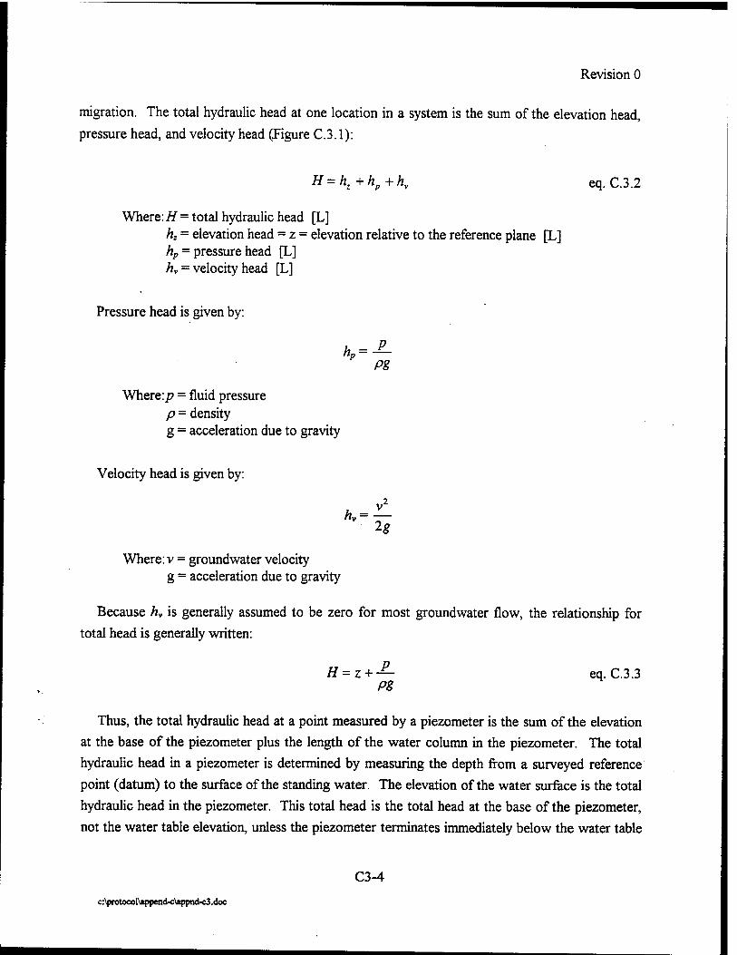
Revision 0
migration. The total hydraulic head at one location in a system is the sum of the elevation head,
pressure head, and velocity head (Figure C.3.1):
H = hz+hp+hv eq. C.3.2
Where: H = total hydraulic head [L] hz = elevation head = z = elevation relative to the reference plane [L] hp = pressure head [L] hv = velocity head [L]
Pressure head is given by:
Pg
Where:/? = fluid pressure p = density g = acceleration due to gravity
Velocity head is given by:
2g
Where: v = groundwater velocity g = acceleration due to gravity
Because hv is generally assumed to be zero for most groundwater flow, the relationship for
total head is generally written:
H=z + — eq. C.3.3 Pg
Thus, the total hydraulic head at a point measured by a piezometer is the sum of the elevation
at the base of the piezometer plus the length of the water column in the piezometer. The total
hydraulic head in a piezometer is determined by measuring the depth from a surveyed reference
point (datum) to the surface of the standing water. The elevation of the water surface is the total
hydraulic head in the piezometer. This total head is the total head at the base of the piezometer,
not the water table elevation, unless the piezometer terminates immediately below the water table
C3-4
c:\protocol\append-c\appnd-c3 .doc

Depth to Water
B /— Measurement Datum
I \ /— Open-ended Tube (Piezometer)
Depth to Water
T T
Ground Surface
Water Table
Pressure Head = J1
P9
Total Head (H)
Elevation Head (z)
i
T
- Pressure Head = ^=
\ i
Total Head (H)
Elevation Head (z)
; c:\protocof\append-c\figures\fig-c3-1.cdr
Mean Sea Level (Reference Elevation)
Figure C. 3.1
Hydraulic Head
C3-5

Revision 0
or is a well screened across the water table. Figure C.3.1 shows a pair of nested piezometers that
illustrate the relationships between total hydraulic head, pressure head, and elevation head.
Because groundwater flows from areas with high total head (point A, Figure C.3.1) to areas with
lower total head (point B), this figure depicts a water table aquifer with a strong upward vertical
gradient. This figure illustrates how nested piezometers (or wells) are used to determine the
importance of vertical gradients at a site. This figure also illustrates the importance of using wells
screened in the same portion of the aquifer (preferably across the water table) when preparing
potentiometric surface maps.
The hydraulic gradient (dH/dL) is a dimensionless number that is the change in hydraulic head
(dH) between two points divided by the length of groundwater flow between these same two
points, parallel to the direction of groundwater flow, and is given by:
dH Hydraulic Gradient = — eq. C.3.4
dL
Where: dH= change in total hydraulic head between two points [L] dL = distance between the two points used for head measurement [L]
In a system where flow is not occurring, the total hydraulic head, H, is the same everywhere in
the system and the hydraulic gradient is zero. To accurately determine the hydraulic gradient, it is
necessary to measure groundwater levels in all monitoring wells at the site. Because hydraulic
gradients can change over a short distance within an aquifer, it is essential to have as much site-
specific groundwater elevation information as possible so that accurate hydraulic gradient
calculations can be made. In addition, seasonal variations in groundwater flow direction can have
a profound influence on contaminant transport. To determine the effect of seasonal variations in
groundwater flow direction on contaminant transport, quarterly groundwater level measurements
should be taken over a period of at least 1 year.
The hydraulic gradient must be determined parallel to the direction of groundwater flow.
Unless two monitoring wells screened in the same relative location within the same hydrogeologic
unit are located along a line parallel to the direction of groundwater flow, the potentiometric
surface map is generally used to determine the hydraulic gradient. To determine the hydraulic
gradient, an engineer's scale is used to draw a line perpendicular to the equal-potential lines on
the potentiometric surface map (i.e., parallel to the direction of groundwater flow). Measure the
distance between the two equal-potential lines, making note of the groundwater potential at each
equal-potential line. Subtract the larger potential from the smaller potential, and divide this
number by the distance between the two equal potential lines, being sure to use consistent units.
C3-6
c:\protocol\append-c\appnd-c3.doc
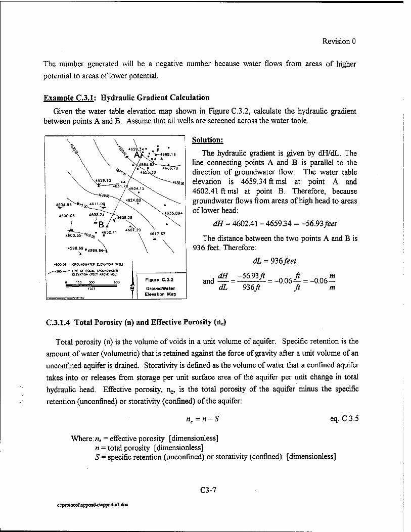
Revision 0
The number generated will be a negative number because water flows from areas of higher
potential to areas of lower potential.
Example C.3.1; Hydraulic Gradient Calculation
Given the water table elevation map shown in Figure C.3.2, calculate the hydraulic gradient between points A and B. Assume that all wells are screened across the water table.
650.00
4600.0« CROUNDWATER ELEVATION (USD
, 4JS0 UNE Or EOUAl GROUNDWATER ELEVATION (FEET ABOVE MS.)
Figur» C.3.2
GroundWater Elevation Map
Solution:
The hydraulic gradient is given by dH/dL. The line connecting points A and B is parallel to the direction of groundwater flow. The water table elevation is 4659.34 ft msl at point A and 4602.41 ft msl at point B. Therefore, because groundwater flows from areas of high head to areas of lower head:
dH = 4602.41 - 465934 = -56.93 feet
The distance between the two points A and B is 936 feet. Therefore:
and
dL = 936 feet
dL 936^ ft m
C.3.1.4 Total Porosity (n) and Effective Porosity (ne)
Total porosity (n) is the volume of voids in a unit volume of aquifer. Specific retention is the
amount of water (volumetric) that is retained against the force of gravity after a unit volume of an
unconfined aquifer is drained. Storativity is defined as the volume of water that a confined aquifer
takes into or releases from storage per unit surface area of the aquifer per unit change in total
hydraulic head. Effective porosity, rig, is the total porosity of the aquifer minus the specific
retention (unconfined) or storativity (confined) of the aquifer:
ne =n-S eq. C.3.5
Where: we = effective porosity [dimensionless] n = total porosity [dimensionless] S = specific retention (unconfined) or storativity (confined) [dimensionless]
C3-7
c:\protocoI\append-c\appnd-c3.doc
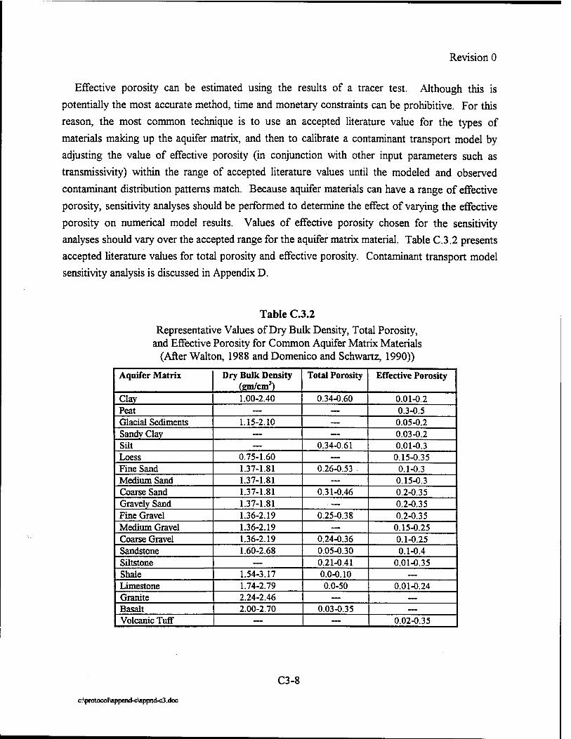
Revision 0
Effective porosity can be estimated using the results of a tracer test. Although this is
potentially the most accurate method, time and monetary constraints can be prohibitive. For this
reason, the most common technique is to use an accepted literature value for the types of
materials making up the aquifer matrix, and then to calibrate a contaminant transport model by
adjusting the value of effective porosity (in conjunction with other input parameters such as
transmissivity) within the range of accepted literature values until the modeled and observed
contaminant distribution patterns match. Because aquifer materials can have a range of effective
porosity, sensitivity analyses should be performed to determine the effect of varying the effective
porosity on numerical model results. Values of effective porosity chosen for the sensitivity
analyses should vary over the accepted range for the aquifer matrix material. Table C.3.2 presents
accepted literature values for total porosity and effective porosity. Contaminant transport model
sensitivity analysis is discussed in Appendix D.
Table C.3.2 Representative Values of Dry Bulk Density, Total Porosity,
and Effective Porosity for Common Aquifer Matrix Materials (After Walton, 1988 and Domenico and Schwartz, 1990))
Aquifer Matrix Dry Bulk Density (gm/cm3)
Total Porosity Effective Porosity
Clay 1.00-2.40 0.34-0.60 0.01-0.2 Peat — — 0.3-0.5 Glacial Sediments 1.15-2.10 — 0.05-0.2 Sandy Clay — — 0.03-0.2 Silt — 0.34-0.61 0.01-0.3 Loess 0.75-1.60 — 0.15-0.35 Fine Sand 1.37-1.81 0.26-0.53 0.1-0.3 Medium Sand 1.37-1.81 — 0.15-0.3 Coarse Sand 1.37-1.81 0.31-0.46 0.2-0.35 Gravelv Sand 1.37-1.81 — 0.2-0.35 Fine Gravel 1.36-2.19 0.25-0.38 0.2-0.35 Medium Gravel 1.36-2.19 — 0.15-0.25 Coarse Gravel 1.36-2.19 0.24-0.36 0.1-0.25 Sandstone 1.60-2.68 0.05-0.30 0.1-0.4 Siltstone — 0.21-0.41 0.01-0.35 Shale 1.54-3.17 0.0-0.10 —
Limestone 1.74-2.79 0.0-50 0.01-0.24 Granite 2.24-2.46 — —
Basalt 2.00-2.70 0.03-0.35 —
Volcanic Tuff — — 0.02-0.35
c:\protocol\append-c\appnd-c3.doc
C3-8

Revision 0
C.3.1.5 Linear Groundwater Flow Velocity (Seepage or Advective Velocity)
The average linear groundwater flow velocity (seepage velocity) in one dimension in the direction parallel to groundwater flow in a saturated porous medium is given by:
K dH v*= — eq.C.3.6 ne dL
Where: vx= average linear groundwater velocity parallel to groundwater flow direction (seepage velocity) [L/T]
K = hydraulic conductivity [L/T] nt = effective porosity [L3/L3] dH —— = hydraulic gradient [L/L] dL
The average linear groundwater flow velocity should be calculated to estimate groundwater flow and solute transport velocity, to check the accuracy of groundwater models, and to calculate first-order biodegradation rate constants.
Example C.3.2: Linear Groundwater Flow Velocity Calculation
Calculate the linear groundwater flow velocity in a medium-grained sandy aquifer. The hydraulic gradient as determined from the potentiometric surface map in the previous example is -0.06 m/m. The hydraulic conductivity is 1.7X10"1 m/day as determined by pumping tests.
Solution:
Because the effective porosity of this sediment is not known, it is necessary to estimate this parameter. From Table C.3.2, the effective porosity for a medium-grained sand is approximately 23 percent.
rnrr (0.17-f-)(-0.06™) Vx = -E.M = ^ «_ = 0.044-^-
ne dL 0.23 day
C.3.1.6 Coefficient of Retardation and Retarded Contaminant Transport Velocity
When the average linear velocity of a dissolved contaminant is less than the average linear velocity of the groundwater, the contaminant is said to be "retarded." The difference between the
C3-9
c:\protocol\append-c\appnd-c3.doc
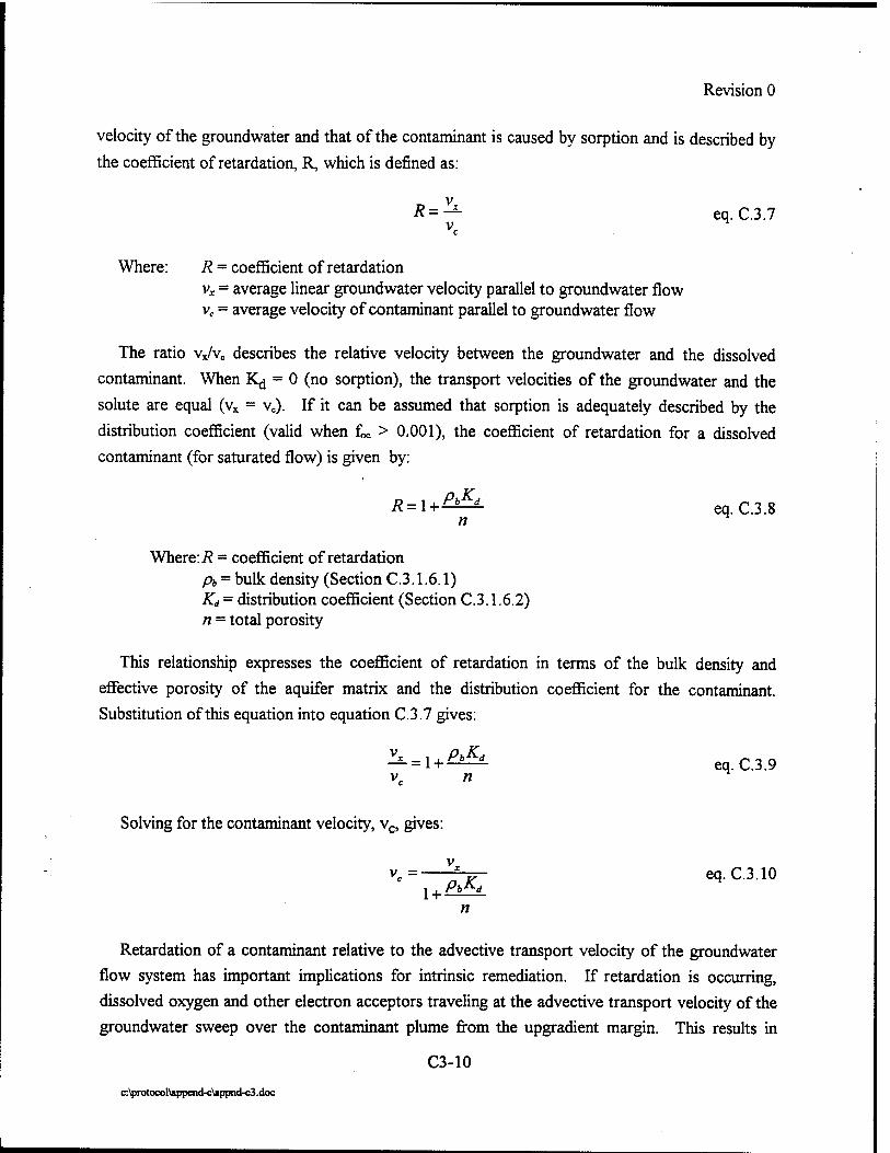
Revision 0
velocity of the groundwater and that of the contaminant is caused by sorption and is described by the coefficient of retardation, R, which is defined as:
R = — eq. C.3.7
Where: R = coefficient of retardation vx = average linear groundwater velocity parallel to groundwater flow vc = average velocity of contaminant parallel to groundwater flow
The ratio vx/vc describes the relative velocity between the groundwater and the dissolved contaminant. When K^ = 0 (no sorption), the transport velocities of the groundwater and the solute are equal (vx = vc). If it can be assumed that sorption is adequately described by the distribution coefficient (valid when f« > 0,001), the coefficient of retardation for a dissolved contaminant (for saturated flow) is given by:
R = l+£& eq.C.3.8 n
Where: R = coefficient of retardation Pi = bulk density (Section C.3.1.6.1) Kd = distribution coefficient (Section C.3.1.6.2) n = total porosity
This relationship expresses the coefficient of retardation in terms of the bulk density and effective porosity of the aquifer matrix and the distribution coefficient for the contaminant. Substitution of this equation into equation C.3.7 gives:
Y*. = U.£J£L C39
Solving for the contaminant velocity, vc, gives:
v. = ^-— eq. C.3.10 1 + PbKd
n
Retardation of a contaminant relative to the advective transport velocity of the groundwater flow system has important implications for intrinsic remediation. If retardation is occurring, dissolved oxygen and other electron acceptors traveling at the advective transport velocity of the groundwater sweep over the contaminant plume from the upgradient margin. This results in
C3-10
c:\protocoI\append-c\appnd-c3.doc
Revision 0
greater availability of electron acceptors within the plume for biodegradation of fuel
hydrocarbons. In addition, adsorption of a contaminant to the aquifer matrix results in dilution of the dissolved BTEX plume.
C.3.1.6.1 Bulk Density
The bulk density of a soil, pt, as used in most groundwater models, expresses the ratio of the
mass of dried soil to its total volume (solids and pores together).
_ Ms _ Ms P" VT ~ (Vs + Va + V„) eq.C.3.11
Where: pi = bulk density Ms = mass of solid in the system Vj = total volume in the system Vs = volume of solid in the system Va = volume of air (or gas) in the system Vw = volume of water (or liquid) in the system
Bulk density is related to particle density by:
pb=(l-n)ps eq. C.3.12
Where: fh, = bulk density n = total porosity p, = density of grains comprising the aquifer
The bulk density is always less than the particle density, p,; for example, if pores constitute half
the volume, then pb is half of p,. The bulk density of a soil is affected by the structure of the soil
(looseness and degree of compaction), as well as by its swelling and shrinking characteristics, both
of which depend on clay content and soil moisture. Even in extremely compacted soil, the bulk
density remains appreciably lower than the particle density. This is because the particles can never
interlock perfectly, and the soil remains a porous body, never completely impervious. In sandy
soils, pb can be as high as 1.81 gm/cm3. In aggregated loams and clayey soils, pj, can be as low as
1.1 gm/cm3. TableC.3.2 contains representative values of dry bulk density for common sediments and rocks.
C3-11
c:\protocol\append-c\appnd-c3 .doc
Revision 0
C.3.1.6.2 Distribution Coefficient and Total Organic Carbon Content
The distribution coefficient is described in Section B.4.3. Recall equation B.4.10, which gives
the relationship between/« and K«:
Kd = Koefoe eq.C.3.13
Where: Kd = distribution coefficient [L3/M] Koc= soil adsorption coefficient for soil organic carbon content [L3/M] foe = fraction soil organic carbon (mg organic carbon/mg soil) [M/M]
Representative K^. values are given in Table B.4.1. The fraction of soil organic carbon must
be determined from site-specific data. Representative values of total organic carbon (TOC) in
common sediments are given in Table C.3.3. Because most solute transport occurs in the most
transmissive aquifer zones, it is imperative that soil samples collected for total organic carbon
analyses come from these zones in background areas. To be conservative, the average of all total
organic carbon concentrations from sediments in the most transmissive aquifer zone should be
used for retardation calculations.
Example C.3.3; Retarded Solute Transport Velocity Calculation
For groundwater flow and solute transport occurring in a shallow, saturated, well-sorted, fine-
grained, sandy aquifer, with a total organic carbon content of 0.7 percent, a hydraulic gradient of
-0.015 m/m, and an hydraulic conductivity of 25 m/day, calculate the retarded contaminant
velocity for benzene.
Solution;
Because the total porosity, effective porosity, and the bulk density are not given, values of
these parameters are obtained from Table C.3.2. The median values for total porosity, effective
porosity, and bulk density are approximately 0.4, 0.2, and 1.6 kg/L respectively.
The first step is to calculate the average linear groundwater velocity, vx.
25-^- -0.015^ V day)\ mJ m
v = = i_9- 0.2 day
C3-12
c:\protocol\append-c\appnd-c3.doc

Revision 0
Table C.3.3
Representative Values of Total Organic Carbon for Common Sediments
Texture medium sand fine sand fine to coarse sand organic silt and peat silty sand silt with sand, gravel and clay (glacial till) medium sand to gravel loess (silt) fine - medium sand
fine to medium sand
fine to coarse sand
sand coarse silt medium silt fine silt silt fine sand medium sand to gravel
Depositional Environment fluvial-deltaic
back-barrier (marine) glacial (lacustrine) glaciofluvial glacial moraine
glaciofluvial eolian glaciofluvial or glaciolacustrine glaciofluvial
glaciofluvial
fluvial fluvial fluvial fluvial lacustrine glaciofluvial glaciofluvial
a/Karickhoff, 1981 b/ Domenico and Schwartz (1990)
Fraction Organic Carbon 0.00053-0.0012 0.0006-0.0015 0.00026 - 0.007 0.10-0.25 0.0007 - 0.008 0.0017-0.0019
0.00125 0.00058-0.0016 < 0.0006-0.0061
0.00021 - 0.019
0.00029 - 0.073
0.0057 0.029 0.020 0.0226 0.0011 0.00023-0.0012 0.00017 - 0.00065
Site Name Hill AFB, Utah Boiling AFB. P.C. Patrick AFB, Florida Elmendorf AFB, Alaska Elmendorf AFB. Alaska Elmendorf AFB, Alaska
Elmendorf AFB, Alaska Ofrutt AFB, Nebraska Truax Field, Madison Wisconsin King Salmon AFB, Training Area, Alaska
Fire
Dover AFB, Delaware Creek Battle
Michigan ANGB,
Oconee River, Georgia57" Oconee River, Georgia*7" Oconee River, Georgia*7" Oconee River, Georgia*7" Wildwood, Ontario^ Various sites in Ontario^ Various sites in Ontario57"
The next step is to determine the distribution coefficient, Kd. Values of K^ for BTEX are
obtained from Table B.4.1 and are listed in Table C.3.4.
For benzene Koc = 79 L/kg, and (using equation C.3.13):
^=(79-g(0.007) = 0.553-|
The retarded contaminant velocity is given by (equation C.3.10):
C3-13
c:\protocoI\append-c\apptxl-c3.doc

Revision 0
v„ = = 0.59 m
day
This example illustrates that contaminant sorption to total organic carbon can have a profound influence on contaminant transport by significantly slowing the rate of dissolved contaminant
migration.
Table C.3.4 Example Retardation Calculations for the BTEX Compounds
Fraction Distribution Bulk Advective Contaminant
K« Organic Coefficient Density Total Coefficient of Groundwater Velocity
Compound L/kg Carbon (L/kg) (kg/L) Porosity Retardation Velocity (m/day) (m/day)
Benzene 79 0.007 0.553 1.60 0.40 3.21 1.90 0.59
Toluene 190 0.007 1.33 1.60 0.40 6.32 1.90 0.30 Ethylbenzene 468 0.007 3.276 1.60 0.40 14.10 1.90 0.13 m-xylene 405 0.007 2.835 1.60 0.40 12.34 1.90 0.15 o-xyiene 422 0.007 2.954 1.60 0.40 12.82 1.90 0.15
p-xylene 357 0.007 2.499 1.60 0.40 11.00 1.90 0.17 1,2,3-trimethyIbenzene 884 0.007 6.188 1.60 0.40 25.75 1.90 0.07 1,2,4-trimethylbenzene 772 0.007 5.404 1.60 0.40 22.62 1.90 0.08 1,3,5-trimethylbenzene 676 0.007 4.732 1.60 0.40 19.93 1.90 0.10
C.3.2 CONTAMINANT SOURCE TERM CALCULATIONS
NAPLs present in the subsurface can represent a continuing source of groundwater contamination. Sorption of fuel hydrocarbons onto the aquifer matrix occurs when NAPL enters the subsurface. When sufficient quantities of NAPL are present, the unsaturated zone may initially be saturated with NAPL, but after a period of time the NAPL will drain from the pores under the influence of gravity, leaving a thin coating of NAPL. Depending on the surface area of the materials comprising the subsurface, the surface tension of the NAPL, and the porosity and permeability of the subsurface materials, some NAPL also may be held between the grains by capillarity. NAPL adhering to the grains of the aquifer matrix or retained by capillarity is herein referred to as residual NAPL. If the NAPL is mobile within and among the pores of the aquifer matrix, as is generally the case near the water table, the NAPL is referred to as mobile NAPL.
If BTEX concentrations in the residual and mobile LNAPL are not decreasing over time, or if they are decreasing very slowly, extremely long times will be required for natural attenuation of the dissolved contaminant plume. This will likely make intrinsic remediation unattractive to regulators and will reduce the chance of implementation. In order for intrinsic remediation to be a
C3-14
c:\protocol\append-c\appnd-c3.doc

Revision 0
viable remedial option, the source of continuing groundwater contamination must be decreasing
over time (decaying), either by natural weathering processes or via engineered remedial solutions
such as mobile LNAPL recovery, bioventing, or bioslurping. Because natural weathering
processes can be fairly slow, especially in static systems where the groundwater elevation does
not fluctuate significantly, it will generally be necessary to implement engineered remedial
solutions to remove the LNAPL. However, in cases where the LNAPL has been in the ground
for a long period of time, it may be weathered to the point that it no longer acts as a source of
significant groundwater contamination (Section C.3.2.3). Because of their physical and chemical
properties, the BTEX compounds are generally the first to be removed from the LNAPL via
natural weathering processes. Wiedemeier et al. (1993) used mass fraction BTEX analyses from
mobile LNAPL at a jet fuel spill site in Colorado to show that the weathered LNAPL was not
capable of producing dissolved BTEX concentrations above regulatory groundwater quality standards.
To determine how long it will take for a dissolved contaminant plume to disappear, it is
necessary to estimate how fast the contaminant source (LNAPL) is being removed. Source
removal rates can be estimated where bioventing is being used to remediate residual LNAPL by
collecting soil samples in the source area at the start of remedial activities. After the system has
been operating for a period of time, soil samples are collected from approximately the same
location(s). Comparison of BTEX concentrations in samples collected from the same location
makes it possible to determine when the source area has been remediated. This approach has
been used successfully at several Air Force bases where pilot-scale bioventing systems had been
installed and where 1-year sampling data were available. Experience with the bioventing initiative
shows that at most of the 105 sites where data are available, 99 percent of the BTEX mass in the
subsurface vadose zone is remediated in 1 year. In areas with mobile LNAPL it is much more
difficult to estimate cleanup times, so conservative estimates should be made based on LNAPL
removal rates. Predicting the cleanup time for sites with mobile LNAPL is especially difficult
because residual LNAPL will remain after the recoverable mobile LNAPL has been removed.
One remedial technology that has shown promise for both residual and mobile LNAPL is
bioslurping. Bioslurping removes mobile LNAPL via suction lift. During bioslurping operations,
a vacuum is induced in the unsaturated zone. This vacuum draws oxygen from uncontaminated
areas into the area contaminated with residual LNAPL and extracts soil gas into which VOCs
have volatilized. A properly installed bioslurping system thus acts as a mobile LNAPL recovery system, a bioventing system, and a soil vapor extraction system.
C3-15
c:\protocoI\append-c\appnd-c3.doc
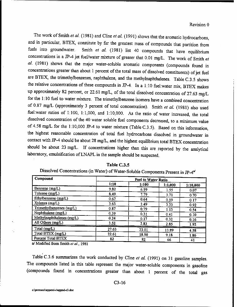
Revision 0
The work of Smith et al. (1981) and Cline et al. (1991) shows that the aromatic hydrocarbons, and in particular, BTEX, constitute by far the greatest mass of compounds that partition from
fuels into groundwater. Smith et al. (1981) list 40 compounds that have equilibrium concentrations in a JP-4 jet fuel/water mixture of greater that 0.01 mg/L. The work of Smith et
al. (1981) shows that the major water-soluble aromatic components (compounds found in concentrations greater than about 1 percent of the total mass of dissolved constituents) of jet fuel are BTEX, the trimethylbenzenes, naphthalene, and the methylnaphthalenes. Table C.3.5 shows the relative concentrations of these compounds in JP-4. In a 1:10 fuel: water mix, BTEX makes
up approximately 82 percent, or 22.61 mg/L, of the total dissolved concentration of 27.63 mg/L for the 1:10 fuel to water mixture. The trimethylbenzene isomers have a combined concentration of 0.87 mg/L (approximately 3 percent of total concentration). Smith et al. (1981) also used fuel:water ratios of 1:100, 1:1,000, and 1:10,000. As the ratio of water increased, the total dissolved concentration of the 40 water soluble fuel components decreased, to a minimum value of 4.58 mg/L for the 1:10,000 JP-4 to water mixture (Table C.3.5). Based on this information, the highest reasonable concentration of total fuel hydrocarbons dissolved in groundwater in
contact with JP-4 should be about 28 mg/L, and the highest equilibrium total BTEX concentration should be about 23 mg/L. If concentrations higher than this are reported by the analytical laboratory, emulsification of LNAPL in the sample should be suspected.
Table C.3.5 Dissolved Concentrations (in Water) of Water-Soluble Components Present in JP-4^
Compound Fuel to Water Ratio 1:10 1:100 1:1,000 1:10,000
Benzene (mg/L) 9.82 6.99 1.55 0.07 Toluene (mg/L) 8.49 7.79 3.71 0.70 Ethylbenzene (mg/L) 0.67 0.64 0.59 0.17 Xylenes (mg/L) 3.63 3.49 3.33 0.92 Trimethylbenzenes (mg/L) 0.87 0.79 1.13 0.54 Naphthalene (mg/L) 0.39 0.31 0.41 0.10 Methylnaphthalenes (mg/L) 0.24 0.17 0.32 0.16 All Others (mg/L) 3.52 2.83 2.85 1.92 Total (mg/L) 27.63 23.01 13.89 4.58 Total BTEX (mg/L) 22.61 18.90 9.18 1.86 Percent Total BTEX 82 82 66 41
a/ Modified from Smith et al., 1981
f
Table C.3.6 summarizes the work conducted by Cline et al. (1991) on 31 gasoline samples. The compounds listed in this table represent the major water-soluble components in gasoline (compounds found in concentrations greater than about 1 percent of the total gas
C3-16 c:\protocol\append-c\appnd-c3 .doc

Revision 0
chromatography/flame ionization detector peak area for all compounds detected in the aqueous
phase), which are BTEX, n-propylbenzene, 3- and 4-ethyltoluene, and 1,2,3-trimethylbenzene.
Based on the information presented in Table C.3.6, the highest reasonable concentration of total
fuel hydrocarbons dissolved in groundwater in contact with gasoline should be about 135 mg/L,
and the highest equilibrium total BTEX concentration should be about 132 mg/L. If
concentrations higher than this are reported by the analytical laboratory, emulsification of LNAPL in the sample should be suspected.
There are two methods that can be used to determine the concentration of contaminants
dissolved in groundwater beneath NAPL and thus quantify the contaminant source loading. The
first method involves directly measuring the concentration of dissolved contaminants in
groundwater beneath the NAPL plume. The second method involves the use of partitioning
calculations. The following sections describe each approach.
Table C.3.6
Weight Percent Water-Soluble Components in Gasoline and Their Concentrations in Water in Contact with Gasoline
Compound Gasoline Composition*'
(Weight Percent)
Dissolved Concentration*'
(mg/L)
Gasoline Composition'1'
(Weight Percent)
Dissolved Concentration1''
(mg/L) benzene 1.73 42.6 1.94 58.7 toluene 9.51 69.4 4.73 33.4 ethylbenzene 1.61 3.2 2.0 4.3 m- and p-xylene 5.95 11.4 — .. o-xylene 2.33 5.6 2.27 6.9 m-xvlene - — 5.66 11.0 p-xylene - — 1.72 4.4 n-propylbenzene 0.57 0.4 _ —m
3-,4-ethyltoluene 2.20 1.7 _ __ 1,2,3-trimethylbenzene 0.8 0.7 _ -» 1,2,4-trimethylbenzene - - 3.26 1.1 Total 24.7 135 21.58 119.8 Total BTEX 132.2 118.7 Percent Total BTEX 98 99
a/CIinee/a/. (1991) b/ American Petroleum Institute (1985) average of 24 analyses from nine fuel:water solutions
(l:10fuel:water)
C3-17
c:\protocol\append-c\appnd-c3.doc
Revision 0
C.3.2.1 Direct Measurement of Dissolved Contaminant Concentrations in Groundwater in Contact with NAPL
Two methods can be used to determine the dissolved concentration of contaminants in groundwater beneath a NAPL plume. The first method involves collecting groundwater samples
from beneath a LNAPL lens in monitoring wells. The second method involves collecting samples of mixed LNAPL and water from monitoring wells.
C.3.2.1.1 Collecting Groundwater Samples From Beneath the LNAPL
This method involves carefully sampling groundwater beneath a floating LNAPL lens. One
way of collecting a groundwater sample from beneath a lens of floating LNAPL involves using a
peristaltic pump. The depth to the base of the mobile LNAPL is measured, a length of high- density polyethylene (HDPE) tubing that will reach 1 to 2 feet beneath the LNAPL is lowered into the well, and the sample is collected. Another useful technique for obtaining such a sample where the depth to groundwater is too deep to allow use of a peristaltic pump is to use a Grundfos® pump. If a Grundfos® pump is used to collect a water sample from beneath LNAPL, it is imperative that the pump be thoroughly cleaned after each use, and that good sampling logic be used (e.g., sample less contaminated wells first). Also, dedicated bladder pumps that are being used for long-term monitoring (LTM) in wells with LNAPL can be used to collect water samples from beneath the LNAPL.
C.3.2.1.2 Collecting Mixed Groundwater/NAPL Samples
This method involves collecting a sample of groundwater and floating LNAPL from a monitoring well, placing the sample in a sealed container used for volatile organics analysis being careful to ensure there is no headspace, allowing the sample to reach equilibrium, and submitting the water beneath the floating NAPL to a qualified laboratory for analysis. A disposable bailer generally works best for collection of this type of sample. Smith et al. (1981) has information on how to conduct such a test. Two or three samples should be collected from different monitoring wells containing LNAPL at the site. This test should only be done when it is not possible to collect a discrete sample from beneath the LNAPL.
C3-18
c:\protocol\append-c\appnd-c3.doc
Revision 0
C.3.2.2 Partitioning Calculations
LNAPL present at a site represents a continuing source of contamination because BTEX and other aromatic compounds will partition from the LNAPL into the groundwater. In such cases, it is generally necessary to estimate the dissolved concentration of BTEX expected in groundwater
near the LNAPL. Partitioning calculations can be performed for sites with NAPL to quantify contaminant loading from the NAPL into the groundwater. Such calculations allow estimation of
the impact of continuing sources of contamination on dissolved BTEX concentrations. The results of partitioning calculations may show that even if the NAPL is allowed to remain in the ground, dissolved contaminant concentrations will remain below regulatory guidelines. This is especially true when weathered NAPLs with initially low BTEX concentrations, such as jet fuels (Jet A, JP-4, etc.) are present. Partitioning calculations made by Wiedemeier et al. (1993) showed that NAPL present in the subsurface at a fueling facility near Denver, Colorado was
incapable of producing dissolved BTEX concentrations in groundwater above regulatory standards. Partitioning calculations should be confirmed with a LTM program.
If partitioning calculations suggest that partitioning from the LNAPL could increase dissolved BTEX concentrations in groundwater to above regulatory guidelines at a point of compliance, then this continuing source of groundwater contamination should be remediated. Residual LNAPL contamination in the unsaturated zone is generally best remediated using bioventing, a technique that introduces air (oxygen) into the subsurface, thus stimulating aerobic biodegradation of fuel hydrocarbons. When found in the saturated zone, residual LNAPL is extremely difficult to remove. Maximum BTEX concentrations resulting from such partitioning will occur when the groundwater and LNAPL reach equilibrium. Assuming that equilibrium is reached gives the most conservative modeling results. Alternate, less conservative models for partitioning from LNAPL into the aqueous phase are given by Hunt et al. (1988) and Johnson and Pankow (1992). These models are described below.
C.3.2.2.1 Equilibrium Partitioning of BTEX from Mobile LNAPL into Groundwater
The fuel-water partitioning coefficient, K^,, is defined as the ratio of the concentration of a compound in the fuel to the compound's equilibrium concentration in water in contact with the fuel:
Kfiv=-J- eq.C.3.14 C w
Where:^ = fuel-water partitioning coefficient [dimensionless]
C3-19
c:\protocol\append-c\appnd-c3.doc

Revision 0
Cf= concentration of the compound in the fuel [M/L3] Cw = concentration of the compound dissolved in groundwater [M/L3]
Table C.3.7 lists values of Kfy, for BTEX and trimethylbenzenes (TMB) in jet fuel and gasoline.
The relationships relating Kfw to the aqueous solubility of a pure compound in pure water, S,
presented in Table C.3.8 can be used to estimate Kjw for compounds not listed in this table.
Table C.3.7
Fuel-Water Partitioning Coefficients (Kf«,) for Those Compounds Most Commonly found in the Aqueous Phase in Water in Contact with Jet Fuel or Gasoline
Compound (JP-4 Jet Fuel) (Gasoline) (Gasoline)
Benzene 2,455 231 350 Toluene 2,754 895 1,250 Ethylbenzene 4,786 3,411 4,500 o-xylene 7,079 3,162 3,630 m-xylene 3,715 3,539 4,350 p-xylene 7,586 2,961 4,350 1,2,3 -Trimethylbenzene NA NA 13,800 1,2,4-Trimethylbenzene 8,913 12,270 NA 1,3,5-Trimethylbenzene NA 6,493 NA
a/ From experiments conducted by Smith et aL, 1981 (For JP-4) b/ Model of Bruce et aL, 1991 (for gasoline) c/ Model of Cline et aL, 1991 (for gasoline) NA = not analyzed
Table C.3.8
Relationships Relating Fuel-Water Partitioning Coefficients (K&) to Pure Aqueous-Phase Solubility
LNAPL Type Relationship Relating S to K*,"' Reference JP-4 log K,w = -0.7971ogS +1.681 Smiths a/., 1981 JP-5 log Kfw = -0.7461ogS + 1.757 Smith et aL, 1981 JP-8 log K^ = -0.8641ogS + 1.508 Smith et aL, 1981 Gasoline log Kfw = -1.151ogS +6.099 Bruce et aL, 1991 Gasoline log Kfw = -1.001ogS +0.85 Cline et aL, 1991
a/ Determined using linear regression on data for dissolved compound concentrations in a fuel-water mix.
Using the definition of Kf* presented above, the maximum (equilibrium) total dissolved BTEX
concentration resulting from the partitioning of BTEX from NAPL into groundwater is given by:
Cw - 'f K
eq. C.3.15 fw
C3-20
c:\protocol\append-c\appnd-c3.doc

Revision 0
This relationship predicts the concentration of dissolved BTEX in the groundwater if the
LNAPL is allowed to remain in contact with the groundwater long enough so that equilibrium
between the two phases is reached.
To complete partitioning calculations, samples of the mobile LNAPL must be collected and
analyzed to determine the type of fuel and the mass fraction of BTEX present in the fuel. From
the mass fraction BTEX data, the concentration of each BTEX compound in the fuel on a
volumetric basis, Q-, can be calculated by using the relationship:
cf = FfPf eq. C.3.16
Where: pf = Density of fuel (Table C.3.9)
Ff= Mass fraction of compound in the fuel
Using mass fraction BTEX data from the LNAPL analyses, and the fuel-water partitioning
coefficients presented in Table C.3.7, the maximum dissolved benzene, toluene, ethylbenzene, and
total xylene concentrations expected in groundwater caused by the partitioning of these
compounds from the LNAPL can be calculated using equation C.3.15.
Table C.3.9
Density of Common Liquids
Type of Liquid Density (gm/cm3) Density (gm/m3 = mg/L)
Miscellaneous Liquids: Water 1.0 1,000,000 Gasoline 0.68-0.76 680,000 - 760,000 Jet Fuel 0.74-0.85 740,000 - 850,000
JP-4 0.75 750,000 Kerosene 0.78-0.82 780,000 - 820,000
Fuel Oil and Diesel Oil: 0.82-0.95 820,000 - 950,000 BTEX and TMB
Benzene 0.868 868,000 Toluene 0.8669 866,900 Ethylbenzene 0.8669 866,900 o-xylene 0.8802 880,200 m-xylene 0.8642 864,200 p-xylene 0.8610 861,000 /, 2,3-trimethylbenzene 0.88 880,000 1,2,4-trimethylbenzene 0.88 880,000 7,3,5-trimethylbenzene 0.87 870,000 1,2,4,5-tetramethylbenzene 0.84 840,000
c:\protocol\append-c\appnd-c3.doc
C3-21
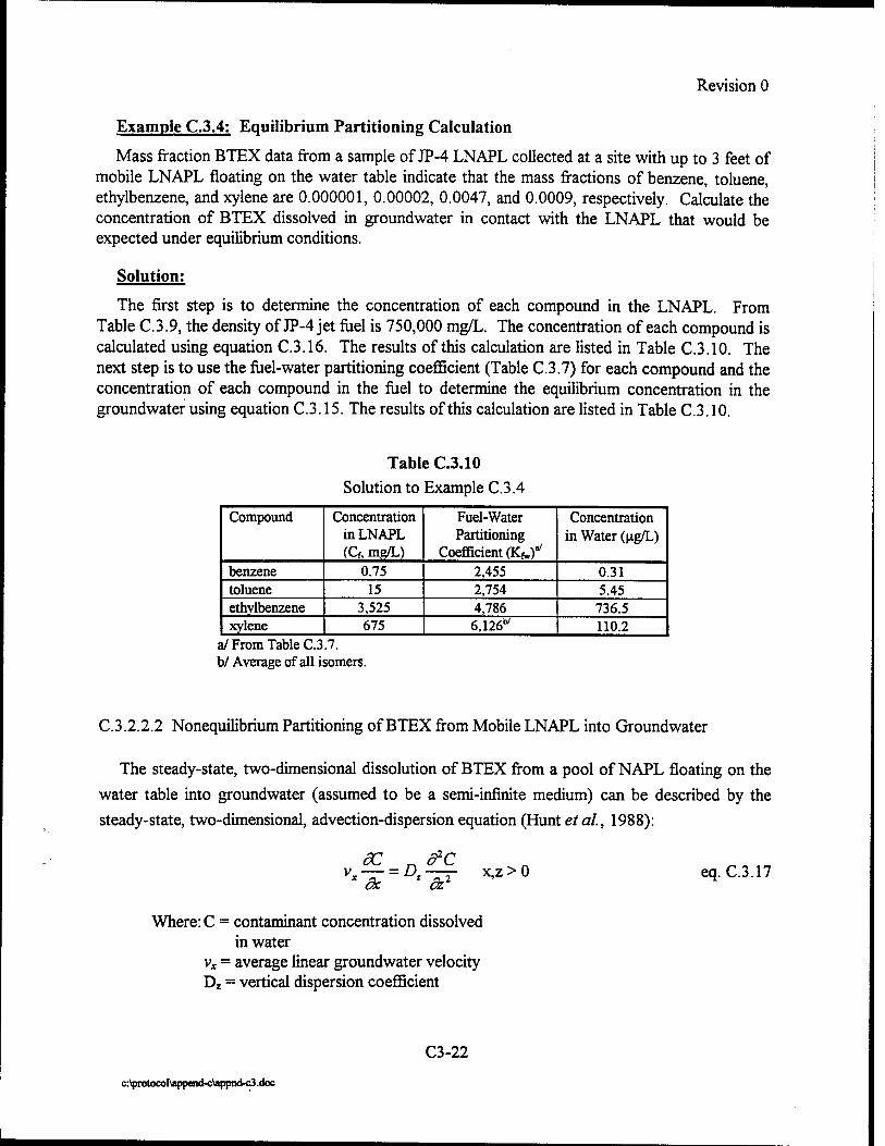
Revision 0
Example C.3.4: Equilibrium Partitioning Calculation
Mass fraction BTEX data from a sample of JP-4 LNAPL collected at a site with up to 3 feet of mobile LNAPL floating on the water table indicate that the mass fractions of benzene, toluene, ethylbenzene, and xylene are 0.000001, 0.00002, 0.0047, and 0.0009, respectively. Calculate the concentration of BTEX dissolved in groundwater in contact with the LNAPL that would be expected under equilibrium conditions.
Solution:
The first step is to determine the concentration of each compound in the LNAPL. From Table C.3.9, the density of JP-4 jet fuel is 750,000 mg/L. The concentration of each compound is calculated using equation C.3.16. The results of this calculation are listed in Table C.3.10. The next step is to use the fuel-water partitioning coefficient (Table C.3.7) for each compound and the concentration of each compound in the fuel to determine the equilibrium concentration in the groundwater using equation C.3.15. The results of this calculation are listed in Table C.3.10.
Table C.3.10 Solution to Example C.3.4
Compound Concentration in LNAPL (Cf, mg/L)
Fuel-Water Partitioning
Coefficient (Kfw)"/
Concentration in Water (ng/L)
benzene 0.75 2,455 0.31 toluene 15 2,754 5.45 ethylbenzene 3,525 4,786 736.5 xylene 675 6,126w 110.2
a/From Table C.3.7. b/ Average of all isomers.
C.3.2.2.2 Nonequilibrium Partitioning of BTEX from Mobile LNAPL into Groundwater
The steady-state, two-dimensional dissolution of BTEX from a pool of NAPL floating on the
water table into groundwater (assumed to be a semi-infinite medium) can be described by the
steady-state, two-dimensional, advection-dispersion equation (Hunt etal, 1988):
3C „ d2C vx — = D2 —- x,z > 0 1 dx. z 8L
2 eq. C.3.17
Where: C = contaminant concentration dissolved in water
vx = average linear groundwater velocity Dz = vertical dispersion coefficient
C3-22
c:\protocol\append-c\appnd-c3.doc
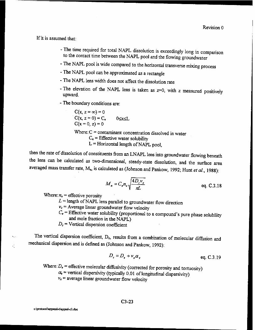
Revision 0
If it is assumed that:
- The time required for total NAPL dissolution is exceedingly long in comparison to the contact time between the NAPL pool and the flowing groundwater
- The NAPL pool is wide compared to the horizontal transverse mixing process
- The NAPL pool can be approximated as a rectangle
- The NAPL lens width does not affect the dissolution rate
- The elevation of the NAPL lens is taken as z=0, with z measured positively upward.
- The boundary conditions are:
C(x, z = oo) = 0 C(x, z = 0) = Ce 0<x<L C(x = 0, z) = 0
Where: C = contaminant concentration dissolved in water Ce = Effective water solubility L = Horizontal length of NAPL pool,
then the rate of dissolution of constituents from an LNAPL lens into groundwater flowing beneath
the lens can be calculated as two-dimensional, steady-state dissolution, and the surface area
averaged mass transfer rate, M,, is calculated as (Johnson and Pankow, 1992; Hunt et ah, 1988):
M„=C.nJ4D>V*
nL eq. C.3.18
Where: ne = effective porosity L = length of NAPL lens parallel to groundwater flow direction vx = Average linear groundwater flow velocity Ce = Effective water solubility (proportional to a compound's pure phase solubility
and mole fraction in the NAPL) Dz = Vertical dispersion coefficient
The vertical dispersion coefficient, Dz, results from a combination of molecular diffusion and mechanical dispersion and is defined as (Johnson and Pankow, 1992):
D,=Dt+vxa, eq. C.3.19
Where:Z)e = effective molecular diffusivity (corrected for porosity and tortuosity) a, = vertical dispersivity (typically 0.01 of longitudinal dispersivity) vx = average linear groundwater flow velocity
C3-23
c:\protocol\append-c\appnd-c3.doc
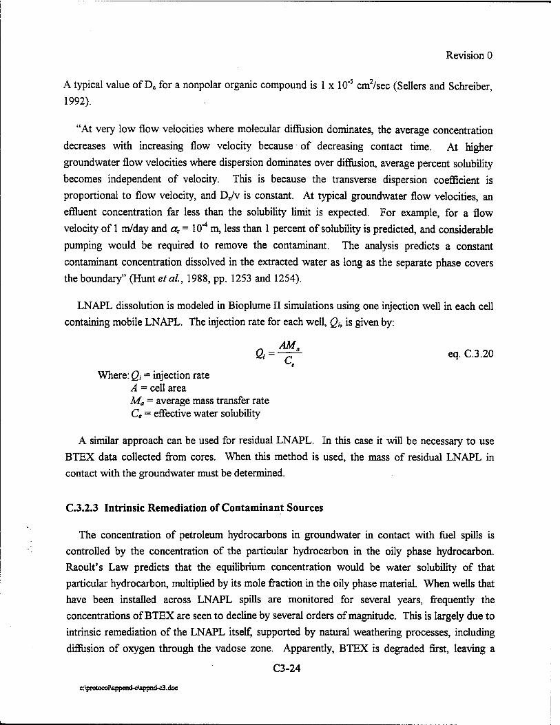
Revision 0
A typical value of De for a nonpolar organic compound is 1 x 10"5 cm2/sec (Sellers and Schreiber, 1992).
"At very low flow velocities where molecular diffusion dominates, the average concentration
decreases with increasing flow velocity because of decreasing contact time. At higher groundwater flow velocities where dispersion dominates over diffusion, average percent solubility becomes independent of velocity. This is because the transverse dispersion coefficient is proportional to flow velocity, and Dz/v is constant. At typical groundwater flow velocities, an effluent concentration far less than the solubility limit is expected. For example, for a flow
velocity of 1 m/day and a* = 10"4 m, less than 1 percent of solubility is predicted, and considerable pumping would be required to remove the contaminant. The analysis predicts a constant
contaminant concentration dissolved in the extracted water as long as the separate phase covers the boundary" (Hunt etai, 1988, pp. 1253 and 1254).
LNAPL dissolution is modeled in Bioplume II simulations using one injection well in each cell containing mobile LNAPL. The injection rate for each well, Qh is given by:
Qi = ~£JL eq.C.3.20
Where: Qt = injection rate A = cell area Ma = average mass transfer rate Ce = effective water solubility
A similar approach can be used for residual LNAPL. In this case it will be necessary to use BTEX data collected from cores. When this method is used, the mass of residual LNAPL in contact with the groundwater must be determined.
C.3.2.3 Intrinsic Remediation of Contaminant Sources
The concentration of petroleum hydrocarbons in groundwater in contact with fuel spills is controlled by the concentration of the particular hydrocarbon in the oily phase hydrocarbon. Raoult's Law predicts that the equilibrium concentration would be water solubility of that particular hydrocarbon, multiplied by its mole fraction in the oily phase material. When wells that have been installed across LNAPL spills are monitored for several years, frequently the concentrations of BTEX are seen to decline by several orders of magnitude. This is largely due to intrinsic remediation of the LNAPL itself, supported by natural weathering processes, including diffusion of oxygen through the vadose zone. Apparently, BTEX is degraded first, leaving a
C3-24
c:\protocol\append-c\appnd-c3.doc

Revision 0
residual of branched and normal alkanes. As a result, hydrocarbon contamination (i.e., BTEX)
disappears from the groundwater, although considerable quantities of total petroleum
hydrocarbons (TPH) may remain in the aquifer. The effect is well illustrated in the following case study.
In 1988, at least 1,200 gallons of unleaded gasoline was inadvertently pumped from an
underground storage tank onto the land surface at the petroleum, oil, and lubricants (POL) facility
at Eglin AFB, Florida. The fuel flowed overland toward a small creek 160 feet from the spill,
then infiltrated until it reached the water table. When sampled in 1993, the spill remained as
LNAPL in a smear zone extending from the point of release to the point of discharge of
groundwater to a wetland (Figure C.3.3).
Core samples were collected across the water table at (1) the location of the original spill, (2) a
location intermediate between the spill and the creek, and (3) the bank of the creek
(Figure C.3.3). Core samples were analyzed for TPH and BTEX. Wells were installed in the
boreholes used to acquire the cores and were screened across the interval containing TPH.
Cline et al. (1991) examined the variation in fuel to water partition coefficients for 31 gasoline
samples. Their estimates of Kfw for various gasoline components are presented in TableC.3.7.
TPH- and BTEX-concentration data in core samples from the spill at Eglin AFB are presented in
Table C.3.11. Assuming the specific gravity of gasoline is 0.74, the following relationship was
used to estimate C/for a given BTEX compound (e.g., benzene) in a given core sample.
c _ Benzenejmg/kg)x0.74(kg)TPH \06(mg)TPH f TPH(mgllcg) X \.0(J)TPH * \.Q{kg)TPH
The concentrations of BTEX in groundwater in contact with that particular core material were
predicted by dividing C/by Kf* from Table C.3.7. Table C.3.12 compares the predictions to the
actual measured concentrations of BTEX in groundwater from monitoring wells screened across
the depth interval from which the core samples were acquired.
The gasoline near the receptor, and half way between the source and the receptor, was so
weathered that no BTEX was detectable at concentrations greater than 0.01 mg/kg, although
considerable quantities of TPH remained (Table C.3.11). Duplicate samples at the TPH maximum
near the source were weathered, but appreciable concentrations of BTEX remained, and the
pattern of weathering varied between the cores.
C3-25
c:\protocol\append-c\appnd-c3.doc
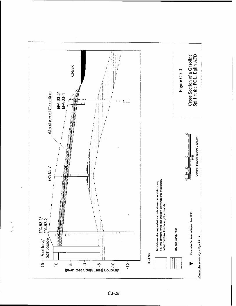
Q LiJ CD
iO lO O lO O lO
(|SA3i Das UDSIAJ jaaj) uojjDAaig
Ü
3 ao
u CQ .£ u, o< S.S
CO U
o a. c
o 1/3 ^
CO —«
c
£
*r tr> 1
I ■n
ii
2 Q
H- S UJ
1 UJ (3
LU
8!| S O > 1 QZ
"i S °L
C3-26
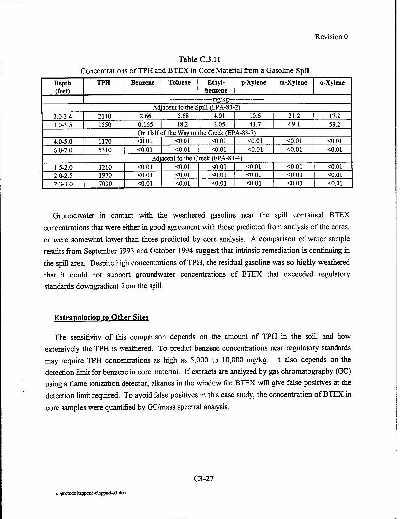
Revision 0
Table C.3.11 Concentrations of TPH and BTEX in Core Material from a Gasoline Spill
Depth (feet)
TPH Benzene Toluene Ethyl- benzene
p-Xylene m-Xylene o-Xylene
rnn/l^n "" "ing/Kg—
Adjacent to the Spill (EPA-83-2) 3.0-3.4 2140 2.66 5.68 4.01 10.6 21.2 17.2 3.0-3.5 1550 0.165 18.2 2.05 41.7 69.1 59.2
On Half of the Way to the Creek (EPA-83-7) 4.0-5.0 1170 <0.01 <0.01 <0.01 <0.01 <0.01 <0.01 6.0-7.0 5310 <0.01 <0.01 <0.01 <0.01 <0.01 <0.01
Adjacent to the Creek (EPA-83-4)
1.5-2.0 1210 <0.01 <0.01 O.01 <0.01 <0.01 <0.01 2.0-2.5 1970 <0.01 <0.01 <0.01 <0.01 <0.01 <0.01 2.3-3.0 7090 <0.01 <0.01 <0.01 <0.01 <0.01 <0.01
Groundwater in contact with the weathered gasoline near the spill contained BTEX concentrations that were either in good agreement with those predicted from analysis of the cores, or were somewhat lower than those predicted by core analysis. A comparison of water sample results from September 1993 and October 1994 suggest that intrinsic remediation is continuing in the spill area. Despite high concentrations of TPH, the residual gasoline was so highly weathered that it could not support groundwater concentrations of BTEX that exceeded regulatory
standards downgradient from the spill.
Extrapolation to Other Sites
The sensitivity of this comparison depends on the amount of TPH in the soil, and how extensively the TPH is weathered. To predict benzene concentrations near regulatory standards may require TPH concentrations as high as 5,000 to 10,000 mg/kg. It also depends on the detection limit for benzene in core material. If extracts are analyzed by gas chromatography (GC) using a flame ionization detector, alkanes in the window for BTEX will give false positives at the detection limit required. To avoid false positives in this case study, the concentration of BTEX in
core samples were quantified by GC/mass spectral analysis.
C3-27
c:\protocol\append-c\appnd-c3.doc

Revision 0
Table C.3.12. Comparison of BTEX in Groundwater to Predictions Based on the BTEX Content of the Weathered Residual Gasoline.
Sample Interval (ftbgs)
Benzene Toluene Ethyl- benzene
p-Xylene m-Xylene o-Xylene
ue/L Well EPA 83-2, Near the Gasoline Spill
3.0-3.4 prediction 2600 1600 310 840 1700 1600 3.0-3.5 prediction 230 7000 217 4600 7600 7800
measured 09/93 300 1400 350 540 410 measured 10/94 46 75 13 93 179 219
Well EPA 83-7, 70 feet Downgradient (One Half of the Distance to the Receptor) 4.0-5.0 prediction <18 <5 <1.4 <1.5 <1.5 <1.7 6.0-7.0 prediction <4 <1 <0.3 <0.3 <0.3 <0.4
measured 09/93 2.2 4.3 36 36 26 measured 10/94 1.9 1.0 <1 <1 <1 <1
Well EPA 83-4, 150 feet Downgradient, Adjacent to the Receutor 1.5-2.0 prediction <17 <5 <1.4 <1.4 <1.4 <1.7 2.0-2.5 prediction <11 <3 <0.8 <0.9 <0.9 <1.0 2.3-3.0 prediction <3 <0.8 <0.2 <0.2 <0.2 <0.3
measured 09/93 <1 <1 <1 <1 <1 <1 measured 10/94 <1 1.4 <1 <1 <1 <1
C.3.3 CONFIRMING AND QUANTIFYING BIODEGRADATION
Chemical evidence of two types can be used to document the occurrence of biodegradation. The first type of evidence is graphical and is provided by the electron acceptor and metabolic byproduct maps discussed in Section C-2. The second line of evidence involves using a conservative tracer.
C.3.3.1 Isopleth maps
The extent and distribution of contamination relative to electron acceptors and metabolic byproducts can be used to qualitatively document the occurrence of biodegradation. Depleted dissolved oxygen concentrations in areas with fuel hydrocarbon contamination indicates that an active zone of aerobic hydrocarbon biodegradation is present. Depleted nitrate and sulfate concentrations in areas with fuel hydrocarbon contamination indicate that an active zone of anaerobic hydrocarbon biodegradation is present and that denitrification and sulfate reduction are occurring. Elevated iron (II) and methane concentrations in areas with fuel hydrocarbon contamination indicate that an active zone of anaerobic hydrocarbon biodegradation is present and that iron reduction and methanogenesis are occurring. Isopleth maps of contaminants, electron
C3-28
c:\protocol\append-c\appnd-c3 .doc
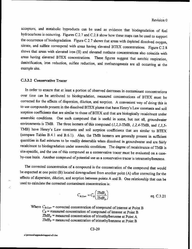
Revision 0
acceptors, and metabolic byproducts can be used as evidence that biodegradation of fuel
hydrocarbons is occurring. Figures C.2.7 and C.2.8 show how these maps can be used to support
the occurrence of biodegradation. Figure C.2.7 shows that areas with depleted dissolved oxygen,
nitrate, and sulfate correspond with areas having elevated BTEX concentrations. Figure C.2.8
shows that areas with elevated iron (II) and elevated methane concentrations also coincide with
areas having elevated BTEX concentrations. These figures suggest that aerobic respiration,
denitrification, iron reduction, sulfate reduction, and methanogenesis are all occurring at the example site.
C.3.3.2 Conservative Tracer
In order to ensure that at least a portion of observed decreases in contaminant concentrations
over time can be attributed to biodegradation, measured concentrations of BTEX must be
corrected for the effects of dispersion, dilution, and sorption. A convenient way of doing this is
to use compounds present in the dissolved BTEX plume that have Henry's Law constants and soil
sorption coefficients that are similar to those of BTEX and that are biologically recalcitrant under
anaerobic conditions. One such compound that is useful in some, but not all, groundwater
environments is TMB. The three isomers of this compound (7,2,3-TMB, 1,2,4-TMB, and 1,3,5-
TMB) have Henry's Law constants and soil sorption coefficients that are similar to BTEX
(compare Tables B.4.1 and B.6.1). Also, the TMB isomers are generally present in sufficient
quantities in fuel mixtures to be readily detectable when dissolved in groundwater and are fairly
recalcitrant to biodegradation under anaerobic conditions. The degree of recalcitrance of TMB is
site-specific, and the use of this compound as a conservative tracer must be evaluated on a case-
by-case basis. Another compound of potential use as a conservative tracer is tetramethylbenzene.
The corrected concentration of a compound is the concentration of the compound that would
be expected at one point (B) located downgradient from another point (A) after correcting for the
effects of dispersion, dilution, and sorption between points A and B. One relationship that can be used to calculate the corrected contaminant concentration is:
C =C rTMB^
TMB, eq. C.3.21
Where Cß.corr - corrected concentration of compound of interest at Point B Cs = measured concentration of compound of interest at Point B TMBA = measured concentration of trimethylbenzene at Point A TMBB = measured concentration of trimethylbenzene at Point B
C3-29
c:\protocol\append-c\appnd-c3.doc

Revision 0
Trimethylbenzene is slightly more hydrophobic than BTEX and therefore has a higher soil
sorption coefficient. This causes preferential sorption of TMB. In addition, TMB generally is not
entirely recalcitrant under anaerobic conditions, and appears to degrade rapidly under aerobic
conditions. The degree of recalcitrance of TMB is site-specific, and the use of this compound
must be evaluated on a case-by-case basis. However, if any TMB mass is lost to the processes of
biodegradation or preferential sorption, equation C.3.21 becomes more conservative (i.e., lower
mass losses due to biodegradation and lower biodegradation rate constants will be calculated).
After correcting measured BTEX concentrations for the effects of dispersion, dilution, and
sorption, it is possible to estimate the amount of BTEX removed from the system (converted to
carbon dioxide and water) via biodegradation, ACBioAB, between the two points (A) and (B) using the relationship:
AC Bio.AB ^A.Obs ^B.Corr eq. C.3.22
Where: AC5lo^ = change in BTEX concentration between points A and B caused by biodegradation
CA. obs = observed BTEX concentration at point A CB.COTT - corrected BTEX concentration at point B
The mass of BTEX lost between these two points can be calculated if the volume of water between the two points is known.
The percent of BTEX lost to biodegradation between the two points (A) and (B) can now be calculated, and is given by:
ABTEXBio = ^Bio,AB
Uc • 100 = Total.AßJ
C -C ^ ^A.Obs ^B.Corr
V ^A.Obs ^B.Obs J
•100 eq. C.3.23
Where: AB7EXBio = percent BTEX lost to biodegradation Cß.corr = TMB-corrected BTEX concentration at point B CA. obs = observed BTEX concentration at point A Cß.obs = observed BTEX concentration at point B ACjbtaMs = observed change in BTEX concentration between points A and B ^CBWAB = change in BTEX concentration between points A and B
caused by biodegradation
C3-30
c:\protoOTl\apprad-c\appnd-c3.doc
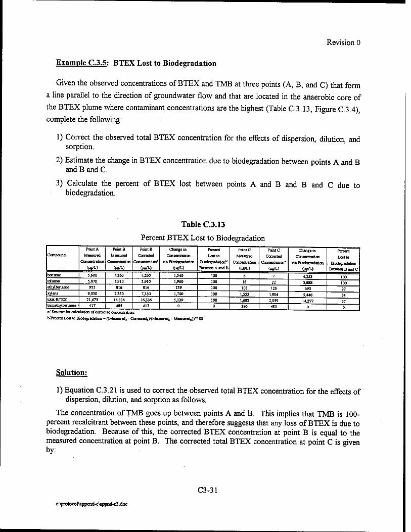
Revision 0
Example C.3.5: BTEX Lost to Biodegradation
Given the observed concentrations of BTEX and TMB at three points (A, B, and C) that form
a line parallel to the direction of groundwater flow and that are located in the anaerobic core of
the BTEX plume where contaminant concentrations are the highest (Table C.3.13, Figure C.3.4), complete the following:
1) Correct the observed total BTEX concentration for the effects of dispersion, dilution, and sorption.
2) Estimate the change in BTEX concentration due to biodegradation between points A and B and B and C.
3) Calculate the percent of BTEX lost between points A and B and B and C due to biodegradation.
Table C.3.13
Percent BTEX Lost to Biodegradation
Compound
Point A
Measured
Concentration
Point B
Measured
Concentration
(MS/W
Point B
Canceled
Concentration*'
(M8/L)
Change in
Conceotnti on
via Biodegradation
(ug/L.)
Percent
Lortto
Biodegradationw
Between A and B
PcintC
Measured
Concentration
Point C
Corrected
Concentration*'
(ug/L)
Change in
Concentration
via Biodegradation
(ug/L)
Percent
Lento
Biodegradation
BenMenBandC benzene 5,600 4,260 4,260 1,340 100 6 7 4,253 100 toluene 5,870 3,910 3,910 1,960 100 18 22 3.888 100 ethylbenzene 955 816 816 139 100 103 126 690 97 x\4ene 9,050 7,350 7,350 1,700 100 1,555 1,904 5,446 94 total BTEX 21,475 16,336 16336 5,139 100 1,682 2,059 14,277 97 trimethyiboiaene 417 485 417 0 0 396 485 0 0
b/Pereent Lost to Biodegradation - ((MeajuredA - Corrected,y(MeaniredA - Meaiured,))" 100
Solution:
1) Equation C.3.21 is used to correct the observed total BTEX concentration for the effects of dispersion, dilution, and sorption as follows.
The concentration of TMB goes up between points A and B. This implies that TMB is 100- percent recalcitrant between these points, and therefore suggests that any loss of BTEX is due to biodegradation. Because of this, the corrected BTEX concentration at point B is equal to the measured concentration at point B. The corrected total BTEX concentration at point C is given by:
C3-31
c:\protocol\appcnd-c\appnd-c3.doc
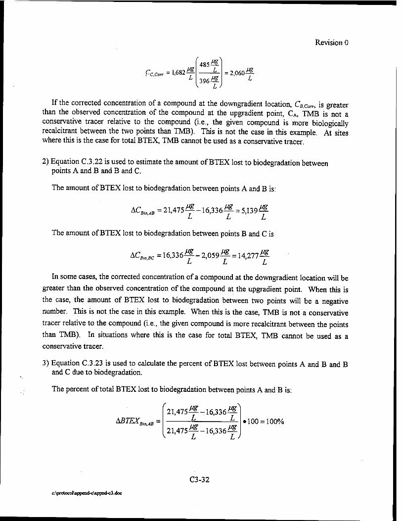
Revision 0
CCCOTT = 1.682— 485 Mg
396^ ^ L J
= 2,060 Mg
If the corrected concentration of a compound at the downgradient location, CB,corr, is greater than the observed concentration of the compound at the upgradient point, CA, TMB is not a conservative tracer relative to the compound (i.e., the given compound is more biologically recalcitrant between the two points than TMB). This is not the case in this example. At sites where this is the case for total BTEX, TMB cannot be used as a conservative tracer.
2) Equation C.3.22 is used to estimate the amount of BTEX lost to biodegradation between points A and B and B and C.
The amount of BTEX lost to biodegradation between points A and B is:
AC, ■'Bio.AB = 21,475^-16,336^ = 5,139^ ILL
The amount of BTEX lost to biodegradation between points B and C is
ACmBC = 16,336^- 2,059^ = 14,277-^
In some cases, the corrected concentration of a compound at the downgradient location will be
greater than the observed concentration of the compound at the upgradient point. When this is
the case, the amount of BTEX lost to biodegradation between two points will be a negative
number. This is not the case in this example. When this is the case, TMB is not a conservative
tracer relative to the compound (i.e., the given compound is more recalcitrant between the points
than TMB). In situations where this is the case for total BTEX, TMB cannot be used as a conservative tracer.
3) Equation C.3.23 is used to calculate the percent of BTEX lost between points A and B and B and C due to biodegradation.
The percent of total BTEX lost to biodegradation between points A and B is:
MTEXBio<AB = 21,475^-16,336^
L L
21,475^-16,336^ V L LJ
»100 = 100%
C3-32
c:\protocol\append-c\appnd-c3.doc

20
1000 ■
TOTAL BTEX CONCENTRATION (ng/L)
LINE OF EQUAL BTEX CONCENTRATION &ig/L)
CONTOUR INTERVAL = VARIABLE
c\crc«occAax»x3-c\ri guT-svo-c^. ca
Figure C.3.4
Points Along Flow Path for Example C.3.5
C3-33
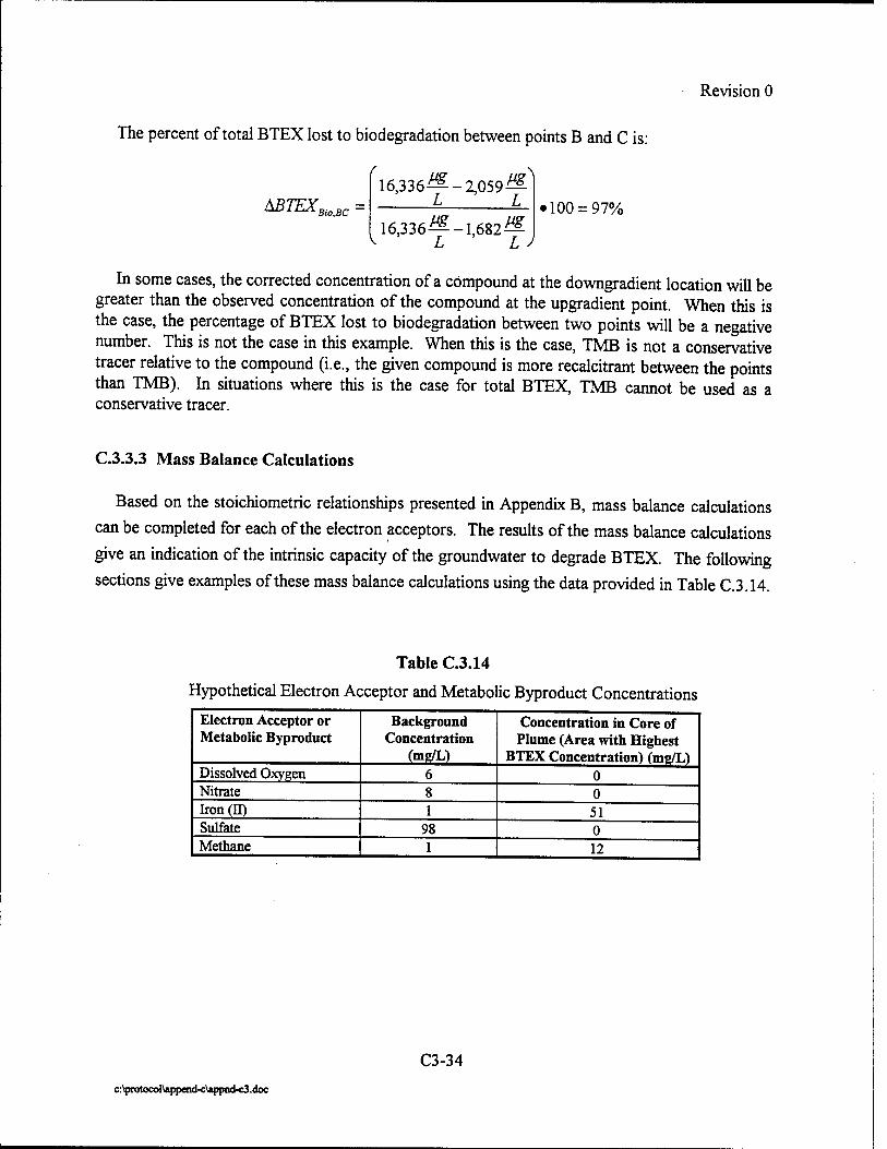
Revision 0
The percent of total BTEX lost to biodegradation between points B and C is:
16,336^-2,059^ MTEXBio<BC =
16,336^-1,682^ L L J
'100 = 97%
In some cases, the corrected concentration of a compound at the downgradient location will be greater than the observed concentration of the compound at the upgradient point. When this is the case, the percentage of BTEX lost to biodegradation between two points will be a negative number. This is not the case in this example. When this is the case, TMB is not a conservative tracer relative to the compound (i.e., the given compound is more recalcitrant between the points than TMB). In situations where this is the case for total BTEX, TMB cannot be used as a conservative tracer.
C.3.3.3 Mass Balance Calculations
Based on the stoichiometric relationships presented in Appendix B, mass balance calculations
can be completed for each of the electron acceptors. The results of the mass balance calculations
give an indication of the intrinsic capacity of the groundwater to degrade BTEX. The following
sections give examples of these mass balance calculations using the data provided in Table C.3.14.
Table C.3.14
Hypothetical Electron Acceptor and Metabolic Byproduct Concentrations
Electron Acceptor or Metabolic Byproduct
Background Concentration
(mg/L)
Concentration in Core of Plume (Area with Highest
BTEX Concentration) (me/L) Dissolved Oxygen 6 0 Nitrate 8 0 Iron (II) 1 51 Sulfate 98 0 Methane 1 12
C3-34
c:\protocol\append-c\appnd-c3.doc
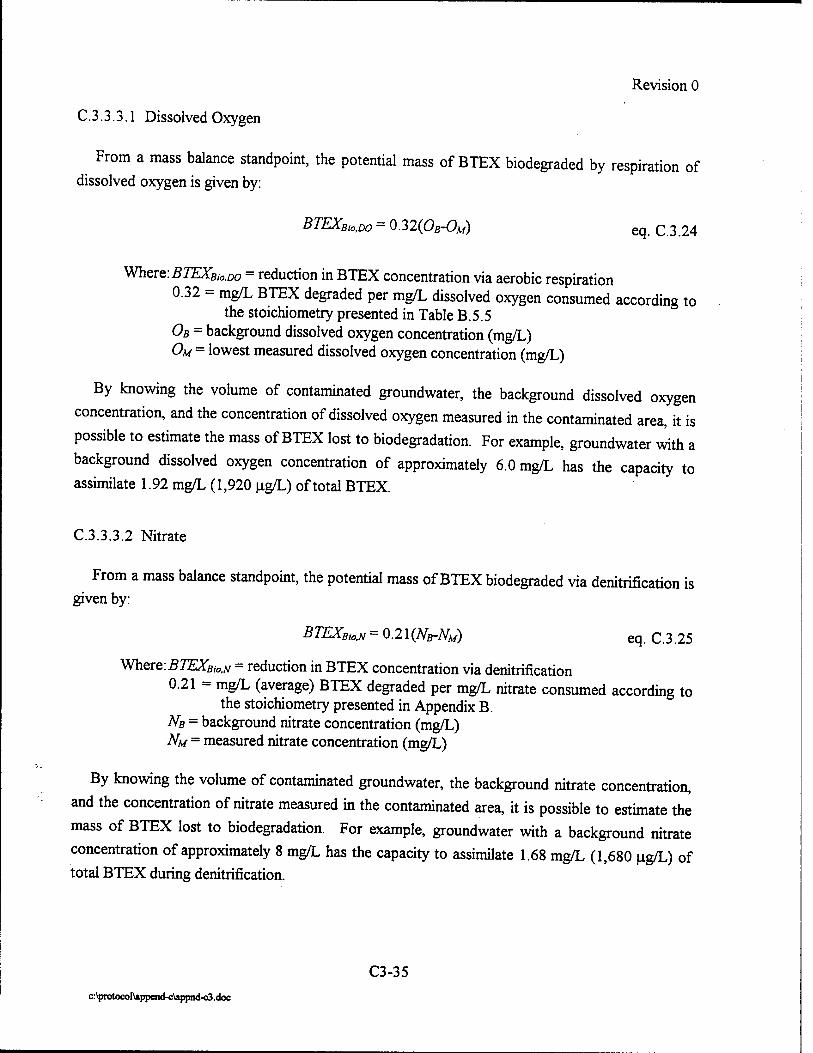
Revision 0
C. 3.3.3.1 Dissolved Oxygen
From a mass balance standpoint, the potential mass of BTEX biodegraded by respiration of dissolved oxygen is given by:
BTEXBJO,DO = 0.32(OB-OM) eq. C.3.24
Where: BTEXBio.Do = reduction in BTEX concentration via aerobic respiration 0.32 = mg/L BTEX degraded per mg/L dissolved oxygen consumed according to
the stoichiometry presented in Table B.5.5 0B = background dissolved oxygen concentration (mg/L) 0M = lowest measured dissolved oxygen concentration (mg/L)
By knowing the volume of contaminated groundwater, the background dissolved oxygen
concentration, and the concentration of dissolved oxygen measured in the contaminated area, it is
possible to estimate the mass of BTEX lost to biodegradation. For example, groundwater with a
background dissolved oxygen concentration of approximately 6.0 mg/L has the capacity to assimilate 1.92 mg/L (1,920 ug/L) of total BTEX.
C.3.3.3.2 Nitrate
From a mass balance standpoint, the potential mass of BTEX biodegraded via denitrification is given by:
BTEXBio,N=0.2l(NB-NM) eq. C.3.25
Where:BIEXBW.N - reduction in BTEX concentration via denitrification 0.21 = mg/L (average) BTEX degraded per mg/L nitrate consumed according to
the stoichiometry presented in Appendix B. NB = background nitrate concentration (mg/L) NM = measured nitrate concentration (mg/L)
By knowing the volume of contaminated groundwater, the background nitrate concentration,
and the concentration of nitrate measured in the contaminated area, it is possible to estimate the
mass of BTEX lost to biodegradation. For example, groundwater with a background nitrate
concentration of approximately 8 mg/L has the capacity to assimilate 1.68 mg/L (1,680 ug/L) of total BTEX during denitrification.
C3-35
c:\protocol\append-c\appnd-c3.doc

Revision 0
C.3.3.3.3 Iron
From a mass balance standpoint, the potential mass of BTEX biodegraded by iron (III)
reduction is given by:
BTEXBio,Fe = 0.05(FeM-FeB) eq. C.3.26
Where: BTEXBi0,Fe - reduction in BTEX concentration via iron reduction 0.05 = mg/L (average) BTEX degraded per mg/L iron (II) produced according to
the stoichiometry presented in Table B.5.5 FeB = background iron (II) concentration (mg/L) FeM = measured iron (II) concentration (mg/L)
By knowing the volume of contaminated groundwater, the background iron (II) concentration,
and the concentration of iron (II) measured in the contaminated area, it is possible to estimate the
mass of BTEX lost to biodegradation. As an example, consider a site where the groundwater that
has a background iron (II) concentration of 1 mg/L. If the highest measured iron (II)
concentration within the BTEX plume is 51 mg/L, the groundwater at this site has the capacity to
assimilate at least 0.05(51 mg/L - 1 mg/L) = 2.50 mg/L (2,500 ug/L) of total BTEX during iron
reduction.
C.3.3.3.4 Sulfate
From a mass balance standpoint, the potential mass of BTEX biodegraded by sulfate reduction
is given by:
BTEXBio,s = 0.21 (SB-SM) eq. C.3.27
Where: BTEXBw,s = reduction in BTEX concentration via sulfate reduction 0.21 = mg/L (average) BTEX degraded per mg/L sulfate consumed according to
the stoichiometry presented in Table B.5.5 SB = background sulfate concentration (mg/L) SM = measured sulfate concentration (mg/L)
By knowing the volume of contaminated groundwater, the background sulfate concentration,
and the concentration of sulfate measured in the contaminated area, it is possible to estimate the
mass of BTEX lost to biodegradation. For example, if the groundwater at a site has a sulfate
concentration of 98 mg/L the potential mass of BTEX that could be degraded by sulfate reduction
is 20.6 mg/L (20,600 ug/L).
C3-36
e:\protocol\append-c\appnd-c3.doc
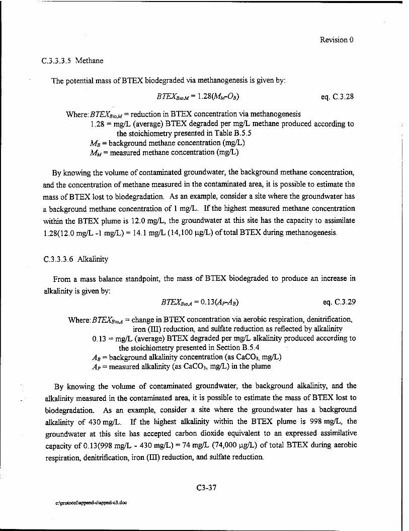
Revision 0
C.3.3.3.5 Methane
The potential mass of BTEX biodegraded via methanogenesis is given by:
BTEXBioM = 1.2S(MM-OB) eq. C.3.28
Where:BTEXBWM = reduction in BTEX concentration via methanogenesis
1.28 = mg/L (average) BTEX degraded per mg/L methane produced according to the stoichiometry presented in Table B.5.5
MB = background methane concentration (mg/L) MM = measured methane concentration (mg/L)
By knowing the volume of contaminated groundwater, the background methane concentration,
and the concentration of methane measured in the contaminated area, it is possible to estimate the
mass of BTEX lost to biodegradation. As an example, consider a site where the groundwater has
a background methane concentration of 1 mg/L. If the highest measured methane concentration
within the BTEX plume is 12.0 mg/L, the groundwater at this site has the capacity to assimilate
1.28(12.0 mg/L -1 mg/L) = 14.1 mg/L (14,100 ug/L) of total BTEX during methanogenesis.
C.3.3.3.6 Alkalinity
From a mass balance standpoint, the mass of BTEX biodegraded to produce an increase in
alkalinity is given by:
BTEXBioA = 0.13(4r-AB) eq. C.3.29
Where:BTEXBWA ~ change in BTEX concentration via aerobic respiration, denitrification, iron (III) reduction, and sulfate reduction as reflected by alkalinity
0.13 = mg/L (average) BTEX degraded per mg/L alkalinity produced according to the stoichiometry presented in Section B.5.4
AB = background alkalinity concentration (as CaC03, mg/L) AP = measured alkalinity (as CaC03, mg/L) in the plume
By knowing the volume of contaminated groundwater, the background alkalinity, and the
alkalinity measured in the contaminated area, it is possible to estimate the mass of BTEX lost to
biodegradation. As an example, consider a site where the groundwater has a background
alkalinity of 430 mg/L. If the highest alkalinity within the BTEX plume is 998 mg/L, the
groundwater at this site has accepted carbon dioxide equivalent to an expressed assimilative
capacity of 0.13(998 mg/L - 430 mg/L) = 74 mg/L (74,000 ug/L) of total BTEX during aerobic
respiration, denitrification, iron (HI) reduction, and sulfate reduction.
C3-37
c:\protocoI\append-c\appnd-c3 .doc
Revision 0
C.3.3.4 Calculating Rates of Biodegradation
C. 3.3.4.1 Instantaneous Reaction
Borden and Bedient (1986) show that the microbially mediated reaction between dissolved
oxygen and BTEX can be considered instantaneous relative to normal groundwater flow
velocities. Thus, all available dissolved oxygen will be utilized instantaneously, and the change in
BTEX concentration resulting from aerobic biodegradation is given by modifying equation C.3.24 to the form:
ACBTEX = 032(OB) eq. c.3.30
Where: ACBTEX = change in BTEX concentration [M/L3] 0.32 = ratio of mass BTEX degraded per unit mass of dissolved oxygen consumed 0B = background dissolved oxygen concentration
Example C.3.6; Instantaneous Reaction
Aerobic biodegradation is occurring in a sandy aquifer. The measured total BTEX concentration in a unit volume of saturated aquifer material is 10 mg/L. If this same unit volume of aquifer material has a dissolved oxygen concentration of 7 mg/L, what is the resulting total BTEX concentration resulting from aerobic respiration?
Solution:
From equation C.3.30, the mass of total BTEX biodegraded is:
ACmnr= 0.32(7^) = 2.24^ Li L,
Subtracting the change in BTEX concentration caused by the biodegradation reaction gives:
Resulting total BTEX concentration = 10 mg/L - 2.24 mg/L = 7.76 mg/L
C.3.3.4.2 First-Order Decay
As with a large number of processes, the change in solute concentration in the groundwater
over time often can be described using a first-order rate constant. In one dimension, first order decay is described by the following ordinary differential equation:
dC , -£ = ** eq.C.3.31
Where: C = concentration at time t [M/L3] k = overall attenuation rate (first-order rate constant) [1/T]
C3-38
c:\protocol\append-c\appnd-c3.doc
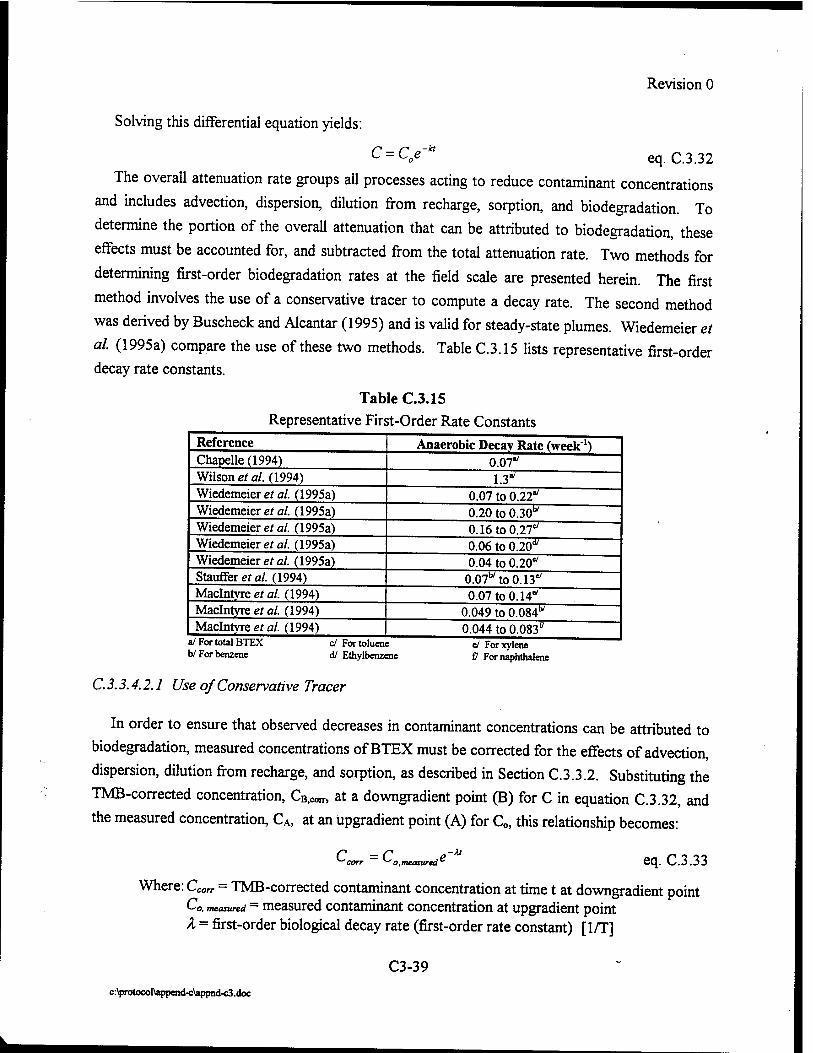
Revision 0
Solving this differential equation yields:
C = Ce -kt eq. C.3.32
The overall attenuation rate groups all processes acting to reduce contaminant concentrations
and includes advection, dispersion, dilution from recharge, sorption, and biodegradation. To
determine the portion of the overall attenuation that can be attributed to biodegradation, these
effects must be accounted for, and subtracted from the total attenuation rate. Two methods for
determining first-order biodegradation rates at the field scale are presented herein. The first
method involves the use of a conservative tracer to compute a decay rate. The second method
was derived by Buscheck and Alcantar (1995) and is valid for steady-state plumes. Wiedemeier et
al. (1995a) compare the use of these two methods. Table C.3.15 lists representative first-order decay rate constants.
Table C.3.15 Representative First-Order Rate Constants
Reference Anaerobic Decay Rate (weekh Chapelle (1994) 0.07"
__ Wilson et al. (1994) 1.3" Wiedemeier et al. (1995a) 0.07 to 0.22" Wiedemeier et al. (1995a) 0.20 to 0.30* Wiedemeier et al. (1995a) 0.16 to 0.27" Wiedemeier et al. (1995a) 0.06 to 0.20* Wiedemeier et al. (1995a) 0.04 to 0.20" Stauffer et al. (1994) 0.07wto0.13" Maclntyre eM/. (1994) 0.07 to 0.14" Maclntyre et al. (1994) 0.049 to 0.0841" Maclntyre et al. (1994) 0.044 to 0.083"
a/ For total BTEX c/ For toluen b/For benzene d/ Ethylbenz<
5 d Forxylene nie £7 For naphthalene
C. 3.3.4.2.1 Use of Conservative Tracer
In order to ensure that observed decreases in contaminant concentrations can be attributed to
biodegradation, measured concentrations of BTEX must be corrected for the effects of advection,
dispersion, dilution from recharge, and sorption, as described in Section C.3.3.2. Substituting the
TMB-corrected concentration, CB>con-, at a downgradient point (B) for C in equation C.3.32, and
the measured concentration, CA, at an upgradient point (A) for C0, this relationship becomes:
= C e o, measured -Xt
eq. C.3.33
Where: Ccorr = TMB-corrected contaminant concentration at time t at downgradient point C0i measured = measured contaminant concentration at upgradient point Z = first-order biological decay rate (first-order rate constant) [1/T]
C3-39
c:\protocoI\append-c\appnd-c3.doc

Revision 0
The rate constant in this equation is no longer the total attenuation rate, k, but is the biological
decay rate, X, because the effects of advection, dispersion, dilution from recharge, and sorption
have been removed (Section C.3.3.2). This relationship can be used to calculate the first-order
biological decay rate constant between two points by solving equation C.3.33 for X:
( C \ In _^c-_ i /i
. v'-'o,measured J _ A = eq. C.3.34
The travel time, t, between two points is given by:
t = — eq. C.3.35
Where: x = distance between two points [L] vc = retarded solute velocity [L/T]
Another way to determine the first-order rate constant from a set of TMB-corrected data is to
make a log-linear plot of TMB-corrected total BTEX concentration (or the TMB-corrected
concentration of a specific compound, such as benzene) versus travel time. If the data plot along
a straight line, the relationship is first order and an exponential regression analysis can be
performed. The exponential regression analysis gives the equation of the line of best fit for the
data being regressed from a log-linear plot and has the general form:
y = bemx eq. C.3.36
Where :y = y axis value b = y intercept m = slope of regression line x = x-axis value
When using TMB as a conservative tracer, y is the contaminant concentration, x is the
downgradient travel time from point (A), and m is the biodegradation rate constant, X. The
correlation coefficient, R2, is a measure of how well the regression relationship approximates the
data. Values of R2 can range from 0 to 1; the closer R2 is to 1, the more accurate the equation
describing the trend in the data. Values of R2 greater than 0.80 are generally considered good; R2
values greater than 0.90 are considered excellent. Several commonly available spreadsheets can
be used to facilitate the exponential regression analysis. The following example illustrates the use
of this technique.
C3-40
c:\protocol\append-c\appnd-c3.doc
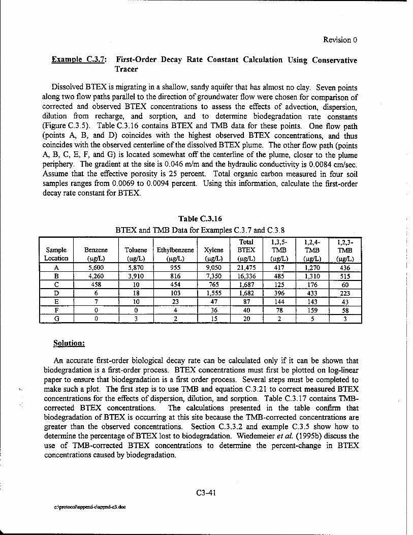
Revision 0
Example C.3.7: First-Order Decay Rate Constant Calculation Using Conservative Tracer
Dissolved BTEX is migrating in a shallow, sandy aquifer that has almost no clay. Seven points along two flow paths parallel to the direction of groundwater flow were chosen for comparison of corrected and observed BTEX concentrations to assess the effects of advection, dispersion, dilution from recharge, and sorption, and to determine biodegradation rate constants (Figure C.3.5). Table C.3.16 contains BTEX and TMB data for these points. One flow path (points A, B, and D) coincides with the highest observed BTEX concentrations, and thus coincides with the observed centerline of the dissolved BTEX plume. The other flow path (points A, B, C, E, F, and G) is located somewhat off the centerline of the plume, closer to the plume periphery. The gradient at the site is 0.046 m/m and the hydraulic conductivity is 0.0084 cm/sec. Assume that the effective porosity is 25 percent. Total organic carbon measured in four soil samples ranges from 0.0069 to 0.0094 percent. Using this information, calculate the first-order decay rate constant for BTEX.
Table C.3.16 BTEX and TMB Data for Examples C.3.7 and C.3.8
Sample Location
Benzene Toluene
(VUfL)
Ethylbenzene
(wsfc) Xylene (Hg/L)
Total BTEX
(HR/L)
1,3,5- TMB
(Hß/L)
1,2,4- TMB (WtfL)
1,2,3- TMB (Hg/L)
A 5,600 5,870 955 9,050 21,475 417 1,270 436 B 4,260 3,910 816 7,350 16,336 485 1,310 515 C 458 10 454 765 1,687 125 176 60 D 6 18 103 1,555 1,682 396 433 223 E 7 10 23 47 87 144 143 43 F 0 0 4 36 40 78 159 58 G 0 3 2 15 20 2 5 3
Solution;
An accurate first-order biological decay rate can be calculated only if it can be shown that biodegradation is a first-order process. BTEX concentrations must first be plotted on log-linear paper to ensure that biodegradation is a first order process. Several steps must be completed to make such a plot. The first step is to use TMB and equation C.3.21 to correct measured BTEX concentrations for the effects of dispersion, dilution, and sorption. Table C.3.17 contains TMB- corrected BTEX concentrations. The calculations presented in the table confirm that biodegradation of BTEX is occurring at this site because the TMB-corrected concentrations are greater than the observed concentrations. Section C.3.3.2 and example C.3.5 show how to determine the percentage of BTEX lost to biodegradation. Wiedemeier et al. (1995b) discuss the use of TMB-corrected BTEX concentrations to determine the percent-change in BTEX concentrations caused by biodegradation.
C3-41
c:\protocoI\append-c\appnd-c3.doc
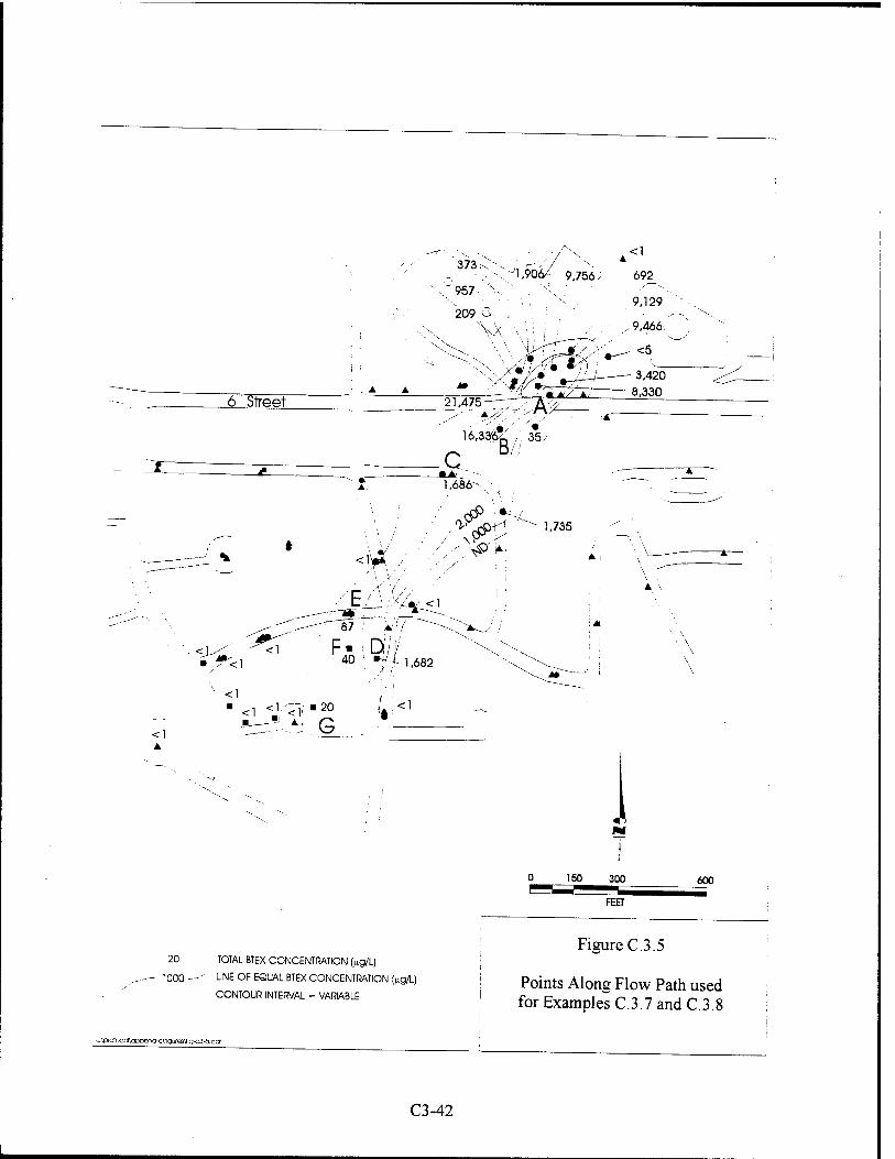
6" Street 21,475
c 16,33'^. , 35/
oll
<1'<
1,686--
<$§> ''■■•!. 1,735
C /\ A// , •• t_i : /.•'■i*-' <i
--nr^j ■• __?----
40 \ »w-i. -f /!
1,682
<1
<1 <V^B2° <]
20 TOTAL BTEX CONCENTRATION (Mg/L)
1000 —' LINE OF EQUAL BTEX CONCENTRATION fjig/L)
CONTOUR INTERVAL = VARIABLE
▲ \
M (
150 300
FEET
600
Figure C.3.5
Points Along Flow Path used for Examples C.3.7 and C.3.8
^'j^oioccftaDDena-c\ngursvig-c3-6.ca'
C3-42
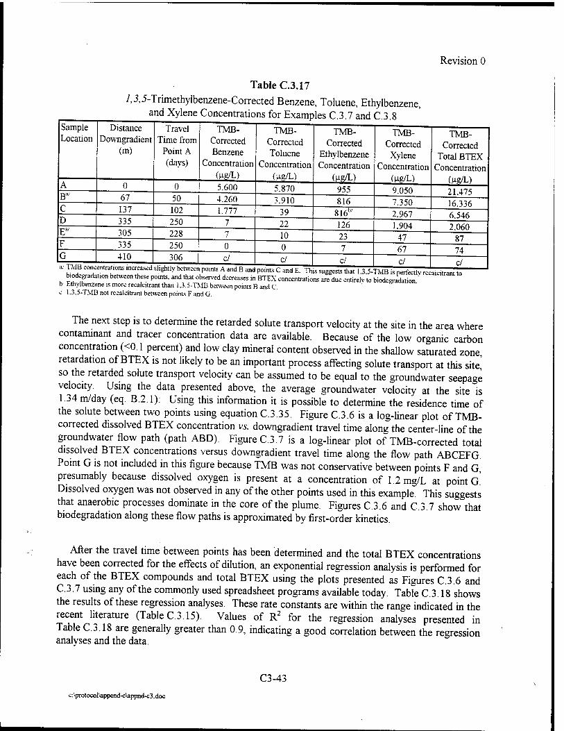
Revision 0
Sample Location
B"
D E*
Table C.3.17
/,3,5-Trimethylbenzene-Corrected Benzene, Toluene, Ethylbenzene, and Xylene Concentrations for Examples C.3.7 and C.3.8
Distance Downgradient
(m)
67 137 -» o e
305 335 410
Travel Time from
Point A (days)
0 50 102 250 228 250 306
TMB- Corrected Benzene
Concentration
5.600 4.260 1.777
0 c/
TMB- Corrected Toluene
Concentration (ug/L) 5.870 3.910
39 22 10 0
TMB- Corrected
Ethylbenzene Concentration
(Hfi/D 955 816
816b
126 23
c/ 7 c/
TMB- Corrected
Xylene Concentration
9.050 7.350 2.967 1.904
47 67 c/
TMB- Corrected
Total BTEX Concentration
(HB/L) 21.475 16.336 6.546 2.060
87 74 c/
a, TMB concentrations increased slightly between point. A and B and points C and E. This suggests that 1.3.5-TMB is perfectly relaictrant to ^degradation between these pomts. and that observed decreases in BTEX concentrations are due entirely to biodegradation "
b; hthylbenzene is more recalcitrant than 1.3.5-TMB between points B and C. c 1.3.5-TMB not recalcitrant between points F and G.
The next step is to determine the retarded solute transport velocity at the site in the area where contaminant and tracer concentration data are available. Because of the low organic carbon concentration (<0.1 percent) and low clay mineral content observed in the shallow saturated zone, retardation of BTEX is not likely to be an important process affecting solute transport at this site' so the retarded solute transport velocity can be assumed to be equal to the groundwater seepage velocity. Using the data presented above, the average groundwater velocity at the site is 1.34 m/day (eq. B.2.1): Using this information it is possible to determine the residence time of the solute between two points using equation C.3.35. Figure C.3.6 is a log-linear plot of TMB- corrected dissolved BTEX concentration vs. downgradient travel time along the center-line of the groundwater flow path (path ABD). Figure C.3.7 is a log-linear plot of TMB-corrected total dissolved BTEX concentrations versus downgradient travel time along the flow path ABCEFG Point G is not included in this figure because TMB was not conservative between points F and G presumably because dissolved oxygen is present at a concentration of 1.2mg/L at point G Dissolved oxygen was not observed in any of the other points used in this example. This suggests that anaerobic processes dominate in the core of the plume. Figures C.3.6 and C.3.7 show that biodegradation along these flow paths is approximated by first-order kinetics.
After the travel time between points has been determined and the total BTEX concentrations have been corrected for the effects of dilution, an exponential regression analysis is performed for each of the BTEX compounds and total BTEX using the plots presented as Figures C.3.6 and C.3.7 using any of the commonly used spreadsheet programs available today. Table C.3.18 shows the results of these regression analyses. These rate constants are within the range indicated in the recent literature (Table C.3.15). Values of R2 for the regression analyses presented in Table C.3.18 are generally greater than 0.9, indicating a good correlation between the regression analyses and the data.
C3-43
c:\protocol\append-c\appnd-c3.doc

Figure C.3.6 Plot of Trimethylbenzene-Corrected BTEX Concentration versus Travel
Time Along Flow Path ABD
100.000 T
c o 13 10,000
c 0> o c o V X u H 02 "O u o u I— u. O u I u c u N c u
E
1,000
50 100 150 200
Travel Time from Point A (days)
250
c:\protocoIVappend-cvtablesTmb.xls C3-44
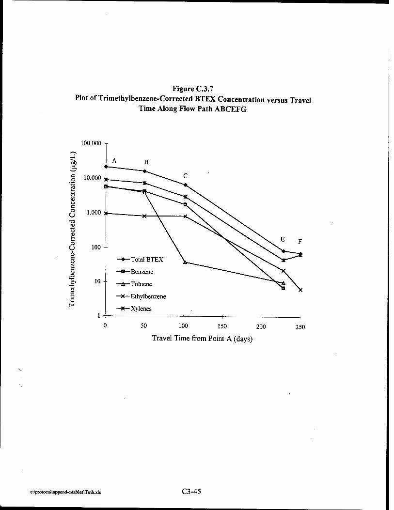
Figure C.3.7 Plot of Trimethylbenzene-Corrected BTEX Concentration versus Travel
Time Along Flow Path ABCEFG
100,000
-4
§ 10.000
c <u o e o U -a u o u o U
i u c u N c 0)
*- <U S
1,000
50 100 150 200
Travel Time from Point A (days)
250
c:\protocol\append-c\tables\Tmb.xls C3-45
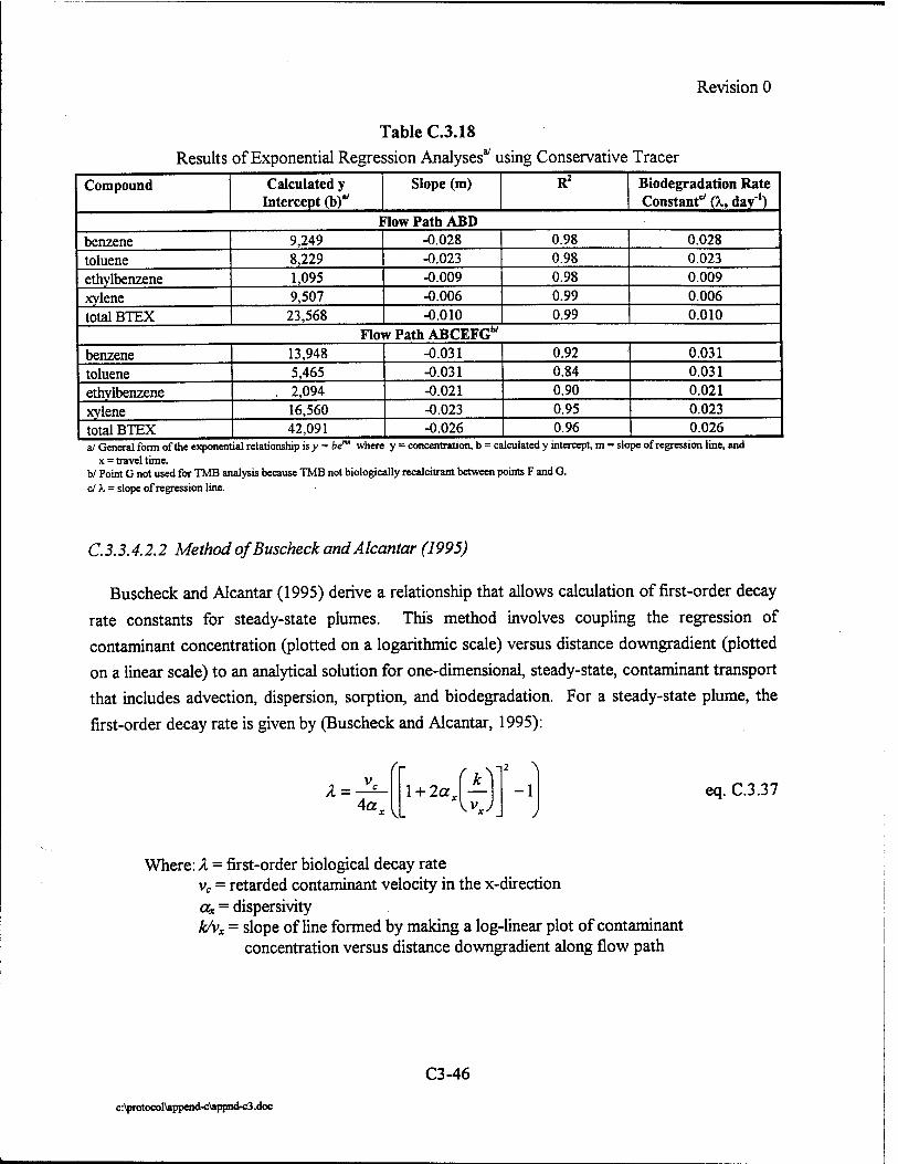
Revision 0
Table C.3.18
Results of Exponential Regression Analyses37 using Conservative Tracer
Compound Calculated y Intercept (b)"7
Slope (m) R2 Biodegradation Rate Constant'' (X, day"1)
Flow Path ABD benzene 9,249 -0.028 0.98 0.028
toluene 8,229 -0.023 0.98 0.023
ethvlbenzene 1,095 -0.009 0.98 0.009
xylene 9,507 -0.006 0.99 0.006
total BTEX 23,568 -0.010 0.99 0.010 Flow Path ABCEFGW
benzene 13,948 -0.031 0.92 0.031
toluene 5,465 -0.031 0.84 0.031
ethylbenzene . 2,094 -0.021 0.90 0.021
xylene 16,560 -0.023 0.95 0.023
total BTEX 42,091 -0.026 0.96 0.026 a/ General form of the exponential relationship is y = be1" where y = concentration, b = calculated y intercept, m =
x = travel time. b/ Point G not used for TMB analysis because TMB not biologically recalcitrant between points F and G. c/ X = slope of regression line.
slope of regression line, and
C. 3.3.4.2.2 Method of Buscheck andAlcantar (1995)
Buscheck and Alcantar (1995) derive a relationship that allows calculation of first-order decay
rate constants for steady-state plumes. This method involves coupling the regression of
contaminant concentration (plotted on a logarithmic scale) versus distance downgradient (plotted
on a linear scale) to an analytical solution for one-dimensional, steady-state, contaminant transport
that includes advection, dispersion, sorption, and biodegradation. For a steady-state plume, the
first-order decay rate is given by (Buscheck and Alcantar, 1995):
fr
A = 4a.
l + 2a, Vvr
2 >
-1 J
eq. C.3.37
Where: Ä = first-order biological decay rate vc = retarded contaminant velocity in the x-direction Ox = dispersivity k/vx = slope of line formed by making a log-linear plot of contaminant
concentration versus distance downgradient along flow path
C3-46
c:\protocol\append-c\appnd-c3 .doc
Revision 0
Example C.3.8: First-Order Rate Constant Calculation Using Method of Buscheck and Alcantar (1995)
From the data given in Table C.3.16 calculate the first order-decay rate constant due to biodegradation. The locations of the data points are shown in Figure C.3.4. Because of extremely low total organic carbon in the aquifer matrix, and lack of clay minerals, the retarded contaminant velocity, vc, is assumed to be the same as the advective groundwater velocity (1.34 m/day). A longitudinal dispersivity of 15 m was estimated by using one-tenth of the distance between the spill source and the longitudinal centroid of the plume.
Solution:
The first step is to confirm that the contaminant plume has reached a steady-state configuration. This is done by analyzing historical data to make sure the plume is no longer migrating downgradient and contaminant concentrations are not changing significantly through time. This is generally the case for older spills where the source has not been removed. The next step is to make a log-linear plot of contaminant concentration versus distance downgradient. Figures C.3.8 and C.3.9 present log-linear plots of measured BTEX concentrations versus distance downgradient along flow paths ABD and ABCEFG, respectively using the data presented in Table C.3.16. Using linear regression, the ratio k/v is determined and entered into equation C.3.37. Exponential regressions were completed for each of the BTEX compounds and total BTEX along each flow path using the relationship shown in equation C.3.37. When using the method of Buscheck and Alcantar (1995), y in the regression analysis is the contaminant concentration, x is the distance downgradient from point (A), and m is the ratio k/v. The value of k/v determined from the regression analysis is entered into equation C.3.37 and the biodegradation rate constant, X, is calculated. Table C.3.19 presents the results of the regression analyses.
Values of R2 for the regression analyses presented in Table C.3.19 are generally greater than 0.9, and in some cases approach 1.0. Only one regression has an R2 value less that 0.80. First- order biodegradation rate constants calculated using the method of Buscheck and Alcantar (1995) range from 0.008 day'1 (xylene) to 0.038 day'1 (benzene) along flow path ABD and range from 0.028 day"1 (xylene and ethylbenzene) to 0.042 day"1 (benzene) along flow path ABCEFG. This method also shows (like example C.3.7) that benzene is the most readily degraded compound at this site, as indicated by the biodegradation rate. Use of two methods to determine first-order decay rate constants at the field scale is a good check on the accuracy of the calculations.
C.3.3.4.2.3 Comparison of Conservative Tracer Method and Method of Buscheck and Alcantar (1995)
The use of a conservative tracer and the method of Buscheck and Alcantar (1995) provide comparable results in examples C.3.7 and C.3.8. For all of the BTEX compounds, the rate constants calculated using TMB as a tracer are less than those calculated using the method of Buscheck and Alcantar. This suggests that TMB-corrected data can be used to conservatively estimate biodegradation rates, particularly for plumes that have not reached steady-state.
C3-47
c:\protocol\append-c\appnd-c3.doc
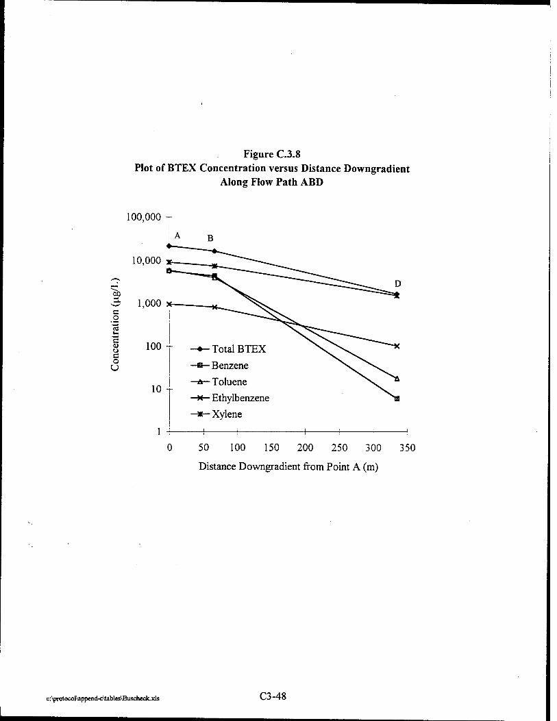
Figure C.3.8 Plot of BTEX Concentration versus Distance Downgradient
Along Flow Path ABD
100,000 -
10,000
3 1,000 c o 03 u. c u o c o U
100 -
10
•Total BTEX
• Benzene
■ Toluene
■ Ethylbenzene
■ Xylene
50 100 150 200 250 300
Distance Downgradient from Point A (m)
350
c:\protocol\append-c\tables\Buscheclcxls C3-48
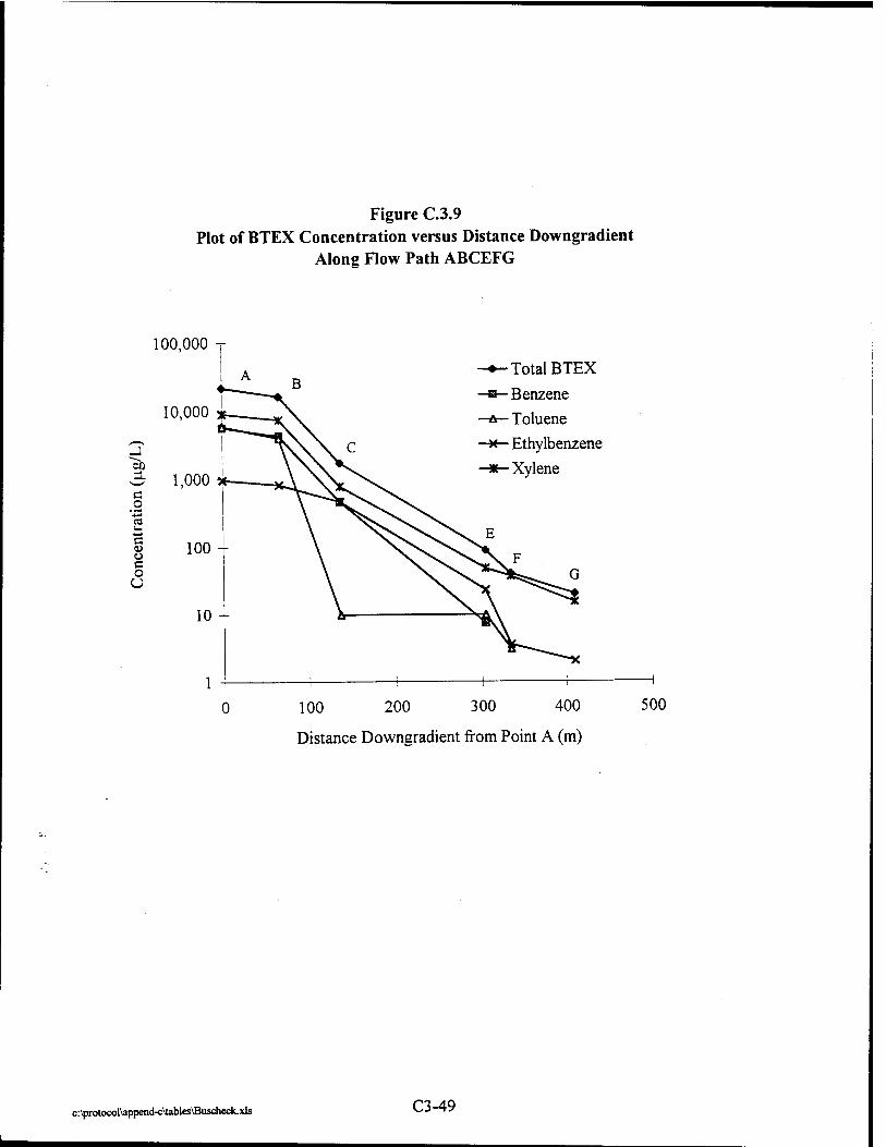
Figure C.3.9 Plot of BTEX Concentration versus Distance Downgradient
Along Flow Path ABCEFG
100,000 -
10,000
aß n c .2 '-♦-»
CO u +-» c <u u c o U
1,000
100
Total BTEX
Benzene
Toluene
Ethylbenzene
Xylene
100 200 300 400
Distance Downgradient from Point A (m)
500
c:\protocol\append-c\lables\Buscheck. xls C3-49
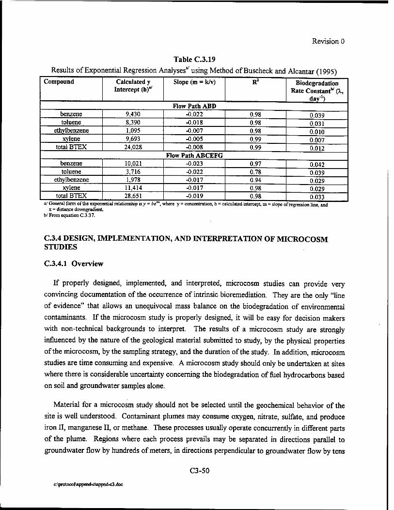
Revision 0
Table C.3.19 Results of Exponential Regression Analyses37 using Method of Buscheck and Alcantar (1995)
Compound Calculated y Intercept (b)"7
Slope (m = k/v) R2 Biodegradation
Rate Constant'"' (k, dav1)
Flow Path ABD benzene 9,430 -0.022 0.98 0.039 toluene 8,390 -0.018 0.98 0.031
ethylbenzene 1,095 -0.007 0.98 0.010 xylene 9,693 -0.005 0.99 0.007
total BTEX 24,028 -0.008 0.99 0.012 Flow Path ABCEFG
benzene 10,021 -0.023 0.97 0.042 toluene 3,716 -0.022 0.78 0.039
ethylbenzene 1,978 -0.017 0.94 0.029 xvlene 11,414 -0.017 0.98 0.029
total BTEX 28,651 -0.019 0.98 0.033 a/ General form of the exponential relationship is>> = be1", where y = concentration, b = calculated intercept, m = slope of regression line, and
x = distance downgradient b/ From equation C.3.37.
C.3.4 DESIGN, IMPLEMENTATION, AND INTERPRETATION OF MICROCOSM STUDIES
C.3.4.1 Overview
If properly designed, implemented, and interpreted, microcosm studies can provide very convincing documentation of the occurrence of intrinsic bioremediation. They are the only "line of evidence" that allows an unequivocal mass balance on the biodegradation of environmental contaminants. If the microcosm study is properly designed, it will be easy for decision makers with non-technical backgrounds to interpret. The results of a microcosm study are strongly influenced by the nature of the geological material submitted to study, by the physical properties of the microcosm, by the sampling strategy, and the duration of the study. In addition, microcosm studies are time consuming and expensive. A microcosm study should only be undertaken at sites where there is considerable uncertainty concerning the biodegradation of fuel hydrocarbons based on soil and groundwater samples alone.
Material for a microcosm study should not be selected until the geochemical behavior of the site is well understood. Contaminant plumes may consume oxygen, nitrate, sulfate, and produce iron II, manganese II, or methane. These processes usually operate concurrently in different parts of the plume. Regions where each process prevails may be separated in directions parallel to groundwater flow by hundreds of meters, in directions perpendicular to groundwater flow by tens
C3-50
c:\protocol\append-c\apprid-c3.doc
Revision 0
of meters, and vertically by only a few meters. Rate constants and constraints for petroleum
hydrocarbon biodegradation will be influenced by the prevailing geochemistry. Material from
microcosms must be acquired for depth intervals and locations that have been predetermined to be
representative of the prevailing geochemical milieu in the plume.
Hydrocarbon biodegradation supported by oxygen and nitrate can not be adequately
represented in microcosm. In the field, organisms that use oxygen or nitrate proliferate until they
become limited by the supply of electron acceptor. After that time, the rate of hydrocarbon
degradation is controlled by the supply of electron acceptor through diffusion or hydrodynamic
dispersion. Microcosms have been used successfully to simulate sulfate-reducing, iron-reducing,
and methanogenic regions of plumes. Oxygen is toxic to sulfate-reducing and methanogenic
microorganisms. Material should be collected and secured in a manner that precludes oxygenation of the sample.
Batch microcosms that are sacrificed for each analysis usually give more interpretable results
than column microcosms or batch microcosms that are sampled repetitively. For statistical
reasons, at least three microcosms should be sampled at each time interval. If one assumes a first
order rate law, and no lag, a geometrical time interval for sampling should be the most efficient.
An example would be sampling after 0 weeks, 2 weeks, 1 month, 2 months, 4 months, and 8
months. As a practical matter, long lags frequently occur, and the rate of bioremediation after the
lag is rapid. A simple linear time scale is most likely to give interpretable results.
The batch microcosms should have approximately the same ratio of solids to water as the
original material. Most of the microbes are attached to solids. If a microcosm has an excess of
water, and the contaminant is mostly in the aqueous phase, the microbes must process a great deal
more contaminant to produce the same relative change in the contaminant concentration. The kinetics at field scale would be underestimated.
Microcosms are inherently time consuming. At field scale, the residence time of a plume may
be several years to decades. Slow rates of transformation may have a considerable environmental
significance. A microcosm study that lasts only a few weeks or months may not have the
resolution to detect slow changes that are still of environmental significance. Further, microcosms
often show a pattern of sequential utilization, with toluene and the xylenes degrading first, and
benzene and ethylbenzene degrading at a later time. Degradation of benzene or ethylbenzene may be delayed by as much as a year.
C3-51
c:\protocol\append-c\appnd-c3.doc

Revision 0
As a practical matter, batch microcosms with an optimal solids to water ratio, sampled every 2
months in triplicate for up to 18 months, can resolve biodegradation from abiotic losses with a
rate detection limit of 0.001 to 0.0005 per day. Many plumes show significant attenuation of contamination at field-calibrated rates that are slower than the detection limit of today's
microcosm technology. The most appropriate use of microcosms is to document that contaminant attenuation is largely a biological process. Rate constants for modeling purposes are more appropriately acquired from field-scale studies.
C.3.4.2 Case Study on a Gasoline Spill at Arvida, North Carolina
One of the best case studies comparing field scale processes and microcosms is still underway. Prepublication material on the study was generously supplied on February 14, 1995 by Melody J. Hunt, Morton A. Barlaz, and Robert C. Borden at North Carolina State University. Their study will be used to illustrate the most recent practices for using microcosms to simulate BTEX plumes.
C.3.4.2.1 Material and Methods
C. 3.4.2.1.1 Sediment and Groundwater Collection
Three separate cores of aquifer sediment were obtained at a site in Rocky Point, NC: one near the source area (RP0), one approximately halfway between the source area and the end of the plume boundaries (RP150), and one near the end of the detected plume boundaries (RP300) (Figure C.3.10). All sediment was obtained under strictly anaerobic conditions by drilling below the water table with a hollow-stem auger, and advancing a sterile coring tube. The tube was brought to the surface, immediately capped with sterile butyl rubber stoppers and transported to the laboratory on ice, where it was extruded in an anaerobic glovebox under nitrogen atmosphere within 12 hours. The first and last 1.00 centimeter of soil were removed, and the outer portions of the soil pared away. The remaining sediment was anaerobically transferred into sterile mason jars and stored at 4°C. Prior to use, soil from each core was mixed and passed through a No. 8 sieve in an anaerobic chamber.
Anaerobic groundwater was collected at the time of sediment removal from adjacent wells screened at the same depth interval as the borehole from which the sediment was recovered. The dissolved oxygen, pH, Eh, and temperature of the groundwater were measured at the time of collection. The water was pumped from the well using a Waterra pump through a closed
C3-52
c:\protocol\append-c\appnd-c3.doc
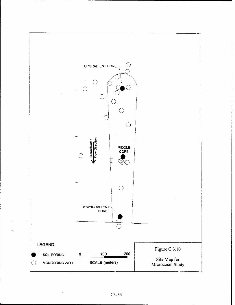
UPGRADIENT CORE-| O
o o
o o
c#o ^ o
o
o
o
c o
o
DOWNGRADIEN"K CORE
o
o
MIDDLE CORE
)0
o
o
o
LEGEND
SOIL BORING 0
MONITORING WELL
100 200
SCALE (meters)
Figure C.3.10
Site Map for Microcosm Study
C3-53
Revision 0
system of polyethylene tubing equipped with a 0.45-micron filter, and collected in a nitrogen- sparged, 2.3-L (80-ounce) bottle. The collection bottle was sealed with a two-holed rubber
stopper connected to a second nitrogen-sparged bottle, which released pressure as water entered
the collection bottle and prevented air from entering the system on the backstroke of the pump. Well headspace was continually sparged with argon during collection. The water was transported
on ice to the laboratory where it was stored at 4°C prior to use. All equipment and containers coming into contact with the water and sediment were pre-sterilized.
C. 3.4.2.1.2 Microcosm Construction
The study objective was to simulate ambient conditions to the maximum extent possible. Multiple replicate microcosms were prepared within 2 weeks of sample collection for each of the three locations. Microcosms were constructed in a Coy anaerobic chamber. The microcosms contained 35 gm wet sediment and 16 mL groundwater (dry soil:water= 1.8 g/mL). All of the microcosms were spiked with a stock solution containing sterile anaerobic deionized water, resazurin (0.0002 percent final concentration), benzene, toluene, ethylbenzene, o-xylene, and m- xylene (BTEX) to yield final concentrations representative of field conditions. BTEX concentration ranged from 10 to 20 micromoles (uM). Anaerobic water was prepared by boiling deionized water under a nitrogen headspace. The water was then autoclaved for 20 minutes at 121°C. After addition of the spike solution(s), the microcosms were filled with groundwater to eliminate all headspace, and sealed with a teflon lined, grey butyl rubber stopper (West Co., Lititz, PA) and an aluminum crimp.
Abiotic controls were amended with 1 to 2 millimoles (mM) mercuric chloride and autoclaved at 250°C for 30 minutes on two consecutive days prior to addition of the BTEX spike solution.
A second set of abiotic controls contained autoclaved groundwater, mercuric chloride, resazurin, and BTEX, but no aquifer material. These latter microcosms enabled differentiation between sorption to aquifer material and sorption-difrusion into the stopper. All manipulations were performed in an anaerobic chamber. All bottles, caps, and instruments coming in contact with the sediment or water were autoclaved prior to use. All microcosms were incubated in the dark at 16°C in anaerobic incubation jars with oxygen scavenging catalyst envelopes (BBL Gas Pak Jar System, Fisher Scientific, Raleigh, NC) and dry redox indicator strips. The incubation jars were evacuated and refilled with nitrogen three times after removing microcosms for sampling. Triplicate live and abiotic microcosms were destructively sampled at monthly intervals for approximately 1 year. Results are presented as the average of three destructively sampled microcosms measured at each time point.
C3-54
c:\protocol\append-c\appnd-c3.doc
Revision 0
C.3.4.2.1.3 Aqueous Sampling and Analyses
The microcosms were sampled in the anaerobic chamber by simultaneously removing approximately 2.0 mL of free liquid in a gas-tight syringe while puncturing the stopper with a
needle so that a vacuum did not develop. The first 1.0 mL was injected into a 10 mL vial sealed with a black butyl rubber stopper (Geomicrobial Technologies, Inc., Ochelata, OK). The vials were then inverted to minimize losses and stored at 4°C for methane analysis (performed within
48 hours). To prepare a sample for methane analysis, 3.0 mL of high purity deionized water was injected to pressurize the vial slightly. Next, a 1.0 mL headspace sample was removed from the vial using a gas-tight syringe and immediately injected into a Shimadzu 9A GC equipped with a 1.5 m by 3.2 mm stainless steel column packed with Hayesep T 100/120 mesh (Altech, Deerfield , IL) and an FID. The dissolved concentration of methane in a microcosm was calculated using Henry's Law constants and assuming that all dissolved methane in the 1.0 mL aliquot volatilized in the sampling viaK Between 0.25 and 1.0 mL of the remaining 1.0 mL of sample from the microcosm was placed in a closed test tube and diluted to 5 mL for BTEX analysis. BTEX analysis was performed in accordance with USEPA Method 602 using a Tekmar® Purge-and-Trap Model LSC 2000 and a Perkin Elmer® Model 900 auto system or Perkin Elmer® 8500 Gas Chromatograph equipped with a 75m DB-624 Megabore capillary column (J & W Scientific, Folsom, CA) and a flame ionization detector. Measurements of dissolved iron, total sulfur, sulfate, thiosulfate, and sulfite were obtained by passing 3 mL of remaining liquid in the microcosm through a 0.2-micron filter (Gelman Sciences, Ann Arbor, MI) into separate vials containing 0.5N HCL. Samples were stored at 4°C and analyzed within 2 weeks of BTEX sampling. Iron and total sulfur were analyzed using Perkin Elmer® II plasma coupled argon emission spectrometer (AES ICP). Sulfate, thiosulfate, and sulfite were analyzed by ion chromatography. The aqueous concentrations of BTEX and the inorganics were determined by comparing peak areas in samples with those of external standards. The pH of the microcosms was measured in the anaerobic chamber after liquid was removed for all other dissolved analysis.
C. 3.4.2.1.4 Results
Comparison of the attenuation of benzene and toluene in microcosms constructed from material from the midpoint of a plume of BTEX undergoing iron reduction shows that toluene has been largely depleted at the midpoint of the plume, but is present in material immediately upgradient. Toluene attenuated rapidly and without a lag. Toluene also attenuated in the abiotic control. This represents loss from solution due to diffusion through the septum of the microcosm, and sorption to the microcosm solids. The attenuation of benzene was not different from the
C3-55
c:\protocol\append-c\appnd-c3.doc
Revision 0
controls for at least 180 days, then benzene attenuated to trivial concentrations over the next 220
days. The rate of attenuation of benzene and toluene in the abiotic controls were very similar,
indicating that removal was truly due to an abiotic process (Figure C.3.11).
Figure C.3.12 presents data on microcosms constructed from the end-point of the plume. The
residence time between the mid-point and end-point samples is approximately 6 years. Toluene is
entirely depleted in groundwater at this location. Notice that the degradation of toluene is much
slower than in microcosms constructed from the mid-point samples. Toluene attenuation is not
different from the control until after day 70. This material was not preacclimated to toluene,
because there was no significant exposure to toluene in the field. Benzene attenuation was not
different from its control until toluene was depleted, then its concentration was reduced to low
levels. The attenuation in the controls at the end point of the plume was very similar to
attenuation in the controls at the mid-point, suggesting that the mechanisms that attenuate the
organics in the controls act very uniformly.
Microcosms constructed from material collected from the source area showed no evidence of
biological attenuation (Figure C.3.13). It is possible that microorganisms at this location have
failed to acclimate to anaerobic biodegradation. It is also possible that soluble electron acceptors,
such as oxygen, nitrate, and sulfate have been depleted, and long term exposure to the BTEX has
exhausted the supply of iron minerals available for iron reduction.
Figure C.3.14 illustrates frequently seen responses in microcosm studies. Notice that the
concentration of benzene in the microcosms containing sediment actually appears to increase in
the initial sampling intervals. This effect is not well understood, but is very commonly seen. Also
notice that the rate of attenuation in the microcosms containing only water is slower than the
living but inactive microcosms, which in turn are slower than the abiotic control with sediment.
This indicates that the sediment is actively sorbing benzene from water, and that sorption is
stronger in the autoclaved control. This effect reduces the sensitivity of the microcosm assay, but
is a conservative error.
BTEX Removal Rates: Effective first-order removal rates for BTEX were estimated using the
equation C=C0e'lct, where k is the apparent first-order decay rate (T1), t is time, and C0 is the
initial concentration. Decay rates were calculated over the time period in which biological losses
were observed. The rate of biological loss is represented as the difference between the decay rates
in the live and abiotic microcosms taken over the time period of measured loss.
C3-56
c:\protocol\append-c\appnd-c3.doc
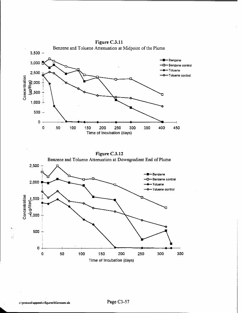
Figure C.3.11 Benzene and Toluene Attenuation at Midpoint of the Plume
Benzene
Benzene control
Toluene
Toluene control
50 100 150 200 250 300 Time of Incubation (days)
350 400 450
2,500 T
2,000
■2 J.,500 |
§ 3 o "T.OOO - O
500
Figure C.3.12 Benzene and Toluene Attenuation at Downgradient End of Plume
Benzene
Benzene control
Toluene
Toluene control
50 100 150 200 250
Time of Incubation (days)
300 350
c:^>rotocol\append-C'iigures\Microcsm.xls Page C3-57

Figure C.3.13 Attenuation of Benzene and Toluene in the Source Area
| 55 1,500 T 3 f ß 1,000 -
500 -t-
0
■Benzene
- Benzene control
-Toluene
-Toluene control
100 200 300 Time of Incubation (days)
400
Figure C.3.14 Benzene Depletion in Live Microcosm and Two Controls
Benzene
Benzene control
- Benzene water control
100 200 300 Time of Incubation (days)
400
c:\protocol\append-c\fi gures\Microcsm.xls Page C3-58

Revision 0
The microcosm decay rates are compared to field-measured intrinsic remediation rates in Table C.3.20. The rate constants in the microcosms were much greater than rates actually achieved in
the field. Microcosms are most appropriate as indicators of the potential for intrinsic bioremediation, and to prove that losses are biological, but it may be inappropriate to use them to
generate rate constants.
Table C.3.20 Microcosm vs. Field BTEX Intrinsic Remediation Rates
Compound Microcosms*' Field1" Live Microcosms Control
Microcosms Biological Loss
7irst-Order Rate Constant (per day) Benzene 0.0258 0.0021 0.0237 0.0002 Toluene 0.0489 0.0043 0.0446 0.0021
Ethylbenzene 0.0056 0.0037 0.0019 0.0015 o-Xylene 0.0611 0.0052 0.0559 0.0011
m+p-Xylene 0.0013 m-Xylene 0.0234 0.0030 0.0204
a/ From Hunt et cd. (1995) b/ From Borden et cd. (1994)
C3-59
c:\protoeol\append-c\appnd-c3.doc

APPENDIX D
MODELING THE FATE AND TRANSPORT OF FUEL HYDROCARBONS DISSOLVED IN GROUNDWATER
C:\PROTOCOL\APPEND-D\TOC-D.DOC
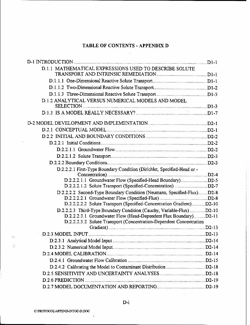
TABLE OF CONTENTS - APPENDIX D
D-l INTRODUCTION Dl-1 D. 1.1 MATHEMATICAL EXPRESSIONS USED TO DESCRIBE SOLUTE
TRANSPORT AND INTRINSIC REMEDIATION Dl-1 D.I.1.1 One-Dimensional Reactive Solute Transport Dl-1 D.I.1.2 Two-Dimensional Reactive Solute Transport Dl-2 D.I.1.3 Three-Dimensional Reactive Solute Transport Dl-3
D. 1.2 ANALYTICAL VERSUS NUMERICAL MODELS AND MODEL SELECTION Dl-3
D.1.3 IS A MODEL REALLY NECESSARY? Dl-7
D-2 MODEL DEVELOPMENT AND IMPLEMENTATION D2-1 D.2.1 CONCEPTUAL MODEL D2-1 D.2.2 INITIAL AND BOUNDARY CONDITIONS D2-2
D.2.2.1 Initial Conditions D2-2 D.2.2.1.1 Groundwater Flow D2-2 D.2.2.1.2 Solute Transport D2-3
D.2.2.2 Boundary Conditions D2-3 D.2.2.2.1 First-Type Boundary Condition (Dirichlet, Specified-Head or -
Concentration) D2-4 D.2.2.2.1.1 Groundwater Flow (Specified-Head Boundary) D2-5 D.2.2.2.1.2 Solute Transport (Specified-Concentration) D2-7
D.2.2.2.2 Second-Type Boundary Condition (Neumann, Specified-Flux) D2-8 D.2.2.2.2.1 Groundwater Flow (Specified-Flux) D2-8 D.2.2.2.2.2 Solute Transport (Specified-Concentration Gradient) D2-10
D.2.2.2.3 Third-Type Boundary Condition (Cauchy, Variable-Flux) D2-10 D.2.2.2.3.1 Groundwater Flow (Head-Dependent Flux Boundary) D2-11 D.2.2.2.3.2 Solute Transport (Concentration-Dependent Concentration
Gradient) D2-13 D.2.3 MODEL INPUT D2-13
D.2.3.1 Analytical Model Input D2-14 D.2.3.2 Numerical Model Input D2-14
D.2.4 MODEL CALIBRATION D2-14 D.2.4.1 Groundwater Flow Calibration D2-15 D.2.4.2 Calibrating the Model to Contaminant Distribution D2-18
D.2.5 SENSITIVITY AND UNCERTAINTY ANALYSES D2-18 D.2.6 PREDICTION D2-19 D.2.7 MODEL DOCUMENTATION AND REPORTING D2-19
D-i
C:\PROTOCOL\APPEND-D\TOC-D.DOC
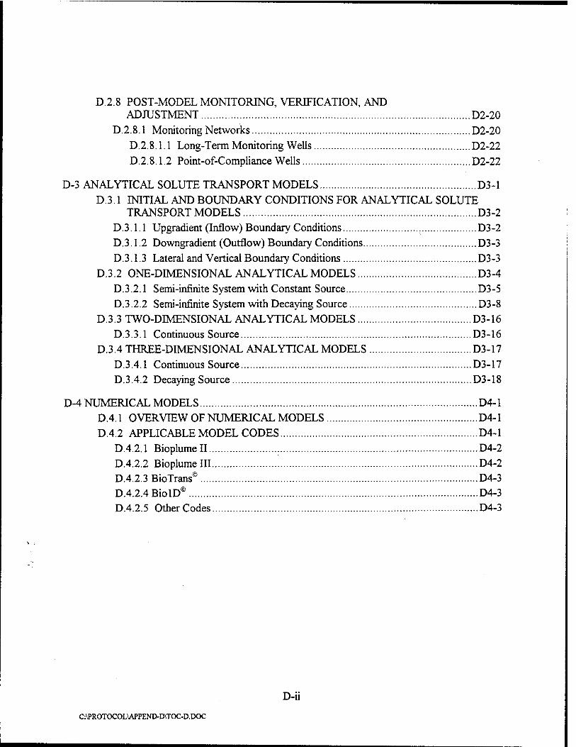
D.2.8 POST-MODEL MONITORING, VERIFICATION, AND ADJUSTMENT D2-20
D.2.8.1 Monitoring Networks D2-20 D.2.8.1.1 Long-Term Monitoring Wells D2-22 D.2.8.1.2 Point-of-Compliance Wells D2-22
D-3 ANALYTICAL SOLUTE TRANSPORT MODELS D3-1 D.3.1 INITIAL AND BOUNDARY CONDITIONS FOR ANALYTICAL SOLUTE
TRANSPORT MODELS D3-2 D.3.1.1 Upgradient (Inflow) Boundary Conditions D3-2 D.3.1.2 Downgradient (Outflow) Boundary Conditions D3-3 D.3.1.3 Lateral and Vertical Boundary Conditions D3-3
D.3.2 ONE-DIMENSIONAL ANALYTICAL MODELS D3-4 D.3.2.1 Semi-infinite System with Constant Source D3-5 D.3.2.2 Semi-infinite System with Decaying Source D3-8
D.3.3 TWO-DIMENSIONAL ANALYTICAL MODELS D3-16 D.3.3.1 Continuous Source D3-16
D.3.4 THREE-DIMENSIONAL ANALYTICAL MODELS D3-17 D.3.4.1 Continuous Source D3-17 D.3.4.2 Decaying Source D3-18
D-4 NUMERICAL MODELS D4-1 D.4.1 OVERVIEW OF NUMERICAL MODELS D4-1 D.4.2 APPLICABLE MODEL CODES D4-1
D.4.2.1 Bioplumell D4-2 D.4.2.2 Bioplumelll D4-2 D.4.2.3 BioTrans® D4-3 D.4.2.4BiolD® D4-3 D.4.2.5 Other Codes D4-3
D-ii
C:\PROTOCOL\APPEND-D\TOC-D.DOC
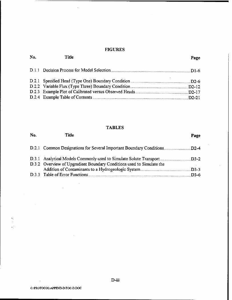
FIGURES
No. Title Page
D.l.l Decision Process for Model Selection Dl-6
D.2.1 Specified Head (Type One) Boundary Condition D2-6 D.2.2 Variable Flux (Type Three) Boundary Condition D2-12 D.2.3 Example Plot of Calibrated versus Observed Heads D2-17 D.2.4 Example Table of Contents D2-21
TABLES
No. Title Page
D.2.1 Common Designations for Several Important Boundary Conditions D2-4
D.3.1 Analytical Models Commonly used to Simulate Solute Transport D3-2 D.3.2 Overview of Upgradient Boundary Conditions used to Simulate the
Addition of Contaminants to a Hydrogeologie System D3-3 D.3.3 Table of Error Functions D3-6
D-iii
C:\PROTOCOL\APPEND-D\TOC-D.DOC
Revision 0
SECTION D-l
INTRODUCTION
Prediction of the migration and degradation of a dissolved contaminant plume using a solute transport model is an important component of the intrinsic remediation demonstration. In order
for a model to adequately predict the fate and transport of a dissolved hydrocarbon plume, it must be capable of modeling solute transport under the influence of advection, dispersion, sorption, and biodegradation. Models used to simulate groundwater flow and solute transport can be classified according to the mathematical technique used to solve the governing partial differential equation. Analytical solutions and numerical solutions are the two mathematical techniques most commonly used to solve the advective-dispersive equation. The following sections describe the mathematical relationships that describe one-, two-, and three-dimensional solute transport and the numerical techniques used to solve these relationships. Also included is a discussion of analytical and numerical models and model selection. Finally, consideration is given to whether or not a model is necessary to successfully implement intrinsic remediation at a given site.
D.1.1 MATHEMATICAL EXPRESSIONS USED TO DESCRIBE SOLUTE TRANSPORT AND INTRINSIC REMEDIATION
The mathematical relationships that describe groundwater flow and solute transport are based on the equation of continuity and Darcy's Law. Combination of these relationships for transient conditions yields a parabolic partial differential equation. Combination of these relationships for steady-state conditions yields an elliptical partial differential equation. The following sections present the one-, two-, and three-dimensional partial differential equations that describe solute transport by the processes of advection, dispersion, sorption, and biodegradation. Several texts derive these equations (Bear, 1972; Freeze and Cherry, 1979; Bedient et al, 1994; Segol, 1994).
D.I.1.1 One-Dimensional Reactive Solute Transport
The one-dimensional partial differential equation describing transient solute transport with first-order biodegradation in the saturated zone is given by:
DM c:\protocol\append-d\appnd-dl.doc
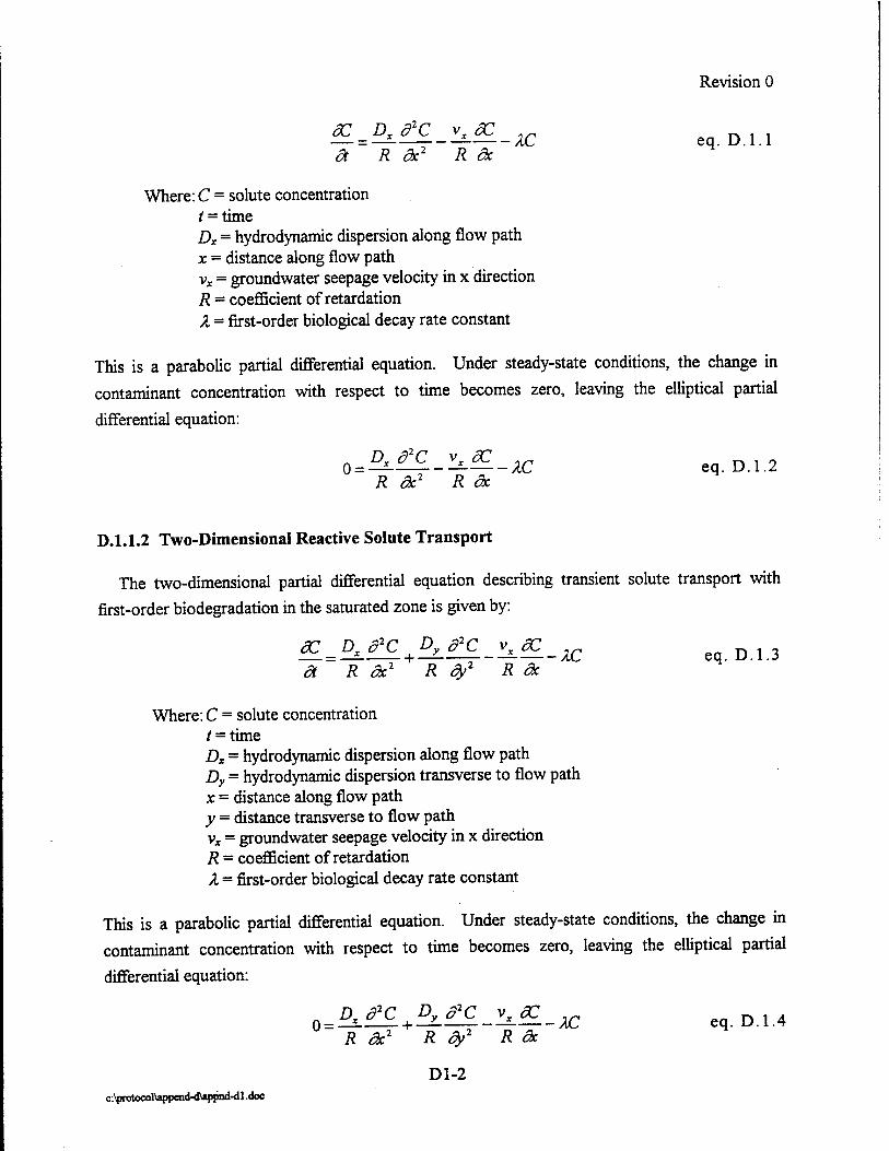
Revision 0
^ = ^£_^_;tc eq.D.1.1 ä R dx2 R dx.
Where: C = solute concentration / = time At = hydrodynamic dispersion along flow path x = distance along flow path vx = groundwater seepage velocity in x direction R = coefficient of retardation X = first-order biological decay rate constant
This is a parabolic partial differential equation. Under steady-state conditions, the change in
contaminant concentration with respect to time becomes zero, leaving the elliptical partial
differential equation:
O^f^-^-AC eq.D.1.2 R ac2 R ac
D.l.1.2 Two-Dimensional Reactive Solute Transport
The two-dimensional partial differential equation describing transient solute transport with
first-order biodegradation in the saturated zone is given by:
i£-i££ + i££_ v^,^ eq. D.1.3 a R ac2 R dy2 R ac
Where: C = solute concentration / = time Dx = hydrodynamic dispersion along flow path Dy = hydrodynamic dispersion transverse to flow path x = distance along flow path v = distance transverse to flow path vx = groundwater seepage velocity in x direction R = coefficient of retardation X = first-order biological decay rate constant
This is a parabolic partial differential equation. Under steady-state conditions, the change in contaminant concentration with respect to time becomes zero, leaving the elliptical partial
differential equation:
R ac2 R dy2 R de
Dl-2 c:\protocol\append-d\appnd-dl.doc
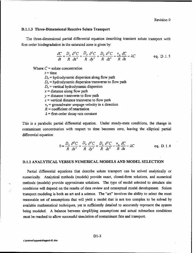
Revision 0
D.I. 1.3 Three-Dimensional Reactive Solute Transport
The three-dimensional partial differential equation describing transient solute transport with
first-order biodegradation in the saturated zone is given by:
dC_Dsd2C Dytfc Dtd
2C vxdC Mnn — = — H r-H : —/tc eq. D.1.5 a R ac2 R By2 R dz1 R äc H
Where: C = solute concentration / = time Dx = hydrodynamic dispersion along flow path Dy = hydrodynamic dispersion transverse to flow path D2 = vertical hydrodynamic dispersion x = distance along flow path v = distance transverse to flow path z = vertical distance transverse to flow path vx = groundwater seepage velocity in x direction R = coefficient of retardation X = first-order decay rate constant
This is a parabolic partial differential equation. Under steady-state conditions, the change in contaminant concentration with respect to time becomes zero, leaving the elliptical partial
differential equation:
Dxd2C Dy d
2C Dt d2C vx dC R ac2 + R dy2 R a2 R ac
0 = ±^^ + -Z.^ + -i.^.-^-!±--ZC eq. D.I.6
D.1.2 ANALYTICAL VERSUS NUMERICAL MODELS AND MODEL SELECTION
Partial differential equations that describe solute transport can be solved analytically or numerically. Analytical methods (models) provide exact, closed-form solutions, and numerical methods (models) provide approximate solutions. The type of model selected to simulate site conditions will depend on the results of data review and conceptual model development. Solute transport modeling is both an art and a science. The "art" involves the ability to select the most reasonable set of assumptions that will yield a model that is not too complex to be solved by available mathematical techniques, yet is sufficiently detailed to accurately represent the system being modeled. A balance between simplifying assumptions and actual subsurface conditions must be reached to allow successful simulation of contaminant fate and transport.
Dl-3 c:\protocol\append-d\appnd-d 1 .doc
Revision 0
Analytical solutions provide exact, closed-form solutions to the governing advection-dispersion
equation by making significant simplifying assumptions. The more closely the actual system
approximates these assumptions, the more accurate the analytical model will be in predicting
solute fate and transport. Analytical solutions are continuous in time and space and provide
information on the temporal and spatial distribution of hydraulic head or solute concentrations for
the governing initial and boundary conditions. The main advantage of analytical solutions is that
they are simple to use and they provide a good first approximation of solute transport in relatively
simple hydrogeologic settings. Analytical solutions are generally limited to steady, uniform flow
or radial flow, and should not be used for groundwater flow or solute transport problems in
strongly anisotropic or heterogeneous media. In some cases, such as where potential receptors
are a great distance away, or where the aquifer is extremely homogeneous and isotropic, the
analytical solution may adequately describe contaminant fate and transport. At a minimum,
analytical models are useful for conceptual model development and can aid in siting additional
data collection points. The analytical solutions of the advective-dispersive equation presented
herein give solute concentration as a function of time and distance from the source of
contamination. Analytical solutions are sometimes used to verify the accuracy of numerical
solutions. This is done by applying both the exact analytical solution and the numerical solution
to the same groundwater flow system and comparing the results. Several well-documented and
widely accepted analytical models are available for modeling the fate and transport of fuel
hydrocarbons under the influences of advection, dispersion, sorption, and biodegradation. The
use of analytical solute transport models is described in Section D-3.
Analytical models are used to estimate the impacts of contamination on a site given the
qualifying assumptions used to develop the model. Analytical models are best utilized for order-
of-magnitude results because a number of potentially important processes are treated in the model
in an approximate manner, or are ignored completely. For example, analytical models may
include terms describing a variety of chemical and hydrological processes, but usually are not
capable of incorporating subsurface heterogeneity. Because of the nature of the simplifying
assumptions, analytical models may overestimate the spread of contamination. This makes the
model predictions conservative. The more conservative a model is, the more confidence there
should be that potential receptors will not be impacted by site contamination. This will aid in
implementation of intrinsic remediation.
Numerical solutions provide approximate solutions to the advection-dispersion equation.
Numerical solutions are particularly useful for complex groundwater flow and contaminant
transport systems having irregular geometry and significant aquifer heterogeneity. Many of the
Dl-4 c:\protocol\append-d\appnd-dl.doc
Revision 0
assumptions required for the analytical solutions are not necessary when numerical techniques are
used to solve the governing solute transport equation. Several well-documented and widely
accepted numerical models are available for modeling the fate and transport of fuel hydrocarbons
dissolved in groundwater under the influences of advection, dispersion, sorption, and
biodegradation. Numerical fate and transport models are described in Section D-4.
Figure D. 1.1 shows a decision process that can be used to determine if an analytical or a
numerical model is most appropriate to simulate site conditions. The specific modeling objectives
of the project, the available data, and the conceptual model should be the primary factors
governing model selection. Much of the success of solute fate and transport modeling lies in the
ability to properly conceptualize the processes governing contaminant transport, to select a model
that simulates the most important processes at a site, and to achieve reasonable model predictions.
Any model used for an intrinsic remediation demonstration should be properly validated through
sufficient previous application at a variety of field sites.
Subsurface contaminant transport models incorporate a number of theoretical assumptions
about the natural processes governing the transport and fate of contaminants. All modeling
involves simplifying assumptions concerning parameters of the physical and chemical system that
is being simulated. These parameters will influence the type and complexity of the equations that
are used in the model to represent the system mathematically. Relatively simple analytical models
may be useful to define the possible magnitude of a contaminant problem. Analytical models
provide exact solutions, but employ simplifying assumptions to provide tractable solutions. If
limited data are available, or the hydrogeologic conditions are simple, an analytical model can be
selected to simulate contaminant fate and transport. If an analytical model is selected to perform
the modeling, basic source, aquifer hydraulic, and chemical parameters are entered into the model.
The basic parameters typically include groundwater seepage velocity, hydraulic conductivity,
saturated thickness of the aquifer, porosity, source area configuration and contaminant
concentrations, leakage rates, dispersion coefficients, retardation values, and decay rates.
Numerical models are less burdened by simplifying assumptions and are capable of addressing
more complicated problems. However, they require significantly more data, and their solutions
are inexact numerical approximations. Numerical models require input parameters similar to
those used for analytical models, but their spatial distribution must be known to make the use of a
numerical model warranted. Unlike analytical models, numerical models allow subsurface
heterogenieties and varying aquifer parameters to be simulated if the requisite data are available.
Dl-5 ::\protocol\append-d\appnd-dl.doc
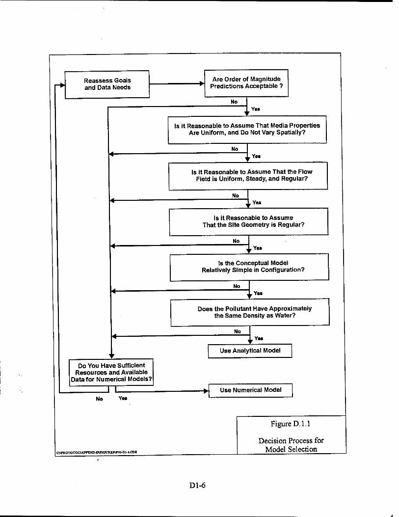
Reassess Goals and Data Needs
Do You Have Sufficient Resources and Available
Data for Numerical Models?
JT No Yes
C:\mOTOCOL\APPIMMJ\nGUIttS\riC-Dl-1.CDR
Are Order of Magnitude Predictions Acceptable ?
No Yet
Is it Reasonable to Assume That Media Properties Are Uniform, and Do Not Vary Spatially?
No Ye*
Is it Reasonable to Assume That the Flow Field is Uniform, Steady, and Regular?
No Ye«
Is it Reasonable to Assume That the Site Geometry is Regular?
No Yes
Is the Conceptual Model Relatively Simple in Configuration?
No Yes
Does the Pollutant Have Approximately the Same Density as Water?
No Yes
Use Analytical Model
Use Numerical Model
Figure D. 1.1
Decision Process for Model Selection
Dl-6
Revision 0
Numerical models require a reasonably good understanding of the three-dimensional distribution
of both aquifer hydraulic properties and the contaminants. Implementation of a numerical model
is much more complex than implementation of an analytical model, and generally requires an
experienced hydrogeologist who is familiar with the model code. The groundwater flow and
transport equations in numerical models typically are solved using either finite difference or finite
element mathematical solution techniques. These solution methods are iterative numerical
approximations to the governing partial differential equation describing solute fate and transport.
The final decision to use an analytical or numerical solute transport model should be based on
the complexity of the problem, the amount of available data, and the importance of the decisions
that will be based upon the model. As an example, consider a site located 5 miles from the
nearest potential receptor. The database for this site consists of five sampling points with one
round of sampling data from each point. The aquifer system at the site consists of 50 feet of
unconsolidated, well-sorted, medium-grained sand overlying a horizontal shale unit. The shallow
water table is 5 feet below the surface. Such a site is an excellent candidate for an analytical
model. Consider on the other hand, a site located approximately 1,000 feet from the nearest
potential receptor. The database for this site consists of 40 data points for which there are 5 years
of quarterly groundwater quality sample analyses. The aquifer at this site consists of 10 feet of
poorly sorted, silty sand, underlain by 5 feet of well-sorted, medium-grained sand, underlain by 20
feet of silt. The quarterly groundwater quality data indicate that a dissolved benzene, toluene.
Ethylbenzene, and xylene (BTEX) plume is migrating downgradient from the source area. In this
situation, a numerical model would be the most appropriate tool to predict the fate and transport
of the dissolved BTEX plume.
D.1.3 IS A MODEL REALLY NECESSARY?
One of the first questions to ask before proceeding with implementation of a solute transport
model is: "Is a model really necessary?" The answer to this question will depend on several
factors, including the rate of plume migration and expansion and the locations of potential
receptors. For example, if there are abundant historical data available for the site, and these data
show that the dissolved BTEX plume has reached a steady-state configuration or is receding, then
a solute transport model probably is not necessary to determine if potential receptors will be
impacted. However, a model of this site would allow an investigator to estimate how long it will
take for the plume to entirely degrade. If on the other hand, the plume is close to a potential
receptor and there are no historical data available, then a solute transport model in conjunction
Dl-7 c:\protocol\append-d\appnd-dl .doc
Revision 0
with the appropriate data can be useful in predicting solute fate and transport, including clean up
times and potential migration distance.
Two questions will invariably arise during an intrinsic remediation demonstration. These
questions are: 1) will potential receptors be impacted by the contaminant plume?, and 2) how long
will the contaminant plume persist? If the proponent of intrinsic remediation is unable to provide
plausible and defensible answers to these questions, it is unlikely that intrinsic remediation will be
accepted by regulators. When properly used with an adequate database of appropriate data,
solute transport models can help provide answers to these questions.
Dl-8 c:\protocol\append-d\appnd-d 1 .doc
Revision 0
SECTION D-2
MODEL DEVELOPMENT AND IMPLEMENTATION
An overview of the steps that must be taken to successfully implement a groundwater flow and
solute transport model is presented in this section. The majority of the material presented herein
is applicable to both analytical and numerical solute transport models. A distinction is made when
the material is relevant to one type of model.
D.2.1 CONCEPTUAL MODEL
The first step in the modeling process is development of the conceptual model. Preliminary
versions of the conceptual model can be as simple as plotting the location of the contaminant
source on a topographic map. The conceptual model is a three-dimensional representation of the
groundwater flow and solute transport system based on available geological, hydrological,
climatological, and geochemical data for the site. The purpose of the conceptual model is the
integration of available data into a coherent representation of the system to be modeled. After
development, the conceptual model is used to aid in model selection and to develop the
appropriate analytical or numerical solute transport model. When possible, the preliminary
conceptual model should be developed before arriving in the field to collect additional data so that
data collection points can be optimized. After collection of site-specific data during the iterative
site-characterization phase of the intrinsic remediation demonstration, the preliminary conceptual
model should be refined.
Successful conceptual model development involves:
• Definition of the problem to be solved;
• Designing the conceptual model;
• Model selection;
• Determination of additional data requirements; and
• Integration of available data including: - Local geologic and topographic maps - Hydraulic data - Site stratigraphy - Contaminant concentration and distribution data (isopleth maps).
D2-1 c:\protocol\append-d\appnd-d2.doc

Revision 0
Most of the conceptual model development process will be completed when all of the maps,
sections, and calculations discussed in section C-2 have been completed. The only requirement
will then be to integrate these data into a coherent representation of the site.
D.2.2 INITIAL AND BOUNDARY CONDITIONS
The solution of any time-dependent (transient) differential equation requires specification of
the conditions at the periphery of the flow system (boundary conditions) and the conditions at the
beginning of the model simulation (initial conditions). For steady-state models, only boundary
conditions must be specified. The purpose of any model is to transform a given set of input
parameters (e.g., hydraulic conductivity, dispersivity, sorption, and biodegradation) into a set of
predictions (e.g., water levels, contaminant concentrations and fluxes, etc.). The results of a
model are made applicable to the area of interest by choosing input parameters and boundary
conditions that are representative of the site. Accurate definition of boundary and initial
conditions is a very important part of the groundwater flow and solute transport modeling
process. The following sections describe the initial and boundary conditions commonly used for
groundwater flow and solute transport models.
D.2.2.1 Initial Conditions
Initial conditions are used to describe conditions at the instant the simulation begins. Initial
conditions must be specified for transient groundwater flow and solute transport problems. It is
not necessary to define initial conditions for steady-state models. This is because steady-state
conditions are used to represent a system that is not changing with time.
D.2.2.1.1 Groundwater Flow
For groundwater flow models, initial conditions are used to specify the values of the variable
under consideration (usually hydraulic head) at the instant the model simulation begins (i.e., at
t = 0) and generally have the form:
h(x,y,z,0)=f(x,y,z) eq.D.2.1
Where f(x,y,z) is a function that describes the variation in hydraulic head, h, in the x, y, and z
directions at time t = 0.
D2-2 c:\protocol\append-d\appnd-d2.doc
Revision 0
D.2.2.1.2 Solute Transport
Initial conditions for solute transport models are used to specify the solute concentration, C, in
the system at the instant the model simulation begins (i.e., at t = 0) and have the form:
C(x,yz,0)=f(x,yz) eq. D.2.2
Where f(x,y,z) is a function that describes the variation in contaminant concentration in the x, y,
and z directions at time t=0. Initial conditions for solute transport generally have the form:
C(x,y,z,0) = 0 eq. D.2.3
or
C(x,y,z,0) = C, eq. D.2.4
Where: C = contaminant concentration d = initial contaminant concentration x = distance downgradient of the source y = distance transverse to the source in the horizontal direction z = distance transverse to the source in the vertical direction
Equation D.2.3 is used as the initial condition for systems devoid of contamination prior to the
introduction of the contaminant or prior to the model simulation. Equation D.2.4 is used as the
initial condition for systems that have dissolved contamination prior to the introduction of
additional contamination or prior to the model simulation.
D.2.2.2 Boundary Conditions
Model boundaries are mathematical statements that specify the dependent variable (head or
contaminant concentration) or the flux (derivative of the head or contaminant concentration with
respect to time) at the model grid boundaries. Boundary conditions describe the interaction
between the system being modeled and its surroundings. The solution of any differential equation
requires specification of the conditions at the periphery of the flow system. Boundary conditions
are used to include the effects of the hydrogeologic system outside the area being modeled with
the system being modeled, while at the same time allowing the isolation of the desired model
domain from the larger hydrogeologic system. In effect, the boundaries of the model tell the area
immediately inside the boundaries what to expect from the outside world. Three types of
boundary conditions generally are utilized to describe groundwater flow and solute transport.
D2-3 c:\protocolVappend-d\appnd-d2.doc

Revision 0
Boundary conditions are referred to as the first type (Dirichlet), the second type (Neumann), and
the third type (Cauchy). Table D.2.1 summarizes boundary conditions for ground water flow and
solute transport.
Table D.2.1
Common Designations for Several Important Boundary Conditions (Modified From Franke et al, 1987)
Boundary Condition Boundary Type Formal Name
General Mathematical Description Groundwater Flow Contaminant
Transport Specified-Head or Specified- Concentration
Type One Dirichlet H=f(x,y,z,t) C =f(x,y,z,t)
Specified-Flux Type Two Neumann — = f(x,y,z.t)
en -— = f(x,y.zj) on
Head-Dependent or Concentration- Dependent Flux
Type Three (mixed-boundary
condition) Cauchy
— + cH = f(x,y,z,t) on
— + cC = f(x,y,z.t) on
Proper design of model boundary conditions is of paramount importance in numerical model
implementation. When using a numerical model, hydrologic boundaries such as constant-head
features (e.g., lakes, etc.) or constant-flux features should, when possible, coincide with the
perimeter of the model. In areas that lack obvious hydrologic boundaries, constant-head or
constant-flux boundaries can be specified at the numerical model perimeter as long as the
perimeter is far enough removed from the contaminant plume that transport calculations will not
be affected. It is generally a good idea to make the modeled area large enough so that model
boundaries can be placed far enough away from the plume to have minimal impact. This may not
be possible in all cases, such as where the plume is near a surface water body. In such cases, it
may be necessary to calibrate the model using different boundary conditions until a good match to
observed conditions is achieved. In this case, sensitivity analyses should be performed to analyze
the effects of various combinations of boundary conditions.
D.2.2.2.1 First-Type Boundary Condition (Dirichlet, Specified-Head or -Concentration)
This type of boundary condition is referred to as the first-type boundary condition or the
Dirichlet boundary condition. With this type of boundary condition, values of head (groundwater
flow) or concentration (solute transport) are specified along the boundary. Type one boundary
conditions are used to describe the boundary if the hydraulic head or solute concentration at the
D2-4 c:\protocolappend-d\appnd-d2.doc
Revision 0
boundary is independent of flow conditions in the model domain. The constant-head or constant-
concentration boundary is a special type of specified-head boundary wherein the head or solute
concentration is fixed at the boundary.
D. 2.2.2.1.1 Groundwater Flow (Specified-Head Boundary)
Specified-head boundaries (Dirichlet condition) are boundaries for which the hydraulic head is
specified as a function of location and time. Specified-head boundaries are expressed
mathematically as:
H = f(x,y,zJ) eq.D.2.5
Where:// = total hydraulic head x = distance downgradient of the source y = distance transverse to the source in the horizontal direction z = distance transverse to the source in the vertical direction t - time
Hydraulic head in surface water bodies is commonly a function of location and time. The type
one boundary condition is often used to model the interaction between surface water bodies and
groundwater. As an example, consider an aquifer that is bounded by a large stream whose stage
is independent of groundwater seepage. Moving upstream or downstream along the boundary,
the hydraulic head changes in relation to the slope of the stream channel and decreases
downstream. If the surface elevation of the stream is fairly constant in time, the head can be
specified as a function of position alone, H =f(x,y,z) at all points along the streambed. If the
stream stage varies with time, the head is specified as a function of position and time, and
H =f(x,y,z,t) at all points along the streambed. In both examples, heads along the stream are
determined by circumstances external to the groundwater flow system and maintain these
specified values throughout the problem solution, regardless of the stresses to which the
groundwater system is subjected (Franke et ai, 1987). Figure D.2.1 shows an example of a
specified-head boundary.
A constant-head boundary is a special type of specified-head boundary that occurs where a
part of the boundary of the aquifer system coincides with a surface that has a total hydraulic head
that is constant in both time and space. An example of a constant-head boundary would be a large
lake where water levels do not fluctuate significantly through time. The hydraulic head is fixed
(constant) for all points of this boundary, i.e.,
H = constant eq. D.2.6
D2-5 c:\protocoi\append-d\appnd-d2.doc

Surface-Water Body
C:\PROTOCOL\Al>PEND-D\FIGURES\FIG-D2-l.CDR
Figure D.2.1
Specified Head (Type One) Boundary Condition
D2-6

Revision 0
Both specified-head and constant-head boundaries have an important "physical" characteristic
in models of groundwater systems because in order to maintain the prescribed head, they provide
an inexhaustible source of water. No matter how much water is removed from the system, the
specified-head boundaries will continue to supply the amount of water necessary to maintain the
head specified at the boundary, even if that amount is not reasonable in the real system (Franke et
al, 1987). Careful consideration should be given to this fact when a specified-head boundary is
selected. It is generally considered acceptable to use this type of boundary as long as the
boundary is located far enough from a pumping well that it will be unaffected or only minimally
affected by pumping.
D. 2.2.2.1.2 Solute Transport (Specified-Concentration)
Specified-concentration boundaries (Dirichlet condition) are boundaries for which the
contaminant concentration is specified as a function of location and time. Specified-concentration
boundaries are expressed mathematically as:
C = C0(x,y,z,t) eq. D.2.7
Where: C = contaminant concentration C0 = initial contaminant concentration x = x coordinate of boundary v = y coordinate of boundary z = z coordinate of boundary / = time
A constant-concentration boundary is a special type of specified-concentration boundary that
occurs where a part of the boundary surface of the aquifer system coincides with a surface that
has a contaminant concentration that is constant in both time and space. At the upgradient end of
the system, the first-type boundary condition states that at x = 0, and for all time, t, the
concentration is C0 (i.e., a continuous source of constant concentration). This is described
mathematically as:
C(0,t) = Co eq. D.2.8
This boundary condition is used to calculate concentrations in a system where there is a
continuous source of dissolved contamination at the upgradient flow boundary. An example
would be a light nonaqueous-phase liquid (LNAPL) spill that receives fresh product at a rate that
is balanced by LNAPL mass loss through weathering. The maximum BTEX concentration in
groundwater beneath the LNAPL plume is dictated by the partitioning relationships described in
D2-7 c:\protocol\append-d\appnd-d2.doc
Revision 0
Section C.3.2.2. In reality, such a system is rare. Once a source of LNAPL contamination has
been identified it is generally removed and the LNAPL is subjected to weathering though the
processes of volatilization, dissolution, and biodegradation. Because of their physiochemical
characteristics, the BTEX compounds are some of the first compounds to be removed from the
LNAPL in the subsurface. As a result, their mass fractions will be reduced, and through time, the
concentrations of BTEX being released into the underlying groundwater will be reduced.
Because of this, most contaminant source areas should be modeled as decaying sources.
D.2.2.2.2 Second-Type Boundary Condition (Neumann, Specified-Flux)
This type of boundary condition is referred to as the second-type boundary condition or the
Neumann boundary condition. This boundary condition specifies the flux of groundwater or
contaminant mass perpendicular to the boundary, and is equated to the normal derivative of head
or concentration with respect to the direction perpendicular to the flow boundary.
D. 2.2.2.2.1 Groundwater Flow (Specified-Flux)
Speoified-flux boundaries are boundaries for which the flux of water across the boundary can
be specified as a function of position and time. Flux, q, is defined as the volume of water crossing
a unit cross-sectional area per unit time and, following Darcy's Law, is given by the hydraulic
conductivity times the first derivative of head with respect to the direction perpendicular to the
flow boundary. The units of flux are L3/L2/T. If the direction perpendicular to the boundary
corresponds with an axis of hydraulic conductivity, then the flux is given by (Franke et al., 1987):
q = -K^~ eq.D.2.9 on
Where: q = volumetric flux K = hydraulic conductivity H = total hydraulic head n = distance perpendicular to the boundary
In the most general case, the flux across the boundary is specified as a function of position and
time, i.e.:
q=f(x,y,z,t) eq.D.2.10
or, if K is constant:
D2-8 c:\protocol\append-d\appnd-d2.doc
Revision 0
ai = f(x,y,z,t) eq.D.2.11
In some cases, the flux might be constant with time, but specified as a function of position, i.e.:
q=f(x,y,z) eq. D.2.12
or, if K is constant:
cH ~^ = f(x'y>z>> eq.D.2.13
In the simplest case, the flux across the boundary is specified in space and in time, i.e.:
q = constant eq. D.2.14
or, if K is constant:
— = constant eq. D.2.15
An example where the flux across the boundary is often assumed to be specified in space and in
time is areal recharge to a water-table aquifer by infiltration.
No-flow boundaries (impervious boundaries) are a special type of specified-flux boundary
where the flux is constant in space and time and is zero, i.e.:
q = constant = 0 eq. D.2.16
or, if K is a constant:
ÖH —— = constant = 0 eq. D.2.17 at
Examples of no-flow boundaries include groundwater divides and impermeable hydrostratigraphic
units.
It is important to note that in all three of the cases listed above, the flux across the boundary is
specified prior to the modeling simulation, is not affected by stresses to the groundwater system,
and therefore is not allowed to deviate from the value specified prior to modeling. For systems
where the flux varies as a function of hydraulic head along the boundary, the third-type boundary
condition should be used.
D2-9 c:\protocol\append-d\appnd-d2.doc
Revision 0
D.2.2.2.2.2 Solute Transport (Specified-Concentration Gradient)
The second-type boundary condition specifies the concentration gradient across a section of
the boundary surface and is described mathematically by the first derivative of concentration with
respect to the direction perpendicular to the flow boundary.
In the most general case the concentration gradient is a function of location and time:
dC — = /(x,.y,z,/) eq.D.2.18 an
Where: C-= solute concentration n = distance perpendicular to the boundary x = distance downgradient of the source v = distance transverse to the source in the horizontal direction z = distance transverse to the source in the vertical direction / = time
In some cases, the flux might be constant with time, but specified as a function of position:
^ = /(x,v,z) eq.D.2.19
In the simplest case, the flux across the boundary is specified in space and in time:
dC „. _ _,. —— = constant eq. D. 2.20 dn
In some cases there may be no concentration gradient across the boundary. This is a special
type of specified-concentration-gradient boundary where the concentration gradient is constant in
space and time and is zero:
— = constant = 0 eq. D.2.21 dn
D.2.2.2.3 Third-Type Boundary Condition (Cauchy, Variable-Flux)
The third-type boundary condition specifies the flux of groundwater (volumetric flow rate) or
contaminant along the boundary as a function of hydraulic head or contaminant concentration,
and is equated to the normal derivative of head or concentration with respect to the direction
normal to the flow boundary and the hydraulic head or contaminant concentration. This type of
boundary condition is referred to as the third-type boundary condition or the Cauchy boundary
condition.
D2-10 c:\protocol\append-d\appnd-d2.doc

Revision 0
D. 2.2.2.3.1 Groundwater Flow (Head-Dependent Flux Boundary)
This type of boundary condition is used to describe situations where the flux across a part of
the boundary surface changes in response to changes in hydraulic head within the aquifer system
adjacent to the boundary. In these situations the flux is a specified function of that head, and
varies during the model simulation as the head varies (Franke et ai, 1987). Head-dependent flux
boundaries (Cauchy or mixed-boundary conditions) occur where the flux across the boundary is
calculated from a given boundary head value. This type of flow boundary is sometimes referred
to as a mixed-boundary condition because it is a combination of a specified-head boundary and a
specified-flow boundary. The general mathematical description of the variable-flux boundary is
given by (Franke et ai, 1987):
q = -K + cH eq. D.2.22 äx
Where: q = volumetric flux K = hydraulic conductivity c = constant H = total hydraulic head n = distance perpendicular to the boundary
Head-dependent flow boundaries are used to model leakage across semipermeable boundaries.
An example is the upper surface of an aquifer overlain by a semiconfining unit that is in turn
overlain by a surface water body. Aquifers in contact with lakes typically exhibit this type of
boundary condition because clay and silt tends to accumulate at the bottom of lakes. Figure D.2.2
illustrates this scenario. The flux across the semiconfining bed in this figure is expressed
mathematically as (Bear, 1979):
q = _KX o- ) eq.D.2.23 B'
Where: q = volumetric flux H = head in the aquifer Ho = head in external zone (separated from the aquifer by semipermeable layer) K' = hydraulic conductivity of semipermeable layer B' = thickness of semipermeable layer
D2-11 c:\protocol\append-dteppnd-d2.doc
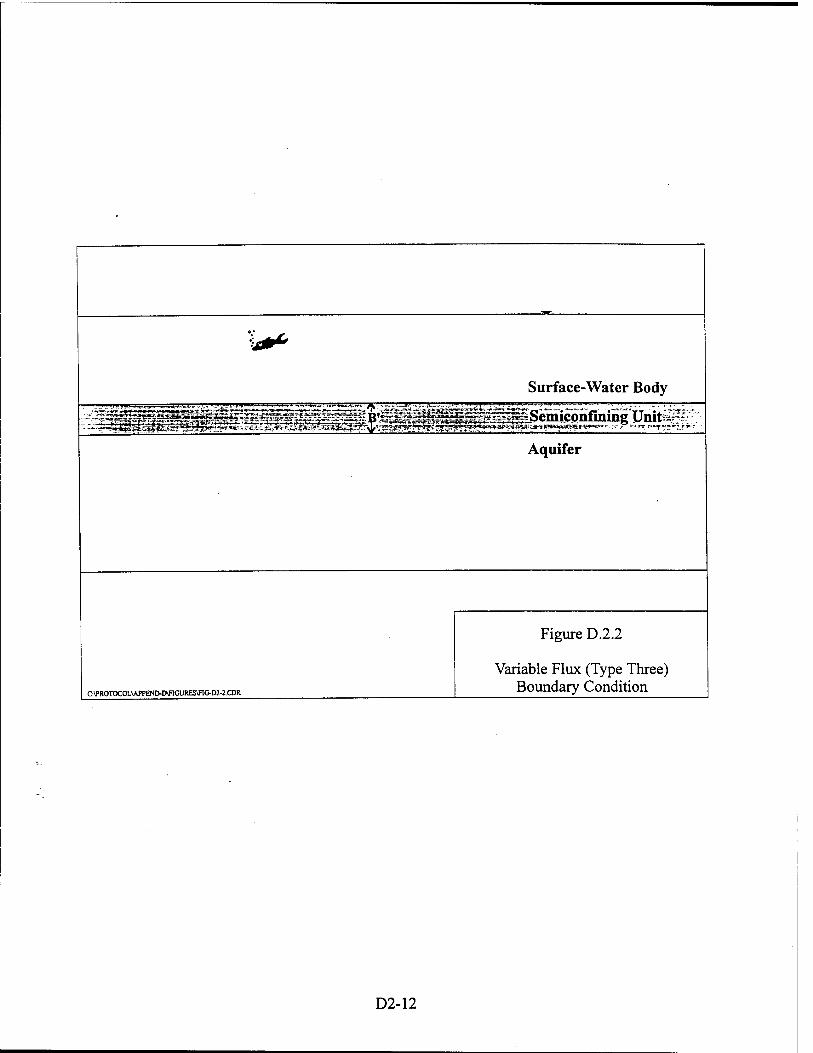
Surface-Water Body aB.frrr^?-=:,'»^^-^B L—i L. u. HLüWTB-.-tk-=-JJ--.:.LJJIL .t IJL jjljiii .^JMafeM^Juyg
Semicohfining Unit 1 B^atf^Sgaf rjE'ä pwgaa^fpg '■t ,f.*«-f ™»-;_iF.i"
Aquifer
C:\PROTOCOL\AI>PEND-D\F1GURES\FIG-D2-2.CDR
Figure D.2.2
Variable Flux (Type Three) Boundary Condition
D2-12
Revision 0
D. 2.2.2.3.2 Solute Tramport (Concentration-Dependent Concentration Gradient)
This type of boundary condition is used where the concentration gradient across the boundary
is dependent on the difference between a specified concentration on one side of the boundary and
the solute concentration on the opposite side of the boundary (Wexler, 1992). For a one-
dimensional system, this type of boundary condition is described mathematically as (Wexler, 1992;
Bear, 1979):
vxC-Z)x~ = vIC0, x = 0 eq.D.2.24 ox.
This boundary condition best describes solute concentrations at the upgradient boundary of a
homogeneous flow system where a well-mixed solute enters the system by advection across the
boundary and is transported downgradient from the boundary by advection and dispersion
(Wexler, 1992).
D.2.3 MODEL INPUT
Data required to complete a groundwater model, analytical or numerical, include:
• Hydraulic conductivity;
• Initial hydraulic head distribution;
• Flow direction and gradient;
• Effective porosity;
• Coefficient of hydrodynamic dispersion;
• Coefficient of retardation;
• Initial solute concentrations;
• Contaminant source concentration configuration, and rate of source decay (or removal);
• Distribution and continuity of aquifer and aquitards (thickness, continuity, areal extent, interconnections, etc.);
• Groundwater recharge and discharge (infiltration, evapotransporation, pumpage from wells, discharges to surface water, etc.);
• Definition of physical and chemical boundary conditions; and
• Rates of chemical reactions, particularly biodegradation.
Collection of data is discussed in Appendix A. Premodeling calculations are discussed in
Appendix C.
D2-13 c:\protocol\append-d\appnd-d2.doc

Revision 0
D.2.3.1 Analytical Model Input
Analytical modeling can be performed using commonly available spreadsheets or mathematical
analysis programs such as MathCAD*. Because analytical solutions are algebraic expressions,
input into these models is very straightforward and usually consists of entering the parameter
values in appropriate locations.
D.2.3.2 Numerical Model Input
Numerical models are developed by replacing the continuous hydrogeologic domain with a
discretized domain consisting of an array of nodes and associated blocks or elements (a model
grid). Aquifer hydraulic and chemical parameters are assigned to each grid cell. Design of an
appropriate model grid at the outset of modeling is important for successful model
implementation. The most important aspects of grid design are selecting an appropriate size for
the model grid, proper orientation of the grid, and choosing appropriate boundary conditions.
Numerous factors must be considered when selecting the size of grid cells to be used. There is
a trade-off between grid spacing, model accuracy, and being able to model the entire area
potentially affected by the contaminant plume. As in differential calculus, the smaller the grid
spacing, the more accurate the numerical model will be, and the numerical solution will approach
the exact solution as the grid spacing approaches zero. Additionally, more grid nodes increases
the demands placed on the computer and longer calculation times will result. Because large
numerical errors may arise if the solute being modeled comes in contact with a model boundary,
the model grid must be designed so that it is large enough that the solute plume will not intersect
a model boundary.
D.2.4 MODEL CALIBRATION
To ensure that a groundwater flow and solute transport model is capable of accurately
predicting the future extent and concentration of a contaminant plume, it must be calibrated to
observed hydraulic and contaminant data. Calibration involves trial-and-error adjustment of key
model input parameters such as hydraulic conductivity, dispersivity, soil sorption coefficient,
recharge, effective porosity, boundary conditions, and biodegradation rate until an adequate
match between observed and simulated hydraulics and contaminant distribution is achieved. In
general, the parameters that have the most impact on the results of contaminant fate and transport
modeling are hydraulic conductivity, head distribution (gradient), boundary conditions, and
D2-14 c:\protocol\append-d\appnd-d2.doc

Revision 0
biodegradation rates. Historical groundwater data are required to properly calibrate a
groundwater flow and solute transport model.
Numerical solute transport model calibration differs from analytical solute transport model
calibration. Calibration of a numerical solute transport model is a two-step process; first the
groundwater flow system is calibrated, and then the solute transport system is calibrated.
Calibration of the numerical flow model demonstrates that the model is capable of matching
hydraulic conditions observed at the site; calibration of a contaminant transport model
superimposed upon the calibrated flow model helps verify that contaminant loading and transport
conditions are being appropriately simulated. Groundwater flow is calibrated by altering
transmissivity in a trial-and-error fashion until simulated heads approximate observed field values
within a prescribed accuracy. After calibration of the flow model, the numerical solute transport
model should be calibrated by altering hydraulic parameters and transport parameters in a trial-
and-error fashion until the simulated BTEX plume approximates observed field values. Because
analytical models do not calculate head as a function of time (gradients and hydraulic head
considerations are addressed by the groundwater velocity that is entered into the model), only
solute transport can be calibrated. The analytical solute transport model is calibrated by altering
hydraulic parameters and transport parameters in a trial-and-error fashion until the simulated
BTEX plume approximates observed field values.
D.2.4.1 Groundwater Flow Calibration
Calibrating the model to groundwater flow involves comparing measured water levels against
simulated water levels over the same period of time. If the flow simulation is steady-state, then
the simulated water levels need only be compared with one set of data. Hydraulic conductivity is
an important aquifer characteristic that determines the ability of the water-bearing strata to
transmit groundwater. Transmissivity is the product of the hydraulic conductivity and the
thickness of the aquifer. In conjunction with boundary conditions, hydraulic conductivity or
transmissivity values will govern the calculated head solution. An accurate estimate of hydraulic
conductivity is also important to help quantify advective groundwater flow velocities and to
define the flushing potential of the aquifer and the quantity of electron-acceptor-charged
groundwater that is entering the site from upgradient locations.
Saturated thickness data from previous reports, geologic logs, and water level measurements
are used in conjunction with hydraulic conductivity to estimate an initial transmissivity for the
model domain. To better match heads in the model to observed values, transmissivities are
D2-15 c:\protocol\append-d\appnd-d2.doc

Revision 0
progressively varied in blocks and rows until the simulated water levels for cells corresponding to
the selected well locations match' the observed water levels as closely as possible. This is often
done manually, although codes that can determine the most appropriate parameter values are
available.
The root mean squared (RMS) error is commonly used to express the average difference
between simulated and measured heads. RMS error is the average of the squared differences
between measured and simulated heads, and can be expressed as:
RMS = ■ n ;=1
~P.5 2
eq. D.2.25
Where:« = the number of points where heads are being compared h„ = measured head value hs = simulated head value.
The RMS error between observed and calibrated values should be such that the calculated
calibration error is less than 10 percent of the average head drop over the model domain. If
sufficient data are available, it may be possible to produce a model with a calibration error of less
than 5 percent. Calibration error may be described by:
AHT
Where: CE = Calibration error (as a percentage) RMS = Root mean square error [L] AHr = Total head change over model domain [L]
Another qualitative method of checking the calibrated model head distribution involves a
comparison of calculated heads and observed heads. When calculated heads are plotted versus
observed heads, the points should scatter randomly about a straight line. Such a plot also can be
used to check if there are any variations in the modeled head distribution that indicate a need to
reevaluate parameters in a specific portion of the model domain (e.g., heads are consistently low
in the vicinity of a boundary). Figure D.2.3 is an example of such a plot.
Other parameters that may be adjusted during model calibration include effective porosity,
recharge, and hydraulic boundary conditions.
D2-16 c:\protocol\append-d\appnd-d2.doc
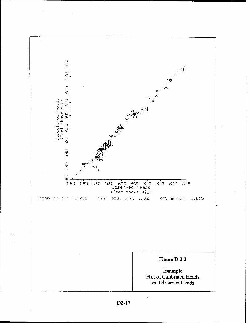
in CM -, \o
o CM - MD
in V* \o
^2- ?* ^ </> \o
j^V* tu in
-0 > 0 - H<*S: d O M) 4- 12
=k/^
ula
t a
00
U 0; V3 _ <b ID U- ,_
CJ ~ ^ ^ CO- LO
O CO - in
in 00 - in /*% a CD -
«hi 30 585 590 595 600 605 610 615 620 625 Observed heads (feet above MSL)
Mean err or: -0.716 Mean abs. err: 1.32 RMS error: 1.815
Figure D.2.3
Example Plot of Calibrated Heads
vs. Observed Heads
D2-17

Revision 0
D.2.4.2 Calibrating the Model to Contaminant Distribution
Calibrating a model to contaminant fate and transport involves comparing the observed
changes in plume extent and concentration to the predicted changes in extent and concentration
over the same period of time. This requires historical contaminant data that may not be available
when the model is first developed. Because of this, there will be uncertainty in the model
predictions and the model should be reevaluated as more groundwater analytical data become
available.
Model input parameters affecting the distribution and concentration of the simulated BTEX
plume should be modified so that model predictions match dissolved BTEX concentrations. To
do this, model runs are made using the calibrated hydraulic parameters with available BTEX
plume data. If the contaminant distribution is known at two different times, the plume can be
calibrated over time. Plume calibration is achieved by varying the source terms, the anaerobic
decay coefficient, the coefficient of retardation, the effective porosity, and dispersivity until the
BTEX plume is calibrated reasonably well to the existing plume in terms of migration distance,
configuration, BTEX concentrations, and BTEX concentration changes in the plume area.
D.2.5 SENSITIVITY AND UNCERTAINTY ANALYSES
Any groundwater model is influenced by uncertainty owing to the inability to define the exact
spatial and temporal distribution of aquifer and chemical parameter values at the field site. A
sensitivity analysis is performed by varying model input parameters over reasonable ranges to
establish the effect of uncertainty on the model. Sensitivity analyses should be performed on all
models to evaluate the reasonableness of model predictions.
The iterative model calibration process involves modifying several input parameters until a
reasonable match of the hydraulic regime and contaminant fate and transport observations is
reached. Thus, numerous variations of model input could produce the same results. To
determine those model input parameters that have the greatest impact on modeling results,
sensitivity analyses should be performed. Sensitivity analysis involves varying model input
parameters to determine the impact of different parameter values on the model output. All solute
transport models are sensitive to hydraulic conductivity (which has a great effect on transport
velocity), dispersivity, retardation coefficients, and biodegradation rates. Based on the work of
Rifai et al. (1988), the Bioplume II model is most sensitive to changes in the coefficient of
reaeration, the coefficient of anaerobic decay, and the hydraulic conductivity of the media, and is
less sensitive to changes in the retardation factor, porosity, and dispersivity. At a minimum, the
D2-18 c:\protocol\append-d\appnd-d2.doc

Revision 0
sensitivity analyses must involve varying these model input parameters over the range of plausible values.
The results of sensitivity analyses can be shown graphically by displaying the modeled BTEX
concentrations versus distance along the centerline of the plume. This manner of displaying data
is useful because the figures allow easy visualization of the changes in BTEX concentration
caused by varying model input parameters. The results of the sensitivity analysis will tell the
modeler which parameters have the greatest influence on the site model. This allows the
prediction of worst-case scenarios.
In conjunction with (or as part of) the sensitivity analysis, the modeler may also provide an
uncertainty analysis. This is done to determine the sensitivity of the model results to uncertainty
in site-specific parameters. For example, a range of values for a specific parameter may be
measured at a site, and the calibrated model may use an intermediate value. To check the
sensitivity of the model to the uncertainty in this parameter, model runs would be made using the
upper and lower values of the measured range of that parameter. By comparing the results of
these model runs to the calibrated model results, the effects of uncertainty associated with that
parameter and the effect of the uncertainty on model predictions can then be assessed. In effect,
the uncertainty analysis is a focused sensitivity analysis in which the parameters are varied within a
range indicated by a statistical evaluation of site data. Where limited data are available, such an analysis may not be feasible.
D.2.6 PREDICTION
After the solute transport model has been calibrated and the sensitivity analyses have been
performed, the model can be used to predict the fate and transport of contaminants. To do this,
the model should be run with the input parameters determined to be most accurate based on
model calibration and sensitivity analyses. Additional scenarios also can be simulated, such as
source removal or reduction.
D.2.7 MODEL DOCUMENTATION AND REPORTING
Model documentation is a very important component of the modeling effort. If the reader
cannot determine how the model was set up and implemented, the model is of little use. At a
minimum, model documentation must include a discussion of how the model code was selected, a
listing of all simplifying assumptions, boundary and initial conditions used, how model input
parameters were determined (whether measured, estimated, or assumed), the process used to
D2-19 c:\protocol\append-d\appnd-d2.doc
Revision 0
interpolate the data spatially, how the model was calibrated and what types of
sensitivity/uncertainty analyses were performed. Figure D.2.4 gives an example table of contents
from a report that was used to successfully implement intrinsic remediation at a site contaminated
with fuel hydrocarbons. Appendices E and F present examples of such reports.
D.2.8 POST-MODEL MONITORING, VERIFICATION, AND ADJUSTMENT
An important component of the intrinsic remediation demonstration is development of a long-
term monitoring (LTM) plan that will allow the contaminant plume to be tracked through time.
Long-term monitoring of the contaminant plume will allow the solute transport model to be
verified. A model is considered verified if data collected after model implementation supports the
predictions made by the model. If these data do not agree with what the model predicted, then
the model should be recalibrated using the new data.
To demonstrate attainment with site-specific remediation goals and to verify the predictions
made by the solute transport model developed for the site, the LTM plan consists of identifying
the locations of two separate groundwater monitoring networks and developing a groundwater
sampling and analysis strategy. The strategy described in this section is designed to monitor
BTEX plume migration over time and to verify that intrinsic remediation is occurring at rates
sufficient to protect potential receptors. In the event that data collected under the LTM program
indicate that naturally occurring processes are insufficient to protect human health and the
environment, contingency controls to augment the beneficial effects of intrinsic remediation can
be implemented.
D.2.8.1 Monitoring Networks
Two separate sets of wells should be installed at the site as part of the intrinsic remediation
with LTM remedial alternative. The first set should consist of at least four LTM wells located in,
upgradient, and downgradient of the observed BTEX plume to verify the results of the solute
transport model and to ensure that natural attenuation is occurring at rates sufficient to minimize
D2-20 c:\protocol\append-d\appnd-d2.doc
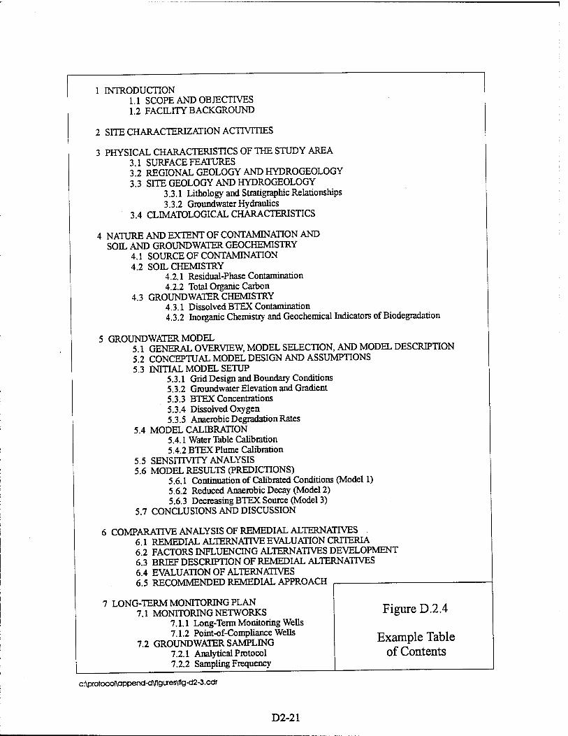
1 INTRODUCTION 1.1 SCOPE AND OBJECTIVES 1.2 FACILITY BACKGROUND
2 SITE CHARACTERIZATION ACTIVITIES
3 PHYSICAL CHARACTERISTICS OF THE STUDY AREA 3.1 SURFACE FEATURES 3 2 REGIONAL GEOLOGY AND HYDROGEOLOGY 3.3 SITE GEOLOGY AND HYDROGEOLOGY
3.3.1 Lithology and Stratigraphic Relationships 3.3.2 Groundwater Hydraulics
3.4 CLIMATOLOGICAL CHARACTERISTICS
4 NATURE AND EXTENT OF CONTAMINATION AND SOIL AND GROUNDWATER GEOCHEMISTRY
4.1 4.2
4.3
SOURCE OF CONTAMINATION SOIL CHEMISTRY
4.2.1 Residual-Phase Contamination 4.2.2 Total Organic Caibon
GROUNDWATER CHEMISTRY 4.3.1 Dissolved BTEX Contamination 4.3.2 Inorganic Chemistry and Geochemical Indicators of Biodegradation
5 GROUNDWATER MODEL 5 1 GENERAL OVERVIEW, MODEL SELECTION, AND MODEL DESCRIPTION 5.2 CONCEPTUAL MODEL DESIGN AND ASSUMPTIONS 5.3 INITIAL MODEL SETUP
5.3.1 Grid Design and Boundary Conditions 5.3.2 Groundwater Elevation and Gradient 5.3.3 BTEX Concentrations 5.3.4 Dissolved Oxygen 5.3.5 Anaerobic Degradation Rates
5.4 MODEL CALIBRATION 5.4.1 Water Table Calibration 5.4.2 BTEX Plume Calibration
5.5 SENSrrrvTTY ANALYSIS 5.6 MODEL RESULTS (PREDICTIONS)
5.6.1 Continuation of Calibrated Conditions (Model 1) 5.6.2 Reduced Anaerobic Decay (Model 2) 5.6.3 Decreasing BTEX Source (Model 3)
5.7 CONCLUSIONS AND DISCUSSION
6 COMPARATIVE ANALYSIS OF REMEDIAL ALTERNATIVES 6.1 REMEDIAL ALTERNATIVE EVALUATION CRITERIA 6 2 FACTORS INFLUENCING ALTERNATIVES DEVELOPMENT 6.3 BRIEF DESCRIPTION OF REMEDIAL ALTERNATIVES 6.4 EVALUATION OF ALTERNATIVES 6.5 RECOMMENDED REMEDIAL APPROACH
7 LONG-TERM MONITORING PLAN 7.1 MONITORING NETWORKS
7.1.1 Long-Term Monitoring Wells 7.1.2 Point-of-Compliance Wells
7.2 GROUNDWATER SAMPLING 7.2.1 Analytical Protocol 7.2.2 Sampling Frequency
Figure D.2.4
Example Table of Contents
c:\proto^apirend-dVigures\fig-cl2-3.cdr
D2-21
Revision 0
plume expansion. This network of wells can consist of existing or newly installed wells screened
within the shallow aquifer to provide short-term confirmation and verification of the quantitative
groundwater modeling results. The second set of groundwater monitoring wells, point-of-
compliance (POC) wells, should be located downgradient from the plume along a line
perpendicular to the groundwater flow direction. The purpose of the POC wells is to verify that
no BTEX compounds exceeding state or federal health-protective groundwater standards migrate
beyond the area under institutional control. This network should consist of at least three
groundwater monitoring wells. The LTM wells should be sampled for analysis of the parameters
listed in Table 2.1. The POC wells should be sampled for dissolved oxygen and BTEX, plus any
other parameters required for regulatory compliance.
D. 2.8.1.1 Long-Term Monitoring Wells
In at least four locations, groundwater wells within, upgradient, and downgradient of the
existing BTEX contaminant plume should be used to monitor the effectiveness of intrinsic
remediation in reducing total contaminant mass and minimizing contaminant migration at the site.
At least one of these wells should be placed in the anaerobic treatment zone, one should be placed
in the aerobic treatment zone, and another well is typically placed downgradient from the aerobic
treatment zone. An upgradient well provides background data. This network will supplement the
POC wells to provide early confirmation of model predictions and to allow additional response
time if necessary.
D.2.8.1.2 Point-of-Compliance Wells
Three POC monitoring wells should be installed downgradient from the leading edge of the
BTEX plume. The purpose of the POC wells is to verify that no contaminated groundwater
exceeding state or federal regulatory standards migrates beyond the area under institutional
control. Although these wells should be placed beyond the point where model results suggest that
the contaminant plume will migrate (at concentrations exceeding chemical-specific groundwater
standards), these POC wells are the technical mechanisms used to demonstrate protection of
human health and the environment and compliance with site-specific numerical remediation goals.
As with the LTM wells, the POC wells must be screened in the same hydrogeologic unit(s) as the
contaminant plume.
D2-22 c:\protocol\append-d\appnd-d2.doc
Revision 0
SECTION D-3
ANALYTICAL SOLUTE TRANSPORT MODELS
Analytical models provide exact, closed-form solutions to the governing advection-dispersion equations presented in Section D-l. The use of analytical models requires the user to make several simplifying assumptions about the solute transport system. For this reason, analytical
models are most valuable for relatively simple hydrogeologic systems that are relatively homogeneous and isotropic and have uniform geometry (straight boundaries and constant thickness, width, and length). Heterogeneous and anisotropic hydrogeologic systems can be modeled using analytical models only if the system is simplified and average hydraulic characteristics are used. As an example, consider a hydrogeologic system composed of several layers with differing thicknesses and hydraulic conductivities. This system could be simulated using an analytical model by averaging the hydraulic conductivity over the entire thickness being modeled by dividing the sum of the products of each layer's thickness and hydraulic conductivity by the total aquifer thickness (Walton, 1991).
Table D.3.1 lists the analytical models presented in this section. Each model presented is capable of simulating advection, dispersion, sorption, and biodegradation (or any first-order decay process). The assumptions required for each modeling scenario are listed in the relevant section. One-, two-, and three-dimensional analytical solutions to the advection-dispersion equation that are capable of simulating systems that have a continuing source of contamination or a source that is decaying over time are presented in this section (with the exception of a two-dimensional solution for a decaying source). Models that simulate a continuous source of contamination are good for determining the worst-case distribution of the dissolved contaminant plume. This is unrealistic, however, if for no other reason, because source concentrations decrease over time via natural weathering processes. As discussed in Appendix C, natural weathering processes can be slow, so it often will be necessary to implement an engineered solution for source removal. The models used to simulate a decaying source are especially applicable where an engineered solution is implemented for source removal. An important model input parameter for such models is the source decay rate. Appendix C discusses methods that can be used to quantify source-removal rates.
D3-1 c:\protocol\append-d\appnd-d3.doc

Revision 0
Table D.3.1
Analytical Models Commonly used to Simulate Solute Transport
Processes Simulated | Description Authors Section One-Dimensional Models
Advection, dispersion, linear sorption, and biodegradation - Constant Source Term
Solute transport in a semi-infinite system with a continuous source of contamination. Biodegradation is simulated using a first-order decay rate constant. Solute concentration is given as a function of time and distance
Bear, 1972; van Genuchten and Alves, 1982; and Wexler, 1992
D.3.2.1
Advection, dispersion, linear sorption, and biodegradation - Decaying Source Term
Solute transport in a semi-infinite system with a decaying source of contamination. Biodegradation is simulated using a first-order decay rate constant. Solute concentration is given as a function of time and distance
van Genuchten and Alves, 1982
D.3.2.2
Two-Dimensional Models Advection, dispersion, linear sorption, and biodegradation - Constant Source Term
Solute transport in a semi-infinite system with a continuous source of contamination. Biodegradation is simulated using a first-order decay rate constant. Solute concentration is given as a function of time and distance
Wilson and Miller, 1978
D.3.3.1
Three-Dimensional Models Advection, dispersion, linear sorption, and biodegradation - Constant Source Term
Solute transport in a semi-infinite system with a continuous source of contamination. Biodegradation is simulated using a first-order decay rate constant. Solute concentration is given as a function of distance from the source and time
Domenico, 1987 D.3.4.1
Advection, dispersion, linear sorption, and biodegradation - Decaying Source Term
Solute transport in a semi-infinite system with a decaying source of contamination. Biodegradation is simulated using a first-order decay rate constant. Solute concentration is given as a function of distance from the source and time
Domenico, 1987 modified for decaying source concentration
D.3.4.2
D.3.1 INITIAL AND BOUNDARY CONDITIONS FOR ANALYTICAL SOLUTE TRANSPORT MODELS
D.3.1.1 Upgradient (Inflow) Boundary Conditions
The first-type and third-type boundary conditions discussed in Section D-l are used to describe
solute concentrations at the upgradient (inflow) boundary of an analytical model. The third-type
boundary condition is more accurate than the first-type boundary condition. This is because the
first-type boundary condition assumes that the concentration gradient across the upgradient
boundary is zero the instant flow begins (Wexler, 1992). This tends to overestimate the mass of
solute in the system for early time (Wexler, 1992). Table D.3.2 lists typical boundary conditions
used to describe the upgradient boundary of a solute transport system for analytical models.
D3-2 c:\protocol\append-d\appnd-d3.doc
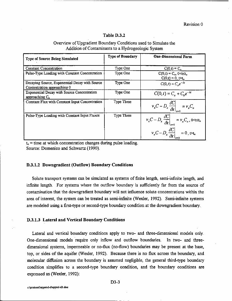
Revision 0
Table D.3.2
Overview of Upgradient Boundary Conditions used to Simulate the Addition of Contaminants to a Hydrogeologie System
Type of Source Being Simulated Type of Boundary One-Dimensional Form
Constant Concentration Type One C(0,t) = c0
Pulse-Type Loading with Constant Concentration Type One C(0,t) = C0, (XfcSto C(0,t) = 0, t>t,
Decaying Source, Exponential Decay with Source Concentration approaching 0
Type One C(0,f) = Coe-*
Exponential Decay with Source Concentration approaching C,
Type One C(0,0 = Ca+Q^
Constant Flux with Constant Input Concentration Type Three
^■§ x=0
Pulse-Type Loading with Constant Input Fluxes Type Three = vxC0, (KtSto
= 0,t>to x=0
to = time at which concentration changes during pulse loading. Source: Domenico and Schwartz (1990).
D.3.1.2 Downgradient (Outflow) Boundary Conditions
Solute transport systems can be simulated as systems of finite length, semi-infinite length, and
infinite length. For systems where the outflow boundary is sufficiently far from the source of
contamination that the downgradient boundary will not influence solute concentrations within the
area of interest, the system can be treated as semi-infinite (Wexler, 1992). Semi-infinite systems
are modeled using a first-type or second-type boundary condition at the downgradient boundary.
D.3.1.3 Lateral and Vertical Boundary Conditions
Lateral and vertical boundary conditions apply to two- and three-dimensional models only.
One-dimensional models require only inflow and outflow boundaries. In two- and three-
dimensional systems, impermeable or no-flux (no-flow) boundaries may be present at the base,
top, or sides of the aquifer (Wexler, 1992). Because there is no flux across the boundary, and
molecular diffusion across the boundary is assumed negligible, the general third-type boundary
condition simplifies to a second-type boundary condition, and the boundary conditions are
expressed as (Wexler, 1992):
D3-3 c:\protocol\append-d\appnd-d3.doc
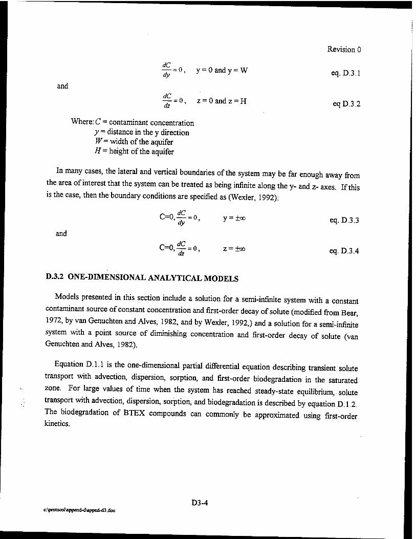
and
dy
dC
y = 0 and y = W
— = 0, z = 0andz = H dz
Revision 0
eq. D.3.1
eqD.3.2
Where: C = contaminant concentration y = distance in the y direction W= width of the aquifer H= height of the aquifer
In many cases, the lateral and vertical boundaries of the system may be far enough away from
the area of interest that the system can be treated as being infinite along the y- and z- axes. If this is the case, then the boundary conditions are specified as (Wexler, 1992):
and
dy
dz
y = ±oo
Z = ±QO
eq. D.3.3
eq. D.3.4
D.3.2 ONE-DIMENSIONAL ANALYTICAL MODELS
Models presented in this section include a solution for a semi-infinite system with a constant
contaminant source of constant concentration and first-order decay of solute (modified from Bear,
1972, by van Genuchten and Alves, 1982, and by Wexler, 1992,) and a solution for a semi-infinite
system with a point source of diminishing concentration and first-order decay of solute (van Genuchten and Alves, 1982).
Equation D. 1.1 is the one-dimensional partial differential equation describing transient solute
transport with advection, dispersion, sorption, and first-order biodegradation in the saturated
zone. For large values of time when the system has reached steady-state equilibrium, solute
transport with advection, dispersion, sorption, and biodegradation is described by equation D.1.2.
The biodegradation of BTEX compounds can commonly be approximated using first-order kinetics.
D3-4 c:\protocol\append-d\appnd-d3.doc
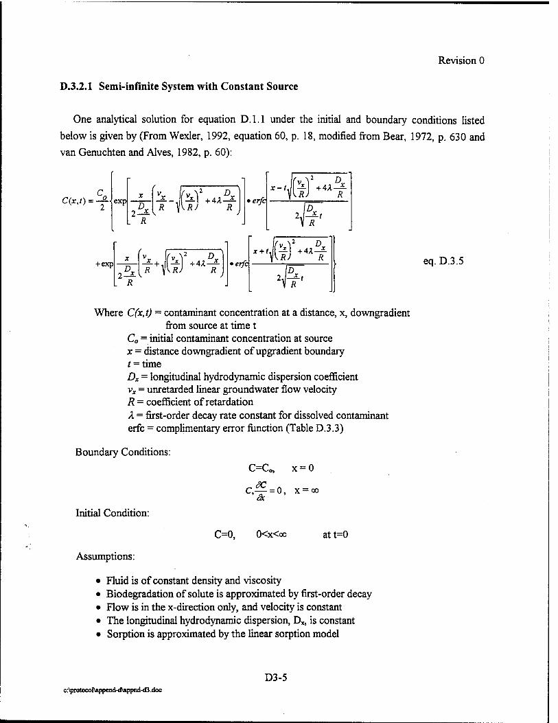
Revision 0
D.3.2.1 Semi-infinite System with Constant Source
One analytical solution for equation D.l.l under the initial and boundary conditions listed
below is given by (From Wexler, 1992, equation 60, p. 18, modified from Bear, 1972, p. 630 and
van Genuchten and Alves, 1982, p. 60):
CCO-^ exp
R
R \\RJ R lerfc
\(v v £> X-
■'\ h 1 +u X
R
1 D 2J -£-t V R
+exp 25L
R
R \\RJ R *erfc
x + t fe)-4 D x_ R
eq. D.3.5
Where C(x,t) = contaminant concentration at a distance, x, downgradient from source at time t
C0 = initial contaminant concentration at source x = distance downgradient of upgradient boundary t = time Dx = longitudinal hydrodynamic dispersion coefficient Vx = unretarded linear groundwater flow velocity R = coefficient of retardation X = first-order decay rate constant for dissolved contaminant erfc = complimentary error function (Table D.3.3)
Boundary Conditions:
Initial Condition:
Assumptions:
C=0,
C=Co, x = 0
C,^ = 0, x = oo ax.
0<x<oo at t=0
• Fluid is of constant density and viscosity • Biodegradation of solute is approximated by first-order decay • Flow is in the x-direction only, and velocity is constant • The longitudinal hydrodynamic dispersion, Dx, is constant • Sorption is approximated by the linear sorption model
D3-5 c:\protocol\append-dtappnd-d3.doc

Revision 0
Table D.3.3 Table of Error Functions
X erf(x) erfc(x) X erf(x) erfc(x) 0 0 1 1.1 0.880205 0.119795
0.05 0.056372 0.943628 1.2 0.910314 0.089686 0.1 0.112463 0.887537 1.3 0.934008 0.065992 0.15 0.167996 0.832004 1.4 0.952285 0.047715 0.2 0.222703 0.777297 1.5 0.966105 0.033895 0.25 0.276326 0.723674 1.6 0.976348 0.023652 0.3 0.328627 0.671373 1.7 0.983790 0.016210 0.35 0.379382 0.620618 1.8 0.989091 0.010909 0.4 0.428392 0.571608 1.9 0.992790 0.007210 0.45 0.475482 0.524518 2.0 0.995322 0.004678 0.5 0.520500 0.479500 2.1 0.997021 0.002979 0.55 0.563323 0.436677 2.2 0.998137 0.001863 0.6 0.603856 0.396144 2.3 0.998857 0.001143 0.65 0.642029 0.357971 2.4 0.999311 0.000689 0.7 0.677801 0.322199 2.5 0.999593 0.000407 0.75 0.711156 0.288844 2.6 0.999764 0.000236 0.8 0.742101 0.257899 2.7 0.999866 0.000134 0.85 0.770668 0.229332 2.8 0.999925 0.000075 0.9 0.796908 0.203092 2.9 0.999959 0.000041 0.95 0.820891 0.179109 3.0 0.999978 0.000022
1 0.842701 0.157299
erfc(x)=l-erf(x) erfc(-x)=l+erf(x) erf(-x)=-erf(x)
erf(x) = -2=\e-' du
c:\protocol\append-d\appnd-d3.doc D3-6

Revision 0
For steady-state conditions, solute transport is described by equation D.I.2 and the solution reduces to (Wexler, 1992, equation 62, p. 20):
C(x) = C0 exp 5L R
R
rvy KRJ R
eq. D.3.6
Example D.3.1:
Given the hydrauhc and contaminant transport parameters below plot the change in concentration through time at a location 30 m downgradient of the source using equation D.3.5. At what time does the concentration at this point reach steady-state equilibrium?
Solution: Hydrogeologie Data
Hydraulic conductivtiy K=(3.15)— diy
Hydraulic gradient I: =0.02-
Effective porosity ne=0.25
Total porosity n :=0.35
Longitudinal dispersivity ox*=30m
Initial Contaminant C„:=12-!5- Concentration
Retardation Coefficient Calculation
X=0.01 — dty
Contaminant Decay Rate
Soil sorption coefficient K x -19--
Parücle mass density (for quartz) p, =2.65
Bulk density
Organic carbon content
Retardation coefficient
Pb:=Pi<l-n) pb-1.722--1
=0.8-S
. Pb'Koc*foc R:=l+ R- 5.354
Groundwater Hydraulics Calculations
Groundwater velocity (pore-water) vx =— Vj-0.252-— Retarded Contaminant velocity v =— <tay
Longitudinal dispersion coefficient Dx'-=tx-ix Dx«7.56' diy
Change in Concentration with Time Calculation i =1- 1000 it=l<hy i. =A t-i x =30m
„ vc- 0.047"^- R c 4iy
— +4*— R/ R
1-erf 1-erf +4-X-
Px "I R '
C.-0J5. l ma
C200-'-303-^
C,„.. 1.455- ■=g
C^-l.494-^2-
C«» • 1.504-
CIMB-1.J0S,3. 1000 |Uer
"300 iju,
Plume reaches steady-state equilibrium after approximately 400 days
c:\protocol\append-d\appnd-d3 .doc
D3-7
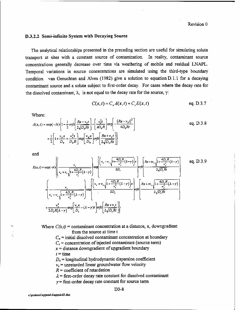
Revision 0
D.3.2.2 Semi-infinite System with Decaying Source
The analytical relationships presented in the preceding section are useful for simulating solute
transport at sites with a constant source of contamination. In reality, contaminant source
concentrations generally decrease over time via weathering of mobile and residual LNAPL.
Temporal variations in source concentrations are simulated using the third-type boundary
condition, van Genuchten and Alves (1982) give a solution to equation D. 1.1 for a decaying
contaminant source and a solute subject to first-order decay. For cases where the decay rate for
the dissolved contaminant, A,, is not equal to the decay rate for the source, y:
C(x,t) = CgA{x,t) + C,E(x,t) eq. D.3.7
Where:
A(x, t) = exp(-/U)< 1 - — erfc Rx-vJ
2JDJli vlt
exp
1 + —
2 1+-
vvx vtt
Dr DTR exp
DT
T£>XR
Rx + vj
{Rx-vjf_
erfc 2^DxRt
eq. D.3.8
and
£(*,/) = exp(-?*> I, 4D.R.. "
»»+w"J1+-^-(A-^ exp
[,-,,pM^ 2D,
erfc xx-»,y^-r)
2^DxRt
,, 4DSR,, v exp
v.+v.J1+^^(*-r)i*
2D,R{X-Y) exp
v x erfc
2D,
Rx+vt
erfc
I, 4D.R,, «
2jDRt
2jDxRt
eq. D.3.9
Where C(x,t) — contaminant concentration at a distance, x, downgradient from the source at time t
C0 = initial dissolved contaminant concentration at boundary C, = concentration of injected contaminant (source term) x = distance downgradient of upgradient boundary / = time Dx = longitudinal hydrodynamic dispersion coefficient vx = unretarded linear groundwater flow velocity R = coefficient of retardation A = first-order decay rate constant for dissolved contaminant y= first-order decay rate constant for source term
D3-8 c:\protocol\append-d\appnd-d3 .doc
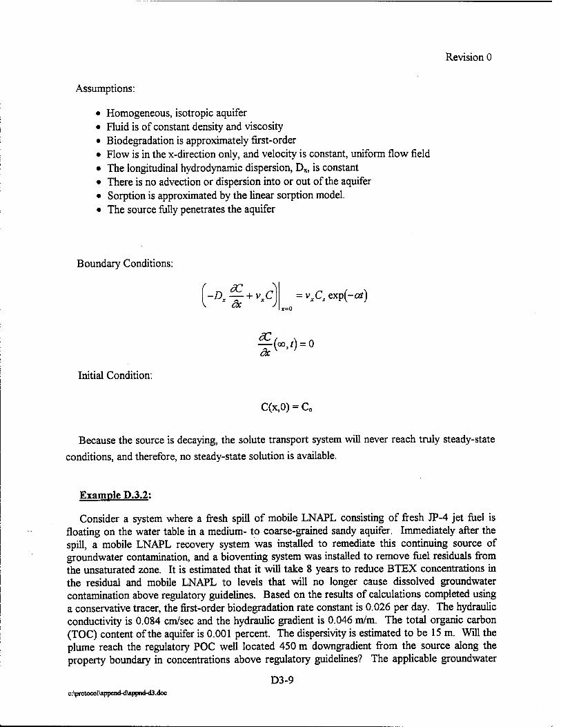
Revision 0
Assumptions:
Homogeneous, isotropic aquifer Fluid is of constant density and viscosity Biodegradation is approximately first-order Flow is in the x-direction only, and velocity is constant, uniform flow field The longitudinal hydrodynamic dispersion, Dx, is constant There is no advection or dispersion into or out of the aquifer Sorption is approximated by the linear sorption model. The source fully penetrates the aquifer
Boundary Conditions:
fr. N // + v, y
ac 1 J = vxCs exp(-otf) 1=0
§(„,,)=„ Initial Condition:
C(x,0) = C0
Because the source is decaying, the solute transport system will never reach truly steady-state
conditions, and therefore, no steady-state solution is available.
Example D.3.2:
Consider a system where a fresh spill of mobile LNAPL consisting of fresh JP-4 jet fuel is floating on the water table in a medium- to coarse-grained sandy aquifer. Immediately after the spill, a mobile LNAPL recovery system was installed to remediate this continuing source of groundwater contamination, and a bioventing system was installed to remove fuel residuals from the unsaturated zone. It is estimated that it will take 8 years to reduce BTEX concentrations in the residual and mobile LNAPL to levels that will no longer cause dissolved groundwater contamination above regulatory guidelines. Based on the results of calculations completed using a conservative tracer, the first-order biodegradation rate constant is 0.026 per day. The hydraulic conductivity is 0.084 cm/sec and the hydraulic gradient is 0.046 m/m. The total organic carbon (TOC) content of the aquifer is 0.001 percent. The dispersivity is estimated to be 15 m. Will the plume reach the regulatory POC well located 450 m downgradient from the source along the property boundary in concentrations above regulatory guidelines? The applicable groundwater
D3-9 c:\protocol\append-d\appnd-d3.doc
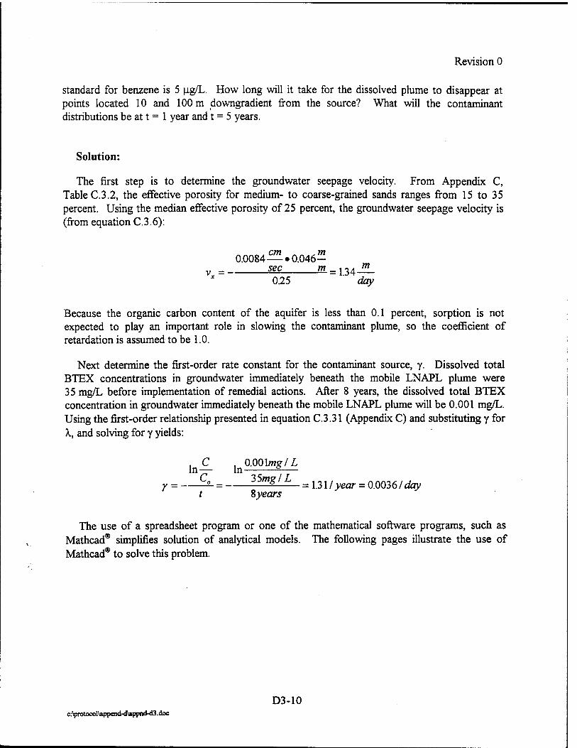
Revision 0
Standard for benzene is 5 ug/L. How long will it take for the dissolved plume to disappear at points located 10 and 100 m downgradient from the source? What will the contaminant distributions be at t = 1 year and t = 5 years.
Solution:
The first step is to determine the groundwater seepage velocity. From Appendix C, TableC.3.2, the effective porosity for medium- to coarse-grained sands ranges from 15 to 35 percent. Using the median effective porosity of 25 percent, the groundwater seepage velocity is (from equation C. 3.6):
0.0084—«0.046- = sec m = U4. *
025 day
Because the organic carbon content of the aquifer is less than 0.1 percent, sorption is not expected to play an important role in slowing the contaminant plume, so the coefficient of retardation is assumed to be 1.0.
Next determine the first-order rate constant for the contaminant source, y. Dissolved total BTEX concentrations in groundwater immediately beneath the mobile LNAPL plume were 35 mg/L before implementation of remedial actions. After 8 years, the dissolved total BTEX concentration in groundwater immediately beneath the mobile LNAPL plume will be 0.001 mg/L. Using the first-order relationship presented in equation C.3.31 (Appendix C) and substituting y for X, and solving for y yields:
ln£ ln00°^/L
Y = ^2- = 35/wg/Z, =zUljyear = 0.0036/ day t Syears
The use of a spreadsheet program or one of the mathematical software programs, such as Mathcad® simplifies solution of analytical models. The following pages illustrate the use of Mathcad® to solve this problem.
D3-10 c:\protocol\append-d\appnd-d3.doc
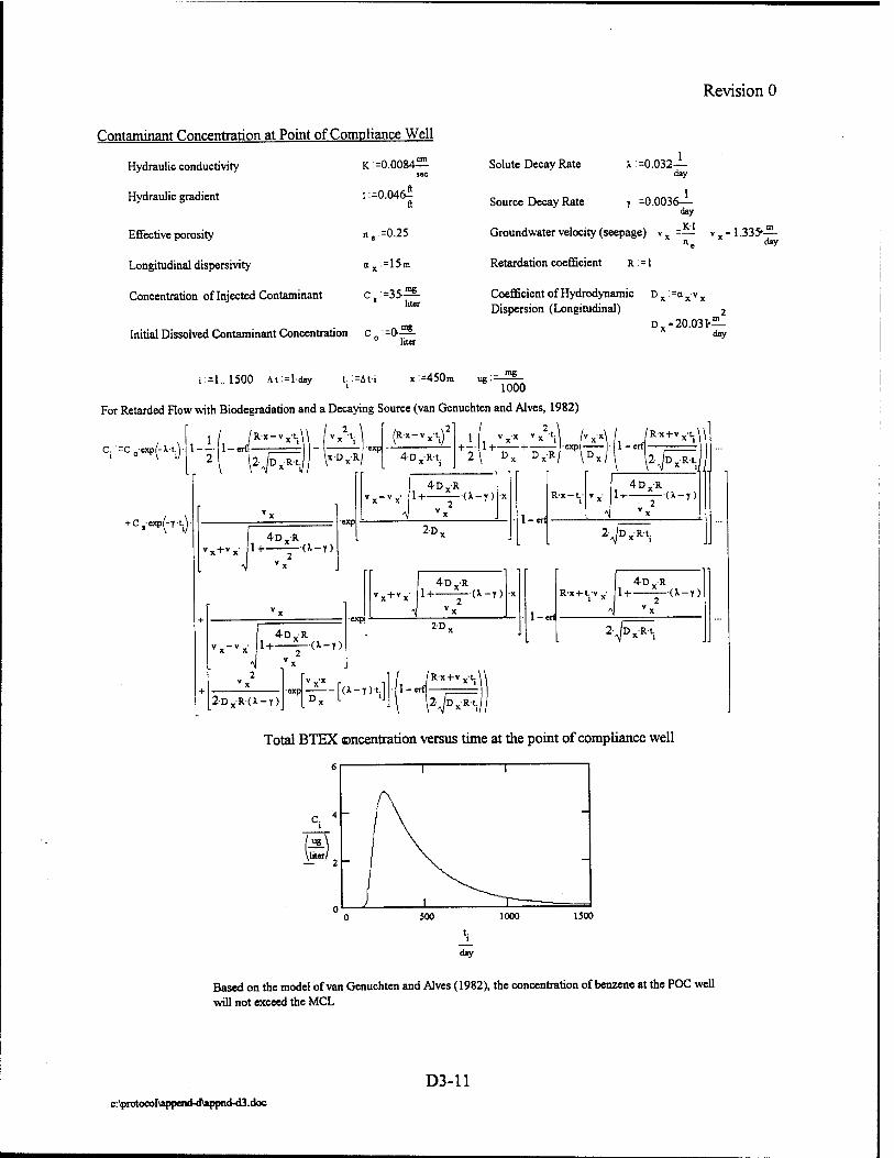
Revision 0
Contaminant Concentration at Point of Compliance Well
Hydraulic conductivity K: =0.0084^ sec
Hydraulic gradient I =0.046^ ft
Effective porosity ne =0.25
Longitudinal dispersivity a x =15m
Concentration of Injected Contaminant * liter
Initial Dissolved Contaminant Concentration c : =0-^ liter
Solute Decay Rate X =0.032-
Source Decay Rate
Groundwater velocity (seepage)
Retardation coefficient R :=1
day
T : =0.0036-1- day
K-I 1.335--
Coefficient of Hydrodynamic D x: =a xv x
Dispersion (Longitudinal) 2
D - 20.031-— x day
day
i :=1.. 1500 At:=lday t. :=it-i x:=450m ug: . mg
1000
For Retarded Flow with Biodegradation and a Decaying Source (van Genuchten and Alves, 1982)
C. =C -exp-M.
i-C.W-rt.
'■■fc R-t.
'vA \it'DvR
[R-x-v -t.\
4 D -R-t. +— 1H +
2 I D„ D.-R
/RX + V -t-W
».+", 1+- 4 D v R
-V--1)
■exp
4D,R -U-T)
2D, 1-eri
Rx-t.-
*\j x Ml 4 D X R
x- i+——-a-i)
J-^~RT.
4-D.-R i+—~a-D
exp
4-D -R 1+—^-a-r)
2DXR-(X-T) exp ^-[(X-T),]
2D,
/Rx+v -t.
1-eri
Rx-t-t.v, 4D -R
1+—~a-r)
!-^Px^i
• 1-
Total BTEX ©ncentration versus time at the point of compliance well
6
1500
t. l
day
Based on the model of van Genuchten and Alves (1982), the concentration of benzene at the POC well will not exceed the MCL
D3-11 c:\protocor\apperjd-d\appndHi3.doc

Revision 0
Contaminant Concentration versus Time at a Well Located 10 meters Downgradient of the Source Area
K:=0.0084^- 1=0.046- n==0.25 vx=— v =1.335-— ax:=15m Dx=axvx DX=20.031-— sec ft n day day
X : =0.032— T : =0.0036— day day
c.:=35 mg
liter C„:=0 -ni"8
liter R:=1
= 1.. 1700 At=lday t. =Ati x: = 10m ug:=- mg
1000
For Retarded Flow with Biodegradation and a Decaying Source (van Genuchten and Alves, 1982)
C.:=C0exp-Xt.
+ C.exp-Tt.
1-1 1- /R,X~V^ 2 12, W |"'DXR|
•exp (R-x-vx-t.)2
4D -Rt. +-■ 1+- , .,
2 Dx DXR D exp 1-erf
Rxtv ,1.
vx+vx- 1+- 4D,R
■■(X-y)
exp
4-DxR ■v8- l+-^-(l-T)
2D, 1-erf
Rx-t.
'■■f^il 4-D -R
lfi**\
4-DxR 1+ ^'(X-T)
2D -R-(I-J)
exp
4DXR t+v„- 1+ — (X-T)
exp vx*
D„ [<X-1>\] • 1-
2-D,
/R-x+v -t.
1-erf
Rx-t-t.vv
4DXR i+——-a-T)
•J^i
'•JÖx^
Concentration versus time at a point 10 m downgradient of the source
„4
2000
BTEX will not be detected in the well located 10 m from the mobile LNAPL source after approximately 1650 days (4.5 years)
D3-12 c:\protocol\append-d\appnd-d3 .doc
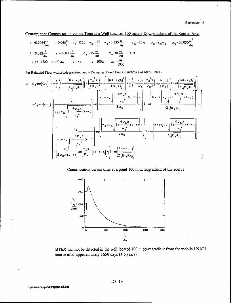
Revision 0
Contaminant Concentration versus Time at a Well Located 100 meters Downgradient of the Source Area 2
K : =0.0084^2. i: =0.046- n ,:=0.25 .K-I v =1.335-— ax: = 15m Dx:=a -vY D = 20.031-— * day" x x x x ^
X =0.032— T :=0.003<si- Cs=35^ c.:=fta R:=1 day day liter liter
= 1.. 1700 At: = lday t. :=At-i :=100 m ug • . mg
1000
For Retarded Flow with Biodegradation and a Decaying Source (van Genuchten and Alves, 1982)
<V=C0exp(-U.y !_I LJ^U^,«-
+ C5exp(-Tt.)-
\2'JW// ^ (R-X-V^t;1
4D -Rt. x I
-1—1+ H -expl 2 Dx DXR
4DXR vx+vx p+——-a-T)
exp
4DX-R vx~vx M+—r-(*-T)
2D, 1-erf
Rx-t.
\lf>*** 4DVR
v ■ 1-t-- ■■a-T)
'JDxR'i
4D -R i+—~a-T)
2DXR(X-T)
exp
4-D _R
exp K-["-''-J
2D,
/R-x+v -t.
1-erf
Rx-K.v ■ 1 x
4D -R 1+ ^-(X-T)
vx
:■^/w
^ 2- D.-R-t.
Concentration versus time at a point 100 m downgradient of the source
4000
3000
liter«
2000 ~
1000
2000
BTEX will not be detected in the well located 100 m downgradient from the mobile LNAPL source after approximately 1650 days (4.5 years)
D3-13 c:\protocol\append-d\appnd-d3.doc
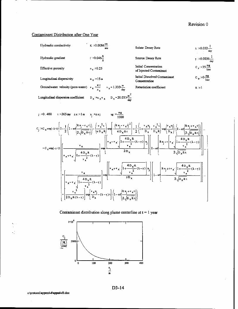
Revision 0
Contaminant Distribution after One Year
Hydraulic conductivtiy K: =0.0084
Hydraulic gradient I: =0.046- ft
Effective porosity ne:=0.25
Longitudinal dispersivity a,: = 15n
K-I Groundwater velocity (pore-water) v x: =— v x - 1.335*- day
Solute Decay Rate
Source Decay Rate
Initial Concentration of Injected Contaminant
Initial Dissolved Contaminant Concentration
Retardation coefficient
X : ^.032- day
=0.0036- day
CS:=35ÜÜ s liter
C„:=0
R:=l
nig
liter
Longitudinal dispersion coefficient Dx:=ax'vx D x - 20.031*—
day
j:=0.400 t:=365day 4x:=lm x. :=Äxj ug- . mg
1000
a:=c0exp(-xt)- 1 /Rx.-v -t 1__. M_erri J— 21 Vfc
exp f'V,x't) 1 I, vxxj vx't| /vx-x\ / /R-Xs + v.-t
1 + H -exp i ■ 1 - 2 Dx D_-Rl D
+ Csexp(-rt)-
4DXR vx+vx \l+ —-tt-r)
exp
4DXR vx-vx i+——-a-T)
2D, 1-erl
Rx. -1- J
\*fi** 4D R
*x 1+ r(X-T)
2-^ Rt
4DXR K~
VX !+ —-(^-T)
2D_R(X-T)
exp
4DXR vx+vx l+——'(*-r)
v xx. •exp(—i-(X-T)-t
2DV
K-x.+v vt |1_-J -J-
1-erl
4D^R
2 Rx.+tvx- 1+ i-(X-T)
2-,/D~R~t
*fi**
Contaminant distribution along plume centerline at t = 1 year
1M04
c. J
kliter/
400
c:\protocol\append-d\appnd-d3.doc
D3-14
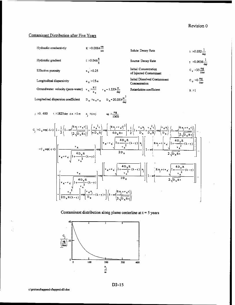
Contaminant Distribution after Five Years
Revision 0
Hydraulic conductivtiy K: =0.0084- Solute Decay Rate k : ^.032-
day
Hydraulic gradient
Effective porosity
Longitudinal dispersivity
I =0.046-
n,:=0.25
ox :=15m
Source Decay Rate
Initial Concentration of Injected Contaminant
Initial Dissolved Contaminant Concentration
Groundwater velocity (pore-water) v : =— v - 1.335-— Retardation coefficient
=0.0036-
Cs:=35üü 5 liter
day
C„:=0
R:=l
rag
liter
Longitudinal dispersion coefficient D x: =a xv x D x - 20.031' day
j.=0.400 t: = 1825day Ax: = lm x. =Axj ug=-^5- J 1000
C. :=C0exp(-Xt)
+ Csexp(-Tt)-
1 1--- 1-
2 \ l2>/5~£
Rx. -v -t\ \ / v "t
7iDvR/ exp
fV'x') 4DvRt
Mi Vx'xj V*M rx'x* H—■ IH in -exp 2 °x DXR <
/ /R-X.+V l-erff- '
4DXR vx + vx i+—j-a-r)
exp *
4D R vx~vx 1+ —(X-T)
<J vx 2D,
1-erf
Rx-t J
\2^D~Rt
4-D R
^ DvRt
4DXR vx-vx 1+ ;-(x-T)
2-DxR(x-r)
exp
4DXR rx + vx 1+ ^-(X-T)
exp)—---tt-y)-t
2D,
/R-x. + v„-t\ |1 r/ J
1-eri
Rx. [j+fvx- 1+ —(X-T)
2VD~Rt
2>P**V
Contaminant distribution along plume centerline at t = 5 years
X. J
400
c:\protocol\append-d\appnd-d3.doc D3-15

Revision 0
D.3.3 TWO-DIMENSIONAL ANALYTICAL MODELS
The model presented in this section is for a semi-infinite system with a constant source of
constant concentration and first-order decay of solute (Wilson and Miller, 1978).
Equation D.I.3 is the two-dimensional partial differential equation describing transient solute
transport with advection, dispersion, sorption, and first-order biodegradation in the saturated
zone. For large values of time when the system has reached steady-state equilibrium, solute
transport with advection, dispersion, sorption, and biodegradation is described by equation D.1.4
The biodegradation of BTEX compounds can commonly be approximated using first-order
kinetics.
D.3.3.1 Continuous Source
Wilson and Miller (1978) give the following solution to equation D.I.3 (Bedient et al, 1994,
p. 136, eq. 6.27)
C(x,v,0 = eq.D.3.10 AmepxDy V 'BJ
Where: fm = continuous rate of contaminant injection per vertical unit aquifer [M/LT]
, >,BÄ y=\+2
Vx
u,—}= Hantush Well Function BJ
r2
u = - AyDxt
r = ' , . DJ> X +■
I D, J
B = 2^ Vx
Wilson and Miller (1978) give an approximate solution to the Hantush well function. This
relationship is:
D3-16 c:\protocol\append-d\appnd-d3.doc
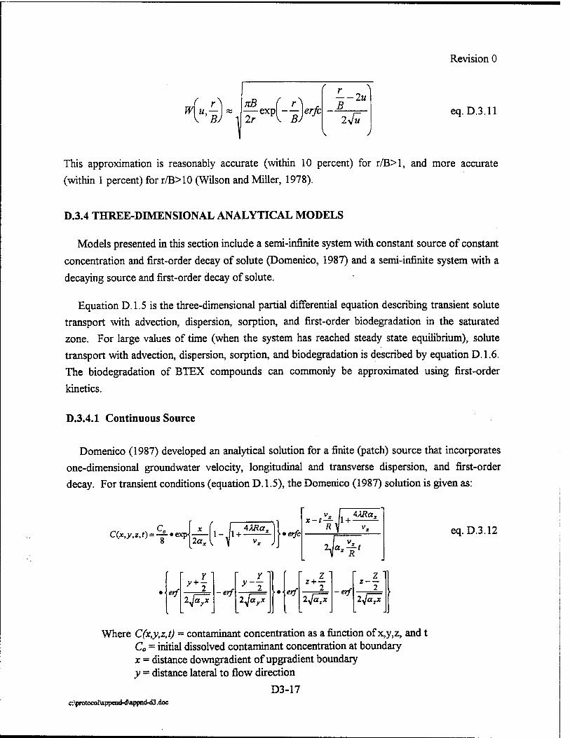
Revision 0
f
\^V[-L]erfc B — 2u
2yfÜ \
eq.D.3.11
This approximation is reasonably accurate (within 10 percent) for r/B>l, and more accurate
(within 1 percent) for r/B>10 (Wilson and Miller, 1978).
D.3.4 THREE-DIMENSIONAL ANALYTICAL MODELS
Models presented in this section include a semi-infinite system with constant source of constant
concentration and first-order decay of solute (Domenico, 1987) and a semi-infinite system with a
decaying source and first-order decay of solute.
Equation D.1.5 is the three-dimensional partial differential equation describing transient solute
transport with advection, dispersion, sorption, and first-order biodegradation in the saturated
zone. For large values of time (when the system has reached steady state equilibrium), solute
transport with advection, dispersion, sorption, and biodegradation is described by equation D.1.6.
The biodegradation of BTEX compounds can commonly be approximated using first-order
kinetics.
D.3.4.1 Continuous Source
Domenico (1987) developed an analytical solution for a finite (patch) source that incorporates
one-dimensional groundwater velocity, longitudinal and transverse dispersion, and first-order
decay. For transient conditions (equation D.1.5), the Domenico (1987) solution is given as:
^4'4('-ff) erfc
vx 1 4Max
2f»*' eq.D.3.12
erf y + -
2jayx -erf
y~l ayx I
erf
Z z + —
2 2^
-erf
Z z
2 2Jarx
Where C(x,y,z,t) = contaminant concentration as a function of x,y,z, and t C0 = initial dissolved contaminant concentration at boundary x = distance downgradient of upgradient boundary v = distance lateral to flow direction
D3-17 c:\protocol\append-d\appnd-d3 .doc
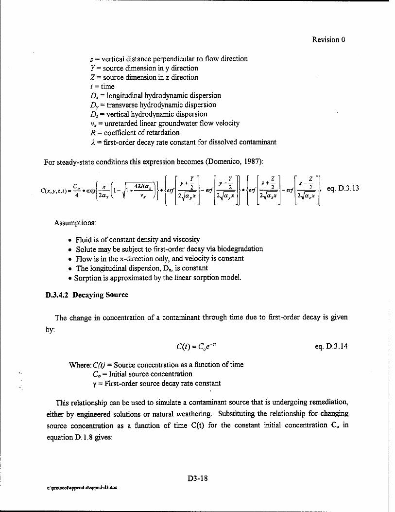
Revision 0
z = vertical distance perpendicular to flow direction Y = source dimension in y direction Z = source dimension in z direction / = time Dx = longitudinal hydrodynamic dispersion Dy = transverse hydrodynamic dispersion Dz = vertical hydrodynamic dispersion vx = unretarded linear groundwater flow velocity R = coefficient of retardation X = first-order decay rate constant for dissolved contaminant
For steady-state conditions this expression becomes (Domenico, 1987):
C(W,0 = 7-exp — 1-.1 + 4ARar erf
y + -
2-ft^x ■erf
y—2
ifiyX erf
z + -
2^/^T -erf
z--
2A/Ö^"
eq.D.3.13
Assumptions:
• Fluid is of constant density and viscosity • Solute may be subject to first-order decay via biodegradation • Flow is in the x-direction only, and velocity is constant • The longitudinal dispersion, Dx, is constant • Sorption is approximated by the linear sorption model.
D.3.4.2 Decaying Source
The change in concentration of a contaminant through time due to first-order decay is given
by:
Cit) = Cjf*
Where: C(t) = Source concentration as a function of time Co = Initial source concentration y = First-order source decay rate constant
eq.D.3.14
This relationship can be used to simulate a contaminant source that is undergoing remediation, either by engineered solutions or natural weathering. Substituting the relationship for changing source concentration as a function of time C(t) for the constant initial concentration C0 in
equation D. 1.8 gives:
D3-18 c:\protocol\appcnd-d\appnd-d3.doc

Revision 0
C0e-* x C(W.*)—y—«d — 1-,1 +
AÄRar >erfc
vx AXRaz
T*Vf
erf
Y ' y+2 -erf
Y ' y~2
2jayx ... erf
z " z + —
2
2^ -erf
z T z 2
2^x „ J L J L L J L JJ
eq.D.3.15
Where C(x,y,z,t) = contaminant concentration as a function of x, y, z, and t C0 = initial dissolved contaminant concentration at boundary x = distance downgradient of upgradient boundary y = distance lateral to flow direction z = vertical distance perpendicular to flow direction Y= source dimension in y direction Z = source dimension in z direction t = time Dx = longitudinal hydrodynamic dispersion Dy = transverse hydrodynamic dispersion Dz = vertical hydrodynamic dispersion vx - unretarded linear groundwater flow velocity R = coefficient of retardation Y = first-order decay rate constant for contaminant source X = first-order decay rate constant for dissolved contaminant
Assumptions:
• Fluid is of constant density and viscosity • Solute may be subject to first-order decay via biodegradation • Source may be subject to first-order decay via weathering or engineered remediation • Flow is in the x-direction only, and velocity is constant • The longitudinal dispersion, Dx, is constant • Sorption is approximated by the linear sorption model.
D3-19 c:\prrtocol\append-d\appnd-d3 .doc

Revision 0
SECTION D-4
NUMERICAL MODELS
D.4.1 OVERVIEW OF NUMERICAL MODELS
Numerical models provide inexact and, in some cases, nonunique solutions to the governing advection-dispersion equations presented in Section D-l. As with analytical models, the use of numerical models requires the user to make some simplifying assumptions about the solute transport system. However, fewer simplifying assumptions must be made, so numerical models can simulate more complex systems. For this reason, numerical model codes can be used to simulate complex hydrogeologic systems or contaminant transport affected by complex sets of reactions. Heterogeneous and anisotropic hydrologic systems can be modeled using numerical models, as can transient systems (i.e., systems in which stresses, parameters, or boundary conditions change over time). Another advantage of numerical models is that most codes are capable of simulating contaminant sources that vary over time, allowing simulation of scenarios including source reduction through weathering or through engineered solutions. Appendix C discusses methods that can be used to quantify source removal rates.
D.4.2 APPLICABLE MODEL CODES
Numerical model codes used for the evaluation of natural attenuation processes in groundwater should be capable of simulating advection, dispersion, sorption, and biodegradation (or any first-order decay process). Several codes are available that can be applied to the evaluation of contaminant fate and transport under the influence of these processes. At least four codes are designed specifically for the simulation of reactant-limited solute transport influenced by biodegradation. These include: Bioplume n, Bioplume HI, BioTrans®, and BiolD®. Other codes that are available can be used to evaluate contaminant transport with biodegradation, but biodegradation reaction rates are controlled by a first-order rate constant, rather than by the availability of the reactants. This is not a thorough review of available codes; rather, this
D4-1 c:\protocol\append-d\appnd-d4.doc
Revision 0
overview is to illustrate the variety of available codes that may be useful in evaluating the natural attenuation of contaminants dissolved in groundwater. The selection of a code will ultimately depend upon the user's needs, the available data, the sophistication of the desired predictions and the limitations of the available model codes.
D.4.2.1 BioplumeH
The Bioplume II model is based upon the US Geological Survey (USGS) two-dimensional (2- D) groundwater flow and solute transport model [method of characteristics (MOC) model] modified to include an oxygen-limited biodegradation component that is controlled by a superimposed plume of dissolved oxygen (Konikow and Bredehoeft, 1978; Rifai et al, 1988). This code also computes concentration changes (for a single species) over time due to advection, dispersion, and sorption. Bioplume II solves the USGS 2-D solute transport equation twice, once
for hydrocarbon concentrations in the aquifer and once for a dissolved oxygen plume. The two plumes are combined using superposition at every particle move to simulate the biological reaction between hydrocarbons and oxygen. The model incorporates modified Monod kinetics to simulate the degradation of hydrocarbon compounds and assumes that the hydrocarbons are directly mineralized to carbon dioxide and water through an instantaneous reaction. Anaerobic decay can be simulated using a first-order rate constant, and sources of contaminants or oxygen can be simulated using injection wells or specified-concentration cells. If properly used, the Bioplume II model can present a very conservative estimate of the amount of biodegradation
occurring in the subsurface.
D.4.2.2 Bioplume m
Bioplume II is being modified and extended to allow simulation of biodegradation dependent on multiple electron acceptors. The resulting code will be called Bioplume in. This model is being developed by researchers from Rice University and, like the Bioplume II model, will be based upon the USGS two-dimensional (2-D) groundwater flow and solute transport model [method of characteristics (MOC) model]. Bioplume IE will allow simulation of first-order biodegradation, instantaneous reactions between electron acceptors [dissolved oxygen, nitrate, iron (HI), sulfate, and carbon dioxide) and the dissolved contaminant plume, and Monod kinetics. This model is currently undergoing Beta testing and verification, and should be available by the
end of 1995.
D4-2 c:\protocol\append-d\appnd-d4.doc
Revision 0
D.4.2.3 BioTrans®
BioTrans® is a proprietary solute transport code developed and distributed by Environmental
Systems and Technologies, Inc. This code can simulate 2-D dissolved transport and oxygen- limited decay of up to five separate chemical species in fractured or porous aquifers. Fate and
transport calculations can incorporate the effects of advection, dispersion, sorption, and volatilization. Anaerobic biodegradation can be simulated using a first-order rate constant.
Contaminant source loading rates can be defined as in Bioplume n, or BioTrans® can compute a time-dependent source rate due to dissolution of LNAPL. This code does not include a routine for simulation of a groundwater flow system. Instead, groundwater velocity data can be imported
from other models using a preprocessor.
D.4.2.4 BiolD®
Bio ID®, a proprietary code developed by GeoTrans, Inc., is a one-dimensional, finite- difference code for simulation of reactive solute transport. This code is capable of simulating aerobic and anaerobic biodegradation and sorption. Compared to other numerical modeling codes, BiolD® is relatively simple and only offers a few advantages relative to the analytical codes presented in Section D-3. BiolD® is relatively sophisticated in its ability to simulate substrate- limited biodegradation using different kinetic relations and to simulate sorption under different equilibrium conditions. However, like the analytical models in Section D-3, the code can only simulate conditions in homogeneous steady-state systems, and has the same limitations with respect to source terms. BiolD® would be most useful for modeling simple systems in which a more rigorous evaluation of the effects of biodegradation and/or sorption is desired. This code also would be useful for estimation of parameters to be used in a more sophisticate solute
transport model.
D.4.2.5 Other Codes
Several other codes can simulate solute transport under the influence of advection dispersion, and biodegradation. In these codes, biodegradation can be represented only by a first-order decay constant. However, these codes may be useful in many different situations, depending on the user's needs and the available data, or if a groundwater flow model of the site already has
been completed.
D4-3 c:\protocol\append-d\appnd-d4.doc

Revision 0
MT3D® is a three-dimensional (3D) transport model that can be linked to any block-centered
finite-difference flow model (e.g., a model created using the USGS MODFLOW code). This code can simulate advection, dispersion, sorption, and biodegradation (using a first-order decay constant), with source terms specified by the user. This code could be used where a 3D simulation is needed, or where a flow model has previously been constructed and calibrated.
MT3D® is a proprietary code developed by S.S Papadopulos and Associates.
FLOTRANS® is another proprietary code, developed by Waterloo Hydrogeologie Software.
FLOTRANS® is a 2D code that can simulate steady-state groundwater flow in complex and heterogeneous systems and can simulate transient solute transport in that steady-state flow field. This code can simulate advection, dispersion, sorption, and biodegradation (using a first-order decay coefficient). FLOTRANS® utilizes an interactive graphical interface format, simplifying data input and model output display. FTWORK®, another code developed by GeoTrans, Inc., is a finite-difference code for simulation of complex groundwater flow systems, as well as single- species transport under the influence of advection, dispersion , sorption, and first-order decay. This code also contains a parameter estimation option to assist in calibration of the flow model.
A public-domain code that may be useful is RANDOM WALK. RANDOM WALK is a 2D groundwater flow and solute transport code developed by workers at the Illinois State Water Survey. Groundwater flow solutions may be analytical or numerical (finite difference). Solute transport simulation is achieved through the use of a particle-tracking routine. With respect to solute transport options, this code offers options similar to most of the other codes discussed above, except that wider variety of source-term options are available.
D4-4 c:\protocol\append-d\appnd-d4.doc
Copyright © 2022 FDOKUMEN