Mathematical and Computer Modelling 50 (2009) 1177–1187

Contents lists available at ScienceDirect

Mathematical and Computer Modelling

journal homepage: www.elsevier.com/locate/mcm

Adaptive stochastic numerical scheme in parallel random walk modelsfor transport problems in shallow waterW.M. Charles a,∗, E. van den Berg b,1, H.X. Lin b,1, A.W. Heemink b,1a University of Dar-es-salaam, Faculty of Science, Department of Mathematics, P.O. Box 35062, Dar-es-salaam, Tanzaniab Delft University of Technology, Faculty of Electrical Engineering, Mathematics and Computer Science, Department of Applied Mathematical Analysis, Mekelweg4, 2628 CD Delft, The Netherlands

a r t i c l e i n f o

Article history:Received 21 May 2008Received in revised form 23 April 2009Accepted 26 May 2009

Keywords:Wiener processesStochastic differential equationRandom walk modelVariable step sizeParallel processingSpeed upEfficiency

a b s t r a c t

This paper deals with the simulation of transport of pollutants in shallow water usingrandom walk models and develops several computation techniques to speed up thenumerical integration of the stochastic differential equations (SDEs). This is achieved byusing both random time stepping and parallel processing.We start by considering a basic stochastic Euler scheme for integration of the diffusion

and drift terms of the SDEs, with a strong order 1 in the strong sense. The errors due tothis scheme depend on the location of the pollutant; it is dominated by the diffusion termnear boundaries, and by the deterministic drift further away from the boundaries. Using apair of integration schemes, one of strong order 1.5 near the boundary and one of strongorder 2.0 elsewhere, we can estimate the error and approximate an optimal step size for agiven error tolerance. The resulting algorithm is developed such that it allows for completeflexibility of the step size, while guaranteeing the correct Brownian behaviour.Modelling pollutants by non-interacting particles enables the use of parallel processing

in the simulation. We take advantage of this by implementing the algorithm using theMPI library. The inherent asynchronic nature of the particle simulation, in addition tothe parallel processing, makes it difficult to get a coherent picture of the results atany given points. However, by inserting internal synchronisation points in the temporaldiscretisation, the code allows pollution snapshots and particle counts to be made at timesspecified by the user.

© 2009 Elsevier Ltd. All rights reserved.

1. Introduction

Environmental management of water areas needs a clear knowledge of the consequences of, e.g., ship accidents and bothsolid and liquid waste disposal. Therefore, a good environmental control systemmust allow for the possibility of accuratelypredicting the dispersion of pollutants if such scenarios arise. Pollutant dispersion is quite often described by thewell-knownadvection–diffusion equations. These partial differential equations are deterministic in nature [1,2]. This Eulerian approachconsiders the movement of a group of particles by describing what happens at a fixed region in space. Another approach,which describes the dispersion processes, is called the Lagrangian approach and tracks themovement of individual pollutantparticles as they move through space in time. The Lagrangian approach is stochastic in nature and is often called a particlemodel.

∗ Corresponding author. Tel.: +255 222410388.E-mail addresses:maheraii@yahoo.com, cwmahera@maths.udsm.ac.tz (W.M. Charles), vandenberg_ewout@yahoo.co.uk (E. van den Berg),

haix_lin@yahoo.com (H.X. Lin), A.W.Heemink@ewi.tudelft.nl (A.W. Heemink).1 Tel.: +31 15 2787228; fax: +31 15 2787295.

0895-7177/$ – see front matter© 2009 Elsevier Ltd. All rights reserved.doi:10.1016/j.mcm.2009.05.034

1178 W.M. Charles et al. / Mathematical and Computer Modelling 50 (2009) 1177–1187

The advantage of the Lagrangian approach over the Eulerian ones is that it models well the steep concentration gradientfor particles that are independent of one another.Moreover, unlike in the Eulerian approach, particle tracking is independentof the domain, and the concentration can not be negative [3–5]. However, when domain is large, a large number of particleis required to accurately predict the dispersion of the concentration of pollutants. This implies that particle models requiremore efficient integration schemes.Thework in this article aims for the design and implementing of amore accurate and efficient scheme used in the particle

model. It was noted by Stijnen et al. [6] that the simulation of pollutant transport in shallow waters using random walkmodels requires small step sizes to stably integrate in highly irregular areas. Traditional random walk models are based onfixed step size implementation of numerical methods and are thus forced to choose a small step size throughout. This isunnecessary in regular areas where the integration error is very small and larger time steps can be used. In such situations,the use of adaptive numerical schemes is more appropriate.In their work Gaines and Lyons [7] and Burrage and Burrage [8] introduced a variable time stepping procedure for the

pathwise (strong) numerical integration of a system of stochastic differential equations. In this paper we extend the workfrom [9], and use pairs of adaptive schemes to determine appropriate step sizes. Each pair consists of a lower and higherorder scheme and, by evaluating the performance of each scheme, it is possible to decide whether higher order schemes, orsmall step sizes are needed.For the numerical integration of the pollutant transport models we use an explicit order 1 strong scheme. The

displacement of a pollutant particle is due to drift and diffusion terms. Depending on the location of a particle, the errorfrom the first order scheme arises predominantly from either the drift or diffusion term. Near boundaries it is the diffusionterm that dominates and we pair up the first order scheme with an explicit order 1.5 strong scheme. Further away from theboundary, the drift term becomes dominant and the 1.5 order scheme becomes order 1 strong. Consequently, it is necessaryto concentrate on the drift term leading us to derive an explicit order 2 strong scheme that concentrates on this drift errorwhile approximating the diffusion term using a linear stochastic differential equation with additive noise.Outside particle models, the concept of adaptive schemes by mesh refining in Eulerian methods has been used in [10].

Unlike these methods, random walk models do not suffer from numerical diffusion in the source points [5,4], however,they do potentially require large numbers of particles [11]. Fortunately, since particles are simulated independent from oneanother, parallel processing techniques can be applied naturally. This approach was used to speed up the implementationof the model discussed in this paper.This remainder of this paper is organised as follows. Section 2 discusses the set of stochastic differential equations

governing the transport of pollutants in shallowwater. The concept of the higher order strong adaptive schemes for transportproblems in shallow water as well their implementation is discussed in Section 3. The procedure for determining thevariable step sizes is described in Section 3.4. The parallel implementation of the adaptive scheme is given in Section 4and experimental results and concluding remarks appear in Sections 5.1 and 6.

2. The random walk model for pollution transport

Randomwalk models describe the behaviour of a large number of particles, each representing a part of the total mass ofpollutant [12,1,13,14]. In such particle models, pollution is described by a set of particles and the position of individualparticles is described by means of stochastic differential equations (SDEs). In particular, the three-dimensional particleposition at time t by Pt = [Xt , Yt , Zt ], is given by the (Îto) stochastic differential equation [15–17]

dP = f (t, P)dt + σ(t, P)dW (t), t ≥ 0,

where f (t, P)dt is a vector-valued drift term, σ(t, P) is a matrix function, and dW (t) represents the Brownian motionprocess. The movement of individual particles is subject to a deterministic part, mainly given by the flow field; anda stochastic part, which represents the turbulence in the fluid, and is modelled by the diffusion part of the stochasticdifferential equations [5]. Using the particle positions, a probability density function, which is related to the ensemblemeanconcentration, can be approximated [1,14,18].The particle model derived in this paper is a vertically integrated model, which integrates over depth and results in a

two-dimensional model:

dXtItô=

[U(x, y)+

DXX (x, y)H(x, y)

(∂H(x, y)∂x

)+∂DXX (x, y)

∂x

]dt +

√2DXX (x, y)dW x

dYtItô=

[V (x, y)+

DYY (x, y)H(x, y)

(∂H(x, y)∂y

)+∂DYY (x, y)

∂y

]dt +

√2DYY (x, y)dW y.

(1)

Here, (Xt , Yt) is the position of a particle, which is assumed to be a Markov process,W x(t) andW y(t) are Gaussian–Wienerprocesses [11], (U(x, y), V (x, y))T are flow velocities, and H(x, y) is the total water depth. The latter two quantities,flow velocity and water depth, are assumed to be inputs to the model. In our case they are computed over a fixed gridusing a hydrodynamic model known as WAQUA [19], and extended to the entire domain by using (linear) interpolationtechniques.

W.M. Charles et al. / Mathematical and Computer Modelling 50 (2009) 1177–1187 1179

The two-dimensional random walk model Eq. (1) were developed by Heemink [5] and shown to be consistent withthe two-dimensional advection–diffusion equation by deriving the Fokker–Planck equations. In this article we modify thismodel by using a different dispersion coefficient function to model pollutants dispersion in shallow waters. In addition,we design the horizontal dispersion coefficient functions DXX (x, y), and DYY (x, y) in the x and y direction respectively. Weassume that DXY (x, y) = DYX (x, y) = 0 in the dispersion tensor and that

DXX (x, y) =D11

1+ e−(((x−xb)2+(y−yb)2)−K2)

{1+

([1+ eK

2] cos(α)− 1

)e−((x−xb)

2+(y−yb)2)

}(2)

DYY (x, y) =D22

1+ e−(((x−xb)2+(y−yb)2)−K2)

{1+

([1+ eK

2] sin(α)− 1

)e−((x−xb)

2+(y−yb)2)

}, (3)

where D11 and D22 are the horizontal dispersion parameters, (xb, yb) is intersection point on the boundary between theline from (x, y) perpendicular to the boundary, K ≥ 0 is a parameter modelling the decrease of diffusion coefficientnear the boundary and α is the assumed to be the angle between the boundary, and x or y direction. Furthermore wehave

eT1c = ‖e1‖‖c‖ cos(α), sin(α) =|c2|√c21 + c

22

,

with ek the kth column of the identity matrix. Finally, c = (c1, c2)T is a direction vector along the side of a given boundary

cell.In this article the diffusion functions are designed in such a way that DXX (x, y) and DYY (x, y) model the dispersion as

realistically as possible. This means, for instance, that the dispersion decreases near the boundary and that no particle willcross a physical boundary. By setting DXY = DYX = 0 we assume for simplicity that the dispersion tensor is an ellipsoidwith main axes in the x and y direction only. This assumption is not essential to the derivation and it would not be hard toincorporate nonzero coefficients [20].

3. Adaptive scheme with higher order strong for pollution transport

In this paper we make use of strong convergence of pairs of numerical schemes to approximate the error of the schemeat each step. To achieve this, we have developed three numerical schemes for transport of pollutant in shallow waters: oneexplicit order 1 strong scheme, discussed in Section 3.1, and two higher order schemes, formulated in Sections 3.2 and 3.3.These higher order strong numerical schemes avoid the use of derivatives of the drift and diffusion terms and are of order1.5 strong and 2.0 strong, respectively [21]. We only give a brief overview of the schemes; an interested reader is referredto [21,11]. Based on the error information at each step the optimal time step size for adaptive schemes is determined, asexplained in Section 3.4.

3.1. An explicit order 1 strong scheme

The explicit order 1 scheme for transport of pollutants in shallow waters is as follows:

Xn+1Itô= Xn +

[U(x, y)+

DXX (Xn, Yn)H(x, y)

∂H(x, y)∂x

+∂DXX (Xn, Yn)

∂x

]1tn

+(1W xn )

2−1tn

2√1tn

[√2DXX (X∗+1n+1 , Y

∗+1n+1 )−

√2DXX (Xn, Yn)

]+

√2DXX (Xn, Yn)1W xn , (4)

where W xn = W x(tn), 1W xn = W xn+1 − Wxn is an independent increment of a Wiener process for the time interval

[tn, tn+1], n = 0, 1, . . . . The expression for Yn+1 is similar to the above equation, with Xn in the first right hand side termreplaced by Yn, all DXX (·, ·) terms substituted by DYY (·, ·) and the superscripts x modified to y. We further have supportvector

X∗+1n+1 = Xn + a1(Xn, Yn)1tn +

√2DXX (Xn, Yn)1tn.

and similarly for Y ∗+1n+1 along y direction. The drift along the x direction is given by

a1(Xn, Yn) =[U(x, y)+

DXX (Xn, Yn)H(x, y)

(∂H(x, y)∂x

)+∂DXX (Xn, Yn)

∂x

], (5)

and along the y direction we have, likewise

a2(Xn, Yn) =[V (x, y)+

DYY (Xn, Yn)H(x, y)

(∂H(x, y)∂y

)+∂DYY (Xn, Yn)

∂y

]. (6)

1180 W.M. Charles et al. / Mathematical and Computer Modelling 50 (2009) 1177–1187

3.2. An explicit order 1.5 strong scheme

Besides the explicit order 1 strong scheme we also derived an order 1.5 scheme (see [21]) which avoids evaluatingderivatives of the drift and diffusion terms:

Xn+1Itô= Xn +

{a1+n (X

∗+zn+1 , Y

∗+zn+1 )− a

1−n (X

∗−zn+1 , Y

∗−zn+1 )

}×1tn4

(Rxn,1 +

1√3Rxn,2

)+1tn4

{a1+n (X

∗+zn+1 , Y

∗+zn+1 )+ a

1−n (X

∗−zn+1 , Y

∗−zn+1 )

}+

√2DXX (Xn, Yn)1W xn

+1

4√1t

{√2DXX (X∗+zn+1 , Y

∗+zn+1 )−

√2DXX (X∗−zn+1 , Y

∗−zn+1 )

}[(1W xn )

2−1tn]

+

{√2DXX (X∗+zn+1 , Y

∗+zn+1 )− 2

√2DXX (Xn, Yn)+

√2DXX (X∗−zn+1 , Y

∗−zn+1 )

}×

{1W xn −

12

(Rxn,1 +

1√3Rxn,2

)√1tn

}+

[√2DXX (X

∗+φ

n+1 , Y∗+φ

n+1 )−

√2DXX (X

∗−φ

n+1 , Y∗−φ

n+1 )−

√2DXX (X∗+zn+1 , Y

∗+zn+1 )

+

√2DXX (X∗−zn+1 , Y

∗−zn+1 )

]×141t

{13(1W xn )

2−1tn

}1W xn . (7)

The expression for Yn+1 is again similar, with the first right hand side term, Xn, replaced by Yn, all terms DXX (·, ·) changedto DYY (·, ·), and the superscripts x modified to y forW and R, likewise substitute the 1+ and 1− superscripts for a by 2+and 2−. The terms Rn,1 and Rn,2 denote i.i.d. normally distributed random variables. Using the shorthand notation of⊕ foreither+ or−, the following supporting vectors (used in Eq. (7)) are defined by

X∗⊕zn+1 = Xn +12a1n(Xn, Yn)1tn ⊕

√2DXX (Xn, Yn)1tn

X∗⊕φn+1 = X∗⊕zn+1 ⊕

√2DXX (X∗+zn+1 , Y

∗+zn+1 )1tn.

For the expressions Y ∗+zn+1 , Y∗−zn+1 , Y

∗+φ

n+1 , and Y∗−φ

n+1 change the first termX to Y , and replace a1n andDXX by a

2n andDYY respectively.

Rxn,2 generates random numbers that are uniformly distributed. By applying Eq. (5), we get

a1+(X∗+zn+1 , Y

∗+zn+1

)=

[U(x, y)+

DXX (X∗+zn+1 , Y∗+zn+1 )

H(x, y)∂H(x, y)∂x

+∂DXX (X∗+zn+1 , Y

∗+zn+1 )

∂x

]

a1−(X∗−zn+1 , Y

∗−zn+1

)=

[U(x, y)+

DXX (X∗−zn+1 , Y∗−zn+1 )

H(x, y)∂H(x, y)∂x

+∂DXX (X∗−zn+1 , Y

∗−zn+1 )

∂x

],

and likewise for a2+(X∗+zn+1 , Y

∗+zn+1

)and a2−

(X∗−zn+1 , Y

∗−zn+1

).

The functions DXX (·, ·) and DYY (·, ·) are constant away from the boundary but approach zero towards the boundary. Inthis region, the error of the numerical scheme is mainly due the deterministic part of the model. To deal with this, we needa scheme with a higher strong order of convergence. We now describe such a strong order 2 scheme.

3.3. An explicit order 2 strong scheme

The derivative-free order 1 and 1.5 strong schemes discussed abovewere obtained by replacing the derivativeswith finitedifferences [21]. Although this technique works well for low order explicit schemes, it results in increasingly complicatedformulae as the order increases. To somewhat reduce the complexity we take advantage of the structure of the stochasticdifferential equations and assume that the noise is additive, i.e., that the diffusion coefficient is not space dependent. Thisway, we obtain a relatively simple explicit higher order scheme for the transport of pollutants is shallow waters.Under additive noise, the Itô and Stratonovich concepts coincide. For the derivation of the explicit order 2 strong scheme

for the additive noise we have chosen to use the Stratonovich interpretation. Taking into account the independence of timeof Dxx and Dyy, the resulting scheme is as follows:

Xn+1Strat= Xn +

12

{a1(X+n+1, Y

+

n+1

)+ a1

(X−n+1, Y

−

n+1

)}1tn +

√2DXX (Xn, Yn)1W xn (8)

Yn+1Strat= Yn +

12

{a2(X+n+1, Y

+

n+1

)+ a2

(X−n+1, Y

−

n+1

)}1tn +

√2DYY (Xn, Yn)1W yn . (9)

W.M. Charles et al. / Mathematical and Computer Modelling 50 (2009) 1177–1187 1181

0 0.2 0.4 0.6 0.8 1

t

BB

(t)

–1

–0.5

0

0.5

1

Fig. 1. A sample Brownian bridge path.

The supporting vectors are defined by

X⊕n+1 = Xn +12a1(Xn, Yn)1tn +

11tn

√2DXX (Xn, Yn)

{1Mxn ⊕

√2Jx,p(1,1,0)1tn − (1Mxn)2

}(10)

Y⊕n+1 = Yn +12a2(Xn, Yn)1tn +

11tn

√2DYY (Xn, Yn)

{1Myn ⊕

√2Jy,p(1,1,0)1tn − (1M

yn)2}, (11)

where ⊕ denotes the plus or minus operator. The definition of a1(X, Y ) is obtained by using the Itô–Stratonovichtransformation [11] of Eq. (5), yielding

a1(X, Y ) =[U(x, y)+

DXX (X, Y )H(x, y)

(∂H(x, y)∂x

)+12∂DXX (X, Y )

∂x

].

a2(X, Y ) =[V (x, y)+

DYY (X, Y )H(x, y)

(∂H(x, y)∂y

)+12∂DYY (X, Y )

∂y

].

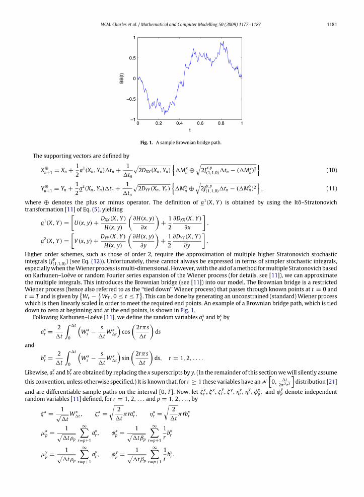
Higher order schemes, such as those of order 2, require the approximation of multiple higher Stratonovich stochasticintegrals (Jp(1,1,0)) (see Eq. (12)). Unfortunately, these cannot always be expressed in terms of simpler stochastic integrals,especiallywhen theWiener process ismulti-dimensional. However,with the aid of amethod formultiple Stratonovich basedon Karhunen–Loève or random Fourier series expansion of the Wiener process (for details, see [11]), we can approximatethe multiple integrals. This introduces the Brownian bridge (see [11]) into our model. The Brownian bridge is a restrictedWiener process (hence also referred to as the ‘‘tied down’’ Wiener process) that passes through known points at t = 0 andt = T and is given by

{Wt − t

TWT , 0 ≤ t ≤ T}. This can be done by generating an unconstrained (standard)Wiener process

which is then linearly scaled in order to meet the required end points. An example of a Brownian bridge path, which is tieddown to zero at beginning and at the end points, is shown in Fig. 1.Following Karhunen–Loève [11], we define the random variables axr and b

xr by

axr =21t

∫ 1t

0

(W xs −

s1tW x1t

)cos

(2rπs1t

)ds

and

bxr =21t

∫ 1t

0

(W xs −

s1tW x1t

)sin(2rπs1t

)ds, r = 1, 2, . . . .

Likewise, ayr and byr are obtained by replacing the x superscripts by y. (In the remainder of this sectionwewill silently assume

this convention, unless otherwise specified.) It is known that, for r ≥ 1 these variables have anN[0, 1t2π2r2

]distribution [21]

and are differentiable sample paths on the interval [0, T ]. Now, let ζ xr , ξx, ζ

yr , ξ

y, ηxr , ηyr , φ

xp, and φ

yp denote independent

random variables [11] defined, for r = 1, 2, . . . and p = 1, 2, . . ., by

ξ x =1√1tW x1t , ζ xr =

√21tπraxr , ηxr =

√21tπrbxr

µxp =1√1tρp

∞∑r=p+1

axr , φxp =1√1tβp

∞∑r=p+1

1rbxr

µyp =1√1tρp

∞∑r=p+1

ayr , φyp =1√1tβp

∞∑r=p+1

1rbyr .

1182 W.M. Charles et al. / Mathematical and Computer Modelling 50 (2009) 1177–1187

The variance of µxp =√1tρpµxp can be computed by noting that the variance of a

xr is given by var[a

xr ] = 1t/(2π

2r2) [21].Since the variance of two independent Gaussian variables equals the sum of variances and using the fact that

∑∞

r=1 1/r2=

π2/6 and∑∞

r=1 1/r4= π4/90, we find that

ax0 = −1π

√21t

p∑r=1

1rζ xr − 2

√1t · ρpµxp, ρp =

112−12π2

p∑r=1

1r2.

Using the definition of axr , ayr and denoting p the truncation index in the approximation of multiple integrals, we then define

Bx =

√1t2

p∑r=1

1r2ηxr +

√1tβpφxp, βp =

π2

180−12π2

p∑r=1

1r4.

Furthermore, we have

1Mxn =121t[√1tξ x + ax0

], Cpx,x = −

12π2

p∑r,l=1r 6=l

rr2 − l2

{1lζ xr ζ

xl −

lrηxrη

xl

}and similar for 1Myn and C

py,y and with superscripts changed from x to y. Using these random variables it follows from a

lengthy computation, that we can approximate the multiple integral by:

Jx,p(1,1,0) =16(1t)2(ξ x)2 +

141t(ax0)

2−12π(1t)

32 ξ xBx +

14(1t)

32 ax0ξ

x− (1t)2Cpx,x, (12)

Jy,p(1,1,0) =16(1t)2(ξ y)2 +

141t(ay0)

2−12π(1t)

32 ξ yBy +

14(1t)

32 ay0ξ

y− (1t)2Cpy,y, (13)

Jx,p(1,1,0) is an approximation of Jx(1,1,0) and it is known [11] that J

x(1,1,0) ≥

(1Mx)2

21tnalways. If it turns out Jx,p(1,1,0) <

(1Mx)2

21tn, we take

1Mx as the better approximation for J(1,1,0). Similarly for Jy,p(1,1,0) and finally the evaluations of Eqs. (8) and (9) can take place.

3.4. Determination of variable time step sizes

Given a current particle position (Xn, Yn) we can apply the explicit order 1 string scheme in Eq. (4) to obtain anapproximate solution, (Xn+1, Yn+1), for step n+1. Similarly, depending onwhether the current location is near a boundary ornot, we can use the explicit order 1.5 (Eq. (7)) or 2.0 (Eqs. (8) and (9)) schemes to obtain the reference location, (X0n+1, Y

0n+1).

Based on these two positions, we estimate the absolute error, as explained in [8], and from that the final step length. Ineither case the higher order reference scheme is used to advance the numerical computation to the next time step. Notethat all of this is done individually for each particle.Let τi be the tolerance accepted for the ith component. Then an error estimate of the order q+ 12 for the two-dimensional

adaptive random walk model is given by:

ε =

√√√√12

(∣∣∣∣∣X0n+1,1 − X1n+1,1τ1

∣∣∣∣∣+∣∣∣∣∣Y 0n+1,2 − Y1n+1,2τ2

∣∣∣∣∣), (14)

where q is considered to be either order o or order o. It is desirable that |X0n+1,1 − Xn+1,1| ≈ τ1 and |Y0n+1,2 − Yn+1,2| ≈ τ2.

Therefore, a step is rejectedwhenever ε > 1 and a new step size1t := 1t/√ε is tried, until the desired accuracy is attained.

For efficient implementation of the adaptive scheme using, an optimal step size can be decreased by a safety factor,e.g., γ = 0.8. This avoids unnecessary computations by ensuring the step size does not increase or decrease too quickly [8]:

1t := 1t ·min(γmax,max(γmin, γ /

√ε)), (15)

with γmax and γmin respectively the maximal andminimal step size scaling factors allowed [8]. In case the initial time step isunnecessarily small, Eq. (15) is used to enlarge it. Finally, our approach avoids uncontrolled jumps in the step size by settingthe final step length to

1tn = max (1t, 0.9 ·1tn−1) .

4. Implementation of variable time stepping in random walk models

The implementation of an adaptive scheme differs substantially from one with a fixed step size in that it is no longerpossible to have a single major loop governing the time and taking single steps of fixed size [22]. Instead, the current timediffers between the particles and, in addition to the coordinates, each particle nowneeds to have a local time associatedwithit. This concept of local time introduces a high level of asynchronicity into themodel, making it harder to gather informationabout the model at a given point in time. Before discussing how this problem is dealt with, we take a brief look at the globalarchitecture of the program.

W.M. Charles et al. / Mathematical and Computer Modelling 50 (2009) 1177–1187 1183

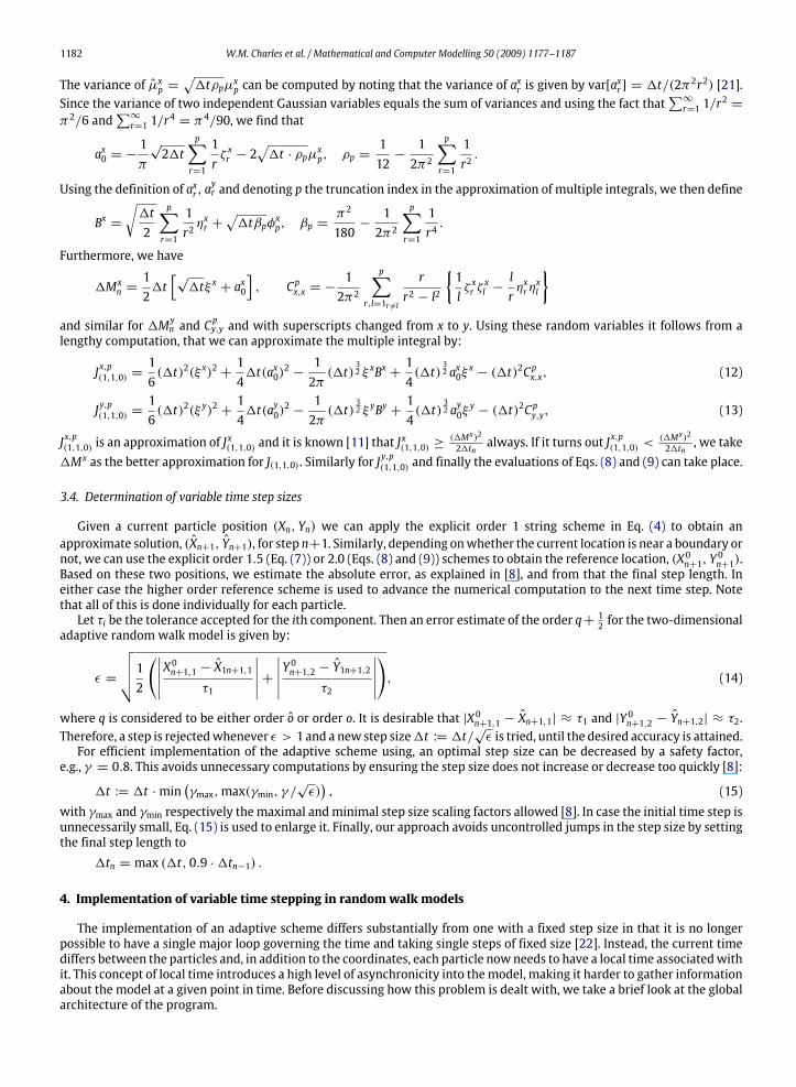
Fig. 2. An overview of the implementation of the parallel adaptive random walk model for pollution dispersion in shallow water.

As shown in Fig. 2, the program consists of a number of modules, the most important of which are:(1) Simulation engine; the central component of the application orchestrating all other parts(2) Domain module; deals with the loading and interpolation of flow and depth information of the domain(3) Statistics repository; collects all desired information about the model during the run(4) Integration module; performs the numerical integration of the stochastic differential equations on a set of particles.The first three of these modules define events that arise at certain times during the simulation. The simulation engine has astop simulation event that arises when the final simulation time has been reached. The domain module needs to update thecurrent flow and depth information at regular intervals. These data were computed at regular time intervals of 60min each,using a hydrodynamic model called WAQUA [19]. Finally, the statistics repository may request a snapshot of the currentsituation to be taken at user defined times. As shown in the pseudocode of the simulation engine in Algorithm 1, the eventsdefine the time intervals betweenwhich the integrationmodule simulates the particles. Based on the particle’s current time(which can be larger than the last event time, e.g., if a particle was determined to flow in from across the boundary at thattime) it can use whatever step sizes are deemed appropriate until either the event time has been reached, or the particlehas ceased to exist, for instance when they flow out of the open boundaries or degrade naturally. With this mechanismthe synchronicity, albeit at a coarser and irregular level, is restored; whenever an event happens all particle information isguaranteed to be valid at that point in time.

Algorithm 1. Simplified representation of the main event loop of the simulation engine.1: Set up and configure the simulation2: t ← t03: loop4: Get event e from queue5: while t(e) = t do6: Handle event e and add any new events to the queue7: if type(e) = quit then8: Raise quit flag9: end if10: Get event e from queue11: end while12: Exit main loop if quit flag is set

13: Generate all new particles until t(e)14: Integrate all particles from t until t(e)

15: Handle event e and add any new events to the queue16: t ← t(e)17: end loop18: Finalise simulation

5. Experiments of parallel processing in the adaptive scheme

The particles in the random walk model do not interact with one another and can therefore be simulated completelyindependent. As such, the simulation lends itself extremely well for parallel processing with each processor simulating anequal fraction of all particles. This means that instead of doing domain decomposition, we use workload distribution.In this section, we discuss parallel experiments for the prediction of pollutants dispersion, carried out on a distributed

memory parallel architecture called DAS-2 [23]. This system is a wide-area distributed system with 200 dual processornodes. More detailed information can be found in [23].We ran two sets of experiments; one on a simple artificial domain and a second one on a realistic model of the Dutch

coastal waters.

1184 W.M. Charles et al. / Mathematical and Computer Modelling 50 (2009) 1177–1187

a b

c d

Fig. 3. Plots of (a) the artificial domain, (b) variation of the step size along one track, (c) snapshots of the particle positions at times t = 0, 300, 600, and900 s, and (d) the ideal and actual speed up curves, based on simulation with 100,000 particles.

5.1. Simulation results on the artificial domain

For the first set of experimentswe look at a simple artificial domain consisting of a river flowing from thewest to the east,a lake and two islands, as shown in Fig. 3(a). In the experiments 2000 particles were released at coordinate (−20,−1.8) attime t = 0. At every multiple of 300 time units, a snapshot was taken along with a number of particle traces with locationand step size stored at each iteration step. Fig. 3(b) shows one such trace plotted in the horizontal plane with the associatedstep sizes plotted on the vertical axis. It is clear to see, and in line with our expectations, that the step size is small whenthe particle approaches and bends along the boundaries whereas it is allowed to grow larger in open water with smoothlyvarying flow. The maximum step size at t = 0 is chosen relatively small which explains the rapid initial growth of the stepsize. Fig. 3(c) shows four snapshots, taken at times t = 0, 300, 600, and 900 respectively, illustrating how the particle cloudslowly diffuses as it flows down the stream. At time t = 900most particles have flowed out of the domain at the south-east.For the parallel processing experiment we increased the number of particles from 2000 to 100,000 and used up to 30

processors to simulate the model. The measured speed up, along with the ideal curve is plotted in Fig. 3(d). When using 30processors the speed up is approximately 29.38, which is quite near to the ideal value of 30 (the endpoint of the solid line).The parameters used in the simulation were γ = 0.8, γmin = 0.6, γmax = 1.1. Detection of a nearby boundary was done byconsidering the box of 6 by 6 grid cells around the particle, i.e. with a radius of 3. A maximum of 30 consecutive Brownianbridge refinements per iteration were allowed in this experiment.Fig. 4(a) plots the step size versus the iteration number. In particular it shows that while fixing the step size to around 0.1

would suffice in most regions, this size would be overly pessimistic in other regions where step sizes up to 2 can be taken.Since the relation between step size and processing time is approximately linear, this implies that in those regions we caneasily obtain a speed up of 10–15. For the entire simulation, this amounts to a reduction of the number of integration stepsby about a factor five, per particle. In part (b) of the same plot we counted the number of steps taken for different intervals ofdt and computed which percentage of the total simulation time was covered by those steps (i.e., by summing the dt valuesand dividing by the total simulated time). This shows that only about 4% of the time is covered by the smallest time stepand a total of 20% in the smallest three bars, leaving around 80% of the total simulation time covered by larger steps. Theconstruction of the adaptive method ensures that the same level of accuracy is attained while allowing these larger stepsizes.

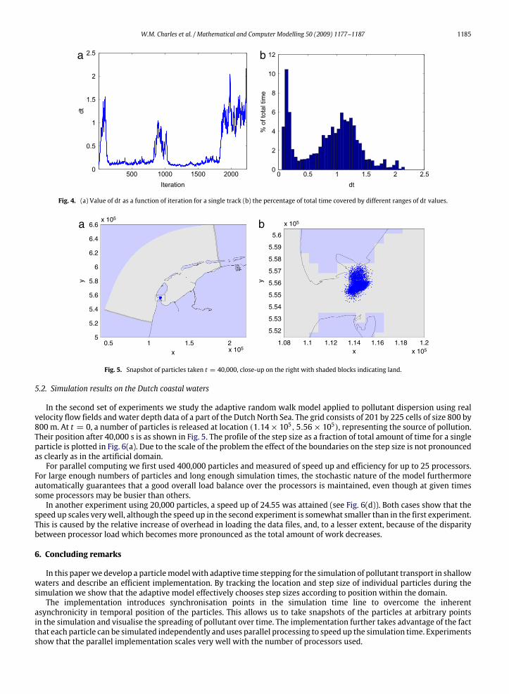
W.M. Charles et al. / Mathematical and Computer Modelling 50 (2009) 1177–1187 1185

a b

Fig. 4. (a) Value of dt as a function of iteration for a single track (b) the percentage of total time covered by different ranges of dt values.

6.6

6.4

6.2

6

5.8

5.6

5.4

5.2

50.5 1 1.5 2

x 105 x 105

x 105x 105

x

5.59

5.58

5.57

5.56

5.55

5.54

5.53

1.1 1.12 1.14 1.16 1.181.08 1.2x

5.52

5.6

y y

a b

Fig. 5. Snapshot of particles taken t = 40,000, close-up on the right with shaded blocks indicating land.

5.2. Simulation results on the Dutch coastal waters

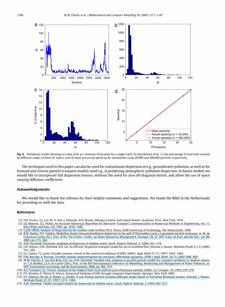
In the second set of experiments we study the adaptive random walk model applied to pollutant dispersion using realvelocity flow fields and water depth data of a part of the Dutch North Sea. The grid consists of 201 by 225 cells of size 800 by800 m. At t = 0, a number of particles is released at location (1.14× 105, 5.56× 105), representing the source of pollution.Their position after 40,000 s is as shown in Fig. 5. The profile of the step size as a fraction of total amount of time for a singleparticle is plotted in Fig. 6(a). Due to the scale of the problem the effect of the boundaries on the step size is not pronouncedas clearly as in the artificial domain.For parallel computing we first used 400,000 particles and measured of speed up and efficiency for up to 25 processors.

For large enough numbers of particles and long enough simulation times, the stochastic nature of the model furthermoreautomatically guarantees that a good overall load balance over the processors is maintained, even though at given timessome processors may be busier than others.In another experiment using 20,000 particles, a speed up of 24.55 was attained (see Fig. 6(d)). Both cases show that the

speed up scales verywell, although the speed up in the second experiment is somewhat smaller than in the first experiment.This is caused by the relative increase of overhead in loading the data files, and, to a lesser extent, because of the disparitybetween processor load which becomes more pronounced as the total amount of work decreases.

6. Concluding remarks

In this paperwe develop a particlemodelwith adaptive time stepping for the simulation of pollutant transport in shallowwaters and describe an efficient implementation. By tracking the location and step size of individual particles during thesimulation we show that the adaptive model effectively chooses step sizes according to position within the domain.The implementation introduces synchronisation points in the simulation time line to overcome the inherent

asynchronicity in temporal position of the particles. This allows us to take snapshots of the particles at arbitrary pointsin the simulation and visualise the spreading of pollutant over time. The implementation further takes advantage of the factthat each particle can be simulated independently and uses parallel processing to speed up the simulation time. Experimentsshow that the parallel implementation scales very well with the number of processors used.

1186 W.M. Charles et al. / Mathematical and Computer Modelling 50 (2009) 1177–1187

a b

c d

Fig. 6. Simulation results showing (a) value of dt as a function of iteration for a single track, (b) distribution of dt , (c) the percentage of total time coveredby different ranges of those dt values, and (d) ideal and actual speed up for simulations using 20,000 and 400,000 particles respectively.

The techniques used in this paper can also be used for contaminant dispersion in e.g., groundwater pollution, aswell as forforward and reverse particle transportmodels used e.g., in predicting atmospheric pollution dispersion. In futuremodels wewould like to incorporate full dispersion tensors, without the need for zero off-diagonal entries, and allow the use of spacevarying diffusion coefficients.

Acknowledgements

We would like to thank the referees for their helpful comments and suggestions. We thank the RIKZ in the Netherlandsfor providing us with the data.

References

[1] H.B. Fischer, E.J. List, R.C.Y. Koh, J. Imberger, N.H. Brooks, Mixing in Inland and Coastal Waters, Academic Press, New York, 1979.[2] J.R. Manson, S.G. Wallis, An Accurate Numerical Algorithm for Advective Transport. Communication in Numerical Methods in Engineering, vol. 11,John Wiley and Sons, Ltd, 1995, pp. 1039–1045.

[3] G.J.M. Uffink, Analysis of dispersion by the random walk method, Ph.D. Thesis, Delft University of Technology, The Netherlands, 1990.[4] R.W. Barber, N.P. Volakos, Modelling depth-integrated pollution dispersion in the gulf of Thermaikos using a Lagrangian particle technique, in: M. deConceicao Cunha (Ed.), Proc. of the 3rd of Inter. Confer. on Water Resources Management, Portugal, UK, in: WIT Trans. on Ecol. and the Env., vol. 80,2005, pp. 173–184.

[5] A.W. Heemink, Stochastic modeling of dispersion in shallow water, Stoch. Hydrol. Hydraul. 4 (1990) 161–174.[6] J.W. Stijnen, A.W. Heemink, H.X. Lin, An efficient 3d particle transport model for use in stratified flow, Internat. J. Numer. Methods Fluids 51 (3) (2006)331–350.

[7] J.G. Gaines, T.J. Lyons, Variable stepsize control in the numerical solutions of SDEs, SIAM J. Appl. Math 57 (5) (1997) 1455–1484.[8] P.M. Burrage, K. Burrage, Variable stepsize implementation for stochastic differential equations, SIAM J. Appl. Math. 24 (3) (2002) 848–864.[9] W.M. Charles, E. van den Berg, H.X. Lin, A.W. Heemink, Variable time stepping in parallel particle models for transport problems in shallow waters,in: C.A. Brebbia, J.S.A. do Carmo (Eds.), Proc. of the 8th International Conference on Modelling, Monitoring and Management of Water Pollution, in:WIT Transactions on Ecology and the Environment, 2006, pp. 465–475.

[10] R.A. Trompert, J.G. Verwer, Analysis of the implicit Euler local uniform grid refinement method, SIAM J. Sci. Comput. 14 (1993) 259–278.[11] P.E. Kloeden, E. Platen, H. Schurz, Numerical Solutions of SDE through Computer Experiments, Springer, New York, 2003.[12] P.S. Addison, Bo Qu, A. Nisbet, G. Pender, A non-Fickian particle-tracking diffusion model based on fractional Brownian motion, Internat. J. Numer.

Methods Fluids 25 (0) (1997) 1373–1384.[13] A.W. Heemink, Tidally averaged models for dispersion in shallow water, Stoch. Hydrol. Hydraul. 3 (1993) 607–617.

W.M. Charles et al. / Mathematical and Computer Modelling 50 (2009) 1177–1187 1187

[14] J.W. Stijnen, A.W. Heemink, Numerical treatment of stochastic river quality models driven by colored noise, Water Resour. Res. 39 (3) (2003) 1–9.[15] L. Arnold, Stochastic Differential Equations: Theory and Applications, Wiley, London, 1974.[16] A.H. Jazwinski, Stochastic Processes and Filtering Theory, Academic Press, New York, 1970.[17] B. Oksendal, Stochastic Differential Equations. An Introduction with Applications, Springer, New York, 2003.[18] E. van den Berg, A.W. Heemink, H.X. Lin, J.G.M. Schoenmakers, Probability density estimation in stochastic environmental models using reverse

representations, Serra 20 (1–2) (2006) 126–139.[19] G.S. Stelling, Communications on construction of computational methods for shallow water flow problems, Ph.D. Thesis, Delft University of

Technology, The Netherlands, 1983.[20] D. Spivakovskaya, A.W. Heemink, E. Deleersnijder, Lagrangian modelling of multi-dimensional advection-diffusion with space-varying diffusivities:

Theory and idealized test cases, Ocean Dyn. 57 (3) (2007) 189–203.[21] P.E. Kloeden, E. Platen, Numerical Solutions of Stochastic Differential Equations. Application of Mathematics, Stochastic Modelling and Applied

Probability, Springer-Verlag, Berlin Heidelberg, 1999.[22] H.X. Lin, A.W. Heemink, J.W. Stijnen, Parallel simulation of the transport phenomena with the particle model Simpar, in: B.H. Li (Ed.), Proc. of the 4th

Inter. Confer. on System Simulation and Scientific Computing, Academic Press, Beijing, 1999, pp. 17–22.[23] The distributed ASCI supercomputer home page, www.cs.vu.nl/das2, 2005.