Stochastic Processes and their Applications 41 (1992) 157-177

North-Holland

157

Random walk in dynamic environment with mutual influence

C. Boldrighini” Diparrimento di Matemaricn e Fisica, Universitri di Camerino, &merino, Italy

I.A. Ignatyuk Moscow State University, Moscow, Russia

V.A. Malyshev*j_ Dipartimenro di Matematica e Fisica, Universitci di Camerino, Camerino, Italy

A. Pellegrinotti” Dipartimento di Matematica, Uniuersitd ‘La Sapienza’, Rome, Italy

Received 5 April 1990

Revised 7 January 1991

We study a discrete time random walk in L” in a dynamic random environment, when the evolution of

the environment depends on the random walk (mutual influence). We assume that the unperturbed

environment evolves independently at each site, as an ergodic Markov chain, and that the interaction

is strictly local. We prove that the central limit theorem for the position X, of the random walk (particle)

holds, whenever one of the following conditions is met: (i) the particle cancels the memory of the

environment and the influence of the environment on the random walk is small; (ii) the exponential

relaxation rate of the environment is large; (iii) the mutual interaction of the environment and the

random walk is small. We also prove convergence of the distribution of the ‘environment as seen from

the particle’. Proofs are obtained by cluster expansion techniques.

random walk in random environment * mutual influence * central limit theorem

Introduction

The expression ‘random walk in random environment’ has more than one meaning.

LetX,EZ’, t=O,l,... , be the path of a particle performing a discrete-time random

walk on the lattice Z”, and &(x) the random variable describing the value of the

environment at the space point x and at time t. (We assume for simplicity that

Correspondence to: Dr. C. Boldrighini, Dipartimento di Matematica e Fisica, Universitl di Camerino, Via Madonna delle Carceri, 62032 Camerino, Italy.

* Partially supported by M.P.I. and C.N.R.-G.N.F.M. research funds. t Permanent address: Moscow State University, 119808 Moscow, Russia.

0304-4149/92/$05.00 0 1992-Elsevier Science Publishers B.V. All rights reserved

158 C. Boldrighini et al. / Random walk

t,(x) E S where S is a finite set.) Different situations arise depending on the behavior

of the environment and on the interaction between the particle and the environment.

The situation which has been mostly investigated is that of a static environment:

&(x) = t(x), i.e. the variables l(x) are chosen at random, according to some

distribution, and kept fixed. There are fairly general mathematical results only in

the one-dimensional case: it was proved that under some natural assumptions the

random walk can behave in a quite nonuniform way, and the central limit theorem

for X, can fail [lo]. For v 2 2 the central limit theorem can be proved when the

influence of the environment on the particle is weak and some symmetry condition

is imposed [l, 61. There are by now several results for various types of symmetry

conditions, but little is known for the general nonsymmetric case. The reader is

referred to the comprehensive paper [5] and to the references quoted there.

The analysis of the random walk in dynamic (i.e. nonstatic) environments could

begin from the case in which the environment is described by some stationary

process t,(x) with good mixing properties in space and time. If the motion of the

particle has no influence on the environment it should be possible to get a central

limit theorem by proving some sort of mixing conditions for the increments 7, =

X, -X,_, , or some bounds for the corresponding semiinvariants [8], or by some

other probabilistic technique. Up to now there are, as far as we know, only results

for special situations [7]. (A proof for the special case when the processes t.(x) are

identical and independent, for fast exponential relaxation of the environment, is a

consequence of our results: see Remark 2.3.)

The most general situation is that of mutual influence, when the transition

probabilities of the random walk depend on the environment, and the particle that

performs the random walk induces in its turn changes in the transition probabilities

of the environment. In general one can expect to get the central limit theorem for

X, (or the Wiener behavior) only if the interaction between particle and environment

is in some sense small.

In the present paper we consider random walks in dynamic environments with

mutual influence in a simple situation: we assume that the environment in absence

of the particle relaxes to a stationary distribution exponentially fast, uniformly in

space and time. Such a uniform exponential relaxation cannot hold, for instance,

in the more physical situation of a particle in a lattice gas.

Our results are based on cluster expansion techniques, which give a good control

over the situation by disentangling the recollision mechanism. The main aim of the

present paper is to work out cluster expansion techniques for the investigation of

random walks in dynamical random media, that might be generalized in various

directions.

Different techniques for special cases of random walks in dynamic environments

are considered in the papers [2,4].

Our main result is expressed for brevity in the form of a central limit theorem

for X,. Other important properties, such as the existence of a stationary process for

the environment ‘as seen from the particle’s point of view’, can be derived by

C. Boldrighini et al. / Random walk 159

applying the cluster expansion techniques developed in the proofs. This is discussed

in the concluding remarks.

1. Definitions and formulation of the results

We denote the random walk by X, E Z”, t E Z,. The ‘free’ transition probability P

for the reference random walk (independent of the environment) is subject to the

natural conditions

(pi) P(x, x’) = P(x’- x);

(pii) P(y) = 0 if lyl> d, for some d > 0;

(piii) P is nondegenerate, i.e. P( y ) < 1 for all y E Z”.

The environment at the space site XEZ” and at time FEZ, is described by a

variable t,(x) E S, where S is a finite set. The whole environment at time t is denoted

by 5, = {t,(x), x E Z”}. The free (in absence of the particle) evolution of the environ-

ment is described by a process [. = {t.(x), x E Z”} with the following properties:

(ci) t.(x) is a stationary ergodic Markov chain with transition probabilities

p(s s’), s, S’E S independent of x E Z”;

((ii) the Markov chains t.(x), ~~22”’ are independent.

We denote by n(s), s E S the (unique) stationary distribution of the Markov

chains t.(x). By assumption (si) there are constants c, y>O such that

r(t)=max17r(s)-P’(S’,S)IGce-y’, tEZ+, S,\’

(1.1)

where p’ denotes the tth iteration of the matrix p.

The random walk in random environment with mutual influence that we want to

study is the Markov process 5, = (X,, 5,) with space state Z” x SzD, defined by the

following conditions:

(i) (Conditional independence.) For fixed b, the random variables X,,, , [,+,(x),

x E Z”, are mutually independent;

(ii) P(X,+, =x’IX, =x, 5,) = P(x’-x)+&(x’-x, t,(x)), for some 6>0;

(iii) $(5,+,(x) = s’/ X, = x’, 5,) = (1 - i&)p(s, s’) + 6,.~5(s, s’), where 6,,, is the

Kronecker S-function, s = l,(x), and b is any stochastic matrix;

(iv) (Initial condition.) X0 = 0, and at time t = 0 the environment is distributed

according to some initial distribution p. on S”“.

The function c is subject to the following conditions:

(ci) P( 0) + 6c(. , s) is a probability distribution for any s E S, which implies that

for any s E S, y E Z”, P(y) + Sc( y, s) E [0, l] and I,, c( y, s) = 0;

(cii) c( y, s) = 0 if lyl> d, s E S;

(ciii) 1, max,)c(y, s)I = 1;

(civ) Es 7r(s)c(y, s) = 0, y E Z”.

Condition (ciii) is an obvious normalization condition. As for condition (civ) it

can always be enforced by redefining the free random walk transition probabilities

160 C. Boldrighini et al. / Random walk

as P(y) + 6 IS r(s)c( y, s). This would just change the drift of the reference random

walk. It can be regarded as a sort of normalization condition: if the distribution of

the environment is the stationary one and the particle does not act on the environment

(i = p) then the (average) transition probabilities of the random walk are equal to

the free ones.

We impose an additional condition to simplify the proofs:

(a) P(0) = ~(0, S) = 0, s E S.

If we do not impose condition (a) then the ‘effective rate’ of relaxation of the

environment is not controlled by the parameter y alone, one should take into account

the probability of the random walk to stay at the same place as an additional

parameter. This would actually cause no real difficulty, only more complicated

estimates.

It is convenient to single out a special case:

Case A. $(s, s’) =b(s’), where b is any probability distribution on S.

In Case A the particle performing the random walk ‘cancels the memory’ of the

environment.

In the general case we set

e(s, 3’) =J~(s, s’) -p(s, s’), E z max 2 ]e(s, s’)l. 5 5'

(1.2)

F E [0,2] is the maximum of the variation distances between b(s, . ) and p(s, . ), and

is a measure of the influence of the particle on the environment.

It is to be expected that in general the central limit theorem for X, will hold only

if the influence of the environment on the random walk and the inverse influence

of the random walk on the environment are weak (small 6 and small E), or the

speed of relaxation of the environment is large (large y). There are actually two

additional relevant parameters. One of them, the probability of the random walk

to stay at its place, which changes the effective relaxation rate, was removed by

condition (a). The other one is the constant c appearing in (l.l), which will be

assumed to be fixed: the role that it plays is clear from the estimates.

We shall use the following notation. The jump of the random walk at time t E Z,

is denoted by 7, =X,+, -X,, and its expected value and dispersion are denoted by

m,=lEn, and vf=E(q,-m,)*, respectively. P will always denote the probability

distribution induced by the process 5..

Our main results can be formulated as follows. If the process l. satisfies the

conditions listed above, then

(I) in Case A for any fixed y > 0 and 6 small enough, or for any fixed 8 2 0

compatible with condition (ci) and y large enough,

(II) in the general case for any fixed y and 6, and E small enough, or for any

fixed values of 6 2 0 compatible with condition (ci) and of e E [0,2], and y large

enough,

C.

the following statements hold:

Theorem 1.1. There are constants cl, c,>O andpE(O,l) such thatforall tEZ+,

Im ,+, - m,l s G’,

Iv,+, - a,l s CZP’.

(1.3a)

(1.3b)

Theorem 1.2. There are absolute constants c > 0, and p E (0, l), such that for any

choice of T, H, n E Z,, of the finite sequences of times t, , t2, . . . , t, E Z, such that

t, > t,-, >. . . > t, > H, and sites y,, . . . , y, E Z”, and of the condition lr = f= (2, i),

the following inequality holds:

lW%,+T = Ylr~rz+T=y2,...r~r,,+T=Yn }I 5T = t,

-p({%,+T=yl, %z+T=y2,.‘.r %,,+T=Yn})lsC@H. (1.4)

Theorem 1.2 states that for the process {~,}~, the strong mixing (or $-mixing)

property holds, with exponential decay of the coefficient.

Theorem 1.3. The central limit theorem holds for the process X,.

The proof of these results in the general case for any y and E fixed and 6 small

enough cannot be obtained by a straightforward application of the methods of the

present paper. (See however Remark 2.4 below.)

2. Proofs

The first part of the present paragraph contains some preliminary notions and results.

To make the exposition more transparent it is divided into 5 points. Point 2 contains

an easy proof of Theorem 1.1 for large y, which can be regarded as a guideline to

the proof in the general case.

In what follows, if no confusion can arise, we write for brevity 5 in the arguments

of functions depending on the environment.

2.1. Graphs and clusters

The main technical tool in proving the cluster expansion estimates that we need is

the representation of probabilities as sums of contributions associated to graphs in

Z” x Z,. A trajectory of the random walk up to time T,

r ={(O, O), (l, x,), . . . , (T, xT))

is represented by a graph with vertices at zi = (i, xi), i = 0, . . , T, and bonds bi =

(z;, Zi+l). The path r can be understood as a sequence of bonds {b,}:;‘, and its

time length is denoted by Irl: in this case jr1 = T. To take account of the evolution

162 C. Boldrighini et al. / Random walk

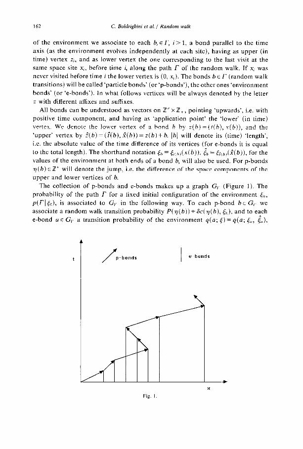
of the environment we associate to each b, E r, i > 1, a bond parallel to the time

axis (as the environment evolves independently at each site), having as upper (in

time) vertex zi, and as lower vertex the one corresponding to the last visit at the

same space site x,, before time i, along the path I’ of the random walk. If x, was

never visited before time i the lower vertex is (0, x,). The bonds b E r (random walk

transitions) will be called ‘particle bonds’ (or ‘p-bonds’), the other ones ‘environment

bonds’ (or ‘e-bonds’). In what follows vertices will be always denoted by the letter

z with different affixes and suffixes.

All bonds can be understood as vectors on Z” x Z,, pointing ‘upwards’, i.e. with

positive time component, and having as ‘application point’ the ‘lower’ (in time)

vertex. We denote the lower vertex of a bond b by z(b) = (t(b), x(b)), and the

‘upper’ vertex by i(b) = (i(b), 2(b)) = z(b) + b. lb/ will denote its (time) ‘length’,

i.e. the absolute value of the time difference of its vertices (for e-bonds it is equal

to the total length). The shorthand notation .$,, = .$,Chl(x(b)), .& = &(,,)(Xl(b)), for the

values of the environment at both ends of a bond b, will also be used. For p-bonds

v(b) E Z” will denote the jump, i.e. the difference of the space components of the

upper and lower vertices of b.

The collection of p-bonds and e-bonds makes up a graph G,. (Figure 1). The

probability of the path I‘ for a fixed initial configuration of the environment &,

p(TI &), is associated to G,. in the following way. To each p-bond b E G,. we

associate a random walk transition probability P( v( 6)) + 6c( 77 (b), &,), and to each

e-bond a E G,. a transition probability of the environment q(a; 5) = q(a; &, &),

e-bonds

Fig. 1

C. Boldrighini et al. / Random walk 163

given by

(

p’“‘(s S’) q(a;s,s’)= ’

ift(a)=O, x(a)#O,

c b(s, s,)p’“‘+‘(s s’) (2.1)

I, otherwise. s I

There is a one-to-one correspondence between e-bonds a and p-bonds b, since

the lower vertex of a p-bond is the upper vertex of an e-bond (except for bO, which

has no e-bond: we can agree that it has a degenerate e-bond, corresponding to the

factor 1). Denoting by a(b) the e-bond associated to the p-bond b E I’, the conditional

probability p(T I&,) of the path r for a fixed choice of the initial environment &

can be written as

P(TISCJ =L: ,fI,_ (P(db))+Wv(b), &)Ma(b); 0, (2.2)

where CT means, here and in the following, that summation goes over all values of

the environment l,(x) on which the expression that is summed depends, keeping

& = {&(x), x E ZU} fixed. The contribution of an e-bond is decomposed as

q(a; s, s’) = cY(a; s, s’)+ n-(d), (2.3a)

p’q s, s’) - n-( s’) ift(a)=O, x(a)#O,

1 F(s, s,)(p’“‘~‘(s,, s’) - I) otherwise. (2.3b) ,’ I

(Here the notation ~(a; 5) is used in analogy with q(a; 5) above.)

By ‘opening the brackets’ ofthe factors q = (Y + T corresponding to e-bonds (except

for the degenerate e-bond associated to b,,), we get a sum over the subsets B c T\b,

of the bonds b E I‘ for which the factor a(a(b); .$) appears:

(2.4a)

“JI,, (P(rl(b))+Sc(rl(b), 4))d&). (2.4b)

For fixed r and I3 the e-bonds for which the factor a appears will be called a-bonds.

2.2. Proof of Theorem 1 for large y

Let T, r, Irj = T and B be fixed. We say that the time t, 0~ t < T, is separating for

(I; B) if in expression (2.4b) there is no a-bond a such that t(a) < t G t*(a).

Consider the quantities

Qo(r, x 15”) = cp,.x, w, ~‘1 w - x,d

O(~,XI~~)=C~,,.~,~(~‘, ~J~x--,J.

164 C. Boldrighini et al. / Random walk

Here Cj),,X) denotes summation over all r’, B’ such that jr’1 = t, X, =x (X,_, is of

course a function of F), and (r’, B’) has no separating times, and Cc,,.+) denotes

the same sum with the additional condition on (F, B’) that there are no a-bonds

a with lower vertex (t(a), x(a)) such that t(a) = 0, x(a) # 0. Clearly the quantity

is the contribution to E( T+, I&) of all pairs (r’, B’), IFI = T, with no separating

times. Moreover, setting

where II denotes the environment equilibrium distribution (which can be formally

written as IT(&) = n, rr(&(x))), ‘t . 1 1s not hard to see, by translation invariance of

the transition probabilities, that the contribution to E( nT_, I &J of all pairs (r’, B’),

IPI = T, which have 7 as maximal separating time is given by

C ~(X,=XI~~)O(T-~,~-XI~) .x.y c z *’

To see this note that for all a-bonds a with t(a)> 0 the lower vertex (t(a), x(a))

lies on the trajectory. Hence if T is a maximal separating time and X, =x there is

at most one a-bond a with t(a) = T, and for it x(a) = x. The process after the

separating time T depends only on the position X, =x, and is independent of the

distribution of the environment before time 7.

We find

~(r)~-,l5o)=Q(Tt&J+ C Q(T-TI~TT), 7=2

(2.5a)

~(~T~~0)-[E(~T-1~5b)=~(T+11~0)-~(TI~0)+~(TI~). (2Sb)

Now the number of different pairs (r, B) with Ir( = T is bounded by cT, where c

is a constant depending on v and d. Moreover, by assumption (a) of Section 1,

P(0) = ~(0, s) = 0, hence all a-bonds have length not smaller than 2, except for the

a-bond associated to b, , which gives a contribution to QO( t, x I to). Hence, by position

(2.3b) and condition (1.1) for each pair (F’, B) with Irl= T and no separating times

we havep*(T, BJ&)<(c’~~~)~‘*, where c’ is some constant independent of y. Hence

for y large enough the first assertion of the theorem is proved. The second assertion

follows easily by changing x-XT_, for (x-XT_,)*.

2.3. Clusters

By ‘opening the brackets’ of the factors (P(n( b)) + 6c( r]( b), &)) in equations (24a),

(2.4b), p(Tl&) can be written as a double sum over the subset B and over the

C.

subset A of the bonds b E r for which the factor Gc(v(b), &,) appears:

P(rl&J= c Ac,. &, drT A, Bl‘s.

0

(2.6a)

p(T, A, B 1 eo) is given by

x n P(q(b)b(a(b); 5) h,Jn,L P(v(b)), Wb) htA=r\E

where A’, I?” denote the complements of the sets A, B with respect to L’.

We now fix r, A, B and consider the right-hand side of the expression (2.6b). At

a given site x E Z” one can have more than one cr-bond. They can be grouped into

a certain number of maximal connected sequences. (A sequence of a-bonds

a,,..., ak at the site x, labeled in order of increasing time, is connected if t(a,+,) =

f(a,), i = 1,. . . , k- 1.) If a,, . . . , ak is a maximal connected sequence ak(al) is the

‘final bond’ (‘initial bond’) and f(a,)(z(a,)) is the ‘final vertex’ (initial vertex’) of

the sequence.

When summing over the environment .$’ we note the following.

Remark 2.1. (i) If b E A n B, then z(b) can be either a final or an intermediate vertex

of a maximal connected sequence of a-bonds.

(ii) If b E An B’ we can assume that z(b) is an initial vertex of a maximal

connected sequence of a-bonds. In fact, if z(b) is not the lower vertex of an a-bond,

the only factor depending on & is n-(th)c(v(b), &), which gives 0 when summed

over s’, by condition (civ).

(iii) If b E A” n B we can assume that z(b) is an intermediate vertex of a maximal

connected sequence of a-bonds. Otherwise the only factor depending on & would

be a(a(b); 5 o(h), &), which gives 0 when summed over &, since cY(a; s, .) is the

difference of two probability distributions.

(iv) If b E A” n B’ then z(b) can be the initial vertex of a maximal connected

sequence of a-bonds. If it is not, then the only factor that is left is P(T(b)).

This is obvious for b = b,. If b # b,, i.e. t(b) > 0, summing over & we get

P(T(b)) c d&h) = f’(rl(b)L

If z = z(a) = (t, x) is the initial vertex of a maximal connected sequence of

a-bonds, then if t = 0, x # 0 the e-bond a gives the relaxation of the environment

at x from the initial fixed value to(x), whereas if t > 0, or t = 0, x = 0, a describes

the relaxation after the perturbation induced by the particle at x, in which case z

lies on the path r’. We denote by Z the set of the initial vertices z of maximal

connected sequences of a-bonds that belong to the path lY Note that the a-bonds

are uniquely determined by 2 and 2, = {z(b), b E B}.

166 C. Boldrighini et al. / Random walk

ForafixedchoiceofO<t,<...<t,,y,EZ”,j=l,...,nwehave

W{77t1 = Yl 3 . . . 3 ~,,.=Y~}15,)=tP(T15,)j~,X(~,,=Y,)r (2.7)

and the sum can be limited to paths with time length IT\ = T= t, + 1. We insert

expressions (2.6a,b) into (2.7) and sum over all paths r, Irl= T which are compatible

with a given choice of A, Z,, z, and of the jumps r],, = y;. The sum is over all

compatible values of P(r](b)), bc A', excpet for b such that t(b) = tj, j= 1,. . . , n

(for which v(b) is fixed). As a result we get factors corresponding to transition

probabilities for the free random walk. They are the probabilities of paths that

connect the bonds of A, go through the vertices of Z, and Z, avoid intersection of

the a-bonds at other points, and have the prescribed jumps y, at the times t,,

j=l,..., n. (We keep the notation 2, even though we are summing over some

T(b), b E B: Z, denotes the set of the lower vertices of the bonds of B in all the

terms p(T, A, B I &,) which give contribution to the sum.) In the graphical representa-

tion these paths are represented by bonds which connect either two subsequent (in

time) vertices of Z - Z, u Z or a vertex 2(b), b E A with the subsequent (in time)

vertex of Z. We call these bonds ‘p-bonds of type 0’, since they refer to free transition

probabilities, and denote the collection of such bonds by L. The bonds of A will

be called ‘p-bonds of type I’. Denoting by E the set of the a-bonds (which determines

both Z and Z,), we can write

W{%, = Yl > . . 3 ~~,,=~,,ll&J= 1 WA,E;y,,...,ynL (2.7a) A,E

WA,E;Y,,...,YJ=C; II 4&;(x)) cr,x)cz\(o.o)

x Fl P(c) n ata; 5) FI W4bL &I, (2.7b) CCL (IF E htA

where P(c) denotes the probability of the path represented by c.

W(4 E; Y,, . . . , yn) is then described by a graph GA,E;,. ,,..., I;, with three types of

bonds: (i) the p-bonds of type 0, c E L, associated to the free transition probabilities

P(c); (ii) the p-bonds of type I, b E A, corresponding to factors SC; (iii) the e-bonds

of E corresponding to factors cy (a- bonds). In addition there are factors r associated

to the vertices of Z\{(O, 0)).

In what follows we shall omit as a rule to write y,, . . . , y, in the notation.

For the topological classification of the graph GA,E we identify all vertices (0, x)

with (0,O). A ‘subgraph’ of GA,E is any collection of bonds of GA,E containing at

least one p-bond.

In order to avoid confusion with the definition of clusters some preliminary

remarks are in order. Note that we can sti!l identify a trajectory in the graph GA,E:

the curve obtained by joining the p-bonds (of type 0 or I), which is connected.

Hence it is clear what we mean by subsequent (in time) p-bonds. By ‘disconnecting’

two subsequent (in time) p-bonds we mean that the connection between the two

C. Boldrighini et al. / Random walk 167

bonds at their common vertex z is removed. The graph which arises from the

operation is ambiguous if z is also a vertex of a-bonds: we remove the ambiguity

by prescribing that the connection at z between the p-bond which is higher in time

(i.e. the one which has z as lower vertex) and the a-bonds is not removed. We define:

Definition 1. GA,E is said to be simple if it cannot be decomposed into two connected

subgraphs just by disconnecting two subsequent p-bonds. (So, e.g., the graph in

Figure 2 is not simple.)

Definition 2. A cluster graph of G A,E is any maximal simple subgraph of GA,E.

In what follows there will be some abuse of language. We shall apply the term

‘cluster’ sometimes to cluster graphs, sometimes to equivalence classes of cluster

t

p-bonds of type 0

p-bonds of type I

o( -bonds

Fig. 2. A graph with two clusters.

168 C. Boldrighini et al. / Random walk

graphs with respect to translations in Z” x Z,. Moreover, although by our definition

a cluster graph might consist of a single p-bond of type 0, in what follows we always

mean by that cluster graphs which contain at least one p-bond of type I.

GA,E is decomposed into cluster subgraphs, and a cluster subgraph C is identified

by subsets A’c A, E’c E (or equivalently by A’ CA, Z,.cZ, and z’cz): C=

G A,,ES. Figure 2 shows a graph with two cluster graphs.

The ‘initial’ and ‘final’ vertices of C (i.e. the ones with lowest and highest time

coordinate), are denoted by z(C) = (r(C), x(C)) and ?(C) = (G(C), i(C)) respec-

tively, and their coordinates are the ‘initial’ and ‘final’ times and positions. The

‘height’ of the cluster C is h(C) = G(C) - T(C). The ‘initial’ bond b, (‘final’ bond

&) of C is the p-bond with lower vertex z(C) (with upper vertex ;(C)).

We label the cluster subgraphs of G A,E in order of increasing time: {C,},“=, . We

denote by li, i > 1, the p-bonds of type 0 connecting the (i - 1)th and the ith cluster:

I, is the path connecting ;(C,_,) and z(C,) (if they do not coincide), subject only

to the condition of having the prescribed jumps v,,, for i> 1. We denote by P(&)

the free random walk probability of 1,. If ;(C,_,) = z(C,)1, is by convention a

‘degenerate’ bond with P(1,) = 1. I, is the degenerate bond at (0, 0), P(/,) = 1.

W(A, E) can then be written as

W(A, E) = fi P(l;) Wcl. r=,

(2.8)

The contribution of each cluster W,, = W(A,, E,) is computed using equation

(2.7b), except of course for obvious changes: in particular the product nviL P(c)

goes into flTcEL, P(c), the product of the probabilities of the p-bonds of type 0 of

C, (which are prescribed to have the jumps qk for fk E [r( C,), ;( C,))). An important

remark is that if T( C,) > 0, then by translation invariance W,; does not depend on

the initial vertex z( Ci) E z.

The important point with clusters is factorization: if we sum up expression (2.8)

over all possible initial positions x(Ci), which corresponds to summing over all

admissible final positions of the bonds I;, we get for the contribution to P({r],, =

Yl,..., n,,, = v,,} I&,) of all graphs with clusters C,, . . . , C,,

WC,,..., C,)- ir WC, n P(Y;) ,=, l,Ed

(2.9)

where

n--l

A = U [G(Ci-l), ~(C,))u[q(Crt), T). i=,

2.4. Estimate of cluster contributions: Case A

We estimate the contribution of all clusters graphs C with a given initial vertex

z(C)=z and height h(C)=H+l, H>O. Suppose first that T(C)>O, and let A,

Z,, z be the sets of bonds and vertices defining C. Going back to Remark 2.l(iii),

C. Boldrighini et al. / Random walk 169

we see that in case A the set A”n B is empty. In fact if b E A’n B, z(b) = (t, x) is

the upper vertex of the a-bond a(b) and, since the factor ~3 of the ‘next’ a-bond

does not depend on s’= &,, the only term depending on s’ is a(a(b); s, s’) which

gives 0 when summed over s’. This corresponds to the fact that when the particle

goes through some site it cancels the memory of the previous history. Hence each

a-bond can be associated to a bond of B, = B n A c A. According to equation (2.7b)

we can write

1 W,.I s 61A’ fl F(b) Jj P(c), hsA CFL

where, setting c^( y) = max,lc( y, s)l, we have

(2.10a)

C 4s)Ic(q(b), s)l s t(v(b)), b E A\B,,

max C Ia(a(b); s, s,)llc(rl(b), SIN ~2dla(b)l- 1)8v(b), b E 8. (2.10b)

x ‘I (Here and in the following we use for any finite set A the notation IAl = card A.)

The estimate of the total contribution of all clusters C such that IAJ = n, (B,( = m,

andthetimesofthebondsofAandB,,~~~{t(b),bEA},~~,~{t(b),bEB,}c~~,

are specified, is obtained by summing expression (2.10a) over all transition prob-

abilities P(c) and F(b) over all jumps T(b). If b E A\B,, then z(b) is the initial

vertex of a maximal connected sequence of cr-bonds (Remark 2.l(ii)). Hence there

are at least n -m such sequences. If n -m > 1 any one of them must have a

superposition in time with some other sequence, hence the total length of the a-bonds

is not less than H + (n - m - 1). Since moreover all a-bonds have length not smaller

than 2, inequality (2.10b) shows that the total contribution for 9+,, YB, fixed is

bounded by

S”(2c)rn e-(Y/2Nn~m~l) e-(y/2)H (2.11)

It is not hard to see that the estimate for the corresponding sum of clusters

contributions for T(C) =O, is the same, with the only change of the factor e-(Y/‘)(‘-m-‘) which becomes e~‘Y/2)(“-“~2’, due to the fact that there may be one

a-bond with length 1. The final estimate is now obtained by summing up the

contributions for all possible choices of .Y BI for fixed F* and for all possible choices

of y/,:

e-(~12W ni, ( y ) i, (3 S”(~C)~ e~(v’2)(n-m-2).

The result is stated as a lemma:

Lemma 2.1. In Case A for the total contribution of cluster graphs with a given initial

vertex z and height h(C) = H + 1 the following estimate holds:

c C:z(C)=z,h(C)=H+I

p = eey’*( 1-t S(2c+ eeY”)), (2.12)

where F is a constant independent of z and H. 0

170 C. Boldrighini et al. / Random walk

2.5. Estimate of cluster contributions: General case

By (1.2) we decompose p’ as p” =p + e, and substituting into formula (2.3b) the

product over the a-bonds in equation (2.7b) can be written as

(2.13a) E,rF aeE, atE\E,

cq(a; s, s’)=C e(s,s,)(p’+‘(s,, s’)-77(s))), c1 (2.13b)

cu’(a; s, s’) =$‘(s, s’) - 7r(s’).

Clearly

max 1 Jcw,(a; s, s’)l S u(lal- I), \ r’

max 1 la’(a; s, s’)l = r(lal). (2.13~) .5 5’

Two types of a-bonds arise, the ‘a,-bonds’ of E,, and the ‘a’-bonds’, of E\E,,

and the contribution W(A, E) of GA,, decomposes into a sum over the subsets E, ,

W(A E) = C W(A, E, E,). E,iE

Let 2, = {z = z(b): b E A} be the set of the lower vertices of the bonds of A. When

summing over the environment the following should be noted.

Remark 2.2. (i) If z = (t, x) E z\Z,, t > 0 is the lower vertex of an a/-bond, i.e.

z = z(a), a E E\E,, then the sum over s = &, gives a factor x,, r(s)cu’(a; s, s’), which

is 0, since rr is the stationary measure for the transition matrix p. Hence we can

assume that the vertices of z\Z, are lower vertices of a--bonds.

(ii) If z E Z,\Z,, then by Remark 2.l(iii), z is an intermediate vertex of a maximal

connected sequence of a-bonds: z = z(a) = ;(a’), a, a’E E. If a E E\E, then the

sum over s = &, gives by the composition rule

1 &(a’; s’, s)a’(a; s, s”) = &(a”; s’, s”),

where Lu can be either a, (a’E E,) or CI’ (a’e E\E,), and a” is the e-bond obtained

by ‘joining’ a’ and a.

For a given choice of A, E, E, c E we introduce a new set of a-bonds l?, obtained

by ‘glueing together’ the a-bonds of E which have a common vertex ZE Z-

{zEZe\Z A : z = z(a), a E E\E,}, as described in Remark 2.2(ii). I?, C_ I? will denote

the set of the new a,-bonds. We sum up all contributions W(A, E, E,) for A, E, E,

which differ only by the choice of Z (and hence correspond to the same sets of

new a-bonds I?, I?, c I?). Summation over the intermediate vertices of Z gives rise

to new p-bonds of type 0 (which have, as before, the prescribed jumps yj at the

times t,). Note that by Remark 2.2, z can be a lower vertex of an al-bond only if

ZEZ,.

C. Boldrighini et al. / Random walk 171

- - - - The total contribution for a given choice of A, E, E, c I?, @(A, E, E,), is represen-

ted by a new graph, Ga,~,~,, with p-bonds of type 0; p-bonds of type I, and two

types of a-bonds, the cu,-bonds of E,, and the cY’-bonds of l?\E,. We extend the

notion of simple and cluster graph to the new graphs by stating that GA,~,~., is simple

or cluster whenever GA,~ (in the sense of the previous definition) is simple or cluster.

A cluster subgraph is now identified by subsets A’ c A, J?‘G I?, _!?{ G I?, In analogy - - with (2.8) we have @(A, E, E,) = n P(l,) l&.,, where C, are the cluster subgraphs,

and the paths 1; are as before.

We now come to the estimate of the contribution of all cluster graphs with fixed

initial vertex z(C) = (t, x), t > 0, and height h(C) = H + 1, H > 0. It is not hard to

see (by (2.10b), (2.13b)) that the contribution of such a cluster graph GA,E,E, is

bounded by

As before we have, by Remark 2.1, that the final bonds of the maximal connected

sequences of a-bonds are in A. We denote them by a, and by Zi = {z = z(a): a E a}

their lower vertices. We introduce furthermore the set of the lower vertices of the

cu,-bonds Z’ = {z = z(a), a E E,}, and of the cr’-bonds Z’= {z = z(a), a E E\E,}. By

Remark 2.2, Z’c Z,\Zi. Z = Z,- u Z’ u Z’ is the set of all lower vertices of the

bondsofthegraph. WesetIAI= n,lAj = rn~n,/Z’[=/E\E,l =ps n-m,(Z’I =lE,l=

n - m -p + k, where k is the number of the vertices of Z\Z, (which by Remark 2.2

are all in Z’). Summing up, as before, all contributions (2.14a) of the graphs for

which the times of all vertices of the various kinds are fixed (i.e. for fixed &,

~~={t=t(b):b~~},~={t=t(a):a~E\E,},~={t=t(a):a~E,}),andtaking

into account that there are at least m maximal connected sequences of a-bonds

(which must overlap in time if m > l), we find

8nCn-m+kEn-m-pik e-yp e-‘y/2)(n~-l) e-‘y/2’H. (2.14b)

Multiplying by the number (“6”‘) of the possible choices of Y’c Y+,\Yi, and by

the number (G) of the possible choices of YA G &, and summing over p and m we

find

(s*)“(~~)I’ e~‘~/“‘H~“, f5*=G(c(e-Y+~)+eP(y’2)). (2.14~)

This is again multiplied by the number (“r”) of all possible choices of the times of

the vertices of Z\Z, and by the number (y) of all possible choices of &, and

summed over k and n. For clusters with T(C) = 0 one has to apply the same

modification as in the previous case.

Note that the sum of all contributions W(A, E) for A, E corresponding to cluster

graphs with a given initial vertex z and height H is the same as the sum of all - - @‘(A, E, E,) corresponding to cluster (in the new sense, with two kinds of a-bonds)

with initial vertex z and height H. In fact the new graphs are obtained by joining

some a-bonds of the previous graphs (as explained in Remark 2.2(ii)), without

canceling any bond.

172 C. Boldrighini et al. / Random walk

Hence we can state the result:

Lemma 2.2. In the general case for the total contribution of cluster graphs with a given

initial vertex z and height h(C) = H + 1 the following estimate holds:

c IWclS@3H, p=e-‘Y’2’[1+c~+S*], (2.15) C:z(C)=z,h(C)=H+l

where c? is a constant independent of z and H, and S* is given in formula (2.14~). 0

Remark 2.3. The estimate for F = 0 (no influence of the particle on the environment)

is similar to the one for Case A. This is due to the fact that there is only one kind

of a-bonds (there are no a,-bonds).

Remark 2.4. The result for the case when y and E are fixed and 6 is small follows

from Lemma 2.2 if (1 + CE) e-v’2 < 1. The restriction can probably be removed by a

more detailed analysis of the graph contributions.

Proof of Theorem 1.1. We have

In the cluster expansion of P({n, = y}l &J only clusters with height h(C) s t + 1

appear. Consider first the contribution of all N-cluster graphs W(A, E) for which

the last bond b, is above the final cluster CN, i.e. such that t( C,) G t. By (2.9),

W(C,, . . , C,) = P(Y) fi WC,. i=l

Let b = gee, be the final bond of the cluster CN. By Remark 2.1, b E A, and hence

it is associated to a factor &(7(b), 5). q(b) is ‘free’, i.e., as the upper vertex of b,

2(b), cannot be the lower vertex of an cr-bond, there is no term in WCN depending

on T(b), except c( v(b), 5). Summing over v(b) (which corresponds to summing

over a subclass of graphs C,) we get 0, as C, c( y, s) = 0. Hence only the term with

N = 0 gives a contribution, and by (2.8) we find

c W(A, E) = P(Y). A,E:i(C,)=r

On the other hand if we sum up all contributions for which the clusters

C,,..., C,--* and the last cluster C, are fixed, and G( C,) = t + 1, we get a sum

over all possible compatible choices of the cluster CN_, , which, by (2.9), gives

N-2

(If Q-( CNPI) > 0 the sum is meant as a sum over cluster graphs with a fixed initial

vertex, i.e. on equivalence classes with respect to shifts of the initial vertex.) We

C. Boldrighini et al. / Random walk 173

see again that this is 0 by summing over the jump of the last bond of CNPI, ~(6~~_,).

Hence the sum of the contributions W(A, E) for which the last cluster C is fixed

and !(C) = t+ 1 is simply WC. Therefore, with obvious notation

$({rlr=Y)l&)=P(Y)+ c WC.. C:h,eC

(2.16)

Since for r(C) > 0, Wc does not depend on the initial vertex, (2.16) implies that

the contribution to the difference P({n, = y}( 5”) -iP’({n,+, = y} ( &,) is bounded by

the total contribution of the graphs with height t + 2 and t + 1. Hence by Lemma

2.1 and Lemma 2.2 we have

P({n, =Y)l&J -${rlt+, =Y>I &))I

6 c lWcl+2 c ) W,( d c(p’+‘+2p’). C‘:h(C‘)=r+* C.k(C)=r+I

For p < 1, since the sum over y is finite, this implies

1~~~‘+*15~~-~~~1l5~~l~~,P’, I~~77:+1l5o~-~~~Il5o~l~~zP’,

for some constants c, , c2> 0. The theorem is proved. 0

(2.17)

Remark 2.5. As it follows from (2.16), by taking out the contribution of the graphs

with at least one p-bond of type I (i.e. with A f B), we can write

m, =CyP(y)+&?rj”, (T;=~yQJ(y)+&7)“, I‘ Y

where mj’), a:‘) are bounded quantities. Hence 112, = 0(s) if C,YP(Y) = 0.

Proof of Theorem 1.2. Since the transition probabilities defining the Markov process

5, do not depend on time and space, we have

$({rl r,+7- = YI , . . . , 77~<r+T=Yn~15T=~)

= WI%, = Yl, . . . , 77,,, = Yn} 1501, (2.18)

where tU = S& and S. denotes the space translation: S;(x) = [(x -2). By the cluster

decomposition, P({ q,, = y, , . . . , n,,, = y,} I &) is written as a sum of N-cluster contri-

bution of the form (2.9). Applying the same argument as above one sees that the

contributions W(A, E) for which the initial cluster C, is such that ?(C,) d H+ 1

are absent. Similarly the cluster decomposition applied to P({ r],1+7 = Y, , . . . , v,,,+~ = yn} ( $f), for any choice of the initial environment [t, is given by the sum of the

N-cluster contributions of the type (2.9) with the first cluster such that ;(C,) >

T+ H+ 1. It is readily seen that for any N-cluster contribution W(C,, . . , C,) to

$({rlll =YI, . . . , q,, = y,} ( &J with 7(C,) > 0, $( C,) > H + 1 there is a corresponding contribution W( C’, , . . , Cl,) with T(C;)> T, G(C{)> T+H+l to P({T,,+~=

y,, . , v,,,+~ = y,,}ltx) such that the C:‘s differ from the C,‘s by a translation of

the initial vertex. It is actually a one-to-one correspondence and the contributions

174 C. Boldrighini et al. / Random walk

are independent of .$, & and equal. So the only contribution to the difference is

given by the N-cluster contributions for which h( C,) > H + 1. If C, is such a cluster

then it is easy to see that the contribution to P’({~I,,+~ = y,, . . . , v,,,+~ = y,} 15;) of

all N-cluster graphs with initial cluster equal to C, is equal to W,, times the

probability that some fixed jumps occur in the time interval [ G( C,), t, + 1). Hence,

by Lemma 2.1 and Lemma 2.2, we have, for /3 < 1,

P({rl I,+T = Yl 3 . . ., 771,8+-r=Yn115T=~)

-W{77 r,+T.=Yl,...,rlr,,+T=Yn })I G @.

The theorem is proved. 0

The following Corollary is a simple consequence of the proof above.

Corollary 2.1. The shifted process qir): v(kT) = v~+~, k = 1, 2,. . , , tends, as T-+co,

to a limiting process r]?, which is again a strong mixing process with exponentially

decaying coeficien t.

Proof. In proving Theorem 1.2 we found that for any choice of the initial environ-

ment & and of the sequences k,, . . . , k, E if’,, y,, . . . , y, E if”, the probability

p({vT+k, = Yl > . . . , )7T+k,, = Yn) I&)

is equal, except for a term of order O(p’), to a sum of terms rkr corresponding to

iv-cluster contributions with T( C,) = T - k, ;( C,) 2 T (k < T), which are indepen-

dent of T and &;,. Since 1 rkl (constant /3” the series ~~=I rh defines the limiting

probability W{rl: =Y1, . . , VT, = Y,,}), and it is easy to see that for some constant E

lW{v T+k,=yl,..., %+k,, = .vn> 150)

-WV; =y,, . . . , q;, =ynI)I~ EPT. (2.19)

The strong mixing property for the process v?c now follows from the strong mixing

property of the process v.. 0

Proof of Theorem 1.3. The proof could be deduced by Theorems 1.1 and 1.2, using,

for instance, the semiinvariant method [8], or some other probabilistic technique.

An immediate proof is provided by Corollary 2.1 above. In fact the limiting distribu-

tions, as T + ~0, of the random variables

coincide. To see this one can, for instance, set

C. Boldrighini et al. / Random walk 175

where M =[n] ([ *] d enotes the integer part). w”, tends to 0 in distribution, as

T + 00. (This follows for instance, from Theorem 1.1.) If we denote by A the

a-algebra of the process n = {~,}~, , clearly I& is measurable with respect to the

sub-v-algebra .A,,, c A generated by the random variables {~,+,+k}~=, . For A E ./u

we denote by S,,,A its translate: SMA = (77: KM7 E A} (where S_, is the shift,

(S-rn)k = n,+k> k = 132,. . .). It follows from (2.19) that for any choice of the initial

environment &,

IWLAI &A - P*(A)1 c @‘,

where P” denotes the probability associated to the process v*. Hence the probability

of the event { $- < x} is reduced, as T + co to the probability of the event {GT < x},

where

which is asymptotically equal to the probability of the event {w: < x}.

The result now follows by applying the classical theorems for stationary processes

with the strong mixing property (see, for instance [3]). The proof of the invariance

principle is also straightforward. 0

3. Concluding remarks

We have seen (Corollary 2.1) that the process r]kT’= nr+a, k = 1, , . . , tends, as

T + co, to a limiting process q*. One could also consider the limiting behavior of

the process 5. ‘as seen from the particle position’, i.e. in a moving neighborhood

around the particle position XT for a large time T. This amounts to studying the

limit as T+ 00 of the finite dimensional distributions

P({r]T=y” )...) ~-r+m=~m;~r(Xr+X~O~)=~:O~ )..., Sr(Xr+X~~‘)=S(,?I);...;

&+fn(X-rtnl +xl”‘) = P,. . ., ~T+m(XT+m +d:‘1 = d:)H. (3.1)

The limiting behavior of the probabilities (3.1) can be studied by using a simple

modification of the cluster technique introduced above: one should add new vertices

at the points (T-t k, X7+L + XI”‘), and the corresponding e-bonds. Carrying out the

estimates, which are essentially the same as before, except for more clumsy formulas,

one can see that in the range of the parameters for which p < 1, as T + cc the

probabilities (3.1) tend exponentially fast to limiting probabilities

Q(x(,(‘), . . . , xjl:,);. . . ; xp,. . . , x!;‘; s’,o’, . . , SE;;. . . ; p,. . . , q,.

That is, there is a stationary distribution for the environment as seen from the particle.

Deeper results can be obtained by using a refined estimate of the semiinvariants.

The semiinvariants 191 corresponding to the random variables vl,, j = 1,. . . , n,

176 C. Boldrighini et al. / Random walk

t, < t2 < . . ‘<t,,, and to the vectors k’-“EL’“, j= 1,. . . , n, with nonnegative com-

ponents kj’)E Z+, are linear combinations of the expected values of all possible

products of the factors ( nt,):i”, i = 1, . . , v, and are denoted by

(rl;y . . . 77;p”‘)),

We claim that under the same conditions for which we proved Theorems 1, 2

above the following estimate holds for some constants C > 0 and p E (0, l),

(Here I kl = C,“=, k,.) For large y (both in Case A and in the genera1 case) the estimate

(3.2) is straightforward since this case admits a regular cluster expansion [9].

The estimates (3.2) and similar ones for the environment are the main ingredients

in investigating the spectrum of the system, in analogy to what is done for the

transfer matrix of the Gibbs fields. In particular it is important to find the renormal-

ized one-particle space and the spectrum in this space.

In conclusion we may say that the present paper is intended to be a first contribu-

tion to the study of random walks in dynamic environments with mutual influence.

As a next step one could study the situation in which the environment has nonzero

space correlations, which decay exponentially, as, for instance, in the case of Glauber

dynamics in the high temperature region. This case can probably be treated in

analogy to what is done in the present paper. A further more difficult step is the

extension to the situation when the decay of the space correlations of the environment

is slow (nonsummable).

Acknowledgements

We thank the referees for the careful reading of the manuscript and for pointing

out corrections and improvements. One of us (V.A. Malyshev) is grateful to the

Department of Mathematics and Physics of the University of Camerino for kind

hospitality, in the framework of the exchange agreement between the University of

Camerino and Moscow State University.

References

[l] V.V. Anshelevich, K.M. Khanin and Ya.G. Sinai, Symmetric random walks in random environments,

Comm. Math. Phys. 85 (1982) 449-470. [2] P. Ferrari, S. Goldstein and J.L. Lebowitz, Diffusion, mobility and the Einstein relation, in: J. Fritz,

A. Jaffe and D. S&z, ed., Statistical Physics and Dynamical Systems. Rigorous Results (Birkhguser,

Basel, 1985).

[3] LA. lbragimov and Yu.V. Linnik, Independent and Stationary Sequences of Random Variables (Wolters-Noordhoff, Groningen, 1971).

[4] C. Kipnis and S.R.S. Varadhan, Central limit theorem for additive functionals of reversible Markov

processes and applications to simple exclusion, Comm. Math. Phys. 104 (1986) I-19.

C. Boldrighini et al. / Random walk 177

[5] SM. Kozlov, The method of averaging and walks in inhomogeneous environments, Russian Math.

Surveys 40 (1985) 73-145.

[6] SM. Kozlov and S.A. Molchanov, The application of the central limit theorem to walks on a

random lattice, Soviet Math. Doklady 30 (1984) 410-413. [7] N. Madras, A process in a randomly fluctuating environment, Ann. Probab. 14 (1986) 119-135.

[8] V.A. Malyshev, The central limit theorem for gibbsian random fields, Soviet Math. Doklady 16

(1975) 1141-1145. [9] V.A. Malyshev and R.A. Minlos, Gibbs Random Fields (Kluwer, Amsterdam, 1991).

[lo] Ya.G. Sinai, The limiting behavior of a one-dimensional random walk in a random environment,

Theory Probab. Appl. 27 (1982) 256-268.