A CLASSIFICATION METHODOLOGY FOR COLOR TEXTURES USING MULTISPECTRAL RANDOM FIELD MATHEMATICAL MODELS

Mathematical and Computational Applications, Vol. 11, No. 2, pp. 111-120, 2006.

© Association for Scientific Research

A CLASSIFICATION METHODOLOGY FOR COLOR TEXTURES USING

MULTISPECTRAL RANDOM FIELD MATHEMATICAL MODELS

Alireza Khotanzad and Jesse W. Bennett

kha, [email protected]

Electrical Engineering

Southern Methodist University

Dallas, Texas 75275-0338, USA

Orlando J. Hernandez

[email protected]

Electrical and Computer Engineering

The College of New Jersey

Ewing, New Jersey 08628-0718, USA

Abstract- A large number of texture classification approaches have been developed in

the past but most of these studies target gray-level textures. In this paper, supervised

classification of color textures is considered. Several different Multispectral Random

Field models are used to characterize the texture. The classifying features are based on

the estimated parameters of these model and functions defined on them. The approach is

tested on a database of sixteen different color textures. A near 100% classification

accuracy is achieved. The advantage of utilizing color information is demonstrated by

converting color textures to gray-level ones and classifying them using gray-level

random field models. It is shown that color based classification is significantly more

accurate than its gray-level counterpart.

Keywords- Color Texture, Color Texture Features, Mutispectral Random Field Models,

Texture Classification

1. INTRODUCTION

Texture classification has received a great deal of attention in the past and a large

body of literature exists on it. However, a large majority of previously published studies

on this subject consider classification of gray-level textures. Although color is an

important visual cue, classification of color textures has not received much attention in

the past since simultaneous consideration of textural activity and color information

creates a higher degree of complexity. In this work, we focus on color texture

classification and utilize a number of recently developed multispectral random field

models for this purpose. This class of models is capable of characterizing color texture

and as such provides the right tool for classifying such textures. We introduce features

defined on the estimated parameters of the multispectral random field models and use

these features in supervised classification schemes. It is shown that a near perfect

classification would be achieved for a database that contains sixteen different color

textures.

The advantage of considering color in texture classification is also demonstrated in

this work. An equivalent gray-level database is created for the color database used in

this study. The gray-level textures are then classified using features derived from gray-

level random field models and the performance is compared to that of color textures.

There is considerable gain in classification accuracy indicating that color information

does provide substantial advantage to the recognition task.

Alireza Khotanzad, Jesse W. Bennett and Orlando J. Hernandez

112

2. MULTISPECTRAL RANDOM FIELD MODELS

Multispectral Random Field Models are the generalization of the gray-level random

field models. They were initially developed in [1, 2]. These models are capable of

characterizing color textures and are able to synthesize a color texture from the

estimated parameters of the model fitted to it [2, 1]. In this work, we utilize three such

models for the classification task.

2.1 Multispectral Simultaneous Autoregressive (MSAR) Model

The Multispectral Simultaneous Autoregressive (MSAR) model is the first

considered model. A pixel location within a two-dimensional M x M lattice is denoted

by s = (i, j), with i, j being integers from the set J = 0, 1, …, M-1. The set of all lattice

locations is defined as Ω = s = (i, j) : i, j ∈ J. The MSAR model relates each lattice position to its neighboring pixels, both within and between image planes, according to

the following model equation: ∑ ∑= ∈

=ρ+⊕θ=P

1j N

iiiiji

ij

P1i),(w)(y)()(yr

srsrs K

with,

yi(s) = Pixel value at location s of the ith plane

s and r = two dimensional lattices

P = number of image planes (for color images, P = 3, representing: Red, Green, and

Blue planes)

Nij = neighbor set relating pixels in plane i to neighbors in plane j (only interplane

neighbor sets, i.e. Nij, i ≠ j, may include the (0,0) neighbor)

θij = coefficients which define the dependence of yi(s) on the pixels in its neighbor set Nij

ρi = noise variance of image plane i wi(s) = i.i.d. random variables with zero mean and unit variance

⊕ denotes modulo M addition in each index (a toroidal lattice structure is assumed so a complete neighbor set could be defined for pixels on the boundary of the image)

The image observations are assumed to have zero mean (i.e., the sample mean is

computed and subtracted from all pixels).

The parameters associated with the MSAR model are θθθθ and ρρρρ vectors which collectively characterize the spatial interaction between neighboring pixels within and

between color planes. A least-squares (LS) estimate of the MSAR model parameters is

obtained by equating the observed pixel values of an image to the expected value of the

model equations. This leads to the following estimates [2, 1]:

= ∑∑

∈

−

∈ ΩsΩs

ssqsqsq )(y)()()(θ ii

1

T

iii and ( )∑∈

−=ρΩs

sqθs2

i

T

ii2i )(ˆ)(yM

1ˆ where

[ ]TT

iP

T

2i

T

1ii θθθθ L= , [ ]TT

iP

T

2i

T

1ii )()()()( sysysysq L= , and

ijjij N:)(ycol)( ∈⊕= rrssy

A Classification Methodology for Color Textures

113

2.2 Multispectral Markov Random Field (MMRF) Model

The second kind of model considered is the Multispectral Markov Random Field

(MMRF) Model. A multispectral image may be considered Markovian with respect to

its neighbor set if it has the following property:

p( yi(s) | all other image observations ) = p( yi(s) | neighborhood observations)

Because the conditional distribution of yi(s) given all other observations and yi(s)

given the neighborhood observations are the same, the best linear estimator of the

observed values may be written in terms of the neighborhood observations as:

∑ ∑= ∈

=+⊕θ=P

1j N

iiiji

ij

P1i),(e)(y)()(yr

srsrs K where the estimation error

∑ ∑= ∈

=⊕=P

1j

jiji P1i),(w)(c)(eΩr

rsrs K is a stationary noise sequence with unit

variance i.i.d variates, wi(s) for some choice of cij’s.

Since the resulting system of equations that could be employed to obtain a LS

estimate of the model parameters is nonlinear, an approximate LS estimate approach is

employed here. This is an iterative method that involves repeatedly solving the pair of

equations [2, 1]: K,2,1,0n,)()()()(ˆn

1

T

nn1n =

= ∑∑

∈

−

∈+

ΩsΩs

sysQsQsQθ and

[ ] [ ] K,2,1,0n,ˆ)()(M

1ˆˆˆˆ

2T

n2

T

3211n =−=ρρρ= ∑∈

+Ωs

θsQsyρ

where

T

T

33

T

32

2

3TT

31

1

3TT

TT

23

T

22

TT

21

1

2T

TTTT

13

T

12

T

11

)()()(

)()()(

)()()(

)(

ρ

ρ

ρ

ρρ

ρ=

sysy0sy00

0sysy0sy0

000sysysy

sQ and

>∈−⊕

<∈⊕

=∈−⊕+⊕

=

ji,N:)(ycol

ji,N:)(ycol

ji,N:)(y)(ycol

)(

jij

ijj

iiii

ij

rrs

rrs

rrsrs

sy

Q(s) is evaluated using nρρ ˆ= and 0ρ is taken as [ 1 1 1 ]T . The iteration terminates

when convergence is obtained, i.e. subsequent iterations fail to produce significant

changes in θθθθ. This approach works well in practice, typically requiring less than 10 iterations to obtain the LS estimate of MMRF model parameters.

2.3 Pseudo-Markov Random Field (PMRF) Model

The third model is the Pseudo-Markov Random Field (PMRF) model which has the

same model equations as the MMRF: P1i),(e)(y)()(yP

1j N

ijiji

ij

K=+⊕θ=∑ ∑= ∈r

srsrs


114

However, by restricting the correlation structure of the stationary noise sequences

ei(s) of the PMRF model, it lends itself to a linear LS estimation scheme of its model

parameters, instead of the non-linear iterative approach used for the MMRF model. The

assumed correlation structure for ei(s) is:

==ρ

∈ρρθ−

=⊕=

otherwise,0

jiand0,

N,)(

)(e)(eE)(v j

ijjiij

jiij r

rr

rssr

The LS estimate of the PMRF model parameters is given by [2, 1]:

= ∑∑

∈

−

∈ ΩsΩs

sysQsQsQθ )()()()(ˆ

1

T and [ ] [ ]∑∈

−=ρρρ=Ωs

θsQsyρ2

T

2

T

321ˆ)()(

M

1ˆˆˆˆ

where:

T

T

33

T

32

TT

31

TT

TT

23

T

22

TT

21

T

TTTT

13

T

12

T

11

)()()(

)()()(

)()()(

)(

=

sysy0sy00

0sysy0sy0

000sysysy

sQ and

[ ] ΩsθsQθsyssssy ∈=== ,)(|)(E)(y)(y)(y)( TT

321

3. DEFINED FEATURES

The features that are used for classification of color textures are derived from the

estimated parameters of the discussed multispectral random field models. In this work,

classification of color textures will be compared to classification of gray-level converted

versions of the same color textures in order to illustrate the advantage of using color

information. As such, in this section both color and grey-level random field model

textural features are discussed.

3.1 Features for Color Textures

The features for color textures are defined on the estimated θθθθ and ρρρρ parameters of the considered multispectral model (i.e., MSAR, MMRF, or PMRF). The estimated θθθθ parameters are used directly whereas ratios of the ρρρρ parameters of different color planes

in the form of g

r

ρ

ρ and

b

r

ρ

ρ are utilized. The justification for using ratios is to make the

features robust to illumination changes. To see this, take a linear imaging model. For

such a model, the observed values at each lattice position are assumed to be a product of

illumination and spectral reflectance. Under this assumption the θθθθ ‘s and ratios of ρρρρ ‘s are invariant to changes in illumination intensity, i.e., the power of the illumination

source changes uniformly across the spectrum. Such a change in illumination will

correspond to a linear change in the image observations that is constant across image

planes, affecting the mean and variance of the observed image. Changes in the mean

vector do not impact the feature set because Random Field model parameters are

estimated from mean normalized images. Changes in image variance that are uniform

across image planes are reflected in the model parameters as a constant scale factor

applied to each ρi, hence the ratios of ρi ‘s are invariant to such changes.


115

The parameter vectors θθθθij are a function of the selected neighbor sets. For the MSAR model a 4-element unilateral neighbor set is chosen, given by

Nij = (1, 0), (0, 1), (1, 1), (1, -1) ∀i,j . This choice of neighbor set is illustrated in Figure 1 for within a single plane, (i.e.,

i=j), and it results in a 38-dimensional feature set, fMSAR,

ρ

ρ

ρ

ρ= bbbgbrgbgggrrbrgrr

b

r

g

rMSAR ,,,,,,,,,, θθθθθθθθθf

with each θθθθij representing four parameters 1,11,11,00,1 ,,, −θθθθ .

The neighbor sets for the MMRF and PMRF models must be symmetric, i.e., r ∈ Nij ⇔ -r ∈ Nji. The same four-element neighbor set Nij is used for these models. However; the θθθθij of symmetric neighbors are taken to be equal in these models. Consequently, only half of θθθθij parameters are used resulting in a 26-dimensional feature vector for each model:

ρ

ρ

ρ

ρ= bbgbggrbrgrr

b

r

g

rMMRF ,,,,,,, θθθθθθf and

ρ

ρ

ρ

ρ= bbgbggrbrgrr

b

r

g

rPMRF ,,,,,,, θθθθθθf

It should be noted that the selected four-element neighbor set is not optiml in the

sense that it cannot re-generate a visually close image to the original in conjunction with

the utilized model. However, as shown later, this compact and rather sub-optimal (from

image regeneration point of view) neighbor set can produce excellent classification

results.

3.2 Features for Grey-Level Textures

The grey-level version of each of the color textures considered in this study is also

generated using a conversion method discussed later. The features considered for grey-

level texture are also based on random field models. The one plane version (P = 1) of

MSAR and MMRF are used for modeling these textures. These models are referred to

as SAR and MRF [3, 4]. The LS estimation method is used to estimate θθθθi and ρρρρ parameters for these models [3, 4]. Since there is only one ρ parameter, illumination invariance is obtained by dividing this parameter by the image sample variance, 2σ [5].

Therefore the feature set is:

σρ

= θf ,ˆ 2

SAR and

σρ

= θf ,ˆ 2

MRF

Various neighbor sets containing from 8 to 80 symmetric neighbors are considered

for these models and the ones producing the best results are used in this study. It turns

out that the best neighbor sets are a 36 and a 20 element set as shown in Figure 1. These

neighbor sets are used for 64×64 and 16×16 textures, respectively. The numbers of features associated with these neighbor sets are 19 and 11 for the 36 and 20-element set,

respectively, for both the SAR and MRF models.


116

4. CLASSIFICATION METHOD

A supervised non-parametric nearest-neighbor classifier, along with the leave-one-

out error estimation method is used for evaluating the efficacy of the discussed features.

In this simple classification scheme, an unknown feature vector f(t) is assigned to the

class associated with its nearest neighbor, as defined by a distance metric d(x, y), i.e.,

assign the unknown image sample to the class k associated with the training sample for

which d(f(t), fi(k)) is minimized, with fi

(k) representing the ith training sample of class k.

In order to compensate for scale variations and correlations within each feature

vector, a normalized distance metric is used ( ) ( ) ( ))k(i)t(1

k

T)k(

i

)t()k(

i

)t( ˆ,d ffffff −∑−= −

where the superscript (t) denotes the test sample, and kΣ is the sample covariance

matrix of the training feature set (including nk samples) for class k

( )( )Tk)k(

i

n

1ik

(k)

i

k

kˆˆ

n

1ˆkl

mfmfΣ −∑ −==

, with km being the corresponding sample mean

∑==

kn

1i

(k)

i

k

kn

1ˆ fm .

This normalization method prevents features with large magnitude from dominating the

nearest-neighbor distance and compensates for redundancy in the feature set.

5. IMAGE DATABASES

A sixteen-class color natural texture database constructed from images available in

[6] is used in this study. These are full color Red, Green, and Blue (RGB) images with

up to 256 intensity levels for each of the red, green, and blue color components. For

each natural texture, two image resolutions are included in the database, 512×512 and 128×128. The selected texture images are shown in Figure 2. Each original image is partitioned into 64 non-overlapping sub-images, providing a

total of 1024 images at each selected resolution. These sub-images are 64×64 and 16×16 derived from the original 512×512 and 128 x 128 images, respectively. A second database of gray-level textures is generated from this color database by

converting all of the 1024 color images into gray-level ones. This process is carried out

using the linear RGB to CIE luminance conversion [7]

YCIE = 0.2125 R + 0.7154 G + 0.0721 B .

No re-quantization of the image data was performed and the resultant gray-level

images were kept in a floating-point format. Figure 2 also illustrates the gray-level

converted images.

6. CLASSIFICATION RESULTS AND CONCLUSIONS

The leave-one-out classification results are shown in Tables 1 through 4. In the

leave-one-out scheme used here, one sample out of 1024 available samples is taken out

and used as the test sample. This left out test sample is then classified using the other

1023 samples as the training set. This procedure is repeated for each of the 1024

samples one at a time resulting in independent classification of each sample.


117

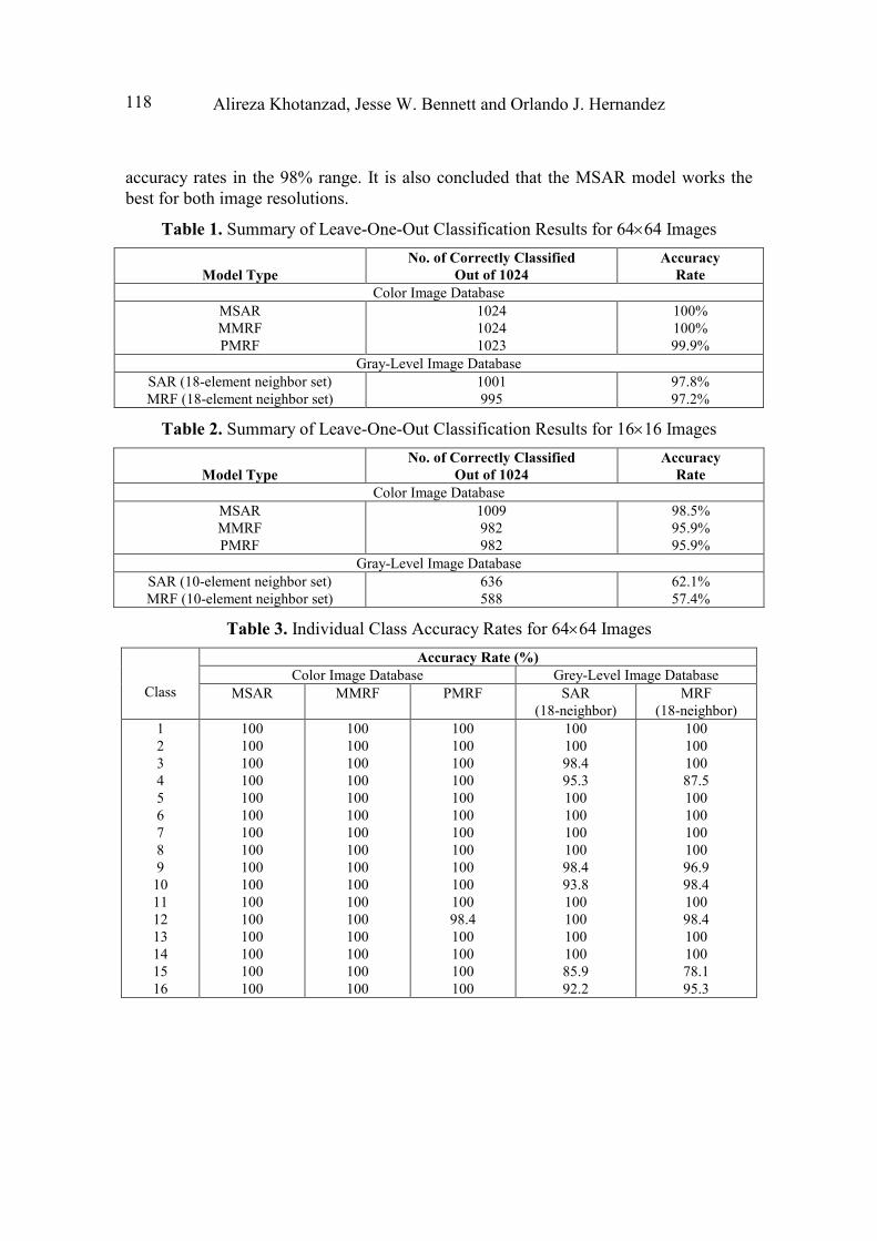
Tables 1 and 2 summarize the results for the 64×64 and 16×16 images, respectively. The number of correctly classified samples out of the total of 1024 tested samples

(tested one at a time) is shown for the color and gray-level images for features derived

from different models. Tables 3 and 4 show the individual classification accuracy rates

for each of the sixteen classes.

These results demonstrate that perfect classification can be achieved for 64×64 color texture images using features of either MSAR or MMRF model. For the PMRF model,

there is a single misclassification; one sample from class 12 (Candy Sprinkles) is

incorrectly assigned to class 10 (Fabric). For the lower image resolution of 16×16, classification accuracies remain high at 98.5% for the MSAR model and 95.9% for both

the MMRF and PMRF models, respectively. The majority of misclassified samples are

from class 4 (Leaves), which has textural characteristics that are similar to class 7

(Sand) and class 16 (Grass). Considering the results for both resolutions, it may be

concluded that the MSAR based features would be the best choice for the classification

task.

As for classification results of the gray-level counterparts images, the accuracy rates

for the 64×64 resolution are high and the SAR and MRF models perform equally well resulting in correct classification rate of 97.8% and 97.2%, respectively. However, when

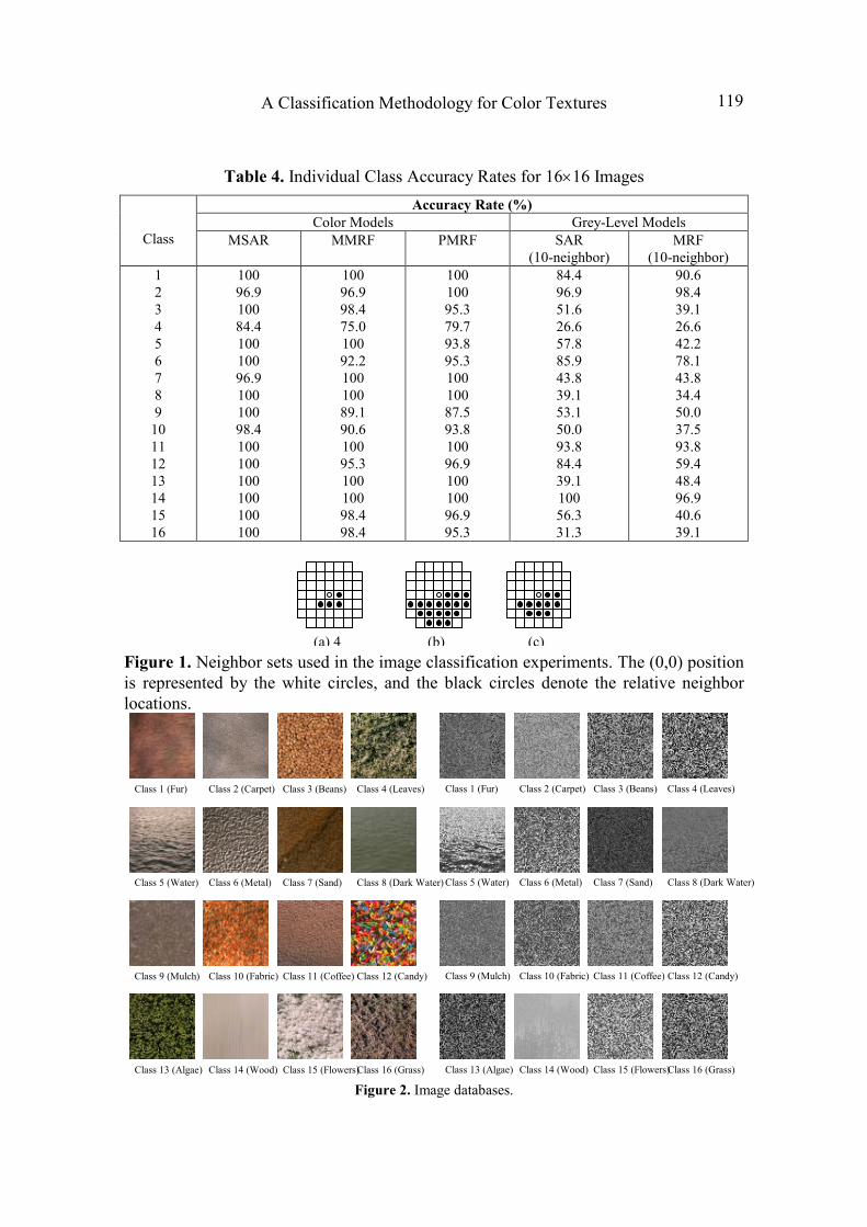
the resolution is reduced to 16×16, the performance degrades significantly yielding only 62.1% and 57.4% accuracies for the SAR and MRF models, respectively. In this case

many of the samples are misclassified and the confusion is spread over almost all

classes. As noted before, the structure of the utilized neighbor set is also different for the

two resolutions. The 18-element set of Figure 1(a) is used for the 64×64 case and the 10-element set of Figure 1(b) is utilized for the 16×16 resolution. These are neighbor sets that produce the best results from among many that were examined.

By comparing the classification results of color images to their gray-level converted

counterparts, the advantage of using color becomes apparent. At the 64×64 resolution, the color results are clearly better even though an optimal neighbor set is used with the

gray-level images. If the same 4-element neighbor set used for color images is utilized

for the gray-level images, the accuracy will be much lower. At the 16×16 resolution, the difference in performance becomes much more pronounced. While the color textures are

classified in the high 90% range, the rate for gray-level images is in the 60% range. At

this resolution, the textural detail within a single plane becomes fuzzy and interaction

between different image planes becomes more dominant. The inter-pane interactions,

which are somewhat invariant to image resolution, are captured by the multispectral

models causing them to perform better than their single plane, gray-level counterparts.

In this work three different multispectral random field models are used for supervised

color texture classification. These models capture both inter-plane and intra-plane

interactions of image pixels resulting in richer characterization of the image compared

to its gray-level counterpart. The performance is tested on 1024 images from a sixteen-

class database at two resolutions, 64×64 and 16×16. It is shown that a small and compact neighbor set is all that is needed for the classification task. In a leave-one-out

performance evaluation scheme and utilizing a normalized nearest-neighbor classifier,

perfect classification is obtained for 64×64 images whereas16×16 images produce


118

accuracy rates in the 98% range. It is also concluded that the MSAR model works the

best for both image resolutions.

Table 1. Summary of Leave-One-Out Classification Results for 64×64 Images

Model Type

No. of Correctly Classified

Out of 1024

Accuracy

Rate

Color Image Database

MSAR

MMRF

PMRF

1024

1024

1023

100%

100%

99.9%

Gray-Level Image Database

SAR (18-element neighbor set)

MRF (18-element neighbor set)

1001

995

97.8%

97.2%

Table 2. Summary of Leave-One-Out Classification Results for 16×16 Images

Model Type

No. of Correctly Classified

Out of 1024

Accuracy

Rate

Color Image Database

MSAR

MMRF

PMRF

1009

982

982

98.5%

95.9%

95.9%

Gray-Level Image Database

SAR (10-element neighbor set)

MRF (10-element neighbor set)

636

588

62.1%

57.4%

Table 3. Individual Class Accuracy Rates for 64×64 Images

Accuracy Rate (%)

Color Image Database Grey-Level Image Database

Class MSAR MMRF PMRF SAR

(18-neighbor)

MRF

(18-neighbor)

1

2

3

4

5

6

7

8

9

10

11

12

13

14

15

16

100

100

100

100

100

100

100

100

100

100

100

100

100

100

100

100

100

100

100

100

100

100

100

100

100

100

100

100

100

100

100

100

100

100

100

100

100

100

100

100

100

100

100

98.4

100

100

100

100

100

100

98.4

95.3

100

100

100

100

98.4

93.8

100

100

100

100

85.9

92.2

100

100

100

87.5

100

100

100

100

96.9

98.4

100

98.4

100

100

78.1

95.3


119

Table 4. Individual Class Accuracy Rates for 16×16 Images

Accuracy Rate (%)

Color Models Grey-Level Models

Class MSAR MMRF PMRF SAR

(10-neighbor)

MRF

(10-neighbor)

1

2

3

4

5

6

7

8

9

10

11

12

13

14

15

16

100

96.9

100

84.4

100

100

96.9

100

100

98.4

100

100

100

100

100

100

100

96.9

98.4

75.0

100

92.2

100

100

89.1

90.6

100

95.3

100

100

98.4

98.4

100

100

95.3

79.7

93.8

95.3

100

100

87.5

93.8

100

96.9

100

100

96.9

95.3

84.4

96.9

51.6

26.6

57.8

85.9

43.8

39.1

53.1

50.0

93.8

84.4

39.1

100

56.3

31.3

90.6

98.4

39.1

26.6

42.2

78.1

43.8

34.4

50.0

37.5

93.8

59.4

48.4

96.9

40.6

39.1

Figure 1. Neighbor sets used in the image classification experiments. The (0,0) position

is represented by the white circles, and the black circles denote the relative neighbor

locations.

Figure 2. Image databases.

(b) (c) (a) 4

Class 1 (Fur) Class 2 (Carpet) Class 3 (Beans) Class 4 (Leaves)

Class 5 (Water) Class 6 (Metal) Class 7 (Sand) Class 8 (Dark Water)

Class 9 (Mulch) Class 10 (Fabric) Class 11 (Coffee) Class 12 (Candy)

Class 13 (Algae) Class 14 (Wood) Class 15 (Flowers) Class 16 (Grass)

Class 1 (Fur) Class 2 (Carpet) Class 3 (Beans) Class 4 (Leaves)

Class 5 (Water) Class 6 (Metal) Class 7 (Sand) Class 8 (Dark Water)

Class 9 (Mulch) Class 10 (Fabric) Class 11 (Coffee) Class 12 (Candy)

Class 13 (Algae) Class 14 (Wood) Class 15 (Flowers) Class 16 (Grass)


120

7. REFERENCES

1. J. W. Bennett, Modeling and Analysis of Gray Tone, Color, and Multispectral

Texture Images by Random Field Models and Their Generalizations, Ph.D. Dissertation,

Southern Methodist University, 1997.

2. J. Bennett and A. Khotanzad, Maximum Likelihood Estimation Methods for

Multispectral Random Field Image Models, IEEE Trans. on Pattern Analysis and

Machine Intelligence, 21, 537-543, June 1999.

3. R. Chellappa and R. L. Kashyap, Synthetic Generation and Estimation in Random

Field Models of Images, Proc. IEEE Computer Society Conference on Pattern

Recognition and Image Processing, 577-582, Dallas, TX, Aug. 1981.

4. R. L. Kashyap and R. Chellappa, Estimation and Choice Neighbors in Spatial-

Interaction Models of Images, IEEE Trans. on Information Theory, IT-29, 60-72, 1983.

5. R. Chellappa and S. Chatterjee, Classification of Textures Using Gaussian Markov

Random Fields, IEEE Trans. on Acoustics, Speech, and Signal Processing, ASSP-33,

959-963, Aug. 1985.

6. Vision and Modeling Group, MIT Media Laboratory, Vision Texture (VisTex)

Database, http://www-white.media.mit.edu/vismod/, 1995.

7. "Basic parameter values for the HDTV standard for the studio and for international

programme exchange," Tech. Rep. ITU-R Recommendation BT.709, ITU, 1211 Geneva

20, Switzerland, 1990, formerly CCIR Rec. 709.

A CLASSIFICATION METHODOLOGY FOR COLOR TEXTURES USING MULTISPECTRAL RANDOM FIELD MATHEMATICAL MODELS

Documents

Transcript of A CLASSIFICATION METHODOLOGY FOR COLOR TEXTURES USING MULTISPECTRAL RANDOM FIELD MATHEMATICAL MODELS