IEEE

Proo

f

IEEE TRANSACTIONS ON GEOSCIENCE AND REMOTE SENSING, VOL. 46, NO. 12, DECEMBER 2008 1

Seabed Segmentation Using Optimized Statisticsof Sonar Textures

1

2

Imen Karoui, Ronan Fablet, Jean-Marc Boucher, Member, IEEE, and Jean-Marie Augustin3

Abstract—In this paper, we propose and compare two super-4vised algorithms for the segmentation of textured sonar images,5with respect to seafloor types. We characterize seafloors by a set of6empirical distributions estimated on texture responses to a set of7different filters. Moreover, we introduce a novel similarity measure8between sonar textures in this feature space. Our similarity mea-9sure is defined as a weighted sum of Kullback–Leibler divergences10between texture features. The weight setting is twofold. First,11each filter is weighted according to its discrimination power: The12computation of these weights are issued from a margin maxi-13mization criterion. Second, an additional weight, evaluated as an14angular distance between the incidence angles of the compared15texture samples, is considered to take into account sonar-image16acquisition process that leads to a variability of the backscattered17value and of the texture aspect with the incidence-angle range.18A Bayesian framework is used in the first algorithm where the19conditional likelihoods are expressed using the proposed similarity20measure between local pixel statistics and the seafloor prototype21statistics. The second method is based on a variational framework22as the minimization of a region-based functional that involves the23similarity between global-region texture-based statistics and the24predefined prototypes.25

Index Terms—Active regions, angular backscattering, feature26selection, level sets, maximum marginal probability (MMP), seg-27mentation, sonar images, texture.28

I. INTRODUCTION29

ACOUSTIC remote sensing, such as high-resolution multi-30

beam and sidescan sonars, provides new means for in situ31

observation of the seabed. The characterization of these high-32

resolution sonar images is important for a number of practical33

applications such as marine geology, commercial fishing, off-34

shore oil prospecting, and drilling [1]–[4].35

The segmentation and the classification of sonar images with36

respect to seafloor types (rocks, mud, sand, . . .) is the key37

goal behind the analysis of these acoustic images. This task,38

however, raises two major difficulties. The first task is to deal39

with texture in these images. Previous methods are generally40

based only on backscattered (BS) intensity models, and several41

parametric families of probabilistic distribution functions have42

Manuscript received January 4, 2008; revised May 20, 2008 andAugust 11, 2008.

I. Karoui, R. Fablet, and J.-M. Boucher are with the Department of Signaland Communications, École Nationale Supérieure des Télécommunications deBretagne, 29238 Brest Cedex 3, France (e-mail: imin.karoui@enst-bretagne.fr).

J.-M. Augustin is with the Department of Acoustics and Seismics, InstitutFrançais de Recherche et d’Exploitation de la Mer, 29280 Brest, France.

Color versions of one or more of the figures in this paper are available onlineat http://ieeexplore.ieee.org.

Digital Object Identifier 10.1109/TGRS.2008.2006362

Fig. 1. Typical sidscan sonar image (Rebent, IFREMER).

Fig. 2. BS evolution with the incidence angles for the three seafloor types ofFig. 1: sand, mud, and sand ripples.

been suggested (Rayleigh distribution, K distribution, Weibull 43

distribution, etc.) [3]–[8]. These first-order statistics are not 44

sufficient when high-resolution sonar images involve textures, 45

which is the case of most sonar images (Fig. 1). 46

The other important issue arising in seabed texture charac- 47

terization is a built-in feature of sonar observation: The value 48

of BS measure depends both on the seafloor type and on the 49

incident angle of the reflected acoustic signal, ranging typically 50

from −85◦ to +85◦. Fig. 2 shows the BS evolution for three 51

different seafloor types: sand, sand ripples, and mud. In addition 52

to the BS variability within incidence angles, seafloor textures 53

0196-2892/$25.00 © 2008 IEEE

IEEE

Proo

f

2 IEEE TRANSACTIONS ON GEOSCIENCE AND REMOTE SENSING, VOL. 46, NO. 12, DECEMBER 2008

Fig. 3. Sonar image composed of sand ripples. (Left) [5◦, 40◦].(Right) [80◦, 85◦].

are dependent on the incidence angles. Figs. 3 and 4 show a54

sonar image composed by sand ripples and rocks, respectively,55

for two angular sectors: [80◦, 85◦] and [5◦, 40◦]. The texture56

of sand ripples shows a loss of contrast in the specular sec-57

tor [5◦, 40◦]: The steep grazing angle reduces the backscatter58

differences between facing and trailing slopes, while at low59

incidence angles, much of the variation is lost due to increasing60

sonar shadow. A similar loss of contrast is observable in the61

rock samples (Fig. 4). BS behavior according to the incidence62

angles has been of wide interest for sonar imaging [3], [9]–[12].63

Parametric and nonparametric techniques have been proposed64

to model sonar-image behavior with respect to the incidence65

angle variations. The effect of the incidence angle on the BS66

has also been explored as a discriminating feature for seafloor67

recognition [4], [13], [14]. However, no studies have proposed68

a method to accurately compensate this phenomena because69

of the joint dependence of the seafloor types and on the local70

bathymetry which is generally unknown for sidescan sonar71

images. To our knowledge, the effects of the incidence angle on72

textured seabed features have not been addressed for segmen-73

tation issues. Only some studies were interested in simulating74

the behavior of oriented and textured seafloor types [15]–[18].75

These methods are mainly based on shape-from-shading [19]76

and were restricted to synthetic images or to real sonar images77

involving only one seafloor type.78

In this paper, we aim at using texture information within79

sonar seabed images and at developing segmentation algo-80

rithms that take into account angular variability of BS and81

textural features. We propose to characterize seafloors by a82

wide set of marginal distributions of their filter responses, and83

we measure seafloor similarities according to a weighted sum84

of Kullback–Leibler divergences [28] in this feature space.85

To cope with seafloor angular dependence, we introduce an86

additional weighting factor, evaluated as an angular distance87

between the compared texture samples: This angular distance88

is measured according to Gaussian kernels, whose variance89

sets the level of the angular variability, depending on textures90

and seafloor types. The proposed incidence-angle-and-texture-91

based similarity measure is exploited to develop two different92

Fig. 4. Rock texture for two angular sectors. (Left) [5◦, 40◦].(Right) [80◦, 85◦].

segmentation schemes. We first state the segmentation issue 93

as a Bayesian pixel-based labeling according to local texture 94

features. The second approach relies on a region-level vari- 95

ational framework, which resorts to a level-set minimization 96

of an energy criterion involving global-region-based seafloor 97

statistics. 98

This paper is organized as follows. The seafloor similarity 99

measure is introduced in Section II. The Bayesian segmentation 100

method is detailed in Section III. The region-based segmen- 101

tation algorithm is described in Section IV. Experiments are 102

reported and discussed in Section V, and conclusions are drawn 103

in Section VI. 104

II. SONAR-TEXTURE SIMILARITY MEASURE 105

Texture-based segmentation of seabed sonar images gener- 106

ally relies on Haralick [30] parameters or scalar spectral and 107

filter coefficients to model textures [20]–[22]. Recently, in the 108

field of texture analysis, features computed as statistics of local 109

filter responses have been shown to be relevant and discriminant 110

texture descriptors [23]–[27]. Motivated by these studies, we 111

propose to use texture features computed as marginal distrib- 112

utions of a wide set of filter seafloor responses. Each seafloor 113

type denoted by Tk is characterized by a set Qk composed of 114

the marginal distributions of the seafloor with respect to the 115

predefined filters. The following conditions are issued. 116

1) 121 cooccurrence distributions with horizontal and ver- 117

tical displacements denoted by dx and dy , respectively, 118

(dx, dy) ∈ {0, 1, . . . , 10}. 119

2) 50 distributions of the magnitude of Gabor filter 120

responses, computed for combination of parameters 121

(f0, σ, θ), where f0 is the radial frequency, σ is 122

the standard deviation, and θ is the orientation, such 123

that f0 ∈ {√

2/2k}k=1:6, σ ∈ {2k√

2}k=2:5, and θ ∈ 124

{0◦, 25◦, 45◦, 90◦, 135◦}. 125

3) 48 distributions of the energy of the image wavelet packet 126

coefficient computed for different bands (we used three 127

wavelet types: Haar, Daubechies, and Coiflet). 128

IEEE

Proo

f

KAROUI et al.: SEABED SEGMENTATION USING OPTIMIZED STATISTICS OF SONAR TEXTURES 3

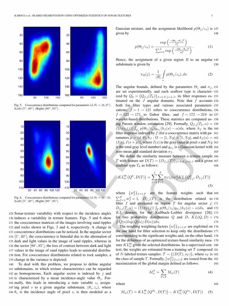
Fig. 5. Cooccurrence distributions computed for parameters (d, θ) = (6, 0◦).(Left) [5◦, 40◦]. (Right) [80◦, 85◦].

Fig. 6. Cooccurrence distributions computed for parameters (d, θ) = (6◦, 0).(Left) [5◦, 40◦]. (Right) [80◦, 85◦].

Sonar-texture variability with respect to the incidence angles129

induces a variability in texture features. Figs. 5 and 6 show130

the cooccurrence matrices of the images involving sand ripples131

and rocks shown in Figs. 3 and 4, respectively. A change in132

cooccurrence distributions can be noticed. In the angular sector133

[5◦, 40◦], the cooccurrence is bimodal due to the alternation of134

dark and light values in the image of sand ripples, whereas in135

the sector [80◦, 85◦], the loss of contrast between dark and light136

values in the image of sand ripples leads to unimodal distribu-137

tion. For cooccurrence distributions related to rock samples, a138

change in the variance is depicted.139

To deal with this problem, we propose to define angular140

subdomains, in which texture characteristics can be regarded141

as homogeneous. Each angular sector is indexed by j and142

is characterized by a mean incidence-angle value Θj . For-143

mally, this leads in introducing a state variable zs assign-144

ing pixel s to a given angular subdomain. (θs, zs), where145

θs is the incidence angle of pixel s, is then modeled as a146

Gaussian mixture, and the assignment likelihood p(Θj/zs) is 147

given by 148

p(Θj/zs) =exp

(−(Θj−θs)2

σ2j

)∑J

i=1 exp(

−(Θi−θs)2

σ2i

) . (1)

Hence, the assignment of a given region R to an angular 149

subdomain is given by 150

πR(j) =1|R|

∫s

p(Θj/zs), ds. (2)

The angular bounds, defined by the parameters Θj and σj , 151

are set experimentally, and each seafloor type is character- 152

ized by Qk = {Qf,j(Tk)}f=1:F,j=1:J , its filter responses es- 153

timated on the J angular domains. Note that f accounts 154

both for filter types and various associated parameteri- 155

zations: f = 1 → 121 refers to cooccurrence distributions, 156

f = 122 → 171 to Gabor filter, and f = 172 → 219 to 157

wavelet-based distributions. These statistics are computed us- 158

ing Parzen window estimation [29]. Formally, Qf,j(Tk, α) = 159

(1/πTk(j))

∫Tk

p(Θj/zs)gσf(hf (s) − α)ds, where hf is the 160

filter response indexed by f (for a cooccurrence matrix with pa- 161

rameters μ = (d, θ), hf : Ω → [1, Ng] × [1, Ng], and hf (s) = 162

(I(s), I(s + μ)), where I(s) is the gray value at pixel s and Ng 163

is the total gray level number) and gσfis a Gaussian kernel with 164

zero mean and standard deviation σf . 165

We define the similarity measure between a texture sample 166

T with feature set D(T ) = {Df,j(T )}f=1:F,j=1:J and a given 167

seafloor type Tk as follows: 168

KLΘw

(Qk,D(T )

)=

J∑j=1

F∑f=1

πT (j)w2fKL

(Qk

f,j ,Df,j(T ))(3)

where {w2f}f=1:F are the feature weights such that 169∑F

f=1 w2f = 1, Df,j(T ) is the distribution related to 170

filter f and estimated on region T for angular sector j: 171

Df,j(T, α) = (1/πT (j))∫

T p(Θj/zs)gσf(hf (s) − α)ds, and 172

KL denotes for the Kullback–Leibler divergence [28]; 173

for two probability distributions Q and D, KL(Q,D) = 174∫Q(α)log(Q(α)/D(α))dα. 175

The resulting weighting factors {w2f}f=1:F are exploited on 176

the one hand for filter selection to keep only the distributions 177

corresponding to the significant weights and, on the other hand, 178

for the definition of an optimized texture-based similarity mea- 179

sure KLΘw given the selected distributions. In a supervised con- 180

text, the weights are estimated from a training set T composed 181

of N -labeled texture samples: T = {(D(T ), sT )}, where sT is 182

the class of sample T . Formally, {w2f}f=1:F are issued from the 183

maximization of the global margin defined as follows: 184

MTw =

∑T∈T

Mw(T ) (4)

where 185

Mw(T ) = KLΘw

(QdT ,D(T )

)− KLΘ

w (QsT ,D(T )) (5)

IEEE

Proo

f

4 IEEE TRANSACTIONS ON GEOSCIENCE AND REMOTE SENSING, VOL. 46, NO. 12, DECEMBER 2008

where dT is the nearest class to T different from sT according186

to the similarity measure KLΘw187

dT = arg mink �=sT

KLΘw

(Qk,D(T )

). (6)

The maximization of the margin criterion MTw is carried out188

using a stochastic gradient method as detailed in our previous189

work [39].190

III. BAYESIAN SONAR-IMAGE SEGMENTATION191

As far as Bayesian image segmentation is concerned, the192

most popular criteria are the maximum a posteriori (MAP)193

[31] and the maximum marginal probability (MMP) [32]. It194

has been shown that the MMP estimation criterion is more195

appropriate for image segmentation than the MAP criterion196

[32]. The MAP estimate assigns the same cost to every incorrect197

segmentation regardless the number of pixels at which the198

estimated segmentation differs from the true one, whereas the199

MMP algorithm minimizes the expected value of the number of200

misclassified pixels. As shown in [32], the MMP procedure is201

equivalent to maximizing the marginal of the class labels. Let202

us introduce the following notations:203

1) S, the image lattice composed of N pixels;204

2) X = {xs}s∈S , the label random field;205

3) Y = {ys}s∈S , the random field of the observations, the206

textural feature in our case.207

Formally, the MMP scheme is equivalent to the maximi-208

zation of209

x̂MMPs = arg max

k∈{1:K}p(xs = k/y). (7)

In general, pixel conditional likelihood is computed according210

to local texture features like Gabor or wavelet coefficients.211

Here, we aim at using the proposed similarity measure KLΘw .212

We associate to each pixel s a set of features D(Ws) =213

{Df (Ws)}f=1:F estimated according to a Parzen estimation214

method [29], within a square window Ws centered at s. The215

window size that we denote by TW is set by the user according216

to texture coarseness. In our case, the observation denoted217

by a random field Y is specified by {ys = D(Ws)}s∈S . The218

conditional likelihood at each pixel s with respect to class k is219

then defined from the similarity measure KLΘw by220

p(ys/xs = k) =exp−KLΘ

w(Qk,D(Ws))∑Ki=1 exp−KLΘ

w(Qi,D(Ws)). (8)

As a prior PX , we consider a Markov random field associ-221

ated to an eight-neighborhood system with potential functions222

given by223

U2(x) =∑s∈S

∑t∈cs

αc (1 − δ(xs, xt)) (9)

where δ is the delta function and αc ∈ {αH , αV , αD} are real224

parameters assigned, respectively, to horizontal, vertical, and225

diagonal cliques. These parameters are estimated using the226

iterative conditional estimation procedure [42]. Using Bayes 227

rule, the posterior distribution is expressed as follows: 228

p(X,Y ) = p(Y/X)p(X) = p(X)∏s

p(ys/xs)

≈ exp

(∑s∈S

∑t∈cs

−αc(1−δ(xs,xt))+log(p(ys/xs))

). (10)

The maximization of local probabilities p(xs = k/y) is car- 229

ried out as follows [32]: We use the Gibbs sampler to gen- 230

erate a discrete-time Markov chain X(t) which converges in 231

distribution to a random field with probability mass functions 232

P (X/Y ). The marginal conditional distributions p(xs = k/y) 233

are then approximated as the fraction of time the Markov chain 234

spends in state k for each class k and each pixel s. The MMP 235

segmentation steps are the following. 236

1) Simulation of Tmax realizations of x1, x2, . . . , xTmax of 237

X using Gibbs sampler. 238

2) Using the realizations x1, x2, . . . , xTmax , p(xs/y) is esti- 239

mated using the frequency of each realizations 240

p(xs = k/y) =δ(x1

s − k)

+ · · · + δ(x1

s − k)

Tmax.

3) Choose as xs the class that maximizes p(xs = k/y). 241

IV. VARIATIONAL SONAR-IMAGE SEGMENTATION 242

Unlike the Bayesian scheme, the second approach is stated 243

at a region level as the minimization of a constrained energy 244

criterion E({Ωk}k=1:K) = E1 + E2, where Ωk is the domain 245

composed of all pixels attributed to the class k, E1 is a texture- 246

based data-driven term, and E2 is a regularization term detailed 247

as follows. 248

A. Functional Terms 249

E1({Ωk}k=1:K) is evaluated as the log-likelihood of a given 250

partition with respect to texture models. It is evaluated as the 251

sum of the similarities according to the measure KLΘw between 252

each region Ωk and its corresponding class Tk 253

E1 ({Ωk}k=1:K) =K∑

k=1

KLΘw

(Qk,D(Ωk)

)(11)

where Df,j(Ωk) is the marginal distribution of the image 254

response to the filter indexed by f . For angular domain j, 255

Df,j(Ωk) is estimated according to Parzen method [29]. 256

E2 is a regularization term, it penalizes the lengths of region 257

contours and is expressed by 258

E2 =K∑

k=1

γk|Γk|, γk ∈ �+ (12)

where |Γk| is the length of the contour Γk associated to the 259

region Ωk. 260

IEEE

Proo

f

KAROUI et al.: SEABED SEGMENTATION USING OPTIMIZED STATISTICS OF SONAR TEXTURES 5

B. Computation of the Evolution Equation261

We solve for the minimization of the functional E using262

a gradient-descent technique. It relies on the computation of263

the first derivative of E according to regions {Ωk}k=1:K . The264

evolution equation of region contours {Γk}k=1:K is then given265

by the following dynamic scheme [33]:266 {∂Γk(x,t)

∂t = Fk(x, t) �Nk

Γk(x, 0) = Γ0k

(13)

where �Nk is the unit inward normal to Γk at pixel x and at267

time t and Fk is the velocity field (in our case, Fk = ∇Ek, the268

derivative of E with respect to Γk).269

The explicit implementation of the curve evolution according270

to the latter dynamic scheme using a difference-approximation271

scheme cannot deal with topological changes of the moving272

front. This could be avoided by introducing the level-set method273

proposed by Osher and Sethian [34]. The basic idea of the274

method is the implicit representation of the moving interface Γ275

by a higher dimensional hypersurface ϕ (the level-set function)276

such that the zero level set of ϕ is actually the set of Γ and277 {Ωinside = {s ∈ Ω/ϕ(s) > 0}Ωoutside = {s ∈ Ω/ϕ(s) < 0} .

The evolution of the contours {Γk}k=1:K (13) is then equiv-278

alent to the evolution of the level-set functions {ϕk}k=1:K [34]279

∂ϕk(s, t)∂t

= Fk(s, t) |∇ϕk(s, t)| ∀s ∈ Ωk. (14)

E2 can be expressed using level-set functions ϕk [36]280

E2 =K∑

k=1

γk limα→0

∫Ω

δα(ϕk)|∇ϕk|ds (15)

where δα is a regularized delta function281

δα(s) ={

12α

(1 + cos

(πsα

)), if |s| ≤ α

0, if |s| < α.(16)

In order to cope with multiclass segmentation and to fulfill the282

image-partition constraint, we use an additional term E3 given283

by the following functional [38]:284

E3 =λ

2

∫Ω

(K∑

k=1

Hα(ϕk) − 1

)2

ds, λ ∈ �+ (17)

where Hα is a regularized Heaviside function285

Hα(s) =

⎧⎨⎩

12

(1 + s

α + 1π sin

(πsα

)), if |s| ≤ α

1, if s > α0, if s < −α.

(18)

As E = E1 + E2 + E3, we have286

∂ϕk

∂t(s, t) =

∂ϕ1k

∂t(s, t) +

∂ϕ2k

∂t(s, t) +

∂ϕ3k

∂t(s, t)

where ∂ϕik/∂t, i = 1, 2, 3 are the evolution equation terms 287

associated, respectively, to functionals Ei, i = 1, 2, 3. 288

The derivatives of the energy terms E2 and E3 are directly 289

estimated from level-set functions [35], [36] 290

∂ϕ2k

∂t(s, t) = γkδα(ϕk)div

(∇ϕk

|∇ϕk|

)∀k ∈ {1 : K} (19)

∂ϕ3k

∂t(s, t)=−δα(ϕk)λ

(K∑

k=1

(Hα(ϕk)−1)

)∀k ∈ {1 : K}.

(20)

The evolution equation related to E1 is more complex, since it 291

involves computations over the spatial support of each region. 292

To differentiate E1, we use shape-derivative tools, particularly 293

the Gâteaux derivative theorem given in [37]. As detailed in the 294

Appendix, it leads to 295

∂ϕ1k

∂t(s, t) = −

J∑j=1

F∑f=1

w2fp(Θj/zs)

[KL

(Qk

f,j ,Dkf,j

)

−(Qk

f,j/Df,j ∗ gσf(hf (s)) − 1

)]|∇ϕk| (21)

where ∗ is the convolution symbol. 296

The evolution equation related to the energy E1 (21) is 297

composed of two terms. 298

1) A global term −∑J

j=1

∑Ff=1 w2

fp(Θj/zs)KL(Qkf,j , 299

Df,j): This term is always negative or null. It is a contrac- 300

tion force that reduces the size of heterogeneous regions. 301

2) A local term∑J

j=1

∑Ff=1 w2

fp(Θj/zs)((Qkf,j/Df,j) − 302

1) ∗ gσf(hf (s)): This term locally compares the features 303

values at each pixel. This term can be positive or neg- 304

ative and aims at readjusting the statistics inside the 305

regions Df,j(Ωk) to fit to prototype models Qkf,j . The 306

contribution of each descriptor f is weighted by w2f and 307

p(Θj/zs), the relative contribution of descriptor f and of 308

angular sector j. 309

The overall evolution equations of the contours {Γk}k=1:K 310

are the following: 311

∂ϕk

∂t(s, t)

=−δα(ϕk)

×

⎡⎣ J∑

j=1

F∑f=1

w2fp(Θj/zs)

×(

KL(Qkf,j ,Df,j)−

Qkf,j

Df,j∗ gσf

(hf (s))+1

)

+ γkdiv(

∇ϕk

|∇ϕk|

)−λ

(K∑

k=1

(Hα(ϕk)−1)

)]∀k.

(22)

We apply these coupled evolution equations until convergence. 312

IEEE

Proo

f

6 IEEE TRANSACTIONS ON GEOSCIENCE AND REMOTE SENSING, VOL. 46, NO. 12, DECEMBER 2008

Fig. 7. Test images and their manual segmentation (in black line).

V. EXPERIMENTAL RESULTS AND DISCUSSION313

In previous work, we have tested the method on various314

optic textures (Brodatz textures). The method was compared315

to other texture-classification methods, and some results are316

reported in [39] and [40]. Here, we evaluate the proposed317

seabed-segmentation technique for different real sonar images318

acquired by a sidescan sonar, as part of a natural seabed-319

mapping project (IFREMER, Rebent Project) [41]. A reference320

interpretation by an expert is available [41]. Fig. 7 shows the321

set of images on which we carried out the experiments. We322

superimposed on these images the manual expert segmentation.323

Image I1 is composed of three seafloor types: rock, mud, and324

marl ripples [41]; I2 of rock, marl ripples, and mud seafloors;325

I3 of mud, sand, and marl ripples; I4 of marl and marl ripples;326

and I5 of sand, sand ripples, and rock. For I2 and I3, the angular327

variability of the sefloors, particularly marl ripples (for I2) and328

marl (for I3), is visually clear.329

For all these images, we first determine the most discriminant330

features among the initial set of 219 features: We apply the331

algorithm described in Section II and detailed in [39], and332

we keep only the feature set such that the cumulative sum333

of weights exceeds 0.9. Only a small number of features are334

retained. For example, Fig. 8 shows the plot of feature weights335

computed for image I1 and I5. For I1, the two cooccurrence336

matrices account for more than 90% of the total weight sum;337

these cooccurrence are computed for parameters (dx, dy) ∈338

{(1, 4), (2, 1)}. For I5, the cooccurrence distributions com-339

puted for parameters (dx, dy) ∈ {(2, 1), (2, 2)} are selected.340

For sonar images, we noticed that cooccurrence matrices are the341

Fig. 8. Feature weights. 1 → 121 cooccurrence distributions, 122 → 171Gabor filter-based features and 172 → 219 wavelet-based distributions.(a) I1. (b) I5.

TABLE ISEGMENTATION ERROR RATES

most selected features. In previous work on Brodatz textures 342

[39], [40], we remarked that Gabor and wavelet filters were 343

selected for oriented textures, whereas cooccurrence distribu- 344

tions, which, in addition to the detection of texture structures, 345

detect the intensity values change, are selected in the case of 346

texture having different intensity values and texture with regular 347

motifs. 348

For the five test images, three segmentation algorithms are 349

compared. 350

1) The maximum-likelihood (ML) segmentation denoted by 351

ML. This method consists in maximizing at each pixel the 352

conditional probability p(ys/xs) given by (8) 353

x̂s = arg maxk

p(ys/xs = k). (23)

Several analysis-window sizes are compared: TW ∈ {7 × 354

7, 17 × 17, 33 × 33}. 355

2) The MMP segmentation described in Section III, applied 356

for several analysis-window sizes: TW ∈ {7 × 7, 17 × 357

17, 33 × 33}. 358

3) The region-based variational segmentation described in 359

Section IV that we denote by V ar. 360

Table I summarizes the different error classification rates for all 361

segmentations. 362

All segmentation methods give quite good results according 363

to the mean classification error rates. MMP and variational 364

approaches are more efficient than the ML-based segmentation 365

because they take into account the spatial dependence between 366

pixels. The difference between these later approaches (MMP 367

and variational methods) mainly lies in the accuracy of the 368

localization of region boundaries and in the dependence of 369

MMP-based segmentation on the window size TW . In fact, 370

for the MMP segmentation, the use of small neighborhood 371

(TW = 7 × 7) leads to more accurate region frontiers but 372

small misclassified patches appear because of the neighborhood 373

IEEE

Proo

f

KAROUI et al.: SEABED SEGMENTATION USING OPTIMIZED STATISTICS OF SONAR TEXTURES 7

Fig. 9. MMP segmentation of I1 using TW = 7 × 7, τ = 12.5%.

Fig. 10. MMP segmentation of I1 using TW = 17 × 17, τ = 9.2%.

inefficiency for texture characterization. Conversely, the use374

of large window sizes (TW = 33 × 33) resorts to a lack of375

accuracy in the localization of the boundaries of the seabed376

regions because texture features extracted for pixels close to377

region boundaries involve a mixture of texture characteris-378

tics. The variational region-based approach does not need the379

choice of an analysis window and operates globally on region380

composed of pixels belonging to the same class. It resorts381

to a tradeoff between segmentation accuracy and region ho-382

mogeneity. Figs. 9–13 show examples of the dependence of383

MMP segmentation on the sizes of analysis window and on the384

robustness of the variational approach. In Fig. 14, we plot the385

mean error rate for different window sizes.386

We note that MMP and variational segmentations give sim-387

ilar results when the analysis-window size is well chosen for388

instance, TW = 17 × 17 for image I2 (Figs. 15 and 16), but389

its performance depends a lot on the choice of this parameter.390

This method can however be appropriate when the aim of the391

segmentation is to detect texture regions and without seeking392

for accurate boundaries.393

The variational approach is also interesting because it is394

much faster than the MMP segmentation. Being deterministic,395

the variational approach can be very fast particularly if we use396

appropriate initialization such as an initial segmentation based397

on the ML criterion. Whereas the MMP segmentation needs398

Fig. 11. MMP segmentation of I1 using TW = 33 × 33, τ = 13%.

Fig. 12. Region-based segmentation of I1, τ = 7.5%.

a large number of iterations, each iteration is also complex 399

and involves Gibbs sampling. For our implementations, the 400

convergence time of a variational image typically corresponds 401

to one iteration of the MMP algorithm. 402

To stress the interest of taking into account texture variability 403

with respect to incidence angles, additional segmentation re- 404

sults are reported for image I2 and I3 for which the seafloor 405

texture variability is clearer. In Table II, we summarize the 406

segmentation error rates for the segmentation with (J = 3) and 407

with no angular weighting, i.e., using only one angular domain 408

J = 1, for ML, MMP, and variational methods. In Figs. 17 and 409

18 are reported the associated segmentation results. It can be 410

noticed that a classical segmentation (without taking into ac- 411

count texture variability within incidence angles) cannot distin- 412

guish between visually similar seafloors (mud and marl ripples 413

for I2 and marl and sand for I3) near the specular domain. 414

VI. CONCLUSION 415

We proposed two segmentation algorithms for sonar-image 416

segmentation: a Bayesian algorithm using local statistics and a 417

region-based variational algorithm, both based on a novel sim- 418

ilarity measure between seafloor-type images according to the 419

statistics of their responses to a large set of filters. This similar- 420

ity measure is expressed as a weighted sum of Kullback–Leibler 421

IEEE

Proo

f

8 IEEE TRANSACTIONS ON GEOSCIENCE AND REMOTE SENSING, VOL. 46, NO. 12, DECEMBER 2008

Fig. 13. Segmentations of I4. (a) MMP: TW = 7, τ = 4%. (b) MMP: TW = 33, τ = 6%. (c) Variational method: τ = 3%.

Fig. 14. Mean segmentation error rate for several window sizes.

Fig. 15. MMP-based segmentation of I2 TW = 17, τ = 4%.

divergences between individual seafloor filter-response statis-422

tics. The resulting weighting factors are exploited on the one423

hand for filter selection and, on the other hand, for taking424

into account the incidence angular dependence of seafloor tex-425

tures. The conclusion is the cooccurrence matrices outperform426

the other features for our sonar images. The results show427

that the performance of the Bayesian approach depends on428

the size of the analysis window. For pixel-based segmenta-429

tion (ML and MMP segmentations), the size must be tuned430

according to the coarseness of given textures. The results431

also stress the suitability of the region-based approach as432

compared to the Bayesian pixel-based scheme for texture seg-433

mentation and demonstrate the interest of taking into account434

Fig. 16. Variational-based segmentation of I2, τ = 3%.

TABLE IISEGMENTATION ERROR RATES

Fig. 17. I2 region-based segmentation with and without angular weighting.(a) J = 1, τ = 23.5%. (b) J = 3, τ = 3%.

Fig. 18. I3 MMP-based segmentation with and without angular weighting.(a) J = 1, τ = 16%. (b) J = 3, τ = 8%.

the angular backscatter variabilities to discriminate between 435

seafloor types particularly near the specular sector. 436

IEEE

Proo

f

KAROUI et al.: SEABED SEGMENTATION USING OPTIMIZED STATISTICS OF SONAR TEXTURES 9

APPENDIX437

EVOLUTION EQUATION COMPUTATION438

Using the shape-derivative tools, we want to differentiate the439

functional440

F (Ωk) = KLΘw

(Qk,D(Ωk)

)which can be written as follows:441

J∑j=1

F∑f=1

πΩk(j)w2

f

∫Rf

Qkf,j(α) log

(Qk

f,j(α)Df,j(Ωk, α)

)dα.

Let us introduce the following notations.442

1)443

Hkj = Qk

f,j(α) log

(Qk

f,j(α)Df,j(Ωk, α)

).

2)444

G1 =∫Ωk

p(Θj/zs)gσf(hf (s) − α) ds.

Then, we have445

F (Ωk) =J∑

j=1

F∑f=1

w2fπΩk

(j)∫

Rf

Hkj .

The Gâteaux derivative of F (Ωk) in the direction of a vector446

field �V is given by447

dF (Ωk, �V ) =J∑

j=1

F∑f=1

w2fdπΩk

(j)(Ωk, �V )∫

Rf

Hkj dα

+ πΩk(j)

∫Rf

dHkj (Ωk, �V )dα. (24)

Theorem: See [37].448

The Gâteaux derivative of a functional of the type K(Ω) =449 ∫Ω k(s,Ω)ds is given by450

dK(Ω, �V ) =∫Ω

ksh(s,Ω, �V )ds −∫Γ

k(s,Ω)(�V �N)da(s)

where Ω denoted a region and Γ its boundary; ksh(s,Ω, �V ) is451

the shape derivative of k(s,Ω).452

In our case453

dπΩk(j)(Ωk, �V ) = −

∫Γk

p(Θj/zs)(�V · �Nk)d�a(s)

Hkj can be written as454

Hkj = Qk

f,j(α) log

(πΩk

(j)Qkf,j(α)

G1(Ωk, f, j, α)

).

Using the chain rule, we get 455

dHkj (Ωk, �V )=

(∂Hk

j

∂G1dG1(Ωk, �V )+

∂Hkj

∂πΩk(j)

dπΩk(j)(Ωk, �V )

)

∂Hkj

∂G1= −

Qkf,j

G1

∂Hkj

∂πΩk(j)

=Qk

f,j

πΩk(j)

.

According to the previous theorem, we get 456

dG1(Ωk, �V ) = −∫Γk

p(Θj/zs)gσf(hf (s) − α) (�V · �Nk)d�a(s).

Finally, we get 457

dHkj (Ωk, �V )

=∫Γk

p(Θj/zs)

[Qk

f,j(α)G1(f, α,Ωk)

gσf(hf (s) − α) − Qf (α)

πΩk(j)

]

× (�V · �Nk)d�a(s)

=1

πΩk(j)

∫Γk

p(Θj/zs)

[Qk

f,j(α)Df,j(Ωk, α)

gσf(hf (s)−α) Qf (α)

]

× (�V · �Nk)d�a(s)∫

Rf

dHkj (Ωk, �V )dα

=1

πΩk(j)

∫Γk

p(Θj/zs)

[Qk

f,j

Df,j(Ωk)∗ gσf

(hf (s)) − 1

]

× (�V · �Nk)d�a(s).

Finally, according to (24) 458

dF (Ωk, �V )

= −J∑

j=1

F∑f=1

p(Θj/zs)w2f

×∫Γk

[KL

(Qk

f,j ,Df,j

)−

(Qk

f,j

Df,j(Ωk)−1

)∗ gσf

(hf (s))

]

×(

�V · �Nk

)d�a(s).

REFERENCES 459

[1] P. Brehmer, F. Gerlotto, J. Guillard, F. Sanguinède, Y. Guénnegan, and 460D. Buestel, “New applications of hydroacoustic methods for monitoring 461shallow water aquatic ecosystems: The case of mussel culture grounds,” 462Aquat. Living Resour., vol. 16, no. 3, pp. 333–338, Jul. 2003. 463

[2] M. Mignotte, C. Collet, P. Perez, and P. Bouthemy, “Hybrid genetic 464optimization and statistical model based approach for the classification 465of shadow shapes in sonar imagery,” IEEE Trans. Pattern Anal. Mach. 466Intell., vol. 22, no. 2, pp. 129–141, Feb. 2000. 467

IEEE

Proo

f

10 IEEE TRANSACTIONS ON GEOSCIENCE AND REMOTE SENSING, VOL. 46, NO. 12, DECEMBER 2008

[3] L. Hellequin, J. M. Boucher, and X. Lurton, “Processing of high-468frequency multibeam echo sounder data for seafloor characterization,”469IEEE J. Ocean. Eng., vol. 28, no. 1, pp. 78–89, Jan. 2003.470

[4] G. Le Chenadec and J. M. Boucher, “Sonar image segmentation us-471ing the angular dependence of backscattering distributions,” in Proc.472Oceans—Europe, Brest, France, 2005, vol. 1, pp. 147–152.473

[5] G. Le Chenadec, J.-M. Boucher, and X. Lurton, “Angular dependence474of K-distributed sonar data,” IEEE Trans. Geosci. Remote Sens., vol. 45,475no. 5, pp. 1224–1236, May 2007.476

[6] E. Jakeman, “Non-Gaussian models for the statistics of scattered waves,”477Adv. Phys., vol. 37, no. 5, pp. 471–529, Oct. 1988.478

[7] A. P. Lyons and D. A. Abraham, “Statistical characterization of high-479frequency shallow-water seafloor backscatter,” J. Acoust. Soc. Amer.,480vol. 106, no. 3, pp. 1307–1315, Sep. 1999.481

[8] D. A. Abraham and A. P. Lyons, “Novel physical interpretations of482k-distributed reverberation,” IEEE J. Ocean. Eng., vol. 27, no. 4, pp. 800–483813, Oct. 2002.484

[9] N. C. Mitchell, “Processing and analysis of Simrad multibeam sonar485data,” Mar. Geophys. Res., vol. 18, no. 6, pp. 729–739, Dec. 1996.486

[10] G. Le Chenadec, J. M. Boucher, X. Lurton, and J. M. Augustin, “Angular487dependence of statistical distributions for backscattered signals: Model-488ing and application to multibeam echosounder data,” in Proc. Oceans,489Sep. 2003, vol. 2, pp. 897–903.490

[11] D. R. Jackson, D. P. Winbrenner, and A. Ishimaru, “Application of the491composite roughness model to high-frequency bottom backscattering,”492J. Acoust. Soc. Amer., vol. 79, no. 5, pp. 1410–1422, May 1986.493

[12] C. de Moustier and D. Alexandrou, “Angular dependence of 12-kHz494seafloor acoustic backscatter,” J. Acoust. Soc. Amer., vol. 90, no. 1,495pp. 522–531, Jul. 1991.496

[13] J. E. Hughes-Clarke, “Toward remote seafloor classification using the497angular response of acoustic backscatter: A case study from multiple498overlapping GLORIA data,” IEEE J. Ocean. Eng., vol. 19, no. 1, pp. 112–499127, Jan. 1994.500

[14] E. Pouliquen and X. Lurton, “Automated sea-bed classification system for501echo-sounders,” in Proc. Oceans, Oct. 1992, vol. 1, pp. 317–321.502

[15] D. Langer and M. Herbert, “Building qualitative elevation maps from side503scan sonar data for autonomous underwater navigation,” in Proc. IEEE504Int. Conf. Robot. Autom., Apr. 1991, vol. 3, pp. 2478–2483.505

[16] R. Li and S. Pai, “Improvement of bathymetric data bases by shape from506shading technique using side-scan sonar images,” in Proc. OCEANS,507Oct. 1991, vol. 1, pp. 320–324.508

[17] E. Dura, J. Bell, and D. Lane, “Reconstruction of textured seafloors from509side-scan sonar images,” Proc. Inst. Elect. Eng.—Radar Sonar Navig.,510vol. 151, no. 2, pp. 114–125, Apr. 2004.511

[18] A. E. Johnson and M. Hebert, “Seafloor map generation for autonomous512underwater vehicle navigation,” Auton. Robots, vol. 3, no. 2, pp. 145–168,513Jun. 1996.514

[19] R. Zhang, P. Tsai, J. E. Cryer, and M. Shah, “Shape from shading:515A survey,” IEEE Trans. Pattern Anal. Mach. Intell., vol. 21, no. 8, pp. 690–516705, Aug. 1999.517

[20] T. H. Eggen, “Acoustic sediment classification experiment by means518of multibeam echosounders,” Acoust. Classification Mapping Seabed,519vol. 15, no. 2, pp. 437–444, 1993.520

[21] L. M. Linnett, S. J. Clarke, and D. R. Carmichael, “The analysis of521sidescan sonar images for seabed types and objects,” in Proc. 2nd Eur.522Conf. Underwater Acoust., 1994, vol. 22, pp. 187–194.523

[22] M. Lianantonakis and Y. R. Petillot, “Sidescan sonar segmentation using524active contours and level set method,” in Proc. OCEANS—Europe, Brest,525France, 2005, vol. 1, pp. 719–724.526

[23] L. Xiuwen and W. DeLiang, “Texture classification using spectral his-527tograms,” IEEE Trans. Image Process., vol. 12, no. 6, pp. 661–670,528Jun. 2003.529

[24] O. G. Cula and K. Dana, “3D texture recognition using bidirectional530feature histograms,” Int. J. Comput. Vis., vol. 59, no. 1, pp. 33–60,531Aug. 2004.532

[25] R. Fablet and P. Bouthemy, “Motion recognition using nonparametric im-533age motion models estimated from temporal and multiscale co-occurrence534statistics,” IEEE Trans. Pattern Anal. Mach. Intell., vol. 25, no. 12,535pp. 1619–1624, Dec. 2003.536

[26] P. Nammalwar, O. Ghita, and P. F. Whelan, “Integration of feature distrib-537utions for colour texture segmentation,” in Proc. Int. Conf. Pattern Recog.,538Aug. 2005, vol. 1, pp. 716–719.539

[27] Q. Xu, J. Yang, and S. Ding, “Texture Segmentation using LBP embedded540region competition,” Electron. Lett. Comput. Vis. Image Anal., vol. 5,541no. 1, pp. 41–47, 2004.542

[28] S. Kullback, “On information and sufficiency,” in The Annals of Mathe-543matical Statistics, vol. 22. New York: Wiley, 1951.544

[29] E. Parzen, “On estimation of a probability density function and mode,” 545Ann. Math. Stat., vol. 33, no. 3, pp. 1065–1076, Sep. 1962. 546

[30] R. M. Haralick, “Statistical and structural approaches to texture,” Proc. 547IEEE, vol. 67, no. 5, pp. 786–804, May 1979. 548

[31] S. Geman and G. Geman, “Stochastic relaxation, Gibbs distributions, and 549the Bayesian restoration of images,” IEEE Trans. Pattern Anal. Mach. 550Intell., vol. PAMI-6, no. 6, pp. 721–741, Nov. 1984. 551

[32] J. Marroquin, S. Mitter, and T. Poggio, “Probabilistic solution of ill-posed 552problems in computational vision,” J. Am. Stat. Assoc., vol. 82, no. 397, 553pp. 76–89, Mar. 1987. 554

[33] M. Kass, A. Withkin, and D. Terzopoulos, “Snakes: Active contour mod- 555els,” Int. J. Comput. Vis., vol. 1, no. 4, pp. 321–331, Jan. 1988. 556

[34] J. A. Sethian, Level Set Methods. Cambridge, U.K.: Cambridge Univ. 557Press, 1996. 558

[35] J. F. Aujol, G. Aubert, and L. Blanc-Féraud, “Wavelet-based level set evo- 559lution for classification of textured images,” IEEE Trans. Image Process., 560vol. 12, no. 12, pp. 1634–1641, Dec. 2003. 561

[36] C. Samson, L. Blanc-Féraud, G. Aubert, and J. Zerubia, “A level set 562method for image classification,” Int. J. Comput. Vis., vol. 40, no. 3, 563pp. 187–197, 2000. 564

[37] S. Jehan-Besson, M. Barlaud, and G. Aubert, “Image segmentation using 565active contours: Calculus of variations or shape gradients?” SIAM J. Appl. 566Math., vol. 63, no. 6, pp. 2128–2154, 2003. 567

[38] H. K. Zhao, T. Chan, B. Merriman, and S. Osher, “A variational level 568set approach to multiphase motion,” J. Comput. Phys., vol. 127, no. 1, 569pp. 179–195, Aug. 1996. 570

[39] I. Karoui, R. Fablet, J. M. Boucher, and J. M. Augustin, “Separability- 571based Kullback divergence weighting and filter selection for texture clas- 572sification and segmentation,” in Proc. 18th ICPR, Hong Kong, Aug. 2006. 573

[40] I. Karoui, R. Fablet, J. M. Boucher, W. Pieczynski, and J. M. Augustin, 574“Fusion of textural statistics using a similarity measure: Application 575to texture recognition and segmentation,” Pattern Anal. Appl., vol. 11, 576no. 3/4, pp. 425–434, Sep. 2008. Computer Science. 577

[41] A. Ehrhold, D. Hamon, and B. Guillaumont, “The Rebent monitor- 578ing network, a spatially integrated, acoustic approach to surveying 579nearshore macrobenthic habitats: Application to the bay of Concarneau 580(South Brittany, France),” ICES J. Mar. Sci., vol. 63, no. 9, pp. 1604– 5811615, Jan. 2006. 582

[42] W. Pieczynski, “Statistical image segmentation,” Mach. Graph. Vis., 583vol. 1, no. 2, pp. 261–268, 1992. 584

Imen Karoui received the M.Sc. degree in telecom- 585munications from École Polytechnique de Tunis, 586Tunisia, in 2002, the D.E.A. degree in STIR (sig- 587nal, télécommunications, images, radar) from the 588Université de Rennes 1, Rennes, France, in 2003, 589and the Ph.D. degree in signal processing and 590telecommunications from the Department of Signal 591and Communications, École Nationale Supérieure 592des Télécommunications de Bretagne (Telecom 593Bretagne), Brest Cedex 3, France, in 2007. 594

She is currently a Postdoctor with Telecom 595Bretagne. Her research interests include texture analysis and segmentation with 596application to acoustic imaging and fisheries. 597

Ronan Fablet receive the M.Sc. degree in signal 598processing and telecommunications from École Na- 599tionale Supérieure de l’Aéronautique et de l’Espace, 600Toulouse Cedex 4, France, in 1997 and the Ph.D. 601degree in signal processing and telecommunications 602from the University of Rennes 1, Rennes, France, 603in 2001. 604

In 2002, he was an INRIA Postdoctoral Fellow 605with Brown University, Providence, RI. From 2003 606to 2007, he had a full-time research position with the 607Institut Français de Recherche et d’Exploitation de 608

la Mer, Brest, France, in the field of biological oceanography. Since 2008, he 609has been an Assistant Professor with the Department of Signal and Commu- 610nications, École Nationale Supérieure des Télécommunications de Bretagne, 611Brest Cedex 3, France. His main interests include sonar and radar imaging 612particularly applied to biological and physical oceanography and signal and 613image processing applied to biological archives. 614

IEEE

Proo

f

KAROUI et al.: SEABED SEGMENTATION USING OPTIMIZED STATISTICS OF SONAR TEXTURES 11

Jean-Marc Boucher (M’83) was born in 1952.615He received the M.Sc. degree in telecommunica-616tions from École Nationale Supérieure des Télé-617communications, Paris, France, in 1975 and the618Habilitation à Diriger des Recherches degree from619the University of Rennes 1, Rennes, France, in 1995.620

He is currently a Professor with the Department621of Signal and Communications, École Nationale622Supérieure des Télécommunications de Bretagne,623Brest Cedex 3, France, where he is also an Education624Deputy Director. He is also the Deputy Manager of625

a National Scientific Research Center Laboratory (Institut Telecom-Telecom626Bretagne-UMR CNRS 3192 lab-STICC, Université Européenne de Bretagne-627France). His current researches are related to statistical signal analysis, in-628cluding estimation theory, Markov models, blind deconvolution, wavelets,629and multiscale-image analysis. These methods are applied to radar and sonar630images, seismic signals, and electrocardiographic signals. He published about631a hundred technical articles in these areas in international journals and632conferences.633

Jean-Marie Augustin received the Master degree in 634signal processing from the University of Rennes 1, 635Rennes, France, in 1982. 636

Since 1984, he has been with the Institut Français 637de Recherche et d’Exploitation de la Mer, Brest, 638France, the French public institute for marine re- 639search, where he is currently a Senior Engineer 640with the Department of Acoustics and Seismics. 641His main interests include software development for 642sonar seafloor mapping and backscatter reflectivity 643analysis. 644

IEEE

Proo

f

IEEE TRANSACTIONS ON GEOSCIENCE AND REMOTE SENSING, VOL. 46, NO. 12, DECEMBER 2008 1

Seabed Segmentation Using Optimized Statisticsof Sonar Textures

1

2

Imen Karoui, Ronan Fablet, Jean-Marc Boucher, Member, IEEE, and Jean-Marie Augustin3

Abstract—In this paper, we propose and compare two super-4vised algorithms for the segmentation of textured sonar images,5with respect to seafloor types. We characterize seafloors by a set of6empirical distributions estimated on texture responses to a set of7different filters. Moreover, we introduce a novel similarity measure8between sonar textures in this feature space. Our similarity mea-9sure is defined as a weighted sum of Kullback–Leibler divergences10between texture features. The weight setting is twofold. First,11each filter is weighted according to its discrimination power: The12computation of these weights are issued from a margin maxi-13mization criterion. Second, an additional weight, evaluated as an14angular distance between the incidence angles of the compared15texture samples, is considered to take into account sonar-image16acquisition process that leads to a variability of the backscattered17value and of the texture aspect with the incidence-angle range.18A Bayesian framework is used in the first algorithm where the19conditional likelihoods are expressed using the proposed similarity20measure between local pixel statistics and the seafloor prototype21statistics. The second method is based on a variational framework22as the minimization of a region-based functional that involves the23similarity between global-region texture-based statistics and the24predefined prototypes.25

Index Terms—Active regions, angular backscattering, feature26selection, level sets, maximum marginal probability (MMP), seg-27mentation, sonar images, texture.28

I. INTRODUCTION29

ACOUSTIC remote sensing, such as high-resolution multi-30

beam and sidescan sonars, provides new means for in situ31

observation of the seabed. The characterization of these high-32

resolution sonar images is important for a number of practical33

applications such as marine geology, commercial fishing, off-34

shore oil prospecting, and drilling [1]–[4].35

The segmentation and the classification of sonar images with36

respect to seafloor types (rocks, mud, sand, . . .) is the key37

goal behind the analysis of these acoustic images. This task,38

however, raises two major difficulties. The first task is to deal39

with texture in these images. Previous methods are generally40

based only on backscattered (BS) intensity models, and several41

parametric families of probabilistic distribution functions have42

Manuscript received January 4, 2008; revised May 20, 2008 andAugust 11, 2008.

I. Karoui, R. Fablet, and J.-M. Boucher are with the Department of Signaland Communications, École Nationale Supérieure des Télécommunications deBretagne, 29238 Brest Cedex 3, France (e-mail: imin.karoui@enst-bretagne.fr).

J.-M. Augustin is with the Department of Acoustics and Seismics, InstitutFrançais de Recherche et d’Exploitation de la Mer, 29280 Brest, France.

Color versions of one or more of the figures in this paper are available onlineat http://ieeexplore.ieee.org.

Digital Object Identifier 10.1109/TGRS.2008.2006362

Fig. 1. Typical sidscan sonar image (Rebent, IFREMER).

Fig. 2. BS evolution with the incidence angles for the three seafloor types ofFig. 1: sand, mud, and sand ripples.

been suggested (Rayleigh distribution, K distribution, Weibull 43

distribution, etc.) [3]–[8]. These first-order statistics are not 44

sufficient when high-resolution sonar images involve textures, 45

which is the case of most sonar images (Fig. 1). 46

The other important issue arising in seabed texture charac- 47

terization is a built-in feature of sonar observation: The value 48

of BS measure depends both on the seafloor type and on the 49

incident angle of the reflected acoustic signal, ranging typically 50

from −85◦ to +85◦. Fig. 2 shows the BS evolution for three 51

different seafloor types: sand, sand ripples, and mud. In addition 52

to the BS variability within incidence angles, seafloor textures 53

0196-2892/$25.00 © 2008 IEEE

IEEE

Proo

f

2 IEEE TRANSACTIONS ON GEOSCIENCE AND REMOTE SENSING, VOL. 46, NO. 12, DECEMBER 2008

Fig. 3. Sonar image composed of sand ripples. (Left) [5◦, 40◦].(Right) [80◦, 85◦].

are dependent on the incidence angles. Figs. 3 and 4 show a54

sonar image composed by sand ripples and rocks, respectively,55

for two angular sectors: [80◦, 85◦] and [5◦, 40◦]. The texture56

of sand ripples shows a loss of contrast in the specular sec-57

tor [5◦, 40◦]: The steep grazing angle reduces the backscatter58

differences between facing and trailing slopes, while at low59

incidence angles, much of the variation is lost due to increasing60

sonar shadow. A similar loss of contrast is observable in the61

rock samples (Fig. 4). BS behavior according to the incidence62

angles has been of wide interest for sonar imaging [3], [9]–[12].63

Parametric and nonparametric techniques have been proposed64

to model sonar-image behavior with respect to the incidence65

angle variations. The effect of the incidence angle on the BS66

has also been explored as a discriminating feature for seafloor67

recognition [4], [13], [14]. However, no studies have proposed68

a method to accurately compensate this phenomena because69

of the joint dependence of the seafloor types and on the local70

bathymetry which is generally unknown for sidescan sonar71

images. To our knowledge, the effects of the incidence angle on72

textured seabed features have not been addressed for segmen-73

tation issues. Only some studies were interested in simulating74

the behavior of oriented and textured seafloor types [15]–[18].75

These methods are mainly based on shape-from-shading [19]76

and were restricted to synthetic images or to real sonar images77

involving only one seafloor type.78

In this paper, we aim at using texture information within79

sonar seabed images and at developing segmentation algo-80

rithms that take into account angular variability of BS and81

textural features. We propose to characterize seafloors by a82

wide set of marginal distributions of their filter responses, and83

we measure seafloor similarities according to a weighted sum84

of Kullback–Leibler divergences [28] in this feature space.85

To cope with seafloor angular dependence, we introduce an86

additional weighting factor, evaluated as an angular distance87

between the compared texture samples: This angular distance88

is measured according to Gaussian kernels, whose variance89

sets the level of the angular variability, depending on textures90

and seafloor types. The proposed incidence-angle-and-texture-91

based similarity measure is exploited to develop two different92

Fig. 4. Rock texture for two angular sectors. (Left) [5◦, 40◦].(Right) [80◦, 85◦].

segmentation schemes. We first state the segmentation issue 93

as a Bayesian pixel-based labeling according to local texture 94

features. The second approach relies on a region-level vari- 95

ational framework, which resorts to a level-set minimization 96

of an energy criterion involving global-region-based seafloor 97

statistics. 98

This paper is organized as follows. The seafloor similarity 99

measure is introduced in Section II. The Bayesian segmentation 100

method is detailed in Section III. The region-based segmen- 101

tation algorithm is described in Section IV. Experiments are 102

reported and discussed in Section V, and conclusions are drawn 103

in Section VI. 104

II. SONAR-TEXTURE SIMILARITY MEASURE 105

Texture-based segmentation of seabed sonar images gener- 106

ally relies on Haralick [30] parameters or scalar spectral and 107

filter coefficients to model textures [20]–[22]. Recently, in the 108

field of texture analysis, features computed as statistics of local 109

filter responses have been shown to be relevant and discriminant 110

texture descriptors [23]–[27]. Motivated by these studies, we 111

propose to use texture features computed as marginal distrib- 112

utions of a wide set of filter seafloor responses. Each seafloor 113

type denoted by Tk is characterized by a set Qk composed of 114

the marginal distributions of the seafloor with respect to the 115

predefined filters. The following conditions are issued. 116

1) 121 cooccurrence distributions with horizontal and ver- 117

tical displacements denoted by dx and dy , respectively, 118

(dx, dy) ∈ {0, 1, . . . , 10}. 119

2) 50 distributions of the magnitude of Gabor filter 120

responses, computed for combination of parameters 121

(f0, σ, θ), where f0 is the radial frequency, σ is 122

the standard deviation, and θ is the orientation, such 123

that f0 ∈ {√

2/2k}k=1:6, σ ∈ {2k√

2}k=2:5, and θ ∈ 124

{0◦, 25◦, 45◦, 90◦, 135◦}. 125

3) 48 distributions of the energy of the image wavelet packet 126

coefficient computed for different bands (we used three 127

wavelet types: Haar, Daubechies, and Coiflet). 128

IEEE

Proo

f

KAROUI et al.: SEABED SEGMENTATION USING OPTIMIZED STATISTICS OF SONAR TEXTURES 3

Fig. 5. Cooccurrence distributions computed for parameters (d, θ) = (6, 0◦).(Left) [5◦, 40◦]. (Right) [80◦, 85◦].

Fig. 6. Cooccurrence distributions computed for parameters (d, θ) = (6◦, 0).(Left) [5◦, 40◦]. (Right) [80◦, 85◦].

Sonar-texture variability with respect to the incidence angles129

induces a variability in texture features. Figs. 5 and 6 show130

the cooccurrence matrices of the images involving sand ripples131

and rocks shown in Figs. 3 and 4, respectively. A change in132

cooccurrence distributions can be noticed. In the angular sector133

[5◦, 40◦], the cooccurrence is bimodal due to the alternation of134

dark and light values in the image of sand ripples, whereas in135

the sector [80◦, 85◦], the loss of contrast between dark and light136

values in the image of sand ripples leads to unimodal distribu-137

tion. For cooccurrence distributions related to rock samples, a138

change in the variance is depicted.139

To deal with this problem, we propose to define angular140

subdomains, in which texture characteristics can be regarded141

as homogeneous. Each angular sector is indexed by j and142

is characterized by a mean incidence-angle value Θj . For-143

mally, this leads in introducing a state variable zs assign-144

ing pixel s to a given angular subdomain. (θs, zs), where145

θs is the incidence angle of pixel s, is then modeled as a146

Gaussian mixture, and the assignment likelihood p(Θj/zs) is 147

given by 148

p(Θj/zs) =exp

(−(Θj−θs)2

σ2j

)∑J

i=1 exp(

−(Θi−θs)2

σ2i

) . (1)

Hence, the assignment of a given region R to an angular 149

subdomain is given by 150

πR(j) =1|R|

∫s

p(Θj/zs), ds. (2)

The angular bounds, defined by the parameters Θj and σj , 151

are set experimentally, and each seafloor type is character- 152

ized by Qk = {Qf,j(Tk)}f=1:F,j=1:J , its filter responses es- 153

timated on the J angular domains. Note that f accounts 154

both for filter types and various associated parameteri- 155

zations: f = 1 → 121 refers to cooccurrence distributions, 156

f = 122 → 171 to Gabor filter, and f = 172 → 219 to 157

wavelet-based distributions. These statistics are computed us- 158

ing Parzen window estimation [29]. Formally, Qf,j(Tk, α) = 159

(1/πTk(j))

∫Tk

p(Θj/zs)gσf(hf (s) − α)ds, where hf is the 160

filter response indexed by f (for a cooccurrence matrix with pa- 161

rameters μ = (d, θ), hf : Ω → [1, Ng] × [1, Ng], and hf (s) = 162

(I(s), I(s + μ)), where I(s) is the gray value at pixel s and Ng 163

is the total gray level number) and gσfis a Gaussian kernel with 164

zero mean and standard deviation σf . 165

We define the similarity measure between a texture sample 166

T with feature set D(T ) = {Df,j(T )}f=1:F,j=1:J and a given 167

seafloor type Tk as follows: 168

KLΘw

(Qk,D(T )

)=

J∑j=1

F∑f=1

πT (j)w2fKL

(Qk

f,j ,Df,j(T ))(3)

where {w2f}f=1:F are the feature weights such that 169∑F

f=1 w2f = 1, Df,j(T ) is the distribution related to 170

filter f and estimated on region T for angular sector j: 171

Df,j(T, α) = (1/πT (j))∫

T p(Θj/zs)gσf(hf (s) − α)ds, and 172

KL denotes for the Kullback–Leibler divergence [28]; 173

for two probability distributions Q and D, KL(Q,D) = 174∫Q(α)log(Q(α)/D(α))dα. 175

The resulting weighting factors {w2f}f=1:F are exploited on 176

the one hand for filter selection to keep only the distributions 177

corresponding to the significant weights and, on the other hand, 178

for the definition of an optimized texture-based similarity mea- 179

sure KLΘw given the selected distributions. In a supervised con- 180

text, the weights are estimated from a training set T composed 181

of N -labeled texture samples: T = {(D(T ), sT )}, where sT is 182

the class of sample T . Formally, {w2f}f=1:F are issued from the 183

maximization of the global margin defined as follows: 184

MTw =

∑T∈T

Mw(T ) (4)

where 185

Mw(T ) = KLΘw

(QdT ,D(T )

)− KLΘ

w (QsT ,D(T )) (5)

IEEE

Proo

f

4 IEEE TRANSACTIONS ON GEOSCIENCE AND REMOTE SENSING, VOL. 46, NO. 12, DECEMBER 2008

where dT is the nearest class to T different from sT according186

to the similarity measure KLΘw187

dT = arg mink �=sT

KLΘw

(Qk,D(T )

). (6)

The maximization of the margin criterion MTw is carried out188

using a stochastic gradient method as detailed in our previous189

work [39].190

III. BAYESIAN SONAR-IMAGE SEGMENTATION191

As far as Bayesian image segmentation is concerned, the192

most popular criteria are the maximum a posteriori (MAP)193

[31] and the maximum marginal probability (MMP) [32]. It194

has been shown that the MMP estimation criterion is more195

appropriate for image segmentation than the MAP criterion196

[32]. The MAP estimate assigns the same cost to every incorrect197

segmentation regardless the number of pixels at which the198

estimated segmentation differs from the true one, whereas the199

MMP algorithm minimizes the expected value of the number of200

misclassified pixels. As shown in [32], the MMP procedure is201

equivalent to maximizing the marginal of the class labels. Let202

us introduce the following notations:203

1) S, the image lattice composed of N pixels;204

2) X = {xs}s∈S , the label random field;205

3) Y = {ys}s∈S , the random field of the observations, the206

textural feature in our case.207

Formally, the MMP scheme is equivalent to the maximi-208

zation of209

x̂MMPs = arg max

k∈{1:K}p(xs = k/y). (7)

In general, pixel conditional likelihood is computed according210

to local texture features like Gabor or wavelet coefficients.211

Here, we aim at using the proposed similarity measure KLΘw .212

We associate to each pixel s a set of features D(Ws) =213

{Df (Ws)}f=1:F estimated according to a Parzen estimation214

method [29], within a square window Ws centered at s. The215

window size that we denote by TW is set by the user according216

to texture coarseness. In our case, the observation denoted217

by a random field Y is specified by {ys = D(Ws)}s∈S . The218

conditional likelihood at each pixel s with respect to class k is219

then defined from the similarity measure KLΘw by220

p(ys/xs = k) =exp−KLΘ

w(Qk,D(Ws))∑Ki=1 exp−KLΘ

w(Qi,D(Ws)). (8)

As a prior PX , we consider a Markov random field associ-221

ated to an eight-neighborhood system with potential functions222

given by223

U2(x) =∑s∈S

∑t∈cs

αc (1 − δ(xs, xt)) (9)

where δ is the delta function and αc ∈ {αH , αV , αD} are real224

parameters assigned, respectively, to horizontal, vertical, and225

diagonal cliques. These parameters are estimated using the226

iterative conditional estimation procedure [42]. Using Bayes 227

rule, the posterior distribution is expressed as follows: 228

p(X,Y ) = p(Y/X)p(X) = p(X)∏s

p(ys/xs)

≈ exp

(∑s∈S

∑t∈cs

−αc(1−δ(xs,xt))+log(p(ys/xs))

). (10)

The maximization of local probabilities p(xs = k/y) is car- 229

ried out as follows [32]: We use the Gibbs sampler to gen- 230

erate a discrete-time Markov chain X(t) which converges in 231

distribution to a random field with probability mass functions 232

P (X/Y ). The marginal conditional distributions p(xs = k/y) 233

are then approximated as the fraction of time the Markov chain 234

spends in state k for each class k and each pixel s. The MMP 235

segmentation steps are the following. 236

1) Simulation of Tmax realizations of x1, x2, . . . , xTmax of 237

X using Gibbs sampler. 238

2) Using the realizations x1, x2, . . . , xTmax , p(xs/y) is esti- 239

mated using the frequency of each realizations 240

p(xs = k/y) =δ(x1

s − k)

+ · · · + δ(x1

s − k)

Tmax.

3) Choose as xs the class that maximizes p(xs = k/y). 241

IV. VARIATIONAL SONAR-IMAGE SEGMENTATION 242

Unlike the Bayesian scheme, the second approach is stated 243

at a region level as the minimization of a constrained energy 244

criterion E({Ωk}k=1:K) = E1 + E2, where Ωk is the domain 245

composed of all pixels attributed to the class k, E1 is a texture- 246

based data-driven term, and E2 is a regularization term detailed 247

as follows. 248

A. Functional Terms 249

E1({Ωk}k=1:K) is evaluated as the log-likelihood of a given 250

partition with respect to texture models. It is evaluated as the 251

sum of the similarities according to the measure KLΘw between 252

each region Ωk and its corresponding class Tk 253

E1 ({Ωk}k=1:K) =K∑

k=1

KLΘw

(Qk,D(Ωk)

)(11)

where Df,j(Ωk) is the marginal distribution of the image 254

response to the filter indexed by f . For angular domain j, 255

Df,j(Ωk) is estimated according to Parzen method [29]. 256

E2 is a regularization term, it penalizes the lengths of region 257

contours and is expressed by 258

E2 =K∑

k=1

γk|Γk|, γk ∈ �+ (12)

where |Γk| is the length of the contour Γk associated to the 259

region Ωk. 260

IEEE

Proo

f

KAROUI et al.: SEABED SEGMENTATION USING OPTIMIZED STATISTICS OF SONAR TEXTURES 5

B. Computation of the Evolution Equation261

We solve for the minimization of the functional E using262

a gradient-descent technique. It relies on the computation of263

the first derivative of E according to regions {Ωk}k=1:K . The264

evolution equation of region contours {Γk}k=1:K is then given265

by the following dynamic scheme [33]:266 {∂Γk(x,t)

∂t = Fk(x, t) �Nk

Γk(x, 0) = Γ0k

(13)

where �Nk is the unit inward normal to Γk at pixel x and at267

time t and Fk is the velocity field (in our case, Fk = ∇Ek, the268

derivative of E with respect to Γk).269

The explicit implementation of the curve evolution according270

to the latter dynamic scheme using a difference-approximation271

scheme cannot deal with topological changes of the moving272

front. This could be avoided by introducing the level-set method273

proposed by Osher and Sethian [34]. The basic idea of the274

method is the implicit representation of the moving interface Γ275

by a higher dimensional hypersurface ϕ (the level-set function)276

such that the zero level set of ϕ is actually the set of Γ and277 {Ωinside = {s ∈ Ω/ϕ(s) > 0}Ωoutside = {s ∈ Ω/ϕ(s) < 0} .

The evolution of the contours {Γk}k=1:K (13) is then equiv-278

alent to the evolution of the level-set functions {ϕk}k=1:K [34]279

∂ϕk(s, t)∂t

= Fk(s, t) |∇ϕk(s, t)| ∀s ∈ Ωk. (14)

E2 can be expressed using level-set functions ϕk [36]280

E2 =K∑

k=1

γk limα→0

∫Ω

δα(ϕk)|∇ϕk|ds (15)

where δα is a regularized delta function281

δα(s) ={

12α

(1 + cos

(πsα

)), if |s| ≤ α

0, if |s| < α.(16)

In order to cope with multiclass segmentation and to fulfill the282

image-partition constraint, we use an additional term E3 given283

by the following functional [38]:284

E3 =λ

2

∫Ω

(K∑

k=1

Hα(ϕk) − 1

)2

ds, λ ∈ �+ (17)

where Hα is a regularized Heaviside function285

Hα(s) =

⎧⎨⎩

12

(1 + s

α + 1π sin

(πsα

)), if |s| ≤ α

1, if s > α0, if s < −α.

(18)

As E = E1 + E2 + E3, we have286

∂ϕk

∂t(s, t) =

∂ϕ1k

∂t(s, t) +

∂ϕ2k

∂t(s, t) +

∂ϕ3k

∂t(s, t)

where ∂ϕik/∂t, i = 1, 2, 3 are the evolution equation terms 287

associated, respectively, to functionals Ei, i = 1, 2, 3. 288

The derivatives of the energy terms E2 and E3 are directly 289

estimated from level-set functions [35], [36] 290

∂ϕ2k

∂t(s, t) = γkδα(ϕk)div

(∇ϕk

|∇ϕk|

)∀k ∈ {1 : K} (19)

∂ϕ3k

∂t(s, t)=−δα(ϕk)λ

(K∑

k=1

(Hα(ϕk)−1)

)∀k ∈ {1 : K}.

(20)

The evolution equation related to E1 is more complex, since it 291

involves computations over the spatial support of each region. 292

To differentiate E1, we use shape-derivative tools, particularly 293

the Gâteaux derivative theorem given in [37]. As detailed in the 294

Appendix, it leads to 295

∂ϕ1k

∂t(s, t) = −

J∑j=1

F∑f=1

w2fp(Θj/zs)

[KL

(Qk

f,j ,Dkf,j

)

−(Qk

f,j/Df,j ∗ gσf(hf (s)) − 1

)]|∇ϕk| (21)

where ∗ is the convolution symbol. 296

The evolution equation related to the energy E1 (21) is 297

composed of two terms. 298

1) A global term −∑J

j=1

∑Ff=1 w2

fp(Θj/zs)KL(Qkf,j , 299

Df,j): This term is always negative or null. It is a contrac- 300

tion force that reduces the size of heterogeneous regions. 301

2) A local term∑J

j=1

∑Ff=1 w2

fp(Θj/zs)((Qkf,j/Df,j) − 302

1) ∗ gσf(hf (s)): This term locally compares the features 303

values at each pixel. This term can be positive or neg- 304

ative and aims at readjusting the statistics inside the 305

regions Df,j(Ωk) to fit to prototype models Qkf,j . The 306

contribution of each descriptor f is weighted by w2f and 307

p(Θj/zs), the relative contribution of descriptor f and of 308

angular sector j. 309

The overall evolution equations of the contours {Γk}k=1:K 310

are the following: 311

∂ϕk

∂t(s, t)

=−δα(ϕk)

×

⎡⎣ J∑

j=1

F∑f=1

w2fp(Θj/zs)

×(

KL(Qkf,j ,Df,j)−

Qkf,j

Df,j∗ gσf

(hf (s))+1

)

+ γkdiv(

∇ϕk

|∇ϕk|

)−λ

(K∑

k=1

(Hα(ϕk)−1)

)]∀k.

(22)

We apply these coupled evolution equations until convergence. 312

IEEE

Proo

f

6 IEEE TRANSACTIONS ON GEOSCIENCE AND REMOTE SENSING, VOL. 46, NO. 12, DECEMBER 2008

Fig. 7. Test images and their manual segmentation (in black line).

V. EXPERIMENTAL RESULTS AND DISCUSSION313

In previous work, we have tested the method on various314

optic textures (Brodatz textures). The method was compared315

to other texture-classification methods, and some results are316

reported in [39] and [40]. Here, we evaluate the proposed317

seabed-segmentation technique for different real sonar images318

acquired by a sidescan sonar, as part of a natural seabed-319

mapping project (IFREMER, Rebent Project) [41]. A reference320

interpretation by an expert is available [41]. Fig. 7 shows the321

set of images on which we carried out the experiments. We322

superimposed on these images the manual expert segmentation.323

Image I1 is composed of three seafloor types: rock, mud, and324

marl ripples [41]; I2 of rock, marl ripples, and mud seafloors;325

I3 of mud, sand, and marl ripples; I4 of marl and marl ripples;326

and I5 of sand, sand ripples, and rock. For I2 and I3, the angular327

variability of the sefloors, particularly marl ripples (for I2) and328

marl (for I3), is visually clear.329

For all these images, we first determine the most discriminant330

features among the initial set of 219 features: We apply the331

algorithm described in Section II and detailed in [39], and332

we keep only the feature set such that the cumulative sum333

of weights exceeds 0.9. Only a small number of features are334

retained. For example, Fig. 8 shows the plot of feature weights335

computed for image I1 and I5. For I1, the two cooccurrence336

matrices account for more than 90% of the total weight sum;337

these cooccurrence are computed for parameters (dx, dy) ∈338

{(1, 4), (2, 1)}. For I5, the cooccurrence distributions com-339

puted for parameters (dx, dy) ∈ {(2, 1), (2, 2)} are selected.340

For sonar images, we noticed that cooccurrence matrices are the341

Fig. 8. Feature weights. 1 → 121 cooccurrence distributions, 122 → 171Gabor filter-based features and 172 → 219 wavelet-based distributions.(a) I1. (b) I5.

TABLE ISEGMENTATION ERROR RATES

most selected features. In previous work on Brodatz textures 342

[39], [40], we remarked that Gabor and wavelet filters were 343

selected for oriented textures, whereas cooccurrence distribu- 344

tions, which, in addition to the detection of texture structures, 345

detect the intensity values change, are selected in the case of 346

texture having different intensity values and texture with regular 347

motifs. 348

For the five test images, three segmentation algorithms are 349

compared. 350

1) The maximum-likelihood (ML) segmentation denoted by 351

ML. This method consists in maximizing at each pixel the 352

conditional probability p(ys/xs) given by (8) 353

x̂s = arg maxk

p(ys/xs = k). (23)

Several analysis-window sizes are compared: TW ∈ {7 × 354

7, 17 × 17, 33 × 33}. 355

2) The MMP segmentation described in Section III, applied 356

for several analysis-window sizes: TW ∈ {7 × 7, 17 × 357

17, 33 × 33}. 358

3) The region-based variational segmentation described in 359

Section IV that we denote by V ar. 360

Table I summarizes the different error classification rates for all 361

segmentations. 362

All segmentation methods give quite good results according 363

to the mean classification error rates. MMP and variational 364

approaches are more efficient than the ML-based segmentation 365

because they take into account the spatial dependence between 366

pixels. The difference between these later approaches (MMP 367

and variational methods) mainly lies in the accuracy of the 368

localization of region boundaries and in the dependence of 369

MMP-based segmentation on the window size TW . In fact, 370

for the MMP segmentation, the use of small neighborhood 371

(TW = 7 × 7) leads to more accurate region frontiers but 372

small misclassified patches appear because of the neighborhood 373

IEEE

Proo

f

KAROUI et al.: SEABED SEGMENTATION USING OPTIMIZED STATISTICS OF SONAR TEXTURES 7

Fig. 9. MMP segmentation of I1 using TW = 7 × 7, τ = 12.5%.

Fig. 10. MMP segmentation of I1 using TW = 17 × 17, τ = 9.2%.

inefficiency for texture characterization. Conversely, the use374

of large window sizes (TW = 33 × 33) resorts to a lack of375

accuracy in the localization of the boundaries of the seabed376

regions because texture features extracted for pixels close to377

region boundaries involve a mixture of texture characteris-378

tics. The variational region-based approach does not need the379

choice of an analysis window and operates globally on region380

composed of pixels belonging to the same class. It resorts381

to a tradeoff between segmentation accuracy and region ho-382

mogeneity. Figs. 9–13 show examples of the dependence of383

MMP segmentation on the sizes of analysis window and on the384

robustness of the variational approach. In Fig. 14, we plot the385

mean error rate for different window sizes.386

We note that MMP and variational segmentations give sim-387

ilar results when the analysis-window size is well chosen for388

instance, TW = 17 × 17 for image I2 (Figs. 15 and 16), but389

its performance depends a lot on the choice of this parameter.390

This method can however be appropriate when the aim of the391

segmentation is to detect texture regions and without seeking392

for accurate boundaries.393

The variational approach is also interesting because it is394

much faster than the MMP segmentation. Being deterministic,395

the variational approach can be very fast particularly if we use396

appropriate initialization such as an initial segmentation based397

on the ML criterion. Whereas the MMP segmentation needs398

Fig. 11. MMP segmentation of I1 using TW = 33 × 33, τ = 13%.

Fig. 12. Region-based segmentation of I1, τ = 7.5%.

a large number of iterations, each iteration is also complex 399

and involves Gibbs sampling. For our implementations, the 400

convergence time of a variational image typically corresponds 401

to one iteration of the MMP algorithm. 402

To stress the interest of taking into account texture variability 403

with respect to incidence angles, additional segmentation re- 404

sults are reported for image I2 and I3 for which the seafloor 405

texture variability is clearer. In Table II, we summarize the 406

segmentation error rates for the segmentation with (J = 3) and 407

with no angular weighting, i.e., using only one angular domain 408

J = 1, for ML, MMP, and variational methods. In Figs. 17 and 409

18 are reported the associated segmentation results. It can be 410

noticed that a classical segmentation (without taking into ac- 411

count texture variability within incidence angles) cannot distin- 412

guish between visually similar seafloors (mud and marl ripples 413

for I2 and marl and sand for I3) near the specular domain. 414

VI. CONCLUSION 415

We proposed two segmentation algorithms for sonar-image 416

segmentation: a Bayesian algorithm using local statistics and a 417

region-based variational algorithm, both based on a novel sim- 418

ilarity measure between seafloor-type images according to the 419

statistics of their responses to a large set of filters. This similar- 420

ity measure is expressed as a weighted sum of Kullback–Leibler 421

IEEE

Proo

f

8 IEEE TRANSACTIONS ON GEOSCIENCE AND REMOTE SENSING, VOL. 46, NO. 12, DECEMBER 2008

Fig. 13. Segmentations of I4. (a) MMP: TW = 7, τ = 4%. (b) MMP: TW = 33, τ = 6%. (c) Variational method: τ = 3%.

Fig. 14. Mean segmentation error rate for several window sizes.

Fig. 15. MMP-based segmentation of I2 TW = 17, τ = 4%.

divergences between individual seafloor filter-response statis-422

tics. The resulting weighting factors are exploited on the one423

hand for filter selection and, on the other hand, for taking424

into account the incidence angular dependence of seafloor tex-425

tures. The conclusion is the cooccurrence matrices outperform426

the other features for our sonar images. The results show427

that the performance of the Bayesian approach depends on428

the size of the analysis window. For pixel-based segmenta-429

tion (ML and MMP segmentations), the size must be tuned430

according to the coarseness of given textures. The results431

also stress the suitability of the region-based approach as432

compared to the Bayesian pixel-based scheme for texture seg-433

mentation and demonstrate the interest of taking into account434

Fig. 16. Variational-based segmentation of I2, τ = 3%.

TABLE IISEGMENTATION ERROR RATES

Fig. 17. I2 region-based segmentation with and without angular weighting.(a) J = 1, τ = 23.5%. (b) J = 3, τ = 3%.

Fig. 18. I3 MMP-based segmentation with and without angular weighting.(a) J = 1, τ = 16%. (b) J = 3, τ = 8%.

the angular backscatter variabilities to discriminate between 435

seafloor types particularly near the specular sector. 436

IEEE

Proo

f

KAROUI et al.: SEABED SEGMENTATION USING OPTIMIZED STATISTICS OF SONAR TEXTURES 9

APPENDIX437

EVOLUTION EQUATION COMPUTATION438

Using the shape-derivative tools, we want to differentiate the439

functional440

F (Ωk) = KLΘw

(Qk,D(Ωk)

)which can be written as follows:441

J∑j=1

F∑f=1

πΩk(j)w2

f

∫Rf

Qkf,j(α) log

(Qk

f,j(α)Df,j(Ωk, α)

)dα.

Let us introduce the following notations.442

1)443

Hkj = Qk

f,j(α) log

(Qk

f,j(α)Df,j(Ωk, α)

).

2)444

G1 =∫Ωk

p(Θj/zs)gσf(hf (s) − α) ds.

Then, we have445

F (Ωk) =J∑

j=1

F∑f=1

w2fπΩk

(j)∫

Rf

Hkj .

The Gâteaux derivative of F (Ωk) in the direction of a vector446

field �V is given by447

dF (Ωk, �V ) =J∑

j=1

F∑f=1

w2fdπΩk

(j)(Ωk, �V )∫

Rf

Hkj dα

+ πΩk(j)

∫Rf

dHkj (Ωk, �V )dα. (24)

Theorem: See [37].448

The Gâteaux derivative of a functional of the type K(Ω) =449 ∫Ω k(s,Ω)ds is given by450

dK(Ω, �V ) =∫Ω

ksh(s,Ω, �V )ds −∫Γ

k(s,Ω)(�V �N)da(s)

where Ω denoted a region and Γ its boundary; ksh(s,Ω, �V ) is451

the shape derivative of k(s,Ω).452

In our case453

dπΩk(j)(Ωk, �V ) = −

∫Γk

p(Θj/zs)(�V · �Nk)d�a(s)

Hkj can be written as454

Hkj = Qk

f,j(α) log

(πΩk

(j)Qkf,j(α)

G1(Ωk, f, j, α)

).

Using the chain rule, we get 455

dHkj (Ωk, �V )=

(∂Hk

j

∂G1dG1(Ωk, �V )+

∂Hkj

∂πΩk(j)

dπΩk(j)(Ωk, �V )

)

∂Hkj

∂G1= −

Qkf,j

G1

∂Hkj

∂πΩk(j)

=Qk

f,j

πΩk(j)

.

According to the previous theorem, we get 456

dG1(Ωk, �V ) = −∫Γk

p(Θj/zs)gσf(hf (s) − α) (�V · �Nk)d�a(s).

Finally, we get 457

dHkj (Ωk, �V )

=∫Γk

p(Θj/zs)

[Qk

f,j(α)G1(f, α,Ωk)

gσf(hf (s) − α) − Qf (α)

πΩk(j)

]

× (�V · �Nk)d�a(s)

=1

πΩk(j)

∫Γk

p(Θj/zs)

[Qk

f,j(α)Df,j(Ωk, α)

gσf(hf (s)−α) Qf (α)

]

× (�V · �Nk)d�a(s)∫

Rf

dHkj (Ωk, �V )dα

=1

πΩk(j)

∫Γk

p(Θj/zs)

[Qk

f,j

Df,j(Ωk)∗ gσf

(hf (s)) − 1

]

× (�V · �Nk)d�a(s).

Finally, according to (24) 458

dF (Ωk, �V )

= −J∑

j=1

F∑f=1

p(Θj/zs)w2f

×∫Γk

[KL

(Qk

f,j ,Df,j

)−

(Qk

f,j

Df,j(Ωk)−1

)∗ gσf

(hf (s))

]

×(

�V · �Nk

)d�a(s).

REFERENCES 459

[1] P. Brehmer, F. Gerlotto, J. Guillard, F. Sanguinède, Y. Guénnegan, and 460D. Buestel, “New applications of hydroacoustic methods for monitoring 461shallow water aquatic ecosystems: The case of mussel culture grounds,” 462Aquat. Living Resour., vol. 16, no. 3, pp. 333–338, Jul. 2003. 463

[2] M. Mignotte, C. Collet, P. Perez, and P. Bouthemy, “Hybrid genetic 464optimization and statistical model based approach for the classification 465of shadow shapes in sonar imagery,” IEEE Trans. Pattern Anal. Mach. 466Intell., vol. 22, no. 2, pp. 129–141, Feb. 2000. 467

IEEE

Proo

f

10 IEEE TRANSACTIONS ON GEOSCIENCE AND REMOTE SENSING, VOL. 46, NO. 12, DECEMBER 2008

[3] L. Hellequin, J. M. Boucher, and X. Lurton, “Processing of high-468frequency multibeam echo sounder data for seafloor characterization,”469IEEE J. Ocean. Eng., vol. 28, no. 1, pp. 78–89, Jan. 2003.470

[4] G. Le Chenadec and J. M. Boucher, “Sonar image segmentation us-471ing the angular dependence of backscattering distributions,” in Proc.472Oceans—Europe, Brest, France, 2005, vol. 1, pp. 147–152.473

[5] G. Le Chenadec, J.-M. Boucher, and X. Lurton, “Angular dependence474of K-distributed sonar data,” IEEE Trans. Geosci. Remote Sens., vol. 45,475no. 5, pp. 1224–1236, May 2007.476

[6] E. Jakeman, “Non-Gaussian models for the statistics of scattered waves,”477Adv. Phys., vol. 37, no. 5, pp. 471–529, Oct. 1988.478

[7] A. P. Lyons and D. A. Abraham, “Statistical characterization of high-479frequency shallow-water seafloor backscatter,” J. Acoust. Soc. Amer.,480vol. 106, no. 3, pp. 1307–1315, Sep. 1999.481

[8] D. A. Abraham and A. P. Lyons, “Novel physical interpretations of482k-distributed reverberation,” IEEE J. Ocean. Eng., vol. 27, no. 4, pp. 800–483813, Oct. 2002.484

[9] N. C. Mitchell, “Processing and analysis of Simrad multibeam sonar485data,” Mar. Geophys. Res., vol. 18, no. 6, pp. 729–739, Dec. 1996.486

[10] G. Le Chenadec, J. M. Boucher, X. Lurton, and J. M. Augustin, “Angular487dependence of statistical distributions for backscattered signals: Model-488ing and application to multibeam echosounder data,” in Proc. Oceans,489Sep. 2003, vol. 2, pp. 897–903.490

[11] D. R. Jackson, D. P. Winbrenner, and A. Ishimaru, “Application of the491composite roughness model to high-frequency bottom backscattering,”492J. Acoust. Soc. Amer., vol. 79, no. 5, pp. 1410–1422, May 1986.493

[12] C. de Moustier and D. Alexandrou, “Angular dependence of 12-kHz494seafloor acoustic backscatter,” J. Acoust. Soc. Amer., vol. 90, no. 1,495pp. 522–531, Jul. 1991.496

[13] J. E. Hughes-Clarke, “Toward remote seafloor classification using the497angular response of acoustic backscatter: A case study from multiple498overlapping GLORIA data,” IEEE J. Ocean. Eng., vol. 19, no. 1, pp. 112–499127, Jan. 1994.500

[14] E. Pouliquen and X. Lurton, “Automated sea-bed classification system for501echo-sounders,” in Proc. Oceans, Oct. 1992, vol. 1, pp. 317–321.502

[15] D. Langer and M. Herbert, “Building qualitative elevation maps from side503scan sonar data for autonomous underwater navigation,” in Proc. IEEE504Int. Conf. Robot. Autom., Apr. 1991, vol. 3, pp. 2478–2483.505

[16] R. Li and S. Pai, “Improvement of bathymetric data bases by shape from506shading technique using side-scan sonar images,” in Proc. OCEANS,507Oct. 1991, vol. 1, pp. 320–324.508

[17] E. Dura, J. Bell, and D. Lane, “Reconstruction of textured seafloors from509side-scan sonar images,” Proc. Inst. Elect. Eng.—Radar Sonar Navig.,510vol. 151, no. 2, pp. 114–125, Apr. 2004.511

[18] A. E. Johnson and M. Hebert, “Seafloor map generation for autonomous512underwater vehicle navigation,” Auton. Robots, vol. 3, no. 2, pp. 145–168,513Jun. 1996.514

[19] R. Zhang, P. Tsai, J. E. Cryer, and M. Shah, “Shape from shading:515A survey,” IEEE Trans. Pattern Anal. Mach. Intell., vol. 21, no. 8, pp. 690–516705, Aug. 1999.517

[20] T. H. Eggen, “Acoustic sediment classification experiment by means518of multibeam echosounders,” Acoust. Classification Mapping Seabed,519vol. 15, no. 2, pp. 437–444, 1993.520

[21] L. M. Linnett, S. J. Clarke, and D. R. Carmichael, “The analysis of521sidescan sonar images for seabed types and objects,” in Proc. 2nd Eur.522Conf. Underwater Acoust., 1994, vol. 22, pp. 187–194.523

[22] M. Lianantonakis and Y. R. Petillot, “Sidescan sonar segmentation using524active contours and level set method,” in Proc. OCEANS—Europe, Brest,525France, 2005, vol. 1, pp. 719–724.526

[23] L. Xiuwen and W. DeLiang, “Texture classification using spectral his-527tograms,” IEEE Trans. Image Process., vol. 12, no. 6, pp. 661–670,528Jun. 2003.529

[24] O. G. Cula and K. Dana, “3D texture recognition using bidirectional530feature histograms,” Int. J. Comput. Vis., vol. 59, no. 1, pp. 33–60,531Aug. 2004.532

[25] R. Fablet and P. Bouthemy, “Motion recognition using nonparametric im-533age motion models estimated from temporal and multiscale co-occurrence534statistics,” IEEE Trans. Pattern Anal. Mach. Intell., vol. 25, no. 12,535pp. 1619–1624, Dec. 2003.536

[26] P. Nammalwar, O. Ghita, and P. F. Whelan, “Integration of feature distrib-537utions for colour texture segmentation,” in Proc. Int. Conf. Pattern Recog.,538Aug. 2005, vol. 1, pp. 716–719.539

[27] Q. Xu, J. Yang, and S. Ding, “Texture Segmentation using LBP embedded540region competition,” Electron. Lett. Comput. Vis. Image Anal., vol. 5,541no. 1, pp. 41–47, 2004.542

[28] S. Kullback, “On information and sufficiency,” in The Annals of Mathe-543matical Statistics, vol. 22. New York: Wiley, 1951.544

[29] E. Parzen, “On estimation of a probability density function and mode,” 545Ann. Math. Stat., vol. 33, no. 3, pp. 1065–1076, Sep. 1962. 546

[30] R. M. Haralick, “Statistical and structural approaches to texture,” Proc. 547IEEE, vol. 67, no. 5, pp. 786–804, May 1979. 548

[31] S. Geman and G. Geman, “Stochastic relaxation, Gibbs distributions, and 549the Bayesian restoration of images,” IEEE Trans. Pattern Anal. Mach. 550Intell., vol. PAMI-6, no. 6, pp. 721–741, Nov. 1984. 551

[32] J. Marroquin, S. Mitter, and T. Poggio, “Probabilistic solution of ill-posed 552problems in computational vision,” J. Am. Stat. Assoc., vol. 82, no. 397, 553pp. 76–89, Mar. 1987. 554

[33] M. Kass, A. Withkin, and D. Terzopoulos, “Snakes: Active contour mod- 555els,” Int. J. Comput. Vis., vol. 1, no. 4, pp. 321–331, Jan. 1988. 556

[34] J. A. Sethian, Level Set Methods. Cambridge, U.K.: Cambridge Univ. 557Press, 1996. 558

[35] J. F. Aujol, G. Aubert, and L. Blanc-Féraud, “Wavelet-based level set evo- 559lution for classification of textured images,” IEEE Trans. Image Process., 560vol. 12, no. 12, pp. 1634–1641, Dec. 2003. 561

[36] C. Samson, L. Blanc-Féraud, G. Aubert, and J. Zerubia, “A level set 562method for image classification,” Int. J. Comput. Vis., vol. 40, no. 3, 563pp. 187–197, 2000. 564

[37] S. Jehan-Besson, M. Barlaud, and G. Aubert, “Image segmentation using 565active contours: Calculus of variations or shape gradients?” SIAM J. Appl. 566Math., vol. 63, no. 6, pp. 2128–2154, 2003. 567

[38] H. K. Zhao, T. Chan, B. Merriman, and S. Osher, “A variational level 568set approach to multiphase motion,” J. Comput. Phys., vol. 127, no. 1, 569pp. 179–195, Aug. 1996. 570

[39] I. Karoui, R. Fablet, J. M. Boucher, and J. M. Augustin, “Separability- 571based Kullback divergence weighting and filter selection for texture clas- 572sification and segmentation,” in Proc. 18th ICPR, Hong Kong, Aug. 2006. 573

[40] I. Karoui, R. Fablet, J. M. Boucher, W. Pieczynski, and J. M. Augustin, 574“Fusion of textural statistics using a similarity measure: Application 575to texture recognition and segmentation,” Pattern Anal. Appl., vol. 11, 576no. 3/4, pp. 425–434, Sep. 2008. Computer Science. 577

[41] A. Ehrhold, D. Hamon, and B. Guillaumont, “The Rebent monitor- 578ing network, a spatially integrated, acoustic approach to surveying 579nearshore macrobenthic habitats: Application to the bay of Concarneau 580(South Brittany, France),” ICES J. Mar. Sci., vol. 63, no. 9, pp. 1604– 5811615, Jan. 2006. 582

[42] W. Pieczynski, “Statistical image segmentation,” Mach. Graph. Vis., 583vol. 1, no. 2, pp. 261–268, 1992. 584

Imen Karoui received the M.Sc. degree in telecom- 585munications from École Polytechnique de Tunis, 586Tunisia, in 2002, the D.E.A. degree in STIR (sig- 587nal, télécommunications, images, radar) from the 588Université de Rennes 1, Rennes, France, in 2003, 589and the Ph.D. degree in signal processing and 590telecommunications from the Department of Signal 591and Communications, École Nationale Supérieure 592des Télécommunications de Bretagne (Telecom 593Bretagne), Brest Cedex 3, France, in 2007. 594

She is currently a Postdoctor with Telecom 595Bretagne. Her research interests include texture analysis and segmentation with 596application to acoustic imaging and fisheries. 597

Ronan Fablet receive the M.Sc. degree in signal 598processing and telecommunications from École Na- 599tionale Supérieure de l’Aéronautique et de l’Espace, 600Toulouse Cedex 4, France, in 1997 and the Ph.D. 601degree in signal processing and telecommunications 602from the University of Rennes 1, Rennes, France, 603in 2001. 604

In 2002, he was an INRIA Postdoctoral Fellow 605with Brown University, Providence, RI. From 2003 606to 2007, he had a full-time research position with the 607Institut Français de Recherche et d’Exploitation de 608

la Mer, Brest, France, in the field of biological oceanography. Since 2008, he 609has been an Assistant Professor with the Department of Signal and Commu- 610nications, École Nationale Supérieure des Télécommunications de Bretagne, 611Brest Cedex 3, France. His main interests include sonar and radar imaging 612particularly applied to biological and physical oceanography and signal and 613image processing applied to biological archives. 614

IEEE

Proo

f

KAROUI et al.: SEABED SEGMENTATION USING OPTIMIZED STATISTICS OF SONAR TEXTURES 11

Jean-Marc Boucher (M’83) was born in 1952.615He received the M.Sc. degree in telecommunica-616tions from École Nationale Supérieure des Télé-617communications, Paris, France, in 1975 and the618Habilitation à Diriger des Recherches degree from619the University of Rennes 1, Rennes, France, in 1995.620

He is currently a Professor with the Department621of Signal and Communications, École Nationale622Supérieure des Télécommunications de Bretagne,623Brest Cedex 3, France, where he is also an Education624Deputy Director. He is also the Deputy Manager of625

a National Scientific Research Center Laboratory (Institut Telecom-Telecom626Bretagne-UMR CNRS 3192 lab-STICC, Université Européenne de Bretagne-627France). His current researches are related to statistical signal analysis, in-628cluding estimation theory, Markov models, blind deconvolution, wavelets,629and multiscale-image analysis. These methods are applied to radar and sonar630images, seismic signals, and electrocardiographic signals. He published about631a hundred technical articles in these areas in international journals and632conferences.633

Jean-Marie Augustin received the Master degree in 634signal processing from the University of Rennes 1, 635Rennes, France, in 1982. 636

Since 1984, he has been with the Institut Français 637de Recherche et d’Exploitation de la Mer, Brest, 638France, the French public institute for marine re- 639search, where he is currently a Senior Engineer 640with the Department of Acoustics and Seismics. 641His main interests include software development for 642sonar seafloor mapping and backscatter reflectivity 643analysis. 644