�������� ����� ��

Development of empirical models with high accuracy for estimation of dragcoefficient of flow around a smooth sphere: An evolutionary approach

Reza Barati, Seyed Ali Akbar Salehi Neyshabouri, Goodarz Ahmadi

PII: S0032-5910(14)00182-XDOI: doi: 10.1016/j.powtec.2014.02.045Reference: PTEC 10070

To appear in: Powder Technology

Received date: 23 October 2013Revised date: 12 February 2014Accepted date: 14 February 2014

Please cite this article as: Reza Barati, Seyed Ali Akbar Salehi Neyshabouri, GoodarzAhmadi, Development of empirical models with high accuracy for estimation of dragcoefficient of flow around a smooth sphere: An evolutionary approach, Powder Technology(2014), doi: 10.1016/j.powtec.2014.02.045

This is a PDF file of an unedited manuscript that has been accepted for publication.As a service to our customers we are providing this early version of the manuscript.The manuscript will undergo copyediting, typesetting, and review of the resulting proofbefore it is published in its final form. Please note that during the production processerrors may be discovered which could affect the content, and all legal disclaimers thatapply to the journal pertain.

ACC

EPTE

D M

ANU

SCR

IPT

ACCEPTED MANUSCRIPT

1

Development of empirical models with high accuracy for estimation of drag coefficient of

flow around a smooth sphere: An evolutionary approach

Reza Barati1 Seyed Ali Akbar Salehi Neyshabouri2 Goodarz Ahmadi3

An accurate correlation for the smooth sphere drag coefficient with wide range of applicability is

a useful tool in the field of particle technology. The present study focuses on the development of

high accurate drag coefficient correlations from low to very high Reynolds numbers (up to 106)

using a multi-gene Genetic Programming (GP) procedure. A clear superiority of GP over other

methods is that GP is able to determine the structure and parameters of the model,

simultaneously, while the structure of the model is imposed by the user in traditional regression

analysis, and only the parameters of the model are assigned. In other words, in addition to the

parameters of the model, the structure of it can be optimized using GP approach. Among two new

and high accurate models of the present study, one of them is acceptable for the region before

drag dip, and other is applicable for the whole range of Reynolds numbers up to 106 including the

transient region from laminar to turbulent. The performances of the developed models are

examined and compared with other reported models. The results indicate that these models

respectively give 16.2% and 69.4% better results than the best existing correlations in terms of

the sum of squared of logarithmic deviations (SSLD). On the other hand, the proposed models

are validated with experimental data. The validation results show that all of the estimated drag

coefficients are within the bounds of ± 7% of experimental values.

Keywords: Particle motion; Sphere drag; Reynolds number; Multi-gene genetic programming.

1 Ph.D. candidate, Faculty of Civil and Environmental Engineering, Tarbiat Modares University, Tehran, Iran. E-

mail: r88barati@gmail.com; reza.barati@modares.ac.ir 2 Prof., Water Engineering Research Center, Department of civil Engineering, Tarbiat Modares University, Tehran,

Iran. E-mail: salehi@modares.ac.ir 3 Prof., Department of Mechanical and Aeronautical Engineering, Clarkson University, Potsdam, New York, USA.

E-mail: gahmadi@clarkson.edu

ACC

EPTE

D M

ANU

SCR

IPT

ACCEPTED MANUSCRIPT

2

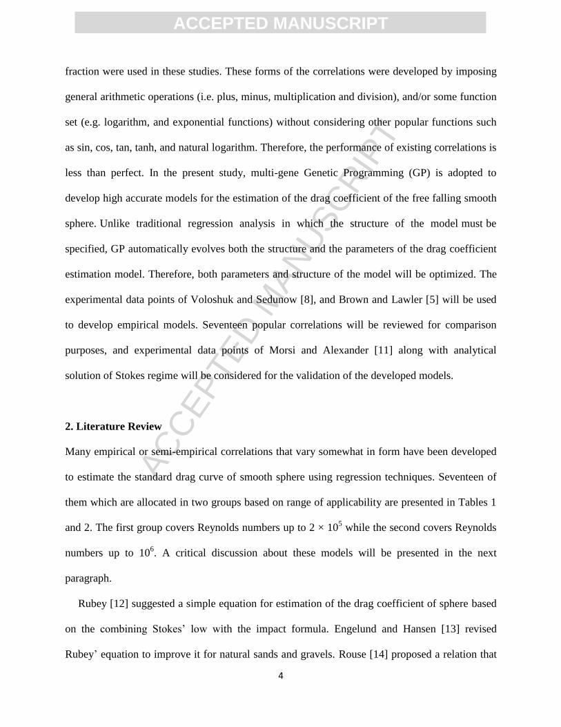
1. Introduction

The motion of particles in fluids is a key subject in many problems in the fields of chemical and

metallurgical engineering as well as mechanical and environmental engineering. The solution of

these problems generally involves determining the local behaviour of flow and the interaction

between solid and liquid phases through the knowledge of hydrodynamic forces such as drag.

The drag force is the combination of the normal (i.e. pressure) and tangential (i.e. wall shear

stress) forces on the body in the flow direction. However, the distributions of the pressure and

wall shear stress are often very difficult to achieve, so the magnitude of the drag force can be

determined only through the knowledge of drag coefficient. Analytical determination of the drag

coefficient such as Stokes’ law is only valid for Reynolds number, Re, less than 0.1 (Flemmer

and Banks [1], Kreith [2]), although the drag coefficient can be ascertained using empirical and

semi-empirical correlations based on experimental data when inertial effects are significant (i.e.

higher Reynolds numbers).

The drag coefficient of a smooth sphere in incompressible flow is function of Re based on

both theoretical investigations and numerous experimental data (Kreith [2]). The main classes of

the dependence of drag coefficient on Reynolds number are (1) very low Reynolds number flow

(i.e. creeping flow), (2) moderate Reynolds number flow (i.e. laminar boundary layer), and (3)

very large Reynolds number flow (i.e. turbulent boundary layer) (Munson et al. [3]). In the first

class (Re < 1), the flows reflects entirely the viscous effect of flow with no separation results. By

increasing Reynolds numbers (i.e. increasing the particle size or flow velocity for a given

Kinematic viscosity), the separation region can be observed at Re ≈ 10, and the region increases

until Re ≈ 1000, where the most of the drag is due to pressure drag rather than frictional drag.

Parenthetically, it should be noted that the value of the drag coefficient decreases, as wake area

becomes larger. At a sufficiently high Reynolds number (103 < Re < 10

5), the drag coefficient is

ACC

EPTE

D M

ANU

SCR

IPT

ACCEPTED MANUSCRIPT

3

relatively constant (Munson et al. [3]). When transition from laminar to turbulent flow occurs, a

dramatic dip (up to almost 80%) in the drag coefficient appears at critical value Re ≈ 2 ×105 since

the turbulent boundary layer travels further along the surface into the adverse pressure gradient

on the rear portion of the sphere before the separation, so the wake is smaller, causing less

pressure drag. After this abrupt descent, the value of the drag coefficient increases by increasing

Reynolds numbers. Finally, for Re > 106

a constant value of the drag coefficient (≈ 0.2) is

acceptable (Potter et al. [4]).

Most of the information pertaining to drag force on the sphere arises from numerous

experiments with wind tunnels, water tunnels, towing tanks, and other ingenious devices

(Munson et al. [3]). Experimental data of the drag coefficient of spherical particles have been

presented in the literature having a wide range of Re. However, some of the available

experimental data are not accurate, adequately. Brown and Lawler [5] reviewed the experimental

studies of sphere drag coefficient for Re < 2 × 105. They assembled 606 data points which were

originally presented in tabular form. By excluding some experimental data form various reasons,

Brown and Lawler [5] presented 480 very high quality data points by considering wall effects.

This data set seems acceptable among other researchers for developing correlations (Cheng [6],

Mikhailov and Freire [7]). On the other hand, Voloshuk and Sedunow [8] presented the

experimental data for higher Reynolds numbers with good quality. This data set were also used in

several studies such as Ceylan et al. [9] and Almedeij [10]. Fig. 1 illustrates all of the mentioned

data. The variations of the drag coefficient with Reynolds numbers can follow as explained in the

previous paragraph by considering Fig. 1.

In the previous studies, the regression analyses were applied to obtain a correlation for the

estimation of the drag coefficient of spherical particles. Several forms and procedures such as

multi-segment polynomial, exponential function, piecewise matched, power function and rational

ACC

EPTE

D M

ANU

SCR

IPT

ACCEPTED MANUSCRIPT

4

fraction were used in these studies. These forms of the correlations were developed by imposing

general arithmetic operations (i.e. plus, minus, multiplication and division), and/or some function

set (e.g. logarithm, and exponential functions) without considering other popular functions such

as sin, cos, tan, tanh, and natural logarithm. Therefore, the performance of existing correlations is

less than perfect. In the present study, multi-gene Genetic Programming (GP) is adopted to

develop high accurate models for the estimation of the drag coefficient of the free falling smooth

sphere. Unlike traditional regression analysis in which the structure of the model must be

specified, GP automatically evolves both the structure and the parameters of the drag coefficient

estimation model. Therefore, both parameters and structure of the model will be optimized. The

experimental data points of Voloshuk and Sedunow [8], and Brown and Lawler [5] will be used

to develop empirical models. Seventeen popular correlations will be reviewed for comparison

purposes, and experimental data points of Morsi and Alexander [11] along with analytical

solution of Stokes regime will be considered for the validation of the developed models.

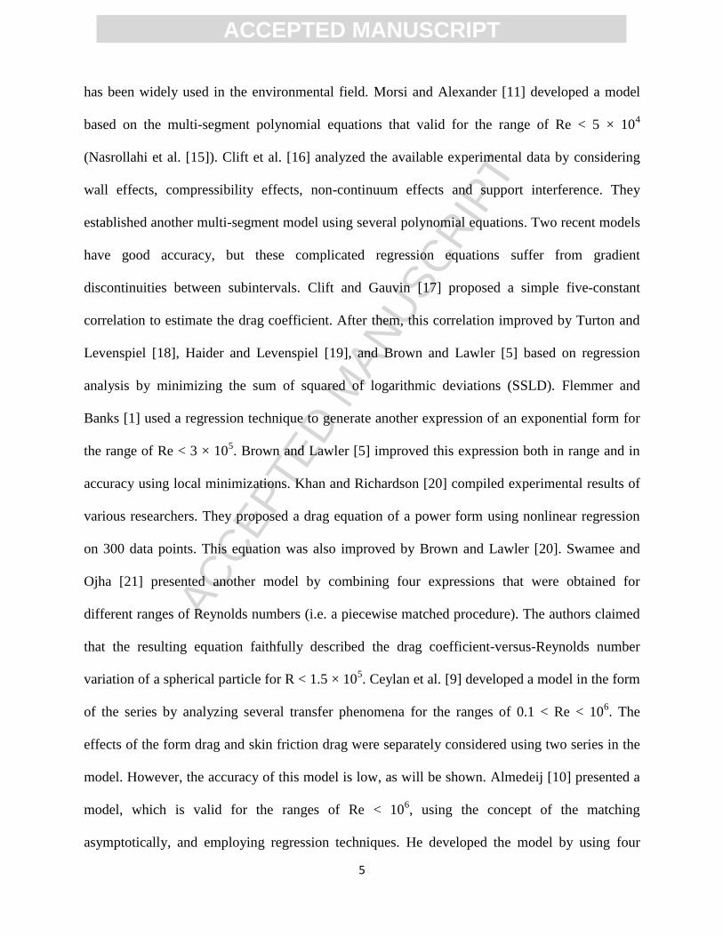
2. Literature Review

Many empirical or semi-empirical correlations that vary somewhat in form have been developed

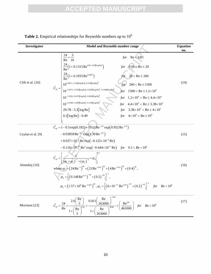
to estimate the standard drag curve of smooth sphere using regression techniques. Seventeen of

them which are allocated in two groups based on range of applicability are presented in Tables 1

and 2. The first group covers Reynolds numbers up to 2 × 105 while the second covers Reynolds

numbers up to 106. A critical discussion about these models will be presented in the next

paragraph.

Rubey [12] suggested a simple equation for estimation of the drag coefficient of sphere based

on the combining Stokes’ low with the impact formula. Engelund and Hansen [13] revised

Rubey’ equation to improve it for natural sands and gravels. Rouse [14] proposed a relation that

ACC

EPTE

D M

ANU

SCR

IPT

ACCEPTED MANUSCRIPT

5

has been widely used in the environmental field. Morsi and Alexander [11] developed a model

based on the multi-segment polynomial equations that valid for the range of Re < 5 × 104

(Nasrollahi et al. [15]). Clift et al. [16] analyzed the available experimental data by considering

wall effects, compressibility effects, non-continuum effects and support interference. They

established another multi-segment model using several polynomial equations. Two recent models

have good accuracy, but these complicated regression equations suffer from gradient

discontinuities between subintervals. Clift and Gauvin [17] proposed a simple five-constant

correlation to estimate the drag coefficient. After them, this correlation improved by Turton and

Levenspiel [18], Haider and Levenspiel [19], and Brown and Lawler [5] based on regression

analysis by minimizing the sum of squared of logarithmic deviations (SSLD). Flemmer and

Banks [1] used a regression technique to generate another expression of an exponential form for

the range of Re < 3 × 105. Brown and Lawler [5] improved this expression both in range and in

accuracy using local minimizations. Khan and Richardson [20] compiled experimental results of

various researchers. They proposed a drag equation of a power form using nonlinear regression

on 300 data points. This equation was also improved by Brown and Lawler [20]. Swamee and

Ojha [21] presented another model by combining four expressions that were obtained for

different ranges of Reynolds numbers (i.e. a piecewise matched procedure). The authors claimed

that the resulting equation faithfully described the drag coefficient-versus-Reynolds number

variation of a spherical particle for R < 1.5 × 105. Ceylan et al. [9] developed a model in the form

of the series by analyzing several transfer phenomena for the ranges of 0.1 < Re < 106. The

effects of the form drag and skin friction drag were separately considered using two series in the

model. However, the accuracy of this model is low, as will be shown. Almedeij [10] presented a

model, which is valid for the ranges of Re < 106, using the concept of the matching

asymptotically, and employing regression techniques. He developed the model by using four

ACC

EPTE

D M

ANU

SCR

IPT

ACCEPTED MANUSCRIPT

6

functions that can be combined into an overall relationship. However, this model suffers from the

complicated form. Cheng [6] recommended a five-parameter correlation, and compared it with

seven previously-developed formulas. This correlation consists of two terms (1) an extended

Stokes' law applicable approximately for Re< 100, and (2) an exponential function accounting for

slight deviations from the Newton's law for high Re. Cheng [6] claimed that the proposed

correlation gives the best representation of the historical data for the region before drag dip.

Terfous et al. [22] developed an equation for Re <5×104 by using the simple series function and

applying the least-squares method. However, this model is not applicable for Re < 0.1 because

they used the term 21.683/Re instead of the traditional term 24/Re in the equation. Morrison [23]

used a piecewise matched procedure to develop a model that covers the transition from laminar to

turbulent flow region. Recently, Mikhailov and Freire [7] presented an expression for the

estimation of the drag coefficient of a falling sphere for the ranges of Re < 118300 based on

Shanks transform which is a non-linear rational fractional transform of the series of Goldstein to

Oseen's equation.

Briefly, it can be said that the above equations of the drag coefficient estimation suffer from

the complicated correlation, bounds of applicability, and/or low accuracy. Therefore, the

development of a simple and accurate model with high range of applicability is vital.

3. Genetic Programming

Genetic programming (GP) is a random-based procedure for automatically learning the most “fit”

computer programs by means of artificial evolution (Johari et al. [24]). Recently, GP has been

successfully applied in many applications such as the prediction of the soil–water characteristic

of soils (Johari et al. [24]), the estimation of the bridge pier scour (Azamathulla et al. [25]), and

the prediction of the outflow hydrograph from earthen dam breach (Hakimzadeh et al. [26]).

ACC

EPTE

D M

ANU

SCR

IPT

ACCEPTED MANUSCRIPT

7

GP, which is a branch of the conventional genetic algorithm (GA; Holland [27]), was initially

developed by Koza [28]. The significant superiority of GP over GA is that, in GP there is no need

to define the structure of the model a priori. In other words, GP can determine not only the

coefficients and parameters of the model, but also and more importantly, the form of the model

itself (Johari et al. [24]). GP randomly generates a population of equal or unequal length

computer programs (or symbolic expression) with a high level of diversity. The programs are

represented by tree-based structures using variables (terminal) and several mathematical

operators (function) that can be selected from sets of terminals and functions, respectively. The

terminal set contains the numerical constants and external inputs of the program while the

function set contains the basic arithmetic operators such as +, -, *, / and function calls such as ex,

sin, cos, tan, tanh, log, ln, sqrt, power. After choosing the best symbolic expressions through

defining a fitness function, an improved population will be created using crossover and mutation

operators. The iterations proceed until they meet stopping criteria (e.g. reaching the specified

number of generations). It is informative to express that GP is often known as symbolic

regression, when an empirical model is developed using collected data from a process or system.

More details of GP procedure can be found in Koza [28].

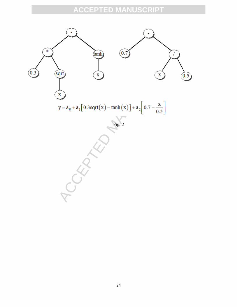
In order to improve fitness for non-linear behaviour procedures, the multi-gene GP which is a

branch of standard GP can be used (Hinchliffe et al. [29], and Hiden [30]). In the traditional GP,

the model expresses as a single tree while, in the multi-gene GP, several trees may define the

model through a weighted linear combination of each gene plus a bias term as

0 1 1 2 2 n ny a a gene a gene ... a gene (18)

Where y is the output variable, a0 is the bias term and ai is weight of the ith gene.

ACC

EPTE

D M

ANU

SCR

IPT

ACCEPTED MANUSCRIPT

8

An example of multi-gene tree-based model is presented in Fig. 2, where an output variable y

is predicted using an input variable x. As can be seen in Fig. 2, multi-gene GP is a linear

combination of nonlinear terms, and this feature makes it possible to recognize the pattern of

engineering problems in a highly precise manner (Hinchliffe et al. [29]).

In the present study, GPTIPS, which is a new “Genetic Programming and Symbolic

Regression” code (Searson [31]), was adapted to perform a multi-gene GP for the development of

the sphere drag coefficient models. GPTIPS which uses lexicographic tournament selection as an

effective technique for controlling the bloating of the model has the capability of setting some

restrictions on initial parameters such as the maximum number of genes, maximum depth of trees

and genes, maximum number of nodes per tree to avoid most recent problems of bloat in GP.

There are several successful application of GPTIPS in the different fields such as predicting the

liquefaction resistance of sand-silt mixtures (Baziar et al. [32]), and predicting the ultimate

bearing capacity of shallow foundations on cohesionless soils (Shahnazari and Tutunchian [33]).

The ranges of the initial parameters of multi-gene GP for runs of this study are summarized in

Table 3. More descriptions about the initial parameters and specifications of multi-gene GP can

be found in Searson [31].

4. Developed models based on multi-gene GP

The sum of the squared deviations is a good objective function to minimize the errors between

experimental data and calculated results by considering previous studies (Turton and Levenspiel

[18]; Haider and Levenspiel [19]; Brown and Lawler [5]; Barati [34], Barati [35]). Therefore, the

fitness function of multi-gene GP is to minimize the sum of squared of logarithmic deviations

(SSLD) between the estimated drag coefficient and experimental data points

ACC

EPTE

D M

ANU

SCR

IPT

ACCEPTED MANUSCRIPT

9

2N

D D

1

ˆMinimize SSLD logC logC (19)

Where CD is the experimental value of the drag coefficient, DC is the estimated drag

coefficient, and N is the total number of the data.

For assessing the performance of the proposed models compared to existing correlations, root-

mean-square of logarithmic deviation (RMSLD) and sum of the relative errors (SRE), as well as

SSLD are used as

2N

D D

1

ˆlog C log CR SL NM D (20)

ND D

1 D

ˆC C

CSRE

(21)

It is notable that SSLD and RMSLD were calculated based on logarithmic values of the drag

coefficients while SRE can be used to evaluate the original value of the drag coefficients.

In order to select appropriate models, GPTIPS is run over 100 times, because multi-gene GP is

a stochastic procedure. As will be shown, the best representation of available experimental data

of the smooth sphere drag coefficient in the literature for Reynolds numbers up to 2 × 105

and up

to 106

can be estimated by Eqs. (22) and (23), respectively.

9 -9

5

ˆ 5.4856 10 tanh 4.3774 10 Re 0.0709tanh 700.6574 Re

0.3894tanh 74.1539 Re -0.1198tanh 7429.0843 Re

+ 1.7174tanh 9.9851 Re + 2.3384 + 0. 247 4 104

D

Rfor e

C

(22)

ACC

EPTE

D M

ANU

SCR

IPT

ACCEPTED MANUSCRIPT

10

224

43 2

2

2

ln 10.7563 ln 10 9.98672.08 10

1620 10

-

3 370

6

-

6530 tˆ 8 10

0.4119 2.1344e

0.1357 8.5 10 2ln tanh tanh Re ln 10 - 2825.7162 Re

anh

+ 2.47

8ln ln 0

95

1

Re ReRe Re

D

Re Re

Re Re RC e

Rf e

e

e

or

610

(23)

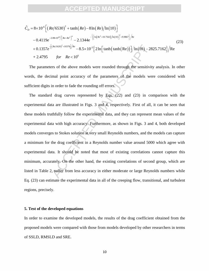
The parameters of the above models were rounded through the sensitivity analysis. In other

words, the decimal point accuracy of the parameters of the models were considered with

sufficient digits in order to fade the rounding off errors.

The standard drag curves represented by Eqs. (22) and (23) in comparison with the

experimental data are illustrated in Figs. 3 and 4, respectively. First of all, it can be seen that

these models truthfully follow the experimental data, and they can represent mean values of the

experimental data with high accuracy. Furthermore, as shown in Figs. 3 and 4, both developed

models converges to Stokes solution at very small Reynolds numbers, and the models can capture

a minimum for the drag coefficient in a Reynolds number value around 5000 which agree with

experimental data. It should be noted that most of existing correlations cannot capture this

minimum, accurately. On the other hand, the existing correlations of second group, which are

listed in Table 2, suffer from less accuracy in either moderate or large Reynolds numbers while

Eq. (23) can estimate the experimental data in all of the creeping flow, transitional, and turbulent

regions, precisely.

5. Test of the developed equations

In order to examine the developed models, the results of the drag coefficient obtained from the

proposed models were compared with those from models developed by other researchers in terms

of SSLD, RMSLD and SRE.

ACC

EPTE

D M

ANU

SCR

IPT

ACCEPTED MANUSCRIPT

11

Performance evaluation criteria for the correlation of first and second groups together with the

corresponding values of the developed models are listed in Tables 4 and 5, respectively. It should

be stated that the models are ranked in the increasing order of SSLD in Tables 4 and 5. Generally,

other criteria (i.e. RMSLD and SRE) also increase in Tables 4 and 5 by increasing order of

accuracy. The ranges of using the models in the calculation of the criteria were applicability

range of them, which presented in Tables 1 and 2. Therefore, it should be noted that some of the

correlations such as recently developed models of Terfous et al. [22] and Mikhailov and Freire

[7] have large values of SSLD (i.e. low accuracy) although SSLD of them were calculated for 0.1

< Re < 5 × 104 and Re < 118300, respectively, instead of whole range of Reynolds numbers up to

2 × 105.

As shown in Tables 1 and 2, both proposed models have lowest values of SSLD, RMSLD and

SRE (higher accuracy). Eqs. (22) and (23) improved 16.2% and 69.4% to match with the

experimental data points than the best existing correlations of the first and second groups in terms

of SSLD, respectively. The new models substantially improve the fit to experimental data.

Consequently, for the accurate estimation of the smooth sphere drag coefficient of engineering

problems, Eq. (22) and Eq. (23) can be utilized for problems with Reynolds numbers in the

region before drag coefficient dip and with Reynolds numbers greater than Re > 2 × 105,

respectively. Finally, it must be stated that a constant value of the drag coefficient (≈ 0.2) is

acceptable for higher Reynolds numbers (i.e. Re > 106) (Almedeij [10], Potter et al. [4]).

As mentioned previously, the developed equations were calibrated using the data of Voloshuk

and Sedunow [8], and Brown and Lawler [5]. The data of Morsi and Alexander [11] along with

analytical solution of Stokes regime will be used to validate the proposed models.

ACC

EPTE

D M

ANU

SCR

IPT

ACCEPTED MANUSCRIPT

12

Fig. 5 represents the comparison between the validation data of the drag coefficient and the

associated calculation results. The figure shows that the results of both models are comparable

with the measurement data.

The experimental values of the drag coefficient and ± 5% of them are compared with the

estimated values by the proposed models in Table 6. The results indicated that the models have

no significant error compared to the experimental data. All of the estimated drag coefficients by

both models are within the bounds of ± 5% of validation data except for 3 data points. If the

bounds are increased until ± 7%, 3 data points will also be covered.

6. Discussion

In this section, two issues about the multi-gene GP procedure will be discussed. 1) Compatibility

of multi-gene GP approach with the natural of the problem and 2) evaluation of the level of the

accuracy of the developed models.

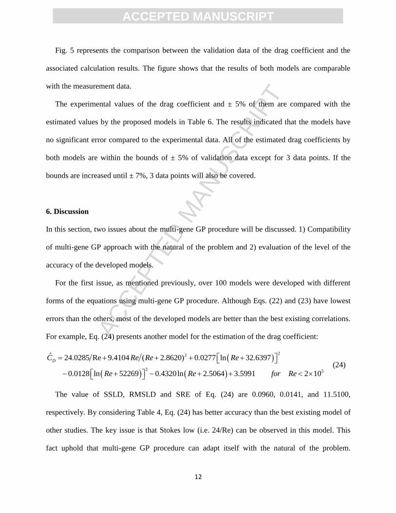
For the first issue, as mentioned previously, over 100 models were developed with different

forms of the equations using multi-gene GP procedure. Although Eqs. (22) and (23) have lowest

errors than the others, most of the developed models are better than the best existing correlations.

For example, Eq. (24) presents another model for the estimation of the drag coefficient:

5

22

2

9.4104 ( 2.8620) 0.0277 ln 32.6397

0.0128 ln 52269 0ln 2.5064

ˆ 24.028

3.5991 2 1

5 Re

0.432 0

D Re Re Re

Re

C

foRe er R

(24)

The value of SSLD, RMSLD and SRE of Eq. (24) are 0.0960, 0.0141, and 11.5100,

respectively. By considering Table 4, Eq. (24) has better accuracy than the best existing model of

other studies. The key issue is that Stokes low (i.e. 24/Re) can be observed in this model. This

fact uphold that multi-gene GP procedure can adapt itself with the natural of the problem.

ACC

EPTE

D M

ANU

SCR

IPT

ACCEPTED MANUSCRIPT

13

However, for Eqs. (22) and (23), other functions appear instead of 24/Re. For example, a form of

tangent hyperbolic function play same role for the calculation of the drag coefficients in low

Reynolds number (Stokes low region).

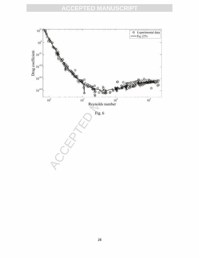
For the second issue, interestingly, it is observed that the value of SSLD can be decreased [less

than the values of Eqs. (22) and (23)] by increasing the maximum depth of trees in the multi-gene

GP procedure. However, the obtained correlations by higher number of depth of trees have a non-

smooth curve. For example, Eq. (25) presents one of these models

( )

10 10

9 14

24.03 1.3255 0.5756ln 12.3504 0.3910ln 30.2029

0.0062 0.13993 3.3243

237119ln 164358 5 10 4.8396 10

1.5 10 0.4343ln( )

ˆ

10

ta

D

nh ReRe e Re Re

cos Re tanh Re tanh sinh Re

Re sin Re

sin Re co

C

s Re tanh Re

5

5

6ln( ) ln 10 1.04 10 1.60 10

14.91 9.24 0.3996 2 10

sin Re Re

sin tanh Re log Re Refor

(25)

The value of SSLD, RMSLD and SRE of Eq. (25) are 0.0777, 0.0127, and 10.3246,

respectively. By considering Table 4, Eq. (25) has the lower errors than Eq. (22) and other

correlations. However, as it can be seen in Fig. (6), the curve of Eq. (25) is non-smooth which is

not acceptable. In other words, for reach a model with a lower error than Eq. (22), the curve of

the model become non-smooth. Therefore, by considering available experimental data of drag

coefficient, it can be said that Eqs. (22) and (23) are almost the best possible smooth standard

curve which can be constructed.

7. Conclusions

In the present study, the existing correlations of drag coefficient were discussed, critically. Then,

a reliable and complete set of historical data were collected for the development and validation of

ACC

EPTE

D M

ANU

SCR

IPT

ACCEPTED MANUSCRIPT

14

correlations for the estimation of the smooth sphere drag coefficient. An effective procedure (i.e.

multi-gene genetic programming) was used to develop drag coefficient models through

optimizing both parameters and structure of models. Because the procedure is stochastic, the

multi-gene GP was run over 100 times for selecting appropriate models. Results of the numerical

and experimental validations indicated that two new correlations which are accurate, simple, and

explicit illustrated the best representation of available experimental data for both subcritical and

turbulent regions. The developed models by multi-gene GP substantially (up to almost 70%)

improved the fit to experimental data than the best existing correlations in terms of SSLD. The

correlations were also verified using another set of experimental data points. The results showed

that all of the estimated drag coefficients were within the bounds of ± 7% of experimental values.

Finally, it can be said that the proposed models are useful tools for computer programs

because of the high accuracy and simplicity of them. Moreover, for future researches, it is hoped

that the procedure of this study can be successfully adopted for other problems in the field of

particle transport.

REFERENCES

[1] R.L.C. Flemmer, C.L. Banks, On the drag coefficient of a sphere, Powder

Technology 48(1986) 217-221.

[2] F. Kreith, Mechanical engineering handbook, CRC Press LLC, 1999.

[3] B.R. Munson, D.F. Young, T.H. Okiishi, W.W. Huebsch, Fundamentals of fluid mechanics,

John Wiley & Sons, Inc., New York, 2009.

[4] M.C. Potter, D.C. Wiggert, B.H. Ramadan, Mechanics of Fluids, SI Version, Cengage

Learning, 2011.

ACC

EPTE

D M

ANU

SCR

IPT

ACCEPTED MANUSCRIPT

15

[5] P.P. Brown, D.F. Lawler, Sphere drag and settling velocity revisited, Journal of

Environmental Engineering 129(2003) 222-231.

[6] N.S. Cheng, Comparison of formulas for drag coefficient and settling velocity of spherical

particles, Powder Technology 189(2009) 395-398.

[7] M.D. Mikhailov, A.P. Freire, The drag coefficient of a sphere: An approximation using

Shanks transform, Powder Technology (2013).

[8] V.M. Voloshuk, J.S. Sedunow, The processes of coagulation in dispersed systems, Nauka,

Moscow, 1971.

[9] K. Ceylan, A. Altunbaş, G. Kelbaliyev, A new model for estimation of drag force in the flow

of Newtonian fluids around rigid or deformable particles, Powder technology 119(2001) 250-

256.

[10] J. Almedeij, Drag coefficient of flow around a sphere: Matching asymptotically the wide

trend, Powder Technology 186(2008) 218-223.

[11] S. A. Morsi, A.J. Alexander, An investigation of particle trajectories in two-phase flow

systems, Journal of Fluid Mechanics 55(1972) 193-208.

[12] W.W. Rubey, Settling velocity of gravel, sand, and silt particles, American Journal of

Science 148(1933) 325-338.

[13] F. Engelund, E. Hansen, Monograph on sediment transport in alluvial streams, Monograpsh

Denkmark Technical University, Hydraulic Lab, Denkmark, 1967.

[14] H. Rouse, Fluid mechanics for hydraulic engineers, Dover, New York, N.Y., 1938.

[15] A. Nasrollahi, S.A.A. Salehi Neyshabouri, G. Ahmadi, M.M. Namin, Numerical simulation

of particle saltation process, Particulate Science and Technology 26(2008) 529-550.

[16] R. Clift, J.R. Grace, M.E. Weber, Bubbles, drops, and particles, Academic, New York, 1978.

ACC

EPTE

D M

ANU

SCR

IPT

ACCEPTED MANUSCRIPT

16

[17] R. Clift, W.H. Gauvin, The motion of particles in turbulent gas streams, In Proc.

Chemeca 70(1970) 14-28.

[18] R. Turton, O. Levenspiel, A short note on the drag correlation for spheres, Powder

Technology 47(1986) 83-86.

[19] A. Haider, O. Levenspiel, Drag coefficient and terminal velocity of spherical and

nonspherical particles, Powder technology 58(1989) 63-70.

[20] A.R. Khan, J.F. Richardson, The resistance to motion of a solid sphere in a fluid, Chemical

Engineering Communications 62(1987) 135-150.

[21] P.K. Swamee, C.S.P. Ojha, Drag coefficient and fall velocity of nonspherical

particles, Journal of Hydraulic Engineering 117(1991) 660-667.

[22] A. Terfous, A. Hazzab, A. Ghenaim, Predicting the drag coefficient and settling velocity of

spherical particles, Powder Technology 239(2013) 12–20.

[23] F.A. Morrison, An Introduction to Fluid Mechanics, Cambridge University Press, New

York, 2013.

[24] A. Johari, G. Habibagahi, A. Ghahramani, Prediction of soil–water characteristic curve using

genetic programming, Journal of Geotechnical and Geoenvironmental Engineering 132(2006)

661-665.

[25] H.M. Azamathulla, A.A. Ghani, N.A. Zakaria, A. Guven, Genetic programming to predict

bridge pier scour, Journal of Hydraulic Engineering 136(2009) 165-169.

[26] H. Hakimzadeh, V. Nourani, A.B. Amini, Genetic programming simulation of dam breach

hydrograph and peak outflow discharge, Journal of Hydrologic Engineering Posted ahead of

print May 18 (2013) doi:10.1061/(ASCE)HE.1943-5584.0000849.

[27] J.H. Holland, Adaptation in natural and artificial system, University of Michigan Press Ann

Arbor Mich., 1975.

ACC

EPTE

D M

ANU

SCR

IPT

ACCEPTED MANUSCRIPT

17

[28] J.R. Koza, Genetic programming: On the programming of computers by means of natural

selection, MIT Press, Cambridge, Mass, 1992.

[29] M.P. Hinchliffe, M.J. Willis, H.G. Hiden, M.T. Tham, B. McKay, G. Barton, Modelling

chemical process systems using a multi-Gene genetic programming algorithm, Late Breaking

Paper, GP'96, Stanford: USA, 1996.

[30] H.G. Hiden, Data-Based Modelling using Genetic Programming, PhD Thesis, Dept.

Chemical and Process Engineering, University of Newcastle, UK, 1998.

[31] D.P. Searson, GPTIPS: Genetic Programming & Symbolic Regression for MATLAB, User

Guide, 2009.

[32] M. H. Baziar, Y. Jafarian, H. Shahnazari, V. Movahed, M. Amin Tutunchian, Prediction of

strain energy-based liquefaction resistance of sand-silt mixtures: An evolutionary approach,

Computers and Geosciences 37(2011) 1883-1893.

[33] H. Shahnazari, M.A. Tutunchian, Prediction of ultimate bearing capacity of shallow

foundations on cohesionless soils: An evolutionary approach, KSCE Journal of Civil

Engineering 16(2012) 950-957.

[34] R. Barati, Parameter estimation of nonlinear Muskingum models using Nelder-Mead

Simplex algorithm, Journal of Hydrologic Engineering-ASCE 16(2011) 946-954.

[35] R. Barati, Application of Excel Solver for parameter estimation of the nonlinear

Muskingum models, KSCE Journal of Civil Engineering 17(2013) 1139-1148.

[36] W.H. Graf, Hydraulics of Sediment Transport, Water Resources Publications, Littleton,

Colorado, 1984.

[37] B. C. Yen, Sediment fall velocity in oscillating flow, University of Virginia, Department of

Civil Engineering, 1992.

ACC

EPTE

D M

ANU

SCR

IPT

ACCEPTED MANUSCRIPT

18

FIGURE CAPTIONS

Figure 1. Illustration of the variations of the drag coefficient with Reynolds numbers using

reliable data points of Stokes regime and available experiments in the literature [5, 8, and 11].

Figure 2. A typical multi-gene tree-based model.

Figure 3. Developed drag coefficient model for the region before drag dip along with

experiments data of Brown and Lawler [5].

Figure 4. Developed drag coefficient model for the wide range of particle Reynolds numbers

along with experiments data of Brown and Lawler [5], and Voloshuk and Sedunow [8].

Figure 5. Comparison between the validation data of the drag coefficient and the associated

calculation results

Figure 6. Illustration of non-smooth curve of Eq. (25)

ACC

EPTE

D M

ANU

SCR

IPT

ACCEPTED MANUSCRIPT

19

Table 1. Summary of some empirical relationships for Re < 2 ×105

Investigator Model and Reynolds number range Equation

no.

Rouse [14] 5

0.5

24 3ˆ 0.34 Re 2 10Re Re

DC for (1)

Engelund and

Hansen [13] 524ˆ 1.5 Re 2 10

ReDC for

(2)

Clift and Gauvin

[17]* 0.677 5

0.94

24 0.417ˆ 1 0.152Re Re 2 10Re 1 5070Re

DC for

(3)

Morsi and Alexander

[11]

2

2

2

2

4

2

24Re 0.1,

Re

22.7300 0.09033.6900 0.1 Re 1,

Re Re

29.1667 3.88891.2220 1 Re 10,

Re Re

46.5000 116.67000.6167 10 Re 100,

Re Reˆ98.3300 2778

0.3644 100 Re 1000,Re Re

148.6200 4.75 100.35

Re Re

D

for

for

for

for

C

for

4

2

6

2

70 1000 Re 5000,

490.5460 57.87 100.4600 5000 Re 10000,

Re Re

1662.5000 5.4167 100.5191 10000 Re 50000

Re Re

for

for

for

(4)

Graf [36] 5

0.5

24 7.3ˆ 0.25 Re 2 10Re 1 Re

DC for

(5)

Flemmer and Banks

[1]*

0.356 0.396 5

2

24 0.143ˆ 10 0.383Re 0.207 Re Re 2 10Re 1 log Re

E

DC where E for

(6)

Khan and Richardson

[20]*

3.180.328 0.067 5ˆ 2.49Re 0.34Re Re 2 10DC for

(7)

Swamee and Ojha

[21]

0.252.5 0.25

1.6 0.72 2

524 130 40000ˆ 0.5 16 1 Re 1.5 10Re Re Re

DC for

(8)

Yen [37] 5

4 0.5

24 0.208ˆ 1 0.15 Re 0.017 Re Re 2 10Re 1 10 Re

DC for

(9)

Haider and

Levenspiel [19]* 0.681 5

1

24 0.407ˆ 1 0.150Re Re 2 10Re 1 8710 Re

DC for

(10)

Cheng [6]

0.43 0.38 524ˆ 1 0.27 Re 0.47 1 exp 0.04 Re Re 2 10Re

DC for

(11)

Terfous et al. [22] 4

2 0.1 0.2

21.683 0.131 10.616 12.216ˆ 2.689 0.1 Re 5 10Re Re Re Re

DC for (12)

Mikhailov and Freire

[7]

2

2

3808 1617933 2030 178861 1063 Re 1219 1084 Reˆ Re

681Re 77531 422 13529 976 Re 1 71154 Re118300DC for

(13)

* These models were improved by Brown and Lawler [5]

ACC

EPTE

D M

ANU

SCR

IPT

ACCEPTED MANUSCRIPT

20

Table 2. Empirical relationships for Reynolds numbers up to 106

Investigator Model and Reynolds number range Equation

no.

Clift et al. [16]

2

2 3

0.82 0.05 log Re

0.6305

1.6435 1.1242 log Re 0.1558 log Re

2.4571 2.5558 log Re 0.9295 log Re 0.1049 log Re

24 3Re 0.01

Re 16

241 0.1315Re 0.01 Re 20

Re

241 0.1935Re 20 Re 260

Re

10 260 Re 1500ˆ

10 1500 ReD

for

for

for

forC

for

2

2

4

1.9181 0.6370 log Re 0.0636 log Re 4 4

4.3390 1.5809 log Re 0.1546 log Re 4 5

5 5

5 6

1.2 10

10 1.2 10 Re 4.4 10

10 4.4 10 Re 3.38 10

29.78 5.3 log Re 3.38 10 Re 4 10

0.1 log Re 0.49 4 10 Re 10

for

for

for

for

(14)

Ceylan et al. [9]

2 3 1 4

4 3 1 2

4 4

10 2 5 6

ˆ 1 0.5exp(0.182) 10.11Re exp 0.952Re

0.03859Re exp 1.30Re

0.037 10 Re exp 0.125 10 Re

0.116 10 Re exp 0.444 1 0.1 10 R 0e

DC

f eo Rr

(15)

Almedeij [10]

0.1

41 1

1 2 3

10 10 10 101 0.67 0.33

1

110 100.11

2

110 10 108 1.625 17 2.63

3

6

4 10

1ˆ

where 24Re 21Re 4Re 0.4 ,

0.148Re 0.5 ,

1.57 10 Re , 6 10 Re 0.2

DC

eor Rf

(16)

Morrison [23]

7.94

0.8

1.52 8.00

6

Re Re2.6 0.411

24 Re5 263000ˆRe 461000Re Re

1 15 2630

10

00

DC for Re

(17)

ACC

EPTE

D M

ANU

SCR

IPT

ACCEPTED MANUSCRIPT

21

Table 3. Range of parameters of multi-gene GP

Parameter Range

Population size 200-10000

Number of generations 400-10000

Maximum number of genes 1-10

Maximum number of nodes per tree 1-15

Maximum depth of trees 3-15

Probability of multi-gene GP tree mutation* 0.1-0.2

Probability of multi-gene GP tree cross over* 0.75-0.85

Probability of multi-gene GP tree direct copy* 0.05

Size of the tournament 2-3

Arithmetic operations and function set (+, -, ×, ÷, square, tanh, sin,

cos, tan, log, ln, exp)

* Sum must be equal to 1

Table 4. Comparison of the performance evaluation criteria of the relationships for Re < 2 ×105

Order of

accuracy

Reference SSLD RMSLD SRE

1 Present study Eq. (22) 0.0881 0.0136 10.7171

2 Cheng [20] 0.1051 0.0148 11.8567

3 Morsi and Alexander [11] 0.1314 0.0176 13.0465

4 Clift and Gauvin [17]* 0.1502 0.0177 15.4402

5 Haider and Levenspiel [19]* 0.1510 0.0177 15.5260

6 Flemmer and Banks [1]* 0.1978 0.0203 17.4739

7 Khan and Richardson [20]* 0.2091 0.0209 17.4464

8 Swamee and Ojha [21] 0.2778 0.0242 20.4107

9 Terfous et al. [22] 0.4670 0.0322 23.1950

10 Mikhailov and Freire [7] 0.4703 0.0319 25.9766

11 Yen [37] 0.8475 0.0420 38.7227

12 Rouse [14] 2.1313 0.0666 51.3652

13 Graf [36] 5.2163 0.1042 63.1865

14 Engelund and Hansen [13] 61.5283 0.3580 545.4005

* These models were improved by Brown and Lawler [5]

Table 5. Comparison of the performance evaluation criteria of the relationships for Reynolds

numbers up to 106

Order of

accuracy

Reference SSLD RMSLD SRE

1 Present study Eq. (23) 0.0982 0.0142 11.2853

2 Almedeij [10] 0.3210 0.0257 23.2094

3 Clift et al. [16] 0.4467 0.0303 17.4004

4 Morrison [23] 0.5672 0.0342 29.1768

5 Ceylan et al. [9] 0.9186 0.0449 33.2925

ACC

EPTE

D M

ANU

SCR

IPT

ACCEPTED MANUSCRIPT

22

Table 6. Validation of the developed models using the experimental data of Morsi and Alexander

[11], and the analytical solution of Stokes regime

Re CD -5% of CD Eq. (22) Eq. (23) +5% of CD

0.002 12000 11400.00 12008.86 12034.71 12600.00

0.004 6000 5700.00 6005.70 6017.32 6300.00

0.007 3429 3257.14 3432.91 3438.94 3600.00

0.01 2400 2280.00 2403.80 2407.74 2520.00

0.04 600 570.00 602.85 603.54 630.00

0.07 343 325.71 345.57 345.88 360.00

0.1 240 228.00 242.66 242.84 252.00

0.2 120 114.00 122.59 122.63 126.00

0.3 80 76.00 82.57 82.57 84.00

0.5 49 46.55 50.56 50.53 51.45

0.7 36.5 34.68 36.83 36.80 38.32

1 26.5 25.18 26.54 26.50 27.82

2 14.4 13.68 14.50 14.48 15.12

3 10.4 9.88 10.46 10.44 10.92

5 6.9 6.56 7.12 7.10 7.24

7 5.4 5.13 5.60 5.58 5.67

10 4.1 3.90 4.36 4.36 4.31

20 2.55 2.42 2.73 2.76 2.68

30 2 1.90 2.12 2.14 2.10

50 1.5 1.42 1.58 1.57 1.58

70 1.27 1.21 1.31 1.30 1.33

100 1.07 1.02 1.08 1.07 1.12

200 0.77 0.73 0.77 0.77 0.81

300 0.65 0.62 0.65 0.66 0.68

500 0.55 0.52 0.56 0.55 0.58

700 0.5 0.48 0.51 0.50 0.52

1000 0.46 0.44 0.47 0.46 0.48

2000 0.42 0.40 0.41 0.41 0.44

3000 0.4 0.38 0.40 0.40 0.42

5000 0.385 0.36 0.39 0.39 0.40

7000 0.39 0.37 0.40 0.40 0.41

10000 0.405 0.38 0.41 0.41 0.42

20000 0.45 0.43 0.44 0.44 0.47

30000 0.47 0.44 0.45 0.45 0.49

50000 0.49 0.46 0.46 0.46 0.51

ACC

EPTE

D M

ANU

SCR

IPT

ACCEPTED MANUSCRIPT

23

Fig. 1

ACC

EPTE

D M

ANU

SCR

IPT

ACCEPTED MANUSCRIPT

24

Fig. 2

ACC

EPTE

D M

ANU

SCR

IPT

ACCEPTED MANUSCRIPT

25

Fig. 3

ACC

EPTE

D M

ANU

SCR

IPT

ACCEPTED MANUSCRIPT

26

Fig. 4

ACC

EPTE

D M

ANU

SCR

IPT

ACCEPTED MANUSCRIPT

27

Fig. 5

ACC

EPTE

D M

ANU

SCR

IPT

ACCEPTED MANUSCRIPT

28

Fig. 6

ACC

EPTE

D M

ANU

SCR

IPT

ACCEPTED MANUSCRIPT

29

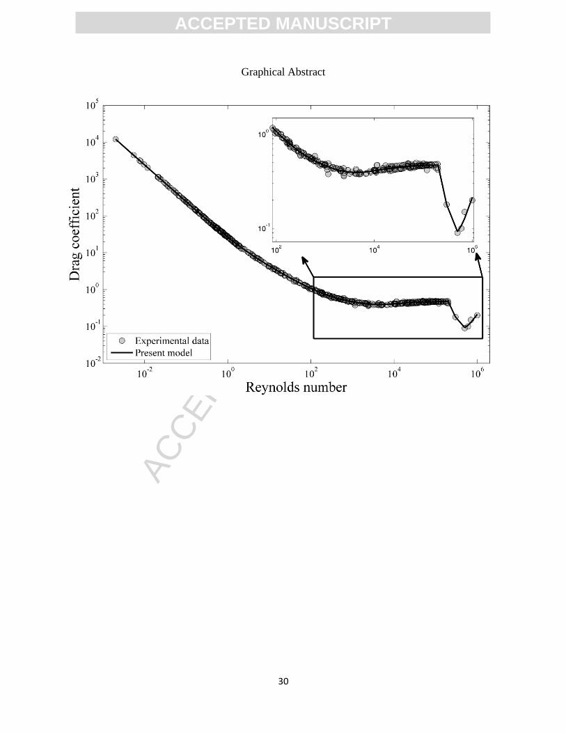
Highlights

The existing correlations of drag coefficient were reviewed. Multi-gene genetic programming

was used to develop drag coefficient models. Both parameters and structure of models were

optimized. The developed models give (up to almost 70%) better results than the best existing

correlations in terms of the sum of squared of logarithmic deviations (SSLD).

ACC

EPTE

D M

ANU

SCR

IPT

ACCEPTED MANUSCRIPT

30

Graphical Abstract