SPHERE ZIMPOL: Overview and performance simulation

Christian Thalmanna, Hans M. Schmida, Anthony Boccalettib, David Mouilletc, KjetilDohlend, Ronald Roelfsemae, Marcel Carbilletf, Daniel Gislera, Jean-Luc Beuzitc, Markus

Feldtg, Raffaele Grattonh, Franco Joosa, Christoph U. Kelleri, Jan Kragte, Johan H. Pragte,Pascal Pugetc, Florence Rigale, Frans Sniki, Rens Watersj, Francois Wildik

aInstitute of Astronomy, ETH Zurich, 8092 Zurich, Switzerland;

bLESIA, Observatoire de Paris, 5 place J. Janssen, 92195 Meudon, France;

cLAOG, UMR5571, CNRS/Universite J. Fourier, BP 53X, 38041 Grenoble cedex 9, France;

dLAM, UMR6110, CNRS/Universite de Provence, 13388 Marseille cedex 13, France;

eNOVA-ASTRON, Oude Hoogeveensedijk 4, 7991 PD Dwingeloo, The Netherlands;

fUMR 6525 H. Fizeau, UNS/CNRS/OCA, Campus Valrose, 06108 Nice cedex 2, France;

gMax-Planck-Institut fur Astronomie, Konigstuhl 17, 69117 Heidelberg, Germany;

hINAF, Osservatorio Astronomico di Padova, 35122 Padova, Italy;

iSterrekundig Instituut Utrecht, Princetonplein 5, 3584 CC Utrecht, The Netherlands;

jAstronomical Institute “Anton Pannekoek”, 1098 SJ Amsterdam, The Netherlands;

kObservatoire Astronomique de l’Universite de Geneve, 1290 Sauverny, Switzerland

ABSTRACT

The ESO planet finder instrument SPHERE will search for the polarimetric signature of the reflected light fromextrasolar planets, using a VLT telescope, an extreme AO system (SAXO), a stellar coronagraph, and an imagingpolarimeter (ZIMPOL). We present the design concept of the ZIMPOL instrument, a single-beam polarimeterthat achieves very high polarimetric accuracy using fast polarization modulation and demodulating CCD detec-tors. Furthermore, we describe comprehensive performance simulations made with the CAOS problem-solvingenvironment. We conclude that direct detection of Jupiter-sized planets in close orbit around the brightest nearbystars is achievable with imaging polarimetry, signal-switching calibration, and angular differential imaging.

Keywords: SPHERE, ZIMPOL, extrasolar planets, direct detection, imaging polarimetry, signal switching,angular differential imaging

1. INTRODUCTION

The detection of reflected light from an old (> 1 Gyr) Jupiter-sized extra-solar planet has not yet been achieveddue to the very high intensity contrast (10−8) and the small angular separation between the planet and its parentstar. One goal of the ESO planet finder instrument SPHERE1 (Spectro-Polarimetric High-contrast ExoplanetREsearch) is to perform such a direct detection using a large telescope (VLT), an extreme AO system, a stellarcoronagraph, and a sophisticated polarization imager. Near-infrared imagers will be used for spectral differentialimaging, e.g. in the methane bands.

Light scattered off a gas planet’s atmosphere becomes polarized in the process. This provides the possibilityto detect a polarization signal from a planet among the unpolarized residual light halo of the coronagraphic,AO-corrected image of a bright star with a sufficiently powerful polarimeter.2 In SPHERE, polarimetry willbe possible with the Zurich Imaging Polarimeter (ZIMPOL3–5), an instrument concept based on fast (kHz)polarization modulation and demodulating CCD detectors. ZIMPOL has been proven to achieve polarimetricsensitivities of 10−5.

VLTunit

HWP2SAXO(AO)

NIRcorona-graph

IRDIS

IFS

visiblecorona-graph

WFS

BS

BSHWP1

calib.polar.

dero-tator

ZIMPOL

pol.comp.

calib.polar.

HWPZFLCpol.

modul.pol. BS CCD1

CCD2

ZIMPOL

M4

light path— , high instr. pol.infrared light pathinformationremovable component

Focal-PlaneInstruments

Common Path

Figure 1. Schematic of the SPHERE instrument design, focusing on the components relevant to ZIMPOL. The com-ponents causing strong instrumental polarization (thick arrows) are marked with a thick outline. The mirror M4 andthe polarization compensator (pol. comp.) are used to counteract these detrimental effects. Abbreviations: BS = beamsplitter, HWP = half-wave plate, WFS = wave-front sensor, FLC = ferro-electric liquid crystal.

In order to investigate the feasibility of the required performance of this instrument (contrast 10−8 at aseparation of 1′′), we provide simulations6 made with the software package SPHERE7 (a simulation code forAO, diffraction, photometry and reduction developed within the CAOS problem-solving environment8), usingup-to-date instrumental error estimations from the current SPHERE ZIMPOL design study as input parameters.

2. INSTRUMENT OVERVIEW

The SPHERE instrument is divided into four basic components: The three focal-plane scientific detectors IRDIS9

(InfraRed Dual-beam Imaging and Spectroscopy), IFS10 (Integral Field Spectrograph) and ZIMPOL, and thecommon path, an umbrella term for all other optics between the telescope interface and the scientific detectors.Figure 1 shows a block diagram of the SPHERE ZIMPOL branch.

2.1 Common Path

The light coming from the VLT unit telescope is afflicted with instrumental polarization from the off-axis mirrorM3. A half-wave plate (HWP1) and a tiltable mirror (M4) are used to compensate this polarization offset. Aset of polarizers can be inserted at this point for calibration purposes (calib. polar.).

Another half-wave plate (HWP2) mounted on a rotation stage can be used to reverse the sign of the (as-tronomical) polarization of the light beam, allowing for a convenient form of beam-exchange calibration duringobservations (subsequently referred to as “signal switching”).

Further downstream, a three-mirror field derotator can physically reorient the coordinate system of the skyfield image by a given angle. If this component is deactivated, the motion of the altitude-azimuth mounting of theVLT unit telescope while tracking a target on the continuously spinning globe of the sky will result in a rotationof the field image over time. The derotator can be activated to counteract the natural field rotation, resultingin a constant field orientation during the whole observation. Finally, to avoid smearing during long exposures

synchronization

beamsplitter

modulatedintensity

modulatedpolarization

polarizedlight

polarizationmodulator

demodulating CCD detectors

Figure 2. A schematic of the ZIMPOL detector concept. Note that a single CCD camera would suffice for a fully functionalimaging polarimeter; the second camera merely ensures that no photons are wasted.

without field stabilization, the derotator can be set to compensate the differential field rotation during eachsingle exposure of the science detector, but to reset to its starting position between exposures. The derotatorallows the field orientation to be arbitrarily changed so as to facilitate angular differential imaging.

Then follow the various corrective components of the adaptive optics system SAXO (SPHERE Adaptiveoptics for eXoplanet Observation). It uses a deformable mirror of 180 mm diameter with 41× 41 actuators withinter-actuator stroke > ±3.5µm, and a two-axis tip-tilt mirror with ±0.5mas resolution.11 Further downstreamin the visible branch of the optical path, a Shack-Hartman wavefront sensor (WFS) with 40×40 lenslets operatingin the 0.45–0.95µm band at a temporal sampling frequency of 1.2 kHz using a 240×240 pixel electron-multiplyingCCD detector feeds the corrective optics with real-time information, enabling a global AO loop delay below 1 ms.

A dichroic beam splitter (BS) separates the visible from the near-infrared (NIR) part of the light, allowingthe wavefront sensor to use the full visible flux during NIR observations. Further beamsplitters divide the beamsbetween the WFS and ZIMPOL, and IRDIS and IFS, respectively.

Finally, the common path includes one full coronagraph assembly for each of the two spectral bands. Eachfeatures selection wheels that allow the focal mask and pupil stop to be chosen from a set of Lyot or four-quadrant phase mask (4QPM) components. The coronagraphs attenuate the central peak of the target star’simage, greatly reducing the total brightness contrast in the image and thereby allowing longer frame exposuretimes, while at the same time purging the diffraction features caused by the propagated pupil edges from theimage.

2.2 ZIMPOL

The first component of the ZIMPOL science instrument is a device for compensating the instrumental polarizationintroduced by components further upstream, in particular the field derotator. It consists of a glass plate thatis tilted and rotated to produce an opposite polarization offset in the transmitted beam. The compensation isnecessary to minimize the impact of detector nonlinearities. Then follow a set of calibration polarizers and ahalf-wave plate (HWPZ) with which the linear polarization can be aligned with the orientation of ZIMPOL.These two components are retractable.

The final four components form the ZIMPOL polarimeter per se. A ferro-electric liquid crystal (FLC)polarization modulator exchanges the two complementary polarization components of the light at up to 1 kHz,and a subsequent polarizing beamsplitter (pol. BS) translates the polarization-modulated beam into two intensity-modulated beams. Each beam is focused onto a specialized CCD camera which performs the demodulation inreal-time on the sensor, using masked buffer pixel rows interlaced between the sensitive pixel rows to store onepolarized image while the other is being exposed to light. The photocharges are shifted between the buffer rowsand the sensitive rows in synchronization with the modulation. This way, the sensor can integrate both componentimages quasi-simultaneously over normal frame exposure times (e.g. one second), using the same detection pixels

VLTunit

Fieldderotator

ZIMPOLHWP2

Angular differential imaging PolarimetrySignal switching

AOCorona-graph

Figure 3. A simplified scheme of the SPHERE ZIMPOL instrument pointing out the key components for the threedifferential imaging techniques explained in Section 3. Angular differential imaging can be based on the “natural” fieldrotation caused by the telescope tracking, or on artificial “active” field rotation performed by the derotator optics.

for both images. The shifting of the charge map by one row is quick enough to allow for modulation frequenciesin the kHz range. The speckle noise issue of the conventional single-beam setup is effectively defeated. Figure 2illustrates this working principle.

Although there are two sensors, ZIMPOL is a single-beam design; each sensor acts as a fully functionalimaging polarimeter. This redundancy can be exploited to calibrate residual instrumental effects, or to selecttwo different areas of interest in the field, for instance.

While ZIMPOL is remarkably free of differential flatfielding and calibration issues, laboratory tests for high-contrast duty in SPHERE12 have revealed a more subtle weakness of the system: Polarized differential aberrations.Switching the FLC modulator between its two retardance states also slightly changes its other optical properties.A slight state-dependent wedge effect that affects the pointing of the transmitted beam (“differential pointing”)as well as some higher-order phase-like differential aberrations have been found. Although these effects arevery small (of the order 1 nm RMS), they constitute the primary limiting factor to the polarimetric precision ofZIMPOL in high-contrast applications.

The ZIMPOL detector of SPHERE is designed to work in the V , R and I bands and is optimized for 600–900 nm. The field of view is a square of 3.5′′ that can be shifted around the target star within a field of 4′′ radius.A polarimetric accuracy of at least 10−5 has been attested to the system in laboratory tests,13 and 10−6 appearsfeasible.

Aside from the differential imaging polarimetry, the ZIMPOL camera will also provide high-resolution directimaging in a variety of broad- and narrow-band visible filter ranges, filling the important niche of imagingcircumstellar regions at high contrast and high angular resolution.

3. DIFFERENTIAL TECHNIQUES

In order to meet the extreme constrast requirements of direct planet imaging, the ZIMPOL branch of SPHEREemploys several stages of differential imaging. The raw intensity image of the coronagraphically masked targetstar will be dominated by speckle-like noise caused by the static and quasi-static aberrations of the instrument,about four orders of magnitude above the level where a planet signal could be detected.

The ZIMPOL-specific requirements that instrumental polarization must be kept low and that measurementsof the absolute degree of polarization must be possible impose restrictions on the optical design and thereforeon the differential methods available. Figure 3 shows the components of the instrument responsible for eachdifferential method.

Polarimetry. The most obvious differential technique employed in SPHERE ZIMPOL is imaging polarimetry:By taking an image of two complementary polarization states and subtracting them from each other, the unpo-larized component of the image, including all the starlight, should be removed. In practice, polarized differentialaberrations between the two polarization channels will limit the efficiency of this subtraction, leaving behindan artificial background landscape in the polarization image. Nevertheless, the S/N gain brought about bypolarimetry is on the order of 102.

Signal switching. To calibrate away the spurious background in the polarization image, a second level ofdifferential imaging is employed. By rotating a half-wave plate (HWP2) far upstream in the optical path by 45◦,the sign of the incoming Stokes Q polarization is reversed. The instrumental aberrations, on the other hand,

double difference

frames

software

derotation

0°

90°

180°

270°

averaging

B

planet

aberration noise

double difference

frames

Ai Ai

C

median

R(Ai)

–C

D

double difference

frames

background

subtraction

0°

90°

180°

270°

software

derotation

–C

–C

–C

averaging

Ai Ai – C R(Ai – C)Figure 4. Schematic illustration of angular differential methods on the example of active field rotation with four positions.For angular averaging, the individual exposures (Ai) are simply derotated into the coordinate system of the sky (R(Ai))and added up (B), whereby the background structures are averaged down. For proper angular differential imaging withbackground subtraction, a median background of the raw exposures is first calculated (C) and subtracted from eachexposure (Ai − C) before derotation (R(Ai − C)) and final co-addition (D).

remain unchanged, resulting in the same background landscape as before. If the polarization images before andafter the signal switching are subtracted from one another, the real polarization signals of the astronomical targetadd up constructively while the static background is canceled out.

Again, this method is only effective down to the level at which the background can be reproduced in thesecond image; any change to the optical path on the time scale of the signal switching (i.e. temporal differentialaberrations) will lead to residual structures surviving in the double-difference image, limiting the detectivity offaint signals. The half-wave plate is foreseen to be switched about every 5 minutes during observation.

This calibration method is comparable to the conventional subtraction of a reference PSF (taken from anotherstar) from the target image; the half-wave plate switching is simply an elegant solution to obtaining a referencePSF with a minimum of differential effects and without a substantial amount of overhead time.

Angular differential imaging (ADI). A third level of noise suppression is achieved through angular differentialimaging. Over the course of the observation, the VLT unit telescope’s tracking will cause the observed sky fieldto rotate slowly with respect to the detector, whereas the optical elements responsible for aberrations will remainfixed in the instrument’s frame of reference. This property can be exploited to discern the real signals originatingin the sky from spurious instrumental effects through so-called angular differential imaging.14

A median average of all exposures of the observation run is calculated and subtracted from each individualexposure, removing all static parts of the image. Since the planet moves across the field in an arc during theobservation, it does not leave a strong footprint in the median background and therefore survives the backgroundsubtraction. The exposures are then rotated into the sky’s frame of reference such that the planet signals coincideand add up constructively, whereas any residual background noise is averaged down. This technique is illustratedin Figure 4.

If the background evolves on the time scale of the field rotation, the background subtraction becomes inef-fective. Nevertheless, the field rotation can be exploited for angular averaging, a less effective version of ADI.

In cases where the natural field rotation is insufficient (e.g. for a star near the celestial pole) or erratic (nearthe zenith), the image orientation on the detector can be artificially changed in discrete steps using the fieldderotator optics. This “active” field rotation extends the limited natural rotation arc to 2π. This is particularlybeneficial in the center of the field, where the natural arc length is very limited.

With all three differential methods applied, the noise can likely be suppressed down to the statistical photonnoise for a four-hour observation, as shown by the performance simulation presented below.

4. SIMULATION

4.1 Architecture

To determine the feasibility of detecting exoplanets with SPHERE ZIMPOL and to investigate how its per-formance can be maximized, we have developed a detailed end-to-end performance simulation code.6,7 It iscomposed of two distinct programs.

The diffraction code produces point-spread functions (PSFs) both for the central star occluded by the coron-agraph, and for the off-center planets. It is implemented in the IDL-based problem-solving environment CAOS8

as part of the software package SPHERE. The code simulates the effects of AO-corrected atmospheric turbulenceand various static and differential aberrations. The output is saved to file.

The photometry and reduction code combines a set of PSFs provided by the diffraction code with numericalparameters describing properties of the target star, the planets, the observation procedure, the optical path andthe detector, to simulate the final output pictures of an observation run. Differential imaging and optional signalenhancement methods are applied, and the resulting signal-to-noise curves are plotted to a PS file. This code isimplemented as a free-standing IDL routine.

4.2 Input parameters

During the evolution of the SPHERE project, the accepted set of standard input parameters for the performancesimulation has been updated regularly. The following tables provide an overview of the Standard Case 3 (SC3)as defined in Thalmann (2008)15 and references therein. The differential techniques have been improved for SC4.

Atmospheric parameters

Seeing at 500 nm 0 .′′85Turbulent Layers: 3– altitude z [m]: 0; 1000; 10000– C2

nprofile [%]: 20; 60; 20

– wind speed v [m/s]: 12.5; 12.5; 12.5– direction [◦]: 0; 45; 90

AO guide star parameters

Magnitude: 4Zenith angle [◦]: 30Azimuth angle [◦]: 0

Telescope parameters

Diameter [m]: 8Obscuration ratio: 0.14Zero point [e−/m2 s] 2.1 · 1010

AO system parameters

Imaging wavelength [nm] 750Linear # sub-apertures: 40Integration time [s]: 0.000833Loop delay [s]: 0.001Loop gain: 0.465999WFS wavelength [nm]: 650Read-out noise [e−]: 0.5Dark current [e−/s]: 2Spatial filter efficiency: 0.526298

The AO performance is insensitive to the guide star brightness down to ∼ 8mag, where it starts to degradedue to photon noise in the WFS. For this reason, an arbitrary bright magnitude of 4 is chosen.

Static Aberrations

Telescope Mirror M1 [nm]: 11.9Telescope Mirror M2 [nm]: 11.9Telescope Mirror M3 [nm]: 16.6Instrument [nm]: 34.5AO calibration [nm]: 7.4Fresnel propagation [nm]: 0Beam shift [nm]: 0

Temporal Aberrations

Defocus [nm]: 0.1Pupil shear [D unit]: 0.002Pupil rotation [◦]: 0.3Differential rotation [◦]: 0Temporal beam shift [nm]: 0Temporal high-freq. aberr. [nm]: 11Temporal pointing [mas]: 0.1

The temporal aberrations describe the changes and drifts in the common path on the time scale of the signalswitching, which therefore cause differential effects between the target and reference channel, and limit theeffectiveness of this calibration method. The half-wave plate responsible for signal switching (HWP2) is foreseento toggle its state every few minutes in order to minimize these effects. For this reason, most parameters can

be set to small values or zero. The imperfect surface of the half-wave plate itself, however, introduces its owntemporal aberration whenever it rotates. While the low spatial frequencies of these aberrations are corrected bythe AO, a high-frequency term remains (11 nm RMS in SC3, new goal 5.5 nm in SC4).

Coronagraph parameters

Mask radius [λ/D at 600 nm]: 5Pupil stop transmission [%]: 80Filter bandwidth [nm]: 300Filter central wavelength [nm]: 750Number of wavelengths simulated: 6 or 30

ZIMPOL Aberrations

ADC residuals [mas RMS]: 3.97Phase differential aberr. [nm]: 1Pointing differential aberr. [nm]: 1.5Downstream static aberr. [nm]: 50Beam shift [nm]: 1.1

Laboratory tests conducted at ASTRON and ETH Zurich12 have shown that the beams emerging from theFLC modulator in its two states are not exactly parallel. This differential pointing corresponds to a gradient-shaped aberration of 1.5 nm RMS. Furthermore, an interferometer test revealed “phase-like” (higher-order)differential aberrations of 1 nm RMS. Finally, the differential pointing causes the outgoing beams to pass throughslightly different crosssections of the subsequent optical surfaces, thus the static aberrations induced by theimperfections of those surfaces are not identical between the two polarizations. This so-called beam shift effectadds another 1.1 nm of phase-like differential aberrations. These three specifications are cut in half for SC4.

Photometric parameters

Star type: G0VStar distance [pc]: 3Exposure time [h]: 4Total transmission: 0.067Full-well capacity [photons/px]: 105

Read-out noise [photons/px]: 10

Planet parameters

Angular separations [′′]: 0.05–0.5Size [Jupiter radii]: 1Phase angle [◦]: 80Phase-dependent albedo: 0.13Degree of polarization [%]: 10 and 50

Here, [px] refers to a CCD hardware pixel. A pixel in the final reduced image, on the other hand, is implementedwith 32 such hardware pixels (8 exposed and 8 masked pixels on each of 2 cameras).

Since a planet’s PSF core extends over more than one pixel, convolving the final image with a correspondinglysized aperture removes all noise on the pixel-to-pixel scale while preserving the planet signal. We find that thisspecific form of low-pass filtering improves the S/N ratio by a factor of at least 2 if the image is dominatedby statistical photon noise. The method fails in aberration-dominated images, where the background landscapeshares the planet’s spatial scale. By default, we apply a Gaussian weighted convolution aperture with a FWHMof 2 pixels in all simulations.

5. RESULTS

5.1 Standard Case Performance

The detectivity curves for a simulation under Standard Case 3 conditions (G0V star at 3 pc, classical Lyotcoronagraph, 4 h observation time) are presented in Figure 5. For visual reference, the two-dimensional detectionimages at each stage are shown. In the double-difference image (curve C), a spurious background landscapecaused by the combination of static, polarized and temporal aberrations still obscures any planet signals. Angulardifferential imaging is necessary to reduce this background to a level where planets can be detected.

In the worst-case scenario of a double-difference background fluctuating on the time scale of field rotation,only angular averaging is possible. Curves D and E show the performance for active field rotation over 23 discretepositions and for natural field rotation over a continuous arc of 45◦, respectively. In either case, the best-case sce-nario is a complete elimination of the aberration-dominated background, leaving only the photon noise (curve F).

The detection zone for planets ranges from 0 .′′08 (the edge of the 5λ/D coronagraph) to 0 .′′3 (the controlradius of the AO). The S/N ratios improve with decreasing angular separation. At the photon limit, a 25%polarized Jupiter-sized planet is detectable at 0 .′′3 with ∼ 5σ confidence; at 0 .′′1, the same planet reaches ∼ 50σ.

Note that a prolongation of the observation time by the factor N will lower the photon limit by a factor of1/√

N . However, this gain can only be harnessed if all other noise sources are successfully suppressed below thephoton noise level, which then presents an increasingly challenging task.

A

B

scale = ±0.0050

C

±0.0010

F

±0.0002

E

±0.0002

D

±0.0003

Figure 5. Left: Performance plot for a Standard Case 3 simulation (G0V star at 3 pc) using a Lyot coronagraph with5 λ/D mask radius at λ = 600 nm, after 4 h of observation. The detectivity curves show the level at which a signal isdetected with a confidence of 5σ. The simulated broadband images were composed from 30 monochromatic PSFs, andconvolved with a Gaussian aperture of 2 px width in order to suppress noise below the spatial scale of planet signals. Theplanet at θ = 0 .′′05 is obscured by the coronagraphic mask. Angular averaging (D, E) is the worst-case performance ofADI; in the ideal case, the photon limit (F) is reached. Right: The images corresponding to the plotted curves. Apertureconvolution was not applied here in order to preserve visual detail.

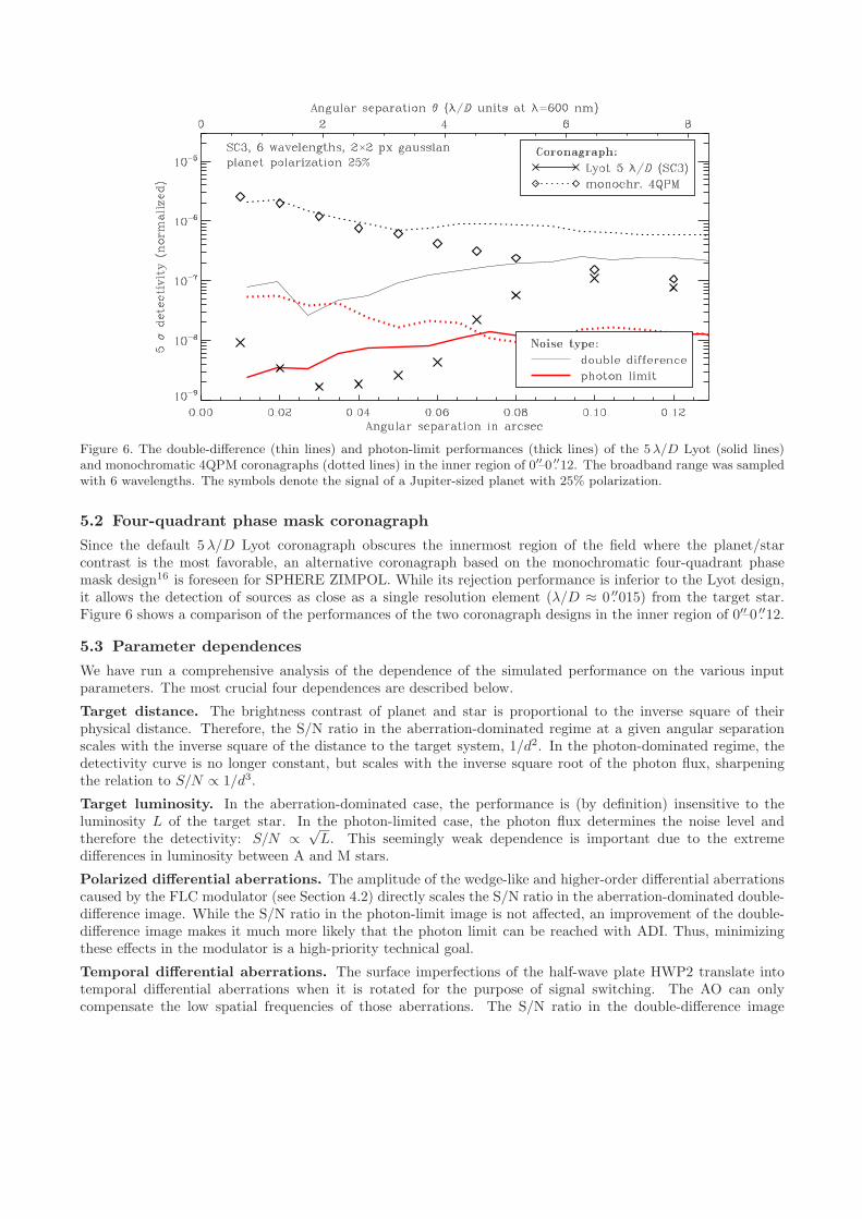
Figure 6. The double-difference (thin lines) and photon-limit performances (thick lines) of the 5 λ/D Lyot (solid lines)and monochromatic 4QPM coronagraphs (dotted lines) in the inner region of 0′′–0 .′′12. The broadband range was sampledwith 6 wavelengths. The symbols denote the signal of a Jupiter-sized planet with 25% polarization.

5.2 Four-quadrant phase mask coronagraph

Since the default 5λ/D Lyot coronagraph obscures the innermost region of the field where the planet/starcontrast is the most favorable, an alternative coronagraph based on the monochromatic four-quadrant phasemask design16 is foreseen for SPHERE ZIMPOL. While its rejection performance is inferior to the Lyot design,it allows the detection of sources as close as a single resolution element (λ/D ≈ 0 .′′015) from the target star.Figure 6 shows a comparison of the performances of the two coronagraph designs in the inner region of 0′′–0 .′′12.

5.3 Parameter dependences

We have run a comprehensive analysis of the dependence of the simulated performance on the various inputparameters. The most crucial four dependences are described below.

Target distance. The brightness contrast of planet and star is proportional to the inverse square of theirphysical distance. Therefore, the S/N ratio in the aberration-dominated regime at a given angular separationscales with the inverse square of the distance to the target system, 1/d2. In the photon-dominated regime, thedetectivity curve is no longer constant, but scales with the inverse square root of the photon flux, sharpeningthe relation to S/N ∝ 1/d3.

Target luminosity. In the aberration-dominated case, the performance is (by definition) insensitive to theluminosity L of the target star. In the photon-limited case, the photon flux determines the noise level andtherefore the detectivity: S/N ∝

√L. This seemingly weak dependence is important due to the extreme

differences in luminosity between A and M stars.

Polarized differential aberrations. The amplitude of the wedge-like and higher-order differential aberrationscaused by the FLC modulator (see Section 4.2) directly scales the S/N ratio in the aberration-dominated double-difference image. While the S/N ratio in the photon-limit image is not affected, an improvement of the double-difference image makes it much more likely that the photon limit can be reached with ADI. Thus, minimizingthese effects in the modulator is a high-priority technical goal.

Temporal differential aberrations. The surface imperfections of the half-wave plate HWP2 translate intotemporal differential aberrations when it is rotated for the purpose of signal switching. The AO can onlycompensate the low spatial frequencies of those aberrations. The S/N ratio in the double-difference image

Table 1. The most favorable target stars for SPHERE ZIMPOL in terms of detectivity. For each star, the absolute V -bandmagnitude and distance in parsecs is given, as well as the S/N ratio for the detection of a 25% polarized Jupiter-sizedplanet at two angular separations (0 .′′03, 0 .′′2) and two different noise level assumptions (active angular averaging over 23field orientations, photon limit), and the frame exposure time texp needed to reach 80% of full well capacity. The 5 λ/Dclassical Lyot coronagraph is assumed for the θ = 0 .′′2 case, and the monochromatic 4QPM coronagraph for θ = 0 .′′03.Otherwise, SC3 conditions are used. Integration time is 4 hours.

absolute S/N ratio framemagnitude distance act. ang. avg. photon limit exp. time

star MV d (pc) 0 .′′03 0 .′′2 0 .′′03 0 .′′2 texp (s)

G0V at 3 pc 4.24 3.00 12.2 5.56 159 7.78 5.1M0V at 3 pc 8.62 3.00 11.4 1.54 9.66 1.13 293

α Cen A 4.36 1.34 83.6 39.9 1475 100 1.2α Cen B 5.72 1.34 56.7 31.8 822 52.2 4.0Sirius A 1.40 2.67 20.8 9.44 486 48.8 0.3Procyon 2.68 3.50 12.6 5.45 163 12.2 1.7

Altair 2.20 5.14 4.88 2.21 46.1 4.85 2.3ε Eri 6.18 3.22 13.4 2.99 34.9 3.08 36τ Cet 5.68 3.65 7.44 2.57 27.4 2.57 29ε Ind 6.89 3.63 8.53 1.59 24.9 1.49 87

AX Mic 8.71 3.95 5.65 0.61 12.4 0.47 55182 Eri 5.35 6.06 2.92 0.70 12.0 0.67 59δ Pav 4.62 6.11 2.92 0.87 10.6 0.88 31o2 Eri 5.92 5.04 4.99 0.97 9.54 0.95 68

70 Oph A 5.67 5.09 4.37 1.09 9.58 0.92 305Barnard’s 13.2 1.82 6.04 0.38 9.47 0.72 7574Proxima 15.5 1.29 5.00 0.30 8.39 0.67 29159

Lacaille 9352 9.76 3.29 5.96 0.55 8.09 0.62 1009GJ 783 6.41 6.05 2.00 0.45 7.96 0.43 155

36 Oph A 6.41 6.10 2.75 0.35 7.57 0.41 151ξ Boo A 5.57 6.70 2.32 0.47 7.50 0.46 88

70 Oph B 7.51 5.11 2.66 0.42 6.72 0.44 305Sirius B 11.3 2.64 4.92 0.39 5.25 0.52 2759

36 Oph B 6.45 5.87 4.39 0.52 4.76 0.40 151GJ 570 A 6.86 5.90 2.92 0.41 4.19 0.43 225ξ Boo B 7.84 6.70 1.62 0.13 2.54 0.16 711

Formalhaut 2.00 6.76 2.56 1.35 35.5 2.33 3.3Arcturus −0.30 11.3 1.25 0.53 16.5 1.28 1.1

Pollux 1.00 10.8 1.08 0.50 15.3 0.89 3.4β Hyi 3.45 7.47 2.81 0.76 8.32 0.83 16δ Eri 3.74 9.04 1.31 0.40 8.04 0.45 221 Ori 3.67 8.02 1.83 0.51 6.44 0.60 30

Canopus −3.10 29.9 0.15 0.08 3.47 0.30 0.6

scales linearly with the amplitude of the remaining high-frequency terms. The surface roughness of HWP2 musttherefore be kept as low as possible.

5.4 Target stars

The relations given in Section 5.3 imply that the S/N ratio for planet detection drops rapidly with increasingtarget distance or decreasing target luminosity. Only the nearest and brightest stars are therefore promisingcandidates.

A list of the most favorable target stars and their S/N ratios for 25% polarized Jupiter-sized planets at twodifferent angular separations is given in Table 1, assuming a 4 h observation. The angular averaging is to betaken as the worst-case scenario for the effectiveness of ADI, whereas the photon limit marks the ideal case. Thetable shows that Jupiter-sized planets can in principle be detected within the AO control radius (0 .′′3) around the

Figure 7. The performance plots for α Centauri A (left) and ε Eridani (right), using the 5 λ/D (top) and 4QPM (bottom)coronagraphs. Otherwise, Standard Case 3 conditions are applied.

eight best target stars in a matter of a few nights using the 5λ/D Lyot coronagraph. The 4QPM coronagraphallows detection of similar planets at very close separations (< 0 .′′1) around at least 20 stars. Due to the extremedependence on target distance, even Neptune-sized planets (S/N reduced by a factor of ∼0.1) or super-Earths(∼0.01) could be found around the closest bright stars (α Cen A and B, Sirius A etc.), and Jupiter-sized planetsare detectable even outside the AO control radius.

Figure 7 presents the performance for two particular target stars, α Cen A and ε Eri. The former is bothcloser and inherently brighter than the latter, resulting in stronger planet signals and lower photon noise. Notethat the double-difference detectivity is insensitive to those astronomical parameters.

For its secondary science objects such as circumstellar disks, SPHERE ZIMPOL’s range will extend muchfurther. For example, the debris disk of TW Hydrae at a distance of 56 pc will be visible in detail.

6. CONCLUSION

We have developed a comprehensive end-to-end performance simulation and analysis for SPHERE ZIMPOL.We find that the detection of exoplanets is feasible by combining three differential noise reduction techniques:High-precision imaging polarimetry, signal-switching calibration, and angular differential imaging. With thedefault 5λ/D Lyot coronagraph, the candidate list for finding Jupiter-sized planets comprises 8 target stars.Furthermore, a monochromatic four-quadrant phase mask coronagraph grants access to the innermost 0 .′′1 ofthe field, extending the candidate list to over 20 stars. Even Neptune-sized planets or super-Earths could bedetected around the best few target stars. Finally, we have identified the polarization modulator of ZIMPOLand the signal-switching half-wave plate as the most critical components; in response, the specifications for theirdifferential behavior have been cut in half in order to improve the instrument performance.

REFERENCES

[1] Beuzit, J.-L., Feldt, M., Dohlen, K., Mouillet, D., Puget, P., Antichi, J., Baruffolo, A., Baudoz, P., Berton,A., Boccaletti, A., Carbillet, M., Charton, J., Claudi, R., Downing, M., Feautrier, P., Fedrigo, E., Fusco, T.,Gratton, R., Hubin, N., Kasper, M., Langlois, M., Moutou, C., Mugnier, L., Pragt, J., Rabou, P., Saisse,M., Schmid, H. M., Stadler, E., Turrato, M., Udry, S., Waters, R., and Wildi, F., “SPHERE: A ‘PlanetFinder’ Instrument for the VLT,” The Messenger 125, 29–34 (2006).

[2] Schmid, H. M., Beuzit, J.-L., Feldt, M., Gisler, D., Gratton, R., Henning, T., Joos, F., Kasper, M., Lenzen,R., Mouillet, D., Moutou, C., Quirrenbach, A., Stam, D. M., Thalmann, C., Tinbergen, J., Verinaud, C.,Waters, R., and Wolstencroft, R., “Search and investigation of extra-solar planets with polarimetry,” IAU

Colloq. 200, 165–170 (2006).

[3] Povel, H. P., Aebersold, F., and Stenflo, J., “Charge-coupled device image sensor as a demodulator in a 2-Dpolarimeter with a piezoelastic modulator,” Appl. Opt. 29, 1186 (1990).

[4] Povel, H. P., Keller, C., and Yadigaroglu, I.-A., “Two-dimensional polarimeter with a charge-coupled-deviceimage sensor and a piezo-elastic modulator,” Appl. Opt. 33, 4254 (1994).

[5] Povel, H., “Imaging stokes polarimetry with piezoelastic modulators and charge-coupled-device image sen-sors,” Optical Engineering 34, 1870 (1995).

[6] Thalmann, C., Applications of High-Precision Polarimetry to Extrasolar Planet Search and Solar Physics,PhD thesis, ETH Zurich (Switzerland) (2008).

[7] Carbillet, M., Boccaletti, A., Thalmann, C., Fusco, T., Vigan, A., Mouillet, D., and Dohlen, K., “Thesoftware package SPHERE: a numerical tool for end-to-end simulations of the VLT instrument SPHERE,”Proc. SPIE 7015 (2008).

[8] Carbillet, M., Verinaud, C., Guarracino, M., Fini, L., Lardiere, O., Le Roux, B., Puglisi, A. T., Femenia,B., Riccardi, A., Anconelli, B., Correia, S., Bertero, M., and Boccacci, P., “CAOS: a numerical simulationtool for astronomical adaptive optics (and beyond),” Proc. SPIE 5490, 637–648 (2004).

[9] Dohlen, K., Langlois, M., and Saisse, M., “The infra red dual imaging and spectrograph for SPHERE:design and performance,” Proc. SPIE 7014 (2008).

[10] Claudi, R., Turatto, M., Gratton, R., Antichi, J., Bruno, P., Cascone, E., De Caprio, V., Desidera, S., Mesa,D., and Scuderi, S., “SPHERE IFS: the spectro differential imager of the VLT for exoplanets search,” Proc.

SPIE 7014 (2008).

[11] Petit, C., Fusco, T., Conan, J.-M., Sauvage, J.-F., Rousset, G., Gigan, P., Charton, J., Mouillet, D., Rabou,P., Kasper, M. E., Fedrigo, E., Hubin, N., Feautrier, P., Beuzit, J.-L., and Puget, P., “The SPHERE XAOsystem: design and performance,” Proc. SPIE 7015 (2008).

[12] Roelfsema, R. and Gisler, D., “ZIMPOL FLC Test Report,” ESO internal document VLT-TRE-SPH-14690-0185, ASTRON (2007).

[13] Thalmann, C., Testing the ZIMPOL Concept for Exoplanet Search, Master’s thesis, ETH Zurich (2004).

[14] Marois, C., Lafreniere, D., Doyon, R., Macintosh, B., and Nadeau, D., “Angular Differential Imaging: APowerful High-Contrast Imaging Technique,” ApJ 641, 556–564 (2006).

[15] Thalmann, C., “Zimpol simulations and performance analysis report,” ESO internal document VLT-TRE-SPH-14690-0191 issue 2, ETHZ (2008).

[16] Rouan, D., Riaud, P., Boccaletti, A., Clenet, Y., and Labeyrie, A., “The Four-Quadrant Phase-MaskCoronagraph. I. Principle,” PASP 112, 1479–1486 (2000).