
The Sphere Anemometer – Optimization for Atmospheric Wind ...
169
The Sphere Anemometer – Optimization for Atmospheric Wind Measurements Hendrik Heißelmann Von der Fakultät für Mathematik und Naturwissenschaften der Carl von Ossietzky Universität Oldenburg zur Erlangung des Grades und Titels eines DOKTORS DER NATURWISSENSCHAFTEN DR . RER . NAT. angenommene Dissertation von Herrn Hendrik Heißelmann geboren am 24. August 1980 in Osnabrück
-
Upload
khangminh22 -
Category
Documents
-
view
0 -
download
0
Transcript of The Sphere Anemometer – Optimization for Atmospheric Wind ...

The Sphere Anemometer – Optimization for
Atmospheric Wind Measurements
Hendrik Heißelmann
Von der Fakultät für Mathematik und Naturwissenschaftender Carl von Ossietzky Universität Oldenburg
zur Erlangung des Grades und Titels eines
DOKTORS DER NATURWISSENSCHAFTEN
DR. RER. NAT.
angenommene Dissertation
von Herrn Hendrik Heißelmanngeboren am 24. August 1980 in Osnabrück

Gutachter: Prof. Dr. Joachim Peinke
Zweiter Gutachter: Prof. Dr. Martin Kühn
Tag der Abgabe: 27. Juni 2017
Tag der Disputation: 12. September 2017

iiiAbstract
This thesis deals with the development of a sphere anemometer for the measure-
ments of wind speed and direction in the complex conditions of wind energy and
meteorology applications. It is optimized in several development stages regarding its
2D calibration and temporal resolution. Systematic investigations on the impact of
tube material and sphere surface properties on the 2D calibration function yield a fi-
nal development stage of the anemometer.
The assessment in wind tunnel experiments confirms this prototype to be competi-
tive with commercial anemometers regarding the measurement accuracy, precision
and temporal resolution. A tilt experiment is performed to mimic vertical wind com-
ponents and thereby quantify their impact on the cross-flow response of the sphere
anemometer. The observed asymmetric response characteristic shows a reduction of
the measured wind speeds in down-wind scenarios, which is explained by consider-
ations of the flow around the sphere and its support tube.
Comparative measurements of the sphere anemometer and two commercial ane-
mometers are performed in two different turbulent flow situations. In the first exper-
imental campaign, the sphere anemometer, a cup anemometer and a sonic anemo-
meter are exposed to a reproducible turbulent flow in the wind tunnel, while the sec-
ond campaign is a multi-day field test in real atmospheric turbulence. The compared
wind speed and direction measurements of the sphere anemometer agree well with
the sonic anemometer in the wind tunnel. Some deviations are found in the field data
for the wind speeds and in particular for the wind directions, as effects of the ambient
conditions and the imperfections of the installation site come into play.
iv Abstract / Zusammenfassung
Zusammenfassung
Diese Arbeit befasst sich mit der Weiterentwicklung eines Kugelanemometers zur Mes-
sung der Windgeschwindigkeit und -richtung unter den komplexen Bedingungen von
Windenergie- und Meteorologieanwendungen. Es wird in mehreren Entwicklungs-
schritten hinsichtlich seiner 2D Kalibrierung und seiner Zeitauflösung optimiert. Der
Einfluss der eingesetzten Materialien und Kugeloberflächen wird dabei systematisch
untersucht und mündet in einer finalen Entwicklungsstufe des Kugelanemometers.
Windkanaluntersuchungen bestätigen, dass dieser Prototyp in Bezug auf Zeitauflö-
sung und Messgenauigkeit mit kommerziellen Anemometern wettbewerbsfähig ist.
Der Einfluss von vertikalen Windkomponenten auf das Kugelanemometer wird in
einem Neigungsexperiment quantifiziert. Ein asymmetrisches Antwortverhalten wird
dabei beobachtet und mittels der Strömung um die Kugel und ihre Halterung erklärt.
Um Kenntnisse über die Leistungsfähigkeit des Kugelanemometer zu gewinnen,
werden vergleichende Messungen mit zwei kommerziellen Anemometern in turbu-
lenten Strömungen durchgeführt. Dazu werden das Kugelanemometer, ein Scha-
lensternanemometer und ein Ultraschallanemometer zunächst in einer künstlichen,
turbulenten Anströmung im Windkanal untersucht und anschließend in einem mehr-
tägigen Freifeld-Experiment realer, atmosphärischer Turbulenz ausgesetzt.
Die mit dem Kugelanemometer und dem Ultraschallanemometer gemessenen Wind-
geschwindigkeiten und -richtungen stimmen in den Labormessungen gut überein.
In den Freifeldmessungen zeigen sich hingegen einige Abweichungen, die insbeson-
dere bei der Windrichtungsmessung zu Tage treten. Sie können auf die Umgebungs-
bedingungen und die baulichen Gegebenheiten des Installationsorts zurückgeführt
werden.

Contents
Abstract iii
Zusammenfassung iv
Contents vii
List of Figures xii
List of Tables xiii
1 Introduction 1
1.1 Motivation and Objective . . . . . . . . . . . . . . . . . . . . . . . . . . . . 1
1.2 Structure of this Thesis . . . . . . . . . . . . . . . . . . . . . . . . . . . . . . 3
2 Reference Sensors for Laboratory and Field Applications 5
2.1 Reference Sensors for Wind Tunnel Applications . . . . . . . . . . . . . . 5
2.1.1 Pressure Sensors . . . . . . . . . . . . . . . . . . . . . . . . . . . . . 6
2.1.2 Hot-wire Anemometry . . . . . . . . . . . . . . . . . . . . . . . . . . 9
2.2 Cup Anemometer & Vane . . . . . . . . . . . . . . . . . . . . . . . . . . . . 10
2.3 Ultrasonic Anemometers . . . . . . . . . . . . . . . . . . . . . . . . . . . . 13
2.4 Drag Force Anemometers . . . . . . . . . . . . . . . . . . . . . . . . . . . . 15
3 The Sphere Anemometer Principle 19
3.1 Principle of Operation . . . . . . . . . . . . . . . . . . . . . . . . . . . . . . 19
3.2 Drag Coefficients of Sphere and Cylinder . . . . . . . . . . . . . . . . . . . 20
3.3 Measuring Method of the Sphere Deflection . . . . . . . . . . . . . . . . . 23
3.4 Previous Investigations in Oldenburg . . . . . . . . . . . . . . . . . . . . . 25
3.5 Summary & Discussion . . . . . . . . . . . . . . . . . . . . . . . . . . . . . 28
4 Anemometer Design Criteria 29
4.1 Wind Speed Range of Operation . . . . . . . . . . . . . . . . . . . . . . . . 29
4.2 Calibration Function . . . . . . . . . . . . . . . . . . . . . . . . . . . . . . . 30
4.3 Spatial and Temporal Resolution . . . . . . . . . . . . . . . . . . . . . . . . 31
4.4 Summary & Discussion . . . . . . . . . . . . . . . . . . . . . . . . . . . . . 33
vi CONTENTS
5 1st Generation Sphere Anemometer 35
5.1 Sphere Anemometer Setup . . . . . . . . . . . . . . . . . . . . . . . . . . . 35
5.2 Sensor Calibration . . . . . . . . . . . . . . . . . . . . . . . . . . . . . . . . 39
5.2.1 Acoustic Wind Tunnel in Oldenburg . . . . . . . . . . . . . . . . . . 39
5.2.2 Setup for 1D & 2D Calibration . . . . . . . . . . . . . . . . . . . . . 40
5.2.3 1D Calibration Function . . . . . . . . . . . . . . . . . . . . . . . . . 42
5.2.4 2D Calibration Function . . . . . . . . . . . . . . . . . . . . . . . . . 43
5.3 Impact of Sphere Patterns and Tube Material . . . . . . . . . . . . . . . . . 47
5.3.1 1D Calibration Function with Different Spheres . . . . . . . . . . . 49
5.3.2 2D Calibration Function with Different Spheres . . . . . . . . . . . 53
5.4 Temporal Resolution & Natural Frequency . . . . . . . . . . . . . . . . . . 55
5.5 Summary & Discussion . . . . . . . . . . . . . . . . . . . . . . . . . . . . . 59
6 2nd Generation Sphere Anemometer 61
6.1 Sphere Anemometer Setup . . . . . . . . . . . . . . . . . . . . . . . . . . . 61
6.2 Sensor Calibration . . . . . . . . . . . . . . . . . . . . . . . . . . . . . . . . 63
6.2.1 1D Calibration Function . . . . . . . . . . . . . . . . . . . . . . . . . 63
6.2.2 2D Calibration Function . . . . . . . . . . . . . . . . . . . . . . . . . 65
6.3 Temporal Resolution & Natural Frequency . . . . . . . . . . . . . . . . . . 68
6.4 Summary & Discussion . . . . . . . . . . . . . . . . . . . . . . . . . . . . . 70
7 3rd Generation Sphere Anemometer 71
7.1 Sphere Anemometer Setup . . . . . . . . . . . . . . . . . . . . . . . . . . . 71
7.2 Sensor Calibration . . . . . . . . . . . . . . . . . . . . . . . . . . . . . . . . 75
7.2.1 1D Calibration Function . . . . . . . . . . . . . . . . . . . . . . . . . 77
7.2.2 2D Calibration Function . . . . . . . . . . . . . . . . . . . . . . . . . 78
7.2.3 Impact of Different Amplification Factors . . . . . . . . . . . . . . . 81
7.3 Precision and Accuracy of the Measurements . . . . . . . . . . . . . . . . 83
7.4 Temporal Resolution & Natural Frequency . . . . . . . . . . . . . . . . . . 85
7.5 Response to Cross-Flow . . . . . . . . . . . . . . . . . . . . . . . . . . . . . 86
7.6 Summary & Discussion . . . . . . . . . . . . . . . . . . . . . . . . . . . . . 92
8 Turbulent Wind Measurements 95
8.1 Turbulent Inflow Measurements . . . . . . . . . . . . . . . . . . . . . . . . 95
8.1.1 Experimental Setup . . . . . . . . . . . . . . . . . . . . . . . . . . . 95
8.1.2 Data Acquisition & Processing . . . . . . . . . . . . . . . . . . . . . 96
8.2 Comparison of Horizontal Wind Speed Measurements . . . . . . . . . . . 97
8.3 Comparison of Wind Direction Measurements . . . . . . . . . . . . . . . . 103
8.4 Summary & Discussion . . . . . . . . . . . . . . . . . . . . . . . . . . . . . 104
9 Sphere Anemometer Field Test 107
9.1 Preparative Experiments . . . . . . . . . . . . . . . . . . . . . . . . . . . . . 107
9.2 Installation & Site Description . . . . . . . . . . . . . . . . . . . . . . . . . 112
9.3 Data Acquisition & Processing . . . . . . . . . . . . . . . . . . . . . . . . . 113

CONTENTS vii
9.4 Anemometer Comparison . . . . . . . . . . . . . . . . . . . . . . . . . . . . 115
9.4.1 Wind Speed Measurements . . . . . . . . . . . . . . . . . . . . . . . 115
9.4.2 Wind Direction Measurements . . . . . . . . . . . . . . . . . . . . . 119
9.5 Summary & Discussion . . . . . . . . . . . . . . . . . . . . . . . . . . . . . 120
10 Conclusions 123
10.1 Summary . . . . . . . . . . . . . . . . . . . . . . . . . . . . . . . . . . . . . . 123
10.2 Outlook and Recommendations . . . . . . . . . . . . . . . . . . . . . . . . 127
A Convergence of the Calibration 131
B 1st & 2nd Generation Sphere Anemometer Electronics 133
C 3rd Generation Sphere Anemometer Electronics 135
D Synchronization of the Field Test Data 139
Bibliography 145
Danksagung 147
Curriculum Vitae 149
Erklärungen 151
List of Publications 153

viii CONTENTS

List of Figures
2.1 Sketch of a Pitot-static tube . . . . . . . . . . . . . . . . . . . . . . . . . . . 7
2.2 Photos of two state-of-the-art cup anemometer models . . . . . . . . . . 11
2.3 Operational principle of a sonic anemometer . . . . . . . . . . . . . . . . 13
2.4 Sketch of Gill WindMaster Pro 3D senor head . . . . . . . . . . . . . . . . 15
2.5 Hole ball anemometer by Norwood et al. [1966] . . . . . . . . . . . . . . . 16
2.6 Ping pong ball anemometer by Reed III and Lynch [1963] . . . . . . . . . 16
3.1 Tip displacement of the sphere due to acting drag forces . . . . . . . . . . 20
3.2 Definition of the flow regimes for a sphere . . . . . . . . . . . . . . . . . . 22
3.3 Drag coefficient of spheres with different surfaces . . . . . . . . . . . . . . 23
3.4 Displacement measurements with a light pointer . . . . . . . . . . . . . . 24
3.5 Sketch of a linear 2D-PSD . . . . . . . . . . . . . . . . . . . . . . . . . . . . 25
3.6 Photo of two position sensitive detector types . . . . . . . . . . . . . . . . 25
3.7 Sphere anemometer setup by Schulte [2007] . . . . . . . . . . . . . . . . . 27
3.8 Sphere anemometer setup by Heißelmann [2008] . . . . . . . . . . . . . . 28
4.1 Link between sphere anemometer design parameters . . . . . . . . . . . 34
5.1 Drawing of the 1st generation sphere anemometer setup . . . . . . . . . . 36
5.2 Photo of the laser diode . . . . . . . . . . . . . . . . . . . . . . . . . . . . . 37
5.3 Photo of the lens and lens mount . . . . . . . . . . . . . . . . . . . . . . . . 37
5.4 Photo of the sphere with regularly dimpled surface pattern . . . . . . . . 39
5.5 Sketch of the acoustic wind tunnel of the University of Oldenburg . . . . 40
5.6 Photo of the calibration setup for the 1st generation sphere anemometer 41
5.7 (x, y)-components of 1D calibration for the 1st generation sphere ane-
mometer . . . . . . . . . . . . . . . . . . . . . . . . . . . . . . . . . . . . . . 43
5.8 Displacement magnitude of the 1D calibration for the 1st generation
sphere anemometer . . . . . . . . . . . . . . . . . . . . . . . . . . . . . . . 44
5.9 3D plot of the 2D calibration for the 1st generation sphere anemometer . 45
5.10 Projected 2D calibration for the 1st generation sphere anemometer . . . 46
5.11 Angular deviations of the laser displacement from the mean . . . . . . . 46
5.12 Deviation of the measured inflow angle from the set inflow angle . . . . . 47
5.13 Photo of the re-designed spheres with different surface patterns . . . . . 49
5.14 Photo of the improved 1st generation sphere anemometer . . . . . . . . . 50

x LIST OF FIGURES
5.15 1D calibration function with fine and coarsely dimpled spheres . . . . . 52
5.16 Comparison of the 1D calibrations for both irregularly dimpled spheres . 53
5.17 Projected 2D calibration for smooth and coarsely dimpled spheres . . . 54
5.18 Angular deviations of the laser displacement from the mean for smooth
and coarsely dimpled spheres . . . . . . . . . . . . . . . . . . . . . . . . . . 54
5.19 Maximal angular deviation of the laser displacement from the mean for
smooth and coarsely dimpled spheres . . . . . . . . . . . . . . . . . . . . . 55
5.20 Power spectrum of the sphere anemometer with regularly dimpled sphere 57
5.21 Power spectra of the sphere anemometer with smooth and coarsely dim-
pled spheres . . . . . . . . . . . . . . . . . . . . . . . . . . . . . . . . . . . . 58
6.1 Drawing and photo of the 2nd generation sphere anemometer . . . . . . 64
6.2 Photo of the calibration setup for the 2nd generation sphere anemometer 65
6.3 (x, y)-components of 1D calibration for the 2nd generation sphere ane-
mometer . . . . . . . . . . . . . . . . . . . . . . . . . . . . . . . . . . . . . . 66
6.4 Displacement magnitude of the 1D calibration for the 2nd generation
sphere anemometer . . . . . . . . . . . . . . . . . . . . . . . . . . . . . . . 66
6.5 2D calibration for the 2nd generation sphere anemometer . . . . . . . . . 67
6.6 Angular deviations of the laser displacement from the mean . . . . . . . 68
6.7 Deviation of the measured inflow angle from the set inflow angle . . . . . 69
6.8 Power spectrum of the 2nd generation sphere anemometer with smooth
sphere . . . . . . . . . . . . . . . . . . . . . . . . . . . . . . . . . . . . . . . . 69
7.1 Drawing and photo of the 3rd generation sphere anemometer setup . . . 73
7.2 Modified sphere construction to improve the robustness . . . . . . . . . 75
7.3 Photo of the calibration setup for the 3rd generation sphere anemometer 76
7.4 (x, y)-components of 1D calibration for the 3rd generation sphere ane-
mometer . . . . . . . . . . . . . . . . . . . . . . . . . . . . . . . . . . . . . . 77
7.5 Displacement magnitude of the 1D calibration for the 3rd generation
sphere anemometer . . . . . . . . . . . . . . . . . . . . . . . . . . . . . . . 78
7.6 2D calibration for the 3rd generation sphere anemometer . . . . . . . . . 79
7.7 Angular deviations of the laser displacement from the mean . . . . . . . 80
7.8 Deviation of the measured inflow angle from the set inflow angle . . . . . 80
7.9 Impact of individual channel amplification on the 2D calibration . . . . 82
7.10 Schematic display of measurement precision and accuracy . . . . . . . . 83
7.11 Precision and accuracy of the sphere anemometer . . . . . . . . . . . . . 85
7.12 Power spectrum of the sphere anemometer with smooth sphere . . . . . 86
7.13 Setup for the cross-flow characterization of the sphere anemometer . . . 87
7.14 Measured offset due to gravitation upon tilting the anemometer . . . . . 88
7.15 Cross-flow response to horizontal wind speed of the tilted anemometer . 89
7.16 Illustration of the flow separation for different orientations of the sphere
support . . . . . . . . . . . . . . . . . . . . . . . . . . . . . . . . . . . . . . . 91
7.17 Thread at the transition region between sphere and support . . . . . . . 92

LIST OF FIGURES xi
7.18 Impact of premature separation on the acting drag forces . . . . . . . . . 93
8.1 Photo of the experimental setup with the active grid . . . . . . . . . . . . 96
8.2 Measurements behind the active grid for 8 m/s wind speed . . . . . . . . 98
8.3 Measurements behind the active grid for 20 m/s wind speed . . . . . . . 101
8.4 Power spectra of the horizontal wind speed measured behind the active
grid . . . . . . . . . . . . . . . . . . . . . . . . . . . . . . . . . . . . . . . . . 103
8.5 Wind direction measurements behind the active grid . . . . . . . . . . . . 105
8.6 Power spectra of the wind direction measured behind the active grid . . 105
9.1 Sketch of the setup for the anemometer cross-talk characterization . . . 108
9.2 Impact of the spacing on the signals of sphere and sonic anemometer . . 109
9.3 Impact of the spacing on the signals of sphere and cup anemometer . . . 110
9.4 Impact of the spacing on the signals of sphere and cup anemometer for
different inflow angles . . . . . . . . . . . . . . . . . . . . . . . . . . . . . . 111
9.5 Aerial view of the site for the field test . . . . . . . . . . . . . . . . . . . . . 112
9.6 Photo of the installed anemometers on a common boom . . . . . . . . . 113
9.7 Excerpts of the measured time series of horizontal wind speeds . . . . . 116
9.8 10-minute averages of the measured horizontal wind speed and turbu-
lence intensity . . . . . . . . . . . . . . . . . . . . . . . . . . . . . . . . . . . 116
9.9 Histograms and power spectra of the horizontal wind speed measure-
ments . . . . . . . . . . . . . . . . . . . . . . . . . . . . . . . . . . . . . . . . 117
9.10 Impact of the vertical wind component on the measurements . . . . . . 119
9.11 Time series excerpt of the measured wind directions and histogram of
direction fluctuations . . . . . . . . . . . . . . . . . . . . . . . . . . . . . . 120
9.12 Sketch of the experimental site with adjacent building structures . . . . . 120
10.1 Sphere design suggestion to improve cross-flow response . . . . . . . . . 128
10.2 Ice accretion on sphere and sonic anemometer . . . . . . . . . . . . . . . 129
A.1 Convergence of the mean laser displacement magnitude . . . . . . . . . 132
A.2 Convergence of the measured mean wind speed . . . . . . . . . . . . . . . 132
B.1 Plan of the sensor circuit for the 1st and 2nd generation sphere anemo-
meters. . . . . . . . . . . . . . . . . . . . . . . . . . . . . . . . . . . . . . . . 134
B.2 Board design of sensor circuit for the 1st and 2nd generation sphere ane-
mometers. (a) top layer; (b) bottom layer . . . . . . . . . . . . . . . . . . . 134
C.1 Circuit diagram of the sphere anemometer sensor electronics for the ap-
plication in field sites. . . . . . . . . . . . . . . . . . . . . . . . . . . . . . . 136
C.2 Circuit board of the sphere anemometer sensor electronics for the ap-
plication in field sites. The 2D-PSD was fitted on the board such that it
was located in the center of the anemometer housing. . . . . . . . . . . . 137

xii LIST OF FIGURES
D.1 Assessment of the data logging system. (a) Saw-tooth signals recored
with both AD converters and (b) time lag τderived from the cross-correlation
for each recorded two-minute block. . . . . . . . . . . . . . . . . . . . . . 140

List of Tables
5.1 Specifications of the laser diode . . . . . . . . . . . . . . . . . . . . . . . . 38
5.2 Specifications of the lens and lens mount . . . . . . . . . . . . . . . . . . . 38
5.3 Maximal angular deviation of the laser displacement from the mean . . 47
5.4 List of sphere properties . . . . . . . . . . . . . . . . . . . . . . . . . . . . . 51
5.5 Fit parameters for 1D calibrations with both irregularly dimpled spheres 53
6.1 Maximal angular deviation of the laser displacement from the mean . . 67
7.1 Maximal angular deviations of the laser displacement from the mean . . 79
8.1 Average values measured behind the active grid for 8 m/s wind speed . . 99
8.2 Average values measured behind the active grid for 20 m/s wind speed . 102
9.1 Properties of full data set and selected wind direction sectors . . . . . . . 114
9.2 Mean quantities for the selected wind direction sector II . . . . . . . . . . 115

Chapter 1
Introduction
1.1 Motivation and Objective
The worldwide demand for energy is projected to increase by 48% from 2012 to 2040
[EIA, 2016]. As the vast majority of countries committed to the Paris climate accord in
2015, the need for renewable energy sources to play a major role in the future energy
supply is undeniable. Renewables are the fastest growing source of electric energy
and wind energy in particular is one of its most powerful contributers. Hence, wind
energy is of paramount importance to achieve the climate protection goals while cop-
ing with mankind’s growing demand for electricity.
Wind energy projects vary in size and type, ranging from single wind turbines to
large wind farms at on-shore and off-shore sites. All of these projects rely on the wind
resource itself and a thorough site assessment is crucial for the estimation of the wind
power generation of a wind turbine or wind farm. Even small errors in the wind speed
measurements can make a significant difference in terms of the annual energy pro-
duction due to the cubic relation between wind speed and wind power. Accurate
knowledge of the prevailing wind conditions on-site is thus paramount for the esti-
mation of the expected annual energy production and consequently the generated
revenue of any wind energy project.
The site assessment and the characterization of the wind turbine’s power curve are
typically performed in measurement campaigns with conventional anemometers in-
stalled on meteorological masts. However, the emergence of ground-based remote
sensing techniques, such as Light Detection And Ranging (LiDAR), can change this
practice in the future. In any case, it is important to minimize the errors in the wind
speed and wind direction measurements.
Today, mainly cup anemometers are used for wind resource assessment. De-
veloped in the 19th century, their design is intriguingly simple: A vertical axis rotor
with attached cups is rotating due to the horizontal wind speed and its rotational fre-
quency is proportional to the wind speed. Cup anemometry has been intensively
investigated over the years and several issues have been identified [Wyngaard, 1981].
Most notably, cup anemometers suffer from the effects related to their rotational mea-

2 1. Introduction
suring principle: the wear-out of bearings and the high moment of inertia. These is-
sues have been investigated since the 1920s [Schrenk, 1929] and optimizations nowa-
days focus mostly on the design of the light-weight rotors and the conical shape of the
cups, in order to reduce inertial effects and mitigate the unfavorable over-speeding
[Strangeways, 2003; Deacon, 1951; Kristensen, 1993].
During the last decades, sonic anemometers evolved into an alternative to cup ane-
mometers. They make use of the velocity-dependent time shift, which is experienced
by an ultrasonic wave when it passes through the measurement volume. Sonic ane-
mometers can provide a higher temporal resolution than cup anemometers and lack
any wearing parts. The combination of several transducer pairs additionally allows for
the measurement of all three velocity components of the wind, i.e. horizontal wind
speed, wind direction and vertical wind speed. The required ultrasonic transducers
are, however, more vulnerable to mechanical disturbances as even small misalign-
ments of the transducers may prevent the anemometer from correct measurements.
For years, cup anemometers were the only certified sensors for the measurement of
the wind conditions during site assessment and for the characterization of a wind
turbine’s power curve according to the IEC standard 64100-12-1 [IEC, 2005]. The lat-
est revision of the standard, however, includes sonic anemometers as an alternative
sensor for those purposes [IEC, 2015]. Although it even allows for the use of ground-
based LiDARs for the power curve characterization in flat terrain, those are required
to be complemented by conventional anemometers on a nearby met-mast.
Motivated by the shortcomings of the established anemometers for atmospheric
applications, the sphere anemometer has been developed at the University of Olden-
burg as an alternative. The employed principle of drag-based flow measurements is
not entirely new and various attempts have been made in the past to incorporate it in
an anemometer setup [Smith, 1980; McNally, 1970; Kirwan et al., 1975]. Nevertheless,
none of those anemometer prototypes could be established and most of them disap-
peared shortly after their introduction.
The aim of the sphere anemometer is to combine the robustness of cup anemometers
with the sonic anemometers’ capability of wind speed and direction measurements
at a high temporal resolution. The concept pursued at the University of Oldenburg
relies therefor on a highly resolving laser measuring technique to detect the drag-
dependent displacement of a sphere. Conceptual studies have been performed at the
University of Oldenburg in the past and a first prototype of this sphere anemometer
for two-dimensional measurements has been realized [Heißelmann, 2008]. It consti-
tutes the basis for the further developments.
The objective of this thesis is the optimization of the sphere anemometer towards
its application in atmospheric field measurements. It is therefore essential to charac-
terize the issues of the existing sphere anemometer prototypes and improve it based
on the gained insights. A systematic investigation of the different design parame-
ters of the sphere anemometer, in particular the sphere surface patterns and the tube
material, is thus indispensable. The knowledge of these properties and their im-

1.2 Structure of this Thesis 3
pact on the sphere anemometer can than be employed for the improvement of the
sphere anemometer setup. It is therefor crucial to achieve a reliable and unique two-
dimensional calibration function and a sufficiently high natural frequency of the me-
chanical setup.
Once the design parameters are found, the setup can be adapted to the application in
the complex outdoor conditions by making it weather-proof.
In a final step of this thesis, the sphere anemometer prototype is characterized in de-
tail by means of wind tunnel experiments, before a field measurement campaign is
performed as a proof of its capability to operate in atmospheric wind conditions.
1.2 Structure of this Thesis
This thesis starts in Chapter 2 with a brief introduction of the velocity measurement
techniques used during the course of this work. Methods for pressure measurements
using mechanical and electrical gauges will be introduced as well as the commonly
used hot-wire anemometry. Moreover, cup and ultrasonic anemometers as the two
mostly used commercial wind speed sensors for meteorological applications are de-
scribed. A selection of previously developed drag-based anemometers – mainly spher-
ical anemometers of different kinds – is also presented to provide a historic overview
of the topic.
Chapter 3 introduces the general operational principle of the sphere anemometer
and the laser-based measuring technique in particular. Basic properties of the flow
around a sphere and its implications on the generated drag will be explained and
properties and issues of the previous sphere anemometer prototypes developed at
the University of Oldenburg are summarized. It is followed by a brief overview of the
design criteria for the sphere anemometer development in Chapter 4. Key features
like the measuring range and resolution are treated as well as the expected calibration
function. The entanglement of different design parameters is explained to assist in
the selection of proper materials and geometry for the sphere anemometer setups.
Constituting the starting point of the further development of the sphere anemo-
meter towards a robust and reliable sensor for wind energy applications in complex
environments, the 1st generation sphere anemometer is presented in Chapter 5. Its
sensor setup is described in detail and its characteristics are concluded from calibra-
tion measurements and spectral analyses. Particular emphasis is given to the identifi-
cation of the impact of the tube material and the sphere surface on the 2D calibration.
These findings trigger modification of the mechanical setup, which are embodied
in the 2nd generation sphere anemometer, specified in Chapter 6. It can be consid-
ered an intermediate development stage, before a further improvement of the setup
towards field applications is made in the final development stage – the 3rd generation
sphere anemometer. A description of the changes made and a detailed analysis of the
sensor properties is presented in Chapter 7. Special emphasis is given to the accuracy,
precision and the resolution of the sphere anemometer as well as its response to up-

4 1. Introduction
and down-wind components.
Turbulent inflow under laboratory conditions is used to compare the performance
of the 3rd generation sphere anemometer with commercial cup and ultrasonic ane-
mometers. The results of these measurements are presented in Chapter 8. In a further
assessment of the anemometers, a field test is carried out with these three sensors.
Preparative investigations and the actual wind speed and direction measurements
on-site are addressed in Chapter 9.
Finally, Chapter 10 concludes this thesis as it summarizes the different stages of
the sphere anemometer development and the findings from the various wind tun-
nel and field experiments. An outlook at the future of the sphere anemometer is at-
tempted and some investigations and modifications for the further advancement of
the sensor are recommended.

Chapter 2
Reference Sensors for Laboratoryand Field Applications
This chapter will give a brief introduction to the anemometers, which served as ref-
erence sensors for the evaluation of the sphere anemometer prototypes during the
wind tunnel measurements presented later on in Chapters 5–8. Additionally, the most
common techniques for atmospheric wind measurements in wind energy and meteo-
rology applications will be introduced as they were used for comparison during wind
tunnel and field testing of the sphere anemometer (Ch. 8 & 9). The focus will be on
invasive sensors such as cup anemometers and sonic anemometers. For information
on non-invasive laser-based methods (LDA, PIV) and remote sensing techniques (Li-
DAR, SoDAR) it is referred to literature, e.g. Ruck [1987]; Raffel et al. [2007]; Werner
[2005].
2.1 Reference Sensors for Wind Tunnel Applications
One of the crucial demands for the development and characterization of wind speed
and wind direction sensors is the choice of proper reference anemometers for the
evaluation. The question of which reference anemometer should be used cannot be
generally answered, since each type of anemometer has certain features, like resolu-
tion, accuracy, and many others. Whether an anemometer feature is considered ad-
vantageous or a limitation is subject to the field of application. For example, a highly
resolving hot-wire anemometer may be suitable for the assessment of the quality of
other small sized laboratory anemometers, such as a 2D-LCA [Barth, 2004; Hölling,
2008; Puczylowski, 2015] or an NSTAP (Princeton probe) [Bailey et al., 2010]. How-
ever, it may be a case of comparing apples and oranges if miniaturized anemometers
are used for comparison with larger meteorological sensors or even remote sensing
devices such as LiDARs or SoDARs. A comprehensive assessment of an anemometer
needs to cover different features and can therefor only be achieved by comparison to
different reference sensors.
Moreover, the accuracy of any wind tunnel experiment or calibration of anemometers

6 2. Reference Sensors for Laboratory and Field Applications
is limited by the reproducibility of the wind tunnel reference speed and the accuracy
of the used reference sensors. Although some sensors, such as Laser Doppler Anemo-
meters (LDA), do not require calibration with reference sensors, still the accuracy is
what determines the quality of the results obtained from their application. Thus, the
choice of well-adjusted and calibrated reference sensors is crucial for the reliability of
any wind tunnel study.
The subsequently presented studies will rely on the widely used and very well es-
tablished pressure sensor technology as a calibration reference in laminar flows. Al-
though semiconductor pressure gauges can allow response times in the range of 1 kHz
or even faster, pressure sensors typically feature a lower temporal resolution. This
can be mainly attributed to the tube connections which result in a low-pass filtering
depending on the length and diameter of the used tubings. For common wind tun-
nel applications, temporal response times in the order of 10–100 ms may be achieved
which makes pressure gauges less suitable for the use in turbulent flows. For these
cases, highly resolving hot-wire anemometers are chosen for comparison. Both tech-
niques will be briefly presented hereafter, but for more details, the reader is referred
to standard literature, e.g. by Bruun [1995]; Eckelmann [1997] or Baker [2000].
2.1.1 Pressure Sensors
Pressure sensing can be considered a standard measurement technique for a wide
range of applications in laboratory flows. According to Bernoulli’s Equation
%
2u2︸︷︷︸
pd
+ %g z0 +p0︸ ︷︷ ︸ps
= const (2.1)
pd+ ps = pt (2.2)
the total pressure pt along a trajectory of constant velocity (a stream line) can be con-
sidered constant for the case of incompressible flows and is given as the sum of the
static pressure ps and the dynamic pressure pd . For Mach numbers M a ≤ 0.3, i.e.
fluid velocities smaller that 30 % of the speed of sound, the above stated simplified
Bernoulli Equation (Eq. (2.1)) is valid and can be used to determine the wind speed u
along a stream line from the pressure pd in a fluid flow of constant density % [Baker,
2000]. This will be the case for all pressure measurements treated within this work.
Practically, pressure sensors often consist two parts: A probe with one or more pres-
sure holes which is placed in the flow and a sensing device such as a manometer or an
electrical transducer. So-called Pitot probes feature a single hole at their tip, which is
to be aligned such that it coincides with the front stagnation point of the flow around
the device. The pressure at the front stagnation point is equal to the total pressure
pt . While Pitot tubes possess only a single pressure hole, Pitot-static tubes feature an
additional ring (or a set of connected holes, cf. Figure 2.1) located about 4–5 probe
diameters downstream the tip [Eckelmann, 1997]. This type of probe is also often
referred to as Prandtl tube, originating from the special design Ludwig Prandtl devel-
oped for it during the early 20th century. For visualization purposes, the concept of

2.1 Reference Sensors for Wind Tunnel Applications 7
Figure 2.1: Sketch of the Pitot-static tube probe head. The total pressure pt is obtained at
the front stagnation point (arrow) and the static pressure ps is measured via a set of holes
downstream the probe tip.
stream lines, which can be used for laminar flow situations, is adapted here. Each
stream line marks the trajectory of a infinitesimal fluid element with a fixed flow ve-
locity. The downstream pressure holes are aligned perpendicular to the stream lines
of the flow around the tip of the Prandtl tube and thus allow for the detection of solely
the static pressure ps .1 The differential pressure, which in fact is the dynamic pressure
pd = pt−ps , can be measured and thus the flow velocity can be calculated accordingly
from Equation (2.3)
u =√
2 ·pd
%. (2.3)
The probe head of the Pitot-static tubes has to be carefully aligned with the main flow
direction. Otherwise flow distortions may occur which can clearly affect the measure-
ment of the static pressure at the pressure holes downstream the probe tip. The sever-
ity of such flow distortions depends on the geometry of the probe tip and the down-
stream distance of the static pressure holes. Squared probe tips are less prone to flow
distortions and offer an larger acceptance angle than Prandtl probes, which feature
acceptance angles of about ±10, while hemispheric tips are even stronger affected
[Eckelmann, 1997; Baker, 2000]. Pressure readings obtained with Pitot-static probes
may be subject to errors stemming from different sources, like placement close to
boundary layers or too low flow velocities. These errors may vary depending on the
design of the probe tip as may blockage effects and flow accelerations around the tip.
The Prandtl probe design used for many measurements presented within this work
has been designed by Ludwig Prandtl in an effort to achieve error cancellation by
carefully choosing the probe dimensions and the downstream distances of the pres-
sure holes and support tube [Baker, 2000].
Pitot- and Prandtl probes cannot measure the flow velocity by itself, but have to be
connected to a manometer or pressure sensor. Classical setups employ different types
of liquid manometers, such as U-tube manometers or inclined tube manometers with
one or more fluid columns. These manometers may display several pressure chan-
1Note that the static pressure ps is not equivalent to the hydrostatic pressure at height z0, pg = %g z0,
due to Eq. (2.1).

8 2. Reference Sensors for Laboratory and Field Applications
nels at the same time, but the readings are usually obtained manually or by means
of image analysis techniques. Their analog nature makes them unfeasible for most
of today’s measurement applications, in particular considering the comparably low
temporal resolution of less than 1 Hz and the low degree of measurement automation.
Thus, pressure probes are mainly used in combination with fast pressure transducers
utilizing either small deforming diaphragms or solid state piezoelectric sensors. Both
types provide high time resolutions in the order of 100 Hz or even 1 kHz, respectively.
These sensors usually maintain their calibration over a long time and their electric
output can be directly connected to the used analog-digital (AD) conversion system.
The piezoelectric system is employed in the Setra C239 pressure gauges [Setra Sys-
tems Inc., 2013], which are used for the comparisons throughout this work.
The differential pressure measurement via Prandtl tube is practically carried out
directly within the pressure gauge or manometer. Therefore, the total pressure tubing
is connected to one side of the detector and the static pressure tubing to the other one.
In case of the liquid manometer, both pressure connections are separated internally
by the liquid column, which is consequently shifted due to the pressure difference pd
between the connections. The dynamic pressure pd can either be directly read (as for
a Betz manometer) or has to be calculated from the height difference z of the liquid
with density %liq. For the inclined tube manometer used during some measurements
within this work, pd and consequently the flow velocity can be obtained by
pd = %
2u2
= %liq g z ξ
⇒ u =√
2%liq g z ξ
%. (2.4)
Here, % and g denote the air density and gravitational constant, respectively, while ξ
is an inclination factor of the manometer.
Electric pressure gauges function quite similarly with both tubing being separated
either by the diaphragm or the piezo element. The reading of the transducer is usually
a voltage or current signal which has to be translated to a pressure via the device’s
calibration function. It can than be converted to a velocity using Equation (2.3).
Pressure measurements are not independent of the air density %, as is evident
from Equations (2.3) and (2.4). The actual air density can be calculated from the am-
bient pressure and temperature readings using
%= p
Rh ·T(2.5)
with gas constant of humid air
Rh = Rs
1− r H ·pd /p · (1−Rs/Rv ). (2.6)
Here, Rs and Rv are the specific gas constants of dry air and water vapor, respectively.
T and r H are the absolute temperature and relative humidity of the air and p is the
hydrostatic pressure.

2.1 Reference Sensors for Wind Tunnel Applications 9
2.1.2 Hot-wire Anemometry
Hot-wire anemometry is probably the most used measurement technique for flow
measurements under laboratory conditions. The small probe head of the sensor con-
sists of an electrically conducting wire which is spanned between the tips of a pair of
prongs. The prongs are connected to a regulated supply voltage, causing the wire to
heat up due to the applied current I . Since any metallic wire material changes its re-
sistance Rhw with temperature, once the hot-wire is exposed to the flow, the thermal
transport of the fluid causes the wire to cool down depending on properties like tem-
perature of fluid and wire and the flow velocity u. A Wheatstone bridge circuit is used
to measure the changing resistance of the wire. In order to relate the bridge output
voltage Q to the flow velocity, a calibration function of the hot-wire system has to be
performed. The resulting calibration function can be fitted by a 4th order polynomial
u = u0 +a1Q +a2Q2 +a3Q3 +a4Q4 , (2.7)
where u is the wind speed and the parameters a1 . . . a4 are obtained from the fitting.
Hot-wire anemometers can be either operated in constant current mode (CCA) or
constant temperature mode (CTA), which is used for all applications throughout the
presented work. A single hot-wire or hot-film sensor can only be utilized to measure
the magnitude of the flow velocity without directional information, since all parts of
the wire contribute equally to the thermal transport. However, several differently ori-
ented wires can be combined to one multi-component sensor, permitting the calcu-
lation of two (for a x-wire) or three (for a three or more wires) components of the flow
velocity. While these multi-wire probes can be very useful for the detailed characteri-
zation of turbulence and near wall flows, only single hot-wires were used as reference
anemometers in the presented work.
The hot-wire anemometer’s spatial resolution is determined by the sensor dimen-
sions, i.e. the length of the wire for a single hot-wire or the spatial extent of the probe
prongs for multi-wire probes. Even for single wire probes, the wire length may vary
significantly from several millimeters down to fractions of a millimeter. The probe
dimensions are mainly dictated by the field of application and the wire’s length-to-
thickness ratio, which should not exceed l/d = 200 [Bruun, 1995]. The standard Dan-
tec Dynamics 55P01 single wire probes used within the presented work consist of a
gold-plated tungsten wire with a 1.25 mm long active length and a thickness of 5µm,
resulting in l/d = 250.
Hot-wires are in general quite filigree probes due to the filament, which may be
easily broken by mishandling or even by larger particles suspended in the flow. In or-
der to avoid rapid breakage of the hot-wire probe in more hostile environments such
as water and atmospheric flows, hot-film probes are usually preferred. While the gen-
eral sensor principle is equivalent to hot-wires, their mechanical stability is increased
by using thicker, metal-coated quartz cylinders instead of single wires. Electric insu-
lation from the flow is also achieved by additional coatings. The thermal inertia of
the wire as well as the response time of the used electronics impacts the temporal

10 2. Reference Sensors for Laboratory and Field Applications
resolution of the hot-wire anemometer. Thus, it is only logical, that smaller hot-wires
feature a higher temporal resolution and that on the consequently the added stability
of hot-film probes yields a reduced temporal resolution compared to hot-wires of the
same size.
Hot-wire anemometers served only as a reference for turbulent laboratory mea-
surements presented in Chapter 8 of this work, because of the above mentioned is-
sues regarding robustness in outdoor applications. In these cases, the commercial
Dantec 55P01 hot-wire probes were operated with the Dantec StreamLine® 90S10
frame and the Dantec StreamWare® software (version 3.1) [Dantec Dynamics A/S,
2003]. All outdoor reference sensors were either cup or sonic anemometers described
in the following Sections 2.2 & 2.3.
2.2 Cup Anemometer & Vane
The most used anemometers in meteorological applications and in wind energy are
cup anemometers. The invention of the cup anemometer dates back to 1845 when
J. T. R. Robinson2 first used a four-armed vertical axis rotor with hemispherical drag
bodies fixed to its tips [Wyngaard, 1981; Strangeways, 2003]. While the sensor princi-
ple remained widely unchanged during the last decades, the dimensions of the cup
anemometers decreased significantly from about L =2 m diameter of Robinson’s ane-
mometer to L =0.1–0.2 m in modern types allowing for faster response times and im-
proved spatial resolution. Figure 2.2 shows two state-of-the-art cup anemometers
from Vector Components and Thies Clima as an example.
Measuring Principle
Cup anemometers make use of the drag force FD acting on the cups which are mounted
to each tip of the vertical axis rotor. The drag force caused by the wind speed u on a
body of cross-section A is given by
FD = 1
2·% · cD · A ·u2, (2.8)
with air density % and dimensionless drag coefficient cD . The different shapes of the
closed side and the open side of the cup yields different drag coefficients cD , i.e. differ-
ent drag forces FD . This translates into a torque differential, which causes a rotation
of the rotor with a rotational frequencyω proportional to the prevailing wind speed u
[Eckelmann, 1997]
ω∝ u. (2.9)
The measurement of the rotational frequency is mostly done in common anemome-
ters using either light barriers, magnetic reed relays or hall sensors. Some lower qual-
ity cup anemometer models still use mechanical potentiometers to measure the ro-
tation, but these are outdated due to unavoidable wear-out. The sensor output can
2John Thomas Romney Robinson, 1792–1882

2.2 Cup Anemometer & Vane 11
either be a pulsed (frequency), current or voltage signal and is usually factory-set by
the manufacturer upon request. The pulsed output is favorable for any application
with constraints of the power consumption, as they often occur in field campaigns.
(a) (b)
Figure 2.2: Photos of two state-of-the-art cup anemometer models with three cups (not to
scale). (a) Vector Components model with conical plastic cups on a three-armed wire ro-
tor. (b) Thies First Class Advanced cup anemometer with three conically shaped cups on a
lightweight carbon fiber rotor. The rotor features tilted cups and horizontal extensions to
minimize the effect of cross-flows.
Properties and Issues of Cup Anemometers
Typically, the response of an anemometer is characterized by the time τ the anemo-
meter needs to reach 63% (1/e) of the maximum value of a velocity step∆u. However,
MacCready and Jex [1964] showed that a better characterization of cup anemometers
can be achieved by using the concept of a distance constant l0 instead, which is linked
to τ via Taylor’s hypothesis, l0 = u ·τ. The distance constant l0 can be considered a
measure of the reaction of a cup anemometer being initially in equilibrium at a veloc-
ity u when it is exposed to a velocity step of magnitude ∆u. Practically, the distance
constant l0 corresponds to the length of a fluid column which passes the anemometer
until it reaches 63% of the value of the wind speed step u +∆u [MacCready and Jex,
1964; Wyngaard, 1981; Kristensen, 1999]. Although the distance constant does not
depend on the actual (mean) wind speed, it may differ significantly between various
cup anemometer types. The Risø WindSensor for example is listed with l0 = 1.8 m,
while the significantly cheaper NRG 40C anemometer’s distance constant is a mere
50% larger at l0 = 2.55 m.
Although the cup anemometer is widely used in wind energy and meteorology,
there are several shortcomings of these sensors – amongst them the lack of direction
measurement, the vulnerability to vertical flows and the wear of mechanical parts
like bearings. Still, the most significant problem of cup anemometry is the so-called
over-speeding, which constitutes the over-estimation of the wind speed under tur-
bulent conditions. Over-speeding is caused by the asymmetric characteristics of the

12 2. Reference Sensors for Laboratory and Field Applications
drag forces for increasing and decreasing wind speeds u with it’s severity depend-
ing on the rotor design and inertia. This issue has been very well known for decades
and many models for the description have been developed, e.g. by Schrenk [1929];
Kaganov and Yaglom [1976]; Busch and Kristensen [1976] and Wyngaard [1981], but
since the asymmetric characteristics of the anemometer is an intrinsic feature of its
principle of operation, it will never be entirely avoided. Nevertheless, many attempts
of improvement have been carried out over the years. A lot of research has been done
on the number and the shape of the cups aiming at a reduction of the inertial forces of
the rotor and faster response dynamics. Nowadays rotors of advanced cup anemome-
ters usually consist of a three-armed rotor made of light weight materials, e.g. carbon
fibers, since they provide a more constant torque over a single revolution [Strange-
ways, 2003]. They mostly employ conically shaped cups, which provide better charac-
teristics and less vulnerability to turbulent wind speed fluctuations than hemispheres
[Deacon, 1951]. Special designs of the rotor bars are also often pursued in an attempt
to reduce the impact of cross-flows on the cup anemometer readings.
Additionally, anemometer specific correction schemes for the impact of over-speed-
ing on the wind measurements have been developed and are usually applied on the
measured data [Kristensen, 1993, 1998; Hristov et al., 2000].
As already mentioned, cup anemometers only allow for the measurement of the hor-
izontal wind speed magnitude and do not provide any directional informations. Tho
overcome this shortcoming of the anemometer principle, cup anemometers are usu-
ally complemented with an additional direction sensor, mostly a vane. The wind vane
translates a change of wind direction into a rotational motion, which can be measured
in a similar way as described for the cup anemometer rotation itself. Since a second
sensor is utilized, the wind speed and direction measurements are not obtained at the
same point in space3, but from two spatially separated points. This makes the com-
bination of cup anemometer and vane inappropriate for some applications, e.g. the
measurement of fluxes.
Among today’s commercially distributed anemometers, cup anemometers and vanes
constitute the most used type. This is on the one hand due to its very simple principle
of operation and the rather low pricing of high-end cup anemometers. On the other
hand, no other anemometer (or combination) could be used as reference anemome-
ter for certification purposes according the International Electrotechnical Commis-
sion standard 64100-12-1 [IEC, 2005, Ch. 6.2] for years. Only a recent revision of the
IEC standard 64100-12-1 (Ed. 2) allowed sonic anemometers and LiDAR techniques
for the wind resource assessment and power curve measurement, which is required
for wind turbine installation and financing [IEC, 2015].
3No measurement is performed in a single (perfect) point, but the effect of integration over the sensor
volume is neglected here.

2.3 Ultrasonic Anemometers 13
2.3 Ultrasonic Anemometers
In order to avoid the shortcomings of the cup anemometers – e.g. the low tempo-
ral resolution and the lack of direction measurements – ultrasonic anemometers can
be used for wind speed measurements. Ultrasonic anemometers (often just called
sonic anemometers) have been applied in meteorology for years and lately are gain-
ing ground in wind energy applications as well. They can provide measurements of
several components of the wind speed depending on their design.
Measuring Principle
There are three different principles of sonic anemometer operation, which are used
for various applications. The most used sonic anemometers employ the run-time
method to determine velocities along the sound path [Baker, 2000]. For this purpose
two combined emitter-receiver-modules – so-called transducers – are aligned oppos-
ing each other in a known distance d , as sketched in Figure 2.3 (a). The time of flight
of the acoustic wave traveling from the emitting transducer T1 to the receiving trans-
ducer T2 is measured when it is oriented with the flow direction (t1) and when it is
oriented against it (t2). The difference in time of flights is used to calculate the line of(a) (b)
Figure 2.3: (a) Sketch of the sound path between two transducers, which are inclined to the
flow direction by an angle α. A sonic pulse (blue) sent between one pair of transducers
(green) is used to detect the velocity along the transducer axis. (b) Sensor head of the Gill
3D sonic anemometer with three pairs of inclined transducers.
sight velocity along the transducer axis according to
u = d
2·(
1
t1− 1
t2
)· cos(α). (2.10)
If the flow direction is inclined with respect to the transducer axis, only the projection
on the sound path is obtained. The inclined transducer alignment can be utilized
by combining two or three transducer pairs, which allows for the simultaneous mea-
surement of two or three velocity components, respectively. This technique was for
example realized in the commercial Gill WindMaster 3D sonic anemometer shown in
Figure 2.3 (b).
Two alternative techniques of ultrasonic anemometry are used for some applica-
tions. They will be briefly introduced for completeness in the following, but constitute

14 2. Reference Sensors for Laboratory and Field Applications
only a niche.
The first of these methods to use ultrasonic signals for the detection of flow veloc-
ities is based on the Doppler shift of the scattered signal from tracer particles sus-
pended to the flow. These tracers can either be artificially seeded, e.g. glass spheres
in a Rayleigh-Bénard system, or be of natural descent like aerosols in the atmosphere.
The scattered sonic wave is Doppler shifted once it interacts with the particles and
by overlaying the backscattered signal with the reference sonic signal, a Doppler shift
frequency is obtained. This Doppler frequency fD is directly related to the line of sight
velocity of the reflecting particle,
u = c
2· fD
fS, (2.11)
which is assumed to be traveling with the speed of the surrounding fluid. Here, fS
denotes the sonic frequency of the emitter and c is the speed of sound. While this
principle is rarely used for atmospheric sonic anemometer applications, it is widely
used for the remote sensing LiDAR devices (Light Detection And Ranging).
As a second alternative, sonic anemometer based on acoustic resonance have been
recently developed for wind energy applications. These anemometers use piezoelec-
tric actuators to create a standing acoustic wave inside a horizontally aligned cavity.
The flow across the cavity alters the phase of the sonic signal, which in turn is read-
justed by the piezoelectric actuators to conserve the standing wave. Thus, the flow
velocity can be concluded [FT Technologies Ltd., 2015].
Since no anemometer used for the presented work employed these two alterna-
tive principles, the following sections will only treat properties of common time-of-
flight sonic anemometers like the Gill WindMaster Pro [Gill Instruments Ltd., 2009].
Directional Bias and other Error Sources
Some sonic anemometer setups have been known to systematically distort the flow
due to their sensor design and the alignment of the transducers and support struc-
tures. Wiesner et al. [2001] have investigated the angular dependency of these flow
distortions for five different anemometers manufactured by Kaijo Denki, METEK and
Gill Instruments Inc. Their study included the comparison of three different sensor
head designs made by Kaijo Denki, amongst them a three component anemometer
with predominant acceptance direction featuring two horizontal sound paths and
one vertical sound path. A combination of a two-dimensional sensor head with ver-
tical sound path and a one-dimensional transducer pair with vertical alignment was
employed in another anemometer head, while the third anemometer head consisted
of three transducer pairs whose sound paths were tilted against the horizontal and
vertical direction – much like it is shown in Figure2.3 (b). Wiesner et al. concluded
from the comparison of these different sensor head concepts, that the least deviations
from the reference wind speed occurred for the combination of three tilted sound
paths in one sensor head. Besides the three Kaijo Denki anemometers, they also in-
vestigated the flow distortion produced by a Gill 3D Research anemometer - with the

2.4 Drag Force Anemometers 15
anemometer showing the least distortions of all tested devices. This is of particular
interest, since the sensor geometry is similar to the one of the Gill 3D WindMaster Pro
anemometer used for the investigations in this work.
The Gill 3D WindMaster Pro 3D employs three pairs of transducers, which are sym-
metrically aligned as sketched in the top view in Figure 2.4. The sensor head has
three support structures, which are located along the north direction (north spar)
and ±120 apart. The measurement volume is entirely enclosed in the sensor head.
The WindMaster Pro features an internal calibration correction scheme, which can
Figure 2.4: Top view of the transducer alignment inside the sensor head of the Gill 3D Wind-
Master Pro anemometer (nt to scale). The solid transducers are on top of the measurement
volume, while the dashed counterparts are at the bottom. The three support structures are
120 apart and enclose the transducers with one support coinciding with the north align-
ment. The coordinate system indicates the direction of positive Cartesian wind speed com-
ponents in the horizontal plane.
be switched on and off via the user interface of the anemometer.
2.4 Drag Force Anemometers
Besides the above mentioned cup and sonic anemometers, which are today’s stan-
dard anemometers in wind energy and meteorology applications, a couple of dif-
ferent approaches have been made on the development of drag force anemometers.
Starting in the 1960s, Reed III and Lynch [1963] proposed a spherical anemometer for
the measurement of the dynamic pressure (thus also wind speed) at a NASA rocket
launch site. Two types of anemometers were investigated: the one-dimensional "Ping-
Pong Ball Anemometer" and the two-dimensional "Hole Ball Anemometer". The "Ping-
Pong Ball Anemometer" utilized a commercially available load cell to which a ping
pong ball with smooth surface was mounted. In case of the "Hole Ball Anemometer"

16 2. Reference Sensors for Laboratory and Field Applications
a sphere with about 90 mm diameter and about 16 mm large holes was fixed to a verti-
cally mounted tube of 31 mm diameter. Both anemometer types used metallic strain
gauges in a Wheatstone bridge circuit [Hoffmann, 1987] for the detection of the acting
drag force.
Based on the idea of Reed III and Lynch, Norwood et al. [1966] later designed a drag
based sensor using a hole ball in combination with semiconductor strain gauges (Fig-
ure 2.5). The advantage of semiconductors over conventional metallic strain gauges
is an up to 60 time higher sensitivity. Despite their ability to detect smaller material
strains, they exhibit several disadvantages, among them are higher costs and difficult
handling. But mainly the non-linear signal characteristics and temperature depen-
dence causes problems which make them unfeasible even for many of today’s indus-
trial applications [Hoffmann, 1987]. Norwood et al. also tested a setup including a
cylindrical drag body, but they favored the spherical body since it is less prone to ver-
tical flow components due to the higher degree of symmetry [Norwood et al., 1966].
Figure 2.5: Drag based Hole Ball Anemo-
meter by Norwood et al. [1966] utilizing
semiconductor strain gauges in a force cell
with interchangeable drag bodies. Taken
from [Norwood et al., 1966, p. 888, Fig.1].
©American Meteorological Society. Used
with permission.
Figure 2.6: Photo of drag based Ping-
Pong Ball Anemometer by Reed III and
Lynch [1963]. Taken from [Reed III and
Lynch, 1963, p. 413, Fig.2; p. 415, Fig.6].
©American Meteorological Society. Used
with permission.
In 1980, Smith made another attempt to construct a sphere anemometer, mount-
ing the spherical drag body on top of a vertical rod which was supported by several
springs. The displacement of the sphere was translated via the rigid rod and detected
by means of proximity sensors instead of strain gauges.
In contrast to the above mentioned approaches, McNally [1970] and later on Kir-
wan et al. [1975] designed a drag based anemometer consisting of a perforated poly-
styrene sphere, which was supported by several rods: Four rods in the vertical plane
and one additional rod in the horizontal plane kept the sphere in place with the restor-
ing force for the rods being achieved via connected springs. The movement of the
rods is measured via differential transformers, translating directly into a movement of

2.4 Drag Force Anemometers 17
a metal core inside a coil. The vertical axis transducer signals are canceling (no verti-
cal wind detection), while horizontal transducer signals are used for calibration. The
authors claim that silicon-oil filled dash-pots provide additional damping for each
rod, thus allowing for a maximal time resolution of up to 10 Hz. Reduced vortex shed-
ding from the sphere was accomplished due to the porous polystyrene sphere, which
was previously also observed for Reed III and Lynch’s "Hole Ball Anemometer". Prop-
erties which also distinguish Kirwan et al.’s thrust anemometer from the previously
described sensors are the limitation to an acceptance angle of ±40 and a limited
measurement range to below 14 m/s.
While all previously described anemometer prototypes are based on mechani-
cally detecting sensors, Gunnlaugsson et al.’s "Telltale Wind Indicator" device of the
"Phoenix" mission’s Mars lander stands out by an optical measurement of a drag-
based displacement. An ultra-light cylindrical pendulum body supported by thin
Kevlar fibers is deflected by the wind in the Martian atmosphere. The magnitude
and direction of the deflection is detected using a digital camera, which is observ-
ing both the pendulum and its mirror image [Gunnlaugsson et al., 2008]. However,
this device not only stands out due to the used measurement technique, but also due
to the unique field of application: The expected very low wind speeds (u << 30 m/s)
in the much thinner Martian atmosphere (atmospheric pressure pMars ≈ 0.006 pEarth)
in combination with the restrictions on payload and power consumption during as-
trophysical missions. In this special field of application, the limited velocity range
(2–10 m/s) and even the extremely poor temporal resolution of up to one sample per
minute (1/60 Hz) can be accepted, while both are way below standards for meteoro-
logic sensors in terrestrial sites.
Generally speaking, various different types of drag based sensors have been devel-
oped during the last couple of decades. The sensors not only varied widely in terms of
used measuring techniques – partly owed to the constraints of the technological level
of the epoch. There have also been quite different approaches regarding the form and
the surface of the used drag bodies. Simple ping pong balls have been used as well as
hole balls, (rough) cylinders and even porous spheres. None of the mentioned drag-
based anemometers could be established either in oceanography, meteorology or at-
mospheric turbulence research. Since literature usually does not cover the reasons for
this, one can only speculate or make some guesses about the reasons, amongst which
one might find the long-term instabilities of strain gauges and maybe the issues re-
garding the drag body design itself. Since the most recent attempts to construct a
sphere anemometer date back to the early 1990s, it may well be worth taking another
shot at it, using today’s advanced sensors and measuring techniques.

18 2. Reference Sensors for Laboratory and Field Applications

Chapter 3
The Sphere Anemometer Principle
The aforementioned drawbacks of conventional anemometers – e.g. fragility, low res-
olution or systematic biases – give rise to the idea of following a different approach for
wind measurements. While previous drag-based anemometers using various types of
sensors could not be established, the simplicity of the drag-based measurement is still
intriguing and well worth approaching with todays measurement techniques. This
chapter introduces the general principle of operation of the sphere anemometer de-
veloped in Oldenburg. An overview of the past and current setups of the sphere ane-
mometer will be given including a comparison of the setups as developed by Schulte
[2007] and Heißelmann [2008].
3.1 Principle of Operation
The sphere anemometer is a drag based wind speed sensor. The measuring principle
exploits the drag force, which is acting on a body when it is exposed to whatsoever
flow. In general, the drag force FD acting on a body of cross-section A is proportional
to the flow velocity u, where the exact relation is given by
FD = 1
2·% · cD · A ·u2. (3.1)
% denotes the fluid density and cD is the non-dimensional drag coefficient, which
depends on the shape of the body. Once a body of characteristic dimension D , e.g.
sphere diameter, is attached on top of a flexible support rod of length l , the acting
drag force FD when the setup is exposed to the flow will cause the flexible support to
bend by an amount of s′1 (Fig. 3.1). If the force acting on the support rod is taken into
account as well, this will cause an additional displacement s′2 of the tip, and the total
tip displacement is s′ = s′1 + s′2. If we assume that the drag force Fs of the sphere is
acting in a single point at the tip of the support, while the drag force of the support
Ft is acting as an areal force [Barth, 2004], the total tip displacement s′ can then be
calculated as
s′ = l 3
E · J·(
Fs
3+ Ft
8
). (3.2)
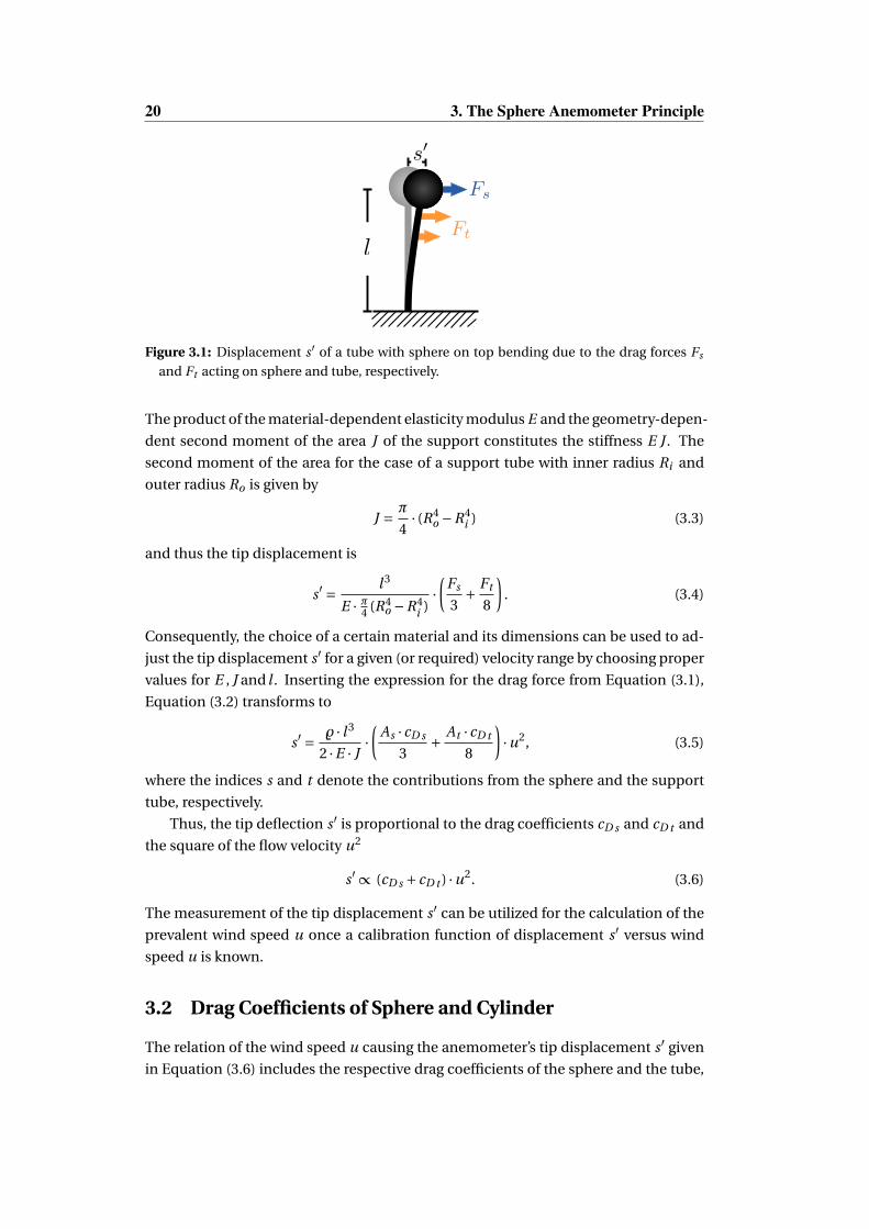
20 3. The Sphere Anemometer Principle
Fs
Ft
s0
l
Figure 3.1: Displacement s′ of a tube with sphere on top bending due to the drag forces Fs
and Ft acting on sphere and tube, respectively.
The product of the material-dependent elasticity modulus E and the geometry-depen-
dent second moment of the area J of the support constitutes the stiffness E J . The
second moment of the area for the case of a support tube with inner radius Ri and
outer radius Ro is given by
J = π
4· (R4
o −R4i ) (3.3)
and thus the tip displacement is
s′ = l 3
E · π4 (R4o −R4
i )·(
Fs
3+ Ft
8
). (3.4)
Consequently, the choice of a certain material and its dimensions can be used to ad-
just the tip displacement s′ for a given (or required) velocity range by choosing proper
values for E , J and l . Inserting the expression for the drag force from Equation (3.1),
Equation (3.2) transforms to
s′ = % · l 3
2 ·E · J·(
As · cD s
3+ At · cD t
8
)·u2, (3.5)
where the indices s and t denote the contributions from the sphere and the support
tube, respectively.
Thus, the tip deflection s′ is proportional to the drag coefficients cD s and cD t and
the square of the flow velocity u2
s′ ∝ (cD s + cD t ) ·u2. (3.6)
The measurement of the tip displacement s′ can be utilized for the calculation of the
prevalent wind speed u once a calibration function of displacement s′ versus wind
speed u is known.
3.2 Drag Coefficients of Sphere and Cylinder
The relation of the wind speed u causing the anemometer’s tip displacement s′ given
in Equation (3.6) includes the respective drag coefficients of the sphere and the tube,

3.2 Drag Coefficients of Sphere and Cylinder 21
cD s and cD t . In order to narrow the meaning of this equation down, one should have
a closer look at the properties of the drag coefficient. A direct comparison of drag
forces acting on objects is only reasonable, if the objects have the same size and prop-
erties while being exposed to the same flow situation. Practically, this is very hard to
achieve and results of experiments or simulations are not immediately comparable.
Considering the drag coefficient instead is a way out of this dilemma, since it is a
non-dimensional representation of the drag force acting on a body in a certain flow
situation. The characterization and comparison of flow situations by means of non-
dimensional quantities is an oft-used concept in fluid dynamics. The most prominent
non-dimensional quantity is the Reynolds number, but other non-dimensional char-
acteristic numbers such as the Mach number M a or the Strouhal number St may be
used depending on the field of investigation.
The Reynolds number Re relates the turbulent production in the flow to the en-
ergy dissipation due to viscous forces and is given by
Re = %u D
µ= u D
ν. (3.7)
Here D is the characteristic dimension (or length scale) of the flow with mean veloc-
ity u. % is the fluid density and µ and ν= µ% are the dynamic and kinematic viscosity,
respectively. The value of the Reynolds number is typically used to distinguish differ-
ent flow regimes or to match similar flow conditions for various characteristic length
scales D .
A similar approach for the definition of a non-dimensional drag coefficient cD can be
found by means of dimensional analysis yielding
cD = 2 ·FD
%Au2 , (3.8)
with drag force FD , and cross-section A of the exposed object. This drag coefficient
depends on the flow velocity and density and thus is a function of the Reynolds num-
ber Re.
Experiments conducted by Wieselsberger [1914] using smooth spheres of differ-
ent size proved the scaling with Reynolds number, since the obtained results for the
drag coefficients were in fair agreement when plotted against the Reynolds number. A
subcritical flow regime could be identified, which is marked by a rather constant drag
coefficient of about 0.45–0.5 for a smooth sphere. Towards higher Reynolds num-
bers, a sudden drop in the drag coefficient occurs until a minimal value is reached at
the critical Reynolds number Rec . This critical regime is followed by a supercritical
regime in which the drag coefficient slowly recovers to a higher value before being
rather constant again in the transcritical regime (Fig. 3.2). The Reynolds number at
which the transition from one flow regime to another occurs cannot be strictly given,
because boundary conditions like background turbulence level, blockage and surface
roughness strongly affect the transition process [Achenbach, 1972]. Wieselsbergers
experiments helped deduce the effect of turbulence on the drag coefficient and he

22 3. The Sphere Anemometer Principle
Re
c Dsub
critical
criticalsuper
critical
trans
critical
Rec
Figure 3.2: Definition of the flow regimes for the drag coefficient depending on Reynolds
number according to Achenbach [1972]. The range of subcritical flow exhibits a rather con-
stant drag coefficient of about 0.45–0.5, while a sudden drop in cD happens in the critical
regime. In the supercritical regime beyond the critical Reynolds number Rec the drag coef-
ficient rises again, before it saturates in the transcritical regime.
concluded, referring to Ludwig Prandtl, that the presence of background turbulence
in the flow and the impact of surface roughness like dimples yields the same effect of
premature drag reduction, shifting the critical region towards lower Reynolds num-
bers. It is apparent for smooth and rough spheres in laminar and turbulent flows
either way but varies in strength and critical Reynolds number. Investigations by
Achenbach [1972, 1974a] have been conducted for smooth and rough spheres, while
Bearman and Harvey [1976] contributed results for what is called a "British golf ball".
Achenbach [1974a] glued spherical glass particles of different diameter k on the sur-
face of the test body to achieve different roughness parameters k/D – the ratio of
pattern diameter k and sphere diameter D . He additionally used as sphere surface
roughened with sand paper to deduce the effect of surface roughness on the drag
coefficient. Achenbach observed a reduction of the critical Reynolds number Rec
with increasing roughness parameter k/D followed by a quick recovery to a value of
cD ≈ 0.4. The amount of drag reduction in the critical regime was reduced for larger
k/D , while the recovery was enhanced in these cases yielding a smaller region of re-
duced drag.
In contrast to Achenbach [1974a]’s findings, Bearman and Harvey [1976] and later
Choi et al. [2006] used dimples to roughen the sphere surface instead of adding ‘pos-
itive’ roughness elements. For these golf ball type of spheres, a larger supercritical re-
gion of constantly reduced drag coefficient was observed beyond the critical regime
in both experiments, giving rise to the conclusion that dimples serve as more effi-
cient patterns for drag reduction. Bearman and Harvey and Choi et al. attribute this
to an efficient tripping of the boundary layer at a fixed transition location, while the

3.3 Measuring Method of the Sphere Deflection 23
5.103 104 5.104 105 5.1050.0
0.2
0.4
0.6
0.8
1.0
1.2
Re
c D
smooth, Achenbach 1972
dimpled, Bearman & Harvey 1976
dimpled, Choi et al. 2006
smooth, Strutz 2014
dimpled, Strutz 2014
Figure 3.3: Drag coefficient cD for spheres with different surface properties plotted against
Reynolds number Re. The baseline case of a smooth sphere taken from Achenbach [1972]
exhibits the drag crisis at Re ≈ 4.5 · 105 while the investigations by Bearman and Harvey
[1976] and Choi et al. [2006] show a premature onset of the drag crisis for dimpled surface
patterns. The same early drag crisis can be seen in the data from Strutz [2014] of an experi-
ment using a smooth and a dimpled sphere of same dimensions.
added surface roughness elements used by Achenbach generate a thickened bound-
ary layer, which still separates at fluctuating locations. After Bearman and Harvey
suggested this mechanism in 1976, Choi et al. [2006] performed flow visualizations
and explained the drag reduction by a dimpled surface pattern.
In general, the drag coefficient of an object like a sphere or a cylinder depends not
only on the Reynolds number but also on properties of the objects surface. This be-
comes evident if one compares the drag coefficient of a smooth sphere exposed to
laminar flow and turbulent flows. Figure 3.3 shows the drag coefficient of different
smooth and dimpled spheres. However, the drag reduction is not per se a wanted
feature for a sphere anemometer. Instead, it is aimed for a simple and analytic cali-
bration function, and it is consequently desirable to operate the sphere anemometer
in the range of almost constant drag coefficient. As Schlichting [2000] pointed out
based on measurements by Wieselsberger, the drag coefficient of a circular cylinder
with smooth surface also varies only little over a broad range of subcritical Reynolds
numbers, 10,000 ≤ Re ≤ 200,000. A similar case can thus be made for the impact of
the drag coefficient of a cylinder on the calibration of a drag-based anemometer.
3.3 Measuring Method of the Sphere Deflection
The principle of measuring the resulting displacements of a mechanical system as
described in Section 3.1 can be carried out in various ways, as was already indicated
in Section 2.4. Up to now, the approaches to drag-based anemometry relied on the

24 3. The Sphere Anemometer Principle
use of mechanically deforming elements, like strain gauges [e.g. Norwood et al., 1966;
Kirwan et al., 1975; Green et al., 1991] or inductive proximity sensors [Smith, 1980]. In
contrast to these approaches, the sphere anemometer developed in Oldenburg aims
to combine the principle of drag-based deflection with the benefits of the contact-less
light pointer technique. This measurement technique was first employed in atomic
force microscopes (AFM) by Martin et al. [1987] and has since been refined. It is used
for the detection of minimal displacements of a cantilever beam at very high sam-
pling rates well beyond fs = 10 kHz.
In general, a light pointer is used as an optical amplifier of small mechanical defor-
mations. As an example, consider a flexible beam which is supported on one side
and free on the other side. A laser beam is aimed from the tip along the beam orien-
tation on a screen or detector, as sketched in Figure 3.4. Once the beam is bending
due to the applied forcing, the tip of the beam will be displaced by an amount s′.The position of the laser spot on the screen or detector is, however, displaced by a
larger length s. Thus, the light pointer can be considered an optical amplifier, which
translates very small mechanical displacements into a measurable displacement of
the laser spot. The displacement s of the laser can be measured by means of a a two-
s
screen /detector
laser
supports0
Figure 3.4: Optical amplification of a displacement s’ by means of a light pointer aimed on a
screen or detector. The larger displacement s on the detector can be measured with higher
accuracy and resolution.
dimensional position sensitive detector (2D-PSD) either with the laser directly aimed
on the detector or by capturing a reflection. Its incident spot induces photo currents
In , n ∈ 1. . .4, at the corners of the detector and the magnitudes of the currents de-
pend on the position of the center of gravity of the light spot. It can be calculated in
Cartesian coordinates (x, y) according to the detector data sheet [Hamamatsu, 2007]
x = (I2 + I3)− (I1 + I4)∑4n=1 In
y = (I2 + I4)− (I1 + I3)∑4n=1 In
, (3.9)

3.4 Previous Investigations in Oldenburg 25
where In are defined as depicted in Figure 3.5. These non-dimensional coordinates
have to be linked to wind speeds and directions via a calibration in order to measure
the flow.
Figure 3.5: Sketch of the linear 2D position sensitive detector. The laser spot (red dot) incident
at the center of the active area induces photo currents I1 . . . I4, which are depending on the
position of the spot and can be converted to (x, y)-coordinates.
The most common types of semiconductor position sensitive detectors are linear
detectors and 4-quadrant detectors as depicted in Figure 3.6. While the linear detec-
tors feature one single active surface, the quadrant detectors consist of four equally
sized areas, which are separated by a small gap. Quadrant detectors provide high spa-
tial resolution, but all four quadrants need to be hit by the incident laser spot in order
to operate properly. This allows for the measurement of very small deflections, but
at the same time demands a better quality (shape, intensity distribution) of the inci-
dent laser spot. Consequently, lasers and lenses have to be of higher quality, which
increases the costs and size of the system. Therefore, the linear type of 2D-PSD was
preferred for the sphere anemometer application described hereafter.
(a) (b)
Figure 3.6: Photo of two different types of two-dimensional position sensitive detectors (2D-
PSDs). (a) Hamamatsu linear PSD S5990-01 [Hamamatsu, 2007] and (b) Silicon Sensors
4-quadrant PSD QP100-6 [Silcon Sensors, Inc., 2010].
3.4 Previous Investigations in Oldenburg
The first implementations of a spherical drag force sensor at the University of Old-
enburg started with two conceptual studies by Henning and Mehmet [2004] and by
26 3. The Sphere Anemometer Principle
Schulte [2007]. Both attempts can be considered proof-of-concept studies, which will
be only briefly described before the first 2D sphere anemometer setup by Heißelmann
[2008] will be introduced as the starting point of the developments presented in this
thesis.
In 2004, Henning and Mehmet set up a first open, one-dimensional setup on a
50× 40 cm2 grid board. It consisted of a ping-pong ball with about 40 mm diame-
ter, which was attached to the tip of a thin metallic rod with squared cross-section.
A mirror glued to the side of the rod, was used to reflect a laser beam onto an one-
dimensional position detector. Their work was followed up by the realization of a first
closed setup by Schulte [2007], who used a 12 cm long transparent acrylic glass4 tube
and mounted a polystyrene sphere with about 69 mm diameter on top of it. The final
setup employed a polystyrene sphere with 49 more or less equally distributed dimples
of 11 mm diameter. The bottom of the support tube with the sphere atop was fixed
to a drill chuck on top of a rectangular aluminum box as displayed in Figure 3.7 (left).
A Flexpoint® laser module with a size of 70×11.7 mm2 (length × diameter) was fitted
through a hole in the anemometer box, and although the housing was not lightproof,
this setup can be considered the first integrated sphere anemometer setup realized in
Oldenburg. Inside the housing, the laser was aimed on a beam splitter, which redi-
rected the beam onto a mirror attached to the top of the acrylic glass tube. The re-
flected beam passed the beam splitter again and hit the two-dimensional position
sensitive detector (2D-PSD) at the bottom of the aluminum box as sketched in Fig-
ure 3.7 (right). Despite the use of a two-dimensional sensor, which generally permits
2D measurements, only 1D calibrations and experiments in main flow direction were
performed and analyzed by Schulte [2007].
Using this setup, Heißelmann [2008] found, that it was suffering from some ma-
jor problems jeopardizing the performance and reliability of the sphere anemometer.
Minor issues were related to the mechanical stability and handling of the used beam
splitter, which caused reflections on the 2D-PSD and required a higher laser inten-
sity. To improve the handling and adjustment of the anemometer, an integrated setup
was built without beam splitter. This was achieved using a laser diode atop the tube,
which was directly focused on the 2D-PSD (Fig. 3.8, right). The most severe prob-
lems were related to the used acrylic glass tube, though. Like many thermoplastics,
the used acrylic glass was prone to strong creeping when it was exposed to the drag
force. Response times until reaching an equilibrium state of the tip deflection were
in the order of ten minutes and more, depending on initial state of the deflection and
the strength of the applied drag force. The tip displacement of the bending tube was
also subject to severe hysteresis. In addition, another problem was found to be crit-
ical for the usability of the anemometer. The creeping of the tube material initially
caused the two-dimensional calibration function of the anemometer to be smooth,
yet it only masked the drag force variations for different inflow angles caused by the
4The historic name "acrylic glass" is used instead of the chemical name of the thermoplastic Poly-
methylmetacrylate (PMMA) to improve the readability.

3.4 Previous Investigations in Oldenburg 27
coarse dimple structure of the sphere. These problems related to the tube and sphere
were critical impediments making the setup inapplicable for any reliable measure-
ment and lead to the substitution of the acrylic glass tube with one made of glass-fiber
reinforced plastics (GFP).
In the assessment of this re-designed setup, the coarse surface pattern of the
polystyrene sphere was found to cause an asymmetric and ambiguous two-dimensio-
nal calibration function, which exhibits significant scattering between consecutive
inflow angles [Heißelmann et al., 2008]. This effect was reduced for a calibration
recorded with a smooth polystyrene sphere, although still deviations could be seen
for certain angles. Since the setups were similar in all other features, the scattering of
the calibration has been attributed to the dimple structure.
An additional radiation experiment carried out in order to investigate the sphere ane-
mometer behavior in direct exposure to sun light revealed, that the dome-shaped
housing made of 10 mm thick plastics was not completely impermeable to light and
thus the diffuse light inside the housing caused the 2D-PSD to overload. An attempt
to avoid this by coating the housing with several layers of paint failed since it only
reduced the effect, but could not completely avoid it. However, the impermeability
to ambient light is of relevance for the development of a sensor, which is exposed to
constantly varying light conditions in the atmosphere. Therefore, any spoiling influ-
ence on the optical measuring technique needs to be ruled out and a re-design of the
anemometer housing is required.
sphere
acrylic glasstube
mirror
laserbeamsplitter
2D-PSD
Figure 3.7: Photo and schematic setup of the first integrated sphere anemometer realized
by Schulte [2007]. The coarsely dimpled polystyrene sphere atop an acrylic glass tube was
mounted to the aluminum box containing the laser module, beam splitter and position
detection circuit board.

28 3. The Sphere Anemometer Principle
sphere
tube
laser
2D-PSD
Figure 3.8: Photo and sketch of the modified sphere anemometer setup with directly aimed
laser diode atop the tube by Heißelmann [2008].
3.5 Summary & Discussion
The general principle of a sphere anemometer based on the drag-dependent deflec-
tion of a flexible tube has been presented in this chapter as well as the drag coeffi-
cient in general and its dependence on the surface roughness. With the light pointer
principle, a highly resolving optical measuring technique for the deflection detection
has been introduced. Investigations on the first realizations of this principle at the
University of Oldenburg were briefly summarized. The comparison of the 2D calibra-
tions for a sphere anemometer with coarsely dimpled and smooth sphere revealed
severe clustering and ambiguities of the calibrations for the dimpled case. While the
tube material has already been changed from acrylic glass in previous setups to glass-
fiber reinforced plastics in order to enhance the reproducibility of the calibrations,
the coarse sphere surface of the setup needs to be addressed as well as the issue of the
light permeability of the housing. Both issues lead to the conclusion, that changes of
the setup of Heißelmann [2008] are inevitable to make the sphere anemometer appli-
cable for outdoor measurements.

Chapter 4
Anemometer Design Criteria
The sphere anemometer based on the principle described in Chapter 3 has several
parameters, which can be adjusted to match specific design criteria such as its oper-
ational range or spatial and temporal resolution. These criteria cannot be fulfilled by
tuning isolated setup parameters, but are usually affected by a combination of sev-
eral parameters. An overview of the most relevant anemometer properties and the
determining parameters will be given in this chapter.
4.1 Wind Speed Range of Operation
The range of operation, i.e. the measurable minimum and maximum wind speeds,
and the survival wind speed are important features of any anemometer, since it de-
termines the suitability for a measurement application. The survival wind speed is
simply given by the strength of the used materials and connections. Although wind
speeds up to 50 m/s were successfully tested in the wind tunnel, a detailed treatment
of the survival wind speed is not part of this work. Higher survival wind speeds can
be expected, though, due to the absence of mechanically vulnerable parts of the ane-
mometer, such as bearings or precisely aligned transducers.
The range of operation for the sphere anemometer is determined by the mini-
mum resolvable displacement of the laser spot on the detector surface smin– giving
the minimum wind speed – and by the maximal displacement smax of the laser spot
before partially leaving the active area of the 2D-PSD. Both values can be obtained
from the data sheet of the detector. While the minimal detector resolution of 7 µm is
no practical limitation to the lower wind speed bound, the maximal detectable dis-
placement for the used Hamamatsu 2D-PSD of 2.25 mm from the center needs to be
considered for the upper bound of measurable wind speeds [Hamamatsu, 2007]. The
wind speeds umin and umax corresponding to these two laser spot displacements are
given by the respective tip displacements s′min and s′max of the sphere according to
Equation (3.2). Considering this, the displacement s of the laser spot can be obtained
from the distance L of laser and detector and the tilt angle of laser diode by simple
geometrical considerations. Note that L is the sum of the tube length l from the tube

30 4. Anemometer Design Criteria
fixation to the position of the laser diode and the height l ′ of the anemometer housing
from the 2D-PSD to the tube fixation, L = l + l ′.The tip displacement s′, and consequently the spot displacement s, are functions
of the tube’s elasticity E and the geometry of sphere and tube. This dependence allows
for a fine tuning of the range of operation by variation of the tube material and most
notably the dimensions, i.e. tube length l , inner and outer radii Ri and Ro and sphere
diameter D . This approach is very useful for the design process, since it enables the
selection of tubes with desired properties and also allows for an estimation of the re-
quired geometric parameters of the tube, sphere and housing. Moreover, adjustment
of the sphere anemometer design can be based on this consideration in order to adapt
the setup to different applications, e.g. measurements in low wind speeds or excep-
tionally high wind speed environments such as Typhoons. This approach comprises
some uncertainties, mainly in the estimation of the drag forces Fs and Ft . Section 4.2
addresses these uncertainties and gives a brief overview of the impact of the drag co-
efficient on the anemometer properties.
4.2 Calibration Function
The drag forces acting on the sphere and the tube are the base of the sphere anemo-
meter approach to wind speed and direction measurements. The properties of the
anemometer, in particular the calibration function, are therefore influenced by the
aerodynamic characteristics of the two bluff bodies. The drag forces Fs and Ft de-
pend on the physical dimensions of the sphere and tube, respectively, and also on the
squared wind speed u. The drag coefficients of the respective body may also vary for
different wind speeds and dimension, i.e. for different Reynolds numbers Re, as was
introduced in Section 3.2. These parameters are included in the design of the setup,
but may pose some challenges as well. While effects like the varying drag coefficients
cDs and cD t due to the surface structure of sphere and tube may be utilized during
the design process, they are much harder to control due to the uncertainty of the drag
reduction mechanism (Sec. 3.2). This is also a limiting factor to the precision of the
adjustments presented in Section 4.1 and in turn means, that the design based on the
mentioned material and geometry parameters can only be an estimation.
The sphere diameter is selected in order to yield sufficiently large drag forces to
ensure measurable tip deflections for a wide range of wind speeds. Both, the sphere
and tube diameters are kept constant for all anemometer setups. Emphasis lays on a
simple and analytic calibration function as a design criterion, and it is consequently
desirable to operate the sphere anemometer in the range of almost constant drag co-
efficients cDs and cD t . In this case, the relation for the tip deflection s′ from Equation
(3.6) transforms to the simpler
s′ ∝ u2, (4.1)

4.3 Spatial and Temporal Resolution 31
resulting in a square root calibration function for the laser spot displacement s
u = m · s0.5 (4.2)
with slope m. m decreases for spheres with larger drag coefficients cDs while it in-
creases for reduced cDs . Although the slope accounts for different drag coefficients,
i.e. different sphere surface properties, this idealized form of the calibration function
still relies on the condition of a constant cD . The subcritical Reynolds number range
of approximately 10,000 to 350,000 for a smooth sphere exhibits an almost constant
drag coefficient. Schlichting [2000] showed similar behavior for the drag coefficient
of a circular cylinder with smooth surface over a broad range of subcritical Reynolds
numbers of 10,000 ≤ Re ≤ 200,000. However, some variations of cD can be seen in the
double-logarithmic plot in Figure 3.3 for the data from Achenbach [1972] or Strutz
[2014]. These will result in deviations of the sphere anemometer calibration func-
tion from the idealized shape. It can be phrased slightly more general to handle the
inevitable variations of cD with the Reynolds number. Two additional parameters s0
and n are therefor included in a power law for the calibration function
u = m · (s − s0)n (4.3)
to allow for better fitting to actual measurement data. The difference of n from the
case of n = 0.5 can be used as a measure for the deviation of the calibration function
from its ideal square-root shape and s0 accounts for possible offset displacements of
the laser spot on the 2D-PSD.
While even smooth spheres exhibit variations of the drag coefficient with Reynolds
number, dimpled surface patterns pose a challenge of its own due to the premature
occurrence of the drag crisis. However, when the roughness parameter k/D is care-
fully chosen, spheres with dimpled patterns, may also exhibit a wide range of rela-
tively constant drag coefficient as can be seen in the measurements by Strutz [2014]
(Fig. 3.3, blue). The drag reduction by means of dimpled surface patterns is not per se
a wanted feature for a sphere anemometer as a drag-based sensor, but effects like re-
duced vortex shedding from the sphere may be beneficial due to reduced oscillations
of the sphere-tube combination. Possibly larger variations of cD might cause further
deviations from the idealized shape of the calibration function, but will by no means
harm the uniqueness of the calibration. Consequently, smooth and dimpled spheres
can be considered for the sphere anemometer without jeopardizing its functionality.
4.3 Spatial and Temporal Resolution
Another design criterion of an anemometer is the provided resolution, which may
be divided in temporal and spatial resolution, although both are linked via Taylor’s
hypothesis of frozen turbulence [Taylor, 1938].
The spatial resolution of an anemometer is either given by its dimensions or, as
in the case of cup anemometers, by the characteristic length scale until its rotation

32 4. Anemometer Design Criteria
reached an equilibrium state. Regarding the sphere anemometer, the two main pa-
rameters to adjust the spatial resolution are the sphere diameter D and the size of the
tube l . Considering a turbulent fluid column passing the sensor with a certain mean
wind speed u, it is easy to understand, that no turbulent structures smaller than these
dimensions will be resolved, since the sensor integrates them.
The temporal resolution marks one of the key features of any sensor. While elec-
tronic properties of the entire measuring system, such as sampling rate of analog-
digital (AD) converters and response times of electronic amplifiers, may be limiting
the temporal resolution of very fast sensors, the critical property of a mechanical
sensor like the sphere anemometer is the natural frequency of the system. Any ex-
citation of the anemometer by mechanical oscillations, e.g. from the anemometer
boom or other support structures, causes the anemometer to oscillate with its natu-
ral frequency f0. Furthermore, these oscillations can also be wind induced vibrations,
which are caused by vortex shedding from the sphere and the supporting tube. The
vortex shedding from these structures results in a Kármán5 vortex street and the fre-
quency of the shedding vortices depends on the wind speed. The relation of both,
the wind speed u and vortex shedding frequency fu , is given by the non-dimensional
Strouhal6 number
St = fu ·D
u, (4.4)
where D denotes the characteristic dimension of the object – in this case the sphere
diameter [Tritton, 1988]. The Strouhal number cannot generally be considered con-
stant for the flow around a sphere, and for low Reynolds numbers even two co-existing
values for the Strouhal number are found [Sakamoto and Haniu, 1990]. However,
Achenbach [1974b] showed, that a rather constant value of St = 0.19 ∼ 0.195 can
be assumed for a smooth sphere in the treated Reynolds number range of Re = 2 ·104 . . .3.7 ·105. The vortex shedding frequency fu thus varies with the flow velocity u
in this range and can be calculated according to Equation (4.4).
Each shedding vortex transports some energy and thus excites the mechanical os-
cillation of the structure with the frequency fu . Attempts to reduce the energy content
of the shed vortices include the use of patterned sphere surfaces, which is challenging
for various reasons as pointed out in Section 4.2.
Once the vortex shedding frequency fu is close to the natural frequency f0 of the sys-
tem, resonance effects may occur. Excitation frequencies close to the natural fre-
quency of a system can lock-in and amplify the oscillation of the structure even to
the point of breakage 7. In order to avoid or at least reduce the lock-in related amplifi-
cation of oscillations, it is important to estimate the natural frequency of the anemo-
meter and possibly adapt it to the desired range of operation. Several parameters can
be used to tune the natural frequency accordingly, like the elasticity modulus E , the
5Theodore von Kármán, 1881–19636Vincenc Strouhal, 1850–19227A prominent examples of these resonance phenomena is the collapse of the Tacoma Narrows bridge
in 1940 due to wind induced vibrations locking in with one natural oscillation mode of the structure.

4.4 Summary & Discussion 33
second moment of the area J , the length of the tube material l and also the mass M
of the sphere and laser diode on top of it. Moreover, measures can be taken to reduce
vortex shedding, e.g. shifting the range of vortex shedding frequencies fu in order to
separate it from the natural frequency f0.
A first analytic approach based on the work by Rubin [2004] was used to estimate
the natural frequency of a bending beam with constant mass distribution %mS, where
%m is the density of the material and S = π · (R2o −R2
i ) is the area of the tube’s cross-
section. Disregarding the tip mass M of the sphere and the laser diode in this an-
alytical approach results in an over-estimation of the theoretical natural frequency
compared to the real natural frequency of the sphere anemometer, though [Heißel-
mann, 2008]. In a more accurate estimation of the natural frequency for a setup with
tip mass M , the eigenvalue κ is obtained by numerically solving the characteristic
equation
1 + cos(κ l )cosh(κ l ) + M
Mtκ l (cos(κ l ) si nh(κ l ) − si n(κ l )cosh(κ l )) = 0 (4.5)
proposed by Wandinger [2007, Sec. 3.2.4]. In this equation, Mt is the mass of the tube
with length l and κ4 =ω2 %m SE J is the first eigenvalue of the characteristic equation. The
natural frequency f0 =ω/2π can than be calculated from
ω=√κ4 E J
%mS
⇒ f0 = 1
2π
√κ4 E J
%mS(4.6)
for a given combination of geometry and material parameters. Since larger tip masses
M result in lower natural frequencies f0, the mass of sphere and laser should be kept
as small as possible to achieve a high temporal resolution of the sphere anemome-
ter. However, the tip mass is not the only determining parameter, and while it can
be adjusted without affecting the other design criteria of the anemometer, other pa-
rameters like tube length and material have to be also considered in the context of all
desired sphere anemometer properties.
4.4 Summary & Discussion
A wide set of parameters can be used to adapt the sphere anemometer to meet de-
sired design criteria, particularly the operational wind speed range and temporal res-
olution. As has been pointed out in this chapter, the sphere and tube parameters
which impact these anemometer properties cannot be tuned independently. Fig-
ure 4.1 gives an overview of the most relevant parameters and their contribution to
the design criteria. Considering the mutual dependency of the tip deflection s′ and
the natural frequency f0 on the sphere and tube geometry, it is immediately evident
that some trade-offs have to be made in the design process of the sphere anemometer.

34 4. Anemometer Design Criteria
L
l
s
s0 E
J
RiRo
Ft
cDt
u
Re
f0
m M
cDs
Re
Fs
D
sphere parameter
tube parameter
housing parameter
design criterion
Figure 4.1: Entanglement of the sphere (blue) and tube (orange) parameters and their link to
key sphere anemometer properties, such as wind speed u, laser displacement s and natural
frequency f0.
The above consideration constitute the basis for the design of the sphere anemome-
ter setups presented in the following Chapters 5–7. All of these setups are designed
to operate in a wind speed range of about 0.3 m/s to 45 m/s and the sphere diam-
eter D = 70 mm and outer tube radius Ro = 4 mm are not varied for the different
anemometers. Consequently, the tube length l and inner radius Ri are the main pa-
rameters used to adjust the expected laser spot displacement s for a selected tube
material. Given the size of the active area of the 2D-PSD, the maximal acceptable
laser displacement smax = 1.85 mm was fixed and the tube length was chosen accord-
ingly. Calculations of the anemometer’s natural frequency have been considered in
order to rule out combinations of tube material and geometry leading to lower values
than f0 ≈ 20 Hz, to ensure competitiveness to sonic anemometry. During the design
process no emphasis was given to the expected theoretical accuracy and its variation
for different wind speeds due ot the proportionality s ∝ u2, which it has already been
treated by Heißelmann [2008]. An experimental assessment of the measurement pre-
cision and accuracy is performed for the final stage of the anemometer development
presented in Section 7.3.

Chapter 5
The First Generation SphereAnemometer
This chapter describes the sphere anemometer hardware setup based on the measur-
ing principle introduced in Chapter 3. Persisting issues of the earlier realizations are
accounted for in this 1st generation sphere anemometer by modifications made to key
components. The design criteria and methodology of Chapter 4 have therefor been
employed. These crucial sensor characteristics are analyzed experimentally, as the
one- and two-dimensional calibration functions are treated as well as the impact of
different sphere surface patterns on it. The natural frequencies are also investigated
as a limitation to the temporal resolution.
5.1 Sphere Anemometer Setup
The 1st generation sphere anemometer setup is based on the principle of a drag-force
anemometer as described in Section 3.1 and realized by Heißelmann [2008]. Its hous-
ing consists of a dome-shaped cover mounted to a robust base plate. As a conse-
quence of the radiation experiment mentioned in Section 3.4 both the cover and the
base plate are made from milled aluminum in order to avoid permeability to light and
torsion of the housing. The aluminum cover is split off-center in two parts and can
be opened to access the sensor parts by removing the smaller piece of the cover. A
threaded aluminum ring fitted to the center of the dome cover allows for the fast and
easy substitution of the mounted sphere-tube combination, which has the counter-
part fixed to the lower end of the tube as sketched in Figure 5.1.
The tube made of glass fiber reinforced plastics (GFP, "fiber glass") consists of sev-
eral layers of glass fibers with different orientations, which are embedded in a matrix
of resin or polyamide. No exact fiber orientation is known for the used tubes, since no
information on the production process was available from the retailer. A strain test
resulted in an estimate of the tube’s elasticity modulus E ≈ 36 GPa8. The information
8The strain experiment was operated by Roland Kruse of the Acoustics Research Group, University of
Oldenburg, using the Gabo Eplexor 500 N.

36 5. 1st Generation Sphere Anemometer
laser diode
thread
electronics
(thread)*
dome-shapedcover
base
∗Not used for regularly dimpled sphere.
Figure 5.1: Drawing of the 1st generation sphere anemometer setup. A sphere is mounted
on top of a GFP tube, which is fixed to the dome-shaped aluminum housing be means of
a thread. The laser diode atop is directly focused on the 2D-PSD and sensor electronics
located at the bottom inside the housing.
about the elasticity modulus is utilized during the design process for the calculation
of the expected tip deflections s′ and thus the required tube length l as described in
Section 4.1. It is also be used for the estimation of the approximate natural frequency
of the anemometer as described in Section 4.3. Both calculations cannot be exact
due to uncertainties in the manufacturing processes of the materials and the assem-
bly of the anemometer, so no exact match of calculated and practically determined
quantities can be expected. Thus, an uncertainty of some GPa in the measurement
of E is not considered critical for the design process. The used GFP tube with in-
ner radius Ri = 3.5±0.05 mm and outer radius Ro = 4.0±0.05 mm is cut to a length
l = 285± 0.5mm between the top of the aluminum thread and the top of the tube.
Its upper end is milled to slightly increase the inner radius on a length of approxi-
mately 5 mm in order to ensure a rigid fitting of the laser diode’s lens mount, as this
was found to be a weakness during the anemometer assembly. The sphere is glued

5.1 Sphere Anemometer Setup 37
Figure 5.2: 5 mW laser diode in 3.3mm pack-
aging with integrated laser driver. A 1 cent
coin is depicted for comparison.
Figure 5.3: Photo of the CAW100 colli-
mator lens inside the custom made lens
holder (silver) and custom made laser
diode mount (black) with precision thread
to adjust the focus.
to the tip of the tube with its lower edge being in a distance of 40 mm from the top of
the tube and consequently the lens of the laser is located in the center of the sphere
once the anemometer is assembled. A drawing of the sphere anemometer setup with
all relevant components is depicted in Figure 5.1.
The tip displacement is measured exploiting the light pointer principle described
in Section 3.1. A laser beam is therefor aimed on the 4.5× 4.5mm2 large sensitive
area of a two-dimensional position sensitive detector (2D-PSD) S5990-01 by Hama-
matsu [2007]. The laser spot induces four photo currents in the semiconductor sen-
sor, which depend on the position of the incident laser spot on the active area of the
detector. The induced photo currents can be converted to Cartesian coordinates of
the spot location according to Equation (3.9).
Instead of using the bulky Flexpoint® laser module used in the setup of Schulte, a
low-cost laser diode is used in the sphere anemometer. The main benefit of the used
laser diode is its very lightweight construction with a small packaging of dl = 3.3 mm
diameter and only ll = 8 mm overall length (Fig. 5.2). The laser diode of type ADL-
65055SA2 by Arima Lasers has a typical wavelength λ = 655nm and provides a rated
power of P0 = 5 mW. The laser power is regulated by an external resistor RVR, which
is directly soldered to the diode’s ground and VR pins. A laser driver is integrated in
order to ensure the power of the laser to be constant even with slightly varying supply
voltage [Laser Components, 2007]. The laser diode is fixed to a custom made hold-
ing piece with a precision thread on its outside as seen in Figure 5.3. It allows for the
precise positioning of the lens mount holding the aspheric collimating lens CAW100
with a diameter dlens = 5.2 mm [Laser Components, 2008], such that the laser beam is
focused on the active area of the 2D-PSD. The total weight of the laser diode including
lens and mount is 2.2 g.
The incident light on the position sensitive detector causes a photo current as de-
scribed in Section 3.3. In order to comply with the voltage input channels of most AD
converters used, the induced current signals of the 2D-PSD are converted to voltage

38 5. 1st Generation Sphere Anemometer
signals and amplified before further data handling using a trans-impedance circuit
as depicted in Appendix B. Taking the amplification into account, a metallic resistor
of RVR =180 kΩ (± 1%) is used to adjust the laser power to be about 250µW in or-
der to achieve a maximal signal output of 5 V for spot positions close to the 2D-PSD’s
corners. The specifications and dimensions of laser diode and lens mount are sum-
marized in Tables 5.1 and 5.2.
Table 5.1: Specifications of the ADL-65055SA2 laser diode. The output power Pset was ad-
justed with the variable resistance RVR for a supply voltage VS.
λ VS Pset RVR Ml dimensions (dl × ll )
655 nm 5 V 250 µW 180 kΩ±1% 0.1 g 3×8 mm2
Table 5.2: Specifications of the used lens and lens mount.
lens dlens Mm dimensions (dm × lm)
CAW100 5.2 mm 2.1 g 8×17 mm2
The trans-impedance amplifier is supplied with ±6V DC from a voltage regula-
tion circuit powered by two 9 V block batteries while the laser diode is supplied with
5 V DC provided by the USB port of the used measurement computer. Both supply
voltages could also be obtained from a standard laboratory power supply, but the sim-
pler battery and USB connection is preferred, since it is less prone to electronic noise
and permits more mobility. The supply cables for the laser diode are attached at the
outside of the tube. Two-wired ribbon cables with cross-section ∅ = 0.9± 0.05mm
are chosen over the previously used speaker cables (∅= 1.25±0.05mm). The cables
are only fixed at the top and bottom of the tube and are covered by a shrinking hose.
This has similarly been employed in the previous anemometer setup for the benefit
of reducing the induced oscillations of the sphere-tube-combination.
As a consequence of the highly scattered calibration function obtained for the
previous anemometer setup with coarsely dimpled polystyrene sphere [Heißelmann
et al., 2008], a re-design of the sphere was considered essential for the sphere ane-
mometer improvement. While the diameter of the sphere is fixed at D = 70 mm, a
different surface with reduced dimple diameter and depth is designed. Instead of
the previously hand-made polystyrene spheres, the more accurate rapid prototyping
method is used to produce a hollow sphere made of ABS plastics.
This sphere is patterned with 306 regularly ordered dimples of d = 4.9 ± 0.1 mm diam-
eter and depth k = 1.3 ± 0.1 mm, resulting in a roughness parameter of k/D = 0.0186.
The alignment of the dimples along lateral circles is chosen to be equidistant in cir-
cumferential direction as shown in the top view of the sphere in Figure 5.4 (a). A sin-
gle dimple is located right at the top pole of the sphere and circles of equally spaced

5.2 Sensor Calibration 39
(a) (b)
Figure 5.4: (a) Top view and (b) side view of the sphere with 306 regularly aligned dimples on
its surface. The dimples are located along lateral circles with uniform distance in circum-
ferential direction.
dimples align below for larger radii. The sphere consists of two hemispheres which
are later bonded to one sphere along its equator (Fig 5.4, b). While the top half of
the sphere is patterned with dimples as seen in Figure 5.4 (a), the bottom half has an
8 mm diameter hole with tubular joint at its pole for the fixation of the support tube.
Besides this difference, the hemispheres are similarly patterned.
The weight of the complete sphere is Ms = 38 g, which results in a total tip mass
M ≈ 40.2 g for this sphere anemometer setup. Once it is attached to the tip of the
tube, it is not possible to unmount or change the sphere non-destructively.
5.2 Sensor Calibration
The sphere anemometer as a drag-based measuring device is not based on first prin-
ciples and thus needs to be calibrated with a flow of known velocity in order to enable
the wind speed and direction measurements. All calibration functions of the sphere
anemometer and the reference sensors discussed during the course of this work are
measured in the acoustic wind tunnel of the University of Oldenburg, which is de-
scribed in brief before introducing the actual sphere anemometer calibration. The
characterization methodology of the sphere anemometer calibration introduced for
the 1st generation setup will be carried forward for both later anemometer stages de-
scribed in Chapters 6 & 7.
5.2.1 Acoustic Wind Tunnel in Oldenburg
The acoustic wind tunnel of the University of Oldenburg is a return-type facility (Göt-
tingen type) with an outlet cross-section of 1×0.8 m2. The 88 kW motor generates
wind speeds up to 50 m/s at a background turbulence level of about 0.3 %. The wind

40 5. 1st Generation Sphere Anemometer
tunnel can be operated either with a closed test section of 2.6 m length or as an open
jet with 1.8 m length as depicted in Figure 5.5. The air flow temperature can be kept
constant by means of a heat exchanger downstream the motor, and an additional
water-cooler system for the motor can be used in high velocity operation. The con-
traction cone of the wind tunnel is equipped with eight connected Pitot tubes for the
detection of the total pressure pt and eight connected pressure holes in the nozzle are
used for the detection of the static pressure ps .
The calibration measurements presented within this work are performed using the
open jet configuration as depicted in the sketch in Figure 5.5.
heatexchanger
fan
settelingchamber
rectifier netspressure
tubes & holes
testsection
ptps
Figure 5.5: Sketch of the closed-loop acoustic wind tunnel of the University of Oldenburg
with open configuration (side view, not to scale). The anemometers were calibrated and
characterized in the open test section in measurement chamber (gray dashed). Wind speed
readings can be obtained from the differential pressure pd = pt −ps .
Calibration functions, which are used for qualitative comparison and develop-
ment purpose only, rely on the wind tunnel speed display as reference. The reference
wind speeds for the comparison with other anemometers presented in later chapters
are measured with the built-in Pitot tubes and pressure holes (Fig. 5.5) in combina-
tion with an analogue Betz type 2500 micro-manometer providing a range of 2500 Pa
at 0.1 Pa resolution [acin instrumenten bv, 2013] or a Setra C239 pressure transducer
[Setra Systems Inc., 2013].
5.2.2 Setup for 1D & 2D Calibration
The sphere anemometer is placed on top of a motor-driven turntable in the wind
tunnel to perform the anemometer calibration. The table top at a height of 1.15 m en-
sures, that the sphere-tube element is located in the central region of the nozzle. The
anemometer is positioned in the center of the turntable at a downstream distance of
35 cm from the wind tunnel outlet to the center of the sphere anemometer. The x-axis

5.2 Sensor Calibration 41
of the 2D-PSD’s coordinate system is aligned parallel to the main flow direction (at 0
inflow direction) and the y-axis was oriented cross-flow.
The first qualitative tests rely on the reference wind speed u, read from the wind tun-
Figure 5.6: Photo of the 1st generation sphere anemometer mounted on the turntable in the
wind tunnel for the two-dimensional calibration.
nel control panel. This is sufficient for the evaluation of the principle shape and re-
producibility of the anemometer’s calibration function since the ambient conditions
can be considered constant during the respective experiments.
The sphere anemometer is connected to its supply box. The power supply for the
laser is provided from the measuring PC via USB and the trans-impedance ampli-
fier of the 2D-PSD was supplied with ±6 V from a battery powered voltage regulator
circuit. The four output signals U1 . . .U4 are connected with coaxial cables to a 16 Bit
AD-converter DT9816-A from Data Translation in the single ended mode [Data Trans-
lation, Inc., 2013] and simultaneously acquired with a sampling rate of fs = 1 kHz. It
is operated in the measurement range ±5V resulting in a resolution of δU ≈ 0.153mV.
The entire equipment including the sphere anemometer is granted a warm-up time
of at least 30 minutes prior to the first measurement in order to eliminate electronic
signal drift. The data acquisition is controlled by a customized LabVIEW program.
While the anemometer position is fixed for the measurement of a one-dimensional
calibration function, it is rotated along its vertical axis on the turntable to obtain a
two-dimensional calibration function. For this case a stepper motor is used for the
turntable rotation and controlled by the measuring PC with LabVIEW software via se-
rial connection. The two-dimensional calibration procedure is basically carried out
in a loop of three steps:
1. Set reference wind speed

42 5. 1st Generation Sphere Anemometer
2. Rotate anemometer counter-clockwise along its vertical axis to next inflow an-
gle.
3. Acquire 2D-PSD signals for each set inflow angle
The convergence of the mean values is tested in order to ensure the validity of the
calibration data. In this test specified in Appendix A, the average of the 2D-PSD signal
is calculated for different windows of increasing time intervals up to ten seconds. An
averaging time of about one second is found to be sufficiently long to reach the correct
mean value of the laser position signal within ±0.5%. Consequently, the acquisition
of the signals for ten seconds at fs = 1 kHz sampling for each wind speed and inflow
angle can be considered absolutely reliable and the settings are therefore used for all
1D and 2D calibration functions presented in this thesis.
5.2.3 1D Calibration Function
A one-dimensional calibration function for the 1st generation sphere anemometer
with regularly dimpled sphere is measured in a range of reference wind speeds be-
tween 0 and 20 m/s. The raw voltage signals are acquired at each reference wind
speed u and the (x, y)-coordinates of the laser spot on the 2D-PSD are computed ac-
cording to Equation (3.9). The x- and y-offset signals, i.e. the mean of the resulting
signals for u = 0m/s, are subtracted from all x- and y-signals to obtain the 1D calibra-
tion of the anemometer.
The reference wind speed u plotted against the calculated x- and y-components
of the voltage signals is displayed in Figure 5.7 for an inflow angle ofΦ= 0. Although
the values for the displacement s are mirrored due to the alignment of the 2D-PSD’s
coordinate system, it can be clearly seen that the shape of the x-component of the sig-
nal follows the expected power law function of Equation (4.3). Due to the alignment of
the main flow direction with the x-axis of the 2D-PSD, y exhibits only minimal varia-
tions, which stem from a slight misalignment of the detector. The right plot in Figure
5.7 (b) displays the squared wind speed u2 plotted against the sphere anemometer
signal, fitted by a linear function. The coefficient of determination R2 = 0.9997 of the
linear fit to the data gives evidence of the well-matching proportionality u2 ∝ s. Al-
though both plots in Figure 5.7 are based on data for the main wind direction of the
calibration coinciding with the x-axis of the 2D-PSD, the general behavior of the cal-
ibration can be seen. Different inflow angles with respect to the 2D-PSD coordinate
system will however yield different slopes for the linear fit in Figure 5.7 (b).
For a 2D calibration, the data of all inflow angles will inevitably have x- and y-
components of either sign, which makes fitting a power law function to the data of
all inflow angles Φ impossible. A solution to the problem of fitting the power law
function to these data can be found by calibrating the magnitude
|s|(u,Φ) =√
x2 + y2 (5.1)

5.2 Sensor Calibration 43
–0.25 –0.20 –0.15 –0.10 –0.05 0.000
5
10
15
20
s
u [m
/s]
x-componenty-component
–0.25 –0.20 –0.15 –0.10 –0.05 0.000
100
200
300
400
s
u2 [m
2 /s2
]
x-componenty-component
R2=0.9997
(a) (b)
Figure 5.7: One-dimensional calibration function of the sphere anemometer recorded for 0
inflow angle. (a) The x-component (solid bullets) follows a negative power-law function
while the y-component (open triangles) remains almost unchanged with increasing refer-
ence wind speed u. (b) Square of reference wind speed, u2, plotted against the anemome-
ter’s x- and y-signals. A linear regression line is fitted to the data for the x-component with
coefficient of determination R2 = 0.9997.
of the anemometer signal rather than the two Cartesian components (x, y). Practically
this can be achieved quite conveniently by interpreting the (x, y)-components as real
and imaginary parts of a complex laser spot displacement s = x + i y . The magnitude
|s| and phase angleΦ of the complex variable can than be determined to be modulus
and argument of the complex displacement
|s| = Mod(s)
Φ= Ar g (s). (5.2)
One constraint of using the complex variable s is the requirement of the laser spot
position for u = 0 m/s to be at (x = 0, y = 0) coordinates. Only for this case, the values
of the displacement magnitude and angle according to Equation (5.2) will be correct.
Although focusing the laser spot exactly in the center of the 2D-PSD area can be con-
sidered practically impossible, the constraint can be fulfilled by measuring the offset
for both coordinates and subtracting them from the signal prior to the conversion to
a complex coordinate s. The wind speed u plotted against the complex magnitude
of the displacement |s| = |x + i y | may then be fitted with the power law function as
shown in the graph of the 1D calibration in Figure 5.8. The fit function according to
Equation (4.3) obeys almost a square-root shape with only a slightly deviating expo-
nent n = 0.505 and a slope m = 40.33.
5.2.4 2D Calibration Function
For the application of wind speed and simultaneous direction measurements, it is
necessary to perform a two-dimensional calibration of the sphere anemometer. There-
fore, the anemometer is rotated on the turntable along its vertical axis in angle incre-
ments of ∆Φ = 5 and the corresponding signals U1 . . .U4 are recorded for the ref-
erence wind speeds u. The computed (x, y)-components of the 2D calibration are

44 5. 1st Generation Sphere Anemometer
0.00 0.05 0.10 0.15 0.20 0.250
5
10
15
20
|s|
u [m
/s]
|(x+iy)|fit
Figure 5.8: One-dimensional calibration function of the wind speed u plotted against the
complex magnitude |s| of the displacement signal (points). The data is fitted with a square-
root-function (line).
plotted along with the reference wind speed u in the three-dimensional plot in Figure
5.9. As expected, the rotation of the one-dimensional power law function obtained in
the previous section resembles a potential well. Although the three-dimensional plot
gives an impression on the general shape of the 2D calibration function, it is difficult
to assess even qualitative features like the uniqueness and isotropy of the calibration
from this representation.
While the one-dimensional calibration function of Section 5.2.3 and the three-
dimensional plot of the calibration in Figure 5.9 appear to be quite smooth and well-
defined, the two-dimensional projection of the measured data in Figure 5.10 (a), cor-
responding to a top view on the active area of the 2D-PSD, reveals major deviations
from the idealized expectations. In contrast to the expected axis-symmetric 2D cali-
bration function – ideally a system of concentric circles – a significant variation of the
radial displacement with changing inflow angle Φ can be identified from Figure 5.10.
Additional clustering of the data for subsequent inflow angles Φ is apparent for wind
speeds around 9 m/s (Fig. 5.10, b).
In a method to quantify the deviations from the rotational symmetry of the 2D
calibration, the magnitude |s| of the laser spot displacement from the 2D-PSD’s center
is considered. The single displacements |s|(u,Φ) for each combination of inflow angle
and reference speed are compared to the ensemble average over all inflow angles Φ
for one reference wind speed
|sΦ|(u) = 1
N
∑Φ
|s|(u,Φ) with N = Φmax
∆Φ(5.3)
The angular bias of the displacement magnitude |s| can be expressed in terms of nor-
malized deviation from the angular mean
χ= |s|(u,Φ)
|sΦ|(u)−1, (5.4)

5.2 Sensor Calibration 45
Figure 5.9: 3D plot of the two-dimensional calibration function of the sphere anemometer.
with values of χ < 0 referred to as under-shooting while values χ > 0 are called over-
shooting. While this metric allows for the identifications of inflow angles with partic-
ularly strong deviations of the expected displacement magnitude |s|, it cannot cover
the appearance of angular clustering found for medium wind speeds. The deviation
of the measured and the set inflow angle, Φmeasured −Φset, can be used instead to
identify these angular clusters and gaps. Both representations will be used for the
characterization of this anemometer setup and the modified setups presented in the
following.
Figure 5.11 shows the laser displacement magnitude |s| as a function of the set
inflow angle Φ for the measured reference wind speeds between 0 m/s and 20 m/s.
The ensemble mean according to Equation (5.3) is also plotted for all wind speeds.
The constant values |sΦ|(u) for each wind speed correspond to a circular shape of the
2D calibration. An increased laser displacement, i.e. values above average, is found
in the inflow angle region of 20 to 60. The plot of the angular dependence of the
displacement magnitude |s| in Figure 5.11 indicates large regions of significantly fluc-
tuating values. Exemplary quantification of the deviations for 20 m/s reference wind
speed show the largest over-shooting of up to 7% occurring between Φ ≈ 20 . . .60.
The region of Φ ≈ 280 . . .340 is characterized by even stronger under-shooting of
the displacement magnitude for this wind speed. Generally, the relative deviations
are more severe for lower wind speeds as shown in the comparison of the maximal
over- and under-estimation for each reference wind speed between 5 m/s and 20 m/s
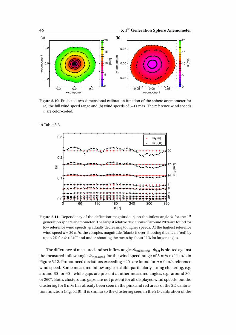
46 5. 1st Generation Sphere Anemometer
–0.2 0.0 0.2
–0.2
0.0
0.2
x-component
y-co
mpo
nent
0
5
10
15
20
u [m
/s]
–0.05 0.00 0.05
–0.05
0.00
0.05
x-component
y-co
mpo
nent
0
5
10
15
20
u [m
/s]
(a) (b)
Figure 5.10: Projected two-dimensional calibration function of the sphere anemometer for
(a) the full wind speed range and (b) wind speeds of 5–11 m/s. The reference wind speeds
u are color-coded.
in Table 5.3.
0 60 120 180 240 300 3600.0
0.1
0.2
0.3
Φ [°]
|s|
|sφ|(u)|s|(u,Φ)
20
17
14
11 9 7 5 3
u Ref
[m/s
]
Figure 5.11: Dependency of the deflection magnitude |s| on the inflow angle Φ for the 1st
generation sphere anemometer. The largest relative deviations of around 20 % are found for
low reference wind speeds, gradually decreasing to higher speeds. At the highest reference
wind speed u = 20 m/s, the complex magnitude (black) is over-shooting the mean (red) by
up to 7% forΦ< 240 and under-shooting the mean by about 11% for larger angles.
The difference of measured and set inflow anglesΦmeasured−Φset is plotted against
the measured inflow angle Φmeasured for the wind speed range of 5 m/s to 11 m/s in
Figure 5.12. Pronounced deviations exceeding ±20 are found for u = 9 m/s reference
wind speed. Some measured inflow angles exhibit particularly strong clustering, e.g.
around 60 or 90, while gaps are present at other measured angles, e.g. around 80
or 260. Both, clusters and gaps, are not present for all displayed wind speeds, but the
clustering for 9 m/s has already been seen in the pink and red areas of the 2D calibra-
tion function (Fig. 5.10). It is similar to the clustering seen in the 2D calibration of the

5.3 Impact of Sphere Patterns and Tube Material 47
Table 5.3: Deviations χ of the displacement magnitude from the angular averaged displace-
ment for a given reference wind speed u according to Eq. (5.4).
1st generation sphere anemometer
u [m/s] 5 7 9 11 14 17 20
χmax [%] +20.2 +10.4 +9.3 +8.0 +6.6 +7.0 +7.2
χmin [%] -22.6 -14.1 -11.8 -11.3 -9.7 -9.9 -11.2
0 60 120 180 240 300 360–40
–20
0
20
40
φmeasured [°]
φm
easu
red
- φse
t [°]
5 m/s7 m/s9 m/s11 m/s
Figure 5.12: Deviation of the measured inflow angle from the set inflow angle as function of
measured angle for the 1st generation sphere anemometer setup with GFP tube and regu-
larly dimpled sphere.
previous sphere anemometer setups [Heißelmann et al., 2008]. Although the cluster-
ing itself can be identified, the cause cannot be isolated from the measurement data
with regularly dimpled sphere, since it is fixed to the GFP tube and cannot be sub-
stituted. It can thus be either an anisotropy of the tube material or an influence of
the regularly dimpled sphere surface. A more detailed investigation of the impact of
the sphere surface pattern on the sphere anemometer calibration is necessary and
requires some changes to the sphere anemometer setup, which are addressed in Sec-
tion 5.3.
5.3 Impact of Sphere Patterns and Tube Material on the Cali-
bration
The results of the previous section give rise to the question whether the sphere surface
pattern or the tube material is the root cause for the angular deviations and clustering
of the anemometer’s 2D calibration. While the overall design of the anemometer is
unaltered with regard to its housing and the position sensing electronics, some minor

48 5. 1st Generation Sphere Anemometer
setup modifications of the 1st generation sphere anemometer are required.
A GFP tube with the same length l and radii Ri and Ro as described in Section 5.1 is
used, and as the sole change an aluminum jacket with thread is added to its tip, in
order to allow for the substitution of the sphere while keeping the exact same tube.
Three hollow spheres with 70 mm diameter are designed and produced from ABS
plastics by means of rapid prototyping. Their lower pole features a thread in order to
mount and unmount it to the tube. All spheres have the same dimensions as before to
maintain the same Reynolds number range of operation for the sphere anemometer.
They differ in their surface patterns, though.
Irregular, surface-filling dimples To improve the surface pattern of the dimpled
sphere, two spheres with irregularly placed dimples are produced. The focus for this
surface pattern is to obtain an equally distanced distribution of the dimple centers
across the sphere surface.
A completely covered surface with equally sized patterns can be easily achieved
for the alignment of the pattern centers in one flat plane. Once the same constraint
has to be fulfilled on a spherical surface, the task turns out to be non-trivial and re-
sembles the "Thomson problem", which arises from the model of the atom proposed
by J. J. Thomson in 1904 – the so-called "Plum Pudding Model". Wales and Ulker
[2006] used Monte Carlo Simulations to solve the problem for several numbers of
ions N, where each ion corresponds to one pattern center. Although the distribu-
tion of these centers on a sphere surface will inevitably result in some defects, it can
be considered a close enough match to the stated goal of equally distributed dimples
for the sphere anemometer application. The coordinates for N =812 ions shared in
the Cambridge Cluster Database9 are used for the placement of the dimple centers
on the sphere surface during the design of the two spheres with surface-filling dimple
patterns.
The coarsely dimpled version of this sphere shown in Figure 5.13 (a) has 812 dim-
ples of similar diameter d and depth k as the regularly dimpled sphere (d = 4.9± 0.1 mm,
k = 1.3 ± 0.1 mm) of the previous setup. Thus, the roughness parameter k/D intro-
duced in Section 3.2 is also similar for these two spheres.
The fine dimpled sphere depicted in Figure 5.13 (b) has also 812 dimples, which are
centered in the same positions but differ in diameter and depth from its coarse sib-
ling as listed in Table 5.4. Hence, the surface is not filled with dimples but still the
irregular alignment is maintained. This also yields a small difference of the weights of
both spheres, due to a deviation in wall thicknesses.
Both irregularly patterned spheres have a hole with a tubular joint at their bottom
poles. Unlike the regularly dimpled sphere, they are made as one piece and feature an
aluminum thread, which permits the substitution of the spheres while still using the
same tube and laser diode on the sphere anemometer. Consequently, it may be dis-
criminated between effects stemming from tube material and sphere surface during
9http://www-wales.ch.cam.ac.uk/CCD.html

5.3 Impact of Sphere Patterns and Tube Material 49
(a) (b) (c)
Figure 5.13: Photo of the re-designed spheres with coarse (a) and fine (b) surface-filling dim-
ple patterns as well as smoothly sanded surface (c).
the anemometer characterization.
Smooth sphere In order to be able to compare the obtained data using the different
dimpled sphere patterns, investigations are also performed with a smooth sphere of
the same size (Fig. 5.13, c). This sphere is produced as one piece in the same fash-
ion as the two surface-filled spheres and also features a tubular joint with aluminum
thread at the bottom pole. The production process via rapid prototyping causes some
imperfections of the sphere surface, which are mainly apparent at the poles of the
sphere. The roughened surface at the poles is due to the minimal step size of the
plastic layers produced by the 3D printer. In order to avoid roughness effects on the
boundary layer of the sphere, the surface is sanded in several steps and afterwards
polished. Although the surface roughness was not measured for the smooth sphere, a
mean roughness ∼ 0.8µm can be assumed based on the described surface treatment
[Labisch and Weber, 2013, p. 119]. It is therefore given instead of the dimple depth for
the smooth sphere.
An overview of the specifications of the different patterned spheres and the smooth
sphere is given in Table 5.4. Despite the addition of an aluminum thread at the bot-
tom pole of the re-designed spheres, the total weight of the irregularly dimpled and
smooth spheres is reduced by more than a factor of two due to thinner walls, which
are enabled by the production as one piece. The weight between the three different
spheres varies by a couple of grams because of the different surface patterns.
Figure 5.14 shows a photo of the assembled 1st generation sphere anemometer with
aluminum housing and coarse surface-filling dimpled sphere.
5.3.1 1D Calibration Function with Different Spheres
One-dimensional calibration functions are measured for the sphere anemometer with
each of the three different spheres in the same procedure as described in Section 5.2.3.
Aerodynamic characteristics like the flow separation point or the drag are quite sen-
sitive to the surface properties and may be prone to hysteresis. In order to rule out

50 5. 1st Generation Sphere Anemometer
Figure 5.14: Improved sphere anemometer with impermeable, dome-shaped aluminum
housing. The coarsely dimpled sphere with surface filling pattern is attached to the GFP
tube. The supply cables for the laser are fixed to the downstream side of the tube and cov-
ered with a shrinking hose to reduce oscillations.

5.3 Impact of Sphere Patterns and Tube Material 51
Table 5.4: List of sphere properties. Dimple number N , dimple diameter d , dimple depth k
and roughness parameter k/D are given for the patterned spheres only, while sphere diam-
eter D and mass Ms are given for all spheres.
pattern N d [mm] k [mm] k/D Ms [g]
smooth – – 0.0008 1.14 ·10−5 13.6 ± 0.1∗
regular dimples 306 4.93 1.3 ± 0.2 0.0186 38 ± 0.1
irregular, fine 812 2.08 0.2 ± 0.0014 16 ± 0.1∗
irregular, coarse 812 4.3 1.3 ± 0.2 0.0186 15.7 ± 0.1∗
∗ weight incl. thread
effects of hysteresis in the assessment of the 1D calibration function of the anemome-
ter with dimpled spheres, the calibrations are performed three times with alternating
order of reference wind speeds u. The first and third calibration start at a reference
wind speed u = 0 m/s, which is then stepwise increased to 25 m/s, while the second
calibration is carried out in reversed order starting at u = 25 m/s. This procedure is
employed for the 1D calibration with both dimpled spheres and the output results are
compared to the baseline case of the anemometer with smooth sphere surface.
Figure 5.15 (a) shows the three recorded 1D calibrations for the fine dimpled sphere
while the 1D calibration for the coarsely dimpled sphere is shown in Figure 5.15 (b).
Both plots also include the 1D calibration of the anemometer with smooth sphere for
comparison, and all calibrations were fitted using a power law function according to
Equation (4.3). The fit parameters obtained for each calibration function are given in
Table 5.5 along with the mean values for the respective sphere pattern.
The three measured instances of 1D calibration functions with fine sphere pat-
tern exhibit only little variation and it can therefore be concluded, that hysteresis ef-
fects do not affect the resulting calibrations. The three calibrations are not differing
among each other, but the 1D calibration with smooth sphere in Figure 5.15 (a) shows
a clearly different shape. This manifests in the obtained fit parameters summarized
in Table 5.5. While the calibration with smooth sphere is characterized by an almost
perfect square-root dependence with exponent n = 0.505 and slope m = 39.22, the av-
erage fit exponent and slope, n = 0.535 and m = 43.91, are larger for the fine dimpled
sphere. The same behavior is found for the comparison of the three 1D calibrations
measured with the coarsely patterned sphere with irregular dimples (Fig. 5.15, b).
While the overall variation between the three calibrations is small and any effects of
hysteresis can be ruled out, a pronounced difference from the smooth baseline case
is observed. Again, the averaged fit parameters n = 0.54 and m = 43.5 are larger than
for the smooth sphere.
The increased exponent n and slope m of the 1D calibration function with both
patterned spheres implies, that the same reference wind speed u causes smaller laser
displacements |s|. It indicates a reduction of the drag coefficient for these spheres

52 5. 1st Generation Sphere Anemometer
(a)
(b)
0.00 0.05 0.10 0.15 0.20 0.25 0.30 0.35 0.400
5
10
15
20
25
|s|
u [m
/s]
|s|, smooth (up)power law fit, smooth (up)|s|, fine 1 (up)power law fit, fine (up)|s|, fine 2 (down)power law fit, fine (down)|s|, fine 3 (up)power law fit, fine (down)
0.00 0.05 0.10 0.15 0.20 0.25 0.30 0.35 0.400
5
10
15
20
25
|s|
u [m
/s]
|s|, smooth (up)power law fit, smooth (up)|s|, coarse 1 (up)power law fit, coarse (up)|s|, coarse 2 (down)power law fit, coarse (down)|s|, coarse 3 (up)power law fit, coarse (up)
Figure 5.15: One-dimensional calibration data and power law fit functions of the sphere ane-
mometer for (a) fine dimpled and (b) coarsely dimpled sphere. The calibration for each
sphere is measured three times and compared to the calibration function with smooth
sphere (black).
compared to the smooth sphere, which is matching with the expected effects of the
surface patterns stated in Section 3.2.
A comparison of both dimpled spheres is based on the first of the three obtained 1D
calibrations, since the differences within one triplet are negligible. The 1D calibra-
tions for both dimpled spheres are shown in Figure 5.16 along with the 1D calibration
of the smooth sphere. While both patterned spheres deviate from the smooth case as
already observed in Figure 5.15, only minimal differences between the fine and coarse
dimple patterns are apparent. This is confirmed by the rather small differences in the
average exponent n and slope m for the power law fits of the 1D calibrations with
both spheres (Tab. 5.5). It is a strong indication of a similar drag coefficient cD for
both considered dimpled spheres. As a consequence, all further investigations are
focusing on the coarsely dimpled sphere and the smooth sphere only.

5.3 Impact of Sphere Patterns and Tube Material 53
Table 5.5: Comparison of fit parameters for one-dimensional calibrations for both irregularly
dimpled spheres.
irregular fine dimples irregular coarse dimples
m s0 n m s0 n
0 → 25 m/s 43.59 0.729 ·10−3 0.518 44.45 1.0394 ·10−3 0.549
25 → 0 m/s 42.66 1.74 ·10−3 0.55 43.59 1.678 ·10−3 0.537
0 → 25 m/s 44.47 1.23 ·10−3 0.54 42.46 2.598 ·10−3 0.533
average 43.91 1.234 ·10−3 0.535 43.5 1.771 ·10−3 0.54
0.00 0.05 0.10 0.15 0.20 0.25 0.30 0.35 0.400
5
10
15
20
25
|s|
u [m
/s]
|s|, coarse 1 (up)power law fit, coarse|s|, smooth (up)power law fit, smooth|s|, fine 1 (up)power law fit, fine
Figure 5.16: One-dimensional calibration and power law fit of the 1st generation sphere
anemometer with fine dimpled (red), coarsely dimpled sphere (blue) and smooth sphere
(black).
5.3.2 2D Calibration Function with Different Spheres
The angular effects of the sphere surface pattern are assessed in the two-dimensional
calibration. Results from the anemometer with mounted regularly dimpled sphere
presented in Section 5.2.4 give rise to the question whether the tube material or the
sphere pattern is the cause for the deviations from the circular shape. The observed
clusters and gaps were particularly pronounced in the wind speed range of 5–11 m/s
of this 2D calibrations, and this range is therefore investigated for one distinct GFP
tube with the replaceable smooth and coarsely dimpled spheres. A set of 2D cali-
brations is measured for the sphere anemometer with both spheres using the proce-
dure described in Section 5.2.2. Figure 5.17 shows the projected 2D calibrations of
both cases using the same color scale for the wind speed range as previously used
(Fig. 5.10).
Larger displacements of the measured data from the center are observed for the

54 5. 1st Generation Sphere Anemometer
(a) (b)
–0.05 0.00 0.05
–0.05
0.00
0.05
x-component
y-co
mpo
nent
0
5
10
15
20
u [m
/s]
smooth
–0.05 0.00 0.05
–0.05
0.00
0.05
0
5
10
15
20
x-component
y-co
mpo
nent
u [m
/s]
coarse
Figure 5.17: Projected plot of the two-dimensional calibration functions of the sphere ane-
mometer with (a) smooth and (b) irregularly coarsely dimpled sphere. The reference wind
speed u in the range of 5–11 m/s is color-coded. Sudden jumps attributed to the tube struc-
ture are present across all wind speeds with a periodicity of about 60.
0 60 120 180 240 300 3600.00
0.02
0.04
0.06
0.08
0.10
Φ [°]
|s|
|sφ|(u)|s|(u,Φ)
11
9
75
u Ref
[m/s
]
0 60 120 180 240 300 3600.00
0.02
0.04
0.06
0.08
0.10
Φ [°]
|s|
|sφ|(u)|s|(u,Φ)
11
9
7 5
u Ref
[m/s
]
(a) (b)
Figure 5.18: Dependency of the deflection magnitude |s| on the inflow angle Φ for the 1st
generation sphere anemometer setup with GFP tube and (a) smooth and (b) irregularly,
coarsely dimpled sphere.
2D calibration with smooth sphere (Fig. 5.17, a) in comparison to the calibration with
coarsely dimpled sphere (Fig. 5.17, b). This is consistent with the results of the 1D cal-
ibrations in the previous section, since the lower drag coefficient of the coarse sphere
yields smaller forces and consequently smaller laser displacements for the same ref-
erence wind speed. Moreover, both 2D calibrations exhibit regions with high scatter
and even sudden jumps.
These six pronounced jumps appear in both calibrations in a rather regular pat-
tern with a periodicity of about 60. The considerations of Section 5.2.4 are analo-
gously followed, as the deviation of the measured displacement magnitude |s|(u,Φ) is
compared to the angular mean displacement |sΦ|(u) for each reference wind speed u,
to grasp this effect in more detail. Both quantities are plotted in Figure 5.18 against the
set inflow angleΦ for the smooth and coarsely dimpled sphere. An angular deviation
is present for both investigated spheres. Additionally, the jumps in the displacement
magnitude are found in both plots for similar inflow angles Φ at approximately 20,
80, 140, 190, 250 and 310.
A closer look at the deviation of the measured inflow angle Φmeasured from the set

5.4 Temporal Resolution & Natural Frequency 55
0 60 120 180 240 300 360–40
–20
0
20
40
φmeasured [°]
φm
easu
red
- φse
t [°]
7 m/s, smooth9 m/s, smooth11 m/s, smooth
0 60 120 180 240 300 360–40
–20
0
20
40
φmeasured [°]
φm
easu
red
- φse
t [°]
7 m/s, coarse9 m/s, coarse11 m/s, coarse
(a) (b)
Figure 5.19: Deviation of the measured inflow angle from the set inflow angle as function
of measured angle for the 1st generation sphere anemometer setup with GFP tube and (a)
smooth and (b) irregularly, coarsely dimpled sphere.
inflow angle Φset is presented in Figure 5.19 for both examined sphere surfaces. The
deviation Φmeasured −Φset is plotted against the measured angle Φmeasured for refer-
ence wind speeds between 7 and 11 m/s in order to identify systematic errors and to
quantify the impact of the jumps seen in Figure 5.17. Both plots show some system-
atic deviations from the set angles across all measured angles. The magnitude of these
deviations has been greatly reduced from more than ±20 for the regularly dimpled
sphere to about ±10 for the re-designed spheres. The more striking feature of both
plots is however the appearance of gaps at distinct measured inflow angles for each
reference wind speed. They are more pronounced for 7 m/s and 9 m/s reference wind
speed, which has also been observed in the 2D calibration function with the regularly
dimpled sphere in Section 5.2.4. These gaps occur at about 30, 150, 220 and 320
measured inflow angle for both spheres, which strongly indicates the independence
of the angular gaps from the sphere surface.
Consequently, the structures identified in the 2D calibration functions of smooth
and coarsely dimpled sphere can be attributed to the properties of the tube instead
of the sphere surface. It can also be concluded from the rather constant positions of
the jumps in Figure 5.18, that the tube material exhibits a kind of angle-dependent
resistance to strain with a periodicity of about 60. The root cause for this effect is
suspected to originate from the fiber alignment within the glass-fiber matrix of the
tube. As mentioned in Section 5.1, the fiber orientation is not known and it is also
not possible to assure isotropy in this regard. The GFP material of the tube can thus
be considered a crucial issue for the quality of the angular calibration of the sphere
anemometer, which needs to be addressed for further improvement of the sensor.
5.4 Temporal Resolution & Natural Frequency
The temporal resolution of the sphere anemometer is related to its natural frequency,
as described in Section 4.3. It constitutes an upper boundary to the detectable tem-
poral variations in the flow and any flow pattern of similar or higher frequency than

56 5. 1st Generation Sphere Anemometer
the natural frequency will be masked by the resonant oscillation of the sensor itself.
The dynamics of the sphere anemometer can be assessed by mechanical exci-
tation of the sensor, which can be achieved by exposing the sphere anemometer to
wind flow. As pointed out in Section 4.3, the sphere is subject to vortex shedding like
any bluff body, and the induced vibrations will appear in the spectral analysis. It is
characterized by the non-dimensional Strouhal number St (Eq. (4.4)), which can be
considered a constant of St ≈ 0.19 in the treated Reynolds number range. For the
investigated spheres with diameter D = 70 mm, the vortex shedding frequency
fu = u ·St
D(5.5)
thus varies with the flow velocity u. Exploiting this relation, the velocity-dependence
of fu can be utilized to distinguish the vortex shedding frequencies from the material-
and geometry-dependent natural frequencies f0 of the anemometer, which will not
be altered with changing wind excitation. The experimental characterization is there-
fore performed for a set of three different wind speeds u for each sphere-tube-combi-
nation and the power spectra of the displacements |s| are computed.
The dynamic response behavior of the 1st generation sphere anemometer is as-
sessed for the initial setup with GFP tube and fixed, regularly dimpled sphere (Sec. 5.1)
as well as for the modified setup using the spheres with smooth and irregular, coarse
dimple pattern supported by the same GFP tube. The characterization is performed
in an experimental setup similar to the calibration setup of Section 5.2 with the ane-
mometer placed on top of the turntable in front of the acoustic wind tunnel nozzle.
Its x-component is aligned in 0 position of the 2D-calibration function, i.e with the
main flow direction, and the four signals of the 2D-PSD are simultaneously acquired
at a sampling rate of 1 kHz for 10 seconds per wind speed u. (x, y)-components and
the complex spot displacement s are calculated during post-processing.
The sphere anemometer with regularly dimpled sphere is exposed to three differ-
ent reference wind speeds u = 9 m/s, u = 14 m/s and u = 17 m/s. Theoretically ex-
pected vortex shedding frequencies corresponding to the reference wind speeds are
fu=9 = 24 Hz, fu=14 = 38 Hz and fu=17 = 46 Hz, while the theoretical natural frequency
of the setup is f0 ≈ 15 Hz, according to Equation (4.6).
The power spectral density of the complex signals for each wind speed is plotted
against the frequency f in Figure 5.20. Each power spectrum contains three promi-
nent peaks at approximately 8 Hz, 19 Hz and 39 Hz, while other peaks with less in-
tensity are present at higher frequencies. The highest peak at 19 Hz is not coinciding
with the expected Strouhal frequency fu=9 for 9 m/s inflow and it is also present for
the two higher wind speeds. Both other peaks cannot be linked to the vortex shedding
frequencies either and since none of them is shifting towards higher frequencies with
increasing wind speeds, they are presumably related to the sphere anemometer’s nat-
ural frequency. Given the uncertainties in the estimation of the elasticity modulus E
of the GFP tube, the highest peak at f0 = 19 Hz close to the expected value of 15 Hz

5.4 Temporal Resolution & Natural Frequency 57
1 10 100 50010–1210–1110–1010–910–810–710–610–510–410–3
f [Hz]
PSD
[m2 /
s]
9 m/s14 m/s17 m/s
19Hz 39Hz8Hz
Figure 5.20: Power spectrum of the complex displacement magnitude of the 1st generation
sphere anemometer with regularly dimpled sphere for 9 m/s (black), 14 m/s (red) and
17 m/s (blue) inflow velocity. The dashed lines mark the natural frequency f0 ≈ 19 Hz and
its first harmonic and sub-harmonic frequency.
can be considered the anemometer’s natural frequency. Its first harmonic is found at
f ′0 ≈ 39 Hz and the 8 Hz peak might be a sub-harmonic oscillation frequency.
The re-design of the sphere, employing different surface patterns, was triggered
by the flaws of the 2D calibration and not by the aim for an improved frequency re-
sponse. However, the re-designed spheres feature significantly reduced masses, as
listed in Table 5.4. This yields a reduction of the tip mass and thereby affect the
anemometer’s natural frequency. Consequently, the theoretically expected natural
frequencies are increased to f0 = 23 Hz and f0 = 25 Hz for the sphere anemometer
with coarsely dimpled and smooth sphere, respectively. The expectations for both
cases are compared to experimentally determined natural frequencies. A similar ex-
periment as presented above is therefore carried out, where the sphere anemometer
with both spheres is exposed to reference wind speeds u = 9 m/s, u = 14 m/s and
u = 25 m/s. Corresponding Strouhal frequencies are fu=9 = 24 Hz, fu=14 = 38 Hz and
fu=25 = 67 Hz, respectively.
The calculated power spectra of the measurements with both spheres are depicted in
Figure 5.21. Two pronounced peaks are present in the power spectral density for the
three different reference wind speeds measured with the smooth sphere surface in
Figure 5.21 (a). The peaks coincide in frequencies of f0 ≈ 30±1 Hz and f ′0 ≈ 60±1 Hz
and are of similar magnitude for all wind speeds. They do not match the expected
Strouhal frequencies fu , though, and they can thus be identified as the natural fre-
quency of the sphere anemometer and its first harmonic.
The plot of the power spectral density for the sphere anemometer with coarsely dim-
pled sphere is almost identical to the case with smooth sphere. However, the deter-
mined natural frequency of f0 ≈ 28±1 Hz and its harmonic f ′0 ≈ 57±1 Hz are reduced,

58 5. 1st Generation Sphere Anemometer
1 10 100 50010–9
10–8
10–7
10–6
10–5
10–4
10–3
f [Hz]
PSD
[m2 /
s]
9 m/s14 m/s25 m/s
30Hz 60Hz
1 10 100 50010–10
10–9
10–8
10–7
10–6
10–5
10–4
10–3
f [Hz]
PSD
[m2 /
s]
9 m/s14 m/s25 m/s
28Hz 57Hz
(a)
(b)
Figure 5.21: Power spectrum of the complex displacement magnitude of the 1st generation
sphere anemometer with (a) smooth sphere and (b) coarsely dimpled sphere for different
reference wind speeds. Two peaks at the natural frequency f0 ≈ 30 Hz and its first harmonic
f ′0 ≈ 60 Hz are observed.

5.5 Summary & Discussion 59
as is the magnitude of the frequency peaks. The reduction of the natural frequency is
expected due to the slightly heavier coarsely dimpled sphere. Although the values of
the natural frequencies for either sphere are not exactly predicted due to uncertain-
ties in the measured elasticity modulus of the tube, the predicted difference between
the to spheres matches the experimentally determined difference well. The reduced
magnitude of the spectral peaks – albeit it is not very pronounced – is an indicator for
minimally reduced vortex shedding by the patterned sphere surface and it thus con-
sistent with theoretical expectations.
Considering these findings, the limit of the temporal resolution of the 1st genera-
tion sphere anemometer with re-designed sphere, given by the natural frequency, is
beyond 20 Hz. In this regard, it enables the sphere anemometer to compete with com-
mercial sonic anemometers, which are typically operated at 10–20 Hz. Despite this
encouraging result of the anemometer assessment, improvements towards higher
natural frequencies exceeding 35 Hz are desirable to challenge the fast operational
mode of the high-end Gill WindMaster Pro 3D sonic anemometer, which is used as a
reference sensor within this work.
5.5 Summary & Discussion
The 1st generation sphere anemometer was set up based on the anemometer princi-
ple introduced in Chapter 3. The polystyrene sphere of previous setups was replaced
with a more robust ABS sphere with regularly dimpled surface. The calibration pro-
cedure for the sphere anemometer was introduced and calibration functions of the
one-dimensional and two-dimensional signals were analyzed. The characterization
revealed an angular dependence of the sphere anemometer signal, which also showed
pronounced clustering and gaps for some wind speeds. The angular response has
been quantified by means of the deviation from a perfectly circular 2D calibration
function and by means of difference between set and measured inflow angles. Mod-
ifications to the sphere and support were made to enable the discrimination of the
impact of the sphere and the support tube on the calibration. Measurements were
performed for one tube combined with three spheres with different surface patterns
– a smooth sphere and two spheres with irregularly aligned dimples of different size.
1D calibrations for both dimpled spheres were steeper than for the smooth sphere,
which confirmed the expectation of a drag reduction by means of the surface rough-
ness. However, no significant difference between the two dimpled spheres was found
and the fine dimpled sphere was therefore discarded for further tests. 2D calibrations
for the sphere anemometer with smooth and coarsely dimpled sphere were compared
for the wind speed range with the most severe angular effects. Both calibrations func-
tions exhibited a similar pattern of periodic jumps of the displacement magnitude,
which indicates an angle-dependent strain behavior of the GFP tube. The fiber align-
ment of the material seems to be the root cause for this effect and strongly demands

60 5. 1st Generation Sphere Anemometer
for a better suited tube material in order to improve the anemometer setup.
The temporal resolution of the anemometer setup has been assessed theoretically
based on the considerations in Section 4.3 and experimentally based on the anemo-
meter’s frequency response to wind flows of different velocities. Power spectra of the
anemometer with regularly dimpled sphere have therefore been analyzed as well as
for the re-designed spheres with smooth and coarsely dimpled pattern. Several fre-
quency peaks were found in the power spectra for the regularly dimpled sphere, and
as none of them coincided with the expected vortex shedding frequencies, they were
attributed to be the anemometer’s natural frequency of 19 Hz and its harmonics.
The power spectral analysis of the sphere anemometer with the much lighter re-de-
signed spheres included two pronounced peaks of the natural frequency and its har-
monic. They varied only slightly between the two spheres due to their different mass.
The natural frequency was increased to 30 Hz and 28 Hz for the smooth and dimpled
sphere, respectively, and they agree reasonably well with the theoretical expectations.
The sphere anemometer with re-designed spheres consequently provides a temporal
resolution in the range of commercial sonic anemometers.

Chapter 6
The Second Generation SphereAnemometer
This Chapter introduces the improvements made to the sphere anemometer design
based on the findings of Chapter 5 and presents the resulting 2nd generation sphere
anemometer. Particular emphasis is given to the choice of a more favorable tube ma-
terial and the required re-design of the anemometer. The one- and two-dimensional
calibrations of the anemometer are treated analogously to the analysis of the previous
anemometer setup.
6.1 Sphere Anemometer Setup
Investigations in Chapter 5 identified the fiber structure of the glass-fiber reinforced
plastics (GFP) tube to spoil the isotropy of the 2D calibration function of the 1st gener-
ation sphere anemometer. A different tube material is therefore used in the 2nd gen-
eration sphere anemometer to improve the calibration and make the anemometer
more reliable. Since thermoplastics are prone to creeping and fiber materials are ex-
cluded for their anisotropic strain behavior, stainless steel is chosen as a tube material
instead.
Although stainless steel is not prone to creeping, isotropy is identified as an issue in
first feasibility experiments with commonly rolled and welded tubes. The welding
seam causes a sudden change in strain behavior of the tube for a narrow range of in-
flow directions. This is avoided by the choice of a tube which has been cold-drawn to
its final dimensions instead of the usual rolling and welding process. These seamless
tubes are slightly more expensive than regular tubes, but the cold-drawing eliminates
the anisotropies otherwise caused by the weld seam and enhances the precision of
their diameter and wall thickness along its span [Kötter, 2009]. Hence, a cold-drawn
tube made of stainless steel (1.4301) is selected for the 2nd generation sphere anemo-
meter setup presented in the following.
The elasticity modulus of the stainless steel material is measured in a strain exper-

62 6. 2nd Generation Sphere Anemometer
iment10 as an input for the anemometer design process. The determined elasticity of
E ≈ 100 GPa makes the stainless steel tube about three times stiffer than a compa-
rable glass-fiber tube of similar dimensions. Considering Equation (3.2) for the tip
displacement of the tube, one way of handling the higher stiffness E J would be to
simply increase the tube length to l = 330±0.05 mm, so that the displacement of the
laser spot for a given wind speed would be similar to the previous anemometer with
GFP tube (l = 285±0.05 mm). A consequence of this approach would inevitably be
a reduction of the anemometer’s natural frequency and thus also its temporal reso-
lution. This is – to some extent – avoided by the choice of a stainless steel tube with
reduced wall thickness. While the outer radius of the tube Ro = 4.0±0.05 mm is unal-
tered from the previous anemometer generation, the inner radius has been increased
to Ri = 0.38±0.05 mm, i.e. the wall thickness has been reduced from 0.5 mm to only
0.2 mm.
Additional considerations for the anemometer optimization take the desired dynamic
response of the sensor into account. Hence, the tube length is chosen on the condi-
tion of pushing the natural frequency of the sphere-tube-combination to approxi-
mately f0 ≈ 35 Hz in order to obtain a temporal resolution comparable to sonic ane-
mometers (∼ 32 Hz). This is achieved with a stainless steel tube of l = 215±0.05 mm
length from the housing to the center of the sphere, which coincides with the lens of
the mounted laser diode. Despite the reduced wall thickness, the shorter tube yields
a reduction of the tip deflection of the sphere, which consequently affects the mea-
suring range and sensitivity of the anemometer. This is compensated by tuning the
optical amplification of the signal, i.e. increasing the distance L between the laser
diode and the two-dimensional position sensitive detector (2D-PSD) as sketched in
Section 3.3. In order to achieve the necessary amplification and increased optical
path, a larger housing is constructed for the 2nd generation sphere anemometer. It
consists of a tubular housing with rounded top cover, which is fitted with a thread at
its center to fix the substitutable sphere-tube-element, as sketched in the drawing in
Figure 6.1 (a). A large cover plate at the back of the anemometer housing provides ac-
cess to the sensor interior with the amplifier electronics and the 2D-PSD (Fig. 6.1, b).
A threaded sphere mount, similar to the type used in the previous sphere ane-
mometer, is bonded to the top part of the steel tube. A second thread at the bottom
end is fitted with two cable channels to allow for the connection of the laser diode
to the power supply without causing a gap in the anemometer housing. Two filigree
plastic coated single copper wires of ∅ = 0.37± 0.01 mm diameter are used for the
laser connection. Both wires are helically wound around the outside of the tube and
covered with a shrinking hose in order to reduce the directional dependency of the
cross-section. The helical alignment can also reduce vortex induced vibrations since
the wires serve as helical strakes, as they are often used to stabilize large chimneys
from wind induced vibrations [Scruton and Eugene, 1963]. Larger diameter speaker
10The value was measured in a strain experiment operated by Andreas Häussler of the Acoustics Re-
search Group, University of Oldenburg.

6.2 Sensor Calibration 63
cables are used inside the anemometer housing to improve the robustness of the con-
nection to the plug of the anemometer’s data cable.
The sphere mount at the top of the tube allows for the use of different spheres. How-
ever, only the 2nd generation sphere anemometer with attached smoothly sanded
sphere is treated in the following. This is on the one hand motivated by the results
from Chapter 5 regarding the regularly dimpled and irregularly, finely dimpled sphere.
On the other hand, the coarsely dimpled sphere can be expected to be prone to dirt
accretion in field applications and it is therefore excluded. The specifications of the
smooth sphere are listed in Table 5.4 in Section 5.3.
The tip displacement of the sphere-tube-element is measured based on the light
pointer principle, as employed in the previous anemometer setup, also using a ADL-
65055SA2 laser diode with 5 mW maximum output power and 3.3 mm package. The
lens holder carrying a 5.2 mm plastic collimator lens CAW100 has been slightly adapt-
ed to the larger inner radius of the stainless steel tube to provide a rigid fit, but is other-
wise similar to the description in Section 5.1. The proven combination of Hamamatsu
S5990-01 2D-PSD and trans-impedance amplification circuit is used for the laser spot
detection in the re-designed sphere anemometer (Appendix B). Consequently, the
laser output power is adjusted to a similar value of about 250µW by means of a metal-
lic resistor (RVR =180 kΩ (±1%)) directly soldered to the pins of the laser diode.
6.2 Sensor Calibration
The 2nd generation sphere anemometer is calibrated in the acoustic wind tunnel of
the University of Oldenburg (Sec. 5.2.1). It was therefor mounted in the center of a
motor driven turntable with its centerline being in a downstream distance of 35 cm
from the wind tunnel nozzle. The height of the motor-driven turntable has been re-
duced by 20 cm due to the increased size of the sphere anemometer housing. This
ensures the active part of the sensor, i.e. the bending tube-sphere-element, to be
placed in the center region of the wind tunnel cross-section as displayed in Figure 6.2.
The sphere anemometer data is recorded by means of a 16 Bit Data Translation DT9816-
A analog-digital (AD) converter, which is connected to a measurement computer via
USB. Ten seconds of the four sphere anemometer channels are simultaneously ac-
quired at a sampling rate fs = 1kHz for each wind speed and converted to (x, y)-
coordinates of the laser displacement according to Equation (3.9) during post-pro-
cessing.
6.2.1 1D Calibration Function
A one-dimensional calibration function for the 2nd generation sphere anemometer is
measured for reference wind speeds between 1 m/s and 20 m/s. All reference wind
speeds are read from the wind tunnel display, since the calibration is intended for
qualitative assessment only. The main flow direction coincides with the x-axis of the
2D-PSD in this setup.

64 6. 2nd Generation Sphere Anemometer
laser diode
sealed thread
electronics
thread
tubular housing
base
(a) (b)
Figure 6.1: (a) Drawing and (b) photo of the 2nd generation sphere anemometer with stain-
less steel tube and smooth sphere. The helically wound supply cables are covered with a
shrinking hose.
The measured signals U1 . . .U4 of the 2D-PSD are converted to (x, y)-coordinates. The
reference wind speed u is plotted against both components in Figure 6.3 (a), where
the "inverted power law" behavior of the x-component can be seen. Figure 6.3 (b)
shows u2 plotted against both signal components. A linear dependence is observed
for the x-component, which is fitted with a linear regression function, while the y-
component remains almost constant. This is expected due to the alignment of the
2D-PSD’s x-axis in main flow direction. As a result of one outlier at 2 m/s, the coef-
ficient of determination of the linear regression for the x-component is R2 = 0.9988,
which slightly reduced compared to the value for the 1st generation sphere anemo-
meter (Fig. 5.7, p. 42). Masking the value for 3 m/s in the linear regression improves
the quality of the fit to a value of R2 = 0.9997. However, R2 must not be taken as the
only indicator for the quality of the calibration function, since it only quantifies the
deviation from the perfect square-root shape.
The complex one-dimensional calibration function for the sphere anemometer
at Φ = 0 is shown in Figure 6.4. The previously mentioned outlier at 2 m/s is still
present in this representation and has hence been masked for the calculation of the

6.2 Sensor Calibration 65
Figure 6.2: Photo of the 2nd generation sphere anemometer mounted on the motor-driven
turntable in the wind tunnel for the two-dimensional calibration.
fit parameters. The fitted power-law function (Eq. (4.3)) in Figure 6.4 matches all non-
masked data points quite well. As expected from the value of R2 for the linear fit of
the x-component, the fit exponent n = 0.48 of the power law deviates marginally from
the theory (n = 0.5).
6.2.2 2D Calibration Function
The two-dimensional calibration of the sphere anemometer is performed analogously
to the procedure described in Section 5.2.4 for the previous anemometer setup. Ref-
erence wind speeds are varied in the range of 0 to 17 m/s for inflow angles Φ be-
tween 0 and 350. For angle increments of ∆Φ= 10, ten seconds of the four sensor
channels are recorded at fs = 1 kHz for each combination of reference wind u speed
and inflow angle Φ. A three-dimensional plot of reference wind speed u against the
x- and y-component of the laser displacement on the active area of the 2D-PSD is
shown in Figure 6.5 (a). The 3D plot exhibits the expected shape of a potential well
with a smooth alignment of the data points without any kinks or gaps. This is more
obvious in the plotted projection of the wind speed on the detector area shown in
Figure 6.5 (b). The same color-coding is used for the reference wind speed in both
representations of the 2D calibration.
While the 2D calibration function of the 1st generation sphere anemometer, pre-
sented in Section 5.2.4, was affected by the structural anisotropies of the used tube
material resulting in varying displacement magnitudes, the 2nd generation of the ane-
mometer exhibits a 2D calibration with a fair degree of isotropy. This is particularly
evident in Figure 6.5 (b), where the data points for one given reference wind speed u

66 6. 2nd Generation Sphere Anemometer
–0.25 –0.20 –0.15 –0.10 –0.05 0.000
5
10
15
20
s
u [m
/s]
x-componenty-component
–0.25 –0.20 –0.15 –0.10 –0.05 0.000
100
200
300
s
u2 [m
2 /s2
]
x-componenty-component
R2=0.9988
(a) (b)
Figure 6.3: One-dimensional calibration function of the 2nd generation sphere anemometer
recorded for 0 inflow angle. (a) The x-component (solid bullets) follows a negative power
law function while the y-component (open triangles) remains unchanged with increasing
reference wind speed u. (b) Square of reference wind speed, u2, plotted against the anemo-
meter’s x- and y-signals. A linear regression line is fitted to the data for the x-component
with a coefficient of determination R2 = 0.9988.
0.00 0.05 0.10 0.15 0.20 0.250
5
10
15
20
|s|
u [m
/s]
|(x+iy)|fit
Figure 6.4: Complex one-dimensional calibration function of the 2nd generation sphere ane-
mometer. The wind speed u is plotted against the complex magnitude |s| of the displace-
ment signal (points) for 0 inflow angle and is fitted with a power law function (line)
are aligned on an almost perfect circle throughout the entire range of measured wind
speeds. The wind speed range of 5–10 m/s represented by the red and pink areas
of Figure 6.5 (b) is particularly noteworthy, since this wind speed range was strongly
affected by the structural anisotropies in the previous anemometer setup. The re-
designed 2nd generation sphere anemometer is clearly improved in this range as no
significant deviations from the circular shape of the 2D calibration are found.
A further analysis is based on the characterization of the previous setup in Sec-
tion 5.2.3. The angular variation of the displacement magnitude |s|(u,Φ) for each
given reference wind speed u and inflow angle Φ is compared to the angular average
of the respective displacements |sΦ|(u). The plotted angular deviations in Figure 6.6
pinpoint the improvement of the 2D calibration of the anemometer setup.

6.2 Sensor Calibration 67
–0.2 0.0 0.2
–0.2
0.0
0.2
x-component
y-co
mpo
nent
0
5
10
15
u [m
/s]
(a) (b)
Figure 6.5: Two-dimensional calibration function of the 2nd generation sphere anemometer.
The reference wind speed u is plotted against the x− and y-components of the laser dis-
placement on the 2D-PSD in (a) a 3D plot and (b) the projection on the detector area. Both
plots use the same color-coding.
Table 6.1: Deviations χ of the displacement magnitude from the angular averaged displace-
ment for a given reference wind speed u according to Eq. (5.4).
2nd generation sphere anemometer
u [m/s] 5 7 10 13 17
χmax [%] +6.4 +2.8 +1.5 +1.1 +0.9
χmin [%] -6.4 -2.9 -1.6 -1.4 -1.5
The maximum of the relative angular deviation χ, defined in Equation (5.4), is listed
in Table 6.1 for each wind speed beyond 3 m/s. The largest deviations from the ideal
shape are found for 5 m/s reference wind speed as the displacements vary by ±6.4%.
However, this is a significant improvement over the ∼ 20% deviations observed in the
previous anemometer setup for this reference wind speed. In fact, the deviations at
5 m/s are smaller than the observed deviations for any wind speed in the previous
anemometer setup with GFP tube. As expected, χ decreases for higher wind speeds to
values below ±3% for all other considered wind speeds measured with the 2nd gener-
ation sphere anemometer setup. This improvement of the anemometer’s 2D calibra-
tion and the transition towards the more isotropic stainless steel tube thus constitutes
a significant optimization of the sphere anemometer setup.
Furthermore, the set and measured inflow angles, Φset and Φmeasured, are com-
pared for all considered reference wind speeds. The difference Φmeasured −Φset is
therefore plotted against the measured angle Φmeasured in Figure 6.7. Maximal de-
viations of the inflow angle measurements are below 5 for all wind speeds with the
highest deviations occurring at 5 m/s. The measured data shows no clusters and gaps
as found in the previous setups, but the points are rather evenly spaced. Both findings
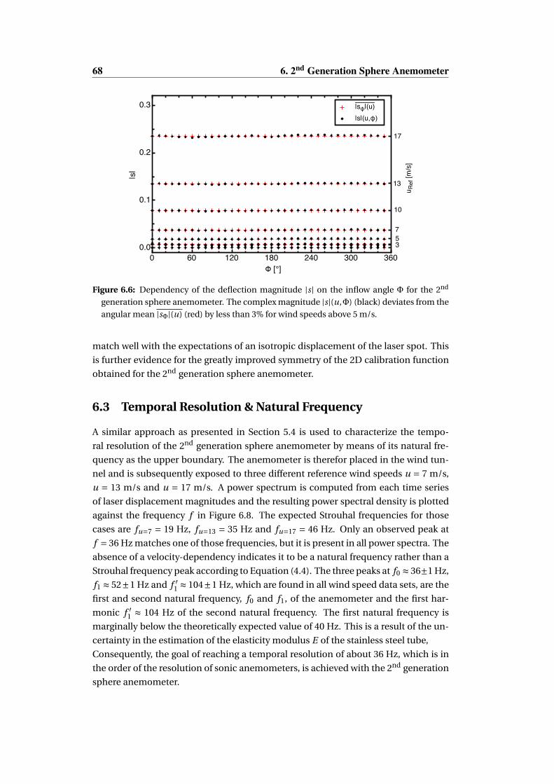
68 6. 2nd Generation Sphere Anemometer
0 60 120 180 240 300 3600.0
0.1
0.2
0.3
Φ [°]
|s|
|sφ|(u)|s|(u,φ)
17
13
10
7 5 3
u Ref
[m/s
]
Figure 6.6: Dependency of the deflection magnitude |s| on the inflow angle Φ for the 2nd
generation sphere anemometer. The complex magnitude |s|(u,Φ) (black) deviates from the
angular mean |sΦ|(u) (red) by less than 3% for wind speeds above 5 m/s.
match well with the expectations of an isotropic displacement of the laser spot. This
is further evidence for the greatly improved symmetry of the 2D calibration function
obtained for the 2nd generation sphere anemometer.
6.3 Temporal Resolution & Natural Frequency
A similar approach as presented in Section 5.4 is used to characterize the tempo-
ral resolution of the 2nd generation sphere anemometer by means of its natural fre-
quency as the upper boundary. The anemometer is therefor placed in the wind tun-
nel and is subsequently exposed to three different reference wind speeds u = 7 m/s,
u = 13 m/s and u = 17 m/s. A power spectrum is computed from each time series
of laser displacement magnitudes and the resulting power spectral density is plotted
against the frequency f in Figure 6.8. The expected Strouhal frequencies for those
cases are fu=7 = 19 Hz, fu=13 = 35 Hz and fu=17 = 46 Hz. Only an observed peak at
f = 36 Hz matches one of those frequencies, but it is present in all power spectra. The
absence of a velocity-dependency indicates it to be a natural frequency rather than a
Strouhal frequency peak according to Equation (4.4). The three peaks at f0 ≈ 36±1 Hz,
f1 ≈ 52±1 Hz and f ′1 ≈ 104±1 Hz, which are found in all wind speed data sets, are the
first and second natural frequency, f0 and f1, of the anemometer and the first har-
monic f ′1 ≈ 104 Hz of the second natural frequency. The first natural frequency is
marginally below the theoretically expected value of 40 Hz. This is a result of the un-
certainty in the estimation of the elasticity modulus E of the stainless steel tube,
Consequently, the goal of reaching a temporal resolution of about 36 Hz, which is in
the order of the resolution of sonic anemometers, is achieved with the 2nd generation
sphere anemometer.

6.3 Temporal Resolution & Natural Frequency 69
0 60 120 180 240 300 360
–40
–30
–20
–10
0
10
20
30
40
φmeasured [°]
φm
easu
red
- φse
t [°]
5 m/s, smooth7 m/s, smooth10 m/s, smooth13 m/s, smooth17 m/s, smooth
Figure 6.7: Deviation of the measured inflow angleΦmeasured from the set inflow angleΦset as
function of measured angle for the 2nd generation sphere anemometer setup with stainless
steel tube and smooth sphere.
1 10 100 50010–9
10–8
10–7
10–6
10–5
10–4
10–3
f [Hz]
PSD
[m2 /
s]
7 m/s13 m/s17 m/s
36Hz52Hz
104Hz
Figure 6.8: Power spectrum of the laser displacement magnitude of the 2nd generation sphere
anemometer with smooth sphere for different reference wind speeds. Three peaks at the
natural frequencies f0 ≈ 36 Hz, f1 ≈ 52 Hz and its first harmonic f ′1 ≈ 104 Hz are present.

70 6. 2nd Generation Sphere Anemometer
6.4 Summary & Discussion
A re-design of the sphere anemometer setup was undertaken as a further step to opti-
mize the anemometer’s calibration. The problematic properties of the GFP tube were
addressed by using a stainless steel tube instead. This helped solving the concerns
about isotropic deflections, but in turn also implied a re-modeling of the anemome-
ter housing in order to make up for the increased bending stiffness. A higher housing
was thus constructed and equipped with a smaller tube of significantly reduced wall
thickness, in order to maintain the desired measuring range. This also allowed for an
improved natural frequency f0 = 36 Hz of the 2nd generation sphere anemometer and
makes it competitive to sonic anemometers regarding the temporal resolution. Fur-
thermore, the improvements to the setup greatly reduced the angular dependence of
the 2D calibration yielding an almost perfectly circular shape.
The optimized geometry and material parameters of the 2nd generation sphere ane-
mometer can therefore serve as a foundation for the improvement of the anemometer
towards field applications in the next development stage.
Chapter 7
The Third Generation SphereAnemometer
Systematic investigations of the sphere anemometer properties in the previous chapters
were performed to identify and resolve crucial issues related to the used sphere ane-
mometer components. This chapter introduces the changes made to the anemometer
design in order to improve its robustness and usability. The construction is enhanced
towards field application, with changes made to the anemometer housing, sealing and
the sensor electronics. The calibration function of the new setup is measured and its
accuracy and resolution is characterized in wind tunnel experiments as well as its re-
sponse to vertical wind components.
7.1 Sphere Anemometer Setup
The 3rd generation of the sphere anemometer is based on the experience from the
previous version and the general choice of dimensions and materials – e.g. tube
length and material, sphere diameter – is widely unaltered. However, some further
optimization steps are necessary to enhance the performance under field conditions
and to make the anemometer setup more refined.
Although the 2nd generation sphere anemometer exhibits many desirable features,
some further optimization steps were necessary to for field applications and to im-
prove its handling and applicability. First and foremost, the installation on met mast
or wind turbines – in particular at off-shore sites – demands a higher level of water-
tightness, which was not accounted for so far. A reduction of the wind loading is also
beneficial and consequently efforts to design a new slender housing, that can sustain
the environmental condition of on- and offshore installations, is required. Besides
these mechanical aspects, an effort to overhaul the sensor electronics needs to be
considered. The combination of USB-powered laser and battery powered amplifier
circuit is not feasible for field installations and needs to be replaced by an integrated
circuit to cover both. This new sensor electronic should also output current signals
of 4-20 mA to comply with signals in industrial automation as they are often required

72 7. 3rd Generation Sphere Anemometer
for stand-alone data loggers.
The 3rd generation sphere anemometer features a slender aluminum housing with
a dome-shaped bottom part and a tubular top part (Fig. 7.1). Its design is meant to
minimize the wind load on the anemometer by reducing its diameter where the space
inside the housing is not needed. Thus, the top shaft, which holds only the laser sup-
ply cables and needs to provide only space for the laser beam to pass, can be thinned,
while more space is needed in the bottom part for the electronics compartment. This
is realized by the larger dome-shaped cover at the bottom of the anemometer, which
is wide enough to contain the sensor electronics with 2D-PSD and the laser supply
circuit. Moreover, this part of the anemometer can be opened for maintenance and
adjustments without the need for a disassembly of the anemometer. The blocked
cross-sectional area of 308 cm2 is reduced by 44% from 550 cm2 of the 2nd generation
sphere anemometer (Sec. 6.1). However, the overall height of the housing measured
from the base of the dome-shaped electronics compartment to the top of the tubular
part given in Figure 7.1 is similar to its predecessor. This is meant to maintain the
desired tube size and to keep the optical amplification, i.e. the laser path, constant
from the previous setup.
A thread at the top of the tubular housing allows for the fixation of the sphere-tube
combination. This active part of the sphere anemometer remains almost unchanged
from the previous version: A stainless steel (1.4301) tube with outer radius Ro = 4.0 mm
and inner radius Ri = 3.8 mm is fitted with two threads at the top and bottom. Only
the length of the support tube is slightly reduced to l = 195±0.05 mm, in order to in-
crease the natural frequency of the anemometer and extend its measuring range. The
top thread supports the smooth sphere of the previous setups with 70 mm diameter.
Additional sealing is included to make the anemometer withstand the challenges
of heavy rain and ocean spray at near-shore and off-shore sites. A pair of rubber seal-
ing rings is located at the transitions of the dome-cover to the tubular shaft and the
base plate of the electronics compartment. Two additional rubber rings are used to
seal the connection of the top thread of the shaft with the sphere-tube-combination
as well as the connection of the sphere mount on the support tube (Fig. 7.1). In com-
bination with the watertight IP67 socket at the anemometer bottom, the 3rd genera-
tion sphere anemometer setup is waterproof to the level of submergence. A mounting
plate at the anemometer base allows for the fixation of the sensor on flat surfaces –
it can be omitted for the installation on tubular supports. All aluminum parts of the
housing are anodized to improve the surface robustness and prevent corrosion under
outdoor conditions, particularly in salty offshore environments.
The tip displacement of the sphere is measured with a light pointer, as it was done
in the previous setups. However, the sensor electronics is completely re-designed in
order to match the demand for standardized output signals of 4–20 mA currents in-
stead of the voltage output used so far. This aims at the use of the sphere anemometer
in combination with industrial data loggers, which typically require this input range
commonly used in industrial automation and control. Each anemometer channel has
its own amplifier and the amplification rate can be individually adjusted via a vari-

7.1 Sphere Anemometer Setup 73
laser diode
sealed thread
electronics
sealed thread
sealed dome
base with socket
160
519
(a) (b)
Figure 7.1: (a) Drawing and (b) photo of the 3rd generation sphere anemometer. The slender
tubular housing reduces the wind loading while the optical path remains unchanged com-
pared to the previous version. The sealed dome at the bottom holds the sensor electronics
and is connected with a water-tight socket at the bottom of the base.
able resistor. The output currents Ii are linearly proportional to the induced photo
currents Ii
Ii =Gi · Ii ∀i ∈ [1,4] (7.1)
with the gain factor Gi being specific for each amplifier.
As an additional improvement, the laser supply circuit with voltage regulator is inte-
grated in the new electronics layout. A description of the plan and layout of the sphere
anemometer electronics can be found in Appendix C. In all previously described ane-
mometer setups, two power supplies were required – one for the amplification circuit
and a second one for the laser supply. The new integrated design allows for the use
of only one combined power supply for the sphere anemometer operation, which is
connected to the mains and operated at ±12V DC output voltage.

74 7. 3rd Generation Sphere Anemometer
The ADL-65055SA2 laser diode with integrated laser driver is adopted for the 3rd gen-
eration sphere anemometer as are the lens and lens holder with precision thread. As
a result of the modified sensor electronics, some adjustments have to be made to the
laser, though. The laser supply voltage is reduced to 3 V, which yields a reduction of
the laser output power. In addition, the new amplification circuit is designed for a
target laser power of 1 mW, which is about four times larger than the laser power of
the previous setups. As a consequence, the resistor for the laser output regulation,
which is directly soldered to the pins of the laser diode, is reduced to RVR = 6.8 kΩ
in order to compensate for this. This is well in the specified range of resistance for
the laser diode, while the previous configuration was significantly off of the specified
values for RVR.
To adjust the gain factors Gi for the single channel amplifications, the laser diode is
focused on the sensitive area of the 2D-PSD using the precision thread of the lens
holder. The incident spot is subsequently aimed at each corner of the sensitive area
using a micro-translation stage and the amplification of the corresponding signal
channel is adjusted to match the 20 mA current by means of a variably trimmed resis-
tor.
A further reduction of the diameter of the laser supply cables compared to the coated
copper wires of the last setup is achieved by using silicon-coated single wires with a
cross-section of 0.07 mm2. These wires are not wound around the outside of the tube,
but instead led through the inside of the tube. Any angular dependent effects of the
cables on the exposed cross-section of the anemometer can be ruled out in this way.
The added cover of the tube with a shrinking hose is also dispensable, which elimi-
nates the risk of introducing angular dependencies of the strain behavior during the
shrinking process.
To enable the usage of the sphere anemometer with common AD converters with
voltage inputs, a signal conversion circuit was built. It features a precision shunt re-
sistor with RS = 1.38 Ω and a voltage amplifier with a fixed amplification rate of 200
for each of the four sphere anemometer signals. The signal conversion box is supplied
by the same power supply used for the sphere anemometer.
Modifications to the Sphere Construction
The spheres used for the 3rd generation sphere anemometer are based on the 70 mm
diameter hollow plastic spheres of the previous setup. However, the intent of this new
anemometer generation is the operation in field conditions and different constraints
regarding weathering and humidity have to be considered. Generally, the ABS plastic
material which is used for the spheres is not water-tight. It has to be sealed by a cover-
ing layer of water-resistant coating. An additional impact of the environment can be
safely assumed, since plastics tend to wear noticeably under exposure to ultra-violet
radiation in field application. To handle both issues, the spheres are covered with
several layers of spray paint, including a cover layer of UV-resistant paint. The slightly
increased weight of the spheres has to be accepted as a trade-off for its indispensable

7.2 Sensor Calibration 75
water-tightness. The combination of the coated spheres with an added rubber seal-
ing ring at the top thread of the tube makes the anemometer completely water-tight,
even when it is slightly submerged11.
An additional environmental impact has already been foreseen regarding the dimpled
surface patterns. It is expected to be prone to dirt accretion inside the dimples, which
causes a changing drag coefficient due to the altered surface roughness. This effect is
unwanted and may lead to changes in the sphere anemometer’s calibration function,
as has been pointed out in Section 5.3.1. The dimpled sphere has therefore also been
discarded for the 3rd generation sphere anemometer in order to avoid uncertainties
in the results caused by changing sphere surface properties.
First tests of the sphere-tube-connection shown in Figure 7.2 (a) revealed a weak
connection of the rather thin hollow body of the sphere and the support joint at its
bottom. A higher stiffness is required since the joint holds the aluminum thread and
is responsible for the transmission of the drag force on the tube tip. The pointy edge
connecting both parts tends to break when exposed to large forces and thus expose
the laser to the environment as seen in Figure 7.2 (b). Although these large forces
are not expected to occur during regular operation in the wind flow, the anemometer
may experience extreme forces during transport, field installation or in cases of ice
shedding from wind turbine blades. The pointy sphere joint depicted in Figure 7.2 (c)
was therefore modified with a rounded transition region to increase the stiffness and
distribute the force inlet (Fig. 7.2, d).
(a) (b) (c) (d)
Figure 7.2: Close-up of the sphere (a) before installation and (b) the tube with remainders of
the joint after the hollow sphere broke. Drawings of (c) the old sphere with pointy joint and
(d) new sphere with rounded and stiffened joint.
7.2 Sensor Calibration
The 3nd generation sphere anemometer is calibrated in the acoustic wind tunnel of
the University of Oldenburg (Sec. 5.2.1). The calibration setup is similar to the setup
used for the 2nd generation anemometer, where the anemometer is mounted in the
center of a motor-driven turntable with its centerline being in a downstream distance
11In a simple test, the assembled anemometer with coated sphere was submerged over night without
any signs of water intrusion into the sphere or the anemometer housing.

76 7. 3rd Generation Sphere Anemometer
of 0.35 m from the wind tunnel nozzle. The turntable is used in its lower configuration
in order to ensure the active part of the sensor, i.e. the bending tube-sphere-element,
to be placed in the center region of the wind tunnel cross-section. A photo of the
setup for the calibration is shown in Figure 7.3.
Figure 7.3: Setup for the calibration of the 3rd generation sphere anemometer.
The sphere anemometer data is recorded by means of a 16 Bit DataTranslation DT9816-
A analog-digital (AD) converter with ±5V measurement range, which is connected to
a computer via USB. Ten seconds of the four sphere anemometer channels are simul-
taneously acquired at a sampling rate of fs = 1kHz and converted to (x, y)-coordinates
of the laser displacement according to Equation (3.9) during post-processing. In case
of the 3rd generation sphere anemometer, the calibration is not only performed for the
assessment of the anemometer itself, but a later comparison to sonic and cup anemo-
meters is also intended. It is necessary for such a comparison to base the calibration
of all anemometers on the same wind speed reference. While the calibration proce-
dure of the previous anemometers referred to the displayed wind speed of the wind
tunnel panel, the one- and two-dimensional calibration of the sphere anemometer
presented hereafter are based on reference wind speed measurements in the wind
tunnel contraction. uRef is therefor measured using the eight Pitot tubes and eight
static pressure taps of the wind tunnel contraction and nozzle (cf. Sec. 5.2.1). Each set
of pressure probes is integrated via common tubings and connected to a calibrated
Setra C239 differential pressure gauge [Setra Systems Inc., 2013]. Differential pres-
sures pd are converted to wind speeds during post-processing using Equation (2.3).
The air density % is therefor calculated from the ambient pressure and temperature
readings of a combined meteorological sensor in the wind tunnel according to Equa-
tions (2.5) and (2.6) as described in Section 2.1.1.

7.2 Sensor Calibration 77
–0.3 –0.2 –0.1 0.00
5
10
15
20
s
u [m
/s]
x-componenty-component
–0.3 –0.2 –0.1 0.00
100
200
300
400
s
u2 [m
2 /s2
]
x-componenty-component
R2=1.0000
(a) (b)
Figure 7.4: One-dimensional calibration function of the sphere anemometer recorded for 0
inflow angle. (a) The x-component (solid bullets) follows an negative square root function
while the y-component (open triangles) remains almost unchanged with increasing refer-
ence wind speed u. (b) Square of reference wind speed, u2, plotted against the anemome-
ter’s x- and y-signals. A linear regression line is fitted to the data for the x-component with
coefficient of determination R2 = 1.000.
7.2.1 1D Calibration Function
A one-dimensional calibration function of the sphere anemometer is recorded with
the setup described above. The anemometer is therefore aligned in 0 position with
the x-coordinate of the 2D-PSD corresponding to the main flow direction. The ref-
erence wind speed is varied between 0 m/s and about 20 m/s and the exact value is
determined from the dynamic pressure reading. The reference wind speed is plotted
against the calculated (x, y)-coordinates of the laser spot position on the active area of
the 2D-PSD in Figure 7.4 (a). The "inversed square-root" shape of the x-component
is similar to the findings for the previous anemometers, but a visible inclination of
the y-component is also found. This is a result of a slight misalignment between the
main flow direction and the 0 position of the anemometer, which is determined by
the orientation of the 2D-PSD inside the anemometer housing. It indicates a minor
inaccuracy during soldering of the electronics or anemometer assembly, which may
result in a constant angle offset for the direction measurements without jeopardizing
the functionality of the anemometer.
The squared reference wind speeds is plotted against the components of the laser
spot displacement in Figure 7.4 (b). A linear regression function fitted to the data of
the x-component is illustrated by the straight line. No significant deviation from the
linear relation of u2 and x is present, which results in the perfect value of the coeffi-
cient of determination R2 = 1.000. The slight negative bending of the y-component in
Figure 7.4 (a) translates to a steep negative slope in the plot of the squared wind speed
(b). No variation of the y-component with wind speed is expected for the supposed
perpendicular component, but as aforementioned it indicates an angle offset. How-
ever, it constitutes no issue for the sphere anemometer calibration, since it can be
included in the 2D-calibration. An impression of the complex one-dimensional cal-
ibration can be gained from Figure 7.5. The reference wind speed is plotted against

78 7. 3rd Generation Sphere Anemometer
the complex displacement magnitude |s| = |x+i y | for the 0 orientation of the sphere
anemometer. The data is fitted with a power-law function according to Equation (4.3).
The exponent n = 0.469 varies slightly from the square-root form of n = 0.5, caused
by the above mentioned angle offset between the 2D-PSD’s y-axis and the main flow
direction.
0.0 0.1 0.2 0.30
5
10
15
20
|s|
u [m
/s]
|x+iy|power law fit
Figure 7.5: 1D calibration function of the displacement magnitude |s| for the 3rd generation
sphere anemometer. The data is fitted with a power law according to Eq. (4.3).
7.2.2 2D Calibration Function
The two-dimensional calibration function of the 3rd generation sphere anemome-
ter was recorded, making use of the same setup described in the beginning of Sec-
tion 7.2. The anemometer is rotated along its vertical axis on the motor-driven turn-
table shown in Figure 7.3. The wind speed was kept constant for each rotation of
the anemometer, which comprised 36 measured inflow angles between 0 and 350
(∆Φ= 10). An offset measurement at u = 0 m/s was initially performed and the wind
speed was subsequently increased up to approximately 20 m/s. The 3D plot in Fig-
ure 7.6 (a) shows the reference wind speed from the Setra C239 pressure gauge plotted
against the (x, y)-coordinates of the laser spot on the active area of the 2D-PSD. The
varying reference wind speeds are color coded. The 3D plot of the calibration func-
tion exhibits the shape of a potential well, which is consistent with the expectations
and also found for the previous anemometers. Its projection on the detector plane is
presented in Figure 7.6 (b) for a better judgment of the quality of the calibration func-
tion in terms of isotropy and uniqueness. The same color coding is therefor used in
the projected display.
A unique behavior of the 2D calibration is found for the 3rd anemometer genera-
tion, as no crossings of neighboring inflow angle data can be seen. This is expected
since the problems with the ambiguous anemometer behavior have been attributed
to the tube material of the outdated anemometer setups, which were abandoned from
the 2nd generation onwards.

7.2 Sensor Calibration 79
–0.3 –0.2 –0.1 0.0 0.1 0.2 0.3–0.3
–0.2
–0.1
0.0
0.1
0.2
0.3
x-component
y-co
mpo
nent
0
5
10
15
20
u [m
/s]
(a) (b)
Figure 7.6: Two-dimensional calibration function of the 3rd generation sphere anemometer.
The reference wind speed u is plotted against the x− and y-components of the laser dis-
placement on the 2D-PSD in (a) a 3D plot and (b) the projection on the detector area. Both
plots use the same color-coding.
Table 7.1: Deviations χ of the displacement magnitude from the angular averaged displace-
ment for a given reference wind speed u according to Eq. (5.4) for the 3rd generation sphere
anemometer.
3rd generation sphere anemometer
u [m/s] 5 7 9 11 14 17 20
χmax [%] +17.1 +9.3 +4.9 +2.6 +2.9 +3.4 4.0
χmin [%] -16.4 -8.3 -5.2 -4.2 -3.7 -2.9 3.0
The uniformity of the two-dimensional calibration is analyzed in terms of the rel-
ative deviation from a circular shape. As in the previous anemometer setups, the devi-
ation χ is calculated to relate the displacement magnitude for each set inflow angleΦ
and wind speed u to the angular average of it for each reference wind speed. Figure 7.7
shows the measured displacement magnitude |s|(u,Φ) plotted against the inflow an-
gle Φ set with the turntable for wind speeds between 0 and 20 m/s. For comparison,
the angular average of the displacement, |sΦ|(u), is also plotted as a representation of
an ideal circle. Deviations from the ideal circle can be clearly observed, but the rela-
tive deviation χ is about 5% or below for wind speeds of 9 m/s or higher, as listed in
Table 7.1. The positive deviations occur at the same inflow angles around Φ= 10 for
all wind speeds, while the negative deviations are mainly present aroundΦ= 90.
The sphere anemometer data recorded during the 2D calibration procedure is
used to assess the performance for direction measurements. The difference of the
measured inflow angle and the inflow angle set by the turntable is therefore analyzed.
Figure 7.8 shows the angle difference as a function of measured angle for all reference
wind speeds, where a subscript was added to distinguish both angles Φmeasured and
Φset. Only small differences are observed for wind speeds higher than 7 m/s, but a

80 7. 3rd Generation Sphere Anemometer
0 60 120 180 240 300 3600.0
0.1
0.2
0.3
Φ [°]
|s|
|sΦ|(u)|s|(u,Φ)
17
14
11
7 5
9
u Ref
[m/s
]
20
Figure 7.7: Dependency of the deflection magnitude |s| on the inflow angle Φ. The complex
magnitude (black) is slightly overshooting the angular mean (red) around Φ = 180 and
undershooting the mean aroundΦ= 90.
pronounced systematic difference is obvious for 5 m/s and 7 m/s. These wind speeds
are also subject to the larger deviations in terms of deviations from the circular cal-
ibration function, as listed in Table 7.1. This is only logical to manifest also in the
wind direction, because the laser displacement s is used for both, the wind speed
calibration and the direction calculation, in Equations (5.2). Unlike the scattering
and clustering found for the 1st generation sphere anemometer (Sec. 5.2.4), the dif-
ferences of the measured inflow angles from the set angles are continuously varying
withΦmeasured and can therefore be fitted and corrected.
0 60 120 180 240 300 360
–40
–30
–20
–10
0
10
20
30
40
φmeasured [°]
φm
easu
red
- φse
t [°]
5 m/s7 m/s9 m/s11 m/s13 m/s17 m/s20 m/s
Figure 7.8: Deviation of the measured inflow angle Φmeasured from the set inflow Φset angle
plotted against the measured inflow angle for the 3rd generation sphere anemometer.
7.2 Sensor Calibration 81
A possible explanation of the slight but systematic deformation of the 2D calibra-
tion can be found in the use of individual amplification with gain factors Gi for each
of the anemometer’s four photo currents. The gain factors relate the actually induced
photo currents I1 . . . I4 to the sensor outputs I1 . . . I4 linearly,
Ii =Gi · Ii ∀i ∈ [1,4]. (7.2)
While exact identical amplification of the signals would, material effects aside, lead
to a circular 2D calibration, different shapes of the 2D calibration can be achieved
depending on the relation between the four gain factors G1 . . .G4. The impact of dif-
ferent signal amplifications is treated in more detail in the Section 7.2.3, where an
exemplary calculation of a synthetic 2D calibration is presented.
7.2.3 Impact of Different Amplification Factors on the2D Calibration
The concept of individual channel amplification is introduced for the 3rd generation
sphere anemometer in order to allow for the adjustment of each signal channel to
match the input range of industrial data loggers. The impact of different gain factors
Gi for each of the four induced photo currents is investigated using an artificial cali-
bration data set, which obeys a perfectly circular shape. The four channels of this data
set are then distorted by multiplication with the four amplification factors G1 . . .G4 in
order to mimic the individual amplification carried out in the sensor circuit of the
3rd generation sphere anemometer. Three different scenarios are therefor treated:
I. The amplification factors of each set of diagonal electrodes are different, but
both factors in a diagonal are identical.
G1 = G2 = 1 (7.3)
G3 = G4
G1,2 < G3,4
II. The amplification factors of each side of electrodes are different, but both fac-
tors on a side are identical.
G1 = G4 (7.4)
G2 = G3
G1,4 > G2,3
III. The amplification factors of all electrodes are different and vary increasingly
from G1 . . .G4.
G1 <G2 <G3 <G4 (7.5)

82 7. 3rd Generation Sphere Anemometer
The resulting calibration of case I. is deformed to become an ellipse with its semi-
major axis aligned diagonally facing the electrodes with the higher amplification. The
semi-minor axis is shortened, which flattens the ellipse compared to the equally am-
plified case of a circle, shown in Figure 7.9 (left). The different colored ellipses corre-
spond to a 10% higher and 25% higher amplification of the original circular signal.
Case II. shows a deformation, which cannot be clearly identified with an elliptical
shape anymore. An additional shift of the center of the 2D calibration is present due
to the lopsided amplification, which becomes more severe for the larger difference in
factors. However, this shift will be constant for a 2D calibration and not vary as long
as the gain factors Gi , which are hardware settings, remain unchanged.
The individually varying case III. contains both effects as well, but they are less pro-
nounced. The calibration may on first glance be considered elliptical, but due to the
presence of different amplifications on the diagonals, a distorted ellipse is produced.
The observed shift of the center is also present here. It is worth noting, that the de-
x-component
y-component
10%25%
I2
I3I1
I4 x-component
y-component
10%25%
I2
I3I1
I4 x-component
y-component
0-15%0-30%
I2
I3I1
I4
I. II. III.
Figure 7.9: Impact of differing amplification factors of the sensor circuit demonstrated on
artificial data of a perfectly circular 2D calibration (black). I. Identical amplification of the
diagonal signals., II. Identical factors on each side. III. Four different factors.
scribed shift in the cases II. and III. is only observed with respect to the ideal, circular
2D calibration. By no means can be concluded, that the uniqueness of the calibration
is in jeopardy due to this effect, because the shift does not change within a calibration
with fixed hardware amplification factors. It is therefore automatically incorporated
in a real calibration function recorded in the wind tunnel. Although these deforma-
tions found in the previous section are included in a full 2D calibration, it is desirable
to achieve the highest degree of rotational symmetry in order to allow for a fast cali-
bration procedure with only few required inflow angles. Considering the above find-
ings, the concept of individual signal amplification should be abandoned in future
anemometer setups in order not to complicate the sphere anemometer calibration.
The benefit of a higher degree of rotational symmetry of the 2D calibration clearly
outweighs the use of the entire measuring range of the connected AD converter or
data logger. The individually adjustable amplification of the photo currents should
thus be replaced by a choice of similar gain factors, i.e. similar gain resistors.

7.3 Precision and Accuracy of the Measurements 83
7.3 Precision and Accuracy of the Measurements
Two key features of every sensor are its precision and its accuracy, which can be de-
fined as follows:
Precision: A measurement with a sensor is considered precise if repeated measure-
ments of the same reference instance cause the sensor to output the same value within
a certain error range. The existence of such a precise measurement, however, does not
imply that the measured value is correct with respect to a "true" reference value.
Accuracy: A sensor is considered accurate if repeated measurements of the same
reference instance yield sensor outputs scattered in the vicinity of the "true" reference
value.
The arbitrary deviations from the reference value are attributed to the sensors
precision, while the systematic deviation from the reference is considered in the ac-
curacy. Figure 7.10 illustrates the above definitions using an ensemble of ten data
points located on a target and the center of the target is considered to be the "true"
reference value. Sketch (a) is an example of poor accuracy, due to the large offset of
the scattered points from the center. At the same time, the large scatter between the
data points shows the poor precision. An example with less scatter, i.e. good pre-
cision, but also an offset from the reference value is shown in picture (b), while the
opposite case of a relatively accurate measurement with poor precision is shown in
the scattered points around the center in (c). Figure 7.10 (d) show the desired case
of a low amount of scatter around the "true" reference value, i.e. high precision and
accuracy of the measurements.
(a) (b) (c) (d)
Figure 7.10: Schematic display of measurement precision and accuracy. The red data shows
(a) no precision and no accuracy, (b) precision but no accuracy, (c) accuracy but no preci-
sion and (d) accuracy and precision.
These rather theoretical concept of measurement precision and accuracy trans-
lates into the question, whether the sphere anemometer measurements can be con-
sidered any of those. Two experiments were therefore carried out to assess the preci-
sion and accuracy of the sphere anemometer. Repetitive measurements of the same
wind speed references uRef were performed for four different wind speeds in the range
of 2.8 m/s to 11 m/s. Measurements with a reference anemometer performed at the
position of the sphere anemometer provided an estimate for a confidence interval in

84 7. 3rd Generation Sphere Anemometer
which the wind tunnel speed fluctuates during the regular operation.
Five instances of the anemometer reading were recorded for each reference wind
speed with the anemometer being shielded from the flow in between each measure-
ment. The wind tunnel was not switched off or set to 0 m/s between measurements
to ensure the set reference wind speed to be the same for the five readings per wind
speed. The precision of the sphere anemometer measurements was investigated by
assessing the scatter between five subsequent readings of the same reference wind
speed. The ensemble average ⟨uSphere⟩ of the five measured instances was therefore
calculated as well as the fluctuations of the individual measurements
u′Sphere = uSphere −⟨uSphere⟩. (7.6)
Figure 7.11 (a) shows the fluctuations plotted against the average value to visualize the
amount of scattering of the individual measurements and the estimated wind tunnel
confidence interval. The lowest velocity ⟨uSphere⟩ exhibits the largest fluctuations of
up to 0.1 m/s while the fluctuations are significantly decreasing below 0.05 m/s with
increasing reference wind speed. The confidence interval is in the same order as the
fluctuations of the sphere anemometer measurements for wind speeds short below
5 m/s up to about 11 m/s. The increasing precision of the sphere anemometer read-
ings can be easily explained by the increasing sensitivity of the anemometer setup due
to the squared velocity dependence of the acting drag force. In the low wind speed
range, small changes in the anemometer signal are associated with large changes in
the measured wind speed due to the steep slope of the square-root calibration func-
tion, while similar changes in the higher wind speed range yield smaller differences
in the measured speeds as the calibration has a lower slope. The precision for higher
wind speeds can thus be expected to be similar or even better, although only wind
speeds up to 11 m/s were investigated. A precision of 0.1 m/s for the investigated
wind speed range is similar to the values claimed by the manufacturers of state-of-
the-art anemometers, such as the Thies First Class Advanced cup anemometer [Thies
Clima, 2009] or the Gill WindMaster Pro sonic anemometer [Gill Instruments Ltd.,
2009].
The second key feature – the accuracy of the measurements – has been assessed
in the same experiment. The reference wind speed uRef has therefore been calculated
from dynamic pressure measurements with Prandtl tube connected to a calibrated
Betz micro-manometer. The measured instances of the sphere anemometer wind
speed uSphere were plotted against the wind speed reference in Figure 7.11 (b). Error
bars indicate the standard deviation of each individual measurement of uSphere. The
reference measurement is treated to be without error, besides the uncertainty con-
sidered as the wind tunnel confidence interval, which is plotted as error bars. Only
minimal differences between the five data points for uRef = 3 m/s can be observed,
while the measured values for each reference wind speed beyond that collapses. This
finding is well in line with the result of the precision assessment.
In the ideal case of a perfect match of sphere anemometer and reference data, the
plotted data points should be located on the line with slope 1. A slope of 1.021 is ob-

7.4 Temporal Resolution & Natural Frequency 85
(a) (b)
2 3 4 5 6 7 8 9 10 11–0.2
–0.1
0.0
0.1
0.2
⟨uSphere⟩ [m/s]
u'Sp
here
[m/s
]u'Sphere
confidenceinterval
2 3 4 5 6 7 8 9 10 1123456789
1011
uRef [m/s]
u Sph
ere
[m/s
]
uSphere = 1.021・uRefR2=0.9998
uSphere
Figure 7.11: Repetitive measurements with the sphere anemometer at four different refer-
ence wind speeds. (a) The fluctuations u′Sphere of the individual wind speed measurements
plotted against the corresponding ensemble average ⟨uSphere⟩ of the sphere anemometer
to assess the measurement precision. (b) Sphere anemometer wind speed uSphere plotted
against reference wind speed from Prandtl tube uRef and linear fit to assess the measure-
ment accuracy.
tained via linear regression with a coefficient of determination R2 = 0.9998 as shown
in the Figure 7.11 (b). This corresponds to a minimal over-prediction of the wind
speed, but 2% deviation can still be considered a fair agreement with the reference
and compares well to typical values of about 1% accuracy for high-end commercial
anemometers.
7.4 Temporal Resolution & Natural Frequency
The frequency response of the 3rd generation sphere anemometer is assessed based
on the power spectra of measured wind speed time series. The goal is the estimation
of its natural frequency as an upper limit to the anemometer’s temporal resolution in
an analogous approach as used to characterize the previous anemometer setups.
A wind tunnel experiment is therefore performed in a setup similar to the calibra-
tion setup described in Section 7.2. The sphere anemometer with the coated smooth
sphere is thereby exposed to flow with different reference wind speeds u = 7 m/s, u =13 m/s and u = 17 m/s. The corresponding vortex shedding frequencies fu according
to the Strouhal number (Eq. (4.6)) are fu=7 = 19 Hz, fu=13 = 35 Hz and fu=17 = 46 Hz.
Based on the theoretical considerations of Section 4.3, a natural frequency f0 ≈ 45 Hz
is expected for the setup.
The first natural frequency of f0 = 45 Hz is slightly higher than the prediction of
40 Hz, which was also observed for the 1st anemometer generation. It is close to the
expected Strouhal frequency fu=17 = 46 Hz, yet it can be clearly identified as the natu-
ral frequency, because it is present in the power spectra for all wind speeds. However,
the magnitude is increased for u = 17 m/s, possibly due to resonance with the shed-

86 7. 3rd Generation Sphere Anemometer
1 10 100 50010–9
10–8
10–7
10–6
10–5
10–4
10–3
f [Hz]
PSD
[m2 /
s]
7 m/s13 m/s17 m/s
45Hz57Hz
90Hz
Figure 7.12: Power spectral density of the complex displacement magnitude of the 3rd gener-
ation sphere anemometer with smooth sphere for 7 m/s, 13 m/s and 17 m/s reference wind
speeds. Two natural frequency peaks at f0 = 45 Hz f1 = 57 Hz are observed as well as the
first harmonic f ′0 = 90 Hz.
ding vortices. A second peak at f1 ≈ 57 Hz appears in all spectra, and it can thus be
assumed to be a second natural frequency.
A broader peaks in the power spectra at single wind speeds are observed between
10––20 Hz for u = 7 m/s and around 30–35 Hz for u = 13 m/s. The magnitude of these
peaks is small compared to the magnitude of the natural frequency peaks, and they
can be attributed to vortex shedding due to their velocity dependence.
Overall, the natural frequency of about 45 Hz enables the latest sphere anemome-
ter generation to not only compete with, but to provide a higher temporal resolution
than the commercial Gill WindMaster Pro 3D sonic anemometer.
7.5 Response to Cross-Flow
Atmospheric wind conditions feature three components of the wind vector all the
time, albeit the vertical wind component is usually an order of magnitude smaller
than the two horizontal components. The sign of the vertical component depends on
several boundary conditions like the atmospheric stability, obstacles in the vicinity
and buoyancy. Although the sphere anemometer measures only the two horizontal
flow components, these readings may be affected by the vertical wind component
and the effect of this cross-flow is assessed in the following.
The response behavior of the sphere anemometer to cross-flow conditions is in-
vestigated using the 3rd generation anemometer with smooth sphere surface. For the
experiments performed in the wind tunnel at the University of Oldenburg the sphere
anemometer is placed on a tilting stage with the sphere located in the center of the
wind tunnel cross-section in a distance of 0.35 m from the nozzle. The stage can be
tilted manually between γ = ±20 in steps of 2.5. Negative tilt angles, i.e. a forward

7.5 Response to Cross-Flow 87
γ=−20
→u
γ= 0
→u
γ=+20
→u
Figure 7.13: Setup for the measurement of the tilt response of the sphere anemometer. The tilt
stage at the bottom of the anemometer is set to γ=−20 (left), γ= 0 (center) and γ=+20
(right).
tilt, correspond to a down-wind scenario in a field measurement, while positive an-
gles, i.e. backward tilt, correspond to an upwind scenario as can be seen in Figure
7.13. The accuracy of the set tilt angle γ is verified by means of image analysis and the
deviations of less than 0.2 are considered acceptable to give a general impression of
the anemometer’s tilt response. The wind tunnel is set to constant horizontal refer-
ence wind speeds uRef, which is measured using the installed Pitot-tubes and pres-
sure holes in the wind tunnel outlet connected to a calibrated Setra C239 differential
pressure gauge. The sphere anemometer channels are acquired simultaneously with
the same Data Translation DT9816-A AD converter used in the previous experiments,
while the differential pressure, ambient temperature and atmospheric pressure are
acquired with a multiplexing NI-6211 AD converter. Both AD converters sample with
fs = 1 kHz and cover their respective measuring range of ±5 V and ±10 V with 16 Bits
resolution.
The experiment is intended to mimic flow situations with a vertical wind speed
component as they occur in field measurements on met-masts or wind turbine na-
celles. However, vertical wind components can only be achieved in the wind tunnel
by tilting the anemometer, but a gravitational force component, which is not present
in field installation, will inevitably be added. In order to account for this, the impact
of the gravitational force Fg acting on the sphere and the tube is measured by tilt-
ing the anemometer without any wind flow. The resulting (x, y)-components and the
displacement magnitude |s| = |x+ i y | of the 2D-PSD signal are calculated for each tilt
angleγ. Although the main flow direction coincided with the y-component, |s| is used
for the assessment in order to account for slight misalignments of the detector. The
displacement magnitude for the offset case is plotted in Figure 7.14 against the set tilt
angle γ. A representation in terms of an equivalent wind speed uequiv is given on the
right ordinate in order to relate the gravitational effect on |s| to a hypothetical wind

88 7. 3rd Generation Sphere Anemometer
speed. Deviations from the upright anemometer position at γ= 0 result in increased
displacements |s| of the laser spot due to gravitation. Only the projection of Fg on the
plain perpendicular to the tube can be measured with the sphere anemometer and a
sinusoidal dependence of |s| is thus expected for an ideal system. The observed linear
trend of the magnitude fulfills this expectation quite well as the sine function can be
linearly approximated in the vicinity of 0, and the pronounced tilt angle dependency
is a clear proof of the high sensitivity of the sphere anemometer even to such small
gravitational forces in the range of Fg ≈ 0. . .0.08 N.
–20 –10 0 10 200.00
0.01
0.02
0.03
0.04
0.05
0
1
2
3
4
5
6
7
8
γ [°]
|s|
|s| offset
u equ
iv [m
/s]
Figure 7.14: Offset signal from the sphere anemometer when it is tilted at uRef = 0 m/s. The
displacement magnitude |s| increases for positive and negative inclinations γ due to the
effect of gravitation.
Two different reference wind speeds uRef ≈ 6.5 m/s and uRef ≈ 9 m/s are investi-
gated to characterize the cross flow response. The sphere anemometer is tilted in both
positive and negative directions from the vertical position, resulting in mimicked ver-
tical wind components of up to ±2.2 m/s and ±3 m/s, respectively. The offset signals
obtained from the previous experiment without wind flow are subtracted from the
calculated displacement magnitudes |s| and the offset-corrected data is calibrated us-
ing the 1D calibration function recorded prior to the experiment. Figure 7.15 shows
the calibrated wind speed magnitude |s| plotted against the tilt angle γ. Only the wind
speed component perpendicular to the tube contributes to the sphere anemometer
deflection and thus, the projected wind speed
uproj = uRef · cos(γ) (7.7)
for each reference wind speed is represented with the dotted line. The two investi-
gated cases are not differentiated in the following analysis, since the response of the
sphere anemometer to the vertical flow is similar for both reference wind speeds.
For the vertical anemometer position (γ = 0) a slightly higher wind speed is ob-
tained with the sphere anemometer compared to the reference sensor. Slowly de-

7.5 Response to Cross-Flow 89
creasing measured wind speeds uSphere are found for the upwind scenario of positive
tilt angles γ > 0. In this range, the measured wind speeds agree well with the ex-
pected projection of the respective reference wind speed uRef. On the contrary, the
measured wind speeds of the sphere anemometer deviate from the projected refer-
ence for all negative tilt angles, starting at γ = −2.5. The effects seen for negative
–20 –10 0 10 200
2
4
6
8
10
12
14
γ [°]
u [m
/s]
uSphere, 9 m/suSphere, 6.5 m/suRef ⋅ cos(γ)
Figure 7.15: Measured wind speed uSphere of the the sphere anemometer (bullets) compared
to projection of the reference wind speed uRef (dotted line). Data for uRef = 9 m/s is plotted
in blue and data for uRef = 6.5 m/s are shown in red.
inclinations are unexpected, since an ideal system response would result in a sym-
metric cosine projection of the wind speed at γ = 0. Nevertheless, an attempt to
explain the asymmetric cross-flow response can be made based on the knowledge of
the flow around a sphere with a support normal to the flow direction:
The flow around an ideal, i.e. unsupported, sphere is characterized by a front stag-
nation point in the center plain of the sphere and a symmetric flow around the sphere.
In this case, the mean flow separation occurs symmetrically on both sides at a separa-
tion angle ϑs between 80 and 102 from the front stagnation point. The actual value
of ϑs depends on the Reynolds number regime, which is affected by the sphere sur-
face properties and background turbulence [Son et al., 2010]. The flow separation and
definition of the separation angle is depicted in Figure 7.16, for a subcritical (a) and a
supercritical Reynolds number (b). The separation line indicates the plain of the great
circle of the symmetric flow separation on the sphere surface, which is shifted further
downstream with the flow becoming supercritical. As already discussed in Section 3.2,
the drag coefficient cD decreases in the supercritical region, because a smaller frac-
tion of the sphere surface is immersed in the sphere wake. Raithby and Eckert [1968]
investigated the flow around a sphere on a support normal to the flow direction with
flow visualization techniques and compared it to the flow around a sphere, which is
supported from its back side as the experimental equivalent of the ideal case. They
found the separation locations to be altered due to the impact of the normal support

90 7. 3rd Generation Sphere Anemometer
at certain Reynolds numbers. Almost no effect of the support on the flow separation
is found for the subcritical case as depicted in Figure 7.16 (c), since the flow separa-
tion at ϑs ≈ 80 sets in upstream of the support rod. Consequently, the wake is not
increased by the support and cD remains the same as in the unsupported case. As the
flow becomes supercritical (Fig. 7.16, d), the separation region moves downstream
and the location of the support is in the (ideally) attached flow region. Raithby and
Eckert showed by flow visualizations, that the support causes a premature separation
of the flow at a different separation angle ϑ′s in the lower hemisphere. The separation
line is bent as indicated by the dashed red line and as the wake of the sphere increases
compared to the ideal case (dashed line) also the drag coefficient cD does, which they
claim to be inversely proportional to the separation angle, cD ∝ 1/ϑs .
Raithby and Eckert [1968] did not consider a tilted support of the sphere in their
study. An attempt to explain the tilt response of the sphere anemometer will there-
fore be made by carrying their results forward in a gedanken experiment of the flow
around the sphere with forward and backward tilted support, which is illustrated in
Figures 7.16 (e–h).
Once the sphere is tilted forward at negative tilt angles γ, the support is moving fur-
ther leewards. The separation would thus be unaffected in the subcritical regime and
occur symmetrically at ϑs as sketched in Figure 7.16 (e). Supercritical flow occur-
ring at high wind speeds or higher background turbulence would shift the separa-
tion location further downstream and cause the support to trigger premature separa-
tion on the lower hemisphere (Fig. 7.16, f). In this case, the wake would be extended
compared to the ideal case, but presumably reduced compared to the upright sup-
port. The opposite case of positive tilt angles is treated in Figure 7.16 (g, h) for both
Reynolds number regimes. Here, even in the subcritical range, a premature separa-
tion due to the support is present in the lower hemisphere and thus the wake and
consequently the drag of the sphere are increased compared to the negatively tilted
and upright case. This effect gets more severe for the supercritical regime in which
the largest increase of the wake region will be present compared to the cases with-
out and with upright support. A result of the premature flow separation on the lower
hemisphere would be an increased drag coefficient, i.e. also an increased drag force
FD , of the sphere due to the larger wake.
Raithby and Eckert’s investigations were performed on a 12.06 cm diameter sphere
with a 1.27 cm support, resulting in a support-sphere-ratio of 10.5%. Although this ra-
tio is almost identical to the support-sphere-ratio of 11.4% of the sphere anemometer,
the geometry of the sphere anemometer support varies slightly from the considera-
tions by Raithby and Eckert due to the additional thread right underneath the sphere.
The prevailing Reynolds numbers Re ≈ 68,000 and Re ≈ 95,000 in the cross-flow ex-
periment are well in the subcritical range and will stay subcritical up to approximately
40 m/s by design. However, the resulting tilt response resembles the above cases for
a supercritical flow as the measured wind speed agrees well with the expected pro-
jection for positive tilt angles γ and the drag force FD appears to be constant. The

7.5 Response to Cross-Flow 91
#s#s
#s#s
#0s
#s#s
#0s
#s
#0s
#s
#0s
SUBCRITICAL SUPERCRITICAL
(a) (b)
(c) (d)
(e) (f )
(g) (h)
Figure 7.16: Illustration of the flow separation associated with the plain sphere (a, b) com-
pared to the sphere on a support normal to the flow. The supported sphere is considered
for both Reynolds numbers with upright support (c, d) as well as forward (e, f) and back-
ward tilted (g, h) support. A subcritical Reynolds number is depicted in the left column and
a supercritical Reynolds number in the right including the separation line (red) and the re-
spective separation angles ϑs and ϑ′s . The wakes of the unsupported (dashed) and untilted
(dotted) case are marked, when different.

92 7. 3rd Generation Sphere Anemometer
deviation from the expectation in the range of negative tilt angles is an indication for
a reduced drag force F ′D < FD acting on the sphere. Consequently, the two cases of
upright support (γ = 0) and positive tilt (γ < 0) of the support tube with upstream
shifted tube fixation seem to impact the flow around the sphere and tube such that
premature separation of the flow occurs. It can be suspected that premature separa-
tion is triggered even at γ= 0 by the additional thread (Fig. 7.17), which increases the
support-sphere-ratio and disturbs the flow further upstream. In this case, both ane-
thread
Figure 7.17: Photo and sketch of the sphere with widened support due to the thread at the
bottom of the sphere.
mometer alignments cause premature separation and thus generate a drag forcing
FD , which is larger than expected without premature separation, as sketched in Fig-
ure 7.18 (a) and (b). This larger drag force is reflected in the anemometer calibration
function, since it occurs already in the upright alignment used during the calibration.
On the contrary, the negative tilt of the anemometer (γ < 0) causes a downstream
shift of the sphere fixation beyond the separation point of the sphere. This yields a
lower drag force F ′D < FD compared to the calibration (Fig. 7.18, c), which would re-
sult in the steeper wind speed decrease found for negative tilt angles. This is however
only the case, if the the upright support is already causing premature separation and
an additional drag force. Further knowledge about the flow separation is required for
this geometry in order to prove this hypothesis. These investigations are beyond the
scope of this thesis, though.
7.6 Summary & Discussion
Based on the material choice and the setup of the previous chapter, the sphere ane-
mometer setup was optimized toward the application in turbulent atmospheric flows.
This 3rd anemometer generation features a slender housing to reduce the wind load.
It is completely water-tight to withstand the environmental impacts, which are ex-
pected for the installation on wind turbines and met-masts. The sphere construction
was re-designed to improve the robustness of this crucial component and, most no-
tably, the sensor electronics was overhauled to comply with commercial data logger
systems and include the power supply for the laser diode. A characterization of the

7.6 Summary & Discussion 93
FD
FD
FD · cos()
FD
F 0D · cos()
F 0D
(a)
γ= 0
(b)
γ> 0
(c)
γ< 0
Figure 7.18: Illustration of flow separation line (red) and drag force acting on the sphere in
the upright case (a) and for positive (b) and negative (c) tilt angles γ. (c) shows the reduced
drag force F′D (green) and the projection of the horizontal drag force FD and F ′
D (dashed) on
the plain normal to the support (solid) is included in (b) and (c). The blue line indicates the
wake for each case (solid) compared to the case without premature separation (dashed).
anemometer’s 1D and 2D calibration functions was performed in a similar procedure
as presented for both previous sphere anemometer development stages. Both calibra-
tion functions agreed well with the expectations, although the 2D calibration function
deviated slightly from the ideal case of perfectly concentric circles. Theoretical con-
siderations of a synthetic 2D calibration confirmed this effect to originate from the
individually amplified sphere anemometer channels, which were introduced in the
re-designed sensor electronics. As a consequence, the individual gain factors should
be abandoned for future setups or at least the gain resistors should be set to the same
value for all four channels of the 2D-PSD, in order to achieve the highest degree of
rotational symmetry for the 2D calibration function and thus facilitate the sensor cal-
ibration procedure.
The 3rd sphere anemometer generation constitutes the final development stage
presented in this thesis. Its properties were therefore characterized in more detail
than the previous setups, assessing the precision and accuracy of the anemometer as
well as its frequency response to different wind speeds in wind tunnel experiments.
Both, precision and accuracy of the sphere anemometer, were found to be competi-
tive to commercial cup and sonic anemometers, while the temporal resolution even
exceeds the typical resolution of those anemometers.
Additionally, the cross flow response of the sphere anemometer was investigated.
Results of the performed tilt experiments showed good agreement with the expecta-
tions for the scenario of vertical upwinds, while deviations from the expected wind
speed projection were found for down-winds. An attempt to explain this behavior
was made based on the occurrence of premature flow separation on the lower hemi-
sphere for horizontal winds and upwinds, which yield higher drag forces compared to
the down-wind case without premature separation.
Although this hypothesis is supported by the flow visualization experiments by Raithby
and Eckert [1968], a detailed experimental investigation of the flow around the sphere

94 7. 3rd Generation Sphere Anemometer
anemometer is necessary to improve the understanding of its cross flow response.
The impact of turbulent inflow should also also incorporated in such investigations,
since turbulence reduces the critical Reynolds number at which transition between
subcritical and supercritical flow occurs. Non-intrusive measurement techniques like
Laser Doppler Anemometry (LDA) and Particle Image Velocimetry (PIV) used in par-
ticular in the sphere-support region are required to fortify the knowledge of the un-
derlying mechanisms of drag increase or reduction and would therefore be of great
benefit. Results from such investigations could be used in combination with addi-
tional techniques to detect the flow separation on the sphere in order to correct for
cross flow effects or even detect the vertical wind component. However, significant
experimental effort is required for a detailed investigation of the boundary layer flow
in the vicinity of sphere, partly because of the three-dimensional surface curvature
and partly because of the common challenges of using laser-based measuring tech-
niques close to reflecting surfaces. These investigations are beyond the scope of this
work and are left for future studies.

Chapter 8
Turbulent Wind Measurements
This chapter describes the first characterization of the 3rd generation sphere anemo-
meter in turbulent wind conditions. Wind tunnel experiments are presented with the
sphere anemometer and two commercial anemometers for wind energy and meteo-
rology applications. The measurements are analyzed regarding the wind speed and
wind direction to assess the performance of the anemometers and identify their lim-
itations.
8.1 Turbulent Inflow Measurements Behind the Active Grid
The sphere anemometer is designed for the operation on wind turbines and met-
masts and it is therefore meant to measure turbulent atmospheric flows. Flow con-
ditions in field experiments can however neither be controlled nor reproduced. To
avoid the uncertainties of field sites, the performance of the sphere anemometer is
first investigated under turbulent inflow conditions in the wind tunnel.
8.1.1 Experimental Setup
The measurements in the acoustic wind tunnel at the University of Oldenburg are
performed using the 3rd generation sphere anemometer (Ch. 7) as well as two com-
mercial sensors for atmospheric applications – the Thies First Class Advanced cup
anemometer and the Gill WindMaster Pro 3D sonic anemometer (Sec. 2.2 & 2.3). A
reference measurement to compare all three anemometers to is conducted with a
single wire hot-wire probe connected to a Dantec Dynamics Streamline frame and
operated with Dantec’s Streamware software. The hot-wire probe is calibrated with a
Dantec Dynamics Flow Unit calibrator.
Turbulent inflow is generated by means of an active grid, which was developed
at the University of Oldenburg. The active grid consists of 16 shafts with attached
squared flaps with a diagonal of 0.105 m [Knebel et al., 2011; Weitemeyer et al., 2013].
Each of the nine vertical and seven horizontal shafts can be individually rotated by a
stepper motor in a customized way at 900/s maximum angular velocity. The move-
ment pattern, called grid protocol, is controlled by a LabVIEW software such that the

96 8. Turbulent Wind Measurements
Figure 8.1: Photo of the sphere anemometer placed 1.35 m downstream of the active grid on
the wind tunnel center line.
total blockage of the wind tunnel cross-section remains constant. The grid protocol
can be repeated to reproduce the same flow pattern at a certain downstream position
[Wächter et al., 2012] and even customized patterns from field measurements can be
mimicked in the wind tunnel [Reinke et al., 2017]. The grid protocol for the com-
parison of the sphere anemometer to the other anemometers generates a 30 minute
pattern of artificial turbulent fluctuations in the center region of the active grid wake.
For the investigations of the anemometers, all sensors are subsequently placed
in a downstream distance of 1.35 m from the active grid, with the center of their re-
spective measuring volume (i.e. sphere center, rotor center or crossing point of sound
paths) located on the wind tunnel center line as shown in Figure 8.1. The Gill Wind-
Master Pro 3D sonic anemometer features two significantly different orientations: the
northern orientation (0) with the support upstream of the measuring volume and
the southern orientation (180) with free inflow into the measuring volume. To cover
possible differences, both orientations are measured with the sonic anemometer. Al-
though the sonic anemometer is principally capable of measuring the 3D wind speed
vector, only the 2D contribution to the horizontal wind speed magnitude and direc-
tion is considered in this experiment.
8.1.2 Data Acquisition & Processing
The analogue output signals of the sphere anemometer, sonic anemometer and cup
anemometer are acquired during subsequent runs of the grid protocol by using the
DT9816-A AD converter at a sampling rate fs = 1 kHz per channel, while a sampling
rate of fs = 10 kHz is used for the higher resolving hot-wire reference. The raw voltage

8.2 Comparison of Horizontal Wind Speed Measurements 97
data for the subsequently acquired measurements is calibrated with the respective
sensor calibration functions recorded prior to the measurements. Since no trigger-
ing system is available to synchronize the active grid movement with the start of the
measurements, signals are shifted during post-processing to allow for a time series
comparison. In order to find the correct time shift between the signals of hot-wire,
sonic, sphere and cup anemometer, the cross-correlation coefficient
CC F (τ) =N∑
i=1a1(i ) ·a∗
2 (i +τ) (8.1)
is calculated for different time lags τ between the hot-wire reference a1 and the re-
corded data from each atmospheric anemometer a2. Here (·)∗ denotes the complex
conjugate of the quantity. An excerpt of 29 minutes is extracted from each data set,
starting at the determined time shift of the respective signal. All subsequent analy-
ses are carried out based on this cut time series of equal length and common starting
pattern.
While the hot-wire is capable of measuring at 10 kHz temporal resolution, the 1 kHz
sampling of the atmospheric anemometers constitutes already a significantly over-
sampling of the data. The hot-wire data is therefore down-sampled to 1 kHz by means
of block-wise averaging for the spectral comparison presented in the following. As a
consequence of the limited temporal resolution of the three atmospheric sensors, fur-
ther down-sampling of all measured time-series was performed. Although all anemo-
meters provide significantly different temporal resolutions, the data has been down-
sampled to 50 Hz for all of them in order to allow for a comparison of mean values u,
standard deviations σu and turbulence intensity
Iu = σu
u(8.2)
without effects of different sample size and resolution.
8.2 Comparison of the Horizontal Wind Speed Measurements
The described experiment is performed for two different reference wind speeds – one
at a rather low speed of approximately 8 m/s and one at about 20 m/s. While the com-
parison of the data for both wind speeds yields similar tendencies, some differences
in the results are present.
Figure 8.2 shows an excerpt of 60 seconds of the horizontal wind speed measure-
ments with cup, sonic and sphere anemometer at the lower reference wind speed of
approximately 8 m/s. The plotted time series are complemented by the recorded time
series of the hot-wire reference anemometer. All three anemometers are qualitatively
capable of following the general structure of the gusts produced with the active grid.
The cup anemometer measurements in Figure 8.2 (a) over-estimates the wind speed
in most cases for the sudden gusts with strong negative wind speed gradient. This can
be clearly identified throughout the entire 60 s excerpt, but is particularly evident for

98 8. Turbulent Wind Measurements
the pronounced dips in the wind speed between 15 s and 20 s. In contrast to the cup
anemometer, the sonic anemometer is following the strong gusts reasonably well. No
significant difference between the 0 orientation (Fig. 8.2, b) and the 180 orientation
(Fig. 8.2, c) of the sonic anemometer is found. Similar to the sonic anemometer, the
sphere anemometer (Fig. 8.2, d) is also capable of resolving the imposed gusts. The
time series appears to be shifted towards higher wind speeds compared to the hot-
wire, though.
0
5
10
15
u [m
/s]
hot-wirecup
0 10 20 30 40 50 600
5
10
15
t [s]
u [m
/s]
hot-wiresphere
0
5
10
15
u [m
/s]
hot-wiresonic 0°
0
5
10
15
u [m
/s]
hot-wiresonic 180°
(a)
(b)
(c)
(d)
Figure 8.2: Excerpts of the first 60 seconds of the down-sampled time series measured behind
the active grid at u ≈ 8 m/s. The hot-wire reference (gray) is compared to (a) cup anemome-
ter, (b) sonic anemometer in 0 orientation and (c) in 180 orientation as well as (d) sphere
anemometer.
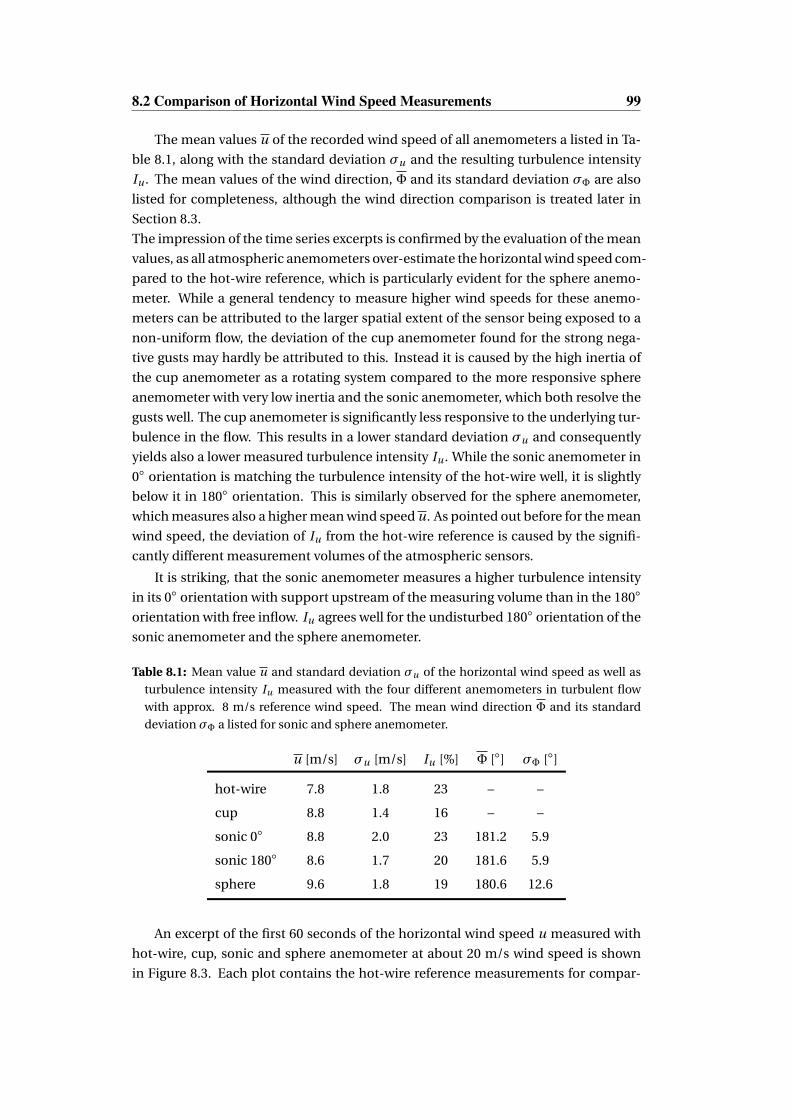
8.2 Comparison of Horizontal Wind Speed Measurements 99
The mean values u of the recorded wind speed of all anemometers a listed in Ta-
ble 8.1, along with the standard deviation σu and the resulting turbulence intensity
Iu . The mean values of the wind direction, Φ and its standard deviation σΦ are also
listed for completeness, although the wind direction comparison is treated later in
Section 8.3.
The impression of the time series excerpts is confirmed by the evaluation of the mean
values, as all atmospheric anemometers over-estimate the horizontal wind speed com-
pared to the hot-wire reference, which is particularly evident for the sphere anemo-
meter. While a general tendency to measure higher wind speeds for these anemo-
meters can be attributed to the larger spatial extent of the sensor being exposed to a
non-uniform flow, the deviation of the cup anemometer found for the strong nega-
tive gusts may hardly be attributed to this. Instead it is caused by the high inertia of
the cup anemometer as a rotating system compared to the more responsive sphere
anemometer with very low inertia and the sonic anemometer, which both resolve the
gusts well. The cup anemometer is significantly less responsive to the underlying tur-
bulence in the flow. This results in a lower standard deviation σu and consequently
yields also a lower measured turbulence intensity Iu . While the sonic anemometer in
0 orientation is matching the turbulence intensity of the hot-wire well, it is slightly
below it in 180 orientation. This is similarly observed for the sphere anemometer,
which measures also a higher mean wind speed u. As pointed out before for the mean
wind speed, the deviation of Iu from the hot-wire reference is caused by the signifi-
cantly different measurement volumes of the atmospheric sensors.
It is striking, that the sonic anemometer measures a higher turbulence intensity
in its 0 orientation with support upstream of the measuring volume than in the 180
orientation with free inflow. Iu agrees well for the undisturbed 180 orientation of the
sonic anemometer and the sphere anemometer.
Table 8.1: Mean value u and standard deviation σu of the horizontal wind speed as well as
turbulence intensity Iu measured with the four different anemometers in turbulent flow
with approx. 8 m/s reference wind speed. The mean wind direction Φ and its standard
deviation σΦ a listed for sonic and sphere anemometer.
u [m/s] σu [m/s] Iu [%] Φ [] σΦ []
hot-wire 7.8 1.8 23 – –
cup 8.8 1.4 16 – –
sonic 0 8.8 2.0 23 181.2 5.9
sonic 180 8.6 1.7 20 181.6 5.9
sphere 9.6 1.8 19 180.6 12.6
An excerpt of the first 60 seconds of the horizontal wind speed u measured with
hot-wire, cup, sonic and sphere anemometer at about 20 m/s wind speed is shown
in Figure 8.3. Each plot contains the hot-wire reference measurements for compar-

100 8. Turbulent Wind Measurements
ison with the respective atmospheric anemometer. Given the deviations apparent
in the lower wind speed measurements, the cup anemometer shows some surpris-
ingly good agreement with the hot-wire data for the first couple of seconds including
some strong gusts (Fig. 8.3, a). As time evolves past 20 seconds, however, the de-
viations from the reference measurements increase notably towards the end of the
60 second excerpt. One possible reason for this behavior of the cup anemometer may
be a spatially extended flow pattern, which hits a larger part of the cup anemome-
ter rotor and is not resolved by the smaller hot-wire probe. One could argue, that
a pattern like this would be present in the measurements of the other two sensors,
which are also affected by larger structures due to their extended measuring volumes.
Neither the sonic anemometer in any orientation (Fig. 8.3, b & c) nor the sphere ane-
mometer (Fig. 8.3, d) exhibit a similar wind speed drop with comparable deviations,
although the measuring volumes of the anemometers are comparable. Spatial varia-
tions in the flow cannot be ruled out entirely to cause the cup anemometer deviation,
since the part of the wind tunnel cross-section covered by each of the anemometers
is slightly different and each anemometer may be affected in a different way. How-
ever, a more likely explanation for the cup anemometer deviation is the inertia of the
rotor, which prevents the cup anemometer from reaching the "equilibrium state" for
the wind speed in time before a following gust hits the anemometer and thus causes
a lock-in on a lower wind speed.
The sonic anemometer measurements in both orientations match reasonably well
with the hot-wire reference, albeit some of the gusts are not fully covered by the ane-
mometer. Since the sonic anemometer has no inertia, the reason for these rather
small deviations are either the spatial extent of the flow structure or a bias due to
the internal signal processing and averaging procedure. This cannot be distinguished
from the conducted experiment.
Good consistency between the hot-wire reference measurement and the sphere ane-
mometer wind speed is found for this comparison in Figure 8.3 (d). The overall qual-
itative agreement seems to be significantly better than found for the reference ane-
mometer and cup anemometer, while a similar level of agreement with the sonic data
can be concluded. Some of the gusts are not entirely covered by the sphere anemo-
meter, but the results are matching the data obtained with sonic anemometer in this
regard.
The comparison of the basic statistical values, i.e. mean value u, standard devia-
tionσu and turbulence intensity Iu of the time series are given in Table 8.2 along with
the directional average Φ and its standard deviation σΦ for 20 m/s reference wind
speed.
The hot-wire reference measurement shows a mean value of 17.0 m/s at 20% turbu-
lence intensity. The sonic anemometer at 180 and the sphere anemometer mea-
sure slightly higher wind speeds, which has already been observed for the experiment
with lower reference wind speed. An underestimation of 0.5 m/s for the mean value
is found for the sonic anemometer in 0 orientation, which seems to be caused by
the support rod upstream of the measuring volume. The lowest mean wind speed

8.2 Comparison of Horizontal Wind Speed Measurements 101
05
101520253035
u [m
/s]
hot-wirecup
05
101520253035
u [m
/s]
hot-wiresonic
0 10 20 30 40 50 6005
101520253035
t [s]
u [m
/s]
hot-wiresphere
05
101520253035
u [m
/s]
hot-wiresonic 180°
(a)
(b)
(c)
(d)
Figure 8.3: Excerpts of the first 60 seconds of the down-sampled time series measured behind
the active grid at u ≈ 20 m/s mean velocity. The hot-wire reference (gray) is compared to
(a) cup anemometer, (b) sonic anemometer in 0 orientation and (c) in 180 orientation as
well as (d) sphere anemometer.
of u = 15.9 m/s is measured by the cup anemometer, which confirms the impres-
sion gained from the 60-second excerpt of the time series. At the same time the cup
anemometer measurement exhibits by far the lowest standard deviation σu and tur-
bulence intensity Iu due to its inertia and lack of temporal resolution. The sonic and
sphere anemometer agree well and match the hot-wire reference in both regards. It
is worth noting, that the over-estimation of the turbulence intensity, which is found

102 8. Turbulent Wind Measurements
Table 8.2: Mean value u and standard deviation σu of the horizontal wind speed as well as
turbulence intensity Iu measured with the four different anemometers in turbulent flow
with approx. 20 m/s reference wind speed. The mean wind direction Φ and its standard
deviation σΦ a listed for sonic and sphere anemometer.
u [m/s] σu [m/s] Iu [%] Φ [] σΦ []
hot-wire 17.0 3.4 20 – –
cup 15.9 2.58 16.2 – –
sonic 0 16.5 3.4 21 182.0 5.9
sonic 180 17.6 3.5 20 180.6 5.2
sphere 17.8 3.5 20 180.2 13.7
in the 8 m/s wind speed case for the 0 orientation of the sonic anemometer, is not
observed at 20 m/s inflow. Although this contradicts the findings of the 8 m/s case
at first sight, the internal calibration correction of the sonic anemometer can be as-
sumed to cause the different effects.
The comparison of the power spectra of the four anemometers for the 8 m/s and
20 m/s inflow, respectively, is based on the fully resolved 1 kHz data of all sensors and
the resulting spectra are depicted in Figure 8.4.
The hot-wire anemometer as a reference sensor features the highest temporal reso-
lution and hence it is expected that the power spectral density slope covers the entire
range of frequencies up to 500 Hz. One peak at 3 Hz can be clearly seen in the spec-
trum for u ≈ 8 m/s (Fig. 8.4, a), while two peaks at about 3 Hz and 4.5 Hz are present
in the flow for u ≈ 20 m/s (Fig. 8.4, b). The power spectra of the cup anemometer data
for both inflow velocities show a significant drop-off in power spectral density even
below frequencies of 1 Hz and show no response at all to frequencies above 2 Hz. This
is not surprising, since cup anemometers are known for their limited temporal reso-
lution in the order of 1 Hz. The sonic anemometer spectra follow those of the hot-wire
reference well up to approximately 10 Hz for the low wind speed and up to 5 Hz for the
higher wind speed. A reduced dynamic response can be seen beyond 10 Hz and a dip
at the maximal temporal resolution of 32 Hz is clearly visible. This first minimum of
the power spectral density is followed by recurring periodic dips. Structures like these
indicate a moving averaging, which has not been performed during post-processing,
but is probably part of the sonic anemometer’s internal signal processing.
Moreover, the power spectral densities for both reference wind speeds saturate at a
higher level in case of the 0 orientation of the sonic anemometer than for the 180
orientation. This can be presumed to stem from wake effects due to the upstream
support structure in the 0 orientation.
A well-matching power spectral density at the lower mean wind speed is observed
for the sphere anemometer, which resolves the peak at 3 Hz and is fairly close to the

8.3 Comparison of Wind Direction Measurements 103
(a) (b)
1 10 100 50010–4
10–3
10–2
10–1
100
101
f [Hz]
PSD
[m2 /
s]
hot-wiresonic 0°sonic 180°cupsphere
1 10 100 50010–4
10–3
10–2
10–1
100
101
f [Hz]
PSD
[m2 /
s]
hot-wiresonic 0°sonic 180°cupsphere
Figure 8.4: Power spectral density of the horizontal wind speed measurements with hot-wire
(gray), cup (blue), sphere anemometer (red) and sonic in 0 (dark green) and 180 orienta-
tion (light green). The spectra are shown for approx. (a) 8 m/s mean wind speed and (b)
20 m/s mean wind speed.
sonic and hot-wire signals up to 20 Hz. Unlike for the sonic anemometer, no drop-off
of the spectral density is found beyond 20 Hz, but two pronounced peaks at the two
natural frequencies of 45 Hz and 57 Hz are present as well as their harmonics. An
almost similar spectrum is found for the higher wind speed of approximately 20 m/s,
albeit the peaks at 3 Hz and 4.5 Hz are not resolved, but instead appear to be merged
to one broader peak.
8.3 Comparison of the Wind Direction Measurements
The wind direction measurements of the sphere anemometer can only be compared
to the sonic anemometer measurements, since neither hot-wire nor cup anemometer
are capable of directional measurements. Although reproducible inflow patterns are
generated with the active grid protocol, it is not designed to generate distinct inflow
angle variations, but rather to produce varying wind speeds due to changes in the
local wind tunnel blockage.
The measurements with the sonic anemometer performed in two different orien-
tations are analyzed in order to estimate the impact of the support structures on the
wind direction measurements. The 0 orientation with the support rod upstream the
measuring volume and the 180 orientation with the support exactly downstream the
measuring volume are selected for the experiment, since these cases are likely to ex-
hibit the largest differences. The wind direction measurements in the 0 case include
sudden jumps between values around 0 and values close to 360 due to the fluc-
tuations in the flow. Wind directions close to Φ = 360 are therefore wrapped to be
around 0. The measured wind directions for the sphere anemometer and the sonic
anemometer in 0 alignment are shifted by 180 in order to match the data range from
the sonic anemometer’s 180 orientation for easier comparison.

104 8. Turbulent Wind Measurements
Exemplary, the first 60 seconds of the wind direction measurements with sphere
anemometer and both sonic anemometer orientations are depicted in Figure 8.5 (a)
for u ≈ 8 m/s and in Figure 8.5 (c) for u ≈ 20 m/s inflow velocity. The measured in-
flow angle variations agree for both sonic anemometer orientations, and several pro-
nounced wind direction peaks from the turbulent inflow are resolved. The inflow an-
gle time series from the sphere anemometer covers these peaks as well, but the mag-
nitude of the peaks is larger. The mean wind directionsΦ and corresponding standard
deviations σΦ are listed in Tables 8.1 and 8.2 for the reference wind speeds of 8 m/s
and 20 m/s, respectively. The sphere anemometer means agree well with the sonic
anemometer measurements for both considered wind speeds. However, the overall
fluctuations around the mean wind direction are increased for the sphere anemome-
ter, which is also evident in the standard deviation of the 1-minute mean values of
the wind direction Φ, presented in Figures 8.5 (b) and (d). This is probably caused
by the mechanical oscillations due to vortex shedding from the sphere and is further
analyzed by means of the power spectra from both anemometers.
The power spectral density of both sonic anemometer measurements and of the
sphere anemometer measurement are compared in Figure 8.6. A higher power spec-
tral density is observed in the sphere anemometer direction measurements, which ex-
ceeds the sonic anemometer data by about a half order of magnitude in the frequency
range up to 10 Hz. This can be attributed to the mechanical excitation of the anemo-
meter. The two natural frequencies of the sphere anemometer at about 45 Hz and
57 Hz are present in the spectrum as well as their higher harmonics. A comparison of
the two sonic anemometer orientations reveals a higher power spectral density for the
case of the 0 orientation than the 180 case with undisturbed inflow to the measuring
volume. Both spectra feature the periodic dips beyond 32 Hz, which were also found
in the wind speed spectra presented in Section 8.2. A striking difference between the
spectra of both anemometer orientations is the appearance of sharp peaks coincid-
ing with these spectral minima in the 0 case. It is worth noting, that these spikes are
not present in the spectra of horizontal wind speeds for the 0 case (Fig. 8.4), which
is somewhat surprising and cannot be explained based on the measurements. Both
effects are likely caused by the internal data processing and calibration correction of
the sonic anemometer.
8.4 Summary & Discussion
A comparison of the 3rd generation sphere anemometer and two commercial anemo-
meters in wind tunnel experiments has been presented.
The response of cup, sonic and sphere anemometer was thereby assessed for two dif-
ferent reference wind speeds in reproducible turbulent inflow conditions generated
with an active grid.
For the higher reference wind speed of 20 m/s, the evaluated average wind speeds
of the sphere anemometer matched the sonic anemometer data and – considering

8.4 Summary & Discussion 105
(a) (b)
(c) (d)
0 10 20 30 40 50 6090
120
150
180
210
240
270
t [s]
Φ [°
]spheresonic 0°sonic 180°
0 5 10 15 20 25 30150
160
170
180
190
200
210
220
t [min]
Φ [°
]
spheresonic 0°sonic 180°
0 10 20 30 40 50 6090
120
150
180
210
240
270
t [s]
Φ [°
]
spheresonic 0°sonic 180°
0 5 10 15 20 25 30150
160
170
180
190
200
210
220
t [min]
Φ [°
]
spheresonic 0°sonic 180°
Figure 8.5: 60-seconds excerpt of the wind direction measured with sphere anemometer
(red), sonic anemometer in 0 orientation (dark green) and 180 orientation (light green)
for (a) u ≈ 8 m/s and (c) u ≈ 20 m/s mean wind speed. Figures (b) and (d) show the respec-
tive wind direction averages for 1-minute bins and the corresponding standard deviation.
(a) (b)
1 10 100 50010–2
10–1
100
101
102
f [Hz]
PSD
[°2 s]
sonic 0°sonic 180°sphere
1 10 100 50010–2
10–1
100
101
102
f [Hz]
PSD
[°2 s]
sonic 0°sonic 180°sphere
Figure 8.6: Power spectral density of the wind directions measured with sonic in 0 orienta-
tion (dark green) and 180 orientation (light green) as well as sphere anemometer (red) for
(a) u ≈ 8 m/s and (b) u ≈ 20 m/s mean velocity.

106 8. Turbulent Wind Measurements
the significantly different spatial resolutions – agree well with the hot-wire reference.
Larger deviations of the mean value were found for 8 m/s reference speed, but in this
case deviations occurred for all atmospheric anemometers. The turbulence intensi-
ties of sphere and sonic anemometer were similar in both wind speed cases, while
the cup anemometer under-estimated it. The capability of the sphere anemometer
to resolve gust events and fast fluctuations on a sub-second scale is evident from the
considered time series excerpts. The power spectral analysis of the horizontal wind
speeds showed fair agreement with the sonic anemometer, and it also confirmed the
known issues of cup anemometry, i.e the high inertia and limited temporal resolution.
A good agreement of the measured mean wind directions was observed between
the sphere anemometer and the sonic anemometer in both orientations. Neverthe-
less, the sphere anemometer directions feature a higher standard deviation, which is
likely caused by the mechanical oscillations of the sensor due to vortex shedding. This
is also reflected in the higher levels of the power spectral density of the wind direction
measurements with the sphere anemometer.
Both investigated orientations of the sonic anemometer exhibited almost similar
response behavior, although the upstream support in 0 orientation induced higher
standard deviations of the wind direction and a higher noise level in the power spec-
tra of wind speed and direction. However, these effects have not been observed to
the same extent for both wind speeds. Impacts of the internal calibration correction
scheme may be responsible for this, but one can only speculate about this without
access to the proprietary correction algorithm, which is not shared by the manufac-
turer.
The overall capability of the sphere anemometer to resolve the turbulent struc-
tures in the flow is evident from the experimental investigations. The assessment
proves its competitiveness to commercial sonic anemometers regarding wind speed
measurements and temporal resolution.

Chapter 9
The Sphere Anemometer Field Test
The characterization of the sphere anemometer in an outdoor installation is treated
in this chapter. The investigated anemometers – the 3rd generation sphere anemo-
meter along with a This First Class Advanced cup anemometer and a Gill WindMaster
Pro 3D sonic anemometer – are subject to a field test in order to investigate the ane-
mometer behavior under realistic operational conditions. They are installed on the
flat top roof of the WindLab building (W33) of University of Oldenburg’s physics de-
partment. Although the site is clearly not comparable to met-mast installations, it is
selected for the benefit of easy accessibility and little constraints regarding the data
acquisition system.
Experiments to prepare the installation of the sensors on a common boom are pre-
sented and the actual setup of the on-site installation is introduced. The results from
this field test are analyzed regarding horizontal wind speed and direction measure-
ments, to assess the performance of the sphere anemometer prototype.
9.1 Preparative Experiments
The spacing between the installed sphere, sonic and cup anemometer on one com-
mon boom is limited in the field test and thus preparative experiments are conducted
to assess possible cross-talking effects between the anemometers.
A wind tunnel experiment is set up using two of the anemometers in defined con-
stant flow while varying the distance between the anemometers. The main focus
of the work is on the evaluation of the sphere anemometer, so the cross-talking is
only investigated between sphere and sonic anemometer and between sphere and
cup anemometer. However, the cup anemometer is finally located next to the sonic
anemometer and therefore the sphere anemometer signal was not influenced by the
cup anemometer.
A measuring setup similar to the one of the calibration is used. The acoustic wind
tunnel is operated in open jet configuration and the anemometers are installed on the
turntable in its lower position. The experiments are performed at two different inflow

108 9. Sphere Anemometer Field Test
wind speeds of approximately 8.5 m/s and 19 m/s. Reference wind speeds uRef are
measured with the pairings of Pitot tubes in the settling chamber and static pressure
holes in the wind tunnel nozzle, which are connected to an analogue Betz micro-
manometer. The electric signals of the sphere anemometer and the respective com-
mercial sensor are recorded using a Data Translation DT9816-A AD-converter con-
nected to the measuring PC with LabVIEW software. Signals are acquired for 15 sec-
onds at fs = 1 kHz sampling frequency for each combination of sensor position and
reference wind speed.
As first pairing, sphere and sonic anemometer are placed next to each other on a alu-
minum x-profile in the center of the turntable, so the that the distance of both sen-
sors can be varied. The center of the measurement volumes for both sensors are on
the same height level in 35 cm downstream distance from the wind tunnel outlet. The
sonic anemometer is used in southward orientation (180) with its two support rods
located at ±60 from the flow direction as sketched in the top view of the setup in Fig-
ure 9.1 (a). The center of the sphere is at the same downstream distance of the wind
tunnel nozzle as the two support rods of the sonic anemometers. The arrangement of
the sensors is sketched in Figure 9.1. The variation of the signal is measured depend-
ing on the distance between the front support rod and the sphere edges. While the
sonic anemometer is fixed at its position, the sphere anemometer is initially located
in a distance of 56 cm (8 D) and is gradually moved closer in steps of 3.5 cm (0.5 D) up
to a distance of 2.5 cm.
u
d
sphere anemometer
sonic anemometer
d
sphere anemometer
sonic anemometer
d
u
(a) (b)
Figure 9.1: Sketched setup for the measurement of the anemometer cross-talk. The distance
d between the edge of the sphere anemometer and the support rod of the fixed sonic ane-
mometer was varied. (a) Top view of the setup with the center of the sphere anemometer
being in the same distance to the wind tunnel as the two front rods of the sonic anemome-
ter in southward orientation. (b) View from downstream. The measurement volume of the
sonic anemometer is on the same height as the center of the sphere.
Figure 9.2 shows the dependency of the measured wind speeds on the distance
d between the two sensors for the sphere and the sonic anemometer. The measured
wind speed is normalized with the reference wind speed from the pressure probes

9.1 Preparative Experiments 109
and the distance is given in absolute values d and normalized to the sphere diameter
D in both plots. As seen in Figure 9.2 (a), there is no noticeable influence of the sphere
anemometer on the sonic anemometer measurements for almost all distances. Only
a minimal speed-up can be observed for the lower reference wind speed at very short
distances below 5 cm. Similarly, no influence on the sphere anemometer measure-
ments is visible for spacings larger than 30 cm. A slight increase of the measured wind
speed is present for closer distances, which yields in a significant drop-off in the very
vicinity of the sonic anemometer support rod (d<5 cm). In general, the mutual influ-
ence of the sensors distance on the measurement is more pronounced for the lower
reference wind speeds. The widely unaffected sonic anemometer measurement can
0 10 20 30 40 50 60
0 1 2 3 4 5 6 7 8
0.90
0.95
1.00
1.05
1.10
d [cm]
u / u
Ref
d / D
uRef = 8.54 m/suRef = 19.1 m/s
0 10 20 30 40 50 60
0 1 2 3 4 5 6 7 8
0.90
0.95
1.00
1.05
1.10
d [cm]
u / u
Ref
d / D
uRef=9.01 m/suRef=16.12 m/s
(a) (b)
Figure 9.2: (a) Normalized sphere anemometer wind speed over distance to sonic anemome-
ter rod and (b) normalized sonic anemometer wind speed as function of the sphere ane-
mometer distance.
be explained by its sensor construction. Only the passive support structures are in
the immediate vicinity of the altered flow region around the sphere anemometer. The
measuring volume of the sonic anemometer is located further inboard and remains
therefore widely unaffected. On the contrary, the active sphere-tube-element of the
sphere anemometer is directly exposed to the altered flow in the vicinity of the sonic
support rod. Although the support is small, this effect is found in the wind speed
measurements for close distances as seen in Figure 9.2 (a). Consequently, the spacing
between the anemometers in the field experiment needs to be larger than 30 cm and
should likely be chosen to be even larger.
A similar treatment is performed for the cup anemometer and sphere anemome-
ter pairing. Although both anemometers are not installed directly next to each other
in the field experiment, the general behavior of the sphere anemometer in the vicin-
ity of the cup anemometer rotor might be of interest for future installations. Simi-
lar to the above mentioned experiment, the cup anemometer is moved towards the
sphere anemometer. The wind speed measurements with both sensors are normal-
ized with the reference wind speed for two different inflow velocities around 10 m/s
and around 20 m/s. As a consequence of the cup anemometer rotation, two different
situations are accounted for in the experiment. In the first case, the cup anemome-
ter is moved towards the sphere anemometer from the right, causing the closer cup to

110 9. Sphere Anemometer Field Test
move against the inflow, while in the second case, the anemometer is approaching the
sphere anemometer from the left, and thus the closer cup is moving downstream with
the wind. Both cases are treated for the lower wind speed of approximately 10 m/s
and the normalized wind speeds are plotted against the distance d and the normal-
ized distance d/D in Figure 9.3. The normalized cup anemometer wind speeds shown
in Figure 9.3 (a) collapse for large distances to the sphere anemometer, but the effect
of the anemometer becomes clear for smaller distances below approximately 20 cm.
Moreover, the two different cases can be easily distinguished. Approaching the sphere
anemometer from the right, the upstream movement of the cup in its vicinity leads
to a speed-up before the wind speed measurement collapses at distances below 5 cm.
On the contrary, the approach from the left with the closer cup moving downstream
with the wind, starts to impact the wind speed measurements earlier. A slight wind
speed decrease can already be noticed at distances of 20 cm between cup and sphere
anemometer and the effect is significantly stronger compared to the other case.
0 10 20 30 40 50 60
0 1 2 3 4 5 6 7 8
0.90
0.95
1.00
1.05
1.10
d [cm]
u / u
Ref
d / D
right, uRef=10.3 m/sleft, uRef=9.7 m/s
0 10 20 30 40 50 60
0 1 2 3 4 5 6 7 8
0.95
1.00
1.05
1.10
1.15
1.20
1.25
d [cm]
u / u
Ref
d / D
right, uRef=8.93 m/sleft, uRef=9.12 m/s
(a) (b)
Figure 9.3: (a) Normalized cup anemometer wind speed depending on distance to the sphere
anemometer. (b) Normalized sphere anemometer wind speed depending on distance to
cup anemometer.
Considering the sphere anemometer measurements (Fig. 9.3, b), an increasing
wind speed is found for the case of the cup approaching form the left for distances
closer than about 40 cm. The other case of the cup movement from the right causes
a speed-up of the sphere anemometer measurement already at around 52 cm, which
remains at a constant level up to 10 cm distance. Below 10 cm, the measured wind
speed increases drastically, exceeding the case of an approach from the left by about
0.1. As a consequence from these considerations, the sphere anemometer should not
be located closer than 56 cm from the cup anemometer, regardless of the side.
In order to estimate the acceptance angles of the anemometer depending on the
distance, the above experiment is conducted for three rotations of the anemometer
boom (x-profile) exposing it to flow directions of 30, 45 and 60. Only the com-
bination of sphere anemometer and cup anemometer is treated, since the previous
experiment for 0 inflow showed a stronger distance dependence between those two
anemometers than between sphere and sonic anemometer. It is thus considered a
"worst-case" scenario. Measurements are taken with the sphere anemometer posi-

9.1 Preparative Experiments 111
tioned left of the cup anemometer. The counter-clockwise rotations of 30, 45 and
60 with respect to the anemometer’s 0 position result in the sphere anemometer
moving further downstream and thus being subject to the wake of the upstream cup
anemometer.
Figure 9.4 shows the dependency of the normalized sphere anemometer wind speed
(Fig. 9.4,a) and the dependency of the normalized cup anemometer wind speed mea-
surement (Fig. 9.4,b) on the the distance for the three different inflow angles between
30 and 60. The sphere anemometer wind speed measurement shows no impact of
the presence of the upstream cup anemometer for all inflow angles down to a distance
of d = 30 cm between both anemometer edges. Smaller spacing causes a speed-up of
the signal at the largest inflow angleΦ= 60. The speed-up occurs at closer distances
for smaller inflow angles, which is expected as the projected distance
dproj = d · cos(Φ) (9.1)
between both anemometers is larger for smaller inflow anglesΦ. The cup anemome-
ter on the other hand shows only a relatively small effect of the presence of the down-
stream sphere anemometer. An impact can be seen only for spacings below 20 cm for
the largest inflow angleΦ= 60.
0 10 20 30 40 50 60
0 1 2 3 4 5 6 7 8
1.00
1.20
1.40
d [cm]
u / u
Ref
d / D
30°45°60°
0 10 20 30 40 50 60
0 1 2 3 4 5 6 7 8
0.90
0.95
1.00
1.05
1.10
d [cm]
u / u
Ref
d / D
30°45°60°
(a) (b)
Figure 9.4: Impact of the distance between sensors on the measured wind speed for 30, 45
and 60 inflow direction. Horizontal wind speed of (a) the sphere anemometer and (b) the
cup anemometer measurements.
As a consequence of the wind tunnel experiments on the impact of the distance
between the anemometers on the common anemometer boom for the field experi-
ment, it can be concluded, that a distance of 50 cm or more between the anemome-
ters is desirable in order to avoid cross-talking and wake effects in a wide range of
inflow angles. For this anemometer spacing, the experiments also confirm that an ac-
ceptance angle of ±60 can be chosen without the risk of wake effects impacting the
measurements with the three sensors.
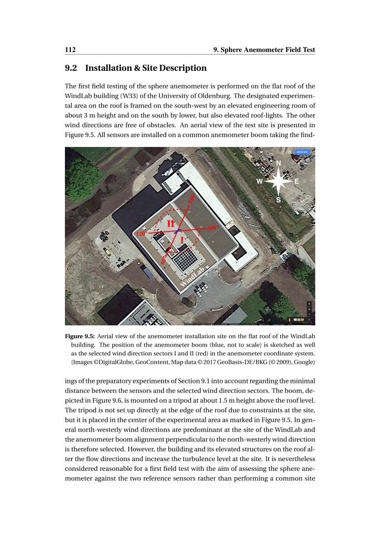
112 9. Sphere Anemometer Field Test
9.2 Installation & Site Description
The first field testing of the sphere anemometer is performed on the flat roof of the
WindLab building (W33) of the University of Oldenburg. The designated experimen-
tal area on the roof is framed on the south-west by an elevated engineering room of
about 3 m height and on the south by lower, but also elevated roof-lights. The other
wind directions are free of obstacles. An aerial view of the test site is presented in
Figure 9.5. All sensors are installed on a common anemometer boom taking the find-
I300°
60°
II120°
240°
N
EW
S
WindLab
Figure 9.5: Aerial view of the anemometer installation site on the flat roof of the WindLab
building. The position of the anemometer boom (blue, not to scale) is sketched as well
as the selected wind direction sectors I and II (red) in the anemometer coordinate system.
(Images ©DigitalGlobe, GeoContent, Map data © 2017 GeoBasis-DE/BKG (© 2009), Google)
ings of the preparatory experiments of Section 9.1 into account regarding the minimal
distance between the sensors and the selected wind direction sectors. The boom, de-
picted in Figure 9.6, is mounted on a tripod at about 1.5 m height above the roof level.
The tripod is not set up directly at the edge of the roof due to constraints at the site,
but it is placed in the center of the experimental area as marked in Figure 9.5. In gen-
eral north-westerly wind directions are predominant at the site of the WindLab and
the anemometer boom alignment perpendicular to the north-westerly wind direction
is therefore selected. However, the building and its elevated structures on the roof al-
ter the flow directions and increase the turbulence level at the site. It is nevertheless
considered reasonable for a first field test with the aim of assessing the sphere ane-
mometer against the two reference sensors rather than performing a common site

9.3 Data Acquisition & Processing 113
assessment. The benefit of this easily accessible site therefor outweighs possible is-
sues linked to altered wind conditions.
Figure 9.6: Photo of the anemometer boom with sphere, sonic and cup anemometer (left
to right) installed on the roof top of the WindLab building. View from 0 wind direction
(south-east).
9.3 Data Acquisition & Processing
The data acquisition (DAQ) at the test site is performed using a measurement PC with
two connected USB analog-digital converters. A combination of a Data Translations
DT9816-A AD converter and a National Instruments NI-6211 AD converter is set up in
order to be able to acquire the four sphere anemometer signals and the five signals of
the reference sensors (4× sonic, 1× cup). Both AD converters provide 16 Bits resolu-
tion for an input range of ±5 V. Synchronization of the sphere anemometer channels
is crucial, since the four signals are used to calculate the instantaneous components
of the laser displacement (x, y). The DT9816-A allows for the simultaneous sampling
of the input signals and is thus chosen for the sphere anemometer, while the NI-6211
acquires the channels in multiplexed operation. It is used for the acquisition of the
four sonic anemometer signals, i.e. the horizontal wind speed magnitude, horizon-
tal wind direction, vertical wind speed and anemometer status signal, and the cup
anemometer signal. A minimal time lag between the reference signals is inevitably
caused by the multiplexing in this setup, but it is not considered crucial due to the
low temporal resolution of the anemometers and the independence of the acquired
signals.
The data acquisition with the two AD converters is controlled by a LabVIEW program.
Signals are sampled at fs = 200 Hz with both devices and the buffered data is stored
in two minute intervals. However, the use of two separate DAQ devices results in a
timing disparity beyond the multiplexing as each AD converter uses its internal sam-
ple clock. The synchronization of the signals is thus addressed in the first step of post

114 9. Sphere Anemometer Field Test
processing by shifting the calibrated signals of the sphere anemometer against those
of the reference sensors based on the maximum of the cross-correlation function as
described in Appendix D.
The full data set comprises measurements of all anemometer channels during five
consecutive days from 23.–27. December 2016. Data corresponding to the two pre-
ferred wind direction sectors of 0±60 (I) and 180±60 (II) is extracted from the full
data set. The wind direction Φ is selected based on the sonic anemometer measure-
ments, since it is the designated reference sensor. Averaged properties of the entire
measuring period are summarized in Table 9.1 for the full data and the selected data
sets I and II. At 58% data share, the majority of the recorded data is found for wind
directions in the sector II, which is expected as it is centered around the designated
main wind direction at the WindLab site. The rather free inflow conditions for this
sector are reflected in higher horizontal mean wind speeds u = 3.4 m/s compared to
very low speeds or u = 1.9 m/s for the obstructed wind sector I, which has a data share
of only 18% during the measured five days. Both sectors feature a slight downward
vertical wind component w =−0.4 m/s.
Table 9.1: Properties of full data set and selected wind direction sectors from five days of field
testing. The data share of each selected sector is given as well as the mean horizontal and
vertical wind speeds, u and w , and the direction Φ measured with the sonic anemometer
reference.
wind sectorI II
0 – 360 0± 60 180± 60
data share [%] 100 18 58
u [m/s] 3.2 1.9 3.4
w [m/s] -0.5 -0.4 -0.4
Φ [] 6 22 156
As a result of the site conditions, it is desirable for the anemometer evaluation to
limit the further data analysis to the unobstructed wind direction sector II of 180± 60
with respect to the sonic and sphere anemometer orientation. However, the horizon-
tal mean wind speed for this sector (Tab. 9.1) is very low regarding typical wind energy
applications and for the sphere anemometer measuring range in particular. A subset
of the data from sector II is thus chosen for the comparison of sonic, sphere and cup
anemometer in the field test. The subset contains three hours of measured data from
26. December 2016, 12:30 h to 15:30 h, which features an 83% data share in wind di-
rection sector II. At a mean wind speed of about 7 m/s, this subset is more suitable
for a comparison of the three anemometers than the entire data set of sector II. For
better visibility of trends, the selected data set has been down-sampled to 20 Hz for
the wind speed and 1 Hz for the wind direction measurements. The spectral analyses
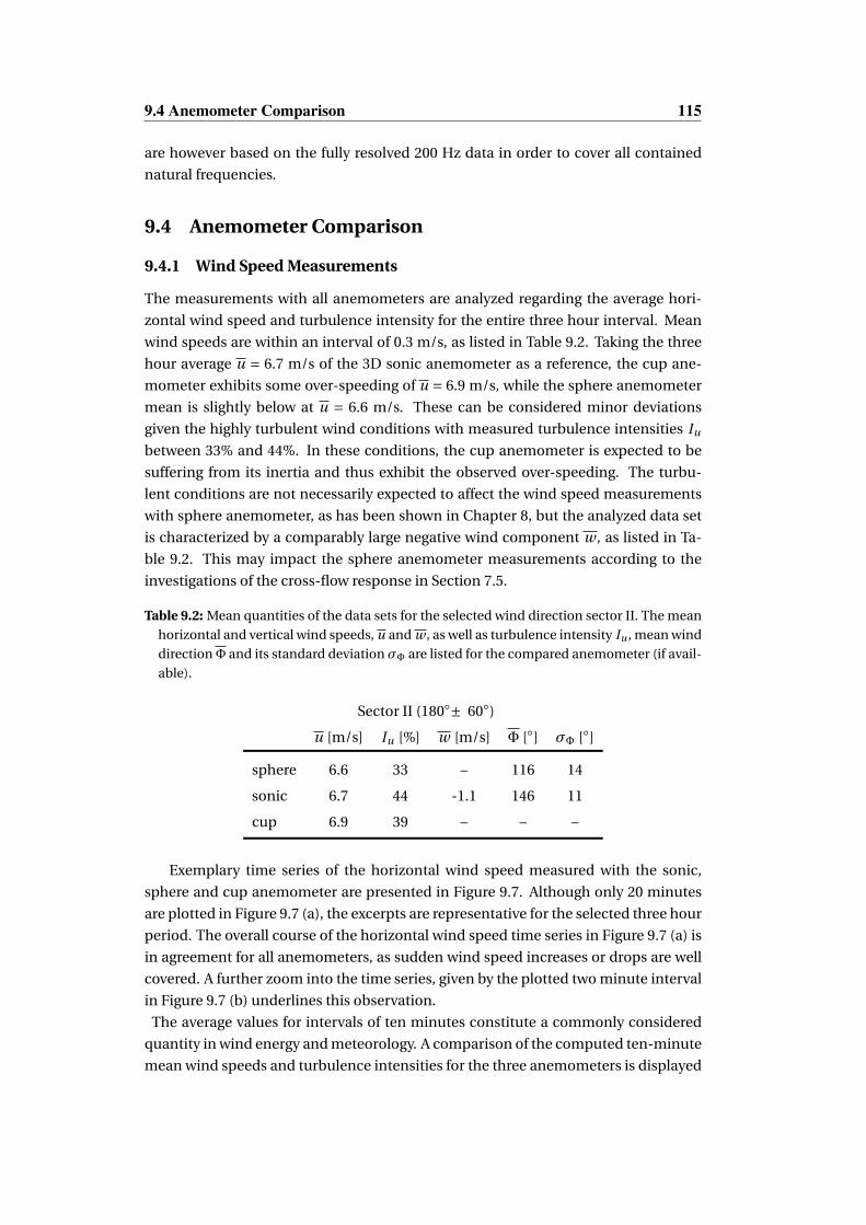
9.4 Anemometer Comparison 115
are however based on the fully resolved 200 Hz data in order to cover all contained
natural frequencies.
9.4 Anemometer Comparison
9.4.1 Wind Speed Measurements
The measurements with all anemometers are analyzed regarding the average hori-
zontal wind speed and turbulence intensity for the entire three hour interval. Mean
wind speeds are within an interval of 0.3 m/s, as listed in Table 9.2. Taking the three
hour average u = 6.7 m/s of the 3D sonic anemometer as a reference, the cup ane-
mometer exhibits some over-speeding of u = 6.9 m/s, while the sphere anemometer
mean is slightly below at u = 6.6 m/s. These can be considered minor deviations
given the highly turbulent wind conditions with measured turbulence intensities Iu
between 33% and 44%. In these conditions, the cup anemometer is expected to be
suffering from its inertia and thus exhibit the observed over-speeding. The turbu-
lent conditions are not necessarily expected to affect the wind speed measurements
with sphere anemometer, as has been shown in Chapter 8, but the analyzed data set
is characterized by a comparably large negative wind component w , as listed in Ta-
ble 9.2. This may impact the sphere anemometer measurements according to the
investigations of the cross-flow response in Section 7.5.
Table 9.2: Mean quantities of the data sets for the selected wind direction sector II. The mean
horizontal and vertical wind speeds, u and w , as well as turbulence intensity Iu , mean wind
directionΦ and its standard deviationσΦ are listed for the compared anemometer (if avail-
able).
Sector II (180± 60)
u [m/s] Iu [%] w [m/s] Φ [] σΦ []
sphere 6.6 33 – 116 14
sonic 6.7 44 -1.1 146 11
cup 6.9 39 – – –
Exemplary time series of the horizontal wind speed measured with the sonic,
sphere and cup anemometer are presented in Figure 9.7. Although only 20 minutes
are plotted in Figure 9.7 (a), the excerpts are representative for the selected three hour
period. The overall course of the horizontal wind speed time series in Figure 9.7 (a) is
in agreement for all anemometers, as sudden wind speed increases or drops are well
covered. A further zoom into the time series, given by the plotted two minute interval
in Figure 9.7 (b) underlines this observation.
The average values for intervals of ten minutes constitute a commonly considered
quantity in wind energy and meteorology. A comparison of the computed ten-minute
mean wind speeds and turbulence intensities for the three anemometers is displayed

116 9. Sphere Anemometer Field Test
751 752 7530
5
10
15
20
25
t [min]
u [m
/s]
soniccupsphere
(a) (b)
Figure 9.7: Measured time series with sonic (green), cup (blue) and sphere anemometer (red)
from wind directions sector of 180±60. (a) 20-minutes excerpt and (b) 2-minute excerpt
of the horizontal wind speed measurements.
770 800 830 860 89002468
1012
t [min]
u [m
/s]
soniccupsphere
770 800 830 860 8900.0
0.1
0.2
0.3
0.4
0.5
t [min]
I u
soniccupsphere
(a) (b)
Figure 9.8: 10-minute averages of (a) horizontal wind speed u and (b) corresponding turbu-
lence intensity Iu for sonic (green), cup (blue) and sphere anemometer (red) from wind
directions sector of 180 ± 60. The error bars indicate the standard deviation σu on the
10-minute scale.
in Figure 9.8. The plotted wind speeds agree well for most 10-minute intervals. De-
viations with respect to the commercial anemometers are however observed in the
sphere anemometer data, showing a reduced 10-minute wind speed between 770 and
800 minutes, while it is increased between 870 and 880 minutes. Moreover, the stan-
dard deviation σu is reduced for the sphere anemometer and cup anemometer com-
pared to the sonic anemometer, as visible in the plotted as error bars (Fig. 9.8, a). This
also affects the turbulence intensity Iu in Figure 9.8 (b), with the lowest values mea-
sured by the sphere anemometer and the highest values by the sonic anemometer.
In the comparison of the wind time series, the sphere anemometer and the cup
anemometer appear to exhibit less dynamics than the sonic anemometer. This is re-
flected in a smaller range of the measured velocities and lower standard deviations. A
closer look at the dynamics is gained by means of the wind speed histograms and the
power spectra for the three anemometer.
The histogram of the 50 Hz wind speed measurements with all anemometers is cal-

9.4 Anemometer Comparison 117
0 2 4 6 8 10 12 14 16 18 200
1
2
3
4
u [m/s]
N /
104
soniccupsphere
0 1 10 10010–4
10–3
10–2
10–1
100
101
f [Hz]
PSD
[m2 /
s]
soniccupsphere
(a) (b)
Figure 9.9: (a) Histogram of horizontal wind speeds for the three hour interval and (b) power
spectral density of the horizontal wind speed measurements for sonic (green), cup (blue)
and sphere anemometer (red) in wind sector II (180±60).
culated for bin sizes of 1 m/s. The number of counts N per wind speed bin is plotted
against the wind speed u in Figure 9.9 (a). The cup anemometer histogram agrees
with the sonic anemometer histogram for the higher wind speeds. Lower wind speeds
are less frequently measured, while values close to the mean are overly present. The
sphere anemometer histogram covers an even smaller range of measured wind speeds
leading to a narrower histogram with reduced counts at the higher and lower end of
the wind speed bins. This is compensated for by an over-estimation for the wind
speed bin around the mean value. The reduced dynamic range, i.e. the narrowed his-
togram, is expected for cup anemometry due to inertial effects and spatial averaging.
It is however surprising that the range of the sphere anemometer data is lower than
that of the sonic anemometer – and even the cup anemometer – measurements.
A better estimate of the dynamics can be obtained from the plot of the power
spectral density of the 200 Hz wind speed data given in Figure 9.9 (b). The sonic ane-
mometer spectrum is characterized by an almost linear decay region for frequencies
lower than f ≈ 30 Hz, before effects of the internal averaging procedures can be iden-
tified at f = 32 Hz and beyond. This is consistent with the observations from the wind
tunnel tests in Section 8.2.
The cup anemometer spectrum is on the same level with the sonic anemometer only
for the very low frequencies at f ≈ 0.1 Hz, but it drops off significantly for higher fre-
quencies and reaches the noise level for f ≤ 3 Hz. It can thus be concluded, that
the cup anemometer dynamics is reduced due to its inertial properties, which lim-
its its temporal resolution and causes the spectral drop-off. This effect has already
been identified in the spectral comparison of the wind tunnel measurements treated
in Section 8.2 and is therefore independent of the field operation.
The spectrum of the sphere anemometer features lower power spectral densities
compared to the sonic reference across all frequencies up to f ≈ 10 Hz, although the
decay region is also almost linear. Pronounced peaks are present for higher frequen-
cies due to vortex shedding and natural frequencies. The reduced magnitude of the
sphere anemometer in this frequency range has not been observed in the wind tunnel
118 9. Sphere Anemometer Field Test
measurements presented in Section8.2, when sonic and sphere anemometer spectra
agreed quite well up to about 20 Hz. The reason of the different spectral response is
thus likely related to the conditions during the field test.
Two possible effects can be plausibly assumed to affect the sphere anemometer
performance in the field measurements:
First, the observed deviations can be caused by an altered sphere anemometer cal-
ibration function between the wind tunnel calibration and the field installation. An
increased air density due to lower ambient temperatures results in an increased slope
m of the anemometer’s calibration function, and higher wind speed readings for sim-
ilar laser deflections are consequently calculated for the field measurements. The
assumption of increased the air density due to temperature differences between the
wind tunnel measurements and field operation is very likely to hold in case of these
exemplary measurements, since the calibration was performed at room temperature
of about 20C, while the ambient temperature during the selected measuring period
was approximately 7C. The deviations of the air density between both cases are thus
in the order of 5%. However, the impact of the changed air density affects lower
wind speeds stronger than higher speed due to the non-linearity of the calibration,
which can explain the significant disparity between sonic and sphere anemometer
histograms at the low wind speeds, while it is marginal for the high wind speed bins.
A second contributing effect to the deviations between sonic and sphere anemo-
meter measurements is related to its cross-flow response, assessed in Section 7.5. In-
formation of the vertical wind component are therefore incorporated in the evalua-
tion of the sphere anemometer field test.
The vertical wind component w at the site is analyzed from the sonic anemometer
measurements, since it is the only sensor to resolve this wind component. A 20-
minute excerpt of the 50 Hz time series is shown in Figure 9.10 (a). The vertical wind
exhibits a net downward speed w = −1.1 m/s averaged over the three hour interval
(Tab 9.2) and based on the average horizontal wind speed u, the angle of the net
down-wind is γ≈ 9. The 10-minute averages of the vertical wind component w and
the horizontal wind speed u from sonic and sphere anemometer are plotted in Fig-
ure 9.10 (b). The underestimation of the horizontal wind speed by the sphere anemo-
meter occurs for intervals with strong negative vertical wind component, while the
small overestimation is related to the smallest vertical down-wind. This is explained
by the findings of Section 7.5, since the vertical wind component causes the sphere
anemometer to underestimate of the horizontal wind speed and thus deviate from the
sonic anemometer. Consequently, the downward wind component also contributes
to the deviation of the power spectral densities of sphere and sonic anemometers.
The altered calibration function due to the changed air density and the presence
of a pronounced down-wind component are two concurring effects, which both af-
fect the wind speed measurements with the sphere anemometer. While the higher air
density yields an overestimation of the measured wind speed, a reduced wind speed
reading is caused by the down-wind component. The question which of these effects
is dominating depends on the boundary conditions,in particular on ambient temper-

9.4 Anemometer Comparison 119
750 755 760 765 770–8–6–4–2
02468
t [min]
w [m
/s]
sonic
770 800 830 860 8900
2
4
6
8
10
–2.0
–1.5
–1.0
–0.5
0.0
t [min]
u [m
/s]
u sonicu spherew sonic
w [m
/s]
(a) (b)
Figure 9.10: (a) Measured time series of the vertical wind component w with the sonic ane-
mometer. (b) 10-minute means of the horizontal wind speed u measured with sonic (green
solid) and sphere anemometer (red) as well as vertical wind speed w (green dashed)
ature, vertical and horizontal wind speed, due to the non-linearity of the calibration
function.
9.4.2 Wind Direction Measurements
Wind direction measurements from the field test are only available for sonic and
sphere anemometer, because the cup anemometer is insensitive to wind direction
changes. Both time series are compared for the entire three hour period in terms of
the overall mean wind direction and one-second averages. As listed in Table 9.2 for
the entire data set, the mean sphere anemometer wind direction Φ = 116 deviates
from the sonic wind direction Φ = 146 by 30. Figure 9.11 (a) shows a 20-minute
excerpt of both direction measurements on a one-second scale, which is represen-
tative for the entire three hours of selected data. The systematic difference is clearly
visible in the plotted time series. Two pronounced peaks are present in the this ex-
cerpt of the sphere anemometer data, while one peak in the sonic data is apparent.
These peaks are not occurring simultaneously, which indicates different prevailing
inflow angles even though both anemometers are not far apart. However, the overall
difference between the mean values of both direction measurements can hardly be
caused by these peaks. Figure 9.11 (b) shows the histogram of wind direction fluc-
tuations, Φ′ =Φ−Φ, measured with sonic and sphere anemometer during the three
hours. Both histograms are covering similar angle fluctuations, but the sphere ane-
mometer histogram features slightly less counts around the mean value while posi-
tive angle fluctuations are occurring more frequent. These differences between the
sonic and sphere anemometer direction fluctuations Φ′ appear to be minor. Never-
theless, the higher standard deviationσΦ = 14 for the sphere anemometer compared
to the sonic anemometer (σΦ = 11) indicates the impact of mechanical oscillations
on the sphere anemometer direction measurements. A similar result was obtained
for the comparison of wind directions measurements in the wind tunnel experiments
of Section 8.3. The mean wind directions of both anemometers were matching well,
in the wind tunnel experiments, though. The larger deviation of 30 found in the field
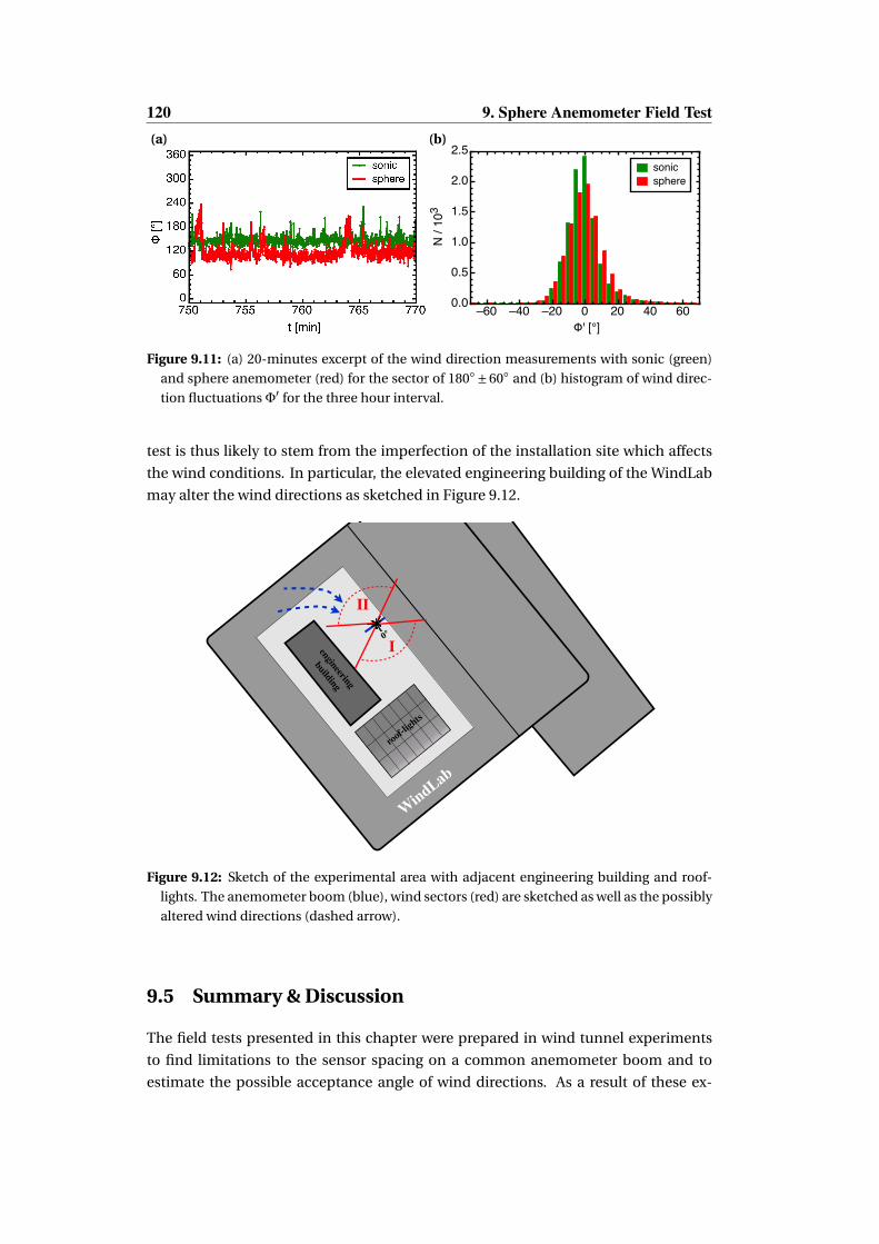
120 9. Sphere Anemometer Field Test
–60 –40 –20 0 20 40 600.0
0.5
1.0
1.5
2.0
2.5
Φ' [°]
N /
103
sonicsphere
(a) (b)
Figure 9.11: (a) 20-minutes excerpt of the wind direction measurements with sonic (green)
and sphere anemometer (red) for the sector of 180±60 and (b) histogram of wind direc-
tion fluctuationsΦ′ for the three hour interval.
test is thus likely to stem from the imperfection of the installation site which affects
the wind conditions. In particular, the elevated engineering building of the WindLab
may alter the wind directions as sketched in Figure 9.12.
WindLab
0°
engineering
building
roof-lights
I
II
Figure 9.12: Sketch of the experimental area with adjacent engineering building and roof-
lights. The anemometer boom (blue), wind sectors (red) are sketched as well as the possibly
altered wind directions (dashed arrow).
9.5 Summary & Discussion
The field tests presented in this chapter were prepared in wind tunnel experiments
to find limitations to the sensor spacing on a common anemometer boom and to
estimate the possible acceptance angle of wind directions. As a result of these ex-

9.5 Summary & Discussion 121
periments a minimal distance of about 30 cm between the cup anemometer and any
other sensor was found to be necessary, but an even larger spacing was chosen for
the final construction of the boom as a safety margin. Regarding the direction, an ac-
ceptance angle of ±60 was found to be reasonable and it was thus used for the data
selection in the field measurements.
The flat roof of the WindLab building of the University of Oldenburg was selected
as site for the anemometer field test, although it cannot offer perfect conditions for
the anemometer comparison. Installed on the common boom, the anemometers
were placed on a tripod in the center of the experimental area on the roof. Data was
acquired for a duration of five days during December 2016. The calibrated data of two
rather free wind direction sectors was compared regarding their mean velocities and
a significant difference in the data share of each wind direction sector was found. A
more detailed comparison of the sphere anemometer and the two reference sensors
was based on a three-hour data set with a high data share in the free wind sector (II),
which coincides roughly with the expected main wind direction at the site.
The analyzed mean values of the horizontal wind speeds agree within 0.3 m/s for
all three anemometer, while the measured turbulence intensities at about 40% were
quite high. The time series of all anemometers resolved similar wind speed trends
and covered the occurring gusts. However, histograms and power spectra of the hor-
izontal wind speeds revealed a reduced dynamical range of the sphere anemometer
data, which can likely be attributed to an altered calibration due to temperature and
air density changes. Measurements indicate an additional impact of the negative ver-
tical wind component in the highly turbulent environment. Although the occurring
underestimation of the mean wind speed in case of the strong down-winds can be
explained with the sphere anemometer’s response behavior to cross-flows, further
investigations are needed on this topic (cf. Sec. 7.5).
Wind direction measurements with the sonic and sphere anemometer exhibited
an offset of about 30, which cannot be explained by anemometer properties. It can
be assumed, that the imperfections of the installation site with its elevated building
structures caused these deviations. The fluctuations of the wind directions matched
very well for the sphere and sonic anemometer, albeit the histogram of wind direc-
tion fluctuation was slightly wider spread for the sphere anemometer measurements.
This is also reflected in the about 3 higher standard deviation found for the sphere
anemometer.
The overall performance of the sphere anemometer in the field test is quite promis-
ing, although some subjects for future research have been identified. These include
the impact of the air density and vertical wind components on the wind speed mea-
surements, as well as the effect of mechanical vibrations of the wind direction mea-
surement.
122 9. Sphere Anemometer Field Test

Chapter 10
Conclusions
This chapter summarizes the presented work on the development of the sphere ane-
mometer at its different stages and conclusions are drawn from the characterization
of the latest anemometer. Recommendations for further improvements and required
investigations are also given.
10.1 Summary
The presented work aimed at the optimization of a drag based sphere anemometer
for wind speed and direction measurements. It is intended to operate in the complex
conditions of atmospheric wind flows, which is always present in meteorology and
wind energy applications.
Its principle of operation exploits the deflection of the anemometer’s flexible sup-
port tube due to the drag force exerted on the tube and an attached sphere. The highly
resolving light pointer principle introduced in Chapter 3 translates the sphere deflec-
tion in a laser spot displacement on a two-dimensional position sensitive detector,
which can be subsequently linked to the wind speed and direction via calibration.
A square-root function for the relation between wind speed and laser displacement
is expected in case of a constant drag coefficient of a smooth sphere and tube. The
impact of the surface pattern on the drag of the sphere has been explained and a de-
viation from the square-root function is expected for patterned spheres. Although the
constant drag coefficient can only be considered an approximation, it may by design
be assumed for a wide range of Reynolds numbers in the subcritical regime for the
smooth and dimpled spheres used on the sphere anemometer.
The first truly two-dimensional sensor constructed by Heißelmann in 2008 served
as a foundation to built the further optimizations on. While some severe problems of
the earlier anemometers, like the creeping and hysteresis of the acrylic glass tube, had
already be addressed in this sensor, more critical issues of this anemometer design re-
mained to be solved. In particular the pronounced scattering and anisotropy of the
two-dimensional calibration spoiled this anemometer’s functionality.

124 10. Conclusions
The first stage of the sphere anemometer development, the 1st generation sphere
anemometer, was set up addressing these issues. The polystyrene sphere used by
Heißelmann [2008] was replaced by a set of ABS spheres with similar diameter but
varying surface patterns. A regular dimple alignment was tested at first, and while the
overall 1D and 2D calibrations showed improved isotropy, still some angular depen-
dency of the deflection remained. Since neither the regularly dimpled sphere pattern
nor the tube structure could be ruled out in this setup, a further modification was
made to the setup. The addition of a threaded sphere support at the tip of the GFP
tube allowed for the investigation of different spheres on the very same tube. Two ir-
regularly patterned spheres and a smooth sphere of similar size were tested in order
to discriminate between effects of the sphere pattern and the tube properties on the
anemometer’s calibrations. While no significant difference was found between the
two irregularly dimpled patterns in the one-dimensional calibration, the comparison
of both irregularly dimpled spheres with the smooth sphere confirmed the drag re-
duction due to the surface pattern. It was reflected in a steeper calibration function,
which deviated from the theoretical square-root shape. This was expected from the
design considerations of the sphere anemometer and had already been accounted for
by using a more general power-law function instead for the calibration.
In the analysis of the two-dimensional calibration, the coarse irregularly dimpled
sphere and the smooth sphere were attached to the same GFP tube. The overall an-
isotropy of the 2D calibration was reduced for both spheres compared to the first ap-
proach with a regularly dimpled sphere. Nevertheless, the comparison revealed the
problematic angular dependence of the anemometer deflection caused by the inter-
nal fiber alignment within the epoxy matrix. These structural anisotropies resulted in
sudden jumps of the tube deflection in a approximately 60 steps.
In order to overcome the angular anisotropy of the tube deflection caused by the
fiber structure, the glass-fiber material was abandoned and a stainless steel tube was
chosen instead to support the sphere in the 2nd generation sphere anemometer. This
consequently implied changes regarding the tube length and subsequently also the
height of the anemometer housing. Both changes, the reduction of the tube length
and the increased laser path in the housing, helped to improve the anemometer’s nat-
ural frequency from 30 Hz to 36 Hz while maintaining the desired measuring range.
The characterization of the 1D and 2D calibrations for the 2nd generation anemo-
meter gave evidence of a greatly improved isotropy. The optimizations consequently
yielded significantly reduced angular deviations of the laser deflection below 3% off
of a perfectly circular shape for the wind speed range above 5 m/s.
As a consequence of the promising results obtained with the 2nd anemometer
generation, the materials and geometry of this sensor remained unchanged for the
3rd generation. Improvements were focused towards the installation in the complex
conditions associated with field experiments. The housing was therefor modified in
order to reduce the wind load and in particular to provide water-tightness with the
addition of rubber sealings between sphere, tube and housing. Moreover, the electric
circuit was completely remodeled in order to comply with the industrial standards

10.1 Summary 125
of 4-20 mA current signals and the power supply for the laser diode was at the same
time integrated in the signal amplification circuit. Investigations of the 2D calibration
function revealed an increase of the angular dependence of the deflections signals,
which was caused by the changes to the sensor electronics due to different amplifi-
cation factors for the individual channels. However, the angle-dependence did not
manifest in sudden jumps of the calibration as caused by the previously used tube
materials. Instead, it resulted in a smooth, slightly elliptic shape of the 2D calibration.
The eccentricity of the elliptic shape is depending on the difference between the in-
dividual amplification factors, as was theoretically confirmed.
The 3rd generation sphere anemometer has been thoroughly assessed beyond the
characteristics of the 1D and 2D calibration functions, as the precision and accuracy
of the wind speed readings were investigated in wind tunnel experiments. Measur-
ing uncertainties of only 0.05 m/s were found in the relevant wind speed range above
3 m/s. This uncertainty is absolutely comparable to values for commercial anemo-
meters, as is the sphere anemometer’s only marginal deviation of 2% from the "true"
reference wind speed. The temporal resolution, limited by the anemometer’s natural
frequency, was pushed to 45 Hz for the latest development stage of the sphere anemo-
meter, even exceeding the commercial sonic anemometer used for comparisons. Tilt
experiments in the wind tunnel were carried out to identify the impact of cross-flow
components, i.e. up- and down-winds, on the anemometer readings. It features an
asymmetric response characteristic with a cosine projection for the upwind case and
a strong under-estimation for the down-wind case. An attempt to explain the asym-
metry has been made by considering the effect of the support tube on the flow separa-
tion angles. The support may yield an increased wake region by triggering premature
separation on the lower hemisphere. The consequence is an altered drag force for the
upwind and down-wind scenario, which plausibly explains the observed cross-flow
response. However, the experimental investigation of this hypothesis was not within
the scope of this work and constitutes a basis for further investigations.
The latest stage of the sphere anemometer development has been applied to tur-
bulent wind flows in two fundamentally different scenarios: A comparison of the
sphere anemometer against the commercial cup and sonic anemometers was there-
fore conducted in wind tunnel experiments and in a multi-day field test. The wind
tunnel experiment was performed using reproducible turbulent inflow generated for
two different wind speeds with an active grid. A common and repeated motion pat-
tern of the flaps was employed and the turbulent flow was measured with the sphere
anemometer, a Thies First Class Advanced cup anemometer, a Gill WindMaster Pro
3D sonic anemometer and a highly resolving hot-wire anemometer as a reference.
The wind speed measurements with the sphere anemometer were in good agreement
with the sonic anemometer regarding mean wind speed and turbulence intensity. Mi-
nor deviations between these sensors and the hot-wire reference could be explained
with the significantly different sensor dimensions. The cup anemometer suffered
from its low temporal resolution, which resulted in a limited coverage of the large
wind speed fluctuations and consequently lead to lower mean values and an under-

126 10. Conclusions
estimated turbulence intensity. Both, the agreement of sphere and sonic anemome-
ter as well as the limitations of the cup anemometer were also present in the analysis
of the power spectral density. Besides the horizontal wind speeds, the wind direc-
tion measurements with sonic and sphere anemometer were compared. The sonic
anemometer was used in both distinct orientations – with an upstream support rod
(north alignment, 0) and with free inflow (south alignment, 180). Due to its ro-
tational symmetry only one orientation of the sphere anemometer was considered.
Wind direction measurements agreed quite well for both anemometers. The sphere
anemometer exhibits larger fluctuations, though, which could be seen in the standard
deviations of the averaged wind directions as well as in the power spectral densities
of the direction data. A likely cause of these larger fluctuations is the lateral vibration
of the sphere due to vortex shedding.
In the field experiment, the sphere, sonic and cup anemometer were installed on
a common anemometer boom on the flat roof of the University of Oldenburg’s Wind-
Lab building for several days of continuous wind measurements.
As preparation for the site installation, experiments were performed to investigate
necessary spacing between the anemometers and the acceptance angles in order to
obtain reliable measurements. The anemometer boom with the three sensors was
than placed on a tripod in the center of the experimental area of the flat roof. Two
wind direction sectors have been selected based on the previously analyzed accep-
tance angles. While one of the wind sectors was spoiled by the elevated structures of
the WindLab building, the other one featured rather free inflow from the north-west,
which is the predominant wind direction at this site. A three hour interval with a high
data share in the free sector was thus selected for the assessment of the anemometers’
performance. While all three sensors agreed well in terms of the three-hour horizon-
tal mean wind speed, deviations were found for the turbulence intensity. However,
turbulence intensities in the range of 40% were present on-site and the contributing
short term fluctuations may thus be different depending on the very anemometer lo-
cation.
In general, a reduced dynamic range of the horizontal wind speed measured with the
sphere anemometer was found compared to the sonic anemometer. A possible expla-
nation is the reduced ambient temperature compared to the calibration in the wind
tunnel, which alters the air density by about 5% and would cause an over-estimation
of the wind speed. An additional impact of the vertical wind was suspected, since
a strong down-wind component was observed. Consideration of the cross-flow re-
sponse, as quantified during the anemometer assessment in the wind tunnel, bears a
reduction of the measured wind speed due to the down-wind conditions. Both effects
can be suspected to play a role in the field experiment, but their concurring nature
makes it impossible to discriminate them in this field experiment.
Large deviations of 30 were observed for the wind direction measurements with sphere
and sonic anemometer. These deviations were not expected, since the wind direction
measurements with both anemometers agreed well in the wind tunnel experiments.
The consideration of the wind direction fluctuations revealed only minor differences

10.2 Outlook and Recommendations 127
between both anemometers, as the sphere anemometer exhibited a marginally higher
standard deviation. This effect, presumably caused by lateral oscillations due to vor-
tex shedding, could hardly explain the large offset. It was thus concluded to be caused
by the site conditions, which feature complex wind flows around the elevated build-
ing structures.
The performance of the latest development stage of the sphere anemometer is
quite satisfying, despite the remaining challenges discovered in the field test.
The reliability of its calibration has been greatly improved by optimizations of the
sphere properties and the choice of the tube material. The achieved degree of iso-
tropy for the 2D calibration facilitates the sensor calibration procedure significantly,
which is crucial for the future commercialization of the sphere anemometer.
The precision and accuracy of the 3rd generation sphere anemometer are competitive
to commercial cup and sonic anemometers, while its temporal resolution exceeds
those of industrial sonic anemometers.
The attempted transition from a conceptual laboratory sensor towards a capable ane-
mometer for the operation in the more complex atmospheric conditions has thus
been successfully achieved with the development of the latest sphere anemometer
prototype – the 3rd generation sphere anemometer.
10.2 Outlook and Recommendations
The optimizations presented in this thesis constitute a significant advancement of
the sphere anemometer toward field applications. Nevertheless, some topics have
not been treated in-depth or have yet to be addressed because they were beyond the
scope of this work.
Among those topics, which have already been handled during this work, is at first and
foremost the sensor electronics circuit. It needs to be remodeled with particular em-
phasis on the equal signal amplification in order to cause less angular dependency
of the 2D calibration. The aim for the 2D calibration should be the highest possible
degree of isotropy, to allow for a simple and fast calibration procedure for only few
inflow angles.
The reduction of the power consumption of the anemometer should also be pursued.
Despite this topic has not be treated through the course of this thesis, several experi-
enced sensor developers in the meteorology branch have urged during personal dis-
cussions to bring it well below the approximately 3 W of the latest sphere anemome-
ter.
Another interesting and relevant characteristic to be further investigated is the
anemometer’s response to cross-flows. Only a brief test of this feature has been con-
ducted in the tilt experiment and a hypothesis of the possible cause has been stated.
Deeper understanding of not only the anemometer response for a broader range of
wind speeds, but also in-depth scrutiny regarding the underlying flow around the

128 10. Conclusions
sphere and its support is required. Resolving the flow in the boundary layer and in
particular the separation point poses a challenge to both experimental and compu-
tational studies. Non-invasive measuring techniques like Particle Image Velocimetry
(PIV) or Laser-Doppler Anemometry (LDA) need to be employed in order to grasp
these sensitive flow properties. However, the vicinity of the sphere boundary severely
increases the difficulties due to reflections and the surface curvature alike. On the
other hand, computational investigations would need to resolve the boundary layer
flow around the curved surface and the support. This poses quite a challenge on both
the mesh resolution and quality to ensure stable and yet accurate simulations and
consequently increases the computational costs. It is inevitable, though, to follow
either path in order to gain more insight into the root cause of the asymmetric tilt
characteristics found in the experiments shown in Chapter 7.
Once the flow for different tilt angles is characterized, one can proceed by re-designing
the sphere such that the asymmetric deflection is mitigated. Possible designs should
remain symmetric in the horizontal plane in order to retain the circular 2D calibra-
tion, but need to deviate from the symmetry in vertical direction. A suggestion for
such a sphere design is sketched in Figure 10.1. However, coming up with a suitable
design of a drag body, which compensates tilt effects, can be a tedious challenge by
itself.
TOP VIEWSIDE VIEW
Figure 10.1: Sphere design suggestion to improve cross-flow response
Some other aspects of the sphere anemometer improvement reside on the engi-
neering side of the development. The operation on wind turbine sites and meteoro-
logical masts in cold climate regions and even in Germany during winters requires for
the prevention of icing of the sphere anemometer. Although all atmospheric anemo-
meters are prone to icing, this topic is of particular importance for the sphere anemo-
meter. Ice accretion on the sphere surface, as shown in Figure 10.2, changes its drag
characteristics while accretion on the tube will also affect the stiffness and the natural
frequency of the anemometer. Thus, also the calibration function of the sphere ane-

10.2 Outlook and Recommendations 129
(a) (b)
Figure 10.2: Ice accretion on the sensing elements of (a) sphere anemometer and (b) sonic
anemometer.
mometer would be altered. Research regarding the severity of the impact of icing is
necessary as well as a mechanism to prevent or mitigate icing on the functional com-
ponents. A heating system for the support tube and possibly also the sphere needs to
be implemented. Additional measures might include the use of repellent coatings to
minimize dirt and ice accretion on the sphere surface without requiring a powerful
heating system.

130 10. Conclusions

Appendix A
Convergence of the Mean ValuesUsed for the Calibration
The use of ten-second averages of the recorded signals per wind speed and inflow an-
gle is the basis of the one- and two-dimensional calibration functions of the sphere
anemometers presented in Chapters 5, 6 & 7. However, this approach is only feasible,
if the signal readings converge to their mean value within this time span. A conver-
gence test is thus performed starting with the raw signal time series, of which the
mean value is calculated over gradually expanded sample windows. The displace-
ment magnitude |s| is therefor averaged for the first n samples of the signal, corre-
sponding to a window of length τ. The relation of samples n and time τ is given by
the sampling frequency fs .
|s|τ = 1n
∑τi=0 |s|i ∀τ ∈]0;10]s (A.1)
with n = τ · fs
Figure A.1 (a) shows a ten-second time series of the displacement magnitude |s| of the
sphere anemometer reading at uRef = 17 m/s andΦ= 0 inflow angle. Variations of |s|in the course of the time series occur due to the impact of vortex shedding from the
sphere, but the evolution of the mean value in Figure A.1 (a) pinpoints the conver-
gence of the mean within the tenseconds interval. For this particular case, the mean
value |s|τ is found to be within ±0.5% of the ten-second mean after approximately 1 s
(Fig. A.1, b).
However, a closer look at the actually calibrated wind speed is worthwhile, since
the non-linearity of the calibration function itself may alter the outcome for the wind
speed evolution and the implications on the convergence test. Using the aforemen-
tioned procedure with the calibrated wind speed time series u, the resulting conver-
gence of the mean value |u|τ in dependence on the averaging window is shown in
Figure A.2, where |u|τ is defined analogous to |s|τ in Equation (A.1). While the overall
shape of the fluctuating time series is similar to those of the raw displacements |s|, a
significantly faster convergence of the averaging is observed. Approximately 0.5 s are
sufficient for |u|τ to reach the ±0.5% interval around the ten second mean wind speed

132 A. Convergence of the Calibration
0 1 2 3 4 5 6 7 8 9 100.10
0.15
0.20
0.25
τ [s]
|s|
0 1 2 3 4 5 6 7 8 9 100.170
0.175
0.180
0.185
0.190
τ [s]
|s|
|s|τ±0.5%
Figure A.1: (a) Fully resolved time series of the laser displacement magnitude |s| (black) and
mean value |s|τ (red) as function of averaging time τ. (b) Zoom in the mean value |s|τ. The
dashed lines mark the interval of ±0.5 % deviation from the mean value of the entire time
series.
as is apparent in Figure A.2 (b).
0 1 2 3 4 5 6 7 8 9 1013
14
15
16
17
18
19
20
21
τ [s]
u [m
/s]
0 1 2 3 4 5 6 7 8 9 10
16.50
16.75
17.00
17.25
t [s]
u [m
/s]
|u|τ±0.5%
Figure A.2: (a) Fully resolved wind speed time series |u| (black) and mean value |u|τ (red) as
function of averaging time τ. (b) Zoom of the mean wind speed |u|τ. The dashed lines mark
the interval of ±0.5 % deviation from the mean value of the entire time series.
Similar levels of convergence have been found throughout the entire calibrated
wind speed range. Taking these results into consideration, the ten-second mean val-
ues can safely be assumed to constitute a sound basis for the one- and two-dimensional
calibration functions of the sphere anemometer setups.

Appendix B
Electronics of the1st & 2nd Generation SphereAnemometer
The sensor circuit of the first sphere anemometer versions makes use of a two-dimen-
sional Hamamatsu P5990-S1 position sensitive detector (2D-PSD). The sensor out-
puts four photo currents at its anodes which are used for the calculation of the loca-
tion of the laser spot’s center of gravity. In order to be able to measure the small photo
currents, a trans-impedance circuit is used to convert the signals to voltages and am-
plify them at same time. The circuit drawing for the trans-impedance amplifier circuit
used in the 1st and 2nd generation sphere anemometers is depicted in Figure B.1. A
pair of OPA2227 dual channel operational amplifiers is used to amplify the four ane-
mometer channels. Each signal of the 2D-PSD is passing the trans-impedance circuit
– a combination of a fixed metallic resistor and a capacitor – prior to the amplifica-
tion. The resistor for the trans-impedance circuit also serves as a gain resistor. All
amplified output voltages U1 . . .U4 are connected to the signal ground via a 100nF ca-
pacitor to reduce signal noise. Figure B.2 shows the layout of the board with its top
and bottom layer. No particular constraints had to be matched for the layout since
both anemometer housings offer enough space.

134 B. 1st & 2nd Generation Sphere Anemometer Electronics
Figure B.1: Plan of the sensor circuit for the 1st and 2nd generation sphere anemometers.
(a) (b)
Figure B.2: Board design of sensor circuit for the 1st and 2nd generation sphere anemometers.
(a) top layer; (b) bottom layer

Appendix C
Electronics of the 3rd GenerationSphere Anemometer
The 3rd generation sphere anemometer was designed for the operation in field cam-
paigns. The electronics has therefore been re-designed to match the standard inputs
of 4–20 mA currents required by industrial data loggers. The complete overhaul lead
to a combination of the laser supply circuit and the sensor and amplification circuit
with the two-dimensional position sensitive detector (2D-PSD) as main component.
The entire circuit takes a supply voltage of ± 10 V from an external Mean Well T-40B
switching power supply [Mean Well, 2010]. The voltage is reduced to supply the four
signal amplifiers of the 2D-PSD. Additionally, it is utilized to provide the supply volt-
age of approximately +3.3 V for the laser diode, which can be adjusted by means of a
variable resistor to prescribe a desired laser intensity.
The four channels of the induced photo currents on the 2D-PSD are amplified individ-
ually and the gain factor Gi of each amplifier is set separately by means of a variable
resistor. The variable resistors are set such that the required value of 20 mA maximum
current is reached for each channel when the laser spot has its maximal displacement
from the center. As a consequence different amplification factors can occur for each
channel.
The circuit plan of the sensor electronics is depicted in Figure C.1 and its board design
is shown in Figure C.2.

136 C. 3rd Generation Sphere Anemometer Electronics
Figure C.1: Circuit diagram of the sphere anemometer sensor electronics for the application
in field sites.

137
Figure C.2: Circuit board of the sphere anemometer sensor electronics for the application in
field sites. The 2D-PSD was fitted on the board such that it was located in the center of the
anemometer housing.

138 C. 3rd Generation Sphere Anemometer Electronics

Appendix D
Synchronization of the Field TestData
A data logging system based on a measuring PC with two different USB AD converters
(ADC) was used during the field installation of the sphere, sonic and cup anemometer
presented in Chapter 9. While the four sphere anemometer channels were acquired
simultaneously with a Data Translations DT9816-A AD converter, a multiplexing Na-
tional Instruments NI-6211 ADC was used for the signals of the reference sonic and
cup anemometers. The data of the reference sensors and of the sphere anemometer
are temporally shifted due to a different buffering of the two DAQ devices. Moreover,
both devices use their own internal sample clock to time the data acquisition, which
results in a gradual de-correlation of the measured signals. An additional time shift
occurs between signals acquired with the NI-6211 due to the multiplexing, but it is in
the order of µs and may be neglected. While the effect of the different sample clocks
can also be neglected for short data acquisition periods, it has to be accounted in
longer measurements as in the five days of field experiment.
The amount of de-synchronization was therefore assessed using a known signal,
which was acquired with both DAQ devices. A saw tooth voltage variation was gen-
erated with a period of 20 seconds and the same data storage intervals were used
as in the actual measurements with the anemometers in order to replicate the same
conditions. An excerpt of the first channels of both AD converters is shown in Fig-
ure D.1 (a). The cross-correlation of the two signals was calculated for various time
lags τ between the signals and the maximum of the cross-correlation coefficient was
used to determine the time shift between the signals. The calculated time shift for
each two-minute-block of measured data is shown in Figure D.1 (b). An initial time
lag τ0 = 9.8078 s occurred between the channels of the two AD converters which grad-
ually increased over time. The linear fit to the time lag data shows a rate of 8.2 ms
per minute for the time lag evolution. This is well below the temporal resolution of
the anemometers, which is between 22 ms for the sphere anemometer and 500 ms
(cup anemometer). However, the time shift resulting from the de-correlating sample
clocks needs to be considered for the comparison of the anemometer on larger time

140 D. Synchronization of the Field Test Data
τ
0 20 40 60 80 100 120
−4
−2
0
2
4
6
t [s]
u [m
/s]
NI6211DT9816A
0 10 20 30 40 50 60 70
−10.4
−10.3
−10.2
−10.1
−10.0
−9.9
−9.8
t [min]
τ [s
]
R2 = 0.9999
τ = −9.8078 − 0.0082 ⋅ t
time laglin. fit
(a) (b)
Figure D.1: Assessment of the data logging system. (a) Saw-tooth signals recored with both
AD converters and (b) time lag τ derived from the cross-correlation for each recorded two-
minute block.
scales. The data analysis in Chapter 9 is therefore based on time signals, which have
been shifted by the time lag τt calculated for the respective measuring interval.

Bibliography
Achenbach, E. (1972). Experiments on the flow past spheres at very high Reynolds
numbers. Journal of Fluid Mechanics, 54(3):565–575.
Achenbach, E. (1974a). The effects of surface roughness and tunnel blockage on the
flow past spheres. Journal of Fluid Mechanics, 65:113–125.
Achenbach, E. (1974b). Vortex shedding from spheres. Journal of Fluid Mechanics,
62(02):209–221.
acin instrumenten bv (2013). Betz Micromanometer - Factory Standard For Pressure
Calibration. Handelskade 76, 2288 Bg Rijswijk, The Netherlands.
Bailey, S. C. C., Kunkel, G. J., Hultmark, M., Vallikivi, M., Hill, J. P., Meyer, K. A., Tsay,
C., Arnold, C. B., and Smits, A. J. (2010). Turbulence measurements using a
nanoscale thermal anemometry probe. Journal of Fluid Mechanics, 663:160–179.
Baker, R. C. (2000). Flow Measurement Handbook: Industrial Designs, Operating Prin-
ciples, Performance, and Applications. Cambridge University Press.
Barth, S. (2004). Entwicklung eines hochauflösenden Geschwindigkeitssensors. PhD
thesis, University of Oldenburg, Carl-von-Ossietzky-Str. 9-11, D-26111 Olden-
burg.
Bearman, P. and Harvey, J. (1976). Golf ball aerodynamics. Aeronautical Quarterly,
27:112–122.
Bruun, H. H. (1995). Hot-wire Anemometry - Principles and Signal Analysis. Oxford
University Press, USA.
Busch, N. and Kristensen, L. (1976). Cup anemometer overspeeding. Journal of Ap-
plied Meteorology, 12(12):1328–1332.
Choi, J., Jeon, W.-P., and Choi, H. (2006). Mechanism of drag reduction by dimples on
a sphere. Physics of Fluids, 18(4):041702.
Dantec Dynamics A/S (2003). StreamLine®/StreamWare®Installation Guide & User’s
Guide. Dantec Dynamics A/S, P.O. Box 121, Tonsbakken 18, DK–2740 Skovlunde,
Denmark, 2 edition.

142 BIBLIOGRAPHY
Data Translation, Inc. (2013). ECONseries - Low Cost USB Data Acquisition Modules.
Deacon, E. L. (1951). The over-estimation error of cup anemometers in fluctuating
winds. Journal of Scientific Instruments, 28(8):231.
Eckelmann, H. (1997). Einführung in die Strömungsmeßtechnik. Teubner Studien-
bücher.
EIA (2016). International energy outlook 2016. Report DOE/EIA-0484(2016), US En-
ergy Information Administration.
FT Technologies Ltd. (2015). http://www.fttech.co.uk/acu-res-technology/. Checked
online on 17. December 2015.
Gill Instruments Ltd. (2009). WindMaster Pro. Gill Instruments Ltd., Saltmarsh Park,
67 Gosport Street, Lymington, Hampshire, SO41 9EG UK.
Green, A., Judd, M., McAneney, J., Astill, M., and Prendergast, P. (1991). A rapid-
response 2-d drag anemometer for atmospheric turbulence measurements.
Boundary-Layer Meteorology, 57:1–15.
Gunnlaugsson, H. P., Holstein-Rathlou, C., Merrison, J. P., Jensen, S. K., Lange, C. F.,
Larsen, S. E., Madsen, M. B., Nørnberg, P., Bechtold, H., Hald, E., Iversen, J. J.,
Lange, P., Lykkegaard, F., Rander, F., Lemmon, M., Renno, N., Taylor, P., and Smith,
P. (2008). Telltale wind indicator for the mars phoenix lander. Journal Of Geo-
physical Research, 113.
Hamamatsu (2007). Two-dimensional PSD S5990-01, S5991-01. Hamamatsu Photon-
ics K.K., 1126-1 Ichino-cho, Higashi-ku, Hamamatsu City, 435-8558 Japan.
Heißelmann, H. (2008). Optimierung des Kugelanemometers für die Messung zwei-
dimensionaler Strömungen. Diplomarbeit, University of Oldenburg, Carl-von-
Ossietzky-Str. 9-11, D-26111 Oldenburg.
Heißelmann, H., Hölling, M., and Peinke, J. (2008). Dynamic behavior of the sphere
anemometer. In Proceedings of DEWEK 2008.
Henning, A. and Mehmet, M. (2004). Das Kugelanemometer. Bachelor’s thesis, Uni-
versity of Oldenburg, Carl-von-Ossietzky-Str. 9-11, D-26111 Oldenburg.
Hoffmann, K. (1987). Eine Einführung in die Technik des Messens mit
Dehnungsmeßstreifen. Hottinger Baldwin Messtechnik GmbH Darmstadt.
Hölling, M. (2008). Sensorentwicklung für Turbulenzmessungen. PhD thesis, Univer-
sity of Oldenburg, Carl-von-Ossietzky-Str. 9-11, D-26111 Oldenburg.
Hristov, T. S., Miller, S. D., and Friehe, C. A. (2000). Linear time-invariant compensa-
tion of cup anemometer and vane inertia. Boundary-Layer Meteorology, 97:293–
307.

BIBLIOGRAPHY 143
IEC (2005). Wind Turbine Generator Systems, Part 12: Wind turbine power perfor-
mance testing. International Standard 61400-12-1, International Electrotechni-
cal Commission.
IEC (2015). Wind Turbines – Part 12-1: Performance measurements of electricty pro-
ducing wind turbines. International Standard 61400-12-1 (Ed.2), International
Electrotechnical Commission.
Kaganov, E. I. and Yaglom, A. M. (1976). Errors in wind speed measurements by rota-
tion anemometers. Boundary-Layer Meteorology, 10:1–11.
Kirwan, Jr, A., McNally, G., and Mehr, E. (1975). Response characteristics of a three-
dimensional thrust anemometer. Boundary-Layer Meteorology, 8(8):365–381.
Knebel, P., Kittel, A., and Peinke, J. (2011). Atmospheric wind field conditions gen-
erated by active grids. Experiments in Fluids, pages 1–11. 10.1007/s00348-011-
1056-8.
Kötter, H. (2009). Ein Beitrag zum Schrägschneiden von Leichtbauprofilen. PhD thesis,
Fakultät Maschinenwesen, Technische Universität Dresden.
Kristensen, L. (1993). The Cup Anemometer – And Other Exciting Instruments. PhD
thesis, Risø National Laboratory, Roskilde, Denmark.
Kristensen, L. (1998). Cup anemometer behavior in turbulent environments. Journal
of Atmospheric and Ocean Technology, 15:5–17.
Kristensen, L. (1999). The perennial cup anemometer. Wind Energy, 2:59–75.
Labisch, S. and Weber, C. (2013). Technisches Zeichnen: Selbstständig lernen und ef-
fektiv üben. Springer Vieweg, 4 edition.
Laser Components (2007). APC Laser Diode ADL-65055sA2. Laser Components
GmbH, 2 edition.
Laser Components (2008). Datasheet Plastic Collimator Lens CAW100. Laser Compo-
nents GmbH.
MacCready, P. B. and Jex, H. R. (1964). Response characteristics and meteorological
utilization of propeller and vane wind sensors. Journal of Applied Meteorology,
3:182–193.
Martin, Y., Williams, C. C., and Wickramasinghe, H. K. (1987). Atomic force micro-
scope - force mapping and profiling on a sub 100-a scale. Journal of Applied
Physics, 61(10):4723–4729.
McNally, G. J. (1970). A thrust anemometer for the measurement of the turbulent
wind vector. Technical report, New York University. School of Engineering and
Sciences, Department of Meteorology and Oceanography.

144 BIBLIOGRAPHY
Mean Well (2010). T40 Series – 40W Triple Output Switching Power Supply.
Norwood, M., Cariffe, A., and Olszewsiki, V. (1966). Drag force solid state anemometer
and vane. Journal of Applied Meteorology, 5:887–892.
Puczylowski, J. (2015). Sensor development for highly resolved measurements in tur-
bulent flows. PhD thesis, University of Oldenburg, Carl-von-Ossietzky-Str. 9-11,
D-26111 Oldenburg.
Raffel, M., Wereley, C. E. W. A. T., and Kompenhans, J. (2007). Particle Image Velocime-
try - A Practical Guide. Springer-Verlag Berlin Heidelberg, 2 edition.
Raithby, G. D. and Eckert, E. R. G. (1968). The effect of support position and turbu-
lence intensity on the flow near the surface of a sphere. Wärme - und Stoffüber-
tragung, 1(2):87–94.
Reed III, W. H. and Lynch, J. W. (1963). A simple fast response anemometer. Journal
of Applied Meteorology, 2:412–416.
Reinke, N., Homeyer, T., Hölling, M., and Peinke, J. (2017). Flow Modulation by an
Active Grid. ArXiv e-prints, pages 1–17.
Rubin, H. (2004). Analytische Berechnung der Eigenfrequenzen von Stäben mit kon-
stantem Querschnitt und konstanter Massenbelegung. Stahlbau, 73(11):916–
922.
Ruck, B. (1987). Laser-Doppler-Anemometrie. AT-Fachverlag.
Sakamoto, H. and Haniu, H. (1990). A study on vortex shedding from spheres in a
uniform flow. Journal of Fluids Engineering, 112(4):386–392.
Schlichting, H. (2000). Boundary Layer Theory. Springer, 8 edition.
Schrenk, O. (1929). Über die Trägheitsfehler des Schalenkreuz-Anemometers bei
schwankender Windstärke. Zeitschrift für technische Physik, 10(2):57–66.
Schulte, B. (2007). Entwicklung und Untersuchung der Dynamik eines Widerstand-
sanemometers für Anwendungen in der Windenergie. Diplomarbeit, University
of Oldenburg, Carl-von-Ossietzky-Str. 9-11, D-26111 Oldenburg.
Scruton, C. and Eugene, J. (1963). Stabilisation of wind-excited structures. Patent US
3076533 A.
Setra Systems Inc. (2013). Model 239 – High accuracy, low-differential pressuretrans-
ducer.
Silcon Sensors, Inc. (2010). Pacific Silicon Sensors Quadrant Series Data Sheet – Part
Description QP100-6-SM. Silcon Sensors, Inc.
BIBLIOGRAPHY 145
Smith, S. D. (1980). Evaluation of the mark 8 thrust anemometer-thermometer
for measurement of boundary-layer turbulence. Boundary-Layer Meteorology,
19(3):273–292.
Son, K., Choi, J., Jeon, W.-P., and Choi, H. (2010). Effect of free-stream turbulence on
the flow over a sphere. Physics of Fluids, 22(4):045101.
Strangeways, I. (2003). Measuring the Natural Environment. Cambridge University
Press.
Strutz, D. (2014). Messung des Strömungswiderstandskoeffizienten stumpfer Körper
mittels DMS Messtechnik. Master’s thesis, University of Oldenburg, Carl-von-
Ossietzky-Str. 9-11, D-26111 Oldenburg.
Taylor, G. I. (1938). The spectrum of turbulence. Proc R Soc Lond A Math Phys Sci,
164(919):476–.
Thies Clima (2009). Anemometer First Class Advanced. Adolf Thies GmbH & Co. KG.
Tritton, D. (1988). Physical Fluid Dynamics. Oxford Science Publications, 2 edition.
Wächter, M., Heißelmann, H., Hölling, M., Morales, A., Milan, P., Mücke, T., Peinke, J.,
Reinke, N., and Rinn, P. (2012). The turbulent nature of the atmospheric bound-
ary layer and its impact on the wind energy conversion process. Journal of Tur-
bulence, 13:N26.
Wales, D. J. and Ulker, S. (2006). Structure and dynamics of spherical crystals charac-
terized for the Thomson problem. Phys. Rev. B, 74.
Wandinger, J. (2007). Elastodynamik 2, Kapitel 3. Skript zur Vorlesung.
Weitemeyer, S., Reinke, N., Peinke, J., and Hölling, M. (2013). Multi-scale genera-
tion of turbulence with fractal grids and active grids. Fluid Dyn. Res., 45:061407
(16pp).
Werner, C. (2005). Lidar: Range-Resolved Optical Remote Sensing of the Atmosphere,
chapter Doppler Wind Lidar, pages 325–354. Springer New York, New York, NY.
Wieselsberger, C. (1914). Mitteilungen aus der Göttinger Modelversuchsanstalt: Der
Luftwiderstand von Kugeln. Zeitschrift für Flugtechnik und Motorluftschiffahrt,
5(9):140–145.
Wiesner, A., Fiedler, F., and Corsmeier, U. (2001). The influence of the sensor design
on wind measurements with sonic anemometer systems. Journal of Atmospheric
and Oceanic Technology, 18:1585–1608.
Wyngaard, J. C. (1981). Cup, porpeller, vane, and sonic anemometers in turbulence
research. Ann. Rev. Fluid Mech., 13:399–423.

146 BIBLIOGRAPHY

Danksagung
Ich danke meinen Kolleginnen und Kollegen bei ForWind, die mich über die Jahre bei
der Anfertigung dieser Arbeit unterstützt haben – sei es durch ihre fachlichen Beiträge
oder durch die manchmal notwendige Ablenkung von der Arbeit.
Insbesondere bedanke ich mich bei Prof. Dr. Joachim Peinke, der mir in seiner Ar-
beitsgruppe Turbulenz, Windenergie & Stochastik die Möglichkeit gegeben hat, diese
Arbeit anzufertigen. Die hilfreichen Diskussionen mit ihm haben mich stets anges-
pornt, Probleme zu lösen und ein tieferes Verständnis meiner Thematik zu entwick-
eln. Die Freiheit die er mir in der Ausgestaltung meines Forschungsthemas gegeben
hat schätze ich sehr und ich bin ihm dankbar für das mir entgegengebrachte Ver-
trauen.
Des Weiteren danke ich Prof. Dr. Martin Kühn für seine Bereitschaft als Zweitgutachter
dieser Arbeit zu fungieren.
Dr. Michael Hölling gebührt eine besonderer Dank, denn als Betreuer und Freund
hat er mich in meiner Arbeit immer unterstützt. Mit seiner kritischen und gleichzeitig
motivierenden Art hat er in zahllosen Diskussionen zum Gelingen dieser Arbeit beige-
tragen.
Ohne die Hilfe von Agnieszka Hölling und Jörg Dapperheld, die zur Konstruktion
beigetragen haben, sowie von Apl.-Prof. Dr. Achim Kittel, Dr. Gerd Gülker, Dr. Thomas
Madena, Dr. Jörg Ohland, Renard Kluin und Axel Braun, die bereit waren, ihr Wis-
sen über die verschiedenen Aspekte der Messtechnik, Elektronik und Materialwis-
senschaft mit mir zu teilen, wäre die Entwicklung des Kugelanemometers nicht mög-
lich gewesen. Dafür danke ich ihnen allen.
Für ihre Unterstützung bei meinen Experimenten danke ich Dr. Roland Kruse und
Andreas Häussler, die die Messung der Elastizätsmoduln durchgeführt haben sowie
meinen Experimentalos-Kollegen. Dr. Nico Reinke, der mich bei der Messungen mit
dem Aktiven Gitter unterstützt hat, gilt an dieser Stelle ein besonderer Dank, ebenso
wie Gerrit Kampers und Jannik Schottler, die sich die Zeit genommen haben, Teile
dieser Arbeit auf ihre Verständlichkeit und Konsistenz zu überprüfen.

148 Danksagung
Bei meinen Freunden und meiner Familie – insbesondere bei meinen Eltern – möchte
ich mich dafür bedanken, dass sie mich stets in meiner Entscheidung für die Wis-
senschaft unterstützt haben. Meinem Bruder Daniel danke ich für die Unterstützung
in unseren Diskussionen über die fachlichen und menschlichen Herausforderungen
des Doktorandendaseins.
Den Soundtrack zur Erstellung dieser Dissertation steuerte die Band Bush bei.
Teile dieser Arbeit wurden vom Bundministerium für Wirtschaft und Energie im Rah-
men des Verbundprojekts "Weiterentwicklung eines Kugelanemometers für die Ver-
wendung in der Windenergie" (FKZ 0325207) gefördert.

Curriculum Vitae
Persönliche Daten
Name Hendrik Heißelmann
Geburtsdatum 24. August 1980
Geburtsort Osnabrück
Schulbildung
08/1987–07/1991 Grundschule Hollage, Wallenhorst
08/1991–07/1993 Orientierungsstufe Thomas-Morus-Schule, Osnabrück
08/1993–06/2000 Angelaschule Gymnasium in kirchlicher Trägerschaft, Osnabrück
Studium
10/2001–12/2008 Physikstudium (Diplom) an der Carl-von-Ossietzky Universität Old-
enburg
11/2007–11/2008 Studentische Hilfskraft in der Arbeitsgruppe Hydrodynamik und
Windenergie
12/2007–12/2008 Diplomarbeit mit dem Thema Optimierung des Kugelanemome-
ters für die Messung zweidimensionaler Strömungen in der Arbeits-
gruppe Hydrodynamik und Windenergie
seit 06/2012 Promotionsstudent an der Universität Oldenburg, Fakultät V, In-
stitut für Physik
Wissenschaftliche Arbeit
seit 2/2009 Wissenschaftlicher Mitarbeiter bei ForWind – Zentrum für Winden-
ergieforschung
Carl-von-Ossietzky Universität Oldenburg

150

Erklärungen
Ich erkläre hiermit, dass ich die vorliegende Arbeit selbst verfasst habe und nur die im
Literaturverzeichnis (Bibliography) angegebenen Quellen und Hilfsmittel verwendet
habe.
Ich erkläre hiermit, dass die vorliegende Arbeit weder in Teilen noch in ihrer Gesamtheit
einer anderen wissenschaftlichen Hochschule zur Begutachtung in einem Promo-
tionsverfahren vorgelegen hat.
Ich erkläre hiermit, dass die vorliegende Arbeit bereits in Teilen veröffentlicht wurde.
Oldenburg, den 27. Juni 2017 . . . . . . . . . . . . . . . . . . . . . . . . . . . . . . . . . . . .
Hendrik Heißelmann

152

List of Publications
Parts of this thesis have been published in the following publications:
Journals & Proceedings
M. Wächter, H. Heißelmann, M. Hölling, A. Morales, P. Milan, T. Mücke, J.
Peinke, N. Reinke, and P. Rinn
Wind energy and the turbulent nature of the atmospheric boundary layer and
its impact on the wind energy conversion process
Journal of Turbulence,13, 2012
H. Heißelmann, J. Puczylowski, M. Hölling and J. Peinke
Development of highly resolving drag-based anemometers
in Progress in Turbulence IV, Springer Proceedings in Physics 141, eds. J. Peinke,
M. Oberlack, A. Talamelli and L. Castillo (Springer, Berlin) pp. 101 - 104, 2012
H. Heißelmann, J. Peinke and M. Hölling
The sphere anemometer: characteristics and results from field test
DEWEK 2012 Proceedings, Bremen, Germany, 2012
H. Heißelmann, J. Peinke and M. Hölling
Comparing the sphere anemometer to standard anemometers for wind energy
Proceedings of the 7th EAWE PhD Seminar on Wind Energy in Europe, Delft, The
Netherlands, 2011
H. Heißelmann, M. Hölling and J. Peinke
The sphere anemometer - A fast alternative to cup anemometry
in Progress in Turbulence III, Springer Proceedings in Physics 131, eds. J. Peinke,
M. Oberlack, and A. Talamelli (Springer, Berlin) pp. 69 - 72, 2010
H. Heißelmann, M. Hölling and J. Peinke
Using the sphere anemometer for wind speed and direction measurements
TORQUE 2010 - The Science of Making Torque from Wind, Heraklion, Greece, pp.
13-18, 2010
H. Heißelmann, M. Hölling and J. Peinke
Development and characterisation of the sphere anemometer

154 List of Publications
Proceedings of the 5th EAWE PhD Seminar on Wind Energy in Europe, Durham,
United Kingdom, 2009
H. Heißelmann, M. Hölling, M. Wächter and J. Peinke
Wind velocity measurements using the sphere anemometer
EWEC2009 Proceedings, Marseille, France, 2009
Oral Presentations
H. Heißelmann, J. Peinke and M. Hölling
Evaluation of the sphere anemometer for atmospheric wind measurements
67rd Annual Meeting of the American Physical Society Division of Fluid Dynam-
ics, 23.–25.11.2014, San Francisco, USA, 2014
H. Heißelmann, J. Peinke and M. Hölling
Experimental investigation of a sphere anemometer: Wind tunnel and field
tests
66th Annual Meeting of the American Physical Society Division of Fluid Dynam-
ics, 24.–26.11.2014, Pittsburgh, USA, 2013
H. Heißelmann, J. Peinke and M. Hölling
Near-Shore Wind Measurements with the Sphere Anemometer and Standard
Sensors in Wind Energy
9th EAWE PhD Seminar on Wind Energy in Europe, 18.–20.09.2013, Visby, Swe-
den, 2013
H. Heißelmann, D. Strutz, J. Peinke and M. Hölling
Drag coefficient measurements of spheres with different surface patterns
65th Annual Meeting of the American Physical Society Division of Fluid Dynam-
ics, 18.–20.11.2012, San Diego, USA, 2012
H. Heißelmann, J. Puczylowski, M. Hölling and J. Peinke
Development of highly resolving drag based anemometers
iTi - Conference on Turbulence, Bertinoro, Italy, 2012
H. Heißelmann, J. Peinke and M. Hölling
The sphere anemometer: characteristics and results from field test
DEWEK, 07.–08.11.2012, Bremen, Germany, 2012
H. Heißelmann, J. Peinke and M. Hölling
Comparing the sphere anemometer to standard sensors for 2D wind measure-
ments
64th Annual Meeting of the American Physical Society Division of Fluid Dynam-
ics, 20.–22.11.2011, Baltimore, USA, 2011

List of Publications 155
H. Heißelmann, J. Peinke and M. Hölling
Comparing the sphere anemometer to standard anemometers for wind energy
7th EAWE PhD Seminar on Wind Energy in Europe, 27.–28.10.2011, Delft, The
Netherlands, 2011
H. Heißelmann, M. Hölling and J. Peinke
A new anemometer for 2D atmospheric flow measurements in rough environ-
ments
63rd Annual Meeting of the American Physical Society Division of Fluid Dynam-
ics, 21.–23.11.2010, Long Beach, USA, 2010
H. Heißelmann, J.Puczylowski, M. Hölling, M. Wächter and J. Peinke
Development and characterisation of highly resolving wind speed and direction
sensors
DEWEK, 17.–18.11.2010, Bremen, Germany, 2010
H. Heißelmann, M. Hölling and J. Peinke
The sphere anemometer - A fast alternative to cup anemometry
iTi - Conference on Turbulence, 19.–23.09.2010, Bertinoro, Italy, 2010
H. Heißelmann, M. Hölling and J. Peinke
Using the sphere anemometer for wind speed and direction measurements
TORQUE 2010 - The Science of Making Torque from Wind, 28.–30.06.2010, Her-
aklion, Greece 2010
H. Heißelmann, M. Hölling and J. Peinke
Wind speed and direction measurements using the sphere anemometer
62rd Annual Meeting of the American Physical Society Division of Fluid Dynam-
ics, 22.–22.11.2009, Minneapolis, USA, 2009
H. Heißelmann, M. Hölling and J. Peinke
Development and characterisation of the sphere anemometer
5th EAWE PhD Seminar on Wind Energy in Europe, 30.09.–01.10.2009, Durham,
United Kingdom, 2009
Poster Presentations
H. Heißelmann, J. Puczylowski, J. Peinke and M. Hölling
New anemometers for atmospheric flow measurements on different scales
International Conference Renewable Energy 2030 - Experts’ Visions, 01.–02.10.2012,
Oldenburg, Germany, 2012
H. Heißelmann, J. Puczylowski, J. Peinke and M. Hölling
New anemometers for atmospheric flow measurements on different scales
DPG Frühjahrstagung der Sektion Kondensierte Materie, 25.–30.03.2012, Berlin,
Germany, 2012

156
H. Heißelmann, J. Puczylowski, J. Peinke and M. Hölling
New anemometers for atmospheric flow measurements on different scales
EUROMECH Colloquium 528, 22.–24.02.2012, Oldenburg, Germany, 2012
H. Heißelmann, M. Hölling, M. Wächter and J. Peinke
Wind velocity measurements using the sphere anemometer
European Wind Energy Conference, 16.–19.03.2009, Marseille, France, 2009
M. Hölling, J. Puczylowski, H. Heißelmann and J. Peinke
New anemometers based on the laser pointer principle
12th EUROMECH European Turbulence Conference (ETC), 07.–10.09.2009, Mar-
burg, Germany, 2009