arX

iv:c

ond-

mat

/040

6320

v3 [

cond

-mat

.mtr

l-sc

i] 2

8 Ju

n 20

05

Random–Field Ising Models of Hysteresis

James P. Sethna

Laboratory of Atomic and Solid State Physics (LASSP), Clark Hall, Cornell University, Ithaca, NY 14853-2501,USA

Karin A. Dahmen

Physics Department, University of Illinois at Urbana/Champaign, 1110 West Green Street, Urbana, IL 61801-3080,USA

Olga Perkovic

URS Corporation, 600 Montgomery Street, 26th floor, San Francisco, CA 94111-2727, USA

This is a review article of our work on hysteresis, avalanches, and criticality. We provide anextensive introduction to scaling and renormalization–group ideas, and discuss analytical andnumerical results for size distributions, correlation functions, magnetization, avalanche durationsand average avalanche shapes, and power spectra. We focus here on applications to magneticBarkhausen noise, and briefly discuss non-magnetic systems with hysteresis and avalanches.

Contents

I. Introduction 1

II. Models 3

III. The Renormalization Group and Scaling 5

IV. Critical Exponents, Scaling Functions 7

V. Measuring Exponents and Scaling Functions 11A. Magnetization Curves 11B. Avalanche Size Distribution 11C. Avalanche Correlations 13D. Avalanche Duration Measurement 14E. Energy Spectrum 15F. Tables of Results 16

VI. Exponent relations 17A. Exponent equalities 17B. Two violations of hyperscaling 17C. Exponent inequalities 18

VII. Finite Sweeprate 18

VIII. Subloops and History Induced Critical Behavior 18A. Return–Point Memory 18B. Critical Behavior in Subloops 19C. Demagnetization Curves 20

IX. Real Experiments 20A. Magnetic hysteresis loops 20B. Disorder effects on Barkhausen Noise 21C. Imaging magnetic avalanches and states 21D. Random Bonds and Random Anisotropy 22E. Other dynamics at high sweep rates 22F. Nonmagnetic noisy hysteretic systems 22

1. Systems with avalanches 232. Martensites 233. Liquid Helium in Nuclepore 244. Superconductors 245. Prewetting on a disordered substrate 25

X. Unsolved problems 25

Acknowledgments 25

A. Derivation of the scaling forms and corrections 26

References 29

I. INTRODUCTION

Our group has devoted several years to the study ofthe dynamics of a simple model, the random–field Isingmodel at zero temperature. We do clever simulations in-volving the dynamics of billions of domains (figure 1), andwe develop sophisticated analytical methods for extract-ing and explaining the properties of this model. We dothis because we believe our model – despite its dramati-cally simplified nature – may well describe the propertiesof Barkhausen noise in many real physical systems.

We present here the results of our simulations and anal-ysis, together with an explanation of why we believe theyshould (or could) describe real experiments. Our argu-ments for the applicability of our model are based onrenormalization group and scaling theories, first devel-oped to study continuous phase transitions in equilibriumsystems. To a large extent, these theories can be seen asthe underlying reason why many if not most theories ofnature apply to the real world, and (more specifically)why different magnets share common features in theirdynamics despite having microscopically rather differentmorphologies and energetics.

Why is the noise in magnets interesting? As one ap-plies an external field to most magnetic materials, themagnetization changes through the nucleation and mo-tion of domain walls. This motion is not smooth, andthe resulting jumps in the net magnetization is termedBarkhausen noise. These jumps, corresponding to thereorganization (or avalanche) of a region of spins, usu-ally span many decades in size: there will be many smallavalanches of spins, and fewer and fewer avalanches oflarger and larger sizes (what we call crackling noise). In-deed, the probability D of having a jump or avalanche

2

FIG. 1 Cross section of all avalanches in a billion–spinsimulation at the critical disorder (1). The white backgroundis the infinite, spanning avalanche, which would not existabove Rc.

of a given size S often decreases as a power law1 inthe size of the avalanche D(S) ∼ S−τ for a significantrange of sizes (figures 2 and 3). Simple behavior (likea power law) emerging out of complicated microscopicdynamics is a good sign that something needs explana-tion! Power laws in particular are the defining signatureof continuous phase transitions, and a large fraction ofthe statistical physics community focuses on problemsinvolving these power laws: a new class of systems tostudy is exciting. Finally, similar power laws for cracklingnoise emerge in many other systems (1), from flux–lineavalanches in superconductors, to crumpling paper (4),to earthquakes (the Gutenberg–Richter law). MagneticBarkhausen noise forms a manageable experimental pro-totype of a whole class of behavior.

Why should crackling noise in magnets be comprehen-sible? Very small jumps in the magnetization, corre-sponding to avalanches on scales comparable to the mi-crostructure, will certainly depend upon the details ofthe individual magnetic material. Large jumps, spanningthe entire sample, will depend upon the sample geome-try. Indeed, these extremes in sizes are not regions inwhich simple power laws should be observed experimen-tally. But these extremes are separated by many powersof ten in a typical experiment. Just as the complex mi-

1 In our model, this law is obtained only at the critical field andat the critical disorder (figure 3: integrating over field yields adifferent power law Dint(S) ∼ S−(τ+σβδ) at the critical disorder,see equation 10.

100

102

104

106

108

S (Avalanche Size)

10−6

10−1

104

109

D(S

)

Experiment (τ = 1.46)Front Propagation Model (τ = 1.33)Nucleation Model (τ = 1.60)

FIG. 2 Avalanche size distributions (2). The figureshows the number D(S) of avalanches of size S measured inan experiment (2) measuring near the center of the hystere-sis loop, our (nucleation) model near Rc, and a related frontpropagation model. Notice the straight lines on a log–log plotindicate power–law behaviors D(S) ∼ S−τ .

croscopic properties of the molecules in a fluid only affectthe viscosity and density on long length scales, so also onemight expect the complicated microstructure in a mag-net could be subsumed into a few constants when dealingwith events of sizes much larger than the microstructure.The smooth power–law behavior suggests exactly this:something simple is happening on intermediate scales,independent of either the microscopic or macroscopic de-tails.

What should be explicable? How ambitious can we bein our expectations of a successful theory? As we shallexplain in this review, we cannot expect to be able totell when and where to expect an avalanche. (Our toolshence will likely not be effective at predicting large earth-quakes.) However, a successful theory should predict sta-tistical averages of almost any quantity that is dominatedby events on large length and time scales, up to certainoverall parameter–dependent scales (analogous to viscos-ity and density for fluids). For example, the probabilityD(S, T, L, W, R, H) in our theory of having an avalancheof size S, duration T , long axis L, short axis W , at dis-order R and external field H should be predicted by thetheory, up to an overall size scale Ss, time scale Ts, fieldscale Hs and offset Hc, and disorder scale Rs and offsetRc. Indeed, we shall see that functions like these take

3

100

102

104

106

Avalanche size (S)

10-15

10-10

10-5

100

105

Din

t(S,R

)

0.0 0.5 1.0 1.5S

σr

0.0

0.1

0.2

Sτ+

σβδ D

int(S

σ r)

R=4 R=2.25

FIG. 3 Avalanche size distributions for our model (3),integrated over the hysteresis loop, for a range of disordersabove Rc = 2.16: at Rc one gets a power law (the straight

dashed line) Dint(S, Rc) ∝ s−(τ+σβδ). The inset shows a scal-ing collapse of the data (equation 10). In the main figure, thethin lines show the scaling function prediction for the associ-ated curves. The true power–law behavior only emerges veryclose to Rc, but the universal scaling function governs a rangeof disorders spanning a factor of two above Rc. Notice alsothat we get six orders of magnitude of scaling at 5% aboveRc, without any self–organization.

scaling forms

Dmulti(S, T, L, W, R, H)

= DsS−(τ+σνz)Dmulti(

S

Ssr1/σ,

T

Tsrzν ,

L

W,

h

rβδ)(1)

where r = R−Rc

Rs, h = H−Hc

Hs, Ds is a normalization fac-

tor, and τ + σνz is another universal critical exponent.We shall derive these scaling forms from self–similarityor scale invariance: the avalanche dynamics is inherentlythe same when observed (say) at microns and hundredsof microns. This scale invariance allows us to write func-tions of N variables as power laws times functions ofN − 1 variables; hence, functions of one variable becomepure power laws, as for D(S) above. What makes thesetheories predictive is that both the power law τ and theentire multivariable function Dmulti are universal: theyare independent of the microscopic model (within largeclasses of systems). If your theory is in the same univer-

sality class as the experiment, it will predict all criticalexponents and scaling functions.

There are three important qualifications about thesepredictions.

1. Analytic corrections. The various scales Ss, Ts,Rc, Hc, . . . will not be constants, but will dependsmoothly and analytically on the control parame-ters in a given system. This is a serious issue, asthe function we are describing (Dmulti above) willtypically itself be a smooth and analytic function ofits parameters except at a phase transition where

something qualitatively changes in the behavior ofthe system. Indeed, it is precisely at these phasetransitions when events of all scales arise, where weexpect our theory to apply. These analytic correc-tions usually become less and less important as weconfine our attention to large, slow events near thetransition.

2. Universality Classes. The power of the theoryrests in the prediction that quite different experi-mental systems, or a theoretical model and an ex-periment, may be in the same universality class.We shall see that universality classes are stud-ied by considering a space of possible systems: iftwo systems flow towards the same fixed point asone coarse–grains to larger scales, then their longlength scale behaviors must agree. In many cases,and for magnetic noise in particular, there can bemore than one candidate theory. Our model whichincorporates short–range interactions and nucle-ation of new domains has competitors which al-low only interface depinning (5; 6) and which in-corporate long–range fields in a mean–field fashion(7; 8; 9; 10; 11; 12). For many properties, the pre-dictions of the various theories are not strikinglydifferent: careful experiments may be needed todistinguish between the rival theories if it is notobvious whether nucleation or long–range interac-tions are relevant in a given experiment.

3. Dynamic criticality. The static, equal–timeproperties of these models have historically beenless fussy than the time–dependent behavior. Morespecifically, there will often be several dynamic uni-versality classes for each static universality class, atleast in the well–studied cases of equilibrium con-tinuous phase transitions. We will see clear evi-dence that our theories are not predicting the dy-namical behavior within the avalanches properly,but that the various theories are rather successfulat describing the distributions of avalanches andother static quantities.

II. MODELS

Several variations of the zero temperature random fieldIsing model have been proposed to explain the power lawsin Barkhausen noise. They are differentiated on the basisof the presence of long range forces, and the details of thedynamics. Our summary follows reference (13).

The model is composed of a large number of ‘spins’si = ±1 on a cubic lattice (square lattice in two dimen-sions, hypercubic for dimensions D > 3). These spinsrepresent domains or small regions of the material. Themodel is subject to an external field H , which varies

4

−1.0 −0.5 0.0 0.5 1.0Magnetization (M)

−3.0

−2.0

−1.0

0.0

1.0

2.0

3.0A

pplie

d m

agne

tic fi

eld

(H/J

)

FIG. 4 Hysteresis loop and subloops. The magnetizationin our model (for R > Rc), as the external field H is rampedup and down. Our focus will primarily be on the upper, outerloop as the external field is ramped from −∞ to ∞.

slowly in time,2 usually ramping upward from H = −∞to H = ∞. The value of a spin si represents whether thatdomain is aligned (+1) or anti-aligned (−1) with the fi-nal H = +∞. The energy function, or Hamiltonian, forthe models is

H = −∑

nn

Jnnsisj −∑

i

Hsi −∑

i

hisi (2)

+∑

i

Jinf

Nsi −

∑

i,j

Jdipole3 cos2(θij) − 1

r3ij

sisj.

Here Jnn is the strength of the ferromagnetic nearestneighbor interactions, hi is a random field representingthe effects of compositional and morphological disorder,Jinf is the strength of an infinite range demagnetizingfield, (8) and θij is the angle between the positive spindirection and the difference vector between lattice posi-tions i and j, and Jdipole is the strength of the dipole-dipole interactions. The critical exponents of the powerlaws are independent of the particular choice of randomfield distributions ρ(hi) for a large variety of distribu-tions. We use a Gaussian distribution of random fields,with zero mean and standard deviation R. (When werefer to the strength of the disorder, we are referring tothe width, R, of the random field distribution.)3

2 Except when otherwise mentioned, the field varies slowly enoughthat each avalanche finishes before the field changes.

3 In this review we focus specifically on zero temperature mod-els; there are also finite temperature studies especially for puresystems (14; 15) and micromagnetic systems (16), interface de-pinning models in the presence of temperature (17; 18) and hys-teresis due to driven interfaces at finite temperature (19; 20; 21).

Two different dynamics have been considered. Thefirst is a front propagation dynamics in which a spin on

the edge of an existing front flips as soon as it woulddecrease the energy to do so, introduced by Ji and Rob-bins (5). Spins with no flipped neighbors cannot flip evenif it would be energetically favorable. Second is the dy-namics we use (23), which includes domain nucleation.Any spin can flip when it becomes energetically favor-able to do so. In both cases, spins flip in shells—all spinswhich can flip at time t flip, then all of their newly flip-pable neighbors flip at time t + 1, causing an avalanche.The number of spins flipped in each shell gives the timeseries of the avalanche (figure 5), whose irregular fluctua-tions and near halts are typical also of experimental timeseries.

t

V(t

)

FIG. 5 Typical avalanche time series. (13) Voltage (num-ber of domains flipped) pulse during a single large avalanche(arbitrary units). Notice how the avalanche almost stops sev-eral times: if the forcing were slightly smaller, this largeavalanche would have broken up into two or three smallerones. The fact that the forcing is just large enough to onaverage keep the avalanche growing is the cause of the self-similarity: on average a partial avalanche of size S will triggerone other on size S.

Depending on which terms are included in the Hamil-tonian, the behavior appears to fall into three differentuniversality classes.

1. Front propagation model (5). The front prop-agation model has a critical field Hc for a rangeof disorders R. As the field approaches Hc, largerand larger avalanches arise. As one approaches Hc

from below these avalanches develop a power–law

We are currently working on hysteresis at finite temperatureswith randomness and nucleation (22).

5

distribution in sizes with a cutoff which diverges atHc. Above Hc the entire front is depinned, and thefront moves forward with an inhomogeneous veloc-ity which begins jerky on all length and time scales(echoing the avalanches below Hc) but which be-comes smoother and more uniform at large H .

−1.0 −0.5 0.0 0.5 1.0Magnetization (M)

0.8

1.0

1.2

1.4

1.6

App

lied

Fie

ld (

H/J

) R=2

R=2.16

R=2.6

β

δ

FIG. 6 Infinite avalanche, jump in M(H) for R < Rc.

2. Our model (nucleation allowed, Figure 4).For our model where domain nucleation is allowedand only nearest neighbor interactions are included,there is a continuous transition at a critical pointwith disorder Rc and external field Hc. At verylarge disorder, the couplings between spins Jnn area small perturbation and each spin si flips roughlywhen the external field H(t) is equal and oppositeto the local random field hi. For all disorders aboveRc this qualitative behavior persists: all avalanchesare finite, dying out after a number of spin flips thatdoes not depend on the number of spins N , yieldinga smooth hysteresis loop (figure 6). For very smalldisorder, an early spin will trigger almost the entiresystem to flip over. This too extends qualitativelyto all disorders below Rc, where finite fraction ofthe spins in the system (even as the system sizebecomes large) flip in a single event, the infinite orspanning avalanche. The critical disorder Rc is de-fined as the disorder at which the infinite avalanchefirst arises, and where a jump in the magnetizationper spin m(H) first arises in the limit of an infi-nite system.4 Figure 1 shows the avalanches in across–section of our system at the critical disorder:the white background is the spanning, or infinite

4 Each avalanche produces a jump in the magnetization ∆M , butall finite avalanches produce jumps in the magnetization per spin∆MN

which vanish as the number of spins N diverges.

avalanche.5 One does not need to be exactly atRc to observe power laws in our model: one getsa large region of power–law scaling rather far fromthe critical point (figure 3 and reference (3)).

3. Infinite Range and Dipolar Fields. For dis-orders below Rc, or when domain nucleation isnot allowed, the addition of an infinite-range de-magnetizing field6 (8) can self-organize the systemto a different critical behavior. (Self-organizationmeans that the system naturally sits at a criti-cal point, without having to tune any parameters.)The infinite-ranged interaction is sometimes intro-duced to mimic the effects of the boundaries of ma-terials with dipolar, or other long-ranged interac-tions (10); these interactions also self-organize themodel to the critical point (9). Our use of the term“infinite-range models” perhaps obscures the clearphysical origin of this universality class of models.

Zapperi et al. (10) argue that the addition of dipole-dipole interactions to the model lowers the uppercritical dimension to three and produces mean-field exponents in three dimensions. Since largemean-field simulations are much easier than largesimulations with dipole-dipole interactions, we willgive results from mean-field simulations in this pa-per. Dipolar interactions without an infinite-rangeterm were explored by Magni (24) in two dimen-sions, who found labyrinthine patterns and hystere-sis loops similar to those seen in garnet films.

The infinite–range model is apparently also equiv-alent to the rather successful single–degree of free-dom ABBM models (10; 25; 26).

Unless we specify otherwise, we will focus on ourmodel, allowing nucleation with parameters Jnn, H , andhi but without long–range interactions (Jinf = Jdipole =0).

III. THE RENORMALIZATION GROUP AND SCALING

To study crackling noise, we use renormalization-grouptools developed in the study of continuous phase transi-tions.7 The word renormalization has roots in the study

5 It may seem as if the spanning avalanche is occupying quitea large fraction of the volume. As the system size increases,the “holes” formed by the finite avalanches (and other spanningavalanches) will gradually become larger and larger fractions ofthe total, and the spanning avalanche at Rc should grow withthe number of spins N to a power below one.

6 This is not the same as a mean-field model, because the modelcontains nearest neighbor interactions along with the infiniterange interactions.

7 This section and the next follow closely the presentation in ref-erence (1). References to the broader literature may be foundthere.

6

of quantum electrodynamics, where the effective chargechanges in size (norm) as a function of length scale. Theword group refers to the family of coarse-graining opera-tions basic to the method: the group product is compo-sition (coarsening repeatedly). The name is unfortunate,however, as the basic coarse-graining operation does nothave an inverse, and thus the renormalization group doesnot have the mathematical structure of a group.

SpaceSystem

S*

C

Critical M

anifold

RRc

Infinite

Avalanche

Small

Avalan

ches

Our Model

FIG. 7 Renormalization–group flows (1). Therenormalization–group uses coarse–graining to longer lengthscales to produce a mapping from the space of physical sys-tems into itself. Consider the space of all possible systemsexhibiting magnetic hysteresis (including, in our imagination,both real models and experimental systems). Each model canbe coarse–grained, removing some fraction of the microscopicdomains and introducing more complex dynamical rules sothat the remaining domains still flip over at the same exter-nal fields. This defines a mapping of our space of models intoitself. A fixed point S∗ in this space will be self–similar: be-cause it maps into itself upon coarse–graining, it must havethe same behavior on different length scales. Points that flowinto S∗ under coarse–graining share this self–similar behav-ior on sufficiently long length scales: they all share the sameuniversality class.

The renormalization group studies the way the spaceof all physical systems maps into itself under coarse-graining (see figure 7). The coarse-graining operationshrinks the system, and removes degrees of freedom onshort length scales. Under coarse-graining, we often finda fixed point S∗: many different models flow into thefixed point and hence share long-wavelength properties.To get a schematic view of coarse-graining, look at fig-ures 1 and 8: the 10003 cross section looks (statistically)like the 1003 section if you blur your eyes by a factor of10.

Much of the mathematical complexity of this field in-volves finding analytical tools for computing the flow di-agram in figure 7. Using methods developed to studythermodynamical phase transitions and the depinning of

charge-density waves, we can calculate for our model theflows for systems in dimensions close to six (the so-calledǫ expansion, where ǫ = 6 − D, D being the dimension ofthe system). Interpolating between dimensions may seema surprising thing to do. In our system it gives rathergood predictions even in three dimensions (i.e., D = 3),but it’s hard work, and we won’t discuss it here. Nor willwe discuss real-space renormalization-group methods orseries expansion methods. We focus on the relativelysimple task of using the renormalization group to justifyand explain the universality, self-similarity, and scalingobserved in nature.

FIG. 8 Cross section of all avalanches in a million–spinsimulation at the critical disorder (1). Compare with themuch larger simulation in figure 1.

Consider the “system space” for disordered magnets.There is a separate dimension in system space for eachpossible parameter in a theoretical model (disorder, cou-pling, next-neighbor coupling, dipolar fields etc.) or in anexperiment (temperature, annealing time, chemical com-position ...). Coarse-graining, however one implements it,gives a mapping from system space into itself: shrinkingthe system and ignoring the shortest length scales yields anew physical system with identical long-distance physics,but with different (renormalized) values of the param-eters. We’ve abstracted the problem of understandingcrackling noise in magnets into understanding a dynami-cal system acting on the space of all dynamical systems.

Figure 7 represents a two-dimensional cross section ofthis infinite-dimensional system space. We’ve chosen thecross section to include our model: as we vary the dis-order R, our model sweeps out a straight line in systemspace. The cross section also includes a fixed point S∗,which maps into itself under coarse-graining. The sys-tem S∗ looks the same on all length and time scales,

7

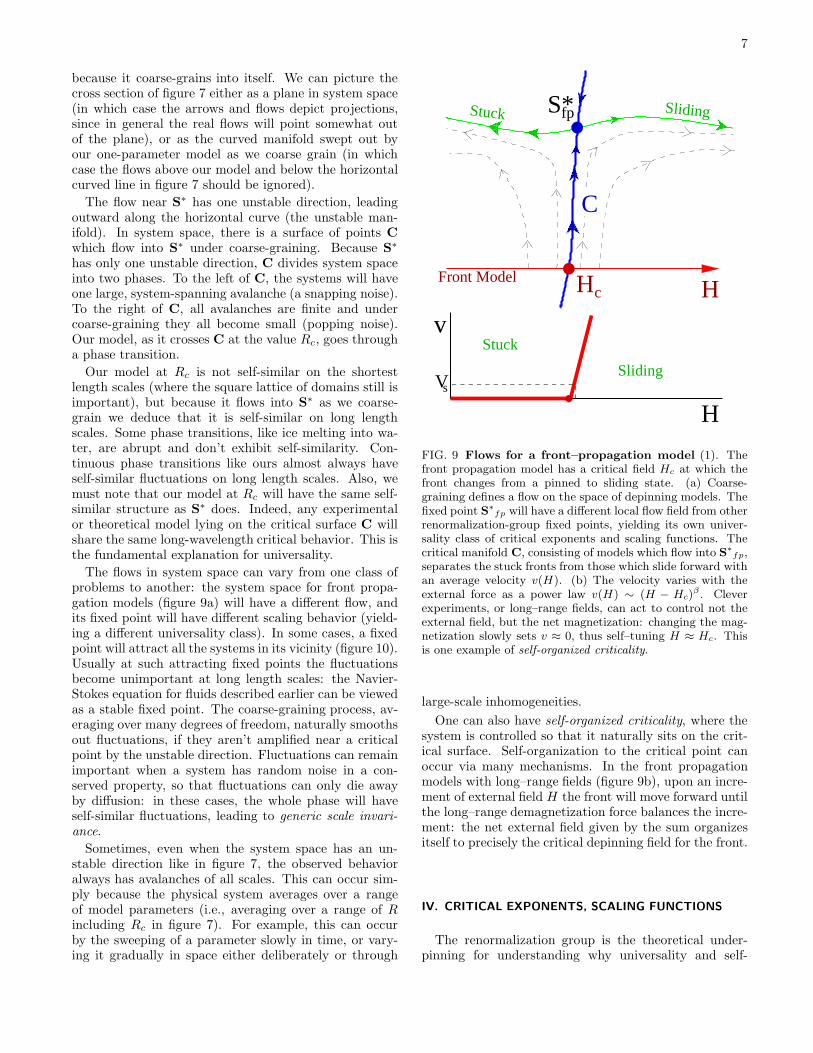
because it coarse-grains into itself. We can picture thecross section of figure 7 either as a plane in system space(in which case the arrows and flows depict projections,since in general the real flows will point somewhat outof the plane), or as the curved manifold swept out byour one-parameter model as we coarse grain (in whichcase the flows above our model and below the horizontalcurved line in figure 7 should be ignored).

The flow near S∗ has one unstable direction, leadingoutward along the horizontal curve (the unstable man-ifold). In system space, there is a surface of points Cwhich flow into S∗ under coarse-graining. Because S∗

has only one unstable direction, C divides system spaceinto two phases. To the left of C, the systems will haveone large, system-spanning avalanche (a snapping noise).To the right of C, all avalanches are finite and undercoarse-graining they all become small (popping noise).Our model, as it crosses C at the value Rc, goes througha phase transition.

Our model at Rc is not self-similar on the shortestlength scales (where the square lattice of domains still isimportant), but because it flows into S∗ as we coarse-grain we deduce that it is self-similar on long lengthscales. Some phase transitions, like ice melting into wa-ter, are abrupt and don’t exhibit self-similarity. Con-tinuous phase transitions like ours almost always haveself-similar fluctuations on long length scales. Also, wemust note that our model at Rc will have the same self-similar structure as S∗ does. Indeed, any experimentalor theoretical model lying on the critical surface C willshare the same long-wavelength critical behavior. This isthe fundamental explanation for universality.

The flows in system space can vary from one class ofproblems to another: the system space for front propa-gation models (figure 9a) will have a different flow, andits fixed point will have different scaling behavior (yield-ing a different universality class). In some cases, a fixedpoint will attract all the systems in its vicinity (figure 10).Usually at such attracting fixed points the fluctuationsbecome unimportant at long length scales: the Navier-Stokes equation for fluids described earlier can be viewedas a stable fixed point. The coarse-graining process, av-eraging over many degrees of freedom, naturally smoothsout fluctuations, if they aren’t amplified near a criticalpoint by the unstable direction. Fluctuations can remainimportant when a system has random noise in a con-served property, so that fluctuations can only die awayby diffusion: in these cases, the whole phase will haveself-similar fluctuations, leading to generic scale invari-

ance.

Sometimes, even when the system space has an un-stable direction like in figure 7, the observed behavioralways has avalanches of all scales. This can occur sim-ply because the physical system averages over a rangeof model parameters (i.e., averaging over a range of Rincluding Rc in figure 7). For example, this can occurby the sweeping of a parameter slowly in time, or vary-ing it gradually in space either deliberately or through

H

H

Vs

c

Sliding

Front Model

v

C

Stuck

Stuck

Sliding

S*fp

H

FIG. 9 Flows for a front–propagation model (1). Thefront propagation model has a critical field Hc at which thefront changes from a pinned to sliding state. (a) Coarse-graining defines a flow on the space of depinning models. Thefixed point S∗

fp will have a different local flow field from otherrenormalization-group fixed points, yielding its own univer-sality class of critical exponents and scaling functions. Thecritical manifold C, consisting of models which flow into S∗

fp,separates the stuck fronts from those which slide forward withan average velocity v(H). (b) The velocity varies with theexternal force as a power law v(H) ∼ (H − Hc)

β . Cleverexperiments, or long–range fields, can act to control not theexternal field, but the net magnetization: changing the mag-netization slowly sets v ≈ 0, thus self–tuning H ≈ Hc. Thisis one example of self-organized criticality.

large-scale inhomogeneities.

One can also have self-organized criticality, where thesystem is controlled so that it naturally sits on the crit-ical surface. Self-organization to the critical point canoccur via many mechanisms. In the front propagationmodels with long–range fields (figure 9b), upon an incre-ment of external field H the front will move forward untilthe long–range demagnetization force balances the incre-ment: the net external field given by the sum organizesitself to precisely the critical depinning field for the front.

IV. CRITICAL EXPONENTS, SCALING FUNCTIONS

The renormalization group is the theoretical under-pinning for understanding why universality and self-

8

S*a

Attracting Fixed Point

FIG. 10 Attracting fixed point (1). Often there will befixed points that attract in all directions. These fixed pointsdescribe phases rather than phase transitions. Most phasesare rather simple, with fluctuations that die away on longlength scales. When fluctuations remain important, they willexhibit self-similarity and power laws called generic scale in-variance.

similarity occur.8 Once we grant that different systemsshould sometimes share long-distance properties, though,we can quite easily derive some powerful predictions.

To take a tangible example, lets consider the relationbetween the duration of an avalanche and its size. If welook at all avalanches of a certain duration T in an experi-ment, they will have a distribution of sizes S around someaverage 〈S〉exp(T ). If we look at a theoretical model, itwill have a corresponding average size 〈S〉th(T ). If ourmodel describes the experiment, these functions must beessentially the same at large S and large T . We must al-low for the fact that the experimental units of time andsize will be different from the ones in our model: the bestwe can hope for is that

〈S〉exp(T ) = A〈S〉th(T/B), (3)

for some rescaling factors A and B.Now, instead of comparing to experiment, we can com-

pare our model to itself on a slightly larger time scale. Ifthe time scale is expanded by a small factor B = 1/(1−δ),then the rescaling of the size will also be small, say 1+a.Hence

〈S〉(T ) = (1 + aδ)〈S〉((1 − δ)T ). (4)

Making δ very small yields the simple relation a〈S〉 =Td〈S〉/dT , which can be solved to give the power law re-lation 〈S〉(T ) = S0T

a. The exponent a is called a criticalexponent, and is a universal prediction of a given theory.

8 This section also follows closely the presentation in reference (1).

(That means that if the theory correctly describes an ex-periment, the critical exponents will agree.) In our work,we write the exponent a relating time to size in terms ofthree other critical exponents, a = 1/σνz.

1

1.5

2

2.5

3

3.5

Exp

onen

t Val

ue τ +

σβδτ

(τ−1

)/σνz

+1

(τ+σ

βδ−1

)/σνz

+1

1/σν

z

[3−(

τ+σβ

δ)]/σ

νz

(τ−1

)/(2−

σνz)

+1

Size Duration Power Energy

Mean Field TheoryOur Model

ExperimentsFront Propagation

FIG. 11 Universal Critical Exponents vs. Experi-ment. (1) Different experiments on crackling noise in mag-nets measure different combinations of the universal criticalexponents. Here we compare experimental measurements (seetable I of reference (3)) to the theoretical predictions for threemodels: our model, the front-propagation model and the dipo-lar mean-field theory. Power laws giving the probability ofgetting an avalanche of a given size, duration, or energy atthe critical point are shown; also shown is the critical expo-nent giving the power as a function of frequency (13) (due tothe internal structure of the avalanches, figure 5). In each pairof columns, the first column includes only avalanches at exter-nal fields H near Hc where the largest avalanches occur, andthe second column (when it exists) includes all avalanches.The various combinations of the basic critical exponents canbe derived from exponent equality calculations similar to theone discussed in the text. Many of the experiments were doneyears before the theories were developed: many did not reporterror bars. All three theories do well (especially consideringthe possible systematic errors in fitting power laws to the ex-perimental measurements: see in figure 3 how a bit away fromRc the effective slopes change).(A more systematic and criti-cal review of the exponent measurements in the literature maybe found in Table I of reference (11). One may also find insection V.A of their paper a discussion of the relation betweenthe experiments and the theoretical universality classes.)

There are several basic critical exponents, which arisein many different combinations depending on the phys-ical property being studied. We’ve seen that at Rc andnear Hc the probability of having an avalanche of size Sgoes as S−τ .9 The cutoff in the avalanche size distribu-tion in figure 3 gets larger as one approaches the critical

9 We will see that when the entire hysteresis loop is considered thischanges to S−(τ+σβδ).

9

disorder as (R − Rc)−σ (figure 3). The typical length of

the largest avalanche goes as (R − Rc)−ν . The jump in

the magnetization (figure 6) goes as (R−Rc)β , and at Rc

the magnetization (M − Mc) ∼ (H − Hc)1/δ.10 Finally,

we need to know how time rescales: the duration of anavalanche of spatial extent L typically will go as Lz.

Any physical property that shows singular behavior atthe critical point will have a critical exponent that canbe written in terms of these basic ones (figure 11).11

To specialists in critical phenomena, these exponentsare central; whole conversations will seem to rotatearound various combinations of Greek letters. Criticalexponents are one of the relatively easy things to calcu-late from the various analytic approaches, and so haveattracted the most attention. They are derived from theeigenvalues of the linearized flows about the fixed pointS∗ in figure 7. Figure 12 shows our numerical estimatesfor several critical exponents in our model in various spa-tial dimensions, together with our 6 − ǫ expansions forthem. Of course the key challenge is not to get analyticalwork to agree with numerics: it’s to get theory to agreewith experiment. Figure 11 shows that our model doesrather well in describing a wide variety of experiments,but that the two rival models (with different flows aroundtheir fixed points) also fit.

Critical exponents are not the be-all and end-all: manyother scaling predictions, explaining wide varieties of be-havior, are quite easy to extract from numerical simu-lations. Universality extends even to those long lengthscale properties for which one cannot write formulas.Perhaps the most important of these other predictionsare the universal scaling functions. For example, lets con-sider the time history of the avalanches, V (t), denotingthe number of domains flipping per unit time. (We call itV because it’s usually measured as a voltage in a pickupcoil.) Each avalanche has large fluctuations, but one canaverage over many avalanches to get a typical shape. Fig-ures 13 and 14 show averages over all avalanches of fixedduration T . Lets call this 〈V 〉(T, t). Universality againsuggests that this average should be the same for experi-ment and a successful theory, apart from an overall shiftin time and voltage scales:

〈V 〉exp(T, t) = A〈V 〉th(T/B, t/B). (5)

Comparing our model to itself with a shifted time scalebecomes simple if we change variables: let v(T, t/T ) =〈V 〉(T, t), so v(T, t/T ) = Av(T/B, t/T ). Here t/T is aparticularly simple example of a scaling variable. Now,if we rescale time by a small factor B = 1/(1 − δ), wehave v(T, t/T ) = (1 + b)v(t/T, (1 − δ)T ). Again, makingδ small we find bv = T∂v/∂T , with solution v = v0T

b.

10 Don’t confuse the small change in scale δ earlier with the criticalexponent δ here.

11 Indeed, there are relations even between these exponents: seesection VI.

2 3 4 5 6Dimension (d)

0.0

1.0

2.0

Exp

onen

ts

τ+σβδ

σν

τ1/ν

σνz

FIG. 12 Universal Critical Exponents in Various Spa-tial Dimensions. (1) We test our ǫ-expansion predic-tions (27) by measuring the various critical exponents nu-merically in up to five spatial dimensions (3; 28). The var-ious exponents are described in the text. All of the ex-ponents are calculated only to linear order in ǫ, except forthe correlation length exponent ν, where we use results fromother models. The agreement even in three dimensions is re-markably good, considering that we’re expanding in 6 − Dwhere D = 3! We should note that perturbing in dimen-sion for our system is not only complicated, but also contro-versial. Our expansion uses the Martin Siggia Rose formal-ism (29; 30; 31; 32; 33; 34; 35; 36) to describe a determinis-tic dynamical system without any temperature fluctuations,while the calculation for the equilibrium model involves tem-perature fluctuations and no history dependence at all. Evenso, we have shown that our 6− ǫ expansion for the critical ex-ponents of the zero-temperature, nonequilibrium model mapsto all orders in ǫ onto that of the equilibrium model. The6− ǫ expansion for the equilibrium model, however, has beencontroversial for decades (37). Recently the thermal 6 − ǫexpansion of the equilibrium model has been called into ques-tion (37; 38; 39) not just due to non perturbative corrections,as was previously assumed, but due to previously neglectedhigher order terms in the expansion. The implications of thiscontroversy for our non–equilibrium renormalization grouptreatments is not yet known.

However, the integration constant v0 will now depend ont/T , v0 = V (t/T ), so we arrive at the scaling form

〈V 〉(t, T ) = T bV (t/T ), (6)

where the entire scaling function V is a universal predic-tion of the theory.

Figures 13 and 14 show the universal scaling functionsV for two models and three experiments. For our model,we’ve drawn what are called scaling collapses, a simplebut powerful way to both check that were in the scalingregime, and to measure the universal scaling function.Using the form of the scaling equation Eq.[2], we simplyplot T b〈V 〉(t, T ) versus t/T , for a series of long times T .All the plots fall onto the same curve. This tells us thatour avalanches are large enough to be self-similar. (If in

10

0 0.2 0.4 0.6 0.8 1t/T

0

0.2

0.4

0.6

0.8

1 <

V(t

,T)>

/Vm

ax

Durin et alThis paperSpasojevic et al

FIG. 13 Comparison of experimental average pulseshapes for fixed pulse duration, as measured by three dif-ferent groups (2; 11; 12; 40). Our theories don’t only predictpower laws: they should describe all behavior on long lengthand time scales (at least in a statistical sense). In particular,by fixing parameters one can predict what are called scalingfunctions. If we average the voltage as a function of time overall avalanches of a fixed duration, we get an average shape. Inthese three experiments, they find that this shape is the samefor different durations: by rescaling the time by the dura-tion T and the voltage by the maximum of the average curve,the curves within a given experiment collapse onto one. Thethree experiments, however, do not all collapse onto the samecurve. This could mean that they are in different universalityclasses, or that we don’t understand this dynamical scalingcompletely.

your scaling collapse the corresponding plots do not alllook alike, then any power laws you have measured areprobably accidental.) It also provides us with a numericalevaluation of the scaling function V . Note that we use1/σνz− 1 for the critical exponent b. This is an exampleof an exponent equality: easily derived from the fact that

〈S〉(T ) =

∫〈V 〉(t, T ) dt =

∫T bV (t/T )dt ∼ T b+1, (7)

and the scaling relation 〈S〉(T ) ∼ T−1/σνz.Notice that the two models and the three experiments

have quite different shapes for V . How do we react tothis? Our models are falsified if any of the predictionsare shown to be wrong asymptotically on long lengthand time scales: hence our theory is either wrong (in-applicable to these systems) or somehow at least incom-

0 0.2 0.4 0.6 0.8 1t/T

0

0.2

0.4

0.6

T1−

1/σν

z <V

(t,T

)>

Front Propagation ModelNucleation Model

FIG. 14 Comparison of theoretical average pulse shapescaling functions for our nucleated model and the frontpropagation model (2). The front propagation models have1/σνz = 1.72 ± 0.03 in this collapse; our nucleation modelhas 1/σνz = 1.75 ± 0.03 (in principle, there is no reason tobelieve these two should agree). The inset shows the twocurves rescaled to the same height (the overall height is a non–universal feature): they are quantitatively different, but farmore similar to one another than either is to the experimen-tal curves in figure 13. The mean–field model apparently hasa scaling function which is a perfect inverted parabola (41).The ABBM model, which is also mean–field like, interestinglyhas a different shape, that of one lobe of a sinusoid (42, eq.102).

plete. Incorporating insights from careful experiments torefine the theoretical models has historically been crucialin the broad field of critical phenomena. The messagewe emphasize here is that scaling functions can providea sharper tool for discriminating between different uni-versality classes than critical exponents.

Broadly speaking, most common properties that in-volve large length and time scales have scaling forms:using self-similarity, one can write functions of N vari-ables in terms of scaling functions of N − 1 variables:F (x, y, z) = z−αF (x/zβ, y/zγ). In the inset to figure 3,we show the scaling collapse for the integrated avalanchesize distribution (derived as equation 10):

Dint(S, R) = S−(τ+σβδ)Dint((R − Rc)/S−σ). (8)

This example illustrates that scaling works not only at Rc

but also near Rc; the unstable manifold in figure 7 gov-erns the behavior for systems near the critical manifold

11

C.

V. MEASURING EXPONENTS AND SCALING

FUNCTIONS

The simulations provide a rich variety of measuredquantities, each with a characteristic universal scalingform and associated critical exponents. In this sectionwe focus on a few key ones of particular experimentalsignificance.12

We’ll discuss the following properties obtained fromthe simulation

• the magnetization M(H, R) as a function of theexternal field H .

• the avalanche size distribution integrated over thefield H , Dint(S, R).

• the avalanche correlation function integrated overthe field H , Gint(x, R).

• the distribution of avalanche durations D(int)t (S, t)

as a function of the avalanche size S, at R = Rc,integrated over the field H .

• the energy spectrum E(ω) of the Barkhausen noisefor various models at criticality.

A. Magnetization Curves

Unfortunately the most obvious measured quantity inour simulations, the magnetization curve M(H), is theone which collapses least well in our simulations. Westart with it nonetheless.

The top figure 15 shows the magnetization curves ob-tained from our simulation in 3 dimensions for severalvalues of the disorder R. As the disorder R is decreased,a discontinuity or jump in the magnetization curve ap-pears where a single avalanche occupies a large fraction ofthe total system. In the thermodynamic limit this wouldbe the infinite avalanche: the largest disorder at which itoccurs is the critical disorder Rc. For finite size systems,like the ones we use in our simulation, we observe anavalanche which spans the system at a higher disorder,which gradually approaches Rc as the system size grows.

Figure 16 shows the slope dM/dH and its scaling col-lapse. By using this derivative, the critical region is em-phasized as the peak in the curve, and the dependenceon the parameter Mc drops out. The lower graphs infigure 15 and 16 show the scaling collapses of the mag-netization and its slope. Clearly in neither case is all thedata collapsing onto a single curve. This would be dis-tressing, were it not for the fact that this also occurs in

12 This section follows closely the presentation in (28).

0.5 1.0 1.5 2.0Magnetic Field (H/J)

−1.0

0.0

1.0

Mag

netiz

atio

n (M

)

R=2.20R=2.60R=3.00

(a)

−10.0 0.0 10.0(h+Br)/|r|

βδ

−2.0

−1.0

0.0

(M−

Mc)

/|r|β

(b)

FIG. 15 M(H) curves at different disorders, and (poor)universal scaling collapse. (28)

mean field theory (43) at a similar distance to the criticalpoint.

Because the scaling of the magnetization is so bad, weuse other quantities to estimate the critical exponentsand the location of the critical point (Tables I and III).Fixing these quantities, we use the collapse of the dM/dHcurves to extract the rotation B mixing the experimentalvariables r and h into the scaling variable h′ = h + Br(equation A13 and following discussion). Recent worksuggests that much of the difficulty in collapsing the mag-netization curves is surmountable by adding analyticalcorrections to scaling (44).

B. Avalanche Size Distribution

In our model the spins flip in avalanches: each spincan kick over one or more neighbors in a cascade.These avalanches come in different sizes. The integratedavalanche size distribution is the size distribution of allthe avalanches that occur in one branch of the hystere-sis loop (for H from −∞ to ∞). Figure 3 (3) showssome of the raw data (thick lines) in 3 dimensions. Notethat the curves follow an approximate power law behav-

12

1.2 1.3 1.4Magnetic Field (H/J)

0.0

30.0

60.0

dM/d

H(a)

−10.0 0.0 10.0(h+Br)/|r|

βδ

0.0

0.3

0.6

0.9

|r|βδ

−β d

M/d

H

(b)

FIG. 16 dMdH

(H) curves at different disorders, and(poor) universal scaling collapse. (28) While the curvesare not collapsing onto a single curve, the quality of the col-lapse is quite similar to that found at similar distances fromRc in mean field theory (43), for which we know analyticallythat scaling works as R → Rc.

ior over several decades. Even 50% away from criticality(at R = 3.2), there are still two decades of scaling, whichimplies that the critical region is large. In experiments,a few decades of scaling could be interpreted in terms ofself-organized criticality. However, our model and simu-lation suggest that several decades of power law scalingcan still be present rather far from the critical point (notethat the size of the critical region is non–universal). Theslope of the log-log avalanche size distribution at Rc givesthe critical exponent τ + σβδ. Notice, however, that theapparent slopes in figure 3 continue to change even afterseveral decades of apparent scaling is obtained. The cut-off in the power law diverges as the critical disorder Rc

is approached. This cutoff size scales as S ∼ |r|−1/σ .These critical exponents can be obtained by using a

scaling collapse for the curves of figure 3, shown in theinset. The scaling form for the avalanche sizes as a func-tion of R and H is

D(S, R, H) ∼ S−τD(Sσ|r|, h/rβδ). (9)

We can find the scaling form for the distribution ofavalanche sizes integrated over H by integrating this for-mula, changing variables to y = h/rβδ, and rewritingthe resulting formula in terms of S to a power times afunction of Sσr. For R > Rc,

Dint(S, R) =

∫D(S, R, H) dH (10)

∝

∫S−τD(Sσr, h/rβδ) dh

= S−τrβδ

∫D(Sσr, y) dy

= S−(τ+σβδ)(Sσr)βδ

∫D(Sσr, y) dy

= S−(τ+σβδ)D(int)+ (Sσr)

where D(int)+ is the scaling function for the integrated

avalanche size distribution (the + sign indicates that thecollapsed curves are for R > Rc). We are sufficientlyfar from the critical point that corrections to scaling areimportant: as described in reference (43), we do collapsesfor small ranges of R and then linearly extrapolate thebest–fit critical exponents to Rc. We estimate from thiscurve that the critical exponents τ + σβδ = 2.03 andσ = 0.24

The scaling function D(int)+ (X) with X = Sσ|r| is a

universal prediction of our model. To facilitate compar-isons with experiments, we fit a curve to the data collapsein the inset of figure 3. We have fit the scaling collapsesin dimensions 3, 4, and 5 to a phenomenological form ofan exponential times a polynomial. In three dimensions,our fit is

D(int)+ (X) = e−0.789X1/σ

× (11)

(0.021 + 0.002X + 0.531X2 − 0.266X3 + 0.261X4)

where 1/σ = 4.20. The distribution curves obtained us-ing the above fit are plotted (thin lines in figure 3) along-side the raw data (thick lines). They agree remarkablywell even far above Rc. We should recall though, thatthe fitted curve to the collapsed data can differ from the“real” scaling function even for large sizes and close tothe critical disorder (in mean field (43) the error in thecorresponding curve was about 10%). The scaling func-tion in the inset of figure 3 has a peculiar shape: it growsby a factor of ten before cutting off. The consequence ofthis bump in the shape is that in the simulations it takesmany decades in the size distribution for the slope toconverge to the asymptotic power law. This can be seenfrom the comparison between a straight line fit throughthe R = 2.25 (billion spin) simulation in figure 3 and theasymptotic power law S−2.03 obtained from extrapolat-ing the scaling collapses (thick dashed straight line in thesame figure). A similar bump exists in other dimensionsand mean field as well. Figure 17 shows the scaling func-tions in different dimensions and in mean field. In thisgraph, the scaling functions are normalized to one andthe peaks are aligned (the scaling forms allow this). The

13

curves plotted in figure 17 are not raw data but fits tothe scaling collapse in each dimensions, as was done inthe inset of figure 3.

0.0 2.0 4.0S

σ|r|

0.0

0.5

1.0

Sτ+σβ

δ Din

t(S,R

)

2 dimensions3 dimensions4 dimensions5 dimensionsMean field

FIG. 17 Universal scaling functions Dint(Sσ|r|) for the

avalanche size distributions in different spatial dimen-sions. (28) The inset of figure 3 shows the scaling collapse forthree dimensions.

It is clear from the figure that the growing bump in thescaling curves as the dimension decreases is a foreshad-owing of a zero in the scaling curve in two dimensions.

C. Avalanche Correlations

The avalanche correlation function G(x, R, H) mea-sures the probability that the initial spin of an avalanchewill trigger, in that avalanche, another spin a dis-tance x away. From the renormalization group descrip-tion (27; 45), close to the critical point and for largedistances x, the correlation function is given by:

G(x, R, H) ∼1

xd−2+ηG±(x/ξ(r, h)) (12)

where r and h are respectively the reduced disorder andfield, G± (± indicates the sign of r) is the scaling function,d is the dimension, ξ is the correlation length, and η iscalled the “anomalous dimension”. Corrections can beshown to be subdominant (appendix A). The correlationlength ξ(r, h) is a macroscopic length scale in the systemwhich is on the order of the mean linear extent of thelargest avalanches. At the critical field Hc (h=0) andnear Rc, the correlation length scales like ξ ∼ |r|−ν , whilefor small field h it is given by

ξ ∼ |r|−ν Y±(h/|r|βδ) (13)

where Y± is a universal scaling function. The avalanchecorrelation function should not be confused with the clus-ter or “spin-spin” correlation which measures the prob-ability that two spins a distance x away have the same

1 10 100Distance (x)

10−15

10−10

10−5

Gin

t(x,R

)

R=2.35R=2.45R=2.70R=3.00

10−2

10−1

100

101

x |r|ν

100

102

104

106

xd+β/

ν Gin

t(x,R

)

(a)

FIG. 18 Avalanche correlation function integrated overfield H at various disorders, with scaling collapse (28).

value. (The algebraic decay for this other, spin-spin cor-relation function at the critical point (r = 0 and h = 0),is 1/xd−4+η (45).)

We’ve mostly used, for historical reasons, a slightlydifferent avalanche correlation function, which scales thesame way as the “triggered” correlation function G de-scribed above. Our function basically ignores the differ-ence between the triggering spin and the other spins inthe avalanche: alternatively, it calculates for avalanchesof size S the correlation function for pairs of spins,and then averages over all avalanches (weighting eachavalanche equally). We’ve checked that our correlationfunction agrees to within 3% with the “triggered” cor-relation function described above, for R > Rc in threedimensions and above. (In two dimensions, the two def-initions differ more substantially, but appear to scale inthe same way.)

We have measured the avalanche correlation functionintegrated over the field H , for R > Rc. For everyavalanche that occurs between H = −∞ and H = +∞,we keep a count on the number of times a distance xoccurs in the avalanche. The spanning avalanches are

14

not included in our correlation measurement. Figure 18shows several avalanche correlation curves in 3 dimen-sions for L = 320. The scaling form for the avalanchecorrelation function integrated over the field H , close tothe critical point and for large distances x, is obtainedby integrating equation (12):

Gint (x, R) ∼

∫1

xd−2+ηG±

(x/ξ(r, h)

)dh (14)

Using equation (13) and defining u = h/|r|βδ, equation(14) becomes:

Gint (x, R) ∼ |r|βδx−(d−2+η)

∫G±

(x/|r|−νY±(u)

)du

(15)The integral (I) in equation (15) is a function of x|r|ν

and can be written as:

I = (x|r|ν )−βδ/ν G±(x|r|ν ) (16)

to obtain the scaling form:

Gint (x, R) ∼1

xd+β/νG±(x|r|ν ) (17)

where we have used the scaling relation (2−η)ν = βδ−β(see (45) for the derivation).

The bottom figure 18 shows the integrated avalanchecorrelation curves collapse in 3 dimensions for L = 320and R > Rc. The exponent ν is obtained from suchcollapses by extrapolating to R = Rc as was done forother collapses (43). The exponent β/ν can be obtainedfrom these collapses too, but we found it better to usethe jump in magnetization (28), which near the criti-cal point involves several spanning avalanches. Recentwork (46; 47; 48) suggests that the jump in magnetiza-tion may be dominated by only one of these spanningavalanches, and their work suggests that there may betwo exponents related to our β, one substantially larger(their βc ∼ 0.15±0.08). The value of β/ν listed in Table Iis derived exclusively from the magnetization discontinu-ity collapses.

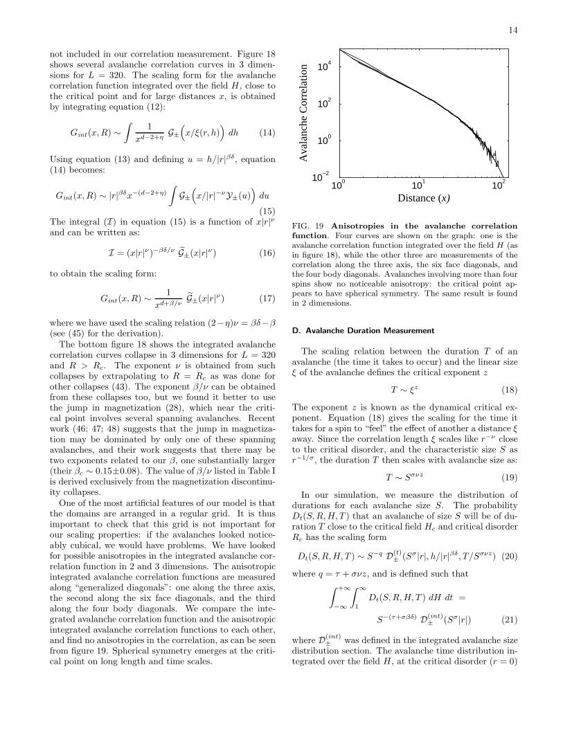
One of the most artificial features of our model is thatthe domains are arranged in a regular grid. It is thusimportant to check that this grid is not important forour scaling properties: if the avalanches looked notice-ably cubical, we would have problems. We have lookedfor possible anisotropies in the integrated avalanche cor-relation function in 2 and 3 dimensions. The anisotropicintegrated avalanche correlation functions are measuredalong “generalized diagonals”: one along the three axis,the second along the six face diagonals, and the thirdalong the four body diagonals. We compare the inte-grated avalanche correlation function and the anisotropicintegrated avalanche correlation functions to each other,and find no anisotropies in the correlation, as can be seenfrom figure 19. Spherical symmetry emerges at the criti-cal point on long length and time scales.

100

101

102

Distance (x)

10−2

100

102

104

Ava

lanc

he C

orre

latio

n

FIG. 19 Anisotropies in the avalanche correlationfunction. Four curves are shown on the graph: one is theavalanche correlation function integrated over the field H (asin figure 18), while the other three are measurements of thecorrelation along the three axis, the six face diagonals, andthe four body diagonals. Avalanches involving more than fourspins show no noticeable anisotropy: the critical point ap-pears to have spherical symmetry. The same result is foundin 2 dimensions.

D. Avalanche Duration Measurement

The scaling relation between the duration T of anavalanche (the time it takes to occur) and the linear sizeξ of the avalanche defines the critical exponent z

T ∼ ξz (18)

The exponent z is known as the dynamical critical ex-ponent. Equation (18) gives the scaling for the time ittakes for a spin to “feel” the effect of another a distance ξaway. Since the correlation length ξ scales like r−ν closeto the critical disorder, and the characteristic size S asr−1/σ, the duration T then scales with avalanche size as:

T ∼ Sσνz (19)

In our simulation, we measure the distribution ofdurations for each avalanche size S. The probabilityDt(S, R, H, T ) that an avalanche of size S will be of du-ration T close to the critical field Hc and critical disorderRc has the scaling form

Dt(S, R, H, T ) ∼ S−q D(t)± (Sσ|r|, h/|r|βδ, T/Sσνz) (20)

where q = τ + σνz, and is defined such that∫ +∞

−∞

∫ ∞

1

Dt(S, R, H, T ) dH dt =

S−(τ+σβδ) D(int)± (Sσ|r|) (21)

where D(int)± was defined in the integrated avalanche size

distribution section. The avalanche time distribution in-tegrated over the field H , at the critical disorder (r = 0)

15

is:

D(int)t (S, T ) ∼ t−(τ+σβδ+σνz)/σνz D

(int)t (T/Sσνz) (22)

as obtained from equation (20) (reference (43)).

102

103

Time

10−6

10−4

10−2

Tim

e D

istr

ibut

ion

S=2,328

S=43,044

(a)

0.0 2.0 4.0t S

−σνz

104

106

108

t(τ

+σβδ

+σνz

)/σνz

Dt(i

nt) (S

,t)

(b)

FIG. 20 Distribution of avalanche durations foravalanches of fixed size S, for various sizes S, andtheir scaling collapse. (28)

Figures 20 show the avalanche time distribution inte-grated over the field H for different avalanche sizes, anda collapse of these curves using the above scaling form.

E. Energy Spectrum

The energy spectrum of the voltage V (t) as a functionof time for our model (given by adding up the the voltagetraces of each avalanche, as in figure 5),

E(ω) =

∫e−iωτ 〈V (t)V (t + τ)〉 = |V (ω)|2 (23)

is a commonly measured experimental quantity.13 Thereare two distinct contributions to this power spectrum:

13 The power spectrum is E(ω) divided by the integration time.

10−3

10−2

10−110

−5

100

105

S(1/T)P(ω)P(ω|S)/Sω−1/σνz

ω(τ−3)/σνz

10−3

10−2

10−110

−4

10−2

100

102

104

S(1/T)P(ω)P(ω|S)/Sω−1/σνz

ω(τ−3)/σνz

FIG. 21 Power spectrum scaling and relatives. Top:short–range model; bottom: mean field (long–range dipolarforces (13).)

(1) at high frequencies, the incoherent sum of the powerspectra Einc of the individual avalanches, and (2) at lowfrequencies, a term representing the correlations betweenavalanches. As the system is forced more and moreslowly, the internal dynamics of the avalanches is un-changed but their separation in time increases, so thesetwo contributions separate. Typical experiments seem tobe dominated by the contribution (1) from the internaldynamics within an avalanche (13). In this section, theresults we discuss are valid for all three models of hystere-sis.14 See also (42) in this volume for a more completediscussion of our power spectrum theory and the experi-mental context.

14 In the short–range model, we concentrate on the case where wemeasure only near Rc and Hc: we do not integrate over the loop.Integrating over the loop yields τ very close to two, where bothforms of the scaling should compete.

16

There have been a number of naive arguments for thepower law for E(ω), stretching back to 1972 (3; 27; 40;49), which yield a power law which is only valid if τ > 2:

Enaive(ω) ∝ ω−(3−τ)/σνz (only for τ > 2). (24)

Let Smax be the typical largest avalanche in the system,say because the system is finite in size. At root, thesederivations fail for τ < 2 because

∫ Smax

0

SD(S) dS =

∫ Smax

0

S1−τ dS = S2−τmax (25)

diverges. Since there are S spins in each avalanche, itwould seem that equation 25 should represent the numberof spins in the system. This is roughly correct for τ > 2,but for τ < 2 the amplitude of the power law D(S) =D0S

−τ depends on this cutoff D0 ∼ S−2max. Continuing a

detailed analysis (13), we get a different scaling form

Enaive(ω) ∝ ω−1/σνz (for τ < 2). (26)

It is not a surprise that this new prediction fixes a numberof discrepancies between theory and experiments (13).

Figure 21 shows the power spectrum P (ω) (equalto E(ω) divided by the duration of the measurement),together with four other curves, for both the front–propagation model and the infinite–range model (13).The top two curves are the naive power law (equation 24,obviously not correct) and the correct law (equation 26).We compare with the relation between the avalanche sizeS and the duration T (equation 19), which has the samecombination of critical exponents S ∼ (1/T )−1/σνz. Wealso show that the energy spectrum of individual largeavalanches is proportional to S and has the same powerlaw in frequency ω as that of the entire time series, so weplot P (ω|S)/S for a variety of avalanche sizes S.

F. Tables of Results

Here we summarize, from (28), our numerical estimates of the universal critical exponents and various non–universalquantities used in the scaling collapses above.15

measured exponents 3d 4d 5d mean field

1/ν 0.71±0.09 1.12±0.11 1.47±0.15 2

θ 0.015±0.015 0.32±0.06 1.03±0.10 1

(τ + σβδ − 3)/σν -2.90±0.16 -3.20±0.24 -2.95±0.13 -3

1/σ 4.2±0.3 3.20±0.25 2.35±0.25 2

τ + σβδ 2.03±0.03 2.07±0.03 2.15±0.04 9/4

τ 1.60±0.06 1.53±0.08 1.48±0.10 3/2

d + β/ν 3.07±0.30 4.15±0.20 5.1±0.4 7 (at dc = 6)

β/ν 0.025±0.020 0.19±0.05 0.37±0.08 1

σνz 0.57±0.03 0.56±0.03 0.545±0.025 1/2

Table I. Measured universal critical exponents. Values for the exponents extracted from scaling collapses in 3, 4,and 5 dimensions. The mean field values are calculated analytically (23; 45). ν is the correlation length exponent andis found from collapses of avalanche correlations, number of spanning avalanches, and moments of the avalanche sizedistribution data. The exponent θ is a measure of the number of spanning avalanches and is obtained from collapsesof that data. (τ + σβδ − 3)/σν is obtained from the second moments of the avalanche size distribution collapses.1/σ is associated with the cutoff in the power law distribution of avalanche sizes integrated over the field H , whileτ + σβδ gives the slope of that distribution. τ is obtained from the binned avalanche size distribution collapses (28).d + β/ν is obtained from avalanche correlation collapses and β/ν from magnetization discontinuity collapses. σνz isthe exponent combination for the time distribution of avalanche sizes and is extracted from that data. Error bars arebased on variations in the results based on different approaches to the analysis: statistical fluctuations are typicallysmaller.

15 Some of the scaling collapses shown used exponents slightly dif-ferent from those in the tables: see (28).

17

calculated exponents 3d 4d 5d mean field

σβδ 0.43±0.07 0.54±0.08 0.67±0.11 3/4

βδ 1.81±0.32 1.73±0.29 1.57±0.31 3/2

β 0.035±0.028 0.169±0.048 0.252±0.060 1/2

σν 0.34±0.05 0.28±0.04 0.29±0.04 1/4

η = 2 + (β − βδ)/ν 0.73±0.28 0.25±0.38 0.06±0.51 0Table II. Calculated universal critical exponents. Values for exponents in 3, 4, and 5 dimensions that arenot extracted directly from scaling collapses, but instead are derived from Table I and the exponent relations (seesection VI). The mean field values are obtained analytically (23; 45). Both σβδ and βδ could have larger systematicerrors than the errors listed here (28). Recent work (46) on small systems, but with sophisticated scaling analysis,suggests a larger value for β.

3d 4d 5d mean field

Rc 2.16±0.03 4.10±0.02 5.96±0.02 0.79788456

Hc 1.435±0.004 1.265±0.007 1.175±0.004 0

B 0.39±0.08 0.46±0.05 0.23±0.08 0Table III. Non-universal scaling variables. Numerical values for the critical disorders and fields, and the rotationparameter B (equation A13 and subsequent discussion), in 3, 4, and 5 dimensions extracted from scaling collapses.The critical disorder is obtained from collapses of the spanning avalanches and the second moments of the avalanchesize distribution. The critical field is obtained from the binned avalanche size distribution (28) and the magnetizationcurves. Hc is affected by finite sizes, and systematic errors could be larger than the ones listed here. The mean fieldvalues are calculated analytically (23; 45). The rotation B is obtained from the dM/dH collapses.

VI. EXPONENT RELATIONS

In the following sections we list various exponent re-lations for the nonequilibrium RFIM, for which we givedetailed arguments in (27; 50).

A. Exponent equalities

The exponents introduced above are related by the fol-lowing exponent equalities:

β − βδ = (τ − 2)/σ if τ < 2, (27)

(2 − η)ν = βδ − β, (28)

β =ν

2(d − 4 + η), (29)

and

δ = (d − 2η + η)/(d − 4 + η). (30)

(The latter three equations are not independent andare also valid in the equilibrium random-field Isingmodel).

B. Two violations of hyperscaling

In the nonequilibrium RFIM there are two differentviolations of hyperscaling.

(1) In (27; 50), we show that the connectivity hyper-scaling relation 1/σ = dν−β from percolation is violatedin our system. There is a new exponent θ defined by

1/σ = (d − θ)ν − β (31)

with θν = 1/2 − ǫ/6 + 0(ǫ2) and θν = 0.021 ± 0.021 inthree dimensions. θ is related to the number of systemspanning avalanches observed during a sweep through thehysteresis loop: see also (46).

(2) As we discuss in (27) there is a mapping of theperturbation theory for our problem to that of the equi-librium random-field Ising model to all orders in ǫ. Fromthat mapping we deduce the breakdown of an infamous(“energy”)-hyperscaling relation

β + βδ = (d − θ)ν, (32)

with a new exponent θ, which has caused much contro-versy in the case of the equilibrium random-field Isingmodel.

In (27; 50) we discuss the relation of the exponent θto the energy output of the avalanches. The ǫ expansionyields θ = 2 to all orders in ǫ. Nonperturbative correc-tions are expected to lead to deviations of θ from 2 asthe dimension is lowered. The same is true in the caseof the equilibrium RFIM. The numerical result in three

18

dimensions is θ = 1.69 ± 0.28. (In the three-dimensionalequilibrium RFIM (51) it is θeq = 1.5 ± 0.4).

Another strictly perturbative exponent equality, whichis also obtained from the perturbative mapping to therandom-field Ising model is given by

η = η. (33)

It, too, is expected to be violated by nonperturbativecorrections below six dimensions.

C. Exponent inequalities

In (27; 50) we give arguments for the following twoexponent-inequalities.16

ν/βδ ≥ 2/d, (34)

which is formally equivalent to the “Schwartz-Soffer”inequality, ν ≤ 2ν, first derived for the equilibriumrandom-field Ising model, and

ν ≥ 2/d, (35)

which is a weaker bound than Eq. (3) so long as βδ ≥ 1,as appears to be the case both theoretically and numer-ically at least for d ≥ 3.

VII. FINITE SWEEPRATE

Originally the nonequilibrium RFIM was studied in theadiabatic limit, where the external field is kept constantduring each spin flip avalanche and only increased be-tween subsequent avalanches. In real experiments, how-ever, the driving field H is typically increased at a finiterate Ω such that H = Ωt where t is time. This finiterate allows for new avalanches to be triggered by the in-creasing external field while an earlier avalanche is stillpropagating. In (52; 53) the effect of finite field sweeprates on the power spectra and avalanche size distribu-tions is discussed in detail for a large class of systems withcrackling noise. In particular, it is asked how the scalingbehavior of the avalanche size and duration distributionand the power spectra of Barkhausen noise or cracklingnoise in general depend on the field sweep rate Ω. One ofthe results is an exponent inequality as a criteria for therelevance of adding a small driving rate Ω > 0 to the adi-abatic case Ω → 0: If in the adiabatic case the avalancheduration distribution scales as D(T ) ∼ T−α with α = 2(such as in the ABBM model or the mean field version of

16 From the normalization of the avalanche size distributionD(s, r, h) it follows that τ > 1.

the RFIM), then at (small enough) finite field sweep ratethe corresponding noise “pulse” duration distribution isexpected to scale as D(T, Ω) ∼ T 2−a(H)CΩ where a(H)and C are nonuniversal constants (54; 55; 56; 57).

If, however, in the adiabatic limit the exponent α iseither greater or smaller than 2, then at (small) finitefield sweep rate the pulse duration distribution exponentremains the same as in the adiabatic limit. Note that inthe case α < 2 especially, Ω has to be particularly small inorder to be able to still see distinct pulses even at finitefield sweep rate, since at higher sweep rate the systemwill very quickly develop runaway events. In (52; 53)quantitative criteria for the meaning of “small sweeprate”are given. Also, the zero temperature nonequilibriumRFIM and recent variants are used to numerically testthe analytic results, which are expected to be applicableto a much larger class of systems with crackling noise(the exact conditions are discussed in (52; 53)). It isfound that the results agree well with both simulationsand recent experiments on Barkhausen noise in varioussoft magnetic materials with and without applied stress(with α < 2 and α = 2 respectively (11)). A brief reviewof other, related studies of the effects of finite field sweeprate is also given in (52).

VIII. SUBLOOPS AND HISTORY INDUCED CRITICAL

BEHAVIOR

One of the characteristic features of magnetic hystere-sis are the subloops, seen as the external field is changedup and down an amount insufficient to saturate the mag-netization (figure 4).

A. Return–Point Memory

Much attention has been paid to modeling thesesubloops with the Preisach model (58) Preisach modelsare quite different in spirit to ours: they represent thesystem as a large number of uncoupled hysteretic two–state domains, and fit the distribution to the observedbehavior. They are able to model a hysteretic systemif it possesses return–point memory (16), also known aswiping out (59).

Return–point memory states that the magnetizationafter a subloop rejoins a larger loop (perhaps itself asubloop) equals the magnetization at which the subloopleft the outer loop. That is, if the subloop representsan excursion downward from a local maximum exter-nal field H , then when H returns to its previous max-imum the magnetization M returns to its previous value– remembering its previous magnetization on returning,and wiping out all effects of the excursion. Return–pointmemory states that the subloops in figure 4 should closeperfectly, without a gap and without crossing themselves(as observed).

Indeed, our interacting, three-dimensional, disorderedmodels exhibit the return–point memory in an even

19

stronger form. Upon rejoining the larger loop, the en-tire state of the system is microscopically identical to thestate it had when it left the larger loop (a microscopicreturn–point memory, as opposed to a macroscopic mem-ory constraining only the net magnetization). In (23),we showed in great generality that return point memoryshould be true of any system with

1. A partial ordering of states. Here, one mi-crostate A is “ahead” of another B, A > B, if everyspin in A is greater than or equal to the correspond-ing spin in B.

2. No passing. That is, the dynamics preserves thepartial ordering.

3. Adiabatic. The external field is raised and low-ered slowly enough that the system does not lagbehind.

Return–point memory can be quite remarkable: in ourmodel (and in some experimental systems) repeating asubloop plays back precisely the same Barkhausen noise.Indeed, the return–point memory can be used as a way ofretrieving analogue magnetic memories that is (at leasttheoretically) significantly superior to measuring the re-manent magnetization (60). On the other hand, the ab-sence of exact (microscopic) return point memory hasalso been observed (61; 62; 63), and there are variousinteresting experiments testing for the reproducibility ofmagnetic avalanches (64; 65; 66) and for microscopic re-turn point memory and complementary point memoryin magnets at various disorders (67).17 In (67) the au-thors experimentally study the influence of disorder onmajor loop return point memory and complementary re-turn point memory in Co/Pt samples with varying in-terfacial roughness and find with increasing disorder theonset and saturation of both return point memory andcomplementary point memory.

Disorder dependence of return point memory versusreptation (i.e. is gradual subloop closure (68; 69)) hasrecently been reported for the zero temperature ran-dom coercivity model with antiferromagnetic-like inter-actions (70).

A related memory effect, recently reported for the hys-teresis of spin glasses, is the reversal field memory ef-fect (71). Katzgraber et al. show that this memory effectemerges in the nonequilibrium Edwards Anderson spinglass (EASG) when the magnetic field is first decreasedfrom its saturation value and then increased again fromsome reversal field HR. The authors find that EASG ex-hibits a singularity at the negative of the reversal field,

17 The complementary point memory relates the magnetic domainsat one point on the major hysteresis loop to the domains at thecomplementary point on the major loop during the same andduring subsequent cycles.

−HR, in the form of a kink in the reversal of the mag-netization of the reversal curve. They show that thismemory effect is due to a local spin-reversal symmetry ofthe Hamiltonian. This symmetry and thus the reversalfield memory effect is present in spin glasses where thedisorder is due to random couplings between spins. Ingeneral it is not expected in systems with random mag-netic fields such as the RFIM, since there the disorderbreaks local spin reversal symmetry.

As an extension to memory effects for a driving fieldthat varies in two dimensions, a vector form of wipe-outmemory for situations when the magnetic field varies inboth direction and magnitude, has been suggested basedon the two dimensional vector Preisach model in (72),and has been experimentally tested in (73).

B. Critical Behavior in Subloops

-1

-0.5

0

0.5

1

-3 -2 -1 0 1 2 3

M

(a)

-1

-0.5

0

0.5

1

-3 -2 -1 0 1 2 3

M

H/J

(b)

FIG. 22 Saturation hysteresis loops with concentricinner subloops. Top: R = 2.225J > Rc; bottom: R =2.1 < Rc. (74)

The disorder induced critical scaling for hysteresisloops in the RFIM that we discussed so far all referredto the saturation hysteresis loop. However, often it is

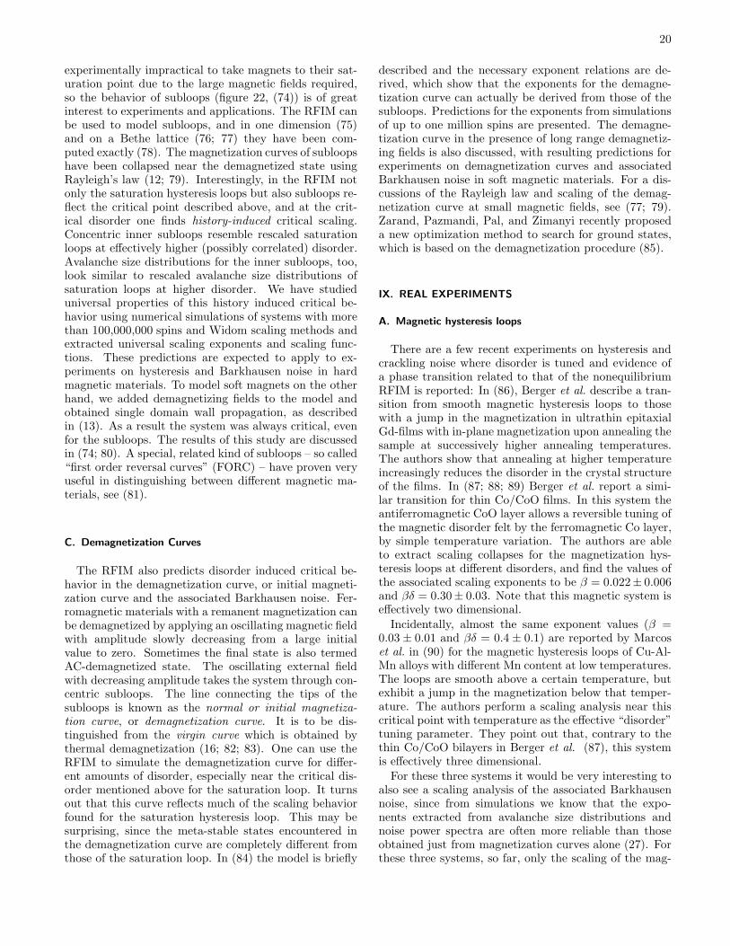
20

experimentally impractical to take magnets to their sat-uration point due to the large magnetic fields required,so the behavior of subloops (figure 22, (74)) is of greatinterest to experiments and applications. The RFIM canbe used to model subloops, and in one dimension (75)and on a Bethe lattice (76; 77) they have been com-puted exactly (78). The magnetization curves of subloopshave been collapsed near the demagnetized state usingRayleigh’s law (12; 79). Interestingly, in the RFIM notonly the saturation hysteresis loops but also subloops re-flect the critical point described above, and at the crit-ical disorder one finds history-induced critical scaling.Concentric inner subloops resemble rescaled saturationloops at effectively higher (possibly correlated) disorder.Avalanche size distributions for the inner subloops, too,look similar to rescaled avalanche size distributions ofsaturation loops at higher disorder. We have studieduniversal properties of this history induced critical be-havior using numerical simulations of systems with morethan 100,000,000 spins and Widom scaling methods andextracted universal scaling exponents and scaling func-tions. These predictions are expected to apply to ex-periments on hysteresis and Barkhausen noise in hardmagnetic materials. To model soft magnets on the otherhand, we added demagnetizing fields to the model andobtained single domain wall propagation, as describedin (13). As a result the system was always critical, evenfor the subloops. The results of this study are discussedin (74; 80). A special, related kind of subloops – so called“first order reversal curves” (FORC) – have proven veryuseful in distinguishing between different magnetic ma-terials, see (81).

C. Demagnetization Curves

The RFIM also predicts disorder induced critical be-havior in the demagnetization curve, or initial magneti-zation curve and the associated Barkhausen noise. Fer-romagnetic materials with a remanent magnetization canbe demagnetized by applying an oscillating magnetic fieldwith amplitude slowly decreasing from a large initialvalue to zero. Sometimes the final state is also termedAC-demagnetized state. The oscillating external fieldwith decreasing amplitude takes the system through con-centric subloops. The line connecting the tips of thesubloops is known as the normal or initial magnetiza-tion curve, or demagnetization curve. It is to be dis-tinguished from the virgin curve which is obtained bythermal demagnetization (16; 82; 83). One can use theRFIM to simulate the demagnetization curve for differ-ent amounts of disorder, especially near the critical dis-order mentioned above for the saturation loop. It turnsout that this curve reflects much of the scaling behaviorfound for the saturation hysteresis loop. This may besurprising, since the meta-stable states encountered inthe demagnetization curve are completely different fromthose of the saturation loop. In (84) the model is briefly

described and the necessary exponent relations are de-rived, which show that the exponents for the demagne-tization curve can actually be derived from those of thesubloops. Predictions for the exponents from simulationsof up to one million spins are presented. The demagne-tization curve in the presence of long range demagnetiz-ing fields is also discussed, with resulting predictions forexperiments on demagnetization curves and associatedBarkhausen noise in soft magnetic materials. For a dis-cussions of the Rayleigh law and scaling of the demag-netization curve at small magnetic fields, see (77; 79).Zarand, Pazmandi, Pal, and Zimanyi recently proposeda new optimization method to search for ground states,which is based on the demagnetization procedure (85).

IX. REAL EXPERIMENTS

A. Magnetic hysteresis loops

There are a few recent experiments on hysteresis andcrackling noise where disorder is tuned and evidence ofa phase transition related to that of the nonequilibriumRFIM is reported: In (86), Berger et al. describe a tran-sition from smooth magnetic hysteresis loops to thosewith a jump in the magnetization in ultrathin epitaxialGd-films with in-plane magnetization upon annealing thesample at successively higher annealing temperatures.The authors show that annealing at higher temperatureincreasingly reduces the disorder in the crystal structureof the films. In (87; 88; 89) Berger et al. report a simi-lar transition for thin Co/CoO films. In this system theantiferromagnetic CoO layer allows a reversible tuning ofthe magnetic disorder felt by the ferromagnetic Co layer,by simple temperature variation. The authors are ableto extract scaling collapses for the magnetization hys-teresis loops at different disorders, and find the values ofthe associated scaling exponents to be β = 0.022± 0.006and βδ = 0.30± 0.03. Note that this magnetic system iseffectively two dimensional.

Incidentally, almost the same exponent values (β =0.03 ± 0.01 and βδ = 0.4 ± 0.1) are reported by Marcoset al. in (90) for the magnetic hysteresis loops of Cu-Al-Mn alloys with different Mn content at low temperatures.The loops are smooth above a certain temperature, butexhibit a jump in the magnetization below that temper-ature. The authors perform a scaling analysis near thiscritical point with temperature as the effective “disorder”tuning parameter. They point out that, contrary to thethin Co/CoO bilayers in Berger et al. (87), this systemis effectively three dimensional.

For these three systems it would be very interesting toalso see a scaling analysis of the associated Barkhausennoise, since from simulations we know that the expo-nents extracted from avalanche size distributions andnoise power spectra are often more reliable than thoseobtained just from magnetization curves alone (27). Forthese three systems, so far, only the scaling of the mag-

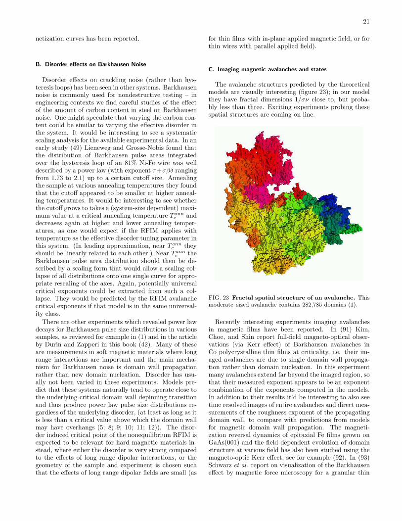
21

netization curves has been reported.

B. Disorder effects on Barkhausen Noise

Disorder effects on crackling noise (rather than hys-teresis loops) has been seen in other systems. Barkhausennoise is commonly used for nondestructive testing – inengineering contexts we find careful studies of the effectof the amount of carbon content in steel on Barkhausennoise. One might speculate that varying the carbon con-tent could be similar to varying the effective disorder inthe system. It would be interesting to see a systematicscaling analysis for the available experimental data. In anearly study (49) Lieneweg and Grosse-Nobis found thatthe distribution of Barkhausen pulse areas integratedover the hysteresis loop of an 81% Ni-Fe wire was welldescribed by a power law (with exponent τ +σβδ rangingfrom 1.73 to 2.1) up to a certain cutoff size. Annealingthe sample at various annealing temperatures they foundthat the cutoff appeared to be smaller at higher anneal-ing temperatures. It would be interesting to see whetherthe cutoff grows to takes a (system-size dependent) maxi-mum value at a critical annealing temperature T ann

c anddecreases again at higher and lower annealing temper-atures, as one would expect if the RFIM applies withtemperature as the effective disorder tuning parameter inthis system. (In leading approximation, near T ann

c theyshould be linearly related to each other.) Near T ann

c theBarkhausen pulse area distribution should then be de-scribed by a scaling form that would allow a scaling col-lapse of all distributions onto one single curve for appro-priate rescaling of the axes. Again, potentially universalcritical exponents could be extracted from such a col-lapse. They would be predicted by the RFIM avalanchecritical exponents if that model is in the same universal-ity class.

There are other experiments which revealed power lawdecays for Barkhausen pulse size distributions in varioussamples, as reviewed for example in (1) and in the articleby Durin and Zapperi in this book (42). Many of theseare measurements in soft magnetic materials where longrange interactions are important and the main mecha-nism for Barkhausen noise is domain wall propagationrather than new domain nucleation. Disorder has usu-ally not been varied in these experiments. Models pre-dict that these systems naturally tend to operate close tothe underlying critical domain wall depinning transitionand thus produce power law pulse size distributions re-gardless of the underlying disorder, (at least as long as itis less than a critical value above which the domain wallmay have overhangs (5; 8; 9; 10; 11; 12)). The disor-der induced critical point of the nonequilibrium RFIM isexpected to be relevant for hard magnetic materials in-stead, where either the disorder is very strong comparedto the effects of long range dipolar interactions, or thegeometry of the sample and experiment is chosen suchthat the effects of long range dipolar fields are small (as

for thin films with in-plane applied magnetic field, or forthin wires with parallel applied field).

C. Imaging magnetic avalanches and states

The avalanche structures predicted by the theoreticalmodels are visually interesting (figure 23); in our modelthey have fractal dimensions 1/σν close to, but proba-bly less than three. Exciting experiments probing thesespatial structures are coming on line.

FIG. 23 Fractal spatial structure of an avalanche. Thismoderate–sized avalanche contains 282,785 domains (1).

Recently interesting experiments imaging avalanchesin magnetic films have been reported. In (91) Kim,Choe, and Shin report full-field magneto-optical obser-vations (via Kerr effect) of Barkhausen avalanches inCo polycrystalline thin films at criticality, i.e. their im-aged avalanches are due to single domain wall propaga-tion rather than domain nucleation. In this experimentmany avalanches extend far beyond the imaged region, sothat their measured exponent appears to be an exponentcombination of the exponents computed in the models.In addition to their results it’d be interesting to also seetime resolved images of entire avalanches and direct mea-surements of the roughness exponent of the propagatingdomain wall, to compare with predictions from modelsfor magnetic domain wall propagation. The magneti-zation reversal dynamics of epitaxial Fe films grown onGaAs(001) and the field dependent evolution of domainstructure at various field has also been studied using themagneto-optic Kerr effect, see for example (92). In (93)Schwarz et al. report on visualization of the Barkhauseneffect by magnetic force microscopy for a granular thin

22

film with perpendicular anisotropy. The authors are ableto localize individual Barkhausen volumes and distin-guish them as either newly nucleated or grown by domainwall propagation. They find a Gaussian size distributionof nucleated Barkhausen volumes indicating an uncorre-lated random process, and a power law distribution forgrown Barkhausen volumes, reflecting critical behaviorduring domain wall motion. Another very interesting ex-perimental approach is x-ray speckle metrology (67). Ina recent preprint Pierce et al use this method to studycorrelations between microstates with different historiesand test for microscopic return point memory of subloopsin magnetic systems.

D. Random Bonds and Random Anisotropy

Renormalization group treatments, symmetry argu-ments (27), and simulations (94; 95) show, that the hys-teretic, zero temperature random bond Ising model withferromagnetic mean bond strength is expected to be inthe same universality class as the nonequilibrium RFIM.Vives et al. also point out that their numerical scalingexponents in two dimensions of the two models also haveoverlapping error bars with the corresponding exponentsof Blume-Emery Griffiths models with disorder, in whichthe spins take three values ±1, 0 (95). An analysis of theshort time dynamics of first-order phase transitions in adisordered system, using the random bond Ising modelis given in (96). The diluted ferromagnetic random Isingmodel (97) has both nonuniform bond strengths that re-flect dilution due to nonmagnetic impurities, and randommagnetic fields. Symmetry arguments suggest (27) that amodel with uncorrelated random (ferromagnetic) bondsand random fields should again be in the same univer-sality class as the RFIM, since it has no new symmetriescompared with the RFIM. Similarly, daSilveira and Kar-dar developed a O(N) vector spin model with randomfields and showed through a renormalization group cal-culation that, in general, it can displays the same con-tinuous phase transition in the hysteresis loop as theRFIM (98), i.e. the two critical points are in the sameuniversality class.18 The reason is that the applied ex-ternal field breaks any added rotational symmetry (27)so that the behavior on long length scales is determinedby the same the same symmetries in both models. Sim-ilarly the random anisotropy model of (99), was shownnumerically to be in the same universality class as theRFIM: this is again as expected, since the external ap-plied field not only breaks rotational symmetry but alsotime-reversal symmetry. Perhaps somewhat surprisingly,a transition from hysteresis loops with a jump to thosewithout, like the one of the RFIM, is also seen in a plas-tic depinning model for charge density waves (100). If

18 They also find a new universality class, see section X.

in the random field Ising model a certain fraction of thebonds between neighboring spins is enhanced to a verylarge value, one obtains a simple model for exchange bias(101).

Hysteresis loops observed for the Ising glass with zeroferromagnetic mean bond strength are smooth and con-tinuous (102; 103) – qualitatively this agrees with exper-imental hysteresis loops seen for example in AuFe sys-tems (104). For Ising glasses with strong ferromagneticmean bond strength (compared to the width of the distri-bution of bond strengths, which is the disorder), a jumpin the magnetization curve appears, just as in the low dis-order phase of the RFIM. The hysteresis loops resemblethose seen for more concentrated AuFe systems (104) aswell as CuMn and AgMn systems (105; 106). A brief re-view of these and other glassy spin systems such as Isingspin glasses with long-range interactions and Heisenbergspin glasses with long-range interactions in both theoryand experiment is given for example in (103).

An interesting hysteresis model with rather differentproperties than ours based on an infinite–range spin glass(Sherrington-Kirkpatrick model) is reported to show self-organized criticality; see (102) for details.

E. Other dynamics at high sweep rates

Much interesting work has been done in both the-ory and experiment on dynamic hysteresis loops at fi-nite field sweep rate in the presence of temperature. Atfield sweep rates higher than a critical value that de-pends on sweep amplitude and temperature, the systemtransitions to a symmetry broken phase with a flatterhysteresis loop, centered around a nonzero average mag-netization. Similar dynamic transitions also are seenfor pulsed and stochastically varying fields. Chakrabartiand Acharyya published a review article on both modelsand experiments in this regime (107). Some of the ad-dressed questions deal with scaling of the hysteresis looparea with field sweep frequency, amplitude, and temper-ature. While in the initial approaches to these issuesquenched randomness in the system was neglected, thereare recent model approaches and experiments studyingdynamic hysteresis of a moving domain wall in the pres-ence of quenched disorder and temperature at finite fieldsweep rate (19; 21).

F. Nonmagnetic noisy hysteretic systems

In this section we briefly discuss a broad range of re-lated work on avalanches and hysteresis in non-magneticsystems. We start with a general overview, and thenfocus on a few particular systems.

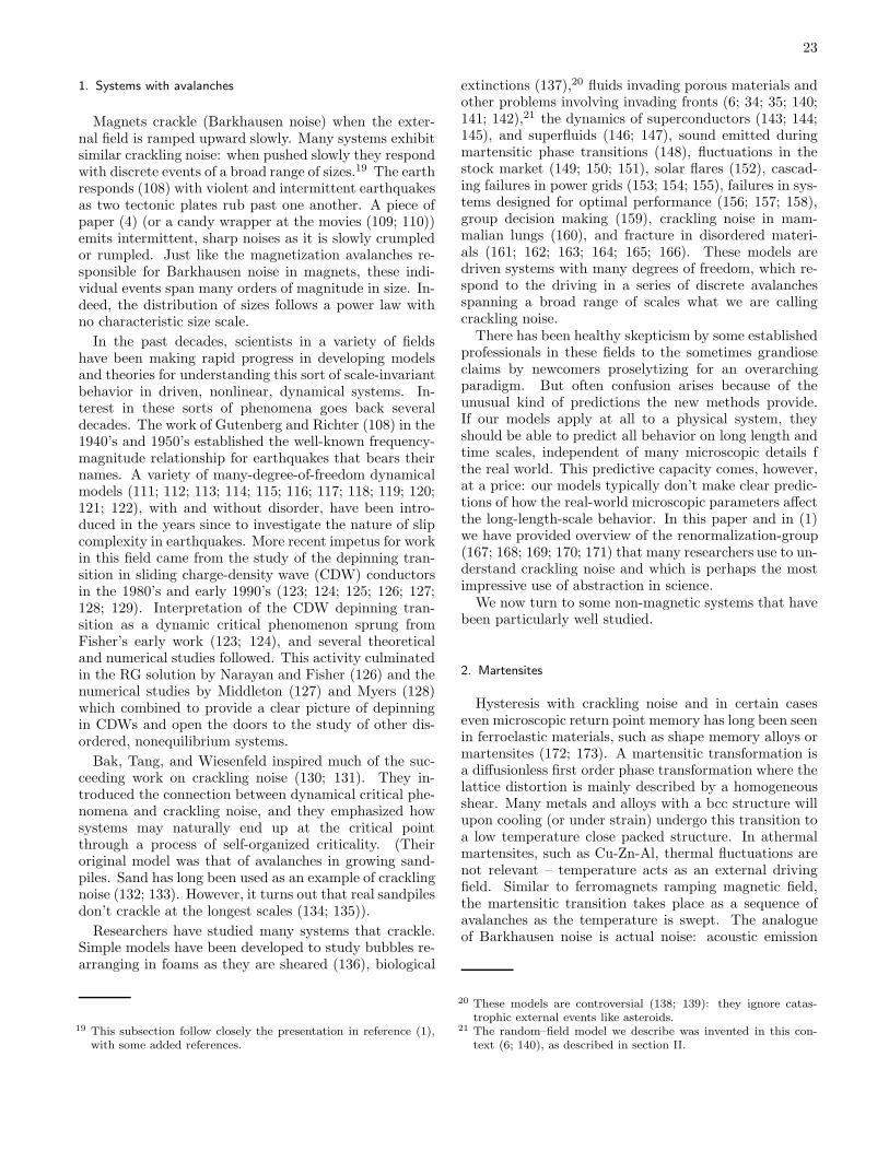
23

1. Systems with avalanches

Magnets crackle (Barkhausen noise) when the exter-nal field is ramped upward slowly. Many systems exhibitsimilar crackling noise: when pushed slowly they respondwith discrete events of a broad range of sizes.19 The earthresponds (108) with violent and intermittent earthquakesas two tectonic plates rub past one another. A piece ofpaper (4) (or a candy wrapper at the movies (109; 110))emits intermittent, sharp noises as it is slowly crumpledor rumpled. Just like the magnetization avalanches re-sponsible for Barkhausen noise in magnets, these indi-vidual events span many orders of magnitude in size. In-deed, the distribution of sizes follows a power law withno characteristic size scale.

In the past decades, scientists in a variety of fieldshave been making rapid progress in developing modelsand theories for understanding this sort of scale-invariantbehavior in driven, nonlinear, dynamical systems. In-terest in these sorts of phenomena goes back severaldecades. The work of Gutenberg and Richter (108) in the1940’s and 1950’s established the well-known frequency-magnitude relationship for earthquakes that bears theirnames. A variety of many-degree-of-freedom dynamicalmodels (111; 112; 113; 114; 115; 116; 117; 118; 119; 120;121; 122), with and without disorder, have been intro-duced in the years since to investigate the nature of slipcomplexity in earthquakes. More recent impetus for workin this field came from the study of the depinning tran-sition in sliding charge-density wave (CDW) conductorsin the 1980’s and early 1990’s (123; 124; 125; 126; 127;128; 129). Interpretation of the CDW depinning tran-sition as a dynamic critical phenomenon sprung fromFisher’s early work (123; 124), and several theoreticaland numerical studies followed. This activity culminatedin the RG solution by Narayan and Fisher (126) and thenumerical studies by Middleton (127) and Myers (128)which combined to provide a clear picture of depinningin CDWs and open the doors to the study of other dis-ordered, nonequilibrium systems.

Bak, Tang, and Wiesenfeld inspired much of the suc-ceeding work on crackling noise (130; 131). They in-troduced the connection between dynamical critical phe-nomena and crackling noise, and they emphasized howsystems may naturally end up at the critical pointthrough a process of self-organized criticality. (Theiroriginal model was that of avalanches in growing sand-piles. Sand has long been used as an example of cracklingnoise (132; 133). However, it turns out that real sandpilesdon’t crackle at the longest scales (134; 135)).

Researchers have studied many systems that crackle.Simple models have been developed to study bubbles re-arranging in foams as they are sheared (136), biological

19 This subsection follow closely the presentation in reference (1),with some added references.

extinctions (137),20 fluids invading porous materials andother problems involving invading fronts (6; 34; 35; 140;141; 142),21 the dynamics of superconductors (143; 144;145), and superfluids (146; 147), sound emitted duringmartensitic phase transitions (148), fluctuations in thestock market (149; 150; 151), solar flares (152), cascad-ing failures in power grids (153; 154; 155), failures in sys-tems designed for optimal performance (156; 157; 158),group decision making (159), crackling noise in mam-malian lungs (160), and fracture in disordered materi-als (161; 162; 163; 164; 165; 166). These models aredriven systems with many degrees of freedom, which re-spond to the driving in a series of discrete avalanchesspanning a broad range of scales what we are callingcrackling noise.

There has been healthy skepticism by some establishedprofessionals in these fields to the sometimes grandioseclaims by newcomers proselytizing for an overarchingparadigm. But often confusion arises because of theunusual kind of predictions the new methods provide.If our models apply at all to a physical system, theyshould be able to predict all behavior on long length andtime scales, independent of many microscopic details fthe real world. This predictive capacity comes, however,at a price: our models typically don’t make clear predic-tions of how the real-world microscopic parameters affectthe long-length-scale behavior. In this paper and in (1)we have provided overview of the renormalization-group(167; 168; 169; 170; 171) that many researchers use to un-derstand crackling noise and which is perhaps the mostimpressive use of abstraction in science.

We now turn to some non-magnetic systems that havebeen particularly well studied.

2. Martensites

Hysteresis with crackling noise and in certain caseseven microscopic return point memory has long been seenin ferroelastic materials, such as shape memory alloys ormartensites (172; 173). A martensitic transformation isa diffusionless first order phase transformation where thelattice distortion is mainly described by a homogeneousshear. Many metals and alloys with a bcc structure willupon cooling (or under strain) undergo this transition toa low temperature close packed structure. In athermalmartensites, such as Cu-Zn-Al, thermal fluctuations arenot relevant – temperature acts as an external drivingfield. Similar to ferromagnets ramping magnetic field,the martensitic transition takes place as a sequence ofavalanches as the temperature is swept. The analogueof Barkhausen noise is actual noise: acoustic emission

20 These models are controversial (138; 139): they ignore catas-trophic external events like asteroids.

21 The random–field model we describe was invented in this con-text (6; 140), as described in section II.

24

due to elastic waves in the ultrasonic range, generatedby propagating domain walls during the avalanches.

Experimental studies of the acoustic emission gener-ated during a thermally induced martensitic transfor-mation of a Cu-Zn-Al single crystal revealed an appar-ent absence of characteristic scales in the distribution ofavalanches (174). After an initial number of hysteresiscycles (ramping temperature) the system reaches a fi-nal attractor yielding two decades of power law scalingin the time distribution of acoustic emission pulse dura-tions. The authors argue that the cutoff at large times isprobably due to experimental limitations (amplifier cut-off), and interpret the observed scaling behavior in termsof self-organized criticality. Of course, the system couldhave a tunable parameter that lies close to the criticalpoint (two decades of power–law scaling arises in a range50% away from our critical point).

In a more recent study, Perez-Reche, Stipcich, Vives,Manosa, Planes, and Morin (175) study the evolution ofthe kinetic features of the martensitic transition in a Cu-Al-Mn single crystal under thermal cycling. The authorsuse several experimental techniques, including optical mi-croscopy, calorimetry, and acoustic emission, to performan analysis at multiple scales. Focussing especially onavalanches, they find that there are significant differencesbetween the kinetics at large and small scales during theinitial cycles. Upon repeated temperature cycles, how-ever, the system evolves from displaying a supercriticalavalanche size distribution to a critical power-law dis-tribution. In the language of the RFIM this could bedescribed as the effective disorder being increased by thetemperature cycles from R < Rc to R = Rc. (The criti-cal exponents, and thus the universality class, is differentfrom our RFIM).

Both of these systems demand repeated cycling to pro-duce critical behavior. This is quite different from sys-tems with return–point memory, where repeated cyclesdon’t change the behavior. A recently introduced, simpletwo dimensional phenomenological model for the marten-sitic transformation is shown to mimic near full reversalof morphology under thermal cycling in (176; 177).

A crossover from the hysteresis loops with a jump or“burst” to smooth hysteresis loops (ramping tempera-ture) has been recorded in (178), as the grain size ofmacroscopic, polycrystalline specimen of an Fe-Ni-C al-loy is reduced. The crossover is explained in terms of fi-nite size effects in defect induced nucleation within eachgrain (due to extended defects like dislocation tangles,however, rather than random point disorder). It seemsclear that one should look for critical fluctuations nearthe crossover that would promote an interpretation of thegrain size as the analogue of the disorder parameter R inour model.

3. Liquid Helium in Nuclepore

In (179) Lilly, Finley, and Hallock show a hysteresisloop for the capillary condensation of superfluid heliumin the porous material Nuclepore. Nuclepore is a polycar-bonate sheet perforated by a high density of nearly cylin-drical holes with a nominal diameter of about 2000A.The pores intersect. The most probable number of in-tersections per pore is about 5. Most pores participatein a macroscopic interconnected network, (i.e. they areapparently internally connected beyond the percolationthreshold). In the experiment the authors measure theamount of helium absorbed and capillary condensed inthe Nuclepore sample as a function of the number of he-lium atoms present (chemical potential) at fixed temper-ature T = 1.52 K.

Pore intersections result in weak interactions amongthe pores which lead to avalanches that have been ob-served upon slow withdrawal of helium from the cell. Theupper branch of the hysteresis loop (upon withdrawalof He from the sample) actually has microscopic jumps.The largest avalanche observed involves 2.6 107 pores,which is about 2.6% of the system. The distribution ofavalanche sizes is described by power laws.

This system has clear analogies to our model. The cou-pling between the pores is certainly “ferromagnetic”: If apore is emptied it becomes more likely for an intersectingpore to be emptied also. Different pore radii and differentcross-sections of the pore intersections introduce a cer-tain randomness which might be used to tune the systemto a critical point. In (180) the avalanches are studiedfor different characteristic pore sizes and the revelanceof various theoretical models which one might apply tothe system is discussed. In (181) a unifying theoreticalapproach to hysteresis phenomena associated with capil-lary condensation of gases in disodered mesoporous solidsis given, and the connection with the zero-temperaturetheoretical studies of magnetization-reversal hysteresis ofdriven interfaces in disordered media is discussed (seealso (182)).

4. Superconductors

a. Superconducting vortex avalanches In an interestingexperiment on the dynamics of superconducting vorticesin the Bean state in Nb47%T i53%, Field, Witt and Norirecorded vortex avalanches as the system was driven tothe threshold of instability by the slow ramping of theexternal magnetic field (143). The individual avalancheswere ranging in size from 50 vortices up to about 107 vor-tices, which is about 10−6 of the total number of vorticesin the system. The distribution of avalanches sizes wasrecorded for the events occurring in three 450 G widewindows of the external magnetic field range, centeredat 2.25 kG, 5.33 kG, and 7.55 kG. At all three values forthe field H there seems to be a power law up to somecutoff size, which varies with H . The authors suggest

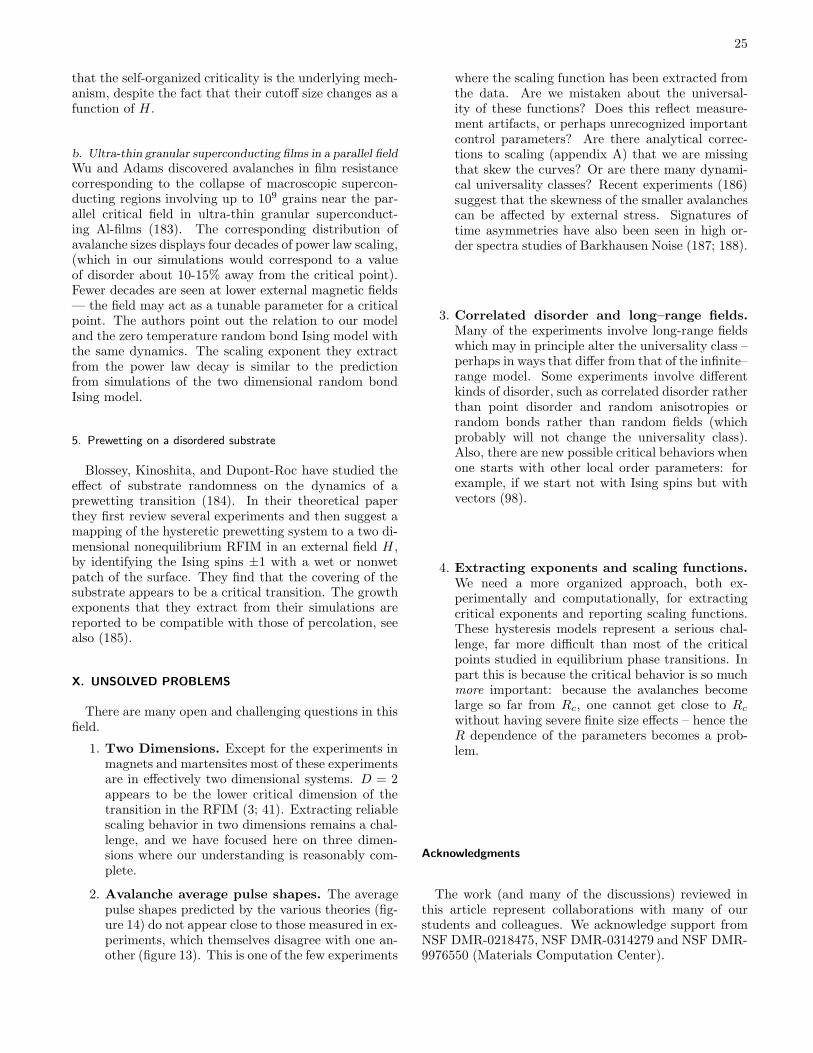
25

that the self-organized criticality is the underlying mech-anism, despite the fact that their cutoff size changes as afunction of H .

b. Ultra-thin granular superconducting films in a parallel field

Wu and Adams discovered avalanches in film resistancecorresponding to the collapse of macroscopic supercon-ducting regions involving up to 109 grains near the par-allel critical field in ultra-thin granular superconduct-ing Al-films (183). The corresponding distribution ofavalanche sizes displays four decades of power law scaling,(which in our simulations would correspond to a valueof disorder about 10-15% away from the critical point).Fewer decades are seen at lower external magnetic fields— the field may act as a tunable parameter for a criticalpoint. The authors point out the relation to our modeland the zero temperature random bond Ising model withthe same dynamics. The scaling exponent they extractfrom the power law decay is similar to the predictionfrom simulations of the two dimensional random bondIsing model.

5. Prewetting on a disordered substrate

Blossey, Kinoshita, and Dupont-Roc have studied theeffect of substrate randomness on the dynamics of aprewetting transition (184). In their theoretical paperthey first review several experiments and then suggest amapping of the hysteretic prewetting system to a two di-mensional nonequilibrium RFIM in an external field H ,by identifying the Ising spins ±1 with a wet or nonwetpatch of the surface. They find that the covering of thesubstrate appears to be a critical transition. The growthexponents that they extract from their simulations arereported to be compatible with those of percolation, seealso (185).

X. UNSOLVED PROBLEMS

There are many open and challenging questions in thisfield.

1. Two Dimensions. Except for the experiments inmagnets and martensites most of these experimentsare in effectively two dimensional systems. D = 2appears to be the lower critical dimension of thetransition in the RFIM (3; 41). Extracting reliablescaling behavior in two dimensions remains a chal-lenge, and we have focused here on three dimen-sions where our understanding is reasonably com-plete.

2. Avalanche average pulse shapes. The averagepulse shapes predicted by the various theories (fig-ure 14) do not appear close to those measured in ex-periments, which themselves disagree with one an-other (figure 13). This is one of the few experiments

where the scaling function has been extracted fromthe data. Are we mistaken about the universal-ity of these functions? Does this reflect measure-ment artifacts, or perhaps unrecognized importantcontrol parameters? Are there analytical correc-tions to scaling (appendix A) that we are missingthat skew the curves? Or are there many dynami-cal universality classes? Recent experiments (186)suggest that the skewness of the smaller avalanchescan be affected by external stress. Signatures oftime asymmetries have also been seen in high or-der spectra studies of Barkhausen Noise (187; 188).

3. Correlated disorder and long–range fields.Many of the experiments involve long-range fieldswhich may in principle alter the universality class –perhaps in ways that differ from that of the infinite–range model. Some experiments involve differentkinds of disorder, such as correlated disorder ratherthan point disorder and random anisotropies orrandom bonds rather than random fields (whichprobably will not change the universality class).Also, there are new possible critical behaviors whenone starts with other local order parameters: forexample, if we start not with Ising spins but withvectors (98).

4. Extracting exponents and scaling functions.We need a more organized approach, both ex-perimentally and computationally, for extractingcritical exponents and reporting scaling functions.These hysteresis models represent a serious chal-lenge, far more difficult than most of the criticalpoints studied in equilibrium phase transitions. Inpart this is because the critical behavior is so muchmore important: because the avalanches becomelarge so far from Rc, one cannot get close to Rc

without having severe finite size effects – hence theR dependence of the parameters becomes a prob-lem.

Acknowledgments

The work (and many of the discussions) reviewed inthis article represent collaborations with many of ourstudents and colleagues. We acknowledge support fromNSF DMR-0218475, NSF DMR-0314279 and NSF DMR-9976550 (Materials Computation Center).

26

APPENDIX A: Derivation of the scaling forms and

corrections

In our work we make extensive use of scaling col-lapses.22 Many variations are important to us: Widomscaling, finite-size scaling, singular corrections to scaling,analytic corrections to scaling, rotating axes, and expo-nentially diverging correlation length scaling. The un-derlying theoretical framework for scaling is given by therenormalization group, in the context of equilibrium crit-ical phenomena and by now well explicated in a varietyof texts.

We have discovered that we can derive all the scalingforms and corrections that have been important to usfrom two simple hypotheses (found in critical regions):universality and invariance under reparameterizations.Universality is the statement that two completely differ-ent systems will behave the same near their critical point(for example, they can have exactly the same kinds ofcorrelations). Reparameterization invariance is the state-ment that smooth changes in the units or methods ofmeasurement should not affect the critical properties –or rather, that the predictions of our scaling theories areonly valid up to a smooth change of coordinates in thecontrol parameters (the analytic corrections to scalingwe discussed in section I). We use these properties todevelop the scaling forms and corrections we use in thispaper. Each example we cover will build on the previousones while developing a new idea.

Our first example repeats our discussion of size versusduration in section IV. Consider some property F of asystem at its critical point, as a function of a scale x. Fmight be the spin-spin correlation function as a functionof distance x (or it might be the avalanche probabilitydistribution as a function of size x, etc.) If two differentexperimental systems are at the same critical point, theirF ’s must agree. It would seem clear that they cannot beexpected to be equal to one another: the overall scaleof F and the scale of x will depend on the microscopicstructure of the materials. The best one could imaginewould be that

F1(x1) = AF2(Bx2) (A1)

where A would give the ratio of, say, the squared mag-netic moment per domain of the two materials, and Bgives the ratio of the domain sizes.

Now, consider comparing a system with itself, but witha different measuring apparatus. Universality in this self-referential sense would imply F (x) = AF (Bx), for suit-able A and B. If instead of using finite constant A andB, we arrange for an infinitesimal change in the measure-ment of length scales, we find:

F (x) = (1 − αǫ) F((1 − ǫ)x

)(A2)

22 This appendix follows closely the presentation in (43).

where ǫ is small and α is some constant. Taking thederivative of both sides with respect to ǫ and evaluatingit at ǫ = 0, we find −αF = xF ′, so

F (x) ∼ x−α. (A3)

The function F is a power–law! The underlying reasonwhy power–laws are seen at critical points is that powerlaws look the same at different scales.

Now consider a new measurement with a distorted

measuring apparatus. Now F (x) ∼ A[F

(B(x)

)]where

A and B are some nonlinear functions. For example,one might measure the number of microscopic domains xflipped in an avalanche, or one might measure the totalacoustic power B(x) emitted during the avalanche; thesetwo “sizes” should roughly scale with one another, butnonlinear amplifications will occur while the spatial ex-tent of the avalanche is small compared to the wavelengthof sound emitted: we expand B(x) = Bx+b0 +b1/x+ . . .Similarly, our microphone may be nonlinear at largesound amplitudes, or the absorption of sound in themedium may be nonlinear: A(F ) = AF + a2F

2 + . . .So,

A[F

(B(x)

)]≈

A(F (Bx) + F ′(Bx)(b0 + b1/x + . . .) +

F ′′(Bx)(. . .) + . . .)

+ a2F2(Bx) + . . . (A4)

We can certainly see that our assumption of universalitycannot hold everywhere: for large F or small x the as-sumption of reparameterization invariance (A4) preventsany simple universal form. Where is universality pos-sible? We can take the power-law form F (x) ∼ x−α =xlog A/ log B which is the only form allowed by linear repa-rameterizations and plug it into (A4), and we see that allthese nonlinear corrections are subdominant (i.e., small)for large x and small F (presuming α > 0). If α > 1,the leading correction is due to b0 and we expect x−α−1

corrections to the universal power law at small distances;if 0 < α < 1 the dominant correction is due to a2, andwe expect corrections of order x−2α. Thus our assump-tions of universality and reparameterization invarianceboth lead us to the power-law scaling forms and informus as to some expected deviations from these forms. No-tice that the simple rescaling led to the universal power-law predictions, and that the more complicated nonlinearrescalings taught us about the dominant corrections: thiswill keep happening with our other examples.

For our second example, let us consider a property Kof a system, as a function of some external parameterR, as we vary R through the critical point Rc for thematerial (so r = R − Rc is small). K might representthe second moment of the avalanche size distribution,where R would represent the value of the randomness;alternatively K might represent the fractional change inmagnetization ∆M at the infinite avalanche . . . If twodifferent experimental systems are both near their critical

27

points (r1 and r2 both small), then universality demandsthat the dependence of K1 and K2 on “temperature” Rmust agree, up to overall changes in scale. Thus, using a

simple linear rescaling K(r) = (1−µǫ)K((1− ǫ)r

)leads

as above to the prediction

K(r) = r−µ. (A5)

Now let us consider nonlinear rescalings, somewhat dif-ferent than the one discussed above. In particular, thenonlinearity of our measurement of K can be dependenton r. So,

Ar

(K(r)

)= a0 +a1r+a2r

2 + . . .+a01K(r)+ . . . (A6)

If µ > 0, these analytic corrections don’t change the dom-inant power law near r = 0. However, if µ < 0, all theterms an for n < −µ will be more important than the sin-gular term! Only after fitting them to the data and sub-tracting them will the residual singularity be measurable.For the fractional change in magnetization: ∆M ∼ rβ

has 0 < β < 1 (at least above three dimensions), so wemight think we need to subtract off a constant term a0,but ∆M = 0 for R ≥ Rc, so a0 is zero. On the otherhand, in a previous paper(27), we discussed the singu-larity in the area of the hysteresis loop: Area ∼ r2−α,where 2 − α = β + βδ is an analogue to the specific heatin thermal systems. Since α is near zero (slightly positivefrom our estimates of β and δ in 3, 4, and 5 dimensions),measuring it would necessitate our fitting and subtract-ing three terms (constant, linear, and quadratic in r): wedid not measure the area for that reason.

For our third example, let’s consider a function F (x, r),depending on both a scale x and an external parameterr. For example, F might be the probability Dint thatan avalanche of size x will occur during a hysteresis loopat disorder r = R − Rc. Universality implies that twodifferent systems must have the same F up to changes inscale, and therefore that F measured at one r must havethe same form as if measured at a different r. To startwith, we consider a simple linear rescaling:

F (x, r) = (1 − αǫ) F((1 − ǫ)x, (1 + ζǫ)r

). (A7)

Taking the derivative of both sides with respect to ǫ givesa partial differential equation that can be manipulated toshow F has a scaling form. Instead, we change variablesto a new variable y = xζr (which satisfies y′ = y to order

ǫ). If F (x, y) ≡ F (x, r) is our function measured in thenew variables, then

F (x, r) = F (x, y) = (1 − αǫ) F((1 − ǫ)x, y

)(A8)

and −αF = x∂F/∂x shows that at fixed y, F ∼ x−α,with a coefficient F(y) which can depend on y. Hencewe get the scaling form

F (x, r) ∼ x−α F(xζr). (A9)

This is just Widom scaling. The critical exponents α andζ, and the scaling function F(xζr) are universal (twodifferent systems near their critical point will have thesame critical exponents and scaling functions). We don’tneed to discuss corrections to scaling for this case, asthey are similar to those discussed above and below (andbecause none were dominant in our cases).

Notice that if we sit at the critical point r = 0, theabove result reduces to equation (A3) so long as F(0) isnot zero or infinity. If, on the other hand, F(y) ∼ yn

as y → 0, the two-variable scaling function gives a sin-gular correction to the power–law near the critical point:F (x, r) ∼ x−α F(xζr) ∼ x−α+nζ for x << r−1/ζ : onlywhen x ∼ r−1/ζ will the power-law x−α be observed.This is what happened in two dimensions to the in-tegrated avalanche size distribution and the avalanchecorrelation functions (figures 35, 36, and 37b in refer-ence (43)).

For the fourth example, we address finite-size scaling ofa property K of the system, as we vary a parameter r. Ifwe measure K(r, L) for a variety of sizes L (say, all withperiodic boundary conditions), we expect (in completeanalogy to (A9))

K(r, L) ∼ r−µ K(rL1/ν). (A10)

Now, suppose our “thermometer” measuring r is weaklysize-dependent, so the measured variable is C(r) = r +c/L + c2/L2 + . . . The effects on the scaling function is

K(C(r), L

)∼ r−µ ×(K(rL1/ν ) +

(cL1/ν−1 + c2L1/ν−2) K′(rL1/ν) + . . .

). (A11)

In two and three dimensions, ν > 1 and these correc-tion terms are subdominant. In four and five dimensions,we find 1/2 < ν < 1, so we should include the term mul-tiplied by c in equation (A11). However, we believe thisfirst term is zero for our problem. For a fixed boundaryproblem (all spins “up” at the boundary) with a first or-der transition, there is indeed a term like c/L in r(L).At a critical transition, the leading correction to r(L)can be c/L or a higher power of L (1/L2 and so on).This seems to depend on the model studied, the geom-etry of the system, and the boundary conditions (free,periodic, ferromagnetic, . . .) Furthermore, for the samekind of model, the coefficient c itself depends on the ge-ometry and boundary conditions, and it can even vanish,which leaves only higher order corrections. In a periodicboundary conditions problem like ours, we expect thatthe correction is smaller than c/L. Our finite-size scalingcollapses for spanning avalanches N , the second moments〈S2〉, and the magnetization jump ∆M , were successfullydone by letting c = 0.

For the fifth example, consider a property K dependingon two external parameters: r (the disorder for example)

28

and h (could be the external magnetic field H − Hc).Analogous to (A9), K should then scale as

K(r, h) ∼ r−µ K(h/rβδ). (A12)

Consider now the likely dependence of the field h on thedisorder r. A typical system will have a measured fieldwhich depends on the randomness: C(h) = h+b r+b2r

2+. . . (Corresponding nonlinearities in the effective value ofr are subdominant.) This system will have

K(r, C(h)

)= r−µ ×

(K(h/rβδ) + (b r + b2r

2) r−βδ K′(h/rβδ)).(A13)

Now, for our system 1 < βδ < 2 for dimensions three andabove. This means that the term multiplied by b is domi-nant over the critical scaling singularity: unless one shiftsthe measured h to the appropriate h′ = h+b r, the curveswill not collapse (e.g., the peaks will not line up horizon-tally). We measure this (non-universal) constant for oursystem using the derivative of the magnetization withfield dM/dH(r, h). The magnetization M(r, h) and thecorrelation length ξ(r, h) should also collapse accordingto equation (A12) (but with h+b r instead of h); we don’tdirectly measure the correlation length, and the collapseof M(r, h) in the bottom figure 15 includes the effects ofthe tilt b. In two dimensions, βδ is large (probably infi-nite), so in principle we should need an infinite number ofcorrection terms: in practice, we tried lining up the peaksin the curves (with no correction terms); because we didnot know β (which we usually obtained from ∆M , whichgives β/ν = 0 in two dimensions), we failed to extractreliable exponents in two dimensions from dM/dH .

For the sixth example, suppose F depends on r, h, anda size x. Then from the previous analysis, we expect

F (x, r, h) ∼ x−α F(xζr, h/rβδ). (A14)

Notice that universality only removes one variable fromthe scaling form. One could in practice do two–variablescaling collapses (and we believe someone has probablydone it), but for our purposes these more general scalingforms are used by fixing one of the variables. For exam-ple, we measure the avalanche size distribution at variousvalues of h (binned in small ranges), at the critical dis-order r = 0. We can make sense of equation (A14) bychanging variables from h/rβδ to xζβδh:

F (x, r, h) ∼ x−αF(xζr, xζβδh). (A15)

Before we can set r = 0, we must see what are the pos-sible corrections to scaling in this case. If the disorder rdepends on the field, then instead of the variable r, wemust use r + ah (the analysis is analogous to the one inexample five; other corrections are subdominant). Set-ting r = 0 now, leaves F dependent on its first variable,as well as the second:

F (x, r, h) ∼ x−α F(xζ(ah), xζβδh) ≈ x−α ×

(F(0, xζβδh) +

ahxζ F (1,0)(0, xζβδh)), (A16)

where F (1,0) is the derivative of F with respect to thefirst variable (keeping the second fixed).

For the binned avalanche size distribution, xζ is Sσ,where 0 ≤ σ < 1/2 as we move from two dimensions tofive and above. Thus, the correction term will only beimportant for rather large avalanches, S > h−1/σ, so longas we are close to the critical point. Expressed in termsof the scaling variable, important corrections to scalingoccur if the scaling variable X = Sσβδh > h1−βδ. For us,βδ > 3/2, and we only use fields near the critical field(h < 0.08), so the corrections will become of order onewhen X = 4 for the largest h we use. In 3 and 4 di-mensions, this correction does not affect our scaling col-lapses, while in 5 dimensions some of the data needs thiscorrection. We have tried to avoid this problem (since wedon’t measure our data such that it can be used in a two–variable scaling collapse) by concentrating on collapsingthe regions in our data curves where this correction isnegligible.

A similar analysis can be done for the avalanche timedistribution, which has two “sizes” S and t and one pa-rameter r which is set to zero; because we integrate overthe field h the correction in (A16) does not occur, andother scaling corrections are small.

Finally, we discuss the unusual exponential scalingforms we developed to collapse our data in two dimen-sions. If we assume that the critical disorder Rc is zeroand that the linear term in the rescaling of r vanishes(ζǫr in equation (A7) vanishes), then from symmetry thecorrection has to be cubic, and equation (A7) becomes:

F (x, r) = (1 − αǫ) F((1 − ǫ)x, (1 + kǫ r2)r

). (A17)

with k (which is not universal) and α constants, and ǫsmall.

Taking the derivative of both sides with respect toǫ and setting it equal to zero gives a partial differen-tial equation for the function F . To solve for F , wedo a change of variable: (x, r) → (x, y) with y =

x e−a∗/r2

. The constant a∗ is determined by requiringthat y rescales onto itself to order ǫ: we find a∗ = 1/2 k.We then have:

0 = −α F (x, y) −∂F

∂xx (A18)

which gives

F (x, r) = x−α F(xe−1/2 k r2

). (A19)

This is one of the forms we use in 2 dimensions forthe scaling collapse of the second moments 〈S2〉int, theavalanche size distribution Dint integrated over the fieldH , the avalanche correlation Gint, and the spanning

29

avalanches N . We use another form too which is ob-tained by assuming that the critical disorder Rc is notzero but that the linear term in the rescaling of r stillvanishes. Instead of equation (A17), we have:

F (x, r) = (1 − αǫ) F((1 − ǫ)x, (1 + ℓǫ r)r

). (A20)

The function F becomes:

F (x, r) = x−α F(xe−1/ℓ r

). (A21)

The corrections to scaling for the last two forms (equa-tions (A19) and (A21)) are similar to the ones discussedabove. They are all are subdominant.

References

[1] Sethna, J. P., Dahmen, K. A., and Myers, C. R. (2001).Crackling Noise. Nature 410, 242.

[2] Mehta, A., Mills, A. C., Dahmen, K. A., and Sethna,J. P. (2002). Universal pulse shape scaling function andexponents: Critical test for avalanche models applied toBarkhausen noise. Phys. Rev. E 65, 046139/1–6.

[3] Perkovic, O., Dahmen, K., and Sethna, J. P. (1995).Avalanches, Barkhausen Noise, and Plain Old Critical-ity. Phys. Rev. Lett. 75, 4528.

[4] Houle, P. A., and Sethna, J. P. (1996). Acoustic Emis-sion from Crumpling Paper. Phys. Rev. E 54, 278.

[5] Ji, H., and Robbins, M. O. (1992). Percolative, self–affine, and faceted domain growth in random 3-dimensional magnets. Phys. Rev. B 46, 14519.

[6] Koiller, B., and Robbins, M. O. (2000). Morphologytransitions in three-dimensional domain growth withGaussian random fields. Phys. Rev. B 62, 5771–5778,and references therein.

[7] Cizeau, P., Zapperi, S., Durin, G., and Stanley, H.(1997). Dynamics of a Ferromagnetic Domain Wall andthe Barkhausen Effect. Phys. Rev. Lett. 79, 4669.

[8] Urbach, J. S., Madison, R. C., and Markert, J. T.(1995). Interface depinning, self–organized criticality,and the Barkhausen effect. Phys. Rev. Lett. 75, 276.

[9] Narayan, O. (1996). Self-similar Barkhausen noise inmagnetic domain wall motion. Phys. Rev. Lett. 77,3855–3857.

[10] Zapperi, S., Cizeau, P., Durin, G., and Stanley, E. H.(1998). Dynamics of a ferromagnetic domain wall:Avalanches, depinning transition, and the Barkhauseneffect. Phys. Rev. B 58, 6353–6366.

[11] Durin, G., and Zapperi, S. (2000). Scaling exponentsfor Barkhausen avalanches in polycrystalline and amor-phous ferromagnets. Phys. Rev. Lett. 84, 4705–4708.

[12] Dante, L., Durin, G., Magni, A., and Zapperi, S. (2002).Low–field hysteresis in disordered ferromagnets. Phys.Rev. B 65, 144441.

[13] Kuntz, M., and Sethna, J. P. (2000). Noise in disorderedsystems: The power spectrum and dynamics exponentsin avalanche models. Phys. Rev. B 62, 11699.

[14] Sides, S., Rickvold, P., and Novotny, M. (1998). KineticIsing model in an oscillating field: Finite-size scalingat the dynamic phase transition. Phys. Rev. Lett. 81,834–837, and references therein.

[15] G.Korniss, White, C., Rikvold, P., and Novotny, M.(2001). Dynamic Phase Transition, Universality, andFinite-Size Scaling in the Two-dimensional Kinetic IsingModel in an Oscillating Field. Phys. Rev. E 63, 016120,and references therein.

[16] Bertotti, G. (1998). Hysteresis in Magnetism. AcademicPress.

[17] Roters, L., Lubeck, S., and Usadel, K. (2002). The de-pinning transition of a driven interface in the randomfield Ising model around the upper critical dimension.Phys. Rev. E 2002, 026127, 069901(E), and referencestherein.

[18] Middleton, A. (1992). Thermal rounding of the charge-density-wave depinning transition. Phys. Rev. B 45,9465–9468, and references therein.

[19] Nattermann, T., and Pokrovsky, V. (2004). Hysteresismediated by a domain wall motion. Physica A 340, 625–635, and references therein.

[20] Glatz, A., Nattermann, T., and Pokrovsky, V. (2003).Domain wall depinning in random media by ac fields.Phys. Rev. Lett. 90, 047201, and references therein.

[21] Nattermann, T., Pokrovsky, V., and Vinokur, V. M.(2001). Hysteretic dynamics of domain walls at finitetemperatures. Phys. Rev. Lett. 87, 197005.

[22] White, R., Dahmen, K., and Sethna, J. (work inprogress).

[23] Sethna, J. P., Dahmen, K. A., Kartha, S., Krumhansl,J. A., Roberts, B. W., and Shore, J. D. (1993). Hys-teresis and Hierarchies: Dynamics of Disorder-DrivenFirst-Order Phase Transformations. Phys. Rev. Lett. 70,3347.

[24] Magni, A. (1999). Hysteresis properties at zero tempera-ture in the dipolar random-field Ising model. Phys. Rev.B 59, 985–990.

[25] Alessandro, B., Beatrice, C., Bertotti, G., and Montorsi,A. (1990). Domain–wall dynamics and Barkhausen ef-fect in metallic ferromagnetic materials. 2. Experiments.J. Appl. Phys. 68, 2908–2915.

[26] Alessandro, B., Beatrice, C., Bertotti, G., and Montorsi,A. (1990). Domain–wall dynamics and Barkhausen ef-fect in metallic ferromagnetic materials. 1. Theory. J.Appl. Phys. 68, 2901–2907.

[27] Dahmen, K., and Sethna, J. P. (1996). Hysteresis,Avalanches, and Disorder Induced Critical Scaling: ARenormalization Group Approach. Phys. Rev. B 53,14872.

[28] Perkovic, O., Dahmen, K., and Sethna, J. (1999).Disorder-Induced Critical Phenomena in Hysteresis:Numerical Scaling in Three and Higher Dimensions.Phys. Rev. B 59, 6106.

[29] Martin, P. C., Siggia, E., and Rose, H. (1973). Sta-tistical dynamics of classical systems. Phys. Rev. A 8,423–437.

[30] Bausch, R., Janssen, H., and Wagner, H. (1976). Renor-malized field theory of critical dynamics. Z. Phys. B 24,113–27.

[31] Dominicis, C. D. (1978). Dynamics as a substitute forreplicas in systems with quenched random impurities.Phys. Rev. B 18, 4913–4919.

[32] Sompolinsky, H., and Zippelius, A. (1982). Relaxationaldynamics of the Edwards-Anderson model and themean-field theory of spin-glasses. Phys. Rev. B 25,6860–6875.

[33] Zippelius, A. (1984). Critical dynamics of spin-glasses.

30

Phys. Rev. B 29, 2717–2723.[34] Nattermann, T., Stepanow, S., Tang, L., and

Leschhorn, H. (1992). Dynamics of interface depinningin a disordered medium. J. de Physique II 2, 1483–8.

[35] Narayan, O., and Fisher, D. (1993). Threshold criticaldynamics of driven interfaces in random media. Phys.Rev. B 48, 7030–42.

[36] Narayan, O. (2000). Anomalous scaling in depinningtransitions. Phys. Rev. E 62, R7563–R7566.

[37] Feldman, D. (2002). Critical Exponents of the Random-Field O(N) Model. Phys. Rev. Lett. 88, 177202/1–4.

[38] Brezin, E., and Dominicis, C. D. (1998). New Phenom-ena in the random field Ising model. Europhys. Lett. 44,13–19.

[39] Brezin, E., and Dominicis, C. D. (1999). Dynamics ver-sus replicas in the random field Ising model. ComptesRendus del Academie des Sciences Serie II Fascicule B-Mecanique Physique Astronomie 327, 383–390.

[40] Spasojevic, D., Bukvic, S., Milosevic, S., and Stanley,H. E. (1996). Barkhausen noise: Elementary signals,power laws, and scaling relations. Phys. Rev. E 54,2531–2546.

[41] Kuntz, M. (1999). Barkhausen noise: simulations, ex-periments, power spectra, and two dimensional scaling.Ph.D. thesis, Cornell University.

[42] Durin, G., and Zapperi, S. (2004). The Barkhausen ef-fect. In Science of Hysteresis, Vol. II (G. Bertotti, andI. Mayergoyz, eds.), Elsevier, London.

[43] Perkovic, O., Dahmen, K., and Sethna, J. P. (1996).Disorder–Induced Critical Phenomena in Hysteresis:A Numerical Scaling Analysis. http://arXiv.org/cond-mat/9609072 .

[44] Sethna, J. P. (work in progress).[45] Dahmen, K., and Sethna, J. P. (1993). Hysteresis Loop

Critical Exponents in 6-epsilon Dimensions. Phys. Rev.Lett. 71, 3222–5.

[46] Perez-Reche, F., and Vives, E. (2003). Finite–size scal-ing analysis of the avalanches in the three–dimensionalGaussian random–field Ising model with metastable dy-namics. Phys. Rev. B 67, 134421/1–16.

[47] Vives, E., and Perez-Reche, F. (2004). Avalanche prop-erties of the 3d-RFIM. Physica B 343, 281–285.

[48] Illa, X., and Vives, E. (2004). Statistical properties ofpinning fields in the 3d Gaussian RFIM. Physica B 343,308–313.

[49] Lieneweg, U., and Grosse-Nobis, W. (1972). Distribu-tion of size and duration of Barkhausen pulses and en-ergy spectrum of Barkhausen noise investigated on 81%nickel-iron after heat treatment. Int. J. Magn. 3, 11–16.

[50] Dahmen, K. A. (1995). Hysteresis, Avalanches, andDisorder Induced Critical Scaling: A RenormalizationGroup Approach. Ph.D. thesis, Cornell University.

[51] Middleton, A., and Fisher, D. (2002). Three-dimensional random-field Ising magnet: Interfaces,scaling, and the nature of states. Phys. Rev. B 65,134411/1–31.

[52] White, R. A., and Dahmen, K. A. (2003). Driving rateeffects on crackling noise. Phys. Rev. Lett. 91, 085702.

[53] Travesset, A., White, R. A., and Dahmen, K. A. (2002).Crackling noise, power spectra, and disorder-inducedcritical scaling. Phys. Rev. B 66, 024430.

[54] Durin, G., Bertotti, G., and Magni, A. (1995). Fractals,Scaling, and the Question of Self–Organized Criticalityin Magnetization Processes. Fractals 3, 351–370.

[55] Bertotti, G., Durin, G., and Magni, A. (1994). Scalingaspects of domain–wall dynamics and Barkhausen effectin ferromagnetic materials. J. Appl. Phys. 75, 5490.

[56] Durin, G. (1997). Thermal magnetic noise with 1/fshape in ferromagnetic alloys. In Proceedings of the14th International Conference on Noise in Physical Sys-tems and 1/f Fluctuations (C. Claeys, and E. Simoen,eds.), p. 83, World Scientific, Singapore.

[57] Durin, G., Cizeau, P., Zapperi, S., and Stanley, H.(1998). New elements for a theory of the Barkhauseneffect. J. Phys. IV 8, 319–322.

[58] Mayergoyz, I. (1991). Mathematical Models of Hystere-sis. Springer-Verlag, Berlin.

[59] Mayergoyz, I. (1986). Mathematical Models of Hystere-sis. Phys. Rev. Lett. 56, 1518–1521.

[60] Perkovic, O., and Sethna, J. P. (1997). Improved mag-netic information storage using return–point memory.J. Appl. Phys. 81, 1590–1597.

[61] Torre, E. D., and Vajda, F. (1995). Properties of Ac-commodation Models. IEEE Trans. Mag. 31, 1775.

[62] Guilmart, J. (1970). Reproducibility of Barkhausen Fer-romagnetic Noise. Z. Angew. Phys. 28, 266.

[63] Zapperi, S., and Durin, G. (2001). New perspectives forthe Barkhausen effect. Comp. Mat. Sci. 20, 436.

[64] Urbach, J. S., Madison, R. C., and Markert, J. T.(1995). Reproducibility of Magnetic Avalanches in anFe-Ni-Co Ferromagnet. Phys. Rev. Lett. 75, 4694–4697.

[65] Petta, J., Weissman, M., and Durin, G. (1997). Depen-dence of Barkhausen pattern reproducibility on hystere-sis loop size. Phys. Rev. E 56, 2776–2780.

[66] Petta, J., Weissman, M., and O’Brien, K. (1996). Mul-tiple magnetization paths in Barkhausen noise. Phys.Rev. E 54, R1029–R1031.

[67] Pierce, M. S., Buechler, C. R., Sorensen, L. B., Jagler,E. A., Turner, J. J., Kevan, S. D., Chesnel, K. M.,Kortright, J. B., Hellwig, O., Fullerton, E. E., Davies,J. E., Liu, K., and Dunn, J. H. (2005). Disorder-inducedmicroscopic magnetic memory. Phys. Rev. Lett. 94,017202/1–4.

[68] Neel, L. (1958). Sur les effets d’un couplage en-tre grains ferromagnetiques doues d’hysteresis. Compt.rend. (Paris) 246, 2313.

[69] Neel, L. (1959). Sur les effets des interactions entreles domaines elementaires ferromagnetiques – basculeet reptation. J. Phys. radium 20, 215–221.

[70] Hovorka, O., and Friedman, G. (2003). Onset of repta-tions and critical hysteretic behavior in disordered sys-tems. http://arXiv.org/cond-mat/0306300 .

[71] Katzgraber, H., Pazmandi, E., Pike, C., Liu, K., Scalet-tar, R., and Zimanyi, K. V. G. (2002). Reversal FieldMemory in the Hysteresis of Spin Glasses. Phys. Rev.Lett. 89, 257202/1–4.

[72] Friedman, G. (1999). Conditions for the representationof vector hysteresis by the vector Preisach model. J.Appl. Phys. (2A) 85, 4379–4381.

[73] Friedman, G., Cha, K., Huang, Y., and Kouvel, J.(2000). Vector form of wipe-out memory and its exper-imental testing. IEEE Transactions on Magnetics 36,3185–3188.

[74] Carpenter, J., Dahmen, K., Sethna, J., Friedman,G., Loverde, S., and Vanderveld, A. (2001). Subloops,Barkhausen noise, and disorder induced critical behav-ior. J. Appl. Phys. 89, 6799–801.

[75] Shukla, P. (2000). Exact Solution of return hysteresis

31

loops in a one-dimensional random-field Ising model atzero temperature. Phys. Rev. E 62, 4725–4729.

[76] Dhar, D., Shukla, P., and Sethna, J. (1997). Zero-temperature hysteresis in the random-field Ising modelon a Bethe lattice. J. Phys. A 30, 5259–5267.

[77] Colaiori, F., Gabrielli, A., and Zapperi, S. (2002).Rayleigh loops in the random field Ising model on theBethe lattice. Phys. Rev. B 65, 224404.

[78] Shukla, P. (2001). Exact expressions for minor hysteresisloops in the random field Ising model on a Bethe latticeat zero temperature. Phys. Rev. E 63, 027102/1–4.

[79] Zapperi, S., Magni, A., and Durin, G. (2002). Micro-scopic foundations of the Rayleigh law of hysteresis. J.Magn. Magn. Mat. 242-245P2, 987.

[80] Carpenter, J., Dahmen, K., Mills, A., Weissman,M., Berger, A., and Hellwig, O. (2004). History–induced critical phenomena in disordered systems.http://arXiv.org/cond-mat/0401023 .

[81] Katzgraber, H., Gary, F., and Zimanyi, G. (2004). Fin-gerprinting Hysteresis. Physica B 343, 10–14.

[82] Frontera, C., and Vives, E. (2002). Avalanches in theground state of the 3D Gaussian random field Isingmodel driven by an external field. Comput. Phys. Com-mun. 147, 455–458.

[83] Frontera, C., and Vives, E. (2000). Studying avalanchesin the ground state of the two-dimensional random fieldIsing model driven by an external field. Phys. Rev. E62, 7470–7473.

[84] Carpenter, J., and Dahmen, K. (2003). Barkhausennoise and critical scaling in the demagnetization curve.Phys. Rev. B 67, 020412(R).

[85] Zarand, G., Pazmandi, F., Pal, K., and Zimanyi, G.(2002). Using hysteresis for optimization. Phys. Rev.Lett. 89, 150201.

[86] Berger, A., Pang, A. W., and Hopster, H. (2000).Studies of hysteresis loop criticality in ultrathinGd(0001)/W(110)-films. J. Mater. Process Manu. 9,131–142.

[87] Berger, A., Inomata, A., Jiang, J. S., Pearson, J. E.,and Bader, S. D. (2000). Experimental observationof disorder-driven hysteresis-loop criticality. Phys. Rev.Lett. 85, 4176–4179.

[88] Berger, A., Inomata, A., Jiang, J. S., Pearson, J. E.,Bader, S. D., and Dahmen, K. (2001). Disorder-drivenhysteresis-loop criticality in Co/CoO films. J. Appl.Phys. 89, 7466–7468.

[89] Berger, A., Pechan, M. J., Compton, R., Jiang, J. S.,Pearson, J. E., and Bader, S. D. (2001). Disorder-tuningof hysteresis-loop properties in Co/CoO-film structures.Physica B 306, 235–239.

[90] Marcos, J., Vives, E., nosa, L. M., Acet, M., Duman, E.,Murin, M., Novak, V., and Planes, A. (2003). Disorder-induced critical phenomena in magnetically glassy Cu-Al-Mn alloys. Phys. Rev. B 67, 224406/1–5.

[91] Kim, D. H., Choe, S. B., and Shin, S. C. (2003). Directobservation of Barkhausen avalanche in Co thin films.Phys. Rev. Lett. 90, 087203/1–4.

[92] Lee, W., Choi, B., Xu, Y., and Bland, J. (1999). Mag-netization reversal dynamics in epitaxial Fe/GaAs(001)thin films. Phys. Rev. B 60, 10216–10221.

[93] Schwarz, A., Liebmann, M., Kaiser, U., Wiesendanger,R., Noh, T., and Kim, D. W. (2004). Visualization ofthe Barkhausen Effect by Magnetic Force Microscopy.Phys. Rev. Lett. 92, 077206/1–4.

[94] Vives, E., and Planes, A. (1994). Avalanches in a fluctu-ationless first-order phase transition in a random-bondIsing model. Phys. Rev. B 50, 3839–48.

[95] Vives, E., Goicoechea, J., Ortin, J., and Planes, A.(1995). Universality in models for disorder-inducedphase transitions. Phys. Rev. E 52, R5–R8.

[96] Zheng, G. (2002). Short-time dynamics of first-orderphase transition in a disordered system. J. Phys. A -Math. Gen. 35, 10549–10561, and references therein.

[97] Tadic, B. (1996). Nonuniversal Scaling Behavior ofBarkhausen Noise. Phys. Rev. Lett. 77, 3843–3846.

[98] daSilveira, R., and Kardar, M. (1999). Critical hystere-sis for n-component magnets. Phys. Rev. E 59, 1355.

[99] Vives, E., and Planes, A. (2001). Hysteresis andavalanches in the random anisotropy Ising model. Phys.Rev. B 63, 134431/1–14.

[100] Marchetti, M., and Dahmen, K. (2002). Hysteresis indriven disordered systems: From plastic depinning tomagnets. Phys. Rev. B 66, 214201.

[101] Illa, X., Vives, E., and Planes, A. (2002). Metastablerandom-field Ising model with exchange enhancement:A simple model for exchange bias. Phys. Rev. B 66,224422.

[102] Pazmandi, F., Zarand, G., and Zimanyi, G. T.(1999). Self-organized criticality in the hysteresis ofthe Sherrington-Kirkpatrick model. Phys. Rev. Lett. 83,1034.

[103] Banerjee, V., and Puri, S. (2001). Hysteresis effects inspin systems with quenched disorder. Phys. Rev. E 63,026106/1–7.

[104] Borg, R., and Kitchens, T. (1973). Magnetization ofGold–Iron Alloys. J. Phys. Chem. Solids 34, 1323–1334.

[105] Monod, P., Prejean, J., and Tissier, B. (1979). Mag-netic hysteresis of CuMn in the spin–glass state. J. Appl.Phys. 50, 7324–7329.

[106] Prejean, J., Joliclerc, M., and Monod, P. (1980). Hys-teresis in CuMn – The effect of spin–orbit scattering onthe anisotropy in the spin–glass state. J. Phys. (Paris)41, 427–435.

[107] Chakrabarti, B., and Acharyya, M. (1999). Dynamictransitions and hysteresis. Rev. Mod. Phys. 71, 847.

[108] Gutenberg, B., and Richter, C. F. (1954). Seismicity ofthe Earth and Associated Phenomena. Princeton Uni-versity, Princeton, NJ.

[109] Kramer, E., and Lobkovsky, A. (1996). Universal PowerLaw in the Noise from a Crumpled Elastic Sheet. Phys.Rev. E 53, 1465–1469.

[110] Glanz, J. (June 1, 2000). No Hope of Silencing the Phan-tom Crinklers of the Opera. New York Times NationalDesk p. A14.

[111] Burridge, R., and Knopoff, L. (1967). Model and the-oretical seismicity. Bull. Seismol. Soc. Am. 57, 3411–3471.

[112] Rice, J., and Ruina, A. (1983). Stability of steady fric-tional slipping. J. Appl. Mech. 50, 343.

[113] Carlson, J., and Langer, J. (1989). Mechanical model ofan earthquake fault. Phys. Rev. A 40, 6470–6484.

[114] Bak, P., and Tang, C. (1989). Earthquakes as a self-organized critical phenomenon. J. Geophysical Res. 94,15635–7.

[115] Chen, K., Bak, P., and Obukhov, S. (1991). Self-organized criticality in a crack-propagation model ofearthquakes. Phys. Rev. A 43, 625–630.

[116] Olami, Z., Feder, H., and Christensen, K. (1992). Self-

32

organized criticality in a continuous, nonconservativecellular automaton modeling earthquakes. Phys. Rev.Lett. 68, 1244–1247.

[117] Miltenberger, P., Sornette, D., and Vanette, C. (1993).Self-Organization and Optimal Random Paths Selectedby Spatiotemporal Dynamics of Earthquakes. Phys.Rev. Lett. 71, 3604–3607.

[118] Carlson, J., Langer, J., and Shaw, B. (1994). Dynamicsof earthquake faults. Rev. Mod. Phys. 66, 657–70.

[119] Myers, C., Shaw, B., and Langer, J. (1996). Slip com-plexity in a crustal-plane model of an earthquake fault.Phys. Rev. Lett. 77, 972–975.

[120] Shaw, B., and Rice, J. (2000). Existence of continuumcomplexity in the elastodynamics of repeated fault rup-tures. J. Geophysical Res. 105, 23791–23810.

[121] Ben-Zion, Y., and Rice, J. (1995). Slip patterns andearthquake populations along different classes of faultsin elastic solids. J. Geophysical Res. 100, 12959–12983.

[122] Fisher, D., Dahmen, K., Ramanathan, S., and Ben-Zion, Y. (1997). Statistics of Earthquakes in SimpleModels of Heterogeneous Faults. Phys. Rev. Lett. 78,4885–4888.

[123] Fisher, D. (1983). Threshold behavior of charge-densitywaves pinned by impurities. Phys. Rev. Lett. 50, 1486–1489.

[124] Fisher, D. (1985). Sliding charge-density waves as a dy-namic critical phenomenon. Phys. Rev. B 31, 1396–1427.

[125] Littlewood, P. (1986). Sliding charge-density waves: anumerical study. Phys. Rev. B 33, 6694–6708.

[126] Narayan, O., and Fisher, D. (1992). Critical behaviorof sliding charge-density waves in 4-epsilon dimensions.Phys. Rev. B 46, 11520–11549.

[127] Middleton, A., and Fisher, D. (1993). Critical behaviorof charge-density waves below threshold: numerical andscaling analysis. Phys. Rev. B 47, 3530–52.

[128] Myers, C., and Sethna, J. (1993). Collective dynamicsin a model of sliding charge-density waves. I. Criticalbehavior. Phys. Rev. B 47, 11171–11192.

[129] Thorne, R. (1996). Charge-density-wave conductors.Physics Today 49, 42–47.

[130] Bak, P., Tang, C., and Wiesenfeld, K. (1987). Self-organized Criticality: An explanation for 1/f noise.Phys. Rev. Lett. 59, 381–384.

[131] Bak, P., Tang, C., and Wiesenfeld, K. (1988). Self-organized criticality. Phys. Rev. A 38, 364–374.

[132] deGennes, P. (1966). Superconductivity of Metals andAlloys. Benjamin, New York.

[133] Feynman, R., Leighton, R., and Sands, M. (1963-65).The Feynman Lectures on Physics. Addison Wesley,Redwood City, CA, section 37-3.

[134] Jaeger, H., Liu, C., and Nagel, S. (1989). Relaxation atthe Angle of Repose. Phys. Rev. Lett. 62, 40–43.

[135] Nagel, S. (1992). Instabilities in a sandpile. Rev. Mod.Phys. 64, 321–325.

[136] Tewari, S., Schiemann, D., Durian, D., Knobler, C.,Langer, S., and Liu, A. (1999). Statistics of shear-induced rearrangements in a two-dimensional modelfoam. Phys. Rev. E 60, 4385–4396.

[137] Sole, R., and Manrubia, S. (1996). Extinction and self-organized criticality in a model of large-scale evolution.Phys. Rev. E 54, R42–R45.

[138] Newman, M. (1996). Self-organized criticality, evolu-tion, and the fossil extinction record. Proc. R. Soc. Lon-

don B 263, 1605–1610.[139] Newman, M., and Palmer, R. (1999), Models of

Extinction: A Review. Http://xxx.lanl.gov/abs/adap-org/9908002.

[140] Cieplak, M., and Robbins, M. (1988). Dynamical Tran-sition in Quasistatic Fluid Invasion in Porous Media.Phys. Rev. Lett. 60, 2042–2045.

[141] Leschhorn, H., Nattermann, T., Stepanow, S., andTang, L. (1997). Driven interface depinning in a dis-ordered medium. Ann. Phys. (Leipzig) 6, 1–34.

[142] Roters, L., Hucht, A., Lubeck, S., Nowak, U., and Us-adel, K. (1999). Depinning transition and thermal fluc-tuations in the random-field Ising model. Phys. Rev. E60, 5202–7.

[143] Field, S., Witt, J., Nori, F., and Ling, X. (1995). Su-perconducting vortex avalanches. Phys. Rev. Lett. 74,1206–1209.

[144] Ertas, D., and Kardar, M. (1994). Anisotropic Scalingin Depinning of a Flux Line. Phys. Rev. Lett. 73, 1703–1706.

[145] Ertas, D., and Kardar, M. (1996). Anisotropic scalingin threshold critical dynamics of driven directed lines.Phys. Rev. B 53, 3520–3542.

[146] Lilly, M., Wooters, A., and Hallock, R. (1996). Spatiallyextended avalanches in a hysteretic capillary condensa-tion system: Superfluid He-4 in nuclepore. Phys. Rev.Lett. 77, 4222–4225.

[147] Guyer, R., and McCall, K. (1996). Capillary condensa-tion, invasion percolation, hysteresis, and discrete mem-ory. Phys. Rev. B 54, 18–21.

[148] Ortin, J., Rafols, I., Carrillo, L., Goicoechea, J., Vives,E., Manosa, L., and Planes, A. (1995). Experiments andmodels of avalanches in martensites. J. de Physique IV5, 209–214.

[149] Bouchaud, J. (2005). Power-laws in economy and fi-nance: some ideas from physics. In Beyond Efficiency,proceedings of the Santa Fe conference (J. D. Farmer,and G. Geanakoplos, eds.), Oxford University Press,Oxford, cond-mat/0008103, and references therein, tobe published.

[150] Bak, P., Paczuski, M., and Shubik, M. (1997). PriceVariations in a Stock Market with Many Agents. Phys-ica A 246, 430–453.

[151] Iori, G., and Jafarey, S. (2001). Criticality in a modelof banking crises. Physica A 299, 205–212.

[152] Lu, E., Hamilton, R., McTiernan, J., and Bromond, K.(1993). Solar Flares and Avalanches in Driven Dissipa-tive Systems. Astrophysical Journal 412, 841–852.

[153] Carreras, B., Newman, D., Dobson, I., and Poole, A.(2004). Evidence for self-organized criticality in a timeseries of electrical power system blackouts. IEEE Trans-actions on Circuits and Systems I-Regular Papers 51,1733–1740.

[154] Sachtjen, M., Carreras, B., and Lynch, V. (2000). Dis-turbances in a power transmission system. Phys. Rev.E 61, 4877–4882.

[155] Watts, D. (2002). A simple model of global cascades onrandom networks. P. Natl. Acad. Sci. USA 99, 5766–5771.

[156] Carlson, J., and Doyle, J. (1999). Highly optimized tol-erance: A mechanism for power laws in designed sys-tems. Phys. Rev. E 60, 1412–1427.

[157] Carlson, J., and Doyle, J. (2000). Highly optimizedtolerance: Robustness and design in complex systems.

33

Phys. Rev. Lett. 84, 2529–2532.[158] Newman, M. (2000). The power of design. Nature 405,

412–413.[159] Galam, S. (1997). Rational group decision making: a

random field Ising model at T=0. Physica A 238, 66–80.

[160] Alencar, A., Buldyrev, S., Majumdar, A., Stanley,H. E., and Suki, B. (2003). Perimeter growth of abranched structure: Application to cracke sounds in thelung. Phys. Rev. E 68, 011909/1–12.

[161] Petri, A., Paparo, G., Vespignani, A., Alippi, A., andCostantini, M. (1994). Experimental Evidence for Crit-ical Dynamics in Microfracturing Processes. Phys. Rev.Lett. 73, 3423–3426.

[162] Garcimartn, A., Guarino, A., Bellon, L., and Ciliberto,S. (1997). Statistical Properties of Fracture Precursors.Phys. Rev. Lett. 79, 3202–3205.

[163] Curtin, W., and Scher, H. (1991). Analytic model forscaling of breakdown. Phys. Rev. Lett. 67, 2457–2460.

[164] Herrman, H., and Roux, S., (Eds.) (1990). StatisticalModels for the Fracture of Disordered Media. NorthHolland, Amsterdam, and references therein.

[165] Chakrabarti, B., and Benguigui, L. (1997). StatisticalPhysics of Fracture and Breakdown in Disordered Sys-tems. Clarendon Press, Oxford, and references therein.

[166] Zapperi, S., Ray, P., Stanley, H., and Vespignani, A.(1997). First-Order Transition in the Breakdown of Dis-ordered Media. Phys. Rev. Lett. 78, 1408–1411.

[167] Kadanoff, L. (1966). Scaling Laws for Ising Models nearTc. Physics (Long Island City, NY) 2, 263–272.

[168] Wilson, K. (1979). Problems in physics with many scalesof length. Scientific American 241, 140–57.

[169] Pfeuty, P., and Toulouse, G. (1977). Introduction to theRenormalization Group and to Critical Phenomena. Wi-ley and Sons, London.

[170] Yeomans, J. (1992). Statistical Mechanics of PhaseTransitions. Oxford, Oxford.

[171] Fisher, M. (1998). Renormalization group theory: Itsbasis and formulation in statistical physics. Rev. Mod.Phys. 70, 653–681.

[172] Bruce, A., and Cowley, R. (1981). Structural PhaseTransitions. Taylor and Francis, London.

[173] Planes, A., and Manosa, L. (2001). Vibrational proper-ties of shape-memory alloys. SOLID STATE PHYS 55,159–267.

[174] Vives, E., Ortin, J., nosa, L. M., Rafols, I., Perez-Magrane, R., and Planes, A. (1994). Distributions ofavalanches in martensitic transitions. Phys. Rev. Lett.72, 1694–1697.

[175] Perez-Reche, F., Stipcich, M., Vives, E., nosa, L. M.,Planes, A., and Morin, M. (2004). Kinetics of marten-sitic transitions in Cu-Al-Mn under thermal cycling:Analysis at multiple length scales. Phys. Rev. B 69,064101/1–7.

[176] Sreekala, S., and Ananthakrishna, G. (2003). AcousticEmission and shape memory effect in the martensitictransformation. Phys. Rev. Lett. 90, 135501/1–4.

[177] Ahluwalia, R., and Ananthakrishna, G. (2001). Power-law statistics for avalanches in a martensitic transfor-mation. Phys. Rev. Lett. 86, 4076–4079.

[178] Raghavan, V. (1992). Kinetics of Martensitic Transfor-mations. In Martensite (G. Olson, and W. Owen, eds.),ASM International.

[179] Lilly, M., Finley, P., and Hallock, R. (1993). Memory,

congruence, and avalanche events in hysteretic capillarycondensation. Phys. Rev. Lett. 71, 4186–4189.

[180] Lilly, M., and Hallock, R. (2001). Avalanche behaviorin the draining of superfluid helium from the porousmaterial Nuclepore. Phys. Rev. B 64, 024516.

[181] Detcheverry, F., Kierlik, E., Rosinberg, M., and Tarjus,G. (2004). Hysteresis in capillary condensation of gasesin disordered porous solids. Physica B 343, 303–313.

[182] Detcheverry, F., Kierlik, E., Rosinberg, M., and Tarjus,G. (2003). Local mean-field study of capillary conden-sation in silica aerogels. Physical Review E 68, 061504.

[183] Wu, W., and Adams, P. (1995). Avalanches and slowrelaxation – Dynamics of ultrathin granular supercon-ducting films in a parallel magnetic field. Phys. Rev.Lett. 74, 610–613.

[184] Blossey, R., Kinoshita, T., and Dupont-Roc, J. (1998).Random-field Ising model for the hysteresis of theprewetting transition on a disordered substrate. PhysicaA 248, 247–272.

[185] Sabhapandit, S., Dhar, D., and Shukkla, P. (2002). Hys-teresis in the random-field Ising model and bootstrappercolation. Phys. Rev. Lett. 88, 197202/1–4.

[186] Durin, G. Invited talk at the Second SPIE InternationalSymposium on Fluctuations and Noise, Maspalomas,Gran Canaria, Spain, May 25-28, 2004.

[187] O’Brien, K., and Weissman, M. (1994). Statistical char-acterization of Barkhausen noise. Phys. Rev. E 50,3446–3452.

[188] Petta, J., Weissman, M., and Durin, G. (1998).Barkhausen pulse structure in an amorphous ferrmag-net: Characterization by high-order spectra. Phys. Rev.E 57, 6363–6369.