Report Number 11/08

Hysteresis and Post Walrasian Economics

by

R. Cross, H. McNamara, L. Kalachev, and A. Pokrovskii

Oxford Centre for Collaborative Applied Mathematics

Mathematical Institute

24 - 29 St Giles’

Oxford

OX1 3LB

England

Hysteresis and Post Walrasian Economics

R. Cross1, H. McNamara∗,2, L. Kalachev3, and A. Pokrovskii†,4

1Department of Economics, University of Strathclyde2Oxford Centre for Collaborative Applied Mathematics, Oxford University3Department of Mathematical Sciences, University of Montana, Missoula

4Department of Applied Mathematics, University College Cork

February 11, 2011

Abstract

Macroeconomics, hysteresis The “new consensus” dsge (dynamicstochastic general equilibrium) macroeconomic model has microfoun-dations provided by a single representative agent. In this modelshocks to the economic environment do not have any lasting effects.In reality adjustments at the micro level are made by heterogeneousagents, and the aggregation problem cannot be assumed away. Inthis paper we show that the discontinuous adjustments made by het-erogeneous agents at the micro level mean that shocks have lastingeffects, aggregate variables containing a selective, erasable memoryof the shocks experienced. This hysteresis framework provides foun-dations for the post-Walrasian analysis of macroeconomic systems.

∗E-mail: mcnamara@maths.ox.ac.uk†It is with deep sadness that we record that Alexei Pokrovskii died after this paper

had been completed. Alexei, along with Mark Krasnosel’skii, pioneered the mathematicalanalysis of hysteresis as a general systems property in the seminal monograph, Systemswith Hysteresis (1989).

1

1 Introduction.

The mathematical study of hysteresis is an innovative and wide-rangingarea of applied mathematics, actively pursued by engineers, scientists andmathematicians in a variety of fields and drawing on methods of nonlin-ear analysis, dynamical systems and control theory. A striking feature ofthis work is the wide spread of the fields to which hysteresis is thoughtto be relevant. From its original observation in ferromagnetism (Ewing,1881), hysteretic features and phenomena have been observed and studiedin elasticity (also studied by Ewing, 1890), porous fluid flows (its identi-fication by Haines, 1930 resolving a dispute with Fisher, 1925, who haddisputed Haines’ earlier work 1925) and the related adsorption hysteresis(see, for example Tompsett et al., 2005, and the references therein), in phys-iological situations such as the excitability of muscle cells (Lorente et al.,1991) and neuroscience (Goldman et al., 2003), and in economics, the topicof this paper.1

The mathematics of hysteresis as a general systems property is foundedon the monograph Krasnosel’skii & Pokrovskii (1989). The general math-ematical definition of hysteresis (omitting some technicalities) is that anoperator which relates an input function to an output function is a hys-

teresis operator if the operator is both deterministic and rate-independent (seefigure 1).

f(t)

f(γ(t))

Input

Time

Output

Time

g(t)

g(γ(t))

Figure 1 – The action of a rate independent operator on an input functionf (t) produces the output function g(t). Rate independence means thatthe action of the operator on the transformed input f (γ(t)), where γ(t)is monotonically increasing, produces a similarly scaled output, g(γ(t)).

Complex hysteresis operators can be conceived as being constructedfrom simpler, elementary hysteresis operators, or hysterons. The exact typeof hysteron used and the nature of the connection between them deter-

1This is not an exhaustive list, other fields include superconducting hysteresis, opticalhysteresis, electron beam hysteresis, etc.

2

mine the properties of the complex operator which they combine to form.Once such an operator is constructed, its properties can be analysed anddeduced from those of the simpler hysterons. Examples of these hysteronsinclude the Play and Stop operators, and the operator which underlies thePreisach nonlinearity2, the non-ideal relay3. For more details on the funda-mentals of hysteresis models including the Preisach nonlinearity and theirapplication, see Krasnosel’skii & Pokrovskii (1989), Mayergoyz (1991), Vis-intin (1994), Brokate & Sprekels (1996), Mayergoyz (2003) and Bertotti &Mayergoyz (2006). Particular applications to economic systems can befound in Cross (1993), Göcke (2002) and Cross et al. (2009).

The application of hysteresis to economics is the focus of this paper,and in particular the implications of hysteresis nonlinearities at the microlevel for macroeconomic thought. “Memory effects”, described as hys-teresis, have been employed in economics, however these have largelyinvolved linear systems of differential (difference) equations with zero(unit) roots (see Göcke, 2002, section 4, for example). Hysteresis in theKrasnosel’skii-Pokrovskii sense, however, is a strongly nonlinear effect, inthat linearisation cannot encapsulate the observed behaviour. Further, hys-teretic systems provide a natural mechanism for the description of persis-tence and memory effects—the long term influence of short term stimuli—and automatically provide a link between micro- and macro-behaviourand theory. This framework can help resolve some of the theoretical diffi-culties present in the mainstream “new consensus” in macroeconomics.

Problems with mainstream economic theory.

The roots of mainstream models in economics can be found in the neo-classical revolution of the 1870s. Neoclassical economists, such as Jevons,Walras and Fisher, used methods drawn from mathematical physics toanalyse economic systems (Mirowski, 1989). The reformulations of eco-nomic theory on an axiomatic basis from the 1930s onwards retained keyproperties imported with the analytical methods, such as conservation andreversibility. In this world temporary shocks do not have permanent ef-fects, and economic systems can retrace their steps when perturbed awayfrom equilibria (see Colander et al., 2009, for a more general critique).

Marshall was aware of the limitations of this method of analysis, ar-guing that “. . . if the normal production of a commodity increases andafterwards diminishes to its old amount, the demand price and the sup-ply price are not likely to return, as the pure theory assumes that they

2The terms Preisach operator, Preisach model and Preisach nonlinearity all refer to thesame mathematical object, and can be used interchangeably.

3Also termed the thermostat nonlinearity, lazy switch or hysteretic relay.

3

will, to their old positions for that amount” (Marshall, 1890, p.426). Ata more aggregate level, Keynes answered his question “is the economicsystem self-adjusting?” in the negative (Keynes, 1934).

In the 1950s a “neoclassical synthesis” model came to be the conven-tional wisdom in macroeconomics. Neoclassical equilibria were taken todescribe the long-run states of macroeconomic systems, with Keynesian is-lm type models describing short-run deviations from such equilibria. Af-ter a series of controversies sparked by the monetarist counter-revolutionagainst Keynesian orthodoxy, a “new consensus” emerged (Blanchard,2008). This was organised around a dynamic stochastic general equilib-rium (dsge) model apparently founded in microeconomic analysis. Theshort-run Keynesian features arise from various frictions such as fixed-price contracts, but neoclassical output and employment levels are re-stored reasonably quickly once the shocks affecting the system abate. Atthe onset of the post-2007 world financial crisis many finance ministriesand cental banks were using this type of model to guide policy.

As Hoover argues (Hoover, 2009, p.389), “the reigning ideology ofmacroeconomists is that macroeconomics is secondary to microeconomics”.This means that macroeconomic analysis needs to be founded in microe-conomic theory, but in the practice of the dsgemodel this has meant in-venting a “representative agent” who maximises a utility function subjectto a national income identity budget constraint, and simultaneously max-imises profits subject to an aggregate production function. This fiction notonly violates the obvious fact that economic agents are different in impor-tant respects, but also leaves the model without sound micro foundations:“we continue to treat economic aggregates as though they correspond toeconomic individuals” (Kirman, 2006, p.xii).

The hysteresis model presented in Section 2 of this paper incorporatesheterogeneous agents, and addresses rather than bypasses the aggrega-tion problem. Thus the distribution of the switching points across agents,specifying the conditions under which behaviour changes, helps deter-mine how economic systems respond to shocks. This is an importantmethodological contribution to the post-Walrasian research programmeof reconstructing macroeconomic analysis (see Colander, 2006).

In microeconomics different models attempt to capture different as-pects of economic reality, the models being tailored to the problem inhand. The “real options” model addresses the sunk costs, risks and tim-ing problems associated with investment projects (Dixit & Pindyck, 1994).An interesting question is how “real options” affect the standard neoclas-sical analysis of supply and demand. In Section 3 of this paper we usea “non-ideal relay” to modify the standard neoclassical supply curve to

4

take account of such factors affecting investment. The implication is thatmarkets contain a selective, erasable memory of the past shocks that haveaffected market prices. This is a novel and interesting result.

5

2 Macroeconomic flows.

The current mainstream models of macroeconomics have their equilibriumroots in the “neoclassical revolution” of the late nineteenth century. Theprotagonists in this revolution, such as Walras, Edgeworth and Jevons,applied paradigms and analogies drawn from Newtonian mechanics toeconomic systems.4 A commonly used metaphor compared economicsystems with a set of connected reservoirs at different levels, Edgeworthhimself is one of those who used this analogy. Later economists suchas Fisher (1925), and Phillips (1950), constructed actual hydro-mechanicalmachines for the determination of market prices and of macroeconomicflow variables such as output (respectively). Indeed, a number of “Phillipsmachines”, or MONIACs, were constructed to order, both for study andpolicy making, see figure 2.

The neoclassical economic model was reformulated and axiomatisedfrom the 1930s onwards, however many of the original analogies andparadigms were retained. In the modern version, decisions of produc-tion and consumption are undertaken by “representative” agents, whorespond “smoothly” to variations in economic variables, often with linearresponses. This is entirely in keeping with the “reservoir” model — thebehaviour of a representative agent deciding between two states (say, aninvestor deciding whether to hold assets in US dollars or in euros) canbe modelled with two connected reservoirs. The volume of water in eachdetermines the proportion of holdings in dollars and euros respectively,and the relative height difference between them represents the economicvariables (in this case possibly the relative interest rates for each currency).This is illustrated in figure 3.

A flaw in the mainstream model, as illustrated by the reservoir analogy,is the assumption that economic agents behave homogenously, and thattheir collective behaviour can be captured by looking at a “representative”agent. The reality is somewhat different — for example, financial capitalflows may be intended for start-up of production, or it may be intendedas a deposit for a fixed term. Furthermore, different agents use differentmethods to predict the future behaviour of the markets, and so two agentstoday could have quite different expectations of future returns. There is afurther problem with this assumption from a mathematical point of view

4William Stanley Jevons studied chemistry, mathematics and logic at University CollegeLondon, while Francis Ysidro Edgeworth (a close friend and neighbour of Jevons) taughthimself mathematics and statistics, an interest perhaps influenced by William RowanHamilton, who was a friend of his father’s. Leon Walras’ father was also an economist, andencouraged his son to pursue the study of mathematical economics (see the biographiesin Fonseca, web page).

6

Figure 2 – Phillips’ Economic Computer, the MONIAC (Monetary NationalIncome Automatic Computer), as described in Phillips (1950). About13 of these were built for various organisations worldwide, carefullycalibrated to the economy of the destination country.

Interestrate$

Interestrate€

Holdings€

Holdings$

Figure 3 – A representative investor modelled by two reservoirs. The in-vestors funds will flow smoothly towards the currency where interestrates are higher. A reversal of a change in interest rates will reverse thecorresponding change in holdings.

7

— the behaviour of the aggregate of a large number of individual agentsmay not be similar to the behaviour of the “average” agent. A good ex-ample of this is seen in the Preisach nonlinearity, where a “representative”agent would be a non-ideal relay (which is discontinuous), whereas theaggregate behaviour is given by the relatively smooth overall output ofthe Preisach nonlinearity.

A second difficulty lies in the implicit assumption that the “flows” canbe reversed without cost. This assumption does not stand up to scrutiny.An increase of production will involve some costs which cannot be recov-ered if the increase is reversed; a change in equity or bond investmentsrequires transaction costs; many deposits are fixed term and incur penaltycharges if the investor does not complete the term; the act of making newdecisions, of re-forming expectations, itself incurs a cognitive cost. These“sunk” costs give rise to infrequent, relatively large adjustments to eco-nomic behaviour, rather than almost continuous small corrections. Thepresence of substantial uncertainty in some situations further increasesthe tendency to “wait it out”, and make large changes once the situationis more clear. This is clearly divergent from the analogy of fluid flowingbetween reservoirs.

2.1 “Porous” flows.

A better analogy may be the dynamics of the water content of a porousmedium, for example a body of soil or a large sponge. On a small scale,the “sponge” is composed of pores, each of which can wither be empty orcontain water. Due to surface tension there is a “cost” incurred in changingfrom one of these states to the other, in the “currency” of physics — energy.This cost leads to abrupt changes of the water content of a pore — the porecannot be partially full as it is energetically unfavourable. To develop thisanalogy for our test case, we let the stock of financial assets held in euros(as opposed to dollars) be described by the water content of a sponge. Thesponge is “attached” to the wall of a container, and the level of water in thecontainer is used to describe the relative interest rate differential betweeneuro and dollar deposits.

The question then is whether this new analogy is useful in some sense— does it give a more illuminating description of the behaviour of macroe-conomic flows? This question can be addressed by modelling this type ofsystem. New models to describe fluids in porous media have recently beenproposed, using new types of equation. This paper will outline the eco-nomic rationale of a simple economic model which draws on the “sponge”analogy and discuss qualitative features of the model in the context ofmacroeconomic modelling.

8

Proportionof Holdings

in €

Relative $/€Interest RateDifferential

Figure 4 – A simple example of a porous flow model in an economic context.The proportion of stocks and funds held as AC relative to $ is modelledas the water content of a sponge, with the exterior water level (or thewater potential) describing the relative interest rate differential.

2.2 Heterostasis and irreversibility.

Mainstream macroeconomic models, derived from neoclassical theories,assume that equilibrim time paths are unaffected by actual economic out-comes. An example is in aggregate output flow — periods in which theactual output contracts (recessions) and periods of vigourous expansion(booms) in output are taken to have no lasting impact on the equilibrium

growth rate. This feature of standard models, such as the “plucking”model of Friedman (1993), contrasts with alternatives such as in Hamilton(1989), in which (for example) recessions cause a permanent lowering ofthe output growth path.

The return to equilibrium in the “plucking” models arises from dimin-ishing returns to capital in production. Thus if a negative (positive) shockreduces (increases) capital per effective worker below (above) its equilib-rium level, the higher (lower) marginal return to capital would stimulatean increase (reduction) in investment in capital which would be strongbut diminishing as capital, and hence the output produced with it, returnsto the equilibrium value. In the alternative accounts, either productionrelationships involve constant returns per effective worker, or sunk costsintroduce irreversibilities to production and capital stock adjustments. Theterm heterostasis is used to describe such phenomena — where the equilib-rium value is permanently changed by a temporary stimulus.

Some recent empirical studies document recession curses. Cerra &Saxena (2005) used World Bank data for 192 countries from 1960 – 2001to investigate whether recovery from recession following financial crises,wars and so on is associated with a return to the pre-recession trend value.The Calvo et al. (2006) study of the “Phoenix miracle” of recovery from re-

9

cession deals with financial crises in emerging market economies 1980 –2004, and with the recovery from the US Great Depression of 1929 – 1932.The key finding is that although recoveries are steep, output regaining itspre-crisis level within three years of the recession trough, the recoveriesleft the economies in question below the pre-crisis trend or equilibriumlevel of output. The implication is that countries experiencing frequentcrisis-induced recessions, as in sub-Saharan Africa, tend to have low trendor equilibrium output growth rates. Of particular interest, in view of thefinancial crisis affecting much of the world since 2007, are the Cerra & Sax-ena (2008) estimates of the permanent effects on output of the recessionsfollowing such crises. In high income countries, for example, the impulseresponse functions estimated indicate a 15% lower value for GDP ten yearsafter the crisis.

The recent literature on boom blessings has largely concentrated on theextent to which the US asset market boom of the 1990s left lasting effectson productivity and equilibrium output growth in its wake. Caballeroet al. (2006) provide an analysis of how the stock market boom could haveled to a feedback from higher output growth to a lower long-term costof capital. They paraphrase Keynes on the investment boom precedingthe US Great Depression: “while some part of the investment which wasgoing on was doubtless ill judged and unfruitful, there can, I think, beno doubt that the world was enormously enriched by the construction ofthe quinquennium from 1925 to 1929 . . . its wealth expanded in those fiveyears by as much as in any other ten or twenty years in its history . . . a fewmore quinquennia of equal activity might, indeed, have brought us near tothe economics Eldorado where all our reasonable economic needs wouldbe satisfied” (Keynes 1931, cited in Keynes (1934, p.1178)). Kindleberger(2000) provides an historical review.

2.3 A simple example.

Consider a simple case where the relative price of capital in terms of out-put in normalised to unity, so that one unit of capital is used to produceone unit of output. Each firm, or more realistically, each operational unitwithin actual or potentially viable firms, has a choice between using itsresources to be active, in the sense of using capital to produce output, orof being inactive and leaving any net resources on deposit in a bank. Each“firm” can thus be considered as an “elementary carrier of economic inter-ests” (ECEI) that can switch back and forth between two different modesof behaviour: active and producing one unit of output, or inactive andproducing zero units of output. The state of the aggregate macroeconomicenvironment, or the control variable, is a single number I(t) which is the

10

cost of borrowing faced by all “firms”, being a markup over the repo rateset by the central bank. In this framework aggregate output is equal tothe number of active “firms”, x(t). The dynamics of x are modelled by acontinuous function that takes values within the unit interval 0 ≤ x ≤ 1.

The aim is to describe the dynamics of x(t) after some t0 = 0. Forconvenience suppose that x(0) = 1. The control, or input, variable de-pends on the repo interest rate, i, set by the central bank. So we writethe input variable as I(t) = Function of i(t). The distinction is madebetween a value of the function I(τ) at a particular time moment t ≥ 0,and the whole prehistory Iτ(·) of the variability of intensity I from thereference moment 0 up to the moment τ. For a given τ > 0 the value I(τ)

is a number, whereas Iτ(·) is a function defined on 0 ≤ t ≤ τ. The nextstep is to suggest that, ignoring other factors, the value x(τ) at a certainmoment τ > 0 depends not on I(τ) but on the prehistory of the inputvariable, Iτ(·). This implies the relationship x(τ) = Function of the pre-history Iτ(·), i.e., the rate of change of the relative number of active firmsis a function of Iτ(·). Without the recession curse and boom blessing phe-nomena outlined earlier, the relationships between economic activity andinterest rates might be captured by an ordinary differential equation suchas x(t) = F(I(t), x(t)). The question arises: How can heterostatic phenom-

ena be incorporated into a mathematical model of the macroeconomic dynamics of

x(t)?

2.3.1 Basic Assumptions.

The basic assumptions are all based on taking a “wide-angle” view ofthe dynamics. In other words, the short-run volatility and variability issmoothed over by looking at the longer view. This allows the use of somevery powerful mathematical tools — for example, it means the functionx(t) can be considered to be continuous as described above.

Assumption 1. A restriction Iτ(·) of the input I(·) to some interval 0 ≤ t ≤ τ

uniquely defines the corresponding restriction xτ(·).

This basically makes the assumption that the dynamics of the systemare deterministic — there is no uncertainty, and no randomness in therelationship between I(·) and x(·) (although this does not mean that theinput variable I(t) cannot contain a random element). It is emphasisedthat the value I(τ) does not necessarily determine the value x(τ), the entireprehistory Iτ(·) up to the time τ may be needed to find the value x(τ)

(indeed this will turn out to be the case).In mathematical terms assumption 1 implies the existence of an opera-

tor, say W, that relates the input function Iτ(·) to the output function xτ(·),

11

i.e.

xτ(·) = WIτ(·) .

From the discussion earlier it is expected that some memory-type ef-fects might manifest themselves in the I − x relationship, and these ef-fects will be determined by the form which the operator W will finallytake. Having said that, the Volterra property described in Krasnosel’skii& Pokrovskii (1989) must hold: for any 0 < σ < τ the function xσ(·) =

WIσ(·) must coincide with the restriction of the function xτ(·) to the inter-val 0 ≤ t ≤ σ. In other words, the future behaviour of the input functioncannot have any effect on the dynamics of x.

Assumption 2. The number, x(t), of “active” firms changes smoothly, and its

rate of change with respect to time is denoted x(t).

This assumption is reasonable provided the size of the system con-sidered is large, as is the case for a macroeconomic system with a largenumber of firms.

Assumption 3. At any given time moment τ there exists a unique “equilibrium

rate”, which is denoted y = y(τ).

The equilibrium rate is defined as being that hypothetical value ofthe input variable which, if instantaneously achieved by the actual in-put variable, would cause the activity rate to remain constant. That is,if I(t) = y(t) for all t ≥ τ, then the activity level remains constant:x(t) ≡ x(τ), t ≥ (τ). It is emphasised that the behaviour in areas separated

from equilibrium is of interest — it is not expected that I(t) will remain atthe equilibrium level. Further, the equilibrium rate y(t) will likely also de-pend on the prehistory of the problem, an obvious example of this wouldbe that the “equilibrium rate” at which activity would remain constantwould be different if the current state was reached by a large recessionthan if the same state was reached by a boom period.

Assumption 4. The rate of change of the level of activity at a time t is propor-

tional to the difference between the actual input variable I(t) and the equilibrium

rate y(t).

x(t) = k(

I(t)− y(t))

. (2.1)

This relationship is analogous to Darcy’s law for porous flows, with I

the analogue of the external potential, y of the matric potential and x thewater content of the porous medium (with k a conductivity parameter).It can also be seen as analogous to Ohm’s law in electric circuits: I − y

12

is a potential difference, x is a current and k is electrical conductivity. Inphysical situations the “potentials” have units of energy — the “cost” ofwork. The natural correspondence is that the rates I and y are in “cost ofactivity” units (actually, in our context, “cost of capital”).

The differential relationship (2.1) is not yet “closed” — it cannot besolved numerically, analytically, or produce results which could verify orfalsify the assumptions made. In order to close the system, some relation-ship between the “equilibrium rate” y(t) and the current level of activityx(t) needs to be established.

2.3.2 Closing the equation.

In order to complete the relationship between x(·) and I(·), the differentialequation (2.1) needs to be closed by establishing a relationship betweenx(·) and y(·). This relationship only admits certain pairs of functions y(·)and x(·). The totality of such pairs, (x(·) , y(·)) which are possible in oursystem is denoted Π, where both components x(·) and y(·) are definedfor the same interval 0 ≤ t ≤ τ0. For a particular interval τ, the subset ofΠ consisting only of pairs defined for 0 ≤ t ≤ τ is denoted Πτ.

Assumption 5. The totality Π is rate-independent: i.e. if a pair (x(·) , y(·)),

0 ≤ t ≤ τ, is in Πτ, then for any positive γ the pair (xγ(·) , yγ(·)) given by

(xγ(t), yγ(t)) = (x(γt), y(γt)) , 0 ≤ t ≤ τ/γ, belongs to Πτ/γ. This is the

technical definition of rate-independence as introduced in section 1.

This means that a scaling of the rate of change of the input results inthe same scaling being applied to the output, and is shown in figure 1.Note that suggesting rate independence of (x(·) , I(·)) or (y(·) , I(·)) pairswould not be appropriate, as transient processes would be ignored. Thisdirectly corresponds to recent developments in soil hydrology, where themoisture content and matric potential are related in a rate independentmanner. Thus this is the first appearance of the new “sponge” analogy inour model.

Assumption 6. For any given function y(t), 0 ≤ t ≤ τ, there exists exactly

one function x(t), 0 ≤ t ≤ τ such that (x(·) , y(·)) ∈ Π.

This is equivalent to the hypothesis that for any admissible functiony(t), 0 ≤ t ≤ τ, the corresponding value x(τ) is uniquely defined. How-ever it is emphasized that this value x(τ) cannot be uniquely defined interms of the number y(τ) only. Taking into account assumption 5, it isclear that all relevant information about the prehistory yτ(·) may be con-densed into the form of a sequence SV (yτ(·)) of the shock values, i.e. intothe sequence of the alternating locally maximal and locally minimal values

13

of the function yτ(·). An example of the special role of the shock valuesis the awareness of technical traders of supports and resistances — shockvalues which a commodity does not easily break through.

In mathematical terms, this means that there must exist an operator G

which relates each unique function x(·) with its pair in Π, i.e. x(·) = Gy(·),such that for any t ∈ [0, τ], the value y(t) is the equilibrium rate for thefunction x(·) at the moment t. From assumption 5, it is clear that thisoperator G must also be rate-independent. The general relationship (2.1)can now be written

x(t) = k(

I(t)− y(t))

,

x(·) = Gy(·)

All that remains in order to close the system is a useful and justifi-able form for the rate independent operator G. The theory of rate inde-pendent memory operators has been developing rapidly in recent years.As described in section 1, such operators are called hysteresis operators.The reader is referred again to the fundamental texts (Krasnosel’skii &Pokrovskii (1989), Mayergoyz (1991), Brokate & Sprekels (1996), Visintin(1994)) and the recent three-volume set (Bertotti & Mayergoyz, 2006) sur-veying the current state of research in hysteresis.

2.3.3 The operator G.

In order to justify a particular form for the operator G, the “slow-time”limit of the process is examined. Given a function y(t), 0 ≤ t ≤ τ, andx(·) = Gy(·), consider a hypothetical “slow” function

yγ(t) = y(γt), 0 ≤ t ≤ τ/γ

for small γ ≪ 1. This function varies very “slowly” with respect to time, so|yγ| ≪ 1. By assumption 6 there exists a well-defined counterpart xγ(·) =

Gyγ(·), and moreover by assumption 5 this function xγ(t) = x(γt). Therethus exists an input function Iγ(t) such that

xγ(t) = k(

Iγ(t)− yγ(t))

, (2.2)

xγ(·) = Gyγ(·) . (2.3)

Since everything is “slow”, xγ is very small, and thus for sufficiently smallγ:

Iγ(t) ≈ yγ(t). (2.4)

14

Following from assumption 1, the function xγ(·) can be understood as

xγ(·) = WIγ(·) ≈ GIγ(·) since Iγ(t) ≈ yγ(t). (2.5)

For the remainder of the derivation the focus will be on describing thisoperator.

Assumption 7. We treat the totality of agents in the economy as an infinite

ensemble Ω, and we assume that members of Ω behave independently.

The point in swapping a large finite set with an infinite set is purelytechnical: it is easier to integrate a continuous function, rather than to suma finite series.

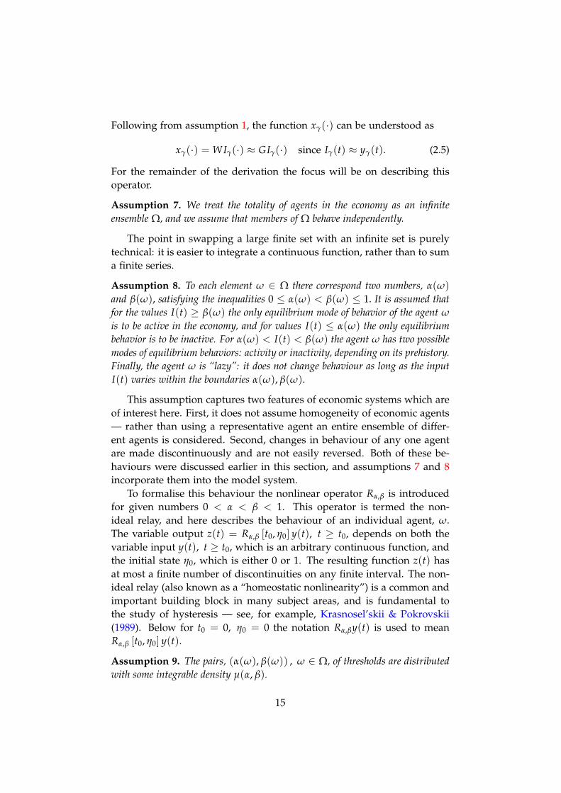
Assumption 8. To each element ω ∈ Ω there correspond two numbers, α(ω)

and β(ω), satisfying the inequalities 0 ≤ α(ω) < β(ω) ≤ 1. It is assumed that

for the values I(t) ≥ β(ω) the only equilibrium mode of behavior of the agent ω

is to be active in the economy, and for values I(t) ≤ α(ω) the only equilibrium

behavior is to be inactive. For α(ω) < I(t) < β(ω) the agent ω has two possible

modes of equilibrium behaviors: activity or inactivity, depending on its prehistory.

Finally, the agent ω is “lazy”: it does not change behaviour as long as the input

I(t) varies within the boundaries α(ω), β(ω).

This assumption captures two features of economic systems which areof interest here. First, it does not assume homogeneity of economic agents— rather than using a representative agent an entire ensemble of differ-ent agents is considered. Second, changes in behaviour of any one agentare made discontinuously and are not easily reversed. Both of these be-haviours were discussed earlier in this section, and assumptions 7 and 8incorporate them into the model system.

To formalise this behaviour the nonlinear operator Rα,β is introducedfor given numbers 0 < α < β < 1. This operator is termed the non-ideal relay, and here describes the behaviour of an individual agent, ω.The variable output z(t) = Rα,β [t0, η0] y(t), t ≥ t0, depends on both thevariable input y(t), t ≥ t0, which is an arbitrary continuous function, andthe initial state η0, which is either 0 or 1. The resulting function z(t) hasat most a finite number of discontinuities on any finite interval. The non-ideal relay (also known as a “homeostatic nonlinearity”) is a common andimportant building block in many subject areas, and is fundamental tothe study of hysteresis — see, for example, Krasnosel’skii & Pokrovskii(1989). Below for t0 = 0, η0 = 0 the notation Rα,βy(t) is used to meanRα,β [t0, η0] y(t).

Assumption 9. The pairs, (α(ω), β(ω)) , ω ∈ Ω, of thresholds are distributed

with some integrable density µ(α, β).

15

It is now possible to write

(WIγ)(t) =∫ 1

0

∫ 1

αz(α, β)µ(α, β)dαdβ

z(α, β) =(

Rα,β Iγ

)

(t), t ≥ 0

This is an expression of the Preisach nonlinearity, which was intro-duced in the context of ferromagnetism by Preisach (1935), but has founda more general applicability. In hydrology the independent domain model isequivalent to the Preisach nonlinearity, and was developed in parallel toit by Néel (1942,1943), Everett & Whitton (1952) and others. For a succinctexplanation of the development of the Preisach model, and its relation tothe independent domain model, see Mayergoyz (2003).

Returning to statements (2.3),(2.5), the relations become

(Gyγ)(t) =∫ 1

0

∫ 1

αz(α, β)µ(α, β)dαdβ

z(α, β) =(

Rα,βyγ

)

(t).(2.6)

Thus the principle system of equations can be written

x(t) = k(

I(t)− y(t))

x(t) =∫ 1

0

∫ 1

αz(α, β)µ(α, β)dαdβ

z(α, β) =(

Rα,βyγ

)

(t).

(2.7)

Once a density function µ(α, β) (sometimes called a Preisach function) isgiven this is a closed differential-operator system of equations. What formof density is suitable for use in this economic context is an open ques-tion. In this section a so-called “wedge density”, as described in Flynnet al. (2006) and McNamara (2008), is used for demonstration purposes.The use of this class of density follows from the analogy with fluid in aporous medium (wedge densities were first used in describing soil-waterhysteresis), but not from any compelling empirical justification. A shorternotation for (2.7) writes P [η0]y for the Preisach nonlinearity with a givendensity and an initial state η0. Then the system of equations can be ex-pressed as

x(t) = k(

I(t)− y(t))

x(t) =(

P [η0]y)

(t)(2.8)

This is a new type of equation, which has only recently been studied.The key feature of the equation, which is more clearly seen in the compact

16

notation, is that the action of the Preisach nonlinearity is under the highestderivative in the equations. This contrasts with the relatively well studiedcase of the Preisach nonlinearity on the right-hand side of such differentialoperator equations (i.e. x = f (x, t)+ (P x)(t)). Some of the main questionsin a mathematical sense, such as existence and uniqueness of solutions,have been addressed, see Flynn & Rasskazov (2005) and the referencestherein. What remains in this application is to examine the behaviour ofthis system in a qualitative sense, and assess whether it could be useful inan economic context. The next section attempts to address this question.

2.4 Dynamics of the system.

In this section some of the main qualitative features of the simple modelderived above are explored, with particular interest in the relevance tomodelling macroeconomic flows. The algorithm used for producing nu-merical trajectories of the system in (2.8) is taken from Flynn & Rasskazov(2005), and implemented in C++ (see appendix in McNamara (2008) forfurther details).

Looking at (2.8):

x(t) = k(

I(t)− y(t))

x(t) =(

P [η0]y)

(t)

there are three different components of the system — I(t) which is the“input” or control rate; y(t) which is the “equilibrium” rate; and x(t),which is the activity level (the rate of flow). In control terms, and sincex(·) and y(·) are “simply” related by the Preisach nonlinearity, the twofunctions x(·) and y(·) are “outputs” of the system, while I(·) is the soleinput. In this presentation, the main qualitative features of the model arebeing investigated, so the exact form of the density function in (2.7) is notimportant.

An example trajectory of the system is illustrated in figure 5. There area number of key features to be noted.

• The two “outputs” of the system – x(t) and y(t) – change directionat the same moments in time. In other words if y(t0) is an extremumof y(t) then x(t0) is an extremum of x(t).

• The graph of y(t) changes direction whenever it crosses the graph ofI(t). This is expected from the form of the equation, where the righthand side involves I(t)− y(t). This also means that turning points ofy (and thus x) are somewhat delayed with respect to turning pointsof I.

17

Input I(t)

Equilibrium rate y(t)

Output x(t)

Figure 5 – An example trajectory of the model equations, (2.8). The outputx(t) is on a different scale to the input, I(t) and equilibrium rate, y(t).

• Turning points of y(t) are “non-smooth”, giving a “shark-toothed”appearance. I immediately following a turning point, y(t) behavesin a near-linear fashion, and closely follows the graph of I(t).

• Some evidence of heterostasis in the behaviour of x(t) can be seen. In particular, there is a clear “upward” trend in x from the left of thediagram to the right.

The asymmetry of y(t) is of particular interest, as similar behaviour isseen in the dynamics of many economic indicators and financial stocks onintermediate to long timescales. Immediately following a turning pointin y(t) the rate of change of y is large in magnitude. Similar qualitativebehaviour can be observed in real systems. An example is the asymmetryaround turning points in the Dow Jones industrial share price Index. Thisis illustrated in figure 6.

2.4.1 Periodic inputs.

An interesting question to examine is the behaviour of the system in re-sponse to periodic inputs of different frequencies. This can give some veryuseful qualitative information, and is particularly interesting in the con-text of economics, where cycles of periods from less than a year to over50 years have been identified, for example in Schumpeter (1939). Outputscorresponding to specific periodic inputs do not accumulate to give out-puts of other inputs since the system is strongly nonlinear. However, thebehavior of such simple outputs can still shed some light on the contribu-tions to the output of the components of a general type of input.

18

10500

11000

11500

12000

12500

13000

13500

14000

02/07/2006 10/10/2006 18/01/2007 24/04/2007

Clo

sing V

alu

e

Date

Figure 6 – Historical data for the Dow Jones Industrial Average (DJIA). Theturning points in July ‘06 and around February ‘07 illustrate an asym-metric behaviour similar to that of y(t) in figure 5.

Given a periodic input function, I(t + T) = I(t), the correspondingoutputs, x(t) and y(t), also become periodic, with the same period —after some transients. By plotting pairs of the three components of thesystem, a loop structure can be seen. Each such pair illustrates qualitativefeatures of the system.

When two periodic functions are related by a Preisach nonlinearity andplotted against each other, the area enclosed by the loops is identified withdissipation caused by the action of the hysteresis. In physical systemsthese losses are easily identified, for example as energy lost to heat. Inan economic context these losses are more difficult to pin down, but arelikely to be caused by losses of potential output.

• Behaviour of loops: y against I

Plotting the equilibrium rate, y(t) against the input, I(t), there aretwo behaviours which are of interest — the transient behaviour,which depends on initial conditions, and the convergent loops.

The transient behaviour is shown in figure 7. The transient behaviourquickly dies down, and the trajectory converges to a closed loop.This loop is not dependent on the initial state of the system at t = 0,and so is entirely defined by the input function I(t).

The behaviour of the I − y loops for different frequencies is shownin figure 8, where the transient is discarded to leave the convergedloops for the different frequencies. These loops are vaguely ellipticalin shape, with “corners” at the highest and lowest points. For each

19

Input I(t)

Eq

uil

ibri

um

rat

e y(t

)

Figure 7 – The transient behaviour of y(t) for a simple periodic input func-tion I(t) with two different initial states. The two trajectories are in blueand green, it is clear that both converge to the same closed loop, shownin red.

Input I(t)

Eq

uil

ibri

um

rat

e y(t

)

Figure 8 – The long-time behaviour of y(t) plotted against I(t) for periodicinputs with different frequencies. The highest frequency in this image isshown in black, the lowest in red. The dashed black line passes throughthe corners on each loop.

frequency, these corners lie on the same straight line, which impliesa linear relationship between the frequency of I(t) and the ampli-tude of y(t). The equilibrium rate clearly responds more stronglyto a slowly changing I(t), approaching a linear relationship for verylow frequencies. Very high frequency inputs, in contrast, result inan equilibrium rate which changes less and less, becoming almostconstant. Note also that the loops have a common “centre” aroundwhich they are symmetrical.

• Behaviour of loops: x against I

Again, when plotting the output, x(t) , against the input, I(t), boththe transient and long-time behaviour are of interest. The transientbehaviour is shown in figure 9. In this case the transient behaviour

20

Input I(t)

Ou

tpu

t x(t

)

Figure 9 – The transient behaviour of x(t) for a given periodic I(t), with twodifferent initial states. The two trajectories are in blue and green, eachconverges to a different loop (both in red).

Input I(t)

Ou

tpu

t x(t

)

Figure 10 – The long-time behaviour of x(t) for periodic inputs of differ-ent frequency. The initial state is the same in each case. The highestfrequency is in black, the lowest in red.

for different initial states leads to different outcomes. The shapeof the loop to which each converges is the same, however they aredisplaced from each other by a constant.

The I − x loops for different frequencies are shown in figure 10. Verysimilar behaviour to that in figure 8 is seen, although the “corners”are not present here. Also different is the lack of a common “centre”around which the loops for all frequencies lie. Loops for lower fre-quencies have a higher average output, as well as a larger amplitude.

• Behaviour of loops: x against y The transient behaviour of x − y loopsis not as interesting as for the other cases. The final behaviour is veryinteresting however, and is shown in figure 11. Note that x and y arerelated by the Preisach nonlinearity, as stated in (2.8), i.e.:

x(t) =(

P [η0]y)

(t).

21

Output x(t)

Eq

uil

ibri

um

rat

e y(t

)

Figure 11 – Graphs of the output, x(t) against the equilibrium rate, y(t) fordifferent frequencies. The same colouring scheme is used as before.

Are

a o

f h

yst

eres

is l

oo

ps

Frequency

Figure 12 – Estimates of the areas of x − y loops per unit time,

i.e. 1T

∫ T0 y(t)dx(t).

In other applications there is a direct correspondence between thearea of these loops and the energy dissipated due to hysteresis. Asmentioned before, this can be interpreted as lost potential output inan economic context.

The areas of these loops were estimated for a large number of differ-ent periods. The results of this calculation as shown in figure 12. The“losses”, per unit time, for higher frequency inputs are substantiallylower than those for slower inputs.

22

Input I(t)

Output x(t)

Equilibrium rate y(t)

Figure 13 – The effect of a temporary shock on the system. I(t) is periodicexcept for a small region where a continuous perturbation is added. Theresulting y(t) quickly returns to pre-shock levels, x(t) displays hetero-static behaviour.

2.4.2 The effect of temporary shocks.

Of key importance to the model under consideration is the response totemporary stimuli — or shocks. As discussed in section 2.2, economicbehaviour does not “forget” the effects of boom periods or recessions.This heterostasis, therefore, is an important feature for any macroeconomicmodel to display.

It has already been established that the long-term behaviour of theoutput function x(t) depends specifically on the initial conditions of thesystem, while the equilibrium rate, y(t), does not. This suggests that het-erostasis is present in the I − x relationship, but not in that of I − y.

To test this, a simple periodic input function I(t) with a small shockwas used as the input of the system. This function is plotted with thecorresponding y(t) and x(t) in figure 13. As expected, y(t) is disturbed bythe shock, but quickly retains its former levels. In contrast x(t), the outputitself, is permanently altered by the influence of the shock, and does notreturn to previous levels.

This system is a particularly simple model, and can only serve as aprototype model in order to demonstrate the potential for models incoro-rating hysteresis. As such its clear derivation from first principles allowsfor qualitative behaviour to be matched closely to the associated assump-tions, and the richness of the behaviour to be demonstrated. In order to beuseful in a quantitative sense, however, work needs to be done in severaldirections, including the identification of a suitable Preisach density func-

23

tions, and fitting to actual data. We return to this question after the nextsection.

3 Hysteresis and price plasticity in analysis of supply

and demand.

In this section we apply the ideas developed in the previous section toanother key aspect of fundamental macroeconomic thought. The analysisof supply and demand curves is one of the central ideas behind neoclassi-cal qualitative economic analysis. They express the relationships betweenthe prices of products or services and the aggregate quantities demandedby the consumers or potentially supplied by producers at the prices inquestion.

The standard illustration of the supply and demand curves is shown infigure 14. Often they are represented as segments of straight lines (approx-imating more complex nonlinear functions on finite intervals). Economicstextbooks (for example Mankiw, 2006) use the horizontal axis for quantityof the product and the vertical axis for the price. Generally, it is assumedthat the supply curve S = fS(P), where S is the quantity that producerschoose to supply to the market at a particular price P, is a monotonouslyincreasing function of price P, and the demand curve D = fD(P), whereD is the quantity demanded by consumers at a particular price P, is amonotonously decreasing function of price P.

price

quantity0

supply

demand

Equilibriumquantity

Equilibriumprice

Figure 14 – Supply and demand curves.

The intersection of the two curves defines an equilibrium price and anequilibrium quantity of the product in question. The equilibrium price Peq

24

is the solution of the equation:

fS(·) = fD(·),

and the equilibrium quantity Qeq is defined by

Qeq = S = D.

The classical assumptions are that (a) all the of processes in the econ-omy occur at a slow pace without “frictions” (adiabatic process assump-tion); (b) the supply and demand curves are the same for rising and fallingprices (symmetry assumption); (d) tastes and production technologies donot change when prices are away from their equilibrium values; and (d)these curves do not change on the characteristic time scale of interest, (seeFisher, 1989). Under these assumptions the quantity of product on themarket and the price of the product both reach their respective equilib-rium values.

3.1 Supply with memory.

In real markets not all of the assumptions of the classical supply–demandmodel are satisfied. In particular, the characteristic times of the variousprocesses that take place in the economy do matter, and the final equilib-

rium production and price for a product or service may depend on thesecharacteristic times. Marshall (1890) used the example of the burningof cotton fields during the US Civil War of the 1860s to point out thatlearning by consuming, or by producing, produced shifts in demand andsupply that would remain after the cotton fields were replanted after thewar. In the often substantial time interval between investing in produc-tive capacity and bringing a product to the market, the market price couldwell change. This does not mean, though, that the production originallyplanned given a particular expected product price will cease if the actualprice turns out to be lower than expected. Once production has takenplace on the basis of an expected product price P1 = β it will only beeconomically sensible to cease production if the actual market price fallsto some P2 = α < β. This is due to the investment which has been sunk

in the production process, which includes the costs of product-specific in-vestment, the cost of expanding the workforce, etc., and is illustrated infigure 15. The values of β (start price) and α (stop price) are likely to be dif-ferent for various companies, depending on the local investment profile,the product-specificity of the investment, marketing exposure and othercompany-specific conditions. This means that the supply curve, in gen-eral, should behave differently for increases and decreases in price. This

25

α β

“on”

“off”

Price

Figure 15 – Individual firm’s production decision. If price rises above β,production starts if it was not already in progress. If the price is belowα, no production takes place. In the region between the two thresholds,either situation is possible. This type of system is known as a non-idealrelay, and underlies the Preisach nonlinearity

behaviour is related to the traditional notion of price elasticity in the samemanner as plasticity is related to elasticity in mechanics, hence the term“price plasticity”.

In the model that follows we retain a simple specification of the de-mand side of the market. Over the time frame used the shape of thedemand curve is assumed to be fixed. A “par” price will be defined asone lying on this demand curve. In the illustrative example discussed be-low we use a straight line with a negative slope to describe demand curvebehavior. In general, however, the demand curve could be a monotonicallydecreasing nonlinear function.

The main innovation comes in the specification of the supply side ofthe market (see Piscitelli et al., 1999). As the market price increases, newproducers may choose to join the already active ones in production, or ac-tive producers may choose to expand their production. The increase fromsome initial price to a new higher price stimulates additional productionand an increase in market supply. Thus the supply curve depends on thedistribution of the thresholds at which firms switch from inactivity to ac-tivity (β) or in the other direction (α). This distribution of thresholds is ameasure on the half plane β > α, and in the continuum limit can be mod-elled by a density function (the Preisach function mentioned in the previoussection) µ(α, β). The Preisach nonlinearity (2.6) as described in the pre-vious section describes the behaviour of such an aggregation of non-idealrelays. A good interactive demostration of the Preisach nonlinearity can befound at the interactive website by Flynn et al. (web page). A major effectof Preisach hysteretic behaviour is that the supply relationship now alsodepends upon the prehistory of the price, and not just the current valueof the price. The “loop” behaviour of hysteretic systems, in particular thePreisach nonlinearity, is shown in figure 16. For a given value of the input

26

Input

Output

Figure 16 – The Preisach nonlinearity, illustrating the major hysteresis loop(blue) and a smaller secondary loop (green).

(price in our application), an interval of possible outputs (supply here)exists. The particular branch taken is determined by the prehistory of theinput — in particular the non-dominated extremum values of the input.

There is a finite adjustment time for both prices and production. If thesystem finds itself shocked away from a particular equilibrium it will try torestore some other equilibrium through price adjustments and/or changesin the level of production. However, these changes are not instantaneous.The characteristic times of price and output adjustments (or, more exactly,their inverses) are parameters in the model.

3.2 Model definition.

The dynamics of the system described above can be presented in terms ofthe variables Q (total quantity of production) and P (market price) by thefollowing system of operator-differential equations incorporating Preisachhysteresis.

dQ

dt= k1 (S − Q) ,

dP

dt= k2

(

Ppar − P)

,

S = P [η0] P, (hysteresis link)

Ppar = FD(Q).

The parameters k1 and k2 are, as mentioned, the inverse characteristic ad-justment times for production and price respectively. The interaction linksare S = P [η0] P, which is a Preisach nonlinearity, the main innovation in

27

this model; and Ppar = FD(Q), which is the “par” price based upon thedemand curve. In other words, FD(Q) is the price that would be requredto clear the market given a production quantity of Q. The demand curveis assumed to be fixed over the time-scale of the model.

The system is determined fully by the choice of suitable initial con-ditions. These include the initial price and production levels, P0 and Q0

respectively, and an initial state, η0, for the Preisach nonlinearity in thehysteresis link. The system will evolve to an equilibrium state, as in theclassical model. In this model, however, a range of possible equilibriumprice–output pairs arises. This is illustrated in figure 17, where the enve-lope curves of the hysteresis link are plotted with the demand curve. Theparticular demand curve and Preisach nonlinearity shown in the figureswere chosen for illustrative purposes.5

.

.

.

.

.

.. . . . . .

Demandcurve Supply “curve”

(hysteresisenvelope)

Possible equilibria

Figure 17 – Hysteresis envelope (blue) and demand curve (green), showingthe range of allowable equilibrium points (red). Any point within theenvelope is an allowable input-output pair for the Preisach nonlinearity.This leads to an interval of allowable equilibrium prices. The partic-ular price “chosen” by the system depends on the prehistory of pricevariations.

This system is closed by the choice of initial conditions — both theinitial price-output pair, (P0, Q0), and an initial state for the Preisach non-linearity, which encodes prior variations in the price. The eventual rangeof equilibrium values of P and Q are determined by these choices. Anextreme example is given in figure 18, where the same initial price andoutput conditions give rise to very different equilibria due to differences inthe initial state of the Preisach nonlinearity. This extreme example brings

5The Preisach nonlinearity in these illustration uses a “uniform” density, where allthreshold pairs (α, β) are equally likely. This is purely for simplicity because the typeof density functions to use in economic models is an open question. In an econometricapplication to explaining unemployment time series (Darby et al., 2006) the estimates werenot sensitive to the density functions used.

28

out the qualitative property that the equilibrium price and output levelsdepend on past variations in the market price. Introducing hysteretic ef-fects into a model of supply and demand dynamics provides for a muchricher behaviour, where past shocks have permanent effect on market out-comes.

.

.

.

.

.

.. . . . . .

Demandcurve

Supply “curve”(hysteresis)

Figure 18 – Evolution of the system to equilibrium price/production levels.The same initial values P0 and Q0 give rise to different equilibria due tothe influence of historical price variations.

4 Conclusions.

The purpose of this paper has been to investigate the implications of relax-ing some fundamental assumptions in mainstream macroeconomic theory.When applied to some very simple example models, this change leads toheterostasis and the persistence of the effects of temporary shocks. Hys-teresis effects are very plausible characteristics of economic behaviour, andthe simple models outlined show how hysteresis can be introduced intothe bedrock of economic assumptions. Further, the use of the Preisachnonlinearity is a link between micro-level behaviour, in the form of thenon-ideal relay, and aggregate macroeconomic outcomes. This integrationof micro and macro analysis provides an important contribution to thepost-Walrasian reconstruction of macroeconomics.

A major open question in efforts to use the Preisach nonlinearity inmacroeconomic modelling is the identification problem — finding a suit-able Preisach density function for the distribution decision thresholds.Empirical implementation requires being able to identify such densityfunctions. Some of the suitable data is not publicly available due to com-mercial sensitivity (an example considered in Twomey (2008) is the Irishmobile phone market). A further possibility is the use of experimentalmethods to identify switching points and their distributions.

29

Acknowledgements.

Leonid Kalachev was partially supported by the University of Montanafaculty exchange grant. Some of this research was carried out while HughMcNamara was supported by IRCSET Embark grant RS/2004/92. A por-tion of this paper is adapted from McNamara (2008).

References

Bertotti, G. & Mayergoyz, I. D. (eds) 2006 The science of hysteresis. Amster-dam: Elsevier Academic Press.

Blanchard, O. J. 2008 The state of macro. MIT Dept. Economics Working

Paper (SSRN eLibrary), (08–12).

Brokate, M. & Sprekels, J. 1996 Hysteresis and phase transitions, vol. 121 ofApplied Mathematical Sciences. New York: Springer-Verlag.

Caballero, R., Farhi, E. & Hammour, M. L. 2006 Speculative growth: Hintsfrom the us economy. American Economic Review, 96(4), 1159–1192.

Calvo, G. A., Izquierdo, A. & Talvi, E. 2006 Phoenix miracles in emerg-ing markets: recovering without credit from systemic financial crises.NBER Working Paper 12101, National Bureau of Economic Research,Cambridge, MA.

Cerra, V. & Saxena, S. C. 2005 Growth dynamics: the myth of economic re-covery. IMF Working Paper WP/05/147, International Monetary Fund.

Cerra, V. & Saxena, S. C. 2008 Growth dynamics: The myth of economicrecovery. American Economic Review, 98(1), 439–57.

Colander, D. (ed.) 2006 Post Walrasian macroeconomics: Beyond the dynamic

stochastic general equilibrium model. Cambridge University Press.

Colander, D., Follmer, H., Haas, A., Goldberg, M. D., Juselius, K., Kirman,A., Lux, T. & Sloth, B. 2009 The financial crisis and the systemic fail-ure of academic economics. University of Copenhagen Dept. of Economics

Discussion Paper (SSRN eLibrary), (09–03).

Cross, R. 1993 On the foundations of hysteresis in economic systems. Eco-

nomics and Philosophy, 9(1), 53–74.

Cross, R., Grinfeld, M. & Lamba, H. 2009 Hysteresis and economics. Con-

trol Systems Magazine, IEEE, 29(1), 30–43. (doi:10.1109/MCS.2008.930445)

30

Darby, J., Cross, R. & Piscitelli, L. 2006 Hysteresis and unemployment: apreliminary investigation. In Bertotti & Mayergoyz (2006), pp. 667–699.

Dixit, A. K. & Pindyck, R. S. 1994 Investment under uncertainty. PrincetonUniversity Press.

Everett, D. H. & Whitton, W. I. 1952 A general approach to hysteresis.Transactions of the Faraday Society, 48, 749–757.

Ewing, J. A. 1881 On the production of transient electric currents in ironand steel conductors by twisting them when magnetised or magnetisingthem when twisted. Proceedings of the Royal Society of London, 33, 21–23.(doi:10.1098/rspl.1881.0067)

Ewing, J. E. 1890 On hysteresis in the relation of strain to stress. Reports of

the British Society for the Advancement of Science, 59, 502–504.

Fisher, F. M. 1989 Disequilibrium foundations of equilibrium economics. Eco-nomic Society Monographs. Cambridge University Press. (doi:10.2277/0521378567)

Fisher, I. 1925 Mathematical investigation in the theory of value and prices. YaleUniversity Press, New Haven.

Flynn, D., McNamara, H., O’Kane, P. & Pokrovskii, A. V. 2006 Applicationof the Preisach model to soil-moisture hysteresis. In Bertotti & Mayer-goyz (2006), pp. 689–744.

Flynn, D. & Rasskazov, O. 2005 On the integration of an ODE involvingthe derivative of a preisach nonlinearity. Journal of Physics: Conference

Series, 22, 43–55.

Flynn, D., Rasskazov, O., Zhezherun, A. & Donnegan, M. web page Sys-tems with hysteresis. http://euclid.ucc.ie/hysteresis/. Dept. Ap-plied Maths, University College Cork.

Fonseca, G. L. web page The history of economic thought web-site. http://homepage.newschool.edu/het. Dept. of Economics, NewSchool for Social Research, New York.

Friedman, M. 1993 The “plucking model” of business fluctuations revis-ited. Economic Enquiry, 31(2), 171–177.

Göcke, M. 2002 Various concepts of hysteresis applied in economics. Jour-

nal of Economic Surveys, 16(2), 167–188.

31

Goldman, M. S., Levine, J. H., Major, G., Tank, D. W. & Seung, H. a. 2003Robust persistent neural activity in a model integrator with multiplehysteretic dendrites per neuron. Cerebral Cortex, 13(11), 1185–1195. (doi:10.1093/cercor/bhg095)

Haines, W. B. 1925 Studies in the physical properties of soils. II. A noteon the cohesion developed by capillary forces in an ideal soil. Journal of

Agricultural Science, 15, 529–535.

Haines, W. B. 1930 Studies in the Physical Properties of Soil: V. The hys-teresis effect in Capillary Properties, and the Modes of Moisture Distri-bution Associated Therewith. Journal of Agricultural Science, pp. 97–116.

Hamilton, J. D. 1989 A new approach to the economic analysis of nonsta-tionary time series and the business cycle. Econometrica, 57(2), 357–384.

Hoover, K. 2009 Microfoundations and the ontology of macroeconomics.In The Oxford handbook of philosophy of economics (eds H. Kincaid &D. Ross), chap. 14, pp. 386–409. Oxford University Press.

Keynes, J. M. 1934 Poverty in plenty: is the economic system self-adjusting? The Listener, BBC, London, November 21.

Kindleberger, C. P. 2000 Manias, panics and crashes: a history of financial

crises. New York: Wiley, 4th edn.

Kirman, A. 2006 Foreword. In Colander (2006), p. xiii.

Krasnosel’skii, M. A. & Pokrovskii, A. V. 1989 Systems with hysteresis.Berlin: Springer-Verlag.

Lorente, P., Delgado, C., Delmar, M., Henzel, D. & Jalife, J. 1991 Hysteresisin the excitability of isolated guinea pig ventricular myocytes. Circ Res,69(5), 1301–1315.

Mankiw, N. G. 2006 Principles of macroeconomics (4th ed.). South-WesternCollege Publishing.

Marshall, A. 1890 Principles of economics. London: Macmillan.

Mayergoyz, I. D. 1991 Mathematical models of hysteresis. Berlin: Springer-Verlag.

Mayergoyz, I. D. 2003 Mathematical models of hysteresis and their applications.Amsterdam: Elsevier.

32

McNamara, H. 2008 Development and analysis of macroeconomic modelsincorporating Preisach hysteresis. Ph.D. thesis, Department of AppliedMathematics, University College Cork.

Mirowski, P. 1989 More heat than light. Cambridge University Press.

Néel, L. 1942,1943 Theories des lois d’aimantation de Lord Rayleigh.Cahiers de Physique, 12 & 13, 1–20, 19–30.

Phillips, A. W. 1950 Mechanical models in economic dynamics. Economica,17(67), 283–305.

Piscitelli, L., Grinfeld, M., Lamba, H. & Cross, R. 1999 On entry and exitin response to aggregate shocks. Applied Economics Letters, 6(9), 569–72.

Preisach, F. 1935 Über die magnetische nachwirkung. Zeitschrift für Physik,94(5–6), 277–302.

Schumpeter, J. A. 1939 Business cycles: a theoretical, historical and statistical

analysis of the capitalist process. New York: McGraw-Hill.

Tompsett, G. A., Krogh, L., Griffin, D. W. & Conner, W. C. 2005 Hystere-sis and scanning behavior of mesoporous molecular sieves. Langmuir,21(18), 8214–8225. (doi:10.1021/la050068y)

Twomey, C. 2008 Hysteresis in consumer markets with focus on the mobilecommunications market. In International workshop on multi-rate processes

and hysteresis, vol. 138 of Journal of Physics: Conference Series.

Visintin, A. 1994 Differential models of hysteresis, vol. 111 of Applied Mathe-

matical Sciences. Berlin: Springer-Verlag.

33

RECENT REPORTS51/10 STOCHSIMGPU Parallel stochastic simulation for the Systems

Biology Toolbox 2 for MATLABKlingbeilErbanGilesMaini

52/10 Order parameters in the Landau-de Gennes theory - the staticand dynamic scenarios

Majumdar

53/10 Liquid Crystal Theory and Modelling Discussion Meeting MajumdarMottram

54/10 Modeling the growth of multicellular cancer spheroids in a bioengi-neered 3D microenvironment and their treatment with an anti-cancer drug

LoessnerFleggByrneHallMoroneyClementsHutmacherMcElwain

55/10 Scalar Z, ZK, KZK, and KP equations for shear waves in incom-pressible solids

DestradeGorielySaccomandi

56/10 The Influence of Bioreactor Geometry and the Mechanical Envi-ronment on Engineered Tissues

OsborneODeaWhiteleyByrneWaters

57/10 A numerical guide to the solution of the bidomain equations ofcardiac electrophysiology

PathmanathanBernabeuBordasCooperGarnyPitt-FrancisWhiteleyGavaghan

58/10 Particle-scale structure in frozen colloidal suspensions from smallangle X-ray scattering

SpannuthMochriePeppinWettlaufer

59/10 Spin coating of an evaporating polymer solution MunchPleaseWagner

60/10 Stochastic synchronization of neuronal populations with intrinsicand extrinsic noise

BressloffLai

61/10 Metastable states and quasicycles in a stochastic Wilson-Cowanmodel of neuronal population dynamics

Bressloff

62/10 Adsorption and desorption dynamics of citric acid anions in soil OburgerLeitnerJonesZygalakisSchnepf

66/10 Dynamics of colloidal particles in ice SpannuthMochriePeppinWettlaufer

01/11 Improving the efficiency of optical coherence tomography by usingthe non-ideal behaviour of a polarising beam splitter

LippokNielsenVanholsbeeck

02/11 Self-diffusion in remodelling and growth EpsteinGoriely

03/11 Spontaneous rotational inversion in Phycomyces GorielyTabor

04/11 From individual to collective behaviour of coupled velocity jumpprocesses: a locust example

ErbanHaskovec

05/11 Solving Eigenvalue problems on curved surfaces using the closestpoint method

MacDonaldBrandmanRuuth

06/11 A numerical methodology for the Painleve equations FornbergWeideman

07/11 Strong stability preserving two-step Runke-Kutta methods KetchesonGotliebMacDonald

Copies of these, and any other OCCAM reports can be obtainedfrom:

Oxford Centre for Collaborative Applied MathematicsMathematical Institute

24 - 29 St Giles’Oxford

OX1 3LBEngland

www.maths.ox.ac.uk/occam