Position Self-Sensing in the Presence of Creep, Hysteresis ...
189
Position Self-Sensing in the Presence of Creep, Hysteresis, and Self-Heating for Piezoelectric Actuators by Mohammad Nouroz Islam B.Sc. in Industrial and Production Engineering, Bangladesh University of Engineering and Technology, 2005 M.Sc. in Industrial and Production Engineering, Bangladesh University of Engineering and Technology, 2008 A THESIS SUBMITTED IN PARTIAL FULFILLMENT OF THE REQUIREMENTS FOR THE DEGREE OF DOCTOR OF PHILOSOPHY in THE COLLEGE OF GRADUATE STUDIES (Mechanical Engineering) THE UNIVERSITY OF BRITISH COLUMBIA (Okanagan) July 2013 © Mohammad Nouroz Islam, 2013
-
Upload
khangminh22 -
Category
Documents
-
view
2 -
download
0
Transcript of Position Self-Sensing in the Presence of Creep, Hysteresis ...

Position Self-Sensing in the Presence ofCreep, Hysteresis, and Self-Heating for
Piezoelectric Actuatorsby
Mohammad Nouroz Islam
B.Sc. in Industrial and Production Engineering, Bangladesh University of Engineeringand Technology, 2005
M.Sc. in Industrial and Production Engineering, Bangladesh University of Engineeringand Technology, 2008
A THESIS SUBMITTED IN PARTIAL FULFILLMENT OFTHE REQUIREMENTS FOR THE DEGREE OF
DOCTOR OF PHILOSOPHY
in
THE COLLEGE OF GRADUATE STUDIES
(Mechanical Engineering)
THE UNIVERSITY OF BRITISH COLUMBIA
(Okanagan)
July 2013
© Mohammad Nouroz Islam, 2013
Abstract
Piezoelectric ceramic actuators are widely used in micro-/nano-positioningsystems due to expedient characteristics such as fast response time, high stiff-ness, high resolution, etc. However, nonlinear effects such as hysteresis andcreep affect the position accuracy of the systems if not compensated. Often,feedback position sensors are mounted to the systems to eliminate hysteresisand creep. Nonetheless, installation of feedback sensors can be prohibitive dueto space constraints, reliability and cost. Alternatively, position self-sensing tech-niques are used to eliminate the position sensor. In this research, the objectiveis to develop a position self-sensing technique considering the nonlinear effects.To model the actuators for control or self-sensing, they are often considered ascapacitive elements. A novel real-time impedance measurement technique isdeveloped based on high frequency measurements to obtain clamped capaci-tance. Based on the real-time measurement, an improved constitutive modeland parameter identification technique is presented which includes the posi-tion dependent capacitance. As a means for position self-sensing, position islinearly related to charge. However, charge measurement is prone to drift andrequire sophisticated hardware to implement. The new relationship betweenposition and capacitance opens a new avenue for non-traditional position self-sensing; however, due to measurement noise, this new technique is only usefulfor slow operations. In this research, a novel position observer is presented thatfuses the capacitance-based self-sensing with the traditional charge-based self-sensing. This allows the position estimation over a frequency band ranges from0Hz to 125Hz where creep and rate-dependent hysteresis are observed. The es-timation error is close to 3% when compared to a position sensor. Continuousoperations at frequencies larger than 20Hz contribute to self-heat generation inthe actuators. This elevated temperature is detrimental to the performance andlife of the actuator. In this research, a self-heat generation model is presentedbased on power loss in the actuator to predict the temperature rise. The pre-dicted temperature is then used to compensate the temperature related varia-tion in the position observer. The temperature prediction error is less than 2◦Cwhich creates a position estimation error close to 4% up to a temperature varia-tion of 55◦C.
ii
Preface
The thesis presents the research findings on position self-sensing and con-
trol of piezoelectric actuator which was conducted in the Control and Automa-
tion Laboratory, at the School of Engineering, UBC, under supervision of Dr.
Rudolf Seethaler. Part of the thesis has been published in peer-reviewed jour-
nals and conference proceedings. The contributions highlighted in the thesis
are as follows:
A novel real-time piezoelectric impedance measurement technique is pre-
sented in Chapter 3 which was published in World Intellectual Property Orga-
nization in November 2012 for a patent application as "Apparatus and Method
for In Situ Impedance Measurement of a Piezoelectric Actuator"1. The results
and the measurement technique were also published in IEEE Canadian Confer-
ence for Electrical and computer engineering in 2011 as "Hysteresis indepen-
dent on-line capacitance measurement for piezoelectric stack actuators"2. The
technique was developed by Dr. Seethaler while I was responsible for experi-
mental validation and writing the conference manuscript.
In Chapter 4, an improved electromechanical model for piezoelectric actua-
tors is presented that employs the real-time impedance measurement technique
developed in Chapter 3. Part of the chapter was published in the Journal of
Intelligent Material, Systems and Structures published by Sage Journals as "An
Improved Electromechanical Model and Parameter Identification Technique for
Piezoelectric Actuators"3. The article presents a novel method to identify the pa-
1Rudolf J. Seethaler, and Islam, Mohammad N. "Apparatus and method for in situ impedancemeasurement of a piezoelectric actuator", WO2012149649, WIPO, (2012).
2Islam, Mohammad, N., Rudolf J., Seethaler, and Mumford, David. "Hysteresis independenton-line capacitance measurement for piezoelectric stack actuators." Electrical and Computer En-gineering (CCECE), 24th Canadian Conference on. IEEE, (2011):1149–1153.
3Islam, Mohammad N., and Rudolf J. Seethaler. "An improved electromechanical model andparameter identification technique for piezoelectric actuators." Journal of Intelligent Material
iii

Preface
rameters of the electromechanical piezoelectric model. My responsibility was to
simulate the model, conduct experiments to validate the model and prepare the
manuscript.
A novel position observer is presented in Chapter 5 which partly is published
in IEEE/ASME Transaction on Mechatronics as "Sensorless Position Control for
Piezoelectric Actuators Using a Hybrid Position Observer"4. The observer is able
to predict the position of the piezoelectric actuator over a wide range of fre-
quencies where nonlinearities such as creep and rate-dependent hysteresis take
place. The results of creep and rate dependent hysteresis in open loop condi-
tion presented in this chapter is published in Review of Scientific Instruments as
"Note: Position self-sensing for piezoelectric actuators in the presence of creep
and rate-dependent hysteresis"5. Experimental results of closed loop control
are presented in Chapter 6 which are partly published in IEEE/ASME Transac-
tion on Mechatronics4. My roles were to conduct the experiments, analyze the
data and prepare the manuscript for the articles.
Finally, a new model for self-heat generation is presented in Chapter 7 where
power loss due to self-heating is yielded to estimate the temperature increase
in piezoelectric actuators. A version of this chapter is submitted in Review of
Scientific Instruments entitled as "Real-Time Temperature Estimation Due To
Self-Heating in Piezoelectric Actuators"6. In this study, I developed the self-heat
generation model, conduct the experimental validation of the model and pre-
pare the manuscript for the article. In accordance to the copyright law, the pub-
lished materials in the journals, transactions and conference proceedings are
included with the permission of the publishers.
Systems and Structures (2013):1049–1058.4Islam, Mohammad N., and Rudolf J. Seethaler. "Sensorless position control for piezoelec-
tric actuators using a hybrid position observer." Mechatronics, IEEE/ASME Transactions on,(2013):1âAS-9.
5Islam, Mohammad N., and Rudolf J. Seethaler. "Note: Position self-sensing for piezoelectricactuators in the presence of creep and rate-dependent hysteresis." Review of Scientific Instru-ments (2012): 116101–116103.
6Islam, Mohammad N., and Rudolf J. Seethaler. "Real-time temperature estimation due to self-heating in piezoelectric actuators." Review of Scientific Instruments(2013): submitted.
iv

Table of Contents
Abstract . . . . . . . . . . . . . . . . . . . . . . . . . . . . . . . . . . . . . . . ii
Preface . . . . . . . . . . . . . . . . . . . . . . . . . . . . . . . . . . . . . . . . iii
Table of Contents . . . . . . . . . . . . . . . . . . . . . . . . . . . . . . . . . . v
List of Tables . . . . . . . . . . . . . . . . . . . . . . . . . . . . . . . . . . . . . x
List of Figures . . . . . . . . . . . . . . . . . . . . . . . . . . . . . . . . . . . . xii
Glossary of Notation . . . . . . . . . . . . . . . . . . . . . . . . . . . . . . . . xvi
Acknowledgments . . . . . . . . . . . . . . . . . . . . . . . . . . . . . . . . . xviii
Dedication . . . . . . . . . . . . . . . . . . . . . . . . . . . . . . . . . . . . . . xx
Chapter 1: Introduction and Literature Review . . . . . . . . . . . . . . 1
1.1 Piezoelectricity . . . . . . . . . . . . . . . . . . . . . . . . . . . . . . . 2
1.2 Hysteresis . . . . . . . . . . . . . . . . . . . . . . . . . . . . . . . . . . 5
1.3 Creep . . . . . . . . . . . . . . . . . . . . . . . . . . . . . . . . . . . . 7
1.4 Vibration . . . . . . . . . . . . . . . . . . . . . . . . . . . . . . . . . . 8
1.5 Piezoelectric Actuators (PEAs) . . . . . . . . . . . . . . . . . . . . . . 9
1.5.1 Stack Actuators . . . . . . . . . . . . . . . . . . . . . . . . . . 10
1.5.2 Bender Actuators . . . . . . . . . . . . . . . . . . . . . . . . . 10
1.6 Piezoelectric Actuator Modeling . . . . . . . . . . . . . . . . . . . . . 11
1.6.1 Linear IEEE Model . . . . . . . . . . . . . . . . . . . . . . . . 11
1.6.2 Nonlinear Physical Model . . . . . . . . . . . . . . . . . . . . 12
v

TABLE OF CONTENTS
1.6.3 Phenomenological Model . . . . . . . . . . . . . . . . . . . . 18
1.6.3.1 Rate-independent Model . . . . . . . . . . . . . . 19
1.6.3.2 Rate-dependent Model . . . . . . . . . . . . . . . 23
1.6.3.3 Other Phenomenological Hysteresis Models . . . 24
1.6.4 Cascaded Phenomenological Model for Hysteresis, Creep,
and Vibrational Dynamics . . . . . . . . . . . . . . . . . . . 24
1.7 Position Control of PEA . . . . . . . . . . . . . . . . . . . . . . . . . . 25
1.7.1 Feedforward (FF) Voltage Control . . . . . . . . . . . . . . . 26
1.7.2 Feedback (FB) Voltage Control . . . . . . . . . . . . . . . . . 27
1.7.3 Feedforward/Feedback (FF/FB) Control Scheme . . . . . . 30
1.7.4 Charge Control Scheme . . . . . . . . . . . . . . . . . . . . . 31
1.7.5 Integrated Voltage/Charge Control . . . . . . . . . . . . . . 32
1.8 Position Self-sensing (PSS) . . . . . . . . . . . . . . . . . . . . . . . . 33
1.8.1 PSS Using Capacitance Bridge . . . . . . . . . . . . . . . . . 33
1.8.2 PSS Using Charge Measurement . . . . . . . . . . . . . . . . 35
1.8.3 PSS Using Piezoelectricity . . . . . . . . . . . . . . . . . . . . 36
1.9 Errors in Piezoelectric Positioning . . . . . . . . . . . . . . . . . . . 38
1.10 Self-Heating . . . . . . . . . . . . . . . . . . . . . . . . . . . . . . . . 41
1.11 Scope of the Work and Objectives . . . . . . . . . . . . . . . . . . . . 42
1.12 Thesis Organization . . . . . . . . . . . . . . . . . . . . . . . . . . . . 45
Chapter 2: Experimental Setup . . . . . . . . . . . . . . . . . . . . . . . . 47
2.1 Mechanical Components . . . . . . . . . . . . . . . . . . . . . . . . . 47
2.1.1 Actuator . . . . . . . . . . . . . . . . . . . . . . . . . . . . . . 48
2.1.2 Frame . . . . . . . . . . . . . . . . . . . . . . . . . . . . . . . 48
2.1.3 Preload Assembly . . . . . . . . . . . . . . . . . . . . . . . . . 50
2.1.4 Needle . . . . . . . . . . . . . . . . . . . . . . . . . . . . . . . 50
2.1.5 Ball Seats . . . . . . . . . . . . . . . . . . . . . . . . . . . . . . 50
2.2 Electrical Components . . . . . . . . . . . . . . . . . . . . . . . . . . 52
2.2.1 Piezoelectric Actuator Driver . . . . . . . . . . . . . . . . . . 52
2.2.2 Current Sensor . . . . . . . . . . . . . . . . . . . . . . . . . . 52
2.2.3 Force Sensor . . . . . . . . . . . . . . . . . . . . . . . . . . . . 53
2.2.4 Position Sensor . . . . . . . . . . . . . . . . . . . . . . . . . . 53
vi

TABLE OF CONTENTS
2.2.5 Temperature Sensor . . . . . . . . . . . . . . . . . . . . . . . 53
2.2.6 Data Acquisition . . . . . . . . . . . . . . . . . . . . . . . . . 55
2.3 Summary . . . . . . . . . . . . . . . . . . . . . . . . . . . . . . . . . . 56
Chapter 3: Impedance Measurement . . . . . . . . . . . . . . . . . . . . 57
3.1 Measurement Principle . . . . . . . . . . . . . . . . . . . . . . . . . . 58
3.2 Superpositioning Through Summing Circuit . . . . . . . . . . . . . 58
3.3 Superpositioning Through Boost Converter . . . . . . . . . . . . . . 59
3.4 Effect of Frequency on the Actuator Capacitance . . . . . . . . . . . 59
3.5 Impedance Measurement Algorithm . . . . . . . . . . . . . . . . . . 63
3.5.1 Selection of the Sampling Frequency . . . . . . . . . . . . . 63
3.5.2 Real-time Fourier Transformation . . . . . . . . . . . . . . . 67
3.5.3 Parameter Identification from Fourier Series Coefficients . 68
3.6 Results . . . . . . . . . . . . . . . . . . . . . . . . . . . . . . . . . . . . 69
3.7 Summary . . . . . . . . . . . . . . . . . . . . . . . . . . . . . . . . . . 74
Chapter 4: An Improved Electromechanical Model for Piezoelectric Ac-
tuators . . . . . . . . . . . . . . . . . . . . . . . . . . . . . . . . 76
4.1 Proposed Piezoelectric Model . . . . . . . . . . . . . . . . . . . . . . 80
4.1.1 Mechanical Subsystem . . . . . . . . . . . . . . . . . . . . . 80
4.1.2 Electrical Subsystem . . . . . . . . . . . . . . . . . . . . . . . 80
4.2 Power Balance . . . . . . . . . . . . . . . . . . . . . . . . . . . . . . . 84
4.3 Parameter Identification . . . . . . . . . . . . . . . . . . . . . . . . . 85
4.3.1 Identification of α, k, b, and m for the Traditional Model
with Constant Capacitance . . . . . . . . . . . . . . . . . . . 85
4.3.2 Identification of α, k, b, and m for the Proposed Model
with Variable Capacitance . . . . . . . . . . . . . . . . . . . 86
4.3.3 Identification of Free Capacitance, CT . . . . . . . . . . . . 88
4.3.4 Identification of Material Properties . . . . . . . . . . . . . . 89
4.3.4.1 Piezoelectric Strain or Charge Coefficient, d33 . . 89
4.3.4.2 Piezoelectric Coupling Coefficient, k33 . . . . . . 90
4.4 Experimental Results . . . . . . . . . . . . . . . . . . . . . . . . . . . 90
4.4.1 Experimental Procedure . . . . . . . . . . . . . . . . . . . . . 90
vii
TABLE OF CONTENTS
4.4.2 Model Validation Through Charge-position Relationship . 93
4.4.3 Hysteresis Voltage . . . . . . . . . . . . . . . . . . . . . . . . 95
4.5 Summary . . . . . . . . . . . . . . . . . . . . . . . . . . . . . . . . . . 97
Chapter 5: Position Self-sensing of Piezoelectric Actuators . . . . . . . 98
5.1 Charge Based Position Self-sensing, xI . . . . . . . . . . . . . . . . . 102
5.2 Capacitance Based Position Self-sensing, xCP . . . . . . . . . . . . . 104
5.3 Hybrid Position Observer Design . . . . . . . . . . . . . . . . . . . . 108
5.4 Hybrid Position Observer Implementation . . . . . . . . . . . . . . 111
5.5 Open Loop HPO Performance . . . . . . . . . . . . . . . . . . . . . . 111
5.6 Summary . . . . . . . . . . . . . . . . . . . . . . . . . . . . . . . . . . 116
Chapter 6: Self-sensing Position Control of Piezoelectric Actuators . . 117
6.1 The Integral Controller . . . . . . . . . . . . . . . . . . . . . . . . . . 117
6.2 Experimental Results . . . . . . . . . . . . . . . . . . . . . . . . . . . 119
6.2.1 Step Profile with Variable Strokes, P1 . . . . . . . . . . . . . 119
6.2.2 Sinusoidal Profile with Different Frequencies, P2 . . . . . . 120
6.2.3 DC Profile with Fast Transient Section, P3 . . . . . . . . . . 131
6.3 Summary . . . . . . . . . . . . . . . . . . . . . . . . . . . . . . . . . . 132
Chapter 7: Self-heat Generation . . . . . . . . . . . . . . . . . . . . . . . 133
7.1 Proposed Model . . . . . . . . . . . . . . . . . . . . . . . . . . . . . . 135
7.2 Experimental Approach . . . . . . . . . . . . . . . . . . . . . . . . . . 136
7.3 Parameter Identification . . . . . . . . . . . . . . . . . . . . . . . . . 138
7.4 Temperature Prediction Using a Dedicated Position Sensor . . . . 141
7.5 Temperature Compensation of HPO . . . . . . . . . . . . . . . . . . 144
7.6 Temperature and Position Predictions Using the HPO and the Self-
Heating Model . . . . . . . . . . . . . . . . . . . . . . . . . . . . . . . 147
7.7 Summary . . . . . . . . . . . . . . . . . . . . . . . . . . . . . . . . . . 152
Chapter 8: Conclusions and Future Research . . . . . . . . . . . . . . . . 153
8.1 Conclusions . . . . . . . . . . . . . . . . . . . . . . . . . . . . . . . . 153
8.2 Future Research . . . . . . . . . . . . . . . . . . . . . . . . . . . . . . 156
viii

TABLE OF CONTENTS
Bibliography . . . . . . . . . . . . . . . . . . . . . . . . . . . . . . . . . . . . 158
ix

List of Tables
Table 1.1 Comparison of the feedback sensors . . . . . . . . . . . . . . 29
Table 1.2 Error comparison between different models . . . . . . . . . 40
Table 2.1 Actuator properties . . . . . . . . . . . . . . . . . . . . . . . . 49
Table 3.1 Sampling frequency and folded ripple frequency at differ-
ent values of ns with four times folding . . . . . . . . . . . . 67
Table 3.2 Passband and bandwidth as a function of sampling peri-
ods for a 48 kHz sampling frequency, and ns = 12 . . . . . . 68
Table 4.1 Comparison of parameters from different piezoelectric mod-
els . . . . . . . . . . . . . . . . . . . . . . . . . . . . . . . . . . 79
Table 4.2 Model parameter identification . . . . . . . . . . . . . . . . 92
Table 4.3 Sensitivity of parameter identification to changes in ca-
pacitance measurement . . . . . . . . . . . . . . . . . . . . . 94
Table 5.1 Fitting errors in regression models of different orders . . . . 106
Table 5.2 ANOVA table for capacitance based PSS regression model . 107
Table 5.3 Hybrid position observer parameters . . . . . . . . . . . . . 110
Table 5.4 Observer error, (εO = x − x) at different frequencies . . . . . 112
Table 6.1 Steady-state errors at segments ‘a’– ‘h’ for P1 . . . . . . . . 122
Table 6.2 Error comparison for different profiles . . . . . . . . . . . . 123
Table 7.1 Self-heating model parameters . . . . . . . . . . . . . . . . 141
Table 7.2 Comparison of the regression statistics . . . . . . . . . . . . 147
x

LIST OF TABLES
Table 7.3 ANOVA table for capacitance based PSS regression model
with temperature . . . . . . . . . . . . . . . . . . . . . . . . . 148
xi

List of Figures
Figure 1.1 (a) Direct effect of piezoelectricity (b) indirect effect of
piezoelectricity . . . . . . . . . . . . . . . . . . . . . . . . . . 2
Figure 1.2 Piezoelectric crystal structure (a) Cubic (above Curie tem-
perature, TC ) (b) Tetrahedral (below Curie temperature, TC 3
Figure 1.3 Effect of poling on polarization . . . . . . . . . . . . . . . . 4
Figure 1.4 Nonlinear effects on piezoelectric actuator response at
various frequencies . . . . . . . . . . . . . . . . . . . . . . . 5
Figure 1.5 Polarization-electric field hysteresis . . . . . . . . . . . . . 6
Figure 1.6 Strain-electric field hysteresis . . . . . . . . . . . . . . . . . 6
Figure 1.7 Piezoelectric creep behaviour . . . . . . . . . . . . . . . . . 8
Figure 1.8 Multilayer piezoelectric stack actuator . . . . . . . . . . . . 11
Figure 1.9 Piezoelectric bender actuator . . . . . . . . . . . . . . . . . 12
Figure 1.10 Electromechanical model of PEA . . . . . . . . . . . . . . . 13
Figure 1.11 Elementary elasto-slide operator . . . . . . . . . . . . . . . 14
Figure 1.12 Generalized Maxwell slip model for piezoelectric hysteresis 15
Figure 1.13 Extended electromechanical model with a drift operator . 17
Figure 1.14 Drift operator with lossy resistance . . . . . . . . . . . . . . 18
Figure 1.15 Voltage-stroke hysteresis loops at different voltages . . . . 19
Figure 1.16 Preisach operator and model . . . . . . . . . . . . . . . . . 20
Figure 1.17 Play operators and superpositioning of the operators . . . 21
Figure 1.18 Dead-zone operator . . . . . . . . . . . . . . . . . . . . . . . 22
Figure 1.19 A modified structure of PI model . . . . . . . . . . . . . . . 22
Figure 1.20 Cascaded model of PEA . . . . . . . . . . . . . . . . . . . . . 25
Figure 1.21 Visco-elastic creep model with elastic component . . . . . 25
Figure 1.22 Different position control schemes . . . . . . . . . . . . . . 26
xii

LIST OF FIGURES
Figure 1.23 Feedforward control scheme for the PEA . . . . . . . . . . 27
Figure 1.24 Feedback control scheme . . . . . . . . . . . . . . . . . . . 30
Figure 1.25 Feedforward branch with feedback control scheme . . . . 31
Figure 1.26 Feedback-linearized inverse feedforward control . . . . . 31
Figure 1.27 Typical charge control scheme . . . . . . . . . . . . . . . . 32
Figure 1.28 Integrated voltage/charge control . . . . . . . . . . . . . . . 33
Figure 1.29 Capacitance bridge based self-sensing . . . . . . . . . . . . 34
Figure 1.30 Charge based position self-sensing . . . . . . . . . . . . . . 36
Figure 1.31 Piezoelectric position self-sensing . . . . . . . . . . . . . . 37
Figure 1.32 Maximum errors with operating frequencies . . . . . . . . 39
Figure 1.33 Projection of objectives and sub-goals . . . . . . . . . . . . 44
Figure 2.1 Piezoelectric actuator and ball-seats . . . . . . . . . . . . . 48
Figure 2.2 Frame of the test-bed . . . . . . . . . . . . . . . . . . . . . . 49
Figure 2.3 Preload assembly . . . . . . . . . . . . . . . . . . . . . . . . 51
Figure 2.4 CAD drawing of the test-bed . . . . . . . . . . . . . . . . . . 51
Figure 2.5 Schematic of the experimental setup . . . . . . . . . . . . . 54
Figure 2.6 Experimental setup and the test-bed . . . . . . . . . . . . . 54
Figure 3.1 Superposition of signals through summing circuit . . . . . 59
Figure 3.2 Velocity measurement in clamped and free condition . . . 60
Figure 3.3 Normalized voltage and current at 10 Hz . . . . . . . . . . 61
Figure 3.4 Normalized ripple voltage and ripple current at 100 kHz . 62
Figure 3.5 Amplifier output while supplying the driving voltage . . . 64
Figure 3.6 Piezoelectric impedance measurement circuit . . . . . . . 64
Figure 3.7 Ripple signal folding at different frequencies . . . . . . . . 66
Figure 3.8 Resistance-capacitance model and phasor diagram . . . . 69
Figure 3.9 Voltage, position, effective capacitance and resistance mea-
surement . . . . . . . . . . . . . . . . . . . . . . . . . . . . . 71
Figure 3.10 Hysteresis in effective capacitance-voltage relationship . . 72
Figure 3.11 Effective capacitance measurement with position . . . . . 72
Figure 3.12 Hysteresis in effective position-voltage relationship . . . . 73
xiii

LIST OF FIGURES
Figure 3.13 Effective capacitance measurement with position at var-
ious frequencies . . . . . . . . . . . . . . . . . . . . . . . . . 73
Figure 3.14 Effective measurements of resistance and capacitance . . 74
Figure 4.1 Schematic representation of the test setup . . . . . . . . . 81
Figure 4.2 Force measurement at 50 Hz . . . . . . . . . . . . . . . . . . 81
Figure 4.3 Capacitance-position relationship at various frequencies . 83
Figure 4.4 Capacitance-position relationship at various frequencies . 87
Figure 4.5 Driving signal, U at 10 Hz . . . . . . . . . . . . . . . . . . . 91
Figure 4.6 Charge-position and current-position relationship . . . . 93
Figure 4.7 Comparison of charge-position relationship . . . . . . . . 96
Figure 4.8 Comparison of driving voltage and hysteresis voltage . . . 97
Figure 5.1 Rate-dependent hysteresis and creep . . . . . . . . . . . . 99
Figure 5.2 Charge-position relationship between 10 Hz – 300 Hz . . . 101
Figure 5.3 Magnitude and phase response . . . . . . . . . . . . . . . . 103
Figure 5.4 Position estimation from charge measurement . . . . . . . 104
Figure 5.5 Capacitance-position relationship at low frequencies . . . 105
Figure 5.6 Capacitance-position relationship at low frequencies . . . 106
Figure 5.7 Capacitance-position relationship at low frequencies . . . 107
Figure 5.8 Position estimation from capacitance measurement . . . 108
Figure 5.9 Hybrid position observer . . . . . . . . . . . . . . . . . . . . 109
Figure 5.10 Magnitude plot of different transfer function . . . . . . . . 109
Figure 5.11 Hybrid position observer implementation . . . . . . . . . . 111
Figure 5.12 Measured position, HPO position and observer error be-
tween 0.01 Hz and 1 Hz . . . . . . . . . . . . . . . . . . . . . 113
Figure 5.13 Measured position, HPO position and observer error be-
tween 10 Hz and 100 Hz . . . . . . . . . . . . . . . . . . . . 114
Figure 5.14 Measured position, HPO position and observer error be-
tween 50 Hz and DC signal in the presence of creep . . . . 115
Figure 6.1 An integral controller schematic . . . . . . . . . . . . . . . 119
Figure 6.2 Results with P1 profile . . . . . . . . . . . . . . . . . . . . . 121
Figure 6.3 Results with P2a profile . . . . . . . . . . . . . . . . . . . . . 125
xiv

LIST OF FIGURES
Figure 6.4 Results with P2b profile . . . . . . . . . . . . . . . . . . . . . 126
Figure 6.5 Results with P2c profile . . . . . . . . . . . . . . . . . . . . . 127
Figure 6.6 Results with P2d profile . . . . . . . . . . . . . . . . . . . . . 128
Figure 6.7 Results with P3 profile . . . . . . . . . . . . . . . . . . . . . 129
Figure 6.8 Voltage profiles in open loop and closed loop condition . 130
Figure 7.1 Effect of frequencies on self-heat generation . . . . . . . . 137
Figure 7.2 Change in steady-state temperature increase with driv-
ing frequency (at 100 V sinusoidal signal) . . . . . . . . . . 138
Figure 7.3 Change in temperature increase with driving voltage (at
150 Hz) . . . . . . . . . . . . . . . . . . . . . . . . . . . . . . 139
Figure 7.4 Self-heat generation model with position sensor input . . 141
Figure 7.5 Self-heat generation prediction and errors . . . . . . . . . 142
Figure 7.6 Temperature profile using self-heat generation at various
frequencies . . . . . . . . . . . . . . . . . . . . . . . . . . . . 143
Figure 7.7 Effect of temperature on (a) capacitance-position rela-
tionship (b) capacitance measurement at 50Hz . . . . . . . 145
Figure 7.8 Effect of frequency on capacitance-position relationship . 145
Figure 7.9 (a) Self-heat generation model with HPO input (b) tem-
perature compensated HPO . . . . . . . . . . . . . . . . . . 146
Figure 7.10 (a) Temperature prediction by self-heat generation model
(b) errors in prediction at 100 Hz . . . . . . . . . . . . . . . 149
Figure 7.11 (a) Temperature prediction by self-heat generation model
(b) errors in prediction at 50 Hz . . . . . . . . . . . . . . . . 149
Figure 7.12 Position and temperature estimation and error compari-
son . . . . . . . . . . . . . . . . . . . . . . . . . . . . . . . . . 151
xv

Glossary of Notation
A Surface area of the actuator.
CP Clamped piezoelectric capacitance.
CT Free piezoelectric capacitance.
Ce Effective piezoelectric capacitance.
E Electric field.
F External force.
G(s) Real system.
L(s) Observer gain.
RP Piezoelectric resistance.
∆T Change in temperature.
Γ Function for capacitance based position self-
sensing.
α Force-voltage proportionality constant.
x Measured piezoelectric position.
ε0 Permittivity in vaccuum.
εCC Lmax Maximum controller error in closed loop.
εOC Lmax Maximum observer error in closed loop.
εTC Lmax Maximum total error in closed loop.
εT OLmax Maximum total error in open loop.
γ Self-heating model parameter.
G(s) Modeled system.
x Estimated piezoelectric position using an ob-
server.
xI Charge based position self-sensing.
xCp Capacitance based position self-sensing.
xvi

Glossary of Notation
ωs Switiching frequency of HPO.
ρ density.
τ Time constant.
ζs Observer damping.
a0 Charge-position relationship slope.
b Actuator damping.
b0 Model intercept.
b j Model coefficients.
bT n Self-heat geneation model coefficients.
c Specific heat.
d33 Piezoelectric charge/strain coefficient.
fr Ripple frequency.
fs Sampling frequency.
fBW Bandwidth.
fPB Passband width.
fr f ol ded Folded ripple frequency.
g Self-heat geneation model coefficient.
k Stiffness.
kP Piezoelectric stiffness.
kT Overall heat transfer coefficient.
ks Spring stiffness.
k33 Piezoelectric coupling coefficient.
m Moving mass in the test-bed.
n f Number of frequency folds.
np Number of cycles over which Fourier transform
is performed.
ns Number of Samples per folded ripple frequency.
q Charge.
tss Timespan in steady-state.
u Hysteresis loss per driving cycle per unit vol-
ume.
x Piezoelectric position.
xvii

Acknowledgments
I would like to express my heartiest gratitude to my thesis supervisor Dr.
Rudolf Seethaler who provided me the opportunity to work on an interesting
topic of piezoelectric actuators. Through his professional guidance and gener-
ous support throughout the period, the goals were possible to achieve in this
study. His honest dedication to the research, attention to detail and quest for
innovation has set an example in front of me which I have aimed to achieve in
my professional career.
I would like to thank the members of my thesis supervisory committee Drs.
Abbas Milani, Solomon Tesfamariam, and Ryozo Nagamune for their valuable
comments to the research findings. I also would like to thank Drs. Lukas Bichler,
Kenneth Chau and Wilson Eberle for providing access to their lab facilities.
This thesis would not be smooth without the kind and timely support of
the Laboratory manager Russell LaMountain and the machinist Alex Willer who
generously helped me to build the test-setup for the experiments and granted
access to different tools and facilities.
I would like to acknowledge the funding support from NSERC on a strate-
gic grant project which provided the necessary financial support throughout the
period.
I also would like to thank David Mumford, from Westport Innovations Inc.
for his initial support in developing test setup and setting the goals for this re-
search. Also, I would like acknowledge the feedback of Dr. Nimal Rajapakse, the
principal investigator of the project, for his valuable comments at the progress
meetings.
My deepest gratitude goes to my parents who sacrificed their pleasure for the
betterment of me throughout their lives. Without their continual support from
a distant place, it would be extremely difficult to continue this long journey.
xviii

Acknowledgments
Finally, I would like to take the opportunity to thank my wife, Angela Nusrat
for her continual support, encouragement and appreciation since I met her.
xix

Dedication
This thesis is dedicated
to my ever caring parents
Selina Akhter
Mohd. Nazrul Islam Fakir
to my beloved wife
Angela Nusrat
and to my loving son
Nazif Islam
xx

Chapter 1
Introduction and Literature
Review
Piezoelectric ceramic actuators are widely used in micro-/nano-positioning
applications due to their superior mechanical and electrical properties over tra-
ditional actuators. The active material permits miniaturization of the actuators
which is a very desirable property in different micro-/nano-positioning applica-
tions. However, piezoelectric ceramic actuators suffer from nonlinearities such
as hysteresis and creep which affects the positioning accuracy. Several attempts
have been made earlier to address these issues by developing different models
for hysteresis and creep and using these models for sensorless position control.
Another branch of sensorless control is the self-sensing technique where posi-
tion is reconstructed by measuring some electrical parameter such as charge,
capacitance, etc. In this research, the goal is to develop a reliable position self-
sensing for feedback control in the presence of hysteresis and creep nonlinear-
ity. This eliminates the requirement of a dedicated position sensor in the actu-
ation system. Most of the self-sensing techniques are affected by temperature
variation. Hence, the effect of temperature on the position self-sensing is also
investigated in this research.
This chapter provides required background for the research which includes
the fundamentals of piezoelectricity, hysteresis behaviour and their modeling
approaches, creep nonlinearity and modeling, actuator modeling, different po-
sition control schemes, self-sensing position estimation and self-heating phe-
nomenon. Finally, the motivation, objective and the thesis organization is pre-
sented at the end of the chapter.
1

1.1. Piezoelectricity
Figure 1.1: (a) Direct effect of piezoelectricity (b) indirect effect of piezoelectric-ity
1.1 Piezoelectricity
Piezoelectricity is a material property which generates charge when pres-
sure is applied to the material. This property is first discovered by Jacques and
Pierre Curie in 1880 during a study of charge generation due to pressure in differ-
ent crystalline structures such as quartz, tourmaline, etc. [1]. The term ‘piezo-
electricity’is first proposed by Hankel where the prefix ‘piezo’ is derived from a
Greek word ‘piezen’which means ‘to press’ [1]. A reverse effect of piezoelectric-
ity, based on the fundamental thermodynamic principles, is proposed by Lipp-
mann in 1881 which is later verified by the Curies [1].
Thus, the piezoelectric effect is classified either as direct effect or the indirect
effect. Figure 1.1 (a) shows the direct effect where electric charge or voltage is
generated due to applied mechanical stress. Piezoelectric sensing applications
such as displacement or force sensors are based on the direct effect of piezoelec-
tricity. The indirect effect is shown in Figure 1.1 (b), where mechanical strain is
generated due to applied electric charge or voltage. Piezoelectric actuation is
based on the indirect effect of piezoelectricity [2].
The natural piezoelectric materials such as quartz, Rochelle salt etc. demon-
strate little piezoelectric effect. In the 20th century, metal oxide based piezo-
electric ceramic materials such as Barium titanate B aT iO3 and Lead zirconate
2

1.1. Piezoelectricity
Figure 1.2: Piezoelectric crystal structure (a) Cubic (above Curie temperature,TC ) (b) Tetrahedral (below Curie temperature, TC )[4]
titanate (PZT, PbZ ix T i(1−x)O3 [0 ≤ x ≤ 1]) were developed with improved piezo-
electric properties. PZT is a solid solution of PbZ iO3 and PbT iO3. Among the
artificial piezoelectric materials, PZT is the most widely used for sensing and
actuation due to its large sensitivity and high operating temperature in compar-
ison to other ceramic materials [3]. The crystallographic structure of PZT ma-
terials is similar to the perovskite structure where the oxygen ions (O2−) are face
centered in the unit cell (Figure 1.2 (a)) [5]. There are two types of metal ions: a
small tetravalent ion[4], usually Titanium (T i 4+) or Zirconium (Z r 4+), is located
in the lattice of relatively larger divalent metal ions such as Lead (Pb2+) or Bar-
ium (B a2+). Depending on the temperature, the crystal structure varies. Above
the Curie temperature, the perovskite crystal structure demonstrates a simple
cubic shape without any dipole in the structure. However, below the critical
Curie temperature, a tetragonal or a rhombohedral lattice structure is observed
depending on the composition of the material. In the tetragonal or rhombohe-
dral phase, the central Titanium (T i 4+) or Zirconium (Z r 4+) ion is moved to one
side and creates an asymmetry in the structure which leads to a spontaneous po-
larization, PS . Due to the polarization, a dipole moment is created in the crystal
(Figure 1.2 (b)). Regions having the same dipole direction are called Weiss do-
3
1.1. Piezoelectricity
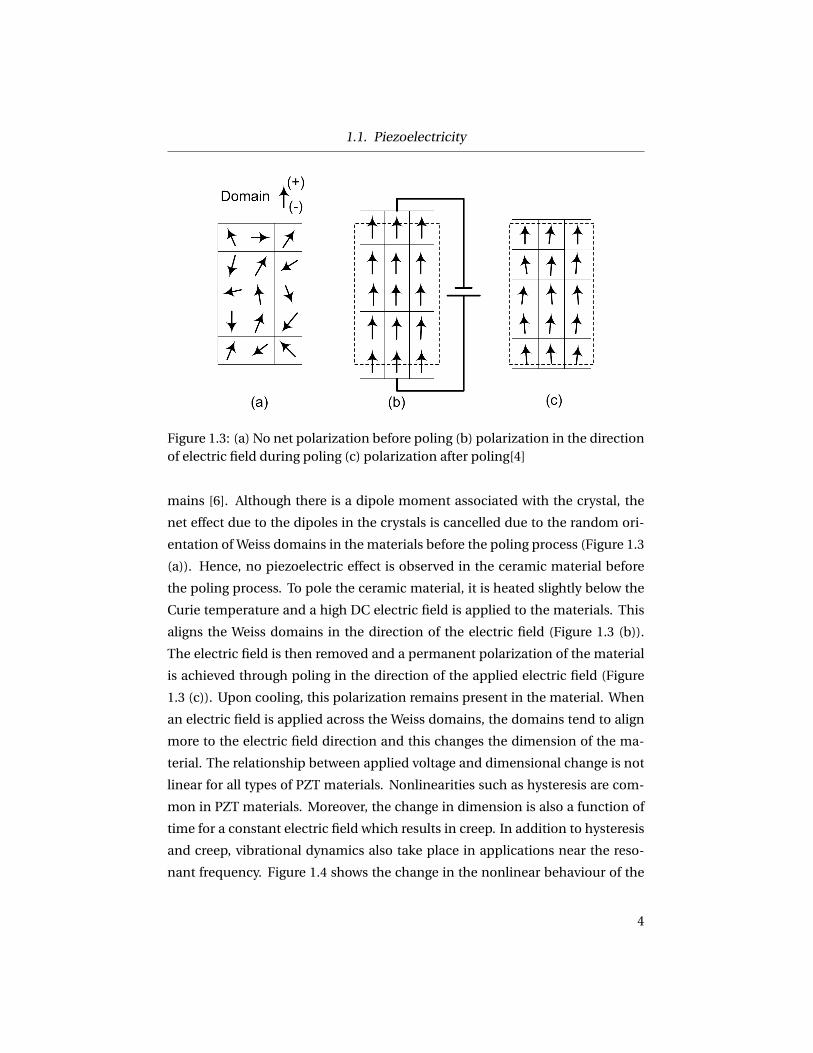
Figure 1.3: (a) No net polarization before poling (b) polarization in the directionof electric field during poling (c) polarization after poling[4]
mains [6]. Although there is a dipole moment associated with the crystal, the
net effect due to the dipoles in the crystals is cancelled due to the random ori-
entation of Weiss domains in the materials before the poling process (Figure 1.3
(a)). Hence, no piezoelectric effect is observed in the ceramic material before
the poling process. To pole the ceramic material, it is heated slightly below the
Curie temperature and a high DC electric field is applied to the materials. This
aligns the Weiss domains in the direction of the electric field (Figure 1.3 (b)).
The electric field is then removed and a permanent polarization of the material
is achieved through poling in the direction of the applied electric field (Figure
1.3 (c)). Upon cooling, this polarization remains present in the material. When
an electric field is applied across the Weiss domains, the domains tend to align
more to the electric field direction and this changes the dimension of the ma-
terial. The relationship between applied voltage and dimensional change is not
linear for all types of PZT materials. Nonlinearities such as hysteresis are com-
mon in PZT materials. Moreover, the change in dimension is also a function of
time for a constant electric field which results in creep. In addition to hysteresis
and creep, vibrational dynamics also take place in applications near the reso-
nant frequency. Figure 1.4 shows the change in the nonlinear behaviour of the
4

1.2. Hysteresis
Figure 1.4: Nonlinear effects on piezoelectric actuator response at various fre-quencies
piezoelectric ceramics with the driving frequency. For low operating frequen-
cies, the creep and hysteresis phenomena take place. At higher frequencies, the
creep phenomenon is absent but the hysteresis phenomenon is still present. For
long time continuous operation, another phenomenon named ‘self-heat gener-
ation’ is observed with hysteresis. These nonlinear effects are discussed in the
upcoming sections.
1.2 Hysteresis
Hysteresis is a common phenomenon in piezoelectric materials due to their
domain switching behaviour. It results from the rotation of the domains by ei-
ther 180◦ or non-180◦ in the presence of an electric field or a mechanical stress
larger than a critical value. For the non-polarized piezoelectric ceramics, the
polarization-electric field (P-E) hysteresis is shown in Figure 1.5.
At point ‘A’, the domains are oriented randomly and hence, no net polariza-
tion is present in the element. When an electric field is applied and the domains
start to align in the direction of the electric field. At point ‘B’ most of the domains
are in the direction of the electric field. When the electric field is reversed, the
polarization is not zero for zero electric field. The polarization at point ‘C’ is
5

1.2. Hysteresis
Figure 1.5: Polarization-electric field hysteresis [7]
Figure 1.6: Strain-electric field hysteresis [7]
6
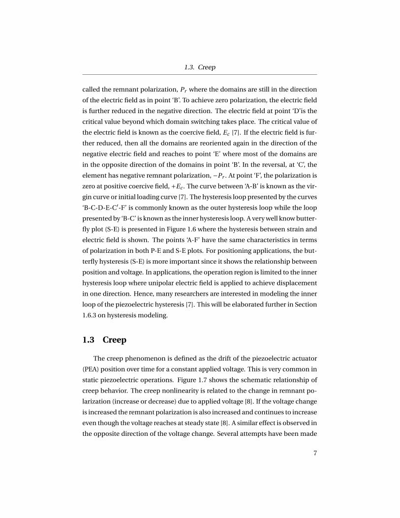
1.3. Creep
called the remnant polarization, Pr where the domains are still in the direction
of the electric field as in point ‘B’. To achieve zero polarization, the electric field
is further reduced in the negative direction. The electric field at point ‘D’is the
critical value beyond which domain switching takes place. The critical value of
the electric field is known as the coercive field, Ec [7]. If the electric field is fur-
ther reduced, then all the domains are reoriented again in the direction of the
negative electric field and reaches to point ‘E’ where most of the domains are
in the opposite direction of the domains in point ‘B’. In the reversal, at ‘C’, the
element has negative remnant polarization, −Pr . At point ‘F’, the polarization is
zero at positive coercive field, +Ec . The curve between ‘A-B’ is known as the vir-
gin curve or initial loading curve [7]. The hysteresis loop presented by the curves
‘B-C-D-E-C′-F’ is commonly known as the outer hysteresis loop while the loop
presented by ‘B-C’ is known as the inner hysteresis loop. A very well know butter-
fly plot (S-E) is presented in Figure 1.6 where the hysteresis between strain and
electric field is shown. The points ‘A-F’ have the same characteristics in terms
of polarization in both P-E and S-E plots. For positioning applications, the but-
terfly hysteresis (S-E) is more important since it shows the relationship between
position and voltage. In applications, the operation region is limited to the inner
hysteresis loop where unipolar electric field is applied to achieve displacement
in one direction. Hence, many researchers are interested in modeling the inner
loop of the piezoelectric hysteresis [7]. This will be elaborated further in Section
1.6.3 on hysteresis modeling.
1.3 Creep
The creep phenomenon is defined as the drift of the piezoelectric actuator
(PEA) position over time for a constant applied voltage. This is very common in
static piezoelectric operations. Figure 1.7 shows the schematic relationship of
creep behavior. The creep nonlinearity is related to the change in remnant po-
larization (increase or decrease) due to applied voltage [8]. If the voltage change
is increased the remnant polarization is also increased and continues to increase
even though the voltage reaches at steady state [8]. A similar effect is observed in
the opposite direction of the voltage change. Several attempts have been made
7

1.4. Vibration
Figure 1.7: Piezoelectric creep behaviour
to model piezoelectric creep behaviour. Since creep is logarithmic with time,
a nonlinear logarithmic function can represent the creep behaviour [8–10]. A
nonlinear log(t)-type creep model is shown in Equation 1.1.
GCr 1 = x(t ) = x0
[1+γ log10
t
t0
](1.1)
where, x(t ) is the model output, x0 is the nominal displacement of the actuator
at t0 seconds after applying the driving voltage, and γ is the creep parameter
which defines the rate of logarithmic function [8]. A major limitation with the
nonlinear creep model is that the creep rate is dependent on the time parameter,
t0 which is used to fit the model [11]. In addition to that, model inversion is not
very convenient for feedforward control approaches [10].
1.4 Vibration
Vibration effects in the PEAs may occur when they are operated close to the
first natural frequency of the system. In some applications, such as scanning
8

1.5. Piezoelectric Actuators (PEAs)
tubes or cantilevers, the natural frequency is low and substantial vibrations are
observed. In some systems such as scanning tubes, the vibrations occur at such
a low frequency that the rate-dependent hysteresis effect is modeled as a vibra-
tion effect [12]. Usually to incorporate the vibration dynamics, a second order
system model is sufficient [13–15]. However, for high levels of accuracy, higher
order models are used specially when pure inverse models are required for open
loop control [12, 16]. The parameters of the vibration dynamic models are usu-
ally obtained through appropriate fitting of the frequency response of the actu-
ator by selecting the order in a dynamic signal analyzer [12, 16, 17]. Usually the
displacement range is limited to 10% of the stroke to neglect the hysteresis effect
in measurement [16]. In contrast to scanning tube type actuators, or bending ac-
tuators, stack type actuators have a very high mechanical natural frequency. It
is recommended by the manufacturer that for positioning applications of actu-
ators, resonant frequency should be avoided [18].
1.5 Piezoelectric Actuators (PEAs)
Piezoelectric materials are extensively used as sensors, actuators, or trans-
ducers utilizing either the direct or indirect piezoelectric effect. Based on the
indirect effect, an applied voltage or charge is used to create a strain in the piezo-
electric system for force or position applications. Properties such as high com-
pressive strength, fast rise time, high resolution, high pressure resistance, com-
pactness etc. made the piezoelectric actuators (PEAs) ideal candidates for nu-
merous micro-/nano-systems such as micro-positioning stages, inkjet-printing,
surgical robots, fuel injection, drug delivery, etc. Due to advanced manufactur-
ing technologies, piezoelectric materials can be formed almost into any shape.
Different types of PEAs are developed by the manufacturers for different appli-
cations. Broadly, they are classified as rod or stack type actuators (extensional
mode) and bender type or stripe actuators (flexural mode) [19] which have wide
variety of applications.
9

1.5. Piezoelectric Actuators (PEAs)
1.5.1 Stack Actuators
Stack actuators are usually multilayered where several piezoelectric ceramic
layers are connected in series mechanically and in parallel electrically [14]. In
multilayered stack type actuators, piezoelectric ceramic layers are sandwiched
between two electrodes where the polarization of the ceramics is in the opposite
direction for two consecutive layers. The stack type actuators provide low strain
and high blocking force. The stack actuators are classified into either discrete
type or co-fired type. In discrete type actuators, separately prepared piezoelec-
tric discs or rings are connected to the metal electrode with adhesive. The layer
thickness of these actuators is usually larger than 0.1 mm (as an example in [20]).
The operating voltage is usually high for these type actuators typically ranging
from 500 V to 1000 V to obtain the required electric field. The co-fired actua-
tors (monolithic type) are manufactured by high temperature sintering of the
ceramic material and electrode. Since they are co-fired, the layer thickness of
the ceramics can be reduced to 0.02 mm [21]. This makes it possible to drive
these co-fired actuators with relatively low voltage typically less than 200 V. The
construction of a multilayered stack actuator is shown in Figure 1.8.
1.5.2 Bender Actuators
In comparison to the stack type actuator, the bender type actuator provide
larger displacement. The generated force for bender type actuators is small in
comparison to stack actuators. The natural frequency of the benders is also
small in comparison to stack actuators. The deflection in bender type of ac-
tuator is perpendicular to the electric field direction. Usually, the bender actua-
tors consist of a piezo/metal combination or a piezo-piezo combination. In the
piezo-metal combination (in Figure 1.9(a)), when the ceramic is energized the
actuator deflects proportional to the voltage. This arrangement is usually used
when deflection is required in a single direction. In piezo/piezo combinations,
both the layers can be polarized in the same direction (parallel connection (in
Figure 1.9(b))) or in opposite direction (series (in Figure 1.9(c))). In the parallel
connection, the deflection is twice as large as in the series connection [22]. The
piezo-piezo combination allows bending in both directions. Figure 1.9 shows
10

1.6. Piezoelectric Actuator Modeling
Figure 1.8: Multilayer piezoelectric stack actuator
the construction of different bender type actuators.
1.6 Piezoelectric Actuator Modeling
Piezoelectric actuator models are broadly classified into linear and nonlin-
ear models. Linear models do not consider hysteresis or creep related nonlinear-
ities and are applicable for hard piezoelectric materials. Nonlinear models try to
incorporate hysteresis and/or creep phenomena. Phenomenological models are
widely used to describe the nonlinear behaviour of the piezoelectric materials
since the nonlinear effects such as creep and hysteresis and their dependencies
are often difficult to describe.
1.6.1 Linear IEEE Model
In the classical description of piezoelectric constitutive equations [23], the
piezoelectric materials are modeled by linear equation as follows:
Sλ = sλµT µ+dλi E i , (1.2)
11

1.6. Piezoelectric Actuator Modeling
Figure 1.9: Piezoelectric bender actuator (a) Piezo-metal combination (b) Piezo-piezo combination in parallel connection (c) Piezo-piezo combination in seriesconnection [22]
Di = dµi T µ+εi l E l , (1.3)
where, independent variables, T denotes the applied stress and E is the electric
field which are linearly related to dependent variables, S strain and D electrical
displacement with constants such as, mechanical compliance (s), piezoelectric
constant (d) and dielectric constant (ε). The indices, λ, µ = 1,2,3. . . ,6 and i ,
l = 1,2,3 are the ’tensor’ expression in the material coordinate system. Based
on the operating modes of the actuators, the expression can be reduced to one
directional case for simplicity. It is important to note that the IEEE model does
not include the dynamics of the PEA. Moreover, the piezoelectric hysteresis is
not considered in the model.
1.6.2 Nonlinear Physical Model
Goldfarb and Celanovic [13] proposed an electromechanical model for PEAs
that attempts to include both dynamic actuation and hysteresis effects. Since
12

1.6. Piezoelectric Actuator Modeling
Figure 1.10: Electromechanical model of PEA [24]
their model aims to service control applications, they used readily measurable
variables of voltage, charge, force and displacement instead of electric field,
electric displacement, stress and strain. A diagram of this model for stack ac-
tuators is shown in Figure 1.10 and the constitutive relationships are shown in
Equations 1.4-1.7:
mx +bx +kx =αUP +F, (1.4)
q =CPUP +αx, (1.5)
U =UP +UH , (1.6)
UH = f (q). (1.7)
Equation 1.4 is known as the ‘force equation’ which models the mechanical sub-
system of the actuator while Equation 1.5 is known as ‘charge equation’ which
models the electrical subsystem of the actuator. The electrical subsystem is cou-
pled to the mechanical subsystem with the force-voltage proportionality con-
stant, α. In the mechanical subsystem, the generated piezoelectric force is lin-
early related to the linear piezo voltage, UP through the force-voltage propor-
tionality constant, α. In the ‘force equation’, both the generated piezoelectric
force, αUP and the externally applied force, F drive the second order mass-
spring-damper system that is comprised of a moving mass, m, viscous damp-
13

1.6. Piezoelectric Actuator Modeling
Figure 1.11: (a) An elementary elasto-slide hysteresis operator, (b) force-displacement hysteresis mapping of a single operator [13]
ing with a coefficient, b and stack stiffness, k while x, x and x are the position,
velocity and acceleration respectively. In the electrical subsystem described in
the ‘charge equation’, the linear piezoelectric voltage, UP results in charge, q
flowing into the actuator. The charge flow is proportional to the clamped capac-
itance, CP and the elongation of the actuator. To include hysteresis, a dipole,
H is introduced in the electrical subsystem which reduces the voltage available
to drive the actuator. This reduction in voltage occurs due to the polarization
voltage associated with the dipoles within the piezoelectric ceramic [25]. The
polarization voltage, UH opposes the applied voltage, U and reduces the piezo
voltage to UP . Equation 1.6 shows that the applied voltage is a summation of
the linear voltage and the polarization or hysteresis voltage. Equation 1.7 rep-
resents the hysteresis model which describes the hysteresis voltage as a func-
tion of charge. This is due to the assumption in the model that the hysteresis is
solely present in the electrical subsystem. A Maxwell elasto-slide operator is the
building block for the generalized Maxwell slip model which is used to capture
14

1.6. Piezoelectric Actuator Modeling
Figure 1.12: Generalized Maxwell slip model for piezoelectric hysteresis [13]
15

1.6. Piezoelectric Actuator Modeling
the rate-independent hysteresis behaviour in the proposed model [13]. Similar
to hysteresis phenomenon observed in the elastic-plastic deformation of stress
and strain in solid materials or electric field strength vs the flux density in mag-
netic material; the model can be used for piezoelectric hysteresis modeling. The
basic model consist of massless energy storage elements such as a mechanical
spring connected to a massless block. The massless system is considered sliding
on a surface with Coulomb friction which is the rate-independent dissipative el-
ement in the system. This system is called a Maxwell elasto-slide operator which
is presented in Figure 1.11(a). The constitutive equation of the system is shown
in Equation 1.8:
F (t ) =k{x(t )−xb(t )}, k{x(t )−xb(t )} < f =µN ,
f sg n(x), el se,(1.8)
where, k is the stiffness of the spring, xb is the block displacement, x is the dis-
placement of the block which is the input, f , is the break-away friction force
(µN ),µ is the friction coefficient and N is the normal force. A fundamental force-
displacement hysteresis behaviour, observed for a displacement input, x(t ) to
the system, is shown in Figure 1.11. To capture the complete hysteretic be-
haviour, n elements are connected in parallel, where each of the elements has
a monotonically increasing break-away force, fi . The schematic of the Maxwell
slip model comprising of n elasto-slide elements is shown in Figure 1.12. The
complete model is shown in Equation 1.9:
Fi (t ) =ki {x(t )−xbi (t )}, k{x(t )−xbi (t )} < fi =µNi ,
fi sg n(x), el se,(1.9)
F (t ) =n∑
i=1fi (t ) (1.10)
where, i is the index for n number of elements connected in parallel in Figure
1.12. A similar analogy can be drawn for voltage and charge in the electrical
domain which represents the piezoelectric hysteresis. In that case the stiffness
term, ki is replaced with inverse capacitance, C−1i and the input displacement
is replaced with charge, qi . The break-away force is essentially replaced with a
16

1.6. Piezoelectric Actuator Modeling
Figure 1.13: Extended electromechanical model with a drift operator [26]
break-away voltage, vi . The equivalent constitutive model, known as Maxwell
Resistive Capacitive (MRC) model, is shown in Equation 1.11:
UHi (t ) =C−1
i {q(t )−qbi (t )}, k{q(t )−qbi (t )} < vi ,
vi sg n(q), el se,(1.11)
UH (t ) =n∑
i=1UHi (t ), (1.12)
where, UH is the hysteresis voltage.
The electromechanical model is augmented by Adriaens et al. [14] where
a mechanical operator is proposed to include the higher order dynamics for a
large frequency range. To include the higher harmonics it is necessary to model
the mechanical system as a distributed model instead of a lumped mass system.
Also, the hysteresis behaviour is modeled with a differential equation instead
of an MRC model. However, for most of the piezoelectric stack actuators, the
application frequency range is well below the mechanical resonance frequency
which reduces the mechanical operator into stiffness compliance [27], [28]. An
extension of the model presented in [14] is proposed in [26] which accounts for
the creep behaviour in addition to the hysteresis phenomenon with a drift op-
17

1.6. Piezoelectric Actuator Modeling
Figure 1.14: Drift operator with lossy resistance [26]
erator, D . Similar to the model presented in [13], the hysteresis phenomenon is
modeled using the generalized Maxwell operator, H . The extended model with
a drift operator (electrical domain) is shown in Figure 1.13.
The proposed drift operator, D consists of N number of series RC elements
which are connected in parallel shown in Figure 1.14. The creep is considered
similar to charge drift and hence the drift charge, qd is obtained through the
model shown in Equation 1.13:
GCr1 (s) = qd (s)
UP (s)= 1
Rs+
N∑i=1
Ci
Ri Ci +1, (1.13)
where, UP is the linear piezoelectric voltage, R is a resistive element to account
for the dielectric losses while the Ri and Ci elements model the creep behaviour.
These linear models accurately predict the creep behaviour when the model
starts from a known initial state. However, the past history of the hysteresis af-
fects the creep behaviour which in not accounted in the linear models [29].
1.6.3 Phenomenological Model
The hysteresis behaviour between voltage and position attracts a large re-
search interest since it is useful for designing feedforward controllers for posi-
tion actuation applications. Figure 1.15 shows a typical hysteresis loop. It is
observed that the voltage-position hysteresis phenomenon is a function of the
rate of the input [27, 30–32]. Based on this, voltage-position hysteresis is clas-
sified into two groups: 1) rate-independent hysteresis and 2) rate-dependent
18

1.6. Piezoelectric Actuator Modeling
Figure 1.15: Voltage-stroke hysteresis loops at different voltages
hysteresis. The corresponding hysteresis models are then also classified as rate-
dependent models and rate-independent models. The rate-independent hys-
teresis modeling assumes that the hysteresis behavior is not influenced by the
rate of change of input or frequency. However, in practice rate dependence of-
ten plays an important role.
1.6.3.1 Rate-independent Model
Initial hysteresis models consider that the hysteresis behaviour is indepen-
dent of driving frequencies or rate of operation. Several attempts were made to
model the rate-independent hysteresis phenomenon. Among which, the classi-
cal Preisach model (CPM) [12, 33], and the Prandtl-Ishlinskii (PI) operator [29]
are the most studied and modified. The CPM is a phenomenological model,
where a function is defined to model the piezoelectric hysteresis through nu-
19

1.6. Piezoelectric Actuator Modeling
Figure 1.16: (a) Preisach operator or hysteron (b) Preisach model with N opera-tors
merous Preisach operators, called Hysterons [34], γαβ[u(t )] as presented in Fig-
ure 1.16 (a). For an input value, u(t ) larger thanα, the Hysteron value is set to +1
and for values lower than β the value is set to −1. A weighting function, µ(αβ) is
multiplied with the hysteron. Connecting the hysterons in parallel provides the
output shown in Figure 1.16(b). The CPM model is realized in Equation 1.14:
x(t )C P M =Ïα<β
µ(α,β)γαβ[u(t )]dαdβ, (1.14)
where, x(t ) is the output of the operator for an input of u(t ). The accuracy of
the classical Preisach model is limited to a single operating frequency. More-
over, the smoothness of the hysteresis modeling is dependent on the number of
hysterons (numerous) which is computationally expensive [28, 30].
The Prandtl-Ishlinskii (PI) model is an important sub-model of the Preisach
model that is developed to address the computational complexity and inversion
problem of CPM [29, 30]. The PI hysteresis model is based on the play or back-
lash operator which is generally used in gear backlash modeling with one degree
of freedom [30]. Equation 1.15 presents an expression for the PI model with n
play operators:
x(t )PI =N∑
i=1γi
wr [u, y0](t )
20

1.6. Piezoelectric Actuator Modeling
Figure 1.17: (a), (b) Elementary play operators with different weights and thresh-old values (c) superpositioning of the play operators in (a) and (b) [35]
=N∑
i=1w i max{x(t )− r i ,mi n{x(t )+ r i , y(t −T )}} (1.15)
where, γiwr [u, y0](t ) is the i th play operator with w is the weight (slope) which is
the gain of the backlash operator, r is the control input threshold value, y0 ∈ R
and usually set to zero, T is the sampling time, u(t ) is the model input, and x(t )PI
is the model output. Figure 1.17 (a) and (b) show the elementary play operators
with different weight functions, w and threshold values, r . A simple PI model is
created by the superposition of the two play operators shown in Figure 1.17 (a)
and (b), which leads to the Figure 1.17 (c).
Although the PI hysteresis model is simpler than the CPM, the classical PI is
limited to the symmetric hysteresis modeling. In many practical scenarios, the
piezoelectric hysteresis is not symmetric in nature. Hence a modified PI opera-
tor is proposed by [30] where a saturation operator is connected to the hysteresis
operator in series. A saturation operator, defined as a superposition of weighted
linear one-sided dead-zone operators, is shown in Equation 1.16:
Sd[x](t ) = [Sd0[x](t ),Sd2[x](t ), · · ·,Sdm[x](t )] (1.16)
where,
Sd [x](t ) =max{x(t )−d ,0}, f or d > 0,
x(t ), f or d = 0,
21
1.6. Piezoelectric Actuator Modeling
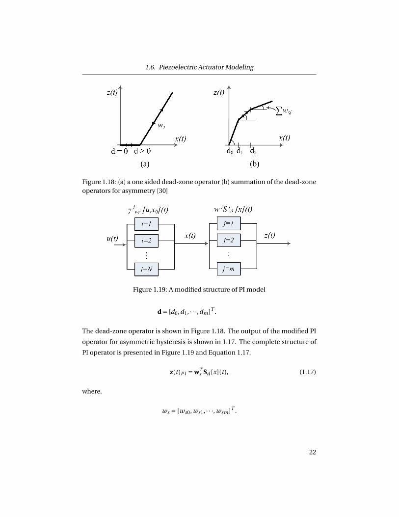
Figure 1.18: (a) a one sided dead-zone operator (b) summation of the dead-zoneoperators for asymmetry [30]
Figure 1.19: A modified structure of PI model
d = [d0,d1, · · ·,dm]T .
The dead-zone operator is shown in Figure 1.18. The output of the modified PI
operator for asymmetric hysteresis is shown in 1.17. The complete structure of
PI operator is presented in Figure 1.19 and Equation 1.17.
z(t )PI = wTs Sd [x](t ), (1.17)
where,
ws = [ws0, ws1, · · ·, wsm]T .
22
1.6. Piezoelectric Actuator Modeling
1.6.3.2 Rate-dependent Model
The hysteresis models discussed in the previous section are rate-independent
models which can predict the hysteresis behaviour for a limited frequency range.
For large frequency ranges, the aforementioned models require modifications
to achieve acceptable levels of accuracy. Modifications have been suggested for
both the Preisach and PI hysteresis models to incorporate the rate-dependent
effects [30, 32, 33, 36, 37]. The dynamic Preisach model (DPM) includes a struc-
ture where the weighting functionµ(α,β) is modified to address the rate-dependency.
This is achieved by introducing additional dynamic operators [33, 36] or a neural
network [32]. The additional dynamic operators are functions which are depen-
dent on the average input voltage between two consecutive input extrema and
the rate of change of the input voltage between the input extrema [33]. More-
over, an additional function, named mirror function is defined to correlate the
CPM to the DPM. The output of the DPM suggests that it is a function of both
the output of the closest extremum value and the output of the CPM value at
the nearest extremum. Although, it is shown that the hysteresis can be modeled
over a frequency range of 0-800 Hz within reasonable error (6.4%), it required
a priori knowledge of the input voltage waveform to attain the dynamic oper-
ators [33]. Unfortunately, this is not very convenient when the future input is
not known. A slightly different method is proposed in [36] where the weight-
ing function is extended to include a parameter which is a function of the rate
of the input voltage. The function is simplified with the assumption that the
higher order derivatives are negligible. This limits the model accuracy to a fre-
quency range of 0.01-10 Hz. A neural network to address the rate dependency
is proposed in [32]. In this case, the weighting function is modified using a neu-
ral network. It is shown that the modeling accuracy is achieved within 4% of
the maximum displacement for a frequency range of 2-32 Hz. The PI model can
also be modified to incorporate rate dependent phenomena [30]. The weights in
Equation 1.16 are modified with the rate of actuation, u(t ). The percentage error
for a frequency range of 1-19 Hz continuous operation is measured at 5.3%. One
of the major drawbacks of the PI operators is a singularity problem when the PI
weight turns to zero. A similar problem occurs if the slope is negative. Then the
23

1.6. Piezoelectric Actuator Modeling
preliminary assumption of a monotonically increased loading curve is violated
and the model fails. In the proposed model, the singularity occurs at 40 Hz [30].
1.6.3.3 Other Phenomenological Hysteresis Models
Other phenomenological models in the literature include the Bouc-Wen (BW)
model [38], the Duhem model [39], a memory based model (MBM) [40], a poly-
nomial based model [41], a first order differential equation model, [42] etc. Al-
though these models can predict the hysteresis behaviour, significant improve-
ment in accuracy is not realized over the previously discussed methods. More-
over, some of these models require more complex computation in comparison
to their modeling performance which limits their wide acceptability.
1.6.4 Cascaded Phenomenological Model for Hysteresis, Creep, and
Vibrational Dynamics
A phenomenological model structure is proposed in [12] where the hystere-
sis and creep phenomena are modeled using hysteresis and creep operators.
Once the models are developed they are cascaded to complete the piezoelec-
tric model shown in Figure 1.20. In the proposed model by [12], CPM is used to
model the hysteresis.
To overcome the limitations of the model described in Equation 1.1, a linear
creep model is presented in [12] which is a series connection of several springs
and dampers as shown in Equation 1.18:
GCr 2(s) = x(s)
U (s)= 1
k0+
N∑i=1
1
ci s +ki, (1.18)
where, k0 is the elastic constant, ci and ki are the dampers and springs of the i th
creep element. The model is presented in Figure 1.20.
The vibrational dynamics is modeled by a higher order transfer function. To
develop the complete model, first the creep submodel is constructed at low fre-
quency condition where the vibrational dynamics is not present. Then the vi-
bration submodel is developed at high frequencies when the creep is neglected.
Finally the hysteresis model is developed and cascaded to the other submod-
24

1.7. Position Control of PEA
Figure 1.20: Cascaded model of PEA [12]
Figure 1.21: Visco-elastic creep model with elastic component [12]
els. The input voltage, U generates a mechanical output through the hysteresis
model which is the input for the creep and vibration submodel. Finally, the posi-
tion, x is obtained from the complete model. It is important to note that the rate-
dependent hysteresis is embedded in the vibration submodel since the model is
aimed for a system (piezo tube scanner for atomic force microscope) whose first
natural frequency is very small (typically in the range of 500-1000 Hz). Hence, vi-
bration occurs at relatively low frequencies even before observing considerable
rate dependency in the hysteresis behaviour. The advantage of the model is that
it is purely phenomenological which does not require the underlying physics for
the system. Moreover, the hysteresis model is not restricted to a particular op-
erator rather any model previously discussed (CPM, PI or MRC) can be used to
represent hysteresis. Similarly, any linear model can be implemented to model
the creep behaviour. The major drawback of this type of model is that the mod-
eling uncertainty limits the accuracy of the position controller. Moreover, if the
hysteresis behaviour changes due to some external factors such as temperature
or aging the model cannot predict the piezoelectric behaviour accurately.
1.7 Position Control of PEA
PEAs are widely used in many micro-nano positioning applications. How-
ever, due to nonlinearities such as creep or hysteresis, position control of these
25

1.7. Position Control of PEA
Figure 1.22: Different position control schemes
actuators is challenging. Hysteresis can result in up to 15% position error [43].
The positioning error due to creep varies from 1-40% [43, 44]. For high accu-
racy positioning applications, the nonlinearities must be compensated. The
control schemes to counter the nonlinearities are classified into five major cat-
egories: 1) feedforward voltage control [12, 27, 30, 38, 43, 45, 46], 2) feedback
voltage control [47–50], 3) feedforward with feedback control [24, 27, 47, 48, 50],
4) charge control [51–53], and 5) integrated voltage/charge control [17, 54]. The
schematic shown in Figure 1.22 presents different position control principles for
PEAs which are discussed in the following sub-sections.
1.7.1 Feedforward (FF) Voltage Control
Feedforward voltage control scheme is a model based control scheme where
a dedicated position sensor cannot be incorporated due to space and/or cost
constraints. Moreover, additional sensors can lead to reliability problems which
can be avoided through a feedforward control scheme. The broad idea is pre-
sented in [12] where an accurate phenomenological model of the PEA is devel-
oped and inverted. The inverted model is then fed with the desired position,
xd input and a voltage, Um is obtained from the inverted model. The inverted
model output, Um is the input voltage for the piezoelectric plant which is re-
sponsible for the required displacement, x. The feedforward control structure
is presented in Figure 1.23. All three effects (hysteresis, creep and vibration) are
considered in [12, 44] where the hysteresis is compensated by inverse CPM [12]
and an inverse PI model [44], respectively. The creep is modeled by a Kelvin-
viogt system in [12] and an ARMAX (Auto Regressive Moving Average with eXter-
nal inputs) model in [44], respectively. Finally, the vibration is compensated by
26
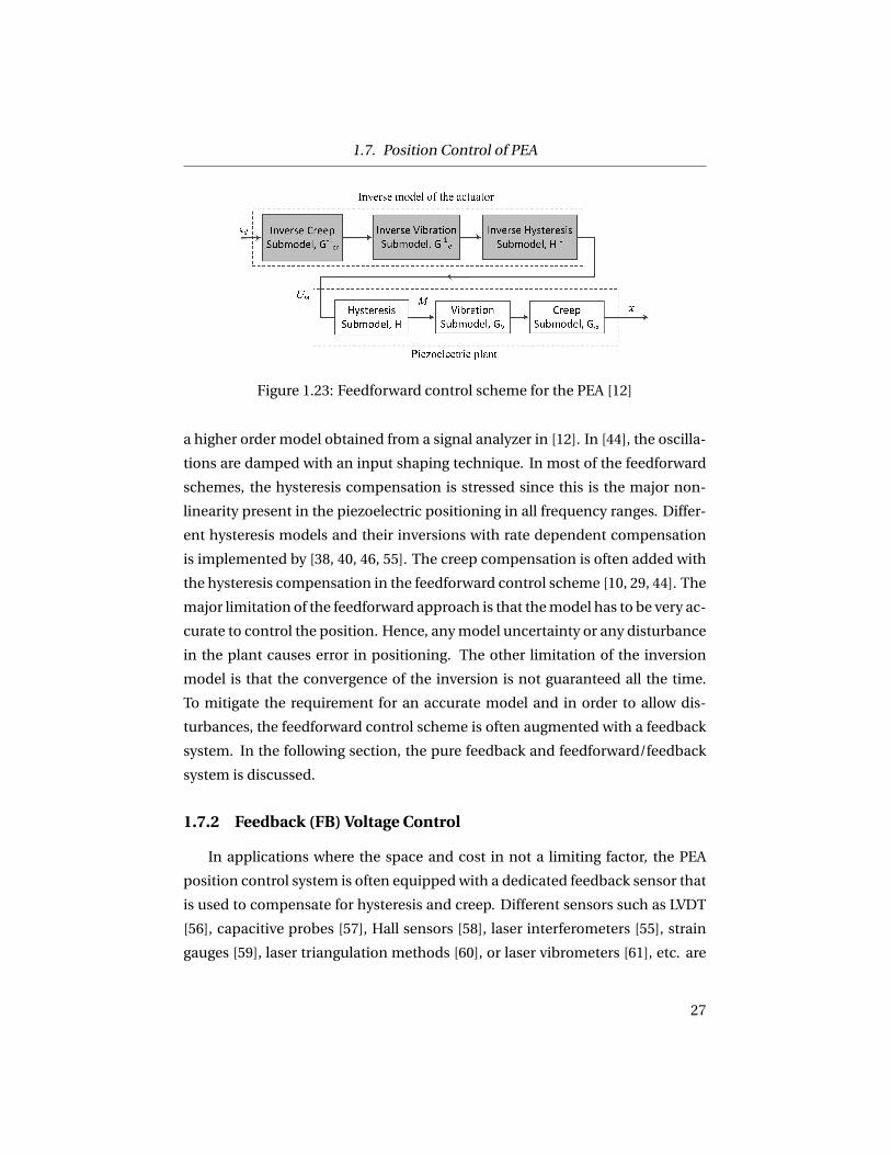
1.7. Position Control of PEA
Figure 1.23: Feedforward control scheme for the PEA [12]
a higher order model obtained from a signal analyzer in [12]. In [44], the oscilla-
tions are damped with an input shaping technique. In most of the feedforward
schemes, the hysteresis compensation is stressed since this is the major non-
linearity present in the piezoelectric positioning in all frequency ranges. Differ-
ent hysteresis models and their inversions with rate dependent compensation
is implemented by [38, 40, 46, 55]. The creep compensation is often added with
the hysteresis compensation in the feedforward control scheme [10, 29, 44]. The
major limitation of the feedforward approach is that the model has to be very ac-
curate to control the position. Hence, any model uncertainty or any disturbance
in the plant causes error in positioning. The other limitation of the inversion
model is that the convergence of the inversion is not guaranteed all the time.
To mitigate the requirement for an accurate model and in order to allow dis-
turbances, the feedforward control scheme is often augmented with a feedback
system. In the following section, the pure feedback and feedforward/feedback
system is discussed.
1.7.2 Feedback (FB) Voltage Control
In applications where the space and cost in not a limiting factor, the PEA
position control system is often equipped with a dedicated feedback sensor that
is used to compensate for hysteresis and creep. Different sensors such as LVDT
[56], capacitive probes [57], Hall sensors [58], laser interferometers [55], strain
gauges [59], laser triangulation methods [60], or laser vibrometers [61], etc. are
27

1.7. Position Control of PEA
used as position sensors. A comparison of the sensors is presented in Table 1.1
[62].
28

1.7. Position Control of PEA
Tab
le1.
1:C
om
par
iso
no
fth
efe
edb
ack
sen
sors
Typ
eC
ost
Size
Pre
cisi
on
Res
olu
tio
nO
ther
s
Tria
ngu
lati
on
Hig
hLa
rge
Hig
hH
igh
Lim
ited
mea
su-
rem
entr
ange
Lase
rVe
ryh
igh
Larg
eH
igh
Hig
hH
igh
ban
dw
idth
,vi
bro
met
erSe
nso
rd
rift
Stra
ingu
age
Low
Smal
lLo
wM
ediu
mFr
agile
,te
mp
erat
ure
effe
ctLV
DT
Low
Smal
lM
ediu
mM
ediu
mR
equ
ires
con
tact
Cap
acit
ive
or
Low
Med
ium
Hig
hH
igh
Req
uir
esin
du
ctiv
ep
rob
eo
rM
ediu
mp
roxi
mit
yH
alle
ffec
tLo
wM
ediu
mM
ediu
mH
igh
Req
uir
esse
nso
ro
rM
ediu
mo
rLa
rge
pro
xim
ity
29

1.7. Position Control of PEA
Figure 1.24: Feedback control scheme [11]
A Block diagram of the feedback (FB) control scheme is presented in Figure
1.24. For low frequency applications or point to point control, classical Proportiona-
Intergral-Derivative (PID) controllers or multiple integrators are commonly used
for tracking [11, 63–66]. The advantage of PID or integral controllers is that they
provide high gain feedback which can substantially minimize the hysteresis and
creep at low frequencies. However, at large frequencies, the PID controller is
limited by the phase lag and limited gain margin [11]. This results in tracking er-
ror in classical PID controllers at high frequencies. To overcome this limitation,
PID controllers can be augmented with feedforward control schemes [47, 48], or
Neural networks [67]. Advanced controllers such as state feedback [60, 68] slid-
ing model control [27], H-infinity control [69], etc. have also been developed for
tracking control of PEAs.
1.7.3 Feedforward/Feedback (FF/FB) Control Scheme
To improve the gain margin of the classical PID controller, a feedforward
model is often included with feedback control. This not only improves the low
gain margin of the feedback control, but it also improves the performance of
the feedforward control since the feedback loop accounts only for model un-
certainty and plant disturbance [11]. A common feedforward/feedback control
scheme is presented in Figure 1.25. This FF/FB structure is used by [15, 24, 46–
48]. To model the feedforward branch, different inverse hysteresis models have
been used, such as CPM [15, 48], MRC [13, 70], PI [30, 44], or Boc-Wen [46]. In
[47], a high gain feedback is used to compensate for the nonlinear hysteresis
and creep while the feedforward branch accounts for linear vibration dynam-
30

1.7. Position Control of PEA
Figure 1.25: Feedforward branch with feedback control scheme [11]
Figure 1.26: Feedback-linearized inverse feedforward control [47]
ics. Another FF/FB structure is presented in [47] and is shown in Figure 1.26.
Here, an inverse model of the closed loop system is cascaded to the closed loop
system. In the closed loop system, the feedback controller uses a high gain to
compensate the non-linear hysteresis. Once a linearized closed loop system,
GC L is obtained, the feedforward branch is implemented by inverting the linear
system, GC L . The advantage of the system lies in the simplicity of the inversion
of the linear system, GC L in contrast to the inversion of the complex nonlinear
hysteresis models such as CPM and higher order dynamic models. However, the
low gain margin of the feedback is still present in this structure [11].
1.7.4 Charge Control Scheme
Unlike the voltage-position relationship, charge is linearly related to posi-
tion in PEAs [13, 17, 53, 62]. Charge based controllers are based on this lin-
31

1.7. Position Control of PEA
Figure 1.27: Typical charge control scheme [52]
ear charge-position relationship. Significant hysteresis reduction is possible by
charge based position control. A typical charge control scheme is presented in
Figure 1.27. A sensing capacitance, CS is added to the piezoelectric capacitive
load, CL . An amplifier with a gain, K A compensates the difference between the
reference voltage, Ui n and voltage across the sensing capacitance. To include
the parasitic resistances, RL and RS are added to the model shown in Figure 1.27.
The major problem with charge based controllers is the poor low frequency or
DC performance due to charge drift. Improved charge control schemes require
additional circuitry which adds complexity in the implementation [52, 53]. A
different architecture for charge control is shown in [71]. In this case, additional
electrode layers are added to the PEA and the induced charge in the electrodes
were used for position estimation through an inverse function between charge
and position. However, long-term charge drift is not considered in this study.
1.7.5 Integrated Voltage/Charge Control
An interesting integration of the charge based control and voltage based
feedfroward technique is presented in [17] for piezoelectric tube scanners. In
this article, the charge based technique handles the hysteresis nonlinearity while
the voltage feedforward accounts for the dynamics. In this architecture, the
charge amplifier is used for a traditional charge based control. This can suc-
cessfully reduce the hysteresis non-linearity. However, in the presence of higher
32

1.8. Position Self-sensing (PSS)
Figure 1.28: Integrated voltage/charge control [17]
dynamics, the charge based control cannot compensate for these errors. So, a
simple inverse function of the hysteresis linearized charge control is developed
which produces the feedforward voltage, UF F . The advantage of this system is
that it avoids complicated and sensitive models for vibration and hysteresis. The
structure for this type of control structure is shown in Figure 1.28. However, this
also requires a sophisticated charge amplifier.
1.8 Position Self-sensing (PSS)
Self-sensing is a technique where position or force is obtained in PEAs with-
out having dedicated sensors. Such a technique is first proposed in [72] for
vibration suppression of structures. Later, this technique is used in vibration
suppression of beams [73–75], scanning tubes [76], etc. Self-sensing techniques
are also used for position reconstruction and control applications. Broadly, the
self-sensing technique can be classified into three types: 1) capacitance bridge
self-sensing, 2) charge based self-sensing, and 3) piezoelectric self-sensing.
1.8.1 PSS Using Capacitance Bridge
In capacitance based self-sensing, a capacitance of equal value of the PEA is
used in a capacitance bridge [72, 73]. Since, piezoelectric materials act as both
sensor and actuator, in the presence of any deformation or strain in the actua-
tor, a voltage, UPE A , proportional to the strain or deformation is induced to the
actuator. A schematic of the capacitance bridge is shown in Figure 1.29. The
objective of the self-sensing structure is to obtain a sensing signal, Us which is
proportional to the induced voltage which can then be used as a feedback signal
33

1.8. Position Self-sensing (PSS)
Figure 1.29: Capacitance bridge based self-sensing [73]
to control the vibration through a gain Ks . To obtain the sensing signal, a capac-
itance bridge is created similar to the Figure 1.29. A voltage source, U is applied
to both the piezoelectric capacitive load, CP and the reference capacitor, Cs . An
induced voltage, UPE A is generated due to strain in the actuator. This creates an
imbalance in the bridge and the voltage difference between the two branches
provides a sensing signal, Us proportional to the induced voltage. Considering
the leakage resistances, R1 and R2 sufficiently large and unity gain of the op-amp
the following relationships can be deduced:
U1 = Cs
(C1 +Cs)U , (1.19)
U2 = CP
C2 +CP(U −UPE A), (1.20)
Us =U1 −U2 = Cs
C2 +CsU − CP
(C2 +CP )(U −UPE A). (1.21)
Considering the ideal condition where Cs = CP , the strain voltage is related to
34

1.8. Position Self-sensing (PSS)
the induced voltage as follows:
Us = CP
C2 +CPUPE A . (1.22)
The sensing signal is feedback to the source voltage and hence the vibra-
tion control is achieved. A slight variation of the similar structure is proposed
where the sensing signal is obtained as a rate of change of the induced voltage
[77]. Though this proposed technique is simple to implement, it has several lim-
itations in practice. The size of the reference capacitance, CS has to be equally
large as the piezoelectric capacitance, CP . Moreover, the temperature change
has an effect on the capacitance values which demand a tedious continual tun-
ing of the reference capacitance [73]. The other problem is to obtain an accurate
piezoelectric capacitance, CP . Hence, any mismatch in the capacitance value
creates instability in the feedback control. An adaptive implementation is sug-
gested in [78, 79] to address this problem.
1.8.2 PSS Using Charge Measurement
The other class of position self-sensing technique relies on the linear charge-
position relationship [13, 17, 53, 62]. Current is integrated through a charge am-
plifier and the position is estimated from the charge measurement and the con-
stitutive relationships. The estimated position can then be used in a feedback
control scheme employing PID or PI controllers similar to the ones discussed
in sections 1.7.4. A charge based position self-sensing structure is presented in
Figure 1.30. The position is estimated in two steps: 1) an applied voltage, Ui n
produces a strain, x and charge, q . The charge is measured through an integra-
tor circuit and a charge amplifier. Then the output voltage, Uout , is related to
the measured charge, 2) In the second step, the position is estimated using the
constitutive relationships between output voltage and charge as well as charge
and position. Charge drift usually occurs when charge is obtained from current
integration in the presence of any offset voltage. The position estimator in Fig-
ure 1.30 aims to compensate for this charge drift. Charge feedback approaches
are presented in [25, 71].
35

1.8. Position Self-sensing (PSS)
Figure 1.30: Charge based position self-sensing [80]
1.8.3 PSS Using Piezoelectricity
Position self-sensing is also obtained from the direct effect of the PEA itself.
This approach is used in piezoelectric tube scanners where a part of the piezo-
electric material is used for actuation while the remainder is used for sensing
[81]. In this approach, the driving voltage, U creates an induced voltage, US in
the sensing part of the tube which is proportional to the piezoelectric extension.
The signal can be used for position estimation or vibration suppression in the
scanners. An implementation diagram of this setup is shown in Figure 1.31. The
disadvantage of this approach is that since a part of the actuator is used for sens-
ing, the range of the actuator is reduced.
36

1.8. Position Self-sensing (PSS)
Figure 1.31: Piezoelectric position self-sensing
37

1.9. Errors in Piezoelectric Positioning
1.9 Errors in Piezoelectric Positioning
To verify the performance of different position controllers for PEAs, max-
imum tracking errors are usually compared as an indicator for improvement.
For step responses, sometimes steady-state errors are also compared. There are
a number of factors which may affect the performance of the controller. Among
them driving frequency plays an important role, since the nonlinear effects of
creep, hysteresis and vibrational dynamics appear at different frequency ranges.
A number of controllers are based on feedforward phenomenological models
(in Figure 1.23) only, which are designed to operate only for a limited frequency
range where multiple effects are not visible. Moreover, modeling inaccuracy and
plant uncertainty also affect the controller performance. To obtain a more reli-
able controller, often these feedforward controllers are added to a feedback con-
trollers (in Figure 1.25) where the latter compensate for modeling inaccuracy
and plant uncertainty while the feedforward model improves the dynamics of
the controller [11]. Figure 1.32 shows some of performance of various position
control schemes in terms of maximum tracking error where sinusoidal signals
of fixed frequencies or mixed frequencies are used as a reference signal. The er-
rors and the aim for different models presented in the literature as well as the
performance of the models are presented in Table 1.2.
38

1.9. Errors in Piezoelectric Positioning
Figure 1.32: Maximum errors with operating frequencies. The circular markersindicate the FF controller while the solid markers show the FF/FB controller re-sults.
39

1.9. Errors in Piezoelectric Positioning
Tab
le1.
2:E
rro
rco
mp
aris
on
bet
wee
nd
iffe
ren
tmo
del
s
Mo
del
Ref
eren
ceR
ate,
RC
on
tro
lTy
pe
of
Freq
uen
cy%
erro
rty
pe
Hys
tere
sis,
Hm
eth
od
pro
file
sra
nge
[Hz]
max
imu
mC
reep
,CV
ibra
tio
n,V
PI
[45]
HF
FSi
nu
soid
al0.
12.
5
PI
[27]
R–H
FF
Mix
edSi
nu
soid
al1–
502.
12–2
.7F
F/F
BM
ixed
Sin
uso
idal
1–10
00.
84–2
.32
CP
M[4
8]H
FF
Sin
uso
idal
0.01
8.8
PD
FB
6.5
PD
FB
/FF
2.5
PI
[30]
R–H
OL
Mix
edSi
nu
soid
al1–
1917
.3R
IF
F8
RD
FF
5.3
BW
[46]
H
FF
Sin
uso
idal
0.5
2.6–
3.1
FF
/FB
0.88
–1F
FSi
nu
soid
al1
4.8
FF
/FB
2.5
MR
C[7
0]H
FF
/SS-
FB
Trap
ezo
idal
2m
sst
atic
22
ms
dyn
amic
3
Self
-sen
sin
g[6
2]H
–CF
F+
Mo
del
Step
0.55
–2.5
Tran
sfer
fun
ctio
n[4
7]H
-C-V
FF
Sin
uso
idal
1–30
04.
88F
F/F
BTr
ian
gula
r20
02.
95F
BSt
ep1.
48
Mem
ory
bas
ed[8
2]H
FF
Ram
p60
sec
0.7
Tria
ngu
lar
11.
4M
ixed
Sin
uso
idal
4.3
PI
[31]
R–H
FF
Mu
ltiS
inu
soid
alR
and
om
1–6
Sin
uso
idal
122–
3
40
1.10. Self-Heating
1.10 Self-Heating
Self-heat generation is a phenomenon which occurs in PEAs when they are
continuously driven at high frequency under high electric field. Substantial tem-
perature rise is observed in [21, 83–85] which may affect the performance and
durability of the actuator. Moreover, the hysteresis behavior may change due
to temperature variation which affects the phenomenological model and feed-
forward control of the actuator. Also, due to temperature variation, the model
parameter such as piezoelectric capacitance (in Equation 1.5) is also affected. It
is reported in [21] that the self-heating phenomenon is a function of frequency,
electric field and effective volume of the actuator. In [83], it is shown that a tem-
perature rise increases the current in the actuator.
Self-heat generation results from losses such as mechanical damping and di-
electric losses. At high frequencies close to resonance, it is thought that the me-
chanical losses play a major role in heat generation while at frequencies lower
than the resonance frequency, the dielectric losses contribute most to heat gen-
eration [86]. The dielectric loss is caused by the ferroelectric hysteresis loss
which primarily occurs due to domain switching [84, 86, 87]. A theoretical model
is proposed in [21] to model the self-heating phenomenon which is based on the
law of energy conservation. The model assumes that rate of heat generation is
proportional to the frequency and the hysteresis loss per driving cycle per unit
volume, u. Zheng et al. [21] also studied the geometric changes in different ac-
tuators. They conclude that the steady-state temperature rise is a linear function
of ratio of effective actuator volume to surface area. They also show that hystere-
sis varies with temperature. However, the temperature effect on the hysteresis
loss is not considered in their model.
The self-heating model presented in [21] is extended in [84] which includes
a heat sink attached to the actuator in order to reduce the actuator tempera-
ture due to self-heat generation. Instead of the loss term, u presented in [21],
displacement hysteresis, D f (an equivalent parameter to u calculated from the
strain-electric field hysteresis) is introduced in the model. The model predicts
the self-heating phenomenon in the presence of a heat sink and concludes that
the self-heating temperature increase is reduced by 39% by the introduction of
41

1.11. Scope of the Work and Objectives
the heat-sink. However, the model does not account for the mechanical losses
due to friction between the heat sink and the actuator. A different temperature
prediction model is proposed in [83], where it is shown that temperature change
due to self-heating increases the current flow. The change in the current mea-
surement is used to measure the change in temperature.
1.11 Scope of the Work and Objectives
PEAs exhibit rate-dependent hysteresis and creep in voltage driven scheme.
These phenomena occur over a wide frequency range. Charge based operation
reduces the hysteresis significantly. However, it requires sophisticated hard-
ware to implement charge based schemes. Position feedback sensors reduce
the hysteresis and creep behavior significantly. However, implementation of
dedicated position sensors is sometimes prohibitive due to cost and space con-
straints. Researchers have developed several hysteresis models for use in feed-
forward position controllers. However, complex mathematical modeling is re-
quired to obtain accurate models which are often affected by uncertainty of the
plant. Hence, these models are only useful for a limited range of frequencies.
Piezoelectric position self-sensing provides a means to predict the position from
charge information. However, charge based PSS is limited to high frequencies
and prone to drift due to any offset present in the current measurement. Other
self-sensing approaches have limitations such as temperature instability due to
piezoelectric capacitance variation, loss of stroke, etc. In addition to that, tem-
perature variation due to self-heat generation phenomenon substantially affects
the self-sensing strategies which are not very well studied in earlier research.
Considering these aspects, the main objectives in this research are:
o To develop a PSS scheme which is independent of phenomenological mod-
els of hysteresis and creep.
o To obtain a self-heat generation model for actuator temperature predic-
tion.
o To adapt the developed PSS for temperature variation due to self-heat gen-
eration.
42

1.11. Scope of the Work and Objectives
To achieve the main goals, several sub-goals are set. They are as follows:
o To characterize the behaviour of piezoelectric actuator, a real-time imped-
ance measurement is required. The impedance measurement provides a
novel quasi-static parameter identification technique based on the con-
stitutive relationship.
o To obtain an improved electromechanical model with the real-time imped-
ance measurement. The improved model is based on a position depen-
dent capacitance which is considered constant in the original model pro-
posed in [13].
o To obtain an improved PSS scheme that is useful over an extended fre-
quency range. A new capacitance based self-sensing method is presented
which is combined with a traditional charge based self-sensing to improve
the position estimation through an observer over a wide frequency range.
o To obtain a closed loop position control system that employs the devel-
oped PSS scheme as a feedback sensor. The newly developed position ob-
server is used as a replacement of a traditional position sensor to obtain a
self-sensing control strategy.
o To obtain a sensorless temperature measurement for an improved self-
sensing scheme in the presence of self-heat generation. A self-heat gener-
ation model is proposed based on the hysteresis loss relying on the consti-
tutive relationship to predict the temperature of the actuator in the pres-
ence of self-heating.
o To obtain a temperature compensated PSS in the presence of self-heating.
This is a novel contribution where a temperature compensated position
self-sensing is proposed based on the self-heat generation model devel-
oped in the previous sub-goal. The arrangement provides temperature
and position estimation in the presence of self-heat generation.
The objectives and sub-goals that are connected to the chapters are presented
in Figure 1.33.
43

1.11. Scope of the Work and Objectives
Figure 1.33: Projection of the objectives and sub-goals connected to differentchapters
44

1.12. Thesis Organization
1.12 Thesis Organization
The chapters in this dissertation are organized as follows. The experimental
setup is presented in Chapter 2 where a test-bed with a high mechanical natural
frequency is designed. This allows to perform high frequency tests in the current
test-bed.
In Chapter 3, a novel real-time impedance measurement technique is pre-
sented which provides impedance measurements during the normal operation
of the actuator. High frequency ripple signals are superimposed on driving sig-
nals which facilitates the real-time impedance measurement. This measure-
ment technique shows that effective actuator impedance varies with actuator
stroke.
In Chapter 4, position dependent capacitance is added to the traditional
electromechanical model by Goldfarb et al. [13] and the improved model is
verified experimentally. The power balance is also checked and proved unaf-
fected due to the inclusion of the position dependent capacitance. Finally, a
novel method to identify the model parameters is also presented in this chapter.
In Chapter 5, the position-capacitance relationship is exploited in order to
define a novel position self-sensing technique. A hybrid position observer (HPO)
is presented which combines two separate position self-sensing signals: 1) charge
based PSS and 2) capacitance based PSS. The charge based PSS suffers at low
frequencies due to integration error while the capacitance based PSS is lim-
ited to low frequency operation due to measurement noise. Hence, the posi-
tion observer yields the advantages of each PSS technique and provides an im-
proved position self-sensing over a wide frequency range. The position observer
is tested in open loop and compared with a traditional position sensor from 0
Hz to 100 Hz where creep and rate dependent hysteresis are present.
In Chapter 6, the newly developed HPO is used as a position feedback in a
simple integral position controller and results are shown for single and multiple
driving frequencies as well as for a scenario with actuator creep.
In Chapter 7, actuator self-heating is studied. This phenomenon occurs dur-
ing continuous operation at driving frequencies higher than 20 Hz. A self-heat
generation model is proposed based on the power loss of the PEA which em-
45

1.12. Thesis Organization
ploys the constitutive model of the PEA. The model predicts the temperature
due to self-heating with 3% accuracy in the presence of different frequencies
from 0 Hz to 150 Hz. Further, the presented HPO is adapted for temperature
variation and employed to the self-heat generation model to predict the tem-
perature. A circular arrangement is proposed where the predicted temperature
is used to correct the temperature related variation in the HPO. HPO position
estimation is then compared with a traditional position sensor in the presence
of self-heat generation.
Finally, the contributions of the present research and future research recom-
mendations are presented in Chapter 8.
46

Chapter 2
Experimental Setup
To investigate the characteristics and validate the model of piezoelectric ac-
tuators, an experimental test-bed is designed and manufactured. The purpose
of the test stand is to facilitate the preloading of the actuator for high frequency
operations (for high speed applications, the actuator manufacture recommends
a preload of 15 MPa [18]) and mounting the sensors for parameter measure-
ments. In [20], an experimental test setup is presented to characterize the piezo-
electric actuator. However, the actuator used in that setup is large and the setup
design require a large mass for the preloading. The large moving mass reduces
the natural frequency significantly which limits the high frequency operations in
that setup. Moreover, a force sensor is mounted between the large preload mass
and the actuator which lowered the natural frequency even further. The natural
frequency of the test-bed presented in [20] is 511 Hz. Hence, the test setup is
limited to operate in the quasi-static range.
To improve the operational range, a new design presented in this research
with an aim to reduce the moving mass. Also, the force sensor is moved between
the PEA and the solid base in the proposed design. In addition, a soft spring is
used to provide the necessary preload to the actuator. The preload assembly is
redesigned which has a much smaller mass than the one in [20]. The natural fre-
quency of the newly developed test-bed is 2500 Hz which allows high frequency
operations up to 500 Hz. In the following sections, the mechanical and the elec-
trical components of the test-bed and the experimental setup are discussed.
2.1 Mechanical Components
The mechanical components include the actuator, frame, preload assembly,
needle and ball seats. The individual components are discussed below.
47
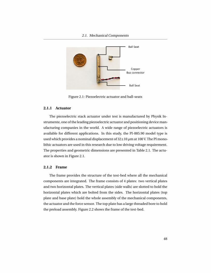
2.1. Mechanical Components
Figure 2.1: Piezoelectric actuator and ball-seats
2.1.1 Actuator
The piezoelectric stack actuator under test is manufactured by Physik In-
strumente, one of the leading piezoelectric actuator and positioning device man-
ufacturing companies in the world. A wide range of piezoelectric actuators is
available for different applications. In this study, the PI-885.90 model type is
used which provides a nominal displacement of 32±10µm at 100 V. The PI mono-
lithic actuators are used in this research due to low driving voltage requirement.
The properties and geometric dimensions are presented in Table 2.1. The actu-
ator is shown in Figure 2.1.
2.1.2 Frame
The frame provides the structure of the test-bed where all the mechanical
components are integrated. The frame consists of 4 plates: two vertical plates
and two horizontal plates. The vertical plates (side walls) are slotted to hold the
horizontal plates which are bolted from the sides. The horizontal plates (top
plate and base plate) hold the whole assembly of the mechanical components,
the actuator and the force sensor. The top plate has a large threaded bore to hold
the preload assembly. Figure 2.2 shows the frame of the test-bed.
48
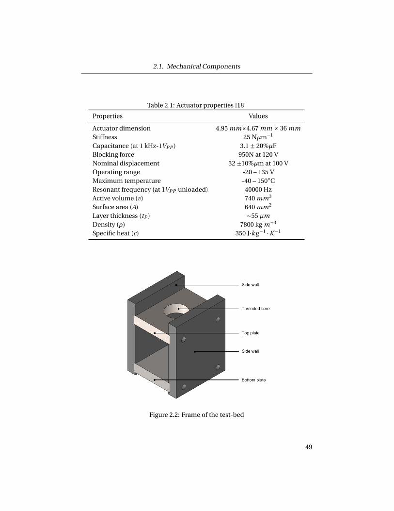
2.1. Mechanical Components
Table 2.1: Actuator properties [18]
Properties Values
Actuator dimension 4.95 mm×4.67 mm × 36 mmStiffness 25 Nµm−1
Capacitance (at 1 kHz-1VPP ) 3.1 ± 20%µFBlocking force 950N at 120 VNominal displacement 32 ±10%µm at 100 VOperating range -20 – 135 VMaximum temperature -40 – 150◦CResonant frequency (at 1VPP unloaded) 40000 HzActive volume (v) 740 mm3
Surface area (A) 640 mm2
Layer thickness (tP ) ∼55 µmDensity (ρ) 7800 kg·m−3
Specific heat (c) 350 J·kg−1 ·K −1
Figure 2.2: Frame of the test-bed
49

2.1. Mechanical Components
2.1.3 Preload Assembly
The preload assembly includes a cap, a preload plate, a thrust bearing and a
steel ball attached to the needle. The cap is an essential part of the preload as-
sembly. The top of the cap is machined to a hexagonal nut to facilitate preload-
ing. The cap is threaded externally which fits into the threaded bore in the top
plate. Figure 2.3 shows that the cross sectional view of the cap. A pocket is
created inside the cap which holds the preload spring and the thrust bearing.
The preload spring is a soft helical spring of stiffness 40 N ·mm−1. To achieve
a preload of 15 MPa, 360 N force is required for the cross sectional area of the
selected actuator. For a pitch of 1.5 mm, 6 turns of the cap is sufficient to pro-
vide necessary preload to the actuator. The thrust bearing prevents any torsional
force (torque) to the actuator while preloading it. The spring is placed between
the thrust bearing and the preload plate which provides the preload to the actu-
ator through a steel ball. The steel ball holds the needle and it is placed on a ball
seat which is attached to the actuator. Any movement in the actuator results in
needle displacement.
2.1.4 Needle
A steel needle is connected to the steel ball through a tolerance fitting. Any
misalignment in the needle and the preload assembly during preloading causes
friction between the cap and the needle. A Teflon sleeve (in Figure 2.3) is placed
between the needle and the cap which reduces the frictional force from 25 N to
5 N during the needle movement. A force sensor is used to measure the force
variation during the operation. The position measurement is performed at the
free end of the needle.
2.1.5 Ball Seats
While mounting the actuator in the test-bed and preloading, any misalign-
ment may cause damage to the actuator. Hence, it is suggested to use steel balls
while mounting the actuator. To facilitate the mounting of the actuator between
the steel balls, end caps are attached to the piezoelectric actuator. The end caps
50

2.1. Mechanical Components
Figure 2.3: Preload assembly
Figure 2.4: CAD drawing of the test-bed
51

2.2. Electrical Components
are indented with the ball-end mills having the same radius as the steel balls to
ensure a better contact between the balls and the caps. High temperature epoxy
is used to attach the end caps to the actuator. The ball seats are shown in Figure
2.1. The complete test-bed is shown in Figure 2.4.
2.2 Electrical Components
The electrical components are responsible to drive the actuator, perform the
measurements and data acquisition. This includes the piezoelectric amplifier
which drives the actuator. Different types of sensors are used to measure cur-
rent, force, position and temperature. A simple 1:100 voltage divider is used to
measure the voltage signal. The measured quantities are recorded with a fast
data acquisition system through dSPACE/Controldesk®. The models are run in
MATLAB/SIMULINK®. The electrical components are illustrated in brief in the
following subsections.
2.2.1 Piezoelectric Actuator Driver
Piezoelectric actuator driver or amplifier are required to amplify the control
signal to drive the actuator. The power of the amplifier is one of the deciding
factors in amplifier selection. Large driving current is required to operate the
actuator at high frequencies. In this research, a high power piezoelectric ampli-
fier (E617.00F) is used which provides 2000 mA of peak current while the average
current output is 1000 mA. The amplifier has an input range of -2 to 12 V and a
gain of 10. A separate 24 V DC power supply is used to feed the power amplifier.
2.2.2 Current Sensor
To measure the current flow, a high resolution (1 mA) current sensor (Tek-
tronix TCP312) is used. Once measured, charge is calculated from the current
measurement through integration in the MATLAB/SIMULINK®.
52
2.2. Electrical Components
2.2.3 Force Sensor
A force sensor (PCB-208C2) is mounted at the bottom of the test setup which
measures the force variation during piezoelectric actuation. The force sensor is
considered stiff enough (1.05 kN·µm−1) to resist the deflection due to piezoelec-
tric actuation and hence the complete displacement is registered at the other
end of the actuator which is connected to the needle. Contrary to setup pre-
sented in [20], the force sensor is not mounted between needle and actuator,
but rather between actuator and frame. This has two advantages: 1) mounting
the actuator is simplified, and 2) the moving mass is reduced and the bandwidth
of the test-bed is increased.
2.2.4 Position Sensor
A pair of high speed laser vibrometers (Polytec-HSV2002) is employed to
measure the position of the needle through a differential measurement of laser
sensors. One of the sensor is used for the piezoelectric actuator movement while
the other sensor is used to measure the test-bed vibration due to external sources.
The differential measurement cancelled any unwanted noise present in the mea-
surement. The resolution of the measurement system is 0.3 µm while the band-
width of the measurement is 250 kHz. A high resolution capacitive sensor (PI
D510.050) is also employed to measure the displacement of the actuator. How-
ever, the sensor bandwidth is not attractive for high speed measurements (close
to the mechanical bandwidth of the test-bed).
2.2.5 Temperature Sensor
Infrared (IR) temperature sensors (Micro Epsilon CT-CF15) are used to mea-
sure the temperature change in the actuator due to self-heating or environmen-
tal temperature variation. The infrared sensors are calibrated for the piezoelec-
tric actuator surface using thermistors at room temperature. A converging lens
is used in front of the IR sensors to reduce the spot size to less than 5 mm which
is the width of the actuator. Three IR sensors are used to measure the tempera-
ture at the top, middle and at the bottom of the actuator. A sensor mount is used
53
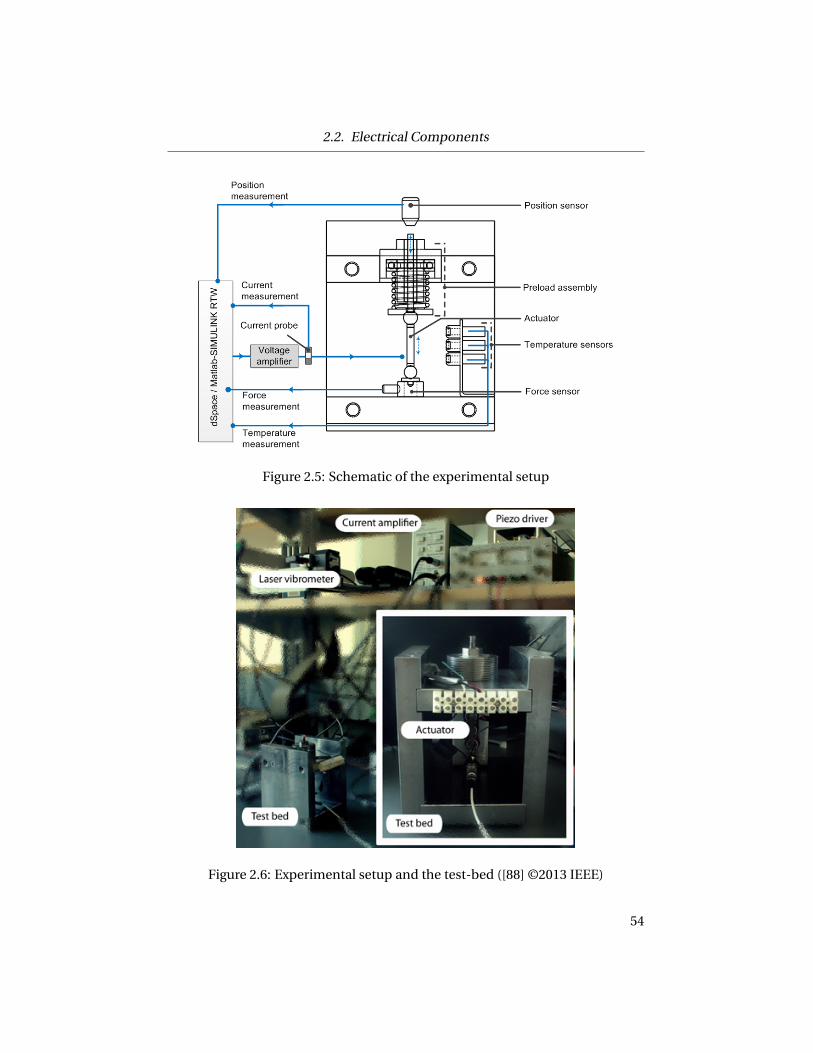
2.2. Electrical Components
Figure 2.5: Schematic of the experimental setup
Figure 2.6: Experimental setup and the test-bed ([88] ©2013 IEEE)
54

2.2. Electrical Components
which ensures the correct spacing (10 mm) between the sensors and the piezo-
electric actuator surface. The complete schematic of the experimental setup is
shown Figure 2.5. Figure 2.6 presents the picture of the setup and the test-bed.
2.2.6 Data Acquisition
A high speed data acquisition system (dSpace CPL1103) is employed to cap-
ture the experimental data. The experiments are modeled in SIMULINK® envi-
ronment and implemented through MATLAB/Real Time Workshop®. The graph-
ical user interface is designed in dSpace/ControlDesk® to facilitate real-time
plotting and data recording.
55

2.3. Summary
2.3 Summary
The experimental setup that is used to characterize and test the actuator is
presented in this chapter. The setup is carefully designed to provide a high oper-
ational range by reducing the moving mass in the setup. The experimental setup
is divided into two major components: 1) mechanical components and 2) elec-
trical components. The mechanical components are mostly related to the parts
which facilitate the mounting of the actuator. The electrical components are
responsible for measurements and data collection. The setup is used to charac-
terize the actuator first and then the control experiments are performed on the
setup.
56

Chapter 3
Impedance Measurement
As an electromechanical component, modeling of PEAs is an essential part
in implementation of these elements in real systems. In Chapter 1 (Section
1.6.2), it is shown that in the electrical domain, the piezoelectric actuators are
modeled as capacitive elements. To obtain an accurate model of the actuator,
the clamped capacitance of the actuator [13, 24] needs to be measured. Usually
the clamped capacitance is measured from the free capacitance. The principle
of the capacitance measurement technique is simple and relies on the basic the-
ory of electric fields:
C = Ir ms
2π f ·Ur ms(3.1)
where, the root mean square (rms) value of a sinusoidal driving voltage is de-
noted by Ur ms , Ir ms is the rms value the resulting current, f is the frequency of
the voltage signal, and C is the measured capacitance. This type of measure-
ment is usually carried out at frequencies around 1 kHz. However this leads
to two problems when applied to piezoelectric actuators. Firstly, the applied
voltage and resultant current include charge and voltage hysteresis that distorts
the capacitance measurement. Secondly, the measured capacitance is the un-
clamped capacitance since the actuator displaces due to the applied voltage
[89]. Thus, constitutive relationships are required to convert it to the clamped
capacitance value used in the standard control model by Goldfarb et al. [13]. In
this chapter, a novel real-time impedance measurement technique is presented
which facilitates the clamped capacitance measurement required for the model.
Also, it provides an effective resistance measurement of the piezoelectric actua-
tor.
57

3.1. Measurement Principle
3.1 Measurement Principle
To resolve the limitations in traditional measurements, an improved approach
is proposed where a high frequency low voltage signal (termed ripple voltage in
the remainder of this thesis) is used to measure the capacitance instead of a tra-
ditional low frequency signal. The ripple voltage frequency, fr must be much
larger than the resonant frequency of the test bed. This will ensure that there
is no mechanical movement of the actuator due to the ripple voltage. Also, the
magnitude of the ripple voltage needs to be small in order to ensure that hys-
teresis is minimized [90]. To yield the additional benefit of a real-time capaci-
tance measurement, the high frequency ripple signal is superimposed with the
low frequency driving signal. In this way, the capacitance measurement can take
place in real-time without influencing the low frequency displacement of the ac-
tuator or vice versa. This real-time capacitance measurement is not only novel
[91], but also very useful since it provides the basis for the sensorless control al-
gorithms presented in Chapters 5. There are two possible ways to superimpose
the ripple onto the driving signal: 1) using a summing circuit which merges the
high frequency ripple signal with a low frequency driving signal, and 2) using
a boost converters with fixed carrier frequency which provides a constant fre-
quency ripple voltage.
3.2 Superpositioning Through Summing Circuit
A summing circuit similar to the one shown in Figure 3.1 may be used to su-
perposition the ripple signal, Ur , on the driving voltage, U . The driving voltage,
U is sourced from the piezoelectric amplifier. The ripple signal, Ur may be gen-
erated through a signal generator. Transient voltage suppression (TVS) diode is
used to protect the signal generator from voltage spikes. Also, a low pass filter
may be required to filter out any noise present in the driving signal. The ripple
frequency is varied through a function generator.
58

3.3. Superpositioning Through Boost Converter
Figure 3.1: Superposition of signals through summing circuit
3.3 Superpositioning Through Boost Converter
To drive the piezoelectric actuator, a DC-DC boost converter is employed to
amplify the control signal from the data acquisition board (Section 2.2.1). This
amplifier automatically superimposes a high frequency ripple voltage (∼0.1% of
the maximum voltage range) onto the driving voltage. The magnitude and fre-
quency of the amplifier output voltage ripple is close to ∼100 mV and ∼100 kHz
respectively. While driving the actuator, the high frequency (∼100 kHz) ripple
voltage is superimposed onto the driving voltage, U , which results in a ripple
current, Ir . For the test bed in this thesis, the ripple voltage, Ur does not affect
the displacement of the actuator. This is due to the fact that the ripple frequency
is much larger than the mechanical bandwidth (∼2500 Hz) of the setup. Figure
3.2 shows the velocity of the actuator due to the ripple voltage. The free veloc-
ity is measured when the actuator is not mounted in the test-bed (mechanical
bandwidth ∼40 kHz) while the clamped velocity is measured when the actuator
is mounted in the test-bed (mechanical bandwidth∼2500 Hz). The figure clearly
indicates that the actuator shows close to zero velocity due to the ripple voltage
when placed in the test-bed.
3.4 Effect of Frequency on the Actuator Capacitance
Piezoelectric capacitance measurement is largely affected by the measure-
ment frequency. Hence, it is important to specify the frequency at which the
59

3.4. Effect of Frequency on the Actuator Capacitance
Figure 3.2: Velocity measurement in clamped and free condition [89] ©2011IEEE
capacitance measurement takes place. The piezoelectric actuator is modeled as
a pure capacitor near the driving frequency since the phase angle between the
voltage, U and resultant current, I is close to 90◦. The phase lag between the low
frequency normalized voltage and normalized current is shown in Figure 3.3.
The normalization of the signals are obtained by dividing the signals with their
maximum magnitudes. So, the expressions for the capacitance measurement in
Equation 3.1 are valid. However, at frequencies close to the ripple frequency of
100 kHz the phase angle between the ripple voltage, Ur and ripple current, Ir
is close to 65◦. The phase difference between the high frequency ripple voltage
and current is presented in Figure 3.4.
60
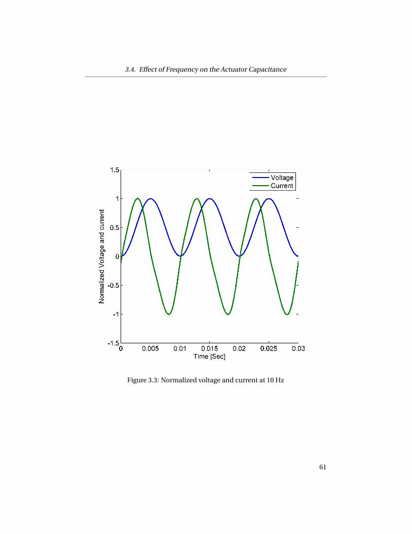
3.4. Effect of Frequency on the Actuator Capacitance
Figure 3.3: Normalized voltage and current at 10 Hz
61

3.4. Effect of Frequency on the Actuator Capacitance
Figure 3.4: Normalized ripple voltage and ripple current at 100 kHz
62

3.5. Impedance Measurement Algorithm
At high frequencies, the piezoelectric actuator is modeled as a resistor-capacitor
combination connected in series instead of a pure capacitive load. To avoid am-
biguity with the capacitance measured at low frequencies, the measured capac-
itance at 100 kHz is called ‘effective capacitance’ in the remainder of the thesis.
The expression for the effective capacitance measurement is as follows:
Ce =Irr ms
2π fr ·Urr ms
. (3.2)
3.5 Impedance Measurement Algorithm
The voltage amplifier/driver uses a boost converter, which amplifies the con-
trol voltage by a factor of ten and superimposes a 100 kHz ripple voltage, Ur ,
onto the driving voltage, U . The superpositioning of the low frequency driving
voltage, U (100 Hz) and high frequency ripple voltage, Ur (100 kHz) is shown in
Figure 3.5. To apply the proposed measurement technique, it is imperative to
extract the high frequency ripple voltages from the low frequency driving volt-
ages since the ripple quantities are employed to measure the impedance. To
facilitate this extraction, the current and voltage signals are passed through two
identical second order high pass active filters. The circuit diagram of the active
filter is shown in Figure 3.6. The capacitance and resistance values for the filter
were obtained from a Sullen-key topology implementation [92]. The cut-off fre-
quency of the filters is set to 18000 kHz. Once the ripple quantities are extracted,
the next step in the measurement is to decide on the sampling frequency of the
measurement.
3.5.1 Selection of the Sampling Frequency
The sampling frequency selection plays an important part in the proposed
measurement technique. Shannon’s sampling theorem indicates that for a rip-
ple frequency of 100 kHz, one would need to sample at more than 200 kHz in
order to ensure that the ripple signal can be reconstructed without frequency
folding. Unfortunately, sampling at this high frequency is expensive. However,
63

3.5. Impedance Measurement Algorithm
Figure 3.5: Amplifier output while supplying the driving voltage [89] ©2011 IEEE
Figure 3.6: Piezoelectric impedance measurement circuit
64
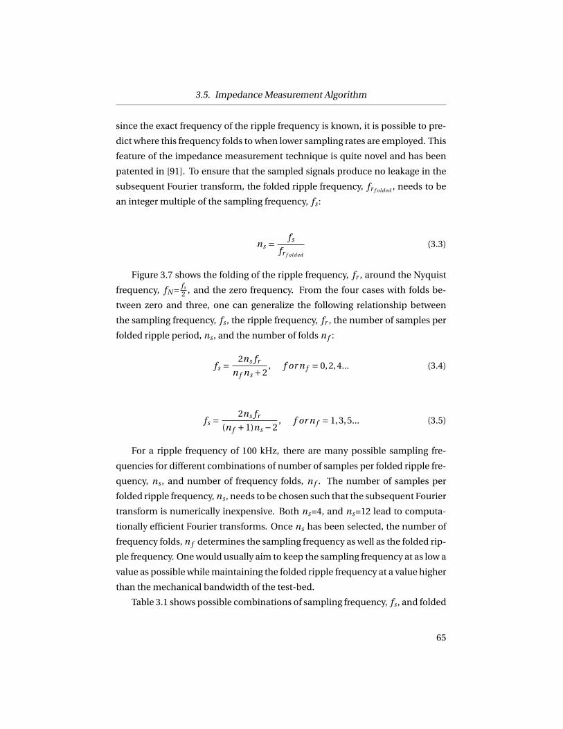
3.5. Impedance Measurement Algorithm
since the exact frequency of the ripple frequency is known, it is possible to pre-
dict where this frequency folds to when lower sampling rates are employed. This
feature of the impedance measurement technique is quite novel and has been
patented in [91]. To ensure that the sampled signals produce no leakage in the
subsequent Fourier transform, the folded ripple frequency, fr f olded , needs to be
an integer multiple of the sampling frequency, fs :
ns = fs
fr f olded
(3.3)
Figure 3.7 shows the folding of the ripple frequency, fr , around the Nyquist
frequency, fN = fs
2 , and the zero frequency. From the four cases with folds be-
tween zero and three, one can generalize the following relationship between
the sampling frequency, fs , the ripple frequency, fr , the number of samples per
folded ripple period, ns , and the number of folds n f :
fs = 2ns fr
n f ns +2, f or n f = 0,2,4... (3.4)
fs = 2ns fr
(n f +1)ns −2, f or n f = 1,3,5... (3.5)
For a ripple frequency of 100 kHz, there are many possible sampling fre-
quencies for different combinations of number of samples per folded ripple fre-
quency, ns , and number of frequency folds, n f . The number of samples per
folded ripple frequency, ns , needs to be chosen such that the subsequent Fourier
transform is numerically inexpensive. Both ns=4, and ns=12 lead to computa-
tionally efficient Fourier transforms. Once ns has been selected, the number of
frequency folds, n f determines the sampling frequency as well as the folded rip-
ple frequency. One would usually aim to keep the sampling frequency at as low a
value as possible while maintaining the folded ripple frequency at a value higher
than the mechanical bandwidth of the test-bed.
Table 3.1 shows possible combinations of sampling frequency, fs , and folded
65

3.5. Impedance Measurement Algorithm
Figure 3.7: Ripple signal with (a) no fold, (b) one fold, (c) two folds, and (d) threefolds
66

3.5. Impedance Measurement Algorithm
ripple frequency, fr f ol ded .
Table 3.1: Sampling frequency and folded ripple frequency at different values ofns with four times folding
ns n f fs [kHz] fr f olded [kHz]
4 0 400 1004 2 80 204 12 16 4
12 0 1200 10012 4 48 4
3.5.2 Real-time Fourier Transformation
A real-time Fourier transformation of the ripple voltage Vr and the ripple
current Ir is performed to obtain their magnitudes and phases. The Fourier co-
efficients of the ripple voltage, AVr and BVr as well as of the ripple current, AIr
and BIr can be obtained using the following discrete transfer functions:
AIr
Ir= AVr
Vr= 1
2np
np∑i=1
ns∑j=1
si n
(2π
nsj
)z j−i ns (3.6)
BIr
Ir= BVr
Vr= 1
2np
np∑i=1
ns∑j=1
cos
(2π
nsj
)z j−i ns (3.7)
Here, np is the number of cycles the Fourier transform is performed across. It
should be noted that the division by 2np does not actually have to be performed,
since the impedances of the actuator are determined from ratios of the Fourier
coefficients which are independent of np . Selection of a larger np , has two ef-
fects. First, the frequency is filtered around a narrower band. Mathematically
this can be stated as follows:
fPB = fs
nsnp, (3.8)
67

3.5. Impedance Measurement Algorithm
where, fPB is the passband of the Fourier transform. It should be pointed out
that this passband applies to both the folded ripple frequency as well as the
original ripple frequency. Too wide a passband can pick up mechanical vibra-
tions close to the folded ripple frequency. Too narrow a passband could miss the
ripple frequency, if the ripple frequency is not exactly constant. In addition to
the reduction of the passband size, the bandwidth of the capacitance measure-
ment is also reduced when more cycles are employed. Assuming that the Fourier
transform provides an average capacitance measurement over the number of
cycles used, the bandwidth of the measurement can be approximated as:
fBW = fs
nsnpπ. (3.9)
Table 3.2: Passband and bandwidth as a function of sampling periods for a 48kHz sampling frequency, and ns = 12
Cycles, np Passband, fPB [kHz] Bandwidth, fBW [kHz]
1 4 1.272 2 0.6374 1 0.3188 0.5 0.159
12 0.33 0.10616 0.25 0.08
For the test-bed in this thesis, the ripple voltage frequency is not exactly con-
stant at 100 kHz and so using more than four cycles could lead to a loss of fre-
quency content of the ripple. Also, using more than twelve cycles would result
in a capacitance measurement with lower bandwidth than the actuator driving
frequency [89].
3.5.3 Parameter Identification from Fourier Series Coefficients
The equivalent RC model for the piezoelectric actuator is presented in Fig-
ure 3.8 (a). The phasor diagram is shown in Figure 3.8 (b). By summing up the
quantities in real and imaginary directions, the following relationships can be
68

3.6. Results
Figure 3.8: (a) Resistance-capacitance model for the piezoelectric actuator (b)phasor diagram
deduced:
AVr = AIr Re +BIr
ωr Ce(3.10)
BVr = BIr Re −AIr
ωr Ce(3.11)
Once the Fourier coefficients are obtained, piezoelectric capacitance and resis-
tance can be calculated using Equations 3.12 and 3.13 as follows:
Ce =− 1
ωr
A2Ir+B 2
Ir
AIr BVr − AVr BIr
, (3.12)
Re =AIr AVr +BVr BIr
A2Ir+B 2
Ir
. (3.13)
3.6 Results
The measured capacitance and resistance values are observed during a 100
V-10 Hz sinusoidal operation. Plots of driving voltage, actuator displacement, as
well as effective capacitance and resistance are shown in Figure 3.9. These mea-
69

3.6. Results
surements help to deduce relationships between different measured quantities
such as capacitance-voltage, capacitance-position, and capacitance-resistance
relationships. Figure 3.10 shows the relationship between the driving voltage
and the effective capacitance. A large hysteresis (∼10% of the voltage) is present
between the driving voltage and the measured capacitance. Similarly, a large
hysteresis is observed between voltage and position in Figure 3.12. However,
when effective capacitance is plotted against position in Figure 3.11, minimal
hysteresis is observed. The hysteresis between voltage and capacitance and
hysteresis between voltage and position cancel each other. In Figure 3.13, the
effect of frequency is shown on the capacitance-position relationship. It shows
that the capacitance-position relationship slightly changes at relatively large fre-
quency (10 Hz). However, for quasi-static cases, the effect of frequency is small.
Two important conclusions can be drawn from these figures: 1) the capacitance
which is considered constant in the models (in Section 1.6.2) is not constant dur-
ing the piezoelectric actuator movement, and 2) the capacitance-position rela-
tionship provides a means for position self-sensing at least for low frequency
operations due to low hysteresis. These findings lead to two potential contri-
butions in this dissertation: 1) an improved electromechanical model is pre-
sented in Chapter 4 which includes the position dependency of the capacitance
in the model, and 2) an improved position self-sensing scheme is presented in
Chapter 5 which extends the traditional self-sensing schemes applicable in the
presence of creep and rate-dependent hysteresis. In Figure 3.14, the effective
resistance-capacitance relationship is shown. The resistance values decrease
with increased capacitance. The hysteresis present between the resistance and
capacitance is 6.25%.
Typically, capacitance is affected by temperature variation which affects the
position self-sensing strategy presented in Chapter 5. In Chapter 7, the effect
of temperature on capacitance due to self-heat generation and a temperature
compensated position self-sensing are presented.
70

3.6. Results
Figure 3.9: (a) Voltage, (b) position, (c) effective capacitance, and (d) effectiveresistance at 10 Hz
71

3.6. Results
Figure 3.10: Hysteresis in effective capacitance-voltage relationship
Figure 3.11: Effective capacitance measurement with position
72

3.6. Results
Figure 3.12: Hysteresis in effective position-voltage relationship
Figure 3.13: Effective capacitance measurement with position at various fre-quencies
73

3.7. Summary
Figure 3.14: Effective resistance measurement with effective capacitance
3.7 Summary
A novel real-time impedance measurement technique is presented in Chap-
ter 3. To obtain a real-time measurement of the piezoelectric clamped capac-
itance for an accurate model of the piezoelectric actuator, high frequency rip-
ple voltage and ripple current are employed. The high frequency ripple signals
are superimposed on the driving signal and hence provide real-time measure-
ment of the impedance. Since the ripple frequency is significantly higher than
the first natural frequency of the test bed, no movement is induced by the rip-
ple. Thus the ripple signals can be used to determine clamped impedance. The
impedance of the piezoelectric actuator is modeled as an equivalent resistance-
capacitance element connected in series. The impedance values are obtained
using Fourier series transformations of the ripple voltage and ripple current.
This real-time impedance measurement shows that the capacitance variation is
related to position change in piezoelectric actuator without significant hystere-
sis. Based on this finding, an extended electromechanical model is proposed in
Chapter 4. In addition, a position self-sensing scheme is developed in Chapter
74

3.7. Summary
5 based on the capacitance-position relationship.
75

Chapter 4
An Improved Electromechanical
Model for Piezoelectric Actuators
Piezoelectric actuator models can be classified into two broad groups: 1)
physical models, and 2) phenomenological models. The physical models are
based on measurable quantities such as voltage, charge, force, displacement or
the equivalent quantities such as electric field, current, stress and strain. Usu-
ally, the physical models are the augmented version of the linear IEEE model
discussed in Section 1.6.1. The eminent Goldfarb and Celanovic model [13]
includes the dynamics and hysteresis phenomenon in piezoelectric actuators
which are missing in the IEEE model. The dynamics are included using a sec-
ond order lumped mass system. The hysteresis is modeled using generalized
Maxwell’s resistive-capacitive operator. The model is presented earlier in Sec-
tion 1.6.2. Phenomenological models rely upon the input-output relationship
(voltage and position) of the piezoelectric actuator. Hence,these models do not
require knowledge of the underlying physical interaction between the variables
to implement the model which makes these models very popular. However,
highly accurate phenomenological models are required to implement the feed-
forward control. Due to the limitations in the phenomenological models, elec-
tromechanical models are used in this study.
In the physical model presented by Goldfarb and Celanovic [13], the piezo-
electric actuators are modeled as capacitors in the electric domain. A hystere-
sis block is added in series with the capacitor model of the actuator (Figure
1.10). In this model, the piezoelectric capacitance (similar to dielectric permit-
tivity in the IEEE model in Section 1.6.1) and force-voltage proportionality con-
stant(similar to piezoelectric strain coefficient in the IEEE model) are assumed
76
Chapter 4. An Improved Electromechanical Model for Piezoelectric Actuators
constant. These parameters are identified from the measurements of stiffness
and DC gain between charge and displacement [13]. A frequency analyzer pro-
gram is used to identify the piezoelectric capacitance. The other model param-
eters such as force-voltage proportionality constant and stiffness are identified
experimentally from force vs voltage and force vs displacement relationships re-
spectively. Badel et al. [41] employ a hyperbolic function to model the hysteresis
in the Goldfarb model and identify the function coefficients for ascending and
descending hysteresis paths. Also, the force-voltage proportionality constant is
identified using one of the function parameters in relation to force and volt-
age. Finally, free capacitance is measured and clamped capacitance is obtained
from the free capacitance using constitutive equations. Juhasz et al. [93] pro-
pose a parameter identification process for an embedded piezoelectric micro-
positioning system. In this study, the force-voltage proportionality constant is
measured when the hysteresis slope between the applied voltage and the po-
sition is constant. Quant et al. [94] also use a similar model as proposed by
Goldfarb et al. [13] for a piezoelectric bending actuator. However, in an attempt
to provide a better model fit, the force-voltage proportionality constant is con-
sidered a 6th order polynomial function of voltage derived from a piezoelectric
strain coefficient measurement. The models introduced above are extension
of the traditional model proposed by Goldfarb and Celanovic [13]. In most of
the cases, the model parameters, such as the capacitance, stiffness and force-
voltage proportionality constant are assumed constant. However, all the stated
models differ in the parameter identification technique.
Table 4.1 shows how close the identification techniques of different research
groups come to the manufacturer specifications. Every model has at least one
parameter that is significantly different from the suggested values by the man-
ufacturer. Since the manufacturer measurements are based on the linear IEEE
constitutive equations, which do not include hysteresis, the variation between
the manufacturer stipulated data and parameters from the different models is
expected. However, these parameters should not be orders of magnitude differ-
ent.
This chapter presents an improved electromechanical model of the piezo-
electric actuator which relies upon the real-time capacitance measurement pre-
77

Chapter 4. An Improved Electromechanical Model for Piezoelectric Actuators
sented in Chapter 3. A new model is developed based on the position dependent
capacitance. This leads to an improved fit between charge and position when
compared to the traditional electromechanical model. Thus, the new model
can be used to improve the accuracy of charge based sensorless position con-
trol. Another advantage of the new model is that the model parameters can be
identified from a single set of current, voltage, position and capacitance mea-
surements. Finally, other material parameters such as piezoelectric strain coeffi-
cient, d33, piezoelectric coupling coefficient, k33, and the permittivity constant,
ε33 can be deduced by employing the constitutive relationships.
78

Chapter 4. An Improved Electromechanical Model for Piezoelectric Actuators
Tab
le4.
1:C
om
par
iso
no
fpar
amet
ers
fro
md
iffe
ren
tpie
zoel
ectr
icm
od
els
wit
hm
anu
fact
ure
rd
ata
[95]
αco
mp
aris
on
CP
com
par
iso
nk
Pco
mp
aris
on
Mo
del
Man
ufa
ctu
rer
-α
iden
t.α
ma
nu
f.7
CP
iden
t.C
Pm
an
uf.
kP
iden
t.k
Pm
an
uf.
Mo
del
nu
mb
er[N
V−1
][N
V−1
][µ
F]
[µF
][Nµ
m−1
][Nµ
m−1
]
Go
ldfa
rbet
al.
NE
C-
AE
0505
D16
10.0
09.
311.
201.
406.
0048
.85
Bad
elet
al.
NE
C-
AE
0505
D44
H40
F7.
199.
312.
773.
4028
.70
20.2
4Ju
has
zet
al.
PI
-P
885-
5017
.55
8.05
1.50
81.
5010
0.29
50.0
0
7O
bta
ined
fro
mα=
d33
As 3
3t P
wh
ere,
s 33
isth
em
ech
anic
alco
mp
lian
ce,A
isth
est
ack
cro
ssse
ctio
nal
area
,an
dt P
isth
ela
yer
thic
knes
s8
Man
ufa
ctu
rer
spec
ified
valu
e[18
]
79

4.1. Proposed Piezoelectric Model
4.1 Proposed Piezoelectric Model
In order to better describe the behavior of the experimental test-bed and the
piezo stack used within that test-bed, both the constitutive Equations 1.4 and 1.5
in the model presented by Goldfarb and Celanovic describing the mechanical
and the electrical domain require modification. The modification proposed in
the new model are outlined in the following sections.
4.1.1 Mechanical Subsystem
The mechanical domain of the test setup is described by the force Equation
1.4. The test setup is shown in Figure 2.3. A schematic diagram of the mechan-
ical system is shown in Figure 4.1. The moving mass term includes the mass
of the needle assembly, mn and the mass of the piezo actuator, mP . Since the
piezoelectric actuator behaves like a heavy spring, only one third of the piezo
mass is also considered [96]. Traces from the force sensor indicate that the fric-
tion between needle and the Teflon sleeve is negligible 4.2. Finally, the stiffness
is comprised of the preload spring stiffness, ks and the piezo stiffness, kP . The
updated force equation describing this model is given in Equations 4.1 and 4.2:
αUP = mx +bx +kx, (4.1)
αUP =(mn + mP
3
)x +bx + (kP +ks)x. (4.2)
4.1.2 Electrical Subsystem
Goldfarb and Celanovic [13] model the piezoelectric actuators as capacitors
in the electrical domain. Change in piezoelectric capacitance with voltage is ob-
served in [97, 98], which is not reflected in Equation 1.5. This change of capac-
itance with position is confirmed by the online effective capacitance measure-
ment presented in Chapter 3. Traditional capacitance measurements employ a
relatively low frequency and high voltage (1 kHz, 1 VPP) in comparison to the
80
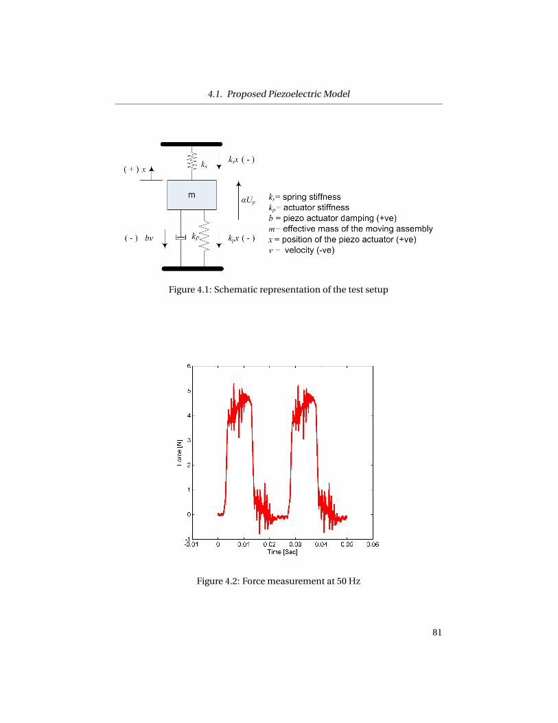
4.1. Proposed Piezoelectric Model
Figure 4.1: Schematic representation of the test setup
Figure 4.2: Force measurement at 50 Hz
81
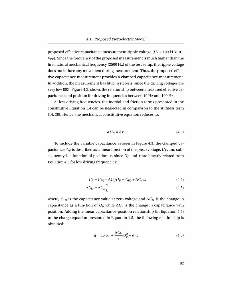
4.1. Proposed Piezoelectric Model
proposed effective capacitance measurement ripple voltage (Ur = 100 kHz, 0.1
VPP). Since the frequency of the proposed measurement is much higher than the
first natural mechanical frequency (2500 Hz) of the test setup, the ripple voltage
does not induce any movement during measurement. Thus, the proposed effec-
tive capacitance measurement provides a clamped capacitance measurement.
In addition, the measurement has little hysteresis, since the driving voltages are
very low [90]. Figure 4.3, shows the relationship between measured effective ca-
pacitance and position for driving frequencies between 10 Hz and 100 Hz.
At low driving frequencies, the inertial and friction terms presented in the
constitutive Equation 1.4 can be neglected in comparison to the stiffness term
[14, 28]. Hence, the mechanical constitutive equation reduces to:
αUP = kx. (4.3)
To include the variable capacitance as seen in Figure 4.3, the clamped ca-
pacitance, CP is described as a linear function of the piezo voltage, UP , and sub-
sequently is a function of position, x, since UP and x are linearly related from
Equation 4.3 for low driving frequencies:
CP =CP0 +∆CUUP =CP0 +∆Cx x, (4.4)
∆CU =∆Cxα
k, (4.5)
where, CP0 is the capacitance value at zero voltage and ∆CU is the change in
capacitance as a function of Up while ∆Cx is the change in capacitance with
position. Adding the linear capacitance-position relationship (in Equation 4.4)
to the charge equation presented in Equation 1.5, the following relationship is
obtained:
q =CPUP + ∆CU
2U 2
P +αx. (4.6)
82

4.1. Proposed Piezoelectric Model
Figure 4.3: Capacitance-position relationship at various frequencies
83

4.2. Power Balance
4.2 Power Balance
In the previous section, an additional term is introduced into the consti-
tutive equation for the electrical domain (Equation 4.6) and no adjustment is
made to the mechanical domain (Equation 4.1). This section uses a power bal-
ance to show that these equations are still consistent with each other. Ignoring
the hysteresis, the total power delivered to the stack is equal to the product of
applied current, I , and piezo voltage, UP . The portion of the power that is not
lost to friction is stored in the stack as spring, kinetic, and capacitive energy:
UP I = P f r i ct i on + d
d tEspr i ng + d
d tEki neti c +
d
d tEcapaci tor . (4.7)
For a nonlinear capacitor the energy stored can be calculated as follows [99]:
Ecapaci tor =U qcap −∫
qcap dU = 1
2CP0U 2 + 1
3∆CUU 3. (4.8)
Substituting Equation 4.8 into Equation 4.7 and replacing U with UP yields a
simple expression for the power balance:
UP I = d
d t
∫bxd x + d
d t
(1
2kx2
)+ d
d t
(1
2mx2
)+ d
d t
(1
2CP0U 2
P + 1
3∆CUU 3
P
), (4.9)
UP I = bx2 +kxx +mxx +CP0UPUP +∆CUU 2PUP . (4.10)
It is now demonstrated that the constitutive Equations 4.1 and 4.6 provide the
same expression for power balance. First, Equation 4.1 is divided by α in order
to obtain an expression for the piezo voltage UP :
UP = mx +bx +kx
α. (4.11)
Then, a time derivative is taken of Equation 4.6 in order obtain the current sup-
plied to the stack, I :
I =αx +CP0UP +∆CUUPUP . (4.12)
84

4.3. Parameter Identification
Finally, Equations 4.11 and 4.12 are multiplied to obtain the same expression as
the original power balance shown in Equation 4.10:
UP I = bx2 +kxx +mxx + mx +bx +kx
α(CP0UP +∆CUUPUP ), (4.13)
UP I = bx2 +kxx +mxx +CP0UPUP +∆CUU 2PUP . (4.14)
Since Equations 4.10 and 4.14 are identical, it is concluded that the mechanical
constitutive equation is unaffected by the introduction of the nonlinear capaci-
tance in the electrical constitutive equation.
4.3 Parameter Identification
Traditional models have usually assumed that CP , α, k, and b are time in-
variant. The proposed model suggests a position dependent capacitance. In
order to show the improvements attainable with this approach, a separate iden-
tification procedures for the base case with a constant capacitance and the new
variable capacitance model are defined in Sections 4.3.1 and 4.3.2. Thereafter,
additional material parameters are derived in Sections 4.3.4, 4.3.4.1 and 4.3.4.2.
4.3.1 Identification of α, k, b, and m for the Traditional Model with
Constant Capacitance
When Equations 1.4 and 1.5 are combined for quasi static conditions, an
expression linking charge linearly to displacement is obtained:
q =(CP
k
α+α
)x. (4.15)
The relationship between charge and position only allows the identification of
one of the three parameters α, k, or CP . Two of these parameters need to be
identified by other relationships. The clamped capacitance can be measured
using the technique described in Chapter 3.
The stiffness is obtained by dividing the force, Fext developed at maximum
85

4.3. Parameter Identification
voltage and zero stroke by the displacement achieved at maximum voltage and
no externally applied force. This measurement technique is only an approxima-
tion, since it assumes that the hysteresis voltage, UH , is the same for clamped
and free conditions.
k = Fext |Umax=0,x=0
x|Umax=0,F=0(4.16)
Given CP and k, one can then use Equation 4.15 to identify the force-voltage
proportionality constant, α from a quasi-static charge vs displacement exper-
iment. In order to obtain values for the damping coefficient b, and mass m,
one can perform dynamic experiments. In this case, a minimization of the error
between measured charge, q and charge calculated from position, velocity and
acceleration (using the model) is solved:
er rl i n = q − CP
α(mx +bx +kx)−αx. (4.17)
This minimization procedure can be performed with a simple quadratic error
minimization algorithm, or a nonlinear search algorithm. In this research, a
MATLAB function ‘fminsearch’ is used which is based on the the Nelder-Mead
optimization function in [100]. Both approaches provide similar answers. In
theory, Equation 4.17 can be used to identify b, and m with the given values
of α, CP , and k. However, the experiments are performed well below the first
mechanical eigenfrequency of the stack assembly, and so the sensitivity for de-
termining the moving mass m, is poor. Instead, the mass m, is determined by
adding a third of the stack mass mP , to the needle mass mn .
4.3.2 Identification of α, k, b, and m for the Proposed Model with
Variable Capacitance
The constitutive Equations 4.1 and 4.6 are characterized by the clamped ca-
pacitance, CP , the mass, m, the force-voltage proportionality constant, α, the
stiffness, k and the damping, b. Given measurements of capacitance as a func-
tion of position, both stiffness k, and force-voltage proportionality constant, α
can be obtained directly from the quasi static relationship between charge and
86

4.3. Parameter Identification
Figure 4.4: Capacitance-position relationship at various frequencies
position, since this is now a second order polynomial:
q =CP0k
αx + ∆Cx
2
k
αx2 +αx. (4.18)
An alternative way to determine k and α using quasi static experiments is to fit
current over velocity. This avoids integrating current in order to obtain charge
[101]:
q
x=
(CP0k
α+α
)+∆Cx
k
αx. (4.19)
It is shown in Equation 4.19 that the ratio of current over velocity is not a con-
stant as would be the case for the original model by Goldfarb and Celanovic
(compare Equation 4.15). This is confirmed by the measurements shown in Fig-
ure 4.4 where driving voltages of different frequencies are applied to the actua-
87
4.3. Parameter Identification
tor. It should be pointed out that Equation 4.19 leads to a division by zero close
to the beginning and the end of the stroke (where velocities are zero). Thus,
measurements are only physically meaningful towards the center of the stroke.
The mass of the actuator system is estimated by adding a third of the stack
mass mP , to the needle mass mn . To obtain the damping coefficient b, dynamic
experiments need to be performed. In this case, b, is found by using the Nelder-
Mead optimization algorithm (1965) to minimize the error between measured
charge, q and charge calculated from measured position, velocity, and accelera-
tion:
er rnonli near =(
q −CP0UP − ∆Cx
2
α
kU 2
P −αx
), (4.20)
where,
UP = mx +bx +kx
α. (4.21)
4.3.3 Identification of Free Capacitance, CT
Free capacitance is measured under stress free condition that are present
when there is no or constant external load. The relationship between the clamped
and free capacitance can be deduced from the constitutive charge Equation 4.6
as follows:
qP
UP=CP + α2
k=CT . (4.22)
where, CT is the free capacitance. From the free capacitance, the free permittiv-
ity can be obtained through Equation 4.23 where, εT is the free permittivity, A is
the area of the electrode (∼ to cross sectional area of actuator), nl is the number
for layers in the actuator and ε0 is the permittivity constant at vacuum:
εT = CT A
ε0tP nl. (4.23)
88
4.3. Parameter Identification
4.3.4 Identification of Material Properties
The piezoelectric material properties such as piezoelectric strain coefficient,
d33 and piezoelectric coupling coefficient, k33 can also be obtained from the
constitutive relationships once the model parameters are obtained. In this sec-
tion, the material parameters are attained from the identified model parameters
and compared with the manufacturer specification where available.
4.3.4.1 Piezoelectric Strain or Charge Coefficient, d33
The piezoelectric strain or charge coefficient, d33 is an important design pa-
rameter for piezoelectric actuator systems. It is defined as the strain developed
per unit of applied electric field in the piezoelectric materials. Alternatively, this
is equivalent to the polarization generated due to the applied stress. The first
subscript 3 represents the direction of the strain or polarization while the sec-
ond subscript represents direction of the applied electric field or stress. Tradi-
tionally, it is measured using the linear IEEE constitutive Equation 1.2 which as-
sumes the applied stress is negligible and strain is a function of applied electric
field. Measuring both strain and electric field provides the d33 measurement.
However, the traditional measurement employs the applied voltage instead of
the linearized voltage, UP , as a measure of electric field. As a result, different d33
are obtained at different voltage levels due to hysteresis. To minimize this hys-
teresis effect, traditional measurements are often performed at the maximum
level of the applied voltage, U . Also, since d33 provides an estimate of the quality
of the materials, large signal values provide more practical representation. The
term d33 is an equivalent term to the force-voltage proportionality constant, α
in the electromechanical model. The following equation [102] presents the rela-
tionship between d33 and α:
d33 = α
nl k= αtP
LP k, (4.24)
where, nl is the number of layers in the actuator and k is the stiffness of the ac-
tuator. The number of layers is calculated from the thickness of the piezoelectric
layers, tP and the length of the actuator, LP .
89

4.4. Experimental Results
4.3.4.2 Piezoelectric Coupling Coefficient, k33
The piezoelectric coupling coefficient, k33 is an important parameter which
represents the fraction of electromechanical energy conversion in the piezo-
electric system. It is an indication of the effectiveness or efficiency with which
the piezoelectric actuator converts electrical to mechanical energy or vice versa.
The first subscript 3 represents the direction of the applied electric field while
the second subscript represents the direction of the mechanical movement. A
higher value of the coefficient is desired. It does not include the dielectric or
mechanical losses. The coupling coefficient can be obtained from the following
relationship [102] of clamped and free capacitance:
k233 = 1− CP
CT. (4.25)
From the identified values of CP and CT , the piezoelectric coupling coefficient
can be obtained.
4.4 Experimental Results
The model parameters are identified through experiments using the setup
discussed in Section 2.2 and the identification algorithms outlined in Section
4.3.
4.4.1 Experimental Procedure
The model identification experiments use a sinusoidal voltage profile with
frequencies between 10 Hz, 100Hz and a magnitude of 100V. The actuators are
allowed sufficient time to reach a state where little hysteresis voltage is present
before starting the experiments. The position measurement is zeroed at the be-
ginning of the measurement and data are recorded for 5 cycles shown in Fig-
ure 4.5. At every frequency, 5 sets of data are recorded in order to ensure the
statistical significance. The model parameters are obtained using the methods
described in Section 4.3 and listed in Table 4.2 together with the manufacturer
specifications. Two cases are presented in the table, where Case 1 presents the
90

4.4. Experimental Results
Figure 4.5: Driving signal, U at 10 Hz
traditional model with a constant capacitance while Case 2 depicts the improved
model with variable capacitance.
In Case 1, the value of capacitance is considered constant in the traditional
model. The value of the capacitance at zero V matches with the value prescribed
by the manufacturer in Case 2, the new proposed model. However, in the man-
ufacturer specification, it is prescribed that there is 20% variability present in
the capacitance measurement. The slope in the capacitance measurement is
not specified by the manufacturer, but similar trends have been reported by
[97, 98] when a DC voltage is applied to piezoelectric components. The iden-
tified stiffness values are largely different in Case 1 and Case 2. In Case 1, it is
measured from static loading test using Equation 4.16 while in Case 2, it is ob-
tained from the dynamic measurement of charge and position using Equation
4.19. This identification is very close to the manufacturer specification. Also, the
other parameters such as α, d33 and k33 values are close to the values stipulated
91

4.4. Experimental Results
Tab
le4.
2:M
od
elp
aram
eter
iden
tifi
cati
on
Cas
e1
Std
.C
ase
2St
d.
Man
ufa
ctu
rer’s
Mo
del
par
amet
ers
Un
it(T
rad
itio
nal
dev
.9(P
rop
ose
dd
ev.10
Spec
ifica
tio
nM
od
el,
Mo
del
,∆
Cx=
0)∆
Cx6=
0)
Cap
acit
ance
at0V
,CP
0[µ
F]
3.13
110.
033.
1310
0.03
3.112
Cap
acit
ance
at10
0V,C
P10
0[µ
F]
3.13
100.
032.
1610
0.01
-C
apac
itan
cesl
op
e,∆
Cx
[Fm
−1]
0–
-0.0
36e
-4-
Act
uat
or
Stif
fnes
s,k
P[Nµ
m−1
]11
.20
25.3
0.16
25A
ctu
ato
rd
amp
ing,
b[N
sm−1
]31
0037
721
2012
0-
Forc
e-vo
ltag
ep
rop.
con
stan
t,α
[NV
−1]
14.0
50.
039.
340.
279.
0113
Pie
zoel
ectr
icst
rain
coef
f.,d
33[p
mV
−1]
2400
3069
520
68014
Pie
zoel
ectr
icco
up
l.co
eff.
,k33
0.92
00.
720.
010.
7014
9C
alcu
late
dov
erth
ree
sets
ofe
xper
imen
ts10
Cal
cula
ted
over
thre
ese
tso
fexp
erim
ents
11Id
enti
fied
cap
acit
ance
valu
esar
em
easu
red
at10
0kH
zan
d0.
1V
12M
anu
fact
ure
r’ssp
ecifi
edva
lues
are
mea
sure
dat
1kH
zan
d1
VP
P[1
8]13
Ob
tain
edfr
omα=
d33
As 3
3t P
[102
]14
Man
ufa
ctu
rer
dat
ash
eet[
103]
92

4.4. Experimental Results
Figure 4.6: (a) Charge-position relationships modeled (proposed) and mea-sured, and (b) current-position relationships modeled and measured for variousfrequencies
from manufacturer’s specification with the proposed model. It is important to
note that the identified parameters are sensitive to the capacitance measure-
ment which includes both the CP0 and ∆Cx . The sensitivity of the identified
parameters to changes in the capacitance measurement is shown in Table 4.3.
To identify the parameters, the parameters presented in 4.2 for Case 2 are used
considering the capacitance measurement is unaffected.
4.4.2 Model Validation Through Charge-position Relationship
For model validation, measured values of charge-position relationships are
compared with the modeled charge-position relationship in Figure 4.6(a) using
Equation 4.18. The nearly linear relationship between charge and position is
largely independent of driving frequency, since friction forces and inertial forces
are small at the tested frequencies. A more detailed comparison for the qual-
ity of fit is obtained by plotting current against position as shown in in Fig-
ure 4.6(b). Since current is closely related to velocity, one expects to see el-
lipses that open up with increasing frequency. In Figure 4.7(a) and 4.7(b), the
charge-position relationship is compared between the traditional model (∆Cx =0) and the proposed model (∆Cx < 0). The modeling errors, presented in Figure
93

4.4. Experimental Results
Tab
le4.
3:Se
nsi
tivi
tyo
fpar
amet
erid
enti
fica
tio
nto
chan
ges
inca
pac
itan
cem
easu
rem
ent
Para
met
ers
No
chan
ge20
%in
crea
se20
%in
crea
se20
%in
crea
sein
CP
0in∆
Cx
inC
P0
and∆
Cx
k[Nµ
m−1
]25
.120
.724
.020
.9α
[NV
−1]
9.36
7.72
10.7
79.
36d
33[p
mV
−1]
700
697
841
840
k33
0.72
0.66
0.77
0.73
UP
ma
x[V
]86
8672
72
94

4.4. Experimental Results
4.7(c) and 4.7(d), are calculated using Equation 4.17 for the traditional model
and using Equation 4.20 for the proposed model. Figure 4.7 indicates that the
proposed model shows slight improvements in terms of fitting the measured
charge-position relationship. Both the 10 Hz and the 100 Hz cases show iden-
tical trends where the proposed model provides lower fitting errors especially
towards the center of the stroke. This is because of the ability of the proposed
model to capture the curvature in the charge-displacement relationship with the
additional term in the charge constitutive equation.
4.4.3 Hysteresis Voltage
The driving piezoelectric voltage, U is composed of the linear piezoelectric
voltage, UP and the hysteresis voltage, UH . Once the model parameters are iden-
tified, one can obtain UP using Equation (4.14).The hysteresis voltage, UH is ob-
tained through the traditional model in Equation 1.6. Figure 4.8(a) shows the
driving voltage, piezoelectric voltage and the hysteresis voltage obtained for the
traditional model with different frequency ranges. Figure 4.8(b) presents the
same voltages for the proposed model. In both cases, the hysteresis voltage
and the linear piezoelectric voltage show similar trends for all tested frequen-
cies. However, the hysteresis voltage obtained through the traditional model is
significantly large than for the proposed model. To be physically meaningful,
hysteresis voltages should be in the order of approximately 20% of the applied
voltage. This is the case for the parameters of the proposed model, but not for
the traditional model parameters.
95
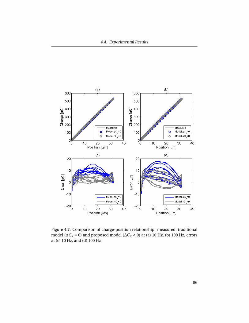
4.4. Experimental Results
Figure 4.7: Comparison of charge-position relationship: measured, traditionalmodel (∆Cx = 0) and proposed model (∆Cx < 0) at (a) 10 Hz, (b) 100 Hz, errorsat (c) 10 Hz, and (d) 100 Hz
96

4.5. Summary
Figure 4.8: (a) U and UH vs charge for ∆Cx = 0 (traditional model), and (b) Uand UH vs charge for ∆Cx < 0 (proposed model) at 10 Hz and 100 Hz
4.5 Summary
In this chapter, an improved piezoelectric model is proposed by introduc-
ing a nonlinear capacitance term. This new term provides a better fit of the re-
lationship between charge and position. A second advantage of this model is
that actuator stiffness and force-voltage proportionality constant can be iden-
tified from quasi static measurements of position, charge, and effective capac-
itance. Quantitative comparisons with manufacturer data show that the pro-
posed model provides meaningful identification of the model parameters. Fur-
ther, quantitative analyses through hysteresis voltage identification justify the
improvement of the proposed model over traditional model.
97
Chapter 5
Position Self-sensing of
Piezoelectric Actuators
Piezoelectric actuators demonstrate nonlinear phenomena such as hystere-
sis and creep at different frequency ranges [26, 30, 43]. Examples of hystere-
sis and creep behavior are shown in Figure 5.1, where the actuator position is
plotted against applied voltage for frequencies ranging from 0 Hz (creep) to 100
Hz. Usually, feedback position sensors are used to mitigate these nonlinearities
successfully. However, there are many applications where dedicated position
sensors are difficult to implement due to space and/or cost constraints. Exam-
ples for applications that suffer from these constraints are fuel injectors, inkjet
printing nozzles, micro-pumps etc. Moreover, an additional component may af-
fect the overall reliability of the control system. Chapter 1 highlighted some of
the model based sensorless position control techniques for piezoelectric actua-
tors that have been used to avoid additional sensor elements. These techniques
are designed to compensate for hysteresis (Section 1.6.3) and creep phenom-
ena (Section 1.3). However, these sensorless control techniques are typically de-
signed for a very narrow frequency range. Thus, they cannot simultaneously
compensate for both creep and rate-dependent hysteresis effects. Moreover, an
accurate model is a prerequisite for these sensorless control schemes. These
models are often difficult to obtain and susceptible to modeling uncertainties
[11, 12]. A number of studies include a feedforward model to a dedicated feed-
back sensor (Section 1.7.3) in order to improve the dynamic properties of the
feedback system. This approach improves the bandwidth of the controller and
leads to more robustness towards modeling uncertainties.
Position self-sensing (PSS), which was first proposed for vibration suppres-
98

Chapter 5. Position Self-sensing of Piezoelectric Actuators
Figure 5.1: Rate-dependent hysteresis and creep at different frequencies(Reprinted with permission [61]. Copyright 2012, American Institute of Physics.)
99

Chapter 5. Position Self-sensing of Piezoelectric Actuators
sion in different structures [72], is another technique used to improve actuator
positioning. In this approach, a single piezoelectric element is used both as a
sensor and an actuator. True collocation of actuator and sensor is realized based
on the direct and indirect effect of piezoelectricity. A capacitance bridge circuit
is used to extract strain or position. This approach is often used in piezoelectric
cantilevers or patches. Jones et al. [104] implemented this approach with mul-
tilayered actuators for micro positioning. The self-sensing approach works well
assuming ideal conditions. However, in practice, this approach poses a number
of challenges. The main problem is associated with the bridge balancing since
it employs a similar capacitor as the piezoelectric capacitance where the accu-
rate measurement of the piezoelectric capacitance is difficult [62, 73]. So, any
change in the piezoelectric actuator capacitance other than the strain may af-
fect the measurement and hence the overall control system. The capacitance
bridge based self-sensing is presented in Section 1.8.1. Unlike voltage, piezo-
electric charge flow is found to be linearly related to the position over a wide
range of frequencies [13, 52]. Figure 5.2 shows the charge-position relationship
from 10 Hz to 300 Hz with negligible hysteresis. A linear fitting line with a slope
of a0 is also shown in Figure 5.2. Based on this linear relationship, charge based
controllers are designed. Charge based PSS can also be realized relying on the
linear charge-position relationship. In this case, current is integrated and the
piezoelectric actuator position is obtained from the charge measurement. In
this approach, the major challenge is the charge drift due to an offset current
which result in estimated position drift specially during slow operations (<10
Hz). Section 1.8.2 highlights the charge based self-sensing scheme in more de-
tail. The other self-sensing technique presented in Section 1.8.3 is based on the
direct effect of piezoelectricity where a portion of the actuator is designed to
function as sensor. Due to the strain in the piezoelectric actuator, a voltage is
induced. The induced voltage is proportional to the actuator displacement and
position information is obtained from the induced voltage. The major short-
coming in this technique is that the actuator range is reduced since some of the
actuator is used as a sensor.
The real-time effective capacitance measurement of the piezoelectric actua-
tor presented in Chapter 3 provides yet another avenue to estimate actuator po-
100

Chapter 5. Position Self-sensing of Piezoelectric Actuators
Figure 5.2: Charge-position relationship over a frequency range of 10 Hz – 300Hz ([88] ©2013 IEEE)
101

5.1. Charge Based Position Self-sensing, xI
sition. Here one exploits the finding that the position of the actuator is related
to effective capacitance with negligible (<3%) hysteresis. The problem with the
capacitance based PSS is that the signal is noisy and requires low pass filtering
which limits its application to slow operations (<10 Hz).
All of the self-sensing techniques discussed so far have advantages and short-
comings. By combining charge based PSS and capacitance based PSS which on
their own only work well for high and low driving frequencies respectively, a po-
sition self-sensing for a wide frequency range can be achieved. It is important to
define the high and low frequencies at this point. By high frequency, it refers to
the range where the actuator is driven below the range to avoid the vibrational
dynamics (see Figure 1.4). To this end, a novel hybrid position observer (HPO)
is developed which fuses the charge based PSS and capacitance based PSS. It
achieves good position estimates over a wide range of frequencies where both
creep and hysteresis effects are present. The objective of this chapter is to intro-
duce position estimation using the HPO. The following sections will detail the
two PSS approaches, the operating principle of the HPO, and the implementa-
tion of the HPO. Finally, the HPO results are compared with a dedicated position
sensor.
5.1 Charge Based Position Self-sensing, xI
Charge based PSS is based on the linear fitting of the charge-position rela-
tionship shown in Figure 5.2. The maximum position error observed in the cen-
ter of the curve is less than one micrometer (<3% of the maximum stroke) for a
frequency range of 10-300 Hz. This experimental linear relationship can also be
found analytically. By manipulating the piezoelectric constitutive Equations 1.4
and 1.5, an expression relating charge to position can be obtained,
q =CPmx +bx +kx −F
α+αx. (5.1)
102

5.1. Charge Based Position Self-sensing, xI
Figure 5.3: Magnitude and phase response ([88] ©2013 IEEE)
If external Force, F is neglected, then Equation 5.1 can be transformed into a
transfer function in the Laplace-domain,
G(s) = x(s)
q(s)= x(s)s
I (s)= 1
CPα (ms2 +bs +k)+α
. (5.2)
Figure 5.3 shows the measured frequency response of G(s). The targeted fre-
quency range (<150 Hz) in this research is well below the mechanical natural
frequency of the test setup (2500 Hz) and the electromechanical resonance fre-
quency (700 Hz). Hence, the dynamic terms in Equation 5.1 are neglected and
the following simplified expression is obtained for relating estimated position,
xI to measured charge, q through G(s):
G(s) = xI (s)
q(s)= 1
α+CPkα
= 1
a0. (5.3)
The dynamic transfer function G(s) in Equation 5.2 reduces to a constant gain
in the reduced frequency transfer function G(s). Traditional feedforward charge
control schemes use Equation 5.3 by controlling the amount of charge supplied
to the piezoelectric actuator. Rather than controlling charge, charge based PSS
integrates measured current, I to obtain charge and hence position from the
charge measurement. Figure 5.2 presents the position estimation technique
from charge measurement based on Equation 5.3. To differentiate between the
103

5.2. Capacitance Based Position Self-sensing, xCP
Figure 5.4: Position estimation from charge measurement ([88] ©2013 IEEE)
measured quantities and estimated quantities, a ‘bar’ above the variables is used
to represent the measured quantities and ‘hat’ is used for estimated values.
The main challenge with this approach is charge leakage, which requires so-
phisticated hardware architectures. Charge leakage leads to an offset current,
I0 which results in a drift of identified charge and hence estimated position.
To identify and compensate for the amount of offset current, a second low fre-
quency position estimate based on an effective piezoelectric capacitance mea-
surement is proposed. The next section details the capacitance based PSS.
5.2 Capacitance Based Position Self-sensing, xCP
Effective piezoelectric capacitance measurement is discussed in Chapter 3.
Figure 5.5 shows that the piezoelectric capacitance changes with stroke with lit-
tle hysteresis (<3% maximum stroke). Based on a real-time measurement, effec-
tive capacitance provides a means for position self-sensing. To yield the position
information from the effective capacitance measurement, a higher order poly-
nomial is chosen. For fitting purpose, 0.1 Hz is selected which lies in between
0.01 Hz to 1 Hz. Equation 5.4 presents the fitting function, Γ for capacitance
based PSS,
Γ= xCP (CP ) = b0 +5∑
j=1b j C j
P , (5.4)
where, j is the order of the polynomial and b0 and b j are the constant and the
coefficients of the polynomial. To obtain the order of the polynomial, j , the rela-
tionship between capacitance and position is fitted with different orders and the
residuals and standard errors were compared to obtain a reliable fitting of the
104
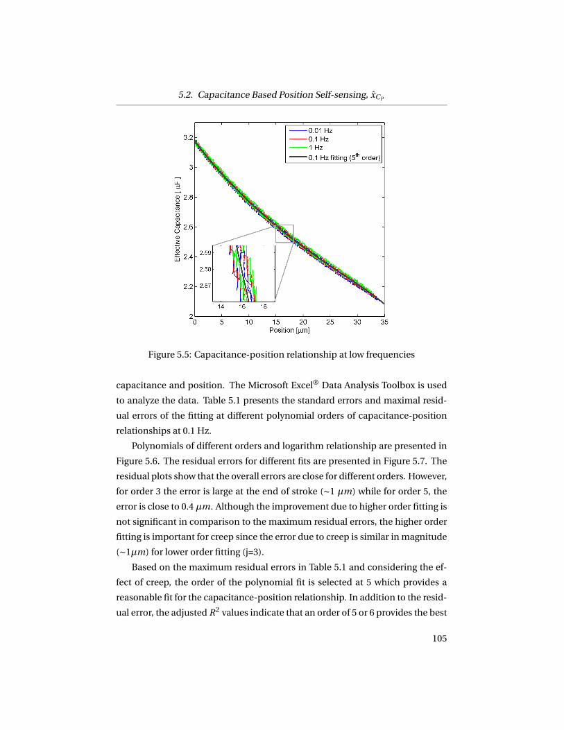
5.2. Capacitance Based Position Self-sensing, xCP
Figure 5.5: Capacitance-position relationship at low frequencies
capacitance and position. The Microsoft Excel® Data Analysis Toolbox is used
to analyze the data. Table 5.1 presents the standard errors and maximal resid-
ual errors of the fitting at different polynomial orders of capacitance-position
relationships at 0.1 Hz.
Polynomials of different orders and logarithm relationship are presented in
Figure 5.6. The residual errors for different fits are presented in Figure 5.7. The
residual plots show that the overall errors are close for different orders. However,
for order 3 the error is large at the end of stroke (∼1 µm) while for order 5, the
error is close to 0.4 µm. Although the improvement due to higher order fitting is
not significant in comparison to the maximum residual errors, the higher order
fitting is important for creep since the error due to creep is similar in magnitude
(∼1µm) for lower order fitting (j=3).
Based on the maximum residual errors in Table 5.1 and considering the ef-
fect of creep, the order of the polynomial fit is selected at 5 which provides a
reasonable fit for the capacitance-position relationship. In addition to the resid-
ual error, the adjusted R2 values indicate that an order of 5 or 6 provides the best
105

5.2. Capacitance Based Position Self-sensing, xCP
Figure 5.6: Capacitance-position relationship at low frequencies
regression model. The ANOVA of the regression model ( j =5) is shown in Table
5.2 where coefficients and intercept for the model are shown. The p-values in-
dicate that all the coefficients are significantly important. The block diagram
Table 5.1: Fitting errors in regression models of different orders
Parameters j=3 j=4 j=5 j=6 ln
Maximum residual error [µm] 1.34 1.24 1.17 1.15 1.49R2 value 0.99881 0.99886 0.99889 0.99889 0.997Adjusted R2 value 0.99881 0.99886 0.99889 0.99889 –
of the capacitance based PSS is shown in Figure 5.8. Due to the noise in the ca-
pacitance measurement, the capacitance based PSS is only applicable for low
frequencies.
106
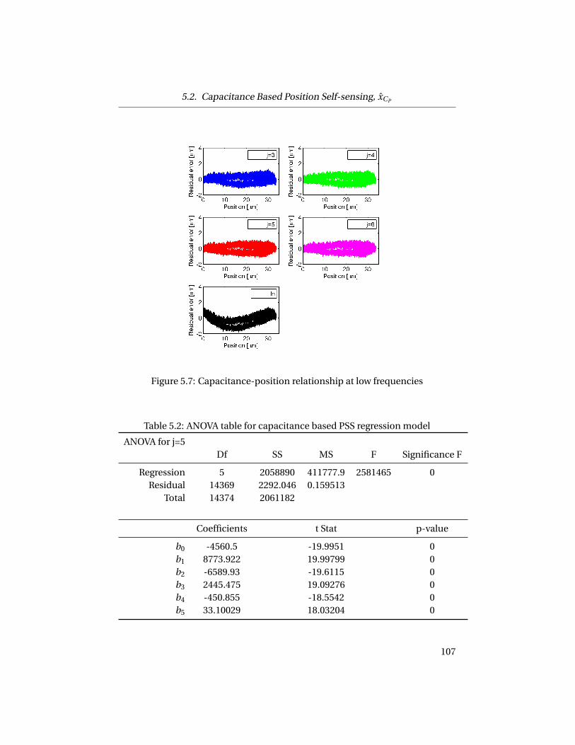
5.2. Capacitance Based Position Self-sensing, xCP
Figure 5.7: Capacitance-position relationship at low frequencies
Table 5.2: ANOVA table for capacitance based PSS regression model
ANOVA for j=5Df SS MS F Significance F
Regression 5 2058890 411777.9 2581465 0Residual 14369 2292.046 0.159513
Total 14374 2061182
Coefficients t Stat p-value
b0 -4560.5 -19.9951 0b1 8773.922 19.99799 0b2 -6589.93 -19.6115 0b3 2445.475 19.09276 0b4 -450.855 -18.5542 0b5 33.10029 18.03204 0
107

5.3. Hybrid Position Observer Design
Figure 5.8: Position estimation from capacitance measurement ([88] ©2013IEEE)
5.3 Hybrid Position Observer Design
Since the charge based PSS provides position estimate at relatively high fre-
quencies (below the high dynamic range shown in Figure 1.4) and capacitance
based PSS is suitable only at low frequencies, a hybrid position observer (HPO)
is proposed which utilizes both PSS signals for position estimation. The block
diagram of the hybrid position observer is shown in Figure 5.9 where the pre-
viously discussed charge based PSS is fused with capacitance based PSS. The
shaded section of the Figure represents the real system while, the clear section
represents the HPO. The structure of the HPO is very similar to a conventional
observer. The plant model, which is represented by G(s)s is driven by the mea-
sured current, I . The position obtained through effective capacitance, xCP can
be thought of as a measurement unit in a traditional observer structure. In con-
trary to a conventional observer however, the feedback term L(s) is not used to
adjust the poles of the plant, but rather to estimate the offset current, I0 present
in the measured current, I . The estimated I0 is then subtracted from the mea-
sured current to eliminate the drift in charge based PSS. This is achieved through
the use of a proportional plus integral operator:
L(s) = LP + L I
s. (5.5)
The identified current offset is then subtracted from the current measurement.
Assuming that the modeled plant, G(s) equals the real plant, G(s), the following
transfer functions for the estimated position signal, x can be obtained:
x(s)
xI (s)= 1
1+ s−1G(s)L(s)= a0s2
a0s2 +LP s +L I, (5.6)
108
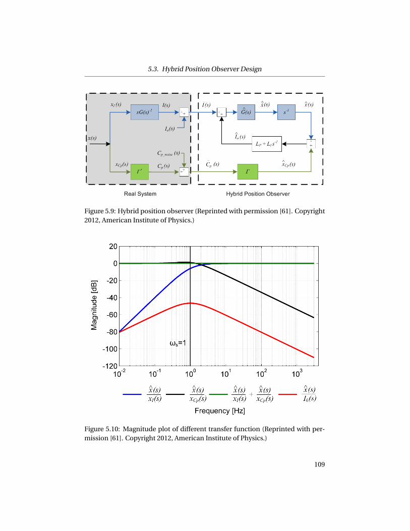
5.3. Hybrid Position Observer Design
Figure 5.9: Hybrid position observer (Reprinted with permission [61]. Copyright2012, American Institute of Physics.)
Figure 5.10: Magnitude plot of different transfer function (Reprinted with per-mission [61]. Copyright 2012, American Institute of Physics.)
109
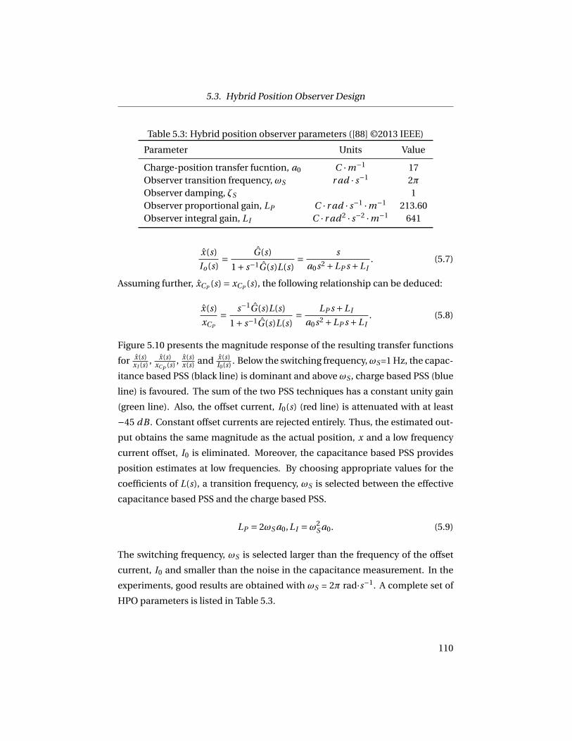
5.3. Hybrid Position Observer Design
Table 5.3: Hybrid position observer parameters ([88] ©2013 IEEE)
Parameter Units Value
Charge-position transfer fucntion, a0 C ·m−1 17Observer transition frequency, ωS r ad · s−1 2πObserver damping, ζS 1Observer proportional gain, LP C · r ad · s−1 ·m−1 213.60Observer integral gain, L I C · r ad 2 · s−2 ·m−1 641
x(s)
Io(s)= G(s)
1+ s−1G(s)L(s)= s
a0s2 +LP s +L I. (5.7)
Assuming further, xCP (s) = xCP (s), the following relationship can be deduced:
x(s)
xCP
= s−1G(s)L(s)
1+ s−1G(s)L(s)= LP s +L I
a0s2 +LP s +L I. (5.8)
Figure 5.10 presents the magnitude response of the resulting transfer functions
for x(s)xI (s) , x(s)
xCP (s) , x(s)x(s) and x(s)
I0(s) . Below the switching frequency,ωS=1 Hz, the capac-
itance based PSS (black line) is dominant and above ωS , charge based PSS (blue
line) is favoured. The sum of the two PSS techniques has a constant unity gain
(green line). Also, the offset current, I0(s) (red line) is attenuated with at least
−45 dB . Constant offset currents are rejected entirely. Thus, the estimated out-
put obtains the same magnitude as the actual position, x and a low frequency
current offset, I0 is eliminated. Moreover, the capacitance based PSS provides
position estimates at low frequencies. By choosing appropriate values for the
coefficients of L(s), a transition frequency, ωS is selected between the effective
capacitance based PSS and the charge based PSS.
LP = 2ωS a0,L I =ω2S a0. (5.9)
The switching frequency, ωS is selected larger than the frequency of the offset
current, I0 and smaller than the noise in the capacitance measurement. In the
experiments, good results are obtained with ωS = 2π rad·s−1. A complete set of
HPO parameters is listed in Table 5.3.
110

5.4. Hybrid Position Observer Implementation
Figure 5.11: Hybrid position observer implementation ([88] ©2013 IEEE)
5.4 Hybrid Position Observer Implementation
The flowchart of the HPO self-sensing setup is presented in Figure 5.9. The
actuator is fed with a low frequency driving voltage, U for positioning and high
frequency ripple voltage, Ur for effective capacitance measurement. The low
frequency voltage, U creates a driving current, I which upon integration, pro-
vides a charge measurement that is employed to infer the position from Equa-
tion 5.3. The high frequency voltage, Ur provides a high frequency ripple current
which are separated and processed to obtain the effective capacitance measure-
ment through the algorithm shown in Chapter 3. A second position measure-
ment is obtained from the effective capacitance measurement using Equation
5.4. Based on the two position self-sensing measurements, the HPO provides a
reliable position estimate over a frequency range from 0 to 125 Hz.
5.5 Open Loop HPO Performance
To evaluate the performance of the HPO, the position estimated from the
HPO is compared with a position sensor (laser vibrometer) during open loop
operations. In the first experiment, the actuator is driven with sinusoidal fre-
111
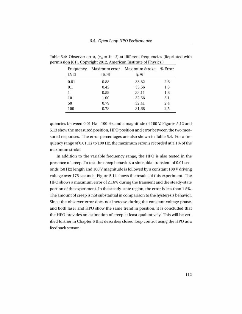
5.5. Open Loop HPO Performance
Table 5.4: Observer error, (εO = x − x) at different frequencies (Reprinted withpermission [61]. Copyright 2012, American Institute of Physics.)
Frequency Maximum error Maximum Stroke % Error[H z] [µm] [µm]
0.01 0.88 33.82 2.60.1 0.42 33.56 1.31 0.59 33.11 1.810 1.00 32.56 3.150 0.79 32.41 2.4100 0.78 31.68 2.5
quencies between 0.01 Hz – 100 Hz and a magnitude of 100 V. Figures 5.12 and
5.13 show the measured position, HPO position and error between the two mea-
sured responses. The error percentages are also shown in Table 5.4. For a fre-
quency range of 0.01 Hz to 100 Hz, the maximum error is recorded at 3.1% of the
maximum stroke.
In addition to the variable frequency range, the HPO is also tested in the
presence of creep. To test the creep behavior, a sinusoidal transient of 0.01 sec-
onds (50 Hz) length and 100 V magnitude is followed by a constant 100 V driving
voltage over 175 seconds. Figure 5.14 shows the results of this experiment. The
HPO shows a maximum error of 2.16% during the transient and the steady-state
portion of the experiment. In the steady-state region, the error is less than 1.5%.
The amount of creep is not substantial in comparison to the hysteresis behavior.
Since the observer error does not increase during the constant voltage phase,
and both laser and HPO show the same trend in position, it is concluded that
the HPO provides an estimation of creep at least qualitatively. This will be ver-
ified further in Chapter 6 that describes closed loop control using the HPO as a
feedback sensor.
112

5.5. Open Loop HPO Performance
Figure 5.12: Measured position, HPO position and observer error between 0.01Hz and 1 Hz (Reprinted with permission [61]. Copyright 2012, American Insti-tute of Physics.)
113

5.5. Open Loop HPO Performance
Figure 5.13: Measured position, HPO position and observer error between 10 Hzand 100 Hz (Reprinted with permission [61]. Copyright 2012, American Instituteof Physics.)
114

5.5. Open Loop HPO Performance
Figure 5.14: Measured position, HPO position and observer error between 50 Hzand DC signal in the presence of creep (Reprinted with permission [61]. Copy-right 2012, American Institute of Physics.)
115

5.6. Summary
5.6 Summary
Position self-sensing technique provides an alternative to traditional posi-
tion sensors where mounting a dedicated position sensor is not feasible. In this
chapter, a novel HPO approach is presented which relies on two different PSS
schemes: 1) PSS based on current or charge measurement and 2) PSS based on
effective capacitance measurement. The charge based PSS provides a good PSS
signal at high frequencies while the capacitance based PSS provides reliable po-
sition estimate at low frequencies. The proposed HPO provides an improved
position self-sensing over a wide frequency range by combining the advantages
of each PSS technique. The HPO performance is compared with a traditional
position sensor in open loop condition for sinusoidal signals with frequencies
between 0 Hz and 100 Hz. This frequency range contains both creep and rate-
dependent hysteresis. The proposed HPO provides around 3% error over the
whole range of operation which makes it applicable for real-time applications
and a potential substitute of traditional position sensors.
116

Chapter 6
Self-sensing Position Control of
Piezoelectric Actuators
A novel position observer (HPO) is developed in Chapter 5 by fusing two
self-sensing signals to obtain an improved position signal over a wide frequency
range. It is also shown how accurately the HPO can predict the position in open
loop and the results are compared with a traditional sensor. The objective of this
chapter is to show that the HPO can be used as a reliable substitute for a tradi-
tional position feedback sensor in the control of soft piezoelectric actuators. To
show the HPO performance in closed loop, results with HPO feedback is com-
pared with the results obtained by a traditional position sensor. To minimize
the steady-state error, a simple integral controller is used in this research. Dif-
ferent types of profiles including long DC signals and AC signals with variable
frequencies and lifts are part of the comparison.
The advantages of the HPO feedback system are: 1) it is based on self-sensing
technique (no position sensor is required), 2) it is voltage controlled (no sophis-
ticated hardware requirement), 3) it does not require a hysteresis model, and 4)
a wide frequency range from DC to 125 Hz.
6.1 The Integral Controller
Integral controllers with dedicated feedback sensors are often used in piezo-
electric systems due to hysteresis and unknown force disturbances. The major
advantage of the I–controller is it provides high gain which can overcome hys-
teresis problems when operated at frequencies below the vibrational dynamics
[11]. One of the pitfalls of the I–controller is a velocity dependent error at high
frequencies typical for a Type–I control system. At higher frequencies, the track-
117

6.1. The Integral Controller
ing error is quite substantial and more advanced control strategies that include
a feedforward branch [15, 27, 46, 48] could be implemented for improved track-
ing. However, the main objective in this chapter is to validate the performance
of the HPO in the closed loop and so no feedforward strategy is added.
The simple integral control schematic is shown in Figure 6.1. The plant
model, P (s) is obtained from the constitutive relationship in Equations 1.4 and
1.6, assuming zero hysteresis voltage, UH , and neglecting small external forces,
F . Since the targeted frequency range is much lower than the mechanical nat-
ural frequency of the plant, the mass and damping terms can be neglected and
the following relationship is established for the plant model:
P (s) = x(s)
UP (s)= α
ms2 +bs +k≈ α
k. (6.1)
The overall transfer function for this simple linear plant with an integral con-
troller gain, K I is given by:
x(s)
xR (s)= K I
αk
s +K Iαk
= ωC
s +ωC. (6.2)
The position controller gain is obtained by selecting a control bandwidth, ωC ,
and using the identified model parameter, kα ,
K I = ωC k
α. (6.3)
In this application,ωC is selected at 250 Hz which is at least twice the maximum
targeted frequency range. The ratio of kα can be obtained from the parameter
identification section. For simplicity, the term can also be estimated from the
ratio of maximum voltage to maximum stroke neglecting hysteresis at maximum
displacement using Equation 4.3.
118

6.2. Experimental Results
Figure 6.1: An integral controller schematic
6.2 Experimental Results
To achieve sensorless position control, the HPO is used as a feedback posi-
tion sensor in the piezoelectric system. To investigate the performance of the
HPO in a controlled environment, different profiles have been tested: 1) step
profile with variable lift (P1), 2) sinusoidal profiles (P2), and 3) DC profile with
fast transient (P3). To gauge the accuracy of the HPO, a laser vibrometer is added
to the experiment for reference position measurements. The laser vibrometer is
not used in the control loop. It simply provides an absolute reference to com-
pare the position estimates of HPO to measured position (from laser vibrome-
ter). The primary objective of the experiments then is to investigate the tracking
error between the position measurement of the laser vibrometer, x, and the po-
sition estimate of the HPO, x . This error is denoted as observer error, εO . The
other error of interest is the total error, εT which is calculated from the difference
between the reference position, xR and the position measured with the refer-
ence laser sensor, x. The controller error, εC is calculated from the difference
between the reference position, xR , and the HPO position, x.
6.2.1 Step Profile with Variable Strokes, P1
The HPO performance is evaluated for profile, P1 (in Figure 6.2(a)) which in-
cludes the variable lifts (minor loops) in both ascending and descending paths.
Figure 6.2(a) shows the reference signal, xR , the open loop response and the
119

6.2. Experimental Results
closed loop response. The open loop response shows a large overshoot (due to
step profile) while in the closed loop response with the HPO feedback, there is
no overshoot observed. The response times are in the same order of magnitude
(<5 ms) for both the open loop and the closed loop experiments. In Figure 6.2(b)
the errors are plotted. The observer error in closed loop operation between the
laser vibrometer and the HPO, εOC L is recorded at less than 0.82 µm, both dur-
ing transients and in the steady-state conditions. To compare the steady-state
errors, steady-state segments (tss :‘a’–‘h’) are defined by Equation 6.4 where, tp
is the width of the pulse and ts is the settling time of the measured signal.
tss = tp − ts . (6.4)
Settling time, ts is equal to 5 time constants, 5ωC
where,ωC is the controller band-
width. The open loop total error (εTOL ) and closed loop total error (εTC L ) are also
compared over segments ‘a’– ‘h’ in Figure 6.2. Due to hysteresis in the open
loop condition, εTOL reaches up to 2.75 µm. In the closed loop condition, εTC L is
less than 0.67 mum. In the segments ‘a’– ‘h’, maximum values of total error, εTC L
and maximum values of observer error, εOC L are marked with circles. Due to the
variation in the experiments, 50 tests were performed and statistical inference is
obtained over the segments ‘a’– ‘h’ based on the maximum values of εTC L , εTOL ,
and εOC L in each test. The statistical results over the maximum errors (εTC L , εTOL ,
and εOC L ) are shown in Table 6.1. The mean of the maximum total error during
open loop experiments is 2.69 µm which is 8.97% of the maximum stroke. The
mean of the maximum total error in closed loop, εTC Lmaxis 0.78µm which is 2.6%
of the maximum position and a 71% improvement over the conventional open
loop control strategy. The mean of the maximum observer error, εOC Lmaxis 0.72
µm which is 2.4% of the maximum lift.
6.2.2 Sinusoidal Profile with Different Frequencies, P2
Four types of sinusoidal profiles are used to show the tracking performance
of the control system. The first sinusoidal profile, P2a , uses a single low fre-
120
6.2. Experimental Results
Fig
ure
6.2:
(a)
P1
refe
ren
cep
osi
tio
n,H
PO
po
siti
on
,mea
sure
do
pen
loo
pan
dcl
ose
dlo
op
po
siti
on
(b)
Tota
lerr
or
(op
enlo
op
and
clo
sed
loo
p)
and
clo
sed
loo
po
bse
rver
erro
r;m
axim
um
clo
sed
loo
pto
tale
rro
ran
do
bse
rver
erro
rin
each
seg-
men
t([8
8]©
2013
IEE
E)
121

6.2. Experimental Results
Table 6.1: Steady-state errors at segments ‘a’– ‘h’ for P1 ([88] ©2013 IEEE)
Test St ati st i cs Seg ment s[µm] a b c d e f g h
max(εTOLmax ) 0.89 3.08 0.89 1.75 1.73 1.62 0.76 1.85mean(εTOLmax ) 0.54 2.69 0.60 1.38 1.33 1.34 0.48 1.52
σ(εTOLmax ) 0.15 0.16 0.14 0.14 0.17 0.15 0.10 0.17
max(εTC Lmax ) 0.83 0.99 0.83 0.82 0.89 0.66 0.95 0.63mean(εTC Lmax ) 0.45 0.78 0.58 0.34 0.40 0.36 0.63 0.31
σ(εTC Lmax ) 0.18 0.14 0.17 0.15 0.17 0.11 0.17 0.13
max(εOC Lmax ) 0.78 0.93 0.85 0.90 0.78 0.64 0.92 0.84mean(εOC Lmax ) 0.41 0.72 0.56 0.44 0.39 0.38 0.58 0.40
σ(εOC Lmax ) 0.18 0.14 0.15 0.15 0.14 0.11 0.16 0.14
quency at 125th of the controller bandwidth:
P2a : xR = [15−15cos(20πt )]µm.
The second profile, P2b , uses a single high frequency at half the controller band-
width:
P2b : xR = [15−15cos(250πt )]µm.
The third profile, P2c , uses four separate frequencies with the highest frequency
at 15th of the controller bandwidth:
P2c : xR = 17.6−4.4[cos(20πt )+ cos(30πt )+ cos(80πt )+ cos(100πt )]µm.
The fourth profile, P2d , uses four separate frequencies with the highest frequency
at 12.5th of the controller bandwidth.
P2d : xR = 17.6−4.4[cos(60πt )+ cos(100πt )+ cos(150πt )+ cos(200πt )])µm.
Figure 6.3(a) shows the open loop and closed loop responses of P2a (at 10
Hz). The errors are plotted in Figure 6.3(b). The observer error in closed loop,
122
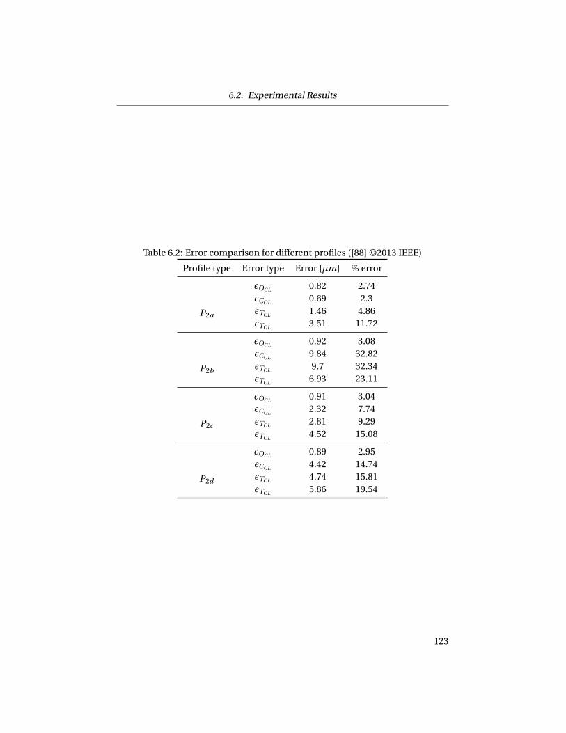
6.2. Experimental Results
Table 6.2: Error comparison for different profiles ([88] ©2013 IEEE)
Profile type Error type Error [µm] % error
P2a
εOC L 0.82 2.74εCOL 0.69 2.3εTC L 1.46 4.86εTOL 3.51 11.72
P2b
εOC L 0.92 3.08εCC L 9.84 32.82εTC L 9.7 32.34εTOL 6.93 23.11
P2c
εOC L 0.91 3.04εCOL 2.32 7.74εTC L 2.81 9.29εTOL 4.52 15.08
P2d
εOC L 0.89 2.95εCC L 4.42 14.74εTC L 4.74 15.81εTOL 5.86 19.54
123

6.2. Experimental Results
εOC L is less than 0.82µm which is 2.74% of the total error. There is a consid-
erable (64%) improvement observed in closed loop total error, εTC L over open
loop total error, εTC L using a simple I–controller (see Table 6.2). Since the driv-
ing frequency at 10 Hz is substantially lower than the control loop frequency of
250 Hz, the Type–II controller is able to substantially reduce hysteresis error and
track the reference position closely for low frequency tracking control. When the
same controller is applied for P2b profile (125 Hz), large εTC L is observed (Figure
6.4, Table 6.2). Even though the total errors shown in Table 6.2 are in the same
order of magnitude for both the open and the closed loop condition, the sources
of error are different. In the open loop condition, hysteresis is the main source
of error; in the closed loop condition the error is mainly due to the phase lag in-
troduced by the Type–I control system at high frequency. This can be confirmed
from the controller error, εCC L in Table 6.2 for 10 Hz and 125 Hz. The controller
error, εCC L is quite small in P2a while in case of P2b the controller error is quite
high. However, the εOC L is still in small ( 3%) and similar to the low frequency
case (P2a).
Figures 6.5(a) and 6.6(a) show the responses in open loop and closed loop
conditions for profiles P2c and P2d , respectively. The profiles are selected so that
multiple frequency components (10 Hz to 50 Hz in P2c and 30 Hz to 100 Hz in
P2d ) as well as the minor loops can be included in the tests. Similar to the fixed
frequency results, the εTC L increases at high frequencies. However, from Table
6.2, we can conclude that the HPO performance is not affected by the frequency
changes even in the presence of mixed frequency cases (rate-dependency). The
errors for P2c and P2d are shown in Figures 6.5(b) and 6.6(b), respectively.
124

6.2. Experimental Results
Figure 6.3: (a) P2a (10 Hz) reference position, HPO position, measured open loopand closed loop position (b) Total error (Open loop and closed loop) and closedloop observer error ([88] ©2013 IEEE)
125

6.2. Experimental Results
Figure 6.4: (a) P2b (125 Hz) reference position, HPO position, measured openloop, and closed loop position (b) Total error (open loop and closed loop) andclosed loop observer error ([88] ©2013 IEEE)
126

6.2. Experimental Results
Figure 6.5: (a) P2c ) reference position, HPO position, measured open loop, andclosed loop position (b) Total error (open loop and closed loop) and closed loopobserver error ([88] ©2013 IEEE)
127
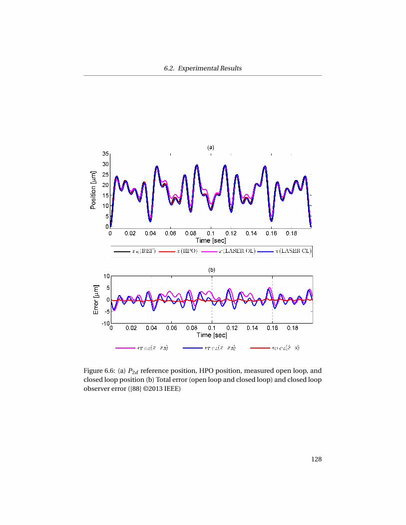
6.2. Experimental Results
Figure 6.6: (a) P2d reference position, HPO position, measured open loop, andclosed loop position (b) Total error (open loop and closed loop) and closed loopobserver error ([88] ©2013 IEEE)
128

6.2. Experimental Results
Figure 6.7: (a) P3 reference position, HPO position, measured open loop, andclosed loop position (b) Total error (open loop and closed loop) and closed loopobserver error (Reprinted with permission [61]. Copyright 2012, American Insti-tute of Physics.)
129
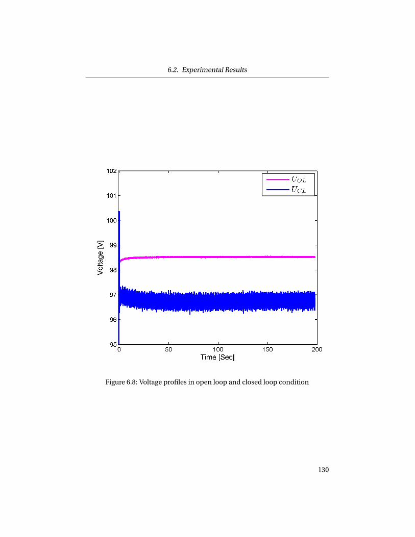
6.2. Experimental Results
Figure 6.8: Voltage profiles in open loop and closed loop condition
130

6.2. Experimental Results
6.2.3 DC Profile with Fast Transient Section, P3
This profile is selected to compare the HPO performance in the presence of
creep with a fast transient path. The transient part of the profile is a 50 Hz sig-
nal followed by a DC signal over 175 seconds. The results are shown in Figure
6.7. Although the amount of creep is not large in open loop condition (<1 µm),
the improvement is visible in the error when the HPO feedback is introduced
in closed loop control. In addition to that, the voltage signal is shown for both
open loop and closed loop conditions in Figure 6.8. The voltage signal is increas-
ing over time in the open loop while the controlled voltage in the closed loop is
decreasing which tries to minimize the creep voltage and hence the position.
The HPO error for profile P3 is 0.53 µm.
131

6.3. Summary
6.3 Summary
In this chapter, the HPO is used as a feedback sensor to achieve sensorless
feedback control. It is shown that the HPO feedback results in a maximum ob-
server error of 3% of maximum scale when compared to a laser reference sensor
over a very wide frequency range (DC to 125 Hz). There is a 58% improvement
in low frequency tracking operation observed compared to open loop operation
with the HPO feedback. The observer error does not increase with the frequency.
However, the overall tracking error is increased due to the controller error (Ta-
ble 6.2). The HPO performance compares well with other sensorless position
control algorithms shown in the literature (in Section 1.9). Different profiles are
selected to include the creep behavior, rate dependency and minor loops. How-
ever, since a Type–I control system was used, tracking error at frequencies ap-
proaching the bandwidth of the control loop are high. A feedforward controller
could be added to the control system shown here in order improve tracking per-
formance at higher frequencies. However, this would distract from the HPO per-
formance and so it was opted not to include a feedforward term in the controller
implementation shown here.
132

Chapter 7
Self-heat Generation
A large number of piezoelectric actuators are made of soft PZT materials
which provide high piezoelectric coefficient, d . However, soft PZT material pos-
sesses a high dielectric loss factor, tanδ [20]. For non-resonant applications such
as in high speed positioning stages or high speed inkjet printing, it is reported
that the total loss encountered is primarily due to dielectric loss [86]. In contrary,
for resonant applications such as in ultrasonic cleaning, the total loss is related
to the mechanical or elastic losses in the actuator [86]. Irrespective of the type of
the application (resonant or non-resonant), during continuous operation, the
total loss, due to dielectric loss or elastic loss, contributes to the temperature
rise of the actuator [86]. This phenomenon is known as self-heat generation.
The self-heating phenomenon for PEAs was first addressed in [21] where it is
shown that under continuous high frequency and high voltage loading, signifi-
cant heat generation is observed. In Chapter 5, it has been shown that the HPO
is able to predict position over a frequency range of 0 Hz to 100 Hz. However,
self-heat generation occurs already at 50 Hz operation if the actuator is contin-
uously driven over a long period of time [85]. The temperature increase due to
self-heat generation affects the capacitance of the piezoelectric actuator. This
indicates that during continuous operation even at 50 Hz, the performance of
the HPO may deteriorate since it uses capacitance based PSS. Hence, it is neces-
sary to predict the temperature rise of the piezoelectric actuator due to self-heat
generation. Also, the estimated temperature may be used to ensure that the ac-
tuator is not operated beyond the Curie temperature (150◦), where it may lose
piezoelectric properties.
In [21, 85], it is shown that the temperature rise due to self-heating in non-
resonant applications is a function of driving frequency, f, electric field, E and
effective volume to surface area ratio, veA . A model to predict the self-heating
133

Chapter 7. Self-heat Generation
temperature is shown in Equation (7.1):
T −T0 = u f ve
kT A
(1−e−
kT Avρc t
), (7.1)
where, u is the loss of the sample per driving cycle per unit volume, kT is the
overall heat transfer coefficient, ρ is the density of the PZT material, v is the ac-
tuator volume and t is the time [21]. The loss term u is obtained from the P-E
hysteresis loop using a Sawyer-Tower circuit, whereas P is the polarization and
E is the electric field. It is reported that the parameter, u is dependent on tem-
perature variation. The term kT accounts for the convection and radiation heat
transfer. It is reported that kT is constant for low electric fields and varies when
exposed to high electric fields. In addition, the term kT , slightly varies with tem-
perature. The prescribed range of kT is 20−40W m−2 ·K −1. To summarize, the
prediction of actuator temperature by using [21, 85] requires the knowledge of
driving frequency, as well as parameters u and kT that themselves are dependent
on temperature.
The literatures found to date describe how to model the temperature in-
crease due to self-heat generation where a hysteresis loss component and fre-
quency is known. The limitations are: 1) the hysteresis loss component itself is
a temperature dependent parameter, 2) the models require the exact knowledge
of frequency which limits the model to predict the temperature for mixed fre-
quency operation, and 3) the term kT is a function of electric field and driving
frequency. In this chapter, self-heat generation is modeled in piezoelectric ac-
tuators using the constitutive relationship of first law of thermodynamics and
power loss due to hysteresis voltage in the actuator. The model does not require
any known frequency and hence should be independent of the type of the pro-
file and knowledge of frequency. However, since the constitutive equations are
used in the model, position signal is required as an input to the model. It should
be noted that self-heating of non-resonant operations of the PEAs is considered
only, since the actuators usually operate at frequencies lower than the first me-
chanical resonant frequency. This leads to the assumption that the dielectric
losses are the main contributor to the total losses which result in self-heat gen-
eration.
134

7.1. Proposed Model
This chapter is organized as follows. In Section 7.1, a self-heat generation
model that requires voltage, current, as well as position is presented to esti-
mate the temperature. Experiments to characterize the temperature behavior
are shown in Section 7.2. The parameter identification of the model is presented
in Section 7.3. Experimental results, showing temperature estimates using a
dedicated position sensor input are shown in Section 7.4. To obtain a sensorless
(eliminating position sensor) temperature prediction, a temperature compen-
sated HPO and temperature model is shown in Section 7.5. Finally, the combi-
nation of temperature compensated HPO and the new temperature model are
validated in Section 7.6.
7.1 Proposed Model
The self-heat generation model proposed in this chapter is based on the law
of energy conservation of a closed system presented in [21]:
qG − qD = ρcvdT
d t(7.2)
where, qG is the rate of heat generation, qD is the rate of heat dissipation, ρ, c and
v are the density, specific heat and total volume of the actuator, respectively. It is
assumed that the system is in perfect insulation. For non-resonant applications,
it is reported that the dielectric loss is equivalent to the hysteresis loss and hence,
is the major contributor of heat generation [20, 21, 85, 86]. Therefore, Equation
(7.2) can be rewritten as follows:
PLoss −kT A4T =UH I −kT A4T = ρcvdT
d t, (7.3)
where, PLoss is the power loss due to hysteresis loss, kT is the overall heat trans-
fer coefficient, ∆T is the temperature difference between the actuator and the
environment due to self-heating and A is the surface area of the actuator. The
overall heat transfer coefficient considers the heat conduction, convection and
radiation [21]. The term UH is the hysteresis voltage in [13] and I is the current.
135
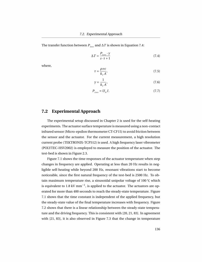
7.2. Experimental Approach
The transfer function between PLoss and ∆T is shown in Equation 7.4:
∆T = PLoss ·γs ·τ+1
(7.4)
where,
τ= ρvc
kT A, (7.5)
γ= 1
kT A, (7.6)
PLoss =UH I . (7.7)
7.2 Experimental Approach
The experimental setup discussed in Chapter 2 is used for the self-heating
experiments. The actuator surface temperature is measured using a non-contact
infrared sensor (Micro-epsilon thermometer CT-CF15) to avoid friction between
the sensor and the actuator. For the current measurement, a high resolution
current probe (TEKTRONIX-TCP312) is used. A high frequency laser vibrometer
(POLYTEC-HSV2002) is employed to measure the position of the actuator. The
test-bed is shown in Figure 2.3.
Figure 7.1 shows the time responses of the actuator temperature when step
changes in frequency are applied. Operating at less than 20 Hz results in neg-
ligible self-heating while beyond 200 Hz, resonant vibrations start to become
noticeable, since the first natural frequency of the test-bed is 2500 Hz. To ob-
tain maximum temperature rise, a sinusoidal unipolar voltage of 100 V, which
is equivalent to 1.8 kV mm−1, is applied to the actuator. The actuators are op-
erated for more than 400 seconds to reach the steady-state temperature. Figure
7.1 shows that the time constant is independent of the applied frequency, but
the steady-state value of the final temperature increases with frequency. Figure
7.2 shows that there is a linear relationship between the steady-state tempera-
ture and the driving frequency. This is consistent with [20, 21, 83]. In agreement
with [21, 83], it is also observed in Figure 7.3 that the change in temperature
136

7.2. Experimental Approach
Figure 7.1: Effect of frequencies on self-heat generation. It is important to notethat the frequencies are high enough to result in self-heat generation. However,the frequencies are still well below the resonant frequency (see Figure 1.4) of thetest-bed and hence a quasi-static approximation is still valid.
137

7.3. Parameter Identification
Figure 7.2: Change in steady-state temperature increase with driving frequency(at 100 V sinusoidal signal)
is related to the square of the applied voltage. The temperature increase is not
substantial when the driving voltage is less than 50 V at 150 Hz.
7.3 Parameter Identification
The model presented in Section 7.1 requires two parameters to be identified:
τ and γ. The time constant, τ is 100 seconds for the frequency ranges from 20 Hz
to 150 Hz obtained from Figure 7.1. The value of overall heat transfer coefficient,
kT can be attained from Equation 7.5. Using the values of total surface area, A
and kT , the second model parameter, γ, is obtained from Equation 7.6. The
term UH , in Equation 7.7 can be obtained from the piezoelectric constitutive
equations proposed by Goldfarb et al. in [13]. The constitutive force equation
138
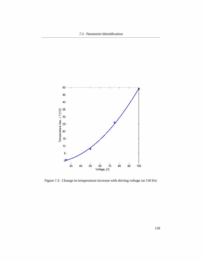
7.3. Parameter Identification
Figure 7.3: Change in temperature increase with driving voltage (at 150 Hz)
139

7.3. Parameter Identification
at quasi-static region and the expression for hysteresis voltage is recalled from
Equations 4.3 and 4.8 as follows:
kx =αUP (7.8)
UH =U −UP (7.9)
where, k is the stack stiffness, α is the force-voltage proportionality constant,
and UP is the linear piezoelectric voltage. Using Equations (7.7), (7.8) and (7.9)
the following function can be obtained for power loss due to hysteresis:
PLoss = (U − k
αx)I (7.10)
where, x is the measured position of the actuator. At maximum supply volt-
age, Umax , and maximum displacement, xmax , the term kα can be attained from
Equation (7.11):k
α= Umax
xmax. (7.11)
It is important to note that although self-heat generation occurs at high fre-
quency operations, the range of frequency is still below than the dynamic range
mentioned in Figure 1.2. Hence, the quasi-static approximation is still valid for
the frequency range where self-heating phenomenon occurs. The final model
for self-heating is shown in Equation 7.12 where TRe f is the reference tempera-
ture. The flowchart is shown in Figure 7.4.
TSH = TRe f +(U − k
αx)I ·γτ · s +1
(7.12)
The properties of the PZT material are summarized in Table 2.1 and the self-
heating model parameters are shown in Table 7.1. The parameters are obtained
by fitting the experimental results shown in Figure 7.1 and Equations 7.5 and 7.6.
The ratio of kα is considered unaffected since the maximum stroke is unaffected
due to temperature variation in the setup. The value of the overall heat transfer
coefficient, kT compares well with the prescribed values in [21].
140

7.4. Temperature Prediction Using a Dedicated Position Sensor
Figure 7.4: Self-heat generation model with position sensor input
Table 7.1: Self-heating model parameters
Parameters Values
Time constant, τ 100 sec.Overall heat transfer coefficient, kT 28 W ·m−2 ·K −1
γ 57 W ·K −1
Stiffness to coupling coeff. ratio, kα 2.85 e6 V ·m−1
Ambient temperature, TRe f 23◦C
7.4 Temperature Prediction Using a Dedicated Position
Sensor
Once the model parameters are identified, real-time measurements of cur-
rent, voltage and position provide an accurate measurement of temperature rise
of the actuator due to self-heating. The experimental results and the predicted
temperatures (from the model) for various driving frequencies are plotted in Fig-
ure 7.5. Both the temperature rise and fall can be predicted using the proposed
self-heating model. For recording the temperature fall, the actuator is driven
at 150 Hz-50 V, 10 Hz-100 V and 0 Hz-0 V. In another experiment, the actuator is
driven by a combination of voltages and frequencies to observe the performance
of the model under complex operating conditions. The results are shown in Fig-
ure 7.6. The prediction error is within ±2◦ which is less than 3% of the maximum
temperature rise due to self-heating at 150 Hz-100 V.
141

7.4. Temperature Prediction Using a Dedicated Position Sensor
Figure 7.5: (a) Self-heat generation at different frequencies: measured and pre-dicted temperature (b) prediction error
142

7.4. Temperature Prediction Using a Dedicated Position Sensor
Figure 7.6: (a) Temperature profile using self-heating by driving at different fre-quencies and voltages: measured and predicted temperature (b) Prediction er-ror
143

7.5. Temperature Compensation of HPO
7.5 Temperature Compensation of HPO
In Section 7.3, a self-heat generation model is proposed which predicts the
temperature increase due to self-heating based on driving current, driving volt-
age and a position measurement. This limits the model to a system where a ded-
icated position measurement is available. In this section, the HPO presented in
Chapter 5 will be employed as a position input to the self-heat generation model
to obtain a pure self-sensing temperature and position estimation.
Before employing the HPO signal as an input to the self-heating model, the
effect of temperature on the capacitance based PSS needs to be evaluated. Fig-
ure 7.7 (a), shows the effect of temperature variation on the capacitance-position
relationship. The capacitance increases with temperature increase while the po-
sition is unaffected at least for the investigated temperature range (upto 60◦C).
Figure 7.7(b) shows the corresponding capacitance-time relationships. It is ob-
served that temperature creates an offset in the capacitance measurements. The
size of the offset is linearly related to temperature. This offset in the capacitance-
position relationship is expected to affect the HPO estimation. Since the self-
heating phenomenon is dependent on frequency of operation, the effect of fre-
quency on the capacitance-position relationship is also shown in Figure 7.8.
Only small variation in the charge-position relationship is observed due to fre-
quency variation.
From Figure 7.7, it is evident that a new fitting function is required to de-
fine the capacitance-position relationship with temperature variation to obtain
a reasonable estimate of position from the capacitance based PSS. The new fit-
ting function, ΓT is presented in Equation 7.13 which requires a temperature
input to predict the position from capacitance measurement in the presence of
temperature variation:
ΓT = xCP (CP ,T ) = bT 0 +N∑
n=1bT nC n
P + g T , (7.13)
where, bT 0 is the intercept, bT n is the expression for coefficients for capacitance
and g is the temperature coefficient. The coefficients are obtained through a re-
144

7.5. Temperature Compensation of HPO
Figure 7.7: Effect of temperature on (a) capacitance-position relationship (b)capacitance measurement at 50Hz
Figure 7.8: Effect of frequency on capacitance-position relationship
145
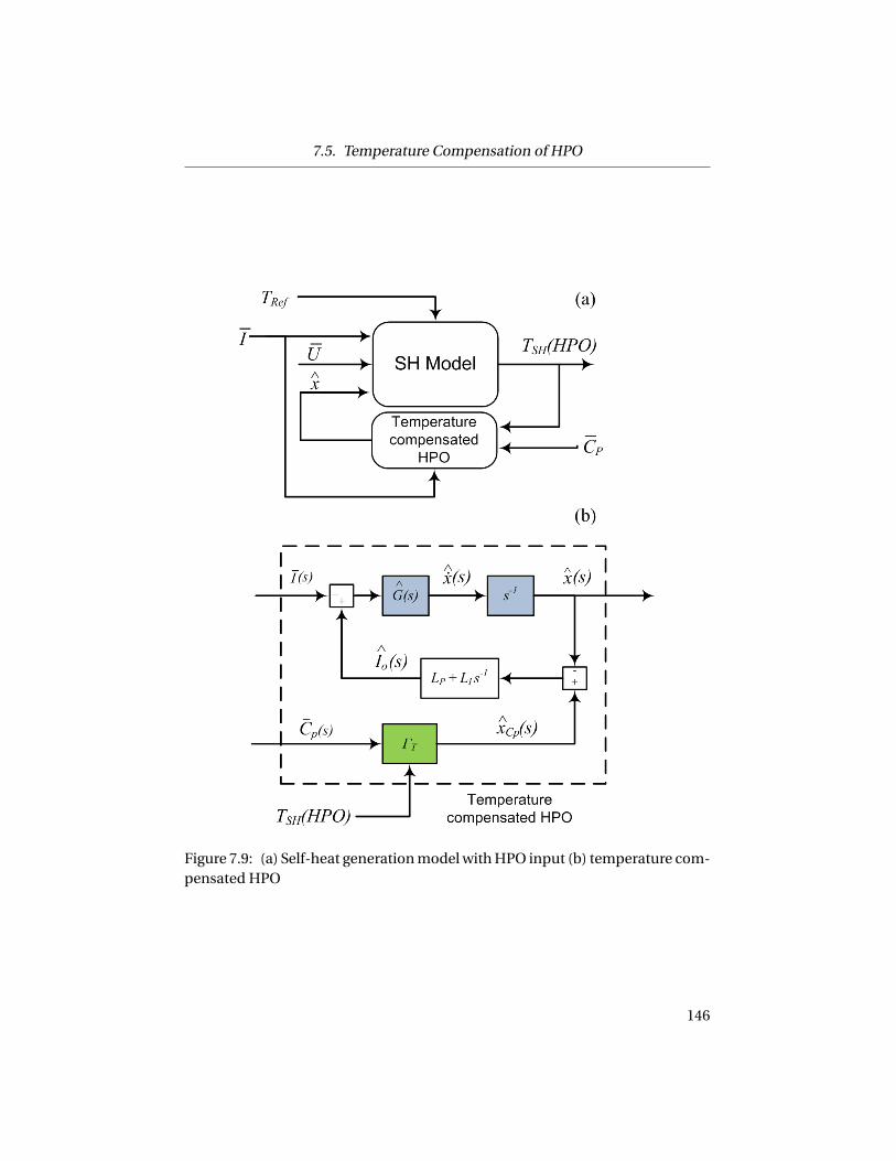
7.5. Temperature Compensation of HPO
Figure 7.9: (a) Self-heat generation model with HPO input (b) temperature com-pensated HPO
146

7.6. Temperature and Position Predictions Using the HPO and the Self-Heating Model
gression analysis. The orders are selected by comparing the adjusted R2 value
which indicates that an order more than 5 would not improve the adjusted R2
value (Table 7.2). Also, an interaction between capacitance and temperature
does not have any effect on adjusted R2 value. In addition to that, the p-value
for the interaction is quite high (0.33) which indicates that the coefficient for
interaction is redundant. The model is obtained based on 50 Hz data. The com-
parison is shown in Table 7.2.
Table 7.2: Comparison of the regression statistics
n=4 n=5 n=6 n=5 with CP
and T interaction
Regression Statistics
R Square 0.998189 0.998194 0.998194 0.998193Adjusted R Square 0.998188 0.998193 0.998193 0.998193Standard Error 0.474422 0.473808 0.47377 0.473825
An updated HPO structure is shown in Figure 7.8 which includes tempera-
ture compensation using the self-heat generation model (from Equation 7.13).
The compensated HPO output is fed back to the self-heat generation model.
This feedback mechanism between the HPO and the temperature model works
quite well, because the temperature variation is relatively slow in comparison to
the piezoelectric position changes.
7.6 Temperature and Position Predictions Using the HPO
and the Self-Heating Model
A sensorless temperature prediction due to self-heating was presented in
Section 7.5 where the temperature compensated HPO is employed as an input to
the self-heating model to estimate the position of the actuator. In this section,
experiments are carried out to validate temperature and position predictions
using the HPO as the position input to the temperature model. To distinguish
between the two position inputs to the temperature model, TSH (PS) is used to
define the self-heating model using the laser position input while TSH (HPO) is
147

7.6. Temperature and Position Predictions Using the HPO and the Self-Heating Model
Table 7.3: ANOVA table for capacitance based PSS regression model with tem-perature
ANOVA for n=5
df SS MS F Significance FRegression 6 992110.4 165351.7 1096054 0
Residual 7993 1205.832 0.150861Total 7999 993316.2
Coefficients t Stat p-value
bT 0 -870.776 -7.50918 0bT 1 1639.54 7.873573 0bT 2 -1132.54 -7.61792 0bT 3 376.6851 7.140752 0bT 4 -61.8409 -6.64742 0bT 5 4.036799 6.187723 0
g 0.263115 860.7364 0
used to denote the self-heating model that uses temperature compensated HPO
position input.
In Figures 7.10 and 7.11, 100 Hz and 50 Hz self-heating temperature pre-
dictions are shown for both TSH (PS) and TSH (HPO). The measurements are
compared with the infrared sensor and found to agree within less than 2◦. In
Figure 7.12, a mixed frequency case is tested where temperature cycling is ob-
tained with a combination of frequencies to heat up and cool down the actuator.
Heating up is achieved through a series of sections (‘a’–‘c’) with increasing fre-
quencies (20 Hz–50 Hz–100 Hz). This sequence of driving frequencies leads to
a final temperature larger than 50◦C. To cool the actuators back down, driving
frequencies of 50 Hz and 0 Hz (‘d’ and ‘e’) are used. The HPO position com-
pares well with the laser sensor position in Figure 7.13 (a). The laser vibrometer
has some drift in long term measurements which is visible in sections (‘a’ and
‘d’) in the profile. Although the contact between the needle and the PEA is very
small (hence most of the heat is assumed to be transferred through convection
and conduction is neglected), combined effect of expansion of the needle and
contraction of the piezoelectric actuator due to temperature increase may con-
148
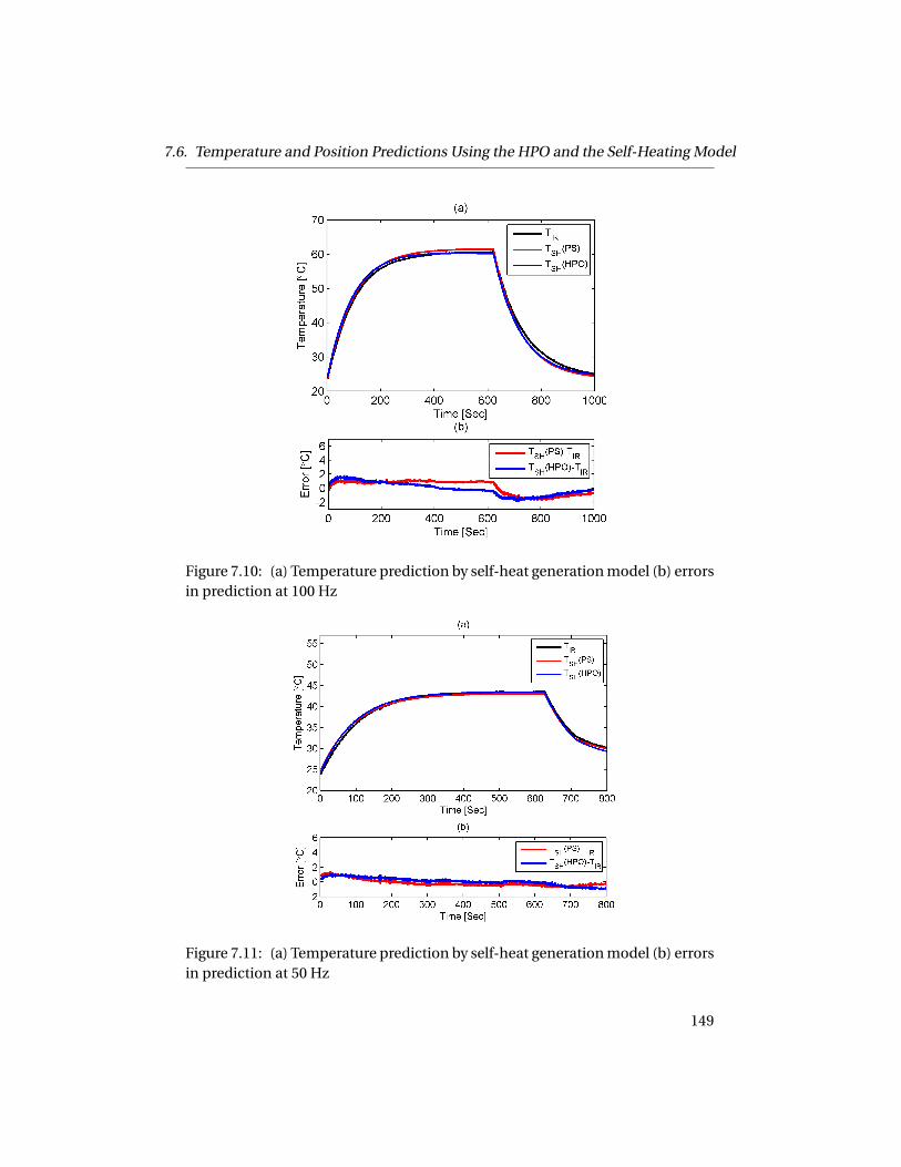
7.6. Temperature and Position Predictions Using the HPO and the Self-Heating Model
Figure 7.10: (a) Temperature prediction by self-heat generation model (b) errorsin prediction at 100 Hz
Figure 7.11: (a) Temperature prediction by self-heat generation model (b) errorsin prediction at 50 Hz
149

7.6. Temperature and Position Predictions Using the HPO and the Self-Heating Model
tribute to this drift. However, it is interesting to see that at the maximum temper-
ature region (section ‘c’), the laser measurement does not show any drift while
in section ‘d’ (temperature decreasing), a maximum drift of 0.6 µm is observed.
Further, careful investigation including the temperature distribution in the nee-
dle assembly and actuator is required to conclude on thermal expansion of the
PEA and the needle assembly; however, this is not included in the scope of this
study.
The HPO position also shows some changes at the beginning of frequency
switches (beginning of different sections). This is attributed to the change in the
unmodeled capacitance frequency dependency shown in Figure 7.12. The HPO
output is used in the self-heating model to predict the temperature and which
in turn is feed back to the HPO to compensate the temperature. This circular
feedback is possible due to the slow temperature variation in comparison to the
position change of the actuator. Considering the presence of laser drift and HPO
error due to frequency changes, the maximum observer error is recorded at 1.38
µm (4.18% of the maximum stroke) in Figure 7.12(c) over the frequency range of
0 Hz to 100 Hz and a temperature change of up to 55◦C. To the best knowledge of
the author, this is the first time in scientific literature that a successful position
estimation algorithm has been presented for a wide range of frequencies and
operating temperatures. The HPO output is used in the self-heating model to
predict the temperature and which in turn is feed back to the HPO to compen-
sate the temperature. This circular feedback is possible due to the slow temper-
ature variation in comparison to the position change of the actuator. The errors
in temperature prediction from the two different position sources (position sen-
sor and HPO) are compared in Figure 7.12 (d). In some portions, TSH (PS), which
uses the laser position measurement, provides slightly better temperature pre-
dictions than the HPO based values of TSH (HPO). However, the maximum error
is recorded 1.45◦C in both the cases.
150
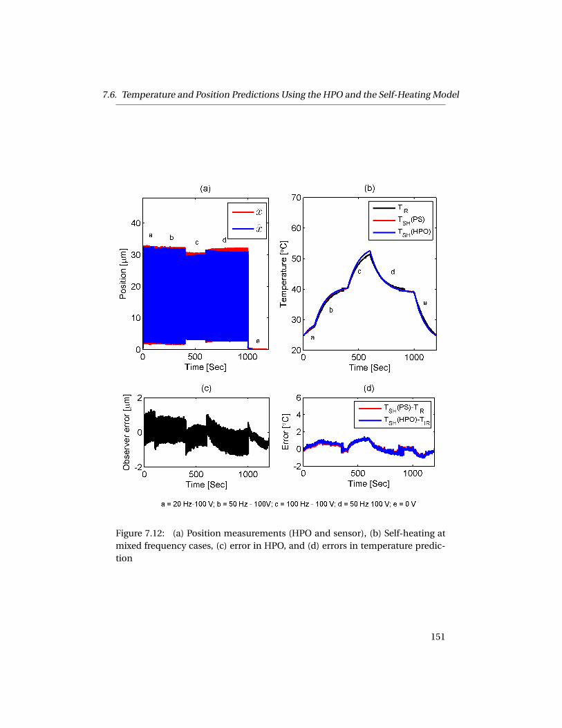
7.6. Temperature and Position Predictions Using the HPO and the Self-Heating Model
Figure 7.12: (a) Position measurements (HPO and sensor), (b) Self-heating atmixed frequency cases, (c) error in HPO, and (d) errors in temperature predic-tion
151

7.7. Summary
7.7 Summary
A novel sensorless temperature measurement is presented in this chapter
which is based on power loss due to self-heating and the piezoelectric consti-
tutive relationship. The advantage of the proposed model is that it does not re-
quire the knowledge of the driving frequency in contrast to the earlier developed
models. Moreover, the new method is much simpler than the models in [21, 85],
which require the term energy loss per cycle per volume, u and the overall heat
transfer coefficient, kT which are functions of the electric field and temperature.
The proposed model is tested in fixed and mixed frequency cases and compared
with a traditional temperature sensor. The temperature prediction is accurate
with in ±2◦C which is close to 3% of the investigated range. When the HPO
is updated to include temperature dependencies and combined with the new
model, sensorless temperature and position estimation is obtained in the pres-
ence of self-heating. This provides a maximum position error of 4.18% over the
frequency range of 0 Hz to 100 Hz and up to 55◦C of temperature increase due
to self-heat generation.
152
Chapter 8
Conclusions and Future Research
The foremost objective of this dissertation is to develop a PSS technique for
position feedback control in PEA over a wide frequency range where creep and
rate-dependent hysteresis lead to large errors in traditional feedforward posi-
tioning systems. In addition to that, a self-heat generation model is developed
and temperature compensation of the position self-sensing scheme is proposed
in this research. The research outcome can be extended to different applications
some of which are outlined in the future research section.
8.1 Conclusions
The research findings are based on a novel real-time piezoelectric impedance
measurement algorithm which facilitates the parameter identification of the elec-
tromechanical models. The measurement technique superimposes a high fre-
quency voltage ripple onto the normal driving voltage and extracts impedance
of PEA from the relationship between voltage and current ripples. Since the
measurement frequency is very high in comparison to the natural frequency of
the test bed, the measurement is obtained in a clamped condition. This leads to
a relationship between capacitance and position where the hysteresis is negli-
gible (<3%). The capacitance value decreases with the actuator displacement.
This finding leads to two major conclusions: 1) the capacitance in the elec-
tromechanical model is not constant, and 2) the capacitance-position relation-
ship provides a means for position self-sensing through a regression model. The
first conclusion indicates that an improved electromechanical model is required
to include the position dependent capacitance. The proposed modeled is veri-
fied experimentally and compared with the traditional model. Based on the up-
dated electromechanical model, a novel parameter identification technique is
153

8.1. Conclusions
proposed where a single set of experiments provide all the required parameters
in the model. In addition to that, some important material parameters such as
piezoelectric strain coefficient, coupling coefficient, and permittivity constant
are also obtained through constitutive relationships. These values compare well
with the manufacturers specified values.
The second conclusion of the capacitance-position relationship (through
regression model) promotes a self-sensing technique applicable to slow oper-
ations where creep and hysteresis are present. By combining this capacitance
based PSS technique with conventional charge based PSS, using a novel hybrid
position observer, position is estimated over an extended frequency range where
creep and rate dependent hysteresis are prominent. This is achieved by exploit-
ing the advantages of each technique where the hysteresis free charge based
PSS provides the position estimate at high frequencies (lower than the dynamic
range) while the capacitance based PSS (Γ) is employed at slow operations. The
major problem with the charge based PSS is the drift in position estimation due
to offset currents in the charge measurement. The capacitance based measure-
ment then serves two purposes: 1) to provide a PSS signal at low frequency op-
eration where charge is difficult to measure, 2) to eliminate offset currents in the
charge based PSS. The performance of the position observer is compared with a
traditional position sensor. The comparison shows that position observer is able
to predict the position from static operations up to 100 Hz with an error close to
3% of full scale.
The developed HPO is then tested in a controlled environment with different
waveforms from variable lift step profiles to mixed frequency sinusoidal pro-
files. The creep profile is also tested in conjunction with a fast transient sec-
tion. A simple Integral-controller is implemented to observe the performance.
Similar to the open loop conditions, the HPO is compared to a reference sen-
sor and the error is recorded at around 3% of full scale. Even though the HPO
error is fairly constant at all frequencies, the overall controller error increases
at higher frequencies, since a simple Type-I controller was used in the experi-
ments. In the future, other control schemes like Type-II controllers or feedfor-
ward/feedback controllers presented in the literature may be implemented to
reduce the controller error at higher frequencies. Self-heating phenomena are
154

8.1. Conclusions
observed in piezoelectric actuators when operated at relatively high frequencies
over an extended period of time. The frequency range, over which the HPO is
proposed, is high enough to generate heat due to self-heating when continu-
ously operated. The temperature of the actuator may increase up to 60◦C at 100
Hz driving frequency. The temperature rise may have several effects: 1) the life
of the actuator is reduced if continued over an extended period of time, 2) the
stroke of the actuator may be affected, and 3) the position self-sensing scheme
may be affected. A self-heat generation model is proposed based on the power
loss of the piezoelectric actuator that relies on the electromechanical model of
the actuator. The advantages of the model are: 1) unlike the other self-heating
models, it does not require a known frequency of operation which makes the
model applicable for different profiles, and 2) it is based on the power loss of the
actuator over time due to self-heating and not dependent on other temperature
dependent parameters such as overall heat transfer coefficient and hysteresis
loss per unit volume. Since, self-heating is a function of voltage, frequency and
length of actuation, the experiments to validate this model contain multiple fre-
quencies and voltage magnitudes. Since the temperature model requires driving
voltage, driving current, and measured position as its inputs, the model is tested
both with a laser position measurement, and a temperature compensated HPO
as the position input. The temperature prediction error is less than 2◦C for both
position sensor input and HPO input to the self-heat generation model which
is close to 3% of the maximum investigated scale. The errors position estimates
obtained with the combined HPO and temperature model is less than 5%.
The major goals in this research are met with experimental validations. The
following contributions are significant in this research:
o A novel impedance measurement algorithm is proposed which provides
real-time clamped capacitance and resistance measurement for piezoelec-
tric actuators.
o An improved electromechanical model and parameter identification is pro-
posed based on the real-time capacitance measurement.
o A novel hybrid position observer is presented which relies upon two self-
sensing techniques to provide improved position information over an ex-
155
8.2. Future Research
tended frequency range where creep and rate-dependent hysteresis are
present. The HPO is helpful for sensorless position control in piezoelec-
tric actuators.
o A self-heat generation model is presented which predicts the temperature
rise in the piezoelectric actuator due to self-heat generation.
o A novel sensorless temperature and position estimation technique is pre-
sented based on temperature compensated HPO to predict self-heating
temperature variation.
8.2 Future Research
Some of the future research possibilities are outlined as follows:
o The real-time impedance measurement presented in this thesis provides
capacitance and resistance measurements for piezoelectric actuators. The
impedance measurement is obtained at constant loading condition where
force changes are negligible. In future research, the effect of preloading or
external load variation should be investigated.
o During the work on this thesis it is observed, that capacitance and resis-
tance values of new actuators stabilize over the first several thousand cy-
cles of use. Even though no measurable changes are observed after this
initial break in period during the work on this thesis, it is expected that
over the life of the actuator changes will take place. This may result due
to failing of the piezoelectric layers, or cracks developing in the actuator.
Hence, by comparing the capacitance/resistance measurement, a health
monitoring strategy can be developed for the piezoelectric actuator.
o The HPO is tested in closed loop condition with a Type-I controller where
the reference tracking performance is poor for high frequency profiles. It
has been shown in the literature that a feedforward branch is often used
to improve the dynamic performance of the feedback controller. How-
ever, most of the control systems are based on a dedicated position sen-
sor. The proposed HPO can be used as a replacement of the traditional
156

8.2. Future Research
sensor where a simple hysteresis model can be included in the feedfor-
ward branch of the controller to improve the tracking performance.
o When the HPO is updated for the self-heat generation cases, a good esti-
mate for piezoelectric actuator positioning is obtained. In further investi-
gations, the HPO should be tested over a wide temperature range specially
from subzero condition to high temperature range up to 100◦C. This study
will be helpful to implement the HPO in applications such as piezoelectric
fuel injectors.
o Piezoelectric paint sensors (PPS) [105, 106] are a relatively new technol-
ogy to obtain structural health monitoring for large infrastructures such
as bridges, buildings, etc. The main advantage of the paint sensor is that it
can be used on different surfaces where traditional strain sensors cannot
be mounted easily. The impedance measurement of the PPS may provide
a relationship between the capacitance and crack related strains which
can be used for structural crack monitoring in large structures. Often tra-
ditional strain sensors are equipped with temperature sensors which cor-
rect the temperature related changes in the sensor signal. The proposed
impedance/resistance measurement can be used to correct the tempera-
ture related error in the impedance/capacitance measurement to monitor
the crack growth.
o Piezoelectric micro-cantilever beams are used to detect the mass of bio-
markers through the shift in the natural frequency of the beam [107]. The
newly developed impedance measurement can be helpful to identify the
temperature of the biomarker in addition to the mass. This can be helpful
to detect cancer cells which have higher temperatures than other cells due
to rapid replication of the cells.
157

Bibliography
[1] T. Ikeda, Fundamentals of Piezoelectricity. New York, USA: OxfordUniversity Press, 1996. → pages 2
[2] J. Yang, An introduction to the theory of piezoelectricity. Springer, 2004.→ pages 2
[3] R. Guo, L. E. Cross, S. E. Park, B. Noheda, D. E. Cox, and G. Shirane,“Origin of the high piezoelectric response in pbzr1−x t ix o3,” PhysicalReview Letters, vol. 84, no. 23, pp. 5423–5426, 2000. → pages 3
[4] I. Patel, Advances in Ceramics - Electric and Magnetic Ceramics,Bioceramics, Ceramics and Environment. InTech, 2011. → pages 3, 4
[5] J. e. Huber, N. a. Fleck, C. M. Landis, and R. M. McMeeking, “Aconstitutive model for ferroelectric polycrystals,” Journal of theMechanics and Physics of Solids, vol. 47, no. 8, pp. 1663–1697, 1999. →pages 3
[6] G. Ballas, Rudiger, Piezoelectric multilayer beam bending actuators: staticand dynamic behavior and aspects of sensor integration. Springer, 2007.→ pages 4
[7] L. Gaul and J. Becker, “Model-based piezoelectric hysteresis and creepcompensation for highly-dynamic feedforward rest-to-rest motioncontrol of piezoelectrically actuated flexible structures,” InternationalJournal of Engineering Science, vol. 47, no. 11-12, pp. 1193–1207, 2009. →pages 6, 7
[8] S. Salapaka, A. Sebastian, J. P. Cleveland, and M. V. Salapaka, “Highbandwidth nano-positioner: A robust control approach,” Review ofScientific Instruments, vol. 73, no. 9, pp. 3232–3241, 2002. → pages 7, 8
[9] H. Jung, J. Y. Shim, and D. Gweon, “New open-loop actuating method ofpiezoelectric actuators for removing hysteresis and creep,” Review ofScientific Instruments, vol. 71, no. 9, pp. 3436–3440, 2000. → pages
158

Bibliography
[10] R. Changhai and S. Lining, “Hysteresis and creep compensation forpiezoelectric actuator in open-loop operation,” Sensors and Actuators A:Physical, vol. 122, no. 1, pp. 124–130, 2005. → pages 8, 27
[11] S. Devasia, E. Eleftheriou, and S. O. R. Moheimani, “A survey of controlissues in nanopositioning,” Control Systems Technology, IEEETransactions on, vol. 15, no. 5, pp. 802–823, 2007. → pages 8, 30, 31, 38,98, 117
[12] D. Croft, G. Shed, and S. Devasia, “Creep, hysteresis, and vibrationcompensation for piezoactuators: Atomic force microscopy application,”Journal of Dynamic Systems, Measurement, and Control, vol. 123, no. 1,pp. 35–43, 2001. → pages 9, 19, 24, 25, 26, 27, 98
[13] M. Goldfarb and N. Celanovic, “Modeling piezoelectric stack actuatorsfor control of micromanipulation,” Control Systems Magazine, IEEE,vol. 17, no. 3, pp. 69–79, 1997. → pages 9, 12, 14, 15, 16, 18, 30, 31, 35, 43,45, 57, 76, 77, 80, 100, 135, 138
[14] H. J. M. T. S. Adriaens, W. L. De Koning, and R. Banning, “Modelingpiezoelectric actuators,” Mechatronics, IEEE/ASME Transactions on,vol. 5, no. 4, pp. 331–341, 2000. → pages 10, 17, 82
[15] H. Hu, H. Georgiou, and R. Ben-Mrad, “Enhancement of tracking abilityin piezoceramic actuators subject to dynamic excitation conditions,”Mechatronics, IEEE/ASME Transactions on, vol. 10, no. 2, pp. 230–239,2005. → pages 9, 30, 118
[16] K. K. Leang and S. Devasia, “Hysteresis, creep, and vibrationcompensation for piezoactuators: Feedback and feedforward control,” inThe 2nd IFAC Conference on Mechatronic Systems, 2002, pp. 283–289. →pages 9
[17] G. Clayton, S. Tien, A. Fleming, S. Moheimani, and S. Devasia,“Inverse-feedforward of charge-controlled piezopositioners,”Mechatronics, vol. 18, no. 5, pp. 273–281, 2008. → pages 9, 26, 31, 32, 33,35
[18] PI. (2008) Physik instrumente manufacturer specification@ONLINE.[Online]. Available: http://www.physikinstrumente.com/en/products/prspecs.php?sortnr=100810 → pages 9, 47, 49, 79, 92
159

Bibliography
[19] H. Zhou, B. Henson, A. Bell, A. Blackwood, A. Beck, and R. Burn, “Linearpiezo-actuator and its applications,” University of Leeds, pp. 1–5, 2011.[Online]. Available: http://zhouhx.tripod.com/piezopaper.pdf. → pages9
[20] M. S. Senousy, F. X. Li, D. Mumford, M. Gadala, and R. K. N. D. Rajapakse,“Thermo-electro-mechanical performance of piezoelectric stackactuators for fuel injector applications,” Journal of Intelligent MaterialSystems and Structures, vol. 20, no. 4, pp. 387–399, 2009. → pages 10, 47,53, 133, 135, 136
[21] J. Zheng, S. Takahashi, S. Yoshikawa, K. Uchino, and J. d. Vries, “Heatgeneration in multilayer piezoelectric actuators,” Journal of the AmericanCeramic Society, vol. 79, no. 12, pp. 3193–3198, 1996. → pages 10, 41, 133,134, 135, 136, 140, 152
[22] L. Q. Yao, J. G. Zhang, L. Lu, and M. O. Lai, “Nonlinear staticcharacteristics of piezoelectric bending actuators under strong appliedelectric field,” Sensors and Actuators A: Physical, vol. 115, no. 1, pp.168–175, 2004. → pages 10, 12
[23] “IEEE standard on piezoelectricity,” ANSI/IEEE Std 176-1987, 1988. →pages 11
[24] A. Badel, Q. Jinhao, and T. Nakano, “Self-sensing force control of apiezoelectric actuator,” Ultrasonics, Ferroelectrics and Frequency Control,IEEE Transactions on, vol. 55, no. 12, pp. 2571–2581, 2008. → pages 13, 26,30, 57
[25] J. A. Main, E. Garcia, and D. V. Newton, “Precision position control ofpiezoelectric actuators using charge feedback,” Journal of Guidance,control, and dynamics, vol. 18, no. 5, pp. 1068–1073, 1995. → pages 14, 35
[26] H. M. S. Georgiou and R. B. Mrad, “Dynamic electromechanical driftmodel for PZT,” Mechatronics, vol. 18, no. 2, pp. 81–89, 2008. → pages 17,18, 98
[27] S. Bashash and N. Jalili, “Robust multiple frequency trajectory trackingcontrol of piezoelectrically driven micro/nanopositioning systems,”Control Systems Technology, IEEE Transactions on, vol. 15, no. 5, pp.867–878, 2007. → pages 17, 18, 26, 30, 40, 118
160
Bibliography
[28] H. M. S. Georgiou and R. B. Mrad, “Electromechanical modeling ofpiezoceramic actuators for dynamic loading applications,” Journal ofDynamic Systems, Measurement, and Control, vol. 128, no. 3, pp. 558–567,2006. → pages 17, 20, 82
[29] H. Janocha and K. Kuhnen, “Real-time compensation of hysteresis andcreep in piezoelectric actuators,” Sensors and Actuators A: Physical,vol. 79, no. 2, pp. 83–89, 2000. → pages 18, 19, 20, 27
[30] A. Wei Tech, P. K. Khosla, and C. N. Riviere, “Feedforward controller withinverse rate-dependent model for piezoelectric actuators intrajectory-tracking applications,” Mechatronics, IEEE/ASME Transactionson, vol. 12; 12, no. 2, pp. 134–142, 2007. → pages 18, 20, 21, 22, 23, 24, 26,30, 40, 98
[31] U. X. Tan, W. T. Latt, F. Widjaja, C. Y. Shee, C. N. Riviere, and W. T. Ang,“Tracking control of hysteretic piezoelectric actuator using adaptiverate-dependent controller,” Sensors and Actuators A: Physical, vol. 150,no. 1, pp. 116–123, 2009. → pages 40
[32] D. Song and C. J. Li, “Modeling of piezo actuator’s nonlinear andfrequency dependent dynamics,” Mechatronics, vol. 9, no. 4, pp. 391–410,1999. → pages 18, 23
[33] H. Hu and R. B. Mrad, “On the classical preisach model for hysteresis inpiezoceramic actuators,” Mechatronics, vol. 13, no. 2, pp. 85–94, 2002. →pages 19, 23
[34] I. Mayergoyz, “Mathematical models of hysteresis,” Magnetics, IEEETransactions on, vol. 22, no. 5, pp. 603–608, 1986. → pages 20
[35] J. Peng, “Modeling and control of piezoelectric actuators,” PhD Thesis,2012. → pages 21
[36] Y. Yu, Z. Xiao, N. G. Naganathan, and R. V. Dukkipati, “Dynamic preisachmodelling of hysteresis for the piezoceramic actuator system,”Mechanism and Machine Theory, vol. 37, no. 1, pp. 75–89, 2002. → pages23
[37] M. A. Janaideh, “Development of the rate-dependent prandtl–ishlinskiimodel for smartÂaactuators,” Smart Materials and Structures, vol. 17,no. 3, pp. 035 026–035 036, 2008. → pages 23
161

Bibliography
[38] M. Rakotondrabe, “Bouc–wen modeling and inverse multiplicativestructure to compensate hysteresis nonlinearity in piezoelectricactuators,” Automation Science and Engineering, IEEE Transactions on,vol. 8, no. 2, pp. 428–431, 2011. → pages 24, 26, 27
[39] W.-F. Xie, J. Fu, H. Yao, and C. Su, “Observer based control of piezoelectricactuators with classical duhem modeled hysteresis,” in American ControlConference, 2009, pp. 4221–4226. → pages 24
[40] N. J. Saeid Bashash and, “Intelligence rules of hysteresis in thefeedforward trajectory control of piezoelectrically-driven nanostagers,”Journal of Micromechanics and Microengineering, vol. 17, no. 2, pp.342–350, 2007. → pages 24, 27
[41] A. Badel, Q. Jinhao, and T. Nakano, “A new simple asymmetric hysteresisoperator and its application to inverse control of piezoelectric actuators,”Ultrasonics, Ferroelectrics and Frequency Control, IEEE Transactions on,vol. 55, no. 5, pp. 1086–1094, 2008. → pages 24, 77
[42] B. D. Coleman and M. L. Hodgdon, “A constitutive relation forrate-independent hysteresis in ferromagnetically soft materials,”International Journal of Engineering Science, vol. 24, no. 6, pp. 897–919,1986. → pages 24
[43] B. Mokaberi and A. A. G. Requicha, “Compensation of scanner creep andhysteresis for afm nanomanipulation,” Automation Science andEngineering, IEEE Transactions on, vol. 5, no. 2, pp. 197–206, 2008. →pages 26, 98
[44] M. Rakotondrabe, C. Clevy, and P. Lutz, “Complete open loop control ofhysteretic, creeped, and oscillating piezoelectric cantilevers,”Automation Science and Engineering, IEEE Transactions on, vol. 7, no. 3,pp. 440–450, 2010. → pages 26, 27, 30
[45] M. Rakotondrabe, “Classical prandtl-ishlinskii modeling and inversemultiplicative structure to compensate hysteresis in piezoactuators,” inAmerican Control Conference. IEEE, 2012, pp. 1646–1651. → pages 26, 40
[46] D. H. Wang, W. Zhu, and Q. Yang, “Linearization of stack piezoelectricceramic actuators based on bouc-wen model,” Journal of IntelligentMaterial Systems and Structures, vol. 22, no. 5, pp. 401–413, 2011. →pages 26, 27, 30, 40, 118
162
Bibliography
[47] K. K. Leang and S. Devasia, “Feedback-linearized inverse feedforward forcreep, hysteresis, and vibration compensation in afm piezoactuators,”Control Systems Technology, IEEE Transactions on, vol. 15, no. 5, pp.927–935, 2007. → pages 26, 30, 31, 40
[48] G. Song, Z. Jinqiang, Z. Xiaoqin, and J. A. D. Abreu-Garcia, “Trackingcontrol of a piezoceramic actuator with hysteresis compensation usinginverse preisach model,” Mechatronics, IEEE/ASME Transactions on,vol. 10, no. 2, pp. 198–209, 2005. → pages 26, 30, 40, 118
[49] M. Rakotondrabe, Y. Haddab, and P. Lutz, “Quadrilateral modelling androbust control of a nonlinear piezoelectric cantilever,” Control SystemsTechnology, IEEE Transactions on, vol. 17, no. 3, pp. 528–539, 2009. →pages
[50] A. S. Putra, S. Huang, K. K. Tan, S. K. Panda, and T. H. Lee, “Self-sensingactuation with adaptive control in applications with switchingtrajectory,” Mechatronics, IEEE/ASME Transactions on, vol. 13, no. 1, pp.104–111, 2008. → pages 26
[51] K. A. Yi and R. J. Veillette, “A charge controller for linear operation of apiezoelectric stack actuator,” Control Systems Technology, IEEETransactions on, vol. 13, no. 4, pp. 517–526, 2005. → pages 26
[52] B. J. G. Vautier and S. O. R. Moheimani, “Charge driven piezoelectricactuators for structural vibration control: issues and implementation,”Smart Materials and Structures, vol. 14, no. 4, pp. 575–586, 2005. → pages32, 100
[53] A. J. Fleming and S. O. R. Moheimani, “Improved current and chargeamplifiers for driving piezoelectric loads, and issues in signal processingdesign for synthesis of shunt damping circuits,” Journal of IntelligentMaterial Systems and Structures, vol. 15, no. 2, pp. 77–92, 2004. → pages26, 31, 32, 35
[54] P. Ronkanen, P. Kallio, M. Vilkko, and H. N. Koivo, “Displacement controlof piezoelectric actuators using current and voltage,” Mechatronics,IEEE/ASME Transactions on, vol. 16, no. 1, pp. 160–166, 2011. → pages 26
[55] S. Lining, R. Changhai, R. Weibin, C. Liguo, and K. Minxiu, “Trackingcontrol of piezoelectric actuator based on a new mathematical model,”Journal of Micromechanics and Microengineering, vol. 14, no. 11, pp.1439–1444, 2004. → pages 27
163

Bibliography
[56] S. H. Chang, C. K. Tseng, and H. C. Chien, “An ultra-precision xy/spltheta//sub z/piezo-micropositioner. i. design and analysis,” Ultrasonics,Ferroelectrics and Frequency Control, IEEE Transactions on, vol. 46, no. 4,pp. 897–905, 1999. → pages 27
[57] S.-S. Ku, U. Pinsopon, S. Cetinkunt, and S.-i. Nakajima, “Design,fabrication, and real-time neural network control of athree-degrees-of-freedom nanopositioner,” Mechatronics, IEEE/ASMETransactions on, vol. 5, no. 3, pp. 273–280, 2000. → pages 27
[58] P. Kallio, M. Lind, Q. Zhou, and H. N. Koivo, “A 3-DOF piezohydraulicparallel micromanipulator,” in Robotics and Automation, IEEEInternational Conference on. IEEE, 1998. → pages 27
[59] K. Takagi, J.-F. Li, S. Yokoyama, and R. Watanabe, “Fabrication andevaluation of pzt/pt piezoelectric composites and functionally gradedactuators,” Journal of the European Ceramic Society, vol. 23, no. 10, pp.1577–1583, 2003. → pages 27
[60] Y. Haddab, N. Chaillet, and A. Bourjault, “A microgripper using smartpiezoelectric actuators,” in Intelligent Robots and Systems, IEEE/RSJInternational Conference on, vol. 1, 2000, pp. 659–664. → pages 27, 30
[61] N. Islam, Mohammad and R. Seethaler, “Note: Position self-sensing forpiezoelectric actuators in the presence of creep and rate-dependenthysteresis,” Review of Scientific Instruments, vol. 83, no. 11, pp.116 101–116 103, 2012. → pages 27, 99, 109, 112, 113, 114, 115, 129
[62] I. A. Ivan, M. Rakotondrabe, P. Lutz, and N. Chaillet, “Quasistaticdisplacement self-sensing method for cantilevered piezoelectricactuators,” Review of Scientific Instruments, vol. 80, no. 6, pp.065 102–065 111, 2009. → pages 28, 31, 35, 40, 100
[63] L. E.-W. Sung, Baek-Ju and I.-s. Kim, “Displacement control ofpiezoelectric actuator using the pid controller and system identificationmethod,” in Power System Technology and IEEE Power India Conference,Joint International Conference on, 2008. → pages 30
[64] G. Gu and L. Zhu, “High-speed tracking control of piezoelectric actuatorsusing an ellipse-based hysteresis model,” Review of ScientificInstruments, vol. 81, no. 8, pp. 085 104–085 109, 2010. → pages
164
Bibliography
[65] E. Kouno and P. McKeown, “A fast response piezoelectric actuator forservo correction of systematic errors in precision machining,” CIRPAnnals-Manufacturing Technology, vol. 33, no. 1, pp. 369–372, 1984. →pages
[66] J. F. Cuttino, J. Miller, A. C., and D. E. Schinstock, “Performanceoptimization of a fast tool servo for single-point diamond turningmachines,” Mechatronics, IEEE/ASME Transactions on, vol. 4, no. 2, pp.169–179, 1999. → pages 30
[67] W. Qiang, H. Chengzhong, and Z. Dong, “Precision control ofpiezoelectric actuated mechanism in scanning tunneling microscope,” inIntelligent Control and Automation , 8th World Congress on, 2008, pp.1262–1267. → pages 30
[68] Y. Okazaki, “A micro-positioning tool post using a piezoelectric actuatorfor diamond turning machines,” Precision Engineering, vol. 12, no. 3, pp.151–156, 1990. → pages 30
[69] M. Rakotondrabe, J. Agnus, K. Rabenorosoa, and N. Chaillet,“Characterization, modeling and robust control of a nonlinear 2-dofpiezocantilever for micromanipulation/microassembly,” in IntelligentRobots and Systems, IEEE/RSJ International Conference on. IEEE, 2009,pp. 767–774. → pages 30
[70] A. Badel, J. Qiu, G. Sebald, and D. Guyomar, “Self-sensing high speedcontroller for piezoelectric actuator,” Journal of Intelligent MaterialSystems and Structures, vol. 19, no. 3, pp. 395–405, 2008. → pages 30, 40
[71] K. Furutani, M. Urushibata, and N. Mohri, “Improvement of controlmethod for piezoelectric actuator by combining induced chargefeedback with inverse transfer function compensation,” in Robotics andAutomation, IEEE International Conference on. IEEE, 1998. → pages 32,35
[72] J. J. Dosch, D. J. Inman, and E. Garcia, “A self-sensing piezoelectricactuator for collocated control,” Journal of Intelligent Material Systemsand Structures, vol. 3, no. 1, pp. 166–185, 1992. → pages 33, 100
[73] S. O. R. Moheimani, “A survey of recent innovations in vibration dampingand control using shunted piezoelectric transducers,” Control SystemsTechnology, IEEE Transactions on, vol. 11, no. 4, pp. 482–494, 2003. →pages 33, 34, 35, 100
165
Bibliography
[74] M. Kanjuro and K. M. Junjiro Onoda and, “A self-sensing method forswitching vibration suppression with a piezoelectric actuator,” SmartMaterials and Structures, vol. 16, no. 2, pp. 455–461, 2007. → pages
[75] W. W. Law, W. H. Liao, and J. Huang, “Vibration control of structures withself-sensing piezoelectric actuators incorporating adaptivemechanisms,” Smart Materials and Structures, vol. 12, no. 5, pp. 720–730,2003. → pages 33
[76] S. O. R. Moheimani, “Invited review article: Accurate and fastnanopositioning with piezoelectric tube scanners: Emerging trends andfuture challenges,” Review of Scientific Instruments, vol. 79, no. 7, pp.071 101–071 111, 2008. → pages 33
[77] E. Anderson, N. Hagood, and J. Goodlife, “Self-sensing piezoelectricactuation- analysis and application to controlled structures,” inAIAA/ASME/ASCE/AHS/ASC Structures, Structural Dynamics andMaterials Conference, 33rd, Dallas, TX. ASME/ASCE, 1992, pp.2141–2155. → pages 35
[78] S. Carabelli and A. Tonoli, “System properties of flexible structures withself-sensing piezoelectric transducers,” Journal of sound and vibration,vol. 235, no. 1, pp. 1–23, 2000. → pages 35
[79] D. G. Cole and R. L. Clark, “Adaptive compensation of piezoelectricsensoriactuators,” The Journal of the Acoustical Society of America,vol. 95, no. 5, pp. 2989–2989, 1994. → pages 35
[80] M. Rakotondrabe, I. A. Ivan, S. Khadraoui, C. Clevy, P. Lutz, andN. Chaillet, “Dynamic displacement self-sensing and robust control ofcantilever piezoelectric actuators dedicated for microassembly,” inAdvanced Intelligent Mechatronics, IEEE/ASME International Conferenceon. IEEE/ASME, 2010, pp. 557–562. → pages 36
[81] S. O. R. Moheimani and Y. K. Yong, “Simultaneous sensing and actuationwith a piezoelectric tube scanner,” Review of Scientific Instruments,vol. 79, no. 7, pp. 073 702–073 706, 2008. → pages 36
[82] S. Bashash and N. Jalili, “A polynomial-based linear mapping strategy forfeedforward compensation of hysteresis in piezoelectric actuators,”Journal of Dynamic Systems, Measurement, and Control, vol. 130, no. 3,pp. 031 008–031 017, 2008. → pages 40
166

Bibliography
[83] P. Ronkanen, P. Kallio, M. Vilkko, and H. N. Koivo, “Self-heating ofpiezoelectric actuators: measurement and compensation,” inMicro-Nanomechatronics and Human Science, 2004 and The FourthSymposium Micro-Nanomechatronics for Information-Based Society,2004. Proceedings of the 2004 International Symposium on, pp. 313–318.→ pages 41, 42, 136
[84] M. S. Senousy, R. K. N. D. Rajapakse, D. Mumford, and M. S. Gadala,“Self-heat generation in piezoelectric stack actuators used in fuelinjectors,” Smart Materials and Structures, vol. 18, pp. 045 008–045 018,2009. → pages 41
[85] J. Pritchard, R. Ramesh, and C. R. Bowen, “Time–temperature profiles ofmulti–layer actuators,” Sensors and Actuators A: Physical, vol. 115, no. 1,pp. 140–145, 2004. → pages 41, 133, 134, 135, 152
[86] K. Uchino, J. Zheng, Y. Chen, X. Du, J. Ryu, Y. Gao, S. Ural, S. Priya, andS. Hirose, “Loss mechanisms and high power piezoelectrics,” in Frontiersof Ferroelectricity. Springer US, 2007, pp. 217–228. → pages 41, 133, 135
[87] P. J. Chen and S. T. Montgomery, “A macroscopic theory for the existenceof the hysteresis and butterfly loops in ferroelectricity,” Ferroelectrics,vol. 23, no. 1, pp. 199–207, 1980. → pages 41
[88] N. Islam, Mohammad and R. Seethaler, “Sensorless position control forpiezoelectric actuators using a hybrid position observer,” Mechatronics,IEEE/ASME Transactions on, vol. PP, no. 99, pp. 1–9, 2013. → pages 54,101, 103, 104, 108, 110, 111, 121, 122, 123, 125, 126, 127, 128
[89] M. Islam, R. Seethaler, and D. Mumford, “Hysteresis independent on-linecapacitance measurement for piezoelectric stack actuator,” in Electricaland Computer Engineering (CCECE), 24th Canadian Conference on, 2011,pp. 1149–1153. → pages 57, 60, 64, 68
[90] S. Sherrit, H. D. Wiederick, B. K. Mukherjee, and M. Sayer, “Fielddependence of the complex piezoelectric, dielectric, and elasticconstants of motorola pzt 3203 hd ceramic,” pp. 99–109, 1997. → pages58, 82
[91] R. Seethaler and N. Islam, Mohammad, “Apparatus and method for insitu impedance measurement of a piezoelectric actuator,” 2012, WIPOPatent 2,012,149,649. → pages 58, 65
167
Bibliography
[92] C. Bruce and M. Ron, Op Amp For Everone. Oxford, UK: Elsevier, 2009.→ pages 63
[93] L. Juhasz, J. Maas, and B. Borovac, “Parameter identification andhysteresis compensation of embedded piezoelectric stack actuators,”Mechatronics, vol. 21, no. 1, pp. 329–338, 2011. → pages 77
[94] M. Quant, H. Elizalde, A. Flores, R. Ramarez, P. Orta, and G. Song, “Acomprehensive model for piezoceramic actuators: modelling, validationand application,” Smart Materials and Structures, vol. 18, no. 12, pp.125 011–125 024, 2009. → pages 77
[95] M. N. Islam and R. J. Seethaler, “An improved electromechanical modeland parameter identification technique for piezoelectric actuators,”Journal of Intelligent Material Systems and Structures, vol. 24, no. 9, pp.1049–1058, 2013. → pages 79
[96] C. W. De Silva, Vibration: Fundamentals and Practice. Boca Raton: CRCPress, 2000. → pages 80
[97] S. Sherrit, C. M. Jones, J. B. Aldrich, C. Blodget, X. Bao, M. Badescu, andY. Bar-Cohen, “Multilayer piezoelectric stack actuator characterization,”in Smart Structures and Materials & Nondestructive Evaluation andHealth Monitoring, The 15th International Symposium on, 2008, pp.692 909–692 919. → pages 80, 91
[98] D.-Y. Chen and J. Phillips, “Electric field dependence of piezoelectriccoefficient in ferroelectric thin films,” Journal of Electroceramics, vol. 17,no. 2, pp. 613–617, 2006. → pages 80, 91
[99] U. Drofenik, A. Musing, and J. W. Kolar, “Voltage-dependent capacitors inpower electronic multi-domain simulations,” in Power ElectronicsConference (IPEC), International, 2010, pp. 643–650. → pages 84
[100] J. A. Nelder and R. Mead, “A simplex method for function minimization,”The Computer Journal, vol. 7, no. 4, pp. 308–313, 1965. → pages 86
[101] M. N. Islam and R. Seethaler, “Identification of constitutive parametersfor piezo stack actuators based on online capacitance measurements,” inMechatronic and embedded systems and applications, ASME/IEEEinternational conference on. ASME, 2011, pp. 457–464. → pages 87
[102] D. J. Leo, Active Vibration Control. John Wiley and Sons, Inc., 2008, pp.467–510. → pages 89, 90, 92
168

Bibliography
[103] PI. (2008) Physik instrumente manufacturer specification@ONLINE.[Online]. Available: http://www.piceramic.com/pdf/piezo_material.pdf→ pages 92
[104] L. Jones and H. W. E Garcia and, “Self-sensing control as applied to a PZTstack actuator used as a micropositioner,” Smart Materials andStructures, vol. 3, no. 2, pp. 147–156, 1994. → pages 100
[105] X. Li and Y. Zhang, “Analytical study of piezoelectric paint sensor foracoustic emission-based fracture monitoring,” Fatigue & Fracture ofEngineering Materials & Structures, vol. 31, no. 8, pp. 684–694, 2008. →pages 157
[106] G. Song, H. Gu, and H. Li, “Application of the piezoelectric materials forhealth monitoring in civil engineering: An overview,” Earth & Space, pp.680–687, 2004. → pages 157
[107] K. S. Hwang, S.-M. Lee, S. K. Kim, J. H. Lee, and T. S. Kim, “Micro-andnanocantilever devices and systems for biomolecule detection,” AnnualReview of Analytical Chemistry, vol. 2, pp. 77–98, 2009. → pages 157
169