arX

iv:1

111.

0539

v1 [

cond

-mat

.sta

t-m

ech]

2 N

ov 2

011

Slow relaxation in microcanonical warming of a Ising lattice

E. Agliari1,2,3, M. Casartelli1,2 and A. Vezzani1,4

1 Dipartimento di Fisica, Universita di Parma, Viale G.P. Usberti n.7/A (Parco Area delle Scienze),43100 - Parma - ITALY2 INFN, gruppo collegato di Parma, Viale G.P. Usberti n.7/A (Parco Area delle Scienze), 43100 - Parma- ITALY3 Laboratoire de Physique Theorique de la Matiere Condensee, Place Jussieu 4, 75252 - Paris - FRANCE4 Centro S3, CNR Istituto di Nanoscienze, via Campi 213A, 41125 - Modena - ITALY

Abstract. We study the warming process of a semi-infinite cylindrical Ising lattice initially ordered andcoupled at the boundary to a heat reservoir. The adoption of a proper microcanonical dynamics allows adetailed study of the time evolution of the system. As expected, thermal propagation displays a diffusivecharacter and the spatial correlations decay exponentially in the direction orthogonal to the heat flow.However, we show that the approach to equilibrium presents an unexpected slow behavior. In particular,when the thermostat is at infinite temperature, correlations decay to their asymptotic values by a powerlaw. This can be rephrased in terms of a correlation length vanishing logarithmically with time. Atfinite temperature, the approach to equilibrium is also a power law, but the exponents depend on thetemperature in a non-trivial way. This complex behavior could be explained in terms of two dynamicalregimes characterizing finite and infinite temperatures, respectively. When finite sizes are considered, weevidence the emergence of a much more rapid equilibration, and this confirms that the microcanonicaldynamics can be successfully applied on finite structures. Indeed, the slowness exhibited by correlationsin approaching the asymptotic values are expected to be related to the presence of an unsteady heat flowin an infinite system.

1. Introduction

The transient regime of an Ising system starting from equilibrium at a uniform temperature and thensuddenly coupled to a thermostat at a different temperature, is an issue involving both practical problemsand theoretical aspects of non equilibrium. For instance, as it is well known, cooling a system at atemperature smaller [1, 2, 3, 4] or equal [5, 6] to the critical one, gives rise to interesting dynamicalout-equilibrium phenomena, where the transient regimes become indefinitely long. This approach, even foran artificial Monte Carlo dynamics, provides a deep insight in important physical problems, such as agingphenomena and coarsening of magnetic domains.

We remark that within the usual canonical approach used in these studies (e.g. Metropolis), theinteraction with the reservoir yields a uniform thermalization, a fact avoiding heat transport. Therefore, ina canonical frame, the investigation of heat propagation during a out-equilibrium warming process is noteven possible. This excludes interesting issues related to transport: which are the relevant parameters ofthe warming process, the role of boundary conditions, the space-time scales, the evolution of correlationsaligned or transversal to the heat flow, etc. [7, 8, 9, 10]. In this canonical context heat transport can bestudied only at interface separating two systems at different fixed temperatures [11].

Thus, in order to investigate heat transport phenomena in a transient regime, the appropriatedynamical approach should be the microcanonical one. This approach allows to couple the system toa thermostat and to investigate how the conserved energy flows within the system itself. However, so far,this approach has been largely neglected, possibly because of the need of a unique dynamical frame ina wide range of temperatures and/or of underlying geometries, not matched by standard microcanonicalrules [12, 13, 14, 15, 16, 17, 18].

Now, a new efficient microcanonical dynamics has been recently introduced in [19], allowing forenhancements in the study of heat flow for a spin lattice coupled to thermostats at arbitrary fixedtemperatures. Indeed, among the advantages of this dynamics (including e.g. the simple definition oflocal temperatures, the direct computability of conductivity, the possibility of applying to a great varietyof discrete topologies and coupling patterns), there is also a property that the previous rules lacked, i.e.an efficient behavior in the whole range of temperatures from 0 to ∞. We remark, that previous resultsfor such a dynamics on homogeneous or disordered systems, are limited to the stationary regime, whichis established after a long-time interaction between the systems and the thermostats [19, 20, 21]. On theother hand, as already mentioned, here we focus on genuine non-stationary phenomena emerging when thesystem is suddenly put in contact with a thermostat at different temperature.

Slow relaxation in microcanonical warming of a Ising lattice 2

In particular, the system under study is an initially ordered rectangular lattice, where at time 0 oneside is coupled to a reservoir at fixed temperature T , and consequently a heat diffusion takes place in thedirection orthogonal to the hot side. This rectangle, in order to have a permanent state of transience,should be thought of as infinite in the diffusing direction. In practice, we shall take this size L greaterthan the grid thermalized by the expanding heat front during a long observation time. Periodic boundaryconditions are assumed in the transverse direction, so that the geometry reduces to a semi-infinite cylinder.

Some basic concepts of out-equilibrium physics, which have been developed for instance in the studyof coarsening process, will be very useful also in our approach. In particular, dynamical scaling is a generaltool that on one hand gives a simple description of the system evolution, and on the other it providesa theoretical basis for the introduction of universal concepts, such as correlation length and dynamicalexponents. In this perspective, since for our dynamics a diffusive behavior has been proven [19, 20, 21], ageneric observable O is expected to depend on the time t and on the distance x from the reservoir accordingto the dynamical scaling:

O(x, t) ∼ f(t) , t = t/x2 .

Notice that the rescaling procedure allows to introduce a stationary approach even in the transient problem;indeed, data obtained at different times can be compared to each other by a simple redefinition of distances:

x = x/t1/2 ∝ x/ℓ(t) ,

where ℓ(t) is a characteristic diffusive length.The most interesting feature we will evidence is that, in the presence of non-stationary heat

propagation, the approach to equilibrium may be very slow, even when heating a system at hightemperature.

In this context an interesting observable is the correlation 〈σx,y(t) σx,y+n(t)〉, measured at time tbetween the value of spins at sites y and y+n of a line orthogonal to the heat flow at distance x from the hotside. For n = 1 this correlation corresponds to the magnetic energy. Since we are interested in the relaxationtowards the equilibrium, we shall consider the quantity Cn(x, t) ≡ 〈σx,y(t) σx,y+n(t)〉− 〈σx,yσx,y+n〉, where〈σx,yσx,y+n〉 is the correlation function of a system at equilibrium at the temperature of the heat reservoir.Thus, Cn(x, t) tends to 0 in the limit t → ∞; moreover, according to the scaling ansatz Cn(t, x) is a functionFn(t).

By numerical simulations, first we check the scaling hypothesis, then we study the behavior of thescaling functions Fn(t). In particular, after extensive Monte Carlo simulations, we obtain Fn ∼ t−α(n,T ),where α(n, T ) = α1(T )n+α0(T ). In this context two simple behaviors emerge, namely α(n, T ) ∼ n/2 andα(n, T ) ∼ 1/2, for large and small temperatures respectively. We will show that a dynamics characterizedby α(n, T ) = n/2 provides a reasonable description of the system evolution at infinite temperature. Onthe other hand, α(n, T ) = 1/2 is expected to be a good behavior for finite temperature systems. In thisperspective the complex dependence on T displayed by the exponents α(n, T ) emerges as due to a dynamicalcrossover between the dynamics pertaining to finite and infinite temperature respectively.

We notice that the diffusive behavior characterizing the dynamical scaling, as well as the exponentialdecay of the correlations as a function of n, are expected features of the model; indeed, the correlationdecay is typically exponential in the Ising model as soon as the magnetic domains are regular, i.e. outsidethe critical regime. On the other hand, the way the correlations tend to their equilibrium values, i.e. bya power law in t, is not so obvious. It seems that the system persists in a transient regime even for timesmuch larger than the characteristic timescale of diffusion, which is proportional to x2. In some way, evenat fixed distance from the thermostat there is not a characteristic time for which the equilibrium could beconsidered as reached.

We will finally show that such a slow relaxation is a typical feature of open infinite systems where non-steady heat transport is present for all times. Indeed, in a finite system, a rapid decay to the equilibriumvalue takes place as soon as the diffusion characteristic length ℓ(t) is of the order of magnitude of thesystem size L. For this reason the dynamics considered here can be adopted for the study of the stationaryproperties of finite systems, as it was done in [19, 20, 21].

The paper is organized as follows: In Sec. 2 we briefly review the microcanonical dynamics exploited tosimulate the evolution of the system, then, in Sec. 3 we present the numerical results focusing on diffusionfeatures, on correlations and on finite-size effects; finally, Sec. 4 is left for conclusions.

2. Microcanonical Dynamics and Model

In order to be self-contained, we briefly recall the dynamics introduced in [19], whose main novelty consistsin assigning to the links, beyond the usual magnetic energy Em

ij , a sort of “kinetic” term Ekij which is

a non-negative definite quantity able to compensate the variations of magnetic energy due to the spin

Slow relaxation in microcanonical warming of a Ising lattice 3

flips involving the adjacent nodes i and j. This makes an essential difference with respect to the Creutzmicrocanonical procedure [16, 17], where a bounded amount of kinetic energy is assigned to each node: inthat case, indeed, both the energy boundedness and the connectivity of the nodes entail many limitations,ranging from geometrical or topological constraints to non-ergodicity at low energy density.

Such limitations, as shown in [19], are efficiently solved by the new dynamics. An elementary movefor it, starting from a random distribution of link energies, consists in the following:

(i) select randomly one of the four spin configurations for a randomly extracted link {i, j}, and evaluatethe magnetic energy variation ∆Em

ij due to this choice. If the coupling Jij ≡ 1, as in the present case,∆Em

ij is an integer whose value depends on the connectivity of the nodes i and j;

(ii) if ∆Emij ≤ 0, accept the choice and increase the link kinetic energy Ek

ij of ∆Emij ; if ∆Em

ij > 0, accept

the choice and decrease Ekij of ∆Em

ij only if the link energy remains non negative, otherwise reject thechoice.

The unit time step consists of N moves, where N is the total number of links. Since a link is definedonly by the adjacent nodes, this rule applies on arbitrary non-oriented connected graphs, providing a greatgenerality to the dynamics.

We remark that at low energies the dynamics is rather time-consuming as for most of the extractedlinks the move is typically rejected; yet, differently from the Creutz procedure, here the dynamics works atany energy.

In [19, 20], where a cylindrical lattice was considered, many points have been numerically ortheoretically supported, for both homogeneous and disordered cases. For instance, starting from thefact that magnetic and kinetic energies are non-correlated observables, that the Boltzmann distributionis recovered at equilibrium and that the system results to be ergodic at all finite temperatures, it is possibleto define the temperature Tij by the averaged kinetic energy 〈Ek

ij〉: this is a link observable, and thereforea local quantity working as a temperature also in stationary states far from equilibrium, i.e. states forcedby thermostats at different temperatures.

3. Results

In order to study the transient regime, we deal here with the same simple cylindrical geometry consideredin [19, 20]. It consists of a rectangular lattice of LX × LY sites, periodical in the Y direction and openin the X direction: the first and last columns, discrete circles of LY sites, are therefore open borders, incontact with heat reservoirs constituted by supplementary columns (two for each side are enough). Thesereservoirs are kept at constant temperatures T1 and T2 by using the Metropolis dynamics at equilibriumwith appropriate temperatures. In most cases, for our present exigences, only the thermostat at the leftborder is fixed, while the right border is open and virtually placed at infinity (i.e. very large LX). In thefollowing we report and discuss the results obtained by means of Monte Carlo (MC) simulations performedon cylinders initially set at zero temperature, that is displaying an ordered magnetic configuration andzero kinetic energy on links. A given site i will be denoted by the couple {x, y}, where the integers x andy represent the distance from the reservoir and the position along the column respectively. Moreover, inorder to focus on the main features of the transient, presently we limit to the homogeneous case, i.e. thecoupling constants are set equal to 1 for any couple of neighboring sites.

Time is measured in MC steps, each corresponding to a total extraction of LX × LY links, withconsequent operations 1. and 2., as described in the previous section. In this way we get temporal seriesfor the main observables, such as the average magnetization M(x, t) and the average energy E(x, t), forthe x-th column at time t, being

M(x, t) =1

LY

LY∑

y=1

〈σx,y(t)〉, (1)

E(x, t) = − 1

LY

LY∑

y=1

〈σx,y(t)σx,y+1(t)〉, (2)

where σx,y is the value of the spin on site (x, y) at time t and 〈.〉 is the average over different thermalrealizations (typically in our simulation we average over 104 thermal histories). Thus, as the simulation isonset, heat starts to propagate within the cylinder: the absolute average magnetization decreases and theaverage energies of columns close to the thermostat increase.

The first part of simulations is devoted to the analysis of heat propagation, and the longitudinal size istaken rather large and equal to LX = 300, so that heat can flow for long times without feeling the influenceof the second border. In the following part we focus on finite-size effects and we consider relatively small

Slow relaxation in microcanonical warming of a Ising lattice 4

0 100 200 300 400 500

100

t/x2

−E

(x,t

)

10 1000

100

101

t

−E

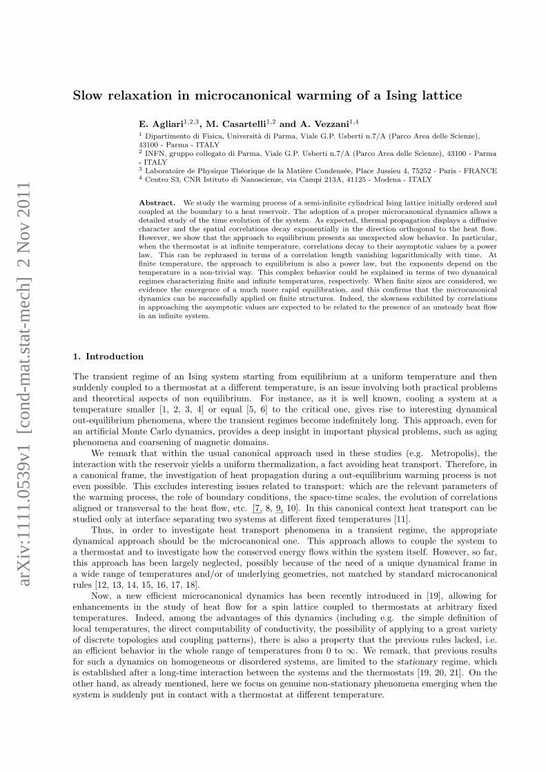
Figure 1. (Color on line) Main figure: Each curve, depicted in different color, represents the magnitudeof the mean energy −E(x, t), as a function of the rescaled time t. Different columns of the system x havebeen taken into account. Inset: the energy E (red symbols) as a function of time t, compared with thepower law ∼ t1/2 (black line). Numerical data can be fitted by a power-law with exponent 0.48; the smalldifference with respect to the expected value 0.5 can be ascribed to the existence of a long pre-asymptoticregime. All data represented in this plot refer to a system of size LY = 300 initially ordered and subjectto a thermostat at T = 10000.

longitudinal sizes, that is LX = 20. In any case, LY is kept fixed and equal to 300; this large value is usefulto avoid finite size effects and improves the statistics of the measures.

3.1. Diffusion features

In the presence of a static heat flux, the system behaves diffusively, as already noticed in [19, 20]. The presentsimulations confirm this picture even in a transient regime. In particular, relevant physical quantities suchas the total energy along the Y direction

E(t) =

LX∑

x=1

E(x, t),

grows as t1/2, that is the characteristic law of diffusive processes; this asymptotic regime is reached onlyat very large times due to the extensive routines of the dynamics (see inset of Fig. 3.1). Moreover,Fig. 3.1 evidences that focusing on the direction of heat propagation, the system can be studied within theframework of dynamical scaling which is typical of out-equilibrium systems. More precisely, the quantities(e.g. the local energy) depending on both time t and distance x can be plotted in terms of a single rescaledvariable x = x/ℓ(t), where ℓ(t) ∼ t1/2 is the characteristic length of the process, so that data obtainedat different spaces and times can be plotted together on a single curve. The fact that in our system ℓ(t)grows as t1/2 confirms the diffusive behavior of the model. Of course, an equivalent scaling (which hasbeen used in our plot) consists in introducing a rescaled time t = t/x2. Moreover, we remark that thescaling approach is very general and does not depend on the observable we have considered. Indeed wehave checked that different observables, such as the magnetization and the correlation functions, displayan analogous diffusive dynamical scaling.

Finally, it is worth deepening the relation between the dynamical scaling introduced above and thegeneralized Fourier equation used in [19] for the description of the model

∂E

∂t=

∂

∂x

(

D(E)∂E

∂x

)

, (3)

where D(E) is a diffusivity factor which, in quasi-equilibrium states, is just the ratio between theconductivity and the specific heat, so that the standard Fourier equation is recovered. We recall thatthe previous equation is able to describe the heat propagation in very general conditions, independently ofthe existence of a local temperature [22]. Now, it is straightforward to verify that posing E(x, t) = E(x)

Slow relaxation in microcanonical warming of a Ising lattice 5

100

101

102

103

10−4

10−3

10−2

10−1

100

t/x2

Cn(x

,t)

x = 10, n = 1

x = 10, n = 2

x = 10, n = 3

x = 20, n = 1

x = 20, n = 2

x = 20, n = 3

∼ t−1/2

∼ t−1

∼ t−3/2

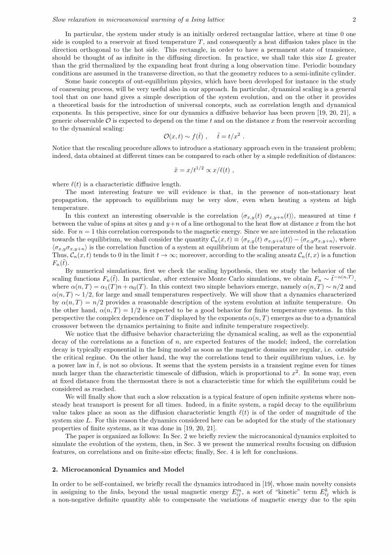
Figure 2. (Color on line) Log-log scale plot of the correlation function Cn, for n = 1 (blue), n = 2 (red)and n = 3 (black), as a function of the rescaled time t = t/x2. Measures have been performed on twocolumns, at distance 10 (•) and 20 (×) from the thermostat, respectively; due to time rescaling, datapertaining to different columns are collapsed. The green curves represent power-laws functions ∼ t−n/2

and provide a good fit for experimental data, over a proper time range. All data represented in this plotrefer to a system of size LY = 300 initially ordered and subject to a thermostat at temperature T = 10000.

leads to

− x

2

∂E

∂x=

∂

∂x

(

D(E)∂E

∂x

)

, (4)

i.e. the equation can be rewritten in terms of x only. Moreover, assuming that D(E) is a sufficientlysmooth function writable as D(E) = D0 +D1E, from Eq. 4 we can derive that the energy can be writtenas E(x) = E0 + E1x, namely E(t, x)− E0 ∼ x/

√t (at least at long times). As we will see in the following

subsection, this estimate is consistent with our numerical results.

3.2. Correlations

The transient regime presents interesting properties not only along the direction of heat flow but also alongthe orthogonal lines. In this framework, the simplest observable to consider is the two-point correlationfunction between spins of the same column at distance n, i.e.:

Cn(x, t) =1

LY

LY∑

y=1

〈σx,y(t)σx,y+n(t)〉 . (5)

Clearly, C1(x, t) is simply the negative of the energy E(x, t) of the x-th column, i.e. C1(x, t) = −E(x, t).Since we are interested in the long-time asymptotic behavior, we consider the quantity

Cn(x, t) = Cn(x, t) − C∞

n , (6)

where C∞

n = 〈σx,yσx,y+n〉 = 〈σx,yσx+n,y〉 is the equilibrium two-point correlation function between spinsat distance n in a 2-dimensional system evaluated at the same temperature of the thermostat. Therefore,if the system approaches to the equilibrium, we have limt→∞ Cn(x, t) = 0, as it has been indeed verified inall our numerical simulations.

In the Ising model outside the critical regime, when simply connected domains are prevalent, thecorrelation functions decay exponentially with the distance n, i.e. as exp(−n/λ), where λ is defined as thecorrelation length. At equilibrium, λ depends on the temperature, while, in the coarsening processes, itgrows as t1/2, due to the diffusion of the magnetic domains [1, 3, 4].

Fig. 3.2 shows the behavior of Cn(x, t) when the thermostat is at very large temperature, i.e. infinitefor all practical purposes. In this case the equilibrium correlation function vanishes. The dynamical scalingpicture is verified, since data evaluated at different columns (e.g. x = 10 and x = 20) collapse by using therescaled variable t = t/x2, i.e. Cn(x, t) = Fn(t). Moreover, for large enough t, simulations evidence that

Fn(t) ∼ t−n/2. (7)

Therefore, the correlation function presents an exponential decay with the distance n and this is peculiarof the Ising model outside the critical regime.

On the other hand, an unexpected and interesting feature is the slow decay of Fn(t) as a functionof t, consistently with the predictions drawn in the previous section for n = 1. While in the standard

Slow relaxation in microcanonical warming of a Ising lattice 6

100

102

10−4

10−3

10−2

10−1

100

t/x2

Cn(x

,t)

1 1.5 2 2.5 3

0.5

1

1.5

nα

T = 3

T = 5

T = 100

T = 1000

T = 10000

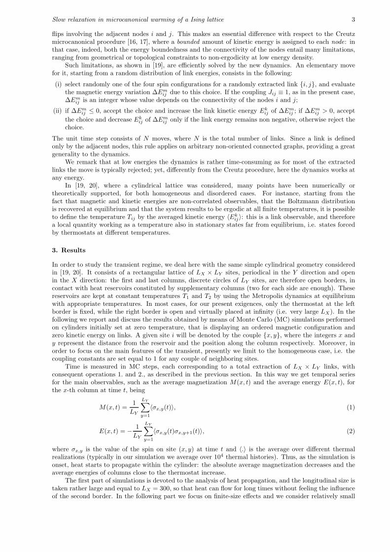
Figure 3. (Color on line) Main figure: log-log scale plot of the correlation function Cn, for n = 1 (blue),n = 2 (red) and n = 3 (black), as a function of the rescaled time t, for a system of size LY = 300initially ordered and subject to a thermostat at temperature T = 5. Measures have been performed ontwo columns, at distance 10 (•) and 20 (×) from the thermostat, respectively; due to time rescaling, datapertaining to different columns are collapsed. The green curves represent power-laws functions ∼ t−α(n,T )

and provide a good fit for experimental data, over a proper time range. Inset: Exponent α(n, T ) obtainedby fitting data from numerical simulations, as a function of n. Different temperatures for the thermostatare considered and compared, as explained by the legend.

MC approach a slow equilibration is typical of freezing only (below the critical temperature), here we canappreciate a similar behavior also during the warming phase. In fact, a rapid equilibration would involvean exponential decay in t. In particular, the heating process can not be considered concluded even forthose sites whose distance from the thermostat is much smaller than ℓ(t), i.e. the characteristic length ofheat diffusion. From a different point of view, the very slow approach to equilibrium can be described interms of correlation length λ which, in our model, turns out to tend to zero logarithmically in t; indeed thecorrelation function can be written as:

Cn(x, t) = Fn(t) ∼ t−n/2 = exp

[

−n log(t)

2

]

= exp(−n/λ). (8)

We will show that the unexpected slow relaxation at high temperature emerges in open systems, while inthe next section we verify that in small systems, where the boundary effects can not be discarded and heatcan not flow freely, the thermalization process is exponentially fast at large enough times.

The scaling function in Eq. 8 presents a very simple structure. Let us define gn(x) ≡ Fn(t) and expandgn(x) for small x (i.e. large times); we get

gn(x) =

∞∑

k=0

Ak,nxk. (9)

Then, formula (7) can be recast as Ak,n = 0 if k < n, giving a description, at infinite temperature, ofthe asymptotic behavior of the model in terms of the analytic properties of gn(x). Now, when the borderis thermalized at a finite temperature, the main features characterizing the heat transport are preserved:as evidenced in Fig. 3, scaling still holds with a definite diffusive length, the correlation functions decayexponentially and the approach to equilibrium is slow since the scaling functions vanish as a power law.However, here the analytic form of Fn(t) is not so simple; in fact we have Fn ∼ t−α(n,T ), and fittingprocedures suggest that

α(n, T ) = α1(T )n+ α0(T ) (10)

as shown in the inset of Fig. 3.

3.3. Dynamical regimes

The exponents characterizing the slow decays appear to be temperature dependent with a non-trivialbehavior. However, Fig. 3 evidences that for high (practically infinite) temperature, α(n, T ) = n/2, while,

Slow relaxation in microcanonical warming of a Ising lattice 7

for low enough temperatures, α(n, T ) ∼ 1/2 independently of n. This suggests that two simple (asymptotic)behaviors are present in the model: for infinite temperature the scaling function should be given by

Fn(t) ∼ t−n/2 = exp

[

−n log(t)

2

]

, (11)

hence, at infinite temperature, the dynamics is characterized by indefinitely shortening correlation lengthλ(t) = 2/ log(t). This is clearly consistent with the fact that at infinite temperature there is not anequilibrium characteristic length, since the correlation function between any couple of sites is vanishing.On the other hand, at small temperature, Fn(t) decays as t

−1/2. However, since the exponential decay ofCn(t) as a function of the distance n is an expected feature, we have

Fn(t) ∼ t−1/2 exp(−n/λ′) (12)

where a characteristic length λ′ naturally emerges. We remark that at finite temperature the equilibriumcorrelation functions decay with a characteristic length λeq(T ). Since a similar behavior is expected tobe reached asymptotically also out of equilibrium, we expect that, eventually, λ′ ∼ λeq(T ). Therefore theabove regimes (11,12) provide a reasonable description for infinite and finite temperature respectively.

In this perspective, the complex behavior characterizing intermediate temperatures would result froman interplay between these regimes. In particular, when the thermostat is at a finite temperature T ,Fn(t) evolves according to Eq. (11) until the correlation length λ(t) becomes comparable to λ′ ∼ λeq(T );afterwards an evolution described by (12) takes place. At very large temperatures λ′ ∼ λeq(T ) is almostzero and, in the considered time regimes, λ(t) ≫ λ′, therefore only the infinite temperature evolution (11)is observed. At low temperatures the correlation λ′ is so large that λ(t) becomes quickly comparable toλ′ and Fn(t) evolves according to (12). Finally, the temperature dependent exponents α(n, T ) observed atintermediate temperatures should be the result of the crossover between the two regimes which is ongoingin the considered time window.

3.4. Finite-size effects

Let us now discuss the finite-size effects in the processes of heat transfer from the thermostat to thesystem. Finite-size effects can clarify some features outlined in the previous analysis, in particular themutual influence between the transport regime and the way the asymptotic values are approached.

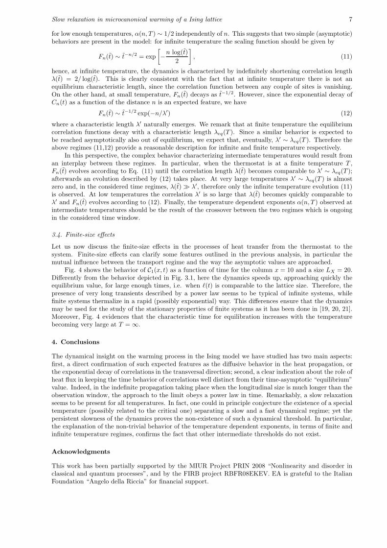
Fig. 4 shows the behavior of C1(x, t) as a function of time for the column x = 10 and a size LX = 20.Differently from the behavior depicted in Fig. 3.1, here the dynamics speeds up, approaching quickly theequilibrium value, for large enough times, i.e. when ℓ(t) is comparable to the lattice size. Therefore, thepresence of very long transients described by a power law seems to be typical of infinite systems, whilefinite systems thermalize in a rapid (possibly exponential) way. This differences ensure that the dynamicsmay be used for the study of the stationary properties of finite systems as it has been done in [19, 20, 21].Moreover, Fig. 4 evidences that the characteristic time for equilibration increases with the temperaturebecoming very large at T = ∞.

4. Conclusions

The dynamical insight on the warming process in the Ising model we have studied has two main aspects:first, a direct confirmation of such expected features as the diffusive behavior in the heat propagation, orthe exponential decay of correlations in the transversal direction; second, a clear indication about the role ofheat flux in keeping the time behavior of correlations well distinct from their time-asymptotic “equilibrium”value. Indeed, in the indefinite propagation taking place when the longitudinal size is much longer than theobservation window, the approach to the limit obeys a power law in time. Remarkably, a slow relaxationseems to be present for all temperatures. In fact, one could in principle conjecture the existence of a specialtemperature (possibly related to the critical one) separating a slow and a fast dynamical regime; yet thepersistent slowness of the dynamics proves the non-existence of such a dynamical threshold. In particular,the explanation of the non-trivial behavior of the temperature dependent exponents, in terms of finite andinfinite temperature regimes, confirms the fact that other intermediate thresholds do not exist.

Acknowledgments

This work has been partially supported by the MIUR Project PRIN 2008 “Nonlinearity and disorder inclassical and quantum processes”, and by the FIRB project RBFR08EKEV. EA is grateful to the ItalianFoundation “Angelo della Riccia” for financial support.

Slow relaxation in microcanonical warming of a Ising lattice 8

103

104

105

10−4

10−3

10−2

10−1

100

t

C1(x

,t)

T = 3

T = 5

T = 10

T = 1000

T = 10000

Figure 4. (Color on line) Correlation function C1 as a function of time t, for a system of size LY = 300,LX = 20 and x = 10, subject to a thermostat set at different temperature, each temperature beingrepresented by a different color as explained by the legend.

References

[1] Humayun K, Bray AJ, 1991 J. Phys. A 24 1915[2] Baumann F, Pleimling M, 2007 Phys. Rev. B 76 104422[3] Furukawa H, 1985 Adv. Phys. 34, 703[4] Bray AJ, 1994 Adv. Phys. 43, 357[5] Godreche C and Luck JM, J. Phys.:Cond. Matt. 14, 1589 (2002);[6] Calabrese P, Gambassi A, 2005 J. Phys. A 38, R133[7] Lebon G, Jou D and Casas-Vazquez J, 2008 Understanding Non-Equilibrium Thermodynamics: Foundations,

Applications, Frontiers, Springer-Verlag, Berlin (Germany)[8] Henkel M and Pleimling M, 2010 Non-Equilibrium Phase Transitions: Volume 2: Ageing and Dynamical Scaling Far

from Equilibrium (Theoretical and Mathematical Physics), Springer-Verlag (Berlin).[9] Ngai KL, 2011 Relaxation and Diffusion in Complex Systems, Springer-Verlag (Berlin).[10] Lepri S, Livi R and Politi A, 2003 Phys. Rep. 377, 1[11] Piscitelli A, Corberi F and Gonnella G, 2008 J. Phys. A: Math. Gen. 41, 332003[12] Vichniac GY, 1984 Physica D 10, 96[13] Pomeau Y and Vichniac GV, 1988 J. Phys. A: Math. Gen. 21, 3297[14] Harris R and Grant M, 1988 Phys. Rev. B 38, 9323[15] Saito K, Takesue S and Miyashita S, 1999 Phys. Rev. E 59, 2783[16] Creutz M, 1983 Phys. Rev. Lett. 50, 1411[17] Creutz M, 1986 Annals of Physics 167, 62[18] Agliari E, Casartelli M and Vezzani A, 2008 Eur. Phys. J. B 65, 257[19] Agliari E, Casartelli M and Vezzani A, 2009 J. Stat. Mech. P07041[20] Agliari E, Casartelli M and Vezzani A, 2010 J. Stat. Mech. P10021[21] Agliari E, Casartelli M and Vivo E, 2010 J. Stat. Mech. P09002[22] Casartelli M, Macellari N and Vezzani A, 2007 Eur. Phys. J. B 56, 149