On estimating and testing associations between random coefficients from multivariate generalized...

XML Template (2015) [24.1.2015–5:06pm] [1–16]//blrnas3.glyph.com/cenpro/ApplicationFiles/Journals/SAGE/3B2/SMMJ/Vol00000/140142/APPFile/SG-SMMJ140142.3d (SMM) [PREPRINTERstage]

Article

On estimating and testingassociations between randomcoefficients from multivariategeneralized linear mixed modelsof longitudinal outcomes

Susan K Mikulich-Gilbertson,1,2 Brandie D Wagner,2

Paula D Riggs1 and Gary O Zerbe2

Abstract

Different types of outcomes (e.g. binary, count, continuous) can be simultaneously modeled with

multivariate generalized linear mixed models by assuming: (1) same or different link functions, (2) same

or different conditional distributions, and (3) conditional independence given random subject effects.

Others have used this approach for determining simple associations between subject-specific

parameters (e.g. correlations between slopes). We demonstrate how more complex associations

(e.g. partial regression coefficients between slopes adjusting for intercepts, time lags of maximum

correlation) can be estimated. Reparameterizing the model to directly estimate coefficients allows us to

compare standard errors based on the inverse of the Hessian matrix with more usual standard errors

approximated by the delta method; a mathematical proof demonstrates their equivalence when the gradient

vector approaches zero. Reparameterization also allows us to evaluate significance of coefficients with

likelihood ratio tests and to compare this approach with more usual Wald-type t-tests and Fisher’s z

transformations. Simulations indicate that the delta method and inverse Hessian standard errors are

nearly equivalent and consistently overestimate the true standard error. Only the likelihood ratio test

based on the reparameterized model has an acceptable type I error rate and is therefore recommended

for testing associations between stochastic parameters. Online supplementary materials include our medical

data example, annotated code, and simulation details.

Keywords

Joint modeling, random coefficient associations, stochastic parameter associations, delta method, Fisher’s

z transformation, likelihood ratio tests

1Department of Psychiatry, School of Medicine, University of Colorado Anschutz Medical Center, Aurora, USA2Department of Biostatistics and Informatics, Colorado School of Public Health, University of Colorado Anschutz Medical Center,

Aurora, USA

Corresponding author:

Susan K Mikulich-Gilbertson, University of Colorado Anschutz Medical Campus, Mail Stop F478, 12469 East 17th Place, Aurora,

CO 80045, USA.

Email: [email protected]

Statistical Methods in Medical Research

0(0) 1–16

! The Author(s) 2015

Reprints and permissions:

sagepub.co.uk/journalsPermissions.nav

DOI: 10.1177/0962280214568522

smm.sagepub.com

at UNIV OF CO HEALTH SCIENCE CTR on February 16, 2015smm.sagepub.comDownloaded from

http://smm.sagepub.com/


1 Introduction

Biological and medical research is often designed to investigate changes in a collection of responsevariables which are measured repeatedly over time on the same subjects. Multivariate longitudinaldata of this kind provide the opportunity to address a variety of clinically relevant questions withjoint analyses of outcomes. Early research on simultaneously modeling multiple longitudinaloutcomes is restricted to normal multivariate linear models.1–3 More recently, the approach hasbeen extended to multivariate nonlinear models for outcomes with normal residuals4,5 andmultivariate generalized linear models.6–13

We describe a multivariate generalized linear mixed model for multiple outcomes which may benonnormal and differently distributed and evaluate random coefficient associations among theoutcomes, beginning with simple correlation coefficients discussed by others.7,9–13 A series ofextensions and novel contributions follow that together inform procedures for estimating andtesting random coefficient associations. We demonstrate how more complex partial correlationand regression coefficients may be obtained through recursion and indicate that the alternatemethod discussed by Zucker et al.3 for computing partial regression coefficients can be extendedto nonnormal, differently distributed outcomes. We describe correlation between predictedoutcomes at different times and determine the time lag of maximum correlation. Areparameterization of the model allows us to directly estimate association coefficients of interestas model parameters and to obtain standard errors based on the inverse of the Hessian matrix. Theseinverse Hessian-based standard errors can be compared with more usual standard errorsapproximated by the delta method; a mathematical proof demonstrates their equivalence whenthe gradient vector associated with model convergence is zero and approximate equivalence whenthe gradient is small. Importantly, the reparameterization also facilitates likelihood ratio tests(LRTs) of the significance of these simple and more complex correlation and regressioncoefficients. We compare them with results from more usual Wald-type t-tests and with Fisher’s ztransformations using data from a pharmacotherapy trial and simulations and we show that onlythe LRTs achieve the nominal significance level. The dataset, annotated code, and simulationmethods and results are included in an online supplement (available at: http://smm.sagepub.com/).

2 Multivariate generalized linear mixed model

For subjects i¼ 1,. . ., N, assume independent vectors

yi ¼ yT1i yT2i � � � yTri� �T

Here, yi denotes a vector of observations on r outcomes at multiple times, and yhi is the subvector ofthese observations for outcome h. Neither the times nor the number of outcomes need be identicalfor different subjects, although we will assume that such differences are not informative of outcome.Let the joint distribution of the likely correlated observations on subject i be conditional on a k� 1vector of population parameters b, a p� 1 vector of subject-specific random effects ui, and acovariate matrix Xi. Additionally, the random effects are assumed to have multivariate normaldistribution n uij �ð Þ, with mean 0 and p� p covariance D, a function of m, a vector of unknownparameters. Then inferences about b and � are based on the joint likelihood (density)

L ¼YNi¼1

Zf yijb, ui,Xi

� �n ui j�ð Þ@ui

2 Statistical Methods in Medical Research 0(0)




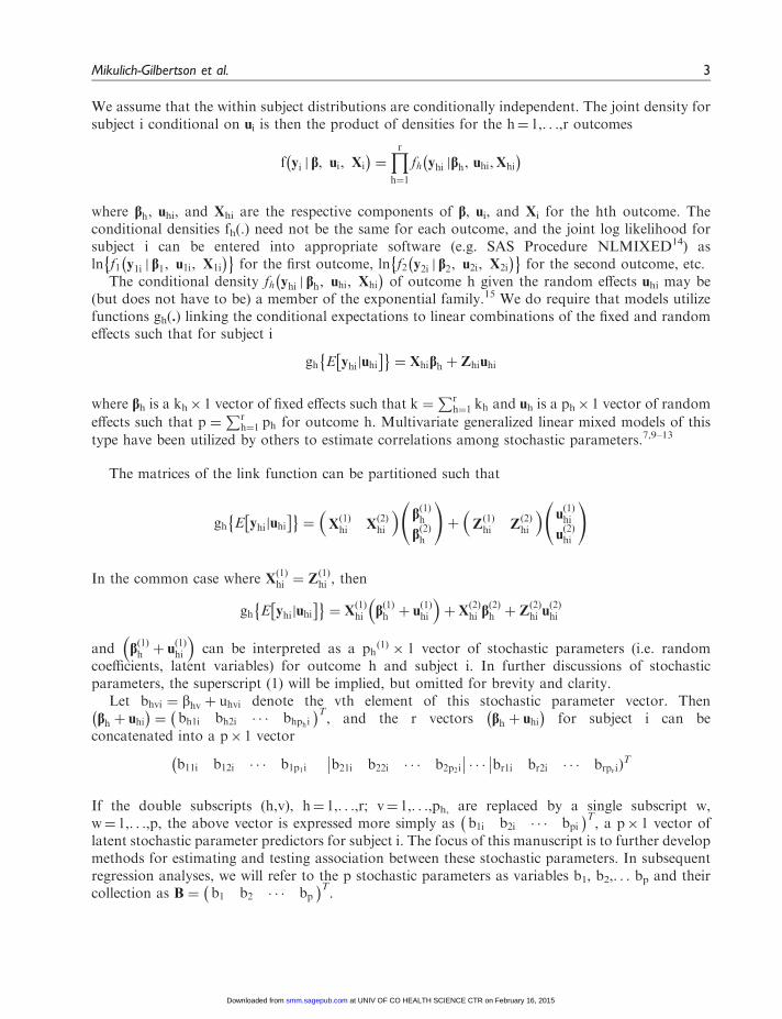
We assume that the within subject distributions are conditionally independent. The joint density forsubject i conditional on ui is then the product of densities for the h¼ 1,. . .,r outcomes

f yi j b, ui, Xi

� �¼Yrh¼1

fh yhi jbh, uhi,Xhi

� �

where bh, uhi, and Xhi are the respective components of b, ui, and Xi for the hth outcome. Theconditional densities fh(.) need not be the same for each outcome, and the joint log likelihood forsubject i can be entered into appropriate software (e.g. SAS Procedure NLMIXED14) asln f1 y1i j b1, u1i, X1i

� �� for the first outcome, ln f2 y2i j b2, u2i, X2i

� �� for the second outcome, etc.

The conditional density fh yhi j bh, uhi, Xhi

� �of outcome h given the random effects uhi may be

(but does not have to be) a member of the exponential family.15 We do require that models utilizefunctions gh(.) linking the conditional expectations to linear combinations of the fixed and randomeffects such that for subject i

gh E yhi uhij� ��

¼ Xhibh þ Zhiuhi

where bh is a kh� 1 vector of fixed effects such that k ¼Pr

h¼1 kh and uh is a ph� 1 vector of random

effects such that p ¼Pr

h¼1 ph for outcome h. Multivariate generalized linear mixed models of this

type have been utilized by others to estimate correlations among stochastic parameters.7,9–13

The matrices of the link function can be partitioned such that


¼ Xð1Þhi X

ð2Þhi

� bð1Þhbð2Þh

!þ Z

ð1Þhi Z

ð2Þhi

� uð1Þhi

uð2Þhi

!

In the common case where Xð1Þhi ¼ Z

ð1Þhi , then


¼ Xð1Þhi bð1Þh þ u

ð1Þhi

� þ X

ð2Þhi bð2Þh þ Z

ð2Þhi uð2Þhi

and bð1Þh þ uð1Þhi

� can be interpreted as a ph

ð1Þ � 1 vector of stochastic parameters (i.e. randomcoefficients, latent variables) for outcome h and subject i. In further discussions of stochasticparameters, the superscript (1) will be implied, but omitted for brevity and clarity.

Let bhvi ¼ bhv þ uhvi denote the vth element of this stochastic parameter vector. Thenbh þ uhi� �

¼ bh1i bh2i � � � bhphi� �T

, and the r vectors bh þ uhi� �

for subject i can beconcatenated into a p� 1 vector

b11i b12i � � � b1p1i b21i b22i � � � b2p2i � � � br1i br2i � � � brpriÞ

T�

If the double subscripts (h,v), h¼ 1,. . .,r; v¼ 1,. . .,ph, are replaced by a single subscript w,w¼ 1,. . .,p, the above vector is expressed more simply as b1i b2i � � � bpi

� �T, a p� 1 vector of

latent stochastic parameter predictors for subject i. The focus of this manuscript is to further developmethods for estimating and testing association between these stochastic parameters. In subsequentregression analyses, we will refer to the p stochastic parameters as variables b1, b2,. . . bp and theircollection as B ¼ b1 b2 � � � bp

� �T.

Mikulich-Gilbertson et al. 3




3 Illustrative example: Daily marijuana and alcohol usein adolescent patients

One useful application of the methods discussed here is to understand the interrelationships amongaddiction to multiple drugs, especially due to high rates of polysubstance use in adolescents. Datafor this example come from a multisite pharmacotherapy trial of cooccurring attention-deficithyperactivity disorder and substance use in adolescents.16 Self-reported daily use of marijuana,alcohol, and other drugs are available on up to 112 days of the treatment period and allparticipants received cognitive behavioral therapy treatment targeting their primary addictionwhich was predominantly marijuana.16 The sample utilized here are the 65 adolescents whocompleted the trial, used marijuana on 14 or more days in the month before treatment, and whoalso used alcohol at least once in the month prior to treatment.

If treatment is successful, adolescents who receive treatment should reduce their marijuana use;their concurrent or subsequent alcohol use might feasibly also decrease as an indirect result of drugtreatment or might feasibly increase in compensation for reduced marijuana use. Research questionsof interest include

(1) What is the association between daily number of marijuana joints smoked and daily use ofalcohol at baseline (prior to treatment)?

(2) What is the association between the rates of change in daily joints smoked and daily use ofalcohol during treatment?

(3) Is the association of their use stronger at specific times during treatment (e.g. midtreatment) orfor specific time lags for each drug (e.g. marijuana use two weeks prior to alcohol use)?

Evaluating the time of maximum correlation between use of the drug that treatment is targeting(marijuana) and use of a second drug (alcohol) might provide indication of when secondary drug useshould be addressed in treatment. Strong correlation for one outcome early in treatment with asecond outcome subsequently could be suggestive of causality and could indicate that the firstoutcome might be predictive of the second. We have not seen methods for evaluating thefollowing more complicated associations discussed in the literature.

(4) For alcohol use at a specific time (e.g. midtreatment, day 56), when is it most strongly correlatedwith marijuana use and how strong is that correlation?

(5) What is the association between the rates of change in daily joints smoked and daily use ofalcohol adjusting for their baseline use of both prior to treatment?

(6) Is the subject-specific rate of change of marijuana usage (targeted by treatment) predictive ofthe subject-specific rate of change of alcohol usage,with orwithout adjusting for their baseline use?

Negative binomial regression is often used to model count variables where distributions areoverdispersed Poisson (e.g. Hayaki et al.17) as is the case with marijuana joints smoked per day. Tosimultaneously model daily counts of joints smoked with daily use of alcohol (yes, no), we assume theconditional likelihood is a negative binomial distribution with natural log link for marijuana use(h¼ 1) and we assume the conditional likelihood is a Bernoulli distribution with logit link foralcohol use (h¼ 2). Assuming the natural log of the conditional expectation of number ofmarijuana joints is linear in time, the log of expected daily marijuana use for subject i at time t is

ln E Y1i tð Þð Þ u1ij , u2i, u3i, u4i� �

¼ �1 þ u1i� �

þ �2 þ u2i� �

t





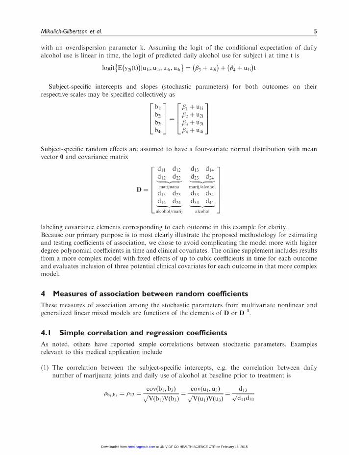
with an overdispersion parameter k. Assuming the logit of the conditional expectation of dailyalcohol use is linear in time, the logit of predicted daily alcohol use for subject i at time t is

logit E y2i tð Þ� �

u1ij , u2i, u3i, u4i� �

¼ �3 þ u3i� �

þ �4 þ u4i� �

t

Subject-specific intercepts and slopes (stochastic parameters) for both outcomes on theirrespective scales may be specified collectively as

b1ib2ib3ib4i

2664

3775 ¼

�1 þ u1i�2 þ u2i�3 þ u3i�4 þ u4i

2664

3775

Subject-specific random effects are assumed to have a four-variate normal distribution with meanvector 0 and covariance matrix

D ¼

d11 d12d12 d22|fflfflfflfflfflffl{zfflfflfflfflfflffl}marijuana

d13 d14d23 d24|fflfflfflfflfflffl{zfflfflfflfflfflffl}marij=alcohol

d13 d23d14 d24|fflfflfflfflfflffl{zfflfflfflfflfflffl}alcohol=marij

d33 d34d34 d44|fflfflfflfflfflffl{zfflfflfflfflfflffl}

alcohol

26666664

37777775

labeling covariance elements corresponding to each outcome in this example for clarity.Because our primary purpose is to most clearly illustrate the proposed methodology for estimatingand testing coefficients of association, we chose to avoid complicating the model more with higherdegree polynomial coefficients in time and clinical covariates. The online supplement includes resultsfrom a more complex model with fixed effects of up to cubic coefficients in time for each outcomeand evaluates inclusion of three potential clinical covariates for each outcome in that more complexmodel.

4 Measures of association between random coefficients

These measures of association among the stochastic parameters from multivariate nonlinear andgeneralized linear mixed models are functions of the elements of D or D–1.

4.1 Simple correlation and regression coefficients

As noted, others have reported simple correlations between stochastic parameters. Examplesrelevant to this medical application include

(1) The correlation between the subject-specific intercepts, e.g. the correlation between dailynumber of marijuana joints and daily use of alcohol at baseline prior to treatment is

�b1,b3 ¼ �13 ¼cov b1, b3ð ÞffiffiffiffiffiffiffiffiffiffiffiffiffiffiffiffiffiffiffiffiffiffiffiV b1ð ÞV b3ð Þ

p ¼cov u1, u3ð ÞffiffiffiffiffiffiffiffiffiffiffiffiffiffiffiffiffiffiffiffiffiffiffiV u1ð ÞV u3ð Þ

p ¼d13ffiffiffiffiffiffiffiffiffiffiffiffiffid11d33p





(2) The correlation between the subject-specific slopes, e.g. the correlation between the rates of dailynumber of joints and daily use of alcohol during treatment is

�b2,b4 ¼ �24 ¼cov u2, u4ð ÞffiffiffiffiffiffiffiffiffiffiffiffiffiffiffiffiffiffiffiffiffiffiffiV u2ð ÞV u4ð Þ

p ¼d24ffiffiffiffiffiffiffiffiffiffiffiffiffid22d44p

(3) The correlation between number of joints smoked on day t and alcohol use on day t0 is

�b1þb2t, b3þb4t0 ¼cov u1 þ u2t, u3 þ u4t

0ð ÞffiffiffiffiffiffiffiffiffiffiffiffiffiffiffiffiffiffiffiffiffiffiffiffiffiffiffiffiffiffiffiffiffiffiffiffiffiffiffiffiffiffiffiffiffiffiffiffiV u1 þ u2tð ÞV u3 þ u4t0ð Þ

p ¼d13 þ td23 þ t0d14 þ tt0d24ffiffiffiffiffiffiffiffiffiffiffiffiffiffiffiffiffiffiffiffiffiffiffiffiffiffiffiffiffiffiffiffiffiffiffiffiffiffiffiffiffiffiffiffiffiffiffiffiffiffiffiffiffiffiffiffiffiffiffiffiffiffiffiffiffiffiffiffiffiffiffiffiffiffiffiffiffiffiffiffiffiffiffiffiffiffi

d11 þ 2td12 þ t2d22� �

d33 þ 2t0d34 þ t02d44� �q

When t and t0 are both zero, this is simply the correlation between the random intercepts. As t and t0

increase, the marginal correlation converges to the correlation between the random slopes.

(4) For a specified day t of marijuana use (h¼ 1), the day (designated t0max) that maximizes thecorrelation between joints smoked and alcohol use (h¼ 2) can be obtained by differentiating (3)with respect to t0 and setting the resulting derivative equal to zero. Then

t0max ¼� t d24d33 � d34d23ð Þ þ d14d33 � d34d13ð Þ½ �

2d14d34 � d34d14 � d44d13 þ t 2d24d34 � d34d24 � d44d23ð Þ½ �

(5) The regression coefficient of the alcohol slope on the marijuana slope is the ratio

�b4jb2 ¼ �4j2¼ cov u2, u4ð Þ=V u2ð Þ ¼ d24=d22

4.2 Partial correlation and partial regression coefficients obtainedthrough recursion

Using well-known recursive formulae18

6. the partial correlation coefficient between marijuana slope b2 and alcohol slope b4 adjusting foralcohol intercept b3 is

�b2, b4�b3 ¼ �24�3 ¼ �24 � �23�34ð Þ=ffiffiffiffiffiffiffiffiffiffiffiffiffiffiffiffiffiffiffiffiffiffiffiffiffiffiffiffiffiffiffiffiffiffiffiffiffi1� �223� �

1� �234� �q

The residual variance from the regression of marijuana slope on alcohol intercept, i.e. b2 on b3 isd22�3 ¼ d22 1� �223

� �and the residual variance from the regression of alcohol slope on alcohol

intercept, i.e. b4 on b3 is d44�3 ¼ d44 1� �234� �

. Then,

7. the partial regression coefficient of b4 on b2 adjusting for b3 is

�4 2j �3 ¼ �24 �3ffiffiffiffiffiffiffiffiffiffiffiffiffiffiffiffiffiffiffiffiffiffiffid44�3=d22 �3

p:





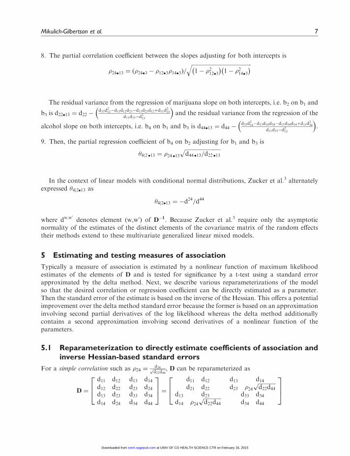
8. The partial correlation coefficient between the slopes adjusting for both intercepts is

�24�13 ¼ �24�3 � �12�3�14�3ð Þ=ffiffiffiffiffiffiffiffiffiffiffiffiffiffiffiffiffiffiffiffiffiffiffiffiffiffiffiffiffiffiffiffiffiffiffiffiffiffiffiffiffiffiffiffi1� �212�3� �

1� �214�3� �q

The residual variance from the regression of marijuana slope on both intercepts, i.e. b2 on b1 and

b3 is d22�13 ¼ d22 �d33d

212�d13d12d23�d13d23d12þd11d

223

d11d33�d213

� and the residual variance from the regression of the

alcohol slope on both intercepts, i.e. b4 on b1 and b3 is d44�13 ¼ d44 �d33d

214�d13d14d34�d13d34d14þd11d

234

d11d33�d213

� .

9. Then, the partial regression coefficient of b4 on b2 adjusting for b1 and b3 is

�4 2j �13 ¼ �24 �13ffiffiffiffiffiffiffiffiffiffiffiffiffiffiffiffiffiffiffiffiffiffiffiffiffiffid44 �13=d22 �13

p

In the context of linear models with conditional normal distributions, Zucker et al.3 alternatelyexpressed �4j2�13 as

�4j2�13 ¼ �d24=d44

where dw,w0

denotes element (w,w0) of D�1. Because Zucker et al.3 require only the asymptoticnormality of the estimates of the distinct elements of the covariance matrix of the random effectstheir methods extend to these multivariate generalized linear mixed models.

5 Estimating and testing measures of association

Typically a measure of association is estimated by a nonlinear function of maximum likelihoodestimates of the elements of D and is tested for significance by a t-test using a standard errorapproximated by the delta method. Next, we describe various reparameterizations of the modelso that the desired correlation or regression coefficient can be directly estimated as a parameter.Then the standard error of the estimate is based on the inverse of the Hessian. This offers a potentialimprovement over the delta method standard error because the former is based on an approximationinvolving second partial derivatives of the log likelihood whereas the delta method additionallycontains a second approximation involving second derivatives of a nonlinear function of theparameters.

5.1 Reparameterization to directly estimate coefficients of association andinverse Hessian-based standard errors

For a simple correlation such as �24 ¼d24ffiffiffiffiffiffiffiffiffid22d44p , D can be reparameterized as

D ¼

d11 d12d12 d22

d13 d14d23 d24

d13 d23d14 d24

d33 d34d34 d44

264

375 ¼

d11 d12d21 d22

d13 d14d23 �24

ffiffiffiffiffiffiffiffiffiffiffiffiffid22d44p

d13 d23d14 �24

ffiffiffiffiffiffiffiffiffiffiffiffiffid22d44p

d33 d34d34 d44

264

375





Similarly, for a simple regression such as �4j2 ¼d24d22, D can be reparameterized to include

d24 ¼ �4j2d22.To reparameterize D in terms of partial correlation and partial regression coefficients, consider

the partitioned random effects distribution

v1v2

�� N

0

0

�,

�11 �12

�21 �22

��

where v1 is the 2� 1 vector of stochastic parameters that we wish to associate, v2 is the (p–2)� 1vector of stochastic parameters for which we wish to adjust, and �21 ¼ �012. The covariance matrixof v1 conditional on v2 is �11�2 ¼ �11 ��12�

�122 �21, implying that the 2� 2 matrix

�11 ¼ �11�2 þ A11�2 may be used to express the covariance matrix of v1 as the sum of theconditional covariance matrix �11�2 of v1 on v2 and a matrix A11�2 ¼ �12�

�122 �21 of adjustments

for v2. Reparameterization is now made simple since only three elements of the p�p Dmatrix, thosecorresponding to the three distinct elements of �11�2 need to be modified.

For a partial correlation between two stochastic parameters, e.g. u2 and u4, adjusted for two other

stochastic parameters, e.g. u1 and u3, v1 ¼u2u4

�, v2 ¼

u1u3

�, the conditional covariance matrix of

v1 on v2 is

�11�2 ¼d22�1 3 d24�13d24�13 d44 �13

�¼

d22 �13 �24�13ffiffiffiffiffiffiffiffiffiffiffiffiffiffiffiffiffiffiffiffiffiffiffiffid22�13d44 �13p

�24 �13ffiffiffiffiffiffiffiffiffiffiffiffiffiffiffiffiffiffiffiffiffiffiffiffid22�13d44 �13p

d44 �13

�

where �24�13 is the partial correlation coefficient between u2 and u4 adjusted for u1 and u3, the matrixA11�2 of adjustments is

a22�13 a24 �13

a24�13 a44 �13

�¼

d12 d23

d14 d34

�d11 d13

d13 d33

��1 d12 d14

d23 d34

�

¼

d33d212 � d13d12d23 � d13d23d12 þ d11d

223

d11d33 � d213

d33d12d14 � d13d14d23 � d13d34d12 þ d11d34d23

d11d33 � d213

d33d12d14 � d13d14d23 � d13d34d12 þ d11d34d23

d11d33 � d213

d33d214 � d13d14d34 � d13d34d14 þ d11d

234

d11d33 � d213

0BBBB@

1CCCCA

and the unconditional covariance matrix �11 is

d22 d24d24 d44

�¼

d22 �13 �24 �13ffiffiffiffiffiffiffiffiffiffiffiffiffiffiffiffiffiffiffiffiffiffiffiffiffid22 �13d44 �13p

�24 �13ffiffiffiffiffiffiffiffiffiffiffiffiffiffiffiffiffiffiffiffiffiffiffiffiffid22 �13d44 �13p

d44 �13

�þ

a22 �13 a24 �13a24 �13 a44 �13

�

Substituting �11 for the appropriate elements of D yields the reparameterized D

d11 d12 d13 d14d12 d22 d23 d24d13 d23 d33 d34d14 d24 d34 d44

2664

3775 ¼

d11 d12 d13 d14d12 d22�13 þ a22�13 d23 �24 �13

ffiffiffiffiffiffiffiffiffiffiffiffiffiffiffiffiffiffiffiffiffiffiffid22�13d44�13p

þ a24�13d13 d23 d33 d34d14 �24 �13

ffiffiffiffiffiffiffiffiffiffiffiffiffiffiffiffiffiffiffiffiffiffiffid22�13d44�31p

þ a24�13 d34 d44�13 þ a44�13

2664

3775





Likewise, D can be reparameterized to include a partial regression coefficient adjusted for twostochastic parameters �4j2�13 ¼

d24�13d22�13

, with the same elements in D as for the analogous partialcorrelation coefficient except that d24 ¼ d24�13 þ a24�13 ¼ �4j2�13d22�13 þ a24�13, where

d22�13 �4j2�13d22 �13�4j2�13d22 �13 d44�13

�is the covariance matrix of u2 and u4 adjusted for u1 and u3, and

a22 �13 a24 �13a24 �13 a44 �13

�is the matrix of adjustments for u1 and u3.

5.2 Relationship between delta method and inverse Hessian-basedstandard errors

Reparameterizing the model to directly estimate the association coefficient of interest provides astandard error estimate based on the inverse of the Hessian. We conjectured this inverse Hessian-based standard error would be superior to the delta method standard error obtained after moreconventionally estimating covariances in D as parameters and computing association coefficients asnonlinear functions of those covariance estimates and we investigated their mathematicalrelationship.

Consider a model where c ¼ b�

�denotes the entirety of m maximum likelihood estimators, both

fixed effects and variance components. Then c minimizes g cð Þ, the – log likelihood with respect to c.Nonlinear functions of c, say a ¼ f�1ðcÞ, are also maximum likelihood estimators if thereparameterization of the parameter space from c onto a is a one-to-one mapping, such that f,the inverse of f�1 exists, and c ¼ f ðaÞ. Then a minimizes h að Þ, the – log likelihood with respect to a.At maximization the two likelihoods with respect to a and with respect to c are equal, and we haveh að Þ ¼ g cð Þ ¼ g f að Þð Þ.

Using the chain rule, Magnus and Neudecker19 (p. 96) prove the relationship

Dh að Þ|fflffl{zfflffl}1�m

¼ Dg cð Þð Þ|fflfflfflffl{zfflfflfflffl}1�m

Df að Þ|fflffl{zfflffl}m�m

between Dh að Þ the gradient vector of first partial derivatives of h with respect to a evaluated at a,Dg cð Þ the gradient of g with respect to c evaluated at c, and Df að Þ ¼ @�i=@�j

� �the m�m Jacobian

matrix of first partial derivatives of f with respect to a evaluated at a. Using the chain rule again,Magnus and Neudecker19 (p. 110) prove that

H h a|{z}m�1

!|fflfflfflfflffl{zfflfflfflfflffl}

1�1|fflfflfflfflfflfflffl{zfflfflfflfflfflfflffl}m�m

¼ D f a|{z}m�1


m�1|fflfflfflfflfflfflffl{zfflfflfflfflfflfflffl}m�m

0BBBBBBBB@

1CCCCCCCCA

0

|fflfflfflfflfflfflfflfflfflfflffl{zfflfflfflfflfflfflfflfflfflfflffl}m�m

H g c|{z}m�1

0@

1A

|fflfflfflfflffl{zfflfflfflfflffl}1�1|fflfflfflfflfflfflfflffl{zfflfflfflfflfflfflfflffl}

m�m

0BBBBBBBB@

1CCCCCCCCAD f a|{z}

m�1


m�1|fflfflfflfflfflfflffl{zfflfflfflfflfflfflffl}m�m

|fflfflfflfflfflfflfflfflfflfflfflfflfflfflfflfflfflfflfflfflfflfflfflfflfflfflfflfflfflfflfflfflfflfflfflfflfflffl{zfflfflfflfflfflfflfflfflfflfflfflfflfflfflfflfflfflfflfflfflfflfflfflfflfflfflfflfflfflfflfflfflfflfflfflfflfflffl}m�m

þ D g c|{z}m�1

0@

1A

|fflfflfflfflffl{zfflfflfflfflffl}1�1|fflfflfflfflfflfflfflffl{zfflfflfflfflfflfflfflffl}

1xm

� Im|{z}m�m

0BBBBBBBB@

1CCCCCCCCA

|fflfflfflfflfflfflfflfflfflfflfflfflfflfflfflfflfflfflffl{zfflfflfflfflfflfflfflfflfflfflfflfflfflfflfflfflfflfflffl}m�m2

Hf a|{z}m�1


m�1|fflfflfflfflfflfflffl{zfflfflfflfflfflfflffl}m2�m

|fflfflfflfflfflfflfflfflfflfflfflfflfflfflfflfflfflfflfflfflfflfflfflfflfflfflfflfflfflffl{zfflfflfflfflfflfflfflfflfflfflfflfflfflfflfflfflfflfflfflfflfflfflfflfflfflfflfflfflfflffl}m�m

where Hh að Þ is the m�m Hessian (matrix of second partial derivatives) of the scalar h with respectto a and a0 evaluated at a, Hg cð Þis the m�m Hessian of the scalar g with respect to c and � 0





evaluated at c, and Hf að Þ is the m2�m Hessian matrix of second partial derivatives of the vector f

with respect to a and a0 evaluated at a; dimensions are included for clarity. Then if the likelihood isnearly maximized such that the gradient vector Dg cð Þ ffi 0

Hh að Þð Þ�1¼ Df að Þð Þ

0Hg cð Þð ÞDf að Þ þ Dg cð Þ � Inð ÞHf að Þ

� ��1ffi Df að Þð Þ

0Hg cð Þð ÞDf að Þ

� ��1¼ Df að Þð Þ

�1Hg cð Þð Þ

�1Df að Þð Þ

0� ��1

¼ Df�1 cð Þ� �

V cð Þ Df�1 cð Þ� �

recalling that the Jacobian of a transformation Df�1 cð Þ� �

is equal to the inverse of the Jacobian ofthe inverse transformation Df að Þð Þ

�1. Hence, Hh að Þð Þ

�1, the inverse Hessian approximation of the

covariance matrix of a and Df�1 cð Þ� �

V cð Þ Df�1 cð Þ� �

, the delta method approximation of thecovariance matrix of a, are equal when the gradient vector Dg cð Þ ¼ 0 (when the likelihood ismaximized), and approximately equal when the gradient is small (when the likelihood is nearlymaximized). In particular, if we choose a reparameterization a ¼ f�1 ð�Þ such that �j estimates acorrelation or regression coefficient of interest, then the two standard errors of �j, the square roots ofthe jth diagonal elements of the two covariance matrices, will be approximately equal.

5.3 LRTs of association using reparameterized models

The t-tests using inverse Hessian or delta method standard errors are Wald-type tests. Fears et al.20

note that even though the Wald test is convenient to compute from standard computer output, it is alarge sample procedure with a value dependent on the parameterization and it has been shown tohave poor power in certain situations.21–23 After studying their behavior for hypothesis testing inexponential families, Vaeth23 concludes that Wald tests should be used with caution in discreteprobability models.

There are several reasons to prefer LRTs to Wald tests. Unlike Wald tests, LRTs are invariant forany monotonic transformation of the parameters. Whereas LRTs require only the approximate chi-square distribution of the test statistic, Wald tests require additional approximations about thestandard error. Reparameterizing the model to directly estimate the coefficient of interest enablesa LRT of that coefficient. The model can be run again, constraining the coefficient to be 0 and thedifference between these models’ –2 log likelihoods provides the approximate LRT for thesignificance of the coefficient.

5.4 Fisher’s Z transformation

A common test of significance for correlation and partial correlation coefficients between two u’sadjusted for k other u’s where the u’s have a multivariate normal distribution is Fisher’s z where

z ¼

12 ln

1þ�1��

� ffiffiffiffiffiffiffiffiffiffiffi

1n�k�3

qhas a standard normal distribution under the null hypothesis. Here the u’s are latent (unobserved),but z can still be computed from an observed estimate of r. The standard error depends only on thesample size n without delta method or inverse Hessian approximations.





6 Results from the illustrative example

We fit two independent univariate models of daily marijuana use (number of joints smoked)and daily alcohol use (yes, no) as a joint model by setting appropriate covariance termsequal to zero, resulting in a –2 log likelihood of 22,741.03. The corresponding –2 loglikelihood in the bivariate model with nonzero covariances between the random effectsis 22,729.33. The LRT to simultaneously test these covariances does not requirereparameterization and its significance (�2¼ 11.73, df¼ 4, p< 0.0194) supports the modelwith nonzero covariances, i.e. that it is better to fit the outcomes simultaneously thanindependently.

6.1 Estimates of fixed effects, variances, covariances, and simplecorrelation coefficients

Table 1 shows the maximum likelihood estimates from fitting the bivariate model withNLMIXED.14 The log of the expected number of marijuana joints smoked on day t is:ln E Y1ðtÞj u ¼ 0½ ��

¼ �0:21� 0:0095t and the overdispersion parameter k is significant(p< 0.0001) supporting the negative binomial distribution for modeling joints per day. Thelogit for expected alcohol use on day t is: logit E Y2ðtÞj u ¼ 0½ �

� �¼ �2:86� 0:0019t. Tests

using standard errors approximated from the inverse of the Hessian (Inv H) show that themarijuana slope is significantly less than zero, but the alcohol slope is not, suggesting that onaverage, only marijuana use (i.e. number of joints smoked per day) decreases significantlyduring treatment.

Table 1. Estimates from the bivariate random effect model of marijuana use (mar) and alcohol use (alc).

Label Parameter Estimate (InvH SE) tInvH (p> jtj)

Overdispersion k 0.87 (0.037) t¼ 23.5 (< 0.0001)

Mar intercept (int) b1 –0.21 (0.23) t¼ –0.90 (0.37)

Mar slope b2 –0.0095 (0.0030) t¼ –3.19 (0.0023)

Alc int b3 –2.86 (0.32) t¼ –9.04 (< 0.0001)

Alc slope b4 –0.0019 (0.0036) t¼ –0.52 (0.61)

Variances (Var) and Covariances (Cov)

Var mar int d11 3.12 (0.72) t¼ 4.34 (<0.0001)

Cov mar int/slope d12 –0.76 (0.64) t¼ –1.19 (0.24)

Var mar slope d22 4.43 (1.02) t¼ 4.36 (<0.0001)

Cov mar int/alc int d13 1.15 (0.61) t¼ 1.89 (0.063)

Cov mar slope/alc int d23 –0.27 (0.69) t¼ –0.39 (<0.70)

Var alc int d33 4.84 (1.26) t¼ 3.84 (0.0003)

Cov mar int/alc slope d14 –0.09 (0.65) t¼ –0.14 (0.90)

Cov mar slope/alc slope d24 1.018 (0.73) t¼ 1.39 (0.17)

Cov alc int/alc slope d34 –3.18 (1.14) t¼ –2.79 (0.0070)

Var alc slope d44 4.64 (1.26) t¼ 3.69 (0.0005)

Simple Correlations (Corr) Parameter Estimate (delta SE) tdelta (p> jtj)Corr mar int/alc int r13 0.30 (0.14) t¼ 2.17 (0.03)

Corr alc slope/alc slope r24 0.22 (0.16) t¼ 1.47 (0.15)





Variances and covariances from Table 1 can be used to estimate simple correlation coefficientsamong stochastic parameters; p-values are determined from Wald-type t-tests using standard errorsbased on the delta method approximation as have been reported by others.7,9–13 Use of marijuana(number joints smoked) and alcohol (yes, no) at baseline prior to treatment is moderately correlated(~�13¼ 0.30, p¼ 0.03), but the unadjusted subject-specific rate of change in daily use of both drugsduring treatment is not significantly correlated (~�24¼ 0.22, p¼ .15).

6.2 Correlations between stochastic parameters on specific days

To investigate whether a change in use of one drug might precede a change in use of the other, wecompute a ‘‘grid’’ of correlations at specific time combinations as follows: (1) evaluate theassociation between marijuana use (log of expected number joints smoked) and alcohol use (logitof predicted alcohol use, yes, no) at four-week intervals during the 16-week treatment period, i.e.days 0, 28, 56, 84, and 112, (2) estimate the correlation of marijuana use on each of those same dayswith alcohol use one day or seven days earlier to determine (via a strong correlation coefficient) if areduction (or increase) in alcohol use preceded a reduction (or increase) in marijuana use by aspecific lag time (e.g. one day) and at a specific time during treatment (e.g. after 28 days oftreatment), (3) then reverse the process, evaluating the correlation of alcohol use on each of thosesame days with marijuana use one day or seven days earlier to determine if a reduction (or increase)in marijuana use precedes a reduction (or increase) in alcohol use by a specific lag time and at aspecific time during treatment. The section of Table 2 labeled ‘‘Grid: ~�b1þb2t, b3þb4t0 for Alc on Dayt0’’ shows the resulting estimates. Correlations at the selected time points range from 0.28 to 0.43 andall differ significantly (p< 0.0001) from zero using delta method standard errors. The weakestcorrelations are for marijuana use at day 0 (before treatment) with alcohol use one or seven daysearlier and there is a fairly consistent increase in the correlation between use of the two drugs later intreatment (day 84, day 112).

For specific days of use of one drug (e.g. alcohol day 56), we can also evaluate the day of use ofthe other drug (e.g. marijuana) t0max corresponding to the maximum correlation between their use.The section of Table 2 labeled ‘‘Maximum: Alc on Day t0’’ estimates t0max for alcohol use and~�b1þb2t, b3þb4t0max

for specified days (t) of marijuana use. Note that until treatment end (day 112), themaximum correlation between marijuana and alcohol use for specified days of marijuana use isalways for subsequent days of alcohol use, suggesting that earlier marijuana usage might bepredictive of subsequent alcohol usage.

Table 2. Correlations: marijuana use (mar) on day t and alcohol use (alc) on day t0.

Mar onGrid: ~rb1þb2t, b3þb4t0 for Alc on Day t0 Maximum: Alc on Day t0

day t

t0 ¼ t–7

days

t0 ¼ t–1

day t0 ¼ t

t0 ¼ tþ 1

day

t0 ¼ tþ 7

days t0 ¼ t0max ~�b1þb2t, b3þb4t0max

t¼ day 0 0.30 0.30 0.31 63.7 0.38

t¼ day 28 0.33 0.35 0.35 0.35 0.37 77.7 0.43

t¼ day 56 0.38 0.40 0.40 0.40 0.42 89.2 0.44

t¼ day 84 0.41 0.42 0.42 0.42 0.43 98.8 0.43

t¼ day 112 0.41 0.41 0.41 106.9 0.41





6.3 Partial correlation and regression coefficients: Estimates andevaluating significance

Partial correlation coefficients and partial regression coefficients that are of medical interest from theexample are reported in Table 3. Estimates and delta method standard errors in column 2 and tstatistics and p-values in column 3 are computed as nonlinear functions of covariance parameters(elements of D). Estimates and inverse Hessian standard errors in column 4 and t statistics andp-values in column 5 are estimated directly as parameters in the reparameterized models. LRTscomputed as the difference in –2 log likelihoods and their p-values are reported in column 6. Fisher’sz and its p-value are reported in column 7.

For this example, Fisher’s z transformation always results in smaller p-values. As expected the p-values for LRTs for correlation and regression coefficients with the same numerators (i.e. �24 and�4j2 ; �24�3 and �4j2�3 ; �24�13 and �4j2�13 ) are always identical, whereas the p-values for Wald-typet-tests (using either delta method standard errors or inverse Hessian standard errors) are not. Wealso note that delta method standard errors and inverse Hessian-based standard errors from thereparameterized models are nearly identical, as are their p-values, which led us to investigate theirmathematical relationship in Section 5.2. Although not addressed here, approximate confidenceintervals for the correlation and regression coefficients could be easily constructed from themethods used here or with bootstrap intervals.

Unadjusted, the simple correlation between stochastic slopes for marijuana and alcohol use isnonsignificant (p> 0.05) by all methods; adjusting for the alcohol intercept, slopes are minimallycorrelated (~�24�3¼ 0.25, significant only after Fisher’s z transformation p¼ 0.046). Stochastic slopesare significantly correlated by all methods after adjusting for both intercepts (~�24�13¼ 0.31),indicating that rates of change in alcohol and marijuana use are correlated after adjusting forbaseline (i.e. pretreatment) use of both drugs. Similarly, the regression coefficient of latent alcoholslopes on latent marijuana slopes (~�b4jb2 ¼ 0.23) increases slightly and becomes significant byavailable methods after adjusting for baseline use of both drugs (~�b4jb2� ¼ 0.24).

Data and annotated code to reproduce results in this section are included in online supplementarymaterial. For illustrative purposes we kept this example simple with linear fixed and random effectsand no covariates. Supplementary material also includes results from a more complex model

Table 3. Estimating and testing correlation and regression coefficients among stochastic parameters.

Estimated as nonlinear functions of D

Estimated directly as parameters

in reparameterized model

CoefficientaEstimate

(delta SE)

tdelta

(p> jtj)Estimate

(InvH SE)

tInvH

(p> jtj)LRT

(p>�2)

Fisher’s Z

(p> jzj)

�13 0.30 (0.14) t¼ 2.17 (0.03) 0.30 (0.14) t¼ 2.17 (0.03) 4.23 (0.040) 2.40 (0.016)

�24 0.22 (0.16) t¼ 1.47 (0.15) 0.23 (0.15) t¼ 1.48 (0.15) 2.010 (0.16) 1.81 (0.070)

�24�3 0.25 (0.15) t¼ 1.66 (0.10) 0.25 (0.15) t¼ 1.65 (0.10) 2.54 (0.11) 1.99 (0.046)

�24�13 0.31 (0.15) t¼ 2.15 (0.036) 0.31 (0.15) t¼ 2.14 (0.036) 4.10 (0.043) 2.51 (0.012)

�4j2 0.23 (0.16) t¼ 1.42 (0.16) 0.23 (0.16) t¼ 1.4 (0.16) 2.010 (0.16)

�4j2�3 0.19 (0.12) t¼ 1.61 (0.11) 0.19 (0.12) t¼ 1.60 (0.11) 2.54 (0.11)

�4j2�13 0.24 (0.12) t¼ 2.03 (0.047) 0.24 (0.12) t¼ 2.02 (0.048) 4.10 (0.043)

a1¼marijuana use intercept, 2¼marijuana use slope, 3¼ alcohol use intercept, 4¼ alcohol use slope.





including significant higher order terms in time (up to cubic) for fixed effects in combination withintercept and linear random effects and evaluating inclusion of potential clinical covariates. Clinicalconclusions are similar to those from the simpler model.

7 Size and power of tests of correlation coefficients

We conducted limited simulations based on scenarios similar to the example to evaluate type I errorand power of the different approaches for testing a correlation between two stochastic parametersfrom a multivariate generalized linear mixed model. Simulations were based on a sample size ofn¼ 80, each with 100 days of observations. Values for the two outcomes and the subject-specific u

vectors were generated using parameter estimates from the medical example, i.e. estimates fromTable 1 including a specified correlation between slopes of �24¼ 0.00, �24¼ 0.22 (the observed �24),and �24¼ 0.60; 1000 datasets were simulated for each condition.

Results from analyses of the simulated datasets agree with those for the example in the nearequivalence between the delta method and inverse Hessian method standard errors for these modelsand show that they consistently overestimate the standard error of the association. Details of themethodology used and the specific results are included in supplementary materials.

Table 4 shows type 1 error rate and power for testing �24¼ 0 via each test. The LRT was the onlytest with a type I error near 5% (5.6%) and thus the only test where power can be reasonablyassessed. The LRT had 31.4% power to detect a correlation between stochastic parameters of themagnitude observed in the medical example (�24¼ 0.22) and 97.4% power to detect a larger�24¼ 0.60.

8 Discussion

Others have used the multivariate generalized linear mixed model to estimate simple correlationsbetween random subject effects (e.g. subject-specific slopes) using Wald-type tests with delta methodstandard errors to test significance.7,9–13 We consider an example where both outcomes arenonnormal and more importantly, we extend the association options to include partialcorrelation coefficients, regression coefficients, partial regression coefficients, and to determinetime of maximum correlation.

Reparameterizing the models to directly estimate association coefficients leads to twocontributions. First, we have demonstrated that standard errors based on delta methodapproximation and standard errors based on the inverse of the Hessian after reparameterization

Table 4. Probability of type I error for null hypothesis �24¼ 0 and power for alternative

hypotheses �24¼ 0.22 and �24¼ 0.60 by test.

�24¼ 0.00; aNsim¼ 1000 �24¼ 0.22; aNsim¼ 1000 �24¼ 0.60; aNsim¼ 991

Test Type I error (%) Power (%) Power (%)

tDelta 6.8 33.9 97.8

tInvH 6.8 33.7 97.7

Fisher’s z 7.4 51.7 99.8

LRT 5.6 31.4 97.4

aNsim¼ number of simulated datasets where models converged with a positive definite Hessian matrix and

without errors regarding optimization.





are nearly equivalent when gradient vectors are near zero, raising the specter that inverse Hessianapproximations may be no better than their delta method counterparts and corresponding Wald-type tests. Second, reparameterization provides a LRT as an alternative to Wald-type tests ofassociation.

These models require some (but not unreasonable) finesse in fitting. To analyze the example, wefirst fit separate models to marijuana use and alcohol use in NLMIXED using the default method ofadaptive Gaussian quadrature with specified negative binomial and binomial likelihoods,respectively. For both outcomes, we divide time (days) by 100. In joint models, we use roundedstarting estimates from separate models as initial values and the general option in NLMIXED tospecify different log-likelihoods of the outcomes conditional on the random effects. Completeindependence is assumed in the initial joint model by setting all covariance terms betweenoutcomes equal to zero; we then fit the more complex model allowing for partial dependence(conditional independence) by estimating the four between subject covariances between outcomes.It is difficult to fit models with complete dependence except for the case where all distributions arenormal; Zucker et al.3 and Fieuws and Verbeke7 estimate within subject covariances betweenoutcomes for the normal case. To fit reparameterized models that directly estimate a correlationor regression coefficient, we use rounded starting estimates computed from prior runs that estimatedthe covariance matrix D. In general, computational difficulties can sometimes result from startingwith initial values that are too close to the final estimated parameter.

In their discussion of pitfalls of joint modeling, Fieuws and Verbeke7 distinguish between twosituations for joint modeling: (1) where the primary interest is in the fixed effects parameters versus(2) where the covariance parameters are of interest as is our case in determining associations betweenthem. In this second situation, more scrutiny of the correctness of the covariance structure isnecessary because the interpretation of a covariance parameter depends on the set of othercovariance parameters in the model. Our experience (and the more complex example in thesupplement) suggests that including more predictors, nonlinear functions, etc. in the fixedcomponent of a generalized linear mixed model does not hamper convergence and often improvesfit, but expanding the random effects beyond a four-dimensional covariance matrix leads tocomputational difficulties discussed next.

Theoretically, evaluating associations among more complex curves with higher order terms asrandom effects is possible with our proposed methodology, but we struggle with the clinical meaningof associations in the higher order terms and with computational difficulties. An importantlimitation to successful model convergence is the number of random effects. Like others,11,12,24

our experience suggests that model fitting becomes slow and intractable beyond four-dimensionalcovariance matrices of random effects when using adaptive Gaussian-quadrature implemented inwidely available software such as NLMIXED. Fieuws et al.6,8 describe a solution for when the highdimensionality arises from increasing the number of outcome variables. Their method first fitsbivariate mixed models to all possible pairs of outcomes and averages across shared covarianceparameters to provide estimates for the full multivariate model; inference follows from pseudo-likelihood arguments. This pairwise fitting does not solve the problem for when the number ofrandom effects per outcome increases. Simulation methods based on the EM algorithm have beenused successfully in other applications involving high dimensionality11–13 but can be verycomputationally intensive.13 Gueorguieva and Sanacora12 recommend considering alternativesbased on analytical approximations to the marginal likelihood for generalized linear mixedmodels25 or a Bayesian paradigm for parameter estimation in higher dimensions.

Others have used LRTs in the context of multivariate generalized linear mixed models to testsubsets of D, i.e. test for covariance between outcomes evaluating whether outcomes are completely





independent versus conditionally independent, and to test the assumption of conditionalindependence for the special case of normal outcomes (e.g. Fieuws and Verbeke7). By introducingmodel reparameterizations, we extend the ability to apply LRTs to more complex functions of Dsuch as partial correlation and partial regression coefficients. One referee suggested noting that thetests of association described here are not subject to the problems of testing a parameter being equalto a value on the boundary of its space (e.g. testing a variance equals zero) discussed by others.26 Oursimulation study suggests that only the LRT has an acceptable type I error rate near the nominal5%, with the other methods being inflated, and the LRT is therefore recommended for testingassociations between stochastic parameters.

Funding

This work was supported in part by the National Institute of Drug Abuse (NIDA) (grant numbers

R01DA034604, R01DA034604-02S1).

REFERENCES

1. Grizzle JE and Allen DM. Analysis of growth and doseresponse curves. Biometrics 1969; 25: 357–381.

2. Schluchter MD. Estimating correlation between alternativemeasures of disease progression in a longitudinal study.Modification of Diet in Renal Disease Study. Stat Med1990; 9: 1175–1188.

3. Zucker DM, Zerbe GO and Wu MC. Inference for theassociation between coefficients in a multivariate growthcurve model. Biometrics 1995; 51: 413–424.

4. Reinsel G. Estimation and prediction in a multivariaterandom-effects generalized linear model. J Am Stat Assoc1984; 79: 406–414.

5. Marshall G, De la Cruz-Mesia R, Baron AE, et al. Non-linear random effects model for multivariate responses withmissing data. Stat Med 2006; 25: 2817–2830.

6. Fieuws S, Verbeke G, Boen F, et al. High-dimensionalmultivariate mixed models for binary questionnaire data.Appl Stat 2006; 55: 1–12.

7. Fieuws S and Verbeke G. Joint modelling of multivariatelongitudinal profiles: pitfalls of the random-effectsapproach. Stat Med 2004; 23: 3093–3104.

8. Fieuws S and Verbeke G. Pairwise fitting of mixed modelsfor the joint modeling of multivariate longitudinal profiles.Biometrics 2006; 62: 424–431.

9. Fieuws S, Verbeke G and Molenberghs G. Random-effectsmodels for multivariate repeated measures. Stat MethodsMed Res 2007; 16: 387–397.

10. Fitzmaurice GM. Longitudinal data analysis. Boca Raton:CRC Press, 2009, p.xiv, 618p.

11. Gueorguieva R. A multivariate generalized linear mixedmodel for joint modeling of clustered outcomes in theexponential family. Stat Model 2001; 1: 177–193.

12. Gueorguieva RV and Sanacora G. Joint analysis ofrepeatedly observed continuous and ordinal measures ofdisease severity. Stat Med 2006; 25: 1307–1322.

13. Gueorguieva RV and Agresti A. A correlated probit modelfor joint modeling of clustered binary and continuousresponses. J Am Stat Assoc 2001; 96: 1102–1112.

14. SAS Institute Inc. The NLMIXED Procedure, Chapter 70in SAS/STAT� 13.2 User’s Guide. Cary, NC: SASInstitute Inc., 2014.

15. McCulloch CE and Searle SR. Generalized, linear, andmixed models. New York: John Wiley & Sons, 2001.

16. Riggs PD, Winhusen T, Davies RD, et al. Randomizedcontrolled trial of osmotic-release methylphenidate withcognitive-behavioral therapy in adolescents with attention-deficit/hyperactivity disorder and substance use disorders.J Am Acad Child Adolesc Psychiatry 2011; 50: 903–914.

17. Hayaki J, Hagerty CE, Herman DS, et al. Expectanciesand marijuana use frequency and severity among youngfemales. Addict Behav 2010; 35: 995–1000.

18. Afifi AA and Azen SP. Statistical analysis: a computeroriented approach. New York: Academic Press, 1972,p.xviii, 366p.

19. Magnus JR and Neudecker H. Matrix differential calculuswith applications in statistics and economics. New York:John Wiley & Sons, 1990.

20. Fears TR, Benichou J and Gail MH. A reminder of thefallibility of the Wald statistic. Am Stat 1996; 50: 226–227.

21. Hauck Jr WWJr and Donner A. Wald’s test as applied tohypotheses in logit analysis. J Am Stat Assoc 1977; 72:851–853.

22. Storer BE, Wacholder S and Breslow NE. Maximumlikelihood fitting of general risk models to stratified data.J R Stat Soc 1983; 32: 171–181.

23. Vaeth M. On the use of Wald’s test in exponential families.Int Stat Rev 1985; 53: 199–214.

24. Diggle PJ, Heagerty P, Liang KY, et al. Analysis oflongitudinal data. Oxford: Clarendon, 2002.

25. Wolfinger R and O’Connell M. Generalized linear mixedmodels: a pseudo-likelihood approach. J Stat ComputSimulat 1993; 43: 233–243.

26. Molenberghs G and Verbeke G. Likelihood ratio, score,and Wald tests in a constrained parameter space. Am Stat2007; 61: 22–27.




On estimating and testing associations between random coefficients from multivariate generalized...

Documents

Transcript of On estimating and testing associations between random coefficients from multivariate generalized...