
The Ratchet Effect - UCL Discovery
148
The Ratchet Effect with cold atoms Soliman Edris PhD Thesis Physics UCL April 2019 Principal Supervisor: Professor Ferruccio Renzoni Second Supervisor: Professor Phil Jones
-
Upload
khangminh22 -
Category
Documents
-
view
3 -
download
0
Transcript of The Ratchet Effect - UCL Discovery

The Ratchet Effectwith cold atoms
Soliman Edris
PhD Thesis
Physics
UCL
April 2019
Principal Supervisor: Professor Ferruccio Renzoni
Second Supervisor: Professor Phil Jones

2

Declaration
I, Soliman Edris, confirm that the work presented in this thesis is my own.Where information has been derived from other sources, I confirm that thishas been indicated in the thesis.
3

Abstract
This thesis describes the development and presents the results of a series ofexperiments on the ratchet effect with laser-cooled caesium atoms in a two-dimensional dissipative optical lattice.The ratchet effect describes the directed motion of atoms that are undergoingan unbiased (time-average equal to zero) driving force, which can be realisedexperimentally using cold atoms in a driven optical lattice.The thesis describes the experimental set-up and methods used to cool andtrap atoms in a two-dimensional optical lattice using well-known laser-coolingtechniques, as well as the computer software used to control the experiment.It then goes on to present the results of ratchet experiments with cold atomsin the two-dimensional driven optical lattice.Using specific forms of the driving force – namely the biharmonic and split-biharmonic driving – the atoms undergo directed transport even though thedriving forces time-average to zero, corresponding to a manifestation of theratchet effect. The ratchet transport of the atoms is characterised for variousparameters of the driving force.The transport for quasiperiodic driving forces is considered by examining thevelocity resonance as a function of relative frequency, and it is shown thatthe finite duration of the driving becomes a relevant parameter for determ-ining the transport behaviour. An analysis of the structure of the velocityresonance is provided. The results of this work establish that quasiperiodicbehaviour can only be guaranteed for long driving times and for those irra-tional numbers that have poor rational approximations.The final chapter presents the work performed at the National Physical Labor-atory on the rubidium atomic fountain in order to measure the rubidium-87ground-state hyperfine splitting frequency. This work led to a publication [57]and subsequent redefinition [7] of the official value based on those measure-ments.
4

Impact statement
The work in this thesis addresses several aspects of active research withapplications ranging across various subject fields, including cold atom physics,stochastic dynamics, and quasiperiodically driven systems. Both stochasticdynamics and quasiperiodicity are ubiquitous across much of science and evenfind a role in financial systems, and so enhancing their study is an ever-fruitfulavenue of research.
The thesis details the production of a classical ratchet experiment usinglaser-cooled atoms in a two-dimensional dissipative optical lattice and, by us-ing this ratchet, quantitatively investigates the transition to quasiperiodicityin driven systems. These new results equip us with knowledge of the regimesin which a system exhibits quasiperiodic phenomena, and can be immediatelyextended to any quasiperiodically driven system.
The ratchet effect describes the generation of motion out of unbiased fluc-tuations and finds its uses in biological systems as well as in nanotechno-logy, such as for particle separators and electron pumps. In two dimensionsthere is strong coupling between the degrees of freedom which has previouslycaused the overall direction of ratchet motion to be unpredictable. This thesisdemonstrates a method to decouple the degrees of freedom using quasiperiodicdriving fields, therefore making ratchet motion more predictable, which hasparticular implications for the aforementioned devices that utilise the ratcheteffect.
The characterisation of the ratchet effect using ‘split-biharmonic’ drivinghas revealed subtle details about how the symmetries of the driving fieldsgovern ratchet motion, showing that the shape of the motion and the direc-tion of the motion are determined by separate symmetries; a fact which waspreviously obscured.
In the final part of the thesis a new measurement for the rubidium-87ground-state hyperfine splitting frequency is presented. The rubidium fre-quency standard is currently the most popular secondary frequency standardused in practice, so excellent knowledge of this frequency is essential. Beforethis new result, only one other lab in the world had measured the frequencyand the new measurement has already led to a redefinition of the value bythe BIPM.
5

Acknowledgements
Firstly I would like to acknowledge Professor Ferruccio Renzoni and thankhim for the opportunity to work in his buzzing lab. Also I would like tothank Professor Phil Jones, who was my secondary supervisor for this thesisand, before then, was my tutor during my undergraduate studies. I hold fondmemories of my tutorials with him and wish I could have been more activelyengaged with him during my PhD.
During my time as a post-grad at UCL I have had the privilege to workon several experiments with many talented people.
When I first joined the lab I was shown the ropes by Arne, Nihal, Boeingand Meliz on the rubidium-87 Bose-Einstein condensate experiment. Arnewas my primary port of call when any issues arose – he is a very talentedexperimental physicist (even after his German advantage is taken into ac-count). I enjoyed also the company of Cosimo, although he was generallytucked away in a corner soldering his electronics inventions, and Michal “TheTheoretician” Hemmerling whose joviality injected the lab with a positiveatmosphere. He could be found tapping away on his laptop, endlessly tryingto locate files on his Linux laptop. I used to wonder why he didn’t just makehis life easier and get Windows. I am slowly but surely discovering why.
I then had the privilege of working for nine months with Professor Yuri Ovch-innikov on his rubidium atomic fountain at the National Physical Laboratory,Teddington. I am eternally grateful to him for sharing with me many experi-mental techniques and I admire his vast knowledge of cold atom physics. Heis truly a walking encyclopaedia of experimental physics.
Upon returning to UCL to work on the ratchet experiment I found new mem-bers in the ever-expanding group – Michaela, Raffa, Roberta, Luca, Brendan(80% of whom are Italian. The clue is in the vowel endings!). Working withRoberta to develop her master LabVIEW program was a particular highlight.I enjoyed the conversations with Albert and Sarunas, who were talented Mas-ters students and now PhD students elsewhere. I am sure they will go farand am expecting to read their names on some future seminal papers. LaterSarah, Pik and Cameron joined the group. I wish them the best success.
A lot of items in the lab were home-made and so John Dumper was cru-cial in sorting all our mechanical needs; drilling, hewing and carving out ouraluminium designs.Rafid “The Electrimagician” Jawal resolved all our electronic woes, with the
6
ability to pinpoint the exact dastardly capacitor that was bringing our systemto its knees. No matter what sort of electronic ailment it is, Rafid can findthe cure and so it was always a relief to go and visit him (with his stack of“WARRANTY VOID IF REMOVED” stickers piled in the corner).
I also had the rare opportunity to spend several days at the INF in Italywith Professor Emilio Mariotti and Dr Luca Tomassetti for an intensive stintto study the spectroscopy of Francium. These were a very memorable threedays, with work continuing through the night for the entirety of the time.There my colleagues were all Italian, so it sufficed to use sign-language tointerpret most of what they were saying. It was there that I first workedalongside Luca Marmugi, who later joined the group at UCL.
As well as those who I worked with directly, there are many people I en-countered along the corridors of the physics department. I would like tothank Professor Peter Barker, who first sowed the idea in my mind to con-tinue with a PhD. Much of his advice and warnings I now see manifest. AlsoProfessor Ian Ford, whom I admired from afar. I respect his refined know-ledge and scrupulous explanations of deep concepts.
My family have kept me going through the good and rough times. It wasin fact my Aunty Sarah who instigated my step into a PhD and was alwayssupportive with her caring encouragement and smiling eyes. And my UncleMagdy, who had the special gift to make everyone around him happy, wasalways prompting me with new ideas. Tragically, they both passed away dur-ing my studies. I miss you both.
I’m surrounded on all sides by sisters! Salma, Sara, Amna. Their energyand warmth always keeps me smiling and I couldn’t ask for better sisters andcompanions. Forgive me for all those “physics rants”.
Finally I am ever grateful to my parents, Ayesha and Jimmy, who are theloves of my life and my strength and with their nurturing equipped me toface the world. They are truly the best role-models and I am honoured whenin their presence.
Ultimately I glorify The Subtle Creator for creating our universe with itsinfinite depths and for giving us minds to marvel.
7

For my parents
8

Contents
List of Figures 13
1 Introduction 17
1.1 The Ratchet Effect . . . . . . . . . . . . . . . . . . . . . . . . . 17
1.1.1 The Gedanken Experiments . . . . . . . . . . . . . . . . 18
1.1.2 Requirements for the ratchet effect . . . . . . . . . . . . 19
1.1.3 Ratchet realisations . . . . . . . . . . . . . . . . . . . . 20
1.2 Irrationality and Quasiperiodicity . . . . . . . . . . . . . . . . . 21
1.2.1 Irrational numbers and incommensurate magnitudes . . 22
1.2.2 Quasiperiodicity in physical systems . . . . . . . . . . . 23
1.2.3 The emergence of quasiperiodicity in real experiments . 23
1.2.4 Decoupling the degrees of freedom . . . . . . . . . . . . 24
1.3 This Thesis . . . . . . . . . . . . . . . . . . . . . . . . . . . . . 24
2 Theoretical Background 28
2.1 Atomic structure . . . . . . . . . . . . . . . . . . . . . . . . . . 28
2.2 Cooling and trapping atoms . . . . . . . . . . . . . . . . . . . . 28
2.2.1 Laser cooling and optical molasses . . . . . . . . . . . . 30
2.2.2 Magneto-optical trap (MOT) . . . . . . . . . . . . . . . 31
2.3 Optical lattices . . . . . . . . . . . . . . . . . . . . . . . . . . . 33
2.3.1 Lattice geometry . . . . . . . . . . . . . . . . . . . . . . 33
2.3.2 Sub-Doppler cooling in an optical lattice . . . . . . . . . 34
2.4 The ratchet effect with cold atoms . . . . . . . . . . . . . . . . 35
2.4.1 Symmetry analysis . . . . . . . . . . . . . . . . . . . . . 36
2.4.2 Specific forms of driving f(t) . . . . . . . . . . . . . . . 38
3 Experimental Set-up 44
3.1 The science chamber . . . . . . . . . . . . . . . . . . . . . . . . 44
3.2 Magneto-optical trap system . . . . . . . . . . . . . . . . . . . 45
3.2.1 External cavity diode lasers . . . . . . . . . . . . . . . . 46
3.2.2 Cooling light . . . . . . . . . . . . . . . . . . . . . . . . 47
3.2.3 Repumper system . . . . . . . . . . . . . . . . . . . . . 51
3.2.4 Magnetic coils . . . . . . . . . . . . . . . . . . . . . . . 52
3.2.5 MOT temperature measurements . . . . . . . . . . . . . 55
9

3.3 Optical lattice system . . . . . . . . . . . . . . . . . . . . . . . 56
3.4 Generating a rocking ratchet . . . . . . . . . . . . . . . . . . . 58
3.5 The imaging . . . . . . . . . . . . . . . . . . . . . . . . . . . . . 63
3.6 Experimental procedure . . . . . . . . . . . . . . . . . . . . . . 65
4 Computer control 68
4.1 Control programs . . . . . . . . . . . . . . . . . . . . . . . . . . 69
4.1.1 The sequencing program . . . . . . . . . . . . . . . . . . 69
4.1.2 The imaging program . . . . . . . . . . . . . . . . . . . 71
4.1.3 The Controller . . . . . . . . . . . . . . . . . . . . . . . 73
4.2 Summary . . . . . . . . . . . . . . . . . . . . . . . . . . . . . . 76
5 Results of Experiments with the Ratchet Effect in 1D 80
5.1 The First Experiment - a simple biharmonic driving . . . . . . 80
5.2 Dependence of transport on the driving amplitude A . . . . . . 82
5.3 Dependence of transport on the relative driving strength ε . . . 83
5.4 Dependence of transport on the driving frequency ω . . . . . . 84
5.5 Dependence of transport on the frequency ratio ω2/ω1 = p/q . 85
5.6 Dependence of transport on the relative phase φr . . . . . . . . 85
5.7 Summary . . . . . . . . . . . . . . . . . . . . . . . . . . . . . . 87
6 Results of Experiments with the Ratchet Effect in 2D 90
6.1 Split-biharmonic driving . . . . . . . . . . . . . . . . . . . . . . 91
6.2 Direction of motion . . . . . . . . . . . . . . . . . . . . . . . . . 92
6.3 Irrationality and quasiperiodicity in the ratchet effect . . . . . 94
6.3.1 Resonance width dependence on interaction time Td . . 97
6.3.2 Resonance width dependence on q . . . . . . . . . . . . 100
6.3.3 Higher values of q and Td . . . . . . . . . . . . . . . . . 102
6.3.4 Shift-symmetry zeros . . . . . . . . . . . . . . . . . . . . 104
6.3.5 Relation to quasiperiodicity . . . . . . . . . . . . . . . . 107
6.3.6 Decoupling the degrees of freedom using quasiperiodicdriving . . . . . . . . . . . . . . . . . . . . . . . . . . . . 110
6.3.7 Practical applications . . . . . . . . . . . . . . . . . . . 111
6.4 Summary . . . . . . . . . . . . . . . . . . . . . . . . . . . . . . 113
7 Discussion and Outlook 116
7.1 Results presented . . . . . . . . . . . . . . . . . . . . . . . . . . 116
7.2 Future of the ratchet effect with cold atoms . . . . . . . . . . . 116
7.2.1 Extending control of ratchet motion . . . . . . . . . . . 117
7.2.2 Extension to studies of quasiperiodicity . . . . . . . . . 119
7.2.3 Bose-Einstein condensate in a ratchet . . . . . . . . . . 121
7.2.4 The ratchet effect in other fields . . . . . . . . . . . . . 122
10

Part II: Rubidium Atomic Fountain Clock at NPL 123
8 The Rubidium Atomic Fountain Clock 1248.1 Atomic clocks . . . . . . . . . . . . . . . . . . . . . . . . . . . . 1248.2 Working principle of an atomic fountain clock . . . . . . . . . . 1258.3 The NPL rubidium atomic fountain . . . . . . . . . . . . . . . 130
8.3.1 Modifications to existing fountain . . . . . . . . . . . . . 1308.3.2 Characterising the frequency shifts . . . . . . . . . . . . 132
8.4 Absolute measurement of the rubidium-87 ground-state hyper-fine splitting frequency . . . . . . . . . . . . . . . . . . . . . . . 1348.4.1 Measurement procedure . . . . . . . . . . . . . . . . . . 1348.4.2 Analysis of results . . . . . . . . . . . . . . . . . . . . . 1368.4.3 Rubidium-87 ground-state hyperfine splitting frequency 137
8.5 Summary . . . . . . . . . . . . . . . . . . . . . . . . . . . . . . 139
Bibliography 141
11

12

List of Figures
1.1 Classical ratchet thought experiments . . . . . . . . . . . . . . 18
1.2 Incommensurate magnitudes . . . . . . . . . . . . . . . . . . . 22
2.1 Atomic energy levels . . . . . . . . . . . . . . . . . . . . . . . . 29
2.2 MOT working principle . . . . . . . . . . . . . . . . . . . . . . 32
2.3 Sisyphus cooling mechanism . . . . . . . . . . . . . . . . . . . . 35
2.4 Biharmonic time-periods . . . . . . . . . . . . . . . . . . . . . . 42
3.1 Vacuum chamber . . . . . . . . . . . . . . . . . . . . . . . . . . 45
3.2 Caesium D2 line . . . . . . . . . . . . . . . . . . . . . . . . . . 46
3.3 ECDL in Littrow configuration . . . . . . . . . . . . . . . . . . 47
3.4 Double-pass AOM . . . . . . . . . . . . . . . . . . . . . . . . . 49
3.5 MOT beams through chamber . . . . . . . . . . . . . . . . . . 50
3.6 DF-DAVLL locking principle . . . . . . . . . . . . . . . . . . . 51
3.7 AOM frequency shifts . . . . . . . . . . . . . . . . . . . . . . . 52
3.8 MOT coils anti-Helmholtz configuration . . . . . . . . . . . . . 53
3.9 Compensation coils Helmholtz configuration . . . . . . . . . . . 54
3.10 MOT temperature . . . . . . . . . . . . . . . . . . . . . . . . . 55
3.11 Lattice beams through chamber . . . . . . . . . . . . . . . . . . 56
3.12 Lattice lifetimes . . . . . . . . . . . . . . . . . . . . . . . . . . . 58
3.13 Total experimental layout of optics . . . . . . . . . . . . . . . . 59
3.14 Light flow schematic . . . . . . . . . . . . . . . . . . . . . . . . 60
3.15 Ratchet vectors . . . . . . . . . . . . . . . . . . . . . . . . . . . 61
3.16 Hexagonal lattice geometry and vectors . . . . . . . . . . . . . 62
3.17 Camera magnification measurement . . . . . . . . . . . . . . . 64
3.18 Experimental programme . . . . . . . . . . . . . . . . . . . . . 65
3.19 Experimental cycle . . . . . . . . . . . . . . . . . . . . . . . . . 66
4.1 Computer control architecture . . . . . . . . . . . . . . . . . . . 70
4.2 Smart naming scheme . . . . . . . . . . . . . . . . . . . . . . . 72
4.3 Loopy nested loops . . . . . . . . . . . . . . . . . . . . . . . . . 74
4.4 Software control flow network . . . . . . . . . . . . . . . . . . . 75
4.5 Code decomposition . . . . . . . . . . . . . . . . . . . . . . . . 77
4.6 Table of parameter formats . . . . . . . . . . . . . . . . . . . . 78
13

4.7 Command value formats . . . . . . . . . . . . . . . . . . . . . . 79
5.1 1D biharmonic driving . . . . . . . . . . . . . . . . . . . . . . . 81
5.2 Atomic velocity vs. driving amplitude . . . . . . . . . . . . . . 82
5.3 Atomic velocity vs. relative amplitude of harmonics . . . . . . 83
5.4 Atomic velocity vs. driving frequency . . . . . . . . . . . . . . 84
5.5 Atomic velocity for different values of κ = p/q . . . . . . . . . . 86
5.6 Fitted q values plot . . . . . . . . . . . . . . . . . . . . . . . . . 87
5.7 Relative phase plot . . . . . . . . . . . . . . . . . . . . . . . . . 88
6.1 SBH driving along each direction; p = 2, q = 1 . . . . . . . . . 92
6.2 SBH driving along each direction; p = 1, q = 2 . . . . . . . . . 93
6.3 SBH driving; p = 3, q = 2 & p = 2, q = 3 . . . . . . . . . . . . 94
6.4 Depiction of the Diophantine approximation . . . . . . . . . . . 96
6.5 Linewidth narrowing with driving time Td . . . . . . . . . . . . 97
6.6 Incommensurate frequencies, transport suppression example . . 99
6.7 Incommensurate frequencies, dependence of phase on Td . . . . 100
6.8 Linewidth narrowing and velocity reduction with q . . . . . . . 101
6.9 Linewidth narrowing with q . . . . . . . . . . . . . . . . . . . . 102
6.10 Incommensurate frequencies, dependence of phase on q . . . . . 103
6.11 Linewidth narrowing with time Td for q = 2 and q = 3 . . . . . 103
6.12 Matching and overtaking widths . . . . . . . . . . . . . . . . . 104
6.13 Drastic linewidth narrowing . . . . . . . . . . . . . . . . . . . . 104
6.14 Zeros of different character . . . . . . . . . . . . . . . . . . . . 105
6.15 Phase-dependent zeros . . . . . . . . . . . . . . . . . . . . . . . 108
6.16 Onset of quasiperiodicity . . . . . . . . . . . . . . . . . . . . . . 109
6.17 Cubero’s decoupling degrees of freedom simulations . . . . . . . 111
6.18 Overlapping zeros . . . . . . . . . . . . . . . . . . . . . . . . . . 111
6.19 Frequency-dependent transport mechanisms . . . . . . . . . . . 112
6.20 Particle separation method . . . . . . . . . . . . . . . . . . . . 113
7.1 Triharmonic axes . . . . . . . . . . . . . . . . . . . . . . . . . . 118
7.2 Triharmonic frequency switching . . . . . . . . . . . . . . . . . 118
7.3 Triharmonic ratchet control . . . . . . . . . . . . . . . . . . . . 119
7.4 Briefly interrupted ratchet . . . . . . . . . . . . . . . . . . . . . 120
8.1 Atomic fountain clock working principle . . . . . . . . . . . . . 126
8.2 State-selection procedure . . . . . . . . . . . . . . . . . . . . . 127
8.3 Ramsey fringes for NPL’s rubidium atomic fountain . . . . . . 128
8.4 Modified detection region . . . . . . . . . . . . . . . . . . . . . 131
8.5 NPL’s rubidium fountain uncertainty budget . . . . . . . . . . 132
8.6 Fountain temperature measurements . . . . . . . . . . . . . . . 134
8.7 The fountain set-up at NPL . . . . . . . . . . . . . . . . . . . . 135
8.8 Typical frequency measurement graph . . . . . . . . . . . . . . 136
14
8.9 Uncertainties of NPL’s atomic fountains . . . . . . . . . . . . . 1368.10 Rubidium ground-state frequency measurements . . . . . . . . 1388.11 Rubidium-87 D2 line . . . . . . . . . . . . . . . . . . . . . . . . 139
15

16

Chapter 1
Introduction
All is Number
Pythagorean Brotherhood6th century BC
This thesis explores the emergence of quasiperiodicity in driven systems byusing the ratchet effect with cold atoms in a two-dimensional dissipative op-tical lattice. The thesis begins by introducing the ratchet effect and the laser-cooling techniques used to obtain a cloud of cold atoms. It then goes on todescribe the experimental set-up that was built to generate a two-dimensionalratchet system with cold caesium atoms. It culminates by presenting the res-ults of the ratchet effect experiments, focussing chiefly on the emergence ofquasiperiodic behaviour. The final chapter of the thesis describes the workperformed at the National Physical Laboratory in Teddington to measure thehyperfine splitting frequency of the rubidium-87 ground-state.
This chapter introduces the ratchet effect from its theoretical conception toits modern use. It then discusses quasiperiodicity in driven systems and mo-tivates its use in the ratchet effect. Finally, a brief outline of the thesis isprovided.
1.1 The Ratchet Effect
To begin we provide a brief introduction to the ratchet effect. There areseveral exhaustive reviews [3, 15, 36, 66, 67, 68, 69] that cover most of theinformation in this section and much more in great detail, and I do not aimto compete with them but rather to give the reader a summary of what theratchet effect is and a flavour of some of its implementations in research today.
The ratchet effect refers to the generation of directed motion out of un-biased fluctuations. It may at first appear unfeasible that a non-zero direc-
17

CHAPTER 1: Introduction
ted motion can occur as a result of zero-mean fluctuations, so to elucidatehow this may be achieved let us introduce two classical thought experimentsthat demonstrate the idea behind the ratchet effect – they are the Feynman-Smoluchowski ratchet, and Brillouin’s rectifier.
1.1.1 The Gedanken Experiments
(a) Feynman ratchet (b) Brillouin rectifier
Figure 1.1: Depictions of the Feynman-Smoluchowski ratchet (left) andthe Brillouin rectifier (right). Both of these provide examples of howat first sight it might appear that useful work can be extracted fromzero-mean fluctuations. For the Feynman ratchet, the impact from theBrownian motion of particles on the paddle wheel induces a net rotationof the ratchet. Useful work could be extracted by lifting a weight attachedto the axle. For the Brillouin rectifier, consisting of a resistor in serieswith a diode, it appears to be possible that random thermal noise in theresistor is rectified by the diode. Enough of these circuits in series couldbe used to charge a battery. The correspondence between the two devicesis paddles⇔resistor, ratchet⇔diode.
The Feynman-Smoluchowski ratchet is the name given to a device firstconsidered by Smoluchowski in 1912 [75], popularised by Feynmann in 1964[22], and artistically rendered by Edris in figure 1.1a, in the so-called Feynman-Smoluchowski gedanken experiment. In that thought experiment it is con-sidered whether a ratchet and pawl could be used to rectify the Brownianmotion of particles. This is demonstrated in figure 1.1a, where particles un-dergoing Brownian motion bombard a paddle wheel. This paddle wheel isconnected by an axle to a ratchet and pawl mechanism that restricts the sys-tem to rotate in one direction only. Even though the Brownian motion of theparticles averages to zero, with this set-up it appears that the ratchet will
18

CHAPTER 1: Introduction
eventually rotate in a specific direction.So here is a device that produces directed motion (ratchet rotating) out ofunbiased fluctuations (Brownian motion). The problem, however, is that ifsuch a device were to function then it could be used to do useful work (forexample by lifting an item attached to the axle), and this would violate thesecond law of thermodynamics, as it would constitute a heat-engine at thermalequilibrium. Feynman resolved this apparent dilemma by realising that if theratchet/pawl mechanism is sensitive enough to be affected by the Brownianmotion of atoms, then it surely will experience Brownian motion itself. Thismeans that even though the mechanism has a likelihood to rotate one way,it also has a likelihood to rotate back due to its own Brownian fluctuations.Therefore, in thermal equilibrium the net motion remains zero and no network can be done; the second law of thermodynamics is obeyed.
The Brillouin rectifier is another classic example of a device that appearsto extract useful work from unbiased fluctuations. It was first introducedas a thought experiment by Brillouin in 1950 [8], and it is a simple circuitcomprising a diode in series with a resistor, as depicted in figure 1.1b. At afinite temperature, but at thermal equilibrium, there is non-zero (but zero-average) thermal noise in the resistor. With the diode present it appearsthat the noise can be rectified and with enough of these circuits one could,for example, charge a battery, thereby extracting useful work. As with theFeynman ratchet, this would violate the second law of thermodynamics and,as with the Feynman ratchet, the resolution lies in the microscopic dynamicsof the system. In the case of the diode, the microscopic inductive responsemeans that electron motion one way is exactly balanced by motion the otherway and no net motion occurs. This was of course resolved by Brillouin inthat same paper.
In both cases the symmetry of detailed balance is obeyed, which states thatin thermal equilibrium the probability of the forward and reverse processes isbalanced.
Therefore, the first vital ingredient to observe the ratchet effect in a systemis that the system must be out of equilibrium. This was already considered byFeynman when he extended the idea so that the ratchet/pawl and the paddleare held at different temperatures. In this case the system is not in thermalequilibrium and directed motion can in fact occur.
1.1.2 Requirements for the ratchet effect
There are two necessary requirements for the ratchet effect. The first is thatthe system must be out of equilibrium, as revealed in the previous section.The second requirement is that there must be a system symmetry that isbroken, in order for there to be directed motion. In the case of the Feynman-Smoluchowski ratchet this second requirement is fulfilled by the asymmetric
19

CHAPTER 1: Introduction
teeth of the ratchet, which ensures rotation is in one direction only. For theBrillouin rectifier, the asymmetry is provided by the current-flow directionimposed by the diode.
In fact, it has been suggested that any system possessing these two at-tributes should exhibit directed transport [24]. This can be regarded as amanifestation of Curie’s principle, which is expressed in many different forms,from the colloquial “if it can happen it will happen”, to the more formal “thesymmetries (or asymmetries) present in causes of phenomena must be presentin the phenomena themselves”. For the purposes of our experiments we usethe mantra “if the symmetries don’t forbid it, we expect to see transport”.
1.1.3 Ratchet realisations
Since the ratchet effect is generic to systems out of equilibrium and with abroken symmetry, it can be found in a wide variety of systems, ranging frombiological all the way to financial.
It has been proposed as the mechanism behind molecular motors [4, 5,83]. The ratchet transport of biological molecular motors is responsible formuscle contraction in most living organisms. The protein motors are driven bychemical combustion and they undergo directed motion along an asymmetriclandscape in a highly damped environment in the absence of any net force.The ratchet effect is believed to be responsible for this.
It is also exhibited in macroscopic objects such as in mercury drops [30]and Leidenfrost droplets [49], where these liquids undergo directed motionwith a low frequency zero-mean driving.
There has also been consideration for its application as a particle pump[79] and particle separator [61, 71, 82]. In these schemes the inherent sensitiv-ity of the motion to the system parameters is exploited to provide the requiredratchet motion. The diffusion constant is dependent on the particle proper-ties and, since ratchet motion is sensitive to the diffusion constant, differentparticles can be manipulated differently. Under certain circumstances differ-ent particles can be made to move in opposite directions, providing separationmechanisms.
In all of the above ratchets the asymmetry is provided by an asymmetricpotential and the system is driven out of equilibrium by some applied zero-mean force.
More exotic forms of the ratchet effect have been observed in solid-statedevices, such as ratchet-like motion of magnetic flux quanta (vortices) in su-perconductors [84, 74] and voltage rectification across Josephson junctions[85, 52]. There have also been demonstrations in graphene [25], where im-purities introduced by adatoms or on the substrate provide the asymmetricpotential landscape. With an electric field driving, a ratchet-like motion ofthe electrons occurs producing a measurable current.
20

CHAPTER 1: Introduction
Also there is evidence of the ratchet effect in nanowires [63], where the char-acteristic current reversals produced a pronounced change in the resistance ofthe wires by up to several orders of magnitude.The ratchet effect has even found its use in game theory [58], where by playingtwo losing games in a specific alternating sequence, one can produce a winningresult. This amounts to a rectification of a dissipative (losing) process.
Another field that is expanding is the study of quantum ratchets [20, 19,72]. With quantum ratchets new effects arise, such as quantum resonanceswhere the velocity spikes at specific multiples of photon recoil frequency dueto a mixing/interference of states. Another characteristic feature of quantumratchets is that the transport depends on the starting phase of the driv-ing force, which is contrary to classical ratchets where the system holds nomemory of the initial conditions.
The ratchet effect was first observed with cold atoms in 1999 [51] for rubid-ium atoms in an asymmetric optical lattice potential. Since then there havebeen multiple realisations of cold atom ratchets [39, 27, 28, 26]. Cold atomsin optical lattices provide an excellent test-bed for studying the ratchet effectas optical lattices are generally quite adjustable, permitting many differentratchet configurations to be realised. For example, different lattice topologiescan be formed, providing customisable asymmetric potentials, and also thedriving forces can be varied with ease. Furthermore, the level of dissipationcan be controlled via the optical lattice detuning.
For this thesis, cold caesium atoms in a two-dimensional dissipative opticallattice are used to observe the ratchet effect. In this case the atoms undergoBrownian motion and move stochastically across the symmetric lattice. Whenthey are driven out of equilibrium by an asymmetric driving field, the atomsundergo directed motion even though the driving force time-averages to zero,corresponding to a realisation of the ratchet effect.
1.2 Irrationality and Quasiperiodicity
In this section we illustrate how irrationality manifests itself in physical sys-tems in the form of quasiperiodicity. We begin by demonstrating what ismeant by an irrational number in terms of incommensurate magnitudes. Inthis way we illustrate how incommensurate magnitudes must be treated in-dependently, thereby extending the system’s number of degrees of freedom.When this is transferred to quasiperiodically driven systems, the two incom-mensurate driving frequencies act independently, which can have profoundimplications for the system dynamics.
21
CHAPTER 1: Introduction
1.2.1 Irrational numbers and incommensurate magnitudes
To begin we reintroduce irrational numbers in the context of incommensuratemagnitudes.The real numbers can be split into the set of rational numbers and the set ofirrational numbers. An irrational number is one that cannot be representedas a ratio of two integers. This means that it usually requires its own specialrepresentation in the form of a symbol, such as π,
√2, e, ϕ. These each require
their own individual hieroglyph because they are impossible to express as afraction or in decimal form.
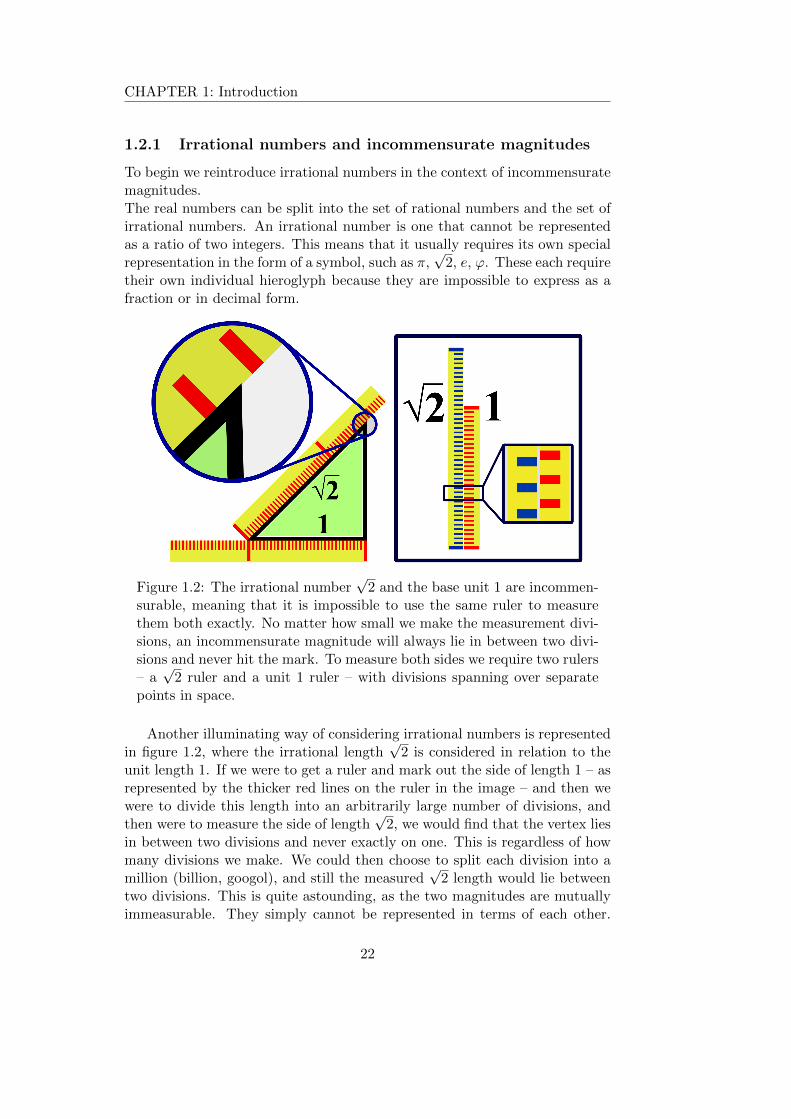
Figure 1.2: The irrational number√
2 and the base unit 1 are incommen-surable, meaning that it is impossible to use the same ruler to measurethem both exactly. No matter how small we make the measurement divi-sions, an incommensurate magnitude will always lie in between two divi-sions and never hit the mark. To measure both sides we require two rulers– a√
2 ruler and a unit 1 ruler – with divisions spanning over separatepoints in space.
Another illuminating way of considering irrational numbers is representedin figure 1.2, where the irrational length
√2 is considered in relation to the
unit length 1. If we were to get a ruler and mark out the side of length 1 – asrepresented by the thicker red lines on the ruler in the image – and then wewere to divide this length into an arbitrarily large number of divisions, andthen were to measure the side of length
√2, we would find that the vertex lies
in between two divisions and never exactly on one. This is regardless of howmany divisions we make. We could then choose to split each division into amillion (billion, googol), and still the measured
√2 length would lie between
two divisions. This is quite astounding, as the two magnitudes are mutuallyimmeasurable. They simply cannot be represented in terms of each other.
22
CHAPTER 1: Introduction
When two values are as such, they are termed incommensurate or incom-mensurable. Irrational numbers are incommensurate with rational numbers,and in most cases irrational numbers are incommensurate to other irrationalnumbers.
When two values are incommensurate they are in some sense independentquantities. They must be treated as spanning separate spaces and in this waythe dimensionality, or the number of degrees of freedom, is increased.
1.2.2 Quasiperiodicity in physical systems
Quasiperiodic means almost-periodic; quasi meaning ‘almost’ in Latin. Qua-siperiodicity can be manifest spatially, such as in a quasiperiodic lattice, ortemporally, such as with quasiperiodic driving. The concepts of quasiperi-odicity and irrationality in numbers are linked. The irrationality arises inthe ratio of the constituents that compose the quasiperiodic structure. Forexample, in the case of a quasiperiodic atomic lattice these two componentsmay be the number of atoms of two species constituting the lattice. If theratio of the number of the two species is irrational, then the lattice becomesquasiperiodic. For an optical lattice, the quasiperiodicity is determined bythe irrational ratio of the laser beam wavevectors forming the lattice [34]. Fora driven system, the quasiperiodicity is determined by the irrational ratio ofthe driving frequencies [28, 12].
Just as with the treatment of irrational numbers, quasiperiodicity res-ults in an increase in the number of degrees of freedom [23], such that theincommensurate magnitudes are treated independently.
1.2.3 The emergence of quasiperiodicity in real experiments
Strictly, quasiperiodicity in driving frequencies is only defined for infinite-timeexperiments, and quasiperiodic geometric lattices are only defined for infinitelattices. To make a direct numerological analogy, an irrational number is onlydefined by an infinite decimal expansion, an infinite series, or an infinite con-tinued fraction. Indeed the current record for the number of decimal placesof the famous irrational π currently stands at just under 22.5 trillion, and itis irrational up to that digit. If, however, it was found to start repeating itselfthen it would formally be a rational number1. Similarly, two frequencies canonly be defined as absolutely quasiperiodic in the infinite-time limit. At shorttimes, however, a quasiperiodic driving and a periodic driving with a longtime period are indistinguishable. This then raises the question – at whatpoint does a system transition from periodic to quasiperiodic?
1There is actually a mathematical proof that π is irrational, so this is unlikely to happenany time soon.
23

CHAPTER 1: Introduction
What is deemed as “quasiperiodic behaviour” is difficult to define in ageneral sense as it depends on the system at hand, but the general treatmentfor dealing with quasiperiodic systems [23, 12] is to introduce an additionaldegree of freedom into the system. This additional degree of freedom canimpact the system dynamics, thereby manifesting “quasiperiodic behaviour”.In some cases the transition from periodic to quasiperiodic behaviour canmean quite a pronounced change in dynamics, for example in [52] a transitionto quasiperiodicity in their solid-state device corresponds to a phase trans-ition from a resistive to a super-conductive state.The transition from periodicity to quasiperiodicity for driven systems is ex-plored and characterised in this thesis, specifically in chapter 6, where it isdemonstrated that the transition to quasiperiodicity has a discernible effecton the atomic dynamics, completely suppressing ratchet motion.
1.2.4 Decoupling the degrees of freedom
In a two-dimensional lattice it is possible to produce ratchet motion along eachdirection. The motions along each direction are not independent however, andthis means that predictability of ratchet motion is lacking. Previous experi-ments by the group [43, 42] have demonstrated that the direction of motionis difficult to predict as a result of the coupling between transverse degrees offreedom. It has been suggested [14] that by using quasiperiodic driving fields,the degrees of freedom can become decoupled and the direction of motion morepredictable. This decoupling is due to the increase in the system’s number ofdegrees of freedom, which comes about as a result of the quasiperiodic driving.
In this thesis we demonstrate that the coupling between transverse degreesof freedom is suppressed for quasiperiodic driving fields, and quantify underwhat conditions a driven system may be regarded as quasiperiodic, as it isnot guaranteed for all driving parameters.
1.3 This Thesis
This thesis explores the transition from periodic to quasiperiodic behaviour indriven systems by using the ratchet effect. A quasiperiodic driving arises whenthe ratio of the driving frequencies is irrational, and so the transition fromperiodic to quasiperiodic driving corresponds to a transition from a rationalto an irrational frequency ratio. This transition is not so stark as the rationalnumbers and irrational numbers form a tight weave where between everypair of rational numbers there lies (uncountably) infinitely many irrationalnumbers and (countably) infinitely many rational numbers. Alas, what hopecan there be in exploring the transition between the two?
We use the ratchet effect to observe the transition to quasiperiodicity. In
24

CHAPTER 1: Introduction
order to do this we make use of the split-biharmonic driving, which relies onthe coupling between two transverse driving fields in order to produce mo-tion. When the driving fields are quasiperiodic they become independent,due to an increase in the system’s number of degrees of freedom (since wenow require two ‘rulers’ instead of one). This means that the driving fieldsbecome decoupled as a result of the transition to quasiperiodicity and so withthe split-biharmonic driving, where the coupling between the driving fieldsis essential for transport to occur, we are able to witness this decoupling byobserving a suppression of transport. In this way it is possible to explore andquantify the transition from periodic to quasiperiodic driving by measuringthe atoms transition from a regime of transport to no transport.
The structure of the thesis is as follows:Chapter 2 provides a theoretical background for the topics in this thesis,starting with a brief summary of the concepts of laser cooling and trapping incold atom experiments. Then the ratchet effect is considered and a powerfulsymmetry analysis is introduced that allows us to establish regimes where theratchet effect can be observed.Chapter 3 provides a description of the experimental set-up used to producethe ratchet effect in a two-dimensional optical lattice. There the laser systemsfor the magneto-optical trap and lattice are described as well as the genera-tion of the ratchet driving forces.Chapter 4 describes the computer control software, which represents quite asophisticated software architecture developed specifically for this project.Chapter 5 presents results of the one-dimensional ratchet effect in the two-dimensional optical lattice. It illustrates the manifestation of the symmetryconditions in the transport, and it also serves to characterise the transportcurrent as a function of the different driving force parameters.Chapter 6 presents results for the two-dimensional ratchet effect, where it isdemonstrated that the transverse degrees of freedom are strongly coupled.The condition for quasiperiodicity is investigated and it is shown that in areal experiment incommensurability is determined by the finite interactiontime, where quasiperiodic behaviour is shown to be only guaranteed at longerdriving times. It is also considered how the coupling between transverse de-grees of freedom can be suppressed using quasiperiodic driving fields and howthis may be used to create ratchet currents with arbitrary, but deterministic,directions.Chapter 7 concludes the ratchet experiments and provides a discussion of theresults and presents an outlook for the next generation of ratchet experiments.Finally chapter 8 describes the work performed at NPL, where I spent ninemonths during the beginning of my PhD working on the rubidium atomicfountain clock. During this time the fountain was upgraded and data wastaken for an absolute measurement of the rubidium ground-state hyperfine
25

CHAPTER 1: Introduction
splitting frequency. This new measurement is published in Metrologia [57],and the BIPM subsequently adjusted the recommended value based on thisnew result.
26

CHAPTER 1: Introduction
27

Chapter 2
Theoretical Background
This chapter presents some theoretical background for the topics in this thesis.First it describes the principles of laser cooling of neutral atoms, which wasdeveloped mainly in the past 50 years. It then presents a symmetry ana-lysis treatment of the ratchet effect, which proves to be a powerful tool fordetermining the expected form of ratchet current.
2.1 Atomic structure
In modern laser cooling experiments, alkali metals such as rubidium and cae-sium are favoured as study cases because they possess a single valence electron,making them Bohr-like atoms. Laser cooling manipulates the hyperfine statesof the valence electron, labelled by quantum number F . The energy splittingfor different depths of atomic structure is represented in figure 2.1, showinghow a relatively simple atomic system has many internal states.
The energy splitting between different hyperfine states is typically of theorder of several hundred MHz to several GHz. The hyperfine splitting of thecaesium ground-state is used as a primary frequency standard to define thesecond. It has a value of 9 192 631 770 Hz, which is an exact value in virtue ofthe definition of the second.
2.2 Cooling and trapping atoms
An excellent and accessible review of the birth and development of laser cool-ing for neutral atoms is given by Bill Phillips in his Nobel prize lecture [59].
The term laser cooling refers to the use of laser fields to reduce the velo-city of atoms. A velocity-dependent temperature is associated to the atomsby equating their average kinetic energy
⟨12mv
2⟩
to their thermodynamic en-ergy 1
2kBT . In this way, slow atoms are described as ‘cold’ atoms and theprocess of slowing the atoms is described as ‘cooling’.
28

CHAPTER 2: Theoretical Background
Figure 2.1: The energy-level splitting for a simple electron transition.Here the minimum possible quantum numbers are chosen, and alreadythere are four ground sub-states and sixteen excited sub-states. Neg-lecting selection rules there would be sixty-four possible transitions,but the transition selection rules limit this number significantly. Ifhigher quantum numbers were chosen there would be even more pos-sible states and more possible transitions.
Although laser cooling and trapping started as a study in its own right[44, 37, 45], it is now used in many modern atomic physics experiments asa method to obtain a cloud of cold atoms, which are subsequently used formyriad purposes.
Laser cooling has become particularly popular since the mid-90’s when itwas demonstrated that it can be used to cool atoms down to quantum de-generacy [2, 18], as is done with Bose-Einstein Condensates. When a cloudof atoms is cooled to quantum degeneracy, the atomic de-Broglie waves be-come coherent and the entire cloud can be formally described by a single
29
CHAPTER 2: Theoretical Background
wavefunction, with the coherence length of this wavefunction extended overthe entire ensemble. In some experiments this macroscopic coherence of theatomic cloud wavefunction is exploited to make quantum sensors such as gra-vimeters and gravity gradiometers [41].
It often surprises non-specialists that lasers, which are usually portrayedas burning and blinding, can end up reducing the energy of delicate atoms.It is by exploiting the interaction of light and atomic energy levels that weare able to play this trick.
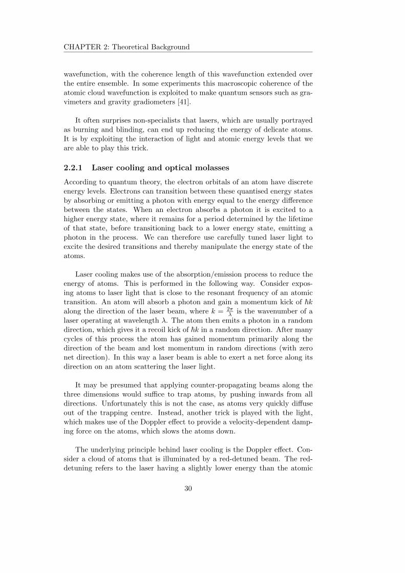
2.2.1 Laser cooling and optical molasses
According to quantum theory, the electron orbitals of an atom have discreteenergy levels. Electrons can transition between these quantised energy statesby absorbing or emitting a photon with energy equal to the energy differencebetween the states. When an electron absorbs a photon it is excited to ahigher energy state, where it remains for a period determined by the lifetimeof that state, before transitioning back to a lower energy state, emitting aphoton in the process. We can therefore use carefully tuned laser light toexcite the desired transitions and thereby manipulate the energy state of theatoms.
Laser cooling makes use of the absorption/emission process to reduce theenergy of atoms. This is performed in the following way. Consider expos-ing atoms to laser light that is close to the resonant frequency of an atomictransition. An atom will absorb a photon and gain a momentum kick of ~kalong the direction of the laser beam, where k = 2π
λ is the wavenumber of alaser operating at wavelength λ. The atom then emits a photon in a randomdirection, which gives it a recoil kick of ~k in a random direction. After manycycles of this process the atom has gained momentum primarily along thedirection of the beam and lost momentum in random directions (with zeronet direction). In this way a laser beam is able to exert a net force along itsdirection on an atom scattering the laser light.
It may be presumed that applying counter-propagating beams along thethree dimensions would suffice to trap atoms, by pushing inwards from alldirections. Unfortunately this is not the case, as atoms very quickly diffuseout of the trapping centre. Instead, another trick is played with the light,which makes use of the Doppler effect to provide a velocity-dependent damp-ing force on the atoms, which slows the atoms down.
The underlying principle behind laser cooling is the Doppler effect. Con-sider a cloud of atoms that is illuminated by a red-detuned beam. The red-detuning refers to the laser having a slightly lower energy than the atomic
30

CHAPTER 2: Theoretical Background
transition energy (lower energy corresponds to lower frequency, which corres-ponds to a longer (‘redder’) wavelength). Atoms moving with respect to thislaser will experience the light as Doppler-shifted – blue-shifted for atoms mov-ing towards the beam and red-shifted for atoms moving away from the beam.Therefore an atom moving towards the red-detuned beam will experience thebeam as closer to resonance in the atom’s reference frame, and atoms mov-ing away from the beam will experience the beam as further from resonance.This means that atoms scatter more photons from the beam they are movingtowards, which acts as an effective velocity-dependent damping force.
When six red-detuned laser beams are impinged on the atoms from thesix directions of space, we obtain a velocity-dependent damping along all dir-ections [10]. This configuration is called optical molasses, referring to theviscous damping of molasses.
Optical molasses works well for slowing down – or cooling – atoms, but itis not very effective as an atomic trap as the atoms may be damped but theyare not localised. In order to apply a position-dependent force that will workas a trap we make use of the magnetic sub-structure of the hyperfine states,and use magnetic fields in collaboration with the light.
2.2.2 Magneto-optical trap (MOT)
As has been mentioned, the atomic energy levels are given by the hyperfineenergy levels. Each of the hyperfine energy levels, F , has additionally 2F + 1magnetic sub-states, which can be labelled by quantum numbers mF . Withzero magnetic field the magnetic sub-states are energy-degenerate and theatoms are distributed equally across all sub-states. With non-zero magneticfield the degeneracy is lifted and the sub-states attain an additional energy∆E = ±mF gFµB|B| corresponding to the Zeeman splitting. These sub-statesand their corresponding transition selection rules are exploited to form themagneto-optical trap.
The transition selection rules for magnetically sensitive hyperfine levelsare given by ∆mF = ±1 for σ± circularly polarised light respectively. There-fore, absorption of σ+ light has the tendency to optically pump atoms intothe higher mF states, and absorbing σ− will pump atoms to lower mF states.These selection rules along with the Zeeman splitting dependence on the mag-netic field and a circularly-polarised, red-detuned laser beam are used in con-junction to trap atoms. This is demonstrated in figure 2.2, where a magneticfield with a linear dependence in space produces a spatial dependence of themagnetic sub-state energies. As atoms move away from the centre (where themagnetic field is zero) they are optically pumped to a state with an energy
31

CHAPTER 2: Theoretical Background
closer to resonance with the opposing beam, causing them to scatter morelight from that beam, which produces a net force back to the centre. In thisway atoms have a spatially dependent force that tends to keep them localisedaround the magnetic field minimum.
Figure 2.2: The working principle of the MOT along one axis. Theconfiguration of the laser beams with respect to the orientation of themagnetic field means that as atoms move further from the centre theyare closer to resonance with the counter-propagating beam, whichproduces a net force back towards the centre.
Since our cooling and trapping techniques require the absorption and sub-sequent re-emission of light, it is necessary to work with atomic energy statesthat have a high rate of absorption and re-emission. Therefore we require acycling transition with a relatively short life-time of the excited state. Forcaesium-133 alkali metal we use the D2 F = 4→ F ′ = 5 hyperfine transition.This is a cycling transition, meaning that atoms excited from F = 4→ F ′ = 5then decay back to the F = 4 ground-state. In practice, there is a small prob-ability that atoms decay to the F = 3 ground-state and are lost from thecycling transition. To counteract this effect we use a repumping beam, whichtransfers atoms from F = 3→ F ′ = 4, which then decays back into the F = 4ground-state to rejoin the cycling transition.
32
CHAPTER 2: Theoretical Background
2.3 Optical lattices
Optical lattices are formed by the interference of overlapping coherent laserbeams [35]. In this configuration, the light field produces a perfectly orderedarray/lattice of nodes and anti-nodes corresponding to high and low intensityregions of the light field. Optical lattices are typically classified in termsof their detuning. Far-detuned optical lattices provide a conservative (non-dissipative) potential to trap atoms. Near-detuned lattices also trap atoms aswell as providing a dissipative cooling mechanism – called Sisyphus cooling– that can cool atoms below the Doppler limit. The difference between thetwo regimes arises as a result of the repressed scattering rate as the detuningis increased, since the scattering rate Γ′ scales as the inverse square of thedetuning ∆: Γ′ ∝ 1/∆2.
2.3.1 Lattice geometry
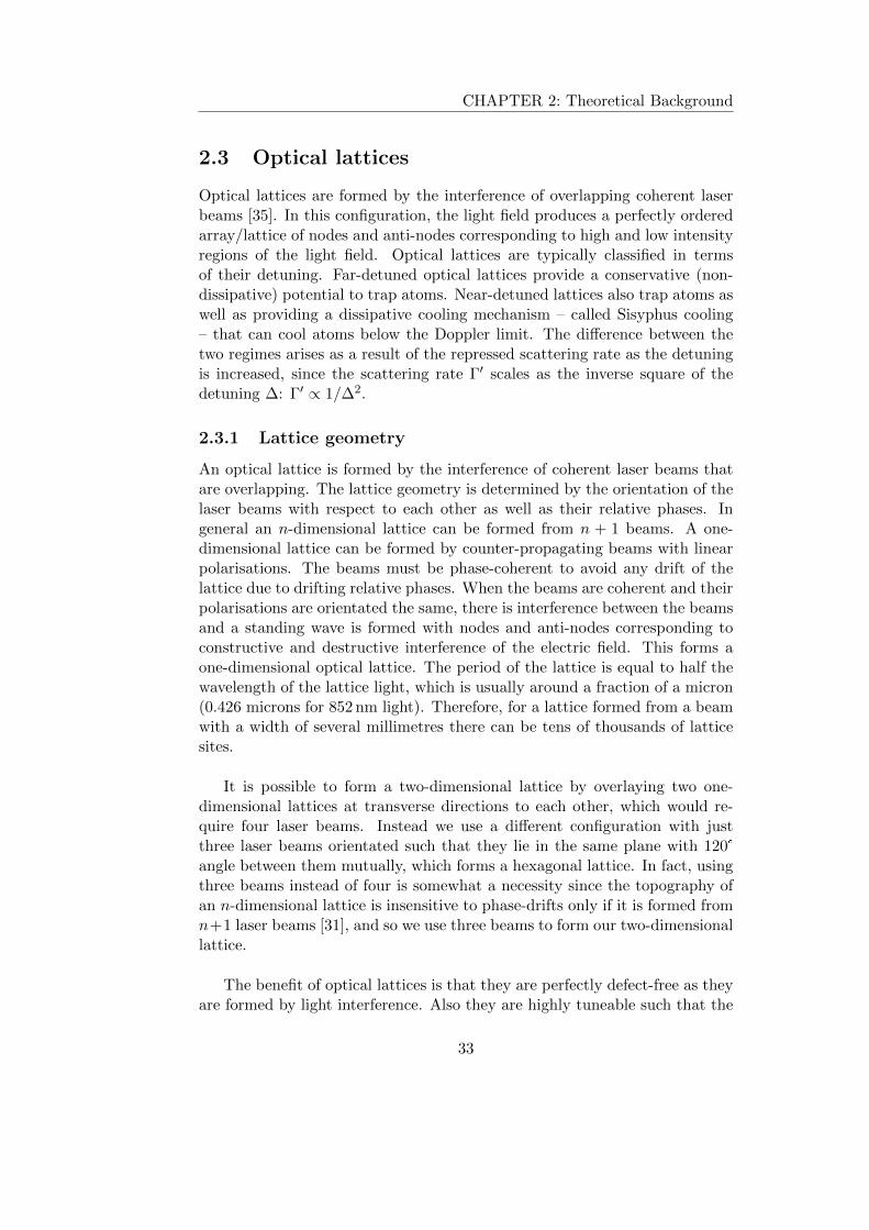
An optical lattice is formed by the interference of coherent laser beams thatare overlapping. The lattice geometry is determined by the orientation of thelaser beams with respect to each other as well as their relative phases. Ingeneral an n-dimensional lattice can be formed from n + 1 beams. A one-dimensional lattice can be formed by counter-propagating beams with linearpolarisations. The beams must be phase-coherent to avoid any drift of thelattice due to drifting relative phases. When the beams are coherent and theirpolarisations are orientated the same, there is interference between the beamsand a standing wave is formed with nodes and anti-nodes corresponding toconstructive and destructive interference of the electric field. This forms aone-dimensional optical lattice. The period of the lattice is equal to half thewavelength of the lattice light, which is usually around a fraction of a micron(0.426 microns for 852 nm light). Therefore, for a lattice formed from a beamwith a width of several millimetres there can be tens of thousands of latticesites.
It is possible to form a two-dimensional lattice by overlaying two one-dimensional lattices at transverse directions to each other, which would re-quire four laser beams. Instead we use a different configuration with justthree laser beams orientated such that they lie in the same plane with 120°
angle between them mutually, which forms a hexagonal lattice. In fact, usingthree beams instead of four is somewhat a necessity since the topography ofan n-dimensional lattice is insensitive to phase-drifts only if it is formed fromn+1 laser beams [31], and so we use three beams to form our two-dimensionallattice.
The benefit of optical lattices is that they are perfectly defect-free as theyare formed by light interference. Also they are highly tuneable such that the
33

CHAPTER 2: Theoretical Background
lattice geometry can be changed drastically and in-situ. These two featuresare not true of solid-state lattices, and so optical lattices make an excellentcandidate as a test-bed for concepts in solid-state physics.
The force experienced by the atoms in a lattice is produced by the potentialgradient of the laser potential, corresponding to the light shift. This dipolepotential gradient means that atoms are generally localised around latticesite minima, where the force reduces to zero. The Brownian motion randomwalk of an atom in a lattice corresponds to the atom scattering photons andmoving stochastically across lattice sites.
2.3.2 Sub-Doppler cooling in an optical lattice
The scattering of photons imposes a fundamental limitation on the temper-ature that can be achieved with Doppler cooling. This limit is termed theDoppler temperature TD and is directly proportional to the natural linewidthΓ of the transition, that is kB TD = ~Γ/2. For the caesium-133 D2 coolingtransition the Doppler temperature is 125µK.
It is possible to surpass this Doppler limit, however, as was experimentallydiscovered in 1988 [46], and shortly after a theory for sub-Doppler coolingbased on polarisation gradients was developed [17]. The following sectiongives a brief description of this mechanism occurring in an optical lattice,termed Sisyphus cooling.
Sisyphus cooling
Sisyphus cooling refers to the cooling of atoms in an optical lattice as a resultof the changing polarisation landscape experienced by the atoms [11, 87]. Theprocess is represented in figure 2.3, where an atom moving through the latticeis optically pumped to the state with the lowest potential energy, therebycausing the atom to dissipate energy to the light field.
This form of cooling is termed ‘polarisation-gradient cooling’ because theinterference of the lattice beams produces a position-dependent polarisation.The Zeeman sub-states of the atom experience different lattice potentials,and the correspondence between the lattice nodes and the polarisation nodesensure that the atom is optically pumped to the state at the lattice minimajust as they reach the maxima. The atoms lose energy with each transitionand so are cooled after multiple cycles.The name Sisyphus cooling stems from the Greek legend of Sisyphus, Kingof Ephyra, who is doomed to roll a boulder up one of Hades’ many ever-inclining slopes. Just before Sisyphus can reach the summit, the boulder rollsback down again on account of its weight so that apparently, according to mysources in the Underworld, poor Sisyphus is still going to this day.
34

CHAPTER 2: Theoretical Background
Figure 2.3: An illustration of the mechanism for Sisyphus cooling. Anatom moving across the lattice converts its kinetic energy to internal en-ergy as it climbs up the potential hill. Just as it reaches the top it hasa high probability to transition to the state with lower potential energydue to the corresponding polarisation maximum. After several cycles ofthis process the atom dissipates its energy and can be cooled below theDoppler limit.
2.4 The ratchet effect with cold atoms
The ratchet effect refers to the generation of directed transport out of un-biased fluctuations. The ratchet effect has its origins in a thought-experimentby Smoluchowski [75] where it was considered whether random Brownianfluctuations could be used to do useful work. If this were the case it wouldconstitute a Maxwell demon. Due to the second law of thermodynamics itis not possible for Brownian motion to perform useful work when the systemis in thermal equilibrium. Out of equilibrium, however, the dynamics changeand the ratchet effect can be realised.
In order to observe the ratchet effect two ingredients are required: first, thesystem must be out of equilibrium, which in our experiments is provided by atime-dependent rocking force driving the system out of equilibrium. Second,the system requires a broken symmetry, spatial or temporal, to permit theasymmetric transport that is characteristic of a ratchet. In the case of atomsin a hexagonal optical lattice, as in our experiments, the system is spatiallysymmetric and so we use the driving force to break the temporal symmetryof the system.
35

CHAPTER 2: Theoretical Background
Therefore the driving force supplies both of the necessary elements to pro-duce a ratchet.
Even with these ingredients at hand, it is still left to determine the correctrecipe to cook up a ratchet. In order to analyse the conditions under whichthe ratchet effect can be observed we make use of a symmetry analysis, whichis found to be a powerful tool enabling accurate predictions of the form ofdirected transport. This symmetry analysis was first introduced by Flach etal. [24], but it is presented here in a way that is tailored for our specific formof driving.
2.4.1 Symmetry analysis
Consider a particle of mass m experiencing a spatially-dependent potentialU(x), subject to friction with coefficient γ, under the influence of a time-dependent driving force f(t), and subject to noise ξ(t). The equation ofmotion for this particle is given by the following Langevin equation:
mx = −γx−U′ (x) + f (t) + ξ (t) ,
which can be rewritten in terms of momentum p as
p = − γm
p−U′ (x) + f (t) + ξ (t) , (2.1)
where the dot and prime denote differentiation with respect to time and spacerespectively.
In the case of cold atoms in an optical potential, the p term correspondsto the inertia; the −U′(x) term describes the dipole force due to the opticallattice potential; the −γp/m term corresponds to the optical damping dueto Sisyphus cooling; the f(t) term corresponds to the time-dependent drivingforce, implemented by modulating the lattice frequency; and the noise termξ(t) is the Brownian motion expressing the random walk of the atoms due tolight scattering.
The purpose of the symmetry analysis is to find those symmetries of theequations of motion that forbid directed transport. By this knowledge of theconditions where transport is forbidden, we can move to regimes where thesesymmetries are broken and transport is permitted.
In order to determine the symmetries of the system that forbid directedtransport we consider transformations that reverse the particle’s momentumsuch that p → −p. The reason we do this is because if the system (ie: theLangevin equation) is invariant under such a transformation it means thatp = −p and therefore p ≡ 0; the momentum is zero and so directed transport
36

CHAPTER 2: Theoretical Background
is forbidden. If the Langevin equation is invariant under such a transforma-tion we say that the system is symmetric under that transformation.
There are in fact two transformations that invert the momentum p →−p. Considering that the momentum is defined as p = mdx
dt , then the twotransformations are
T1 : dx→ −dx dt→ dt
T2 : dt→ −dt dx→ dx ,
or by integrating
T1 : x→ −x + x0 t→ t+ τ
T2 : t→ −t+ t0 x→ x + χ .
We will now apply these transformations to the Langevin equation in orderto determine the regimes for which transport is forbidden. In the followingsymmetry analysis we drop the noise term ξ from the Langevin equation, asit is symmetric Gaussian noise and so should not contribute to the long-timemacroscopic drift velocity.
The T1 transformation and “shift-symmetry”
Applying the T1 transformation
T1 : p→ −p x→ −x + x0 t→ t+ τ
to the Langevin equation
p = − γm
p−U′ (x) + f (t)
−→ −p = − γm
(−p)
+ U′ (−x + x0) + f (t+ τ)
p = − γm
p−U′ (−x + x0)− f (t+ τ) .
Using the fact that the optical potential is spatially symmetric U′ (−x + x0) =U′ (x), a condition on the driving is obtained:
f (t+ τ) = −f (t) .
Applying the transformation twice gives f (t+ 2τ) = f ((t+ τ) + τ) =−f (t+ τ) = f (t). From this fact that f (t+ 2τ) = f (t) it is deduced thatτ = T/2 where T is the characteristic time-period of the driving.
37

CHAPTER 2: Theoretical Background
So the condition for the system to be symmetric under the T1 transform-ation is that the driving has the form
f (t+ T/2) = −f (t) . (2.2)
When the driving has this property we say the driving possesses “shift-symmetry”.
The T2 transformation and “time-reversal symmetry”
Applying the T2 transformation
T2 : p→ −p t→ −t+ t0 x→ x + χ
to the Langevin equation
p = − γm
p−U′ (x) + f (t)
−→ p = − γm
(−p)−U′
(x + χ
)+ f (−t+ t0) .
To simplify this consider first the dissipationless case of a Hamiltonianratchet where the damping term is zero. The following condition on thedriving is then obtained:
f (−t+ t0) = f (t)
for the system to be invariant under the T2 transformation. When thedriving obeys the above condition we say it possesses “time-reversal sym-metry”.
When the driving possesses shift-symmetry or time-reversal symmetrythen transport is forbidden.
We now consider specific forms of the driving, and the conditions for themto be shift-symmetric and time-reversal symmetric.
2.4.2 Specific forms of driving f(t)
Single harmonic driving
Consider a periodic drive consisting of a single harmonic f(t) = cos(ωt +φ). The driving is shift-symmetric (f(t + T/2) = −f(t)) for all φ becausecos(ω(t+ T/2) + φ) = cos(ωt+ φ+ π) = − cos(ωt+ φ). Therefore transportis forbidden for this form of driving for all values of phase φ.
The situation changes, however, when we add an additional harmonic toform the biharmonic drive.
38
CHAPTER 2: Theoretical Background
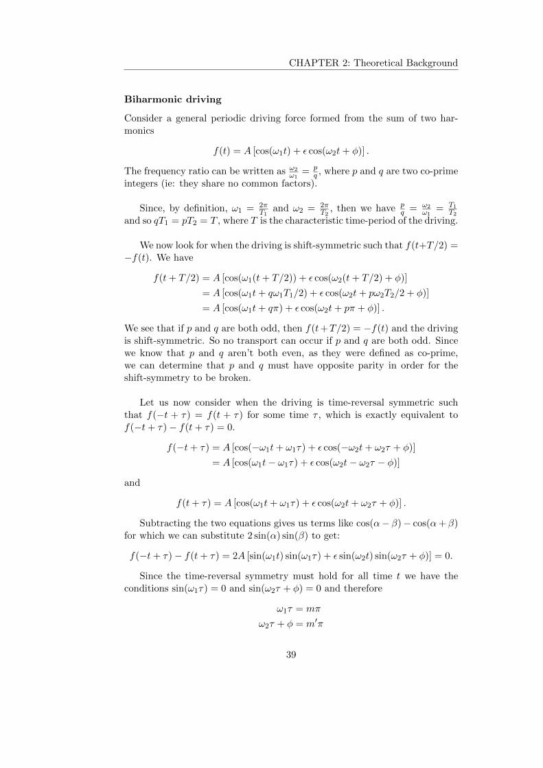
Biharmonic driving
Consider a general periodic driving force formed from the sum of two har-monics
f(t) = A [cos(ω1t) + ε cos(ω2t+ φ)] .
The frequency ratio can be written as ω2ω1
= pq , where p and q are two co-prime
integers (ie: they share no common factors).
Since, by definition, ω1 = 2πT1
and ω2 = 2πT2
, then we have pq = ω2
ω1= T1
T2and so qT1 = pT2 = T , where T is the characteristic time-period of the driving.
We now look for when the driving is shift-symmetric such that f(t+T/2) =−f(t). We have
f(t+ T/2) = A [cos(ω1(t+ T/2)) + ε cos(ω2(t+ T/2) + φ)]
= A [cos(ω1t+ qω1T1/2) + ε cos(ω2t+ pω2T2/2 + φ)]
= A [cos(ω1t+ qπ) + ε cos(ω2t+ pπ + φ)] .
We see that if p and q are both odd, then f(t+T/2) = −f(t) and the drivingis shift-symmetric. So no transport can occur if p and q are both odd. Sincewe know that p and q aren’t both even, as they were defined as co-prime,we can determine that p and q must have opposite parity in order for theshift-symmetry to be broken.
Let us now consider when the driving is time-reversal symmetric suchthat f(−t + τ) = f(t + τ) for some time τ , which is exactly equivalent tof(−t+ τ)− f(t+ τ) = 0.
f(−t+ τ) = A [cos(−ω1t+ ω1τ) + ε cos(−ω2t+ ω2τ + φ)]
= A [cos(ω1t− ω1τ) + ε cos(ω2t− ω2τ − φ)]
and
f(t+ τ) = A [cos(ω1t+ ω1τ) + ε cos(ω2t+ ω2τ + φ)] .
Subtracting the two equations gives us terms like cos(α− β)− cos(α+ β)for which we can substitute 2 sin(α) sin(β) to get:
f(−t+ τ)− f(t+ τ) = 2A [sin(ω1t) sin(ω1τ) + ε sin(ω2t) sin(ω2τ + φ)] = 0.
Since the time-reversal symmetry must hold for all time t we have theconditions sin(ω1τ) = 0 and sin(ω2τ + φ) = 0 and therefore
ω1τ = mπ
ω2τ + φ = m′π
39

CHAPTER 2: Theoretical Background
for integers m, m′. Substituting ω2τ = pqω1τ = p
qmπ into the second line andmultiplying through by q gives the condition:
qφ =
integer︷ ︸︸ ︷(qm′ − pm)π = nπ . (2.3)
Therefore, the driving is time-reversal symmetric when qφ = nπ for ninteger, and we expect to see no transport at these values of φ. This suggeststhat a function describing the transport vc(φ) will have zeros at qφ = nπ,which implies that the velocity measurements will have some periodic struc-ture corresponding to the time-reversal symmetry breaking governed by φ.
We note that if the first harmonic had a phase φ1, then the conditionswould become
ω1τ + φ1 = mπ
ω2τ + φ2 = m′π .
Upon substituting ω2τ = pqω1τ = p
qmπ−pqφ1, we would get the condition:
q(φ2 −p
qφ1) = qφr = nπ , (2.4)
where we have defined the relative phase φr = φ2 − (p/q)φ1. Therefore,we see that the time-reversal symmetry condition of qφ = nπ applies to therelative phase. Usually we take φ1 = 0 so that the relative phase is determinedby φ2.
The role of dissipation
When deriving the condition for the time-reversal symmetry to hold, the fric-tion term that expresses the dissipation in the system was neglected. There-fore the above results apply to the dissipationless Hamiltonian regime. Whendissipation is introduced to the system it breaks the time-reversal symmetry,and so transport should be expected even when qφ = nπ.
Theoretical work in this field [24, 89] has demonstrated that the intro-duction of dissipation results in an additional phase-shift θ0 on the resultantcurrent, meaning that the condition for time-reversal symmetry to hold be-comes qφ+ θ0 = nπ. This additional phase-shift can be used to characterisethe degree of dissipation in the system [27].
40

CHAPTER 2: Theoretical Background
The two-dimensional case
The derivations of the symmetry conditions were vector equations, meaningthat each component of the vector must satisfy the conditions independently.If a particular component does not satisfy the shift-symmetry condition thenthe symmetry is broken along that direction, while the other direction mightretain its shift symmetry.Explicitly, the requirement for the shift-symmetry to hold is
fx(t+ T/2) = −fx(t)
fy(t+ T/2) = −fy(t),
where we can see that the symmetries for each direction appear to be de-coupled (that is fx does not depend on fy and vice-versa). There is one con-necting factor that prevents the vector components being entirely decoupled,however, and that is the time-period T appearing in both transformations.This T represents the characteristic time-period for the entire vector drivingforce f(t), and so depends on both components. It is the lowest commonmultiple of the time-periods of each driving frequency, and it represents thetime at which the summed waveform starts repeating itself. The varioustime-periods associated to a biharmonic driving are portrayed in figure 2.4.
To elaborate on this point, let us consider the case of a split-biharmonicdriving of the form
fx(t) = Ax cos(ω1t)
fy(t) = Ay cos(ω2t+ φ),
where ω2/ω1 = p/q. In this case the time-period of the entire driving is givenby T = q T1 = p T2. Applying the shift-symmetry transformation gives:
fx(t+ T/2) = Ax cos(ω1t+ qπ)
fy(t+ T/2) = Ay cos(ω2t+ pπ + φ).
If both p and q are odd then the shift-symmetry holds, but if either of themare even then the shift-symmetry is broken along that direction and transportcan occur along that direction. Even though the driving component alongeach direction is a single harmonic, which was shown to always retain shift-symmetry, transport still occurs because the time-period T appearing in theshift-symmetry condition is determined by both components in conjunction.This is the coupling between the transverse degrees of freedom that is exploredlater in the thesis, specifically in chapter 6.
The quasiperiodic case
The previous section highlighted that the key to coupling comes from the sameoverall time-period T applying to the different directions. This means that
41

CHAPTER 2: Theoretical Background
Figure 2.4: The various time-periods associated to a typical biharmonicdriving. Each harmonic has an associated time-period T1 and T2, whichcomes from the fundamental relation Ti = 2π/ωi. Then there is theoverall time-period T , which represents the time for the entire summedwaveform to start repeating. It is the lowest common multiple of T1
and T2 and is the time-period relevant for the shift-symmetry condition.Yet another time-scale is T0 – the highest common factor of T1 and T2
– which represents the time ‘unit’ that fits into both T1 and T2 by aninteger multiple.
even though the shift-symmetry applies to each direction independently, theyare still coupled via this time-period T . When we make the driving frequen-cies quasiperiodic something rather interesting happens. Since quasiperiodityincreases the number of degrees of freedom in the system [52, 14, 9], therenow exists two effectively independent variables Ψ1 = ω1t and Ψ2 = ω2t.
The shift-symmetry condition is then modified so that it is a function ofthe two phases Ψ1, Ψ2, ie: f(t) becomes f(Ψ1,Ψ2). Then the shift-symmetrycondition becomes
f(Ψ1 + Ψ(0)1 ,Ψ2 + Ψ
(0)2 ) = −f(Ψ1,Ψ2).
Applying this twice gives the condition
f(Ψ1 + 2Ψ(0)1 ,Ψ2 + 2Ψ
(0)2 ) = f(Ψ1,Ψ2),
and since the Ψ’s represent phase, which is 2π periodic, then it is possible to
identify Ψ(0)1 = Ψ
(0)2 = π and the shift-symmetry condition is
f(Ψ1 + π,Ψ2 + π) = −f(Ψ1,Ψ2).
42

CHAPTER 2: Theoretical Background
In our specific case of the split-biharmonic driving expressed in terms ofthe Ψ1 and Ψ2
fx(Ψ1) = Ax cos(Ψ1)
fy(Ψ2) = Ay cos(Ψ2 + φ),
the shift-symmetry condition f(Ψ1 + π,Ψ2 + π) = −f(Ψ1,Ψ2) is always satis-fied, which means that transport is always forbidden when ω2/ω1 is irrationalfor the split-biharmonic driving.
To summarise, in the quasiperiodic regime, when ω2/ω1 is irrational, thevariables Ψ1 = ω1t and Ψ2 = ω2t are treated as independent variables, whichincreases the number of degrees of freedom - or dimensionality - of the sys-tem; from a single time variable to two incommensurate phase variables. Thismeans that the shift-symmetry condition, which was f(t + T/2) = −f(t) forcommensurate frequencies, is modified to f(ω1t+ π, ω2t+ π) = −f(ω1t, ω2t)for incommensurate frequencies. In the specific case of the split-biharmonicdriving this condition is always satisfied and so it is concluded that transportis forbidden for split-biharmonic driving in the quasiperiodic regime.
This increase in the dimensionality of the system is entirely analogousto the situation we came across in the introduction, with the right-angledtriangle having sides of length 1 and
√2. There it was shown that we can
not use a single ruler to measure both sides, but instead would need twoincommensurable rulers. This amounts to an increase in the number of de-grees of freedom needed to fully represent the system. With commensuratemagnitudes we can use a single parameter – the single ruler, or shared timevariable – but with incommensurate magnitudes we require two independentparameters – two rulers, or two time-dependent phases. Since, in the case ofour driving field, the single time-variable couples the x and y directions, whenthe dimensionality of the system is increased the x and y directions acquiretheir own independent phase parameters and so become decoupled. This de-coupling has a discernible impact on the dynamics of the split-biharmonicdrive, which relies on the coupling in order to produce transport. This isexplored further in chapter 6.
43

Chapter 3
Experimental Set-up
This chapter describes the experimental set-up used to produce and measurethe ratchet effect with cold caesium atoms in a two-dimensional dissipativeoptical lattice.
It begins by describing the vacuum, laser and magnetic systems used toobtain a cloud of cold atoms. It then describes the optical lattice set-up andcorresponding modulation control, which supplies the driving forces for theratchet. Finally a brief outline of the experimental procedure is given.
3.1 The science chamber
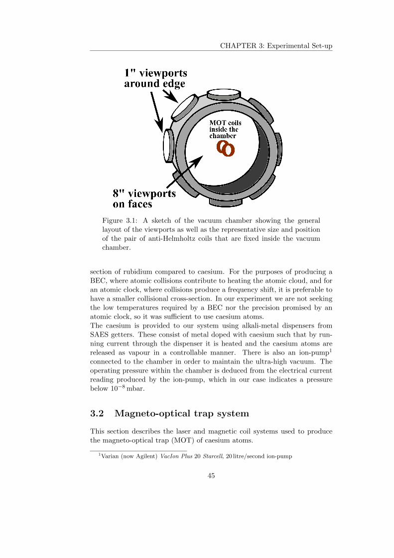
The ultra-high vacuum chamber was inherited from a previous experiment[86]. The basic structure is depicted in figure 3.1 but a more detailed and,dare I admit, attractive diagram of the vacuum chamber can be found in [86],figure 3.2 on page 40. The main chamber has eight 1 inch viewports aroundthe circumference and two large 8 inch viewports on the faces. Through thefour pairs of 1 inch viewports and the two large viewports there are passedthe retro-reflected MOT beams, the repumper beam, and the three latticebeams orientated at 120° to each other. In addition to this, a camera with anobjective lens is positioned to observe the atomic cloud.
Our experiment uses caesium-133 alkali metal element, for which the en-ergy level structure of the caesium D2 line at 852 nm is displayed in figure3.2.
Another popular alkali metal is rubidium, which comes in two isotopes(87Rb and 85Rb) both of which are used extensively in laser cooling experi-ments. Rubidium-87 is used by our group at UCL on a separate Bose-EinsteinCondensation (BEC) experiment, and was also the element of choice for theNPL atomic fountain that I had the privilege of working on and is describedin the final chapter of this thesis.There is wisdom in choosing rubidium over caesium for a BEC experiment andfor an atomic fountain clock, and this is due to the smaller collisional cross-
44
CHAPTER 3: Experimental Set-up
Figure 3.1: A sketch of the vacuum chamber showing the generallayout of the viewports as well as the representative size and positionof the pair of anti-Helmholtz coils that are fixed inside the vacuumchamber.
section of rubidium compared to caesium. For the purposes of producing aBEC, where atomic collisions contribute to heating the atomic cloud, and foran atomic clock, where collisions produce a frequency shift, it is preferable tohave a smaller collisional cross-section. In our experiment we are not seekingthe low temperatures required by a BEC nor the precision promised by anatomic clock, so it was sufficient to use caesium atoms.The caesium is provided to our system using alkali-metal dispensers fromSAES getters. These consist of metal doped with caesium such that by run-ning current through the dispenser it is heated and the caesium atoms arereleased as vapour in a controllable manner. There is also an ion-pump1
connected to the chamber in order to maintain the ultra-high vacuum. Theoperating pressure within the chamber is deduced from the electrical currentreading produced by the ion-pump, which in our case indicates a pressurebelow 10−8 mbar.
3.2 Magneto-optical trap system
This section describes the laser and magnetic coil systems used to producethe magneto-optical trap (MOT) of caesium atoms.
1Varian (now Agilent) VacIon Plus 20 Starcell, 20 litre/second ion-pump
45

CHAPTER 3: Experimental Set-up
Figure 3.2: The caesium D2 line at 852 nm, showing the cooling andrepumping transitions. This image was inspired by Daniel Steck’scaesium D-line data [78], and the values were taken from that paper.
3.2.1 External cavity diode lasers
The lasers used in our experiment are home-built external cavity diode lasers(ECDLs) in the Littrow configuration [70], as depicted in figure 3.3. In thisconfiguration the light from the laser-diode is incident on a diffraction grat-ing several centimetres away. The zeroth-order diffracted beam is reflectedback into the laser-diode, effectively creating an extended cavity, and the firstorder is diffracted to be used in the experiment. The benefit of having thisextended cavity is a reduction in the linewidth of the laser light. Our ECDLs
46

CHAPTER 3: Experimental Set-up
were previously measured [60] to have a linewidth of less than 300 kHz whenlocked, which can be compared to the natural linewidth of the cooling trans-ition Γ = 5.22 MHz. Comparing the natural linewidth of 5.22 MHz to thelasing frequency of 351 THz (corresponding to 852 nm) reveals just how pre-cisely tuned the laser frequency must be in order to be on resonance with thetransition. Such fine tuning is analogous to a positional accuracy of a hair’sbreadth over five kilometres! Alternatively, if the excited state linewidth asshown in figure 3.2 were to scale (ie: 2 mm = 5.22 MHz), then the page wouldneed to extend 135 km in order to accommodate the ground-state line – aproposition that my bookbinder will surely refuse.
Figure 3.3: An external cavity diode laser in the Littrow configuration.Light from the laser-diode is incident on a holographic diffractiongrating that has an angle controlled by a piezo transducer. The zeroth-order diffracted beam allows the formation of an extended opticalcavity, and the first-order diffracted beam is used for the experiment.
The frequency of the zeroth-order re-injected light is determined by theangle of the diffraction grating. For our lasers this angle is controlled by apiezo transducer and modulation of the laser frequency can be achieved bymodulating the piezo about some prescribed value. The temperature alsoaffects the lasing frequency and so the entire system sits on a platform abovea peltier element, which has its temperature carefully stabilised by a PID2
controller.
3.2.2 Cooling light
The cooling light is used to drive the cycling transition F = 4 → F ′ = 5.This transition has a high probability of decaying back to the F = 4 ground-state, for the process of absorption and emission to repeat.
2PID stands for Proportional-Integral-Derivative, representing the three feedback mech-anisms used for stabilisation.
47

CHAPTER 3: Experimental Set-up
Our cooling laser system is in a so-called ‘master-slave’ configuration. In thisscheme, one laser (the master) has its light injected into another laser (theslave). If properly injected, the slave laser’s emission follows the frequencydistribution of the master laser. Contrary to conventional master-slave rela-tionships, it is in fact the slave that has more power than the master. Themaster only governs the slave’s frequency.Our master laser is a low power (≈ 20 mW at output) diode3 laser in theLittrow configuration (as described above). The laser emission has an ellipt-ical cross section, so a pair of anamorphic prisms is used to shape the beamand achieve a circular cross section. An anamorphic prism pair is used toexpand (or reduce) the beam in one dimension, with the magnification beingdependent on the angle of incidence of the incoming beam. By a suitableconfiguration of the prisms, one can produce a circular collimated beam. Theanamorphic prism pair works just like a cylindrical lens telescope but it has acouple of advantages, which are that it is compact and it is easily adjustable.The latter is a significant advantage for the long-term, spanning laser diodelifetimes and generations, since separate laser diodes tend to have differentelliptical eccentricities and so the same anamorphic prism pair can simply bere-adjusted for each laser diode.
After this shaping the beam is passed through an optical isolator, which isused to prevent back-scattered light from re-entering the laser cavity as thisoptical feedback reduces the stability of the laser lock.
The beam is then split using a half-wave plate (HWP) and polarisingbeam-splitter (PBS), a small portion for the spectroscopy and locking, and therest is passed through an acousto-optic modulator (AOM) in the double-passconfiguration. This AOM is used as the main frequency control of the coolinglaser, as the double-pass configuration permits us to change the frequency ofthe beam without worrying about the corresponding change in beam angle.
The set-up of the double-pass configuration has a few subtleties, whichare depicted in figure 3.4 and are described next. Firstly, we require a systemwhere the output beam does not change position, even though there is afrequency change and corresponding change in angle of the diffracted beam.This is achieved by suitably positioning a lens and a mirror to reflect thelight back through the AOM. The lens is positioned at a distance equal to itsfocal length away from the AOM. In this way, an angular shift in the beamis translated into a parallel shift after the lens. The light is then reflecteddirectly back through this lens, which focusses it back into the AOM whereit undergoes a second frequency shift. The twice diffracted beam exits theAOM such that it is counter-propagating over the original input beam. Whatnow remains is to separate the input beam and the frequency-shifted outputbeam. This is done neatly by using a polarising beam-splitter before the AOMand a quarter-wave plate (QWP) after it, such that the reflected light has a
3Hitachi HL8342-MG, 852 nm, 50 mW laser-diode
48
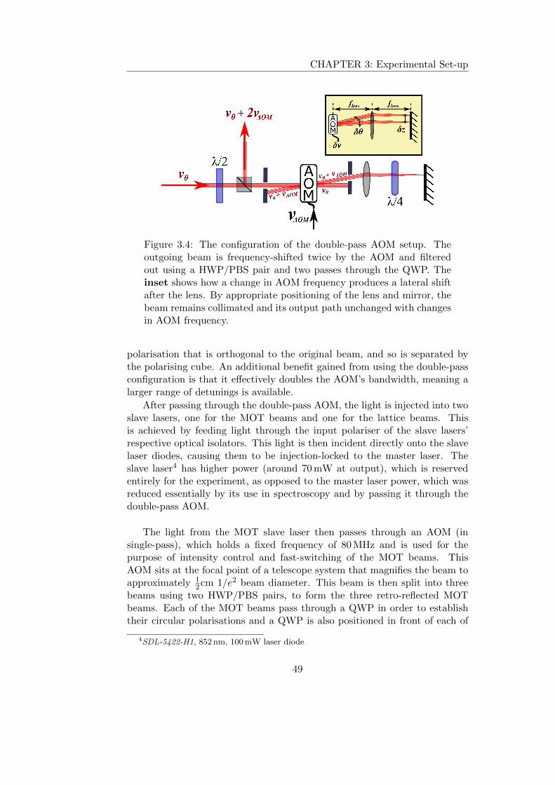
CHAPTER 3: Experimental Set-up
Figure 3.4: The configuration of the double-pass AOM setup. Theoutgoing beam is frequency-shifted twice by the AOM and filteredout using a HWP/PBS pair and two passes through the QWP. Theinset shows how a change in AOM frequency produces a lateral shiftafter the lens. By appropriate positioning of the lens and mirror, thebeam remains collimated and its output path unchanged with changesin AOM frequency.
polarisation that is orthogonal to the original beam, and so is separated bythe polarising cube. An additional benefit gained from using the double-passconfiguration is that it effectively doubles the AOM’s bandwidth, meaning alarger range of detunings is available.
After passing through the double-pass AOM, the light is injected into twoslave lasers, one for the MOT beams and one for the lattice beams. Thisis achieved by feeding light through the input polariser of the slave lasers’respective optical isolators. This light is then incident directly onto the slavelaser diodes, causing them to be injection-locked to the master laser. Theslave laser4 has higher power (around 70 mW at output), which is reservedentirely for the experiment, as opposed to the master laser power, which wasreduced essentially by its use in spectroscopy and by passing it through thedouble-pass AOM.
The light from the MOT slave laser then passes through an AOM (insingle-pass), which holds a fixed frequency of 80 MHz and is used for thepurpose of intensity control and fast-switching of the MOT beams. ThisAOM sits at the focal point of a telescope system that magnifies the beam toapproximately 1
2cm 1/e2 beam diameter. This beam is then split into threebeams using two HWP/PBS pairs, to form the three retro-reflected MOTbeams. Each of the MOT beams pass through a QWP in order to establishtheir circular polarisations and a QWP is also positioned in front of each of
4SDL-5422-H1, 852 nm, 100 mW laser diode
49
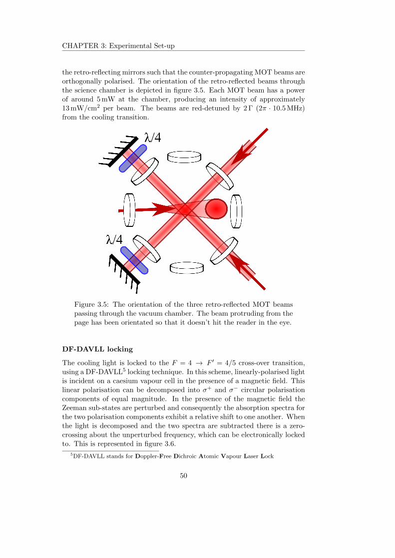
CHAPTER 3: Experimental Set-up
the retro-reflecting mirrors such that the counter-propagating MOT beams areorthogonally polarised. The orientation of the retro-reflected beams throughthe science chamber is depicted in figure 3.5. Each MOT beam has a powerof around 5 mW at the chamber, producing an intensity of approximately13 mW/cm2 per beam. The beams are red-detuned by 2 Γ (2π · 10.5 MHz)from the cooling transition.
Figure 3.5: The orientation of the three retro-reflected MOT beamspassing through the vacuum chamber. The beam protruding from thepage has been orientated so that it doesn’t hit the reader in the eye.
DF-DAVLL locking
The cooling light is locked to the F = 4 → F ′ = 4/5 cross-over transition,using a DF-DAVLL5 locking technique. In this scheme, linearly-polarised lightis incident on a caesium vapour cell in the presence of a magnetic field. Thislinear polarisation can be decomposed into σ+ and σ− circular polarisationcomponents of equal magnitude. In the presence of the magnetic field theZeeman sub-states are perturbed and consequently the absorption spectra forthe two polarisation components exhibit a relative shift to one another. Whenthe light is decomposed and the two spectra are subtracted there is a zero-crossing about the unperturbed frequency, which can be electronically lockedto. This is represented in figure 3.6.
5DF-DAVLL stands for Doppler-Free Dichroic Atomic Vapour Laser Lock
50

CHAPTER 3: Experimental Set-up
Figure 3.6: Principle of the DF-DAVLL locking technique. In the pres-ence of a magnetic field, the spectra for σ+ and σ− light are shiftedwith respect to each-other due to the Zeeman shift of the magneticsub-levels. Since the shifts are symmetric about the centre frequency,subtracting the signals gives a zero-crossing at the required transitionfrequency.
Our DF-DAVLL set-up is rather unique in that instead of a solenoid,permanent neodymium magnets are used to produce the magnetic field. Theuse of permanent magnets has several advantages over using solenoids: firstlythe permanent magnets are cheap, compact, and do not entail the tedioustask of winding a coil. Also, being fixed magnets, they do not consume powerand don’t require a power supply, which are often in high demand in anexperimental physics lab. Another benefit is that they are not dependent onthe stability of the electrical supply. This is particularly beneficial for the DF-DAVLL locking, where the stability of the magnetic field affects the stabilityof the laser lock.
Since the light from the master laser is locked to the F = 4 → F ′ = 4/5cross-over transition, which is 125 MHz below the cooling transition, this lightmust be brought closer to resonance. For this purpose AOMs are used in orderto provide the fine-tuning frequency shifts. The frequency tuning of the AOMsused in this experiment with respect to the hyperfine energy levels is shownin figure 3.7.
3.2.3 Repumper system
For the cooling beam we use the cycling transition F = 4 → F ′ = 5, whichdecays mostly to the F = 4 ground-state, but it also has a likelihood to decayto the F = 3 ground-state. It is a small probability but nonetheless, with
51

CHAPTER 3: Experimental Set-up
Figure 3.7: The laser frequencies in relation to the atomic hyperfinetransition frequencies, showing how the AOMs in the experiment areused to shift the frequency of the light and bring it to our desireddetunings for the MOT and lattice.
millions of atoms and millions of Rabi cycles per second, this small probabilitybecomes a considerable factor. This F = 3 ground-state is transparent to ourcooling laser and so, with just the cooling light on, all of the atoms soondecay into this invisible state and stop being cooled. In order to address thisproblem we introduce another laser, the aptly named repumping laser, whichpumps atoms from F = 3→ F ′ = 4, which then decays to the F = 4 ground-state and back into the cooling cycle.The repumper laser is a home-built ECDL laser, similar to the master laser.
3.2.4 Magnetic coils
There are two sets of magnetic coils in our experiment – the MOT coils andthe compensation coils. The MOT coils produce the magnetic field necessaryto trap the atoms. The compensation coils are used to counter the Earth’smagnetic field in the vicinity of the chamber, so that the magnetically sensitivestates of the atom aren’t affected by it.
52
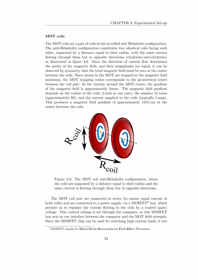
CHAPTER 3: Experimental Set-up
MOT coils
The MOT coils are a pair of coils in the so-called anti-Helmholtz configuration.The anti-Helmholtz configuration constitutes two identical coils facing eachother, separated by a distance equal to their radius, with the same currentflowing through them but in opposite directions (clockwise/anti-clockwise)as illustrated in figure 3.8. Since the direction of current flow determinesthe parity of the magnetic field, and their magnitudes are equal, it can beobserved by symmetry that the total magnetic field must be zero at the centrebetween the coils. Since atoms in the MOT are trapped at the magnetic fieldminimum, the MOT trapping centre corresponds to the geometrical centrebetween the coil pair. In the vicinity around the MOT centre, the gradientof the magnetic field is approximately linear. The magnetic field gradientdepends on the radius of the coils (1 inch in our case), the number of turns(approximately 80), and the current supplied to the coils (typically 1 amp).This produces a magnetic field gradient of approximately 13 G/cm at thecentre between the coils.
Figure 3.8: The MOT coil anti-Helmholtz configuration, wherethe coils are separated by a distance equal to their radius and thesame current is flowing through them but in opposite directions.
The MOT coil pair are connected in series (to ensure equal current inboth coils) and are connected to a power supply via a MOSFET6 box, whichpermits us to regulate the current flowing to the coils by a control (gate)voltage. This control voltage is set through the computer, so this MOSFETbox acts as our interface between the computer and the MOT field strength.Since the MOSFET chip can be used for switching high current loads, it sits
6MOSFET stands for Metal-Oxide-Semiconductor Field-Effect Transistor
53

CHAPTER 3: Experimental Set-up
on a metal plate that is water-cooled. The MOSFET box was used as it wasalready implemented in the set-up from the previous experiment [86], butjust as effective for our purposes is a solid-state relay (SSR) switch, whichwas in fact used during the initial stages of the experiment. The SSR switchis a triggerable switch allowing on-off switching of the coil current, but notcontrol of the actual current magnitude.
Compensation coils
The compensation coils are used to reduce the effect of the Earth’s magneticfield so that the magnetically sensitive Zeeman sub-states aren’t affected byit. Coils in the Helmholtz configuration are used to provide a magnetic fieldstrength equal and opposite to the Earth’s magnetic field. The Helmholtzconfiguration is the same as the anti-Helmholtz configuration but the cur-rent is flowing through the coils in the same direction. This provides anapproximately constant magnetic field offset in the space between the coils.By forming a cube with three pairs of coils, each independently controlledby a separate power supply, one is able to compensate for Earth’s magneticfield in all three dimensions of space. The compensation coil arrangement isillustrated in figure 3.9.
Figure 3.9: The compensation coil Helmholtz configuration, wherethere is a pair of coils for each dimension of space, forming a cube.Each pair has the same current flowing in the same direction, whichprovides an approximately constant offset field in the cube’s interiorto compensate for Earth’s magnetic field.
Since each coil is controlled independently by a separate power supply, itis non-trivial finding the optimal setting to absolutely compensate the Earth’smagnetic field. There are certain methods we can employ, but none of themprovide the prime solution. On the up-side, since the Earth’s magnetic field
54

CHAPTER 3: Experimental Set-up
doesn’t vary substantially for a given location, once the prime settings arefound they generally remain set and unchanged.
3.2.5 MOT temperature measurements
Figure 3.10: Time-of-flight imaging of the atoms in the MOT. The tem-perature of the cloud in the x and y direction is extracted by fitting thewidth of the cloud to equation 3.1.
The temperature of atoms in the MOT can be measured using time-of-flight imaging, where atoms in the MOT are left to freely diffuse for a specifiedtime and the width of the atomic cloud is measured. The width of an atomiccloud in free diffusion is presumed to evolve according to σ(t)2 = σ2
0 +v2rms t
2,where σ represents the width (standard deviation) of a Gaussian distributedcloud of atoms (σ0 being the initial width), vrms is the root-mean-squaredvelocity of the atoms presumed to obey Maxwell-Boltzmann statistics, and tis the free diffusion time (the time-of-flight). The temperature of the atomsis related to the root-mean-squared velocity by kBT = mv2
rms, where kB isthe Boltzmann constant and m is the atomic mass (of caesium in our case),and so the width of the cloud evolves according to
σ(t) =
√σ2
0 +kBT
mt2 (3.1)
= σ0
√1 +
kBT
mσ20
t2 .
55

CHAPTER 3: Experimental Set-up
Therefore by measuring the width σ for various diffusion times t we are ableto extract the temperature T of the atoms. The results of our time-of-flighttemperature measurements are shown in figure 3.10.
3.3 Optical lattice system
The two-dimensional optical lattice is formed by intersecting laser beams ori-entated as shown in figure 3.11.
Figure 3.11: The orientation of the lattice beams used to create thetwo-dimensional optical lattice. The small circles represent the 1 inchviewports and the front and back faces also have large 8 inch windows.The red border indicates the region where the beams intersect and forma two-dimensional hexagonal optical lattice.
In this configuration the three lattice beams are orientated with a mutual120° angle between them, and are each linearly polarised such that gravity isperpendicular to the plane of the lattice. The beams are red-detuned by ap-proximately 15 Γ to form a near-detuned dissipative two-dimensional opticallattice.
When the beams have the same frequency the lattice that is formed isstationary. When the beams have a relative frequency difference, however,the lattice moves with a velocity proportional to the frequency difference.Therefore we are able to impose a driving force on the atoms in the latticeby applying a time-varying frequency shift of the lattice beams. This is thelattice modulation that is used to create the driving force for our ratchet.
The light for the three lattice beams is obtained from a single slave laser,which is injection-locked to the cooling master laser. Therefore the frequency
56

CHAPTER 3: Experimental Set-up
of this beam is also controlled by the double-pass AOM in the master laser’sbeam path. The beam from the lattice laser passes through an anamorphicprism pair and an optical isolator and is then guided through an AOM, whichshifts its frequency down by 75 MHz so that it is close to atomic resonance.This single AOM also allows intensity control and fast synchronous switchingof all three lattice beams. The beam after this AOM is then split into threeseparate beams, which pass through an additional AOM each. These AOMshave a carrier frequency of 75 MHz and can be individually modulated. Thusit is by modulating these final AOMs that the driving force on the atoms inthe optical lattice is realised.
Each lattice beam has a power of around 5 mW at the chamber and aradius just under 2 mm, giving a peak intensity of approximately 80 mW/cm2.With a typical detuning of 15 Γ the lattice depth is expected to be of the orderof ∼ 100µK.
There was a continuous effort on my part to try to improve the lifetime ofatoms in the lattice as this lifetime limits the duration that the atoms can ex-perience the rocking forces. Optimisation of the lattice loading was achievedby careful alignment of the lattice beams and by varying their relative intens-ities (via HWP/PBS pairs).The procedure for optimising the loading of the lattice was as follows:The three lattice beams are initially aligned by individually overlapping themwith the MOT. When properly overlapped, the atoms in the MOT are blownaway by the free-running lattice beam and so a rough alignment of the latticeis achieved.Then the experimental sequence is run so that the lattice is loaded and thenimaged very soon after. At the early stages, if necessary, the MOT beamsare left on for some time in order to provide additional confinement. Thefluorescence images provide an indication of whether any atoms are beingheld in the lattice and, if not, which direction they are being pushed away in.The beams’ alignments and relative powers are then altered iteratively to getatoms loaded in the lattice.The experimental sequence is then changed so that the lattice holding time islonger and the sequence of optimisation is repeated until the atoms are beingtrapped for a sufficient time in the lattice. As the lattice holding times getlonger any small imbalances between the beams become clearly exposed.
Figure 3.12 shows some lattice lifetime measurements taken at differentstages of the experiment. The data was taken by observing the atomic fluor-escence of the atoms after a specified holding time in the lattice. When thefluorescence became small the gain of the camera was increased, and then thisgain was factored out in the analysis. The fluorescence (in arbitrary units)is plotted against the lattice holding time t and fitted to an exponentially
57

CHAPTER 3: Experimental Set-up
(a) τ 12
= 22 ms (b) τ 12
= 127 ms
Figure 3.12: The lattice lifetimes at the ‘best’ of times (right) and the‘worst’ of times (left).
decaying function e−λt with decay constant λ, from which the half-life can beextracted (the half-life of the lattice – the time at which the number of atomsremaining in the lattice diminishes by half – is given by τ 1
2= ln(2)/λ).
The total layout of the experiment’s optical elements is shown in figure3.13 and the general schematic of light distribution is given in figure 3.14.
3.4 Generating a rocking ratchet
The three ratchet AOMs are supplied with a frequency of 75 MHz by separ-ate Marconi function generators7, which can be mutually phase-locked andcan also accept frequency modulation inputs. These modulation inputs aresupplied externally by two Agilent function generators8, which are also phase-locked and are used to implement the rocking forces on the lattice by mod-ulating the frequency of the Marconi generators. They are connected to theMarconi generators via an intermediate buffer-box, which adds and subtractsthe Agilent signals. As a result of this and the lattice geometry, the two Agi-lent generators produce motion along the x and y direction respectively, as isdemonstrated in figures 3.15 and 3.16.
According to the geometry of the lattice, the force experienced by theatoms is given by
F = (Fx, Fy) = −m (ax, ay) = −m3k
(Σ,√
3∆), (3.2)
where Σ = ψ1(t) + ψ2(t) is the sum of the frequency-modulations, and∆ = ψ1(t)− ψ2(t) is the difference of the frequency-modulations.
In this experiment we use two function generators producing the signals:
7Marconi 2024 9 kHz–2.4 GHz signal generator8Agilent A33220
58

CHAPTER 3: Experimental Set-up
Fig
ure
3.13
:T
he
exp
erim
ent’
sop
tica
lla
you
tsh
owin
gth
ep
ath
ofli
ght
thro
ugh
our
exp
erim
enta
lse
t-u
p.
59
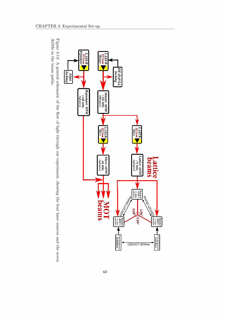
CHAPTER 3: Experimental Set-up
Figu
re3.1
4:
Agen
eralsch
ematic
of
the
flow
ofligh
tth
rough
our
exp
erimen
t,sh
owin
gth
efou
rlaser
sources
and
the
sevenA
OM
sin
the
bea
mp
ath
s.
60

CHAPTER 3: Experimental Set-up
Figure 3.15: The configuration of the lattice beams, as well as the forcevectors associated with the modulation forces. Because of the latticegeometry, the sum and difference of the lattice modulation vectors ψ1,ψ2 produce modulation along the x and y axis respectively.
Vx(t) = A1
[sin(ω1t) +
1
2ε1 sin (2ω1t+ φ1)
]Vy(t) = A2
[sin(ω2t) +
1
2ε2 sin (2ω2t+ φ2)
].
Then, with the help of a buffer box that adds and subtracts the signals,we use ψ1 = Vx + Vy to drive one of the AOMs and ψ2 = Vx − Vy to driveanother. There is one AOM that is left unmodulated, as is shown in figure3.15.From our definitions of Σ and ∆,
Σ ≡ ψ1 + ψ2 = (Vx + Vy) + (Vx − Vy) = 2Vx
∆ ≡ ψ1 − ψ2 = (Vx + Vy)− (Vx − Vy) = 2Vy ,
and so differentiating yields
Σ = 2Vx = 2ω1A1 [cos(ω1t) + ε1 cos (2ω1t+ φ1)]
∆ = 2Vy = 2ω2A2 [cos(ω2t) + ε2 cos (2ω2t+ φ2)] .
Thus, from equation 3.2 we see that the force is given by: F = (Fx, Fy)
61

CHAPTER 3: Experimental Set-up
Figure 3.16: The hexagonal lattice geometry and associated lat-tice vectors b1, b2. The function generators produce signals Vx,Vy, which are added and subtracted to form ψ1 = Vx + Vy and
ψ2 = Vx − Vy. ψ1 is implemented along the −b2 direction and
ψ2 is implemented along the b2− b1 direction, which then ensuresthat the Vx driving is along the (negative) x direction and the Vydriving is along the (negative) y direction.
with:
Fx = −2mω1A1
3k[cos(ω1t) + ε1 cos (2ω1t+ φ1)] (3.3a)
Fy = −2mω2A2√3k
[cos(ω2t) + ε2 cos (2ω2t+ φ2)] , (3.3b)
62

CHAPTER 3: Experimental Set-up
which are of the form of the general biharmonic driving given in equation2.3 on page 40, which is used throughout this thesis.
3.5 The imaging
There are two types of imaging that are used most often in cold atom ex-periments: fluorescence imaging and absorption imaging, both of which havebenefits as well as drawbacks.
Fluorescence imaging collects the light emitted from atoms undergoingthe cycling cooling transition. Thus the fluorescence image produced is aglowing cloud. It is useful because it is a direct image of the MOT and itsposition, and it can be set up by simply pointing an infra-red sensitive cam-era at the radiant cloud. Its drawback, however, is that it must be calibratedcarefully to provide accurate results for the number of atoms. The fluores-cence picked up by the camera is directly related to the number of atomsbut its proportionality is determined by several empirical factors, such as thecamera’s shutter speed and numerical aperture, the quantum efficiency of theCCD at the specified wavelength, and losses occurring due to optics in thepath of the beam, such as viewports or lenses. Performing this calibrationaccurately can be an extensive task and so, for measurements of atom num-ber, another type of imaging – called absorption imaging – is usually favoured.
In absorption imaging a resonant probe beam is used to cast a shadow ofthe atomic cloud on the CCD camera. Then the cloud is removed and anotherimage is taken of the probe beam without the cloud present. By dividing theimages one can get an image of the optical depth of the cloud, from which theatom number can be extracted directly. In most schemes an additional thirdimage is taken with the cloud removed and all beams off entirely in order tosubtract any dark current produced by the camera itself. The drawback ofabsorption imaging is that it is a destructive imaging technique, as the cloudmust be removed to take the second (and third) image. Also, an additionalresonant probe beam and corresponding optical elements must be introducedinto the experiment, thereby increasing its complexity.
Since our experiment involves determining the centre-of-mass position ofthe cloud, and atom number does not play a primary role, we chose fluores-cence imaging as this gives a straightforward means of determining the cloudposition. The number of atoms can be estimated, however. Assuming a typ-ical peak MOT density of some 1010 atoms/cm3, and a cloud size of aroundone millimetre, gives something of the order of tens of millions of atoms inthe MOT.
63

CHAPTER 3: Experimental Set-up
The camera we use is an AVT Guppy NIR with a variable objective lensallowing variable magnification. In order to determine the velocity of atomsfrom the displacement in the image it was necessary to calibrate the camerapixel-size. This was achieved initially by imaging a piece of graph paper. Firstthe fluorescence from the cloud of atoms in the MOT was observed generallyand the objective lens was adjusted to magnify and bring the cloud into focus.Then, with the objective lens fixed, the camera was directed towards a sheetof graph paper. The graph paper was carefully positioned so that it was insharp focus, where it was fixed and an image was taken. Using computersoftware the number of pixels forming a 1 millimetre grid-line was determinedfor several portions of the graph paper; 115 pixels/mm for the x directionand 100 pixels/mm for the y direction. This gives a size of 8.7µm/pixel and10µm/pixel for the x and y direction respectively. Comparing this value tothe CCD pixel size for our camera (8.4µm and 9.8µm) gives a magnificationvery close to unity.
Figure 3.17: Measurement of the pixel size using TOF imaging of thecentre of mass falling under gravity. Since all masses free-fall under gravityin the same way, the pixel size can be derived from the parabolic trajectoryof the atoms under the influence of gravity. The value agrees well withthat measured by imaging the graph paper (measured as 10µm/pixel).
A more robust method of determining the magnification is by using time-of-flight (TOF) imaging of a cloud falling freely under gravity, although thisonly allows the determination along one axis (along the direction of gravity).The idea is that under the influence of gravity the acceleration is the same forall masses – that is, it’s purely geometrical – and so by imaging the trajectory
64

CHAPTER 3: Experimental Set-up
of a cloud falling under the influence of gravity one can determine what theimage magnification must be. Results for the camera magnification calibra-tion9 using TOF imaging are shown in figure 3.17. In our case the atomsaccelerate at just under 1 pixel/ms2, which must correspond to the gravita-tional acceleration g = 9.8 m/s2, and so from this it is deduced that the pixelsize is 10.2µm. This corresponds well with the value obtained by the graphpaper camagnifibration.
The camera is controlled by imaging software that was developed usingLabVIEW. This software obtains images from the camera, displays them andsaves them, as well as providing some in-situ measurements of the intensitydistribution. It is also used to control the camera’s shutter speed, gain, andtrigger delay. The camera is triggered externally by a digital signal deliveredfrom the NI PCI boards that are controlled by a separate software. Detailsof the computer control and acquisition are given in the dedicated chapter 4,as its development formed a significant part of the project.
3.6 Experimental procedure
To sum up the experimental sequence by a single function, it is to inputdifferent driving forces for the atoms, and to output the resulting velocity ofthe atomic cloud.How this is accomplished forms the subject of this section.
Experimental stages
The general programme of operation is shown in figure 3.18 and a typicalexperimental cycle is shown in figure 3.19.
Figure 3.18
Atoms are trapped and cooled in a magneto-optical trap and are thenloaded into an optical lattice. The atoms in the lattice are then rocked ac-cording to the driving f(t) for a certain duration Td. The lattice is thenswitched off and, after some short diffusion time, the centre-of-mass (CoM)position of the cloud is read off from an image by fitting a 2D Gaussian profileto the atomic cloud. Combining this CoM position with the duration of themodulation and diffusion, as well as knowledge of the initial CoM position,
9camagnifibration for “short”
65

CHAPTER 3: Experimental Set-up
we are able to deduce the CoM velocity of the cloud. It is this velocity v thatwe seek to measure for different driving forces f(t) and driving times Td.
Figure 3.19: A typical experimental cycle, showing the settings for thedigital and analogue channels. The entire sequence typically lasts around3 seconds.
Each cycle produces one image of the cloud. An average of 5 images istaken for a single data point. A graph, such as the one shown in figure 5.1 onpage 81, requires 13 velocity measurements to cover the range of 0 to 2π insteps of π/6, requiring 13× 5 = 65 images. A graph like that shown in figure6.5 on page 97, is such that each and every data point requires a graph with13 velocity measurements, so that in total it is made from just under 14 000images!It soon became painfully apparent that I needed an efficient means of (a) chan-ging the parameters to take all the data necessary for a plot, (b) meaningfullynaming and organising those images, (c) analysing the copious images, so thatI wouldn’t have to crop and upload each one individually. In order to accom-plish these repetitive but crucial tasks I developed a primitive yet powerfulcommand language that allowed me overarching control over the experiment.This software is described in the next chapter.
66

CHAPTER 3: Experimental Set-up
67

Chapter 4
Computer control
LabVIEW’s controlling.Mathematica’s analysing.MATLAB’s matrix making.Excel tabulating.Inkscape for art making.Powerpoint for showcasing.Word use for jotting.LaTeX for producing.JabRef does job ref’ing.
These are a few of myfa-vour-ite things.
This chapter describes the software, developed chiefly in LabVIEW, thatis used to control the experiment.
It is standard practice in modern atomic physics experiments to have somesoftware that controls the experimental sequence. This software interfaceswith a digital and/or analogue PCI board that can provide output voltagesignals with µs temporal resolution. These voltage signals are then connectedto various components to achieve some control over the experimental appar-atus.
The problem, however, is that some devices can not be controlled by basicvoltage signals, such as the Agilent function generators used in this experi-ment to control the driving force on the ratchet. These generators can beremotely controlled but only via a USB connection with device-specific in-structions and appropriate drivers installed. Therefore I set about developinga software to control the multiple generators.
The next issue, however, was how to interface these generators with the
68

CHAPTER 4: Computer control
sequence and imaging programs. The reason this was necessary is becausethe general scheme of operation is:(1) set and output driving parameters – controlled by Agilent software(2) run sequence with new parameters – controlled by sequencing soft-ware(3) image cloud a prescribed number of times – controlled by imagingsoftware(4) repeat...
As can be seen, the programs require some degree of communicationbetween them in order to ensure, for example, that the imaging doesn’t startuntil the new settings are in place or that the settings don’t get changed whilethe imaging is still happening!It is worth noting that the imaging and sequencing programs were alreadydeveloped before the Agilent program was required, as they had been usedfor first production of the MOT and lattice loading before the ratchet drivingwas necessitated. Therefore the new Agilent software required some specialfeatures in order to be able to communicate with the pre-existing programs.
This chapter describes the software architecture that was developed inorder to accomplish this. It also gives a brief description of the primitivecommand language I developed that allows the user to specify the ratchetdriving forces as well as control all elements of the apparatus.
4.1 Control programs
There are three LabVIEW programs that make up the experiment’s computercontrol – the sequencing, the imaging, and The Controller. The Controlleris the main software I developed, incorporating a novel primitive commandlanguage that establishes control over the ratchet driving parameters, as wellas the ability to disrupt and alter both the sequencing and imaging programs.
The three LabVIEW programs all run independently whilst maintainingsome degree of communication between them. The sequencing program isused to control the experimental cycle and analogue/digital outputs; the ima-ging program controls the camera settings, takes images and saves them; TheController chiefly manipulates the Agilent function generators but it can alsoalter parameters on both the imaging and sequencing programs. The generalarchitecture of the computer controlled apparatus is given in figure 4.1.
4.1.1 The sequencing program
The sequencing program is based on an inherited software, to which I addedsome additional features and also added the capability for it to communicate
69

CHAPTER 4: Computer control
Figu
re4.1:
Sch
ematic
ofth
eco
mp
uter
contro
lfor
our
exp
erimen
talap
paratu
san
dro
ckin
gratch
etforces,
show
ing
allof
the
exp
erimen
tal
com
pon
ents
that
are
contro
lledby
the
comp
uter
software.
70

CHAPTER 4: Computer control
with The Controller. The sequencing software controls analogue1 and digital2
boards, which are connected to BNC distribution boards to allow transmissionof analogue voltage signals and digital triggers to the experimental apparatus.The boards are used to electronically control the AOM frequency and amp-litude (via the VCO controllers), the MOT coil current (via the MOSFET),the lattice modulation amplitude (via the ratchet buffer-box), the cameratriggering, and the shutters.The layout of the sequence control program is a 2D array much like thatshown in figure 3.19 on page 66, with the columns corresponding to time-steps and the rows corresponding to different output channels (analogue ordigital). The time interval of each step is user-set, and the channels’ valuesat each time-step can be typed in (or toggled on and off for digital channels).For analogue channels, the program can also produce a linear ramp betweentwo values over a given time. This feature was used to ramp the modulationforces on and off.I included features to calibrate the analogue channels, so that the user entersvalues that are more intuitive than basic voltages, as the relationship betweenthe voltage control and the parameter value is unscaled and not necessarilylinear. An example is the AOM detuning, which is calibrated to be measuredin units of the natural linewidth of the transition, and the AOM intensity,which is input as a percentage of the maximum possible power (type 50 for50% laser power).
4.1.2 The imaging program
The imaging program was developed specifically for this project. It is builtin LabVIEW and communicates with the camera via a firewire cable. Thisfirewire allows the transmission of images from the camera buffer to the com-puter, and is also able to change the camera’s settings, such as the exposuretime and trigger delay. It can also change the mode of the camera, fromtriggered mode to video mode (the latter mode was developed as part of thesoftware).When in triggered mode, the software reads the camera buffer and waits un-til it encounters an image. The camera is triggered separately from the NIboards, which in turn are controlled by the sequencing program, which meansthat the sequencing program controls when the camera exposure starts. Evenwhile the camera is awaiting an external trigger, the software permits one toforce the trigger and obtain an image.Video mode was also developed as part of the software. In this mode, twobuffers are allocated on the camera, which are read out consecutively. Thisis done to optimise the frame-rate, as one buffer is read off and transmitted
1NI PCI-67132Viewpoint DIO-64
71

CHAPTER 4: Computer control
while the other is being filled. This way the waiting time between framesis not limited by the buffer readout time. Video mode was very useful forgeneral observation of the MOT fluorescence.
Smart naming
Aside from controlling the camera and extracting and viewing its images,the imaging program had the role of naming and saving the images to thecomputer. Since we were dealing with a large quantity of images, it wasnecessary to have some meaningful and automated naming scheme that couldinclude information about the current parameter settings. To this end a“smart name” program was developed, which allows the user to define arelevant name that incorporates updated parameter values.
Figure 4.2: Decomposition of the “smart name” scheme. By inputtingspecial commands between inverted commas the image names becomerelevant to the current experimental settings.
The current parameter values are fed to the imaging program by TheController every time they are updated and by using the specified syntax(figure 4.2) the file names provide relevant and specific information about theparameter settings.
72
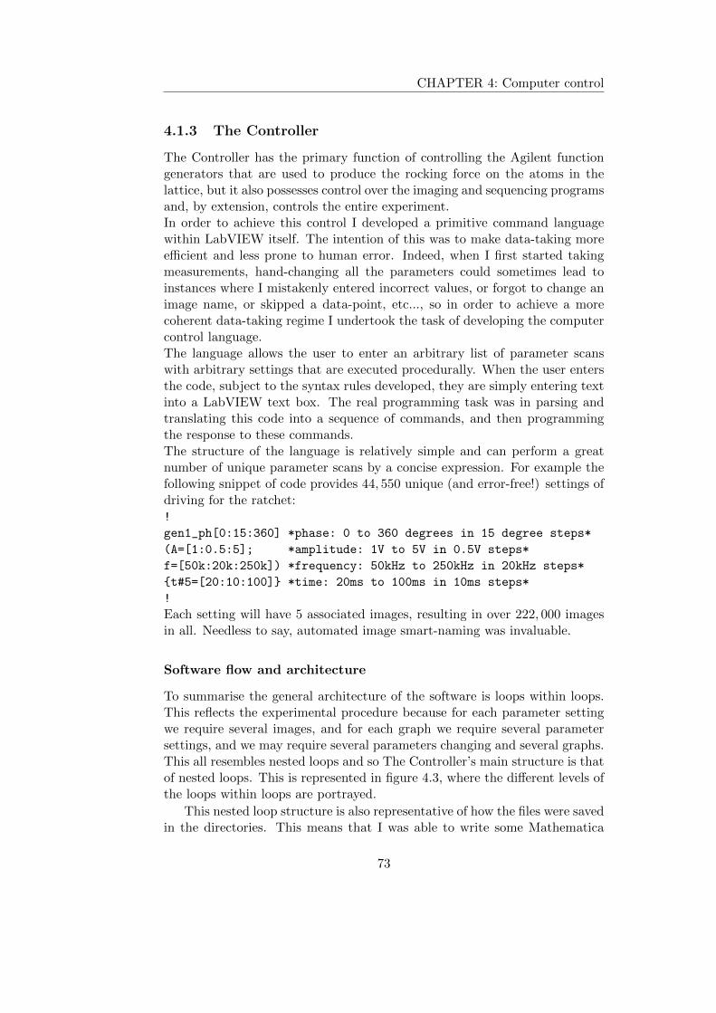
CHAPTER 4: Computer control
4.1.3 The Controller
The Controller has the primary function of controlling the Agilent functiongenerators that are used to produce the rocking force on the atoms in thelattice, but it also possesses control over the imaging and sequencing programsand, by extension, controls the entire experiment.In order to achieve this control I developed a primitive command languagewithin LabVIEW itself. The intention of this was to make data-taking moreefficient and less prone to human error. Indeed, when I first started takingmeasurements, hand-changing all the parameters could sometimes lead toinstances where I mistakenly entered incorrect values, or forgot to change animage name, or skipped a data-point, etc..., so in order to achieve a morecoherent data-taking regime I undertook the task of developing the computercontrol language.The language allows the user to enter an arbitrary list of parameter scanswith arbitrary settings that are executed procedurally. When the user entersthe code, subject to the syntax rules developed, they are simply entering textinto a LabVIEW text box. The real programming task was in parsing andtranslating this code into a sequence of commands, and then programmingthe response to these commands.The structure of the language is relatively simple and can perform a greatnumber of unique parameter scans by a concise expression. For example thefollowing snippet of code provides 44, 550 unique (and error-free!) settings ofdriving for the ratchet:!
gen1_ph[0:15:360] *phase: 0 to 360 degrees in 15 degree steps*
(A=[1:0.5:5]; *amplitude: 1V to 5V in 0.5V steps*
f=[50k:20k:250k]) *frequency: 50kHz to 250kHz in 20kHz steps*
t#5=[20:10:100] *time: 20ms to 100ms in 10ms steps*
!
Each setting will have 5 associated images, resulting in over 222, 000 imagesin all. Needless to say, automated image smart-naming was invaluable.
Software flow and architecture
To summarise the general architecture of the software is loops within loops.This reflects the experimental procedure because for each parameter settingwe require several images, and for each graph we require several parametersettings, and we may require several parameters changing and several graphs.This all resembles nested loops and so The Controller’s main structure is thatof nested loops. This is represented in figure 4.3, where the different levels ofthe loops within loops are portrayed.
This nested loop structure is also representative of how the files were savedin the directories. This means that I was able to write some Mathematica
73

CHAPTER 4: Computer control
Figure 4.3: The nested loop architecture of the software showing thefive main loops. Inner loop (1): each data point requires an imagingloop. (2): multiple data points require a variable loop. (3): multiplevariables require a sweep loop. (4): multiple sweeps require a codeloop. Outer loop (5): multiple codes require a queue loop.
code that would analyse the copious number of images in a systematic andefficient manner, making it able to decipher the sweep code and plot graphsaccordingly. The ambition was to input the location of the code directory andto have as an output the final graphs.
Sweep code
The ‘sweep code’ refers to the code that the user inputs in order to controlthe experiment. This sweep code was developed in order to make data-takingmore efficient and error-free. It is input in The Controller LabVIEW programas a string according to the syntax rules described below. This string isthen translated by LabVIEW and the experimental parameters are changedaccordingly. The sweep code was developed in order to have total controlover the ratchet driving parameters as well as the sequencing and imagingprograms. This section describes the primitive control language that is usedto set the ratchet driving parameters via the Agilent function generators aswell as to control the imaging and sequencing programs. The general structureof the sweep code is given in figure 4.5, and the specific parameter name valuesare provided in figure 4.6
The settings are applied in the order they are written, meaning that it ispossible to over-ride an existing value by redefining it after.
When inputting a parameter, the values it can take can be either floats,
74

CHAPTER 4: Computer control
Fig
ure
4.4:
Net
work
grap
hof
the
soft
war
eco
ntr
olfl
owsh
owin
gh
owT
he
Con
trol
ler
rule
sth
ed
ata-
takin
gp
roce
ssu
sin
gn
oti
fica
tion
sto
affec
tth
e‘i
mage
loop
’an
d‘s
equ
ence
loop
’,w
hic
hre
pre
sent
ind
epen
den
tst
and
-alo
ne
pro
gram
sth
atw
ere
dev
elop
edbe
fore
Th
eC
ontr
olle
r.W
ith
min
orm
od
ifica
tion
sto
the
exis
tin
gp
rogr
ams
plu
sa
tou
chof
crea
tive
pro
gram
min
gT
he
Contr
olle
rw
as
able
toco
mp
lete
lyta
ke
char
geof
the
enti
resy
stem
.T
his
auto
mat
ion
mad
ed
ata-
takin
gm
ore
stre
am-l
ined
an
deffi
cien
tas
wel
las
less
pro
ne
to‘s
tud
ent
erro
r’.
75

CHAPTER 4: Computer control
integers, or booleans. The floats can be entered as a decimal or as a frac-tion function, which takes the form frac(p,q,m), which outputs the number(p/q)*m. Boolean values can be input as a 0/1, FALSE/TRUE, OFF/ON,NO/YES. The input value formats are summarised in figure 4.7
A particularly helpful feature of the sweep code is the ability to input nes-ted loops. This saves a lot of effort when inputting the code. As an exampleconsider we wish to scan the phase (eg: from 0 to 2π in steps of π/6) for fivedifferent frequencies (eg: 100 kHz to 300 kHz), and to do this for five differentvalues of amplitude (eg: 1 V to 5 V).This can be written as twenty-five separate lines (one line for each frequencysetting at each amplitude setting), but a neater way to do it is by using thein-built nested loop feature of the code. So rather than writing:gen1_ph[0:15:360] (A=1;f=100k) & *scan 1*
gen1_ph[0:15:360] (A=1;f=150k) & *scan 2*
... ... ... ... ... ...
gen1_ph[0:15:360] (A=2;f=100k) & *scan 6*
... ... ... ... ... ...
gen1_ph[0:15:360] (A=5;f=300k) *scan 25*
the user may instead simply write in a single succinct line:gen1_ph[0:15:360] (A=[1:1:5];f=[100k:50k:300k])
One point worth bearing in mind is that the nested loops are expanded outin the order they are written. This ordering may be important for appropriatefile management.
4.2 Summary
This chapter described the three main computer programs that were de-veloped in order to control the ratchet experiment. It presented the softwarearchitecture and then outlined the structure of the command language thatwas developed specifically for the experiment.
So what’s new?
The sophisticated software architecture and basic command language havebeen developed specifically to enable overarching control over the experiment.
76

CHAPTER 4: Computer control
Figure 4.5: Deconstruction of the sweep code format in order to generatearbitrary experimental sequences. The box at the top gives the generallayout, which is further expanded in the boxes below it. The code ismodularised; different sweeps are separated by an ‘&’ symbol and, withineach sweep, the different command sets are distinguished by brackets and,within each bracket, commands are separated by semi-colons. The ac-ceptable syntax of genName, genPar, seqPar and imgPar are given in thetables of figure 4.6.
77

CHAPTER 4: Computer control
(a) Commands to control ratchet parameter settings and driving forces.The highlighted column indicates the replacements for genName andgenPar in figure 4.5.
(b) Commands to influence sequencing program and experimental ap-paratus. The highlighted column indicates the replacements for seqParin figure 4.5.
(c) Commands to influence imaging program and data-saving. The high-lighted column indicates the replacements for imgPar in figure 4.5.
Figure 4.6: Table of the input command format to control all the para-meters of the experiment. The highlighted columns correspond to thecommands referenced in figure 4.5.
78

CHAPTER 4: Computer control
Figure 4.7: The possible formats of the values for the experimental para-meters, allowing numerical, boolean and string inputs. Any numericalvalue can be written as a float or as a fraction using the developed frac()function. An arbitrary range of floating point and integer values can alsobe constructed using the helpful range notation.
79

Chapter 5
Results of Experiments withthe Ratchet Effect in 1D
This chapter looks at the 1D ratchet effect in our two-dimensional opticallattice. The ‘1D’ refers to the fact that a force is applied along one dimensiononly, be it the x or y direction. A biharmonic driving can be expressed in thefollowing general form:
f(t) = A [cos(ω1t+ φ1) + ε cos(ω2t+ φ2)] ,
where ω2/ω1 = p/q for some integers p and q. Our symmetry analysis inchapter 2 revealed that p and q must both be odd for the shift-symmetry tohold, and the relative phase must obey qφr = nπ for the time-reversal sym-metry to hold, where the relative phase is φr = φ2 − (p/q)φ1. Usually we setthe phase of the first harmonic to zero (φ1 = 0) so that the relative phasesimply follows the phase φ2 of the second harmonic.This chapter characterises the dependence of the atomic current on the vary-ing forms of the biharmonic driving force f(t).
5.1 The First Experiment - a simple biharmonicdriving
To get a glimpse of this much talked about ratchet effect, let’s take a look ata driving of the form
f(t) = A[cos(ωt) + cos(2ωt+ φ)]
applied to either the x or y direction. This driving force time-averages to zero,but we can still observe directed transport (ie: the ratchet effect) providedthe shift-symmetry and time-reversal symmetry are broken. For the abovedriving ω2/ω1 = p/q = 2/1 and so the characteristic time-period of the system
80

CHAPTER 5: Results of Experiments with the Ratchet Effect in 1D
is determined by the slow ω harmonic, such that T = 2πω . The shift symmetry
requires f(t+T/2) = −f(t), and so the presence of the harmonic at 2ω breaksthis shift symmetry since cos(2ω(t+T/2)+φ) = cos(2ωt+φ) 6= − cos(2ωt+φ).The time-reversal symmetry is then determined by the value of φ, which isour experimental parameter that we vary from 0 to 2π in steps of π
6 . Thetime-reversal symmetry holds for values of φ = nπ, for which values we expectto see no transport.The results of separate bihamonic driving along the x direction and y directionare shown in figure 5.1, where the leading order sine-like structure of thetransport is clearly visible. As suggested by the symmetry analysis, there iszero transport for φ = nπ.
Atoms moving due to the ratchet effect typically travel with a velocityof the order of the recoil velocity, which is vrec = 3.5 mm/s, and so they aremoving quite literally at a snail’s pace.
(a) x-axis driving (b) y-axis driving
Figure 5.1: The results of the biharmonic drive along the x and y dir-ections, with ω2/ω1 = 2/1, clearly showing the sine-like structure of theatomic velocity when the relative phase is scanned from 0 to 2π. Themotion occurs along the direction of the driving force when the phasecorresponds to values that break the time-reversal symmetry. The driv-ing parameters for this experiment were ω = 2π · 140 kHz, A = 2 V. Eachdata point corresponds to the average velocity taken from five images.The velocity is given in units of the recoil velocity, vrec = 3.5 mm/s.
In figure 5.1 the phase-shift of the driving is small. This occurs whenthe driving force dominates over the damping force, which can be a result ofstrong driving or low damping (as in the case of a Hamiltonian ratchet) orboth. The damping is controlled by the detuning of the lattice beams, whichdetermines the scattering rate and level of dissipation in the system.
It may be noted that producing transport along each direction independ-ently was reliant on the correct lattice geometry as well as the signals beingappropriately added and subtracted in the buffer-box. These results are agood indication that both of these necessities were in place.
81

CHAPTER 5: Results of Experiments with the Ratchet Effect in 1D
5.2 Dependence of transport on the driving amp-litude A
In this section we look at the driving form
f(t) = A[cos(ωt) + cos
(2ωt+
π
2
)]as a function of A, which determines the strength of the force on the atoms.The rocking force is implemented by a voltage signal from the Agilent signalgenerators that is fed into the Marconi function generators controlling theratchet AOM frequencies. The maximum modulation depth of the Marconigenerators is 100 kHz/V, which means an input of ±1 V will shift the AOMfrequency by ±100 kHz about its carrier frequency (typically 75 MHz).The results in figure 5.2 show that there is an approximately linear dependenceof the atomic current on the driving amplitude for our range of voltages.
Figure 5.2: The atomic velocity as a function of the driving amplitude,showing a linear dependence with amplitude (as set by user on Agilentfunction generators). In this experiment φ = π
2 , ω = 2π · 90 kHz. Eachdata point corresponds to the average velocity taken from five images.
As can be seen there are none of the expected current reversals [39] for ourrange of driving amplitudes. This could be a result of the low dissipation, andonly with much stronger driving strengths would a current reversal appear.The fact that the biharmonic curves in figure 5.1 exhibit a small phase-shiftcorroborates this evidence that we are working in a low-dissipation regime.In general the amplitude was varied on a run-to-run basis in an attempt tooptimise the quality of the results.
82

CHAPTER 5: Results of Experiments with the Ratchet Effect in 1D
5.3 Dependence of transport on the relative drivingstrength ε
In this section we look at the driving form
f(t) = A[cos(ωt) + ε cos
(2ωt+
π
2
)]as a function of ε, which determines the relative strength of each harmonic.A plot of the maximum velocity versus the relative driving strength is given infigure 5.3. There it can be seen that there is an optimum balance between thetwo harmonics that gives maximum transport. It also exhibits the role thatboth harmonics have to play in manifesting the symmetry breaking. Whenonly one harmonic dominates, the effect of the second harmonic is so reducedthat transport is forbidden, because it is as if the atoms are only experiencinga single harmonic and not a biharmonic and so the shift-symmetry is restored.This is represented in the graph by the low velocity near the origin and in thetail end.
Figure 5.3: The maximum velocity as a function of the relative drivingstrength of the harmonics, showing that there is an optimum driving ratio.At low and high ratios the velocity drops off because the atoms effectivelyexperience a single harmonic driving, for which transport is forbidden.The driving parameters for this experiment were ω = 2π ·90 kHz, A = 2 V.Each data point corresponds to a phase-scan from 0 to 2π in 13 steps, likethat shown in figure 5.1, and the maximum velocity was extracted fromthe fitted sine curves. Therefore each data point represents 65 images.
83

CHAPTER 5: Results of Experiments with the Ratchet Effect in 1D
5.4 Dependence of transport on the driving fre-quency ω
In this section we look at the driving form
f(t) = A[cos( ω t) + cos
(2 ω t+
π
2
)]as a function of the driving frequency ω.
Measurements were taken of the cloud velocity for different driving fre-quencies, and are shown in figure 5.4. The relative phase was set to π
2 , cor-responding to maximum current for our biharmonic drive of ω2 = 2ω1.
Figure 5.4: The atomic velocity as a function of the driving frequencyfor a biharmonic driving with φ = π
2 and A = 2 V. The velocity increasesuntil the optimum value around ω = 2π ·100 kHz, before dropping off athigh frequencies. Each data point corresponds to the average velocitytaken from five images.
The structure of the resulting curve displays some interesting dynamics,such as the peak at approximately 100 kHz corresponding to a resonant activ-ation [29]. This is a consequence of the driving frequency resonating with anatural frequency of the system, which in this case is the vibrational frequencyof atoms in the lattice. When the two frequencies are resonant, transport ismaximised corresponding to an optimised rectification of fluctuations.As the frequency is increased the velocity begins to drop off as a result of thelattice moving too fast for the atoms to respond. Therefore the atoms exper-ience an averaged out ‘painted’ potential and the effects of the biharmonicdriving are dissolved.
84

CHAPTER 5: Results of Experiments with the Ratchet Effect in 1D
5.5 Dependence of transport on the frequency ratioω2/ω1 = p/q
The following explores the driving
f(t) = A [cos(ω1t) + cos(ω2t+ φ)]
= A
[cos(ω1t) + cos
(p
qω1t+ φ
)]
for different values of the frequency ratio ω2/ω1 = p/q. The symmetryanalysis in chapter 2 indicated that transport is forbidden when p and qare both odd, and so p and q must have opposite parity to break the shiftsymmetry. The time-reversal symmetry condition was qφ = nπ, which de-pends only on q. Results for the biharmonic driving for different valuesof frequency ratio κ = p/q are shown in figure 5.5. Each plot representsthe velocity as a function of the relative phase φ, for the driving f(t) =A [cos(ωt) + cos(κωt+ φ)].There the sine-like structure v0 sin(qφ) is clearly visible, exemplifying thetime-reversal condition that transport goes to zero for qφ = nπ.
Figure 5.6 shows a plot of the values of qfit when the graphs in figure 5.5are fitted to v0 sin(qfitφ).
5.6 Dependence of transport on the relative phaseφr
In this section we look at the driving form
f(t) = A
[cos(ωt+ φ1 ) + cos
(p
qωt+ φ2
)]for different values of the phase φ1.
From our symmetry analysis, the time-reversal symmetry is governed bythe relative phase φr between the harmonics. In chapter 2 we saw that trans-port is forbidden for qφr = nπ, where φr = φ2− (p/q)φ1 is the relative phase,so the condition becomes qφ2 − pφ1 = nπ. So far we have taken φ1 = 0 andhave only varied φ2.In order to confirm that the velocity is dependent on the relative phase weperform biharmonic scans for φ2 from 0 to 2π, as has been done before, but wedo this for several different values of φ1. When φ1 = 0, we expect a sine-waveof the form sin(qφ2), which corresponds to the time-reversal symmetry condi-tion of no transport at qφr = nπ. For non-zero values of φ1 the time-reversalcondition becomes qφ2 − pφ1 = nπ, and so we expect to see transport follow
85

CHAPTER 5: Results of Experiments with the Ratchet Effect in 1D
(a) κ = pq =
21 (b) κ = p
q =12
(c) κ = pq =
23 (d) κ = p
q =25
(e) κ = pq =
47 (f) κ = p
q =49
Figure 5.5: Atomic cloud centre-of-mass velocity as a function of therelative phase for different harmonic frequency ratios. When fitted witha curve v = v0 sin(φ − φ0) we see that for different relative frequencies,κ = p
q , φ scales with q.
a sine-curve of the form sin(qφ2−pφ1). This corresponds to the original sine-
86

CHAPTER 5: Results of Experiments with the Ratchet Effect in 1D
Figure 5.6: Plot of fitted values of qfit when the velocity is fitted withfunction v0 sin(qfitφ) for different values of driving frequency ratiop/q. The plot clearly shows that the dependence is on the value of q.
curve, but phase-shifted by −pφ1. Figure 5.7 gives the measured phase-shiftas a function of φ1 for two sets of p and q values.
5.7 Summary
This chapter examined the 1D ratchet effect in a two-dimensional opticallattice using the biharmonic driving force. The form of the velocity wascharacterised as a function of the various driving parameters and explanationsof the dependencies were provided.
So what’s new?
The characterisation of the ratchet transport as a function of the variousdriving parameters of the biharmonic force were presented. Some of theseparameter dependencies have not been characterised previously, such as therelative driving strengths of the harmonics, which exposes the role that eachharmonic plays in producing transport. The results for the biharmonic forceas a function of phase for higher values of the p and q were also presented.
87

CHAPTER 5: Results of Experiments with the Ratchet Effect in 1D
Figure 5.7: The plot of the fitted phase-shift vs. phase of first harmonic,showing that our symmetry condition qφ = nπ applies to the relativephase such that qφ2 − pφ1 = nπ. The red data points correspond top = 2, q = 1 biharmonic driving, and the blue data points correspond top = 1, q = 2. The inset plots show the data scans of φ2 from 0 to 2π forsome selected points. The parameters for the driving were ω = 2π ·90 kHzand A = 2 V.
88

CHAPTER 5: Results of Experiments with the Ratchet Effect in 1D
89

Chapter 6
Results of Experiments withthe Ratchet Effect in 2D
This chapter examines the ratchet effect in two dimensions, that is, whendriving is applied along both the x and y directions simultaneously. Whenthe system is extended to two dimensions it is found that the transverse direc-tions are coupled and can not be treated as two independent one-dimensionaldrivings. As a result of this coupling the form of the driving along one direc-tion can influence the transport along the other direction. The chapter beginsby demonstrating this coupling using the split-biharmonic drive.
By considering the commensurability of the relative driving frequencieswe arrive at an analogy to quasiperiodicity in driven systems, and examinehow this can be exploited to decouple the transverse degrees of freedom. Wealso consider how quasiperiodicity is defined in finite-time experiments anddemonstrate that it is dependent on the interaction time of the atoms withthe driving force.
Additionally, we explore how the specific values of p and q representingthe frequency ratio ω2
ω1= p
q affects the transport for finite interaction times. Itis shown that transport is dependent on the value of the denominator q, whichleads to the conclusion that, for finite-time experiments, irrational frequencyratios with poor rational approximations are better at exhibiting quasiperi-odic behaviour.
It is also demonstrated that the measured velocity profile picks up anadditional phase-shift that is proportional to the interaction time and thevalue of q when ω2 is in the vicinity of (p/q)ω1 but not equal to it, leading todynamical current reversals. By examining the amplitude and the measuredphase of the velocity curves for different values of q and Td we arrive at anexperimentally determined velocity master equation.
90

CHAPTER 6: Results of Experiments with the Ratchet Effect in 2D
6.1 Split-biharmonic driving
The split-biharmonic driving refers to the two-dimensional driving of the form:
fx(t) = A cos(ω1t)
fy(t) = B cos(ω2t+ φ),
where each direction is driven by a single harmonic with a relative phase-shiftbetween them.
This is a particularly interesting case as the two harmonics are now sep-arated and drive perpendicular directions, thereby allowing a distinction ofeffects arising from the presence of each harmonic.Previous work [42, 43] has considered this driving for the specific case ofω2/ω1 = 2/1. This chapter considers this driving for higher values of p andq and also uses it to understand the role of coupling between the transversedegrees of freedom.
If one considers this driving form such that the transverse directions arecompletely independent, then it may appear that no driving can occur alongeither direction. This is because the driving along x is a single harmonic,which we have shown produces no transport, and the driving along y is anothersingle harmonic, which produces no transport along y. This would be true ifthe x and y directions are decoupled and independent. The reality, however,is that the x and y directions are coupled, and the system must be treated inits entirety. This means that the characteristic time-period of the system isdetermined by considering both harmonics, and is given by T = qT1 = pT2.This is in contrast to the case where T1 and T2 would be treated as separatecharacteristic time periods along their respective directions. The symmetryanalysis given in chapter 2 determined that p and q must have opposite parity(even/odd) in order for transport to occur.We now explore the transport for specific values of p and q.
Split-biharmonic drive along each direction
To begin we use ω1 = ω, ω2 = 2ω (p = 2, q = 1), such that the driving forcesalong each direction are:
fx(t) = A cos(ωt)
fy(t) = B cos(2ωt+ φ).
In this case, the presence of the 2ω harmonic breaks the shift-symmetrycondition f(t+ T/2) = −f(t) where T = 2π/ω. The time-reversal symmetrystill holds for φ = nπ. When φ 6= nπ we expect to observe transport.
Figure 6.1 shows results for split-biharmonic driving along the x and ydirections. There we see that transport occurs along the direction of the 2ωdriving.
91

CHAPTER 6: Results of Experiments with the Ratchet Effect in 2D
(a) fx(t) = A cos(ωt)and fy(t) = B cos(2ωt+ φ)
(b) fx(t) = A cos(2ωt+ φ)and fy(t) = B cos(ωt)
Figure 6.1: Split-biharmonic driving along the x and y directions. Inthis case the motion occurs along the direction of the 2ω driving. Asexpected, the transport takes on a sine-like structure, with zero transportwhen φ = nπ. The driving parameters are ω = 2π · 90 kHz, A = 2 V,B = 1.5 V. Each data point corresponds to the average velocity (unitsvrec = 3.5 mm/s) taken from five images.
The significance of this result is that the presence of the harmonic alongone direction (let’s say x) affects the transport along the other (y) direc-tion, thereby clearly exhibiting that they are coupled. If the driving alongx were absent the system would be shift-symmetric due to the fact that thecharacteristic time-period would be that of the y direction’s ω2 = 2ω drive,which is T2 = 2π/ω2 = π/ω. With the presence of the harmonic ω1 = ωalong the x direction the characteristic time-period becomes the time-periodof this slower ω1 component, which is T = 2π/ω1 = 2π/ω = 2T2. With thisnew characteristic period, the ω2 component now breaks the shift-symmetry.The time-reversal symmetry is then governed by the relative phase φ and weexpect no transport for φ = nπ, as the results in figure 6.1 demonstrate.
6.2 Direction of motion
In this section we explore the direction of motion for the split-biharmonicdrive.
According to our symmetry analysis, we require p and q to have oppositeparity in order to break the shift-symmetry, and we require the relative phaseto obey qφ 6= nπ for n integer in order to break the time-reversal symmetry.
It is in fact the shift-symmetry that determines the direction that motionoccurs. This becomes apparent when we consider the split-biharmonic case,because the two harmonics are spatially separated and it is only the even
92
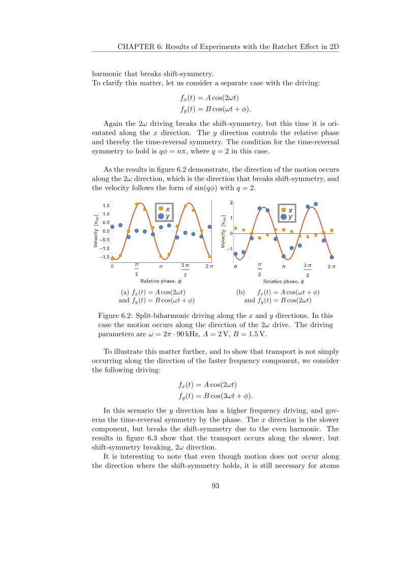
CHAPTER 6: Results of Experiments with the Ratchet Effect in 2D
harmonic that breaks shift-symmetry.To clarify this matter, let us consider a separate case with the driving:
fx(t) = A cos(2ωt)
fy(t) = B cos(ωt+ φ).
Again the 2ω driving breaks the shift-symmetry, but this time it is ori-entated along the x direction. The y direction controls the relative phaseand thereby the time-reversal symmetry. The condition for the time-reversalsymmetry to hold is qφ = nπ, where q = 2 in this case.
As the results in figure 6.2 demonstrate, the direction of the motion occursalong the 2ω direction, which is the direction that breaks shift-symmetry, andthe velocity follows the form of sin(qφ) with q = 2.
(a) fx(t) = A cos(2ωt)and fy(t) = B cos(ωt+ φ)
(b) fx(t) = A cos(ωt+ φ)and fy(t) = B cos(2ωt)
Figure 6.2: Split-biharmonic driving along the x and y directions. In thiscase the motion occurs along the direction of the 2ω drive. The drivingparameters are ω = 2π · 90 kHz, A = 2 V, B = 1.5 V.
To illustrate this matter further, and to show that transport is not simplyoccurring along the direction of the faster frequency component, we considerthe following driving:
fx(t) = A cos(2ωt)
fy(t) = B cos(3ωt+ φ).
In this scenario the y direction has a higher frequency driving, and gov-erns the time-reversal symmetry by the phase. The x direction is the slowercomponent, but breaks the shift-symmetry due to the even harmonic. Theresults in figure 6.3 show that the transport occurs along the slower, butshift-symmetry breaking, 2ω direction.
It is interesting to note that even though motion does not occur alongthe direction where the shift-symmetry holds, it is still necessary for atoms
93
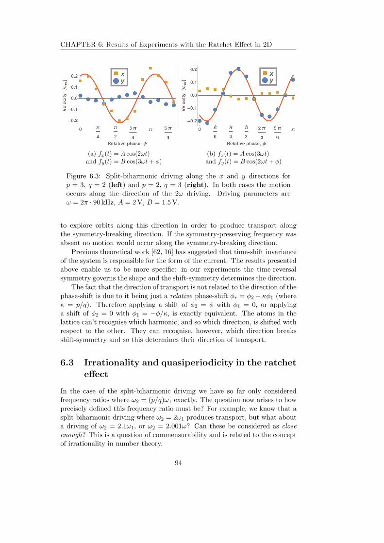
CHAPTER 6: Results of Experiments with the Ratchet Effect in 2D
(a) fx(t) = A cos(2ωt)and fy(t) = B cos(3ωt+ φ)
(b) fx(t) = A cos(3ωt)and fy(t) = B cos(2ωt+ φ)
Figure 6.3: Split-biharmonic driving along the x and y directions forp = 3, q = 2 (left) and p = 2, q = 3 (right). In both cases the motionoccurs along the direction of the 2ω driving. Driving parameters areω = 2π · 90 kHz, A = 2 V, B = 1.5 V.
to explore orbits along this direction in order to produce transport alongthe symmetry-breaking direction. If the symmetry-preserving frequency wasabsent no motion would occur along the symmetry-breaking direction.
Previous theoretical work [62, 16] has suggested that time-shift invarianceof the system is responsible for the form of the current. The results presentedabove enable us to be more specific: in our experiments the time-reversalsymmetry governs the shape and the shift-symmetry determines the direction.
The fact that the direction of transport is not related to the direction of thephase-shift is due to it being just a relative phase-shift φr = φ2 − κφ1 (whereκ = p/q). Therefore applying a shift of φ2 = φ with φ1 = 0, or applyinga shift of φ2 = 0 with φ1 = −φ/κ, is exactly equivalent. The atoms in thelattice can’t recognise which harmonic, and so which direction, is shifted withrespect to the other. They can recognise, however, which direction breaksshift-symmetry and so this determines their direction of transport.
6.3 Irrationality and quasiperiodicity in the ratcheteffect
In the case of the split-biharmonic driving we have so far only consideredfrequency ratios where ω2 = (p/q)ω1 exactly. The question now arises to howprecisely defined this frequency ratio must be? For example, we know that asplit-biharmonic driving where ω2 = 2ω1 produces transport, but what abouta driving of ω2 = 2.1ω1, or ω2 = 2.001ω? Can these be considered as closeenough? This is a question of commensurability and is related to the conceptof irrationality in number theory.
94

CHAPTER 6: Results of Experiments with the Ratchet Effect in 2D
Approximating irrational numbers: the good, the bad, and the ugly
An irrational frequency ratio ω2/ω1 can be characterised by |ω2/ω1 − p/q|,which quantifies how close the value is to the rational approximation p/q.This measure |N − p/q| is in fact a familiar quantity in number theory and aswith all things familiar it is assigned a name: the Diophantine approximation.It is specifically used to measure how close a rational approximation p/q isto an irrational number N . Though the Diophantine approximation tells ushow close the number is to a rational approximation, it doesn’t tell us howwell the rational number approximates it. Consider for example two rationalapproximations of the irrational number π: 22/7 and 1571/500. Both ofthese numbers are accurate to two decimal places but which one is a betterapproximation? If we look at the basic Diophantine approximation |N − p/q|which measures the difference, then the latter fraction 1571/500 serves as abetter approximation. This is not surprising as the precision is in incrementsof 1/500 and not 1/7. If, however, we consider how close it is as a fraction
of the increment then we have |N−p/q|1/q = |N − p/q|q and we find that the
approximation 1571/500 is accurate to 20% of an increment whereas the 22/7approximation is accurate to within 1% of an increment. So it appears that22/7 does uncannily well at approximating π given that the precision is arelatively coarse factor of 1/7. This is illustrated in figure 6.4.
In number theory the measure of how well a rational number p/q approx-imates an irrational number N is determined by the quantity |N − p/q|q2,which can be considered as the fractional difference |N − p/q|q expressed inunits of 1/q. It is the favoured quantity in several theorems such as Hur-witz’s theorem, which states that there are infinitely many rational approx-imations to an irrational number such that |N − p/q|q2 < 1/
√5. These
rational approximations are termed ‘good’ rational approximations. Theapproximation 22/7 counts as a good rational approximation because |π −22/7|72 = 0.061... < 1/
√5 whereas 1571/500 is a ‘bad’ approximation be-
cause |π − 1571/500|5002 = 101.8... 1/√
5.
This section looks at this question of the commensurability of two fre-quencies and considers the emergence of quasiperiodic behaviour in drivensystems, as theoretically explored in [14]. It is shown that those irrationalnumbers that admit poor rational approximations are better candidates forquasiperiodic behaviour in finite-time systems.
Incommensurability in the split-biharmonic drive
In this chapter we demonstrate the coupling between the transverse degrees offreedom using the split-biharmonic driving, and then show how this couplingis suppressed when the driving frequencies are incommensurate.
In the case of split-biharmonic driving, the symmetry analysis presented in
95
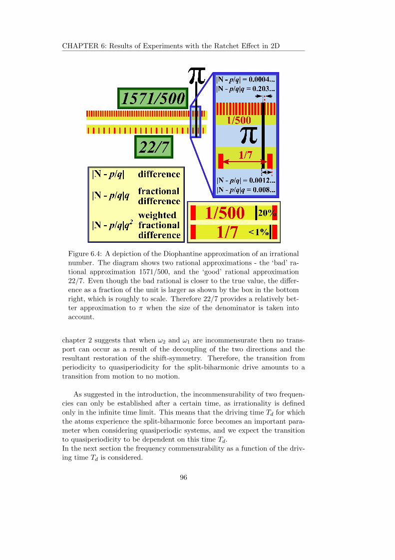
CHAPTER 6: Results of Experiments with the Ratchet Effect in 2D
Figure 6.4: A depiction of the Diophantine approximation of an irrationalnumber. The diagram shows two rational approximations - the ‘bad’ ra-tional approximation 1571/500, and the ‘good’ rational approximation22/7. Even though the bad rational is closer to the true value, the differ-ence as a fraction of the unit is larger as shown by the box in the bottomright, which is roughly to scale. Therefore 22/7 provides a relatively bet-ter approximation to π when the size of the denominator is taken intoaccount.
chapter 2 suggests that when ω2 and ω1 are incommensurate then no trans-port can occur as a result of the decoupling of the two directions and theresultant restoration of the shift-symmetry. Therefore, the transition fromperiodicity to quasiperiodicity for the split-biharmonic drive amounts to atransition from motion to no motion.
As suggested in the introduction, the incommensurability of two frequen-cies can only be established after a certain time, as irrationality is definedonly in the infinite time limit. This means that the driving time Td for whichthe atoms experience the split-biharmonic force becomes an important para-meter when considering quasiperiodic systems, and we expect the transitionto quasiperiodicity to be dependent on this time Td.In the next section the frequency commensurability as a function of the driv-ing time Td is considered.
96

CHAPTER 6: Results of Experiments with the Ratchet Effect in 2D
6.3.1 Resonance width dependence on interaction time Td
We now examine the time-dependence of the velocity when ω2 is scannedabout the primary value 2ω1 for the split-biharmonic drive. Figure 6.5 showsexperimental results for the resonance of ω2 around 2ω1 for different drivingtimes Td. There it is seen that the response of the system is time-dependentfor values of ω2 different to 2ω1.
The ‘peculiar’ driving times of 7.24 ms and 14.5 ms in figure 6.5 correspondto 1024 waves and 2048 waves output at 141.42 kHz, these values being a rem-nant of my early attempts at quasiperiodicity (141.42 kHz may be recognisedas ∼
√2 · 100 kHz, and 1024/2048 being to do with the number of bits that
the Agilent arbitrary waveform generator could output). The driving timesof 10 ms, 20 ms, and 40 ms correspond to 1000 waves at 100 kHz, 1000 wavesat 50 kHz, and 2000 waves at 50 kHz, respectively.
Figure 6.5: Maximum velocity as a function of ω2 when ω2 is scannedabout 2ω1 for various interaction times with the split-biharmonic driving.The plots display a narrowing of the linewidth for longer driving times.Each data point corresponds to a phase-scan from 0 to 2π in 13 steps, likethat shown in figure 6.1, and the maximum velocity was extracted fromthe fitted sine curves. Behold!, this graph is the culmination of almost14 000 images.
The results in figure 6.5 were obtained by scanning the relative phase φfrom 0 to 2π in steps of π/6 and fitting the resulting curves with the functionv = v0 cos(φ+θ). This was done for each value of ω2−2ω1, represented by thex axis in figure 6.5. Therefore, the plot expresses the value of v0 vs ω2− 2ω1.
97

CHAPTER 6: Results of Experiments with the Ratchet Effect in 2D
This means that when the velocity goes to zero in the above graph, it is zerofor all values of the relative phase φ.
The solid lines represent a fit of
v0 = vmax Sinc
[(ω2 − 2ω1)
Td2
].
If we define the width of a Sinc function Ω, such that Sinc(πxΩ ), then thisΩ represents the value at which the function first becomes zero. Since ourvariable is in fact the frequency x = f2 − 2f1 and not the angular frequency,then the fitting equation is given by v0 = vmax Sinc(2πxTd/2), from whichthe width can be readily identified as
Ω =1
Td.
The significance of the results presented in figure 6.5 is that the atomshave an entirely different response to the driving fields for different drivingtimes when ω2 is not commensurate with ω1. This is demonstrated in theplot, where the resonance width becomes narrower with time meaning thattransport is suppressed at longer driving times. This can be interpreted asthe atoms “realising” that the frequencies are not perfectly commensurate. Inthe case of our split-biharmonic driving, this realisation amounts to a drasticchange of dynamics - the atoms stop moving. This is a striking result thatthe dynamics can completely change due to the time-dependent incommen-surability.
This can in fact be interpreted as a dynamical decoupling of the degreesof freedom with longer driving times as a result of the incommensurabilityof the two frequencies. This decoupling causes the x and y directions tohave independent shift-symmetry conditions and, in the case of our split-biharmonic driving, this means that transport is prohibited along x and alongy due to separate and independent conditions.
Since the system’s response to the incommensurability of two frequenciesis time-dependent, in a finite-time experiment to guarantee quasiperiodic be-haviour in a driven system one must ensure that the interaction time is longenough.
To illustrate this idea further, consider a driving with ω2 6= 2ω1, but veryclose to it. On figure 6.6 this is indicated by the red dashed line that is offsetfrom 2ω1. For short driving times the system treats the two frequencies ascommensurate. At longer times, and after more cycles, the system responds tothe difference in frequency and transport is suppressed. This is demonstratedin figure 6.6 and the inset, which shows that transport goes to zero by simplyincreasing the driving time.
This is a remarkable result. A system that is driven by a force that pro-duces transport at short times might be expected to also produce transport
98

CHAPTER 6: Results of Experiments with the Ratchet Effect in 2D
Figure 6.6: Suppression of transport with increasing driving time. Thered dashed line corresponds to a frequency offset of less than 0.05 %, andthe dynamics are already drastically changed. Inset: Split-biharmonicsine curves at green highlighted points for driving times of Td = 7.24ms(blue) and Td = 20ms (orange). The solid curves are for ω2/ω1 ≈ 1.999and the dashed curves are for ω2/ω1 = 2.
at longer times. If anything, it might be expected that the longer the driv-ing is applied, the more transport is produced. But here it is the contrary;even though the driving produces transport at short times, as the drivingtime increases transport then ceases. This is a result of the time-resolutionresponse of the system to the incommensurability of the two numbers. Asthe time is progressing, the system is responding to the fact that the twofrequencies are incommensurate, resulting in the two directions becoming dy-namically decoupled. For the split-biharmonic driving, this decoupling meansthat transport is forbidden along both directions due to independent shift-symmetry conditions.
As can be seen in the inset of figure 6.6, a phase-shift occurs that appearsto be dependent on the interaction time when ω2 − 2ω1 is non-zero, but atω2 = 2ω1 the phase-shift is time-independent. To explore this further, aplot was made of the phase-shifts θ corresponding to the fitted curves v =v0 cos(φ + θ), for the different values of ω2 − 2ω1. The results are shown infigure 6.7, and they show a linear dependence with a gradient equal to Td/2.
Combining this result that θ = θ0 + (ω2 − 2ω1)Td/2 with the fits fromfigure 6.5 v0 = vmax Sinc((ω2 − 2ω1)Td/2) determines the observed velocity
99

CHAPTER 6: Results of Experiments with the Ratchet Effect in 2D
Figure 6.7: The phase-shift θ for the velocity function fit v = v0 cos(φ+θ),showing a linear dependence with a gradient that scales with interactiontime. The parameters for this measurement are the same as those in figure6.5, where each data point corresponds to a phase-scan from 0 to 2π in13 steps and the phase-shift was extracted from the fitted sine curves.
master equation for p = 2, q = 1, as
v = v0 cos(φ+ θ)
= vmax Sinc
[(ω2 − 2ω1)
Td2
]cos
[φ+ θ0 + (ω2 − 2ω1)
Td2
].
The next section considers how the specific values of the frequency ratioaffects the velocity resonance.
6.3.2 Resonance width dependence on q
In this section we explore how the values of p and q in the frequency ratioω2/ω1 = p/q affects the resonance width. In a similar way as was done withthe driving times, we analyse how the maximum velocity and the phase of thevelocity curves varies with ω2−(p/q)ω1. The results are displayed in figure 6.8and figure 6.9, and they show a narrowing of the linewidth that is proportionalto q, as well as a proportional reduction in the maximum velocity.
The solid lines represent fits with the curve
v0 = vmax Sinc
[(ω2 −
p
qω1)
q Td2
],
100

CHAPTER 6: Results of Experiments with the Ratchet Effect in 2D
Figure 6.8: Split biharmonic driving for p/q = 2 and p/q = 1/2, showinga narrowing of the linewidth and reduction in the velocity that is propor-tional to q. The driving parameters for this experiment are ω = 2π·50 kHz,A = 2 V, B = 1.5 V, Td = 20 ms. Velocity in units of vrec = 3.5 mm/s.
where the driving time was Td = 20 ms.The plots of the corresponding phase-shifts are shown in figure 6.10. There
it is seen that the gradient is proportional to q as well as Td.The velocity master equation is thus given by
v = v0 cos(qφ+ θ)
= vmax Sinc
[(qω2 − pω1)
Td2
]cos
[qφ+ θ
(q)0 + (qω2 − pω1)
Td2
]. (6.1)
This result is in fact identical to the one derived in [9] and expoundedupon in the supplementary material of [12] (see [13]), but in those papers ittakes on a different form, namely:
v = vmaxsin [(qω2 − pω1)Td + θ]− sin [θ]
(qω2 − pω1)Td. (6.2)
To see how these are the same, we define α = (qω2 − pω1)Td2 + θ and
β = (qω2 − pω1)Td2 such that α+ β is the argument of the first sine function,and α−β is the argument of the second. Then we can readily use the identitysin(α+ β)− sin(α− β) = 2 sin(β) cos(α) to obtain
v = vmaxsin [(qω2 − pω1)Td/2)]
(qω2 − pω1)Td/2cos [θ + (qω2 − pω1)Td/2] ,
101

CHAPTER 6: Results of Experiments with the Ratchet Effect in 2D
Figure 6.9: Split-biharmonic driving for different values of q, showinga proportional narrowing of the linewidth that is dependent on q andnot dependent on p. The driving parameters for this experiment areω = 2π · 50 kHz, A = 2 V, B = 1.5 V, Td = 20 ms.
which is the experimentally determined result given in equation 6.1, whereθ = qφ+ θ0.Since in an experiment we measure the cosine curves as a function of rel-ative phase φ, then fitting to equation 6.1 is more applicable. In this case,it corresponds to the anticipated cos(qφ + θ0) curve describing the periodicresponse, but with an additional phase-shift equal to (qω2−pω1)Td/2. This isthen multiplied by a phase-independent amplitude envelope, which is a Sincfunction with zeros separated by 2π/q Td.
6.3.3 Higher values of q and Td
As was shown in the previous sections, the values of q and Td have a directimpact on the measured ratchet velocity when ω2 is different to (p/q)ω1. Thekey parameter is in fact the product q Td, as is demonstrated in this section.In figure 6.11 the velocity profiles for q = 2 and q = 3 at various driving timesare shown. There we see that the width scales inversely with q Td.
The fact that the width depends on the product q Td means that thevelocity profiles are not unique for different values of q. Indeed we can finddifferent values of Td such that the widths match each other, as is shownin figure 6.12a. The only feature that distinguishes the two profiles is the
102

CHAPTER 6: Results of Experiments with the Ratchet Effect in 2D
Figure 6.10: The phase-shift θ for the velocity function fit v = v0 cos(qφ+θ), showing a linear dependence with a gradient equal to q Td/2.
(a) q = 2 (b) q = 3
Figure 6.11: Narrowing of linewidth with time for q = 2 (left) and q = 3(right).
maximum velocity, which scales inversely with q.
The dependence on the product also means that we can achieve quitedrastic linewidth reductions with a relatively small range of q and Td values,as is demonstrated in figure 6.13 where the linewidth is reduced by a factor12 when q is changed from 1 to 3 and the atoms are modulated for just anadditional 30 ms.
This portrays just how sensitive the transport is to the system parameters,showing entirely different behaviour (transport to no transport) for minor
103

CHAPTER 6: Results of Experiments with the Ratchet Effect in 2D
(a) Matching widths (b) q = 1 narrower than q = 2
Figure 6.12: Illustration of the fact that the different values of q and Tdcan provide essentially the same velocity profiles. The effective parameteris in fact the product q Td.
Figure 6.13: Narrowing of linewidth for various q and Td showing drasticlinewidth narrowing for minor parameter changes.
changes to parameter values.
6.3.4 Shift-symmetry zeros
In this section we explore the character of the zeros of the velocity resonancecurve. It is shown that there are in fact two distinct ‘types’ of zero occurring,differing in their sensitivity to the driving phase φ. Figure 6.14 shows the
104

CHAPTER 6: Results of Experiments with the Ratchet Effect in 2D
velocity as a function of ∆ω2 = ω2− (p/q)ω1 for a fixed driving phase, wherethe phase-sensitive and phase-insensitive zeros are both indicated.
Figure 6.14: The measured velocity for fixed phase φ, depicting the twotypes of zero-crossing that occur. There are zeros that are dependent onthe value of φ, and then there are zeros that are insensitive to φ. Theparameters in the above graph are φ = 7π/2, q = 2, θ0 = 2.08. Theinsets show the velocity when the phase φ is varied, portraying how thezero-crossings have a different phase-dependence. The highlighted pointin each of the insets corresponds to φ = 7π/2, which is plotted in themain graph.
The origins of the zeros can be traced to the shift-symmetry of the velo-city, as will be described in this section. The following analysis relies on theresults presented in [9, 12, 13] where it is shown that the periodic velocity vpqpossesses shift-symmetry on its argument, that is:
vpq(θ + π) = −vpq(θ) (6.3)
where θ = qφ + θ0. This means that over a period of 2π any motion in onedirection is balanced by motion in the opposite direction.
The equation for the finite-time average drift velocity vTd as a function of∆ω2 can be derived in the following rather neat way.The drift velocity is given by the following general expression
vTd =1
Td
∫ Td
0v(t) dt , (6.4)
105

CHAPTER 6: Results of Experiments with the Ratchet Effect in 2D
which is the average velocity over a driving time Td.
A driving force that is given by f(t) =
cos(ω1t) , cos(ω(0)2 t+ φ)
, where
ω(0)2 = (p/q)ω1, results in a velocity v(φ) = cos(qφ + θ0) that is independent
of time.For ω2 = ω
(0)2 + ∆ω2, the driving force is given by
f(t) =
cos(ω1t) , cos(ω(0)2 t+ ∆ω2t+ φ)
, which equivalently results in a ve-
locity v(φ+ ∆ω2t) = cos(qφ+ θ0 + q∆ω2t) that is now a function of time. Itis this latter form of the velocity that is used as v(t) in the integral 6.4.
We now transform the integral 6.4 by setting θ = qφ + θ0 and redefiningour time-dependent integration variable as θ′ = θ + q∆ω2t such that dt =dθ′/(q∆ω2) and the limits on the integration become
∫ θ+q∆ω2Tdθ . Then the
finite-time average velocity is transformed to
vTd =1
q∆ω2Td
∫ θ+q∆ω2Td
θv(θ′) dθ′ (6.5)
and upon substituting v(θ′) = cos(θ′) we obtain the previously stated equation6.2, which, along with 6.5, was originally derived (by a different method) in[9, 12] and is repeated below:
v = vmaxsin (q∆ω2Td + θ)− sin(θ)
q∆ω2Td.
This was shown to be equivalent to the result determined experimentally inthis thesis given by equation 6.1, repeated here
v = vmax Sinc
[∆ω2
q Td2
]cos
[θ + ∆ω2
q Td2
].
This latter equation mathematically exposes the occurrence of the twotypes of zero - there are zeros of the Sinc function whenever q∆ω2Td is amultiple of 2π, regardless of the phase θ – these shall be referred to as phase-insensitive zeros. Then there are zeros of the cosine function whenever θ +q∆ω2Td/2 = (n+ 1/2)π, which do depend on the value of the phase θ – thesewill be called phase-dependent zeros.
The origin of both of these zeros can be traced to the shift-symmetry prop-erties of the velocity vpq in equation 6.3. For the phase-insensitive zeros, theshift-symmetry property 6.3 means that when the velocity given in the integ-ral 6.5 is averaged over a period of 2π – that is, when the integral
∫ θ+q∆ω2Tdθ
is taken over∫ θ+2πθ – then motion in one direction is cancelled by motion in
the other direction and the net motion goes to zero. This means that thereis zero transport at ∆ω2 = 2π/qTd, regardless of the driving phase θ, as aconsequence of the shift-symmetry of the velocity vpq.
Since these zeros are insensitive to variations in the phase θ they are ro-bust against variations in experimental parameters, which typically affect θ
106

CHAPTER 6: Results of Experiments with the Ratchet Effect in 2D
through its dependence on θ0, which is a system-dependent phase-shift thatis related to the dissipation in the system.
The above considerations have described the origin of the zeros occurringwhen ∆ω2 is an integer (excluding zero) multiple of 2π/q Td, as indicated infigure 6.14.
The second type of zeros are phase-sensitive and occur whenever θ +q∆ω2Td/2 = (n + 1/2)π. These phase-dependent zeros can also be tracedback to the shift-symmetry condition given by equation 6.3; since the cur-rent reverses after a phase-shift of π then there must be a zero in the regionθ → θ + π. That is, aside from the phase-insensitive zero at ∆ω2 = 2π/qTd,there must be a zero in the region ∆ω2 = 0 → ∆ω2 = 2π/qTd. This zero isdependent on the value of the initial phase θ, contrary to the phase-insensitivezero at ∆ω2 = 2π/qTd.
The origin of the phase-dependent zeros can be seen geometrically byconsidering the measured velocity profiles as a function of phase. The earlierresults of figures 6.7 and 6.10 demonstrated that the measured velocity as afunction of phase attains a time-dependent phase-shift equal to q∆ω2Td/2.Therefore, for a fixed phase, there will be values of the phase-shift q∆ω2Td/2such that the velocity becomes zero dynamically. This is represented in figure6.15, which shows that the velocity profile can go to zero as a result of thetime-dependent phase-shift that is incurred when ∆ω2 is non-zero.
The above considerations have attempted to show that the zeros of thevelocity resonance are of two types that possess different phase-dependencies.The zeros occurring at ∆ω2 = ±2π/q Td and integer multiples thereof do notdepend on the phase of the driving, but only depend on q and Td, whereasthe other type of zeros depend on the phase θ = qφ+ θ0 as well as q and Td.
Since the velocity resonance width narrows with time, as has been demon-strated earlier in this chapter, the positions of the zeros will also move towardsthe origin with increasing driving time. This means that with all parametersbeing fixed and with the frequency ω2 in the vicinity of (p/q)ω1 (but notequal to it), the measured atom velocity will reduce to zero dynamically, andcan even undergo current reversals. This is in contrast to the case whenω2 = (p/q)ω1 exactly, where no such dynamical reversals take place for fixeddriving parameters.
6.3.5 Relation to quasiperiodicity
How does this relate to quasiperiodicity? Consider we have two frequencies,ω1 and ω2 such that ω2/ω1 is irrational. For our finite-time experiment,can we be certain that quasiperiodic behaviour will occur? For an irrational
107

CHAPTER 6: Results of Experiments with the Ratchet Effect in 2D
Figure 6.15: A depiction of how, for a fixed phase, the velocity goesto zero as a result of the time-dependent phase-shift of the measuredvelocity profile. These zeros are in general different to the phase-insensitive zeros, which are instead associated to the overall amplitudebecoming zero.
ω2/ω1 there may exist certain rational approximations p/q such that in thetime-frame of the experiment the system will behave periodically.
To put the discussion on firmer footing, let’s consider a specific examplewhere ω2/ω1 = π is irrational and the ω1 frequency is 1 Hz, so there’s simplyone wave per second and T1 = 1 s. It may be presumed that since it isan irrational ratio then quasiperiodic behaviour is expected, but this is notnecessarily the case for some time-periods as is demonstrated in figure 6.16.
The rational approximation 355/113 is close enough to the value of π thatfor a driving time of Td = 2000 s the frequency ratio lies within the resonancewidth for q = 113, Td = 2000 s. This means that even though ω2/ω1 isirrational, periodic instead of quasiperiodic behaviour is observed. In thefigure, with a driving time of Td = 2000 s the velocity is within 5 % of the
108
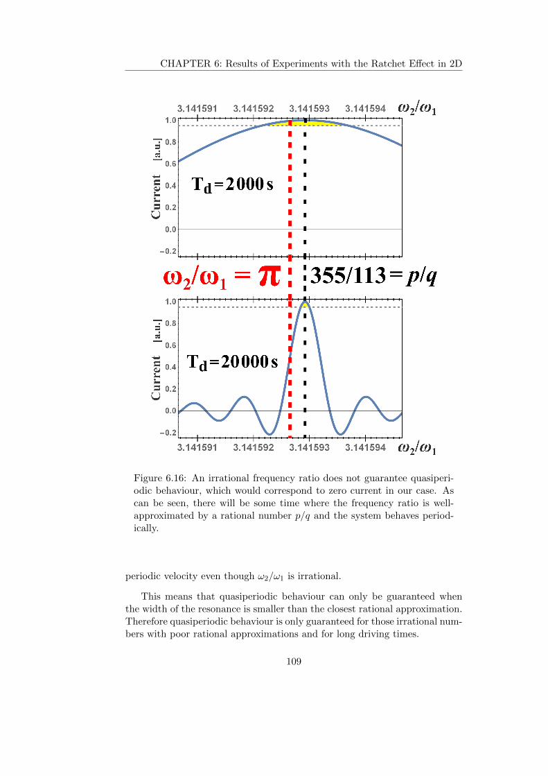
CHAPTER 6: Results of Experiments with the Ratchet Effect in 2D
Figure 6.16: An irrational frequency ratio does not guarantee quasiperi-odic behaviour, which would correspond to zero current in our case. Ascan be seen, there will be some time where the frequency ratio is well-approximated by a rational number p/q and the system behaves period-ically.
periodic velocity even though ω2/ω1 is irrational.
This means that quasiperiodic behaviour can only be guaranteed whenthe width of the resonance is smaller than the closest rational approximation.Therefore quasiperiodic behaviour is only guaranteed for those irrational num-bers with poor rational approximations and for long driving times.
109

CHAPTER 6: Results of Experiments with the Ratchet Effect in 2D
6.3.6 Decoupling the degrees of freedom using quasiperiodicdriving
Our experiments with the split-biharmonic driving have demonstrated thatthe x and y directions are coupled. If they weren’t coupled transport wouldbe prohibited for all values p, q, and φ because the shift-symmetry would holdalong each direction independently. The fact that they’re coupled, however,means that the shift-symmetry along one direction is dependent on the other,and we can exploit this fact to break this symmetry and observe transport.This transport is then in the direction of the shift-symmetry breaking direc-tion, as was shown earlier in this chapter.
The situation changes, however, when the system is driven quasiperiodic-ally such that ω1 and ω2 are incommensurate. A standard method for dealingwith quasiperiodic systems is to treat the two incommensurate quantities asindependent degrees of freedom [23]; in essence, increasing the dimensional-ity of the system as was discussed in chapter 2. How this translates to oursplit-biharmonic drive is that the two directions (driven by each frequency)become independent and decoupled when the driving frequencies are incom-mensurate. When the two directions are decoupled, the shift-symmetry alongeach direction is restored and transport is forbidden.
The coupling between the transverse degrees of freedom has further im-plications. We may consider two separate biharmonic drives along the x andy directions, given by
fx(t) = A [cos(ω1t) + cos(2ω1t+ π/2)]
fy(t) = B [cos(ω2t) + cos(2ω2t+ π/2)] .(6.6)
If we were to naıvely presume that the x and y directions are independentand decoupled, we would expect to observe transport with a magnitude anddirection determined by the relative strengths A and B (with ω2 = ω1). Weare wiser, however, because our split-biharmonic results have shown us thatthe transverse directions are in fact coupled. The impact of this is that thedirection of motion is difficult to predict and is not a simple vector sum ofthe components. This has been demonstrated in previous experiments by ourgroup [43] and by numerical simulations [14].
The decoupling of the degrees of freedom can be exploited, as is invest-igated in [14]. If we consider the driving given in equation 6.6, where wenow use ω2/ω1 incommensurate, then with the degrees of freedom decoupleda more predictable direction of motion is expected, which is the vector sumof the components. This is demonstrated by numerical simulations in [14],which are displayed in figure 6.17.
110

CHAPTER 6: Results of Experiments with the Ratchet Effect in 2D
Figure 6.17: Numerical simulations by David Cubero showing that coup-ling between transverse degrees of freedom (exemplified on the left) issuppressed (right diagram) when ω1 and ω2 are incommensurate. Thisgraph is from the paper [14].
6.3.7 Practical applications
Figure 6.18: At the specific value of qφ + θ0 = 3π/2 (or π/2) the phase-dependent restorations match the phase-insensitive zeros, except at theorigin where there is a phase-dependent zero and a frequency-dependentcurrent reversal. The parameters for this graph are q = 2, φ = 5π/12,θ0 = 2.08, such that qφ+ θ0 ≈ 3π/2.
In figure 6.18 the value of qφ has been chosen such that the phase-dependent zeros and the phase-insensitive zeros coincide, corresponding toqφ + θ0 ≈ 3π/2. This point is particularly interesting as there is a current
111

CHAPTER 6: Results of Experiments with the Ratchet Effect in 2D
reversal around ω2 = (p/q)ω1, which means that atoms travel in opposite dir-ections depending on whether ω2 is bigger or smaller than it’s closest rationalapproximation. This current reversal may be utilised to provide frequency-dependent separation mechanisms. Another noteworthy feature is that, asidefrom the current reversal at the origin, there are no further current reversalsat higher and lower values, meaning that the separation mechanism would berobust. Also, the direction of motion can be used to determine whether thefrequency is above or below the central value.
Figure 6.19: About the central frequency there is a current reversal, whichcan be exploited to provide frequency-sensitive motion. The sensitivity(gradient) about this point scales as q Td.
The sensitivity of a device using this feature will then scale with q andTd, since the gradient of the velocity about this centre point can be shown toscale as v′(∆ω2 = 0) = vmax sin(θ)q Td/2, where θ = qφ+θ0. In the particularcase where θ = 3π/2 or π/2, then the magnitude of the gradient is maximised,and so these phases offer the most sensitive response as shown in figure 6.18.At these values of phase the gradient is equal to ±vmax q Td/2 respectively.
This feature may also have direct applications as a result of its sensitivityto various system parameters. If the phase φ is chosen so that qφ+θ0 is equalto 3π/2 (or its inverted counterpart at π/2) then a small change to any systemparameter will displace the velocity curve. Any displacement of the velocitycurve will result in transport in a specified direction, the direction beingdetermined by the direction of the change. This changing parameter may befrequency, phase or even something more implicit such as noise strength [27]
112
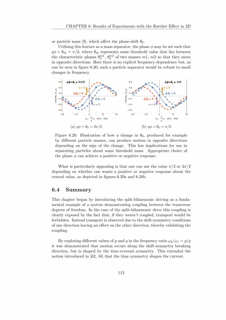
CHAPTER 6: Results of Experiments with the Ratchet Effect in 2D
or particle mass [9], which affect the phase-shift θ0.
Utilising this feature as a mass separator, the phase φ may be set such thatqφ + θth = π/2, where θth represents some threshold value that lies betweenthe characteristic phases θm1
0 , θm20 of two masses m1, m2 so that they move
in opposite directions. Here there is no explicit frequency-dependence but, ascan be seen in figure 6.20, such a particle separator would be robust to smallchanges in frequency.
(a) qφ+ θ0 = 3π/2 (b) qφ+ θ0 = π/2
Figure 6.20: Illustration of how a change in θ0, produced for exampleby different particle masses, can produce motion in opposite directionsdepending on the sign of the change. This has implications for use inseparating particles about some threshold mass. Appropriate choice ofthe phase φ can achieve a positive or negative response.
What is particularly appealing is that one can use the value π/2 or 3π/2depending on whether one wants a positive or negative response about thecentral value, as depicted in figures 6.20a and 6.20b.
6.4 Summary
This chapter began by introducing the split-biharmonic driving as a funda-mental example of a system demonstrating coupling between the transversedegrees of freedom. In the case of the split-biharmonic drive this coupling isclearly exposed by the fact that, if they weren’t coupled, transport would beforbidden. Instead transport is observed due to the shift-symmetry conditionsof one direction having an effect on the other direction, thereby exhibiting thecoupling.
By exploring different values of p and q in the frequency ratio ω2/ω1 = p/qit was demonstrated that motion occurs along the shift-symmetry breakingdirection, but is shaped by the time-reversal symmetry. This extended thenotion introduced in [62, 16] that the time symmetry shapes the current.
113

CHAPTER 6: Results of Experiments with the Ratchet Effect in 2D
Analysis of the velocity for quasiperiodic driving for different values of q,Td and φ allowed a precise determination of the shape of the functional curve,and an experimentally determined velocity master equation was derived. Thiswas shown to be exactly equivalent to the equation theoretically derived inthe literature [13].
By exploring the character of the zeros of the velocity resonance curveas a function of ∆ω2 it was shown that there are two distinct types of zerooccurring that are characterised by their dependence on the driving phase.The origin of both of these zeros was shown to be traceable to the shift-symmetry of the velocity.
Next it was considered how the velocity resonance width has implicationsfor quasiperiodic driving and it was shown that quasiperiodic behaviour isonly expected for irrationals with poor periodic approximations and for longdriving times.
Then it was mentioned how this may be utilised to decouple the degreesof freedom, as theoretically explored in [14].
Finally, practical applications of the derived functional dependence werebriefly considered. The feasibility for use as a particle separator was con-sidered, and it was shown that transport is expected to be sensitive to systemparameters, in some cases producing current reversals. These mechanismsdiffer from previous proposals as they rely on frequency-sensitive schemes.
So what’s new?
The split-biharmonic driving, first introduced in [43] has been studied verylittle experimentally, even though it is exemplary for demonstrating the coup-ling between the transverse degrees of freedom. In this chapter, the split-biharmonic driving was studied for higher values of p and q for the first time,which allowed us to determine that the shift-symmetry governs the directionof motion.
Quasiperiodic behaviour in two dimensions for the split-biharmonic drivewas also examined for the first time. The linewidth of the velocity resonancecurve was extensively studied. It was observed that the measured velocityprofile as a function of driving phase incurs a phase-shift that is proportionalto the driving time. The velocity resonance zeros were shown to be of twodistinct types, differing in their dependence on driving phase, and their originwas traced to the shift-symmetry of the velocity.
An experimentally determined velocity master equation was derived, whichwas shown to be equivalent to that derived theoretically in the literature [12].Also, a novel theoretical derivation for the velocity equation was presented.The velocity equation was used to discuss possible frequency-dependent trans-port schemes.
114

CHAPTER 6: Results of Experiments with the Ratchet Effect in 2D
115

Chapter 7
Discussion and Outlook
7.1 Results presented
This thesis described the development of an experiment to produce a coldatom ratchet in a two-dimensional optical lattice and, using this ratchet,explored the transition to quasiperiodicity in driven systems. It was demon-strated that the transition from periodicity to quasiperiodicity decouples thetransverse degrees of freedom, which manifests as a suppression of ratchetcurrent for our choice of driving. In order to demonstrate the coupling ofthe transverse degrees of freedom, a split-biharmonic drive was used. In thisscheme the coupling is crucial for transport to occur and so a decoupling be-comes clearly evident as going from a regime of transport to a regime of notransport.
This was the first extensive study of the split-biharmonic driving in atwo-dimensional lattice.
It was experimentally demonstrated that the interaction time Td and thevalue of q in the frequency ratio p/q determine the response of the system toquasiperiodic driving. This means that, in a real experiment, quasiperiodicityis only guaranteed for longer driving times and for irrational numbers thathave poor rational approximations.
It was also demonstrated that the direction of the current correspondsto the direction of shift-symmetry breaking and the shape of the currentis determined by the time-reversal symmetry, this latter fact being alreadysuggested in the literature [62, 16]. This distinction between the effects ofeach symmetry was obscured in previous experiments due to the fact thatthe forces governing the shift-symmetry and time-reversal symmetry weredirectionally overlapped.
7.2 Future of the ratchet effect with cold atoms
In this section it is considered what lies in store for the ratchet effect.
116

CHAPTER 7: Discussion and Outlook
First I present the next steps in relation to the results in this thesis,and those investigations that could be explored with the current setup of coldcaesium atoms in a two-dimensional optical lattice. These are avenues I wouldhave liked to venture had time permitted.
Then it is considered what may happen in the next generation of ratchetexperiments in our lab. For this purpose the group has produced a Rb Bose-Einstein condensate. Already the experimental setup is promising on accountof the ultra-cold Rb atoms in the double MOT system, with good opticalaccess. This will provide longer holding times in the lattice and so provide achance to better distinguish more subtle features. Not to mention the peculiarquantum characteristics that may introduce intriguing effects.
Further studies
There are some interesting extensions to the results presented in this thesis,based mainly on continuing the study of quasiperiodicity and how it may beused in some novel mechanisms.
7.2.1 Extending control of ratchet motion
The dependence of the atomic current on the values of Td and q mean that onecan manufacture interesting dynamics that are sensitive to system parameters,as was discussed at the end of chapter 6.This can be further extended to some novel new schemes of operation usingmultiple frequencies - a so-called ‘tri-harmonic’ driving.
In two dimensions, one such scheme could mix the biharmonic driving in-troduced in chapter 5 with the split-biharmonic driving introduced in chapter6, to form the following driving
fx(t) = Ax cos(ω1t) +Bx cos(ω2t+ φ2)
fy(t) = By cos(ω3t+ φ3) .
Alternatively, a three-dimensional lattice could be used where the ω1 harmonicdrives the third ‘z’ axis, so that there is one harmonic driving each direction.In that case the x direction and the y direction are both essentially undergoingseparate split-biharmonic drivings.
fz(t) = Az cos(ω1t)
fx(t) = Ax cos(ω2t+ φ2)
fy(t) = Ay cos(ω3t+ φ3) .
These two possible configurations (2D or 3D) are represented in figure 7.1.
There are a few interesting aspects about this. First, let us consider the2D case with ω1 = ω and ω2 = ω3 = 2ω. In this case we have the standard
117

CHAPTER 7: Discussion and Outlook
Figure 7.1: Examples of triharmonic driving. The frequency of thedriving along each axis is labelled. The left panel is for a two-dimensional lattice, and the right panel is for a three-dimensionallattice. By controlling the relative frequencies of the driving, we maymanufacture the desired frequency-dependent transport.
biharmonic along x and split-biharmonic along y. Therefore we expect tosee transport along the respective directions depending on the values of φ2
and φ3. What is nice about this is that transport along both directions isimmediately stopped if we switch off the first harmonic (Ax = 0).
(a) φ2 = φ3 = 0(b) φ2 = 0
φ3 = π
Figure 7.2: The frequency ω1 can be varied so as to produce directedtransport along one direction only, or no motion. This is a frequency-sensitive transport mechanism, for fixed phase of the driving.
Perhaps more interesting, however, is if we start playing with the mutualcommensurabilities of ω1, ω2, ω3. It is not clear what the extent of coupling isbetween ω2 and ω3 when they are almost equal. This can be investigated byanalysing the motion along the y axis while varying Bx (or vice versa alongx while varying By). We may flip-flop the value of ω1 so that it changes itscommensurability with each harmonic, thereby swapping directions of motion,as portrayed in figure 7.2.
Alternatively, it would be possible to fix ω1 and then vary ω2 and ω3
118

CHAPTER 7: Discussion and Outlook
Figure 7.3: With ω1 fixed, it is the frequencies ω2 and ω3 that determineratchet motion. Specific values of their phases can be used to provide therequired transport. The values of the phase are φ2 = 3π/2 and φ3 = π/2.
providing a frequency-dependent directional transport mechanism. This isrepresented in figure 7.3 where it is shown that a change in the frequencyof ω2 or ω3 will produce a change in amount of transport. The phases canbe chosen to produce the desired shift, and the sensitivity/gradient of thetransport change is dependent on the value of the driving time Td and thevalue of q.Three-dimensional lattices also enable the creation of a blue-detuned opticallattice to trap atoms, which is not possible in two- or one-dimensional blue-detuned lattices. In a blue-detuned lattice the atoms sit at nodes where theintensity is a minimum. This means that atoms will scatter less light, and sothe Hamiltonian regime of ratchets becomes more accessible.
7.2.2 Extension to studies of quasiperiodicity
As has been shown in chapter 6, there is a time-dependence of the motion forquasiperiodic driving. Since long driving times and short driving times exhibitsuch different behaviour, it is yet to be determined how crucial the continuityof the driving signal is. This is not considering the case of a pulsed ratchet,but rather something like an ‘interrupted’ ratchet, as the actual driving timeis extended over a longer period than that associated to a pulse.
We may consider applying a quasiperiodic driving for a determined periodof time, with brief periods of interruption, such as that shown in figure 7.4.
In that figure a quasiperiodic driving is cyclically ramped on for a certaintime Ton, and off for a time Tgap. In order to understand why this is aninteresting case we can look at the two limiting scenarios – the first where
119

CHAPTER 7: Discussion and Outlook
Figure 7.4: It is interesting to consider how the system transitions froman interrupted/slowly pulsed ratchet to a continuous ratchet. This canbe explored using quasiperiodic driving as the two regimes correspondto different driving times, and this leads to entirely different behaviourwhen using quasiperiodic driving. This could perhaps provide some cluesto relaxation mechanisms.
Tgap goes to zero, and the second where Tgap goes to some large value.
In the first scenario where Tgap is zero the driving time will become thatof Ttotal, and so quasiperiodic behaviour is expected, which amounts to notransport for the split-biharmonic driving.
In the other scenario where Tgap is large, the atoms experience a driving ofTon (and not Ttotal as before), and they experience this driving multiple times.Therefore it is expected that the motion would correspond to the Ton time-period, which can be chosen to be a time-period that produces transport forsplit-biharmonic driving. So there is now an additional time-variable, Tgap,that produces two very different behaviours. It would be interesting to tryto understand how the system transitions from one regime to the other. Aninitial presumption would be that it will depend on the level of dissipationand noise strength of the system, as this will determine the relaxation rate.Also, quantum ratchets would be expected to display a different responsethan classical ratchets as quantum ratchets are sensitive to the initial (andsubsequent) conditions of the driving, in a sense preserving memory of thehistory of the driving. This is not the case with classical cold atom ratchets,which preserve no memory of initial conditions.
120

CHAPTER 7: Discussion and Outlook
7.2.3 Bose-Einstein condensate in a ratchet
The next generation of ratchet experiments in our group hopes to explorea Bose-Einstein condensate (BEC) in a ratchet. A BEC is produced whenatoms are cooled to quantum degeneracy, and the atomic ensemble behavesas a single coherent matter-wave.A BEC in a ratchet would constitute a quantum ratchet, which renders it anintriguing subject on account of the peculiar features of a quantum ratchet,such as quantum resonances and a dependence on the initial driving phases[20, 19, 72]. Another feature of quantum ratchets that makes them interestingis that there exists another transport mechanism for atoms in the lattice,namely quantum tunnelling between lattice sites.
BECs can provide a test-bed for solid-state phenomena as there are somestriking resemblances between the two fields and phenomena occurring in oneoften find a counterpart in the other.
One such example is the presence of vortices occurring in a BEC, whichresemble the vortices occurring in a type-II superconductor associated to mag-netic flux quanta. Such vortices can be generated in a BEC by rotating itand once the rotation stops the vortices remain in the BEC as a result of thesuperfluid state of the atoms [1].
Although the heart of a vortex represents an absence of the underlyingfluid, the vortices display behaviours typically associated to particles, such asforming lattices (some with defects)[1] as well as nucleation of vortices [64].Already the ratchet effect has been observed with superconducting vortices -or magnetic flux quanta - in solid-state systems [84, 74], but to my knowledgeit has not yet been observed for vortices embedded in a BEC.
This is perhaps unsurprising as it would be technically very challenging.Examining the ratchet current of vortices in a BEC requires a different ap-proach to observing the ratchet effect with the BEC itself. In the case of theratchet effect with the BEC, it is the optical potential that is rocked, and theBEC undergoes ratchet transport. This already is non-trivial, as any near-resonant fields and strong perturbing rocking forces can excite the BEC cloudand destroy the quantum degeneracy. The solution lies in using a far-detunedoptical lattice to provide a conservative potential; for a Rb BEC operating at780 nm, a 1064 nm Nd-YAG laser is used.
This effect, however, is distinct from a vortex ratchet. For a vortex ratchet,its potential landscape is the matter field that it sits in. So the rockingforce should perhaps be supplied by the BEC itself acting on the vortices,and not by the optical potential acting on the BEC. In this way, it may bethe internal vibrational state of the BEC that provides the rocking force toproduce vortex ratchet transport. This internal rocking could perhaps beinduced by displacing the BEC from the centre of a harmonic trap, or evenpossibly may come about as a by-product of a ratchet driven BEC.
121
CHAPTER 7: Discussion and Outlook
7.2.4 The ratchet effect in other fields
Parrondo’s game [58] has displayed how the ratchet effect can make an ap-pearance in contexts other than physical and biological. This is due to thefact that the two fundamental requirements of a ratchet are (1) a systemout of equilibrium and (2) a broken symmetry. Therefore directed motion inother systems can not be precluded if these conditions are satisfied. One suchalternative scheme for the ratchet effect may be in finance theory, as it is wellknown that share prices behave stochastically and are modelled by methodsoriginally developed for stochastic mechanics.
Final remarks
Over one hundred years since its inception and the field of ratchets is bur-geoning. This is on account of the recognition of its influence in biologicalprocesses and its potential for use in nano-technology, such as in particlepumps and nano-motors.
The ability to observe macroscopic quantum effects in a BEC, as well as insolid-state superconductors, has allowed experimental realisations of quantumratchets.
Cold atoms in optical lattices provide an excellent test-bed for investigat-ing ratchet phenomena, and particularly for investigating phenomena occur-ring in solid-state physics. This correlation between superfluidity in matterand superconductivity in electromagnetic systems is a neat manifestation ofthe underlying connection between the two fields, and is of course a hint ofthe unifying principal principle from which all of physics stems
... but that is the subject of my next thesis.
122

Part II
Rubidium Atomic FountainClock at NPL
123
Chapter 8
The Rubidium AtomicFountain Clock
Once upon a time...
This chapter describes the work performed on the rubidium atomic foun-tain at the National Physical Laboratory (NPL) in Teddington to measurethe hyperfine frequency-splitting of the rubidium-87 ground-state, which ledto a new published result [57] and subsequent redefinition of the value by theInternational Bureau for Weights and Measures (BIPM) [7].
The chapter begins by briefly introducing the main features of an atomicfountain clock, and then goes on to describe the process for taking the meas-urements in that paper. Finally I present the results of the rubidium-87ground-state hyperfine splitting frequency.
8.1 Atomic clocks
Man has had the need to keep track of the relentless progression of time since,well, a very long time ago. Conventionally we use a cyclical process with aseemingly constant rate – that way we can count the number of cycles andthus keep track of the ‘time’ elapsed. The cycles of the seasons constituted ayear, the rotation of the Earth was a day, the swing of a pendulum a second.All of these clocks served well for their respective measurement intervals butfor more precise definitions of time they are lacking. As the world developedthere was a growing need for more accurate, more precise, and more stableclocks.
James Clerk Maxwell was first to posit some time in 1870 [76, 81] thatthe radiation of atoms could be used as a fundamental frequency standard in
124
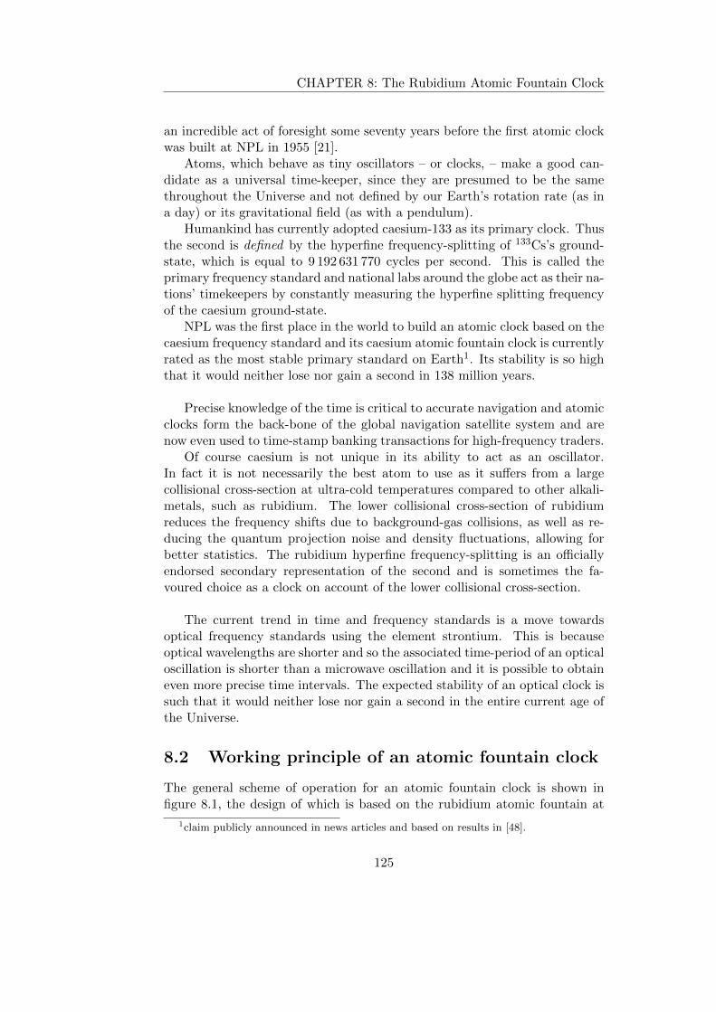
CHAPTER 8: The Rubidium Atomic Fountain Clock
an incredible act of foresight some seventy years before the first atomic clockwas built at NPL in 1955 [21].
Atoms, which behave as tiny oscillators – or clocks, – make a good can-didate as a universal time-keeper, since they are presumed to be the samethroughout the Universe and not defined by our Earth’s rotation rate (as ina day) or its gravitational field (as with a pendulum).
Humankind has currently adopted caesium-133 as its primary clock. Thusthe second is defined by the hyperfine frequency-splitting of 133Cs’s ground-state, which is equal to 9 192 631 770 cycles per second. This is called theprimary frequency standard and national labs around the globe act as their na-tions’ timekeepers by constantly measuring the hyperfine splitting frequencyof the caesium ground-state.
NPL was the first place in the world to build an atomic clock based on thecaesium frequency standard and its caesium atomic fountain clock is currentlyrated as the most stable primary standard on Earth1. Its stability is so highthat it would neither lose nor gain a second in 138 million years.
Precise knowledge of the time is critical to accurate navigation and atomicclocks form the back-bone of the global navigation satellite system and arenow even used to time-stamp banking transactions for high-frequency traders.
Of course caesium is not unique in its ability to act as an oscillator.In fact it is not necessarily the best atom to use as it suffers from a largecollisional cross-section at ultra-cold temperatures compared to other alkali-metals, such as rubidium. The lower collisional cross-section of rubidiumreduces the frequency shifts due to background-gas collisions, as well as re-ducing the quantum projection noise and density fluctuations, allowing forbetter statistics. The rubidium hyperfine frequency-splitting is an officiallyendorsed secondary representation of the second and is sometimes the fa-voured choice as a clock on account of the lower collisional cross-section.
The current trend in time and frequency standards is a move towardsoptical frequency standards using the element strontium. This is becauseoptical wavelengths are shorter and so the associated time-period of an opticaloscillation is shorter than a microwave oscillation and it is possible to obtaineven more precise time intervals. The expected stability of an optical clock issuch that it would neither lose nor gain a second in the entire current age ofthe Universe.
8.2 Working principle of an atomic fountain clock
The general scheme of operation for an atomic fountain clock is shown infigure 8.1, the design of which is based on the rubidium atomic fountain at
1claim publicly announced in news articles and based on results in [48].
125

CHAPTER 8: The Rubidium Atomic Fountain Clock
NPL built by Yuri Ovchinnikov.
Figure 8.1: The working principle of an atomic fountain clock with the mainsteps of the experimental cycle numbered. Atoms are launched upwardsin the fountain, undergo a Ramsey interaction, and then are detected atthe bottom of the fountain. The fountain image was produced by YuriOvchinnikov but the annotations and beam orientation inset were added forthis thesis.
Cold-atom preparation
Atoms are cooled in a 2D-MOT and transferred to the main MOT chamberby an LVIS2 beam [54] where they are accumulated in the main six-beamMOT before being launched upwards in “moving molasses” [40], by detuning
2LVIS stands for Low Velocity Intense Source (of cold atoms) [50]
126

CHAPTER 8: The Rubidium Atomic Fountain Clock
the upward-pointing beams relative to the downward-pointing beams (theorientation of the six MOT beams is depicted in the inset of figure 8.1).
State-selection
On their ascent the atoms undergo state-selection, where atoms in the magnetically-insensitive |F = 2,mF = 0〉 ground-state are transferred to the |F = 1,mF = 0〉ground-state by a resonant microwave π-pulse and the remaining atoms in|F = 2〉 are blown away by a resonant laser (‘blown away’ as in gentle breathnot violent explosion!). This blowing-away laser is resonant to the F = 2 →F ′ = 3 transition (which is the cooling transition) so the state-selected atomsin F = 1 are unaffected by it and they continue their flight into the Ramseycavity. The state-selection process is depicted in figure 8.2.
Figure 8.2: The state-selection procedure. A π-pulse induces atransition between the magnetically-insensitive ground-states, asshown on the left. The atoms remaining in the F = 2 ground-stateare then removed by a beam resonant to the F = 2 → F ′ = 3transition. It may be noted that the π-pulse is also resonant tosome other transition frequencies (mF = +1 → −1 and mF =−1→ +1) but these transitions are prohibited by selection rules.
Ramsey interaction
When the state-selected atoms enter the Ramsey cavity they receive a π/2pulse, which transfers them to a coherent superposition of the two hyperfineground-states. The atoms leave the cavity and their phases freely evolve inthe drift region. On their return descent they pass through the Ramsey cavitya second time where they receive another π/2 pulse.
127

CHAPTER 8: The Rubidium Atomic Fountain Clock
The purpose of the microwave pulses is explained next. The first π/2 pulseputs the atoms into a superposition of the two ground-states. If a second π/2pulse were applied instantly then it would be equivalent to a π-pulse and allthe atoms would be transferred to the F = 2 ground-state.In the fountain, however, there is a diffusion time between the pulses as theatoms ascend, reach the apex and then descend under gravity. During thisfree-fall time the atoms’ phases evolve. The phase-difference between the twostates is proportional to the detuning of the pulse from the resonant frequency(as well as the diffusion time between the pulses, which is constant for a se-quence of measurements).If the microwave pulse is exactly resonant, the phase-difference between thetwo states is zero and all atoms are transferred to the F = 2 ground-state bythe second π/2 pulse on their descent.If the microwave pulse is non-resonant, however, then the two states accu-mulate a relative phase-difference and when the second π/2 pulse is applied,only a fraction of the atoms are transferred to the F = 2 ground-state.
Figure 8.3: The measured Ramsey fringes of NPL’s rubidium atomic foun-tain exhibiting the relative population in the F = 2 ground-state as afunction of the microwave pulse detuning, where each point represents asingle launch. The main graph was produced by Yuri Ovchinnikov. Theinset portrays the split-Ramsey method used to determine the centralfrequency by hopping the frequency about the central fringe. The threediagrams illustrate three separate regimes of pulse detuning and indicatethe relative number of atoms in the F = 1 and F = 2 states, which areequal when their mid-frequency is on resonance.
The evolution of the phase with respect to the microwave pulse detuningis depicted by Ramsey fringes, which shows the relative number of atoms
128

CHAPTER 8: The Rubidium Atomic Fountain Clock
in the F = 2 ground-state when the pulse frequency is scanned about theresonant frequency. The Ramsey fringes for NPL’s rubidium atomic fountainare shown in figure 8.3. The very centre of the fringes is a maximum andcorresponds to the resonant pulse frequency where all atoms are transferredto the F = 2 ground-state.
The width of the entire Ramsey fringes is dependent on the time spent inthe Ramsey cavity, and the width of the central peak is dependent on the evol-ution time between the pulses. This is the benefit of a fountain clock, wherethe free-diffusion time is longer than in traditional caesium clocks with twoseparated Ramsey cavities, allowing a narrower line-width about the centrefrequency.
Atomic state measurement
After the atoms have undergone the Ramsey interaction, the number of atomsin each state is measured in the detection chambers. This is achieved byobserving the fluorescence of the falling atomic sample. First, atoms in theF = 2 ground-state are detected by a beam resonant with the F = 2→ F ′ = 3transition. Then the atoms in the F = 1 ground-state are excited to theF = 2 ground-state by a repumping beam and then detected with the beamresonant to the F = 2 → F ′ = 3 transition. This provides a measurementof the relative number of atoms in the F = 2 state, which is related to thefrequency detuning of the pulse, as depicted in figure 8.3.
Split-Ramsey method
The actual process for measuring the central fringe frequency, correspond-ing to the ground-state hyperfine splitting frequency, uses the split-Ramseymethod – sometimes called the method of separated oscillatory fields [65].The measurement is performed by ‘hopping’ the pulse frequency between thetwo sides about the central fringe and determining the centre point, as depic-ted in the inset of figure 8.3. The amount by which the frequency is jumpedcorresponds to the FWHM of the central fringe, which is about 1 Hz for ourrubidium fountain. When the beam is exactly resonant there is an equal num-ber of atoms in each state and so the measurement of the number of atomsis fed back to the pulse-synthesiser in a servo loop in order to minimise thedifference in population of each state.After many measurements an accurate statistical average for the ground-statehyperfine splitting can be obtained by measurements of the relative atomicfluorescence in each state. This average value provides us with a measurementof the rubidium ground-state hyperfine splitting frequency or, in the case ofthe caesium frequency standard, is used to define the second.The quantum projection noise [38, 73] is a consequence of the measurementprocedure in the split-Ramsey method and is the limiting factor to the sta-
129

CHAPTER 8: The Rubidium Atomic Fountain Clock
bility of an atomic fountain clock using this method. It arises from the factthat measurements are made about the half-maximum where atoms are inan equal superposition of the two ground-states. When the atoms are thenmeasured, they are projected onto one of the two states F = 1 and F = 2with equal probability. Therefore, there is some degree of uncertainty as towhich state the atom will be projected to and only by gathering statisticswith a large number of atoms can the distribution be accurately determined.This uncertainty is the source of the quantum projection noise, which scalesas the inverse-root of the number of atoms 1/
√N and so can be reduced by
using a larger number of atoms. The quantum projection noise is at a max-imum when the splitting ratio is 50–50, which corresponds to the regime ofthe split-Ramsey method, and so it limits the stability of an atomic fountainclock. In the NPL rubidium atomic fountain the flux of atoms from the LVISto the main MOT is 8 × 10⁹ atoms per second and so can provide a largenumber of atoms in a relatively short time.
8.3 The NPL rubidium atomic fountain
The rubidium atomic fountain at NPL was designed and built by Prof. YuriOvchinnikov, and its characterisation is given in [56, 47, 53, 55] and its designis shown in figure 8.1.
8.3.1 Modifications to existing fountain
There were several modifications made to the fountain during my time atNPL, including a modification to the vacuum system therefore breaking theultra-high vacuum after six years undisturbed.
A new detection chamber was added beneath the existing detection cham-ber so that there would be a separate chamber for detecting each state in orderto increase the signal-to-noise ratio and obtain better statistics. In the originaldesign both states were detected in the same chamber, limiting the opticalaccess and reducing the signal obtained by the CCDs. With the additionalchamber, larger beams can be used to read out the number of atoms in eachstate.
When adding the new detection chamber to the existing fountain, thefountain had to be opened and so lost its vacuum. This was also benefi-cial as the fountain had been operating for several years and so rubidiumvapour had accumulated. Opening the fountain and subsequently re-bakingand pumping the system enabled a de-contamination after so many years inservice. Improvement of the vacuum allows for cooler atoms due to reducedbackground-gas collisions and leads to better statistics.
130

CHAPTER 8: The Rubidium Atomic Fountain Clock
Once the new detection chamber had been appended the system was bakedand pumped. The baking was achieved by covering the entire (two-metretall) fountain by a heat-proof blanket to act as a thermal insulator and pla-cing several radiator heaters underneath the fountain. Thermocouples werepositioned along the length of the fountain in order to monitor its temper-ature and there were also thermocouples embedded beneath the magneticshields from the original construction. Particularly important were the ther-mocouples located next to the indium seals near the Ramsey cavity, sinceindium has a melting point of 156°C and so it was necessary to ensure thetemperature didn’t exceed this value.
Figure 8.4: Photograph of the modified detection and surround-ing optics, also showing the 2D-MOT and main MOT chambers.Light is delivered to the detection region by fibres. The addi-tional detection chamber means that optical access is not limitedand better statistics can be obtained.
With the new detection chamber in place the optical detection systemwas upgraded to take advantage of the enhanced optical access (figure 8.4).The upper detection chamber is used to measure the atoms in the F = 2ground-state. A retro-reflected light-sheet is used to excite atoms by a F =2 → F ′ = 3 transition and the atom fluorescence is picked up by a CCDcamera. The lower part of the beam is not retro-reflected in order to providea free-running beam that pushes the atoms away. The remaining atoms arethose in the F = 1 ground-state. In the lower detection chamber there isthe repumping beam resonant to the F = 1 → F ′ = 2 transition, whichtransfers atoms into the F = 2 ground-state. Then these atoms pass througha light-sheet resonant to the F = 2→ F ′ = 3 transition and are detected by
131

CHAPTER 8: The Rubidium Atomic Fountain Clock
a CCD.
8.3.2 Characterising the frequency shifts
There are many effects that shift the energy, and so frequency, of the atoms.These include all effects that perturb the system, such as magnetic fields,temperature, gravity, background-gas collisions, and even shifts from the mi-crowave pulses used to probe the transitions.These shifts must be accounted for and they are summarised in an “uncer-tainty budget”, which gives details of the energy-shift produced by the effectas well as the uncertainty on that energy-shift value. The uncertainty budgetfor NPL’s rubidium fountain is shown in figure 8.5.
Figure 8.5: The uncertainty budget of the rubidium fountain,characterising the systematic frequency shifts of the fountain.The total uncertainty is obtained by adding all the uncertain-ties in quadrature.
It is not necessarily the frequency shift that must be reduced, but ratherit is the uncertainty of the shift that is most important for an accurate atomicclock. For example it is currently impossible to stop the effects of the Earth’sgravitational field on the atoms but it is possible to try to characterise theeffect well. If we have a good knowledge (low uncertainty) about how it isshifted, then we can account for this shift and thereby deduce the true fre-quency. Therefore, when using an uncertainty budget to determine how gooda clock is, it is often the uncertainty on the shift that interests us most andnot necessarily the actual magnitude of the shift.
The source of each shift is described briefly below but more in-depth de-scriptions can be found in [88].The second-order Zeeman shift is a result of the non-zero magnetic fieldin the drift region as a result of the C-field coil, which is used to establish the
132

CHAPTER 8: The Rubidium Atomic Fountain Clock
quantisation axis.The black-body radiation shift is the energy shift due to the non-zerotemperature of the environment. The uncertainty on this shift is minimisedby using the temperature-stabilised water-jacket that maintains the temper-ature of the interrogation region to within ±0.1°C.Collisions with residual gas also shift the energy of the atoms. This ef-fect is less for rubidium-87 than for caesium because rubidium has a smallercollisional cross-section.There is also a gravitational shift as a result of the general-relativistic red-shift produced by the Earth.Then there are a few shifts that are a result of the microwave interaction,these are distributed cavity-phase shift, cavity-pulling shift, microwave leak-ing and microwave lensing.The distributed cavity-phase shift is a result of the atoms experiencing avarying phase of the microwave pulse during their trajectory.The cavity-pulling shift is a result of the Ramsey-cavity resonance beingdetuned with respect to the atomic resonant frequency, which creates an ef-fective shift on the measured frequency. This can be minimised by stabilisingthe cavity’s temperature so that it is resonant to the atomic frequency.The microwave leaking describes the energy perturbation to the atoms asa result of any microwave-field leaking into the drift-region of the chamber,where the atoms are meant to evolve undisturbed.The microwave lensing shift arises from the non-uniformity of the mi-crowave pulse across the finite-sized atomic sample, which produces an effect-ive lensing of the atomic states that, upon detection, looks like a frequencyshift, which must be accounted for.
Most of these shifts have been characterised previously [56, 55]. I parti-cipated in measuring the second-order Zeeman shift as well as characterisingthe cavity-pulling and black-body radiation shifts through taking temperat-ure measurements. The measurements of the temperature stability, shownin figure 8.6, supply information for the uncertainty on the black-body radi-ation shift and the cavity-pulling shift. The temperature is regulated by awater jacket connected to a thermo-electric heater/cooler that maintains thefountain’s temperature to within 0.1°C over many months.
There are two important reasons why the temperature must be stabilised.Firstly, the temperature is the source of the black-body radiation shift andso the temperature stability determines the uncertainty on this shift, whichtransfers to an uncertainty on our final measurements. The second reasonaccurate knowledge of the temperature is important is because the microwavecavity resonance condition is dependent on its temperature. The length ofthe cavity determines its resonant frequency and so thermal expansion of thealuminium cavity affects that resonance.
133

CHAPTER 8: The Rubidium Atomic Fountain Clock
Figure 8.6: The temperature measurements of the atomic fountain showthat the temperature is maintained to within ±0.1°C over months.
8.4 Absolute measurement of the rubidium-87 ground-state hyperfine splitting frequency
This section describes the measurement of the frequency-splitting betweenthe F = 1 and F = 2 hyperfine levels of the 52S1/2 ground-state of 87Rb.
The fact that it is an absolute measurement comes from our ability todirectly reference it to the caesium atomic fountain primary frequency stand-ard at NPL [80, 48], which defines the second in the UK. The rubidium andcaesium fountains have frequency synthesisers that are locked to a single hy-drogen maser at NPL, which works as an excellent short-term stable oscillator.This means that any shifts in the maser frequency are experienced by bothfountains, and can be factored out. In this way a comparison of the rubidiumfrequency with respect to the primary frequency standard gives an absolutemeasurement.
8.4.1 Measurement procedure
In order to measure the hyperfine frequency averages are taken using thesplit-Ramsey method, as described previously.The pulse frequency is hopped between the two sides of the central Ramseyfringe, the number of atoms is measured and the microwave pulse frequencyis adjusted in a servo in order to maintain the frequency about the centralfringe. The adjustments to the pulse frequency provide a measurement ofthe frequency offset and after averaging many measurements the centre fre-quency can be inferred very accurately. Figure 8.8 shows a graph of typicalmeasurement results.
The frequency about which the value oscillates is the ground-state hyper-fine splitting frequency inclusive of all systematic frequency shifts. Therefore,by using the knowledge of the measured systematic shifts we can calculate
134

CHAPTER 8: The Rubidium Atomic Fountain Clock
Figure 8.7: The inter-connection of the frequency standards at NPL,showing how the rubidium atomic fountain and caesium atomic foun-tain primary standard are referenced to the same hydrogen maser,thereby allowing us to cancel out relative shifts and obtain an abso-lute frequency measurement.
the unperturbed frequency.
The two types of uncertainty on this value are called type-A and type-Buncertainty. Type-A uncertainty represents the statistical uncertainty of theresults like those measured in figure 8.8, and so is given as the standard erroron the mean. Type-B uncertainty relates to the uncertainty on the systematicshifts as portrayed in the final column of the uncertainty budget in figure 8.5.The type-A and type-B uncertainties for the rubidium and caesium atomicfountains relevant to the measurements in this chapter are given in figure 8.9.
When measuring the absolute frequency of the rubidium ground-state hy-perfine splitting, the results must be compared to the caesium fountain andso the uncertainty on the caesium fountain results must also be accounted for.This is accomplished by adding the uncertainties in quadrature to obtain thetotal uncertainty
σTOT =√
(σRbA )2 + (σRbB )2 + (σCsA )2 + (σCsB )2 .
135

CHAPTER 8: The Rubidium Atomic Fountain Clock
Figure 8.8: Typical graph of the microwave frequency, displaying howafter many cycles we can obtain a statistically accurate mean valuefor the frequency. The statistical error on the mean contributes to thetype-A uncertainty. The measured value includes all systematic shiftsand so subtracting these shifts allows us to derive the true unperturbedfrequency.
Figure 8.9: The type-A and type-B uncertainties of NPL’s ru-bidium and caesium fountain frequency standards for the threemeasurement sessions.
8.4.2 Analysis of results
The frequency of an atomic fountain clock as measured in the lab fRbm is a sumof the unperturbed frequency fRb0 plus any systematic shifts in the frequencyfRbss minus any shift in the frequency of the microwave field used to measurethe transition. That is
fRbm = fRb0 + fRbss − βfRbm ,
where β is the fractional error of the hydrogen maser’s frequency given by
β =fHM−fHM
0
fHM0
. Since the caesium fountain is running concurrently and is
referenced to the same hydrogen maser, the coefficient β is derived from the
136

CHAPTER 8: The Rubidium Atomic Fountain Clock
caesium measurements. Therefore
β =fCs0 + fCsss − fCsm
fCsm,
giving us a relatively simple expression for the rubidium-87 ground-state hy-perfine splitting frequency:
fRb0 = fRbm
(fCs0 + fCsss
fCsm
)− fRbss . (8.1)
The values on the right-hand side of equation 8.1 are all measured ordefined. fCs0 defines the second, fCsss was measured at NPL by those in chargeof the caesium fountain [48], fCsm is constantly being measured and the valuescorresponding to the times of our measurement were extracted and used, fRbsswas measured and characterised in [56], and fRbm is of course the value we aremeasuring by averaging. Then from all of these an absolute measurement forthe rubidium ground-state hyperfine splitting frequency fRb0 can be inferred.
8.4.3 Rubidium-87 ground-state hyperfine splitting frequency
Before the measurement at NPL, the recommended CCTF value3 for therubidium-87 ground-state hyperfine splitting frequency was based on measure-ments performed at LNE-SYRTE in Paris [33]. The CCTF found it “prudent”to increase the uncertainty threefold on account of it being based on a meas-urement performed at a single laboratory. Therefore this new measurementperformed at NPL allows a more precise and conclusive definition of the fre-quency. Furthermore, another measurement at another location that agreeswell with the original result also indicates the validity of the current ap-proaches to frequency measurements.
There were three separate measurement sessions performed with NPL’srubidium atomic fountain – I participated only in the third measurement in2013. The measurement results are as follows:
fRb(NPL 2010) = 6 834 682 610.904 308(4.6) Hz
fRb(NPL 2012) = 6 834 682 610.904 305(5.5) Hz
fRb(NPL 2013) = 6 834 682 610.904 306(6.1) Hz .
Combining these results gives an overall frequency of
fRb(NPL) = 6 834 682 610.904 307(3.1) Hz
3the report [6] for the previous recommended value can be found online at https://www.bipm.org/utils/common/pdf/mep/87Rb_6834MHz_2013.pdf.
137

CHAPTER 8: The Rubidium Atomic Fountain Clock
The only other published independent values come from LNE-SYRTE, themost recent of which was in 2012 [32] with a value of fRb(SYRTE 2012) =6 834 682 610.904 312(3) Hz, and so combining this with our measured valuegives a final result for the ground-state hyperfine splitting frequency as
fRb(NPL & SYRTE) = 6 834 682 610.904 310(2.4) Hz
Figure 8.10: A graph of the rubidium-87 frequency measurementsover previous years. The official recommended value has been ad-justed in 2015 [7] based on the newly published [57] measurementsat NPL.
Figure 8.10 displays the results of measurements performed over previousyears by NPL and LNE-SYRTE, so far the only two places to have publishedvalues for this secondary frequency standard.
This new measurement has already been incorporated into the BIPM re-commended values4 and the recommended rubidium-87 frequency has beenadjusted accordingly.
4The report [7] for the new recommended value based on our result can be found onlineat https://www.bipm.org/utils/common/pdf/mep/87Rb_6.8GHz_2015.pdf.
138
CHAPTER 8: The Rubidium Atomic Fountain Clock
Figure 8.11: The hyperfine energy levels for the 87Rb D2 transition at780 nm. The diagram was inspired by Daniel Steck’s rubidium-87 D-line data [77] and the values were taken from that paper except for thehighlighted value for the ground-state splitting, which is the central andnew result presented in this chapter.
8.5 Summary
This chapter described the procedure for the measurement of the 87Rb ground-state hyperfine splitting frequency using the rubidium atomic fountain atNPL. The fact that the rubidium fountain is driven by the same hydrogenmaser as the caesium primary frequency standard at NPL means that it is pos-sible to make an absolute measurement of the rubidium hyperfine frequency-splitting.
The new published result has corroborated the previous measurementsperformed at LNE-SYRTE, the only other laboratory to have published ameasurement, and has resulted in a redefinition of the rubidium-87 ground-state hyperfine splitting frequency, which is currently the most popular sec-ondary frequency standard used in practice.
139

CHAPTER 8: The Rubidium Atomic Fountain Clock
140

Bibliography
[1] Abo-Shaeer, J. R., Raman, C., Vogels, J. M., and Ketterle, W.Observation of Vortex Lattices in Bose-Einstein Condensates. Science292, 5516 (2001), 476–479.
[2] Anderson, M. H., Ensher, J. R., Matthews, M. R., Wieman,C. E., and Cornell, E. A. Observation of Bose-Einstein Condensationin a Dilute Atomic Vapor. Science 269, 5221 (1995), 198–201.
[3] Astumian, D., and Hanggi, P. Brownian Motors. Physics Today 55(Feb 2002), 33.
[4] Astumian, R. D., and Bier, M. Fluctuation Driven Ratchets: Mo-lecular Motors. Phys. Rev. Lett. 72 (Mar 1994), 1766–1769.
[5] Bartussek, R., Hanggi, P., and Kissner, J. G. Periodically RockedThermal Ratchets. EPL (Europhysics Letters) 28, 7 (1994), 459.
[6] BIPM. Recommended values of standard frequencies for applicationsincluding the secondary representations of the definition of the Second,2013 – Rubidium 87.available online athttps://www.bipm.org/utils/common/pdf/mep/87Rb_6834MHz_
2013.pdf.
[7] BIPM. Recommended values of standard frequencies for applicationsincluding the practical realization of the Metre and secondary repres-entations of the definition of the Second, 2015 – Rubidium 87.available online athttps://www.bipm.org/utils/common/pdf/mep/87Rb_6.8GHz_2015.
pdf.
[8] Brillouin, L. Can the Rectifier Become a Thermodynamical Demon?Phys. Rev. 78 (Jun 1950), 627–628.
[9] Casado-Pascual, J., Cubero, D., and Renzoni, F. UniversalAsymptotic Behavior in Nonlinear Systems Driven by a Two-FrequencyForcing. Phys. Rev. E 88 (Dec 2013), 062919.
141

BIBLIOGRAPHY
[10] Chu, S., Hollberg, L., Bjorkholm, J. E., Cable, A., and Ashkin,A. Three-Dimensional Viscous Confinement and Cooling of Atoms byResonance Radiation Pressure. Phys. Rev. Lett. 55 (Jul 1985), 48–51.
[11] Cohen-Tannoudji, C., and Phillips, W. D. New Mechanisms forLaser Cooling. Physics Today 43, 10 (1990), 33–40.
[12] Cubero, D., Casado-Pasqual, J., and Renzoni, F. Irrationalityand Quasiperiodicity in Driven Nonlinear Systems. Phys. Rev. Lett. 112(2014), 174102.
[13] Cubero, D., Casado-Pasqual, J., and Renzoni, F. Irrationalityand Quasiperiodicity in Driven Nonlinear Systems - Supplemental Ma-terial. Phys. Rev. Lett. 112 (2014), 174102.
[14] Cubero, D., and Renzoni, F. Control of Transport in Two-dimensional Systems via Dynamical Decoupling of Degrees of Freedomwith Quasiperiodic Driving Fields. Phys. Rev. E 86 (Nov 2012), 056201.
[15] Cubero, D., and Renzoni, F. Brownian Ratchets: From StatisticalPhysics to Bio and Nano-motors. Cambridge University Press, 2016.
[16] Cuesta, J. A., Quintero, N. R., and Alvarez-Nodarse, R. Time-Shift Invariance Determines the Functional Shape of the Current in Dis-sipative Rocking Ratchets. Phys. Rev. X 3 (Nov 2013), 041014.
[17] Dalibard, J., and Cohen-Tannoudji, C. Laser Cooling Below theDoppler Limit by Polarization Gradients: Simple Theoretical Models. J.Opt. Soc. Am. B 6, 11 (Nov 1989), 2023–2045.
[18] Davis, K. B., Mewes, M. O., Andrews, M. R., van Druten, N. J.,Durfee, D. S., Kurn, D. M., and Ketterle, W. Bose-EinsteinCondensation in a Gas of Sodium Atoms. Phys. Rev. Lett. 75 (Nov1995), 3969–3973.
[19] Denisov, S., Morales-Molina, L., and Flach, S. Quantum Res-onances and Rectification in AC-Driven Ratchets. EPL (EurophysicsLetters) 79, 1 (2007), 10007.
[20] Denisov, S., Morales-Molina, L., Flach, S., and Hanggi, P.Periodically Driven Quantum Ratchets: Symmetries and Resonances.Phys. Rev. A 75 (Jun 2007), 063424.
[21] Essen, L., and Parry, J. An Atomic Standard of Frequency and TimeInterval: A Caesium Resonator. Nature 176 (1955), 280–282.
[22] Feynman, R. The Feynman Lectures, vol. 1. Addison-Wesley, 1964.
142

BIBLIOGRAPHY
[23] Flach, S., and Denisov, S. Symmetries and Transport with Qua-siperiodic Driving. Acta Phys. Pol. B 35 (Mar 2004), 1437.
[24] Flach, S., Yevtushenko, O., and Zolotaryuk, Y. Directed Cur-rent due to Broken Time-Space Symmetry. Phys. Rev. Lett. 84 (Mar2000), 2358–2361.
[25] Ganichev, S. D., Tarasenko, S. A., Olbrich, P., Karch, J.,Hirmer, M., Mller, F., Gmitra, M., Fabian, J., Yakimova, R.,Lara-Avila, S., Kubatkin, S., Wang, M., Vajtai, R., Ajayan,P. M., Kono, J., and Drexler, C. Magnetic Quantum Ratchet Ef-fect in Graphene. Nature Nanotechnology 8 (June 2013), 104–107.
[26] Gommers, R. Symmetry and Transport in Cold Atom Ratchets. PhDthesis, University College London (UCL), June 2007.
[27] Gommers, R., Bergamini, S., and Renzoni, F. Dissipation-InducedSymmetry Breaking in a Driven Optical Lattice. Phys. Rev. Lett. 95(Aug 2005), 073003.
[28] Gommers, R., Denisov, S., and Renzoni, F. QuasiperiodicallyDriven Ratchets for Cold Atoms. Phys. Rev. Lett. 96 (Jun 2006), 240604.
[29] Gommers, R., Douglas, P., Bergamini, S., Goonasekera, M.,Jones, P. H., and Renzoni, F. Resonant Activation in a Nonadiabat-ically Driven Optical Lattice. Phys. Rev. Lett. 94 (Apr 2005), 143001.
[30] Gorre, L., Ioannidis, E., and Silberzan, P. Rectified Motion of aMercury Drop in an Asymmetric Structure. EPL (Europhysics Letters)33, 4 (1996), 267.
[31] Grynberg, G., Lounis, B., Verkerk, P., Courtois, J.-Y., andSalomon, C. Quantized Motion of Cold Cesium Atoms in Two- andThree-dimensional Optical Potentials. Phys. Rev. Lett. 70 (Apr 1993),2249–2252.
[32] Guena, J., Abgrall, M., Clairon, A., and Bize, S. Contributingto TAI with a secondary representation of the SI second. Metrologia 51,1 (2014), 108.
[33] Guena, J., Rosenbusch, P., Laurent, P., Abgrall, M., Rovera,D., Lours, M., Santarelli, G., Tobar, M. E., Bize, S., andClairon, A. Demonstration of a Dual Alkali Rb/Cs Atomic FountainClock. IEEE Transactions on Ultrasonics, Ferroelectrics and FrequencyControl 57 (2010), 647.
[34] Guidoni, L., Triche, C., Verkerk, P., and Grynberg, G. Qua-siperiodic Optical Lattices. Phys. Rev. Lett. 79 (Nov 1997), 3363–3366.
143
BIBLIOGRAPHY
[35] Guidoni, L., and Verkerk, P. Optical Lattices: Cold Atoms Orderedby Light. Journal of Optics B: Quantum and Semiclassical Optics 1, 5(1999), R23.
[36] Hanggi, P., Marchesoni, F., and Nori, F. Brownian Motors. An-nalen der Physik 14, 1-3 (2005), 51–70.
[37] Hansch, T., and Schawlow, A. Cooling of Gases by Laser Radiation.Optics Communications 13, 1 (1975), 68 – 69.
[38] Itano, W. M., Bergquist, J. C., Bollinger, J. J., Gilligan,J. M., Heinzen, D. J., Moore, F. L., Raizen, M. G., and Wine-land, D. J. Quantum projection noise: Population fluctuations in two-level systems. Phys. Rev. A 47 (May 1993), 3554–3570.
[39] Jones, P. H., Goonasekera, M., and Renzoni, F. Rectifying Fluc-tuations in an Optical Lattice. Phys. Rev. Lett. 93 (Aug 2004), 073904.
[40] Kasevich, M. Atom Interferometry in an Atomic Fountain. PhD thesis,Stanford University, June 1992.
[41] Kasevich, M., and Chu, S. Atomic Interferometry using StimulatedRaman Transitions. Phys. Rev. Lett. 67 (Jul 1991), 181–184.
[42] Lebedev, V. AC Driven Ratchets for Cold Atoms: Beyond 1D RockingRatchets. PhD thesis, University College London (UCL), October 2009.
[43] Lebedev, V., and Renzoni, F. Two-dimensional Rocking Ratchet forCold Atoms. Phys. Rev. A 80 (Aug 2009), 023422.
[44] Letokhov, V. S. Narrowing of the Doppler Width in a Standing LightWave. JETP Lett. 7 (1968), 272.
[45] Letokhov, V. S., and Minogin, V. G. Cooling, Trapping, and Stor-age of Atoms by Resonant Laser Fields. J. Opt. Soc. Am. 69, 3 (Mar1979), 413–419.
[46] Lett, P. D., Watts, R. N., Westbrook, C. I., Phillips, W. D.,Gould, P. L., and Metcalf, H. J. Observation of Atoms LaserCooled below the Doppler Limit. Phys. Rev. Lett. 61 (Jul 1988), 169–172.
[47] Li, R., and Gibble, K. Comment on ‘Accurate Rubidium AtomicFountain Frequency Standard’. Metrologia 48, 5 (2011), 446.
[48] Li, R., Gibble, K., and Szymaniec, K. Improved Accuracy of theNPL-CsF2 Primary Frequency Standard: Evaluation of Distributed Cav-ity Phase and Microwave Lensing Frequency Shifts. Metrologia 48, 5(2011), 283.
144

BIBLIOGRAPHY
[49] Linke, H., Aleman, B. J., Melling, L. D., Taormina, M. J.,Francis, M. J., Dow-Hygelund, C. C., Narayanan, V., Taylor,R. P., and Stout, A. Self-Propelled Leidenfrost Droplets. Phys. Rev.Lett. 96 (Apr 2006), 154502.
[50] Lu, Z. T., Corwin, K. L., Renn, M. J., Anderson, M. H., Cor-nell, E. A., and Wieman, C. E. Low-Velocity Intense Source ofAtoms from a Magneto-optical Trap. Phys. Rev. Lett. 77 (Oct 1996),3331–3334.
[51] Mennerat-Robilliard, C., Lucas, D., Guibal, S., Tabosa, J.,Jurczak, C., Courtois, J.-Y., and Grynberg, G. Ratchet for ColdRubidium Atoms: The Asymmetric Optical Lattice. Phys. Rev. Lett. 82(Jan 1999), 851–854.
[52] Neumann, E., and Pikovsky, A. Quasiperiodically Driven JosephsonJunctions: Strange Nonchaotic Attractors, Symmetries and Transport.The European Physical Journal B - Condensed Matter and Complex Sys-tems 26, 2 (2002), 219–228.
[53] Ovchinnikov, Y., and Marra, G. Reply to ‘Comment on ‘AccurateRubidium Atomic Fountain Frequency Standard’ ’. Metrologia 48, 5(2011), 448.
[54] Ovchinnikov, Y. B. Compact Magneto-optical Sources of Slow Atoms.Optics Communications 249, 4 (2005), 473 – 481.
[55] Ovchinnikov, Y. B. Development of NPL Rb Fountain FrequencyStandard. In Proceedings of European Time and Frequency Forum(2012), [arXiv:1206.1158].
[56] Ovchinnikov, Y. B., and Marra, G. Accurate Rubidium AtomicFountain Frequency Standard. Metrologia 48, 3 (June 2011), 87.
[57] Ovchinnikov, Y. B., Szymaniec, K., and Edris, Soliman. Measure-ment of Rubidium Ground-State Hyperfine Transition Frequency UsingAtomic Fountains. Metrologia 52 (2015), 595–599.
[58] Parrondo, J., and Dinıs, L. Brownian Motion and Gambling: FromRatchets to Paradoxical Games. Contemporary Physics 45, 2 (2004),147–157.
[59] Phillips, W. D. Nobel Lecture - Laser Cooling and Trapping of NeutralAtoms. Reviews of Modern Physics 70 (1998), 721.
[60] Phoonthong, P. State-Insensitive Traps for Caesium Atoms. PhDthesis, University College London (UCL), February 2012.
145

BIBLIOGRAPHY
[61] Prost, J., Chauwin, J.-F. m. c., Peliti, L., and Ajdari, A. Asym-metric Pumping of Particles. Phys. Rev. Lett. 72 (Apr 1994), 2652–2655.
[62] Quintero, N. R., Cuesta, J. A., and Alvarez-Nodarse, R. Sym-metries Shape the Current in Ratchets Induced by a Biharmonic DrivingForce. Phys. Rev. E 81 (Mar 2010), 030102.
[63] Rahman, A., Sanyal, M. K., Gangopadhayy, R., De, A., andDas, I. Evidence of a Ratchet Effect in Nanowires of a ConductingPolymer. Phys. Rev. B 73 (Mar 2006), 125313.
[64] Raman, C., Abo-Shaeer, J. R., Vogels, J. M., Xu, K., and Ket-terle, W. Vortex Nucleation in a Stirred Bose-Einstein Condensate.Phys. Rev. Lett. 87 (Nov 2001), 210402.
[65] Ramsey, N. F. Nobel Lecture - Experiments with Separated OscillatoryFields and Hydrogen Masers. Reviews of Modern Physics 62 (Jul 1990),541–552.
[66] Reimann, P. Brownian Motors: Noisy Transport far from Equilibrium.Physics Reports 361 (2002), 57–265.
[67] Reimann, P., and Hanggi, P. Introduction to the Physics of BrownianMotors. Applied Physics A 75, 2 (2002), 169–178.
[68] Renzoni, F. Chapter 1 Driven Ratchets for Cold Atoms . In Advancesin Atomic Molecular and Optical Physics, P. R. B. E. Arimondo andC. C. Lin, Eds., vol. 57 of Advances In Atomic, Molecular, and OpticalPhysics. Academic Press, 2009, pp. 1 – 32.
[69] Renzoni, F. Ratchets from the Cold: Brownian Motors with ColdAtoms in Optical Lattices. Europhysics News 43, 1 (2012), 26.
[70] Ricci, L., Weidemuller, M., Esslinger, T., Hemmerich, A., Zi-mmermann, C., Vuletic, V., Konig, W., and Hansch, T. A Com-pact Grating-Stabilized Diode Laser System for Atomic Physics. OpticsCommunications 117, 5 (1995), 541 – 549.
[71] Rousselet, J., Salome, L., Ajdari, A., and Prost, J. DirectionalMotion of Brownian Particles induced by a Periodic Asymmetric Poten-tial. Nature 370 (1994), 446–447.
[72] Salger, T., Kling, S., Hecking, T., Geckeler, C., Morales-Molina, L., and Weitz, M. Directed Transport of Atoms in a Hamilto-nian Quantum Ratchet. Science 326, 5957 (2009), 1241–1243.
146
BIBLIOGRAPHY
[73] Santarelli, G., Laurent, P., Lemonde, P., Clairon, A., Mann,A. G., Chang, S., Luiten, A. N., and Salomon, C. Quantum Pro-jection Noise in an Atomic Fountain: A High Stability Cesium FrequencyStandard. Phys. Rev. Lett. 82 (Jun 1999), 4619–4622.
[74] Shalom, D. E., and Pastoriza, H. Vortex Motion Rectification inJosephson Junction Arrays with a Ratchet Potential. Phys. Rev. Lett.94 (May 2005), 177001.
[75] Smoluchowski, M. Experimentell Nachweisbare, der Ublichen Ther-modynamik Widersprechende Molekularphanomene. Physikalische Zeits-chrift 13 (1912), 1069–1080.reprinted in Pisma Mariana Smoluchowskiego 2, 1 (1927), 226-251.
[76] Snyder, W. F. Lord Kelvin on Atoms as Fundamental Natural Stand-ards (for Base Units). IEEE Transactions on Instrumentation and Meas-urement 22, 1 (March 1973), 99–99.
[77] Steck, D. Rubidium 87 D Line Data.available online athttp://steck.us/alkalidata/rubidium87numbers.pdf.
[78] Steck, D. Cesium D Line Data.available online athttp://steck.us/alkalidata/cesiumnumbers.pdf.
[79] Switkes, M., Marcus, C. M., Campman, K., and Gossard, A. C.An Adiabatic Quantum Electron Pump. Science 283, 5409 (1999), 1905–1908.
[80] Szymaniec, K., Park, S. E., Marra, G., and Chalupczak, W.First Accuracy Evaluation of the NPL-CsF2 Primary Frequency Stand-ard. Metrologia 47, 4 (2010), 363.
[81] Tait, P. G., and Kelvin, W. T. Elements of Natural Philosophy.Cambridge University Press, 1879.
[82] van der Meer, D., Reimann, P., van der Weele, K., and Lohse,D. Spontaneous Ratchet Effect in a Granular Gas. Phys. Rev. Lett. 92(May 2004), 184301.
[83] van Oudenaarden, A., and Boxer, S. G. Brownian Ratchets: Mo-lecular Separations in Lipid Bilayers Supported on Patterned Arrays.Science 285, 5430 (1999), 1046–1048.
[84] Villegas, J. E., Savel’ev, S., Nori, F., Gonzalez, E. M., An-guita, J. V., Garcıa, R., and Vicent, J. L. A Superconducting
147
BIBLIOGRAPHY
Reversible Rectifier That Controls the Motion of Magnetic Flux Quanta.Science 302, 5648 (2003), 1188–1191.
[85] Weiss, S., Koelle, D., Mller, J., Gross, R., and Barthel, K.Ratchet Effect in dc SQUIDs. EPL (Europhysics Letters) 51, 5 (2000),499.
[86] Wickenbrock, A. Cold Atoms in Light Fields: From Free-space OpticalLattices to Multi-mode Optical Cavities. PhD thesis, University CollegeLondon (UCL), March 2012.
[87] Wineland, D. J., Dalibard, J., and Cohen-Tannoudji, C. Sis-yphus Cooling of a Bound Atom. J. Opt. Soc. Am. B 9, 1 (Jan 1992),32–42.
[88] Wynands, R., and Weyers, S. Atomic Fountain Clocks. Metrologia42, 3 (2005), S64.
[89] Yevtushenko, O., Flach, S., Zolotaryuk, Y., and Ovchinnikov,A. A. Rectification of Current in ac-Driven Nonlinear Systems and Sym-metry Properties of the Boltzmann Equation. EPL (Europhysics Letters)54, 2 (2001), 141.
148