jHASik-CR-17486S) HXGH BCCUBACY EfJEL N36-3 1030

CC,) 3Q6 p GSCL 34B FLoEJ~~ZTEE F i n a l tieport fGenera1 Electric

U n c l a s G 3 j 3 5 43138

J PHASE II - FINAL REPORT

PREPARED FOR NATIONAL AERONAUTICS & SPACE ADMINISTRATION

LEWIS RESEARCH CENTER 21,000 BRQOKPARK ROAD

LEVELAND, OH 44135

WILMINGTON, MA 01887

FOREWORD

We wish to recognize the technical contributions made by Dr. James Whetstone of the National Bureau of Standards, in Gaithersburg, Maryland as well as Douglas B. Mann and Dr. James D. Siegwarth of the National Bureau of Standards in Boulder, Colorado.

ii

- -

TABLE OF CONTENTS

1 *o S W Y

2.0 INTRODUCTION

3.0 TEST AND CALIBRATION SYSTEM STUDY

3-1 3.2 3.3

3.4

3.5

3.6

3.7 3.8 3.9

3.10 3.11 3-12 3.13 3.14

Introduction Survey of Calibration Laboratories Survey of Patent Literature on Liquid Flowmeter Calibration Summary of the Various Methods of Liquid Flowmeter Calibration Methods of Liquid Flowmeter Calibration Using Volumetric Standards Methods of Liquid Flowmeter Calibration Using Gravimetric Standards Fluid Density Measurement Properties of Jet Fuels Accuracy Statement for a Calibration System Using the Flow-Thru Calibrator Conclusions and Recommendations Nomenclature References Tables Figures

4-0 VORTEX FLOWMETER

4.1 Introduction 4.2 Experimental and Analytical Investigation Plan

4.3* 4.4 Conclusions and Recommendations 4.5* Tables 4.6* Figures

Formulations (Task 2) Experimental and Analytical Investigation, (Task 4)

5 .O DUAL-TURBINE FLOWMETER

5.1 5.2

5.3 5.4 5.5

5.6 5.7 5.8

Introduction Experimental and Analytical Investigation Plan Formulations (Task 2) Experimental and Analytical Investigation (Task 4) Prototype Design and Test Plan Formulations (Task 5) Fabrication, Tests and Analyses of Prototype Design (Tasks 6 & 7 ) Conclusions and Recommendations Tables Figures

Page

1

2

4

5 7

9

10

11

25 35 39

40 41 43 46 48 67

105

105

106 110 1.10 111 114

125

125

125 129 135

144 153 154 159

TABLE OF C.0NTENTS Page

I 6.0 ANGULAR MOMENTUM FLOWMETER 200

6.1 692

6.3 6 -4 6.5

6.6 6.7 6.8

Introduction Experimental and Analytical Investigation Plan Formulations (Task 2) Experimental and Analytical Investigation (Task 4) Prototype Design and Test Plan Formulations (Task 5) Fabrication, Tests and Analyses of Prototype Design (Tasks 6 & 7) Conclusions and Recommendations Tables Figures

7.0 DENSI-VISCOMETER

7.1 Introduction 7,2 Experimental and Analytical Investigation Plan

7.3* 7.4* Prototype Design and Test Plan Formulations (Task 5 ) 7.5* Fabrication, Tests and Analyses of Prototype Design

7,6* Conclusions and Recommendations 7.7* Tables 7.8* Figures

Formulations (Task 2) Experimental and Analytical Investigation (Task 4)

(Tasks 6 & 7)

8.0 CONCLUSIONS AND RECOMMENDATIONS

APPENDICES A

B

C

D

E

F

Derivation of the Equation for a Buoyancy Correction Factor Applicable to Weigh (Flow Calibration) Stands

Relationship Between Change in Momentum of a Falling Liquid to Volume of the Column of Liquid

Surmnary of Patents Related to Liquid Flow Rate Calibration

Dynamic Equations for the Motion of the Tare Beam in a Dynamic Weigh Stand (Type G-1)

Detailed Sketches of Piece Parts, and Subassemblies for Dual Turbine Flowmeter Prototype

Detailed Sketches of Piece Parts, and Subassemblies for Angular Momentum Flowmeter Prototype

G* Detailed Sketches of Piece Partsp and Subassemblies for Densi-Viscometer Prototype

200

200 203 . *

210

21 7 220 222 225

2 78

278

278 28 1

28 2

28 6

291

296

306

3 18

3 24

H* Densi-Viscometer Calibration Data and Regression Analyses

* These sections are included in a separate report Supplement No. 1, dated December 15, 1984, as protectable data in accordance with contract NAS3-22139, Item 8C.

V

1 .o SUMMARY

This report concludes the Phase I1 effort of NASA contract NAS3-22139 to develop a high accuracy fuel flowmeter. were completed:

The following tasks

o o o

o

Comprehensive study on Test and Calibration System Experimental and analytical investigation on Vortex Flowmeter Prototype evaluation on Dual Turbine Flowmeter with Densi-viscometer Prototype evaluation on Angular Momentum Flowmeter

All three flowmeter concepts (vortex, dual turbine and angular momentum) were subjected to experimental and analytical investigation under Tasks 1 through 4 to determine the potential prototype performance. The three concepts were the subjected to a comprehensive rating. evaluated on a zero-to-tenscale,weighted and summed. The relative ratings of the vortex, dual turbine and angular momentum flowmeters are 0.71, 1.00 and 0.95 respectively. At the conclusion of Task 4, the dual turbine flowmeter concept was selected as the primary candidate and the angular momentum flowmeter as the secondary candidate for prototype development and evaluation.

Eight parameters of performance were

The detailed design and evaluation on the Test and Calibration System and the three flowmeter concepts and their potential in meeting overall NASA requirements are described in respective sections.

In summary, the existing COX weigh-time calibration stand will not be adequate for the intended accuracy requirement. calibration investigated was through the use of a Flow-Thru Calibrator for volumetric measurement combined with a densitometer for density measurement. It is estimated that this combination would have an overall accuracy of within 0.13 percent throughout the required range of operating conditions.

The vortex flowmeter does not have the required dynamic range and it also exhibits high non-repeatability at all flow rates. achieve the required time response and the pressure drop across the flowmeter is too excessive.

The most accurate method of

It +is not likely to

Test results indicate that the dual turbine concept with an accurate densitometer offers the best opportunity to meet NASA requirements. turbine portion of the flowmeter is accurate enough for its intended application while the densitometer will require further investigation to reduce the noise level under vibration and high viscosities.

The dual

The angular momentum flowmeter exhibits highly non-linear calibration characteristics at flow rates above 5450 kg/hr (12,000 lb/hr). that this concept will meet NASA requirements for the whole dynamic range. Potential application is to use the existing design for up to 5450 kg/hr (12,000 lb/hr).

It is unlikely

Investigation of the problem areas in the dual turbine/densi-viscometer and angular momentum concepts is to be continued in Phase IIC of the development contract.

1

2.0 INTRODUCTION

Precision flight-type fuel f ters are needed to make accurate measurements of engine fuel consumption r flight conditio present time much effort is being focused on improving engine components which have a direct effect on fuel consumption. improvements that result in fuel consumption improvements of only a few tenths of a percent, although costly to implement, have been shown to produce significant net savings over engine and/or airframe life cycles. However, the ability to accurately measure such small changes in fuel consumption during short duration flight tests is presently beyond the state of the art.

Component

Precision fuel flowmeters also have application in computerized systems for minimizing fuel consumption during a given flight mission. future engine control systems can potentially be improved by the direct and precise measurement of fuel mass flow rate.

In addition,

To a lesser degree there is a need to improve the accuracy of determination of fuel mass remaining in order to reach a desired gross weight at a particular point in a flight mission. Totalizing is also required for center-of-gravity. adjustments in flight. the fast two applications.

Near real-time data processing is a requirement for

Technology related to aircraft fuel mass flowmeters was comprehensively reviewed in Phase I of NASA contract NAS3-22139 to determine what flowmeter types could pr.ovide 0.25%-of-point accuracy over a 50 t o 1 range in flow rates. Three types of flowmeters were identified, namely, the vortex precession flowmeter with densitometer, dual turbine flowmeter with densitometer, and angular momentum flowmeter. This report covers the development efforts in experimental and analytical analyses, prototype design, fabrication and evaluation associated with each flowmeter concept.

In conjunction with the prototype flowmeter development, a comprehensive study was also performed on existing calibration systems,to review if they are accurate enough for the purpose of this project..

The work statement of Phase I1 of NASA contract NAS3-22139 consisted of nine separate tasks, providing a methodical and controlled approach to the development of a Test and Calibration System and a high accuracy flowmeter. In brief, the tasks were the following:

Task 1. flow rate calibration suitable for use on the High Accuracy Fuel Flowmeter with potentials of meeting NASA requirements.

Calibration Study - Conduct a study to determine the method of mass

Task 2. - Formulate a plan for the comprehensive investigation of the problem areas associated with the three methods selected for further study in Task 4 .

Task 3. Center e

Review - Conduct a review of the Task 2 test plan at Lewis Research

2

Task 4. Experimental and Analytical Investigation - Execute the Experimental and Analytical Investigation Plan developed in Task 2 and approved in Task 3.

Task 5. 4, two prototype flowmeters shall be designed based on the method selected and approved in Task 4. Plans for testing the prototype flowmeters shall also be formulated and presented to NASA for approval.

Task 6 . apparatus based on the designs and test plans of Task 5 , of all tests performed in this task to determine the extent to which each flowmeter meets the contract goals.

Task 7. desfgns.havethe best potential of meeting contract goals based on the test results and analysis of Task 6 .

- Using results of Task

Fabrication and Tests - Fabricate two prototype flowmeters and test Analyoe the results

Further Analysis of Protatype Design - Determine which prototype

Task 8. detailed discussions of Task 1 and Task 7.

Briefing - Conduct a one day oral briefing at NASA facilities with

Task 9 . Reporting Requirements - Technical, financial, and schedular reporting, including this report were required.

Task 1 for the Test and Calibration Study is covered in Section 3.0 of this report. The rest of the tasks are divided into each flowmeter prototypes and the densi-viscometer, Sections 4.0 through 7.0 cover the vortex flowmeter, dual turbine flowmeter, angular momentum flowmeter, and densi-viscometer respectively for Tasks 2 through 7.

Each of the three flowmeter concepts were evaluated in Tasks 2 through 4, resulting in selecting the dual turbine flowmeter as the primary concept and the angular momentum flowmeter as the secondary concept for prototype development in Tasks 6 and 7.

3

3.0 TEST AND CALIBRATION SYSTEM STUDY

This section describes the conclusions and recommendations resulting from a study performed by the General Electric Company, Aircraft Instruments Department (GE/AID), Wilmington, MA under Task 1 of Phase I1 of NASA Contract No. NAS 3-22139 to develop a high accuracy fuel flowmeter (IBAPF). of calibrating high accuracy fuel flowmeters. program is to develop a mass flowmeter having an absolute accuracy within 0.25 percent of reading. Since this accuracy requirement is approx best that many excellent testing laboratories are willing to ce calibrations, it was necessary to search for a calibration method having an accuracy of within 0.10 to 0.15 percent.

The purpose of this study under Task 1 was to determine the best method of calibration of a MSS flow rate meter for a maximum flow rate of 3.15 liters/sec (20,000 lb/hr) and a 50:f operating flow range using various jet fuels over a temperature range of -55 to 130°C (-67 to 266OF).

The primary purpose of the study was to determine a suitable method The primary goal of the BAFF

A survey was made of the (1) patent literature, (2) fluid flow measurement lfterature, (3) manufacturers of flow calibration equipment and (4) various government flow ealibratfon laboratories as a basis for this study. It was concluded that the most advanced and accurate method of fluid flow calibration available is by the use of a **Flow-Thru Calibrator" as a primary standard for calibration. The type of Flow-Thru Calibrator which was selected from this study is a rigid piston Flow-Thru Calibrator which displaces fluid as the piston moves through a precision bored cylindrical pipe section. Since the Flow-Thru Calibrator is a precise volumetric calibration deviceg it must be used in conjunction with a precision density measuring device to determine average MSS flow rate over an interval of time. Calibrator has a calibrated displacement volume of approximately 18.93 liters (5 gallons). A high accuracy densitometer will directly sample the calibration fluid during flowmeter testing with the Flow-Thru Calibrator.

Several government calibration laboratories fn the United States, Canada and Europe have acquired, or are in the process of acquiring, a Flow-Thru Calibrator of one particular manufacturer due t o the many features incorporated in the design. National Bureau of Standards by a water draw test which is performed by the manufacturer. the user. - draw test within 0.03 percent. The proposed flow calibration system will be capable of an absolute calibration accuracy of within 0.1 percent at room temperature and an accuracy of within 0.13 percent from -55 to 200°C (-67 to 392OF).

A suitable Flow-Thru

The inside diameter of the cylinder is precision honed.

This Flow-Thru Calibrator is traceable to the

The relatively simple water draw test can also be performed by The manufacturer certifies the volume displacement of the water

4

3.1 Introduction

The primary method of calibrating aircraft fuel flowmeters at GE/AID since 1969 has been the use o f dynamic weigh stands. instructions for one of these stands states that the time for two sequential runs should be within 2 0.2 percent. Such a repeatability was probably quite satisfactory to many users 13 years ago, since these flowmeters were never guaranteed to an accuracy greater than within 5 0.5 percent. weigh stands are also relatively easy to operate and the average mass flow rate for a given run is calculated simply by dividing the mass of the accumulated calibration fluid by the run the.

The operating

The dynamic

Shafer and Ruegg [l] reviewed the various techniques for liquid flowmeter calibration in 1958. error associated with the dynamic weigh stand. inertia error related to the movement of the balanced weigh beam. Although this is a bias error that can be predicted to a reasonable accuracy, the correction apparently has not been widely adopted as a means of increasing the absolute accuracy. calibration flow rate. The timing error can be approximately 0.1 percent at a flow rate of 9091 kg/hr (20,000 lb/hr) for one particular dynamic weigh stand.

They gave a rather extensive discussion of one inherent . They elaborated on a timing or

The timing error increases with an increase in the

There is also a significant correction related to the buoyancy effect of the air in precision weighing. calibrated with, brass weights which have a density of 8400 kg/m3. buoyancy effect can be illustrated by the following examples:

Most precision mass balance systems use or are The

(1) a precisian balance, the apparent mass indicated by the balance will be 0.999698 kg. This discrepancy occurs because the larger volume of the aluminum mass experiences a greater buoyant force due to the density of the surrounding air than a one kilogram brass weight.

If a one kilogram mass of aluminum (2700 kg/m3) is placed on

(2) the apparent mass would be 0.9985826 kg or an error of 0.142 percent if the apparent mass is not corrected for the air buoyancy effect.

If a one kilogram mass of jet fuel (770 kg/m3) is weighed,

A precision gravimetric system obviously requires a correction for buoyancy. The equation for the buoyancy correction factor is somewhat different for a gravimetric calibration system than for the case of weighing a material other than brass on a precision balance. A derivation of the correction factor for a gravimetric calibration system is presented in Appendix A.

Ruegg and Shafer [2] also published a paper in 1972 where they discussed the capabilities of the National Bureau of Standards in Gaithersburg, MD [NBS(G)]. This paper also refers to the timing errors due to the change in inertia of the weigh system during a run. corrections. dynamic weigh stands and a flow calibration range of 0.03 to 2 liters/sec (0.5 to 30 gpm) with liquid hydrocarbons.

They do not discuss buoyancy NBS(G) claims a calibration capability within 0.1 percent using

5

Olsen [3] published NBS TN-831 in 1974. methods of liquid flow rate calibration. buoyancy correction in gravimetric flow calibration systems which neglects the contribution of vapor density as shown in Appendix A.

Bean et a1 141 and Mann [5] describe the cryogenic liquid flow metering facilities at the National Bureau of Standards Boulder, CO [NBS(B)] which use a dynamic gravimetric system. Dean and his coworkers 161 present an excellent accuracy statement in tabular form for the cryogenic flow calibration stand at NBS(B). flow measurement with liquid nitrogen. and used as a model for the accuracy statement in this report for the proposed flow rate calibration system using a Flow-Thru Calibrator.

This paper also surveyed various Olsen gives an equation for the

They arrived at an overall accuracy of within 0.12 percent for mass This accuracy statement was modified

- .

Scott [7] conducted a survey of the capabilities of the world-wide flow calibration facilities. countries to submit a description of their flow calibration facilities with about a SO percent response. Apparently no specific information was requested in the letter such as details to support the accuracy claims. The results tabulated by Scott indicated that most respondents only described (1) the calibration method used, (2) types of calibration fluids used, ( 3 ) types of flowmeters that were calibrated and (4) the flow rate range, Scott did not summarize temperature range capabilities if such information was provided by the respondents.

A letter was sent inviting various groups and

Only a few respondents mentioned traceability.

Relatively few respondents to Scott [7] mentioned the accuracy of their flow calibration facilities. water in a static gravimetric system. they use dynamic flow calibration methods as a standard for calibration.

National Engineering Laboratory (NEL), Glasgow, Scotland, UK claimed an accuracy for pipe provers and a static gravimetric system with oils (1 to 800 centistoke viscosity) of within 0.1 percent.

NBS(G) stated an accuracy of within 0.13 percent with NBS(G) apparently did not mention that

The British Petroleum Co. , Ltd, UK claimed and accuracy of within 0.055- percent with a "dynamic gravimetric" test facility using water, kerosene or oils up to 36 liter/sec.

In a comment on accuracy statements, Hayward 181 suggests that where a pessimist might arrive at an accuracy claim of within 0.2 percent for a given facility an optimist might claim an accuracy of within 0.05 percent for the

/ same facility.

McIrvin et a1 [9] present an accuracy statement for a ballistic flow calibrator. This method of calibration is discussed further in Section 3.5.2. They estimated a calibration accuracy of within 0.05 percent using this calibration method with water at ambient conditions.

6

A "rule-of-thumb" in metrology is to use a calibration standard which is 10 times.as accurate as the accuracy requirement for the device being calibrated. Those experienced in flow rate measurements seem to agree that such a rule is generally difficult to apply to liquid flow rate calibration if an accuracy of within 0.5 percent or less is sought for the instrument being calibrated a

It seems unfortunate that more attention has not been given to improving the repeatability and absolute accuracy of the dynamic flow calibration stands. This type of stand has several advantages and, in particular, the ability to directly calibrate a mass flow rate meter;

3-2 Survey of Calibration Laboratories

Several calibration laboratories were contacted regarding their flow calibration capabilities. The laboratories contacted are listed as f 01 lows :

(1)

(3)

(4)

U. S. Department of Commerce National Bureau of Standards FM-105 Volume, Density and Fluid Meters Group Gaithersburg, MD 20877

U. S. Department of Commerce National Bureau of Standards Thermophysical Properties Division Boulder, CO 80303

Alden Research Laboratories Worcester Polytechnic Institute Holden, MA 01520

Bionetics Corp. Kennedy Space Center, FL 32899

3.2.1 Bureau of Standards, NBS(G) in Gaithersburg, MD only performs flow calibrations at room temperature using water or calibration fluid (MIL-C-7024C, Type 11 Special R u n Stoddard Solvent). rates of interest to this program, they would use a COX 311 Flowmeter Calibrator. principal corrections:

National Bureau of Standards, Gaithersburg - NBS(G) - The National

Within the range of flow

The COX 311 is a dynamic weigh stand which requires three

(1) Buoyancy correction which is a function of the density of the air-vapor mixture and the density of the fluid in the weigh tank.

(2) Correction for time measurement errors due to the dynamic response of the weighing mechanism.

(3) Correction for the volume of the calibration fluid collected in the weigh tank during a calibration run.

7

The above corrections are discussed in more detail in COX Flowmeter Calibrator. NBS(G) only correction factor they use for buoyanc surrouriding the weigh tank - it will b be based on the density of the air-vap calibration fluid accumulated in the weigh tank.

EVBS(G) does not make a correction for dynamic response even though Shafer and Ruegg 613 of NBS(G) appear to have been the first to discuss these errors. NBS(G) periodically checks the.weigh beam for sensitivity and to insure the beam scale ratio of 50:l is within 0.03 percent.

Shafer et a1 [I] also suggest that the third error above is canceled in the differential weighing process. jet spilling into the weigh tank is an important factor in the dynamics of the weighing system and may have to be treated independently depending on the weigh tank configuration. The relationship between the mass of a falling fluid jet and impulse forces is derived in Appendix B.

3.2.2 - The National Bureau of Standards at Boulder, CO perform liquid flow rate calibrations from 1.3 to 13.2 fiters/sec with either liquid nitrogen (72-90 K/-201 to -183OC) or liquid argon (85-100 K/-188 to -173'C). Although these temperatures are considerably below our range of interest, their attention to making a precise and careful assessment of the accuracy of their flow calibrations has been very instructive. They have also recently tested various turbine flowmeters and densitometers at low temperature. Since they have tested components at such temperature extremes, their results are rather conservative when applied at -55OC (-67OF).

The writer believes that impulse of the fluid

Dean et a1 [41 and Mann [SI describe the cryogenic flow measurement facilities at NBS(B) and Dean et a1 161 give a provisional statement of the accuracy of their measurements. NBS(B) is also presented by Brennan et a1 [lo].

A schematic diagram of the flow calibration facility at

They achieved an estimated accuracy of within 0.18 percent for mass flow rate measurements and an estimated accuracy of within 0.47 percent for volumetric flow measurements wSth liquid nitrogen. of 0.06 percent for random error. measurement was 0.12 percent (excluding the random error). due t o the uncertainty in the buoyancy correction related to predicting the density of helium - nitrogen vapor mixtures.

These error estimates include a value The inaccuracy of the mass flow rate

This was largely

The error experienced in the volumetric flow measurement is largely due to uncertainty in the density of liquid nitrogen. The density is used to convert the mass flow rate measurement to a volumetric flow rate measurement. The use of a densitometer for improvement in volumetric flow rate measurements in the future.

measurement of density will probably permit

More details of this system are described in Section 3.6.3.

8

- The Alden Research Polytechnic Institute.

They calibrate f lowmeters with water at ambient temperature conditions a

These facilities are primarily designed for high fluid flbw rates. smallest flow calibration facility uses a 4536 kg (10,000 lb) weigh a diverter valve to rapidly divert the flow from a s and vice versa. Large head tanks are used to maint steady flow during calibration. The source of water is from nearby ponds. ARL will certify a volumetric displacement or turbine type flowmeter to an accuracy of 50.25 percent - they certify a venturi type flowmeter to 50.5 percent.

tank t o the weigh tank

3.2.4 metrology laboratory which is dedicated, at this time, to the calibration of turbine flowmeters for the Space Shuttle. flowmeters. at ambient temperature using MIL-B-5606 hydraulic fluid and simulate the properties of hypergolic fuels with water-ethylene glycol mixtures and polymers. the viscosity of fuels to -34OC (-3OOF).

Bionetics Corp, Kennedy Space Center, FL - This company has a They customarily calibrate

The room temperature calibrations are used to simulate

A Brooks dynamic weigh stand calibrator similar to the COX 311 stand is currently used at Bionetics for flow calibration. in Batfield, PA and installed around 1968-69.

This unit was manufactured

Bionetics is currently in the process of acquiring a 0.0568 m3 (15 gallon) Brooks flow prover permitting a flow calibration range of 1.1 to 110 liters/sec (1.75 to 1750 gpm). construction for use with water-ethylene glycol mixtures. interest in the use of the Brooks flow prover at Bionetics is the ability to provide on site traceability'to NBS. draw" test using calibrated Seraphin volumetric cans certified by NBS.

The flow prover will be of all stainless steel The primary

This is easily accomplished by a "water

3.3 Survey of Patent Literature on Liquid Flowmeter Calibration

The search of the patent literature conducted by the Washington - Patent Operation of the General Electric Co. resulted in a total of 80 patent descriptions. The search covered the period from 20 February 1962 through 12 May 1981.

Only 57 patents of the 81 reviewed were related to calibration of liquid flowmeters. the key word "calibration" in the title or abstract. The word "calibration" was often used to connote a means of adjustment for a flowmeter.

The other 24 patents were related to gas flow calibration or used

A brief abstract of the 57 patents is given in Appendix C. in the words of the writer and not taken from the patent abstracts. Each patent was reviewed with enough depth to determine the essential embodiments of the patent.

The abstracts are

9 .

The 57 patents which were related to fluid flow calibration were also classified. Table 3-1 gives the classification of the patents and the number of patents related to each classification.

The following two patents found in the search were the only patents considered pertinent to high accuracy flow calibration:

(A) FLOWMETER CALIBRATOR 3,034,331 15 May 1962 Inventor: A. W. Brueckner Assignee: George L. Nankervis, Detroit, MI

(B) APPARATUS AND METHOD FOR DETERMINING THE CHARACTERISTIC OF A FLOWMETER. 4,152,122 8 May 1979 Inventor: E. E. Francfsco, Jr. Assignee: Flow Technology Inc,, Phoenix, AR

Item A above gives an elementary description of the COX Flow Calibrator (Weigh Stand). Calibrator which was developed by Flow Technology,

Item B above gives a rather complete description of the Flow-Thru

304 Sunrmary of the Various Methods of Liquid Flowmeter Calibration

A search of the technical literature was made to determine if any precision methods of calibration of liquid flowmeters had been recently described. methods which would lead to an improved and more precise flow calibration method than currently used.

The search revealed several publications which discuss the various methods of calibrating flowmeters with liquids. Hayward (111 formerly of the National Engineering Laboratory (NEL), Glasgow, U e L calibrating liquid flowmeters than customarily described in earlier papers..

The search was in the interest of discovering any new or novel

An excellent survey paper was written by

This was the only paper that referred to a more advanced method of

The literature search revealed no liquid flow calibrating devices which were as advanced as the Flow-Thru Calibrator invented by Francisco (Pat. 4,152,922 on 8 May 1979).

3.4.1 Comparison of Various Methods of Calibrating Liquid Flowmeters - There are two principal methods for precision calibration of liquid flowmeters, They are:

(1) Volumetric methods

(2) Gravimetric methods

Since we are primarily interested in measuring the absolute accuracy of a mass flowmeter, the volumetric method has the slight disadvantage that it must be used with a precision densitometer to determine true mass flow rate.

. 10

Two types of flowmeters which are volumetric devices were investigated at GE/AID under the BAFF program. determine the mass flow rate with a volumetric type flowmeter by multiplying volumetric flow rate times density to achieve a high measurement accuracy over a range of flow rates, temperatures and pressure conditions. goal, itis first necessary to develop a liquid flowmeter which determines volumetric flow rate to a high accuracy.

A method for precisely determining volumetric flow rate is thus essential during the early development of a basic flowmeter. viscosity is also needed for the compensation of the volumetric flowmeters - this is particularly true at low flow rates and with high viscosity which occurs at low temperature. This logic leads to the conclusion that a precise method of volumetric flow rate calibration (coupled with viscosity and precision liquid density measurements) is the most advantageous approach to mass flow rate Calibration.

It is expected that it will be possible to

To achieve this

A measurement of the fluid

situ liquid

Tables 3-2 and 3-3 present a condensed description of each calibration method. -- flow rate calibration, for gravimetric flow rate calibration. advantages and disadvantages of each method. be a comprehensive summary of all existing methods. eliminated from the summary due to low potential accuracy. description of each method is presented in Sections 3.5 and 3.6.

An "alpha numeric" code was used %n Tables 3-2 and 3-3 to clarify the identity of the method in the tables and elsewhere in this report. A prefix "V" was used to classify the volumetric methods and a prefix "G 'I was used to identify the gravimetric methods. identify each type in the "V" or "G" series.

Table 3-2 gives a brief description of various methods of volumetric Table 3-3 gives a brief description of various methods

These tables are not intended to Many methods were

Both Tables 3-2 and 3-3 list the

A more complete

A "dash number" after the letter was used to

3.5 Methods of Liquid Flowmeter Calibration Using Volumetric Standards

Table 3-2 gives a summary of the various methods of using volumetric standards for liquid flowmeter calibration. present a more detailed description of these methods.

The following sections

3.5.1 relatively recent development in liquid flow rate calibration technology. could be considered a refinement of the pipe prover (Type V-3). The pipe prover has been a highly successful liquid flow rate calibration device in the petroleum industry. overcome with the Flow-Thru Calibrator.

Flow-Thru Calibrator (Type V-1) - The Flow-Thru Calibrator is a It

The pipe prover has certain limitations which have been

The most advanced Flow-Thru Calibrator design found was one currently being manufactured by Flow Technology. The Flow-Thru Calibrator is referred to as a Flow Prover when used as transportable flow meter calibration device. Prover is often trucked to a remote site in an oil field for flow meter calibration.

A Flow

11

The Flow-Thru Calibrator with a few minor modifications appears to meet all of our requirements for a highly accurate calibration.

The Flow-Thru Calibrator could be coupled to a COX weigh stand for a low cost installation. pumping, flow control, temperature control and filtration of the calibration fluid and the Flow-Thm Calibrator would determine the precise volume of fluid which has passed through the flow meter dur3ng a calibration run,

3.5.1,l originally developed at Flow Technology, Inc., Phoenix, AZ, The essential features of the Flow-Thru Calibrator are described in US Patent 4,152,922 issued on 8 May 1979. Edward E, Francisco, Jr. is the inventor and also the founder of Flow Technology to which the patent is assigned.

means of volumet

The COX weigh stand would then provide the functions of

History of the Flow-Thru Calibrator - The Flow-Thru Calibrator was

MK. Francisco has had two previous patents relating to piston type calibration devices. "Ballistic" flow calibrators (Type V-2) are also being marketed by Flow Technology, Flow-Thru Calibrator device but only permit a transient precision volumetric . flow calibration.

The ballistic flow calibration devices are similar to the

3-5.1.2 Operating Principles of the Flow-TRru Calibrator - The Flow-Thru Calibrator is a precision piston displacement device with a provision for establishing steady state flow and temperature conditions prior to precise displacement of a quantity of fluid by an essentially rigid "calibrator" pis ton.

The ability to establish steady state operating conditions is accomplished by an ingenious poppet valve which is built into the calibrator piston as shown in Figures 3-1 through 3-4. The poppet valve remains open until thermal and fluid flow equilibrium conditions are established. piston initiates the calibration sequence by first closing the poppet valve. The poppet valve is sealed against a conical seat within the calibrator piston and the pneumatic actuator piston serves as a boo& to minimize the differential pressure across the calibrator pist& which has been measured as 0-25 to 0.75 kPa (1 to 3 in. water) differential.

A pneumatic actuator

Figures 3-2 through 3-4 show the operating sequence of the Flow-Thru Calibrator. Three position sensors control the precision volumetric measurement sequence. f of lows :

The function of these position sensors is described as

(1) Standby Position: The actuator piston and the calibrator piston are returned to a start position by hydraulic fluid (MIL-H-5606) pumped against the actuator piston. position sensor causes the hydraulic fluid to be diverted when the calibrator piston is returned to the starting position.

4

The standby

(2) Start Position: At the start of a run, a solenoid valve opens allowing dry nitrogen from a storage bottle (plenum) to pressurize the actuator piston. The actuator piston first drives the poppet

1 2

valve closed. piston starts to move. fluid at the calibrated flow rate. perturbation of the flow at the instant the'poppet valve closes due to the inertia of the calibrator piston. The calibrator piston travels approximately.18 to 20 cm (7 to 8 in.) before the start position sensor is reached and the actual timed displacement begins. required for the starting transient perturbation to die out.

As soon as the poppet valve closes, the calibrator The calibrator piston is now displ

There may be a slight

Only 2.5 to 5 cm (1 to 2 in,) of piston travel is actually

(3) approximately 75 cm (29.5 in.) the end position sensor is actuated

End Position: After the calibrator piston has traveled

aid the timed piston displacement ends.- The actual distance traveled by the Calibrator piston is not important. The volume displaced between the actuating positions of the start and end position sensors is precisely determined by a "water draw" test which is described in Para 3.5,1,4.

After the end position is passed, a solenoid valve is actuated to cause hydraulic fluid to be pumped against the hydraulic side of the actuator piston. and thus return the calibrator to the start position. The hydraulic pump runs continuously. The return of the actuator piston first causes the poppet valve to open and then the travel of calibrator piston to cease since the controlled flow rate now passes through the calibrator piston. After the poppet valve is fully opened, the actuator piston then returns the calibrator piston to the starting position. stopped at the instant the calibrator piston returns to the start position.

The flow of hydraulic fluid to the actuator piston is

A double seal with a weep hole between the two seals is used to seal the poppet valve actuator rod. calibrating fluid leaks through these essential seals, seals which are made from graphite filled TeflonR and spring loaded radially outward with metal leaf springs.

As the hydraulic pressure drives the actuator piston back to the starting. position, the dry nitrogen is compressed and returned to the nitrogen storage bottle (plenum). As long as the operating pressure in the Flow-Thru Calibrator is essentially constant, the pressure in the nitrogen storage bottle (plenum) remains constant. The following formulas are typically used to determine the pressure to be stored in the plenum:

This assures that neither hydraulic fluid nor The two seals are cup

This arrangement conserves the use of nitrogen.

Plp(kPa) = 413.7 + Pc(kPa) 4

where PN = Nitrogen pressure in the actuator cylinder

Pc = Pressure in the Flow-Thru Calibrator cylinder

13

' The Flow-Thru Calibrator has a tube mounted on the outlet head an$ which is concentric with the outlet pipe. shown in Figure 3-l(b) and Figure 3-4 to drive the pop calibrator piston open in the event that the control s actuator piston to return to the start position. mechanically driven open, the calibration fluid would continue to circulate through the system at the rate previously set.

Three separately mounted magnetic reed switches were originally used to detect the movement of a magnet attached to the pneumatic piston. The calibration sequence started at the position of the first reed switch and the other two reed switches actuated the timer at the start and end of the calibrated displacement interval. consistent volme displacement calibrations were difficult to achieve. Technology has made the following improvements to the above displacement measuring method:

This tube acts as a "fail safe stop" as n the not cause the

Sho poppet valve be

Since reed switch actuation was somewhat erratic, Flow

(1) extends to outside the cylinder through a seal gland. referred to in this report as the "extension rod."

A separate rod was attached to the calibrator piston which This is

(2) A flag was attached to the extension rod which can actuate three electro-optical sensors for position sensing within 20.008 mm (0.0003 in. )

(3) is used to maintain the relative position of the two electro-optical sensors which determine the calibrated displacement.

An invar rod which is approximately 6.4 nun (0.25 in.) diameter

The repeatability of the electro-optical sensors was established by testing an assembly on a milling machine which used a digital readout having a resolution of 0.0025 mm (0.0001 in.). sensors at slewing speeds approximating the maximum calibrator piston speed of 0.6 m/s (2.0 ft/s).

This test arrangement permitted evaluating the

3.5.1,3 Advantages of the Flow-Thru Calibrator - The Flow-Thru Calibrator has the following advantages when compared to a dynamic (flow calibration) weigh stand:

(1) The Flow-Thru Calibrator can be operated in a pressurized, closed system. fluid contamination due to water condensation at low temperatures and boil-off of the lighter hydrocarbon fractions at high temperature. add an icing inhibitor to absorb condensed moisture and introduce changes in the fluid properties of the calibration fluid.

This gives the hydrocarbon test fluid immunity from

The use of a closed system also obviates the need to

(2) The Flow-Thru Calibrator is a precision volumetric displacement measuring device that is particularly suited to the calibration of flow meters which are primarily sensitive to volumetric flow rate such as turbine , vortex shedding .or positive displacement flow meters. volumetric flow rate calibration if the temperature at the instrument is significantly different from the temperature in the Flow-Thru Calibrator.

(3) When the Flow-Thru Calibrator is used with a precision densitometer, it is possible to calibrate mass flow rate sensitive instruments to a greater accuracy than is achievable with a dynamic weigh stand. Using a conservative accuracy of within 0.05 percent for a densitometer and knowing the displaced volume af the Flow-Thru Calibrator within 0.04 percent, the accuracy of a mass flow rate determination would be within 0.13 percent'over a wide temperature range. known and estimated errors as described in Section 3.9.

'

Some density correction is st511 required for precise

This estimate of accuracy is based on other

(4) The accuracy of the Flow-Thru Calibrator not only depends on - the precision to which the metered volume is known, but also depends on having essentially zero leakage across the calibrator piston seals. for verifying zero leakage. These procedures and an analysis of problems with leakage testing are discussed in Para. 3.5.1.5.

Flow Technology has developed some unique procedures

The control console for the Flow-Thru Calibrator can be set for repeated runs. the standby position. A thumbwheel switch on the control console allows dialing in as many repeated runs as desired by the operator.

A new run is started as soon as the calibrator piston is returned to

3.5.1.4 Flow-Thru Calibrator is primarily calibrated by a method referred to as a "water draw". used to transfer fluid from the flow tube to a series of SeraphinR cans. . The Seraphin cans are stainless steel cans with a graduated, narrow neck for precise volumetric calibration. percent.

Volumetric Displacement Calibration of a Flow-Thru Calibrator - The A solenoid valve and several quick-operating hand valves are

The cans are certified by NBS to within 50.03

Flow at the outlet of the Flow-Thru Calibrator is blanked off either by a blank-off plate or a double block and bleed valve. hand valve are connected to the end of the calibrator cylinder to allow liquid t o be bled from the cylinder to a 5 gallon Seraphin can. Calibrator is filled with fluid and trapped air is bled off through a port in the cylinder head. The actuator piston is pressurized with nitrogen to cause the poppet valve to close and fluid to be displaced by the calibrator piston. Fluid flows out of the open solenoid valve and is diverted away from the Seraphin can until the start position is reached. The solenoid valve is closed when the start position sensor is reached. The movement of the calibrator piston also stops at this time since the closed solenoid valve will not allow fluid to leave the flow tube. outlet of the solenoid valve and a manual override switch opens the solenoid

A solenoid valve and a

The Flow-Thru

The Seraphin can is placed under the

15

valve to begin the sample collection. The manual override switch is actuated until there is sufficient movement of the calibrator piston to allow the flag on the optical shaft to clear the position sensor at the start position. The solenoid valve will then remain open until the flag on the optical shaft reaches the stop position. The time'for the collection process is reduced by opening the hand valve to increase the flow rate into the Seraphin can. hand valve is closed when the end position sensor is neared to allow the .solenoid valve to stop the sample collection process. The volume displaced by

* the Flow-Thru Calibrator is matched closely enough to the volume of a Seraphin can that the actual volume displaced can be accurately determined at the end of the ''water draw" test by reading a calibrated sight glass attached to the neck of the can.

The total volume of fluid collected is recorded and the "water draw" is repeated until there is 8 satisfactory agreement among several such tests. Flow Technology normally conducts three to four "water draw" tests prior to shipment. two "water draw" tests or until two successive tests agree within 0.02 percent at the site of the installation.

The

- .

Flow Technology recommends that the user conducts on site at least

Flow Technology uses tap water to conduct the "water draw" tests. temperature must be carefully measured within the cylinder of the Flow-Thru Calibrator as well as within Seraphin cans since an error of 0 .5OC alone will result in a 0.01 percent error in the volumetric determination. of the tap water is determined by weighing a water sample in a narrow-neck, certified flask.

The water

The density

If the "water draw" test were conducted with Stoddard solvent, an error of O.S°C would produce 0.055 percent error because of the higher coefficient of volumetric expansion. It will generally be more convenient to conduct"the ''water draw" test on site using the test fluid currently in use rather than risk contamination of the calibration fluid.

3e50%e5 Calibrator depends not only on the precision to which the metered volume of .

liquid is known but also depends on there being zero leakage across the seals of the calibrator piston.

The calibrator piston uses two (redundant) TeflonR (TFE) U-shaped seals with an internal spring to cause the lip of the seal to maintain contact with the cylindrical wall of the flow tube. If the flow tube is manufactured from carbon steel, an electroless nickel finish is applied on the inside of the flow tube. Chrome plating is used on the inside of a stainless steel flow tube. finish. calibrator piston centered and reduce the wear on the Oxmiseals*.

Calibrator Piston Seal Leakage - The accuracy of the Flow-Thru

Low friction and low wear is achieved with TFE rubbing over a 12 mas Two RulonR (glass filled TFE) glide rings are used to keep the

16

3 -5.1.5.1 - Flow Technology has developed a unique procedure to verify that essentially zero leakage exists across the calibrator piston. The procedure is as follows:

(1) Any outlet piping is detached and a blind flange'is sealed against the outlet flange of the Flow-Thru Calibrator.

(2) The actuator piston is pressurized at 620 kPa ( 9 0 psig).

(3) Fluid is bled off the top of the flow tube to exclude air.

(4) Any movement of the calibrator piston is sensed by a dial indicator resting on the end of the extension rod used for detecting piston displacement.

(5) Step (4) is repeated with an actuator cylinder pressure of 69 kPa (10 psig).

The OnmisealsR are self energizing (i.e. a differential pressure across the seal tends to increase the force of the lip against the cylindrical wall of the flow tube, thus improving the seal effectiveness). of approximately 12.5:l between the calibrator piston and actuator piston resulting in a simulated 5.5 kPa (0.8 psid) differential pressure across the calibrator piston with 6 9 LPa (10 paig) at the actuator piston. leakage pressure is low although the normal maximum differential pressure across the calibrator piston is 0.7 kPa (0.1 psid) during a calibration run.

A so-called double block and bleed valve is sometimes used at the outlet of the Flow-Thru Calibrator in lieu of a blind flange for sealing. The double block and bleed valve is a valve with two O-ring seals with a weep hole between the seals to insure that no leakage is occurring at either seal of the valve. the piping to run the leak test.

There is an area ratio

The simulated

The double block and bleed valve makes it unnecessary to disconnect

The inside diameter of the flow tube of the Flow-Thru Calibrator is checked for ovality and uniformity of the bore size every length. The leakage test may be conducted at any position should leakage be suspected. The possibility of leakage at some intermediate position can be eliminated by comparing a 7.57 liter (2 gallon) run with a subsequent 11.36 liter (3 gallon) run at a low flow rate and while using a turbine flowmeter to indicate steady flow.

15 cm (6 in.) along the

3.5.1.5.2 thermal volumetric expansion coefficient for JP-4 and other jet fuels is approximately O.OOl/"C (0.00055/0 F). in. from the outlet head of the flow tube, a 0.5"C temperature change will produce a 0.14 mm (0.0055 in.) movement of the calibrator piston. indicator, which is used to sense the movement at the end of the extension rod, has a resolution of 0.0025 mm (0.0001 in.). This amount of movement is equivalent to a 0.01OC (0.02OF) temperature change.

Thermal Effects During Calibrator Piston Leakage Testing - The

If the calibrator piston is located 10

A good dial

17

The above example illustrates the need for good te temperature measurement during a leak check. correlate the’temperature of the liquid in the Flow-Thru Calibrator with the movement of the calibrator piston versus time. as a sensitive liquid bulb thermometer during the leak check.

Flow Technology normally conducts this test with tap water, Water has a thermal expansion coefficient which is 0.00022/°C (0.00013/°F) near room temperature, or about 25 percent of jet fuel. The temperature sensitivity during the leak check can be reduced by conducting the test with the calibrator piston close to the outlet head of the flow tube. the temperature sensitivity with hydrocarbon fluids is reduced to 0.1°C/0.0025 mm (0.2O F/O.OOOl in,) movement.

ture control and robably be necessary to It

The Flow-Thru Calibrator acts

If the calibrator piston is within 2.54 cm (1 in.) of the outlet head

Brooks normally conducts the leakage test for 600 sec (10 min) with the calibrator piston located 5 to 7.5 cm (2 to 3 in.) from the standby position. This will produce a temperature sensitivity of 0.25 m/*C (0.0055 in./’F) since there is approximately 28.3 liters (1.0 ft”) of water in the prover at such a position. observed in 600 sec (10 minutes) indicating leakage past tRe piston and the movement appears not to be due to temperature change, such a leakage amounts to only 0.01 per cent of the minimum flow rate 0.016 literlsec (0.25 gpm) recommended for use with the 20.3 cm (8 in. ) Flow-Thru Calibrator.

If a calibrator piston movement of 0.038 mm (0.0015 in*]-is..

3.5.1.6 calibrated using a Flow-Thru Calibrator, there is a discrete time when the proving run begins and a fraction of a second later the passing of a blade is detected by a proximity detector. simultaneous. The same situation occurs at the end of the run.

Theory of Double Chronometry - When a turbine flowmeter is

It is impossible to make these two events

If the number of blades N b are counted during a calibration run starting with the first blade detected after the start of the run and ending with the first blade detected after the end of the run the turbine flowmeter calibration constant KM could be determined from the following equation: ~

where KM = Flowmeter constant, pulses/m3 (pulses/gal)

Vp = Certified Flow-Thru Calibrator volume, m3 (gallon)

N b = No of blades counted during the calibration run

The maximum error introduced by Equation (3-2) can be estimated from the following equation:

e= (percent 3: 100 = 100 (Nb - 1) KnVp

(3-3)

18

The potential error introduced by using Equation ( eliminated by measuring the time interval tM for the passing of N b blades as well as the time interval tc for the displacement of the Flow-Thru Calibrator. simultaneous time interval measurements is referred to as

The two time measurements are illustrated graphically in Figure 3-5. The volume of liquid displaced by the Flow-Thru Calibrator is proportional to time. Equation (3-2) can then be rewritten to correct the certified displacement volume VC to correspond to the eff.ective displaced volume which occurs during the time interval for N b blades to pass or

2) can be virtually

The calibration correction procedure which uses two nearly

where Ka Corrected flowmeter constant, pulses/unit volume

tM = Time to count N b blades, sec

t, = Time for certified displacement of Flow-Thru Calibrator, sec

3.5.1.7 control console for the Flow-Thru Calibrator is shown in Figure 3-6. control console has the following features:

Control Console for Flow-Thru Calibrator - A photograph of the The

(1) Precision internal 100 kHz clock which is accurate to - + 0.000010 sec.

(2) Provision for double chronometry.

(3) A series of switches €or setting a constant corresponding to the certified displacement volume are inside the console t o prevent accidental change in setting.

.

(4) Operator can set external thumbwheel switch for N sequential runs. The console automatically returns the calibrator piston to standby position and stops after N runs.

( 5 ) Built in frequency meter displays blade passing frequency for turbine, vortex shedding or other flowmeters having a discrete pulsed output.

(6) Internal microprocessor calculates and displays results from each proving run including corrected flowmeter constant per Equation (3-4).

(7 ) Microprocessor averages the results for N runs.

( 8 ) IEEE-488 interface can transfer data to an external microprocessor.

19

3.5.1.8 - Figure 3-7 shows a using a Flow-Thru Calibrator as the primary standard for the calibration of flowmeters.

Liquid .is continuously circulated through the system by use of one o f two centrifugal pumps. flow rates. of the liquid through the non-operating pump.

Three flow regulating valves are used in parallel to achieve a wide range of controlled flow rates. ratio of 15 to 1. ratio of 500 to 1. volumetric flow rate. within 5 1.5 percent of the set point with a variation in differential pressure across the valve of 69 to 1034 LPa (10 to 150 psid).

The densitometer and viscometer are located in the low flow rate line. This allows controlling the sample flow rate without a significant effect on the higher flow rates.

One pump is used for high flow rates and the other for low A check valve at the outlet of each pump prevents recirculation

A typical flow regulating valve has a "turn down" The regulathg valve combination gives a controllable flow Each regulating valve has a scale which is calibrated in

A single'scale setting will maintain the flow rate

One heat exchanger is used for low temperature operation and electrical pipe heaters are used for high temperature operation. The circulating pumps tend to heat the circulating fluid. for cooling, is used to maintain operating temperature near ambient conditions. The liquid flows continuously through the check valve located in the piston of the Flow-Thru Calibrator. This allows flow rate, temperature and pressure to stabilize before the control system initiates a "calibration run".

A piston accumulator is used to control the pressure in the closed liquid system. operating temperature range as well as damping out pressure pulsations produced by the pumps.

An additional heat exchanger, which uses water

The accumulator provides for thermal expansion of the liquid over the

In addition to providing a flow calibration system having a high accuracy, the system shown in Figure 3-7 is completely immune to boiloff of the lighter fractions of hydrocarbons and to freezing.

3,s. 1.9 the Flow-Thru Calibrator will vary with operating temperature due to thermal expansion effects. The volume displaced is a product of the cross-sectional area of the flow tube and the actual calibrator piston travel between actuation points of the optical sensors. The seals on the calibrator piston can conform to slight differences in radial expansion between the calibrator piston and flow tube. The change in the effective area of the displacement is determined by the thermal expansion of the flow tube.

Effect of Thermal Expansion on Design - The volume displaced by

Figure 3-8 shows the thermal expansion characteristics of several materials. Considering the wide range of operating temperatures for the HAFF program, One manufacturer recommended that the calibrator piston be manufactured from 400 series stainless steel if the flow tube was made from 1020 carbon steel. These two materials have about the same thermal expansion characteristics as shown in Figure 3-8.

The calibrator piston is customarily made from 300 series stainless steel but few customers use the Flow-Thru Calibrator at extreme temperature conditions. It would be preferable to manufacture the cylinder and the calibrator piston from 300 series stainless steel and completely avoid the problem of differential thermal expansion as well as achieving excellent protection against corrosion.

The area correction factor versus temperature is shown in Figure 3-9 for various materials. correction factors due to different values of uncertainty in the thermal expansion effects.

Figure 3-10 shows curves for estimated errors in the area

3.5.1.10 Transient Thermal Expansion of the Extension Rod (Stroke Measurement) - The correction for piston stroke due to thermal expansion effects is somewhat more difficult to estimate. The extension rod is near the ambient temperature prior to a calibration run. contacts the calibration liquid at the operating temperature during the runa The extension rod thus may experience a transient change in temperature during an initial calibration run. The extension rod has more time to equilibrate to the temperature of the calibration liquid at low flow rates than at high flow. rates.

The extension rod directly

The problem of estimating the effect of temperature change on the effective stroke is further complicated by the sequential calibration runs where the extension rod has already acquired the temperature of the working fluid, but is slow to equilibrate to the ambient temperature when the calibrator piston returns to the standby position. When the extension rod is external to the flow tube, the heat transfer mechanism between the extension rod and the ambient is by free convection in a gas. When the extension rod is inside the flow tube, the heat transfer mechanism is by-forced convection in a liquid. The transient temperature is thus biased towards the temperature of the calibration liquid since the latter heat transfer mechanism is more effective. The effective stroke length, as determined by the temperature distribution in the extension rod, will finally reach an equilibrium length after one or more sequential calibration runs. is used at a temperature significantly different from ambient, the results from the first of several sequential calibration runs should be ignored until the results agree within an acceptable deviation. on the length of the extension rod is a function of the time the rod is directly exposed to the liquid and the exposure time is dependent on the calibration flow rate. The thermal effects on extension rod length are thus dependent on both liquid flow rate and the calibration temperature.

When the Flow-Thru Calibrator-

The effect of temperature

The effect of temperature on the change in length of the extension rod constitutes a bias error. One way to reduce the effect of this error is to make the extension rod of a material with a low expansion coefficient such as InvarR. extension rod is shown in Figure 3-10. It would be desirable to further reduce this error. should make it possible to significantly reduce the error caused by this thermal effect.

A conservative estimate of the error introduced by using an Invar

Further analysis using transient heat transfer theory

2 1

- There are two options the extension rod from

These options are described in the Invar, to make the Flow-Thru Calibrator practical over a wide range of operating temperatures and flow rates. following paragraphs,

3,5.1.11.1 - The present design of the Flow-Thru Calibrator provides a thin tubular cover about 12.7 cm (5 in.) in diameter and 122 cm (48 in.) long which protects the displacement measuring mechanism (extension rod, optical sensors, etc.) from accidental damage or stray light effects. Icing or condensation would probably affect this mechanism at low temperature. temperature operation by the following modifications:

The mechanism could be adapted to lower

(1) Use an O-ring gasket seal where the protective tube fits over a cylindrical adapter at the surface of the inlet flange.

(2) Use an O-ring gasket seal where the protective tube fits over a tie rod at its end cap.

(3) Provide a hermetic electrical connector for penetration of the electrical leads for the optical sensors.

(4) Provide fittings for purging the interior of the protective tube with dry nitrogen.

3.5.1,11.2 Additional Optional Sensors - Table 3-5 shows the displacement measuring time for various flow rates with the 20.3 cm (8 in.) Flow-Thru Calibrator including the effect of adding two additional position sensors. The standard metered displacement-stroke is 75 cm (29.5 in.). times become unreasonably long below 315 cm3/sec (5 gpm). additional optical sensor positioned at 15 cm (5.9 in.) or 3.785 liters (1 gallon) displacement would greatly reduce the metering time at low flow rates without a significant compromise in accuracy.

A fourth optical sensor in an intermediate position at 30 cm (11.8 in.) or 7.57 liters (2.0 gallons) would further improve the calibration run times which could be selected with only a minor design change. a total of five (5) optical sensors, one (1) for the standby positioning of the calibrator piston and four (4) for displacement measurement.

The metering Just one

This would result in

3.5.2 Ballistic Flow Calibrator (Type V-2) - The ballistic flow calibrator is similar to the Flow-Thru Calibrator described earlier. A schematic diagram of the ballistic flow calibrator is shown in Figure 3-11. Both the ballistic flow calibrator and the Flow-Thru Calibrator use a rigid metal piston with dual glide rings and dual elastic seal rings on the piston. The piston is fitted inside a metal cylinder having a precision bore.

The piston in the ballistic Flow-Thru Calibrator does not have an internal poppet valve which allows flow to pass through the piston to establish steady state conditions prior to a run.

2 2

The ballistic flow calibrator is actuated by gas pressure acting.on one side of the calibrator piston which forces the calibration fluid through the flowmeters and into a storage tank. This makes a simple calibration system since no pumps, valves or filters are required, but there is no provision for temperature calibration at other than room temperature. The ballistic flow calibrator and its associated equipment could be soaked in an environmental chamber to permit calibration over a wide temperature range.

The ballistic flow calibrator only provides a flow calibration under transient conditions. flowmeters which have a relatively high rate of response to change in flow rate.

flowmeter. McIrvin et a1 [9] discuss the use and accuracy of a commercial version of the ballistic flow calibrator.

.

B

A commercial version is designed for calibrating turbine

This ballistic flow calibrator is not suitable for calibrating a - , flowmeter having a significantly lower rate of response than a turbine

. An extension rod is attached to the piston of the ballistic flow calibrator. The rod extends through a seal on the inlet end of the flow tube to detect precise movement of the piston. extension arm. The optical encoder provides a means of counting lines which. are precisely photo-etched on a glass grid which is rigidly attached to the frame. displacement resolution of 0.00127 mm (0.00005 in.). be reduced to decrease the testing time for low flow rates by setting the counter to stop the test at a reduced stroke.

An optical encoder is attached to the

Up to 20,000 lines per inch are etched on the grid providing a The volume displaced can

3.5.3 Flow-Thru Calibrator and ballistic flow calibrator. pictorial view of a calibration system using a bidirectional pipe prover. pipe prover literally uses a pipe for the cylindrical sections. displacer is a sphere made from an elastomeric material. characteristic of the sphere makes it possible to maintain a "piston seal" as it moves through pipe sections having long radius bends. propelled by the differential pressure created by the flow of liquid behind the sphere.

' Pipe Prover (Type V-3) - The pipe prover is similar to the Figure 3-12 shows a

The The piston

The pliable

The sphere is

A typical pipe prover having a capacity similar to the 18.927 liter (5 gallon) Flow-Thru Calibrator is presented in Table 3-6. "proving" displacement of 227 liters (60 gallons). be 12 times as long as for a comparable Flow-Thru Calibrator. "proving volume" is necessary to reduce errors due to the inaccurate method of detecting the sphere at the start and stop of a run.

This pipe prover has a The run times would thus

The large

The inside of the elastomeric sphere is hollow and filled with an ethylene-glycol mixture to prevent freezing. The sphere is filled through a flush mounted valve similar to a football valve. The sphere is overinflated by two percent - that is, the sphere has a larger diameter than the pipe it transverses through. in.) greater than the inside diameter of the pipe.

A 15.2 cm (6 in.) sphere has a diameter about 3 mm (0.12

23

The sphere is typically "launched" at one end of a "U-shaped" pipe through a 25.4 em (10 in.) section. After the sphere enters the 15.2 cm ( 6 in.) pipe section, it strikes a pin which actuates a microswitch to start a time timer is-stopped at a corresponding position at the ot The sphere comes to rest after it is captured in the 2 section at the far end'of the pipe.

The pipe prover shown in Figure 3-12 is a bidirectional pipe prover. four-way valve arrangement reverses the flow through the prover for the next "proving" run. pipe provers and 21 relating to unidirectional pipe provers.

The sphere which acts as a piston seal is recirculated in a unidirectional pipe prover. The spheres are transferred from the outlet to the inlet through an interchange passage. the interchange passage - two or more spheres in the interchange passage act as seals to prevent leakage from the inlet to the outlet of the pipe prover.

A

The patent review revealed 5 patents relating to bidirectional

Some patents describe the use of multiple spheres in

The pipe prover is in very common usage in the petro-chemical industry and is often referred to as a @'custody transfer" standard, prover is traceable to INBS(G) by a "water draw" test. in a pipe prover unless they are near a flange where the inside diameter can be ground smooth. smooth surface and to prevent pipe corrosion as a consequence of "water draw" testing .

The volume of a pipe No weld joints are used

The inside of the pipe typically has an epoxy coating for a

Figure 3-13 shows a rigid piston design for use in a pipe prover which is described briefly by Hayward [Ill. an improvement over the use of an elastomeric sphere in a pipe prover. been used at the Central Measurement Laboratory in Budapest, Hungary and NEL, UK. redundant seals. NEL claims the ability to detect discrete positions of the piston within + 0.02 mm (0.0008 in.). accuracy claimgd for the Flow-Thru Calibrator manufactured by Flow Technology. This accuracy is, however, an improvement over that obtained by using a pin - actuated microswitch when struck by a elastomeric, spherical prover piston.

This piston device apparently is used as It has

The piston device has a provision for capturing any leakage past the

This is not as accurate as the position-

The pipe prover is limited to an operating temperature range of -18 to +82OC (0 to 18OOF). designed Flow-Thru Calibrators (similar to Type V-1) for liquid propane applications where fluid temperatures are near -42OC (-44'F).

One manufacturer of pipe provers also manufactures custom

The pipe prover can demonstrate a typical repeatability of a run to 0.01 percent. American Petroleum Institute Standard API-2531.

The pipe prover is also recognized by an international standard -

24

3.5.4 Volumetric Tank Calibration Methods - Various calibration methods using calibrated volumetric tanks have been used. Hayward [ll] discusses a . method which has been used at the National Engineering Laboratory (NEL), Glasgow, Scotland. A schematic diagram of the method is shown in Figure 3-14. Detail of the tank design is shown in Figure 3-15. tank has a narrow tubular entrance and a narrow tubular neck at the top of the tank. on the entrance tube and a reference level on the neck of the tank.

The volumetric calibration method shown in Figures 3-14 and 3-15 utilizes a standing start and finish. flow conditions as the stop valve opens and closes.

The calibrated volumetric

The volume of the tank is precisely determined between a reference level

There is substantial error produced by transient

A similar volumetric calibration method has been tried at NJ3L using a-flying start and finish, but accuracy achieved was insufficient to justify continued use.

3.6 Methods of Liquid Flowmeter Calibration Using Gravimetric Standards

Table 3-3 gives a summary of four (4) methods of.using gravimetric The following paragraphs present standards for liquid flowmeter calibrations.

a more detailed description of these methods.

3.6.1 calibrating mass flowmeters at; GE/AID has been to use a dynamic flowmeter calibration stand. mass rate flowmeters, the dynamic weigh stand has represented a direct and accurate method of calibrating flowmeters. The weigh stand in current use is not considered to have sufficient accuracy for the high accuracy fuel- flow 'meter (HAFF) development program. A study of this flow calibration equipment was undertaken to determine if the equipment could be used as an interim flow calibration facility for the HAFF program. The dynamic weigh stand which is used as the primary calibration equipment for quality assurance was manufactured by the COX Instrument Division of AMETEC (formerly of the Lynch Corp).

Dynamic Weight Stand Using a Weigh Beam (Type G-1) - The method of Since the principal product to be calibrated has been true

3.6.1.1 of the COX Flowmeter Calibrator system. the fluid flow components and the flow calibrator. which affects the accuracy of the system, consists of a weigh tank suspended on a precision weigh beam mechanism. The weigh tank is suspended on the mechanism using knife-edge pivots made from hardened tool steel. weighing mechanism are high quality knife-edge pivots.

COX Flowmeter Calibrators - Figure 3-16 shows a schematic diagram Figure 3-17 shows a pictorial view of

The principal assembly,

All pivots in the

Figure 3-18 shows a pictorial drawing of the weigh tank and weigh beam mechanism for the COX 311R Flowmeter Calibrator. The weigh beam has a lever arm ratio of approximately 4 to 1 and the tare beam has a lever arm ratio of approximately 12.5 to 1. The knife-edge pivot which supports the weight pan is adjustable such that the overall lever arm system can be adjusted to a'ratio of 50 to 1 within 0.03 percent. There is a proximity switch located at the end of

25

the "tare" beam. "button" 19 mm diameter x 12.6 mm thick mounted on the top and at the end of the tare beam. These stops are located between the weigh pan and the proximity switch. The stops limit the travel of the tare beam to horizontal position. switch. approximately 0.26 mm (0.010 in.) above the horizontal position of the tare beam. approximately 1.0 mm (0.04 in.) before actuating the proximity switch.

The sensitivity of the balanced system is such that a single 400 mg weight when added to the weigh tank will cause the beam to "trip" and start the timing mechanism with 189.6 kg mass on the weigh tank pivots including the mass of the weigh tank. percent.

The proximity switch senses the position of an aluminum

There are two stops to limit the travel of the tare beam.

0.76 mm (0.03 in.) from the The tare beam never strikes the end of the proximity

The proximity switch is.actuated when the end of the tare beam rises

After the tare beam rises off the lower stop it thus travels

This is equivalent to a sensitivity of 0.0002

Table 3-7A gives the design and accuracy characteristics of the COX 3118 Flowmeter Calibrator. Flowmeter Calibrator,

Table 3-7B gives the same information for the COX 305T

Figure 3-18 shows a slidSng weight on the tare beam. sliding (tare) weights. attached to the tare beam and an additional 1.0 kg (2.2 lb) weight can be stacked on the permanent weight. - time. guide to positioning the tare weight (or weights) prior to a run.

The sequence of events during a run on the COX 311R ca1ib;ation stand is as follows :

There are actually two One sliding weight 1.0 kg (2.2 lb) is permanently

These tare weights are used to vary the tare A linear scale 40.6 cm (16 in.) long is attached to the tare beam as a

(I) The sliding tare weight or weights are set to achieve the minimum "tare time" recommended by COX as follows:

kg/sec - lb/hr Tare Time

0.063-0.126 500-1,000 15 sec 0.126-18.9 1,000-150,000 5 sec

(2) The dump value at the bottom of the weigh tank is closed and fluid starts accumulating in the weigh tank. "down" due to the force of gravity of the sliding tare weights and the weight of the scale beam mechanism.

The tare beam is

(3) As soon as sufficient fluid accumulates in the weigh tank - the tare beam rises and causes the proximity switch to start the I000 Ez clock.

(4) A weight or combination of precision brass weights are now placed on the weigh pan forcing the tare beam "down". weight placed on the pan is equal to 1/50th of the total weight of fuel to be accumulated in the weigh tank.

The total

26

(5) When the total accumulated fuel in the weigh tank is in balance with the counterweights and scale beam mechanism, (a) the tare beam again rises, (b) the proximity switch at the end of the are beam is actuated and (c) the 1000 Bz clock is stopped.

( 6 ) The fluid in the weigh tank is dumped into the storage tank in preparation for the next calibration run.

The flow rate of the calibration fluid from the above sequence of events is calculated from the following equation:

Ws = MBRO tA

(3-5 1

where WS = Mass rate of fluid flow based on static balance (kg/sec)

Ro = Scale beam ratio (1.e. 50)

Mg = Mass of brass weights placed on the scale pan (kg)

tA = Actual clock time between proximity switch actuation at start and end of run

Equation (3-5) is generally the only equation used to determine mass rate of flow during a calibration run. be applied to the value given by Equation (3-51, they are as follows:

There are three correction factors that should

(1) Buoyancy correction factor (see Appendix A)

(2) fluid spilling into the weigh tank and the inertia of the weighing mechanism

Timing errors caused by the momentum forces resulting from the

(3) in the weigh tank but is not counterbalanced by the force of the reference mass.

Mass of fluid jet which is captured by the rising fluid level

The buoyancy correction factor is derived in Appendix A. generally calibrated with precision brass weights for which a true MSS is known. If the MSS balance is used to determine the mass of a material which has a density significantly different than brass, a correction factor mst be applied which is caused by a difference in the buoyancy forces of the air surrounding the two masses being weighed. The buoyancy forces on the mass being weighed are equal to the volume of the mass times the density of the surrounding air according to Archimedes principle. material being weighed has half the density of brass, the buoyancy forces on the material would be twice as great as that for brass - depending on the desired accuracy, this difference could be significant.

A mass balance is

If the density of a given

27

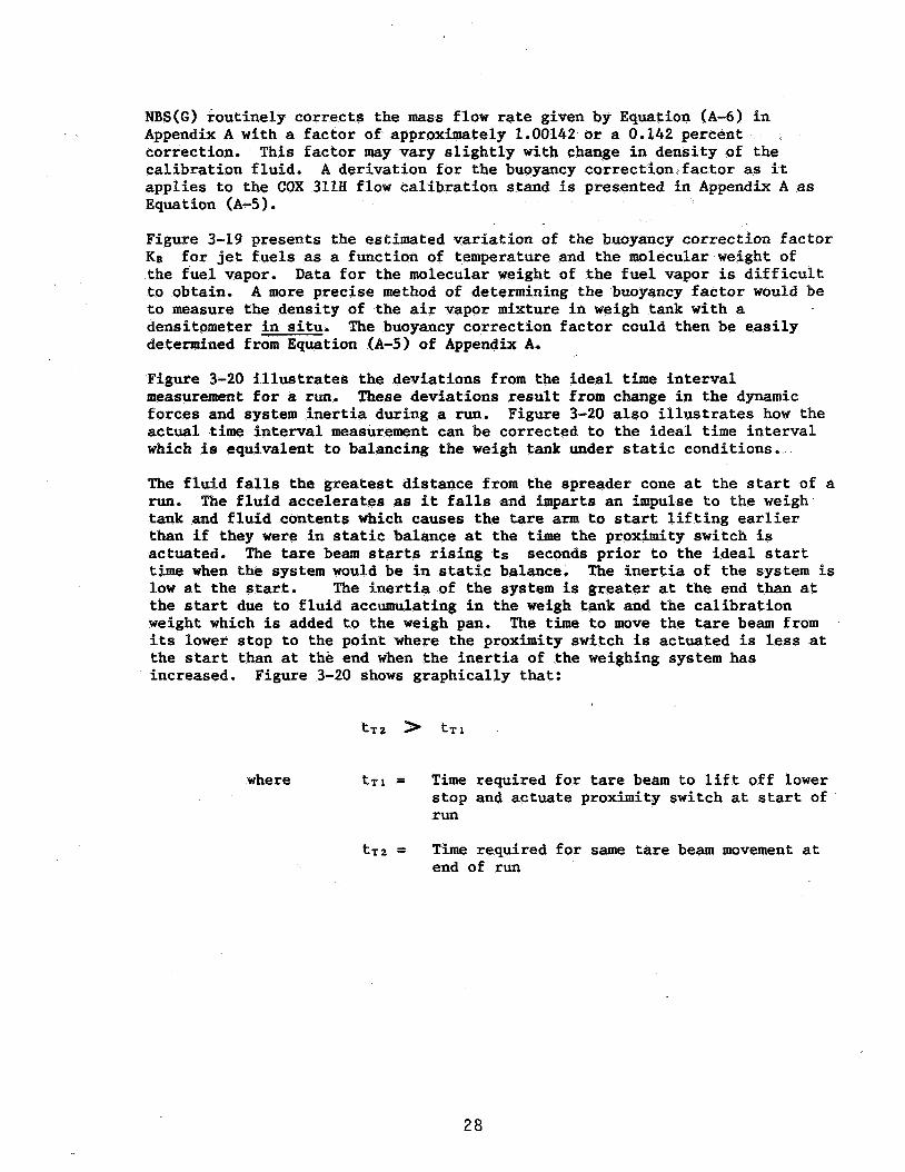
NBS(G) routinely corrects the mass flow rate given by Equation (A-6) in Appendix A with a factor of approximately 1.00142 or a 0,142 percent correction. This factor may vary slightly with change in density of the calibration fluid. applies to the COX 311H flow calibration stand is presented in Appendix A as Equation (A-5).

Figure 3-19 presents the estimated variation of the buoyancy correction factor KB the fuel vapor. to obtain, to measure the density of the air vapor mixture in weigh tank with a densitometer in situ. determined from Equation (A-5) of Appendix A.

Figure 3-20 illustrates the deviations from the ideal time interval measurement for a run. These deviations result from change in the dynamic forces and system inertia during a run. actual time interval measurement can be corrected to the ideal time interval which is equivalent to balancing the weigh tank under static conditions.

A derivation for the buoyancy correction factor as it

for jet fuels as a function of temperature and the molecular weight of Data for the molecular weight of the fuel vapor is difficult

A more precise method of determining the buoyancy factor would be

The buoyancy correction factor could then be easily

Figure 3-20 also illustrates how the

The fluid falls the greatest distance from the spreader cone at the start of a run. tank and fluid contents which causes the tare arm to start lifting earlier than if they were in static balance at the time the proximity switch is actuated, The tare beam starts rising ts seconds prior to the ideal start time when the system would be in static balance. low at the start. the start due to fluid accumulating in the weigh tank and the calibration weight which is added to the weigh pan. its lower stop to the point where the proximity switch is actuated is less at the start than at the end when the inertia of the weighing system has increased.

The fluid accelerates as it Palls and imparts an impulse to the weigh-

The inertia of the system is The inertia of the system is greater at the end than at

The time to move the tare beam from

Figure 3-20 shows graphically that:

where t ~ 1 = Time required for tare beam to lift off lower stop and actuate proximity switch at start of run

tT2 = Time required for same tare beam movement at end of run

28

The fluid does not fall as far before impacting on the surface of t tank bottom at the end of a run as it does at the start of a run. from the velocity of the falling fluid is thus smaller at the end o the tare beam does not start to rise as early, or as shown in Figure 3-20:

ts1 > ts2

where . tsl = Time of start of tare beam movement in advance of ideal (static balance) trip time at start of run

t ~ 2 = Time of start of tare beam movement in advance of ideal (static balance) trip time at end of run

Equation (3-5) assumes that a static balance exists in the dynamic flow calibration system. actuation time should be replaced in Equation (3-5) with the corrected time tc. The corrected time tc is from the start to the end of the run if no fluid momentum or inertia effects existed. shows that the corrected time can be calculated Prom the following equation:

The actual clock time tA between proximity switch

An examination of Figure 3-20

and a timing correction factor KT can be used to correct the flow rate from Equation (3-6) for timing errors where

Equation (3-7) can be rewritten as the following approximation with negligible error:

The timing correction factor will always be greater than unity or KT s l . 0 . The timing error is a function of mass flow rate - the greater the flow rate, the greater the timing error KT.

29

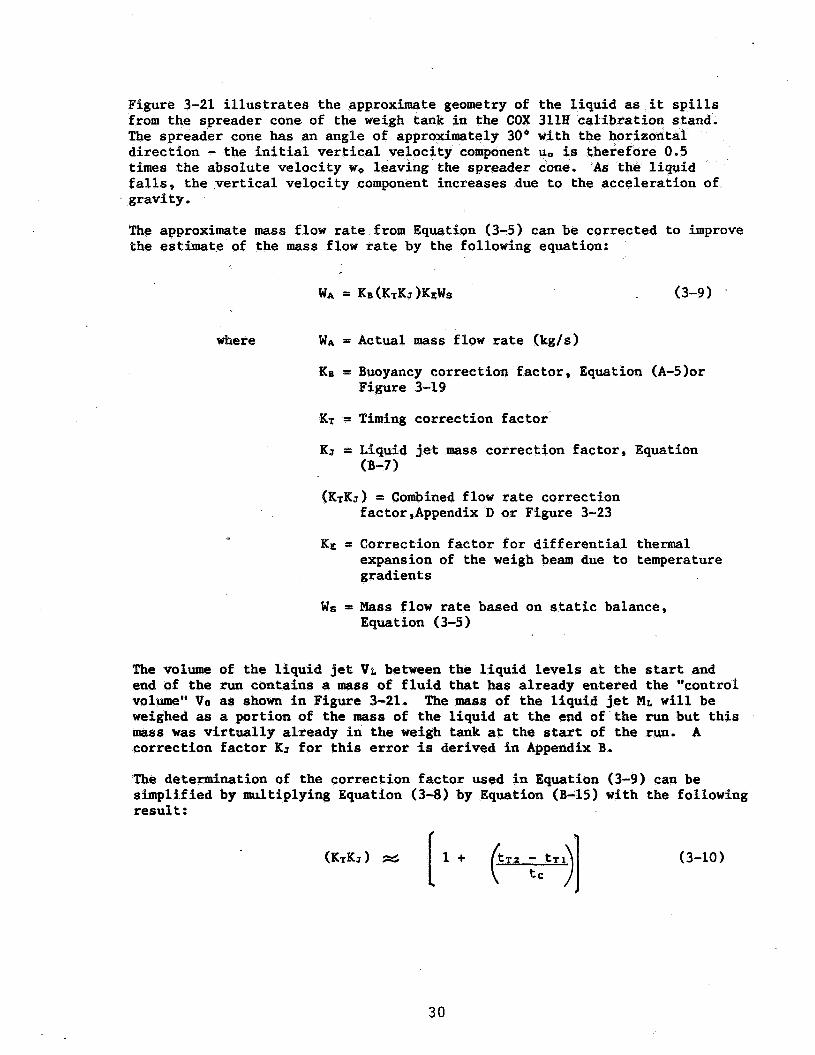
Figure 3-21 illustrates the approximate geometry of the li from the spreader cone.of the weigh tank in the COX 3118 c The spreader cone has an angle of approximat O with t direction - the initial vertical velocity co t uo is times the absolute velocity wo leaving the spreader cone. falls, the vertical velocity component increases due to the acceleration of gravity

The approximate mass flow rate from Equation (3-5) can be corrected to improve the estimate of the mass flow rate by the following equation:

where wA = Actual mass flow rate (kg/s)

KB = Buoyancy correction factor, Equation (A-5)or Figure 3-19

KT = Timing correction factor

KJ = Liquid jet mass correction factor, Equation (B-7 1

(KTKY) = Combined flow rate correction factor,Appendix D or Figure 3-23

KE 3: Correction factor for differential thermal expansion of the weigh beam due to temperature gradients

WS = Mass flow rate based on static balance, Equation (3-5)

The volume of the liquid jet VL between the liquid levels at the start and end of the run contains a mass of fluid that has already entered the "control volume" VO as shown in Figure 3-21. The mass of the liquid jet ML will be weighed as a portion of the mass of the liquid at the end of the run but this mass was virtually already in the weigh tank at the start of the run. correction factor KY for this error is derived in Appendix B.

The determination of the correction factor used in Equation (3-9) can be simplified by multiplying Equation (3-8) by Equation (B-15) with the following result :

A

(3-10 1

30

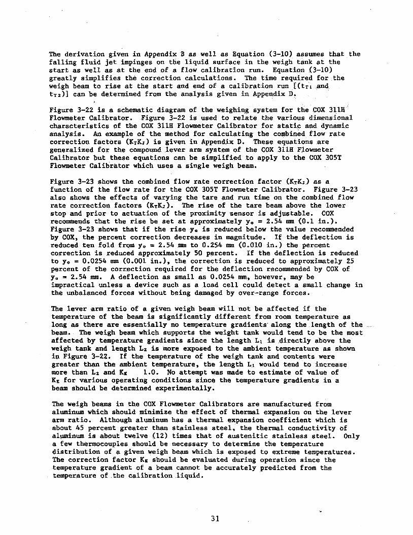
The derivation given in Appendix 3 as well as Equation (3-10) assumes that the falling fluid jet impinges on the liquid surface in the weigh tank at the start as well as at the end of a flow calibration run. Equa greatly simplifies the correction calculations. The time re weigh beam to rise at the start and end of a calibration run [(tTl and t~~)] can be determined from the analysis given in Appendix D.

Figure 3-22 is a schematic diagram of the weighing system for the COX 311H Flowmeter Calibrator. characteristics of the COX 311H Flowmeter Calibrator for static and dynamic analysis. correction factors ( K T K ~ ) is given in Appendix I). These equations are generalized for the compound lever arm system of the COX 31111 Flowmeter Calibrator but these equations can be simplified to apply to the COX 305T Flowmeter Calibrator which uses a single weigh beam.

Figure 3-22 is used to relate the various dimensional

An example of the method for calculating the combined flow rate

Figure 3-23 shows the combined flow rate correction factor (KTKJ) as a function of the flow rate for the COX 305T Flowmeter Calibrator. Figure 3-23 also shows the effects of varying the tare and run time on the combined flow rate correction factors (K,KJ). The rise of the tare beam above the lower stop and prior to actuation of the proximity sensor is adjustable. recommends that the rise be set at approximately yo = 2.54 llpa (0.1 in.). Figure 3-23 shows that if the rise yo is reduced below the value recommended by COX, the percent correction decreases in magnitude. If the deflection is reduced ten fold from yo = 2.54 mm to 0.254 mm (0.010 in.) the percent correction is reduced approximately 50 percent. to yo = 0.0254 mm (0.001 in.), the correction is reduced to approximately 25 percent of the correction required for the deflection recommended by COX of yo = 2.54 mm. impractical unless a device such as a load cell could detect a small change in the unbalanced forces without being damaged by over-range forces.

COX

If the deflection is reduced

A deflection as small as 0.0254 mm, however, may be

The lever arm ratio of a given weigh beam will not be affected if the temperature of the beam is significantly different from room temperature as long as there are essentially no temperature gradients'along the length of the beam. The weigh beam which supports the weight tank would tend to be the most affected by temperature gradients since the length L1 is directly above the weigh tank and length LZ is more exposed to the ambient temperature as shown in Figure 3-22. greater than the ambient temperature, the length LI would tend to increase more than LZ and KE No attempt was made to estimate of value of KE for various operating conditions since the temperature gradients in a beam should be determined experimentally.

If the temperature of the weigh tank and contents were

1.0.

The weigh beams in the COX Flowmeter Calibrators are manufactured from aluminum which should minimize the effect of thermal expansion on the lever arm ratio. Although aluminum has a thermal expansion coefficient which is about 45 percent greater than stainless steel, the thermal conductivity of aluminum is about twelve (12) times that of austenitic stainless steel. a few thermocouples should be necessary to determine the temperature distribution of a given weigh beam which is exposed to extreme temperatures. The correction factor KE should be evaluated during operation since the temperature gradient of a beam cannot be accurately predicted from the temperature of the calibration liquid.

Only

3.6.1.2

Since several correction factors are needed to properly correct the apparent mass flow rate WS based on a static balance to the actual mass flow rate as given by Equation (3-91, it is difficult to achieve an accuracy greater than 0.25 percent using the COX flowmeter calibrators. several things that can be doneg however, to improve the accuracy of the COX flowmeter calibrators as interim calibration facilities.

During the calibration of true mass rate flowmeters, there are possibly two types of readouts: (1) continuous and (2) sequential. devices should be averaged over the same interval of time as for the flow calibration run on the COX Flowmeter Calibrator. Some mass flow rate meters require a finite amount of time for each read out. This type of flow rate meter should be read out sequentially at equal time intervals from the start to the end of a calibration run. The average indicated flow rate during the run can then be found by dividing the sum of the sequential readings by the number of readings during a run.

There are

The continuous readout

During the calibration of volumetric type flowmeters (i.e. turbine flowmeters), the following improvements should be made:

(1) The number of pulses from the output of the turbine flowmeter should be counted for the time interval between the start and end of a run for a COX Flowmeter Calibrator in the determination of the flowmeter calibration constant, KH.

(2) Use a precision densitometer in situ for converting mass flow rate from Equation (3-9) to volumetric flow rate corresponding to the proportional output of the' turbine flowmeter.

(3) Use a viscometer in situ for establishing the correlation between the calibration constant KH and the parameter equal to output frequency divided by kinematic viscosity, f/3 for a turbine flowmeter.

One possible source of error and a cause of lack of repeatability during the calibration of turbine flowmeters is the flow of entrained gas through the flowmeter. prevent air entrainment from causing calibration errors. NEL uses 60 mesh wire screen in the sumps at the pump suction inlets to prevent bubbles from entering the suction lines. NEL also uses a transparent plastic section in the calibration line to visually determine if gas bubbles are approaching a flowmeter being calibrated,

There is some indication that the COX Flowmeter Calibrators are designed such that a pocket of air or fuel vapor can develop in the standpipe at the entrance to the weigh tank. piping after the back pressure control valve and above the spreader cone (see Figures 3-16 and 3-17). changes in flow rate during a calibration run. The repeatability of the COX flowmeter calibrators would thus be affected due to a change in the mass of fluid retained in the standpipe.

Hayward [ll] describes two precautions used at NEL, Glasgow, UK to

This pocket of gas would tend to occur in the

The volume of this gas pocket could vary due to

32

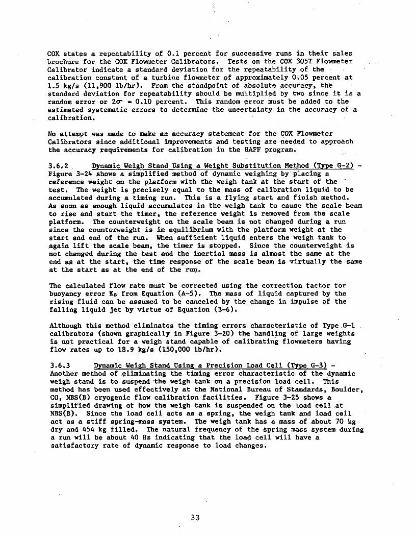
COX states a repeatability of 0.1 percent for successive runs in their sales brochure for the COX Flowmeter Calibrators. Tests on the COX 305T Flowmeter Calibrator indicate a standard deviation for the repeatability of the calibration constant of a turbine flowmeter of approximately 0.05 percent at 1-5 kg/s (11,900 lb/hr). standard deviation for repeatability should be multiplied by two since it is a random error or 2cr = 0.10 percent. This random error must be added to the estimated systematic errors to determine the uncertainty in the accuracy of a calibration.

From the standpoint of absolute accuracy, the

No attempt was made to make an accuracy statement for the COX Flowmeter Calibrators since additional improvements and testing are needed to approach the accuracy requirements for calibration'in the HAFF program.

3-6.2 Figure 3-24 shows a simplified method of dynamic weighing by placing a reference weight on the platform with the weigh tank at the start of the test. accumulated during a timing run. This is a flying start and finish method. As soon as enough liquid accumulates in the weigh tank to cause the scale beam to rise and start the timer, the reference weight is removed from the scale platform. The counterweight on the scale beam is not changed during a run since the counterweight is in equilibrium with the platform weight at the start and end of the run. When sufficient liquid enters the weigh tank to again lift the scale beam, the timer is stopped. not changed during the test and the inertial mass is almost the same at the end as at the start, the time response of the scale beam is virtually the same at the start as at the end of the run.

Dynamic Weigh Stand Using a Weight Substitution Method (Type 6-2) - ~

The weight is precisely equal to the mass of calibration liquid to be

Since the counterweight is

The calculated flow rate must be corrected using the correction factor for buoyancy error KB from Equation (A-5). The mass of liquid captured by the rising fluid can be assumed to be canceled by the change in impulse of the falling liquid jet by virtue of Equation (B-6).

Although this method eliminates the timing errors characteristic of Type G-1 calibrators (shown graphically in Figure 3-20) the handling of large weights is not practical for a weigh stand capable of calibrating flowmeters having flow rates up to 18.9 kg/s (150,000 lb/hr).

3.6.3 Another method of eliminating the timing error characteristic of the dynamic weigh stand is to suspend the weigh tank on a precision load cell. This method has been used effectively at the National Bureau of Standards, Boulder, 60, NBS(B) cryogenic flow calibration facilities. simplified drawing of how the weigh tank is suspended on the load cell at NBS(B). act as a stiff spring-mass system. dry and 454 kg filled. a run will be about 40 Hz indicating that the load cell will have a satisfactory rate of dynamic response to load changes.

Dynamic Weigh Stand Using a Precision Load dell (Type 6-3) -

Figure 3-25 shows a

Since the load cell acts as a spring, the weigh tank and load cell The weigh tank has a mass of about 70 kg

The natural frequency of the spring mass system during

3 3

Figure 3-26 shows a schematic diagram of the complete NBS(B) Cryogenic Flow Research Facility. used to control the flow rate through the flowmeter under test. used to pressurize the cryogenic liquids allowing operation from 0.22 to 0.77 MPa (32 to 112 psia). During a calibration run, the dump valve on the weigh tank is closed and the change in mass of fluid accumulated in the weigh tank is determined from a calibrated load cell having a maximum range of 4450 N (1000 lbt). need for temperature corrections. used to check the load cell calibration in situ. of the NBS(B) facilities are given by Dean, Brennan and Mann [41 and Mann [51.

A centrifugal pump driven by a variable speed motor. is Helium is

The load cell is maintained near room temperature to avoid the Four 113-4 kg (250 lb) brass weights were

More complete description6

Table 3-8 presents an accuracy'statement revised from a table presented by Dean et a1 [a]. The estimated error for mass flow rate measurements is estimated to be 0.18 percent with 0.12 percent from systematic errors and 0.06 percent from random errors. The random error is based on a statistical variation in the standard deviation of Q = 0.02 percent observed during repeated runs. deviation or 3tT = 0.06. calibrate the load cell in situ. percentage of full scale readout. that long calibration run times are necessary to achieve a high weighing accuracy at low flow rates.

The random error was taken as three times the standard

The load cell accuracy is based on a This accuracy was partially achieved by ability to

One disadvantage to using load cells is

3.6.4 Static Weigh Stand Using a Diverter Valve (Type 6-41 - One method of eliminating the dynamic problems associated with the dynamic weigh stands has been to determine the mass of the weigh tank before and after a run under static conditions. shown in Figure 3-27. A flying start and finish is achieved by designing the diverter valve to switch the flow from the sump tank to the weigh tank in a fraction of a second.

This is accomplished by using a diverter valve such as

This method has two bias errors:

(1) A buoyancy error which can be correCted by an estimate using Equation (A-5 )

(2) A differential timing error associated with the increase and decay of the flow rate into the weigh tank at the start and end of a run. on the diverter valve.

This error is minimized by adjusting the proximity switch

Since it takes a finite time for the actuation of the diverter valve, Hayward E111 shows in Figure 3-28 that there is an increase in the flow rate at the beginning and a decay at the end of a calibration run. would be desirable if the diverter valve could be actuated in an infinitesimal time at the start and the end of a run. The flow variation with time would then follow the dotted line EFGH. The actual variation in flow rate with time is the curve ABCD. If the following relationship exists (see Figure 3-28):

Ideally it

34

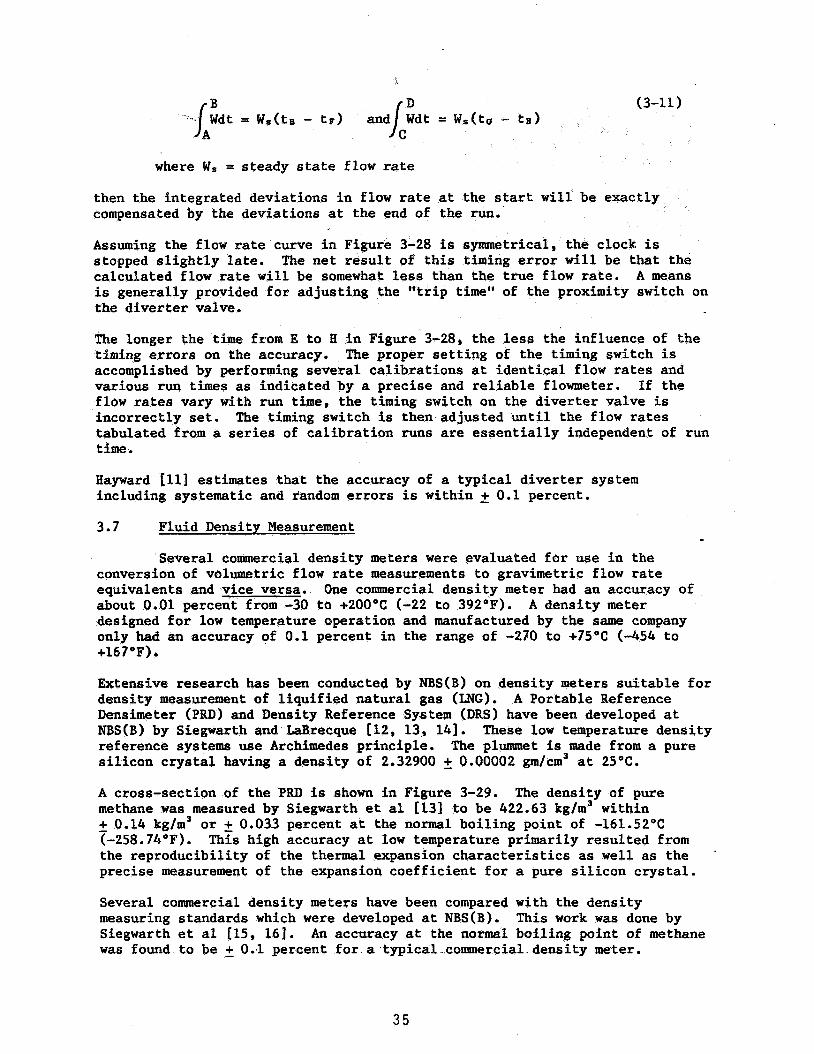
where Ws = steady state flow rate

then the integrated deviations in flow rate at the start will be exactly compensated by the deviations at the end of the run:

Assuming the flow rate curve in Figure 3-28 is symmetrical, the clock is stopped slightly late. The net result of this timing error will be that the calculated flow rate will be somewhat less than the true flow rate. A means is generally provided for adjusting the **trip time" of the proximity switch on the diverter valve,

The longer the time from E to H in Figure 3-28, the less the influence of the timing errors on the accuracy, accomplished by performing several calibrations at identical flow rates and various run times as indicated by a precise and reliable flowmeter. If the flow rates vary with run time, the timing switch on the diverter valve is incorrectly set. The timing switch is then adjusted until the flow rates tabulated from a series of calibration runs are essentially independent of run time .

The proper setting of the timing switch is

Hayward [ll] estimates that the accuracy of a typical diverter system including systematic and tandom errors is within 2 0.1 percent.

3.7 Fluid Density Measurement

-Several commercial density meters were evaluated for use in the conversion of volumetric flow rate measurements to gravimetric flow rate equivalents and vice versa. about 0.01 percent from -30 to +2OO0C (-22 to 392OF). designed for low temperature operation and manufactured by the same company only had an accuracy of 0.1 percent in the range of -270 to +7S°C (-454 to +167OF).

One commercial density meter had an accuracy of A density meter

Extensive research has been conducted by NBS(B) on density meters suitable for density measurement of liquified natural gas (LNG). Densimeter (PRD) and Density Reference System (DRS) have been developed at NBS(B) by Siegwarth and LaBrecque [12, 13, 141. reference systems use Archimedes principle. silicon crystal having a density of 2,32900 2 0.00002 gm/cm3 at 25OC.

A Portable Reference

These low temperature density The plummet is made from a pure

A cross-section of the PRD is shown in Figure 3-29, The density of pure methane was measured by Siegwarth et a1 [131 to be 422.63 kg/m3 within - + 0.14 kg/m3 or 2 0.033 percent at the normal boiling point of -161.52OC (-258.74"F). the reproducibility of the thermal expansion characteristics as well as the . precise measurement of the expansion coefficient for a pure silicon crystal.

This high accuracy at low temperature primarily resulted from

Several commercial density meters have been compared with the density measuring standards which were developed at NBS(B). Siegwarth et a1 [15, 161. An accuracy at the normal boiling point of methane was found to be 5 0.1 percent for a typical.commercial.density meter.

This work was done by

35

3.7.1 Paar Density Meter - The density meter which appeared to have the highest potential accuracy was the Paar Density Meter manufactured by Anton. Paar, Graz, Austria and distributed in the United States by the Mettler Instrument Co, Hightstown, NJ.

Figure 3-30 shows a cross-sectional view of the Paar Density Meter Model 602HT. excitation coil and vane oscillation is sensed by a pickup coil. phase-locked loop oscillator assures that the U-tube oscillates at its natural frequency. envelope is hermetically sealed and contains hydrogen at a pressure of approximately 50 kPa (0.5 bar or 7.25 psia). which permit circulation of a liquid for stabilizing the temperature of the liquid contained in the U-tube. The hermetically sealed jacket around the U-tube gives complete assurance that condensation on the exterior of the tube will not affect the accuracy. The hydrogen within the jacket provides a high thermal conductivity medium for equilibrating the temperatures between the fluid sample and the fluid circulating through the outer jacket.

The magnetic vane attached to the end of the'U-tube is pulsed by an A

The glass U-tube is enclosed in two glass envelopes.. The inner

The outer glass jacket has ports

The period of oscillation of the U-tube can be determined from the.following. fundamental equation from vibration theory:

= 2T7/ Mo Vd

where t = Period of oscillation, sec

(3-12)

M, = Equivalent mass of glass tube and magnetic vane, gm

d = Density of fluid in tube, gm/cm3

v = Volume of capillary, cm3

C = Constant

Solving Equation (3-12) for density and combining the constants gives the following equation:

where C1 and CZ are constants which are determined from calibration

Table 3-10 lists various fluids which can be used to calibrate a density meter. room temperature. be used over a wide temperature range but the density of these hydrocarbon fluids is only known to 5 1.0 kg/m3. This is equivalent to an accuracy of 0.13 percent. and meter calibrated with the Portable Reference Densimeter (PRD) at NBS(B).

The Paar density meter is normally calibrated with water and air at Table 3-10 also lists several hydrocarbon fluids which may

Higher accuracy could be attained by having the density cell

36

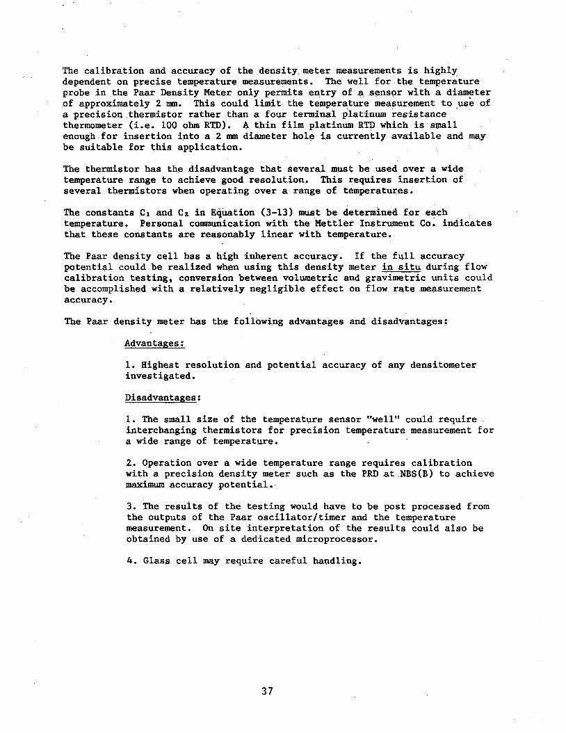
The calibration and accuracy of the density meter measurements is highly dependent on precise temperature measurements. probe in the Paar Density Meter only permits entry of a sensor wit of approximately 2 mm. a precision thermistor rather than a four terminal platinum resistance thermometer (i.e. 100 ohm RTD). enough for insertion into a 2 mm diameter hole is currently available and may be suitable for this application,

The thermistor has the disadvantage that several must be used over a wide temperature range to achieve good resolution. This requires insertion of several thermistors when operating over a range of temperatures.

The constants C1 and C2 in Equation (3-13) must be determined for each temperature. Personal communication with the Mettler Instrument Co. indicates that these constants are reasonably linear with temperature.

The well for the temperature

This could limit the temperature measurement to use of

A thin film platinum RTD which is small

The Paar density cell has a high inherent accuracy. potential could be realized when using this density meter in situ during flow calibration testing, conversion between volumetric and gravimetric units could

If the full accuracy

be accomplished with a accuracy.

The Paar density meter

Advantages:

relatively negligible effect

has the following advantages

on flow rate measurement

and disadvantages:

1. Highest resolution and potential accuracy of any densitometer investigated.

Disadvantages:

1. The small size of the temperature sensor "well" could require interchanging thermistors for precision temperature measurement for a wide range of temperature.

2. Operation over a wide temperature range requires calibration with a precision density meter such as the PRD at NBS(B) to achieve maximum accuracy potential.

3. The results of the testing would have to be post processed from the outputs of the Paar oscillator/timer and the temperature measurement. On site interpretation of the results could also be obtained by use of a dedicated microprocessor.

4. Glass cell may require careful handling.

37

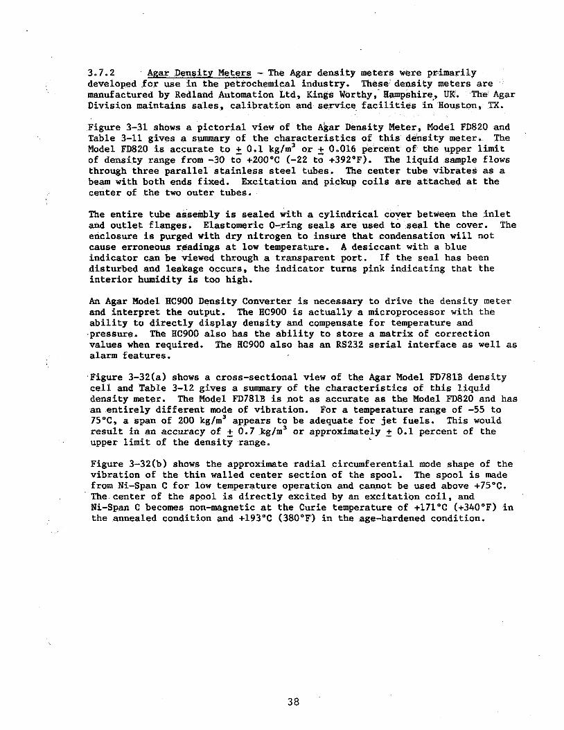
- The Agar density meters we chemical industry. These den

manufactured by Redland Automation Ltd, Kings Worthy,' Hamps Division maintains sales, calibration and service, facilitie

Figure 3-31 shows a pictorial view of the Agar Density Meter, Model FD820 and Table 3-11 gives a summary of the characteristics of this density meter. The Model FD820 is accurate to fi 0.1 kg/m3 or fi 0,016 percent of the upper limit of density range from -30 to +2004C (-22 to +392OF). The liquid sample flows through three parallel stainless steel tubes. The center tube vibrates as a beam with both ends fixed. center of the two outer tubes.

Excitation and pickup coils are attached at the

The entire tube assembly is sealed with a cylindrical cover between the inlet and outlet flanges. enclosure is purged with dry nitrogen to insure that condensation will not cause erroneous readings at low temperature. indicator can be viewed through a transparent port. disturbed and leakage occurs, the indicator turns pink indicating that the interior humidity is too high.

Elastomeric O-ring seals are used to seal the cover. The

A desiccant with a blue If the seal has been

An Agar Model H6900 Density Converter is necessary to drive the density meter and interpret the output. ability to directly display density and compensate for temperature and .pressure. values when required. alarm features.

Figure 3-32(a) shows a cross-sectional view of the Agar Model FD781B density cell and Table 3-12 gives a summary of the characteristics of this liquid density meter. an entirely different mode of vibration. 75"C, a span of 200 kg/m3 appears to be adequate for jet fuels. result in an accuracy of 2 0.7 kg/m3 or approximately fi 0.1 percent of the upper limit of the density range.

The HC900 is actually a microprocessor with the

The HC900 also has the ability to store a matrix of correction The HC900 also has an RS232 serial interface as well as

The Model FD781B is not as accurate as the Model FD820 and has For a temperature range of -55 to

This would

Figure 3-32(b) shows the approximate radial circumferential mode shape of the vibration of the thin walled center section of the spool. The spool is made from Ni-Span C for low temperature operation and cannot be used above +75"C.

Ni-Span C becomes non-magnetic at the Curie temperature of +171"C (+340°F) in the annealed condition and +193OC (380°F) in the age-hardened condition.

. The center of the spool is directly excited by an excitation coil, and

38

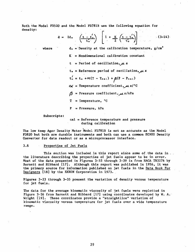
Both the Model FD520 and the Model FD781B use the following equation for densitv:

d = 2d0 (t - t'.) 1 1 + K 1 / t o 1 I '

where do = Density at the calibration temperature, g/cm3

K = Nondimensional calibration constant

t = Period of oscillation,,a s

to = Reference period of osciflation,,us

06 = Temperature coefficient,,as/'C

13 = Pressure coefficient ,/CA s/kPa

T = Temperature, OC

P = Pressure, kPa

Subscripts: cal = Reference temperature and pressure

during calibration

The low temp Agar Density Meter Model FD781B is not as accurate as the Model FD820 but both are durable instruments and both can use a common HC900 Density Converter for data readout or as a microprocessor interface.

3.8 Properties of Jet Fuels

This section was included in this report since some of the data in the literature describing the properties of jet fuels appear to be in error. Most of the data presented in Figures 3-33 through 3-39 is from NACA TN3276 by Barnett and Hibbard 1171. Although this report was published in 1956, it was the primary source for information published on jet fuels in the Data Book For Designers E181 by the EXXON Corporation in 1973.

Figures 3-33 through 3-35 present the variation of density versus temperature for jet fuels.

The data for the average kinematic viscosity of jet fuels were replotted in Figure 3-36 from Barnett and Hibbard [171 using coordinates developed by W. A. Wright [19]. These coordinates provide a "straightline" variation of kinematic viscosity versus temperature for jet fuels over a wide temperature range e

39

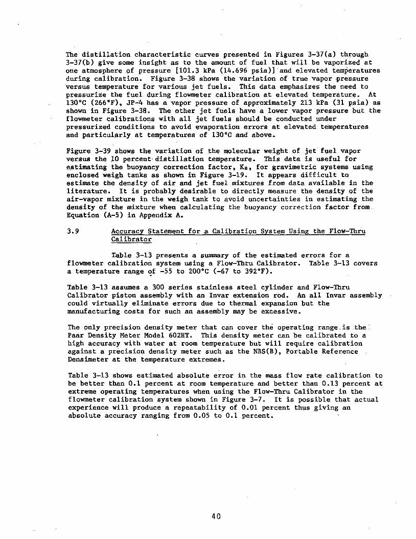
The distillation characteristic curves presented in Figures 3-37(a) through 3-37(b) give some insight as to the amount of fuel that will be vaporized at one atmosphere of pressure [101.3 kPa (14.696 psiall and elevated temperatures during calibration. Figure 3-38 shows the variation of true vapor -pressure versus temperature for various jet fuels. This data emphasizes the need to pressurize the fuel during flowmeter calibration at elevated temperature. 13OoC (266"F), JP-4 has a vapor pressure of approximately 213 kPa (31 psia) as shown in Figure 3-38, The other jet fuels have a lower vapor pressure but the flowmeter calibrations with all jet fuels should be conducted under pressurized conditions to avoid evaporation errors at elevated temperatures and particularly at temperatures of 130°C and above.

At

Figure 3-39 shows the variation of the molecular weight of jet fuel vapor versus the 10 percent-distillation temperature. e,atimating the buoyancy correction factor, KB, for gravimetric systems using enclosed weigh tanks as shown in Figure 3-19. It appears difficult to estimate the density of air and jet fuel mixtures from data available in the literature. It is probably desirable to directly measure the density of the air-vapor mixture in the weigh tank to avoid uncertainties in estimating the density of the mixture when calculating the buoyancy correction factor from. Equation (A-5) in Appendix A.

This data is useful for

3.9 Accuracy Statement for a Calibration System Using the Flow-Thru Calibrator

Table 3-13 presents a summary of the estimated errors for a flowmeter calibration system using a Flow-Thru Calibrator. a temperature range of -55 to 200°C (-67 to 392°F).

Table 3-13 assumes a 300 series stainless steel cylinder and Flow-Thru Calibrator piston assembly with an Invar extension rod. could virtually eliminate errors due to thermal expansion but the manufacturing costs for such an assembly may be excessive.

Table 3-13 covers

An all Invar assembly

The only precision density meter that can cover the operating range is the Paar Density Meter Model 602HT. This density meter can be calibrated to a high accuracy with water at room temperature but will require calibration against a precision density meter such as the NBS(B), Portable Reference Densimeter at the temperature extremes.

Table 3-13 shows estimated absolute error in the mass flow rate calibration to be better than 0.1 percent at room temperature and better than 0.13 percent at extreme operating temperatures when using the Flow-Thru Calibrator in the flowmeter calibration system shown in Figure 3-7. experience will produce a repeatability of 0.01 percent thus giving an absolute accuracy ranging from 0.05 to 0.1 percent.

It is possible that actual

40

3.10 Conclusions and Recommendations

The following conclusions resulted from a study of possible methods of verifying the absolute accuracy of mass flow rate meters being developed under the NASA HAFF program:

(1) that meet the calibration requirements of the NASA HAFF program. The only known planned facility that would have the potential accuracy is dedicated to the NASA Space Shuttle program. Any testing at this facility will use the Flow-Thru Calibrator as a volumetric standard but tests will only be conducted with referee water solutions at ambient temperatures.

(2) 3flH Flowmeter Calibrator) is inadequate to meet the ultimate calibration accuracy requirements for the flowmeters being developed under the NASA-HAFF development program. This facility could be improved, however, on a short term basis until a more precise facility is available. possible without the luxury of coupling the COX 3118 to a Flow-Thru Calibrator. Reproducibility of results is more important than absolute accuracy at the present stage of the development program.

There are no flow rate calibration facilities known at present

The best flow rate calibration facility at GE/AID (the COX

Some necessary improvements are

(3) calibration facilities at GE/AID, are inadequate to meet the accuracy requirements for the NASA-HAFF program for the following reasons: (a) calibration fluid properties may change significantly during a runs at high temperature, (b) the published repeatability of 0.1 percent is normally considered the random error to which other systematic errors must be added to obtain absolute accuracy, (c) it is necessary to estimate and apply several correction factors, which are not customarily used, to improve the absolute accuracy and (d) it is not presently possible to compare the accuracy of dynamic weigh stands to a standard which has a higher accuracy than the dynamic weigh stands at GE/AID.

The dynamic weigh stands, which are used in flow rate

(4) The best approach to acquiring a high accuracy flow rate calibration facility in the least time would be to purchase a Flow-Thru Calibrator and connect the Flow-Thru Calibrator in series with flowmeters under calibration on the COX 311H Flowmeter Calibrator at the Wilmington, MA facility of GE/AID. arrangement would also require the use of a precision density meter, and viscometer as well as precision temperature measurements for adequate data correction and correlation. achieve two important results (a) provide an interim calibration facility and (b) ultimately expand the flow rate calibration facilities by determining the true accuracy capability of the COX 311H Flow Calibrator.

This

This approach would

41

( 5 )

system similar to the system shown in Figure 3-7. This would be used with a Paar Density Meter, calibrated against a NBS(B) PRD, for determination of true mass flow rate.

The ultimate flow calibration facility, wi - state of the art, is to use a Flow-Thru Calibra

The following reconmendations are listed in the approximate order in which they can be accomplished:

(1) Incorporate corrections for buoyancy and timing errors into the procedures for interpretation of the data resulting from COX 311H flow calibration testing.

-(2) Conduct an experimental investigation to determine why the COX 3LlE Flow Calibrator is apparently lacking in reproducibility under certain operating conditions.

(3) required to improve the repeatability and use for Phase I1 testing.

(4) Calibrator in a closed calibration system similar to that shown in Figure 3-7.

Make changes in the COX 311H flow calibration facility as

Plan a flow calibration facility using the Flow-Thru

(5) Procure a Flow-Thru Calibrator.

( 6 )

(7) viscosity measurement.

(8) in a closed-loop calibration facility.

Procure precision equipment for in situ density measurement.

Procure an instrument of adequate accuracy for in situ

Conduct final calibration tests using the Flow-Thru Calibrator

42

3.11

A

C

d'

dA < . \. .i ,

d AT

80

K

KB

K E

KJ

KM

Kl

L

M

m

Nb

P

Q R,

Nomenclature

Cross-sectional area, cm2

Cons tan t

Density, gm/cm3

Density of air

Density of air surrounding brass weights

Density of air surrounding weigh tank

Relative timing error

Output frequency, Hz

Vertical height or head, cm

Local acceleration of gravity, cm/sec2

Standard acceleration of gravity = 980.665 cm/sec2

Calibration constant

Buoyancy correction factor

Correction factor for thermal expansion

Liquid jet mass correction factor

Flowmeter constant, (volume/pulse)

Timing correction factor

Length, cm

Mass, kg

Molecular Weight

Number of passing blades (flow meter pulses)

Pressure, kPa

volume, cm3

Lever arm ratio (overall)

4 3

T

t

tc

ts

tr

U

V

W

WA

ws

W

X

Y

P 9 6

.t/

Temperature, O C

Time, s

Corrected time, s

Start time (weigh beam), s

Tare time (weigh beam), s

Vertical fluid velocity component, cm/s

Vertical velocity of tare beam, cm/s

Mass rate of flow, kg/s

Mass rate of flow (actual)

Mass rate of flow (static balance)

Mean fluid velocity

Distance of tare weight from center of rotation

Vertical displacement of tare beam at weigh pan pivot

Temperature coefficient or coefficient of expansion

Pressure coefficient

Angle

Standard deviation

Kinematic viscosity, mm2/s (centistokes)

44

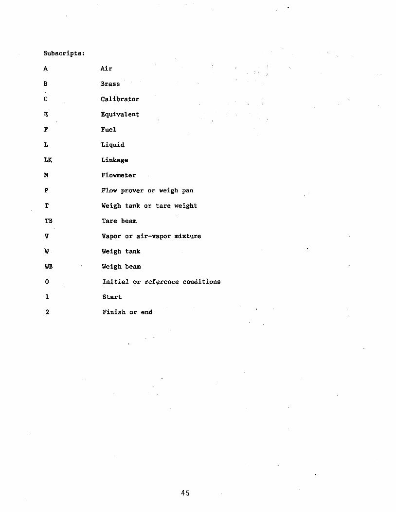
Subscripts:

A

B

C

E

F

L

LK

M

P

T

TB

V

W

WB

0

1

2

Air

Brass

Calibrator

Equivalent

Fuel

Liquid

Linkage

Flowmeter

Flow prover or weigh pan

Weigh tank or tare weight

Tare beam

Vapor or air-vapor mixture

Weigh tank

Weigh beam

Initial or reference conditions

Start

Finish or end

45

3.12 References

1.

2.

3.

4.

5.

6.

7.

8.

9.

10 e

Shafer, M. R. and Ruegg, F. W.: "Liquid-Flowmeter

Trans ASME v. 80, pp. 1369-1379, (1958). Calibration Techniques"

Ruegg, F. W. and Shafer, M. R e : "Flow Measurement: Procedures and Facilities at National Bureau of Standards" , ASERAF, Bulletin, pp. 1-8 (1972).

Olsen, L, 0,: "Introduction to Liquid Flowmetering and Calibration of Liquid Flowmeters", NBS TN-831 (June 1974).

Dean, J. W., Brennan, J. A. and Mann, D. B.: "Cryogenic Flow ReseaTch Facility of the National Bureau of Standards", Advances in Cryogenic Engineering, V. 14, pp. 299-305, Plenum Press, 1969

Mann, D. B.: "Flowmetering Research at NBS",

(NBS Rept R-646), (June 1971). Cryogenics, Voll, n.3, pp. 179-85,

Dean, J. W., Brennan, J. A., Mann, D, B. and Kneebone, C. E.: "Cryogenbc Flow Research Facility Provisional Accuracy Stat emen t 'I, NBS TN 606, July, 1971.

Scott, R. W. We: Flow Measurement Calibration Facilities of the World", NEL Rept 622, Glasgow, Scotland, (Sept. 1976)

Hayward, A. T. J: "Cost-Effectiveness of Liquid Flowmeter Calibration SysteiPs," Flow Measurement of Fluids, pp; 65-75, North-Holland Pub Co (1978).

McIrvin, L. Lo, Gibbs, C. and Jones, F. L.: "Performance Characterisitcs of a Time Volume Flow Calibrator", Flow: Its Measurement and Control in Science and Industry, V.I., pp .679-84, 1974.

Brennan, J. A., Stokes, R. W., Mann, Do B. and Kneebone, C. E.: An Evaluation of Several Cryogenic Turbine Flowmeters", NBS TN 624 (Oct. 1972)

46

11 0

12.

13.

14.

Hayward, A. T. J., "Methods of Calibrating Flowmeters with Liquids", Measurement and Control", V. 10, pp. 106-116, March 1977.

Siegwarth, J. D. and Younglove, B. A,: "Cyrogenic Fluids Density Reference System: Provisional Accuracy Statement," NBS TN698 (R-10631, Nov. 1977

Siegwarth, J. D. and LaBreque, J. F.: "A Portable Densimeter for Use in Cryogenic Liquids," NBS TN1035 (R-12781, March 1981,

Siegwarth, J. D. and LaBreque, J. F.: "Cyrogenic Fluids Density Reference System: Provisional Accuracy Statement (1980) ,'I NBS TN1041 (R-1279) , April 1981.

15.

16.

17.

18.

19

Siegwarth, J. D., Younglove, B. A., and LaBreque, J. F.: "An Evaluation of Commercial Densimeters for Use in LNG", NBS TN697 (R-1064), Oct. 1977.

Siegwarth, J. 1). and LaBreque, J. F.: "Tests of Comercia1 Densimeters for LNG Service", NBS TN 1055, June 1982.

Barnett, H. C. and Hibbard, R. R.: "Properties of Aircraft Fuels", NACA TN 3276, August 1956

Annon: Data Book for Designers, EXXON Corp, Marketing Tech Services, Houston, TX (1973)

Wright, W. A.: "An Improved Viscosity - Temperature Chart for Hydrocarbons", Jour of Materials, V. 4, pp. 19-27, March 1969

47

Section 3.13

TABLES

4%

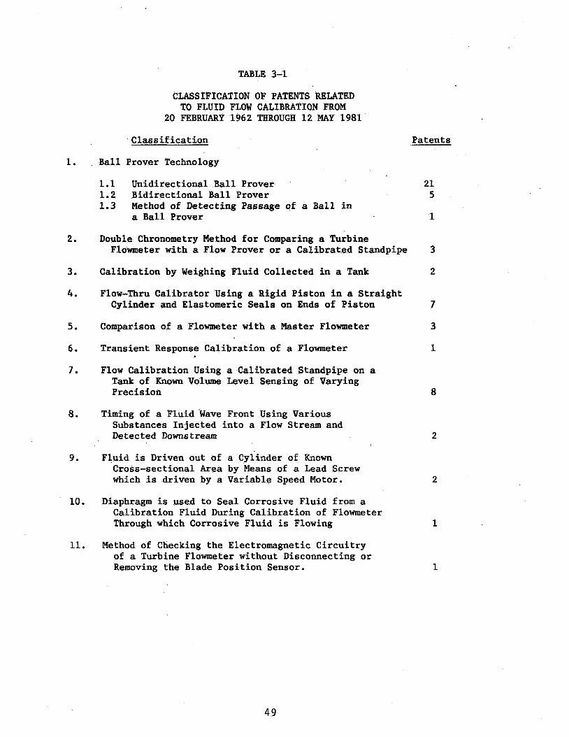
TABLE 3-1

1.

2.

3.

4.

5 .

6.

7.

8.

9 .

10 a

11.

CLASSIFICATION OF PATENTS RELATED TO FLUID FLOW CALIBRATION FROM

20 FEBRUARY 1962 THROUGH 12 MAY 1981

Classification Patents

Ball Prover Technology

1.1 Unidirectional Ball Prover 21 1.2 Bidirectional Ball Prover 5 1.3 Nethod of Detecting Passage of a Ball in

a Ball Prover 1

Double Chronometry Method for Comparing a Turbine Flowmeter with a Flow Prover or a Calibrated Standpipe 3

Calibration by Weighing Fluid Collected in a Tank 2

Flow-Thru Calibrator Using a Rigid Piston in a Straight Cylinder and Elastomeric Seals on Ends of Piston 7

Comparison of a Flowmeter with a Master Flowmeter 3

Transient Response Calibration of a Flowmeter 1

Flow Calibration Using a Calibrated Standpipe on a Tank of Known Volume Level Sensing of Varying Precis ion 8

Timing of a Fluid Wave Front Using Various Substances Injected into a Flow Stream and Detected Downstream

Fluid is Driven out of a Cylinder of Known Cross-sectional Area by Means of a Lead Screw which is driven by a Variable Speed Motor.

Diaphragm is used to Seal Corrosive Fluid from a Calibration Fluid During Calibration of Flowmeter Through which Corrosive Fluid is Flowing

Method of Checking the Electromagnetic Circuitry of a Turbine Flowmeter without Disconnecting or Removing the Blade Position Sensor.

49

D p e V-1:

TABLE 3-2

PRINCIPAL VOLUMETRIC METHODS

SUMNARY OF ADVANTAGES AND DISADVANTAGES OF CALIBRATING LIQUID FLOWMETERS -

I

FLOW-THRU CALIBRATOR

Displacement of fluid with a rigid piston in a honed cylinder with flying start and finish (a separate pump is required to produce flow fluid through a Flow-Thru Calibrator).

Advantages:

A direct and convenient method of calibrating volumetric flowmeterso

Can be used to directly calibrate a mass flowmeter when used in conjunction with a precision densitometer.

One or more fixed displacement volumes resulting from precise movements of the calibrator piston can be traced to NBS by the '*water draw" method of collecting displaced water in vessel having a certified volume.

Highest potential accuracy of any flow calibration system at the present time.

Can be coupled to a dynamic weigh stand (see Type G-1 Table 3-2) for calibration and verification of dynamic timing errors when used with a precision densitometer.

Can be used in a system which is totally sealed to prevent condensed water vapor causing contamination of the calibration fluid at low temperature and to prevent change in compodition of a hydrocarbon fluid at high temperature due to boiloff of light endsa

The only calibration system which has the capability of operating from -55 to 20OOC with virtually no compromise.

High operating pressures are possible. pressurized at a pressure greater than the vapor pressure of the calibration fluid.

Total system can be

A valve incorporated in the prover calibrator allows flowrate, temperature and pressure conditions can be stabilized to steady state prior to a calibration run.

Can be portable if stationary ancillary equipment such as fluid storage, pump valves and filters are available for completing a flow system.

Can be coupled into a fluid system containing an active flowmeter.

50

TABLE 3-2 (Continued)

Type V-1: FLOW-THRU CALIBRATOR (Continued)

(12) Since a proving run lasts only a few seconds at high flowrates there is little time for the steady state conditions to fluctuate and several prover runs can automatically be repeated within 30 to 60 seconds.

(13) Low fire hazard when used in a totally enclosed system.

Disadvantages:

(1) Internal area of cylinder (flow tube) of Flow-Thru Calibrator must be corrected for a difference in temperature between the operating temperature and the temperature at the time of a water draw test. (This is a simple correction).

(2) Stroke of calibrator may have to be corrected for change in temperature as the extension rod which attaches to the calibrator piston comes in contact with fluid in the cylinder. experiences a transient change in temperature but the error is significantly minimized by making the extension rod of INVAR.

The extension rod

Type V-2: BALLISTIC FLOW CALIBRATOR

Fluid is displaced with a rigid piston in a honed cylinder - transient start and finish.

Advantages:

(1) Simple system for calibrating flowmeters with same,accuracy potential as the Flow-Thru Calibrator (Type V-1) described above.

(2) No auxillary pumps or valves are required since Calibrator piston is propelled by an attached air actuated piston.

(3 1 Potentially lower cost installation than the Flow-Thru Calibrator (Type V-1).

Disadvantages:

(1 1 Not very suitable for wide temperature range operation since entire system including the flowmeters and piping would have to be stabilized in a temperature controlled chamber prior to a proving run. .

(2) Transient startup time would not allow sufficient time for certain types of flowmeters to reach steady state ouput prior to the proving run under high flowrate operating conditions. calibrate turbine type flowmeters.

Generally used to

51

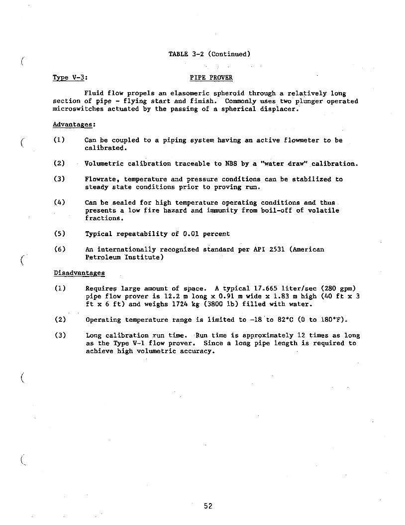
TABLE 3-2 (Continued)

Type V-3: PIPE PROVER

Fluid flow propels an elasomeric spheroid through a relatively long section of pipe - flying start and finish. microswitches actuated by the passing of a spherical displacer.

Commonly uses two plunger operated

Advantages:

(1) ( calibrated.

Can be coupled to a piping system having an active flowmeter to be

(2 1

(3 1

Volumetric calibration traceable to NBS by a "water draw" calibration.

Flowrate, temperature and pressure conditions can be stabilized to steady state conditions prior t o proving run.

(4) Can be sealed for high temperature operating conditions and thus presents a low fire hazard and immunity from boil-off of volatile fractions.

(5 1 Typical repeatability of 0.01 percent

(6 1 An internationally recognized standard per API 2531 (American Petroleum Institute)

Disadvantages

(1) Requires large amount of space. A typical 17.665 literlsec (280 gp) pipe flow prover is 12.2 m long x 0.91 m wide x 1.83 m high (40 ft x 3 ft x 6 ft) and weighs 1724 kg (3800 lb) filled with water.

(2 ) Operating temperature range is limited to -18'to 82°C (0 to 180°F).

( 3 ) Long calibration run time. as the Type V-1 flow prover. achieve high volumetric accuracy.

Run time is approximately 12 times as long Since a long pipe length is required to

i

52

TABLE 3-3 GRAVIMETRIC

PRINCIPAL METHODS OF

SUMMARY OF ADVANTAGES AND DISADVANTAGES CALIBRATING LIQUID FLOWMETERS -

Type G-1: DYNAMIC WEIGH STAND (WEIGH BEAM BALANCE)

Dynamic weighing using weigh beam for balancing weigh tank with flying start and finish. fluid in weigh tank.

Small weights can be used to determine change in mass of

Advantages:

(1)

(2)

A direct and convenient method of calibrating mass flowmeters.

Reasonable degree of sealing of hydrocarbon fluids against contamination from water condensation at low temperature and boiloff at high temperature.

(3 1 Vapor in weigh tank is transferred to sump tank during a run. of air-hydrocarbon vapor can thus be more accurately determined for buoyancy corrections.

Density

(4) Flowrate, temperature and presure conditions can reach steady state prior to a calibration run.

Disadvantages:

(1) Timing errors become significant at moderate and high flowrates since mass of weighing system changes during run. this error but is not usually done due to complexity of error determination.

Data can be corrected for

(2) Sealing is not perfect - methanol must be added to hydrocarbon at very low temp and fluid density will change at high temperature due to boiloff of light fractions.

(3) Correction for density required if a volumetric flowmeter (i.e. turbine flowmeter) is being calibrated.

(4 1 Methanol must be added to hyrodrocarbon fuels for operation from 0 to -55OC to prevent icing of piping from condensed water vapor.

5 3

TABLE 3-3 (Continued)

Type G-2: DYNAMIC WEIGH STAND (WEIGHT SUBSTITUTION)

Dynamic weighing by direct weight substitution on weigh stand and with flying start and finish.

Advantages:

(1) No timing errors due to change since mass of weigh tank and contents are same at start and finish.

Disadvantages:

(1) Only suitable for small flowrates since weight removed from Eank platform must equal weight of fluid accumulated.

Type (2-3: DYNAMIC WEIGHING STAND (PRECISION LOAD CELL)

Dynamic weighing using load cell to determine changes in weight of weigh stand and with flying start and finish.

Advantages:

(1) Tightly sealed system can be used (method has been used for cryogenic flow calibration at very low temperatures).

Dynamic errors are not reduced compared with Type G-1 since suspension of tank on a load cell produces a stiff spring-mass system, thus reducing total deflection during a run.

(2)

Disadvantages:

(1) Inert gas such as helium used to pressurize vapor spaces to control system pressure results in some inaccuracy in estimating density of helium-vapor mixture for buoyancy correction.

Low weighing accuracy compared with beam balance method (typical accuracy is 0.1 percent of rated output) and accuracy is also reduced if nearly full range of load cell is not utilized.

Flexible piping or bellows connections needed for complete sealing - such piping may produce weighing errors when pressurized.

(21

(3)

(4) Weights for-calibration must be sealed within enclosure and suspended during a run for maximum calibration accuracy.

54

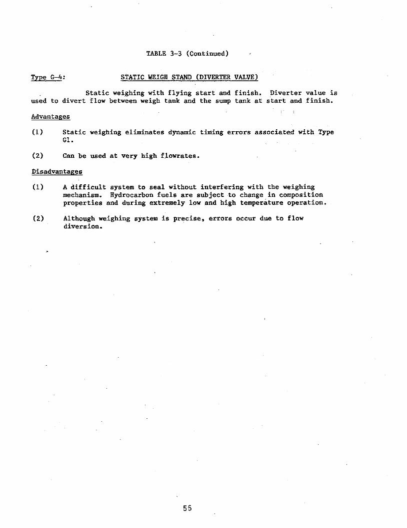
Type 6-4:

TABLE 3-3 (Continued)

STATIC WEIGH STAND (DIVERTER VALVE)

Static weighing with flying start and finish. Diverter value is used to divert flow between weigh tank and the sump tank at start and finish.

Advantages

(1 1 Static weighing eliminates dynamic timing errors associated with Type G1.

(2) Can be used at very high flowrates.

Disadvantages

(1) A difficult system to seal without interfering with the weighing mechanism. properties and during extremely low and high temperature operation.

Hydrocarbon fuels are subject to change in composition

(2) Although weighing system is precise, errors occur due to flow diversion.

55

TABLE 3-4

TYPICAL CHARACTERISTICS OF AN 8 INCH FLOW-THRU CALIBRATOR

Cylinder (Flow Tube) Length (Approx) 1.22 m (48 in.)

Metered displacement length 74.9 cm (29.5 in.)

Inside diameter (Nom) 17.9 m (7.060 in.)

Pneumatic/Hydraulic Actuator Piston

Actuator Rod Diameter

5.08 cm (2.00 in diam)

2.54 cm (1.00 in.)

Extension Rod Diameter 1.27 cm (0.50 in.)

Calibrator Displacement 18,927 cm3 (5.00 gal)

Minimurn flow rate

Maximum flow rate

Standard flow tube (cylinder)

( Optional flow tube

Pressure drop (Piston only)

15.77 cm3/s (.25 gpm) 0.0121 kg/s (96 lbm/hr)*

15,770 cm3/s (250 gpm) 12.13 kg/s (96,250 lbm/hr)*

Carbon steel with electroless nickel plating

304 stainless steel with chrome plating

0.25 to .75 kPa (0.036 to 0.108 psid) diff

Pressure Drop (Between inlet and outlet flanges at max. flow) 69 kPa (10 psid)

Calibrator Piston Seals

Calibrator Piston (Riders) or Glide Rings bearing

Spring loaded TFE U-cup (OMNI- SEAL^ )

RULONR (glass filled) (TFE)

Operating Pressures (Maximum) ' 9*9 MPa (1440 psig)

Operating Temperatures Standard -29 to 93'6 (-20 to +200° F) Optional -129 to 204'C (-200 to +400° F)

Repeatability 0.02 percent

*Based on fluid density = 0.77 gm/cm3

56

TABLE 3-5

TYPICAL CALIBRATION RUN TIME FOR AN 8 IN. FLOW-THRU CALIBRATOR WITH VARIOUS DISPLACEMENT LENGTHS

DISPLACEMENT LENGTH AND VOLUMES 15.0 cm 300 cm 75 cm (5.9 in . ) (11.8 i n . ) (29.5 in . )

VOLUMETRIC FLOW RATE MASS FLOWRATE 3788 cm3 7571 cm3 18,927 cm3 cm3/s (gpm) kg/s (1bJhr) (1 gal) (2 gal) (5 gal)

~ -~ ~

15.8 (0.25) 0.012 (96) (4 min) (8 min) (20.0 min)

63.1 (1.00) 0.048 (385) 60 sec (2 min) (5.0 min)

126.2 (2) 0.097 (770) 30 160 sec. (2.5 min)

315.5 (5) 0.243 (1925) 12 24 60 sec

631 (10) 0.485 (3850) 6 12 30

1,262 (20) 0.97 (7700) 3 6 15

3,155 (50) 2.245 (19250) 1.2 2.4 6

6,309 (100) 4.85 (38500) 1.2 3

12,618 (200) 9.70 (77000) 1.5

15,772 (250) 12.13 (96250) 1.2

*Based on a fluid density = 0.77 gm/cm3

57

i

Overall Dimensions

TABLE 3-6

PHYSICAL CHARACTERISTICS OF TYPICAL PIPE PROVER

Volumetric Flowrate (Max)

Operating Temperature Range

Pipe Size (6 in. Sch 40)

(

Pipe Displacement Length

Volumetric Displacement

Run Time for a Flowrate of 63 x m3/s

Elastomeric sphere material

Dimensions of Spherical Piston

1.83 x 0.91 (6 x 3 x 40

x 1 2 m ( H x W x L ) ft)

18 x m3/s (280 gpm)

-18 to +82OC (0 to +l8O0F)

16.83 X 15.40 cm (6.625 X 6.065 in.)

18.3 m (60 ft)

0.341 m3 (90 gal)

5400 (90 min)

Buna-N (Nitrile) or Polyurethane Rubber 0

15.2 cm OD x 5.1 cm wall (6.0 in. OD x 2 in. wall)

58

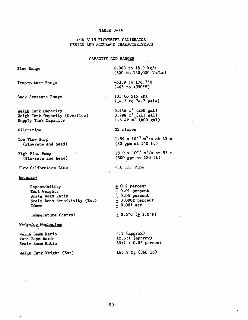
TABLE 3-7A

Flow Range

Temperature Range

Back Pressure Range

COX 311B FLOWMETER CALIBRATOR DESIGN ANI) ACCURACY CHARACTERISTICS

CAPACITY AND RANGES

Weigh Tank Capacity Weigh Tank Capacity (Overflow) Supply Tank Capacity

Filtration

Low Flow Pump (Flowrate and head)

Bigh Flow Pump (Flowrate and head)

Flow Calibration Line

Accuracy

Repeatability Test Weights Scale Beam Ratio Scale Beam Sensitivity (Est) Timer

Temperature Control

Weighing Mechanism

Weigh Beam Ratio Tare Beam Ratio Scale Beam Ratio

Weigh Tank Weight ( E s t )

0.063 to 18.9 kg/s (500 to 150,000 lb/hr)

-53.9 to 176.7OC (-65 to +350°F)

101 to 515 kPa (14.7 to 74.7 psia)

0.946 m3 (250 gal) 0.798 m3 (211 gal) 1.5142 m3 (400 gal)

25 micron

1.89 x (30 gpm at 140 ft)

18.9 x l W 3 m3/s at 55 m (300 gpm at 180 ft)

m3/s at 43 m

4.0 in. Pipe

+ 0.2 percent + 0.01 percent + 0.03 percent + 0.0002 percent + 0.001 sec

+ 0.6OC (2 l.O°F)

- - - - - -

4:l (approx) 12 e 5 : 1 (approx) 50:l 2 0.03 percent

166.9 kg (368 lb)

59

TABLE 3-7B

COX 305T FLOWMETER CALIBRATOR DESIGN AND ACCURACY CHARACTERISTICS

Flow Range

Temperature Range

Back Pressure Range

Weigh Tank Capacity (Usable) Supply Tank Capacity

CAPACITY AND OPERATING RANGES

Filtration

Circulating Pump (Flowrate and Head)

Accuracy

Repeatability Test Weights Scale Beam Ratio Scale Beam Sensitivity (Est) T ~ E K

Temperature Control

Weighing Mechanism

Weigh Beam Ratio

0.189 to 113 kg/s (25 to 15,000 lb/hr)

-53.9 to 176.7"C (-65 to +350°F)

101 to 515 kPa (14.7 to 74.7 psia)

0.114 m3 (30 gal) 0.170 m3 (45 gal)

10 microns

3.785 x (60 gpm at 160 ft)

m3/s at 49 m

- + 0.2 percent - + 0.01 percent - + 0.03 percent - + 0.0002 percent - + 0.001 sec

- + 0.6OC (2 l.O°F)

60

5:l 2 0,03 percent

TABLE 3-8

SUMMARY OF ESTIMATED ERRORS FOR CRYOGENIC FLOW RESEARCH FACILITY 161

NATIONAL BUREAU OF STANDARDS CRYOGENICS DIVISION, BOULDER, CO

A. MASS FLOWRATE MEASUREMENTS

Source of Error Relative Error

Estimated From (Percent)

1.0 Calibration weights Calibration . 2.0 Load Cell

2.1 Non-linearity Manufacturer 61 Measurement

2.2 Calibration Measurement 2.3 Temperature (Operates at

design temp.) 3.0 Buoyancy

0.01

0.05 0.02

0.00

3.1 Helium-Nitrogen

3.2 Diffuser suspended Vapor Density Est (Density error) 0.10

in liquid Est (Density error) 0.03 4.0 Reaction Forces Est from dynamics 0.01 5.0 Impact Forces Designed to be zero 0.00 6.0 Systematic Error Quadrature* 0.12

0.06 7.0 Random Error ( 3 6 ) Estimated - Mass Flowrate Sum of Estimates 0.18

8.0 Estimated Error of

B. ESTIMATES OF DENSITY

Source of Error Relative Error

Estimated From (Percent)

1.0 Equation of State for Liquid Nitrogen Strobridge (1962) 0.39

2.0 Temperature Measurement Calibration to 5 0.05'K 0.03

0.00 4.0 Pressure Effects Calibration 3.0 Thermometry Circuit Calibration 0.01

- 5.0 Systematic Error Quadrature* Oi39

6.0 Summation with Item A.6.0 Quadrature* 0.41 0.06

8.0 Estimated Error of Volumetric Flow Sum of Estimates 0.47

7.0 Random Error ( 3 a ) Estimated -

* Square root of sum of the squares of systematic.errors.

61

TABLE 3-9

Manufacturer:

US Distributor:

CHARACTERISTICS OF THE PAAR DENSITY METER

Anton Paar K.G. Graz, Austria

Mettler Instrument Co. Hightstown, NJ

Type : Vibrating Glass U-Tube

Glass U-Tube: Material Tube Size Cantilever Length Internal Volume Tube Length

Glass Thermistor Well: Thermistor Size (mx) Density Cell Model

Duran (Borosilicate) Glass 20 mm OD x 2 mm ID 7.4 cm 0.7 cm3 22 cm

2.3 ~ I U ID x 100 mm long 2 mm diameter DMA602HT

Temperature Range . -160 to +150"C (-256 to 392°F)

Pressure Range 0 to 100 kPa (0 to 145 psia)

+ 0.5 gm/cm3 Range - Accuracy (Note A) - + O.OOOI gm/cm3

+ 0. 00000 1 ' gm/ cm3 Resolution - Physical Properties of Duran Glass:

Dens i ty 2.23 gm/cm3 Modulus of Elasticity Poissons s Ratio at 20°C 0.22

67.8 GPa (9.8 X 10' psia)

Tensile Strength (Safety Factor = 5) Fire-bright Surface Cut Surface

Coefficient of Expansion (20°C to 3OOOC)

Resistance to sudden change in temperature (DIN 52325) 250°C (482°F)

Thermal Conductivity 1,168 W/m-OK Specific Heat at 20°C 0.18 cal/gm"K Glass Transition Temp 530°C (986°F)

7.8 MPa (11,400 psia) 3.9 MPa ( 5,700 psia)

3.2 I 10-6/0C

NOTES: A. Higher accuracies obtainable depending on range and environmental conditions

62

TABLE 3-10

Fluid

Water

Hexane, C6H14

Heptane, C7H16 -

Toluene, C7H8

Chlorobenzene C6HsCl

Chinoline, CsR7N

Aniline, C6H7

Nonane, CsHzo

SUMMARY OF FLUIDS SUITABLE FOR

DENSITY METER CALIBRATION [A]

Temp. Range Resolution gm/cm3

0 to 40°C 1 x [B] (32 to 104°F)

-100 to +60°C 1 x 1 0 - ~ [CI (-148 t o 140°F)

-90 to +70°C 1 [CI (-130 to 158'F)

+14 to +llO°C 1 x 10-~ [CI (57 to 230'F)

+13 to +132"C 1 x 10-~ [CI (55 to 270°F)

0 to +15OoC 1 1 0 - ~ [CI

+20 to +15OoC 1 1 0 - ~ [CI

(32 to 302°F)

(68 to 302°F)

Proposed low temperature calibrated fluid

Ne, Ar -100 to +150°C 1 x [D] (-148 to 302°F)

Data from Density Seminar, Dr. H. Heimel, Institute for Measuring Technique, Research Center, Graz, Austria (Sept. 1981)

Water is the only officially authorized substance for calibration of the Paar density meter.

Landolt-Bornstein, Numerical Data and Functional Relationships in Science and Technology, New Series Group IV, Vol I, Part A (1974)

Wagenbreth, H. and Blanke, W., Physikalisch Technische Bundesanstalt-Mitteilungen, Braunschweig, Germany, 6/71, 412

63

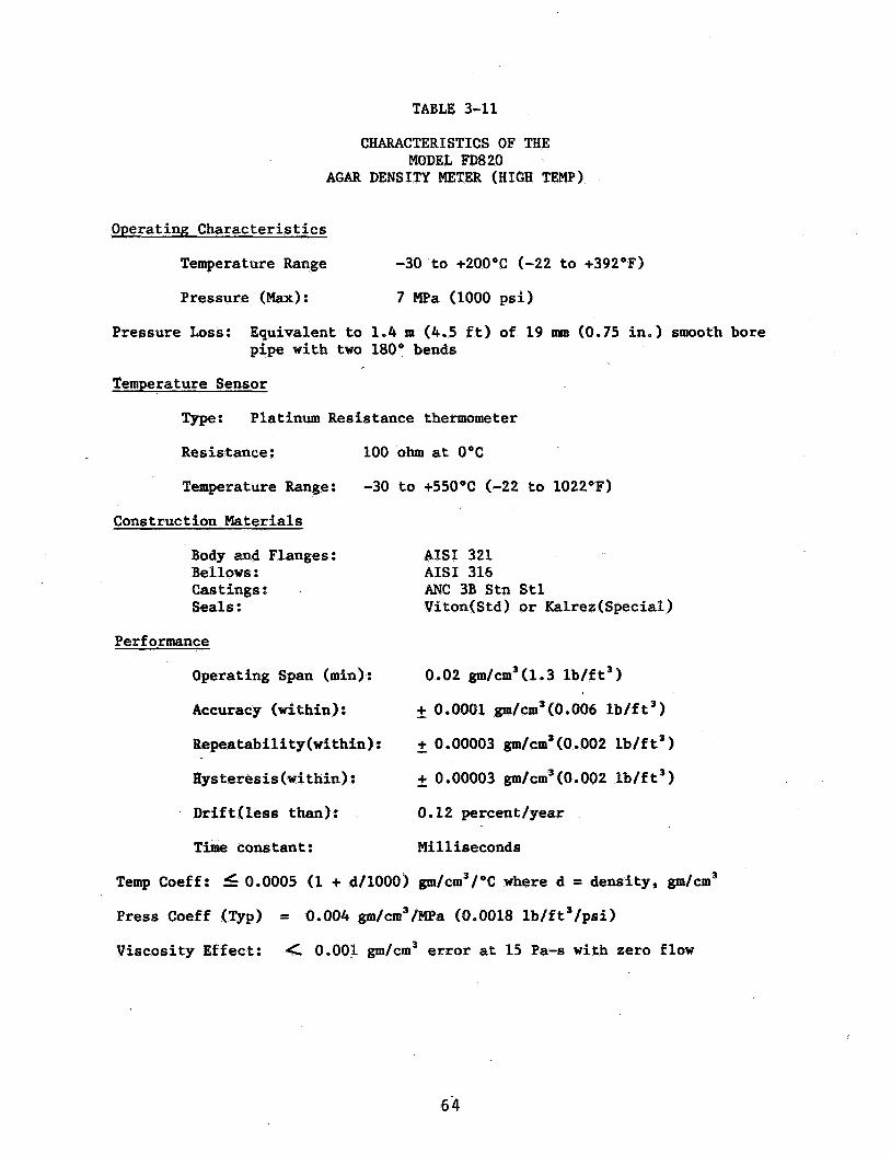
TABLE 3-11

CHARACTERISTICS OF THE MODEL FD820

AGAR DENSITY METER (HIGH TEMP)

Operating Characteristics

Temperature Range -30 to +2OO0C (-22 to +392*F)

Pressure (Max) : 7 !@a (1000 psi)

Pressure Loss: Equivalent to 1.4 m (4.5 ft) of 19 mm (0.75 in.) smooth bore pipe with two 1800 bends

Temperature Sensor

Type: Platinum Resistance thermometer

Resistance: 100 ohm at O°C

Temperature Range: -30 to +550°C (-22 to 1022OF)

Construction Materials

Body and Flanges: AISI 321 Bellows : AISI 316 Castings : Seals : Viton(Std) or Kalrez(Specia1)

ANC 3B Stn Stl

Perf o.rmance

Operating Span (min): 0.02 gm/cm3(l.3 lb/ft3)

Accuracy (within) :

Wepeatability(within):

Hysteresis (within) :

Drift(1ess than): 0.12 percent/year

- -I- 0.0001 gm/cm3(0.006 lb/ft3)

- + 0.00003 gm/cm3 (0.002 lb/f t"

- + 0.00003 gm/cm3(0.002 lb/ft3)

Time constant: Milliseconds

Temp Coeff: 5 0.0005 (1 + d/1000) gm/cm3/OC where d 3: density, gm/cm3 Press Coeff (Typ) = 0.004 gm/cm3/MPa (0.0018 lb/ft3/psi)

Viscosity Effect: 0.001 gm/cm3 error at 15 Pa-s with zero flow

64

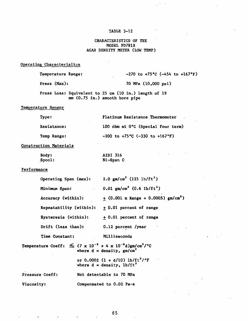
TABLE 3-12

CHARACTERISTICS OF THE MODEL FD781B

AGAR DENSITY METER (LOW TEMP)

Operating Characterisitcs

Temperature Range: -270 to +75"C (-454 to +167"F)

Press (Max):

Press Loss: Equivalent to 25 em (10 in.) length of 19 mm (0.75 in.) smooth bore pipe

70 MPa (10,000 psi)

Temperature Sensor

Type :

Resistance:

Temp Range:

Construction Materials

Body: .Spool:

Performance

Operating Span (max):

Minimum Span:

Accuracy (within):

Repeatability (within):

Hysteresis (within):

Drift (less t'han) :

Time Constant:

Platinum Resistance Thermometer

100 ohm at 0°C (Special four term)

-200 to +75"C (-330 to +167"F)

AIS1 316 Ni-Span C

2.0 gm/cm3 (125 lb/ft3)

0.01 gm/cm3 (0.6 lb/ft3)

- + (0,001 x Range + 0.0005) gm/crn5)

+ 0.01 percent of range

- + 0.01 percent of range

0.12 percent /year

Milliseconds

Pkessure Coeff :

Viscosity:

Temperature Coeff : (7 x + 4 x lO-'d)gm/~m~/~C where d = density, gm/cm3

or 0.0002 (1 + d/lO) 1b/ft3/'F where d = density, lb/ft3

Not detectable to 70 MPa

Compensated to 0-02 Pa-s

65

TABLE 3-13

FOR A FLOW-TBRU CALIBRATOR IN A FLOWRATE CALIBRATION SYSTEM

SUMMARY OF ESTIMATED ERRORS (PER CENT)

TEMPERATURE, O C (OF)

-55 20 130 200 SYSTEMATIC ERRORS (-67) - (68 1 (266 1 (392)

Flow Prover Volume 0.03 0.03 0.03 0.03

NBS Volumetric Certification

Displacement Volume Corr [a1

0.01 0.01 0.01 0.01

0.042 0.0155 0 0.025

Temperature [bl 0.007 0.007 0.007 0.007

Density O.O5[cl O.OOlS[d] O.O5[cl O.O5[cl

Systematic Errors [e] 0.062 0.032 0.065 0.073

RANDOM ERRORS

Position.Sensor Error [f] 0.002 0.002 0.002 0.002

Timing Error [g] 0.0003 0.0003 0.0003 0.0003

0.06

Random Errors [e] Oh06 0.q6 0.06 0.06

- 0.06 - 0.06 Run Reproducibility (2C){h] - 0.06 -

Uncertainty of Flowrate Calibration [i] 0.122 0.092 0.125 0 ,. 133

.. NOTES :

[a] 300 series Stn Stl Cylinder with Invar'Ext Rod [Figure 3- 101 [b] 2 0.05OC Uncertainty in Temperature (Flow Prover to Flowmeter

[c] Paar Densimeter calibrated with PRD, NBS(B) [dl Paar Densimeter calibrated with Distilled Water [e] Quadrature Surmnation [Square Root of Sum of Squares] [f] 2 0.0076 mm (2 0.0003 in.) per Position Sensor in 75 cm

Lg]

[h] Estimated [i]

and Densitometer to Flowmeter)

(29.5 in.) ~f: 0.00001 sec per Position Sensor in 6 sec at 146 kg/s (19250 lb/hr)

Algebraic sum of Systematic and.Random Errors

66

Section 3.14

FIGURES

67

n a W

rl I M

I

0 > I

68

LL 0

I ry 0

4 I M w ry a 63

69

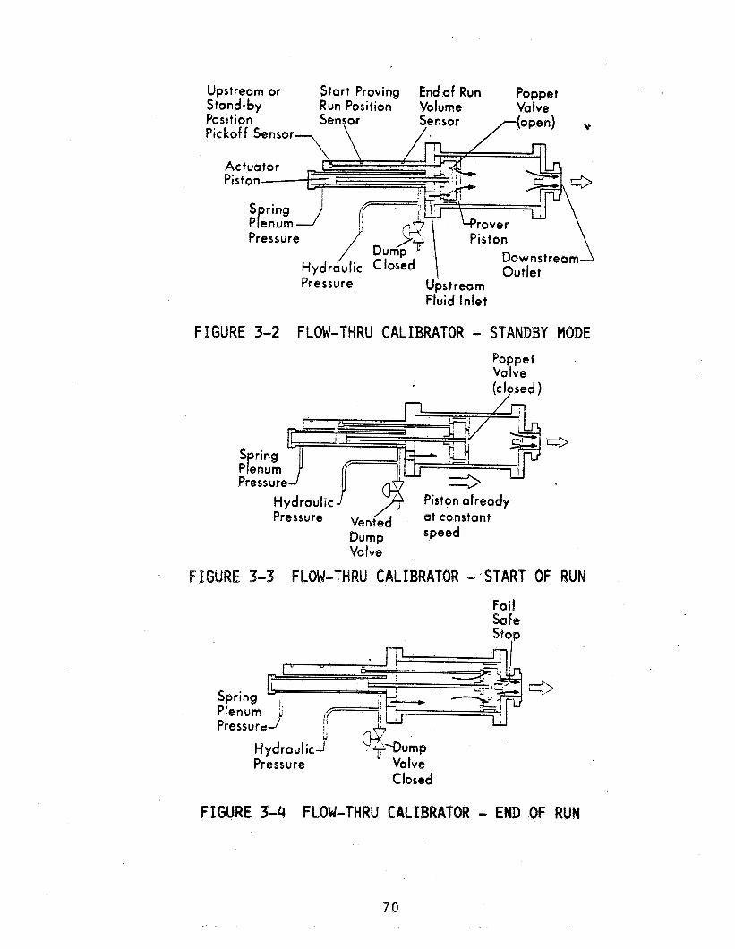
Upstream or Start Proving Endof Run Poppet Stand- by Run Position Volume Va b e

Fluid Inlet

F IGURE 3-2 FLOW-THRU CALIBRATOR - STANDBY MODE Boppst va Ive

at constant

Valve

FIGURE 3-3 FLOW-THRU ~ A L ~ ~ R A T O R - 'START OF RUN

Foil Sa !e

PF ess u re Closed

FIGURE 3-4 FLOW-YHRU CALIBRATOR - END OF RUN

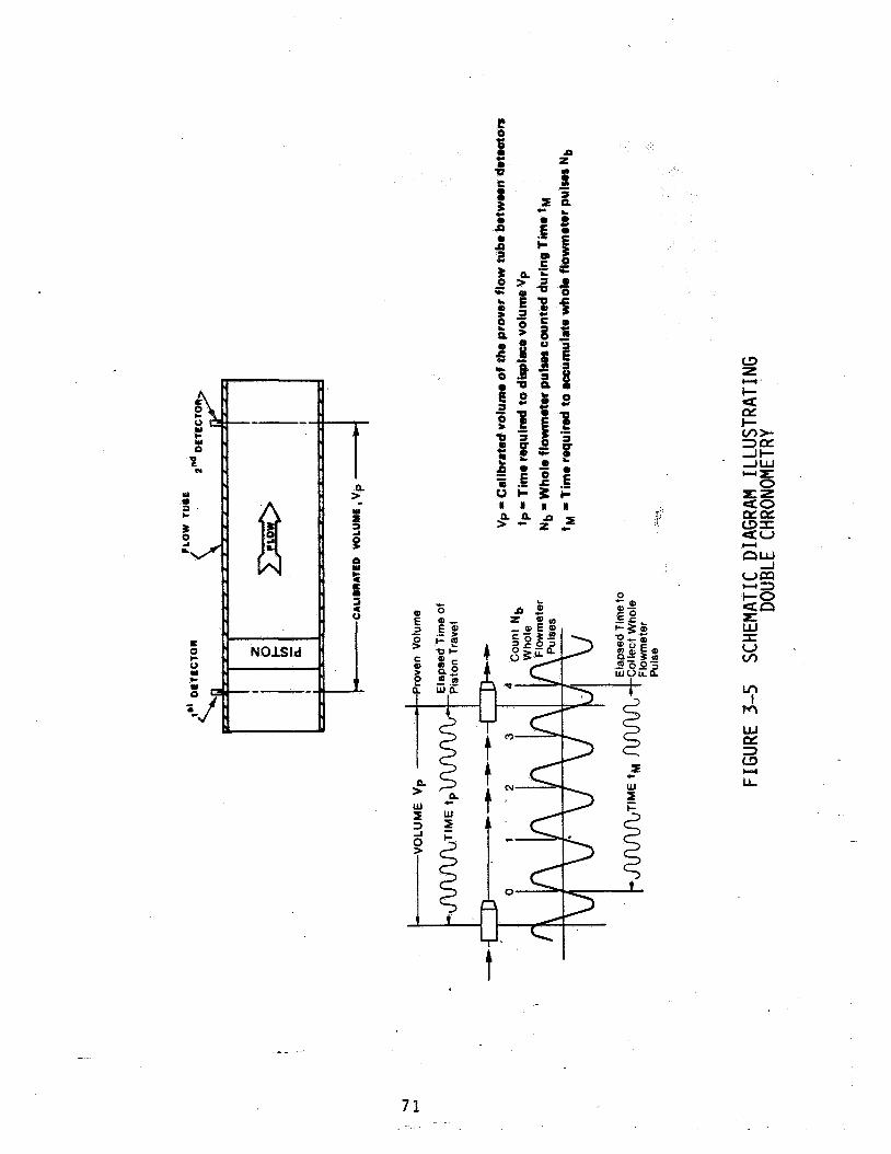
0

VI I M

7 1

W D n

a a w w + I -

z

73

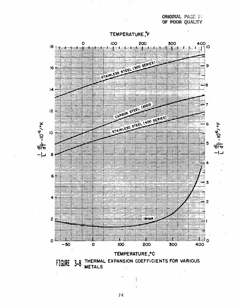
M 0 \

(D t

i- U

J

12

IO

8

E

4

2

n

TEMPERATURE ,OF

18

16

14

7

6

5

4

t

3

2

I

n W

-50 0 108 280 300 Y

400

LL 0

L

TEMPERATURE ,*C THERMAL EXPANSION COEFFI CtENTS FOR VARIOUS ~I~R~ 3-8 METALS

i

74

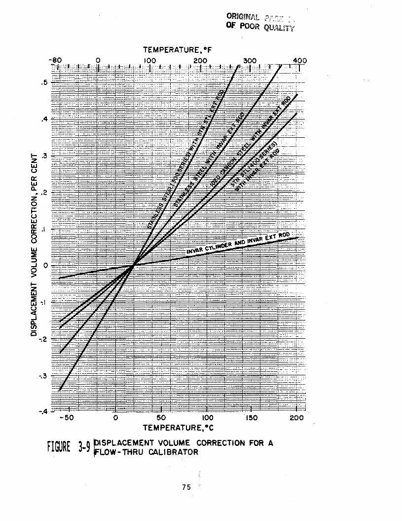
.5

.4

a n W

z 0

* .2

i= 0 W

. I 8 rw 3 0 P

-. 3

e-4 - 50 0 50 100 T&MPERATURE,OC

I50 200

ISPLACEMENT VOLUME CORRECTION FOR A FIGURE 3-9 p LOW-THRU CALIBRATOR

75

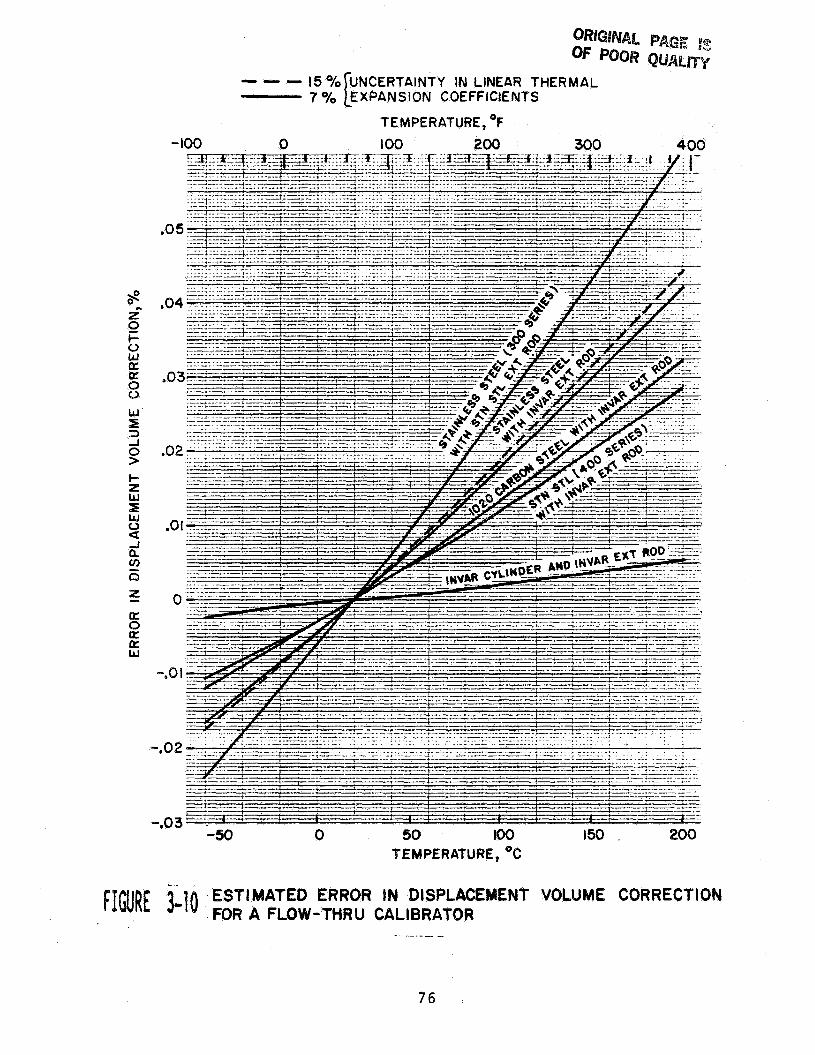
- 100 0 TEMPERATURE, O f

IO0 200 300 400

.O 5

.04

.03

.02

.81

0

-,o I

-.02

1- - -50 0 50 Do0

TEMPERATURE, OC

.._ ESTIMATED ERROR IN DISPLACEMENT ~ ' ~ ' ~ 3-'o . FOR A FLOW-THRU CALIBRATOR

-

150

VOLUME

200

COR RECf I ON

76

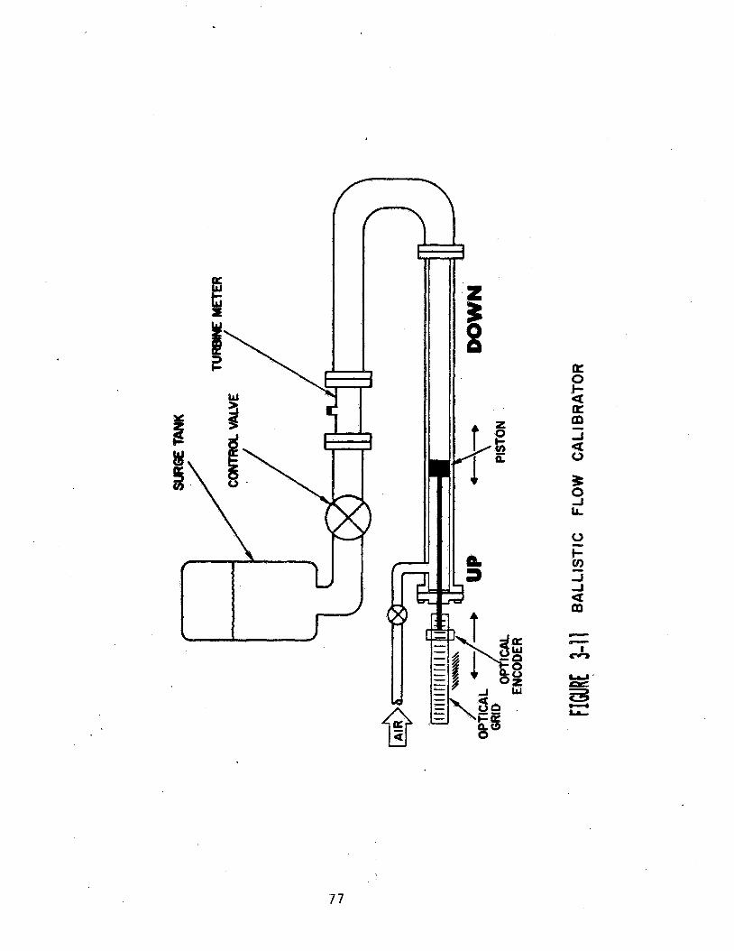
7 7

CL W w 0 CL e W e Y

a,

n

Y

a U

m eu

B c3

7

!

78

FINRE 3-13 RIGID PISTON DESIGN FOR A PIPE PROVER

(Reproduced f r o m Hayward [lq by p e r m i s s i o n from Measurement and Control)

79

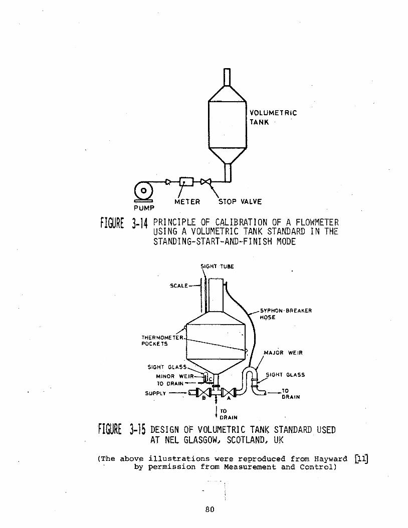
VOLUMETRIC

PUMP

FIGURE 3-14 PRINCIPLE OF CALIBRATION OF A FLOWMETER USING A VOLUMETRIC TANK STANDARD I N THE STANDING-START-AND-FINISH MODE

SIGHT TUBE i

/ SYPHON- BREAKER

THERMOMET

MAJOR WEIR

SIGHT GLASS SIGHT GLASS

SUPPLY -

(The above illustrations were reproduced from Hayward [ll] by permission from Measurement and C o n t r o l )

- . .

80

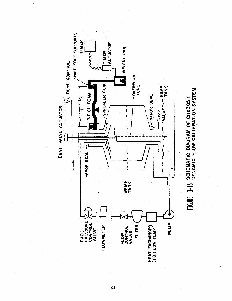
t

81

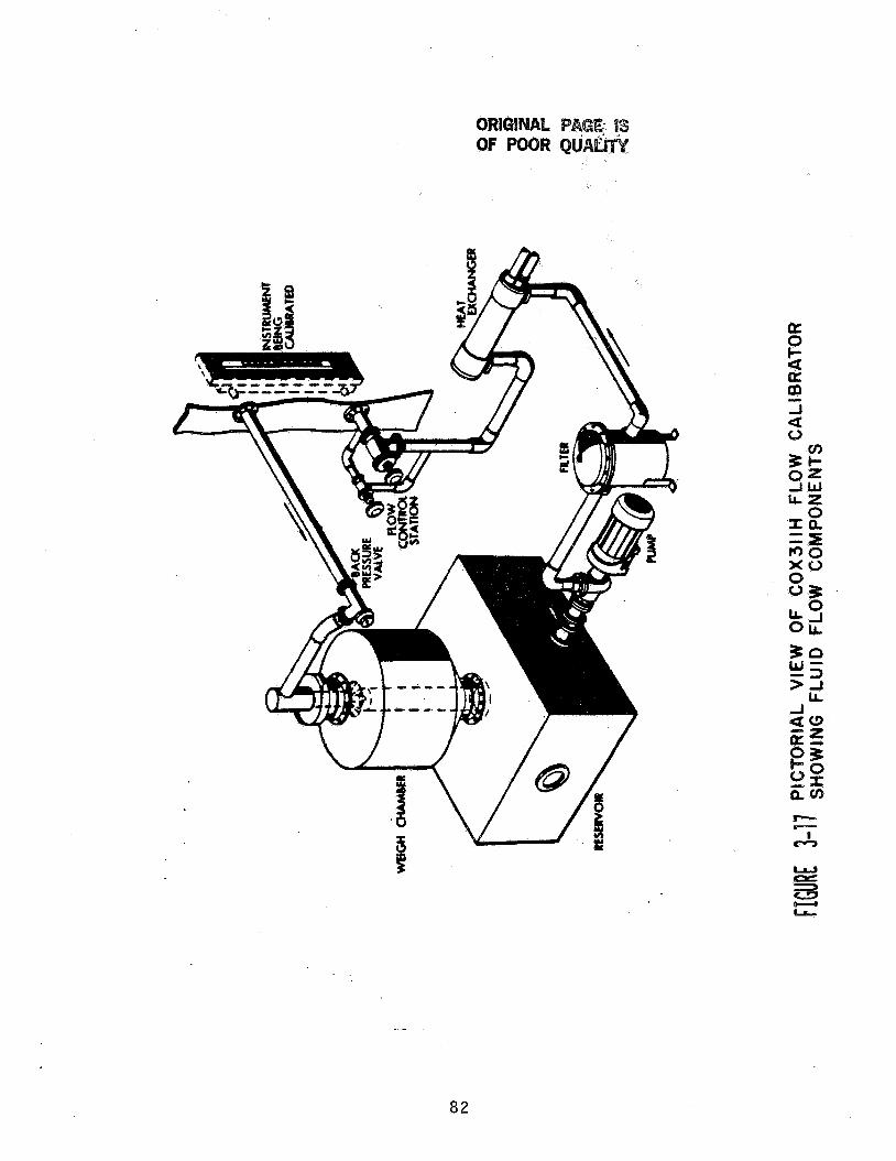
OR1 OF

82

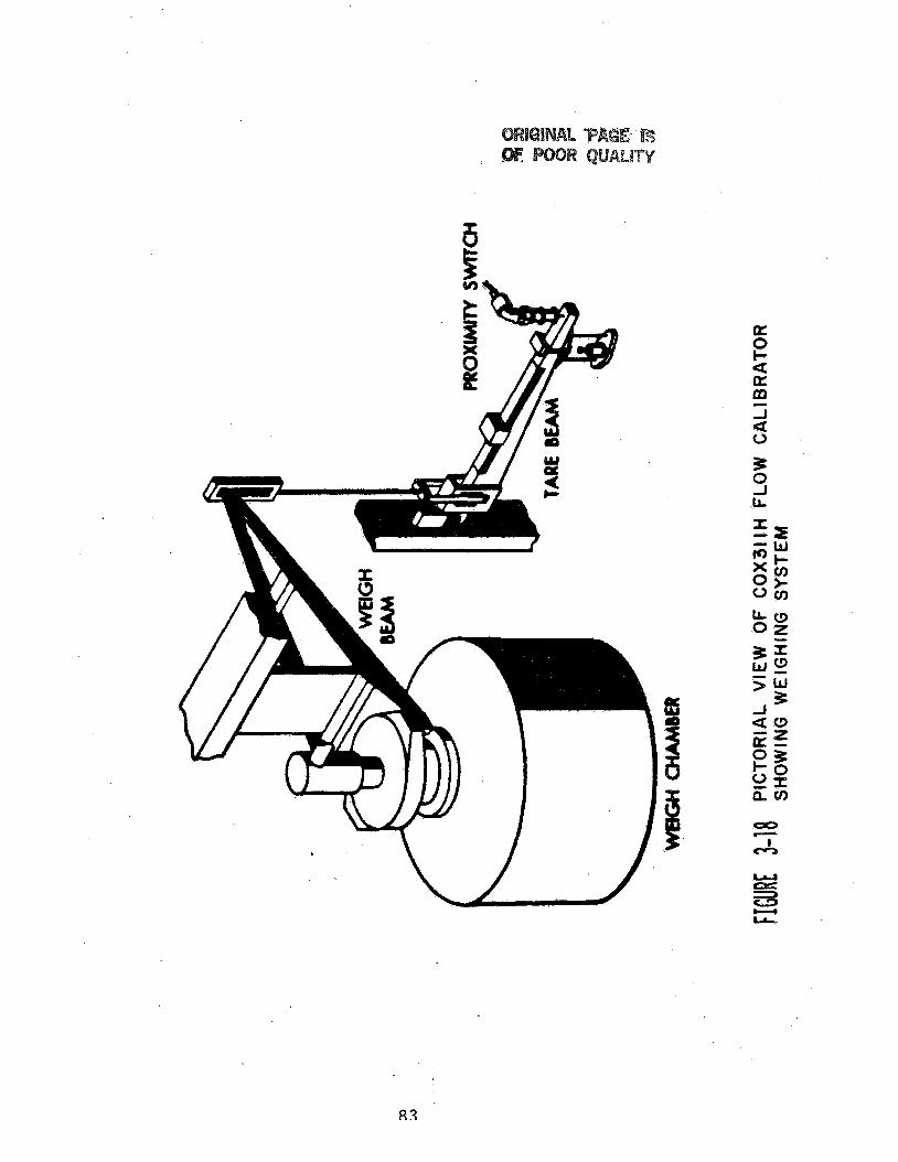
6

L1: 0 l- a a m J

0 a

83

m = MOLECULAR WEIGHT OF FUEL VAPOR’

PA= 101.32 kPU ( 14.696 psid )

m v

L

& -. 0

P 0 U L

z 0

0 w [L 0: 0 0

F:

> 0 z 0 3 3 m

TEMPERATURE, OF

-50 0 50 100 150 280

TEMPERATURE, aC .

FINRE 3-19 ; ESTIMATED BUOYANCY CORRECTION FACTORS FOR JET FUELS IN A.WElGH TANK CALIBRATION SYSTEM

8 4

4 1

Fl

I I

I IDEAL I CLOCK STOP TIME

(STATIC BALANCE)

I - I I 1

TARE BEAM LIFTS OFF

STOP

SWITCH STARTS

TARE BEAM LIFTS OFF

STOP

3 V a i u e s S h o w n are Typical for a COX 311H Cal ib ra t ion Run a t 2.52 kg/s (20,000 1 b / h r )

FIGURE 3-10 DIAGRAM ILLUSTRATING TIMING DEVIATIONS WHICH OCCUR Ih' A DYNAMIC WEIGH STAND (TYPE 6-11

85

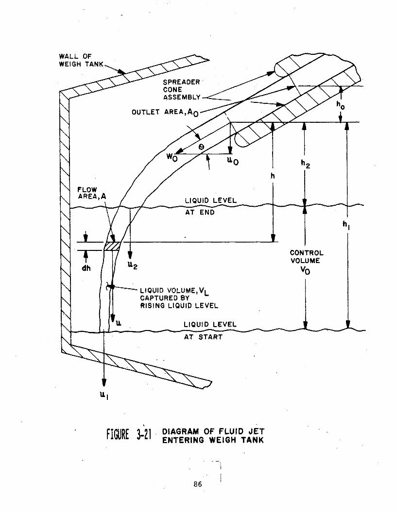
WALL OF WEIGH TANK

CAPTURED BY RISING LIQUID LEVEL

L

DIAGRAM O f FLUID JET 3m21 ’ ENTERING WEIGH TANK

i

TT

2. c

I - - M X 0 0 LL 0

87

1.006

I .005

1.004

1.003

1.002

I .0Ol

0

LIQUiD FLOW RATE, Ib / hr

0 5,000 10,000 I5,OOO

-7 10+10

10+3Q

30+IQ

10+1Q

I 0 +30

30+10

189 10 10+3Q 30+ 10

- 0 0.5 I .o 1.5 2.0

LIQUID FLOW RATE, k g / s

RE 3-23 ESTIMATED TlMING CORRECTIONS FOR COX 305T FLOWMETER CALIBRATOR

88

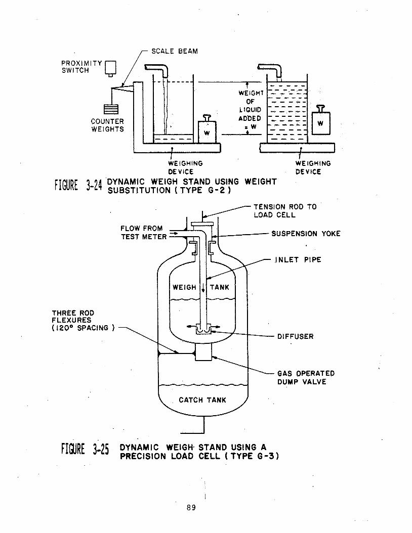
SCALE BEAM f PROXl M SWITCH

WE ICHlNC WE IGHlNG DEVICE DEVICE

'DYNAMIC WEIGH STAND USING WEIGHT 'IGURE 3-24 SUBSTITUTION ( TYPE 6-2 9

FLOW TEST

THREE ROD FLEXURES ( 120° SPACING )

TENSION ROD TO

SUSPENSION

CATCH TANK v

- INLET PIPE

DIFFUSER ---_

YOKE

- GAS OPERATED DUMP VALVE

FIGURE 3-25 DYNAMIC WEIGH- STAND USING A PRECISION LOAD CELL ( T Y P E G - 3 9

89

..

! i I

90

n 0 ,rl,

a c c Q) k m E k kl

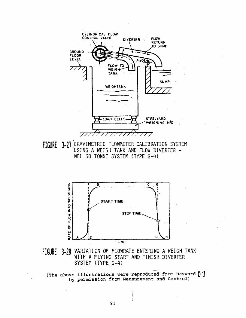
CYLINDRICAL FLOW

--c--

,

Y .

CON1 t O L

L

VALVE "LVERTER FLOW \ RETURN

J'F; LEVEL

WEIGH TA N K I -=-

1

///// / / / / / //// / / / A'

~ I ~ R E 3-27 :GRAVIMETRIC FLOWMETER CALIBRATION SYSTEM 'USING A WEIGH TANK AND FLOW DIVERTER - NEL 50 TONNE SYSTEM (TYPE 6-41

r z 4 I:

w

I-

e 3 START TIME 2 I % 2. K LL 0 w t 4 a

TIME

FIGURE 3-21 VARIATION OF FLOWRATE ENTERING A WEIGH TANK WITH A FLYING START AND F I N I S H DIVERTER SYSTEM (TYPE 6-41

_- (The above i l l u s t r a t i o n s w e r e reproduced from Hayward [ll)

by p e r m i s s i o n from Measurement and Control)

91

CYLl NDRICAL ALUMINUM CASE

PRECISION BALANCE

TOP SUPPORT TO CLAMP CANTILEVERED

SUPPORT PLANE

ELECTRICAL LEADS

SEAL GLAND BELL CRANK MECHANISM

SU SPENSl ON TUBE ( 1.6 MM OD)

OUTER STN STL TUBE ( 25.4 MM OD)

INNER STN STL TUBE ( 15MM OD)

UPPER SUPPORT SUSPENSION CAGE

SlNGLE SILICON CRYSTAL

LOWER SUPPORT

~~~R~ 3-29 , PORTABLE REFERENCE DENSIMETER

92

A - d

0 -# - =a ,"do

cn a

A -I W 3 a e cn

k I (u

3 J W n 0 5 J J W 0

LL 0

93

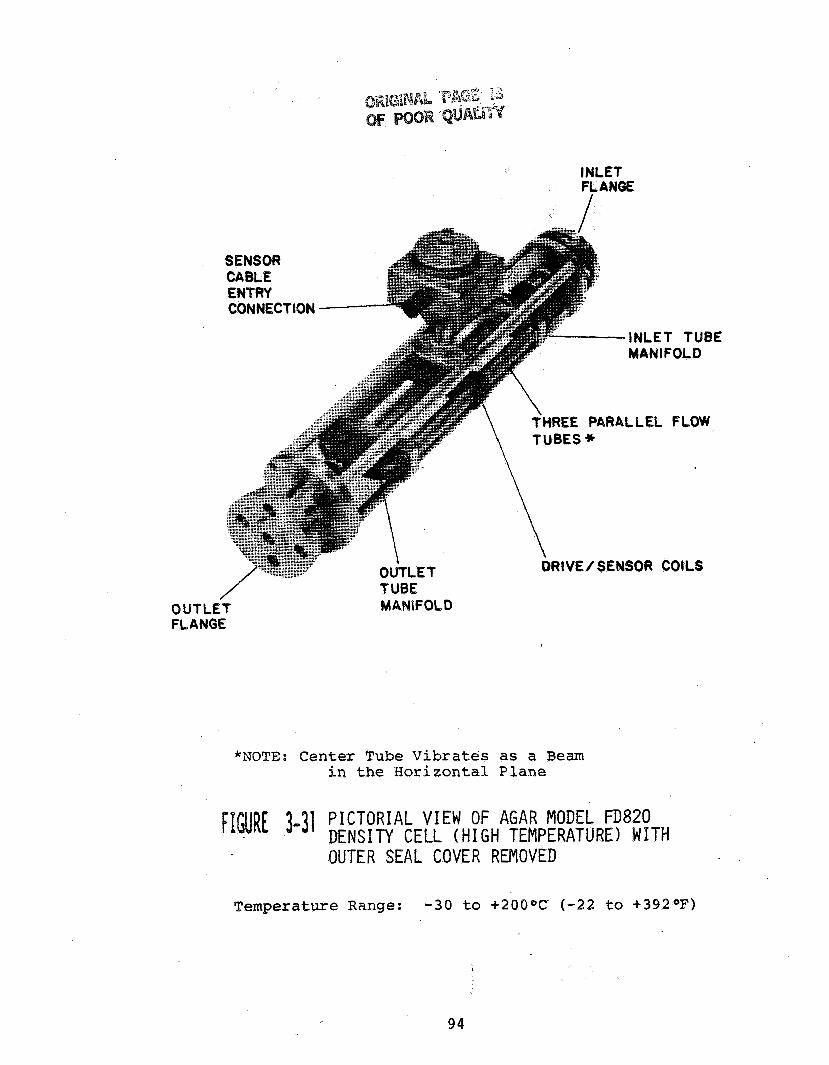
INLET FLANGE I

SENSOR CABLE

- INLE MAN1

,RALLEL

iENSOR

T TUBE IFOLD

~ FLOW

COILS

/ OUTLET FLANGE

TUBE MANlFObD

*NOTE: C e n t e r Tube V i b r a t e s as a Beam i n the H o r i z o n t a l Plane

~ I ~ U R ~ 1-31 PICTORIAL VIEW OF AGAR MODEL FD820 DENSITY CELL ( H I G H TEMPERATURE) WITH OUTER SEAL COVER REMOVED

Temperature Range: -30 to +200eC (-22 to +392*F)

94

1

END CAPS

BODY ASSEMBLY

FLANGED TUBE FOR SENSOR ELECTRICAL LEADS

SPOOL

LOCK R I N G VERTICAL LIQUID FLOW PATH

(a) C r o s s S e c t i o n a l Drawing of D e n s i t y C e l l '

SECTION A-A

(b) eross S e c t i o n of Tubular C e n t e r S e c t i o n of Spool Showing Mode of V i b r a t i o n During Dens i ty De te rmina t ion

F~~~~ 3-32 AGAR MODEL 781-B DENSITY CELL

(LON TEMPERATURE) Temperature Range: -270 t o +75OC ( -454 t o +167OF)

95

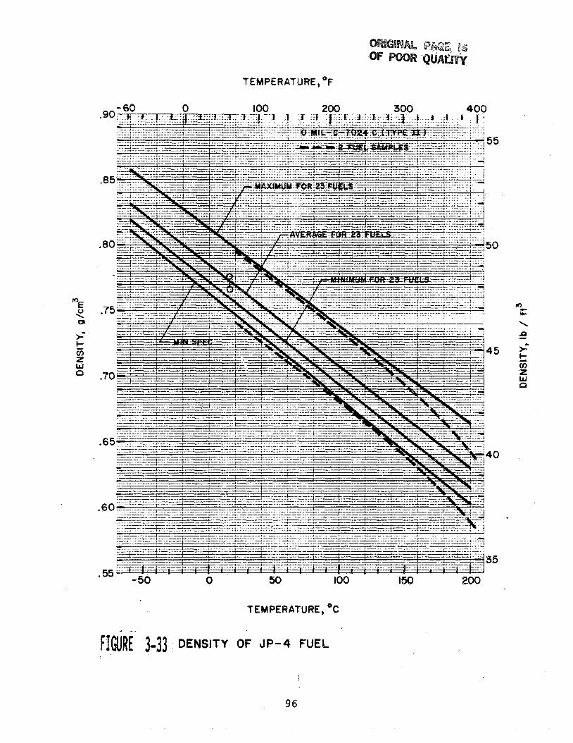
TEMPERATURE, O F

FIGURE 3-31 DENSITY

TEMPERATURE, O C

OF 3P-4 FUEL

96

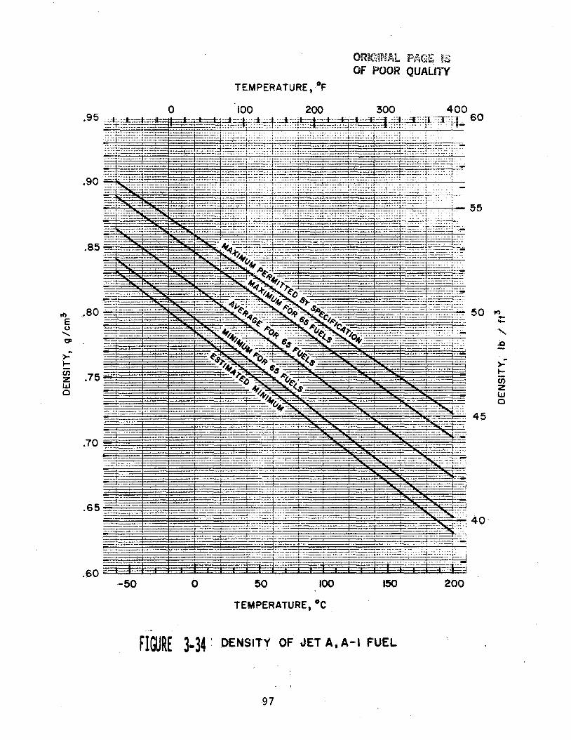
n E 0 \ 0

i k cn z w 0

.9 5

.90

.85

.80

.75

.70

.65

.60

TEMPERATURE, OF

0 100 200 300 400

-50 0 50 loo 150 200

TEMPERATURE, OC

FIGURE 3-34 ' DENSITY OF JET A, A-l FUEL

60

55

50

45

v) z w

97

TEMPERATURE, O F

.90

- 8 5

.80

. 7 5

.70

. 65

.60

0 50 100 150 200 . 5 5

-50

TEMPERATURE, *c

FIGURE 3-35 DENSITY OF dP-5 FUEL

1

55

50

+ rc m \ e *- t

45 v) P w D

40

35

98

TEMPERATWIE: C

I .

99

I

0 20 40 60 Percentage evaporated

80

[INRE 3-J( a) DISTILLATION CHARACTERIST ASTM D-86 FOR JP-4,dET B

(DATA FROM NACA TN3276 [I?])

CS PER FUEL

300

250

200 v 0 W K 3 I-

K W

a n

150 ,E

too

50 ' i

I00

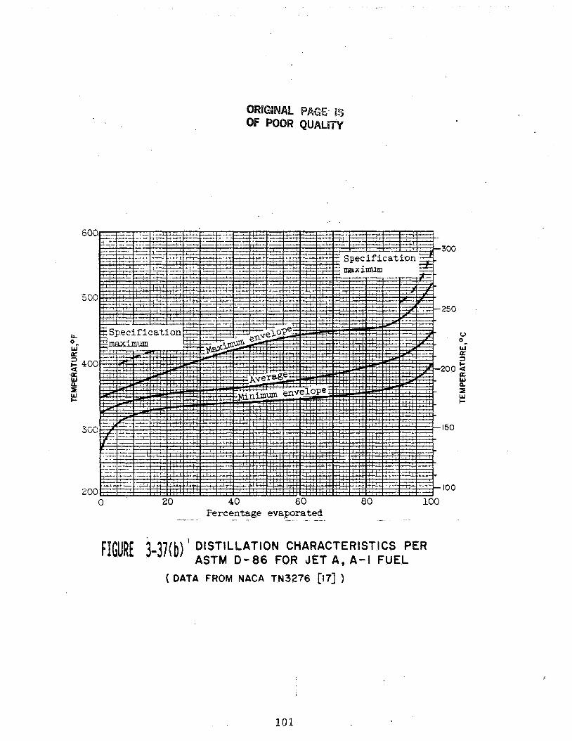
,300

250

,200

,150

. IO0

Percentsge evaporated __ ._ .- - _ _ -- -

’ DISTILLATION CHARACTERISTICS PER ASTM 0-86 FOR JET A, A- I FUEL FIGURE j-m)

(DATA FROM NACA TN3276 [I71 )

101

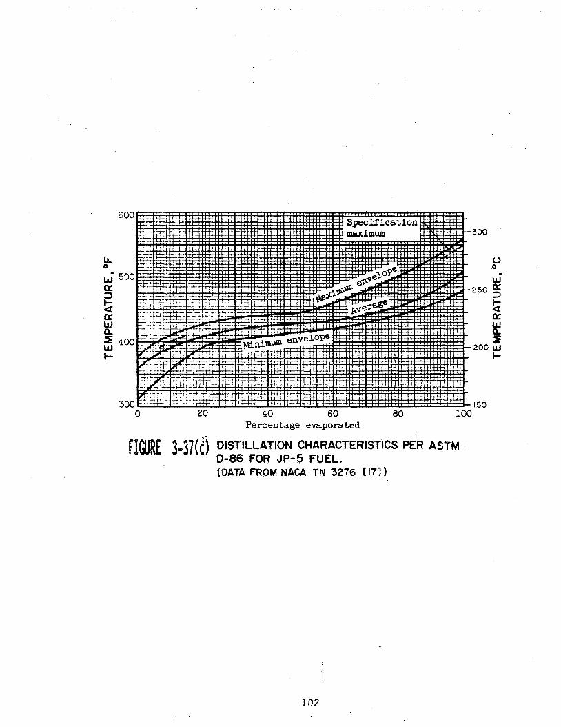
FIGURE yjl(f j DISTILLATION CHARACTERISTICS PER ASTM 0-86 FOR JP-5 FUEL. (DATA FROM NACA TN 3276 [ I ? ] )

102

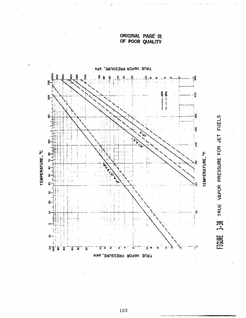
ou c

W

3 a

a t

3 W 0

I-

LL 0 L

a: Q

U 0 a s W

103

200

150

100

5 0

( RANGE OF 10% DISTILLATION TEMPERATURE SHOWN FOR EACH FUEL TYPE)

TEMPERATURE, OF 100 200 300 400 500

50 100 150 200 2 50

TEMPERATURE, OC

MOLECULAR WEIGHT OF FUEL VAPOR FROM SLIGHPLY VAPORIZED FUEL VS. IO % DISTILLATION TEMPERATURE FIGURE 3-39

104

4.0 VORTEX FLOWMETER

This section describes the experimental and analytical investigation performed on the vortex flowmeter concept under Task 2 d 4 f Phase I1 of NASA contract 'No. NAS3-22139 to develop a- High Accuracy Fuel Flowmeter (HAFF).

4.1 Introduction

The best approach to gain a better understanding of the capabilities and limitations of this technology is to pursue vigorous testing of various models. vortices wif.1 have to wait for the development of three-dimensional, non-axisymmetric time-marching computer techniques for geometries having no core, which is beyond the scope for this program with respect to time and content. designed with the intent of learning the most about vortex generation and sensing by building and testing several models, and then evaluating overall performance, especially repeatability of the best candidate model.

Comprehensive analysis of the fluid dynamics of precessing

Accordingly, a test approach described in section 4-2 has been

The first task in testing is to determine the contour of the flow passage and the geometry of the swirl generator which together produce strong and regular vortex precession over a 65:l volumetric flow range. presented in the literature and patents that were reviewed in Phase I and serve as a starting point for design of the models. Plexiglass (acrylic), will provide visual evidence of the vortex which can be "stopped" by synchronized strobe flash and enhanced with injections of dyed fuel or air bubbles in the central core. Dynamic pressure sensors are to be placed at the inside diameter at various axial and radial positions to help determine vortex physics and evaluate model performance.

Several concepts are

Each model, made of clear

. After testing several models, a "best" candidate is to be selected for comprehensive evaluation of the fluid dynamics of the vortex. Complete charting of fluid velocity profiles over selected radial and axial positions is to be performed using hot film or hot wire anemometer probes and using high speed movies of fuel with aluminum particles in suspension. The evaluations are to be made at several flow ranges including the minimum and maximum. Anemometer readings will provide data on flow speed and oscillation frequency and strength but will not provide data on flow direction. movies can provide indication of flow direction in such a complex flow pattern. This information will then be analyzed with two objectives in mind: (1) an optimum vortex sensor.

Only high speed

description of the fluid dynamics in quantitative terms and (2) design of

The next step will be to build and test several sensor designs with information from the preceding work. signal over the flow range, as judged by signal-to-noise ratio and regularity of sensed vortex frequency, will then be subjected to a series of tests that are intended to provide data on linearity, repeatability and stability.

The sensor that generates the best

105

4.2

To evaluate the design concept of the vortex flowmeter and its potential in meeting NASA HAFF requirements, five major test groups were planned to be-conducted in Task IV. They are:

(1) Vortex Generator study

(2) Fluid Dynamics Study

(3) Sensor Evaluation

( 4 ) Linearity and Repeatability Measurement

4.2.1

(5) Time Response' Evaluation

Vortex Generation

Problem - Most of the vortex precession flowmeters described in the literature performed over a 20:l range of Reynolds number with water, which falls short of the required l300:l range (65:l volumetric times 20:l viscosity). The minimum Reynolds number for vortex precession t o occur was found to be 250 for one device while the maximum Reynolds number was as high as 230,000 for another device (920:l ratio), yet no one device spanned the whole range. extent of Reynolds number range for a single device, (2) find out what phenomenon limits the range (cavitation?) and (3) ascertain what aspects of swirler design and what contours of the flow passage extend the dynamic range.

The objectives of this test group are to: (1) determine the

Solution Approach - Several clear plastic models will be made with various inlet area ratios, expansion ratios, tapers and curves, and several swirler concepts will be made. passage contours will be tested on a flow stand and evaluated for dynamic range. The test approach will be one of flexibili,ty so that configurations which show promise can be studied'in more detail while those showing little promise may be dispensed with quickly. tentative and most likely will change as work progresses and new ideas and understanding of operation evolve.

Combinations of these swirlers and flow

In this regard, this plan is strictly

The flow passages are designed with multiple "0" ring sealed sections that are quickly interchanged so as to permit testing of a large number of combinations. Each venturi or central section of the vortex generator will have two diametrically opposed pressure sensors to provide a vortex signal output that will serve as one measure of performance.

The following swirler types are to built and tested:

a) Multiple Flat Blade Assembly Figure 4-1

b) Machined Passages Figure 4-2

c) Tangential Inlet Figure 4-3

d) Delta Wing Figure 4-4

Each swirler will be mounted in a section of clear plastic tube that snaps into place upstream of each vortex section. Upstream of the swirler there may be a constant diameter section and flow straightener section, to eliminate incoming swirl.

Each vortex section will actually consist of three parts: (1) tapered inlet (2) constant diameter and (3 ) expansion outlet. The parameters of the vortex sections and different vortex precession models to be investigated are listed in Table 4-1 and Table 4-2 respectively.

Placement of a central core obstruction downstream of the expansion section may adversely affect the central flow reversal that is so critical to vortex precession. of various sizes at various distances downstream as shown in Figure 4-5. information is vital to future design of the densitometer housing.

Its effect will be tested by placing a model densitometer section This

AI31 of these sections - straightener, swirler, vortex generator and densitometer - will be placed in a 45.7 cm (18 in.) section of a 3.81 cm (1.5 in.) diameter pipe flow stand, as shown in Figure 4-6. the entire section under test may be removed, reconfigured and replaced in a matter of minutes. oscilloscope and a frequency spectrum analyzer. The sum of the two output voltages will indicate common mode noise while the difference will represent the vortex frequency: the ratio of difference to sum will therefore provide an approximation of signal to noise ratio. indicate the fundamental frequency, bandwidth and harmonic content of the pressure signals. will be made for indications of cavitation and vortex behavior.

4.2.2 Fluid Dynamics -

With this set-up,

The two pressure sensor signals will be monitored on an

The frequency analyzer will

Visual observations aided with a stroboscope flash unit

Problem - There is very little information currently available on the velocity distribution, strength of velocity changes in the precessing vortex and basic frequency of precession. Without this type of information the design of suitable sensors cannot proceed with any degree of confidence, and formulation of theories of operation have no valid basis.

Solution Approach - Several of the better performing configurations, as judged by lack of cavitation and flow separation, by regularity of vortex precession and by dynamic range, will have the flow velocities and directions mapped from the swirler to the de-swirl vanes. following techniques will be employed to quantify flow characteristics:

The

1) Anemometers - - Hot film type - Wedge side flow

- Wedge end flow - Cylindrical

2) High Speed Movies - Flow enhancement with injected aluminum particles and dye.

3 ) Pressure Sensors - Various sensitivities and types - Quartz, strain gage.

107

ANEMOMETERS - Maximum flow velocity, through a vortex section, with a swirl ratio of 5 and a 2.69 cm (1.06 in.) diameter throat is 28.7 m/sec (94 ft/sec) which precludes the use of thin wire probe elements, which are reliable at flow rates below 2.13 m/sec

.

( 7 ft/sec) Wedge-end-flow hot-film sensors have been used to evaluate vortex flow but lack the directional sensitivity of the thin wire types. Other styles which are listed above are subject to cavitation and may also disturb the.vortex itself, these limitations, a series of tests will be conducted using thin film type sensors at flow rates below 636 kg/hr (1400 lb/hr) and wedge-end type sensors at higher flow rates, will be done with apparatus shown in Figure 4-7 over flow ranges from the minimum for vortex precession to the maximum prior to cavitation, and for viscosities of one centistoke and ten centistokes (Tellus Oil).

A miniature drag force anemometer ‘of the style developed by Krause and Fralick at LeRC can provide data on both velocity head and flow angle and will be useful in this investigation. Frequency response of the cantilever beams far exceeds the maximum expected vortex frequency (500 Hz) so the frequency compensation network can be replaced with a simple low-pass filter (at 2,000 Hz). beam to handle the forces in liquid may be required. consult with LeRC on the design and availability of a unit for use in this test sequence,

Despite

Flow velocity mapping

Resizing the We will

HIGH SPEED MOVIES - Tracing individual particle paths and velocities will provide the best visual and quantitative evidence of vortex behavior, A frame rate of 7000 per second (which is typically attainable) will provide adequate frame to frame resolution of 4.3 mm (1.7 in.) for a particle moving 305 m/sec (IO0 ft/sec) which is the estimated maximum velocity. of the vortex can be achieved by injecting aluminum particles and/or dye in various locations, as shown in Figure 4-8.

Enhancement

PRESSURE SENSORS - Spatial and temporal variations in total pressure through the region of vortex generation and dispersion can be measured by placing miniature pressure transducers directly in the flow stream or by inserting a small tube through the meter wall, as shown in Figure 4-9. Data from pressure distributions, in conjunction with velocity information, will provide excellent evidence from which theories of vortex precession can be based and from which sensors may be designed. Two types of pressure sensors will be tried: quartz and semiconductor strain gage. Both types have small sensitive areas 64 mm (0.25 in.) diameter or less and adequate sensitivity in 690 kPa (100 psig) range devices (4 volts output at 690 kPa). be evaluated by placing matched sensors at the desired points and electronically differencing, rather than by purchasing integral differential units, to provide flexibility and lower-costs.

Differential pressure between two points will

108

4.2-3 Sensor Evaluation

Problems - The vortex sensor must provide a signal sufficiently free from noise at all flows and environmental conditions (including vibration, pressure pulsations and turbulence) such that essentially no false triggers or lapses in triggering occur. sufficiently low impedance (50 ohms preferred, less than 1,000 ohms acceptable) such that signal transmission over lengthy cables is unaffected by conducted and radiated noise. The unique advantage of this sensor is that it must be sensitive to cyclic pressure or velocity variations (since volumetric flow rate is proportional to frequency of precession) but need not provide accurate data on absolute velocity or pressure.

The output device must be of

Solution Approach - Velocity and pressure data from the previous test will be analyzed and several candidate sensors will be designed, built and tested. combinations which were previously selected for the fluid dynamics studies. The tests will determine the maximum flow range where reliable signals can be obtained with Stoddard solvent (1 cs) and Tellus oil (10 cs). parameters such as peak-to-peak voltage, signal-to-noise ratio, frequency jitter of the fundamental vortex signal and noise spectrum will also be evaluated for each candidate sensor. "families" will be evaluated, provided that previous tests and experience deem it reasonable:

Each sensor candidate will be tested in the vortex generator

Output

One from each of the following

- Heat transfer - Pressure - Flow direction

4.2-4 Linearity and Repeatability Measurements

Problems - Vortex precession data for gas flow measurement show - + 0.15% repeatability and ~t 2.25% linearity over a 35:l flow range. the literature indicates linearity of 5 12% over a range of 333:1, but provides no indication of repeatability over the expanded range. there is no indication of repeatability with water or jet fuel. In this program, non-linearities that are a function of Reynolds number are compensated for via a microcomputer and repeatability is most important. Reynolds number dependence cannot be too great, otherwise precise measurement of viscosity would be required for accurate compensation of the non-linearities.

Data in

Furthermore,

Solution Approach - The efforts in the preceding test groups will produce several configurations suitable for evaluation of repeatability and linearity. The tests will be conducted on the flow stand with two calibrated turbine meters in parallel, and one selected according to the flow range that is applicable (see Turbine section). Three viscosities of liquid will be run over the available flow range to ascertain the degree of Reynolds number dependence and nonlinearity.

109

4.2.5 Time Response

Problem - Present estimates indicate a 0.032 sec response time at maximum flow rate and 1.6 see at minimum flow rate, which exceeds the design requirement of 0.025 sec. Transport lag, measurement period and filter time were estimated but vortex re-establishment time remains an unknown.

Solution Approach - The vortex meter configuration selected for linearity and repeatability tests will be placed in a test rig designed to produce rapid reductions in flow rate. A turbine flowmeter will be placed upstream to provide an indication of actual flow change as shown in Figure 4-10. Since the vortex meter response is expected to be slow, the turbine meter and test rig do not have to produce step flow changes faster than 0.050 see at mid-range flows, which is easily achievable. A hot film probe will also be installed as a velocity change monitor.

4,3 Experimental and Analytical Investigations

Data relating to the vortex precession flowmeter is included in the accompanying report supplement No. 1 dated December 15, 1984 as protectable data in accordance with contract NAS3-22139i; Item 8C.

4.4 Conclusions and Recommendations

The vortex precession concept exhibits greater non-repeatability at all flow rates and is not likely to achieve the required time response. .

Improvements in swirler and de-swirler designs may lower the now excessive pressure drop, but any gains here are likely to be lost when overall diameter is reduced to speed up time response, increase signal amplitude and improve linearity. Furthermore, the risks of cavitation of the central core and entrapment of any air in the fuel line make the concept less attractive.

110

Tables and Figures

Tables and figures for this Section 4 relating to the vortex precession flowmeter are included in a separate report supplement, as protectable -data in accordance with contract NAS3-22139, Item 8C.

1 1 1

Table 4-1 Intentionally Left Blank

112

Tab le 4-2 Intentionally Left Blank

113

Figures Intentionally Left Blank

114

Figure 4-1 Intentionally Left Blank

115

Figure 4-2 Intentionally Left Blank

116

Figure 4-3 Intentionally Left Blank

117

Figure 4-4 Intentionally Left Blank

118

Figure 4-5 Intentionally Left Blank

119

Figure 4-6 Intentionally Left Blank

120

Figure 4-7 Intentionally Left Blank

121

Figure 4-8 Intentionally Left Blank

122

Figure 4-9 Intentionally Left Blank

123

Figure 4-10 Intentionally Left Blank

124

5.0 DUAL TURBINE FLOWMETER

This section describes the experimental and analytical investigation, the prototype construction and evaluation performed on the dual turbine flowmeter concept under Tasks 2 through 7 of Phase I1 of NASA contract No. NAS3-22139 to develop a High Accuracy Fuel Flowmeter,

5.1 Introduction

The turbine flowmeter is a widely accepted flowmeter with proven !t was therefore considered an excellent potential precision and accuracy.

candidate for a high accuracy mass flowmeter. The major drawback with the turbine type flowmeter is that it is only a volumetric device, and it needs a density measurement to yield mass flow rate. Also, it.requires a viscosity measurement in order to cover the full flow range with reasonable accuracy.

The dual turbine flowmeter concept identified in Phase I offers a design that will enhance current turbine meter technology. The problems associated with standard turbine meters of sensitivity to upstream swirl, bearing friction/wear, limited range, and viscosity sensitivity are mitigated by the addition of a second free counter-rotating turbine element immediately downstream of the first element. The secoad turbine has only a fraction, say 20%, of the main turbine pitch (and, therefore, free rotational speed). The speed of each is measured and the sum of the speeds is used as the volumetric flow signal. An analysis of the flow vectors entering and leaving each turbine shows that this sum of speeds (as measured by blade passing frequency) is nearly independent of upstream swirl content and of bearing or viscosity induced drag on the main (high speed) turbine. ratio of the two speeds the health of the flowmeter bearings can be monitored.

Furthermore, by measuring the

The mass flow rate can then be achieved by combining the outputs of the two turbines plus the precision density measurement from the densitometer.

5.2 Experimental and Analytical Investigation Plan Formulations

To evaluate the design concept of the dual turbine flowmeter and its potential in meeting NASA HAFF requirements, the following tests were planned to be conducted in Task 4:

Turbine Start-up

Turbine Blade Geometry

Optimum Rotor Design

Verify Dual Turbine Theory

Repeatability in Critical Zone and Low Reynolds Number

Viscosity Accuracy

Signal Interaction

125

5.2.1 Turbine Start-up

range 0.050 0.025

Problem - The General Electric concept for 65:l volumetric flow capability from a turbine meter depends on low-end repeatability at kg/s (400 lb/hr) and worst case (low temperature) start-up at about kg/s (200 lb/hr) flow. Prediction of start-up flow depends on bearing

friction (which can and will be measured) and on torque versus flow over a stalled blade, which is not addressed with sufficient detail in the literature. adequate repeatability exists is unknown.

The difference between start-up flow and minimum flow where

Solhion Approach - Measure the "start rotating" and "stop rotating" flows for two turbine flowmeters in fluids with 1 and 20 centistokes

Size - 0 1.27 cm (0.50 in.)

0 2.54 cm (1.00 in.)

Also, the smaller meter will be used

viscosity. The flowmeters will be the following:

Flow Range

0.02 to 0.38 liter/sec (0.3 to 6 gpm)

0.1 to 4.1 liters/sec (1.6 to 65 gpm)

3 accurately determine the repe tability of tie larger one in its low flow range (start-up critical). be used to determine the flow range between "start-up" and "minimum adequate repeatability"

The results will .

5,2-2 Turbine Blade Geometry

Problem - The optimal design of turbine blades depends on better understanding of the following effects:

Surface Roughness

Trailing & Leading Edge Sharpness

Solidity Ratio

- Its effects on boundary layer thickness and drag coefficient versus surface conditions and imperfections, Unknown.

- Critical to low drag coefficient in turbine blades.

- Is solidity ratio of unity required and how sensitive is momentum exchange to this ratio? What is torque versus Re before startup for various ratios?

126

Solution Approach - A large scale clear plastic model (Figure 5-1) will be built. The rig consists of a variable speed motor driven upstream swirler section and a downstream section where the stationary test item is observed and where measurements in flow are to be made. measurements will be made with this apparatus:

The following

1)

2)

Axial and tangential velocities via hot film anemometers.

Blade/vane pressure distribution via multiple ports and high accuracy pressure sensor,

3) Flow patterns with dye injection and high speed movies.

The following tests will be conducted:

Surface Roughness: - ground and polished - sand (various grits) - using one vane - measure boundary layer versus Re

Trailing & Leading Edge Effects:

- 10" end - 30" end - 0" end - 12" taper - measure tangential flow downstream of vane e - photograph wake with dye injection. - determine effect of boundary layer.

Solidity Ratio: - construct turbine rotors with ratios of 0.5, 0.75, 1.0, and 1.3 and evaluate stalled flow patterns versus Re.

5.2.3 Optimum Rotor Design

Problem - Results of the preceding tests must be incorporated into the analytical model and from this model the optimum turbine rotor design must be extracted.

Solution Approach - The measured and calculated data from the above tests will be compared to actual calibration curves and the theoretical model will be validated and updated. Bearing friction and torque versus flow for a stalled rotor will predict start-up flow for the low speed sensor turbine. Leading and trailing edge test results, along with surface finish test results, will guide the design of turbine blades. Results of solidity ratio tests will also be taken into account in the updated model. The conceptual design from Phase I will then be optimized by taking into account all these factors.

1 2 7

5.2.4 Verify Dual Turbine Theory

Problem - Determine the relationship between the calculated . calibration expression for a two rotor flowmeter and the actual curve. Determine if swirl effects have been negated and if other flow phenomenon affecting calibration are present.

Solution Approach - Test optimized turbine and sensor rotors; both separately and combined. predicted calibration expression for each rotor and then for the two rotor design. has been negated or reduced to an acceptable level, will be used, which for flow measurement utilizes two precalibrated turbine flowmeters (see Figure 5-2). A smaller flowmeter has 0.02% repeatability capability over its linear (2 5%) range of 0.02 to 0.38 liter/sec (0.3 to 6-0 gpm) when used with calibrating fluid of 1 cs. same order of repeatability will cover the flow range of 0.1 to 4.1 liters/sec (1.6 to 65 gpm). A working model (Figure 5-3) will be fabricated which will be capable of accepting either turbine or sensor rotor in either upstream or downstream position or tested with both rotors. signal conditioners will be purchased, analysis and calculation will be undertaken.

Investigate any significant deviations- from the

Mount a pre-swirler upstream of the flowmeter to ascertain that swirl A circulating flow stand

A larger unit with the

The modulated RF pickoff and The following order of testing,

1. Determine start-up flow and actual calibration curve for each rotor.

2. Analyze data to determine retarding torques and other variations from theoretical flow conditions.

3. Derive a calibration expression for the two rotor flowmeter.

4. Test and measure actual calibration.

5 . Further investigate by test and analysis significant variations from the predicted curve.

6. Test, with known pre-swirfers, the effect of swirl and determine the level to which it has been eliminated or minimized.

5.2.5 Repeatability in Critical Zone and Low Reynolds Number

Problem - Repeatability, especially at "start-up/high viscosity" and in the "critical flow zone" must be evaluated so that overall system accuracy can be estimated.

Solution Approach - Measure repeatability of test model under worst case flow conditions by comparing with 0.02% known repeatability turbine flowmeters. circulating stand with 20 cs fluid and measured with the smaller, 0.02 to 0.32 liter/sec (0.3 to 6.0 gpm) calibrated turbine flowmeter and also on a small COX weight stand with the temperature reduced to -55°C. Testing for repeatability in the critical zone will be similar, except the 0.1 to 4.1 liters/sec (1.6 to 65 gpm) flowmeter, in the circulating stand and the larger COX weight stand will be used.

Testing of low flow conditions will be conducted in the

128

5-2.6 Viscosity Accuracy

Problem - Determine the accuracy required of viscosity measurement for less than 0.05% contribution to overall system error.

Solution Approach - Measure change in calibration to the test model A circulating stand with when tested with a 1 cs and a 20 cs viscosity fluid,

two turbine flowmeters will be used to measure flow rate as previously described. test viscosities.

.

These flowmeters will have been previously calibrated at the two

5.2.7 Signal Interaction -

. Problem - Two RF amplitude modulated signals need to be conducted over long, adjacent leads and must not interact,

Solution - Twenty foot cables of the following conductor styles e

will be evaluated for signal interaction on the dual turbine model:

1. Untwisted Pair

2. Twisted Pair (independent grounds)

3. Twisted Shielded (mutual grounds)

4. Coaxial

5.3 Experimental and Analytical Investigation

Responding to a NASA requirement for a highly accurate mass flowmeter operating over a 65:l volumetric flow range and a 30:l viscosity range, General Electric proposed a dual turbine flowmeter with a densitometer. The significance of the dual turbine is its ability to detect and compensate for fluid swirl along with variations in retarding torque or turbine slip that are due to viscosity and mechanical changes, thereby reducing the effect on the flowmeter turbine speed versus volumetric flow relationship.

Along with a need to prove out the concept, problem areas were anticipated and the approaches to address these problems were outlined in Section 5.2.

To answer these questions, an engineering model was built and tested. section contains a description of these tests, the test results and their meaning, and a discussion on recommended additional actions emanating from the test results.

This

5.3.1 consisted of a clear acrylic housing in which the main and sensor turbines rotated. lubricating" duroid retainer was used for each turbine.

Engineering Model - The model used for engineering evaluation A single miniature ball bearing containing a machined "self

See Figure 5-4.

The central shaft was designed to be either rotated by the dither mechanism or locked to prevent rotation. The turbines were spaced apart by a separator which was planned to be modified into a dither mass.

129

As constructed, the turbines could be individually tested or combined as a dual unit. The main turbine had 8 blades with a helical angle of approximately 52 degrees. Two sensing.rotors were fabricated. Initially both had 8 blades; one with a 15" helical angle and the other with 22O: Later fgur blades were removed from the 22O rotor.

A flow straightener from a COX flowmeter was modified to provide the front support for the central shaft. three vanes. The modulated RF pickoffs were purchased from COX along with their driving electronic modules.

The rear support was centrally positioned by

5.3.2 Test Results

. 5.3.2.1 Bearing Friction - A major factor that affected the flowmeter design, mainly because of the lower operating speed of the sensor turbine and the large dynamic operating range of the turbines, was the retarding torque value at low flow/high viscosity conditions; principally bearing friction.

In the pro osed concept, slip calculations used a static bearing friction of 14,7 x 10- mechanism it was planned to seduce this value by a factor of two. adequate starting torque to overcome bearing friction, a larger diameter, narrow annulus, restricted flow passage was proposed. While this design generated larger torques at lower operational speeds, it did have the disadvantages of a higher pressure drop and an increased response time.

g N-m and a design of two bearings per turbine. With a dither To develop..

Tests on the main and sensing turbines revealed that for this application and with the type bearing chosen, friction is significantly lower than assumed. The main turbine readily rotated at a flow rate below 0.013 kg/s (100 lb/hr) in fluid with a viscosity of 12 cs. started coincidently with the main turbine.

The 22" helical angle sensor turbine

As expected, the 15" sensor slightly lagged the main turbine in starting, and rotation beginning at a flow rate of 0.013 kg/s (100 lb/hr). It was smoothly rotating and fully operational at a flow rate of about 0.025 kg/s (200 lb/hr). friction was ascertained to be approximately 0.98 x lo-' N-me

From the results of rotational speed and flow values, bearing

These test results are highly significant. mechanism" is not needed; nor is the narrow annulus. A more standard configuration can be used. Response time and pressure drop will therefore be typical of that for a 2.54 cm (1 in.) tube size turbine flowmeter.

They show that a "dither

5-3.2.2 Swirl Effect Test - A flow swirler consisting of a cluster of canted, small diameter, tubes was introduced upstream of the engineering model. swirl. on the main turbine to about a 0.5% change. Attempts to introduce greater swirl through the use of a rotating impeller in a modified flowmeter mounted upstream of the model also proved to be ineffective. Of great importance, however, was the fact that the introduction of this swirl which normally would have caused an error in the flowmeter reading, was sensed by the sensor turbine and the combined readings of the sensor and main turbines remained unchanged.

It had been hoped to introduce up to 5% calibration change due to However, the flow straighteners in the model limited the swirl effect

130

The graphic results of the Swirl Test are shown in Figure 5-5. series of points are a calibration plot of the main turbine speed versus flow rate. They show an increase in the "K" factor with the introduction of swirl. speeds showing that the calibration, is the same with and without swirl.

It should be noted that because of functional difficulties, a spectrum analyzer with 0.5% frequency resolution was used to measure sensor turbine speed, and a frequency counter was used for the main turbine. equivalent to about 0.1% on the combined speed so that measurement resolution was no greater than the flowmeter repeatability it was hoped to.prove. Essentially, the spread shown for the combined readings is equivalent to the resolution of the measuring equipment.

The bottom

The top series of points are a plot of the combined turbine and sensor

This was

5.3.2.3 conducted on both the COX AN-16 flowmeter supplied by NASA and an 8 blade rotor used as the main turbine in the engineering model. These tests were conducted over the specified operating range to check repeatability throughout and if it degraded, in the critical transitional flow range and at low starting flow rates.

Turbine Repeatability - Several room temperature tests were

It was found that repeatability in these ranges was no different from that in the more linear turbulent range. AN-16 flowmeter. by General Electric. lower 0.050 kg/s (400 lb/hr) flow condition is equivalent to a chordal Reynolds number (Re) of 2000. It can be seen that the calibration shows no inflection at the critical Reynolds number of 5000. points is no greater for Re = 2000 than at higher Reynolds numbers.

The plot of data indicates a spread of about 2 0.4%, raising the question as to whether or not the COX weigh stands used were a source of error. Two separate tests on a newly operational flow stand that uses turbine meter masters at General Electric, indicated an extremely linear calibration, all data points falling within 0.1% linearity from 0.63 to 5,04 kg/s (5000 to 40,000 lb/hr); pointing to the COX weigh stands as the probable cause of the data spread. within 0.1% would require better flow measuring approaches than those presently available.

Figure 5-6 is a calibration plot of the Points shown are from NASA supplied data and tests conducted

At typical room temperature viscosity and density, the

Also the scatter of data

To mre fully prove that the turbine flowmeter repeatability is

5.3.2-4 in calibration fluid (5 cs viscosity) and at room temperature in Tellus #lo (12 cs viscosity). Figure 5-6.

Viscosity Effects Test - Tests were conducted at cold temperature The results of these tests for the AN-16 are shown in

When plotted against Reynolds number, good agreement was achieved for the cold and Tellus runs. 0.03 liter/sec (0.5 gpm), below which the output became unreliable. Because of this problem at low frequencies it was difficult to determine whether the calibration between room temperature and cold was predictable solely by Reynolds number. AN-16 was approximately 20 Hz. Below this value, the signal rapidly attenuated, mixed with side frequencies and caused count inaccuracy.

Data were taken at a lower output frequency equivalent to

At room temperature and at Re of 1500, the output of the

The two

131

test points shown at Re of 1000 could therefore be in error. it is likely that some error exists, sufficient experimentation was done in this flow range to indicate a high probability that the room temperature calibration drops off faster than the cold temperature calibration.

Further testing is required before this phenomenon can be definitely. established. can readily be corrected using viscosity and temperature measurements. shift can be minimized by changes in the turbine rotor design (see Section

However, while

If confirmed, this apparently small shift, (on the order of 2%) This

5.4).

No valid viscosity information could be derived for the engineering model, Though still rotating, no signals could be read from the sensor turbine at the lower flow rate. The lowest room temperature Reynolds number attained was 3700, and the minimum for cold was 500. Therefore, between 3700 and 500, the area of possible calibration shift, no data are available.

5.3,2.5 Calibration Predictability Tests - Four turbines were tested to determine if their actual calibration corresponded to the calibration which was predicted using calculations based on drag torque and momentum theory.

Testing of both a six blade, 45" helical turbine and an eight blade, 52" helical turbine (used in the engineering model) revealed that the cusp in the calibration curve occurred we%% below the predicted chordal Reynolds number (Re) of 5000 and that the degree of **speed-up** or nonlinearity at the cusp was two to four times greater than predicted, as shown in Figure 5-7. slope of the actual calibration curves for both turbines was two to four times greater than the'predicted curve in the laminar flow range where Re is less than 1000. Furthermore, the six blade turbine had excellent linearity at flow rates above 2.52 kg/s (20,000 lb/hr) while the eight blade turbine cavitated at flow rates above 1.89 kg/s (15,000 lb/hr) - an effect that is not predicted by momentum theory.

Also, the

Calibration curves of the low speed sensor turbine proved equally unpredictable, as shown in Figure 5-8. blade, 22" and a four blade, 22" turbine are compared. Of significance here is evidence that the airfoil theory for isolated blades, modified to account for blade interference, is more representative of actual performance than momentum theory. four of the eight original blades were removed; and that the relatively steep curve of the eight blade rotor was reduced by going to four blades. interference and the space/chord ratio were reduced by reducing the number of blades, but rotor speed increased. Momentum theory predicts lower speed with fewer blades due to reduced guidance of the flow.

Here the performance of an eight

The figure shows that the 22" rotor actually speeded up when

Blade

The top curve of Figure 5-8 shows how the sensor turbine was speeded up by the rotation imparted to the liquid by the upstream main turbine.

The design of a high accuracy turbine flowmeter in conjunction with a microprocessor dictates different design objectives than those used for normal turbines. Usually the turbine is designed for the best linearity over a 10:l range above the critical Re so that sensitivity to viscosity is kept to a

132

minimum and calibration is via a single constant. transition may be disregarded, and the calibration curve usually falls off steeply as the flow goes into the laminar regime. However, with a microprocessor that memorizes the calibraFion curve and computes Re with viscosity information, the dynamic range can be extended far below the normal range. But to do this, the linearity below transition must be improved with some allowable sacrifice of high-end linearity. The factors in turbine design that can produce this new characteristic performance must be evaluated further and better understood.

Performance below

5.3.4 Discussion and Conclusions - While the testing of the engineering model proved the feasibility of the dual turbine concept and settled the critical question of the sensor's ability to operate at low flow, it did reveal some problems which have an impact on the turbine design.

Whlle the actual turbiie calibration was not as expected, this does not necessarily present a problem but, if anything, points to a change in rotor design philosophy which, in the end, means an improvement in overall performance.

As mentioned previously in this report, linearity over a typical turbine range of 1O:l is not a design objective. The calibration curves on Figure 5-6 show little difference for Reynolds numbers above 10,000. The major changes are at lower Reynolds numbers and it is important to minimize these variations and to have a repeatable calibration for changes in temperature, density and viscosity.

Different turbZne geometry is also suggested. For example, a viscosity change, with its effect on boundary layer thickness and therefore the average velocity at the rotor blades, could possibly have its effect reduced by a larger blade tip clearance. are not adversely slowing down the turbine speed, the introduction of additional drag could possibly flatten out the overall calibration.

Alternately, since tests show that drag forces

While reducing the number of sensor blades proved beneficial, this only amplified the problem of the already too low sensor output frequency. The attenuation of the output at low frequencies by the electronics should be correctable. However, the delay in generating updated information is more serious.

At 0.050 kg/s (400 lb/hr) flow rate, the six blade main turbine would rotate at approximately 3 Hz, an output frequency of 18 Hz. A four blade sensor, even speeded up to run at 1/3 the main turbine speed or 1 Hz, would have an output of 4 Hz or a signal update rate of 250 ms, which is not adequate to meet the time response requirement. There are a number of ways to reduce this time. greater number of pulses. the use of a slotted rim over the rotor blades. serve a dual function: generating a greater number of pulses while reducing the change in calibration at lower Reynolds numbers.

Several pickoffs per turbine or a multi-core pickoff could generate a More attractive from cost and simplicity would be

This type of device could

133

While the sensor signal update rate is probably the most significant shortcoming of the dual turbine approach, the many alternate solutions to this problem could undoubtedly reduce the delay time by an order of magnitude.

Test results were generally very favorable although one unanticipated problem, the inability to measure low rotational speeds limited testing at low flow rates. A brief summary.of the significant results are listed below.

1,

2.

3.

4,

5 .

6.

7.

The sensor turbines accurately described and compensated for swirl introduced into the flow stream.

Bearing friction proved significantly lower than the values used for the proposal conceptual design.

The dither mechanism is not required.

Repeatability measurements of the dual turbine meter over the full flow range were within that of the measuring equipment.

The calibration curves of the main and sensor turbines were not predictable from drag force calculations alone.

At Reynolds numbers below 1000, the relationship between flow rate and Reynolds number apparently cannot be represented by a single calibration curve.

At frequencies below 20 Hz the pickoff output was attenuated by filters in the drive electronics making it impossible to measure low rotational speeds.

5.3.5 demonstrated the feasibility of the dual turbine concept and the practicality of a lower operating speed sensor. The dual turbine flowmeter is still, therefore, a viable candidate for the high accuracy flowmeter. However, further investigation and testing are required an$ the following recommendations are made:

Recommendations - The swirl effects and bearing friction tests have

1.

2.

3.

Based on the results of the friction tests, the restricted area, narrow annulus concept originally proposed is no longer a necessity. Future designs should utilize more typical turbine flowmeter sizing. will be more to specification and in keeping with a 2.54 cm (1 in,) tube size turbine flowmeter,

Pressure drop and response time

Signal update rate must be improved. approaches are suggested. These are:

Several alternate

a. More than one pickoff per turbine. b. A single, multi-core, pickoff c. A multi-slotted rim over the turbine blades. d. Slots in the rotor blade tip.

The electronics must be corrected to eliminate the attenuation problem at low frequencies.

134

4, Flow factors affecting calibration must be better understood and rotor geometry optimized to reduce changes in calibration and minimize viscosity effects. investigation are:

Areas requiring further

a, Blade number/w'idth relationship b. Optimum space/chord c. d. Blade tip clearance effects e. Added drag coupling effects

Main turbine and sensor turbine axial spacing relationship

In summary, the inherent repeatability, dynamic range and fast-time response of the dual turbine concept make it the best candidate for the NASA high accuracy fuel flowmeter. viscosity measurements extend the useable range of the turbine meter below the flow rates where transition and laminar flow normally introduce unacceptable non-linearity and viscosity dependence. clearance, solidity ratio and blade edge shape are not yet fully understood, the combined effects of these parameters on repeatability and non-linearity are so slight that they are not of great concern. Further investigation in these areas will provide the answers necessary to more carefully design the next prototype.

Additions of a microprocessor and density and

Although the effects of blade tip

5.4 Prototype Design and Test Plan Formulations

A prototype high accuracy fuel flowmeter has been designed based on the Dual-turbine Densi-viscometer concept that was selected by General Electric and NASA as the best of three alternatives at the conclusion of Phase 11, Task 4. in.) size units, but makes use of a second low speed turbine to compensate for swirl of incoming flow and to increase linearity of the characteristic calibration curve at low Reynolds numbers. mounted directly in the flow stream and when driven by the closed loop electronics oscillates torsionally at a frequency that depends on fuel density. fuel viscosity can be derived. shifting. A platinum resistance temperature device compensates for temperature sensitivity of the Densi-viscometer. Calibration constants and computation algorithms that lead to mass flow rate will be programmed into the data acquisition and processing system, not considered as part of the flowmeter at this stage of development.

The turbine design is based on currently available 2.54 cm (1.0

The Densi-viscometer sensor is

The electronics also modulates the frequency of oscillation so that The circuit does this with precision phase

A two phase test plan has been formulated to allow calibration of the Dual-turbine half and the Densi-viscometer half of the flowmeter independently of each other. subjected to the following performance evaluations: repeatability, accuracy over the temperature range, vibration, inlet swirl, pressure drop, attitude, time response, and alternate fuels.

Following calibration the two halves will be joined and

135

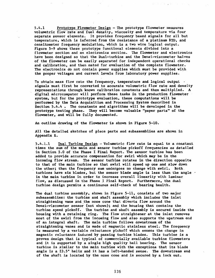
5.4-1 volumetric flow rate and fuel density, viscosity and temperature via four separate sensor elements. temperature, which is inferred from the resistance of a.platinum RTD, and densitometer frequency modulation, which is a two wire logical output. Figure 5-9 shows these prototype functional elements divided into a flowmeter section and an electronics section. The flowmeter and electronics have been designed so that the Dual-turbine and the Densi-viscometer halves of the flowmeter can be easily separated for independent operational checks and calibration, and then mated for evaluation of the complete flowmeter. The electronics do not contain power supplies which must be provided with the proper voltages and current levels from laboratory power supplies.

Prototype Flowmeter Design - The prototype flowmeter measures It provides frequency based signals for all but

To obtain mass flow rate the frequency, temperature and logical output . signals must first be converted to accurate volumetric flow rate and density representations through known calibration constants and then multiplied. digital microcomputer will perform these tasks in the production flowmeter system, but for the prototype evaluation, these computations will be performed by the Data Acquisition and Processing System described in Section 5.4.4 e

prototype testing phase. They will become valuable "paper parts" of the flowmeter, and will be fully documented.

A

The constants and algorithms will be developed in the

An outline drawing of the Plowmeter is shown in Figure 5-10.

All the detailed sketches of piece parts and subassemblies are shown in Appendix E.

5,4,%.l Dual Turbine Design - Volumetric flow rate is equal to a constant times the sum of the main and sensor turbine pickoff frequencies as detailed in Section 5.0 of the Phase I Final Report. The sensor turbine has been added to provide accurate compensation for swirl which may be in the incoming flow stream. The sensor turbine rotates in the direction opposite to that of the main turbine so that swirl will speed up one and slow down the other; then the frequency sum undergoes no change with swirl. Both turbines have six blades, but the sensor blade angle is less than the angle in the main turbine in order to increase overall linearity with laminar flow, as discussed in the Phase I Final Report. turbine design permits a continuous self-check of bearing health.

Furthermore, the dual

The dual turbine assembly, shown in Figure 5-11, consists of two major subassemblies: the turbine and shaft assembly which includes the inlet straightening vane and.the nose cone that diverts flow around the Densi-viscometer sensor (not shown); and the housing that contains the turbine speed pickoff. housing with a retaining ring. most of the swirl from the incoming flow and also supports the upstream end of an integral shaft. straightening vanes and is made of magnetic stainless steel. The frequency is measured by a variable reluctance pickoff which senses the change in magnetic reluctance induced by passing turbine blades. This turbine is a proven design that is typical of commercially available turbine flowmeters and it is supported by a single high quality ball bearing. The sensor turbine is similar to the main turbine with the exceptions that its blade angle is a 23.5O helix and it has a left-handed sense. The downstream end of the shaft is located by the nose cone and is secured by a lock nut.

The turbine and shaft assembly is secured inside the The flow straightener at the inlet removes

The main turbine follows downstream of the

136

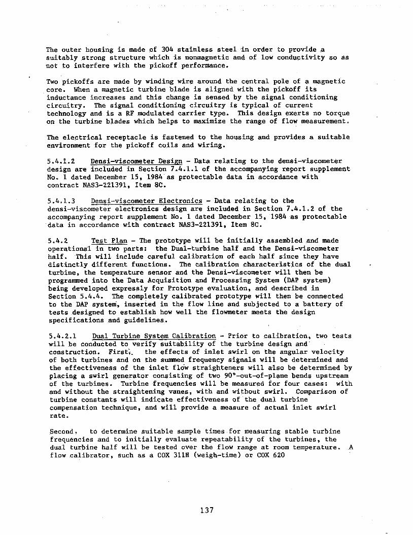
The outer housing is made of 304 stainless steel in order to provide a suitably strong structure which is nonmagnetic and of low conductivity so as not to interfere with the pickoff performance.

Two pickoffs are made by winding wire around the central pole of a magnetic core. When a magnetic turbine blade is aligned with the pickoff its inductance increases and this change is sensed by the signal conditioning circuitry. The signal conditioning circuitry is typical of current technology and is a RF modulated carrier type. This design exerts no torque on the turbine blades which helps to maximize the range of flow measurement.

The electrical receptacle is fastened to the housing and provides a suitable environment for the pickoff coils and wiring.

5.4.1.2 design are included in Section 7.4.1.1 of the accompanying report supplement No. 1 dated December 15, 1984 as protectable data in accordance with contract NAS3-221391, Item 8C.

Densi-viscometer Design - Data relating to the densi-viscometer

5.4.1.3 Densi-viscometer Electronics - Data relating to the densi-viscometer electronics design are included in Section 7.4.1.2 of the accompanying report supplement No. 1 dated December 15, 1984 as protectable data in accordance with contract NAS3-221391, Item 8C.

5.4.2 operational in two parts: half. distinctly different functions. The calibration characteristics of the dual turbine, the temperature sensor and the Densi-viscometer will then be programmed into the Data Acquisition and Processing System (DAP system) being developed expressly for Prototype evaluation, and described in Section 5.4.4. The completely calibrated prototype will then be connected to the DAP system, inserted in the flow line and subjected to a battery of tests designed to establish how well the flowmeter meets the design specifications and guidelines.

Test Plan - The prototype will be initially assembled and made the Dual-turbine half and the Densi-viscometer

This will include careful calibration of each half since they have

5.4.2-1 Dual Turbine System Calibration - Prior to calibration, two tests will be conducted to verify suitability of the turbine design and construction. First;, of both turbines and on the summed frequency signals will be determined and the effectiveness of the inlet flow straighteners will also be determined by placing a swirl generator consisting of two 90°-out-of-plane bends upstream of the turbines. Turbine frequencies will be measured for four cases: with and without the straightening vanes, with and without swirl. Comparison of turbine constants will indicate effectiveness of the dual turbine compensation technique, and will provide a measure of actual inlet swirl rate.

the effects of inlet swirl on the angular velocity

Second, to determine suitable sample times for measuring stable turbine frequencies and to initially evaluate repeatability of the turbines, the dual turbine half will be tested over the flow range at room temperature. A flow calibrator, such as a COX 311H (weigh-time) or COX 620

137

(volumetric-density), and a monitor turbine will provide stable references against which the dual turbine will be compared. to 60 seconds (minimum 10 sec with flow calibrators, less with monitor turbine) and flow rates from 0.050 kg/s (400 lb/hr) to 2.52 kg/s (20,000 lb/hr) will be evaluated with multiple readings at each of several points.

Measurement times from 1/5

After these initial. checks indicate satisfactory performance, the calibration factor K vs Reynolds number characteristics will be measured and programmed into the DAP system, temperature with three different fluids having viscosities of approximately P.39 5.0 and 15 centistolres. MIL-C-7024A, Type I1 calibration fluid will be used for the 1.3 cs viscosity, and mixtures of Almag and Tellus #lO oils will be used for higher viscosities, Further, several runs will be made with calibration fluid near the temperature extremes (-55 and + 100OC) to verify the predicted effects that material expansion and contraction have on the turbine constants.

This calibration will be done at room

For purposes of these calibrations and subsequent prototype evaluations it is necessary to establish "in house" standards of mass flow rate, volumetric flow rate, density and viscosity. For the above turbine calibrations, the two volumetric flow rate standards will be 2.54 ern (1.0 in) and 1.27 cm (0.5 in) size turbineso These monitor turbbes will be calibrated using COX 305 and 311H weigh-time stands (mass flow rate) combined with in-line density measurements using a Mettler-Paar DMA 60 and DMA 620HT high accuracy digital density meter.

During calibration of the monitor turbines, the number of flow measurkments that are taken at each flow rate will be determined by statistical analysis. Typically, enough measurements will be taken at a particular flow rate to ensure that the mean of the COX flow stand outputs is known within + 0.05% at a 95% confidence level using the Students'-t statistic. mass flow rate divided by density will then be the reference volumetric flow rate that determines the turbine K factors. During subsequent prototype evaluations (described in the following section) t;he same weigh-time stand outputs and the prototype output will be in terms of mass flow rate and may be compared directly, without the conversion to volumetric flow rate. However, tests may show that the outputs of the monitor turbines and the densitometer standard can be combined to provide a more repeatable indication of mass flow rate than the COX stands, in which case, the monitor turbines will serve as the standards against which prototype accuracy is determined.

Average

If the COX stands prove to be adequate for use as a standard in the evaluation phase, then the tare- and sample weights used during evaltla-tim-. for each range of flow measurement will be used again in the calibration phase. the Section 3.0 Calibration Study) depend heavily on the selection of tare and sample times (and weight) this technique will effectively eliminate any variations in the systematic errors caused by buoyancy effects and timing errors resulting from changes in fluid forces, holding tank inertia and

Since the systematic errors of the COX flow stand (as reported in

138

sample control volume. flow rate without compensation for the systematic errors and greatly simplifies the task.

This technique also permits direct readout of COX

While these techniques will not provide evaluation of absolute accuracy (i.e*, the known systematic errors of the COX flow stands are not corrected) they will provide an excellent measure of prototype repeatability. future, when a more accurate flow standard is available, the biases introduced with the COX flow stands can be easily compensated out by introducing new calibration constants in the software,

In the

Viscosity of the calibration fluid will be calculated from an accurate temperature measurement at the flowmeter and from a viscosity versus temperature eurve which is evaluated just prior to the test. temperature sensor will be an RTD and the viscosity measuredents will be made with a suspended capillary type viscometer. listing of these measurement standards.

The

See Table 5-1 for a

For purposes of this prototype evaluation, it is also riecessary t o establish standards for time, temperature, density and viscosity that are accurateg stable and readily available. Table 5-1 describes these standards.

5.4.2.2 Densi-Viscometer Calibration - Density and viscosity ranges for JET-A, Jet A-1, JP-3, JP-4, and JP-5 fuels taken from the Test and Calibration System Study (Section 3.0 of this report), are summarized in Table 5-2. by mixing various liquids also listed in the table. With these mixtures held at fixed temperature, in the apparatus shown in Figure 5-12, the . frequency characteristic of the Densi-viscometer to both density and viscosity will be evaluated. This will expedite adjustment of the electronics and calibration of the sensor because shifts caused by temperature changes will be minimized.

These fuel characteristics will be simulated at room temperature

After initial calibration over the density and viscosity ranges, the Densi-viscometer will be calibrated over the temperatur,e range, (-55OC to + 100°C with the electronics at room temperature) in air and in calibration fluid. The test apparatus shown in Figure 5-12 will circulate heat transfer fluid in a loop that includes a temperature controller, the fully assembled Densi-viscometer with RTD, the density standard and the viscosity standard. Insulating the loop will assure temperature stability. The calibration fluid samples will be closed and pressurized so that atmospheric water vapor will not condense into and contaminate them at low temperatures, and so that light disrillates will not vaporize at high temperatures and thereby prevent gradual increase in density with time. Concurrent with density calibration, the temperature-viscosity characteristics of the test fluid will be derived from a kinematic viscometer standard immersed in the heat transfer medium. The results of the calibration will be correlated by a least squares polynomial that will be programmed into the DAP system for subsequent evaluation of the prototype.

A third test will be conducted to assure insensitivity of the sensor to fluid flow. The Densi-viscometer half will be placed in a flow stand with

139

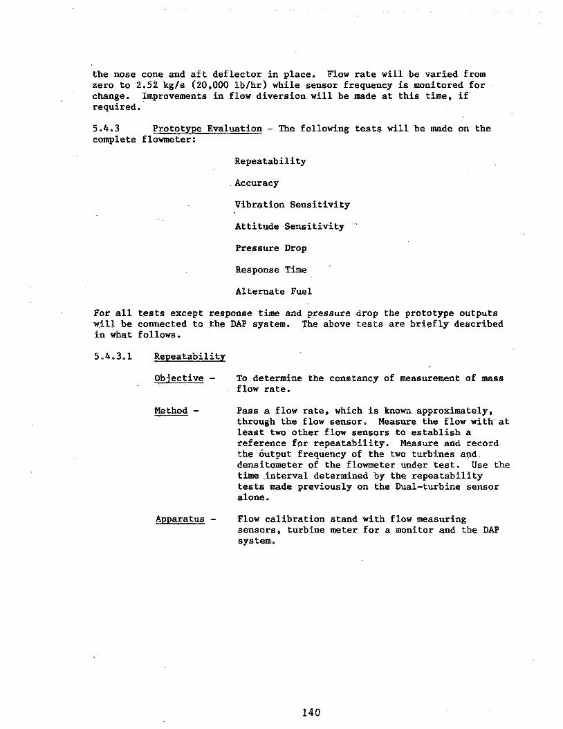
the nose cone and aft deflector in place. Flow rate will be varied from zero to 2.52 kg/s (20,000 lb/hr) while sensor frequency is monitored for change. Improvements in flow diversion will be made at this time, if required.

5.4.3 complete flowmeter:

Prototype Evaluation - The following tests will be made on the

Repeatability

Accuracy

Vibration Sensitivity

Attitude Sensitivity .'

Pressure Drop

Response Time

Alternate Fuel

For all tests except response time and pressure drop the prototype outputs will be connected to the DAP system. in what follows.

The above tests are briefly described

5.4.3-1 Repeatability

Objective - To determine the constancy of measurement of mass flow rate.

Method - Pass a flow rate, which is known approximately, through the flow sensor. least two other flow sensors to establish a reference for repeatability. the output frequency of the two turbines and densitometer of the flowmeter under test. Use the time interval determined by the repeatability tests made previously on the Dual-turbine sensor alone.

Measure the flow with at

Measure and record

Apparatus - Flow calibration stand with flow measuring sensors, turbine meter for a monitor and the DAP sys tem.

140

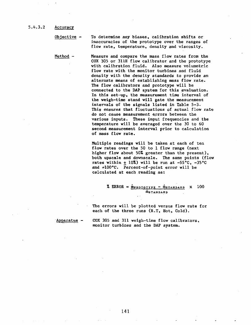
5.4.3.2 Accuracy

Objective - To determine any biases, calibration shifts or inaccuracies of the prototype over the ranges of flow rate, temperature, density and viscosity.

Method - Measure and compare the mass flow rates from the COX 305 or 311H flow calibrator and the prototype with calibration fluid. Also measure volumetric flow rate with the monitor turbines and fluid density with the density standards to provide an alternate means of establishing mass flow rate. The flow calibrators and prototype will be connected to the DAP system for this evaluation. In this set-up, the measurement time interval of the weigh-time stand will gate the measurement intervals of the signals listed in Table 5-3. This ensures that fluctuations of actual flow rate do not cause measurement errors between the various inputs. These input frequencies and the temperature will be averaged over the 30 to 60 second measurement interval prior to calculation of mass flow rate.

Multiple readings will be taken at each of ten flow rates over the 50 to 1 flow range (next higher flow about 50% greater than the present), both upscale and downscale. The same points (flow rates within 2 10%) will be run at -55"C, -35OC and +lOO°C. calculated at each reading as:

Percent-of-point error will be

% ERROR = & P R O T O T Y P E - & S T A N D A R D x 100 ~ ~ ~ S T A N D A P D

The errors will be plotted versus flow rate for each of the three runs (R.T, Hot, Cold).

Apparatus - COX 305 and 311 weigh-time flow calibrators, monitor turbines and the DAP system.

1 4 1

5.4.3.3 Vibration Sensitivity

Objective - To determine the sensitivity of flow rate performance to vibration inputs.

Methods - Mount the flowmeter on a vibration machine by means . of a suitable fixture. Pass a constant fuel flow rate of about 25 percent of full scale through the flowmeter. specified in the design guidelines and monitor the indicated flow rate from the flowmeter during vibration. inputs along each of three orthogonal axes. During each Vibration scan, particular attention will be paid to mechanical resonances and variations of indicated flow.

Vary the vibration input over the range

Repeat the procedure with vibration

Apparatus - Servo type sinusoidal vibration machine, flow stand, flow sensor to monitor flow input to flowmeter being tested, and DAP system.

5.4.3.4 Attitude Sensitivity

Objective - To determine if accuracy is adversely affected by the orientation of the flowmeter.

Method - Mount the flowmeter in a selected orientation. Pass a constant fuel flow rate of about 25 percent of full scale through the flowmeter using a standard turbine to monitor flow. Change the orientation of the flowmeter under test and record any changes in mass flow rate output. each orientation desired. The positions to be tested are with axis of flow vertical and with the axis of flow horizontal and the flowmeter rotated 90" between successive orientations.

Repeat the procedure for

Apparatus - Flow stand, turbine meter to monitor flow, means to hold the flowmeter under test in the desired orientation, and the DAP system.

5.4.3.5 Pressure DroE

Objective - To determine the pressure drop across the flowmeter for a range of flow rates up to full scale.

Method - Mount the flowmeter with the axis of flow horizontal. across the flowmeter. Pass fuel flow through the flowmeter and measure flow rate and differential pressure for each point from low flow to full scale.

Connect a differential pressure meter

Apparatus - Flow stand, differential pressure meter, inlet and outlet pipes with pressure taps.

1 4 2

5 4 ., 3 6 Time Response

Objective - To measure the time constant of the turbine speeds when subjected to step changes in flow rates.

Method - The square wave output from both signal conditioners of the main and sensor turbines and the output from a hot film anemometer placed in the flow stream just ahead of the prototype will be .recorded on magnetic tape. An inlet pipe fixture with two parallel pipes, each pipe having a throttle valve and one having a snap action valve, will be used both to create a fast step change in flow rate and to control the initial and final flow rates. The recorded tape will be played back at reduced speeds while the outputs are.recorded on strip chart paper for detailed analyses.

1 .

Apparatus - Parallel pipe manifold with valves, tape recorder, strip chart recorder, hot film anemometer system.

5.4.3..7 Alternate Fuel

Repeat Accuracy test (5.4.3.2) at room, hot, and cold temperatures with JP-8.

5.4.4 flowmeter has a total of five electrical signal outputs with the ranges and characteristics listed in Table 5-3. Synchronization of the measurement interval for these signals with flow calibrator and monitor turbine signals is essential to obtaining reliable measurements of prototype repeatability and accuracy. Furthermore, the conversion of the signals to mass flow rate through the various calibration functions requires a dedicated computer to obtain meaningful results in a timely fashion (i.e., real time). requirements were recognized early in the test plan formulation and led to the design of a Data Acquisition and Processing System, herein referred to as the DAP system. key elements of the system.

Data Acquisition and Processing System (DAP) - The prototype

These

Figure 5-13 is a functional block diagram showing the

Frequency signals are routed to digital counters that output to a digital bus (IEEE 488 compatible, HPIB) and are controlled (synchronized) by the bus. This includes the prototype frequency signals and the monitor turbine frequency signal. and the modulation output of the Densi-viscometer electronics are converted to digital signals through a General Purpose Input/Output Port (GPIO). The RTD resistance is output to the digital bus via a digital multimeter. An HP86A computer controls the data flow and is programmed in BASIC to compute mass flow rates for both the flow calibrator and the prototype. A monitor, disk storage and printer/plotter make the DAP system a complete and versatile tool necessary for the successful development of the high accuracy fuel flowmeter for NASA.

The weigh-time interval of the COX 311H flow calibrator

143

5.5 Fabrication, Tests, and Analyses of Prototype Design

The design and test plan described in Section 5.4 were carried out by fabrication of the prototype design outlined in Appendix E. expected, several minor design changes were made and test plan was slightly altered. Adjustments to calibration equipment and techniques were also deemed necessary. These changes together with the actual test data and analyses are covered in this section.

As

5.5.1 Introduction - This portion of the report covers Task 6 and Task 7 of the dual turbineldensi-viscometer concept. high accuracy turbine meter with a high accuracy densi-viscometer. turbine meter provides a precise measurement of volumetric flow rate when the meter is corrected for viscosity effects. the'densi-viscometer measures fluid densitx which is used to convert volumetric flow rate to mass flow'rate, and the viscometer provides the viscosity information that is needed for the turbine meter viscosity corrections.

The design combines a The

The densitometer portkon of

The dual turbine/densi-viscometer should satisfy the following specification requirements:

Specification

Flow Range

Accuracy Requirement Accuracy Goal

Response-Time Constant Below 10% of Full Scale Above 10% of Full Scale

Ambient Temperature Fuel Temperature

Maximum Fuel Pressure

Maximum Pressure Drop

Vibration - 5 to 40 Hz 14 to 23 Hz 23 to 90 Hz 90 to 2000 Hz

Mounting Position

0.050 to 2.52 kg/s (400 to 20,000 lb/hr)

- + Oe25% of reading - + 0.10% of reading

100 ms 25 ms

-55OC to 130°C -55OC to 130°C

7000 kPa (1000 psi)

69 kPa (10 psi)

- + 1.2 mm + 1 g - + 0.45 mm - + 15 g

Performance to be Unaffected by Operating Attitude

1 4 4

5 . 5 - 2 volumetric flow rate simply, reliably, and repeatably, but it has some limitations. bearing speed of about 250 rps. constant that is linear down to about one-tenth of maximum flow rating, so the specified 5O:l range of mass flow rate (65:l volumetric flow rate) requires special consideration.

Background - A turbine meter is an established method of measuring Maximum flow for a given size is limited by maximum allowable

Turbine meters typically have a calibration

Earlier sections of this report theorized that the calibration curve of a turbine meter could be made more nearly linear for a wider range by including a counter rotating turbine in the flowmeter design. curve would be a single valued function of output frequency divided by kinematic viscosity, so the volumetric flow rate could be determined by measuring turbine frequency and fuel viscosity. mass flow rate could be derived. The densitometer portion of this report presents an approach to derive both density and viscosity information from a proven densitometer design.

Moreover, the calibration

By adding a densitometer,

The primary goal of Phase 11, Task 6 is to determine the validity of the theory of Phase 11, Task 1. and built. The turbine meter was calibrated over a range of viscosities and flow rates, and the calibration information was stored in the program of a data acquisition and processing system. The densi-viscometer was calibrated by using fluids of known density and viscosity as references and adjusting the electronic drive and control circuits to give the required outputs.

To do this, a dual turbine flowmeter was designed

After each portion had been calibrated separately, the dual turbine and the densi-viscometer were mated into one assembly for testing as a complete flowmeter. discussed in the Phase 11, Task 5 report detailing the prototype design and test plan. The following sections of this present report on Phase 11, Task 6 cover calibration and testing of each of the two portions and of the entire flowmeter.

The product design and the test program were presented and .

5.5 .3 Fuel flowing from left to right first passes through the main turbine (6 blades of 45" helix angle) and then the sensor turbine ( 6 blades at 23.5" left hand helix). The blades of both turbines are magnetic, so, as each blade passes the pickoff coil, the 45 kHz excitation current is modified. change in current is detected by the signal conditioning electronics which output one pulse for each blade passing.

One important reason for having the sensor turbine as part of the design is to provide compensation for any swirl that might be in the in-flowing fuel stream. Depending on the direction of rotation of the swirl, it could either increase or decrease the speed of the main turbine. but opposite effect on the counter-rotating sensor turbine, so the effects of swirl should be cancelled when the frequencies of the two are summed.

Dual Turbine Portion - Figure 5-11 shows the8dual turbine design.

The

There will be an equal

5.5.3.1 Effects df Swirl - Several tests were made on the dual turbine to determine the effectiveness of the swirl compensation. First the turbine meter was temporarily modified by removing the flow straightener from the inlet end

145

so that any swirl in the incoming flow stream would affect the operation of the main turbine directly. Then the transmitter was tested to measure the effects of the swirl.

Swirl was generated by a double elbow configuration at the inlet of the dual turbine meter as shown in Figure 5-14. The amount of swirl that was added to the incoming flow by the double elbow arrangement was determined by measuring the "K" factor of the main turbine first with the swirl generator and then with a straight inlet pipe that would have no swirl. The two "K" factors are plotted in Figure 5-15 and show that the swirl affected the main turbine by about 10%. This is enough swirl to give a good indication of the degree of compensation provided by the sensor turbine. Figure 5-16 shows that the sum of the frequencies of the main and sensor turbines, which is the output from the dual turbine, is affected by 2.5 parts in 550, or 0.45%, when 10% swirl is - introduced. The swirl compensation thus seems to be effective.

The flow straightener was put back into the inlet of the turbine and the turbine meter was retested to determine if the flow straightener would also remove swirl. The "K" factor of the main turbine was measured with and without the swirl generator at the inlet. Figure 5-17 demonstrates that the flow straightener is very effective in removing swirl because the two curves for tests with swirl and without swirl are indistinguishable from each other.

5.5.3.2 Characterization - After the swirl sensitivity tests had been completed, the dual turbine characterization was started. The purpose was to measure the "K" factor of the dual turbine over the specified mass flow rate range for the specified fuel temperatures and viscosities. The test data are stored in the memory of the Data Acquisition and Processing System. In serviceo fuel temperature and viscosity are measured by the densi-viscometer so the "K" factor of the dual turbine can be determined from the stored information, Being able to determine the "K" factor means that the turbine meter need not have a precisely linear calibration in order to be used over a wide range of flow rates and still yield accurate results. The turbine meter need only be repeatable, which is an inherent characteristic of turbine meters in general, and have a calibration curve that is single valued and does not show rapid changes over the operating flow range.

The characterization of the dual turbine meter was determined by using a weigh-time stand to measure mass flow rate of calibration fluid for which density and viscosity had been determined over the specified fuel temperature range. the turbine meter so the density and viscosity of the fuel which the turbine meter had measured were known.. Volumetric flow rate was calculated by dividing the measured mass flow rate by the density of the fuel. The "K" factor, whfch is expressed in terms of pulses per cubic meter (or turbine frequency divided by cubic meters per second), was calculated from measured turbine frequency and volumetric flow rate.

The temperature of the calibration fluid was measured at the outlet of

A conventional turbine meter was included in the flow loop to act as a monitor in case some anomaly should appear. loop is shown in Figure 5-18. stand and normally passes first through the dual turbine and then the monitor

A schematic representation of the flow The flow comes in from the weigh-time flow

146

turbine. There is a length of straight pipe, about 40 diameters long, in front of each turbine meter to minimize swirl in the incoming fuel. Valves in the main loop and in a by-pass give flexible control of both steady state and transient flows. There is a calibrated resistance temperature detector (RTD) measuring probe at the outlet of each turbine meter. from the turbine meters, the resistance measurements of the temperature probes, together with the weight and time from the flow stand are all fed into the Data Acquisition and Processing System where the desired parameters are calculated and printed out.

The turbine meter characteristics were measured for following conditions:

The frequency outputs

a - Calibration fluid, room temperature b - Calibration fluid, 100°C c - Calibration fluid, - 3 5 " ~ (viscosity = 3.5 cs) d - Calibration fluid, - 55OC (viscosity = 8.5 cs) e - Vacmul f - Tellus oil, room temperature (viscosity = 11 cs)

oil, room temperature (viscosity = 7.3 cs)

The test results for these characterization runs are plotted on several curves:

Dual Turbine - Figure 5-19 Main Turbine - Figure 5-20 Sensor Turbine - Figure 5-21 Monitor Turbine - Figure 5-22

All of these curves show separations that seem to be viscosity dependent - separations which could introduce serious errors in volumetric and mass flow calculations. In order to identify the cause of these separations, the monitor turbine was sent to an outside facility that regularly calibrates turbine meters. cold fuel, but could use fuels that covered a range of viscosity of Figures 5-19 through 5-22.

This outside facility could not readily test with hot and

The results of tests (Figure 5-23) of the monitor turbine at the outside facility are different from those shown in Figure 5-22 for the same-turbine meter, and the difference is ascribed to the mass flow measurement equipment. Phase I11 of the High Accuracy Fuel Flowmeter program addresses the need for the Test and Calibration System (TACS) which has much better flow measurement capability. fourth quarter of 1984 which is too late for testing the dual turbine/densi-viscometer prototype.

The TACS as described in Section 3.0 will be available in the

The monitor turbine appeared to be the best means of measuring mass flow rate if accurate density and viscosity were available. be obtained by measuring the temperature of pre-characterized fuel. The characterization of the monitor turbine, as determined by measurements at the outside facility, was converted to an eleventh order equation and stored in the data processing system. The characteristic curve that is calculated from this equation is shown in Figure 5-24. The measured points are also plotted in Figure 5-24 to indicate the correlation between the measured points and the calculated curve.

Density and viscosity could

147

The next step was to re-calculate all the previously measured values of the dual turbine (shown in Figure 5-19) using the monitor turbine curve of Figure 5-24 as the flow standard. before the tests of Figure 5-19 through 5-22 were made, and temperature was measured at each flow point,. so the fuel characteristics were known for each test point. The re-calculated points for the dual turbine, together with the calculated curve to fit the points, are plotted in Figure 5-25. If the data for -55OC calibration fluid is omitted, the re-calculated points' and curve are as in Figure 5-26, and there is much less scatter than in Figure 5-25. The extra scatter of Figure 5-25 is probably associated with temperature errors in the mass flow measurement equipment which is used to obtain the data. curve of Figure 5-26 was used as the dual turbine characterization curve for the prototype test program that follows.

Fuel density and viscosity had been determined

The

. 5.5.4 Mass Flowmeter Tests - After the dual turbine meter and the densi-viscometer had each been calibrated as separate units, the two portions were mated to form a complete flowmeter. evaluated by performing the tests that are listed in Section 5.4.3. results are presented in the same order in which the tests were made.

The prototype flowmeter was then Test

5.5.4,l Pressure Drop - Pressure drop across the flowmeter was measured for several flow rates from 0,25 kg/s (2000 lb/hr) to 2,77 kg/s (22,000 lb/hr). The data were plotted on a log-log scale in Figure 5-27, and the points form a

psi) as determined graphically from Figure 5-28. greater than the specified pressure drop of 69 kPa (10 psi) at 2.52 kg/s (20,000 lb/hr). allowing for the second turbine is about 50 kPa (7.3 psi), so a large portion of the pressure drop is across the densitometer portion of the assembly. If the pressure drop is critical and must be brought down to 69 kPa (10 psi), it should be possible to redesign the densitometer housing to give a lower pressure drop.

I straight line. The pressure drop at 2.52 kg/s (2O,OOO lb/hr) is 110 kPa (16 That value is about 60%

Quoted pressure drop for a turbine meter of the size used and

5.5-4.2 out how many times the flow rate at any calibration point has to be measured i n order to be sure, at the 95% confidence level as determined from the student "t" test, that the measured values were correct, Another purpose of repeatability testing was to provide some insight into the quality of the dual turbine sensor by seeing how closely the flow measurements were clustered.

Repeatability - The purpose of the repeatability tests was to find

The monitor turbine, the dual turbine, and a weigh-time calibrator were set up to have the same mass flow rate pass through all three units. The flow rate as measured by each unit was recorded 20 times in succession at nominal flow rates of 0,063 (5001, 0.63 (50001, 1-26 (lO,OOO), and 2.52 kg/s (20,000 lb/hr) which covers the full rated flow range. statistically, based on the assumption that the actual flow rate was constant, and a sunrmary of these calculations is given in Table 5-4.

These measurements were analyzed

The repeatability of the dual turbine as related to the monitor turbine (last column in Table 5-4) is better than for the monitor turbine alone which indicates that the flow rate did not actually remain constant at each flow

148

point. that of the Monitor Turbine which reinforced the decision to use the Monitor Turbine output as the time measure of flow rateo

The repeatability of the weigh-time calibrator is much poorer than

The last column of Table 5-4 shows that ten readings are enough to provide repeatability of better than 0.05% at any flow rate. each flow rate were taken for all later tests that required an accurate flow measurement.

Ten or more readings at

5.5.4.3 Attitude - Flow rate was measured 20 times with approximately 0.63 kg/s (5,000 lb/hr) flow rate through the dual turbine with the flow axis vertical and with the flow axis horizontal and the electrical receptacle positioned at 12, 3, 6, and 9 o'clock. The results are summarized in Table 5-5. nearly alike which shows that the flowmeter accuracy is not affected by munting position. All the errors were positive which were probably caused by a shift in the densi-viscometer calibration.

5.5.4.4 output of the dual turbineldensi-viscometer to the output of the monitor turbine. The volumetric flow rate of the dual turbine was obtained from the characterization equation that is plotted in Figure 5-26 by using the sum of the main and sensor turbine frequencies divided by the kinematic viscosity, as measured by the viscometer, to determine the turbine "K" factor which in turn gave the volumetric flow rate. The density of the fluid was measured directly by the densitometer and the product of volumetric flow rate times density yielded the mass flow rate as measured by the product under test.

The percent errors for the five different orientations are all

Accuracy - Accuracy was measured by comparing the mass flow rate

The actual mass flow rate was measured by means of the monitor turbine together with fluid density and viscosity characteristics that had been pre-determined as a function of temperature. Volumetric flow rate came from the curve of Figure 5-24 by using the measured frequency from the Monitor Turbine and kinematic viscosity derived from a temperature measurement of the pre-calibrated fuel in the flowmeter. the same temperature measurement of pre-calibrated.-fueL, and the product provided mass flow rate.

The fuel density was also obtained from

All of the calculations mentioned above were performed by the Data Acquisition and Processing System which also calculated percentage errors for mass flow rate, density, and viscosity. Ten flow rate measurements, each about 11 seconds long, were made at each test flow point and the averages were calculated and printed out by the computer. point is shown in Figure 5-28.

A typical printout for one test

The accuracy of the dual turbine/densi-viscometer was measured both upscale and downscale at 25"C, lOO"C, -35°C and -55°C using MIL-C-7024A, Type I1 calibration fluid for flow rates from 0.050 kg/s (400 lb/hr) to 2.52 kg/s (20,000 lb/hr). At high flow rates, fluid flow forces affected the operation of the densi-viscometer giving invalid outputs of density and viscosity. Figure 5-29 is a plot of the transmitter error at room temperature from 0.050 kg/s (400 lb/hr) to 1.76 kg/s (14,000 lb/hr). Above that flow rate, the densi-viscometer output was unreliable so the 2.52 kg/s (20,000 lb/hr) point

149

was not plotted. percent specification limit for the entire flow range, the error is within limits for most of the flow range and is only slightly out at the lowest and highest portions. The mass flow rate error curve is divided into measured density and calculated volumetric flow rate error curves in order to understand the source of errors. error in the densitometer measurement and that most of the flow rate error is due to the measurement of volumetric flow rate. volumetric flow rate measurements from both the monitor turbine and the Dual Turbine, will be much improved when TACS is available so that the MSS flow rate measurement from the Dual Turbine/Densi-viscometer will be within 20025%0

Accuracy at 100°C is shown in Figure 5-30, again for the flow range of 0.050 kg/s (400 lb/hr) to 1.76 kg/s (14,000 lb/hr). is not far above the 50.25% specification limit and should improve when the new calibrator is available. is an important reason that the mass flow rate is 0.3 to 0.4% above 0.25 %g/s ( 2000 fb/hr).

Although the flowmeter error does not remain within 20.25

Figure 5-29 shows that there is virtually no

It is expected that the

Again the mass flow rate

The density measurement error also increases and

Figure 5-31 for -35'C fuel and Figure 5-32 for -55OC fuel show a similar density measurement error which is about 1% too.high over the full flow range. For both -35OC and -5SoC, the volumetric flow rate is also out of limits for portions of the flow range and contributes to the mass flow error. Much of the error in volumetric flow results from the errors in viscosity measurement which are shown in Figure 5-33. An error in viscosity means that the wrong value of the Hdcs will be used when determining the "K" factor from Figure 5-26, Figure 5-31.

Volumetric flow rate equals the sum of the turbine frequencies divided by the "K" factor, so if the calculated "K" factor is too small, the volumetric and mass flow rates will be too large. The measured sum of the fre uencies from the Dual Turbine at 0.25 kg/s (ZOO0 lb/hr)mass flow rate at -35 C was 174 Hz and the measured kinematic viscosity was 5.6 centistokes which gives a value of Hz/cs equal to 31, 5-26. Since the viscosity measured by the Densi-viscometer is too high, and because the "K" factor curve of Figure 5-26 falls off sharply below the maximum point, the calculated value of the Hz/cs will be too low, the derived "K" factor will also be too low and the flow rate will be too high. increase in flow rate error in Figure 5-31 below 0.25 kg/s (2000 lb/hr) reflects this effect.

This effect is particularly noticeable for the -35'C tests,

8

This is just at-the maxim- "K" factor point of Figure

The steep

The error at -55'C, Figure 5-32 also shows the effects of viscosity error. The peak "K" factor again comes at 0.25 kg/s (2000 lb/hr) where the sum of turbine frequencies equals 175 Hz, the measured viscosity equals 6.0 cs, and Hz/cs equals 29. For smaller flow rates, measured viscosity remains too large which gives a "K" factor that is too low and leads to an increasingly positive flow rate error with decreasing flow rate.

The analysis of anticipated dual turbine performance that was presented in the Phase I report indicated that the "K" factor curve for the dual turbine would be flatter than test data have shown it to be, meaning that an accurate

150

measurement of viscosity would not be needed. 5-31 and 5-32 indicate that the "K" factor curve (Figure 5-26) must be made flatter, or viscosity must be measured more accurately, or both must be done. The repeat tests to be made when the new flow calibration system is available will help to determine how accurate the viscosity measurement must be..

Figures 5-31 and 5-32 also show that the densitometer has a large error at cold temperatures, and that the temperature error contributes greatly to the mass flow rate error. The subject of the densi-viscometer errors is treated in Section 7.0 of this report.

The results shown in Figure

5.5.4.5 Vibrat'ion Sensitivity - This test was to see if the performance of the dual turbine/densi-viscometer changed when it was subjected to sinusoidal vibration inputs along any of the three main axes. The vibration inputs were:

5-14 HZ 2,4 mm double amplitude

14-23 Hz 2 fg

23-90 HZ . 0.90 mm double amplitude

90-2000 HZ - + 15 g A constant flow rate of approximately 25% of full scale was maintained through the flowmeter while the vibration frequency was changed up to 2000 Hz and back down to 5 Hz. frequencies and the densitometer output as well as the flow rate output, were monitored throughout the vibration scans in order to determine how vibration would affect the operation of the flowmeter. In addition, an output accelerometer was fastened to the flowmeter so that mechanical resonances could be measured. The three directions of vibration input and the mechanical resonance test results are shown in Figure 5-34. resonances occur at relatively high frequencies and the amplifications are low so there should not be vibration induced structural fatigue problems..

The main turbine and the sensor turbine output

All

The operational flow data showed that the main and sensor turbine frequencies were unaffected by vibration but the densitometer had a large vibration induced error for vibration frequencies greater than about 45 Hz. This is discussed in greater detail in the densi-viscometer portion of this report.

Flowmeter accuracy was measured after all vibration tests were completed and is plotted in Figure 5-35. temperature test before vibration, Figure 5-29, shows that the densitometer output has increased by about 0.25% but that volumetric flow rate curves are very similar which indicates that the dual turbine meter calibration was not permanently affected by temperature and vibration stresses.

A comparison of Figure 5-35 to the room

5.5.4.6 removed from the flow stand and refilled with JP-5 fuel to see if the Dual Turbine/Densi-viscometer flowmeter was capable of measuring the rate of flow of fuel having different density and viscosity characteristics.

Alternate Fuel - The MIL-C-7024A Type I1 calibration fluid was

151

Figure 5-36 shows the accuracy at room temperature with JP-5 and should be compared to Figure 5-35 which was the preceding room temperature curve with calibration fluid. All three curves - mass flow, volumetric flow, and density - of Figures 5-35 and 5-36 look similar to each other showing that there is little error with an alternate fuel. Comparing Figure 5-37 which is the JP-5 curve at 100°C with Figure 5-30 shows some discrepancies, but if the permanent changes in the densi-viscometer caused by temperature and vibration are considered, the discrepancies in the flowmeter are greatly reduced.

Near the start of tests at -55°C with JP-5, the flow stand suffered serious damage and the testing program had to be halted before measurements could be made with JP-5 at -55OC and -35*C.

5.5.4.7 putting a step input in and measuring the output versus time. d$.fficult to produce an abrupt change in flow rate to simulate the step input. If it is possible to measure actual flow by using some sort of fast responding auxiliary equipment, then the time response of the flowmeter under test can be determined by comparing flowmeter output to the fast response measurement.

Time Response - Response time of an instrument can be measured by It is

It was planned to measure the time response of the dual turbine/densi-viscometer prototype by using a hot wire anemometer probe to monitor actual flow rate. A great deal of time and effort was spent trying to obtain usable signals from the hot wire anemometer, but the output was always too noisy to be useful, and the anemometer approach was abandoned.

A more successful approach to measuring response time was made by opening a quick-opening valve upstream from the flowmeter and recording the output from the Main Turbine signal conditioning electronics. A typical frequency trace is shown in Figure 5-38. the trace (Figure 5-39) is approximately 25 ms, but the change in flow rate was probably far from being instantaneous.

Other considerations indicate that the response of a turbine meter is much faster than 25 ms. Characteristics of Turbine Meters" and published in the ASME Journal of Basic Engineering shows several time response curves which were plotted from experimental data. time constant of about 5 ms. This is probably typical for small turbine meters.

The time constant of the response curve from

An article by M.R. Shafer entitled "Performance '

These curves are reproduced in Figure 5-40 and show a

The data for the curve of Figure 5-40 was obtained by recording and plotting the peak voltage of each output pulse of an induced voltage type pickoff. It had previously been determined that the voltage level was directly proportional to speed, so the peak value was a measure of instantaneous turbine speed. recordings and each point contains one half of the time for the turbine to turn from one blade to the next. In practice, the response time would contain the full time for the turbine to turn through the angle between two adjacent blades, and at slow turbine speeds this would be the most important element in the response time. For example, at 0.071 kg/s (560 lb/hr), the

The data for Figure 5-39 was derived from frequency

152

main turbine output frequency measured about 40 Hz which is a time interval of 25 ms between successive blade passings. It appears, then, that even if the turbine responds in 5 ms or so, the time to obtain that information may be much greater and may be the limiting factor.

5.6 Conclusions and Recommendations

5.6.1 Conclusions - Test results indicate that the dual turbine concept does not offer an advantage over a conventional flow straightener for eliminating the effects of swirl in the incoming flow stream.

The "K" factor of both the monitor turbine and the dual turbine is a single yalued function of turbine frequency divided by kinematic viscosity for room temperature fuel.

Since the dual turbineldensi-viscometer concept requires that each turbine meter be accurately mathematically modeled based on test data, a very accurate flow test facility is essential to characterize the turbine and to test the complete flowmeter.

Fuel viscosity must be accurately measured if errors at low flow and high viscosity must be kept small.

Although the dual turbine/densi-viscometer flowmeter had errors greater than 0.25% for a number of test conditions, tests with room temperature and 100°C fuel were very encouraging.

5.6.2 accuracy or swirl compensation and has a slower response time. Consider using only the main turbine to measure flow rate but retain the sensor . turbine to provide an auxiliary output to measure bearing degradation. When the new high accuracy test and calibration system is operational, use it to characterize the dual turbine and to evaluate the complete flowmeter.

Recommendations - The dua.1 turbine seems to offer no advantage in

153

Section 5.7

TABLES

154

TABLE 5-1 STANDARDS FOR PROTOTYPE EVALUATION

MASS FLOW RATE Weigh-Time Flow Calibrators COX 3llH COX 305.

VOLUMETRIC FLOW RATE Turbine flowmeters 0.64 liter/sec (10 gpm) maximum flow

- Nominal 1.3 em (0.5 in.) size

3.8 literslsee (60 gpm) maximum flow - Nominal 2.5 em (1-0 in,) size

DENSITY

TEMPERATURE

VISCOSITY

Mettler-PAAR Densitometer DMA 60 Processing Unit DMA 602HT Density Measuring Cell

Platinum RTD Sensor

Cannon-Ubbelohde Kinematic Viscometers Suspended Level Type Certificate of Calibration from Mfg. Four Ranges, 0.5 to 30 cs.

1 5 5

TABLE 5-2 DENSITY AND VISCOSITY RANGES

Ranges €or JP-5, JP-4 JET-A, Jet A-1; JP-8

Temp Viscosity(&) Density(gm/cm3) ("C)

-55 Min. 7.0 Min. 0.80 Max.18.0 Max. 0.90

20 " Min. 1,1 Min. 0.74 Max. 2,2 Max. 0-85

+130 Min. 0.38 Min. 0.65 Max. 0.64 . Max. 0.77

Simulated at 25OC with Fluid Mixture

Tellus #lo -+ Freon TMC Tellus #lo

Cal. Fluid + Heptane Tellus #lO + Heptane

Cal. Fluid + Heptane Pentane

TABLE 5-3 PROTOTYPE OUTPUT SIGNAL OHARACTERISTICS

Signal

Main Turbine Frequency

Sensor Turbine Frequency

Densi-viscometer Frequency

Resistance (Temperature)

Densi-viscometer Frequency

Range Amp1 i t ude

24 to 1600 Hz 0 to 5V Square Wave

12 to 800 Hz 0 to 5V Square Wave

4500 to 6000 Hz 0 to 5V Square Wave

76 to 150 Ohms 0.385 R /"C

Two wire logical 0 to 5 v output

156

TABLE 5-4 REPEATABILITY

PERCENT DEVIATION FROM MEAN - 95%. CONFIDENCE LEVEL Number Weigh-Time Calib Monitor Turbine Dual Turbine Freq of Tests (Mass Flow Rate) (Mass Flow Rate) Monitor Turbine Freq

. + % + % + %

0.063 kg/s (500 lb/hr)

5 0.93

10 0.75

20 0.55

0.63 kg/s (5000 lb/hr)

5 0.41

10 0.26

20 0.15

1.26 kg/s (10,000 lb/hr) '

5 0.20

10 0.13

20 0.092

2.52 kg/s (20,000 lb/hr)

5 0.15

10 0.087

20 0.059

0.15

0.083

0,057

0.084

0.038

0.022

0.094

0.046

0.031

0.038

0.029

0.019

0.088

0 a 046

Not calculated

0.093

0.038

Not calculated

0.022

0.018

Not calculated

0,023

0.011

Not calculated

157

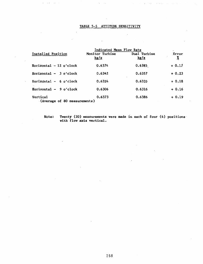
TABLE 5-5 ATTITUDE SENSITIVITY

Indicated Mean Flow Rate Installed Position Monitor Turbine Dual Turbine Error

- %

Horizontal - 12 o'clock 0.6374 0.6385. + 0.17 Horizontal - 3 o'clock 0 e 6342 0.6357 + 0.23

I Horizontal - 6 o'clock 0.6324 0.6335 + 0.18 Horizontal - 9 o'clock 0.6306

Vertical 0.6373 (Average of 80 measurements)

0.6316 + 0.16 0.6386 + 0.19

Note: Twenty (20) measurements were made in each of four (4) positions with flow axis vertical.

158

Section 5-8

FIGURES

159

?

160

161

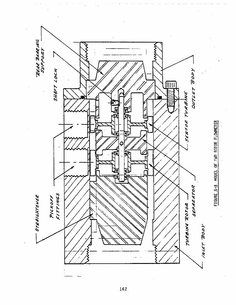
1 6 2

\ '.

9

1 f

. . '. -. w

m z

cr: =) I-

Y

163

!A a: c

Ir:

J

FIGURE 5-5 K vs FLOWRATE FOR THE ENGINEERING MODEL SHOWING THE EFFECTS OF SWIRL ON K.

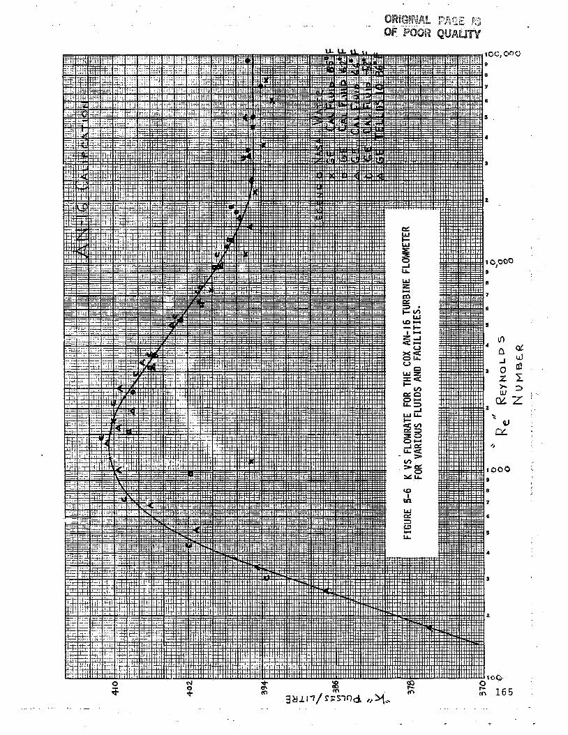
'e

. ... . . _. . . - . . . . .. - . ~ -... . . .- .... I... - . _.

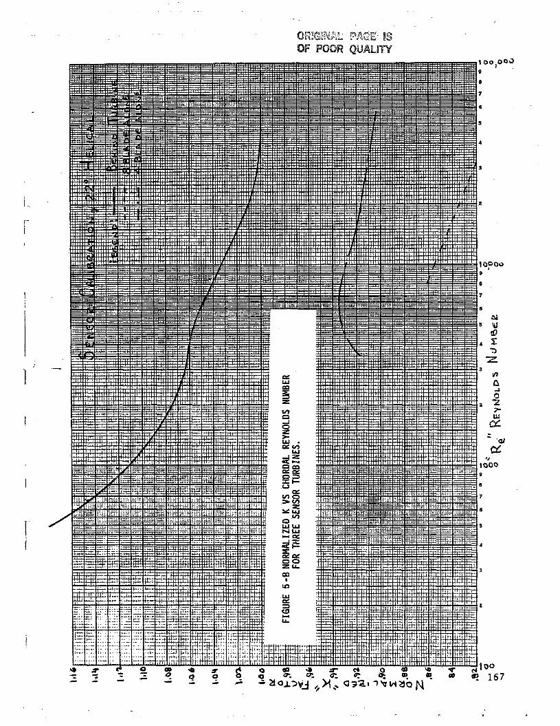
1

;--

i f

I I

i

1

i

I

1 i

FIGURE 5-9 DUAL-TURBINE OENSI-VISCOMETER

FLOWMETER

PROTOTYPE 'FLOWMETER

FLOW

1

Q

ELECTRONICS

POWER

A OUTPUTS

DUAL- TURBINE HALF

VISCOMETER ELECTRONICS

DENSI-VISCOMETER HALF WICONNECTORS

(2)

c==) FREQ.

FREQ.

~- i- 15VOC

RESISTANCE t TEMP.)

FREQ

MODULATION

POWER

168

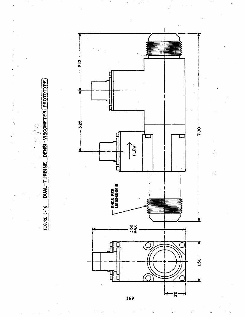
1 6 9

. . .

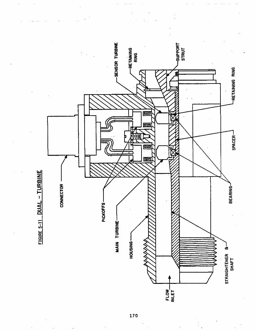
170

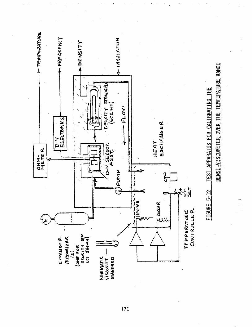
171

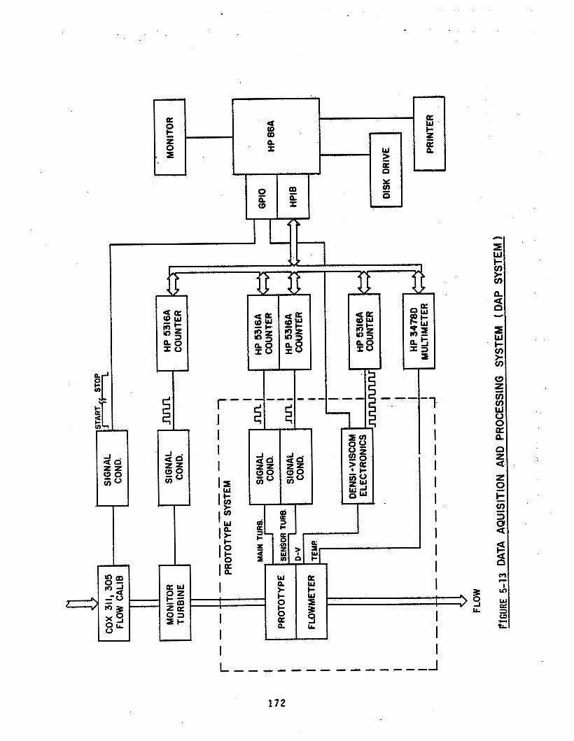
Y T b

I

-1 i I I I I I I 1 I I

I I

e 0 a U

1 7 2

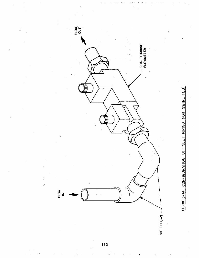
173

175 I

. .

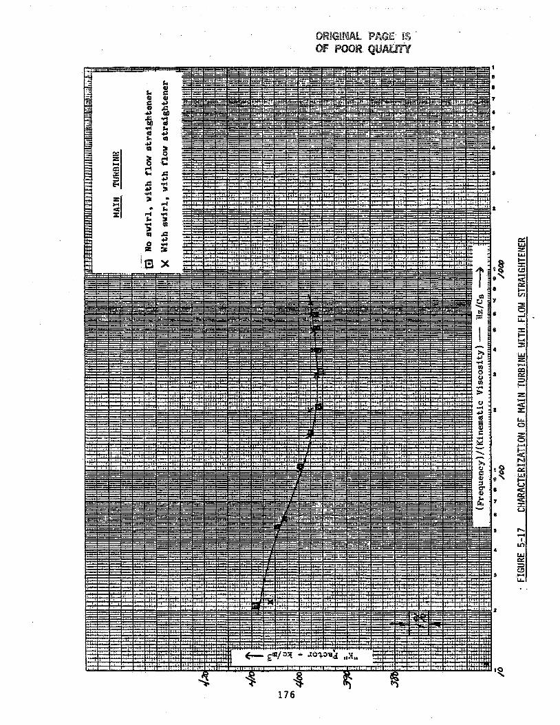
176

177

a U

3

E LL c fz Lbl LL LL U a E

178

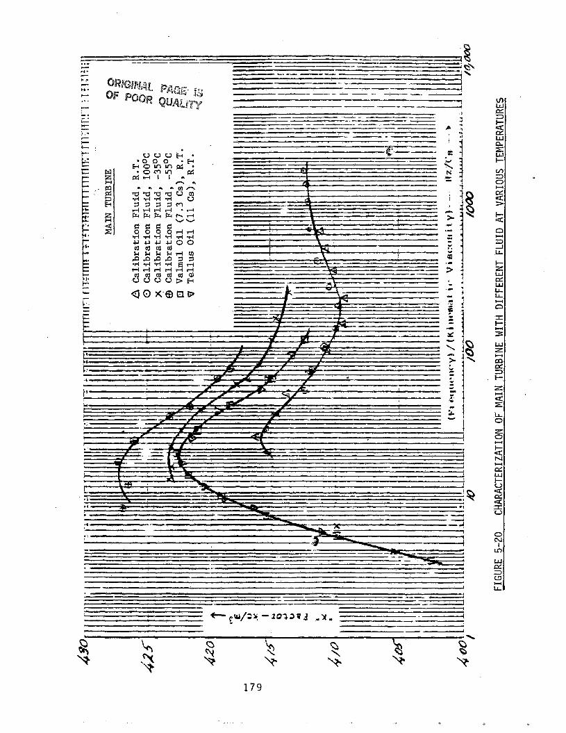
179

A

3 -%

180

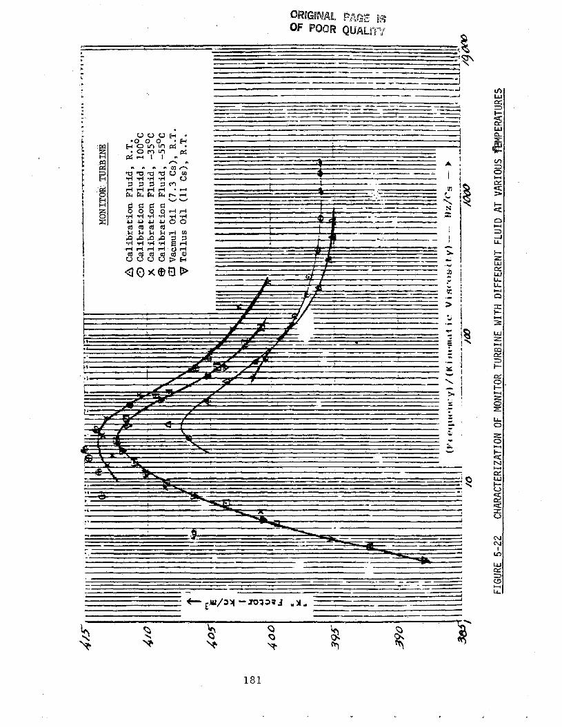
Y

181

E %

E 91 ld 1 u (d t.l 91

91 U

e 0 0 $4

h! U 1-I rl 1-I CJ (d vc 91

01 u

2

a

U (d

01 U m 91 l3

l l u u m ai

I I I I +

= I c I ' dd ? . .4

t l

D h a - m

182

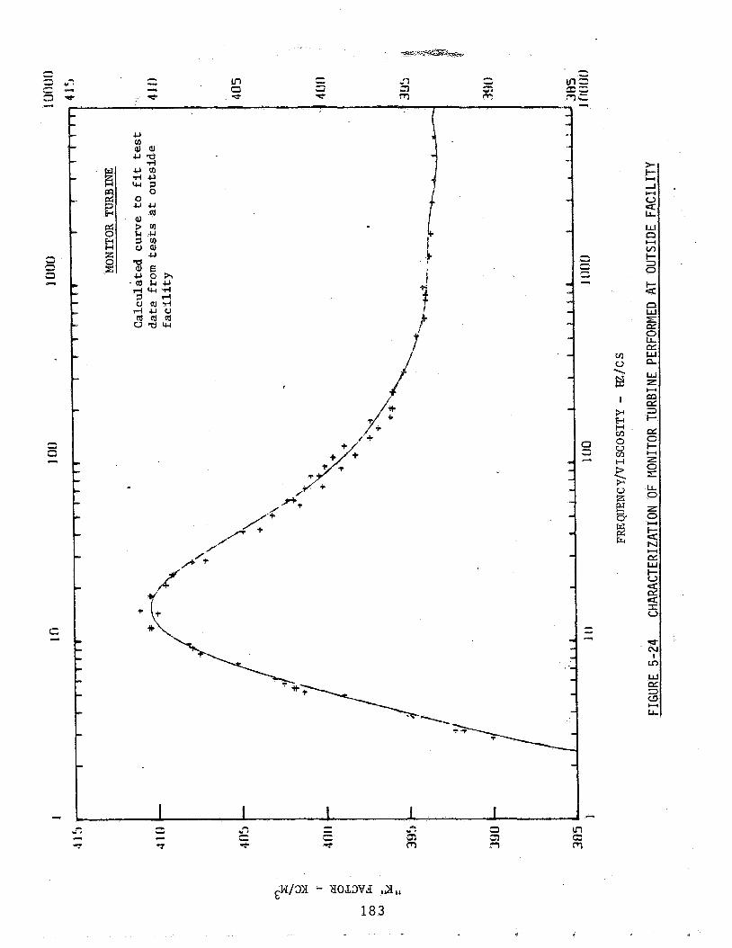
c c

CI

Ei m

k

Cla P

d 3

f-- 6 d P c : 3 a

184

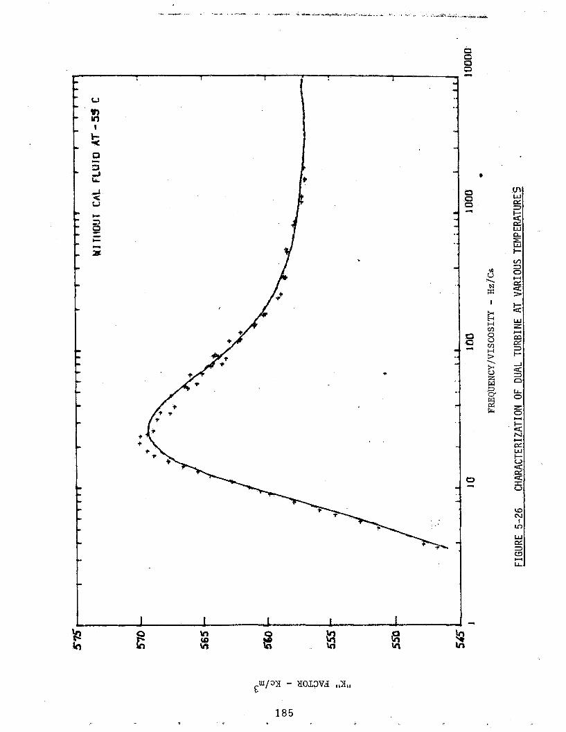
0 C 0 s

i 1 1 I U

I

v, => 0

(Y 4 >

w

k

185

. . . - . . . . .- - . . . . . . .

. . - .-__ ................... ---_ ... .---. -- -.--.-.-.I---

--

* I ! I

\ . .

\ .................... _---._ . _--- - ._ -. ---.__.- ................. _-.. .......... --... . . .

. . . . 4 . .

TEMPDENSREF = 6 ;DENS IREF 780.3368 DENSALPHA = .773772

YOUR PROGRAM IS FINALDVT1

THE NAME OF YOUR FILE IS FINRTl1/14

YOUR FLOWSTANR S/N IS 100251

THIS FLOWMETER IS DUAL TURB ROOM TEMP FINAL TEST

THE QPERATOR IS MR. LINGEL

THIS TEST IS RUN ON NOVEMBER 14 1983

t * * * t * * * * * * * * * ~ * * * * * $ $ $ * $ * $ * * * * ~ * ~ * $ * * $ * * * $ $ * * $ * $ ~ * * ~ * ~ * ~ * ~ * * * ~ * *

-

YOUR TEST FOINT IS APPROXIMATELY 40k PPH

THE MEIGHT IS 1.5 LB

THE TARE IS 5 INCHES

DrJFFCfS D'JFPJEG

THE FCSLLDWING AF;E

COX-F'FH MCWl-FPH

413.5 417.7 416.7 414. 'J 415.1 411.4 4tJ.7 311.5 423.7 421.7

MONITOR MAIN SENSOR SUMTljRB DVTEMP MOP1 I TOR TElW

YOUR TOTAL OUTF'UTS

4. I(>. 9 -. 53 418.3 -. 37 412.1 -. 72 414.5 . 4;. 415.6 -. 68 444. 0 7.37 417.8 -. 26 41'2.4 - 41'3.6 -1.41 .1 1 3 . 4:) -. 14

-Y-

- 7 . .:a,

FIGURE 5-28 TYPICAL COMPUTER OUTPUT OF ACCURACY ANALYSIS 187

. . . . . . . . . . . . . . . . . . ............ ..................... . . . . . . . . . . . . . . .

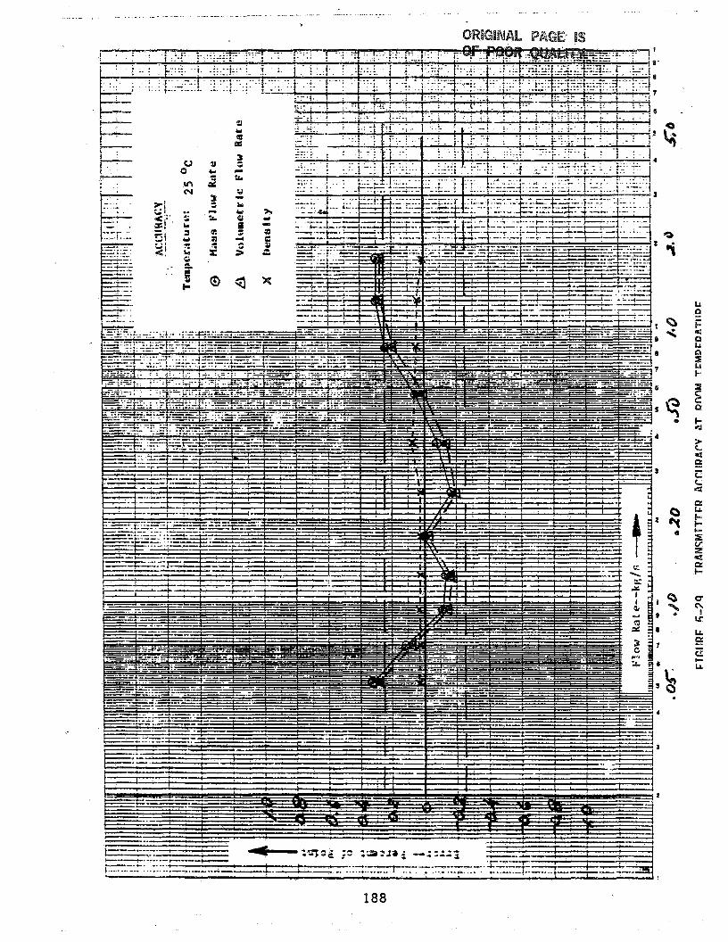
1

P'

8

7

I-. t

. . . . . . ; . :., : i 1 :::.: .: c:: -. _._ .- . . . . . . r . . . . . . . . . . I -.:. .;. I . t ; .l+;i . . -

. . . . . . , . .- :::= i : , :

Li P

S

4

3

z c ea

188

. . _ _ . .. . . .. ~

.. . ... - -

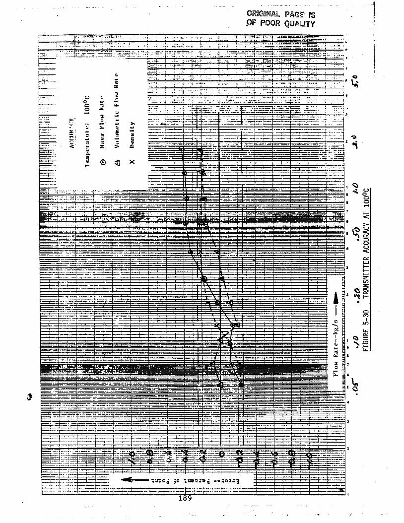
A 1

0 -?

. -. . . . . . . .

190 c-3

. . . .....-.I: t

._ ~ .. 1 . . . - .- .-.- - -. ..... - ..- . . ... -. - ..

I

_ _ _ . _ _ ._ . . ... ...... __._ _- .__. .. . . . .. -. ._~ .- __. _ _ _ . _ _ __ -. _- . .. __ ___ . . .

. .

-i, OUTPUT ACCELEROMETER ' i

TRANSVERSE V BRAT ION

ME C HAN ICAL RE SONMCE S:

LONG ITUD INAL VIBRATION ..

MECHANICAL RE SONANCE S:

VERT ICAL V B R A T ION '

Hz TNPUT OUTPUT

7 57 15 g 's 23 g's

-

118118 15 g q s 47 g f s

Hz INPUT OUTPUT

826 15 g ' s 28 g's

1446 15 g ' s 26 g 's

-

Hz INPUT OUTPUT -

ME C HAN ICAL 1844 15 g ' s 52 g ' s RESONANCE S:

FIGURE 5-34 INPUT AND OUTPUT DAId--OF VIBRATION TEST

- VIBRAT ION INPUT

OUTPUT ACCELEROMETER

VIBRATION

i INPUT

193

. . . . . . . .. . . . - . . . _ .. . ... . . .. . .. . . . . . . __ - . - __ - .

194

0 3

0

m m

a m

- . . -. - - .. . .. . . . . . . .

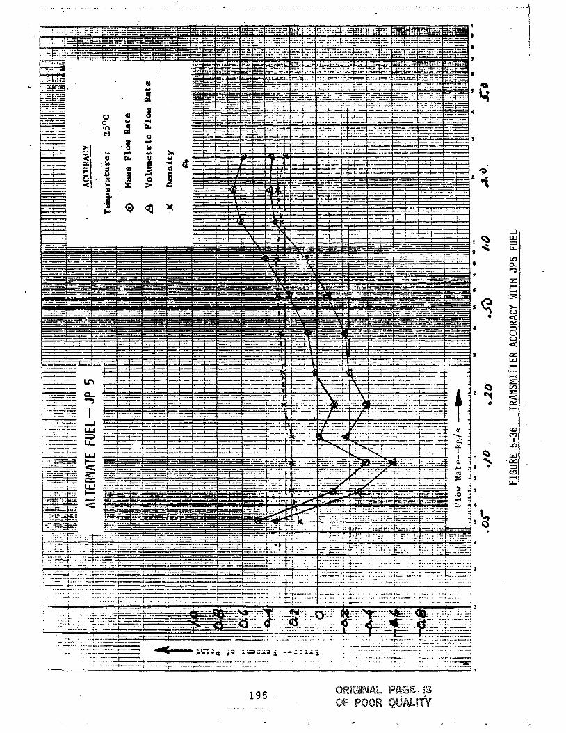
-. 1 . . . . . .. . .... . .. - . . .- . - . _ _ I . .. . . .. . _ _ _ . ._L_._ ..__- . . .

b

195

. . , . ._ ___- ... .. . . . . . . . -- -___ - . - . ... . - .

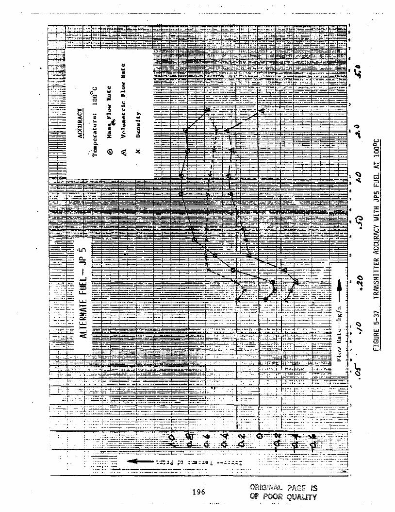
h

. . . . ._ . . . . . . . . .. . . . --. . ..--. -. __+_ . . . . . . . . . .

196 . .

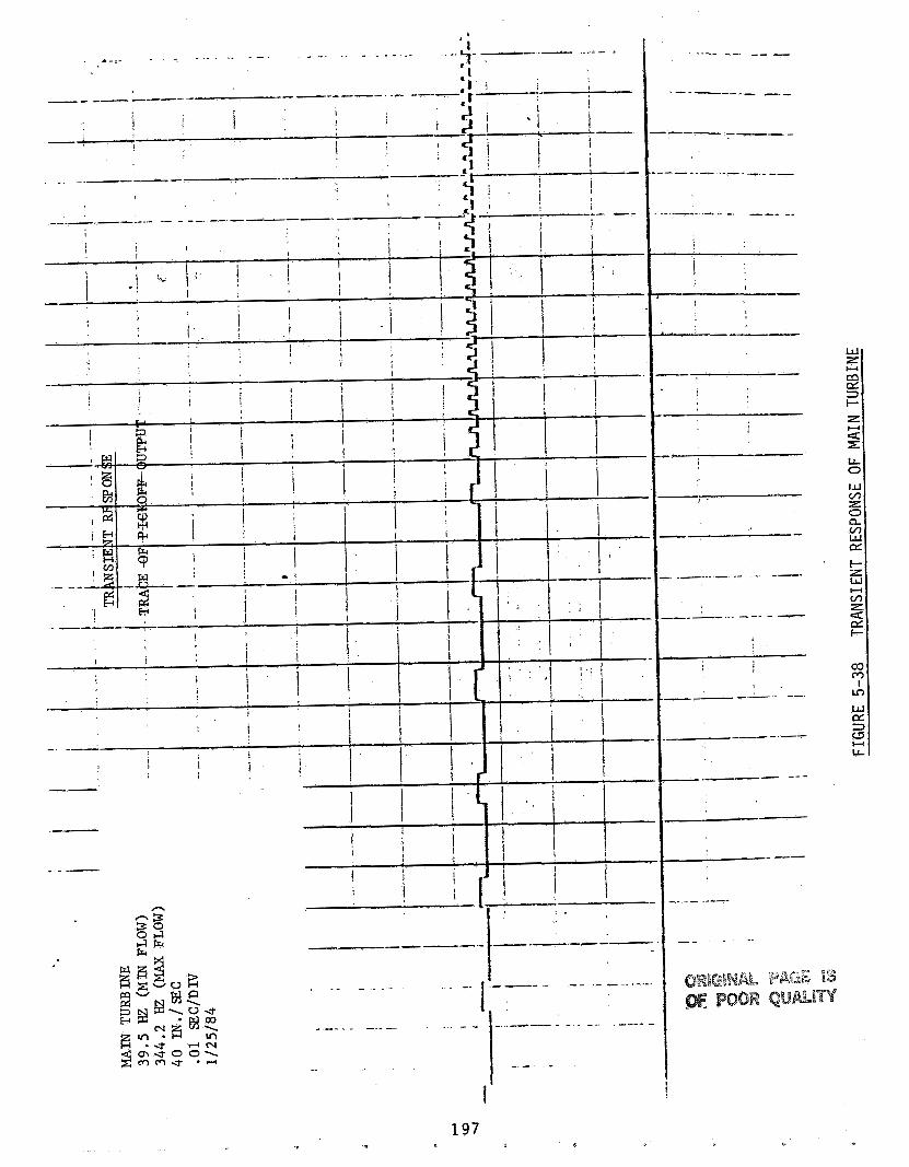
I 197

..-- -- -

------.- --

---- 7-- -

---- - - - --- --

- I

I

-__I__- ---

i

i . >

!

. !

i t I I ! i I

7/lr;7E 1 -see FIGURE 5-39 RESPONSE OF MAIN TURBINE TO RAPID CHANGE I N FLOW RATE

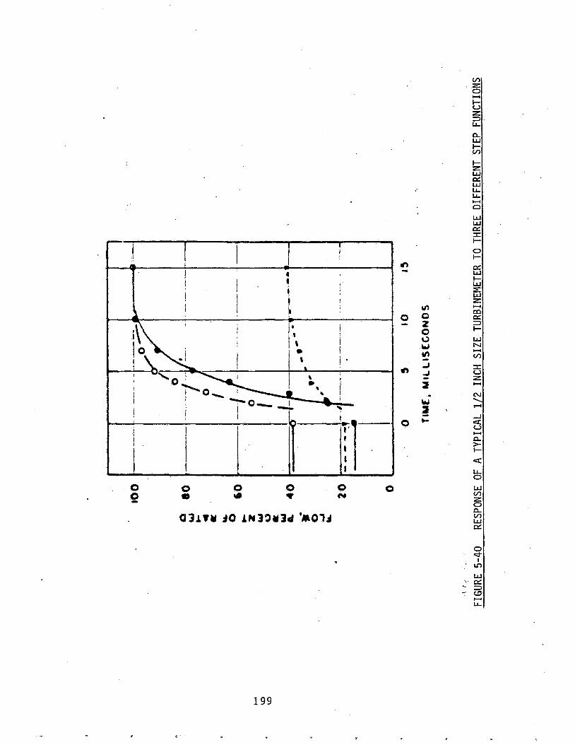
1 I I I I !

1 9 9

Y

6 ,O ANGULAR MOMENTUM FLOWMETER

This section describes the experimental and analytical investigations, the prototype construction, and evaluation performed on the angular momentum flowmeter concept under Tasks 2 through 7 of Phase I1 of NASA contract No. NAS3-22139 to develop a High Accuracy Fuel Flowmeter.

6e1 Introduction

The flowmeter as shown in Figure 6-1 is essentially a single ,

element angular momentum flowmeter. Straightened flow enters the long straight passages of a motor driven rotor where the entire flow achieves the same rotational speed. rotational speed is proportional to the product of the mass rate of flow and the rotor speed. until balanced by the torque of the rotor spring. proportional to the product of mass flow rate and rotor speed, is measured by the time difference between the passage of a reference point on the drive shaft and a similar point on the rotor. The two reference points are aligned at zero flow rate. Since the time required for the rotor to traverse the deflection angle is proportional to that angle divided by the rotor speed, the speed term cancels from the equation, and the time difference %s directly proportional to mass flow. prevents viscous drag from introducing an 'error into the t h e delay. driving the viscosity shroud through a precision spring similar to that driving the rotor, and measuring %ts deflection relative to the same reference on the drive s Viscous drag between the outer diameter of the shroud and the housing deflects the shroud spring resulting in a time based signal analogous to that for mass flow. A Reynolds number correction can also be performed by the microcomputer, further improving the accuracy of the measurement.

The torque required to accelerate the flow to this

This torque turns the rotor relative to its drive shaft This angle, which is

A viscosity srtiroud rotating with the rotor By

ft, viscosity can be measured.

Since the response time of the spring-mass system described is high (approximately l second), a free spinning turbine element is added upstream of the flowmeter. overall accuracy of the mass flowmeter to meet the requirements of the specification.

The fast response rate of the turb'ine is combined with the

6,2 Experimental and Analytical Investigation Plan Formulations

To evaluate the design concept of the angular momentum flowmeter and its potential in meeting NASA requirements, the following areas for investigation were identified in Phase I, to be conducted in Task 4:

(1) Spring Characteristics

(2) Rotor Blade Geometry

(3 ) Inlet Geometry and Flow Profiles Versus Reynolds Number

200

6.2.1 Spring Characteristics

Problem - The following effects directly influence the accuracy of an angular momentum flowmeter:

- Thermo-elastic coefficient (T.E.C.) - Hysteresis - Mounting

The most important is T.E.C. which is a combination of modulus and expansion effects with temperature and which can produce significant temperature' dependences if not properly controlled. of time (months) is also of interest here.

Stability of T.E.C. over long periods

Solution Approach - A spring test fixture (Figure 6-2) will be built. an actual flowmeter installation by using a production shaft, spring and rotor. heat treat temperature will be varied over the following ranges to determine where improvements can be made:

This fixture provides an overall indication of spring performance in

The spring material will be NI-SPAN-C alloy 902. Spring thickness and

Thickness: 0.25 to 0.51 mm (0.01 to 0.04 in.), four thicknesses

Heat Treat Temperatures: 649°C (1200°F) to 871°C (1600°F)

6.2.2 Rotor Vane Geometry

Problem - The optimal design of rotor vanes depends on better understanding of the following effects:

Surface Roughness - The effects on boundary layer thickness and drag coefficient versus surface condition and imperfections.

Trailing C Leading - Critical to rotor vanes in angular Edge Sharpness momentum type flowmeters; proven to

have large effect on skew stability versus Reynolds number (based on fluid passage hydraulic diameter) but not well understood.

Passage Length - What length and aspect ratio are needed to assure repeatable momentum capture over range of Reynolds number (based on fluid passage hydraulic diameter) ? In angular momentum flowmeters at low flows, flow deflection angle is large (70") and requires long passages to settle out eddys. minimum Reynolds number design the best? (see Figure 6-3).

Is

2 0 1

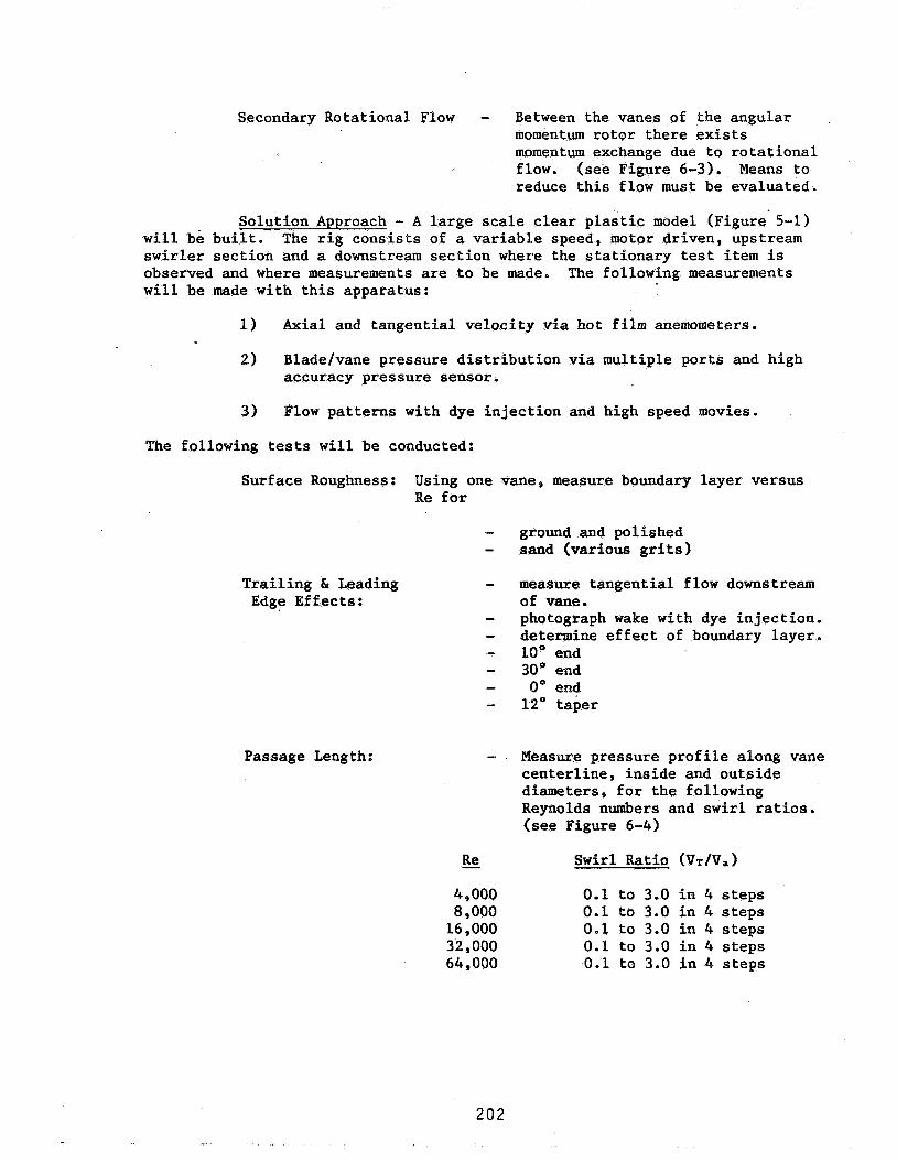
Secondary Rotational Flow - Between the vanes of the angular momentum rotor there exists momentum exchange due to rotational flow. (see Figure 6-3). Means to reduce this flow must be evaluated,

Solution Approach - A large scale clear pla ic model (Figure 5-11 will be built. swirler section and a downstream section where the stationary test item is observed and where measurements are to be made. will be made with this apparatus:

The rig consists of a variable speed, motor driven, upstream

The following measurements

1) Axial and tangential velocity via hot film anemometers.

2) Blade/vane pressure distribution via multiple ports and high accuracy pressure sensor.

3) Flow patterns with dye injection and high speed movies-

The following tests will be conducted:

Surface Roughness: Using one vane, measure boundary layer versus Re for

Trailing b Leading Edge Effects:

Passage Length:

Re

4 , 000 8 , 000 16,000 32,000 64,000

-

ground and polished sand (various grits)

measure tangential flow downstream of vane. photograph wake with dye injection. determine effect of boundary layer. 10" end 30" end 0" end 12" taber

Measure pr-ssure profile along van centerline, inside and outside diameters, for the following Reynolds numbers and swirl ratios. (see Figure 6-4)

Swirl Ratio (Vr/V,)

0.1 to 3.0 in 4 steps 0.1 to 3.0 in 4 steps 0.1 to 3.0 in 4 steps 0.1 to 3.0 in 4 steps 0.1 to 3.0 in 4 steps

!

2 0 2

Secondary Rotational Flow: - Observe flow with dye injection techniques for the following vane geometries in aspect ratio (ratio of passage height to mean passage width) :

Aspect Ratio

4 : 2 1 0.5

6.2.3 Inlet Geometry and Flow Profiles Versus Reynolds number

Problem - Inlet design has a large effect on the profile of flow entering the rotor. Unpredictable changes in profile with Re change thP radius of gyration and thus meter accuracy.

Solution Approach - A large scale model of the present inlet design (see Phase I Report) will be constructed with clear plastic (see Figure 6-5). Flow profiles will be plotted versus Re, and analyzed for change in radius of gyration.

6.3 Experimental and Analytical Investigations

There are three major areas of investigation for the angular momentum flowmeter, namely, the spring characteristics, the rotor geometry, and the inlet geometry. The test equipment, models and set-ups for each of these areas of investigation are described in detail. presented and discussed in subsequent sections to address all the significant findings and merits of the design.

Test results are also

6.3.1 Equipment Set-up and Test Procedures

6.3.1.1 Spring - The spring characteristics study involved heat treating nine springs of 0.46 mm (0.018 in.) thick at temperatures of 500"C, 666°C and 732°C (932"F, 1230°F and 1350°F). best simulate the operating range of the prototype flowmeter. The medium temperature 666°C (1230°F) is the optimal temperature for minimum TEC recommended by the manufacturer. performance spring calibration equipment and each spring was tested upscale and downscale three times with a maximum wind-up angle of 180 degrees.

This spring thickness was chosen to

Tests were performed using existing high

6.3.1.2 constructed for the rotor-vane geometry study. This rig consisted of a variable speed, motor driven, upstream swirler section and a downstream section where the stationary test item could be observed and flow measurements made. The following measurements were performed using this apparatus:

Rotor-Vane Geometry - A large scale rotating model (Figure 6-6) was

203 F

a) Pressure profile along an adjacent pair of vanes via multiple ports and high accuracy pressure sensor for different flow parameters. See Figure 6-7.

b) Velocity profiles across two adjacent vanes via hot film anemometer for different parameters.

c) Velocity profiles across two adjacent vanes having their trailing edges tapered.

d) Velocity profiles across two adjacent vanes having different degree of surface roughness.

The different flow parameters under consideration were Reynolds number, angle of attack, and aspect ratio (or solidity ratio).

6,3.1.3 dimensional scale model (Figure 6-8) for velocity profile assessments. The model is made of plexiglass and velocity profiles were measured using a hot film anemometer.

Inlet Geometry Study - The inlet geometry study utilized a two

6.3,2 Test Results and Discussion

6.3-2.1 defective) by measuring the torque versus angle of deflection at every ten degrees up to 180 degrees. times and linear regression analysis was performed. and downscale data points from their corresponding torque values were normalized as percentage of point error and plotted versus angle of deflection. 500°C (932'F), 666°C (1230°F) and 732°C (1350°F), and results are as shown in Figures 6-9 through 6-15. The solid line shows the upscale nonlinearity while the dotted line shows that of the downscale. The difference between these two lines is the hysteresis of the spring and spring tester.

Springs - Each of the nine springs was tested (and two were found

Each test was repeated upscale and downscale three The deviation of upscale

Tests were performed on springs heat treated at temperatures of

The average hysteresis at the mid-point and the nonlinearity of the seven springs are tabulated in Table 6-1 and the averages for each heat treating temperature are tabulated in Table 6-2. much lower at low heat treating temperatures than at high heat treating temperatures. kind of spring material (NI-SPAN-C alloy 902). The average nonlinearity, however, does not exhibit a clear trend of its dependance on heat treating temperature. can be expected for this spring material. source of error in flowmeter performance. for in the proposed angular momentum flowmeter by microprocessor technology. The calibration curve of the flowmeter which includes the effect of the spiral spring can be stored in memory and retrieved during the operation of the flowmeter, thus eliminating any system calibration error caused by this nonlinearity. However, the mechanical hysteresis can be minimized but cannot be eliminated as error source,

The average mechanical hysteresis is

This agrees very closely with the manufacturer's data for this

But on the average, a nonlinearity of about 0.2% of point value This nonlinearity is an inherent But it can be easily compensated

204 P 5

6-3.2.2 Rotor-Vane Geometry

6.3.2.2.1 adjacent vanes (see Figure 6-7) were measured under different conditions,

Pressure Distribution - The pressure distributions along two namely, aspect ratio (AR), Reynolds number (Re) and angle of attack (a). The static pressure (Ptap) along the passage referenced to system inlet static pressure was normalized by the ‘inlet dynamic pressure (pV2/2 ). This pressure coefficient (P,ap-P,)/(pV2/2) ) was plotted versus the nondimensionalized passage length (X/L) as shown typically in Figure 6-16. The solid line represents the pressure distribution of the leading surface of the incoming flow while the dotted line represents that of the trailing surf ace.

As fluid enters the channel, it becomes separated at the trailing surface of the leading edge and, depending on the flow conditions, this separation will propagate downstream or re-attach to the surface after a certain entrance distance. When the fXow passage has a very large aspect ratio (AR = 3.7) as shown in Figures 6-16, 6-17 and 6-18, fluid always gets re-attached to the surface after about 20% of the passage length. This distance decreases with decreasing flow angle. The pressure coefficient, on the average, is about 2% higher on the trailing surface than the leading surface at the end of the passage. high velocity due to the incoming flow angle, and the channel is not long enough to allow the flow to become fully developed. Again, this difference in

. pressure coefficient decreases with decreasing flow angle.

This agrees with the fact that fluid on the leading surface has a

When the aspect ratio is decreased to 1.5 (Figures 6-19, 6-20, 6-21), the separation distance increases to about 30%. coefficient at the channel exit ranges from 12% at a = 13.1O (Figure 6-19) to 17% at a = 27.6O (Figure 6-20) at the same Reynolds number. pressure coefficient increases to about 25% when the Reynolds number is reduced while the angle of attack remains about the same (Figure 6-20 and

The difference in pressure

This

6-21 ) . When the aspect ratio is further reduced to 0.69, fluid tends to remain separated throughout the whole length of the passage under all flow conditions.

An interesting phenomenon about the pressure coefficient is that it remains negative throughout the passage at AR = 3.7 (Figure 6-16) and yet it is positive at AR = 1.6 (Figure 6-19) or 0.69 (Figure 6-22) except at the very short separation region at the inlet. Theoretically, the pressure coefficient should be zero at the inlet for non-rotating flow, if the system static pressure is used as a reference. Furthermore this pressure coefficient should decrease along the flow passage as surface roughness induces head loss. The pressure coefficients for AR = 1.5 and 0.6 are higher because the incoming rotating fluid has converted the swirl component of velocity head into static pressure resulting in higher pressure coefficients. When the aspect ratio is increased to 3.7, however, the blockage effect of the vane thickness becomes more prominent resulting in a head loss at the channel entrance. loss is larger than the gain from the swirl component and the net result is a lower than zero pressure coefficient.

This head

205

It was pointed out earlier that there is always a separation zone at the chaanel entrance caused by the swirl component of incoming fluid. One possible solution to reduce this separation length is to apply boundary layer suction techniques, which can be accomplished by cutting slots on the rotor vane at some distance from the entrance during rotor fabrication. pressure difference across,the vane can be greatly reduced and this will enhance the symmetry of the pressure distribution across the channel. This technique could reduce the large L/Dh requirement and the pressure drop could also be decreased.

The

6.3.2.2.2 edge of two adjacent vanes were measured using a hot-film anemometer for two di€ferent aspect ratios, three different Reynolds numbers and three different angles of attack (defined as tan-'Vr/Va in Figure 6-4). measured velocities (u) were normalized to the maximum channel velocity (U) and plotted against the nondimensionalized channel width (y/W) where y is the linear dimension from the center of the channel and W is the half width of the channel. A typical velocity profile is as shown in Figure 6-25 of which the zero ordinate indicates the center of the channel, and 1 and -1 indicate the leading and trailing edges of the channel respectively (see Figure 6-7). vanes and are insignificant for data presentation,

Velocity Profiles - The axial velocity profiles at the trailing

The

Data beyond the 1 and -1 values indicate the wakes on the

The results for AR = 3.7 are shown in Figures 6-25 through 6-29. the curves exhibit unsyrmnetric velocity profiles skewed toward the leading surface of the channel. distribution measurements in section 6.3.2.2.1. When the aspect ratio and angle of attack are kept constant (Figures 6-25, 6-26, and 6-27), Reynolds number plays an important role in the shape of the velocity profile. High Reynolds numbers tend to distort the profile more severely than low Reynolds numbers. (Figures 6-27, 6-28, and 6-29), the velocity profiles seem to be relatively insensitive to the angle of attack and show little or no distortion.

All of

These agree very closely with the pressure

When the aspect ratio and Reynolds number are kept constant

Howeverp when the aspect ratio is reduced to 1.5 and the angle of attack is kept constant (Figures 6-30, 6-31 and 6-32), distorted velocity profiles exist throughout a large range of Reynolds numbers. If the Reynolds number is kept constant (Figures 6-32, 6-33, and 6-34), the velocity profiles remain distorted and also shift at different angles of attack. evident that the aspect ratio and the hydraulic diameter of the passage play a very important role in the performance of fuel flow transmitters. would be ideal to have moderate aspect ratio and yet small hydraulic diameter so that a large length to hydraulic diameter ratio can be realized. and separation, resulting in a more evenly distributed velocity profile. distorted velocity profile, however, does not adversely affect the performance of the flowmeter if it remains a constant shape over a wide range of Reynolds numbers.

,

It is

It

This will allow viscous dissipation of any upstream disturbances A

In the proposed angular momentum flowmeter, viscosity will be measured directly and this can be easily transformed into Reynolds number, thus allowing compensation for Reynolds number effects which will reduce the overall system error.

c

2 06 'i

6 . 3 . 2 . 2 . 3 very important part in the performance of angular momentum flowmeters. General Electric's experience has been that chamferred edges will produce unfavorable skew effects, especially when there are changes in viscosities or Reynolds numbers.

Tapered-Vane Effect - The condition of trailing edges plays a

The effect of the trailing edge condition of two adjacent vanes was studied using a hot film anemometer. adjacent vanes at the channel exit were ground to a 15' taper. The velocity profiles at the trailing edge were measured across the channel with and without the 15" taper for two different aspect ratios. Results are as shown in Figures 6-35 and 6-36 for AR = 3 . 7 and 1.5 respectively. The solid line is for square edges while the dotted line is that of the tapered edges, In both cases, the tapered edge improves the original3unevenly distributed velocity profile. And the effect for small aspect ratio is more pronounced than large aspect ratio.

The trailing and leading surfaces of the two

These results seem to be contradictory to what is generally believed. The true effect of trailing edge condition is still not known, and further experimental work is necessary to cover a wider range of Reynolds numbers.

6 . 3 . 2 . 2 . 4 Surface Roughness - Another item of interest for the satisfactory performance of angular momentum type flowmeters is the surface roughness of the channel. Roughness of the surface has little effect in laminar flow but profoundly influences turbulent flow. This is because the inner or viscous dominated region in laminar flow is very wide but in turbulent flow it is very thin. Therefore, small roughness elements at the surface will break up the viscous layer and cause strong changes in the velocity profile.

A piece of medium grade sandpaper (Grit Number 50) was glued on the trailing surface of the passage to simulate the rough surface finish. Velocity profile measurements were taken for two different aspect ratios at the trailing edges of the vanes and compared with those without the sandpaper (the smooth channel condition). It was hoped that the surface roughness would brealc'up the viscous layer at the trailing surface'and produce a more evenly distributed profile. But Figure 6-37 shows that, for an aspect ratio of 3 . 7 , the velocity profile of rough surface is almost the same as that of smooth surface (Figure 6-25) and no major improvement was achieved. Likewise, the same situation exists for a smaller aspect ratio (Figure 6-38 vs Figure 6-30) . insensitive to the surface roughness for Reynolds number up to 31100 which covers about 60% of the range of the proposed angular momentum flowmeter ( 3 4 Re 55000).

This suggests that the velocity profile is relatively

6 . 3 . 2 . 3 by the rotating annular turbine is proportional to the square of the radius of gyration. Slight changes in the radial velocity profile of axial flow at the inlet to the turbine typically occur during transition to laminar flow and can significantly affect the radius of gyration, causing Reynolds number

Inlet Geometry Study - The amount of angular momentum generated

207

dependencies in the non-linearities of the flowmeter calibration. 'Careful design of the inlet, primarily length to hydraulic diameter ratio (L/Dh) can reduce these velocity profile changes and thereby minimize the resultant non-linearity. The inlet of the preliminary design angular momentum flowmeter was designed with this in mind (L/Dh = ,301, and a scale model of the inlet was constructed and tested to evaluate its performance. Figure 6-8 shows this model with the hot film anemometer fixture with traversing micrometer.

The radial velocity profile for axial flow was evaluated at two Reynolds numbers using Stoddard solvent for high Re and Almag oil (viscosity = 5 centistokes) for low Re conditions. Figures 6-39 and 6-40 show hot film anemometer voltage output across the 1.59 cm (0.625 in.) wide channel. slight dip in Figure 6-40 near the center of the channel is thought to be' caused by an uncontrolled shift in liquid temperature, and not to be representative of the flow profile. Of significance here is that over a 200:l range in Reynolds number, no appreciable shift in the radius of gyration occurred, thus indicating adequate L/Dh ratio.

The

6 , 3 . 3 Discussion and Conclusions

6,3,3.1 different heat treating temperatures is quite satisfactory. The average mechanical hysteresis suggests that a lower heat treating temperature is desirable because it reduces the hysteresis of the spring. The inherent nonlinearity of the springs, on the average, is about 0.2% of point. However, this can be easily compensated for by the microprocessor.

Spring - The performance of the seven remaining springs at three

6.3.3.2 Rotor Geometry - The pressure distribution experiment shows that there Is a difference in velocity between the leading and trailing surfaces of the passage, and that is further confirmed by the velocity profile experiment. These differences are larger at a small aspect ratio (radial height to mean width of fluid passage) as the length to hydraulic diameter ratio is not large enough to allow adequate viscous dissipation for fully developed profiles. Also, the angle of attack plays an important role in determining the location of fluid reattachment as the incoming fluid is highly vertical and severe separation takes place in the first few hydraulic diameters, hydraulic diameter ratio (L/Dh = 20) and also a very moderate aspect ratio (AR) on the order of one are necessary to avoid these problems.

These results suggest strongly that an adequate length to

The velocity profile experiment suggests that there is profile shifting when Reynolds number changes and also confirms the importance of large L/Dh ratio. The shift in velocity profile does not present great deficiencies in terms of flowmeter performance, flowmeter will measure the kinemetic viscosity which, when combined with mass flow rate by the microprocessor, will compensate for the changes in velocity profile.

The proposed angular momentum type

208

It was widely believed that a sharp trailing edge condition would be highly desirable for evenly distributed velocity profiles, but the tapered vane experiment suggested otherwise. More experiments are required to gain full understanding of this phenomenon.

The surface roughness of passages has little effect in laminar flow but could greatly influence turbulent flow. It was found, however, that surface roughness had little or no effect in the proposed angular momentum transmitter.

6 . 3 . 3 . 3 Inlet Geometry - Another aspect that could effect flowmeter performance is shifting of radius of gyration in the inlet due to viscosity change. The inlet geometry study has covered a Reynolds number range of about 200 to 1 and no significant shift in the radius of gyration was observed. This indicates that the inlet geometry has sufficient L/Dt, to allow the flow profile to become fully developed at the exit.

6 . 3 . 4 Recommendations - The basic hydraulic design of the angular momentum flowmeter requires sufficient length to hydraulic diameter ratio (L/Dt,) for all channels and passages to obtain fully developed flow. can only be done insofar as the flowmeter geometry will allow without any sacrifice to pressure drop. requirements.

This

The proposed design will satisfy both hydraulic

One of the key requirements of the angular momentum flowmeter is the overall response time. As was pointed out in the Phase I Final Report, the main sensing element (rotor) has a response time of about 4 seconds which can be combined electronically with the fast spinning turbine to meet the 25 ms response requirement. This concept seems to be feasible, but a more in depth look and prototype testing are necessary to determine the actual algorithm.

The temperature performance of the spring requires further investigation, especially the thermo-elastic coefficient (TEC). achieved at the expense of mechanical hysteresis since these properties have opposite behavior with heat treat temperature. These two spring parameters have to be optimized for the optimal performance of the angular momentum flowmeter.

Low TEC only can be

While the angular momentum concept can provide repeatability as good as the turbine meter at flow rates above 1818 kglhr (4000 lb/hr), at lower flow rates bearing friction adds some non-repeatability. includes a turbine for transient response, there is some risk that the combined response of the turbine and angular momentum signals may not provide the desired quickness and accuracy. sensitivity inherent in the angular momentum concept, although it is minimized with precision balancing and 180" pickoffs, while the turbine concept has virtually no attitude sensitivity. the angular momentum concept is the oversize side protrusion beyond the specified envelope where the four pickoffs are located. All these are of concern for the high accuracy concept and make the angular momentum flowmeter less likely to meet NASA requirements as compared with the dual turbine flowmeter. However, further investigation into these areas will provide more clues about the viability of this concept.

Even though the concept

There is some attitude

Another slight detraction of

2 0 9

6.4 Prototype Design and Test Plan Formulation

This section describes the flowmeter prototype design and test plan formulation relating to the secondary candidate, and completes in part Phase If Task 5 of NASA Contract NAS3-22139, Mod 03.

The prototype angular momentum flowmeter as shown in Figure 6-41 measures the true mass flow rate based on the angular momentum principle and does not require any density measurement or compensation. As fluid enters the flowmeter, it passes through the transient turbine which provides the necessary fast response signal. Steady angular speed of the rotor is generated by the motor and gearhead assembly via the magnetic couplers. The angular momentum, or the fluid torque generated, is proportional to the mass flow rate, and causes an angular displacement of the spring restrained rotor. This spring deflection will result in a proportional time interval between the start and stop pulses generated by magnets rotating past fixed pickoff coifs on the flowmeter housing. rotor outer surface and housing inner surface is similar to the rotor construction. also provides a measurement of fluid viscosity which is used to improve the overall flowmeter accuracy. shroud, the reference start signal and the transient turbine signal will interface with the Data Acquisition and Processing (DAP) System. system has been pre-programmed and contains various calibration constants, and computational algorithms to provide an accurate mass flow rate output.

The viscosity shroud between the

It eliminates the viscous drag on the rotor outer surface and

The two s t o p signals from rotor and viscosity

The DAP

A test plan for the calibration of the prototype and subsequent evaluation of system performance regarding repeatability, accuracy over the temperature range, vibration effects, attitude sensitivity, pressure drop, time response and operation with alternate fuels, has also been formulated.

6-4.1 Prototype Component Description - The transient turbine, which measures the volumetric flow rate, is a COX ANC-20 turbine meter. Its primary function is to provide a fast dynamic response in order to enhance the slow responding but highly accurate mass flow rate output from the rotor. utilizing a 45 kHz carrier frequency which is amplitude modulated by the passage of the transient turbine rotor blades.

The transient turbine sensor is a modulated carrier pickoff,

The fluid angular momentum is supplied by a 400 Hz, 26 volt synchronous motor coupled with a high density gearhead via magnetic couplers. This drive mechanism provides a constant angular speed for the rotor assembly,shroud assembly and reference wheel.

210

The rotor assembly, which is spring restrained, has 28 vanes in its fluid passage and is designed with the maximum length to hydraulic diameter ratio (L/Dt, = 11) possible given the size constraint of the flowmeter and other hydraulic parameters such as vane aspect ratio, pressure drop,-etc. fluid enters the rotor, the rotational fluid torque is balanced by the spring torque resulting in an angular displacement of the spring from its null position. This angular displacement is converted to a time-based signal via the magnets on the rotor and the induction pickoff coil on the housing. This signal, in conjunction with the reference signal, yields a time difference measurement (see Figure 6-42) which is directly proportional to the mass flow rate. The rotor spring has a maximum wind-up angle of less than 180" and the dual magnet arrangement at the rotor assembly eliminates any error caused by the imbalance effect of the rotor assembly.

As

The viscosity shroud assembly is similar in construction to the rotor assembly. between the housing internal diameter-and the rotor outside diameter. primary function of the viscosity shroud is to eliminate the viscous drag on the rotor outer surface. thus providing viscosity information for Reynolds number compensation. order to minimize skew effects and the addition of angular momentum fluid torque, the shroud has only five, short vanes in its annulus.

It 3s also spring restrained and has a long thin shell section The

The shroud also measures the fluid viscous drag, In

The reference wheel which was listed as "fluid assist" in earlier sections, has only three very short support struts. It provides a start or reference signal for both the rotor and shroud assemblies through the same magnet and pickoff arrangement. gearhead provides adequate torque at all flow rates.

The fluid assist is not required because the motor

Figure 6-43 shows the prototype fbctional elements divided into a flowmeter section and an electronics section. The mass flow rate will be calculated from the three signal pulses using known calibration constants and a viscosity compensation algorithm. flow rate reading will be combined with the fast responding frequency output of the turbine meter to give the necessary fast responding and accurate mass flow rate. A digital microcomputer will perform these tasks in the production flowmeter system, but for prototype evaluation, these computations will be performed by the Data Acquisition and Processing (DAP) System described later in Section 6 . 4 . 4 .

This slow responding but accurate mass

All the detailed sketches of piece parts, and subassemblies are shown in Appendix F.

6 . 4 . 2 Test Plan - The prototype flowmeter will be calibrated initially without the DAP system. The calibration characteristics of the transient turbine portion and the angular momentum portion of the flowmeter will then be programmed into the DAP system being developed for prototype evaluation. The completely calibrated prototype will then be connected to the DAP system and system performance tests will be run according to the design specifications and guidelines.

2 1 1

6.4.2.1 rotor and viscosity shroud which need to be calibrated as a complete unit. The output characteristic of the rotor in terms of time period (ms) versus mass flow rate (lb/hr) will be determined. characteristic in terms of time period (ms) versus'absolute viscosity will also be measured.

All of the initial calibration will be done at room temperature with three different fluids having viscosities of approximately 103, 5.0 and 15 centistokes. the 1.3 cs viscosity and mixtures of Almag and Tellus #10 oils will be used for higher viscosities. A flow calibrator, such as the COX 311H with a monitor turbine meter and temperature.sensor, will be used for these calibration measurements. comp'onents will be measured at flow rates ranging from 182 kg/hr (400 lb/hr) to 9090 kg/hr (20000 lb/hr) with multiple upscale and downscale readings at each of ten flow points. The sensitivity of these output signals to changes in viscosity and flow rate'can be inferred. compensation can then be determined.

Flowmeter,Calibration - There are two major components - the

The viscosity shroud output

The MIL-C-7024A, Type I1 calibration fluid will be used for

The respective output signals of the three

The algorithm for viscosity

Furthermore, tests will be conducted at -55OC and 100°C to determine if there is any temperature effect on the output characteristics of the flowmeter.

In order to achieve the high accuracy and fast responding output-from the flowmeter, the transient turbine and rotor signals will pass through high-pass and low-pass filters respectively having the same time constant, and these filtered outputs will be summed to create the fast responding and accurate output signal.

For purposes of these calibrations and subsequent prototype evaluations it is necessary to establish "in house" standards of mass flow rate, volumetric flow rate, density and viscosity. For the above prototype calibrations, the two volumetric flow rate standards will be 2.54 cm,(1 in.) and 1.27 em (0,5 in,) size turbines. These monitor turbines will be calibrated using COX 305 and 311H weigh-time stands (mass flow rate) combined with in-line density measurements using a Mettler-Paar DMA 60 and DMA 620HT high accuracy digital density meter.

During calibration of the monitor turbines, the number of flow measurements that are taken at each flow rate will be determined by statistical analysis. Typically, enough measurements will be taken at a particular flow rate to ensure that the mean of the COX flow stand outputs is known within - + 0.05% at a 95% confidence level using the Students'-t statistic. During subsequent prototype evaluations (described in the following section) the prototype output will be in terms of mass flow rate and MY be compared directly to the weigh-time stand outputs. However, tests may show that the outputs of the monitor turbines and the densitometer standard can be combined t o provide a more repeatable indication of mass flow rate than the COX stands, in which case, the monitor turbines will serve as the standards against which prototype accuracy is determined.

2 1 2

c

--uc.p

If the COX flow stands prove to be adequate for use as a standard in the evaluation phase, then the tare and sample weights used during evaluation for each range of flow measurement will be used again in the flowmeter calibration. Since the systematic errors of the COX flow stand (as reported in the Section 3.0 Calibration Study) depend heavily on the selection of tare and sample times (and weight), this technique will effectively eliminate any variations in the systematic errors caused by buoyancy effects and timing errors resulting from changes in fluid forces, holding tank inertia and sample control volume. This technique also permits direct readout of COX flow rate without compensation for the systematic errors and greatly simplifies the task.

- _

While these techniques will not allow evaluation of absolute accuracy ($.e., the known systematic errors of the COX flow stands are not corrected) they wiil provide an excellent measure of prototype repeatability. In the Suture, when a more accurate flow standard is available, the biases introduced with the COX flow stands can be easily compensated out by . introducing new calibration constants in the software.

Viscosity of the calibration Fluid will be calculated from an accurate temperature measurement at the flowmeter and from a viscosity versus temperature curve which is evaluated just prior to-the test. temperature sensor will be *an RTD and the viscosity measurements will be made with a suspended capillary type viscometer.

1

The

6.4.3 prototype flowmeter:

Prototype Evaluation - The following tests will be made on the . . .

Repeatability

Accuracy

Vibration Sensitivity

Attitude Sensitivity

Pressure Drop

Response Time

Alternate Fuel

For all tests except response time and pressure drop the prototype outputs will be connected to the DAP system. will be run at room temperature using MIL-C-7024A, Type I1 calibration fluid. The above tests are briefly described in what follows.

All tests, unless otherwise specified,

213

6.4.3.1 Repeatability

Objective - To determine the repeatability of the measurement of mass flow rate.

Method - Pass a flow rate, which is known approximately, through the flow sensor. Measure the flow with two other flow sensors to establish a reference for repeatability. of the prototype flowmeter under test. Measurements will be made upscale and.downscale at five different flow points and the test procedures will be repeated once after three days.

Measure and record the output

- .

Apparatus - Flow calibration stand with flow measuring sensors, monitor turbine meter and the DAP system,

6-4.3.2 Accuracy

Objective - To measure any calibration shifts of the prototype over the ranges of flow rate, temperature, density and viscosity.

Method - Measure and compare the mass flow rates from the COX 305 or 3118 flow calibrator and the prototype with calibration fluid. Also measure volumetric flow rate with the monitor turbines and fluid density with the density standards to provide an alternate means of establishing mass flow rate. The flow calibrators and prototype will be connected to the DAP system for this evaluation. In this set-up, the measurement time interval of the weigh-time stand will gate the measurement intervals of the signals a This ensures that fluctuations of actual flow rate do not cause measurement errors between the various inputs. The inputs will be averaged over the 30 to 60 second measurement interval prior to calculation of mass flow rate.

Multiple readings will be taken at each of ten flow rates over the 50 to 1 flow range (next higher flow about 50% greater than the present), both upscale and downscale. The same points (flow rates within 5 10%) will be run at -55"C, -35"C, 25°C and +lOO"C. Percent-of-point error will be calculated at each reading as:

214

The errors will be plotted versus flow rate for each of the four runs.

Apparatus - COX 305 and 311 weigh-time flow calibrators, monitor turbines and the DAP system.

6.4.3.3 Vibration Sensitivity

Objective - To determine the effect of vibration on flowmeter performance .

Methods - Mount the flowmeter on a vibration machine by means of a suitable fixture. Pass a constant fuel flow rate of about 25 percent of full scale through the flowmeter. over the range specified in the design guidelines and monitor the indicated flow rate from the flowmeter during vibration. Repeat the procedure with vibration inputs along each of three orthogonal axes. particular attention will be paid to mechanical resonances and variations of indicated flow. Endurance test will not be performed.

Vary the vibration input

During each vibration scan,

Apparatus - Servo type sinusoidal vibration machine, flow stand, flow sensor to monitor flow input to flowmeter being tested, and DAP system.

6.4.3.4 Attitude Sensitivity

Objective - To determine the effect of the orientation of the flowmeter on accuracy.

Method - Mount the flowmeter in a selected orientation. Pass a constant fuel flow rate of about 25 percent of full scale through the flowmeter using a standard turbine to monitor flow. Change the orientation of the flowmeter under test and record any changes in mass flow rate output. Repeat the procedure for each orientation desired. The positions to be tested are with axis of flow vertical and with the axis of flow horizontal and the flowmeter rotated 90' between successive orientations.

Apparatus - Flow stand, monitor turbine meter, fixture to hold the flowmeter under test in the desired orientation, and the DAP system.

215

6.4.3.5 Pressure Drop

Objective - To determine the pressure drop across the flowmeter for a range of flow rates up to full scale.

Method -

Apparatus . -

Mount the flowmeter with the axis of flow horizontal. across the flowmeter. Pass fuel flow through the flowmeter and measure flow rate and differential pressure for each point from low flow to full scale. 'In addition to room temperature testing, this test will be repeated at -55OC.

Flow stand, differential pressure meter, inlet and outlet pipes with pressure taps.

Connect a differential pressure meter

6.4.3.6 Response Time

Objective - To measure the time constant of the flowmeter when subjected t o step changes in flow rate.

Method - The outputs from the transient turbine and rotor and the output from a hot film anemometer placed in the flowstream just ahead of the prototype will be recorded on magnetic tape. An inlet pipe fixture with two parallel pipes, each pipe having a throttle valve and one having a snap action valve, will be used both to create a fast step change in flow rate and to control the initial and final flow rates. The recorded tape will be played back at reduced speeds while the outputs are recorded on strip chart paper for detailed analysis. The two output signals will also be passed through their respective filters ._ and the combined signal will be tested for the time response requirement.

Apparatus - Parallel pipe manifold with valves, tape recorder, strip chart recorder, hot film anemometer system.

6.4.3.7 Alternate Fuel

Repeat Accuracy (6.4.3.2) testing with JP-8.

216

6.4.4 flowmeter has a total of four electrical signal outputs with the ranges and characteristics listed in Table 6-3. Synchronization of the measurement interval for these signals with the flow calibratpr and monitor turbine signals is essential to obtaining reliable measurements of prototype repeatability and accuracy. Furthermore, the conversion of the’ signals to mass flow rate through the various calibration functions requires a dedicated computer to obtain meaningful results in a timely fashion (i.e., real time). These requirements were recognized early in the test plan formulation and led to the design of a Data Acquisition and Processing System, herein referred to as the DAP system. block diagram showing the.key elements of the system.

Data Acquisition and Processing System (DAP) - The prototype

.

Figure 6-44 is a functional .

Frequency signals are routed to digital counters which send the measurements to a digital bus (IEEE 488 compatible, HPIB) and are controlled (synchronized) by the bus. (transient turbine frequency, mass flow rate stop pulse, viscosity stop pulse and common reference pulse) and the monitor turbine frequency signal. The weigh-time interval of the COX 311H flow calibrator and the modulation output of the counter are converted to digital signals through a General Purpose Input/Output Port (GPIO) or through the HPIB. information as measured by the Resistance Temperature Detector (RTD) will be another input to the digital bus via a digital multimeter. computer controls the data flow and is programmed in BASIC to compute mass flow rakes for both the flow calibrator and the prototype from the calibration data taken earlier. A monitor, disk storage and printer/plotter make the DAP system a complete and versatile tool necessary for the successful development of the high accuracy fuel flowmeter for NASA.

These include the prototype flowmeter signals

The temperature

An HP86A

6.5 Fabricatibn, Tests and Analyses of Prototype Design

This section of the report covers Tasks 6 and 7 of the angular It includes the fabrication of the prototype design momentum concept.

described in the Section 6.4.1 and the component drawings in Appendix F. As expected, some minor design changes were made and the test plan was slightly altered. Tests and analyses were performed on the prototype using the DAP system and the results of which are covered in this section.

6.5.1 comprises of 24 major components (Figure 6-41). of the forward and aft housings which are assembled at about the mid-point using O-ring for fluid sealing. This type of arrangement is necessary for ease of assembly and disassembly of all the internal components.

Prototype Description - The angular momentum prototype flowmeter The flowmeter body consist

A transient turbine which provides the fast response of the angular momentum flowmeter is mounted at the housing core. The transient turbine pickoff is a modulated carrier pickoff, utilizing a 45 kHz carrier frequency which is amplitude modulated by the passage of the turbine rotor blades.

The housing core which is located inside the forward housing serves two purposes. It has long annulus vane passages on its outside diameter to provide the necessary deswirling action for the incoming flow after the transient turbine. The inside of the core houses the power train of the miniature motor and reduction gearhead.

* 217

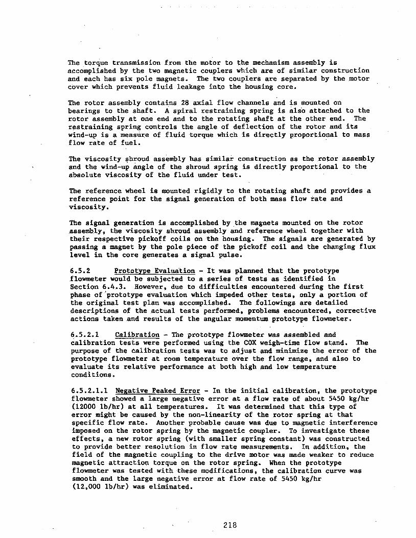
The torque transmission from the motor to the mechanism assembly is accomplished by the two magnetic couplers which are of similar construction and each has six pole magnets. The two couplers are separated by the motor cover which prevents fluid leakage info the housing core.

The rotor assembly contains 28 axial flow channels and is mounted on bearings to the shaft. rotor assembly at one end and to the rotating shaft at the other end. restraining spring controls the angle of deflection of the rotor and its wind-up is a measure of fluid torque which is directly proportional to mass flow rate of fuel.

A spiral restraining spring is also attached to the The

The viscosity shroud assembly has similar construction as the rotor assembly and the wind-up angle of the shroud spring is directly proportional to the absolute viscosity of the fluid under test.

The reference wheel is mounted rigidly to the rotating shaft and provides a reference point for the signal generation of both mass flow rate and viscosity.

The signal generation is accomplished by the magnets mounted on the rotor assembly, the viscosity shroud assembly and reference wheel together with their respective pickoff coils on the housing. The signals are generated by passing a magnet by the pole piece of the pickoff coil and the changing flux level in the core generates a signal pulse.

6.5.2 flowmeter would be subjected to a series of tests as identified in Section 6.4.3. However, due to difficulties encountered during the first phase of’prototype evaluation which impeded other tests, only a portion of the original test plan was accomplished. descriptions of the actual tests performed, problems encountered, corrective actions taken and results of the angular momentum prototype flowmeter.

6.5.2.1 calibration tests were performed using the COX weigh-time flow stand. purpose of the calibration tests was to adjust and minimize the error of the prototype flowmeter at room temperature over the flow range, and also to evaluate its relative performance at both high and low temperature conditions.

Prototype Evalua’tion - It was planned that the prototype

The followings are detailed

Calibration - The prototype flowmeter was assembled and The

6.5.2.1.1 - In the initial calibration, the prototype flowmeter showed a large negative error at a flow rate of about 5450 kg/hr (12000 lb/hr) at all temperatures. error might be caused by the non-linearity of the rotor spring at that specific flow rate. imposed on the rotor spring by the magnetic coupler. To investigate these effects, a new rotor spring (with smaller spring constant) was constructed to provide better resolution in flow rate measurements. field of the magnetic coupling to the drive motor was made weaker to reduce magnetic attraction torque on the rotor spring. flowmeter was tested with these modifications, the calibration curve was smooth and the large negative error at flow rate of 5450 kg/hr (12,000 lb/hr) was eliminated.

It was determined that this type of

Another probable cause was due to magnetic interference

In addition, the

When the prototype

218

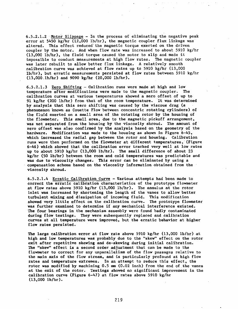
6.5.2.1.2 error at 5450 kg/hr (12,000 lb/hr), the magnetic coupler flux linkage was altered. This effect reduced'the magnetic torque exerted on the driven coupler by the motor. (13,000 lb/hr), the fluid torque caused the motor to slip and made it impossible to conduct measurements at high flow rates. was later rebuilt to allow better flux linkage. calibration curve was achieved at flow rates up to 5910 kg/hr (13,000 lb/hr), but erratic measurements persisted at flow rates between 5910 kg/hr (13,000 lb/hr) and 9090 kg/hr (20,000 lb/hr).

Motor Slippage - In the process of eliminating the negative peak

And when flow rate was increased to about 5910 kg/hr

The magnetic coupler A relatively smooth

6.5.2.1.3 temperature after modifications were made to the magnetic coupler. calibration curves at various temperatures showed a zero offset of up to 91 kg/hr (200 lb/hr) from that of the room temperature. It was determined by analysis that this zero shifting was caused by the viscous drag (a phenomenon known as Couette Flow between concentric rotating cylinders) of the fluid exerted on a small area of the rotating rotor by the housing of the flowmeter. This small area, due to the magnetic pickoff arrangement, was not separated from the housing by the viscosity shroud. zero offset was also confirmed by the analysis based on the geometry of the hardware. which increased the radial gap between the rotor and housing. runs were then performed on the flowmeter at different temperatures, (Figure 6-46) which showed that the calibration error tracked very well at low rates up to about 5910 kg/hr (13,000 lb/hr). kg/hr (50 lb/hr) between the room and cold temperatures was predictable and was due to viscosity changes. compensation scheme based on the viscosity information obtained from the viscosity shroud.

Zero Shifting - Calibration runs were made at high and low The

The amount of

Modification was made to the housing as shown in Figure 6-45, Calibration

The small difference of about 23

This error can be eliminated by using a

6.5.2.1.4 Erratic Calibration Curve - Various attempts had been made to correct the erratic calibration characteristics of the prototype flowmeter at flow rates above 5910 kg/hr (13,000 lb/hr). The annulus at the rotor inlet was increased by shortening the length of the vanes to allow better turbulent mixing and dissipation of incoming fluid. This modification showed very little effect on the calibration curve. was further examined to determine if any mechanical interference existed. The four bearings in the mechanism assembly were found badly contaminated during flow testings. curves at all temperature were improved, but the erratic behavior at higher flow rates persisted.

The prototype flowmeter

They were subsequently replaced and calibration

The large calibration error at flow rate above 5910 kg/hr (13,000 lb/hr) at high and low temperatures was probably due to the "skew" effect on the rotor exit after repetitive skewing and de-skewing during initial calibration. The "skew" effect is a second order adjustment that can be made to the flowmeter to correct for any unparallelism of the flow passages relative to the main axis of the flow stream, and is particularly profound at high flow rates and temperature extremes. In an attempt to reduce this effect, the rotor was modified by machining 0.5 mm (0.02 inch) from the end of the vanes at the exit of the rotor. Testings showed no significant improvement in the calibration curve (Figure 6-47) at flow rates above 5910 kg/hr (13,000 lb/hr).

219

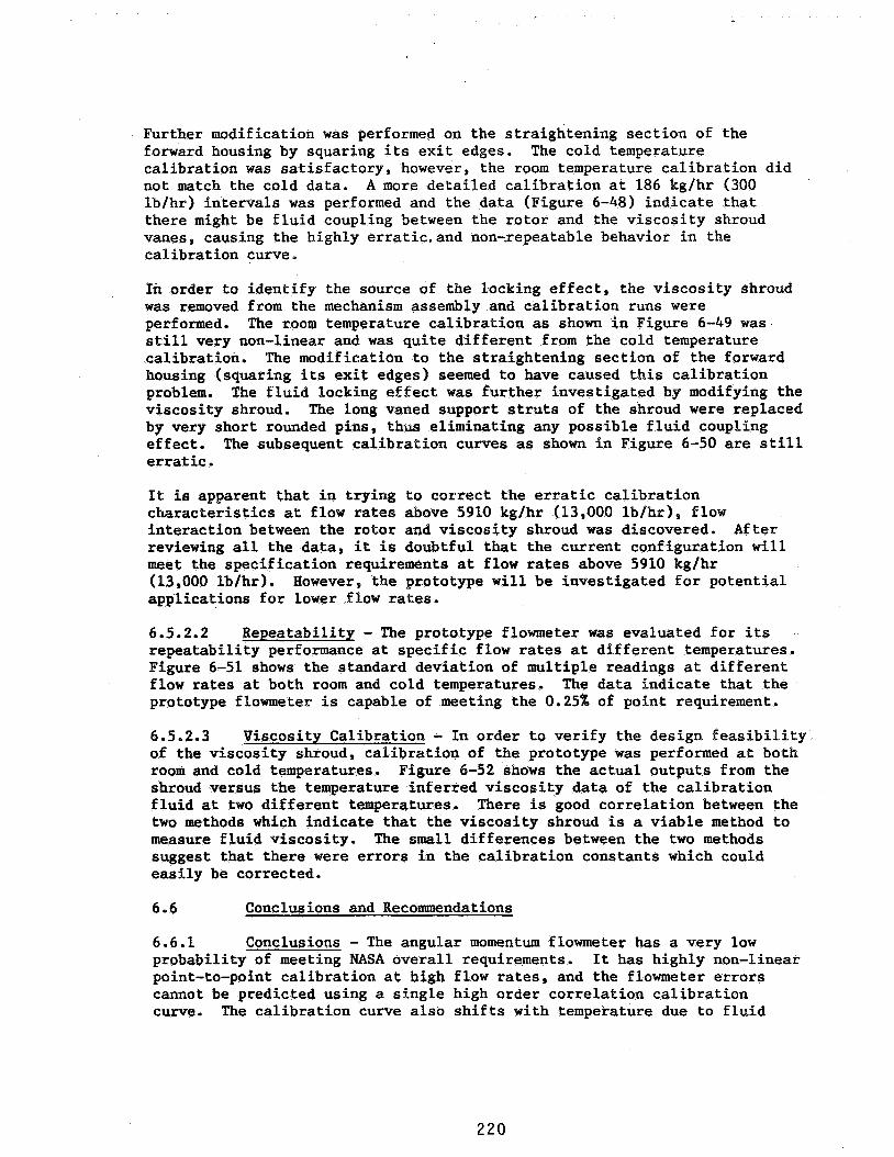
Further modification was performed on the straightening section of the forward housing by squaring its exit edges. calibration was satisfactory, however, the room temperature calibration did not match the cold data. A more detailed calibration at 186 kg/hr (300 lb/hr) intervals was performed and the data (Figure 6-48) indicate that there might be fluid coupling between the rotor and the viscosity shroud vanes, causing the highly erraticeand non-repeatable behavior in the calibration curve.

In order to identify the source of the locking effect, the viscosity shroud was removed from the mechanism assembly and calibration runs were performed. still very non-linear and was quite different from the cold temperature calibration, The modification to the straightening section of the forward housing (squaring its exit edges) seemed to have caused this calibration problem. viscosity shroud. by very short rounded pins, thus eliminating any possible fluid coupling effect, erratic.

The cold temperature

The room temperature calibration as shown in Figure 6-49 was

The fluid locking effect was further investigated by modifying the The long vaned support struts of the shroud were replaced

The subsequent calibration curves as shown in Figure 6-50 are still

It is apparent that in tryiwg to correct the erratic calibration characteristics at flow rates above 5910 kg/hr (13,000 lb/hr), flow interaction between the rotor and viscosity shroud was discovered. reviewing all the data, it is doubtful that the current configuration will meet the specification requirements at flow rates above 5910 kg/hr (13,000 fb/hr). However, the prototype will be investigated for potential applications for lower flow rates.

After

6.5.2.2 repeatability performance at specific flow rates at different temperatures. Figure 6-51 shows the standard deviation of multiple readings at different flow rates at both room and cold temperatures. The data indicate that the prototype flowmeter is capable of meeting the 0.25% of point requirement.

Repeatability - The prototype flowmeter was evaluated for its

6.5.2.3 of the viscosity shroud, calibration of the prototype was performed at both room and cold temperatures. shroud versus the temperature inferred viscosity data of the calibration fluid at two different temperatures. two methods which indicate that the viscosity shroud is a viable method to measure fluid viscosity. The small differences between the two methods suggest that there were errors in the calibration constants which could easily be corrected.

Viscosity Calibration - In order to verify the design feasibility Figure 6-52 shows the actual outputs from the

There is good correlation between the

6.6 Conclusions and Recornendations

6.6.1 probability of meeting NASA overall requirements. point-to-point calibration at high flow rates, and the flowmeter errors cannot be predicted using a single high order correlation calibration curve. The calibration curve also shifts with temperature due to fluid

Conclusions - The angular momentum flowmeter has a very low It has highly non-linear

220

leakage at the radial clearances between the housing and mechanism assembly. flowmeter affecting repeatability between upscale and downscal'e readings. Although the viscosity measurement from the viscosity shroud shows good correlation, it is. questionable whether the compensation algorithm will compensate the viscosity related flow calibration problem at cold temperature.

6.6.2 has a few positive features to be considered. repeatability at fixed flow points. is well within the 0.25% requirement, which indicates that a look-up table for calibration is possible. the active flow range. The prototype flowmeter also shows that calibration within 0.25% can be achieved at flow rates below 5450 Irg/hr (12,000 lb/hr), which suggests that the current design could be upsized to achieve better high flow rate performance.

There is also a considerable amount of hysteresis in the

Recommendations - The current flowmeter configuration, however, It has very good

The standard deviation of repeatability

The viscosity measurement is excellent over

2 2 1

Section 6.7

TABLES

222

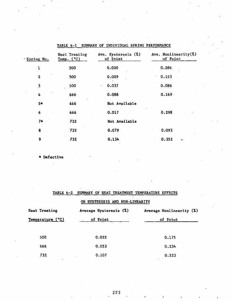
Spring No.

1

2

3

4

5*

6

7*

8

9

TABLE 6-1 SUMMARY OF INDIVIDUAL SPRING PERF CE

Heat Treating Ave. Hysteresis (%I Ave . Nonlinearity (%) Temp. ("C) of Point of Point

500 0.020 0.286

500 0 0009 0.153

500 0.037 0.086

666 0 088 0 I69

666 Not Available

666 0.017 0 e 298

732 Not Available

732 0.079 0.093

732 0.134 0.352 *'

* Defective

TABLE 6-2 SUMMARY OF HEAT TREATMENT TEMPERATURE EFFECTS

ON HYSTERESIS AND NON-LINEARITY

Heat Treating Average Hysteresis (%I Average Nonlinearity (%)

Temperature (*C

500

666

732

of Point

0.022

0.053

0.107

of Point

0.175

0.234

0.223

223 I

TABLE 6-3 PROTOTYPE OUTPUT SIGNAL CHARACTERISTICS

Signal Range Amplitude

Turbine 24 to 1600 Hz 0 to 5V Square Wave

Rotor 6 Hz

Shroud 6 Hz

Reference Wheel 6 Ez

150 mV Zero to Peak 50 mV Zero to Trough 10 ms Pulse Width 36 mV/ms Zero Crossing Slope (See Figure 6-42)

Same as rotor

Same as rotor

2 2 4

Section 6 . 8

FIGURES

2 2 5

226

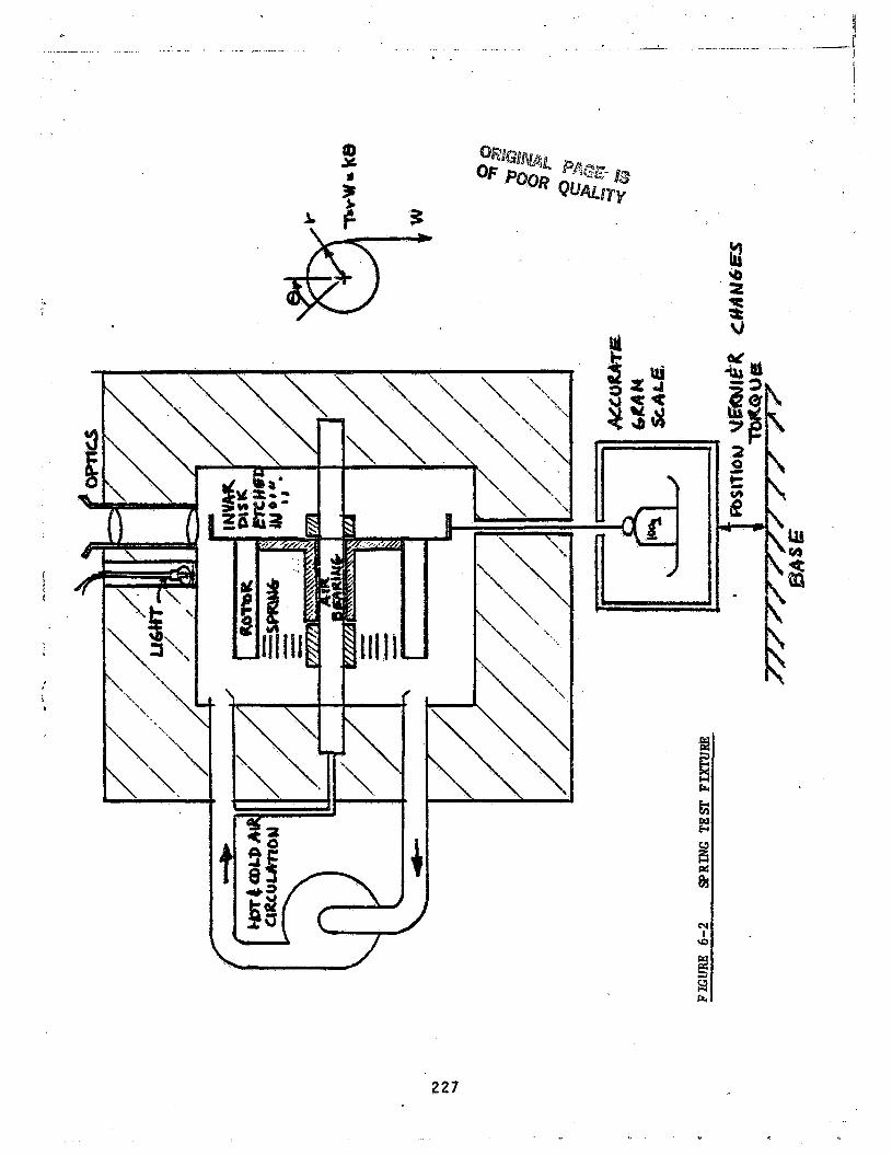
. . . I ----- I

.. _. . .. .. ._ -. . . . . . .. . . . . . . . .. . . ..... _. . . . -- ._ .... . . .

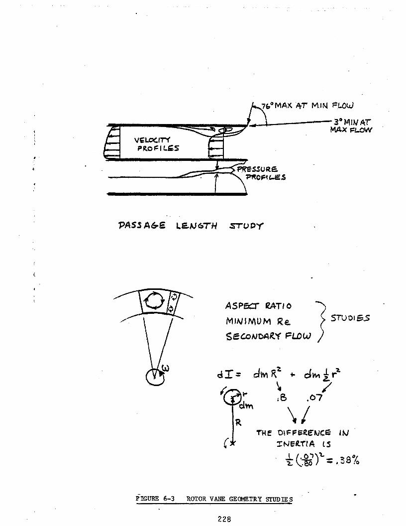
a

. .

IR

FIGURE 6-3 ROTOR VANE GEOMETRY STUDIES

228

.

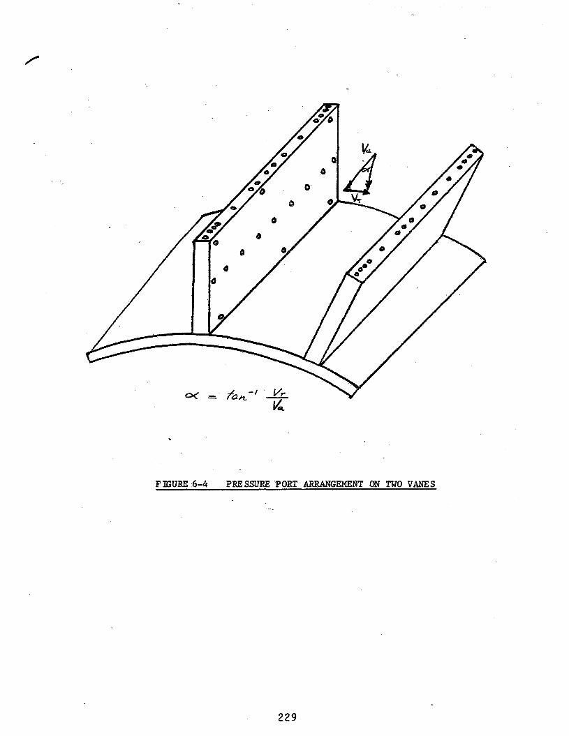
FTGURJZ 6-4 PRESSURE PORT ARRANGEMENT ON TWO VANES

229

,

!

!

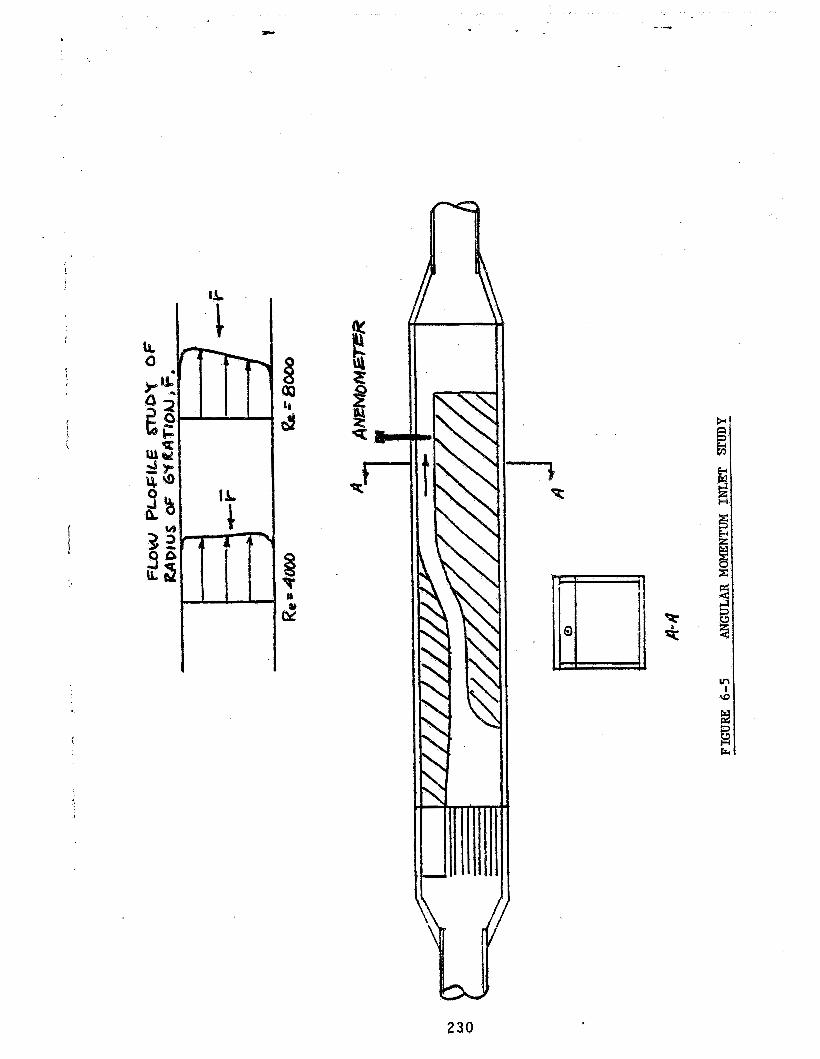
s f-

230

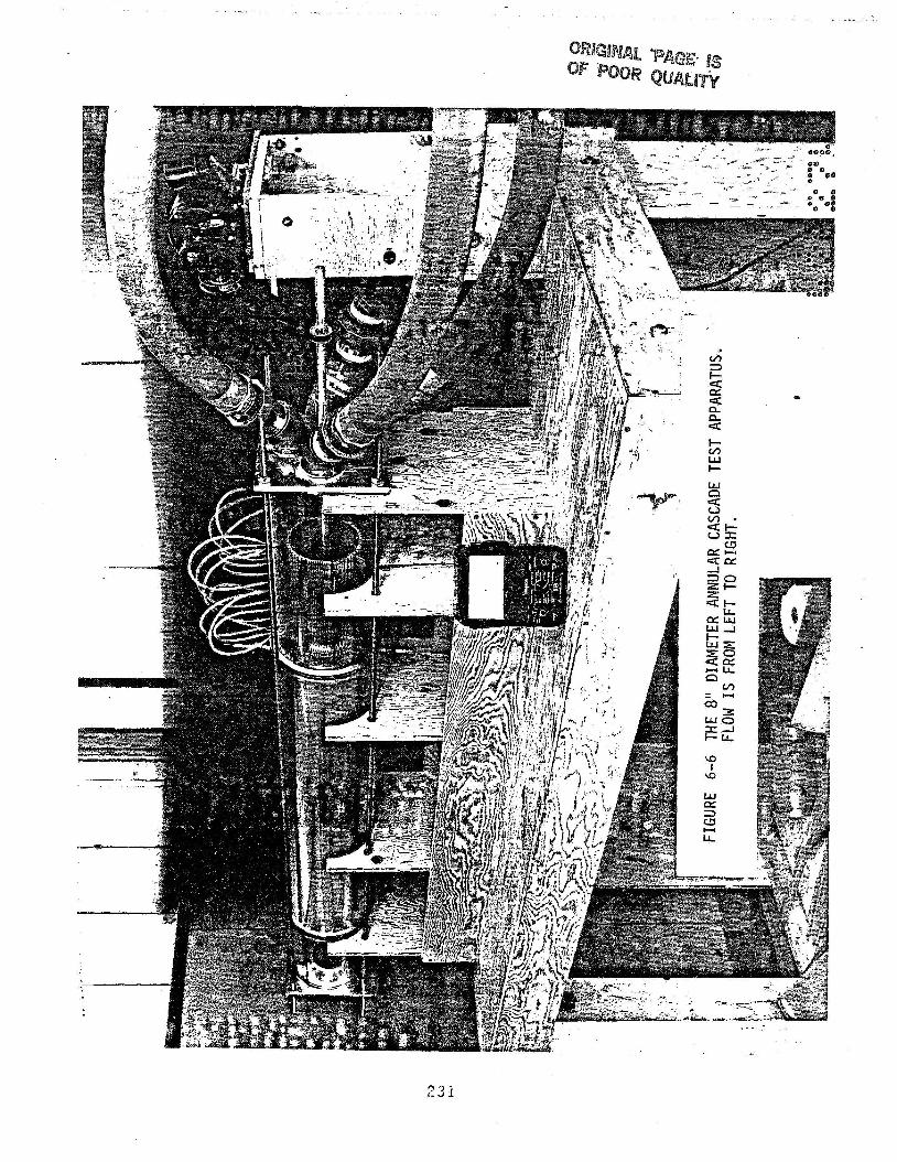
a

2 3 i

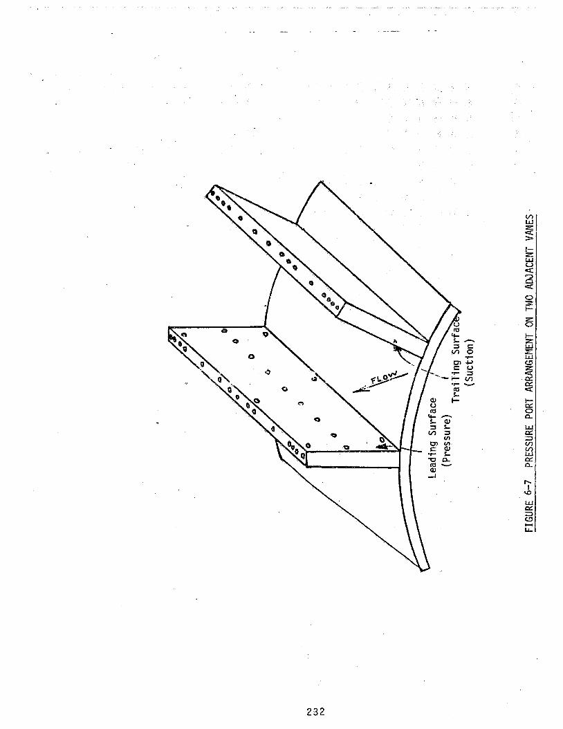
232

233

1 I i

r .

2 3 4

2 3 5

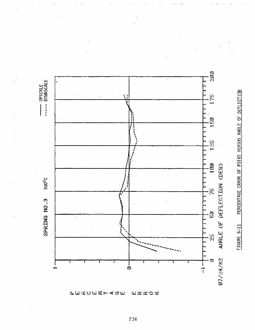
V 0 0 0 v)

i c3

n c3 LLJ n W

z c1 w i- o t;' 1 'A w a

236

w

f , I i T

/

1 I I 1

1 I t I

t

5 LL

LL LL c

-

LL C bL

N ‘A Q l+

2 3 7

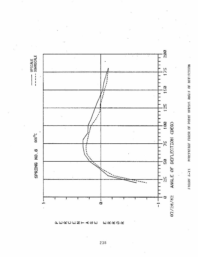
I I

I-

c

i

2 3 8

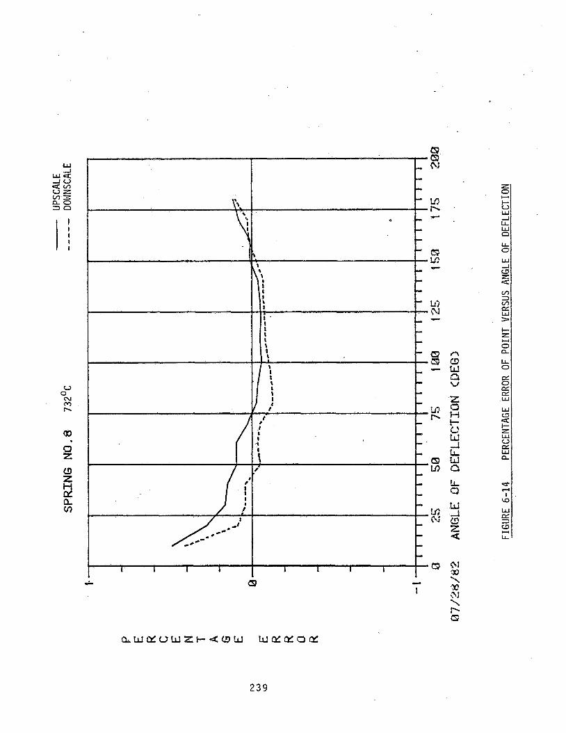
f

u N ' r n h

0

I.

& 1

2 3 9

I I :

/ i

c c;)

t

I-

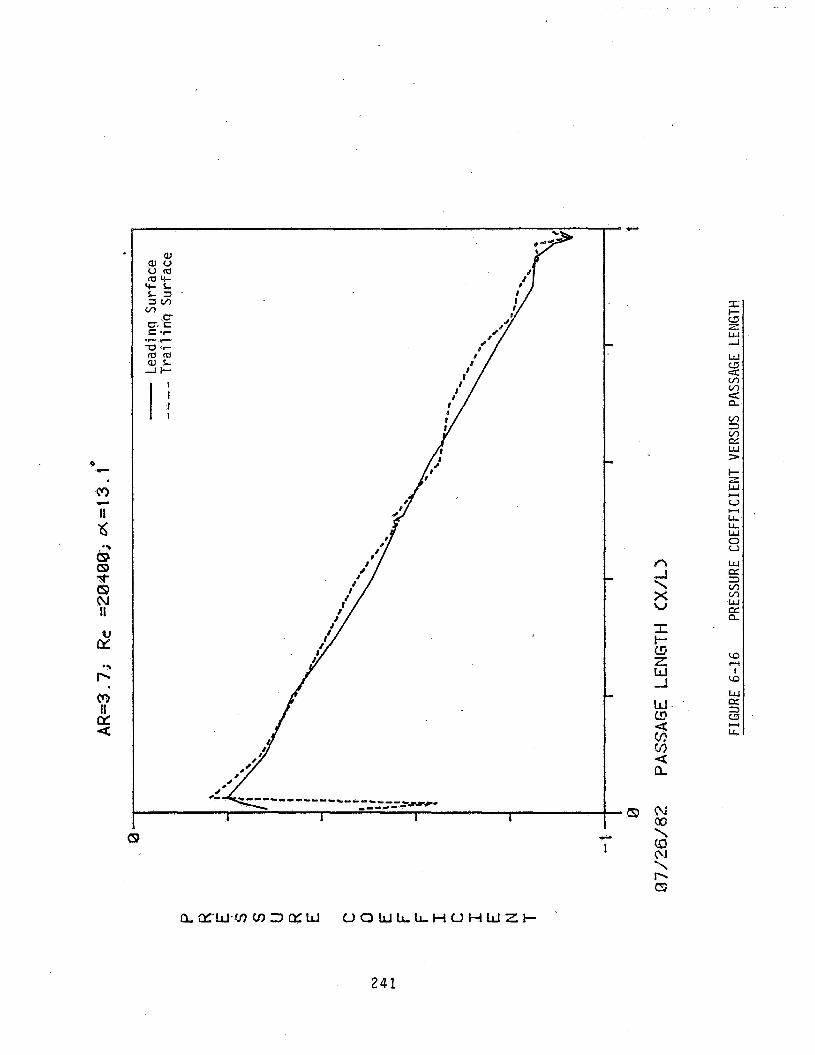
c

1

-e

--cp

c

I

v, 7 v, cr: w > !- zz W

V

LL LL W 0 V

c-(

H

W cr: 7 v, v, W lx p.

n A \ X U

2 4 2

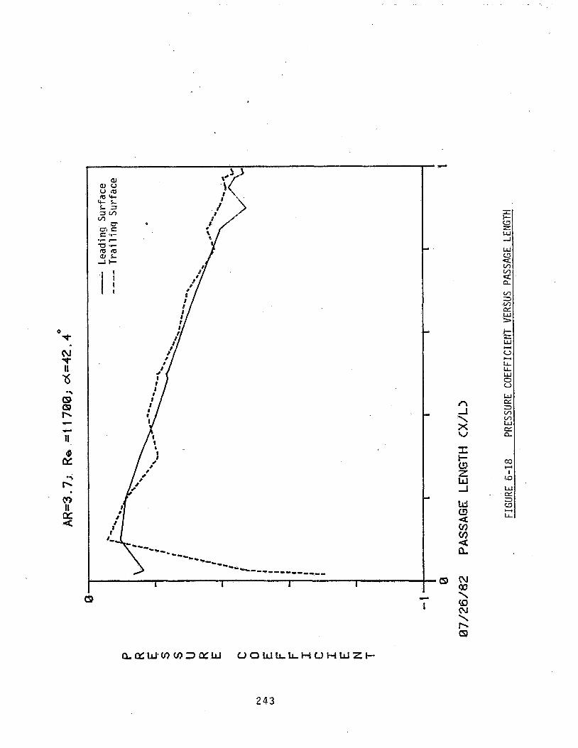
4 hs

2 4 3

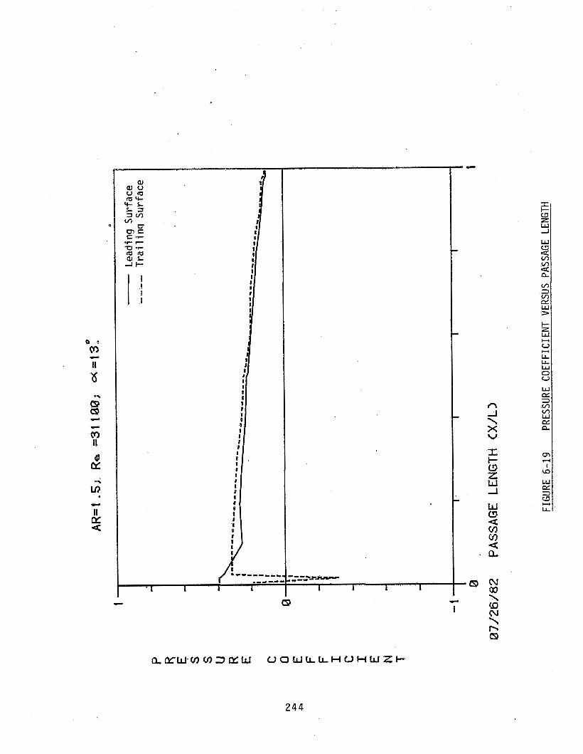
c?

''"5,- --- I 1 1 I

2 4 4

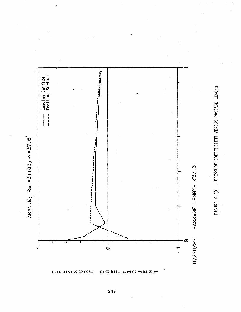
4

5 -. -- . 2

L I- CSI ;E W -.J

pI W

W @z =>

LL

1 1 1 6

L

I

--

-a

I I- a II w d

cn' 31 m cy:' w 'I

P 4 r\I

c3 4 #

4 a

' 2 4 6

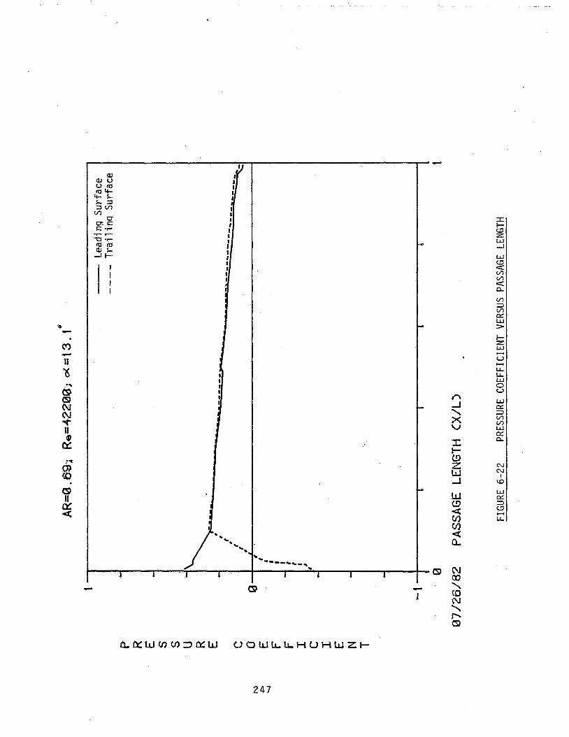
2 4 7

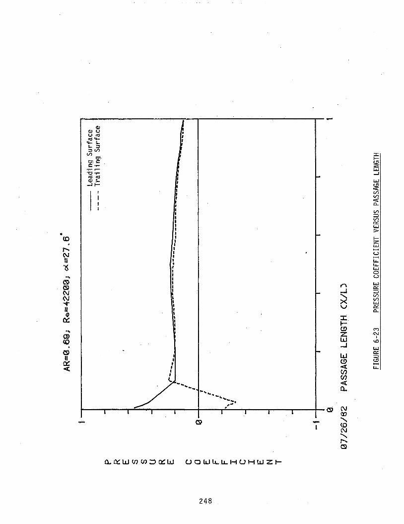
248

I- l

* %.

8 %

I I I I I

# I

1 I I 1

n -1 \ x U

I- z w IL IL w 0 0

H

W cc x v) v) w cc n

2 4 9

Q)

e cp

J \ 3

250

M

N

c

cp

c

1

N I

M 1

c9

2 5 1

2 5 2

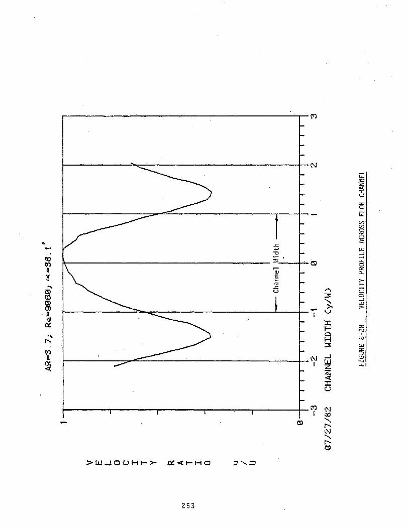
2 5 3

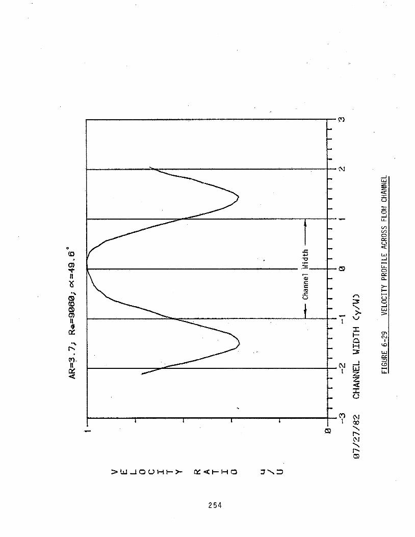
2 5 4

0

to 7

m

L

2 5 5

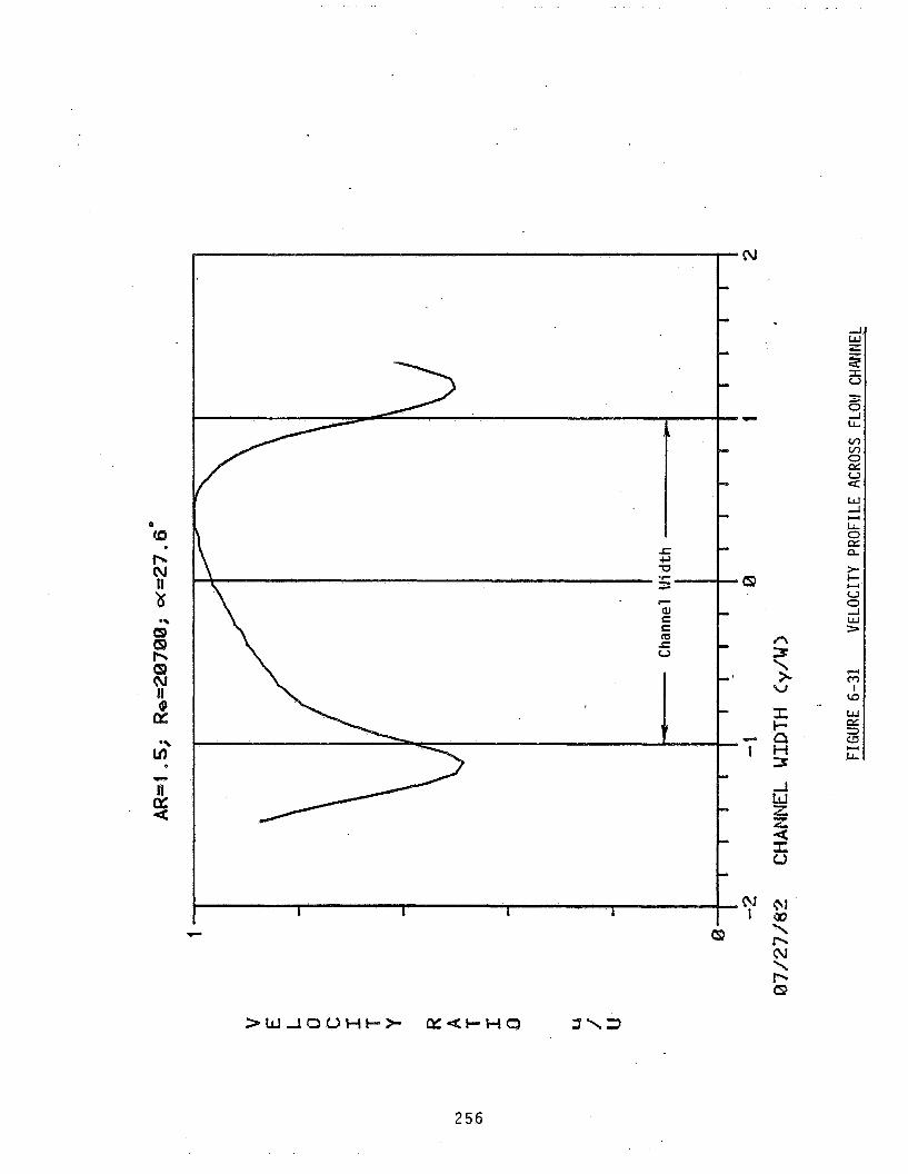
P cp

256

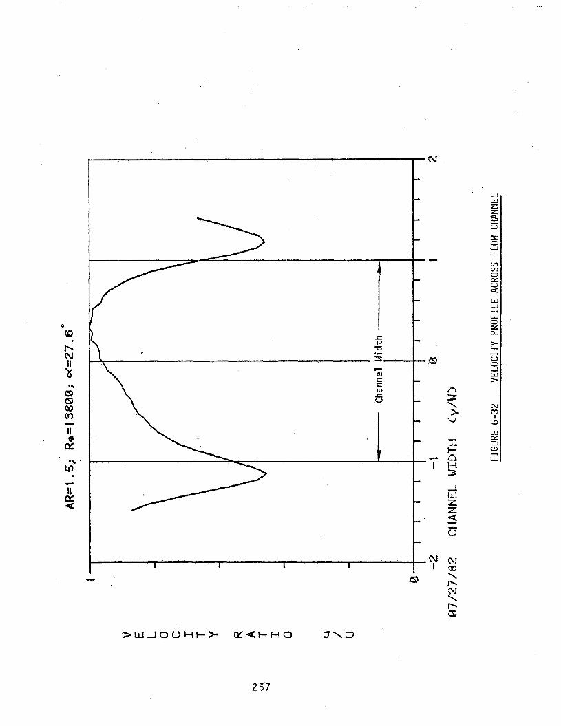
c

257

c cp

2 5 8

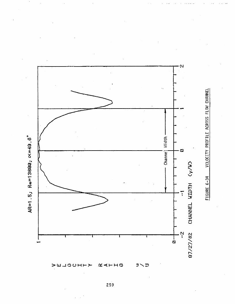
c Q1

-N

-.c-

-a

c - 1

,N t

259

c 6)

-IL

0-D

- 1

2 6 0

261

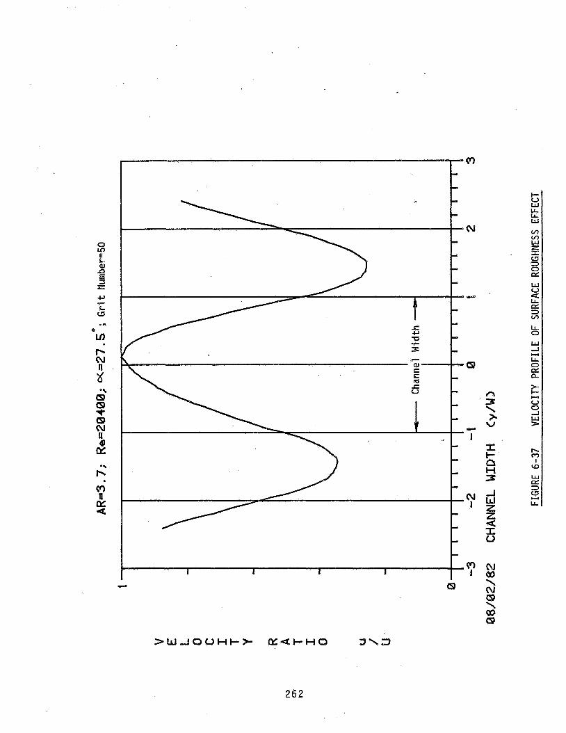
-- a

262

0 M

I I L e, P

z 5 c,

M '- a

QI lY

I- (d w LL LL W

M M W z I a 3 0 er w u Q LL er x M

LL 0 w -I

LL 0 er

).

0 0 -I w >

U

a

t,

03 m

I w w er 3

LL E

263

8 8 Q) M 4 a u 8

8%

A w 3 LL

e----

c c

I L

LL 0 W A LL 0 CIll P

Y

1- t; V 0 A W

n

Y (5 >

264

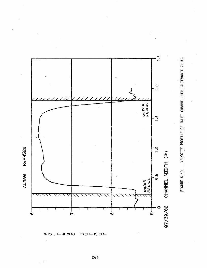
c

oo r-

Lo

cv - .

0 cv

Lo 0 .

4

= ? 4

Lo

'0

--cp

265

L

o Y i. h c

.. 01 E

cz U

3 W z

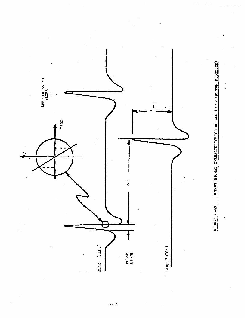
267

C.

a W I- W z 3 0 J LL

&

0 n > w o S a

+ I

r(J

= > 8 s * -

-L,I I

ly.

T

268

t

1

I

! I I I

I

I I

; I I i I I I ! I I 1 f ! !

I

I

I I I

I

I'

c3

a )I 0 n

- 111 w

270

v) >

e G e w

I-

a s Y

L L 4

w E 3 c3 U L

w c3 z 5 i3

n z 4

,-. . , . ,

... . . . . . . . . . .

.. ..............

. . . . . . .

Ull 2 7 1

. . . .

-. . __ . . . . . .

. . . . _ _ ......

. . .

2 7 2

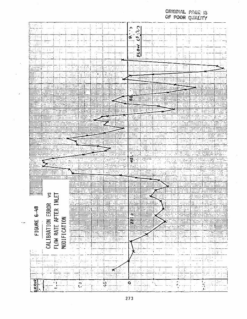
I .

- .-

. . . . . . . . .......... . - . . . . . . . . . . . . . . . . . . . . . . . . . . . . . . ,

. . . .

,-. . .. ... . . . ---- I . . . . . . .. I . ..... __-

.......... --.- . .. . . . . . , . . . . . . . . . . . . . * . . . . . . . . . . . . . . . . . I

............ - . ........... . . . . . . . . . . . . . . 1 , : . . . . . . . . ,.. . . . . . . . . . . . . . . . , ..

-. _-- __ .- . . . . . . ! . . . . ! . I . . a : . . - . . f : - - :. j . , . ! . . .. . i . . ! . . j . : . . . : .:: . ~ . . . . , . . . . . . . . . . . . . . . .

. . . . . . . .

. . , . . .

. . . .

. . , _ . . . . . . . . . . . . . . . . . . -. ~ . . . . . . . . . . . . . . . . . . . . . . . . . . “ i 1:h; 1 i .... . +----_

. . .

273

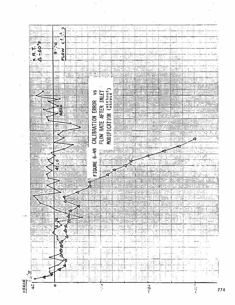
i . . . . ,.. . . . ,----. ._ t ..... -. . . . . . .

, . . . . . . .

,.-. . . . . I ::.,::.: ~~. . . I ....... _.- .... p I.. ... I . .. ’- ... .... _. .......

I.....=-.

. . . . . . . . . .. . . . . . . . ......... , .. .1 II-‘ .... I --.: ~ .... ..~- . ~ - ............. .......... .d I --: . . . . . . . . . . . .

74

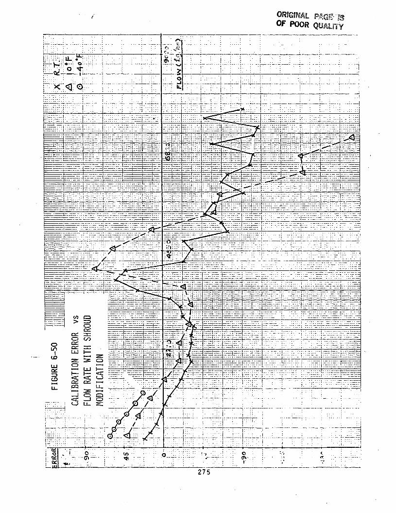
I'

. . . . . . . .

, . . ..

. . .

27 5

. . : . . , . . .

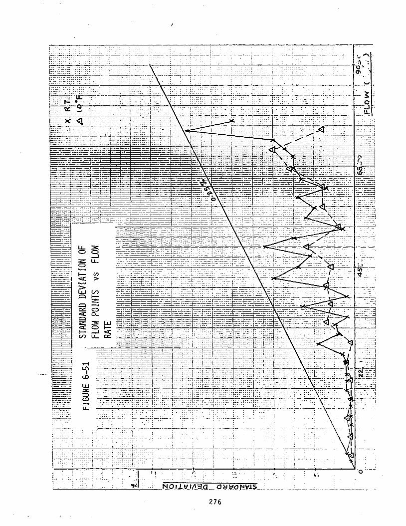
. . . . . . . . I . . . - . . . . . . . . . . . . . . .

. . . , . .

276

. . .

. . .

277

7.0 DENSI-VISCOMETER

This section describes the experimental and analytical investigation, the prototype construction and evaluation performed on the densi-viscometer.

7.1 ' Introduction

The vortex precession and dual turbine flowmeters (Sections 4.0 and 5.0 respectively) are basically volumetric devices and require precise density and approximate viscosity measurements to perform as mass flowmeters. The conceptual design of the densi-viscometer can be found in the Phase I Final Report. It is based on a currently produced General Electric densitometer that oscillates at a frequency determined by fluid density, and from which viscosity data can also be derived.

7.2 Experimental and Analytical Investigation Plan Formulations

There are several characteristics of the densitometer/viscometer The following concept which require additional experimental investigation.

areas for investigation were planned to be conducted in Task 4:

(1) Damping coefficient (Q) versus viscosity

( 2 ) Damping coefficient and natural frequency (f n) versus flow-through velocity

( 3 ) Stability over expanded temperature range

(4) Methods of reducing temperature sensitivity

7.2.1 Damping Coefficient Versus Viscosity

Problem - As viscosity increases, the shear forces and boundary layer on the oscillating surfaces of the fluid couplers increase, thereby increasing the damping coefficient or lowering the Q of 6he spring mass system, as well as lowering the natural frequency, fn. When the gain and phase of the loop-closing circuitry are properly set, the compound effects of lower Q and lower fn are nullified and the closed loop frequency, fa, is made constant so as to provide an accurate measure of density. by modulating the gain and phase of the circuitry, a small 5 change in fa can be generated whose magnitude indicates Q of the damped spring-mass system, from which viscosity is obtained. frequency response (gain and phase vs. frequency) vs. density and viscosity must be known precisely. In addition, the coupling coefficient for couplers with different numbers of vanes must be ascertained.

Furthermore,

In order to design the circuitry, the

278

Solution Approach - Frequency response of several densitometers will be measured in room temperature liquids having viscosities and specific gravities that cover the maximum ranges over which jet fuels vary (from temperature extremes.and JP-4 to JP-8 characteristics), The units will have the following couplers: .

16 vanes - 1.9 cm (0.75 in.) diameter 8 vanes - 1.9 cm (0.75 in.) diameter 4 vanes - 1.9 cm (0.75 in.) diameter

The reason for testing these types of couplers is that it will provide data which indicates how surface area and basic coupler shape affect the Q vs. viscosity function. while the vaned types have minimal area; this difference may produce vastly different response to changing viscosity. Furthermore, the vaned units will have lower coupler inertia which results in improved sensitivity. couplers would also cost much less to produce than the present multi-hole coupler. efficiency is also reduced. See Figure 7-1.

Open loop frequency response will be measured and plotted for each unit in the following liquids.

The production model has a large circumferential area

Vaned

This is a tradeoff since as the number of vanes is reduced, coupling

Approximate Approximate Kinematic Viscosity Simulation of fuel at:

Liquid Specific Gravity Centistokes Temp "C Viscosity

Tellus Oil #lo 0.90 Silicone Oil 0.90 Stoddard Solv. & 0.77

Stoddard Solv. & 0.77

Stoddard Solv. & 0.65

Pentane 0.65

Tellus Oil

Heptane

Heptane

20 -55 Maximum 5 -55 Minimum 5 - 20 Maximum

1 20 Minimum

0.8 130 Maximum

0.25 130 Minimum

All tests will be run at 25°C to minimize frequency variations due to temperature sensitivity. constant output voltage at re onance, and thereby more closely simulate actu closed loop operation. The engineering laboratory at General Electric is equipped with temperature control baths, drive and output circuits, and gain and phase measuring instruments.

The driving voltage will be varied to maintain a

7.2.2 Damping Coefficient (Q) and Natural Frequency (f,) versus Flow-Through Velocity

1

Problem - As flow velocity through the densitometer increases, the energy conducted away by the exiting flow, through the motion of the coupler, increases. This, in turn, lowers both Q and fn. In the turbine and vortex precession flowmeters, at least 1% flow diversion is needed through the

2 7 9

densitometer housing to ensure complete turnover of fuel in less than one minute at the minimum flow of 182 kg/hr (400 lb/hr). flow is approximately 15 cm/sec (6 in./sec), which is of the same order of magnitude as vane tip or outside diameter velocity ( magnitude of the resultant Q and f, changes must be known for future design of the densitometer housing, and for estimation of densitometer/viscometer accuracy e

At the maximum rated of 9090 kg/hr (20,000 lb/hr), flow velocity through the vanes or holes

5 cm/sec). The

Solution Approach - Fuel will be forced through a densitometer placed in a pipe as shown in Figure 7-2. measured at 25OC on the above mentioned densitometer. be minimal, a unit will be tested in a 3.8 cm (1.5 in.) diameter pipe over the 182 to 9090 kg/hr (400 to 20,000 lb/hr) flow range to see if the housing is, in fact, unnecessary.

Open loop Q and f, will be Should the sensitivity

Should flow velocity have adverse effects on Q and.f,, attention will be focused on approaches to control the velocity to the maximum allowed over the wide range of viscosity and mass flow rate. The following techniques will be investigated analytically:

o Boundary layer scoops o Variable orifice control o Port location

7.2.3 Stability Over Expanded Temperature Range

Problem - Temperature sensitivity of closed loop frequency need not be perfectly linear since compensation for these effects is made in the computer algorithms. However, this approach is practical only if the frequency vs. temperature function is highly repeatable and stable for long periods of time (months). shows that some "aging" occurs when the units are initially cycled over temperature extremes (-55 to +70"C) and that they settle out after two cycles and are repeatable within 5 0.12%. This is adequate for current applications but must be reduced t o less than 0.1% over a wider temperature range (-55 to +13OoC) for the NASA application.

Our experience with the current production models

7.2.4 Methods of Reducing Temperature Sensitivity

Problem - If temperature sensitivity is reduced, the temperature sensor may be eliminated, thus lowering the cost and complexity of the flowmeter system. the solution approaches are discussed together.

This problem is closely related to the stability problem so

Solution Approach - Several densitometers will be subjected to temperature cycling in air over a -55°C to +130°C range for the three month duration of Task IV. chamber temperature programmed to cycle hot and cold once daily. At the start, mid-point and finish of the test, three point density calibrations will be made to corroborate the air frequency data.

Frequency will be recorded automatically every hour and

The data will be analyzed at

280

mid-point to determine if any significant trends exists, and, if any changes in test approach are warranted. the electronics at ambient room temperature (20°C) except that open loop gain and phase vs. frequency will be plotted at the start, mid-point and end of the test.

The following units will be built for this evaluation:

The unit will be operated closed-loop with

a) Production Unit b) Minimum Solder Bond Thickness c) Shot Peened Spring

9 .3 Experimental and Analytical Investigations

Data relating to the densi-viscometer are included in the accompanying report supplement No. 1 dated December 15, 1984 as protectable data in accordance with contract NAS3-221394, Item 8C,

281

8.0 CONCLUSIONS AND RECOMMENDATIONS

After considering all the test results in Task 4 for all three different types of flowmeters, a rating scheme was established to evaluate the overall merit of all three flowmeter design; summarizes the probability of meeting the listed requirements for each concept in its conceived final system configuration. vortex, dual turbine and angular momentum flowmeters are 0.71, 1.00 and 0.95 respectfvely.

The dual turbine flowmeter and angular momentum flowmeter were chosen for prototype development and evaluation in Tasks 5 through 7.

The following conclusions and recommendations are made for each of the subsystems for the NASA HAFF program:

A rating chart, (Table 8-1)

The relative ratings of the

Test and Calibration System

Conclusions: 1) There are no flow rate calibration facilities known at present that meet the calibration requirements of NASA BWFF program.

2) The best flow rate calibration facility at GE/AID is inadequate to meet the ultimate calibration accuracy requirements of the flowmeters being developed under NASA HAFF program.

Recommendations: 1) Plan a flow calibration facility using a Flow-Thru Calibrator in a closed calibration system.

2) Procure precision density measuring equipment to combine volumetric flow rate with density to get mass flow'rate.

Vortex Flowmeter

Conclusions: 1) The calibration constant becomes excessively non-linear at low Reynolds numbers.

2) The repeatability is only about 0.5% and it has limited dynamic range.

3 ) Cavitation causes inaccuracy at high flow rates and also the pressure drop is excessive.

4) Existing vortex sensing technique will not meet the time response requirement.

282

kecomendations: 1) Alternate vortex sensing technique should be evaluated,

2) The relafionship between pressure drop and dynamic range should be investigated and optimized.

D u a l Turbine Flowmeter

Conclusions: 1) Dual turbine concept does not offer an advantage over conventional flow straightener for eliminating the effects of swirl in the incoming flow stream. - .

2) The "K" factor is a non-linear but single value function and will require a very accurate flow test facility to characterize the turbine

3) Fuel viscosity must be accurately measured to reduce errors at high and low temperatures.

4) Tests with room and high temperature fuels show that 0.25% accuracy can be achieved.

Recommendations: 1) The main turbine, with or without the input ' from sensor turbine, is adequate to measure

volumetric flow rate. The sensor turbine should be used to measure bearing degradation.

2) The dual turbine should be re-evaluated using the Test and Calibration System for accuracy.

Angular Momentum Flowmeter

Conclusions: I) The angular momentum flowmeter has low probability of meeting 0.25% point accuracy at flow rates above 5450 kg/hr (12,000 lb/hr).

The viscosity shroud provides good measurement of fluid viscosity.

2)

3) The spring of the rotor has considerable amount of hysteresis, thus affecting flowmeter repeatability between upscale and downscale calibration.

Recommendations: 1) The existing prototype design should be considered for application at flow rate below 5450 kg/hr (12,000 lb/hr).

2) Alternatively, the existing design may be upsized to achieve better high flow rate performance.

283

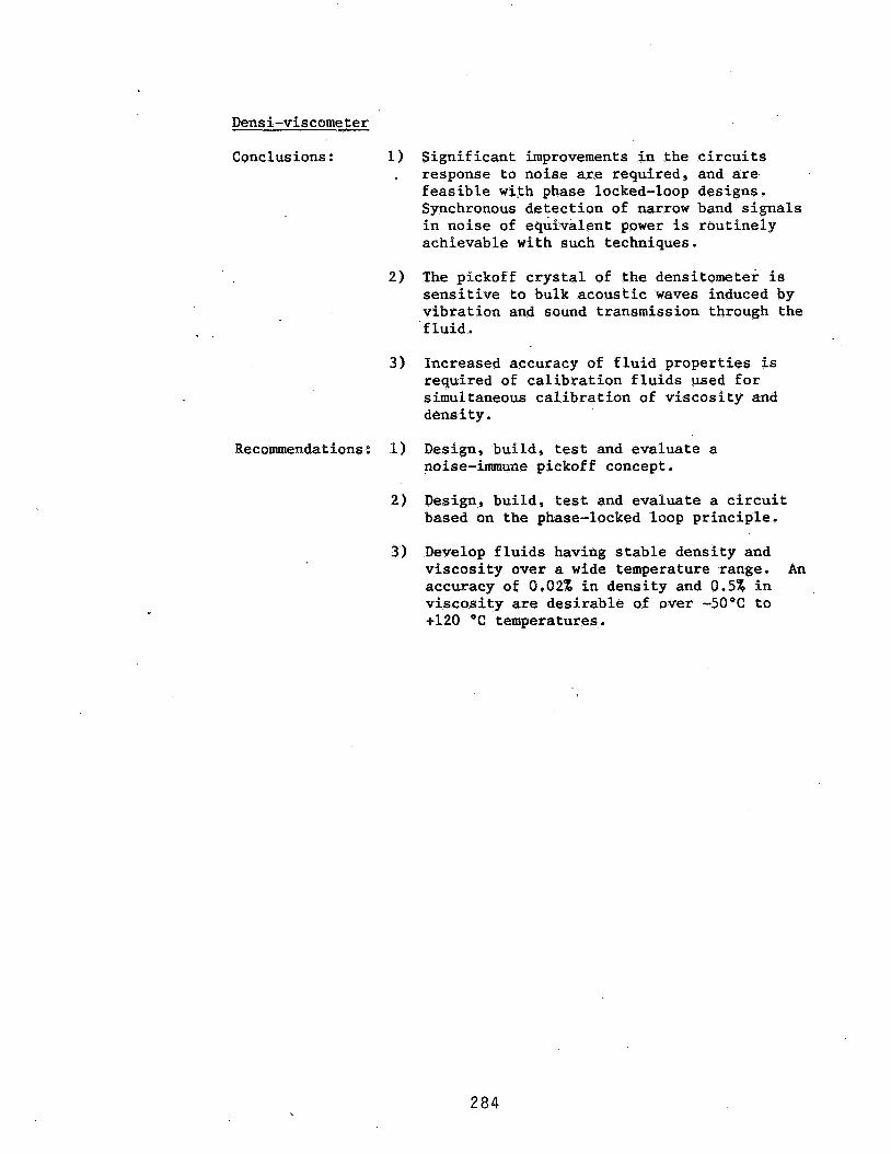
Densi-viscometer

Conclusions : 1) Significant improvements in the circuits response to noise are required, and are feasible with phase locked-loop designs. Synchronous detection of narrow band signals in noise of equivalent power is routinely achievable with such techniques.

2) The pickoff crystal of the densitometer is sensitive to bulk acoustic waves induced by vibration and sound transmission through the

e . fluid.

3 ) Increased accuracy of fluid properties is required of calibration fluids used for simultaneous calibration of viscosity and dens i ty .

Recommendations: l) Design, build, test and evaluate a noise-immune pickoff concept.

2) Design, build, test and evaluate a circuit based on the phase-locked loop principle.

3 ) Develop fluids having stable density and viscosity over a wide temperature range. accuracy of 0.02% in density and 0.5% in viscosity are desirable of over -50°C to +120 "C temperatures.

An

284

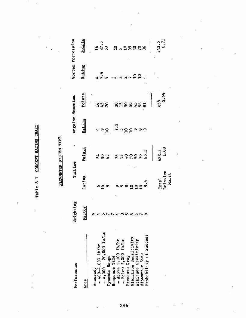
d I GO

VI h V I o o o \ o o m

rid

? \oVIooooVI m d & l n V I h G O

285

APPENDIX A

DERIVATION OF THE EQUATION FOR A BUOYANCY CORRECTION FACTOR APPLICABLE TO WEIGH (FLOW CALIBRATION) STANDS

286

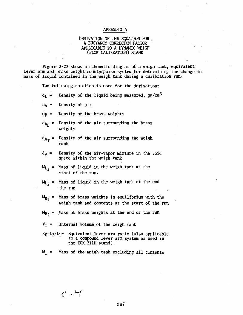
APPENDIX A

DERIVATION OF THE EQUATION FOR. A BUOYANCY CORRECTON FACTOR APPLICABLE TO A DYNAMIC WEIGH

(FLOW CALIBRATION) STAND

Figure 3-22 shows a schematic diagram of a weigh tank, equivalent lever arm and brass weight counterpoise system for determining the change in mass of liquid contained in the weigh tank during a calibration run.

The following notation is used for the derivation:

Density of the liquid being measured, gm/un3

Density of air

Density of the brass weights

Density of the air surrounding the brass weights

Density of the air surrounding the weigh tank

Density of the air-vapor mixture in the void space within the weigh tank

Mass of liquid in the weigh tank at the start of the run.

Mass of liquid in the weigh tank at the end the run

Mass of brass weights in equilibrium with the weigh tank and contents at the start of the run

Mass of brass weights at the end of the run

Internal volume of the weigh tank

RO=LZ/L1= Equivalent lever arm ratio (also applicable to a compound lever arm system as used in the COX 311H stand)

Mass of the weigh tank excluding all contents MT =

287

At the start of the run, the moment on the right side is in equilibrium with the moment on the left side as shown in Figure 3-16. temperature surrounding the brass weights and the weigh tank may be significantly different when the test temperature of the f hid temperature differs from the ambient temperature.

buoyancy forces gives the following relationship:

(Volume of brass weights) X (dg - db) X L2 =

The air

Equating the moments on the right side

e

. of the balance with moment on the left side and accounting for the air

L1 . X (Tank Weight + total mass of liquid in tank + total mass of air and vapor mixture in tank)

.. L1 X (Total volume of weigh tank) X dAT

The above statement reduces to the following equation for the conditions at the start of a calibration run:

A similar equation can be written for the static balance of the lever system at the end of the run or

We can obtain an equation for the difference in the,true liquid mass by subtracting Equation (A-1) from Equation (A-2) or

and rearranging Equation (A-3)

288

The last ratio of terms in Equation (A-4) corrects for the buoyancy forces based on (1) the density of the air surrounding the brass weights, (2) the density of the brass weights, ( 3 ) the density of the air-vapor mixture and (4) the liquid density within the weigh tank. It is fortuitous that the density of the air surrounding the weigh tank does not enter into the correction term inasmuch as it would be dif.ficult to characterize the temperature gradients surrounding the tank. convection forces on the tank are the same at the beginning as at the end of the run, we can also deduce that these forces would cancel since buoyancy

If we assume that the free

terms V f i ~ ~ would be

. The last ratio 1. correction factor KB

- .

KB1 =

the same at the start and end.

of terms in Equation (A-4) becomes the buoyancy

The true change in fluid mass in the weigh (1 ) the buoyancy correction factor, K,, (2 )

tank is equal to the product of the scale beam ratio, R o and

- (3) the change in mass of the brass weights on the scale pan.

determine true mass: Olsen E31 gives the following correction factor for buoyancy to

Olsen's equation does not designate where the density of the air dA in Equation (A-6) is determined. differ by a single quantity dv versus dA. correction is primarily a function of the density of the air-vapor displaced by the liquid entering the weigh tank rather than a function of the density of the air surrounding the weigh tank.

Equations (A-5) and (A-6) basically only This infers that the buoyancy

At a temperature of 21°C (70°F), standard pressure a density for the brass weights of 8.4 gm/cm3, a fluid density of 0.77 gm/cm 3 and an air density of 1.2014 kg/m3, Equation (A-6) gives a buoyancy correction factor of K B ~ = 1.00142.

289

At 21°C (70°F), the true vapor pressure of JP-4 is 10..7 kPa (1.55 psia) and using an estimated molecular weight of Mv = 126 gm/mole for the hydrocarbon vapor, the density of the air y&rwarbon vapor mixture above the

correction factor-from Equation (A-5) is K B ~ = 1.001972 which is greater than the previous correction factor by 0.055 percent.

greater at a temperature of 95°C (203°F). Using a true vapor pressure of JP4 is 90 kPa (13 psia) and a liquid density of 0.714 gm/cm3 results in a buoyancy correction factor from Equation (A-5) of K B ~ = 1.005234. This. value may be compared with Xg2 = 1.00121 from Equation (A-6) or a difference of 0.402 percent. The.only uncertainty in the data used in evaluation of Equation (A-5) is the value of the equivalent molecular weight of the hydrocarbon vapor.

at the temperature of the hydrocarbon liquid. This assumption appears valid for the COX 311H calibration stand since the air-vapor mixture is repeatedly transfered between the weigh tank and the liquid reservoir below the weigh tank through the overflow tube.

liquid is dv = 1.624 kg/m3 (0.1014 lbm!ft P ) and the buoyancy

The difference between the two buoyancy correction factors is even

- .

It was previously assumed that the air vapor mixture is in equilibrium

A further improvement in the accuracy of the determination of the density of the air-vapor mixture would be to directly flow a sample of the mixture through a density meter suited for gas density measurements.

factor K B ~ given by Equation (A-5) is independent of the tare weights or the density of the materials comprising the tare weights. correction factor is also inde endent of the density of the air surrounding

weigh tank as long as the conditions surrounding the tank can be assumed identical at the start and finish of a calibration run. correction factor is only dependent on (a) the density of the air surrounding the brass weights, (b) the density of the brass weights, (c) the density of the air-vapor mixture displaced by the fluid entering the weigh tank and (d) the density of the calibration fluid.

It should be emphasized that the value of the buoyancy correction

The buoyancy

the weigh tank or any thermal -57 or orced convection currents acting on the

The buoyancy

Figure 3-19 gives estimated values of the buoyancy correction factor as a function of temperature and molecular weight of the fuel vapor for two jet fuels.

290

APPENDIX B

RELATIONSHIP BETWEEN CHANGE IN MOMENTUM OF A FALLING LIQUID TO VOLUME OF THE COLUMN OF LIQUID

291

APPENDIX B

RELATIONSHIP OF CHANGE IN MOMENTUM OF A FALLING FLUID TO

THE VOLUME OF THE FLUID

Figufe 3-21 shows the approximate geometry of a liquid as it spills into the weigh tank of a dynamic flowmeter calibrator. velocity of wo as it leaves the edge of the spreader cone as shown in Figure 3-21. nozzle opening, A, (2) the angle of the spreader cone, 8 (3) the height between the center of the flow nozzle and the edge of the spreader cone, & (4 ) component at the edge of the spreader cone is uo = wo sin6 . vertical velocity at any height below the edge of the spreader cone can be Calculated from the following equation:

The liquid has a mean

The velocity wo is a function of the area of (1) the inlet

and the volumetric flowrate, Q = WL/dL. The vertical velocity The

u =d2gh + u2 0

where g = Local acceleration of gravity, cm/sec*

h = Distance below the edge of the spreader cone, cm

uo= h i tial vertical velocity component, cm/sec

The cross-sectional area A of the liquid jet at any height can be calculated from the continuity equation as follows:

A = .- WL dLU

03-21

where

A = Cross-sectional area of the liquid jet in the horizontal plane, cm2

WL= Mass rate of liquid flow, kg/sec

dL= Density of the liquid, kg/cm3

u = Vertical velocity component of liquid jet, cm/sec

The volume of the liquid jet between the liquid levels at start and end can be calculated from the following equation:

2 9 2

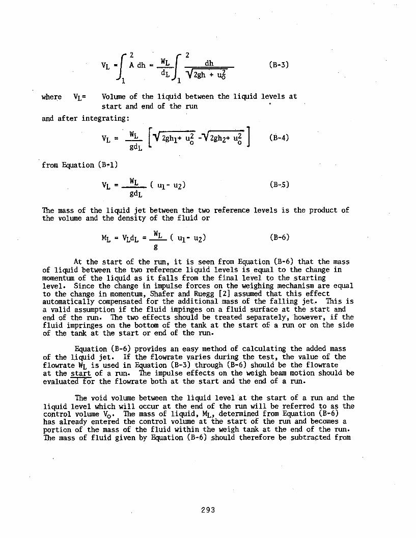
where VL=

and a f t e r integrating :

Volume of the l iquid between the liquid levels a t start and end of the run

from Equation (B-1)

The mass of the liquid j e t between the two reference levels is the product of the volume and the density of the f lu id or

A t the s t a r t of the run, it is seen from Equation (B-6) that the mass of liquid between the two reference l iquid levels is equal t o the change i n momentum of the liquid a s it f a l l s from the f ina l level t o the s ta r t ing level. Since the change i n impulse forces on the weighing mechanism are equal t o the change i n momentum, Shafer and Ruegg 121 assumed that t h i s effect automatically compensated fo r the additional mass of the fa l l ing jet. This is a valid assumption i f the f lu id impinges on a f luid surface a t the start and end of the run. The two effects should be treated separately, however, i f the f lu id impringes on the bottom of the tank a t the start 06 a run or on the side of the tank a t the start or end of the run.

Equation (B-6) provides an easy method of calculating the added mass If the flowrate varies during the test, the value of the of the l iquid je t .

flowrate WL is used i n Equation (B-3) through (B-6) should be the flowrate a t the - start of a run. evaluated f o r the flowrate both a t the start and the end of a run.

The impulse e f fec ts on the weigh beam motion should be

The void volume between the l iquid level a t the start of a run and the liquid level which w i l l occur a t the end of the run w i l l be referred t o as the control volume Vo. has already entered the control volume a t the start of the run and becomes a portion of the mass of the f lu id within the weigh tank a t the end of the run. The mass of f lu id given by Equation (B-6) should therefore be subtracted from

The mass of l iquid, ML, determined from Equation (B-6)

293

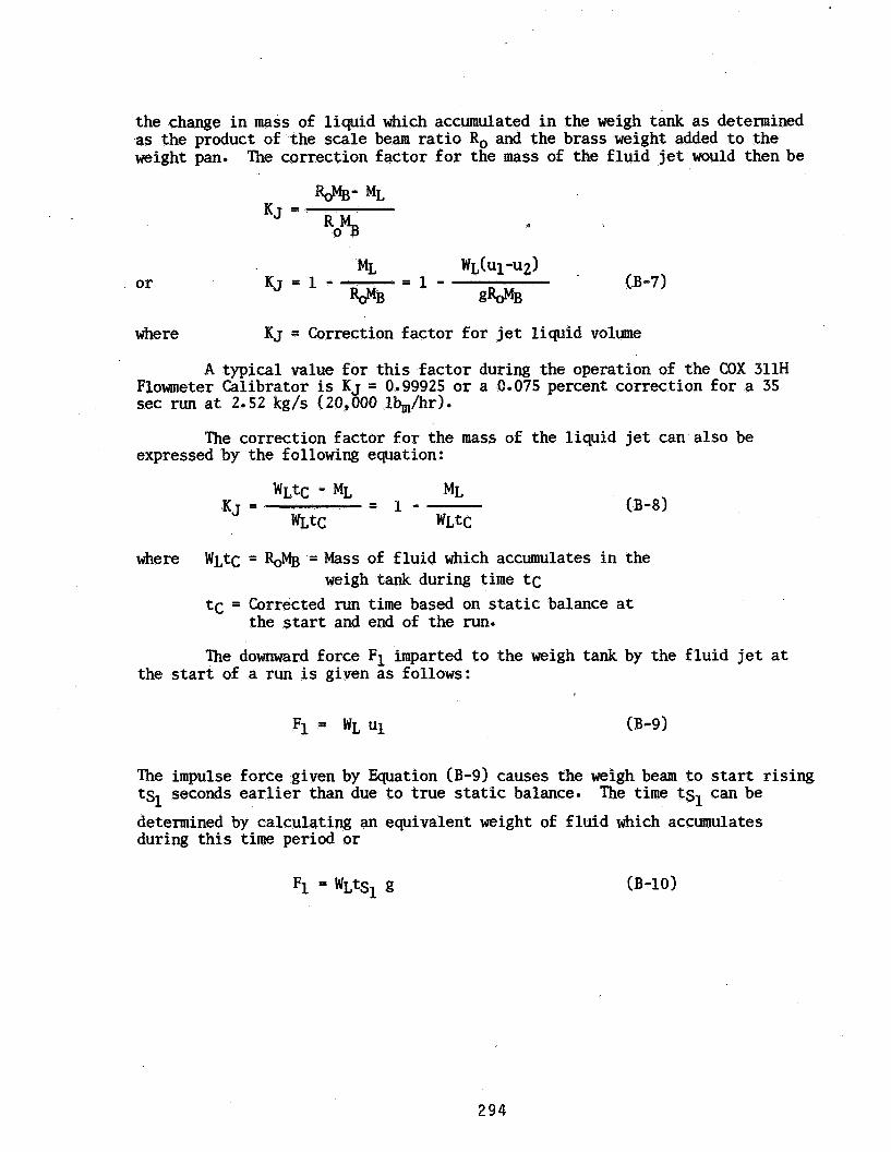
the change in mass of liquid which accumulated in the weigh tank as determined .as the product of the scale beam ratio Ro and the brass weight added to the weight pan. The correction factor for the mass of the fluid jet would then be

w- ML KJ =

R % 0

where KJ = Correction factor €or jet liquid volume

A typical value for this factor during the operation of the COX 311H

at 2-52 kg/s (20,000 lbm/hr).

The correction factor for the mass of the liquid jet can also be

Flowmeter Calibrator is KJ = 0.99925 or a 0.075 percent correction for a 35 sec

expressed by the following equation:

where WLtC = R$rfg = Mass of fluid which accumulates in the weigh tank during time tc

tc = Corrected run time based on static balance at the start and end of the run.

The downward force F1 imparted to the weigh tank by the fluid jet at the start of a run is given as follows:

The impulse force given by Equation (B-9) causes the weigh beam to start rising tS1 seconds earlier than due to true static balance. The time tS1 can be determined by calculating an equivalent weight of fluid which accumulates during this time period or

294

The time tsl can then be determined by equating Equation (B-9) and (B-10) or:

Ul g

tsl= - (B-11)

The impulse force of the falling jet causes the weigh beam to start rising tS2 seconds earlier than due to a true static balance. related to the vertical velocity component of the falling jet as follows:

The time tS2 can be

u2 g

tS2" -

subtracting Equation (B-12) from (B-11) gives

and using Equation (B-6)

(B-12)

(B-13)

(B-14)

The substitution of the equivalence given by EQuation (B-14) into Equation (B-8) results in the following equation:

Equation (B-15) is useful to simplify the determination of the correction factor timing KT as shown in Section 3.6.1.1.

295

APPENDIX C

SUMMARY OF PATENTS RELATED TO LIQUID FLOW RATE CALIBRATION

296

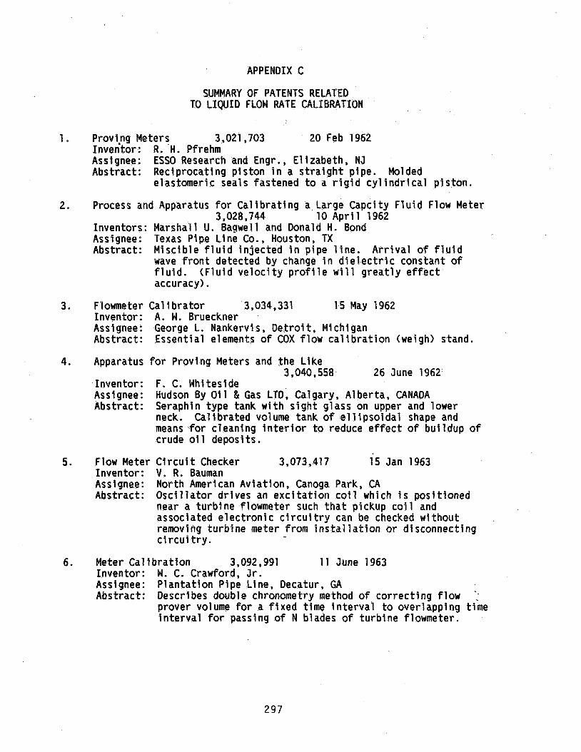
APPENDIX C

SUMMARY OF PATENTS RELATED TO LIQUID FLOW RATE CALIBRATION

1.

2.

3.

4.

5.

6.

Provipg Meters 3,021,703 20 Feb 1962 Inventor: R, 'H. Pfrehm Assignee: ESSO Research and Engr., Elizabeth, NJ Abstract: Reciprocating p is ton I n a s t r a i g h t pipe. Molded

elastomeric seals fastened to a r i g i d c y l i n d r i c a l p iston.

Process and Apparatus for Ca l i b ra t i ng a Large Capcity F l u i d Flow Meter 3,028 , 744 10 A p r i l 1962

Inventors: Marshall U. Bagwell and Donald H. Bond Assignee: Texas Pipe Line Coo, Houston, TX Abstract: MSscible f l u i d i n jec ted i n pipe l i n e . A r r i v a l of f l u i d

wave f r o n t detected by change i n d i e l e c t r i c constant o f f l u i d . (F lu id v e l o c i t y p r o f i l e w i l l g rea t l y e f f e c t accuracy).

Flowmeter Cal i brator 3,034,331 15 May 1962 Inventor: A. W . Brueckner Assignee: George L. Nankervis, De t ro i t , Michigan Abstract: Essential elements of COX flow c a l i b r a t i o n (weigh) stand.

Apparatus for Proving Meters and the Like

Inventor: F. C. Mhiteside Assignee: Hudson By O i l & Gas LTD, Calgary, Alberta, CANADA Abstract: Seraphin type tank w i th s igh t glass on upper and lower

Cal i brated volume tank o f e l 1 ipso lda l shape and

3 , 040,558. 26 June 1962

neck.. means crude

Flow M e t e r Circu Inventor: V. R. Assignee: North Abstract: Osci 1

for cleaning i n t e r i o r to reduce' e f f e c t o f bui ldup o f 01 1 deposits.

t Checker 3,073,417 15 Jan 1963 Bauman American Aviat ion, Canoga Park, CA a to r dr ives an e x c i t a t i o n c o i l which i s posi t ioned

near a turbine flowmeter such t h a t pickup coi 1' and associated e lect ron ic c i r c u i t r y can be checked without removing turbine meter from i n s t a l l a t i o n or disconnecting c i r c u i t r y .

Meter Cal i bra t i on 3,092 , 991 11 June 1963 Inventor: W. C. Crawford, Jr . Assignee: Plantat ion Pipe Line, Decatur, GA Abstract: Describes double chronometry method o f correct ing flow .;

prover volume for a f i x e d time i n t e r v a l t o overlapping time i n t e r v a l for passing of N blades of turb ine flowmeter.

297

I

7.

8.

9.

10.

111.

12.

13.

Fluid Meter Calibration Inventor: R. E. Boyle Assignee: Service Pipe Line Co., Tulsa, OK Abstract: Rigid piston in straight pipe. Piston has molded

elastomeric seals and uses electromagnetic proximi ty sensor for detecting discrete positions of prover piston.

3 , 120 , 1 18 4 Feb 1964

System for Cal i brati ng Pipe Line Flowmeters

Inventor: R. 6 . Smith Assignee: Socony Mobil Oil Co., New York, NY Abstract: Method of comparing a volumetric flowmeter to be calibrated

with a distant master flowmeter located on the same pipeline. Telephone circuit used to coordinate simul taneous measurement by two flowmeters.

3 , 1 38,013 23 June 1964

Dynami c Error Cal i brator 3,148,527 15 Sept. 1964 Inventor: J . J. Lindquist Assignee: North American Aviation, Canoga Park, CA Abstract: Dynamic response of flowmeters - step changes in flowrates

through flowmeter are induced by means of solenoid valves.

\lo1 umetri c Flowmeter Cal i brator 3 177 699 13 Apr. 1965 Inventor: J. J. LIndquist Assignee: Abstract: Liquid flowmeter calibration using a vertical standpipe

North American Aviation, Canoga Park, CA

wi th necked down areas for precise volume determi nation and special means of necking down to prevent sloshing.

Automatic Meter Prover 3,187 551 - 8 June 1965 Inventor: R. W . Hill Assignee: National Tank Co., Tulsa, OK Abstract Method of comparing production flowmeter against a master

flowmeter.

Cal i bration Device 3,212,318 39 Oct. 1965 Inventor: J. S. Lomay Assignee: Unl ted Aircraft Corp., East Hartford, CT Abstract: Insulated tank suspended on loads cells and using flexible

hose to minimize reaction forces of fluid entering and leaving tank. Level sensors in tank are used for volume determination. Integral welghts used for weigh system calibration. cal i bration.

Particularly suitable for cryogenic flowmeter

Proving Flowmeters 3,224,247 21 Dec. 1965 Inventor: M L. Barrett, Jr. Assignee: Sh$ll Oil eo., New York, NY Abstract: Two methods of recycling a neoprene ball In a pipeline

prover.

298

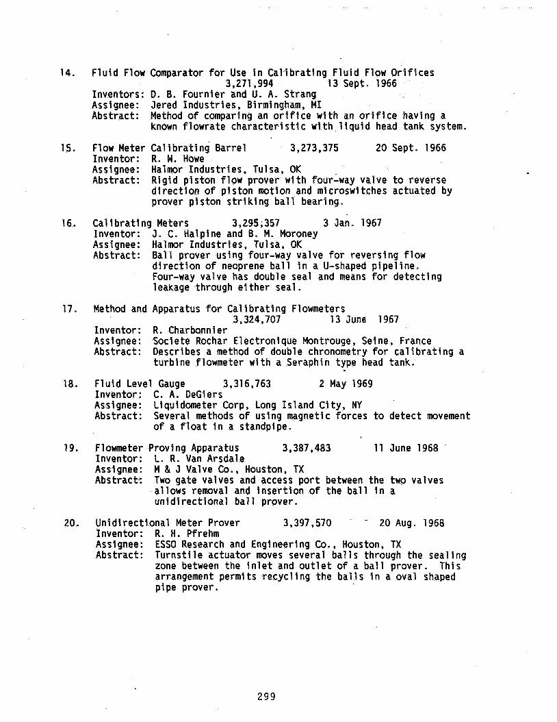
1 4.

95.

'I 6.*

17,

18.

19.

20.

Fluid Flow

Inveritors: Ass 1 gnee : Abstract:

F1 ow Meter I nven tor : Assi gnee : Abstract:

Comparator for Use in Calibrating Fluid Flow Orifices

D. B. Fournier and U. A. Strang Jered Industries, Birmingham, MI Method of comparing an orifice with an orifice havlng a known flowrate characteristic w'ith liquid head tank system.

Cal i brating Barrel 3,273,375 20 Sept. 1966 R. W. Howe Halmor Industries, Tulsa, OK Rigid piston flow prover wlth four-way valve to reverse direction of pi ston motion and m i croswi tches actuated by prover piston striking ball bearing.

3,271,994 13 Sept. 1966

Cali brati ng Meters 3,2~95 ; 357 3 Jan. 1967 Inventor: J. C. Halpine and B. M. Moroney Assignee: Halmor Industries, Tulsa, OK Abstract: Ball prover using four-way valve for reversing flow

direction of neoprene ball in a U-shaped pipeline. Four-way valve has double seal and means for detecting leakage through either seal.

Method and Apparatus for Calibrating Flowmeters

Inventor: R. Charbonnier Assignee: Societe Rochar Electronique Montrouge, Seine, France Abstract:

Fluid Level Gauge 3,316,763 2 May 1969 Inventor: C. A. DeGiers Assignee: Liquidometer Corp, Long Island City, NY Abstract: Several methods of using magnetic forces to detect movement

of a float in a standpipe.

3,324,707 13 June 1967

Describes a method of double chronometry for calibrating a turbine flowmeter with a Seraphin type head tank.

F1 owme ter Prov i ng Apparatus 3,387,483 1 1 June 1968 Inventor: L. R. Van Arsdale Assignee: M & J Valve Co., Houston, TX Abstract: Two gate valves and access port between the two valves

allows removal and insertion of the ball in a unidirectional ball prover.

Unidirectional Meter Prover 3,397,570 - 20 Aug. 1968 Inventor: R. H. Pfrehm Assignee: ESSO Research and Engineering Co., Houston, TX Abstract: Turnstile actuator m v e s several balls through the sealing

zone between the inlet and outlet of a ball prover. arrangement permits recycl ing the ball s in a oval shaped pipe prover.

This

299

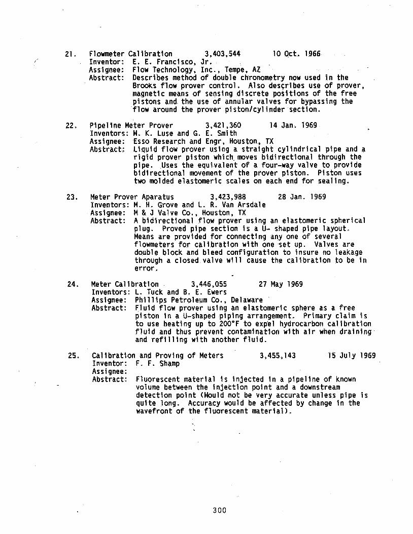
21 e

22 0

23.

24

25 0

Flowmeter Cal i b r a t i o n 3,403,544 10 Oct. 1966 Inventor: E. E. Francisco, J r . Assignee: Flow Technology, Inc., Tempe, AZ Abstract: Describes method of double chronometry now used i n the

Brooks flow prover control . Also describes use of prover, magnetic means o f sensing d iscrete pos i t ions o f the f r e e pistons and. the use of annular valves for bypassing the flow around the prover p is ton/cy l inder section.

PipelSne Meter Prover 3,421,360 14 Jan. 1969 Inventors: W . K. Luse and G. E. Smith Assignee: Esso Research and Engr, Houston, TX Abstract: L iqu id flow prover using a s t r a i g h t c y l i n d r i c a l pipe and a

r i g i d prover p i s ton which-moves b i d i r e c t i o n a l through the plpe. Uses the equivalent of a four-way valve t o provide b i d i r e c t i o n a l movement of the prover piston. Piston uses two molded elastomeric scales on each end for sealing.

Meter Prover Aparatus 3,423,988 28 Jan. 1969 Inventors: M. H. Grove and L. R. Van Arsdale Asslgnee: M & J Valve Co., Houston, TX Abstract: A b i d i r e c t i o n a l flow prover using an elastomeric spherical

plug. Means are provided for connecting any one o f several flowmeters fo r c a l i b r a t i o n w i t h one set up. Valves are double block and bleed conf igurat ion to insure no leakage through a closed valve w i l l cause the c a l i b r a t i o n to be in error .

Proved pipe section i s a U- shaped pipe layout.

Meter Cal i bra t i on 3,446,055 27 May 1969 Inventors: L. Tuck and B. E. Ewers Assignee: P h i l l i p s Petroleum Co., Delaware Abstract: F l u i d flow prover using an elastomeric sphere as a f r e e

p i s ton i n a U-shaped p ip ing arrangement. Primary c la im i s to use heating up t o 200°F to exp'el hydrocarbon c a l i b r a t i o n f l u i d and thus prevent contamination w i th a i r when dra in ing and r e f f l l i n g w i th another f l u i d .

Inventor: F. F. Shamp- A s s 1 snee :

Cal lbrat ion and Proving o f Meters 3.455,143 95 Ju ly 1969

S detect ion PO qu i te long. wavefront of

AbstFact: Fluorescent mater ia l i s i n jec ted i n a p ipe l i ne o f known volume between the i n j e c t i o n po in t and a downstream

n t (Would not be very accurate unless p ipe Accuracy would be af fected by change i n the the f luorescent mater ia l ) .

300

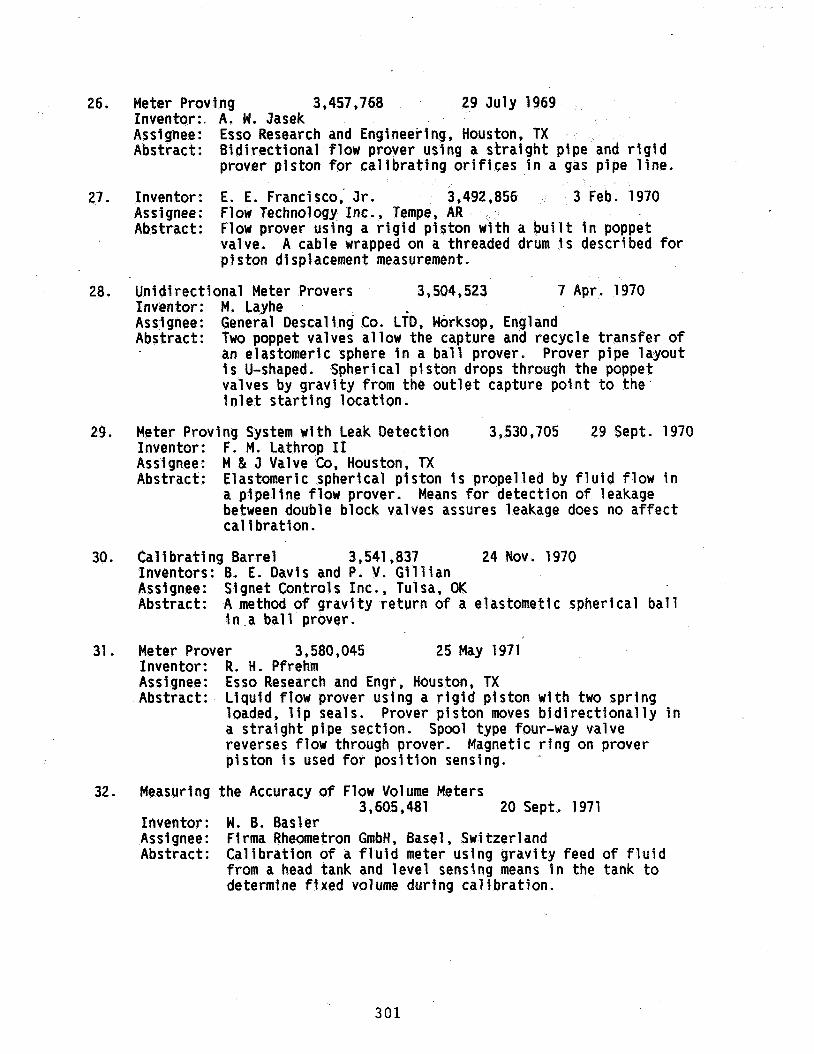
26. Meter Proving 3,457,768 29 July 1969 Inventor:. A. #. Jasek Assignee: Abstract: Bidirectional flow prover using a pipe and rigid

Esso Research and Engineering, Hou

prover piston for calibrating orifices in a gas pipe line.

27. Inventor: E. E. Francisco, Jr. 3,492,856 3 Feb. 1970 Assignee: Flow Technology Inc., Tempe, AR Abstract: Flow prover using a rigid plston with a built in poppet

valve. A cable wrapped on a threaded drum is described for pi ston displacement measurement-

28. Unidirectional Meter Provers 3,504,523 7 Apr. 1970 Inventor: M. Layhe Assignee: General Descal ing Co. L i D , Worksop, England Abstract: Two poppet valves allow the capture and recycle transfer of

an elastomeric sphere in a ball prover. Prover pipe layout is U-shaped. Spherical piston drops through the poppet valves by gravity from the outlet capture point to the inlet starting location.

29. Meter Proving System with Leak Detection 3,530,705 29 Sept. 1970 Inventor: F. M. Lathrop I1 Assignee: M & J Valve Co, Houston, TX Abstract: Elastomeric spherical piston is propelled by fluid flow in

a pipeline flow prover. Means for detection of leakage between double block valves assures leakage does no affect calibration.

30. Cal i brati ng Barrel 3,541,837 24 Nov. 1970 Inventors: B. E. Davis and P. V. Gillian Assignee: Signet Controls Inc., Tulsa, OK Abstract: A method of gravity return of a elastometic spherical ball

in a ball prover.

31. Meter Prover 3,580,045 25 May 1971 Inventor: R. H. Pfrehm Assignee: Esso Research and Engr, Houston, TX Abstract: Liquid flow prover using a rigid piston with two spring

loaded, lip seals. Prover piston moves bidirectionally in a straight pipe section. Spool type four-way valve reverses flow through prover. Magnetic ring on prover piston is used for position sensing. -

32. Measuring the Accuracy of Flow Volume Meters

Inventor: W. B. Basler Assignee: Firma Rheometron GmbH, Basel, Switzerland Abstract: Calibration of a fluid meter using gravity feed of flufd

from a head tank and level sensing means in the tank to determine flxed volume during calibration.

3,605,481 20 Sept. 1971

301

33.

34 I

- 35 0

1 ..

36 e

i, 37.

38

39.

High-speed Calibration of Liquid Flowmeters 3,631,709 4 Jan. 1972 Inventors: E. C. Smith and C. P. Kimball Abstract: A piston is driven by anvariable speed or through a ball

lead screw for call bration of water met

Meter-Proving Method and Apparatus 3,638,475 1 Feb. 1972 Inventors: M. H, Grove and L. R. VanArsdale Assignee: M & J Valve Co., Houston, TX Abstract: Spool valve arrangement for recycle of an elastometic

spherical piston i n a ball flow prover,

Cal i brati ng Barrel 3,643,489 22 Feb. 1972 Inventors: B. E. Davis and P. V. Glllian Assignee: Signet Controls, -Tulsa, OK Abstract: Method of recycling elastomeric spherical balls in a ball

prover by gravity.

Apparatus for Calibrating a Volumetric Flow Metering Device

Inventor: R. A. Brown Assignee: Eastman Kodak Co., Rochester, NY Abstract: An annular, elastomeric diaphragm i s used to separate a

3,657,919 25 Apr. 1972

corrosive fluid being metered from a displaced, non-volatile fluid which is drSven into a standpipe having a narrow entrance and exit for accurate detection of a f i xed volume di spl acement.

Meter Proving Method and Apparatus 3,668,923 13 June 1972 Inventors: M. H. Grove and L. R. VanArsdale Abstract: A bidirectional ball prover using a gate valve constructed

as a four-way valve to reverse the flow. Valve has double seal and means of leak detection to assure leakage is not causlng an error during a prover run.

Meter Prov Inventors: Ass1 gnee : Abstract:

ng System 3,673,851 ’ 4 July 1972 E. L, Wright and E. Meseck Customline Control Products Inc., Linden, NJ Bidirectional piston type prover which may be used to check an active flowmeter.

Meter Proving System 3,678,730 25 July 1972 Inventor: M. L. Barrett, Jr. Abstract: Several elastomeric spherical balls are recycled in a

unidirectional ball prover having a U-shaped piping layout. Various devices are described for capturing the balls in the interchange between the outlet and inlet. Auxilary pumps are used to transfer the balls through the interchange a*$ well as launch one ball into the inlet during a proving run.

302

40.

41.

42 e

43.

44.

45.

46.

47.

Double Ball Meter Prover 3,720,089 13 May 1973 Inventors: 6. E. Davis and R. G. Dunegan Assignee: Signet Controls Inc., Tulsa, OK Abstract: A unidirectional ball prover uses multiple balls in the

U-shaped piping system. The interchange piping between the inlet and outlet has a diameter which is slightly smaller than the proving piping. A hydraulic or pneumatic actuator piston forces an elastomeric, spherical ball into the inlet for a proving run. The remaining balls in the interchange passage form multiple seals against leakage from the inlet to outlet.

Valveless Prover 3,738,153 12 June 1973 Inventor: C. R. Simmons Assignee: Helmerick and Payne Inc., Houston, TX Abstract: Operation is similar to Item 28 (3,304,523)

Meter Prover Apparatus and Method 3,777,545 19 Dec. 9973 Inventors: M. H. Grove and T. I<. Griffen Assignee: M & J Valve Co., Houston, TX Abstract: A unidirectional ball prover which uses a shuttle valve

device for transferring an elastomeric, spherical ball through a sealed interchange from the outlet to the inlet of the prover.

Meter Prover Apparatus 3,798,957 26 Mar 1973 Inventors: C. G. Shannon, 6. M. Moroney and J. R. Neal Assignee: Metric Inc., Tulsa, OK Abstract: Elastometric, spherical balls are used for sealing in a

four-way valve arrangement in conjunction with a bidirectional ball prover.

Three-Sphere Prover Interchange 3,800,587 2 Apr 1974 Inventor: W . D. Clinton Assignee: Signet Controls Inc., Tulsa, OK Abstract: Operation is similar to Item 42 (3,777,545)

Meter Proving Apparatus 3,830,092 20 Aug 1974 Inventors: M. H. Grove and R. G. Dunegan Assignee: M & J Valve Co., Houston, TX Abstract: Operatlon i s similar to Item 42 (3,777,5451

Ball Prover and Components Thereof 3,832,883- 3 Sept. 1974 Inventor: ITT Corp, New York, NY Abstract: Devices for detection of passage of ball in a ball prover

to prevent contact bounce of a microswitch from affecting the timing accuracy.

Meter Proving Apparatus and Method 3,835,695 17 Sept. 1974 Inventor: M. H. Grove Assignee: M & J Valve Co., Houston, TX Abstract: Improvement of Item 42 (3,777,545)

3 0 3

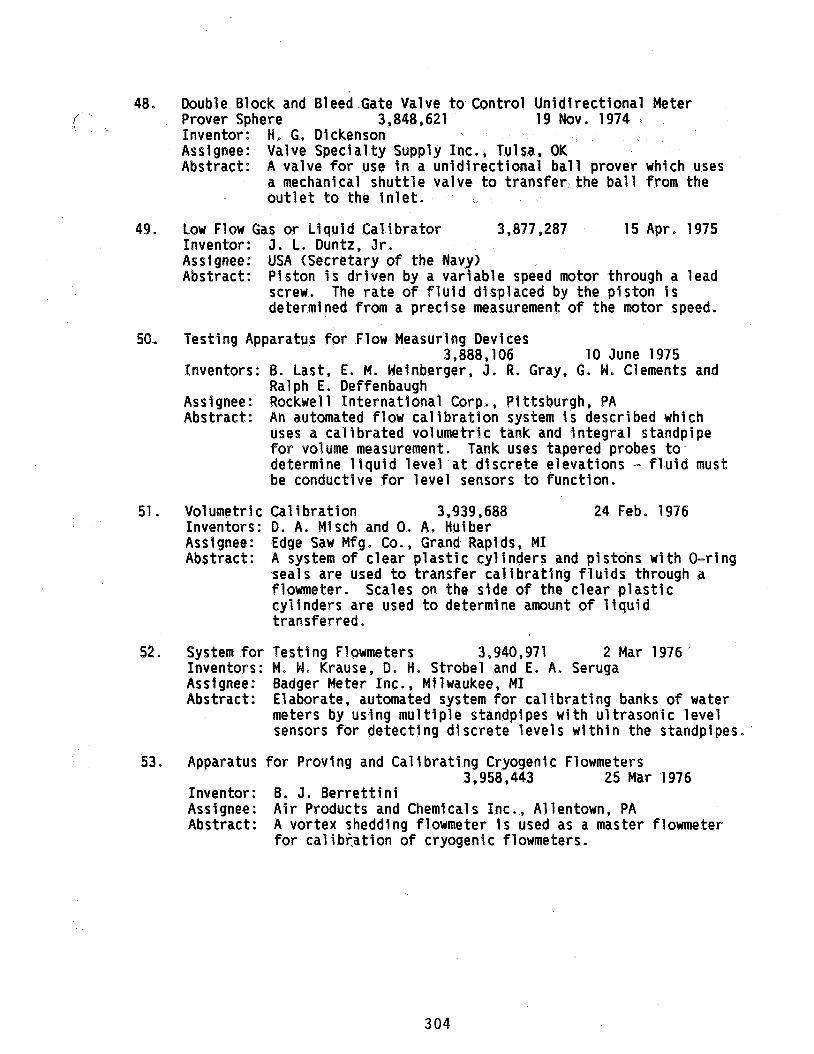
48. Double Block and Bleed Gate Valve to Control Unidirectional Meter Prover Sphere 3,848,621 19 Nov. 1974 Inventor: H e G. Dickenson Assignee: Valve Specialty Supply Inc., Tulsa, OK Abstract: A valve for use In a unidirectional ball prover which uses

a mechanical shuttle valve to transfer the ball from the outlet to the inlet.

49. Low Flow Gas or Liquid Calibrator 3 , 877,287 15 Apr. 1975 Inventor: J. L. Duntz, Jr. Assignee: USA (Secretary of the Navy) Abstract: Piston is driven by a variable speed motor through a lead

screw. The rate of fluid displaced by the piston i s determined from a precise measurement of the motor speed.

50- Testing Apparatus for Flow Measuring Devlces

Inventors: B. Last, E. M. Weinberger, J. R. Gray, G. W. Cilements and Ralph E. Deffenbaugh

Assignee: Rockwell International Corp., Pittsburgh, PA Abstract: An automated flow calibration system is described which

uses a calibrated volumetric tank and integral standpipe for volume measurement. Tank uses tapered probes to determine liquid level at discrete elevations - fluid must be conductive for level sensors to function.

3,888,106 10 June 1975

51 . Volumetric Cal i bration 3,939,688 24 Feb. 9976 Inventors: D. A. Misch and 0. A. Huiber Assignee: Edge Saw Mfg. Co., Grand Rapids, MI Abstract: A system of clear plastic cyllnders and pistons with O-ring

seals are used to transfer calibrattng fluids through a flowmeter. Scales on the side of the clear plastic cylinders are used to determine amount of liquid transferred.

2 Mar 1976 52. System for Testing Flowmeters 3,940,97 1 Inventors: M. W . Krause, D o H. Strobe1 and E. A. Seruga Assignee: Badger Meter Inc., Milwaukee, MI Abstract: Elaborate, automated system for calibrating banks of water

meters by using mu1 tiple standpipes with ultrasonic level sensors for detecting dlscrete levels within the standpipes.

53. Apparatus for Proving and Calibratlng Cryogenic Flowmeters

Inventor: B. J. Berrettini Assignee: Air Products and Chemicals Inc., Allentown, PA Abstract:

3,958,443 25 Mar 1976

A vortex shedding flowmeter i s used as a master flowmeter for calibration of cryogenic flowmeters.

304

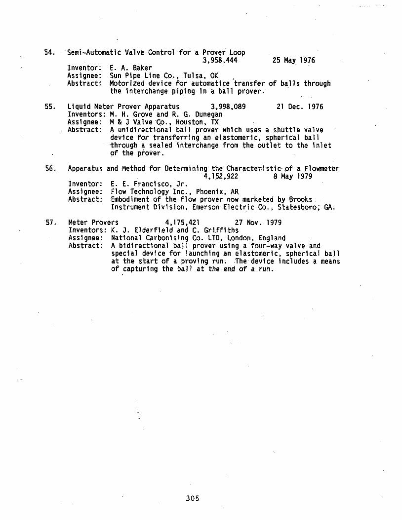
54. Semi-Automati'c Valve Control -for a Prover Loop

Inventor: E. A. Baker Assignee: Sun Pipe Line Co., Tulsa, OK

the interchange piping in a ball prover.

3,958,444 25 May 1976

. Abstract: Motorized device for automatice 'transfer of bqlls through

55. Liquid Meter Prover Apparatus 3,998,089 21 Qec. 1976 Inventors: M. H. Grove and R. G. Dunegan Assignee: M & J Valve Co., Houston, TX Abstract: A unidirectional ball prover which uses a shuttle valve

device for transferring an elastomeric, spherical ball through a sealed interchange from the outlet to the inlet of the prover.

56, Apparatus and Method for Determining the Characteristic of a Flowmeter

Inventor: E. E. Francisco, Jr. Assignee: Flow Technology Inc., Phoenix, AR Abstract:

4,152,922 8 May 1979

Embodiment of the flow prover now marketed by Brooks Instrument Division, Emerson Electric Co., Statesboro; GA.

57. Meter Provers 4,175,421 27 Nov. 1979 Inventors: K. J. Elderfield and C. Griffiths Assignee: National Carbonising Co. LTD, London, England Abstract: A bidirectional ball prover using a four-way valve and

special devlce for launching an elastomeric, spherical ball at the start of a proving run: The device includes a means of capturing the ball at the end of a run.

305

APPENDIX D

DYNAMIC EQUATIONS FOR THE MOTION OF THE TARE BEAM IN A DYNAMIC WEIGHT STAND (TYPE G-1)

306

APPENDIX D

DYNAMIC EQUATIONS FOR THE MOTION OF THE TARE BEAM IN A DYNAMIC WEIGH STAMI

Figure 3-22 shows the geometry of the weighing system as used in the COX 311H Flow Calibrator. There is normally no weight start of a run- The sliding tare weights are adjusted run for 5 to 15 sec after the dump valve is closed.

weigh beam and any tare weight is added directly to weight pan (see Figure 3-16)

the weigh pan at the delay the start of a

The weighing system used in COX 305T Flow Calibrator uses a single

The following notation is used for deriving the equations of motion:

dL =

F =

g =

JWB' Jm= L =

MB =

ME =

Mi '=

MF =

Mm=

MT =

M p j =

Mp

Mp = 1

Density 'of the liquid kg/cm3

Force, N

LX>C& acceleration of gravity , cm/s2

Moment of inertia of weigh beam, kg-cm2

Moment of inertia of tare beam, kg-an2

Beam lengths [see Figure 3-22], cm

Mass of reference (brass) weights on weigh pan, kg

Equivalent 9ynamic mass of weighing system concentrated at the weigh pan pivot including weigh tank, kg

Effective d

mass of brass weights and mass of fuel in weigh tank, kg

ic mass of weighing system concentrat 2F=- at the weigh pan pivot including

Mass of fuel in the tank, kg

Mass of linkage between weigh beam and tare beam, kg

Mass of tare weight or weights, kg

Mass of tare beam, kg

Mass of weight pan, kg

Effective static mass of weigh pan, beams and linkage concentrated at the weigh pan pivot but excluding weigh tank, kg. [See Equation D-11

3 07

Mjnr=

%=

R,=

WA =

t =

t' =

tT

v =

x =

Y =

8 =

Subscripts:

LK =

T =

TB=

w B =

Mass of weigh tank (dry), kg

Mass of weigh beam, kg e)(* Lever arm ratio =

Actual mass rate of liquid flow

Actual time from start of run, s

Theoretical time from start of run, s

Tare beam rise time, s

Vertical velocity of tare beam at weigh pan pivot cm/s

Distance of tare weight from center of rotation, cm

Vertical displacement of tare beam at pan pivot, cm

Angular displacement, radians

Linkage

Weigh tank

Tare beam

Weigh beam

308

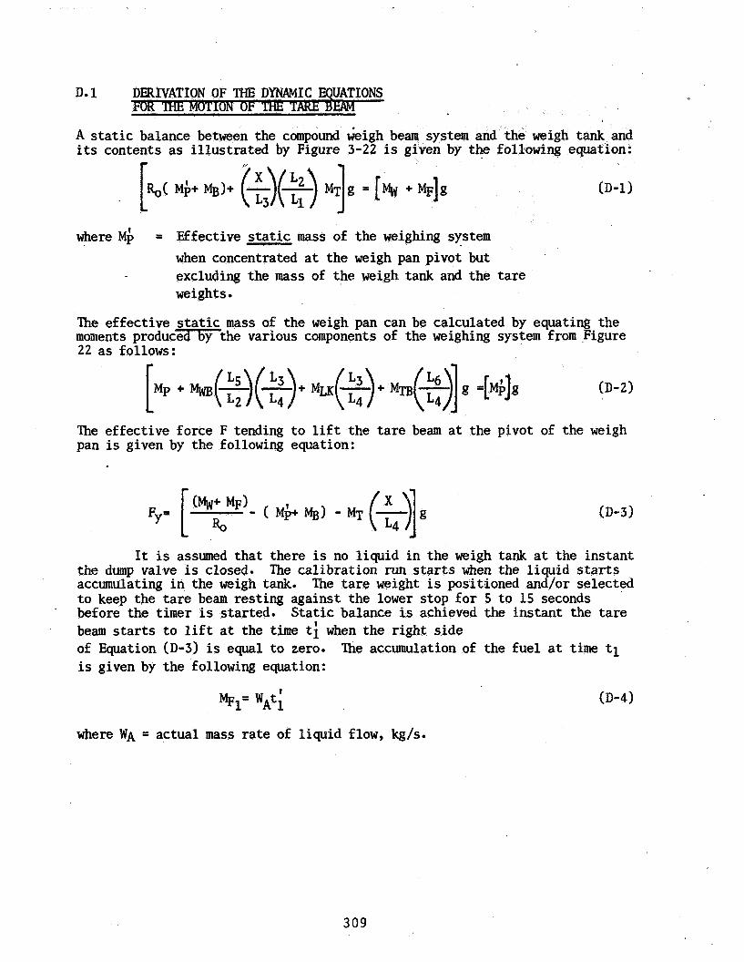
A static balance between the compound weigh beam system a weigh tank and its contents as illustrated by Figure 3-22 is given by the following equation:

(D-1) [.( MB)+ (e)(*) ..]g = [% + MF]g

where Mi = Effective static mass of the weighing system when concentrated at the weigh pan pivot but excluding the mass of the weigh tank and the tare weights .

The effective static mass of the weigh pan can be calculated by equating the moments producmthe various components of the weighing system from Figure 22 as follows:

The effective force F tending to lift the tare beam at the pivot of the weigh pan is given by the following equation:

It is assumed that there is no liquid in the weigh tank at the instant

The tare weight is positioned and/or selected the dump valve is closed. accumulating in the weigh tank. to keep the tare beam resting against the lower stop for 5 to 15 seconds before the timer is started. Static balance is achieved the instant the tare beam starts to lift at the time ti when the right side of Equation (D-3) is equal to zero. is given by the following equation:

The calibration run starts when the liquid starts

The accumulation of the fuel at time tl

where WA = actual mass rate of liquid flow, kg/s.

309

A t the start of a run, there are normally no reference weights on the

ion of the tare. weigh pan thus MB = 0. The tare beam s t a r t s t o l i f t a t ti seconds a f t e f t h e dump valve closes. weight or weights can be calculated by equating the right (D-3) t o zero and solving for X, or

The of Equation

where MT = 1.0 or 2.0 kg f o r the COX 311H Flowmeter Calibrator

For the case of the COX 305T Flowmeter Calibrator, X = L4 since the t a r e weights are added a t the weigh pan. COX 305T weigh pan can be calculated from Equation (D-5) as

The tare weight MT t o be added t o the

A weight or weights having a mass MB is then placed on the weigh pan a f t e r the tare beam rises sufficiently t o actuate the proximity switch and s t a r t the timer.

The t o t a l mass of fuel which has accumulated in the weigh tank a t the end of a run is given by the following equation:

and the change i n mass of fuel i n the weigh tank can be found by subtracting Equation (D-4) from Equation (D-7) or

The change i n mass of fuel i n the weigh tank is equal t o the product of the mass of the weights added t o the weigh pan Mg a f t e r the run starts and the compound lever arm ra t io b, or from Equation (D-8)

where ( t i - ti ) = Run time between the events when the ta re beam s t a r t s t o l i f t a t the s t a r t and end of a run-

310

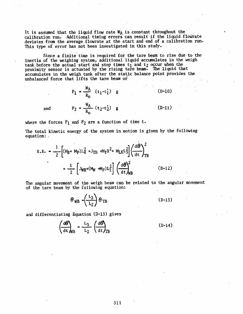
It is assumed that the liquid flow rate WA is constant throug calibration run. Additional timing errors can result if the deviates from the average flowrate at the start and end of a calibration run. This type of error has not been investigated in this study.

Since a finite time is required for the tare beam to rise due to the inertia of the weighing system, additional liquid accumulates in the weigh tank before the actual start and stop times tl and t 2 occur when the proximity sensor is actuated by the rising tare beam. accumulates in the weigh tank after the static balance point provides the unbalanced force that lifts the tare beam or

The liquid that

(D-10)

and (D-11)

where the forces F1 and F2 are a function of time t.

The total kinetic energy of the system in motion is given by the following equation: .

(D-12)

The angular movement of the weigh beam can be related to the angular movement of the tare beam by the following equation:

9WB =(*) &I3

and differentiating Equation (D-13) gives

(D-13)

(D-14)

311

The vertical movement y of the tare beam at the location of the pivot for *he weigh pan can be found from the following equation -for s r movement

Y = L4@TB (D-15)

and the vertical velocity v is found by differentiating Equation (D-15) or

(D-16)

A mass which is equivalent to the total dynamic mass of the sytem but concentrated at the suspension pivot for the weigh pan can be calculated from Equation (D-12) by using Equation (D-16) or

Equation (D-17) becomes

JTB

r

MF letting Mb = ME + Mg + - Ro2

(D-17)

ID-18)

(D-19)

312

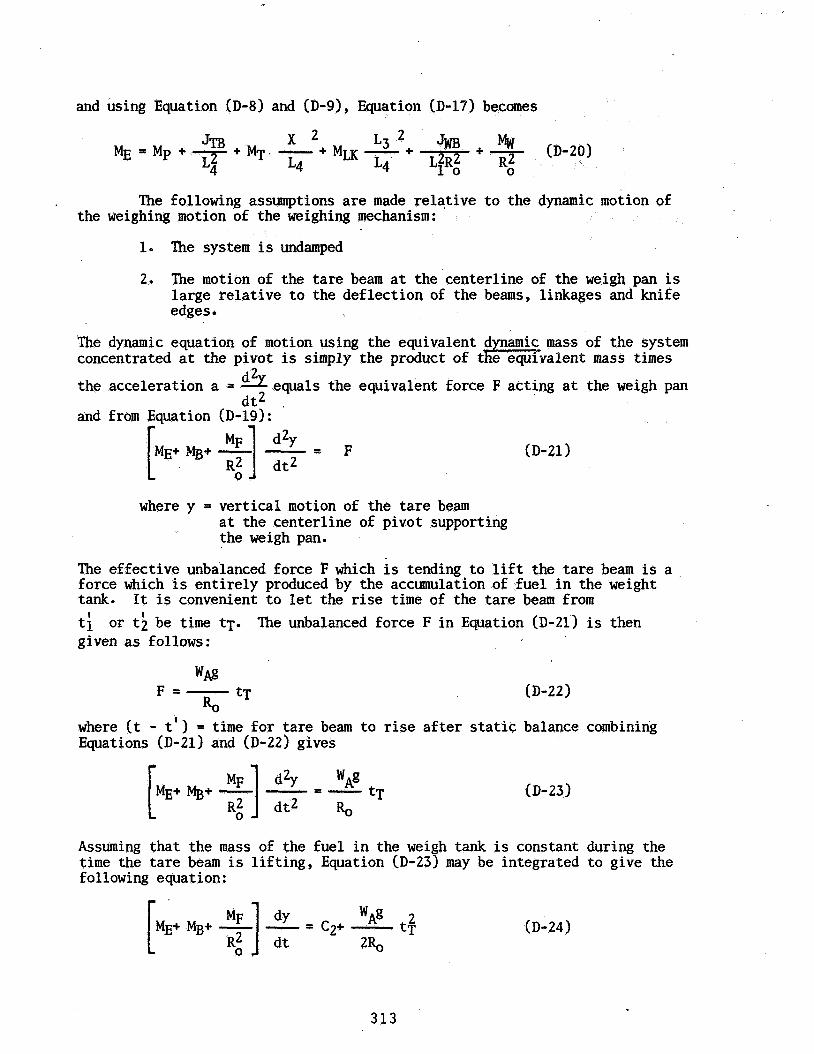
and using Equation (D-8) and (D-91, Equation (D-17) becomes

The following assumptions are made relative to the dynamic motion of

1. The system is undamped

the weighing motion of the weighing mechanism:

2. The motion of the tare beam at the centerline of the weigh pan is large relative to the deflection of the beams, linkages and knife edges

The dynamic equation of motion using the equivalent d ic mass of the system

the acceleration a = !?Y. equals the equivalent force F acting at the weigh pan concentrated at the pivot is simply the product of t IF?=-- e equivalent mass times

dt2 and from Equation

ME+ MB+ [ where y =

(D-19) :

vertical motion of the tare beam at the centerline of pivot supporting the weigh pan.

. .

(D-21)

The effective unbalanced force F which is tending to lift the tare beam is a force which is entirely produced by the accumulation of fuel in the weight tank. It is convenient to let the rise time of the tare beam from ti or ti be time tT. given as follows:

The unbalanced force F in Equation (D-21) is then

*Ag (D-22)

where (t - t') = time for tare beam to rise after static balance combining Equations (D-21) and (D-22) gives

(D-23)

Assuming that the mass of the fuel in the weigh tank is constant during the time the tare beam is lifting, Equation (D-23) may be integrated to give the following equation:

(D-24)

313

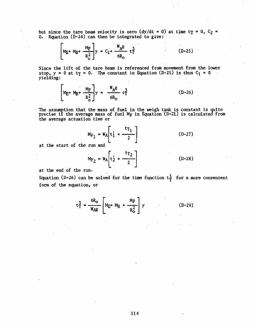
but since the tare beam velocity is zero (dy/dt = 0) a t time t T = 0, C2 = 0. Equation (D-24) can then be integrated t o give:

ME+ Mg+ [ Since the l i f t of stop, y = 0 a t t T yielding :

(D-25)

the tare beam is referenced from movement from the lower = 0. The constant i n Equation (D-25) is thus C1 = 0

(D-26)

The assum tion that the mass of fuel i n the weigh tank is constant is u i t e precise i! the average mass of fuel MF i n Equation (D-21) is calculate8 from the average actuation time o r

(D-27)

a t the s t a r t of the run and

M F ~ = W , ~ ~ + q] (D-28)

a t the end of the run. Equation (D-26) can be solved fo r the time function t; f o r a more convenient form of the equation, or

(D-29) t T 3 = - 6% [.. Mg + %] y

w l s

314

Do 2 CALCULATION OF THE TIMING ERROR 2 The numerical example given below is based on actual weight and

dimensional measurements on a COX 305T Flowmeter Calibrator.

Example :

Y = (beam deflection) = 0.254 cm (0.1 in.)

WA = 1.89 kg/s (15,000 l h h r )

ti (tare time) = 10 seconds

(ti - ti) (run time) = 30 seconds

ti =

Mp =

JWB =

% a = h = L1 =

L2 =

L5 =

40 seconds

4.121 kg (9.085 lbm)

375.75 kg - cm2 (128.4 lbm - in.2) 1.173 kg (2.586 Ibm)

22.53 kg (49.68 Ibm)

7.239 un (2.85 in.)

36.20 cm (14.25 in.)

17.91 cm (7.05 in.)

% = Lz/L1 = 4.988

g = 980.42 cm/s2

The effective static mass of the weigh pan can be determined from Equation (D-2) or

(D-29)

since the last two terms are zero and L3 = L4 due to the absence of a tare beam. Substituting values from the above tabulation into Equation (D-29) gives

Mb = 4.701 kg

315

The tare Equation

weight MT required for ti = 10 second tare time can be found from (D-6) as

22.53 + 1.89(10) MT = .. 4.701 = 3.605 kg

4-988

The reference weight MB required for a ti - ti = 30 second run time can be found from Equation (D-9) as .

1 89( 30) 11-367 kg MB = 4.988

Nominal weights are normally used for testing. example, the exact calculated tare weight and reference weights are used.

For the purpose of this

The equivalent mass of the system can be determined from Equation (D-20) for the COX 305T Flowmeter Calibrator where (1) the weigh beam replaces the tare beam, Jm = 0, (2) there is no linkage, M u = 0 and (3) the tare weights are added to the weigh pan, X = L4. Equation (D-20) then becomes

375 . 75 22.53 ME = 4.121 + + 3.605 +

(7. 239X4.988)2 (4.988) ME = 8.920 kg

The mass of fuel in the weigh tank at time ti substituting into Equation (D-28) gives

= 10 seconds is 18.9 kg and

6(4.988)(8.920 + 18.9/(4.988)2 )(0.254) tT?=

1.89(980.24)

tT;= 0.03971 and tT1= 0.34117 second I

316

The mass of fuel in the weigh tank at ti = 40 seconds is 75.6 kg and substituting into Equation (D-28) gives

6(4.988)(8.920 + 11.367 + 75.6/(4.988>2 )(0.254) t Ti'

1.89(980.42)

tT;= 0.096591 and t ~ ~ = 0.45739 Second

The combined flowrate correction factor can be found from Equation (3-10) where: tc = t2 - ti : 1 1

tT2 .- tT1 * 0.45739 0.34117 1 = 1 + (D-30)

30 (KTKJ) = 1 + t2 - tl

(KTKJ) = 1.00387

This value is comparable to the value given in Figure 3-23 for a deflection'of yo = 2.54 mm and the curve marked 1110 + 30". the average values of the fuel weights given by Equations (D-26) and (D-27) does not substantially change the above value for (K$J)=

An iterative calculation using

317

APPENDIX E

DETAILED SKETCHES OF PIECE PARTS, AND SUBASSEMBLIES FOR DUAL TURBINE FLOWMETER

318

.

319

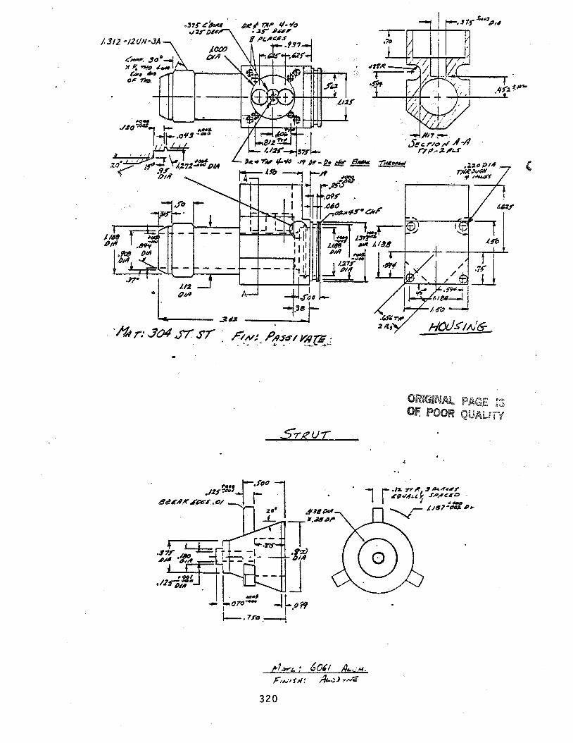
321

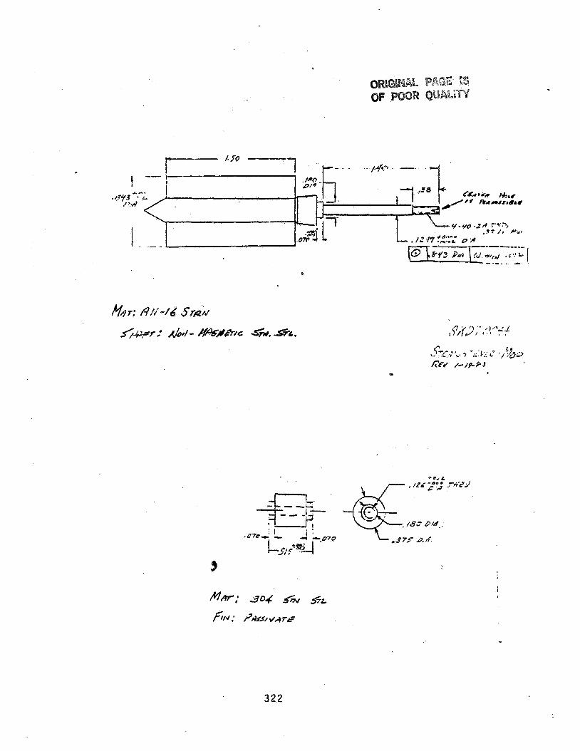
90

322

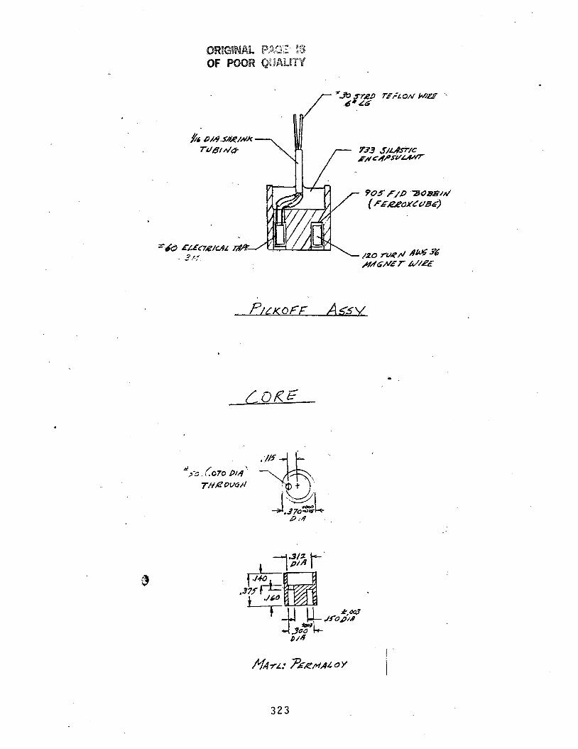
3 2 3

APPENDIX F

DETAILED SKETCHES OF PIECE PARTS, AND SUBASSEMBLIES FOR PROTOTYPE ANGULAR MOMENTUM-FLOWMETER

324

!

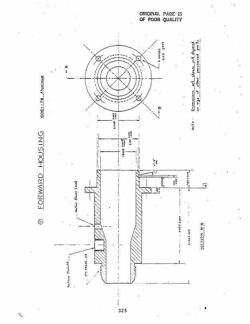
; I

325 ?

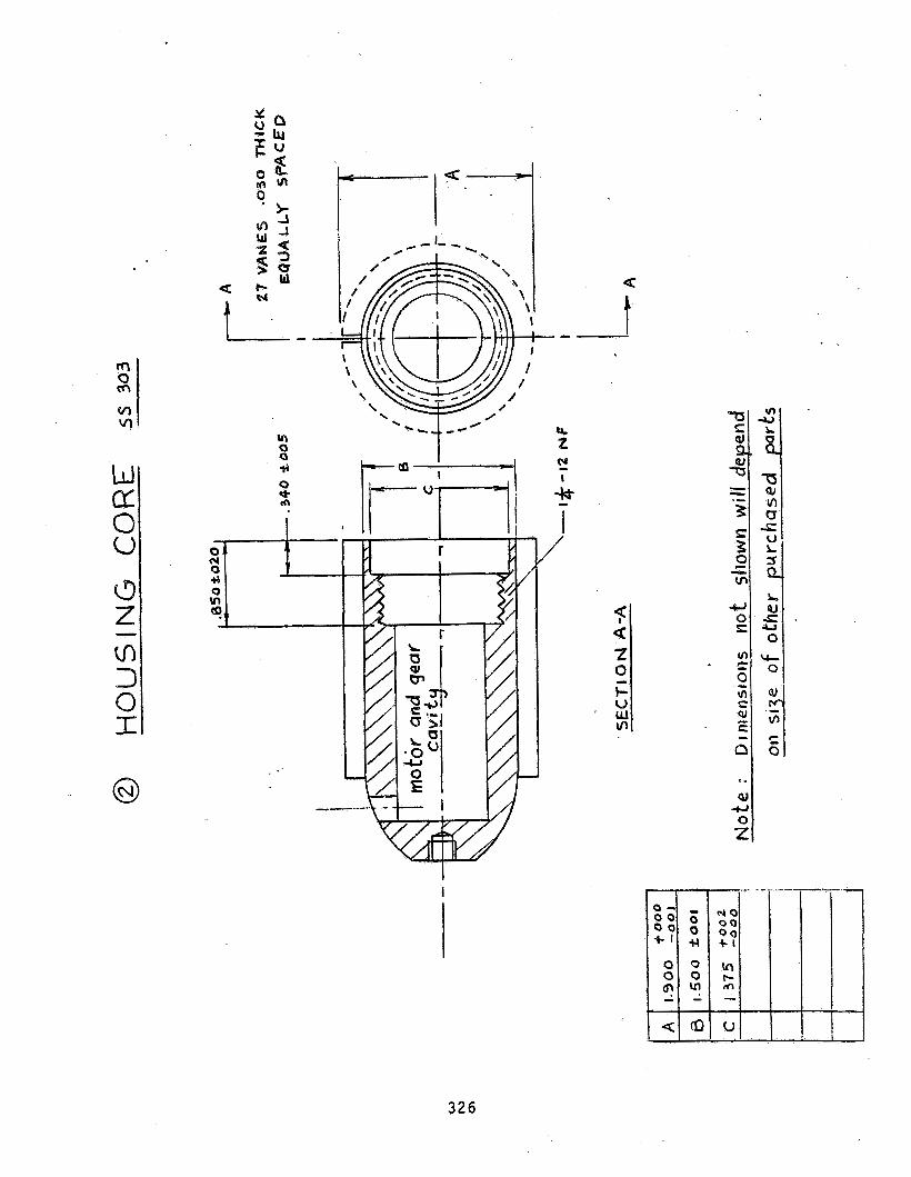
UI 0 0 *

I

326

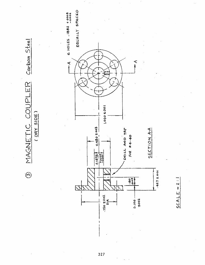
I '

I

3 2 7

328

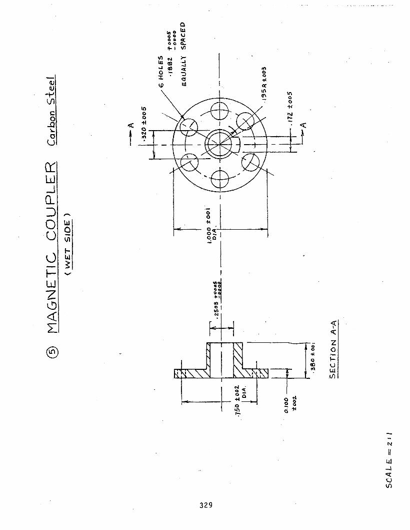
I

329

I

T.

b

0 0 4 cb rD m

-

lLi

r

330

‘ h i

3 3 1

x 9

.1

a

3 32

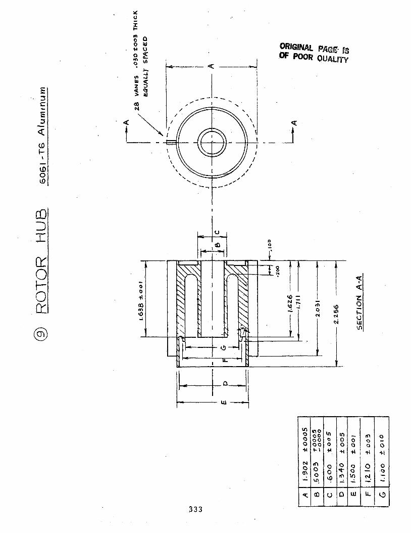
Y

63 3 r K 0 I-

cr.

I

I I" I

3 3 3

0 m --1

334

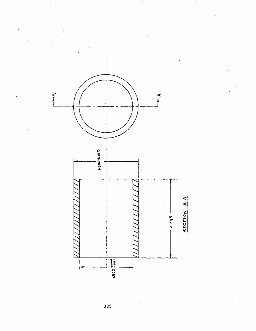
I

t

335

\

4

1

I I

-4 I I - 4 I

a

I -

336

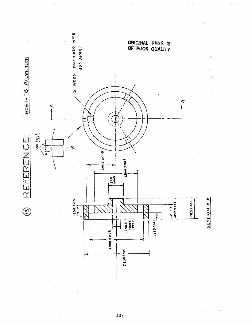
S .- El O OF POOR QUALITY

1 \ .

El

0

: ) I g t o 0 U

rn I U

3 37

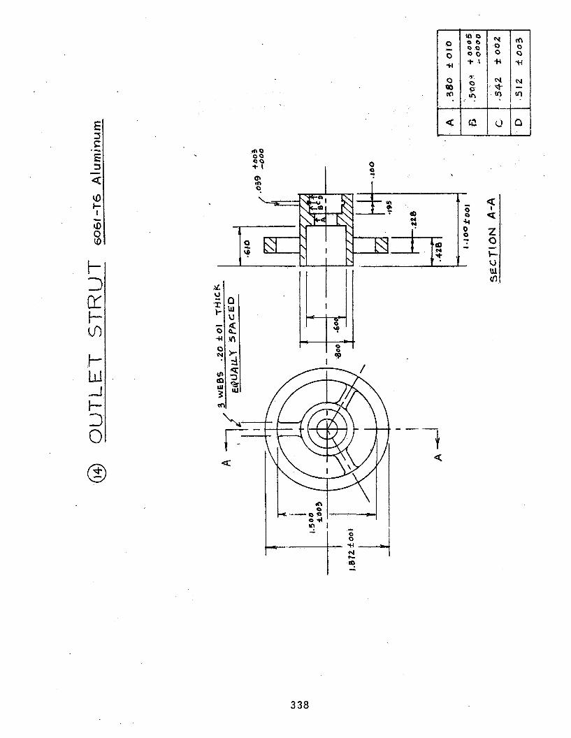
El

I

'+--ti- -

338

\

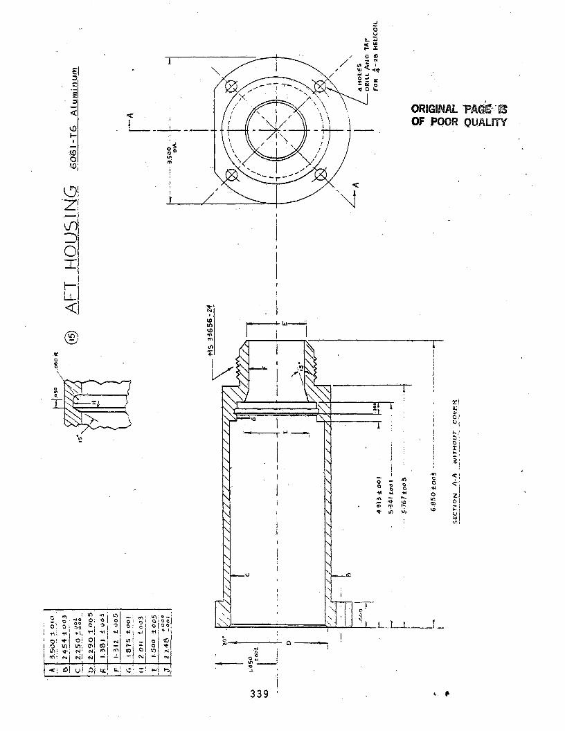
I

I

I ' n- !

! 339 I

340

I I

341

L

COEiTiUCT REPORT DISTRIBUTION LIST

Ins t rumenta t ion RbD Branch

Each addressee w i l l r ece ive o.ne copy un le s s

NASA Lewis Research Center 21000 Brookpark Road Cleveland, OH '44135 Attn: (25 c o p i e s )

NASA Lewis Research Center 2%000 Brookpark Road Cleveland, OH 44135 Attn: Leonard W. Schopen, H-S. 501-11

Ibward F. Hobart , H.S. 77-1

*, *

NASA S c i e n t i f i c and Technical

P* 0. Box 33 Cal lege Park, HD 20740 A t t n : (22 c o p i e s )

Information F a c i l i t y

Acqu is i t ions Branch

NASA Lewis Research CeKter 21000 Brookpark Road Cleveland, OH 44135 Attn: Library , M.S. 60-3 ( 2 c o p i e s )

NASA L e w i s Research Center 2%000 Brookpark Road Cleveland, OH 44135 Aten: Report Cant ro l Of f i ce , 5-5

&cera1 E l e c t r i c Company A i r c r a f t Eagine Group Evendale, OH a5215 Attn: Wayne Shaf fernocker , ISH-78

Ilonald Wise, KSH-78

Stanford Un ive r s i ty S tanford , CA 94305 Attn: Dr. R. J. Hoffat

P s s t . Prof., Mech. Engr. 1) i r . The m o s c i e nc e

Kea surement Cent e r

indica ted otherwise.

A i r Force Wright heronaut ica l

Wright Pa t t e r son A B , OH 45433 Attn: R. Cox/POTC

A i r Force Wright Aeronau t i c a l

Wright Pa t t e r son Am, OH 45443 Attn: E v e r e t t E. Bailey/AFWAL/NASA-W-

Laboratory

Labora t o r y

A i r Force Wright Aeronaut ical

Wright Pa t t e r son A n , OH 45433 A t en: Deborah Finnert y/?OTC

Laboratory i

A i r Force Wright Aeronaut ical

Wright Pa t t e r son Am, OH 45433 A t tn: H Roquemore /WSF

Roto Data, Inc. %0200 Anderson Way Cinc inna t i , OH 452G2 Ae en: David Davidson

Laboratory

umc /OATL Palm Beach Card ens Fzc i 1 i t : y West Palm Beach, FL 33(!02 Attn: John T. C a r r o l l

Bldg. 30 (HS R-25)

Lewis Engineering Coinpany 238 W a t e i S t r e e t Naugatuck, CT 06770 Attn: C. B-r Stegner

Arnold Engineering Development Center

Arnold Air Force S t a t i o n , T N 3 1 ; 3 '

A t t n : Matshal l R i r g e r y

B o e i r i Aercspace Company Eng i n e e ri ng Labor a t o r i e s S e a t c f e , WA 98124 :\<sn: Darrel l R; Har t ing

Enge l h a r d Engelhard I n d u s t r i e s Div. 228 Eas t 1 0 t h S t r e e t Xewport , KY 41075 Attn: Ronald G. Braun

!.i ill i a m s Res e a r c h 2280 West Maple Road Walled Lake, H I 48088 Aten: Henry Hoore, Head

I n s t r . Dept.

S i p g i n i a Poly technic I n s t i t u :

Herhanica l Engineer ing Dept. Blacksburg, VA 24061 At tn : W. F. O ' B r i e n , Jr.

and Stzite U n i v e r s i t y

> ! a m 1 Post Graduate School Department o f Aeronaut ics (Code 67) :&nterey, CA 93940 Attn: Prof . R. P. Shreeve

Pennsylvania S t a t e U n i v e r s i t y 233 b m o n d Bui ld ing U n i v e r s i t y Park, PA 16802 A t t n : Prof . B. Lakshminarayana

X u l i t e Semiconductor P roduc t s , Inc. 1039 Hoyt Avenue Ridgef i e l d , NJ 07657 Attn: John R. Payer

Bol t Beranek and Kevman, Inc . 50 Houlton S t r e e t Cambridge, .HA 02138 Attn: Richard E. b y d e n

Cat e r p i l l a r Trac t or Company Technica l Center , Bui ld ing F 100 h 'or theast Mans S t r e e t Peor i a , I L 61629 Attn: H r . Danaid k ' i l son

A i r F o r c e Wright Aeronau t i ca l

Wright P a t t e r s o n A-FB, OH k5433 Attn : H r . Cha r l e s Bentq/POTC

Hot Sec t i o n Technology

Labora tory

AVCO Corporar ion Lycoming D i v i s i o n 550 South Hain S S t r a t f o r d , CT 06497 - Attn : M r . K. Col l inge *)

MBnager IRAD Hech-anical P r o j e c t s

- .

Eaton Corpora t ion Box 766 Southf i e l d , MI 48037 Attn: Mr. Lamont E l t i n g e

D i r e c t o r of Research

P u b l i c S e r v i c e E lec t rPc d Gas Company 80 Pa rk P l a z a Newark, NJ 07101 At in : D r . Melvin L. Zwi l lenberg

Research & Development Dept.

Raychem Corpora t ion 300 C o n s t i t u t i o n Dr ive Menlo Park, CA 94025 Attn: D r . David C. Chappelear

D i r e c t o r 'of Corpora te Research & Development

F a b r i c a t i o n Development Labora tory Gwens/Corning F i b e r g l a s Techn ica l Cen te r G r a n v i l l e , OH 43023 At tn : H r . Hugh W. Bradley , Jr.

Xerox E l e c t r o - O p t i c a l Systems 1616 h'orth For t Hyer Drive, 16 th F l o o r Ar l ing ton , VA 22209 At tn : Hr. C l i f f o r d I. Cummings

Hanager, I n t e l l i g e n c e & Rec onna i ss anc e

Consiruc t i o n H a t e r i a l s Support Group Ovens/Corning F i b e r g l a s CMG Process Technology Labora tory G r a n v i l l e , OH L3023 At tn : H r . J. W. S c o t t

Hi tec Corpora t ion Nardone I n d u s t r i a l Park Ues t fo rd , HA 01886 Attn: S teve Wnuk

General E l e c t r i c Company . A i r c r a f t Engine Group 1000 Western Avenue Lynn, MA 01910 Attn: George Leperch, A129dD

Gzneral E l e c t r i c Company A i r c r a f t Equipment D i v i s i o n 50 Fordham Road Wilmington, kw 01887 At tn : Rdnald J, Casagrande

D e t r o i t Diesel A l l i s o n Box 894 I n d i a n a p o l i s , I N 46206 Attn: John C u s t e r , W-46

D e t r o i t D iese l A l l i s o n Box 894 I n d i a n a p o l i s , IN 46206 At tn : Ken Cross

Be t ro i t D i e s e '. A 1 1 i s on Box 894 I n d i a n a p o l i s , I N 46206 At tn : David W i l l i s

D e t r o i t Diesel A l l i s o n Box 894 I n d i a c a p o l i s , I N 66206 At tn : Ralph Fox

B a t t e l l e Columbus L a b o r a t o r i e s 505 King Avenue Columbus, OH 43201 Attn: Ross G. Luce, Energy d

-

T h e m a l Tech. S e c t i o n

Teledyne CAE 1350 Laskey Road Toledo, OH 43612 Attn: R. Hugh Gaylord

Garre t-AiRese a rch P. 0. Box 5217 Phoenix, AZ 85010 At tn : N. Fred P r a t t

FluiDyne Engr. Corporat ion

e a p o l i s , EN 55422 Olson Hemoiial Highway I

Attn: T. Hatsuura

AVCO Corporat ion Lycoming Div i s ion 550 South Main S t r e e t S t r a t f o r d , CT 06497 Attn: E. Twarog, Mgr.

E l e c t r o n i c s and Eiistre

Thermonet i c s Corporat ion 1028 Garnet Avenue San Diego, CA 92109 Attn: H. F. Poppendiek

Ba t t e 11 e Co lunibu s La bora t 0s. ;. (I : 505 King Avenue Columbus, OH h3201 Attn: M. X. Lemeoe,

P e t e r X. S t e i n 5602 East Honterosa Phoenix, AZ 85018

' I

Pl;att & Whitney A i r c r a f t Hain P l a n t P. 0. Box 2691 West Palm Beach, FL 331i.07- Attn: John P rosse r (MS C-06)

National Bureau of S t a n d a d s Washington, DC 20234

9Attn: Baldwin Rober:son

Xat iona l Bureau of S t a n d z i ds Washington, DC 20234 Attn: George H a t t i n g l y

General E l e c t r i c Company P. 0. Box 8 Schenectady, NY 12301 Attn: D r . David Ske l l ey

Bldg. K-1, Rm. 3824. -. e

Hechariical Technology, Wnc. 968 Albany-Shaker Road Latham, NY 12110 Attn: R. Hohenberg

NASA Headquarters Washington, DC 20546 Attn: M/Paul N. Herr

Massachuset ts ' I n s t i t u t e of Technology Cambridge, HA 02139' Attn: D r . Alan Eps te in

Rm. 31-266

Sve r d ru'p (AEDC) Arnold AFB, TH 37389 Attn: Paul McCarty

Ro semont , Inc . P a i l Stop F-15 P. 0. Box 959 B u r n s v i l l e , M?-l 55337 Attn: M r . Lar ry N. Wolfe

Lewis Engineering Company 238 Water S t r e e t Naugatuck, CT 06770 Attn: C. E. Stegne r

Babcock & Wilcox R6D D i v i s i o n P. 0. Box 835 A l l i a n c e , OH C4601 Attn: Harold Wahle