Fluid–solid coupling for the investigation of diastolic and systolic human left ventricular...

INTERNATIONAL JOURNAL FOR NUMERICAL METHODS IN BIOMEDICAL ENGINEERINGInt. J. Numer. Meth. Biomed. Engng. (2010)Published online in Wiley Online Library (wileyonlinelibrary.com). DOI: 10.1002/cnm.1405

Fluid–solid coupling for the investigation of diastolic and systolichuman left ventricular function

D. Nordsletten1,∗,†, M. McCormick1, P. J. Kilner2, P. Hunter3, D. Kay1

and N. P. Smith1

1Oxford University, Computing Laboratory, Wolfson Building, Parks Road, Oxford, OX1 3QD, U.K.2Imperial College, Royal Brompton Hospital, Sydney Street, London, SW3 6NP, U.K.

3Bioengineering Institute, 70 Symonds Street, Auckland, New Zealand

SUMMARY

Understanding the underlying feedback mechanisms of fluid/solid coupling and the role it plays in heartfunction is crucial for characterizing normal heart function and its behavior in disease. To improvethis understanding, an anatomically accurate computational model of fluid–solid mechanics in the leftventricle is presented which assesses both the passive diastolic and active systolic phases of the heart.Integrating multiple data which characterize the hemodynamical and tissue mechanical properties ofthe heart, a numerical approach was applied which allows non-conformity in an optimal finite elementscheme (J. Comp. Phys., submitted; Fluid–solid coupling for the simulation of left ventricular mechanics,University of Oxford, 2009). This approach is applied to look specifically at left ventricular fluid/solidcoupling, allowing quantitative assessment of blood flow through the left ventricle, pressure distributions,activation and the loss of mechanical energy due to viscous dissipation. Copyright � 2010 John Wiley &Sons, Ltd.

Received 19 January 2010; Revised 29 March 2010; Accepted 18 April 2010

KEY WORDS: blood flow; cardiac tissue mechanics; fluid–solid coupling; active contraction; heartfunction

1. INTRODUCTION

The heart is a complex electromechanical pump, capable of dramatically altering its functionin response to the varying demands of the body. Both in the normal and diseased heart, thischange to meet cardiovascular demand has significant implications on total energy consumptionand cardiac output. A crucial element within this regulatory process is the feedback betweenblood flow and myocardial tissue mechanics, an energy exchange which drives cardiovasculartransport. Understanding these feedback processes—both in terms of mechanical energetics as wellas kinematics—provides information vital for understanding how alterations in cardiovascular flowtranslate into changes in myocardial mechanical function (and vice versa).

Mathematical modeling has emerged as a key tool for directly analyzing the complex mechanicsand dynamics of the heart. Existing work in this area includes the pioneering works of Peskinand McQueen [1–5], who included both left and right ventricular chambers into their modelsusing immersed boundary methods. Modeling the heart wall as a set of one-dimensional fibersembedded in fluid, the Peskin and McQueen model incorporates many anatomically challengingfeatures of mechanical modeling in the heart (such as the heart valves). In more recent works,

∗Correspondence to: D. Nordsletten, Oxford University, Computing Laboratory, Wolfson Building, Parks Road,Oxford, OX1 3QD, U.K.

†E-mail: [email protected]

Copyright � 2010 John Wiley & Sons, Ltd.

D. NORDSLETTEN ET AL.

Watanabe et al. [6–8] incorporated a more physiologically based material law for the myocardium.Using a coarse grid of low-order elements, the Watanabe model includes both mechanical andelectromechanical aspects of heart function.

Building on the progress of these models, we present a model incorporating both appropriateconstitutive relations and reasonable numerical grid resolutions for the underlying physics—afundamental step towards building a clinically relevant fluid/solid cardiac modeling framework.The constitutive characterization of cardiac tissue builds on over a century of research which hasprovided a detailed picture of cardiac tissue architecture, illustrating its anisotropic structure. Thesedata have been successfully integrated into a number of constitutive models which effectivelycharacterize material response in isolated tissue samples [9–15]. However, a wide use of thesemodels is limited by the complexity involved in their numerical implementation. Furthermore,many coupled models lack sufficient resolution to accurately model the underlying physics. Thislimitation stems largely from difficulties involved in coupling non-conforming domains as well asneeds to maintain computational tractability.

In Nordsletten [16], a linear system fluid–solid system was developed which was coupled usingan additional Lagrange multiplier on the fluid–solid interface. Through the proper constructionof inf-sup stable spaces, the linear fluid–solid system was proven to admit unique solutions andoptimal error estimates. These results were extended to the fully non-linear system in Nordslettenet al. [17], illustrating similar optimal convergence rates using numerical experiments. This method,while maintaining optimal convergence and coupling properties, accommodates arbitrary degreesof non-conformity between finite element domains—allowing refinement to be dependent on thephysics of each domain.

In this paper, these technical developments are applied to develop a framework for anatomicallyaccurate modeling of the left ventricle during both filling (diastole) and contraction (systole). Themyocardial constitutive behavior [14, 18, 19] was tailored to passive measurements on excisedhuman hearts. To incorporate the effects of contraction, an ODE model is developed and fit toexperimental data collected from human myocytes [20, 21]. Using a conservative non-conformingfinite element scheme [17], the numerical approximation of blood flow and tissue deformationwas estimated based on their underlying physics. Finally these results are analyzed, looking at thekinematics of function and energetics observed through the heart cycle.

2. METHODS

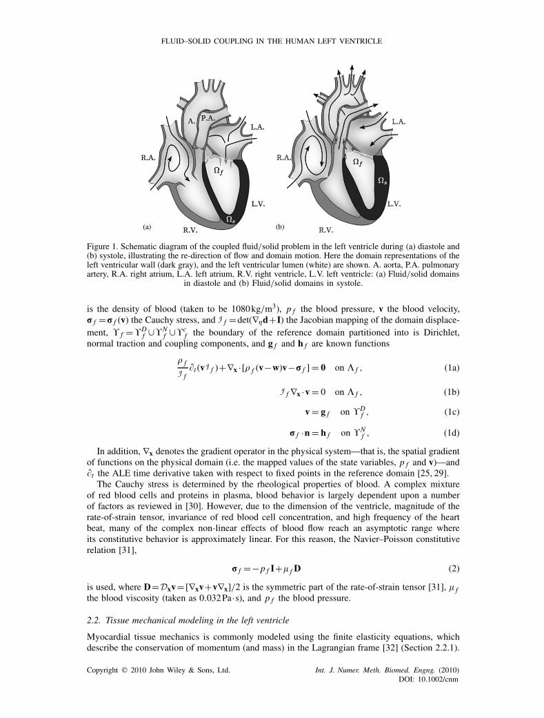
To simulate the mechanical behavior of the left ventricle during the heart cycle, a continuum modelis introduced satisfying the conservation of mass and momentum equations. These laws are upheldon both the blood (given by subscript f ) and tissue (given by subscript s) domains, denoted � f and�s with boundaries � f and �s , respectively (see Figure 1). The fluid mechanical formulation isbased on the Arbitrary Lagrangian–Eulerian (ALE) form of the Navier–Stokes equations [22–27]as presented in Section 2.1. The solid mechanical formulation is then presented in Section 2.2,detailing the construction of the anisotropic tissue structure as well as the orthotropic passiveand active constitutive behavior of the myocardium. Finally, the numerical approach developed inNordsletten et al. [17] is outlined in Section 2.4.

2.1. Blood flow modeling in the left ventricle

To solve blood flow through the heart chambers, it is necessary to examine the principle momentumand mass conservation equations over the time-varying fluid domain, � f . Although immersedboundary and fictitious domain methods have been applied to hemodynamic problems within theheart, use of the ALE formulation of these conservation equations has been shown to have superioraccuracy [28]. Domain motion is accommodated within the ALE formulation by introducing astatic reference domain, � f , which is bijectively related to the moving physical domain, � f , andmoves with velocity, w [23, 24]. In this way, conservation principles may be posed on the referencedomain or, equivalently, along moving coordinates in the physical domain. In Equation (1), � f

Copyright � 2010 John Wiley & Sons, Ltd. Int. J. Numer. Meth. Biomed. Engng. (2010)DOI: 10.1002/cnm

FLUID–SOLID COUPLING IN THE HUMAN LEFT VENTRICLE

Figure 1. Schematic diagram of the coupled fluid/solid problem in the left ventricle during (a) diastole and(b) systole, illustrating the re-direction of flow and domain motion. Here the domain representations of theleft ventricular wall (dark gray), and the left ventricular lumen (white) are shown. A. aorta, P.A. pulmonaryartery, R.A. right atrium, L.A. left atrium, R.V. right ventricle, L.V. left ventricle: (a) Fluid/solid domains

in diastole and (b) Fluid/solid domains in systole.

is the density of blood (taken to be 1080kg/m3), p f the blood pressure, v the blood velocity,r f =r f (v) the Cauchy stress, and f =det(∇�d+I) the Jacobian mapping of the domain displace-ment, � f =�D

f ∪�Nf ∪�c

f the boundary of the reference domain partitioned into is Dirichlet,normal traction and coupling components, and g f and h f are known functions

� f

f�t (v f )+∇x ·[� f (v−w)v−r f ]= 0 on � f , (1a)

f ∇x ·v= 0 on � f , (1b)

v= g f on �Df , (1c)

r f ·n= h f on �Nf , (1d)

In addition, ∇x denotes the gradient operator in the physical system—that is, the spatial gradientof functions on the physical domain (i.e. the mapped values of the state variables, p f and v)—and�t the ALE time derivative taken with respect to fixed points in the reference domain [25, 29].

The Cauchy stress is determined by the rheological properties of blood. A complex mixtureof red blood cells and proteins in plasma, blood behavior is largely dependent upon a numberof factors as reviewed in [30]. However, due to the dimension of the ventricle, magnitude of therate-of-strain tensor, invariance of red blood cell concentration, and high frequency of the heartbeat, many of the complex non-linear effects of blood flow reach an asymptotic range whereits constitutive behavior is approximately linear. For this reason, the Navier–Poisson constitutiverelation [31],

r f =−p f I+� fD (2)

is used, where D=Dxv= [∇xv+v∇x]/2 is the symmetric part of the rate-of-strain tensor [31], � fthe blood viscosity (taken as 0.032Pa·s), and p f the blood pressure.

2.2. Tissue mechanical modeling in the left ventricle

Myocardial tissue mechanics is commonly modeled using the finite elasticity equations, whichdescribe the conservation of momentum (and mass) in the Lagrangian frame [32] (Section 2.2.1).



Key to this model description are the passive and active properties of the heart wall, which dependheavily on the anisotropic structure of the heart (Section 2.2.2). Using the underlying structure,constitutive behavior can be defined based on animal experiments (Section 2.2.3) and tuned tohuman heart data (Section 2.2.4). Finally, the active contractile elements of the heart can beincorporated into the material definition (Section 2.2.5).

2.2.1. Quasi-static finite elasticity equations. Modeling myocardial tissue mechanics in threedimensions has been approached in a number of different ways—assuming the tissue as a dynamiclinear elastic solid [33], a fiberous fluid [34] or a linear hyperelastic solid [35]. However, due to therelative dominance of fluid momentum and large strains observed within the heart, the myocardialmodel used in this work follows the quasi-static, incompressible finite elasticity formulation ofNash and Hunter [36, 37], seen in Equation (3). This solid mechanical model is based on theLagrangian formulation, which, like the ALE formulation, refers solutions to a static referenceframe, �s . In this case, however, �s is the undeformed reference state of the heart, and the mappingbetween the reference and physical domains is given by the solid displacement u. In Equation (3),rs =rs(u) is the Cauchy stress within the solid and s =det(∇�u+I) the mapping Jacobian of thesolid displacement, u, � f =�D

s ∪�Ns ∪�c

s the boundary of the reference domain partitioned intoDirichlet, normal traction and coupling components, and gs and hs are known functions

s∇x ·rs = 0 on �s , (3a)

�t ( s)= 0 on �s , (3b)

u= gs on �Ds , (3c)

rs ·n= hs on �Ns , (3d)

In this formulation, the Cauchy stress is decomposed into hydrostatic and non-hydrostaticcomponents, i.e. rs = rs − psI, introducing the hydrostatic tissue pressure, ps . This scalar field isthen used as a Lagrange multiplier, constraining the displacement field, u, to satisfy both Equations(3a) and (3b). Although the form of the quasi-static solid model in (3) varies from the conservationequations (1) used to model the blood, these two forms are closely related and the quasi-staticsystem can be derived as a special case of the previously introduced ALE form [16] (though rsand r f generally vary).

The mechanical model requires characterization of the constitutive form defining the relationshipbetween rs , discussed later in Section 2.2.3, and the myocardial displacement, and the field ofactively developed tension. Both these quantities are highly anisotropic throughout the tissue,varying according to local tissue structure as introduced in the following section.

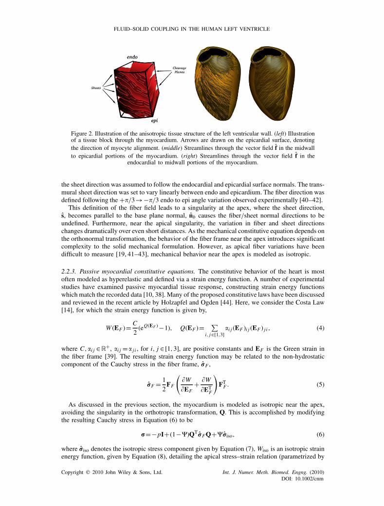
2.2.2. Anisotropic fiber structure. The heterogeneous architecture of the myocardium plays animportant role in the mechanical response of heart tissue. Cardiac myocytes within the heartalign into myofibrils with orientation that varies strongly transmurally through the heart wall [19].Myofibrils are subsequently stacked into laminar sheets separated by cleavage planes (see Figure 2).Experiments have shown that the stress response to strain relies significantly on this underlyingstructure [38].

To incorporate this into the mechanical model, a continuum approach was taken, defining aright-handed coordinate system with principle axes {f, s, n} denoting the fiber, sheet, and sheetnormal directions at all points throughout the myocardium [39]. These vectors in the referencecoordinate frame may be composed to form an orthonormal transformation matrix, QT= (f, s, n)which provides a mapping between quantities in the reference frame and their representations inthe fiber coordinate frame (denoted by adding a subscript F , i.e. F and FF denote the deformationgradient tensor in both the reference and fiber coordinate frames) [39].

To construct this orthonormal tensor field, the fiber, sheet and sheet normal directions, {f, s, n},must be defined throughout the myocardial domain. From observations of myocardial architecture,



Figure 2. Illustration of the anisotropic tissue structure of the left ventricular wall. (left) Illustrationof a tissue block through the myocardium. Arrows are drawn on the epicardial surface, denotingthe direction of myocyte alignment. (middle) Streamlines through the vector field f in the midwallto epicardial portions of the myocardium. (right) Streamlines through the vector field f in the

endocardial to midwall portions of the myocardium.

the sheet direction was assumed to follow the endocardial and epicardial surface normals. The trans-mural sheet direction was set to vary linearly between endo and epicardium. The fiber direction wasdefined following the +�/3→−�/3 endo to epi angle variation observed experimentally [40–42].

This definition of the fiber field leads to a singularity at the apex, where the sheet direction,s, becomes parallel to the base plane normal, nb causes the fiber/sheet normal directions to beundefined. Furthermore, near the apical singularity, the variation in fiber and sheet directionschanges dramatically over even short distances. As the mechanical constitutive equation depends onthe orthonormal transformation, the behavior of the fiber frame near the apex introduces significantcomplexity to the solid mechanical formulation. However, as apical fiber variations have beendifficult to measure [19, 41–43], mechanical behavior near the apex is modeled as isotropic.

2.2.3. Passive myocardial constitutive equations. The constitutive behavior of the heart is mostoften modeled as hyperelastic and defined via a strain energy function. A number of experimentalstudies have examined passive myocardial tissue response, constructing strain energy functionswhich match the recorded data [10, 38]. Many of the proposed constitutive laws have been discussedand reviewed in the recent article by Holzapfel and Ogden [44]. Here, we consider the Costa Law[14], for which the strain energy function is given by,

W (EF )= C

2(eQ(EF )−1), Q(EF )=

∑i, j∈[1,3]

�i j (EF )i j (EF ) j i , (4)

where C,�i j ∈R+, �i j =� j i , for i, j ∈ [1,3], are positive constants and EF is the Green strain inthe fiber frame [39]. The resulting strain energy function may be related to the non-hydrostaticcomponent of the Cauchy stress in the fiber frame, rF ,

rF = 1

2FF

(�W�EF

+ �W�ET

F

)FTF . (5)

As discussed in the previous section, the myocardium is modeled as isotropic near the apex,avoiding the singularity in the orthotropic transformation, Q. This is accomplished by modifyingthe resulting Cauchy stress in Equation (6) to be

r=−pI+(1−�)QTrFQ+�riso, (6)

where riso denotes the isotropic stress component given by Equation (7), Wiso is an isotropic strainenergy function, given by Equation (8), detailing the apical stress–strain relation (parametrized by



an additional scalar, �0),

riso = 1

2F(

�Wiso

�E+ �Wiso

�ET

)FT, (7)

Wiso(E)= C

2(eQiso(E)−1), Qiso(E)=�0E :E (8)

and � is a density function given in Equation (9) which is unity at the apex coordinate, gA, in thereference frame. Here � is given by a Gaussian function, allowing us to localize the impact of �to the apex. This is controlled by a positive parameter, C�, which is selected so that �=0.05 adistance |g−gA| approximately 10% of the ventricular long axis.

�(g)=e−C�|g−gA |2 . (9)

2.2.4. Undeformed state and material parameter estimation. Two challenges in modeling humanmyocardial mechanics are the determination of appropriate passive material properties and theidentification of the undeformed state of the heart. While experiments have been conducted on rat[12, 45], canine [9, 46] and pig [38] myocardium, there has yet to be comprehensive material testingon human myocardial tissue. As these values preferentially scale the stress response to strain,identifying reasonable estimates of human material parameters is crucial towards simulating heartfunction. Also important is the determination of the undeformed state of the heart, a zero-strainstate which results in residual strains in the model. As all constitutive equations for myocardialtissue become increasingly non-linear with increasing strain, inaccurate accounting for residualstrain may lead to an inaccurate estimation of strain response to stress.

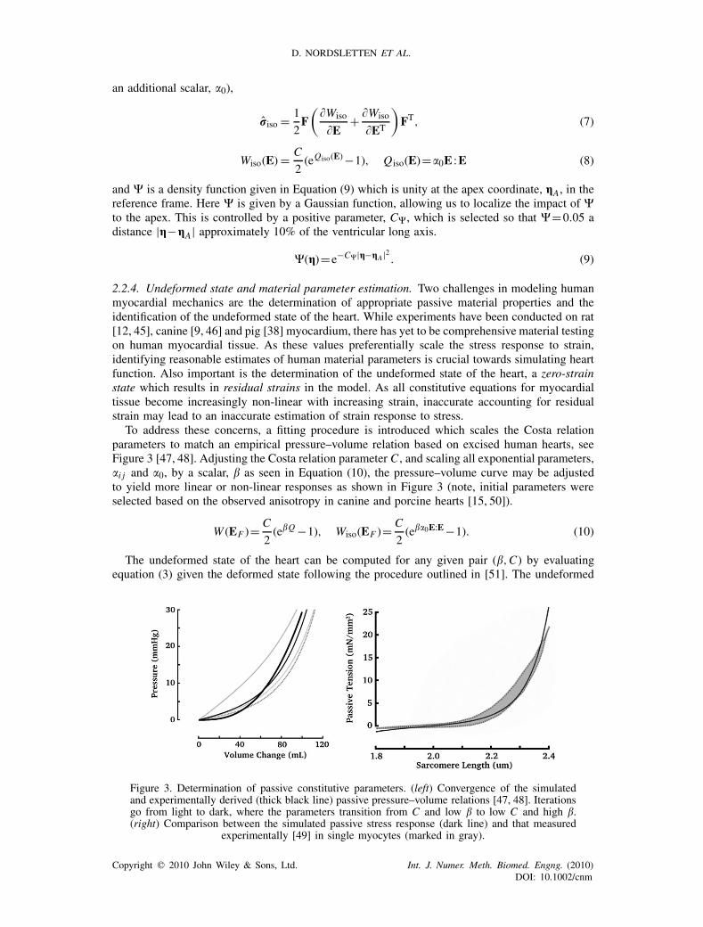
To address these concerns, a fitting procedure is introduced which scales the Costa relationparameters to match an empirical pressure–volume relation based on excised human hearts, seeFigure 3 [47, 48]. Adjusting the Costa relation parameter C , and scaling all exponential parameters,�i j and �0, by a scalar, � as seen in Equation (10), the pressure–volume curve may be adjustedto yield more linear or non-linear responses as shown in Figure 3 (note, initial parameters wereselected based on the observed anisotropy in canine and porcine hearts [15, 50]).

W (EF )= C

2(e�Q−1), Wiso(EF )= C

2(e��0E:E−1). (10)

The undeformed state of the heart can be computed for any given pair (�,C) by evaluatingequation (3) given the deformed state following the procedure outlined in [51]. The undeformed

Figure 3. Determination of passive constitutive parameters. (left) Convergence of the simulatedand experimentally derived (thick black line) passive pressure–volume relations [47, 48]. Iterationsgo from light to dark, where the parameters transition from C and low � to low C and high �.(right) Comparison between the simulated passive stress response (dark line) and that measured

experimentally [49] in single myocytes (marked in gray).



Table I. Parameter values used for the passive tension model developed in Equation (6). Here, the subscriptf, s, and n denote the fiber, sheet and sheet normal directions.

Passive tension model parametersModel parameter Parameter value Parameter units

C 296.57 Pa�ff 38.99 —�fs 17.15 —�fn 12.82 —�ss 7.55 —�sn 5.64 —�nn 4.21 —�0 38.99 —

state was reached when the total left ventricular lumen volume reached a predicted initial value,V0, determined empirically based on excised human hearts (Equation (9) of Klotz [47]). Using thepredicted undeformed state, simulations of inflation were conducted, giving a passive pressure–volume relationship for the given pair (�,C). The pressure–volume relation was then comparedwith the measured pressure–volume relations.

Comparing simulated and experimental data, the parameters (�,C) were fitted to minimizeerror. Letting Vsim=Vsim(p,�,C) denote the simulated volume—as a function of left ventricularpressure, p, and the parameters (�,C)—and Vexp=Vexp(p) denote the experimental volume data,the cost functions, �1 and �2, are given by the least-square constraints

�1(�,C) :=∫ Pmax

0(Vsim−Vexp)

2 dp, �2(�,C) := (Psim−Pexp)2,

where Pmax∼4kPa is the maximal applied pressure, Psim the end-diastolic pressure required toreturn to the end-diastolic state, and Pexp the experimentally observed end-diastolic pressure. Asa result, we seek to determine parameters (�,C) which satisfy Equation (11).

min(�,C)∈R+

�1(�,C)+�2(�,C). (11)

As Equation (11) is non-linear, an iterative approach was used to minimize the constraint usinga non-linear least-square approach. Figure 3 shows passive pressure inflation of the left ventricularmodel compared to the experimental data of Klotz [47, 48]. The selected parameters also producesa stress response that compares well with passive data collected from isolated human myocytes asshown in Figure 3. The final values for the constitutive relation parameters are shown in Table I.

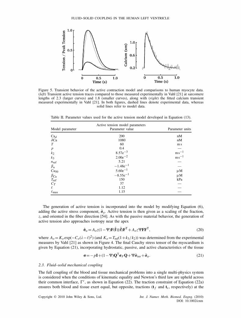
2.2.5. Active myocardial contraction. Contraction of the heart wall is stimulated by a electrochem-ical wave, which travels through the heart. Owing to the lack of comprehensive electrical activationdata for human hearts, a simple model of intracellular calcium dynamics, given in Equation (12),was used to pace cardiac contraction in a uniform spatial distribution. Figure 5 illustrates the modelwhich fits experimental measurements of intracellular calcium transients in human myocytes [21].

Cai =Cad +Ca

(t

T

)p

exp[p(1− t/T )]. (12)

The intracellular calcium ions, Ca2+i , bind with regulatory sites on Troponin C, causing a shiftin the thin-filament molecule, Tropomyosin, which sterically hinders actin–myosin binding in theabsence of Ca2+i . Free to interact, myosin and actin form weakly and strongly bound complexes[52]. The strength of tension is often thought to be proportional to the number of strongly boundmyosin–actin complexes. Incorporated in the model as an active stress, ra , this force causesconstriction of the tissue, transmural thickening of the myocardial wall, and ejection of blood fromthe heart to the systemic circulation. In this section, a simple ODE model is introduced, whichincorporates the length dependent modulation of ra .



Figure 4. Steady behavior of the active contraction model and comparisons to human myocyte data. (left)Steady-state relation between calcium concentration and developed tension normalized by the tension atcalcium saturation. Circles represent data presented in the experimental fit in Gwathmey [20]. Three modelcurves are also plotted varying in color from black to light gray, corresponding to sarcomere lengths of2.3, 2.0 and 1.8, respectively. (right) Normalized peak tension as a function of fiber strain, f . Circles

represent data measured in Vahl [21].

Assuming periodic steady-state conditions, we constructed a model, given by Equation (13),which focuses on the length-dependent variability in active tension (see Appendix A for derivation).Here, =√2EF,ff+1 denotes the strain in the fiber direction and z the concentration ratio ofstrongly bound myosin by total myosin.

d2z

dt2+a1(, [Ca2+i ])

dz

dt+a2(, [Ca2+i ])z=g(, [Ca2+i ]). (13)

The scalar coefficients a1, a2 and the right-hand side term, g, given by Equations (14)–(16),are functions of the reaction constants k1=k1(), k2=k2, k3 and n=n(), which are selected byfitting to experimental data on human myocytes and trabeculae (see Appendix A).

a1(, [Ca2+i ]) := k2+k3+k1[Ca2+i ]n, (14)

a2(, [Ca2+i ]) := k2k3+k1(k2+k3)[Ca2+i ]n, (15)

g(, [Ca2+i ]) := k1k2[Ca2+i ]n . (16)

Using the data gathered by Gwathmey and Hajjar [20], the steady state of Equation (13)

z= [Ca2+i ]n

k3/k1+(1+k3/k2)[Ca2+i ]n

(17)

was used to fit the parameters within the model, see Figure 4. In particular, it was assumed thatk1 and n were length dependent, as seen in Equations (19) and (18), allowing the model to fit theobserved length-dependent steady-state behavior (linear variation in the half-activation of z, andlinear variation in the hill parameter, n). The length dependence of k1 was derived from Gwathmeyand Hajjar [20], whereas the length-dependent modulation of the hill parameter, n, was calculatedfrom the results of van der Velden et al. [53]. In addition to these steady-state human myocyteresults, dynamic traces of the tension transient [21] were used to select the remaining parameters,see Figure 5, which can be found in Table II.

n = nref[1+�n(−�max)], (18)

1

k1= (k2+k3)

k3k2(Ca50[1+�Ca(−�max)])

n . (19)



Figure 5. Transient behavior of the active contraction model and comparisons to human myocyte data.(left) Transient active tension traces compared to those measured experimentally in Vahl [21] at sarcomerelengths of 2.3 (larger curves) and 1.8 (smaller curves), along with (right) the fitted calcium transientmeasured experimentally in Vahl [21]. In both figures, dashed lines denote experimental data, whereas

solid lines refer to model data.

Table II. Parameter values used for the active tension model developed in Equation (13).

Active tension model parametersModel parameter Parameter value Parameter units

Cad 200 nMCa 1080 nMT 60 m sp 0.4 —k2 8.57e−3 ms−1

k3 2.00e−2 ms−1

nref 5.21 —�n −1.48e−1 —Ca50 5.60e−1 �M�Ca −8.55e−1 �MTref 150 kPaCT 37 —� 1.12 —�max 1.15 —

The generation of active tension is incorporated into the model by modifying Equation (6),adding the active stress component, ra . Active tension is then given as a scaling of the fraction,z, and oriented in the fiber direction [54]. As with the passive material behavior, the generation ofactive tension also approaches isotropy near the apex

ra = Aoz(1−�)F(f⊗ f)FT+Aoz�FFT, (20)

where Ao=Ko exp(−Co(−�)2) (and Ko=Tref(1+k3/k2)) was determined from the experimentalmeasures by Vahl [21] as shown in Figure 4. The final Cauchy stress tensor of the myocardium isgiven by Equation (21), incorporating hydrostatic, passive, and active characteristics of the tissue

r=−pI+(1−�)QTrFQ+�riso+ ra . (21)

2.3. Fluid–solid mechanical coupling

The full coupling of the blood and tissue mechanical problems into a single multi-physics systemis considered when the conditions of kinematic equality and Newton’s third law are upheld acrosstheir common interface, �c, as shown in Equation (22). The traction constraint of Equation (22a)ensures both blood and tissue exert equal, but opposite, tractions (t f and ts , respectively) at the



endocardial boundary. Furthermore, the kinematic condition of equal velocity, seen in Equation(22b), requires the adherence of all boundary points through time.

t f +ts = 0 on �C , (22a)

�tu−v= 0 on �C . (22b)

2.4. Finite element approximation

The tissue and blood models were solved using the Galerkin finite element method, where thestrong-form model equations (1) and (3) are reduced to a weak form satisfied over a series offinite dimensional function spaces as outlined in Section 2.4.1. In addition to these equations, anadditional constraint and Lagrange multiplier was added to the model system in Section 2.4.2,allowing the coupling of the tissue and blood models along the endocardial wall. Finally, in Section2.4.3 we briefly overview the numerical solution procedure used to compute the velocity anddisplacement of the heart model.

2.4.1. Discrete weak-form model equations. The state variables of the mechanical models wereapproximated discretely using finite element interpolations over the fluid and solid mechanicalmeshes (linear tetrahedral and curvilinear hexahedral grids, respectively). Dividing the time domain,I , into NI non-overlapping intervals (tn−1, tn), tn−1<tn , t0=0 and t N =T , the discrete solutionsat every time tn–(vh,n , uh,n , ph,n

s , ph,nf )—were approximated by a weighted sum of functions, i.e.

vh,n =V n ·Wv, uh,n =Un ·Wu, ph,nf = Pn

f ·Wp f , ph,ns = Pn

s ·Wps , (23)

where V n , Un , Pnf and Pn

s are vectors of weights and Wv, Wu , Wp f , Wps are vectors of basisfunctions as seen in Equation (24).

Wv =

⎛⎜⎜⎜⎝w1v

...

wNvv

⎞⎟⎟⎟⎠ , Wu =

⎛⎜⎜⎜⎝w1u

...

wNuu

⎞⎟⎟⎟⎠ , Wp f =

⎛⎜⎜⎜⎜⎝

�1p f

...

�Np fp f

⎞⎟⎟⎟⎟⎠ , Wps =

⎛⎜⎜⎜⎝

�1ps

...

�Npsps

⎞⎟⎟⎟⎠ . (24)

Here wkv denotes the kth basis function and the set {w1v, . . .wNvv } the basis of the velocity

interpolation space, Vh (where Nv denotes the span of Vh), and similarly for the displacementand pressures. In this model, the Taylor-hood [55, 56] basis was selected for the fluid (P2−P1)and solid (Q2−Q1) to construct the blood velocity/pressure and tissue displacement/pressureinterpolation spaces given by Vh , Uh , Wh

f , and Whs , respectively. Between time points, solid

displacements were interpolated linearly, whereas all other state variables (fluid velocity, solid/fluidpressure) were constant. The weights of all state variables seen in Equation (23) are determinedas those which satisfy the weak variational forms of Equations (1) and (3).

The solid mechanical weak form is derived (using the typical Galerkin approach [57–60]) byfirst dotting the momentum equation (3a) by each test function wku (for all wku which are zero on�Ds ), multiplying the mass equation (3b) by each test function wmps and integrating over �s and

In = [tn−1, tn] [17]. Applying integration by parts to the hydrostatic and non-hydrostatic stressterms, and assuming �N

s ={∅}, the weak variational form seen in Equation (25) is derived at tn

(and similarly for all other time points).

∫In

∫�s

(rs (uh )− ph,ns I) :∇xw

ku dgd�+

∫In

∫�cs (�)

th,ns ·wku dxd�=0, (25a)



∫In

∫�s

wmps ·�t s(uh)dgd�=0, (25b)

for k=1, . . . ,Nu and m=1, . . . ,Nps .

The fluid variational form, seen in Equation (26), is analogously derived by multiplying the fluidmomentum and mass equations by the test functions wkv and wmp f

, respectively, and integrating

over � f and In = [tn−1, tn] (and similarly for all other time points).

�∫

� f (�)vh,n ·wkv dx−�

∫� f (�)

vh,n−1 ·wkv dx

+�∫In

∫� f (�)

[∇x ·[vh,n−wh,n]vh,n]·wkv dx+�∫

� f (�)Dxvh,n :Dxw

kv dxd�

−∫In

∫� f (�)

ph,nf [∇x ·wkv]dx+

∫�c

f (�)th,nf ·wkv dxd�=0 (26a)

∫In

∫� f (�)

wkp f[∇x ·vh,n]dxd�=0, (26b)

for k=1, . . . ,Nv and m=1, . . . ,Np f .

A key to solving Equations (26) and (25) for all time intervals, In , is establishing the couplingcriteria between the two domains, which requires kinematic continuity and equal, but opposite,traction at the endocardial surface.

2.4.2. Coupling by the introduction of a third variable. To add an additional constraint enforcingkinematic equality as seen in Equation (22), a Lagrange multiplier, kh , is introduced on the coupledinterface. This Lagrange multiplier is used in the finite element approach to satisfy the tractioncondition of Equation (22a), by requiring the weak equivalence relation seen in Equation (27) [17]∫

In

∫�ckh ·(wkv +wku)dgd�=

∫In

∫�c(�)

th,ns ·wku −th,n

f ·wkv dxd� (27)

for k=1, . . .Nv and m=1, . . .Nu . Choosing a wkv or wku which is zero in the coupled interface, wesee that the kh term may be substituted into both the solid and fluid coupled systems. Furthermore,for every test function which is equivalent on the boundary (see Figure 6), i.e. wkv =wku , theconstraint of equal traction on the coupled interface is upheld. As a consequence, the tractionconstraint is held with respect to the intersections of the traces of Vh and Uh on the fluid–solidinterface (note, if the domains are conforming and use the same discrete function spaces, then theconstraint holds for all functions in either space on the boundary).

The added variable, kh , allows the inclusion of an additional constraint, namely, the kinematiccondition in Equation (22b). Multiplying by a test function, qh (belonging to the same set offunctions as kh), and integrating over the coupling interface, an added constraint equation isderived [17]. ∫

In

∫�c(�tuh−vh,n)·qh dgd�=0. (28)

The weak variational solid and fluid equations (25)–(26) with the substitution of Equation (27)and the added constraint (28) form the fully coupled mechanical system. Owing to the underlyingphysics, the discretization of the problem often requires a much higher refinement of the fluiddomain (relative to the solid domain) and, in cases, different basis functions to accurately andefficiently capture physical phenomena (see Figure 6). Accommodating this need while maintainingproper coupling, a method was produced which allows the geometric nesting of finer grids within



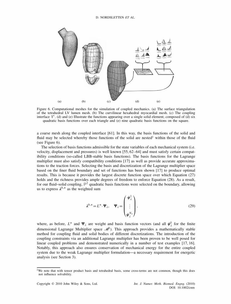
Figure 6. Computational meshes for the simulation of coupled mechanics. (a) The surface triangulationof the tetrahedral LV lumen mesh. (b) The curvilinear hexahedral myocardial mesh. (c) The couplinginterface �c. (d) and (e) Illustrate the functions appearing over a single solid element; composed of (d) six

quadratic basis functions over each triangle and (e) nine quadratic basis functions on the square.

a coarse mesh along the coupled interface [61]. In this way, the basis functions of the solid andfluid may be selected whereby those functions of the solid are nested‡ within those of the fluid(see Figure 6).

The selection of basis functions admissible for the state variables of each mechanical system (i.e.velocity, displacement and pressures) is well known [55, 62–64] and must satisfy certain compat-ibility conditions (so-called LBB-stable basis functions). The basis functions for the Lagrangemultiplier must also satisfy compatibility conditions [17] as well as provide accurate approxima-tions to the traction forces. Selecting the basis and discretization of the Lagrange multiplier spacebased on the finer fluid boundary and set of functions has been shown [17] to produce optimalresults. This is because it provides the largest discrete function space over which Equation (27)holds and the richness provides ample degrees of freedom to enforce Equation (28). As a result,for our fluid–solid coupling, P2 quadratic basis functions were selected on the boundary, allowingus to express kh,n as the weighted sum

kh,n = Ln ·W, W =

⎛⎜⎜⎜⎝w1

...

wNv

⎞⎟⎟⎟⎠ , (29)

where, as before, Ln and W are weight and basis function vectors (and all wk for the finitedimensional Lagrange Multiplier space Mh). This approach provides a mathematically stablemethod for coupling fluid and solid bodies of different discretizations. The introduction of thecoupling constraints via an additional Lagrange multiplier has been proven to be well posed forlinear coupled problems and demonstrated numerically in a number of test examples [17, 16].Notably, this approach also ensures conservation of mechanical energy for the entire coupledsystem due to the weak Lagrange multiplier formulation—a necessary requirement for energeticanalysis (see Section 3).

‡We note that with tensor product basis and tetrahedral basis, some cross-terms are not common, though this doesnot influence solvability.



2.4.3. Numerical solution. The coupled problem may be written as a non-linear vector functionand solved using an iterative approach, such as the global Newton–Raphson method [65, 66].

F(Xn)=0. (30)

Here Xn is defined as the weighted sum of all basis functions for all state variables, i.e.

(Xn)T=�n ·WX=

⎛⎜⎜⎜⎜⎜⎜⎜⎜⎝

vh,n

uh,n

ph,nf

ph,ns

kh,n

⎞⎟⎟⎟⎟⎟⎟⎟⎟⎠

, �n =

⎛⎜⎜⎜⎜⎜⎜⎜⎝

V n

Un

Pnf

Pns

Ln

⎞⎟⎟⎟⎟⎟⎟⎟⎠

, WX=

⎛⎜⎜⎜⎜⎜⎜⎜⎝

Wv

Wu

Wp f

Wps

W

⎞⎟⎟⎟⎟⎟⎟⎟⎠

, (31)

As a result, the iterative update to the solution Xn is accomplished by updating the coefficientvector, �n . Given an initial guess, �n,0, the approximate solution Xn at the nth time step is,

(Xn)T= limk→∞,k∈N+

�n,k ·WX, �n,k :=�n,k−1+�k�n,k,

where the scalar vector �n,k is the Newton update and �k a scalar parameter. The Newton update,�n,k , is selected as the solution to Equation (32), where ∇�n,k−1 is the gradient with respect toeach scalar coefficient of �n,k−1, ∇�n,k−1F(Xn,k−1) the Jacobian, and Xn,k−1= (�n,k−1 ·WX)T.

∇�n,k−1F(Xn,k−1)·�n,k =−F(Xn,k−1). (32)

Having solved Equation (32) for �n,k , the scalar parameter, �k , is selected to ensure a monotonicdecrease in the residual, i.e.

max�k∈(0,1]

|F(yn,k)|<|F(yn,k−1)|, (33)

where |·| is the l2-vector norm. To improve the numerical efficiency, we note that the Jacobianmatrix, Jn,k =∇�n,kF(Xn,k), is bounded above by (derived using the Taylor series expansion,assuming sufficient smoothness in �n,k and small |�n,k |)

|Jn,k+1−Jn,k|�|∇�n,kJn,k | |�n,k|,which implies, for bounded |∇�n,kJn,k |, that the Jacobian converges like |�n,k|. As a consequence,the Jacobian from previous Newton iterations or even previous time steps can often provide a goodapproximation to the true Jacobian (particularly when the time interval In is small).

The Newton–Raphson method requires the solution of the matrix system (32) to determine�n,k . This block matrix system may be solved iteratively using a partitioned approach (where, inthis case, k, is used to pass traction from the fluid to the solid) or monolithically. For the purposesof this paper, the heart model was solved monolithically using the matrix solver, MUMPS§ amultifrontal parallel solver [67]. As the MUMPS software allows multiple right-hand sides, to beapplied to a inverted matrix, the use of non-updated Jacobians was seen to provide up to a tenfoldincrease in run time.

3. RESULTS

A model left ventricle was constructed based on endocardial and epicardial borders traced from acontiguous stack of MRI ventricular short axis stead-state free precession cine images [16]. The

§Available through http://graal.ens-lyon.fr/MUMPS/ avail.html.



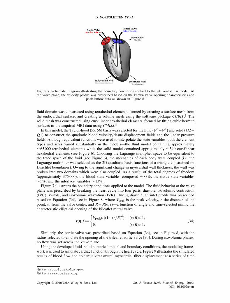
Figure 7. Schematic diagram illustrating the boundary conditions applied to the left ventricular model. Atthe valve plane, the velocity profile was prescribed based on the known valve opening characteristics and

peak inflow data as shown in Figure 8.

fluid domain was constructed using tetrahedral elements, formed by creating a surface mesh fromthe endocardial surface, and creating a volume mesh using the software package CUBIT .¶ Thesolid mesh was constructed using curvilinear hexahedral elements, formed by fitting cubic hermitesurfaces to the acquired MRI data using CMISS.‖

In this model, the Taylor-hood [55, 56] basis was selected for the fluid (P2−P1) and solid (Q2−Q1) to construct the quadratic blood velocity/tissue displacement fields and the linear pressurefields. Although equivalent functions were used to interpolate the state variables, both the elementtypes and sizes varied substantially in the models—the fluid model containing approximately∼65000 tetrahedral elements while the solid model contained approximately ∼540 curvilinearhexahedral elements (see Figure 6). Choosing the Lagrange multiplier space to be equivalent tothe trace space of the fluid (see Figure 6), the mechanics of each body were coupled (i.e. theLagrange multiplier was selected as the 2D quadratic basis functions of a triangle constrained onDirichlet boundaries). Owing to the significant change in myocardial wall thickness, the wall wasbroken into two domains which were also coupled. As a result, of the total degrees of freedom(approximately 375 000), the blood state variables composed ∼83%, the tissue state variables∼5%, and the interface variables ∼13%.

Figure 7 illustrates the boundary conditions applied to the model. The fluid behavior at the valveplane was prescribed by breaking the heart cycle into four parts: diastole, isovolumic contraction(IVC), systole, and isovolumic relaxation (IVR). During diastole, an inlet profile was prescribedbased on Equation (34), see in Figure 8, where Vpeak is the peak velocity, r the distance of thepoint, g, from the valve center, and R= R( , t)—a function of angle and time-selected mimic thecharacteristic elliptical opening of the bileaflet mitral valve.

v(g, t)={Vpeak(t)(1−(r/R)4), (r/R)�1,

0, (r/R)>1.(34)

Similarly, the aortic valve was prescribed based on Equation (34), see in Figure 8, with theradius selected to emulate the opening of the trileaflet aortic valve [70]. During isovolumic phases,no flow was set across the valve plane.

Using the developed fluid–solid numerical model and boundary conditions, the modeling frame-work was used to simulate cardiac function through the heart cycle. Figure 9 illustrates the simulatedresults of blood flow and epicardial/transmural myocardial fiber displacement at a series of time

¶http://cubit.sandia.gov.‖http://www.cmiss.org.



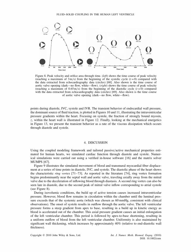
Figure 8. Peak velocity and orifice area through time. (left) shows the time course of peak velocity(reaching a maximum of 3m/s) from the beginning of the systolic cycle (t=0) compared withthe data extracted from echocardiography data (circles) [68]. Also shown is the time course ofaortic valve opening (dark—no flow, white—flow). (right) shows the time course of peak velocity(reaching a maximum of 0.65m/s) from the beginning of the diastolic cycle (t=0) comparedwith the data extracted from echocardiography data (circles) [69]. Also shown is the time course

of aortic valve opening (dark—no flow, white—flow).

points during diastole, IVC, systole and IVR. The transient behavior of endocardial wall pressure,the dominant source of fluid traction, is plotted in Figures 10 and 11, illustrating the intraventricularpressure gradients within the heart. Focusing on systole, the fraction of strongly bound myosin,z, within the heart wall is illustrated in Figure 12. Finally, looking at the mechanical energeticsin Figure 13, we present the transient behavior as a rate of the viscous dissipation which occursthrough diastole and systole.

4. DISCUSSION

Using the coupled modeling framework and tailored passive/active mechanical properties esti-mated for human hearts, we simulated cardiac function through diastole and systole. Numer-ical simulations were carried out using a verified in-house software [16] and the matrix solverMUMPS [67].

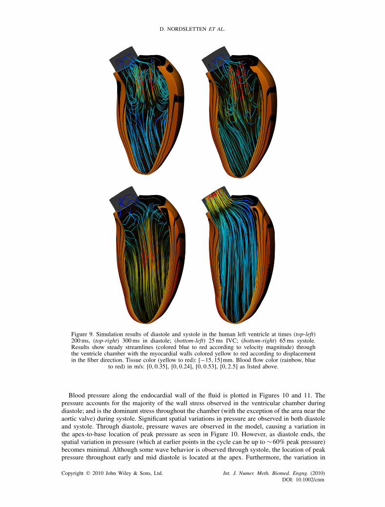
Figure 9 illustrates the simulated movement of blood and transmural myocardial fiber displace-ment at a series of time points in diastole, IVC, and systole. The diastolic phase of the heart showsthe characteristic ring vortex [71–73]. As reported in the literature [74], ring vortex formationbegins predominantly near the septal wall and aortic valve, traveling axially away from the mitralvalve due to the deceleration of inflowing blood through diastasis. A second ring vortex can also beseen late in diastole, due to the second peak of mitral valve inflow corresponding to atrial systole(see Figure 8).

During isovolumic conditions, the build up of active tension causes increased intraventricularpressure. However, blood flow remains in circulation within the chamber until the luminal pres-sure exceeds that of the systemic aorta (which was chosen as 60mmHg, consistent with clinicalobservations). The onset of systole results in outflow through the aortic valve. The left ventricularpressure forms a steep gradient from apex to base, resulting in a build up in kinetic energy asblood is accelerated out of the chamber. This axial pressure gradient causes an initial enlongationof the left ventricular chamber. This period is followed by apex-to-base shortening, resulting ina uniform outflow of blood from the left ventricular chamber. Uniformity is also maintained bysignificant wall thickening, which increases by approximately 40% (relative to end-diastolic wallthickness).



Figure 9. Simulation results of diastole and systole in the human left ventricle at times (top-left)200ms, (top-right) 300ms in diastole; (bottom-left) 25ms IVC; (bottom-right) 65ms systole.Results show steady streamlines (colored blue to red according to velocity magnitude) throughthe ventricle chamber with the myocardial walls colored yellow to red according to displacementin the fiber direction. Tissue color (yellow to red): [−15,15]mm. Blood flow color (rainbow, blue

to red) in m/s: [0,0.35], [0,0.24], [0,0.53], [0,2.5] as listed above.

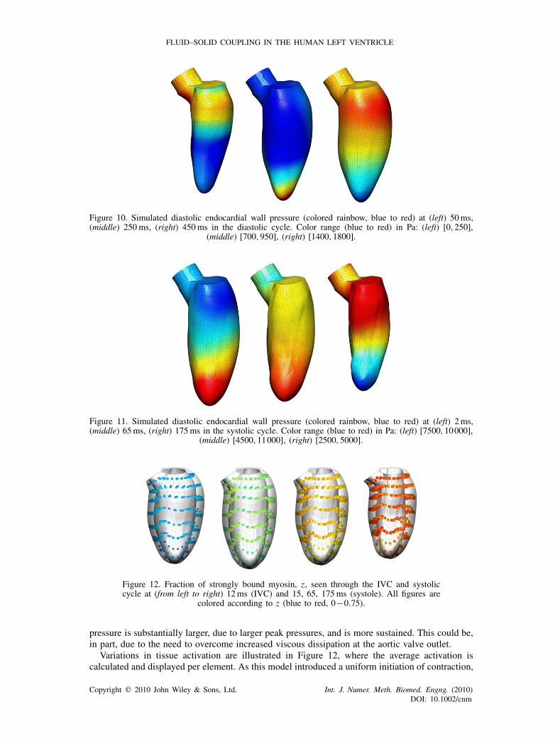
Blood pressure along the endocardial wall of the fluid is plotted in Figures 10 and 11. Thepressure accounts for the majority of the wall stress observed in the ventricular chamber duringdiastole; and is the dominant stress throughout the chamber (with the exception of the area near theaortic valve) during systole. Significant spatial variations in pressure are observed in both diastoleand systole. Through diastole, pressure waves are observed in the model, causing a variation inthe apex-to-base location of peak pressure as seen in Figure 10. However, as diastole ends, thespatial variation in pressure (which at earlier points in the cycle can be up to ∼60% peak pressure)becomes minimal. Although some wave behavior is observed through systole, the location of peakpressure throughout early and mid diastole is located at the apex. Furthermore, the variation in



Figure 10. Simulated diastolic endocardial wall pressure (colored rainbow, blue to red) at (left) 50ms,(middle) 250ms, (right) 450ms in the diastolic cycle. Color range (blue to red) in Pa: (left) [0,250],

(middle) [700,950], (right) [1400,1800].

Figure 11. Simulated diastolic endocardial wall pressure (colored rainbow, blue to red) at (left) 2ms,(middle) 65ms, (right) 175ms in the systolic cycle. Color range (blue to red) in Pa: (left) [7500,10000],

(middle) [4500,11000], (right) [2500,5000].

Figure 12. Fraction of strongly bound myosin, z, seen through the IVC and systoliccycle at (from left to right) 12ms (IVC) and 15, 65, 175ms (systole). All figures are

colored according to z (blue to red, 0−0.75).

pressure is substantially larger, due to larger peak pressures, and is more sustained. This could be,in part, due to the need to overcome increased viscous dissipation at the aortic valve outlet.

Variations in tissue activation are illustrated in Figure 12, where the average activation iscalculated and displayed per element. As this model introduced a uniform initiation of contraction,



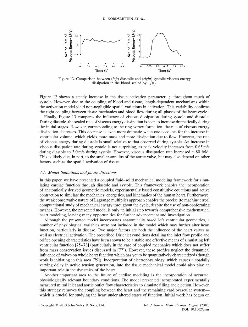
Figure 13. Comparison between (left) diastolic and (right) systolic viscous energydissipation in the blood scaled by 1/� f .

Figure 12 shows a steady increase in the tissue activation parameter, z, throughout much ofsystole. However, due to the coupling of blood and tissue, length-dependent mechanisms withinthe activation model yield non-negligible spatial variations in activation. This variability confirmsthe tight coupling between tissue mechanics and blood flow during all phases of the heart cycle.

Finally, Figure 13 compares the influence of viscous dissipation during systole and diastole.During diastole, the scaled rate of viscous energy dissipation is seen to increase dramatically duringthe initial stages. However, corresponding to the ring vortex formation, the rate of viscous energydissipation decreases. This decrease is even more dramatic when one accounts for the increase inventricular volume, which yields more mass and more dissipation due to flow. However, the rateof viscous energy during diastole is small relative to that observed during systole. An increase inviscous dissipation rate during systole is not surprising, as peak velocity increases from 0.65m/sduring diastole to 3.0m/s during systole. However, viscous dissipation rate increased ∼80 fold.This is likely due, in part, to the smaller annulus of the aortic valve, but may also depend on otherfactors such as the spatial activation of tissue.

4.1. Model limitations and future directions

In this paper, we have presented a coupled fluid–solid mechanical modeling framework for simu-lating cardiac function through diastole and systole. This framework enables the incorporationof anatomically derived geometric models, experimentally based constitutive equations and activecontraction to simulate the mechanics, energetics, and kinematics of the human heart. Furthermore,the weak conservative nature of Lagrange multiplier approach enables the precise (to machine error)computational study of mechanical energy throughout the cycle, despite the use of non-conformingmeshes. However, the presented model is only an initial step towards comprehensive mathematicalheart modeling, leaving many opportunities for further advancement and investigation.

Although the presented model incorporates anatomically based left ventricular geometries, anumber of physiological variables were not included in the model which may further alter heartfunction, particularly in disease. Two major factors are both the influence of the heart valves aswell as electrical activation. The prescribed Dirichlet conditions detailing the inlet flow profile andorifice opening characteristics have been shown to be a stable and effective means of simulating leftventricular function [75–78] (particularly in the case of coupled mechanics which does not sufferfrom mass conservation issues discussed in [77]). However, these profiles neglect the dynamicalinfluence of valves on whole heart function which has yet to be quantitatively characterized (thoughwork is initiating in this area [79]). Incorporation of electrophysiology, which causes a spatiallyvarying delay in active tension generation, into the tissue mechanical model could also play animportant role in the dynamics of the heart.

Another important area to the future of cardiac modeling is the incorporation of accurate,physiologically relevant boundary conditions. The model presented incorporated experimentallymeasured mitral inlet and aortic outlet flow characteristics to simulate filling and ejection. However,this strategy removes the coupling between the heart and the remaining cardiovascular system—which is crucial for studying the heart under altered states of function. Initial work has begun on



incorporatingWindkessel models of the cardiovascular systemwith three-dimensional tissue models[7, 80]. The inclusion of these Windkessel models, such as that proposed by Shi [81, 82], wouldprovide the feedback necessary for studying the heart under altered dynamics. Equally importantare the conditions imposed on the solid mechanical model. The pericardium and surrounding organscouple the atria and ventricles, causing the left atrioventricular volume to remain nearly constantthrough the heart cycle. This creates a cross-coupling between the left atria and left ventricle whichhas yet to be characterized.

A major goal in the mathematical modeling of whole heart function is the eventual translation tothe clinic. While the inclusion of physiologically relevant mechanisms provides the most versatilityfor clinical application, it also proves the most challenging to parametrize. In this context, it isincreasingly becoming important to identify reduced models which capture essential behaviorsrequired for a given clinical study. In this paper, we presented a reduced cellular contraction model,based on known cross-bridge states, which characterized the steady-state length dependence oftension generation. Other authors have similarly used reduced models which capture essentialcharacteristics of function, while remaining tunable to clinical data. The further advancementof reduction techniques which simplify detailed biophysically based models while maintainingessential functionality is crucial to the development of patient-specific heart models.

Another important step towards model translation within the clinic is validation. Although thepresented model presents the characteristic behaviors typical of the left ventricle, a quantitativepatient-specific validation of the model is an important step. In the past, validation of coupledfluid–solid mechanical models remained challenging due to the difficulty of comprehensive in vivodata collection. However, with the advances in three-dimensional velocity encoded MRI, taggedMRI, three-dimensional echocardiography and in vivo diffusion-tensor MRI (as well as the abilityto record some measures simultaneously) it is now possible to collect significant quantitative datato compare with simulated cardiac dynamics.

APPENDIX A: STEADY HUMAN CONTRACTION MODEL

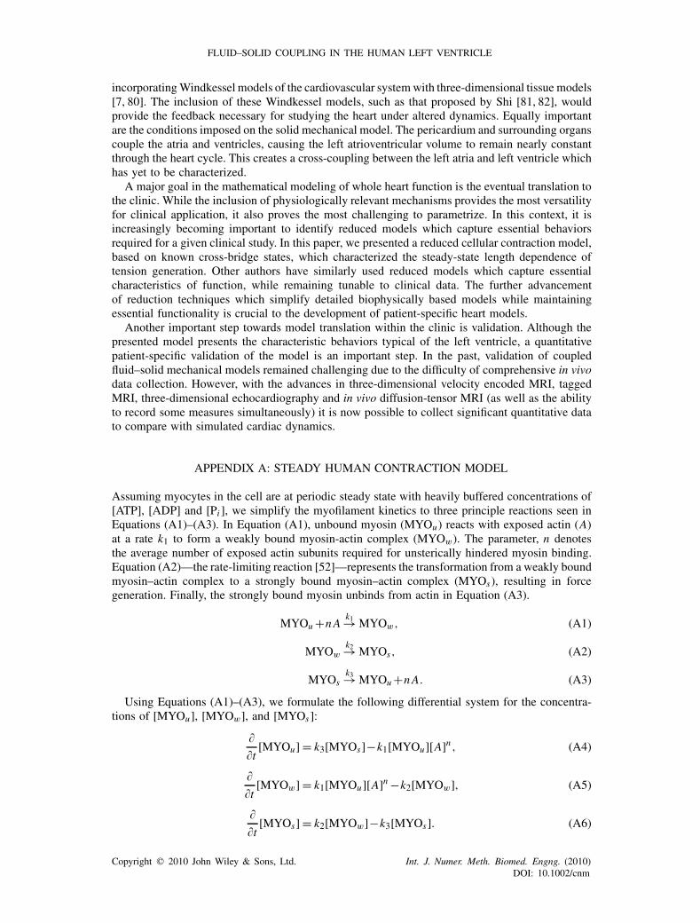
Assuming myocytes in the cell are at periodic steady state with heavily buffered concentrations of[ATP], [ADP] and [Pi ], we simplify the myofilament kinetics to three principle reactions seen inEquations (A1)–(A3). In Equation (A1), unbound myosin (MYOu) reacts with exposed actin (A)at a rate k1 to form a weakly bound myosin-actin complex (MYOw). The parameter, n denotesthe average number of exposed actin subunits required for unsterically hindered myosin binding.Equation (A2)—the rate-limiting reaction [52]—represents the transformation from a weakly boundmyosin–actin complex to a strongly bound myosin–actin complex (MYOs), resulting in forcegeneration. Finally, the strongly bound myosin unbinds from actin in Equation (A3).

MYOu +nAk1→MYOw, (A1)

MYOwk2→MYOs, (A2)

MYOsk3→MYOu+nA. (A3)

Using Equations (A1)–(A3), we formulate the following differential system for the concentra-tions of [MYOu], [MYOw], and [MYOs ]:

��t[MYOu]= k3[MYOs]−k1[MYOu][A]

n , (A4)

��t[MYOw]= k1[MYOu][A]

n −k2[MYOw], (A5)

��t[MYOs]= k2[MYOw]−k3[MYOs]. (A6)



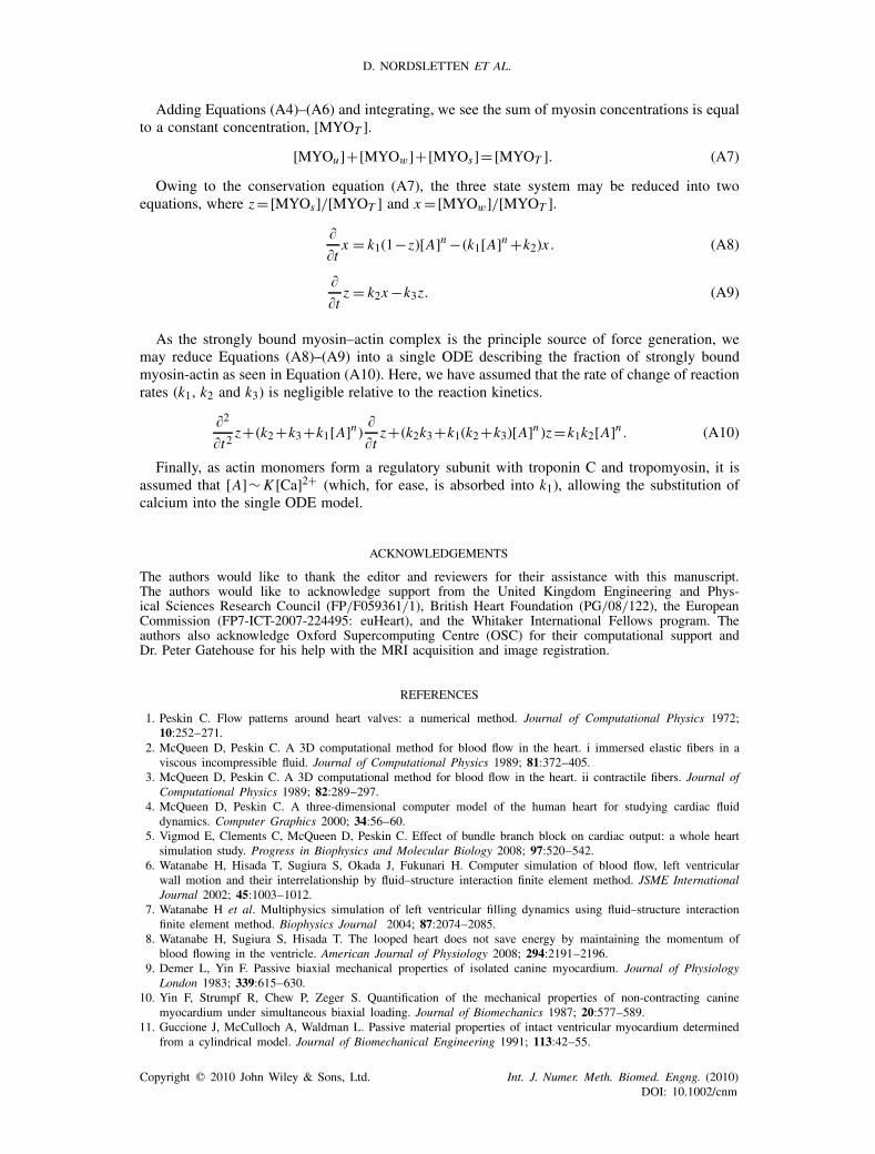
Adding Equations (A4)–(A6) and integrating, we see the sum of myosin concentrations is equalto a constant concentration, [MYOT ].

[MYOu]+[MYOw]+[MYOs]= [MYOT ]. (A7)

Owing to the conservation equation (A7), the three state system may be reduced into twoequations, where z= [MYOs]/[MYOT ] and x = [MYOw]/[MYOT ].

��t

x = k1(1−z)[A]n −(k1[A]n +k2)x . (A8)

��t

z = k2x−k3z. (A9)

As the strongly bound myosin–actin complex is the principle source of force generation, wemay reduce Equations (A8)–(A9) into a single ODE describing the fraction of strongly boundmyosin-actin as seen in Equation (A10). Here, we have assumed that the rate of change of reactionrates (k1, k2 and k3) is negligible relative to the reaction kinetics.

�2

�t2z+(k2+k3+k1[A]

n)��t

z+(k2k3+k1(k2+k3)[A]n )z=k1k2[A]

n . (A10)

Finally, as actin monomers form a regulatory subunit with troponin C and tropomyosin, it isassumed that [A]∼K [Ca]2+ (which, for ease, is absorbed into k1), allowing the substitution ofcalcium into the single ODE model.

ACKNOWLEDGEMENTS

The authors would like to thank the editor and reviewers for their assistance with this manuscript.The authors would like to acknowledge support from the United Kingdom Engineering and Phys-ical Sciences Research Council (FP/F059361/1), British Heart Foundation (PG/08/122), the EuropeanCommission (FP7-ICT-2007-224495: euHeart), and the Whitaker International Fellows program. Theauthors also acknowledge Oxford Supercomputing Centre (OSC) for their computational support andDr. Peter Gatehouse for his help with the MRI acquisition and image registration.

REFERENCES

1. Peskin C. Flow patterns around heart valves: a numerical method. Journal of Computational Physics 1972;10:252–271.

2. McQueen D, Peskin C. A 3D computational method for blood flow in the heart. i immersed elastic fibers in aviscous incompressible fluid. Journal of Computational Physics 1989; 81:372–405.

3. McQueen D, Peskin C. A 3D computational method for blood flow in the heart. ii contractile fibers. Journal ofComputational Physics 1989; 82:289–297.

4. McQueen D, Peskin C. A three-dimensional computer model of the human heart for studying cardiac fluiddynamics. Computer Graphics 2000; 34:56–60.

5. Vigmod E, Clements C, McQueen D, Peskin C. Effect of bundle branch block on cardiac output: a whole heartsimulation study. Progress in Biophysics and Molecular Biology 2008; 97:520–542.

6. Watanabe H, Hisada T, Sugiura S, Okada J, Fukunari H. Computer simulation of blood flow, left ventricularwall motion and their interrelationship by fluid–structure interaction finite element method. JSME InternationalJournal 2002; 45:1003–1012.

7. Watanabe H et al. Multiphysics simulation of left ventricular filling dynamics using fluid–structure interactionfinite element method. Biophysics Journal 2004; 87:2074–2085.

8. Watanabe H, Sugiura S, Hisada T. The looped heart does not save energy by maintaining the momentum ofblood flowing in the ventricle. American Journal of Physiology 2008; 294:2191–2196.

9. Demer L, Yin F. Passive biaxial mechanical properties of isolated canine myocardium. Journal of PhysiologyLondon 1983; 339:615–630.

10. Yin F, Strumpf R, Chew P, Zeger S. Quantification of the mechanical properties of non-contracting caninemyocardium under simultaneous biaxial loading. Journal of Biomechanics 1987; 20:577–589.

11. Guccione J, McCulloch A, Waldman L. Passive material properties of intact ventricular myocardium determinedfrom a cylindrical model. Journal of Biomechanical Engineering 1991; 113:42–55.



12. Omens J, Fung Y. Residual strain in rat left ventricle. Circulation Research 1990; 66:37–45.13. Guccione J, Waldman L, McCulloch A. Mechanics of active contraction in cardiac muscle: part I—constitutive

relations for fiber stress that describe deactivation. Journal of Biomechanical Engineering 1973; 115:72–81.14. Costa K, Holmes J, McCulloch A. Modelling cardiac mechanical properties in three dimensions. Philosophical

Transactions of the Royal Society London A 2001; 359:1233–1250.15. Schmid H, O’Callaghan P, Nash M, Lin W, LeGrice I, Smaill B, Young A, Hunter P. Myocardial material

parameter estimation. Biomechanics and Modeling in Mechanobiology 2008; 7:161–173.16. Nordsletten D. Fluid–solid coupling for the simulation of left ventricular mechanics. University of Oxford, 2009.17. Nordsletten D, Kay D, Smith N. A non-conforming monolithic finite element method for problems of coupled

mechanics. Journal of Computational Physics, submitted.18. LeGrice I, Smaill B, Chai L, Edgar S, Gavin J, Hunter P. Laminar structure of the heart: ventricular myocyte

arrangement and connective tissue architecture in the dog. American Journal of Physiology 1995; 269:571–582.19. LeGrice I, Hunter P, Smaill B. Laminar structure of the heart: a mathematical model. American Heart Journal

1997; 272:2466–2476.20. Gwathmey J, Hajjar R. Relation between steady-state force and intracellular [Ca2+] in intact human myocardium.

Circulation 1990; 82:1266–1278.21. Vahl C, Timek T, Bonz A, Fuchs H, Dillman R, Hagl S. Length dependence of calcium- and force-transients in

normal and failing human myocardium. Journal of Molecular and Cellular Cardiology 1998; 30:957–966.22. Cook J, Hirt C, Amsden A. An arbitrary Lagrangian–Eulerian computing method for all flow speeds. Journal of

Computational Physics 1974; 14:227–253.23. Hughes TJR, Liu W, Zimmermann TK. Lagrangian–Eulerian finite element formulation for incompressible viscous

flows. Computer Methods in Applied Mechanics and Engineering 1981; 29:329–349.24. Huerta A, Liu W. Viscous flow with large free surface motion. Computer Methods in Applied Mechanics and

Engineering 1988; 69:277–324.25. Formaggia L, Nobile F. Stability analysis of second-order time accurate schemes for ale-fem. Computer Methods

in Applied Mechanics and Engineering 2004; 193:4097–4116.26. Nordsletten D, Hunter P, Smith N. Conservative and non-conservative arbitrary Lagrangian–Eulerian forms for

ventricular flows. International Journal for Numerical Methods in Fluids 2008; 56:1457–1463.27. Nordsletten D, Smith N, Kay D. A preconditioner for the finite element approximation to the ale Navier–Stokes

equations. SIAM Journal on Scientific Computing 2010; 32:521–543.28. van Loon R, Anderson P, van de Vosse F, Sherwin S. Comparison of various fluid–structure interaction methods

for deformable bodies. Computers and Structures 2007; 85:833–843.29. Nobile F. Numerical approximation of fluid–structure interaction problems with application to haemodynamics.

Ph.D. Thesis. École Polytechnique Fédérale de Lausanne, 2001.30. Pries A, Neuhaus D, Gaehtgens P. Blood viscosity in tube flow: dependence on diameter and hematocrit. American

Journal of Physiology 1992; 32:1770–1778.31. Malvern LE. Introduction to the Mechanics of Continuous Medium. Prentice-Hall: New York, 1969.32. Bonet J, Wood R. Nonlinear Continuum Mechanics for Finite Element Analysis. Cambridge University Press:

Cambridge, 1997.33. Sermesant M et al. Personalised Electromechanical Model of the Heart for the Prediction of the Acute Effects of

Cardiac Resynchronisation Therapy. Lecture Notes in Computer Science, vol. 5528. Springer: New York, 2009;239–248.

34. Kovacs S, McQueen D, Peskin C. Modeling cardiac fluid dynamics and diastolic function. PhilosophicalTransactions of the Royal Society London A 2001; 359:1299–1314.

35. Cheng Y, Oertel H, Schenkel T. Fluid–structure coupled cfd simulation of the left ventricular flow during fillingphase. Biomedical Engineering 2005; 8:567–576.

36. Hunter P, McCulloch A, ter Keurs H. Modelling the mechanical properties of cardiac muscle. Progress inBiophysics and Molecular Biology 1998; 69:289–331.

37. Nash M, Hunter P. Computational mechanics of the heart. Journal of Elasticity 2000; 61:113–141.38. Dokos S, Smaill B, Young A, LeGrice I. Shear properties of passive ventricular myocardium. American Journal

of Physiology 2002; 283:2650–2659.39. Nordsletten D, Niederer S, Nash M, Hunter P, Smith N. Coupling multi-physics models to cardiac mechanics.

Progress in Biophysics and Molecular Biology, 2009. DOI: 10.1016/j.pbiomolbio.2009.11.001.40. Streeter D, Bassett D. An engineering analysis of myocardial fiber orientation in pig’s left ventricle in systole.

Anatomical Record 1966; 155:503–511.41. Rohmer D, Sitek A, Gullberg G. Reconstruction and visualization of fiber and sheet structure with regularized

tensor diffusion mri in the heart. Lawrence Berkeley National Laboratory Publication, LBNL-60277, 2006.42. Rohmer D, Sitek A, Gullberg G. Reconstruction and visualization of fiber and laminar structure in the normal

human heart from ex vivo diffusion tensor magnetic resonance imaging (dtmri) data. Investigative Radiology2007; 42:777–789.

43. Buckberg G, Mahajan A, Jung B, Markl M, Hennig J, Ballester-Rodes M. MRI myocardial motion and fibertracking: a confirmation of knowledge from different imaging modalities. European Journal of Cardio-thoracicSurgery 2006; 29:165–177.

44. Holzapfel G, Ogden R. Constitutive modelling of passive myocardium: a structurally based framework for materialcharacterization. Philosophical Transactions of the Royal Society A 2009; 367:3445–3475.



45. ter Keurs H, Runsburger W, Heuningen R, Nagelsmit M. Tension development and sarcomere length in ratcardiac trabeculae: evidence of length-dependent activation. Circulation Research 1980; 46:703–714.

46. Costa K, May-Newman K, Farr D, O’Dell W, McCulloch A, Omens J. Three-dimensional residual strain inmidanterior canine left ventricle. American Journal of Physiology 1997; 273:1968–1976.

47. Klotz S, Hay I, Dickstein M, Yi G, Wang J, Maurer M, Kass D, Burkhoff D. Single-beat estimation of end-diastolicpressure–volume relationship: a novel method with potential for noninvasive application. American Journal ofPhysiology 2006; 291:403–412.

48. Klotz S, Dickstein M, Burkhoff D. A computational method of prediction of the end-diastolic pressure volumerelationship by single beat. Nature Protocol 2007; 2:2152–2158.

49. Makarenko I, Opitz C, Leake M, Neagoe C, Kulke M, Gwathmey J, del Monte F, Hajjar R, Linke W. Passivestiffness changes caused by upregulation of compliant titin isoforms in human dilated cardiomyopathy hearts.Circulation Research 2004; 95:708–716.

50. Schmid H. Constitutive laws and material paramter estimation. Ph.D. Thesis, University of Auckland, 2006.51. Rajagopal V, Chung J, Bullivant D, Nielsen P, Nash M. Determing the finite elasticity reference state from a

loaded configuration. International Journal for Numerical Methods in Engineering 2007; 72:1434–1451.52. Katz A. Physiology of the Heart. Raven Press, 2006.53. van der Velden J, de Jong J, Owen V, Burton P, Stienen G. Effect of protein kinase a on calcium sensitivity of

force and its sarcomere length dependence in human cardiomyocytes. Cardiovascular Research 2000; 46:487–495.54. Hunter P, Smaill B. The analysis of cardiac function: a continuum approach. Progress in Biophysics and Molecular

Biology 1988; 52:101–164.55. Brezzi F, Fortin M. Mixed and Hybrid Finite Element Methods. Springer: Heidelberg, 1991.56. Brezzi F, Falk R. Stability of higher-order Hood–Taylor methods. SIAM Journal on Numerical Analysis 1991;

28:581–590.57. Oden J. Finite Element of Nonlinear Continua. McGraw-Hill: New York, 1972.58. Girault V, Raviart PA. Finite Element Methods for the Navier–Stokes Equations. Springer: Berlin, 1986.59. Gresho P, Sani R. Incompressible Flow and the Finite Element Method I, Advection–Diffusion. Wiley: New York,

1998.60. Gresho P, Sani R. Incompressible Flow and the Finite Element Method II, Isothermal Laminar Flow. Wiley:

New York, 1998.61. Nordsletten D, Smith N. Triangulation of p-order parametric surfaces. Journal of Scientific Computing 2007;

34:308–335.62. Babuska I. The finite element method with Lagrange multipliers. Numerical Mathematics 1973; 20:179–192.63. Brezzi F. On the existence, uniqueness and approximation of saddle-point problems arising from Lagrange

multipliers. Mathematical Modelling and Numerical Analysis 1974; 2:129–151.64. Nicolaides R. Existence, uniqueness and approximation for generalized saddle point problems. SIAM Journal on

Numerical Analysis 1982; 19:349–357.65. Eisenstat S, Walker H. Globally convergent inexact Newton methods. SIAM Journal on Optimization 1994;

4(2):393–422.66. Dennis J, Schnabel R. Numerical Methods for Unconstrained Optimization and Nonlinear Equations. SIAM,

Prentice-Hall Inc: NJ, 1996.67. Amestoy P, Duff I, L’Excellent J. Multifrontal parallel distributed symmetric and unsymmetric solvers. Computer

Methods in Applied Mechanics and Engineering 2000; 184:501–520.68. Zoghbi W, Farmer K, Soto J, Nelson J, Quinones M. Accurate noninvasive quantification of stenotic aortic valve

area by doppler echocardiography. Circulation 1986; 73:452–459.69. Kilner P, Henein M, Gibson D. Our tortuous heart in dynamic mode—an echocardiographic study of mitral flow

and movement in exercising subjects. Heart Vessels 1997; 12:103–110.70. Handke M, Jahnke C, Heinrichs G, Schlegel J, Vos C, Schmitt D, Bode C, Geibel A. New three-dimensional

echocardiographic system using digital radiofrequency data—visualization and quantitative analysis of aorticvalve dynamics with high resolution: methods, feasibility, and initial clinical experience. Circulation 2003;107:2876–2879.

71. Pedrizzetti G, Domenichini F. Nature optimizes the swirling flow in the human left ventricle. Physial Review2005; 95:1–4.

72. Domenichini F, Pedrizzetti G, Baccani B. Three-dimensional filling flow into a model left ventricle. Journal ofFluid Mechanics 2005; 539:179–198.

73. Cooke J, hertzberg J, Boardman M, Shandas R. Characterizing vortex ring behavior during ventricular fillingwith doppler echocardiography: an in vitro study. Annals of Biomedical Engineering 2004; 32:245–256.

74. Kilner P, Yang G, Wilkes A, Mohiaddin R, Firmin D, Yacoub M. Asymmetric redirection of flow through theheart. Nature 2000; 404:759–761.

75. Saber N, Gosman A, Wood N, Kilner P, Charrier C, Firmin D. Computational flow modeling of the left ventriclebased on in vivo mri data: initial experience. Annals of Biomedical Engineering 2001; 29:275–283.

76. Saber N, Wood N, Gosman A, Merrifield R, Yang G, Charrier C, Gatehouse P, Firmin D. Progress towardspatient-specific computational flow modeling of the left heart via combination of MRI with computational fluiddynamics. Annals of Biomedical Engineering 2003; 31:42–52.

77. Long Q, Merrifield R, Yang G, Kilner P, Firmin D, Xu X. The influence of inflow boundary conditions on intraleft ventricle flow predictions. Transaction of ASME 2003; 125:922–927.



78. Merrifield R, Long Q, Xu X, Kilner P, Firmin D, Yang G. Combined cfd/mri analysis of left ventricular flow.MIAR, vol. 3150, 2004; 229–236.

79. Wood C, Gil A, Hassan O, Bonet J, Ashraf S. Computational modelling of the beating heart: blood flow throughartificial heart valves. International Journal for Numerical Methods in Biomedical Engineering, 2009.

80. Kerchkhoffs R, Neal M, Gu Q, Bassingthwaighte J, Omens J, McCulloch A. Coupling of a 3D finite elementmodel of cardiac ventricular mechanics to lumped systems models of the systemic and pulmonic circulation.Annals of Biomedical Engineering 2007; 35:1–18.

81. Shi Y, Korakianitis T. Numerical simulation of cardiovascular dynamics with left heart failure and in-seriespulsatile ventricular assist device. Art. Organs, vol. 30, 2006; 929–948.

82. Korakianitis T, Shi Y. A concentrated parameter model for the human cardiovascular system including heartvalve dynamics and atrioventricular interaction. Medical Engineering and Physics 2006; 28:613–628.


Fluid–solid coupling for the investigation of diastolic and systolic human left ventricular...

Documents

Transcript of Fluid–solid coupling for the investigation of diastolic and systolic human left ventricular...