Centrifuge Modelling and Numerical Analysis of ...

Centrifuge Modelling and Numerical Analysis of

Penetrometers in Uniform and Layered Clays

By

Yue Wang

B.Eng.

This thesis is presented for the degree of

Doctor of Philosophy

of The University of Western Australia

School of Civil, Environmental and Mining Engineering

Centre for Offshore Foundation Systems

April 2019

i

THESIS DECLARATION

I, Yue Wang, certify that:

This thesis has been substantially accomplished during enrolment in the degree.

This thesis does not contain material which has been submitted for the award of any

other degree or diploma in my name, in any university or other tertiary institution.

No part of this work will, in the future, be used in a submission in my name, for any

other degree or diploma in any university or other tertiary institution without the prior

approval of The University of Western Australia and where applicable, any partner

institution responsible for the joint-award of this degree.

This thesis does not contain any material previously published or written by another

person, except where due reference has been made in the text and, where relevant, in

the Declaration that follows.

The work(s) are not in any way a violation or infringement of any copyright, trademark,

patent, or other rights whatsoever of any person.

The work described in this thesis was funded by Australian Research Council (ARC)

through the Discovery Grant DP140103997.

This thesis contains published work and/or work prepared for publication, some of

which has been co-authored.

Signature:

Date: 17/09/2018

iii

ABSTRACT

Increasing application of penetrometer tests, including cone and full-flow

penetrometers i.e. T-bar and ball, in offshore site investigations has been muddied by

the lack of accurate interpretation framework for their resistance profiles, especially

in layered seabed sediments. This research has focused on (i) revealing the evolving

soil failure mechanisms around the T-bar, ball and cone penetrometers during their

continuous penetration into layered fine-grained sediments from the surface/mudline;

and (ii) quantifying their effects on the resistance profiles. The overarching aim was

to establish a design framework for interpreting undrained shear strength from the

measured penetration resistance profiles through offshore in-situ site investigations.

To reveal the soil failure mechanism, a series of centrifuge tests was conducted with

the penetrometers penetrating through layered clays, such as soft-stiff, stiff-soft, soft-

stiff-soft, and stiff-soft-stiff clay deposits. Particle image velocimetry (PIV) allowed

accurate resolution of the flow mechanism around a face of the T-bar, half-ball and

half-cone penetrating adjacent to a transparent window. To quantify the layering effect,

an extensive parametric study by large deformation finite element (LDFE) analysis

was conducted for the T-bar, since cone and ball have been analysed numerically

previously.

In centrifuge tests, for T-bar, overall a symmetric rotational flow around the T-bar

dominated the behaviour. A novel ‘trapped cavity mechanism’ was revealed in stiff

clays, with its formation and closure tracked. For the ball, the key features of soil flow

include vertical flow, cavity expansion and rotational flow. For both full-flow

penetrometers, a squeezing mechanism dominated the behaviour when approaching

the soft-stiff interface, with soft soil squeezed sideways before involving the bottom

iv

stiff soil, leading to minimal deformation of the layer interface. In a stiff-soft clay

deposit, a ‘punch-through’ type of failure occurred near the layer interface with large

downward deformation of the layer interface. The effect of layering was also

quantified through comparing trajectories of soil element at different distances from

the interface and penetrometers. A stiff clay plug was trapped at the base of the ball,

which was forced into the softer underlying layer with the ball. However, there was

no soil plug observed from the previous layer trapped at the base of the advancing T-

bar regardless of penetration from stiff to soft clay or the reverse. For the cone in a

single uniform clay layer, based on the centrifuge test results, the existing strain path

method showed reasonable predictions on maximum lateral and vertical displacements

in the soil around the cone shoulder. However, the upheave movement in soil was

overestimated. For the cone in layered soils, the squeezing mechanism at soft-stiff

layer interface and ‘punch-through’ failure mechanism at stiff-soft layer interface was

also observed. Due to the shape of the cone tip, there was no trapped soil from the

previous layer underneath the cone tip when entering the underlying layer in stiff-soft

clays or vice versa.

The penetration resistance profiles in the layered sediments were obtained by

centrifuge tests using separate miniature T-bar, full-ball and full-cone. The resistance

profiles were linked to the mobilised soil failure mechanisms at various penetration

stages. A novel calibration method on cone tip load cell under ambient pressure was

proposed for proper conversion of the cone resistance measured in soils.

In LDFE analysis, the behaviour and T-bar resistance factor profile in both single- and

two-layer clay have been studied, with a T-bar penetrating continuously from the

mudline into both single and layered profiles. For single layer of clays, the formation

of the trapped cavity above the advancing T-bar and its evolution to full flow

v

mechanism was studied extensively, covering a large range of soil normalised

undrained shear strength and the T-bar surface roughness. It was found that the depths

of trapped cavity formation and closure increased with increasing normalised

undrained shear strength and T-bar roughness. The presence of the trapped cavity

could reduce the T-bar bearing capacity factor that was used in current practice, where

a full flow mechanism was assumed. For two-layer clays, the effect of soil layering on

the behaviour of the T-bar penetrometer was explored in both soft-stiff and stiff-soft

clay deposits. The resistance profiles were discussed linking with the mobilised soil

failure mechanisms. Finally, based on the systematic parametric analyses performed,

the interpretation framework accounting for the effect of the trapped cavity and

layering was proposed for more accurate interpretation of soil undrained shear strength

and soil interface elevations.

The soil flow mechanism and shearing around the ends of the T-bar cylinder, termed

as ‘end effect’, was investigated with a three-dimensional finite element model (3D-

FE), with varying T-bar aspect ratio (length/diameter) and surface roughness. A

practical correction method accounting for the end effect was proposed to adjust the

commonly used analytical plane strain solutions.

vii

ACKNOWLEDGEMENTS

First and foremost, I would like to express my deepest gratitude to my supervisors,

Professor Yuxia Hu, Associate Professor Muhammad Shazzad Hossain and Associate

Professor Mi Zhou, for their insightful guidance, continuous involvement and

enormous encouragement throughout my candidature. The numerous discussions we

had during the past four years have always provided me with lasting motivations and

fresh ideas for my research project, which will continue to nourish me in the future.

This thesis would not have been possible without their persistent support.

My sincere thanks go to the powerful centrifuge technician team of NGCF, especially

Kelvin Leong and Manuel Palacios, for providing help in carrying out my centrifuge

test. I would also like to thank David Johns for fabricating the model half- and full-

penetrometers.

Special thanks to my colleagues at COFS/Civil and friends in Perth for always being

available to listen to me, give suggestions and help. I would like to extend my

appreciation to the administration staff, Charlie, Rochelle, Dana and Monica, and IT

support whenever it was needed.

This research was supported by an Australian Government Research Training Program

(RTP) Scholarship. The financial support provided by the Australian Research

Council Discovery Project (DP140103997) is greatly acknowledged, as well as

Scholarship for University International Stipend. Thanks also go to the University of

Western Australia travel award for funding my travel to San Francisco, USA to attend

the 27th International Ocean and Polar Engineering Conference.

viii

I am extremely grateful to my partner, Kuntan Chang, for his endless support and

encouragement during my candidature. I always feel blessed to share this life journey

from Changsha to Shanghai to Perth. My thanks also extend to the whole family who

has been supporting me with their love and care.

ix

AUTHORSHIP DECLARATION: CO-AUTHORED

PUBLICATIONS

This thesis contains work that has been published and/or prepared for publication.

Details of the work:

Wang, Y., Hu, Y. and Hossain, M. S. (2018). Soil Flow Mechanisms of Full-

Flow Penetrometers in Layered Clays – PIV Analysis in Centrifuge Test.

Canadian Geotechnical Journal. Submitted January 2018.

Location in thesis:

Chapter 2

Student contribution to work:

The candidate designed, prepared and carried out the experimental tests and

conducted the image-base data analysis. She compiled a detailed first draft that

was revised addressing comments from the co-authors. The estimated

percentage contribution of the candidate is 70%.


Wang, Y., Hossain, M. S. and Hu, Y. (2018). Soil Flow Mechanisms around

Cone Penetrometer in Layered Clay Sediments – PIV Analysis in Centrifuge

Test. To be submitted.

Location in thesis:

Chapter 3


The candidate designed, prepared and carried out the experimental tests and

conducted the image-base data analysis. She compiled a detailed first draft that

was revised addressing comments from the co-authors. The estimated

percentage contribution of the candidate is 70%.


Wang, Y., Hu, Y. and Hossain, M. S. (2018). Ambient pressure calibration for

cone penetrometer test: necessary? Proceedings of the 9th International

Conference on Physical Modelling in Geotechnics. London, UK.

Location in thesis:

Chapter 4


The candidate designed, prepared and carried out the experimental tests. She

compiled a detailed first draft that was revised addressing comments from the

co-authors. The estimated percentage contribution of the candidate is 70%.

x


Wang, Y., Hu, Y., Hossain, M. S. and Zhou M. (2018). Effect of trapped cavity

mechanism on T-bar penetration resistance in uniform clays. To be submitted.

Location in thesis:

Chapter 5


The candidate tested the numerical model and conducted numerical analysis.

She compiled a detailed first draft that was revised addressing comments from

the co-authors. The estimated percentage contribution of the candidate is 70%.


Wang, Y., Hossain, M. S. and Hu, Y. (2018). Interpretation of T-bar

penetrometer in two-layer cohesive sediments. To be submitted.

Location in thesis:

Chapter 6






Wang, Y., Hu, Y. and Hossain, M. S. (2018). End Effect of T-bar Penetrometer

Using 3D FE Analysis. Proceedings of the 27th International Ocean and Polar

Engineering Conference (ISOPE). San Francisco, US, pp. 497-503.

Location in thesis:

Chapter 7





xi

Student signature:

Date: 17/09/2018

I, Yuxia Hu, certify that the student statements regarding their contribution to

each of the works listed above are correct

Coordinating supervisor signature:

Date: 17/09/2018

Co-author signature:

Date: 17/09/2018

xiii

TABLE OF CONTENTS

THESIS DECLARATION ........................................................................................ I

ABSTRACT ............................................................................................................. III

ACKNOWLEDGEMENTS ................................................................................... VII

AUTHORSHIP DECLARATION: CO-AUTHORED PUBLICATIONS ......... IX

TABLE OF CONTENTS ..................................................................................... XIII

LIST OF TABLES ............................................................................................... XIX

LIST OF FIGURES ............................................................................................. XXI

NOTATIONS ...................................................................................................... XXIX

ABBREVIATIONS ........................................................................................ XXXIII

CHAPTER 1 INTRODUCTION .......................................................................... 1

1.1 IN-SITU INVESTIGATIONS ............................................................................... 1

1.2 IN-SITU PENETROMETERS .............................................................................. 2

1.3 BACKGROUND ............................................................................................... 4

1.3.1 Theoretical solutions ................................................................................ 5

1.3.2 Numerical analyses: single layer fine grained sediments ........................ 6

1.3.3 Numerical analyses: stratified fine grained sediments ............................. 8

1.3.4 Model testing: soil failure mechanisms ................................................. 10

1.4 AIM OF THIS RESEARCH ............................................................................... 10

1.5 OUTLINE OF THIS RESEARCH ....................................................................... 11

1.6 REFERENCES ............................................................................................... 13

xiv

CHAPTER 2 SOIL FLOW MECHANISMS OF FULL-FLOW

PENETROMETERS IN LAYERED CLAYS – PIV ANALYSIS IN

CENTRIFUGE TEST .............................................................................................. 25

2.1 INTRODUCTION ........................................................................................... 26

2.2 CENTRIFUGE MODELLING ............................................................................ 29

2.2.1 Model penetrometers ............................................................................. 29

2.2.2 Sample preparation and soil strength characterisation........................... 31

2.2.3 Image capture and PIV analysis ............................................................. 31

2.3 RESULTS AND DISCUSSION .......................................................................... 32

2.3.1 Resistance profiles ................................................................................. 33

2.3.2 Soil flow mechanisms: T-bar penetrometer ........................................... 34

2.3.3 Soil flow mechanisms: ball penetrometer .............................................. 42

2.4 CONCLUDING REMARKS .............................................................................. 48

2.5 REFERENCES ............................................................................................... 50

CHAPTER 3 SOIL FLOW MECHANISMS AROUND CONE

PENETROMETER IN LAYERED CLAY SEDIMENTS – PIV IN

CENTRIFUGE TEST .............................................................................................. 87

3.1 INTRODUCTION ........................................................................................... 88

3.1.1 Cone penetration mechanisms from theoretical solutions ..................... 88

3.1.2 Cone penetration mechanisms from numerical analyses ....................... 89

3.1.3 Cone penetration mechanisms from physical model tests ..................... 90

3.1.4 Aim of this chapter................................................................................. 91

3.2 CENTRIFUGE MODELLING ............................................................................ 91

3.2.1 Model penetrometer ............................................................................... 91

3.2.2 Sample preparation and soil strength characterisation........................... 93

xv

3.2.3 Image capture and PIV analysis ............................................................. 94

3.3 RESULTS AND DISCUSSION .......................................................................... 95

3.3.1 Cone penetration in single layer clay and comparison with SSPM theory

................................................................................................................ 95

3.3.2 Cone penetration in layered sediments .................................................. 97

3.4 CONCLUDING REMARKS ............................................................................ 107

3.5 REFERENCES ............................................................................................. 109

CHAPTER 4 AMBIENT PRESSURE CALIBRATION FOR CONE

PENETROMETER TEST: NECESSARY? ........................................................ 133

4.1 INTRODUCTION.......................................................................................... 134

4.2 EXPERIMENT DETAILS ............................................................................... 136

4.2.1 Axial load test at 1g.............................................................................. 136

4.2.2 Hydraulic pressure test at 150g ............................................................ 136

4.2.3 Centrifuge penetrometer test on layered clays—cone and ball

penetrometers ................................................................................................... 137

4.3 RESULTS AND DISCUSSION ........................................................................ 137

4.3.1 Calibration factor from axial load test ................................................. 138

4.3.2 Processing of CPT data based on axial load calibration factor ............ 138

4.3.3 Processing of CPT data using both axial load calibration factor and

hydraulic pressure calibration factor ................................................................ 139

4.4 SUMMARY AND CONCLUDING REMARKS ................................................... 142

4.5 REFERENCES ............................................................................................. 142

CHAPTER 5 EFFECT OF TRAPPED CAVITY MECHANISM ON T-BAR

PENETRATION RESISTANCE IN UNIFORM CLAYS ................................. 151

xvi

5.1 INTRODUCTION ......................................................................................... 152

5.2 NUMERICAL ANALYSIS .............................................................................. 155

5.3 VALIDATION OF NUMERICAL MODEL ......................................................... 157

5.3.1 Validation against analytical solutions ................................................ 157

5.3.2 Validation against centrifuge test results ............................................. 158

5.4 PARAMETRIC STUDY-RESULTS AND DISCUSSIONS ..................................... 159

5.4.1 Evolvement of soil flow mechanism and trapped cavity mechanism .. 159

5.4.2 Effect of su/γ'D on the duration of trapped cavity mechanism (Stage II) ..

.............................................................................................................. 161

5.4.3 Effect of trapped cavity mechanism on T-bar resistance factor .......... 163

5.4.4 Effect of roughness factor (α) .............................................................. 166

5.5 INTERPRETATION FRAMEWORK AND EXERCISE ......................................... 168

5.6 CONCLUSIONS ........................................................................................... 169

5.7 REFERENCES ............................................................................................. 171

CHAPTER 6 INTERPRETATION OF T-BAR PENETRATION DATA IN

TWO-LAYER CLAYS .......................................................................................... 195

6.1 INTRODUCTION ......................................................................................... 196

6.2 NUMERICAL MODELLING .......................................................................... 198


6.3.1 T-bar in soft-stiff clay .......................................................................... 200

6.3.2 T-bar in stiff-soft clay .......................................................................... 204

6.4 CONCLUDING REMARKS ............................................................................ 210

6.5 REFERENCES ............................................................................................. 211

CHAPTER 7 END EFFECT OF T-BAR PENETROMETER USING 3D FE

ANALYSIS ...................................................................................................... 233

xvii

7.1 INTRODUCTION.......................................................................................... 234

7.2 3D NUMERICAL MODELLING ...................................................................... 236


7.3.1 3D model validation ............................................................................. 238

7.3.2 T-bar end effect .................................................................................... 239

7.3.3 Effect of aspect ratio and roughness .................................................... 242

7.3.4 A new interpreting formula including end effect ................................. 243

7.4 CONCLUSIONS ........................................................................................... 245

7.5 REFERENCES ............................................................................................. 246

CHAPTER 8 CONCLUDING REMARKS .................................................... 259

8.1 INTRODUCTION.......................................................................................... 259

8.2 MAIN FINDINGS ......................................................................................... 259

8.2.1 Main findings on T-bar penetrometer .................................................. 260

8.2.2 Main findings on ball and cone penetrometers .................................... 265

8.3 RECOMMENDATION FOR FUTURE WORK .................................................... 268

8.3.1 End effect and shaft effect during shallow failure ............................... 268

8.3.2 The penetration of T-bar in normally consolidated (NC) and over-

consolidated (OC) soil...................................................................................... 268

8.3.3 Numerical modelling of T-bar in clay with advanced constitutive models

.............................................................................................................. 269

8.4 REFERENCES ............................................................................................. 270

xix

LIST OF TABLES

Table 2-1. Centrifuge test program ............................................................................ 55

Table 3-1. Summary of centrifuge tests ................................................................... 114

Table 5-1. Summary of LDFE analyses performed on uniform clays ..................... 174

Table 5-2. Comparison of resistance factor of T-bar with and without cavity influence

...................................................................................................................... 175

Table 6-1. Summary of LDFE analyses performed in two-layer clays .................... 216

Table 7-1. End effect with varying aspect ratio and roughness ............................... 249

xxi

LIST OF FIGURES

Figure 1-1. Single, double and multilayered seabed profiles: (a) clay deposits (Gulf of

Mexico and Sunda Shelf: after Handidjaja et al., 2004; Kostelnik et al., 2007;

Menzies & Roper, 2008; Menzies & Lopez, 2011); (b) deposits with sand

layers (Sunda Shelf, offshore India, Gulf of Mexico: after Purwana et al., 2009;

Teh et al., 2009; Menzies & Lopez, 2011); (c) calcareous very soft to stiff clay

(Gulf of Mexico: after Menzies & Lopez, 2011); (d) calcareous clay-sand-

sandy silt (offshore Australia: after Erbrich, 2005; Watson & Humpheson,

2005) .............................................................................................................. 21

Figure 1-2. Collection of in-situ testing tools (after Mayne, 2006) ........................... 22

Figure 1-3. Penetrometer test conduction platforms: (a) onshore (after United States

Geological Survey’s website https://earthquake.usgs.gov/research/cpt/ (b)

offshore (after Randolph & Gourvenec, 2011) .............................................. 23

Figure 1-4. Cone, T-bar and ball penetrometers (after Robertson, 2012) .................. 24

Figure 2-1. Push-in penetrometers in field investigation and centrifuge testing ....... 56

Figure 2-2. Existing mechanisms for T-bar penetrometer: (a) full-flow mechanism

(after Randolph & Houlsby, 1984); (b) pre-embedment less than half diameter

(after Murff et al., 1989); (c) pre-embedment larger than half diameter (after

Aubeny et al., 2005); (d) shallow failure mechanism and flow-round

mechanism (after White et al., 2010); (e) trapped cavity mechanism (after Tho

et al., 2011) .................................................................................................... 57

Figure 2-3. Existing mechanisms for ball penetrometer: (a) flow-round mechanism

(after Randolph et al., 2000); (b) combined mechanism (after Zhou &

Randolph, 2011) ............................................................................................. 58

Figure 2-4. Setup of PIV testing in beam centrifuge: (a) photograph before a PIV T-

bar test (b) schematic representation (unit: mm)............................................ 59

Figure 2-5. Centrifuge model: (a) model penetrometers; (b) schematic diagram of

penetrometers penetration in layered clay...................................................... 60

Figure 2-6. Penetration profiles from full penetrometer test: (a) miniature T-bar test in

B1~B4; (b) T-bar and ball penetrometer test in bottom stiff layer of B1 and B4

........................................................................................................................ 61

Figure 2-7. Soil flow mechanisms from T-bar penetration in soft-stiff clay (B1, TB1;

Table 2-1): (a) d/Dt = 2.0; (b) d/Dt = 5.9; (c) d/Dt = 9.8; (d) d/Dt = 11.8; (e)

d/Dt = 13.9 ...................................................................................................... 62

Figure 2-8. Schematic diagram of tracked soil elements ........................................... 63

Figure 2-9. Displacement paths of soil elements at ~4.4Dt above soft-stiff interface

during continuous T-bar penetration (B1, TB1; Table 2-1): (a) trajectories of

xxii

soil elements M1~M5; (b) horizontal and vertical displacements of soil

element M1; (c) evolvement of normalised velocity of soil element M1; (d)

comparisons of trajectories observed in this study and that from full-flow

mechanism (Martin & Randolph, 2006) ........................................................ 66



soil elements N1~N5; (b) horizontal and vertical displacements of soil element

N1 ................................................................................................................... 67

Figure 2-11. Soil flow mechanisms from T-bar penetration in stiff-soft clay (B2, TB2;

Table 2-1): (a) d/Dt = 1.5; (b) d/Dt = 4.7; (c) d/Dt = 9.7; (d) d/Dt = 12.4; (e)

d/Dt = 14.0; (f) d/Dt = 14.7 ............................................................................ 68

Figure 2-12. Limit analysis of T-bar in stiff-soft clay using observed boundary

condition shown in Figure 2-11 (with trapped cavity) and comparison against

the prediction equation and pre-embedded limit analysis without trapped

cavity .............................................................................................................. 69

Figure 2-13. Displacement paths of soil elements at ~3.4Dt above stiff-soft interface



element M1 .................................................................................................... 70

Figure 2-14. Displacement paths of soil elements at ~0.1Dt above stiff-soft interface



N1 ................................................................................................................... 71

Figure 2-15. Soil flow mechanisms from T-bar penetration in soft-stiff-soft clay (B3,

TB3; Table 2-1): (a) d/Dt = 4.3; (b) d/Dt = 9.9; (c) d/Dt = 12.7 ..................... 72

Figure 2-16. Soil flow mechanisms from T-bar penetration in stiff-soft-stiff clay (B4,

TB4; Table 2-1): (a) d/Dt = 3.5; (b) d/Dt = 4.6; (c) d/Dt = 5.8; (d) d/Dt = 6.8;

(e) d/Dt = 8.3; (f) d/Dt = 9.8; (g) d/Dt = 11.5 ................................................. 74

Figure 2-17. Resistance profile from T-bar penetration in stiff-soft-stiff clay (B4, TB4;

Table 2-1) ....................................................................................................... 75

Figure 2-18. Soil flow mechanisms from ball penetration in soft-stiff clay (B1, Ball1;

Table 2-1): (a) d/Db = 0.4; (b) d/Db = 3.9; (c) d/Db = 8.4; (d) d/Db = 9.0; (e)

d/Db = 10.2 ..................................................................................................... 76

Figure 2-19. Typical streamline of ball penetration mechanism ............................... 77

Figure 2-20. Displacement paths of soil elements at ~2.4Db above soft-stiff interface

during continuous ball penetration (B1, Ball1; Table 2-1): (a) trajectories of


element M1 .................................................................................................... 78

Figure 2-21. Displacement paths of soil elements at ~0.1Db above soft-stiff interface


xxiii


N1 ................................................................................................................... 79

Figure 2-22. Soil flow mechanisms from ball penetration in stiff-soft clay (B2, Ball2;

Table 2-1): (a) d/Db = 8.2; (b) d/Db = 9.2; (c) d/Db = 10.0; (d) d/Db = 10.7 . 80

Figure 2-23. Displacement paths of soil elements at ~3.1Db above stiff-soft interface



element M1..................................................................................................... 81

Figure 2-24. Displacement paths of soil elements at ~0.2Db above stiff-soft interface



N1 ................................................................................................................... 82

Figure 2-25. Soil flow mechanisms from ball penetration in soft-stiff-soft clay (B3,

Ball3; Table 2-1): (a) d/Db = 3.2; (b) d/Db = 5.4; (c) d/Db = 8.0; (d) d/Db = 9.8

........................................................................................................................ 83

Figure 2-26. Soil flow mechanisms from ball penetration in stiff-soft-stiff clay (B4,

Ball4; Table 2-1): (a) d/Db = 2.4; (b) d/Db = 3.3; (c) d/Db = 4.1; (d) d/Db = 5.0;

(e) d/Db = 5.5; (f) d/Db = 6.5; (g) d/Db = 7.1; (h) d/Db = 8.8 ......................... 85

Figure 3-1. Centrifuge test setup: (a) photo; (b) schematic diagram with dimensions

(unit: mm) .................................................................................................... 115

Figure 3-2. Half cone model for PIV testing: (a) photos; (b) schematic diagram of cone

in layered sediment ...................................................................................... 116

Figure 3-3. Soil flow mechanism of cone penetration in soft clay at d/Dc = 13.0 (CPT0,

Table 3-1): (a) PIV analysis in this study; (b) observed mechanism from a cone

penetration in both loose and dense sands (Mo et al., 2015), (c) mechanism

from a cone penetration LDFE analysis in clay (Ma et al., 2017); (d) SSPM

theory prediction .......................................................................................... 118

Figure 3-4. Resistance profiles from cone penetrometer: (a) double layer clay; (b) three

layer clay ...................................................................................................... 119

Figure 3-5. Soil flow mechanisms of cone penetration in soft-stiff clay (CPT1, Table

3-1): (a)d/Dc = 11.8; (b)d/Dc = 18.1; (c)d/Dc = 18.5; (d)d/Dc = 19.6 ........... 120

Figure 3-6. Schematic diagram of tracked point for displacement path .................. 121

Figure 3-7. Displacement paths of soil elements at ~4.5Dc above soft-stiff interface

during continuous cone penetration from y1 = -3Dc to y2 = 2Dc (CPT1; Table

3-1): (a) trajectories of soil particle with varying distance from penetration

track; (b) development of horizontal and vertical displacements of soil element

x = 0.75 Dc with cone penetration ................................................................ 122

Figure 3-8. Soil element displacement path predicted by SSPM theory.................. 123

xxiv

Figure 3-9. Comparison of soil displacement: (a) lateral; (b) vertical ..................... 124


during continuous cone penetration (CPT1; Table 3-1): (a) trajectories of soil

particle with varying distance from penetration track; (b) development of

horizontal and vertical displacements of soil element x = 0.75Dc with cone

penetration.................................................................................................... 125

Figure 3-11. Soil flow mechanisms of cone penetration in stiff-soft clay (CPT2, Table

3-1): (a) d/Dc = 12.4; (b) d/Dc = 17.8; (c) d/Dc = 18.8; (d) d/Dc = 20.7 ...... 126

Figure 3-12. Soil element displacement path with varying distance from stiff-soft

interface (CPT2, Table 3-1) (a) t/Dc = 4.5; (b) t/Dc = 0.1 ............................ 127

Figure 3-13. Comparison of soil element vertical displacement development in CPT1

and CPT2 for soil element originally positioned at t = 4.5Dc and x = 0.75Dc

...................................................................................................................... 128

Figure 3-14. Soil flow mechanisms of cone penetration in soft-stiff-soft clay (CPT3,

Table 3-1): (a) d/Dc = 6.5; (b) d/Dc = 8.3; (c) d/Dc = 14.3; (d) d/Dc = 17.1 129

Figure 3-15. Soil flow mechanism of cone penetration in stiff-soft-stiff clay (CPT4,

Table 3-1): (a) d/Dc = 6.9; (b) d/Dc = 8.0; (c) d/Dc = 9.0; (d) d/Dc = 14.8; (e)

d/Dc = 16.3 ................................................................................................... 131

Figure 4-1. Cone penetrometer: (a) schematic diagram; (b) cone penetrometer used in

centrifuge tests ............................................................................................. 145

Figure 4-2. Cone penetrometer subjected to both ambient pressure and axial resistance

when penetrating in soil ............................................................................... 145

Figure 4-3. Axial load test at 1g.............................................................................. 146

Figure 4-4. Hydraulic pressure test in a centrifuge .................................................. 146

Figure 4-5. Stress-voltage response of cone tip load cell under axial load.............. 147

Figure 4-6. Comparison of undrained shear strength of layered clay from ball

penetrometer test and cone penetrometer test (using calibration factor under

axial load test) .............................................................................................. 147

Figure 4-7. Stress-voltage response of cone tip load cell under ambient pressure from

centrifuge hydraulic calibration test (150g) ................................................. 148

Figure 4-8. Modified shear strength from cone penetrometer test using both calibration

factors under the axial load test and under the ambient pressure test and its

comparison with ball penetrometer result .................................................... 148

Figure 4-9. Axial load calibration test result and centrifuge hydraulic calibration test

for another cone tip load cell ....................................................................... 149

xxv

Figure 5-1. Schematic figures of available geotechnical penetrometers for in-situ

testing ........................................................................................................... 176

Figure 5-2. Existing mechanisms for T-bar penetrometer: (a) full-flow mechanism

(after Randolph & Houlsby, 1984); (b) pre-embedment less than half diameter

(after Murff et al., 1989); (c) pre-embedment larger than half diameter (after

Aubeny et al., 2005); (d) shallow failure mechanism and flow-round

mechanism (after White et al., 2010); (e) trapped cavity mechanism (after Tho

et al., 2011)................................................................................................... 178

Figure 5-3. Comparison between plasticity bound solutions and pre-embedded LDFE

results with varying roughness (Group I, Table 5-1) ................................... 179

Figure 5-4. Validation of soil failure mechanism against centrifuge observation (su/γ'D

= 5.24; Group II, Table 5-1): (a) d/D = 1.5; (b) d/D = 6.7; (c) d/D = 9.8 .... 181

Figure 5-5. Development of a trapped cavity mechanism at (su/γ'D = 3; Group III,

Table 5-1): (a) d/D = 0.5; (b) d/D = 1.5; (c) d/D = 4.4; (d) d/D = 5.9; (e) d/D =

10.1; (f) d/D = 10.5 ...................................................................................... 183

Figure 5-6. Depth required to mobilise trapped cavity mechanism and full flow

mechanism (Groups IV and V, Table 5-1) ................................................... 184

Figure 5-7. Typical resistance profiles with evolving mechanism: (a) scenario 1; (b)

scenario 2 and 3 ............................................................................................ 186

Figure 5-8. Evolving mechanisms and resistance factor stages of T-bar penetrometer

...................................................................................................................... 187

Figure 5-9. Fitting curve of T-bar resistance factor for shallow failure mechanism

...................................................................................................................... 188

Figure 5-10. Resistance factor profiles with varying roughness factor (su/γ'D = 41.6;

Group VI, Table 5-1).................................................................................... 189

Figure 5-11. Effect of roughness on duration of trapped cavity mechanism (Group VII

and VIII, Table 5-1) ..................................................................................... 190

Figure 5-12. Resistance factor profiles for T-bar with α = 0.7 (Groups VII and VIII,

Table 5-1) ..................................................................................................... 191

Figure 5-13. Boundary of trapped cavity for varying roughness at d/D = 16 (su/γ'D =

41.6; Group VI, Table 5-1) .......................................................................... 192

Figure 5-14. Recommended procedure for interpretation of undrained shear strength

in single layer clay from T-bar resistance data ............................................. 193

Figure 5-15. Example of interpretation using proposed framework for a centrifuge T-

bar penetration data (D = 1 m) ..................................................................... 194

Figure 6-1. T-bar penetration in double layer clays: (a) schematic diagram; (b) initial

mesh of LDFE analysis ................................................................................ 217

xxvi

Figure 6-2. Typical resistance profile in soft-stiff clay (h1/D = 9, su1/su2 = 0.2; Group

I, Table 6-1) ................................................................................................. 218

Figure 6-3. Soil flow mechanisms for T-bar penetration in soft-stiff clay (h1/D = 9,

su1/su2 = 0.2; Group I, Table 6-1): (a) d/D = 6; (b) d/D = 8; (c) d/D = 8.85; (d)

d/D = 10; (e) d/D = 11; (f) d/D =18 ............................................................. 220

Figure 6-4. Effect of top layer thickness on normalised penetration resistance in soft-

stiff clays (Group II, Table 6-1) ................................................................... 221

Figure 6-5. Effect of strength ratio on normalised penetration resistance in soft-stiff

clays (Group III, Table 6-1) ......................................................................... 222

Figure 6-6. Typical resistance profile in soft-stiff clay (h1/D = 8, su1/su2 = 4; Group IV,

Table 6-1) ..................................................................................................... 223

Figure 6-7. Soil flow mechanisms for T-bar penetration in stiff-soft clay (h1/D = 8,

su1/su2 = 4; Group IV, Table 6-1): (a) d/D = 2.5; (b) d/D = 3.2; (c) d/D = 5; (d)

d/D = 7.5; (e) d/D = 9; (f) d/D = 12.5 .......................................................... 225

Figure 6-8. Soil flow mechanisms of centrifuge scale T-bar penetration in stiff-soft

clay (h1/D = 12.3, su1/su2 = 3.96; Group V, Table 6-1): (a) d/D = 12.4; (b) d/D

= 14.7 ........................................................................................................... 226

Figure 6-9. Effect of top layer thickness on normalised penetration resistance profiles

in stiff-soft clays (Group VI, Table 6-1) ...................................................... 227

Figure 6-10. Effect of top layer thickness on trapped stiff clay plug in stiff-soft clays

at 6D below layer interface: (a) h1/D = 8; (b) h1/D = 10; (c) h1/D = 15 (Group

VI, Table 6-1)............................................................................................... 228

Figure 6-11. Effect of strength ratio on normalised penetration resistance in stiff-soft

clays (Group VII, Table 6-1) ....................................................................... 229

Figure 6-12. Effect of strength ratio on trapped stiff clay in stiff-soft clay plug at 4.5D

below layer interface: (a) su1/su2 = 4; (b) su1/su2 = 6; (c) su1/su2 = 8 (Group VII,

Table 6-1) ..................................................................................................... 230

Figure 6-13. Effect of strength ratio on normalised penetration resistance in stiff-soft

clays ............................................................................................................. 231

Figure 6-14. Procedure for interpretation of undrained shear strength from measured

T-bar penetration resistance profile in stiff-soft clay ................................... 232

Figure 7-1. Schematic diagram of T-bar penetrometer ............................................ 250

Figure 7-2. 3D modelling of T-bar penetration and mesh discretization ................. 250

Figure 7-3. Validation against plasticity bound solution: (a) 3D infinite long T-bar

model; (b) the mesh density effect on convergence with varying minimum

element size (hmin); (c) comparison between plasticity bound solutions and 3D

FE results with varying roughness ............................................................... 252

xxvii

Figure 7-4. Load-displacement response of T-bar with and without end effect ...... 253

Figure 7-5. Definition of cross-section positions ..................................................... 253

Figure 7-6. Soil failure mechanisms of infinite long T-bar: (a) 3D view; (b) front view

(x = 0.5L) ...................................................................................................... 254

Figure 7-7. Total displacement contour of T-bar with L/D = 6.25: (a) 3D view; (b) left

sub-figure: end section (x = 0); middle sub-figure: longitudinal section; right

sub-figure: middle section (x = 0.5L) ........................................................... 255

Figure 7-8. Total displacement contour of cross-sections at different distances away

from T-bar end: (a) x = 0; (b) x = -0.1r; (c) x = -0.2r; (d) x = -0.3r ............. 256

Figure 7-9. Soil failure mechanism of T-bar at end-section plane (x = 0): (a) back view

(x = 0-); (b) longitudinal view (x = 0); (c) front view (x = 0+) ..................... 256

Figure 7-10. Resistance factor of T-bar with varying aspect ratio and roughness ... 257

Figure 7-11. Total displacement contour at T-bar end section with varying roughness

(x = 0): (a) α = 0.3; (b) α = 0.7; (b) α = 1.0 .................................................. 257

Figure 7-12. 3D FE results with fitted curves .......................................................... 258

xxix

NOTATIONS

a shaft-ball area ratio

A projected area of T-bar

As submerged cross-sectional area of T-bar

cv coefficient of consolidation

C calibration factor

Cax calibration factor from axial load test

Cam calibration factor from hydraulic test

d penetration depth from soil surface (measured from penetrometer tip/invert)

D diameter of T-bar in Chapter 5-8

Db diameter of ball penetrometer

Dc diameter of cone penetrometer

Dt diameter of T-bar in Chapter 1-3

Ds diameter of shaft of ball penetrometer

E Young’s modules

fb buoyancy factor for local heave

F measure tip penetration force of penetrometers

Fb buoyancy force of T-bar

Fin the increase of resistance factor in bottom layer of stiff-soft clay

Fnet net resistance force of unit length T-bar

xxx

h layer thickness (h1; h2; h3 for corresponding layer)

hmin minimum mesh size

ht normalised penetration depth of forming trapped cavity

hf normalised penetration depth of fully backfilling trapped cavity or appearing

fully localised flow-round mechanism

k strength gradient

L length of T-bar cylinder

Nb resistance factor of ball penetrometer

Nc resistance factor of cone penetrometer

Ncf resistance factor of T-bar at the start of trapped cavity mechanism

Nff resistance factor of T-bar with fully localised flow-round mechanism (stage III;

with trapped cavity)

Np resistance factor of the penetrometer

Nsf resistance factor of T-bar during shallow failure mechanism (stage I; with open

cavity)

Nt resistance factor of T-bar penetrometer

Ntc resistance factor of T-bar during trapped cavity mechanism (stage II; with

trapped cavity)

Nt,b resistance factor of T-bar in the bottom layer of stiff-soft clay

Nt,u resistance factor of T-bar using the strength of soft bottom layer of stiff-soft

clay

Nt_3D resistance factor of T-bar penetrometer considering end effect

xxxi

Nt_ideal resistance factor of T-bar penetrometer in plane strain condition

q measured tip resistance of penetrometer

qnet net resistance of penetrometer

r radius of T-bar

St sensitivity

su undrained shear strength of soil (su1; su2; su3 for corresponding layer)

su(CPT) undrained shear strength of soil interpreted from cone penetrometer

su(ball) undrained shear strength of soil interpreted from cone penetrometer

t vertical distance from penetrometer tip to layer interface

v penetration velocity of penetrometers (model scale)

V dimensionless velocity

vt voltage response of penetrometer

barToil vv −/ particles penetration rate of traced soil element relative to T-bar penetration

x horizontal distance from centreline of penetrometer in Chapter 2-3

x horizontal distance from T-bar end in Chapter 7

y vertical distance from the tracked element (downward direction positive)

y1 depth of cone at start of soil trajectory tracking (in corresponding to tracked

element)

y2 depth of cone at the end of soil trajectory tracking (in corresponding to tracked

element)

α roughness factor

xxxii

β contribution of the end effect

γ total unit weight of soil

γ' submerged unit weight of soil (γ'1; γ'2; γ'3 for corresponding layer)

∆d penetration depth interval

∆x lateral displacement of soil element

∆y vertical displacement of soil element

σvo overburden pressure of cone penetrometer

μC Coulomb friction coefficient

τmax the limiting shear stress of soil

xxxiii

ABBREVIATIONS

2D Two-dimensional

3D Three-dimensional

ALE Arbitrary Lagrangian-Eulerian

CPT Cone penetration test

FE Finite element

LDFE Large deformation finite element

PIV Particle image velocimetry

RITSS Remeshing and interpolation technique with small strain

SPM Strain path method

SSPM Shallow strain path method

1

CHAPTER 1 INTRODUCTION

1.1 In-situ investigations

Appropriate design approaches or prediction methods are the cornerstones for safe and

economic designs of offshore pipelines, foundations and anchoring systems. Under

various design codes (e.g. ISO, API, DNV) and joint industry projects (e.g. InSafeJIP),

existing design approaches are being improved continuously based on the large

database of case histories in publications. However, soil site investigations provide

essential input parameters for foundation designs. Hence, it is vitally important to

improve site investigation standards, identifying the most appropriate forms of in-situ

and laboratory testing and interpretation method to select suitable soil strength

parameters for designs.

Recent exploration of hydrocarbon products in deep and ultra deep (in excess of 3000

m) water depths and remote locations has placed more reliance on in-situ testing.

Figure 1-1 shows some examples of single and layered seabed soil profiles from the

Gulf of Mexico, Sunda Shelf, offshore India and Australia (Handidjaja et al., 2004;

Erbrich, 2005; Watson & Humpheson, 2005; Kostelnik et al., 2007; Menzies & Roper,

2008; Purwana et al., 2009; Teh et al., 2009; Menzies & Lopez, 2011). The data from

continuous penetrometer profiles are essential, both in terms of identifying any

anomalous soil layers, and in providing initial guidance on the estimation of

foundation/anchor penetration resistance. This is critical for offshore

foundation/anchoring systems ranging from shallow depths’ pipeline, mudmat, skirted

or bucket foundations to deeper depths’ piles, suction caissons to spudcan foundations,

Chapter 1

2

dynamically installed anchors. For instance, suction caisson’s lid remains in the

mudline but the skirt tip penetrates up to 30 to 40 m below the mudline, and spudcan

penetrates continuously up to 30~50 m in clayey seabed sediments. Therefore, the

need to include in-situ tests in the site investigation program for each offshore project

has been repeatedly emphasised by the offshore industry (API, 2002; Paisley & Chan,

2006; Menzies & Lopez, 2011; Osborne et al., 2011).

In layered sediments, the identification of the layer boundaries and selection of soil

strength parameters for each identified layer are the key procedures based on the in-

situ site investigation data. This is because the adjacent layers can affect the resistance

profile in the current layer in in-situ site investigation data. However, the majority of

well established interpretation methods are for a single soil layer. The rational

identifications of the layer boundaries and soil strength parameters of each layer

underpin the accuracy of the estimated foundation/anchor resistance profile during

installation and capacity under operational loadings. Hence it is an integral part of

improved designs to refine and improve the frameworks for interpreting layer

boundaries and shear strength from in-situ site investigation data in layered deposits.

1.2 In-situ penetrometers

There is a wide range of in-situ site investigation tools (see Figure 1-2) to choose from

depending on the aim of the site investigation. Vane shear and cone penetrometer are

the most commonly used tools for measuring soil shear strength. The relatively recent

inclusions are T-bar and ball penetrometers, which are mostly applicable for clayey

sediments. Compared to vane shear test, push-in penetrometers (cone, T-bar, ball)

generally provide continuous or near-continuous resistance profiles and hence higher

Introduction

3

resolution of soil strength profiles and layer interfaces. Figure 1-3 shows the platforms

for carrying out onshore and offshore push-in penetrometer tests.

The dimensions of three push-in penetrometers have been illustrated in Figure 1-4.

Cone penetrometer test (CPT) has gained wide acceptance for characterisation of soils

due to the reliability and repeatability of the measurements (Lunne et al., 1997). Cone

penetrometers are cylindrical in shape with a conical tip. Although the size varies in

the field, the standard cone penetrometer has a base area of 10 cm2 cone (diameter =

35.7 mm) and a 60° tip-apex angle (Figure 1-4). Along with the tip load cell, friction

sleeves, face and shoulder pore pressure transducers can be embedded to the cone to

determine soil friction, classification, permeability and other properties. Cone

penetrometers are also used for soil characterisation in physical model testing in

laboratory floor (i.e. 1g) tests or in centrifuge (enhanced gravity) test, where the

diameter of the miniature model cone penetrometers vary from 7 mm to 10 mm (Lee,

2009). The standard procedure of cone penetrometer test can be found in Robertson &

Cabal (2015).

The T-bar and ball penetrometers (Figure 1-4) are referred as ‘full-flow’ penetrometer

as they allow soil to flow around the probe as it penetrates into soils, in contrast to the

cone where the adjacent soil is displaced outward to accommodate the cylindrical shaft.

The commonly used T-bar penetrometer is 40 mm in diameter and 250 mm in length

(projection area = 100 cm2), with a shaft connected to the centre of the bar. The ball

penetrometer is 113 mm in diameter (projection area = 100 cm2). A pore pressure

transducer is sometimes installed either at the base face or on the equator of the ball

sphere to evaluate the permeability of soils. The T-bar and ball penetrometers have

been proven to be superior to the cone penetrometer for offshore site investigations (at

least for clayey sediments) in the following aspects (Low, 2009):

Chapter 1

4

(1) relatively large projected area (5~10 times larger than cone), providing high

resolution of penetration resistance profiles in soft sediments (~1kPa), which are

frequently encountered in deep water sites (Randolph et al., 1998; Hefer &

Neubecker, 1999);

(2) relatively small shaft-penetrometer area ratio, producing negligible influence of

overburden pressure to the total resistance i.e. measured resistance q = total

resistance = net resistance qnet; and

(3) negligible influence of soil rigidity index on the measured resistance or resistance

factor (Lu et al., 2000).

It should be also noted that the large projection area of T-bar and ball penetrometer

would lead to large penetration force therefore limit the investigation depth. Similarly,

the sand layers in sediments might lead to T-bar refusal or bending issue. Yet, full-

flow penetrometer is still an advantageous member to the penetrometer family.

1.3 Background

This study focuses on strength profiles of clayey or fine-grained seabed sediments.

The undrained shear strength profile of fine-grained seabed sediments is interpreted

from penetration resistance profiles of penetrometers according to

p

netu =

N

qs (1-1)

where su is the undrained shear strength of soil, qnet is the tip net resistance and Np is

the resistance factor of the penetrometer (Nt for T-bar, Nb for ball and Nc for cone).

For the T-bar and ball penetrometers, as noted previously, the measured resistance q

= total resistance = net resistance qnet, and for the cone penetrometer, the measured tip

Introduction

5

resistance is firstly corrected to total cone resistance (for the piezocone only) and then

the net resistance qnet is calculated through deducting in-situ total overburden stress

from the total resistance. Essentially, in Equation 1-1, only input is the value of

resistance factor, Np. The resistance factors are back calculated calibrating

penetrometer’s net resistance against the measured intermittent shear strength profile

from laboratory tests on cored samples. However, ideally, in-situ testing methods

should be developed to a stage where design parameters may be obtained with minimal

(or ultimately no) requirement for calibration at each site by means of laboratory test

data (Low et al., 2010). For fulfilling that aim, penetrometers’ resistance factors have

been investigated extensively through both theoretical solutions and numerical

analyses.

1.3.1 Theoretical solutions

The theoretical solutions of Np rely on assumed soil failure mechanisms. For the T-bar

and ball penetrometers, a full flow-round mechanism for a plain strain cylindrical bar

and axisymmetric ball respectively was assumed. The plasticity solutions resulted in

resistance factors of Nt = 9.1~11.9 (Randolph & Houlsby, 1984; Martin & Randolph,

2006) for the cylinder bar and Nb = 11.0~15.3 for the spherical ball (Randolph et al.,

2000) depending on the penetrometer’s surface roughness. For the cone penetrometer,

the use of limit analysis is restricted because new intrusive volume is constantly

introduced into the soil during the penetration process (Einav & Randolph, 2005). The

theoretical estimation of resistance factor for the cone is mainly built on spherical

cavity expansion theory (Teh & Houlsby, 1991) or strain path method (Baligh, 1985),

which falls in the range of 10.0~17.5 (Yu et al., 1998). However, the soil failure

mechanisms evolve with the continuous penetration of these penetrometers, and the

Chapter 1

6

existing analytical solutions based on a particular mechanism cannot represent the

evolution.

1.3.2 Numerical analyses: single layer fine grained sediments

Large deformation finite element (LDFE) analysis has been advantageous in respect

of removing the necessity of priori assumption of a soil failure mechanism; exposing

the evolution of soil failure mechanisms and providing corresponding continuous

penetration resistance and hence resistance factor (Wang et al., 2015). This section

will be focusing on previous numerical studies of all three penetrometers in single

layer fine grained sediments (which is prevalent in the Gulf of Mexico; Menzies &

Roper, 2008; Hossain et al., 2015) before moving to stratified sediments.

T-bar Penetrometer

Pushing a plane strain cylindrical bar continuously from the soil surface, there are two

mechanisms found by White et al. (2010): shallow mechanism with an open cavity

above the bar and deep flow-round mechanism around the fully embedded bar. The

depth of attaining the latter mechanism was shown to increase with increasing

normalised undrained shear strength, su/γ'Dt, where γ' is the submerged unit weight of

the soil, and Dt is the diameter of the T-bar cylinder. The T-bar resistance profile was

therefore divided into shallow (before mobilising the flow-round failure) and deep

(after mobilising the flow-round failure) penetration stages. The soil strength

interpretation framework based on these two penetration stages was proposed

accordingly. However, Tho et al. (2011) identified a trapped cavity mechanism, where

an enclosed cavity was found at a distance above the T-bar rather than just above the

T-bar. In soils with su/γ'Dt > 3, the trapped cavity mechanism occurred following the

shallow mechanisms for a smooth T-bar (i.e. roughness factor α = 0). Evidently, the

Introduction

7

trapped cavity led a 12% lower T-bar resistance factor relative to the deep flow-round

failure mechanism. For the standard T-bar penetrometer commonly used in offshore

site investigations (Dt = 0.04 m) and the commonly encountered offshore clays with

undrained shear strengths of su = 5~25 kPa, the normalised strength falls in the range

of su/γ'Dt = 20~100, although shear strength of the seabed surficial sediment can be as

soft as 0~5 kPa. The existing soil strength interpretation framework (White et al., 2010)

was limited to su/γ'Dt ≤ 10 and did not take into account the trapped cavity mechanism.

Tho et al. (2011) considered the trapped cavity, but was also limited to su/γ'Dt ≤ 10

and fully smooth T-bars (i.e. α = 0). Thus it is imperative to conduct a more systematic

study to cover the practical range of su/γ'Dt = 20~100 for T-bar penetrometers with

different roughness factors.

The T-bar penetrometers of various sizes are used in the field and particularly in

centrifuge testing. The length to diameter ratio lies in the range of L/Dt = 4~6.25. The

existing investigations mentioned above were either on pipelines or T-bar with an

infinite length for plane strain conditions. The potential 3D effect of the T-bar end was

not considered.

Ball Penetrometer

For the ball penetrometer (including the shaft) in a single layer clay, a shallow

mechanism with an open cavity above the penetrating ball and a deep flow-round

mechanism were reported by Zhou et al. (2013). LDFE analyses for a pre-embedded

ball have been performed by Zhou & Randolph (2009, 2011). The effect of the shaft-

ball area ratio (a = Ds2/Db

2; where Ds is the shaft diameter and Db is the ball diameter)

on the resistance factor Nb was also explored by Zhou & Randolph (2011) and Zhou

et al. (2013). It was found that the resistance fator Nb for the ball with a shaft (a > 0)

Chapter 1

8

was lower than that without a shaft (a = 0). The combined mechanism of cavity

expansion and localised back flow around the embedded ball was observed for a ball

with a shaft, compared to the classic full-flow mechanism for a spherical ball. The

effect of ball surface roughness on the ball fator Nb was also investigated, leading to

no further study of the ball in single layer clay needed.

Cone Penetrometer

For the cone penetrometer penetration in single layer clay, LDFE analyses have been

carried out by notably Van den Berg et al. (1996), Liyanapathirana (2009), Lu (2004)

and Ma et al. (2014). The former three have focused on the deep resistance factor

corresponding to a mobilised cavity expansion type failure. Ma et al. (2014)

investigated the full penetration process of the cone penetrometer from the soil surface.

A new formula for calculating the stabilised cone bearing capacity factor was proposed,

accounting for the effect of soil rigidity index, soil strength non-homogeneity, in-situ

stress ratio and cone roughness. An interpretation framework was also proposed for

interpreting the cone penetrometer data at shallow penetration depths prior to

mobilising the stable deep resistance. Thus, no further study is needed.

1.3.3 Numerical analyses: stratified fine grained sediments

In order to comply with the global ever-increasing demands for energy, oil and gas

exploration is gradually shifting to deeper waters, and unexplored and undeveloped

provinces. A range of seabed stratifications are encountered in emerging fields such

as in the Sunda Shelf, offshore Malaysia, Australia’s Bass Strait and North-West Shelf,

Gulf of Thailand, South China Sea, Offshore India, and Arabian Gulf (Osborne et al.,

2011).

T-bar Penetrometer

Introduction

9

As of concern, no investigation was reported on the T-bar penetrometer penetration in

layered soil deposits. It is therefore an urgent need to examine the influence of soil

layering on the T-bar penetrometer behaviour, and to establish a design framework for

interpreting undrained shear strength profile along with identifying layer boundaries.

Ball Penetrometer

The ball penetrometer (including a shaft) penetrating continuously from the surface

through layered soft-stiff and stiff-soft clay deposits has been investigated by Zhou et

al. (2013, 2016). The effect of soil layering on the mobilised failure mechanisms, and

critically on trapping of a stiff soil plug beneath the advancing ball, was shown to be

significant. A framework was proposed to account for this effect, along with the effects

of the ball surface roughness and area ratio, for rational interpretation of layer

boundary and undrained shear strength of each layer.

Cone Penetrometer

For the cone penetration in multilayer clays, Walker & Yu (2010) performed analyses

in two layer stiff-soft and three-layer stiff-soft-stiff clay deposits. Ma et al. (2015,

2017a, 2017b) have explored a much wider range of soil layered profiles

encompassing soft-stiff, stiff-soft, soft-stiff-soft and stiff-soft-stiff clay profiles. It was

shown that (i) the undrained shear strength of a soft layer can be interpreted by using

a single layer approach and the resistance profile without the influence of the adjacent

stiff layer; (ii) the interpretation for the interbedded stiff layer necessitates

implementing a correction factor as a function of the layer thickness, rigidity index of

the stiff layer and the strength ratio between that layer and the bottom layer. Design

frameworks have been proposed and illustrated through flowcharts to be used in

practice.

Chapter 1

10

1.3.4 Model testing: soil failure mechanisms

To validate the soil flow patterns exposed from continuous penetration LDFE analyses,

it is of great interests to directly visualise the flow mechanisms during the penetration

process of penetrometers. The soil flow mechanism around a penetrating model is

mostly investigated with properly scaled model testing in the centrifuge as it

reproduces the field stress condition, which is essential for mobilising true soil flow

mechanisms such as soil back flow, deep flow-around mechanism.

Transparent soil substitutes have been developed (Gill & Lehane, 2001; Iskander et

al., 2002) to assist the observation of flow mechanism of penetrometers, since the

opacity of natural soils prevents observations of the soil motion during penetrometer

penetration into the soil sample. Recently, half-model test against a window followed

by particle image velocimetry (PIV) analyses has been a popular technique in

centrifuge testing for revealing the true soil failure mechanisms (e.g. Hossain &

Randolph, 2010; Hossain, 2014; Stanier et al., 2015). However, this technique has yet

to be used for observing the soil failure mechanisms around penetrometers except the

investigations on cone penetrometers in single layer and layered sands by Paniagua et

al.’s (2013), Arshad et al.’s (2014) and Mo et al.’s (2015, 2017).

1.4 Aim of this research

The motivation and goals of this study are emanated directly from the ‘future needs’

and identified based on the background discussed above. Although all three

penetrometers have been studied continuously, there are only limited studies reporting

visualisations of soil flow mechanisms of penetrometers penetration into single and

layered clays. Both cone and ball penetrometer have been studied extensively

numerically in layered clays, but T-bar was only studied for low undrained shear

Introduction

11

strength (su/γ'Dt < 10) in single layer clay. Thus this thesis focuses on the revelation

of the soil flow mechanism of all three penetrometers in layered sediments through

centrifuge testing, with an extensive FE analysis on T-bar only. The selected key aims

are:

(1) revealing the evolution of soil failure mechanisms associated with the continuous

penetration of all three penetrometers (i.e. T-bar, ball and cone) in stratified clay

deposits through model testing in a centrifuge;

(2) investigating the T-bar penetrometer penetration in single layer clay deposits with

a practical range of normalised strength su/γ'Dt through LDFE analyses, and

proposing an improved interpretation framework taking into account the effect of

the trapped cavity mechanism;

(3) exploring the T-bar penetrometer penetration in two-layer stiff-soft and soft-stiff

clay deposits through LDFE analyses, and proposing a new interpretation

framework taking into account the effect of soil layering;

(4) examining the end effect of the T-bar penetrometer through three-dimensional (3D)

small strain finite element analyses;

(5) practising a novel calibration method for the calibration of cone tip load cell to

cope with the issue rising from the conversion of cone tip resistance to net

resistance in centrifuge test.

1.5 Outline of this research

This thesis comprises eight chapters. Following the University of Western Australia’s

regulations regarding to Research Higher Degree, this thesis is presented as a series of

papers that has been published (Chapters 4, 7) or submitted (Chapters 2) or prepared

Chapter 1

12

for submission (Chapter 3, 5, and 6). A conclusive Chapter 8 summarises the major

findings of the thesis and outlines potential future research directions. The

methodology of this study includes centrifuge testing (Chapters 2~4), two-

dimensional LDFE analysis (Chapters 5~6) and three-dimensional FE analysis

(Chapter 7). The outline of this thesis is displayed below.

Chapter 2 presents the results of PIV analysis of centrifuge tests on the T-bar and ball

penetrometers in layered clay deposits. The soil failure mechanisms are revealed in

soft-stiff, stiff-soft, soft-stiff-soft, and stiff-soft-stiff, and the effect of soil layering on

the mobilised soil flow mechanisms is highlighted. The soil displacement paths

induced by the penetration of the full-flow penetrometers are tracked, and the layered

effect is discussed through the comparison of the displacement paths of soil elements

at various locations, as functions of distances away from the layer interface and away

from the centreline of the penetrometer penetration path.

Chapter 3 presents the results of PIV analysis of centrifuge tests on the cone

penetrometer in layered clays. The measurements quantified through PIV analyses are

compared against those from the theoretical Shallow Strain Path Method (SSPM). The

effect of soil layering on the failure mechanisms is revealed through the evolutions of

both flow patterns and displacement paths at various distances from the layer interface.

Chapter 4 presents a novel technique in calibrating ambient pressure on the cone tip

load cell to ensure a correct conversion of overburden pressure. The load cell

behaviours under axial load calibration test (1g test on the laboratory floor) and

ambient pressure calibration test (hydraulic pressure tests in a centrifuge) are

examined in detail.

Introduction

13

Chapter 5 describes the results from LDFE analyses for a T-bar penetrating into a

single clay layer. This is to provide insight into the evolving soil failure mechanisms

in both soft and stiff clays, and corresponding influence on penetration resistance

profiles. Both centrifuge scale T-bar and field scale T-bar are considered, covering a

practical range of su/γ'Dt = 1~100. The influence of the T-bar surface roughness factor

is also investigated. Based on the results, a systematic procedure is established for

interpreting undrained shear strength from T-bar penetration data in a single clay layer.

Chapter 6 reports the results from LDFE analyses for a T-bar penetrating into two-

layer clays, such as stiff-soft and soft-stiff clay deposits. In order to interpret the layer

boundaries and undrained shear strength of each individual layer, an interpretation

framework is proposed considering the effects of layer thickness and soil strength ratio.

Chapter 7 investigates the 3D effect (or end effect) on T-bar resistance factors and

their corresponding soil flow mechanisms. A series of 3D small strain finite element

analysis was conducted to study the effects of T-bar aspect ratio and roughness on T-

bar resistance factors. A correction method accounting for the end effect is proposed

as an adjustment factor to the existing or commonly used analytical plane strain

solutions for an infinite long T-bar.

Chapter 8 summarises the major research findings of this research. Suggestions for

issues requiring further investigations are also included.

1.6 References

API (2002).Recommended Practice for Planning, Designing and Constructing Fixed

Offshore Platforms—Working Stress Design (API RP 2A-WSD), 21st edition,

American Petroleum Institute, Washington.

Chapter 1

14

Arshad, M. I., Tehrani, F. S., Prezzi, M. & Salgado, R. (2014). Experimental study of

cone penetration in silica sand using digital image correlation. Géotechnique

64, No. 7, 551-569.

Baligh, M. M. (1985). Strain path method. Journal of Geotechnical Engineering 111,

No. 9, 1108-1136.

Einav, I. & Randolph, M. F. (2005). Combining upper bound and strain path methods

for evaluating penetration resistance. International Journal for Numerical

Methods in Engineering 63, No. 14, 1991-2016.

Erbrich, C. (2005). Australian frontiers–spudcans on the edge. Proceedings of the

International Symposium on Frontiers in Offshore Geotechnics (ISFOG),

Perth, Australia, pp. 49-74.

Gill, D. R. & Lehane, B. M. (2001). An optical technique for investigating soil

displacement patterns. Geotechnical Testing Journal 24, No. 3, 324-329.

Handidjaja, P., Somehsa, P. & Manoj, M. (2004). A method of degrading soil crust

and minimizing risk to punch through problem on the installation of mobile

offshore drilling unit (MODU). Proceedings of the 15th Southeast Asian

Geotechnical Society Conference, Bangkok, Thailand, pp. 22-26.

Hefer, P. & Neubecker, S. (1999). A recent development in offshore site investigation

tools: the T-bar. Proceedings of Australasian Oil and Gas Conference, Perth,

Australia.

Hossain, M. S. & Randolph, M. F. (2010). Deep-penetrating spudcan foundations on

layered clays: centrifuge tests. Géotechnique 60, No. 3, 157-170.

Hossain, M. S. (2014). Experimental investigation of spudcan penetration in multi-

layer clays with interbedded sand layers. Géotechnique 64, No. 4, 258-277.

Introduction

15

Hossain, M. S., O'Loughlin, C. & Kim, Y. H. (2015). Dynamic installation and

monotonic pullout of a torpedo anchor in calcareous silt. Géotechnique 65, No.

2, 77-90.

Iskander, M. G., Liu, J. & Sadek, S. (2002). Transparent amorphous silica to model

clay. Journal of Geotechnical and Geoenvironmental Engineering 128, No. 3,

262-273.

Kostelnik, A. M., Guerra, M. D., Alford, J., Vazquez, J. & Zhong, J. (2007). Jackup

mobilization in hazardous soils. SPE Drilling & Completion 22, No. 01, 4-15.

Lee, K. K. (2009). Investigation of potential spudcan punch-through failure on sand

overlying clay soils. PhD Thesis, The University of Western Australia, Perth,

Australia.

Liyanapathirana, D. (2009). Arbitrary Lagrangian Eulerian based finite element

analysis of cone penetration in soft clay. Computers and Geotechnics 36, No.

5, 851-860.

Low, H. E. (2009). Performance of penetrometers in deepwater soft soil

characterisation. PhD Thesis, The University of Western Australia, Perth,

Australia.

Low, H. E., Lunne, T., Andersen, K. H., Sjursen, M. A., Li, X. & Randolph, M. F.

(2010). Estimation of intact and remoulded undrained shear strengths from

penetration tests in soft clays. Géotechnique 60, No. 11, 843-859.

Lu, Q. (2004). A numerical study of penetration resistance in clay. PhD Thesis, The

University of Western Australia, Perth, Australia.

Lu, Q., Hu, Y. & Randolph, M. F. (2000). FE analysis for T-bar and spherical

penetrometers in cohesive soil. Proceedings of The Tenth International

Chapter 1

16

Offshore and Polar Engineering Conference (ISOPE), Seattle, USA, pp. 617-

623.

Lunne, T., Robertson, P. K. & Powell, J. J. M. (1997). Cone penetration testing in

geotechnical practice. London, Blackie Academic & Professional.

Ma, H., Zhou, M., Hu, Y. & Hossain, M. S. (2014). Large deformation FE analyses of

cone penetration in single layer non-homogeneous and three-layer soft-stiff-

soft clays. Proceedings of the 33rd International Conference on Ocean,

Offshore and Arctic Engineering. ASME, San Francisco, USA, paper

V003T10A013.

Ma, H., Zhou, M., Hu, Y. & Hossain, M. S. (2015). Interpretation of Layer Boundaries

and Shear Strengths for Soft-Stiff-Soft Clays Using CPT Data: LDFE

Analyses. Journal of Geotechnical and Geoenvironmental Engineering 142,

No. 1, 04015055.

Ma, H., Zhou, M., Hu, Y. & Hossain, M. S. (2017). Effects of cone tip roughness, in-

situ stress anisotropy and strength inhomogeneity on CPT data interpretation

in layered marine clays: numerical study. Engineering Geology 227, 12-22.


and Shear Strengths for Stiff-Soft-Stiff Clays Using Cone Penetration Test:

LDFE Analyses. International Journal of Geomechanics 17, No. 9, 06017011.

Martin, C. & Randolph, M. F. (2006). Upper-bound analysis of lateral pile capacity in

cohesive soil. Géotechnique 56, No. 2, 141-146.

Mayne, P. W. (2006). In-situ test calibrations for evaluating soil parameters.

Proceedings of the Second International Workshop on Characterisation and

Introduction

17

Engineering Properties of Natural Soils. Taylor & Francis, Atlanta, USA, pp.

1601-1652.

Menzies, D. & Lopez, C. (2011). Four atypical jack-up rig foundation case histories.

Proceedings of the 13th international conference on the jack-up platform:

design, construction and operation, London, UK.

Menzies, D. & Roper, R. (2008). Comparison of jackup rig spudcan penetration

methods in clay. Proceedings of Offshore Technology Conference. OTC,

Houston, USA, paper OTC-19545-MS.

Mo, P. Q., Marshall, A. M. & Yu, H. S. (2015). Centrifuge modelling of cone

penetration tests in layered soils. Géotechnique 65, No. 6, 468-481.

Mo, P.-Q., Marshall, A. M. & Yu, H. S. (2017). Layered effects on soil displacement

around a penetrometer. Soils and foundations 57, No. 4, 669-678.

Osborne, J. J., Teh, K. L., Houlsby, G. T., Cassidy, M. J., Bienen, B. & Leung, C. F.

(2011). InSafeJIP: Improved guidelines for the prediction of geotechnical

performance of spudcan foundations during installation and removal of jack-

up units.

Paisley, J. & Chan, N. (2006). SE Asia jack-up punch-throughs: Technical guidance

note on site assessment. Proceedings of the 1st Jack-up Asia Conference and

Exhibition, Singapore, pp. 7-8.

Paniagua, P., Andò, E., Silva, M., Nordal, S. & Viggiani, G. (2013). Global failure

pattern around a penetrating coned tip by x-ray micro tomography and digital

volume correlation. Proceedings of the 1st International Conference on

Tomography of Materials and Structures, Ghent, Belgium, pp. 281-284.

Chapter 1

18

Purwana, O., Quah, M., Foo, K., Nowak, S. & Handidjaja, P. (2009). Leg

extraction/pullout resistance–theoretical and practical perspectives.

Proceedings of the 12th International Conference The Jack-Up Platform

Design, Construction & Operation, London, UK.

Randolph, M. & Gourvenec, S. (2011). Offshore geotechnical engineering. CRC

Press.

Randolph, M. F., Hefer, P., Geise, J. & Watson, P. (1998). Improved Seabed Strenght

Profiling Using T-Bar Penetrometer. Proceedings of Offshore Site

Investigation and Foundation Behaviour 'New Frontiers. Society of

Underwater Technology, London, UK, paper SUT-OSIFB-98-221.

Randolph, M. F., Martin, C. & Hu, Y. (2000). Limiting resistance of a spherical

penetrometer in cohesive material. Géotechnique 50, No. 5, 573-582.

Randolph, M. F. & Houlsby, G. (1984). The limiting pressure on a circular pile loaded

laterally in cohesive soil. Géotechnique 34, No. 4, 613-623.

Robertson, P. K. (2012). The James K. Mitchell Lecture: Interpretation of in-situ tests–

some insights. Proceedings of the 4th International Conference on

Geotechnical and Geophysical Site Characterization, Porto de Galinhas,

Brazil, pp. 3-24.

Robertson, P. K. & Cabal, K. L. (2015). Guide to cone penetration testing 6th Edition.

Gregg Drilling & Testing, Inc. 6th Edition, Signal Hill, California.

Stanier, S. A., Blaber, J., Take, W. A. & White, D. J. (2015). Improved image-based

deformation measurement for geotechnical applications. Canadian

Geotechnical Journal 53, No. 5, 727-739.

Introduction

19

Teh, C. & Houlsby, G. (1991). An analytical study of the cone penetration test in clay.

Géotechnique 41, No. 1, 17-34.

Teh, K.-L., Leung, C.-F., Chow, Y.-K. & Handidjaja, P. (2009). Prediction of punch-

through for spudcan penetration in sand overlying clay. Offshore Technology

Conference. OTC, Houston, USA, pp. OTC-20060-MS.

Tho, K. K., Leung, C. F., Chow, Y. K. & Palmer, A. C. (2011). Deep cavity flow

mechanism of pipe penetration in clay. Canadian Geotechnical Journal 49,

No. 1, 59-69.

Van Den Berg, P., De Borst, R. & Huétink, H. (1996). An Eulerean finite element

model for penetration in layered soil. International Journal for Numerical and

Analytical Methods in Geomechanics 20, No. 12, 865-886.

Walker, J. & Yu, H. S. (2010). Analysis of the cone penetration test in layered clay.


Wang, D., Bienen, B., Nazem, M., Tian, Y., Zheng, J., Pucker, T. & Randolph, M. F.

(2015). Large deformation finite element analyses in geotechnical engineering.

Computers and Geotechnics 65, 104-114.

Watson, P. G. & Humpheson, C. (2005). Geotechnical interpretation for the Yolla A

platform. Proceedings of International Symposium on Frontiers Offshore

Geomechanics (ISFOG). Taylor & Francis, Perth, Australia, pp. 343-349.

White, D., Gaudin, C., Boylan, N. & Zhou, H. (2010). Interpretation of T-bar

penetrometer tests at shallow embedment and in very soft soils. Canadian


Chapter 1

20

Yu, H. S. & Mitchell, J. K. (1998). Analysis of cone resistance: review of methods.

Journal of Geotechnical and Geoenvironmental Engineering 124, No. 2, 140-

149.

Zhou, H. & Randolph, M. F. (2009). Numerical investigations into cycling of full-

flow penetrometers in soft clay. Géotechnique 59, No. 10, 801-812.

Zhou, H. & Randolph, M. F. (2011). Effect of shaft on resistance of a ball

penetrometer. Géotechnique 61, No. 11, 973-981.

Zhou, M., Hossain, M. S., Hu, Y. & Liu, H. (2013). Behaviour of ball penetrometer in

uniform single-and double-layer clays. Géotechnique 63, No. 8, 682-694.

Zhou, M., Hossain, M. S., Hu, Y. & Liu, H. (2016). Scale Issues and Interpretation of

Ball Penetration in Stratified Deposits in Centrifuge Testing. Journal of

Geotechnical and Geoenvironmental Engineering 142, No. 5, 04015103.

Introduction

21

(a) (b)

(c) (d)

Figure 1-1. Single, double and multilayered seabed profiles: (a) clay deposits

(Gulf of Mexico and Sunda Shelf: after Handidjaja et al., 2004; Kostelnik et al.,

2007; Menzies & Roper, 2008; Menzies & Lopez, 2011); (b) deposits with sand

layers (Sunda Shelf, offshore India, Gulf of Mexico: after Purwana et al., 2009;

Teh et al., 2009; Menzies & Lopez, 2011); (c) calcareous very soft to stiff clay

(Gulf of Mexico: after Menzies & Lopez, 2011); (d) calcareous clay-sand-sandy

silt (offshore Australia: after Erbrich, 2005; Watson & Humpheson, 2005)

Chapter 1

22

Figure 1-2. Collection of in-situ testing tools (after Mayne, 2006)

Introduction

23

(a) (b)

Figure 1-3. Penetrometer test conduction platforms: (a) onshore (after United

States Geological Survey’s website https://earthquake.usgs.gov/research/cpt/ (b)

offshore (after Randolph & Gourvenec, 2011)

https://earthquake.usgs.gov/research/cpt/

Chapter 1

24

Figure 1-4. Cone, T-bar and ball penetrometers (after Robertson, 2012)

25

CHAPTER 2 SOIL FLOW MECHANISMS OF FULL-

FLOW PENETROMETERS IN LAYERED CLAYS –

PIV ANALYSIS IN CENTRIFUGE TEST

ABSTRACT

Increasing consideration of full-flow penetrometers, including T-bar and ball, in

offshore site investigation has been muddied by the lack of accurate interpretation

framework for their resistance profile, especially in layered seabed sediments. The

first step is to reveal the associated soil flow mechanisms. This chapter focuses on the

soil flow mechanisms resulting from the continuous penetration of full-flow

penetrometers accounting for the effect of soil layering. A series of centrifuge tests

was conducted with the penetrometers penetrating through soft-stiff, stiff-soft, soft-

stiff-soft, and stiff-soft-stiff clay profiles. Particle image velocimetry (PIV) allowed

accurate resolution of the flow mechanism around a face of the T-bar and half-ball

penetrated adjacent to a transparent window. For the T-bar, overall a symmetric

rotational flow around the half section of the T-bar dominated the behaviour. A novel

trapped cavity mechanism was revealed in stiff clay layer, with the evolution of the

cavity being tracked. No trapped soil plug was detected at the base of the advancing

T-bar regardless of penetration from stiff to soft layer or the reverse. For the ball, the

key feature of soil flow is a combination of vertical flow, cavity expansion type flow

and rotational flow. In stiff-soft clay deposit, punch-through occurred close to the layer

interface that delayed the soil backflow process in the cavity above the ball and

Chapter 2

26

deformed the layer boundary. A stiff clay plug was trapped at the base of the ball,

which was forced into the softer underlying layer.

2.1 Introduction

Accurate characterisation of seabed sediments is crucial for the design of offshore

foundations. Recent exploration of hydrocarbon products in deep water has placed

more reliance on in-situ testing, such as vane shear testing and push-in penetrometer

testing, due to the difficulty and high cost of obtaining high-quality soil samples for

laboratory tests. Unlike vane shear test, push-in penetrometers (cone, T-bar, ball)

generally provide continuous or near-continuous resistance profile and hence higher

resolution of soil strength profiles and layer interfaces. This study focuses on T-bar

and ball penetrometers (Figure 2-1; Randolph et al., 1998; Newson et al., 1999;

Kelleher & Randolph, 2005; Peuchen et al., 2005) that are referred to ‘full-flow’

penetrometers as they allow soil to flow around the probes (except a small region

where the shaft is connected to the ball). These penetrometers are increasingly being

included in deep water soft soil characterisation program mainly due to relatively large

projected area (5~10 times larger than cone), giving high resolution of penetration

resistance profile, and negligible influence of overburden pressure to the total

resistance. The undrained shear strength profile of fine-grained seabed sediments is

therefore deduced according to

p

netu =

N

qs (2-1)

where qnet is the tip net resistance, Np is the penetrometer resistance factor (Nt for T-

bar and Nb for ball) and su is the undrained shear strength of soil. Full-flow

Soil flow mechanisms of full-flow penetrometers in layered clays – PIV analysis in

centrifuge test

27

penetrometers have also been the common tools for characterising fine-grained

sediments in both centrifuge and 1g laboratory experiments (Hossain et al., 2011).

The evolving soil failure mechanisms along the penetrometer penetration depths

dictate the values of Np. However, due to the lack of experimental investigation, a

priori assumption was made in terms of the failure mechanism and corresponding

analytical solutions were derived. For the T-bar with large length-diameter ratio (i.e.

4~6.25), the plasticity solutions for pile and pipe for shallow embedment (Murff et al.,

1989; Aubeny et al., 2005; Randolph & White, 2008) and for deep embedment

(Randolph & Houlsby, 1984; Martin & Randolph, 2006) are considered. The assumed

failure mechanisms are illustrated in Figure 2-2a~c. Analytical solutions for an

embedded ball were reported by Randolph et al. (2000), with the assumed mechanism

shown in Figure 2-3a.

Recently, the T-bar and ball penetration in clay is treated through large deformation

finite element (LDFE) analysis. Pushing a plane strain cylinder bar continuously from

the soil surface, White et al. (2010) found two mechanisms: shallow mechanism with

an open cavity above the bar and deep flow-round mechanism around the fully

embedded bar (Figure 2-2d); while Tho et al. (2011) identified a trapped cavity above

a smooth bar up to a penetration of 10Dt in a relatively stiff clay (su/γ'Dt > 3, where γ'

is the soil effective unit weight and Dt is the bar diameter; Figure 2-2e). The trapped

cavity led to a 12% lower Nt compared to a flow-round mechanism, meaning the soil

strength could be underestimated if the resistance factor for a flow-round mechanism

is adopted. No investigation was carried out on T-bar penetration in layered clays.

For the ball penetrometer in single layer clay, LDFE analyses for a pre-embedded ball

was performed by Zhou & Randolph (2009) and Zhou & Randolph (2011), with the

Chapter 2

28

latter focused on the effect of the shaft-ball area ratio (a = Ds2/Db

2; where Ds is the

shaft diameter and Db is the ball diameter). A combined mechanism of cavity

expansion and localised backflow was exposed, as shown in Figure 2-3b. The

resistance factor Nb for a ball with a shaft, as has also been investigated by Zhou et al.

(2013, 2016), was shown to be lower than that of a spherical ball (a = 0).

Ball penetrometer (including a shaft) penetrating continuously from the surface

through a single layer clay and layered soft-over-stiff and stiff-over-soft clay deposits

has been investigated by Zhou et al. (2013, 2016). A shallow mechanism with the

cavity above the penetrating ball open and a deep flow-round mechanism around the

embedded ball along with sustained cavity above were reported. The effect of soil

layering on the mobilised failure mechanisms, and critically on trapping of a stiff soil

plug beneath the advancing ball, was shown to be significant.

Recently, half-model test against a window followed by particle image velocimetry

(PIV) analyses has been a popular technique in centrifuge testing for revealing the true

soil failure mechanisms (e.g. Hossain & Randolph, 2010; Hossain, 2014; Stanier et al.,

2015). However, this technique has yet to be used for observing the soil failure

mechanisms around penetrometers except Paniagua et al.’s (2013), Arshad et al.’s

(2014) and Mo et al.’s (2015, 2017) investigation on the cone penetrometer in single

layer and layered sands.

This chapter has therefore focused on revealing the soil failure mechanisms around

full-flow penetrometers in layered clays. The soil movement was captured with

penetrometers penetration through clays against a transparent window by a camera

and then quantified through PIV analyses. The effect of soil layering on the mobilised

soil flow mechanisms in soft-stiff, stiff-soft, soft-stiff-soft and stiff-soft-stiff deposits


centrifuge test

29

has been addressed. The soil displacement path induced by penetrometers are tracked,

and the layered effect is discussed through comparison of soil elements at various

distances from the interface.

2.2 Centrifuge modelling

The experimental program was carried out at 50g in the beam centrifuge at the

University of Western Australia (Randolph et al., 1991). The experimental set-up is

shown in Figure 2-4. A purpose design PIV strongbox with a Plexiglas window was

built to allow observation of the soil deformation through the window. The PIV box

has an internal size of 337 mm (length) × 100 mm (width) × 299 mm (depth), and it

was fitted tightly at one side of a beam standard strongbox (see Figure 2-4a and b).

The window was faced to the opposite side of the beam standard strongbox where a

camera was mounted for capturing images.

2.2.1 Model penetrometers

Two model penetrometers machined from duraluminum were used (Figure 2-5a). The

surfaces of the penetrometers were relatively smooth as they were anodised and not

sand blasted during fabrication. The model T-bar consisted of a cylindrical bar of

diameter (Dt) 15 mm and length 100 mm (0.75 m × 5 m at 50g) with a 15 mm

cylindrical shaft connected to the middle of the bar, which allowed to push one face

of the bar adjacent to the strongbox window (and spanning across the PIV strongbox;

see Figure 2-4b) vertically without any other support, permitting the soil deformation

to be captured by the camera. To achieve proper sealing against the strongbox front

window and back plate, predominantly preventing soil ingress between the foundation

and the window, two O-ring strips were fitted into machined grooves along the two

opposite edges of the bar. An O-ring is a loop of elastomer with a round cross-section,

Chapter 2

30

which is designed to be seated in a groove and compressed during assembly between

two or more parts, creating a seal at the interface.

For the ball penetrometer, by contrast, a half model of 20 mm diameter (Db, 1 m at

50g) attached with a 10 mm half cylindrical shaft (Ds) facilitated penetration adjacent

to the window. A 7 mm thick board was connected to the back of the shaft at 30 mm

(1.5Db) away from the half sphere. This was to strengthen the shaft, minimising

potential backward bending while allowing the soil to flow back around and above the

penetrating ball. Again, an O-ring was fitted along the periphery of the flat face of the

half ball, which would be compressed against the window during penetration.

Figure 2-5b shows schematic diagram of the two penetrometers penetration in layered

clay, with d referring to the distance from the tip of the probes to the surface of the

soil and t to the distance from the tip of the penetrometer to the underlying soil layer

interface. The layer shaded with light grey is to represent the stiff clay layer, and this

is consistent with all the mechanism figures in this chapter.

The tests were performed at least 80 mm apart and at a distance of 70~85 mm from

the side boundary (Figure 2-4b). The final penetration depth was around 220 mm,

giving a 50 mm (3.33Dt for the T-bar and 2.5 Db for the ball penetrometer) clearance

from the bottom boundary. These distances allowed for precluding boundary influence

and in between interference, which was confirmed by the measured penetration

resistance profiles (with no significant increase when approaching its final penetration

depth) and soil failure mechanisms. Further, from an extensive investigation, Ullah et

al. (2014) reported that, in clay, a distance of 0.7~1.0 dimeter of the penetrating object

is sufficient for avoiding the influence of the boundary.


centrifuge test

31

The T-bar and ball were penetrated at v = 0.2 mm/s and 0.15 mm/s respectively,

ensuring undrained conditions (Finnie & Randolph, 1994) with a dimensionless

velocity V = vD/cv = 37 (cv = ~2.6 m2/year) for both penetrometers, while allowing

adequate picture taking frequency for PIV analysis.

2.2.2 Sample preparation and soil strength characterisation

Kaolin clay slurry was deaired and pre-consolidated under two final pressures of 100

and 400 kPa to produce soft and stiff clay samples respectively. According to the

predesigned thicknesses of the layers (listed in Table 2-1), rectangular blocks were

sliced from the pre-consolidated samples and slid in the PIV strongbox. To add texture

to the white kaolin clay for PIV analysis and to track the deformation of one layer into

another layer, green and black flock powders were sprinkled respectively on the stiff

and soft clay layer sides facing the window (Dingle et al., 2008; Hossain & Randolph,

2010).

Four boxes were prepared varying the strength profile as soft-stiff, stiff-soft, soft-stiff-

soft, stiff-soft-stiff sediments (Table 2-1). In each box, a miniature T-bar (5 mm × 20

mm) and ball (9 mm) penetrometer tests were carried out in-flight, at the penetration

rate of 1 and 1.25 mm/s respectively, which was sufficiently fast to ensure undrained

conditions in kaolin clay (Finnie & Randolph, 1994). The resistance profiles in layered

sediments will be discussed in the next section. Moisture content tests were conducted

after all penetration tests. The effective unit weights (γ') of the soft and stiff layers

were ~7.0 kN/m3 and ~7.4 kN/m3 respectively.

2.2.3 Image capture and PIV analysis

A Prosilica GC2450C digital still camera was set up in continuous shooting mode to

capture images of the penetrometer and the surrounding soil throughout the tests. The

Chapter 2

32

5 megapixel digital images were taken at every 0.05 mm penetration depth increment

for both T-bar and ball penetrometers. A 50-mm grid consisting of 24 control points

(black dot on a white background) was installed within the Plexiglas window. A

centroiding technique, based on these control points coordinates, was implemented to

calibrate the image space to the object space. In this way, any subsequent image-space

displacement of the control markers incurred by the camera movement was evaluated.

Full details of the PIV and photogrammetric analysis can be found in White et al.

(2003) and Stanier et al. (2015).

2.3 Results and discussion

Throughout this section, due to the symmetry of the penetrometers, soil failure

mechanisms figures are presented using soil displacement vectors on the left and

displacement contours on the right. The displacement fields were resulted from a

penetration interval of ∆d = 2.2 mm, which is equivalent to the displacement interval

during 45 continuous images, with each PIV calculation consisting of 10 images at an

interval of 5. This displacement interval was selected through try and error. Similar

level of displacement interval has been selected in Ni et al. (2010). The vectors were

scaled up by 4 times to provide a better resolution. The displacement contours were

obtained normalising the soil displacement by the penetration interval, ranging from

0.1 to 0.9. The soil displacement beyond the contour of 0.1, corresponding to the total

soil displacement of 0.22 mm, was taken as ‘negligible movement’, giving a

quantitative measurement of the soil displaced zone. Prior to the flow mechanism

results from PIV T-bar and ball, the results of resistance profiles from miniature T-bar

and ball testing are presented.


centrifuge test

33

2.3.1 Resistance profiles

Figure 2-6a presents the resistance profiles from the miniature T-bar test in B1~4. The

profiles of resistance, q = F/A (F is measured tip resistance and A is the projection

area), are plotted as a function of penetration depth, d, in prototype. The layer interface

information is also marked with the dot dashed line in the corresponding colour. It can

be seen that, the resistance profiles decrease abruptly, just at or above the stiff-soft

layering interface followed by a relatively gradually decreases in the soft layer. In

contrast, for soft-stiff layering, the sudden increase in resistance occurs from a distance

above the interface, but it increases relatively sharply in the stiff layer. This transition

zone corresponds to the process with gradual involvement of the underlying soil and

departing the soil above interface. The process of T-bar and ball passing through the

layer interfaces will be illustrated extensively with PIV results.

For B1 in the soft 1st layer, the thickness of h1/Dt = 12.4 is sufficient to mobilise the

full (ultimate) penetration resistance of that layer. However, the thickness of h1/Dt =

4.6 (B3) is apparently not sufficient. As such, the ultimate resistance in the top layer

of B3 before sensing the stiff clay is lower that of of B1. Therefore, the most reliable

undrained shear strength for soft clay layer in this test is based on the ultimate pressure

for 1st layer of B1, i.e. 78.8 kPa, which leads to su = 7.5 when normalized resistance

factor taken as 10.5 (Randolph & Houlsby, 1984).

In the stiff 1st layer, the thickness of h1/Dt = 12.4 (B2) is apparently not sufficient to

mobilise the full (ultimate) resistance of that layer, as well as the interbedded stiff

layer in B3. The full resistance may be significantly higher as can be seen from the

resistance in the stiff 2nd layer (B1) and stiff 3rd layer (B4). As such, the undrained

shear strength of stiff clay is further determined with ball resistance data in the above

two layers (Figure 2-6b). Based on this larger database, the average resistance is found

Chapter 2

34

at 314.5 kPa, with average undrained shear strength equalling to 29.1 kPa when using

normalized resistance for T-bar (10.5, (Randolph & Houlsby, 1984)) and ball (11.2

when shaft-ball diameter ratio = 0.5, (Zhou & Randolph, 2011)) adopted respectively.

2.3.2 Soil flow mechanisms: T-bar penetrometer

2.3.2.1 T-bar penetration in soft-stiff clay

Figure 2-7 depicts the soil flow mechanisms in a two-layer soft-stiff clay deposit (h1/Dt

= 12.4, su2/su1 = 3.88; B1, TB1; Table 2-1). The transition from a shallow mechanism

with an open cavity to a stabilised deep full flow-round mechanism (Figure 2-7a~c) is

observed in the top soft clay layer. At d/Dt = 2 (Figure 2-7a), the soil flow is directed

mostly downward, outward, followed by upward towards the surface, resulting in an

open cavity above the advancing T-bar. The lateral soil displaced zone extends to x/Dt

= 1.8. With the increase of penetration depth and hence overburden pressure (d/Dt =

5.9; Figure 2-7b), the upward flow direction is gradually changed to flow above the

T-bar, leading to the closure of the cavity wall and the mobilisation of a flow around

mechanism. At d/Dt = 9.8 (Figure 2-7c), similar to Figure 2-7b, a nice full flow

mechanism is captured.

When the T-bar approximates to the soft-stiff layer interface by t/Dt = 0.4 (d/Dt = 11.8;

Figure 2-7d), a squeezing out mechanism dominates the behaviour with soil flow

being restricted by the underlying stiff clay layer with su2/su1 = 3.88, indicating

negligible deformation in the lower layer and of the layer interface. A clean T-bar with

no trapped soil plug is therefore enters into the stiff clay layer. The soil flow gradually

becomes localised, with the soft clay above the advancing T-bar being pushed up by

the backfilled stiff clay (d/Dt = 13.9; Figure 2-7e).


centrifuge test

35

More insight of the mechanism in the top soft layer can be found tracking the trajectory

of some materials. Five soil elements (M1~M5) at ~4.4Dt above the layer interface

and five elements (N1~N5) at just ~0.3Dt above the interface were tracked, as shown

in Figure 2-8. The lateral distances between the elements and the centreline of the T-

bar are x/Dt = 0.6, 0.7, 1, 2, 3. The resultant of horizontal displacement (x) and

vertical displacement (y) of each element due to the incremental penetration of the

T-bar from y1/Dt = 3 above to y2/Dt = 2.7 below the original level of the element

provided the trajectory of the element.

Figure 2-9a shows the trajectories of soil elements M1~M5 indicating generally a

rotational flow around path (e.g. for M1 labelled as O → A → B → C → D). As

expected, larger soil movement is associated with closer elements. The downward

movement becomes shallower and lateral outward movement shorter as element

distance x/Dt increases. As the T-bar approaches and leaves element M1, the

normalised incremental horizontal (x/Dt) and vertical (y/Dt) displacements are

plotted in Figure 2-9b as a function of y/Dt (‘-ve’ means above the original level of the

element). Both x/Dt and y/Dt change sharply, increase followed by decrease, only

for y/Dt = ±1, which is termed as ‘active zone’. For y/Dt, the peak value appears at

y/Dt = 0 (at B in Figure 2-9a) i.e. when the T-bar tip is at the element original level,

while for x/Dt, the peak value appears at y/Dt = 0.5 (at C in Figure 2-9a) i.e. when

the center of T-bar reaches the original level. Finally, the element M1 eventually rests

at 0.07Dt above and 0.13Dt away from its original location after being displaced by

the T-bar penetration.

The gradients of y/Dt and x/Dt profiles in Figure 2-9b suggest constantly changing

velocity of element M1 with T-bar penetration, which can be explained further plotting

Chapter 2

36

the element resultant velocity relative to the T-bar penetration velocity

( barToil vv −/ particles ) as well as the relative position of the soil element (square) and T-

bar (patched circle) at critical positions in Figure 2-9c. As the T-bar approaches and

leaves the element, the normalised velocity increases from 0.025 to 0.3 to 0.4 (A to B

to C), forms a peak at around C, decreases to 0.25 (at D), followed by drops drastically

to 0.025 i.e. the element becomes inactive.

In Figure 2-9d, the soil particles trajectories at x/Dt = 0.6, 0.7, 1 have been compared

directly with the classical flow-round mechanism form Martin & Randolph (2006) for

a relatively smooth (roughness factor of 0.3) T-bar used in this study. In contrast to

the tracked trajectories from the centrifuge test, (i) the classical mechanism does not

involve any downward movement prior to flow back, which is because analytical

solutions assume soil as a rigid plastic material neglecting the elastic downward-

outward compression as the T-bar approaches the soil particle; (ii) the upward

movement in the classical mechanism is 3~8 times higher, which might due to the fact

that analytical solutions do not consider confined pressure; (iii) at the end of movement

the particles come to zero lateral location line (x/Dt = 0) i.e. completes the loop.

Nevertheless, the maximum lateral displacements for x/Dt = 0.6, 0.7 are very similar.

The tracked trajectories of five elements near the soil layer interface (N1~N5 in Figure

2-8) are shown in Figure 2-10. The effect of squeezing can be quantified comparing

the various features of the trajectories in Figure 2-10 (with the influence of the

underlying stiff layer; su2/su1 = 3.88) with those in Figure 2-9 (without the influence of

the underlying layer). As the T-bar approaches and leaves the elements, while trends

of the trajectories are very similar, (i) the maximum downward movement of e.g.

element N1 (at B in Figure 2-10a) becomes around half of that of element M1 (at B in


centrifuge test

37

Figure 2-9a) being restricted by the underlying stiff layer; (ii) the maximum lateral

displacement of element N1 in Figure 2-10b is three times of the vertical displacement

whereas that of M1 in Figure 2-9b is about same as vertical displacement; and finally

(iii) element N1 travels back to around its original position but element M1 does not.

2.3.2.2 T-bar penetration in stiff-soft clay

Figure 2-11 displays the soil flow mechanisms in a two-layer stiff-soft clay deposit

(h1/Dt = 12.4, su2/su1 = 0.26; B2, TB2; Table 2-1). For identical penetration depths up

to ~9.7Dt, the flow mechanisms in single layer stiff clay (su1/γ1Dt = 5.24; without the

influence of the underlying layer) illustrated in Figure 2-11a~c are principally similar

to those in soft clay (su1/γ1Dt = 1.42) shown in Figure 2-7a~c. Only exception, and

interestingly, an open cavity is trapped above the advancing T-bar in stiff clay

(su1/γ1Dt = 5.24) for d/Dt ≥ 4.7, hindering the mobilisation of full flow-round

mechanism. This phenomenon was also exposed by Tho et al. (2011) through

numerical analysis of a pipe penetration in uniform single layer clay with su/γDt > 3,

and the trapped cavity was termed as ‘deep cavity mechanism’ (see Figure 2-2e).

With the progress of penetration, the trapped cavity is become narrower by the

continual backfilled soil. When the T-bar tip is at the layer interface (d/Dt = 12.4;

Figure 2-11d), with the trapped cavity still existing, a localised flow-round mechanism

mobilises some of the soil from underlying soft layer, leading to downward

deformation of the layer boundary. At d/Dt = 14.0 (Figure 2-11e) with the T-bar in the

soft clay layer, a column of stiff clay forms around the trapped cavity above the

advancing T-bar. Finally, the T-bar separates from the stiff clay layer and the trapped

cavity disappears at d/Dt = 14.7 (Figure 2-11f). From Figure 2-11e and f, no trapped

Chapter 2

38

stiff soil plug can be observed at the base of the advancing relatively smooth T-bar

when pushed in the soft layer.

In offshore in-situ site investigation, the observed trapped cavity will be filled with

water, same as this study, and the corresponding influence will be a reduction of

resistance or bearing capacity factor compared to the full flow-round mechanism as is

considered in conventionally used plasticity solutions (discussed in introduction). To

quantify the influence of the trapped cavity on the bearing capacity factors, a series of

limit analysis were conducted for the mechanisms observed from Figure 2-11a~e using

the software Optum G2 (Krabbenhøft et al., 2014). The results are shown in Figure

2-12. For comparison, Figure 2-12 also includes (i) the bearing capacity factors in top

layer clay (for d/Dt ≤ 10) using the approach proposed by White et al. (2010), which

considered an open cavity at shallow depths (similar to Figure 2-11a) but a full flow-

round mechanism at deeper depths without any trapped cavity; and (ii) the bearing

capacity factors above and below the interface (for d/Dt = 10~14) for a pre-embedded

T-bar with mobilised flow-round mechanism from limit analyses, accounting for the

interface and bottom soft soil layer but without the trapped cavity and interface

deformation (see the insert in Figure 2-12). It is apparent that the observed soil failure

mechanisms-based bearing capacity factors are 10~18% lower than the classical

mechanism-based plasticity solutions. Tho et al. (2011) quantified this reduction as

12%. Consequently, in the field, the interpreted shear strength would be 10~18%

underestimated if trapped cavity is not considered.

Similar to soft-stiff clay deposit, five elements M1~M5 were tracked 3.4Dt away from

the layer interface, and the trajectories are shown in Figure 2-13. By comparing Figure

2-13 with Figure 2-9 for e.g. element M1, the vertical downward displacement is


centrifuge test

39

significantly higher whereas the vertical upward displacement is markedly lower. For

instance, for element M1, the downward displacement in Figure 2-13b accumulated in

O → A → B is almost twice of the upward displacement during B → C → D for stiff

clay, whereas in soft clay (Figure 2-9b) the downward displacement is only half of

upward displacement. This is mainly because the trapped cavity formed in the stiff

layer hinders the soil backflow so the downward displacement is strengthened and

backward movement is reduced.

Figure 2-14 shows the trajectories of soil elements (N1~N5) near the stiff-soft

interface (t = ~0.1Dt). The relative trend between Figure 2-13and Figure 2-14 (with

and without the underlying layer influence) is reverse of that between Figure 2-9 and

Figure 2-10 as just discussed in the previous section. For elements N1~N3, both lateral

and vertical displacements are higher. This is because for soft-stiff clay the underlying

layer restricted the soil downward flow and for stiff-soft clay the soil flow is being

attracted by the underlying layer.

2.3.2.3 T-bar penetration in soft-stiff-soft and stiff-soft-stiff clays

The influence of three-layer soft-stiff-soft layering on the evolution of the T-bar

penetration mechanisms is illustrated in Figure 2-15 (h1/Dt = 4.6, h2/Dt = 5.3, su2/su1 =

3.88, su3/su2 = 0.26; B3, TB3; Table 2-1). The squeezing mechanism in Figure 2-15a

is consistent to what is presented in Figure 2-7d for soft-stiff clay apart from earlier

backflow owing to the earlier influence of the 2nd (stiff) layer caused by the thinner 1st

layer (h1/Dt = 4.6 in Figure 2-15a vs. 12.4 in Figure 2-7d). The mechanisms in Figure

2-15b and c are very similar to what presented in Figure 2-11d and e for stiff-soft clay

apart from the absence of the trapped cavity.

Chapter 2

40

To examine the effect of three-layer stiff-soft-stiff layering, the corresponding

mobilised soil flow mechanisms are shown in Figure 2-16 (h1/Dt = 5.2, h2/Dt = 5,

su2/su1 = 0.26, su3/su2 = 3.88; B4, TB4; Table 2-1). For the 1st and 2nd stiff-soft layering

(su2/su1 = 0.26; su1/γ1Dt = 5.24), the thin top stiff clay layer (h1/Dt = 5.2) allows for

earlier attraction of the soft layer from nearly the beginning of the T-bar penetration.

This delays the soil backflow and the soil deformation is directed predominantly

vertically downward to the lower soft layer, leading to (i) an open cavity above the T-

bar throughout the penetration in the top layer, and (ii) deformation of the stiff-soft

layer interface. The behaviour of T-bar in the top stiff layer clay can be compared

between TB4 and TB2 (Figure 2-16 vs. Figure 2-11). The mechanisms in Figure

2-11a~c (d/Dt = 1.5~9.7) in stiff-soft clay with a thicker top layer (h1/Dt = 12.4) can

be taken as more similar to the mechanisms in single layer stiff clay. For Figure 2-11b

and Figure 2-16b, although su1/γ1Dt of 5.24 and penetration depth d/Dt (i.e. 4.7) are

identical, interestingly, no trapped cavity is formed in Figure 2-16b as like Figure

2-11b, rather the cavity remains open in the top layer in Figure 2-16b. This reflects the

earlier influence of the underlying soft layer. The soil starts to flow back and covers

the top of the T-bar immediately after penetrating in the soft layer (Figure 2-16c). This

is consistent with the observation of Hossain & Randolph (2010) for a spudcan

penetration in stiff-soft clay deposits. The mechanisms in Figure 2-16c~e are similar

to Figure 2-11d~f apart from the absence of the trapped cavity above the T-bar. For

the 2nd to 3rd soft-stiff layering (su3/su2 = 3.88), the squeezing mechanisms illustrated

in Figure 2-16f and g are consistent with those in Figure 2-7d and e.

The influence of the mechanisms observed in Figure 2-16 on the corresponding T-bar

penetration resistance profile (TB4) is highlighted in Figure 2-17. The depths of Figure

2-16a to g are marked in Figure 2-17. For the thin stiff layer, due to early sensing the


centrifuge test

41

influence of the 2nd (soft) layer and presence of an open cavity above the penetrating

T-bar (Figure 2-16a and b), the penetration resistance profile does attain to the ultimate

(maximum) resistance of the layer followed by a steady profile as like the profile in a

single layer clay. Instead, it increases followed by sharply decreases. The influence of

the mechanisms in Figure 2-16c~e, with the proportion of mobilised soil flow in the

soft soil increases and that in the top layer stiff soil decreases, is the continual decrease

in resistance profile in the 2nd (soft) layer. At Figure 2-16e, the flow-round mechanism

occurs fully in the soft layer (without the influence of the top and bottom layers). As

such, the penetration resistance profile approaches to the ultimate resistance of the soft

layer. Figure 2-16f and g show that the proportion of soil flow increases in the bottom

stiff layer and decreases in the soft layer, leading to a continual increase in penetration

resistance. In summary, the soil layering and mobilised soil failure mechanisms have

significant influence in the penetration resistance profile, which should be taken into

account in the interpretation of shear strength from the measured penetration

resistance profile. For instance, due to the thin top layer (h1/Dt = 5.2), the measured

maximum resistance in the top layer is significantly lower than that at d/Dt = 13.5 in

the bottom layer. Using a constant bearing capacity factor would lead to significantly

lower undrained shear strength of the top layer.

In summary, eight interesting features of soil flow mechanisms that are expected to

have significant influence on the bearing capacity factor and hence on the interpreted

shear strength include; (i) overall a symmetric rotational flow around the half section

of the T-bar is the key feature; (ii) open cavity and subsequent backflow and replenish

the cavity in soft clay regardless of h1/Dt with soft enough sediments (h1/Dt = 12.4 and

4.6, su2/su1 = 3.88, su1/γ1Dt = 1.42, 1st layer in TB1 and TB3); (iii) open cavity and

subsequent backflow above the T-bar maintaining a trapped cavity in deep stiff clay

Chapter 2

42

with h1/Dt = 12.4, su2/su1 = 0.26 (su1/γ1Dt = 5.24, 1st layer in TB2); (iv) open cavity

with delayed backflow up to the stiff-soft interface in a thin stiff clay layer with h1/Dt

= 5.2, su2/su1 = 0.26 (su1/γ1Dt = 5.24, 1st layer in TB4); (v) squeezing close to soft-stiff

interface with negligible deformation of the interface; (vi) deformation of stiff-soft

interface with partial flow into the underlying soft layer; (vii) no trapping of soil plug

at the base of the advancing T-bar regardless of penetration from stiff to soft layer or

the reverse; (viii) stiff or soft soil column above the T-bar while penetrating from stiff

to soft or soft to stiff layer, respectively, and finally detaching from the upper layer.

By comparing with the conventional mechanisms (see Figure 2-2) used for developing

plasticity solutions, the full flow-round mechanism in Figure 2-2a and flow-round

mechanism cut off by the open cavity in Figure 2-2c are consistent with the observed

mechanisms in thick soft clay layer illustrated in Figure 2-7c and Figure 2-7a & Figure

2-11a, respectively. The other observed evolving mechanisms in thick stiff clay layer

and in layered soils are different, urging the necessity of improving bearing capacity

factors accounting for the mobilised failure mechanisms for more accurate

interpretation of undrained shear strength from in situ T-bar test data.

2.3.3 Soil flow mechanisms: ball penetrometer

The mechanisms for the axisymmetric ball penetrometer will be discussed in this

section by comparing with those presented in Figure 2-7~Figure 2-16 for the plane

strain T-bar.

2.3.3.1 Ball penetration in soft-stiff clay

Figure 2-18 displays the soil flow mechanisms in a two-layer soft-stiff clay deposit

(h1/Db = 9.3, su2/su1 = 3.88; B1, Ball1; Table 2-1). A general shallow shear failure leads

to a cavity above the ball. This is followed by soil flow around the ball (Figure


centrifuge test

43

2-18a~b). By comparing Figure 2-18a~c with Figure 2-7a~c, for the T-bar, the deep

flow-round mechanism occurs around nearly the whole (half) T-bar, whereas for the

ball, that takes place around the upper section of the (half) ball (as is evidenced by the

zoomed figure in Figure 2-18) and a classical cavity expansion type failure occurs

around the lower section. To further explore the mechanism around the ball,

streamlines are fitted through flow directions of incremental movement of Figure

2-18c, and presented in the left part of Figure 2-19. Based on the streamlines, the

displacement field can be divided into three zones: (i) A-zone in the extension line of

the shaft; (ii) B-zone between A-zone boundary and H-line, which is the horizontal

level 0.3Db above the ball tip; (iii) C-zone between H-line and the shaft of the ball.

The soil in A-zone directs predominantly vertically downward, and that in C-zone,

flows around the ball. The soil in B-zone flows downward followed by laterally

outward i.e. a cavity expansion type failure takes place. The open cavity is closed by

the backfilled soil in Figure 2-18c.

Near the soft-stiff interface, squeezing mechanism mobilises in Figure 2-18d. Finally,

the ball penetrates in the lower stiff layer with no trapping of soft soil plug underneath

as is the case for the T-bar.

Five soil elements (M1~M5) at ~2.4Db above the layer interface and five elements

(N1~N5) at just ~0.1Db above the interface are tracked during the ball penetration

from ~2.5Db above the element level to ~1.7Db below the level. The lateral distances

between the elements and the centreline of the T-bar are x/Db = 0.6, 0.7, 1, 2, 3. The

trajectories of M1~M5 in x/Db-y/Db space are shown in Figure 2-20a, while the

values of x/Db and y/Db of M1, as a function of y/Db, are plotted in Figure 2-20b.

As x/Db increases, i.e. from M1 to M2, both vertical and lateral displacements reduce.

Chapter 2

44

For element M1, it gradually moves downward and outward (O → A → B) until the

H-line reaches the same level with the element (y = 0.3Db), which is consistent with

the flow pattern observed in A-zone and B-zone (Figure 2-19). When the element

passes the H-line and enters in C-zone, it flows back (B → C → D) until the element

is about the same height with the shoulder of the ball (y = 0.8Db). The backflow

displacement is much lower compared to downward and outward displacement (O →

B). From Figure 2-20b, the vertical displacement y/Db peaks at B and lateral

displacement x/Db at C, with the peak value of y/Db being nearly half of the peak

value of x/Db.

The trend of the trajectories of elements N1~N5, as illustrated in Figure 2-21, are

similar to those of M1~M5. The values of x/Db are also consistent, but the values

y/Db are significantly lower owing to the influence of squeezing.

2.3.3.2 Ball penetration in stiff-soft clay

Figure 2-22 shows the soil flow mechanisms in a two-layer stiff-soft clay deposit

(h1/Db = 9.3, su2/su1 = 0.26; B2, Ball2; Table 2-1). The flow mechanism in Figure 2-22c

for stiff clay (su1/γ1Db = 3.93) is very similar to that in Figure 2-18c for soft clay

(su1/γ1Db = 1.07) apart from the attraction of the lower soft layer and hence deeper

deformation in Figure 2-22c compared to restriction by the lower stiff layer in Figure

2-18c. By comparing the mechanisms in stiff clay presented in Figure 2-22c for the

ball (su1/γ1Db = 3.93) and in Figure 2-11c for the T-bar (su1/γ1Dt = 5.24); no trapped

cavity can be observed above the advancing ball.

Close to the stiff-soft layer interface (just above and below; Figure 2-22b~d), a ‘punch-

through’ type mechanism occurs beneath the axisymmetric ball, with the soil

deformation being directed predominantly vertically downward to the lower layer and


centrifuge test

45

in the lower layer. Here the term ‘punch-through’ only indicates the similarities of the

observed mechanism with that has been revealed with spudcan over stiff-soft interface

(Hossain & Randolph, 2010), because displacement controlled penetrometer test does

not involve punch-through risk. This leads to deformation of the layer interface,

trapping of a stiff clay plug at the base of the ball, which is forced into the softer

underlying layer. The small plug height reflects the fact that a smooth ball has used in

testing. According the results from large deformation analyses reported by Zhou et al.

(2013), the plug height increases with the ball base roughness. For the plane strain T-

bar, in contrast, a rotational failure occurs around the T-bar through both layers,

resulting in no trapping of a stiff clay plug at the base of the T-bar (see Figure 2-11d

and e).

Similar to Figure 2-20 and Figure 2-21, ten elements are tracked, with M1~M5 being

at ~3.1Db and N1~N5 at ~0.2Db from the stiff-soft interface, and the trajectories are

shown in Figure 2-23 and Figure 2-24 respectively. By comparing the trajectories in

stiff clay (Figure 2-23) with those in soft clay (Figure 2-20), the downward and

outward displacements are markedly greater in stiff clay. The peak displacements at

Point B, x/Db and y/Db, are nearly double in stiff clay (see Figure 2-23b and Figure

2-20b). These larger displacements might be caused by two reasons. First, in the soft

clay with lower su/γDb, the soil tends to flow back early, leading to relatively less

outward displacement. This phenomenon can be identified in the flow filed at Point B

of Figure 2-20a and Figure 2-23a, where the average vector of vectors falling within

B-zone / C-zone are compared, and the average zone is 2Db from the ball centre. The

average vector is normalised by the ball penetration interval (2.2 mm in model scale)

and expressed with its x- and y- component. Clearly, at these penetration depths, in the

soft clay, the soil backflow tendency is more prominent with larger average vector in

Chapter 2

46

C-zone listed in Figure 2-20a compared to Figure 2-23a, whereas in the stiff clay, the

soil outward flow tendency is more prominent. Second, the influence of the underlying

layer. The influence zone of the underlying layer, while the ball penetrating in the top

layer, in stiff-soft clay is significantly larger than that in soft-stiff clay. Zhou et al.

(2013) reported this zone as ~4Db above the layer interface for stiff-soft clay and only

~0.25Db for soft-stiff clay. In Figure 2-23 the soil elements at ~3.1Db (i.e. within the

underlying layer influence zone) whereas in Figure 2-20 the elements are at ~2.4Db

(i.e. far beyond the underlying layer influence zone). The attraction of a soft layer

facilitates the soil to deform more vertically downward and laterally outward.

For soft-stiff clay near the interface (Figure 2-21), x/Db has dominated the

displacement owing to squeezing. By contrast, for stiff-soft clay close to the interface

(Figure 2-24), y/Db dictates the displacement due to the influence of punch-through

failure or attraction from the bottom soft layer. For element N1, the peak values of

x/Db and y/Db are very similar.

2.3.3.3 Ball penetration in soft-stiff-soft and stiff-soft-stiff clays

The influence of three-layer soft-stiff-soft layering on the evolution of the ball

penetration mechanisms is illustrated in Figure 2-25 (h1/Db = 3.4, h2/Db = 4.0, su2/su1

= 3.88, su3/su2 = 0.26; B3, Ball3; Table 2-1). For the 1st-2nd layers, the mechanisms in

Figure 2-25a and b are consistent to the patterns illustrated in Figure 2-18d and e for

soft-stiff clay. For the 2nd-3rd layers, the punch-through pattern and trapping of a stiff

soil plug at the base of the ball in Figure 2-25c and d are similar to those in Figure

2-22c and d. The stiff soil column above the ball exist up to d/Db = 9.8 i.e. 2.4Db

penetration in the bottom soft layer.


centrifuge test

47

To examine the effect of three-layer stiff-soft-stiff layering, the corresponding

mobilised soil flow mechanisms are shown in Figure 2-26 (h1/Db = 3.9, h2/Db = 3.7,

su2/su1 = 0.26, su3/su2 = 3.88; B4, Ball4; Table 2-1). Punch-through dominates the

behaviour from the onset of the ball penetration due to the earlier attraction of the 2nd

(soft) layer, compared to Figure 2-22, caused by the thinner 1st layer (h1/Dt = 3.9 for

Figure 2-26 vs. 9.3 for Figure 2-22). This delays soil backflow, resulting in a deeper

cavity depth. The soil (in C-zone) starts to flow back above the ball after the ball

penetrating in the 2nd (soft) layer, as shown by the zoomed inset in Figure 2-26d. With

the progress of penetration in the 2nd (soft) layer (Figure 2-26d~f), the cavity

replenishes, the trapped soil plug at the base of the ball remains, and a stiff soil column

forms above the ball. The connection between the ball and the 1st (stiff) layer through

the stiff soil column has separated completely at d/Db = 5.5 (Figure 2-26f) i.e. after

1.6Db penetration in the 2nd layer. The apparent decreasing of the trapped plug height

may be caused by the pushing back from the window rather than actual diminishing

(Figure 2-26g), as evidenced by Ullah et al. (2017) through comparison of

mechanisms associated with a conical and flat footing and post-test dissected soil

plugs. The squeezing, negligible deformation of the soft-stiff layer interface and post-

squeezing penetration mechanism in the stiff layer (Figure 2-26g~h), all are similar to

Figure 2-18d and e for soft-stiff clay deposit.

In summary, nine interesting features of soil flow mechanisms that are expected to

have significant influence on the bearing capacity factor and hence on the interpreted

shear strength include; (i) overall a combination of vertical flow in A-zone, a cavity

expansion type flow in B-zone and rotational flow around the top 0.7Db section of the

ball in C-zone is the key feature; (ii) open cavity and subsequent backflow and

replenish the cavity in soft clay regardless of h1/Db (h1/Db = 9.3 and 3.4, su2/su1 = 3.88,

Chapter 2

48

su1/γ1Db = 1.07, 1st layer in Ball1 and Ball3); (iii) open cavity and subsequent backflow

above the ball in deep stiff clay with h1/Db = 9.3, su2/su1 = 0.26 (su1/γ1Dt = 3.93, 1st

layer in Ball2); (iv) open cavity with delayed backflow up to the stiff-soft interface in

a thin stiff clay layer with h1/Db = 3.9, su2/su1 = 0.26 (su1/γ1Db = 3.93, 1st layer in Ball4);

(v) squeezing close to soft-stiff interface with negligible deformation of the interface;

(vi) no trapping of soft soil plug at the base of the advancing ball penetrating from soft

to stiff layer; (vii) punch-through failure along with deformation of stiff-soft interface;

(viii) stiff soil plug at the base of the advancing ball penetrating from stiff to soft layer;

(ix) stiff or soft soil column above the ball while penetrating from stiff to soft or the

reverse, respectively, and finally detaching from the upper layer.

By comparing with the existing mechanisms (see Figure 2-3), neither the full flow-

round mechanism (Figure 2-3a) assumed by Randolph et al. (2000) nor the combined

mechanism (Figure 2-3b) proposed by Zhou & Randolph (2011) is observed. Rather,

a combination of vertical flow, a cavity expansion type flow, and rotational flow

around the top part of the ball dominates the behaviour along with the other effects of

soil layering. In particular, the effect of the trapped soil plug may be significant as

presented by Zhou et al. (2013) from large deformation finite element analyses as a

function of ball base roughness.

2.4 Concluding remarks

This chapter presents the soil flow mechanisms a series of centrifuges tests on T-bar

and ball penetration in soft-stiff, stiff-soft, soft-stiff-soft, and stiff-soft-stiff clay

deposits. Digital images of T-bar and ball penetrating through the layered samples

against a transparent window were acquired using a high-speed camera. The PIV

technique was adopted to process the image aiming at quantifying the soil


centrifuge test

49

displacement field resulting from full-flow penetrometer tests, which was then used to

investigate the evolution of soil flow mechanisms. Key conclusions are drawn below.

For the T-bar penetration, it was found that

1. Overall a symmetric rotational flow around the half section of the T-bar

dominated the behaviour.

2. A trapped cavity mechanism was mobilised above the advancing T-bar in the

stiff clay.

3. Close to a soft-stiff interface, a squeezing mechanism was mobilised; and close

to stiff-soft interface, significant downwards movement of stiff-soft interface

was observed but no trapping of stiff soil plug detected.

4. Compared to the conventional mechanisms used for developing plasticity

solutions, the observed evolving mechanisms in thick stiff clay layer and in

stratified clays are different, necessitating an improvement of bearing capacity

factors accounting for the mobilised failure mechanisms for more accurate

interpretation of undrained shear strength from in situ T-bar test data.

For the ball penetration, it was found that

1. Overall a combination of vertical flow, cavity expansion type flow and

rotational flow dominated the behaviour.

2. An open cavity with delayed backflow up to the stiff-soft interface in a thin

stiff clay layer.

3. Close to a soft-stiff interface, a squeezing mechanism was mobilised; and close

to stiff-soft interface, punch-through occurred and hence a stiff soil plug

Chapter 2

50

trapped at the base of the advancing ball penetrated from stiff to soft layer.

4. Different soil flow mechanisms were mobilised in any soil profile compared

to the conventional mechanisms used for developing plasticity solutions. It is

therefore necessary to improve ball bearing factor based on the mobilised soil

flow mechanisms.

2.5 References

Arshad, M. I., Tehrani, F. S., Prezzi, M. & Salgado, R. (2014) Experimental study of

cone penetration in silica sand using digital image correlation. Géotechnique

64, No. 7, 551-569.

Aubeny, C. P., Shi, H. & Murff, J. D. (2005). Collapse loads for a cylinder embedded

in trench in cohesive soil. International Journal of Geomechanics 5, No. 4,

320-325.

Dingle, H. R. C., White, D. J. & Gaudin, C. (2008). Mechanisms of pipe embedment

and lateral breakout on soft clay. Canadian Geotechnical Journal 45, No. 5,

636-652.

Finnie, I. M. S. & Randolph, M. F. (1994). Punch-through and liquefaction induced

failure of shallow foundations on calcareous sediments. In Proceedings of

International Conference on Behaviour of Offshore Structures, Boston, MA,

pp. 217-230.


layered clays: centrifuge tests. Géotechnique 60, No. 3,157-170.


centrifuge test

51

Hossain, M. S., Randolph, M. F. & Saunier, Y. N. (2011). Spudcan deep penetration

in multi-layered fine-grained soils. International Journal of Physical

Modelling in Geotechnics 11, No. 3,100-115.



Kelleher, P. J. & Randolph, M. F. (2005). Seabed geotechnical characterisation with

a ball penetrometer deployed from the portable remotely operated drill. In

Proc. Int. Symp. on Frontiers in Offshore Geotechnics (ISFOG), Perth, pp.

365-371.

Krabbenhøft, K. & Lyamin, A. V. 2014. Optum G2. Optum Comput Eng.

Martin, C. M. & Randolph, M. F. (2006). Upper-bound analysis of lateral pile capacity

in cohesive soil. Géotechnique 56, No. 2, 141-145.


penetration tests in layered soils. Géotechnique 65, No. 6, 468.

Mo, P. Q., Marshall, A. M. & Yu, H. S. (2017). Layered effects on soil displacement

around a penetrometer. Soils and foundations 57, No. 4, 669-678.

Murff, J., Wagner, D. & Randolph, M. F. (1989). Pipe penetration in cohesive soil.


Newson, T. A., Watson, P. G. & Bransby, M. F. (1999). Undrained shear strength

profiling using a spherical penetrometer, Research Report G1469. Crawley,

Australia: Geomechanics Group, The University of Western Australia.

Chapter 2

52

Paniagua, P., Andó, E., Silva, M., Emdal, A., Nordal, S. & Viggiani, G. (2013). Soil

deformation around a penetrating cone in silt. Géotechnique Letters 3, No. 4,

185-191.

Peuchen, J., Adrichem, J. & Hefer, P. A. (2005). Practice notes on push-in

penetrometers for offshore geotechnical investigation. In Proceedings of the

International Symposium on Frontiers in Offshore Geotechnics (ISFOG),

Perth, Australia, pp. 19-21.

Randolph, M., Hefer, P., Geise, J. & Watson, P. (1998). Improved seabed strenght

profiling using T-Bar penetrometer. Proceedings of Offshore Site Investigation

and Foundation Behaviour, Society of Underwater Technology.

Randolph, M. F., Martin, C. M. & Hu, Y. (2000). Limiting resistance of a spherical


Randolph, M. F. & Houlsby, G. T. (1984). The limiting pressure on a circular pile

loaded laterally in cohesive soil. Géotechnique 34, No. 4, 613-623.

Randolph, M. F., Jewell, R. J., Stone, K. J. L. & Brown, T. A. (1991). Establishing a

new centrifuge facility. Proceedings of Internation Conference on Centrifuge

Modelling, vol. 91, pp. 3-9.

Randolph, M. F. & White, D. J. (2008). Upper-bound yield envelopes for pipelines at

shallow embedment in clay. Géotechnique 58, No. 4, 297-302.





centrifuge test

53



No. 1, 59-69.

Ullah, S. N., Hu, Y., White, D. & Stanier, S. (2014) LDFE study of bottom boundary

effect in foundation model tests. International Journal of Physical Modelling

in Geotechnics 14, No. 3, 80-87.

Ullah, S. N., Stanier, S. A., Hu, Y. & White, D. J. (2017). Foundation punch-through

in clay with sand: centrifuge modelling. Géotechnique 67, No. 10, 870-889.

White, D. J., Gaudin, C., Boylan, N. & Zhou, H. (2010). Interpretation of T-bar



White, D. J., Take, W. A. & Bolton, M. D. (2003). Soil deformation measurement

using particle image velocimetry (PIV) and photogrammetry. Géotechnique

53, No. 7, 619-631.

Zhou, H. & Randolph, M. F. (2009). Resistance of full-flow penetrometers in rate-

dependent and strain-softening clay. Géotechnique 59, No. 2, 79-86.

Zhou, H. & Randolph, M. F. (2011). Effect of shaft on resistance of a ball

penetrometer. Géotechnique 61, No. 11, 973-981.



Zhou, M., Hossain, M. S., Hu, Y. & Liu, H. (2016). Scale issues and interpretation of

ball penetration in stratified deposits in centrifuge testing. Journal of

Geotechnical and Geoenvironmental Engineering 142, No. 5, 04015103-1-12.

Chapter 2

54

55

Table 2-1. Centrifuge test program

Box Test Soil

description

Layer thickness

h1*

(mm)

h1†

(m)

h1/Dt h2*

(mm)

h2†

(m)

h2/Dt h3*

(mm)

h3†

(m)

h3/Dt

h1/Db h2/Db h3/Db

B1

TB1

Soft-stiff 185.4 9.27

12.4

84.6 4.23

5.6

--

Ball1 9.3 4.2

B2

TB2

Stiff-soft 185.9 9.295

12.4

84.1 4.205

5.6

--

Ball2 9.3 4.2

B3

TB3

Soft-stiff-soft 68.4 3.42

4.6

79.8 3.99

5.3

121.8 6.09

8.1

Ball3 3.4 4.0 6.1

B4

TB4

Stiff-soft-stiff 77.4 3.87

5.2

74.9 3.745

5.0

117.7 5.89

7.8

Ball4 3.9 3.7 5.9

* Model scale

†Prototype scale

Chapter 2

56

Figure 2-1. Push-in penetrometers in field investigation and centrifuge testing


centrifuge test

57

(a) (b) (c)

(d) (e)

Figure 2-2. Existing mechanisms for T-bar penetrometer: (a) full-flow

mechanism (after Randolph & Houlsby, 1984); (b) pre-embedment less than half

diameter (after Murff et al., 1989); (c) pre-embedment larger than half diameter

(after Aubeny et al., 2005); (d) shallow failure mechanism and flow-round

mechanism (after White et al., 2010); (e) trapped cavity mechanism (after Tho et

al., 2011)

Chapter 2

58

(a) (b)

Figure 2-3. Existing mechanisms for ball penetrometer: (a) flow-round

mechanism (after Randolph et al., 2000); (b) combined mechanism (after Zhou

& Randolph, 2011)


centrifuge test

59

(a)

(b)

Figure 2-4. Setup of PIV testing in beam centrifuge: (a) photograph before a PIV

T-bar test (b) schematic representation (unit: mm)

Chapter 2

60

(a)

(b)

Figure 2-5. Centrifuge model: (a) model penetrometers; (b) schematic diagram

of penetrometers penetration in layered clay


centrifuge test

61

(a)

(b)

Figure 2-6. Penetration profiles from full penetrometer test: (a) miniature T-bar

test in B1~B4; (b) T-bar and ball penetrometer test in bottom stiff layer of B1

and B4

Chapter 2

62

(a) (b) (c)

(d) (e)

Figure 2-7. Soil flow mechanisms from T-bar penetration in soft-stiff clay (B1,

TB1; Table 2-1): (a) d/Dt = 2.0; (b) d/Dt = 5.9; (c) d/Dt = 9.8; (d) d/Dt = 11.8; (e)

d/Dt = 13.9


centrifuge test

63

Figure 2-8. Schematic diagram of tracked soil elements

Chapter 2

64

(a)

(b)


centrifuge test

65

(c)

(d)

Chapter 2

66


during continuous T-bar penetration (B1, TB1; Table 2-1): (a) trajectories of soil

elements M1~M5; (b) horizontal and vertical displacements of soil element M1;

(c) evolvement of normalised velocity of soil element M1; (d) comparisons of

trajectories observed in this study and that from full-flow mechanism (Martin &

Randolph, 2006)


centrifuge test

67

(a)

(b)

Figure 2-10. Displacement paths of soil elements at ~0.3Dt above soft-stiff

interface during continuous T-bar penetration (B1, TB1; Table 2-1): (a)

trajectories of soil elements N1~N5; (b) horizontal and vertical displacements of

soil element N1

Chapter 2

68

(a) (b) (c)

(d) (e) (f)

Figure 2-11. Soil flow mechanisms from T-bar penetration in stiff-soft clay (B2,

TB2; Table 2-1): (a) d/Dt = 1.5; (b) d/Dt = 4.7; (c) d/Dt = 9.7; (d) d/Dt = 12.4; (e)

d/Dt = 14.0; (f) d/Dt = 14.7


centrifuge test

69

Figure 2-12. Limit analysis of T-bar in stiff-soft clay using observed boundary

condition shown in Figure 2-11 (with trapped cavity) and comparison against the

prediction equation and pre-embedded limit analysis without trapped cavity

Chapter 2

70

(a)

(b)

Figure 2-13. Displacement paths of soil elements at ~3.4Dt above stiff-soft


trajectories of soil elements M1~M5; (b) horizontal and vertical displacements of

soil element M1


centrifuge test

71

(a)

(b)

Figure 2-14. Displacement paths of soil elements at ~0.1Dt above stiff-soft



soil element N1

Chapter 2

72

(a) (b)

(c)

Figure 2-15. Soil flow mechanisms from T-bar penetration in soft-stiff-soft clay

(B3, TB3; Table 2-1): (a) d/Dt = 4.3; (b) d/Dt = 9.9; (c) d/Dt = 12.7


centrifuge test

73

(a) (b) (c)

(d) (e) (f)

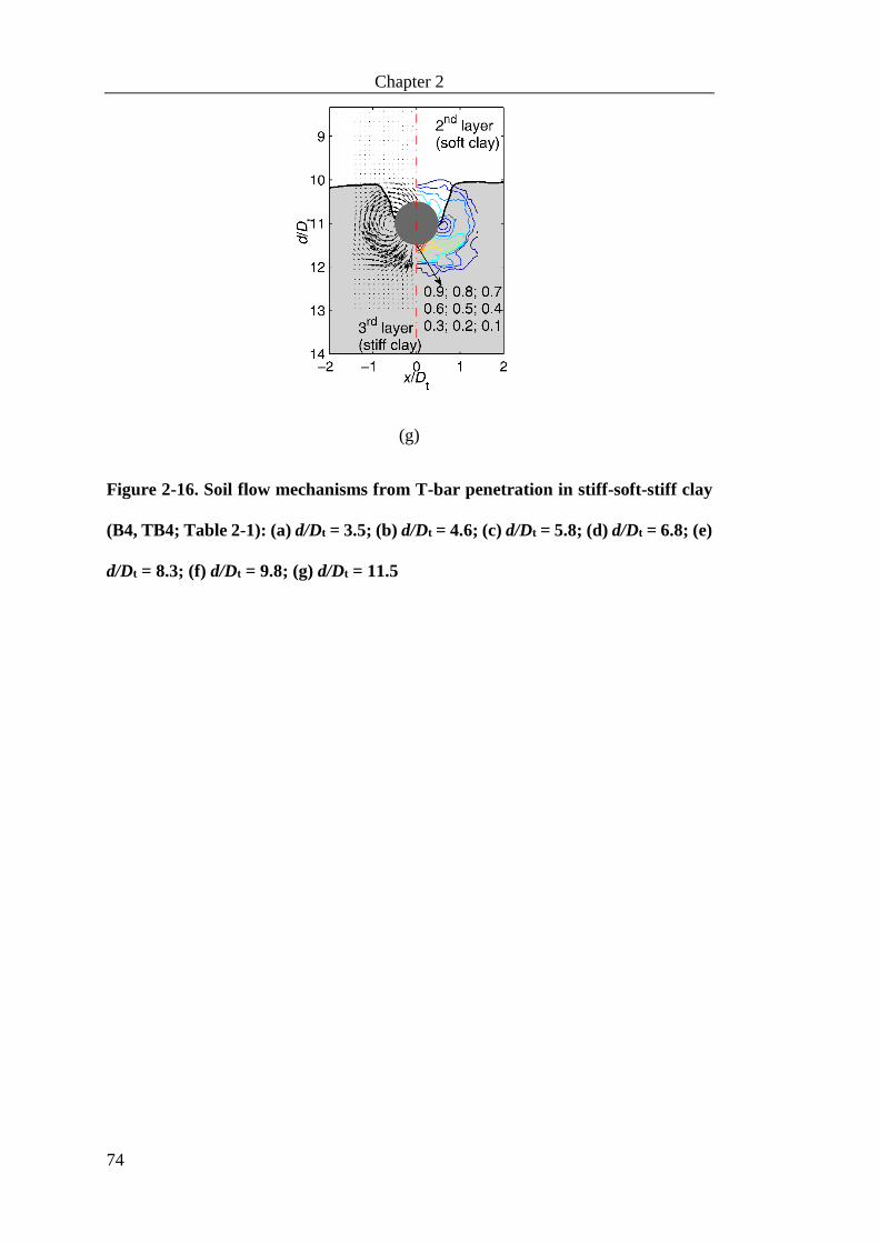
Chapter 2

74

(g)

Figure 2-16. Soil flow mechanisms from T-bar penetration in stiff-soft-stiff clay

(B4, TB4; Table 2-1): (a) d/Dt = 3.5; (b) d/Dt = 4.6; (c) d/Dt = 5.8; (d) d/Dt = 6.8; (e)

d/Dt = 8.3; (f) d/Dt = 9.8; (g) d/Dt = 11.5


centrifuge test

75

Figure 2-17. Resistance profile from T-bar penetration in stiff-soft-stiff clay (B4,

TB4; Table 2-1)

Chapter 2

76

(a) (b) (c)

(d) (e)

Figure 2-18. Soil flow mechanisms from ball penetration in soft-stiff clay (B1,

Ball1; Table 2-1): (a) d/Db = 0.4; (b) d/Db = 3.9; (c) d/Db = 8.4; (d) d/Db = 9.0; (e)

d/Db = 10.2


centrifuge test

77

Figure 2-19. Typical streamline of ball penetration mechanism

Chapter 2

78

(a)

(b)

Figure 2-20. Displacement paths of soil elements at ~2.4Db above soft-stiff

interface during continuous ball penetration (B1, Ball1; Table 2-1): (a)


soil element M1


centrifuge test

79

(a)

(b)

Figure 2-21. Displacement paths of soil elements at ~0.1Db above soft-stiff



soil element N1

Chapter 2

80

(a) (b)

(c) (d)

Figure 2-22. Soil flow mechanisms from ball penetration in stiff-soft clay (B2,



centrifuge test

81

(a)

(b)

Figure 2-23. Displacement paths of soil elements at ~3.1Db above stiff-soft



soil element M1

Chapter 2

82

(a)

(b)

Figure 2-24. Displacement paths of soil elements at ~0.2Db above stiff-soft



soil element N1


centrifuge test

83

(a) (b)

(c) (d)

Figure 2-25. Soil flow mechanisms from ball penetration in soft-stiff-soft clay (B3,


Chapter 2

84

(a) (b)

(c) (d)


centrifuge test

85

(e) (f)

(g) (h)

Figure 2-26. Soil flow mechanisms from ball penetration in stiff-soft-stiff clay (B4,

Ball4; Table 2-1): (a) d/Db = 2.4; (b) d/Db = 3.3; (c) d/Db = 4.1; (d) d/Db = 5.0; (e)

d/Db = 5.5; (f) d/Db = 6.5; (g) d/Db = 7.1; (h) d/Db = 8.8

87

CHAPTER 3 SOIL FLOW MECHANISMS AROUND

CONE PENETROMETER IN LAYERED CLAY

SEDIMENTS – PIV IN CENTRIFUGE TEST

ABSTRACT

Cone penetrometer test (CPT) is widely used for in-situ site investigations and for

establishing direct penetrometer to foundation (e.g. pile) or anchor (e.g. suction

caisson) design correlations. This chapter focuses on the soil flow mechanisms during

the continuous penetration of a cone penetrometer in layered clays. A series of

centrifuge tests was conducted with the cone penetrometer penetrating through soft-

stiff, stiff-soft, soft-stiff-soft, and stiff-soft-stiff clay profiles. Particle image

velocimetry (PIV) allowed accurate resolution of the soil flow mechanism around the

cone where a half cone model was penetrated into layered clays against a transparent

window. The observed soil movement was compared with both previous observations

from pile/cone and shallow strain path method (SSPM) prediction. The comparison

with SSPM results shows that, the SSPM can provide reasonable evaluations on

maximum lateral and vertical displacements even though the upheave movement is

overestimated. The effect of soil layering on the failure mechanisms was studied

extensively by exploiting soil flow mechanisms and soil displacement paths at various

distances from the cone centreline and the soil layer interface. The reported

characteristics of cone penetration in layered soils provided in-depth understanding of

cone penetration responses that will lead to the development of mechanism-based

theoretical model for cone penetration in layered fine-grained soils.

Chapter 3

88

3.1 Introduction

Cone penetrometer test (CPT) is not only one of the most popular in-situ tools for site

investigations, but also regarded as an effective tool for designing pile, suction caisson

and torpedo anchors due to the resemblances of the corresponding penetration process

(DNV, 1992; Borghi et al., 2001; Andersen et al., 2008; Hossain et al., 2015; Koh et

al., 2017). Due to its wide application, the penetration of the cone penetrometer has

been studied extensively to establish the relationship between soil strength and

measured resistance (Baligh, 1975; Teh & Houlsby, 1991; Van den Berg et al., 1996;

Yu & Mitchell, 1998; Yu et al., 2000; Lu et al., 2004; Walker & Yu, 2010; Vermeer,

2013; Gupta et al., 2015; Ma et al., 2017). Since the measured resistance is inherently

linked to the mobilised soil failure mechanisms around the cone, various methods have

been adopted to predict, measure or visualise the soil displacement.

3.1.1 Cone penetration mechanisms from theoretical solutions

Theoretical prediction of soil displacement from the cone penetration mostly falls into

the regime of the cavity expansion theory or the strain path method. The lateral

displacement induced by the cone penetration can be simplified as a two-dimensional

plain strain problem and evaluated with the cylinder cavity expansion theory

(Randolph & Wroth, 1979). A more sophisticated analytical model, the strain path

method (SPM), has been used to estimate the deformation area around the cone at deep

penetration, which simplifies soil as a viscous fluid flowing around a stationary

Soil flow mechanisms around cone penetrometer in layered clay sediments – PIV in

centrifuge test

89

penetrometer located within the flow (Baligh, 1985). Sagaseta et al. (1997) improved

the SPM accounting for stress free ground surface and named as shallow strain path

method (SSPM), which allows the cone penetration to be simulated from the soil

surface. However, these methods do not take into account the effect of soil layering.

3.1.2 Cone penetration mechanisms from numerical analyses

Numerical analysis techniques have been used to explore the soil failure mechanisms

in layered soils. Van den Berg et al. (1996) presented an Eulerian analysis of the cone

penetration tests in multilayer soils. Based on a finite difference approach, analyses

were carried out by Ahmadi & Robertson (2005). A linear elastic analysis studying

the effects of soil layering on penetration resistance was carried out by Vreugdenhil et

al. (1994). For cone penetration in multilayer clays, Walker & Yu (2010) analysed for

two layer stiff-soft and three-layer uniform stiff-soft-stiff clays using arbitrary

Lagrangian-Eulerian (ALE) method.. Large deformation finite element (LDFE)

analyses were carried out using the commercial FE package Abaqus/Explicit. Ma et

al. (2015, 2017a, 2017b) have explored a much wider range encompassing soft-stiff,

stiff-soft, soft-stiff-soft and stiff-soft-stiff clay profiles with LDFE analyses performed

using AFENA. The general consensus is that the penetrometer resistance in the

vicinity of the interface between the two soil layers depends on the strength and

stiffness ratio between the adjacent layers and thickness of the interbedded layer

relative to the cone diameter.

Chapter 3

90

3.1.3 Cone penetration mechanisms from physical model tests

Physical direct measurements or visualisations of soil displacements through

laboratory testing have been achieved in two ways: (i) penetrating a model full-cone

into the body of representative transparent soils (i.e. transparent clay or transparent

sand) in a transparent box or a box with a transparent window side, which removed

the opacity of natural soils and facilitated the soil motion to be captured by a camera

via a laser sheet or markers (Lehane & Gill, 2004; NI et al., 2010; Chini, 2015); (ii)

penetrating a model half-cone into natural soil samples against a transparent window

of the testing box, allowing for the soil motion to be captured by a camera via the

textures added on the soil facing the window (Randolph et al., 1979; Gue, 1984; Mo

et al., 2015). The texture was created by coloured flock powders to provide contrasting

texture to the fine grain soils for image analysis (Hossain & Randolph, 2010). Then

the captured images can be analysed by advanced image analysis techniques of particle

image velocimetry (PIV; White et al. (2003)) to quantify the failure mechanisms. The

half-object technique with PIV analysis is applied for natural soils. This can eliminate

the limitation and dissimilarity of transparent soils compared to natural soils (Liu &

Iskander, 2010). In layered sediments, only Mo et al. (2015) carried out a series of

centrifuge tests and exposed cone penetration mechanisms in layered sand deposits

varying the density of the sand layers by the half-cone model. To the authors’

knowledge, there has no such investigation undertaken of cone penetration in layered

clay deposits.


centrifuge test

91

3.1.4 Aim of this chapter

This chapter fills the knowledge gap by presenting physical visual evidence of soil

failure mechanisms associated with the cone penetration in layered clay deposits. The

soil movements measured in the centrifuge tests and quantified through PIV analyses

are compared with those from the theoretical shallow strain path method (SSPM). The

effect of soil layering on the soil failure mechanisms is revealed through both the

evolving soil flow patterns and soil particle displacement paths at various distances

from the layer interface.

3.2 Centrifuge modelling

All centrifuge tests were carried out at 50g in the beam centrifuge at The University

of Western Australia (Randolph et al., 1991). The experimental set-up is shown in

Figure 3-1. A purposely-designed PIV strongbox with a Plexiglas window was built

to allow the observation of soil deformations through the window. The PIV strongbox

has an internal size of 337 mm (length) × 100 mm (width) × 299 mm (depth), which

was fitted tightly at one side of a beam standard strongbox with a camera mounted on

the other side for image capturing. A 20 mm water layer was maintained above the

soil sample during testing to ensure saturation.

3.2.1 Model penetrometer

A model half-cone penetrometer was fabricated by dissecting a 10 mm diameter

cylindrical duraluminum bar (Dc = 0.5 m in prototype) and machining the apex tip

Chapter 3

92

angle to 60° (Figure 3-2a). A rubber O-ring was fitted along the periphery of the flat

face of the model. This was to achieve a good contact of the cone-face with the window

while penetrating the half-cone against the window avoiding any soil ingress between

the cone face and the window. The surfaces of the model were relatively smooth as

they were anodised and not sand blasted.

Figure 3-2b shows the schematic display of the cone penetrometer penetration in

layered clay, where d is the penetration depth of the cone tip from the soil surface, t is

the distance of the cone tip to the underlying layer interface. sui, hi and γi represent the

undrained shear strength, height, and soil density of the corresponding layer, i = 1, 2,

3. The layer shaded with light grey is to represent the stiff clay layer, and this is

consistent with all the mechanism figures in this chapter.

The model cone was penetrated into the soil at a constant rate of v = 0.3 mm/s, ensuring

undrained conditions (Finnie & Randolph, 1994) with dimensionless velocity vDc/cv

= 37 > 30 (cv = ~2.6 m2/year), and allowing adequate image capturing frequency for

PIV analysis at the same time.

All half-cone PIV tests were performed in the middle section of the window (Figure

3-1b) within the camera field of view. In order to obtain the cone resistance profile in

layer sediments, a standard full-cone penetrometer of the same diameter as the PIV

model (i.e. Dc = 10 mm) is adopted and tested at intervals during each test (Figure

3-1b). The final penetration depth was around 220 mm, leaving a 50 mm (i.e. 5Dc)


centrifuge test

93

clearance from the bottom boundary (soil sample height = 270 mm) and a 90 mm (9Dc)

clearance from the back wall boundary. These clearance distances were to minimise

any boundary influence, which was confirmed by the recorded penetration resistance

profiles, (with no significant increase when approaching its final penetration depth)

and observed soil failure mechanisms. Further, from an extensive investigation, Ullah

et al. (2014) reported that, in clay, a distance of 0.7~1.0 dimeter of the penetrating

object is sufficient for avoiding the influence of the boundary.

3.2.2 Sample preparation and soil strength characterisation

The cone penetration tests were performed on layered specimens of kaolin clay, with

the engineering properties given by Stewart (1992). A homogeneous de-aired slurry

was prepared by mixing commercially available kaolin clay powder with water at 120%

water content in a ribbon-blade mixer with vacuum pump. Clay samples with uniform

strength profile were prepared by performing consolidation at 1g on the laboratory

floor in two separate 625 mm long × 390 mm wide × 325 mm deep cuboid strongboxes.

One-dimensional consolidation was performed in stages, up to final pressures of 400

kPa and 100 kPa to produce comparatively stiff and soft samples. Test specimens were

prepared by cutting the pre-consolidated samples according to the size of the PIV

strongbox and planned layers thickness, and then sliding the layers into the PIV

strongbox according to planned stratification (as in Table 3-1). To add texture to the

white kaolin clay for PIV analysis and to track the deformation of different layers,

green and black flock powders were sprinkled on the stiff and soft clay layers

Chapter 3

94

respectively on the sides facing the window (Dingle et al., 2008; Hossain & Randolph,

2010; Hossain, 2014).

Four boxes of test specimens were prepared varying stratification as soft-stiff, stiff-

soft, soft-stiff-soft, stiff-soft-stiff (B1~4; Table 3-1). In addition, a box was prepared

with single layer soft clay (B0; Table 3-1). The details of layered soil strength

determination can be found in the previous chapter (2.3.1) of the thesis, with the soft

layer is ~7.5 kPa and stiff layer ~29.1 kPa. The effective unit weights (γ') of the soft

and stiff layers were ~7.0 kN/m3 and ~7.4 kN/m3 respectively.

3.2.3 Image capture and PIV analysis

The experimental set up is shown in Figure 3-1. In order to reduce friction, white

petroleum jelly was used to smoothen the flat face of the half cone and rubber O-ring.

A two-dimensional actuator was mounted on the sides of the standard beam strongbox,

and above the PIV strongbox. The half cone was then fitted with the actuator and

pushed in-flight into the soil sample against the window. Pictures were taken

continuously by the camera mounted at right angle to the window. Two LED lights

placed at the top and bottom just in front of the PIV box were used to provide sufficient

light for the pictures.

A Prosilica GC2450C digital still camera operating in continuous shooting mode was

used to capture the images of the penetrometer and the surrounding soil throughout

the tests. The 5 megapixel digital images were taken at 0.05 mm/picture (i.e. 6 Hz) for


centrifuge test

95

each test. A 50-mm grid consisting of 24 control points (black dot on a white

background) was installed within the Plexiglas window. A centroiding technique,

based on the coordinates of these control points from reference axes, was implemented

for photogrammetric corrections and transferring image space to object space. In this

way, any in-flight image-space displacement of the control markers incurred by the

movement of the camera during testing was accounted for. Full details of the PIV and

photogrammetric analysis are described in White et al. (2003) and Stanier et al. (2015).


This section discusses the effect of soil layering on the soil failure mechanisms around

the cone penetrometer. A range of stratification commonly encountered in offshore

fine grained seabed sediments (Osborne et al., 2011) were considered as soft-stiff,

stiff-soft, soft-stiff-soft and stiff-soft-stiff clay. The results from testing on single layer

soft clay (B0) are presented first for comparing with existing mechanisms.

3.3.1 Cone penetration in single layer clay and comparison with SSPM theory

Figure 3-3a illustrates the soil flow mechanism at d/Dc = 13.2 for the cone penetration

in single layer clay (Box B0, cone test CPT0; Table 3-1). The incremental

displacement field (vectors on the left side of Figure 3-3a) was quantified by

successive images with a cone penetration increment of 0.22Dc. The corresponding

contours are displayed on the right side of Figure 3-3a. The vectors are scaled up 6

times for a clear view and the values of contour are normalised by the cone penetration

Chapter 3

96

incremental depth. The contour levels in the figure includes 0.5, 0.45, 0.4, 0.35, 0.3,

0.25, 0.2, 0.15, 0.1 and 0.05 (i.e. the label of 0.5~0.05 in Figure 3-3a). This style is

kept for all following graphs of soil flow mechanisms in the rest of this chapter.

It can be observed that the soil displacement zone is a bulb mainly around the cone tip

and expands radially somewhat perpendicular to the face of the cone tip. This feature

is consistent with the (i) observed mechanism from a cone penetration in both loose

and dense sands (Mo et al., 2015) (Figure 3-3b), (ii) mechanism from a cone

penetration LDFE analysis in clay (Ma et al., 2017) (Figure 3-3c), (iii) SSPM theory

prediction (Figure 3-3d). For the cone, the closest contour line to the cone is 0.5,

showing that the soil near the conical face moves at half of the cone penetration rate.

However, for the cylindrical base of the T-bar or spherical base of the ball

penetrometer, the soil right beneath the penetrometer moves with the penetrometer at

roughly its full penetration rate (i.e. within 0.9 contour line; Figure 2-7). The outer

contour line represents a soil displacement at 5% of the cone penetration depth, which

defines the soil displacement zone. The size of this zone can be measured in Figure

3-3a as 1.1Dc downward (from the cone tip) and 1.2Dc outward (from the cone centre

line). The upper boundary of the influence zone is in accordance with a line with an

inclination of ~40° to the vertical (Figure 3-3a). This is close to the 45 obtained from

the test by Mo et al. (2015) in loose sand (Figure 3-3b).

The contours of soil displacement ratio to the cone incremental penetration depth

predicted by SSPM (Sagaseta et al., 1997) with the same penetration depth (prototype)


centrifuge test

97

are depicted in Figure 3-3d. It is noted that the SSPM is built on the simple pile

solution that originally proposed by Baligh (1975) and, therefore, a round tip was

considered. In general, it shows a reasonable agreement between the present PIV

analysis with a conical tip and SSPM analysis with a round tip for the soil

displacement zone below the cone tip. However, by SSPM, the upper boundary of the

soil displacement zone is over predicted above the cone shoulder. This may be

attributed to the fact that SSPM simplifies the soil as an ideal flow and excludes soil

overburden pressure, cone surface friction etc., hence overestimates the soil upward

movement. For the cone with a round tip (SSPM, Figure 3-3d), the soil displacement

vectors point in the radial direction from the centre of the round tip; while for the cone

with a conical tip, the soil displacements somewhat perpendicular to the face of the

cone tip (PIV, Figure 3-3a).

3.3.2 Cone penetration in layered sediments

3.3.2.1 Cone penetration resistance profiles

Figure 3-4a~b display the resistance profiles from full-cone penetration tests in two

layer (Boxes B1 and B2 in Table 3-1) and three layer (Boxes B3 and B4 in Table 3-1)

deposits, respectively. The net cone resistance is calculated by deducting the

overburden pressure and divided by projection area (details referring to Chapter 4),

and the cone penetration depth is normalised as d/Dc. For stiff-soft layering (B2), the

cone resistance decreases abruptly when the cone tip touches the soil layer interface

followed by a relatively gradual decrease in the soft layer. In contrast, for soft-stiff

Chapter 3

98

layering (B1), there is a sudden increase in resistance when the cone tip touches the

soil layer interface followed by a consistent increase rate in the stiff soil layer till the

resistance reaches its limit. The transition depth from the top layer to the bottom layer

is relatively faster for soft-stiff soil layers (B1) than that for stiff-soft soil layers (B2).

In the soft 1st layer, the thickness of h1/Dc = 18.5 (B1 in Figure 3-4a) is sufficient to

mobilise the full (ultimate) penetration resistance of that layer. In the stiff 1st layer, the

thickness of h1/Dc = 18.6 (B1) seems to be not sufficient to mobilise the full (ultimate)

resistance of that layer. The full resistance may be significantly higher as can be seen

from the resistance in the stiff 2nd layer (B1) and stiff 3rd layer (B4). The four resistance

profiles show that the net resistance of the soft layers fall into the range of 80~120

kPa, and the stiff layer fall into 225~320 kPa. Some softening in the top layer may

account for the discrepancy. The interbedded stiff layer with h2/Dc = 8.0 (B3) is

apparently not sufficient to reach the ultimate resistance of that layer, with the ultimate

resistance lower than any of the stiff layers.

The soil movements during the process of cone passing through the layer interfaces

will be illustrated in detail in the following section with half-cone PIV analysis results

at different depths, which are also marked on Figure 3-4 with filled triangle or circle

at corresponding resistance profile.

3.3.2.2 Cone penetration in soft-stiff clay: soil flow mechanism

Figure 3-5 illustrates the soil flow mechanisms of the cone penetration in soft-stiff

clay (h1/Dc = 18.5; B1, CPT1; Table 3-1). It can be seen that during initial penetration


centrifuge test

99

in the top soft layer (d/Dc = 11.8; Figure 3-5a), the flow mechanism is similar to that

in uniform soft sample (Figure 3-3a). With further penetration as the cone approaches

the interface (d/Dc = 18.1; Figure 3-5b), the soil flow is mostly restricted in the 1st soft

layer with minimal flow in the 2nd stiff layer. The height of the displaced zone is

therefore reduced. With the tip just entering the stiff clay (d/Dc = 18.5; Figure 3-5c),

the soil flow in the 1st layer is displaced laterally, leading to mobilisation of a

squeezing mechanism. This is very similar to the squeezing mechanism mobilised

with a T-bar approaching a stiff clay layer (Figure 2-7). Because of this lateral

squeezing, when the cone tip penetrates fully into the 2nd layer (d/Dc = 19.6; Figure

3-5d), the layer interface deforms only moderately and no soft clay is dragged down

under the interface. The soil flow becomes fully confined within the 2nd (stiff) layer.

This has led to a sharp increase in penetration resistance in the 2nd layer immediately

after the soft-stiff layer interface (see Figure 3-4a).

A series of soil elements are tracked to study the lateral and vertical movements

induced by the cone penetration. The original location of the soil elements, as well as

the cone penetration depth at the start (y = y1) and end (y = y2) of tracking, are defined

in Figure 3-6. To understand the effect of layering on soil displacements, the soil

elements at various distances from the layer interface (t) are studied. At each distance

t, a series of soil elements with various distances from the penetration centreline (x)

are tracked.

Chapter 3

100

For soil elements far away from the soil layer interface, a series of soil element with x

varying from 0.75Dc to 6Dc are tracked as the cone penetrates from 3Dc above the soil

element level (i.e. y1 = -3Dc) to 2Dc under it (i.e. y2 = 2Dc). This is regarded as a case

with little influence of the 2nd layer due to the large distance away from the interface

of t = 4.5Dc. The tracked trajectories are shown in Figure 3-7a. Generally, they all

show a downward-outward movement as the cone passes the soil element. As expected,

the soil element closer to the cone travels deeper and wider distances. At the end of

the displacement path, a slight upward movement is recorded for x ≤ 1Dc. This is

consistent with the observation of a flat-end cone in transparent soil by Lehane & Gill

(2004), where upward movement was observed for x ≤ 0.92Dc. However, their

observed upward movement at the end of the path in transparent soil is greater than

that obtained from this study in clay. The greater upward soil movement observed in

transparent soil may be due to the low overburden pressure from the low unit weight

of the transparent soil, i.e. amorphous silica (Ganiyu et al., 2016), and shallower soil

element embedment depth (114 mm in Lehane & Gill (2004) vs. 7 m in this study).

As the cone approaches (y < 0) and leaves (y > 0) the soil element at x = 0.75Dc, the

evolution of normalised incremental lateral (x/Dc) and vertical (y/Dc) displacements

are plotted in Figure 3-7b as a function of the cone elevation (i.e. y/Dc, negative y

means the position of cone above the original soil element elevation). When the cone

elevation is between -2.5Dc and 0.5Dc, the soil downward displacement accumulate

earlier and faster than the outward movement. Both x/Dc and y/Dc increase sharply


centrifuge test

101

when the cone passes the soil element with y/Dc = -0.5~1.0, which is termed as ‘active

zone’. When the cone is at 1.0Dc below the original level of the soil element, both

lateral and vertical displacement attains to a plateau i.e. the soil movement diminishes.

The soil element rests at 0.11Dc outwards and 0.08Dc downwards from its original

location. The slopes of the curves are the displacement ratio of the soil element to the

cone penetration velocity. Since the cone has a constant penetration velocity, the

slopes of the curves represent the soil element velocity. It is apparent that the peak

velocities of the soil element in both x and y directions occur at about y = 0, i.e. when

the cone tip reaches the original soil element level.

The corresponding theoretical soil displacement trajectories from SSPM are shown in

Figure 3-8 for comparison. The displacement paths for all elements form an arc

showing downward-outward followed by upward-outward trend. By comparing with

the measured displacement in Figure 3-7a, theoretical displacements are shallower and

much more profound in upward movement. Possible explanation might be: (i) rigid

perfectly-plastic material (inviscid fluid) is considered in SSPM, and as such no

downward elastic deformation can be reflected, and (ii) no overburden pressure is

considered, allowing more upward movement.

The measured ultimate lateral and vertical displacements for soil elements at various

distances from the cone penetration track are illustrated in Figure 3-9a and Figure 3-9b

together with the experimental results on cone or pile penetration from the literature

Chapter 3

102

(Cooke & Price, 1973; Randolph et al., 1979; Francescon, 1983; Gue, 1984; Lehane

& Gill, 2004). The cone or pile model geometry and soil sample information of these

experimental programmes are included in the legend, and more details can be found

in Gill & Lehane (2001) and Lehane & Gill (2004). It is evident that the tracked cone

penetration depth in Figure 3-7a covers the full displacement process of the soil

elements selected. Thus the ultimate displacements of the soil elements in the current

study agree very well with the existing data, where the soil displacement tracking was

made for the full penetration of the object (i.e. cone or pile), despite the variation in

experimental procedure, penetrating object and soil material used.

The predictions by two theoretical methods—cavity expansion theory (Randolph et

al., 1979) and SSPM (Sagaseta et al., 1997)—are also included in Figure 3-9 for

comparison. The cylinder cavity expansion theory can only predict lateral outward

movement, which is slightly larger than that measured from this study. SSPM provides

good estimation of the lateral displacement and maximum downward movement

throughout the whole measured range, but underestimates the ultimate vertical

displacement especially for x/Dc < 1 due to the outward-upward movement predicted

after the outwards-downwards movement (see Figure 3-8).

For soil elements near the soil layer interface, the tracked trajectories of soil elements

at t = 0.1Dc with various distances from the penetration track are shown in Figure 3-10.

The effect of squeezing from the underlaying stiff layer, displayed in Figure 3-5b~c,


centrifuge test

103

can be quantified by comparing Figure 3-10 with Figure 3-7. It can be seen that, the

presence of the underlying stiff layer (Figure 3-10) has forced the soil elements more

outward and less downward. For the element at x/Dc = 0.75, the ultimate x/Dc = 0.13,

y/Dc = 0.07 in Figure 3-10; and ultimate x/Dc = 0.11, y/Dc = 0.08 in Figure 3-7,

which means that the maximum lateral displacement is increased by 18% and the

maximum downward movement is reduced by 14%.

3.3.2.3 Cone penetration in stiff-soft clay: soil flow mechanism

The evolvement of soil flow mechanisms with the advancement of the cone in stiff-

soft clay is shown in Figure 3-11 (h1/Dc = 18.6; B2, CPT2; Table 3-1). The soil flow

mechanism in stiff clay (d/Dc = 12.4; Figure 3-11a) is very similar to that in soft clay

(Figure 3-3a and Figure 3-5a), with the outer contour reaches 1Dc (compared to 1.1Dc

in soft clay) below the cone tip and 1.2Dc (compared to 1.2Dc in soft clay) from the

penetration centreline. The upper boundary of the influence zone inclines ~45° to the

vertical, which is slightly higher compared to 40° in soft clay (see Figure 3-3a), but

matches with 45 inclination obtained by Mo et al. (2015) from testing in loose sand.

When the cone approaches the soil layer interface (d/Dc = 17.8; Figure 3-11b), the soil

flow directs mostly downward and laterally outward in the 2nd layer since it is easier

to move the soft soil underneath. This resembles the ‘punch-through’ mechanism

observed by Hossain and Randolph (2010) for spudcan penetration in stiff-soft clay

deposits. As mentioned before, here the term ‘punch-through’ is only for depicting the

enhance soil downwards movement when approaching the bottom soft layer, because

Chapter 3

104

displacement-control penetrometer is not at the risk of punching-through. As the cone

tip penetrates into the soft layer (d/Dc = 18.8; Figure 3-11c), a significant deformation

of the layer boundary occurs by the large downward soil movement. Some stiff soil

material is being dragged down with the cone. After the cone tip passes through the

layer boundary (d/Dc = 20.7; Figure 3-11d), the soil flow is fully confined in the soft

layer. After the cone tip penetration into the 2nd layer, a certain penetration depth is

required for the soil mobilisation zone to be detached from the 1st layer. The mobilised

mechanisms in Figure 3-11c~d, have led to a more gradual decrease in penetration

resistance profile in the 2nd (soft layer) as can be seen in Figure 3-4. Due to the pointy

tip of the cone, no stiff soil plug is trapped under the cone penetrometer, unlike the

spherical ball penetrometer illustrated in Chapter 2.

Similar to the soft-stiff clay study, two groups of elements located originally at ~4.5Dc

(away from the layer interface) and ~0.1Dc (near the layer interface) above the layer

interface were tracked as the cone penetrates from 3Dc above the soil element level

(i.e. y1 = -3Dc) to 2Dc under it (i.e. y2 = 2Dc). Their trajectories are shown in Figure

3-12. The relative trend between Figure 3-12b and Figure 3-12a (with and without the

underlying layer influence) is reversed of that between Figure 3-10 and Figure 3-7.

Compared to Figure 3-12a, the downward movement of Figure 3-12b is augmented

by ~19% and the outward movement is shortened by ~24%. This is because the

underlying soft layer of stiff-soft clay deposit attracts the soil downward movement as

opposed to restriction by the underlying stiff layer of soft-stiff clay deposit.


centrifuge test

105

The displacements of the soil elements away from the interface (Figure 3-12a) can be

compared to those in soft layer (Figure 3-7a) (both with ~4.5Dc from the underlying

layer). For the soil element at x = 0.75Dc, it can be noted that the ultimate vertical

downward displacement (∆y) in stiff clay is significantly higher, for example ∆y =

0.14Dc in stiff layer versus 0.08Dc in soft clay. A direct comparison is made in Figure

3-13 showing the development of soil vertical displacement with the cone penetration

in soft-stiff (CPT1) and stiff-soft (CPT2) clay. For both soil elements, the vertical

displacement initiates from cone at ~3Dc above the original level and attains to the

peak or ultimate displacements at around ~1Dc blow the original level although the

rate of development and the ultimate displacement are remarkably higher in stiff clay

(CPT2). Even though the displacement zones are only slightly different (40° for CPT1

and 45° for CPT2), as described in the previous section, the difference has

accumulated with continuous penetration, resulting in an obvious longer trajectory.

This may be an evidence that soil parameters (including soil layer profiles) have an

accumulated influence on the mobilised flow mechanism zone, especially on the soil

displacements. This is contrary to the assumption adopted in SPM/SSPM analysis

where soil displacement path is insensitive to soil parameters. This influence should

be taken into account for assessing various geotechnical problems such as spudcan-

pile interaction, pile-pile interaction and so on.

Chapter 3

106

3.3.2.4 Cone penetration in three layer clay: soil flow mechanism

Figure 3-14 presents the mechanisms of the cone penetration in soft-stiff-soft clay at

4 critical depths (B3, CPT3; Table 3-1). For cone in the 1st -2nd (soft-stiff) layers, the

mechanism is similar to those from CPT1. However, due to the thinner 1st layer for

CPT3 (h1/Dc = 6.8 for CPT3 vs h1/Dc = 18.5 for CPT1) (see Table 3-1), when the cone

passes through the interface of 1st-2nd (soft-stiff) layers, the overburden pressure (i.e.

γ1h1) for CPT3 is much lower than that for CPT1. The lower overburden pressure for

CPT3 near the interface of 1st-2nd layers has led to more lateral movement of the soft

soil in the 1st layer. As such, by comparing Figure 3-14a with Figure 3-5b, the soil

displacement zone (i.e. 0.05 contour line) is wider (outward) and higher (upward) for

CPT3 in Figure 3-14a.

Once the cone has passed the interface of 2nd-3rd (stiff-soft) layers, some similarity can

be observed between the mechanism from CPT3 (Figure 3-14c and Figure 3-14d) and

those from CPT2 (Figure 3-11b and Figure 3-11d) as the strength ratio and overburden

pressure at the interface level are similar (h1/Dc = 14.8Dc for CPT3 vs h1/Dc = 18.6Dc

for CPT2, see Table 3-1). However, by inspecting Figure 3-11d and Figure 3-14d, it

can be seen that, in Figure 3-11d for CPT2, the stiff soil is dragged downwards into

the bottom soft layer locally (i.e. adjacent to the cone); in Figure 3-14d for CPT3, the

stiff soil bends downward more evenly. This is possibly because the thinner stiff layer

for CPT3 behaves more like a beam. Due to the more even bending of the thin stiff


centrifuge test

107

layer in Figure 3-14d, the soil displacement zone is deeper and more spread in the

bottom soft layer than that in Figure 3-11d.

Figure 3-15 displays the soil flow mechanisms for the cone penetration in stiff-soft-

stiff clay (B4, CPT4; Table 3-1). Similarly, when the cone passes the interface of stiff-

soft (i.e. 1st-2nd) layers, the stiff soil is dragged downwards into the 2nd soft layer

(Figure 3-15b~c). And the squeezing mechanism in the soft soil is observed when the

cone approaches the soft-stiff (2nd-3rd) layer interface (Figure 3-15d).

In summary, as the cone passes the soft-stiff layer boundary, a squeezing mechanism

in the soft layer dominates the behaviour with minimal deformation of the layer

boundary. This squeezing mechanism is more profound when the overburden pressure

is relatively low (i.e. the layer interface is relatively shallow). However, as the cone

passes the stiff-soft layer boundary, a ‘punch-through’ mechanism dominates the

behaviour, leading to significant downward deformation of the layer interface. Due to

the pointy tip of the cone, regardless of the layers strength ratio, no soil plug from the

upper layer can be trapped down into the lower layer after the shoulder of the cone

passes the interface.


This chapter has reported experimental results from a series of centrifuge model tests

investigating the evolution of soil failure mechanisms during a cone penetrometer

penetration in single, two layer and three layer clay deposits. The extensive study has

Chapter 3

108

encompassed soft-stiff, stiff-soft, soft-stiff-soft and stiff-soft-stiff profiles as they are

commonly encountered in the hydrocarbon active seabed sediments. The following

conclusions can be drawn from the presented results.

For a cone penetrating into a single uniform clay layer, the soil deformation

concentrates mainly below the cone shoulder, with a minimal extension above the

shoulder. The soil displacement measured in this study falls in the range from previous

studies. The comparison with SSPM results shows that, the SSPM can provide

reasonable evaluations on maximum lateral and vertical displacements even though

the upheave movement is overestimated, underestimating the ultimate displacement.

For a cone penetrating into layered clays, the layering effects can be summarised as:

(1) When the cone passes a soft-stiff layer interface, the laterally outward soil flow

in the soft layer just above the interface is apparent, which is termed as

squeezing mechanism. More profound squeezing mechanism is associated

with relatively low overburden stress at the interface level, leading to minimal

deformation of the interface;

(2) When the cone passes a stiff-soft layer interface, the layer interface moves

downward, with the stiff soil adjacent to the cone is dragged into the soft layer;

(3) For all investigated layered deposits, no soil plug was trapped at the base of

the advancing cone due to the pointy shape of the cone base.


centrifuge test

109

3.5 References

Ahmadi, M. M. & Robertson, P. K. (2005). Thin-layer effects on the CPT qc

measurement. Canadian Geotechnical Journal 42, No. 5, 1302-1317.

Baligh, M. M. (1975). Theory of deep site static cone penetration resistance.

Cambridge, Mass, Report No. R75-56.

Baligh, M. M. (1985). Strain path method. Journal of Geotechnical Engineering 111,

No. 9, 1108-1136.

Borghi, X., White, D., Bolton, M. & Springman, S. (2001). Empirical pile design

based on cone penetrometer data: an explanation for the reduction of unit base

resistance between CPTs and piles. Proceedings of the 5th International

Conference on Deep Foundations Practice. Citeseer, Singapore, pp. 125-132.

Chini, C. M. (2015). An experimental method for visualizing undrained shearing

failure in a transparent soft clay surrogate. PhD thesis, University of Illinois

at Urbana-Champaign, Champaign, USA.

Cooke, R. & Price, G. (1973). Strains and displacements around friction piles.

Proceedings of the 8th International Symposium on Mechanics of Foundation

Houston: Texas University.

Dingle, H. R. C., White, D. J. & Gaudin, C. (2008). Mechanisms of pipe embedment

and lateral breakout on soft clay. Canadian Geotechnical Journal 45, No. 5,

636-652.

Det Norske Veritas (DNV) (1992). DNV CN 30.4 Foundations. Classification Notes

30.4. Høvik, Norway: DNV.

Chapter 3

110


failure of shallow foundations on calcareous sediments. Proceedings of

International Conference on Behaviour of Offshore Structures, Boston, MA,

pp. 217-230.

Francescon, M. (1983). Model pile tests in clay: Stresses and displacements due to

installation and axial loading. PhD thesis, University of Cambridge,

Cambridge, UK.

Ganiyu, A. A., Rashid, A. S. A. & Osman, M. H. (2016). Utilisation of transparent

synthetic soil surrogates in geotechnical physical models: A review. Journal

of Rock Mechanics and Geotechnical Engineering 8, No. 4, 568-576.

Gill, D. R. & Lehane, B. M. (2001). An optical technique for investigating soil

displacement patterns. Geotechnical Testing Journal 24, No. 3, 324-329.

Gue, S. S. (1984). Ground heave around driven piles in clay. PhD thesis, University

of Oxford, Oxford, UK.

Gupta, T., Chakraborty, T., Abdel-Rahman, K. & Achmus, M. (2015). Large

Deformation Finite Element Analysis of Static Cone Penetration Test. Indian





layered clays: centrifuge tests. Géotechnique 60, No. 3, 157-170.

Koh, K. X., Hossain, M. S., & Kim, Y. (2016). Installation and monotonic pullout of

a suction caisson anchor in calcareous silt. Journal of Geotechnical and

Geoenvironmental Engineering 143, No. 2, 04016098.


centrifuge test

111

Lehane, B. M. & Gill, D. R. (2004). Displacement fields induced by penetrometer

installation in an artificial soil. International Journal of Physical Modelling in

Geotechnics 4, No. 1, 25-36.

Liu, J. & Iskander, M. G. (2010). Modelling capacity of transparent soil. Canadian


Lu, Q., Randolph, M. F., Hu, Y. & Bugarski, I. (2004). A numerical study of cone

penetration in clay. Géotechnique 54, No. 4, 257-267.




No. 1, 04015055.


and Shear Strengths for Stiff-Soft-Stiff Clays Using Cone Penetration Test:

LDFE Analyses. International Journal of Geomechanics 17, No. 9, 06017011-

1 - 06017011-11.

Ma, H., Zhou, M., Hu, Y. & Hossain, M. S. (2017). Effects of cone tip roughness, in-

situ stress anisotropy and strength inhomogeneity on CPT data interpretation

in layered marine clays: numerical study. Engineering Geology.



Ni, Q., Hird, C. & Guymer, I. (2010). Physical modelling of pile penetration in clay

using transparent soil and particle image velocimetry. Géotechnique 60, No. 2,

121-132.

Chapter 3

112




up units.


new centrifuge facility. Proceedings of the international conference on

centrifuge modelling, Centrifuge' 91. Rotterdam, the Netherlands: Balkema.,

Boulder, Colorado, pp. 3-9.

Randolph, M. F., Steenfeld, J. & Wroth, P. (1979). The effect of pile type on design

parameters for driven piles. Proceedings of the 7th European Conference on

Soil Mechanics and Foundation Engineering, Brighton, England.

Randolph, M. F. & Wroth, C. (1979). An analytical solution for the consolidation

around a driven pile. International Journal for Numerical and Analytical

Methods in Geomechanics 3, No. 3, 217-229.

Sagaseta, C., Whittle, A. & Santagata, M. (1997). Deformation analysis of shallow

penetration in clay. International Journal for Numerical and Analytical

Methods in Geomechanics 21, No. 10, 687-719.




Stewart, D. P. (1992). Lateral loading of piled bridge abutments due to embankment

construction. PhD thesis, University of Western Australia, Perth, Australia.

Teh, C. & Houlsby, G. (1991). An analytical study of the cone penetration test in clay.



centrifuge test

113

Van Den Berg, P., De Borst, R. & Huétink, H. (1996). An Eulerean finite element

model for penetration in layered soil. International Journal for Numerical and


Vermeer, P. (2013). Large deformation analysis of cone penetration testing in

undrained clay. Proceedings of the International Conference on Installation

Effects in Geotechnical Engineering (ICIEGE). Rotterdam, pp. 1-7.

Vreugdenhil, R., Davis, R. & Berrill, J. (1994). Interpretation of cone penetration

results in multilayered soils. International Journal for Numerical and


Walker, J. & Yu, H. S. (2010). Analysis of the cone penetration test in layered clay.


White, D. J., Take, W. A. & Bolton, M. D. (2003). Soil deformation measurement

using particle image velocimetry (PIV) and photogrammetry. Géotechnique

53, No. 7, 619-631.

Yu, H. S., Herrmann, L. R. & Boulanger, R. W. (2000). Analysis of steady cone

penetration in clay. Journal of Geotechnical and Geoenvironmental

Engineering 126, No. 7, 594-605.

Yu, H. S. & Mitchell, J. K. (1998). Analysis of cone resistance: review of methods.

Journal of Geotechnical and Geoenvironmental Engineering 124, No. 2, 140-

149.

Chapter 3

114

Table 3-1. Summary of centrifuge tests

Box Test

Soil

description

Layer thickness

h1*

(mm)

h1/Dc

h2*

(mm)

h2/Dc

h3*

(mm)

h3/Dc

B0 CPT0 Soft clay 250 25 -- --

B1 CPT1 Soft-stiff 185.4 18.5 84.6 8.5 --

B2 CPT2 Stiff-soft 185.9 18.6 84.1 8.4 --

B3 CPT3 Soft-stiff-soft 68.4 6.8 79.8 8.0 121.8 12.1

B4 CPT4 Stiff-soft-stiff 77.4 7.4 74.9 7.5 117.7 11.8

*Model scale


centrifuge test

115

Cone

Soil sampleAcutuator

Camera

Lights

(a)

(b)

Figure 3-1. Centrifuge test setup: (a) photo; (b) schematic diagram with

dimensions (unit: mm)

Chapter 3

116

O-ring

Side

view

(a)

Soil surface

Cone

d

1st – 2

nd layer

interface

su1,

h1, γ

1

2nd

– 3rd

layer

interface

su3,

h3, γ

3s

u2,

h2, γ

2

t

Water surface

Dc

(b)

Figure 3-2. Half cone model for PIV testing: (a) photos; (b) schematic diagram of

cone in layered sediment


centrifuge test

117

(a)

(b)

Dense sand Loose sand

118

(c)

(d)

Figure 3-3. Soil flow mechanism of cone penetration in soft clay at d/Dc = 13.0

(CPT0, Table 3-1): (a) PIV analysis in this study; (b) observed mechanism from

a cone penetration in both loose and dense sands (Mo et al., 2015), (c) mechanism

from a cone penetration LDFE analysis in clay (Ma et al., 2017); (d) SSPM theory

prediction


centrifuge test

119

(a)

(b)

Figure 3-4. Resistance profiles from cone penetrometer: (a) two layer clay; (b)

three layer clay

Chapter 3

120

(a) (b)

(c) (d)

Figure 3-5. Soil flow mechanisms of cone penetration in soft-stiff clay (CPT1,

Table 3-1): (a)d/Dc = 11.8; (b)d/Dc = 18.1; (c)d/Dc = 18.5; (d)d/Dc = 19.6


centrifuge test

121

Tracked point

y

Layer interface

y =

y1

y =

y2

x∆x

∆y

dt

Soil surface

Figure 3-6. Schematic diagram of tracked point for displacement path

Chapter 3

122

(a)

(b)


during continuous cone penetration from y1 = -3Dc to y2 = 2Dc (CPT1; Table 3-1):

(a) trajectories of soil particle with varying distance from penetration track; (b)

development of horizontal and vertical displacements of soil element x = 0.75 Dc

with cone penetration


centrifuge test

123

Figure 3-8. Soil element displacement path predicted by SSPM theory

Chapter 3

124

(a)

(b)

Figure 3-9. Comparison of soil displacement: (a) lateral; (b) vertical


centrifuge test

125

(a)

(b)

Figure 3-10. Displacement paths of soil elements at ~0.1Dc above soft-stiff

interface during continuous cone penetration (CPT1; Table 3-1): (a) trajectories

of soil particle with varying distance from penetration track; (b) development of

horizontal and vertical displacements of soil element x = 0.75Dc with cone

penetration

Chapter 3

126

(a) (b)

(c) (d)

Figure 3-11. Soil flow mechanisms of cone penetration in stiff-soft clay (CPT2,

Table 3-1): (a) d/Dc = 12.4; (b) d/Dc = 17.8; (c) d/Dc = 18.8; (d) d/Dc = 20.7


centrifuge test

127

(a)

(b)

Figure 3-12. Soil element displacement path with varying distance from stiff-soft

interface (CPT2, Table 3-1) (a) t/Dc = 4.5; (b) t/Dc = 0.1

Chapter 3

128

Figure 3-13. Comparison of soil element vertical displacement development in

CPT1 and CPT2 for soil element originally positioned at t = 4.5Dc and x = 0.75Dc


centrifuge test

129

(a) (b)

(c) (d)

Figure 3-14. Soil flow mechanisms of cone penetration in soft-stiff-soft clay

(CPT3, Table 3-1): (a) d/Dc = 6.5; (b) d/Dc = 8.3; (c) d/Dc = 14.3; (d) d/Dc = 17.1

Chapter 3

130

(a) (b)

(c) (d)


centrifuge test

131

(e)

Figure 3-15. Soil flow mechanism of cone penetration in stiff-soft-stiff clay (CPT4,

Table 3-1): (a) d/Dc = 6.9; (b) d/Dc = 8.0; (c) d/Dc = 9.0; (d) d/Dc = 14.8; (e) d/Dc =

16.3

133

CHAPTER 4 AMBIENT PRESSURE CALIBRATION

FOR CONE PENETROMETER TEST: NECESSARY?

ABSTRACT

The cone tip load cell needs to be calibrated before the cone penetration test (CPT)

data in soil can be used to interpret the soil properties. The cone tip load cell is

routinely calibrated through cone tip axial loading test. In this study, the CPTs were

conducted in fully saturated layered clay deposits in a centrifuge. The net cone

resistance was found to be negative by using the calibration factor obtained through

axial loading test. This is illogical. Further CPT calibration was performed in water in

the centrifuge under 150 times earth gravity. The CPT calibration factor under ambient

pressure in water was found to be different from that obtained through axial loading

test. By using both calibration factors from axial load test and under ambient pressure,

the net cone resistance was recalculated. The interpreted soil undrained shear strength

using the recalculated net cone resistance was consistent with that from a parallel ball

penetrometer test. Since the soil overburden pressure acts on the cone tip as an ambient

pressure, the cone tip load cell should be calibrated under ambient pressure to provide

logical interpretation of CPT data.

Chapter 4

134

4.1 Introduction

Due to the high cost of obtaining high quality soil samples offshore, field test becomes

a popular choice to determine the geotechnical properties of seabed sediments. Cone

penetrometer test (CPT) is the commonly adopted in-situ test, which is mainly due to

its superior feature of providing a continuous resistance profile, compared to vane

shear test. As shown in Figure 4-1, the cone penetrometer comprises a cone-shaped

tip and a cylindrical shaft. The standard cone penetrometer used in the field has a base

area of 10 cm2 (diameter Dc = 35.7 mm), although the diameter can go up to 71.4 mm

(40 cm2) (Robertson & Cabal, 2015). There are also some miniature cones (Dc = 7 mm;

10 mm) that have been reported for laboratory test applications (Lee, 2009).

The wide use of cone penetration test for soil characterisation in geotechnical practice

rises the demand for accurate measurement, which relies on the accuracy of its sensors.

The cone penetrometer generally consists of cone tip load cell and sleeve friction load

cell. This study focuses on the former. The cone tip load cell is embedded in the shaft

just above the shoulder of the cone (as marked in Figure 4-1). The accuracy of the

cone tip load cell and its calibration factor are crucial in terms of interpreting the

corresponding soil strength. For the normal practice with a cone, zero-load error is a

reliable indicator of output stability (ASTM, 2012). Zero-load error refers to zero-load

readings (or baseline readings; Mayne, 2007) difference before and after a sounding.

Recalibration is only necessary when the zero-load error drifts out of requirement

(ASTM, 2012, Robertson & Cabal, 2015), and ASTM (2012) regulates this critical

error as 2% full scale output.

To ensure sensible calculation using the measured data, in-house check-up for

calibration factor of a load cell is routinely conducted. The recommended method for

Ambient pressure calibration for cone penetrometer test: necessary?

135

in-house calibration check of the cone tip load cell is through axial load test (Lunne et

al., 1997), in which the cone penetrometer is loaded/unloaded against a reference load

cell (Peuchen & Terwindt, 2014). The detail of the test can be found in Chen & Mayne

(1994). Through loading/unloading, the voltage response of the tested cone tip load

cell is recorded and the load on the cone is known from the reference load cell. The

calibration factor can be obtained through best fitting the data, with the gradient

expressed as,

t

qC

v= (4-1)

where vt is the voltage reading of the load cell and q is the corresponding pressure

applied on the load cell, and the pressure-to-voltage ratio is called conversion or

calibration factor (C). A qualified cone should prove good linear behaviour under

loading with nonlinearity satisfy certain requirement (ASTM, 2012).

The calibration factor obtained through the axial load test can only reflect the load cell

behaviour under a tip resistance. However, when the cone penetrates into soil, it

subjects to both tip resistance and ambient pressure (i.e. overburden pressure) (Figure

4-2). In this chapter, firstly an in-house check-up for calibration factor is conducted

through axial load test at 1g on the laboratory floor. Then the load gauge behaviour

under ambient pressure is examined through a series of hydraulic pressure tests in a

centrifuge. The calibration factors are compared, and both factors are used in the CPT

data interpretation framework. Finally, the necessity of performing a calibration test

under ambient pressure is demonstrated.

Chapter 4

136

4.2 Experiment details

A 10 mm diameter miniature cone penetrometer with a 60° cone tip was considered in

this chapter. A tip load cell with 10 MPa capacity was equipped just above the cone

shoulder (Figure 4-1b). No pore pressure transducers were equipped on this

penetrometer so area ratio correction is not needed. In this section, firstly two types of

calibration test are described—the axial load test that considers net tip resistance and

hydraulic test that simulates ambient pressure. Then the CPT and ball tests in a layered

clay sample are introduced.

4.2.1 Axial load test at 1g

In the axial load calibration test, the cone penetrometer concentrically placed on a

high-resolution reference load cell was mounted on a compression machine, as shown

in Figure 4-3. Compression loading and unloading was carried out in steps. In each

step, sufficient time was allowed to stabilise the response readings, and the stabilised

voltage (or bit from the cone tip load cell) and pressure (from the reference load cell)

were recorded. Compression pressure was gradually increased up to 2865 kPa (force

224.9 N/total projection area of the cone 78.5 mm2) prior to unloading.

4.2.2 Hydraulic pressure test at 150g

To test cone tip load cell behaviour under ambient pressure, the cone penetrometer

was penetrated from the water surface to the designed depth (220 mm in model scale).

To achieve a large water pressure, the hydraulic test was conducted under an enhanced

gravity environment of 150 times the earth gravity (150g) in a beam centrifuge at The

University of Western Australia (Randolph et al., 1991). The experimental set-up is

shown in Figure 4-4. The centrifuge strongbox with internal dimensions of 650 mm

(length) × 390 mm (width) × 325 mm (depth) was filled with water. The cone


137

penetrometer was penetrated in water at a constant velocity of 1.15 mm/s, which is the

same as the penetration velocity of the cone in the layered clay sample (described

later). High-speed data acquisition system (10 Hz) was equipped with the centrifuge

to allow in-flight data monitoring and collection. At the final depth of ~220 mm (~33

m in equivalent prototype scale), the maximum prototype hydraulic ambient pressure

was 323 kPa. The load cell response of the penetrometer was tested several times to

ensure the data consistency.

4.2.3 Centrifuge penetrometer test on layered clays—cone and ball

penetrometers

The same cone penetrometer just discussed was used to characterise a soft-over-stiff

layered clay deposit at an acceleration level of 50g. The soft and stiff clay layers were

produced from kaolin clay slurry pre-consolidated under the final pressures of 100 and

400 kPa respectively. The average effective unit weight (γ') of the soft and stiff clay

layers was ~7.2 kN/m3. The thickness of the top soft clay layer and the bottom stiff

clay layer was 9.5 m and 4 m respectively (prototype scale). A ball penetrometer test

was also conducted in parallel to the CPT for comparison. The miniature ball

penetrometer was 9 mm in dimeter. More information on the recently developed ball

penetrometer can be found in Watson et al. (1998) and Newson et al. (1999). Ball

penetrometer test was conducted at 1.25 mm/s and CPT at 1.15 mm/s to target an

identical normalised velocity (nulling relative strain rate effect) and to ensure

undrained conditions in the kaolin clay (Finnie & Randolph, 1994).


The following section discusses the calibration factors for the cone tip load cell derived

from the axial load test at 1g and the ambient pressure test at 150g. The CPT data from

Chapter 4

138

the test in the layered clay are then interpreted using these calibration factors. The

interpreted soil undrained shear strength from the CPT data is compared with that from

the ball penetrometer test data.

4.3.1 Calibration factor from axial load test

The recorded data from axial load test are shown in Figure 4-5. Applied pressure from

the reference load cell is plotted as a function of voltage from the cone tip load cell. A

perfectly linear response can be seen in both loading and unloading stage, with a

negligible divergence between loading and unloading stage and minimal zero-load

error (<0.1% full scale output). A linear fitting provides the calibration factor (Cax, ‘ax’

stands for axial load) of 5184.4.

4.3.2 Processing of CPT data based on axial load calibration factor

The obtained calibration factor from axial load test was used to interpret the cone

penetration test data in the layered clay. The soil undrained shear strength was

interpreted according to Lunne et al. (2011)

( )

netu CPT

c

net vo

qs

N

q q

=

= −

(4-2)

where su (CPT) is the undrained shear strength of clay from CPT, qnet is the net resistance

from the cone tip, q is the total measured resistance from the cone tip, σvo (= × d, is

the total unit weight of the soil and d is the penetration depth of the cone shoulder) is

the overburden pressure at corresponding depth. The bearing capacity factor of

resistance factor of cone in clay, Nc, was taken as 13.56 (Low et al., 2010).

The result from the ball penetrometer test can be processed to obtain the undrained

shear strength as


139

( )u ball

b

qs

N= (4-3)

where the ball bearing capacity factor Nb was taken as 11.17 (Randolph et al., 2000;

Zhou et al., 2013). As the ball penetrometer penetration generally mobilises a full

flow-round mechanism around the ball except for the shaft connection area, the soil

overburden pressure has a minimal influence on the measured resistance (Randolph,

2004).

The interpreted undrained shear strength profiles from the cone su(CPT) and ball su(ball)

penetrometer tests in soft-over-stiff clay (with soft and stiff layer marked with light

and dark shaded column separately) are shown in Figure 4-6. It is interesting to notice

that a negative undrained shear strength profile between 4.5~9.6 m was obtained from

the cone penetration data while an expected positive strength profile was obtained for

the full penetration depths from the ball penetrometer data. The negative undrained

shear strength in Figure 4-6 is resulted from the negative resistance calculated by

Equation 4-2. A similar phenomenon of negative resistance was reported by Boylan

& Long (2006) from a field test on peat. The negative undrained shear strength is

clearly illogical, leading to further investigation on the cone calibration factor.

4.3.3 Processing of CPT data using both axial load calibration factor and

hydraulic pressure calibration factor

The result from hydraulic pressure calibration is shown in Figure 4-7, plotting the

ambient hydraulic pressure as a function of voltage response from the cone tip load

cell. Surprisingly, the voltage-pressure response (Figure 4-7) shows a negative

correlation between the voltage output under ambient pressure, which is the opposite

to the one observed from the axial load test (see Figure 4-5). From the fitting curve in

Figure 4-7, the calibration factor under ambient pressure (Cam, ‘am’ stands for ambient

Chapter 4

140

load) is -18665 kPa/V. It is worthwhile to note that, although the load range of the

hydraulic test (323 kPa) is much less than that of the axial load test (2863 kPa), the

linear response indicates a constant calibration factor. In the tested clay deposit, the

maximum overburden pressure on the cone tip of 206 kPa also lies in this range.

To apply the cone tip load cell calibration factors in the CPT data interpretation, it

should be noted that the measured cone tip resistance includes two parts: (1) the cone

tip resistance from soil shearing during cone penetration; and (2) the cone tip

resistance from the overburden pressure from the soil (see Equation 4-2). The recorded

total voltage output can be seen as the contribution of these two components.

Therefore, it can be derived from Equations 4-1 and 4-2 that

0net v

t

ax am

qv

C C

= + (4-4)

where vt is the total voltage output. It should be noted that, if Cax = Cam, the data

interpretation becomes easier as vt = q/Cax (or q = Cax×vt). In this case, it is apparent

that Equation 4-5 degenerates to Equation 4-1, which was used in the CPT data

interpretation for Figure 4-6. However, in this case, different calibration factors were

obtained from the axial load test and ambient pressure test. Thus, qnet should be

calculated from Equation 4-5

0( )v

net t ax

am

q v CC

= − (4-5)

With the modified net tip resistance from Equation 4-5, a new strength profile can be

interpreted. In this way, the undrained shear strength is modified and compared with

the ball penetrometer result. Figure 4-8 shows that the modified net tip resistance has

produced a soil strength profile of the layered clay that is very close to that from the

ball penetrometer test. This confirms that the modified net tip resistance can provide


141

the logical interpretation of soil undrained shear strength. This exercise shows that

failing to consider the difference in calibration factors for the two components may

lead to interpretation error and even illogical result such as negative strength.

However, it is also worth noting that not all cone tip load cells show two different

calibration factors under axial load and ambient pressure. Another group of parallel

tests were conducted on the cone tip load cells, with the same size and the same type

of cone (i.e. 10 mm in diameter and only equipped with tip load cell). Figure 4-9

depicts the results from both calibration tests. It can be seen that both calibration

factors are consistent, with a difference being < 8%. This difference of the calibration

factors from 1g axial load test and centrifuge hydraulic test might be due to the

Poisson’s strain in the load cell under ambient pressure and the increased self-weight

of the cone tip under enhanced gravity (150g) (Chow et al., 2017). Since the cone

resistance profile was also measured under the influence of enhanced gravity, it is

reasonable to adopt the calibration factor from centrifuge hydraulic test for subsequent

interpretation. In this case, the negative net resistance would not happen because the

overburden pressure would increase the output voltage in a similar ratio, so deducting

it from the total tip resistance would not lead to a negative net resistance. Yet, the

interpreted strength may not be correct, as explained previously, emphasising the

necessity of the ambient pressure test.

This study shows the importance of calibration under ambient pressure because

calibration under pure axial pressure cannot always guarantee the load cell behaves in

the same way under ambient pressure. Calibration of the tip load cell under

atmospheric condition, i.e. pressurised chamber test, has been reported by Peuchen &

Terwindt (2014), which is able to reflect the ambient pressure effect on the load cell

rather than axial load test. However, the pressurised chamber test is not suggested by

Chapter 4

142

the standards for cone tip load cell (ASTM, 2012), and it is not commonly adopted in

in-house calibration check of calibration factor. In fact, the pressurised triaxial

apparatus are normally used to check for pore pressure transducer as well as net area

ratio of cones (Mayne, 2007). In addition and critically, the hydraulic pressure test

introduced in this chapter can also examine the load cell behaviour under water e.g.

potential water ingress and corresponding drifting/oscillation of response during

actual testing, which could not be simulated by the air pressure chamber test.

4.4 Summary and concluding remarks

The total cone resistance measured by CPT is used to interpret soil undrained shear

strength. The total cone resistance includes two parts: the shear resistance and the

overburden pressure. The cone tip load cell needs to be calibrated using the axial load

test (for the shear resistance) and the ambient pressure test (for the overburden

pressure). When the calibration factors under the axial load test and under the ambient

pressure test are the same (or similar), the interpretation can be straightforward.

However, when the two calibration factors are different, both calibration should be

used for interpreting the CPT data. The hydraulic test in centrifuge has been proved to

work well to produce the cone tip load cell calibration factor under ambient pressure.

4.5 References

ASTM (2012). Standard Test Method for Performing Electronic Friction Cone and

Piezocone Penetration Testing of Soils. West Conshohocken, PA: ASTM

International.


143

Boylan, N. & Long, M. (2006). Characterisation of peat using full flow penetrometers.

Proceedings of the 4th International Conference on Soft Soil Engineering

(ICSSE). Vancouver, Canada.

Chen, B. S. & Mayne, P. W. (1994). Profiling the overconsolidation ratio of clays by

piezocone tests. Report No. GIT-CEEGEO-94, 1.

Chow, S., O'Loughlin, C., White, D. & Randolph, M. F. (2017). An extended

interpretation of the free-fall piezocone test in clay. Géotechnique 67, No. 12,

1090-1103.


failure of shallow foundations on calcareous sediments. Proceedings of

International Conference on Behaviour of Offshore Structures. Boston, MA.

Lee, K. K. (2009). Investigation of potential spudcan punch-through failure on sand

overlying clay soils. PhD thesis, The University of Western Australia, Perth,

Australia.

Low, H. E., Lunne, T., Andersen, K. H., Sjursen, M. A., LI, X. & Randolph, M. F.


penetration tests in soft clays. Géotechnique 60, No. 11, 843-859.

Lunne, T., Andersen, K. H., Low, H. E., Randolph, M. F. & Sjursen, M. (2011).

Guidelines for offshore in situ testing and interpretation in deepwater soft clays.

Canadian geotechnical journal 48, No. 4, 543-556.

Lunne, T., Robertson, P. K. & Powell, J. J. M. (1997). Cone penetration testing in

geotechnical practice, London, Blackie Academic & Professional.

Mayne, P. W. (2007). Cone Penetration Testing State-of-Practice. Atlanta, GA,

Georgia Institute of Technology.

Chapter 4

144

Newson, T. A., Watson, P. G. & Bransby, M. F. (1999). Undrained shear strength

profiling using a spherical penetrometer. Crawley, Australia, Geomechanics

Group, The University of Western Australia.

Peuchen, J. & Terwindt, J. (2014). Introduction to CPT accuracy. Proceedings of 3rd

International Symposium on Cone Penetration Testing. Las Vegas, Nevada.

Randolph, M. F., Martin, C. & Hu, Y. (2000). Limiting resistance of a spherical


Randolph, M. F. (2004). Characterisation of soft sediments for offshore applications.

Proceedings of 2nd International Conference on Site Characterization. Porto.


new centrifuge facility. Proceedings of the international conference on

centrifuge modelling, Centrifuge' 91. Boulder, Colorado, Rotterdam, the

Netherlands: Balkema.

Robertson, P. K. & Cabal, K. L. (2015). Guide to cone penetration testing 6th Edition,

Gregg Drilling & Testing, Inc. 6th Edition, Signal Hill, California.

Watson, P., Newson, T. & Randolph, M. (1998). Strength profiling in soft offshore

soils. Proceedings of 1st International Conference on Site Characterisation.

Atlanta.


145

(a) (b)

Figure 4-1. Cone penetrometer: (a) schematic diagram; (b) cone penetrometer

used in centrifuge tests

Figure 4-2. Cone penetrometer subjected to both ambient pressure and axial

resistance when penetrating in soil

Ambient pressure

Axial resistance

Chapter 4

146

Figure 4-3. Axial load test at 1g

Figure 4-4. Hydraulic pressure test in a centrifuge

Reference load cell

Cone penetrometer

Axial load from compression machine

Cone penetrometer

Water

Actuator


147

Figure 4-5. Stress-voltage response of cone tip load cell under axial load

Figure 4-6. Comparison of undrained shear strength of layered clay from ball

penetrometer test and cone penetrometer test (using calibration factor under

axial load test)

Chapter 4

148

Figure 4-7. Stress-voltage response of cone tip load cell under ambient pressure

from centrifuge hydraulic calibration test (150g)

Figure 4-8. Modified shear strength from cone penetrometer test using both

calibration factors under the axial load test and under the ambient pressure test

and its comparison with ball penetrometer result


149

Figure 4-9. Axial load calibration test result and centrifuge hydraulic calibration

test for another cone tip load cell

151

CHAPTER 5 EFFECT OF TRAPPED CAVITY

MECHANISM ON T-BAR PENETRATION

RESISTANCE IN UNIFORM CLAYS

ABSTRACT

This chapter describes large deformation finite element (LDFE) analysis of the

penetration of the T-bar penetrometer in uniform clays, identifying soil flow

mechanisms around the T-bar, the extent of any cavity above the T-bar and the

evolving penetration resistance profile. A trapped cavity above the advancing T-bar

penetrometer and its influence on the corresponding bearing capacity factor are the

crucial findings of this chapter. With the progress of T-bar penetration, a shallow

failure mechanism gradually turns to a flow-round mechanism. However, the soils

backflow around both sides of the T-bar meets at a distance above the top surface of

the T-bar, leaving a trapped cavity above the penetrating T-bar. Finally, the trapped

cavity is being backfilled and a fully localised flow-round mechanism forms. The

formation and evolvement of the trapped cavity mechanism has been studied

extensively exploring a large range of soil normalised undrained shear strength and T-

bar surface roughness. It is shown that the depths of forming a trapped cavity and

being fully filled with soil would increase with normalised undrained shear strength

and T-bar roughness. The duration, i.e. depth span, of trapped cavity mechanism from

forming to end also increases with undrained shear strength. The presence of a trapped

cavity is shown to reduce the T-bar bearing capacity factor that is commonly used in

practice. According to the depth span of trapped cavity stage, there are three scenarios:

Chapter 5

152

(i) for very soft soils (su/γ'D ≤ 1), shallow failure mechanism is directly followed by

full-flow mechanism since the trapped cavity stage is negligible; (ii) for soils with 1 <

su/γ'D ≤ 8.3, all three stages– shallow failure mechanism, trapped cavity mechanism

and full-flow mechanism – can be observed; and (iii) for soil with su/γ'D > 8.3, the

trapped cavity is not fully closed up to 30D, leading to a lower stabilised resistance

factor on the profile compared to the other two scenarios. A systematic interpretation

procedure is therefore proposed to account for the effect of the trapped cavity for more

accurate interpretation of soil undrained shear strength from the T-bar penetration

resistance.

5.1 Introduction

Site investigation tools play a key role in deep water exploration due to the high cost

and difficulty in extracting soil samples from the offshore sites for laboratory testing.

Site investigation tools include shear vane, cone penetrometer and the newly

developed ‘full-flow’ penetrometers (i.e. T-bar or ball penetrometers) (Figure 5-1). T-

bar penetrometer was first implemented by Stewart & Randolph (1994), and identified

as advantageous for investigating deep water fine-grained sediments due to: (i)

providing a continuous resistance profile that can be directly interpreted to

corresponding soil strength profile; (ii) the large projection area ratio (5~10 times

larger than the cone penetrometer) leading to high resolution in soft seabed resistance;

and (iii) the negligible influence of overburden pressure to the total resistance (Lu,

2004; Zhou & Randolph, 2009), eliminating the necessity of overburden pressure

corrections needed for the cone penetrometer. Moreover, the miniature version of the

T-bar penetrometer is now commonly used for characterising fine-grained soil samples

in both centrifuge and 1g tests for soil characterisation (e.g. Purwana et al., 2005;

Effect of trapped cavity mechanism on T-bar penetration resistance in uniform clays

153

Hossain et al., 2011). Therefore, accurate interpretation of the resistance profile from

T-bar tests is of great importance to the geotechnical community.

The foundation of interpretation method was laid by Randolph & Houlsby (1984),

simplifying the problem as a cylinder deeply penetrated in the soil. With the assumed

fully localised flow-round failure (Figure 5-2a), they found that soil undrained shear

strength (su) is in linear relationship with resistance (Equation 5-1) through a resistance

factor (Nt). Later, improved plasticity solutions were provided by Martin & Randolph

(2006). The resistance factor ranges from 9.1~11.9 depending on the T-bar roughness

factor, and 10.5 is recommended and commonly adopted in centrifuge tests.

t

netu =

N

qs (5-1)

To provide guidance for the interpretation of soil strength at shallow depths associated

with a shallow failure mechanism with soil flow towards the surface maintaining an

open cavity above the T-bar, several analytical studies have been conducted (Murff et

al., 1989; Aubeny et al., 2005). A cylidrical bar was pre-embedded at different shallow

depths (up to 5 times the T-bar diameter, D) and an open cavity was considered in the

wake of the bar (Figure 5-2b and c). It is found that the T-bar resistance factor, Nt, for

shallow embedment depths can be 30% lower than that for the deep embedment with

fully localised flow-round failure. The interpretation of soil strength at shallow depths

is particularly critical for the design of shallow foundations, mudmats and pipelines in

deep waters.

The development of large deformation finite element (LDFE) method enables the

evolvement of soil flow mechanisms and resistance factors during continuous

penetration of the T-bar to be studied systematically. White et al. (2010) explored T-

Chapter 5

154

bar penetration in uniform clay. Two failure mechanisms were identified as (i) shallow

failure mechanism with an open cavity above the bar, and (ii) sudden close of the

cavity and deep fully localised flow-round failure mechanism. The depth of attaining

the latter mechanism was shown to increase with increasing normalised undrained

shear strength, su/γ'D, where γ' is the submerged unit weight of the soil, and D is the

diameter of the T-bar cylinder. The T-bar resistance profile was therefore divided into

shallow (before mobilising the flow-round failure) and deep (after mobilising flow-

round failure) penetration stages (Figure 5-2d) and corresponding soil strength

interpretation framework was proposed.

Tho et al. (2011) however identified a trapped cavity mechanism (Figure 5-2e), with

the cavity being closed at a distance above the T-bar rather than just above the T-bar,

in between the shallow and deep mechanisms for su/γ'D > 3 and for a smooth

(roughness factor α = 0) T-bar. Critically, the trapped cavity led a 12% lower T-bar

resistance factor compared to the flow-round failure mechanism. This is due to shorter

flow path or shear failure plane.

Recently, the soil failure mechanisms during the T-bar penetration in two-layer clays

were revealed through centrifuge model tests and subsequent particle image

velocimetry (PIV) analysis (Chapter 2 of the thesis). The penetration in the very thick

top layers relative to the T-bar diameter can represent penetration in uniform layers.

Interestingly, a trapped cavity mechanism was observed for su/γ'D = 5.24, and no

trapped cavity (or may be closed very shortly and hence not evident—can be neglected)

for su/γ'D = 1.42.

For the standard T-bar penetrometer commonly used in offshore site investigations (D

= 0.04 m) and commonly encountered offshore clay strengths (su = 5~25 kPa), the


155

range of normalised strength falls between 20~100. The soil strength interpretation

framework proposed by White et al. (2010) did not take into account the trapped cavity,

and limited to su/γ'D ≤ 10. The framework proposed by Tho et al. (2011) considered

the trapped cavity but it is also limited to su/γ'D ≤ 10, fully smooth T-bar (roughness

factor α = 0) and up to 10D in penetration depth. Thus it is imperative to conduct a

more systematic study to cover the practical range of su/γ'D and T-bar roughness factor.

This chapter describes the results from LDFE analyses to provide insight into the

evolving soil failure mechanisms in both soft and stiff clays, and corresponding

influence on penetration resistance profiles. Both centrifuge scale T-bar and field scale

T-bar were considered, covering a rather wide range of su/γ'D = 1~100. The influence

of T-bar roughness factor was also investigated. Based on the results, a systematic

interpretation procedure was established for offshore designs.

5.2 Numerical analysis

This study has simplified the T-bar as an infinite long cylindrical bar, thus the T-bar

penetration was simulated as a plane strain problem, which is a commonly adopted

assumption (Lu et al., 2000; White et al., 2010). The T-bar was penetrated

continuously from the soil surface. The diameter of the T-bar, D = 0.04 m was

considered for simulating the field scale T-bar used in site investigation, and D = 0.75

m for simulating the prototype scale T-bar of a model miniature T-bar (i.e. D = 0.005

m under 150 g-level) commonly used in centrifuge testing. Due to the symmetry of

the problem, only half of the T-bar and the soil domain was modelled. The size of the

domain was set as 50D in both width and height for the field-scale T-bar and 32D for

the centrifuge-scale T-bar, which were large enough to eliminate boundary effect.

Chapter 5

156

Soil was considered as elastic-perfect plastic material obeying a Tresca failure

criterion, with the yield stress solely determined by the undrained shear stress. The

elastic behaviour was defined by Poisson’s ratio of 0.49 and Young’s modules E =

500su throughout the soil profile. A uniform submerged unit weight of γ' = 6 kN/m3

was adopted over the soil depth, representing a typical average value encountered in

the field. Uniform undrained shear strength profiles with su = 2~31.5 kPa were

considered, covering the most commonly encountered clay strength of hydrocarbon

active seabed sediments (Menzies & Roper, 2008). Therefore, the investigated

normalised strength su/γD ranged from 1 to 100. Table 5-1 lists a summary of the

considered parameters.

The interface between the T-bar and soil was modelled using elastoplastic nodal joint

elements (Herrmann, 1978), and the soil strength at the soil-T-bar interface was

modelled as αsu, where α is the roughness factor, as defined by Randolph & Houlsby

(1984). For this study, an intermediate roughness condition (α = 0.3) was adopted for

the majority of simulations, which is accepted widely for both field and miniature T-

bars. However, the effect of roughness on the depth span of the trapped cavity

mechanism and resistance factor was also examined considering α = 0~0.7 (Groups

VI, VII and VIII; Table 5-1).

In this study, LDFE analysis were conducted using the FE package AFENA (Carter &

Balaam, 1995) developed at the University of Sydney coupled with RITSS (remeshing

and interpolation technique with small strain) by Hu & Randolph (1998a) for

remeshing and interpolation. H-adaptive mesh refinement cycles (Hu & Randolph,

1998b) were implemented to optimise the mesh, hence to minimise discretisation

errors, especially in highly stressed zones. This method falls in the category of ALE

(arbitrary Lagrangian Eulerian) method (Ghosh & Kikuchi, 1991), whereby a series


157

of small-strain analysis increments are followed by remeshing, and then interpolating

the field quantities (stress and material properties) between the Gauss points in the

new mesh and those in the old mesh. The LDFE/RITSS method has been proven its

robustness in various geotechnical boundary value problems (Lu et al., 2001; Ma et

al., 2015; Zhou et al., 2013). Penetration of the T-bar is simulated from the mudline

and by specifying incremental displacements. The displacement incremental size and

number of steps of small strain analysis between each remeshing stage were chosen

such that the cumulative penetration in each remeshing stage remained in the small

strain range and less than half of the minimum element size. Six-node triangle

elements with three internal Gauss points were adopted for all analyses.

5.3 Validation of numerical model

In this section, the FE model was validated against two groups of existing results: (a)

the analytical solutions of the pre-embedded and fully embedded (no cavity) T-bar; (b)

the centrifuge test results of continuously penetrated T-bar. Both T-bar resistance

factors and soil flow mechanisms around the T-bar were studied.

5.3.1 Validation against analytical solutions

The T-bar penetration resistance from the LDFE analysis is compared with previous

analytical solutions (Randolph & Houlsby, 1984; Martin & Randolph, 2006; Group I

in Table 5-1). The T-bar was pre-embedded to 10D under the seabed surface, in order

to eliminate the surface influence and to invoke the classical flow-round mechanism

around the T-bar (Lu, 2004). The roughness factor was varied from fully smooth (i.e.

= 0) to fully rough (i.e. = 1). The comparison between the current FE results and

the upper and lower bounds solutions is shown in Figure 5-3. The resistance factor, Nt,

from the current analysis is obtained by rearranging Equation 5-1 (i.e. Nt = qnet/su =

Chapter 5

158

Fnet/(Asu), where the T-bar net resistance, Fnet, is the measured force deducting the

buoyancy force (Fb), and A is the projection area of the T-bar. For the pre-embedded

T-bar, buoyancy force equals to γ'As, where As is the submerged cross-sectional area

of the T-bar, i.e πD2/4. For the plain strain problems, the projected area of the T-bar

equals to the diameter multiplied by unit length, so the equation can be expressed as

s

t

u

F AN

Ds

−= (5-2)

It can be seen that the results from the current LDFE model lie slightly above the exact

solution with the maximum difference being 3.7%. This over estimation can be due to

the element size used in the LDFE analyses. This difference was thought to be

acceptable and hence the corresponding minimum element size of hmin = 0.022D was

used for all other analyses. The reasonable agreement between the numerical results

and the exact solutions confirms the accuracy of the current LDFE model. It is also

worth to note that although only the field-scale T-bar was adopted for this validation,

corresponding sensitivity analyses confirmed that the T-bar dimensions have no

influence on the fully embedded T-bar resistance factor.

5.3.2 Validation against centrifuge test results

Validation in terms of soil failure mechanisms were carried out against centrifuge

observation reported in Chapter 2. A T-bar penetration test was conducted in a two-

layer stiff-soft clay deposit (TB2; Table 2-1, Chapter 2): (i) the top layer of su1 = 29.1

kPa, h1 = 9.295 m (h1/D = 12.4); (ii) the bottom layer of su2 = 7.5 kPa and h2 = 4.205

m (h2/D = 5.6). The images of soil failure mechanisms were captured by a camera and

subsequently analysed by particle image velocimetry (PIV) analysis. An LDFE

analysis was carried out considering the identical parameters of centrifuge testing and

a T-bar roughness of = 0.3 (Group II, Table 5-1).


159

The soil failure mechanisms from the LDFE analyses were compared with the PIV

results for the top layer in in Figure 5-4 (noting that the depth d is from the soil surface

to the invert of the T-bar; Figure 5-1). The shallow failure mechanism with the soil

deformation directs towards to the surface (Figure 5-4a), and soil flow around the T-

bar with a trapped cavity above the T-bar (Figure 5-4b, c); all captured reasonably by

the LDFE analysis. Note, the trapped cavity remained open even at d/D = 9.8 (Figure

5-4c) for this case with su1/γ'D = 5.24.

It is clear from these two validation exercise that the LDFE/RITSS model can capture

both penetration resistance and soil failure mechanisms with reasonable accuracy,

which provides confidence to use the numerical method for the parametric analyses.

The expected agreement is reached between PIV analysis and numerical analysis on

the features of forming a trapped cavity and decreasing cavity size with penetration

down. However, it is noticed that a wider cavity in PIV analysis, while a longer and

narrower cavity simulated in LDFE analysis. One possible reason is that, in physical

modelling, the shrinkage of the inner cavity could be obstructed by water trapped

inside the cavity. Another possible reason is the adopted isotropic elastic perfect

plastic Tresca model could not consider anisotropic strength in compression and

tension as well as softening behaviour exhibited by soft clay. These might cause the

difference in backflow and cavity shape.

5.4 Parametric study-results and discussions

5.4.1 Evolvement of soil flow mechanism and trapped cavity mechanism

To illustrate typical evolution of soil failure mechanisms with the advancement of a

T-bar penetration, a case with centrifuge-scale T-bar (i.e. D = 0.75 m) and su/γ'D = 3

was selected (Group III, Table 5-1). The mobilised mechanisms at various depths from

Chapter 5

160

LDFE/RITSS analysis are displayed in Figure 5-5. At a very shallow penetration depth

of d/D = 0.5 (Figure 5-5a), the soil flow directs towards the surface, leading to surface

heave adjacent to the T-bar. A cavity is formed at the wake of the T-bar. At d/D = 1.5

(Figure 5-5b), with the increase of overburden pressure, the soil flow direction changes

from towards the surface to flow back towards the open cavity. With further

penetration of d/D = 4.4 (Figure 5-5c), the soil backflow continues and the cavity

above the T-bar becomes significantly narrow.

At a deep penetration of d/D = 5.9 (Figure 5-5d), the backfilled soil completely

touched the vertical centreline axis at a distance of ~1.6D above the T-bar i.e. a

‘trapped cavity’ is formed. This is termed as trapped cavity as there is the open cavity

still standing above the backfilled closed soil and there is no connection between these

two cavities (Figure 5-5d). With further penetration, the soil backflow forces the

trapped cavity to become shorter and narrower (see d/D = 10.1 in Figure 5-5e). The

trapped cavity eventually disappears at d/D = 10.5 and a fully localised flow-round

mechanism mobilised (Figure 5-5f). In this case, the transition from the formation of

a trapped cavity to the mobilisation of the flow-round mechanism takes ~5D

penetration (Figure 5-5d~f). In the following parametric study, this transition period

with the existence of a trapped cavity needs to be identified and the corresponding

influence on the T-bar penetration resistance are quantified for more accurate

interpretation of shear strength.

Based on the above observations, the soil flow mechanisms around a T-bar during its

continuous penetration can be divided to three stages: stage I - shallow failure

mechanism, where the soil flows towards the surface, an open cavity is formed above

the T-bar, and the soil flow is influence by the overburden pressure; stage II - trapped

cavity mechanism, where, along with an open cavity close to the soil surface, a trapped


161

cavity is formed above the T-bar; stage III - deep fully localised flow-round failure

mechanism, where there is no trapped cavity above the T-bar and soil flows around

full T-bar periphery.

5.4.2 Effect of su/γ'D on the duration of trapped cavity mechanism (Stage II)

A series of parametric study (Groups IV & V; Table 5-1) was conducted to study the

effect of su/γ'D on the depth span of existing trapped cavity mechanism for both

centrifuge- and field-scale T-bars. For clarity, the transition depth from stage I to stage

II, ht (i.e. the depth of forming the trapped cavity) was identified when the cavity walls

at the top of the trapped cavity come closer than the criteria, i.e. numerically the

minimum distance between the cavity wall and the centreline vertical axis is ≤ 0.1D

due to the soil backflow. The end of Stage II, hf, was defined as the depth where

trapped cavity closes up, i.e. numerically the maximum width/height of the trapped

cavity is ≤ 0.01D (this is also the beginning of Stage III – deep flow-round/full flow

mechanism). The start and end depths correspond well with the kinks on the resistance

factor profiles, which will be demonstrated in the next section.

The values of ht and hf are plotted in Figure 5-6 as a function of su/γ'D in a semi-

logarithmic scale. The values of ht and hf from Tho et al. (2011) are also included in

Figure 5-6 for comparison. White et al. (2010) did not recognise the trapped cavity

mechanism rather proposed an expression for the depth of attaining (or depth of

transitioning from shallow to) deep flow-round mechanism, and the corresponding

curve is also plotted in Figure 5-6. As noted previously, White et al. (2010) and Tho

et al. (2011) have covered a relatively small range of normalised strength (su/γ'D =

0.1~10), which is mainly applicable to centrifuge scale T-bar and offshore pipelines,

while this study encompassed a much wider range of su/γ'D = 1~100 including in-situ

T-bars.

Chapter 5

162

Overall the results from this study are in good agreement with the existing solutions.

Over the range of su/γ'D = 0.1~1, the trapped cavity mechanism can be ignored as ht

hf. For su/γ'D > 1, the gap between ht and hf increases dramatically with increasing

su/γ'D. The start of the trapped cavity mechanism, ht, increases gradually from 2.4 to

9.7 for su/γ'D = 1~16.8, and then stabilises at ht/D 9.7 for su/γ'D > 16.8, which can

be expressed as

0.46 0.63

2.58 0.24 for 16.8

9.7 for 16.8

u u u

t

u

s s s

h D D D

D s

D

− + =

(5-3)

This means that, for stronger soils of su/γ'D > 16.8, the trapped cavity starts to form at

the same penetration of ht/D = 9.7 regardless of the increase in soil strength. For

example, for a common offshore clay with γ' = 6 kN/m3 and a standard in-situ T-bar

with D = 0.04 m, su/γ'D > 16.8 means su > 4.0 kPa. In other words, in offshore site

investigations, for a uniform clay with strength of su > 4 kPa, a trapped cavity is

expected to form after the penetration reaches 0.4 m (as ht/D = 9.7).

Following the formation of a trapped cavity, all T-bar penetration analyses were

carried out up to d/D = 25 (Groups III, IV and V in Table 5-1). The closure of the

trapped cavity was only observed for su/γ'D ≤ 8.3. The values of hf increase

exponentially with su/γ'D. For su/γ'D > 8.3, the cavity did not close i.e. the depth of hf

was not reached within d/D = 25. Best fitting through the obtained results, a design

formula for hf can be expressed as

0.98

3.51 for 8.3f u u

h s s

D D D

=

(5-4)


163

For su/γ'D > 8.3 (i.e. su > 2.0 kPa for a standard in-situ T-bar with D = 0.04 m),

intuitively the cavity closure will occur down to a deeper penetration depth with

further penetration. It can be assumed that 1st degree calculation for hf can be

calculated by extrapolating Equation 5-4. Regardless, this greater depth span of

existing trapped cavity means a stronger (or longer) influence on the T-bar penetration

resistance and interpreting shear strength.

5.4.3 Effect of trapped cavity mechanism on T-bar resistance factor

Based on the numerical results in Figure 5-6 with the T-bar penetration up to d/D =

25, there are three scenarios: scenario 1 – for very soft clays with su/γ'D ≤ 1, the T-bar

penetration experiences stages I and III of soil failure mechanisms without any trapped

cavity mechanism (i.e. stage II); scenario 2 - for soft clays with 1 < su/γ'D ≤ 8.3, the

T-bar penetration experiences all three stages of soil failure mechanisms (i.e. stages I,

II and III); scenario 3 – for stiff clays with su/γ'D > 8.3, the T-bar penetration could

not mobilise full-flow mechanism (stage III) for up to 25D (i.e. only experience stages

I and II). Three typical profiles resistance factor, Nt, have been selected from these

three range of su/γ'D and are displayed in Figure 5-7. Both critical depths ht and hf are

marked on the profiles. Prediction using White et al.’s (2010) expression is also

included in Figure 5-7 for comparison.

To calculate Nt, the T-bar buoyancy force needs to be deducted from the measured

resistance to obtain net T-bar resistance. In contrast to the pre-embedded case, the

buoyancy force needs to be adjusted by a multiplier, i.e. fbγ'As, to account for the

influence of enhanced buoyancy effect due to the upheave of the soil adjacent to the

pipe (Merifield et al., 2009; White et al., 2010; Tho et al., 2011). The buoyancy

correction multiplier was taken as 1.3 at shallow embedment, which is in consistent

Chapter 5

164

with that proposed by Tho et al. (2011) and Merifield et al. (2009). For submerged

area As with penetration depth (d) up to 0.5D

21 4 ( ) ( )2

sin 2 1 for 0.54

s

d D d d D dD d dA

D D D D

− − −

= − −

(5-5)

After 0.5D, the submerged area gradually increases with the progress of backflow.

Referring to Figure 5-5, As increase to 82% of the maximum As (=πD2/4) at 1.5D, 99%

at 4.4D (~ht) and 100% at 10.5D (~hf). Although the pattern may vary depending on

su/γ'D, for continuity and simplicity, the buoyancy force (Fb) was set to be linearly

increasing from the d = 0.5D to d = ht, with the limiting value of γ'πD2/4.

( )2 2

2

1.3 for 0.5

1.3 0.0875 for 0.5

8 0.5

for 4

s

b t t

t

t

A d D

D DF h d D d h

h D

Dd h

= + −

−

(5-6)

It is worth noting that the influence of buoyancy can be reduced with increased su/γ'D

because the contribution of buoyancy becomes less significantly compared to the

contribution from su term (Tho et al., 2011).

An example resistance factor profile of scenario 1 is shown in Figure 5-7a. For su/γ'D

= 0.67, it shows that Nt increases sharply up to d = hf ht in stage I, and then attains

to the limiting value of Nff = 10.61 (for the T-bar with = 0.3) in stage III. The

expression in White et al. (2010) underestimates Nt in stage I.

The example resistance factor profile of scenario 2 and 3 are shown in Figure 5-7b.

For scenario 2 (su/γ'D = 3), it shows that Nt rises rapidly up to d = ht in stage I, and

then increases slowly up to d = hf in stage II before attaining the same stabilised value

for scenario 1, i.e. Nff = 10.61 at hf = 10.53D. The limiting resistance factor Nff = 10.61


165

agrees well with analytical solutions (Nt = 10.22~10.69 for = 0.3 by Randolph &

Houlsby, 1984; Martin & Randolph, 2006) and pre-embedded LDFE analysis result

(Nt = 10.61 for = 0.3). For scenario 3 (su/γ'D = 41.6), the T-bar penetration depth of

30D is not sufficient to reach hf. However, from the similar trend of increasing

tendency of Nt in stage II, it can be concluded that the profile may reach to the limiting

value down to a very deep penetration depth. Extrapolating Equation 5-4 that depth

can be hf/D = 146. Based on the above study, a typical schematic T-bar resistance

factor profile including all three stages is shown in Figure 5-8, with T-bar resistance

factor defined for different stages. In stage I, Nsf (‘sf’ stands for shallow failure) rises

sharply with depth and reaches Ncf (‘cf’ stands for cavity formed) at d = ht. In stage II,

Ntc (‘tc’ stands for trapped cavity) increases gradually and linearly with depth from Ncf

and attains to Nff (‘ff’ stands for full-flow) at d = hf. In stage III, Nt remains constant

with the value of Nff. The resistance factor associated with the three stages will be

quantified accordingly.

It can be seen that for all the three scenarios, the resistance factor Nsf is either under or

overestimated by White et al.’s (2010) expression (Figure 5-7a~b) because it was

fitted from profiles without considering trapped caivty mechanism. Therefore, a new

prediction formula for Nsf is required. Following the development procedure by White

et al. (2010), the resistance factor (Nsf) and penetration depth (d/D) from the analyses

of Groups III, IV and V (Table 5-1) are normalised by Nff and ht/D for su/γ'D ≤ 1.0 and

Ncf and hf/D for su/γ'D ≥ 1.0. The normalised resistance profiles are shown in Figure

5-9 and can be expressed as

Chapter 5

166

( )0.12

0.6 0.6 for 1

0.6 0.6 for 1 8.3

4.7 4.7 for 8.3

p

u u uff

t

p

u u usf cf

t

ucf

t

s s d sN

D D h D

s s d sN N

D D h D

d sN

h D

− + +

= − + +

− + +

(5-7)

0.43

0.33 usp

D

−

=

(5-8)

The resistance factor at the start of trapped cavity mechanism (d = ht), which is referred

to as Ncf, is around 8% lower than that at d = hf i.e. Nff for both cases in Figure 5-7b.

It also shows that Ntc increases linearly from Ncf to Nff for su/γ'D ≤ 8.3 and stays at Ncf

mostly for su/γ'D > 8.3. Hence the resistance factor Ntc in stage II can be presented as

( ) for 8.3

9.75 for 8.3

ff cf ucf t

f t

tc

u

N N sN d h

h h DN

s

D

−+ − − =

(5-9)

White et al.’s. (2010) prediction curve overestimates resistance factor as high as 8%,

and critically, without consideration of a trapped cavity, shows a different trend for

stage II with earlier attainment to Nff.

5.4.4 Effect of roughness factor (α)

The above investigations are based on α = 0.3. To investigate the effect of α on the

trapped cavity mechanism, formation and span of the trapped cavity, and penetration

resistance profile, further analyses have been carried out varying α = 0 ~ 0.7 for both

centrifuge- and field-scale T-bars (Groups VI, VII and VIII). Typical resistance factor

profiles for α = 0~0.7 but with su/γ'D = 41.6 (Group VI) are plotted in Figure 5-10.

The depth of attaining a trapped cavity, ht/D, is marked on the profiles. It is seen that


167

ht/D increases with increasing α due to delayed soil backflow. To highlight this

difference, the values of ht/D and hf/D for α = 0.3 and 0.7 and su/γ'D = 1~104.2 are

plotted together in Figure 5-11 (Groups IV and V vs. Groups VII and VIII) . Within

the penetration of d/D = 25, the trapped cavity did not close with su/γ'D > 5 for α = 0.7

and with su/γ'D > 8.3 for α = 0.3 (as discussed before). This means the depth of existing

trapped cavity is longer for rougher T-bar. It can be seen from Figure 5-11 that the

overall trend of both ht/D and hf/D for α = 0.7 is very similar to that for α = 0.3. The

difference in both ht/D and hf/D between α = 0.3 and α = 0.7 increases with increasing

su/γ'D. In addition, the gap between ht/D and hf/D (i.e. the span of stage II) for α = 0.7

is much wider that that for α = 0.3. In summary, T-bar roughness has significant

influence on the trapped cavity mechanism and its depth span of existence, and hence

on the interpretation of shear strength.

The profile of Nt for α = 0.7 over su/γ'D = 1~104.2 are shown in Figure 5-12 (Groups

VII and VIII). The resistance factors for both trapped cavity mechanism and full-flow

mechanism (Ncf and Nff) are marked on the profiles. In general, the form of the Nt

profiles in all three stages are very similar to those for α = 0.3. The penetration depth

of d/D = 25 was sufficient for attaining limiting resistance factor Nff for su/γ'D = 1~5,

but not for su/γ'D = 7~104.2. For all normalised strengths, the resistance factor at d =

ht i.e. Ncf of 10.49 is consistent and is around 13% lower than the limiting resistance

factor of Nff = 11.88.

The Figure 5-10 and Figure 5-12 clearly show that the values of Ncf and Nff for a

particular α are somewhat constant regardless of su/γ'D. The values of Ncf and Nff for

various roughness factors are listed in Table 2-1. The difference of Ntc and Nff increases

from 6% for α = 0 to 8% for α = 0.3 and to 13% for α = 0.7. As discussed, this is

because a rougher T-bar tends to delay the soil backflow and maintains a larger trapped

Chapter 5

168

cavity for deeper depth span, as typically evidenced from Figure 5-13 illustrating the

trapped cavity at penetration depth of d/D = 16 for α = 0, 0.3 and 0.7.

5.5 Interpretation framework and exercise

Based on the results presented previously, a suggested procedure for estimating

undrained shear strength from T-bar penetration resistance in a single layer clay is

outlined in Figure 5-14, covering all three scenarios revealed in this chapter. The

procedure is based on a more typical (for both field and centrifuge) T-bar roughness

of = 0.3, though can be modified for other values of using corresponding values

of Ncf, Nff, ht, hf (e.g. for = 0.7 using Figure 5-12, Figure 5-13 and Table 5-2).

Although uniform strength was considered, in field applications, the small size of the

T-bar means that the normalised local soil strength gradient – expressed in

dimensionless for as kD/su – is usually small (White et al., 2010). As such, the

procedure will be applicable in soil with varying strength with depth – allowing the

local value of su/γ'D to be used.

To examine the capability of this framework, a centrifuge test result from a miniature

T-bar (D = 1 m) penetration in single layer kaolin clay deposit (liquid limit, LL = 61%;

plastic limit, PL = 27%; Gs = 2.6; Stewart,1992), as shown in Figure 2-15, is selected.

Following the procedure, first, the soil undrained strength was estimated using

Equation 5-1 with Nff = 10.61, based on which an initial value of su = 29 kPa was

determined, giving su/γ'D = 4.03 where γ' = ~7.2 kN/m3. Then ht/D and hf/D were

calculated using Equations 5-3 and 5-4 respectively, and resistance factors for stage I,

stage II and stage III, using Equations 5-7 and 5-9 and Nff = 10.61 respectively.


169

The deduced shear strength profile shows a nearly uniform clay profile except for

shallow depth with d/D < 3 due to softening of the pre-consolidated sample. This

resembles the expected profile for a pre-consolidated clay deposit. In contrast, the

deduced strength profile using the plasticity solution with flow-round mechanism, i.e.

without considering shallow and trapped cavity mechanisms, shows a gradually

increasing trend up to d/D = 11. This means the shear strength prior to d/D < 11 is

significantly underestimated. For the predicted resistance profile by White et al.

(2010), it matches the first half of stage I and stage III, however it underestimates the

strength for the second half of stage I and stage II. This part may be critical for

designing surface and shallow foundations, mudmats and pipelines. The framework

by Tho et al., (2011) is only for smooth T-bar with a limiting resistance factor value

of 9.14, and as such the corresponding prediction cannot be used directly for

comparison.

5.6 Conclusions

The mechanism and resistance factor during the T-bar penetration in uniform clay has

been studied through LDFE analysis. A novel trapped cavity mechanism has been

revealed and studied extensively by varying normalised soil undrained shear strength

in a large range and T-bar roughness factor. The following conclusions can be drawn

from this chapter.

• Compared to the conventionally used plasticity solutions with deep flow-round

mechanism, shallow failure mechanism and trapped cavity mechanism were

captured prior to mobilising deep flow-round mechanism. In contrast to White

et al. (2010), a trapped cavity mechanism was identified in between shallow

and deep flow-round mechanism.

Chapter 5

170

• The critical depths of forming a trapped cavity mechanism and mobilising deep

flow-round mechanism were quantified, and hence the depth span of shallow

failure mechanism (stage I) and trapped cavity mechanism (stage II).

• Both shallow and trapped cavity mechanisms provided lower T-bar resistance

factors and hence higher undrained shear strength compared to the deep flow-

round mechanism provided resistance factor.

• T-bar roughness factor was found to increase the (i) critical depths of forming

trapped cavity mechanism and depth span of the trapped cavity, and (ii) more

reduction on resistance factor at trapped cavity mechanism stage compared to

that of full-flow mechanism.

• For interpreting the undrained shear strength profile from T-bar penetration

resistance in single layer clay, a new framework was proposed, accounting for

the shallow and trapped cavity mechanisms with different soil undrained shear

strength level (Figure 5-14).

It is worth to mention that the adopted Tresca model does not consider strain softening

and strain rate dependency. The combined effect of rate dependency and progressive

softening has been investigated extensively in Einav & Randolph (2005) and Zhou &

Randolph (2007, 2009). Following their work, Zhou et al. (2016) has conducted a

parallel comparison using the basic Tresca model and Tresca model with implemented

strain softening and rate dependency with typical kaolin clay parameters on ball

penetrometers, which conclude a difference of less than 3% on resistance factor.

Therefore, the proposed framework is considered suitable for low sensitivity clays.

For high-sensitivity clays, further investigation is required to make corrections for

effect of strain softening and rate dependency.


171

5.7 References



320-325.

Carter, J. P. & Balaam, N. P. (1995). AFENA user manual 5.0. Geotechnical Research

Centre, The University of Sydney, Sydney, Australia.

Ghosh, S. & Kikuchi, N. (1991). An arbitrary Lagrangian-Eulerian finite element

method for large deformation analysis of elastic-viscoplastic solids. Computer

Methods in Applied Mechanics and Engineering 86, No. 2, 127-188.

Herrmann, L. R. (1978). Finite element analysis of contact problems. Journal of the

Engineering Mechanics Division 104, No. 5, 1043-1057.

Hossain, M. S., Randolph, M. F. & Saunier, Y. N. (2011). Spudcan deep penetration

in multi-layered fine-grained soils. International Journal of Physical

Modelling in Geotechnics 11, No. 3, 100-115.

Hu, Y. & Randolph, M. (1998a). A practical numerical approach for large deformation

problems in soil. International Journal for Numerical and Analytical Methods

in Geomechanics 22, No. 5, 327-350.

Hu, Y. & Randolph, M. F. (1998b). H-adaptive FE analysis of elasto-plastic non-

homogeneous soil with large deformation. Computers and Geotechnics 23, No.

1, 61-83.

Lu, Q. (2004). A numerical study of penetration resistance in clay. PhD thesis,


Chapter 5

172

Lu, Q., Hu, Y. & Randolph, M. (2000). FE analysis for T-bar and spherical

penetrometers in cohesive soil. Proceedings of the 10th International Offshore

and Polar Engineering Conference. International Society of Offshore and

Polar Engineers. ISOPE, Seattle, USA, 617-623.

Lu, Q., Hu, Y. & Randolph, M. F. (2001). Deep penetration in soft clay with strength

increasing with depth. Proceedings of the 11th International Offshore and

Polar Engineering Conference. International Society of Offshore and Polar

Engineers. ISOPE, Stavanger, Norway, 453-458.




No. 1, 04015055.



Merifield, R., White, D. & Randolph, M. F. (2009). Effect of surface heave on

response of partially embedded pipelines on clay. Journal of Geotechnical and

Geoenvironmental Engineering 135, No. 6, 819-829.



Purwana, O.A., C.F. Leung, Y.K. Chow and K.S. Foo. (2005). Influence of base

suction on extraction of jack-up spudcans. Géotechnique 55, No. 10, 741-753.




173

Stewart, D. P. (1992). Lateral loading of piled bridge abutments due to embankment

construction. PhD thesis, University of Western Australia, Perth, Australia.

Stewart, D. P. & Randolph, M. F. (1994). T-bar penetration testing in soft clay.

Journal of Geotechnical Engineering 120, No. 12, 2230-2235.



No. 1, 59-69.




Zhou, H. & Randolph, M. F. (2009). Numerical investigations into cycling of full-

flow penetrometers in soft clay. Géotechnique 59, No. 10, 801-812.



174

Table 5-1. Summary of LDFE analyses performed on uniform clays

Group ID Scale D (m) su (kPa) su/γ'D α Note

I Field 0.04 10 41.6

0; 0.1; 0.2;

0.3; 0.4; 0.5;

0.6; 0.7; 0.8;

0.9; 1

Pre-embedded LDFE analysis; resistance factor

validation of the LDFE model

II Centrifuge 0.75 29.1 5.24 0.3 With the same layering condition in Chapter 2;

mechanism validation of the LDFE model

III Centrifuge 0.75 13.5 3 0.3 Evolvement of failure mechanism with T-bar

penetration

IV Centrifuge 0.75

3; 4.5; 9; 13.5;

18; 22.5; 27;

31.5

0.67; 1; 2; 3; 4;

5; 6; 7 0.3

Effect of shear strength on trapped cavity

mechanism of centrifuge scale T-bar

V Field 0.04 2; 4; 5; 10; 15;

20; 25

8.3; 16.7; 20.8;

41.6; 62.5; 83.3;

104.2

0.3 Effect of shear strength on trapped cavity

mechanism of field scale T-bar

VI Field 0.04 10 41.6 0; 0.1; 0.3;

0.4; 0.5; 0.7

Effect of roughness on the resistance factor of

deep cavity mechanism

VII Centrifuge 0.75 4.5; 9; 13.5; 18;

31.5 1; 2; 3; 5; 7 0.7

Effect of roughness on trapped cavity

mechanism and resistance profile

VIII Field 0.04 10; 15; 20; 25 41.6; 62.5; 83.3;

104.2 0.7

Effect of roughness on trapped cavity

mechanism and resistance profile

175

Table 5-2. Comparison of resistance factor of T-bar with and without cavity influence

Roughness (α) 0 0.1 0.3 0.4 0.5 0.7

ht (for su/γ'D = 41.6; Group VI) 8.2 8.5 9.5 10.0 11.5 12.6

Ncf

(penetration from mudline, with cavity)

8.73 9.05 9.75 9.85 10.05 10.35

Nff

(pre-embedded, without cavity)

9.31 9.79 10.61 10.97 11.12 11.88

Difference 6% 8% 8% 10% 10% 13%

Chapter 5

176

Figure 5-1. Schematic figures of available geotechnical penetrometers for in-situ

testing


177

(a) (b)

(c) (d)

Chapter 5

178

(e)

Figure 5-2. Existing mechanisms for T-bar penetrometer: (a) full-flow

mechanism (after Randolph & Houlsby, 1984); (b) pre-embedment less than half

diameter (after Murff et al., 1989); (c) pre-embedment larger than half diameter

(after Aubeny et al., 2005); (d) shallow failure mechanism and flow-round

mechanism (after White et al., 2010); (e) trapped cavity mechanism (after Tho et

al., 2011)


179

Figure 5-3. Comparison between plasticity bound solutions and pre-embedded

LDFE results with varying roughness (Group I, Table 5-1)

Chapter 5

180

(a)

(b)


181

(c)

Figure 5-4. Validation of soil failure mechanism against centrifuge observation

(su/γ'D = 5.24; Group II, Table 5-1): (a) d/D = 1.5; (b) d/D = 6.7; (c) d/D = 9.8

Chapter 5

182

(a) (b)

(c)


183

(d) (e)

(f)

Figure 5-5. Development of a trapped cavity mechanism at (su/γ'D = 3; Group III,

Table 5-1): (a) d/D = 0.5; (b) d/D = 1.5; (c) d/D = 4.4; (d) d/D = 5.9; (e) d/D = 10.1;

(f) d/D = 10.5

Chapter 5

184

Figure 5-6. Depth required to mobilise trapped cavity mechanism and full flow

mechanism (Groups IV and V, Table 5-1)


185

(a)

Chapter 5

186

(b)

Figure 5-7. Typical resistance profiles with evolving mechanism: (a) scenario 1;

(b) scenario 2 and 3


187

Figure 5-8. Evolving mechanisms and resistance factor stages of T-bar

penetrometer

Chapter 5

188

Figure 5-9. Fitting curve of T-bar resistance factor for shallow failure mechanism


189

Figure 5-10. Resistance factor profiles with varying roughness factor (su/γ'D =

41.6; Group VI, Table 5-1)

Chapter 5

190

Figure 5-11. Effect of roughness on duration of trapped cavity mechanism

(Group VII and VIII, Table 5-1)


191

Figure 5-12. Resistance factor profiles for T-bar with α = 0.7 (Groups VII and

VIII, Table 5-1)

Chapter 5

192

Figure 5-13. Boundary of trapped cavity for varying roughness at d/D = 16 (su/γ'D

= 41.6; Group VI, Table 5-1)


193

Figure 5-14. Recommended procedure for interpretation of undrained shear

strength in single layer clay from T-bar resistance data

Chapter 5

194

Figure 5-15. Example of interpretation using proposed framework for a

centrifuge T-bar penetration data (D = 1 m)

195

CHAPTER 6 INTERPRETATION OF T-BAR

PENETRATION DATA IN TWO-LAYER CLAYS

ABSTRACT

Accurate interpretation of the T-bar penetrometer data in layered soils is of great

interests to the geotechnical community. This chapter studies the interpretation of

undrained shear strength and layer boundaries from the T-bar penetration resistance

profiles in both soft-stiff and stiff-soft clay sediments. Large deformation finite-

element (LDFE) analyses were performed for the T-bar penetrating continuously from

the soil surface. The proposed interpretation framework was based on extensive

parametric LDFE analyses by varying soil strength ratio between the two layers, and

the thickness of the top layer relative to the T-bar diameter. The evolution of the

mobilised soil flow mechanisms with the progress of the T-bar penetration was

illustrated, and the key features were compared with the visual observations (i.e. PIV

analysis) from centrifuge tests. For soft-stiff clay deposits, squeezing mechanism

dominated the behaviour when the T-bar approached the layer interface. There was no

trapped soil plug from the top layer beneath the advancing T-bar penetrating in the

bottom stiff layer. The interface can be identified as the kink point with sharp increase

of the resistance profile sensing the bottom layer. For stiff-soft clay deposits, the

enhanced downward soil movement, being attracted by the bottom soft layer, led to

deformation of the layer boundary. A stiff soil plug was trapped at the base of the T-

bar and penetrated into the bottom soft layer. The normalised resistance profiles

dropped before reaching the layer interface sensing the bottom soft layer. A minimum

Chapter 6

196

depth of 25D was needed to mobilise the ultimate resistance of the top layer. The layer

boundary can be identified as 4.2D above the kink point on the resistance profile in

the bottom layer. The stabilised resistance in the bottom layer increased with

increasing strength ratio between the top and bottom layer due to a thicker stiff soil

plug.

6.1 Introduction

In-situ testing is crucial for offshore site investigation due to the difficulty and expense

involved in obtaining high-quality soil samples for laboratory testing. Since its first

launch, the novel T-bar penetrometer has been attracting increasing attention for

profiling the shear strength of fine-grained seabed sediments due to its superior

features such as high resolution for soft clay sediments, negligible effect of over-

burden pressure, and insensitivity to soil rigidity index (Lu et al., 2004; Chung, 2005).

The current interpretation of T-bar data relies largely on upper bound and lower bound

plasticity solutions (in terms of bearing capacity factor = net resistance qnet/soil

strength su) for a deeply embedded infinitely long cylindrical bar, or for a pile

undergoing lateral translation (Randolph & Houlsby, 1984; Martin & Randolph, 2006;

Randolph & Andersen, 2006). The upper bound and lower bound values have been

reported for different object-soil interface roughness (fully smooth to fully rough with

= 0 to 1). For shallow embedment depths, the solutions from plasticity solutions and

small strain FE analyses have been reported by Murff et al. (1989), Randolph & White

(2008), and Aubeny et al. (2005).

Large deformation finite element (LDFE) analyses have been carried out for a deeply

embedded plain strain bar by Zhou & Randolph (2007, 2009), and for a bar penetrating

Interpretation of T-bar penetration data in two-layer clays

197

continuously from the soil surface by Barbosa-Cruz & Randolph (2005), White et al.

(2010), Tho et al. (2011), and Chapter 5 of this thesis. There has been no trapped

cavity mechanism present from the interpretation framework for the full penetration

depths proposed by White et al. (2010), which was rectified by Tho et al. (2011)

considering a trapped cavity mechanism, but for a narrow range of normalised shear

strength and an ideally smooth T-bar. A much wider and typical range of normalised

strength and T-bar roughness were considered in Chapter 5 of this thesis.

However, these solutions are limited for single layer clay. A range of fine-grained

seabed stratifications are encountered in the Sunda Shelf, offshore Malaysia, offshore

Africa, and even in the Gulf of Mexico (Menzies & Roper, 2008; Osborne et al., 2011;

Menzies & Lopez, 2011). To rationally interpret the T-bar penetration data, i.e. to

identify the layer boundaries and strength for each identified layer, from in-situ site

investigation in layered fine-grained seabed sediments, a study on the behaviour of T-

bar in layered sediments is needed.

The T-bar penetration in stratified clay deposits has been investigated through

centrifuge model tests and LDFE analyses. The results from centrifuge tests have been

discussed in Chapter 2, and those from LDFE analyses are reported in this chapter.

The behaviour of the T-bar penetrometer in soft-stiff and stiff-soft clay deposits is

investigated. The evolving soil flow mechanisms are compared with the centrifuge

observations. An extensive parametric study, encompassing a practical range of soil

strength ratio between the two layers and the thickness of the top layer relative to the

T-bar diameter, leads to establish a framework for the interpretation of the T-bar

penetrometer data.

Chapter 6

198

6.2 Numerical modelling

The T-bar was simplified as an infinitely long or plane strain bar, which is a commonly

adopted assumption (Lu et al., 2000; White et al., 2010). This study has considered a

T-bar of diameter D = 0.04 m (typical for the T-bar used in the field) penetrating

continuously from the soil surface into two-layer clay deposits varying the undrained

shear strengths of the layers (su1, su2) and the thickness of the top layer (h1). The

problem is illustrated schematically in Figure 6-1a, where d is the penetration depth

of the T-bar invert, t is the distance of the T-bar invert from the layer interface, h1 is

the thickness of the top layer soil, and su1 and su2 are the soil strengths of the top and

bottom layer, respectively.

The numerical method and software package adopted in this chapter are identical to

those considered in Chapter 5. Soil was considered as elastic-perfect plastic material

obeying a Tresca failure criterion, with the yield stress solely determined by the

undrained shear stress. The elastic behaviour was defined by Poisson’s ratio of 0.49

and Young’s modules E = 500su throughout the analyses for all soil profiles. A uniform

submerged unit weight γ = 6 kN/m3 was adopted over the soil depth, representing a

typical average value encountered in the field. Two-layer strength profiles with

uniform undrained shear strength of su = 5~50 kPa for the layers were considered,

covering a range of clay strength commonly encountered in hydrocarbon active seabed

sediments such as Sunda Shelf of south-east Asia, the Gulf of Mexico, offshore Africa

and offshore South America (Castleberry & Prebaharan, 1985; Quirós & Little, 2003;

Randolph, 2004; Borel et al., 2005; Menzies & Lopez, 2011; Osborne et al., 2011).

Table 6-1 summarises the parameters considered for this parametric study.


199

The interface between the T-bar and soil was modelled using elastoplastic nodal joint

elements (Herrmann, 1978), and the soil strength at the soil-T-bar interface was

modelled as αsu, where α is the roughness factor, as defined by Randolph & Houlsby

(1984). α = 0 represents smooth interface and α = 1 represents rough interface. For

this study, an intermediate roughness condition (α = 0.3) was adopted for the majority

of the simulations, as it is believed to be typical for the field T-bar and miniature

centrifuge T-bar (Randolph et al., 1998; Randolph, 2004).

LDFE analysis were conducted using the FE package AFENA (Carter & Balaam,

1995), originally developed at the University of Sydney, coupled with remeshing and

interpolation technique RITSS (remeshing and interpolation technique with small

strain; Hu & Randolph,1998a). H-adaptive mesh refinement cycles (Hu & Randolph,

1998b) were implemented to optimise the mesh by minimising discretisation errors

for it concentrating in the zones with high strains. This method falls within what are

known as arbitrary Lagrangian-Eulerian (ALE) finite element methods (Ghosh &

Kikuchi, 1991), whereby a series of small strain analysis increments (using AFENA)

are combined with fully automatic remeshing of the entire domain, followed by

interpolation of all field values (such as stresses and material properties) on the Gauss

points from the old mesh to the new mesh. The applications of the LDFE/RITSS

technique has proven its robustness simulating various geotechnical boundary value

problems (Lu et al., 2001; Randolph et al., 2008; Zhou & Randolph, 2009; Hossain &

Randolph, 2010; Zhou et al., 2013; Ma et al., 2015; Wang et al., 2015).

Penetration process of a T-bar from the soil surface is simulated by specifying

incremental displacements. The displacement increment size and number of steps of

small strain analysis between each remeshing were chosen such that the cumulative

penetration in each remeshing stage remained in the small strain range and less than

Chapter 6

200

half the minimum element size. Six-node triangle elements with three internal Gauss

points were adopted in all analyses. The minimum element size surrounding the

surface of the T-bar was taken as 2%D, which was obtained through a mesh

convergence study. Hinge and roller conditions were applied at the base and vertical

side of the soil domain, respectively.

Due to the symmetry of the problem, only half of the T-bar and the soil domain were

modelled. Figure 6-1b shows the initial mesh with a minimal pre-embedment depth of

0.00001 m (0.00025D), which was necessary to avoid computational instability during

initial penetration in the soil. Darker shade in a soil layer in all figures stands for stiff

soil and lighter for soft soil. The size of the domain was set as 50D in both width and

height to ensure that the domain boundaries were well outside the soil plastic zone.


6.3.1 T-bar in soft-stiff clay

6.3.1.1 Soil flow mechanisms

Typical soil failure mechanisms in soft-stiff clay deposit are discussed linking to the

corresponding penetration resistance profile to highlight the effect of mobilised

mechanism on the penetration resistance. Figure 6-2 shows a penetration resistance

profile (q/su1) labelling 6 representative depths (a~f), and Figure 6-3 shows the soil

failure mechanisms corresponding to those depths (h1/D =9, su1/su2 = 0.2; su1/γ'D = 20.8,

su2/γ'D = 104.2; Group I, Table 6-1). Two uniform resistance profiles with strength

identical to top and bottom layer are added for reference. Note, all the three q/su1

profiles represent bearing capacity factors with depth in reference to the top layer

strength (i.e. su1 = 5 kPa; su1/γD = 20.8).


201

The resistance profile in the top layer largely follows the response in single layer clay

with strength identical to the top layer (su = 5 kPa) (Figure 6-2), indicating no bottom

stiff clay involved in the soil flow mechanism (Figure 6-3a~c). As the T-bar penetrates

6D into the top layer (d/D = 6, Figure 6-3a), it shows a localised flow around

mechanism with the cavity walls nearly vertical. With further penetration into the top

layer, continual soil backflow pushes the cavity wall to touch the centreline at ~1D

above the T-bar top surface, leading to formation of the trapped cavity (d/D = 8, Figure

6-3b). A fully localised flow-round mechanism is mobilised with a trapped cavity

above the advancing T-bar. The formation of a trapped cavity is consistent with that

obtained in single layer clay through LDFE analyses (Figure 5-5b~d; Chapter 5). As

discussed in Chapter 5, for uniform soil with su1/γD > 8.3, trapped cavity is found to

form and last for a long period. In the current analysis, the normalised undrained shear

strength is su1/γD = 20.8 ≥ 8.3, hence the formation of the trapped cavity is expected

for d/D > 9.7. Meanwhile, at point ‘b’, the resistance factor is marginally higher than

that of single layer clay. The early formation of trapped cavity mechanism and higher

resistance factor may be caused by the strengthened backflow when downwards

movement was restricted by the bottom stiffer layer.

The T-bar resistance starts to increase significantly at just 0.15D above the soil layer

interface, i.e. at d/D = 8.85 (point ‘c’ on Figure 6-2), where the soil deformation is still

completely restricted in the top layer, and the soil flow is directed laterally outward

and then around the T-bar (d/D = 8.85, Figure 6-3c). This soil flow pattern is referred

to squeezing mechanism, causing increased degree of soil backflow above the T-bar,

same as the squeezing mechanism revealed in centrifuge test (Figure 2-7d, Chapter 2).

Chapter 6

202

Once the T-bar penetrates into the bottom stiff clay layer (su2/γD = 104.2), the T-bar

resistance increases rapidly and then gradually reaches the stabilised value. More

specifically, the profiles increase sharply up to ~2D beneath the interface, as the

proportion of soil deformation in the soft layer decreases and that in the stiff layer

increases. The soil deformation is predominantly directed downward followed by

upward around the T-bar, leading to the heave of the top of the bottom stiff layer (or

the soft-stiff layer interface) adjacent to the T-bar (d/D = 10, Figure 6-3d). With the

T-bar penetrating more than ~2D in the bottom layer, the rate of increase penetration

resistance reduces as the T-bar is fully separated from the top layer, and the soil flow

is concentrated in the bottom layer (see Figure 6-3e, f). Finally it merges with the

response of the single layer clay with the strength identical to the bottom layer (su =

25 kPa). The higher undrained shear strength of the bottom layer prolongs the trapped

cavity up to deep penetration in the bottom layer.

6.3.1.2 Parametric study

In order to explore the effect of the relative thickness of the top layer (h1) on the

normalised penetration resistance (q/su1) profile, the results of various thickness ratios

h1/D = 6, 9, 10 and 12 are plotted in Figure 6-4 for a constant strength ratio of su1/su2

= 0.2 (su1/γ'D = 20.8, su2/γ'D = 104.2; Group II, Table 6-1). Two penetration resistance

profiles for the T-bar penetrating in single layer uniform clay with the undrained shear

strengths of the top and bottom layers are also included in Figure 6-4 for comparison.

In the top soft clay layer, regardless of the top layer thickness ratio, h1/D, the

normalised resistance profiles (q/su1) increases with depth and largely follows the

profile for the corresponding single layer clay (su = 5 kPa). As shown in Figure 6-4,

consistent with Figure 6-2, all the profiles deviate slightly from the single layer profile

about ~1.2D above the soft-stiff layer interface and increases sharply just above the


203

interface (t = 0.15D) sensing the bottom stiff clay layer. The T-bar resistance profile

attains to the limiting value for h1/D ≥ 9. The limiting bearing capacity factor of q/su1

= 9.75, that corresponds to the trapped cavity mechanism, is consistent with the

findings in Chapter 5 (referencing to Equation 5-9). After the increase of resistance

profile during the transition stage from top soft layer to bottom stiff layer, finally, all

the resistance profiles merge together with the profile in single clay layer of the

strength of the bottom layer (su = 25 kPa) after a further penetration of around 12D

into bottom layer. This is because no soil plug (from the top layer) was trapped at the

base of the T-bar and the effect of the top soft soil diminished.

In order to demonstrate the effect of the strength ratio, penetration resistance profiles

are plotted in Figure 6-5 for su1/su2 = 0.2, 0.25 and 0.33 with h1/D = 10 (su1/γ'D = 26.0,

su2/γ'D = 78.1~130.2; Group III, Table 6-1). The strength ratios are designed by

varying the strength of the bottom layer, while maintaining the top layer strength at

su1 = 6.25 kPa (su1/γ'D = 26.0). It is found that, regardless of strength ratio, all the q/su1

profiles are identical in the top layer with all the kink points (i.e. the point of sharp

increase/decrease) merge together (at ~0.15D above the interface), suggesting that the

influence distance of the bottom stiff soil is insensitive to the strength (or strength ratio)

of the bottom layer.

Based on the presented results for T-bar in soft-stiff clay, it can be concluded that: (a)

the bottom stiff layer has minimal influence on the T-bar resistance profile in the top

soft layer. Thus, the shear strength of the top layer can be interpreted following the

interpretation framework developed for single layer uniform clay in Chapter 5; (b) the

soft-stiff layer interface can be identified at just ~0.15D below the kink on the

resistance profile in the top layer; (c) the strength of the bottom layer can be interpreted

Chapter 6

204

using only the stabilised resistance in that layer, under that assumption that the bottom

layer is thick enough to reach the stabilised resistance in the layer.

6.3.2 T-bar in stiff-soft clay

6.3.2.1 Soil flow mechanisms

A typical penetration resistance profile in stiff-soft clay deposit (h1/D =8, su1/su2 = 4;

su1/γ'D = 104.2, su2/γ'D = 26.0; Group IV, Table 6-1) is shown in Figure 6-6, with 6

points marked at representative penetration depths (a~f). The corresponding soil flow

patterns of these six depths are shown in Figure 6-7. In the top layer, the T-bar

resistance profile firstly increases with penetration depth following the single layer

resistance profile (Figure 6-6), with shallow failure mechanism dominating, and some

backflow and upheaving movement observed (d/D = 2.5, Figure 6-7a). At the

maximum resistance point (point ‘b’ on Figure 6-6), the soil downward deformation

extends to the bottom layer, and soil backflow becomes restricted (d/D = 3.2, Figure

6-7b).

Then the resistance starts to decrease and deviate from the single layer profile at a

distance of 4.8D above the layer interface, indicating the influence from the bottom

soft layer. Finally, it reaches a stabilised value in the bottom layer at ~4.2D under the

interface (Figure 6-6). In this process (d/D = 5, Figure 6-7c), the soil deformation is

directed predominantly downward to the bottom soft layer, with little or no upward

movement, leading to (i) vertical cavity above the advancing T-bar, (ii) significant

bending of the stiff-soft layer interface. With the progress of the T-bar penetration, the

proportion of soil deformation in the bottom layer and deformation of the interface

increase (d/D = 7.5; Figure 6-7d). This results in a continual decrease in penetration

resistance. For the T-bar penetration in the bottom soft layer, a layer of stiff clay is

dragged down with associated deformation of the interface (d/D = 9; Figure 6-7e). It


205

is worth noting that in the top stiff layer, due to bottom soft layer attraction, the

formation of trapped cavity is delayed compared to that in uniform clays. This is

because the formation of trapped cavity, i.e. two cavity walls approaching the

centreline, needs to be driven by backflow. However, in this case, soil mainly flow

downward rather than backward. Finally, the T-bar is detached from the top soft layer,

but a soil plug was trapped at the base of the T-bar (d/D = 12.5; Figure 6-7f). Owing

to the influence of the stiff soil plug remaining at the base of the advancing T-bar

(Figure 6-7f), this stabilised value is about 5% higher than that of the single layer. A

localised flow-round flow mechanism is mobilised around the T-bar, whilst a trapped

cavity remains open above the T-bar.

The phenomena of soil movements with early attraction to the bottom soft clay and

the trapping of the top stiff soil plug in the bottom soft clay are consistent with those

observed from the centrifuge tests reported in Chapter 2. However, the volume of the

trapped stronger material seems to be greater than that observed in centrifuge testing

(Figure 2-11f in Chapter 2). This may be caused by the stronger backflow associated

with a much smaller normalised strength of the top layer (su1/γD = 104.2 in LDFE vs

su1/γD = 5.2 in centrifuge test). The higher strength ratio in the centrifuge test is due

to the larger prototype diameter (D = 0.75 m) of the T-bar, relative to the field scale

T-bar of D = 0.04 m considered in the LDFE analysis.

An additional LDFE analysis was therefore carried out on the centrifuge T-bar of D =

0.75 m, with strength and layering information same as TB2 in Table 2-1 (h1/D = 12.3,

su1/su2 = 3.96; su1/γ'D = 5.2, su2/γ'D = 1.4; Group V, Table 6-1). As illustrated in Figure

6-8, the soil flow patterns from the LDFE analysis are reasonably consistent with those

observed from the centrifuge test, with enhanced downward movement where the T-

Chapter 6

206

bar approaches the interface (Figure 6-8a) and full flow-round mechanism is mobilised

in the bottom layer (Figure 6-8b). Negligible trapping of stiff clay at the base of the T-

bar can be seen from both PIV and LDFE analyses. Thus, this comparison validates

the LDFE model. Some difference can also be observed between PIV analysis and

numerical analysis on the shape of the trapped cavity, the stiff-soft boundary bending

and the backflow mobilisation zone. It might be due to the incompetency of Tresca

model in accounting for elasto-plastic and softening behaviour of soil, as well as

water-soil interactions as in physical testing.

By comparing Figure 6-7f (su2/γD = 26.0 for field T-bar) and Figure 6-8b (su2/γD =

1.4 for centrifuge T-bar), another difference can be identified as the trapped cavity

above the T-bar exists even after penetrating in the bottom layer by 4.5D in Figure

6-7f. However, the T-bar top has been backfilled in Figure 6-8b with 2.4D penetration

in the bottom layer. This is because that the backflow process relies largely on su/γD

with earlier backflow resulted by lower su/γD (Hossain et al., 2005). Since this chapter

focuses on the interpretation of field T-bar tests, the following parametric studies are

conducted on a field scale T-bar.

6.3.2.2 Parametric study

Effect of top layer thickness (h1/D)

To demonstrate the effect of the relative thickness of the top layer, normalised

penetration resistance profiles (q/su2) are plotted in Figure 6-9 for a range of h1/D from

8 to 25, but with identical su1/su2 = 4 (su1/γ'D = 104.2, su2/γ'D = 26.0; Group VI, Table

6-1). The resistance profiles for single layers of equivalent strength with top and

bottom layer clays are also included in Figure 6-9 for comparison. In general, in the

top layer, the profiles deviate from the single layer profile at a significantly larger


207

distance ( 4.8D) from the interface compared to that in soft-stiff clays (~0.15D). A

local peak is formed and then drops sharply being attracted by the bottom soft layer.

The distance of the peak resistance in the top layer to the layer interface (or the

influence distance of the bottom soft clay layer) increases from 4.8D to 5.3D as h1/D

increases from 8D to 10D. This distance reaches to a stabilised number of 7.5D for

h1/D 15, although a gradual decrease can be observed from as high as 15D away

from the interface for h1/D = 25.

Among all the cases investigated, the profile only for h1/D = 25 attains the stabilised

response of the top layer. As such, for interpreting shear strength, the stabilised

resistance and limiting bearing capacity factor can be used for h1/D 25. For h1/D

25, the resistance profile prior to the peak and shallow bearing capacity factors should

be used for interpretation according to the framework proposed in Chapter 5.

In the bottom layer, the rapid reduction in resistance continues. Eventually, all the

profiles attain a kink consistently at a depth of ~4.2D below the interface, indicating

that the interface can be identified at ~4.2D above the kink in the bottom layer

regardless of h1/D. The stabilised normalised resistance factor in the bottom layer is

around 5% higher than the corresponding normalised resistance factor of single layer

soft clay. To distinguish them, normalised resistance factor for bottom layer of two-

layer clay is defined as Nt,b = q/su2 (‘b’ stands for bottom) and corresponding

normalised resistance factor in single layer soft clay defined as Nt,u = q/su (‘u’ stands

for uniform), with the difference between them denoted as Fin = (Nt,b – Nt,u)/Nt,u, i.e.

2

,

u

t b

qs

N= (6-1)

( ), , 1t b t u inN N F= + (6-2)

Chapter 6

208

where Nt,u can be calculated as the stabilised value for the single layer soil referring to

Chapter 5.

As shown in Figure 6-9, regardless of the top layer thickness, the stabilised value in

the bottom layer are constant, i.e. Fin is independent of h1/D. This is because of

trapping similar size of the stiff soil plug at the base of the T-bar, as shown in Figure

6-10.

Effect of strength ratio (su1/su2)

In order to explore the effect of the strength ratio on the penetration resistance profile,

the results of various strength ratios su1/su2 = 4~8, with su2 = 6.25 kPa, are plotted in

Figure 6-11 (su1/γ'D = 104.2~208.3, su2/γ'D = 26; Group VII, Table 6-1). Based on the

above study on varying top layer thickness, the relative thickness of the top layer was

kept constant at h1/D = 25 (i.e. h1 = 1 m) to ensure mobilisation of the stabilised

resistance in the top layer. As shown in Figure 6-11, in the top layer, although the top

layer strengths are different, all the resistance profiles reach to a peak value at a

penetration depth around 10D (as marked on the profiles by squares), which is

consistent with the findings in Chapter 5. Sensing the soft bottom layer influence, the

resistance profiles start to reduce sharply from a distance of t = 7.5D to 9.4D above

the layer interface when su1/su2 increase from 4 to 8 (as marked on the profile by

circles).

In the bottom layer, regardless of the strength ratio, all the profiles attain a stabilised

resistance at ~4.2D below the interface. This means that the influence depth below the

stiff-soft layer interface is consistently ~4.2D, regardless of the strength ratio (Figure

6-11) and the top layer thickness ratio (Figure 6-9). In other words, the stiff-soft layer

interface can be identified at ~4.2D above the kink in the bottom layer. All the


209

stabilised resistances are higher compared to the resistance on the single layer clay

with the strength of the bottom layer (su = 6.25 kPa), and the difference from that the

single layer, Fin, increases as the strength ratio (su1/su2) increases. This is because, in

contrast to the finding for the top layer thickness ratio (Figure 6-10), the size of the

trapped soil plug at the base of the advancing T-bar increases with increasing the

strength ratio su1/su2, as shown in Figure 6-12.

To facilitate the interpretation of the strength of the bottom soft layer, the influence of

the stiff soil plug, Fin, has been calculated from all the analyses in Figure 6-11. The

values show an exponential trend under the considered condition of su1/su2 ≤ 8 (Figure

6-13) and can be expressed as

3.9

1

2

0.02% uin

u

sF

s

=

(6-3)

so that su2 can be calculated by substituting Equations 6-2 and 6-3 into Equation 6-1.

Based on the above parametric studies on the stiff-soft clays, it can be concluded that:

(a) in the top layer, the resistance profiles deviate from the corresponding single layer

clay profile due to the influence of the bottom soft soil, and the influence depth above

the interface increases with su1/su2 and h1/D; (b) when the top layer thickness is h1/D ≥

25, the stabilised resistance of the top layer can be reached; (c) when the top layer

thickness is h1/D < 25, the thickness is not sufficient to mobilise the limiting resistance,

and as such, the resistance profile prior to dropping and shallow bearing factors should

be used for interpreting the top layer strength; (d) the influence depth below the

interface is constantly ~4.2D regardless of su1/su2 or h1/D, and therefore the stiff-soft

layer interface can be identified as ~4.2D above the kink point on the resistance profile

in the bottom layer; (e) in the bottom layer, the stabilised resistance in the layered soils

Chapter 6

210

are higher than that of the corresponding single layer clay, with the difference

independent of h1/D, but affected by su1/su2, and Equation 6-1~6-3 can be used to

obtain the strength of the bottom layer.

Based on the above findings, the full procedure for interpreting the undrained shear

strength profile of stiff-soft clay sediments is proposed and shown in Figure 6-14.


This chapter reports the results of continuous penetration of T-bar penetrometer from

the seabed surface into two-layer clay sediments through LDFE/RITSS approach. The

extensive parametric study investigates the effect of top layer thickness and the

strength ratio of both stiff-soft and soft-stiff clays.

For soft-stiff clay deposits, in the top layer, squeezing mechanism takes place when

the T-bar invert is within ~1.2D from the interface. All the T-bar resistance profiles

consistently, and regardless of the strength ratio and the thickness ratio of the top layer,

show a kink at ~0.15D above the interface followed by increase sharply with the

influence of the bottom stiff layer. The interface can therefore be identified at 0.15D

beneath the kink. In the bottom layer, no soil plug is trapped at the base of the T-bar,

and hence the stabilised value merges with the stabilised response of the corresponding

single layer profile. The interpretation framework proposed for single layer clay in

Chapter 5 can therefore be used.

For stiff-soft clay deposits, a top layer thickness greater than 25D is required to reach

the stabilised the top layer strength. The resistance profile merges with the single layer

profiles before decreasing and sensing the bottom soft clay layer. In the bottom layer,

regardless of the top layer thickness and strength ratio, the resistance profiles stabilise


211

at ~4.2D below the interface, which can be used to identify the interface. The trapped

stronger material at the base of the T-bar results in higher resistance factor compared

to the response in single layer clay. This increase has been quantified against various

strength ratios. A framework for interpreting the undrained shear strength profile for

stiff-soft clay sediments has been proposed.

6.5 References



320-325.

Barbosa-Cruz, E. & Randolph, M. F. (2005). Bearing capacity and large penetration

of a cylindrical object at shallow embedment. Proceedings of the International

Symposium on Frontiers in Offshore Geotechnics (ISFOG), Perth, Australia,

pp. 615-621.

Borel, D., Puech, A., Dendani, H. & Colliat, J. (2005). Deepwater geotechnical site

investigation practice in the Gulf of Guinea. Proceedings of the International

Symposium on Frontiers in Offshore Geotechnics (ISFOG), Perth, Australia,

pp. 19-21.

Carter, J. P. & Balaam, N. P. (1995). AFENA user manual 5.0. Geotechnical Research

Centre, The University of Sydney, Sydney, Australia.

Castleberry, J. & Prebaharan, N. (1985). Clay crusts of the Sunda Shelf-a hazard to

jack-up operations. Institution of Engineers Malaysia.

Chung, S. F. (2005). Characterisation of soft soils for deep water developments. PhD

Thesis, The University of Western Australia, Perth, Australia.

Chapter 6

212

Ghosh, S. & Kikuchi, N. (1991). An arbitrary Lagrangian-Eulerian finite element

method for large deformation analysis of elastic-viscoplastic solids. Computer

Methods in Applied Mechanics and Engineering 86, No. 2, 127-188.

Herrmann, L. R. (1978). Finite element analysis of contact problems. Journal of the

Engineering Mechanics Division 104, No. 5, 1043-1057.


layered clays: numerical analysis. Géotechnique 60, No. 3, 171.

Hu, Y. & Randolph, M. F. (1998a). A practical numerical approach for large

deformation problems in soil. International Journal for Numerical and


Hu, Y. & Randolph, M. F. (1998b). H-adaptive FE analysis of elasto-plastic non-

homogeneous soil with large deformation. Computers and Geotechnics 23, No.

1, 61-83.


penetrometers in cohesive soil. Proceedings of the 10th International Offshore

and Polar Engineering Conference. ISOPE, Seattle, USA, pp. 617-623.

Lu, Q., Hu, Y. & Randolph, M. F. (2001) Deep penetration in soft clay with strength

increasing with depth. Proceedings of the 11th International Offshore and

Polar Engineering Conference. ISOPE, Stavanger, Norway, pp. 453–458.

Lu, Q., Randolph, M. F., Hu, Y. & Bugarski, I. (2004). A numerical study of cone

penetration in clay. Géotechnique 54, No. 4, 257-267.




213




No. 1, 04015055.

Menzies, D. & Lopez, C. (2011). Four atypical jack-up rig foundation case histories.

Proceedings of the 13th international conference on the jack-up platform:

design, construction and operation, London, UK.

Menzies, D. & Roper, R. (2008). Comparison of jackup rig spudcan penetration

methods in clay. Offshore Technology Conference. Offshore Technology

Conference, Houston, USA, pp. OTC-19545-MS.






up units.

Quirós, G. & Little, R. (2003). Deepwater soil properties and their impact on the

geotechnical program. Proceedings of the Offshore Technology Conference.

(OTC). Houston, Texas, paper OTC-15262-MS

Randolph, M. F. & Andersen, K. H. (2006). Numerical analysis of T-bar penetration

in soft clay. International Journal of Geomechanics 6, No. 6, 411-420.

Randolph, M. F., Hefer, P., Geise, J. & Watson, P. (1998). Improved Seabed Strenght

Profiling Using T-Bar Penetrometer. Proceedings of Offshore Site

Chapter 6

214

Investigation and Foundation Behaviour 'New Frontiers. Society of

Underwater Technology, London, UK, pp. SUT-OSIFB-98-221.

Randolph, M. F. (2004). Characterisation of soft sediments for offshore applications.

Proceedings of 2nd International Conference on Site Characterization. Porto,

Portugal, vol. 1, pp. 209-231.



Randolph, M. F., Wang, D., Zhou, H., Hossain, M. & Hu, Y. (2008). Large

deformation finite element analysis for offshore applications. Proceedings of

the12th International Conference of International Association for Computer

Methods and Advances in Geomechanics. Goa, India, pp. 1-6.

Randolph, M. F. & White, D. J. (2008). Upper-bound yield envelopes for pipelines at

shallow embedment in clay. Géotechnique 58, No. 4, 297-302.



No. 1, 59-69.

Wang, D., Bienen, B., Nazem, M., Tian, Y., Zheng, J., Pucker, T. & Randolph, M. F.

(2015). Large deformation finite element analyses in geotechnical engineering.

Computers and Geotechnics 65, 104-114.





215

Zhou, H. & Randolph, M. F. (2007). Computational techniques and shear band

development for cylindrical and spherical penetrometers in strain-softening

clay. International Journal of Geomechanics 7, No. 4, 287-295.



Zhou, M., Hossain, M., Hu, Y. & Liu, H. (2013). Behaviour of ball penetrometer in


216

Table 6-1. Summary of LDFE analyses performed in two-layer clays

Group ID D (m) su1 (kPa) su1/γ'D su2 (kPa) su2/γ'D su1/su2 h1/D Note

I 0.04 5 20.8 25 104.2 0.2 9

To reveal the flow

mechanism in soft-stiff

soil

II 0.04 5 20.8 25 104.2 0.2 6; 9; 10; 12 Soft-stiff soil; effect of

top layer height

III 0.04 6.25 26.0 18.75;

25; 31.25

78.1; 104.2;

130.2

0.33; 0.25;

0.2 10

Soft-stiff soil; effect of

strength ratio

IV 0.04 25 104.2 6.25 26.0 4 8

To reveal the flow

mechanism in stiff-soft

soil

V 0.75 29.1 5.2 7.5 1.4 3.96 12.3

To compare with

centrifuge test results in

Chapter 2

VI 0.04 25 104.2 6.25 26.0 4 8; 10; 15; 20;

25

Stiff-soft soil; effect of

top layer height

VII 0.04

25;

31.25;

37.5;

43.75; 50

104.2; 130.2;

156.3; 182.3;

208.3

6.25 26.0 4; 5; 6; 7; 8 25 Stiff-soft soil; effect of

strength ratio

Interpretation of T-bar penetration data in double layer clays

217

(a)

(b)

Figure 6-1. T-bar penetration in two-layer clays: (a) schematic diagram; (b)

initial mesh of LDFE analysis

Unit: m

Chapter 6

218

Figure 6-2. Typical resistance profile in soft-stiff clay (h1/D = 9, su1/su2 = 0.2;

Group I, Table 6-1)


219

(a) (b)

(c) (d)

Chapter 6

220

(e) (f)

Figure 6-3. Soil flow mechanisms for T-bar penetration in soft-stiff clay (h1/D = 9,

su1/su2 = 0.2; Group I, Table 6-1): (a) d/D = 6; (b) d/D = 8; (c) d/D = 8.85; (d) d/D

= 10; (e) d/D = 11; (f) d/D =18


221

Figure 6-4. Effect of top layer thickness on normalised penetration resistance in

soft-stiff clays (Group II, Table 6-1)

Interface

Chapter 6

222

Figure 6-5. Effect of strength ratio on normalised penetration resistance in soft-

stiff clays (Group III, Table 6-1)


223

Figure 6-6. Typical resistance profile in soft-stiff clay (h1/D = 8, su1/su2 = 4; Group

IV, Table 6-1)

Chapter 6

224

(a) (b)

(c) (d)


225

(e)

(f)

Figure 6-7. Soil flow mechanisms for T-bar penetration in stiff-soft clay (h1/D = 8,

su1/su2 = 4; Group IV, Table 6-1): (a) d/D = 2.5; (b) d/D = 3.2; (c) d/D = 5; (d) d/D

= 7.5; (e) d/D = 9; (f) d/D = 12.5

Chapter 6

226

(a)

(b)

Figure 6-8. Soil flow mechanisms of centrifuge scale T-bar penetration in stiff-

soft clay (h1/D = 12.3, su1/su2 = 3.96; Group V, Table 6-1): (a) d/D = 12.4; (b) d/D =

14.7


227

Figure 6-9. Effect of top layer thickness on normalised penetration resistance

profiles in stiff-soft clays (Group VI, Table 6-1)

Chapter 6

228

(a) (b) (c)

Figure 6-10. Effect of top layer thickness on trapped stiff clay plug in stiff-soft

clays at 6D below layer interface: (a) h1/D = 8; (b) h1/D = 10; (c) h1/D = 15 (Group

VI, Table 6-1)


229

Figure 6-11. Effect of strength ratio on normalised penetration resistance in stiff-

soft clays (Group VII, Table 6-1)

Chapter 6

230

(a) (b) (c)

Figure 6-12. Effect of strength ratio on trapped stiff clay in stiff-soft clay plug at

4.5D below layer interface: (a) su1/su2 = 4; (b) su1/su2 = 6; (c) su1/su2 = 8 (Group VII,

Table 6-1)


231

Figure 6-13. Effect of strength ratio on normalised penetration resistance in stiff-

soft clays

Chapter 6

232

Figure 6-14. Procedure for interpretation of undrained shear strength from

measured T-bar penetration resistance profile in stiff-soft clay

233

CHAPTER 7 END EFFECT OF T-BAR

PENETROMETER USING 3D FE ANALYSIS

ABSTRACT

Accurate determination of soil in situ shear strength using the T-bar penetrometer

requires full understanding of the soil flow characteristics around the T-bar, including

the three-dimensional soil flow near the ends of the T-bar. The conventional plane

strain solution of the T-bar resistance factor ignores the shearing that takes place

around the ends of the T-bar, thus may blemish the accuracy of the interpretation. A

three-dimensional finite element model has been built to investigate the end effect of

the T-bar on its flow mechanism and resistance factor. The effects of the T-bar aspect

ratio and surface roughness on resistance factor are explored extensively. A new

interpretation formula of the T-bar resistance factor is proposed as a function of the T-

bar aspect ratio and roughness.

Chapter 7

234

7.1 Introduction

The recent exploration of hydrocarbon fields in deep water has placed more reliance

on in situ testing, such as vane shear testing and push-in penetrometer testing, due to

the difficulty and high cost of obtaining high-quality soil sample for laboratory testing.

The T-bar penetrometer was initially developed for characterizing soft fine-grained

soils in centrifuge testing (Stewart & Randolph, 1991) and has been adopted in the

field for site investigation since the 1990s (Stewart & Randolph, 1994). Compared to

the conventional push-in penetrometer, i.e. cone penetrometer, the advantage of the T-

bar penetrometer includes: (a) a 5~10 times larger projected area, leading to higher

resolution of penetration resistance in soft sediments; (b) negligible effect of

overburden pressure and soil rigidity index on penetration resistance due to the full-

flow mechanism (Lu, 2004, Zhou & Randolph, 2009). The T-bar penetrometer

comprises a cylinder bar attached perpendicularly to the end of a smooth shaft, where

a load cell has been embedded, as shown in Figure 7-1. Along with increasingly being

used in offshore in situ site investigation, T-bar is also frequently used for soil strength

determination in laboratory and centrifuge tests (Hossain et al., 2005, Dingle et al.,

2008). Therefore, an accurate interpretation procedure of the T-bar data is of great

interest to the geotechnical community.

The current recommended interpretation method is mostly based on previous

analytical solutions for a pipe or pile, i.e. for an infinite long cylindrical bar, which

has been solved as a plane strain problem (Randolph & Houlsby, 1984, Martin &

Randolph, 2006). The net resistance qnet of a bar deeply embedded in clay was linked

directly to the undrained shear strength (su) of clay through a bar resistance factor Nt

according to,

End effect of T-bar penetrometer using 3D FE analysis

235

net

u

t

qs

N= (7-1)

The values of Nt was presented as a function of the roughness factor (α). Later,

numerous two-dimensional numerical analyses on a fully embedded bar penetration

have resulted resistance factors similar to those from limit analyses for various

roughness (Lu et al., 2000, Randolph & Andersen, 2006, Zhou & Randolph, 2009).

Despite these rigorous solutions, the plane strain solutions ignore the potential effects

of real three-dimensional shape of the T-bar, which refers to shearing that may take

place at the ends of the T-bar, and different failure mechanisms along the bar at

different distance from the end, termed as ‘end effect’. These changes of mechanism

may lead to changes in resistance factor and therefore would blemish the accuracy of

the interpreted shear strength if not considered (see Equation 7-1).

The standard field T-bar penetrometer comprises a 40 mm diameter (D) and 250 mm

long (L) aluminous cylindrical bar (for a shorter version L = 160 mm (Chung &

Randolph, 2004)). For laboratory tests, a miniature T-bar has been designed with D =

5 mm and L = 20 mm. Low & Randolph (2010) also reported a T-bar of D = 8 mm

and L = 42 mm in laboratory tests. Although various sized T-bar has been adopted,

there are only a few studies that has given attention to resistance factors of T-bar with

different geometry. Yafrate et al. (2007) conducted a series of in situ test on T-bar

with various aspect ratios (i.e. length-diameter ratio, L/D) from 1.27 to 9.45 (DeJong

et al., 2010, DeGroot et al., 2010). It was reported that the resistance factor of deeply

embedded T-bar reduces from 10.9 to 7.8 as the aspect ratio increases from 1.28 to

6.25, although for a larger aspect ratio of 9.45, the resistance factor increases slightly,

which is possibly due to the bending effect for a slender T-bar. A similar result has

been reported by Chung (2005). The resistance factor of a deeply embedded T-bar

Chapter 7

236

with L/D = 8 is around 5.3% lower compared to that of a T-bar with L/D = 4. And for

results of T-bar with L/D = 10, the tendency does not apply because of the bending

effect. However, there is currently no systematic study on corrections of resistance

factor with different T-bar geometry.

In this chapter, a three-dimensional (3D) small strain finite element analysis was built

to investigate the end effect on resistance factor of the T-bar and the soil flow

mechanisms around the ends of the T-bar. A series of systematic parametric analyses

in terms of aspect ratio (L/D) and roughness (α) were conducted to quantify the end

effect. A correction method accounting for the end effect was proposed to adjust

analytical plane strain solutions.

7.2 3D numerical modelling

To explore the end effect on the mechanisms and resistance mobilized during

penetration of a T-bar, a 3D finite element (FE) model was built with the commercial

software Abaqus/Standard 6.14 (Dassault, 2014). This study considered the T-bar as

a cylinder, which was modelled as a rigid body because the stiffness of the T-bar can

be considered as infinite large compared to soil material. The T-bar was placed in the

middle of the soil domain to study the deep penetrated T-bar. Small strain analysis

was conducted because, in uniform clay, the resistance-displacement response from

small strain analysis was found to be similar to that from large strain analysis with a

deep pre-emebedment (>4.5D) (Lu, 2004). The utilisation of small-strain analysis

when dealing with T-bar penetration problem can also be found in Randolph &

Andersen (2006).

Considering the symmetry of the problem, only a quarter of the T-bar and soil domain

were modelled. As shown in Figure 7-2, the soil regime was set to 40r (r is the T-bar


237

radius) high, 20r wide and 1.5L long, which is proven large enough to eliminate

boundary effect. At the sides of the model, no horizontal movement was permitted,

and the model base plane was fixed in all three coordinate directions. The mesh

comprised 8-node linear hexahedral elements with full integration (termed C3D8 in

Abaqus). The mesh size around the T-bar was set to 0.1r after initial test on minimum

element size (described in the following section) considering both computational

efficiency and accuracy. A refined mesh zone of 8r surrounding the T-bar was

generated. Figure 7-2 shows the finite element mesh for the T-bar of L/D = 6.25, which

consists of approximately 87,000 elements.

Soil was considered as elastic-perfect plastic material obeying a Tresca failure

criterion, with the yield stress solely determined by the undrained shear stress. A

uniform undrained shear strength profile was considered in this study, so the undrained

shear stress su = 10 kPa was assigned to the whole soil domain, although the stress

level does not affect the normalized results presented in this chapter. The elastic

behavior was defined by Poisson’s ratio of 0.49 and Young’s modules E = 1000su

throughout the soil profile. A uniform submerged unit weight γ' = 6 kN/m3 was

adopted over the soil depth, representing a typical average value of soft clay.

The relative surface roughness at soil-structure (i.e. soil-T-bar) interface is an

estimation of the mobilised shear strength at the interface. Further physical meaning

and determination of relative surface roughness can be found in DeJong et al. (2002).

In this study, the soil strength at the soil-structure interface was modelled as αsu, where

α is the roughness factor and su is the soil undrained shear strength, which is consistent

with Randolph & Houlsby (1984). Both smooth (α = 0) and frictional (α = 0.1~1)

interface between the T-bar and the adjacent soil were modelled. For frictional

interfaces, a general contact algorithm was used, specifying a Mohr-Coulomb friction

Chapter 7

238

law combined with a limiting shear stress (τmax). The Coulomb friction coefficient was

set to a high value (μC = 50) to allow the value of limiting shear stress (τmax) to govern

failure, which was set to αsu. In weightless soil, the penetration of the T-bar would

cause tension force between the top half the T-bar and soil, which could not represent

the T-bar deep penetration condition. This would also underestimate the friction force

because negative pressure leads to zero friction under the Mohr-Coulomb friction law.

To overcome this problem, a surcharge pressure equals to 10su is applied on the top of

the soil domain to ensure positive pressure at the top interface.


This section firstly presents the validation work of the 3D FE model against the

existing plasticity bound solutions. Then the end effect is investigated extensively

through comparison between two cases, with and without considering the end effect.

Following this, a series of parametric analyses was performed to investigate the effects

of L/D and α on the end effect. Based on these results, a correction method on

resistance factor was proposed to be used in practice.

7.3.1 3D model validation

To validate the 3D model, the length of the soil domain was chosen as the same length

as the T-bar (6.25D), which enables it to represent an infinite long T-bar, as shown in

Figure 7-3a. In this case, every cross-section of the domain along the T-bar is

essentially in plane strain condition. The resistance factor of this model is therefore

comparable to plane strain plastic solutions. All the parameters of this infinite long

model are the same as the model in Figure 7-2. A series of small strain analyses were

firstly carried out to assess appropriate mesh density with the minimum element size

(hmin) around the T-bar varying from 0.4r to 0.08r for both smooth (α = 0) and rough


239

(α = 1) conditions. The resistance factors (Nt) were obtained through normalizing the

mobilized ultimate penetration force (F) by the T-bar projected area and soil undrained

shear strength (su), i.e. Nt = F/(r×0.5L)/su, and presented in Figure 7-3b. The upper

bound solution by Martin and Randolph (2006) was also included in Figure 7-3b for

comparison. It can be seen that hmin = 0.1r is sufficiently small enough to obtain results

close to the bound solution, and as such, hmin = 0.1r was adopted for subsequent

analyses. It can also be found that a penetration depth of d = 0.1r is sufficiently large

to achieve the ultimate capacity. The comparison of Nt values for various α from this

model and plastic bound solutions is presented in Figure 7-3c. It is shown that

excellent agreement has been reached between the results from this study and the

upper bound solution (Martin & Randolph, 2006), with maximum error being under

1.8%. This close agreement confirmed the robustness and good mesh quality of the

model.

7.3.2 T-bar end effect

The end effect was investigated in-depth through the T-bar penetration with 3D model

shown in Figure 7-2. The resulted resistance-displacement profile was compared with

the infinite long model shown in Figure 7-3a to quantify how the end effect can impact

the corresponding resistance factor. A typical T-bar used in practice with L/D = 6.25

and α = 0.3 was considered in the 3D model. Figure 7-4 compares the load-

displacement response of the T-bar penetration with and without the end effect. The

resistance factor yielded from the 3D modelling is 10.83 while 10.36 was obtained

from the infinite long modelling. This means, without accounting for the end effect,

the simplified plane strain condition underestimates the resistance factor by 4.6%. This

suggests that the interpreted soil strength (su) can be overestimated without

considering the end effect.

Chapter 7

240

A series of soil flow mechanism is illustrated in the following to investigate the end

effect, with the aid of both longitudinal view (XZ-plane) and front view (YZ-plane),

as indicated in Figure 7-2. To better display the mobilized soil failure mechanisms,

cross-sections at different distance from the end of the T-bar (denoted as x) are defined

in Figure 7-5, with the direction towards the middle of the T-bar taken positive, and

the direction away from the T-bar negative. The positive distance was normalized by

L and the negative distance by r.

The flow mechanism for the T-bar without (Figure 7-6) and with (Figure 7-7) the end

effect can be used to explain the different resistance factors shown in Figure 7-4. For

the infinite long T-bar, the contour and vector plots in Figure 7-6b clearly shows, as

expected, a full flow mechanism at the T-bar mid-section. From the longitudinal view

in Figure 7-6a, all the contour bands are parallel along the T-bar, implying that the

flow pattern of each cross-section along the T-bar is uniform. The legend of contour

plot in Figure 7-6 also applies to the contour plots in all other figures in this chapter.

However, with the presence of the end effect (Figure 7-7a), the T-bar penetration not

only mobilizes the soil along the T-bar, but also shears the soil just beside the T-bar

end. While the total displacement contour at the mid-section (x = 0.5L) still shows the

same as the infinite long T-bar, the displaced zone decreases gradually along the bar

towards the T-bar end, resulting in a much smaller displaced area at the end section (x

= 0) (Figure 7-7b). At the mid-section of the T-bar, due to symmetry, the soil has to

flow within the section itself. In contrast, at the end section, the soil can move in both

cross-section plane and longitudinal plane, restricting the extent of the flow contours

to a smaller area.

To provide a picture of how much soil beside the T-bar end were disturbed, a series of

displacement contour plots of the cross-sections at different distances from the T-bar


241

end are displayed in Figure 7-8, with the projected T-bar position marked by dashed

lines. At the end of the T-bar, the mobilized soil failure zone is mostly restricted in the

soil around the projected T-bar, rather than the soil attached to the end of the T-bar.

This phenomenon is mostly because the T-bar considered here is relatively smooth (α

= 0.3). This flow pattern means that, at least for the relative smooth T-bar, the

resistance contributed by the end effect is resulted mostly from the shear band around

the projected T-bar, not from the friction between the end of the T-bar and the adjacent

soil. This might also explains why Randolph & Andersen (2006) predicted only less

than 1% of the total resistance would be caused by the end faces. Their prediction

might only include the friction force at the end faces, neglecting more intensive soil

failure happens around the projected T-bar and away from the end of the T-bar. With

shear energy dissipation, the displacement becomes less and less intensive with

increasing distance from the end of the T-bar (Figure 7-8b~c). Beyond -0.3r from the

end, the mobilized zone gradually diminished within 0.1r.

Although 3D soil flow magnitude can be unveiled from Figure 7-7~Figure 7-8, soil

flow direction is yet to be discovered. Therefore, the soil flow mechanisms at the end

section of the T-bar are shown in Figure 7-9, with the soil flow vectors at the end

section (x = 0) are observed and displayed from longitudinal view (x = 0), and front

view (x = 0+) and the back view (x = 0-). The longitudinal and front views are indicated

in Figure 7-2, while the back view is the opposite direction of the front view as defined

in Figure 7-5. The front view, together with back view, shows that the soil on the plane

mostly flows around the T-bar. Note, in Figure 7-9a and c, the vectors at the top and

bottom, respectively, are apparently ‘missing’ because those vectors direct

perpendicular into the plane of the paper. This is consistent with the plane observed

from the longitudinal view (Figure 7-9b), where the soil on the top part tends to move

Chapter 7

242

towards the T-bar, and that on the bottom part moves away from the T-bar. In summary,

the three sub-figures together suggest that the flow patterns of the soil beside the end

of the T-bar is a combination of two components. One component directs around the

end of the T-bar on the cross-section plane, being dragged to flow around by the

adjacent soil around the T-bar. The other component, with advancement of the T-bar

penetration, pushes the bottom soil away while allowing the soil on the top to move

towards the end of the T-bar.

7.3.3 Effect of aspect ratio and roughness

The effects of T-bar geometry and interface roughness were investigated by a series

of analyses, exploring a wide range of aspect ratio (L/D = 4, 5, 6.25, 8, 10) and

roughness (α = 0, 0.3, 0.5, 0.7, 1.0). For all the analyses, the diameter (D) was kept

constant with the field size T-bar (0.04 m). The length of the cylinder was varied to

study the effect of aspect ratio, covering both field sized (L/D = 6.25) and laboratory

sized (L/D = 4) T-bar. Although the diameter of the laboratory T-bar is much smaller

(0.005 m), corresponding sensitivity analyses confirmed that the scale effect does not

affect the results when the computing domain is in proportion to the size of the T-bar.

The results of this parametric study are summarized numerically in Table 7-1 and

graphically in Figure 7-10, with L/D = ∞ representing the infinite long T-bar with no

end effect. In Figure 7-10, the solid lines marked with squares represent the results for

the T-bars with the end effect and the corresponding dashed line represent those for

the T-bars without the end effect. The contribution of the end effect to the resistance

factor is quantified as β = (Nt_3D - Nt_ideal)/Nt_ideal×100% (Table 7-1), where, Nt_3D refers

to the T-bar resistance factor with limited aspect ratio (L/D = 4~10), and Nt_ideal is the

resistance factor of the infinite long T-bar (L/D = ∞). It is seen that, overall, the

contribution of the end effect, β, on T-bar resistance factor is significant. For any value


243

of α, β is the highest for L/D = 4 and decreases with increasing L/D. For instance, the

highest resistance factor of the T-bar with end effect is 13.20 for α = 1 and L/D = 4,

which is about 9.7% higher (i.e. β = 9.7%) than that of the infinite long T-bar, and the

gap gradually reduces to β = 3.8% for L/D = 10. For any L/D, β increases with

increasing α. This suggests rough T-bar is more prone to be affected by the end effect.

The reason can be explained with total displacement distribution at the T-bar end

section for the T-bar with same aspect ratio but varying roughness (Figure 7-11). As

expected, the extent of deformation of the soil adjacent to the end of the T-bar

intensifies with increasing roughness factor (Figure 7-11). For fully rough interface

with α = 1 (Figure 7-11c), the deformation zone within T-bar projected area is more

intense than the soil flow around the T-bar extension line. This is because with a

relatively rough interface, the shearing between the T-bar end and soil will be more

profound compared to a relatively smooth interface. The additional high shearing

energy in this area leads to higher resistance factor.

Overall, the computed bar resistance factors accounting for the end effect are in good

agreement with measured data from field tests and laboratory tests. Assembling a

worldwide, high-quality database of lightly over-consolidated clays, Low et al. (2010)

reported an average resistance factor for the field T-bar (L/D = 6.25) of 11.87 (with

the range being 9.81~14.66), while using average of triaxial compression, simple shear

and triaxial extension strength in Equation 7-1, which lie between the computed values

for α = 0.5 and 0.7.

7.3.4 A new interpreting formula including end effect

To develop a unified design expression for the modified resistance factor accounting

for the coupled effect of surface roughness and T-bar geometry, end effect contribution

Chapter 7

244

(β) is expressed in Figure 7-12 as a function of T-bar roughness (α) and aspect ratio

(L/D).

The numerical results plotted in β – L/D space (Figure 7-12a) suggests a power

relationship between β – L/D, and positive correlation between β – α. As such, the

function of the end effect contribution can be presumed to the form

b cL

aD

−

=

(7-2)

where a, b and c are curve fitting constants. The best-fitted constants are obtained

using the least-squares regressions method, leading to a = 0.41, b = 0.25 and c = 1.27.

The fitted curves are also included in Figure 7-12 for comparison, which shows

excellent agreements with the FE results with coefficient of determination R2 = 0.995.

For application, the resistance factor of 3D T-bar can be considered as made up of a

base value, corresponding to the classical upper bound plasticity solution (Martin and

Randolph, 2006) for the given interface friction ratio (α), modified by two factors

represent the effects of roughness and aspect ratio. Thus, the resistance factor of 3D

T-bar can be expressed as

0.25 1.27

_ 3 _ 1 0.41t D t ideal

LN N

D

− = +

(7-3)

From laboratory tests, Low and Randolph (2010) reported an average resistance factor

of 11 for a T-bar with D = 8 mm and L = 42 mm (L/D = 5.3). The corresponding

computed resistance factor from this fitting equation is 10.95 when assuming a

relatively smooth interface of the laboratory T-bar (α = 0.3), which is very close to

their test results. Although this fitting equation is developed based on the FE results

for L/D = 4~10, it has been tested that it is also applicable to a lower or higher aspect

ratio, although for a higher aspect ratio the bending effect needs to be considered. For


245

the infinite long T-bar (L/D = ), Nt_3D becomes equal to Nt_ideal. Besides, Equation 7-

3 can also be used when dealing with other cylinder penetration problems such as pile

or pipeline with deep embedment.

7.4 Conclusions

The end effect of the T-bar penetrometer on both resistance and mobilized soil failure

mechanisms was investigated through 3D finite element analyses. The effect of aspect

ratio and roughness have been explored extensively, with a robust expression proposed

for the modified resistance factor to be used in practice. The following conclusions

can be drawn from this study.

1. Due to the end effect, the size of the soil deformation zone reduced gradually

from the middle cross-section of the T-bar to the end section. The spatial soil

flow consisted of two components. One component moved around the T-bar

extension line in the cross-section plane, dragged by the adjacent soil around

the T-bar. The other component, with the advancement of the T-bar penetration,

pushed the bottom soil away to accommodate the soil on the top moving

towards the bottom.

2. The T-bar resistance factor considering the end effect was found to be higher

than that without considering the effect, meaning the soil strength can be

overestimated if the end effect is not considered. The parametric study showed

that the contribution of the end effect reduces with higher aspect ratio and

increases with higher T-bar surface roughness.

3. The proposed analytical expression was intended to provide a modified

resistance factor (Nt_3D) based on classical upper bound plasticity solution, but

Chapter 7

246

accounting for the end effect with varying roughness and aspect ratio. The

expression (Equation 7-3) is very convenient to apply in interpreting undrained

shear strength and/or in quantifying the overestimation of strength without

considering the end effect.

7.5 References

Chung, S. F. (2005). Characterisation of soft soils for deep water developments, PhD

thesis, The University of Western Australia, Perth, Australia.

Chung, S. F. & Randolph, M. F. (2004). Penetration resistance in soft clay for different

shaped penetrometers, Proceedings of 2nd International Conference on Site

Characterisation, Porto, vol. 1, pp. 671-678.

Dassault Systemes. (2014). “Abaqus 6.14 User's Manual.”

DeGroot, D., Low, H. E., DeJong, J., Randolph, M. F. & Yafrate, N. (2010).

Recommended practice for full-flow penetrometer testing and analysis,

Geotechnical Testing Journal, 33, No. 2, 1-13

Dejong, J. T., Frost, J. D. & Saussus, D. R. (2002). Measurement of relative surface

roughness at particulate-continuum interfaces, Journal of Testing and

Evaluation, 30, No. 1, 8-19.

DeJong, J. T., Yafrate, N. J. & DeGroot, D. J. (2010). Evaluation of undrained shear

strength using full-flow penetrometers, Journal of Geotechnical and

Geoenvironmental Engineering, 137, No. 1, 14-26.

Dingle, HRC., White, D. J. & Gaudin, C. (2008). Mechanisms of pipe embedment and

lateral breakout on soft clay, Canadian Geotechnical Journal, 45, No. 5, 636-

652.


247

Hossain, M. S., Hu, Y., Randolph, M. F. & White, D. J. (2005). Limiting cavity depth

for spudcan foundations penetrating clay, Géotechnique, 55, No. 9, 679-690.

Low, H. E., Lunne, T., Andersen, K. H., Sjursen, M. A., Li, X. & Randolph, M. F.


penetration tests in soft clays, Géotechnique, 60, No. 11, 843-859.

Low, H. E. & Randolph, M. F. (2010). Strength measurement for near-seabed surface

soft soil using manually operated miniature full-flow penetrometer, Journal of

Geotechnical and Geoenvironmental Engineering, 136, No. 11, 1565-1573.

Lu, Q. (2004). A numerical study of penetration resistance in clay, PhD thesis, The



penetrometers in cohesive soil, Proceedings of The Tenth International

Offshore and Polar Engineering Conference. ISOPE, 617-623.


cohesive soil, Géotechnique, 56, No. 2, 141-146.

Randolph, M. & Andersen, K. H. (2006). Numerical analysis of T-bar penetration in

soft clay, International Journal of Geomechanics, 6, No. 6, 411-420.


laterally in cohesive soil, Géotechnique, 34, No. 4, 613-623.

Stewart, D. P. & Randolph, M. F (1991). A new site investigation tool for the

centrifuge, Proceedings of International Conference of Centrifuge, vol. 91, pp.

531-538.

Chapter 7

248

Stewart, D. P. & Randolph, M. F (1994). T-bar penetration testing in soft clay, Journal

of Geotechnical Engineering 120, No. 12, 2230-2235.

Yafrate, N. J., Dejong, J. T. & Degroot, D. J. (2007). The influence of full-flow

penetrometer area ratio on penetration resistance and undrained and remoulded

shear strength,” Offshore Site Investigation and Geotechnics, Confronting New

Challenges and Sharing Knowledge. Society of Underwater Technology.


dependent and strain-softening clay, Géotechnique, 59, No. 2, 79-86.


249

Table 7-1. End effect with varying aspect ratio and roughness

Roughness, α Aspect ratio, L/D

∞ 4 5 6.25 8 10

0 Nt_3D 9.37 10.01 9.86 9.74 9.63 9.56

β (%) -- 6.9 5.2 4.0 2.8 2.0

0.3 Nt_3D 10.36 11.15 10.98 10.83 10.71 10.62

β (%) -- 7.7 5.9 4.6 3.4 2.5

0.5 Nt_3D 10.93 11.83 11.64 11.48 11.34 11.24

β (%) -- 8.2 6.5 5.0 3.8 2.9

0.7 Nt_3D 11.43 12.44 12.23 12.05 11.90 11.80

β (%) -- 8.9 7.0 5.5 4.2 3.2

1.0 Nt_3D 12.03 13.20 12.96 12.77 12.60 12.48

β (%) -- 9.7 7.8 6.2 4.8 3.8

Chapter 7

250

Load

cell

Section A

Soil flow

around the bar

D

L

A

Figure 7-1. Schematic diagram of T-bar penetrometer

Figure 7-2. 3D modelling of T-bar penetration and mesh discretization

Refined mesh zone

T-bar

Front view Longitudinal view

Z


251

(a)

(b)

40r

T-bar

Refined mesh zone

Chapter 7

252

(c)

Figure 7-3. Validation against plasticity bound solution: (a) 3D infinite long T-

bar model; (b) the mesh density effect on convergence with varying minimum

element size (hmin); (c) comparison between plasticity bound solutions and 3D FE

results with varying roughness


253

Figure 7-4. Load-displacement response of T-bar with and without end effect

x =

0-

T-bar end

x =

0+

x = -ar x = bL

Cross-sections at different

positions

Axis

of s

ym

me

try

T-bar

Figure 7-5. Definition of cross-section positions

Chapter 7

254

(a) (b)

Figure 7-6. Soil failure mechanisms of infinite long T-bar: (a) 3D view; (b) front

view (x = 0.5L)


255

(a)

(b)

Figure 7-7. Total displacement contour of T-bar with L/D = 6.25: (a) 3D view; (b)

left sub-figure: end section (x = 0); middle sub-figure: longitudinal section; right

sub-figure: middle section (x = 0.5L)

Chapter 7

256

(a) (b) (c) (d)

Figure 7-8. Total displacement contour of cross-sections at different distances

away from T-bar end: (a) x = 0; (b) x = -0.1r; (c) x = -0.2r; (d) x = -0.3r

(a) (b) (c)

Figure 7-9. Soil failure mechanism of T-bar at end-section plane (x = 0): (a) back

view (x = 0-); (b) longitudinal view (x = 0); (c) front view (x = 0+)


257

Figure 7-10. Resistance factor of T-bar with varying aspect ratio and roughness

(a) (b) (c)

Figure 7-11. Total displacement contour at T-bar end section with varying

roughness (x = 0): (a) α = 0.3; (b) α = 0.7; (b) α = 1.0

Chapter 7

258

(a)

(b)

Figure 7-12. 3D FE results with fitted curves

259

CHAPTER 8 CONCLUDING REMARKS

8.1 Introduction

This thesis has described a series of studies on the behaviour of T-bar, ball and cone

penetrometers in both uniform and layered sediments through experimental and

numerical analysis. Firstly, for the three penetrometers, centrifuge tests of their

penetration in layered clay sediments were conducted, allowing the associated soil

failure mechanisms to be captured by a camera and quantified through particle image

velocimetry (PIV) analyses. Secondly, for T-bar penetrometer, extensive parametric

study of its penetration in both uniform single and layered clays was through large

deformation finite element (LDFE) analyses. Thirdly, the end effect of the T-bar

penetrometer was investigated through 3D-FE modelling. The main findings from this

research are summarised below, followed by recommendations for future work.

8.2 Main findings

The main objectives of this study were (i) to achieve a better understanding of the

behaviour of cone, T-bar and ball penetrometers in single and layered clays; and (ii)

to establish interpretation frameworks for more accurate assessment of undrained

shear strength in each individual layer and locations of layer boundary between

adjacent layers through T-bar penetration resistance profiles. These objectives listed

in Chapter 1 have been achieved successfully. The main findings related to each

penetrometer are summarised below.

Chapter 8

260

8.2.1 Main findings on T-bar penetrometer

8.2.1.1 Visualisation of soil flow mechanism of T-bar penetrometer in layered clay

– Centrifuge PIV analysis

The soil flow mechanisms have been studied by a series of centrifuges tests on the T-

bar penetrometer in four types of layered deposits: soft-stiff, stiff-soft, soft-stiff-soft,

and stiff-soft-stiff clays. The images of T-bar penetrating into layered clays were

captured by a camera through a transparent window and quantified by PIV analyses.

The trajectories of soil at varying distances from the interface were tracked to quantify

soil layering effect.

• At the initial stage of a T-bar penetrating into soil from its surface, a shallow

failure mechanism of soil is mobilised and an open cavity is formed above the

T-bar. The depth of stable open cavity is related to normalised undrained shear

strength su/γ'D.

• When the T-bar penetrates deeper into a thick stiff layer, a trapped cavity is

formed below the open cavity and above the penetrating T-bar. To our

knowledge, this is the first observations of the trapped cavity under a similar

stress level to the field and under water in centrifuge.

• With further penetration of the T-bar, a flow-around mechanism is achieved

with the T-bar deeper penetration in the bottom soft layer, and the trapped

cavity closes up. This is the mechanism used for the classical analytical

solutions for a deeply embedded T-bar.

• When the T-bar approaches a soft-stiff interface, a squeezing mechanism is

mobilised in the soft clay above the interface, where the soft soil squeezed

sideways prior to mobilising the bottom stiff clay. The trajectories of soil close

Concluding remarks

261

to soft-stiff interface shows significant reduction in vertical movement

compared to soil away from the interface.

• When the T-bar approaches a stiff-soft interface, the soil flow is attracted to

bottom soft soil so the soil beneath the T-bar is moving downward

predominantly, leading to obvious deformation (or bending) of the interface.

• For all T-bar tests in layered soils, once the T-bar fully detached from the upper

layer soil, no trapping from the upper layer was observed in the bottom layer.

The trapped cavity phenomenon observed in centrifuge tests has been studied further

parametrically using LDFE analysis. The findings are shown below.

8.2.1.2 Interpretation of T-bar penetration in uniform clay—quantification of

trapped cavity effect

After validating the LDFE/RITSS (Remeshing and interpolation technique with small

strain) method against the measured centrifuge test data in terms of flow mechanism,

and existing theoretical solutions in terms of deep bearing capacity factor, a systematic

parametric study was carried out. The soil flow mechanism and trapped cavity

formation during the T-bar penetration in uniform clay have been investigated. The

effect of the trapped cavity formation on the T-bar bearing capacity factor was

quantified. The findings are listed below.

• There are three stages of the T-bar penetration into a uniform clay: stage I –

shallow penetration with an open cavity; stage II – intermediate penetration

with a trapped cavity; stage III – deep penetration with a flow-round

mechanism.

• There are three scenarios of soil mechanism evolution based on the normalised

soil undrained shear strength (su/γ'D): scenario 1 – low normalised undrained

shear strength level (su/γ'D ≤ 1.0) where T-bar experiences stage I & III soil

Chapter 8

262

flow mechanism with negligible duration of trapped cavity; scenario 2 –

intermediate normalised undrained shear strength level (1 < su/γ'D ≤ 8.3) where

T-bar experience all three stages of soil flow mechanisms with the formation

of trapped cavity; scenario 3 – high normalised undrained shear strength level

(su/γ'D > 8.3) where T-bar experiences stage I & II and a full flow-around

mechanism is not formed up to 30D due to its associated weak backflow. For

scenario 1 and 2, the stabilised value on the resistance profile corresponds to

the full-flow mechanism solution. However, for scenario 3, the stabilised value

on the resistance profile is lower than that of full-flow mechanism.

• The penetration depths to start and close the trapped cavity in stage II are

functions of the normalised soil strength (su/γ'D) (Equations 5-3 & 5-4). These

depths increase with increasing T-bar roughness. Meanwhile, the trapped

cavity lasts longer (i.e. the span of stage II is longer) for rougher T-bar.

• The occurrence of the trapped cavity reduces the T-bar resistance factor (Nt)

by 6% for a smooth T-bar (α = 0) and by 13% for a partially rough T-bar (α =

0.7) (see Table 5-2) relative to that with a full flow-around mechanism.

Based on the findings above, a new framework is proposed to interpret the undrained

shear strength from T-bar penetration resistance in uniform clay, accounting for all

three stages of T-bar penetration and T-bar roughness (Figure 5-14).

8.2.1.3 Interpretation of T-bar penetration resistance in two-layer clay

LDFE analyses on the T-bar penetration in both soft-stiff and stiff-soft clay profiles

were conducted. The effects of top layer thickness and the strength ratio of the clay

layers on T-bar penetration response are investigated. Major findings are listed below.

T-bar in soft-stiff clays

Concluding remarks

263

• When the top layer is thick as h1 ≥ 9D, the resistance profile in the top layer

could reach the stabilised value corresponding to single layer profile (i.e. stage

II in scenario 3); when the top layer is thin as h1 < 9D, shallow mechanism

(stage I) needs to be considered in T-bar resistance profile.

• When T-bar is approaching the soil layer interface, the soft soil is squeezed

sideways with minimal interface deformation. Thus, squeezing mechanism is

dominant.

• The T-bar resistance profile in the top layer is not affected by the soil strength

ratio of the top-to-bottom layer.

• Once the T-bar passes the layer interface, the soil resistance profile increases

rapidly first and then gradually merges with the stabilised resistance of the

corresponding single layer profile of the bottom layer. Thus, the soil strength

can be interpreted using the procedure proposed for single layer clay in Chapter

5.

• Regardless of the strength ratio and top layer thickness ratio, the transition of

the T-bar resistance profile from the top layer to the bottom layer starts from

0.15D above the interface, which can be used to locate the layer boundary. It

takes around 12D below the interface to reach the stabilised resistance of the

bottom layer.

T-bar in stiff-soft clays

• The thickness of the top layer h1 > 25D is required to mobilise the stabilised

resistance of the layer (i.e. stage II in scenario 3).

• For h1 < 25D, resistance factor associated with shallow failure need to be

considered in T-bar resistance profile.

Chapter 8

264

• When the T-bar approaches the layer interface, the dominating soil downward

movement under T-bar leads to the bending of the layer interface. A stiff clay

plug is trapped at the base of the T-bar when penetrating into the bottom soft

clay. The trapped stiff clay plug results in 5%~55% (depending on the strength

ratio as 4~8) higher resistance factor compared to a clean T-bar. A formula

(Equation 6-3) has been proposed to quantify this effect.

• Regardless of the strength ratio and top layer thickness ratio, the resistance

profiles stabilised at ~4.2D after passing the interface, which can be used to

identify the layer boundary. The transition of the T-bar resistance profiles from

the top stiff layer to the bottom soft layer starts from ~4.8D to 15D above the

interface depending on the strength ratio and top layer thickness ratio.

• A procedure for interpreting the undrained shear strength of the bottom soft

layer is proposed accordingly (see Figure 6-14).

It should be noted that the framework build on the simple Tresca model does not

considers the effect of strain softening and rate dependency. Previous studies (Einav

& Randolph (2005) and Zhou & Randolph (2007, 2009), Zhou et al. (2016)) has show

a less than 3% difference on low sensitive clays (e.g. kaolin) and as much as 40%~50%

larger for soil sensitivity St = 5~10. Therefore, further investigation on this problem

would help improve the proposed framework to account for high sensitive clays.

8.2.1.4 End effect of T-bar on penetration resistance

The end effect on both resistance and mobilized soil failure mechanisms were

investigated through 3D FE analyses with varying T-bar aspect ratio (L/D = 4~10) and

roughness ( = 0~1.0). Main findings are listed below.

Concluding remarks

265

• The end effect influences the soil flow mechanism along the whole bar, though

the major influencing zone of the 3D soil failure concentrates in 0.3D away

from the T-bar and 0.5D into the T-bar from the end.

• The spatial soil flow beyond the T-bar end consisted of two components. One

component moved around the T-bar extension line in the cross-section plane,

dragged by the adjacent soil around the T-bar. The other component, with the

advancement of the T-bar penetration, pushed the bottom soil away to

accommodate the soil on the top moving towards the bottom.

• The end effect increases the T-bar resistance factor, relative to the infinite long

T-bar in 2D plane strain conditions, by 2% for a smooth ( = 0) and long (L/D

= 10) T-bar to 9.7% for a rough ( = 1.0) and short (L/D = 4) T-bar. An

interpretation formula is proposed to quantify the end effect (Equation 7-3).

8.2.2 Main findings on ball and cone penetrometers

The ball and cone penetrometers in single and layered clays were studied by a series

of centrifuge model tests. The evolution of soil flow mechanisms around the

penetrometers were visualised by half-model centrifuge PIV tests. The calibration of

cone penetrometer (full model) has been conducted through both centrifuge hydraulic

test and axial load test.

8.2.2.1 Soil flow mechanism of ball penetrometer in layered clay

The main findings on flow mechanisms of ball penetrometer from centrifuge testing

are listed below, and the similarities and differences with another full-flow

penetrometer T-bar are illustrated.

• At shallow penetration depth, a shallow failure mechanism with open cavity

above the ball penetrometer is observed.

Chapter 8

266

• At deep penetration depth, a combined mechanism of vertical flow, cavity

expansion type of flow and rotational flow is dominant. It is the first time this

combined mechanism revealed during the ball penetration process in

centrifuge tests.

• Similar to T-bar, when the ball approaches a soft-stiff interface, a squeezing

mechanism in the top soft clay is mobilised. When the ball approaches a stiff-

soft interface, the soil downward movement towards the bottom soft layer is

dominant that induces soil layer interface bending.

• A stiff soil plug trapped underneath the ball can be observed when it penetrates

into the bottom soft clay from the top stiff clay, which was not observed for T-

bar.

8.2.2.2 Soil flow mechanism of cone penetrometer in layered clay

This study has reported results from a series of centrifuge model tests investigating

the evolution of soil failure mechanisms during a cone penetrometer penetration in

uniform, two layer and three layer clay deposits. The main findings are listed below.

For single uniform layer

• In deep penetration, the soil failure zone concentrates around or just above the

shoulder.

• By comparing with the centrifuge PIV results, the SSPM (shallow strain path

method) can provide reasonable prediction on maximum lateral and vertical

displacements, however the upheave movement is overestimated.

For layered deposits

• Similar to T-bar and ball, when the cone approaches soft-stiff clay interface,

squeezing mechanism is observed in the top soft clay. When the cone

Concluding remarks

267

approaches stiff-soft clay interface, the downwards soil movement towards to

the bottom soft clay is dominant to induce the layer interface bending.

• Due to the pointy shape of the cone, there is no top stiff layer soil plug trapped

underneath the cone tip when it penetrates in the stiff-soft or soft-stiff clay.

8.2.2.3 Ambient pressure calibration of cone penetrometer in centrifuge

The total cone resistance measured by CPT is commonly used to interpret soil

undrained shear strength. The total cone resistance includes two parts: the shear

resistance and the overburden pressure. Although calibration methods for both parts

are available, which are axial load calibration (for the shear resistance) and ambient

pressure calibration (for the overburden pressure), very often only the check-up of

axial load calibration is performed under the assumption of the same calibration factor

for the ambient pressure. From the calibration practise in this study, some findings are

shown below.

• For load cells with the same (or similar) conversion factors from axial load

and ambient pressure calibrations, the axial load calibration is sufficient for

CPT data interpretation.

• For some load cells, the conversion calibration factors from both calibration

tests can be quite different or even opposite (i.e. +ve and –ve factors). In this

case, both calibrations are needed to provide rational CPT data interpretations.

• The hydraulic test performed in centrifuge works well for ambient pressure

calibration.

Chapter 8

268

8.3 Recommendation for future work

This thesis revealed the flow mechanisms of penetrometers in layered clays and

investigated the interpretation of the T-bar penetrometer resistance profile in uniform

and layered clay deposits. However, more studies are needed to extend the current

study to consider 3D effect during continuous penetration, to cover larger range of soil

profiles and to apply more sophisticated models. The recommendations are listed

below.

8.3.1 End effect and shaft effect during shallow failure

The end effect in the 3D FE study here has revealed the combination of rotational soil

flow around T-bar and inward soil flow towards T-bar centre under pre-embedment

condition (see Chapter 7) for a deeply embedded T-bar. However, the 3D FE model

was small strain analysis, which did not consider cavity formation and closure during

shallow penetration. This effect can be examined with 3D LDFE modelling with

continuous penetration of T-bar from soil surface to evaluate this effect. With 3D

LDFE modelling, the effect of shaft-bar area ratio can be also be examined.

8.3.2 The penetration of T-bar in normally consolidated (NC) and over-

consolidated (OC) soil

The sediments considered in this thesis include uniform and layered sediments with a

constant strength in each individual layer. However, normally consolidated (NC) and

over-consolidated (OC) soils are commonly encountered in the field. The penetration

of the T-bar in single layer NC or OC clays has been investigated by Lu (2004), which

revealed that the resistance factor can be less than that in uniform soil because the

softer soils can be dragged under the T-bar. This influence can be increased with

increasing the T-bar roughness factor. However, in the remeshing step of RITSS in Lu

Concluding remarks

269

(2004), the closure of any point behind the T-bar was treated as the fully closure of

the gap, which neglects the trapped cavity stage as revealed in the centrifuge test

presented in this study. Therefore, the effect of the trapped cavity should be examined

in NC and OC clays. Preliminary study (strength gradient, k = 1 kPa/m) shows that in

NC soil, the soil easily flows back at shallow depth, and hence no trapped cavity stage

needs to be considered, while in OC soil (undrained shear strength at mudline, sum = 5

kPa) the trapped cavity stage can be observed. This suggests that more parametric

study on the T-bar in NC and OC soils is needed to establish corresponding

interpretation formulas/framework. At the same time, it is also important to conduct

experimental test on the T-bar penetrometers in NC and OC soils to verify the

corresponding behaviours.

8.3.3 Numerical modelling of T-bar in clay with advanced constitutive models

Advanced soil models are required to capture soil sophisticated soil behaviors, such

as structure effect, strain softening etc. Lu (2004) has demonstrated that MIT-S1 gives

an almost unity ratio of ball/T-bar penetration resistance, which is closer to field test

data compared to 1.2 that resulted from the Tresca/von Mises model. Recently

modified Cam clay (MCC) model has been used for exploring the response of

penetrometers (Mahmoodzadeh et al., 2014; 2015). The effect of strain rate and strain

softening have been explored in Zhou & Randolph (2007) and Zhou & Randolph

(2009). However, most of these studies have been focusing on the pre-embedment

study of the penetrometer, which could not be applied to the T-bar full profile

interpretation. Therefore, it would be beneficial to conduct further comprehensive

studies on continuous T-bar penetration.

Chapter 8

270

8.4 References

Lu, Q. (2004). A numerical study of penetration resistance in clay. PhD Thesis, The



and Shear Strengths for Soft-Stiff-Soft Clays Using CPT Data: LDFE Analyses.

Journal of Geotechnical and Geoenvironmental Engineering 142, No. 1,

04015055.

Mahmoodzadeh, H., Randolph, M. F. & Wang, D. (2014). Numerical simulation of

piezocone dissipation test in clays. Géotechnique 64, No. 8, 657-666.

Mahmoodzadeh H, Wang D, Randolph M F. (2015). Interpretation of

piezoball dissipation testing in clay. Géotechnique, 65, No. 10, 831-842.






Zhou, H. & Randolph, M. F. (2007). Computational techniques and shear band

development for cylindrical and spherical penetrometers in strain-softening

clay. International Journal of Geomechanics 7, No. 4, 287-295.



Zhou, M., Hossain, M., Hu, Y. & Liu, H. (2013). Behaviour of ball penetrometer in


Centrifuge Modelling and Numerical Analysis of ...

Documents

Transcript of Centrifuge Modelling and Numerical Analysis of ...