Modelling floor heating systems using a validated two-dimensional ground-coupled numerical model

ARTICLE IN PRESS

0360-1323/$ - se

doi:10.1016/j.bu

�Correspond

E-mail addr

Building and Environment 40 (2005) 153–163

www.elsevier.com/locate/buildenv

Modelling floor heating systems using a validated two-dimensionalground-coupled numerical model

Peter Weitzmanna,�, Jesper Kragha, Peter Rootsb, Svend Svendsena

aDepartment of Civil Engineering, Technical University of Denmark, Building 118, DK-2800 Kgs, Lyngby, DenmarkbSwedish Energy Agency, P.O. Box 310, SE-631 04 Eskilstuna,Sweden

Received 10 October 2003; received in revised form 1 December 2003; accepted 15 July 2004

Abstract

This paper presents a two-dimensional simulation model of the heat losses and temperatures in a slab on grade floor with floor

heating which is able to dynamically model the floor heating system. The aim of this work is to be able to model, in detail, the

influence from the floor construction and foundation on the performance of the floor heating system. The ground-coupled floor

heating model is validated against measurements from a single-family house. The simulation model is coupled to a whole-building

energy simulation model with inclusion of heat losses and heat supply to the room above the floor. This model can be used to design

energy efficient houses with floor heating focusing on the heat loss through the floor construction and foundation. It is found that it

is important to model the dynamics of the floor heating system to find the correct heat loss to the ground, and further, that the

foundation has a large impact on the energy consumption of buildings heated by floor heating. Consequently, this detail should be in

focus when designing houses with floor heating.

r 2004 Elsevier Ltd. All rights reserved.

Keywords: Floor heating; Numerical modelling; Ground coupling; Energy consumption; Model validation

1. Introduction

The dynamical behaviour of the ground heat loss isnot very well known for single-family houses with floorheating. Especially the influence of the foundation mustbe better investigated. This is of interest since the heatloss to the ground is larger when floor heating is usedand since the ground heat loss is becoming increasinglymore important, as the parts of the building aboveground are getting still better insulated [1].

1.1. Hydronic floor heating

Simulation models of floor heating focusing mainlyon the heat transfer from pipe to room can be found in

e front matter r 2004 Elsevier Ltd. All rights reserved.

ildenv.2004.07.010

ing author. Fax: +45-4588-3282.

ess: [email protected] (P. Weitzmann).

the literature as basis for characterisation and dimen-sioning. Different types of floor heating systems havebeen investigated using finite element models withrespect to thermal properties [2], and dynamicalbehaviour [3]. A classification of the thermal output tothe room for floor heating systems has been establishedwith the purpose of being able to design and dimensionsuch systems in EN1264 [4]. Different control strategiesare investigated in [5], concluding that they have a largeimpact on the energy consumption. Different floorcovering materials have been found to impact tempera-tures, reaction time and energy consumption [6].Dynamical models of hydronic floor heating combinedwith a room model in building energy simulation havebeen elaborated [7–9]. These models have the advantageof realistic dynamic properties of hydronic floor heating.However, the simple ground geometry omits theinfluence from foundation and ground volume.

www.elsevier.com/locate/buildenv

ARTICLE IN PRESSP. Weitzmann et al. / Building and Environment 40 (2005) 153–163154

1.2. Heat loss from floors without floor heating

Another field of interest for this work is the so-calledground coupling between floor and ground volume.Analyses have been carried out to account for the floorconstruction and foundation, focusing on especiallyboundary conditions, multidimensional analysis andlevel of detail including material properties for theground volume conditions [10–14].

The outside boundary condition between air andground surface depends, among others, on the incidentradiation, snow, wind and rain. In the simulations,different boundary conditions can be applied rangingfrom simple convective conditions to more detailed onesincluding short- and long-wave radiation, evaporationand rain. In a theoretical investigation on a basementstructure [14], a comparison of different level of detail inthe boundary condition shows that while a simpleconvective heat transfer gives the same average tem-perature at the ground surface as a formulationincluding radiation, evaporation and rain, the tempera-ture amplitude on the ground surface is much smaller,which means that the heat loss during the winter periodwill be underestimated. In this case, the simplificationleads to about 10% lower predicted heat loss.

In Janssen et al. [15], moisture conditions have beenincluded in a fully coupled model of heat and moisturetransport. Here, it is found that material propertiesdepend on a long list of factors, which cannot be takeninto account when constant values are applied; i.e. theheat-transfer coefficient of soil varies by a factor 10depending on moisture levels and composition of thesoil material. It is concluded that for a poorly insulatedbasement, a model without coupling with simpleconvective boundary conditions underestimates the heatloss of 10–15% compared to the detailed coupled model.However, this underestimation becomes smaller withbetter insulation level and when floor slabs areconsidered instead of basements. In total, these simpli-fications leads to an underestimation of the heat loss,which cannot, however be predicted based on theliterature available.

In addition, it is acknowledged that considering theuncertainties in especially ground volume materialproperties, the use of coupled heat and moisturemodelling cannot be defended because of the relativelysmall difference in the results [14,15]. This is also thecase for simplified boundary conditions compared tomore detailed ones.

The importance of using multidimensional groundcoupling for poorly insulated constructions is wellillustrated in [11]. Here, analyses are carried out onthe consequences of using one-dimensional rather thantwo- or three-dimensional modelling of temperature andheat flow, reporting discrepancies of up to 22% betweentwo- and three-dimensional simulations and up to 41%

between one- and three-dimensional simulations. Inother studies the difference between one-, two-, andthree-dimensional analysis [10–13] generally findsthrough both measurements and theoretical considera-tions that ground heat loss is a three-dimensionalprocess. Anderson [12] introduces a characteristicdimension of the floor defined as the floor area dividedby half the exposed perimeter. If this dimension is usedin the two-dimensional simulation model instead of halfthe width of the building, the three-dimensional problemcan be simplified to a two-dimensional one. This isshown in Eq. (1).

B0 ¼A12P: ð1Þ

Here B0 is the characteristic dimension, while A is thearea and P is the perimeter.

Another investigation [10] has found that large floorscan be considered two dimensional. However, a three-dimensional calculation is needed to accurately accountfor the heat flows in the corner regions and for assessingrisk of condensation due to the lower temperatures inthe corners.

A standard for calculating heat loss to the ground hasbeen established in EN ISO13370 [16], where the widthof the floor construction is required to be at least aslarge as the characteristic dimension defined in [12]. Thebasis for calculating heat losses through buildingcomponents has been described in EN ISO10211.1 [17]and EN ISO10211.2 [18]. Here the total heat loss can besummed from one-, two- and three-dimensional con-tributions. For a floor construction this corresponds tothe slab, the foundation and the corners of the building.In [13,19] it is found that the heat loss through the slaband foundation must be found by transient analysiswhile the heat loss through the corners can be foundfrom steady-state analysis.

1.3. Modelling ground coupling

Different approaches can be used to model the heatflow from buildings. The most detailed (and timeconsuming) are achieved by numerical models basedon finite element, finite difference or finite controlvolume methods. Once the method is implemented, it isstraight-forward to create accurate geometrical modelswith detailed boundary conditions. Other methods usesare (semi)-analytical models [20–24] to reduce thesimulation time considerably compared to numericalimplementations. The reduction in simulation time isachieved through simplifications by finding eigenvaluesor response factors, typically using numerical pre-processing. This approach requires simplifications ofthe geometry, but once they have been established, fastand numerous analyses can be carried out.

ARTICLE IN PRESS

20 m

20 m

B’ m

Foundation

Ground volume

Not drawn to scale

Exterior climate

interior climate

Floor construction withfloor heating pipes

Adiabatic boundarytowards outer wall

Adi

abat

ic

Adiabatic

Adi

abat

ic

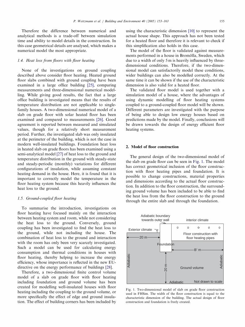
Fig. 1. Two-dimensional model of slab on grade floor construction

used in FHSim. The width of the floor construction is equal to the

characteristic dimension of the building. The actual design of floor

construction and foundation is freely created.

P. Weitzmann et al. / Building and Environment 40 (2005) 153–163 155

Therefore the difference between numerical andanalytical methods is a trade-off between simulationtime and ability to model details in the construction. Inthis case geometrical details are analysed, which makes anumerical model the most appropriate.

1.4. Heat loss from floors with floor heating

None of the investigations on ground couplingdescribed above consider floor heating. Heated groundfloor slabs combined with ground coupling have beenexamined in a large office building [25], comparingmeasurements and three-dimensional numerical model-ling. While giving good results, the fact that a largeoffice building is investigated means that the results oftemperature distribution are not applicable to single-family houses. A two-dimensional numerical model of aslab on grade floor with solar heated floor has beenexamined and compared to measurements [26]. Goodagreement is reported between measured and simulatedvalues, though for a relatively short measurementperiod. Further, the investigated slab was only insulatedat the perimeter of the building, which is not the case inmodern well-insulated buildings. Foundation heat lossin heated slab on grade floors has been examined using asemi-analytical model [27] of heat loss to the ground andtemperature distribution in the ground with steady-stateand steady-periodic (monthly) variations for differentconfigurations of insulation, while assuming constantheating demand in the house. Here, it is found that it isimportant to correctly model the temperature in thefloor heating system because this heavily influences theheat loss to the ground.

1.5. Ground-coupled floor heating

To summarise the introduction, investigations onfloor heating have focused mainly on the interactionbetween heating system and room, while not consideringthe heat loss to the ground. Conversely, groundcoupling has been investigated to find the heat loss tothe ground, while not including the house. Thecombination of heat loss to the ground and interactionwith the room has only been very scarcely investigated.Such a model can be used for calculating energyconsumption and thermal conditions in houses withfloor heating, thereby helping to increase the energyefficiency, whose importance is reflected in the new EU-directive on the energy performance of buildings [28].

Therefore, a two-dimensional finite control volumemodel of a slab on grade floor with floor heatingincluding foundation and ground volume has beencreated for modelling well-insulated houses with floorheating including the coupling to the ground volume, ormore specifically the effect of edge and ground insula-tion. The effect of building corners has been included by

using the characteristic dimension [10] to represent theactual house shape. This approach has not been testedfor a heated floor and therefore it is relevant to check ifthis simplification also holds in this case.

The model of the floor is validated against measure-ments performed in a house in Bromolla, Sweden, whichdue to a width of only 5m is heavily influenced by three-dimensional conditions. Therefore, if the two-dimen-sional model can satisfactorily model these conditions,wider buildings can also be modelled correctly. At thesame time it can be shown if the use of the characteristicdimension is also valid for a heated floor.

The validated floor model is used together with asimulation model of a house, where the advantages ofusing dynamic modelling of floor heating systemscoupled to a ground-coupled floor model will be shown.Different parameters are investigated with the purposeof being able to design low energy houses based onpredictions made by the model. Finally, conclusions willbe drawn towards the design of energy efficient floorheating systems.

2. Model of floor construction

The general design of the two-dimensional model ofthe slab on grade floor can be seen in Fig. 1. The modelhas correct geometrical inclusion of the floor construc-tion with floor heating pipes and foundation. It ispossible to change constructions, material propertiesand dimensions according to the actual floor construc-tion. In addition to the floor construction, the surround-ing ground volume has been included to be able to findthe heat loss from the floor construction to the groundthrough the entire slab and through the foundation.

ARTICLE IN PRESS

1FHSim is a programme for modelling the energy flows and

temperatures in rooms equipped with floor heating systems. The

programme has been developed at the Department of Civil Engineer-

ing at the Technical University of Denmark.

P. Weitzmann et al. / Building and Environment 40 (2005) 153–163156

The characteristic dimension is used as the width ofthe floor construction to include three-dimensionaleffects of the actual building. This approach has beenshown to give good agreement between two- and three-dimensional calculations for models without floorheating.

Floor heating is integrated in the form of a hydronicfloor heating system. The pipes are included as physicalareas, where the temperature in the pipe is based on theflow, supply temperature and cooling from the fluid tothe surrounding concrete. The round geometry of thepipe is approximated by introducing a thermal resis-tance between the four sides of the pipe and thesurrounding concrete. Therefore, the importance ofsuch factors as pipe distance and placement in theconstruction can be accurately investigated. Conse-quently, the model can be used to model arbitrary floorheating systems and constructions in combination, toinvestigate the implications on temperatures and energyconsumption when using floor heating.

The model is implemented using a finite controlvolume approach [29], where only heat transfer isconsidered. The model uses constant values for materialproperties. As described in the introduction the use ofconstant material properties will cause the predictedheat loss to the ground to be underestimated comparedto a model, where heat and moisture has been coupled.

Like for the material properties, simple boundaryconditions are applied. Towards the ground surface aconvective heat transfer with constant surface resistancehas been applied. As described in the introduction, thissimplification is expected to influence the results for theamplitude of the temperature in the ground volumeclose to the ground surface, while the average tempera-ture during the year is not expected to be influenced[14,15]. This will cause a small underestimation of theheat loss.

To ensure undisturbed boundary conditions from thefar field, the ground volume is extended 20 m downwardand outward from the floor construction, whereadiabatic boundaries are applied. This approach hasbeen chosen based on descriptions in EN ISO10211[17,18].

The internal boundary condition from floor surface tothe room is a combination of convection with room airand radiation exchange with internal surfaces, whichwill be described further below.

2.1. Building energy simulation model

The model of the floor construction can be used in amodular simulation model of the thermal conditions in aroom with floor heating under dynamic influence frommeasured weather data. The model considers heattransfer with constant material properties. The singlezone room model includes detailed calculation of

radiation exchange between internal surfaces based onview factors, which is important when modelling floorheating, as the room is heated mainly by radiation.Walls, ceiling, floor and windows are modelled using afinite control volume method with an implicit solutionscheme. Except for the two-dimensional floor construc-tion, the models are one dimensional. The ventilationsystem is a simple balanced system optionally with heatrecovery. Hourly weather data (measured or from adesign reference year) can be used as input. The model isimplemented in a simulation programme with modelsfor walls (including internal distribution of solarradiation), ceiling, floor, ventilation, room, and weatherdata called FHSim for Floor Heating Simulation.1

Using this programme, floor heating can be modelledin detail to find the energy consumption and heat loss tothe ground while at the same time being able to includethe dynamic coupling to the room model.

3. Validation of ground-coupled floor heating model

The validation of the ground-coupled floor heatingmodel will be presented in this section. Initially, adescription of the house and the measurements will bemade before the procedure is described and resultsshown.

3.1. Description of house and measurements

The validation of the numerical model of the floorconstruction has been performed for a well insulatedwooden frame single-family house in Bromolla, Sweden.The house is L-shaped with a size of 137 m2.

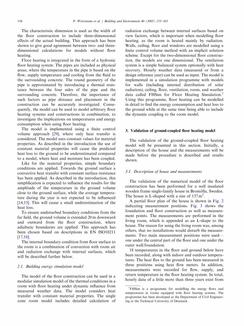
A partial floor plan of the house is shown in Fig. 2indicating measurement positions. Fig. 3 shows thefoundation and floor construction as well as measure-ment points. The measurements are performed in theliving room, which is appended as an L-shape to thehouse. The reason for using the living room was, amongothers, that no installations would disturb the measure-ments. Two main measurement positions were used—one under the central part of the floor and one under theouter wall/foundation.

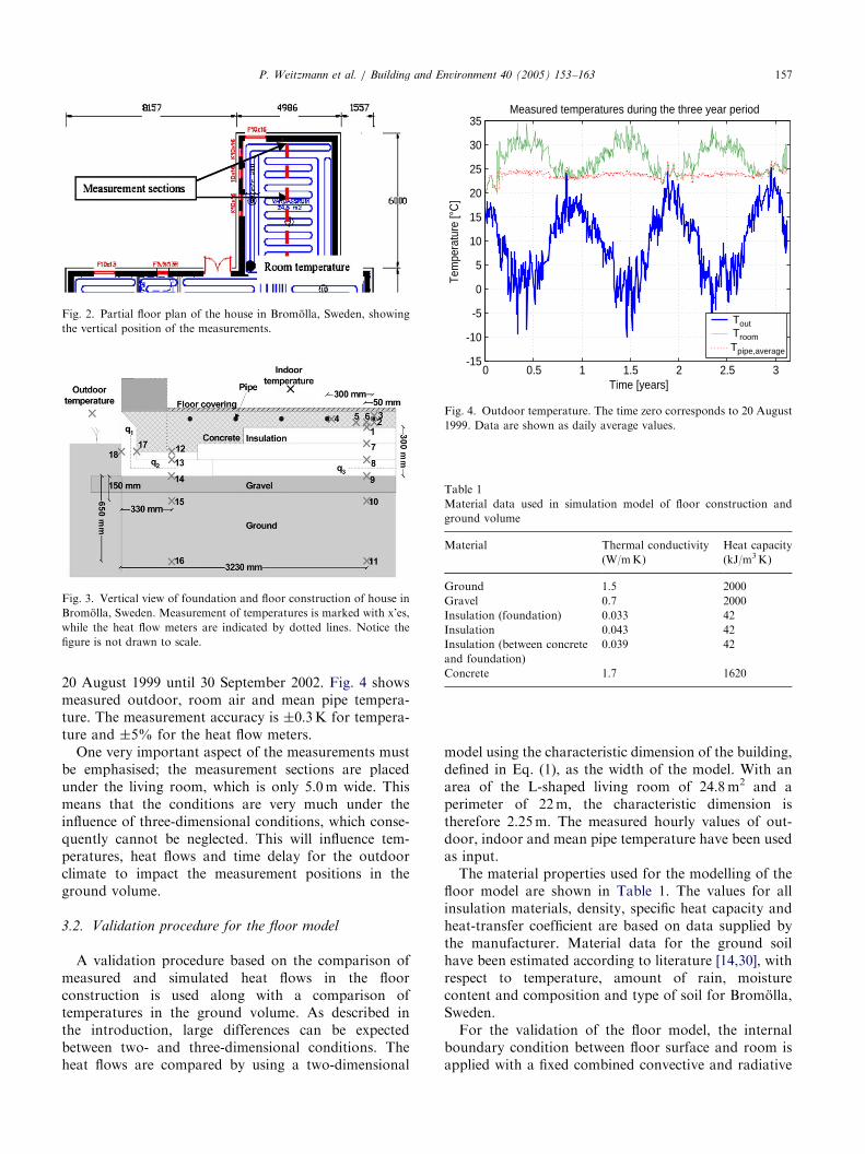
18 temperatures in the floor and ground below havebeen recorded, along with indoor and outdoor tempera-tures. The heat flux to the ground has been measured inthree positions using heat flow meters. In addition,measurements were recorded for flow, supply, andreturn temperature in the floor heating system. In total,hourly data of a little more than three years exist from

ARTICLE IN PRESS

Fig. 3. Vertical view of foundation and floor construction of house in

Bromolla, Sweden. Measurement of temperatures is marked with x’es,

while the heat flow meters are indicated by dotted lines. Notice the

figure is not drawn to scale.

0 0.5 1 1.5 2 2.5 3-15

-10

-5

0

5

10

15

20

25

30

35

Time [years]

Tem

pera

ture

[°C

]

Measured temperatures during the three year period

ToutTroomTpipe,average

Fig. 4. Outdoor temperature. The time zero corresponds to 20 August

1999. Data are shown as daily average values.

Fig. 2. Partial floor plan of the house in Bromolla, Sweden, showing

the vertical position of the measurements.

Table 1

Material data used in simulation model of floor construction and

ground volume

Material Thermal conductivity Heat capacity

(W/mK) (kJ/m3 K)

Ground 1.5 2000

Gravel 0.7 2000

Insulation (foundation) 0.033 42

Insulation 0.043 42

Insulation (between concrete 0.039 42

and foundation)

Concrete 1.7 1620


20 August 1999 until 30 September 2002. Fig. 4 showsmeasured outdoor, room air and mean pipe tempera-ture. The measurement accuracy is �0:3K for tempera-ture and �5% for the heat flow meters.

One very important aspect of the measurements mustbe emphasised; the measurement sections are placedunder the living room, which is only 5.0 m wide. Thismeans that the conditions are very much under theinfluence of three-dimensional conditions, which conse-quently cannot be neglected. This will influence tem-peratures, heat flows and time delay for the outdoorclimate to impact the measurement positions in theground volume.

3.2. Validation procedure for the floor model

A validation procedure based on the comparison ofmeasured and simulated heat flows in the floorconstruction is used along with a comparison oftemperatures in the ground volume. As described inthe introduction, large differences can be expectedbetween two- and three-dimensional conditions. Theheat flows are compared by using a two-dimensional

model using the characteristic dimension of the building,defined in Eq. (1), as the width of the model. With anarea of the L-shaped living room of 24.8 m2 and aperimeter of 22m, the characteristic dimension istherefore 2.25 m. The measured hourly values of out-door, indoor and mean pipe temperature have been usedas input.

The material properties used for the modelling of thefloor model are shown in Table 1. The values for allinsulation materials, density, specific heat capacity andheat-transfer coefficient are based on data supplied bythe manufacturer. Material data for the ground soilhave been estimated according to literature [14,30], withrespect to temperature, amount of rain, moisturecontent and composition and type of soil for Bromolla,Sweden.

For the validation of the floor model, the internalboundary condition between floor surface and room isapplied with a fixed combined convective and radiative

ARTICLE IN PRESS

0 0.5 1 1.5 2 2.5 30

0.5

1

1.5

2

2.5

3

3.5

4

4.5

5

5.5

6Ground heat loss

Time [years]

Hea

t flo

w [W

/m2

floor

are

a]

FHSimMeasured data

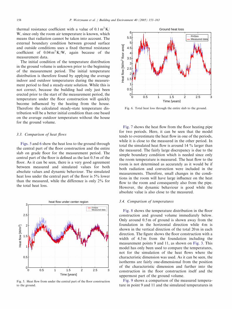
Fig. 6. Total heat loss through the entire slab to the ground.


thermal resistance coefficient with a value of 0.1 m2 K/W, since only the room air temperature is known, whichmeans that radiation cannot be taken into account. Theexternal boundary condition between ground surfaceand outside conditions uses a fixed thermal resistancecoefficient of 0.04 m2 K/W, again because of themeasurement data.

The initial condition of the temperature distributionin the ground volume is unknown prior to the beginningof the measurement period. The initial temperaturedistribution is therefore found by applying the averageindoor and outdoor temperatures during the measure-ment period to find a steady-state solution. While this isnot correct, because the building had only just beenerected prior to the start of the measurement period, thetemperature under the floor construction will quicklybecome influenced by the heating from the house.Therefore the calculated steady-state temperature dis-tribution will be a better initial condition than one basedon the average outdoor temperature without the housefor the ground volume.

3.3. Comparison of heat flows

Figs. 5 and 6 show the heat loss to the ground throughthe central part of the floor construction and the entireslab on grade floor for the measurement period. Thecentral part of the floor is defined as the last 0.5 m of thefloor. As it can be seen, there is a very good agreementbetween measured and simulated values for bothabsolute values and dynamic behaviour. The simulatedheat loss under the central part of the floor is 5% lowerthan the measured, while the difference is only 2% forthe total heat loss.

0 0.5 1 1.5 2 2.5 30

0.5

1

1.5

2

2.5

3heat flow under center region

Time [years]

Hea

t flo

w [W

/m2 ]

FHSimMeasured data

Fig. 5. Heat flow from under the central part of the floor construction

to the ground.

Fig. 7 shows the heat flow from the floor heating pipefor two periods. Here, it can be seen that the modeltends to overestimate the heat flow in one of the periods,while it is close to the measured in the other period. Intotal the simulated heat flow is around 14 % larger thanthe measured. The fairly large discrepancy is due to thesimple boundary condition which is needed since onlythe room temperature is measured. The heat flow to theroom is not determined as accurately as it would be ifboth radiation and convection were included in themeasurements. Therefore, small changes in the condi-tions in the room will have large influence on the heatflow to the room and consequently also from the pipe.However, the dynamic behaviour is good while theabsolute value is also close to the measured.

3.4. Comparison of temperatures

Fig. 8 shows the temperature distribution in the floorconstruction and ground volume immediately below.Only around 0.5 m of ground is shown away from thefoundation in the horizontal direction while 4m isshown in the vertical direction of the total 20 m in eachdirection. The figure shows the floor construction with awidth of 4.5 m from the foundation including themeasurement points 9 and 11, as shown on Fig. 3. Thismodel has only been used to compare the temperatures,not for the simulation of the heat flows where thecharacteristic dimension was used. As it can be seen, theisotherms are fairly one-dimensional from the positionof the characteristic dimension and further into theconstruction in the floor construction itself and theuppermost part of the ground volume.

Fig. 9 shows a comparison of the measured tempera-ture in point 9 and 11 and the simulated temperatures in

ARTICLE IN PRESS

18048 18072 18096 18120-2

0

2

4

6

8

10

12

14

Heat flow from pipe

Time [hours]

Hea

t flo

w [W

/m2 fl

oor

area

] FHSimMeasured data

FHSimMeasured data

9432 9456 9480 9504

0

5

10

15

20

Heat flow from pipe

Time [hours]

Hea

t flo

w [W

/m2 fl

oor

area

]

Fig. 7. Calculated and simulated heat flow from pipe shown for two periods of 3 days.

Fig. 8. Simulated temperature distribution in ground volume shown

for 1 January 2002, for a model which is wider than the characteristic

dimension to be able to show the measurement positions of point 9–11.

The outline of the floor construction is shown with the dotted grey line.

The figure therefore also shows the characteristic dimension, which is

used for the calculation of the heat loss to the ground. The isotherms

are shown for each 0.5 K.

0 0.5 1 1.5 2 2.5 38

9

10

11

12

13

14

15

16

17Temperature in point 9 and 11

Tem

pera

ture

[˚C

]

Time [years]

Simulated point 9Measured point 9Simulated point 11Measured point 11

Fig. 9. Comparison of temperature in the ground volume under the

central part of the floor construction in measurement point 9–11.


the position of the characteristic dimension, using themodel which is only as wide as the characteristicdimension. This comparison is possible because theisotherms are nearly one-dimensional from the point ofthe characteristic dimension as shown in Fig. 8. Again aclose agreement between the measured and simulatedtemperatures can be observed in both of the measure-ment points, especially considering the measurementaccuracy of �0:3K:

3.5. Ground-coupled floor heating

Returning to Fig. 8, an illustration of the importanceof correct geometrical implementing the floor heatingpipes can be seen. Firstly, the temperature in theconcrete slab is not uniform, especially close to the

outer wall because of the different conditions in thecentral part of the floor and near the outer walls.Secondly, the temperature below the floor is not uniformand therefore a one-dimensional model will havedifficulties modelling this.

The importance of correct dynamical implementationhas been investigated by using a constant temperature inthe floor heating pipe as opposed to a dynamical one.EN ISO 13 370 prescribes the use of a constant pipetemperature for calculating the heat loss to the groundwhen the floor is heated. This constant temperaturemust be found based on the expected required heatsupply to the room. However, this value is difficult toestimate. Therefore two simulations using constanttemperatures have been tested: one using the measuredaverage pipe temperature of 24.8 1C and one using30 1C. The latter is to model a situation where theaverage temperature in the slab is guessed. Fig. 10 showsthe calculated ground heat loss for two simulations

ARTICLE IN PRESS

0 0.5 1 1.5 2 2.5 30

0.5

1

1.5

2

2.5

3

3.5

4

4.5

5

5.5

6Ground heat loss

Time [years]

Hea

t flo

w [W

/m2

floor

are

a]

MeasuredSimulated Tpipe=24.8°CSimulated Tpipe=30°C

Fig. 10. Ground heat loss using a constant pipe temperature as input

in the simulation model, using the average temperature during the

measurement period and 30 1C shown together with the measured

heat loss.

Table 2

Simulation input for reference room model used in the parametric

analysis

Parameter Area (m2) U-value (W/m2 K)

Outer walls 22 0.18

Window 8 1.50

Inner walls 32 —


compared to the measurement data. As it can be seen,both models overestimate the heat loss during thesummer periods (with low heat loss), while especiallythe model using the average pipe temperature of 24.8 1Cunderestimates the heat loss during the winter periods(with high heat loss). In total the simulation withaverage pipe temperature predicts a 2% lower heat lossto the ground and the model with 30 1C finds a 23%higher heat loss. The last one shows the need for anaccurate estimate of the average pipe temperature. Forthe model using the average pipe temperature, it isobvious that even though the model finds an averageheat loss that is very close to the measured value, theheat loss is underestimated during the winter period,where it is most important to find accurate values for theheat loss. The fact that the dynamical implementation ofthe floor heating pipe both finds the most accurate valueand does not need to use an estimate of the averagetemperature clearly illustrates the advantage of using adynamical model.

Based on the comparison of the measured andsimulated heat flows and temperatures, it can be seenthat the simulation model used here is able tofully predict the conditions for both heat flows andtemperatures.

Roof 36 0.12

Floor 36 0.12

Ventilation and infiltration 0.5 h�1+ 0.1 h�1

Internal heat load 5W/m2

Control strategy of heating supply On/off

Supply temperature 40 1C

Set point temperature 21 1C

Weather data (Danish reference year) Dry

4. Parametric analysis

The validated floor model is used together with thebuilding model in FHSim to simulate the interactionbetween the floor heating system and the house to findthe thermal indoor climate and energy consumption as

well as the heat loss to the ground. The purpose of theinvestigation is to find the influence of the linear thermaltransmittance of the foundation and the thermaltransmittance of the floor construction in a dynamicalsimulation using the Danish Design Reference Year asinput.

A somewhat different model of foundation and floorconstruction than above has been used. However, as it isbased on the same numerical scheme, the validation isassumed general. In the investigation six differentinsulation thicknesses in the floor construction andthree different levels of insulation in the foundation hasbeen used for the parametric analysis. The insulation ofthe foundation has been altered by changing the thermalconductivity of the insulation material in thefoundation, thereby maintaining the geometry of thefoundation.

4.1. Room model

A simple reference room for the parametrical analysishas been created. The well-insulated square room of36 m2 has two outer walls each with a 4 m2 window. Theventilation system is a simple balanced system with anairchange rate of 0.5 times an hour and an infiltrationrate of 0.1 times an hour. It was chosen not to include aheat recovery unit on the ventilation system. This is ade-facto requirement for energy efficient houses, buthere it was omitted to see the effects of changing theparameters more clearly. A supply temperature of 40 1Cto the floor heating system has been used and a set pointtemperature of 21 1C controlled by an on/off typecontrol. The remaining inputs to the model are shownin Table 2. In the simulations a fixed value of thecharacteristic dimension of 4.6 m has been used. Thisdoes not correspond to a building with the dimensionsgiven here, but to a larger one. However, the results are

ARTICLE IN PRESS

Concrete

Ground

Insu

latio

n

Insulation

Pipes

Concrete

4 m

20 m

20 m

Not drawn to scale

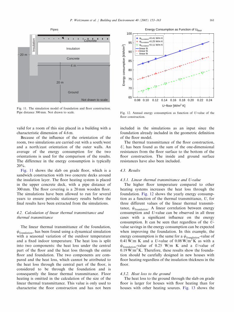
Fig. 11. The simulation model of foundation and floor construction.

Pipe distance 300mm. Not drawn to scale.

0.08 0.10 0.12 0.14 0.16 0.18 0.20 0.22 0.2465

70

75

80

85

90

95

100Energy Consumption as Function of Ufloor

U−floor [W/m2 K]

Ene

rgy

cons

umpt

ion

[kW

h/m

2 ]

ψfoundation=0.41 W/m Kψfoundation=0.25 W/m K

ψfoundation=0.11 W/m K

linear fitlinear fitlinear fit

Fig. 12. Annual energy consumption as function of U-value of the

floor construction.


valid for a room of this size placed in a building with acharacteristic dimension of 4.6 m.

Because of the influence of the orientation of theroom, two simulations are carried out with a south/westand a north/east orientation of the outer walls. Anaverage of the energy consumption for the twoorientations is used for the comparison of the results.The difference in the energy consumption is typically20%.

Fig. 11 shows the slab on grade floor, which is asandwich construction with two concrete decks aroundthe insulation layer. The floor heating system is placedin the upper concrete deck, with a pipe distance of300 mm. The floor covering is a 20mm wooden floor.The simulations have been allowed to run for severalyears to ensure periodic stationary results before thefinal results have been extracted from the simulations.

4.2. Calculation of linear thermal transmittance and

thermal transmittance

The linear thermal transmittance of the foundation,cfoundation; has been found using a dynamical simulationwith a seasonal variation of the outdoor temperatureand a fixed indoor temperature. The heat loss is splitinto two components: the heat loss under the centralpart of the floor and the heat loss through the entirefloor and foundation. The two components are com-pared and the heat loss, which cannot be attributed tothe heat loss through the central part of the floor, isconsidered to be through the foundation and isconsequently the linear thermal transmittance. Floorheating is omitted in the calculation of the size of thelinear thermal transmittance. This value is only used tocharacterise the floor construction and has not been

included in the simulations as an input since thefoundation already included in the geometric definitionof the floor model.

The thermal transmittance of the floor construction,U, has been found as the sum of the one-dimensionalresistances from the floor surface to the bottom of thefloor construction. The inside and ground surfaceresistances have also been included.

4.3. Results

4.3.1. Linear thermal transmittance and U-value

The higher floor temperature compared to otherheating systems increases the heat loss through thefoundation. Fig. 12 shows the yearly energy consump-tion as a function of the thermal transmittance, U, forthree different values of the linear thermal transmit-tance, cfoundation: A linear correlation between energyconsumption and U-value can be observed in all threecases with a significant influence on the energyconsumption. It can be seen that regardless of the U-value savings in the energy consumption can be expectedwhen improving the foundation. In this example, theenergy consumption is the same for a cfoundation-value of0.41 W/m K and a U-value of 0.08 W/m2 K as with acfoundation-value of 0.25 W/m K and a U-value of0.19 W/m2 K. Therefore, these results show the founda-tion should be carefully designed in new houses withfloor heating regardless of the insulation thickness in thefloor.

4.3.2. Heat loss to the ground

The heat loss to the ground through the slab on gradefloor is larger for houses with floor heating than forhouses with other heating sources. Fig. 13 shows the

ARTICLE IN PRESS

0.08 0.11 0.14 0.17 0.2 0.230

5

10

15

20

25

30Entire year

U −floor [W/m2 K] U −floor [W/m2 K]

Hea

t los

s to

the

grou

nd [k

Wh/

m2 ]

With Floor HeatingWithout Floor Heating

0.08 0.11 0.14 0.17 0.2 0.230

5

10

15

20

25

30Heating season

With Floor HeatingWithout Floor Heating

Fig. 13. Heat loss to the ground for the entire year (left) and for the

heating season (right) as a function of the U-value of the floor

construction using models with and without floor heating. A cfoundation

of 0.11W/mK has been used for the simulations.


heat loss to the ground with and without floor heatingfor different U-values for the entire year and for theheating season only (September to May). In order tocompensate for the larger heat loss caused by the floorheating, extra insulation can be used. If a U-value of0.2 W/m2 K of the floor construction in houses withoutfloor heating is considered, this can be seen to result in aheat loss to the ground of around 11 kW h/m2 during theheating season. In order to get the same heat loss in ahouse with floor heating, the U-value of the floorconstructions must be reduced to around 0.11 W/m2 K.This is equal to an extra insulation thickness of approx.150 mm. If the heat loss for the entire year is used, the U-value should only be lowered to 0.14 W/m2 K, corre-sponding to 75 mm.

5. Discussion

In this paper, a two-dimensional model of a housewith floor heating has been implemented in order to findthe thermal behaviour of the floor with floor heating incontact with both ground volume and house. The scopeof this is to create a simulation model of a floorconstruction with floor heating as part of a buildingenergy simulation programme. Normally the couplingto the ground is not included, which means that theinfluence of the foundation cannot be found. This latterpart is shown in this paper to have a large impact on theenergy demand for heating, which is influenced by thefloor heating system.

The two-dimensional model has been validatedagainst measurements from a building in Bromolla,

Sweden, with good results, in spite of a number oflimitations with respect to the level of details, such asconstant thermal properties and simplified boundaryconditions for the ground surface. By introducing thecharacteristic dimension of the floor, which is defined asthe floor area divided by half the perimeter of thebuilding, the comparison of measured and simulatedheat flows and temperatures shows that the model isfully able to predict the heat flows. In particular, thecharacteristic dimension has been found to be useful,also for heated floors. This has not previously beenshown.

One very interesting aspect of the measurements isthat they have been made for a very small and narrowbuilding, which is very much under the influence ofthree-dimensional conditions. Consequently, the accu-rate prediction of heat flows and temperatures suggeststhat larger buildings can also be modelled accuratelybased on this model and using the characteristicdimension.

At the same time such a dynamic model can bedirectly used in a building energy simulation pro-gramme, where the strengths of the accurate implemen-tation of the geometry can be used to find the effect ofchanging different parameters in the floor construction.

In addition, it has also been shown to be important touse a dynamical simulation of the temperature in thefloor heating pipe to accurately find the heat loss to theground if both accurate average and maximum heatflows are needed. Normally, an average value of thetemperature of the heated floor is used. However, thisvalue is difficult to estimate, as this value depends on along list of factors, including the energy consumption ofthe house and the thermal resistance between the floorheating system and room and small errors in thisestimate leads to large differences in the predicted heatloss to the ground.

The model, which has been implemented in this paper,can be used to model the influence from foundationand floor construction on the energy consumption andheat loss to the ground by coupling the floor modelto a room model. Using this integrated model,dynamical simulations of room and floor heating systemcan be performed. Here, the influence of the insulationin the floor construction and foundation has been shownto be important for the energy consumption for thehouse.

The drawback of the model is that it is slow andrequires a large number of inputs. The model cantherefore be seen as a step towards implementingdetailed hydronic floor heating systems in energysimulation programmes. An investigation is underwayto test different approaches for simplifying the modelswhile maintaining the dynamic properties and groundcoupling, or alternatively to quantify the error intro-duced by using simpler models.

ARTICLE IN PRESSP. Weitzmann et al. / Building and Environment 40 (2005) 153–163 163

6. Conclusion

In this paper a two-dimensional ground-coupled floorheating model has been validated against measurementsthat are heavily under three-dimensional influence as avery narrow building has been used. By introducing thecharacteristic dimension (the area divided by half theperimeter) of the floor construction in the model, it hasbeen shown to give accurate predictions of the heat lossto the ground. The characteristic dimension has notbeen tested on heated floors, but here it is shown that itis also valid for these.It has also been shown that anaccurate dynamic implementation of the floor heatingpipe is required to accurately find heat loss to theground, while using the average concrete temperaturecannot fully account for dynamical and absolute valuesof the heat loss. At the same time, the model of the floorconstruction can be used together with a room model tofind the energy consumption from a house with floorheating. In this paper the influence on the design of thefloor construction has been found. Especially, thefoundation has been found to have a large influenceon the energy consumption and heat loss to the ground.

Acknowledgements

The work presented here has been supported by agrant for the measurements on the house in Bromolla,Sweden, by the knowledge foundation and a part of theproducer of thermal insulation (polystyrene) and a grantfrom Danish Energy Agency for the calculations of energyefficient floor heating. Also, thanks to Professor JohanClaesson from Chalmers Technical University for helpingto develop the method of comparing two- and three-dimensional heat flows by creating a difference function.

References

[1] Claesson J, Hagentoft C-E. Heat loss to the ground from a

building—I. General Theory. Building and Environment

1991;26(2):195–208.

[2] Comini G, Nonino C. Thermal analysis of floor heating panels.

Numerical Heat Transfer Part A 1994;26:537–50.

[3] Ho SY, Hayes RE, Wood RK. Simulation of the dynamic

behaviour of a hydronic floor heating system. Heat Recovery

Systems & CHP 1995;15(6):505–19.

[4] CEN: EN ISO 1264. Floor heating—systems and components.

European Committee for Standardization, CEN, 1997.

[5] Cho S-H, Zaheer-uddin M. Predictive control of intermittently

operated radiant floor heating systems. Energy Conversion and

Management 2003;44:1333–42.

[6] Chen Y, Athienitis AK, A three-dimensional numerical investiga-

tion of the effect of cover materials on heat tranfser in floor

heating systems. ASHRAE Transactions. Proceedings of the 1998

ASHRAE Annual Meeting 1998: 104(2);1350–55.

[7] Fort K. Dynamisches Verhalten Von Fussbodenheizungen. ETH

Zurich: Juris Druck, Verlag Zurich; 1989.

[8] Fort K. The dynamic behaviour of floor heating systems. Fuel

and Energy Abstracts 1996;37(5):377.

[9] Weitzmann P, Kragh J, Jensen CF. Numerical investigation of

floor heating systems in low energy houses. In: Proceedings of the

sixth symposium on building physics in the nordic countries.

Norway: Trondheim; 2002. p. 905–12.

[10] Adjali MH, Davies M, Rees WS, Littler J. Temperatures in and

under a slab-on-ground floor: two- and three-dimensional

numerical simulations and comparison with experimental data.

Building and Environment 2000;35:655–62.

[11] Davies M, Tindale A, Littler J. Importance of multi-dimensional

conductive heat flows in and around buildings. Building and

Services Engineering Research Technology 1995;16:83–90.

[12] Anderson BR. Calculation of the steady-state heat transfer

through a slab-on-ground floor. Building and Environment

1991;24(4):405–15.

[13] Hagentoft C-E. Heat loss to the ground from a building. PhD

thesis, Lund University of Tehchnology, 1988.

[14] Janssen H, Carmeliet J, Hens H. The influence of soil moisture in

the unsaturated zone on the heat loss from buildings via the

ground. Journal of Thermal Envelope and Building Science

2002;25(4):275–98.

[15] Janssen H, Carmeliet J, Hens H. The influence of soil moisture

transfer on building heat loss via the ground. Building and

Environment 2004;39:825–36.

[16] ISO/CEN. EN ISO13370—Thermal performance of buildings—

Heat transfer via the ground—calculation method, CEN, 2000.

[17] CEN. EN ISO 10211-1. Thermal bridges in building construc-

tion—Heat flows and surface temperatures—Part 1: general

calculation methods CEN, 1994.

[18] CEN. EN ISO 10211-2. Thermal bridges in building construc-

tion—Heat flows and surface temperatures—Part 2: calculation of

linear thermal bridges, CEN, 1995.

[19] Delsante AE. Comparison between measured and calculated heat

losses through a slab-on-ground floor. Building and Environment

1990;25:25–31.

[20] Lefebvre G. Modal-based simulation of the thermal behavior

of a building: the m2m software. Energy and Buildings

1997;25:19–30.

[21] Davies M, Zoras X, Adjali MH. Improving the efficiency of the

numerical modelling of built environment earth-contact heat

transfers. Applied Energy 2001;68:31–42.

[22] Pan S, Pal J. Reduced order modelling of discrete-time systems.

Applied Mathematical modelling 1995;19:133–8.

[23] Hsieh C-S, Hwang C. Model reduction of continuous-time

systems using a modified Routh approximation method. IEE

Proceedings 1989;136(4).

[24] Menezo C, Rox JJ, Virgone J. Modelling heat transfers in

building by coupling reduced-order models. Building and

Environment 2002;37:133–44.

[25] Adjali MH, Davies M, Ni Riain C, Littler JG. In situ

measurements and numerical simulation of heat transfer beneath

a heated ground floor slab. Energy and Buildings 2000;22:75–83.

[26] Youcef L. Two-dimensional model of direct solar slab-on-grade

heating floor. Solar Energy 1991;46(3):183–9.

[27] Chuangchid P, Krarti M. Foundation heat loss from heated

concrete slab-on-grade floors. Building and Environment

2001;36:637–55.

[28] European Parliament. Directive 2002/91/EC of the European

Parliament and of the Council of the 16 December 2002 on the

Energy Performance of Buildings. 2003, Official Journal of the

European Communities, L 1/65.

[29] Patankar SV. Numerical heat transfer and fluid flow. New York:

Hemisphere; 1980.

[30] Farouki OT. Thermal properties of soils. Series on rock and soil

mechanics, vol. 11. Germany: Trans Tech Publications; 1986.

Modelling floor heating systems using a validated two-dimensional ground-coupled numerical model

Documents

Transcript of Modelling floor heating systems using a validated two-dimensional ground-coupled numerical model