A fixed grid numerical modelling methodology for convection-diffusion mushy region phase-change...

Inf.3. Heor Mars Trunsfir. Vol.30,No.B.~ 1709-1719, 1987 0017-9310/87$3.00+0.00

Printedin Great Britain Q 1987PergamonJoumalsLtd.

A fixed grid numerical mode~~ing methodology for convection-diffusion mushy region

phase-change problems V. R. VOLLER

Mineral Resources Research Center, University of Minnesota, 56 East River Road, Minneapolis, MN 55455, U.S.A.

C. PRAKASH

CHAM North America, 1525-a Sparkman Drive, Huntsville, AL 35805, U.S.A.

(Received 26 August 1986 and i~~naif~r~ 4 February 1987)

Abstract-An enthalpy formulation based fixed grid methodology is developed for the numerical solution of convection-diffusion controlled mushy region phase-change problems. The basic feature of the proposed method lies in the representation of the latent heat of evolution, and of the flow in the solid-liquid mushy zone, by suitably chosen sources. There is complete freedom within the me~odoIo~ for the definition of such sources so that a variety of phase-change situations can be modelled. A test problem of freezing in a

thermal cavity under natural convection is used to demonstrate an application of the method.

1. INTRODUCTION

A LARGE number of numerical techniques are avail- able for the solution of moving boundary problems, a comprehensive review has been presented by Crank [l]. The majority of these techniques are concerned with phase change in which conduction is the principal mechanism ofheat transfer. In physical systems which involve a liquid-soiid phase change, however, convection effects may also be important. AS such, the problem of freezing of a pure liquid in a thermal cavity under conduction and natural convection has received some attention in recent years. For example see Rama- chandran et al. [2], Gadgil and Gobin [3] and Albert and O’Neill [4]. In these works, a temperature formulation is used, and in order to treat the moving liquid-solid interface, deforming grids have been employed. An alternative approach is to use an enthalpy formulation in which case no explicit conditions on the heat flow at the liquid-solid interface need to be accounted for and therefore the potential arises for a fixed grid solution. This will have advantages in terms of simplifying the numerical modelling requirements, particularly in systems for which the phase change may only be a component part. Exam- ples of fixed grid solutions of convection-diffusion phase change can be found in Morgan [5], Gartling [6] and Voller et al. 17-91.

The major problem with fixed grids is in accounting for the zero velocity condition as the liquid region turns to solid. Morgan [5] employs the simple approach of fixing the velocities to zero in a computational cell whenever the mean latent heat content, AH, reaches some predetermined value between 0 (cell

ail solid) and L (cell all liquid), where L is the latent heat of the phase change. Gartling [6] employs a more subtle approach in making the viscosity a function of AH such that as AH decreases from L to 0 the value of the viscosity increases to a large value thus simu- lating the liquid-solid phase change.

Voller et al. [7-91 have investigated various ways of dealing with the zero solid velocities in fixed grid enthalpy solutions of freezing in a thermal cavity. At the same time they proposed an alternative but similar approach to that used by Gartling [6]. Computational cells in which phase change is occurring, i.e. 0 < AH < L, are modelled as pseudo porous media with the porosity, A, decreasing from 1 to 0 as AH decreases from L to 0. In this way, on prescribing a ‘Darcy’ source term, velocities arising from the solution of the momentum equations are inhibited, reaching values close to zero on complete solid formation.

To the authors’ knowledge ail applications of convection~iffusion phase-change numerical met&- odologies have been to isothermal phase-change problems. These applications assume that the liquid-solid phase change occurs in a pure material. In many practical situations, however, the material under consideration is not pure (e.g. a metallurgical alloy). In such cases the phase change takes place over a temperature range, E < T $ --E say. That is, the evolution of latent heat has a functional relationship with temperature, e.g. AH =f(Y), as opposed to the step change associated with an isothermal phase change. Problems of this type are often referred to as mushy region problems to indicate the solid plus liquid state of the material in the phase-change range.

SW 30:&J 1709

1710 V. R. VOLLER and C. PRAKASH

NOMENCLATURE

A porosity function Y, 2 coordinate directions. a’s coefficients in numerical scheme c porosity constant Greek symbols C specific heat

;

thermal diffusivity f( 7’) enthalpy temperature function thermal coefficient of expansion

4 local liquid fraction half mushy range

F, local solid fraction 1 porosity

9 gravity !J viscosity h sensible heat P density. H total enthalpy (sensible plus latent) AH latent heat Subscripts K permeability H high neighboring node k conductivity L low neighboring node L latent heat of phase change 1 liquid value P pressure N north neighboring node

4 small constant to avoid division by zero P node point S,, SZ momentum source term S south neighboring node

& Boussinesq source term S solid value.

S, enthalpy source term T temperature Other symbols I time 0 old value U velocity, (u, w) j]A, B]] maximum value of A and B

ui liquid velocity E In nth iterative value.

In a numerical modelling analysis of a mushy region the problem are the same as previous studies of freez- solidification the enthalpy is a sound starting point in that any functional relationship AH =f(r) may be readily incorporated into the enthalpy definition. Furthermore, in problems that involve convection in the melt, the Darcy source approach proposed by Voller et al. [7-91, something of a numerical ‘fix’ in the isothermal case, now has some physical sig- nificance. For example, in metallurgical problems, it is fairly standard practice to model the flow in the mushy region via a Darcy law, see Mehrabian et al.

HOI. The purpose of this paper is to present an enthalpy

formulation based fixed grid methodology for the numerical solution of convective-diffusion controlled mushy region phase-change problems. The method is general and can handle situations where phase changes occur at a distinct temperature (pure material} or over a temperature range (alloys). Further, the functional relationship AH = f (T) can be of any form, though a linear relationship is used in the current work. The Darcy source approach is used to simulate motion in the mushy region. The essence of the paper is to present the basic methodology ; the test example chosen is primarily a vehicle to explain the details of the procedure.

2. A TEST PROBLEM

The configuration for the test problem employed in this paper is illustrated in Fig. 1. The basic features of

ing in a thermal cavity, see Voller er al. [7-91, Albert and O’Neill [4], and Morgan [5]. Initially the liquid in the cavity is above the freezing temperature. At time t = 0 the temperature at the surface Y = 0 is lowered and fixed at a temperature below the freezing temperature so that as time proceeds a solid layer attaches to this surface. The essential and important difference in this work is the introduction of a mushy region, which is defined as follows. The enthalpy of the material (the total heat content) can be expressed as

H=h+AH

i.e. the sum of sensible heat, h = CT, and latent heat AH. In order to establish a mushy phase change the latent heat contribution is specified as a function of temperature, T

AH =f(T). (1)

On recognizing that latent heat is associated with the liquid fraction in the mushy zone a general form for f(T) can be written

i

L, T> T

Y(T) = L(1 -K), 7-, > T>, 7’s (2) 0, T< T,

where F,(T) is the local solid fraction, T, the liquidus temperature at which solid formation commences and TV is the temperature at which full solidification is achieved. The task of fully defining the nature of the

A fixed grid numerical modelling methodology for convection-diffusion mushy region phase-change problems 1711

INSULATED

DIMENSIONS 1 X 1

T INT = 0.5

FIG. 1. The thermal cavity.

latent heat evolution in the mushy region is that of identifying the form of the local solid fraction-temperature relationship, i.e. F,(T). In the current work a simple linear form is chosen

i

0, T>,&

F,(T) = (&--)I% E> T> --E (3) 1, T< -E

where the temperature has been scaled such that T = E and --a are the liquidus and solidus temperatures, respectively. The quantity E is referred to as the half temperature range of the mushy zone.

The method to be proposed is not restricted to the form for t;,(T) given by equation (3) and it is recognized that in practical cases such a simple definition may not suffice. For example in metallurgical solidification of a binary alloy the function Fs( T) will depend on the nature of the solute redistribution and the associated phase-change equilibrium diagram, see Flemings [ill. A trea~ent such as this, however, is outside the scope of this paper.

The current intention is to develop a basic methodology for the treatment of mushy solidification, In keeping with this approach the thermal properties used are assumed constant with temperature and phase. The values of the properties used along with the value of appropriate dimensionless numbers are given in Table 1.

3. THE GOVERNING EQUATIONS

The form of the governing zquations for the test problem of Fig. 1 are similar to the equations for an

isothermal phase change in a cavity derived by Voller et al. [7-91. Important differences arise, however, in the definition of the source terms and in the treatment of the velocities.

For the purpose of the development of the methodology it is helpful to regard the entire cavity as a porous medium, where the porosity, 2, takes the values, /I = I in the liquid phase, 1= 0 in the solid phase, and 0 -=c I < 1 in the mushy zone. The governing equations can then be written in terms of the superficial velocity (i.e. the ensemble-average velocity) defined as

ll = lu,

where II, is the actual fluid velocity. On recognizing that the porosity 3, = 1 -F, the above relationship can

Table 1. Test problem data

Initial temperature T, = 0.5 Hot wall temperature Tn = 0.5 Cold wall temperature T, = -0.5 Reference temperature r,, = 0.5 Half mushy range E = 0.1,0.05,0 Cavity dimension I=1 Density p=I Specific heat c=l

Viscosity p=l Conductivity k = 0.001 Coefficient of thermal expansion B = 0.01 Gravity $j = 1000 Latent heat L=5

So that : Raleigh number Ra = pzgBc(TH - T#/pk = lo4 Prandtl number Pr = @c/k = 10’ Stefan number Sre = L/c( T, - Tc) = 5

.-


be expanded to give

i

“I> in the liquid phase

” = (1 -F,)“,, in the mushy zone

0, in the solid phase.

Using this definition along with the assumption of Newtonian, incompressible, laminar flow the govern-

ing equations are as follows.

Conservation qf mass

au aw

ay -+z=o

where w and v are the superficial velocities in the z- and y-directions, respectively.

Conservation of momentum

w4 at +div (JJUV) = div (p grad v) - g + S,

ay @a)

a(pw) at +div (puw) = div (p grad W)

-g +S,+S,, (Sb)

where P is pressure, p is density, p is the liquid viscosity, u = (v, w), and S,, S,, and S, are source terms which will be defined below.

The heat equation

aPh at +div (puh) = div (c( grad h)- S, = 0 (6)

where tl = k/c is the thermal diffusivity and S,, is a

phases related source term to be discussed below.

4. DEFINITION OF SOURCE TERMS

The above governing equations are in the general format suggested by Patankar [12] for the numerical solution of heat and fluid flow problems, i.e. a transient term plus a diffusive term plus a convective term plus sources. In this format a problem is driven by the definition of the source terms.

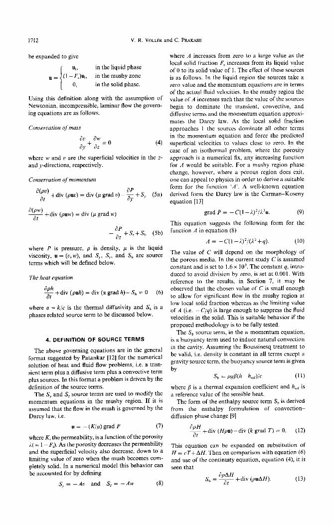
The S, and S, source terms are used to modify the momentum equations in the mushy region. If it is assumed that the flow in the mush is governed by the Darcy law, i.e.

u = -(K/n) grad P (7)

where K, the permeability, is a function of the porosity A( = 1 -F,). As the porosity decreases the permeability and the superficial velocity also decrease, down to a limiting value of zero when the mush becomes com- pletely solid. In a numerical model this behavior can be accounted for by defining

S, = -Au and S,= -Aw (8)

where A increases from zero to a large value as the local solid fraction F, increases from its liquid value of 0 to its solid value of 1. The effect of these sources is as follows. In the liquid region the sources take a zero value and the momentum equations are in terms of the actual fluid velocities, In the mushy region the value of A increases such that the value of the sources begin to dominate the transient, convective, and diffusive terms and the momentum equation approxi- mates the Darcy law. As the local solid fraction approaches I the sources dominate all other terms in the momentum equation and force the predicted superficial velocities to values close to zero. In the case of an isothermal problem, where the porosity approach is a numerical fix, any increasing function for A would be suitable. For a mushy region phase change, however, where a porous region does exit, one can appeal to physics in order to derive a suitable form for the function ‘A’. A well-known equation

derived form the Darcy law is the Carman-Koseny

equation [ 131

grad P = -C(l -1)2/13u. (9)

This equation suggests the following form for the function A in equation (8)

A = -C(l -i)‘/(l’+q). (10)

The value of C will depend on the morphology of the porous media. In the current study C is assumed constant and is set to 1.6 x 103. The constant q, intro- duced to avoid division by zero, is set at 0.001. With reference to the results, in Section 7, it may be observed that the chosen value of C is small enough to allow for significant flow in the mushy region at low local solid fraction whereas as the limiting value of A (i.e. -C/q) is large enough to suppress the fluid velocities in the solid. This is suitable behavior if the proposed methodology is to be fully tested.

The Sb source term, in the w momentum equation,

is a buoyancy term used to induce natural convection in the cavity. Assuming the Boussinesq treatment to be valid, i.e. density is constant in all terms except a gravity source term, the buoyancy source term is given

by (11)

where p is a thermal expansion coefficient and href is a reference value of the sensible heat.

The form of the enthalpy source term S, is derived from the enthalpy formulation of convection- diffusion phase change [9]

y + div (Hpu) -div (k grad T) = 0. (12)

This equation can be expanded on substitution of H = CT+ AH. Then on comparison with equation (6) and use of the continuity equation, equation (4), it is seen that

S =d@H h at +div @AH). (13)

A fixed grid numerical modelling methodology for convection-diffusion mushy region phase-change problems 1713

In the isothermal case due to the step change in AU along with a zero velocity at the solid-liquid interface the convective part of this source term takes the value zero. In a mushy region case, however, the convective term needs to be included.

5. THE BASIC NUMERICAL SOLUTION

To numerically solve the governing equations along with the associated source terms a finite domain method is used. This is fully implicit in time and uses upwind differencing in space. As an example of the form the discretization takes consider the heat equation, equation (6). The finite domain discretization, following the notation in Patankar [12] and referring to Fig. 2, gives

where the subscripts indicate the appropriate nodal values, the a’s are coefficients which depend on the diffusion and convective fluxes in to the pth control volume, as = p 6z 6y/& and ( >” represents evaluation at the previous time step. The parameter b incor- porates a discretized form of the source term S,,.

The discretized form of the momentum equations are very similar to equation (14). An important difference is that the grids used are ‘staggered’ over the enthalpy grid (see the dashed control volumes in Fig. 2). The reason for this is so that the pressure, which is the driving force for the velocities, can be correctly accounted for. For more details see Patankar 1121. A consequence of the staggered grid approach is that care has to be taken in numericaIly implementing momentum sources which depend on enthalpy.

The finite domain equations are solved by employ- ing the PHOENICS code. This code uses a similar algorithm to the SIMPLE algorithm outlined by

Table 2. Grid dependence

Size Fraction of solid at t = 250

10x 10 0.85 20x20 0.82 40x40 0.81

Patankar [ 121. The numerical representation of various source terms is discussed in the Appendix. Of particular importance is the treatment of the latent heat source term S, given by equation (13). Given a distribution of the AH field (and hence S,,), equation (6) can be solved to obtain the sensible heat h. To complete the computational cycle, AH needs to be iteratively updated from the predicted h field. The procedure for this iterative updating is seen as a main contribution of this paper, it is fully described in the Appendix. Details regarding the PHOENICS implementation may be found in ref. [ 141.

6. IMPLEMENTATION

The proposed test problem is solved on a 40 x 40 uniform square grid. A fixed time step of 6t = 10 was used in all runs and the maximum simulation time was t = 1000. The grid size of 40 x 40 was reached after a grid refinement study. Essentially the total fraction of solid at t = 2.50 was recorded for uniform grid sizes 10 x 10, 20 x 20 and 40 x 40. The results of this study are summarized in Table 2. In each time step 50 iteration sweeps were used to solve the discretized equations. No under relaxation parameters were employed. The runs were performed on a Convex Cl, The longest run (simulation to t = 1000) required of the order of 6 cpu hours.

H ---_-c_--_

I I

I whA I I

I I--- ---1 , I

S - south node t - low Vn - velocity at north face

N - north node H - high W,, - velocity at high face

FIG. 2. The numerical control volumes.

-- - __- ------ /.---

-- m___-- -

- -__/I- _A/ _--- ---

_----__/--- __----

---------- _----

-___- -- --- --

-__----- ____--- __----

-- ---

_---- -_d

____

___-- __---

_----

--- _____pw __c-

e---- --___-- .--7 _____--- --

+-tttCttt-C-H-~-t-CC-C-C~~-_L- c - . .

,-,-~-+377~~CCCC~-*-t--C-.C. . . *. . . I

;


e = 0.1 c = 0.5 6 = 0.0 (isothermal) I--

FIG. 6. Effect of mushy size at I = 1000.

Figure 7 shows results using the revised porosity between the morphology of the mushy region and the source with all other conditions the same as in Fig. 3. porosity source need to be investigated. These results clearly indicate the effect of a reduced flow in the mushy region with the liquidus defor- mation very much reduced. If the proposed meth- 8. CONCLUSIONS AND DISCUSSION

odology is to be used to investigate ‘real’ systems then The principal aim of this work has been to develop clearly care has to be taken in defining the nature a generalized methodology for the modelling of mushy of the porosity source. In particular relationships region phase change. This motivated the development

-L +tZ

vector SCeie: @.500E-01

>

FIG. 7. Flow field and mushy region (E = 0. l), t = 1000, for revised source.

A fixed grid nutnerical modelling methodology for co~v~tion~iff~sion mushy region phase-change problems 1717

of a fixed grid approach along with retaining the basic form of the ~ydrom~~~ani~a1 equations. The phenom-

ena associated with a particular phase change can be modelled on careful consideration and choice of source terms. The driving source terms are the ‘Dar& source and the latent heat source.

The Darcy source is used to model the effect of the nature of the porosity of the mushy region on the flow field. ~re~~rnina~ results suggest that the nature of the porosity has a significant effect.

The latent heat source term is a function of the solid fraction which is a function of temperature. In this paper a linear change was assumed. In real systems the solid fraction-temperature relationship may not be such a simple form. In a binary alloy for example F, will depend on the nature of the solitte redistribution and may ‘take a non-linear form possibly with a jump discontinuity at a eutectic front.

There is a need for further studies to be made. In particular :

(i) A comparison between the proposed fixed grid method and a deforming grid technique. Such a study would provide a mechanism by which the relative advantages and disadvantages of each approach could be analyzed.

odotogy to metal systems, where the flow in the mushy zone is significant.

(ii) An investigation into various approaches and models of flow in the mushy zone. Important questions in such a study will be; What is an appropriate form for the mo~boiogy-porosity relationship? and ; Is the Darcy law appropriate? (i.e. should an alternative such as the ~~nkman equation be used [Ifi]). An investigation of this type could have particular relevance in applications of the proposed meth-

8.

9.

10.

11.

12.

N. Ramachandran, J. R. Gupta and Y. Jalunu, Tbermat and fluid flow effects during solidi~~tion in a rectangular cavity, Int. J. Heat Mass Tran@i?r 25, 187-194 (1982). A. Gadgil and D. Gobin, Analysis of two dimensionai melting in rectangular enclosures in the presence of convection, .I. ileat Transfer 106,20-26 (1984). M. R. Albert and K. O’Neill, Transient two-dimensional phase change with convection using deforming finite eiemenls. In Computer Techniques in Heat Transfer (Edited by R. W. Lewis, K. Morgan, J. A. Johnson and W. R. Smith), Vol. l. Pineridge Press, Swansea (1985). K. Morgan, A numerical analysis of freezing and meltinn with convection. Comu. Meth. ADDI. Enana 28, 275-2%4(1981). _ As - _ D. K. Gartling, Finite element analysis of convective heat transfer problems with change of phase. In Cam- pufer Methods in Fluids (Edited by K. Mornan et al.), pp. 257-284. Pentech, London (1980). - V. R. Volier. N. C. Markatos and M. Crass. Techniques for accoun& for the moving interfaie in con- v~tio~/diffusi~n phase change. 1; Numerical Methods in Thermal Problems fEdited bv R. W. Lewis and K. Morgan), Vol. 4, pp. 5&609. Pineridge Press, Swansea (1985). V. R. Voller, N. C. Markatos and M. Cross, Sol- idification in convection and diffusion. In Numerical Simulations of Fluid Flow and Heat/Mass Transfer Pro- cesses (Edited by N. C. Markatos, D. G. Tatchell, M. Cross and N. Rhodes), pp. 425-432. Springer. Berlin (1986). V. R. Voller, M. Cross and N. C. Markatos, An enthalpy method for convection/diffusion phase changes. Inr. J. Num. Meth. Engng 24,2?1&284 (1987). R. Mehrabian, M. Keane and M. C. Flemings, Inter- dendritic fluid flow and macrosegreeation : influence of gravity, Met. Trans. 5 I, 12~.-1~20-(1970~ M. C. Flemings, So~jd~euf~on Processing. McGraw-~il1, New York (1974). S. Y. Pantankar, _~~rner~~o~ Heat Transfer and Fluid Flow. Hemisphere, Washington, DC (1980). ---

4. V. R. Voller &d C. Prakash,‘ A fixed grid numerical

13. P. t‘. Carman, I-&id flow through granular beds> Trans.

modelling methodology for phase change problems involving a mushy region and convection in the melt.

Inst. Chem. Engrs 15, 150-156 (1937).

PHOENICS Demonstration Report PDR/CI-IAM NA/9 (1986).

(iii) Some experimental studies are required. The work presented in this paper lacks any validation. The authors concede that this is a major deficiency but are unaware of any suitable experimental studies of solidification in mushy systems. It is noted, however, that the isothermal case has been checked against limiting analytical solutions by Volier et nl. [8,9].

The questions raised on what is the appropriate form of the sources and the need for further studies does not detract’ from the proposed methodology. Indeed as it stands its framework nature makes it an idea1 vehicle by which such studies can be carried out, thereby adding to the limited understanding of the mushy region solidification.

Ackrrowleni(lemfnls-One ofthe authors, V. R. Voller, would like to acknowledge CHAM of North America for one month’s support during the completion of this work. The authors would also like to acknowledge the referees of the Internatiomzl Journal of Heat and Mass Transfer for their useful and stimulating comments.

REFERENCES

i. J. Crank, Free and booing 5oundary Problems. Ciar- endon Press, Oxford (1984).

5. G. De Vahl Davis, Natural convection of air in a square cavity : a bench mark solution. The University of New South Wales Report l982/FMT/2 (1982).

16. H. C. Brinkman, A calculation of the viscous force exerted by a flowing fluid on a dense swarm of particles, Appl. Scient. Res. Al, 27-34 (1947).

17. C. Prakash, M. Samonds and A. K. Sin&al, A fixed grid numerical methodoloa for phase change problems involving a moving heat source, irk+. f. Heat Mass Tremor (1987), in press.

APPENDIX: NUMERICAL TREATMENT OF SOURCES

Part A. The enthalpy source The latent heat source, S,, in equation (14) is considered

to consist of two parts, a transient term and a convective term. The transient term has the discrete form

ag(AH; -AHp) (AlI

where A.H is the nodal latent heat (i.e. the mean latent heat in con&o1 volume F). An obvious way of treating this source term during an iterative solution of equation (14) would be


to use the iterative update

(AH&+ 1 =f[(~d.l

where ( ), indicates evaluation at the nth iterative step and the functionfis defined by equation (2). A drawback to this approach is that if the mushy range (E) is small, (Tr) may oscillate between values greater than E and values less than --E, and hence. (AH,), will oscillate between 0 and L, and convergence will not be achieved. This problem will become acute as an isothermal phase change is approached. An alternative method which avoids this problem is as follows. At any point in the iterative solution, equation (14) may be rearranged as

[hp]” - h; = [TERMS], + A% - [AHp], 642)

TERMS = [aHhH + aLhL + aNhN + ashs F, = po,dz, etc.

- (a” + aL + aN +as)h, +SzGy x convective source]/aF

with the most current values of the nodal hs used. On convergence this equation becomes

hp--h; = TERMS +AH”,-AH,. (A3)

Adding and subtracting appropriate terms to both sides equation (A3) may be rearranged as

[hp], -h; + h, - [hp]. = [TERMS], + (TERMS)c

are evaluated at the cell faces of the enthalpy control volumes. Note the velocity v, is the y-velocity on the north face of the pth enthalpy control volume, i.e. the nodal velocity of the pth ‘u-velocity’ control volume, see Fig. 2. In essence the formulation of the convective boundary condition states that the convective losses or gains in latent heat are governed by the direction of the flow field. It is noted that Prakash et al. [17] in a steady-state analysis of an arc welding model obtain a similar convective latent heat source which is also treated via an upwind differencing scheme.

+ (AH: - WPI.) - @HP - P&l.) where TERMS has been written as [TERMS],+ (TERMS)c (i.e. the nth iterative value plus a correction). Subtraction of equation (A2) leads to the following expression for the latent heat content

Part B. The momentum soww The momentum source term corresponding to the

Boussinesq approximation is added to the discretized w momentum equation in the form

AHp = [AH& + [hr], + (TERMS)c - hr.

An appropriate iterative scheme can now be developed. The value of (TERM% can be ignored (note its value will be zero on convergence) and the value of the nodal sensible heat can be approximated as

The porosity of a control volume in the mushy phase is equal to the mean liquid fraction of that control volume. This value can be estimated as AH,/L if the control volume is an enthalpy control volume. For velocity control volumes the liquid fraction can be estimated on averaging the latent heat contents of the enthalpy control volumes over which the velocity control volume is staggered. That is in the pth n- velocity control volume

hr = c .f ’ ([~HA) wheref- ’ is the inverse of the latent heat function given in equation (1). These approximations lead to the following updating scheme for calculating the nodal latent heat in the source term equation (Al)

Wbl.,, = Wf~ln + M. -c-f - ' W&l.). (‘44)

Note that, this scheme will be consistent with the case of an isothermal phase change becausef- ’ is well defined, whereas fis multivalued at the phase-change temperature. In addition the scheme ensures that no serious oscillations occur in the predicted temperatures from one iteration to the next.

The convective part of the latent heat source, i.e.

- div @AH)

is treated via an upwinding discretization. The contribution to the source term may be written in the form

(INFLOW) - (OUTFLOW)

with

INFLOW = ][F,,O]]AHs-I[-F,,O]]AH,

(A5)

and

OUTFLOW = I [F,,O]]AH, - I[-F,, OIlAH,

where I [a, b] 1 means the maximum of a and b and

[AH,]” = (AH, +AH,)/2

and in the pth w-velocity control volume

[AHJ = (AHp +AHn)/2.

On dividing these values by the latent heat of the phase change L the appropriate control volume porosities can be calculated. These values can then be used in modifying the ap coefficients of the discretized momentum equations via the use of the function A defined in equation (10).

MODELISATION NUMERIQUE A GRILLE FIXE POUR LA REGION TROUBLE DE CONVECTION DANS LES PROBLEMES DE CHANGEMENT DE PHASE

R&sum&-Une formulation enthalpique basee sur une mtthodologie a grille tixe est developpee pour la resolution numerique des problemes de changement de phase avec une region trouble control&e par la convection. La methode proposte repose sur la representation par des sources convenablement choisies de l’tvolution des chaleurs latentes et de I’ecoulement dans la zone trouble liquid*solide. 11 y a une complete liberte dans la mtthodologie pour la definition de telles sources de telle sorte qu’on peut modtliser une grande variitt de situations. On btudie la congelation dans une cavitb avec convection naturelle pour

demontrer l’application de la methode.

A fixed grid numerical modelling methodology for convectiondiffusion mushy region phase-change problems 1719

EINE NUMERISCHE FESTGITTERMETHODE FUR UBERGANGSGEBIETE BE1 PHASENWECHSELPROBLEMEN MIT KONVEKTION UND DIFFUSION

Zusammenfaaaung-Ein Festgitter-Verfahren, welches auf Enthalpiebilanzen basiert, wurde zur numer- ischen Lijsung von Konvektions-Diffusionsgesteuerten Problemen des Phaseniibergangs entwickelt. Der grundlegende Unterschied der vorgestellten Methode liegt in der Beticksichtigung der Entstehung der latenten WHrme und der Striimung in der Fest-fliissig-Ubergangszone durch geeignet gewiihlte WCr- mequellen. Fiir die Definition solcher Quellen hat man vollkommene Freiheit, sodall eine Vielzahl von Phasenwechselvorglngen modelliert werden kann. Ein Testproblem des Gefriervorganges in einem ther- mischen Einschlul) unter natilrlicher Konvektion wird benutzt, urn die Anwendung dieser Methode zu

zeigen.

9HCJIEHHOE MO~EJIUPOBAHHE 3AjIA9 cDA30BOFO I-IEPEXOAA C Y’IETOM KOHBEKHMH H JHI@@Y3MH

AmsoTamna-Ha ocuoae 3riTanbndhioii @O~M~~X~~OBKH ncnonbsyercn MeTon HenonewmHofi ceTwi arm

wicnetiHor0 peuretisin 3ana9 @a30Boro nepexona c yve~o~ K~HEZ~KUHH H &I@Y~HH. XapaKTepHoB

YepToi npeanaraerdoro MeTona RBJISCTCK npeJlcTaBneHHe yAeJIbHOZi TenJIOTbI ~a3oBoro nepexona w

IlOTOKa B 30He ,$a3OBOrO IIepeXOna TBepnOeTeJIO-IKHlJKOCTb C llOMOUU40 COOTBeTCTBeHHO Bbl6paHHblX

HCTOSHHKOB. Bbr60p ~THX IICTOSHHKOB npennonaraercr TaxHht,wo n0380nneT MonentipoeaTb pa3ntiw

HbrecnyvaH +a308btx npeepauresd B xawcrne iuunocqauw pacchtaTptisaeTcn sanara 0 3aMep3awiki

BllOJNJCTH~pHeCTeCTLleHHOiiKOHBeKUHH.

A fixed grid numerical modelling methodology for convection-diffusion mushy region phase-change...

Documents

Transcript of A fixed grid numerical modelling methodology for convection-diffusion mushy region phase-change...