
Small pelagic fish dynamics: A review of mechanisms in the ...
Upload
khangminh22Category
view
1download
0
Ca’ Foscari Universita di Venezia
and
Centro Euro-Mediterraneo sui CambiamentiClimatici
Numerical modelling of the
benthic-pelagic coupling in coastal
marine ecosystems at contrasting
sites
Corso di Dottorato di ricerca in Science and Management
of Climate Change
Ciclo 32SSD: GEO12
Ph.D. Coordinator:
Carlo Carraro
Ph.D. Candidate:
Carolina Amadio
Ph.D. Matriculation number:
956323
Supervisor:
Simona Masina
Cosupervisors:
Marco Zavatarelli
Tomas Lovato
Momme Butenschon
December, 2019
Abstract
Continental shelves (bottom depth <150-200m) cover less than 5% of the
global ocean surface, but play a crucial role in the marine global biogeo-
chemical cycling. Coastal waters biogeochemical cycling is governed and
constrained by the biogeochemical processes occurring in the benthic do-
main. Such processes define the so called benthic-pelagic coupling (hereafter
BPC), i.e. two-way exchange of organic matter (particulate and dissolved)
and inorganic compounds. The physically mediated exchanges structuring
the BPC are constituted by the sinking and resuspension fluxes of partic-
ulate organic matter and by the diffusion of inorganic nutrients. Despite
the importance of the benthic domain for the coastal water ecosystems and
the continuous enhancement of model resolution, BPC in marine ecosystem
models is in general approximated through a simple closure term for mass
conservation. Moreover, observational data focusing on the BPC dynamics
are scanty and sparse both in time and space, thereby hampering model pa-
rameterization and validation. The main objectives of this study are (i) de-
velop and test a detailed numerical model addressing benthic dynamics and
BPC processes (ii), assess the skills of the coupled physical-biogeochemical
models in simulating the BPC and (iii) evaluate ecosystem dynamics in ma-
rine areas with different climatic and ecological characteristics. The benthic
i
ii
sub-model implemented is based on two crucial parameters: the sinking ve-
locity of particulate matter and the diffusive fluxes of inorganic dissolved
matter at the benthic-pelagic interface. The benthic sub-model has been
calibrated accounting for the complex pelagic food web and for the main
ecological and physical characteristics of continental shelf areas. The model
has been implemented in different sites: Gulf of Trieste (Italy), St Helena
Bay (South Africa), Svinøy Fyr (Norway). At each implementation site,
the one-dimensional coupled BFM-NEMO modelling system was setup with
prescribed temperature and salinity vertical profiles and surface wind stress
as forcing for NEMO, while the surface incident shortwave radiation acts as
forcing for the BFM. Model results have been compared with in situ data.
A set of sensitivity tests has been performed, for each station, to investi-
gate the role of benthic remineralization and organic matter deposition in
the determination of the macronutrient seasonal cycling and primary pro-
ducer biomass and to carry out a comparative analysis between the obtained
results and the ecological and environmental site specific characteristics.

Contents
1 Overview 1
1.1 Overview . . . . . . . . . . . . . . . . . . . . . . . . . . . . . 1
2 Introduction: The Benthic-Pelagic Coupling 4
2.1 Scientific Framework . . . . . . . . . . . . . . . . . . . . . . 4
2.2 State of the art of BPC in numerical modelling . . . . . . . . 7
2.3 Aims of the thesis . . . . . . . . . . . . . . . . . . . . . . . . 8
2.4 Structure of the thesis . . . . . . . . . . . . . . . . . . . . . . 9
3 The NEMO-BFM model 10
3.1 Coupled physical–biogeochemical model . . . . . . . . . . . . 10
3.1.1 NEMO 1D . . . . . . . . . . . . . . . . . . . . . . . . 10
3.1.2 BFM . . . . . . . . . . . . . . . . . . . . . . . . . . . . 17
3.2 The Benthic Submodel . . . . . . . . . . . . . . . . . . . . . . 28
3.2.1 Background . . . . . . . . . . . . . . . . . . . . . . . . 28
3.2.2 Benthic and Pelagic Coupling submodel structure . . 29
3.2.3 Boundary conditions . . . . . . . . . . . . . . . . . . . 31
3.2.4 BFM-NEMO Coupling scheme . . . . . . . . . . . . . 33
iii
CONTENTS iv
4 Implementation sites and experiments design 36
4.1 The choice of the implementation sites . . . . . . . . . . . . . 36
4.2 Numerical experiments and model setup . . . . . . . . . . . . 38
5 Gulf of Trieste 42
5.1 Site characterization . . . . . . . . . . . . . . . . . . . . . . . 42
5.2 Model implementation . . . . . . . . . . . . . . . . . . . . . . 46
5.3 Results . . . . . . . . . . . . . . . . . . . . . . . . . . . . . . . 51
6 Saint Helena Bay 59
6.1 Site characterization . . . . . . . . . . . . . . . . . . . . . . . 59
6.2 Model implementation . . . . . . . . . . . . . . . . . . . . . . 63
6.3 Results . . . . . . . . . . . . . . . . . . . . . . . . . . . . . . . 69
7 Svinøy Fyr 78
7.1 Site characterization . . . . . . . . . . . . . . . . . . . . . . . 78
7.2 Model implementation . . . . . . . . . . . . . . . . . . . . . . 81
7.3 Results . . . . . . . . . . . . . . . . . . . . . . . . . . . . . . . 84
8 Sensitivity analysis 94
8.1 Background . . . . . . . . . . . . . . . . . . . . . . . . . . . . 94
8.2 Methods . . . . . . . . . . . . . . . . . . . . . . . . . . . . . . 96
8.3 Sensitivity Analysis Results and Discussion . . . . . . . . . . 100
9 Conclusions 121
A Appendix 125
A.1 Model Parameterization . . . . . . . . . . . . . . . . . . . . . 126
A.2 Sensitivity Analysis Results . . . . . . . . . . . . . . . . . . . 130

CONTENTS v
A.2.1 SHB . . . . . . . . . . . . . . . . . . . . . . . . . . . . 130
A.2.2 Svinøy Fyr . . . . . . . . . . . . . . . . . . . . . . . . 136
A.2.3 MA21 . . . . . . . . . . . . . . . . . . . . . . . . . . . 141

Chapter 1
Overview
1.1 Overview
Covering about the 70% of the Earth’s surface, interacting with atmo-
sphere, cryosphere, land, and biosphere, the oceans have a deep influence
on the climate system. Oceans ability to store and transport large amounts
of energy, heat and organic/inorganic matter across time and space scales,
depending on the region, depth and nature of interaction with the atmo-
sphere, acts as a giant flywheel to the climate system, moderating change
but prolonging it once change commences [1]. The amount of heat stored,
the pathways and mechanisms of heat transport around the globe (through
currents, eddies and gyres) are critical issues in understanding the present
state of climate system and its future changes [2]. Moreover, the oceans
role in the climate system is enhanced by the fact that oceans are (trough
physico-chemical and biological processes) a large carbon sink.
Starting from the past century, there has been a growing interest about
the development of numerical models of the climate system representing, de-
1
CHAPTER 1. OVERVIEW 2
tecting and predicting the ocean dynamics at different spatial and temporal
scales.
Simulating the large-scale patterns of ocean circulation and water masses
properties distribution is pivotal to understand the climate system dynam-
ics, to provide a quantitative framework for assessing the contributions of
different processes, and to interpret ocean observations [3, 4, 5, 6]. Numeri-
cal simulations also are one of the few tools available for making projections
of the responses and feedbacks of the marine carbon system to past and
future climate change [7, 5, 8, 9].
Given the need to understand the present climate system dynamics driven
by the ’global warming’ issue, the Earth System Models are experiencing
improvements derived from the enhanced coupled atmosphere-ocean model
spatial resolution, from the improvement of the global data service network
and from the increased high spatial and temporal resolution data availabil-
ity [10]. This improvements, supported by the increasing computing capa-
bilities, better data assimilation techniques and the development of more
complex models, is paving the way to the so called ’environmental predic-
tions’, namely the attempt to predict the dynamics of the biogeochemical
state variables not traditionally included in numerical models [10].
The focus on the ocean biogeochemical dynamics is motivated by the fact
that approximately the 93% of the carbon dioxide pool is located in the
oceans (pre-industrial period) likely influencing the future CO2 atmospheric
concentration [11].
Despite the continuous improvements of numerical models, the represen-
tation of shelf and coastal seas is still poorly constrained in the present
generation of Earth System Models because of the still coarse spatial reso-
lution and the processes representation. According to [12] the coarse grid

CHAPTER 1. OVERVIEW 3
spacing of the Ocean General Circulation Models (OGCM’s) can represent
only the largest dominant scale processes affecting shelf dynamics while ver-
tical turbulent processes require finer resolution.
On the biogeochemical side, coastal waters properties are strongly de-
pending on the interactions and boundary fluxes at the sea floor, atmosphere
and land interfaces. This has a strong connection with the global (present
and future) climate state.
Coastal waters host the world’s most productive ecosystems, providing
30% of the global primary production, 80% of the organic matter burial
and 50% of the marine denitrification [13]. All these processes occur in the
marine ecosystem which is usually divided into two different interacting com-
partments: the pelagic (water column) and the benthic (seabed) environ-
ment. The two-way exchanges of energy and matter occurring between the
seafloor and the overlying water column, define the so called Benthic-Pelagic
Coupling (hereafter BPC), that plays an important role in determining the
pelagic biogeochemical characteristics of coastal waters [14, 15].
Despite its importance, there are significant gaps in our understanding of
the inorganic nutrient and organic matter fluxes between the benthic and
pelagic realms [15]. In this framework the effort required in ecological mod-
elling is to consider the BPC as a crucial component for the biogeochemical
elements cycling closure.
The ambition of this thesis is to contribute to improve the representation
of biogeochemical processes in coastal waters by quantifying (through proper
parameterization) the fluxes related to the BPC.
Chapter 2
Introduction: The
Benthic-Pelagic Coupling
2.1 Scientific Framework
The improvements in simulating the biogeochemical processes, occurring
in the pelagic realm of the marine ecosystem, are now calling for the in-
clusion and a better definition of the interactions between the pelagic and
benthic domain (the Benthic-Pelagic coupling, BPC), given the important
role played by the sediment in the general ocean biogeochemical cycling [16]
and given the perturbation of such cycling operated by the anthropogenic
pressure on the coastal domain [17].
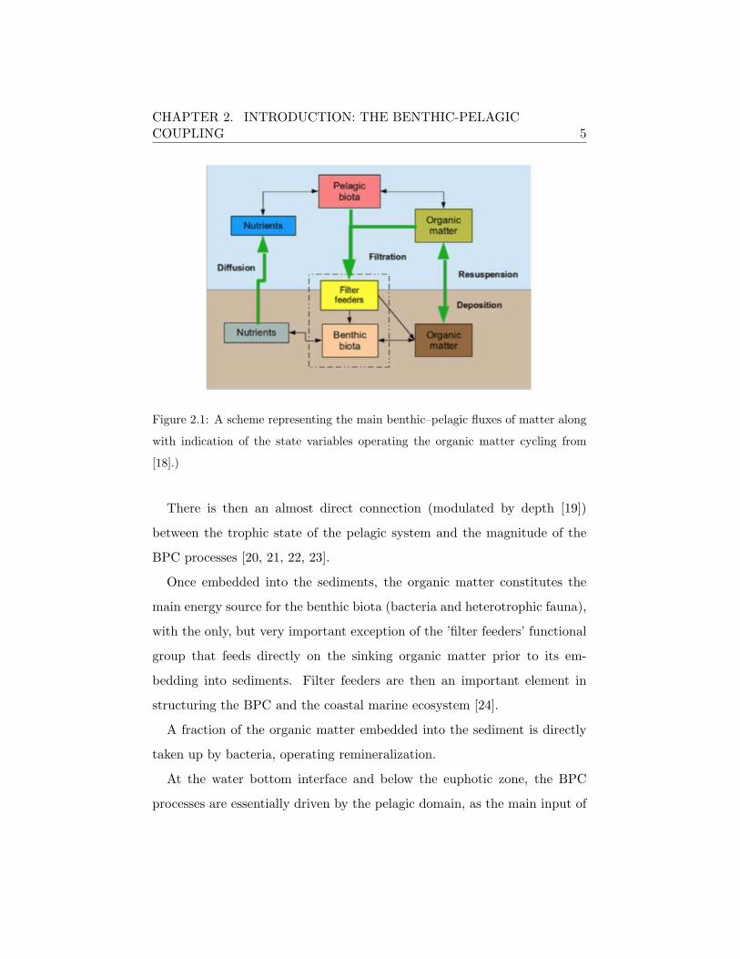
Here it is briefly described the structure of the BPC and the main fluxes
of organic and inorganic matter between the two realms.
In figure 2.1 it is reported a scheme of the matter fluxes connecting the
pelagic and the benthic domain along with the main benthic state variables
operating the organic matter recycling.
4
CHAPTER 2. INTRODUCTION: THE BENTHIC-PELAGICCOUPLING 5
Figure 2.1: A scheme representing the main benthic–pelagic fluxes of matter along
with indication of the state variables operating the organic matter cycling from
[18].)
There is then an almost direct connection (modulated by depth [19])
between the trophic state of the pelagic system and the magnitude of the
BPC processes [20, 21, 22, 23].
Once embedded into the sediments, the organic matter constitutes the
main energy source for the benthic biota (bacteria and heterotrophic fauna),
with the only, but very important exception of the ’filter feeders’ functional
group that feeds directly on the sinking organic matter prior to its em-
bedding into sediments. Filter feeders are then an important element in
structuring the BPC and the coastal marine ecosystem [24].
A fraction of the organic matter embedded into the sediment is directly
taken up by bacteria, operating remineralization.
At the water bottom interface and below the euphotic zone, the BPC
processes are essentially driven by the pelagic domain, as the main input of

CHAPTER 2. INTRODUCTION: THE BENTHIC-PELAGICCOUPLING 6
organic matter into the sediment originates from the net deposition (organic
matter sinking by gravity) and resuspension (benthic organic matter re-
injection into the water column due to turbulent processes [14]).
Benthic fauna feeds on organic matter and contributes to organic mat-
ter biogeochemical cycling through excretion and respiration processes that
contribute to the dissolved nutrients and carbon dioxide [25, 26, 27, 28],
sediment enrichment and to benthic oxygen depletion.
The backward (sediment to water) BPC fluxes determine the return of
the sediment recycled nutrient and carbon dioxide into the water column.
This occurs essentially through diffusive processes at the water sediment
interface.
The connection between the pelagic trophic state, depth and the BPC
intensity, stated above, implies that shallow nutrients enriched areas, such
as coastal regions directly influenced by a river discharge nutrients load are
interested by intense BPC processes determined by an enhanced organic
matte deposition at the water sediment interface [22, 23].
Finally, it has to be stressed that also the mixing/stratification character-
istics and time variability affect BPC processes intensity as intense mixing
(due to the winds) redistribute over the whole water column the inorganic
nutrients remineralized by the benthic cycling and diffused back into the
lower levels of the water column. Conversely stratified conditions partially
isolate the water sediment interface from water column sections, thereby
limiting nutrients input from the bottom.
The mid-latitude seasonal variability of the water column density struc-
ture then acts as a regulator of the trophic dynamics, modulating both the
input and output processes governing the BPC [14, 25, 29, 30].
CHAPTER 2. INTRODUCTION: THE BENTHIC-PELAGICCOUPLING 7
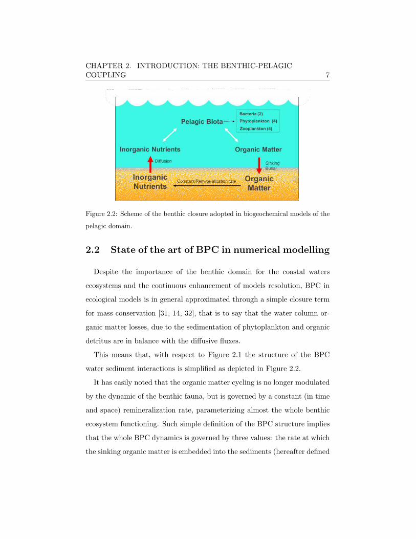
Figure 2.2: Scheme of the benthic closure adopted in biogeochemical models of the
pelagic domain.
2.2 State of the art of BPC in numerical modelling
Despite the importance of the benthic domain for the coastal waters
ecosystems and the continuous enhancement of models resolution, BPC in
ecological models is in general approximated through a simple closure term
for mass conservation [31, 14, 32], that is to say that the water column or-
ganic matter losses, due to the sedimentation of phytoplankton and organic
detritus are in balance with the diffusive fluxes.
This means that, with respect to Figure 2.1 the structure of the BPC
water sediment interactions is simplified as depicted in Figure 2.2.
It has easily noted that the organic matter cycling is no longer modulated
by the dynamic of the benthic fauna, but is governed by a constant (in time
and space) remineralization rate, parameterizing almost the whole benthic
ecosystem functioning. Such simple definition of the BPC structure implies
that the whole BPC dynamics is governed by three values: the rate at which
the sinking organic matter is embedded into the sediments (hereafter defined
CHAPTER 2. INTRODUCTION: THE BENTHIC-PELAGICCOUPLING 8
as ’burial velocity’), the diffusive rate at the water sediment interface and
the constant remineralization rate.
There are few studies (based on rather poor datasets in terms of number
of measurements and area of study) aimed to quantify the sediment–water
exchange processes [33, 34, 35]. However a proper consideration of the
benthic biogeochemical cycling must therefore be done at least at the level
of parameterizations taking into consideration the mentioned parameters.
The parameterization of the temporal and spatial scales of BPC is a very
challenging issue because observational data focusing on the BPC exchanges
are scanty and sparse both in time and space; this thereby hampers model
parameterization and validation. Given the scanty observational base, in
light of what has been said so far, it can be deduced the improvements
work in representing BPC processes neglecting to follow a ”step by step”
procedure in simulating the BPC. In this research, this procedure starts with
the development of a parameterized simple BPC numerical model (using a
one dimension coupled model configuration).
2.3 Aims of the thesis
The purposes of this thesis are: 1. To develop a simple model addressing
BPC processes with the parameterized benthic organic matter cycling (in
view of the use in global models) 2. To assess the skills of one-dimensional
coupled physical-biogeochemical models in simulating the BPC by imple-
menting the NEMO-BFM-1D model in marine areas with different physical
and biogeochemical characteristics, seeking practical parameterizations able
to describe different oceanic regimes.
The numerical tool used in this work is the one-dimensional version of
CHAPTER 2. INTRODUCTION: THE BENTHIC-PELAGICCOUPLING 9
the BFM-NEMO coupled physical-biogeochemical model in order to evalu-
ate the sensitivity of the pelagic biogeochemical dynamics to a simple BPC
parameterization by implementing the numerical tool in different sites char-
acterized by contrasting oceanographic characteristics and covered by rich
observational datasets, so that a meaningful validation procedure could be
carried out.
2.4 Structure of the thesis
The next Chapter (Chapter 3.1) gives an overview of the coupled NEMO-
BFM model with particular reference to the BPC sub-model implementa-
tion. Chapter 4.1 motivates the choice of the model implementation sites
and provides the description of the numerical experiments performed. Chap-
ter 5.1, 6.1 and 7.1 provide a description of the main characteristics of each
implementation site and of the simulation results. The conclusive Chapter
8.1 is devoted to an in depth assessment of the skill of the BPC sub-model in
simulating different environmental characteristics in contrasting sites. This
assessment is achieved through an extensive sensitivity analysis procedure.
Chapter 9 summarizes the achieved results and presents the possible further
developments.

Chapter 3
The NEMO-BFM model
3.1 Coupled physical–biogeochemical model
This work has been carried out using the one-dimensional (1D) version of
the NEMO-BFM modelling system of the coupled physical-biogeochemical
dynamics of the marine environment. The general characteristics of the
modelling system are given here. However, for an in-depth description of
the theoretical basis and the technical implementation of each model, the
reader can refer for NEMO to Madec [36] and for BFM to Vichi et al. [37],
while the coupling strategy between the two models is documented in Vichi
et al. [38].
3.1.1 NEMO 1D
NEMO (Nucleus for European Modelling of the Ocean) 1D is a numerical
tool that enables simulations of the physical vertical dynamics of the ocean
[39]. Here, it is used to simulate the biogeochemical dynamics coupled with
the vertical mixing processes and to perform sensitivity analysis with low
10
CHAPTER 3. THE NEMO-BFM MODEL 11
computational costs [39].
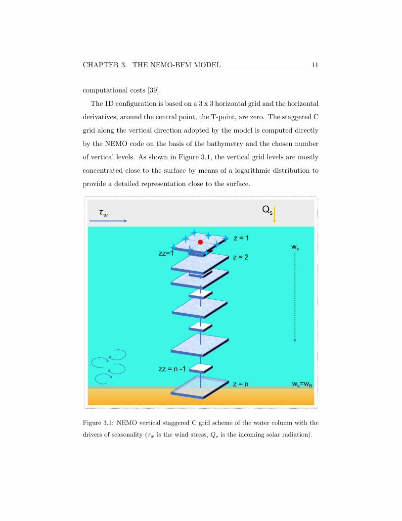
The 1D configuration is based on a 3 x 3 horizontal grid and the horizontal
derivatives, around the central point, the T-point, are zero. The staggered C
grid along the vertical direction adopted by the model is computed directly
by the NEMO code on the basis of the bathymetry and the chosen number
of vertical levels. As shown in Figure 3.1, the vertical grid levels are mostly
concentrated close to the surface by means of a logarithmic distribution to
provide a detailed representation close to the surface.
Figure 3.1: NEMO vertical staggered C grid scheme of the water column with the
drivers of seasonality (τw is the wind stress, Qs is the incoming solar radiation).

CHAPTER 3. THE NEMO-BFM MODEL 12
The primitive set of equations governing NEMO derives from:
• The Reynolds averaged Navier–Stokes equation:
δuiδt
+ ujδ(ui)
δxj= − 1
ρ0
δP
δxi− δ
δxj
(u′jui
′ − υmolδuiδxj
)+ fi (3.1)
• The temperature transport equation:
δT
δt+ uj
δ(T )
δxj= − δ
δxj
(u′jT
′ −KmolδT
δxj
)− 1
ρ0Cp− δI(Fsol, z)
δz(3.2)
• The salinity transport equation:
δS
δt+ uj
δ(S)
δxj= − δ
δxj
(u′jS
′ −KmolδS
δxj
)+ Ef − Pf (3.3)
Reffray [39].
where ui{i=1,2,} is the horizontal component of the velocity field, T and
S are the temperature and salinity respectively, xj{j=1,2,3} = (x, y, z) are
the zonal, meridional and vertical directions, t is the time, fi{i=1,2} is the
Coriolis term, P is the pressure, I is the downward irradiance, Fsol is the
penetrative part of the surface heat flux, Ef and Pf are the evaporation
and precipitation fluxes, and υmol and Kmol are the molecular viscosity and
diffusivity terms.
The u′jui′
term refers to the Reynolds stresses while u′jT′ and u′jS
′ refer
to the turbulent scalar fluxes. Reynolds stresses can be expressed, after a
scale analysis, as:
u′iw′ = −υt
δuiδz
(3.4)
T ′w′ = −KtδT
δz(3.5)
CHAPTER 3. THE NEMO-BFM MODEL 13
S′w′ = −KtδS
δz(3.6)
where υt and Kt are vertical turbulent viscosity and diffusivity terms re-
spectively.
Combining Eqs. 3.1, 3.2, 3.3, respectively with Eqs. 3.4, 3.5 and 3.6, and
considering that the horizontal derivatives in the one-dimensional case are
zero, the general governing equations can be simplified to:
δuiδt
= − δ
δz− υt
δuiδz
+ fi (3.7)
δT
δt= − 1
ρ0Cp− δI(Fsol, z)
δz− δ
δzKtδT
δz(3.8)
δS
δt= − δ
δzKtδS
δz+ Ef − Pf (3.9)
Among the different vertical turbulent schemes available in NEMO, it was
here selected the generic length scale (GLS) turbulent closure scheme that
has the advantage to be easily applicable at different marine regions (see
details in [39]). The GLS scheme is based on the turbulent kinetic energy
(k) equation and the transport equation for a generic statistical field variable
(ψ) [40]. The rate of change of the turbulent kinetic energy deriving from
the contraction of the transport equation of the Reynolds stress tensor, is:
δk
δt= Dk + P +G+ ε (3.10)
where Dk summarizes the turbulent and viscous transport terms (Eq.
3.11), P is the production of turbulent kinetic energy by shear (Eq. 3.12),
G relates to the production of turbulent kinetic energy by buoyancy (Eq.
3.13) and ε is the turbulent kinetic energy rate of dissipation (Eq. 3.14).
CHAPTER 3. THE NEMO-BFM MODEL 14
Dk =δ
δz
δυtδσk
δk
δz(3.11)
P = υtM2 (3.12)
G = ktN2 (3.13)
ε =
(C0µ
)3k3/2
l(3.14)
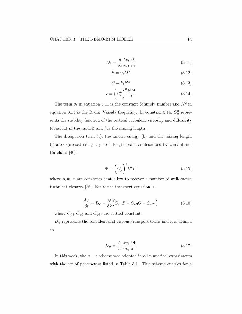
The term σt in equation 3.11 is the constant Schmidt–number and N2 in
equation 3.13 is the Brunt–Vaisala frequency. In equation 3.14, C0µ repre-
sents the stability function of the vertical turbulent viscosity and diffusivity
(constant in the model) and l is the mixing length.
The dissipation term (ε), the kinetic energy (k) and the mixing length
(l) are expressed using a generic length scale, as described by Umlauf and
Burchard [40]:
Ψ =
(C0µ
)pkmln (3.15)
where p,m, n are constants that allow to recover a number of well-known
turbulent closures [36]. For Ψ the transport equation is:
δψ
δt= Dψ −
ψ
δk
(Cψ1P + Cψ3G− Cψ2ε
)(3.16)
where Cψ1, Cψ3 and Cψ2ε are settled constant.
Dψ represents the turbulent and viscous transport terms and it is defined
as:
Dψ =δ
δz
δυtδσψ
δΨ
δz(3.17)
In this work, the κ− ε scheme was adopted in all numerical experiments
with the set of parameters listed in Table 3.1. This scheme enables for a
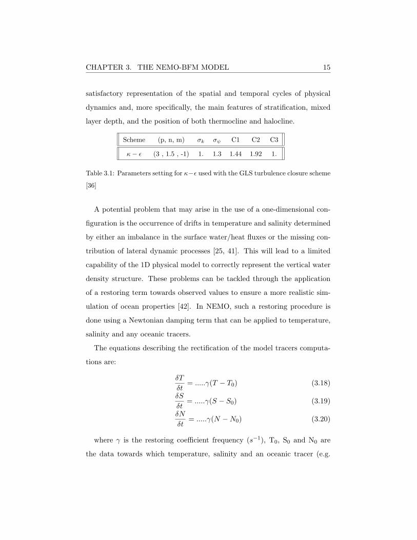
CHAPTER 3. THE NEMO-BFM MODEL 15
satisfactory representation of the spatial and temporal cycles of physical
dynamics and, more specifically, the main features of stratification, mixed
layer depth, and the position of both thermocline and halocline.
Scheme (p, n, m) σk σψ C1 C2 C3
κ− ε (3 , 1.5 , -1) 1. 1.3 1.44 1.92 1.
Table 3.1: Parameters setting for κ−ε used with the GLS turbulence closure scheme
[36]
A potential problem that may arise in the use of a one-dimensional con-
figuration is the occurrence of drifts in temperature and salinity determined
by either an imbalance in the surface water/heat fluxes or the missing con-
tribution of lateral dynamic processes [25, 41]. This will lead to a limited
capability of the 1D physical model to correctly represent the vertical water
density structure. These problems can be tackled through the application
of a restoring term towards observed values to ensure a more realistic sim-
ulation of ocean properties [42]. In NEMO, such a restoring procedure is
done using a Newtonian damping term that can be applied to temperature,
salinity and any oceanic tracers.
The equations describing the rectification of the model tracers computa-
tions are:
δT
δt= .....γ(T − T0) (3.18)
δS
δt= .....γ(S − S0) (3.19)
δN
δt= .....γ(N −N0) (3.20)
where γ is the restoring coefficient frequency (s−1), T0, S0 and N0 are
the data towards which temperature, salinity and an oceanic tracer (e.g.

CHAPTER 3. THE NEMO-BFM MODEL 16
nitrate, phosphate) will be restored.
CHAPTER 3. THE NEMO-BFM MODEL 17
3.1.2 BFM
The Biogeochemical Flux Model, BFM, is a biomass and functional group
based marine ecosystem model, representing the system in eulerian coordi-
nates by a selection of chemical and biological processes that simulates the
pelagic (water column) and the benthic (water sediment interface) dynamics
in the marine ecosystems. The model also includes a sea ice component [43]
not used in this thesis.
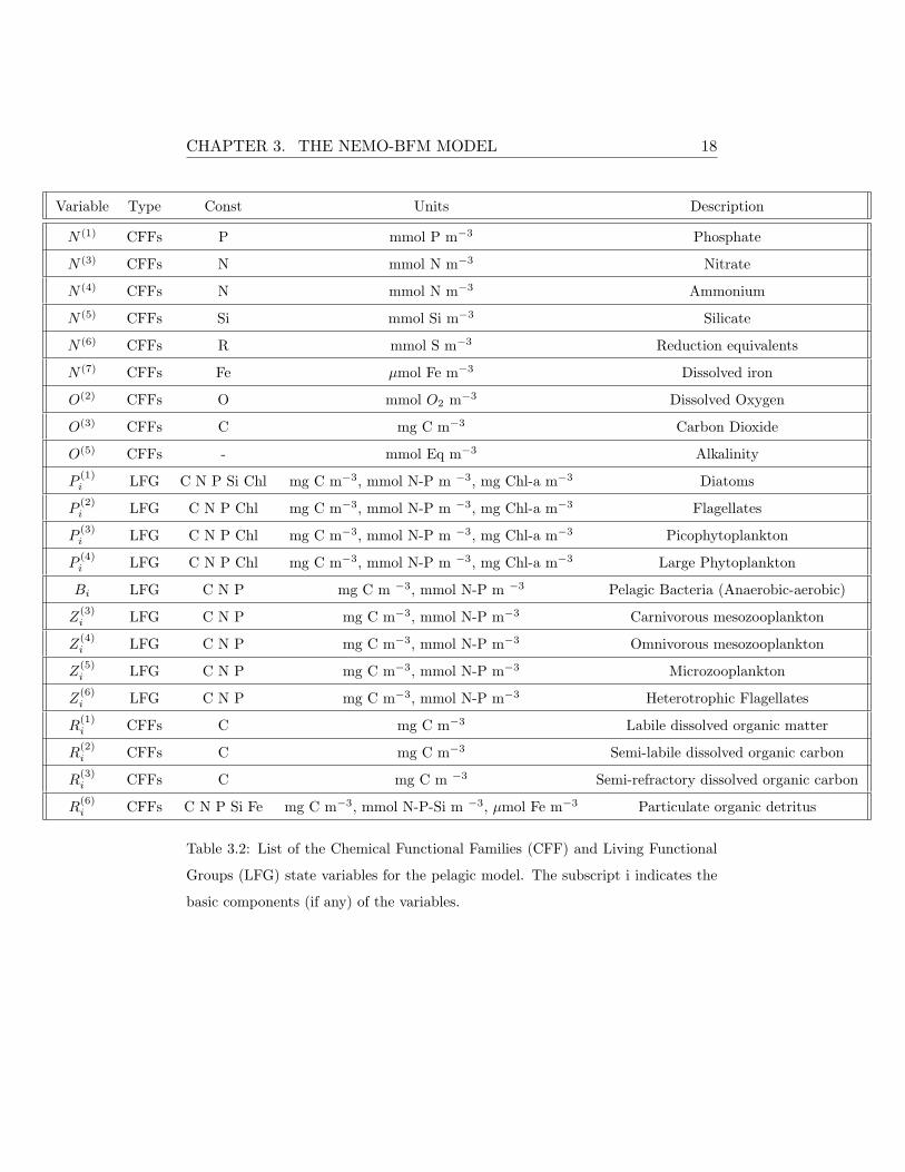
The formalism describing the BFM functional approach is explained in
the reference paper of Vichi et al. [44], and it is based on the concepts of
the Chemical Functional Families (CFF) and the Living Functional Groups
(LFG). CFFs (Table 3.2) are divided into three main groups: non-living
organic, living- organic and inorganic.
The LFG (listed in Table 3.2) notation is based on the concept of a stan-
dard organism that is frequently used in marine and terrestrial ecosystem
modelling as a theoretical construct without any specific taxonomic value
[45, 46, 47]. The biomass of the standard organism is constituted by living
CFFs and interacts with living and non living CFFs by means of physiolog-
ical and ecological processes (see Figure 3.2).
CHAPTER 3. THE NEMO-BFM MODEL 18
Variable Type Const Units Description
N (1) CFFs P mmol P m−3 Phosphate
N (3) CFFs N mmol N m−3 Nitrate
N (4) CFFs N mmol N m−3 Ammonium
N (5) CFFs Si mmol Si m−3 Silicate
N (6) CFFs R mmol S m−3 Reduction equivalents
N (7) CFFs Fe µmol Fe m−3 Dissolved iron
O(2) CFFs O mmol O2 m−3 Dissolved Oxygen
O(3) CFFs C mg C m−3 Carbon Dioxide
O(5) CFFs - mmol Eq m−3 Alkalinity
P(1)i LFG C N P Si Chl mg C m−3, mmol N-P m −3, mg Chl-a m−3 Diatoms
P(2)i LFG C N P Chl mg C m−3, mmol N-P m −3, mg Chl-a m−3 Flagellates
P(3)i LFG C N P Chl mg C m−3, mmol N-P m −3, mg Chl-a m−3 Picophytoplankton
P(4)i LFG C N P Chl mg C m−3, mmol N-P m −3, mg Chl-a m−3 Large Phytoplankton
Bi LFG C N P mg C m −3, mmol N-P m −3 Pelagic Bacteria (Anaerobic-aerobic)
Z(3)i LFG C N P mg C m−3, mmol N-P m−3 Carnivorous mesozooplankton
Z(4)i LFG C N P mg C m−3, mmol N-P m−3 Omnivorous mesozooplankton
Z(5)i LFG C N P mg C m−3, mmol N-P m−3 Microzooplankton
Z(6)i LFG C N P mg C m−3, mmol N-P m−3 Heterotrophic Flagellates
R(1)i CFFs C mg C m−3 Labile dissolved organic matter
R(2)i CFFs C mg C m−3 Semi-labile dissolved organic carbon
R(3)i CFFs C mg C m −3 Semi-refractory dissolved organic carbon
R(6)i CFFs C N P Si Fe mg C m−3, mmol N-P-Si m −3, µmol Fe m−3 Particulate organic detritus
Table 3.2: List of the Chemical Functional Families (CFF) and Living Functional
Groups (LFG) state variables for the pelagic model. The subscript i indicates the
basic components (if any) of the variables.

CHAPTER 3. THE NEMO-BFM MODEL 19
Figure 3.2 summarizes the complexity of the pelagic state variables and
the main biological, physiological and ecological processes accounted by the
BFM model in its standard configuration, while a complete list of the stan-
dard biogeochemical parameterization can be found in Appendix A.1.
Figure 3.2: Scheme of the state variables and pelagic interactions of the BFM model.
Living (organic) Chemical Functional Families (CFF) are indicated with bold-line
square boxes, non-living organic CFFs with thin-line square boxes and inorganic
CFFs with rounded boxes (modified after Blackford and Radford (1995)[48]). Fig.
from BFM manual [44].
CHAPTER 3. THE NEMO-BFM MODEL 20
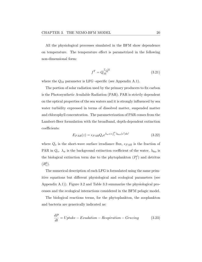
All the physiological processes simulated in the BFM show dependence
on temperature. The temperature effect is parametrized in the following
non-dimensional form:
fT = QT−10
1010 (3.21)
where the Q10 parameter is LFG -specific (see Appendix A.1).
The portion of solar radiation used by the primary producers to fix carbon
is the Photosynthetic Available Radiation (PAR). PAR is strictly dependent
on the optical properties of the sea waters and it is strongly influenced by sea
water turbidity expressed in terms of dissolved matter, suspended matter
and chlorophyll concentration. The parameterization of PAR comes from the
Lambert-Beer formulation with the broadband, depth-dependent extinction
coefficients:
EPAR(z) = εPARQseλwz+
∫ 0z λbio(z
′)dz′ (3.22)
where Qs is the short-wave surface irradiance flux, εPAR is the fraction of
PAR in Qs. λw is the background extinction coefficient of the water, λbio is
the biological extinction term due to the phytoplankton (P jl ) and detritus
(R6c).
The numerical description of each LFG is formulated using the same prim-
itive equations but different physiological and ecological parameters (see
Appendix A.1)). Figure 3.2 and Table 3.3 summarize the physiological pro-
cesses and the ecological interactions considered in the BFM pelagic model.
The biological reactions terms, for the phytoplankton, the zooplankton
and bacteria are generically indicated as:
dP
dt= Uptake− Exudation−Respiration−Grazing (3.23)
CHAPTER 3. THE NEMO-BFM MODEL 21
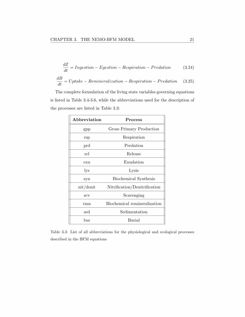
dZ
dt= Ingestion− Egestion−Respiration− Predation (3.24)
dB
dt= Uptake−Remineralization−Respiration− Predation (3.25)
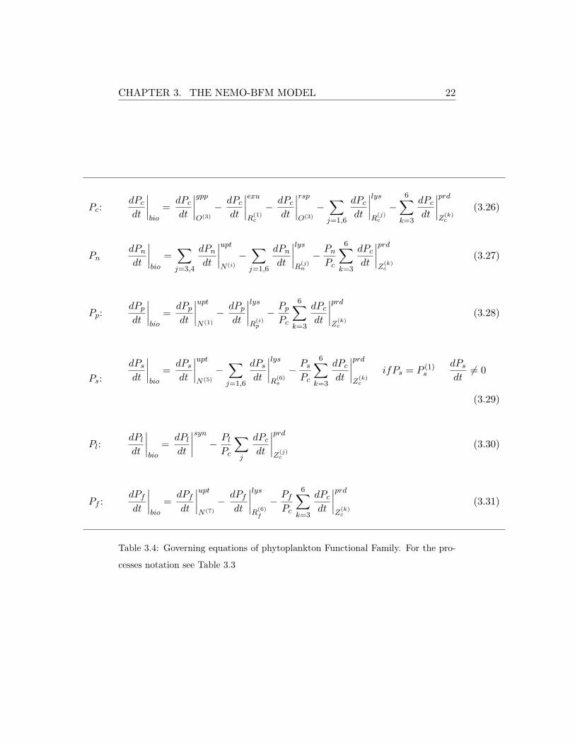
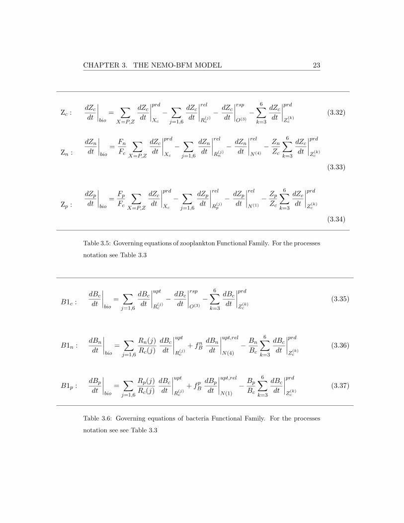
The complete formulation of the living state variables governing equations
is listed in Table 3.4-3.6, while the abbreviations used for the description of
the processes are listed in Table 3.3:
Abbreviation Process
gpp Gross Primary Production
rsp Respiration
prd Predation
rel Release
exu Exudation
lys Lysis
syn Biochemical Synthesis
nit/denit Nitrification/Denitrification
scv Scavenging
rmn Biochemical remineralization
sed Sedimentation
bur Burial
Table 3.3: List of all abbreviations for the physiological and ecological processes
described in the BFM equations
CHAPTER 3. THE NEMO-BFM MODEL 22
Pc:dPcdt
∣∣∣∣bio
=dPcdt
∣∣∣∣gppO(3)
− dPcdt
∣∣∣∣exuR
(1)c
− dPcdt
∣∣∣∣rspO(3)
−∑j=1,6
dPcdt
∣∣∣∣lysR
(j)c
−6∑
k=3
dPcdt
∣∣∣∣prdZ
(k)c
(3.26)
PndPndt
∣∣∣∣bio
=∑j=3,4
dPndt
∣∣∣∣uptN(i)
−∑j=1,6
dPndt
∣∣∣∣lysR
(j)n
− PnPc
6∑k=3
dPcdt
∣∣∣∣prdZ
(k)c
(3.27)
Pp:dPpdt
∣∣∣∣bio
=dPpdt
∣∣∣∣uptN(1)
− dPpdt
∣∣∣∣lysR
(i)p
− PpPc
6∑k=3
dPcdt
∣∣∣∣prdZ
(k)c
(3.28)
Ps:
dPsdt
∣∣∣∣bio
=dPsdt
∣∣∣∣uptN(5)
−∑j=1,6
dPsdt
∣∣∣∣lysR
(6)s
− PsPc
6∑k=3
dPcdt
∣∣∣∣prdZ
(k)c
ifPs = P (1)s
dPsdt6= 0
(3.29)
Pl:dPldt
∣∣∣∣bio
=dPldt
∣∣∣∣syn − PlPc
∑j
dPcdt
∣∣∣∣prdZ
(j)c
(3.30)
Pf :dPfdt
∣∣∣∣bio
=dPfdt
∣∣∣∣uptN(7)
−dPfdt
∣∣∣∣lysR
(6)f
−PfPc
6∑k=3
dPcdt
∣∣∣∣prdZ
(k)c
(3.31)
Table 3.4: Governing equations of phytoplankton Functional Family. For the pro-
cesses notation see Table 3.3
CHAPTER 3. THE NEMO-BFM MODEL 23
Zc :dZcdt
∣∣∣∣bio
=∑
X=P,Z
dZcdt
∣∣∣∣prdXc
−∑j=1,6
dZcdt
∣∣∣∣relR
(j)c
− dZcdt
∣∣∣∣rspO(3)
−6∑
k=3
dZcdt
∣∣∣∣prdZ
(k)c
(3.32)
Zn :
dZndt
∣∣∣∣bio
=FnFc
∑X=P,Z
dZcdt
∣∣∣∣prdXc
−∑j=1,6
dZndt
∣∣∣∣relR
(j)n
− dZndt
∣∣∣∣relN(4)
− ZnZc
6∑k=3
dZcdt
∣∣∣∣prdZ
(k)c
(3.33)
Zp :
dZpdt
∣∣∣∣bio
=FpFc
∑X=P,Z
dZcdt
∣∣∣∣prdXc
−∑j=1,6
dZpdt
∣∣∣∣relR
(j)p
− dZpdt
∣∣∣∣relN(1)
− ZpZc
6∑k=3
dZcdt
∣∣∣∣prdZ
(k)c
(3.34)
Table 3.5: Governing equations of zooplankton Functional Family. For the processes
notation see Table 3.3
B1c :dBcdt
∣∣∣∣bio
=∑j=1,6
dBcdt
∣∣∣∣uptR
(j)c
− dBcdt
∣∣∣∣rspO(3)
−6∑
k=3
dBcdt
∣∣∣∣prdZ
(k)c
(3.35)
B1n :dBndt
∣∣∣∣bio
=∑j=1,6
Rn(j)
Rc(j)
dBcdt
∣∣∣∣uptR
(j)c
+ fnBdBndt
∣∣∣∣upt,relN(4)
− BnBc
6∑k=3
dBcdt
∣∣∣∣prdZ
(k)c
(3.36)
B1p :dBpdt
∣∣∣∣bio
=∑j=1,6
Rp(j)
Rc(j)
dBcdt
∣∣∣∣uptR
(j)c
+ fpBdBpdt
∣∣∣∣upt,relN(1)
− BpBc
6∑k=3
dBcdt
∣∣∣∣prdZ
(k)c
(3.37)
Table 3.6: Governing equations of bacteria Functional Family. For the processes
notation see see Table 3.3
CHAPTER 3. THE NEMO-BFM MODEL 24
The pelagic cycle of inorganic nutrients affects and is affected by phyto-
plankton and bacteria activities of uptake and release and by zooplankton
excretion. Phytoplankton and bacteria production can be limited by in-
organic nutrients concentration. In BFM, nutrients limitation is treated
following Baretta-Bekker et al. [45] i.e. in which nutrients limiting factors
are partitioned in internal or external, based on an internal nutrient quota
or the external dissolved inorganic concentrations. BFM accounts for the
limiting nutrient using the following co–limitation approach:
fnutp = min(fn,pp , ffp , fsp )
The equations governing the dynamics of the pelagic inorganic nutrients are
listed in Table 3.7:

CHAPTER 3. THE NEMO-BFM MODEL 25
N1p:
dN (1)
dt
∣∣∣∣∣bio
= −4∑j=1
dP(j)p
dt
∣∣∣∣∣upt
N(1)
+ fpBdB
(j)p
dt
∣∣∣∣∣upt,rel
N(1)
+
6∑j=3
dZ(k)p
dt
∣∣∣∣∣rsp
N(1)
(3.38)
N3ndN (3)
dt
∣∣∣∣∣bio
= −4∑j=1
dP(j)n
dt
∣∣∣∣∣upt
N(3)
+dN (3)
dt
∣∣∣∣∣nit
N(4)
− dN (3)
dt
∣∣∣∣∣denit
sinkn
(3.39)
N4n:
dN (4)
dt
∣∣∣∣∣bio
= −4∑j=1
dP(j)n
dt
∣∣∣∣∣upt
N(4)
+ fpBdB
(j)n
dt
∣∣∣∣∣upt,rel
N(4)
+6∑j=3
dZ(k)n
dt
∣∣∣∣∣rsp
N(4)
− dN (4)
dt
∣∣∣∣∣nit
N(3)
(3.40)
N5s:dN (5)
dt
∣∣∣∣∣bio
= − dP(1)s
dt
∣∣∣∣∣upt
N(5)
+dR
(6)s
dt
∣∣∣∣∣rmn
N(5)
(3.41)
N5f:dN (7)
dt
∣∣∣∣∣bio
= −dPfdt
∣∣∣∣uptN(7)
+dR
(6)f
dt
∣∣∣∣∣∣rmn
N(7)
+dN (7)
dt
∣∣∣∣∣scv
sinkn
(3.42)
Table 3.7: Governing equations of nutrients. For the processes notation see Table
3.3
CHAPTER 3. THE NEMO-BFM MODEL 26
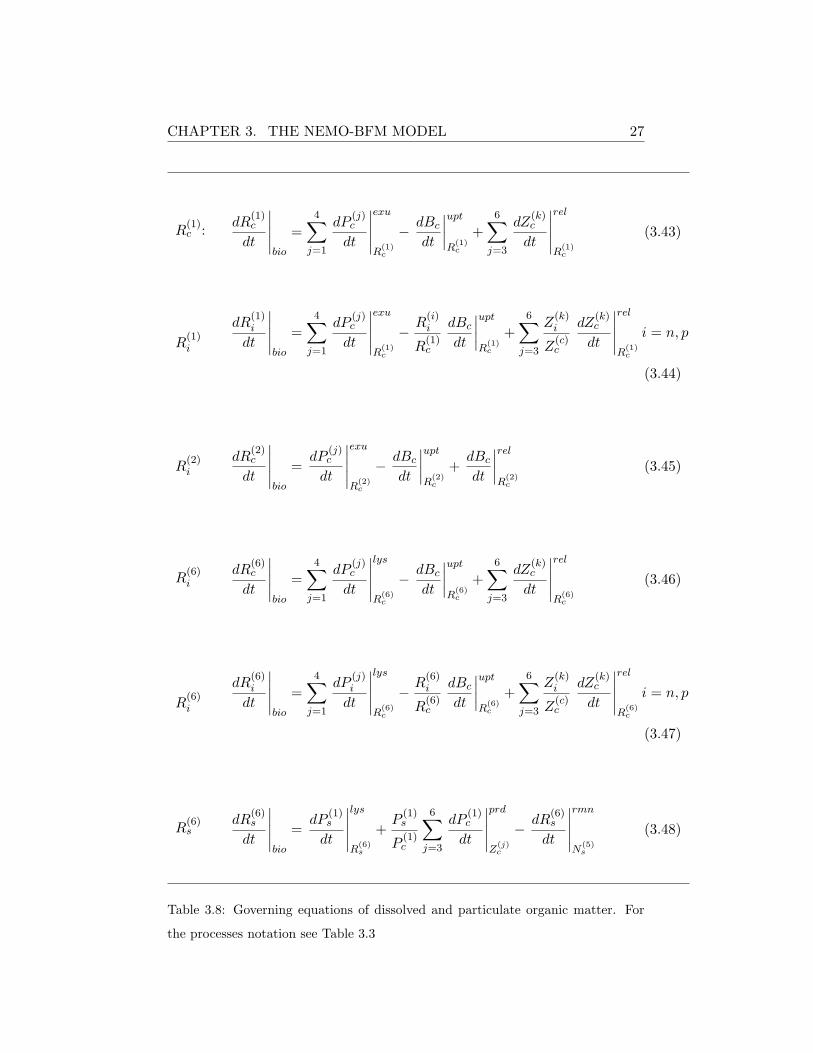
Dissolved organic matter (DOM) dynamics is strongly linked with the
biota activity. DOM is produced by phytoplankton, microzooplankton and
bacteria. In the BFM configuration used in this work, DOM has all the
different degrees of lability/refractivity provided by the model (see Table
3.2), which differ from each others for the turn-over time scale. Only bacteria
are able to degrade the different types of DOM.
Pelagic particulate organic matter (POM) is produced by all the members
of the plankton community except bacteria which use this matter as sub-
strate. The biogenic silica production depends exclusively on the release of
frustules by diatoms while losses are linked to the micro/mesozooplankton
predation. Once produced, particulate organic matter (POM) can be de-
graded by bacteria and deposited in the sediment-water interface with a
proper sinking velocity. The governing equations for DOM and POM are
listed in Table 3.8.
CHAPTER 3. THE NEMO-BFM MODEL 27
R(1)c :
dR(1)c
dt
∣∣∣∣∣bio
=4∑j=1
dP(j)c
dt
∣∣∣∣∣exu
R(1)c
− dBcdt
∣∣∣∣uptR
(1)c
+6∑j=3
dZ(k)c
dt
∣∣∣∣∣rel
R(1)c
(3.43)
R(1)i
dR(1)i
dt
∣∣∣∣∣bio
=
4∑j=1
dP(j)c
dt
∣∣∣∣∣exu
R(1)c
−R
(i)i
R(1)c
dBcdt
∣∣∣∣uptR
(1)c
+
6∑j=3
Z(k)i
Z(c)c
dZ(k)c
dt
∣∣∣∣∣rel
R(1)c
i = n, p
(3.44)
R(2)i
dR(2)c
dt
∣∣∣∣∣bio
=dP
(j)c
dt
∣∣∣∣∣exu
R(2)c
− dBcdt
∣∣∣∣uptR
(2)c
+dBcdt
∣∣∣∣relR
(2)c
(3.45)
R(6)i
dR(6)c
dt
∣∣∣∣∣bio
=
4∑j=1
dP(j)c
dt
∣∣∣∣∣lys
R(6)c
− dBcdt
∣∣∣∣uptR
(6)c
+
6∑j=3
dZ(k)c
dt
∣∣∣∣∣rel
R(6)c
(3.46)
R(6)i
dR(6)i
dt
∣∣∣∣∣bio
=4∑j=1
dP(j)i
dt
∣∣∣∣∣lys
R(6)c
−R
(6)i
R(6)c
dBcdt
∣∣∣∣uptR
(6)c
+6∑j=3
Z(k)i
Z(c)c
dZ(k)c
dt
∣∣∣∣∣rel
R(6)c
i = n, p
(3.47)
R(6)s
dR(6)s
dt
∣∣∣∣∣bio
=dP
(1)s
dt
∣∣∣∣∣lys
R(6)s
+P
(1)s
P(1)c
6∑j=3
dP(1)c
dt
∣∣∣∣∣prd
Z(j)c
− dR(6)s
dt
∣∣∣∣∣rmn
N(5)s
(3.48)
Table 3.8: Governing equations of dissolved and particulate organic matter. For
the processes notation see Table 3.3
CHAPTER 3. THE NEMO-BFM MODEL 28
3.2 The Benthic Submodel
3.2.1 Background
Marine biogeochemical cycles incorporate both the pelagic and benthic
habitats and thus integrate processes and interactions in both environments.
Here, the focus is on how low trophic levels processes such as cycling of ni-
trogen (N), phosphorus (P), carbon (C), silicon (Si), carbon dioxide (CO2),
oxygen (O2), primary production, bacteria production, animal nutrient ex-
cretion, and decomposition, link benthic and pelagic habitats.
The general scheme of BPC used in this thesis is the same described in
[49]. The particulate pelagic organic matter produced via lysis, excretion
and egestion, not consumed or remineralized in the water column sinks to the
seafloor with a specific sedimentation velocity. Once it reaches the seawater-
sediment interface, the pelagic organic matter is buried into the sediments
and, with a certain rates, remineralized by bacteria. It is estimated [50],
that a quarter of all organic material that exits the photic zone reaches the
seafloor without being remineralized and 90% of that remaining material is
remineralized in sediments, consuming oxygen and producing carbon diox-
ide. The benthic nutrient pool is further enriched by the products of the
benthic fauna excretion.
In the sediments, the remineralized inorganic nutrients diffuses into the
lower levels of the water column, and vertical dynamics injects them into the
photic zone. This source of nutrients feeds the lower trophic levels activity,
(bacteria and phytoplankton) that, in turns, stimulates the zooplankton
growth [51, 52] (see Figure 2.2).
CHAPTER 3. THE NEMO-BFM MODEL 29
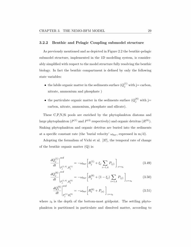
3.2.2 Benthic and Pelagic Coupling submodel structure
As previously mentioned and as depicted in Figure 2.2 the benthic-pelagic
submodel structure, implemented in the 1D modelling system, is consider-
ably simplified with respect to the model structure fully resolving the benthic
biology. In fact the benthic compartment is defined by only the following
state variables:
• the labile organic matter in the sediments surface (Q(1)j with j= carbon,
nitrate, ammonium and phosphate )
• the particulate organic matter in the sediments surface (Q(6)j with j=
carbon, nitrate, ammonium, phosphate and silicate).
These C,P,N,Si pools are enriched by the phytoplankton diatoms and
large phytoplankton (P (1) and P (4) respectively) and organic detritus (R(6)).
Sinking phytoplankton and organic detritus are buried into the sediments
at a specific constant rate (the ’burial velocity’ ωbur, expressed in m/d).
Adopting the formalism of Vichi et al. [37], the temporal rate of change
of the benthic organic matter (Q) is:
dQ(1)j
dt
∣∣∣∣∣sed
P(1,4)j ,R
(1)j
= −ωbur[R
(1)j + ξj
∑i=1,4
P(j)
]z=zb
(3.49)
dQ(6)j
dt
∣∣∣∣∣sed
P(1,4)j ,R
(6)j
= −ωbur[R
(6)j + (1− ξj)
∑i=1,4
P(j)
]z=zb
(3.50)
dQ(6)s
dt
∣∣∣∣∣sed
P(1)j R
(6)s
= −ωbur[R(6)s + P(s)
]z=zb
(3.51)
where zb is the depth of the bottom-most gridpoint. The settling phyto-
plankton is partitioned in particulate and dissolved matter, according to

CHAPTER 3. THE NEMO-BFM MODEL 30
the ξj partitioning coefficient. Comparing Figure 2.1 with 2.2 it is appar-
ent that the ωbur parameter resolves also the particulate organic matter
sediment embedding due not only to sinking but also to the benthic filters
feeders activity.
The remineralization flux (inorganic matter flowing from the sediment to
the water) is parametrized by assuming that a constant portion of organic
matter in the organic sediments is remineralized and released in the pelagic
compartment as follows:
dQ(1)j
dt
∣∣∣∣∣rmn/diff
= µQ
(1)j
Q(1)j
∣∣∣z=zb
(3.52)
dQ(6)j
dt
∣∣∣∣∣rmn/diff
= µQ
(6)j
Q(6)j
∣∣∣z=zb
(3.53)
dQ(6)s
dt
∣∣∣∣∣rmn/diff
= µQ
(6)sQ(6)s
∣∣∣z=zb
(3.54)
where µ(1,6) are the recycling time scales operating the conversion of the
benthic organic matter into pelagic dissolved nutrients.
The oxygen consumption, associated to remineralization process, is sto-
ichiometrically associated to the carbon remineralization rates. Nitrogen
remineralization is partitioned into ammonium and nitrate fluxes with a
constant ratio.
Lastly, the general equation describing the rate of change of organic mat-
ter in the sediments is defined by:
dQ(1,6)j
dt= −
dQ(1,6)j
dt
∣∣∣∣∣rmn
+dQ
(1,6)j
dt
∣∣∣∣∣sed
(3.55)
CHAPTER 3. THE NEMO-BFM MODEL 31
3.2.3 Boundary conditions
Forcing an Ocean General Circulation Model (OGCM) amounts to spec-
ifying surface and bottom boundary conditions for the vertical dynamics of
a model’s prognostic equations for potential temperature, salinity, and the
momentum components [42].
Surface boundary conditions
In NEMO-1D the surface boundary conditions are applied at the surface-
most grid point z = 0. The physical model requires the following fields
as surface boundary conditions with a frequency at which the forcing fields
have to be updated:
• the zonal and meridional components of the wind stress (τx, τy, re-
spectively).
• the surface heat flux partitioned in longwave radiation (Qns) and
shortwave radiation (Qsr). The former is the non penetrative part
of the radiation flux.
• the surface freshwater flux (evaporation - precipitation- runoff)
• the surface salt flux associated with freezing/melting of seawater (sfx)
For the BFM the surface boundary conditions are:
dCidz
∣∣∣∣z=0
= 0 (3.56a)
dCidz
∣∣∣∣z=0
= Fj (3.56b)
dCidz
∣∣∣∣z=0
= γ(Cj − Cjref ) (3.56c)

CHAPTER 3. THE NEMO-BFM MODEL 32
where Equation 3.56a is valid for all the living organic and non living
organic state variables type, while Equation 3.56b is valid for those state
variables interacting at the air-sea or land-sea interface. Finally, Equation
3.56c expresses the surface boundary condition obtained by relaxing (Section
3.1.1) a surface state variable value (e.g. for the inorganic nutrients) to a
prescribed time-varying value.
Bottom boundary conditions
At the water-sediment interface, the bottom boundary conditions are ap-
plied at the bottom-most vertical level (z=zb).
In NEMO the momentum, the tracers, the heat and the velocity deriva-
tives are set to zero.
The BFM benthic submodel provides the bottom boundary conditions for
the pelagic nutrients computation as follows:
dCidz
= 0 (3.57a)
dCidz
=dCiδt
∣∣∣∣rmn/diff (3.57b)
w = wb (3.57c)
where Equation 3.57a is valid for all the Living Organic and Non Liv-
ing Organic state variables and Equation 3.57b is valid for the inorganic
nutrients considered in the BPC.

CHAPTER 3. THE NEMO-BFM MODEL 33
3.2.4 BFM-NEMO Coupling scheme
In describing the NEMO-BFM coupled configuration scheme, we use to
the same conceptual formalism used to express the equations of biogeochem-
ical dynamics.
The conservation equation for an infinitesimal volume of fluid, contain-
ing a certain concentration of a passively transported tracer C, is obtained
applying the continuum hypothesis:
δC
δt= −~∇ · ~F (3.58)
where ~F is the generalized flux of C.
Equation 3.58 can be rewritten expressing separately the physical (han-
dled by the NEMO 1D) and the biogeochemical (handled by BFM) contri-
butions:
δC
δt= −~∇ · ~Fphys − ~∇ · ~Fbio (3.59)
The biological reaction term, is approximated as:
~∇ · ~Fbio = −wBδC
δz+δC
δt
∣∣∣∣bio
(3.60)
where wB refers to the sinking vertical velocity for those variables having a
mass related vertical velocity other than the fluid velocity (e.g. the detritus).
From equations 3.59 and 3.60 is derived the advection-diffusion-reaction
equation for an incompressible fluid:
δC
δt= −u · ∇C +∇H · (AH∇HC) +
δ
δzAV
δC
δz− wB
δC
δz+δC
δt
∣∣∣∣bio
(3.61)

CHAPTER 3. THE NEMO-BFM MODEL 34
where u ≡ (u, v, w) is the three-dimensional velocity, AH , AV horizontal
and vertical turbulent diffusivity coefficient for tracers.
Equation 3.61 can be rewritten indicating the ocean variables solved by
the ocean general circulation model and needed for the biological reaction
term R computation:
δC
δt+u
δC
δx+v
δC
δy+w
δC
δz= ∇H ·(AH∇HC)+
δ
δzAV
δC
δz−wB
δC
δz+R(T, S,W,E)
(3.62)
where T is the temperature, S is salinity, W is the intensity of the wind, and
E is the shortwave radiation.
In the 1D configuration the horizontal derivatives are not considered and
equation 3.62 became:
δC
δt= −wδC
δz+
δ
δzAV
δC
δz− wB
δC
δz+R(T, S,W,E) (3.63)
The NEMO-BFM coupling equation 3.61 requires knowledge of some
ocean physical dynamics, solved by the OGCM and transferred to the BFM.
The conceptual framework of the coupling functioning is schematized in Fig-
ure 3.3. The OGCM model compute and transfer environmental information
to the BFM which, in turn, compute the biological rates using the environ-
mental information passed by the OGCM.
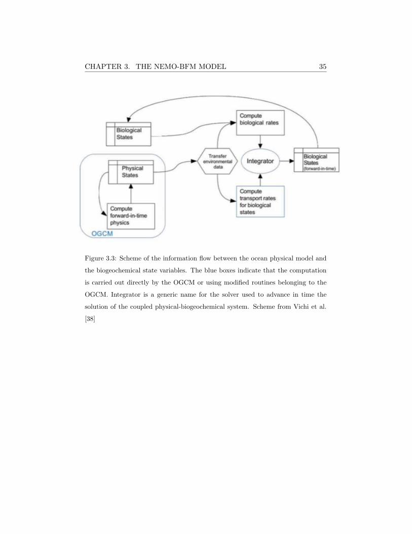
CHAPTER 3. THE NEMO-BFM MODEL 35
Figure 3.3: Scheme of the information flow between the ocean physical model and
the biogeochemical state variables. The blue boxes indicate that the computation
is carried out directly by the OGCM or using modified routines belonging to the
OGCM. Integrator is a generic name for the solver used to advance in time the
solution of the coupled physical-biogeochemical system. Scheme from Vichi et al.
[38]
Chapter 4
Implementation sites and
experiments design
4.1 The choice of the implementation sites
In order to achieve the objectives of this work, the 1D NEMO-BFM BPC
sub-model has been implemented in three different sites. The choice of
the implementation sites has been constrained by two factors: the coastal
character with contrasting environmental features and the availability of
the in-situ observations, which are necessary to assess the model skill with
respect to the BPC dynamics.
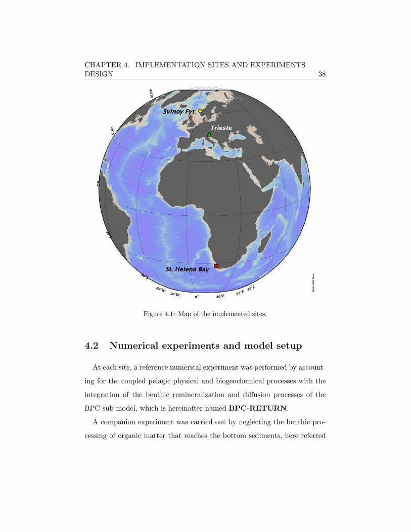
Three different locations were selected to investigate the BPC processes
using the coupled model (Figure XX):
1. Gulf of Trieste, MA21 area (North Adriatic Sea, Italy),
2. St. Helena Bay Monitoring Line, SHB (Atlantic Ocean, South Africa),
3. Svinøy Fyr, SFyr (Norwegian Sea, Norway).
36

CHAPTER 4. IMPLEMENTATION SITES AND EXPERIMENTSDESIGN 37
The numerical experiments performed in the MA21 area in the Gulf of
Trieste served as initial test benchmark, because of the large scientific litera-
ture dealing with observational and numerical modelling studies [53, 54, 55,
56, 57, 41, 23]. This gave an adequate observational basis to be compared
with the output of the coupled model.
As second site, the station number 3 of the BENEFIT (Benguela Envi-
ronment and Fisheries Interactions and Training) monitoring program in
St. Helena Bay has been chosen to simulate the dynamics of an ecosystem
embedded in a complex upwelling area [58, 59].
The third case study corresponds to the first station of the Svinøy Fyr
Section in the Norwegian Sea. The dataset was compiled using the data
publicly distributed by the Institute of Marine Research - Norwegian Marine
Data Centre (INR-NMD) (https://www.nmdc.no and http://www.imr.no).
It is the deepest site implemented in this work and it has been chosen to
asses the skill of the model in reproducing the biogeochemical cycles in a
cold water system and the deep BPC dynamics.
A description of the hydrographical and ecological characteristics of each
site is given in the following dedicated chapters.
CHAPTER 4. IMPLEMENTATION SITES AND EXPERIMENTSDESIGN 38
Figure 4.1: Map of the implemented sites.
4.2 Numerical experiments and model setup
At each site, a reference numerical experiment was performed by account-
ing for the coupled pelagic physical and biogeochemical processes with the
integration of the benthic remineralization and diffusion processes of the
BPC sub-model, which is hereinafter named BPC-RETURN.
A companion experiment was carried out by neglecting the benthic pro-
cessing of organic matter that reaches the bottom sediments, here referred
CHAPTER 4. IMPLEMENTATION SITES AND EXPERIMENTSDESIGN 39
to as NO-RM.
The comparison of the results produced by this twin set of experiments
enables for the immediate evaluation of the benthic activity, e.g. oxygen con-
sumption, nutrients regeneration toward the pelagic environment, in order
to strength the relevance of including the BPC within the coupled NEMO-
BFM model.
The numerical experiments performed at the three contrasting study sites
share a common physical and biogeochemical setup, although specific choices
were made to deal with the representation of local environmental conditions
(detailed in the dedicated chapters). The shared set of parameters was de-
rived from the NEMO-BFM global model configuration (see Appendix Table
A.1, A.2, A.3 and A.4), while site-specific changes were done accounting also
for previous literature findings [41, 54, 60].
The overall description of the common model features, atmospheric forc-
ings, and available biogeochemical observational data for each site is pro-
vided in Table 4.1.
The use of a 1D water-column model may lead to potential drifts in sim-
ulated temperature and/or salinity profiles due to “non zero” surface heat
and/or mass surface fluxes or to missing lateral advective fluxes that are
by necessity not contained in the one-dimensional implementation [61, 41].
Thus, the simulated vertical profiles of temperature and salinity were con-
strained toward the climatological time dependent (monthly varying) profiles
obtained from data using the restoring method described in Section 3.1.1. At
all sites the relaxation time scale toward observation derived climatological
fields was set to 5 days.
The atmospheric forcing used to drive the NEMO-BFM model were se-
lected to deal with specific requirements for a site implementation or the
CHAPTER 4. IMPLEMENTATION SITES AND EXPERIMENTSDESIGN 40
availability of alternative datasets with increasing spatiotemporal resolu-
tion.
Being the test benchmark, MA21 site has been forced in accordance to
previous works [41, 18] using the ERA-Interim reanalysis dataset produced
by the European Center for Medium-Range Weather Forecasts [62], with a
nominal resolution of ∼80 km. The SHB station was forced with the higher
resolution dataset (∼3km) obtained from the WRF-ROMS atmospheric-
ocean coupled model simulations provided by the Climate Systems Analysis
Group (CSAG) at University of Cape Town by G.Fearon. In the case of
SFyr site, the fifth generation of ECMWF atmospheric reanalysis for the
global climate, named ERA5, was preferred to the ERA-Interim reanalysis
because of the higher spatial resolution (∼30 km) [63].
In all experiments, the atmospheric forcing was applied using the NEMO
module of CORE bulk formulae [36] that requires the following input fields:
zonal and meridional wind speed components, air temperature at 2 meters,
specific humidity, snowfall and precipitation, and both downwards solar and
thermal radiation.
The difference in the temporal extension of the experiments performed
for MA21, with respect to SHB and SFyr, was determined by the need to
compare the outcomes of this work also with the results obtained in previous
scientific works ([41, 18]).
As data availability represented a primary constrain in the choice of the
study sites, a significant effort was devoted at the beginning of this work to
determine an appropriate set of criteria for the data selection to ensure the
space-time coherence and continuity of measurements.
Temperature and salinity (T,S) data resulted in general easily available
and abundant. On the contrary, biogeochemical data availability was largely

CHAPTER 4. IMPLEMENTATION SITES AND EXPERIMENTSDESIGN 41
lower and this strongly limited the selection of suitable case study areas.
In fact, the majority of the biogeochemical datasets have incomplete time
series, as in many cases researches are focused on reproducing specific events
or seasons.
The selection of biogeochemical data was done by choosing in situ mea-
surements with metadata containing information about the quality control
and the sampling techniques. In those cases where the time series were not
available or were incomplete, we resorted to derived measurements like, e.g.,
the optical properties measurements to retrieve chlorophyll concentration.
Additional observational datasets were selected from climatology data at-
lases of seasonal properties, when both in situ data or derived measurements
were not available.
The biogeochemical observational variables available for the model ini-
tialization and validation are listed in Table 4.1. A homogeneous initial
condition was set for the other state variables of the model in terms of
carbon content and, where required, the chemical constituents of specific
compartments were initialised through the Redfield ratio [64].
MA21 SHB SF
Damping frequency (T,S) 5 days 5 days 5 days
Atmospheric forcing ERA-interim [62] WRF model ERA5 [65]
Experiment length 10 years 20 years 20 years
Observational data PO4, NO3, NH4, SiO4, SPM PO4, NO3, DOX, SiO4, PO4, NO3, SiO4
Table 4.1: Summary of the model set up features, forcing and available biogeochem-
ical observations for the three study sites. The following abbreviations are used:
T=Temperature; S=Salinity; PO4=Phosphate; NO3=Nitrate; NH4=Ammonium;
SiO4=Silicate; SPM=Suspended Particulate Matter; DOX=Dissolved Oxygen.

Chapter 5
Gulf of Trieste
5.1 Site characterization
The Gulf of Trieste is a very shallow bay located in the northern Adri-
atic Sea, shared by Italy, Slovenia and Croatia. This area, where the MA21
station is located (45.7◦N and 13.65◦E, in Figure 5.1), is a semi-enclosed
basin with a surface of about 600 km2 and a maximum depth of 26 meters
[54]. Hydrography in the Gulf of Trieste is mainly influenced by the sea-
waters exchanges through its open Adriatic western boundary, by the me-
teorological conditions and by the discharge coming from the Isonzo River
that contributes to about 90% of the freshwater inputs [66]. This area is
strongly influenced by the katabatic northeasterly winds of Bora, occurring
frequently in fall and winter seasons with a ’jet-like structure’ over the gulf,
which determine the cooling and mixing of the water column, and shape
the circulation patterns and dense water formation [67, 68, 69]. Conversely,
weaker meteorological conditions observed between May and August lead
to the stratification of the water column [70, 53]. The combination of ex-
42

CHAPTER 5. GULF OF TRIESTE 43
treme meteorological conditions with the specific morphological features of
this site leads to significant sediment transport and resuspension rates of
both organic and inorganic matter. This could have relevant impact on the
dissolved inorganic nutrient budget [69], by increasing the nutrients con-
centrations in the sediment pore waters and in the overlying water, thus
affecting the remineralization in the sediment surface layers [51]. The av-
erage distance of MA21 area from the coast is about 15 kilometers, which
makes the influence of land dynamics fundamental to understand its hy-
drography. The Isonzo River fresh water pulses are the main driver of the
surface salinity dynamic [41], while in depth, salinity is mainly influenced by
the intrusion of deeper and salty waters entering form the Adriatic western
boundary. The year-long discharges of this river represent also the major
source of land-borne nutrients, in particular of nitrate, which largely induces
seasonal fluctuations in the pelagic community structure and the occurrence
of hypoxia/anoxia events [41, 71, 72, 73, 74, 23].
The seasonal evolution of the phytoplankton community in the Gulf of
Trieste is strongly affected by the fresh water and nutrients input [74, 75]. In
particular, the spring bloom primarily depends on the river flow variability,
while the summer-early autumn deep biomass peak appears to be under the
influence of the nutrients recycling [76, 77].
According to [78], the seasonal inorganic nutrients profiles are generally
characterized by higher surface concentrations decreasing along the depth.
Nitrate is higher in winter and it decreases toward summer period in the
whole water column, while phosphate shows the maximum concentrations
during autumn and then it progressively decrease. Silicate instead presents
high concentration values in the deepest part of the water column during
the whole year, due to the exchanges occurring at the sediment water inter-
CHAPTER 5. GULF OF TRIESTE 44
face, and lower concentrations occurs in summer when the phytoplankton
community is well established. The vertical profiles of dissolved oxygen are
rather homogeneous during the entire year, with minimum values in the
layers above the sediments. The highest values of oxygen were observed in
winter and the lowest one in summer thus reflecting the seasonal tempera-
ture cycle.
During winter, the maximum values of ISM can be observed close to
the sea floor, even if the strong vertical mixing causes the homogenization
of the water column enhancing the water turbidity at the surface (Figure
5.2D). The ISM isolines become deeper in late spring and summer and the
strong stratification prevent the ISM homogenization in the water column
encouraging the deep vertical light propagation (also eventually stimulating
primary production at deeper conditions).

CHAPTER 5. GULF OF TRIESTE 45
Figure 5.1: Geographical location and bathymetry of the MA21 monitoring area in
the Gulf of Trieste. Figure from [41]

CHAPTER 5. GULF OF TRIESTE 46
5.2 Model implementation
The 1D BFM-NEMO implementation was made with the aim to produce
results comparable with the reference work of Mussap et al. [41] in simulat-
ing the benthic and pelagic interactions, and to assess the model robustness
against available observational data.
The water column was represented through 31 logarithmically distributed
vertical layers down to a maximum depth of 16 meters, with minimum res-
olution at both surface and bottom boundary layers of about 20cm. Nu-
merical experiments were performed for a period of ten years and the last
five simulated years were used to compute climatological fields in the evalu-
ation of model’s performance. The reference experiment BPC-RETURN
and its companion NO-RM were forced with the same monthly climatolo-
gies from the ERA-interim dataset [62] with 6-hourly wind stress and daily
solar radiation fields (see Table 5.1). The monthly climatologies of temper-
ature and salinity were used for the initial conditions and to perform the
restoring procedure computed using the data coming from the monitoring
campaign carried out by ARPA-FVG (Agenzia Regionale per la Protezione
dell’Ambiente) and OGS (Istituto Nazionale di Oceanografia e di Geofisica
Sperimentale) (Table 5.1). All the biogeochemical components were initial-
ized using the vertically profiles consistent with observed nutrients concen-
trations (see Table 5.1).
As the riverine influence is particularly prominent at this site, numerical
experiments were performed by applying a surface restoring of nutrients (see
3.20) in order to mimic the effect of riverine loads. The restoring was done
with a time frequency of 5 hours acting exclusively in the uppermost level
of the grid and the evolution of nutrients data here applied is illustrated in
CHAPTER 5. GULF OF TRIESTE 47
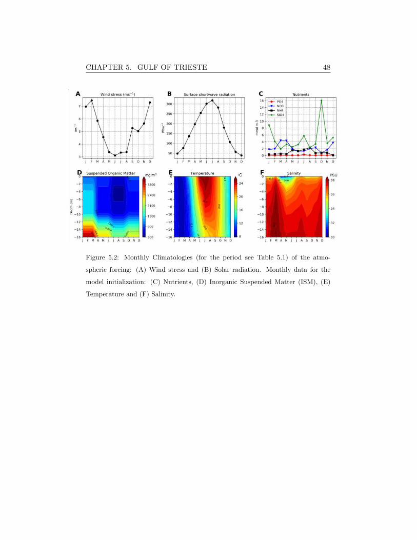
Figure 5.2 C. To further account for the influence of land-borne discharge of
suspended solids, the model was forced with a background seasonal clima-
tology of Inorganic Suspended Matter (ISM) as in [54]. Together with the
shortwave radiation, the ISM vertical profiles are used by the BFM to com-
pute the Photosynthetic Available Radiation EPAR as described in Equation
3.22 to better constrain the way in which the light propagates throughout
the water column.
The initialization of particulate and dissolved organic matter within the
sediments in the performed numerical experiments was done using the refer-
ence values reported in Mussap et al. [41] and are also reported in Table 5.2.
All the biogeochemical variables involved in the BPC sub-model (carbon, ni-
trogen, phosphate and silicate) share the same rate of remineralization, as
well as the benthic burial rate applied to the sinking pelagic particulate
organic matter (Table 5.2).
CHAPTER 5. GULF OF TRIESTE 48
Figure 5.2: Monthly Climatologies (for the period see Table 5.1) of the atmo-
spheric forcing: (A) Wind stress and (B) Solar radiation. Monthly data for the
model initialization: (C) Nutrients, (D) Inorganic Suspended Matter (ISM), (E)
Temperature and (F) Salinity.

CHAPTER 5. GULF OF TRIESTE 49
Variable Units Time Period Frequency
Atmospheric Forcings (ERA-Interim)
Wind speed components m s−1 2000-2013 6 hours
Air temperature at 2m ◦C 2000-2013 6 hours
Specific humidity kg kg−1 2000-2013 6 hours
Snowfall and Precipitation kg m−2 s−1 2000-2013 Daily
Long and Shortwave radiation W m−2 2000-2013 Daily
Observations (ARPA-FVG, OGS)
Temperature ◦C 2000-2011,2013 Monthly
Salinity psu 2000-2011,2013 Monthly
Phosphate mmol PO3 m−3 1998-2001 Seasonal
Nitrate mmol NO3 m−3 1998-2001 Seasonal
Ammonium mmol NH4 m−3 2000-2001 Seasonal
Oxygen mmol O2 m−3 2000,2002-2011,2012 Seasonal
Chlorophyll-a mg Chla m−3 2000-2011,2013 Seasonal
Inorganic Suspended Matter mg C m−3 1997-2000 Seasonal
Table 5.1: Summary of atmospheric forcing fields and observational datasets, re-
porting reference units, temporal coverage and frequency of data.

CHAPTER 5. GULF OF TRIESTE 50
Benthic variables initialisation and Parameters
Variable Value Units Description
Q6c0 520.0 mg C m−2 Particulate organic Carbon in Sediment
Q6n0 220.0 mmol N m−2 Particulate organic Nitrate in Sediment
Q6p0 1.4 mmol P m−2 Particulate organic Phosphate in Sediment
Q6s0 150.0 mmol Si m−2 Particulate organic Silicate in Sediment
Q1c0 10.4988 mg C m−2 Labile organic Matter in Sediment
burvel R6 0.5 m d−1 Burial Velocity for detritus
burvel PI 0.1 m d−1 Burial Velocity for plankton
Remin Q1 0.01 d−1 Remineralization rate of DOM
Remin Q6 0.0025 d−1 Remineralization rate of POM
Table 5.2: Summary of data and parameters used in the BPC sub-model
CHAPTER 5. GULF OF TRIESTE 51
5.3 Results
BPC-RETURN and NO-RM experiments comparison
The outcomes of the reference BPC-RETURN experiment are compared
to those of the NO-RM one by considering the seasonal vertical profiles of
Phosphate, Nitrate, Chlorophyll-a, Oxygen, and Ammonium, along with ob-
servational data, as shown in 5.3. A detailed analysis of the biogeochemical
cycles simulated in the reference experiment is provided in the next section.
Overall, the inclusion of the benthic sub-model significantly contributes to
the improvement in the simulations of the here considered biogeochemical
variables. The seasonal variability of nitrate and phosphate (Figure 5.3A-
B) is poorly reproduced by the NO-RM experiment, with values that are
rather flattened and straight along the vertical direction. In particular, the
lack of the BPC process prevents the correct simulation of the seasonally
nutrients-rich bottom water masses, while the two experiments have a com-
parable deep dynamic during summer when low nutrients concentrations
are observed. The low nutrient concentrations obtained in the NO-RM
test also lead to a significant underestimation of chlorophyll profiles that
are always rather flatten, especially at the bottom levels, and lower than
observations throughout the water column (Figure 5.3C). Conversely, the
chlorophyll profiles of BPC-RETURN area characterized by a clear season-
ality and the annual deep chlorophyll dynamics is also well reproduced. In
both experiments, the oxygen seasonal profiles results to be very similar that
is a direct consequence of air-sea reareation dynamics that are dominant in
this very shallow site. In the BPC-RETURN experiment, a slightly higher
oxygen consumption occurs in the last few meters of the water column as
a consequence of the respiration process associated to the organic matter
CHAPTER 5. GULF OF TRIESTE 52
degradation within the benthic compartment.
The only difference arise form the comparison of the ammonium seasonal
cycle that appears to be slightly better simulated in the NO-RM experiment
(5.3E). This directly points to the nitrogen remineralization dynamic in the
sediments as the fluxes toward the water columns are partitioned between
nitrate and ammonium through a rather simplistic parameterization (3.2.2).
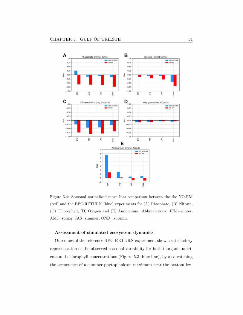
A more quantitative assessment is offered by the comparison of the sea-
sonal normalized mean bias (NMB) calculated over the entire water column
for both the experiments and for all the biogeochemical variables discussed
so far (Figure 5.4). The NMB metric was here selected to give an insight
of the model skills in reproducing the variability along the year and better
constrain critical deviations from observed data.
With the exception of ammonium, the NBM computed from the BPC-
RETURN simulation is generally lower than the NO-RM one. In particular,
it can be observed that the model error appears to be unevenly distributed
along the different seasons, thus indicating that it is not necessarily related
to any periodic physical and/or biogeochemical process (e.g, stratification,
mixing, algal blooms). Moreover, dissolved inorganic nutrients show the
highest error during the strong mixing periods (autumn or winter), while
for chlorophyll during the stratification seasons (spring and summer).
A more in depth investigation about the relationships between the BPC
sub-model parameterizations and the main biogeochemical pelagic state
variables is treated in the sensitivity analysis Chapter 8.1

CHAPTER 5. GULF OF TRIESTE 53
Figure 5.3: Comparison between NO-RM (red) and BPC-RETURN (blue) sim-
ulated seasonal mean climatological profiles for (A) Phosphate, (B) Nitrate, (C)
Chlorophyll, (D) Oxygen and (E) Ammonium. Black dots indicate observations
seasonal average and the horizontal bars their standard deviation. Abbreviations:
JFM=winter, AMJ=spring, JAS=summer, OND=autumn.
CHAPTER 5. GULF OF TRIESTE 54
Figure 5.4: Seasonal normalized mean bias comparison between the the NO-RM
(red) and the BPC-RETURN (blue) experiments for (A) Phosphate, (B) Nitrate,
(C) Chlorophyll, (D) Oxygen and (E) Ammonium. Abbreviations: JFM=winter,
AMJ=spring, JAS=summer, OND=autumn.
Assessment of simulated ecosystem dynamics
Outcomes of the reference BPC-RETURN experiment show a satisfactory
representation of the observed seasonal variability for both inorganic nutri-
ents and chlorophyll concentrations (Figure 5.3, blue line), by also catching
the occurrence of a summer phytoplankton maximum near the bottom lev-

CHAPTER 5. GULF OF TRIESTE 55
els. The rather low surface chlorophyll values are mainly constrained by the
underestimation of nutrients, especially in summer and autumn for phos-
phate. Despite of the relaxation applied at the surface layer to mimic the
influence of the Isonzo river loads, the dynamics of nutrient appears to be
still poorly constrained and mainly driven by the consumption of primary
producers. A possible solution would be to increase this riverine effect by
extending the relaxation to more surface layers, but it was here neglected
to avoid an excessive and potentially detrimental over-parameterization of
this shallow system.
A broad view of the Nutrients-Phytoplankton-Zooplankton food chain
evolution can be retrieved from the BPC-RETURN experiment, as repre-
sented in Figure (5.3) for nutrients and in the Hovmøller diagrams of the
monthly climatological fields computed over last 5 simulated years (Figure
5.5 and 5.6). The spatial and temporal distribution of nutrients and the
inherent response of phytoplankton and zooplankton are clearly reproduced
by the model, also in relation to the seasonal evolution of the thermohaline
vertical structure (see Figure 5.2 E,F). In fact, during autumn and winter,
the high ventilation produces mixing that affects the entire water column
leading the nutrients to rise toward the surface from October to January and
to be uptaken by phytoplankton. Besides the nutrients limitation, chloro-
phyll also depends on other environmental factors such as solar radiation and
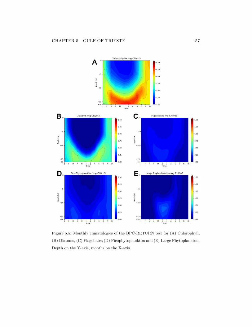
temperature. The rather high concentrations of chlorophyll (Figure 5.5A)
simulated at deeper layers during spring and early autumn are induced by
the optimal environmental conditions of both seawater temperature and so-
lar radiation (with respect to winter conditions) and nutrients availability.
During late autumn and winter, the model water column is largely mixed
as a consequence of the strong wind forcing and quite homogeneous trophic

CHAPTER 5. GULF OF TRIESTE 56
conditions establish along the water column. The seasonal distribution of
phytoplankton groups (Figure 5.5B-E) is characterized by the spring and
summer blooms of diatoms that remain abundant over the whole year, while
small-sized phytoplankton persist in the system but their abundance is far
lower.
As direct measurements of zooplankton biomass or abundance were not
available, the model offered a basis to evaluate their role within this ecosys-
tem. The seasonal and vertical distribution of microzooplankton (Figure
5.6) are directly linked to that of phytoplankton that represents its main
feeding pool, while the omnivorous zooplankton, being at the top of the
model food chain, is characterized by a combined dynamic that follows both
its preys throughout the year. The parameterized food matrix is summa-
rized in Appendix A.5.
CHAPTER 5. GULF OF TRIESTE 57
Figure 5.5: Monthly climatologies of the BPC-RETURN test for (A) Chlorophyll,
(B) Diatoms, (C) Flagellates (D) Picophytoplankton and (E) Large Phytoplankton.
Depth on the Y-axis, months on the X-axis.

CHAPTER 5. GULF OF TRIESTE 58
Figure 5.6: Monthly climatologies of BPC-RETURN experiment results for the Zoo-
plankton component: (A) Carnivorous Mesozooplankton, (B) Omnivorous Meso-
zooplankton, (C) Microzooplankton and (D) Heterotrophic nanoflagellates. Depth
on the Y-axis, months on the X-axis.
Chapter 6
Saint Helena Bay
6.1 Site characterization
St. Helena Bay (SHB) is the largest bay on the west coast of South
Africa and it lies within the Benguela Current Large Marine Ecosystem
(BCLME, Figure 6.1A). The BCLME is considered an eastern open bound-
ary system [79, 58], being characterized by two warm currents at both its
extremities: the Angola current system in the north and the warm Agulhas
current system in the south. The SHB area is part of the Cape Province
region (southernmost area of BCLME) and it is affected by the cold coastal
branch of the Benguela current that, together with the wind stress, is the
main driver of the coastal upwelling. This upwelling systems is more intense
during the austral spring-summer period, when south-easterly trade winds
reach their maxima, and it slows down in winter as the westerly continental
winds start to prevail over the trade winds [58].
Besides the Benguela Current, this region is also characterized by strong
coastal edge jets (Figure 6.1A) and by a poleward undercurrent acting along
59
CHAPTER 6. SAINT HELENA BAY 60
the shelf slope [80], which transports land-borne sediments and organic nu-
trients from the mouth of the Berg River to the St. Helena Bay retention
area.
The general circulation of St. Helena Bay is primarily governed by the
interaction of four factors:
1. Large scale atmospheric circulation patterns determined by the peren-
nial South Atlantic subtropical anticyclone, whose stable atmospheric
high pressure center is opposed to the low pressure field over the sub-
continent, with the consequent enhancement of the wind stress along
the coast [81, 82, 83];
2. Mesoscale atmospheric perturbations, such as the eastward traveling
mid-latitude cyclones (south of the African continent), periodically
weaken or abate the south-easterly winds along the coast [81, 59] lead-
ing to a local weakening of the upwelling process [84];
3. Coastal topography shapes the local circulation system as the narrow
shelves are more affected by the uplift of cold water with respect to
wider ones [58];
4. The retroflection of the Agulhas Current generates a north westerly mi-
gration of warm rings and filaments that occasionally interact with the
coastal upwelling [85, 86, 58, 59], especially when a more pronounced
offshore-inshore thermal gradient occurs (with lower sea surface tem-
perature values inshore and warmer offshore ones).
The interplay of the above factors leads to the peculiar seasonal cycle of
seawater temperatures in St. Helena Bay [58, 59] with surface values that
typically range between 12-15 ◦C and increase toward the offshore zone to
CHAPTER 6. SAINT HELENA BAY 61
more than 17◦C. The rise of cold and deep waters during spring and summer
prevents the vertical propagation of the heating along the water column.
St. Helena Bay is characterized by an annually persistent phytoplank-
ton community that supports a complex food web, thus being an elective
spawning and larvae nursery area for a wide range of zooplankton and fishes
species. Nutrients distribution is closely associated to the upwelling system
[87, 88], with high rates of advected nutrients from the bottom levels toward
the sea surface from September to April and lower concentrations during the
’no-upwelling’ period between May and August. The intensity of the up-
welling event drives nutrients variability that in turn influence the rates of
primary productivity [87, 88]. As stated by Pitcher et al. [89], the weaker
stratification conditions and nutrients injection are frequently responsible
of episodic harmful red tides that lead to mass mortality events for zoo-
plankton and in particular for rock lobster. The interplay of local physical,
hydrodynamical and biological processes leads St. Helena Bay to be peri-
odically characterized by low oxygen water [90]. During late summer-early
autumn the stratification intensifies and phytoplankton become nutrients
limited, so the biomass concentrations decrease occurs at the expense of
excessive consumption of oxygen. Despite the ecosystemic relevance of re-
tention areas such as St. Helena Bay [91, 92], their role in the development
and maintenance of organic rich sediments and coupled elemental cycling is
less understood [93] due to the lack of systematic monitoring activities.
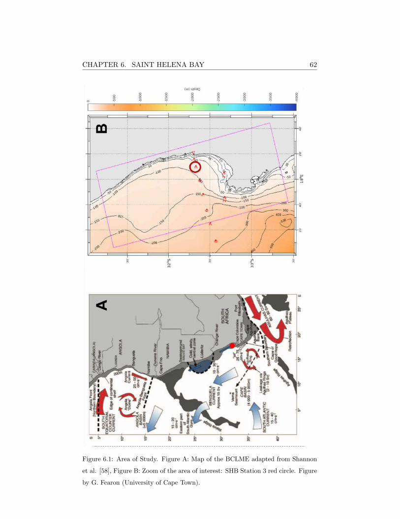
CHAPTER 6. SAINT HELENA BAY 62
Figure 6.1: Area of Study. Figure A: Map of the BCLME adapted from Shannon
et al. [58], Figure B: Zoom of the area of interest: SHB Station 3 red circle. Figure
by G. Fearon (University of Cape Town).
CHAPTER 6. SAINT HELENA BAY 63
6.2 Model implementation
The 1D NEMO-BFM configuration implemented in St. Helena Bay aims
to reproduce the BPC climatology of the station 3 of the St. Helena Bay
monitoring line (SHB, Figure 6.1 B). The station is positioned at a latitude
of 32.16◦S and a longitude of 17.50◦E and has a maximum depth of 78m.
A staggered grid composed by 50 logarithmically distributed vertical levels
was implemented, with a maximum spacing of ∼3m in the bottom-most
level. The model was used to perform 20 years-long simulations (starting
from year 2006) and results from the last 10 years are presented in the
following analyses. This choice was done to exclude the initial adjustment
phases of the model often characterized by drifts in both benthic and pelagic
components.
The atmospheric forcing used in both BPC-RETURN and NO-RM exper-
iments were extracted from the high-resolution (∼ 3km) simulation over the
period 2006-2012 of the atmospheric-ocean coupled regional model WRF-
ROMS provided by the Climate Systems Analysis Group at the University
of Cape Town (courtesy of G. Faeron). Table 6.1 shows the main character-
istics of the atmospheric forcings. Monthly climatology of wind speed and
solar radiation were computed from the high-resolution atmospheric dataset
(Figure 6.2) to provide an overview of the forcing features, similarly to the
other case studies.
Seawater temperature and salinity data come from the hydrographic sam-
pling along the SHB in the framework of the BENEFIT (Benguela Environ-
ment and Fisheries Interactions and Training) program carried out by the
Department of Environmental Affairs of South Africa. Observations are
made of Conductivity-Temperature-Depth (CTD) casts from sea surface to
CHAPTER 6. SAINT HELENA BAY 64
within 5-10 m of seafloor and were performed from April 2000 to December
2017 with a monthly frequency (Table 6.1).
To reproduce a correct density structure and a non drifting annual cycle
of the water column, a relaxation of 5 days was adopted using the above
temperature and salinity monthly climatological fields. From the computed
monthly climatologies (Figure 6.2 C,D) it is clear how the stability of the
water column is mainly driven by temperature and to a lesser extent by
salinity, which is also shows a certain degree of seasonality.
The temperature restoring method ensures that the model is constrained
to maintain the thermocline seasonality, but this condition may not be suffi-
cient to realistically reproduce the vertical distribution of pelagic state vari-
ables induced by the upwelling. A brief characterization of the upwelling sea-
sonality it is here proposed to highlight the specific hydrodynamic features of
SHB station, by considering the climatological distribution of three proxies:
seawater temperature, chlorophyll-a and vertical velocities (see Figure 6.3
A and Table 6.1). The first step for the detection of the upwelling duration
was based on the annual trend of the 11◦C isotherm, which indicates that
vertical water mass motions lasts from September until April. According
to literature, peaks of chlorophyll occur during the upwelling periods [94,
89] with two maxima in late summer and early spring, as in the case of the
SHB area where the phytoplankton activity onset (September) and offset
(April) coherently with the upwelling dynamics. Note that, chlorophyll-a
data used here have been extrapolated from the fluorometer measurements
under the rather crude assumption that in-situ concentrations corresponded
to the original data scaled by one order of magnitude. This appeared to us a
conservative approach, as the determination of chlorophyll-a concentration
by fluorescence depends on the optical properties of the ocean water and

CHAPTER 6. SAINT HELENA BAY 65
the factors for converting units of fluorescence varies up to 50% [95]. Lastly,
the vertical velocity obtained from the WRF-ROMS model simulations show
that the period of inactivity begins in May and ends in August (w < 0 in
all the vertical levels in a range between 10-78m).
As the explicit prescription of vertical velocities would lead to un-reaslistic
features in the one-dimensional model, the vertical motions due to the up-
welling dynamics were here approximated by adjusting the vertical eddy
diffusivity coefficient of tracer transport. This coefficient refers to the verti-
cal turbulent contribution to oceanic properties transport and it was set to
1.0e4 m2/s, namely the double with respect to the other implemented sites.
Observations for nitrate, phosphate, silicate and oxygen were obtained
from the monthly profiles of the CSIRO digital Atlas of Regional Seas
(CARS) [96]. The silicate and chlorophyll-a monthly climatological profiles
were derived from the SHB in-situ samples, with the latter scaled according
to procedure described in the above paragraphs. These data were used to
initialize the corresponding BFM pelagic state variables.
No observational data on the benthic organic matter were found for the
SHB area. However, Monteiro et al. [97] estimate that St Helena Bay is
characterized by high sedimentary flux toward the bottom, thus supporting
the hypothesis that to well reproduce the SHB dynamic a rather active BPC
parametrization should be used. The set of parameters adopted for the BPC
are listed in Table 6.2.
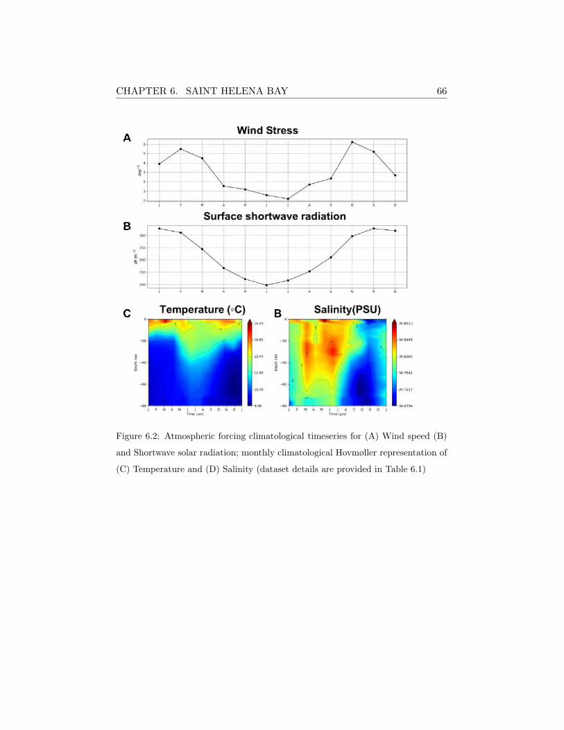
CHAPTER 6. SAINT HELENA BAY 66
Figure 6.2: Atmospheric forcing climatological timeseries for (A) Wind speed (B)
and Shortwave solar radiation; monthly climatological Hovmøller representation of
(C) Temperature and (D) Salinity (dataset details are provided in Table 6.1)
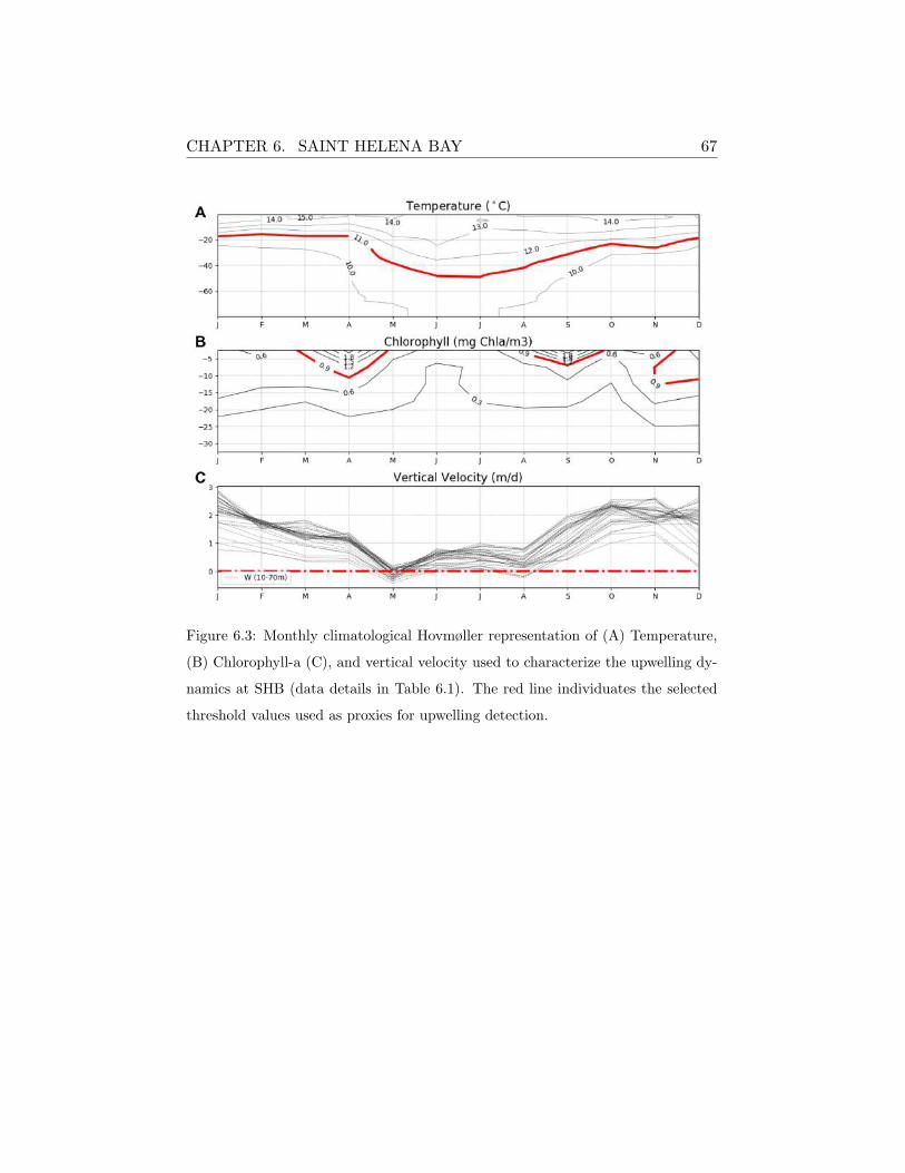
CHAPTER 6. SAINT HELENA BAY 67
Figure 6.3: Monthly climatological Hovmøller representation of (A) Temperature,
(B) Chlorophyll-a (C), and vertical velocity used to characterize the upwelling dy-
namics at SHB (data details in Table 6.1). The red line individuates the selected
threshold values used as proxies for upwelling detection.
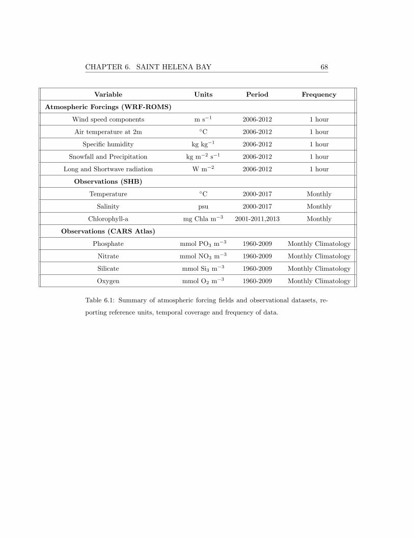
CHAPTER 6. SAINT HELENA BAY 68
Variable Units Period Frequency
Atmospheric Forcings (WRF-ROMS)
Wind speed components m s−1 2006-2012 1 hour
Air temperature at 2m ◦C 2006-2012 1 hour
Specific humidity kg kg−1 2006-2012 1 hour
Snowfall and Precipitation kg m−2 s−1 2006-2012 1 hour
Long and Shortwave radiation W m−2 2006-2012 1 hour
Observations (SHB)
Temperature ◦C 2000-2017 Monthly
Salinity psu 2000-2017 Monthly
Chlorophyll-a mg Chla m−3 2001-2011,2013 Monthly
Observations (CARS Atlas)
Phosphate mmol PO3 m−3 1960-2009 Monthly Climatology
Nitrate mmol NO3 m−3 1960-2009 Monthly Climatology
Silicate mmol Si3 m−3 1960-2009 Monthly Climatology
Oxygen mmol O2 m−3 1960-2009 Monthly Climatology
Table 6.1: Summary of atmospheric forcing fields and observational datasets, re-
porting reference units, temporal coverage and frequency of data.
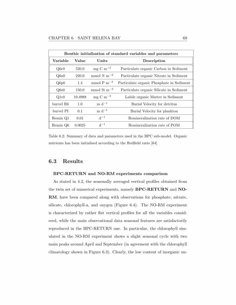
CHAPTER 6. SAINT HELENA BAY 69
Benthic initialisation of standard variables and parameters
Variable Value Units Description
Q6c0 520.0 mg C m−2 Particulate organic Carbon in Sediment
Q6n0 220.0 mmol N m−2 Particulate organic Nitrate in Sediment
Q6p0 1.4 mmol P m−2 Particulate organic Phosphate in Sediment
Q6s0 150.0 mmol Si m−2 Particulate organic Silicate in Sediment
Q1c0 10.4988 mg C m−2 Labile organic Matter in Sediment
burvel R6 1.0 m d−1 Burial Velocity for detritus
burvel PI 0.1 m d−1 Burial Velocity for plankton
Remin Q1 0.01 d−1 Remineralization rate of DOM
Remin Q6 0.0025 d−1 Remineralization rate of POM
Table 6.2: Summary of data and parameters used in the BPC sub-model. Organic
nutrients has been initialised according to the Redfield ratio [64]
6.3 Results
BPC-RETURN and NO-RM experiments comparison
As stated in 4.2, the seasonally averaged vertical profiles obtained from
the twin set of numerical experiments, namely BPC-RETURN and NO-
RM, have been compared along with observations for phosphate, nitrate,
silicate, chlorophyll-a, and oxygen (Figure 6.4). The NO-RM experiment
is characterized by rather flat vertical profiles for all the variables consid-
ered, while the main observational data seasonal features are satisfactorily
reproduced in the BPC-RETURN one. In particular, the chlorophyll sim-
ulated in the NO-RM experiment shows a slight seasonal cycle with two
main peaks around April and September (in agreement with the chlorophyll
climatology shown in Figure 6.3). Clearly, the low content of inorganic nu-

CHAPTER 6. SAINT HELENA BAY 70
trients in the water column at the beginning of the year (JFM) relates to
the absence of benthic remineralization processes. Although the slight deep
underestimation, the inorganic vertical profiles are well reproduced together
with the chlorophyll dynamics. The seasonal dynamic of the oxygen is well
reproduced in the BPC-RETURN simulation, contrarily to the NO-RM ex-
periment, as a consequence of the enhanced pelagic production-consumption
cycle under higher nutrient concentrations and the respiration associated to
the benthic remineralization processes.
A more objective comparison was here carried out by computing the sea-
sonal normalized mean bias (NMB) over the entire water column for both
the experiments (Figure 6.5). As one can see, the NO-RM experiment has
significantly high NMB values throughout the year for all the considered
variables with respect to the BPC-RETURN one. The latter has a rather
uniform error in the simulation of silicate, while deviations from the ob-
served data of the other variables are more evident in austral autumn and
winter when the upwelling is assumed to be weaker. Such a mismatch is
partly attributable to the enhanced mixing introduced by the high vertical
eddy diffusivity that was used to mimic the upwelling dynamics, as it was
not modulated in time to avoid an over-parameterization of the system.

CHAPTER 6. SAINT HELENA BAY 71
Figure 6.4: Comparison between NO-RM (red) and BPC-RETURN (blue) sim-
ulated seasonal mean climatological profiles for (A) Phosphate, (B) Nitrate,
(C) Chlorophyll, (D) Silicate and (E) Oxygen climatological seasonal profiles.
Black dots indicate observations seasonal average and the horizontal bars their
standard deviation. Abbreviations: JFM=winter, AMJ=spring, JAS=summer,
OND=autumn.
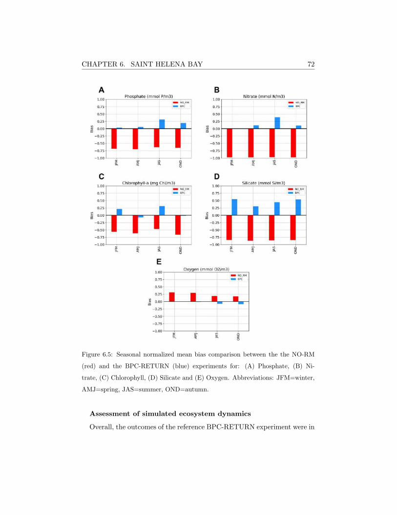
CHAPTER 6. SAINT HELENA BAY 72
Figure 6.5: Seasonal normalized mean bias comparison between the the NO-RM
(red) and the BPC-RETURN (blue) experiments for: (A) Phosphate, (B) Ni-
trate, (C) Chlorophyll, (D) Silicate and (E) Oxygen. Abbreviations: JFM=winter,
AMJ=spring, JAS=summer, OND=autumn.
Assessment of simulated ecosystem dynamics
Overall, the outcomes of the reference BPC-RETURN experiment were in

CHAPTER 6. SAINT HELENA BAY 73
a good spatiotemporal agreement with the available observations, particu-
larly for the bottom inorganic nutrients (Figure 6.4). The seasonal variabil-
ity of chlorophyll was coherently reproduced, although the model slightly
overestimate the subsurface values and it exhibits a rapid decrease of con-
centrations near the bottom with respect to the observed data. Nevertheless,
it is conceivable that the overestimation in the upper 20 meters may be re-
lated to the simulated density structure of the water column. Even making
a strong restoring of temperature and salinity, a small source of errors can
affect the mixed layer features simulated by the model.
In Figure 6.6 the monthly climatologies of the main state variables for the
reference experiment are shown along with the observational data (Table
6.1). In particular, the model well reproduces the evolution of chlorophyll-a
within the first 20 meters and a marked peak takes place around September.
During the austral summer (JFM) a strong stratification setup at about 20
meters and it prevents the penetration of nutrients above the thermocline,
thus determining the low nutrient conditions at the surface. At the end of
the austral summer the stratification lessens as the thermocline is broken up
by upwelled waters and nutrients concentrations at the surface are remark-
ably high. Nevertheless, the model does not properly reproduce the depth of
the nutricline between June and Juky, which results to be very sharp in the
CARS data and rather flattened in BPC-RETURN simulation. Both nutri-
cline and thermocline simulated error propagates in the next level of the food
chain causing a phytoplankton blooms with a certain delay with respect to
the observed data. The oxygen dynamic is fairly reproduced as low and deep
oxygen conditions persist from June until October when the vertical mixing
makes deep waters slightly more oxygenated, whereas low oxygen conditions
occurring between February an April at the bottom layers were not caught

CHAPTER 6. SAINT HELENA BAY 74
by the model. The evolution of the benthic carbon pools represented in
Figure 6.7 shows an initial accumulation phase of organic matter and a near
equilibrium state between pelagic sedimentation and benthic remineraliza-
tion fluxes is achieved after 5 years. This makes hypothesize that there is a
pronounced link between the pelagic inorganic nutrients overestimation of
the BPC-RETURN experiment and the simulated benthic realm. A more
in depth investigation and discussion about the degree of coupling between
the pelagic and benthic realms will be treated in Chapter 8.1.
The seasonal succession of phytoplankton reproduced by the model (Fig-
ure 6.8) appears to be quite consistent with previous literature evidences
[98]. A first diatoms shallow bloom occurs during austral winter (JAS)
followed by a stable diatoms production at about 10m of depth during aus-
tral spring, while flagellates are present during the entire upwelling period
(OND-JFM) and picophytoplankton dominates during the austral summer
period (JFM). Large phytoplankton (not shown) suddenly disappears at the
beginning of the numerical experiment and never recovers.
Although observations of zooplankton biomass were not available, the
analysis of its spatial and temporal distribution is worthy of some consider-
ations (Figure 6.9). The spatio-temporal distribution of all the zooplankton
groups considered by the model is in agreement with the distribution of
the relatives preys. In particular, the diminished herbivorous zooplankton
biomass observed in the first 20 meters during JJA (see Figure 6.9 C-D) is
likely related to the corresponding diatoms bloom visible in Figure 6.8 A.
The parametrized food matrix is summarized in Appendix A.5

CHAPTER 6. SAINT HELENA BAY 75
Figure 6.6: Monthly climatological Howmøller plots of observed data (left panel)
and BPC-RETURN experiment outcomes for (A) Phosphate, (B) Nitrate, (C)
Chlorophyll, (D) Silicate and (E) Oxygen. For the observational data see Table
6.1. Depth on the Y-axis, months on the X-axis.

CHAPTER 6. SAINT HELENA BAY 76
Figure 6.7: Time series of the simulated benthic (A) Dissolved and (B) Particulate
Organic Carbon.
Figure 6.8: Monthly climatologies of BPC-RETURN experiment results for the
Phytoplankton component: (A) Diatoms, (B) Flagellates and (C) Picophytoplank-
ton. Depth on the Y-axis, months on the X-axis.

CHAPTER 6. SAINT HELENA BAY 77
Figure 6.9: Monthly climatologies of BPC-RETURN experiment results for the Zoo-
plankton component: (A) Omnivorous Mesozooplankton,(B) Carnivorous Mesozoo-
plantkon,(C) Microzooplankton, and (D) Heterotrophic Nanoflagellates. Depth on
the Y-axis, months on the X-axis.
Chapter 7
Svinøy Fyr
7.1 Site characterization
The Svinøy Fyr station (hereafter SFyr) is located in the South-West
coast of Norway (∼62.27◦N and ∼5.10◦E in Figure 7.1), over the shelf break
along the Svinøy Fyr hydrographic section.
This monitoring section has been investigated since the beginning of the
last century [99] with major interest on the Atlantic inflow features and its
interannual variability [100], but only few studies dealt with the characteri-
zation of the Norwegian South-Western continental shelf dynamics.
The area is subject to strong winds mainly coming from south south-west
[101] that makes it fall within the category of the sub-polar regions [102,
103]. Its hydrological regime is determined by the interplay between (i) the
poleward extension of the Gulf Stream that serves as a conduit of warm
and saline waters from the North Atlantic to the Arctic Ocean [104] and (ii)
the topography trapped Norwegian Atlantic Current that is considered the
warm barotropic and inner branch of the North Atlantic current (see 7.1).
78
CHAPTER 7. SVINØY FYR 79
The latter prevents the formation of sea ice at these latitudes, conversely to
what happen at the opposite coast in Greenland.
During winter the downward mixing occurs by the convection of cooled
surface waters in addition to the wind-driven turbulence that deepens the
mixed layer [103], persisting until late spring, while warmer and shallow
stratified conditions are established in summer. The Norwegian continental
shelf is a very high productive marine ecosystem [103]. Low temperature
and high nutrients concentrations in SFyr station stay stable during win-
ter, when the strong winds favour the formation of a deep mixed layer, by
setting up favourable trophic conditions to fuel the early spring phytoplank-
ton bloom. The summer stratification prevents the nutrients regeneration
at the surface making the post-bloom period to last around three months.
The weakening of stratification and the convective vertical motions occur-
ring in autumn allow the injection of nutrients to the surface determining a
weak second peak of phytoplankton. According to Loeng et al. [105], this
site is characterized by a phytoplankton-zooplankton-fish short food chain
that generates a high content of sunk organic detritus escaping from the eu-
photic zone. Moreover, observations on biogenic sedimentation indicate how
a large portion of the carbon fixed annually by phytoplankton falls ungrazed
to the sediments [106, 107], thus leading a great proportion of the primary
productivity to be recycled through the benthic activity [108].
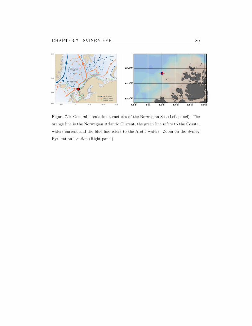
CHAPTER 7. SVINØY FYR 80
Figure 7.1: General circulation structures of the Norwegian Sea (Left panel). The
orange line is the Norwegian Atlantic Current, the green line refers to the Coastal
waters current and the blue line refers to the Arctic waters. Zoom on the Svinøy
Fyr station location (Right panel).

CHAPTER 7. SVINØY FYR 81
7.2 Model implementation
The station here considered is the first and shallowest one of the Svinøy
Fyr hydrographic section, located at the edge of the continental shelf with
an average depth of ∼150m.
A vertical grid composed by 50 vertical levels with the maximum spacing
of around 8 meters in the bottom-most level was used to discretize the water
column.
In this implementation, the 1D NEMO-BFM model simulations were car-
ried out for a 20 years time period (2000-2019) and the results presented in
the next section refer to the monthly and seasonal climatology of the last
10 years. This choice was made to exclude from the analysis the initial drift
that occurs in the biogeochemical dynamics.
Table 7.1 summarizes the main characteristics of the atmospheric data
used in this study, obtained from the ERA5 climate reanalysis produced by
the ECMWF for the period 2000-2019 [65]. As observable in Figure 7.2,
strong winds occur from September to March enhancing convective vertical
motion and the deepening of the thermocline. Similarly total precipitation
(snow and rain) presents maximum values between September and January.
Data used to initialize the model come from the publicly distributed data
of the Institute of Marine Research - Norwegian Marine Data Centre (INR-
NMD) for the period 1995-2015 (see Table 7.1). Seawater temperature and
salinity CTD measurements were carried out with a monthly frequency, with
the exception of the month of December. To overcame this lack of data, a
mean profile was created for December month by considering the data avail-
able from mid November to mid January over the entire dataset and then the
monthly climatology was generated for both variables. As for previous case
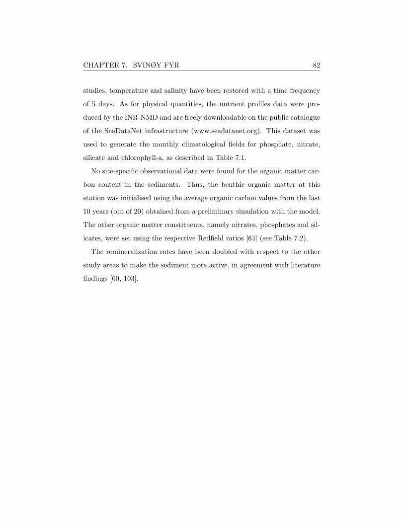
CHAPTER 7. SVINØY FYR 82
studies, temperature and salinity have been restored with a time frequency
of 5 days. As for physical quantities, the nutrient profiles data were pro-
duced by the INR-NMD and are freely downloadable on the public catalogue
of the SeaDataNet infrastructure (www.seadatanet.org). This dataset was
used to generate the monthly climatological fields for phosphate, nitrate,
silicate and chlorophyll-a, as described in Table 7.1.
No site-specific observational data were found for the organic matter car-
bon content in the sediments. Thus, the benthic organic matter at this
station was initialised using the average organic carbon values from the last
10 years (out of 20) obtained from a preliminary simulation with the model.
The other organic matter constituents, namely nitrates, phosphates and sil-
icates, were set using the respective Redfield ratios [64] (see Table 7.2).
The remineralization rates have been doubled with respect to the other
study areas to make the sediment more active, in agreement with literature
findings [60, 103].
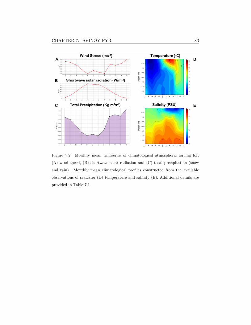
CHAPTER 7. SVINØY FYR 83
Figure 7.2: Monthly mean timeseries of climatological atmospheric forcing for:
(A) wind speed, (B) shortwave solar radiation and (C) total precipitation (snow
and rain). Monthly mean climatological profiles constructed from the available
observations of seawater (D) temperature and salinity (E). Additional details are
provided in Table 7.1

CHAPTER 7. SVINØY FYR 84
Variable Units Period Frequency
Atmospheric Forcings (ERA5)
Wind speed components m s−1 2000-2019 6 hours
Air temperature at 2m ◦C 2000-2019 6 hours
Specific humidity kg kg−1 2000-2019 6 hours
Snowfall and Precipitation kg m−2 s−1 2000-2019 Daily
Long and Shortwave radiation W m−2 2000-2019 Daily
Observations (INR-NMD)
Temperature ◦C 1995-2015 Monthly
Salinity psu 1995-2015 Monthly
Phosphate mmol PO3 m−3 1995-2015 Monthly
Nitrate mmol NO3 m−3 1995-2015 Monthly
Silicate mmol SiOH m−3 1995-2015 Monthly
Chlorophyll-a mg Chla m−3 1995-2015 Monthly
Table 7.1: Summary of atmospheric forcing fields and observational datasets, re-
porting reference units, temporal coverage and frequency of data.
7.3 Results
BPC-RETURN and NO-RM experiments comparison
The cross comparison of the seasonal vertical profiles obtained in BPC-
RETURN and NO-BPC experiments with the observational data for phos-
phate, nitrate, silicate, and chlorophyll-a (Figure 7.3) highlights the substan-
tial improvement achieved by the inclusion of BPC processes in the model.
The seasonal variability of the inorganic nutrients is well reproduced by the
BPC-RETURN experiment, while in the NO-BPC experiment the nutrients
content has very small values at all seasons (Figure 7.3 A-B-D). Regard-
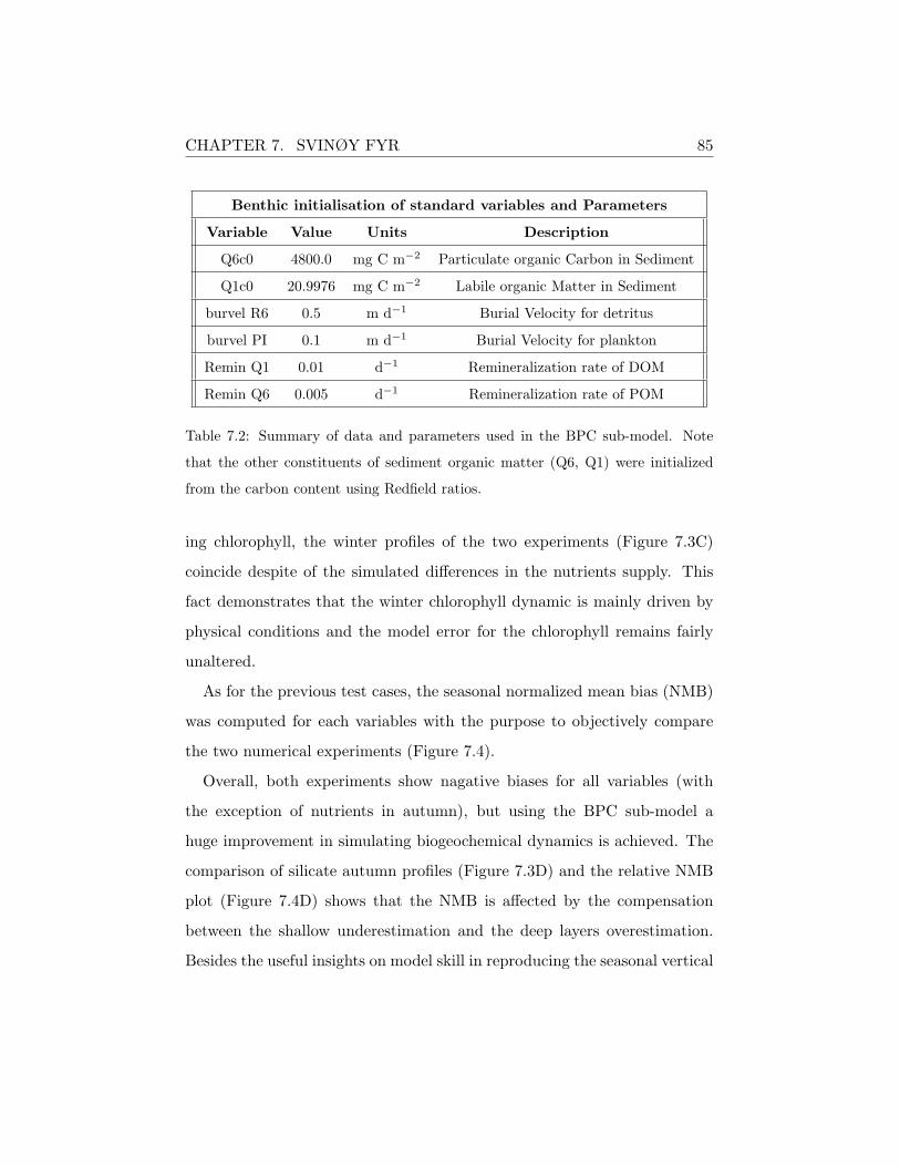
CHAPTER 7. SVINØY FYR 85
Benthic initialisation of standard variables and Parameters
Variable Value Units Description
Q6c0 4800.0 mg C m−2 Particulate organic Carbon in Sediment
Q1c0 20.9976 mg C m−2 Labile organic Matter in Sediment
burvel R6 0.5 m d−1 Burial Velocity for detritus
burvel PI 0.1 m d−1 Burial Velocity for plankton
Remin Q1 0.01 d−1 Remineralization rate of DOM
Remin Q6 0.005 d−1 Remineralization rate of POM
Table 7.2: Summary of data and parameters used in the BPC sub-model. Note
that the other constituents of sediment organic matter (Q6, Q1) were initialized
from the carbon content using Redfield ratios.
ing chlorophyll, the winter profiles of the two experiments (Figure 7.3C)
coincide despite of the simulated differences in the nutrients supply. This
fact demonstrates that the winter chlorophyll dynamic is mainly driven by
physical conditions and the model error for the chlorophyll remains fairly
unaltered.
As for the previous test cases, the seasonal normalized mean bias (NMB)
was computed for each variables with the purpose to objectively compare
the two numerical experiments (Figure 7.4).
Overall, both experiments show nagative biases for all variables (with
the exception of nutrients in autumn), but using the BPC sub-model a
huge improvement in simulating biogeochemical dynamics is achieved. The
comparison of silicate autumn profiles (Figure 7.3D) and the relative NMB
plot (Figure 7.4D) shows that the NMB is affected by the compensation
between the shallow underestimation and the deep layers overestimation.
Besides the useful insights on model skill in reproducing the seasonal vertical

CHAPTER 7. SVINØY FYR 86
profiles provided by the bias analysis, a more in-depth evaluation of the
pelagic response to the selected parameterization was carried out in Chapter
8.1 to better evaluate the consistence of the adopted remineralization and
burial parameters and their potential influence on the positive bias obtained
in deeper layers.

CHAPTER 7. SVINØY FYR 87
Figure 7.3: Comparison between NO-RM (red) and BPC-RETURN (blue) sim-
ulated seasonal mean climatological profiles for (A) Phosphate, (B) Nitrate, (C)
Chlorophyll-a, and (D) Silicate climatological seasonal profiles. Black dots indicate
observations seasonal average and the horizontal bars their standard deviation.
Abbreviations: JFM=winter, AMJ=spring, JAS=summer, OND=autumn.
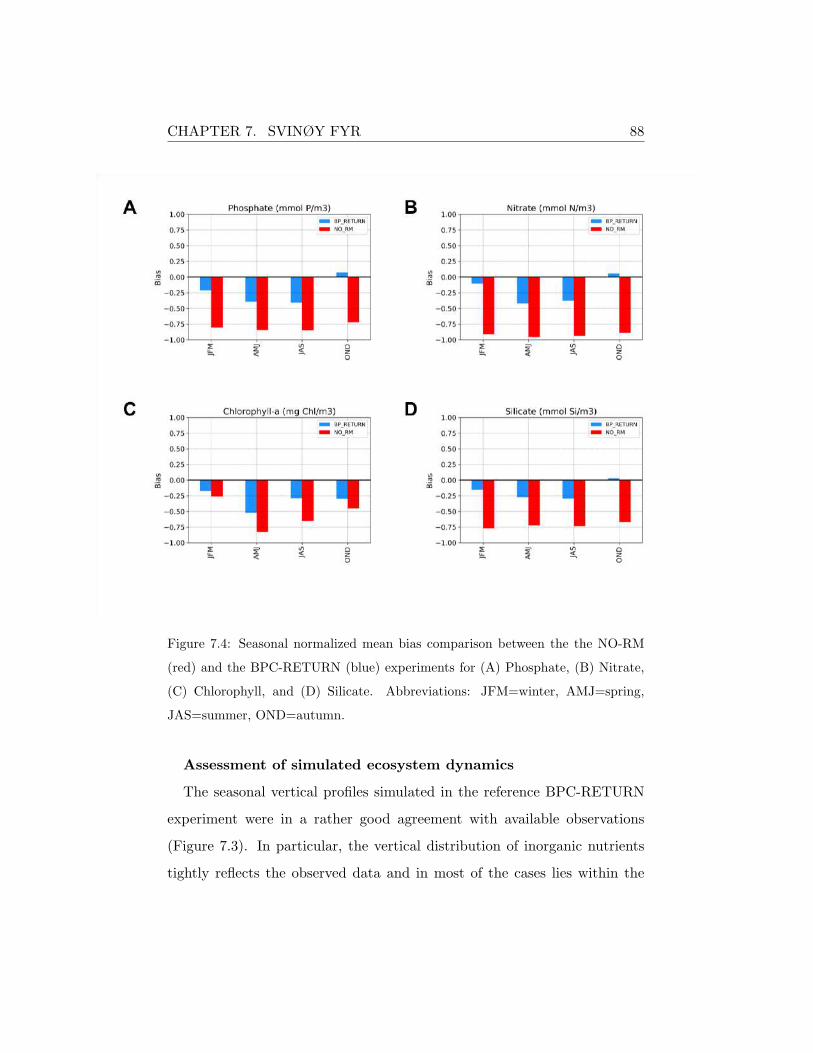
CHAPTER 7. SVINØY FYR 88
Figure 7.4: Seasonal normalized mean bias comparison between the the NO-RM
(red) and the BPC-RETURN (blue) experiments for (A) Phosphate, (B) Nitrate,
(C) Chlorophyll, and (D) Silicate. Abbreviations: JFM=winter, AMJ=spring,
JAS=summer, OND=autumn.
Assessment of simulated ecosystem dynamics
The seasonal vertical profiles simulated in the reference BPC-RETURN
experiment were in a rather good agreement with available observations
(Figure 7.3). In particular, the vertical distribution of inorganic nutrients
tightly reflects the observed data and in most of the cases lies within the
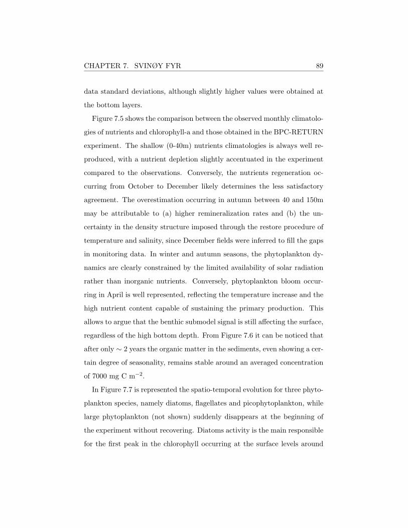
CHAPTER 7. SVINØY FYR 89
data standard deviations, although slightly higher values were obtained at
the bottom layers.
Figure 7.5 shows the comparison between the observed monthly climatolo-
gies of nutrients and chlorophyll-a and those obtained in the BPC-RETURN
experiment. The shallow (0-40m) nutrients climatologies is always well re-
produced, with a nutrient depletion slightly accentuated in the experiment
compared to the observations. Conversely, the nutrients regeneration oc-
curring from October to December likely determines the less satisfactory
agreement. The overestimation occurring in autumn between 40 and 150m
may be attributable to (a) higher remineralization rates and (b) the un-
certainty in the density structure imposed through the restore procedure of
temperature and salinity, since December fields were inferred to fill the gaps
in monitoring data. In winter and autumn seasons, the phytoplankton dy-
namics are clearly constrained by the limited availability of solar radiation
rather than inorganic nutrients. Conversely, phytoplankton bloom occur-
ring in April is well represented, reflecting the temperature increase and the
high nutrient content capable of sustaining the primary production. This
allows to argue that the benthic submodel signal is still affecting the surface,
regardless of the high bottom depth. From Figure 7.6 it can be noticed that
after only ∼ 2 years the organic matter in the sediments, even showing a cer-
tain degree of seasonality, remains stable around an averaged concentration
of 7000 mg C m−2.
In Figure 7.7 is represented the spatio-temporal evolution for three phyto-
plankton species, namely diatoms, flagellates and picophytoplankton, while
large phytoplankton (not shown) suddenly disappears at the beginning of
the experiment without recovering. Diatoms activity is the main responsible
for the first peak in the chlorophyll occurring at the surface levels around
CHAPTER 7. SVINØY FYR 90
April, with a deeper chlorophyll signal that is due to the presence of both di-
atoms and picophytoplankton. The September bloom is instead dominated
by flagellates and picophytoplankton.
Similarly to previous sites, direct observations on mesozooplankton and
microzooplankton were not found. Nevertheless, from Figure 7.8 a presum-
ably correct representation of zooplankton dynamics can be qualitatively
inferred as the temporal and spatial distribution of the predators is in agree-
ment with their preys (following the imposed predator–prey food matrix
summarized in Appendix A.5).

CHAPTER 7. SVINØY FYR 91
Figure 7.5: Monthly climatological Howmøller plots of observed data (left panel)
and BPC-RETURN experiment outcomes (right panel) for (A) Phosphate, (B)
Nitrate, (C) Chlorophyll and (D) Silicate. Depth on the Y-axis, months on the
X-axis.

CHAPTER 7. SVINØY FYR 92
Figure 7.6: Time series of the simulated benthic (A) Dissolved and (B) Particulate
Organic Carbon.
Figure 7.7: Monthly climatologies of BPC-RETURN experiment results for the
Phytoplankton component: (A) Diatoms, (B) Flagellates and (C) Picophytoplank-
ton. Depth on the Y-axis, months on the X-axis.
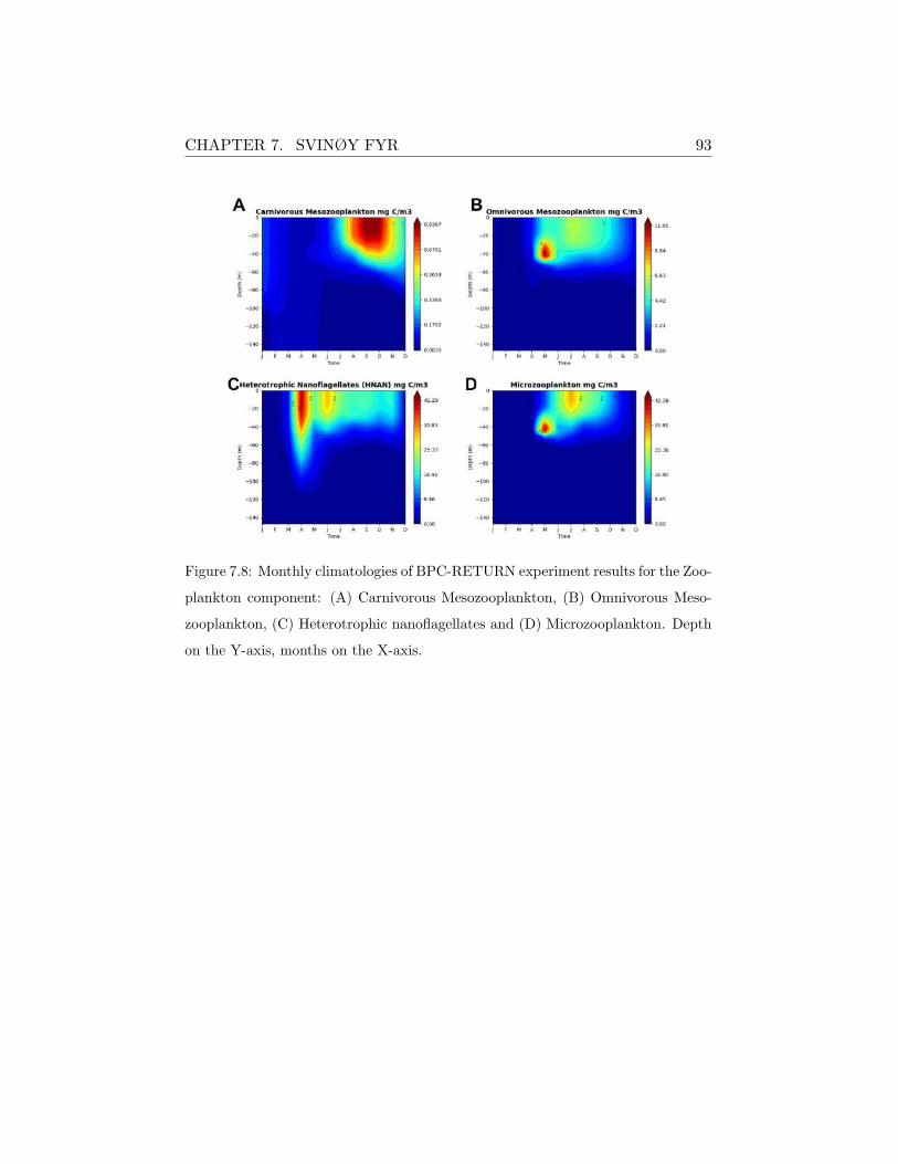
CHAPTER 7. SVINØY FYR 93
Figure 7.8: Monthly climatologies of BPC-RETURN experiment results for the Zoo-
plankton component: (A) Carnivorous Mesozooplankton, (B) Omnivorous Meso-
zooplankton, (C) Heterotrophic nanoflagellates and (D) Microzooplankton. Depth
on the Y-axis, months on the X-axis.
Chapter 8
Sensitivity analysis
8.1 Background
Sensitivity analysis (hereafter SA) is a procedure used in numerical mod-
elling to investigate the variation in the output of a numerical model de-
pending on the variations of the input [109].
It allows to achieve the second objective of this thesis (Section 2.3),
namely to evaluate the skill of the model in BPC fluxes reproduction as
function of the parameterization adopted.
Here the statistical information obtained from the SA is used to (a) iden-
tify the ’best experiment’ starting from the first guess experiment described
in Chapters 5.1, 6.1 and 7.1 (b) investigate the role of benthic remineral-
ization and organic matter deposition in determining the nutrient seasonal
cycles and the chlorophyll dynamic in each site, (c) carry out a comparative
analysis between the best BPC configurations found in each site and their
relative environmental (e.g. water column depth) and ecological (e.g. net
primary production) characteristics.
94

CHAPTER 8. SENSITIVITY ANALYSIS 95
In fact as emphasized in literature [110, 111, 112, 113], the SA is a pow-
erful procedure to investigate the skill of the models (in this case the BPC
sub-model) and to identify the best (BP) parameter configuration.
According to [114], parameters in marine ecosystem models are generally
poorly known quantities. This is mainly due to the fact that the model state
variables are highly integrated pools that comprise different species, which are
affected differently by biotic and abiotic changes in their environment. The
model parameters should represent the integrated behavior of this heterogenic
mixture of species. Furthermore, the proportions of the different species
contributing to the species pool may change in time as ecosystems respond
to changes in environmental conditions.
In this framework, benthic nutrient remineralization and release (repre-
senting the integrated response of the sediment to water physical and bio-
geochemical fluxes) and organic matter deposition (enclosing the integrated
behavior of the biotic and abiotic exchanges between the bottom water col-
umn and the sediment interface) should be considered as the poorly known
quantities strongly affected by the changes in the seasonal and environmen-
tal conditions.
Finally, the marine ecosystem models should be capable of describing all
different regions of the oceans. In this framework, to be considered robust a
model should be equally reliable in different biogeochemical provinces and at
different environmental dynamics [114].
The robustness of the BPC sub-model has been measured assessing the
model reliability in reproducing different ecological and physical dynamics
and evaluating the relationships between the three chosen regions as a good
example of the various conditions found in the global coastal ocean.
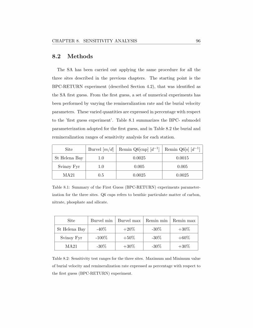
CHAPTER 8. SENSITIVITY ANALYSIS 96
8.2 Methods
The SA has been carried out applying the same procedure for all the
three sites described in the previous chapters. The starting point is the
BPC-RETURN experiment (described Section 4.2), that was identified as
the SA first guess. From the first guess, a set of numerical experiments has
been performed by varying the remineralization rate and the burial velocity
parameters. These varied quantities are expressed in percentage with respect
to the ’first guess experiment’. Table 8.1 summarizes the BPC- submodel
parameterization adopted for the first guess, and in Table 8.2 the burial and
remineralization ranges of sensitivity analysis for each station.
Site Burvel [m/d] Remin Q6[cnp] [d−1] Remin Q6[s] [d−1]
St Helena Bay 1.0 0.0025 0.0015
Svinøy Fyr 1.0 0.005 0.005
MA21 0.5 0.0025 0.0025
Table 8.1: Summary of the First Guess (BPC-RETURN) experiments parameter-
ization for the three sites. Q6 cnps refers to benthic particulate matter of carbon,
nitrate, phosphate and silicate.
Site Burvel min Burvel max Remin min Remin max
St Helena Bay -40% +20% -30% +30%
Svinoy Fyr -100% +50% -30% +60%
MA21 -30% +30% -30% +30%
Table 8.2: Sensitivity test ranges for the three sites. Maximum and Minimum value
of burial velocity and remineralization rate expressed as percentage with respect to
the first guess (BPC-RETURN) experiment.
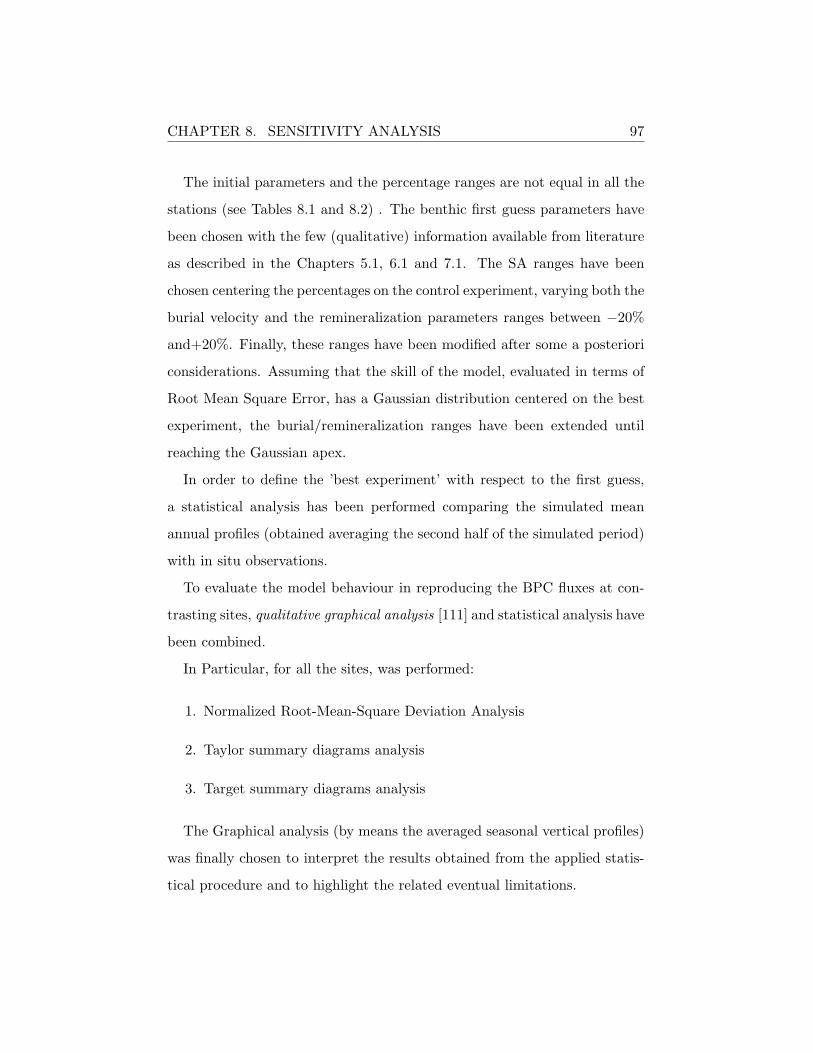
CHAPTER 8. SENSITIVITY ANALYSIS 97
The initial parameters and the percentage ranges are not equal in all the
stations (see Tables 8.1 and 8.2) . The benthic first guess parameters have
been chosen with the few (qualitative) information available from literature
as described in the Chapters 5.1, 6.1 and 7.1. The SA ranges have been
chosen centering the percentages on the control experiment, varying both the
burial velocity and the remineralization parameters ranges between −20%
and+20%. Finally, these ranges have been modified after some a posteriori
considerations. Assuming that the skill of the model, evaluated in terms of
Root Mean Square Error, has a Gaussian distribution centered on the best
experiment, the burial/remineralization ranges have been extended until
reaching the Gaussian apex.
In order to define the ’best experiment’ with respect to the first guess,
a statistical analysis has been performed comparing the simulated mean
annual profiles (obtained averaging the second half of the simulated period)
with in situ observations.
To evaluate the model behaviour in reproducing the BPC fluxes at con-
trasting sites, qualitative graphical analysis [111] and statistical analysis have
been combined.
In Particular, for all the sites, was performed:
1. Normalized Root-Mean-Square Deviation Analysis
2. Taylor summary diagrams analysis
3. Target summary diagrams analysis
The Graphical analysis (by means the averaged seasonal vertical profiles)
was finally chosen to interpret the results obtained from the applied statis-
tical procedure and to highlight the related eventual limitations.

CHAPTER 8. SENSITIVITY ANALYSIS 98
Normalized Root-Mean-Square Deviation Analysis
The Normalized Root-Mean-Square Deviation analysis (NRMSE or NRMSD)
was carried out in order to get general information about the behaviour of
the model with respect to the benthic parameters (burial velocity and rem-
ineralization rate). The NRMSE has been computed normalizing the Root
Mean Square Error (RMSE) with respect to the mean value of the obser-
vations and reporting the model error as percentage, where low NRMSE
values indicate less residual error [115, 116]. NMRSE is defined as:
NMRSE =
√√√√∑Nn=1(mn − rn)∑N
n=1(r2)
2
(8.1)
where mn is the nth simulated (model) data, rn is the nth observation
and N the number of data (references data). Although different metrics
have been proposed in literature [117] for numerical model skill assessment,
the NRMSE remains the dominant metric in order to investigate statistical
results concerning the parameter space [116].
Taylor Analysis and Target Analysis
The Taylor and Target diagrams statistically summarize the degree of
correspondence between the simulated and reference fields, accounting for
more than one statistical operator at a time.
The normalized Taylor diagram is displayed in polar coordinates for pat-
tern comparison between reference and experiment(s) in terms of standard
deviation, correlation, and unbiased Root Mean Square Difference [110].
This statistical metrics [110] at the basis of the Taylor diagrams are:
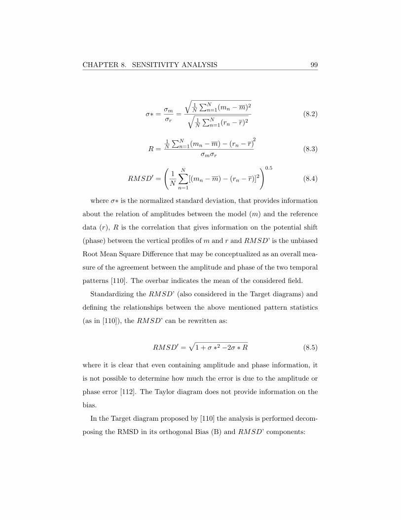
CHAPTER 8. SENSITIVITY ANALYSIS 99
σ∗ =σmσr
=
√1N
∑Nn=1(mn −m)2√
1N
∑Nn=1(rn − r)2
(8.2)
R =1N
∑Nn=1(mn −m)− (rn − r)
σmσr
2
(8.3)
RMSD′ =
(1
N
N∑n=1
[(mn −m)− (rn − r)]2)0.5
(8.4)
where σ∗ is the normalized standard deviation, that provides information
about the relation of amplitudes between the model (m) and the reference
data (r), R is the correlation that gives information on the potential shift
(phase) between the vertical profiles of m and r and RMSD’ is the unbiased
Root Mean Square Difference that may be conceptualized as an overall mea-
sure of the agreement between the amplitude and phase of the two temporal
patterns [110]. The overbar indicates the mean of the considered field.
Standardizing the RMSD’ (also considered in the Target diagrams) and
defining the relationships between the above mentioned pattern statistics
(as in [110]), the RMSD’ can be rewritten as:
RMSD′ =√
1 + σ ∗2 −2σ ∗R (8.5)
where it is clear that even containing amplitude and phase information, it
is not possible to determine how much the error is due to the amplitude or
phase error [112]. The Taylor diagram does not provide information on the
bias.
In the Target diagram proposed by [110] the analysis is performed decom-
posing the RMSD in its orthogonal Bias (B) and RMSD’ components:
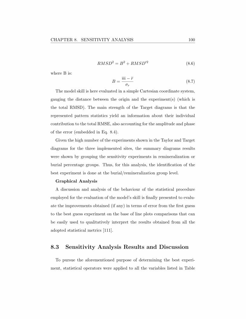
CHAPTER 8. SENSITIVITY ANALYSIS 100
RMSD2 = B2 +RMSD′2 (8.6)
where B is:
B =m− rσr
(8.7)
The model skill is here evaluated in a simple Cartesian coordinate system,
gauging the distance between the origin and the experiment(s) (which is
the total RMSD). The main strength of the Target diagrams is that the
represented pattern statistics yield an information about their individual
contribution to the total RMSE, also accounting for the amplitude and phase
of the error (embedded in Eq. 8.4).
Given the high number of the experiments shown in the Taylor and Target
diagrams for the three implemented sites, the summary diagrams results
were shown by grouping the sensitivity experiments in remineralization or
burial percentage groups. Thus, for this analysis, the identification of the
best experiment is done at the burial/remineralization group level.
Graphical Analysis
A discussion and analysis of the behaviour of the statistical procedure
employed for the evaluation of the model’s skill is finally presented to evalu-
ate the improvements obtained (if any) in terms of error from the first guess
to the best guess experiment on the base of line plots comparisons that can
be easily used to qualitatively interpret the results obtained from all the
adopted statistical metrics [111].
8.3 Sensitivity Analysis Results and Discussion
To pursue the aforementioned purpose of determining the best experi-
ment, statistical operators were applied to all the variables listed in Table

CHAPTER 8. SENSITIVITY ANALYSIS 101
4.1 and shown in Appendix A.2. Moreover the intercomparison between the
best BPC parameterization found in the three implemented sites and their
environmental and ecological characteristics has been executed considering
phosphate, nitrate and chlorophyll. Indeed, these are the variables which
are common to all the test cases.
Experimental SA scheme
The SA matrix of the experiment for SHB and SFyr test cases has been
enlarged in order to reach the minimum NRMSE condition.
St Helena Bay has been the first test of the sensitivity analysis, because
of the richness of the dataset with respect to the SFyr and the MA21 im-
plemented sites. 91 simulations have been performed following the scheme
of parameter variations schematized in Figure 8.1.
Figure 8.1: St. Helena Bay site sensitivity test scheme. The experiments are
expressed as varied burial and remineralization parameters percentages with respect
to the first guest experiment (Red square).
The experiment matrix shown in Figure 8.2 refers to the 160 experiments

CHAPTER 8. SENSITIVITY ANALYSIS 102
carried out for the Svinøy Fyr site. Here, the percentage step (10%)
has been changed with respect to the SHB station (5%) on the light of the
fact that small variations of the benthic parameters does not excessively
affect the model behaviour (not shown). The extension of both the BPC
parameters ranges was performed based on the NRMSE analysis.
Figure 8.2: Svinøy Fyr site sensitivity test scheme. The experiments are expressed
in varied burial and remineralization parameters percentage with respect to the first
guest experiment (Red square).

CHAPTER 8. SENSITIVITY ANALYSIS 103
In the MA21 station the original matrix of the experiment has been main-
tained, limiting the sensitivity analysis to few experiments with respect to
the SHB and SFyr sites. Indeed, the validation dataset has been considered
not particularly suitable for statistical analysis, having a seasonal resolution
(see Table 5.1) and being rather low in number (2-4 nutrient observation for
season). The 49 experiments matrix is shown in Figure 8.3.
Figure 8.3: MA21 site sensitivity test scheme. The experiments are expressed in
varied burial and remineralization parameters percentage with respect to the first
guest experiment (Red square).
Normalized Root-Mean-Square Deviation
The comparison between the NRMSE computed with respect to the vali-
dation data gives a flavour about the behaviour of the model with respect to
decreasing/increasing burial and remineralization parameters. The results
of the NRMSE analysis for each variable and site are shown in Appendix
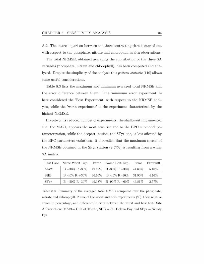
CHAPTER 8. SENSITIVITY ANALYSIS 104
A.2. The intercomparison between the three contrasting sites is carried out
with respect to the phosphate, nitrate and chlorophyll in situ observations.
The total NRMSE, obtained averaging the contribution of the three SA
variables (phosphate, nitrate and chlorophyll), has been computed and ana-
lyzed. Despite the simplicity of the analysis this pattern statistic [110] allows
some useful considerations.
Table 8.3 lists the maximum and minimum averaged total NRMSE and
the error difference between them. The ’minimum error experiment’ is
here considered the ’Best Experiment’ with respect to the NRMSE anal-
ysis, while the ’worst experiment’ is the experiment characterized by the
highest NRMSE.
In spite of its reduced number of experiments, the shallowest implemented
site, the MA21, appears the most sensitive site to the BPC submodel pa-
rameterization, while the deepest station, the SFyr one, is less affected by
the BPC parameters variations. It is recalled that the maximum spread of
the NRMSE obtained in the SFyr station (2.57%) is resulting from a wider
SA matrix.
Test Case Name Worst Exp. Error Name Best Exp. Error ErrorDiff
MA21 B +30% R -30% 49.78% B -30% R +30% 44.68% 5.10%
SHB B -40% R +30% 36.66% B -40% R -30% 31.90% 4.76%
SFyr B +50% R -30% 49.38% B -90% R +60% 46.81% 2.57%
Table 8.3: Summary of the averaged total RMSE computed over the phosphate,
nitrate and chlorophyll. Name of the worst and best experiments (%), their relative
errors in percentage, and difference in error between the worst and best test. Site
Abbreviation: MA21= Gulf of Trieste, SHB = St. Helena Bay and SFyr = Svinøy
Fyr.
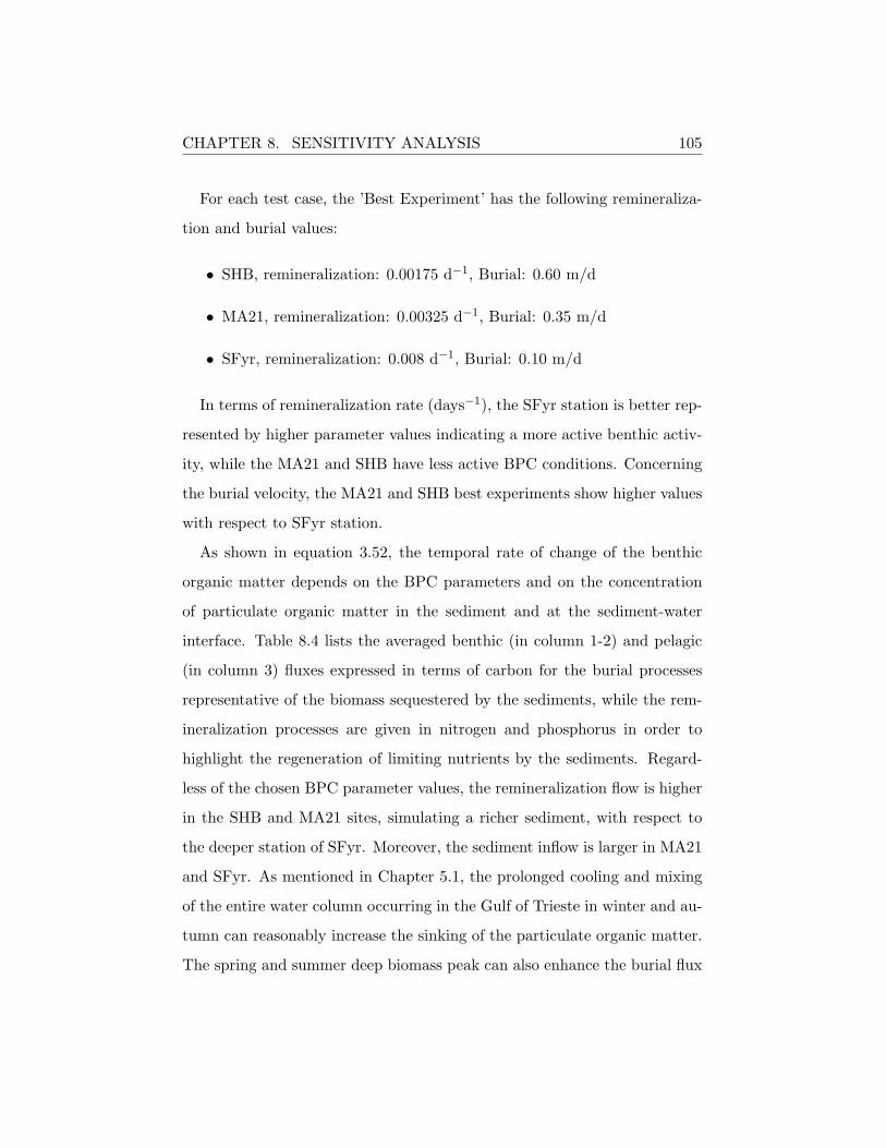
CHAPTER 8. SENSITIVITY ANALYSIS 105
For each test case, the ’Best Experiment’ has the following remineraliza-
tion and burial values:
• SHB, remineralization: 0.00175 d−1, Burial: 0.60 m/d
• MA21, remineralization: 0.00325 d−1, Burial: 0.35 m/d
• SFyr, remineralization: 0.008 d−1, Burial: 0.10 m/d
In terms of remineralization rate (days−1), the SFyr station is better rep-
resented by higher parameter values indicating a more active benthic activ-
ity, while the MA21 and SHB have less active BPC conditions. Concerning
the burial velocity, the MA21 and SHB best experiments show higher values
with respect to SFyr station.
As shown in equation 3.52, the temporal rate of change of the benthic
organic matter depends on the BPC parameters and on the concentration
of particulate organic matter in the sediment and at the sediment-water
interface. Table 8.4 lists the averaged benthic (in column 1-2) and pelagic
(in column 3) fluxes expressed in terms of carbon for the burial processes
representative of the biomass sequestered by the sediments, while the rem-
ineralization processes are given in nitrogen and phosphorus in order to
highlight the regeneration of limiting nutrients by the sediments. Regard-
less of the chosen BPC parameter values, the remineralization flow is higher
in the SHB and MA21 sites, simulating a richer sediment, with respect to
the deeper station of SFyr. Moreover, the sediment inflow is larger in MA21
and SFyr. As mentioned in Chapter 5.1, the prolonged cooling and mixing
of the entire water column occurring in the Gulf of Trieste in winter and au-
tumn can reasonably increase the sinking of the particulate organic matter.
The spring and summer deep biomass peak can also enhance the burial flux

CHAPTER 8. SENSITIVITY ANALYSIS 106
(see Chapter 5.1). Despite the higher burial velocity parameter (0.6 m/d),
SHB exhibits the minimal burial flux (Table 8.4). This clearly indicates the
lower sedimentation flux of particulate detritus and phytoplankton. SHB is
a site characterized by upwelling conditions here idealised as described in
Chapter 6.1. The minimal burial flux can be likely be attributed to pelagic
remineralization.
Test Case Remin * Q6n Remin * Q6p R6c Buried
SHB 1.027 0.068 -0.0021
MA21 0.910 0.050 -0.1344
SFyr 0.336 0.016 -0.0636
Table 8.4: Summary of the averaged total Benthic (column Remin * Q6n and
column Remin * Q6p) and Pelagic (column R6c Buried) fluxes. The benthic fluxes
are expressed in mmol N-P/m2day and the pelagic fluxes in mg C/m2 day. Site
Abbreviation: MA21= Gulf of Trieste, SHB = St. Helena Bay and SFyr = Svinøy
Fyr.
The intercomparison between the maximum and minimum NRMSE differ-
ences (8.3, column ErrorDiff) has been evaluated with respect to the depth of
the three sites. As indicated by Figure 8.4, a certain degree of dependency
between the station depth and the benthic pelagic intensity of the fluxes
can be observed suggesting a decreasing sensitivity to the benthic-pelagic
interface parametrization with depth in agreement with [19].

CHAPTER 8. SENSITIVITY ANALYSIS 107
Figure 8.4: Intercomparison between the Depth (Y-axes) and the error differences
between the maximum and the minimum NRMSE (X-axes) for the three imple-
mented stations see Table 8.3. Green line refers to the regression line, the shaded
area to the confidence interval (0.5) for the regression estimate.
Tables 8.5, 8.6 and 8.7 list the phosphate, nitrate and chlorophyll NRMSE.
As previously observed, the effect of upwelling and the subsequent temporal
extension of the thermocline does not allow to obtain chlorophyll improve-
ments (in terms of NRMSE) even if phosphate and nitrate errors are con-
siderably reduced. Contrarily in the the MA21 and SFyr sites, prolonged
mixed and homogeneous water column conditions allow chlorophyll to be
more affected by the BPC parameterization.
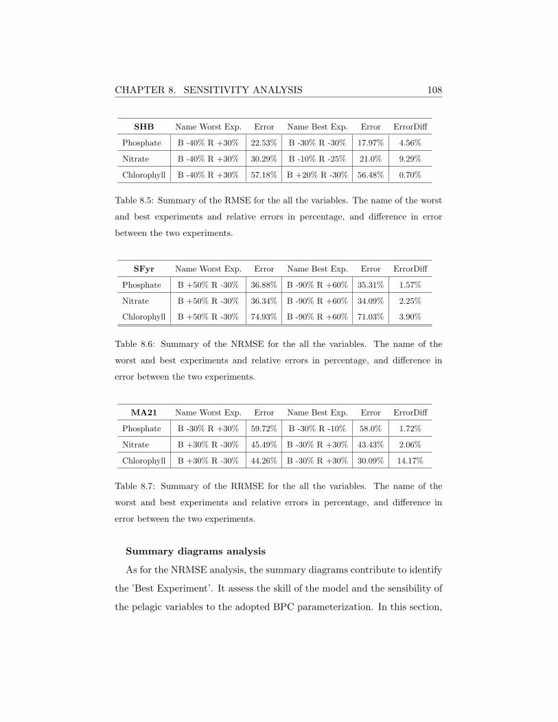
CHAPTER 8. SENSITIVITY ANALYSIS 108
SHB Name Worst Exp. Error Name Best Exp. Error ErrorDiff
Phosphate B -40% R +30% 22.53% B -30% R -30% 17.97% 4.56%
Nitrate B -40% R +30% 30.29% B -10% R -25% 21.0% 9.29%
Chlorophyll B -40% R +30% 57.18% B +20% R -30% 56.48% 0.70%
Table 8.5: Summary of the RMSE for the all the variables. The name of the worst
and best experiments and relative errors in percentage, and difference in error
between the two experiments.
SFyr Name Worst Exp. Error Name Best Exp. Error ErrorDiff
Phosphate B +50% R -30% 36.88% B -90% R +60% 35.31% 1.57%
Nitrate B +50% R -30% 36.34% B -90% R +60% 34.09% 2.25%
Chlorophyll B +50% R -30% 74.93% B -90% R +60% 71.03% 3.90%
Table 8.6: Summary of the NRMSE for the all the variables. The name of the
worst and best experiments and relative errors in percentage, and difference in
error between the two experiments.
MA21 Name Worst Exp. Error Name Best Exp. Error ErrorDiff
Phosphate B -30% R +30% 59.72% B -30% R -10% 58.0% 1.72%
Nitrate B +30% R -30% 45.49% B -30% R +30% 43.43% 2.06%
Chlorophyll B +30% R -30% 44.26% B -30% R +30% 30.09% 14.17%
Table 8.7: Summary of the RRMSE for the all the variables. The name of the
worst and best experiments and relative errors in percentage, and difference in
error between the two experiments.
Summary diagrams analysis
As for the NRMSE analysis, the summary diagrams contribute to identify
the ’Best Experiment’. It assess the skill of the model and the sensibility of
the pelagic variables to the adopted BPC parameterization. In this section,

CHAPTER 8. SENSITIVITY ANALYSIS 109
diagrams for the variables phosphate, nitrate and chlorophyll are shown since
data for the variables were available for all sites. While, supplementary
comparisons to additional data available at individual sites are provided
in Appendix A.2. To make the diagrams clearer, the experiments were
grouped into remineralization groups that had same remineralization values
and different burial values. This grouping scheme was chosen on the basis
that the error is more sensitive to remineralization than to the burial term.
Figures 8.5, 8.6 and 8.7 show the Taylor (left panels) and Target (right
panels) diagrams performed in SHB, SFyr and MA21 sites respectively.
From the Taylor analysis less information can be retrieved, since in the
three sites the cloud of the experiments is condensed for all the test cases.
Nevertheless, it can be noticed that in each site, correlation is generally
constant and high (with the exception of phosphate and nitrate for the
MA21 test case).
In the three Taylor diagrams of SHB (Figure 8.5 left panel), the ’−30%
remineralization’ group (in blue) is characterized by the lowest unbiased
RMSD, providing the closest fit to the data. For chlorophyll and phosphate,
the results are in agreement with the ’Best experiment’ defined in the previ-
ous NRMSE analysis while it is slightly different (5%) for the nitrate. The
nearly constant values of correlation and a higher standard deviation suggest
that the sensitivity analysis averaged vertical profiles share similar phase and
varying amplitude, returning an unbiased RMSE mainly amplitude-driven,
for the phosphate and, even if to a lesser extent, for the nitrate. Contrarily,
the chlorophyll cloud of experiments has a better amplitude agreement.
Investigating the relationship between the bias and the unbiased RMSE,
the Target diagrams in Figure 8.5 (right panel) confirm the results obtained
in the NRMSD and Taylor analysis. From the Target diagram it can be

CHAPTER 8. SENSITIVITY ANALYSIS 110
observed how the inorganic nutrient total NRMSE is mainly determined
by the bias, while in the chlorophyll the bias and unbiased NRMSE equally
contribute to the total NRMSE. The comparison among the results, in terms
of Best Experiment, obtained using the three statistical operators is shown
in the devoted SHB Section of Table 8.8.
In the SFyr test case, the cluster of the model points are extremely
grouped in all the summary diagrams (Figure 8.6). From the Taylor dia-
gram of the chlorophyll (Figure 8.6 bottom-left panel) it can be noticed that
the best experiment belong to the ’remineralization +60%’ group, confirm-
ing the previous analysis. The same results can be observed from the Target
(right panel) diagram where the total RMSE is equally determined by bias
and unbiased RMSE variations. Instead, the Taylor diagrams of the inor-
ganic nutrients were characterized by a good amplitude (σ ∼1). This makes
the unbiased NRMSD mainly phase-driven (Figure 8.6 top and middle-left
panel). In both cases the best experiment group is not enough clear, being
in between the SA percentage ranges. The enlargement of these two dia-
grams is not shown because with this qualitative analysis the results of the
NRMSE are already not confirmed. In the nutrients Target diagrams (right
panel) the unbiased RMSD is constant for the nitrate and fairly constant for
the phosphate cloud of experiments, determining a bias-driven total RMSD.
The comparison among the results, in terms of Best Experiment, obtained
using the three statistical operators is shown in the devoted SFyr Section of
Table 8.8.
In the MA21, chlorophyll is the only variable correlated with the refer-
ence field. This is likely due to the already described dataset limitations
(nutrients profiles have 2-3 averaged measurement for season). The chloro-
phyll Taylor diagram (Figure 8.7 bottom left) shows that the lower reminer-
CHAPTER 8. SENSITIVITY ANALYSIS 111
alization groups (around −20%) are characterized by the lowest unbiased
RMSD, while the Target diagram (right panel) demonstrates that the cloud
of experiments is highly biased (> 1). Phosphate and nitrate Taylor diagram
model points (Figure 8.7 top and middle left) have respectively negative and
weakly positive correlation and extremely low values of standard deviation.
This statistical features indicate a remarkable difference in phase and ampli-
tude of the SA mean vertical profiles with respect to the few observations.
Having highest but low varying values of unbiased RMSE (with respect to
the bias), the phosphate total RMSD is particularly affected by bias, because
the simulations span over a more large range (right panel). The comparison
among the results, in terms of Best Experiment, obtained using the three
statistical operators is shown in the devoted MA21 Section of Table 8.8.
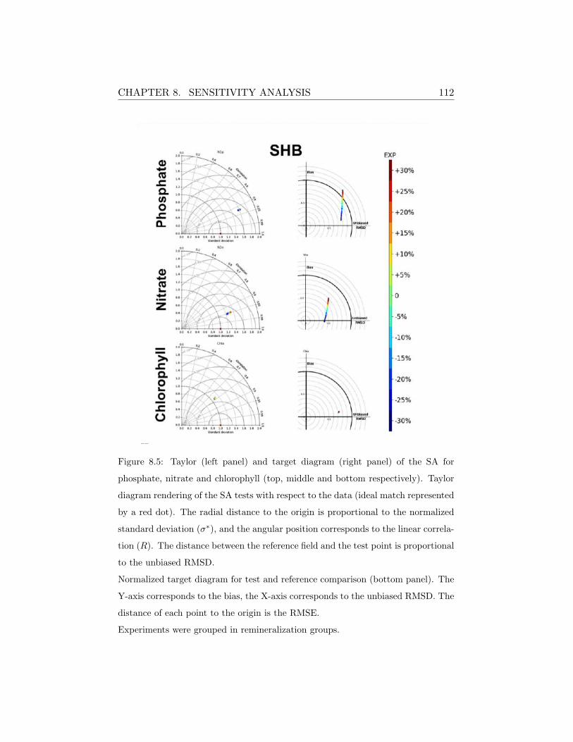
CHAPTER 8. SENSITIVITY ANALYSIS 112
H
Figure 8.5: Taylor (left panel) and target diagram (right panel) of the SA for
phosphate, nitrate and chlorophyll (top, middle and bottom respectively). Taylor
diagram rendering of the SA tests with respect to the data (ideal match represented
by a red dot). The radial distance to the origin is proportional to the normalized
standard deviation (σ∗), and the angular position corresponds to the linear correla-
tion (R). The distance between the reference field and the test point is proportional
to the unbiased RMSD.
Normalized target diagram for test and reference comparison (bottom panel). The
Y-axis corresponds to the bias, the X-axis corresponds to the unbiased RMSD. The
distance of each point to the origin is the RMSE.
Experiments were grouped in remineralization groups.
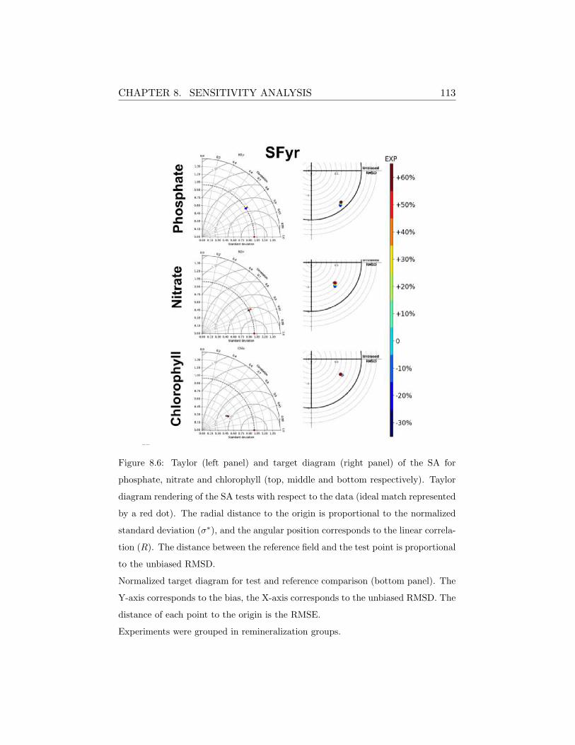
CHAPTER 8. SENSITIVITY ANALYSIS 113
H
Figure 8.6: Taylor (left panel) and target diagram (right panel) of the SA for
phosphate, nitrate and chlorophyll (top, middle and bottom respectively). Taylor
diagram rendering of the SA tests with respect to the data (ideal match represented
by a red dot). The radial distance to the origin is proportional to the normalized
standard deviation (σ∗), and the angular position corresponds to the linear correla-
tion (R). The distance between the reference field and the test point is proportional
to the unbiased RMSD.
Normalized target diagram for test and reference comparison (bottom panel). The
Y-axis corresponds to the bias, the X-axis corresponds to the unbiased RMSD. The
distance of each point to the origin is the RMSE.
Experiments were grouped in remineralization groups.

CHAPTER 8. SENSITIVITY ANALYSIS 114
H
Figure 8.7: Taylor (left panel) and target diagram (right panel) of the SA for
phosphate, nitrate and chlorophyll (top, middle and bottom respectively). Taylor
diagram rendering of the SA tests with respect to the data (ideal match represented
by a red dot). The radial distance to the origin is proportional to the normalized
standard deviation (σ∗), and the angular position corresponds to the linear correla-
tion (R). The distance between the reference field and the test point is proportional
to the unbiased RMSD.
Normalized target diagram for test and reference comparison (bottom panel). The
Y-axis corresponds to the bias, the X-axis corresponds to the unbiased RMSD. The
distance of each point to the origin is the RMSE.
Experiments were grouped in remineralization groups.
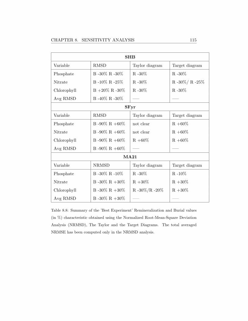
CHAPTER 8. SENSITIVITY ANALYSIS 115
SHB
Variable RMSD Taylor diagram Target diagram
Phosphate B -30% R -30% R -30% R -30%
Nitrate B -10% R -25% R -30% R -30%/ R -25%
Chlorophyll B +20% R -30% R -30% R -30%
Avg RMSD B -40% R -30% —– —–
SFyr
Variable RMSD Taylor diagram Target diagram
Phosphate B -90% R +60% not clear R +60%
Nitrate B -90% R +60% not clear R +60%
Chlorophyll B -90% R +60% R +60% R +60%
Avg RMSD B -90% R +60% —– —–
MA21
Variable NRMSD Taylor diagram Target diagram
Phosphate B -30% R -10% R -30% R -10%
Nitrate B -30% R +30% R +30% R +30%
Chlorophyll B -30% R +30% R -30%/R -20% R +30%
Avg RMSD B -30% R +30% —– —–
Table 8.8: Summary of the ’Best Experiment’ Remineralization and Burial values
(in %) characteristic obtained using the Normalized Root-Mean-Square Deviation
Analysis (NRMSD), The Taylor and the Target Diagrams. The total averaged
NRMSE has been computed only in the NRMSD analysis.

CHAPTER 8. SENSITIVITY ANALYSIS 116
Graphical Analysis
On the basis of what was observed in the three different sites, as regards
the statistical analysis performed, the graphical analysis is finally done to
qualitatively reject or confirm what the best experiment is.
The need to use qualitative analysis mainly arises from the quality of
the observational datasets used to carry out the statistical procedure. In
particular, the implemented sites of SHB and SFyr were characterized by a
high number of measurements, temporal coverage and data frequency (see
Table 6.1 and 7.1) making the SA more reliable with respect to that of the
MA21 test case (Table 5.1).
Figure 8.8, 8.9 and 8.10 show the comparison between the best experiment
(in red), the first guess (in blue) and the reference field (in black) seasonal
climatological profiles for the three test cases.
St. Helena Bay
Going from the first guess to the SA Best test, the inorganic nutrients
profiles (Figure 8.8 A-B-D) show a general and slight improvement, espe-
cially in the deeper levels of the water column (30-80m), while chlorophyll
and oxygen can be considered not sensible to the adopted variations of the
remineralization and burial BPC parameters.
Svinøy Fyr
In Svinøy Fyr station the error difference between the best experiment
and the first guess is not perceived. Indeed, considering all the variables,
the error difference between the first guess and the best experiment in terms
of NRMSD is ∼ 1%.
MA21
In the shallower implemented station, the MA21, improvements can be
observed for the chlorophyll dynamics, while the ammonium seasonal pro-

CHAPTER 8. SENSITIVITY ANALYSIS 117
files match better the observation using the First guess parameters benthic
conditions.
Finally, from the graphical analysis of the seasonal vertical profiles, the
Best Experiment results obtained with the different pattern statistics (NRMSE
and summary diagrams analyses) are successfully confirmed with the ex-
ception of the inorganic nutrients of the MA21 area where the mentioned
limitations of the used dataset make the improvements not at all clear.
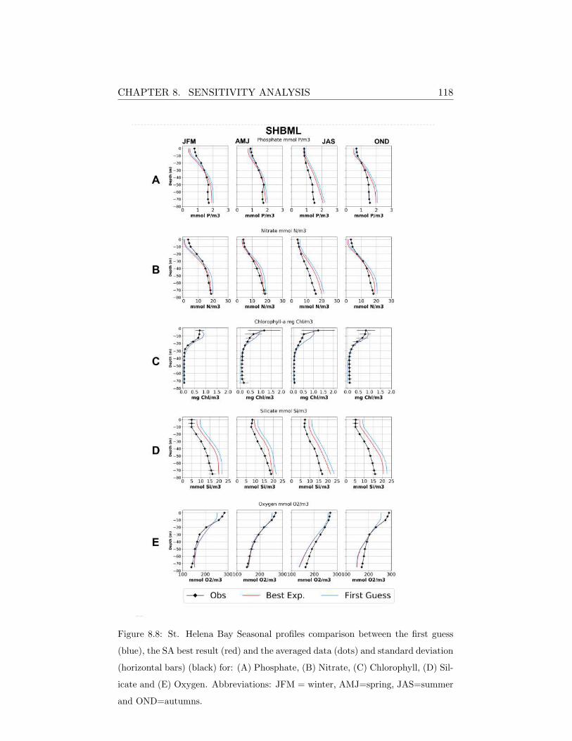
CHAPTER 8. SENSITIVITY ANALYSIS 118
H
Figure 8.8: St. Helena Bay Seasonal profiles comparison between the first guess
(blue), the SA best result (red) and the averaged data (dots) and standard deviation
(horizontal bars) (black) for: (A) Phosphate, (B) Nitrate, (C) Chlorophyll, (D) Sil-
icate and (E) Oxygen. Abbreviations: JFM = winter, AMJ=spring, JAS=summer
and OND=autumns.

CHAPTER 8. SENSITIVITY ANALYSIS 119
H
Figure 8.9: Svinøy Fyr seasonal profiles comparison between the first guess (blue),
the SA best result (red) and the averaged data (dots) and standard deviation
(horizontal bars) (black) for: (A) Phosphate, (B) Nitrate, (C) Chlorophyll and
(D) Silicate. Abbreviations: JFM = winter, AMJ=spring, JAS=summer and
OND=autumns.
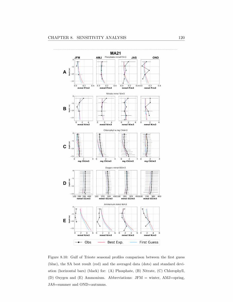
CHAPTER 8. SENSITIVITY ANALYSIS 120
H
Figure 8.10: Gulf of Trieste seasonal profiles comparison between the first guess
(blue), the SA best result (red) and the averaged data (dots) and standard devi-
ation (horizontal bars) (black) for: (A) Phosphate, (B) Nitrate, (C) Chlorophyll,
(D) Oxygen and (E) Ammonium. Abbreviations: JFM = winter, AMJ=spring,
JAS=summer and OND=autumns.
Chapter 9
Conclusions
The benthic-pelagic dynamic processes were successfully implemented in
the coupled physical-biogeochemical NEMO-BFM model and were verified
in a one-dimensional modelling framework for three marine coastal areas
with contrasting climatic and ecological characteristics.
A reference configuration of the model including the benthic component
was setup for each case study seeking for practical parameterizations able to
describe the specific oceanic and biogeochemical regimes. The skill assess-
ment of simulated environmental and ecological dynamics (BPC-RETURN
experiment) was performed against available observational data at both an-
nual and seasonal scales. A companion experiment neglecting the benthic
feedback (NO-BPC experiment) was carried out to further evaluate the im-
portance of both the sedimentation and remineralization processes in coastal
systems.
Overall, the outcomes of the one-dimensional reference simulation allowed
to adequately reproduce the spatio-temporal evolution of key biogeochemical
variables, although some peculiarities emerged from each site. In the MA21
121
CHAPTER 9. CONCLUSIONS 122
area (Gulf of Trieste) the introduction of the BPC sub-model led to an
amelioration of the model skill in reproducing the vertical distribution of
dissolved inorganic nutrients (with the exception of ammonium) and, to a
lesser extent, of the chlorophyll-a concentrations.
In spite of the complex physical regime that characterizes St. Helena Bay,
the achieved setup of the coupled 1D model allowed to reproduce the sea-
sonal upwelling variability. In particular, the inclusion of benthic dynamics
had a remarkable role in shaping the vertical distribution of key biogeo-
chemical variables. The model application to the Svinøy Fyr site led to a
satisfactory representation of the ecosystem dynamics in a deeper continen-
tal shelf system, by showing the role of BPC feedback on the evolution of
the pelagic biogeochemical quantities during both the deep mixing period
(autumn and winter) and the strongly stratified one (spring and summer).
An extensive sensitivity analysis was finally performed to investigate the
response of the pelagic system with respect to different sedimentation-remineralization
rates, by focusing on the changes of inorganic nutrients and chlorophyll-a
distribution within the water column.
From the Normalized Root-Mean-Square Deviation analysis it was shown
that the shallowest implemented site, the MA21, was the most sensitive site
to BPC parameters variations, while the deepest station, the SFyr one, re-
vealed the highest degree of resilience to the different BPC scenarios. More-
over, the analysis of the diffusive inorganic nutrients (Nitrate and Phos-
phate) fluxes from the sediment to the pelagic environment demonstrated
that the MA21 and SHB areas are characterized by a more active benthic
nutrients regeneration with respect to the deepest station of SFyr. The evo-
lution of the pelagic organic carbon sedimentary flux was found to be not
linearly dependent on the station depth, as it emerged from the comparison

CHAPTER 9. CONCLUSIONS 123
of results obtained for the modelled sites.
The reasons for this have been identified in the physical conditions of the
three sites where the mid-latitude MA21 and SFyr site were characterized
by prolonged cooling and mixing periods and in MA21 by a deep biomass
peak both enhancing the sinking flux. Contrarily, in SHB the shallowest
Nutrient-Phytoplankton-Zooplankton food chain reproduced by the model
and the prolonged upwelling period enhances the pelagic remineralization
likely reducing the sedimentation flux.
The Taylor and Target summary diagrams showed and confirmed the
statistical agreement in defining the Best Experiment in all the variables
in the SHB site (the richest dataset used in this study). In Svinøy Fyr,
the Best experiment was identified on the basis of the Target and RMSE
analysis with the total RMSE mainly characterized by a more varying bias,
with the exception of the chlorophyll that was well represented using all the
statistical metrics. Some limitation, mainly due to dataset characteristics
in terms of nutrients measurements availability, has been encountered in
the MA21 area, while Taylor and Target analysis was considered reliable
in describing chlorophyll dynamic. Here, beyond the applied sensitivity
statistical procedure, the graphical analysis has been considered particularly
important.
The graphical analysis generally confirmed the Best Experiments found
using all the statistical patterns.
Moreover, the reproduced BPC fluxes in the MA21 area are qualitatively
in agreement with previous works [41, 18, 118, 119, 120].
The best experiment found for the station implemented in St.Helena Bay
denotes active benthic nutrients diffusive fluxes in agreement with what
described by literature [90, 93].
CHAPTER 9. CONCLUSIONS 124
Although site-specific information were not available for the Svinøy Fyr
site, the reproduced not particularly active BPC conditions allowed to con-
firm previous hypotheses [19] regarding the relationships between the BPC
fluxes and depth. Moreover, the Best Experiment BPC conditions of burial
flux qualitatively represent the dynamic described by [106, 107] where a
large portion of the carbon fixed annually by phytoplankton falls ungrazed
to the sediments.
The future continuation of this study should aim (i) to further extend the
set of study sites to include additional ecosystems and (ii) to validate BPC
sub-models parameterization by means of experimental data.
Although significant results were achieved in this study, the limited exten-
sion of observational datasets hindered a more detailed representation of the
benthic-pelagic coupling processes and experimental evidences are urgently
needed to adequately support the development of benthic system modelling.
In the light of the presented analyses, the proposed BPC sub-model can
be profitably implemented on the wider global ocean scale to complement
the investigation of biogeochemical cycles and improve the assessment of
carbon dynamics.
Finally, aiming to obtain a more robust numerical description of the
sediment-water exchanges in coastal waters, it is strongly recommended to
increase the number of benthic processes numerically described by the BPC
sub-model.

Appendix A
Appendix
125

APPENDIX A. APPENDIX 126
A.1 Model Parameterization
Table A.1: List of the parameters in the BFM pelagic equations for phytoplankton.
Parameter Symbol P (1) P (2) P (3) P (4)
Q10 coefficient p q10 2.0 2.0 2.0 2.0
Cut-off threshold for temperature factor p qtemp 0.0 0.0 0.0 0.0
Maximal productivity at 10◦C (day−1) p sum 1.3 1.02 1.6 0.83
Respiration rate at 10◦C (day−1) p srs 0.05 0.05 0.05 0.1
Max.specific nutrient-stress lysis rate
(day−1)
p sdmo 0.01 0.01 0.01 0.2.
Half saturation constant for nutrient
stress lysis (–)
p thdo 0.1 0.1 0.1 0.5
Extra lysis rate (biomass
density-dependent) (day−1)
p seo 0.0 0.0 0.0 0.5
Half saturation constant for extra lysis
(mgC m−3)
p sheo 0.0 0.0 0.0 100.0
Excreted fraction of primary production
(–)
p pu ea 0.01 0.1 0.1 0.15
Activity respiration fraction (–) p pu ra 0.1 0.1 0.2 0.1
Membrane affinity for N (m3/mgC/day) p qun 0.025 0.025 0.025 0.025.
Half saturation constant for NH4 uptake
preference over NO3 (mmolN/m3 )
p lN4 1.0 0.5 0.1 1.0
Minimum quotum N:C (mmolN/mgC) p qnlc 6.87x10⁻³ 6.87x10⁻³ 6.87x10⁻³ 6.87x10⁻³
Reference quotum N:C (mmolN/mgC) p qncPPY 1.26x10⁻² 1.266x10⁻² 1.266x10⁻² 1.26x10⁻²
Multiplication factor for luxury storage
(–)
p xqn 2.0 2.0 2.0 2.0
Membrane affinity for P (m3 /mgC/day) p qup 0.0025 0.0025 0.0025 0.0025
Minimum quotum P:C (mmolP/mgC) p qplc 4.29x10⁻⁴ 4.29x10⁻⁴ 4.29x10⁻⁴ 4.29x10⁻⁴
Reference quotum P:C (mmolP/mgC) p qpcPPY 7.86x10⁻⁴ 7.86x10⁻⁴ 7.86x10⁻⁴ 7.86x10⁻⁴
Multiplication factor for luxury storage
(–)
p xqp 2.0 2.0 2.0 2.0
Half saturation conc. for dissolved Si
limitation (mmolSi m−3))
p chPs 1.0 0.0 0.0 0.0
Membrane affinity for Si (m3/mgC/day) p qus 0.0025 0.0 0.0 0.0
Minimum quotum Si:C (mmolSi/mgC) p qslc 0.007 0.0 0.0 0.0
Reference quotum Si:C (mmolSi/mgC) p qscPPY 8.5x10⁻³ 0.0 0.0 0.0
Nutrient stress threshold for sinking (–) p esNI 0.7 0.75 0.75 0.75
Maximum Sinking velocity (m day−1) p res 5.0 0.0 0.0 5.0
Specific turnover rate for Chla (day−1) p sdchl 0.2 0.2 0.2 0.2
Initial slope of the P-E curve (mgC s m2
/mgChl/uE)
p alpha chl 1.38x10⁻⁵ 0.46x10⁻⁵ 1.52x10⁻⁵ 0.46x10⁻⁵
Reference quotum Chla:C (mgChla/mgC) p qlcPPY 0.025 0.015 0.02 0.015
Chla-specific extinction coefficient
(m2/mgChla)
p epsChla 0.03 0.03 0.03 0.03
Relaxation rate towards maximum Chla:C
(day−1)
p totchl relt 0.25 0.25 0.25 0.25
Optimal value of E PAR/E K (–) p EpEk or 3.0 3.0 3.0 3.0

APPENDIX A. APPENDIX 127
Table A.2: List of the parameters in the BFM pelagic equations for microzooplank-
ton.
Parameter Symbol Z(5) Z(6)
Q10 value for physiological rates (-) p q10 2.0 2.0
Respiration rate at 10◦C (day−1) p srs 0.02 0.02
Potential growth rate (day−1) p sum 2.0 5.0
Mortality rate due to oxygen limitation (day−1) p sdo 0.25 0.25
Temperature independent mortality (day−1) p sd 0.0 0.0
Assimilation efficiency (-) p pu 0.5 0.3
Fraction of activity excretion (-) p pu ea 0.25 0.35
Half-saturation oxygen concentration (mmolO2 m−3) p chro 30.0 30.0
Half-saturation food concentration for Type II (mgC
m−3)
p chuc 200.0 200.0
Half-saturation food concentration for preference factor
(mgC m−3)
p minfood 50.0 50.0
Portion of egested calcified shells during grazing (-) p pecaco3 0.5 0.5
Maximum quotum N:C (mmolN/mgC) p qncMIZ 1.67d-2 1.67d-2
Maximum quotum P:C (mmolN/mgC) p qpcMIZ 1.85d-3 1.85d-3
Table A.3: List of the parameters in the BFM pelagic equations for mesozooplank-
ton.
Parameter Symbol Z(3) Z(4)
Q10 value for physiological rates (-) p q10 2.0 2.0
Respiration rate at 10◦C (day−1) p srs 0.01 0.02
Potential growth rate (day−1) p sum 2.0 2.0
Specific search volume (m3mgCday−1) p vum 0.0025 0.0025
Assimilation efficiency (-) p puI 0.6 0.6
Fraction of faeces production (-) p peI 0.3 0.35
Specific density-dependent mortality (m3 mgC day−1) p p sdo 0.01 0.01
Background natural mortality (day−1) p p sd 0.02 0.01
Exponent of density-dependent mortality (-) p p sds 2.0 2.0
Portion of egested calcified shells during grazing (-) p pecaco3 0.75 0.75
Maximum quotum N:C (mmolN/mgC) p qncMEZ 0.015 0.015
Maximum quotum P:C (mmolN/mgC) p qpcMEZ 1.67d-3 1.67d-3
Half-saturation oxygen concentration (mmolO2 m−3) p p clO2o 30.0 30.0
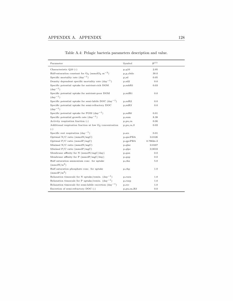
APPENDIX A. APPENDIX 128
Table A.4: Pelagic bacteria parameters description and value.
Parameter Symbol B(1)
Characteristic Q10 (-) p q10 2.95
Half-saturation constant for O2 (mmolO2 m−3) p p chdo 30.0
Specific mortality rate (day−1) p sd 0.05
Density dependent specific mortality rate (day−1) p sd2 0.0
Specific potential uptake for nutrient-rich DOM
(day−1)
p suhR1 0.03
Specific potential uptake for nutrient-poor DOM
(day−1)
p sulR1 0.0
Specific potential uptake for semi-labile DOC (day−1) p suR2 0.0
Specific potential uptake for semi-refractory DOC
(day−1)
p suR3 0.0
Specific potential uptake for POM (day−1) p suR6 0.01
Specific potential growth rate (day−1) p sum 8.38
Activity respiration fraction (-) p pu ra 0.06
Additional respiration fraction at low O2 concentration
(-)
p pu ra 0 0.02
Specific rest respiration (day−1) p srs 0.01
Optimal N/C ratio (mmolN/mgC) p qncPBA 0.0126
Optimal P/C ratio (mmolP/mgC) p qpcPBA 0.7862e-3
Minimal N/C ratio (mmolN/mgC) p qlnc 0.0167
Minimal P/C ratio (mmolP/mgC) p qlpc 0.0018
Membrane affinity for N (mmolN/mgC/day) p qun 0.0
Membrane affinity for P (mmolP/mgC/day) p qup 0.0
Half saturation ammonium conc. for uptake
(mmolN/m3)
p chn 5.0
Half saturation phosphate conc. for uptake
(mmolP/m3)
p chp 1.0
Relaxation timescale for N uptake/remin. (day−1) p ruen 1.0
Relaxation timescale for P uptake/remin. (day−1) p ruep 1.0
Relaxation timescale for semi-labile excretion (day−1) p rec 1.0
Excretion of semi-refractory DOC (-) p pu ea R3 0.0
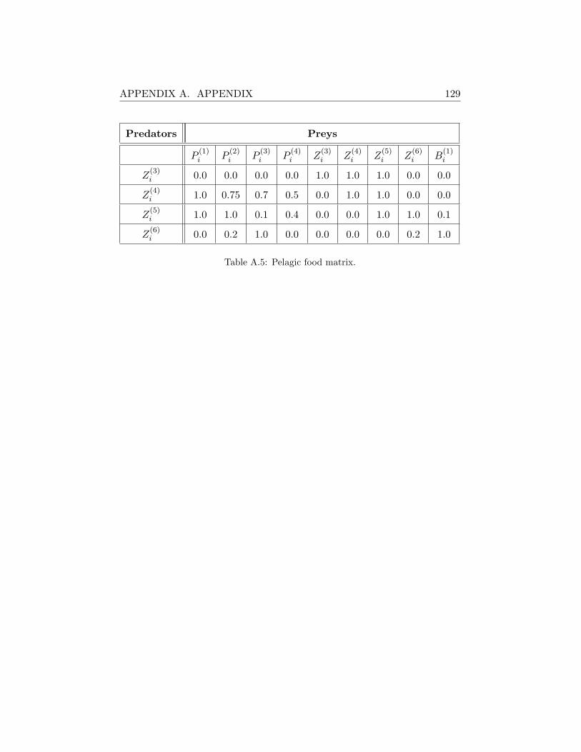
APPENDIX A. APPENDIX 129
Predators Preys
P(1)i P
(2)i P
(3)i P
(4)i Z
(3)i Z
(4)i Z
(5)i Z
(6)i B
(1)i
Z(3)i 0.0 0.0 0.0 0.0 1.0 1.0 1.0 0.0 0.0
Z(4)i 1.0 0.75 0.7 0.5 0.0 1.0 1.0 0.0 0.0
Z(5)i 1.0 1.0 0.1 0.4 0.0 0.0 1.0 1.0 0.1
Z(6)i 0.0 0.2 1.0 0.0 0.0 0.0 0.0 0.2 1.0
Table A.5: Pelagic food matrix.

APPENDIX A. APPENDIX 130
A.2 Sensitivity Analysis Results
A.2.1 SHB
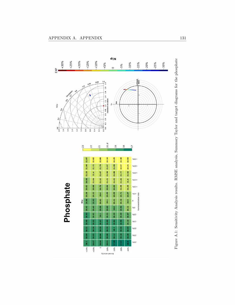
APPENDIX A. APPENDIX 131
Fig
ure
A.1
:S
ensi
tivit
yA
nal
ysi
sre
sult
s.R
MS
Ean
aly
sis,
Su
mm
ary
Tay
lor
an
dta
rget
dia
gra
ms
for
the
ph
osp
hate

APPENDIX A. APPENDIX 132
Fig
ure
A.2
:S
ensi
tivit
yA
nal
ysi
sre
sult
s.R
MS
Ean
aly
sis,
Su
mm
ary
Tay
lor
an
dta
rget
dia
gra
ms
for
the
nit
rate

APPENDIX A. APPENDIX 133
Fig
ure
A.3
:S
ensi
tivit
yA
nal
ysi
sre
sult
s.R
MS
Ean
aly
sis,
Su
mm
ary
Tay
lor
an
dta
rget
dia
gra
ms
for
the
chlo
rop
hyll
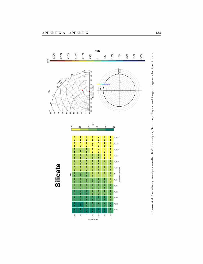
APPENDIX A. APPENDIX 134
Fig
ure
A.4
:S
ensi
tivit
yA
nal
ysi
sre
sult
s.R
MS
Ean
aly
sis,
Su
mm
ary
Tay
lor
an
dta
rget
dia
gra
ms
for
the
Sil
icate

APPENDIX A. APPENDIX 135
Fig
ure
A.5
:S
ensi
tivit
yA
nal
ysi
sre
sult
s.R
MS
Ean
aly
sis,
Su
mm
ary
Tay
lor
an
dta
rget
dia
gra
ms
for
the
oxygen

APPENDIX A. APPENDIX 136
A.2.2 Svinøy Fyr
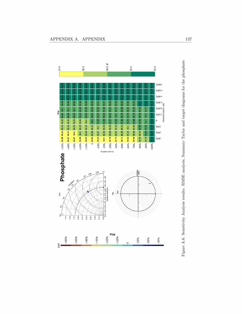
APPENDIX A. APPENDIX 137
Fig
ure
A.6
:S
ensi
tivit
yA
nal
ysi
sre
sult
s.R
MS
Ean
aly
sis,
Su
mm
ary
Tay
lor
an
dta
rget
dia
gra
ms
for
the
ph
osp
hate

APPENDIX A. APPENDIX 138
Fig
ure
A.7
:S
ensi
tivit
yA
nal
ysi
sre
sult
s.R
MS
Ean
aly
sis,
Su
mm
ary
Tay
lor
an
dta
rget
dia
gra
ms
for
the
nit
rate
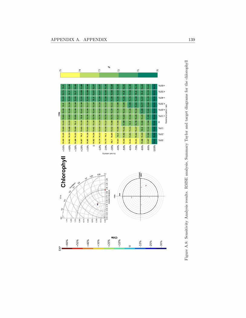
APPENDIX A. APPENDIX 139
Fig
ure
A.8
:S
ensi
tivit
yA
nal
ysi
sre
sult
s.R
MS
Ean
aly
sis,
Su
mm
ary
Tay
lor
an
dta
rget
dia
gra
ms
for
the
chlo
rop
hyll

APPENDIX A. APPENDIX 140
Fig
ure
A.9
:S
ensi
tivit
yA
nal
ysi
sre
sult
s.R
MS
Ean
aly
sis,
Su
mm
ary
Tay
lor
an
dta
rget
dia
gra
ms
for
the
silica
te

APPENDIX A. APPENDIX 141
A.2.3 MA21

APPENDIX A. APPENDIX 142
Fig
ure
A.1
0:S
ensi
tivit
yA
nal
ysi
sre
sult
s.R
MS
Ean
aly
sis,
Su
mm
ary
Tay
lor
an
dta
rget
dia
gra
ms
for
the
ph
osp
hate

APPENDIX A. APPENDIX 143
Fig
ure
A.1
1:S
ensi
tivit
yA
nal
ysi
sre
sult
s.R
MS
Ean
aly
sis,
Su
mm
ary
Tay
lor
an
dta
rget
dia
gra
ms
for
the
nit
rate
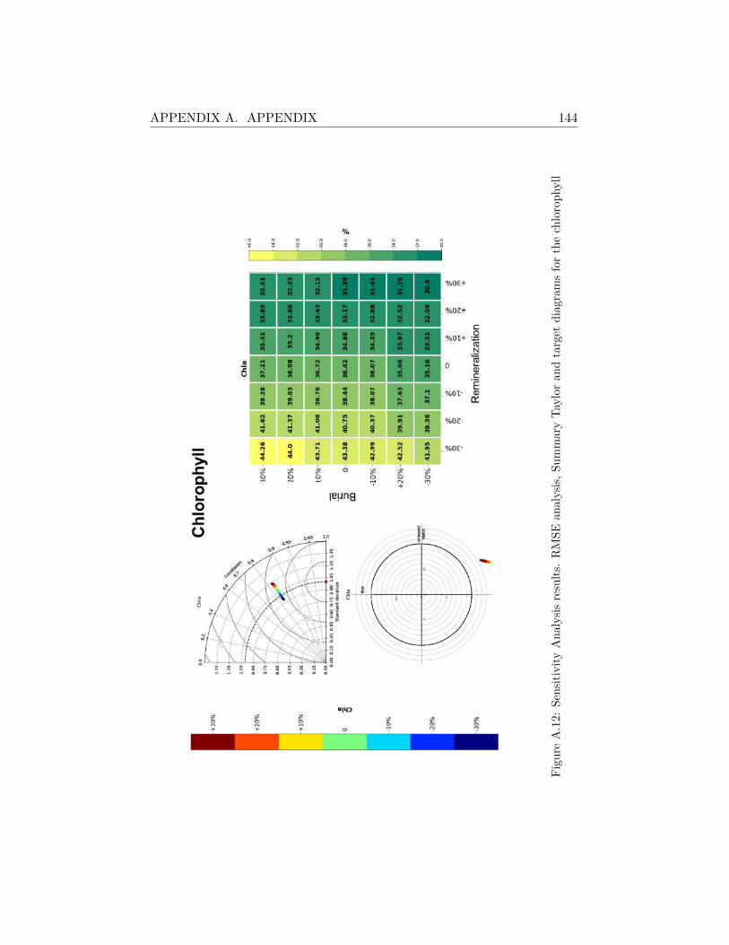
APPENDIX A. APPENDIX 144
Fig
ure
A.1
2:S
ensi
tivit
yA
nal
ysi
sre
sult
s.R
MS
Ean
aly
sis,
Su
mm
ary
Tay
lor
an
dta
rget
dia
gra
ms
for
the
chlo
rop
hyll
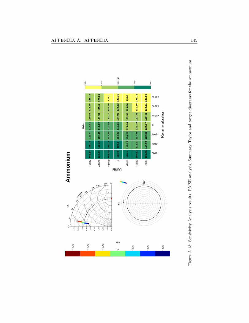
APPENDIX A. APPENDIX 145
Fig
ure
A.1
3:S
ensi
tivit
yA
nal
ysi
sre
sult
s.R
MS
Ean
aly
sis,
Su
mm
ary
Tay
lor
an
dta
rget
dia
gra
ms
for
the
am
mon
ium

APPENDIX A. APPENDIX 146
Fig
ure
A.1
4:S
ensi
tivit
yA
nal
ysi
sre
sult
s.R
MS
Ean
aly
sis,
Su
mm
ary
Tay
lor
an
dta
rget
dia
gra
ms
for
the
oxygen
Bibliography
[1] Peter Burt. “The oceans and climate. By Grant Bigg. Cambridge
University Press, second edition 2003. xi + 273pp. ISBNs 0 521 01634
7, 0 521 81570 3”. In: Weather 59 (Dec. 2006), pp. 190–190. doi:
10.1256/wea.36.04.
[2] A Ganachaud and C Wunsch. “Improved estimates of global ocean
circulation, heat transport and mixing from hydrographic data (vol
408, pg 453, 2000)”. In: Nature 410 (Mar. 2001), pp. 240–240. doi:
10.1038/35065660.
[3] K. Maier-Reimer E. Hasselmann. “Transport and storage of CO2 in
the ocean ——an inorganic ocean-circulation carbon cycle model”.
In: Climate Dynamics 2 (Sept. 1987), pp. 63–90. doi: https://doi.
org/10.1007/BF01054491.
[4] Ernst Maier-Reimer. “Geochemical cycles in an ocean general circu-
lation model. Preindustrial tracer distributions”. In: Global Biogeo-
chemical Cycles 7.3 (1993), pp. 645–677. doi: 10.1029/93GB01355.
[5] Jorge L. Sarmiento, James C. Orr, and Ulrich Siegenthaler. “A per-
turbation simulation of CO2 uptake in an ocean general circulation
147
BIBLIOGRAPHY 148
model”. In: Journal of Geophysical Research: Oceans 97.C3 (1992),
pp. 3621–3645. doi: 10.1029/91JC02849.
[6] Moore J.K. Doney S.C. Lindsay K. “Global Ocean Carbon Cycle
Modeling”. In: Fasham M.J.R. (eds) Ocean Biogeochemistry. Global
Change — The IGBP Series (closed) (2003). Ed. by Springer-Verlag
Berlin Heidelberg. doi: https://doi.org/10.1007/978-3-642-
55844-3_10.
[7] Ernst Maier-Reimer, Uwe Mikolajewicz, and Arne Winguth. “Future
ocean uptake of CO2: interaction between ocean circulation and bi-
ology”. In: Climate Dynamics 12.10 (1996), pp. 711–722.
[8] Fortunat Joos et al. “Global warming and marine carbon cycle feed-
backs on future atmospheric CO2”. In: Science 284.5413 (1999),
pp. 464–467.
[9] G-K Plattner et al. “Feedback mechanisms and sensitivities of ocean
carbon uptake under global warming”. In: Tellus B 53.5 (2001),
pp. 564–592.
[10] A. Navarra. “Ensembles, Forecasts and Predictability”. In: (2002).
Ed. by Springer-Verlag Berlin Heidelberg New York, pp. 131–148.
[11] Christopher L Sabine and Richard A Feely. “The oceanic sink for
carbon dioxide”. In: Greenhouse gas sinks 31 (2007).
[12] Jason Holt et al. “Modelling the global coastal ocean”. In: Philosoph-
ical transactions. Series A, Mathematical, physical, and engineering
sciences 367 (Mar. 2009), pp. 939–51. doi: 10.1098/rsta.2008.
0210.
BIBLIOGRAPHY 149
[13] Amber K. Hardison et al. “Arctic shelves as platforms for biogeo-
chemical activity: Nitrogen and carbon transformations in the Chukchi
Sea, Alaska”. In: Deep Sea Research Part II: Topical Studies in Oceanog-
raphy 144 (2017). The Hanna Shoal Ecosystem of the Northeastern
Chukchi Seashelf, pp. 78–91. issn: 0967-0645. doi: https://doi.
org/10.1016/j.dsr2.2017.08.004.
[14] K Soetaert et al. “On the coupling of benthic and pelagic biogeochem-
ical models”. In: Earth-Science Reviews 51 (Aug. 2000), pp. 173–201.
doi: 10.1016/S0012-8252(00)00004-0.
[15] Jennifer R. Griffiths et al. “The importance of benthic–pelagic cou-
pling for marine ecosystem functioning in a changing world”. In:
Global Change Biology 23.6 (2017), pp. 2179–2196. doi: 10.1111/
gcb.13642. eprint: https://onlinelibrary.wiley.com/doi/pdf/
10.1111/gcb.13642. url: https://onlinelibrary.wiley.com/
doi/abs/10.1111/gcb.13642.
[16] Sandra Arndt et al. “Quantifying the degradation of organic matter
in marine sediments: A review and synthesis”. In: Earth-Science Re-
views 123 (2013), pp. 53–86. issn: 0012-8252. doi: https://doi.
org/10.1016/j.earscirev.2013.02.008. url: http://www.
sciencedirect.com/science/article/pii/S0012825213000512.
[17] Pierre Regnier et al. “Anthropogenic perturbation of the carbon
fluxes from land to ocean”. In: Nature geoscience 6.8 (2013), pp. 597–
607.
[18] Giulia Mussap and Marco Zavatarelli. “A numerical study of the
benthic–pelagic coupling in a shallow shelf sea (Gulf of Trieste)”. In:
Regional studies in marine science 9 (2017), pp. 24–34.
BIBLIOGRAPHY 150
[19] Erwin Suess. “Particulate organic carbon flux in the oceans: Surface
and oxygen utilization”. In: Nature (Jan. 1980).
[20] Jefferson T Turner. “Zooplankton fecal pellets, marine snow and sink-
ing phytoplankton blooms”. In: Aquatic microbial ecology 27.1 (2002),
pp. 57–102.
[21] L Christina and Uta Passow. “Factors influencing the sinking of
POC and the efficiency of the biological carbon pump”. In: Deep
Sea Research Part II: Topical Studies in Oceanography 54.5-7 (2007),
pp. 639–658.
[22] Panagiotis D Dimitriou et al. “One step forward: benthic pelagic
coupling and indicators for environmental status”. In: PloS one 10.10
(2015), e0141071.
[23] M Kralj et al. “Hypoxia and dissolved oxygen trends in the north-
eastern Adriatic Sea (Gulf of Trieste)”. In: Deep Sea Research Part
II: Topical Studies in Oceanography (2019).
[24] Josep-Maria Gili and Rafel Coma. “Benthic suspension feeders: their
paramount role in littoral marine food webs”. In: Trends in ecology
& evolution 13.8 (1998), pp. 316–321.
[25] MM Baustian et al. “Linking the bottom to the top in aquatic ecosys-
tems: mechanisms and stressors of benthic-pelagic coupling”. In: Eco-
DAS X Symposium Proceedings (ed Kemp PF). 2014, pp. 25–47.
[26] Kim Hansen, Steen Mouridsen, and Erik Kristensen. “The impact of
Chironomus plumosus larvae on organic matter decay and nutrient
(N, P) exchange in a shallow eutrophic lake sediment following a phy-
BIBLIOGRAPHY 151
toplankton sedimentation”. In: Hydrobiologia 364.1 (1997), pp. 65–
74.
[27] Andrew M Lohrer, Simon F Thrush, and Max M Gibbs. “Biotur-
bators enhance ecosystem function through complex biogeochemical
interactions”. In: Nature 431.7012 (2004), p. 1092.
[28] Anthony F D’Andrea and Theodore H DeWitt. “Geochemical ecosys-
tem engineering by the mud shrimp Upogebia pugettensis (Crustacea:
Thalassinidae) in Yaquina Bay, Oregon: Density-dependent effects on
organic matter remineralization and nutrient cycling”. In: Limnology
and Oceanography 54.6 (2009), pp. 1911–1932.
[29] Robert A Berner. Early diagenesis: a theoretical approach. 1. Prince-
ton University Press, 1980.
[30] CHR Heip et al. “The role of the benthic biota in sedimentary metabolism
and sediment-water exchange processes in the Goban Spur area (NE
Atlantic)”. In: Deep Sea Research Part II: Topical Studies in Oceanog-
raphy 48.14-15 (2001), pp. 3223–3243.
[31] Gennadi Lessin et al. “Modelling marine sediment biogeochemistry:
Current knowledge gaps, challenges, and some methodological advice
for advancement”. In: Frontiers in marine science 5 (2018), p. 19.
[32] Dominik Hulse et al. “Understanding the causes and consequences of
past marine carbon cycling variability through models”. In: Earth-
science reviews 171 (2017), pp. 349–382.
[33] J Val Klump and Christopher S Martens. “Biogeochemical cycling in
an organic rich coastal marine basin—II. Nutrient sediment-water ex-

BIBLIOGRAPHY 152
change processes”. In: Geochimica et Cosmochimica Acta 45.1 (1981),
pp. 101–121.
[34] Steven Emerson, Richard Jahnke, and David Heggie. “Sediment-water
exchange in shallow water estuarine sediments”. In: Journal of Ma-
rine Research 42.3 (1984), pp. 709–730.
[35] C P Slomp, JFP Malschaert, and W Van Raaphorst. “The role of
adsorption in sediment-water exchange of phosphate in North Sea
continental margin sediments”. In: Limnology and Oceanography 43.5
(1998), pp. 832–846.
[36] Gurvan Madec et al. “NEMO ocean engine”. In: (2015).
[37] M Vichi et al. “The biogeochemical flux model (BFM): Equation
description and user manual, BFM version 5.1”. In: BFM Rep. Ser
1 (2015), p. 104.
[38] M Vichi et al. “Coupling BFM with Ocean models: the NEMO model
(Nucleus for the European Modelling of the Ocean)”. In: BFM Report
series 2 (2015).
[39] Guillaume Reffray, Romain Bourdalle-Badie, and Christophe Calone.
“Modelling turbulent vertical mixing sensitivity using a 1-D version of
NEMO”. In: Geoscientific Model Development 8 (Jan. 2015), pp. 69–
86. doi: 10.5194/gmd-8-69-2015.
[40] Lars Umlauf and Hans Burchard. “A generic length-scale equation
for geophysical turbulence models”. In: Journal of Marine Research
61 (Mar. 2003), pp. 235–265. doi: 10.1357/002224003322005087.
BIBLIOGRAPHY 153
[41] Giulia Mussap et al. “A management oriented 1-D ecosystem model:
Implementation in the Gulf of Trieste (Adriatic Sea)”. In: Regional
Studies in Marine Science 6 (2016), pp. 109–123.
[42] William George Large and Stephen G Yeager. “Diurnal to decadal
global forcing for ocean and sea-ice models: the data sets and flux
climatologies”. In: (2004).
[43] Letizia Tedesco and Marcello Vichi. “A new implementation of the
Biogeochemical Flux Model in sea ice”. In: CMCC Research Paper
81 (2010).
[44] Marcello Vichi, Pinardi Nadia, and Simona Masina. “A generalized
model of pelagic biogeochemistry for the global ocean ecosystem. Part
I: Theory”. In: Journal of Marine Systems 64 (Jan. 2007), pp. 89–
109. doi: 10.1016/j.jmarsys.2006.03.006.
[45] J.G. Baretta-Bekker, J.W. Baretta, and W. Ebenhoh. “Microbial dy-
namics in the marine ecosystem model ERSEM II with decoupled
carbon assimilation and nutrient uptake”. In: Journal of Sea Re-
search 38.3 (1997). European Regional Seas Ecosystem Model II,
pp. 195–211. issn: 1385-1101. doi: https://doi.org/10.1016/
S1385-1101(97)00052-X. url: http://www.sciencedirect.com/
science/article/pii/S138511019700052X.
[46] Thomas Smith et al. “Plant Functional Types”. In: Jan. 1993, pp. 272–
292. isbn: 0-412-03671-1. doi: 10.1007/978-1-4615-2816-6_14.
[47] Corinne Le Quere et al. “Ecosystem dynamics based on plankton
functional types for global ocean biogeochemistry models”. In: Global
BIBLIOGRAPHY 154
Change Biology 11.11 (2005), pp. 2016–2040. doi: 10.1111/j.1365-
2486.2005.1004.x.
[48] J.C. Blackford and P.J. Radford. “A structure and methodology for
marine ecosystem modelling”. In: Netherlands Journal of Sea Re-
search 33.3 (1995), pp. 247–260. issn: 0077-7579. doi: https://
doi.org/10.1016/0077-7579(95)90048-9. url: http://www.
sciencedirect.com/science/article/pii/0077757995900489.
[49] Nancy H. Marcus and Nancy H. Marcus. “Minireview: The impor-
tance of benthic-pelagic coupling and the forgotten role of life cycles
in coastal aquatic systems”. In: Limnology and Oceanography 43.5
(1998), pp. 763–768. doi: 10.4319/lo.1998.43.5.0763. eprint:
https://aslopubs.onlinelibrary.wiley.com/doi/pdf/10.
4319/lo.1998.43.5.0763. url: https://aslopubs.onlinelibrary.
wiley.com/doi/abs/10.4319/lo.1998.43.5.0763.
[50] Jorge L Sarmiento and Nicolas Gruber. Ocean biogeochemical dynam-
ics. Princeton University Press, 2006.
[51] Kent A Fanning, Kendall L Carder, and Peter R Betzer. “Sediment
resuspension by coastal waters: a potential mechanism for nutrient
re-cycling on the ocean’s margins”. In: Deep Sea Research Part A.
Oceanographic Research Papers 29.8 (1982), pp. 953–965.
[52] Sam C. Wainright. “Stimulation of heterotrophic microplankton pro-
duction by resuspended marine sediments.” In: Science 238 4834
(1987), pp. 1710–2.
BIBLIOGRAPHY 155
[53] M Zavatarelli et al. “Diagnostic and prognostic model studies of the
Adriatic Sea general circulation: Seasonal variability”. In: Journal of
Geophysical Research: Oceans 107.C1 (2002), pp. 2–1.
[54] M. Vichi et al. “Calibration and validation of a one-dimensional com-
plex marine biogeochemical flux model in different areas of the north-
ern Adriatic shelf”. In: Annales Geophysicae 21.1 (2003).
[55] L. Tedesco et al. “NW Adriatic Sea biogeochemical variability in the
last 20 years (1986?2005)”. In: Biogeosciences 4.4 (2007), pp. 673–
687. url: https://hal.archives-ouvertes.fr/hal-00297639.
[56] Serena Fonda Umani and Alfred Beran. “Seasonal variations in the
dynamics of microbial plankton communities: first estimates from ex-
periments in the Gulf of Trieste, Northern Adriatic Sea”. In: Marine
Ecology Progress Series 247 (2003), pp. 1–16.
[57] Serena Fonda Umani et al. “Major inter-annual variations in micro-
bial dynamics in the Gulf of Trieste (northern Adriatic Sea) and their
ecosystem implications”. In: Aquatic Microbial Ecology 46.2 (2007),
pp. 163–175.
[58] LV Shannon and G Nelson. “The Benguela: large scale features and
processes and system variability”. In: The south atlantic. Springer,
1996, pp. 163–210.
[59] T Lamont et al. “Hydrographic variability in the S t. Helena Bay re-
gion of the southern Benguela ecosystem”. In: Journal of Geophysical
Research: Oceans 120.4 (2015), pp. 2920–2944.
BIBLIOGRAPHY 156
[60] Gerhard Graf et al. “Benthic-pelagic coupling in the Greenland-Norwegian
Sea and its effect on the geological record”. In: Geologische Rund-
schau 84.1 (1995), pp. 49–58.
[61] D Bianchi et al. “Simulations of ecosystem response during the sapro-
pel S1 deposition event”. In: Palaeogeography, Palaeoclimatology, Palaeoe-
cology 235.1-3 (2006), pp. 265–287.
[62] P Berrisford et al. “The ERA-Interim archive. Technical ERA report
series 1, ECMWF”. In: Reading, United Kingdom (2009).
[63] Copernicus Climate Change Service (C3S). “ERA5: Fifth generation
of ECMWF atmospheric reanalyses of the global climate”. In: (2017).
[64] Alfred Clarence Redfield. “On the proportions of organic derivatives
in sea water and their relation to the composition of plankton”. In:
James Johnstone memorial volume (1934), pp. 176–192.
[65] H Hersbach and D Dee. “ERA5 reanalysis is in production, ECMWF
Newsletter 147, ECMWF”. In: Reading, UK (2016).
[66] Stefano Cozzi et al. “Recent evolution of river discharges in the Gulf
of Trieste and their potential response to climate changes and an-
thropogenic pressure”. In: Estuarine, Coastal and Shelf Science 115
(2012), pp. 14–24.
[67] TS Hopkins et al. “A discussion of the northern Adriatic circulation
and flushing as determined from the ELNA hydrography”. In: The
Adriatic Sea. Vol. 32. European Commission Brussels, 1999, pp. 85–
106.
[68] Pierre-Marie Poulain and Fabio Raicich. “Forcings”. In: Physical Oceanog-
raphy of the Adriatic Sea. Springer, 2001, pp. 45–65.

BIBLIOGRAPHY 157
[69] A Boldrin et al. “Effects of bora wind on physical and biogeochemical
properties of stratified waters in the northern Adriatic”. In: Journal
of Geophysical Research: Oceans 114.C8 (2009).
[70] Vassiliki H Kourafalou. “Process studies on the Po River plume, north
Adriatic Sea”. In: Journal of Geophysical Research: Oceans 104.C12
(1999), pp. 29963–29985.
[71] Momme Butenschon, Marco Zavatarelli, and Marcello Vichi. “Sen-
sitivity of a marine coupled physical biogeochemical model to time
resolution, integration scheme and time splitting method”. In: Ocean
Modelling 52 (2012), pp. 36–53.
[72] Serena Fonda et al. “Is it possible to identify any plankton succession
in the Gulf of Trieste (Northern Adriatic Sea)?” In: (1996).
[73] B Cataletto et al. “Eleven years of time-series analysis on the net-
zooplankton community in the Gulf of Trieste”. In: ICES Journal of
Marine Science 52.3-4 (1995), pp. 669–678.
[74] P Mozetic et al. “Seasonal and inter-annual plankton variability in
the Gulf of Trieste (northern Adriatic)”. In: ICES Journal of Marine
Science 55.4 (1998), pp. 711–722.
[75] Alenka Malej et al. “Phytoplankton responses to freshwater inputs in
a small semi-enclosed gulf (Gulf of Trieste, Adriatic Sea)”. In: Marine
ecology progress series. Oldendorf 120.1 (1995), pp. 111–121.
[76] TC Malone et al. “Influences of river flow on the dynamics of phy-
toplankton production in a partially stratified estuary.” In: Marine
ecology progress series. Oldendorf 48.3 (1988), pp. 235–249.
BIBLIOGRAPHY 158
[77] Thomas E Jordan et al. “Long-term trends in estuarine nutrients
and chlorophyll, and short-term effects of variation in watershed dis-
charge”. In: Marine Ecology Progress Series (1991).
[78] M Zavatarelli et al. “Climatological biogeochemical characteristics
of the Adriatic Sea”. In: Journal of Marine Systems 18.1-3 (1998),
pp. 227–263.
[79] A Hill et al. Eastern ocean boundaries. InThe sea. II. The global
coastal ocean. 1998.
[80] FA Shillington et al. “4 Large scale physical variability of the Benguela
Current Large Marine Ecosystem (BCLME)”. In: Large marine ecosys-
tems. Vol. 14. Elsevier, 2006, pp. 49–70.
[81] G Nelson and L Hutchings. “The Benguela upwelling area”. In: Progress
in Oceanography 12.3 (1983), pp. 333–356.
[82] Thomas D Potter, Bradley R Colman, et al. Handbook of weather,
climate, and water. Wiley Online Library, 2003.
[83] L Hutchings et al. “St Helena Bay (southern Benguela) then and now:
muted climate signals, large human impact”. In: African Journal of
Marine Science 34.4 (2012), pp. 559–583.
[84] Andrew Bakun et al. “Anticipated effects of climate change on coastal
upwelling ecosystems”. In: Current Climate Change Reports 1.2 (2015),
pp. 85–93.
[85] CM Duncombe Rae, AJ Boyd, and RJM Crawford. “” Predation”
of anchovy by an Agulhas ring: a possible contributory cause of the
very poor year-class of 1989”. In: South African Journal of Marine
Science 12.1 (1992), pp. 167–173.

BIBLIOGRAPHY 159
[86] CM Duncombe Rae et al. “An Agulhas ring in the South Atlantic
Ocean and its interaction with the Benguela upwelling frontal sys-
tem”. In: Deep Sea Research Part A. Oceanographic Research Papers
39.11-12 (1992), pp. 2009–2027.
[87] PMS Monteiro et al. “Shellfish mariculture in the Benguela system:
estimates of nitrogen-driven new production in Saldanha Bay using
two physical models”. In: Journal of Shellfish Research 17.1 (1998),
pp. 3–14.
[88] PMS Monteiro and J Ll Largier. “Thermal stratification in Saldanha
Bay (South Africa) and subtidal, density-driven exchange with the
coastal waters of the Benguela upwelling system”. In: Estuarine,
Coastal and Shelf Science 49.6 (1999), pp. 877–890.
[89] GC Pitcher, PC Brown, and BA Mitchell-Innes. “Spatio-temporal
variability of phytoplankton in the southern Benguela upwelling sys-
tem”. In: South African Journal of Marine Science 12.1 (1992), pp. 439–
456.
[90] Pedro MS Monteiro and Anja K van der Plas. “5 Low oxygen water
(LOW) variability in the Benguela system: Key processes and forcing
scales relevant to forecasting”. In: Large Marine Ecosystems. Vol. 14.
Elsevier, 2006, pp. 71–90.
[91] L Hutchings. “Fish harvesting in a variable, productive environment—searching
for rules or searching for exceptions?” In: South African Journal of
Marine Science 12.1 (1992), pp. 297–318.
BIBLIOGRAPHY 160
[92] Claude Roy. “An upwelling-induced retention area off Senegal: a
mechanism to link upwelling and retention processes”. In: South African
Journal of Marine Science 19.1 (1998), pp. 89–98.
[93] Pedro MS Monteiro and Alakendra N Roychoudhury. “Spatial charac-
teristics of sediment trace metals in an eastern boundary upwelling re-
tention area (St. Helena Bay, South Africa): a hydrodynamic–biological
pump hypothesis”. In: Estuarine, Coastal and Shelf Science 65.1-2
(2005), pp. 123–134.
[94] GC Pitcher, DR Walker, and BA Mitchel-Innes. “Phytoplankton
sinking rate dynamics in the southern Benguela upwelling system.”
In: Marine ecology progress series. Oldendorf 55.2 (1989), pp. 261–
269.
[95] Osmund Holm-Hansen et al. “Fluorometric determination of chloro-
phyll”. In: ICES Journal of Marine Science 30.1 (1965), pp. 3–15.
[96] KR Ridgway, JR Dunn, and JL Wilkin. “Ocean interpolation by
four-dimensional weighted least squares—Application to the waters
around Australasia”. In: Journal of atmospheric and oceanic technol-
ogy 19.9 (2002), pp. 1357–1375.
[97] PMS Monteiro et al. “Interannual hypoxia variability in a coastal
upwelling system: Ocean–shelf exchange, climate and ecosystem-state
implications”. In: Deep Sea Research Part I: Oceanographic Research
Papers 55.4 (2008), pp. 435–450.
[98] Stephanie de Villiers. Biogeochemical climatology for the Southern
Benguela Upwelling System, constructed from in situ monthly mon-
itoring data collected from 2001 to 2012. data set. Department of

BIBLIOGRAPHY 161
Environmental Affairs, 2017. doi: 10.1594/PANGAEA.882218. url:
https://doi.org/10.1594/PANGAEA.882218.
[99] Bjørn Helland-Hansen and Fridtjof Nansen. The Norwegian Sea: its
physical oceanography based upon the Norwegian researches 1900-
1904. Det Mallingske bogtrykkeri, 1909.
[100] Kjell Arild Orvik and Martin Mork. “Atlantic water transport from
long term current measurements in the Svinoy section”. In: ICES
Annual Science Conference, Reykjavik, Iceland, CM. 1996.
[101] H Haakenstad and JE Haugen. “A 15-year high resolution meteoro-
logical”. In: (2017).
[102] Kenneth Henry Mann and John RN Lazier. Dynamics of marine
ecosystems: biological-physical interactions in the oceans. John Wiley
& Sons, 2013.
[103] Ahmed Ibrahim et al. “Seasonal variations of the surface nutrients
and hydrography in the Norwegian Sea”. In: International Journal
of Environmental Science and Development 5.5 (2014), p. 496.
[104] Kjell Arild Orvik and Øystein Skagseth. “The impact of the wind
stress curl in the North Atlantic on the Atlantic inflow to the Norwe-
gian Sea toward the Arctic”. In: Geophysical Research Letters 30.17
(2003). doi: 10.1029/2003GL017932.
[105] Harald Loeng and Ken Drinkwater. “An overview of the ecosystems
of the Barents and Norwegian Seas and their response to climate vari-
ability”. In: Deep Sea Research Part II: Topical Studies in Oceanog-
raphy 54.23-26 (2007), pp. 2478–2500.
BIBLIOGRAPHY 162
[106] EG Atkinson and JW Wacasey. “Sedimentation in Arctic Canada:
particulate organic carbon flux to a shallow marine benthic commu-
nity in Frobisher Bay”. In: Polar biology 8.1 (1987), pp. 3–7.
[107] PAUL Wassmann. “Dynamics of primary production and sedimen-
tation in shallow fjords and polls of western Norway”. In: Oceanogr
Mar Biol Annu Rev 29 (1991), pp. 87–154.
[108] Keith A Hobson, William G Ambrose Jr, and Paul E Renaud. “Sources
of primary production, benthic-pelagic coupling, and trophic rela-
tionships within the Northeast Water Polynya: insights from δ13C
and δ15N analysis”. In: Marine Ecology Progress Series 128 (1995),
pp. 1–10.
[109] Francesca Pianosi et al. “Sensitivity analysis of environmental mod-
els: A systematic review with practical workflow”. In: Environmental
Modelling & Software 79 (2016), pp. 214–232.
[110] Jason K Jolliff et al. “Summary diagrams for coupled hydrodynamic-
ecosystem model skill assessment”. In: Journal of Marine Systems
76.1-2 (2009), pp. 64–82.
[111] Watson W Gregg et al. “Skill assessment in ocean biological data
assimilation”. In: Journal of Marine Systems 76.1-2 (2009), pp. 16–
33.
[112] Karl E Taylor. “Summarizing multiple aspects of model performance
in a single diagram”. In: Journal of Geophysical Research: Atmo-
spheres 106.D7 (2001), pp. 7183–7192.
BIBLIOGRAPHY 163
[113] Craig A Stow et al. “Skill assessment for coupled biological/physical
models of marine systems”. In: Journal of Marine Systems 76.1-2
(2009), pp. 4–15.
[114] Katja Fennel et al. “Testing a marine ecosystem model: sensitivity
analysis and parameter optimization”. In: Journal of Marine Systems
28.1-2 (2001), pp. 45–63.
[115] Liana Zambresky. A verification study of the global WAM model:
December 1987-November 1988. na, 1989.
[116] Lorenzo Mentaschi et al. “Problems in RMSE-based wave model val-
idations”. In: Ocean Modelling 72 (2013), pp. 53–58.
[117] Steven R Hanna and David W Heinold. Development and application
of a simple method for evaluating air quality models. 4409. American
Petroleum Institute, 1985.
[118] Ket Fedra et al. “On the ecology of a North Adriatic benthic commu-
nity: distribution, standing crop and composition of the macroben-
thos”. In: Marine Biology 38.2 (1976), pp. 129–145.
[119] V Solis-Weiss et al. “A regional GIS for benthic diversity and environ-
mental impact studies in the Gulf of Trieste, Italy”. In: Proceedings
of the Colour of Ocean Data: International Symposium on Oceano-
graphic Data and Information Management with Special Attention to
Biological Data (IOC Workshop Report 188). UNESCO, Paris. 2004,
pp. 245–255.
[120] Vivianne Solis-Weiss et al. “The benthic macrofauna at the outfalls
of the underwater sewage discharges in the Gulf of Trieste (northern

BIBLIOGRAPHY 164
Adriatic Sea)”. In: Annales, Series Historia Naturalis. Vol. 17. 2007,
pp. 1–16.
Copyright © 2022 FDOKUMEN